Final Technical Report: USGS G11AP20147

Evaluation of slip rates on the Southern San Andreas and San Jacinto faults usingspace geodetic data

PI: Yuri Fialko

Institute of Geophysics and Planetary Physics, Scripps Institution of Oceanography, University ofCalifornia San Diego

9500 Gilman Dr., La Jolla, CA 92093-0225

ph. (858) 822-5028

Start date: Dec. 1, 2010

End date: Nov. 30, 2011 (no-cost extension until May 30, 2012)

1

Abstract

We have processed and analyzed a large set of Synthetic Aperture Radar (SAR) data over theCoachella Valley-San Bernardino segments of the southern San Andreas Fault (SAF), as well asadjacent parts of the plate boundary in Southern California. We inverted the processed geodeticdata using a Monte-Carlo sampling algorithm, allowing us to quantify uncertainties in the modelparameters. The results demonstrate that variations in elastic properties of the crust constrained byseismic tomography have only a minor effect on the inferred slip rates in this area. However, smallchanges in the position of faults at depth are shown to have a significant effect on the inferred sliprates. This effect may explain the large variability in slip rates reported by previous studies. Ourpreferred model includes a Southern San Andreas fault dipping to the Northeast at 60 degrees, andtwo active branches of the Southern San Jacinto fault zone, the Coyote Creek fault and the Clarkfault with a blind southern continuation into the Borrego badlands. The best-fitting models suggesta nearly equal partitioning of slip between the San Andreas and San Jacinto fault zones, with sliprates of 18 ± 2 mm/yr for each. These slip rates are in good agreement with geologic measurementsrepresenting average slip rates over the last 104 − 106 years, implying steady long-term motion onmajor faults of the Southern San Andreas Fault system.

2

class of time-dependent DInSAR algorithms operates

on single-look interferograms generated with respect

to a selected common SAR image (usually referred to

as ‘‘master image’’), with no constraint on the spatial

and temporal separation (baselines) of the SAR data

pairs. The second approach considers a combination

of SAR interferograms generated from an appropriate

selection of the SAR data pairs characterized by

relatively small baselines. In the latter case, both

multi-look (BERARDINO et al., 2002) and single-look

(LANARI et al., 2004a) interferograms can be ana-

lyzed. In this paper, we focus on the advanced SB-

DInSAR technique referred to as Small BAseline

Subset (SBAS) (BERARDINO et al., 2002) approach

that has previously been demonstrated to measure

LOS velocities and displacements with an accuracy

of about 1–2 mm/year and 5–10 mm, respectively

(LANARI et al., 2004b; CASU et al., 2006; MANZO et al.,

2006; LANARI et al., 2007a, b; TIZZANI et al., 2007;NERI et al., 2009).

Deformation monitoring of seismogenetic areas is

a key application of the DInSAR techniques,

including both secular and transient deformation.

However, in this case the presence of phase signal

components within the generated differential inter-

ferograms, caused by inaccuracies in the SAR sensor

orbit information, represents a key limitation. Orbital

errors are typically well approximated by long-

wavelength trends in the radar interferograms (ROSEN

et al., 2000), usually referred to as orbital ramps.

Distinguishing between deformation signals and

phase patterns due to orbital uncertainties is critical

for characterizing surface motions that result from

interseismic deformation due to active faults. On the

other hand, the estimation and subsequent removal of

possible orbital phase artifacts remains a mandatory

Figure 1Shaded topography map of the study area. Black wavy lines denote active faults. Black rectangles represent ERS SAR tracks used in this

study. The red line in the inset denotes the San Andreas Fault (SAF); moreover, the black circles indicate the locations of the 1857 and 1906

earthquakes

M. Manzo et al. Pure Appl. Geophys.

Figure 7SBAS-DInSAR results obtained by applying the modified version of the SBAS algorithm, shown in Fig. 2, where the orbital corrections were

carried out by exploiting the available GPS measurements. a–bMean deformation velocity maps for track 127 (a) and track 356 (b). cMosaic

of the two velocity maps shown in Fig. 7a, b. The trace of the SAF system and the locations of the GPS sites relevant to the plots shown in

Fig. 8 are indicated by the black lines and squares, respectively

M. Manzo et al. Pure Appl. Geophys.

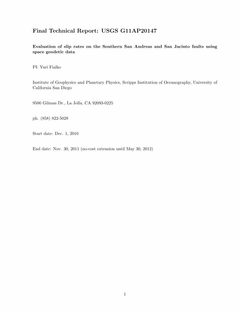
Figure 1: (Left: a) Study area. Black rectangles denote ERS satellite tracks 127 and 356 spanningmajor plate boundary faults. (Right: b) A mosaic of average line-of-sight (LOS) velocities, incentimeters per year, derived from InSAR data. Motion toward the satellite is assumed to bepositive. The velocities represent deformation over a time period of 15 years between 1992 and2007. Black wavy lines denote active faults. Dots denote continuous GPS sites used for orbitalerror corrections.

Report

We have processed and analyzed a large set of Synthetic Aperture Radar (SAR) data over theCoachella Valley-San Bernardino segments of the southern San Andreas Fault (SAF), as well asadjacent parts of the plate boundary in Southern California. Figure 1 shows a mosaic of line-of-sight velocities from the descending tracks 127 and 356 of the ERS-1 and 2 satellites (Manzo et al.,2011). These data extended the previously published results (Fialko, 2006; Lundgren et al., 2009)in terms of both spatial and temporal coverage. Note strong gradients in the LOS velocity acrossthe San Andreas and San Jacinto faults, indicating high deformation rates and build-up of stressin the seismogenic layer.

Figure 2 shows the LOS velocity from the ERS track 356 along with the GPS data from theUNAVCO PBO and the SCEC CMM4 model (courtesy of Tom Herring).

We used these data to refine estimates of geodetic slip rates and locking depths of the southernSan Andreas and San Jacinto faults. In particular, we explored potential biases introduced byassumptions about material heterogeneity and fault geometry, both of which have been proposedas possible causes of the observed asymmetry in strain rate across major faults of the SAF sys-tem (Fialko, 2006; Lundgren et al., 2009). We used the Southern California Earthquake CenterCommunity Velocity Model, SCEC CVM-H 6.3 (Plesch et al., 2009; Suess and Shaw , 2003) toconstrain variations in the elastic properties of the crust across the faults. Figure 3 shows thedistribution of shear modulus deduced from seismic velocities. We computed surface displacementsin a heterogeneous domain using the method of Barbot et al. (2009), which accounts for variationsin material properties by introducing an equivalent distribution of fictitious body forces. The sec-ond potential source of bias we examined is that due to the assumed fault geometry. In elasticmodels, the position of the dislocation edge below the locked fault defines the inflection point in

3

117˚00' 116˚30' 116˚00' 115˚30'

32˚30'

33˚00'

33˚30'

34˚00'

117˚00' 116˚30' 116˚00' 115˚30'

32˚30'

33˚00'

33˚30'

34˚00'

40 mm/yr

AA

A’A’

PMFPMF

SAFSAF

SJFSJF

CF CF CCF

CCF

SHFSHF

EFEF

IFIF

15 10 5 0

mm/yr

Figure 2: (Top) LOS velocities from the ERS track 356 (color map) and horizontal GPS velocities inthe North America Fixed (NAFD) frame (blue trianges, blue arrows). Data used in the inversionwere selected along a 50km-wide profile from A-A′. Open triangles denote GPS sites not usedin the inversion. Faults considered in the model are the Elsinore fault (EF), Coyote Creek fault(CCF), Clark fault(CF), and San Andreas fault (SAF). Also shown are the Superstition Hills (SHF),Imperial (IF), northern San Jacinto (SJF), and Pinto Mountain fault (PMF). (Bottom) InSAR andGPS data along the A-A′ profile and predictions of the best-fitting model.

4

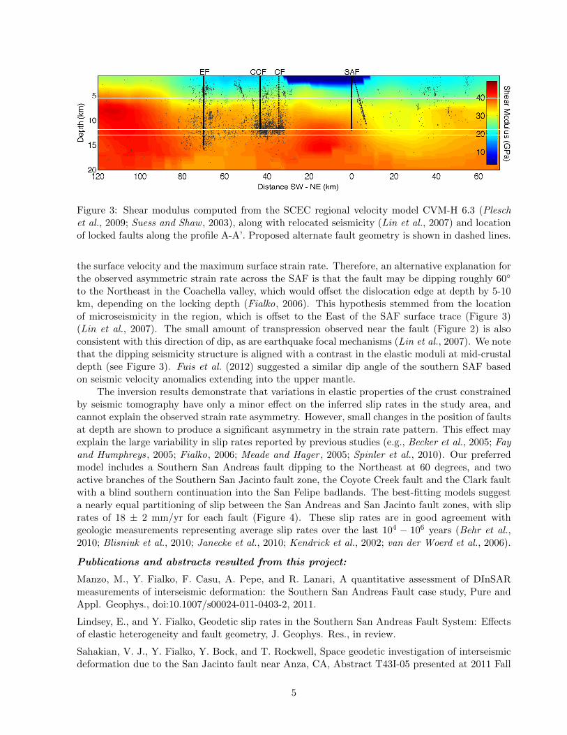
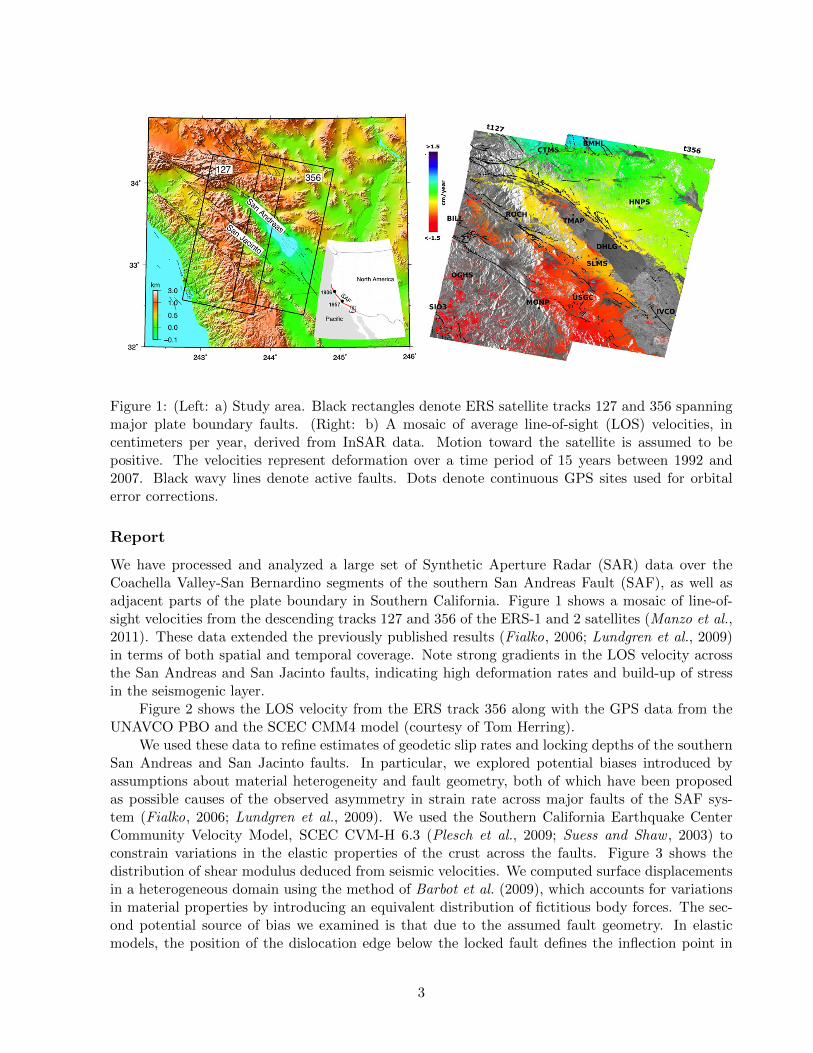
Figure 3: Shear modulus computed from the SCEC regional velocity model CVM-H 6.3 (Pleschet al., 2009; Suess and Shaw , 2003), along with relocated seismicity (Lin et al., 2007) and locationof locked faults along the profile A-A’. Proposed alternate fault geometry is shown in dashed lines.

the surface velocity and the maximum surface strain rate. Therefore, an alternative explanation forthe observed asymmetric strain rate across the SAF is that the fault may be dipping roughly 60◦

to the Northeast in the Coachella valley, which would offset the dislocation edge at depth by 5-10km, depending on the locking depth (Fialko, 2006). This hypothesis stemmed from the locationof microseismicity in the region, which is offset to the East of the SAF surface trace (Figure 3)(Lin et al., 2007). The small amount of transpression observed near the fault (Figure 2) is alsoconsistent with this direction of dip, as are earthquake focal mechanisms (Lin et al., 2007). We notethat the dipping seismicity structure is aligned with a contrast in the elastic moduli at mid-crustaldepth (see Figure 3). Fuis et al. (2012) suggested a similar dip angle of the southern SAF basedon seismic velocity anomalies extending into the upper mantle.

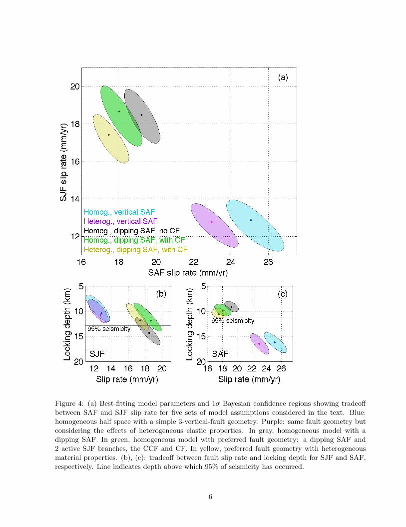
The inversion results demonstrate that variations in elastic properties of the crust constrainedby seismic tomography have only a minor effect on the inferred slip rates in the study area, andcannot explain the observed strain rate asymmetry. However, small changes in the position of faultsat depth are shown to produce a significant asymmetry in the strain rate pattern. This effect mayexplain the large variability in slip rates reported by previous studies (e.g., Becker et al., 2005; Fayand Humphreys, 2005; Fialko, 2006; Meade and Hager , 2005; Spinler et al., 2010). Our preferredmodel includes a Southern San Andreas fault dipping to the Northeast at 60 degrees, and twoactive branches of the Southern San Jacinto fault zone, the Coyote Creek fault and the Clark faultwith a blind southern continuation into the San Felipe badlands. The best-fitting models suggesta nearly equal partitioning of slip between the San Andreas and San Jacinto fault zones, with sliprates of 18 ± 2 mm/yr for each fault (Figure 4). These slip rates are in good agreement withgeologic measurements representing average slip rates over the last 104 − 106 years (Behr et al.,2010; Blisniuk et al., 2010; Janecke et al., 2010; Kendrick et al., 2002; van der Woerd et al., 2006).

Publications and abstracts resulted from this project:

Manzo, M., Y. Fialko, F. Casu, A. Pepe, and R. Lanari, A quantitative assessment of DInSARmeasurements of interseismic deformation: the Southern San Andreas Fault case study, Pure andAppl. Geophys., doi:10.1007/s00024-011-0403-2, 2011.

Lindsey, E., and Y. Fialko, Geodetic slip rates in the Southern San Andreas Fault System: Effectsof elastic heterogeneity and fault geometry, J. Geophys. Res., in review.

Sahakian, V. J., Y. Fialko, Y. Bock, and T. Rockwell, Space geodetic investigation of interseismicdeformation due to the San Jacinto fault near Anza, CA, Abstract T43I-05 presented at 2011 Fall

5

31

Figure 4. (a) Best-fitting model parameters and 1σ Bayesian confidence regions showing

tradeoff between SAF and SJF slip rate for five sets of model assumptions considered in

the text. Blue: homogeneous half space with a simple 3-vertical-fault geometry. Pur-

ple: same fault geometry but considering the effects of heterogeneous elastic properties.

In gray, homogeneous model with a dipping SAF. In green, homogeneous model with

preferred fault geometry: a dipping SAF and 2 active SJF branches, the CCF and CF.

In yellow, preferred fault geometry with heterogeneous material properties. (b), (c):

tradeoff between fault slip rate and locking depth for SJF and SAF, respectively. Line

indicates depth above which 95% of seismicity has occurred.

Figure 4: (a) Best-fitting model parameters and 1σ Bayesian confidence regions showing tradeoffbetween SAF and SJF slip rate for five sets of model assumptions considered in the text. Blue:homogeneous half space with a simple 3-vertical-fault geometry. Purple: same fault geometry butconsidering the effects of heterogeneous elastic properties. In gray, homogeneous model with adipping SAF. In green, homogeneous model with preferred fault geometry: a dipping SAF and2 active SJF branches, the CCF and CF. In yellow, preferred fault geometry with heterogeneousmaterial properties. (b), (c): tradeoff between fault slip rate and locking depth for SJF and SAF,respectively. Line indicates depth above which 95% of seismicity has occurred.

6

Meeting, AGU, San Francisco, Calif., 5-9 Dec.

Lindsey, E., and Y. Fialko, Geodetic slip rates in the southern San Andreas Fault system: Inves-tigation of the effects of heterogeneous elastic structure, Abstract G13B-03 presented at 2011 FallMeeting, AGU, San Francisco, Calif., 5-9 Dec.

ReferencesBarbot, S., Y. Fialko, and D. Sandwell, Three-dimensional models of elasto-static deformation in heterogeneous

media, with applications to the Eastern California Shear Zone, Geophys. J. Int., 179, 500–520, 2009.

Becker, T. W., J. L. Hardebeck, and G. Anderson, Constraints on fault slip rates of the southern california plateboundary from gps velocity and stress inversions, Geophys. J. Int., 160, 634–650, 2005.

Behr, W. M., et al., Uncertainties in slip-rate estimates for the Mission Creek strand of the southern San Andreasfault at Biskra Palms Oasis, southern California, Geol. Soc. Am. Bull., 122, 1360–1377, doi: 10.1130/B30,020.1,2010.

Blisniuk, K., T. Rockwell, L. A. Owen, M. Oskin, C. Lippincott, M. W. Caffee, and J. Dortch, Late Quaternary sliprate gradient defined using high-resolution topography and 10Be dating of offset landforms on the southern SanJacinto Fault zone, California, J. Geophys. Res., 115, B08,401, doi:10.1029/2009JB006,346, 2010.

Fay, N., and G. Humphreys, Fault slip rates, effects of elastic heterogeneity on geodetic data, and thestrength of the lower crust in the Salton Trough region, southern California, J. Geophys. Res., 110, B09,401,doi:10.1029/2004JB003,548, 2005.

Fialko, Y., Interseismic strain accumulation and the earthquake potential on the southern San Andreas fault system,Nature, 441, 968–971, 2006.

Fuis, G. S., D. S. Scheirer, V. E. Langenheim, and M. D. Kohler, A new perspective on the geometry of the SanAndreas fault in Southern California and its relationship to lithospheric structure, Bull. Seism. Soc. Am., 102,236–251, 2012.

Janecke, S. U., et al., High geologic slip rates since early Pleistocene initiation of the San Jacinto and San FelipeFault zones in the San Andreas Fault system, Southern California, USA, GSA Special Papers, 475, 1–48, 2010.

Kendrick, K. J., D. M. Morton, S. G. Wells, and R. W. Simpson, Spatial and temporal deformation along the northernSan Jacinto fault, southern California: Implications for slip rates, Bull. Seism. Soc. Am., 92, 2782–2802, 2002.

Lin, G., P. M. Shearer, and E. Hauksson, Applying a three-dimensional velocity model, waveform cross correlation,and cluster analysis to locate southern California seismicity from 1981 to 2005, J. Geophys. Res., 112, B12,309,doi:10.1029/2007JB004,986, 2007.

Lundgren, P. E., A. Hetland, Z. Liu, and E. J. Fielding, Southern San Andreas-San Jacinto fault system slip ratesestimated from earthquake cycle models constrained by GPS and interferometric synthetic aperture radar obser-vations, J. Geophys. Res., 114, B02,403, doi:10.1029/2008JB005,996, 2009.

Manzo, M., Y. Fialko, F. Casu, A. Pepe, and R. Lanari, A quantitative assessment of DInSAR measurements ofinterseismic deformation: the Southern San Andreas Fault case study, Pure Appl. Geoph., 168, 195–210, 2011.

Meade, B. J., and B. H. Hager, Block models of crustal motion in southern California constrained by GPS measure-ments, J. Geophys. Res., 110, Art. No. B03,403, doi:10.1029/2004JB003,209, 2005.

Plesch, A., C. Tape, J. Shaw, and members of the USR working group, CVM-H 6.0: Inversion integration, the SanJoaquin Valley and other advances in the community velocity model, Proc. Ann. SCEC Meeting, 19, 260–261,2009.

Spinler, J. C., R. A. Bennett, M. L. Anderson, S. F. McGill, S. Hreinsdottir, and A. McCallister, Present-day strainaccumulation and slip rates associated with southern San Andreas and eastern California shear zone faults, J.Geophys. Res., 100, B11,407, doi:10.1029/2010JB007,424, 2010.

Suess, P., and J. Shaw, P-wave seismic velocity structure derived from sonic logs and industry reflection data in thelos angeles basin, california, J. Geophys. Res., 108(B3), 2170, doi:10.1029/2001JB001,628, 2003.

van der Woerd, J., Y. Klinger, K. Sieh, P. Tapponnier, F. Ryerson, and A. Meriaux, Long-term slip rate of thesouthern San Andreas Fault from 10Be-26Al surface exposure dating of an offset alluvial fan, J. Geophys. Res.,111, B04,407, doi:10.1029/2004JB003,559, 2006.

7