Final Report - Defense Technical Information Center

Final Report

Advanced Hard Real-Time Operating System, The Maruti Project

DASG-60-92-C-0055

To DOD - Army - Huntsville and Phillips Lab Phillips Laboratory / PKVC

2251 Maxwell Street SE Kirtland AFB NM 87117-5773

Ashok K. Agrawala and Satish K. Tripathi Department of Computer Science

University of Maryland College Park, MD 20742

January 1997

BTCC QÜA2OT INSPECTED S

19970130 010

THIS DOCUMENT IS BEST

QUALITY AVAILABLE. THE

COPY FURNISHED TO DTIC

CONTAINED A SIGNIFICANT

NUMBER OF PAGES WHICH DO

NOT REPRODUCE LEGIBLY.

TABLE OF CONTENTS

1. Executive Summary i.jji

2. "Optimal Replication of Series-Graphs for Computation-Intensive 1 -37 Applications"

By: A. K. Agrawala and S.-T. Cheng

3. "Designing Temporal Controls" 39-61 By: A. K. Agrawala, S. Choi, and L. Shi.

4. "Scheduling an Overloaded Real-Time System" 63-92 By: S.-L Hwang, C.-M. Chen, and A. K. Agrawala

5. "Notes on Symbol Dynamics" 93-104 By: A. K. Agrawala and C. A. Landauer

6. "Allocation and Scheduling of Real-Time Periodic 105-127 Tasks with Relative Timing Constraints"

By: S.-T. Cheng and A. K. Agrawala

7. "Scheduling of Periodic Tasks with Relative Tinting Contraints" 129-150 By: S.-T. Cheng and A. K. Agrawala

8. "A Scalable Virtual Circuit Routing Scheme for ATM Networks" 151-175 By: C. Alaettinoglu, I. Matta, and A. U. Shankar

9. "Hierarchical Inter-Domain Routing Protocol with 177-212 On-Demand ToS and Policy Resolution"

By: C. Alaettinoglu and A. U. Shankar

10. "Optimization in Non-Preemptive Scheduling for a pPriodic Tasks" 213-257 By: S.-L Hwang, S.-T. Cheng, and A. K. Agrawala

11. "A Decomposition Approach to Non-Preemptive Real-Time Scheduling" 259-279 By: A. K. Agrawala, X. Yuan, and M. Saksena

12. "Viewserver Hierarchy: a Scalable and Adaptive 281-314 Inter-Domain Routing Protocol."

By: C. Alaettinoglu and A. U. Shankar

13. "Temporal Analysis for Hard Real-Time Scheduling" 315-322 By: M. Saksena and A. K. Agrawala

14. "Implementation of the MPL Compiler" 323-340 By: J. M. Rizzuto and J. da Silva

15. "Maruti 3.1 Programmers's Manual, First Edition" 341-380 By: Systems Design and Anlysis Group, Department of Computer Science, UMCP

16. "Maruti 3.1 Design Overview, First Edition" 381-406 By: Systems Design and Anlysis Group, Department of Computer Science, UMCP

DTIC QUALITY INSPECTED 8

Executive Summary

Introduction:

This is the final report on the work done under contract DASG-60-92-C-0055 from Phillips Labs and ARPA to the Department of Computer Science at the University of Maryland. The work started 04/28/92. The goal of this project was to create an environment for development and deployment of critical applications with hard real-time constraints in a reactive environment. We have redesigned Maruti system to address these issues. In this report we highlight the achievements of this contract. A publications list and a copy of each of the publications is also attached.

Application Development Environment:

To support applications in a real-time system, conventional application development techniques and tools must be augmented with support for specification and extraction of resource requirements and timing constraints, The application development system provides a set of programming tools to support and facilitate the development of real-time applications with diverse requirements. The Maruti Programming Language (MPL) is used to develop induvidual program modules. The Maruti Configuration Language (MCL) is used to specify how individual program modules are to be connected together to form an application and the details of the hardware of which the application is to be executed.

In the current version, the base programming language used is ANSI C. MPL adds modules, shared memory blocks, critical regions, typed message passing, periodic functions, and message-invoked functions to the C language. To make analyzing the resource usage of programs feasible, certain C idioms are not allowed in MPL; in particular, recursive function calls are not allowed nor are unbounded loops containing externally visible events, such as message passing and critical region transition.

MPL Modules are brought together into as an executable application by a specification file written in the Maruti Configuration Language (MCL). The MCL specification determines the application's hard real-time constraints, the allocation of tasks, threads, and shared memory blocks, and all message-passing connections. MCL is an interpreted C-like language rather than a declarative language, allowing the instantiation of complicated subsystems using loops and subroutines in the specification.

Analysis and Resource Allocations:

The basic building block of the Maruti computation model is the elemental unit (EU). In general an elemental unit is an executable entity which is triggered by incoming data and signals, operates on the input data, and produces some output data and signals. The behavior of an EU is atomic with respect to its environment. Specifically:

• All resources needed by an elemental unit are assumed to be required for the entire length of its execution.

• The interaction of an EU with other entities of the system occurs either before it starts executing or after it finishes execution.

In order to define complex executions, the EUs may be composed together and properties specified on the composition. Elemental units are composed by connecting an output port of an EU with an input port of another EU. A valid connection requires that the input and output of port types are compatible, i.e., they carry the same message type. Such a connection marks a one-way flow of data or control, depending on the nature of the ports. A composition of EUs can be viewed as a directed acyclic graph, called an elemental unit graph (EUG), in which the nodes are the EUs, and the edges are the connections between EUs. An incompletely specified EUG in which all input and output ports are not connected is termed as ^partial EUG (PEUG). A partial EUG may be viewed as a higher level EU. In a complete EUG, all input and output ports are connected and there are no cycles in the graph. The acyclic requirements come from the required time determinacy of execution. A program with unbounded cycles or recursions may not have a temporally determinate execution time. Bounded cycles in an EUG are converted into a acyclic graph by loop unrolling.

Program modules are independently compiled. In addition to the generation of the object code, compilation also results in the creation of partial EUGs for the modules, i.e., for the services and entries in the module, as well as the extraction of resource requirements such as stack sizes or threads, memory requirements, and the logical resource requirements.

Given an application specification in the Maruti Configuration Language and the component application modules, the integration tools are responsible for creating a complete application program and extracting out the resource and timing information for scheduling and resource allocation. The input of the integration process are the program modules, the partial EUGs corresponding to the modules, the application configuration specification, and the hardware specifications. The outputs of the integration process are: a specification for the loader for creating tasks, populating their address space, creating the threads and channels, and initializing the task; loadable executables of the program; and the complete application EUG along with the resource description for the resource allocation and the scheduling subsystem.

After the application program has been analyzed and its resource requirements and execution constraints identified, it can be allocated and scheduled for a runtime system.

We consider the static allocation and scheduling in which a task is the finest granularity object of allocation and an EU instance is the unit of scheduling. In order to make the execution of instances satisfy the specification and meet the timing constraints, we consider a scheduling frame whose length is the least common multiple of all tasks' periods. As long as one instance of each EU is scheduled in each period within the scheduling frame and these executions meet the timing constraints, a feasible schedule is obtained.

Maruti Runtime System:

The runtime system provides the conventional functionality of an operating system in a manner that supports the timely dispatching of jobs. There are two major components of the runtime system - the Maruti core, which is the operating system code that implements scheduling, message passing, process control, thread control, and low level hardware control, and the runtime dispatcher, which performs resource allocation and scheduling or dynamic arrivals.

11

The core of the Maruti hard real-time runtime system consists of three data structures:

• The calendars are created and loaded by the dispatcher. Kernel memory is reserved for each calendar at the time it is created. Several system calls serve to create, delete, modify, activate, and deactivate calendars.

• The results table holds timing and status results for the execution of each elemental unit; The maruti_calandar_results system call reports these results back up to the user level, usually the dispatcher. The dispatcher can then keep statistics or write a trace file.

• The pending activation table holds all outstanding calendar activation and deactivation requests. Since the requests can come from before the switch time, the kernel must track the requests and execute them at the correct time in the correct order.

The Maruti design includes the concept of scenarios, implemented at runtime as sets of alternative calendars that can be switched quickly to handle an emergency or a change in operating mode. These calendars are pre-scheduled and able to begin execution without having to invoke any user-level machinery. The dispatcher loads the initial scenarios specified by the application and activates one of them to begin normal execution.

in

Optimal Replication of Series-Parallel Graphs for Computation-Intensive Applications*

Sheng-Tzong Cheng Ashok K. Agrawala

Institute for Advanced Computer Studies Systems Design and Analysis Group

Department of Computer Science University of Maryland, College Park, MD 20742

{stcheng.agrawala}@cs.umd.edu

'This work is supported in part by Honeywell under N00014-9l-C.niQ<; >~A A m\.-n- J ^ ~~ <^0055. lie *ews, opinions, »d/« Jbdägi «•**?£ üStS« S ofTwÄ T / ^f^' «**«« « xepreser^ th. oSdal policies, either expressed ÄÄÄÄ% ""

Optimal Replication of SP Graphs for Computation-Intensive Applications

Prof. Ashok K. Agrawala

Department of Computer Science

University of Maryland at College Park

A.V. Williams Building

College Park, Maryland 20742

(Tel): (301) 405-2525

Abstract

We consider the replication problem of series-parallel (SP) task graphs where each task may

run on more than one processor. The objective of the problem is to minimize the total cost

of task execution and interprocessor communication. We call it, the minimum cost replication

problem JOT SP graphs (MCRP-SP). In this paper, we adopt a new communication model where

the purpose of replication is to reduce the total cost. The class of applications we consider

is computation-intensive applications in which the execution cost of a task is greater than

its communication cost. The complexity of MCRP-SP for such applications is proved to be

NP-complete. We present a branch-and-bound method to find an optimal solution as well as

an approximation approach for suboptimal solution. The numerical results show that such

replication may lead to a lower cost than the optimal assignment problem (in which each task

is assigned to only one processor) does. The proposed optimal solution has the complexity of

0{n72nM). while the approximation solution has 0(n4M2), where n is the number of processors

in the system and M is the number of tasks in the graph.

1 Introduction

Distributed computer systems have often resulted in improved reliability, flexibility, throughput,

fault tolerance and resource sharing. In order to use the processors available in a distributed

system, the tasks have to be allocated to the processors. The allocation problem is one of the

basic problems of distributed computing whose solution has a far reaching impact on the usability

and efficiency of a distributed system. Clearly, the tasks of an application have to be executed

satisfying the precedence and other synchronization constraints among them. (Such constraints are

often specified in the form of a task graph.)

In executing an application, denned by its task graph, we have the option of restricting ourselves

to having only one copy of each task. The allocation problem, in this case, is referred to as

assignment problem. If, on the other hand, a task may be replicated multiple times, the general

problem is called the replication problem. In this paper, we consider the replication problem and

present an algorithm to find the optimal replication of series-parallel graphs for computation- intensive applications.

For distributed processing applications, the objective of the allocation problem may be the

minimum completion time, processor load balancing, or total cost of execution and communication,

etc. For the assignment problem where the objective is to minimize the total cost of execution and

interprocessor communication, Stone [11] and Towsley [12] presented 0(n3M) algorithms for tree-

structure and series-parallel graphs, respectively, of M tasks and n processors. For general task

graphs, the assignment problem has been proven [9] to be NP-complete. Many papers [8][9][10]

presented branch-and-bound methods which yielded an optimal result. Other heuristic methods

have been considered by Lo [7] and Price and Krishnaprasad [5]. All these works focused on the

assignment problem.

Traditionally, the main purpose of replicating a task on multiple processors is to increase the

degree of fault tolerance [2][6]. If some processors in the distributed system fail, the application may

still survive using other copies. In such a communication model, a task has to communicate with

multiple copies of other tasks. As a consequence, the total cost of execution and communication

of the replication problem will be bigger than that of the assignment problem. In this paper, we

adopt another communication model in which the replication of a task is not for the sake of fault

tolerance but for decreasing of the total cost. In our model, each task may have more than one copy

and it may start its execution after receiving necessary data from one copy of each preceding task.

Clearly, in a heterogeneous environment the cost of execution of a task depends on the processor on

which it executes, and the communication costs depend on the topology, communication medium,

protocols used, etc. When a task t is allowed to have only one copy in the system, the sum

of the interprocessor communication costs between t and other tasks may be large. Sometimes

it will be more beneficial if we replicate t onto multiple processors to reduce the inter-processor

communication, and to fully utilize the available processors in the systems. Such replication may

lead to a lower total cost than the optimal assignment problem does. An example illustrating this

point is presented in Section 3.

In the assignment problem, polynomial-time algorithms exist for special cases, such as tree-

structure [11] and series-parallel [12] task graphs. This paper represents one of the first few attempts

at finding special cases for the replication problem. The class of applications we consider in this

paper is computation-intensive applications in which the execution cost of a task is greater than its

communication cost. Such applications can be found in an enormous number of fields, such as digital

signal processing, weather forecasting, game searching, etc. We formally define a computation-

intensive application in Section 2.2. In this paper, we prove that for the computation-intensive

applications, the replication problem is NP-complete, and we present a branch-and-bound algorithm

to solve it. The worst-case complexity of the solution is 0(n22nM). Note that the algorithm is

able to solve the problem in the complexity of the linear function of M.

We also develop an approximation approach to solve the problem in polynomial time. Given a

forker task 5 with K successors in the SP graph, the method tries to allocate s to processors based

on iterative selection. The complexity of the iterative selection for a forker is 0(n2K2), while the

overall solution for an SP graph is 0(n4M2).

In the remainder of this paper, the series-parallel graph model and the computation model are

described in section 2. In section 3, the replication problem is formulated as the minimum cost

0-1 integer programming problem and the proof of NP completeness is given. A branch-and-bound

algorithm and numerical results are given in section 4, while the approximation methods and results

are given in section 5. The overall algorithm is presented and conclusion remark is drawn in section

6.

2 Definitions

2.1 Graph Model

A series-parallel (SP) graph, G = (V, f?), is a directed graph of type p, where p € {2^*, r*,,«,

Tand, T^} and G has a source node (of indegree 0) and a sink node (of outdegree 0). An SP graph

can be constructed by applying the following rules recursively.

1- A graph G = (V,E) = ({„}, ,) is tt SP ^ of type ^ (No(k v .$ ^ ^^ ^ ^

sink of G.)

2- If Gy = (V,,^) and G2 = (V2,^) are SP graphs then G' = (V, £') is an SP graph of type

TcHain, where V = V, U V2 and j?' = E, u £fe u {<sink of G1? source of G2 >}.

3. If each graph G, = (!*,£;■) with source-sink pair («,«.•), where « is of outdegree 1, is an SP

graph, V i = 1,2,.. .,n, and new nodes s' £ K and f ff Vit V t are given then G' = (V, E') is

an SP graph of type Tand{oj type T„), where VsV,uV2U...uV,U {*', f} and E' = £j

U£2U...Ui:nU{<,',st->|Vi=l,2,...,n}u{<t„t'>|V: = l,2,...,n}.Thesource of G', s\ is called the forker of G'. The sink of G', r', is called the joiner of G'. G' is an SP

graph of type TBn,(or type T„) if there exists a parullel-and (or pom/ieZ-or) relation among G,'s.

A convenient way of representing the structure of an SP graph is via a parsing tree [4] The

transformation of an SP graph to a parsing tree can be done in a recursive way. There are four

bnds of internal nodes in a parsing tree: Tmdtt T^, Tand and Tmt nodes. A Twit node has only

one duld, while a Tehain node has more than one child. Every internal node x, along with all its

descendant nodes induces a subtree Sx which describes an SP subgraph Gx of G. Each leaf node

m Ss corresponds to an SP graph of type Twit. A Tand(or T„) node y consists of its type Tand(or

T„) along with the forker and joiner nodes of Gy. We give an example of an SP graph G, and its parsing tree T{G) in Figure 1.

2.2 Computational Model

An application program consists of M tasks labeled m — 1. 2,..., M. Its behavior is represented

by an SP graph with the tasks correspond to the nodes. Each task may be replicated onto more

than one processor. A task instance i,iP is a replication of task i on processor p. A directed edge < i,

j > between nodes i and j exists if the execution of task j follows that of task :". Associated with

each edge < i, j > is the communication cost incurred by the application. We are concerned with

types of applications where the cost of execution of a task is always greater than the com muni cation

overhead it needs. The model is stated as follows.

Given a distributed system S with n processors connected by a communication network, an

application is computation-intensive if its associated SP graph G = (V, E) on S satisfies the

following conditions:

2- E?=i M.\;(Pr 9) < miBpKp), v < *"» J >€ £, and 1 < p < n, where

• pij(p. q) is the communication cost between tasks i and j when they are assigned to processors

p and q respectively, and

• eiiP is the execution cost when task : is assigned to processor p.

The first condition states that the communication cost between any two task instances (e.g.

titP and ij,?) is not negative. The second one depicts that for every edge < i,j >, the worst-case

communication cost between any task instance Uj> aod all its successor task instances (i.e. tj,s's, V

q) is less than the minimum execution cost of task i.

2.3 Communication Model

The communication model we considered is different from that of reliability-oriented replication.

In reliability-oriented replication problem,, the objective is to increase the degree of fault tolerance.

To detect fault and maintain data consistency, each task has to receive multiple copies of data from

several task instances if its predecessor is replicated in more than one place.

The purpose of the replication problem considered in this paper is to decrease the sum of

execution and communication costs. Under such consideration, there is no need to enforce plural

communication between any two task instances. Hence, we propose the 1-out-of-n communication

model. In the model, for each edge < i, j > € £, a task instance iii9 may start its execution if it

receives the data from any one task instance of its predecessor, task t.

3 Problem Formulation and Complexity

Based on the computational model presented in Section 2.2, the problem of minimizing the total

sum of execution and communication costs for an SP task graph can be approached by replication

of tasks. An example where the replication may lead to a lower sum of execution costs and

communication costs is given in Figure 2, where the number of processors in the system is two, and

the execution costs and communication costs are listed in e table and fi table respectively. If each

task is allowed to run on at most one processor, then'the optimal allocation will be to assign task

a to processor 1, b to 1, c to 1, d to 2, e to 2, and / to 1. The minimum cost is 68. However, if

each task is allowed to be repBcated more than one copies, (i.e. to replicate task a to processors 1 and 2), then the cost is 67.

We introduce integer variable Xit,'s, V 1 < i < M and 1 < p < », to formulate the problem

where each X;,p = 1 if task : is replicated on processor p; and = 0, otherwise. We define a binarv

function 6(x). If x > 0 then 6(x) = 1 else S(X) = 0. We also associate an allocated flag F(w) with

each node w in the parsing tree, where F(w) = 1 if the allocation for tasks in the subtree Sw is

valid; and = 0, otherwise. A valid allocation for the tasks in Sw is an allocation that follows the

semantics of T^.n, Tand, and T„ subgraphs. A valid allocation is not necessarily the allocation in

which each task in Sw is allocated to at least one processor. Some tasks in T„ subgraphs may be neglected without effecting the successful execution of an SP graph.

Given an SP graph G, its parsing tree T(G) and any internal node w in T(G), allocated flag F(w) can be recursively computed:

1. if w is a Tunit node with a child :', then

F(w) = F{i) = 6(£xij>)

2. if w is a T^am node with c children, F(iu) = F(childi) x F^childj) x ... x F(ckildc).

3. if it- is a Toni node with forker 5, joiner i and c children, then F(w) = F(^) x F(z.) x F(childi)

x F{child2) x ... x F(childe).

4. if tu is a 2V node with forker s, joiner f and c children, then F(w) = .F(s) x F(t) x 6(F(childi)

+ F(child2) + ...+ F(childc)).

The minimum cost replication problem for SP graphs, MCRP-SP, can be formulated as 0-1

integer programming problem, i.e:

Z = Minimize £-Xvj, * e;,p + £ min (fiij(p,q)* Xj,,)) ij> <t"j>€E, l<9<n *

subject to F[T) = 1, where r is the root of T(G) and J^tiP = 0 or l,Vt,p. (1)

The restricted problem which allows each task to run on at most one processor has the following

formulation.

Z = Minimize Q^ Xi<p * a, + ^ A*»o * Xi<v * Xi* 1 ».P <ivj">e£,p,9

subject to ^2 Xi.p ^ 1 an^ F(T) = 1,

where r is the root of T(G) and Xi>? = 0 or 1, Vi,p. (2)

The task assignment problem (2) for SP graphs of M tasks onto n processors, has been solved

in 0(n3M) time [12]. However,the multiprocessor task assignment for general types of task graphs

without replication has been reported to be NP-complete [9]. As for the MCPJP-SP problem, it

can be shown to be NP-complete. In this paper, we are able to solve the problem and present a

linear-time algorithm that is linear in the number of tasks when the number of processors is fixed

for computation-intensive applications.

3.1 Assignment Graph

Bokhari [1] introduced the assignment graph to solve the task assignment problem (2). To prove

the NP completeness of problem (1) and solve the problem, we also adopt the concept of the

assignment graph of an SP graph. The assignment graph of an SP graph can be denned similarly.

The following definitions apply to the assignment graph. And we draw up an assignment graph for an SP graph in Figure 3.

1. It is a directed graph with weighted nodes and edges.

2. It has M x n nodes. Each weighted node is labeled with a task instance, zi>p.

3. A layer a is the collection of n weighted nodes (ttil, i,,2, ..., and *<,„). Each layer of the

graph corresponds to a node in the SP graph. The layer corresponding to the source (sink) is called source (sink) layer.

4. A part of the assignment graph corresponds to an SP subgraph of type T^, Tand or TBT is called a T^i^, Tand or T^ limb respectively.

5. Communication costs are accounted for by giving the weight ^{p, q) to the edge going from

6. Execution costs are assigoed to the corresponding weighted nodes.

Given an assignment graph, Bokhari [1] solves Problem (2) by selecting one weighted node

from each layer and including the weighted edges between any two selected nodes. This resulting

subgraph is called an allocation graph. To solve Problem (1), more than one weighted node from

each layer may be chosen. Similarly, a replication graph for Problem (1) can be constructed from

an assignment graph by including all selected nodes and edges between these nodes. Examples of

an allocation graph and a replication graph are shown in Figure 4 for an assignment graph shown

in Figure 3. Note that for each node x in the replication graph there is only one edge incident to it from each predecessor layer of x.

In a replication graph, each layer may have more than one selected node. Let Variable X,

= (*J,I» Xla, ..., Xi,n) be a replication vector for layer / in a replication graph. We define the

minimum activation cost of vector X{ for layer t , Ai(X{), to be the minimum sum of the weights

of all possible nodes and edges leading to the selected nodes of layer t in a replication graph.

Then the goal of Problem (1) can be achieved by computing the minimal value of {A«;^v(Är«mv) +

Sp=i •X.ink.p * esjnl.,p} over all possible values of Ä'sink.

3.2 Complexity

In this section, we can show that Problem (1) for a computation-intensive application is NP-

complete provided we prove the following:

Lemma 1: For any layer / in the replication graph, the minimum activation cost for two selected

nodes t;iP and i;i9 will be always greater than that for either node i/j, or i/t9 only.

Proof: The Lemma can be proven by contradiction. Let A\ be the the minimum activation cost for

two nodes i/)P and i;i9, and Ai and A% be the minimum costs for titP and t;>? respectively. Assume

ihat Ai < Ai and A\ < A3. Since A\ includes the activation cost of node i/)P, an activation cost

for tiiP only can be obtained from A\. The obtained value c is not necessarily the minimum value

for t;iP, hence A2 < c. The value c is obtained by removing some weighted nodes and edges from

replication graph. This implies that c < A\. From above, we find that A-} < A\, which contradicts

the assumption. The same reasoning can be applied to A$ and reaches a contradiction. Therefore,

the assumptions are incorrect and Lemma 1 holds.

Lemma 1 can be further extended to the cases where more than two weighted nodes are chosen.

The conclusion we can draw is that the more nodes are selected from a layer, the bigger the

activation cost is.

Lemma 2: Given a computation-intensive application with its SP task graph G — (V, E) and its

assignment graph, if node i has outdegree one and edge < i,j > £ E, then for any vector Xj, the

minimal activation cost Aj(Xj) can be obtained by choosing only one weighted node from layer :.

(i.e. £P=:*:> = 1)

Proof: The Lemma can be proven by contradiction. Since node i has outdegree one and edge

10

< *(*?) + £ Xl * e,p + £ min (Xji? • ^-(p, ,)) = P=I ,=i*^

The result, m' < m, contradicts our assumption. It means that the assumption is wrong and Lemma 2 holds.

Lemma 3: Given a computation-intensive application with its SP task graph <?, the objective of

the minimum cost can be achieved by considering only the replication of the forkers.

Proof: We proceed to prove the lemma by contradiction. Let the minimum cost for task replication

problem be z0 if only the forkers(i.e. outdegree > 1) are allowed to run on more than one processor.

Assume the total cost can be reduced further by replicating some task * which is not a forker. Then there are two possible cases for ::

1. : has outdegree 0.

2. t fcas outdegree \.

In case L i is the sink of the whole graph. Also i may be the joiner of some SP subgraphs. If i is

allowed to run on an extra processor b, which is different from the one which i is initially assigned

to (when 20 is obtained), then the new cost will be * + et>fc + £<£,:>€£ Mi. Apparently the new

cos; is greater than zo- This contradicts our assumption that the total cost can be reduced further by replicating task i.

In case 2, i has one successor. Let < i,; > € £. From the assumption, we know that the

replication of i can reduce the total cost. Bence, the minimum activation cost for task instances

in layer j, A^Xj), is obtained when task » is replicated onto more than one processor. This

contradicts Lemma 2. Hence, the assumption is incorrect and the objective of the minimum cost

can be achieved by considering only the replication of the forkers.

Lemma 3 tells that, given an SP graph, if we can find out the optimal replication for the forkers,

Problem (1) for computation-intensive applications can be solved. Now, we show that the problem

11

< i,j > 6 -E, we know that

^■(*i) = *ü*{MXi) + £*,■, * e,-,p + £ a»» Ui.j * /x»j(j>,?))}- A> P=I ,=iA,>=1

Let us assume that the above equation reaches a minimal value m when more than one node

from layer :' is selected and the optimal replication vector is Xf. Since Y%=i %i,v > 1 for Xf, we

may remove one selected node from layer i and obtain a new vector X[. Without loss of generality,

let us remove 1,,T. By removing node t,-tT, a new value m' is obtained. Since m is the minimum

value for layer :', it implies that m < m'.

Prom Lemma 1, we obtain that A;(X-) < A;(Xf). And for a computation-intensive application,

the following holds that Y%=i W,iÜ»,ff) ^ nÜBpte*). V 1 < p < n. Then,

m' = Ai{X■) + J2 X'i,P * e«'.p + SI =tf* (■*;,? * Wj (P, ?)) J>=1 5=1-*.*-1

»i

< *(*?) + L X'i, * a, + 5; min (JTi, * w>, 5))

p=l f=l ^<J_1

n 1»

< ^.-(^) + E X«> * c»> + E JF£.(Xi.? * MajO>,?))] - xnjn(e.>) p=l 9=1 *ij>~1 V

< MX?) + E X?, * e,-, + £ Ä (*M * «JO». ?))] ~ E Wj(ft ?) ?=1 ^srl"*.*-1 9=1

n

P=I

12

< M*i) + E X?.P * «•> + £ ™* (*;., * WJCP, ?)) = m.

The result, m' < m, contradicts our assumption. It means that the assumption is wrong and Lemma 2 holds.

Lemma 3: Given a computation-intensive application with its SP task graph G, the objective of

the minimum cost can be achieved by considering only the replication of the forkers.

Proof: We proceed to prove the lemma by contradiction. Let the minimum cost for task replication

problem be z0 if only the forkers(i.e. outdegree > 1) are allowed to run on more than one processor.

Assume the total cost can be reduced further by replicating some task t which is not a forker. Then there are two possible cases for i:

1. : has outdegree 0.

2. :' has outdegree 1.

In case 1, i is the sink of the whole graph. Also i may be the joiner of some SP subgraphs. If :' is

allowed to run on an extra processor 5, which is different from the one which i is initially assigned

to (when 20 is obtained), then the new cost will be zo + e^ + T.<d,i>eE Mt- Apparently, the new

cost is greater than *o- This contradicts our assumption that the total cost can be reduced further by replicating task i.

In case 2, : has one successor. Let < i,j > £ £. R-om the assumption, we know that the

replication of : can reduce the total cost. Hence, the minimum activation cost for task instances

in layer j, Aj(Xj), is obtained when task :' is replicated onto more than one processor. This

contradicts Lemma 2. Hence, the assumption is incorrect and the objective of the minimum cost

can be achieved by considering only the replication of the forkers.

Lemma 3 tells that, given an SP graph, if we can find out the optimal replication for the forkers,

Problem (1) for computation-intensive applications can be solved. Now, we.show that the problem

13

of finding an optimal replication for the forkers in an SP graph is NP-complete. First, a special form of the replication problem is introduced.

Uni-Cost Task Replication (UCTR) problem is stated as follows:

INSTANCE: Graph G' = (V, E'), V = V{ U V2', where | V{ | = n and | V2' | = m. If x £ V' and

y £ V{ then edge < x,y > £ E' (i.e. \E'\ = mxn). For each i € V{, there is an activation cost

m. Associated with each edge < x,y > £ E\ there is a communication cost dStV = n x m or 0. A positive integer ÜT < n x m is also given.

QUESTION: Is there a feasible subset Vk C V{ such that, we have

[ £™+£min(4.y)]<iir? (3)

[Theorem l]: Uni-Cost Task Replication problem is NP-Complete.

[Proof]: The problem is in NP because a subset Vi, if it exists, can be checked to see if the sum

of activation costs and communication costs is less than or equal to K. We shall now transform

the VERTEX COVER [3] problem to this problem. Given any graph G = (V,E) and an integer C

< | V |, we shall construct a new graph G" = (V',£") and V = V{ U V^ such that there exists a

VEPJTEX COVER of size C or less in G if and only if there is a feasible subset of V{ in G'. Let

| V | = n and j E \ = m. To construct G", (1) we create a vertex t\- for each node in V, (2) we

number the edges in E, and (3) we create a vertex bj for each edge < a,v > € E where u, v £ V.

We define K =mxC, V{ = {vu t*, ..., «„}, V2' = fa, 63, ..., bm) and £' = {< vz.bv > \ vz £

V{y by € "% }. Let ^.i,, = 0, if v- is an end point of the corresponding edge of vertex by; and =

n x m, otherwise. An illustration, where n = 7 and m = 9, is shown in Figure 5.

Let us now argue that there exists a vertex cover of size C or less in G if and only if there is

a feasible subset of V{ in G" to satisfy that the sum of activation cost and communication cost is

m x C or less. Suppose there is a vertex cover of size C, then for p.ach vertex bv (= < u,v >) in V2'>

at least one of v and v belongs to the vertex cover. By selecting all the vertices in the vertex cover

into the subset of Vj', we know that the sum in Eq. (3) will be m x C. Since C < n, it implies that rn x C < nxm.

Conversely, for any feasible subset Vk C V{ such that the total cost is equal to or less than

14

mC, we can see that the second term of Eq. (3) (i.e. the sum of communication cost) must be

zero. Suppose, for some gv € V2', the minimum communication cost between gy and vertices in V

is nonzero, then the communication cost will be at least mxn. Since C < n, it implies that mxn

>mxC. The total cost in Eq. (3) will be greater than mxC, which is a contradiction. Thus the

minimum communication cost between any vertex in V2' and any vertex in Vk is zero. It means that

at least one of two end points of each edge in E belongs to Vk. Since, there is at most C vertices in

Vk (the activation cost for each vertex is m), and by selecting the vertices in Vk, we obtain a vertex cover of size C or less in G.

[Theorem 2): The problem, MCHP-SP for computation-iniensive applications, is NP-complete.

[Proofj: From Lemma 3, we know that only the forker in an SP graph of type Tand needs to run on

more than one processor. Consider the following recognition version of Problem (1) for SP graphs of type Tand:

Given a distributed system of n processors, an SP graph G° = (V°,ED) of type Tond, its

assignment graph E and two positive integers m and r. Let r be a multiple of m, V6 = {s. t,

L2,...,r} and Ea = {< 5,: >\i= 1,2,...,r} U {< i,t >\i= 1,2,...,r}. Task 5 (i) is the forker

(joiner) of Ga. Execution cost e,-, and communication cost Kj(p,q) are denned in E, V < ij >

€ E' and V 1 < p,q < n. Integer variable X^ = 1 if task i is assigned to processor p; and = 0,

otherwise. When a positive integer K < r is given, is there an assignment of XitP% such that

«.? <t'J>€£, *<*<*'*

where £*,-, = 1, Vx # s, and £A't> > 1, if { = 5. (4)

We shall transform the UCTR problem to this problem. Given any graph G' = (V{ U V£,E')

considered in UCTR problem, we construct an SP graph of type Tand> Gc = (V°,E°), and its

assignment graph E, such that G' has a feasible subset of V{ to allow the sum in Eq. (3) is K or

less if and only if there is an assignment of Xi<p's for G° and E to satisfy Eq. (4). Let | V{ | = n,

15

I V2' I = m, then the unit cost / = n x m. Assign r = mx/(=nx m2) and K = n x m. The

forker and joiner of Ga axe 5 and 1 respectively. Then V° = {s, 1,1,2,. ..,r} and J?a = {< s,i > | i

= 1,2,.. -,r} U {< i,z > 11 = 1,2,.. .,T). We assign the execution costs and communication costs in

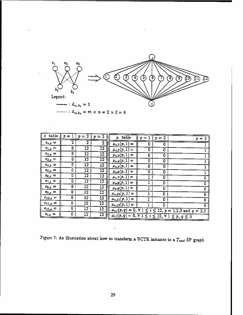
E as follows. An illustration, where m = 2 and n = 3, is shown in Figure 7.

• V 1 < p < n, e«,p = "i.

• Vl<t'<r, Vl<p<n, ifp=l then c,-j, = 0 else e,iP = r.

• Vl<p<n, ifp=l then ei<p = 0 else eitT> = r.

• V 1 < i < r, V 1 < p < n, let q — (:" - 1) div (m x n), where div is the integral division. If d^,fc,43 T 0 then /^-(p, 1) = 1 else /*,,,•(?,!) = 0.

• V 1 < i < r, V 1 < p < n, V 9 # 1, A^(P,9) = 0.

• V 1 < t < T, V 1 < p,q < n, /I.M(P,?) = 0.

It is easy to verify that the SP graph constructed by the the above rules is of type TanJ> and

computation-intensive. For each node in V^ of G', we create / nodes in Gc, where the communica-

tion cost between each node and source s is either one or zero.

Let us now argue that there exists a feasible subset of V{ for UCTR problem if and only if there

exists a valid assignment of A\tp's such that the total sum in Eq. (4) is K or less. Suppose a feasible

subset Vjt of Vj' exists such that the sum in Eq. (3) is C (< K) . Let Vj be {t>j,t>2,.. .,vn} Then we

can obtain a valid assignment by letting X^ = 1, A',-,2 = 0,..., X,-,„ = 0, V 1 < i < r, and Xt,i =

1, Xta = 0, ..., A'j,„ = 0, and Xs,p = 1, if t> € Vk\ and A,,,, = 0, if vr £ Vk, V 1 < p < n. Since

each node x in 1^' corresponds to / nodes in C?°, it is sure that the communication cost between

node x and any node (vp) in VJ is equal to the total communication costs between these / nodes

and any task instance of source (tayV) in G°. By summing up all the costs, we can obtain that the

total sum is C. Since C<K<nxm<r, this is a valid assignment.

Conversely, if there exists an assignment of X^s such that the sum in Eq. (4) is K or less,

then the following must be true that X^\ — 1, X{j = 0,.., Xi,n = 0, V 1 < i < r, and Xiyi = 1,

Xi,2 = 0,..., A'j,„ = 0. It is because for some p ^ 1, if Xij, — 1 then the sum must be greater than

16

r, which causes a conflict. Hence the second term in Eq. (4) must be zero. Thus, we may obtain a

subset of Vl for UCTR problem by selecting node z € V, if Xa* equals 1. Since the first term in

Eq. (3) is equivalent to the first term in Eq. (4), the total sum for UCTR problem will be also K or less then.

4 Optimal Replication for SP Graphs of Type Tand

In this section, we develop the branch-and-bound algorithm to find an optimal solution for Tand

subgraphs. The non-forker nodes only need to run on one processor. Hence, an optimal assignment

of non-forker nodes can be done after an optimal replication for forkers is obtained.

4.1 A Branch-and-Bound Method for Optimal Replication

Consider a Tani SP graph with forker-joiner pair (s,h) shown in Figure 6. There are B subgraphs

connected by 5 and h. These B subgraphs have a parallel-and relationship. Since the joiner h has

only one copy in optimal solution (i.e. ££_, X^j, = 1), we decompose the minimum cost replication

problem V for a Tani SP graph into n subproblems 7", q = 1, 2, ..., n, where V is to find the

minimum cost when the joiner is assigned to processor q (i.e. Xh« = 1).

Given a joiner instance thtV, subgraphs Gh's, b = 1, 2, ...,£, and the minimum costs C^'s

between each forker instance t,f and joiner instance lki„ Vl<p<nandl<6<B. we further

decompose problem V into n subproblems V\, k = 1, 2,..., n, where k is the number of replicated

copies that the forker 5 has. Basically; V\ means the problem of finding an optimal replication for

k copies of forker 5 where the joiner K is assigned to processor q. Since the problem of finding an

optimal replication for forker s is NP-complete, we propose a branch-and-bound algorithm for each

subproblem V\.

We sort the forker instances according to their execution costs e^'s into non-decreasing order.

Without loss of generality, we assume c,tl < e,,2 < ...< eJiB. We represent all the possible

combinations that s may be replicated by a combination tree with (J) leaf nodes. To make the

solution efficient, we shall not consider all combinations since it is time-consuming. We apply a

17

least-cost branch-and-bound algorithm to find an optimal solution by traversing a small portion of

the combination tree.

During the search, we maintain a variable i to record the minimum value known so far. The

search is done by the expansion of intermediate nodes. Each intermediate node v at level y repre-

sents a combination of y out of n forker instances. The expansion of node v generates at most n — y

child nodes, while each child node inherits y forker instances from v and adds one distinct forker

instance to itself. For example, if node v is represented by < i,t,-,, titi3, ..., !,,,„ >-, where »a < 12

< ... < £„, then -< l3i,-,, l,t,-,, ..., t,,;y, ij,i,+j >- represents a possible child node of t;, V 1 < j <

n — iy. A combination tree, where k = 4 and n = 6, is shown in Figure 8. At any intermediate node

of a combination tree, we apply an estimation function to compute the least cost this node can

achieve. If the estimated cost is greater than i, then we prune the node and the further expansion

of the node is not necessary. Otherwise, we insert this node along with its estimated cost into a

queue. The nodes in the queue are sorted into non-decreasing order of their estimated costs, where

the first node of the queue is always the next one to be expanded. When the expansion reaches

a leaf node, the actual cost of this leaf is computed. If the cost is less than 2, we update f. The

algorithm terminates when the queue is empty.

4.1.1 The Estimation Function

The proposed branch-and-bound algorithm is characterized by the estimation function. Let node v

be at level y of the combination tree associated with subproblem V\ and be represented by -< l4t,-j,

lJt,-3, .. -, *»,;„ y, where J'J < »2 < ... < v Any leaf node that can be reached from node r needs

k — y more fork« instances. Let I = •< jy, jf'2,..., jk-y >- be a tuple of k — y instances chosen from

the remaining n — iv instances, where j\ < ji < .. .< jk-y- Let L be the set of all possible £'&. Let

g(v) be the smallest cost among all leaf nodes that can be reached from node v.

y B

18

SiBce the complexity involved in computing ,(*) is (£"), we use the following estimation function

est(v) to approximate g(v):

v t„+*-y £

tst{y) = Y, e*,ü + Yi e*J + D min (Cb ) -f e* r^

Since

£ 21 e*J ^ 53 C

'J* a3ld £ • s"11 (Cj 0) < V min (Cb )

it is easy to see that est(v) < g(v). Hence, we use est(v) as the lower bound of the objective function at node v.

4.1.2 The Proposed Algorithm

Three parameters of the branch-and-bound algorithm are joiner instance (i^), the number of

processors that forker s is allowed to run (*), and the up-to-date minimum cost (£). The algorithm

BB(k%g,t) is shown in Table 1.

The MCRP-SP problem can be solved by invoking BB(k,q,i) r? times with parameters set to

different values. BB(k,q,z) solves the problem V\, while the whole procedure, shown in Table 2, solves V.

4.2 Performance Evaluation

The essence of the branch-and-bound algorithm is the expansion of the intermediate nodes, upon

the removal of a node from the queue its children are generated and their estimated values are

computed. If the estimation function performs well and gives a tight lower bound of objective

function, the number of expanded nodes should be small. Then an optimal solution can be found out as soon as possible.

We conduct two sets of experiments to evaluate the performance of the proposed solution. The

performance indices we consider are the number of enqueued intermediate nodes (EM) and the

number of visited leaf nodes (VLF) during the search. We calculate EIM and VLF by inserting one

19

counter for each index at lines 13 and 8 of Table 1 respectively. Each time the execution reaches line 13 (8), EM (VLF) is incremented by 1.

The first set of experiments is on SP graphs of type Tand where the communication cost between any two task instances is arbitrary and is generated by random number generator within the range

[1,50]. The execution cost for each task instance is also randomly generated within the same range.

The second set of experiments is on SP graphs of type Tani with the constrain of computation-

intensive applications. We vary the size of the problem by assigning different values to the number

of processors in the system (n) and the number of parallel-and subgraphs connected by forker and

joiner (£). For each size of the problem (n, B), we randomly generate 50 problem instances and

solve them. The results, including the average values of EIM and VLF over the solutions of 50 problem instances, are summarized in Table 3.

From Table 3, we find out that the proposed method significantly reduces the number of ex-

pansions for intermediate nodes and leaf nodes. For example, for problem size (n, B) = ( 20, 40),

the total number of leaf nodes is 220 (= 1,048,576) if an exhaustive search is applied. However,

our algorithm only generates 16,857 nodes on the average, because we apply est(v), 2, and the branch-and-bound approach.

The branch-and-bound approach and the estimation function even perform better for the computation-intensive applications. We can see that EIM and VLF values are much more smaller in Set n than those in Set I. It is because that in the computation-intensive applications an optimal number of replications for the forker is smaller than that in general applications. The £ value in function OPT{) is able to reflect this fact and avoid the unnecessary expansions.

5 Sub-Optimal Replication for SP Graphs of Type Tand

The branch-and-bound algorithm in section 4.1 yields an optimal solution for Taru> subgraphs. However, the complexity involved is in exponential time in the worst case. Hence, we also consider to find a near-optimal solution in polynomial time.

20

5.1 Approximation Method

For the problem V\ defined in section 4.1, we exploit an approximation approach to solve it in

polynomial time. The approach is based on iterative selection in a dynamic programming fashion.

Given a joiner instance th<, and subgraphs Gk, b = 1, 2, ..., B, and minimum costs C*, between

tk« aad U,P, P = 1, 2, ..., », and b = 1, 2, ..., B. we define Svb{j>,b) to be the sub-optimal

solution for replication of forker 3 where forker instances i,tI, i,,2 ,..., tStJ> and subgraphs Gl,G2)

..., Gi are taken into consideration.

Strategy 1:

Sub(p, b) can be obtained from Sub(p - 1, b) by considering one more forker instance tajt. Strategy

1 consists of two steps. The first step is to initialize Sub(p, b) to be Svbfr - 1, b) and to determine

if t„ is to be included into Sub(p, b) or not. If yes, then add i„ in. The second step is to examine

if any instances in Sub(p - 1, b) should be removed or not. Due to the possible inclusion of t„ in

the first step, we may obtain a lower cost if we remove some instances i,,,'s, t < p, and reassign' the

communications for some graphs Gj's from ts/s to is

Strategy 2:

Sub(pyb) can also be obtained from Sub(p,b- 1) by taking one more subgraph Gb into account.

Initially, Sub(p, b) is set to be Svb(p, 6-1). The first step is to choose the best forker instance from

*,.i, U,7, • • •, t,,P for Gb. Let the best instance be i«. The second step is to see if tta is in Sub{p, b)

or not. If not, a condition is checked to decide whether t„ should be added in or not. Upon the

addition of t,„ we may remove some instances and reassign the communications to achieve a lower cost.

We compare two possible results obtained from the above two strategies and assign the one with

lower cost to actual Sub(p,b). Hence by computing in a dynamic programming fashion, Sub(n,B)

can be obtained. The algorithm and its graphical interpretation are shown in Figure 9.

5.2 Performance Evaluation

The complexity involved in each strategy described in section 5.1 is 0(nf?). Since the solving

of Svb(n,B) needs to invoke nxB times of strategies 1 and 2, the total complexity of solving

21

Sub(n,B) by the approximation method is 0(n2B7).

We conduct a set of experiments to evaluate the performance of the approximation method. For

each problem size (n, 5), we randomly generate 50 instances and solve them by using approximation

method and exhaustive searching. The data for computation and communication in the experiments

axe based on the uniform distribution over the range [1,50]. We compare the minimum cost obtained

from exhaustive searching (EXHAUST) with those from from approximation (APPROX) and single

assignment solution (SINGLE). The optimal single assignment solution is the one in which only one

forker instance is allowed. Note that the solutions from SINGLE are obtained from the shortest path algorithm [1]. The results are summarized in Table 4. From the table, we find out that the

approximation method yields a tight approximation of the minimum cost. On the contrary, the

error range fox single copy solution is at least 20%. This again justifies that the replication can lead to a lower cost than an optimal assignment does.

6 Solution of MCRP-SP for computation-intensive applications

6.1 The Solution

Given a computation-intensive application with its SP graph, we generate its parsing tree and assignment graph first. The algorithm finds the minimum weight replication graph from the assignment graph. Then the optimal solution is obtained from the T^inimyiTn weight replication graph.

The algorithm traverses the parsing tree in the postfix order. Namely, during the traversal, an optimal solution of the subtree Sz. induced by an intermediate node x along with all I'S descendant

nodes, can be found only after the optimal solutions of x's descendant nodes are found. Given an

SP graph G and a distributed system S, we know that there is a one-to-one correspondence between

each subtree S= in a parsing tree T(G) and a limb in the assignment graph of G on S. Whenever a

child node b of x is visited, the corresponding limb in the assignment graph will be replaced with a

a two-layer Tekain limb if Ms a Td^in- or T„ -type node; and a one-layer Tvnit limb if b is a re„i-type node. The algorithm is shown in Table 5. A graphical demonstration of how the algorithm solves the problem is shown in Figure 10.

Before the replacement of a TeUin Hmb is performed (i.e. x is a TUnm-type node), each con-

stituent child limb has been replaced with a T^n or two-layer Tehain limb. Hence, the shortest

22

path algorithm [1] can be used to compute the weights of the new edges between each node in the

source layer and each node in the sink layer of the new TeKain limb. Tie complexity, from lines 05

to 08 of Table 5, in transformation of the limb, corresponding to an intermediate node i with It

children, into a two-layer T^ limb is 0{Mn*). An example of illustrating the replacement of a

Tannin limb is shown from parts (b) to (c) and parts (d) to (e) in Figure 10.

Fox the replacement of a TBnd limb, we have to compute C*,'.. The values can also be computed

by the shortest path algorithm. Hence, the complexity involved in lines 16 and 17 is 0(Bn*)

According to the computational model in section 2.2, each task instance , may start its execution

if it recess the necessary data from any task instance of its predecessor d. And, from Lemma

2, we know that the minimum sum of initialization costs of multiple task instances of s will be

always from only one task instance of d. Therefore, the initialization of task instance tM p depends

on which task instance of d it communicates with. That is why ,in line 19, the communication

cost w,,(,» is added to the the execution cost of e,„ before OPTQ is invoked. And the most

significant part of the replacement is to compute the weights on the new edges from the source

layer to sink layer. The complexity is n2 x 0(OPTQ), which in the worst case is n22*. However in

the average, OUT OPT function performs pretty well and reduces the complexity significantly. \n

example of illustrating the replacement of a Tan, limb is shown from parts (c) to (d) in Figure 10.

We also consider to use the approximation method to find the sub-optimal replacement of a

Tani hmb. In that case, function OPT{) in line 21 is replaced with Sub(n, B). The total complexity involved is 0(n4B2) then.

Fanally, for the replacement of a T„ limb, if there are B subgraphs connected between the forker

and the joiner, then the complexity will be 0(Bn2) for the new edges and 0(£n3) for Cbp^. An

example of illustrating the replacement of a Tm limb is shown from parts (a) to (b) in Figure 10.

When the traversal reaches the root node of the parsing tree, the result of FINDQ will give

us either one single layer or two layers, depending on the type of root node. AU we have to do is

to select the Hghtest of these » (in single layer) or n* (in two layers) shortest path combinations.

An optimal replication graph itself is found by combining the shortest paths between the selected

23

nodes that were saved earlier. The whole algorithm has the complexity of

0(Xn22") + -£&»*) + DG*3) i i

where A is the number of Tand limbs, R; is the number of subgraphs in the.ith T„. limb, and C,- is

the number of layers in the tth TcUin limb. This is not greater than 0(Mn22n), where M is the

total number of tasks in the SP graph. The complexity of the algorithm is a linear function of M if the number of processors, n, is fixed.

6.2 Conclusion Remark

This paper has focused on MCRP-SP, the optimal replication problem of SP task graphs for

computation-intensive applications. The purpose of replication is to reduce inter-processor communication, and to fully utilize the processor power in the distributed systems. The SP graph model, which is extensively used in modeling applications in distributed systems, is used. The applications

considered in this paper are computation-intensive in which the execution cost of a task is greater than its communication cost. We prove that MCRP-SP is NP-complete. We present branch-and-

bound and approximation methods for SP graphs of type Tani. The numerical results show that the algorithm performs very well and avoids a lot of unnecessary searching. Finally, we present an

algorithm to solve the MCPJP-SP problem for computation-intensive applications. The proposed

optimal solution has the complexity of 0(n22nM) in the worst case, while the approximation solu-

tion is in the complexity of 0(n4M7), where n is the number of processors in the system and M is

the number of tasks in the graph.

For the applications in which the communication cost between two tasks is greater than the execution cost of a task, the replication can still be used to reduce the total cost. However, in the extreme case where the execution cost of each task is zero, the optimal allocation will be to assign each task to one processor. We are studying the optimal replication for the general case.

References

[1] S.H. Bokhari, Assignment Problems in Parallel and Distributed Computing, Kluwer Academic

Publisheds, MA, 1987.

24

[2] Y. Chen and T. Chen, «Implementing Fault-Tolerance via Modular Redundancy with Com-

panson," IEEE Trans. Pliability, Vol. 39, pp 217-225, June, 1990.

[3]. M.R. Garey and D.S. Johnson, Computers and Intractability: A Guide to Theory of NP-

Completeness, San Francisco: W.H. Freeman & Company, Publishers, 1979.

[4] R. Jan, D. Liang and S.K. Tripathi, «A Linear-Time Algorithm for Computing Distributed

Task Rdiability in Pseudo Two-Terminal Series-Parallel Graphs," submitted for publication to Journal of Parallel and Distributed Computing.

[5] C.C. Price and S. Krishnaprasad, "Software Allocation Models for Distributed Computing

Systems," in Proc. 4th Internationa! Conference on Disced Computing Systems, pp 40-48 May 1984.

[6] D. Liang, A.K Agrawala, D. Messe, and Y. Shi, «Designing Fault Tolerant Applications in

MaruU? Proc. Srd International Symposium on Software Reliabüity Engineering, pp. 264-273 Research Triangle Park, NC, Oct. 1992.

[7] V.M. Lo, «Heuristic Algorithms for Task Assignment in Distributed Systems," in Proc. 4th

International Conference on Distributed Computing Systems, pp 30-39, May 1984.

[8] P.R Ma, E.Y.S. Lee and M. Tsuchiya, «A Task Allocation Model for Distributed Computing

Systems," IEEE Trans. Computers, Vol. C-31, pp 41-47, Jan. 1982.

[9] V.F. Magirou and J.Z. Mills, «An Algorithm for the Multiprocessor Assignment Problem."

Operations Research Letters, Vol. 8, pp 351-356, Dec. 1989.

[10] C.C. Price and U.W. Pooch, «Search Techniques for a Nonlinear Multiprocessor Scheduling

Problem," Naval lies. Logisl. Quart., Vol 29, pp 213-233, June 1982.

[11] E.S. Stone, «Multiprocessor Scheduling with the Aid of Network Flow Algorithm," IEEE Trans. Soft. Eng. Vol 3, pp 85-93, Jan. 1977.

[12] D. Towsley, «Allocating Programs Containing Branches and Loops Within a Multiple Pro-

cessor System," IEEE Trans. Software Eng., Vol. SE-12, pp. 1018-1024, Oct, 1986.

25

* chain

\Tcnd, a, d] [Tor, e, h]

■tin»! ' unit Limit 'unit

b c f

Figure 1: Au SP graph and its parsing tree

e table processor 1 processor 2 task o on 5 5 task 6 on 1 7 16 task c on 10 20 task d on | 25 8 task e on 1 14 6 task / on 1 io 13

1 p table 1 li.3 ifc.s *e.l 1 «e.2 1 «O trf.2 lej 1 le.2 1 te.i to 1 4 1 1 4 11 4 | 1 | 4 1 *c2 to 1 4 1 4 1 4 1 | 4 | 1 1 t0 */.: from 1 3 3 3 3 3 3 | 3 | 3

to Z/,2 from 1 3 | 3 3 3 3 | 3 3 3 Optimal Assignment: ee,3 + Mo.i(l,l) + Ma,c(l,l) + Mo.rf(l,2) + M«.e(l,2) + ew + ec,j +eo + ce>2 + Wt/(1,1) + Mci/(1,1) + WJ(2,1) + /xe,,(2,1) + e/j = 68

Optimal Replication: e».i + «es + Mci(l, 1) + ^c,e(l, 1) + Mcrf(2,2) + jxa,e(2,2) + eM

+«e.i + ew + et,2 + /xtj(l, 1) + Mc,/(1,1) + wj(2,1) + /ie,/(2,1) + eJA = 67

Figure 2: An example to show how the replication can reduce the total cost

26

Figure 3: An SP graph and its assignment graph.

Figure 4: An allocation graph and a replication graph of Figure 3.

27

«j t>2 V3 V4 Vs V6 V7

Legend:

: ^.bj, = n x m = 63

Figure 5: An illustration about how to transform a graph to a UCTR instnace

from t. *»j>

G, GB GB

* \

Figure 6: A Tand SP graph and the graphical intertrepation of C* p.f

28

Legend

: dVlK = 0 : d«*,i* =mxn = 2x3=6

e table p=l P=2 p = 3 | (i table p=l p=2 p = l «*,» = 2 2 2 | A*«.i(M) = 0 0 Cl* = 0 12 12 1 ^.2(P,1) = 0 0

1 «2,P = 0 12 12 1 ^.3(M) = 0 0 «3,P = 0 12 12 | A*«.4ÖU)- 0 0

1 e4,P = 0 12 12 | A*3.5(P,1) = 0 0 1 eS,„ = 0 12 12 1 ^.e(M) = 0 0 1 ee* = 1 o 12 12 1 A*J.7(M) = 0 0 1 «T,= 1 o 12 12 1 A*..B(M) = 1 0 0 ! e6,*> = 1 o 12 12 i )U4.9(p,l) = 1 0 0 ! es,p = 1. o 12 12 I A**.IO(P,1) = 1 0 0 ! e30,p = ! o 12 12 1 M..n(M) = i 1 o 0 1 C11,P = 1 Ü 12 12 1 M*.12(P, 1) = 1 0 0 1 e12,p = 0 12 12 1 M*.,-(p,?) = 0, V 1 < i < 12, v = 1.2.3 and a = 2.3 1 eUV = 0| 12 12 W.t0».ff) = 0, V 1 < i < 12, V 1 < p. q < 3

Figure 7: An illustration about how to transform a UCTR instance to a Tand SP graph

29

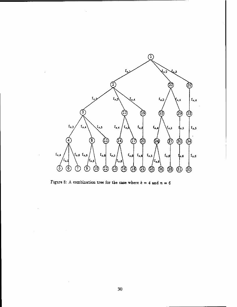
Figure 8: A combination tree for the case where k = 4 and n = 6

30

Table 1: Function BB(k,q,z): branch-and-bound algorithm for solving problem V\

01 Initialize the queue to be empty; 02 Insert root node vo ioto the queue; 03 While the queue is not empty do begin 04 Remove the first node v. from the queue; 05 Generate all child nodes of u ; 06 For each generated child node v do begin 0" If v is a leaf node (i.e. v is at level k) then OS Compute g{v) by setting L to be <p ; 09 Set i = min ( f, g(v)); 10 else begin /* v is an intermediate node */ 11 Compute est(v) by (5) ; 12 If est(v) < i then 13 Insert v into the queue according to est(v) ; 14 end; 15 end; 16 end; 17 Return(f).

Table 2: Function OPT(C^'s, ei<p's): the optimal solution of MCRP-SP of type Tand when Cpi5's and eSjP's are given

01 Sort i^p's into a non-decreasing order by values of eäjP's ; 02 For q = 1 to n do begin 03 Let node v be a leaf node at level 1; 04 Set v to be t4,j and Jt to be 1; 05 Compute g(v) by setting L to be q> ; 06 Initialize £ to be g(v) ; 07 For k = 1 to n do 08 2=BB(k,q,z) ■ 09 Set c(g) = z ; 10 end; 11 Output the combination with the minimum value among c(l), c(2),..., c(n).

31

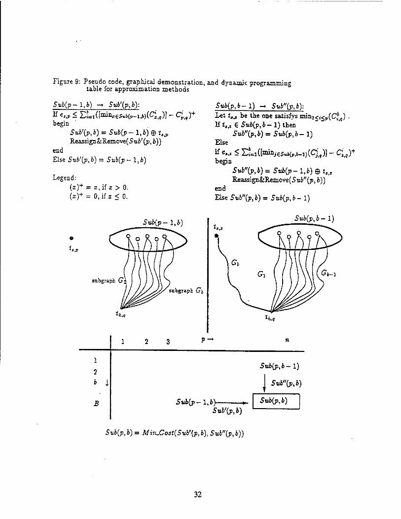
Figure 9: Pseudo code, graphical demonstration, and dynamic programming table for approximation methods

Sub{p-l,b) -» Svb'fab):

If C < n=i([miL.€s«Kp-u)(Ci,,)] - Cjt9)+ begin

5u6'(p,6) = Su6(p-l,6J©iaiP

Reassign&ILemove(5'u6'(p, b)) end Else 5u6'(p,6) = 5u6(p-l,6)

Legend: (z)+ = i, if x > 0. (i)+ = 0, if x < 0.

Sub{p,b-1) -» Stt6"(p,6): Let ttiI be the one satisfys mini<t-<p(C*g) . If 1,,» € Su6(p, 6-1) then

Su6"(p, 6) = S«6(p, 6-1) Else

if ew < ELI([mini€5ui(p,6-i)(q,9)] - £,,)+ begin

5ut"(p,6)=5«6(p-l,i)©ti,2

Reassign&Remove(Su6"(p, 6)) end ElseSti6"(p,6)=Su6(p,6-l)

*>p

5u6(p-l,6)

snbgra.pt G

1

2

i 1

B

subgraph Gb

?->

Svb(p- 1,6> Sttffr,*)

Su6(p, 6) = Min.Cost(Svb\p, 6), Su6"(p, 6))

Sii6(p,6-1)

Su6(p,6-1)

J S«6"(p,6)

Su6(p,6)

32

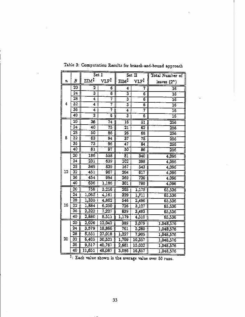
Table 3: Computation Results for branch-and-bound approach

n B

Set I

EIM* VLF*

Setll

EIM* VLF* Total Number of

leaves (2n)

4

20 2 6 4 7 16 24 3 6 3 6 16 28 4 7 3 6 16 32 4 7 3 6 16 36 4 7 4 7 16 40 3 6 3 6 16

8

20 36 74 16 51 256 24 40 75 21 62 256 28 50 86 26 68 256 32 63 94 37 78 256 36 73 96 47 84 256 40 81 97 50 86 256

12

20 186 558 81 340 4,096 24 231 639 102 398 4,096 28 349 839 167 543 4,096 32 | 451 967 204 617 4,096 36 454 984 269 720 4.096 40 | 636 1,186 301 780 4,096

16

20 | 758 3,216 203 1,175 65,536 24 | 1,065 4,161 329 1,711 65,536 28 | 1,335 4,862 546 2,496 65,536 32 1,884 6,250 726 3,127 65.536 36 2,322 7^227 839 3,493 65,536 40 | 2,880 8,511 1,179 4,510 65,536

20

20 2,026 12,042 389 3,079 1,048,576 24 3,579 18,866 761 5,280 1,048,576 28 5*,551 27,018 1,227 7,905 1,048,576 32 6,405 30,521 1,709 10,357 1,048,576 36 9,517 40,767 2,681 15,032 1,048,576 40 11,651 48,087 3,086 16,857 1,048,576

!:£a ,ch value shown is the aver age value over 50 runs.

33

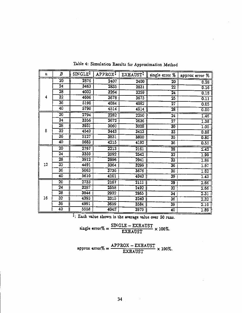
Table 4: Simulation Results for Approximation Method

n B SINGLE* APPROX* EXHAUST* 1 single error % approx error %

4

20 2876 2407 2400 I 20 0.28 24 3463 2835 2831 22 0.16 28 4032 3264 3259 24 0.18 32 4606 3678 3673 25 0.11 36 5198 4084 4082 27 0.05 40 5790 4514 4514 [ 28 0.00

8

20 2794 2282 2250 1 24 1.46 24 3356 2672 2636 1 27 1.38 28 3931 3060 3028 1 30 1.05 32 4540 3443 3413 33 0.88 36 5127 3831 3800 1 35 0.80 40 5683 4215 4192 1 36 0.55

12

20 2767 2213 2161 | 28 2.42 24 3359 2592 2542 1 32 1.99 28 3912 2996 2941 | 33 1.88 32 4491 3364 3299 | 36 1.97 36 5063 3736 3676 | 38 1.62 40 5610 4101 4043 I 39 1.43

16

20 2733 2167 2111 1 29 2.66 24 3287 2558 2492 32 2.66 28 3844 2932 2865 34 2.31 32 4393 3315 3240 36 2.32 36 4991 3659 3584 39 2.10 40 | 5558 4045 3970 40 1.89

+ : Each value shown is the average value over 50 runs.

. . -. SINGLE-EXHAUST sxngle error% = g^^ x 100%.

approx error% = APPROX - EXHAUST EXHAUST

x 100%.

34

Table 5: Algorithm FIND(SX): the algorithm for finding the shortest path combinations from the lamb which corresponds to the subtree Sx induced by an intermediate node x and all I'S descendant nodes in a parsing tree

01 Case of the type of intermediate node x: 02 TypeTcfc.,-« = 03 For b = the first child node of x to the last one do 04 FIND(Si,)\ I* Now the limb corresponding to Sb is replaced */ 05 Replace the limb corresponding to Sx with a two-layer T^*. limb where 06 the source (sink) layer of the old limb is the source (sink) layer of new 2-layer limb; 07 Put weights on the edges between source and sink layers equal to the shortest path 08 between the corresponding nodes; 09 10 Type Tand : /* Let x = [ Tand, forker s, joiner h } */ 11 Let d be the predecessor of forker 5 in G (i.e. < d,s > € V); 12 Let B be the number of child nodes of x in the parsing tree; 13 /* I.e. there are B subgraphs connected by s and h */ 14 For b = the first child node of x to the 2?-th child of x do 15 FIND(Si)\ I* Now the limb corresponding to Si is replaced */ 16 For p = 1 to 7i, 5 = 1 to R and b = 1 to B do 17 Compute the minimum replication cost C* from tttT to U,, w.r.t. child b : 18 For i = 1 to Ti do begin 19 For p = 1 to n do E,j = fidAhP) + e>,v \ 20 /* ESj> accounts for initialization by tri,,- and execution cost itself. */ 21 For g = 1 to R do w.k(», q) = OPT(C* ,'*,£„'*) ; 22 /* Create new edges from l^.-'s to i^'s */ 23 end; 24 Replace the Tani; limb with a run;r limb, where source layer = sink layer = layer h, 25 and there are new edges from laver d to layer n; 26 27 Type T„ : /* Let x = [ TV, forker s, joiner h ) */ 28 Use the same method described above from lines 12 to 17 to compute Cb 's ; 29 Replace the 2V limb with a two-layer TV™ limb, where 30 the source (sink) layer of TV limb is the source (sink) layer of TVotn limb and 31 /*.,*(*>,q) = min^C^), V p and 9 ; 32 end case; 33 Save the shortest paths between any node in source layer and any node

in sink layer for future reference.

35

(c) (d) (.)

Figure 10. A grapnical demostration of how to find an optimal solution for MCPJP-SP

36

REPORT DOCUMENTATION PAGE form Approved

OMB Ho 0704-0188

•wow •TDO'I'-C ow'3?* 'o* t*<\ r»r<i'0*» :• "»T*—*:o' vi.^**rc *D »••'»of ' -w :*•* "rwxy«, ."c:cO"^t; t*«r t»«*f 'c if^fw^ >nt:'wOity>v >c»fCit">.Q r-'ti"*9 CM* *>»/»<cv «~C '-..*•-. — - ••.- -^.^n.e" '■' '— ?.-.»•.<« >».»»o <*>—*•—•».•». '•»OA'O'ftQ l*»<\ Dwrot-n rM»~»*»t O« *nv off «»DCO Ot IIMv

" * - V V---.Ü-—•»! .»-0 SoCTf »»CT'-O" «fOytMO' ►•Oiftl lOEW-O'tS) %»*««>..f.OIO>\ DC SZiOi

1. AGENCY USE ONLY [LeJ"t blinK} 2. REPORT DATE

10/12/94 3. REPORT TYPE AND DATES COVERED

Technical 4. TITLE AND SUBTITLE

Optimal Replication of Series-Parallel Graphs for Computation-Intensive Applications , T, Revised version

6. AUTHOR(S)

Sheng-Tzong Cheng and Ashok K. Agrawala

S. FUNDING NUMBERS

N00014-91-C-0195 DASG-60-92-C-0055

7. PERFORMING ORGANIZATION NAME(S) AND ADDRESS(ES)

Department of Computer Science A. V. Williams Building University of Maryland College Park, MD 20742

8. PERFORMING ORGANIZATION REPORT NUMBER

Revised Version CS-TR-3020.1

UMIACS-TR-93-4.1

9. SPONSORING/MONITORING AGENCY NAME(S) AND ADDRESS(ES)

Honeywell, Inc. 3600 Technology Drive Minneapolis, MN 55418

Phillips Laboratory Directorate of Contracting 3651 Lowry Avenue SE Kirtland AFB NM 87117-5777

10. SPONSORING/MONITORING AGENCY REPORT NUMBER

11. SUPPLEMENTARY NOTES

This version supercedes the previous version.

12a. DISTRIBUTION/AVAILABILITY STATEMENT 12b. DISTRIBUTION CODE

13. ABSTRACT (MBxtmurr. 200v*>orcs)

We consider the replication problem of series-parallel(SP) task graphs where each task may run on more than one processor. The objective of the problem is to minimize the total cost of task execution and interprocessor communication. We call it, the minimum cost replication problem for SP graphs (MCRP-SP). In this paper, we adopt a new communication model where the purpose of replication is to reduce the total cost. The class of applications we consider is computation-intensive applicati in which the execution cost of a task is greater than its communication cost. The complexity of MCRP-SP for such applications is proved to be KP-complete. We present a branch-and-bound method to find an optimal solution as well as an approximation approach for suboptimal solution. The numerical results show that such replication may lead to a lower cost than the optimal assignment problem (in which each task is assigned to only one processor) does. The proposed optimal solution has the complexiv of 0(n 2 M), while the approximation solution has 0(r.4 K2), where n is the number of processors in the system and M is the number of tasks in the graph.

SUBJECT TERMS Operating Systems

Storage Management, Communications Management

15. NUMBER OF PAGES

35 pages 16. PRICE CODE

17. SECURITY CLASSIFICATION OF REPORT

Unclasssified

18. SECURITY CLASSIFICATION OF THIS PAGE

Unclassified

!S. SECURITY CLASSIFICATION OF ABSTRACT

Unclassified

20. LIMITATION OF ABSTRACT

Unlimited

>:St* 75-:O-O--2SO-5S00 37 V.?.r-da'd -o'n J96 Sev ?-89)

Designing Temporal Controls *j

Ashok K. Agrawala Seonho Choi Leyuan Shi Institute for Advanced Computer Studies Department of Industrial Engineering

Department of Computer Science University of Wisconsin University of Maryland Madison, WI 53706 College Park, MD 20742 [email protected]

{agrawala. seonho}@cs.umd.edu

Abstract

Traditional control systems have been designed to exercise control at regularly spaced time instants. When a discrete version of the system dynamics is used, a constant sampling interval is assumed and a new control value is calculated and exercised at each time instant. In this paper we formulate a new control scheme, temporal control, in which we not only calculate the control value but also decide the time instants when the new values are to be used. Taking a discrete, linear, time-invariant system, and a cost function which reflects a cost for computation of the control values, as an example, we show the feasibility of using this scheme. We formulate the temporal control scheme as a feedback scheme and, through a numerical example, demonstrate the significant reduction in cost through the use of temporal control.

'This work is supported in part by ONR and DARPA under contract N00014-91-C-0195 to Honeywell and Com- puter Science Department at the university of Maryland. The views, opinions, and/or findings contained in this report are those of the author(s) and should not be interpreted as representing the official policies, either expressed or implied, of the Defense Advanced Research Projects Agency, ONR, the U.S. Government or Honeywell. Computer facilities were provided in part by NSF grant CCR-6811954.

'This work is supported in part by ARPA and Philips Labs under contract DASG-60-92-C-0055 to Department of Computer Science, University of Maryland. The views, opinions, and/or findings contained in this report are those of the author(s) and should not be interpreted as representing the official policies, either expressed or implied, of the Advanced Research Projects Agency, PL, or the U.S. Government.

39

1 Introduction

Control systems have been used for the control of dynamic systems by generating and exercising

control signals. Traditional approach for feedback controls has been to define the control signals,

u(i), as a function of the current state of the system, x(t). As the state of the system changes

continuously the controls change continuously, i.e. they are defined as functions of time, t, such

that time is treated as a continuous variable. When computers are used for implementing the

control systems, due to the discrete nature of computations, time is treated as a discrete variable

obtained by regularly spaced sampling of the time axis at A seconds. Many standard control

formulations are defined for the discrete version of the system, with system dynamics expressed at

discrete time instants. In these formulations the system dynamics and the control are expressed as

sequences, x(k) and u(k).

Most of the traditional control systems were designed for dedicated controllers which had only

one function, to accept the state values, x(k) and generate the control, u(k). However, when a

general purpose computer is used as a controller, it has the capabilities, and may, therefore, be

used for other functions. Thus, it may be desirable to take into account the cost of computations

and consider control laws which do not compute the new value of the control at every instant.

When no control is to be exercised, the computer may be used for other functions. In this paper

we formulate such a control law and show how it can be used for control of systems, achieving the

same degree of control as traditional control systems while reducing computation costs by changing

the control at a few, specific time instants. We term this temporal control.

To the best of our knowledge this approach to the design and implementation of controls has not

been studied in the past. However, taking computation time delay into consideration for real-time

computer control has been studied in several research papers [1, 5, 6, 9, 11, 13]. But, all of these

papers concentrated on examining computation time delay effects and compensating them while

maintaining the assumption of exercising controls at regularly spaced time instants.

The basic idea of temporal control is to determine not only the values for u but also the time

instants at which the values are to be calculated and changed. The control values are assumed

to remain constant between changes. By exercising control over the time instants of changes the

designer has an additional degree of freedom for optimization. In this paper we present the idea and

demonstrate its feasibility through an example using a discrete, linear, and time invariant system.

Clearly, the same idea can be extended to continuous time as well as non-linear system.

The paper is organized as follows. In Section 2, we formulate the temporal control problem and

introduce computation cost into performance index function. The solution approach for temporal

control scheme is discussed in Section 3. In Section 4, implementation issues are addressed. We

40

provide an example of controlling rigid body satellite in Section 5 . In this example, an optimal

temporal controller is designed. Results show that the temporal control approach performs better

than the traditional sampled data control approach with the same number of control exercises.

Section 6 deals with the application of temporal controls to the design of real-time control systems.

Finally, Section 7, we present our conclusions.

2 Problem Formulation

In temporal control, the number of control changes and their exercising time instants within the

controlling interval [0, Tj] is decided to minimize a cost function. To formulate the temporal control

problem for a discrete, linear time-invariant system, we first discretize the time interval [0, Tj] into

M subintervals of length A = Tj/M. Let DM = {0, A, 2A,..., (M - 1)A} which denote M time

instants which are regularly spaced. Here, control exercising time instants are restricted within

DM for the purpose of simplicity. The linear time-invariant controlled process is described by the

difference equation:

x(k + l) = Ax(k) + Bu(k) (1)

y(k) = Cx(k)

where k is the time index. One unit of time represents the subinterval A, whereas x £ fcn and

u £7Z' are the state and input vectors respectively.

It is well known that there exists an optimal control law [4]

u°(i) = f[x(i)} £ = 0,1,...,M-1 (2)

that minimizes the quadratic performance index function (Cost)

JM= J2 \xT(k)Qx(k) + uT(k)Ru(k)) + xT(M)Ox(M) (3)

where Q £ %nxn is positive semi-definite and R £ Tllxl is positive definite.

As we can see, traditional controller exercises control at every time instant in DM- However,

in temporal control, we are no longer constrained to exercise control at every time instant in DM.

Therefore, we want to find an optimal control law, 6 and g for i = 0,1, ....M - 1:

u°(i) = u°(i-l) ifS(i) = 0 (4)

u°(i) = g[x(i)} if 8(i) = 1

41

that minimizes a new performance index function

A/-1 M-l JM = Y,[xT(k)Qx(k) + vT(k)Ru(k)) + zT{M)Qx(M)+Y,6(k)v (5)

= JM + CM

Mere, ft ** the computation cost of getting a new control value at a time instant, and CM =

Yfk=o f>[k)n~ denotes th« total Computation cost Kote that v = Y%~Q ^('0 is tiie number of

control changes. Also, let D„ = {*o»*i > *2> • • • > **-i} consist of control changing time instants where

*o = 0, i\ = njA, ..., 2„_i = n„_)A. That is, no,^,^,.. .,n„_i are the indices for control

changing time instants and 6{ni) = 1 for i = 0,1,2,.. .u — 1.

With this new setting we need to choose u, £„, and control input values to find an optimal

controller which minimizes JM. This new cost function is different from JM in two aspects. First,

the concept of computational cost is introduced in j'M as CM term to regulate the number of control

changes chosen. If we do not take this computation cost into consideration v is likely to become

M. If computation cost is high (i.e., p has a large value) then v is likely to be small in order to

minimize the total cost function. Second, in temporal control, not only do we seek optimal control

law u(i(l)), but also the control exercising time instants and the number of control changes. In the

next section, we present in detail specific techniques for finding an optimal temporal control law.

3 Temporal Control

We develop a three-step procedure for finding an optimal temporal controller.

Step 1. Find an optimal control law given v and D„

Step 2. Find best D„ given v

Step 3. Find best u

First, ir. the following two subsections(3.1 and 3.2) we derive a temporal control law which

minimizes the cost function JM when Dv is given, i.e., both time instants and number of controls

are fixed. Since v and Dv are fixed we can use JM defined in ( 5) as a cost function instead of

JM. Secondly, assume that v is fixed but D» can vary. Then we present an algorithm in section

3.3 to find a D% such that JM (and JM) is minimized. Finally, we will vary v from 1 to vmax

to search an optimal D°u at which temporal control should be exercised. Section 3.4 presents this

iteration procedure. Section 3.5 explains how to incorporate terminal state constraints into the

above procedure of getting an optimal temporal control law. And a complete algorithm of the

42

above procedure is described in Section 3.6. Finally, in Section 3.7 we explain how to get optimal

temporal controllers over an initial state space.

3.1 Closed-loop Temporal Control with Du Gi ven

Assume that „ and Dv are given. Then a new control input calculated at i,- will be applied to the

actuator for the next time interval from t{ to ti+l. Our objective here is to determine the optimal control law

u°(ni) = g[x(ni)} i = 0,l,...,i/-l

that minimizes the quadratic performance index function (Cost) JM which is defined in ( 5).

State Cost

(6)

1 2 3

Control Input Cost

m+]

5* Fv.,

n D +1... n -1 y-a vis VH».r

"(a.-) u(n ,)

Figure 1: Decomposition of JM into F;.

—— time

, The principle of optimally, developed by Richard Bellman[2, 3] is the approach used here. That

is, if a closed loop control «•>(«,■) = 5[z(n,-)] is optimal over the interval t0 < t < t„, then it is also

optimal over any sub-interval tm < t < *„, where 0 < m < v. As it can be seen from Figure 1, the

43

total cost JM can be decomposed into F,-s for 0 < i < v where

Fi = xT(ni)Qx(n{) + xT(ni + l)Qx{ni + l) (7)

+ xT(ni + 2)Qx(ni + 2) + ... + ir(n1+1 - l)Qx(n,+1 - 1)

+ (n,+1 - n,)ur(n,-)Äu(nt)

That is-, from ( 1),

Fi = xT{ni)Qx(n;)^(Ax{ni) + Bu(ni))TQ(Ax(ni) + Bu{Tii)) (8)

+ (A7x{ni) + ABu(ni) + 5u(n,-))TQ(A2x(nl-) -f ABu(n{) + Bu{m))

+ ... + (yln,'+1 -"'-^(n,-) + An,+,-n'-25u(nI-) + ... + ABu(n.-) + Bu(ni))TQ

(An-^-n<-lx{n,) + i4n'"+1-B,'-2Bu(7i1-) + ... + ABu(n,-) + Ju(n,-))

+ (nt-j.j - ni)v.T(ni)Ru(ni)

This can be rewritten as

n;+j—n,-—1

fi = aT(ni)Qi(nf) + ]£ [A;x(nO + 5;«(nO)TQ[4is(nO+ £;«(T^)] (9)

+ (n,-+i - n,-)uT(n,-)Äu(n,-)

where .4, = ^ and ^ = ££* AkB.

Then Jw can be expressed as

JM = FO + F, + F7 + ... + F„. (10)

Let 5m be the cost from : = v - m -j- 1 to :' = v.

Sm = Fu-m+1 + fUrn+2 + - + P,-l "f Fv, 1 < m < V + 1. (11)

These cost terms are well illustrated in the above Figure 1.

Therefore, by applying the principle of optimality, we can first minimize S\ — Fu, then choose

Fu-\ to minimize S? = .F„_i -r Fv = S° -f F„_i where S\ is the optimal cost occurred at V We

can continue choosing -F„_2 to minimize Sz — F„_2 -r Fi,_i -r F„ = -F„_2 -f Sf ajid so on until

5„+1 = JM is minimized. Note that 5j = F„ = x7 {nJ)Qx{n„) is determined only from x{nv) which

is independent of any other control inputs.

44

3.2 Inductive Construction of an Optimal Control Law with Dv Given

We inductively derive an optimal controller which changes its control at „ time instants l0ih

■ ■ , t„-i. As we showed in the previous section, the inductive procedure goes backwards in time

from S! to S^. Since S> = Fu = x^(n„)Qx(n.) + v?(nu)RuM and *(»„) is independent of

«(»„), we can let «•(„„) = U°(M) = 0 and <?? = ^(n.)0«(„„) where Q is symmetric and positive semi-definite.

Induction Basis: Sf = xT{nu)Qx{nu) where Q is symmetric.

Inductive Assumption: Suppose that

S°m = xT(nv_m+1 )P(V _ m + l)s(nj/_ra+1)

holds for some m where 1 < m < * and P{y - m + 1) is symmetric.

We can write Si as m

From the definition of Sm and ( 9),

'-'"i-i-l = JTn T i:u—m

-i- K-m+i - n„_m )ur(n„_m )£«(»„_,„)

And the above equation becomes

£»+1 = [i^n+!-wl(vm) + 5r._+5_^_rnti(7it,_T7l)]rP(I, _ TO + 1)

l^n1/_>7)+J-nl._m2(Tl1/_jn) + -Bni/_m+3 _^_m li(Tlx/_m)] 7* 1 (^-m)Qs(^-m)

-f (n^-w+i -7i„_m)ti:r(7it,_r7,)Äti(nJ/_77;)

(12)

(13)

(14)

45

If we differentiate Sm-H with respect to u(n1/_Tn), then

' 0 U YTl J- 1 T"

Qu(nu'_m) = 57l"-">+i-"— P^~ m+l)Ar.—+1-n,_mi(n1/_m) (15)

+ Uj,_m+1 _n„_m P(i/ - m + l)£„„_m+1 _n,_m )rx(nI/_TB)

+ 2Bj>_TO+1_nB_mP(1/ - m+ l)5n„.m+1-n.,_m«(nv_m)

+ J2 [2BJQAjx(nu_m)^2BJQBju(n^m)}

+ 2(n„_T7l+a - 7zJ/_m)Au(n1/_Tn)

2{^_m+J_ni/_fBP(v - m + l)An_+]_n_m (16)

+ E PjQAj}I(nl/_m)

+ 1{Blu_n„_nv_nP{v - m + l)Pn_+]_ni/_m

+ 5Z BJQBj + (1I/-TT>+I - ^i/-m)Ä}ii(nI/_m)

Note that P(f - m + 1) is symmetric and the following three rules are applied to differentiate Sm+j

above.

j^{*TQx) = 2Qx

|"(xrQ3/) = Qy ox

■fy(*TQy) = cT-

Let , , """• . = 0. from Lemma 1 and Lemma 2 given later we can obtain u°(ni/_Tr) which

minimizes Sm+i aBd thus obtain S^+i-

where K{y - m) is defined in ( 17).

46

(18)

(19)

Therefore, we can write

An„.m„ -n„_m x(n„_m) + 5n„_m+J _n_m u°(nu_m) =

l^ul/_m+]-„1/_m - 5^_m+j_n„_mA'(i/ - m)]i(n1/_Tn)

If we use ( 17) and ( 18), we have

Sm+\ = {[^n„_m4,-n|/_m - ^nu_m^-n^mK(^-m)]x(nl/_m)}TP(l/-mJrl)

{lj4n1/_m+,-n„_in - •ßn„_m+i-„1/_mÄ'(l/ - 77l)]x(n1/_rri)}

+ xT(nu_m)Qx(n^m) n„_m+j —n„_m —]

+ E ^^--BJir(^-m)^(^-m)}:rC?{[Ai-£Jür(1/-m)]x(n1,_m)}

+ (n^^+j - nu_m)\K(v - m)x(nl/_m))TR[K(u - m)x(nu_m)]

This equation can be rewritten as

£m+i = :rTK-m){[AIll/_7n4]_n_m-£Tlj/_m+i_n>/_m^(j/-m)fp(I/_m+1) (20)

[^•n1/_m+i-7i^_tn - £n„_m+]_ni,_mÄr(^ - m)]

+ Q Tit,—m+J — 1*—m — 1

+ E [Aj - B5K{v - m)]TQ[Aj - B5K{v - m)} i=i

+ (n„-m+i - nu„m)KT{nv-m)RK(v - m)}x{nv_m).

^T{nu-m)P{u-m)x{n^m)

where P(„ - m) is obtained from K{v - m) and P{u - m + 1) as in ( 20). Also note that knowing

P{v - m + 1) is enough to compute K{y - m) because other terms of ( 17) are known a priori. °

Therefore, we find a symmetric matrix P(i/-m) satisfying 5^+1 = xr(nJ/_TO)P(1/-m)z(n1/_m).

From ( 17) and ( 20), we have the following recursive equations for obtaining P(„ - m) from P{v -771+1) where m = 1,2,..., ^.

K(V - m) = {i?J J>(V - 77! 4. IIP ?T _.. ... . ,,„ (21)

"K-U+I —«i/—rr. — 1

+ £ -ßf^- + («,_„+! -»„.„JA}-1

j- nx—T»41 —1i/—rr. —1

i^-^-n^-P^ - m + l)^_m+1_n„_m + J2 BjQAj)

47

P(u-m) = lAn„_n+i-n„_m-Bn„_m»-nv_mK{»-m))TP{»-m+l) (22)

{An„_m+l-n„-m - Bnv_m+l-nu_mK{v - rri))

+ Q

Y: [Aj-BjK^-m))7

3 — 1-

+ (n„_m+i - nv-m)KT(y - m)RK(v - m)

^ \Aj - BjK(v - m))TQ{A5 - BsK(u - m)} 3 — 1-

It

Also, we know that at each time instant n„_mA

u°(n1/_m) = -K{v - m)i(n1/_m) (23)

Hence, with P{y) - Q, we can obtain K(i) and P(i) for i = v - l,i/- 2,...,0 recursively using

( 21) and ( 22). At each time instant n,-A, i = 0,1,2, ...,v - 1 the new control input value will be

obtained using ( 23) by multiplying K(i) by x(n,-) where s(n,-) is the estimate of the system state

at n,-A. Also, note that the optimal control cost is J°M = 5°+1 = xr(0)P(0)x(0) where P(0) is

found from the above procedure.

To prove the optimality of this control law we need the following lemmas.

Lemma 1 IfQ is positive semi-definite and R is positive definite, then P(i), i = v. v—1. v—2..... 0,

matrices are positive semi-definite. Hence. P(i)s are symmetric from the definition of a positive

semi-definite matrix.

Proof Since P{y) = Q , from assumption P(v) is positive semi-definite. Assume that for

it = i 4- 1, P(k) is positive semi-definite. We use induction to prove that P(i) is semi-definite. Note

that Q is positive semi-definite and R is positive definite. From ( 22) we have

PC») = [An,+J_„,-£n,.+5_n,.ir(ofp(; + i) (24)

[ABl.+1_n,.-5Ri.+1_B,.Jir(0]

+ Q

+ '+:JZ [AS - BsK(i)}TQ[As - S:K(i)}

+ (n,-+a - m)KT(i)RK{i)

48

Since P(i + 1) and Q are positive semi-definite, R is positive definite, and (n,-^ - «,-) > 0, it is easy to verify that for Vy £ £« : yrp(£)y > 0 This means that p{.} .g positive ^.^^

This inductive procedure proves the lemma.

Lemma 2 Giuen DU) the inverse matrix in ( 21) always exists.

Proof Let V = J3? Pd>-m+l)B , vn„.m+,-ni,.m-] T

(n1/_m+1 - n„_m)Ä. From Lemma 1, P(i/-m + 1) is positive semi-definite. Therefore, Vy £ Rm :

t/TV'2/ > 0 because Q is positive semi-definite, R is positive definite and n„_m+1 - n„_m > 0. This

implies that V is positive definite. Hence the inverse matrix exists.

Theorem 1 Given D„, K{i) (i = 0,1,2, ...,v-l) obtained from the above procedure are the optimal

feedback gains which minimize the cost function JM (and j'M) on [0,MA].

Proof Note that given D„, JM is a convex function of u{n{), i = 0,1,..., v - 1. Thus the

above feedback control law is optimal.

Lemma 3 If p < q and Dv C Dq , then J^ > J^ where J°Mp and J^ are the optimal costs of

controls which change controls at time instants in Dp and Dg respectively.

Proof Suppose that J°Mj> < J^, then, in controlling the system with Dq, if we do not

change controls at time instants in Dg - Dp and change controls at time instants in Dp to the same

control inputs that were exercised to get J^ with Dv, we obtain jMq which is equal to J°Mp. This

contradicts the fact that J^ is the minimum cost obtainable with D„ since we have found JMq

which is equal to J°M and therefore less than J°M . Hence, Jt, > J%{

This lemma implies that if we do not take computation cost, fi, into consideration, then the

more control exercising points, the better the controller is (less cost). With the computation cost

being included in the cost function, the statement above is no longer true. Therefore we need to

search for an optimal Dv which minimizes the cost function fM. The following sections provide a

detailed discussion on searching for such an optimal solution. Note that if we let Dv = DM then

the optimal temporal control law is the same as the traditional linear feedback optimal control law.

49

3.3 Optimal Temporal Control Law over D„ Space with v Given

When the number of control changing points, v, and an initial system state x(0) are given, we

search over a set of possible Dus and u(D„)s such that the cost function JM is minimized. This

can be done by varying v — 1 control changing time instants, i,-, i = 1,2,...,^ — 1 (since to — 0)

over the discrete set, DM = {0, A,2A,..., (M - 1)A} and applying the technique developed in the

previous section for each given Dv. Let us denote such a Du which minimizes JM as D°v. Note

that when v is given, minimizing JM is equivalent to minimizing JM. Since both Dv and v.(Du)

are control variates, to be able to find a global optimal solution, either an exhaustive search or

some global search methods like Genetic Algorithm or Simulated Annealing should be considered.

taicrWC-pi^sen* * numerical «xa-rapk. in which an exhaustive search with Steepest Descent Search

method is used. Searching for a globally optimal solution for a temporal controller calls for further

research.

3.4 Optimal Temporal Control Law

Assume that a maximum number of control changing points, i/max, is given. By varying v from

1 to vma~ we can find D°u. to obtain a globally optimal temporal controller which minimizes JM.

This can be done by first searching for D°v for each given v and then comparing the cost function

J'M = JM + VV- at eadl Dli v = M,...,z/mcr. That is, let JJ£„-= xr(0)P(0)x(0) + V/J. where

P(0) is calculated at D°v as in the previous section. Then we can obtain a global minimum cost

fM = mini<„<imar{7]i|x/} and an optimal number of control changes, v°. at which JMVC — ^M-

3.5 Terminal State Constraints

The terminal state constraints may be used to check if the optimal temporal controller with D°.

can drive the system state to a permissible final state within a given time. Let Xj be a set of

allowed terminal states, if x(n„) € Xj, then the control law is said to be stable in terms of the

terminal state constraints and not siable if x(7i„) £ Xj. If the globally optimal temporal controller

obtained from the above procedure is not stable, v" should be increased until a stable one is found.

One way of specifying terminal state constraints for regulators might be | x[M\ |< £,- where x{M)i

is the :th element of x(M) state vector.

50

3.6 Algorithm to Derive an Optimal Temporal Controll er

To summarize the above discussion, we provide in Figure-2 a complete algorithm to search for

globally optimal temporal controller under the assumption that the initial state x(0) is gi\ wen.

In the algorithm, a neighbor of D„ = {n0A, nx A, n2A,..., n„_. A} is defined to be any member

ofaset^(I?J/) = {{7i;A,n'1A,...,^_1A}| \n{-m\< 1, i = 1,2,. ..,„ - 1}.

3.7 Optimal Temporal Controllers over an Initial State Space

Note that D°v might become different if a new initial system state x(0) is used instead of i(0) when

the state vector is in PmXl where m > 2. This is because the cost function JM = zT(0)P(0)i(0)

depends on z(0) as well as P(0). Thus, D° is dependent on the initial state z(0). However, when

m = 1 it can be shown that D°v is independent of any initial state. To see this let x(0) = H(0) € ft1

and P(0) and P(0) be the optimal matrices with initial states x(0) and i(0), respectively, i.e.,

JM(x{0)) = x(0)P(0)z(0)

•Mi(0))=x(0)P(0)£(0)

From the optimality of P(0) with respect to z(0),

ir(0)P(0)f(0) > zr(0)P(0)f(0) (25)

Multiplying the above inequality by k2 we have

fc2sr(0)P(0)i(0) = ir(0)P(0)x(0)

> *2xr(0)P(0)£(0)

= zr(0)P(0)z(0) (26)

On the other hand, due to the optimality of P(0) we have

*T(0)P(0)x(0) > xr(0)P(0)x(0) (27)

Therefore, P(0) = P(0). This implies the optimality of P(0) and D°v for any initial state z(0) e Tl\

Generally speaking, the above result will not hold for m > 2 cases. However, using the same

argument discussed above we can prove that for any initial state x(0) = H(0), x(0) and i(0) will

have the same D0» as well as the same P(0).

51

v°= 1

J'ä = cc.

for v = 1 to umax {

/* Several different search starting points */

for i = 1 to NumlnitPtSy {

Du = D™1*

I* Iterate until a local minimum is found - Steepest Descent Search */

while (MinimumFound != True) {

Find optima] costs for neighboring points of Du using theorem 1

if ( JM has a Local Minimum at Du)

then {

MinimumFound = True

J'itv = Cost(J^) at Du }

else

D„ = a neighbor of Du with the smallest j'M

}

}

then {

v° = v

}

Figure 2: Complete algorithm to find an optimal temporal controller.

52

4 Implementation

To implement temporal control, we need to calculate and store K(i) matrices in ( 22) and use them

when controlling the system utilizing ( 23). Note that in traditional optimal linear control a similar

matrix is obtained and used at every time instant in DM to generate control input value. While

the feedback gain matrices for traditional linear optimal controller are independent of initial states,

the number of control exercises, «/, and A'(t) matrices are dependent on initial states for temporal

control systems. But, if the possible set of initial states is in ft1 they are independent of the initial

states. Effective deployment of temporal control requires that we know the range of initial state

values and generate K(i) matrices for each group. A sensitivity analysis is required to determine

how many distinct matrices need to be stored.

In order to implement temporal control we require an operating system that supports scheduling

control computations at specific time instants. The Maruti system developed at the university of

Maryland is a suitable host for the implementation of temporal control [10, 8, 7]. In Maruti, all

executions are scheduled in time and the time of execution can be modified dynamically, if so

desired. This is in contrast with traditional cyclic executives often used in real-time systems, which

have a fixed, cyclic operation and which are well suited only for the sampled data control systems

operating in a static environment. It is the availability of the system such as Maruti that allows

us to consider the notion of temporal control, in which time becomes an emergent property of the system.

5 Example

To illustrate the advantages of a temporal control scheme let us consider a simple example of rigid

body satellite control problem [12]. The system state equations are as follows:

VW =

0 1

-1 2 *(*) +

1 1 X (*)

0.00125 u(k)

where k represents the time index and one unit of time is the discretized subinterval of length

A = 0.05. The linear quadratic performance index fM in ( 5) is used here with the following parameters.

Q = i o 0 1

53

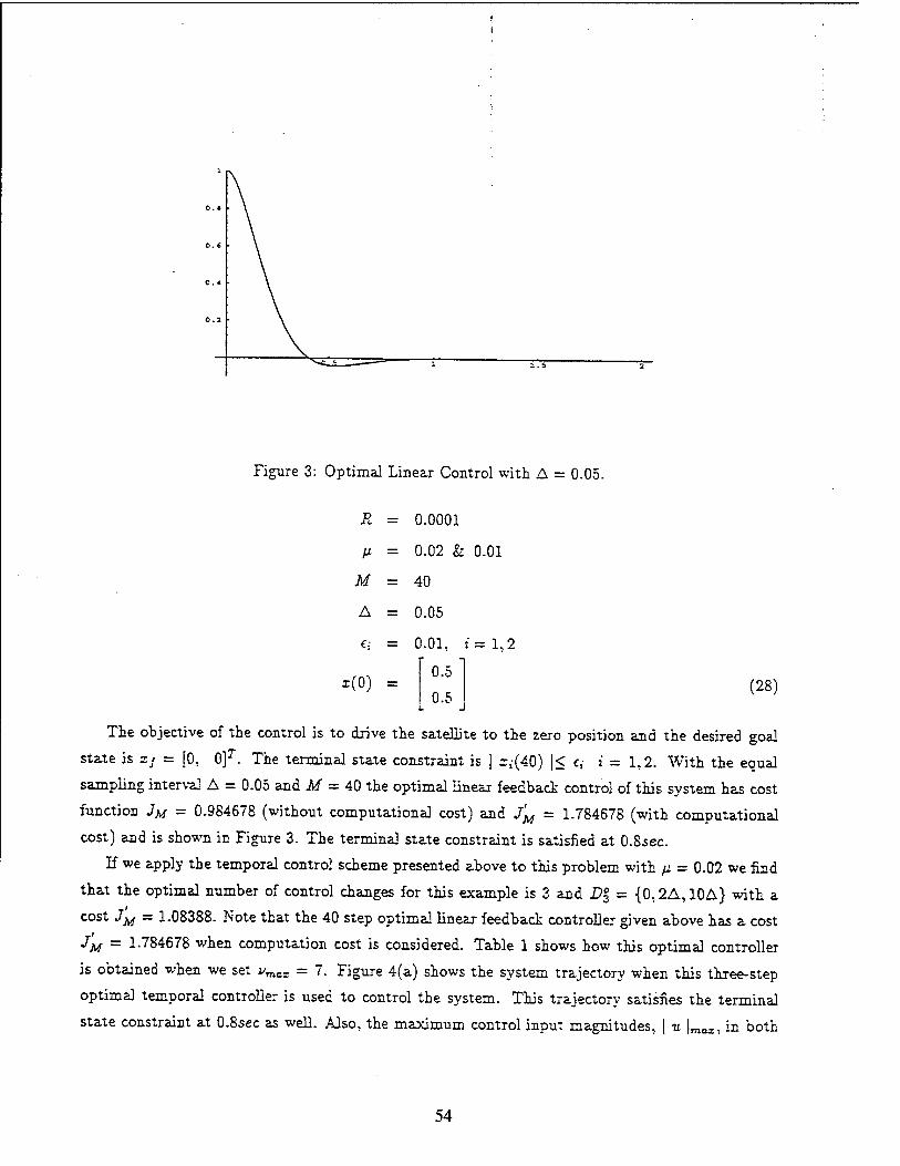
Figure 3: Optima] Linear Control with A = 0.05.

R

V-

M

A

s(0)

0.0001

0.02 & 0.01

40

0.05

0.01,

0.5

0.5

:= 1,2

(28)

The objective of the control is to drive the satellite to the zero position and the desired goal

state is xj = [0, 0]T. The terminal state constraint is | s,-(40) |< £,• i = 1,2. With the equal

sampling interval A = 0.05 and M = 40 the optimal linear feedback control of this system has cost

function JM = 0.984678 (without computational cost) and j'M = 1.784678 (with computational

cost) and is shown in Figure 3. The terminal state constraint is satisfied at O.Ssec.

If we apply the temporal control scheme presented above to this problem with p. = 0.02 we find

that the optimal number of control changes for this example is 3 and £>§ = {0,2A, 10A} with a

cost JM - 1.08388. Note that the 40 step optimal linear feedback controller given above has a cost

^M ~ 1-784678 when computation cost is considered. Table 1 shows how this optimal controller

is obtained when we set umc= = 7. Figure 4(a) shows the system trajectory when this three-step

optimal temporal controller is used to control the system. This trajectory satisfies the terminal

state constraint at 0.8sec as well. Also, the maximum control input magnitudes, | v. |mBI, in both

54

D° Cost(fM) with n = 0.02

{0}

{0,1}

{0,2,10}

{0,2,9,11}

{0,1,3,8,11}

{0,1,3,8,11,24}

{0,1,3,8,11,23,25}

4.630S9 + /2 = 4.65089

1.44603+ 2/2 = 1.48603

1.02388+ 3/2 = 1.08388

1.02224 + 4/2 = 1.10224

0.996968+5/x= 1.096968

0.996746+6//= 1.116746

0.996745+7/1= 1.136745

Cost(J^) with fx = 0.01

4.63089 + /! =

1.44603 + 2// =

1.02388 +3/2 =

1.02224 + 4/2 =

0.996968+5/2 =

0.996746+6/2 =

0.996745 + 7/2 =

4.64089

1.46603

1.05388

1.06224

1.046968

1.056746

1.066745

Table 1: Calculating optimal temporal controllers.

Controllers lie within the same bound B = 50, which may be another constraint on control.

The optimal temporal controller found with y. = 0.01 has v = 5 and D% = {0, A,3A,8A,11A}

with a cost JM = 0.996968. Note that this cost is even less than 1.01269 which is obtained from

the optimal controller with equal sampling period O.lsec and 20 control changes.

If we change control values only at three time instants with equal sampling period, 13M =

0.65.sec, the total cost incurred is 2.2823(without computational cost) on the time interval [0,2].

The cost is more than twice that of our optimal temporal controller and the terminal state constraint

is not satisfied even at the end of the controlling interval of 2.0sec. Figure 4(b) clearly shows the

advantages of using an optimal temporal controller over using an optimal controller of equidistant

samplings. Their performances are noticeably different though both of them are changing controls

at three time instants. It is clear that the optimal temporal control with three control changes

performs almost the same as 40 step linear optimal controller does. This implies that enforcing the

constant sampling rate throughout the entire controlling interval may simply waste computational

power which otherwise could be used for other concurrent controlling tasks in critical systems.

Obtaining D§ for this example was simple since J40 has only one minimum over the entire set

of possible D3s on [0,40A]. Figure 5(a) and Figure 5(b) show that J40 has only one local(global)

minimum at D\ = {0,2A, 10A}. We got this optimal D3 by doing steepest descent search with the

starting point Dfil = {0, A, 10A} after searching for only three points, {0, A, 10A}, {0,2A, 10A},

{0,3A, 10A}. Also, Figure 5(a) shows that choosing m has greater influence on the total cost than

n2 since the cost varies more radically along the n, axis in the figure. This means that the initial

stage of the control needs more attention than the later stage in this linear control problem.

But, if we change one of the parameters of performance index function, R, from 0.0001 to 0.001

we get two local minima at D\ = {0,A,2A} and D\ = {0,3A,19A}, among which D\ is the

55

(a)

(b)

Figure 4: Control trajectories with 3 control changes. (a)Optimal temporal control with U|

{0.2A, 10A}. (b)Optimal linear control with 13A (0.65sec) period.

56

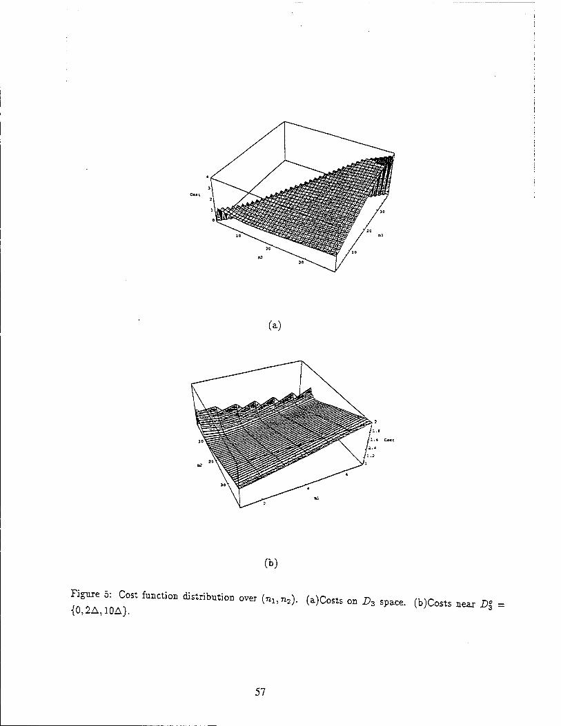
(a)

00

^2! 10AC°St fUnCti011 diStribUti°n °Ver (?ll'n2)- (a)C°StS 0D D* sPace" (b)Costs near D:

57

Figure 6: Costs near D\ and D\ with R = 0.001.

optimal one with less cost. Figure 6 shows this fact. In this case we need to use steepest descent

search method at least twice with different search starting points to get an optimal solution. We

implemented this steepest, descent search algorithm in Mathematica and used it to generate D°v for

several examples by varying v. For our examples of linear time invariant system control problems

the number of local minima was not so large that we could efficiently apply this search method

just a few times with different initial D^s to get a global minimum without doing an exhaustive

search over the entire D„ space.

6 Discussion

Employing the temporal control methodology in concurrent real-time embedded systems will have

a significant impact on the way computational resources are utilized by control tasks. A minimal

amount of control computations can be obtained for a given regulator by which we can achieve

almost the same control performance compared to that of traditional controller with equal sampling

period. This significantly reduces the CPU times for each controlling task and thus increases the

number of real-time control functions which can be accommodated concurrently in one embedded

system. Particularly, in a hierarchical control system if temporal controllers can be employed for

lower level controllers the higher level controllers will have a great degree of flexibility in managing

resource usages by adjusting computational requirements of each lower level controller. For example,

in emergency situations the higher level controller may force the lower level controDer to run as

58

infrequently as they possibly can (thus freeing computational resources for handling the emergency).

In contrast, during normal operations the temporal control tasks may run as necessary, and the

additional computation time can be used for higher level functions such as monitoring and planning, etc.

In addition, the method developed in Section 3.2, which calculates an optimal controller when

control changing time instants are given, can be applied to the case in which the control computing

time instants cannot be periodic. For example, when a small embedded controller is used to

control several functions, it may be a lot better to design a temporal controller for each function

such that the required computational resources are appropriately scheduled while retaining the

required degree of control for each function.

7 Conclusion

In this paper we proposed a temporal control technique based on a new cost function which takes

into account computational cost as well as state and input cost. In this scheme new control input

values are defined at time instants which are not necessarily regularly spaced. For the linear

control problem we showed that almost the same quality of control can be achieved while much less

computations are used than in a traditional controller.

The proposed formulation of temporal control is likely to have a significant impact on the

way concurrent embedded real-time systems are designed. In hierarchical control environment,

this approach is likely to result in designs which are significantly more efficient and flexible than

Traditional control schemes. As it uses less computational resources, the lower level temporal

controllers will make the resources available to the higher level controllers without compromising the quality of control.

References

[1] A. Belleisle. Stability of systems with nonlinear feedback through randomly time-varying

delays. IEEE Transactions on Automatic Control, AC-20:67-75, February 1975.

[2] R. Bellman. Adaptive Control Process: A Guided Tour. Princeton,NJ: Princeton University Press, 1961.

[3] P.. Bellman. Bellman special issue. IEEE Transactions on Automatic Control, AC-26, October 1981.

59

[4] P. Dorato and A. Levis. Optimal linear regulators: The discrete time case. IEEE Transactions

on Automatic Control, AC-16:613-620, December 1971.

[5] A. Gosiewski and A. Olbrot. The effect of feedback delays on the performance of multi variable

linear control systems. IEEE Transactions on Automatic Control, AC-25(4):729-734, August

1980.

[6] K. Hir'ai and Y. Satoh. Stability of a system with variable time delay. IEEE Transactions on

Automatic Control, AC-25(3):552-554, June 1980.

[7] S. T. Levi, Satish K. Tripathi, Scott Carson, and Ashok K. Agrawala. The MARUTI hard

real-time operating system. ACM Symp. on Op. Syst. Principles, Op. Syst. Review, 23(3),

July 1989.

[8] Shem-Tov Levi and Ashok K. Agrawala. Real Time System Design. McGraw Hill, 1990.

[9] Z. Rekasius. Stability of digital control with computer interruptions. IEEE Transactions on

Automatic Control, AC-31:356-359, April 1986.

[10] Manas Saksena, James da Silva, and Ashok K. Agrawala. Design and Implementation of

Maruti-II, chapter 4. Prentice Hall, 1995. In Advances in Real-Time Systems, edited by Sang

H. Son.

[11] K. G. Shin and H. Kim. Derivation and application of hard deadlines for real-time control

systems. IEEE Transactions on Systems. Man and Cybernetics, 22(6):1403-1413, November

1992.

[12] G.S. Virk. Digital Computer Control Systems, chapter 4. McGraw Hill, 1991.

[13] K. Zahr and C. Slivinsky. Delay in multivariable computer controlled linear systems. IEEE

Transactions on Automatic Control, pages 442-443, August 1974.

60

REPORT DOCUMENTATION PAGE form «s^o»M>

OMB Ho 07CK.018S

JJ

- >>c< ->•■>■)::■>. ,- :>:t: ■ >r '"»x r .'C*— 1-. .\ »^^01^ ir#OOu?'lr*i w*Kn l>*fOV#1f f'c 'MO"n*iien 0ofr*l(vw> «no kroonv, W1S #*T1*-<»©*»

V AGENCY USE ONLY (Lc^vr fiiin«; 2. REPORT DATE

July 1995

3. ■REPORT TYPE AND DATES COVERED

Technical Report 4. TITLE AND SUBTITLE

Designing Temporal Controls

6. AU.THOR(S)

Ashok K. Agrawala, Seonho Choi & Leyuan Shi

S. FUNDING NUMBERS

N000K-91-C-0195 and DSAG-60-92-C-0055


University of Maryland A.V. Williams Building College Park, Maryland 20742

PERFORMING ORGANIZATION REPORT NUMBER

CS-TR-3504 UMIACS-TR-95-81


Honeywell 3660 Technology Drive Minneapolis, MN 55418

Phillips Labs 3550 Aberdeen Ave. SE Kirtland AFB, NM

87117-5776



12a. DISTRIBUTION /AVAILABILITY STATEMENT 12b. DISTRIBUTION CODE

13. ABSTRACT (Maximum 200 vorci)

Traditional control systems have been designed to exercise control at regularly spaced time instants. When a discrete version of the system dynamics is used, s constant sampling interval is assumed and a new control value is calculated and exercised at each time instant. In this paper we formulate a new control scheme, temporal control, in which we not only calculate the control value but also decide time instants when the new values are to be used. Taking a discrete, linear, time- invariant system, and a cost function which reflects a cost for computation of the control values, as an example, we show the feasibility of using this scheme."We formulate the temporal control scheme as a feedback scheme and, through a numerical example, demonstrate the significant reduction in cost through the use of temporal control.

i*. SUE;ECT TERMS

Computing Methodologies

IN- SECURITY CLASSIFICATION j 16. SECURITY CLASSIFICATION O? REPORT

Unclassified OF THIS PAGE

Unclassified

IS. SECURITY CLASSIFICATION OF ABSTRACT

Unclassified

IS. NUMBER OF PAGES


20. LIMITATION OF ABSTRAC

Unlimited

.\-SN 7>c0-0i-;S0-S500 61

S-.jr-da'ö -orn :9S !Rev 2-89)

Scheduling an Overloaded Real-Time System *

Shyh-In Hwang, Chia-Mei Chen, and Ashok K. Agrawala

Institute for Advanced Computer Studies


University of Maryland, College Park, MD 20742

Abstract

The real-time systems differ from the conventional systems in that every task in the real-

time system has a timing constraint. Failure to execute the tasks under the timing constraints

may result in fatal errors. Sometimes, it may be impossible to execute all the tasks in the task

set under their timing constraints. Considering a system with limited resources, one solution

to handle the overload problem is to reject some of the tasks in order to generate a feasible

schedule for the rest. In this paper, we consider the problem of scheduling a set of tasks without

preemption in which each task is assigned criticality and weight. The goal is to generate an

optimal schedule such that all of the critical tasks are scheduled and then the non-critical tasks

are included so that the weight of rejected non-critical tasks is minimized. We consider the

problem of finding the optimal schedule in two steps. First, we select a permutation sequence

of the task set. Secondly, a pseudo-polynomial algorithm is proposed to generate an optimal

schedule for the permutation sequence. If the global optimal is desired, all permutation sequences

have to be considered. Instead, we propose to incorporate the simulated annealing technique to

deal with the large search space. Our experimental results show that our algorithm is able to

generate near optimal schedules for the task sets in most cases while considering only a limited

number of permutations.

'This work is supported in part by Honeywell under N00014-91-C-0195 and Army/Phillips under DASG-60-92-

C-0055. The views, opinions, and/or findings contained in this report are those of the author(s) and should not be

interpreted as representing the official policies, either expressed or implied, of Honeywell or Army/Phillips.

63

1 Introduction

Real-time computer systems are essential for all embedded applications, such as robot control, flight

control, and medical instrumentation. In such systems, the computer is required to support the

execution of applications in which the timing constraints of the tasks are specified by the physical

system being controlled. The correctness of the system depends on the temporal correctness as

well as the functional correctness of the tasks. Failure to satisfy the timing constraints can incur

fatal errors. How to schedule the tasks so that their timing constraints are met is crucial to the

proper operation of a real-time system.

As an example of an embedded system, let us consider the air defense system which monitors

an air space continuously using radars. Whenever an intruder is identified, the embedded control

system characterizes it and proceeds to initiate the responsive action in a timely manner. The

temporal constraints for this phase of processing are different depending on the intruder, whether

it is a missile, a fighter, a bomber, a dummy, etc. Such a system is designed to handle a number of

intruders concurrently. If the processing requests exceed the capacity of the system, we expect the

system to handle a set of the most significant intruders, and not any arbitrary set of intruders. This

involves rejecting the processing of some real-time tasks based on their importance. In this paper,

we consider the problem of creating a schedule for a set of tasks such that all critical tasks are

scheduled, and then, among the non-critical tasks we select those which can be scheduled feasibly

while maximizing the sum of the weights of selected non-critical tasks.

As all systems have finite resources, their ability to execute a set of tasks while meeting the

temporal requirements is limited. Clearly, overload conditions may arise if more tasks have to be

processed than the available set of resources can handle. Under such overload conditions, we have

two choices. We may augment the resources available, or reject some tasks (or both). In [8], a

technique was presented to handle transient overloads by taking advantage of redundant computing

resources. Another permissible solution to this problem is to reject some of the tasks in order to

generate a feasible schedule for the rest. Once a task is accepted by the system, the system should

be able to finish it under its timing constraint. Some algorithms may have been shown to perform

64

well under low or moderate resource utilization. However, their performance degrades if the system

is overloaded [2]. For example, the EDF algorithm has been shown to be optimal for a periodic task

set [6].. If there exists a feasible schedule for the task set, EDF can come up with one. However,

if the task set is not feasible, EDF may perform unsatisfactorily. The reason is that a task with

urgent deadline may not be able to finish before its deadline. But, due to its urgent deadline, the

task has a high priority to use the processor and thus keeps wasting the CPU time until the task

expires after its deadline. The waste of CPU time may further prevent other tasks from meeting

their deadlines. The other problem is that there is little control over which tasks will meet their

deadlines and which will not.

For an overloaded system, how to select tasks for rejection on the basis of their importance

becomes a significant issue. When the tasks have equal weight, an optimal schedule can be defined

to be one in which the number of rejected tasks is minimized. In our previous study [3]^ we used a

super sequence based scheduling algorithm to compute the optimal schedule for the tasks. In this

paper, the criticality of the tasks are taken into consideration. Basically, if a task can not meet

its deadline, it is rejected so that the CPU time would not be wasted. Secondly, we would like to

schedule tasks such that the less important tasks may be rejected in favor of the more important

tasks. We classify tasks into two categories: critical and non-critical. The critical tasks are crucial

to the system such that they must not be rejected. The non-critical tasks are given weights to

reflect their importance, and are allowed to be rejected. A schedule is feasible if all critx*i tasks

in the task set are accepted and are guaranteed to meet their timing constraints. If there exists

no feasible schedule for the task set, the task set is considered infeasible. The loss of a schedule is

defined, to be the sum of the weights of the rejected non-critical tasks. A schedule is optimal if it

is feasible and the loss of the schedule is minimum.

We first propose a Permutation Scheduling Algorithm (PSA) to generate an optimal scheduk

for a permutation, which is a well defined ordering of tasks. When it comes to scheduling a task set

of 7i tasks, in the worst case there might be up to n! permutations to consider. We propose a Set

Scheduling Algorithm (SSA) which incorporates the simulated annealing technique [9] to deal with

the large search space of permutations. PSA is invoked by SSA to compute the optimal schedule for

65

each permutation. Taking the feedback from the schedulability and loss of the schedule generated

by PSA, SSA is able to control the progress of search for an optimal schedule for the task set. Our

experimental results show that SSA is able to generate feasible schedules for task sets consisting of

100 tasks with success ratios no less than 98% and loss ratios less than 10% for most cases while

searching less than 5,000 permutations. For each permutation, the average number of schedules

computed to generate an optimal schedule by PSA, which is invoked by SSA, is usually less than

500. The SSA algorithm can be considered efficient in dealing with the exponential search space

for coming up with a satisfactorily near optimal schedule.

In the following section, we define the scheduling problem. In section 3, we present the idea

about how to schedule a permutation. In section 4, we incorporate the technique of simulated

annealing and discuss how to schedule a task set. In section 5, the results of our experiments are

presented, which is followed by our conclusion.

2 The Problem

A task set is represented as T = {TI,T2,—,Tn}. A task T,- can be characterized as a record of

(rt-,C{,d{,u>,), representing the ready time, computation time, deadline, and criticality of the :th

task. Time is expressed as a real number. A task can not be started before its ready time. Once

started, the task must use the processor without preemption for c,- time units, and be finished

by its deadline. If a task is very important for the system such that rejection of the task is not

allowed, v); is set to be CRITICAL. Otherwise, tc,- is assigned an integral value to indicate its

importance, and is subject to rejection if necessary. A permutation sequence, or simply abbreviated

to a permutation, is an ordered sequence of tasks in the task set. Scheduling is a process of binding

starting times to the tasks such that each task executes according to the schedule. Note that a

non-preemptive schedule on a single processor implies a sequence for the execution of tasks. For the

convenience of our discussion, we hereafter use a sequence to represent the schedule in the context.

A permutation is denoted by /*.= {TI,.. /7rp), where -f; is the ith task in the permutation. A prefix

of a permutation is denoted by fj-k = {TI, - • •, "*)•

66

To schedule a task set, we need to take into consideration the possible permutations in the task

set. We first consider an algorithm for scheduling a permutation. The finish time of a schedule is

the finish time of the last task in the schedule. Let Sk(t) denote a schedule of pk with finish time

no more than i. We use W(Sjt(0)t0 represent the weight of Sk{t), which is the sum of the weights

of non-critical tasks in the schedule. A feasible schedule of pk is defined as foDows:

Definition: Sk(t), 1 < k < n, is a feasible schedule of pk at i, if and only if:

1. Sk(i) is a subsequence of pk,

2. the finish time of Sk(i) is less than or equal to t, and

3. all critical tasks in pk are included in Sk(t).

An optimal schedule of pk is defined as follows:

Definition: ak(t) is an optimal schedule of pk at t, if 8-nd only if;

1. ok(t) is a feasible schedule of pk, and

2. for any feasible schedule Sk{i) of //*, W(ak(t)) > W(Sk(t)).

In other words, an optimal schedule is a feasible schedule with minimum loss. There are possibly

more than one optimal schedules for pk with finish time less than or equal to t. We donote by

Ejt(f) the set of all of the optimal schedules for pk at i. Hence, if Sk(i) € £*(*)) Sk{t) is an optimal

schedule for pk at t.

The scheduling problem considered here is NP-complete. To prove that, its related decision

problem, which is defined to be computing a feasible schedule with loss no more than a given

bound, can be easily shown to be NP-complete. This can be done by restricting to PARTITION

problem [1] by setting r,- = 0,i£,- = Ci,d; = | £"=1 Cj, for 1 < t < n.

3 Scheduling a Permutation

We consider the problem of finding an optimal schedule for the task set in two steps - select a

permutation, and find an optimal schedule for the permutation. The methodology is presented in

Figure 1.

67

Loop l: Choose a permutation /tof T

Loop 2; forw, fcs. 1,2,.-.,»

Loop 3: compute ak{t)

Figure 1: Methodology

Clearly, to find the optimal schedule for the task set, all possible permutations have to be

considered. How to search the permutations will be addressed in section 4. In Loop 3, optimal

schedules for y.k are computed at some time instants. Next, we discuss how to compute ak{i) for a

given 1 in the following, and then discuss how to determine the time instants for fik.

3.1 Computing ak{i)

We use dynamic programming to compute ak(t) based on a*_,(i')> w3th *' ^ *• The "iticality of

Tk plays an important role in computing ak(i).

If rk is a critical task, we have to schedule it, possibly at the cost of rejecting some of the

non-critical tasks. Hence, crk{t) = Sk-i(t') © rk, for some schedule Sfc-i(f), where © means

concatenation of the sequence and the task. The finish time of S^i(t') must be no more than

1 - c* in order to accommodate T*, which leads to f < t - ck. The best candidate could be

Ok-i(t-ck). Hence,

ok{i) = ck.l{t-ck)en1 U)

which can be seen in Figure 2. Note that ck(t) only exists for a proper range of i. That is, ok{i) is

infeasible when i is beyond the proper range, e.g., i < Tk -f c*, or if ak-\{t - cfc) is infeasible. The

range would be considered in details later.

If Tfc is non-critical, our concern is to obtain as large a weight for the schedule as possible, while

the critical tasks accepted previously must be kept in the schedule. Computation of ok(t) is based

68

afc_i(t-cfc)

•fass:* ssss 3

(2)

Figure 2: Scheduling for rk

"l')°l'«W „, the toWBty-d the »eights

„, He two candidate schedules. Ttat s, irL.w.sht-etl.ote,^-.»^,

Frcm Eltons 1 »d 2, the „*««»- «*W » he ^ lbou, pwrto ««—*•

time ^ , * i sto^e «** - P*» * »

, •„!« „e »<« to the «As to w = <fl, ".'»'• »4 WeISWS * " „. for m m he easily verified.

The foBcmiig schedule* tor IB fort<6

^-»ma.1* te6<,<7.S

69

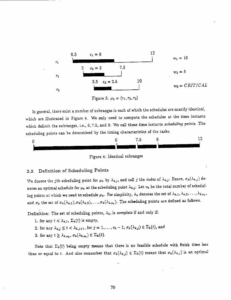
0.5 Cl = 6

2 c2 = 3

12

7.5

T2

?Z

3.5 c3 = 2.5 10

tüj = 10

TÜ2 = 5

tos = CRITICAL

Figure 3: /x3 = (TI,T2,T3)

In general, there exist a number of subranges in each of which the schedules are exactly identical,

which are illustrated in Figure 4. We only need to compute the schedules at the time instants

which delimit the subranges, i.e., 6,7.5, and 9. We call these time instants scheduling points. The

scheduling points can be determined by the timing characteristics of the tasks.

Figure 4: Identical subranges

3.3 Definition of Scheduling Points

We denote the ;th scheduling point for /z* by A4j-, and call j the index of XkJ. Hence, ok{XkJ) de-

notes an optimal schedule for pk at the scheduling point XkJ. Let vk be the total number of schedul-

ing points at which we need to schedule p.k. For simplicity, Xk denotes the set of Afc,i, A*,2,.. •, Xk,Vk,

and ck the set of ok(XkA),ck(Xk,7),.. .,^(A«,VJ. The scheduling points are defined as follows.

Definition: The set of scheduling points, A*, is complete if and only if:

1. for any 1 < \k,i, £*(*) is empty,

2. for any XkJ < t < XkJ+u for j = 1,..., vk - 1, a*(Atj) € X*(«), and

3. for any t > Xk<Vk, ck{XktVt) € £*(*)-

Note that £*(«) being empty means that there is no feasible schedule with finish time less

than or equal to i. And also remember that ak(Xkj) € E*(t) means that ok{Xkj) is an optimal

70

schedule for w at t. The compress cl scheduling points indices that a« tf the optimal

schedules * the positive tea! time don«!» can be represented b, the optimal schedules competed

a, the scheduling points. I. ridHk», «ha set of scheduling points, fc. is »«mum, if and only .f

WMXt iH < V^fe«)), to -» 1 * i < ». - 1. This ensures that there does not exist any

redundant scheduling point which, if removed, does not violate the completeness of the scheduling

points. The sets of scheduling points that we will discuss are complete and rmmmum.

3.4 An Example for Deriving Scheduling Points

The values of A, depend on the temporal relations between rk and W The example in Figure 5

is used to illustrate the relations. We only describe the idea of deriving scheduling points by the

example and will discuss in more detrib later. Assume that there are 5 scheduling pomts for W-r,

^ we consider to compute n based 0» «k-,- Aecurrent task, r», roay be crrticj or non-cr,t,cal.

scheduling points for pk-i :

i ' I I 1 -. 1 »- time

scheduling points for (xk : rk + ck A*_i,2 + ck A*_li3 + cfc

dk Tk Tk + Ck

Figure 5: Scheduling Points

First, let us assume that rk is critical, which means that rk must be the last task in any feasible

schedules for w. A schedule for ^ is thus a schedule for M*-i concatenated by rk. Hence, the

optimal schedules for /ifc can be computed by appending rk to <rfc_i(j), j = l,...,tfc-i- One

restriction is that rk must be able to execute during its time window, from rk to d*. Hence, the

scheduling points are A*_w + «a, j = l,.:.,t*-i, subject to the timing constraint of rk. In the

example, because rk > Afc_w, the first scheduling point is Aw = r* + cfc. The first and the rest

scheduling points are expressed in Equations 3-5. Notice that Xk.,A + ck > dk. Hence, there are

71

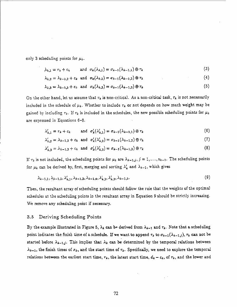
only 3 scheduling points for fik.

h,\ = rk + cfc and ak(Xkti) = a^_i(Ajc_i,i) © rjt (3)

A;-.2 = ^--1,2 + c* and ajÂ^) = Vk~i(Xk-i,2) © rk (4)

Aw = Ajt_-i^ 4- ex- and ai(Aii3) = a.t_i (Ajt_i,3) © rk (5)

On the other hand, let us assume that rk is non-critical. As a non-critical task, rk is not necessarily

included in the schedule of/i*. Whether to include rk or not depends on how much weight may be

gained by including rk. If rk is included in the schedules, the new possible scheduling points for fik

are expressed in Equations 6-8.

•M.-.1 = Tk + Ck and ^(A^rrCTit-Âjfc-!,!)©?-* (6)

X'k 2 = Ajt_i,2 + c* and aÂ'^) = <rk-i{*k-ia) © r* (7)

AJc,3 = ^-1,3 + ck and c'k(X'kz) - ak^(Afc_1>3) ©rk (8)

If Tk is not included, the scheduling points for pk are Xk.ltj, j = 1,..., vk-i. The scheduling points

for pk can be derived by, first, merging and sorting X'k and A^-i, which gives

Then, the resultant array of scheduling points should follow the rule that the weights of the optimal

schedules at the scheduling points in the resultant array in Equation 9 should be strictly increasing.

We remove any scheduling point if necessary.

3.5 Deriving Scheduling Points

By the example illustrated in Figure 5, Xk can b*> derived from Xk-i and rk. Note that a scheduling

point indicates the finish time of a schedule. If we want to append rk to ok-\ (A*_i j), rk can not be

started before Xk-ij. This implies that A* can be determined by the temporal relations between

A*_ls the finish times of ak, and the start time of rk. Specifically, we need to explore the temporal

relations between the earliest start time, rk, the latest start time, dk — ck, of rk, and the lower and

72

„„er Wds to be deSeed Mow. We detoe the lower boued IM , A»-„. »* *■ •«« >-"<

E/*_i = h-\ vk ,- In particular,, they have the following meanings.

2^: the largest time instant such thai there is no feasible schedule for ^ with

finish time less than Lk-\- [/,_,: the least time instant such that the optimal schedule for W-, with finish tune

greater than Uk-\ tan be'<7fc_i(Afc_i,Vk_,)-

The six possible temporal relations in Equations 10-15 can be used to determine Xk.

(10) dk - ck< Lk-i < Uk-i

rk < Lk-i < dk ~Ck < Uk-i (12)

Lu-\ < rk <dk- cjL- < Uk-i (13)

Tk<Lk-y<Uk-i<dk-Ck (14)

Lk-i <rk< Vk-i <dk-ck (lo)

Lk-i < Uk-i < rk

The temporal relations are illustrated in Figure 6, and can be summarized in three cases. The

method for constructing scheduLng points according 10 the temporal regions is discussed »«..

The correctness of the method, i.e., the complete and minimization of the schedubng po.nts ,

is verified later.

3.5.1 rk is Critical

The task rk must be the last task in any feasible schedule of ,k. Remember that ok(t) can be

computed by Equation 1. In the following, we discuss how to derive the scheduling points for the

three cases. The readers may refer to the algorithm in section 3.7 for details- ^ ^

Case ldk-ck< Lk-,: ß is not feasible. Remember Mthere exists no feasible scheme .or

*k with finish time less than Lk-u ** * iWe completeness of scheduling points, and that dk - ck

is the latest start time for rk. Hence, p> is *ot feasible, and thus the whole permutation, „, « not

feasible.

73

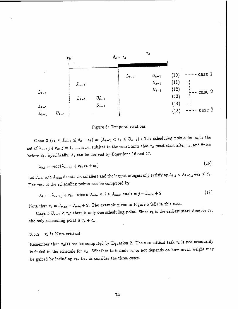
Tk dk - c/c Tk

Lk-i

Lk-i

Lk-i Vi-i

Lk-i Uk-i

Lk-i Vk-i

Lk-\ Vk-x (10) case 1

Uk-i (11) 1

tffc-1 (12)

(13)

1

i— case 2 i

(14) i

(15) case 3

Figure 6: Tempora] relations

Case 2 (r* < I*-i < dk - ck) or (Iw < rk < Vk-i) : The scheduling points for Mfc is the

set of Ajt-u + c,, j = 1, •..,«*-,, subject to the constraints that r, must start after rkl and finish

before d,:. Specifically, Xk can be derived by Equations 16 and 17.

Aw = mo=(Ajt_i,i + Cfc,rjb + cjt)

Let Jmin and Jmo= denote the smallest and the largest integers of j satisfying \k,i < A*_ij+cfc < dk.

The rest of the scheduling points can be computed by

A«,,- = Ajt.ij -f cfc, where Jmin <j< Jmax and i = j- Jmin + 2 (17)

Kote that vk = Jmcr - J»in + 2. The example given in Figure 5 falls in this case.

Case 3 Uk-i < rk: there is only one scheduling point. Since rk is the earliest start time for rk,

the only scheduling point is rk + ck.

3.5.2 Tk is Non-critical

Remember that ak(t) can be computed by Equation 2. The non-critical task rk is not necessarily

included in the schedule for pk. Whether to include rk or not depends on how much weight may

be gained by including rk. Let us consider the three cases.

74

Case 1 du - Ck < Lk-i' do nothing. The latest start time of T* is less than the lower bound,

Lk-\\ hence, T;. can not be included in any feasible schedule. The scheduling points and schedules

for /xjt_i remain the same as the scheduling points and schedules for fik- In our implementation,

to save time and space, Ajt_j and A* use the same memory spaces; also, a*-] and Ok use the same

memory spaces. So now A* = Xk-\ and Ok — Ok-\-

Case 2 (rk < Lk-y < dk - Ck) or (£*_i < rk < Uk-\) ■ If i~k is included, the new possible

scheduling points for p.k is the set of ^k-\,j + Ck, j — 1) • • •, v*-i> subject to the constraints that 77,.

must start after r/.-, and finish before dk- Specifically, the new possible scheduling points , \'k, can

be derived by Equations 18 and 19.

X'kA = max(Xk-i,T. + Ck,rk + ck) (18)

Let Jmin and Jmax denote the smallest and the largest integers of j satisfying X'kl < Xk-\,j + Ck < dk-

The rest of the scheduling points are

A'fcl- = Xk-\,j + ck, where Jmin <j< Jmax and i = j- Jmtn + 2 (19)

If Tk is not included, the scheduling points for fj-k axe the old ones for fik-il i-e.,

A^j^l,...,^. (20)

It is worth mentioning that some optimal schedules may include T^, and some may not. The

scheduling points, Ajt, can be derived by the following two steps.

1. Merge and sort the two arrays of scheduling points, A^ and A*_i, in Equations 18-20.

2. The resultant array of scheduling points should follow the rule that the weights of the optim?-!

schedules at the schedu-ling points should be strictly increasing. We remove any scheduling

point that has a smaller weight thin tV\at of its preceding scheduling point in the array.

The example given in Figure 5 falls in this case.

Case 3 Uk-i < *"*: add one more scheduling point. The earliest start time of T> is greater

than the upper bound, Uk-\\ hence, the new scheduling point is r* + c*. The weight of the

optimal schedule computed at this scheduling point is W(ak-i{Xk-i,Vk_:)) + Wk., which is larger than

75

W(ok-\ (Ajc_i,Vt_, ))• So this scheduling point must be included to make the set of scheduling points

for /I/., complete. Note again that the scheduling points and schedules for p.k-\ remain unchanged

as the scheduling points and schedules for /i*; i.e., Afcj = Afc_li;- and Ok(^kj) = 0k-i{Xk-ij), for

j - l,...,t>*-i. However, Xk,vk = ri + cfc and ck(XkiVk) = ajt-i(Ajt_3lU(t_,)@Tk, where vk = vk-\ + l.

3.6 Completeness and Minimization of Scheduling Points

We would like to show that the sets of scheduling points derived in the three cases are complete

and minimum. Note that cases 1 and 3 are special cases, and are not difficult to verify. Hence, we

will only briefly discuss case 2. If rk is critical, we would like to show that If Afc_] is complete and

minimum, A* derived by Equations 16 and 17 is also complete and minimum.

Condition 1 of completeness: Due to the completeness of Afc_i, Sjt-1(*) is empty when t <

Xk-1,1- Equivalently, Ejt_i(i - ck) is empty when t < A;._lti + ck. According to Equation 1,

Ck(l) = Ok-i(t - Cfc) © rk. Hence, ak(i) does not exist when t < Xk-\,i + ck- On the other hand,

since rk is critical, ok(t) does not exist when t < rk + e*, which is the earhest finish time of

rk. Therefore, Ejt(i) is empty when i < Xk,\. This shows that condition 1 of the definition of

completeness is satisfied.

Condition 2 of completeness: Due to the completeness of Xk-i, ^k-i(Xk-ij) € Efc_i(i), for any

Ai-ij < t < Afc.jjj.}. By Equation 1, ok-i(Xk-ij) © rk is an optimal schedule at Xk-\j + c*

for fik. Hence, ok-i(Xk-\j) © n 6 Et(f), for Xk^j + ck < t < Ajt-ij+i + ck. By Equation 17,

Xk,i = Xk-ij -f et, for : = j - Jmin + 2, which indicates that afc(Afcit) = Ck-i(^k-ij) © Tk- Besides,

Afc,,+J = Afc_jj+1 + cfc, for i + 1 = j + 1 - Jmin + 2, by Equation 17. Therefore, Ck(Xk,i) e £*(*)>

for Afc/ < t < Afct,-+1. This shows that condition 2 of the definition of completeness is satisfied.

Condition 3 of completeness: We know that vk = Jmas - Jmin + 2. By Equation 17, Xk,Vk =

■^Jt-i,Jm.x + cfc> which indicates that ok(Xk<Vk) = 0k-i{Xk-irjmax) © rk. Due to the completeness

of Afc.j, afc_i(Afc_isJm„) € Efc._i(f), for Afc_,tjTOK < t < Afc_x,jm.,+1, or just Afc_liJmor < t if

4o: = wjt-i- By Equation 2, ff*~i(A.*_i,jm„) © rfc is an optimal schedule at Ajt_i,jma, + ck

for }ik. Hence, ^fc-j(Aj.._i,jmox) © rk € 2*(i), for Afc_liJm„ + ck < I. Note that the range of

76

t < ^k-\,Jmcj+i + c* is removed. Because Jmax is the largest integer of j satisfying Afc_-iJ + Cfr < dk%

the schedule ck-i{Xk-itjmax+i)Q rk would not be feasible. Sinrr <7fc(>fc,vJ = ^-i(^-Um«) ® T*>

<7Jt(^Jt,«J € Sjt(0 for A/..^ < t. This shows that condition 3 o{ 'Mne definition 'of completeness is

satisfied.

Minimization: By Equation 1, W(ak(t)) = W(ak-i{i - ck) © rk) = W(crjt_i(t - <*))> $»nce a

critical task has no weight. Because Xk-i is minimum, W(ak-\(^i(~i,j)) < W(ffjt-i(^k--fJ+i))>

for any 1 < j < vk-\ - 1. That is, W(ajk_i(Ajb_ij-) © T*) < W(ajk_i(Ajt_lii+i) © rk), for any

1 < j < vk-i ~ 1. By Equations 16 and 17, W{ak{\k-\j + c*)) < !V((7fc(Afc_lo-+i + c*)), and thus

W(ak{Xk<;)) < W(ok(\k,;+i)), for any 1 < i < vk - 1. This shows that \k is minimum.

If rk is non-critical, rk may be included or not included in the optimal schedules for p.k. Assuming

that rk is not included in any of the optimal schedules, Xk — \k-\ is complete, since A*_i is

complete. However, including Tk. ™ay g^n some more weight, so we also need to consider the

schedules including tk. If rk is included in the optimal schedules, Xk derived by Equations 18 and

19 is the complete set of scheduling points for the optimal schedules including rk, by the same

reason described for the critical task. Hence, it is sufficient to construct the complete set of A^

by selecting from X'k and \k-\. Since whether to include Tk or not does not affect the feasibility

of the schedules, we only need to consider the weights of the optimal schedules. A complete set

of scheduling points indicates that the weights of the optimal schedules at these scheduling points

should be non-decreasing. Furthermore, a complete a>nct minimum sei of scheduling points indicates

that the weights of the optimal schedules at tfres« seWe<U.li'n£ point* should be strictly increasing.

Hence, we can merge and sort the two arrays of A'^ and A*_j, and remove any scheduling point

that has a smaller weight than that of its preceding scheduling point in the array. The resultant

scheduling points is thus complete and minimum.

3.7 The Permutation Scheduling Algorithm (PSA)

Algorithm PSA:

77

Input: a permutation sequence fi = (TI^T^, .. .,Tn)

Output: an optimal schedule an(XntVn)

Initialization: v0 = 1; A0,i = 0; aD(AD,i) = {); W(cr0(A0,i)) = 0

for k = 1 to n

when Tk is critical

case 1 (dk - Ck < Lk-i) : (/* is not feasible)

exit

case 2 (r* < £jt_i < 4 - C*) or (I*_i < rk < Uk-i) :

Computation for the first scheduling point:

Ajt.i = max (A*_i,i + cjt,rjt + cjt)

;' = 1 if Afc_u > Tk; otherwise, j is the greatest integer such that Ajt_u < r*

ff/t{A,k,l) = C7jt_1(Ajfe_lij) © Tfc

W(a,(Au)) = W(a,_1(A,_1J))

Loop: j = Jmin to Jmoz, where Jrot-„ and Jmax denote the smallest and the largest

integers of j satisfying A^ < ^k-i,j + c* < dk-

i = j ~ Jmin + 2

A*,v = Afc_u -f Ck

Ok(>*k,i) = <7*-i(Ajt_ij) © Tfc

W'(afc(A*il-)) = H'(aJb_1(At_1j))

Vfc = «'max — "min T *•

case 3 (i7jt_i < r*) : (only one scheduling point )

Afc.i = rA + Ci

^jt(Ajt.i) = ajk-iCAi-i^.jeTjt

W(aJt(Au)) = W(^-3(Afc_1.Wt_J))

78

/* Hence, A,. = A,_i and a* = cfc-i */

case 2(ri<Il-,<4-ct)or(iM<u<t;l-1)^

~ Con^taüoa for the firs. »• possible schedule po.at.

/: a i, W > u; otherwise, i is the greatest integer srroh that ^ .

WWW,)) = M'^-'(X;-'^ 7 de»ote the smallest aad the largest Loop: J = Jmm lo •'max» . , < dfc.

iKtegcr* df j satisfying Aw < Afc-i J ^

i = J — Jmin "•" *

construct a* from afc_i and c'k by 1) merging and sorting Afc_: and A't into one array Hg tne .eights of the schedules in the recant array stnet,

*«•** removing any schedule off the array if necessary.

case.3 (Uw < rfc) : (»**«* one more scheduling point)

Vk = vk-\ + 1

Ajc,vk = rjc + et

79

W{ok{\k.Vk)) = W'(aifc_i(AJt_1,Vik_J)) + wk

/* Note that A*j = Xk-yj and fffc(A*j) = ajt-i(A*_ij) for j = 1 to T>jt_i */

endfor

4 Scheduling a Task Set

To find an optimal schedule for the task set, we may have to consider all possible (n!) permutations.

It is possible to reduce the search space by eliminating some infeasible permutations. For example,

if d{ < rj, there is no feasible schedule in which T,- is placed after r,-. Even after the reduction, the

search space might still be too large. We propose to use simulated annealing technique, recognizing

that while this technique reduces the search, it may yield sub-optimal results.

4.1 Simulated Annealing

Simulated annealing is a stochastic approach for solving large optimization problems. It was de-

veloped using statistical mechanics ideas to find a global minimum point in the energy space.

Kirkpatrick ei al [o] had demonstrated the power and applications of simulated annealing to the

field of combinatorial optimization.

To find the optimal solution of the optimization problem is similar to finding the lowest energy

state of metal. The metal is melted first. Then it is cooled down slowly until the freezing point

is reached. At each temperature, a number of trials are carried out to reach the equilibrium. The

temperature has to be controlled not to drop too quick; otherwise, it is possible to be trapped

in a local minimum energy configuration. Lower energy generally indicates a better solution.

The annealing process starts from a randomly chosen configuration, proceeding to seek potentially

promising neighbor configurations. The neighbor configuration is derived by perturbing the current

configuration. If the neighbor configuration has a lower energy, the change is always accepted. The

distinct feature is that the neighbor configuration with a higher energy can also be accepted with

the probability of e^E~E'^T, where T is the temperature, and E-E' represents the difference in the

energy of current and neighbor configurations. Notice that when the temperature is high, an energy

80

up jump is more likely than it is when the temperature is low, as it may reach the configuration,

although with higher energy, which may lead to a better solution. An up ju^np means a jump from

low energy to high energy, and a down jump means a jump from high energy to low energy.

4.2 The Set Scheduling Algorithm (SSA)

A permutation is used to represent the configuration. If a permutation is ordered in an Earliest

Deadline First (EDF) fashion, we call it an EDF permutation. An EDF permutation may be a

good starting permutation for the proce&s of Simulated annealing for this problem. If the window

of a task is contained in the window of another task, we say that the latter task contains iV\e former

task. If there are no containing relations among tasks, the EDF permutation is a permutation of

which an optimal schedule of the task set is a subsequence [4]. Thus, an optimal schedule for the

task set can be generated by PSA by scheduling the EOF permutation. The energy function can

be expressed by a loss function:

loss = yj weight of rejected noncritical tasks

A schedule is not acceptable if critical tasks are rejected. We may say that the loss of a rejected

critical task is infinity. However, this kind of assignment makes it difficult to distinguish between

a very bad schedule (e.g., a critical task is rejected) and even a worse schedule (more critical tasks

are rejected). In general, the former schedule can be considered as an improvement over ^Yie latter

one. If the loss incurred by a rejected critical task is assigned infinity, there is no way to tell which

is better between the schedule in which one critical taskH rejected and that in which three critical

tasks are rejected. Hence, we assign a finite amount of loss to rejected critical tasks. The loss

of a critical task must be large enougK such that: the scheduler will not reject a critical task to

accommodate a number of non-critical tasks.

The neighbor function may be obtained using one of the following two methods. In the first,

simple method, we randomly select one task from those rejected. This task is inserted in a randomly

chosen location within a specified distance from its original location, where the distance is the

81

number of tasks between two tasks in a permutation. The distance is used in this approach to

control the degree of perturbation.

The reason of rejecting a task is due to the acceptance of other tasks. Given a schedule for

a permutation, it is sometimes difficult to identify which task results in the rejection of other

tasks, especially when tasks are congested together. However, the task immediately before or after

those rejected is likely to play a role. In the second method, we try to identify the task which

causes the largest loss of weight. As a simple approach, we attribute the rejection of a task to

the task accepted prior to it. Then we choose the task which causes the largest loss of weight and

insert it within a specified distance. Due to the robustness of simulated annealing technique, the

impact of not necessarily selecting the task which caused the largest loss is minimal. Note that in

simulated annealing many parameters are randomized, and the energy function, together with the

temperature, control the progress- of the annealing process. Tindell et al [9] commented that the

great bea.uty of the simulated annealing lies in that you only need to describe what constitutes a

good solution without worrying about how to reach it. According to our experiments, we find that

the first method performs better than the second method. However, the process in the first method

sometimes falls into a local minimum. The combination of the two methods does perform better

than any of the individual one. The Set Scheduling Algorithm (SSA) is presented in Figure 7.

The initial temperature has to be large enough such that virtually all up jumps are allowed in

the beginning of the annealing process. According to [9], the way to compute new temperature is

that new temperature = ac * current temperature, where 0 < a < 1. A step denotes an iteration

in the inner loop in Figure 7, which is the process of scheduling a permutation and determining

whether the permutation would become the current permutation. The thermal equilibrium can be

reached if a certain number of down jumps or a certain number of total steps has been observed;

and the freezing point, or the stopping condition, caa be reached if no further down jump has been

observed in a certain number of steps (5, 9].

82

Algorithm SSA:

Begin

choose initial temperature T

choose edf permutation as the starting permutaion, y

schedule \i by PSA and compute its energy, E

loop

loop

compute neighbor permutation y'

schedule y! by PSA and compute its energy, E'

if E' < E then

making y' the current permutation: y *- y' and E *— E'

else E— £'

if e~T~ > random(O.l) then

making \i' the current permutation: p. — yf and E *- E'

else

fi remains as the current permutation

until thermal equilibrium is reached

compute new temperature: T «— a * T

until stopping condition is reached

End

Figure 7: Set Scheduling Algorithm

83

5 Experiment Result

Experiments are conducted to study the performance of SSA based on:

v j y Wt number of times that the algorithm generates a feasible schedule • SCneauüng aDlUl> - nuinber of times that there does exist a feasible schedule for the task set

1 c at"r> — t°» of the schedule generated by SSA — loss of an optima] schedule lOSS r&UO — lotaj weight of accepted noncritical tasks of an optimal schedule

• iterations = number of permutations that the simulated annealing algorithm goes through to

obtain the sub-optimal schedule

We start with an EDF permutation. To study how good the result would be by using PSA to

schedule the EDF permutation, the scheduling ability and loss ratio for the EDF permutation are

computed as well. In our experiments, a task set consists of 100 tasks. The number of permutations

in such a task set is 100! ss 9.33 * 10157. To study how good the output of SSA is compared to an

optimal schedule, it is rather impractical to go through such a great number of permutations for a

task set to derive the optimal schedule and its minimum loss for comparison. Instead, we choose

to make up a task set such that the task set is feasible and the loss of its optimal schedule is 0.

Although the SSA algorithm is primarily designed for an overloaded system, we apply SSA to such

task sets for measuring the performance. The parameters are shown in Figure 8.

parameters value type

window length mean.Wl = 20.0 truncated normal distribution

computation time mean.C = m^'WI truncated normal distribution

load 20%, 40%, 60%, 80% constants

criticality ratio 25%, 50%, 75% constants

weight W-W=*l, higfc W=50 discrete uniform distribution

Figure 8: Parameters of the experiments

The mean of window length, meanJSft, is set to be 20 time units. The load is the ratio of total

computation time to the largest deadline, D, in the task set. Hence, the load indicates the difficulty

84

of scheduling the task set. The mean of computation time, mean.C, is one third of the mean of

window length, which allows the windows among tasks to overlap to some extent. How much the

windows overlap partially depends on the load. If the load is high, the windows are congested

together, and thus the overlapping is high. We expect some containing relations between tasks

to occur and thus increase the difficulty for scheduling. Note that, without containing relations,

scheduling the task set would be straightforward. The standard deviations of window length and

computation time are set to be their means, respectively. Criticality ratio indicates the percentage

of the critical tasks in the task set. It is set to be 25%, 50%, and 75%. The higher the criticality

ratio, the more difficult it is to generate a feasible schedule for the task set. On the other hand,

although it is easier to come up with a feasible schedule when the criticality ratio is low, the loss

ratio may still be high. It may be necessary to go through many permutations before an acceptable

loss ratio is reached. In our experiments, the acceptable loss ratio is set to be 0%, which means

that SSA will keep trying different permutations until either the loss ratio is 0 or the stopping

condition is reached, in which SSA fails to find an optimal schedule. Note that a big energy (loss),

1000, is incurred for a rejected critical task. Hence, for an infeasible schedule, the loss ratio may

well be more than 100%. The weight of a non-critical task is an integer ranging from low.W=l to

high_W=50, determined by a discrete uniform distribution function. For each individual experiment

with different parameters, 200 task sets, each with 100 tasks, are generated for scheduling. The

way of creating a feasible task set without loss is described in appendix A.

From Figure 9a, The scheduling ability of SSA is 98.5% when criticality ratio is 75% and load

is 80%, and is 100% for other lower criticality ratios and loads. This is because the simulated

annealing algorithm focuses on searching suitable neighbor permutations in such a way that the

rejected critical tasks, if any, may be accepted. Note that scheduling only the EDF permutation

can not always generate a feasible schedule. The scheduling ability of scheduling EDF permutation

degrades when load increases, which means fcaiks congest more together. The scheduling ability

of scheduling EDF permutation also degrades when the criticality ratio increases, which make?

meeting the deadlines of all critical tasks become more difficult.

85

As far as non-critical tasks are concerned, SSA can not guarantee the minimum loss. However,

even in the worst case given in Figure 9b, the loss ratio is less than 10%. The loss ratio becomes

less when criticality ratio or load is less. In many cases, the loss ratios are less than 5%. As for

scheduling the EDF permutation, the loss ratios are significantly larger.

The number of permutations to be searched in simulated annealing depends on the situations

of energy jumps, the way of reducing temperature, and how we define thermal equilibrium and

stopping conditions. In the experiments, we find that reducing temperature faster does not impose

a negative impact on the scheduling ability and loss. How to set the parameters in simulated

annealing differs a great deal from one application to another. We do want to generate the result

as good as possible, but are not willing to spend more computation time than necessary. This

usually requires fine tuning the parameters to get the trade-off between the two goals. We find that

the following parameters are beneficial: initial temperature = 3000, a = 0.8 (instead of 0.95 or even

0.99 suggested in other applications), the number of down jumps to obtain thermal equilibrium =

25, the number of total steps to obtain thermal equilibrium = 300, the number of steps with no

further down jump to obtain the freezing point = 2000, which is also the stopping condition. The

average number of permutations searched in simulates annealing is given in Figure 9c. If SSA can

successfully generate a feasible schedule, the average number of permutations checked is no more

than 4000 times. The number increases a little if SSA fails to find a feasible schedule, because in

this case SSA does not stop until the freezing point is reached. Note that the average numbers of

permutations are less than n7, which can roughly give us the idea about the complexity of searching

over the permutation space. Additional studies have shown that if we modify the above parameters

to increase the average number of permutations by about 10 times, the loss ratios can be further

reduced by about 25% of the loss ratios obtained here.

If time can be expressed in integers, the dynamic programming technique used in PSA can be

applied by computing ak(t) at t = 1,..., D. Let us call this approach the integral PSA, compared to

the original PSA with scheduling points, denoted by PSA SP in Figures 9d. Obviously, the integral

PSA tends to compute more schedules than the original PSA. We would like to see how more

efficient the original PSA algorithm is than the integral PSA. Specifically, we compare the average

86

T 1X0

0.95

0.90

0.1!

0.10

0.75

0.70

0.65

0.«

OJS

OJO

0.45

0.40

0J5

OJO

Oi5(-

021

0.15

0.10

0.05

0.00

■0.05

\

(a) Schedulability (b)Loss

-r-)u.-e»-oJü.o.5o"

_i_ L»)>IO-3

30OJD0 300X0 400.00 500X0 600X0 700.00

(c) * of Permutations FtoCEBUtei

4.03

1» -

7533Ö" i ~)»BÖiic"<SSl'7J

,' ViSürö»iSjB3o_

- -. '-.T-EJi* :tta.ft"

Load 1 Kr1

MO» 300.00 400.00 300X0 «00.00 7MX0

(c) average * of schedules computed per

IOOJD0

task set

>S». tot CMliO "

VsVliü'Ö'Ä'.«" KÄS* £6405"' >sÄ>"ö>'wao"* ?SÄS>.C*M5~

4110-' Ir« latiiWt

300X0 JOOXO JOOXO 400X0 SOOJDO 600X0 700X0 100X0

Figure 9: (a) Schedulability; (b) Loss; (c) ^Permutations; (d) ^Schedules

87

number of schedules required to derive the optimal schedule for a permutation. For the integral

PSA, the number of schedules computed is fixed, or n*D, as can be seen in Figure 1. For the original

PSA, Efc=i vk is the number of schedules needed to schedule a permutation. The average number

of schedules needed to schedule a permutation by PSA is computed over the permutations of a task

set, and is presented in Figure 9d. The number for the original PSA decreases with the criticality

ratio. This is because a critical task never increases the number of scheduling points; instead, the

number of scheduling points might be decreased due to the timing constraint of the critical task.

For the criticality ratios of 0.25,0.50, and 0.75, the average number of schedules required for a task

set of 100 tasks are approximately 480,250, and 150, respectively. The complexity of the original

PSA seems linear in this sense. On the other hand, the complexity of the integral PSA is quite

high. The number decreases with load. This happens to be related to the way of generating the

task set, in which D = total.c / load. The number is equal to n * D, where D might fluctuate a

little.

6 Conclusion

In this paper, we study the scheduling problem for a real-time system which is overloaded. A

significant performance degradation may be observed in the system if the overload problem is not

addressed properly [2]. As not all the tasks can be processed, the set of tasks selected for processing

is crucial for the proper operation of an overloaded system. We assign to the tasks criticalities and

weights on the basis of which the tasks are selected. The objective is to generate an optimal

schedule for the task set such that all of the critical tasks are accepted, and then the loss of weights

of non-critical tasks is minimum.

We present a two step process for generating a schedule. First, we develop a schedule for

a permutation of tasks using a pseudo-polynomial algorithm. The concept of scheduling points

is proposed for the algorithm. In order to find the optimal schedule for the task set, we have to

consider all permutations. The simulated annealing technique is used to limit the search space while

obtaining optimal or near optimal results. Our experimental results indicate that the approach is

88

very efficient.

The work presented in this paper can be easily extended to address the overload issue for

periodic tasks. To schedule a set of periodic tasks with criticalities and weights, we can convert

the periodic tasks in the time frame of the least common multiple of the task periods to aperiodic

tasks. The schedule generated for the frame can be applied repeatedly for the subsequent time

frames.

Our algorithm can also be applied to solving the problem of scheduling imprecise computations

[7], in which a task is decomposed logically into a mandatory subtask, which must finish before

the deadline, and an optional subtask, which may not finish. The goal is to find a schedule such

that the mandatory subtasks can all be finished by their deadlines and the sum of the computation

times of the unfinished optional subtasks is minimum. A schedule satisfies the 0/1 constraint if

every optional subtask is either completed or discarded [7]. We can solve this problem by using

our algorithm by setting the mandatory subtasks to be critical, and the optional subtasks to be

non-critical with weights equal to their computation times.

Appendix A. Generating a task set

Generate computation times for tasks according to mean_C and the standard deviation

D = (total computation time) / load

Assigning starting instants, sk, to tasks such that

the intervals between the computation times are truncated normally distributed

For each task Tk

Determine the criticality by criticality_ratio and/or weight by low.W and high-W

Compute the window length of rk according to mean_Wl and the standard deviation

(note that window length > ck)

align the window with the computation time in their middle points:

Tk = max(0,Sk -f SL _ windowJaiphj

dk = min(D, rk -f window Jength)

89

The load determines how the tasks would be congested. Once the largest deadline, D, has been

computed, we separate the computation times of the tasks in such a way that the positions of the

computation times on the time axis stretches over the range from 0 to D. Note that the starting

instants of the computation times consist in an optimal schedule for the task set. In this way, all of

the tasks in the task set can be accepted. At last, the windows are aligned with the computation

times.

References

[1] M. R. Garey and D. S. Johnson. Computers and Intractability, a Guide to the Theory of

NP-Completeness. W. H. Freeman Company, San Francisco, 1979.

[2] Jayant R. Haritsa, Miron Livny, and Michael J. Carey. Earliest deadline scheduling for real-time

database systems. In IEEE Real-Time Systems Symposium, Dec. 1991.

}3] Shyh-ln Hwang, Sheng-Tzong Cheng, and Ashok K. Agrawala. An optimal solution for schedul-

ing real-time tasks with rejection. In International Computer Symposium, Dec. 1994.

[4] Shyh-ln Hwang, Sheng-Tzong Cheng, and Ashok K. Agrawala. Optimization in non-preemptive

scheduling for aperiodic tasks. Technical Report CS-TR-3216, UM1ACS-TR-94-14, Department

of Computer Science, University of Maryland at College Park, Jan. 1994.

{5] S. Kirkpatrick, CD. Gelatt, and M.P. Vecchi. Optimization by simulated annealing. Sci-

ence(220), pages 671-680,1983.

[6] C. L. Liu and J. Layland. Scheduling algorithm for nraltiprogramming in a hard real-time

environment. Journal oj the ACM, 20(l):46-61, Jan. 1973.

[7] W.K. Shih, J. Liu, and J.Y. Chung. Fast algorithms fox scheduling imprecise computations. In

IEEE Real-Time Systems Symposium, pages 12-19, Dec. 1989.

90

[8] Philip Thambidurai and Kishor S. Trivedi. Transient overloads in fault-tolerant real-time sys-

tems. In IEEE Real-Time Systems Symposium, Dec. 1989.

[9] K.W. Tindell, A. Burns, and A.J. Wellings. Allocating hard real-time tasks: An np-hard

problem made easy. The Journal of Real-Time Systems, 4(2):145-165, June 1992.

91


OMB No 0704-0188

-. AGENCY USE ONLY (Irrf-f DUnK) 2. REPORT DATE

November 1994

3. REPORT TYPE AND DATES COVERED

Technical Report

;iTU AND SUBTITLE

Scheduling an Overloaded Real-Time System

6. AUTHOR(S)

Shyh-ln Hwang, Chia-Mei Chen and Ashok K. Agrawala

5. FUNDING NUMBERS

N00014-91-C-0195

DASG-60-92-C-0055

"PERFORMING ORGANIZATION NAME(S) AND ADDRESS(ES)

University of Maryland Department of Computer Science A. V. Willliams Building College Park, MD 20742

V SPONSORING /MONITORING AGENCY NAM£(S) AND ADDRtSS(ES)

Honeyvell, Inc. Phillips Laboratory 3600 Technology Drive Directorate of Contracting Minneapolis, MN 55418 3651 Lowry Avenue SE

Kirtland AFB NM 87117-5777



10 SPONSORING/MONITORING AGENCY REPORT NUMBER



c u a) •o -H

D! c o u 0)

10 Ol 10 CO u

i. ABSTRACT {Maximum 702*-zrsi)

i Tne real-time systems differ from the conventional systems in that every task in 'the real-time system has a timng constraint. Failure to execute the tasks under the timing constraints may result in fatal errors. Sometimes, it may be impossible to execute all the tasks in the task set under their timing constraints. Considering a svstem vith limited resources, one solution to handle the overload problem is to reject some of the tasks in order to generate a feasible schedule for the rest. In this paper, we consider the problem of scheduling a set of tasks without preemption in which each task is assigned criticality and veight. The goal is to generate an optimal .chedule such that all of the critical tasks are scheduled and then the non-critical •asks are included so that the weight of rejected non-critical tasks is minimized, "we consider the problem of finding the optimal schedule in two steps. First, we selecp a permutation sequence of the task set. Secondly, a pseudo-polynomial algorithm is proposed to generate an optimal schedule for the permutation sequence. If the global optimal is desired, all permutation sequences have to be considered. Instead, we sropose to incorporate the simulated annealing technique to deal with the large searcn

;^»r». n,,r ^H^r.i ~c„irc cw r^r niir ,imri^ ^ »*> ^,r^rpr^fti^rt p

10 o E

C • 1-1 05

c to o

DJ AJ (C CO

.* 3 to E a u

J-> ci C.

Ol

•u O

u u o o)

U-I.O E

03 3 oi c

—1 3"0

"O 0) CD J-l

JZ-* o E W-H

CO CO E

-H >%

cc o o

W. SUEJSC7 TERMS

Process Management; Nonnumerical Algorithms and Problems

IS. NUMBER OF PAGES

29 16. PRICE CODE

.


"unclassified

IB. SECURITY CLASSIFICATION OF THIS PAGE

Unclassified

19. SECURITY CLASSIFICATION OF ABSTRACT

Unclassified


Unlimited

»SN 7SCP-01-2S0-S500 92 Sia^da'd t-oro 296 !Rev 2-B9)

Notes on Symbol Dynamics**

Ashok K. Agrawala Department of Computer Science, University of Maryland


E-mail: [email protected]

Christopher Landauer System Planning and Development Division, The Aerospace Corporation

The Hallmark Building, Suite 187, 13873 Park Center Road, Herndon, Virginia 22071

Phone: (703) 318-1666, FAX: (703) 318-5409

E-mail: [email protected]

13 February 1995

Abstract

This paper introduces a new formulation of dynamic systems that subsumes both the classical discrete and differential equation models as well as current trends in hybrid models. The key idea is to express the system dynamics using symbols to which the notion of time is explicitly attached. The state of the system is described using symbols which are active for a defined period of time. The system dynamics is then represented as relations between the symbolic representations. We describe the notation and give several examples of its use.

«IT^rJÜTn * sup.Portft/n p^> °NR. «d DARPA under contract N00014-91-C-019S to Honevwell and Computer Science Depart, ^ L^«.tr JIf51 y °* MsLTland-u

Ti>lv?e»'s, opinions, and/or findings contained in this report are those of the author(s) and should

ON^th^^ec^»S^BÄSe,"1 ^^ °tbel ^"^ OI in,pUed' °f thC DefenSe AdVZnCe6 R<seMeh PrOJeC" AgenC» Computer fecilities were provided in part by NSF grant CCR-8811954.

TW Jh > ^Al? s^pp5rt<^> ran bv ARPA ud P^P* **** »*6* contract DASG60-92-0055 to Department of Computer Science, rJ.J>?£L0' M2LTylalld: Th« views opinions, and/or findings contained in this report are those of the author(s) and should not be interp.etec as representing the official policies, either expressed or implied, of the Advanced Research Projects Agency, PL, or the U.S. govern men».. • ^ ° ■" '

93

Contents

1 Introduction 3

2 Descriptions of System Behavior 3

3 Concepts and Notations 3 3.1 State Variable • 3 3.2 Symbol 3 3.3 Attribute Identifier 3 3.4 Expression 4 3.5 Interval 4 3.6 Characterizer 4 3.7 Event 4

4 System Description 4 4.1 Dynamics 4 4.2 Normalization and Continuation 5 4.3 Continuation and Continuity 5 4.4 Characterizer Semantics and Inference 6

4.4.1 Inference 6 4.4.2 Prediction 6 4.4.3 Truth Maintenance 7

4.5 Analysis 7

5 Examples 7 5.1 ODE 7

5.1.1 First-Order 7 5.1.2 Second-Order Example 8 5.1.3 Higher-Order Example 9

5.2 Measurement 10

94

1 Introduction

Traditionally, systems have been modelled using state variables denned in a metric space and the system dynamics denned using differentia) equations. This approach uses continuous descriptions of space and time. When we use computers for expressing and manipulating such models we have to use symbols to represent it. Symbols are discrete by their very nature, and require use of mapping from the continuous spaces to discrete spaces. These mappings cause problems unless carried out rather carefully. Further, when we consider the problems in which some aspects of the system are genuinely discrete, hybrid models have been used. As different techniques have to be used for continuous and discrete aspects of the system, significant complexity gets added to such models. Recognizing that the computer systems only use symbols for any representations, in this paper we present a formulation of system dynamics directly in terms of symbols. In order to handle the synamics, time interval over which a symbol is considered valid is explicitly attached. The symbols describing different aspects of the system may be from a set appropriate for that aspect. The dynamics is described in terms of rules connecting the symbolic representations. This paper contains the preliminary formulation of system dynamics in the framework of Symbol Dynamics.

2 Descriptions of System Behavior

For the purposes of this paper, behavior includes all the relationships among parts of a system at the same or different times. In particular, the combined relationships among parts of a system at the same time is usually called structure. Both of these aspects are subsumed in our use of the term behavior. We assume that our ability to generate or derive new information about the system behavior changes only at discrete points in time, since we expect to perform these processes on digital computers. The event times define the time scale. In this paper, we introduce Symbol Dynamics, a totally symbolic way to represent the important aspects of dynamical systems and processes, so that we can reason about them using computers.

3 Concepts and Notations

This section contains the basic notions of Symbol Dynamics.

3.1 State Variable We assume that systems exist and change over time. We are looking for a method of describing those changes so we can compute how LO control them. The systems we consider can be described with state variables. Each state variable is an observation on the system or a derivation from other state variables. We may or may net know a priori which state variables are important, or even which ones are determinable (i.e., the system comes first, and the state variables are chosen to be helpful in describing the behavior). We might call the state variables attributes of the state.

3.2 Symbol We want to measure and compute with information about a system, so we need to map the system into formal spaces we understand better. A type is a symbol set, both representing a set of values and including some operations on those values; this is the notion of formal space used here. It includes collections of mutually dependent types and functions between different types. A symbol of a given type is an element of the set of values that type. Any notions of credibility, confidence, or uncertainty are part of the type system that is used. It is especially important to define the allowable operations on these kinds of types. For example, for measurements of a system, the symbol would include the measured value and the associated uncertainty value.

3.3 Attribute Identifier We assume that we will want to know different things about the system behavior. We need names to keep track of the different things we measure or compute.

95

An attribute identifier is a name for a state variable (a state variable is like a probe into some aspect of the system behavior, and the attribute identifier is only the label).

3.4 Expression

An expression is a pair (attribute identifier: symbol),

which is interpreted to mean the assertion that the state variable can be described by the symbol (when the expression is active). We will describe the precise semantics of these expressions later on. These are models of the state variable values.

3.5 Interval

An interval is a pair jstart time, end time),

assumed to describe a half-open interval (to save us from trouble with the topology). The end time may be omitted, in which case it is interpreted to mean infinity by default.

3-6 Characterizer

A characterizer is a pair (expression, interval),

also written (attribute identifier: symbol; start time, end time),

interpreted to mean that the expression is active during the specified interval. It becomes active at the start time, and becomes inactive at the end time. Each characterizer has a range (its interval of activity) and a scope (the set of attribute identifiers that occur in its expression). We may also consider a symbol set that includes arithmetic expressions that contain an explicit time variable i. For example,

(p:p0-rt;o*i;io,ti) represents a continuous change along the interval. We will also have occasion to reason about conditions at particular points in time, so the assertion language will also have characterizers of the form

(expression, point).

3.7 Event

An event is the activation or deactivation of a characterizer. We make no limiting assumptions about simultaneous events.

4 System Description

A system description is a finite set of characterizers, so we assume explicitly that a system can be described by a finite set of characterizers. We insist that only a finite set of characterizers be active at any one time. Since each of those characterizers is active over a positive interval, there is therefore some small interval thereafter during which all of them are still active. Everything we know about a system's behavior is described by characterizers and relationships among the characterizers. Domain models and context can be written as characterizers, generally with large intervals.

4.1 Dynamics

Relationships among characterizers are rules that define the dynamics. These rules take the form: if these characterizers (with a list) are active on these intervals, then this new one is also active on this other interval (not necessarily contained in the intersection of the original intervals).

96

Rules can contain variable identifiers, with implicit universal quantification. Relationships hold on intervals and the combination may extend the range. We generate new characterizers according to the relationships, either predictive (range extension) or deductive (knowledge extension). The language in which the rules are written is important, since it has to accommodate notations from many different types, many of which will not be known when the language is defined. Some basic concepts that will be in any of these languages are continuity and derivatives. It is important to remember that the system comes first, and that the state variables are our choices for modeling and understanding the system. This means in particular that the coordinate systems we use are temporary, and that the constraints among the state variables are expressed explicitly as relationships.

4.2 Normalization and Continuation Characterizers-may have overlapping intervals. Normalization is the process of breaking each characterizer into two or more others, to fit the time scale. If i is an event time, and

(a : v; s, e) is a characterizer with s < t < e, then we can replace it with two characterizers

(a : v;s,t) and (a : v\t,e). If two characterizers use the same attribute,

(a :v\s,e) and

(a:w\t,u), then we say that the second one continues the first one iff they are adjacent in time, so t = e. Continuity considerations in the transition from v to w at time t are treated in the next section. In any system with a finite density of event times, if we split every characterizer that spans an event time, then we end up with characterizers that start and stop at consecutive event times (though they may be continued by other characterizers). This has some computational conveniences. If we have two characterizers

(a :r;ii,t2) and

(a:tr;£2,i3), so that the second one continues the first, then we need some kind of explicit characterizer for the transition, active in an interval containing the transition time. If there is a description it in an appropriate, domain for which

v, for tj < £ < i2, ■w, for £2 < i < £3,

then we can conclude (a :u;ii,t2).

This is the opposite of normalization. If there is an overlap, that is, if the two characterizers

(e:r:ti,t2) and

nave

and

(c : w;t3,tt)

I*i, £2) n j£3, U) non-empty,

v(i) = w(t) for t € [max(£i,£3),min(£2,£<)), then we can also conclude

(a : u;min(i:,t2),max(£3,£4)).

4.3 Continuation and Continuity- One aspect of continuity is transitions from one symbol to another across interval boundaries. The tradition relations axe extra conditions that have to hold at the transition time (usually they are smoothness conditions for model transitions). A typical smoothness property is infinitesimal: for characterizers

(a:v,t0,ti)

97

and (a:u>;tj,£2),

we normally want smoothness, written d v

dt d VJ

17

'='?

and continuity, written v(t = £7) = u;(i = £+).

Both of these are point conditions on the attributes and their derivatives, and we can consider only conditions on attributes by using whatever derivatives are needed in the conditions: instead of

(a :v\ to.ii), we use

(a :(*,*'); to, *i). and write our smoothness condition as

l) - (5 If we also require continuity in each attribute, so that

then the upper limit in the previous expression can be omitted. It is therefore clear that we must deal with point events at transitions

|to...ti)Iii...t3), but not with point characterize«. If we make the transition continuity a property of the definition of continuation, then we can assert it or not in any given model. Of course, the expression £ — iT means that the interval [£j — e, t{) is part of the limit computation for every £ small enough, so we might be able to use these intervals for some small enough e without having to take the limits. We will deal with these considerations in the simplest way possible. We have a characterizer that asserts continuity of the relevant attribute across a larger interval, such as [£o, £2) above. The only place that the continuity characterizer has new information is at the transition point £j, but we simply do not worry about the redundancy.

4.4 Characterizer Semantics and Inference

A characterizer is what we want to assume about what is true over its interval. It need not be consistent with the other characterizers in a system description; we explicitly allow false assertions here, so we can reason usinf counterfactuals.

4.4.1 Inference

We can make inferences within intervals, according to some rules. If, say, there is a rule S]&52=* S3,

and two characterizers (v : si;io,h)

and (r:sj;t2)t3)

with to < £2 < ij < £3, then we can conclude {v : s3;£2,ti)-

4.4.2 Prediction

We can also make inferences that extend intervals in some cases. They take the form: If (v : si;io.ii)

and (u--: 52;io,£i)

are characterizers with to < ii, then there is a characterizer {= : s3-t2,i2)

for some £2, £3, with t0 < £2 < £1 < £3-

98

4.4.3 Truth Maintenance

Because we do not presume that the characterize, in a system axe truths, we need to be much more j»"M a*°* when they can be used together, especially in the inference and prediction processes. Smce the mference rules rhernsehis aretime^pendent, we need to keep track of the dependencies of every characterizer, both how and£ben !t wat derhed (how tells us about hypotheses and inference rules; when helps us in checking temporal consistent)

We afsVniTi wa^lndicate which characterize, we DO want to be true, so that differentcolonsjof A«* terizers cat be compared and contrasted within the same context. We might want to confer computing various maximal consistent sets of irredundant assertions as an aid in this process e„nowAt> n]A ones- we also Various rules can be activated that lead to new conclusions in an interval, wh,ch can supersede old ones, we also assume partial deduction, not total. We therefore need to use some kind of non-monotonic logic.

4.5 Analysis

IT—* SÄ «c help reduce our reliance on Mh »« ™* ■*«• I™**»

STS « corn^cTa« perked from the symbols active at a given time ^ "^."«ESS with time in this formulation is that we car, sit outside the usual sequencing of events, takmg a k.nd of »»™r look at the entire time line, and piece together parts of the models that we know root« about regardless of whetner or not thev are the first ones in our time interval of interest. , , . „<• „ We n also perform the deductions in an order that is differ«* from border imposed by time^smg any of a number of simple mechanisms, such as rule-based systems or rewrite logics; both are being investigated.

5 Examples

This section contains severa] examples that illustrate the utility of toe notation.

5.1 ODE A simple example that shows range extension is an ordinary differential equation (ODE). For ODEs, the solution method is pan of changing an ODE into a set of characterizes. So let us consider a simple second-order ODE for the sine function,

y" = -y. p'(0) = 1,

and sohlet wV.h Eulers method (a particularly bad one for this kind of pwfcfcm by the way). First we transform the eouations into a first order system (in the usual vuay) Ysy lông x~ y ,

z' = -y,

y = => r(0) = 1,

y(0) = °' , „ and we also define z = =' = y".

5.1.1 FirstÔrder

Now the way Eulers method works is by linear extrapolation, so for a given time t = to, if we have

=(io) = =o.

y(io) = 3/0. then we have

ZQ = z{t0) - -yo, and we take

s(t) = io -r 20 » {t - to).

y{t) = yo-rô* (t-to).

99

for t in some small interval |l0, *i =to + dt).

The characterizers that describe this situation are: (x:x0 + zo*{t-to);to,to + di),

(y :yo + s0 * (t - to); to, to + dt), which we want to be true for all choices of 20,2/0. to, and dt (which ones we actually use in our system description depend on how we choose the time intervals in the solution). The characterizers that describe the initial conditions are difficult, because they cannot be described with half-open intervals of the shape we have thus far described:

(x:l;0), (y:0;0),

which is always going to be a problem in systems that start at a certain time. In a more sophisticated system, the choice of next time interval would depend on the computed accuracy of the current solution. For this example, we simply make all the time intervals the same, and say that the characterizer pair

(s:ii + «i«(t-ti);ti,ta + dl),

(y:yi+*i *{t-U)\h,h+dt) propagates the pair

(2 : so -f 20 * (t - to); to, to + dt),

(y '■ yo -r so * (t - to); to, to ■+■ dt) iff

Zj = 20-fZ0*<£,

yi = yo -r so * dt,

t: — to T dt, which are the conditions for the first pair to meet the second (the condition z3 = — yi is part of the definition of these characterizer pairs). Extending the iteration, we have

x(0) = 1,

y(0) = 0. s(fc-fl) = =(k) - y(k) * dt, y(k + l) = y(k) + x(k).di,

which car. be written as a vector eauation (we put the matrix on the right so we can use row vectors) (=,s0(o) = (1,0),

(=,y)(fc-rl) = (=,y)(i) ( _£ f ). so if we write 1 for the identity matrix and J for the matrix

0 3 -1 0

then we have (with X = (x,v)) *(0) = (1,0),

X(k~l) = X(k)(l + J.di), so

X(fc) = (l,0)(/-fJ.A)k, which can be computed exactly. Since the eigenvalues of (J -j- J * dt) are 1 = i« dt, which have magnitude 1 -f dt7, the successive powers of the matrix diverge for any dt > 0, and therefore so does the iteration.

5.1.2 Second-Order Example

In this section, we use the same differential equation problem, with a different solver, a second-order one that is almost able to converge properly. We therefore have

s' = -j,.

100

V' = r. =(0) = 1,

y(0) = o, as above. Our initial conditions are

(x:l;0),

(y:0;0), as before. The method we use is a simplified second-order Runge-Kutta method [?], [?], which basically amounts to averaging the usual Euler approximation in an interval with a linear reapproximation at the endpoint of the interval. At a given time i = io, if we have

x(io) = x0,

y(to) -= J/o, then we have

x(t) = xD - yo * dt - x0 * dt7/2,

y(0 = yo + x0 * dt - y0 * dt7/2, and it is the extra dt1 terms that make the method second-order. As above, we assume equal time intervals and get an iteration

x(0) = 1,

y(0) = o,

x(k + l) = x(k)-y{k)*dt-x(k)*dt7/2,

3/(^+1) = y(k) + x{k) » dt - y(k) * dr2/2, which can be written as a vector equation

(i.y)(0) - (1,0),

and we have as above *(0) = (1,0),

A"(* + i) = *(*)(/-(i-<ü2/2) + .7«&), so

X(k) = (I,0) (I » (1 - dt7/2) + J * di)k, which can be computed exactly. Since the eigenvalues of (J * (1 - &2/2)-f J * di) are 1 - di7/2±i*dt, which have magnitude 1 + dl*/4, this simple method still does not converge (but much more slowly).

5.1.3 Higher-Order Example

A similar analysis of the usual 4th-order Runge-Kutta method leads to an iteration x{t) = x0-yo*dt-xD' dt7/2 + y0 * dt3/6 -~ x0 * dt4/24,

y(0 = yo-rx0-di-yo'<t2/2-x0'dl3/6-ry0*dt</24, with matrix

/ 1 - dz7/2 ~ dt</2A dt-dt3ß \ \ -dt + dt3/6 \-dl7/2 + dtA/2A J'

and eigenvalue magnitude of 1 + dt'/36 + di-8/242, which is still greater than one. In fact, since this equation (in (=, y) space) represents moving around a circle, any extrapolation method based on tangents at a single point will fail, since all of the tangent vectors point outward from the circle. We note that the iteration equations do have the first terms of the usual Maclaurin series for sin(di) and cos(di), so we try out a different iteration:

=(0 = x0 » cos(dt) - j/o * sin(dt),

y(0 = yo * cos(dt) -f x0 * sin(dt), which can be written as a vector equation

(x,y)(0) = (i,o),

101

/ w, „ i \tu\ ( cos{dl) sin(dt) \ (z,y)(k+l) = (*>y)(k) [ -sin(dt) cos(di) )

and we have as above A'(0) = (1,0),

X{k + l) = X{k)(I*cos{di) + J*sin{dt)), so

and

X{k) = (2,0) (I * ecw{<a) + J * 5m(dt))k, = {1,0) {I *cos{k*dl) + J*sin(k*dl)),

i(fc*dt) = cos(fc*efi), y(fc * eft) = stn(fc * eft),

from which we can hazard a guess as to the correct solution.

5.2 Measurement Let us take a simple system in which the velocity and position are occasionally known through inexact measurement. Our state variables are p for the position, v for the velocity, and a for the unknown acceleration. We assume that the acceleration a is bounded by some constant A, so that for any times io < *i

\v(ti)-v{t0)\ < \ti-to]*A. We assume that we have characterizers

(a{t)\U-i,U) that describe the acceleration, and model characterizers

(* = p';0-,-), (c=r';0-,-).

Therefore, we can compute the velocity and position by

v{t) = v(t0) -f / o(u) du,

p(i) = p(i0) -5- / »(«) °^- •/lc<v<t

The problem is to choose measurement times and variables that maintain a certain accuracy in the estimates oi position. We assume that we can measure position within a bound

bmeas(*)-.P(i)l < P, and thai we can measure velocity within a bound

IvmeasW-vWI < v. but that we want to keep our estimate p^ of position either more accurately tnan the position measurement error (this might or might not be possible) or using as few measurements as possible. We assume first that x0,i>0 are known, and consider an interval [t0,ti). We compute

jr(ti)-«o| < |ii -lo\'A and therefore

|i(ti)-so| < - * |ti - iot2 * A,

so we would have to choose A l = tj - to '

so that A: < \V/A\

to keep the velocity within bounds, and {A if < \2*P/A\

to keeD the Dosition within bounds. . But of course, we don't know x(i) or v{t) after the first time interval, so we need to change the previous derivation a bit. We assume that we know xo and VQ, and that

|=(to)-zol < £=o

102

describes the accuracy of our knowledge of x(t) at time I = t0, and |v(*o) - *o| < A v0

describes the accuracy of our knowledge of v(t) at time t = t0. Then the above inequalities become Mtj)-*ol < A vo+|ti -i0|* A,

and therefore

l=(*i) - *ol < A 20 + |ij - to! * A v0 + I « |tj - i0|2 * X,

so we have to have

At < |(V-At>o)M| to keep the velocity within bounds, and

(A if + ~p£ * (A t) < |2*(P-Ax0)M|

to keep the position within bounds. At this point, we are stuck unless we can say something more helpful about the acceleration. Suppose we know that the acceleration jumps around, and that it has a distribution of values with mean 0 and variance R. In this case, we might be able to reduce the estimates for position and velocity and improve the time intervals.

References

j]J P. Henrici, Elements of Numerical Analysis, Wiley (1954)

|2] J. Stoer, R. Bulirsch, Einführung in die Numerische Mathematik, II Springer (1973)

103

REPORT DOCUMENTATION PAGE OMB no 0704-01SS

j -o #-c ..-.-o'

1. AGfNCY USE ONLY ilf^f £M<nt; 2. REPORT DAU

February 13, 1995

3. REPORT TYPE AND DATES COVERED

Technical Report

*. TITLE AND SUBTITLE

Notes on Symbol Dynamics

6. AUTHOB(S)

• Ashok K. Agrawala and Christopher Landauer



S. FUNDING NUMBERS

N00014-91-C-0195 and DSAG-60-92-C-0055

B. PERFORMING ORGANIZATION REPORT NUMBER

CS-TR- 3411 UMIACS-TR- 95-15

S. SPONSORING/MONITORING AGENCY NAME(S) AND ADDRESS(ES)

Phillips Labs 3550 Aberdeen Ave. SE Kirtland AFB, NM

87117-5776

Honeywell 3660 Technology Drive Minneapolis, MN 55418

TO SPONSORING/MONITORING AGENCY REPORT NUMBER

12b. DISTRIBUTION CODE

12. ABSTRACT (Maximum 200 vorci)

Ih<s paper introduces a new formulation of dynamic systems that subsumes both the classical discrete and differential equation models as well as current trends in hybrid models. The key idea is to express the system dynamics using symbols to which the notion o^ time is explicitly attached. The state of the system is described using symbols which are active for a defined period of time. The system dynamics is then represented as relations . between the symbolic representations. We describe rhe notation and give several examples of its use.

■U. SUEJEC7 TERMS

Cm, Miscellaneous

I IS. NUMBER Of PAGES

11 nages

: 17. SECURITY CLASSIFICATION \ OF REPORT

J Unclassified >:5N 75Cfi.l3-..'Sr)-5Sr)0

IE. SECURITY CLASSIFICATION Or THIS PAGE

Unclassified

IS. SECURITY CLASSIFICATION OF AESTRACT

Unclassified

16. PRICE CODE

20. LIMITATION OF ABS

Unlimited

104 ^•zroi'ü ;0'!^ -S- !-^*v

Allocation and Scheduling of Real-Time Periodic Tasks with Relative Timing Constraints*

Sheng-Tzong Cheng and Ashok K. Agrawala Institute for Advanced Computer Studies

Systems Design and Analysis Group Department of Computer Science


{stcheng,agrawala}@cs.umd.edu

Abstract

Allocation problem has always been one of the fundamental issues of building the applica-

tions in distributed computing systems (DCS). For real-time applications on DCS, the allocation

problem should directly address the issues of task and communication scheduling. In this con-

text, the allocation of tasks has to fully utilize the available processors and the scheduling

of tasks has to meet the specified timing constraints. Clearly, the execution of tasks under

the allocation and schedule has to satisfy the precedence, resources, and other synchronization

constraints among them.

Recently, the timing requirements of the real-time systems emerge that the relative timing

constraints are imposed on the consecutive executions of each task and the inter-task temporal

relationships are specified across task periods. In this paper we consider the allocation and

scheduling problem of the periodic tasks with such timing requirements. Given a set of periodic

tasks, we consider the least common multiple (LCM) of the task periods. Each task is extended

to several instances within the LCM. The scheduling window for each task instance is derived to

satisfy the timing constraints. We develop a simulated annealing algorithm as the overall control

algorithm. An example problem of the sanitized version of the Boeing 777 Aircraft Information

Management System is solved by the algorithm. Experimental results show that the algorithm

solves the problem in a reasonable time complexity.

"This work is supported in part by Honeywell under N00014-91-C-01S5 and Army/Phillips undei DASG-60-92- C-0055. The views, opinions, and/or findings contained in this report are those of the author(s) and should not be interpreted as representing the official policies, either expressed or implied, of Honeywell or Army/Phillips.

105

1 Introduction

The task allocation and scheduling problem is one of the basic issues of building real-time ap-

plications on a distributed computing system (DCS). DCS is typically modeled as a collection of

processors interconnected by a communication network. For hard real-time applications, the allo-

cation of tasks over DCS is to fully utilize the available processors and the scheduling is to meet

their timing constraints. Failure to meet the specified timing constraints or inability to respond

correctly can result in disastrous consequence.

For the hard real-time applications, such as avionics systems and nuclear power systems, the

approach to guarantee the critical timing constraints is to allocate and schedule tasks a priori.

The essential solution is to find an static allocation in which there exists a feasible schedule for the given task sets. Ramamritham [Ram90] proposes a global view where the purpose of allocation

should directly address the schedulability of processors and communication network. A heuristic

approach is taken to determine an allocation and find a feasible schedule under the allocation.

Tindell et al. [TBW92] take the same global view and exploit a simulated annealing technique

to allocate periodic tasks. A distributed rate-monotonic scheduling algorithm is implemented. In

each period a task must execute once before the specified deadline. The transmission times for

the communications are taken into account by subtracting the total communication time from the

deadline and making the execution of the task more stringent.

Simply assuring that one instance of each task starts after the ready time and completes before

the specified deadline is nor enough. Some real-time applications have more complicated timing

constraints for the tasks. For example, the relative timing constraints may be imposed upon

the consecutive executions of a task in which the scheduling of two consecutive executions of a

periodic task must be separated by a minimum execution interval. Communication latency can be

specified to make sure that the time difference between the completion of the sending task and the

start of the receiving task does not exceed the specified value. The Boeing 777 Aircraft Information

Management System is such an example [CDHC94]. For such applications, the algorithms proposed

in literature do not work because the timing constraints axe imposed across the periods of tasks. In

this paper, we consider the relative timing constraints for real examples of real-time applications

in Section 2. Based on the task characteristics, we propose the approach to allocate and schedule

these applications in Section 3. A simulated annealing algorithm is developed to solve the problem

in which the reduction on the search space is given in Section 4. In Section 5, we evaluate the

practicality and show the significance of the algorithm. Instead of randomly generating the ad hoc

test cases, we apply the algorithm to a real example. The example is the Boeing 777 AIMS with

various numbers of processors. The experimental results are shown in Section 5.

106

2 Problem Description

Various kinds of periodic task models have been proposed to represent the real-time system char-

acteristics. One of them is to model an applicator, as an independent set of tasks, in which each

task is executed once every period under the ready time and deaoune constraints. Synchronization

(e.g. precedence and mutual exclusion) and communications are simply ignored. Another model

to take the precedence relationship and communications into account is to model the application

as a task graph. In a task graph, tasks are represented as nodes while communications and prece-

dence relationship between tasks are represented as edges. The absolute timing constraints can

be imposed on the tasks. Tasks have to be allocated and scheduled to meet their ready time and

deadline constraints upon the presence of synchronization and communications. The deficiency

of task graph modeling is inability of specifying the relative constraints across task periods. For

example, one can not specify the minimum separation interval between two consecutive executions of the same task.

In the work [CA93], we modified the real-time system characteristics b>/ taking into account

the relative constraints on the instances of a task. We considered th« Scheduling problem of the

periodic tasks with the relative timing constraints. We analyzed the timing constraints and derive

the scheduling window for each task instance. Based on the scheduling window, we presented

the time-based approach of scheduling a task instance. The task instances are scheduled one by

one based on their priorities assigned by the proposed algorithms. In this paper we augment the

real-time system characteristics by considering the inter-task communication on DCS.

2.1 Task Characteristics

The problem considered in this chapter has the following characteristics.

• The Fundamentals: A task is denoted by the 4-tuple < p,-, e,-, A,-, rji > denoting the period,

computation time, low jitter and high jitter respectively. One instance of a task is executed

each period. The execution of a task instance is non-preemptable. The start times of two

consecutive instances of task r,- are at least p,- - A,- and at most p{ + 77, apart. Let ^ and

/,- be the start time and finish time of task instance rj respectively. The timing constraints

specified in Equations 1 through 4 must be satisfied.

// = *?' + « (1)

^,+1 = 4 + LCM ' (2)

*i > «r1+*■-*,- (3)

107

4 < si'1+pi+17; (4)

Vj = 2,...,n, + 1.

• Asynchronous Communication: Tasks communicate with each others by sending and

receiving data or messages. The frequencies of sending and receiving tasks of a communication

can be different. In consequence, communications between tasks may cross the task periods.

When such asynchronous communications occur, the semantics of undersampling is assumed.

When two tasks of different frequencies are communicating, schedule the message only at

the lower rate. For example, if task A (of 10HZ) sends a message to task B (of 5HZ), then

in every 200ms, one of two instances of task A has to send a message to one instance of

task B. If the sending and receiving tasks are assigned to the same processor, then a local

communication occurs. We assume the time taken by a local communication is negligible.

When an interprocessor communication (IPC) occurs, the communication must be scheduled

on the communications network between the end of the sending task execution and the start

of the receiving task execution. The transmission time required to communicate the message

:' over the network is denoted by /z,-.

• Communication Latency: Each communication is associated with a communication la-

tency which specifies the maximum separation between the start time of the sending task and

the completion time of the receiving task.

• Cyclic Dependency: Research on the allocation problem has usually focused on acyclic

task graphs [Ram90, HS92]. Given an acyclic task graph G = {V",£}, if the edge from task

A to task B is in E then the edge from B to A can not be in E. The use of acyclic task

graphs excludes the possibility of specifying the cyclic dependency among tasks. For example,

consider the following situation in which one instance of task A can not start its execution

until it receives data from the last instance of task B. After the instance of task A finished its execution, it sends data to the next instance of task B. Since tasks A and B are periodic,

the communication pattern goes on throughout the lifetime of the application. To be able to

accommodate this situation, we take cyclic dependency into consideration.

The timing constraints described above are shown in Figure 1. For periodic tasks A and B, the

start times of each and every instance of task execution and communication are pre-scheduled such

that (1) the execution intervals fall into the range between p- A and p + n and (2) the time window-

between the start time of sending task and the completion time of receiving task is less than the

latency of the communication. In Figure 2, we illustrate examples of all possible communication

patterns considered in this paper. The description of the communications in the task system is in

the form of "From sender-task-id (of frequency) To receiver-task-id (of frequency/'-. If the sender

108

Time

PA - *A < T < PA + VA

Prnr-i ■

Proer

T < Latency (B to A)

PB ~ •*£ < T < VB + IB

T < Latency (A to B)

B

A to B B to A A toB

Network:

Figure 1: Relative Timing Constraints

frequency is n times of the receiver frequency and no cyclic dependency is involved, then one

of every n instances of the sending task has to communicate with one instance of the receiving

task. (Examples of this situation are shown in Figures 2.a.l and 2.a.2. Likewise, for the case in

which the receiver frequency is n time that of the sender frequency and no cydfic dependency is

present, the patterns are shown in Figures 2.D.1 and 2.b.2. For an asynchronous communication, the

sending (receiving) task in low frequency sends (receives) the message to (from) the nearest receiving

(sending) task as shown in Figure 2.a (2.b). The cases where cyclic dependency is considered are

shown in Figures 2.c and 2.d.

2.2 System Model

A real-time DCS consists of a number of processors connected together by a communications

network. The execution of an instance on a processor is nonpreemptable. To provide predictable

communication and to Evoid contention for the communication channel at the run time, we make the

following assumptions. (1) Each IPC occurs at the pre-scheduled time as the schedule is generated.

(2) At most one communication can occur at any given time on the network.

109

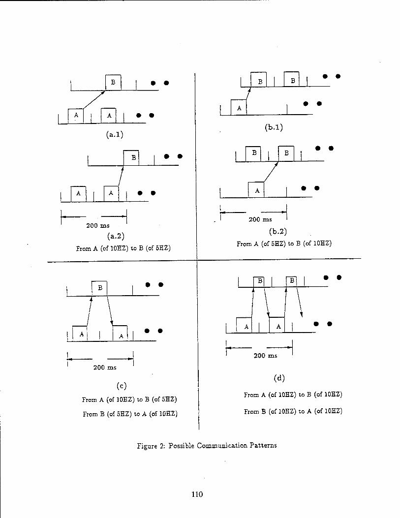
B • •

• •

(a.l)

B • •

• •

200 ms

(a.2)

From A (of 10HZ) to B (of 5EZ)

B • •

• •

200 ms

(c)

From A (of 10HZ) 10 B (of 5HZ)

From B (of 5HZ) to A (of 10HZ)

7 B B

• •

(b.l)

B B • •

• •

200 ms

(b.2)

From A (of 5HZ) to B (of 10EZ)

B B

• •

200 ms

(d)

From A (of 10HZ) to B (of 10HZ)

From B (of 10HZ) to A (of 10HZ)

Figure 2: Possible Communication Patterns

110

2.3 Problem Formulation

We consider the static assignment and scheduling in which a task is the finest granularity object

of assignment and an instance is the unit of scheduling. We applied the simulated annealing

algorithm [KGV83] to solve the problem of real-time periodic task assignment1 and scheduling with

hybrid, timing constraints. In order to make the execution of instances satisfy the specifications

and meet the timing constraints, we consider a scheduling frame whose length is the least common

multiple (LCM) of all periods of tasks. Given a task set T and its communications C, we construct

a set of task instances, I, and a set of multiple communications, M. We extend each task r; € T

to n,- instances, r/, T?, ..., and r"\ These n,- instances are added to I. Each communication r,- *-*

TJ € C is extended to min^^n,-)1 undersampled communications where n,- = LCM/p,- and n,- =

LCM/pj. These multiple communications are added to M. The extension can be stated as follows.

• If rii < rij, then T,- >-* Tj is extended to r/ •-* rj, r? *->■ TJ, ..., and T*' >-*■ TJ.

• If n; > TLJ, then r,- *-+ TJ is extended to T? ►-, rj, TJ >-* TJ, ..., and -/ *-* T-3 .

• If n,- = n,-, then r,- •-> T,- is extended to r/ ►-► rj, r? >-* rj, ...., and rf' i-» TJ-J.

A task ID with a superscript of question mark indicates some instance of the task. For example,

r/ <-* TJ means that r/ communicates with some instance of TJ. We describe how we assign the

nearest instance for each communication in Section 4.1.2.

The problem can be formulated as follows. Given a set of task instance, I, its communications

M, we find an assignment <£, a total ordering cm of all instances, and a total ordering ac of all

communications to minimize

E(o.. am, a£) = E 6(Pi - A,- - s^ + *?) + E *(4+1 - ^' - Pi ~ *?0

+ E *(// - 4) + E «tfTC - **. *«) - 4)

+ E 6(^ - 4 - Latency (T,- to rk)) (5)

subject to sj > r/ and S(tj — tlk,ce) > //, V if — t'fc,

where

'Due to undersampling, when an asynchronous communication is extended to multiple communications, the number of multiple communications is the smaller number of sender and receiver instances.

Ill

• $? is the start time of if under am.

• // is the completion time of rf under om-

• r} = Pi x ü - 1) + Ti» *"* <*; = K x (i -!) + ^-

• <5(x) = 0, if x < 0; and = a, if x > 0.

• <£(T,) is the ID of processor which r,- is assigned to.

• H ~ A 1S t^ie communication from rf to r[. If ^(r,-) = <£(?>), then rf •-+ T( is a local

communication.

• 5(c, oc) is the start time of communication c on the network under ac.

• /"(c, ac) is the completion time of communication c on the network under ac.

The minimum value of E(6.cm,oc) is 2ero. It occurs when the executions of all instances

meet the jitter constraints and all communications meet their latency constraints. A feasible

multiprocessor schedule can be obtained by collecting the values of s\ and //, V i and j. Likewise,

a feasible network schedule can be obtained from S{c.ac)s and F(c.cc)s.

Since the task system is asynchronous and the communication pattern could be in the form of

cyclic dependency, we solve the problem of finding a feasible solution (p. cm, ac) by exploiting the

cvclic scheduling technique and embedding the technique into the simulated annealing algorithm.

3 The Approach

3.1 Bounds of a Scheduling Window

Define the scheduling window for a task instance as the time interval during which the task can

start. Traditionally, the lower and upper bounds of the scheduling window for a task instance are

called earliest start time (est) and latest start time (1st) respectively. These values are given and

independent of the start times of the preceding instances.

We consider the scheduling of periodic tasks with relative timing constraints described in Equa-

tions 3 and 4. The scheduling window for a task instance is derived from the start times of its

preceding instances. A feasible scheduling window for a task instance r/ is a scheduling window

in which any start time in the window makes the timing relation between s?~ and sf satisfy

112

Before: After:

r r + e- LCM

Unscheduled Instance: where F < r < JXM

Figure 3: Insertion of a new time slot

3.2.1 Recurrence

Given any solution point (©, am,ae), we construct the schedule by inserting time slots to the linked

lists. Let cm: task-id x instance-id — integer. The insertion of a time slot for rf precedes that for

Recall that Equations 6 and 7 specify the bounds of the scheduling window for a task instance.

Due to the communications, est(rj) in Equation 6 may not be the earliest time for ij. We define

the effective start time as the time when (1) the hybrid constraints are satisfied and (2) if receives

all necessary data or messages from all the senders.

Given the effective start time r and the assignment of T,- (i.e. p = <£(T>'))> a time slot of processor

p is assigned to 7/ where start-time > r and finish-time - start-time = ej. Jiote that we have

to make sure the new time slot does not overlap existent time slots. Since (ij the executions of

all instances within one scheduling frame recur in the next scheduling frame and (2) it is possible

that the time slot for some instance is over LCM. we subtract one LCM from the start-time or

finish-time if it is greater than LCM. It means the time slot for this task instance will be modulated

113

Equations 3 and 4. Formally, given s}, sj, ..., and ..., s* 1, the problem is to derive the feasible

scheduling window for rf such that a feasible schedule can be obtained if rf is scheduled within

the window.

Proposition 1 {CA93J: Let the est and 1st of rf be

est{r]) = maxUs'-* + p{ - A,-), (*■ + (j - 1) x Pi - (n,- - j + 1) x »*■)}, (6)

and lst(rj) = min{(sj~l + Pi + 17,-), (s] + (j - 1) x p; + (n,- - j + 1) x A,-)}. (")

If S? is in between the esZ(r/) and lst(r?), then the estimated est and isZ of s™', based on 5; and

specify a feasible window. «,■+1

3.2 Cyclic Scheduling Technique

The basic approach of scheduling a set of synchronous periodic tasks is to consider the execution

of all instances within the scheduling frame whose length is the LCM of all periods. The release

times of the first periods of all tasks are zero. As long as one instance is scheduled in each period

within the frame and these executions meet the timing constraints, a feasible schedule is obtained.

In a feasible schedule, all instances complete the executions before the LCM.

On the other hand, in asynchronous task systems, as depicted in Figure 2 in which the LCM

is 200TO5, the periods of the two tasks axe out of phase. It is possible that the completion time

of some instance in a feasible schedule exceeds the LCM. To find a feasible schedule for such an asynchronous system, a technique of handling the time value which exceeds the LCM is proposed.

The technique is based on the linked list structure described in the work [CA93]. Without loss

of generality, we assume the minimum release time among the first periods of all tasks is zero. We

keep a linked list for each processor and a separated list for the communication network. Each

element in the list represents a time slot assigned to some instance or communication. The fields of

a time slot of some processor p: (1) task id i and instance id j indicate the identifier of the time slot.

(2) slari time st and finish time ft indicate the start time and completion time of rf respectively.

(3) prev ptr and next ptr are the pointers to the preceding and succeeding time slots respectively.

The list is arranged in an increasing order of startAime. Any two time slots are nonoverlapping.

Since the execution of an instance is nonpreemptable, the time difference between startjtime and

finish-time equals the execution time of the task.

114

.. o o o o

o o o o e

Py = 4 X pz

Figure 5: Asynchronous communications in mutuality

and k can be stated as (j - 1) x n < i < k < j x n.

A graphical illustration can be found in Figure 5. In the example, the values of t, j, *, and n are

6, 2, 8, 4 respectively. The communications r% ~ r2 and T2 ~ r| are scheduled before and after

the scheduling of r2 respectively.

(8)

4 The Simulated Annealing Algorithm

Kirkpatrick et al. [KGV83] proposed a simulated annealing algorithm for combinatorial optimiza-

tion problems. Simulated annealing is a global optimization technique. It is derived from the

observation that an optimization problem can be identified with a fluid. There exists an analogy

between finding an optimal solution of a combinatorial problem with many variables and the slow

cooling of a molten metal until it reaches its low energy ground state. Hence, the terms about

energy*function, temperature, and thermal equilibrium are mostly used. During the search of an

optimal solution, the algorithm always accepts the downward moves from the current solution point

to the points of lower energy values, while there is still a small chance of accepting upward moves

io the points of higher energy values. The probability of accepting an uphill move is a function of

current temperature. The purpose of Mil climbing is to escape from a local optimal configuration.

If there are no upward or downward moves over a number of iterations, the thermal equilibrium

is reached. The temperature then is reduced to a smaller value and the searching continues from

the current solution point. The whole process terminates when either (1) the lowest energy point

is found or (2) no upward or downward jumps have been taken for a number of successive thermal

equilibrium.

The structure of simulated annealing (SA) algorithm is shown in Figure 7. The first step of

115

CD CD CD

CD CD O

LCM Pseudo Instance

Figure 4: The introduction of a pseudo instance

and wrapped to the beginning of the schedule. As shown in Figure 3 The start-time of the new

slot is r while the completion time is r + e—LCM.

3.3 Pseudo Instances

As stated in Section 2, we consider the communication pattern in which cyclic dependency exists

among tasks. Given a set of tasks, T, a set of task instances. I, a set of communications, C. and

any solution point, {p,cm,cc), we introduce pseudo instances to solve this problem. For any task

r_, if there exists a task ry, in which (1) cm(rz) < om(ry), V :, (2) n. = ny, and (3) r- — ry €

C and ry -* r- € C, then a pseudo instance TJ'3

"*"3 is added to I. A pseudo instance is always a

receiving instance. No insertion of time slots for pseudo instances is needed. For a pseudo instance,

only the effective start time is concerned. The effective start time of a pseudo instance T"r+1 in

the constructed schedule based on (<x>,aTO, ac) is checked to see whether it is less than LCM -f si or

not. If yes, then the execution of 7* for the next scheduling frame may start at LCM + si which

is exactly one LCM away from the execution of r^ for the current scheduling frame. A graphical

illustration of the introduction of pseudo instance to solve the synchronous communications of

cyclic dependency is given in Figure 4 in which n= = 2.

As for the asynchronous communications of cyclic dependency, no pseudo instances are needed.

For example, if both r, -* ry and ry *-, r. exist and n, — ny x n, then for each r->, where j = 1,

2. ..., Tiv, find a sending instance rl £ I and a receiving instance T£ € I such that (1) ft < s'y,

(2) Py < sz, and (3) rx -~ ~i and r-J •-*■ r* are the communications. The relationship between i, j,

116

4.1.1 Priority Assignment of Task Instances: am

In the work [CA93], we presented the SLsF algorithm and the performance evaluation. The re-

sults showed that SLsF outperforms SPF and SJF. In this paper we use the SLsF as the priority

assignment algorithm for the task instances in /.

Formally, if lst{rf) < Ist^), then am(rj) < am(r<). And the insertion of a time slot for

TJ precedes that for 4 if cmtf) < cm(r£). The time-based scheduling algorithm for a task

instance is used to find a time slot for a task instance once the effective start time is given. We

define the effective start time of a task instance as the earliest start time when the incoming

communications are taken into account. Let t be the maximum completion time among all the

incoming communications of a task instance, then the effective start time of the task instance is set

to the bigger value among t and est (as stated in Equation 6).

4.1.2 Scheduling the Incoming Communications:ae

There are two kinds of incoming communications. The first kind is called the synchronous com-

munication in which the frequencies of the sender and receiver are identical. The other kind is

called the asynchronous communication in which the sending task instance is associated with a

question mark. For such an asynchronous communication, we have to decide which instance of the

sending task should communicate with the receiving task instance. The approach we take is to find

xhe nearest instance of the sending task. The reason is that, by finding the nearest instance, the

time difference between start time of the receiving instance and the completion time of the sending

instance is the smallest. The chance of violating the latency constraint of a communication will be

the smallest then.

The nearest instance of a sending task can be found using the following method. Given an

incoming communication T\ -* if, and the effective start time of r], eft we search through the

linked list of processor ö(rfc) up to time eft. If there is some instance of T*, say r{, whose completion

time is the latest among all scheduled instances of rk, then the nearest instance is found. Otherwise,

we continue to search through the linked list until an instance of n is found. We set the effective

start time of the communication to be the completion time of the found instance. We also erase

the question mark such that T\ ~ rj is changed to rjf - rf. For the synchronous communication,

the effective start time of the communication is simply assigned as the finish time of the sending

task instance.

The scheduling of the communication is done by inserting a time slot to the linked list for the

communications network. The start time of the time slot can not be earlier than the effective start

111

the algorithm is to randomly choose an assignment <f>, a total ordering of instances within one

scheduling frame, am, and a total ordering of communications for the instances, oe. A solution

point in the search space of SA is a 3-tuple (4>,crm,oc). The energy of a solution point is computed by

equation (5). For each solution point P which is infeasible, (i.e. Ep is nonzero), a neighbor finding

strategy is invoked to generate a neighbor of P. As stated before, if the energy of the neighbor is

lower than the current value, we accept the neighbor as the current solution; otherwise, a probability

function (i.e. exp( Tj ")) is evaluated to determine whether to accept the neighbor or not. The

parameter of the probability function is the current temperature. As the temperature is decreasing,

the chance of accepting an uphill jump (i.e. a solution point with a higher energy level) is smaller.

The inner and outer loops are for thermal equilibrium and termination respectively. The number of

iterations for the inner loop is also a function of current temperature. The lower the temperature

is, the bigger the number is. Methods about how to model the numbers of iterations and how

to assign the number for each temperature have been proposed [LH91]. In this dissertation, we

consider a simple incremental function. Namely, N = J\7 + A where N is the number of iterations

and A is a constant. The termination condition for the outer loop is £p = 0. Whenever thermal

equilibrium is reached at a temperature, the temperature is decreased. Linear or nonlinear approach

of temperature decrease function can be simple or complex. Here we consider a simple multiplication

function (i.e. T = T x a, where a < 1).

4.1 Evaluation of Energy Value for a Solution Point (d>, em, ac)

The computation of the energy value stated in Equation 5 , is done by constructing multi-processor

schedules and a network schedule, and collecting the the start and completion times of each task

instance and communication from these schedules.

The construction of the schedules is characterized by the priority assignment of the task in-

stances in the set. The priority assignment algorithm determines the scheduling order among all

the task instances. Each time when a task instance is chosen to be scheduled, the incoming com-

munications of the instance are scheduled first and then the task instance itself. After all the task instances have been scheduled, the scheduling of the outgoing communications is performed.

An algorithmic description about how to compute the energy value for a solution point is given

in Figure 6. Note that a communication is an incoming communication to a task instance if the

frequency of the receiving task instance is equal to or less than that of the sending task instance.

For example, r^ -^ rf and r°k •—■ rf are incoming communications to rf. On the other hand, if

the sender frequency is less than the receiver frequency, then the communication is an outgoing

communication, (e.g. r£ »-* iy is the outgoing communication of ri).

118

time of the communication. Once the time slot is inserted, we check the effective start time of rf

to make sure that it is not less than the finish time of the time slot. Kit is, the effective start time

of rf is updated to be the finish time of the time slot.

If a task instance has more than one incoming communication, the scheduling order among these

communications is based on their latency constraints. The bigger the latency value is, the earlier

the communication is scheduled. The incoming communication with the tightest latency constraint

is scheduled last. It is because the effective start time of the receiving task instance is constantly

updated by the scheduling of the incoming communications. It is possible that the scheduling of

the later incoming communications increases the effective start time of the receiving task instance

and make the early scheduled communication violate its latency constraint if the constraint is tight.

4.1.3 Scheduling the Outgoing Communications: ac

The scheduling of the outgoing communications for the whole task set is performed after all the

task instances have been scheduled. The scheduling order among these communications is based

on the finish times of the sending task instances. The task instance with the smallest finish time is

considered first. When a task instance is taken into account, all its outgoing communications are

scheduled one by one according to their latency constraints. The communication with the tightest

latency constraint is scheduled first.

Given an outgoing com muni cation TJ >~* rl, and the finish time of r\, ff, the effective start

time of the communication is set to be //. Based on the effective start time, a time slot in inserted

for this communication. Then the nearest instance of receiving task can be found based on the

finish time of the time slot.

For the example shown in Figure 5, The incoming communication marked with "(l)r is scheduled

before the scheduling of r^. The sixth instance of r- is chosen as the nearest instance. As for the

outgoing communication marked with "(3)n, it is scheduled after the scheduling of r|, rf, rl. and

T|. In this example, r| is the nearest instance of the outgoing communication.

4.2 Neighbor Finding Strategy: 6

The neighbor finding strategy is used to find the next solution point once the current solution point

is evaluated as infeasible (i.e. energy value is nonnegative). The neighbor space of a solution point

is the set of points which can be reached by changing the assignment of one or two tasks. There

are several modes of neighbor finding strategy.

119

• Balance Mode: We randomly move a task from the heavily-loaded processor to the lightest-

loaded processor. This move tries to balance the workload of processors. By balancing the

workload, the chance to find a neighbor with a lower energy value is bigger.

• Swap Mode: We randomly choose two tasks r{ and TJ on processors p and q respectively.

Then we change d> by setting <£(T,-) = q and <P[TJ) = p.

• Merge Mode: We pick two tasks and move them to one processor. By merging two tasks to

a processor, we increase the workload of the processor. There is an opportunity of increasing

the energy level of the new point by increasing the workload of the processor. The purpose of

the move is to perturb the system and allow the next move to escape from the local optimum.

• Direct Mode: When the system is in a low-energy state, only few tasks violate the jitter

or latency constraints. Under such a circumstance, it wiU be more beneficial to change the

assignment of these tasks instead of randomly moving other tasks. From the conducted ex-

periments, we find that this mode can accelerate the searching of a feasible solution especially

when the system is about to reach the equilibrium.

The selection of the appropriate mode to find a neighbor is based on the current system state.

Given a randomly generated initial state (i.e. solution point), the workload discrepancy between

the processors may be huge. Hence, in the early stage of the simulated annealing, the balance

mode is useful to balance the workload. After the processor workload is balanced out, the swap

mode and the merge mode are frequently used to find a lower energy state until the system reaches

near-termination state. In the final stage of the annealing, the direct mode tries to find a feasible

solution. The whole process terminates when a feasible solution is found in which the energy value

is zero.

5 Experimental Results

We implemented the algorithm as the framework of the allocator on MARUTI [GMK+91, MSA92,

SdSA94], a real-time operating system developed at the "university of Maryland, and conducted

extensive experiments under various task characteristics. The tests involve the allocation of real-

time tasks on a homogeneous distributed system connected by a communication channel.

To test the practicality of the approach and show the significance of the algorithm, we consider a

simplified and sanitized version of a real problem. This was derived from actual development work,

and is therefore representative of the scheduling requirements of an actual avionics system. The

Boeing 777 Aircraft Information Management System (AIMS) is to be running on a multiprocessor

120

10-Proc 9-Proc SJProc 7JProc 6JProc 1 Exec.Time (Sec) 2369 5572 19774 36218 78647 1 = Er : Min : Sec | 0:39:29 1:32:52 5:29:34 10:03:38 21:50-47

Table 1: The execution times of the ALMS with different number of processors

system connected by a SafeBus (TM) ultra-reliable bus. The problem is to find the minimum

number of processors needed to assign the tasks to these processors. The objective is to develop

an off-line non-preemptable schedule for each processor and one schedule for the SafeBus (TM)

ultra-reliable bus.

The AIMS consists of 155 tasks and 951 communications between these tasks. The frequencies

of the tasks vary from 5HZ to 40HZ. The execution times of the tasks vary from 0ms to 16.650ms.

The NEI and XEI of a task 1,- axe p,- - 500/xs and p,- + 500/xs respectively. Since 6 = lOOO^s = lms

< 2^, the smallest-period-first scheduling algorithm can be used in this case. Tasks communicate

with others asynchronously and in mutuality. The transmission times for communications are in the

range from 0/xs to 447.733/xs. The latency constraints of the communications vary from 68.993ms

to 200ms. The LCM of these 155 tasks is 200ms. When the whole system is extended, the total

number of task instances within one scheduling frame is 624 and the number of communications is

1580.

For such a real and tremendous problem size, pre-analysis is necessary. We calculate the resource

utilization index to estimate the minimum number of processors needed to run AIMS. The index

is defined as

LCM

where e, is the execution of task i,- and g,- = ^p- The obtained index for AIMS is 5.14. It means

there exist no feasible solutions for the AIMS if the number of processors in the multiprocessor

system is less than 6.

The number of processors which the AIMS is allowed to run on is a parameter to the scheduling

problem. We start the AIMS scheduling problem with 10 processors. After a feasible solution is

found, we decrease the number of processors by one and solve the whole problem again. We run

the algorithm on a DECstation 5000. The execution time for the AIMS scheduling problem with

different numbers of processors is summarized in Table 1. The algorithm is able to find a feasible

solution of the AIMS with six processors which is the minimum number of processors according

to the resource utilization index. The time to find such a feasible solution is less than one day

(approximately 22 hours).

121

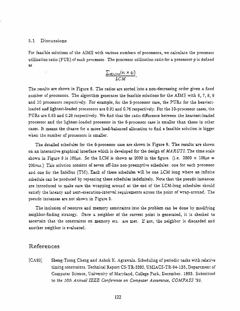
5.1 Discussions

For feasible solutions of the AIMS with various numbers of processors, we calculate the processor

utilization ratio (PUR) of each processor. The processor utilization ratio for a processor p is defined as

E«.,-)a>(e«- x ft) LCM

The results are shown in Figure 8. The ratios are sorted into a non-decreasing order given a fixed

number of processors. The algorithm generates the feasible solutions for the AIMS with 6, 7, 8, 9

and 10 processors respectively. For example, for the 6-processor case, the PURs for the heaviest-

loaded and lightest-loaded processors are 0.91 and 0.76 respectively. For the 10-processor cases, the

PURs are 0.63 and 0.28 respectively. We find that the ratio difference between the heaviest-loaded

processor and the lightest-loaded processor in the 6-processor case is smaller than those in other

cases. It means the chance for a more load-balanced allocation to find a feasible solution is bigger

when the number of processors is smaller.

The detailed schedules for the 6-processor case are shown in Figure 9. The results are shown

on an interactive graphical interface which is developed for the design of MARUTI. The time scale

shown in Figure S is 100/zs. So the LCM is shown as 2000 in the figure, (i.e. 2000 x 100/is =

200ms.) This solution consists of seven off-line non-preemptive schedules: one for each processor

and one for the SafeBus (TM). Each of these schedules will be one LCM long where an infinite

schedule can be produced by repeating these schedules indefinitely. Note that the pseudo instances

are introduced to make sure the wrapping around at the end of the LCM-long schedules should

satisfy the latency and next-execution-interval requirements across the point of wrap-around. The

pseudo instances are no* shown in Figure 9.

The inclusion of resource and memory constraints into the problem can be done by modifying

neighbor-finding strategy. Once a neighbor of the current point is generated, it is checked to

ascertain that the constraints on memory etc. are met. If not, the neighbor is discarded and

another neighbor is evaluated.

References

[CA93] Sheng-Tzong Cheng and Ashok K. Agrawala. Scheduling of periodic tasks with relative

timing constraints. Technical Report CS-TR-3392, UMIACS-TR-94-135, Department of

Computer Science, University of Maryland, College Park, December. 1993. Submitted

to the JOth Annual IEEE Conference on Computer Assurance, COMPASS '95.

122

[CDHC94] T. Carpenter, K. Driscoll, K. Hoyme, and J. Carciofini. Arinc 659 scheduling: Problem

definition. In Proceedings of IEEE Real-Time Systems Symposium, San Juan, PR, Dec. 1994.

[GMK+91] Ö. Gudmundsson, D. Mosse, K.T. Ko, A.K. Agrawala, and S.K. Tripathi. Maruti: A

platform for lard real-time applications. In K. Gordon, A.K. Agrawala, and P. Hwang

(eds.), editors, Mission Critical Operating Systems. IOS Press, 1991.

[HS92] Chao-Ju Hou and Kang G. Shin. Allocation of periodic task modules with precedence

and deadline constraints in distributed real-time systems. In Proceedings of the 1992

IEEE 13th Real-Time Systems Symposium, pages 146-155, Phoenix, AZ, 1992.

[KGV83] S. Kirkpatrick, C. D. Gelatt. and M. P. Vecchi. Optimization by simulated annealing.

Science, 220(4598):671-680, May 1983.

[LH91] Feng-Tse Lin and Ching-Chi Hsu. Task assignment problems in distributed comput-

ing systems by simulated annealing. Journal of the Chinese Institute of Engineers,

14(5):537-550, Sept. 1991.

[MSA92] Daniel Mosse, M.C. Saksena, and Ashok K. Agrawala. Maruti: An approach to real-

time system design. Technical Report CS-TR-2845, UMIACS-TR-92-21, Department

of Computer Science, University of Maryland, College Park, 1992.

[Ram90] Krithi Ramamritham. Allocation and scheduling of complex periodic tasks. In Pro-

ceedings of the 10th International Conference on Distributed Computing Systems, pages

108-115, Paris, France, 1990.

[SdSA94] M. Saksena, J. da Silva, and A. K. Agrawala. Design and implementation of maruti-

ii. Technical Report CS-TR-2845, Department of Computer Science, University of

Maryland, College Park, 1994.

[TBW92] K. W. Tindell, A. Burns, and A. J. "Wellings. Allocating hard real-time tasks: an

NP-hard problem made easy. Real-Time Systems, 4(2):145-165, June 1992.

123

Given a solution point P = (4>, cm,cc) While there is some unscheduled task instance do

Find the next unscheduled instance. /* By the SLsF algorithm */ Let the instance be r/.

Sort all the incoming communications of rf based on the latency values into a descending order.

Schedule each incoming communication starting from the biggest-latency one to the tightest-latency one.

Schedule the instance rj. End While. Mark each instance as un-examined. While there is some un-examined task instance do

Find the next un-examined task instance. /* By the finish times */ Sort all the outgoing communications of the task instance based

on the latency values into an increasing order. Schedule each outgoing communication starting from

the tightest-latency one to the biggest-latency one. Mark the task instance examined.

End While. CoDect the start time and finish time informations for each task instance and communication. Compute the energy value using Equation 5.

Figure 6: The pseudo code for computing the energy value

124

Choose an initial temperature T Choose randomly a starting point P = (<j>, am,ac) Ep := Energy of solution point P if EP = 0 then

output Ep and exit /* Ep = 0 means a feasible solution */ end if repeat

repeat Choose N, a neighbor of P En := Energy of solution point N if En = 0 then

output En and exit /* En = 0 means a feasible solution */ end if if En < Ep then

P :=N Ep := En

else

if er > random(O.l) then P := ^T

EP := En

end if end if

until thermal equilibrium at T T := Q x T (where a < 1)

until stopping criterion

Figure 7: The structure of simulated annealing algorithm.

125

Ptocauof UMuuon utilitfciion luric

1.00 -

e.ts -

C.JO -

0.»i

c.»o |-

e.7s

c>o

o.ts

o.to

0.55

C.SO

0.«5

0.«

O.JS

0.30

0.25

0.20

0.15

0.10

0.05

0.00

-C.05

lO_Proc \-.rroc

^.Trioe" T_?röc*

_J.

Figure 8: Processor Utilization Ratios for different cases

File lnoul.>-«oh Mloeaw Vi<» üortuns File: lovol.BP.Wt6

100 200300 400 500600700800900 1000 1100 12O0 1300 1*00 1500 1600 1700 1B0O 1900 200C

164 515 168 Ü

411

„ . MSf«-JSe92«2 '■W'iMSg* ,:<gg«S4ECS7C, 5«SglB4£32S ■5gSS6'lS<5g<l 5*55175546326 .^^- P 1-rniMiMtirr nmmmrrP^—JITTTTTT-, mrp-i TTTTH nnn: im;, in mii^ m-in till impm d

■tZagSlS? »9a£5 511521 ~trn rmr^^^—rr 7 —

P 2: 33'352 gn250<g3:4TK15GZ22?4< .S3S53 2<a2SC4gr«41115Z223215ggg54 ZJl-25t5g«,E16g223?45234l " Iriii . i in ii-ii'< f !;■■■! nirmi ii:., nr\ t n i mi i, MI i nnn i i ii !

B55 gü-2SS341 1622234 m| i i i in i irm

E - 4V<E602 .447.17 4*44^7318 «S7226 .446 844 5(443 399 313*0228.449,18 S44-17212B , 5:47229 ,450. 5-445 401 p 3= CDU) i—-V' r~-n o i i i I i i i ■■ ■ T-11 in i ir"in i i i" ~l i ii I 1 i i " P 4:

P 5:

26S40J130 2655426 11,1 II

4<4'

2663452 rr-r

<^2662243O0e 24266302118 III ■ ■ II' ■ ) PITT

_, 26622426 J I.I I IT

120 2667 453 EC

*2266Z2429 409 TTI! i ir

>»272g034ggni34g72glW9262, Wg72giy9S2< 342722234S50e ,K272gl^9^Z23a4g72gl0492B3, MZ72211H9S525.*2S221tM 9609 UHU Ü DE ECZDOE ZDU in : T t n; in i n , i , HIT t n ■■ 11 in-Tf i.~ i i in i I

„ ,. 0KEM2»3Är£?l£W<r>4Z3II£X57433ieTVMHy<>O>^^

Figure 9: The Allocation Results and Schedules for AIMS with 6 processors

126

REPORT DOCUMENTATION PAGE

1. AGENCY USE ONLY (leave blank) 2. REPORT DATE January 1995

Form approved OMB No 074-0188

3. REPORT TYPE END DATES COVERED Technical Report

4. TITLE AND SUBTITLE

Allocation and Scheduling of Real-Time Periodic Tasks with Relative Timing Constraints

6. AUTHOR(S)

Sheng-Tzong Cheng and Ashok K. Agrawala

PERFORMING ORGANIZATION NAME(S) AND ADDRESS(ES) University of Maryland Department of Computer Science A.V. Williams Building College Park, MD 20742

SPONSORING/ MONITORING AGENCY NAME(S) AND ADDRESS(ES)|l

Honeywell Inc. Phillips Laboratory 3600 Technology Drive Directorate of Contracting Minneapolis, MN 55148 3651 Lowry Avenue, SE

Kirtland AFB, NM 87117-5777

5. FUNDING NUMNBERS

N00014091-C-0195 DSAG-60-C-0055



I0. SPONSORING/ MONITORING AGENCY REPORT NUMBER


12.a. DISTRIBUTION/ AVAILABILITY STATEMENT 12.b. DISTRIBUTION CODE

13. ABSTRACT (Maximum 200 words) Allocation problem has always been one of the fundamental issues of building the applications in distributed computing

systems (DCS). For real-time applications on DCS, the allocation problem should directly address the issues of task and communication scheduling. In this context, the allocation of tasks has to fully utilize the available processors and the scheduling of tasks has to meet the specified timing constraints. Clearly, the execution of tasks under the allocation and schedule has to satisfy the precedence, resources, and other synchronization constraints among them.

Recently, the timing requirements of the real-time systems emerge that the relative timng constraints are imposed on the consecutive executions of each task and the inter-task temporal relationships are specified across task periods. In this paper we consider the allocation and scheduling problem of the periodic tasks with such timing requirements. Given a set of periodic tasks, we consider the least common multiple (LCM) of the task periods. Each task is extended to several instances within the LCM. The scheduling window for each task instance is derived to satisfy the timing constraints. We develop a simulated annealing algorithm as the overall control algorithm. An example problem of the sanitized version of the Boeing 777 Aircraft Information Management Systems is solved by the algorithm. Experimental results show that the algorithm solves the problem in a reasonable time complexity.

14. SUBJECT TERMS Process Management; Special Purpose and Application-Based Systems

15. NUMBER OF PAGES

22

16. PRICE CODE

17. SECURITY CLASSIFICATION OF REPORT Unclassified

18. SECURITY CLASSIIFICATION OF THIS PAGE

Unclassified


Unclassified


Unlisted

MSN 7540-01 280-5500 127

Standard Form 298 (Rev 2-89)

Scheduling of Periodic Tasks with Relative Timing Constraints

Sheng-Tzong Cheng and Ashok K. Agrawala Institute for Advanced Computer Studies



{stdheng,agrawala}@cs.umd.edu

Abstract

The problem of non-preemptive scheduling of a set of periodic tasks on a single processor

has been traditionally considering the ready time and deadline on each task. As a consequence,

a feasible schedule finds that in each period one instance of each task starts the execution after

the ready time and completes the execution before the deadline .

Recently, the timing requirements of the real-time systems emerge that the relative timing

constraints are imposed on the consecutive executions of each task. In this paper, we consider

the scheduling problem of the periodic tasks with the relative timing constraints imposed on two

consecutive executions of a task. We analyze the timing constraints and derive the scheduling

window for each task instance. Based on the scheduling window, we present the time-based

approach of scheduling a task instance. The task instances are scheduled one by one based on

their priorities assigned by the proposed algorithms in this paper. We conduct the experiments

to compare the schedulability of the algorithms.

T^s *ork.ls SttPP°rted in part by Honeywell under N00014-91-C-0195 and Army/Phillips under DASG-60-92- C-0055. The views, opinions, and/or findings contained in this report are those of the author(s) and should not be interpreted as representing the official policies, either expressed or implied, of Bonevwell or Army/Phillips.

129

1 Introduction

The task scheduling problem is one of the basic issues of building real-time applications in which the

tasks of applications are associated with timing constraints. For the hard real-time applications,

such as avionics systems and nuclear power systems, the approach tp guarantee the critical timing

constraints is to schedule periodic tasks a priori. A non-preemptive schedule for a set of periodic

tasks is generated by assigning a start time to each execution of a task to meet their timing

constraints. Failure to meet the specified timing constraints can result in disastrous consequence.

Various kinds of periodic task models have been proposed to represent the real-time system

characteristics. One of them is to model an application as a set of tasks, in which each task is

executed once every period under the ready time and deadline constraints. These constraints impose

constant intervals in which a task can be executed. In literature, many techniques [2, 3, 4, 5, 6, 7, 8]

have been proposed to solve the scheduling problem in this context. The deficiency of this modeling

is the inability of specifying the relative constraints across task periods. For example, one can not

specify the timing relationship between two consecutive executions of the same task.

Simply assuring that one instance of each task starts the execution after the ready time and

completes the execution before the specified deadline is not enough. Some real-time applications

have more complicated timing constraints for the tasks. For example, the relative timing constraints

may be imposed upon the consecutive executions of a task in which the scheduling of two consecutive

executions of a periodic task must be separated by a minimum execution interval. The Boeing 777

Aircraft Information Management System is such an example [1). One possible solution to the

scheduling problem of such applications is to consider the instances of tasks rather than the tasks.

A task instance is denned as one execution of a task within a period. With the notion of task

instances, one is able to specify the various timing constraints and dependencies among instances

of tasks.

In this paper, we consider the relative timing constraints imposed on two consecutive instances

of a task. The task model and the analysis of the timing constraints are introduced in Sections 2

and 3 respectively. Based on the analysis, we are able to derive the scheduling window for each

task instance. Given the scheduling window of a task instance, we present the time-based approach

of scheduling a task instance in Section 4. We propose three priority assignment algorithms for the

task instances in Section 5. The task instances are scheduled one by one based on their priorities.

In Section 6. we evaluate the three algorithms and show the experimental results.

130

2 Problem Statement

Consider a set of periodic tasks r = { T,- | i — 1, ... n }, where T,- is a 4-tuple < j>;, e,-, A;, T?,- >

denoting the period, computation time, low jitter and high jitter respectively. One instance of a

task is executed each period. The execution of a task instance is non-preemptable. The start times

of two consecutive instances of task r,- are at least p,- — A,- and at most pt- + 77,- apart.

In order to schedule periodic tasks, we consider the least common multiple (LCM) of all periods

of tasks. Let n,- be the number of instances for task r,- within a schedule of length LCM. Hence, n;

= k^M _ A schedule for a set of tasks is the mapping of each task T,- to n,- task instances and the

assigning of a start time s] to the j-th. instance of task ry, ij, V i = 1, ... n and j = 1, ..., n.,-. A

feasible schedule is a schedule in which the following conditions are satisfied for each task r,-:

f! = if + c- a)

^■'+1 = 4 +LCM (2)

s{ > sf+pi-Xi (3)

4 < si-'+pt + v (4)

Vj = 2,...,7i,- + 1.

The non-preemption scheduling discipline leads to Equation 1 where // is the finish time of r,-.

Another condition for non-preemption scheduling is that given any i, j. k and£,if s£ < s[ then //

< s£. It means the schedule for any two instances is non-overlapping. The constructed schedule of

length LCM is invoked repeatedly by wrapping-around the end point of the first schedule to the

start point of the next one. Hence, as shown in Equation 2, the start time of the first instance in

the next schedule is exactly one LCM away from that of the first schedule. Finally, Equations 3

and 4 specify the relative timing constraints between two consecutive instances of a task.

3 Analysis of Relative Timing Constraints

Define the scheduling window for a task instance as the time interval during which the task can

start. Traditionally, the lower and upper bounds of the scheduling window for a task instance are

called earliest start time (est) and latest start time (1st) respectively. These values are given and

independent of the start times of the pre'-e.ding instances.

131

! Instance ID est =■ sTl + Pi - A,- 1st = sf _1 +Pi + TJi actual start time (s])

i ^ 0 40 4

i -■ 39 49 40

" rf 75 85 77

\ rf 112 122 113

i r> 148 158

Table 1: An example to show the wrong setting of scheduling windows

We consider the scheduling of periodic tasks with relative timing constraints described in Equa-

tions 3 and 4. The scheduling window for a task instance is derived from the start times of its

preceding instances. A feasible scheduling window for a task instance rf is a scheduling window

in which any start time in the window makes the timing relation between «f1 and s? satisfy

Equations 3 and 4. Formally, given s], 5?, ..., and ..., «f1, the problem is to derive the feasible

scheduling window for rf such that a feasible schedule can be obtained if rf is scheduled within

the window.

For the sake of simplicity, we assume that r, = 0 and d{ = *, V i, in this section. Then, simply

assigning esi and 1st of rf as sf + Pi - A; a*d 4~* + W + * respectively where i = 1, 2, ..., n

sad j = i, 2, ..., n„ is not tight enough to guarantee a feasible solution. For example, consider

the case shown in Table 1 in which a periodic task r, is to be scheduled. Let LCM, ;>„ A„ and r„-

be 200. 40, 5, and 5 respectively. Hence, there are 5 instances within one LCM (i.e. n,- = 5). The

first column in Table 1 indicates the instance IDs. The second and third columns give the est and

ist of the scheduling windows for the task instances specified in the first column. The last column

shows the actual start times scheduled for the particular task instances. The actual start time is

a value in between est and 1st of each task instance. For instance, the est and 1st of r? are 39 and

49 respectively. It means 39 < s? < 49. The scheduled value for 5?, in the example, is 40. Since

*« = «! J- LCM = 204. we find that any value in the interval [148,158] can not satisfy the relative

timing constraints between rf and rf. As a consequence, the constructed schedule is infeasible.

We draw a picture to depict the relations among the start times of task instances in Figure 1.

When rf is taken into account, the scheduling window for sj is obtained by considering its relation

with s'-1 as well as that with s? and s*,+1 • w^ m*ie sure that once ^ is determined, the estimated

est and 1st of ^\ based on 4 ™ä *"'""' sPecify a feasible scheduMnS window for s?' Name3>?< the

interval-which is specified by the estimated est and 1st of 5?, based on si overlaps the interval

132

J-l

Figure 1: The relations between the task instances

[tf'+1-(ft+ ttO.*r"-(*-*,■)]■

Proposition 1: Let the est and 1st of T? be

esttf) = max{{sTl + Pi - A,-), (s] + (j - 1) x p, - (nj - ; 4- 1) x TJ,-)}, (5)

and 25i(7f') = mm{(^-1 + p,- + r?,), (s,1 + (j - 1) x p,■ + (n, - j + 1) X A,-)}. (6)

If s? is in between the esttf) and Is^rf), then the estimated est and is! of **'', based on sj and

s*'+ , specify a feasible window.

Proof: Let £ and -p be the estimated est and Zst of s?, based on 4, respectively.

Hence,

/ = s? + (»i,- - j) x (P{ - Xi) (7)

p = s>{ + (n,- - j) x (p; + 77,-) (8)

To guarantee the existence of feasible start time of r/1', the interval [£,/z] has to overlap the

interval [S*,T1

- (p, -j- 77,), 5^'+1- (p; - A,-)]. Hence the following conditions have to be satisfied:

„TlV-fl - t > P. - A, (9)

133

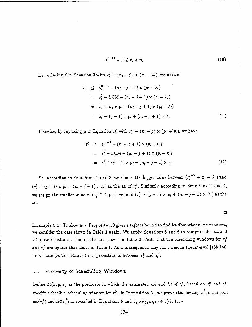
5 n,+1-M <?,- + *?,• (10)

By replacing C in Equation 9 with s{ -f {n; — jf) x (p,- - A,-), we obtain

si < s^+1-{m-j + i)x{pi-Xi)

= s}+ LCM - (n,- - j 4 1) x (p, - A,-)

= s] + n,- x pi - (n,- - j + 1) x (p,- - A,)

= s} + (j-l)xpi + {ni-j + l)x\i (11)

Likewise, by replacing /i in Equation 10 with s? + (n,- - j) x (p; + T?,), we have

= sj + LCM - (n,- - j + 1) x (pv + 7?,)

= s}+(j-l)xpi-(ni-j+l)X7ii (12)

So. According to Equations 12 and 3, we choose the bigger value between (s'~ + p,- - A,-) and

(5J + (j - 1) x p:- - (n,- - j -r 1) x 7?,-) as the esi of rf. Similarly, according to Equations 11 and 4,

we assign the smaller value of (s;_1 -f p; -r »?;) and (s? -f (j - 1) x p,- ~ (n,- - j + 1) x A,-) as the

is!.

Example 3.1: To show how Proposition 3 gives a tighter bound to find feasible scheduling windows,

we consider the case shown in Table 1 again. We apply Equations 5 and 6 to compute the esi and

is! of each instance. The results are shown in Table 2. Note that the scheduling windows for r/

and r? are tighter than those in Table 1. As a consequence, any start time in the interval [159,160]

for T* saiisfys the relative timing constraints between rf and rf.

3.1 Property of Scheduling Windows

Define P,(z,y. z) as the predicate in which the estimated esi and 1st of rf, based on sf and sf,

specify a feasible scheduling window for rf. In Proposition 3 , we prove that for any s:- in between

est(rf) and lst(rf) as specified in Equations 5 and 6, P,-(j. n,-. n, -r 1) is true.

134

Instance ID esi from Equation 5 bt from Equation 6 actual start time (s^)

r! 0 40 4 _2 'i 39 49 40 _3 75 85 77

T? 114 122 115

'i 159 160 159 ~ 160

Table 2: The correct setting of scheduling windows based on Proposition 3.1.

Lemma 1 Given s], sf, ..., and $*, if, V k = 2, ..., j, est(V*J < sf < 1st (rfj as specified in

Equations 5 and 6, then Pi(j,y, n,- + 1) is true, V y = j -f 1, j + 2, ..., n,-.

Proof: We prove that the estimated est and 1st of r*, based on s; and s*' , specify a feasible

scheduling window, by showing that (1) the estimated scheduling window of s?, based on s^, is

specified by the interval

Wi + (y ~ J) * (Pi ~ Ai)» *; + (» - i) x (Pi + >&■)]> (13)

(2) the estimated scheduling window of s*, based on s* , is specified by the interval

[^ - (n,- - y + 1) x (p, + 77,), s^1 - (n,- - y + 1) x (p; - X.;)}

and (3) the intervals in Equations 13 and 14 overlap.

(14)

In Figure 2, we see that the necessary and sufficient conditions for the overlapping of the

intervals specified in Equations 13 and 14 are

*i + (V - J) * (Pv - A,-) < s?+1 - K - y -f 1) x (p,- - A,-)

anc d S*'T1 - (n,- - y + 1) X (p; 4 77.) < *■ + (y - j) X (p; + 7?,-).

(15)

(16)

By solving the Equations 15 and 16, we obtain

4 < ^ + (j-l)xp) + (nl-j'4 1)xAi

and s] > s] + (j - 1) x p,-- (nt-- j + 1) x rti.

The above two equations describe the same conditions as Equations 11 and 12 do. Hence, P,-(j, y. n,- -f 1)

is true, V y = j -f 1. j -f 2, ..., n,-.

135

,n, + l

si + {y- j) X (pi - A,-) 4 + (y - j) x (p; + J?,-)

*?'+ - (n; - y + 1) x (p,- + T?0 ^+1 - (n,- - y + 1) x (■»,- - A,-)

Figure 2: The overlapping of two intervals

Lemma 2 Given s], sj, ..., 4, and an integer no, where 1 < n0 < j, :/, V k = 2, ..., j, estfc )

< s\ < kt(Ti) are specified as in Equations 5 and 6, then P,-(j\y,n,- + n0) is true, V y = j + 1,

j + 2, ..., n,-.

Proof: We use the same method in Lemma 1 to prove it. We show that (1) the estimated scheduling

window of s*, based on s:{. is specified by the interval

[4 + (y- J) * iPi - A,), s< + (y - j) x fo + *)], (17)

(2) the estimated scheduling window of s*. based on £^,"rn°, is specified by the interval

l*r+B0 - (n,- + n0 - y) x (p, + *•), S^*0 " K + *o - y) x (p,- - A,-)], (IS)

and (3) these two intervals overlap.

The following conditions have to be satisfied to make sure the overlapping of the two intervals.

4 < C + 0' ~ 1) x Pi + (ni - J + 1) x A,- - (p,- - A) x no - 1

and sj > s? -f (j - 1) x p,- - (nt- - j + 1) x 77, - (p, + TJ.) X n0 - 1.

(19)

(20)

Since 4 < $T ~ (P=_ A) x (n0- 1) and s? > sf° - (p,--r7?,-) x (n0- 1), we rewrite Equations 19

and 20

4 < s?° + (j - 1) x pj + (m - j + 1) x A,-(p,- - A) x n0 - 1

136

< £J.+ 0" - 1) x Pi + fa - j + 1) x X{

and sj > £^ + (j - 1) x p,- - (n,- - j + 1) x 17,—(p,- + T?,) x np - 1.

> f[ + (i - i) x pi - fa - j +1) x TU

Hence P,-(;', y, n; + n0) holds for any 1 < n0 < j.

Theorem 1 Given $}, s], ..., and s-, if, V k = 2, ..., j, estfrj1) < s- < lstfr^j as specified in

Equations 5 and 6, then Pi(j,y, z) is true, V y = j + 1, j + 2, ..., n,-, and z = n,- + 1, n.,- + 2, ...,

n,-+ j.

By combining the proofs in Lemmas 1 and 2, it is easy to see that Theorem 1 holds. Based on

Theorem 1 , we can assign the scheduling window for rj by using Equations 5 and 6 once s], sa-,

Before we present the scheduling technique for a task instance, let us consider the following

objective. The objective can be formulated as follows. Given a set of tasks with the characteristics

described in Section 2. we schedule the task instances for each task within one LCM to minimize

*= £ «(*? - sf1 - Pi) (2D »j

Subject to the constraints specified in Equations 1 through 4,

where a(x) = 2, if x > 0; = —x, otherwise.

Basically, we try to schedule every instance of a task one period apart from its preceding

instance. An optimal schedule is a feasible schedule with the minimum total deviation value from

one period apart for instances.

4 The Time-Based Scheduling of a Task Instance

We consider the time-based solution to the scheduling problem by using a linked list. Each element

in the list represents a time slot assigned to a task instance. A time slot w has the following fields:

(1) task id i and instance idj indicate the identifier of the time slot. (2) start time st and finish time

ft indicate the start time and completion time of r? respectively. (3) prev ptr and next pir are the

137

new arriving instance: ■ [««(Tf), l5t(rf)]

S2 h 53 /3

LCM

Before:

After:

h S2 h 53

h fi + e •S2 •S3 /3

Figure 3: Insertion of a new time slot

pointers to the preceding and succeeding time slots respectively. We arrange the time slots in the

list in increasing order by using the start time as the key. Any two time slots are non-overlapping.

Since the execution of an instance is non-preemptable, the time difference between start time and

finish time equals the execution time of the task.

4.1 Creating a Time Slot for the Task Instance

Consider a set of n tasks. Given a linked list and a task instance r-, we schedule the instance by

inserting a time slot to the list. According to equations 5 and 6, we compute the est(r-) and lst(r?)

first. Let 5 be the set of unoccupied time intervals that overlap the interval \est{r^), lst(r?)] in the

linked list. The unoccupied time intervals in 5 are collected by going through the list. Each time

when a pair of time slots (w, w + 1) is examined, we compute I = max{ esi(Tf), ft{v>)} and \i =

min{2si(rf), st(w -f 1)}, where ft(w) is the finish time of the time slot w, and st(w +1) is the start

time of the slot next to ic. If I < fi. then we add the interval [£, (i) to 5.

The free intervals in S are the potential time slots which r- can be assigned to. Since we try

to schedule T? as close to one period away from the preceding instance 7^~ as possible, we sort 5,

based on the function of the lower bound of each interval, a(^~: + Pi — ■£), in ascending order.

Without loss of generality, we assume that 5 after the sorting is denoted by {inti. ini^. ..., int\s\)

138

The idea is that if rj is scheduled to intk, then the value in equation 21 will be smaller than that

of the case in which -■ is scheduled to tni/c+j.

The scheduling of rf can be described as follows. Starting from int^ we check whether the

length of the interval is greater or equal to the execution time of rf or not. If yes, then we schedule

the instance to the interval. One new time slot is created in which the start time is the lower bound of the interval and the finish time equals the start time plus the execution time. The created time

slot is added to the linked list and the scheduling is done. If the length is smaller than the execution

time, then we check the length of the next interval until all intervals are examined. An example is

shown in Figure 3 in which the slot with dark area represents rj. In this example we assume that

estiTi) < h and «2 - /i > e. It means the free slot between the first ar.-d second occupied slots

can be assigned to r/.

4.2 Sliding of the Time Slots

In case none of the intervals in S can accommodate a lask instance, the sliding technique is used

to create a big enough interval by sliding the existence time slots in the list.

To make the sliding technique work, we maintain two values for each time slot: left laxity and

right laxity. The value of left laxity indicates the amount of time units by which a time slot can be

left-shifted to a earlier start time. Similarly, the right laxity indicates the amount of time units by

which a time slot can be right-shifted to a later start time.

Given the time slots «;*_!, wk, and wk+i, where a and b are the task and instance identifiers of

wk respectively, the laxity values of the time slot wk can be computed by:

UftJaxity(wk) = min{s\ - est1, s\ - ft(wk-i) + leftdaxity{wk.{)} (22)

rightJaxity(wk) = min{lsi' - sha, st(v>k+1) - /> + right Jaxity{uK^)} (23;

where est' = max{est(rba), s?1 - (pB + 7ja)}

and 1st' = min{lst{rl), s»* - (Pa - Aa)}.

Kote that the interval [est\ lsir\ defines the sliding range during which T* can start without

shifting rcfc-1 or r0

fc+1. A schematic illustration of equations 22 and 23 is given in Figure 4.

From equations 22 and 23, we see that the computing of leftJaxity(wk) depends on that of vik-i

and the computing of rightJaxiiy(vsk) depends on that of wk+i. It implies a two-pass computation

139

si - est>

\ , 1st' - sba

sba - fi{v>k-i) u u

St{wk+i)- fa

M Wk+1

«.fc-1 If* V>k-1

est(sba)

rM-l

2*t(4) Po + 7?c

Po - ^o

es? 1st'

Figure 4: An illustration of leftJaxity(wk) and righUaxity(wk)

is needed to compute the laxity values for all time slots. The complexity is 0(27\r) where N is the

number of time slots in the linked list.

The basic idea of the sliding technique is described as follows. Given a task instance T? and a

set of unoccupied intervals, S = {inly, int2, ..., inl^,}, we check one interval at a time to see if

the interval can be enlarged by shifting the existent time slots. Two possible ways of enlargement

are (3) by either shifting the time slots, that precede the interval, to the left or (2) shifting the

slots, that follow the interval, to the right. The shifting depends on which direction minimizes the

objective function in Equation 21.

4.3 The Algorithm

An algorithmic description about how to schedule a task instance, as described in Sections 4.1

and 4.2, is given in Table 3.

The procedures Left-Shift^*,time-units) and Right-Shift^^time-units) in Table 3 may involve

the shifting of more than one time slot recursively. For example, consider the case in Figure 4, if

Right-Shift^Jsi' - sha) is invoked (i.e. wk is to be shifted right by 1st?. - sb

c time units), then

Wk+i has to be shifted too. It is because the gap between wk and uufc+j is si(tofc+i) - fc which is

140

smaller than 1st' - sba. In this case, Right_Shift(u>*+1,/s*' - sb

a - st(wk+l) + fb) is invoked.

We do not enlarge an interval at both ends. Enlarging an interval at both ends needs to shift

certain amount of preceding time slots to the left and shift some succeeding slots to the right. It is

possible that some task instance r* is shifted left, while r^+1 is shift«! right. As a consequence, the

timing constraints between s% and i^+1 could be violated. For example. Let s% and s£+1 before the

shifting be 10 and 20 respectively. The execution time for rx is 5 time units. Assume the left laxity

of r| is 5 and the right laxity of T*+1 is 5. It implies sy

x+y - s% < 15. Consider the scheduling of a

task instance -/ with execution time 15. If we enlarge the interval between r| and r|+1 by shifting

T% left 5 time units and ry+1 right 5 time units, then we get a new interval vrith 15 time units for

r\. However, it turns out that s*+i = 25, s% = 5, and the relative timing constraints between r|

and r^+1 is violated.

5 The Priority-Based Scheduling of a Task Set

We consider the priority-based algorithms for scheduling a set of periodic tasks with hybrid timing

constraints. Given a set of periodic tasks r = { r,- | :' = 1, ..., n } with the task characteristics

described in Section 2, we compute the LCM of all periods. Each task r,- is extended to n,- task

instances: r/, r?, ..., -"'. A scheduling algorithm a for F is to totally order the instances of all

tasks within the LCM. Namely, a : task-id x instance-id — integer.

Three algorithms are considered. They are smallest latest-starHime/Jrst(SLsF), smallest period

first (SPF), and smallest jitter first (SJF) algorithms.

5.1 SLsF

The scheduling window for a task instance rj depends on the scheduling of its preceding instance.

Once s' is determined, the scheduling window of the instance can be computed by equations 5

and 6. The scheduling window for the ftrst instance of a task T,- is defined as [r,-,d; - e,-].

The idea of the SLsF algorithm is to pick one candidate instance with the minimum 1st among

all tasks at a time. One counter for each task is maintained to indicate the candjdat« instance. All counters are initialized to 1. Each time when a task instance with the smallest 1st is chosen, the

algorithm in Table 3 is invoked to schedule the instance. After the scheduling of the instance is

done, the counter is increased by one. The counter for T,- overflows when it reaches n,- -f 1. It means

141

that all the instances of 77 are scheduled. The algorithm terminates when all counters overflow.

We-can compute the relative deadline for a task instance by adding the execution time to the

1st. If the execution times for all tasks are identical, the SLsF algorithm is equivalent to the earliest

deadline first (EDF) algorithm.

5.2 SPF

The task periods determine the LCM of T and the numbers of instances for tasks within the LCM.

In the most cases, the task with the smaller period has the tighter timing constraints. Namely,

(A,- + rji) < (Aj -f T}J) if pi < pj. To make the tasks with the smaller periods meet their timing

constraints, the SPF algorithm favors the tasks with smaller periods.

The SPF algorithm uses the period as the key to arrange all tasks in non-decreasing order. The

task with the smallest period is selected to schedule first. The instances of a particular task are

scheduled one by one by invoking the algorithm in Table 3. After all the instances of a task are

scheduled, the next task in the sequence is scheduled.

5.3 SJF

We define the jitter of a task r,- as (A,- -f 77,-). It is proportional to the range of the scheduling

window. Hence, The schedulability of a task also depends on the jitter.

Instead of using the period as the measurement, the SJF algorithm assigns the higher priority

to the tasks with the smaller jitters. The task with the smallest jitter is scheduled first.

5.4 The Solution

The composition of the time-based scheduling of a task instance and the priority assignment of

task instances is shown in Figure 5. The priority assignment can be done by using SLsF, SPF, or

SJF. The function Scheduk-AnJnstanceQ is invoked to schedule a single task instance.

6 Experimental Evaluation

We conduct two experiments to study and compare the performance of the three algorithms. The

purpose of the first experiment is to study the effect of the number of tasks and utilization on

142 "

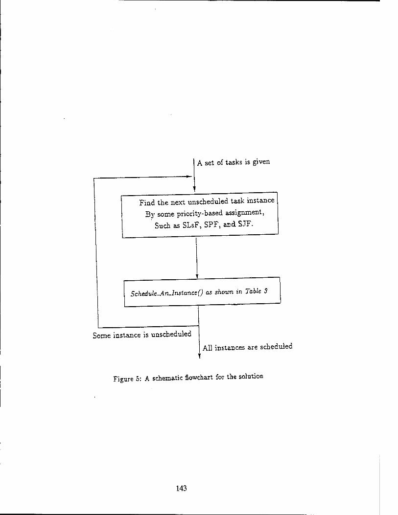
A set of tasks is given

Find the next unscheduled task instance

By some priority-based assignment,

' Such as SLsF, SPF, and SJF.

Sckedule-AnJnstanceO as shown in Table 3

Some instance is unscheduled

All instances are scheduled

Figure 5: A schematic flowchart for the solution

143

the scheduiability of each algorithm. The objective of the second experiment is to compare the

performance of the three algorithms.

6.1 The First Experiment

The task generation scheme for the first experiment is characterized by the following parameters.

• Periods of the tasks: We consider a homogeneous system in which the period of one task

could be either the same as or multiple of the period of another. We consider a system with

40, 80, 160, 320, and 640 as the candidate periods. There may be more than one task with

the same period.

• The execution time of a task, e, : It has the uniform distribution over the range [0,fg], where

Pi is the period of the task r,-. The execution time could be a real value.

• The jitters of a task: A,- = T?,- = 0.1 x p,-.

We define the utilization of a task system as

y£i (24)

In the first experiment, the utilization value and the number of tasks in a set are the controUed

variables. Given an utilization value U and the number of tasks N the scheme first generates a

run of raw data by randomly generating a set of N tasks based on the the selected periods, jitter

values, and the execution time distribution. The utilization of the raw data, v., is then computed by

Equation 24. Finally, the utilization value of the raw data is scaled up or down to Ü by multiplying

£ to the execution time of each generated task. As a consequence, we obtain a set of tasks with

the specified (U,N) value.

For each combination of (U,N) in which U - 5%, 10%, 15%, ... 100% and N = 10, 20, and

30. we apply the scheme to generate 5000 cases of input data and use the three algorithms to

solve them. The scheduiability degree of each {b\N} combination for an algorithm is obtained by

dividing the number of solved cases by 5000. Since the jitter values is 1/10 of periods, it is observed

that the SPF and SJF algorithms yield the same results. The results are shown in Figure 6.

As can be seen in Figures 6(a) and (b) the number of tasks has the different effects on the

three algorithms. For SLsF, given a fixed utilization value, the scheduiability degree increases

144

seh«dulftbimy

26. oe

—I smut. >■» J~SPF/SJF: K • 70

JOCK

Figure 6: The effect of the numbers of tasks on the schedulability

as the numbex of tasks in a system becomes bigger. It is beacuse the execution time of a task hecomes amallex as the mmbH of tasks increases. For a task system with smallex e*ecut,on u«

distribution, the chance fox SLsF to ftnd a feasibie *lu*on U *•-. Tk. sa** ?*«» ,. lo found in Fig™ 6(b) fox SPF and SJF in the iow-utiiiaation oases (i.e. V < 20%). However,

fox the high-utilization cases in Figure 6(h), the complexity of the numbex of tasks dotntnates the

algorithms and the schedulability decreases.

6.2 The Second Experiment

The task generate scheme fox the second experiment is characterized by the following parameters.

. LCM = 300

• The number of tasks is 20.

. Periods of the tasks: We consider the factors of the LCM as the periods. They are 20.. 30,

50, 60, 100, 150, and 300. There may be more than one task with the same period.

145

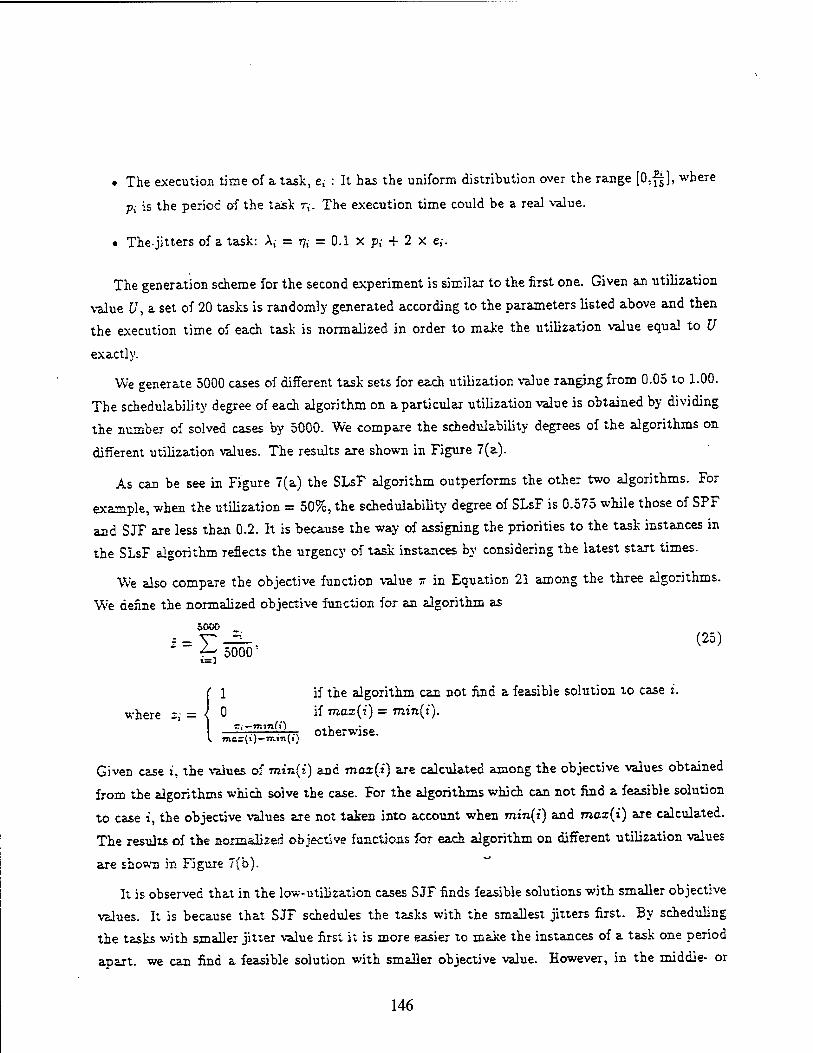
• The execution time of a task, e,- : It has the uniform distribution over the range (O.fi), where

Pi is the period of the task r,-. The execution time could be a real value.

• The-jitters of a task: A,- = 77; = 0.1 x p; + 2 x e,.

The generation scheme for the second experiment is similar to the first one. Given an utilization

value U, a set of 20 tasks is randomly generated according to the parameters listed above and then

the execution time of each task is normalized in order to make the utilization value equal to U

exactly.

We generate 5000 cases of different task sets for each utilization value ranging from 0.05 to 1.00.

The schedulability degree of each algorithm on a particular utilization value is obtained by dividing

the number of solved cases by 5000. We compare the schedulability degrees of the algorithms on

different utilization values. The results are shown in Figure 7(a).

As can be see in Figure 7(a) the SLsF algorithm outperforms the other two algorithms. For

example, when the utilization = 50%, the schedulability degree of SLsF is 0.575 while those of SPF

and SJF are less than 0.2. It is because the way of assigning the priorities to the task instances in

the SLsF algorithm reflects the urgency of task instances by considering the latest start times.

We also compare the objective function value - in Equation 21 among the three algorithms.

W;e define the normalized objective function for an algorithm as

5000

i=V-±-. (25) ^-r 5000 • 1=]

if the algorithm can not find a feasible solution to case i. if mai(i') = min(i).

^— ,., otherwise.

Given case :. the values of min(i) and max(i) are calculated among the objective values obtained

from the algorithms which solve the case. For the algorithms which can not find a feasible solution

to case i, the objective values are not taken into account when min(i) and max{i) are calculated.

The results of the normalized objective functions for each algorithm on different utilization values

are shown in Figure 7(b).

It is observed that in the low-utilization cases SJF finds feasible solutions with smaller objective

values. It is because that SJF schedules the tasks with the smallest jitters first. By scheduling

the tasks with smaller jitter value first it is more easier to make the instances of a task one period

apart, we can find a feasible solution with smaller objective value. However, in the middle- or

146

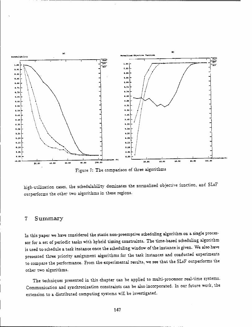
sch*6ul*bimy

X.oo ■ i

0.» ■ ■ :\ ^

o.»o r " '. '• i.ii

0.10 . \ o.is • \ 0.10

0.(S

0.16 _. ', y CSS - o.so ; o.«s \ 6.46 . *..

O.JS *, \

0.36 - ",

0.55 - 0.36 - \ O.JS - 0.30 - COS - 0.00

-COS

- !

Mom*lizad Ot>3«cLJv« nmcLl«

tur Tff" "SJY

tllli»tion I») ÜliMLiontV

Figure 7: The comparison of three algorithms

high-utilization cases, the schedulability dominates the normalized objective function, and SLsF

outperforms the other two algorithms in these regions.

7 Summary

In this paper we have considered the static non-preemptive scheduling algorithm on a single proces-

sor for a set of periodic tasks with hybrid timing constraints. The time-based scheduling algorithm

is used to schedule a task instance once the scheduling window of the instance is given. We also have

presented three priority assignment algorithms for the task instances and conducted experiments

to compare the performance. From the experimental results, we see that the SLsF outperforms the

other two algorithms.

The techniques presented in this chapter can be applied to multi-processor real-time systems.

Communication and synchronization constraints can be also incorporated. In our future work, the

extension to a distributed computing systems will be investigated.

147

References

[1] T. Carpenter, K. Driscoll, K. Hoyme, and J. Carciofmi. Arinc 659 scheduling: Problem defini-

tion. -In Proceedings of IEEE Real-Time Systems Symposium, San Juan, PR, Dec. 1994.

[2] M. L. Dertouzos and A.K. Mok. Multiprocessor on-line scheduling of hard real-time tasks. IEEE

Transactions on Software Engineering, 15(12):1497-1506, Dec. 1989.

[3] M.G- Harbour, M.H. Klein, and J.P. Lehoczky. Fixed priority scheduling of periodic tasks

with varying execution priority. In Proceedings of IEEE Real- Time Systems Symposium, pages

116-128, Dec. 1991.

[4] Krithi Ramamritham. Allocation and scheduling of complex periodic tasks. In Proceedings of

the 10th International Conference on Distributed Computing Systems, pages 108-115, Paris,

France, 1990-

[5] T. Shepard and J.A.M. Gagne. A pre-run-time scheduling algorithm for hard real-time systems.

IEEE Transactions on Soßware Engineering, 17(7):669-677, July 1991.

[6] K. Tindell, A. Burns, and A. Wellings. An extendable approach for analyzing fixed priority hard

real-time tasks. Real-Time Systems, 6(2), March 1994.

{7] J.P.C. Verhoosel, E.J. Luit, D.K. Kammer, and E. Jansen. A static scheduling algorithm for

distributed hard real-time systems. Real-Time Systems, pages 227-246, 1991.

[8] J. Xn and D.L. Parnas. Scheduling processes with release times, deadlines, precedence, and

exclusion relations. IEEE Transactions on Software Engineering, 16(3):360-369, March 1990.

148

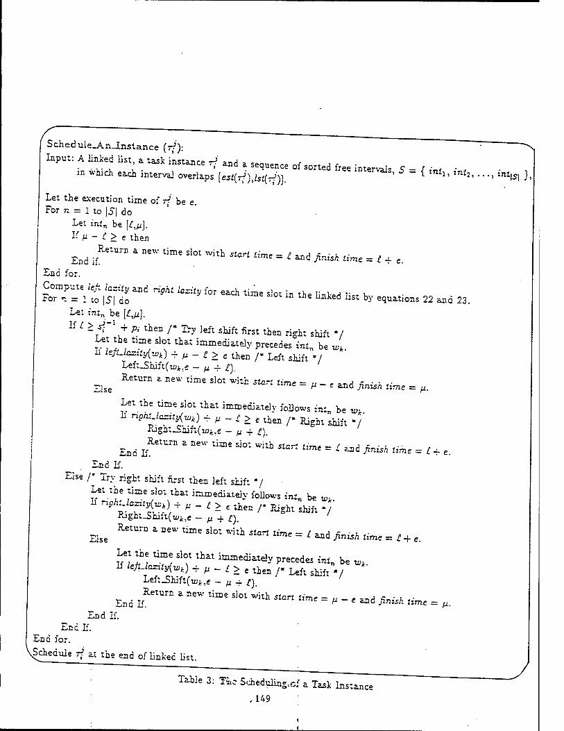
Schedule_An_Instance (r/): Input: A linked list, a task instanrp -> *T,A ,

, las* instance ,. and a sequence of sorted free intervals S - J i*i m which each interval overlaps Mr/),/5i(^')]. intervals, i _ { inil| I71^

Let the execution time of rf be e. For n = 1 to |5| do

Let inl„ be [£,;/]. If H- £> e then

End if11""11 " nCW t]me Sl0t WitL S£Gri Üme = < and *** time = ^ + e. End for.

Let :'ntr. be [ü„u].

If r > s>;-1 -f Ä. then /* Try left shift first then right shift 7

Let the time slot that immediately precedes intn be »1 L /erZJax:^,) + ß _ r > e then ;* Lgfl ^

Left_Shi:t(u>A.e — ^ -r £). ^ Return a new' W slot with start üme = y - e Md ^ !£me = ^

Let the time slot that immediately follows inijt be w. h r^ghU^tyi^) + //-*> e then /• Bight shift -/

rugh:_Shift(u;^,e - y -f £).

I Ead IfRelUrn * DeW time Si0t wilh ««* ««e = < and finish üme = r + e.

End If.

Else /- Try right shift first then left shift 7

Let the time slot that immediately follows intn be wk

-n. , V, .;•' ' ^ * - £ '■nen / Ejght shift V iugnt_Smft(u;i.e - y -1- n

^ Return a new time sloi whh start time = < ^d finish time = £+^

vV^Tf SlT that immediate]y P^es £nin be Wjk. If ^Jcx:iy(^) + „ __ , > e thfin /m Left shift

Lef;^hift(u;A,e - /z + £).

End if"11" £ aeW timC S]0t Wkh 5iCrt W = /* " « »d ^A time = M. End If.

End If. End for.

.Schedule 7/ at the end of linked list.

ini\s\ },

Table 3: Tie Scheduling,^" a Task Instance

,149


1. AGENCY USE ONLY (leave blank) 2. REPORT DATE 1/3/1995

4. TITLE AND SUBTITLE Scheduling of Periodic Tasks with Relative Timing Constraints


3. REPORT TYPE END DATES COVERED Technical Reports

6. AUTHOR(S) S.-T. Cheng and A. K. Agrawala

7. PERFORMING ORGANIZATION NAME(S) AND ADDRESS(ES) University of Maryland Department of Computer Science A.V. Williams Building College Park, MD 20742

9. SPONSORING/ MONITORING AGENCY NAME(S) AND ADDRESS(ES))l PhillipsLaboratory Director of Contracting 3651 Lowry Avenue SE Kirtland AFB, NM 87117-5777


5. FUNDING NUMNBERS

N00014-91-C-0195


CSTR 3392

0. SPONSORING/ MONITORING AGENCY REPORT NUMBER


13. ABSTRACT (Maximum 200 words)

The problem of non-preemptive scheduling of a set of periodic tasks on a single processor has been traditionally considering the ready time and deadline on each task. As a consequence, a feasible schedule finds that in each period one instance of each task starts the execution after the ready time and completes the execution before the deadline. Recently, the timing requirements of the real-time systems emerge that the relative timing constraints are imposed on the consecutive executions of each task. In this paper, we consider the scheduling problem of the periodic tasks with the relative timing constraints imposed on two consecutive executions of a task. We analyze the timing constraints and derive the scheduling window for each task instance. Based on the scheduling window, we present the time-based approach of scheduling a task instance. The task instances are scheduled one by one based on their priorities assigned by the proposed algorithms in this paper. We conduct the experiments to compare the schedulability of the algorithms.

14. SUBJECT TERMS Time constraints, timing requirements



Unclassified

15. NUMBER OF PAGES 21

16. PRICE CODE

19. SECURITY CLASSIFICATION OF ABSTRACT Unclassified

MSN 7540-01 280-5500


Umlimited

150 Standard Form 298 (Rev 2-89)

A Scalable Virtual Circuit Routing Scheme for ATM Networks'

Cengiz Alaettinoglu Ibrahim Matta A. Udaya Shankar Information Sciences Institute Institute for Advanced Computer Studies

University of Southern California Department of Computer Science " Marina del Rey, CA 90292 University of Maryland

College Park, MD 20742

October 1994

Abstract

High-speed networks, such as ATM networks, are expected to support diverse quality-of- service (QoS) requirements, including real-time QoS. Real-time QoS is required by many applications such as voice and video. To support such service, routing protocols based on the Virtual Circuit (VC) model have been proposed. However, these protocols do not scale well to large networks in terms of storage and communication overhead.

In this paper, we present a scalable VC routing protocol. It is based on the recently proposed viewserver hierarchy, where each viewserver maintains a partial view of the network. By querying these viewservers, a source can obtain a merged view that contains a path to the destination. The source then sends a request packet over this path to setup a real-time VC through resource reservations. The request is blocked if the setup fails. We compare our protocol to a simple approach using simulation. Under this simple approach, a source maintains a full view of the network. In addition to the savings in storage, our results indicate that our protocol performs close to or better than the simple approach in terms of VC carried load and blocking probability over a wide range of real-time workload.

Categories and Subject Descriptors: C.2.1 [Computer-Communication Networks]: Network Archi- tecture and Design—packet networks; store and forward networks; C.2.2 [Computer-Communication Net- works]: Network Protocols—protocol architecture; C.2.m [Routing Protocols]; F.2.m [Computer Network Routing Protocols].

" This work is supported in part by ARPA and Philips Labs under contract DASG60-92-0055 to Department of Computer Science, 'University of Maryland, and by National Science Foundation Grant No. NCR 89-04590. The work of C Alaettinoglu is also supported by National Science Foundation Grant No. NCR 93-21043. The views, opinions, and/or findings contained in this report are those of the anthor(s) and should not be interpreted as representing the official policies, either expressed or implied, of the Advanced Research Projects Agency, PL, the National Science Foundation, or the U.S. Government.

151

Contents

1 Introduction j

2 Related Work 4

3 Viewserver Hierarchy Query Protocol 5

4 Update. Protocol for Dynamic Network Conditions 10

5 Evaluation 13

6 Numerical Results 16 6.1 Results for Network 1 16 6.2 Results for Network 2 18

7 Conclusions 19

152

1 Introduction

Integrated services packet-switched networks, such as Asynchronous Transfer Mode (ATM) net-

works [21], are expected to carry a wide variety of applications with heterogeneous quality of ser-

vice (QoS) requirements. For this purpose, new resource allocation algorithms and protocols have

been proposed, including link scheduling, admission control, and routing. Link scheduling defines

how the link bandwidth is allocated among the different services. Admission control defines the

criteria the network uses to decide whether to accept or reject a new incoming application. Routing

concerns the selection of routes to be taken by application packets (or cells) to reach their desti-

nation. In this paper, we are mainly concerned with routing for real-time applications (e.g., voice,

video) requiring QoS guarantees (e.g., bandwidth and delay guarantees).

To provide real-time QoS support, a number of virtual-circuit (VC) routing approaches have

been proposed. A simple (or straightforward) approach to VC routing is the link-state full-view

approach. Here, each end-system maintains a view of the whole network, i.e. a graph with a vertex

for every node1 and an edge between two neighbor nodes. QoS informatio» such as delay, band-

width, and loss rate are attached to the vertices and the edges of the view. This QoS information

is flooded regularly to all end-systems to update their views. When a new application requests ser-

vice from the network, the source end-system uses its current view to select a source route to the

destination end-system that is likely to support the application's requested QoS, i.e., a sequence of

node ids starting from the source end-system and ending with the destination end-system. A VC-

setup message is then sent over the selected source route to try to reserve the necessary resources

(bandwidth, buffer space, service priority) and establish a VC.

Typically, at every node the VC-setup message visits, a set of admission control tests are

performed to decide whether the new VC, if established, can be guaranteed its requested QoS

without violating the QoS guaranteed to already established VCs. At any node, if these admission

tests are passed, then resources are reserved and the VC-setup message is forwarded to the next

node. On the other hand, if the admission tests fail, a VC-rejected message is sent back towards

the source node releasing resource reservations made by the VC-setup message, and the application

request is either blocked or another source route is selected and tried. If the final admission tests

at the destination node are passed, then a VC-established message is sent back towards the source

node confirming resource reservations made during the forward trip of the VC-setup message. Upon

receiving the VC-established message, the application can start transmitting its packets over its

1 We refer to switches and end-systems collectively as nodes.

153

reserved VC. This VC is torn down and resources are released at the end of the transmission.

Clearly, the above simple routing scheme does not scale up to large networks. The storage at

each end-system and the communication cost are proportional to N x d, where N is the number of

nodes and d is the average number of neighbors to a node.

A traditional solution to this scaling problem is the area hierarchy used in routing protocols

such as the Open Shortest Path First (OSPF) protocol [18]. The basic idea is to aggregate nodes

hierarchically into areas: "close" nodes are aggregated into level 1 areas, "close" level 1 areas are

aggregated into level 2 areas, and so on. An end-system maintains a view that contains the nodes

in the same level 1 area, the level 1 areas in the same level 2 area, and so on. Thus an end-system

maintains a smaller view than it would in the absence of hierarchy. Each area has its own QoS

information derived from that of the subareas. A major problem of an area-based scheme is that

aggregation results in loosing detailed link-level QoS information. This decreases the chance of the

routing algorithm to choose "good" routes, i.e. routes that result in high successful VC setup rate

(or equivalently high carried VC load).

Our scheme

In this paper, we present a scalable VC routing scheme that does not suffer from the problems of

areas. Our scheme is based on the viewserver hierarchy we recently proposed in [3, 2] for large

internetworks and evaluated for administrative policy constraints. Here, we are concerned with the

support of performance/QoS requirements in large wide-area ATM-like networks, and we adapt our

viewserver protocols accordingly.

In our scheme, views are not maintained by every end-system but by special switches called

viewservers. For each viewserver, there is a subset of nodes around it, referred to as the viewservers

precinct The viewserver only maintains the view of its precinct. This solves the scaling problem

for storage requirement.

A viewserver can provide source routes for VCs between source and destination end-systems

in its precinct. Obtaining a route between a source and a destination that are not in any single

view involves accumulating the views of a sequence of viewservers. To make this process efficient,

viewservers are organized hierarchically in levels, and an associated addressing structure is used.

Each end-system has a set of addresses. Each address is a sequence of viewserver ids of decreasing

levels, starting at the top level and going towards the end-system. The idea is that when the views

of the viewservers in an address are merged, the merged view contains routes to the end-system

154

from the top level viewservers. We tadle dvnamic topology changes such a, node/liak failures and repairs, and knk cost

changes. Nodes detect topology changes affecting itself aad neighbor nodes. Each node commn-

nicates these changes by «coding to the viewservers in a specified snbset of »odes; thrs subset „

referred «o as its flooä area. Hence, the number of packets used during flooding is proposal to

the si, of tbe iood area. This solves «he scaling problem for the communication recrement.

Thus our VC routing protocol consists of two subprotocols: a nieder, protocol between end-

svstems and viewservers for obtaining merged views; and a »Wote p^tooof between nodes and

viewservers for updating views.

Evaluation

In this paper, we compare our viewserver-based VC routing scheme to the simple scheme using

VC4evel simulation, In our simulation model, we deine network topologies, QoS regents,

viewserver hierarchies, and evasion measures. To «he best of o«rr knowledge, this is the ftrs;

evaluation of a dynamic hierarchical-based VC routing scheme nnder real-time workload.

Onr evaluation measures are the amount of memory paired at «he end-systems, the amount

of «ime needed «o construct a path', «he carried VC load, and «he VC blocking probably. We

use network «opologies each of size 2764 nodes. Onr results indicate «ha« onr viewserver-basecV C

ronting scheme performs dose «o or better than the simple scheme in terms of VC earned load

and blocking probability over a wide range of workload. 1. also rednces the amount of memory

requirement by up to two order of magnitude.

Organization of the paper

H Section 2, we survey recent approaches to VC routing, la Section 3, we present «he view-,uery

protocol for static network conditions, that is, assuming all links and nodes of the network renaaun

operational. la Section 4, w, present the view-trpdate protocol to handle topology changes. In

Section 5, we present onr evaluation model. Onr resnlts are presented ia Section 6. Sec«,on

concludes the paper. s We use the terms route and path mteichangeably.

155

2 Related Work

In this section, we discuss routing protocols recently proposed for packet-switched QoS networks.

These routing protocols can be classified depending on whether they help the network support

qualitative QoS or quantitative (real-time) QoS. For a qualitative QoS, the network tries to provide

the service requested by the application with no performance guarantees. Such a service is often

identified as "best-effort". A quantitative QoS provides performance guarantees (typically required

by real-time applications); for example, an upper bound on the end-to-end delay for any packet

received at the destination.

Routing protocols that make routing decisions on a per VC basis can be used to provide either

qualitative or quantitative QoS. For a quantitative QoS, some admission control tests should be

performed during the VC-setup message's trip to the destination to try to reserve resources along

the VC's path as described in Section 1.

On the other hand, the use of routing protocols that make routing decisions on a per packet

basis is problematic in providing resource guarantees [5], and qualitative QoS is the best service

the network can offer.

Since we are concerned in this paper with real-time QoS. we limit our following discussion to

VC routing schemes proposed or evaluated in this context. We refer the reader to [19, 6] for a good

survey on many other routing schemes.

Most of the VC routing schemes proposed for real-time QoS networks are based on the link-

state full-view approach described in Section 1 [6, 1, 10, 24]. Recall that in this approach, each

end-system maintains a view of the whole network, i.e. a graph with a vertex for every node and

an edge between two neighbor nodes. QoS information is attached to the vertices and the edges of

the view. This QoS information is distributed regularly to all end-systems to update their views

and thus enable the selection of appropriate source routes for VCs, i.e. routes that are likely to

meet the requested QoS. The proposed schemes mainly differ in how this QoS information is used.

Generally, a cost function is defined in terms of the QoS information, and used to estimate the

cost of a path to the VC's destination. The route selection algorithm then favors short paths with

minimum cost. See [17, 22} for an evaluation of several schemes.

A number of VC routing schemes have also been designed for networks using the Virtual Path

(VP) concept [15, 14]. This VP concept has been proposed to simplify network management and

control by having separate (logically) fully-connected subnetworks, typically one for each service

class. In each VP subnetwork, simple routing schemes that only consider one-hop and two-hop

156

paths are used. However, the advantage of using VPs can be offset by a decrease in statistical

multiplexing gains of the subnetworks [15]. In this work, we are interested in general network-

topologies, where the shortest paths can be of arbitrary hop length and the overhead of routing

protocols is of much concern.

All the above VC routing schemes are based on the link-state approach. VC routing schemes

based on the path-vector approach have also been proposed [13]. in this approach, for each desti-

• nation a node maintains a set of paths, one through each of its neighbor nodes. QoS information

is attached to these paths. For each destination, a node exchanges its best feasible path3 with its

neighbor nodes. The scheme in [13] provides two kinds of routes: pre-computed and on-demand.

Pre-computed routes match some well-known QoS requirements, and are maintained using the

path-vector approach. On-demand routes are calculated for specific QoS requirements upon re-

quest. In this calculation, the source broadcasts a special packet over all candidate paths. The

destination then selects a feasible path from them and informs the source [13, 23]. One drawback

of this scheme is that obtaining on-demand routes is very expensive since there are potentially

exponential number of candidate paths between the source, and the destination.

The link-state approach is often proposed and favored over the path-vector approach in QoS

architectures for several reasons [16]. An obvious reason is simplicity and complete control of the

source over QoS route selection.

The above VC routing schemes do not scale well to large QoS networks in terms of storage

and communication requirements. Several techniques to achieve scaling exist. The most common

technique is the area hierarchy described in Section 1.

The landmark hierarchy [26, 25] is another approach for solving the scaling problem. The link-

state approach can not be used with the landmark hierarchy. A thorough $tudy of enforcing QoS

and policy constraints with this hierarchy has not been done.

Finally, we should point out that extensive effort is currently underway to fully specify and

standardize VC routing schemes for the future integrated services Internet and ATM networks [9].

3 Viewserver Hierarchy Query Protocol

In this section, we present our scheme for static network conditions, that is, all links and nodes

remain operational. The dynamic case is presented in Section 4.

A feasible path is a path that satisfies the QoS constraints of the nodes in the path.

157

Conventions: Each node has a unique id. Nodelds denotes the set of node-ids. For anode u, we

use nodeid(u) to denote the id of u. NodeNeighbors(u) denotes the set of ids of the neighbors of u.

In our protocol, a node u uses two kinds of sends. The first kind has the form "Send(m) to v",

where m is the message being sent and v is the destination-id. Here, nodes u and v are neighbors,

and the message is sent over the physical link (u, v). If the link is down, we assume that the packet

is dropped.

The second kind of send has the form "Send(m) to v using sr", where m and v are as above

and sr is a source route between u and v. We assume that as long as there is a sequence of up

links connecting the nodes in sr, the message is delivered to v. This requires a transport protocol

support such as TCP [20].

To implement both kind of sends, we assume there is a reserved VC on each link for sending

routing, signaling and control messages [4]. This also ensures that routing messages do not degrade

the QoS seen by applications.

Views and Viewservers

Views are maintained by special nodes called viewservers. Each viewserver has a precinct, which is

a set of nodes around the viewserver. A viewserver maintains a view, consisting of the nodes in its

precinct, links between these nodes and links outgoing from the precinct4. Formally, a viewserver

x maintains the following:

Precinct^ C Nodelds. Nodes whose view is maintained.

Vieu-. View of z.

= {(u, timestamp, expirytime, {(v, cost) : v € NodeNeighbors(u)}) :

u € Precinct:}

The intention of Viewx is to obtain source routes between nodes in Precinct:. Hence, the

choice of nodes to include in PrecincU and the choice of links to include in Viewx are not arbitrary.

Precinct- and Viewx must be connected; that is, between any two nodes in Precinct:, there should

be a path in Viewx. Note that Viewx can contain links to nodes outside Precinct:. We say that a

node v. is in the view of a viewserver x, if either u is in the precinct of x, or Viewx has a link from

a node in the precinct of x to node u. Note that the precincts and views of different viewservers

can be overlapping, identical or disjoint.

4 Not all the links need to be included.

158

For a link («, v) in the view of a viewserver i, View, stores a cost. The cost of the link («,t>)

equals a vector of values if the link is known to be up; each cost value estimates how expensive it

is to cross the link according to some QoS criteria such as delay, throughput, loss rate, etc. The

cost equals oo if the link is known to be down. Cost of a link changes with time (see Section 4).

The view also includes timestamp and expirytime fields which are described in Section 4.

Viewserver Hierarchy

For scaling reasons, we cannot have one large view. Thus, obtaining a source route between a source

and a destination which are far away, involves accumulating views of a sequence of viewservers. To

keep this process efficient, we organize viewservers hierarchically. More precisely, each viewserver is

assigned a hierarchy level from 0,1,.., with 0 being the top level in the hierarchy. A parent-child

relationship between viewservers is defined as foDows:

1. Every level i viewserver, i > 0, has a parent viewserver whose level is less than t.

2. If viewserver x is a parent of viewserver y then a's precinct contains y and y's precinct

contains x.

3. The precinct of a top level viewserver contains all other top level Viewservers.

In the hierarchy, a parent can have many children and a child can have many parents. We extend

the range of the parent-child relationship to ordinary nodes; that is, if Precinct contains the node

u, we say that u is a child of x, and x is a parent of u. We assume that there is at least one parent

viewserver for each node.

For a node u: an address is defined to be a sequence (x0,xy,...,xt) such that x{ for i < t is

a viewserver-id, xD is a top level viewserver-id, xt is the id of u, and z,- is a parent of x,+1. A

node may have many addresses since the parent-child relationship is many-to-many. Jf a source

node wants to establish a VC to a destination node, it first queries the name servers to obtain a

set of addresses for the destination5. Second, it queries viewservers to obtain an accumulated view

containing both itself and the destination node (it can reach its parent viewservers by using fixed

source routes to them). Then, it chooses a feasible source route from this accumulated view and

initiates the VC setup protocol on this path.

View-Query Protocol: Obtaining Source Routes

We now describe how a source route is obtained. s

Querying the name servers can be done in the same way as is done currently in the Internet.

159

We want a sequence of viewservers whose merged views contains both the source and the

destination nodes. Addresses provide a way to obtain such a sequence, by first going up in the

viewserver hierarchy starting from the source node and then going down in the viewserver hierarchy

towards the destination node. More precisely, let (so,...,St) be an address of the source, and

{d0,. ..,di) be an address of the destination. Then, the sequence {st-y,...,So,d0,...,d/_j) meets

our requirements. In fact, going up all the way in the hierarchy to top level viewservers may not

be necessary. We can stop going up at a viewserver s,- if there is a viewserver dj, j < I, in the view

of Si (one special case is where st- ~ dj).

The view-query protocol uses two message types:

• (RequestViev, Suaddress, d-address)

where s.address and djaddress are the addresses for the source and the destination respec-

tively. A RequestViev message is sent by a source node to obtain an accumulated view con-

taining both the source and the destination nodes. When a viewserver receives a RequestView

message, it either sends back its view or forwards this request to another viewserver.

♦ (ReplyViev, s^address, d-address, accurnview)

where s^address and djaddress are as above and accurnview is the accumulated view. A

ReplyViev message is sent by a viewserver to the source or to another viewserver closer to

the source. The accurnview field in a ReplyViev message equals the union of the views of

the viewservers the message has visited.

We now describe the view-query protocol in more detail (please refer to Figures 1 and 2). To

establish a VC to a destination node, the source node sends a RequestViev packet containing the

source and the destination addresses to its parent in the source address.

Upon receiving a RequestViev packet, a viewserver x checks if the destination node is in its

precinct6. If it is, i sends back its view in a ReplyViev packet. If it is not, x forwards the request

packet to another viewserver as follows (details in Figure 2): x checks whether any viewserver in

the destination address is in its view. If there is such a viewserver, x sends the RequestViev packet

to the last such one in the destination address. Otherwise a is a viewserver in the source address,

and it sends the packet to its parent in the source address.

When a viewserver i receives a ReplyViev packet, it merges its view to the accumulated view-

in the packet. Then it sends the ReplyViev packet towards the source node in the same way it

would send a RequestViev packet towards the destination node (i.e. the roles of the source address

Even though the destination can be in the view of i, its QoS characteristics is not in the view if it is not in the precinct of z.

160

Constants

FixedRoutesu(x), for every viewserver-id x such that x is a parent of u, = {(t/i, ■ • • ,yn) '■ y< € Kodelds}. Set of routes to x

Events RequestViewu(s.address, d.address) {Executed when u wants a source route}

Let s.address be (so. ■ •■ist-i.*t)i asd sr £ FixedRovtesu(st-\); Send(RequestViey, sjaddress, djiddress) to st-i using sr

Äece:veu(ReplyView, s.address, djiddress, accumview) Choose a feasible source route using accumview; If a feasible route is not found

Execute RequestViewu again with another source address and/or destination address

Figure 1: View-query protocol: Events and state of a source node v..

Constants

Precinctz. Precinct of x.

Variables

View~. View of x.

Events -Receiver(RequestView, s.address, djiddress)

Let d.address be (do,...,dt); if dt £ Precinct then /oriDardr (RequestView, sjjddress, d.address, {}); else /oru>ardr(ReplyViey, d.address, s.address, Viewz); endif

{addresses are switched}

Aece:uer(ReplyViey, sjaddress, djjddress, view) forwardz(Keplj\iev, s.address, d.address, viewöViewz)

where procedure forwardz(type, s.address, djaddress, view) Let s.address be (so, ■. -,st), d.address be (d0, . ... di); if 3i : di in Viewz then Let :' = max{j : dj in View?}; target :— d,-; else target :— s,- such that s,-+i = nodeid(x); endif; sr := choose a route to target from nodeid(x) using Vteu)x; if type = RequestViev then Send(RequestViey, s^iddress, djaddress) to target using sr; else Send(ReplyVie¥, sjaddress, djiddress, view) to target using sr; endif

Figure 2: View-query protocol: Events and state of a viewserver x.

and the destination address are interchanged).

161

When the source receives a ReplyVieu packet, it chooses a feasible path using the accumview

in the packet. If it does not find a feasible path, it can try again using a different source and/or

destination addresses. Note that the source does not have to throw away the previous accumulated

views; it can merge them all into a richer accumulated view. In fact, it is easy to change the protocol

so that the source can also obtain views of individual viewservers to make the accumulated view

even richer. Once a feasible source route is found, the source node initiates the VC setup protocol.

Above we have described one possible way of obtaining the accumulated views. There are

various other possibilities, for example: (1) restricting the ReplyView packet to take the reverse

of the path that the RequestView packet took; (2) having ReplyViev packets go all the way

up in the viewserver-hierarchy for a richer accumulated view; (3) having the source poll the

viewservers directly instead of the viewservers forwarding request/reply messages to each other;

(4) not including non-transit nodes (e.g. end-systems) other than the source and the destination

nodes in the accumview: (5) including some QoS requirements in the RequestView packet, and

having the viewservers filter out some nodes and links.

4 Update Protocol for Dynamic Network Conditions

In this section, we first describe how topology changes such as link/node failures, repairs and cost

changes, are detected and communicated to viewservers, i.e. the view-update protocol. Then, we

modify the view-query protocol appropriately.

View-Update Protocol: Updating Views

Viewservers do not communicate with each other to maintain their views. Nodes detect and

communicate topology changes to viewservers. Updates are done periodically and also optionally

after a change in the outgoing link costs.

The communication between a node and viewservers is done by flooding over a set of nodes.

This set is referred to as the flood area. The topology of a flood area must be a connected graph.

For efficiency, the flood area can be implemented by a hop-count.

Due to the nature of flooding, a viewserver can receive information out of order from a node. In

order to avoid, old information replacing new information, each node includes successively increasing

time stamps in the messages it sends. The timestamp field in the view of a viewserver equals the

largest timestamp received from each node.'

162

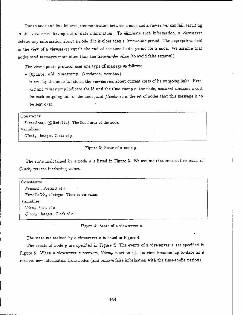
Due to node and link failures, communication between a node and a viewserver can fail, resulting

in the viewserver having out-of-date information. To eliminate such information, a viewserver

deletes any information about a node if it is older than a time-to-die period. The expiryiime field

in the view of a viewserver equals the end of the time-to-die period for a node. We assume that

nodes send messages more often than the time-to-<i»e \alue (to avoid false removal).

The view-update protocol uses one type dt message a& -follows:

• (Update, nid, timestamp, floodarea, ncostset)

is sent by the node to inform the viewservers about current costs of its outgoing links. Here,

nid and timestamp indicate the id and the time stamp of the node, ncostset contains a cost

for each outgoing link of the node, and floodarea is the set of nodes that this message is to

be sent over.

Constants:

FlooiAreag. (C Nodelds) The flood area of the node.

Variables:

Clockg : Integer. Clock of 9-

Figure 3: State of a node g.

The state maintained by a node g is listed in Figure 3. We assume that consecutive reads of

Clockg returns increasing values.

Constants:

Prtcinci-. Precinct of x.

TimeTcDiCz : Integer. Time-to-die value.

Variables:

View-. View of x.

Clockx : Integer. Clock of z.

Figure 4: State of a viewserver x.

The state maintained by a viewserver x is listed in Figure 4.

The events of node g are specified in Figure 5. The events of a viewserver x are specified in

Figure 6. When a viewserver x recovers, Vietvz is set to {}. Its view becomes up-to-date as it

receives new information from nodes (and remove false information with the time-to-die period).

163

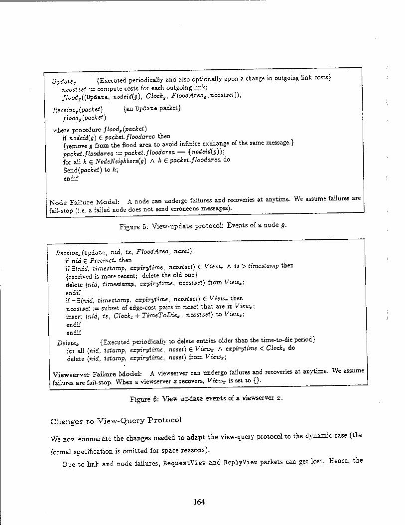
Update9 {Executed periodically and also optionally upon a change in outgoing link costs} ncosiset := compute costs for each outgoing link; flood,((Update, nodeid{g), Clocks, FloodAreas,ncostset));

Receive s(packet) {an Update packet} flood 9{packet)

where procedure floods(packei) if nodeid(g) € packet.floodarea then {remove g from the flood area to avoid infinite exchange of the same message.} packet.floodarea := packet.floodarea — {nodeid(g)}; for ail h e NodeNeighbors(g) A h £ packet.floodarea do Send(pacfcez) to h; endif

Node Failure Model: A node can undergo failures and recoveries at anytime. We assume failures are fail-stop (i.e. a failed node does not send erroneous messages).

Figure 5: View-update protocol: Events of a node g.

Receivez (Update, nid, ts, FloodArea, ncset) if nid € Precinct- then if 3{nid, timestamp, expirytime, ncostset) € View= A ts > timestamp then {received is more recent; delete the old one} delete (nid, timestamp.. expirytime, ncostset) from Viewz;

endif if -3(nid, timestamp, expirytime, ncostset) G Viewz then ncostset := subset of edge-cost pairs in ncset that are in View.; insert (nid, ts, Clockz + TimtToDiez, ncostset) to View?;

endif endif

Delete- {Executed periodically to delete entries older than the time-to-die period} for all {nid, istamp, expirytime, ncset) € View- A expirytime < Clock, do delete (nid, istamp, expirytime, ncset) from Viewx;

Viewserver Failure Model: A viewserver can undergo failures and recoveries at anytime. We assume failures are fail-stop. When a viewserver x recovers, View- is set to {}.

Figure 6: View update events of a viewserveT x.

Changes to View-Query Protocol

We now enumerate the changes needed to adapt the view-query protocol to the dynamic case (the

formal specification is omitted for space reasons).

Due to link and node failures, RequestView and ReplyViev packets can get lost. Hence, the

164

source may never receive a ReplyView packet after it initiates a request. Thus, the source should

try again after a time-out period.

When a viewserver receives a RequestVieu message, it should reply with its views only if the

destination node is in its precinct and its view contains a path to the destination. Similarly during

forwarding of RequestView and ReplyView packets, a viewserver, when checking whether a node

is in its view, should also check if its view contains a path to it.

5 Evaluation

In this section, we present the parameters of our simulation model. We use this model to com-

pare our viewserver-based VC routing protocols to the simple approach. The results obtained are

presented in Section 6.

Network Parameters

We model a campus network which consists of a campus backbone subflei<wot-kand several depart-

ment subnetworks. The backbone network consists of backbone switches and backbone links.

Each department network consists of a hub switch and several non-hub switches. Each non-hub

switch has a link to the department's hub switch. And the department's hub switch has a link to

one of the backbone switches. A non-hub switch can have links to other non-hub switches in the

same department, to non-hub switches in other departments, or to backbone switches.

End-systems are connected to non-hub switches. An example network topology is shown in

Figure 7.

In our topology, there are 8 backbone switches and 32 backbone links. There are 16 departments.

There is one hub-switch in each department. There is a total of 240 non-hub switches randomly

assigned to different departments. There are 2500 end-systems which are randomly connected to

non-hub switches. Thus, we have a total of 2764 nodes.

In addition to the links connecting non-hub switches to the hub switches and hub switches to

the backbone switches, there are 720 links from non-hub switches to non-hub switches in the same

department, there are 128 links from non-hub switches to non-hub switches in different departments,

and there are 64 links from non-hub switches to backbone switches.

The end-points of each link are chosen randomly. However, we make sure that the backbone

network is connected; and there is a link from node u to node t; iff there is a link from node no

165

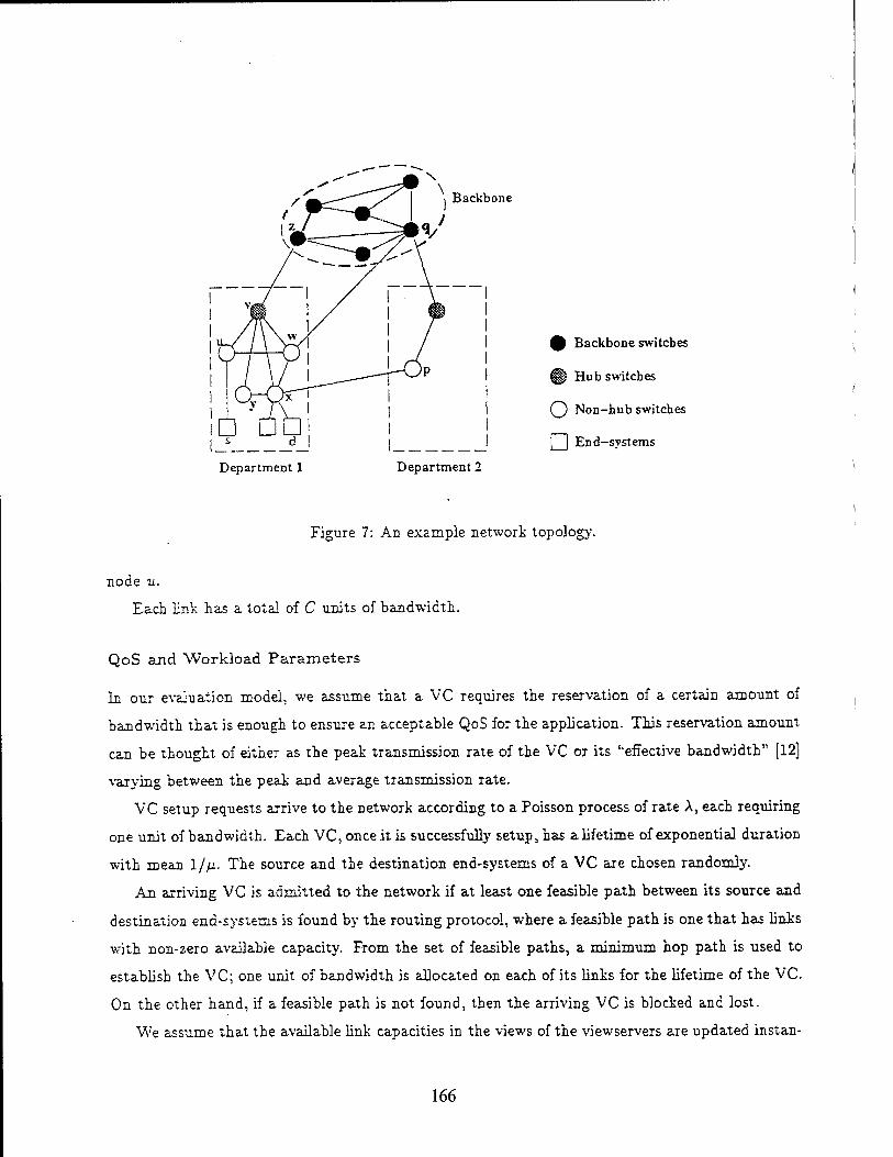
Backbone

0 Backbone switches

^ Hub switches

Q Non-hub switches

1 | End-systems

Department 1 Department 2

Figure 7: An example network topology.

node u.

Each link has a total of C units of bandwidth.

QoS and Workload Parameters

In our evaluation model, we assume that a VC requires the reservation of a certain amount of

bandwidth that is enough to ensure an acceptable QoS for the application. This reservation amount

can be thought of either as the peak transmission rate of the VC ox its ''effective bandwidth" [12]

varying between the peak and average transmission rate.

VC setup requests arrive to the network according to a Poisson process of rate A, each requiring

one unit of bandwidth. Each VC, once it is successfully setup, has a lifetime of exponential duration

with mean 1/ß. The source and the destination end-systems of a VC are chosen randomly.

An arriving VC is admitted to the network if at least one feasible path between its source and

destination end-systems is found by the routing protocol, where a feasible path is one that has links

with non-zero available capacity. From the set of feasible paths, a minimum hop path is used to

establish the VC; one unit of bandwidth is allocated on each of its links for the lifetime of the VC.

On the other hand, if a feasible path is not found, then the arriving VC is blocked and lost.

We assume that the available link capacities in the views of the viewservers are updated instan-

166

taneously whenever a VC is admitted to the network or terminates.

Viewserver Hierarchy Schemes

We have evaluated our viewserver protocol for several different viewserver hierarchies and query

methods. We next describe the different viewserver schemes evaluated. Please refer to Figure 7 in

the following discussion. ,

The first viewserver scheme is referred to as base. Each switch is a viewserver. A viewserver's

precinct consist of itself and the neighboring nodes. The links in the viewserver's view consist of

the links between the nodes in the precinct, and links Outgoing from nodes in the precinct to nodes

not in the precinct. For example, the precinct of viewserver «-consists of nodes u,v, *,,$•

As for the viewserver hierarchy, a backbone switch is a level 0 viewserver, a hub switch is a

level 1 viewserver and a non-hub switch is a level 2 viewserver. Parent of a hub switch viewserver

is the backbone switch viewserver it is connected to. Parent of a non-hub switch viewserver is the

hub switch viewserver in its department. Parent of an end-system is the non-hub switch viewserver

it is connected to.

We use only one address for each end-system. The viewserver-address of an end-system is the

concatenation of four ids. Thus, the address of s is z.v.u.s. Similarly, the address of d is z.v.x.d.

To obtain a route between 6 and d, it suffices to obtain views of viewservers u.v,x.

The second viewserver scheme is referred to as base-QT (where the QT stands for "query up

to top"). It is identical to base except that during the query protocol all the viewservers in the

source and the destination addresses are queried. That is, to obtain a route between s and d, the

views of u, v.x.z are obtained.

The third viewserver scheme is referred to as vertex-extension. It is identical to base except

that viewserver precincts are extended as follows: Let ? denote the precinct of a viewserver in the

base scheme. For each node u in P, if there is a link from node u to node t; and v is not in P, node

v is added to the precinct; among v:s links, only the ones to nodes in P are added to the view. In

the example, nodes r, y,x,q are added to the precinct of «, but outgoing links of these nodes to

other nodes are not included (e.g. (x,p) and (r, q) are not included). The advantage of this scheme

is that even though it increases the precinct size by a factor of d (where d is the average number of

neighbors to a node), it increases the number of links stored in the view by a factor less than 2.

The fourth viewserver scheme is referred to as veriex-extension-QT. It is iaentical to vertex-

extension except that during the query protocol all the viewservers in the source and the destination

167

addresses are queried.

6 Numerical Results

6.1 Results for Network 1

The parameters of the first network topology, referred to as Network 1, are given in Section 5. The

link capacity C is taken to be 20 [6], i.e. a link is capable of carrying 20 VCs simultaneously.

Our evaluation measures were computed for a (randomly chosen but fixed) set of 100,000 VC

setup requests. Table 1 lists for each viewserver scheme (1) the minimum, average and maximum

of the precinct sizes (in number of nodes), (2) the minimum, average and maximum of the merged

view sizes (in number of nodes), and (3) the minimum, average and maximum of the number of

viewservers queried.

Scheme Precinct Size Merged View Size No. of Viewservers Queried

base 5 / 16.32 / 28 4 / 56.46 / 81 1 / 5.49 / 6

base-QT 5 / 26.32 / 28 27 / 59.96 / 81 6 / 6.00 / 6

vertex-extension 22 / 88.11 / 288 14 / 155.86 / 199 1 / 5.49 / 6

vertex- extension-QT 22 / 88.11 / 288 113 / 163.28 / 199 6 / 6.00 / 6

Table 1: Precinct sizes, merged view sizes, and number of viewservers queried for Network 1.

The precinct size indicates the memory requirement at a viewserver. More precisely, the memory

requirement at a viewserver is 0(precinct size x d), except for the vertex-extension and vertex-

extension-QT schemes. In these schemes, the memory requirement is increased by a factor less

than two. Hence these schemes have the same order of viewserver memory requirement as the base

and base-QT schemes.

The merged view size indicates the memory requirement at a source end-system during the

query protocol; i.e. the memory requirement at a source end-system is 0 (merged view size x d)

except for the vertex-extension and vertex-extension-QT schemes. Note that the source end-system

does not need to store information about end-systems other than itself and the destination. The

numbers in Table 1 take advantage of this.

The number of viewservers queried indicates the communication time required to obtain the

merged view at the source end-system. Hence, the "real-time" communication time required to

obtain the merged view at a source is slightly more than one round-trip time between the source

168

and the destination.

As is apparent from Table 1, using a QT scheme increases the merged view size by about 6%,

and the number of viewservers queried by about 9%. Using the vertex-extension scheme increases

the merged view size by about 3 times (note that the amount of actual memory needed increases

only by a factor less than 2).

The above measures show the memory and time requirements of our protocols. They clearly

indicate the savings in storage over the simple approach as manifested by the smaller view sizes. To

answer whether the viewserver hierarchy finds many feasible paths, other evaluation measures such

as the carried VC load and the percent VC blocking are of interest. They are defined as follows:

• Carried VC load is the average number of VCs carried by the network.

• Percent VC blocking is the percentage of VC setup requests that are blocked due to the fact

that a feasible path is not found.7

. In our experiments, we keep the average VC lifetime (l/fi) fixed at 15000 and vary the arrival

rate of VC setup requests (A). Figure 8 shows the carried VC load versus A for the simple approach

and the viewserver schemes. Figure 9 shows the percent VC blocking versus A. At low values of A,

all the viewserver schemes are very close to the simple approach. At moderate values of A, the base

and base-QT schemes perform badly. The vertex-extension and vertex-extension-QT schemes are

stil! very close to the simple approach (only 3.4% less carried VC load). Note that the performance

of the viewserver schemes can be further improved by trying more viewserver addresses.

Surprisingly, at high values of A, all the viewserver schemes perform better than the simple

approach. At A = 0.5, the network with the base scheme carries about 30% higher load than the

simple approach. This is an interesting result. Our explanation is as follows. Elsewhere [2]. we

have found that when the viewserver schemes can not find an existing feasible path, thi? path is

usually very long (more than 11 hops). This causes our viewserver Hierarchy protocols to reject

VCs that are admitted by the simple approach over long paths. The use of long paths for VCs is

undesirable since it ties up resources at more intermediate nodes, which can be used to admit many

shorter length VCs.

In conclusion, we recommend the vertex-extension scheme as it performs close to or better

than all other schemes in terms of VC carried load and blocking probability over a wide range of

workload. Note that for all viewserver schemes, adding QT yields slightly further improvement.

Recall that we assume a blocked VC setup request is cleared (i.e. lost).

169

u >

"E u

2000

1500

1000

500

CARRIED VC LOAD vs Arrival rate , , ,

flat base

base-QT -0-- venex-extensicm

vertex-extension-QT

0.05 0.! 0.15 0.2 0.25 0.3 0.35 0.4 0.45 0.5 Arrival rate

Figure 8: Carried VC load versus arrival rate for Network 1.

PERCENT VC BLOCKING vs Arrival rale 70

60

50 (-

U. >

40

30

20

1 1 i i i i i i

<>

- -

«<f^ /r/

S fiat

—

— // base base-QT -©--

vencx-exiension

-

- * * //

venex-extension-QT -

0". -—- -(/ , i ! 1 1 1 1

0.05 0.1 0.15 0.2 0.25 0.3 0.35 0.4 0.45 0.5 Arrival rate

Figure 9: Percent VC blocking versus arrival rate for Network 1.

6.2 Results for Network 2

The parameters of the second network, referred to as Network 2, are the same as the parameters

of Network 1. However, a different seed is used for the random number generation, resulting in a

different topology and distribution of source-destination end-system pairs for the VCs.

We again take C = 20: and we fix 1/p. at 15000. Our evaluation measures were computed for

170

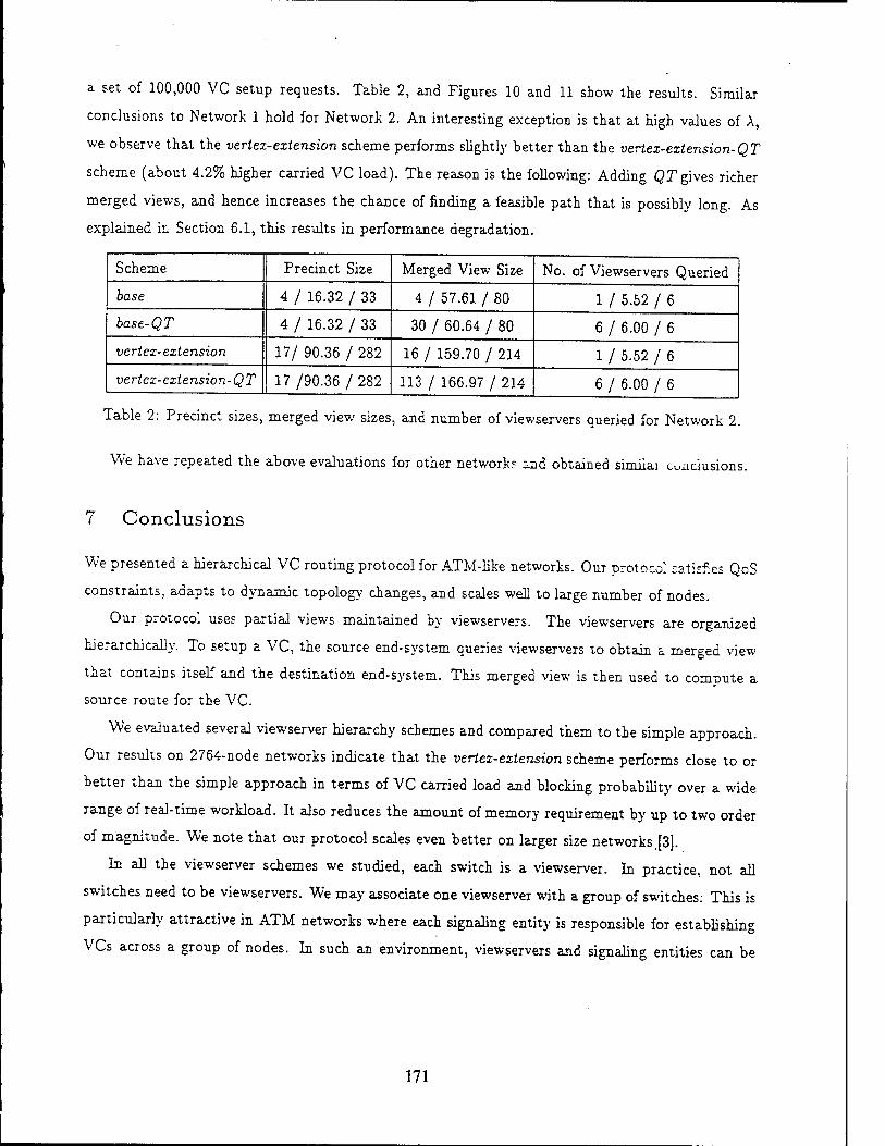
a set of 100,000 VC setup requests. Table 2, and Figures 10 and 11 show the results. Similar

conclusions to Network 1 hold for Network 2. An interesting exception is that at high values of A,

we observe that the vertex-extension scheme performs slightly better than the vertex-extension-QT

scheme (about 4.2% higher carried VC load). The reason is the following: Adding QT gives richer

merged views, and hence increases the chance of finding a feasible path that is possibly long. As

explained in Section 6.1, this results in performance degradation.


base 4 / 16.32 / 33 4 / 57.61 / 80 1 / 5.52 / 6

base-QT 4 / 16.32 / 33 30 / 60.64 / 80 6 / 6.00 / 6

vertex-extension 17/ 90.36 / 282 16 / 159.70 / 214 1 / 5.52 / 6

vertex-extension-QT 17 /90.36 / 282 113 / 166.97 / 214 6 / 6.00 / 6

Table 2: Precinct sizes, merged view sizes, and number of viewservers queried for Network 2.

We have repeated the above evaluations for other network? and obtained simiiar conclusions.

7 Conclusions

We presented a hierarchical VC routing protocol for ATM-like networks. Our protocol satisfies QoS

constraints, adapts to dynamic topology changes, and scales well to large number of nodes.

Our protocol uses partial views maintained by viewservers. The viewservers are organized

hierarchically. To setup a VC, the source end-system queries viewservers to obtain a merged view

that contains itself and the destination end-system. This merged view is then used to compute a

source route for the VC.

We evaluated several viewserver hierarchy schemes and compared them to the simple approach.

Our results on 2764-node networks indicate that the vertex-extension scheme performs close to or

better than the simple approach in terms of VC carried load and blocking probability over a wide

range of real-time workload. It also reduces the amount of memory requirement by up to two order

of magnitude. We note that our protocol scales even better on larger size networks [3].

In all the viewserver schemes we studied, each switch is a viewserver. In practice, not all

switches need to be viewservers. We may associate one viewserver with a group of switches; This is

particularly attractive in ATM networks where each signaling entity is responsible for establishing

VCs across a group of nodes. In such an environment, viewservers and signaling entities can be

171

> •o u •E «

CARRIED VC LOAD vs Arrival rale

2000

I 1 1 1

— ^ s

1 1 _l 1 J. .---<>

1500 //

// II

1000 //

flat base

ft II

base-QT -Q~ vertex-cxtension

venex-exiension-QT 500

> 1 1 1 1 i 1 I 1 1

0.05 0.1 0.15 0.2 0.25 0.3 0.35 0.4 0.45 0.5 Arrival rate

Figure 10: Carried VC load versus arrival rate for Network 2.

PERCENT VC BLOCKING vs Arrival rale 70

60 -

50 -

U >

1 l 1 l ■1111 1

- c& ̂

>

-

- 7 / flat

™

- S/Z / base

base-QT -©-- -

* s /

yj

venex-exiension venex-cxtension-QT

till 1

-

40

30

20

10

0.05 0.1 0.15 0.2 0.25 0.3 0.35 0.4 0.45 0.5 Arrival raie

Figure 11: Percent VC blocking versus arrival rate for Network 2.

combined.

However, there is an advantage of each switch being a viewserver; that is, source nodes do not

require fixed source routes to their parent viewservers (in the view-query protocol). This reduces

the amount of hand configuration required. In fact, the base and base-QT viewserver schemes do

not require any hand configuration.

Our evaluation model assumed that views are instantaneously updated, i.e. no delayed feedback

172

between link cost changes and view/route changes. We plan to investigate the effect of delayed feed-

back on the performance of the different schemes. We expect our viewserver schemes to outperform

the simple approach in this realistic setting as the update of views of the viewservers requires less

time and communication overhead. Thus, views in our viewserver schemes will be more up-to-date.

As we pointed out in [3], the only drawback of our protocol is that to obtain a source route

for a VC, views are merged at (or prior to) the VC setup, thereby increasing the setup time. This

drawback is not unique to our scheme [8, 16, 7, 11]. Reference [3] describes several ways, including

cacheing and replication, to reduce the setup overhead and improve performance.

n References

[1] H. Ahmadi J Chen and R Guerin. Dynamic Routing and Call Control in High-Speed Integrated êtworks. In Proc. Workshop on Systems Engineering and Traffic Engineering, ITC'JS, pages 19-26 Copenhagen, Denmark, June 1991. '

[2] C. Alaettinoflu and A. U Shankar. Viewserver Hierarchy: A New Inter-Domain Routing Protocol and its Evaluataon Technical Report UMIACS-TR-93-98, CS-TR-3151, Department of Computer Science, university of Maryland, College Park, October 1993. Earlier version CS-TR-3033, February 1993.

[3] C. Alaettinoglu and A. V Shankar. Viewserver Hierarchy: A New Inter-Domain Routing Protocol. In Proc. IEEE INFOCOM '94, Toronto, Canada, June 1994.

[4] A. Alles. ATM in Private Networking: A Tutorial. Hughes LAN Systems, 1993.

[5] P Almquist. Type of Service in the Internet Protocol Suite. Technical Report RFC-1349 Network Working Group, July 1992.

[6] L. Breslau. D. Estrin, and L. Zhang. A Simulation Study of Adaptive Source Routing in Integrated Services Networks. Available by anonymous ftp at catarina.usc.edu:pub/breslau, September 1993.

[7] J N Chiappa. A New IP Routing and Addressing Architecture. Big-Internet mailing list., 1992. Available by anonymous ftp from mtmaari.oz.au: big-internet /list-archive.

[8] D.D. Clark. Policy routing in Internet protocols. Request for Comment RFC-1102, Network Information Center. May 1989.

[9] R. Coltun and M. Sosa. VC Routing Criteria. Internet Draft, March 1993.

t10] ^Comerând R Yavatkar. FLOWS: Performance Guarantees in Best Eftort Delivery Svstems In Proc ILEE INFOCOM, Ottawa, Canada, pages 100-109, April 1989. "

I11] ?;0EÄriîr

Y,^|lekllter' "IS. Hotz. Scalable Inter-Domain Routing Architecture. In Proc. ACM SJGCOMM '92, pages 40-o2, Baltimore, Maryland, August 1992.

[12] R Guerin, H. Ahmadi, and M. Naghshineh. Equivalent Capacity and its Application to Bandwidth Avocation m High-Speed Networks. IEEE J. Select. Areas Commun., SAC-9(7):968-981, September

[13] A. Guillen, R. Kia and B. Sales. AD Architecture for Virtual Circuit/QoS Routing. In Proc IEEE International Conference on Network Protocols '9S, pages 80-87, San Francisco, California, October

^ ™P,Ä>' K- Ro?*.fnrd M- $£zrki. Routing in Virtual Path Based ATM Networks. In Proc. GLOBE-

COM 92, pages 0/1-5/5,1992.

[15] R-H. Hwang■ J. Kurose and D. Towsley. MDP Routing in ATM Networks Using Virtual Path Concept. In Proc. IEEE INFOCOM, pages 1509-1517, Toronto, Ontario, Canada, June 1994.

[16] M. Lepp and M. Steenstrup. An Architecture for Inter-Domain Policy Routing. Internet Draft Available from the authors., June 1992.

[17] I. Matta and A.Ü. Shankar. An Iterative Approach to Comprehensive Performance Evaluation of Inte- grated Services Networks. In Proc. IEEE International Conference on Network Protocols '91 Boston Massachusetts, October 1994. To appear.

[18] J. Moy. OSPF Version 2. RFC 1247, Network Information Center, SRI International, July 1991.

173

(19] C. Parris and D. Ferrari. A Dynamic Connection Management Scheme for Guaranteed Performance Services in Packet-Switching Integrated Services Networks. Technical Report TR-93-005, International Computer Science Institute, Berkeley, California, January 1993.

[20] J. Postel. Transmission Control Protocol: DARPA Internet Program Protocol Specification. Request for Comment RFC-793, Network Information Center, SRI International, 1981.

[21] M. Prycker. Asynchronous Transfer Mode - Solution for Broadband ISDN. Ellis Horwood, 1991.

[22] S. Rampal, D. Reeves, and D. Agrawal. An Evaluation of Routing and Admission Control Algorithms for Multimedia Traffic in Packet-Switched Networks. Available from the authors, 1994.

[23] H. Suzuki and F. Tobagi. Fast Bandwidth Reservation Scheme with Multi-Link and Multi-Path Routing in ATM Networks. In Proc. IEEE JNFOCOM '92, pages 2233-2240, Florence, Italy, May 1992.

[24] E. Sykas, K. Vlakos, I. Venieris, and E. Protonotarios. Simulative Analysis of Optimal Resource Allo- cation and Routingin IBCN's. IEEE J. Select Areas Commun., 9(3):486-492, April 1991.

[251 P. F. Tsuchiya. The Landmark Hierarchy: Description and Analysis, The Landmark Routing: Ar- chitecture Algorithms and Issues. Technical Report MTR-87W00152, MTR-87W00174, The MITRE Corporation, McLean, Virginia, 1987.

[26] P. F. Tsuchiva. The Landmark Hierarchv:A New Hierarchy For Routing In Very Large Networks. In Proc. ACM SIGCOMM '88, August 1988".

174


OMB No 0704-01BS

. 9* ^»»«o»

1. AGENCY USE ONLY (left bunt) 2. REPORT DATE

October 1994 3. REPORT TYPE AND DATES COVERED

Technical

A. TITLE AND SUBTITLE

A Scalable Virtual Circuit Routing Scheme for ATM Networks

6. AUTHOR(S)

Cengiz Alaettinoglu, Ibrahim Matta and A. Udaya Shankar


Department of Computer Science A. V. Willliams Building university of Maryland College Park, MD 20742

9. SPONSORING /MONITORING AGENCY NAME(S) AND ADDRESS(ES)

Phillips Laboratory Directorate of Contracting 3651 Lowry Avenue SE Kirtland AFB NM 87117-5777

5. FUNDING NUMBERS

C DASG60-92-0055 G NCR 89-04590 G NCR 93-21043


CSTR-3360 UMIACS-TR 94-115

10. SPONSORING /MONITORING AGENCY REPORT NUMBER



13. AESTRACT (Maximurr. 200 wora)

these protocols do not scale well to large networks in terms of storage and

communication overhead. ..-IT«- ■;= Kaeprf on the In this paper, we present a scalable VC routing protocol. It is based on the

recently proposed viewserver hierarchy, where each viewserver maintains a partial ""oythe network. By querying these viewservers a source c- obtain am«ged vxe. that contains a path to the destination. The source then sends a re£«" J"£C J7" this path to setup a real-time VC through resource reservations. The request is b5o ked if the setup fails. Ve compare our protocol to a .sl-ple «PP --h using simulation. Under this simple approach , a source maintains a full view of the network. In addition to the savings in storage our results «£"" f£ £*ried

U. SUBJECT TERMS

Computer-Communication Networks: Network Architecture and Design, Network Protocols;Routing Protocols: Computer Network Routing Protocols

17. SECURITY CLASSIFICATION OF REPORT unclassified

16. SECURITY CLASSIFICATION Of THIS PAGE unclassified

is. SECURITY CLASSIFICATION OF ABSTRACT

Unclassified

15. NUMBER OF PAGES



unlimited

MSN 75CC-OWSO-5500 175 S-.ar-oa'd -cr-> :9S !*ev 2-89!

Hierarchical Inter-Domain Routing Protocol with On-Demand ToS and Policy Resolution*

Cengiz Alaettinoglu. A. Udaya Shankar


Department of Computer Science University of Maryland


June 20, 1994

Abstract

Traditional inter-domain routing protocols based on superdomains maintain either "strong" or "weak" ToS and policy constraints for each visible superdomain. With strong constraints a valid path may not be found even though one exists. With weak constraints, an invalid domain-level path may be treated as a valid path.

We present an inter-domain routing protocol based on superdomains, which always finds a valid path if one exists. Both strong and weak constraints are maintained for each visible superdomain. If the strong constraints of the superdomains on a path are satisfied, then the path is valid. If only the weak constraints are satisfied for some superdomains on the path the source uses a query protocol to obtain a more detailed "internal" view of these superdomains and searches again for a valid path. Our protocol handles topology changes, including node/link failures that partition superdomains. Evaluation results indicate our protocol scales well to large internetworks. ö

Categories and Subject Descriptors: C.2.1 [Computer-Communication Networks]: Network Archi- tecture and Design-packet networks; start and forward networks: C.2.2 [Computer-Communication Net- works]: Network Protocols-prozoco/ architecture; C.2.m [Routing Protocols]; F.2.m [Computer Network Routing Protocols].

• This work is supported in pan by ARPA ud Philips Labs under contract DASG60-92-0055 to Department of Computer Säen«, University of Maryland, and by National Science Foundation Grant No NCR 89-04590 The views, opiruons, and/or findings contained in this report are those of the author(s) and should not be interpreted as

r*n cnV Po eS' ether exPressed or ™P"«i. rf »ke Advanced Research Projects Agency, PL, NSF or tie U.b. Government. Computer facilities were provided in part by NSF grant CCR-8811954.

177

type-of-service (ToS) constraints of applications (e.g. low delay, high throughput, high reliability,

minimum monetary cost), each node maintains a cost for each outgoing link and ToS. The intra-

domain routing protocol should choose optimal paths based on these costs.

Across all domains, an inter-domain routing protocol is executed that provides routes between

source and destination nodes in different domains, using the services of the intra-domain routing

protocols within domains. This protocol should have the following properties:

(1) It should satisfy the policy constraints of domains. To do this, it must keep track of the

policy constraints of domains [5].

(2) An inter-domain routing protocol should also satisfy ToS constraints of applications. To do

this, it must keep track of the ToS services offered by domains [5].

(3) An inter-domain routing protocol should scale up to very large internetworks, i.e. with a very

large number of domains. Practically this means that processing, memory and communication

requirements should be much less than linear in the number of domains. It should also

handle non-hierarchical domain interconnections at any level [8] (e.g. we do not want to

hand-configure special routes as "back-doors").

(4) An inter-domain routing protocol should automatically adapt to link cost changes and node/link

failures and repairs, including failures that partition domains [13].

A Straight-Forward Approach

A straight-forward approach to inter-domain routing is domain-level source routing with link-state

approach [7, 5]. In this approach, each router3 maintains a domain-level view of the internetwork,

i.e., a graph with a vertex for every domain and an edge between every two neighbor domains.

Policy and ToS information is attached to the vertices and the edges of the view.

When a source node needs to reach a destination node, it (or a router4 in the source's domain)

first examines this view and determines a domain-level source route satisfying ToS and policy

constraints, i.e., a sequence of domain ids starting from the source's domain and ending with the

destination's domain. Then packets are routed to the destination using this domain-level source

route and the intra-domain routing protocols of the domains crossed.

For example, consider the internetwork of Figure 2 (each circle is a domain, and each thin line

2 Not a]] nodes maintain routing tables. A router is a node that maintains a. routing table. 4 referred to zs the policy server in [7]

178

1 Introduction

A computer internetwork, such as the Internet, is an interconnection of backbone networks, regional

networks, metropolitan area networks, and stub networks (campus networks, office networks and

other small networks)1. Stub networks are the producers and consumers of the internetwork traffic,

while backbones, regionals and MANs are transit networks. Most of the networks in an internetwork

are stub networks. Each network consists of nodes (hosts, routers) and links. A node that has a

link to a node in another network is called a gateway. Two networks are neighbors when there is

one or more links between gateways in the two networks (see Figure 1).

Figure 1: A portion of an internetwork. (Circles represent stub networks.)

An internetwork is organized into domains2. A domain is a set of networks (possibly consisting

of only one network) administered by the same agency. Domains are typically subject to policy

constraints, which are administrative restrictions on inter-domain traffic [7, 11, 8, 5]. The policy

constraints of a domain U are of two types: transit policies, which specify how other domains

can use the resources of U (e.g. S0.01 per packet, no traffic from domain V); and source policies,

which specify constraints on traffic originating from U (e.g. domains to avoid/prefer, acceptable

connection cost). Transit policies of a domain are public (i.e. available to other domains), whereas

source policies are usually private.

Within each domain, an intra-domain routing protocolis executed that provides routes between

source and destination nodes in the domain. This protocol can be any of the typical ones, i.e.,

next-hop or source routes computed using distance-vector or link-state algorithms. To satisfy

^ For example, NSFNET, MILNET are backbones, and Suranet, CerfKet are regionals. Also referred to as routing domains or administrative domains.

179

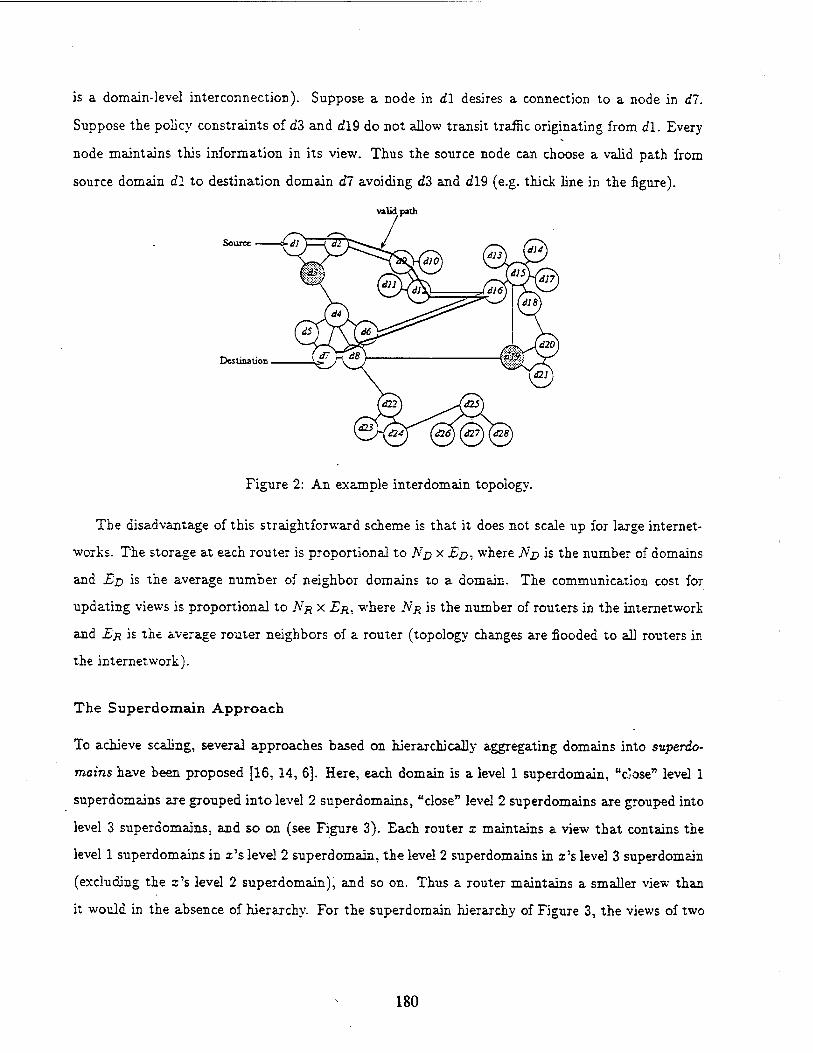
is a domain-level interconnection). Suppose a node in dl desires a connection to a node in dl.

Suppose the policy constraints of d3 and dl9 do not allow transit traffic originating from dl. Every

node maintains this information in its view. Thus the source node can choose a valid path from

source domain dl to destination domain dl avoiding d3 and dl9 (e.g. thick line in the figure).

valid path

Source

Destination

Figure 2: An example interdomain topology.

The disadvantage of this straightforward scheme is that it does not scale up for large internet-

works. The storage at each router is proportional to ND X ED, where ND is the number of domains

and ED is the average number of neighbor domains to a domain. The communication cost for

updating views is proportional to NR X ER, where NR is the number of routers in the internetwork

and ER is the average router neighbors of a router (topology changes are flooded to all routers in

the internetwork).

The Superdomain Approach

To achieve scaling, several approaches based on hierarchically aggregating domains into superdo-

mains have been proposed [16. 14, 6]. Here, each domain is a level 1 superdomain, "dose" level 1

superdomains are grouped into level 2 superdomains, "close" level 2 superdomains are grouped into

level 3 superdomains. and so on (see Figure 3). Each router x maintains a view that contains the

level 1 superdomains in z's level 2 superdomain, the level 2 superdomains in I'S level 3 superdomain

(excluding the s's level 2 superdomain), and so on. Thus a router maintains a smaller view than

it would in the absence of hierarchy. For the superdomain hierarchy of Figure 3, the views of two

180

valid palh

level 1 superdom&in

level 2 superdomain

level 3 tuperdomain

Destination

Figure 3: An example of superdomain hierarchy,

routers (one in domain dl and one in domain dl6) are shown in Figures 4 and 5.

Figure 4: View of a router in dl. Figure 5: View of a Rswterm cfl6.

The superdomain approach has several problems. One problem is that the aggregation results

in loss of domain-level ToS and policy information. A superdomain is usually characterized by a

single set of ToS and policy constraints derived from the ToS and policy constraints of the domains

in it. Routers outside the superdomain assume that this set of constraints applies uniformly to

each of its children (and by recursion to each domain in the superdomain). If there are domains

with different (possibly contradictory) constraints in a superdomain, then there is no good way of

deriving the ToS and policy constraints of the superdomain.

The usual technique [16] of obtaining ToS and policy constraints of a superdomain is to obtain

either a strong set of constraints or a weak set of constraints5 from the ToS and policy constraints of

'strong" and "weak" are referred to respectively as "union" and "intersection" in [16]

181

the children superdomains in it. If strong (weak) constraints are used for policies, the superdomain

enforces a policy constraint if that policy constraint is enforced by some (all) of its children. If

stron^ (weak) constraints are used for ToS constraints, the superdomain is assumed to support a

ToS if that ToS is supported by all (some) of its children. The intention is that if strong (weak)

constraints of a superdomain are (are not) satisfied then any (no) path through that superdomain

is valid.

Each approach has problems. Strong constraints can eliminate valid paths, and weak constraints

can allow invalid paths. For example in Figure 3, dl6 allows transit traffic from dl while dl9 does

not: with strong constraints G would not allow transit traffic from dl, and with weak constraints

G would allow transit traffic from dl to be routed via dl9.

Other problems of the superdomain approach are that the varying visibilities of routers compli-

cates superdomain-level source routing and handling of node/link failures (especially those that par-

tition superdomains). The usual technique for solving these problems is to augment superdomain-

level views with gateways [16] (see Section 3).

Our Contribution

In this paper, we present an inter-domain routing protocol based on superdomains, which finds

a valid path if and only if one exists. Both strong and weak constraints are maintained for each

visible superdomain. If the strong constraints of the superdomains on a path are satisfied, then

the path is valid. If only the weak constraints are satisfied for some superdomains on the path, the

source uses a query protocol to obtain a more detailed "internal" view of these superdomains, and

searches again for a valid path.

We use superdomain-level views with gateways and a link-state view update protocol to handle

topology changes including failures that partition superdomains. The storage cost is OQogNp *

logND) without the query protocol. We demonstrate the scaling properties of the query protocol

by giving evaluation results based on simulations. Our evaluation results indicate that the query

protocol can be performed using '15% extTa space.

Our protocol consists of two subprotocols: a view-query protocol for obtaining views of

«reater resolution when needed: and a view-update protocol for disseminating topology changes

to the views.

182

Several approaches to scalable inter-domain routing have been proposed, based on the super-

domain hierarchy [1, 14, 16, 9, 6], and the landmark hierarchy [18, 17]. Some of these approaches

suffer from loss of ToS and policy information (and hence may not find a valid path which exists).

Others are still in a preliminary stage. (Details in Section 8.)

One important difference between these approaches and ours is that ours uses a query mechanism

to obtain ToS and policy details whenever needed. In our opinion, such a mechanism is needed

to obtain a scalable solution. Query protocols are also being developed to enhance the protocols

in [9, 6]. Reference [2] presents protocols based on a new kind of hierarchy, referred to as the

viewserver hierarchy (more details in Section 8).

A preliminary version of the view-query protocol was proposed in reference [1]. That version

differs greatly from the one in this paper. Here, we augment superdomain-level views with gate-

ways. In [1], we augmented superdomain-level views with superdomain-to-domain edges (details in

Section 8). Both versions have the same time and space complexity, but the protocols in this paper

are much simpler conceptually. Also the view-update protocol is not in reference [l].


In Section 2, we present some definitions used in this paper. In Section 3, we define the view data

structures. In Section 4, we describe how views are affected by topology changes. In Section 5, we

present the view-query protocol. In Section 6, we present the view-update protocol. In Section 7,

we present our evaluation model and the results of its application to the superdomain hierarchy.

In Section 8, we survey recent approaches to inter-domain routing. In Section 9, we conclude and

describe cacheing and heuristic schemes to improve performance.

2 Preliminaries

Each domain has a unique id. Let Domainlds denote the set of domain-ids. Each node has a

unique id. Let Nodelds denote the set of node-ids. For a node z, we use domainid(z) to denote

the domain-id of i's domain.

The superdomain hierarchy defines the following parent-child relationship: & level i, i > 1,

superdomain is the parent of each level i — 1 superdomain it contains. Top-level superdomains

183

have no parents. Level 1 superdomains, which are just domains, have no children. For any two

superdomains X and Y, X is a sibling of Y iff X and Y have the same parent. X is an ancestor

(descendant) of Y iff A' = Y or X is an ancestor (descendant) of Y's parent (child).

Each router maintains information about a subset of superdomains, referred to as its visible

superdomains. The visible superdomains of a router x are (1) x's domain itself, (2) siblings of x's

domain, and (3) siblings of ancestors of x's domain. In Figure 3, the visible superdomains of a

router in dl are dl,d2,d2,B,C,G,J (these are shown in Figure 4). Note that if a superdomain U

is visible to a router, then no ancestor or descendant of U is visible to the router.

Each superdomain has a unique id, i.e. unique among all superdomains regardless of level. Let

SuperDomainlds denote the set of superdomain-ids. Domainlds is a subset of SuperDomainlds.

For a superdomain V, let level(C/) denote the level of U in the hierarchy, let Ancestors(Z7) denote

the set of ids of ancestor superdomains of U in the hierarchy, and let Children(J7) denote the set

of ids of child superdomains of U in the hierarchy.

For a router x, let VisibleSuperDomains(x) denote the set of ids of superdomains visible from

x.

We extend the above definitions by allowing their arguments to be nodes, in which case the node

stands for its domain. For example, if x is a node in domain d, Ancestors(x) denotes Ancestors(d).

3 Sup er domain-Level Views with Gateways

For routing purposes, each domain (and node) has an address, defined as the concatenation of the

superdomain ids starting from the top level and going down to the domain (node). For example in

Figure 3, the address of domain dlo is G.E.dlb, and the address of anode h in dlb is G.E.dlo.h.

When a source node needs to reach a destination node, it first determines the visible superdo-

main in the destination address and then by examining its view determines a superdomain-level

source route (satisfying ToS and policy constraints) to this superdomain. However, since routers

in different superdomains maintain views of different sets of superdomains, this superdomain-level

source route can be meaningless at some intermediate superdomain's router x because the next

superdomain in this source route is not visible to x. For example in Figure 4, superdomain-level

source route (d2,B,G,C) created at a router in d2 becomes meaningless once the packet is in G,

where C is not visible.

184

The usual technique of solving this problem is to augment super domain-level views with gate-

ways and edges between these gateways.

Define the pair U:g to be an sd-gateway iff U is a superdomain and g is a node that is in U and

has a link to a node outside V. Equivalently, we say that g is a gateway ojU.

Define (U:g, h) to be an actual-edge iff U:g is an sd-gateway, A is a gateway not in U, and there

is a link from g to h.

Define (U:g,h) to be a virtual-edge iff U:g and U:h are sd-gateways and g ^ h (note that there

may not be a link between g and h).

(U:g,h) is an edge iff it is an actual-edge or a virtual-edge. An edge (U:g,h) is also said to be

an outgoing edge of U:g. Define edges ofU:g to be the set of edges outgoing from U:g. Define edges

of U to be the set of edges outgoing from any gateway of U.

Let Gateways(Z7) denote the set of node-ids of gateways of U. Let Edges(U:g) denote the edges

of U:g. Note that we never use "edge" as a synonym for link.

A gateway g of a domain can generate many sd-gateways, specifically, U:g for every ancestor U

of g''s domain such that g has a link to a node outside U. A link (g,h) where g and h are gateways

in different domains, can generate many actual-edges; specifically, actual-edge {U:g,h) for every

ancestor U of g:s domain such that U is not an ancestor of fe's domain.

For the internetwork topology of Figure 2, the corresponding gateway-level connections are

shown in Figure 6 where black rectangles are gateways. For the hierarchy of Figure 3, gateway

g in Figure 6 generates sd-gateways dl6:g, E:g, and G:g. The link (g,h) in Figure 6 generates

actual-edges {dl6:g,h), (E:g,h), (G:g,h).

To a router, at most one of the sd-gateways generated by a gateway g is visible, namely U:g

where U is an ancestor of g's domain and U is visible to the router. At most one of the actual-edges

generated by a link {<?, h) between two gateways in different domains is visible to the router, namely

edge (U:g,h) where U:g is visible to the router. None of the actual-edges are visible to the router

if g and h are inside a visible superdomain. For example in Figure 3, of the actual-edges generated

by link (g,h), only (G:g,h) is visible to a router in dl, and only (dl6:g,h) is visible to a router in

die.

A router maintains a view consisting of the visible sd-gateways and their outgoing actual- and

virtual-edges. An edge (U:g.h) in the view of a router connects the sd-gateway U:g to the sd-

185

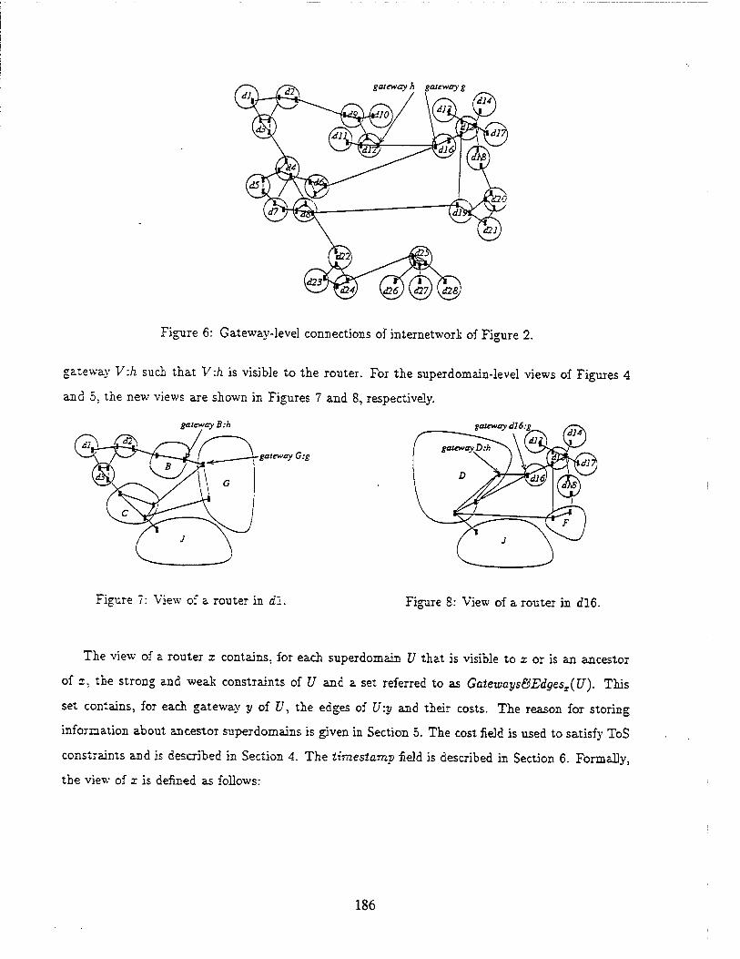
gateway h gateway j

Figure 6: Gateway-level connections of internetwork of Figure 2.

gateway V:h such that V:h is visible to the router. For the superdomain-level views of Figures 4

and 5. the new views are shown in Figures 7 and 8, respectively.

gateway B:h gateway 616:^

gateway D:i gateway G:g

Figure 7: View of a router in dl. Figure 8: View of a router in dl6.

The view of a router x contains, for each superdomain U that is visible to x or is an ancestor

of x, the strong and weak constraints of U and a set referred to as Gateways&Edgesx(U). This

set contains, for each gateway y of U, the edges of U:y and their costs. The reason for storing

information about ancestor superdomains is given in Section 5. The cost field is used to satisfy ToS

constraints and is described in Section 4. The time stamp field is described in Section 6. Formally,

the view of x is defined as follows:

186

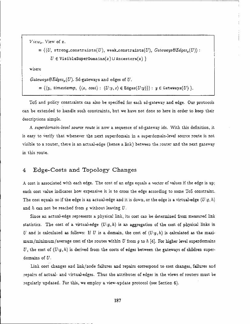
Viewx. View of x.

= {(U, strong_constraints(t/), weak_constraints(C7), Gateways&Edgesz(U))

U £ VisibleSnperDomains(i) U Ancestors(x) }

wnere

Gateways&Edgesx(U). Sd-gateways and edges of U.

= {{y, timestamp, {{z, cost) : (U:y,z) € Edges(U:y)}) : y£ Gateways(£/) }.

ToS and policy constraints can also be specified for each sd-gateway and edge. Our protocols

can be extended to handle such constraints, but we have not done so here in order to keep their

descriptions simple.

A superdornain-level source route is now a sequence of sd-gateway ids. With this definition, it

is easy to verify that whenever the next superdornain in a superdomain-level source route is not

visible to a router, there is an actual-edge (hence a link) between the router and the next gateway

in this route.

4 Edge-Costs and Topology Changes

A cost is associated with each edge. The cost of an edge equals a vector of values if the edge is up;

each cost value indicates how expensive it is to cross the edge according to some ToS constraint.

The cost equals co if the edge is an actual-edge and it is down, or the edge is a virtual-edge (U:g, h)

and h can not be reached from g without leaving U.

Since an actual-edge represents a physical link, its cost can be determined from measured link

statistics. The cost of a virtual-edge (U:g,h) is an aggregation of the cost of physical links in

U and is calculated as follows: If U is a domain, the cost of (U:g,h) is calculated as the maxi-

mum/minimum/average cost of the routes within U from g to h [4]. For higher level superdomains

U, the cost of {U:g,h) is derived from the costs of edges between the gateways of children super-

domains of U.

Link cost changes and link/node failures and repairs correspond to cost changes, failures and

repairs of actual- and virtual-edges. Thus the attributes of edges in the views of routers must be

regularly updated. For this, we employ a view-update protocol (see Section 6).

187

Link/node failures can also partition a superdomain into cells, where a cell of a superdomain

is defined to be a maximal subset of nodes of the superdomain that can reach each other without

leaving the superdomain. Superdomain partitions can occur at any level in the hierarchy. For

example, suppose U is a domain and V is its parent superdomain. U can be partitioned into cells

without V being partitioned (i.e. if the cells of U can reach each other without leaving V). The

opposite can also happen: if all links between U and the other children of V fail, then V becomes

partitioned but Ü does not. Ox both U and V can be partitioned. In the same way, link/node

repairs can merge cells into bigger cells.

We handle superdomain partitioning as follows: A router detects that a superdomain U is

partitioned when a virtual-edge of U in the router's view has cost co. When a router forwards

a packet to a destination for which the visible superdomain, say U, in the destination address is

partitioned into cells, a copy of the packet is sent to each cell by sending a copy of the packet to

each gateway of U; the id U in the destination address is "marked" in the packet so that subsequent

routers do not create new copies of the packet for U.

5 View-Query Protocol

When a source node wants a superdomain-level source route to a destination, a router in its domain

examines its view and searches for a valid path (i.e. superdomain-level source route) using the

destination address6. We refer to this router as the source router. Even though the source route-

does not know the constraints of the individual domains that are to be crossed in each superdomain,

it does know the strong and weak constraints of the superdomains. We refer to a superdomain

whose strong constraints are satisfied as a valid superdomain. If a superdomain's weak constraints

are satisfied but strong constraints are not satisfied, then there may be a valid path through this

superdomain. We refer to such a superdomain as a candidate superdomain.

A path is valid if it involves only valid superdomains. A path cannot be valid if it involves

a superdomain which is neither valid nor candidate. We refer to a path involving only valid and

candidate superdomains as a. candidate path. 6 We assume that the source has the destination's address. H that is not the case, it would first query the name

servers to obtain the address for the destination. Querying the name servers can be done the same way it is done currently in the Internet. It requires nodes to have a set of fixed addresses to name servers. This is also sufficient in

our case.

188

If the source router's view contains a candidate path {t/0:pooi---,#o:pon , b\:glo,..., Jj\:gin , ••• ,

Um'-gma,- ■ ■, Um'-9mnm) to the destination (and does not contain a valid path), then for each candi-

date superdomain [/,- on this path, the source router queries gateway p,0 of £/,• for the internal view of

Ui. This internal view consists of the constraints, sd-gateways and edges of the child superdomains

of Ui.

When a router x receives a request for the internal view of an ancestor superdomain U, it'

returns the following data structure:

IVieivx(U). Internal view of U at router x.

= {{V, strong.constraints(V), weak_constraints(V), Gateways&Edgesx(V)} € Viewx

V £ Children(l/)}

It is to simplify the construction of IViewx(U) that we store information about ancestor su-

perdomains in the view of router x. Instead of storing this information, router x could construct

JViewx(U) from the constraints, sd-gateways and edges of the visible descendants of U. We did

not choose this alternative because the extra information does not increase storage complexity.

When the source router receives the internal view of a superdomain U, it does the following:

(1) it removes the sd-gateways and edges of U from its view; (2) it adds the sd-gateways and edges

of children superdomains in the internal view of U; and (3) searches for a valid path again. If there

is still no valid path but there are candidate paths, the process is repeated.

For example, consider Figure 3. For a router in superdomain dl (see Figure 7), G is visible and

is a candidate domain. The internal view of G is shown in Figure 9, and the resulting merged view

is shown in Figure 10. The valid path through G (visiting <fl6 and avoiding dl9) can be discovered

using this merged view (since the strong constraints of E are satisfied).

Consider a candidate route to a destination: (Z7o:5o0, - • -, #o"-$o , U\-9i<„ ■ ■ -, Uy:gi„ , • • • ,

Um'-gmoT ■ ■■>^m'-97r,nm)- If super domain Ui is partitioned into cells, it may re-appear later in the

candidate path (i.e. for some j =£ i, Uj = £/,-). In this case both gateways gio and gio are queried.

Timestamps are used to resolve conflicts between the information reported by these gateways.

The view-query protocol uses two types of .messages as follows:

• (RequestlViey, sdid.gid,sjiddres3, djiddress)

189

Figure 9: Internal view of G. Figure 10: Merged view at dl.

Sent by a source router to gateway gid to obtain the internal view of superdomain sdid.

s address is the address of the source router, djaddress is the address of the destination

node (of the desired route).

• (ReplylView, sdid, gid, iview, djxddress)

where iview is the internal view of superdomain sdid, and other parameters are as in the

RequestlViev message. It is sent by gateway gid to the source router.

The state maintained by a source router x is listed in Figure 15. PendingReqx is used to

avoid sending new request messages before receiving all outstanding reply messages. WViewx and

PendingRegx axe allocated and deallocated on demand for each destination.

The events of router x are specified in Figure 15. In the figure, * is a wild-card matching any

value. TimeOulx event is executed after a time-out period from the execution of Request- event to

indicate that the request has not been satisfied. The source host can then repeat the same request

afterwards.

The procedure searchx uses an operation "ReliableSend(m) to r", where m is the message being

sent and v is either an address of an arbitrary router or an id of a gateway of a visible superdomain.

ReliableSend is asynchronous. The message is delivered to v as long as there is a sequence of up

links between u and v.7 (Note that an address is not needed to obtain an inter-domain route to a

gateway of a visible superdomain.)

Router Failure Model: A router can undergo failures and recoveries at anytime. We

assume failures are fail-stop (i.e. a failed router does not send erroneous messages). When a router

x recovers, the variables WViewx and PendingReqx are lost for all destinations. The cost of each

edge in Viewx is set to oc. It becomes up-to-date as the router receives new information from other

This involves time-outs, retransmissions, etc. It requires a transport protocol support such as TCP.

190

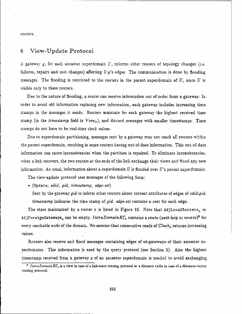
routers.

6 View-Update Protocol

A gateway 5, for each ancestor superdomain U, informs other routers of topology changes (i.e.

failures, repairs and cost changes) affecting U:g's edges. The communication is done by flooding

messages. The flooding is restricted to the routers in the parent superdomain of U, since U is

visible only to these routers.

Due to the nature of flooding, a router can receive information out of order from a gateway. In

order to avoid old information replacing new information, each gateway includes increasing time

stamps in the messages it sends. Routers maintain for each gateway the highest received time

stamp (in the timestamp field in Viewx), and discard messages with smaller timestamps. Time

stamps do not have to he real-time clock values.

Due to superdomain partitioning, messages sent by a gateway may not reach all routers within

the parent superdomain, resulting in some routers having out-of-date information. This out-of-date

information can cause inconsistencies when the partition is repaired. To eliminate inconsistencies,

when a link recovers, the two routers at the ends of the link exchange their views and flood any new

information. As usual, information about a superdomain U is flooded over U's parent superdomain.

The view-update protocol uses messages of the following form:

• (Update, sdid, gid, timestamp, edge-set)

Sent by the gateway gid to inform other routers about current attributes of edges of sdid:gid.

timestamp indicates the time stamp of gid. edge-set contains a cost for each edge.

The state maintained by a router x is listed in Figure 16. Note that AdjLocalRouters. or

AdjForeignGatewaysz can be empty. IntraDomainRTx contains a route (next-hop or source)8 for

every reachable node of the domain. We assume that consecutive reads of Clock- returns increasing

values.

Routers also receive and flood messages containing edges of sd-gateways of their ancestor su-

perdomains. This information is used by the query protocol (see Section 5). Also the highest

timestamp received from a gateway g of an ancestor superdomain is needed to avoid exchanging

8 IntTaDomainBTz is a. view in case of a link-state routing protocol or a distance table in case of a distance-vector routing protocol.

191

the messages of g infinitely during flooding.

The events of router x are specified in Figure 16. We use Ancestor,(L/) to denote the superdomain-

id of the tth ancestor of U, where Ancestor0(J/) = U. In the view-update protocol, a node u uses

send operations of the form uSend(m) to vn, where m is the message being sent and v is the

destination-id. Here, nodes v. and v are neighbors, and the message is sent over the physical link

(u. v). If the link is down, we assume that the packet is dropped.

7 Evaluation

In the superdomain hierarchy (without the query protocol), the number of superdomains in a view

is logarithmic in the number of superdomains in the internetwork [10].9 However, the storage

required for a view is proportional not to the number of superdomains in it but to the number of

sd-gateways in it. As we have seen, there can be more than one sd-gateway for a superdomain in

a view.

In fact, the superdomain hierarchy does not scale-up for arbitrary internetworks; that is, the

number of sd-gateways in a view can be proportional to the number of domains in the internetwork.

For example, if each domain in a superdomain U has a distinct gateway with a link to outside U,

the number of sd-gateways of U would be linear in the number of domains in U.

The good news is that the superdomain hierarchy does scale-up for realistic internetwork topolo-

gies. A sufficient condition for scaling is that each superdomain has at most log Np sd-gateways;

this condition is satisfied by realistic internetworks since most domain interconnections are "hier-

archical connections" i.e. between backbones and regionals, between regionals and MANs, and so

on.

In this section, we present an evaluation of the scaling properties of the superdomain hierarchy

and the query protocol. To evaluate any inter-domain routing protocol, we need a model in which

we can define internetwork topologies, policy/ToS constraints, inter-domain routing hierarchies,

and evaluation measures (e.g. memory and time requirements). We have recently developed such

a model j3]. We first describe our model, and then use it to evaluate our superdomain hierarchy.

Our evaluation measures ate the amount of memory required at the routers, and the amount of

9 Even though the results in [10] were for intra-domain routing, it is easy to show that the analysis there holds foi inter-domain routing as well.

192

time needed to construct a path.

7.1 Evaluation Model

We first describe our method of generating topologies and policy/ToS constraints. We then describe

the evaluation measures.

Generating Internetwork Topologies

For our purposes, an internetwork topology is a directed graph where the nodes correspond to

domains and the edges correspond to domain-level connections. However, an arbitrary graph will

not do. The topology should have the characteristics of a real internetwork, like the Internet.

That is, it should have backbones, regionals, MANS, LANS, etc.; there should^be hierarchical

connections, but some "non-hierarchical'' connections should also be present.

For brevity, we refer to backbones as class 0 domains, regionals as class 1 domains, metropolitan-

area domains and providers as class 2 domains, and campus and local-area domains as class 3

domains. A (strictly) hierarchical interconnection of domains means that class 0 domains are

connected to each other, and for £ > 0, class £ domains are connected to class £ — 1 domains.

As mentioned above, we also want some "non-hierarchicaT connections, i.e., domain-level edges

between domains irrespective of their classes (e.g. from a campus domain to another campus

domain or to a backbone domain).

In reality, domains span geographical regions and domain-level edges are often between do-

mains that are geographically close (e.g. University of Maryland campus domain is connected to

SURANET regional domain which are both in the east coast). We also want some edges that are

between far domains. A class £ domain usually spans a larger geographical region than a class £ + 1

domain. To generate such interconnections, we associate a "region" attribute to each domain. The

intention is that two domains with the same region are geographically close.

The region of a class £ domain has the form ro-ri.---.ri, where the rj's are integers. For

example, the region of a class 3 domain can be 1.2.3.4. For brevity, we refer to the region of a

class £ domain as a class £ region.

Note that regions have their own hierarchy which should not be confused with the superdomain

hierarchy. Class 0 regions are the top level regions. We say that a class £ region ro-rj. • • • .ri_i.ri

193

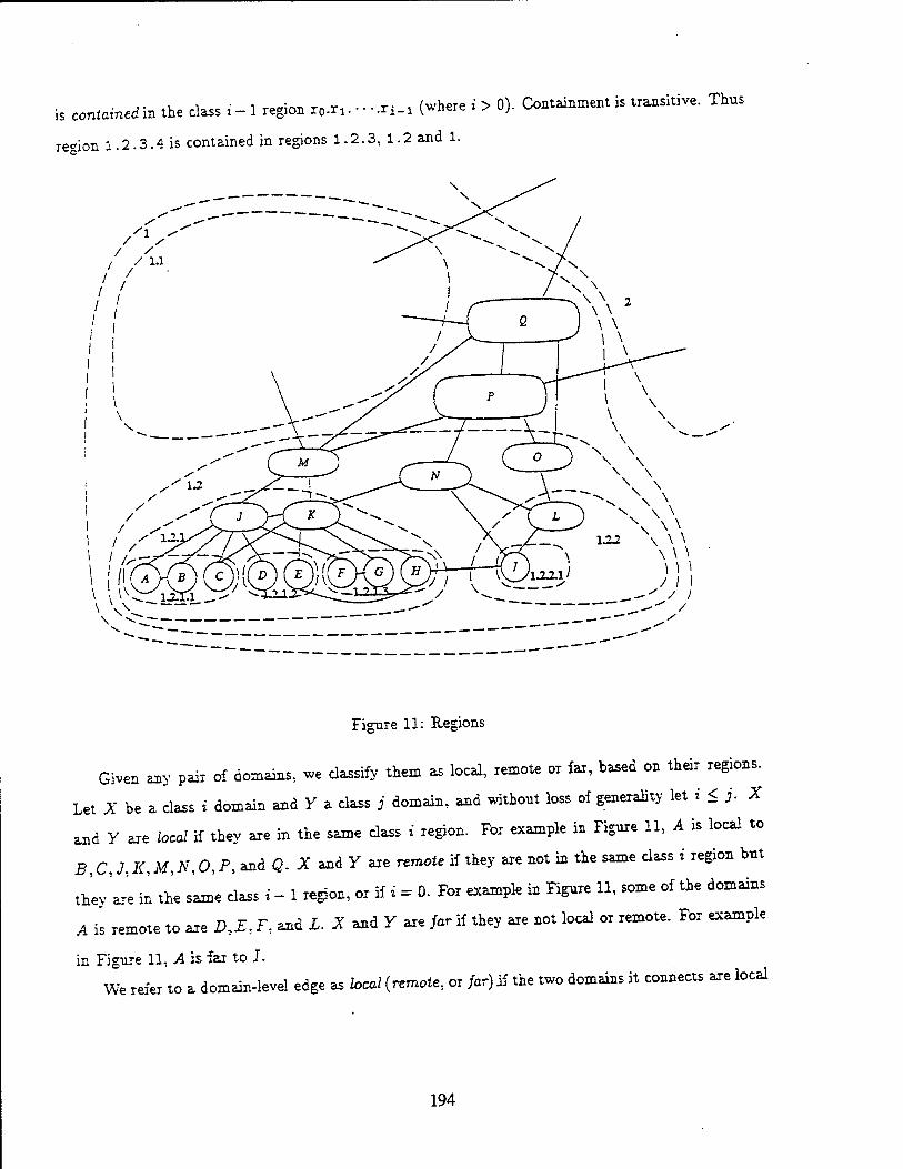
is contained in the class i - 1 region ro-n. - .r^ (-here : > 0). Containment is transitive. Tims

region 1.2.3.4 is contained in regions 1.2.3, 1.2 and 1.

Figure 11: Regions

Given any pair of domains, we classify them as local, remote or fax, based on their regions.

Let X be a class i domain and Y a class j domain, and withont loss of generality let i < j. X

and Y are local if they are in the same class i region. For example in Figure 11, A is local to

B,C.J,K,M,N, 0, P, and Q. X and Y are remote if they are not in the same class f region but

thev'are in the same class i - 1 region, or if i = 0. For example in Figure 11, some of the domains

A is remote to are D,E, F, and L. X and Y are far if they are not local or remote. For example

in Figure 11, A is far to J.

We refer to a domain-level edge as local (remote, or far) if the two domains it connects are local

194

(remote, or far).

We use the following procedure to generate internetwork topologies:

• We first specify the number of domain classes, and the number of domains in each class.

• We next specify the regions. Note that the number of region classes equals the number of

domain classes. We specify the number of class 0 regions. For each class i > 0, we specify a

branching factor, which creates that many class i regions in each class i — 1 region. (That is,

if there are two class 0 regions and the class 1 branching factor equals three, then there are

six class 1 regions.)

• For each class i, we-randomly map the class i domains into the class i regions. Note that

several domains can be mapped to the same region, and some regions may have no domain

mapped into them.

• For every class i and every class j, j > i, we specify the number of local, remote and far

edges to be introduced between class i domains and class j domains. The end points of the

edges are chosen randomly (within the specified constraints).

• We ensure that the internetwork topology is connected by ensuring that the subgraph of class

0 domains is connected, and each class i domain, for i > 0, is connected to a local class i — 1

domain.

• Each domain has one gateway. So all neighbors of a domain are connected via this gateway.

This is for simplicity.

Choosing Policy/ToS Constraints

We chose a simple scheme to model policy/ToS constraints. Each domain is assigned a color: green

or red. For each domain class, we specify the percentage of green domains in that class, and then

randomly choose a color for each domain in that class.

A valid route from a source to a destination is one that does not visit any red intermediate

domains; the source and destination domains are allowed to be red.

This simple scheme can model many realistic policy/ToS constraints, such as security constraints

and bandwidth requirements. It cannot model some important kinds of constraints, such as delay

bounds.

195

Computing Evaluation Measures

The evaluation measures of most interest for an inter-domain routing protocol are its memory, time

and communication requirements. We postpone the precise definitions of the evaluation measures

to the next subsection.

The only analysis method we have at present is to numerically compute the evaluation measures

for a variety of source-destination pairs. Because we use internetwork topologies of large sizes, it

is not feasible to compute for all possible source-destination pairs. We randomly choose a set

of source-destination pairs that satisfy the following conditions: (1) the source and destination

domains are different stub domains, and (2) there exists a valid path from the source domain to the

destination domain in the internetwork topology. (Note that the straight-forward scheme would

always find such a path.)

7.2 Application to Superdomain Query Protocol

We use the above model to evaluate our superdomain query protocol for several different super-

domain hierarchies. For each hierarchy, we define a set of superdomain-ids and a parent-child

relationship on them.

The first superdomain hierarchy scheme is referred to as child-domains. Each domain d (re-

gardless of its class) is a level-1 superdomain, also identified as d. In addition, for each backbone d,

we create a distinct level-4 superdomain referred to as d-4. For each regional d, we create a distinct

level-3 superdomain d-Z and make it a child of a randomly chosen level-4 superdomain e-4 such

that d and e are local and connected. For each MAN d, we create a distinct level-2 superdomain

d-2 and make it a child of a randomly chosen level-3 superdomain e-3 such that d and e are local

and connected. Please see Figure 12.

We next describe how the level-1 superdomains (i.e. the domains) are placed in the hierarchy.

A backbone d is placed in, i.e. as a child of, d-4. A regional d is placed in d-3. A MAN d is placed

in d-2. A stub d is placed in e-2 such that d and e are local and connected. Please see Figure 12.

The second superdomain hierarchy scheme is referred to as sibling-domains. It is identical

to child-domains except for the placement of level-1 superdomains corresponding to backbones,

regionals and MANs. In sibling-domains, a backbone d is placed as a sibling of d-4. A regional d

is placed as a sibling of d-3. A MAN d is placed as a sibling of d-2. Please see Figure 13.

196

Figure 12: child-domains

f bukfao» A J [ backbone G J

Figure 13: sibling-domains

The third superdomain hierarchy scheme is referred to as leaf-domains. It is identical to child-

domains except for the placement of level-1 superdomains corresponding to backbones and regionals.

197

In leaf-domains, backbones and regionals are placed in some level-2 superdomain, as follows. A

regional d, if superdomain d-3 has a child superdomain e-2, is placed in e-2. Otherwise, a new level-

2 superdomain d-2 is created and placed in d-3. d is placed in d-2. A backbone d, if superdomain

d-4 has a child superdomain /-3, is placed in the level-2 superdomain containing the regional /.

Otherwise, a new level-3 superdomain d-2 is created and placed in d-4, a new level-2 superdomain

d-2 is created and placed in d-3. d is placed in d-2. Please see Figure 14.

Note that in leaf-domains, all level-1 superdomains are placed under level-2 superdomains.

Whereas other schemes allow some level-1 superdomains to be placed under higher level superdo-

mains.

Figure 14: leaf-domains

The fourth superdomain hierarchy scheme is referred to as regions. In this scheme, the super-

domain hierarchy corresponds exactly to the region hierarchy used to generate the internetwork

topology. That is, for a class 1 region x there is a distinct level 5 (top level) superdomain 2-5. For

a class 2 region x .y there is a distinct level 4 superdomain x.y-4 placed under level 5 superdomain

2-5. and so on. Each domain is placed under the superdomain of its region. Please see Figure 11.

198

Results for Internetwork 1

The parameters of the first internetwork topology, referred to as Internetwork 1, are shown in

Table 1.

Class i ]\"o. of Domains fto. of Regions10 % of Green Domains Edges between Classes i and j

Class j Local Remote Far

0 10 4 0.80 0 8 6 0

1 1O0 16 0.75 0 190 20 0

1 26 5 0

2 1000 64 0.70 0 100 0 0

1 1060 40 0

2 200 40 0

3 10000 256 0.20 0 100 0 0

1 ic: 0 0

2 10100 50 0

3 50 50 50

Table 1: Parameters of Internetwork 1.

Our evaluation measures were computed for a (randomly chosen but fixed) set of 100,000 source-

destination pairs. For a source-destination pair, we refer to the length of the shortest valid path in

the internetwork topology as the shortest-path length, or spl in short. The minimum spl cf these

pairs was 2. the maximum spl was 15, and the average spl was 6.84.

For each source-destination pair, the set of candidate paths is examined in shortest-first order

until either a valid path was found or the set was exhausted and no valid paths were found.

For each candidate path, RequestlView messages are sent to all candidate superdomains on this

path in parallel. All ReplylView messages are received in time proportional to the round-trip

time to the farthest of these superdomains. Hence, total time requirement is proportional to the

number of candidate paths queried multiplied by the round-trip time to the farthest superdomain

in these paths. Let msgsize denote the sum of average RequestlView message size and average

^Branching factor is 4 for a]l region classes.

199

Scheine No query needed

child-domains

Candidate Paths | Candidate Superdomains |

7.35/38

sibling-domains

leaf-domains

regions

Table 2: Queries for Internetwork 1.

BeplyIVae» message -» The nnmber of -fid- snperdomains qneried times «^« —

2. , «• * -* ^domain — *. «* »a n— nnmber of candle >*

other scenes and W-oo^ - "«* ™- «» «» ^ ™S " ^ " 'f "7" ' " other scnem ^ ^ descc„dallts a p if only one domain d in a snperdomam V « actually gomg

, • vA ~i+h (P cr to cross backbone A m Jrigure LI, containing . may need to be ,neried «o obtam a vaM path (e.g. «.

it may be necessary to qnery fox snperdomain ^ then B-3, then C-2).

Scheme

Initial view size

in sd-ea.tewa.ys | in superdomains

Merged view size

in sd-gateways in superdomains

child-domains 964/1006 42/60

ûômains 1 1167/1269 | 70/99

leaf-domains

regions

963/1006 40/60

1089/1282 1 100/298

148/337 1470/2190

1108/1322 1 130/411

492/715 !I7Ta 1 1042/2687 \ 158/369

Table 3: View sizes for Internetwork 1.

j • crW- the average and maximum of the initial view size Table 3 lists for each supexdomam scheme the average an

^ of the merged view size. The initial view size indicates the memory recrement at oute

, , ,; e turning the initial view has a valid path). The merged view without using the query protocol {i.e. assuming i«

• ôr,t at a router during the query protocol (after finding a vana size indicates the memory requirement at a router awing

200

path). The memory requirement at a router is 0(view size in number of sd-gateways x EG) where

EG is the average number of edges of an sd-gateway. Note that the source does not need to store

information about red and non-transit domains in the merged views (other than the ones already

in the initial view). The numbers for the merged view sizes in Table 3 take advantage of this.

As apparent from the table, leaf-domains, child-domains and regions scale better than sibling-

domains. There are two reasons for this. First, placing a backbone (regional or MAN) domain d as a

sibling to d-4 (d-Z or d-2) doubles the number of level 4 (3 or 2) superdomains in the views of routers.

Second, since these domains have many edges to the domains in their associated superdomains, the

end points of each of these edges become sd-gateways of the associated superdomains. Note that

regions scales much superior to the other schemes in the initial view size. This is because most

edges are local (i.e. contained within regions), thus contained completely in superdomains. Hence,

their end points are not sd-gateways.

Overall, the child-domains and regions schemes scale best in space, time and communication

requirements. We have repeated the above evaluations for two other internetworks and obtained

similar conclusions. The results are in Appendix A.

8 Related Work

In this section, we survey recently proposed inter-domain routing protocols-that Support ToS and

policy routing for large internetworks.

Nimrod (6] and IDPR [16] use the link-state approach with domain-level source routing to

enforce policy and ToS constraints and superdomains to solve scaling problem. Nimrod is still in

a design stage. Both protocols suffer from loss of policy and ToS information as mentioned in the

introduction. A query protocol foT Nimrod is being developed to obtain more detailed policy, ToS

and topology information.

BGP [12] and ID IIP [14] are based on a path-vector approach [15]. Here, for each destination

domain a router maintains a set of paths, one through each of its neighbor routers. ToS and policy

information is attached to these paths. Each router requires 0(ND X ND X ER) space, where ND

is the average number of neighbor domains for t domain and NR is the number of routers in the

internetwork. For each destination, a router exchanges its best valid path with its neighbor routers.

However, a path-vector algorithm may not find a valid path from a source to the destination even

201

if such a route exists [I6]n (i.e. detailed ToS and policy information may be lost). By exchanging k

paths to each destination, the probability of detecting a valid path for each source can be increased.

But to guarantee detection, either all possible paths should be exchanged (exponential number of

paths in the worst case) or source policies should be made public and routers should take this into

account when exchanging routes. However, this fix increases space and communication requirements

drastically. .

IDRP [14] uses superdomains to solve the scaling problem. It exchanges all paths between

neighbor routers subject to the following constraint: a router does not inform a neighbor router

of a route if usage of the route by the neighbor would violate some superdomain's constraint on

the route. IDRP also suffers from loss of ToS and policy information. To overcome this problem,

it uses overlapping superdomains: that is, a domain and superdomain can be in more than one

parent superdomain. If a valid path over a domain can not be discovered because the constraints

of a parent superdomain are violated, the same path may be discovered through another parent

superdomain whose constraints are not violated. However, handling ToS and policy constraints

in general requires more and. more combinations of overlapping superdomains, resulting in more

storage requirement.

Reference [9] combines the benefits of path-vector approach and link-state approach by having

two modes: An NR mode, which is an extension of IDRP and is used for the most common ToS

and policy constraints; and a SDR mode, which is like IDPR and is used for less frequent ToS and

policy requests. This study does not address the scalability of the SDR mode. Ongoing work by

this group considers a new SDR mode which is not based on IDPR.

Reference [19] suggests the use of multiple addresses for each node, one for each ToS and Policy.

This scheme does not scale up. In fact, it increases the storage requirement, since a router maintains

a route for each destination address, and there are more addresses with this scheme.

The landmark hierarchy [18, 17] is another approach for solving scaling problem. Here, each

router is a landmark with a radius, and routers which are at most radius awayfrom the landmark

maintain a route for it. Landmarks are organized hierarchically, such that radius of a landmark

increases with its level, and the radii of top level landmarks include all routers. Addressing and

11 Foi example, suppose a router u has two paths P\ and PI to the destination. Let u have a router neighbor v, which is in another domain, v. chooses and informs v of one of the paths, say Pi. But Pi may violate source policies of r's domain, and P2 may be a valid path for v.

202

packet forwarding schemes are introduced. Link-state algorithms can not be used with the landmark

hierarchy, and a thorough study of enforcing ToS and policy constraints with this hierarchy has

not been done.

In [1], we provided an alternative solution to loss of policy and ToS information that is perhaps

more faithful to the original superdomain hierarchy. To handle superdomain-level source routinr

and topology changes, we augmented each superdomain-level edge (U,V) with the address of an

"exit" domain u in U and an "entry" domain v in V. To obtain internal views, we added for

each visible superdomain U the edges from U to domains outside the parent of U. Surprisingly,

this approach and the gateway-level view approach have the same memory and communication

requirements. However, the first approach results in much more complicated protocols.

Reference [2] presents interdomain routing protocols based on a new kind of hierarchy, referred

to as the viewserver hierarchy. This approach also scales well to large internetworks and does

not lose detail ToS and policy information. Here, special routers called viewservers maintain the

view of domains in a surrounding precinct. Viewservers are organized hierarchically such that

for each viewserver. there is a domain of a lower level viewserver in its view, and views of top

level viewservers include domains of other top level viewservers. Appropriate addressing and route

discovery schemes are introduced.

9 Conclusion

We presented a hierarchical inter-domain routing protocol which satisfies policy and ToS con-

straints, adapts to dynamic topology changes including failures that partition domains, and scales

well to large number of domains.

Our protocol achieves scaling in space requirement by using superdomains. Our protocol main-

tains superdomain-level views with sd-gateways and handles topology changes by using a link-state

view update protocol. It achieves scaling in communication requirement by flooding topology

changes affecting a superdomain U over Vs parent superdomain.

Our protocol does not lose detail in ToS, policy and topology information. It stores both a

strong set of constraints and a weak set of constraints for each visible superdomain. If the weak

constraints but not the strong constraints of a superdomain U are satisfied (i.e. the aggregation has

resulted in loss of detail in ToS and policy information), then some paths through U may be'valid.

203

Our protocol uses a query protocol to obtain a more detailed "internal" view of such superdomains,

and searches again for a valid path. Our evaluation results indicate that the query protocol can be

performed using 15% extra space.

One drawback of our protocols is that to obtain a source route, views are merged at or prior

to the connection setup, thereby increasing the setup time. This drawback is not unique to our

scheme [7, 16, 6, 9]. There are several ways to reduce this setup overhead. First, source routes

to frequently used destinations can be cached. Second, the internal views of frequently queried

superdomains can be cached at routers close to the source domain. Third, better heuristics to

choose candidate paths and candidate superdomains to query can be developed.

We also described an evaluation model for inter-domain routing protocols. This model can be

applied to other inter-domain routing protocols. We have not done so because precise definitions of

the hierarchies in these protocols are not available. For example, to do a fair evaluation of IDPR[16],

we need precise guidelines for how to group domains into superdomains, and how to choose between

the strong and weak methods when defining policy/ToS constraints of superdomains. In fact, these

protocols have not been evaluated in a way that we can compare them to the superdomain hierarchy.

References

[1] C. Alaettinoglu and A. U. Shankar. Hierarchical Inter-Domain Routing Protocol with On-Demand ToS and Poky Resolution. In Proc. IEEE International Conference on Networking Protocols '93, San Fransisco. California, October 1993.

[2] C. Alaettinoglu and A. Ü. Shankar. Viewserver Hierarchy: A New Inter-Domain RoutiDg Protocol and its Evaluation. Technical Report UMIACS-TR-93-98, CS-TR-3151, Department of Computer Science, University of Maryland, College Park, October 1993. Earlier version CS-TR-3033, February 1993.

[3] C. Alaettinoflu and A. U. Shankar. Viewserver Hierarchy: A New Inter-Domain Routing Protocol. In Proc. IEEE INFOCOM '94, Toronto, Canada, June 1994. To appear.

[4] A. Bar-Noy and M. Gopal. Topology Distribution Cost vs. Efficient Routing in Large Networks. In Proc. ACM SIGCOMM '90, pages 242-252, Philadelphia, Pennsylvania, September 1990.

[5] L. Breslau and D. Estrin. Design of Inter-Administrative Domain Routing Protocols. In Proc. ACM SIGCOMM '90, pages 231-241, Philadelphia, Pennsylvania, September 1990.

[6] I. Castineyra, 2. N. Chiappa, C. Lynn, R. Ramanathan, and M. Steenstrup. The Nimrod Routing Archi- tecture. Internet Draft., March 1994. Available by anonymous ftp from research, ftp. com:pub/niisxod.

[7] D.D. Clark. Polin.' routing in Internet protocols. Request for Comment RFC-1102, Network Information Center, May 1989.

[S] D. Estrin. Policy requirements for inter Administrative Domain routing. Request for Comment RFC- 1125, Network Information Center, November 1989.

204

[9] D. Estrin, Y. Rekhter, and S. Hotz. Scalable Inter-Domain Routing Architecture. In Proc. ACM S1GC0MM '92, pages 40-52, Baltimore, Maryland, August 1992.

10] L. Kleinrock and F. Kamoun. Hierarchical Routing for Large Networks. Computer Networks and ISDN Systems, (1): 155-174, 1977.

11] B.M. Leiner. Policy issues in interconnecting networks. Request for Comment RFC-1124, Network Information Center, September 1989.

12] K. Lougheed and Y. Rekhter. Border Gateway Protocol (BGP). Request for Comment RFC-1105, Network Information Center, June 1989.

13] R. Perlman. Hierarchical Networks and Subnetwork Partition Problem. Computer Networks and ISDN Systems, 9:297-303, 1985.

14] Y. Rekhter. Inter-Domain Routing Protocol (IDRP). Available from the author., 1992. T.J. Watson Research Center, IBM Corp.

15] K. G. Shin and M. Chen. Performance Analysis of Distributed Routing Strategies Free of Ping-Pong- Type Looping. IEEE Transactions on Computers, 1987.

16] M. Steenstrup. An Architecture for Inter-Domain Policy Routing. Request for Comment RFC-1478, Network Information Center, July 1993.

17] P. F. Tsuchiya. The Landmark Hierarchy: Description and Analysis, The Landmark Routing: Ar- chitecture Algorithms and Issues. Technical Report MTR-87W00152, MTR-87W00174, The MITRE Corporation, McLean, Virginia, 1987.

18] P. F. Tsuchiya. The Landmark Hierarchy:A New Hierarchy For Routing In Very Large Networks. In Proc. ACM SIGCOMM '88, August 1988.

19] P. F. Tsuchiya. Efficient and Robust Policy Routing Using Multiple Hierarchical Addresses. In Proc. ACM SIGCOMM '91, pages 53-65, Zurich, Switzerland, September 1991.

A Results for Other Internetworks


The parameters of the second internetwork topology, referred to as Internetwork 2, are the same as

the parameters of Internetwork 1 but a different seed is used for the random number generation.

Our evaluation measures were computed for a set of 100,000 source-destination pairs. The

minimum spl of these pairs was 1, the maximum spl was 14, and the average spl was 7.13.

Table 5 and Table 4 shows the results. Similar conclusions as in the case of Internetwork 1 hold.


The parameters of the third internetwork topology, referred to as Internetwork 3, are shown in

Table 6. Internetwork 3 is more connected, more class 0, 1 and 2 domains are green, and more

class 3 domains are red. Hence, we expect bigger view sizes in number of sd-gateways.

205

Scheme

child-domains

sibling-domains

leaf-domains

No query needed

regions

205

205

205

640

Candidate Paths

4.52/20

3.01/8

8.80/32

3.52/10

Candidate Superdomains

10.22/47

6.50/21

21.34/82

7.85/28


Scheme

Initial ^

in sd-gateways

view size

in superdomains

Merged

in sd-gateways

view size

in superdomains

child-domains 958/1012 43/60 1079/1269 118/306

sibling-domains 1153/1283 72/101 1480/2169 160/324

leaf-domains 956/1009 41/58 1095/1281 156/387

regions 624/1024 110/231 1356/3578 206/435


Our evaluation measures were computed for a set of 100,000 source-destination pairs. The

minimum spl of these pairs was 1, the maximum spl was 11, and the average spl was 5.95.

Table 8 and Table 7 shows the results. Similar conclusions as in the cases of Internetwork 1

and 2 hold.

"Brandling factor is 4 for all domain classes.

206

Class i No. of Domains No. of Regions12 % of Green Domains Edges between Classes i and j


0 10 4 0.85 0 8 7 . 0

1 100 16 0.80 0 190 20 0

1 50 20 0

2 1000 64 0.75 0 500 50 0

1 1200 100 0

2 200 40 0

3 10000 256 . 0.10 0 300 50 0

1 250 100 0

2 10250 150 50

3 200 150 100


Scheme No query needed j Candidate Paths Candidate Superdomains

child-domains 142 3.99/29 7.70/43

sibling-domains 142 2.95/10 5.39/22

leaf-domains 142 9.65/70 18.99/103

regions 676 3.47/17 6.25/21


207

Scheme

Initial

in sd-gateways

view size

in superdomains

Merged

in sd-gateways

view size

in superdomains

child-domains 2160/2239 43/60 2354/2647 107/348

sibling-domains 2365/2504 72/101 2606/3314 148/356

leaf-domains 2159/2236 41/58 2386/2645 160/648

regions 1107/1644 110/231 1850/3559 194/436


208

Variables:

VieiVz ■ Dynamic view of x.

WViews(d-address). Temporary view of x. duiddress is the destination address. Used for merging internal views of superdomains to the view of x.

PendingReqx(d.address). Integer, djaddress is the destination address. Number of outstanding request messages.

Events: Requeslx(d.address) {Executed when x wants a valid domain-level source route}

allocate WViexvx(d.address) := Viewx; allocate PendingReqx(dj2ddress) := 0; sear ch.{djaddr ess);

where search-(d.address)

if there is a valid path to d-address in WViewx (duzddress) then result := shortest valid path; deallocate WViewx(djiddress): PendingReqx(djiddress); return result;

else if there is a candidate path to djaddress in WViewx (djaddress) then Let cpath = (U0:g0o,..., Ua:go^,Ui:giD,..., U^g^ , ■ • ■ , Um:gmo,..., Um:gm^ )

be the shortest candidate path; for Ui in cpath such that U, is candidate do

ReliableSend(RequestIVicB, Ui,gi0.address(x),dMddress) to gic

PendingReqx(d.address) := PendingReqx(d.address) 4-1; else

deallocate WViewx(d.address), PendingReqx(djaddress); return failure;

endif endif

TimeOutz{dja.ddress) {Executed after a time-out period and PendingReqx(djiddress) ^ 0.} deallocate WViewx(djiddress), PendingReq.(duiddress); return failure;

Figure 15: view-query protocol: State and events of a router x. (Figure continued on next page.)

209

Receivez (RequestlVies, sdid,x, sjiddress, d.address) ReliableSend(ReplyIVies, scfwi,x, IVicvSz(U),djaddress) to s.address;

Receive^ (ReplyIVier, sdid, gid, iview, djiddress) if PendingReqT{d.address) ? 0 then {No time-out happened}

PendingReqz(d.address) := PendingReqx(d.address) - 1; {merge internal view}

delete (sdid,*,*,*) from WView-; for (child, scons, wcons, gateway-sei) in iview do

if -3{child, *,*,*)€ WView. then insert (child, scons, wcons, gaieway-set) in WView.;

else for (gid, is, edge-set) in gaieway-sel do

if B(gid, timestamp, *) € Gaieways&Edges,(child) A is > iimesiamp then delete (pid, *, *) from Galcways&Edgcss(child);

endif; if-3{pi<i, *, *) € Gaieways&Edges.(child) then

insert (pi<f, is, eige-sti) to Gaieways&Edges.(child);

endif endif

if P ending Reqz(djiddr ess) = 0 then {All pending replies are received; sear chz(d.addr ess);

endif endif

Figure 15: view-query protocol: State and events of a router x. (cont.)

210

Constants:

AdjLocalRoutersr. (C Nodelds). Set of neighbor routers in x's domain.

AdjForeignGateBaysx. (C Nodelds). Set of neighbor routers in other domains.

Ancestor,-(z). (C SuperDomainlds). ith ancestor of x.

Variables:

Viewx.. Dynamic view of x.

lntraDomainRTx. Intra-domain routing table of z. Initially contains no entries.

Clockx : Integer. Clock of x.

Events: Receive.(Update, sdid, gid, is, edge-sti) from sender

i(3{gid, iimestamp, *) £ Gaieways&Edges^sdid) A ts > timestamp then delete {gid, *, *) from Gaieway$&Edgesx\sdid);

endif; \iS{gid, *, *) € Gaieways&Edgesx(sdid) then

floods((Update, sdid, gid, is, edge-sei)); insert {gid, is, edge-sei) to Gaieways&Edgesz(sdid); update.parent.domainsx{level(sdid) ■+ 1);

endif

where update-pa.Teni.dornainsx(siariinglevel)

for level := siariingleve! to number of levels in the hierarchy do sdid := Axicestor/eve;(x); if i € Gateways(sdicf) then

edge-sei := aggregate edges of sdid:x using Viewx,lniraDomainRTx and links of x; iimesiamp = Clockx: /ioodx((Update. sdid. x, timesiamp, edge-sei)); delete (x, *, *) from Gateway s&Edgesx(sdid); insert {x, iimesiamp, edge-sei) to Gaieways&Edges3.{sdid);

endif

DoJJpdatts {Executed periodically and upon a change in lntraDomainRTx or links of x) update jpaTentjdomainsx{\)

LinkJlecovery-{y) {{x,y) is a link. Executed when {x,y) recovers.} for all {sdid, *, *, *) in View- do

if 3» : Ancestor,-(y) = Ancestor (sitti) then for all {gid, iimesiamp, edge-sei) in Gaieways&Edgess(sdid) do

Send((Update, sdid, gid, timesiamp, edge-sei)) to y; endif

floodx {packet) for all y € AdjLocalRouters. do

Send(paciei) to y; for all y € AdjForeignGateyays. A 3i : Ancestor,(y) = Ancestor: (packei.sdid) do

Send (paeie*) to y;

Figure 16: view-update protocol: State and events of a router x.

211

REPORT DOCUMENTATION PAGE form Appro"**!

OMB No 0704-0188

«w-M-y. -..-«--.• * "• , ^Ty:. .--■■-j;,Y. ..*-..„.,.M.C.----. -wir .,Or...t>.«»wun.o"'"oi<-cU0?0*-0igH .».»»,w. DC «SO?

1. AGENCY USE ONLY ILeive bisnk)


2. REPORT DATE

June 20, 1994 3. REPORT TYPE AND DATES COVERED

Technical

Hierarchical Inter-Domain Routing Protocol with On-Demand ToS and Policy Resolution

6. AUTHOR(S)

Cengiz Alaettinoglu and A. Udaya Shankar


University of Maryland A. V. Williams Building Department of Computer Science College Park, MD 20742


Phillips Labs' 3550 Aberdeen Ave. SE Kirtland AFB, NM 87117-5776

5. FUNDING NUMBERS

DASG-60-92-C-0055


CS-TR 3299 ÜM1ACS-TR-94-73




13. ABSTRACT (Maximum 200 woras)

Traditional inter-domain routing protocols based on superdomains maintain either "strong" or "weak" ToS and policy constraints for each visible superdomain. With strong constraints, a valid path may not be found even though one exists. With weak constraints, an invalid domain-level path may be treated as a valid path.

We present an inter-domain routing protocol based on superdomains, which always finds a valid path if one exists. Both strong and weak constraints are maintained for each visible superdomain. If the strong constraints of the superdomains on a path are satisfied, then the path is valid. If only the weak constraints are satisfied for some superdomains on the path, the source uses a query protocol to obtain a more detailed "internal" view of these superdomains, and searches again for a valid path. Our protocol handles topology changes, including node/link failures that partition superdomains. Evaluation results indicate our protocol scales well to large internetworks.

\t. SUBJEC7 TERMS (Routing Protocols) ; (Computer Network Routing Proto I 15. NUMBER OF PAGES

(Computer-Communication Networks): Network Architecture and Design- packet networks; store and forward networks; (Compute^ Communication Networks:NerworV Vmrnml^-nrnrnrr'1 ?Trr\rp

SECURITY CLASSIFICATION OF REPORT

Unclassified


Unclassified

19: SECURITY CLASSIFICATION OF ABSTRACT

Unclassified

34 16. PRICE CODE

N/A 20. LIMITATION OF ABSTRACT

Unlimited

>:SN 75;0-Oi-2SO-5500 212 S'.arda'd ^orm 296 !*ev 2-89)

Optimization in Non-Preemptive Scheduling for

Aperiodic Tasks *

Shyh-In Hwang Sheng-Tzong Cheng

Ashok K. Agrawala


and

Systems Design and Analysis Group


University of Maryland

CoUege Park, MD 20742

Abstract

Real-time computer systems have become more and more important in many ap-

plications, such as robot control, flight control, and other mission-critical jobs. The

correctness of the system depends on the temporal correctness as well as the functional

correctness of the tasks. We propose a scheduling algorithm based on an analytic

model. Our goal is to derive the optimal schedule for a given set of aperiodic tasks

such that the number of rejected tasks is minimized, and then the finish time of the

schedule is also minimized. The scheduling problem with a nonpreemptive discipline

in a uniprocessor system is considered. We first show that if a total ordering is given,

this can be done in 0(n2) time by dynamic programming technique, where n is the

size of the task set. When the restriction of the total ordering is released, it is known

"This work is supported in part by Honeywell under N00014-91-C-0195 and Army/Phillips under DASG- 60-92-C-0055. The views, opinions, and/or findings contained in this report are those of the autbor(s) and should not be interpreted as representing the official policies, either expressed or implied, of Honeywell or Army/Phillips.

213

to be NP-complete [3]. We discuss the super sequence [18] which has been shown to

be useful in reducing the search space for testing the feasibility of a task set. By ex-

tending the idea and introducing the concept of conformation, the scheduling process

can be divided into two phases: computing the pruned search space, and computing

the optimal schedule for each sequence in the search space. While the complexity of

the algorithm in the worst case remains exponential, our simulation results show that

the cost is reasonable for the average case.

214

1 Introduction

In a hard real-time system, the computer is required to support the execution of applications

m which the timing constraints of the tasks are specified. The correctness of the system

depends on the temporal correctness as well as the functional correctness of the tasks. Failure

to satisfy the timing constraints can incur fatal errors. Once a task is accepted by the system

the system should be able to finish it under the timing constraint of the task. A task Tf can'

be characterized as a triple of (r„ c,-, <£,), representing the ready time, the computation time

and the deadline of the task, respectively. A task can not be started before its readv time'

Once started, the task must use the processor for a consecutive period of c,-, and be finished

by its deadhne. The task set is represented as T = {TuT2,...,Tn}. A task set is feasible if

there exists a schedule in which all the tasks in the task set can meet their timing constraints

Scheduling is a process of binding starting times to the tasks such that each task executes

according to the schedule. A sequence S = (7* 2* .. .,Tf), where k < n. Tf represents

the zth task of the sequence S for any 1 < i < k. A sequence specifies the order in which the

tasks are executed. Without confusion, a schedule can be represented as a sequence. How

to schedule the tasks so that the timing constraints are met is nontrivial. Many scheduling

problems are known to be intractable [3] in that finding the optimal schedule requires large amounts of computations to be carried out.

The approaches adopted to date for scheduling algorithms can be generally classified

into two categories. One approach is to assign priorities to tasks so that the tasks can be

scheduled according to their priorities [l, 7, 8, 10,12,15,14]. This approach is called priority

based scheduling. The priority can be determined by deadline, execution time, resource

requirement, laxity, period, or can be programmer-defined [4]. The other is time based

scheduhnc approach [9, 13]. A time based scheduler generates as an output a calendar which specifies the time instants at which the tasks start and finish.

Generally speaking, scheduling for aperiodic task sets without preemption is NP-complete

13]. Due to the intractability, several search algorithms [11, 17,19, 20] are proposed for com-

puting optimal or suboptimal schedules. Analytic techniques may also be used for optimal

scheduling. A dominance concept by Erschler et al [2] was proposed to reduce the search

space for checking the feasibility of task sets. They explored the relations among the tasks

215

and determined the partial orderings of feasible schedules. Yuan and Agrawala [IS] proposed

decomposition methods to substantially reduce the search space based on the dominance

concept. A task-set is decomposed into subsets so that each subset can be scheduled in-

dependently. A super sequence is constructed to reduce search space further. Saksena and

Agrawala [13] investigated the technique of temporal analysis serving as a pre-processing

stage for scheduling. The idea is to modify the windows of two partially ordered tasks

which are generated by the temporal relations so that more partial orderings of tasks may

be generated recursively. The time based model is employed by several real-time operating systems currently being

developed, including MARUTI [5], MARS [6], and Spring [16]. In this paper, we study an

analytic approach to optimal scheduling under the time based model. When compbcated

timing constraints and task interdependency axe taken into consideration, the schedulability

analvsis of priority based scheduling algorithms becomes much more difficult. By analytic

approach, we believe that the time based scheduling algorithm and analysis require reason-

able amounts of computations to produce a feasible schedule. The rest of this paper is organized as follows. In section 2, we describe how to compute

the optimal schedule for a sequence. In section 3, releasing the restriction of total ordering

on a seauence. we present the approach to computing the optimal schedule for a task set.

Related'theorems are also presented. In section 4, a simulation experiment is conducted to

compare the performance of different algorithms. The last section is our conclusions.

2 Scheduling a Sequence

The size of a sequence (task set) is the number of tasks in the sequence(task set), and is

denoted by |S| (|r|). A sequence S is feasible if all tasks in 5 are executed in the order of

the sequence and the timing constraints are satisfied. For convenience, we further define an

instance, I, to be a sequence such that \I\ = \T\. We denote the instance I by

j = (r/, r2;,...,ri).

Notice that {} is used to represent a task set, and () a seauence. Let T; and T5 be two

tasks belonging to sequence S. If Tt is located before Ts in the sequence S, we say that

216

T

Figure 1: An instance I = (T/, T/,..., T/)

(Ti,Tj) conforms to 5. A sequence 51 conforms to a sequence 52, if, for any T,- and Tj,

{Ti.Tj) conforming to 51 implies (Ti,Tj) conforming to 52. We use a(k) to represent the

optimal schedule of {Tj , T/,..., T/) in the sense that for any feasible sequence 5 conforming to {T/,T/,...,T/), either

\S\ < W(k)\t

or

\S\ = |er(*)| and fs > fcr{k), (1)

■where fs and fe^ is the finish time of 5 and a(k) respectively. a(k) is thus the optimal

schedule for the first k tasks of /. The optimal schedule for an instance I can thus be

represented by c(n). For simplicity, let u* = |a(i)|. In this section, we wiD discuss the

scheduling for an instance. However, the approach is generally applicable to any sequence.

2.1 Preliminary

We assume that r,- + c,- < <£,- holds for each task Tt- in the task set T. At the first glance, one

may attempt to compute a(k) based on a(k — 1). However, with careful examination, we

can find that merely computing c(k — 1) does not suffice to compute c{k). This is illustrated

by the example in Figure 1. From this example, we can obtain

er(l) = {Ti)

111

a(2) = (T/,r2;).

At the next step, a(2) © (T/> is not feasible, where the operator © means concatenation

of two sequences. One task must be rejected, which is T3' in this case. Hence, we got

c(3) = a(2)=(Tl,Tl).

A problem arises at the next step. <r(3) © <T/) is not feasible either. If we try to fix it

by taking a task off this sequence, the result is

a'(4:) = a(3)=(TiX)-

However, the correct result should be

Although both <r'(4) and a(A) are of the same size, the latter comes with a shorter finish

time, which becomes significant at next step. We get

a{n) = a{o) = a(4) © (T/) = {^Tltf).

However, with o-'(4), we would have

£r'(5) = a'(4) = (T1J,r2

1}.

This example shows that merely computing a(k - 1) does not suffice to compute a(fc).

When a{k - 1) is obtained, it can not be predicted as to which tasks would be induded m

tr{k). The approach has to be modified as follows.

218

2.2 Sequence-Scheduler Algorithm

We denote by S(kJ) the sequence such that S{k,j) conforms to (T/,r/,.. .,T/) and \S{k,j)\ ■. j, where j < \a{k)\. S(kJ) represents any sequence of j tasks picked up from the first Jfc

tasks of 5. We further define a sequence, denoted by cr(kj), to be the optimal schedule with

degree j for (T/, T/,..., Tj[) in the sense that for any feasible sequence S(k, j), we have

f<r(kj) < fs(kj)-

Notice that a{k) is an abbreviation of cr(k, uk). If a sequence S{kJ) is not feasible, fs(kj) = oo.

We would like to compute cr(kj) based on a(k - 1, j'), where j' <j< \a{k)\. The basic

idea is as follows. We know a(kj) either contains r/ or not. If so, then the other j - 1

tasks are picked up from the first k - 1 tasks, and a(k - 1, j - 1) is one of the best choices.

In this case, a(k,j) = a{k - 1, j - 1) © T/. If a(k,j) does not contain T£, all of the j tasks

should be picked up from the first k - 1 tasks, and a(k - 1. j) is one of the best choices. In

this case, c(kj) = a{k- 1J). Whether taking Tjj or not is determined by comparing which

one of the sequences comes with a shorter finish time. Therefore, a(k, j) can be determined

by a(k - IJ - 1), and a(k - l.j). The computation of a(k - 1,;') is in turn based on

a{k - 2,;* - 1), and a(k - 2,;'). In general, at each step k, we need to compute a(k,j) for

j = 1,2,..., \cr(k)\. The algorithm Sequence-Scheduler in Figure 2 formalizes this idea. It is

worth mentioning that the condition of the rwhile" statement in the algorithm is designed

to let; increase from 1 through \a(k)\. The correctness is verified in the next section.

2.3 Verification of Sequence-Scheduler Algorithm

The proof of the correctness of the algorithm along with some related lemmas are given below.

Lemma 1 Let 51 and S2 be two sequences such that /5l < fS2. If 52 © (Ts) is feasible,

then fsiepx) < fs2&(TT)-

219

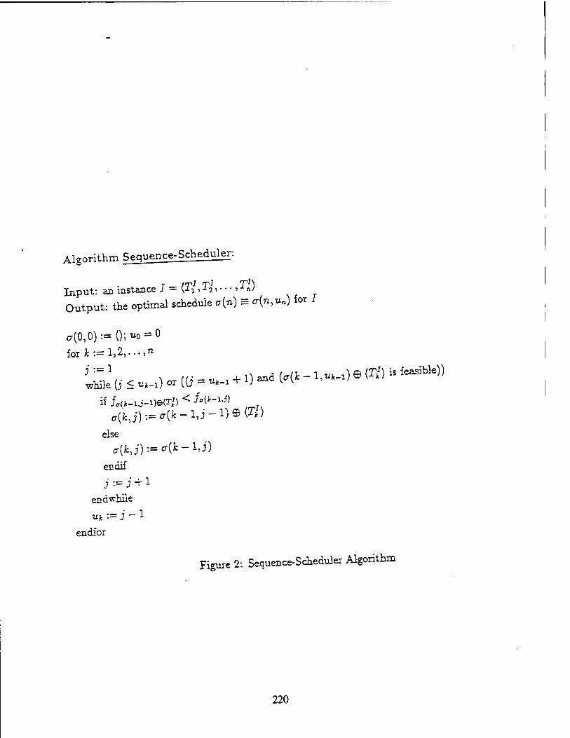
Algorithm «^qnence-Scheduler:

Input: aal instance I = {Ty, T7,. - •, i n) Output: the optimal schedule a(n) s a(n, un) for J

a(0,0):=();-uo = 0

foii:=l,2,...,n

ff(jfc,j):«<r(k-l,j-l)©<r*>

else

endif

endvrhile

endior

Figure 2: Sequence-Scheduler Algorithm

220

PROOF: This is straightforward via the following equations.

fsiePz) = ™.ax (/si, rTx) + cTx

< max(fs2,rTx) + cTx

= IS2Q(TX)

Corollary 1 Let 51 and 52 be two sequences such that /5l < fS2. If 52 9 53 is feasible,

where 53 is another sequence, then fsi®sz < /s2®S3-

PROOF: This is a direct result of applying Lemma 1 repeatedly through the tasks in 53. □

Lemma 2 Uk = ujt-i or u* = Uk-\ + 1.

PROOF: It is obvious that u* > Uk-i, where both u* and u*-i are integers. Let us assume

that Uk = Uk-i+a, and a > 2. We axe going to show that this assumption does not hold. We

know a(k,uk) either contains T{ or not. If a(k,Uk) contains T1/, we can represent a(k,Uk)

as S(k — l,uk - 1) @ (T/), by picking up a proper sequence S(k — JLu* — 1). However,

from the assumption above, we have Uk-i = Uk — a < Uk — 1 = |5(fc — l7i% — l)j. This

contradicts the definition of Uk-i. On the other hand, if p(k,v.k) does not contain T/, we

can represent cr(k, uk) as S(k -1, u*). We have u^_! = u* - a < u*, which is a contradiction.

The assumption thus does not hold. Therefore, we have a < 1. D

From this lemma, cr(kj) does exist for j < u*_i. Furthermore, in the algorithm, j = U'K-i -f 1 is tested to see if u* = u*_a + 1.

Theorem 1 For k = l,2,...,n, and j = l,2,...,u*, if/„(*_! j-,)©^') < Mk-ij), then a(fc, j) = c(k - 1, j - 1) © (r/); otherwise, a{k,j) = a{k - 1, j).

PROOF: The proof is by induction on k. When £ = 1, Ja = (Tj). Since uj < 1 and (T/) is

feasible, a(l, 1) = (Tf). It is easy to come up with the same result through this theorem.

Thus holds the base case. We assume that we can compute a(k— l,j), for j = 1,2,..., u*_i,

221

in the same way, and consider the case of k. Let us first bring forward three basic equations.

Since Lwj-i, < /s(*-i.f-i>.tiie {ollowinS e^ation holds by Lemma 1

(2) /,(A-W-i)e<r/> ^ /s(*-u-i)e(T/)-

By induction hypothesis on cr(fc - 1, j) such that /„(k-ij) < /s(*-i,i)> we tave

From Equation 2, we have

From Lemma 2, we know either uk= u*_1+l or ut= «*-,. The two cases are discussed

below.

Case I- uk= uk !+l. We first discuss the situation when j = 1,2,..., uk - 1. We know

that a feasible sequence S(U) is either in the form of S(k - 1, j) or S(k - 1,; - 1) © {Tk >. x +U-T, f i, < fen- i ,n bv Equation 3. Also we have

J„(* i, W n 2_ This meajis /■ t) < fs{kJ) for any

iSÄi S;;rCoSiquently, ,(*,;, - ^ - l.i - D © (tf>, which justifies the theorem. On the other hand, if fc{k-ij-i)e{T>) > /.(w* then /,(fc_ij) < Jsc.-^-i)^} by Eauation 4. In addition, U^j) < fs^J) by induction hypothesis on a(* - l,j). bo

/.(fc-ij) < /s(fcj) for any feasible sequences S(fc,i)- In this case, a(kj) = a(k - 1, j), which

justifies the theorem. . . , ,, . /Th Then we discuss the situation when j = uk. Since uk= u*_:+l, it » clear that {Tk)

belongs to c(k): otherwise, we need to pick up u^-fl tasks from IM to make a feeble

seauence which violates the definition of u*.,. Therefore, a(kj) can be expressed as S(k-1,

«*!.) 6 («> by picking up a proper sequence S(k -1, **_:). Note that uk>=j - lb«. By

Eauation 2, we have /^-w-aje^) < /*(*->,■-»>•«>»ior «* sequenCe 5(fc" ^1'1}® ^ Thus, a(kj) = a(Jb - l.i - 1) 9 (T/). Now let us check the theorem. The sequence

a(k - 1 j) = aft - 1, ufc-j+l) is not feasible; thus its finish time is oo. The condition

L^n* < /-c^* satisfied- s° *(/:j)=°{k -iJ-l)G {Tl)-THs justiiies tbe

theorem. • o T n Case II: uh= u^-i- The reasoning follows the discussion of the first part m Oase 1.

222

3 Scheduling a Task Set

In this section we discuss how to schedule a task set by using Sequence-Scheduler. The

opiimal schedule, p, of a task set is defined as follows: for any feasible sequence S consisting of tasks in T, we have either

\S\ < \p\,

or

\S\ = \p\ and fs > /,.

For simplicity, we use optimal schedule to represent the optimal schedule of the task

set, when there is no confusion. Note that the optimal schedule of the task set is the best

one of the optimal schedules of all instances in the task set. Erschler et al [2] proposed the

dominance concept to reduce the number of permutations that should be examined for the

feasibility test of a task set. Yuan and Agrawala [18] proposed the super sequence to further

reduce the search space for testing the feasibility of a task set. In this section, we show that

for our optimization problem, the super sequence provides a valid aiwl pruned search space.

In other words, there exists one optimal schedule which conforms to an instance in the super

sequence of the task set. Thus we may use Sequence-Scheduler to schedule for the instances

extracted from the super sequence to derive the optimal schedule. There may exist more

than one optimal schedule for a task set. Our interest is on how to derive one of them.

3.1 Super Sequence

Temporal relations between two tasks Ti and Tj are summarized in the following. They are illustrated by Figure 3.

• leading : T{ -< Tj, if r,- < r,-, d; < dh but both of the equalities do not hold at the same time.

• matching : T || Tj, if r,- = TJ, d; = dj.

• containing : Tt U Tj, if r,- < rj, di > dj.

223

L_ T: L_

Ti T: 1 J Ti

(i)

Tj 1 1 Ti

(»)

Ti 1 J

(iii)

Figure 3: (i) T, < T?, (») £ || Ty, (iii) T U 1}

A task k is caüed a top tos* if there is no task contained by a. A task is calledI a nontop

to, i TtclLs at leastone task. Assume that we have t top tasks ha the task set, tooted

t i it respectively. Demote by jlfc the set of tasks that contam the top task &»,

Ä 'C-hTK thi set of tasks in the tf set P that -^^

that 21 is ~*b I-.B-. to Ü, denoted by K < IJ, >f E -c J> or H II T,. H T, < T,

tei tV^Z^ is o^adiy developed by Erschler - a! Reduce thesearch

Je for testing the feasibility of a task set. The idea is extended „th the sup. sequence

proposed by Yuan and Agrawala 118]. AB mstaz.ce 1 demotes an msta.ee I m.

I' feasible =*■ I feasible.

K cat, be cohered that 1 is a better candidate as a feasible schedule than£ A

***** ins*™ is an instance such that for each possible mstance 1 o the ta^et >

J donates the dommant instance, then the dominant msta.ee domma^L Jhu^the

aominant instance can be considered as the best candidate o the U££* « ^ A s^ Dances is said to be a dammanf set, if J does not belong to the dommant set, ">=> ^XLnt instance in the dommant set such that the dominant mstance dommates

I.

224

A super sequence A serves similarly as a dominant set in that there exists a dominant

instance in the super sequence; and it is more appropriate for solving our problem. A super

sequence is a sequence of tasks, where duplicates of tasks are allowed. The purpose is to

extract instances from the super sequence for scheduling. The super sequence is constructed

according to the dominant rules [2,18] described below. Whenever a task satisfies one of the

conditions specified by the rules, a duplicate of the task is inserted into the super sequence.

Note that duplicates can only be generated for nontop tasks. The top tasks appear once and only once in the super sequence.

Rule Rl: Let Ta and Te be any two top tasks. UTa-< Tß, then Ta is positioned before 2>.

If T0 || Tß, the order of the two top tasks is determined arbitrarily.

A unique order of the top tasks can be thus determined for the super sequence. Let us

denote the sequence composed of the top tasks by H = (hi,h2,...,ht). The rule implies

that if Ta is positioned before Tß in the super sequence, then Ta<Tß. So hi < h2 < ... < ht.

Rule R2:

(1) A nontop task can be positioned before the first top task hi only when it contains hy.

(2) A nontop task can be positioned after the last top task ht only when it contains ht.

(3) A nontop task can be positioned between hk and hk+i only when it contains hie or h^y.

The i top tasks delimit the super sequence into t ■+ 1 regions by rule Rl. Now we have

t -f 1 subsets of nontop tasks separated by the t top tasks by rule R2. Generally speaking,

a nontop task has more than one possible location. Denote the jfcth subset by Ak, which is between top tasks hk and hk+i. From rule R2, it can be deduced that

A* = -B*,*+r U jBi,fc+i U B^k+l, where (5)

BkJ+i = Mk nAfc+i, BkMi =Mkn Mk+l, Bjtk+l = M~kD Mk+y.

Next rule is to specify the order of the tasks within each subset.

225

Rule R3: In each subset A*, for fc = 0,1,..., n, (1) the tasks in Bk^ axe ordered according to their deadlines, and tasks with the same

deadlines are ordered arbitrarily, (2) the tasks in BkMi are ordered arbitrarily, (3) the tasks in BkM, are ordered according to their ready times, and tasks w>th the same

ready times are ordered arbitrarily, (4) the tasks in Bkjri are positioned before those in BkMu which in turn are positioned

before those in Bkk+l-

Now we are ready to construct the super sequence with these three rules. Top tasks are

first picked out and ordered, forming t + 1 regions. In each region, there is a subsequence

of nontop tasks. An instance extracted out of the super sequence is one that conforms to

the super sequence without duplication of tasks. Let q be the number of top tasks that a

nontop task contains. The number of possible regions the nontop task can fall mto is q + 1.

The number of instances in the super sequence thus sums up to

c-t

N = Ufo+ 1)-' 0=1

where nq is the number of nontop tasks which contains q top tasks. Compared with

an exhaustive search which takes up to n! instances (permutations) into account, the super

seouence generally leads to a smaller set. Notice that it takes 0(n) time to check if an

ins'tance is feasible. Hence, the time complexity of the feasibility test for the task set is

0{N * n).

3.2 Leading Theorem

The super seouence is not only useful in testing the feasibility of a task set; we will show that

it is also useful in reducing the number of instances to be examined in order to obtain the

ooiimal schedule of a task set. We will show that there exists at least one optima^ schedule

which conforms to an instance in the super seouence A. Hence, it suffices to check through

A to obtain the optimal schedule of T.

226

It is worth attention that the top tasks in p may not be the same top tasks of T. This

arises because some of the top tasks of T may be rejected, introducing new top tasks in

p. Before proceeding to verify the rules for the super sequence, we will first introduce the

Leading Theorem. It serves as the base for further analysis in the Dominance Theorem and

Conformation Theorem to be described later. The Leading Theorem tells that under certain

condition we can adjust the order of tasks to satisfy the Weakly Leading Condition to be

defined below and do not introduce a schedule with greater finish time.

Assume that S is a feasible sequence, with I^e, X, and ipesl subsequences of S such that

<-> = X/pre © -Li @ Impost ■

Let us denote L by

L = (Tß, T=3, Tx,,..., rXw, TQ),

where u> > 0. A frame F is defined to be a time interval characterized by a beginning

time bF, and an ending time eF. We say that F is a frame corresponding to L, if bF = sß,

and eF = fa, where sß is the starting time of Tß> and fa is the finish time of Ta.

Theorem 2 (Leading Theorem) Assume that 5 = L^ ® L @ Lpost is a feasible sequence,

where L = {Tß, Tx,, TXJ,..., T-w, Ta). Let F be a frame corresponding to L. UTD^. Tß, and

there does not exist a task 71., 1 < i < v, such that FuT=i, then there exists a sequence L which is a permutation of L such that

(i) (Ta,Tß) conforms to X, and

(u) •)LyrceleLj*,., - fLprcBLeL^,, ■

Before we can proceed to prove the theorem, the following definition is useful.

Weakly Leading Condition: a sequence S = {Tf, T/,..., Tj?) satisfies Weakly Leading Condition if Tf<T£<...< If.

Lemma 3 Let 5 be a sequence satisfying Weakly Leading Condition. If (Tj.Tj) conforms to S and T- || T,-, then all tasks located between T,- and Tj in 5 must match T,- and Ty

227

PROOF" For any task r, located between Tt and T;, according to the definition of Weakly

Leading Condition, ,e have r; < r. < r,- and * < dx < d3. Since Tt \\ Th n = r,- and

di = dj. Therefore, we have r.- = rx = r,- and 4 = 4 = <*;• So, T* matches T; and r,-.

To obtain I, let us modify the tasks in L in the following way. If the ready time of a

task is less than bF, then its ready time is set to bF. If the deadhne of a task is greater than

eF, then its deadline is set to tF. The computation times remain unchanged. Let L be a

sequence consisting of the modified tasks with the same order of L, i.e.,

Since Ta ■< 2>, dß > d0 > fa = eF. So rf„ = ta = eF. Also r0 < r, < „ = bF, so

r' = r» = bF. This is illustrated in Fig 4 (ii). ° Note that swapping Tp »d F. in the sequence does not result in a feasible sequence m

this example. It is essential that we adjust the order of the tasks located between them Let

V be a sequence which is a permutation of V and satisfies the Weakly Leacang Condon,

and to which (ro1T.) conforms. Furthermore, L' satisfies an even stronger condition. If Tt

is positioned before if in L\ then if < if; if, furthermore, 2?' || 2? , the corresponcang

tasks TV and I*' satisfies that if < 2$'. The idea of such arrangement as that when

interchanging Tß and Ta, we do not produce a new reversed pazr Hke them. By reversed paar

we mean for example T0 -< Tß but I> is positioned before Ta in the sequence. Son {T{ 1, )

conforms to L\ the corresponcang tasks satisfies the condition that either T, -C Z> or

T-f U Th' or 1^' U l£'. One possibility of L' is illustrated in Fig 4 (iii), or

The existence of such a sequence is proved later. Finally, I can be a sequence with

the same order of L\ but the ready times and deadlines of the tasks are recovered to their

original settings. This is illustrated in Fig 4 (iv). The figures give the rough idea about how

theCadjustment of task order can be made to satisfy the conditions described in the Leadmg

Theorem. Here below is the proof of the Leading Theorem.

228

TJ

a

T x4

T

00

ß

T a

Tß (iii)

Figure 4: (i) L = (Tß,TXi,TXi,TX3,Ts<,T0) (ii) I' = (T^T'^T^T'^) (iii) I' {TXi,T0,T^Tß,T^TXA) (iv) 1 = {TX2,rQ,rTS,r,,rSJ,rx<)

229

, , T din, Theorem)- We would fast show the existence of I. The modification of PE007 (of Leading Theorem). we h t thdl sUrted times ready times and deadlines of the tasks for I » done m such a y ^ ^ ^ not affected. In addition, their computat.on times remain the same.

is feasible, and

in V such that, for anv task T, belongmg to I T, <. To ,

.re no containing relations among the modifie tasks »d £«£ U exchanged with the task located ;ust eft to rt m L. Conb™ ^ ^

until !* occupies the fast location in the ^ ^™, J^ tf, tf <, T,

tf of V is the task in I' such that>r ^^ ^occupies the second location

Exchange 1? with its left neigh or ^~^ ^ ^ fa ,, such tbat, for any task in the sequence. At the .th step the ,th ta* T * ^ ^ ^ ^ ^ neighbor

r- belonging to V except T, throngn i, r, , . ~ „„,,„„ We keep performing this ^ consecutively until it occnpfethetthlocatron in the. uence. ^ ^ rf

operation until we finally ohtain L. ^°*f^±^ " J, OI j, j, not belonging to

the sequence by consecutive swapping is l^**?*^ ttee" Me no containing relations (If ... if i). I- * word, the adjustment is possible ^ ^ moffikd tasks b,

m„ng the modified tasks, and hence there,~* -»^^ ^ 5atirfying ^ the Weakly Leading Condition. The resultant I is existen

Weakly Leading Condition. r^ 3, all tasks located between Tß Thereisachancethat(Te,J<,)comorm difference.

We can thus exchange the pos>t,on of T, and 1„, ^ ^ ^^

Bnrfng the process of adding the ^»^1. O 1^ ^ ^ ^ ^^

with a shorter or equal finish time. This explains

230

L is a sequence with the same order of L', but the ready times and deadlines of the

tasks are recovered to their original values. Each task in L can be started no later than the starting time of the same task in 11. Consequently,

By Corollary 1, we have

Lemma 4 Assume that 51 © 52 © (Tj) © 53 is feasible, where 51,52, and 53 are sequences.

If Tj < 52, then /sie{T>)©S2sS3 < /si©S2©(r,)©S3-

PROOF: We will prove the theorem by induction on |52|. When |52| = 0, it is vacuously

true. Assume that it is true when |52| = k. We would like to show thai it is true when |52| = k -f 1. Let 52 = (T,-) © 52', where |52'| = fc; i.e.,

51 © 52 © (Tj) © 53 = 51 © (T{) © 52' © (Tj) © 53.

We can view 51 © (T.) as a single sequence, and because |S2'( =■ A, by induction hypothesis, we have

JsiG<x,>e(x,)eS2'es3 ^ /sie(r,-)eS2'e{:r,>es3-

By definition,

/sie{r,->e{T,) = max(max(fs, r,-) + a, TJ) + c5

= max{fs + c- + Cj,Ti + a + CJ, T5 + Cj)

Since Tj < 52, which indicates that Tj < Tt-, we have TJ < rt-, and TJ 4- CJ < r,- + a + Cj.

fsie(T,)e&) = rnax(fs -f a .■ Cj.r,- + c,- 4- Cj)

231

On the other hand,

• fsie{Tj)e{Ti) = maximaxifs^ + Cj^ + a

= max{Js + Ci + Cj, TJ + c,- + c,-, r,- + c,-)

Because r,- + d + c3- < r,- + ft + cjs we have

fsie(T,)e{T;) < /sie(r.)e(r,)-

By Corollary 1,

/sie{x,-)e(T.-)eS2'©S3 < /si©<r,)e<:r,)eS2'©S3-

Therefore,

/5is{Xf)e52eS3 < /sieae{T,-)es3-

3.3 Dominance Theorem

The super seouence is constructed for the feasibility test of a task set. If a task set is feasible,

we sav that there exists a full schedule of the task set. There may exist more than one full

schedule for a given task set. An optimal full schedule is a full schedule vrhose finish time is

shortest among all the possible full schedules. Note that a full schedule is a feasible instance.

In this section, we prove that if a task set is feasible, there exists an optimal full schedule

conforming to the super sequence ' Hence, the super sequence provides a valid and pruned

search space for deriving the optimal full schedule of a task set.

'In [2] Erschler et cl. >s theorem implied a similar result: if a task set is feasible, there exists a full schedule

in the dominant set. Our theorem further shows that there exists such" a full schedule, with the minimum

finish time among all full schedules, that conforms to the super sequence. We prove the existence of such an

optimal full schedule in a more systematic way.

232

Theorem 3 Assume that the task set T is feasible and p is an optimal full schedule of T.

Let T0 and Tp be two top tasks of p such that Ta -< Tp. If {Tp, Ta) conforms to p, then there

exists another optimal full schedule p' such that {Ta, Tp) conforms to p'.

Or- PROOF: T0 and Tp are two top tasks. Let F be a frame such that bp = sp and ep = /,

Ta -< Tp means bp = sp > rp > rQ, and ep = fa < d0. If there exists a task Tx such

that F U Tr, then T0 U 3"* too. This contradicts to the fact that Ta is a top task. Hence

F cannot contain any task. By the Leading Theorem, there exists another sequence p' such

that (T0,Tp) conforms to p', and both \p'\ = \p\ and fp> < fp hold, which means p' is an optimal full schedule too. D

When two tasks match each other, it dose not matter which task is executed first. This

gives rise to the following Corollary.

Corollary 2 Assume that the task set T is feasible and p is an optimal full schedule of T.

Also assume that {hi,..., Tp, T0,..., ht), the subsequence of the top tasks in p, conforms to p.

If TB < Tp, then there exists another optimal full schedule p' such that {hi,..., Ta, Tp, ...,ht)

conforms to p'.

PROOF: Theorem 3 holds when T0 < Tp, because when two tasks match each other, the

execution order of the two tasks is arbitrary. Also by looking at the adjustment process of

Leading Theorem, we can find that the tasks located before and after T0 and Tg have not been adjusted. This verifies the corollary. D

Corollary 3 Let H = {h^, h2,..., ht) be top tasks of the task set T such that hi <3 h2 <

...< ht. If T is feasible, there exists an optimal full schedule p' to which H conforms.

PROOF: Since r is feasible, there exists an optimal full schedule p. Let K = {ky, k2,..., kt)

be a sequence which is a permutation of E such that K conforms to p. We would like to

adjust the order of the tasks in K so that K is transformed successively into H. We locate

the corresponding task of hx in K, where x is chosen in the order of 1 through i, and adjust

233

L -+v ;+c Wt neighbor. This leads

H to tfce *th position in if ^««^^"^^L. to H, .eft neighbor, **

to tne sequence *. During the «^* ^^ % ^ ^ exists an optima! M

kr »- »« in P°S,t,0nS **; 7 „ 1, SKroences conform. Therefore, there exists an schedule to which the intermeddle resultant sequences Q

„Jmal full schedule,' to which fc,h,,...,M «*»»■

Therefore the rule Rl is venfied.

Before we can go fmther, the ioHowing dehmtious are «^££ * ^^

r= a nontop tash of a sequence S. We sa, tha (l^W» £ y ^^ to

conforms to S and T,< h, ^'£^t£ «^number of disorder pairs in S. S and ki X T-. The disorder dejree of £ >s detmeo

such that

/jll . ^fc_a) conforms to L^e,

(/n*i, • • • A) conforms to Lpost-

We have the following properties: ^ ^^ ^^ ^ ^ , _

(1) if ü •< k* *><>*• = <h_''' • •'J -'' , d ,r.. 4,\ conforms to I; besjdes, the L^eLeL^, such »hat X is a permntatron of I, and <i.. *)

disorder degree of , is less than that of^ ^ ^ ^ ,

(2) if Hü -c T, ana I = (2), ...,»»>. ™ conforms to I; besides, the jJL © i e L^ snch that i is a permntat.cn of I, and (k„ TJ

disorder degree of p' is less than that dp

£F = /= ^ d= - ^ AlS° = SKl

234

Tx such that F U TWi, then hk U Tw; too. This contradicts to the fact that hk is a top task.

The condition of the Leading Theorem is satisfied. Hence there exists a sequence L which

is a permutation of L such that (Tx, hk) conforms to L and fL rt.eLeL 0„ — U- Therefore,

Lprc @ L © Lpost is also an optimal full schedule. Now let us look at Figure 4(iv). This is

the schedule after the adjustment process of the Leading Theorem is made. For the tasks

whose deadlines axe less than ejr, they all lead to hk- Note that the disorder is a relationship

defined between a nontop task and a top task, and hk is the only top task in the frame

F. Therefore, no new disorder pairs with hk are introduced among these tasks. Similarly,

for the tasks whose ready times are greater than bp, they are all led by hk- Therefore, no

new disorder pairs are introduced. As for the tasks otherwise, including Tx and hk, whose

deadlines are greater than or equal to tp and ready times less than or equal to bp, they can

be ordered arbitrarily. Hence, we can position Tx before hk, and remove the disorder pairs,

if any, in these tasks by rearranging the proper orders for them. Thus the disorder degree of

L is decremented by at least one. So the disorder degree of p' is less than that of p. Property

(2) holds for the same reason. D

Note that Tx does not match hy. or hk+i] otherwise Tx is also a top task, which contradicts

our assumption.

Theorem 5 Assume that the task set T is feasible and p is an optimal full schedule of T.

Let hi < h2 < ... < ht be top tasks of p. There exists an optimal full schedule p' such that

(hi,h^ ...,hi) conforms to p', and for any nontop task Tx such that (hl^TXjfyc+i) conforms

to p', either T- U hk or Ts U hk+i-

PROOF: Assume that Ts is a nontop task such that (hk,Tx,hk+i) conforms to p'. If Tx does

not contain hk and Tx does not contain hk+i, then either Tx -< hk or fc*+i -< Tx. Hence,

either (hk,Ts) or (Tx,hk+i) is a disorder pair. We can eliminate it through Theorem 4, and

the disorder degree is decremented by at least one. Whenever there is a disorder pair in the

schedule, we can always apply Theorem 4 to eliminate it. The disorder degree is decremented

in this way until finally reaching zero. Hence, (hk, Tx, ^jt+i) conforming to p' implies-ib&t Tx

is not leading to hk and A*+1 is not leading to Tx. The only possibilities are either T= U hk

235

or Tx U hk+i.

Theorem 5 confirms the validity of rules Rl and R2.

Theorem 6 (Dominance Theorem) If a task set T is feasible, there exists an optimal

full schedule p such that p conforms to the super sequence of I\

PROOF: In Theorem 5, we verify the existence of the optimal full schedule such that the

top tasks are ordered according to their weakly leading relations, and the nontop tasks

are located in the appropriate subsets between top tasks. The only work left is to order

the nontop tasks in each subset. The adjustment process of the Leading Theorem can be

applied, and the resultant order is exactly specified by rule R3. So we can conclude that

there exists an optimal full schedule p which conforms to the super sequence.

3.4 Conformation Theorem

If there is no task rejected in p, there exists an optimal full schedule conforming to the

super sequence of T. However, if T is not feasible, some tasks in T should be rejected. The

dominant rules are developed based on the assumption that no task is rejected. When tasks

are allowed to be rejected, the situation is different. The issue to be raised is whether the

decent solution for feasibility test can be applied to our optimization problem. Remember

that bv optimization we mean that the number of rejected tasks in the schedule is minimized

and then the finish time of the schedule is also minimized. When a task set is feasible, tue

optimal schedule is also the optimal full schedule. The difficulties are addressed m the next

section, followed by the approach and proof to solving the difficulties.

3.4.1. Difficulties

We wish to make use of the super sequence as search space in our scheduling problem. The

difficulties are twofold. First when a task is allowed to be rejected, the dominant rules specifying the relations

amon* containing tasks and contained tasks need to be modified, because the rules are

236

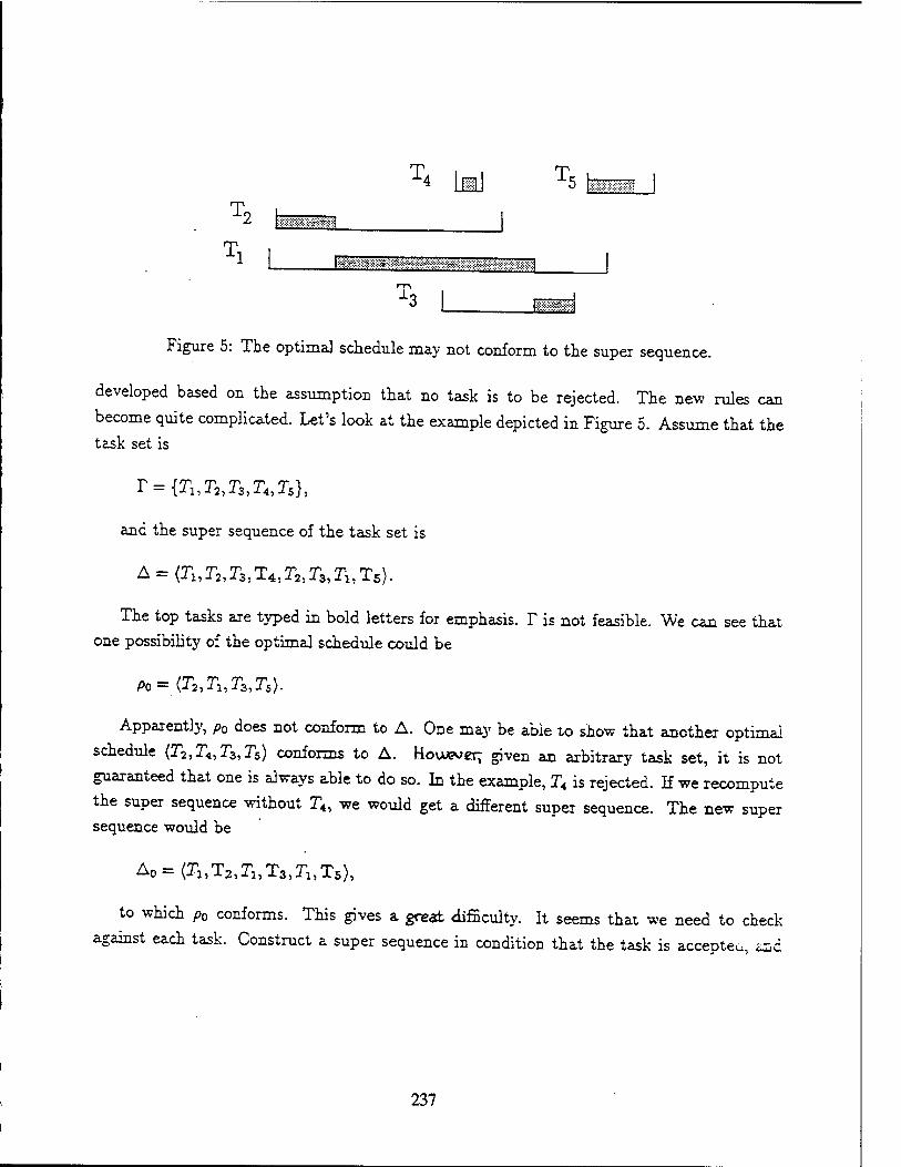
To u_

T4 LaJ T5NSWS 1 2 \m '-*.-*.l J

1 I»-<•-.•:>$-v »-:"■ «.•.;-,.*- . ™», . >.i, .,..•, v I! 1

T3 1

can

Figure 5: The optimal schedule may not conform to the super sequence.

developed based on the assumption that no task is to be rejected. The new rules

become quite complicated. Let's look at the example depicted in Figure 5. Assume that the task set is

r = {r1,r2,r3)r4,Ts},

and the super sequence of the task set is

A = {r1,r2,r3,T4,r2,r3,r1,T5).

The top tasks are typed in bold letters for emphasis. T is not feasible. We can see that one possibility of the optimal schedule could be

Po={r2,Ti,r3,r5).

Apparently, pD does not conform to A. One may be able to show that another optimal

schedule (T2,T4,T3,Ts) conforms to A. Houaver; given an arbitrary task set, it is not

guaranteed that one is always able to do so. In the example, T4 is rejected. If we recompute

the super sequence without T4, we would get a different super sequence. The new super sequence would be

Ao=(T1,T2,T1,T3,r1,T5),

to which po conforms. This gives a great difficulty. It seems that we need to check

against each task. Construct a super sequence in condition that the task is accepter, ^d

237

• ♦ A In general, we need ,. tKe task ^ ie3ectea. 6 considering

t0 co^xuct 2 . P .n ^ lo4Wd» ^

tf*t the number °» a, xejectmg * W stee oI tie t-k set. tMks does **;** even «suit » -»

top tasKs. A« ' _, es^lts m v* ^roce- J TP 5 The re3ection oi U äficalties. Tbe px

\A Vve described ana duxe would be a»

4- T T +randAhetne

olig^ task set, »4 »£> >s „,;„„„„ to us ~- ^ ^ ^ ^

sequeDce t» A »«*-** *e froi»»Tteoiem' it«- »*awe to difiereBt fcom -i w by tie U™ problem«tba* « „.plvmS

compute po sVrappmg ^ü v nccessaiy, so as to tra» inStance

oi &. Tor tie sale K ^ ^ use A a a-

u oi tiE^e a, ^tbe example oi tig«

cr„T4,rs,TsV

238

This example is so simplified that the existence of p can be verified by mere intuition.

However, the reasoning is fax more complicated than it appears at the first glance. We are

going to prove in the following theorem that such an optimal schedule p that conforms to A

always exists. The corresponding lemmas axe preseni ,i in the next section.

Theorem 7 (Conformation Theorem) Given a task set T = {T^T,,...,^}, there exists

an optimal schedule p such that p conforms to the super sequence A of T.

PROOF: Given any task set I\ there exists at least one optimal schedule, which is unknowu

to us. Assume that we need to reject «, tasks from T to make a feasible schedule. Let T0 be

the task set which is composed of the tasks in the unknown optimal schedule. To is a subset

of r The super sequence of T0 is denoted by A0- In addition, we use Th 0 < j < w, to

represent a task set derived by adding j tasks into To, A, the super sequence of I-, and Pj

a, optimal schedule of I> When we say adding j tasks into To, we mean that the resultant

task set r,- is composed of distinct tasks and P; is a subset of P. In particular, P. » T.

We will prove by induction on u> to show that there exists an optimal schedule Pw for T

Cta^A:0: there is no task rejected. P « T, Since P is feasible, by the Dominance

Theorem, there exists an optimal (full) schedule pD for T such that * comormsto A0;

Eduction hypothesis: assume that the theorem holds when u> = j, i.e., W - n - j. *«

the task set r/which is derived by adding j tasks into To, there exisis «no*»* «cDeauie

o- for r such that a conforms to A;. Notice that |PJ1 = |po|, and |r,-| - (To| + J- Now consider the case when » = j + 1, i.e., \Po\ = n - (j + 1). We need to reject j -r 1

tasks to make a feasible schedule. There exists an optimal schedule Pj for T conforming to

Aj bv induction hypothesis. We want to show that, by swapping and replacing the iasks

in Pi. the resultant sequence ,i+1 conforms to Ai+1; besides, |W+1| = |«1, **d /„.„ _ J„,

which imphes that ,*, is also an optimal schedule for P. Let T. be the task added mto P,

to make Tj+1. So, T, U {T=} = Ti+1. There are two possibilities when adding;T If r- is a nontop task of Ti+1, adding Tx does not add a top task into P,, The orders

of the top tasks in both AJ+1 and A, derived through rule Rl are exactly the same. Rule

R2 specifies the relation between a nontop task and a top task. Adding a nontop task J,

239

does not affect the relations between the already existent nontop tasks and top tasks. The

positions (duplicates) of the already existent nontop tasks in A; are preserved m Ai+1 Rule

R3 specifies how to arrange the order of the nontop tasks within each subset. Agam adding

a nontop task Tx does not alter the orders of the already existent nontop tasks m each subset

in A;. Therefore, if the task being added is a nontop task, A,- is a subsequence of Ai+1. Let

us look at the example in Figure 5. Assume that I\,- and rj+1 are

Tj^iTt^T^Ts}, and

ri+1 = {T1,r2,r3,r4,r5},

where T, is a nontop task. The corresponding super sequences would be

Aj = (T2,T3,T4;r2,r3,T5), and

We can see in the example how A, conforms to A,-+i. Otherwise, Ts is a top task of ri+1. T, does not contain other tasks m ri+1. Two

situations are possible. _ (i) T is not contained bv other tasks. The number of top tasks in T& as one more than

that of the top tasks in T,, The order of the top tasks in A, is preserved m Ai+1, since

the relations of the top tasks axe not altered by adding Ts. Furthermore, T= does not alter

anv existent orders among the nontop tasks and top tasks, or among the orders between the

nontop tasks and nontop tasks, specified by rules R2 and R3, respectively. Therefore A, as

a subsequence of Ai+l. Let us look at the example in Figure 6. Assume that Ts and li+1

are

^•«{TJ.T^TB}, and

Tj+y = {T1,T7,T3,T<,Ts],

where T3 is a top task not contained by other tasks. The corresponding super sequences

would be

AJ- = (r1,T2,r1,r4,T5,ro, ^d

240

T2 1_) T3 | | T5

T! 1 I T4 I

Figure 6: The added top task T3 is not contained by other tasks.

Aj+i = (ri,T2,Ti,T,3,T,4,T5,r4).

We can see in the example how Aj conforms to A j+i.

(ii) Tx is contained by some top tasks and/or nontop tasks of Tj. Let the top tasks of

Tj containing Tx be gu... ,gm, indexed in the weakly leading order. This situation is more

complicated, because #, t = 1,..., m, turn out to be nontop tasks in r,-+i- There exists a

total ordering of them by weakly leading relations, because there is no containing relations

among #. By rule Rl, the super sequence of Tj+l can be expressed as

Aj+i = {-•-, Ajfe-l, • • • ,5l, • • • ,9m-, • • ■ , hk, ■ ■ • ,9l, • • • ,9m, • • • , Äfc+i, ...)»

where fc1}..., fcfc_ls hk, Ajt+1,. -. are the top tasks in Ti+1, and in particular, hk represents

Tx. By rule R3, the super sequence of Ij+i can also be expressed as

Aj+i = (•-., fc*-i, ^_l.I^ Bk-i*. Bk=ij<'. hk, BkjZi> Bk*+\, %k+i * A*+i '••-}» (6)

n;+J

n ̂+i

where fiJ+i represents the subsequence of Aj+i between hk-i and Ai+i, excluding /i*_i

and hk+l, as depicted above, and QJ+: = Bfc_ltie^-+1eBE,fc+1, where 9 means concatenation

of sequences. Remember that gy,... ,gm are top tasks of Tj. All the top tasks in Y5 are in

the order of hly..., hk.ugu- ■ .,9m,hk+1,... by the weakly leading relations. By rule Rl,

the super sequence of Tj can be expressed as

241

r A between kM and fe, excluding fc*-i and „here fl, represents the subsequence of A, betwee , subsequences More fcw

iw. es depicted above. Notice that » *^ Edition o£ the top task fe, or T., of both A», -d A, axe exactly the same,> «us th ^ ^^ ^ ^

^ only tbe —--- ImeToo. Hence en instance of A,+, wiH differ from of both A)+, end A,- ere exacuj » instenee of A, only in tbe tbe subsequen es of ^ ^ .^.^ ^ ^ By

Now we would lite to check «bet tasks m A, should ^ ^ ^ ^ ^ ^

I* 7, ell tbe tasks in n, can be found.n>0» - • ^ ^ ^ ^ B e

in a.+1 _ hi. If e tesk contains V* but **fc, ^ „^ the

„ oonteins fc. any task which contams S,.*«** ^ ^ ^ ^ .„ B^ of

^sequence of A, between h> and Su by -> ^ ^ Q£ ^ subsequence „

Aj+1 should follow immediately after lw, and by

exactly the same as BMJ- ,„„*.;„ kt , but do not contain Si. s0 tiey One mey observe that some tasks m *W «*»*£ ^ ^ ^ ^ ^ of

„ould also be positioned between t, end «v ^^ ^ tb

BwI. This is because they do ««^£ ^ ^ ^ of Aj+, should be

teaks in S,,, B- <* ~ »^-n^ *» * *. — - * — *- located immediately before /ifc+i wnen

the A,- can be further expressed as

_ / K 5 - .ft; ;gmi • • •j-L"'k,k+i- ;_ ..., , -1, ^

wbere Hi represents tbe subsequence ^^ ^ ^ ^ Q, ^ eithex

and Bj^v We bave ft,- = Bfc_tf 9 «3- © V" °5

in £*-u or in to- . The task set * tbe figure is Tj+1. And Ti+1 - fc Let us loot at an example m F gure t. ^.^ ^ ^^ t^ in r^,

would be IV 5l and 5, contain only hk. So 5a and *2

242

hk-i u iik LJ hk+iL

si I II T5

S2

T4

T2|__

T3L Tl|

Figure 7: The added top task hk is contained by other tasks,

and as top tasks in Tj. We can compute the super sequences as follows.

Ai+1 = (r1,r2,r3,r4,hk_1, n ,Q2T3,T1,gug3,hk,r2,5l,P2,r3, r: , T5 ,hk+1,ra,T5), B*-i,I £*-i,* BJ-J^ ■BI,MT S*.*+: £I,t+3

n;+:

"j+:

A,- = (r^r^hk.!, r^,>r2,T3,r1,g1,j3,r1,g2,r3,rv, 75-;hk41;ra,rs). B*->; n; **.*,

o>

Now going back to examine Equations 6 and 8, we can find that A,- and Aj+i only differ in

the middle subsequences represented by Q'j and ü'j+1. This can also be seen in the example in

Figure 7. The instances extracted from Aj would conform to Ai+1 except the corresponding

middle subsequence mentioned above. Remember that p5 conforms to Aj. We would try to

adjust the order of the tasks of the subsequence in pj which correspond to &'■ for the purpose

that the resultant schedule pi+i conforms to Ai+1 and pj+1 is also an optimal schedule of

P. The adjustment procedure, called the swapping and replacing method, applied to ps is described below:

243

c^rt^d bv their ready times ry. , . i s A thev are sorted uy "" , „ , „Vs T € fl'i such that /, < h> •the5 K

Ci: for all U* 4» <= > t ; deadlines d„. v T <= ff such that sv > rta, they axe sorted bj

C2: for all tasks Tv e % sat.sfies both c0Edltl0M.

. J >,„ 01 ot C2 described above u m C3: a task can be sorted by Cl d fey ^.

. f ,,. r e £1'. such that sv < rk, and /, >**.> » C4: if there exists a task Ts , ^ ^ ^^

&J, the head and the -1 of „. ^ ^ ^ oi corrforms t^

mi4die —^^d „*«* ^^n ; o*; °f «* tasks * ^ justed by th-PP^ tte ^^ of C!^ A-«, the ; ^ ^ ^

by Lemma 9. Let n ^^ to rfe M so ,t 6 & fey ^

BM j, can be determined « der o{ tiie tasks in £„-,, w

■a seated before which, .^n ^ • ^ ^ ^^ ks or «ed ~ ^

-dy times. Derm,£^£ ^ r£ady times of the tasks in B.-r. - ^ their ready times. We know tha ^^ ^^ p.+ the

ready times of the tasks m BpTj S* ^ ^ the ordeI * these t are positioned before the tasks of B lX 1 ^ „^ ttc ad ustmen

, ♦!,,. adiustment of Cl conforms to A„i ■ ' edition C4, if snch a T, o ■ -. after the aa]usuut ronform to Ai-ti- öw „ *• K Fach

subsequence of ft+l ** ^ ^ be

conforms to Aj+i- in Coition to conforming to ^+a,_ ij I;VP to show that p;+i, » «* , . C1 ^ having tue same Now we would hke to sh ^ ^.^ condrtion Cl as ^ &

tohed no later tha, «- * can vie ^ üme ^ Hence

^„al deadlines of ^ hecause tto * by ^ leadmg -l^ons

total orderins arnon5 the tasks w th - ^ ^ ^ tome of the

U achieved by sorting their reaoy times.

244

schedule after the adjustment of Cl would not be greater than that of the original schedule.

Similarly, the tasks satisfying condition C2 can be viewed as having the same virtual ready

times of r^, because they all start after this time instant. For the same reason, the finish

time of the resultant schedule after the adjustment of C2 would not be greater thai: that of

the original schedule. In condition C3, the qualifying tasks can be sorted in either way and

does not affect the result. In condition C4, if there exists a task Ty whose computation time

covers the whole window of the rejected task hk, we may as well replace Ty by hk, and the

finish time of the resultant schedule after the adjustment of C4 would not be greater than

that of the original schedule. Each task Ty € ^- satisfies one of the conditions by Lemma 11.

Hence, all the tasks in the middle subsequence of pj+i are adjusted in such a way that /?J+1

would be finished no later than pj. Therefore, |^-+1| = |p;-|, and fp.+J < fPj. Since pj is an

optimal schedule of I\ pj+i is also an optimal schedule of T.

How the adjustment procedure makes the finish time shorter is illustrated by Figures 8.

In Figure 8(i), both Ti and T3 satisfy condition C3, and T2 satisfies condition Cl. The

procedure of Cl is applied to all these three tasks and makes the finish time shorter. The

dotted task window frame in the figure indicates that hk is a rejected task. In Figure 8(ii),

Cl is applied to the qualifying tasks Ty and T2. And by C4, T3 is replaced by hk. This,

makes the finish time shorter. While it is hk that is rejected before the adjustment, it turns

out that T3, whose computation time covers the whole window of /i*, is rejected after the

adjustment.

So far, we have shown that pj+a conforms ic Aj-n, and that pj+i is also an optimal

schedule of I\ The theorem is thus verified by the induction. It deserves our attention that

we do not really apply the swapping and replacing procedure to any schedule. We just want

to show the existence of the optimal schedule which is pJ+i in the context. To make it clear,

the structure of the theorem is illustrated in Figure 9. D

3.4.3 Corresponding Lemmas

The lemmas used by the conformation theorem are demonstrated as follows

Lemma 5 Bk_xj D Bk-i,k = Bk-i,k n Bjzi,k = 5jt_lfi n Bjzij = 0

245

*k i :

T,

-iL x 2 kr^--i

T-, L_ «L

Lk !-

Cl &C3

0)

Cl &C4

(S)

^ r

U •l r-j _J

-2 lr—i

^k te

T,

{jzHEEZL

Figure 8: The swapping and replacing procedure Cl, C3 and C4.

Bkj^ n Bfc,fc+1 = JBt.*+i n BI>+1 = BkJ-, n sIffc+1 = C.

PROOF: We fast show that BwJ n A_lJk = I. Given any task Tv € Bk_^ ^ does not

contain fcfc by definition. Hence, Ty does not belong to Bk-^. So Bk_^k n £*-u - <*• The

others can be proved similarly. D

Lemma 6 Bk-\± U B^zi,* = £*,HT u £*•*-»■

PROOF: We fast prove that, if a task Ty € -B*_ijc U ST^,*, then Ty € £fc,i+r U BM+1. Because Ty contains *fc by definition, Ty must have a location after hk too by rule R2.

Ty € B,— U Bjk,t+1 U Bj^. Ty does not belong to -t\t+1, so Ty € -B.JIT U Bk,fc+i. We

can prov7 similarly that if a task Ty € £fcJ?r U AJW, then Tv € £*-i.* U fe,,. So

#fc-U U jBin,fc = BkJ^ U S*.*+i •

246

3 an optimal schedule

Dominance Theorem Dominant Rules po <— Ac < r0

Swapping & I , Adding ^ *?] ■ - Replacing a Task

i i conforming to Dominant Rules Pi > A,- < r,-

. Induction Hypothesis Swapping & i , Adding Replacing ^ conforming to Dominant Rules J, a Task

induction for j + 1 J+1 ft+i "^"^"v-""-* A,-+, < r j+i

p -> q q is derived from p by method r r

p-> q p is related to q by relation r

Figure 9: The Structure of the Conformation Theorem

Lemma 7 If and only if Ty € Bk^;£uBk^1,kUBI=IjlUBkj^uBkjc+1U3EMl then Ty € Slj.

PROOF: We will first prove the "if part. By Lemma 6, Bk-1Jk U Bx=Tft = £A j^ U £*,*+!. So

we only need to check against B^-U £*_!,* U-Br^U-Br^,. If Ty € £fc_ir or Tv € £*_!,*,

then ry has a location between the top tasks hk-\ and gx in Aj. This is because Tv contains

Ai-i, rv has a locatioD after hk-y by rule R2. So Ty € fy. Then consider Ty € -BTZJ,*. Tv

is either a top task or a nontop task in Aj. If Ty is a top task in A^, Ty must be one of

the £,-, :" = 1,... ,77i by the definition of g;. If Tv is a nontop task in A,-, it must contain at

least one top task, which is a top task among gu... ,gm, or hk+z by referring to Equation 7.

Notice that Ty must not contain hk-i since Ty € £rzi>- No matter whether Ty is a top or

nontop task in A,-, Ty has a location in ft,- by rule R2. If Tv € B-tJb+1, then Tj, has a location between the top tasks gm and hk+y in Aj by rule R2. So Ty € Hy.

247

Now we prove the "only if part. Let Ty be a task located in ft,-. If Ty is one of the top

tasks oi *,...,*., r, contains hk. Either Ty € A-i, or Ty € ife, Otherwise, Ty ,. a non-

top task of A - By rule E2, Ty contains at least one of the top tasks of Jt*_i, 9i, • • •, 9m, Afc+i •

If Ty contains one of 5l,... ,*m, then Tv also contains fcfc. So Ty contains either fc a, or hk,

or W By rule R2, T, should fall between hk^ and fc, and/or between hk and kw *><>

Ty € Bt_lti U J3*-u U B—1<k U B^ U £*,fc+i U BIfk+1.

This lemma means that the tasks in ßi+1 - ^ are exactly the same tasks which are in

Lemma 8 If Ty € ty, r„ contains hk.

PROOF- We would like to show that if Ty does not contain hk, then Ty does not belong to

Q'. Since <?,-, i = 1,. - -, m, contains fc, that T, does not contain fc* means that Ty does

not contain 5; either. Hence r, can not have a location in the subsequence between * and

o m Q'- The onlv possible locations of Ty to fall in ty are either between hk., and 5l or

between 9m and W If Ty falls between ^ and *, that Ty does not contain * unphes

that Tv contains fcw by rule R2. That is Ty € 2W A nontop task cannot have duplicate

position- in the same region between two adjacent top tasks. Bk.^ is located between fcw

a^d s, bv Eouation 8. Ty does not have a location in the head of ty before 5l. For the same

reason, Ty does not have a location in the tail of ty after 9m. So Tv does not belong to ^

Therefore, if ry € ty, Ty contains fc*.

Lemma 9 If Ty € ty,ry € Bk_i,fc U B^ = BkJ^ U B^,.

PROOF: If Ty € ty, then Ty € ty. By Lemma 7, Tv € B^j U JW U Bs=j> U B,^U

R, L , i J B- We know that 21 contains hk by Lemma 8, so Ty € Bk-u U Bxrr,fc U Bfc^+1 U

Bi,fc+1. Also by Lemma 6, we have Ty € Bk-1Js U BT-J;,* = £*,*+! U tf*,fe+i •

Lemma 10 Assume that S = LVT<®LeLpost is a feasible sequence, where L = (Tl,, T„,. • •, T«..).

If there exists a sequence L = (Ty:, T„ . ■ •, T*) such that I is a permutaüon of L and the

tasks of L are ordered by the weakly leading relation. We have /VC6L©L„0„ ^ h^eLei^-

248

PROOF: We bubble sort the tasks of L in weakly leading order. The swapping only occurs

between two adjacent tasks. For each swapping, we apply the Leading Theorem to the adja-

cent tasks, which correspond to Tß and Ta- respectively in the theorem. No other tasks lie in

between the two tasks during each individual swapping. So the finish time of the resultant

schedule is not greater than that of the original schedule according to the Leading Theorem.

Lemma 11 A task Ty € ft} should satisfy one of the conditions Cl, C2, C3 or C4.

PROOF: If Ty € ft}, then Ty € Bk-i,k U B^* by Lemma 9, which implies that Ty U hk. We have ry < rhk and dy > dkk. There are four possibilities.

(i) ^ < rhk and /„ > dhk: C4 is satisfied,

(ii) sy > rhk and fy < dhk: C3 is satisfied,

(iii) sy < rkk and /„ < dhk: Cl is satisfied.

(iv) sy > rhk and fy > dhk: C2 is satisfied.

D

3.5 Set-Scheduler Algorithm

By Conformation Theorem, we have shown that there exists an optimal schedule which

conforms to the super sequence A. Hence, we can use Sequence-Scheduier to schedule for

each instance in the super sequence, and pick up the best one. Since Sequence-Scheduler

obtains the optimal schedule for each instance, we end up with the optimal schedule for

the task set. The algorithm for scheduling a task set is given in Figure 10. The Sequence- Scheduler takes 0(n7) time for each instance, while there are

?=1

instances to check in the super sequence as illustrated in the previous section. The time complexity of Set-Scheduler algorithm is thus 0(N * n2).

249

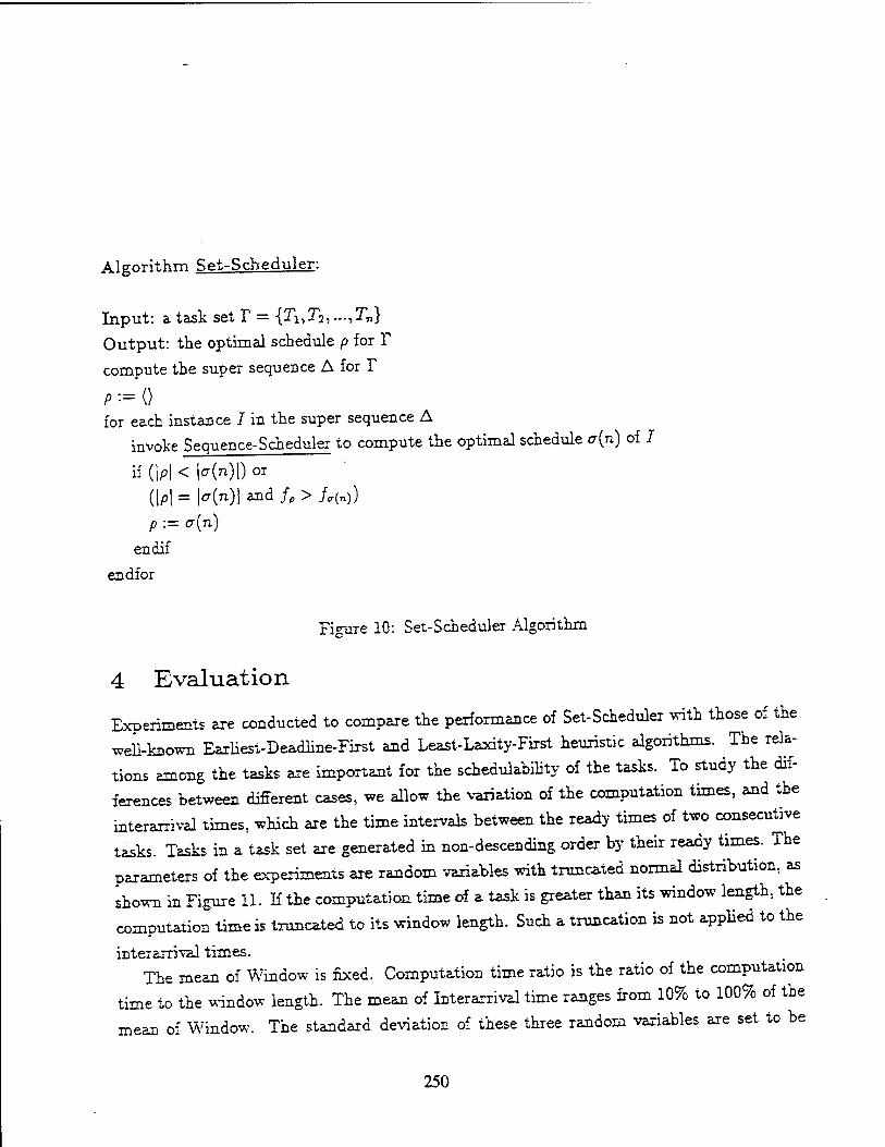
Algorithm Rp.t-Scheduler:

Input: a task set F = {Ti,T2,.-.,T„}

Output: the optimal schedule p for F

compute the super sequence A for F

P ■■= 0 for each instance I in the super sequence A

invoke Sequence-Scheduler to compute the optimal schedule a(n) of I

if (|p| < K*)l) or

(Jp| = |cr(n)| and /„ > /,(„))

p := a(n)

endif

endfor

Figure 10: Set-Scheduler Algorithm

4 Evaluation

Experiments are conducted to compare the performance of Set-Scheduler with those of the

well-known Earliesi-Deadline-First and Least-Laxity-First heuristic algorithms. The rela-

tions among the tasks are important for the schedulahility of the tasks. To study the dif-

ferences between different cases, we allow the variation of the computation times, and the

interarrival times, which axe the time intervals between the ready times of two consecutive

tasks. Tasks in a task set are generated in non-descending order by their ready times. The

parameters of the experiments are random variables with truncated normal distribution, as

"shown in Figure 11. If the computation time of a task is greater than its window length, the

computation time is truncated to its window length. Such a truncation is not applied to the

interarrival times. The mean of Window is fixed. Computation time ratio is the ratio of the computation

time to the window length. The mean of Interarrival time ranges from 10% to 100% of the

mean of Window. The standard deviation of these three random variables are set to be

250

parameters mean

Window length 10.0

Computation time ratio 0.25 0.5 0.75

Interarrival time 1.0, 2.0, ..., 10.0

Figure 11: Parameters of the experiments

20%, 50%, and 80% of their means. For simplicity, the ratios of the three random variables

are set to be the same for each individual experiment. For each experiment with different

parameters, 100 task sets, each with 12 tasks, are generated for scheduling.

We compare the performance of these algorithms by (1) Percentage of accepted tasks:

the number of accepted tasks by the algorithm over the number of the tasks of the optimal

schedule by exhaustive search; (2) Success ratio: the number of times that the algorithm

comes up with an optimal schedule in the 100 task sets; and (3) Comparisons per task set:

the number of comparisons per task set that each algorithm takes. When interarrival times

are small, more containing relations among tasks are likely to happen. Figure 12 shows that

the heuristic algorithms perform worse under this condition and tend to reject more tasks,

especially when the computation time ratio is larger. Set-Scheduler always reaches 100%

acceptance rate since it is an optimal scheduler. In the figure, because the characteristics

of the data with different standard deviation ratios are similar, only the data with standard

deviation ratio equal to 0.8 are depicted. When success ratio is concerned, which can be seen

in Figure 4, the heuristic algorithms performs even worse. Generally speaking, the heuristic

algorithms can usually produce suboptimal schedules, but fail to produce the optimal ones

most of the time. The search space is shown in Figure 'i. Set-Scheduler performs well at

the expense of the complexity, which may become very large when the interarrival times are

small. The cost is more reasonable while the interarrival times between tasks are not too small.

251

Figure 1* Percentage of accepted tasks (a) EDF (b) LLF compared «th

(a)

Set-Scheduler

JT-k~: t—*k ——"-^ST

»CO -a» **° IJ]0 )US

Figure 13: Success Ratio (a) EDF (b) LLF compared with Set-Scheduler

252

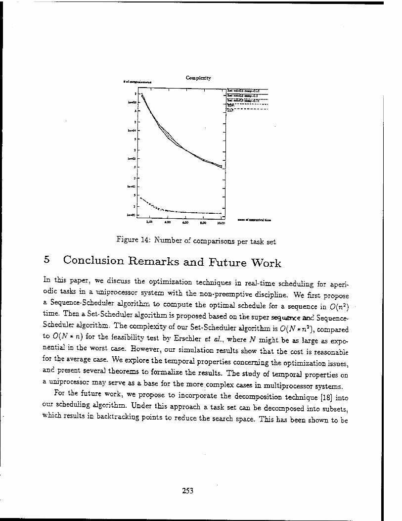
Complexity

1 1 —i 1 r WmWim^jj kilUIa^tj-

u*os

- \

STi'iJEI "<^^y^—

l*«04

\%V

u*ca ^k^^ -

u*m -

s

2

U«01 l„_

sr.

—J 1 ! C

Figure 14: Number of comparisons per task set

5 Conclusion Remarks and Future Work

In this paper, -we discuss the optimization techniques in real-time scheduling for aperi-

odic tasks in a uniprocessor system with the non-preemptive discipline. We first propose

a Sequence-Scheduler algorithm to compute the optimal schedule for a sequence in 0{n2)

time. Then a Set-Scheduler algorithm is proposed based on the super sequence and Sequence-

Scheduler algorithm. The complexity of our Set-Scheduler algorithm is 0(N * n2), compared

to 0(N * n) for the feasibility test by Erschler et a/., where N might be as large as expo-

nential in the worst case. However, our simulation results show that the cost is reasonable

for the average case. We explore the temporal properties concerning the optimization issues,

and present several theorems to formalize the results. The study of temporal properties OB

a uniprocessor may serve as a base for the more complex cases in multiprocessor systems.

For the future work, we propose to incorporate the decomposition technique [18] into our scheduling algorithm. Under this approach a task set can be decomposed into subsets,

which results in backtracking points to reduce the search space. This has been shown to be

253

useful in reducing the search space substantially when the task set is well decomposable.

References [1] M. Dertouzos. Control robotics: The procedural control of physical processes. In

Proceedings of the IFIP Congress, pages 807-813, 1974.

[2, J. Erschler, G. Fontan, C. Meroe, and F. Roubellat. A new dominance concept in

scheduling n Jobs on a single machine with ready times and due dates. Open**»

Research, 31(1):114-127, Jan. 19S3.

13] M IL Garey and D. S. Johnson. Computers and Intractahility, a Guide to the Theory

of HP-Completeness. W. H. Freeman Company, San Franasco, 1979.

[4, D. W. Gillies and J. W-S. Lin. Greed in resource scheduling. In IEEE Red-Time

Systems Symposium, pages 285-294, Dec. 1989.

,5] 0 Gndmundsson, D. Mosse, K.T. Ko, A.K. Agrawala, and S.K. Tripathi. Maxuti: A

platform for bard real-time applications. In Workshop on Operating Systems jor M^on

Critical Computing, pages Cl-CH, Sep. 1989.

[6] H. Kopetz, A. Damm, C Koza, M. Mulazzani, W. Schwabl, C. S**.^ZaiJj£ Distributed fault tolerant real-time systems: The mars approach. IEEE Micro, 9(l)-2o-

40, Feb. 1989.

[7] J. P. Lehoczky. Fixed priority scheduling of periodic tasks with arbitrary deadlines. In

IEEE Real-Time Systems Symposium, pages 201-209, Dec. 1990.

[8] J.Y. Leung and J. Whitehead. OB the Complexity of Fixed-Priority Scheduling of

Periodic, Eeal-Time Tasks. Perjormance Evaluation, 2(4):237-2o0, 1982.

[Ql S T Levi S K Tripathi, S.D. Carson, and A.K. Agrawala. The maruti hard.real-time 11 operat^systm. \cM SIGOPS, 0PeraUn9 Systems *e^, 23:90-106, July 1989.

254

[10] C. L. Liu and J. Layland. Scheduling algorithm for multiprogramming in a hard real-

time environment. Journal of the ACM, 20(l):46-61, Jan. 1973.

[11] G. McMahon and M. Florian. On scheduling with ready times and due dates to minimize

maximum lateness. Operations Research, 23(3):475-482, May 1975.

[12] A. Mok. Fundamental Design Problems of Distributed Systems for the Hard Real-Time

Environment. PhD thesis, MIT Laboratory for Computer Science, May 1983.

[13] Manas Saksena and Ashok Agrawala. Temporal analysis for static hard-real time

scheduling. In Proceedings 12th International Phoenix Conference on Computers and

Communications, pages 538-544, March 1993.

[14] L. Sha, R. Rajkumar, and J. P. Lehoczky. Priority Inheritance Protocols: An Approach

to Real-Time Synchronization. IEEE Transactions on Computers, 39(9):1175-1185,

Sep. 1990.

[15] L. Sha, R. Rajkumar, and J.P. Lehoczky. Priority inheritance protocols: An approach 10

real-time synchronization. Technical Report CMU-CS-87-181, Department of Computer

Science, Carnegie-Mellon University, 1987.

[16] J.A. Stankovic and K. Ramamritham. The spring kernel: Operating system support for

critical, hard real-time systems. In Workshop on Operating Systems for Mission Critical

Computing, pages A1-A9, Sep. 1989.

[17] J. Xu and D. L. Parnas. Scheduling processes with release times, deadlines, precedence,

and exclusion relations. IEEE Transactions on Software Engineering, SE-16(3):360-369,

March 1990.

[18] X. Yuan and A. K. Agrawala. A decomposition approach to nonpreemptive scheduling

in hard real-time systems. In IEEE Real-Time Systems Symposium, Dec. 1989.

[19] W. Zhao, K. Ramamritham, and J. A. Stankovic. Preemptive scheduling under time

and resource constraints. IEEE Transactions on Computers, C-36(8):949-960, Aug.

1987.

255

[20] W. Zhao, K. Ramamritham, and J. A. Stankovic. Scheduling tasks with resource re-

quirements in a hard real-time system. IEEE Transactions on Software Engineering,

SB-13(5):564-577, May 1987.

256


1. AGENCY USE ONLY (leave blank) 2. REPORT DATE January 1994

4. TITLE AND SUBTITLE Optimization in Non-Preemptive Scheduling for Aperiodic Tasks



6. AUTHOR(S) Shyh-ln Hwang, Sheng-Tzong Cheng and Ashok K. Agrawala

7. PERFORMING ORGANIZATION NAME(S) AND ADDRESS(ES) University of Maryland Department of Computer Science A.V. Williams Building College Park, MD 20742

9. SPONSORING/ MONITORING AGENCY NAME(S) AND ADDRESS(ES)|1 Honeywell Inc. Phillips Laboratory 3600 Technology Drive Directorate of Contracting Minneapolis, MN 55148 3651 Lowry Avenue, SE

KirtJand AFB, NM 87117-5777

5. FUNDING NUMNBERS

N00014-91-C-0195 DSAG-60-92-C-0055



I0. SPONSORING/ MONITORING AGENCY REPORT NUMBER



13. ABSTRACT (Maximum 200 words) Real-time computer systems have become more and more important in many applications, such as robot control, flight

control, and other mission-critical jobs. The correctness of the system depends on the temporal correctness as well as the functional correctness of the tasks. We propose a scheduling algorithm based on an analytic model. Our goal is to derive the optimal schedule for a given set of aperiodic tasks such that the number of rejected tasks is minimized, and then the finish time of the schedule is also minimized. The scheduling problem with a nonpreemptive discipline in a uniprocessor system is considered. We first show that if a total ordering is given, this can be done in 0(n2) time by dynamic programming technique, were n is the size to the task set. When the restriction of the total ordering is released, it is known to be NP-complete [3]. We discuss the super sequence [18] which has been shown to be useful in reducing the search space for testing the feasibility of a task set. By extendng the idea and introducing the concept of conformation, the scheduling process can be divided into two phases: computing the pruned search space and computing the optimal schedule for each sequence in the search space. While the complexity of the algorithm in the worst case remains exponential, our simulation results show that the cost is reasonable for the average case.

14. SUBJECT TERMS Operating Systems Process, Process Management Analysis of Algorithms and Problem Complexity, Nonnumerical Algorithms and Problems

15. NUMBER OF PAGES

44

16. PRICE CODE

17. SECURITY CLASSIFICATION OF RETORT Unclassified


Unclassified


Unclassified


Unlisted

MSN 7540-01 280-5500 257 Standard Form 298 (Rev 2-89)

UMIACS-TR-89-109 November, 1989 CS-TR -2345

A Decomposition Approach to Nonpreemptive Real-Time

Scheduling* Xiaoping (George) Yuan* and Ashok K. Agrawala

Institute for Advanced Computer Studies Department of Computer Science


ABSTRACT

Let us consider the problem of scheduling a set of n tasks on a single processor such that, a feasible schedule which satisfies the time constraints of each task is generated. It is recognized that an exhaustive search may be required to generate such a feasible schedule or to assure that there does not exists one. In that case the computational complexity of the search is of the order n!.

We propose to generate the feasible schedule in two steps. In the first step we decompose the set of tasks into m subsets by analyzing their ready times and deadlines. An ordering of these subsets is also specified such that in a feasible schedule all tasks in an earlier subset in the ordering appears before tasks in a later subset. With no simplification of scheduling of tasks in a subset, the scheduling complexity is 0(£™ j n,!), where n,- is the number of tasks in the zth subset.

The improvement of this approach towards reducing the scheduling complexity depends on the the number and the size of subsets generated. Experimental results indicates that significant improvement can be expected in most situations.

•This work is supported in part by contract DSAG60-S7-0066 from the U.S. Army Strategic Defense Command to the Department of Computer Science, university of Maryland'at College Park. The views, opinions and/or findings contained in this report are those of the authors and should not be construed as an official Department of Defense position, policy, or decision, unless so designated by other official documentation.

'System Design and Analysis Group and Department of Computer Science, University of Maryland, College Park, MD.

259

Contents

J Introduction 1

II Background 2

IIIThe Leading Schedule Sequence 3

IV Task Decomposition 5

A. Philosophy 5

B. Decomposition Scheme 5

C. Decomposition Algorithm 6

D. Scheduling Scheme 8

V Empirical Study 8

A. Experiment 8

B. The Result Explanation and Observation 9

VI Final Remarks 11

260

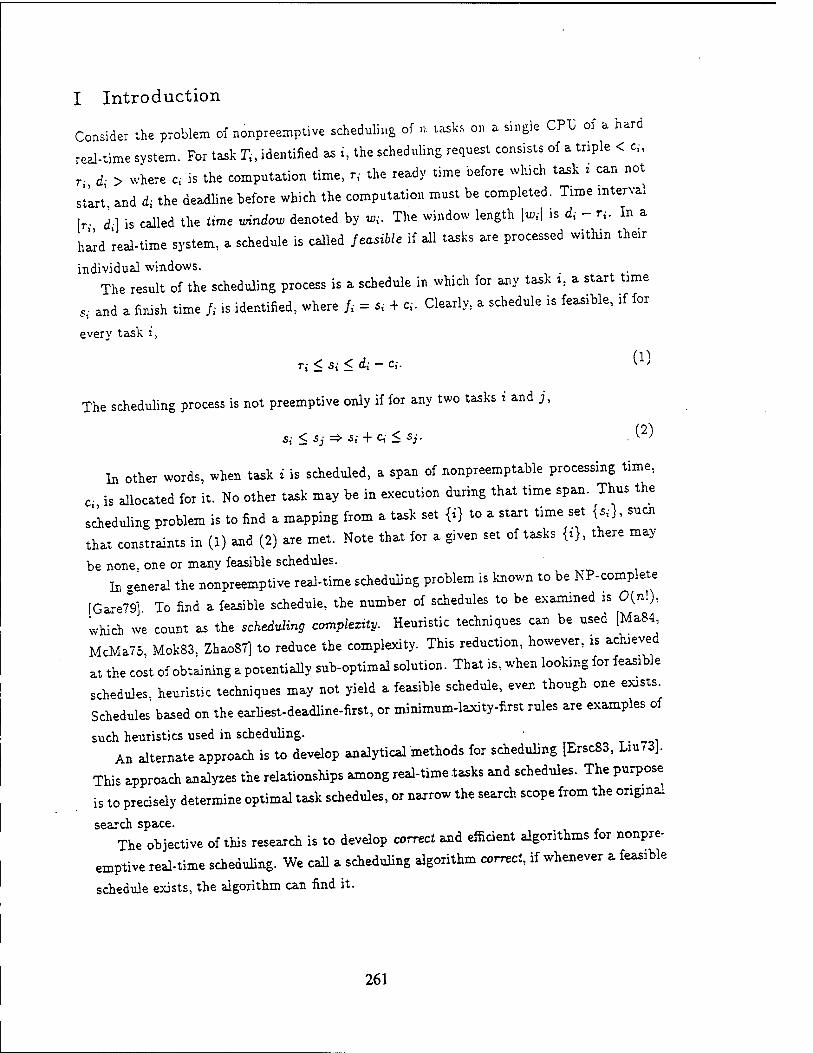
I Introduction

Consider the problem of nonpreemptive scheduling of n tasks on a single CPi; of a hard

real-time system. For task Tu identified as i, the scheduling request consists of a triple < c,-,

r- d- > where c,- is the computation time, r,- the ready time before which task t can not

st'art and d{ the deadline before which the computation must be completed. Time interval

\r- d-] is called the time window denoted by «,,-. The window length \w{\ is d{ - r,-. In a

ha'rd real-time system, a schedule is called feasible if all tasks are processed within their

individual windows. The result of the scheduling process is a schedule in which for any task i, a start time

8i and a finish time /, is identified, where /.■ = « + C Clearly, a schedule is feasible, if for

every task i,

Ti < Si < di - c{. W

The scheduling process is not preemptive only if for any two tasks i and j,

Si<Sj^>Si + Ci<Sj. . (2)

In other words, when task t is scheduled, a span of nonpreemptable processing time,

c- is allocated for it. No other task may be in execution during that time span. Thus the

scheduling problem is to find a mapping from a task set {i} to a start time set {«}, «<*

that constraints in (1) and (2) are met. Note that for a given set of tasks {,}, there may

be none, one or many feasible schedules. In general the nonpreemptive real-time scheduling problem is known to be NP-complete

fGare79j To find a feasible schedule, the number of schedules to be examined is 0{n\),

which we count as the scheduling complexity. Heuristic techniques can be used [Ma84

McMa75 Mok83. ZhaoST] to reduce the complexity. This reduction, however, is achieved

at the cost of obtaining a potentially sub-optimal solution. That is, when looking for feasible

schedules heuristic techniques may not yield a feasible schedule, even though one exists.

Schedules based on the earliest-deadline-first, or minimum-laxity-first rules are examples of

such heuristics used in scheduling. An alternate approach is to develop analytical methods for scheduling [ErscSS, Liu<3J.

This approach analyzes the relationships among real-time tasks and schedules. The purpose

is to precisely determine optimal task schedules, or narrow the search scope from the ongmal

search space. The objective of this research is to develop correct and efficient algorithms for nonpre-

emptive real-time scheduling. We call a scheduling algorithm correct, if whenever a feasible

schedule exists, the algorithm can find it.

261

In this paper, we present, an analytical decomposition approach for real-time scheduling..

The strategy is to divide a set of tasks into a sequence of subsets, such that the search for

feasible schedules is only performed within each subset. The decomposition technique used

for generating the sequence of subsets assures that in a feasible schedule all tasks in a subset

earlier in the sequence are scheduled before any task in a later subset. Backtracking in the

search is bounded within each subset, which significantly reduces the scheduling complexity.

There are several different strategies which can be used to subset tasks. The decompo-

sition strategy discussed in this paper is to use a relation called the leading relation which

depends on the tasks' relative window positions.

We performed an experiment which examined the number and size of subsets with

regard to the number of tasks, task arrival rate, and window length. We found that, in

general, the number of tasks in any subset is independent of the total number of tasks to

be scheduled, if the task window lengths are bounded. The decomposition scheduling is a

polynomial computation. As a consequence, the decomposition method is very practical for

the implementation.

In section II we present some basic notions used in the paper. In section III we discuss

a case where all the tasks have the leading relation with each other. Our approach of

decomposition scheduling is introduced in section IV along with concepts of the single

schedule subset and decomposed leading schedule sequence. We present our experiment

results in section V. Our conclusion and future research in section VII.

II Background

If we consider any two tasks i and j, they must have one of these three relations:

1. leading - i -< j (or j -< i), where if r,- < r,-, d{ < dj and te; ^ u>j.

2. matching - i\\j, if r,- = r,- and d,- = dj.

3. containing - i U j (or j U i),.if r,- < TJ and dj < <2,-.

These three relations are shown in Fig. 1. It is easy to see that the leading, matching

and containing relations are all transitive. Additionally, if i\\j or i U j, we say that i and j

are concurrent.

A length is associated with a schedule which is the finish time of the last task in the

schedule. One example is shown in Fig. 2.

The concept of dominance was introduced in [ErscS3], and we will use it later in the

discussion.

Definition 1 For two schedules Sy and 52, Si dominates S2 if and only if:

S2 feasible =*• 5j feasible.

262

I 1 1 I I I I

j I 1 I I I I

1. Leading 2. Matching 3. Containing

time

Figure 1: Task window relations

Definition 2 A set of schedules, 5, is dominant if V52 £5, 35: €5 such that Sl comWfes S2.

A schedule is dominant if it dominates all other schedules.

Ill The Leading Schedule Sequence

Let us consider the case where for a set of task {t}, every pair of tasks in this set has a leading relation, i.e. i -< j or j -< i, for every ?', j, i 4. j.

Based on the leading relation we can define a total order of tasks for the set. We define

the leading schedule sequence (LSS) to be a sequence cf -taste in which tasks are in order

according to the leading relation, that is, for any : and j, t A j <=» { -< j, where i -^ j means that 1 is scheduled in front of j.

Theorem 1 For a set of tasks all of which have a pairwise le&dirq relation, the schedule

where tasks are sequenced in order of the leading scheme sequence is a dominant one.

Proof: We prove this theorem by construction.

263

time

schedule length

Figure 2: An example of one schedule

Suppose this set of tasks has a feasible schedule S in which tasks occur in a different

sequence than the leading schedule sequence. When we examine this schedule, let : and j

be the first pair of tasks that are not ordered by the leading relation, i.e. : -< j, but j A i.

From the leading relation we know that r,- < r,- and d, < dj.

Since j and i are the first such pair, deadlines of all tasks between j and i in S must

be greater than or equal to dj as well as d,. In 5, let us construct another schedule S' by

moving i from the current position in 5 to the position just in front of j. The start time

and finish time of tasks between j and i including j will be increased by no more than c,.

And so, no task between j and i including j will finish later than <£,-. Meanwhile, the rest of

this schedule is unchanged. Thus if 5 is feasible, the new schedule S' will be feasible too.

By repeating the process of constructing S' from 5, we obtain a schedule which has all

tasks ordered according to the leading relation, such that if the original schedule is feasible,

so is the constructed one. D

Thus if there exists a set of feasible schedules, the set must contain schedules that are

conforming to the order of the leading schedule sequence. The result can be generalized

to the situation where there exist matching windows. The generalization is to combine

264

the tasks with the same window into one task whose computation time is the sum of the

computation times of all these tasks.

We will see that the above leading schedule sequence is a special case of the decomposed

leading schedule sequence introduced in the next section.

IV Task Decomposition

A. Philosophy

To solve the general real-time scheduling problem with n tasks, the number of schedules to

be examined can be as much as 0(n\). However, taking a closer look, we find that every

task has an important property called the locality of a task, that is, a task is time-bounded

by its time window. Furthermore, if any two task windows are not overlapping, there is

only one possible order for them. The above facts motivate us to separate the tasks into

subsets according to their different time localities.

The decomposition scheduling can be divided into two steps: decomposition and scheduling.

First, a set of n tasks is decomposed into a sequence of m subsets such tinat the orders of

subsets are fixed. The order of a task is determined only relative to the other tasks within

its own subset. The sequence of the subsets is called the decomposed schedule sequence.

The decomposition should be so developed that the schedulability of tasks is not damaged

at all. The decomposition by using the leading relation introduced in this paper shows this property.

The second step is to schedule the subsets in the sequence order. It always selects

a schedule for each subset with the shortest length, so that when ft subset is scheduled,

the time span available for it is maximized. In tfo's way, the total number of schedules

to be examined is only 0(££=i n*'!)> where ni JS ii»e number of tasks in the zth subset

(££i *.- = «)■ The only remaining problem is how to decompose a set of tasks into a sequence of

subsets of tasks such that a feasible schedule is guaranteed to be found if one exists. In the

rest of this paper, we outline how to use the leading relation as a means to divide the task set.

B. Decomposition Scheme

A set of tasks is called the single schedule.suhsei{sss), represented as r, if

V: € r 3j e r (:' U j) V (j U i) V (i\\j).

265

In other words, each ia.sk window is contained in the window of another task, contains

the window of another task, or matches the window of another task in the subset.

Given a set of tasks {i}, we can decompose it into a sequence of single schedule subsets

r1. r2, •• •, rk such that all the tasks in r' are leading to all the tasks in r,+1.

The decomposed leading schedule sequence (DLSS) is defined to be a sequence of single

schedule subsets, denoted as:

DIS5 = T1OT

2O---OT"

1,

such that VJfc' € r1' \fl-J € rj fc' -< kj, for 1 < i < j < m, (denoted as r' -< rJ), and r' can not

be further decomposed, for i = 1, • • ■, m. Symbol o represents a concatenating operation.

Note that if a task in r' does not lead another task in rJ' for :' < j, they must have

a matching or containing relation. If this happens, r' and rJ can not be different single

schedule subsets. Clearly, all 71 tasks may belong to a single schedule subset.

Theorem 2 The set of schedules conforming to the decomposed leading schedule sequence

is dominant.

Proof: Assume that if there are two tasks fc' 6 r' and k> G rj, where r1 -< r'. There is no

common concurrent task with both kl and fcJ. k> is positioned in front of /:' in a feasible

schedule (5). Specifically, 5 =(•••) o (#' o • • • k{) o (• • •)• Let us define S' = (kj o • • • fc1') for

abbreviation (5 = (-••) o S' o (• ■ •)). The new schedule created by exchanging k'-'s position

with kJ's is still feasible. Without loss of generality, suppose that k' and fcJ are the first such pair in 5. Tasks

between & and k{ are led by fcJ', or concurrent with kK but not leading to and not concurrent

with k\ Since k{ -< V (i.e. r,- < 7-;), switching /:*"s and k^s positions will not increase the

finish time of 5', which is defined as the finish time of the last task in 5'. All the tasks

between k' and k\ including )-J, are led by k\ i.e. having deadlines greater than or equal

to dki. K 5 is feasible with it' as the last task in 5', it will be still feasible after the

switching;. E lo-

Note that if the set of schedules that are following the decomposed leading schedule

sequence is empty, there is no feasible schedule available for the tasks to be scheduled.

C. Decomposition Algorithm

Decomposing a set of tasks into single schedule subsets, the algorithm starts with the tasks

having been sorted by their ready times (using their deadlines if their ready times are the

same).

266

The algorithm uses one single loop to determine which single schedule subset the cur-

rent task should belong to. The loop consists of two parts. The first part is a while loop

which merges single schedule subsets into one, if the current task is contained by them. The

second part decides whether the current task can form a new single schedule subset, or join

with another single schedule subset.

The Leading-relation Decomposition Algorithm

begin

/* Initialization. */

fc = l;T1 = {l};

rTj = 7v, riTi = di\

for i = 2 to n do /* Go over the task list. */

/ = /: - 1; /* / is the index of single schedule subsets. */

continue = TRUE;

while (/ > 0) A (continue) do

/* Merge single schedule subsets if the current task is concurrent

with tasks in different subsets. */

if {dT, > di)'

Tl = Tk\jTl\

dri — dTk\

k = l\

else

continue = FALSE;

1 = 1-1;

od

if (TV* < O A fa < drk) /* The current task is concurrent with tasks in the current subset.*/

else if (rT* < T{) A (dTk < di)

I* The current task is led by all the tasks in the current subset.

A new single schedule subset is created only containing the current task.*/

k = Jfc + 1;

rk = {;}; Trk = T{\

drk = d{.

od

end

267

In this algorithm, the outer loop is executed 7: times. The while loop is executed no

more than the number of time proportional to n in total, since no more than n subsets can

be merged during the whole execution of the algorithm with n tasks. Thus the complexity

of this algorithm is only 0(n). If we count in the sorting complexity, the decomposition

will cost no more than O(niogn).

D. Scheduling Scheme

After tasks has been decomposed into a sequence of subsets, scheduling should be performed

on each subset in the sequence order, such that the schedule on each subset is of the

shortest length. A brute force method is to give an exhaustive search whose computational

complexity amounts to 0(n,!), where n:- is the number of tasks in the tth subset.

In [Yuan89b], other scheme is explored for scheduling a subset. The method is to first

build a super-sequence where tasks may have several occurrences. The occurrence of a task

is decided by its relative window position in the subset. Selecting one occurrence for every — in- — n \

task in the super-sequence forms a schedule. A complete search costs 0(n? ' ) in the

-tn—n-) worst case. When we made a few calculation samples of nf ' ' with n; less than 100,

n?(n,_71' ^ is a much smaller number than n,-!, as shown in the cited paper.

Since the set of schedules following the decomposed leading schedule sequence is -domi-

nant, and. since the subsets are scheduled in the sequence order with their shortest length, it

is proved that the decomposition scheduling with the leading relation is correct [YuanS9b].

V Empirical Study

A. Experiment

In order to observe the behavior of the number of tasks in a single schedule subset and

number of the subsets to be created with regard to the number of tasks to be scheduled,

task arrival rate, and task window length, we conduct an experiment as an example to see

the feasibility of our approach for practical implementation.

The outputs we are interested in are:

1. the number of single schedule subsets (sss),

2. the number of window concurrences,

3. the maximum number of tasks in single schedule subsets,

4. the minimum number of tasks in single schedule subsets, and

268

5. the average number of tasks in single schedule subsets.

One window concurrence is counted for any two tasks i and j if i and ; have a concurrent

relation. We call the number of tasks in a single schedule subset a, the «re « i. ■- abset

Meanwhile, we change the following parameters independently to watch the cna,ges m

the outputs,

1. the number of total tasks,

2. task arrival rate, and

3. window length.

The data is shown in Table l-4> in the end of this paper. Following are basic rules in

the experiment.

1. The computation time is uniformly distributed over (0,o].

2. The task interarrival is uniformly distributed over [0,/?). The arrival rate is 2/ß.

3 The window length is also randomly created by controlling the laxity for each task.

' The laxitv of a task is the difference between its window length and its computation

time. The laxity is uniformly distributed [0, 7). The distribution guarantees the

window length greater than the computation time for the task.

We notice that the arrival rate should be less than or equal to the service rate otherwise,

there are congestions in the system, which will result in deadline-missing. In other words,

2/ß < 2/JQ. That is, a<ß-

The random numbers are provided by function *«*<) in the UNLX operaring system.

The numbers are uniformly distributed over [0, 1) [StevS6]. I* the experiment, we found that the minimum size of single schedule subsets „ always

one.

B. The Result Explanation and Observation

From the experiment results , we found that when the average window length increases

(7 increases), the number of single schedule subset, reduces and the maxamum S1ze o

single schedule subsets slightly increases. The result * expected, since the larger some «*

- 'In the tables, »«Misrepresented by nurr, Win*» by W. Convene« by concur, Averse by

avg. The Single schedule subset by sss.

269

Windows are, the more tasks may be concurrent with them. These tasks may be in the same

single schedule subset. When ß increases, that is, the arrival rate decreases, the number of single schedule

subsets increases, and maximum size of single schedule subsets decreases. The result is also

expected, since when the arrival rate decreases, the opportunity of tasks concurrent with

each other decreases too. Most tasks have the leading relation with each other.

max^n,)

12

7 = 2

7 = 4

7 = 6

7 = 8

7 = 10

/ \ / \

50 100

n

150 200 250 500

Figure 3: The relationship between the size of single schedule subsets and the number of

tasks with Tegard to the laxity parameter 7, where a = 4, ß = 4.

Fig. 3 shows the relationship between the maximum size of single schedule subsets and

the number of tasks to be scheduled. From the experiment, we found that the size of a

single schedule set never exceeds 14 even when there are 300 tasks being scheduled. The

observation indicates that for most cases max^L^-rn) is a constant.

We show the relationship between the number of subsets (m) and number of tasks to

be scheduled in Fig. 4 and Fig. 5 with regard to different window length and arrival rate

distributions.

270

Figure 4: The relationship between the number of single schedule subsets and the number

of tasks with regard to the laxity parameter 7, where a = 4, ß = 4.

VI Final Remarks

In this paper, we examine the problem of nonpreemptive scheduling of n tasks on a single

CPU in hard real-time systems. We propose a correct decomposition strategy for the

scheduling. The strategy significantly reduces the scheduling complexity for most Clses.

In this paper we have examined a decomposition technique based only on the windows

of tasks. By taking into account the computation time requirements, the decomposition

can be made stronger [Yuan89aj. The decomposition approach may also be extended to

consider precedence and other dependences among tasks. This aspect of decomposition

technique needs further study.

Acknowledgements

Thanks to S. Mukherjee for his help in coding the decomposition algorithm for our

271

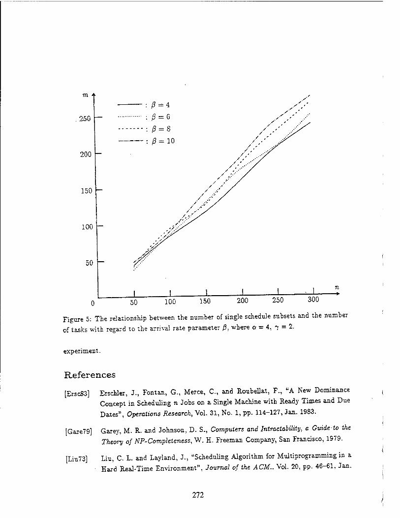
m

.250

200

150

100

50

0 = 4 0 = 6 0 = 8 0 = 10

n —*■

50 100 150 200 250 300

Figure 5: The relationship between the number of single schedule subsets and the number

of tasks with regard to the arrival rate parameter 0, where a = 4, -y = 2.

experiment.

References

[Ersc83] Erschler, J., Fontan, G., Merce, C, and Roubellat, F., "A New Dominance

Concept in Scheduling n Jobs on a Single Machine with Ready Times and Due

Dates", Operations Research, Vol. 31, No. 1, pp. 114-127, Jan. 1983.

[Gare79] Garey, M. R. and Johnson, D. S., Computers and Intractability, a Guide-to the

Theory of NP-Completeness, W. H. Freeman Company, San Francisco, 1979.

[Liu73] Liu, C. L. and Layland, J., "Scheduling Algorithm for Multiprogramming in a

■ Hard Real-Time Environment". Journal of the ACM.. Vol. 20, pp. 46-61. Jan.

272

1973.

IMaS4l Ma. P. R.. "A Model to Solve Timing-Critical Application Problems in Dis-

tributed Computing Systems", IEEE Computer, Vol. 17, pp. 62-6S, Jan. 19S4.

[McMa75] McMahon, G. and Florian, M., "On Scheduling with Ready Times and Due

Dates to Minimize Maximum Lateness", Operations Research, Vol. 23, No. 3,

pp. 475-4S2, May 1975.

[MokS3] Mok, A. K., "Fundamental Design Problems for the Hard Real-time Environ-

ments", May 19S3, MIT Ph.D. Dissertation.

[StevS6] Steven V. Earhart, Ed., UNIX Programmer's Manual: System Calls and Library

Routines, Volume Volume 2, CBS College Publishing, 1986.

[YuanS9a] Yuan, X. and Agrawala, A. K., Decomposition with a Strongly-Leading Relation

for Hard Real-Time Scheduling, Technical Report to be Published, Dept. of

Computer Science, Univ. of Maryland, Coll. Pk., MD 20742. Mar. 1989.

[YuanS9b] Yuan, X. and Agrawala, A. K., Scheduling Real-Time TasK in Single Schedule

Subsets, Technical Report to be Published, Dept. of Computer Science, Univ. of

Maryland, Coll. Pk., MD 20742, Mar. 1989.

[ZhaoS7] Zhao, W., Ramamritham, K., and Stankovic, J. A., "Scheduling Tasks with

Resource requirements in a Hard Real-Time System", IEEE Trans, on Soft.

Eng., Vol. SE-13, No. 5, pp. 564-577, May 1987.

273

Table 1: o.■ = 4, ß = 4

num of ") avg W.

length i

num of

concurr.

num of

S.S5

555 size

tasks i

max avg

50

2 3.02 5 45 2 1.11

4 4.33 IS 35 3 1.43

6 5.08 27 25 5 2.00

S 6.53 14 36 5 1.39

10 7.03 26 30 6 1.67

100

2 3.11 IS 82 3 1.22

4 4.18 2S 74 5 1.35

6 4.34 37 68 6 1.47

8 5.84 • 56 55 6 1.S2

10 7.01 77 41 14 2.44

150

2 3.09 32 118 4 1.27

4 3.78 40 114 4 1.32

6 4.93 68 92 6 1.63

S 5.85 91 73 7 2.05

10 6.56 111 6S 10 2.21

200

2 3.11 41 159 4 1.26

4 3.67 64 144 4 1.39

6 4.94 98 116 6 1.72

8 5.94 102 113 8 1.77

10 7.27 161 81 8 2.47

250

2 3.02 46 204 .4 1.23

4 3.82 93 | 167 5 1.50

6 4.83 107 ! 160 6 1.56

8 6.33 162 | 121 8 2.07

10 7.29 | 186 103 | 11 2.43

300

2 j 2.98 66 | 237 4 1.27

4 j 3.90 105 | 205 5 j 1.46

6 5.09 125 194 6 j 1.55

8 | 6.21 179 j 153 11 1.96

10 j 6.92 228 125 11 2.40

274

Table 2: a = 4, ß = 6

num of

tasks

7 avg W.

length

num of

concurr.

num of sss size |

max avg

50

2 2.79 13 38 3 1.32

4 4.22 7 43 3 1.16

6 4.45 16 36 3 1.39

8 6.21 21 31 4 1.61

10 6.82 23 30 5 1.67

100

2 2.96 16 85 3 1.18

4 3.93 16 85 3 1.18 6 3.93 16 85 3 1.18

8 6.32 31 73 4 1.37

10 7.21 52 58 7 1.72

150

2 3.29 20 130 4 1.15

4 3.98 29 125 5 1.20

6 5.33 42 111 4 1.35

8 5.90 55 100 5 1.50

10 6.'96 77 83 8 1.81

200

2 3.04 25 175 4 1.14

4 3.90 48 153 3 1.31

6 5.18 55 14» 9 1.35

8 5.95 87 128 8 1.56

10 7.18 84 128 6 1.56

250

2 2.93 45 206 3 1.21

4 4.08 55 200 6 1.25

G - 5.10 55 197 5 | 1.27

8 6.15 76 175 8 | 1.43

10 6.78 98 162 7 1.54

300

2 3.00 54 | 250 4 1.20

4 4.13 47 1 254 5 1.18 6 4.97 67 236 4 1.27

8 5.82 96 214 5 1.40

10 6.97 161 159 8 1.89

275

Table 3: Q = 4, ß = 8

mim of

tasks

7 avg W.

length

num of

concurr.

num of i sss size 1

max avg

50 I !

2 3.24 9 42 3 1.19

4 3.56 5 45 3 1.11

6 4.67 11 40 3 1.25

8 5.95 3 ' 47 2 1.06

10 6.51 20 32 5 1.56

100

2 2.99 6 94 2 1.06

4 4.20 13 87 3 1.15

6 5.04 26 75 3 1.33

8 5.77 29 73 5 1.37

10 6.91 33 70 5 1.43

150

2 2.99 23 127 4 1.18

4 4.01 2S 126 4 1.19

6 5.27 28 122 3 1.23

8 6.00 32 120 5 1.25

10 7.22 39 112 6 1.34

200

2 3.09 19 182 3 1.10

4 3.94 18 182 3 1.10

6 4.87 31 171 4 1.17

8 5.91 51 154 5 1.30

10 6.96 78 130 6 1.54

250

2 2.91 23 227 3 1.10

4 4.01 | 48 206 4 1.21

6 5.01 1 52 204 5 1.23

8 | 5.84 | 56 195 5 1.28

10 | 7.48 1 60 191 4 1.31

300

2 2.99 35 267 4 1.12

4 4.05 | 30 270 3 1.11

6 5.07 60 241 4 1.24

8 5.99 63 240 4 1.25

10 7.13 110 199 6 1.51

276

Table A Q = 4, ß = 30

num of

tasks 7 avg W. |

length

num of |

concurr. |

num of

sss

sss size

max avg

50

2 3.44 2 48 2 1.04

4 4.11 5 45 3 1.11

6 5.50 4 46 3 1.09

6 6.69 11 41 4 1.22

10 6.61 15 38 5 1.32

100

2 3.02 89 4 1.12

4 4.01 14 87 4 1.15

6 4.95 21 80 4 1.25

6 6.59 16 62 3 1.22

10 6.68 25 76 5 1.32

150

2 3.00 6 144 2 1.04

4 3.98 11 139 3 1.08

6 4.72 11 139 2 1.08

8 5.91 37 117 5 1.28

10 7.10 43 109 6 1.38

200

2 3.00 18 182 3 1.10

4 3.97 27 174 5 1.15

6 5.19 23 177 3 1.13

8 6.16 34 167 4 1.20

10 6.90 52 153 4 1.31

250

2 | 2.94 24 228 3 1.10

4 4.12 32 | 218 1 3 | 1.15

6 j 5.10 43 j 213 1 < 1 1.« j 8 | 6.07 45 | 206 I 3 | 1.21

10 | 6.96 51 j 200 1 « 1.25

300

2 3.05 27 274 1 3 I 1.09

4 4.07 21 280 3 i 1.07

6 5.04 54 251 6 1.20

8 6.16 46 254 3 1.18

10 6.61 61 243 8 1.23

277

UNCLASSIFIED

»ECUAITT CLAMIFICATIOW or THIS PAOE

Let us consider the problem of scheduling a set of n tasks on a single processor such that a feasible schedule which satisfies the time constraints of each task is generated. It is recognized that an exhaustive search may be required to generate such a feasible schedule or to assure that there does not exists one. In that case the computational complexity of the search is of the order n!.

We propose to generate the feasible schedule in two steps. In the first step we decompose the set of tasks into m subsets by analyzing their ready times and deadlines. An ordering of these subsets is also specified such that in a feasible schedule all tasks in an earlier subset in the ordering appears before tasks in a later subset. With no simplification of scheduling of tasks in a subset, the scheduling complexity is 0(EJ1, n,-!), where n,- is the number of tasks in the xth subset.

The improvement of this approach towards reducing the scheduling complexity depends on the the number and the size of subsets generated. Experimental results indicates that significant improvement can be expected in most situations.

UNCLASSIFIED 278 SECURITY CLASSIFICATION OF THIS PACE


1. AGENCY USE ONLY (leave blank) 2. REPORT DATE Novemebr 1989




A Decomposition Approach to Nonpreemptive Real-Time Scheduling

6. AUTHOR(S)

Xiaoping (George) Yuan, Ashok K. Agrawala, and Manas C. Saksena


9. SPONSORING/ MONITORING AGENCY NAME(S) AND ADDRESS(ES)|l US Army Strategic Defense Command Contr. & Acq. Mgt. Office CSSD-H-CRS, P.O. Box 1500 Huntsville, AL 35807-3801


5. FUNDING NUMNBERS

DASG60-87-X-0066


CS-TR-89-109 UMIACS-TR-2345




Consider the problem of scheduling a set of n tasks on a uniprocessor such that a feasible schedule that satisfies each task's time constraints is generated. Traditionally, researchers have looked at all the tasks as a group and applied heuristic or enumeration search to ft. We propose a new approach called the decomposition scheduling where tasks are decomposed into a sequence of subsets. Tasks are scheduled in each subset independently in the order of the sequence. It is proved that a feasible schedule can be generated as long as one exists for the tasks. In addition, the overall scheduling cost is reduced to the sum of the scheduling costs of the tasks in each subset.

Simulation experiments were conducted to analyze the performance of decomposition scheduling approach. The results show that in many cases decomposition scheduling performs better than the traditional branch-and-bound algorithms in terms of scheduling cost, and heuristic algorithms in terms of percentage of finding feasible schedules over randomly-generated task sets.

14. SUBJECT TERMS


18. SECURITY CLASSIIFICATION OF THIS PAGE

Unclassified

15. NUMBER OF PAGES

17

16. PRICE CODE


Unclassified

MSN 7540-01 280-5500


Unlisted


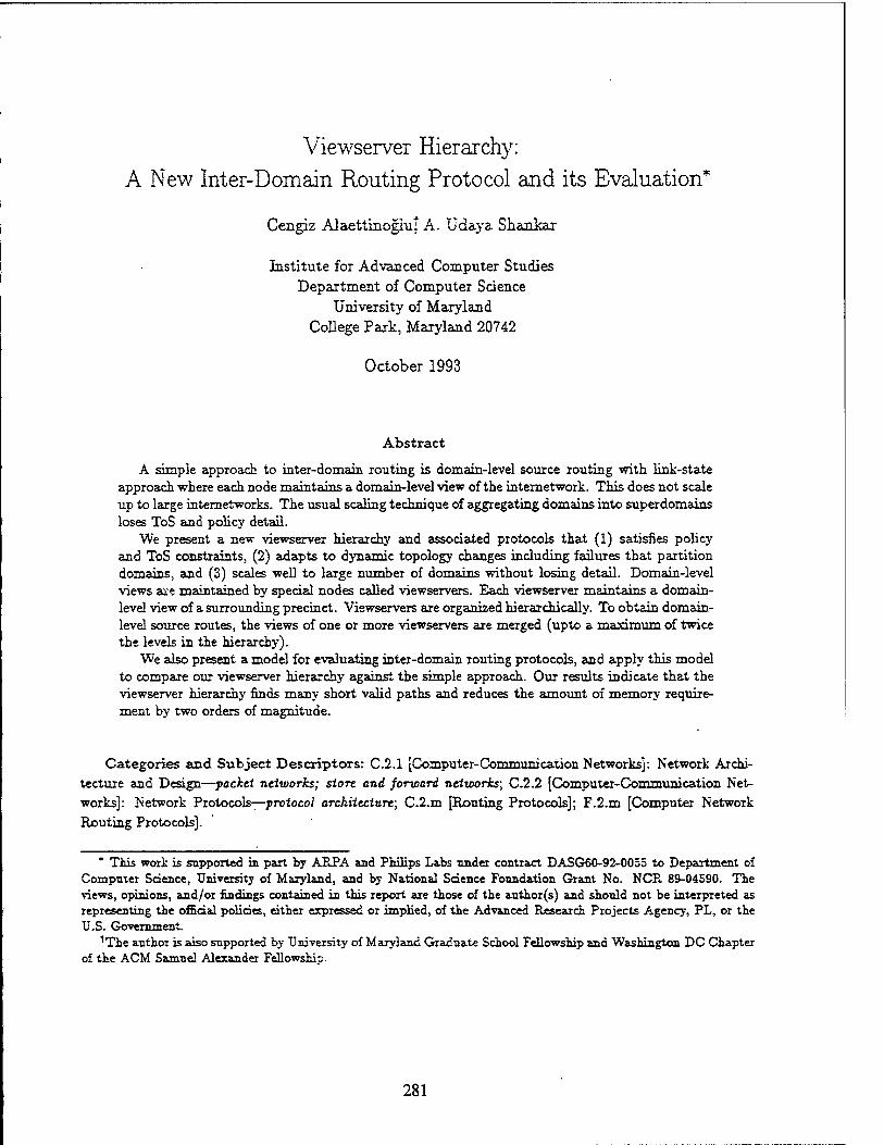
Viewserver Hierarchy: A New Inter-Domain Routing Protocol and its Evaluation"

Cengiz Alaettinoghi! A. Udaya Skaukar


University of Maryland College Park, Maryland 20742

October 1993

Abstract

A simple approach to inter-domain routing is domain-level source routing with link-state approach where each node maintains a domain-level view of the internetwork. This does not scale up to large internetworks. The usual scaling technique of aggregating domains into superdomains loses ToS and policy detail.

We present a new viewserver hierarchy and associated protocols that (1) satisfies policy and ToS constraints, (2) adapts to dynamic topology changes including failures that partition domains, and (3) scales well to large number of domains without losing detail. Domain-level views are maintained by special nodes called viewservers. Each viewserver maintains a domain- level view of a surrounding precinct. Viewservers are organised hierarchically. To obtain domain- level source routes, the views of one or more viewservers are merged (upto a maximum of twice the levels in the hierarchy).

We also present a model for evaluating inter-domain routing protocols, and apply this model to compare our viewserver hierarchy against the simple approach. Our results indicate that the viewserver hierarchy finds many short valid paths and reduces the amount of memory requirement by two orders of magnitude.

Categories and Subject Descriptors: C.2.1 [Computer-Communication Networks]: Network Archi- tecture and Design—packet networks; store and forward networks; C.2.2 [Computer-Communication Net- works]: Network Protocols—proioco/ architecture; C.2.m [Routing Protocols]; F.2.m [Computer Network Routing Protocols].

" This work is supported in part by ARPA and Philips Labs under contract DASG60-92-0055 to Department of Computer Science, University of Maryland, and by National Science Foundation Grant No. NCR 89-04590. The views, opinions, and/oi Undings contained in this report are those of the author(s) and should not be interpreted as representing the official policies, either expressed or implied, of the Advanced Research Projects Agency, PL, or the U.S. Government.

1The author is also supported by University of Maryland Graduate School Fellowship and Washington DC Chapter of the ACM Samuel Alexander Fellowship.

281

1 Introduction

A computer internetwork, such as the Internet, is an interconnection of backbone networks, regional

networks, metropolitan area networks, and stub networks (campus networks, office networks and

other small networks)1. Stub networks are the producers and consumers of the internetwork traffic,

while backbones, regionals, and MANs are transit networks. (Most of the networks in an internet-

work are stub networks.) Each network consists of nodes (hosts, routers) and links. Two networks

are neighbors when there is one or more links between nodes in the two networks (see Figure 1).

Figure 1: A portion of an internetwork. (Circles represent stub networks.)

An internetwork is organized into domains2. A domain is a set of networks (possibly consisting of

only one network) administered by the same agency. Within each domain, an intra-domain routing

protocol is executed that provides routes between source and destination nodes in the domain. This

protocol can be any of the typical ones, i.e., next-hop or source routes computed using distance-

vector or link-state algorithms.

Across all domains, an inter-domain routing protocol is executed that provides routes be-

tween source and destination nodes in different domains. This protocol must satisfy various con-

straints:

(1) It must satisfy policy constraints, which are administrative restrictions on the inter-domain

traffic [8, 12, 9, 5]. Policy constraints are of two types: transit policies and source policies.

The transit policies of a domain A specify how other domains can use the resources of A

(e.g. SO.01 per packet, no traffic from domain £). The source policies of a domain A specify

1 For example, NSFNET, MILNET are backbones and Snranet, CerfNet are regionals. 2 also referred to as routing domains

282

constraints on traffic originating from A (e.g. domains to avoid/prefer, acceptable connection

cost). Transit policies of a domain are public (i.e. available to other domains), whereas source

policies are usually private.

(2) An inter-domain routing protocol must also satisfy type-of-service (ToS) constraints of ap-

plications (e.g. low delay, high throughput, high reliability, miTurmiTn monetary cost). To do

this, it must keep track of the types of services offered by each domain [5].

(3) Inter-domain routing protocols must scale up to very large internetworks, i.e. with a very large

number of domains. Practically this means that processing, memory and communication

requirements should be much less than linear in the number of domains.

(4) Inter-domain routing protocols must automatically adapt to link cost changes, node/link

failures and repairs including failures that partition domains [15]. It must also handle non-

hierarchical domain interconnections at any level [9] (e.g. we do not want to hand-configure

special routes as "back-doors").

A simple (or straightforward) approach to inter-domain routing is domain-level source routing

with link-state approach (8, 5]. In. this approach, each router3 maintains a domain-level view of the

internetwork, i.e., a graph with a vertex for every domain and an edge between every two neighbor

domains. Policy and ToS information is attached to the vertices and the edges of the view.

When a source node needs to reach a destination node, it (or a router4 in the source's domain)

first examines this view and determines a domain-level source route satisfying ToS and policy

constraints, i.e., a sequence of domain ids starting from the source's domain and ending with the

destination's domain. Then, the packets are routed to the destination using this domain-level

source route and the intra-domain routing protocols of the domains crossed.

The disadvantage of this simple scheme is that it does not scale up for large internetworks. The

storage at each router is proportional to Np x ED, where Nz> is the number of domains and ED

is the average number of neighbor domains to a domain. The communication cost is proportional

to NR x ER, where NR is the number of routers in the internetwork and ER is the average router

neighbors of a router (topology changes are flooded to all routers in the internetwork).

To achieve scaling, several approaches based on aggregating domains into superdomains have

Not all nodes maintain routing tabjes. A router is a node that maintains a routing table. 4 referred to as the policy server in [8]

283

been proposed [13, 16, 6]. This approaches have drawbacks because the aggregation results in loss

of detail (discussed in Section 2).

Our protocol

In this paper, we present an inter-domain routing protocol that we have proposed recently[3]. It

combines domain-level views with a novel hierarchical scheme. It scales well to large internetworks,

and does not suffer from the problems of superdomains.

In our scheme, domain-level views are not maintained by every router but by special nodes

called viewservers. For each viewserver, there is a subset of domains around it, referred to as the

viewserver's precinct. The viewserver maintains the domain-level view of its precinct. This solves

the scaling problem for storage requirement.

A viewserver can provide domain-level source routes between source and destination nodes in

its precinct. Obtaining a domain-level source route between a source and a destination that are

not in any single view, involves accumulating the views of a sequence of viewservers. To make this

process efficient, viewservers are organized hierarchically in levels, and an associated addressing

structure is used. Each node has a set of addresses. Each address is a sequence of viewserver ids of

decreasing levels, starting at the top level and going towards the node. The idea is that when the

views of the viewservers in an address are merged, the merged view contains domain-level routes

to the node from the top level viewservers. (Addresses are obtained from name servers in the same

way as is currently done in the Internet.)

We handle dynamic topology changes such as node/link failures and repairs, link cost changes,

and domain partitions. Gateways5 detect domain-level topology changes affecting its domain and

neighbor domains. For each domain, there is a reporting gateway that communicates these changes

by flooding to the viewservers in a specified subset of domains; this subset is referred to as its flood

area. Hence, the number of packets used during flooding is proportional to the size of the flood

area. This solves the scaling problem for the communication requirement.

Thus our inter-domain routing protocol consists of two subprotocols: a view-query proto-

col between routers and viewservers for obtaining merged views; and a view-update protocol

between gateways and viewservers for updating domain-level views.

4 A node is called a gateway if it has a link to another domain.

284

Evaluation

Many inter-domain routing protocols have been proposed, based on various kinds of hierarchies.

How do these protocols compare against each other and against the simple approach? To answer this

question, we need a model in which we can define internetwork topologies, policy/ToS constraints,

inter-domain routing hierarchies, and evaluation measures (e.g. memory and time requirements)

for inter-domain routing protocols. None of these protocols have been evaluated in a way that they

can be compared against each other or the simple approach.

In this paper, we present such a model, and use it to compare our viewserver hierarchy to the

simple approach. Our evaluation measures are the amount of memory required at the source and

at the routers, the amount of time needed to construct a path, and the number of valid paths

found (and their lengths) in comparison to the number of available valid paths (and their lengths)

in the internetwork. We use three internetwork topologies each of size 11,110 domains (roughly the

current size of the Internet). Our results indicate that the viewserver hierarchy finds many short

valid paths and reduces the amount of memory requirement by two orders of magnitude.


In Section 2, we survey recent approaches to inter-domain routing. In Section 3, we present the

view-query protocol for static network conditions, that is, assuming all links and nodes of the

network remain operational. In Section 4, we present the view-update protocol to handle topology-

changes (this section is not needed for the evaluation part). In Section 5, we present our evaluation

model and results from its application to the viewserver hierarchy. In Section 6, we conclude and

describe how to add fault-tolerance and cacheing schemes to improve performance.

2 Related Work

In this section, we survey recently proposed inter-domain routing protocols that support ToS and

Policy routing for large internetworks [14, 16, 13, 10, 6, 20, 2,19,18, 7].

Several inter-domain routing protocols (e.g. BGP [14], IDRP [16], NU [10]) are based on path-

veclor approach [17]. Here, for each destination domain a router maintains a set of paths, one

through each of its neighbor routers. TöS and policy information is attached to these paths. Each

285

router requires 0{ND x ND x £*) space. For each destination, a router exchanges its best valid

path6 with its neighbor routers. However, a path-vector algorithm may not find a valid path

from a source to the destination even if such a route exists [13]7. By exchanging k paths to each

destination, the probability of detecting a valid path for each source can be increased.

The most common approach to solve the scaling problem is to use superdomain^ (e.g. IDPR [13],

IDRF [16], Nimrod [6]). Superdomains extend the idea of area hierarchy [11]. Here, domains are

grouped hierarchically into superdomains: "close" domains are grouped into level 1 superdomains,

"close" level 1 superdomains axe grouped into level 2 superdomains, and so on. Each domain

A is addressed by concatenating the superdomain ids starting from a top level superdomain and

going down towards A. A router maintains a view that contains the domains in the same level 1

superdomain, the level 1 superdomains in the same level 2 superdomain, and so on. Thus a router

maintains a smaller view than it would in the absence of hierarchy. Each superdomain has its own

ToS and policy constraints derived from that of the subdomains.

There are several major problems with using superdomains. One problem is that if there are

domains with different (possibly contradictory) constraints in a superdomain, then there is no good

way of deriving the ToS and policy constraints of the superdomain. The usual techniques are to

take either the union or the intersection of the constraints of the subdomains [13]. Both techniques

have problems9. Other problems axe described in [6, 2]. Some of the problems can be relaxed by

having overlapping superdomains, but this increases the storage requirements drastically.

Nimrod [6j and IDPR [13] use the link-state approach, domain-level source routing, and super-

domains (non-overlapping superdomains for Nimrod). IDRP [16] uses path-vector approach and

superdomains.

Reference [10] combines the benefits of path-vector approach and link-state approach by having

two modes: An NR mode, which is an extension of IDRP and is used for the most common ToS

and policy constraints; and a SDR mode, which is like IDPR and is used for less frequent ToS and

6 A valid path is a path that satisfies the ToS and policy constraints of the domains in the path. 7 For example, suppose a router « has two paths Pi and P2 to the destination. Let u have a router neighbor *,

which is in another domain. « chooses and informs t, of one of the paths, say Pi. Bnt Pi may violate source pohaes

of v's domain, and P2 may be a valid path for v. 8 also referred to as routing domain confederations 9 For example if the union is taken, then a snbdomain A can be forced to obey constraints of other subdomains;

this may eliminate a path through A which is otherwise valid. If the intersection is taken, then a subdomain A can be forced to accept traffic it would otherwise not accept.

286

policy requests. This study does not address the scalability of the SDR mode.

In [2], we proposed another protocol based on superdomains. It always finds a valid path if

one exists. Both union and intersection policy and ToS constraints are maintained for each visible

superdomain. If the union policy constraints of superdomains on a path axe satisfied, then the path

is valid. If the intersection policy constraints of a superdomain are satisfied but the union policy

constraints are not, the source uses a query protocol to obtain a more detailed "internal" view of

the superdomain, and searches again for a valid path. The protocol uses a link-state view update

protocol to handle topology changes, including failures that partition superdomains at any level.

The landmark hierarchy [19, 18] is another approach for solving the scaling problem. Here,

each router is a landmark with a radius, and routers which are within a radius away from the

landmark maintain a route to it. Landmarks are organized hierarchically, such that the radius

of a landmark increases with its level, and the radii of top level landmarks include all routers.

Addressing and packet forwarding schemes are introduced. Link-state algorithms can not be used

with the landmark hierarchy, and a thorough study of enforcing ToS and policy constraints with

this hierarchy has not been done.

The landmark hierarchy may look similar to our viewserver hierarchy, but in fact they are quite

opposite. In the landmark hierarchy, nodes within the radius of the landmark maintain a route to

the landmark, and the landmark may not have a route to these nodes. In the viewserver hierarchy,

viewserver maintains routes (i.e. a view) to the nodes in its precinct.

Route fragments [7] is an addressing scheme. A destination route fragment, called a route

suffix, is a sequence of domain ids from a backbone to the destination domain. A source route

fragment, called a route prefix, is the reverse of a route suffix of that domain. There are also route

middles, which are from transit domains to transit domains. These addresses are static (i.e. they

are not updated with topology changes) and stored at the name servers. A source queries a name

server and obtains destination route suffixes. It then chooses an appropriate route suffix for the

destination and concatenates it with its own route prefix (and uses routes middles if route suffix

and route prefix do not intersect). This scheme can not handle topology changes and does not

address handling policy and ToS constraints.

287

3 Viewserver Hierarchy Query Protocol

ID this section, we present our scheme for static network conditions, that is, all links and nodes

remain operational. The dynamic case is presented in Section 4.

Conventions: Each domain has a unique id. Domainlds denotes the set of domain-ids. Each

node has an id which is unique in its domain. Nodelds denotes the set of node-ids. Thus, a node is

totally identified by the combination of its domain's id and its node-id. Totallds denotes the set

of total node-ids. For a node u, we use domainid(u) to denote the domain-id of u's domain. "We

use nodeia\u) and totalid(u) to denote the node-id and total-id of u respectively. For a domain A,

we use domainid(A) to denote the domain-id of A. NodeNeighbors(v.) denotes the set of node-ids

of the neighbors of u. DomainNeighbors(A) denotes the set of domain-ids of the domain neighbors

of A. We use the term gateway-id (or viewserver-id) to mean the total-id of a gateway node (or a

viewserver node).

In our protocol, a node u uses two kinds of sends. The first kind has the form "Send(m) to t;*,

where m is the message being sent and v is the total-id of the destination. Here, nodes u and v

are neighbors, and the message is sent over the physical link (u, v). If the link is down, we assume

that the packet is dropped.

The second kind of send has the form uSend(m) to v using dlsr"", where m and v are as above

and dlsT is a domain-level source route between u and v. Here, the message is sent using the intra-

domain routing protocols of the domains in dlsr to reach r10. We assume that as long as there is a

sequence of up links connecting the domains in dlsr, the message is delivered to r11. If the u and

v are in the same domain, dlsr equals (}.

Views and Viewservers

Domain-level views are maintained by special nodes called viewservers. Each viewserver has a

precinct, which is a set of domains around the viewserver, and a static view, which is a domain-level

view of the precinct and outgoing edges. The static view includes the ToS and policy constraints

10 Recall that given a domain-level source route to a destination, using the intra-doznain routing protocols we can reach the destination.

ii This involves time-outs, retransmissions, etc. It requires a transport protocol support such as TCP.

288

of domains in the precinct and of domain-level edges12. Formally, a viewserver z maintains the

following:

Precinctx. (C Domainlds). Domain-ids whose view is maintained.

SView=. Static view of x.

= {{A, policy ktos{A), {{B, edgejpolicyktos{A,B)): B € subset of DomainNeighbors{A)}) :

A £ Precinct*}

SView= can be implemented as adjacency list representation of graphs [1]. The intention of

SViewx is to obtain domain-level source routes between nodes in Precinct*. Hence, the choice of

domains to include in Precinct* and the choice of neighbors of domains to include in SViewx is

not arbitrary. Precinct, and SViewx must be connected; that is, between any two domains in

Precinct*, there should be a path in SViewx that lies in Precinct,. Note that SViewx can contain

edges to domains outside Precinct,. We say that a domain A is in the view of a viewserver x, if

either A is in the precinct of x or SViewx has an edge from a domain in precinct to A. Note that

the precincts and views of different view servers can be overiappfofe identical or disjoint.

If there is a viewserver x whose view contains both the source and the destination domains,

then s's view can be used to obtain the required domain-level source route to reach the destination.

The source needs to reach x to obtain its view. If the source and x are in the same domain, i

can be reached using the intra-domain routing protocol. If x is in another domain, then the source

needs to have a domain-level source route to it13. In this case, we assume that source has a set of

fixed domain-level source routes to x.

Viewserver Hierarchy

For scaling reasons, we cannot have one large view. Thus, obtaining a domain-level source route

between a source and a destination which are far away, involves accumulating views of a sequence of

viewservers. To keep this process efficient, we organize viewservers hierarchically. More precisely,

each viewserver is assigned a hierarchy level from 0,1,... with 0 being the top level in the hierarchy.

A parent/child relationship between viewservers is defined as follows: 12 Not all the domain-level edges need to be included. This is because some domains may have many neighbors

causing a big storage requirement. 13 We cannot obtain this domain-level source route from i, i.e. chicken-egg problem.

289

1. Every level i viewserver, i > 0, has a parent viewserver whose level is less than i.

2. If viewserver z is a parent of viewserver y then x's view contains jr's domain and y's view

contains z's domain14.

3. The view of a top level viewserver contains the domains of all other top level viewservers.

(typically, top level viewservers are placed in backbones).

Note that the second constraint does not mean that all top level viewservers have the same view.

In the hierarchy, a parent can have many children and a child can have many parents. We extend

the range of the parent-child relationship to ordinary nodes; that is if the Precinctx contains the

domain of node u, we say that u is a child of x, and x is a parent of u (note that an ordinary node

does not have a child). We assume that there is at least one parent viewserver for each node.

For a node u, an address is defined to be a sequence (xo,xi,...,xt) such that a:,- for.i < t is

a viewserver-id, XQ is a top level viewserver-id, xt is the total-id of u, and X{ is a parent of s,-+i.

Note that a node may have many addresses since the parent-child relationship is many-to-many. If

a source wants a domain-level source route to a destination, it first queries the name servers 15 to

obtain a set of addresses for the destination. Then, it queries viewservers to obtain an accumulated

view containing both its domain and the destination's domain.

Querying the name servers can be done the same way it is done currently in the Internet. It

requires nodes to have a set of fixed addresses to name servers. This is also sufficient in our case.

However, we can improve the performance by having a set of fixed domain-level source routes

instead.

View-Query Protocol: Obtaining Domain-Level Source Routes

We now describe how a domain-level source route is obtained (regardless of whether the source and

the destination are in a common view or not).

We want a sequence of viewservers whose merged views contains both the source and the

destination domains. Addresses provide a way to obtain such a sequence, by first going up in

the viewserver hierarchy starting from the source node and then going down in the viewserver

hierarchy towards the destination node. More precisely, let (so,..., St) be an address of the source,

14 Note that x and y do not have to be in each other's prednct. JS In fact, name servers aie called domain name servers. However, domain names and the domains used in this

paper are different. We use "name servers* to avoid confusion.

290

and (do,..., di) be an address of the destination. Then, the sequence (st-i,. ..,s0,do,.. .,dj_i)

meets our requirements.16 In fact, going up all the way in the hierarchy to top level viewservers

may not be necessary. We can stop going up at a viewserver 5,- if there is a viewservex dj, j < 1

such that the domain of dj is in the view of *,- (one special case is where s,- = dj).

The view-query protocol uses two message types:

• (RequestView, sjiddress, djiddress)

where s^address and d-address are the addresses for the source and the destination respec-

tively. A RequestView message is sent by a source to obtain an accumulated view containing

both the source and the destination domains. When a viewserver receives a RequestView

message, it either sends back its view or forwards this request to another viewserver.

• (ReplyView, s-address, djiddress, accumview)

where sjaddress and djiddress are as above and accumview is the accumulated view. A

ReplyView message is sent by a viewserver to the source or to another viewserver closer to

the source. The accumview field in a ReplyView message equals the union of the views of

the viewservers the message has visited.

We now describe the events of a source node (see Figure 2). The source node17 sends a

RequestView packet containing a source and a destination address to its parent in the source ad-

dress (using a fixed domain-level source route). When the source receives a ReplyView packet, it

chooses a valid path using the accumview in the packet. If it does not find a valid path, it can

try again using a different source and/or destination address. Note that, the source does not have

to throw away the previous accumulated views, but merge all accumulated views into a richer ac-

cumulated view. In fact, it is easy to change the protocol so that source can also obtain views of

individual viewservers to make the accumulated view even richer.

The events of a viewserver x are specified in Figure 3. Upon receiving a RequestView packet,

x checks if the destination domain is in its precinct18. If it is, i sends back its view in a ReplyView

packet. If it is not, x forwards the request packet to another viewserver as follows: x checks if the

domain of any viewserver in the destination address is in its view or not. If there is such a domain,

2t This is similiar to matching route fragments[7]. However, in our case the sequence is computed in a. distributed fashion (these is needed to handle topology changes).

17 or the policy server in the source's domain Even though destination can be in the view of z, its policies and ToS's are not in the view if it is not in the

precinct of x.

291

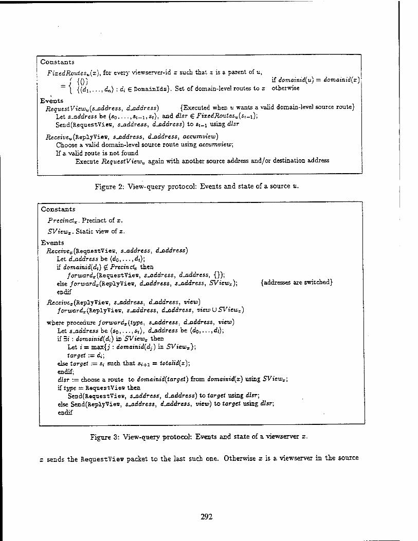
Constants

FixedRoutesu(z), for every viewserver-id r such that 2 is a parent of u, < sty. if domainid(u) = domainid(x)

~ 1 {{dj,..., dn) : di € Domainlds}. Set of domain-level routes to x otherwise

Events RequesiViewu(sj2ddress, djaddress) {Executed when v wants a valid domain-level source route}

Let s-address be (s0, -. .,Sj_i,s,}, and dlsr € FixedRoutesu{st-i); Send(RequestVies, s^iddress, djaddress) to st_i using dlsr

Receive^ (ReplyView, s-address, djaddress, accumview) Choose a valid domain-level source route using accumview; If a valid route is not found

Execute RequestViewu again with another source address and/or destination address

Figure 2: View-query protocol: Events and state of a source u.

Constants

Prccincls. Precinct of x.

SVieuix. Static view of x.

Events Receive-(RequestVies, s-address, djaddress)

Let d-address be (do,..., d<); if domainid(di) £ Precinct^ then

forwards (Request Vies, s-address, d-address, {}); else /oru;ard=(ReplyVies, djaddress, s-address, SViewx); {addresses are switched} endif

Receive^(ReplyVies, sjaddress, d-address, view) /oru;crd-(ReplyVies, sjaddress, djaddress, viewUSView-)

where procedure jorwards(lype. s-address, djaddress, view) Let sjaddress be (sD,...,Si}, djaddress be (d0,...,dj); if 3« : domainid(di) in SViews then

Let :'= max{j : domainid(dj) in SViews}; target := d,;

else target .— 5,- such that s,+i = iola/id(x)', endif; disr := choose a route to domainid(target) from (fomai"nid(i) using SVien^; if type = RequestView then

Send(RequestVies, sjaddress, djaddress) to tarpei using dlsr; else Send(ReplyVies, s-address, djaddress, view) to tarpel using dlsr; endif

Figure 3: View-query protocol: Events and state of a viewservei x.

x sends the RequestView packet to the last such one. Otherwise x is a viewserver in the source

292

address and sends the packet to its parent in the source address. (Note that if x is a viewserver in

the destination address, its child in the destination address is definitely in its view.)

When a viewserver x receives a Reply View packet, it merges its view to the accumulated view

in the packet. Then it sends the ReplyView packet towards the source node same way it would

send a RequestView packet towards the destination node (i.e. the role of the source address and

the destination address are changed).

Above we have described one possible way of obtaining the accumulated views. There are

various other possibilities, for example: (1) restricting the ReplyView packet to take the reverse

of the path that the RequestView packet took; (2) having ReplyView packets go all the way

up in the viewserver-hierarchy for a richer accumulated view; (3) source polling the viewservers

directly instead of viewservers forwarding request/reply messages to each other; (4) not including

the non-transit stub domains other than the source and the destination domains in the accumview;

(5) including some source policy constraints and ToS requirements in the RequestView packet,

and having the viewservers filter out some domains.

4 Update Protocol for Dynamic Network Conditions

In this section, we first examine how topology changes such as link/node failures, repairs, and cost

changes, map into domain-level topology changes. Second, we describe how domain-level topology

changes are detected and communicated to viewservers, i.e. view-update protocol. Third, we modify

the view-query protocol appropriately.

Mapping Topology Changes to Domain-Level Topology Changes

Costs are associated with domain-level edges. The cost of the domain-level edge (AtB) equals a

vector of values if the link is up; each cost value indicates how expensive it is to cross domain A

to reach domain JB according to some criteria such as delay, throughput, reliability, etc. The cost

equals cc if all links from A to B are down19. Each cost value of a domain-level edge (A,B) can

be derived from the cost values of the intra-domain routes in A and links from A to B [4]20.

18 Note that if a gateway connecting A to B is down, its links are also considered to be down. 20 For example, the delay of a domain-level edge (A, B) can be calculated as the maximum/average delay of the

rontes from any gateway in A to first gateway in B.

293

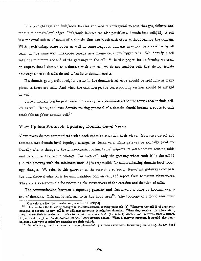
Link cost changes and link/node failures and repairs correspond to cost changes, failures and

repairs of domain-level edges. Link/node failures can also partition a domain into cells[15]. A cell

is a maximal subset of nodes of a domain that can reach each other without leaving the domain.

With partitioning, some nodes as well as some neighbor domains may not be accessible by all

cells. In the same way, link/node repairs may merge cells into bigger cells. We identify a cell

with the TTUTurrm-m node-id of the gateways in the cell. 21 In this paper, for uniformity we treat

an unpartitioned domain as a domain with one cell; we do not consider cells that do not isolate

gateways since such cells do not affect inter-domain routes.

If a domain gets partitioned, its vertex in the domain-level views should be split into as many

pieces as there are cells. And when the cells merge, the corresponding vertices should be merged

as well.

Since a domain can be partitioned into many cells, domain-level source routes now include cell-

ids as well. Hence, the intra-domain routing protocol of a domain should include a route to each

reachable neighbor domain cell.22

View-Update Protocol: Updating Domain-Level Views

Viewservers do not communicate with each other to maintain their views. Gateways detect and

communicate domain-level topology changes to viewservers. Each gateway periodically (and op-

tionally after a change in the intra-domain routing table) inspects its intra-domain routing table

and determines the cell it belongs. For each cell, only the gateway whose node-id is the cell-id

(i.e. the gateway with the miTn-mn-m node-id) is responsible for communicating domain-level topol-

ogy changes. We refer to this gateway as the reporting gateway. Reporting gateways compute

the domain-level edge costs for each neighbor domain cell, and report them to parent viewservers.

They are also responsible for informing the viewservers of the creation and deletion of cells.

The communication between a reporting gateway and viewservers is done by flooding over a

set of domains. This set is referred to as the flood area23. The topology of a flood area must

21 Our cells are like the domain components of IDPB-[13]. 22 This involves the following changes in the intra-domain routing protocol: (1) Whenever the cell-id of a gateway

changes, it reports its new cell-id to adjacent gateways is neighbor domains. When they receive this information, they npdate their intra-domain routes to include the new cell-id. (2) Usually when a node recovers from a failure, it qneries its neighbors in its domain for their intra-domain routes. When a gateway recovers, it should also qnery adjacent gateways in neighbor domains for their cell-ids.

23 For efficiency, the flood area can be implemented by a radius and some forwarding limits (e.g. do not flood

294

be a connected graph. Due to the nature of flooding, a viewserver can receive information out of

order for a domain cell. In order to avoid old information replacing new information, each gateway

includes successively increasing time stamps in the messages it sends.

Due to node and link failures, communication between a reporting gateway and a viewserver

can fail, resulting in the viewserver having out-of-date information. To eliminate such information,

a viewserver deletes any information about a domain cell if it is older than a time-to-die period. We

assume that gateways send messages more often than the time-to-die value (to avoid false removal).

When a viewserver learns of a new domain cell, it adds it to its view. To avoid adding a domain

cell which was just deleted24, when a viewserver receives a delete domain cell request, it only marks

the domain cell as deleted (and removes the entry after the time-to-die period).

The view-update protocol uses two types of messages as follows:

• (UpdateCell, domainid, cellid, timestamp, floodarea, ncostset)

is sent by the reporting gateway to inform the viewservers about current domain-level edge

costs of its cell. Here, domainid, cellid, and timestamp indicate the domain, the cell and the

time stamp of the reporting gateway, ncostset contains a cost for each neighbor domain cell,

and floodarea is the set of domains that this message is to be sent over.

• (DeleteCell, domainid, cellid, timestamp, floodarea)

where the parameters are as in the UpdateCell message. It is sent by a reporting gateway

when it becomes non-reporting (because its cell expanded to include a gateway with lower

id), to inform viewservers to delete the gateway's old cell.

The state maintained by a gateway g is listed in Figure 4. Note that LocalViewserverss and

LocalGatewaySg can be empty. IntraDomainRTs contains a route (next-hop or source) for every

reachable node of the domain and for every reachable neighbor domain cell25. We assume that

consecutive reads of Clockg returns increasing values.

The state maintained by a viewserver x is listed in Figure 5. DViewx is the dynamic part of

x's view. For each domain cell26 known to x, DViewx stores a timestamp field which equals the

beyond backbones) instead of a. set. 24 If the domain cell was removed, the timestamp for that domain cell is also lost. 2i IntraDomainBTg is a view in case of a link-state routing, protocol or a distance table in case of a distance-vector

routing protocol. 26 We use A:g to denote the cell g of domain. A.

295

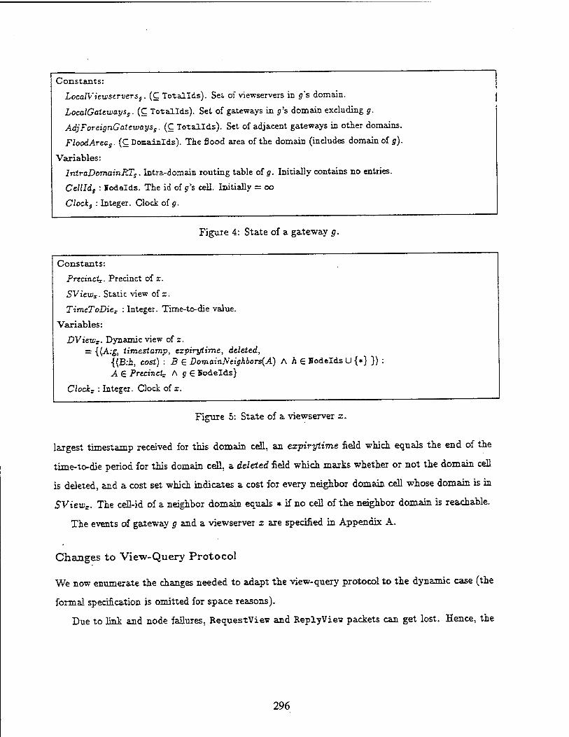
Constants:

LocalViewscrveTss. (C Totallds). Set of viewservers ID g's domain.

LocalGalewayss. (C Totallds). Set of gateways in p's domain excluding g.

AdjForeignGatewayss. (C Totallds). Set of adjacent gateways in other domains.

FloodArtCg. (C Domainlds). The flood area of the domain (includes domain of g).

Variables:

IntraDomainRTg. Intra-domain routing table of g. Initially contains no entries.

Cellldg : lodelds. The id of g's cell. Initially = oo

Clocks : Integer. Clock of g.

Figure 4: State of a gateway g.

Constants:

PrecincL. Precinct of x.

SViewx. Static view of x.

TimeToDieT : Integer. Time-to-die value.

Variables:

DViews. Dynamic view of x. = {(A:g, timestamp, ezpirytime, deleted,

{{B:h, cost) : B € DomainNeighbors(A) A he Hodelds U {*} }) : A 6 PrecincU A g € Bodelds}

Clockz : Integer. Clock of x.

Figure 5: State of a viewserver x.

largest timestamp received for this domain cell, an expirytime field which equals the end of the

time-to-die period for this domain cell, a deleted field which marks whether or not the domain cell

is deleted, and a cost set which indicates a cost for every neighbor domain cell whose domain is in

SViews. The cell-id of a neighbor domain equals * if no cell of the neighbor domain is reachable.

The events of gateway g and a viewserver x are specified in Appendix A.

Changes to View-Query Protocol

We now enumerate the changes needed to adapt the view-query protocol to the dynamic case (the

formal specification is omitted for space reasons).

Due to link and node failures, RequestView and ReplyViey packets can get lost. Hence, the

296

source may never receive a ReplyVie« packet after it initiates a request. Thus, the source should

try again after a time-out period.

When a viewserver receives a RequestView message, in the static case it replies with its view

if the destination domain is in its precinct. Now, because domain-level edges can fail, it must also

check its dynamic view and reply with its views only if its dynamic view contains a path to the

destination. Similarly during forwarding of RequestView and ReplyViev packets, a viewserver,

while checking whether a domain is in its view, should also check if its dynamic view contains a

path to it.

Finally, when a viewserver sends a message to a node whose domain is partitioned, it should

send a copy of the message to each cell of the domain. This is because a viewserver does not know

which cell contains the node.

5 Evaluation

Many inter-domain routing protocols have been proposed, based on various kinds of hierarchies.

How do these protocols compare against each other and against the simple approach? To answer this

question, we need a model in which we can define internetwork topologies, policy/ToS constraints,

inter-domain routing hierarchies, and evaluation measures (e.g. memory and time requirements)

for inter-domain routing protocols.

In this section, we first present such a model, and then use the model to evaluate our viewserver

hierarchy and compare it to the simple approach. Our evaluation measures are the amount of

memory required at the source and at the routers, the amount of time needed to construct a path,

and the number of paths found out of the total number of valid paths.

Even though the model described here can be applied to other inter-domain routing protocols,

we have not done so, and hence have not compared them against our viewserver hierarchy. This

is because of lack of time, and because precise definitions of the hierarchies in these protocols is

not available. For example, to do a fair evaluation of IDPIt[13], we need precise guidelines for

how to group domains into super-domains, and how to choose between the union and intersection

methods when defining policy/ToS constraints of super-domains. In fact, these protocols have not

been evaluated in a way that we can compare them to the viewserver hierarchy. To the best of our

knowledge, this paper is the first to evaluate a hierarchical inter-domain routing protocol against

297

explicitly stated policy constraints.

5.1 Evaluation Model

We first describe our method of generating topologies and policy/ToS constraints. We then describe

the evaluation measures.

Generating Internetwork Topologies

For our purposes, an internetwork topology is a directed graph where the nodes correspond to

domains and the edges correspond to domain-level connections. However, an arbitrary graph will

not do. The topology should have the characteristics of a real internetwork, like the Internet. That

is, it should have backbones, regionals, MANS, LANS, etc.; these should be connected hierarchically

(e.g. regionals to backbones), but "non-hieraxchical" connections (e.g. "back-doors") should also

be present.

For brevity, we refer to backbones as class 0 domains, regionals as class 1 domains, metropolitan-

area domains and providers as class 2 domains, and campus and local-area domains as class 3

domains. A (strictly) hierarchical interconnection of domains means that class 0 domains are

connected to each other, and for i > 0, class i domains are connected to class i — 1 domains.

As mentioned above, we also want some "non-hierarchical" connections, i.e., domain-level edges

between domains irrespective of their classes (e.g. from a campus domain to another campus

domain or to a backbone domain).

In reality, domains span geographical regions and domain-level edges are usually between do-

mains that are geographically close (e.g. University of Maryland campus domain is connected to

SURANET regional domain which is in the east cost). A class t domain usually spans a larger

geographical region than a class i + 1 domain. To generate such interconnections, we associate a

"region" attribute to each domain. The intention is that two domains with the same region are

geographically close.

The region of a class i domain has the form ro.xi. ••• .rj., where the r/s are integers. For

example, the region of a class 3 domain can be 1.2.3.4. For brevity, we refer to the region of a

class i domain as a class i region.

Note that regions have their own hierarchy. Class 0 regions are the top level regions. We say

298

thai a class i region ro-rj. • • • .rj is contained in the class i — 1 region ro-ri. • • • .Xi_i (where i > 0).

Containment is transitive. Thus region 1.2.3.4 is contained in regions 1.2.3, 1.2 and 1.

Figure 6: Regions

Given any pair of domains, we classify them as local, remote or far, based on their regions.

Let AT be a class i domain and Y a class j domain, and (without loss of generality) let i < j.

X and Y axe local if they are in the same class : region. For example in Figure 6, A is local to

B, C, J, K, M,N,0, P, and Q. X and Y are remote if they axe not in the same class i region but

they are in the same class : — 1 region, or if i = 0. For example in Figure 6, some of the domains

A is remote to are D, E, F, and L. X and Y are far if they are not local or remote. For example

in Figure 6, .4 is far to J.

We refer to a domain-level edge as local (remote, or far) if the two domains it connects are local

299

(remote, or far).

We use the following procedure to generate internetwork topologies:

• We first specify the number of domain classes, and the number of domains in each class.

• We next specify the regions. Note that the number of region classes equals the number of

domain classes. We specify the number of class 0 regions. For each class i > 0, we specify a

branching factor, which creates that many class i regions in each class i - 1 region. (That is,

if there are two class 0 regions and the class 1 branching factor equals three, then there are

six class I regions.)

• For each class i, we randomly map the class : domains into the class i regions. Note that

several domains can be mapped to the same region, and some regions may have no domain

mapped into them.

• For every class i and every class j, j > i, we specify the number of local, remote and far

edges to be introduced between class :' domains and class j domains. The end points of the

edges are chosen randomly (within the specified constraints).

We ensure that the internetwork topology is connected by ensuring that the subgraph of class

0 domains is connected, and each class i domain, for i > 0, is connected to a local class i - 1

domain.

Choosing Policy/ToS Constraints

We chose a simple scheme to model Policy/ToS constraints. Each domain is assigned a color: green

or red. For each domain class, we specif}' the percentage of green domains in that class, and then

randomly choose a color for each domain in that class.

A valid route from a source to a destination is one that does not visit any red intermediate do-

mains; the source and destination are allowed to be red. Notice that this models transit policy/ToS

constraints. We are working on extending this model to source policy/ToS constraints.

Computing Evaluation Measures

The evaluation measures of most interest for an inter-domain routing protocol are its memory and

time requirements, and the number of valid paths it finds (and their lengths) in comparison to

the number of available valid paths (and their lengths) in the internetwork (e.g. could it find the

300

shortest valid path in the internetwork).

The only analysis method we have at present is to numerically compute the evaluation measures

for a variety of source-destination pairs. Because we use internetwork topologies of large sizes, it is

not feasible to compute for all possible source-destination pairs. We randomly choose a set of source-

destination pairs that satisfy the following conditions: (1) the source and destination domains are

different, and (2) there exists a valid path from the source domain to the destination domain in

the internetwork topology. (Note that the simple scheme would always find such a path.)

For a source-destination pair, we refer to the length of the shortest valid path in the internetwork

topology as the shortest-path length. Since the number of paths between a source-destination pair

is potentially very large (factorial in the number of domains), and we are not interested in the

paths that are too long, we only count the number of paths whose lengths are not more than the

shortest-path-length plus 2.

The evaluation measures described above are protocol independent. However, there are also

important evaluation measures that are protocol dependent (e.g. number of levels traversed in

some particular hierarchy). Because of this we postpone the precise definitions of the evaluation

measures to the next subsection (their definition is dependent of viewserver hierarchy).

5.2 Application to Viewserver Protocol

We have used the above model to evaluate our viewserver protocol for several different viewserver

hierarchies and query methods. We first describe the different viewserver schemes evaluated. Please

refer to Figure 6 in the following discussion.

The first viewserver scheme is referred to as base. It has exactly one viewserver in each domain.

Each viewserver is identified by its domain-id. The domains in a viewserver's precinct consist of

its domain and the neighboring domains. The edges in the viewserver's view consist of the edges

between the domains in the precinct, and edges outgoing from domains in the precinct to domains

not in the precinct. For example, the precinct of viewserver A (i.e. the viewserver in domain A)

consists of domains A,B, J; the edges in the view of viewserver A consists of domain-level edges

(A, J?), (A, J), (J?, J), (J, M), (J, if), (J, n and (J, D).

As for the viewserver hierarclry, a viewserver's level is defined to be the class of its domain. That

is, a viewserver in a class i domain is a level i viewserver. For each level i viewserver, i > 0, its

301

parent viewserver is chosen randomly from the level: - 1 viewservers in the parent region such that

there is a domain-level edge between the viewserver's domain and the parent viewserver's domain.

For example, for viewserver C, we can pick viewserver J or K\ suppose we pick J. For viewserver

J, we have no choice but to pick M (N and O are not connected to J). For M, we pick P (out of

P and Q).

We use only one address for each domain. The viewserver-address of a stub domain is con-

catenation of four viewserver (i.e. domain) ids. Thus, the address of A is P.M.J.A. Similarly, the

address of E is P.M.K.E. To obtain a route between A and M, it suffices to obtain views of

viewservers A, J, K, H.

The second viewserver scheme is referred to as base-QT (where the QT stands for "query upto

top"). It is identical to base except that during the query protocol all the viewservers in the source

and the destination addresses are queried. That is, to obtain a route between A and H, the views

of A, J,M,P,K,E are obtained.

The third viewserver scheme is referred to as locals. It is identical to base except that now a •

viewserver's precinct also contains domains that have the same region as the viewserver's domain.

That is, the precinct of viewserver A has the domains A,B,J,C. Note that in this scheme a

viewserver's view is not necessarily connected. For example, if the edge (C, J) is removed, the view

of viewserver A is no longer connected. (In Section 3, we said that the view of a viewserver should

be connected. Here we have relaxed this condition to simplify testing.)

The fourth viewserver scheme is referred to as locals-QT. It is identical to locals except that

during the query protocol all the viewservers in the source and the destination addresses are queried.

The fifth viewserver scheme is referred to as vertex-extension. It is identical to base except

that viewserver precincts are extended as follows: Let P denote the precinct of a viewserver in the

base scheme. For each domain X in P, if there is an edge from domain X to domain Y and Y

is not in P, domain Y is added to the precinct; among Y"'s edges, only the ones to domains in P

are added to the view. In the example, domains M, K, F, D are added to the precinct of A, but

outgoing edges of these domains to other domains are not included (e.g. (F, G) is not included).

The advantage of this scheme is that even though it increases the precinct size by a factor which

is potentially greater than 2, it increases the number of edges stored in the view by a factor less

than 2. (In fact, if the same edge cost and edge policies are used for both directions of domain-

302

level edges, then the only other information that needs to be stored by the viewservers is the policy

constraints of the newly added domains.)

The sixth viewserver scheme is referred to as full-QT. It is constructed in the same way as

vertex-extension except that the locals scheme is used instead of base scheme to define the P in

the construction. In full-QT, during the query protocol all the viewservers in the source and the

destination addresses are queried.

In all the above viewserver schemes, we have used the same hierarchy for both domain classes

and viewservers. In practice, not all domains need to have a viewserver, and a viewserver hierarchy

different from the domain class hierarchy can be deployed. However, there is an advantage of

having a viewserver in each domain; that is, source nodes do not require fixed domain-level source

routes to their parent viewservers (in the view-query protocol). This reduces the amount of hand

configuration required. In fact, the base scheme does not require any hand configuration, viewservers

can decide their precincts from the intra-domain routing tables, and nodes can use intra-domain

routes to reach parent viewservers.


The parameters of the first internetwork topology, referred to as Internetwork 1, are shown in

Table 1.

Our evaluation measures were computed for a (randomly chosen but fixed) set of 1000 source-

destination pairs. For brevity, we use spl to refer to the shortest-path length (i.e. the length of

the shortest valid path in the internetwork topology). The mi-nimmn spl of these pairs was 2, the

maximum spl was 13, and the average spl was 6.8. Table 2 lists for each viewserver scheme (1) the

rninimum, average and maximum precinct sizes, (2) the minrrrmm, average and maximum merged

view sizes, and (3) the minimum, average and maximum number of viewservers queried.

The precinct size indicates the memory requirement at a viewserver. More precisely, the memory

requirement at a viewserver is 0 (precinct size x d) where d is the average number of neighbor

domains of a domain, except for the vertex-extension and full-QT schemes. In these schemes, the

memory requirement is increased by a factor less than two. Hence the vertex-extension scheme has

the same order of viewserver memory requirement as the base scheme and the full-QT scheme has

27 Branching factor is 4 for all region classes.

303

Class j No. of Domains No. of Regions27 % of Green Domains Edges between Classes : and j i i

Class j | Local Remote | Far |

0 10 4 0.80 0 8 6 0

1 100 16 0.75 0 190 20 0

1 26 5 0

2 1000 64 0.70 0 100 0 0

1 1060 40 0

2 200 40 0

3 10000 256 0.20 0 100 0 0

1 100 0 0

2 10100 50 0

3 50 50 50



base 2 / 3.2 / 68 7 / 71.03 / 101 3 / 7.51 / 8

base-QT 2 / 3.2 / 68 30 / 76.01 / 101 8 / 8.00 / 8

locals 2 / 52.0 / 103 3 / 95.40 / 143 2 / 7.42 / 8

locals-QT 2 / 52.0 / 103 43 / 101.86 / 143 8 / 8.00 / 8


jull-QT 11 / 102.9 / 796 228 / 396.80 / 519 8 / 8.00 / 8

Table 2: Precinct sizes, merged view sizes, and number of viewservers queried for Internetwork 1.

the same order of viewserver memory requirement as the locals scheme.

The merged view size indicates the memory requirement at a source; i.e. the memory require-

ment at a source is 0(merged view size x d) except for the vertex-extension and full-QT schemes.

Note that the source does not need to store information about red and non-transit domains. The

numbers in Table 2 take advantage of this.

The number of viewservers queried indicates the communication time required to obtain the

merged view at the source. Because the average spl is 6.8, the "real-time" communication time

304

required to obtain the merged view at a source is slightly more than one round-trip time between

the source and the destination.

As is apparent from Table 2, using a QT scheme increases the merged view size and the number

of viewservers queried only by about 5%. Using a locals scheme increases the merged view size

by about 30%. Using the vertex-extension scheme increases the merged view size by 5 times (note

that the amount of actual memory needed increases only by a factor less than 2). The number of

viewservers queried in the locals scheme is less than the number of viewservers queried in the base

scheme. This is because the viewservers in the locals scheme have bigger precincts, and a path from

the source to the destination can be found using fewer views.

Table 3 shows the average number of spl, spl + 1, spl + 2 length paths found for a source-

destination pair by the simple approach and by the viewserver schemes. All the viewserver schemes

are very close to the simple approach. The vertex-extension and full-QTschemes are especially close

(they found 98% of all paths). Table 3 also shows the number of pairs for which the viewserver

schemes did not find a path (ranging from 1.4% to 5.9% of the source-destination pairs), and

the number of pairs for which the viewserver schemes found longer paths. For these pairs, more

viewserver addresses need to be tried. Note that the locals and vertex-extension schemes decrease the

number of these pairs substantially (adding QTyields further improvement). Our policy constraints

are source and destination domain independent. Hence, even a class 2 domain, if it is red, can not

carry traffic to a class 3 domain to which it is connected. We believe that these figures would

improve with policies that are dependent on source and destination domains.

As is apparent from Table 3 and Table 2, the locals scheme does not find many more extra

paths than the base scheme even though it has larger precinct and merged view sizes. Hence it is

not recommended. The vertex-extension scheme is the best, but even base is adequate since it finds

many paths.

We have repeated the above evaluations for two other internetworks and obtained similar con-

clusions. The results are in Appendix B.

6 Concluding Remarks

We presented hierarchical inter-domain routing protocol that (1) satisfies policy and ToS con-

straints, (2) adapts to dynamic topology changes including failures that partition domains, and

305

Scheme

Numl

spl

er of paths found

spl + 1 spl+ 2

No. of pairs

with no path

No. of pairs

with longer paths

simple 2.51 18.48 131.01 N/A N/A

base 2.41 15.84 99.42 59 3 by 1.33 hops

base-QT 2.41 15.86 200.16 54 3 by 1.33 hops

locals 2.41 16.17 103.54 29 3 by 1 hop

locals-QT 2.41 16.29 105.02 20 3 by 1 hop

vertex- extension 2.51 18.38 128.19 22 0 by 0 hops

fvll-QT 2.50 18.40 128.90 14 0 by 0 hops

Table 3: Number of paths found for Internetwork 1.

(3) scales well to large number of domains.

Our protocol uses partial domain-level views to achieve scaling in space requirement. It floods

domain-level topological changes over a flood area to achieve scaling in communication requirement.

It does not abstract domains into superdomains; hence it does not lose any domain-level detail

in ToS and policy information. It merges a sequence of partial views to obtain domain-level source

routes between nodes which are far away. The number of views that need to be merged is bounded

by twice the number of levels in the hierarchy.

To evaluate and compare inter-domain routing protocols against each other and against sim-

ple approach, we presented a model in which one can define internetwork topologies, policy/ToS

constraints, inter-domain routing hierarchies, and evaluation measures. We applied this model to

evaluate our viewserver hierarchy and compared it to the simple approach. Our results indicate

that viewserver hierarchy finds many short valid paths and reduces the amount of memory require-

ment by two order of magnitude.

Our protocol recovers from fail-stop failures of viewservers and gateways. When a viewserver

fails, an address which includes'the viewserver's id becomes useless. This deficiency can be overcome

by replicating each viewserver at different nodes of the domain (in this case a viewserver fails only

if all nodes implementing it fail}. This replication scheme requires viewserver ids to be independent

of node ids, which can be easily accomplished28.

28 Foi «ample, if node-ids of nodes implementing a viewserver share a preß*, this preftx can be used as the

306

The only drawback of our protocol is that to obtaic a domain-level source route, views are

merged at (or prior to) the connection (or flow) setup, thereby increasing the setup time. This

drawback is not unique to our scheme [8, 13, 6, 10].

There are several ways to reduce the setup overhead. First, domain-level source routes to fre-

quently used destinations can be cached. The cacheing period would depend on the ToS require-

ment of the applications and the frequency of domain-level topology changes. For example, the

period can be long for electronic mail since it does not require shortest paths.

Second, views of frequently queried viewservers can be replicated at "mirror" viewservers in the

source domain. A viewserver would periodically update the views of its mirror viewservers.

Third, connection setup also involves traversing the name server hierarchy (to obtain destination

addresses from its names). By integrating the name server hierarchy with the viewserver hierarchy,

we may be able to do both operations simultaneously. This requires further investigation.

References [1] A.V. Aho, J.E. Hopcroft, and J.D. Ulman. The Design and Analysis of Computer Algorithms. Addison-

Wesley, 1974. [2] C Alaettinoglu and A. U. Shankar. Hierarchical Inter-Domain Routing Protocol with On-Deinand

ToS and Poicy Resolution. In Proc. IEEE International Conference on Networking Protocok '9S, San Fransisco, California, October 1993.

[3] C. Alaettinoglu and A. U. Shankar. Viewserver Hierarchy: A Scalable and Adaptive Inter-Domain Routing Protocol. Technical Report UM1ACS-TR-93-13, CS-TR-3033, Department of Computer Sci- ence, University of Maryland, College Park, February 1993.

[4] A. Bar-Noy and M. Gopal. Topology Distribution Cost vs. Efficient Routing in Large Networks. In Proc. ACM SIGCOMM '90, pages 242-252, Philadelphia, Pennsylvania, September 1990.

[5] L. Breslau and D. Estrin. Design of Inter-Administrative Domain Routing Protocols. In Proc. ACM SIGCOMM '90, pages 231-241, Philadelphia, Pennsylvania, September 1990.

[6] J. N. Chiappa. A New IP Routing and Addressing Architecture. Big-Internet mailing list., 1992. Available by anonymous ftp fromsmnnari.oz.an:big-iateriiet/list-axcfci.ve.

[7] D. Clark. Route Fragments, A Routing Proposal. Big-Internet mailing list., July 1992. Available by anonymous ftp from jirajmaxi.oz.au:big-intexnet/list-arch.ive.

[8] D.D. Clark. Policy routing in Internet protocols. Request for Comment RFC-1102, Network Information Center, May 1989.

[9] D. Estrin. PoEcy requirements for inter Aclministrative Domain routing. Request for Comment RFC- 1125, Network Information Center, November 1989.

[10] D. Estrin, Y. Rekhter, and S. Hotz. Scalable Inter-Domain Routing Architecture. In Proc. ACM SIGCOMM '92, pages 40-52, Baltimore, Maryland, August 1992.

viewserver id. lntra-domain routing would forward a packet destined to a. viewserver to any operational node with this prefix.

307

[11] F. Kamoun and L. Kleinrock. Stochastic Performance Evaluation of Hierarchical Routing for Large Networks. Computer Networks and ISDN Systems, 1979.

fl2l B.M. Leiner. Policy issues in interconnecting networks. Request for Comment RFC-1124, Network Information Center, September 1989.

[13] M. Lepp and M. Steenstrup. An Architecture for Inter-Domain Policy Routing. Internet Draft. Available from the authors., June 1992.

[14] K. Lougheed and Y. Rekhter. Border Gateway Protocol (BGP). Request for Comment RFC-1105, Network Information Center, June 1989.

[15] R. Perlman. Hierarchical Networks and Subnetwork Partition Problem. Computer Networks and ISDN Systems, 9:297-303, 1985.

[16] Y. Rekhter. Inter-Domain Routing Protocol (IDRP). Available from the author., 1992. T.J. Watson Research Center, IBM Corp.

[17] K. G. Shin and M. Chen. Performance Analysis of Distributed Routing Strategies Free or Ping-Pong- Type Looping. IEEE Transactions on Computers, 1987.

[18] P. F. Tsuchiya. The Landmark Hierarchy: Description and Analysis, The Landmark Routing: Ar- chitecture Algorithms and Issues. Technical Report MTR-87W00152, MTR-87W00174, The MITRE Corporation, McLean, Virginia, 1987.

[19] P. F. Tsuchiya. The Landmark Hierarchy:A New Hierarchy For Routing In Very Large Networks. In Proc. ACM SIGCOMM '88, August 1988.

[20] P. F. Tsuchiya. Efficient and Robust Policy Routing Using Multiple Hierarchical Addresses. In Proc. ACM SIGCOMM '91, pages 53-65, Zurich, Switzerland, September 1991.

A View-Update Protocol Event Specifications

The events of gateway g are specified in Figure 7. When a gateway g recovers, Celllds is set to

nodeid(g). Thus, when g next executes Updateg, it sends either an UpdateCell or a DeleteCell

message to viewservers, depending on whether it is no longer the minimum id gateway in its cell .

The events of a viewserver x are specified in Figure 5. Note that when x adds an entry to

DView- (upon receiving a UpdateCell message), it selectively chooses subset of neighbors from

the cost set in the packet to include only the neighbor domains which are in SView-. When

a viewserver x recovers, DViewx is set to {}. Its view becomes up-to-date as it receives new

information from reporting gateways (and remove false information with the time-to-die period).

29 Sending a DeleteCell message is essential. Because prior to the failure, g may have been the smallest id gateway in its cell. Hence, some viewserrer's may still contain an entry fox its old domain cell.

308

Updattg {Executed periodically and also optionally upon a change in IntraDomainRTs} {Determines the id of p's cell and initiates UpdateCell and DeleteCell messages if needed.} 01dCellId = CellIdg; Celllds := compute cell id using LocalGateways} and IntraDomainRTg; if nodeid(g) = Celllds then

ncostset := compute costs for each neighbor domain cell using IntraDomainRTg; floods((UpdateCell, domainid(g), Cellldgt Clockg, FloodAreas,ncostset));

endif if nodtid(g) = OldCellId±CelUdg then

floodg ((DeleteCell, domainid(g), nodeid(g), Clocks, Flood Area g))\ endif

Receives (packet) {either an UpdateCell or a DeleteCell packet} floods(packet)

where procedure floodg(packet) if domainid(g) £ packet.floodarea then

{remove domain of g from the flood area to avoid infinite exchange of the same message.} packet.floodarea := packet.floodarea — {domainid(g)}; for all h £ LocalGatewaysg U LocalViewserversg do

Send(packet) to h using {); endif for all h £ AdjForeignGatewaySg A domainid(h) £ packet.floodarea do

Send(packet) to h;

Gateway Failure Model: A gateway can undergo failures and recoveries at anytime. We assume failures are fail-stop (i.e. a failed gateway does not send erroneous messages). When a gateway g recovers, Celllds

is set to nodeid(g).

Figure 7: View-update protocol: Events of a gateway p.

B Results for Other Internetworks


The parameters of the second internetwork topology, referred to as Internetwork 2, are the same

as the parameters of Internetwork 1 (a different seed is used for the random number generation).

Our evaluation measures were computed for-a set of 1000 source-destination pairs. The mini-

mum spl of these pairs was 2, the maximum spl was 13, and the average spl was- 7.2.

Table 4 and Table 5 shows the results. Similar conclusions to Internetwork 1 hold for Internet-

work 2. In Table 5. the reason that local and QT schemes have more pairs with longer paths than

the base scheme is that these schemes found some paths (which are not shortest) for some pairs for

which the base scheme did not find any path.

309

■Receiver(UpdateCell, did, cid, ts, FloodArea, ncset) if did € Precincts then

if 3(did:cid, timestamp, expirytime, deleted, ncostset) £ DViewx A ts > timestamp then {received is more recent; delete the old one}

delete {did:cid, timestamp, expirytime, deleted, ncostset) from DViewx; endif if -B{did:cid, timestamp, expirytime, deleted, ncostset) € DViewx then

Choose ncostset from ncset using SViewx; insert {did:cid, ts, Chckx + TimeToDiex, false, ncostset) to DViewx;

endif endif

Receivex(DeleteCell, did, cid, ts, floodarea) if did € Precinct* then

if 3(did:cid, timestamp, expirytime, deleted, ncostset) £ DViewx A ts > timestamp then {received is more recent; delete the old one}

delete (didxid, timestamp, expirytime, deleted, ncostset) from DViewx; endif if -3(did:cid, timestamp, expirytime, deleted, ncostset) € DViewx then

insert (did:cid, ts, Clock=-\-TimeToDiex, true, {}) to DViewx; endif

endif

Deletex {Executed periodically to delete entries older than the time-to-die period} for all {A:g, tstamp, expirytime, deleted, ncset) £ DViewx A expirytime < Clockx do

delete {A:g, tstamp, expirytime, deleted, ncset) from DViewx;

Viewserver Failure Model: A viewserver can undergo failures and recoveries at anytime. We assume failures are fail-stop. When a viewserver x recovers, DViewx is set to {}.

Figure 8: View update events of a viewserver x.


base 2 / 3.2 / 76 . 4 / 66.62 / 96 3 / 7.55 / 8

base-QT 2 / 3.2 / 76 29 / 72.76 / 96 8 / 8.00 / 8

locals 3 / 69.8 / 149 4 / 101.32 / 148 2 / 7.36 / 8

locals-QT 3 / 69.8 / 149 35 / 110.32 / 152 8 / 8.00 / 8


full-QT 11 / 135.2 / 817 186 / 402.51 / 503 8 / 8.00 / 8

Table 4: Precinct sizes, merged view sizes, and no of viewservers queried for Internetwork 2.


The parameters of the third internetwork topology, referred to as Internetwork 3, are shown in

Table 6. Internetwork 3 is more connected, more class 0, 1 and 2 domains are green, and more

310

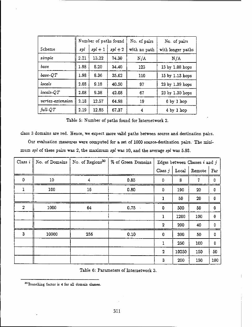
Scheme

Number of paths found

spl spl +1 spl + 2

No. of pairs

■with no path

No. of pairs

with longer paths

simple 2.21 13.22 74.30 N/A N/A

base 1.98 8.20 34.40 123 13 by 1.08 hops

base-QT 1.98 8.36 35.62 110 15 by 1.13 hops

locals 2.08 9.18 40.50 97 23 by 1.39 hops

locals-QT 2.08 9.38 42.08 67 23 by 1.30 hops

vertex-extension 2.18 12.57 64.98 19 6 by 1 hop

full-QT 2.19 12.85 67.37 4 4 by 1 hop


class 3 domains are red. Hence, we expect more valid paths between source and destination pairs.

Our evaluation measures were computed for a set of 1000 source-destination pairs. The mini-

mum spl of these pairs was 2, the maximum spl was 10, and the average spl was 5.93.

Class i No. of Domains No. of Regions30 % of Green Domains Edges between Classes i and j


0 10 4 0.85 0 8 7 0

1 100 16 0.80 0 190 20 0

1 50 20 0

2 1000 64 0.75 0 500 50 0

1 1200 100 0

2 200 40 0

3 10000 256 0.10 0 300 50 0

1 250 100 0

2 10250 150 50

3 200 150 100


'Branching factor is 4 for all domain classes.

311

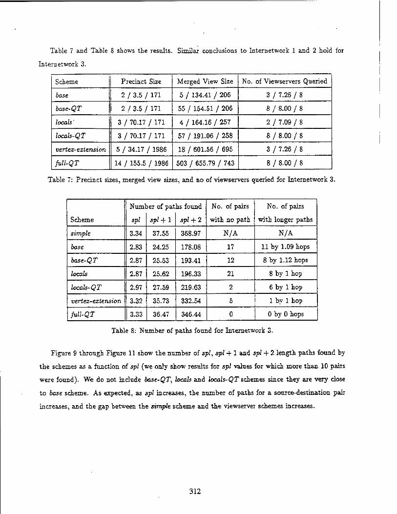
Table 7 and Table 8 shows the results. Similar conclusions to Internetwork 1 and 2 hold for

Internetwork 3.


base 2 / 3.5 / 171 5 / 134.41 / 206 3 / 7.26 / 8

base-QT 2 / 3.5 / 171 55 / 154.51 / 206 8 / 8.00 / 8

locals' 3 / 70.17 / 171 4 / 164.16 / 257 2 / 7.09 / 8

locals-QT 3 / 70.17 / 171 57 / 191.06 / 258 8 / 8.00 / 8


full-QT 14 / 155.5 / 1986 503 / 655.79 / 743 8 / 8.00 / 8

Table 7: Precinct sizes, merged view sizes, and no of viewservers queried for Internetwork 3.

Scheme

Numl

spl

)er of pat

spl+1

b.s found

spl + 2

No. of pairs

with no path

No. of pairs

with longer paths

simple 3.34 37.55 368.97 N/A N/A

base 2.83 24.25 178.08 17 11 by 1.09 hops

base-QT 2.87 25.53 193.41 12 8 by 1.12 hops

locals 2.87 25.62 196.33 21 8 by 1 hop

locals-QT 2.97 27.59 219.63 2 6 by 1 hop

vertex- extension 3.32 35.73 332.54 5 1 by 1 hop

full-QT 3.33 36.47 346.44 0 0 by 0 hops


Figure 9 through Figure 11 show the number of spl, spl 4- 1 and spl + 2 length paths found by

the schemes as a function of spl (we only show results for spl values for which more than 10 pairs

were found). We do not include base-QT, locals and locals-QT schemes since they are very close

to base scheme. As expected, as spl increases, the number of paths for a source-destination pair

increases, and the gap between the simple scheme and the viewservei schemes increases.

312

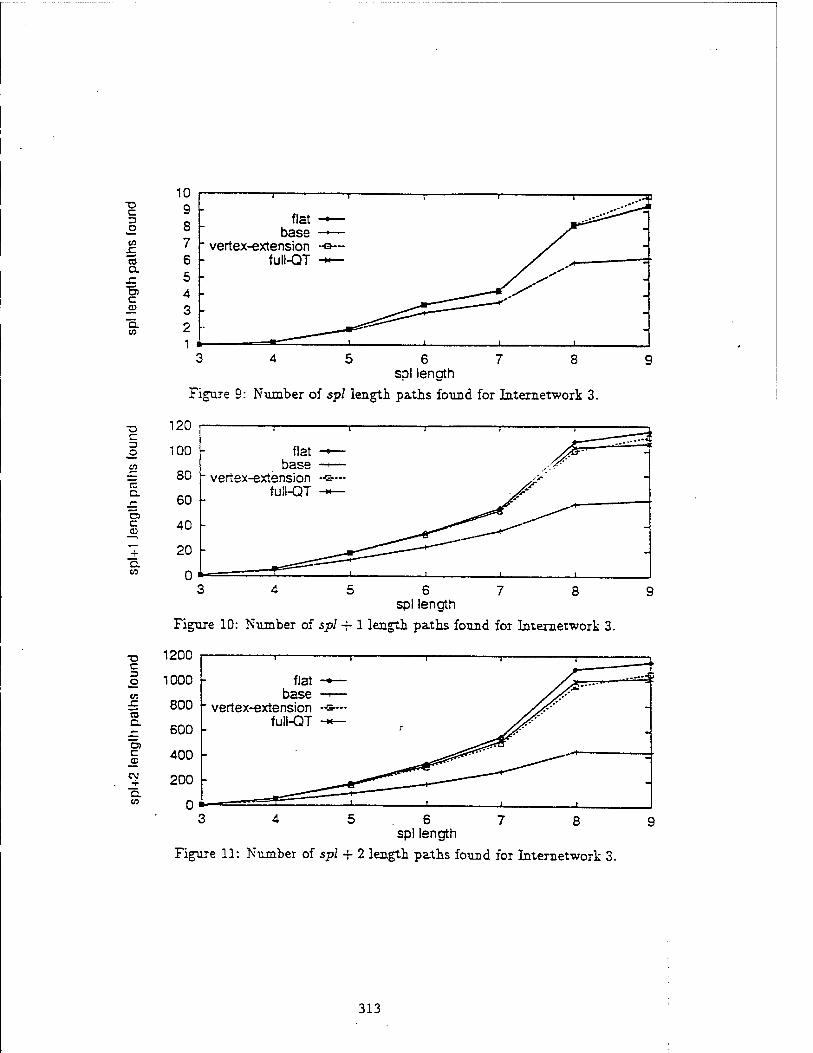
•© c 3 O CO

'S Q. .c B c

_a>

"5. CO

5 6 7 8 spl length

Figure 9: Number of spl length paths found for Internetwork 3.

c 3 O

c

o c 0>

c to

6 spl length

Figure 10: Number of spl -f-1 length paths found for Internetwork 3.

T5 C 3 O

CO c

c

CO -r D. CO

1200

5.6 7 8 spl length

Figure 11: Number of spl + 2 length paths found for Internetwork 3.

313






Viewserver Hierarchy: A New Inter-Domain Routing Protocol and its Evaluation

6. AUTHOR(S) Cengiz Alaettinoglu, and A. Udaya Shankar

5. FUNDING NUMNBERS

DASG-60-92-C-0055


9. SPONSORING/ MONITORING AGENCY NAME(S) AND ADDRESS(ES)|l PhillipsLaboratory Director of Contracting 3651 Lowry Avenue SE Kirtland AFB, NM 87117-5777







A simple approach to inter-domain routing is domain-level source routing with link-state approach where each node maintains a domain-level view of the internetwork. This does not scale up to large internetworks. The usual scaling tecnnique of aggregating domains into superdomains loses ToS and policy detail.

We present a new viewserver hierarchy and associated protocols that (1) satisfies policy and ToS constraints, (2) adapts to dynamic topology changes including failures that partition domains, and (3) scales well to large nuimber of dominas without losing detail. Domain-level views are maintained by special nodes called viewservers. Each viewserver maintains a domain-level view of surrounding precinct. Viewservers are organized hierarchically. To obtain domain-level source routes, the views of one or more viewservers are merged (upto a maximum of twice the levels in the hierarchy.

We also present a model for evaluating inter-domain routing protocols, and apply this model to compare our viewserver hierarchy against the simple approach . Our results indicate that the viewserver hierarchy finds many short valid paths and reduces the amount of memory requirement by two orders of magnitude.

14. SUBJECT TERMS Network Architecture and Design


Unclassified


Unclassified

15. NUMBER OF PAGES 33

16. PRICE CODE


Unclassified MSN 7540-01 280-5500


Unlimited


TEMPORAL ANALYSIS FOR HARD REAL-TIME SCHEDULING'

Manas C. Saksena and Ashok K. Agrawala

Department of Computer Science University of Maryland College Park, MD 20742

Abstract

Static time driven scheduling has been advocated for use in Hard Real-Time systems and is particularly appropriate for many embedded systems. The approaches taken for static scheduling often use search techniques and may reduce the search by using heuristics. In this paper we present a technique for analyzing the temporal relations among the tasks, based on non-preemptive schedulability. The relationships can be used effectively to reduce the average complexity of scheduling these tasks. They also serve as a basis for selective preemption policies for scheduling by providing an early test for infeasibility. We present examples and simulation results to confirm the usefulness of temporal analysis as a phase prior to scheduling.

1 Introduction

Many safety critical real-time applications like process control, embedded tactical systems for military applications, air- traffic control, robotics etc. have stringent timing constraints imposed on their computations due to the characteristics of the physical system. A failure to observe the timing constraints can result in intolerable system degradation and in some cases it may have catastrophic consequences.

Scheduling is the primary means of ensuring the satisfaction of timing constraints for such systems[l]. As a result, significant effort has been invested in research on hard real time scheduling [2, 3, 4]. In this paper we discuss a scheduling technique for static scheduling to guarantee timely execution of time critical tasks.

The time driven scheduling model is being used by many experimental systems, including MARS[5], MARUTI[6] and Spring Kernel[7]. The static time driven scheduling technique involves constructing a schedule offline, which may be represented as a Gantt chart[8] or calendar[6] (Figure 1). Tasks are invoked at run-time whenever they are scheduled to execute. Such a scheduling model is particularly appropriate for many embedded systems. Recent effort in this direction has shown the viability of such an approach for practical real-time applications)}?].

Ti T2 T3 T4

"This research was supported in part by ONR and DARPA under contract. N00014-91-C-0195.

Figure 1: Gantt Chart or Calendar

The intractability of most scheduling problems has led to approaches based on search techniques for scheduling of real- time tasks. The feasibility of a task set is determined through construction of a schedule; failure to construct a schedule denotes infeasibility. Heuristics are often used as a means of controlling the complexity of scheduling. In many cases, heuristics perform well enough to result in an acceptable solution.

There has been little emphasis on the use of analytic techniques to assist in time driven scheduling. Decomposition scheduling[10] based on dominance properties of sequences[ll] uses analytic techniques to decompose a set of tasks into a sequence of subsets. Significant reduction in average complexity can be achieved if the set of tasks can be decomposed into a large number of subsets, each having a small number of tasks.

In this paper, we present an analysis technique for time driven scheduling based on the timing requirements of tasks. The analysis results in the establishment of a set of temporal relations between pairs of tasks based on a non-preemptive scheduling model. These relations can be used by scheduling' algorithms to reduce the complexity of scheduling in the average case, and as an early test for infeasibility. As a. test for infeasibility, it provides a good basis for policies using selective preemption to enhance feasibility. When infeasibility is not detected, the temporal relations may be used by a search algorithm to effectively prune large portions of search space, thereby'controlling the cost of scheduling.

2 Time Driven Scheduling

The time driven scheduling approach constructs a calendar for the set of tasks in the system. The tasks may be scheduled preemptively or non-preemptively. The non-preemptive scheduling problem for a uniprocessor is known to be NP- Complete[12]. When the tasks are mutually independent, and can be preempted at any time, it is known, that the earliest deadline first policy is optimal[13] and obviates the need for non-preemptive scheduling. However, when tasks synchronize

315

using critical sections, the preemptive scheduling problem is also known to be intractable(NP-Hard)[14j.

In general, when the overhead of preemption is negligible, the non-preemptive solutions form a subset of preemptive solutions[8]. However, when tasks may interact with each other, the non-preemptive models are simpler, easier to implement and closer to reality[15]. They are also necessary for certain scheduling domains like I/O scheduling and provide a basis for selective preemption policies.

2.1 Task Model

We consider a set of n tasks T = {r,- : i = l,2,...,n} to be scheduled for execution on a single processor. Each task Ti, abbreviated as i, is a 3-tuple [r,-,Ci,d,-] denoting the ready time, computation time and deadline respectively. The time interval [ri,di\ is called the timing window wi of task r,-, and indicates the time interval during which the task can execute. The computation time of each task is less than the window length \wi\l. All tasks are assumed to be independent for simplicity of exposition even though such a requirement is not necessary for the analysis.

In a hard real-time system, processes may be periodic or sporadic [14]. Such a set of processes may be mapped to our scheduling model by techniques identified in [1, 14, 16] and constructing a schedule for the least common multiple of the periods of the tasks.

2.2 Non-Preemptive Scheduling Model

A non-preemptive schedule is the mapping of each task T,- in T to a start time s,-. The task is then scheduled to run without preemption in the time interval [«»,/,•], with its finish time being ft = st- + c,-. A feasible schedule is a schedule in which the following conditions are satisfied for each task r<:

n < si

ft < di (1)

(2)

It is useful to consider a non-preemptive schedule as an ordered sequence of the set of tasks. To get a maximally packed schedule from a sequence [T\,T2, .. .,Tn], we can recursively derive the start time s,- and finish time ft of the tasks as follows:

Si = maz(ri,/i_1)

ft = St + a (3) (4)

with «l = »"i

The scheduling problem can thus be considered as a search over the permutation space. A permutation (sequence) is feasible if the corresponding schedule is feasible. Notice that for any permutation schedule derived as above, equation 1 is implied by (3) and we only need to verify the deadline constraints for the tasks.

B

r 1 d

Figure 2: Infeasibility of task A executing before task B

3 Temporal Analysis

Temporal analysis uses pairwise schedulability analysis of tasks to generate a set of relations to eliminate sequences which cannot lead to feasible solutions. In this section we define the temporal relations and show how they may be derived from the timing constraints of tasks.

3.1 Definitions of Temporal Relations

Consider two tasks n and r;-. We wish to find out what we can say about the relative ordering of these tasks, given their timing constraints. A set of relations are identified below which identify the different, possibilities.

Precedence Relation: A precedence relation denoted as Ti —► Tj, implies that in any feasible schedule r,- must execute before r;-.

Infeasible Relation: An infeasible relation denoted by Ti 0 TJ implies that in any feasible schedule, n and TJ-

cannot run in a sequential order.

Concurrent Relation: Tj if there is no precedence or infeasible relation between them. A concurrent relation indicates that a feasible schedule may exist with any order of the tasks r,- and TJ. It does not, however, indicate the existence of a feasible schedule.

For each task r,- let us define two terms e; and /,-, denoting the earliest finish time and the latest start time as:

ti = Ti-r a

li = di- a (5)

(6)

A preliminary set of relations can be established using the following rules, for every pair of tasks r,- and TJ .

(ti <lj) A (/,- <ej)

(ti>lj) A (h>ej)

(ti<lj) A (li>ej)

(e{ > lj) A (/,- < ej)

n Ti 0 Tj

(8)

(9) (10)

1\wi\ = di — T{

The basic idea is that if the earliest finish time of a task A is greater than the latest start time of a task B, then a feasible schedule cannot be found in which A is scheduled before B

316

i ;

Figure 3: Window Modification (A —^ B)

Figure 5: Precedence Graph for example of Figure 4

(Figure 2). Thus, for instance the first part of condition for rule 10 says that r,- cannot precede TJ, and the second part says that TJ cannot precede r,-, establishing the infeasible relation.

3.2 Window Modification

Consider two tasks rfl and n, and a precedence relation r0 —* TJ, between them. As this indicates that in any feasible schedule ra must precede rj, we can update the timing windows, as follows (Figure 3):

d'a = min{da,lh)

r'b = max(rb,ea) (11) (12)

The window modification does not alter the scheduling problem in the sense that every feasible sequence with the original timing constraints is a feasible sequence with the modified timing constraints and vice-versa. Further, the schedules for feasible sequences are identical in both cases. A task's window may shrink because of window modification. This may lead to a change in the relation of the modified task with other tasks. The procedure may be applied iteratively till no further changes can be made or an infeasible relation is detected.

3.3 Examples

(a) Consider a set of five tasks as shown in Figure 4. The temporal analysis leads us to the following set of precedence relations, sans the redundant ones:

{T2 —► T3, n —>rh,rz —>T5,T4 —► T5}

The set of precedence relations may be represented as a precedence graph (Figure 5) and impose a partial order on the task set. Only sequences which are consistent

with this partial order need to be considered for scheduling. For 5 tasks, the total number of permutations is 120(= 5!). The number of total orders consistent with the partial order of Figure 5 is 12, which is a drastic reduction in the number of sequences that need to be considered for scheduling. The modified task set is shown in Figure 4(b), with the modified values in bold.

(b) As another example, consider the set of 4 tasks as shown in Figure 6. The task set in different stages of temporal analysis is shown, with the new temporal relations2 at each stage. This example shows how successive refinement of temporal relations can lead to detecting infeasibility.

3.4 Complexity of Temporal Analysis

It is easy to see that the initial set of relations can be established in 0(n2) time. Further, each phase of refinement also takes no more than 0(n2). An upper bound for the number of phases is n. Therefore, the worst case complexity of temporal analysis is 0(n3). In practice, however, the cost of temporal analysis can be significantly less since concurrent relations and relations between non-overlapping tasks need not be generated explicitly. Furthermore, the number of phases required to stabilize window modification can be reduced if the release times are modified in the topological sort order of the precedence graph and deadlines are modified in the reverse topological sort order.

In any case, the cost of temporal analysis for static scheduling is not significant when used in conjunction with an exponential time scheduling algorithm. In section 5, we show em- pirically that the cost of temporal analysis is not. a significant factor for static scheduling.

4 Non Preemptive Scheduling using Temporal Analysis

The relations established through temporal analysis serve as a basis for scheduling of the tasks. Temporal analysis may thus be perceived as a pre-processing stage for scheduling. The result of this pre-processing stage is one of the following:

1. The task set was detected to be infeasible, due to the existence of one or more infeasible relations.

2. A set of precedence relations were established generating a precedence graph. The precedence graph imposes a partial order on the set of tasks. It serves as an input to the scheduler which may exploit the partial order generated to prune the search space.

4.1 Detecting Infeasibility

Whenever, an infeasible relation exists between two tasks, it is known that no ordering of the two tasks is feasible. Thus,

2Concurrent Relations are not shown.

317

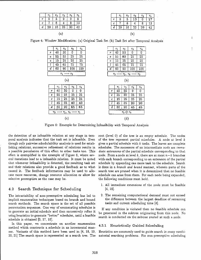
T\ 7"2 T3 7"4 75

r 0 5 9 0 8 c 7 8 4 8 13 d 29 16 23 30 42

T\ 7"2 r3 74 T5 r 0 5 13 0 17 c 7 8 4 8 13 d 29 16 23 29 42

(a) (b)

Figure 4: Window Modification: (a) Original Task Set (b) Task Set after Temporal Analysis

n 72 7-3 7"4

r 40 30 0 0 e 55 55 25 25 c 15 25 25 25 I 45 65 75 75 d 60 90 100 100

TX —»r2

(a)

n 7"2 73 7-4

r 40 30 0 0 e 55 55 25 25 c 15 25 25 25 I 45 65 40 40 d 60 90 65 65

73 —* n, T4 ► n

n 7-2 73 7-4

r 40 55 0 0 e 55 80 25 25 c 15 25 25 25 I 45 65 75 75 d 60 90 100 100

73 ► 7-2, 74 ► T2

(b)

n 7"2 7-3 7-4

r 40 55 0 0 e 55 80 25 25 c 15 25 25 25 I 45 65 20 20 d 60 90 45 45

T3Q>T4

(c) (d)

Figure 6: Example for Determining Infeasibility with Temporal Analysis

the detection of an infeasible relation at any stage in temporal analysis indicates that the task set is infeasible. Even though only pairwise schedulability analysis is used for establishing relations, successive refinement of relations results in a possible percolation of this effect to other tasks too. This effect is exemplified in the example of Figure 6, where several iterations lead to a infeasible relation. It must be noted that whenever infeasibility is detected, the resulting task set and their relations also provide a good feedback as to what caused it. The feedback information may be used to allocate more resources, change resource allocation or allow for selective preemption as the case may be.

4.2 Search Technique for Scheduling

The intractability of non-preemptive scheduling has led to implicit enumeration techniques based on branch and bound search methods. The search space is the set of all possible permutation sequences. One way of enumerating schedules is to generate an initial schedule and then successively refine it using heuristics to generate "better" schedules, until a feasible schedule is obtained [3, 17, 16].

In this paper, we concentrate on another enumeration method which constructs a schedule in an incremental manner. Variants of this method have been used in [4, 18, 19, 20, 21] The search space is represented as a search tree. The

root (level 0) of the tree is an empty schedule. The nodes of the tree represent partial schedules. A node at level k gives a partial schedule with k tasks. The leaves are complete schedules. The successors of an intermediate node are immediate extensions of the partial schedule corresponding to that node. From anode at level k, there are at most n — k branches with each branch corresponding to an extension of the partial schedule by appending one more task to the schedule. Search is done in a branch and bound manner, wherein parts of the search tree are pruned when it is determined that no feasible schedule can arise from them. For each node being expanded, the following conditions must hold.

1. All immediate extensions of the node must be feasible [4, 18].

2. The remaining computational demand must not exceed the difference between the largest deadline of remaining tasks and current scheduling time [4].

If any condition is violated then no feasible schedule can be generated in the subtree originating from this node. No search is conducted on the subtree rooted at such a node.

4.2.1 Heuristically Guided Scheduling

Heuristics are commonly used to guide search in many combinatorial searching problems. For non-preemptive scheduling

318

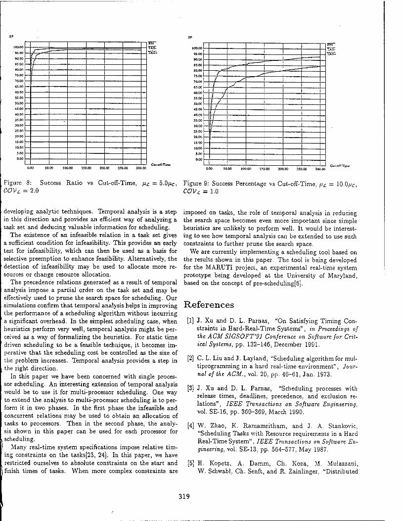
100.00 BW

95.00

90.00

85.00

SO.OO

75.00

70.00

«5.00

60.00

55.00

50.00

45.00

40.00

35.00

30.00

25.00

20.00

15.00

10.00

5.00

0.00

TäS; tf 7 7

■

BM TÄS" VÄ5»

90.00 i

f t ^

1 / / J

50.00 \ / /

:/ \\ I

25.00

5.00

Figure COVc

8: Success = 2.0

Ratio vs Cut-off-Time, fi£ = 5.0/J.C, Figure 9: Success Percentage vs Cut-off-Time, //£ = 10.0//C, COVc = 1.0

- developing analytic techniques. Temporal analysis is a step in this direction and provides an efficient way of analyzing a task set and deducing valuable information for scheduling.

The existence of an infeasible relation in a task set gives a sufficient condition for infeasibility. This provides an early test for infeasibility, which can then be used as a basis for selective preemption to enhance feasibility. Alternatively, the detection of infeasibility may be used to allocate more resources or change resource allocation.

The precedence relations generated as a result of temporal analysis impose a partial order on the task set and may be effectively used to prune the search space for scheduling. Our

; simulations confirm that temporal analysis helps in improving the performance of a scheduling algorithm without incurring a significant overhead. In the simplest scheduling case, when heuristics perform very well, temporal analysis might be perceived as a way of formalizing the heuristics. For static time driven scheduling to be a feasible technique, it becomes imperative that the scheduling cost be controlled as the size of the problem increases. Temporal analysis provides a step in the right direction.

In this paper we have been concerned with single processor scheduling. An interesting extension of temporal analysis would be to use it for multi-processor scheduling. One way to extend the analysis to multi-processor scheduling is to perform it in two phases. In the first phase the infeasible and concurrent relations may be used to obtain an allocation of tasks to processors. Then in the second phase, the analysis shown in this paper can be used for each processor for scheduling.

Many real-time system specifications impose relative timing constraints on the tasks[23, 24]. In this paper, we have restricted ourselves to absolute constraints on the start and finish times of tasks. When more complex constraints are

imposed on tasks, the role of temporal analysis in reducing the search space becomes even more important since simple heuristics are unlikely to perform well. It would be interesting to see how temporal analysis can be extended to use such constraints to further prune the search space.

We are currently implementing a scheduling tool based on the results shown in this paper. The tool is being developed for the MARUTI project, an experimental real-time system prototype being developed at the University of Maryland, based on the concept of pre-scheduling[6]^

References

[1] J. Xu and D. L. Parnas, "On Satisfying Timing Con- straints in Hard-Real-Time Systems", in Proceedings of the ACM SIGSOFT'91 Conference on Software for Crit- ical Systems, pp. 132-146, December 1991.

[2] C. L. Liu and J. Layland, "Scheduling algorithm for multiprogramming in a hard real-time environment", Jour- nal of the ACM., vol. 20, pp. 46-61, Jan. 1973.

[3] J. Xu and D. L. Parnas, "Scheduling processes with release times, deadlines, precedence, and exclusion relations", IEEE Transactions on Software Engineering, vol. SE-16, pp. 360-369, March 1990.

[4] W. Zhao, K. Ramamritham, and J. A. Stankovic, "Scheduling Tasks with Resource requirements in a Hard Real-Time System", IEEE Transactions on Software En- gineering, vol. SE-13, pp. 564-577, May 1987.

[5] H. Kopetz, A. Damm, Ch. Koza, M. Mulazzani, W. Schwabl, Ch. Senft, and R. Zainlinger, "Distributed

319

heuristics may be used to guide search along paths which are more likely to lead feasible schedules. Search is done in a depth first manner until either a complete feasible schedule is found, in which case the search terminates, or it is determined that, no possible extensions of the current node can lead to a feasible schedule. Heuristics are used to determine which of the many children of a node should be searched next. Back- tracking takes place when no further extensions of a node can be made. We evaluate temporal analysis using such a heuristic search for scheduling.

5 Empirical Evaluation of Temporal Analysis

In the previous sections, we have shown how temporal analysis may be used to restrict the search space for scheduling. Clearly, the existence of even a few precedence relations results in a drastic reduction of search space3. However, the usefulness of the scheme is not obvious since we are only interested in feasible schedules, hence a large part of the search space may never need to be examined. We have conducted various simulations to verify that indeed temporal analysis results in improved performance for scheduling. For reasons of space, we mention only a few significant results.

We used a heuristic search technique for scheduling as described in section 4.2. The heuristic used for our simulation study was a two level heuristic. The primary heuristic was earliest start iime(EST).

ESTi~max(n,fk)

where k is the last task in the partial schedule at that node. In the case of a conflict, the secondary heuristic earliest

deadline was used. Further conflicts were resolved arbitrarily. The heuristic has a natural intuitive appeal and is known to produce good results among linear heuristics[22].

For each set of parameters, we generated 200 "feasible" task sets with 100 tasks each. The task sets were generated with 100% utilization as this presents the most difficulty for scheduling. The computation times were generated using uniform distributions and laxities using normal distribution. We compared the success percentage (i.e. percentage of successfully scheduled task sets) of scheduling with and without temporal analysis as a pre-processing stage. The success percentage (SP) is plotted against "cut-ofT-time", indicating the maximum time allowed to the scheduling algorithm to successfully generate a schedule.

Our simulation results show that temporal analysis is not needed for scheduling when both the mean and the variation in laxities is low since the simple heuristics were able to schedule almost all task sets (success ratio ta 1.0). However, when the laxities are high (as compared to computation times) and the variation in laxities is also high4, then the heuristics do

DM TX'S: rxs; 95.00

:/ 90.00

45.00 '

0.00

1

Figure 7: Success COVc = 1.0

Ratio vs Cut-off-Time, fj.c = 5.0//c

Even one relation reduces the search space by half. 4 Note that the task set utilization is 100%

not perform as well and the use of temporal analysis results in 10 — 20% improvement in success ratio.

As an illustration, we show a few plots which plot the success percentage (SP) of scheduling with temporal analysis (TAS) contrasted with success percentage of scheduling without temporal analysis, i.e. the baseline scheduling model (BM). For scheduling with temporal analysis, we consider two cases, one in which overhead of temporal analysis is added to scheduling time (TAS+) and the other in which it is not (TAS- ). The parameters varied are the mean laxity fic in terms of mean computation times fie, and the coefficient of variation for laxity COVc ■ Figures 7 and 8 show the plots for low laxity mean with low and high variation. For this case, there is no significant performance improvement due to temporal analysis and both schemes achieve almost 100% success percentage. On the other hand when the average laxity is high (Figures 9 and 10), coupled with high variation, we see that temporal analysis results in significant improvement in performance. The plots also show that the curves for (TAS+) and (TAS-) are almost identical showing that the overhead of temporal analysis is minimal when compared to the schedulng costs.

6 Concluding Remarks

In this paper we have presented temporal analysis as a technique for analyzing the timing relationships among a set of tasks to establish constraints on scheduling which are dis- cernible from a pairwise analysis. The implications and the benefits of the approach as a pre-processing stage for scheduling has been shown through examples and simulation.

Time Driven Scheduling theory has relied heavily on search techniques for scheduling and little work has been done in

320

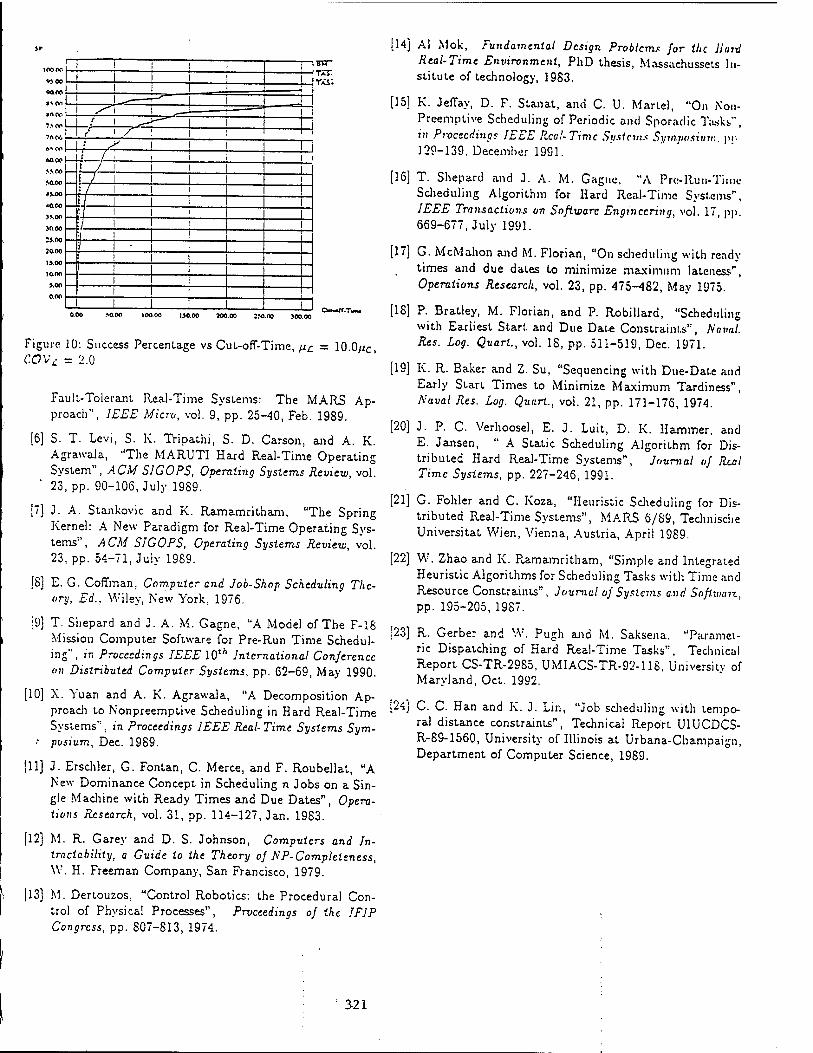
! 1 : 1 BM rxr. TXS: 1 1 i 1 i

1 ! II **<v> 1 - -r^~ \ I ■

| s | | -__j. f

/ 1 .->—" 1 1 ' S ! |

l/^l 1 1 1 l_l t / . , i i

t /

f~7 i i i i i i

t/ i i i I |t i i

3*.0P i 1 Ei l I i

25.00 i i |

\ \ ' \ I 1 \ I

1 i 1

lilt 1

Figure 10: Success Percentage vs Cut-off-Time, fic = 10.G>C

COVc = 2.0

Fault-Tolerant Real-Time Systems: The MARS Ap- proach", IEEE Micro, vol. 9, pp. 25-40, Feb. 1989.

[6] S. T. Levi, S. K. Tripathi, S. D. Carson, and A. K. Agrawala, "The MARUTI Hard Real-Time Operating System", ACM S1G0PS, Operating Systems Review, vol. 23, pp. 90-106, July 1989.

[7] J. A. Stankovic and K. Ramamritham, "The Spring Kernel: A New Paradigm for Real-Time Operating Sys- tems", ACM SIGOPS, Operating Systems Review, vol. 23, pp. 54-71, July 1989.

[8] E. G. Coffman, Computer and Job-Shop Scheduling The- ory, Ed.. Wiley, New York, 1976.

[9] T. Shepard and J. A. M. Gagne, "A Model of The F-18 Mission Computer Software for Pre-Run Time Schedul- ing", in Proceedings IEEE 10,h International Conference on Distributed Computer Systems, pp. 62-69, May 1990.

[10] X. Yuan and A. K. Agrawala, "A Decomposition Ap- proach to Nonpreemptive Scheduling in Hard Real-Time Systems". in Proceedings IEEE Real- Time Systems Sym-

■ posium, Dec. 1989.

[11] J. Erschler, G. Fontan, C. Merce, and F. Roubellat, "A New Dominance Concept in Scheduling n Jobs on a Sin- gle Machine with Ready Times and Due Dates", Opera- tions Research, vol. 31, pp. 114-127, Jan. 1983.

[12] M. R. Garey and D. S. Johnson, Computers and In- tractability, a Guide to the Theory of NP-Compleieness, W. H. Freeman Company, San Francisco, 1979.

[13] M. Dertouzos, "Control Robotics: the Procedural Con- trol of Physical Processes", Proceedings of the IFIP Congress, pp. 807-813, 1974.

[14] Al Mok, Fundamental Design Problems for the Hard Real-Time Environment, PhD thesis, Massachussets In- stitute of technology, 1983.

[15] K. JefTay, D. F. Stan at, and C. U. Martel, "On Non- Preemptive Scheduling of Periodic and Sporadic Tusks", :'« Proceedings IEEE Real-Time Systems Symposium, pi- 129-139. December 1991.

[16] T. Shepard and J. A. M. Gagne, "A Pro-Run-Ti.in- Scheduling Algorithm for Hard Real-Time Systems", IEEE Transactions on Software Engineering, vol. 17, pp. 669-677, July 1991.

[17] G. McMahon and M. Florian, "On scheduling with ready times and due dates to minimize maximum lateness", Operations Research, vol. 23, pp. 475-482, May 1<J75.

[18] P. Bratley, M. Florian, and P. Robillard, "Scheduling with Earliest Start and Due Date Constraints", Naval. Res. Log. Quart, vol. IS, pp. 511-519, Dec. 1971.

[19] K. R. Baker and Z. Su, "Sequencing with Due-Date and Early Start Times to Minimize Maximum Tardiness", Naval Res. Log. Quart., vol. 21, pp. 171-176, 1974.

[20] J. P. C. Verhoosel, E. J. Luit, D. K. Hammer, and E. Jansen, " A Static Scheduling Algorithm for Dis- tributed Hard Real-Time Systems", Journal of Real Time Systems, pp. 227-246, 1991.

[21] G. Fohler and C. Koza, "Heuristic Scheduling for Dis- tributed Real-Time Systems", MARS 6/89, Technische Universität Wien, Vienna, Austria, April 1989.

[22] W. Zhao and K. Ramamritham, "Simple and Integrated Heuristic Algorithms for Scheduling Tasks with Time and Resource Constraints", Journal of Systems and Software, pp. 195-205, 1987.

[23] R. Gerbe: and W. Pugh and M. Saksena, "Paramet- ric Dispatching of Hard Real-Time Tasks", Technical Report CS-TR-2985, UMIACS-TR-92-118, University of Maryland, Oct. 1992.

[24] C. C. Han and K. J. Lin, "Job scheduling with temporal distance constraints", Technical Report UIUCDCS- R-89-1560, University of Illinois at Urbana-Champaign, Department of Computer Science, 1989.

321




3. REPORT TYPE END DATES COVERED Technical Reports

4. TITLE AND SUBTITLE Temporal Analysis and its Application in Non-Preemptive Scheduling

6. AUTHOR(S) Manas C. Saksena and Ashok K. Agrawala


SPONSORING/ MONITORING AGENCY NAME(S) AND ADDRESS(ES)|l PhillipsLaboratory Director of Contracting 3651 Lowry Avenue SE Kirtland AFB, NM 87117-5777

5. FUNDING NUMNBERS

N00014-91-C-0195







In the problem of non-preemptive scheduling of a set of tasks on a single processor, each task has a ready time, a deadline and a computation time. A feasible schedule for this set requires that a start time be assigned to each task. The approaches taken for scheduling often use search techniques and may reduce the search by using heuristics. In this paper we present a technique for analyzing the temporal relations among the tasks to establish pairwise relationships among them. These relationships can then be used effectively to reduce the complexity of scheduling these tasks. We present simulation results to .confirm the usefulness of temporal analysis as a phase prior to scheduling.

14. SUBJECT TERMS


Unclassified


Unclassified

15. NUMBER OF PAGES

7

16. PRICE CODE


Unclassified


Unlisted MSN 7540-01 280:5500


Implementation of the MPL Compiler**

Jan M. Rizzuto and James da Silva



February 14, 1995

Abstract

The Maruti Real-Time Operating System was developed for applications that must meet hard real-time constraints. In order to schedule real-time applications, the timing and resource requirements for the application must be determined. The development environment provided for Maruti applications consists of several stages that use various tools to assist the programmer in creating an application. By analyzing the source code provided by the programmer, these tools can extract and analyze the needed timing and resource requirements. The initial stage in development is the compilation of the source code for an application written in the Maruti Programming Language (MPL). MPL is based on the C programming language. The MPL Compiler was developed to provide support for requirement specification. This report introduces MPL and describes the implementation of the MPL Compiler.

This work is supported in part by ONE. and DARPA under contract N00014-91-C-0195 to Honeywell and Computer Science Department at the University of Maryland. The views, opinions, and/or findings contained in this report are those of the author(s) and should not be interpreted as representing the official policies, either expressed or implied, of the Defense Advanced Research Projects Agency, ONR, the U.S. Government or Honeywell. Computer facilities were provided in part by NSF grant CCB.-8811954.

'This work is supported in part by ARPA and Philips Labs under contract DASG60-92-0055 to Depart- ment of Computer Science, University of Maryland. The views, opinions, and/or findings contained in this report are those of the author(s) and should not be interpreted as representing the official policies, either expressed or implied, of the Advanced Research Projects Agency, PL, or the U.S. Government.

323

1 Introduction

A real-time system requires that an application meet the timing constraints specified for it. For hard real-time, a failure to meet the specified timing constraints may result in a fatal error [2]. Timing constraints are not as critical for soft real-time. The Maruti Operating System was developed to meet the real-time constraints required by many applications. In order to schedule and run an application under Maruti, the timing and resource requirements for that application must be determined. The development environment for Maruti consists of several tools that can be used to extract and analyze these requirements [2].

The Maruti Programming Language (MPL) is a language developed to assist users in creating applications that can be run under Maruti. MPL is based on the C programming language, and assumes the programmer is familiar with C. MPL provides some additional constructs that are not part of standard C to allow for resource and timing specification [1]. In addition, when an MPL file is compiled, some of the resource requirements can be recognized and recorded to an output file. This output file is used as input to the integration stage, which is the next stage in the development cycle. During integration, additional timing requirements may be specified.

Previously, an MPL file was compiled by first running the source code through the Maruti pre-compiler, which created a C file that was then compiled using a C compiler [l]. The pre-compiler extracted the necessary information, and converted the MPL constructs that were not valid C statements into C code. This required the additional pass of the pre-compiler over the source code. We have created a compiler for MPL that integrates both the actions of the pre-compiler and the compiler into one stage. In this report, we present MPL, and a description of the compiler we implemented. Section 2 defines the abstractions used in Maruti. In Section 3, the syntax of the constructs unique to MPL is defined. The details of the implementation of the compiler are given in Section 4. Section 5 describes the resource information that is recorded during compilation. Conclusions appear in Section 6, followed by an Appendix containing a sample MPL file, and the resource information recorded for that file.

2 Maruti Abstractions

An MPL application is broken up into units of computation called elemental units (EUs). Execution within an EU is sequential, and resource and timing requirements are specified for each EU. A thread is a sequential unit of execution that may consist of multiple EUs. MPL allows threads of execution to be specified by the programmer through several of the constructs provided. A task consists of a single address space, and threads that execute in that address space.. Modules contain the source code of the application as defined by the programmer. An application may consist of several modules. During execution, modules are mapped to one or more tasks.

3 MPL Constructs

There are several constructs defined in MPL that are not a part of standard C. These constructs have been implemented in the MPL compiler.

324

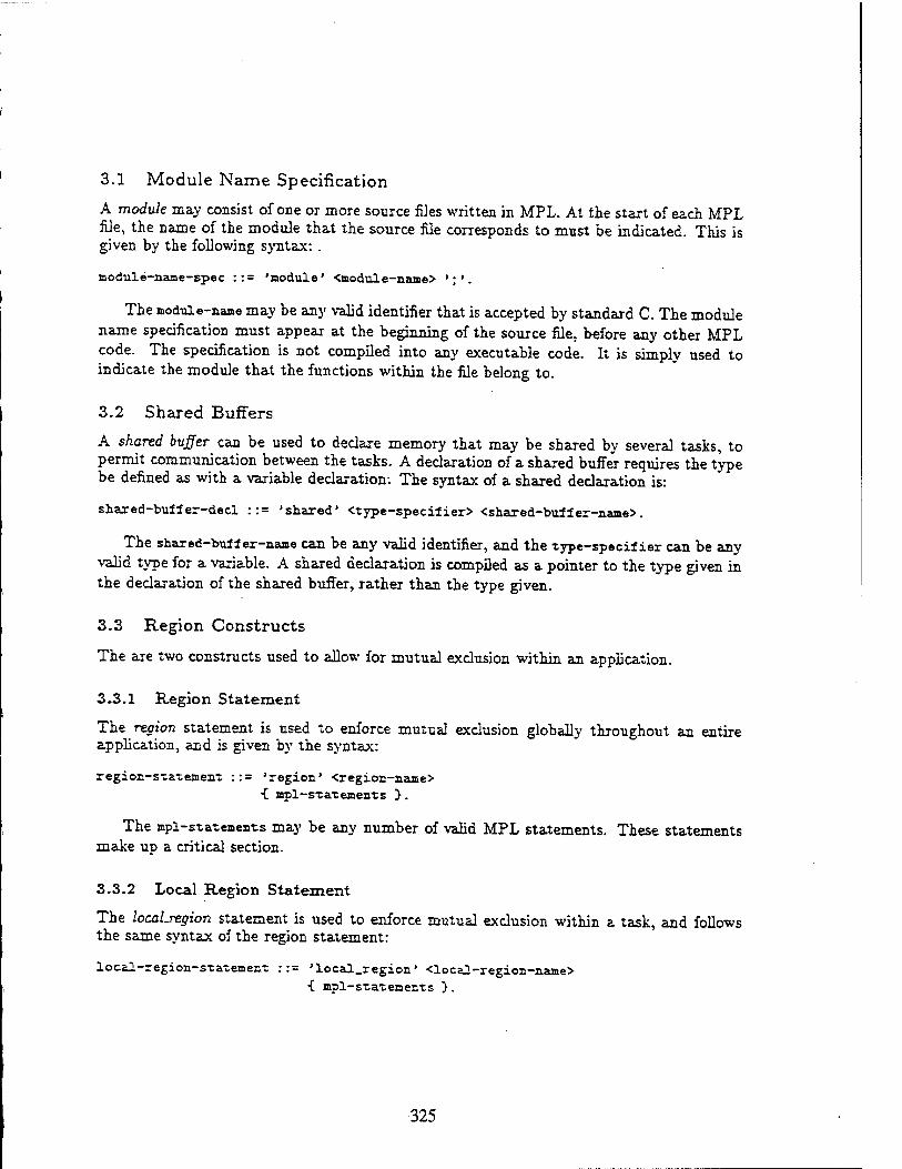
3.1 Module Name Specification

A module may consist of one or more source files written in MPL. At the start of each MPL file, the name of the module that the source file corresponds to must be indicated. This is given by the following syntax: .

«nodule-name-spec ::= 'nodule' <module-name> ';'.

The jnodule-naae may be any valid identifier that is accepted by standard C. The module name specification must appear at the beginning of the source file, before any other MPL code. The specification is not compiled into any executable code. It is simply used to indicate the module that the functions within the file belong to.

3.2 Shared Buffers

A shared buffer can be used to declare memory that may be shared by several tasks, to permit communication between the tasks. A declaration of a shared buffer requires the type be defined as with a variable declaration. The syntax of a shared declaration is:

shared-buffer-decl ::= 'shared' <type-specifier> <shared-buffer-name>.

The shared-buffer-na»e can be any valid identifier, and the type-specifier can be any valid type for a variable. A shared declaration is compiled as a pointer to the type given in the declaration of the shared buffer, rather than the type given.

3.3 Region Constructs

The are two constructs used to allow for mutual exclusion within an application.

3.3.1 Region Statement

The region statement is used to enforce mutual exclusion globally throughout an entire application, and is given by the syntax:

region-statement ::= 'region' <region-najne> •£ apl-stateaents >.

The mpl-statenents may be any number of valid MPL statements. These statements make up a critical section.

3.3.2 Local Region Statement

The local-region statement is used to enforce mutual exclusion within a task, and foDows the same syntax of the region statement:

local-region-statement ::= 'local_region' <local-region-naae> ■i mpl-stateaents >.

325

3.4 Channel Declarations

Channels are used to allow for message passing within a Maruti application. Each channel declared has a type associated with it given by a valid C type-specifier. This type indicates the type of data that the channel will carry.

Channels may be declared in both entry and service functions, which will be defined below. The syntax for channel declarations is:

channel-declaration-list-opt : := ■{ channel-declaration-list }. channel-declaration-list ::= channel-declaration { channel-declaration >. channel-declaration ::= channel-type channels ';'. channel-type ::= 'out' | 'in' I 'in-first' I 'in-last'. channels ::= channel { ',' channel }. channel ::= <channel-naae> ':' type-specifier.

3.5 Entry Functions

An entry function is a special type of function that may be defined in an MPL source file. Each entry function corresponds to a thread within the application. The syntax for an entry function definition is:

entry-function ::= 'entry' <entry-naxne> '(' ')' entry-function-body, entry-function-body : := channel-declaration-list-opt mpl-function-body.

3.6 Service Functions

Service functions are another type of special function supported by MPL. A service function is invoked when a message is received from a client. Each service function definition requires an in channel and message buffer be included in the definition. The service function will be executed when there is a message on the channel given in the definition. The definition of a service function is similar to that of an entry function:

service-function ::= 'service' <service-name> ' ( ' <in-channel-naae> ': ' type_specif ier ',' <jnsg-ptr-naae> ' ) ' service-function-body.

service-function-body ::= channel-declaration-list-opt mpl-function-body.

3.7 Communication Function Calls

There are several library functions used to allow for message passing within a Maruti application.

3.7.1 Send Calls

Each call to the send function must specify an outgoing channel for the message:

void send ( chapel channel_name, void *message_ptr );

326

3.7.2 Receive and Optreceive Calls

Both receive calls, and optreceive calls must be associated with an incoming channel (in, in.firsi, or in.last):

void receive ( channel chaTmel_name, void *message_ptr ); int optreceive ( channel channel_name, void *message_ptr );

A call to receive requires that there be a message on the incoming channel. Optreceive should be used when a message may or may not be on the channel. Optreceive checks for the message, and returns a value indicating if a message was found.

3.8 Initialization Function

Each task has an initialization routine that is executed when the application is loaded. This function is specified by the user with the following name and arguments:

int maruti_!aain (int arge, char **argv)

4 Implementation

We started with version 2.5.8 of the Gnu C compiler. By modifying the source code for the C compiler, we have created a compiler for applications written in MPL. In addition to what the standard Gnu C compiler does, this modified compiler handles the additional constructs defined in MPL, and records information about the scarce code that is needed by Maruti. A source code file written in MPL is specified with an tnpl extension.

4.1 Modifications to GCC File Structure

In the process of modifying the compiler, some existing files were modified. In addition, some new files were also created. The source code for version 2.5.8 of GCC allows compilers to be created for several different languages: C, C-f-f, and Objective C. The GCC compiler uses different executable files for the different languages that it compiles. There are separate files for C. C-f--r, and Objective C (ecl, cclplvs, eclobj). The GCC driver, gcc.c, uses the extension of the source file specified to determine the appropriate executable (and therefore language) to compile the source file. The driver then executes the compiler, passing on the appropriate switches. The driver was modified to accept input files with an mpl extension. CcJmpl is the new executable that was created to compile MPL source files. When a file with an mpl extension is specified as a source file to be compiled, this new executable file is used. When an MPL file is compiled, it automatically passes on the switch -MarutLovtput, which indicates that the needed output should be recorded i© a-file with an eu extension.

The executable files for each language are composed of many object files. Some of these files are common to all the languages, and some of the files are language-specific. The language-specific files added for compiling MPL files are those files with an mpl- prefix.

Gperf is a tool used to generate a perfect hash function for a set of words. Gperf is used to create a hash function for the reserved words for each language. The files containing the input to gperf are indicated by a file name with a gperf extension. There are several different *.gperf files containing the reserved words for the different languages recognized by

327

the compiler. The mpl-parse.gperf file contains all the reserved words for C, in addition to those added for MPL. For each language, the output from running gperf is then incorporated into the *-lex.c file. This output includes a function is.reserved.word() that is used to check if a token is a reserved word. The file mpl-lex.c is basically the c-lez.c filej with the output of running gperf on mpl-parse.gperf instead of c-parse.gperf.

The file maruti.c contains the routines that have been written to implement MPL. This file is linked in with the executable for all of the languages, to prevent undefined symbol errors from occuring- Calls to the routines contained in this file occur in both the language- specific, and the common files. The flag marutLdump is set in mainQ to indicate whether information about the source code should be recorded to the appropriate output file. This flag prevents calls to the routines in maruti.c which are made in the common files from occuring for the languages other than MPL. The files containing these calls are:

• calls.c • explow.c • expr. c • function.c • toplev.c

There are several reasons why the new language-specific files have to be created for MPL. The files mpl-lex.h and mpl-lex.c needed to be created for MPL because MPL contains several additional reserved words not present in C, as mentioned earlier. The file c-common.c relies on information in the header file c-lex.h. Since MPL uses mpl-lex.h, mpl-common.c includes mpl-lex.h, instead of c-lex.h. Bison is a tool that allows a programmer to define a grammar through rules, and converts them into a C program that will parse an input file. The *-parse.y files are the bison files used to create the grammar to parse a source file. Since the grammar for MPL needed to be modified to accept the additional constructs, the mpl-parse.y file was created. There is one function used in compiling MPL source files that is defined in mpl-parse.y. instead of maruti.c. This function needed to access the static variables declared in mpl-parse.y. and in order to do so, the function definition was placed in that file. Finally, the file mpl-decl.c was created, because of its dependence on mpl-lex.h, and also to allow for an additional type specification used in MPL.

4.2 Compiling MPL Constructs

MPL extends the C language to allow for various constructs. In order to implement these extensions, the grammar used to recognize C in GCC had to be extended. The following are recognized as reserved words for MPL, in addition to the standard reserved words for C: shared, region, locaLregion, module, in, out, injirst, inJast, entry, service, send, receive, and optreceive. The keywords in and out were reserved words in the c-* files, because they are used by Objective C, but in MPL they are used as channel types. In addition to the new reserved words, rules were added and modified resulting in the rules in mpl-parse.y.

4.2.1 Module Name Specification

A rule was added to the grammar to parse the module name specification in an MPL file. The rule for a whole program was also modified to include this module statement. This rule expects the module statement to appear before any other definitions. Since the module

328

name specification does not result in any executable code, the only action taken is to record the module name given by the programmer.

4.2.2 Shared Buffers

There are no rules added to the grammar for a shared buffer declaration. When a variable declaration is parsed, a tree is created that keeps track of all the specification information given "for that declaration. For example, lypedef and extern are two of the possible type specifications. The token shared is recognized as a type specification, just as typedef and extern are recognized. When a declaration is made, these specifications are processed in the function grokdeclaratorQ in mpl-decl.c. When a shared specification is encountered, the declaration is converted to a pointer to the type specified, instead of just the type specified. Other than this conversion to a pointer, the declaration is compiled just as any other declaration would be compiled in C.

4.2.3 Region Constructs

The region constructs are considered statements in MPL. Several rules were added to parse these constructs, and the region and local-region statements were added as options for a valid statement in the grammar for MPL.

Both region and local-region statements are compiled in the same manner. Each region has a name, and a body which is the code within the critical section, in order to protect these critical sections, calls are made to the Maruti library function marutLeuQ. When a region is parsed, the compiler generates two calls to marutLeuQ, in addition to the code in the body of the region. The first call is generated just before the body, and the second call just after. These calls are generated through functions in maruti.c. The functions are based on the actions that would have been taken, had the parser actually parsed tue calls to marutLeuQ in the source file.

4.2.4 Channel Declarations

The rules added for a channel declaration allow any number of channels to be declared in either an entry or a service function. Each channel declaration requires several pieces of information:

• Channel-type • Channel-name • Type specifier indicating the type of data that channel carries

A linked list of declared channels is maintained. For each declared channel the following information is saved:

• Channel-name • Type information

1. Size in bytes 2. String encoding the type of the data

• Channel-id

329

The channel-id is a unique identification number assigned to each declared channel. Channel declarations do not add to the compiled code. The channels are not allocated memory. The information describing each channel is simple stored in the linked list. During compilation, whenever a channel is referenced, the appropriate information is obtained from this list.

4.2.5 Entry Functions

Entry function definitions are compiled differently than other function definitions. An entry function would appear in an MPL file in the following form:

entry <entry_naae> () <channel_declaration_list_opt> ■C

<mpl_function_body> }

Where entry .name is an identifier that is the name of the entry function, the channel_declaration.list_opt contains any channels the user wants to define for that function, and mpl-funct ion-body is any function body that would be accepted as a definition in a standard MPL function. Semantically the entry function is equivalent to the following MPL code:

_maruti_entry_name ()

sailed) ■c

namti_eu(); entry_name () ;

> >

entry„name () i

mpl_iunction_body >

An entry function is compiled into two functions, as if the two functions given above had been part of the source file. Essentially, the first function is just a stub function that calls marutLeu(), then calls the second function compiled. As with generating function calls, the routines to generate the code for entry function definitions are based on the actions that would have been taken had the parser actually parsed the code for the two separate functions.

4.2.6 Service Functions

Service functions definitions are handled very much like entry function definitions. The syntax of a service function differs slightly from that of an entry function, since it requires that an incoming channel and a message buffer be defined:

330

service <service_name> (<in_channel_nane> : <type_specifier>, <ttsg_ptr_name>) <channel_declaration list opt> {

<mpl_function_body> >

Like the entry functions, service functions are semantically equivalent to two functions, where one is simply a stub function calling the second function that is generated:

_aamti_service_naine () ■C

type_specifier _naruti_msg_ptr_nane ;

shile(l)

i if ( optreceive ( _aamti_in , id , t _Baruti_msg_ptr_name, size ) )

service_naae (t maruti asg_ptr name )• }

> >

service_name (asg_ptr_name) type_specifier *asg_ptr_naae; {

apl_function_body >

The service _nane, channel .declaration _1 ist, and mpl_function_body are all the same as described previously for entry functions. In addition, service functions have two other items specified in their definitions. The first is a channel. Every service function requires a channel be specified. This channel is always declared as an in channel with the name in.channel_naae. The type is given by type-specifier as if it had been declared in the channel.declaratioii.list. The channel is used to invoke the service function. This in channel is used by the optreceive in the stub function that calls the function containing the service function body. When a message is received on this channel, the service function is executed. The second additional item is a message buffer used by the service function. The name of this message buffer is given by msg _ptr _naae, the type is given by type-specifier. This buffer is used to hold the message received from the client that invoked the service function, and is passed to the second function containing the body of the service function.

4.2.7 Communication Function Calls

There were three library functions provided for message passing mentioned previously: send, receive, and optreceive. Function calls to any of these three library functions are handled differently than other function calls. In the MPL grammar, send, receive, and optreceive are all reserved words. The MPL syntax for all of these calls is the following:

<fTinction-naae> (<cb.annel-naae>, <parameter-2>);

331

Channel-name should be a previously declared channel, and paxameter-2 should be a pointer. These function calls must be compiled differently, since these are not the actual parameters used when the call is generated. In the case of a call to send, the actual parameters must be as follows:

send (<channel-id>, <parameter-2>, <channel-size>);

In the case of a call to either receive, or optreceive, the parameters required are:

receive I optreceive (<channel-type>, <channel-id>, <parameter-2>, <channel-size>);

The channel-type for a receive or optreceive call is an integer generated by the compiler that will indicate an in, in.first, or inJast channel.

When one of these three function calls are encountered, there are special rules in the grammar to handle it. A function in maruti.c is called which generates the appropriate parameters, and then the function call itself. These function calls are generated as mentioned above for the calls to maruti.euQ. The channel-name specified by the user is used to obtain the necessary parameters. Given the channel name, the linked list of channels is searched to find the corresponding channel, then the channel-id and the channel-size are obtained from that node in the linked list. There is also some type checking done at this stage. The compiler verifies that only an outgoing channel is specified for a send call, or an incoming channel for the receive and optreceive calls. The compiler also checks that any channel referenced has been previously defined.

The grammar for MPL was modified so that a call to any of the communication functions may occur anywhere that a primary expression occurs, since that is where other function calls are permitted to occur.

4.2.8 Initialization Function

The user-defined function marutLmain() is compiled as an ordinary C function.

5 PEUG File

The source code of an MPL file is broken up into elemental units. Each elemental unit identifies the resources that it requires. These elemental units are used later in the development process for scheduling the application. The output file created by the MPL compiler creates a Partial Elemental Unit Graph (PEUG) for the given source file. The name of this file is the name of the source file, with the mpl extension replaced by an ev. extension.

There are several different types of information recorded in this PEUG file.

5.1 Module Name

The first line in the output file indicates the name of the module, and will appear as:

peug <module-name>

The module-name is taken directly from the module name specification given in the MPL

source file.

332

5.2 File Name

The second line in the source file indicates the name of the target file that is created by the compiler, where file-name is the target:

file <file-name>

5.3 Shared Buffers

Each time a shared buffer is declared its name and type information is recorded to the output file:

shared <shaxed-buffer-name> : (type-description-string>, <type-size>)

The type-description-string and type-size of a shared buffer is obtained from the type specification, and is represented in the same manner as the type and size for a channel. Although the shared buffer is actually a pointer to the type it is declared as, the type-description-string represents the object being pointed to, and not the pointer itself.

5.4 Entry, Service, and User Function Definitions

In MPL, a user may define ordinary functions in addition to the entry and service functions that are permitted in MPL. For each entry, service or ordinary user-defined function, there is an entry in the output file. This entry has the following format:

<fiinction-type> <fanction-name>

size <stack-size>

Function-type can be either function, entry, or service, indicating which type of function is being defined. Fnnction-name is the declared name of the function in the source file. Stack-size is the maximum stack size needed by this function. This stack-size includes the arguments pushed onto the stack preceding any function calls occuring within the function body. There will also be other information concerning the body of the function that will appear between the function-name, and the stack-size. The entry for the marutLmainQ function will be the same as those for other user defined functions. Entry and service functions will contain some additional information not applicable to ordinary functions that will be described below.

5.4.1 Channels

For each channel that is declared, a description of the channel is written to the output file. These descriptions will occur right after the statement indicating the name of the current function:

<channel-type> <name> : (<description-string>, <size>)

333

The channel-type and channel-name wiU be the type and name specified in the source file. The description-string and size are based on the type specification in the channel declaration. Channel descriptions will occur only in entry and service functions. A service function will always contain at least one channel description, since the syntax of a service function requires a channel be named in the definition. A channel description will also be output for every send, receive, and optreceive call, since these calls require a channel as one of their parameters.

5.4.2 Function Calls

Each time a function call is parsed, there will be a line in the output file:

calls <lunction-name> -Cin.cond} {in_loop}

This line indicates where a function call occurs, and which function is being called. The in_cond and iaJLoop indicate if this function call appears within a conditional statement or within a loop. These labels will be seen only if their respective conditions are true.

5.4.3 Communication Function Calls

Any call to a communication function is recorded similarly to otber function calls. There is a hue indicating the name of the function, as shown above for a function call. In addition, there will be a line describing the channel associated with that communication function call. This line will appear just as the line for the channel definition described above appears.

5.4.4 EU Boundaries

The output file for an MPL source file indicates where each elemental unit (EU) begins by the following:

en <K> <region_list}

The N indicates an EÜ number. Each EU within a source file has a unique number. There are several places where EL" boundaries are created:

• Start of a function • Start of a region • End of a region • Explicit calls to marutLeuQ

The initial EU occuring at the beginning of a function that is not a service or entry function is a special case. This is always labeled as ueu 0" in the output file, and does not represent

an actual EU. Each EU may also be followed by a list describing one or more regions. This list

represents the regions that this EU occurs within. The description of a region appears as:

(region-name instance access type)

The region-name is just that given by the user, and the type indicates if a region is local (local-region construct) or global (region construct). The access indicates if the access is read or write. The instance indicates the instance of this region within the source file. Each instance for a region within a source file is unique.

334

6 Conclusions

Basing MPL on C has simplified the development of both the language and its compiler. The language is easy to learn for any programmer that has used C before, since there are a limited number of additional constructs unique to MPL. Using the GCC C source code provided an existing compiler, rather than implementing a new one. The source code for GCC only needed to be modified to handle some additional constructs, and produce some additional output. This made the implementation fairly simple. However, the GCC C compiler also provides some functionality that is not needed by MPL. Much of this functionality provided is not even permitted. These restrictions are not enforced by the compiler, but should be detected within the development cycle.

Prior to the development of the MPL compiler using GCC, compiling an MPL source file required two steps. The source files were initially passed through a pre-compiler to extract the available resource information and parse the MPL constructs. The pre-compiler was responsible for converting the MPL code into valid C code, which was then compiled using a standard C compDer. The new implementation of the compiler eliminates some of the redundant processing that is done when the pre-compiler is used. The information obtained through the pre-compiler already existed in the internal structure used by the GCC compiler. This information just needed to be recorded. Instead df parsing source code files in the two steps independently, the functionality of the pre-compiler has been incorporated into the compiler itself. The MPL compiler provides a single tool that extracts all the available information at the initial stage of develpment.

In the future, a version of MPL may be implemented that is based on the Ada programming language. GNAT is a compiler for Ada 9X that is being developed at NYU. GNAT depends on the backend of the GCC compiler, using the source code for GNAT, an implementation of MPL based on Ada would be similar to the current implementation based on C.

335

Appendix

A MPL File

The following is a sample of MPL source code:

module timer;

typedef struct { int seconds;

int minutes;

int hours;

} time.type;

shared time_type global_tiae;

maruti_main(axgc, argv)

int arge; char **argv;

■C global_time->seconds = 0;

global_time->minutes = 0;

global_time->hours = 0;

return 0;

>

entry update_second() out cist) : time_type;

tiaie_type nsg;

region time_region {. giobal_time->seconds-'-+; ii Cglobal_tiae->seconäs == 60)

global_time->seconds = 0; msg = *globai_tiae; >

send (disp, fcmsg); >

entry update_ainute() out display : time_type; { tiae_type msg;

region tiae_region •{ global_time->minutes++;

336

if (global_time->minutes == 60) globa.l_time->minutes = 0;

msg = *global_tiae; >

send (display, taasg); >

entry update_hoTir() out display : tine_type; •C tiae_type msg;

region tiaie_region { global_time->hours++; if (global_time->bonxs == 24)

global_time->hours = 0; msg = *global_time; >

send (display, fansg); >

service display_tiaie(inchan : time type, time) { print!("Current Time: 'JA : */.d : 'JA", time->hours, time->minntes, time->seconds);

337

B PEUG File

The corresponding PEUG file for the source code above is:

peug timer file timer.o shared global.time : ($<iii), 12) Inaction mamti_main

en 0 size 4

entry update_second out disp : ($(iii), 12) eu 2 eu 3 (time_region 1 W global) calls mamti_eu en 4

calls marnti_en calls send ont disp : ($(iii), 12)

size 32 entry npdate_minute

ont display : ($(iii), 12) en 5 en 6 (time_region 2 V global)

calls marnti_ea en 7

calls marati_en calls send ont display : ($(iii), 12)

size 32 entry npä&te_h°nr

ont display : (S(iii), 12) en 8 en 9 (time_region 3 V global)

calls mamti_eu en 10

calls mamti_eu calls send out display : ($(iii), 12)

size 32 service display_time

in incaan : ($(iii), 12) en 11

calls optreceive in inchan : ($(iii), 12) calls print;

size 52

338

References

[1] James da Silva, Eric Nassor, Seongsoo Hong, Bao Trinh, and Olafur Gudmundsson. Maruti 2.0 Programmer's Manual. Unpublished.

[2] Manas Saksena, James da Silva, and Ashok Agrawala. Design and Implementation of Maruti-II. In Sang H. Son, editor, Advances in Real-Time Systems, chapter 4. Prentice Hall, 1995.

[3] Richard Stallman. The GNU C compiler, version 2.5.8., Manual. Info file obtained from gcc.texi in source code distribution.

339

REPORT DOCUMENTATION PAGE OM« wo C.'W-OISJ

**o **#cw • •©^•—©•» n#«iin^fe ►»o^-fi co/o«-fri»»l W»\»M»©IO*». DC ?0%03

1. AGfNCY USE ONLY !l»»( &<^n/t,' 2. REPORT D*T£

February 14, 1995 3. REPORT TYPE AND DATES COVERED

Technical Report 4. TJTU AND SUBTITLE

Implementation of the MPL Compiler

6. AUTHOR(S)

Jan M. Rizzuto and James da Silva



9. SPONSORING/MONITORING AGENCY NAM£(S) AND ADDRESS(ES)

Honeywell Phillips Labs 3660 Technology Drive Minneapolis, MN 55418

3550 Aberdeen Ave. SE Kirtland AFB, NM

87117-5776

S. FUNDING NUMBERS

N00014-91-C-0195 and DSAG-60-92-C-0055

E. PERFORMING ORGANIZATION REPORT NUMBER

CS-TR-3413 UMIACS-TR- 95-17

10. SPONSORING / MONITORING AGENCY REPORT NUMBER



12. ABSTRACT (Maximum 2DD word)

The Maruti Real-Time Operating System was developed for applications that must meet hard real-time constraints. In order to schedule real-time applications, the timing and resource requirements for the application must be determined. The development environment provided for Maruti applications consists of several stages that use various tools to assist the programmer in creating an application. By analyzing the source code provided by the programmer, these tools can extract and analyze the needed timing and resource requirements. The initial stage in development is the compilation of the source code for an application written in the Maruti Programming Language (MPL). MPL is based on the C programming language. The MPL compiler was developed to provide support for requirement specification. This report introduces MPL and describes the implementation of the MPL Compiler.

14. SUBJECT TERMS

D.3.2, Language Classifications D.4.7, Organization and Design

17. SECURITY CLASSIFICATION J OF REPORT

i Unclassified

IB. SECURITY CLASSIFICATION OF THIS PAGE

Unclassified

IS. SECURITY CLASSIFICATION OF ABSTRACT

Unclassified

15. NUMBER OF PAGES


20. LIMITATION OF AESTRAC

Unlimited

>:$N 7>;o-0"-2SO-5500 y.2~-3£'C -orrr. J?S fn«-v 2-ES)

340

Maruti 3.1 Programmer's Manual

First Edition

Systems Design and Analysis Group Department of Compter Science


December 1996

341

Contents 1. Introduction 344

1.1 General Program Organization 344 1.1.1. Maruti Programming Language 345 1.1.2. Maruti Configuration Language 345

2. Tutorial 347 2.1. Basic Maruti Program Structure 347 2.2. Using the Graphics Library 350

3. MPL/C Reference 358 3.1. EBNF Syntax Notation 358 3.2. MPL Modules 358 3.3. Module Initialization 358 3.4. Entry Functions 359 3.5. Service Functions 359 3.6. MPL Channels 360 3.7. Communications Primitives 360 3.8. Critical Regions 361 3.9. Shared Buffers 361 3.10. Restrictions to ANSI in MLP 361

4. MCL Reference 362 4.1. Top-Level Declarations 362

4.1.1. The Application Declaration 362 4.1.2. The System Declaration 362 4.1.3. Block Declaration 363 4.1.4. Variable Declarations 364

4.2 Instructions 364 4.2.1. Compound instructions 365 4.2.2. Task 365 4.2.3. Job Initialization 365 4.2.4. Connections 366 4.2.5. Allocation Introduction 366 4.2.6. Link Instructions 366 4.2.7. Print Instructions 367

4.3. Expressions 367

5. Maruti Runtime System Reference 369 5.1. Core Library Reference 369

5.1.1. MPL Built-in Primitives 369 5.1.2. Calendar Switching 370 5.1.3. Calendar Modifications 370 5.1.4. date and Time Manipulation 371 5.1.5. Miscellaneous Functions 372

5.2. Console Library Reference 373 5.2.1. Screen Colors 373 5.2.2. Graphics Functions 374 5.2.3. Keyboards and Speaker Functions 375

5.3. Maruti / Virtual Monitor 376 5.3.1. Controlling Virtual Time 376

342

5.3.2. Single-Keystroke Operation 376 5.3.3. Command-Line Operation .......377

6. Maruti Tools Reference 37g 6.1. Maruti Builder 370 6.2. MPL/C Compiler '.'.'.'.'.".'.'.'.'.'.'.'.'.'.'.'.'.'.'.'.".'.'. 379 6.3. MCL Integrator ..............379 6.4. Allocator / Scheduler ....".................379

. 6.5. Maruti binder ..........."^.379 6.6. Timing Trace Analyzer \\\]\[ 330 6.7. Timing Status Monitor .....................380

343

Chapter 1

Introduction

The Maruti Programming Language (MPL) is used to write Maruti application code. Currently, MPL is based on the ANSI C programming language, with extensions to support modules, real-time constructs, communications primitives, and shared memory.

The Maruti Configuration Language (MCL) is used to specify how individual program modules are to be connected together to form an application and the details of the hardware platform on which the application is to be executed.

1.1. General Program Organization

A complete Maruti system is called an application. Applications can be large, distributed systems made up of many subsystems. Each application is defined by a configuration file, which defines all the subsystems and their interactions. The following entities make up an application:

Jobs Jobs are the active entities in a Maruti application. Jobs are specified in the configuration file with timing constraints, including the job period. A job is made up of multiple entry points, which are the threads of execution that will be run for the job.

Modules The code of an application is divided into modules. Each module consists of entry points, which define the code which will be executed as part of a job, services, which define code to be invoked on behalf of a client module, and functions, which are called from entries and services.

Tasks At run-time, modules map to tasks (a module may be mapped to more than one task). Each task consists of an address spac and threads of execution for the entry points and services of the module.

Channels Channels are the communication paths for Maruti applications. Each channel is a one-way connection through which typed messages are passed. The end points are defined by out and in channel specifiers, and are connected as specified in the application configuration file. Each end point is associated with one entry or service, and its message type and channel type are declared within the entry or service header. The types of the in and out channel specifiers must match.

Regions Regions are the mechanism for mutual exclusion between Maruti threads: only one thread can enter a particular region at a time. Two types of regions may be specified: global regions enforce exclusion for the entire Maruti application, while local regions enforce exclusion only within a single task

Shared buffers Named memory buffers can be shared between tasks. The buffer is mapped into the address space of each task that uses that buffer.

344

1.1.1. Maruti Programming Language

Rather than develop completely new programming languages, we have taken the approach of using existing languages as base programming languages and augmenting them with Maruti primitives needed to provide real-time support.

In the current version, the base programming language used is ANSI C. MPL adds modules, shared memory blocks, critical regions, typed message passing, periodic functions, and message-invoked functions to the C language. To make analyzing the resource usage of programs feasible, certain C idioms are not allowed in MPL; in particular, recursive function calls are not allowed nor are unbounded loops containing externally visible events, such as message passing and critical region transitions.

• The code of an application is divided into modules. A module is a collection of procedures, functions, and local data structures. A module forms an independently compiled unit and may be connected with other modules to form a complete application. Each module may have an initialization function which is invoked to initialize the module when it is loaded into memory. The initialization function may be called with arguments.

• Communication primitives send and receive messages on one-way, typed channels. There are several options for defining channel endpoints that specify what to do on buffer overflow or when no message is in the channel. The connection of two endpoints is done in the MCL specification for the application - Maruti insures that endpoints are of the same type and are connected properly at runtime.

• Periodic functions define entry points for execution in the application. The MCL specification for the application will determine when these functions execute.

• Message-invoked functions, called services, are executed whenever messages are received on a channel.

• Shared memory blocks can be declared inside modules and are connected together as specified in the MCL specifications for the application.

• Critical Regions are used to safely maintain data consistency between executing entities. Maruti ensures that no two entities are scheduled to execute inside their critical regions at the same time.

1.1.2. Maruti Configuration Language

MPL Modules are brought together into as an executable application by a specification file written in the Maruti Configuration Language (MCL). The MCL specification determines the application's hard real-time constraints, the allocation of tasks, threads, and shared memory blocks, and all message-passing connections. MCL is an interpreted C-like language rather than a declarative language, allowing the instantiation of complicated subsystems using loops and subroutines in the specification. The key features of MCL include:

345

•

•

Tasks, Threads, and Channel Binding. Each module may be instantiated any number of times to generate tasks. The threads of a task are created by instantiating the entries and services of the corresponding module. An entry instantiation also indicates the job to which the entry belongs. A service instantiation belongs to the job of its client. The instantiation of a service or entry requires binding the input and output ports to a channel. A channel has a single input port indicating the sender and one or more output ports indicating the receivers. The configuration language uses channel variables for defining the channels. The definition of a channel also includes the type of communication it supports, i.e., synchronous or asynchronous.

Resources. All global resources (i.e., resources which are visible outside a module) are specified in the configuration file, along with the access restrictions on the resource. The configuration language allows for binding of resources in a module to the global resources. Any resources used by a module which are not mapped to a global resource are considered local to the module.

Timing Requirements and Constraints. These are used to specify the temporal requirements and constraints of the program. An application consists of a set of cooperating jobs. A job is a set of entries (and the services called by the entries) which closely cooperate. Associated with each job are its invocation characteristics, i.e., whether it is periodic or aperiodic. For a periodic job, its period and, optionally, the ready time and deadline within the period are specified. The constraints of a job apply to all component threads. In addition to constraints on jobs and threads, finer level timing constraints may be specified on the observable actions. An observable action may be specified in the code of the program. For any observable action, a ready time and a deadline may be specified. These are relative to the job arrival. An action may not start executing before the ready time and must finish before the deadline. Each thread is an implicitly observable action, and hence may have a ready time and a deadline.

Apart from the ready time and deadline constraints, programs in Maruti can also specify relative timing constraints, those which constrain the interval between two events. For each action, the start and end of the action mark the observable events. A relative constraint is used to constrain the temporal separation between two such events. It may be a relative deadline constraint which specifies the upper bound on time between two events, or a delay constraint which specifies the lower bound on time between the occurrence of the two events. The interval constraints are closer to the event-based real-time specifications, which constrain the minimum and/or maximum distance between two events and allow for a rich expression of timing constraints for real-time programs.

• Replication and Fault Tolerance. At the application level, fault tolerance is achieved by creating resilient applications by replicating part, or all, of the application. The configuration language eases the task of achieving fault tolerance, by allowing mechanisms to replicate the modules, and services, thus achieving the desired amount of resiliency. By specifying allocation constraints, a programmer can ensure that the replicated modules are executed on different partitions.

346

Chapter 2

Tutorial

2.1. Basic Maruti Program Structure

Maruti applications are built up out of one or more MPL modules, and tied together with a configuration file written in MCL. Well start our tutorial with an explanation of a very simple application consisting of one module, called simple.mp. Our simple application will contain a producer thread that sends out integer data, and a consumer thread, which receives integer values and prints them out

The Module

module simple;

int data;

maruti_main(int arge, char **argv)

{ if(argc < 1) {

printf("simple: requires an integer argument\n"); return 1;

}

data = atoi(argv[0]); return 0;

}

This first part of the module will be similar in all Maruti modules. The module always starts with the module name declaration. After the module declaration, the MPL module is much like any ANSI C program, but with some special Maruti definitions.

Every module must contain a function named maruti_main, which initializes the module at load time. This initialization would normally include things like device probing or painting the screen. The maruti_main function, exactly like the main function of a C program, takes an argument count and list as its parameters, and returns an error code to its environment. In Maruti, the environment is the system loader, and any non-zero return results in a load failure, in which case the application will not run. In our example, maruti_main is responsible for setting the initial value of our datum from the environment,' and returning a failure code if there is no argument.

347

Periodic Functions

entry producer() out och: int;

{ data++; /* produce data */ send(och, &data);

}

The producer is a periodic function, or Maruti entry point. It serves as the top-level function for a Maruti thread that will be invoked repeatedly, with a period specified in the MCL config file (which we will see below).

The producer outputs its data on a Maruti channel, using the built in MPL send function. The channel och is declared as part of the function header of producer. Maruti channels are declared to have a type, usually a structure but in this case a simple integer. All messages sent on the channel will be of the same type.

Note that there is no open, bind, or connect statement needed to initiate communication on the channel. The connection of the channel will be specified in the config file, and initiated automatically by the runtime system.

Message-Invoked Functions

service consumer(ich: int, msg)

{ printf("consumer got %d\n", *msg); /* consume data */

}

The consumer is a message-invoked function, or Maruti service. It serves as the top-level function for a Maruti thread that is invoked whenever there is a message delivered on the channel declared in the function header. The msg parameter is the name of the pointer to the message buffer that will contain the delivered message.

Since the receipt of the invoking message is automatic for a Maruti service, the only thing our consumer has to do is print out the data value contained in the message.

This completes our simple module, but in order to have a Maruti application, we must have a config file that tells the system how to run our program.

The Config File

The config file is written in the Maruti Configuration Language (MCL), an interpreted C- like language with constructs that allow an application to be built up from pieces and interconnected. The MCL processor, called the integrator, builds a program graph from the specifications, analyses it for type correctness and completeness, and checks for dependency cycles. Here is the config file, simple.cfg, that goes with our application :

348

application simple {

job j; /* declare variables */ task si; channel c;

init j: period Is; /* specify job parameters */ start si: simple(27); /* specify task parameters */

<> si.producer <c> in j; /* producer thread */ <c> sixonsumer <>; /* consumer thread */

}

The variables in MCL correspond to the objects that make up an application, such as channels, tasks, and jobs. As in C, these variables must be declared before they are used.

In Maruti, a. job is a logical collection of threads that run with the same period. All entry functions in the application must be put in some job. The init statement sets the period for a particular job. In our case, the job j will run once every second.

A task is the runtime instantiation of an MPL module, just as in Unix a process is the runtime image of a program. Many tasks may be executed from the same module, each will run independently in the Maruti application. The MCL start command instantiates a task from a module. In our example, we instantiate one task from the module simple and pass it the initial data value of 27.

We instantiate the threads for the entry and service functions inside a particular task, with particular input and output channels. In our example, the statement

<> siproducer <c> in j; /* producer thread */

instantiates the sLproducer thread in job j with no input channels and one output channel, c. Likewise, the statement

<c> siconsumer <>; /* consumer thread */

instantiates the si.consumer thread with one input channel c, and no output channels. Service functions are not put in a job, but rather inherit the scheduling characteristics of the thread that is sending to their invoking channel.

The integrator checks to insure that the use of producer and consumer in the config file match the declarations in the program module.

Building and Running the Application

We can build the simple application by putting simple.mpl and simple.cfg in a directory, and running the mbuild command there:

349

%ls simple.cfg simple.mpl % mbuild mbuild: extracting module Mo from MCL file 'simple.cfg' mbuild: creating obj subdirectory for output files. mbuild: generating obj/simple-build.mk mbuild: running make -f obj/simple-build.mk

Mbuild takes care of running the MPL compiler, the MCL integrator, as well as the analysis and binding programs needed to build the runnable Maruti application. By default, mbuild creates both a stand-alone binary that can be booted on the bare machine, and a Unix binary that runs in virtual real time from within the Unix development environment. These different versions of the runtime system are called flavors.

We can try out the simple application by running the ux+xll flavor from the command line:

% obj/simple.ux+xll <... startup messages ...>

consumer got 28 consumer got 29 consumer got 30 consumer got 31 consumer got 32 consumer got 33 consumer got 34 consumer got 35 consumer got 36 consumer got 37

application quit ^

The application boots up and outputs the consumer message once every second. We can exit the application by typing 'q\

22. Using the Graphics Library Many Maruti programs will want to use the graphical screen as a monitor for an embedded system, producing oscilloscope or bar-graph style displays, or for animating a simulation or demonstration. Maruti provides a console graphics library as an integral part of the system to make the development of visually oriented applications simpler. Our next example application, clock, demonstrates the use of the graphics library as well as the use of multiple jobs to take advantage of Maruti's scheduling abilities.

350

— 3

8^

/ \ / \

Figure 2.1: Dsiplay of clock example application

The clock application will display a circular clock face on the screen, with the hour, minute, and second hands moving as independent Maruti threads in different jobs. The clock screen is shown in Figure 2.1.

We will now go through the clockmpl module and see how it works.

module clock;

#include <maruti/mtime.h> #include <maruti/console.h> #include <math.h>

#include "clockh"

^define CENTER.X (CONSOLE_WIDTH/2) /* useful constants */ #defineCENTER_Y (CONSOLE_HEIGHT/2)

void check_for_quilkey(void); /* subroutines */ void polar_point(int pos, int radius, int *x, int *y); void xor_triangle(int pos, int apex_radius,int color); void xor_ray(int pos, int color);

int sec_pos, min_pos, hour_pos; /* system state */

351

The first part of the module is much like any other ANSI-C program, with # includes, # defines, and function prototype declarations for subroutines to be used later in the program. Notice the two Maruti header files included: <maruti/mtime.h> contains declarations related to Maruti time management, and <maruti/console.h> contains declarations that define the graphics library interface. The "clocth" header, which we'll see below, will contain definitions that customize the look of the clock face.

maruti_main() {

int i, xl, yl, x2, y2, color; charnum_str[4]; mtime curtime; mdate curdate;

/* initialize screen library, paint screen black */

cons_graphics_init(); cons_fill_area(0,0, CONSOLE_WIDTH, CONSOLEJHEIGHT, BLACK);

The maruti_main function in the clock application draws the clock face display and initializes the system state - in our case, the positions of the three clock hands. Before drawing on the screen, the application must call cons_graphics_init, and initialize the contents of the screen. The call to cons_fill_area does this by filling the entire screen with the color BLACK.

/* draw tick marks for clock face */

for(i = 0; i < 60; i++) { polar_point(i*POS_PER_TICMARK, OUTER_RADIUS, &xl, &yl); polar_point(i*POS_PER_TICMARK, INNER_RADIUS, &x2, &y2);

if(i% 5) color = GRAY; else color = WHITE;

cons_draw_line(xl, yl, x2, y2, color); }

The step in initialization is to draw the tick marks for the clock face. There will be sixty tick lines drawn around the circle, one for each second. Every fifth tick mark will be WHITE to mark the hour positions, and the rest will be GRAY. The lines are drawn using the cons_draw_line library routine, which draws a one-pixel-wide line between two points in the desired color.

The location of the endpoints of our tick marks are calculated using a helper routine, polar_point (shown below), which calculates the cartesian coordinates for a given angle

352

and radius. We convenienüy adopt integer angle positions starting from 0 at the top clockwise around up to 60*POS_PER_TICMARK back at the top again.

/* draw numerals for clock face */

for(i = 1; i <= 12; i++) { sprintf(num_str, "%d", i);

polar_point(i*5*POSJ>ER_TICMARK, NUMBER_RADIUS, &xl, &yl); yl -= 8; xl -= strlen(num_str)*8 / 2; /* center the string */ cons_print(xl, yl, num_str, strlen(num_str), YELLOW);

}

The numerals are placed on the clock face similarly to the tick marks. The cons_print graphics library function places text on the screen at a given position and color.

/* initialize the hand positions to current time */

maiuti^et_current_time(&curtime); curdate = maruti_time_to_date(cuitime);

sec_pos = curdate.second * POS_PER_TICMARK; min_pos = curdate.minute * POS_PER_TICMARK +

curdate.second * POS_PER_TICMARK / 60 ; hour_pos = (curdate.hour % 12) * 5 * POS_PER_TICMARK +

curdate.minute * 5 * POS_PER_TICMARK / 60;

return 0;

}

The final part of the initialization is the calculation of the initial placement of the clock hands. The maruti_get_current_timelsystem call returns the current system time, given as a mtime structure. The system time is kept just as in Unix—as the number of seconds and microseconds since the Epoch time, defined as 00:00 GMT on January 1, 1970. The maruti_time_to_date library routine does the job of calculating the date and time-of-day from an mtime value.

entry sec_hand()

{ static int erase = 0;

if (erase) xor_ray(sec_pos, WHITE); else erase = 1;

353

sec_pos = (sec_pos + POS_PER_TICMARK) % NUM_POSmONS; xor_ray(sec_pos, WHITE);

check_for_quitkey ();

}

The periodic function secjiand will be run once per second. It erases the previously placed second-hand ray, calculates the new position and draws again there. The check_for_quitkey subroutine (shown below) will poll the keyboard and exit the application if a key is pressed.

entry min_hand()


if(erase) xor_triangle(min_pos, MIN_RADIUS, MIN_COLOR); else erase = 1;

min_pos = (min_pos + 1) % NUM_POSITIONS; xor_triangle(min_pos, MIN_RADIUS, MEN_COLOR);

}

entry hour_hand()


if(erase) xor_triangle(hour_pos, HOUR_RADIUS,HOUR_COLOR); else erase = 1;

hour_pos = (hour_pos + 1) % NUM_POSITIONS; xor_triangle(hour_pos, HOUR_RADIUS, HOUR_COLOR);

}

The min_hand and hour_hand periodic functions update their respective hand positions by one each time they are called. The second hand jumps forward one second each time it is called, but the minute and hour hands creep forward in smaller relative increments (rather than jumping forward once per minute or hour, which would not look right).

void polar_point(int pos, int radius, int *x, int *y)

{ double angle = (2.0*M_PI/NUM_POSITIONS) * (NUM_POSITIONS-pos) +

M_PI/2;

354

*x = CENTER_X + cos(angle) * radius; *y = CENTER_Y - sin(angle) * radius;

}

Finally we come to the helper functions. The polar_point function converts from our convenient "positions" to real angles in radians, taking into account that radians start at the right and run counter-clockwise, whereas our positions start at the top and run clockwise. Given an angle in radians and a radius from the center, the x and y coordinates of the point are found by taking the cosine and sine of the angle. The final twist is that in cartesian coordinates, the y axis points up, whereas in screen coordinates it traditionally points down, so the y coordinate must be flipped around.

void xor_ray(int pos, int color) {

intx,y; polar_point(pos, SEC_RADIUS, &x, &y); cons_xor_line(CENTER_X, CENTER_Y, x, y, color);

} void xor_triangle(int pos, int apex_radius, int color) {

int xbl, ybl, xb2, yb2, xp, yp; intbpl,bp2; bpl = (pos + TRIANGLE_BASEL/2) % NUM_POSITIONS; bp2 = (pos - TRIANGLE_BASEL/2) % NUM_POSITIONS;

polar_point(bpl, TRIANGLE_BASER, &xbl, &ybl); polar_point(bp2, TRIANGLE_BASER, &xb2, &yb2); polar_point(pos, apex_radius, &xp, &yp);

cons_xor_line(xbl, ybl, xb2, yb2, color); /* base of triangle */ cons_xor_line(xbl, ybl, xp, yp, color); /* first arm */ cons_xor_line(xb2, yb2, xp, yp, color); /* second arm */

}

These graphic helper routines draw the line for the second hand and the triangle for the minute and hour hands. The cons_xor_line routine is similar to cons_draw_Ime, but exclusive-or's its pixels with the screen rather than just painting them. The xor technique is often used in graphics programming because it allows the drawing and erasing of objects without disturbing the background. When multiple objects overlap, the overlapping portions may become a strange color due to xor'ing, but you are guaranteed that when the objects are erased by xor'ing them a second time in the same location, whatever color was there before will be restored.

355

void checkJfor_quitkey( void) {

console_event_t ev;

if(cons_poU_event(&ev) != 0 && ev.device = EVENT KEYBOARD && ev.keycode == KEY_SPACE) quit();

}

The final helper routine polls the console keyboard for events, and quits the application if the space bar is pressed. The cons_poll_eventlsystem call reports both key press and key release events, and reports a scan-code rather than an ASCII value. This interface is rather low level, but allows the application complete access to the up/down state of every key on the keyboard.

This completes the clock.mpl module. The clock.cfg config file follows:

#include "clock.h"

application clock {

job secjob; initsecjob: period SEC_PERIOD s; /*jobs*/ job minjob; init minjob: period MINJPERIOD s; job hourjob; init hourjob: period HOUR_PERIOD s;

task ct; start ct: clock; /* task */

<> ct.sec_hand <> in secjob; /* threads */ <> ct.min_hand <> in minjob; <> ct.hour_hand <> in hourjob;

}

Notice that the config file can include header files just like the MPL module can. This allows the programmer to put configuration-related constants in one header and use them in both the config file and the application modules.

The clock config simply creates one task, plus a job for each hand of the clock. The periods are defined in "clock.h":

#define INNERJRADIUS 235 #define OUTER_RADIUS (INNER_RADIUS+15) #define NUMBER_RADIUS (OUTER_RADIUS+15)

#define TRIANGLE BASER 30

356

#define TRIANGLE_BASEL 50

^define SEC_RADIUS INNER.RADIUS

#define MIN_COLOR YELLOW #defme MINJRADIUS (SEC_RADIUS-50)

#define HOUR_COLOR GREEN #defineHOUR_RADIUS (MIN_RADIUS-50)

#define NUM_POSmONS 240 #define POS_PER_TICMARK (NUM_POSITIONS/60)

#define SEC_PERIOD 1 /* jumps 1 tickmark/sec */ #define MIN_PERIOD (60/POS_PER_TICMARK) /* creeps 1 tickmark/min */ #define HOUR_PERIOD (3600/5/POS_PER_TICMARK) /* creeps 5 tickmarks/hr */

First, a number of constants describing the visual appearance of the clock face are defined. These can be modified to taste.

Second, the timing characteristics of the program are given. The key parameter is NUM_POSITIONS, which gives the number of positions which the minute and hour hands take around the clock face. The larger this number, the smaller the distance the hands move each time, and the more frequently their jobs are executed. The minute hand must move through all 60 tick marks once every hour, and the hour hand 5 tick marks each hour. With NUM_POSITIONS set to 240, each hand moves four times for each tick mark on the face of the clock, which works out to one move every 15 seconds for the minute hand, and one move every 180 seconds for the hour hand.

357

Chapter 3

MPL / C References Maruti Programming Language (MPL) is a simple extension to ANSI C to support modules, synchronization and communications primitives, and shared memory variables. MPL adds some restrictions that enable analysis of the CPU and memory requirements of the program. This chapter will define the MPL-specific features that differ from ANSI C.

3.1. EBNF Syntax Notation

In this manual, syntax is given in Extended Backus-Naur Formalism (EBNF). In this notation:

• literal strings are quoted, e.g. 'module'. • other terminal symbols are bracketed, e.g. <module-name>. • XIY denotes alternatives. • {Z} denotes zero-or-more. • {X} denotes zero-or-one.

32. MPL Modules

The module is the compilation unit in MPL. It is presented to the MPL compiler as one file, but may contain normal C #include directives so that the parts of the module can be kept as distinct files. The MPL compiler generates a binary object file for the module, as well as a partial EU graph file for the module, which contains information about the module needed by the Maruti analysis tools.

At runtime, each MPL module is mapped to a Maruti task, which logically runs in its own address space. Communication between tasks is through channels or shared blocks. Each task can contain multiple threads of execution, each thread corresponding to an entry or service function of MPL.

Each module starts with the module name declaration:

module_name_spec ::= 'module' <module-name>.

33. Module Initialization

When the task corresponding to a module is loaded, the Maruti runtime system executes a non-real-time initializer function provided by the programmer. The initializer is a normal C function, but it must be present in every module. It is declared as:

intmaruti_main(int arge, char **argv);

358

The job of this function is to initialize the state of the task, taking any parameter values into account. If the initializer returns 0, then the task is considered successfully loaded, otherwise the load fails. The initializer thread can not send or receive messages on Maruti channels.

3.4. Entry Functions

Maruti entry functions occur as top-level definitions in the MPL source file, similar in syntax to normal C function definitions.

entry-function ::= 'entry' <entry-name> ('')' entry-function-body, entry-function-body:: = channel-declaration-Hst c-function-body.

Entry functions serve as the top-level function of a Maruti thread which is invoked repeatedly with a period as specified externally, in the MCL configuration. Multiple instances of the entry thread can be active in a single task at runtime, so care must be taken to protect accesses to shared data with a region or localjregion construct.

35. Service Functions

Maruti service functions also occur as top-level definitions in the MPL source file.

service-function ::= 'service' <service-name> ,('<in-channel-name>':'<type_specifier>','<msg-ptr-name>')'

service-function-body, service-function-body :: = channel-declaration-list c-function-body.

Services are declared with the initiating channel and pointer to a message buffer. A service thread is invoked whenever a message on the channel has been received, thus it inherits the scheduling characteristics of the sender to the channel. Multiple instances of the service may be active in a single task at the same time, servicing messages from different senders, so care must be taken to protect accesses to shared data with a region or localjregion construct

The receipt of the invoking message into private storage is automatic, and the service function is called with a pointer to the message buffer. Fore example, given the service declaration:

service consumer(inch: chjype, msg) { ... }

The service is actually invoked as if it were a C function declared:

void consumer(ch_type *msg) { ... }

359

3.6. MPL Channels

In Maruti, channels are one-way, typed, communications paths whose traffic patterns are analyzed and scheduled by the system. The channel end-points are declared as part of the entry or service functions which take part in the communication. The endpoints are connected in the MCL configuration for the application.

The syntax of MPL channels is similar to a C variable declaration:

channel-declaration-list ::= [ channel-decl { channel-decl}]. channel-declaration ::= channel-type channel { ',' channel} ';'•

channel-type ::= 'out' I 'in' I 'injfirst' I 'injasf. channel ::= <channel-name>':' type-specifier.

A channel endpoint declaration will normally be either an out endpoint or an in endpoint, used in the sending thread and receiving thread, respectively. There are two special variants of in endpoint, in_first and in_last, which denote asynchronous channels in which the communications will not be scheduled, and the input buffers are allowed to overflow. For in_first channels, the first messages received will be retained and the rest dropped, for in_last the most recent messages will be retained and older messages overwritten.

3.7. Communication Primitives

The message passing primitives appear as normal C function calls, but they are built in primitives of the MPL compiler, and their use is recorded so that the communications on the channel can be analyzed.

The three primitives each take a channel name and a pointer to a message buffer. Their declarations would look something like this:

void send (out ch_name, chjype* message_ptr); void receive (in ch_name, chjype* message_ptr); int optreceive(in ch_name, chjype* message_ptr);

There are two variants of the receive primitive. A normal receive is used in most cases, and it raises an exception if there is no message delivered at the time it is executed. Normally the Maruti scheduler will arrange things so that this is never happens. When messages might not be present when the receiver is run, as when threads are communicating asynchronously with in_first and in_last channels, or when the sender sometimes will not send the message due to run time conditions, an optreceive must be used. The optreceive variant checks if a message is present, and receives it if so. It returns 1 if a message was delivered, or 0 if no message was delivered.

360

3.8. Critical Regions

Mutual exclusion is often necessary to prevent the corruption of data structures modified and accessed by concurrent threads. In Maruti, the region statement delineates a critical region.

region-statement ::= ('regionTlocal_region') <region-name> c-statement.

The local region variant is used within a task, usually to serialize multiple thread access to data structures. The region variant is global to the application, and is used to serialize access to shared buffers and other application-defined resources, as specified in the MCL configuration for the application.

3.9. Shared Buffers

Finally, MPL adds shared buffers to the C language. Shared buffers declarations are similar in syntax to typedef declarations:

shared-buffer-decl ::= 'shared' <type-specifier> <shared-buffer-name>.

The shared buffer declaration is effectively a pointer declaration. For example:

shared some_type shared_buffer;

is treated as if it were a declaration of the form:

some_type *shared_buffer = &some_buffer;

The MPL specification for the application determines which tasks share each shared memory area. The runtime system takes care of allocating memory for the shared buffers, and initializing the buffer pointers. The MPL program can at all times dereference the pointer.

3.10. Restrictions to ANSI C in MPL

The Maruti real-time scheduling methodology requires that the tools be able to analyze the control flow and stack usage of the MPL programs, and that synchronization points be well known. Thus the following restrictions to ANSI C must be followed by the MPL programmer:

• No receive primitives are allowed within either loops or conditionals. • No region construct are allowed within either loops or conditionals. • No send primitive within a loop. • Direct or indirect recursion is not allowed. • Function calls via function pointers should not be used.

361

Chapter 4

MCL Reference Maruti Configuration Language (MCL) is used to specify how individual program modules are tö be connected together to form an application and to specify the details of the hardware platform on which the application is to be executed.

MCL is an interpreted C-like language. The MCL processor is called the integrator. The integrator interprets the instructions of the MCL program, instantiating and connecting the components of the application, checking for type correctness as it goes, and outputs the application graph and all allocation and scheduling constraints for further processing by other Maruti tools.

4.1. Top-level Declarations Like a C program, an MCL configuration file is composed of a number of top-level declarations. The C preprocessor is invoked first, so the configuration file may contain #include and #define directives to make the configuration very customizable.

configuration ::= {toplevel-declaration}. toplevel-declaration ::= variable-declaration I system-declaration

block-declaration I application-declaration.

The declarations may occur in any order—they do not have to be defined before used. The four types of top level declaration are described in more detail below.

4.1.1. The Application Declaration

application-declaration ::= 'application' <application-name> '{' {instruction}'}'.

Like the main function of C, the application declaration is where the integrator will begin execution of the configuration directives. Only one application may be declared in the configuration.

4.1.2. The System Declaration

system-declaration ::= 'system' <system-name> '{' {node-declaration}'}'.

node-declaration ::= 'node' <variable-name> ['with' attributes], attributes ::= attribute {',' attribute}.

attribute ::= <symbol> ['=' <integer> I '=' <symbol> I '=' <string>].

Like the application declaration, the system declaration can occur at most once in a configuration. It is not needed for single-node operation. The system declaration names the nodes that an application will run on, and specifies attributes for them. For example:

362

system hdw { node northstar with address = "{0x00,0x60,0x8c,0xbl,0xfb,0xc6}"5 master; node raduga with address = *'{0x00,0x60,0x8c,0xbl,0xf6,0x67}";

The integrator does not assign any meaning to the attributes declared for the nodes, it just passes the information along. However, the Maruti binder does require the addresslattribute for each node, which specifies the node's ethernet address, and the master attribute on only one node, to specify which node will be the boot and time master. The Marati/Virtual environment further requires that the node <variable-name> correspond to the hostname of the node in the testbed environment.

4.1.3. Block Declarations

block-declaration ::= 'block' <block-name> '(' [block-parameters]')' block-parameter-channels

'{' {instruction}'}'.

A block is something like a function in C. When a block is declared, it may be called by any other block, except that no self-recursion is allowed. A block can not be declared inside another block. A block is called by giving its name and parameters. There are 2 kinds of parameters: classical parameters and channel parameters.

block-parameters ::= parameter {',' parameter }. parameter ::= ['var'] <parameter-name> ['[]'] [':' type].

Classical parameters are like function parameters in C or Pascal. They can be passed by value or by variable (var for variable passing). Arrays may also be be given as var parameters. The type of the parameter must be given for the first parameter. It may be omitted for following parameters: the integrator will assume that the parameter with no given type has the same type as the previous parameter.

block-parameter-channels ::= { ('inTout') channel-names ';' }. channel-names ::= channel { ',' channel}. channel ::= <channel-name> ['[' <integer> ']' ].

The channel parameters decribe the inputs and outputs of the block. The in and out keywords do not have exactly the same meaning has in MPL: they only show which channels are connected at the left and which are connected at the right of the block call (see connection below). The communication type of the channel in_first, injast, or synchronous) and the type of the messages on the channel are determined by the connections of the channels to the tasks.

When there is an array of channel parameters, the connections will occur in ascending order. For example:

block foo() inch[3]; {••• }

363

application bar { channel a[3]; <a[0..2]> fooO <>; /* a[0]->ch[0], a[l]->ch[2], a[2]->ch[2] */

} '"

4.1.4. Variable Declarations

variable-declaration ::= type variable-names ';'.

type ::= 'float' I 'int' I 'string' I 'time' I 'channel' I 'task' I 'job' I 'node' I 'shared' I 'region'.

variable-names ::= variable { ',' variable }. variable ::= <variable-name> ['[' <integer> ']'] ['[' <integer> ']'].

Variables may be declared globally at the top-level, or locally in a block. Global variables can be accessed in all blocks, while local variables can only be accessed in the block where they are declared. A local variable (or a parameter) may be declared with the same name as a global variable. In this case only the local variable (or the parameter) can be accessed in the block.

The order of the variable declarations does not matter. For example:

block foo() {

i = 4s + 5mn; /* correct */ timei; _J

Arrays may be declared. As in C, the array indicies are numbered from 0 to size-of- array less 1. Arrays of 1 or 2 dimensions are accepted. For example:

block foo() {

string s[10]; s[5] = "a string"; /* correct */ s[0] = s[5] +" foo"; /* correct */ s[10] = ""; /* incorrect: out of array limits */

}

42. Instructions

The MCL integrator interprets a number of instructions that express the way an application is to be built up from components. The different instructions are explained below.

instruction ::= variable-declaration I task-initialization I job-initialization I connect-declaration I link-intruction

364

I allocation-instruction I expression';'

I print-instruction I compound-instruction

I'{' {instruction} '}'.

4.2.1. Compound Instructions

compound-instruction ::= 'if '(' test-expression ')' intruction

I 'if '(' test-expression ')' intruction 'else' instruction I 'do' instruction 'while''(' test-expression ')'';'

I 'while''(' test-expression ')' instruction I 'for''(' expression ';' test-expression ';' expression ')'

instruction, test-expression ::= expression.

The meaning of these constructs is the same as in the C language. The test- expression should evaluate to an integer, where 0 means false, and all other values mean true.

4.2.2. Tasks

task-initialization ::= 'start' names ':' <module-name> [module-parms] [instantiation] [task-allocation]';'

module-parms ::= '(' [module-parameter-list]')'. module-parameter-list ::= expression {',' expression}.

instantiation ::= 'with' <symbol> '=' constant {',' <symbol> '=' constant}.

task-allocation ::= 'on' expression.

A variable of type task must be initialized before it can be used. This initialization consists of giving the name of a module: the task will be an instantiation of this module. Module parameters may be given: after evaluation they will be given to the initializer thread of the module. The initializations during the loading of an application will take place in exactly the same order as thay are found by the intergrator during the execution of the configuration.

AU the shared buffers and the global regions of the module must be instantiated using the with clause: the corresponding shared or region variables must be given.

The on clause may be used to force allocation of the task on a particular node.

4.2.3. Job Initialization

job-initialization ::= 'init' names ':' timing-job ';'. timing-job ::= { 'period' expression }.

A variable of type job must be initialized before it can be used. The job will refer to a collection of threads with the same period.

365

4.2.4. Connections

connect-declaration ::= chan-list connect-name chan-list [in-job] {timing-service} [task-alloc]';',

chan-list ::= '<' [names] '>'. connect-name ::= <task-name> ['['expression']']'.' <routine-name>

I <block-name> '(' [expression {',' expression}]')'. in-job ::= 'in' constant, timing-service ::= ('ready' expression I 'deadline' expression).

There are two types of connections: routine connections and block connections. In both cases the inputs are connected (or mapped) to the channels declared at the left of the connection and the outputs at the right. The number of input (or ouput) channels must be the same as in the definition of the routine (or the block). The mapping is done following the order of this definition.

In a routine connection the inputs and ouputs of an entry or a service of a task are connected to channels. This connection creates a new instance of a service if the routine was a service, otherwise it creates the only instance of an entry. An entry can not be connected many times.

For an entry connection a job name must be given, the entry will be a part of this job. For a service, a job can not be declared: the job of the service is implicitly given by the connection: the first input channel of a service is the triggering channel of the service. The job of the service is the same as the job of the origine of the triggering channel.

A timing characterization may only be given to a routine connection. In a block connection the input and output channels of the block are mapped to the

given channels. A mapping is also done for all the block parameters, following the order in the block definition. The number of parameters must be the same as in this definition, and all the types must be coherent

4.2.5. Allocation Instructions

allocation-instruction ::= 'separate''(' names ')'';' I 'together''(' names ')'';'.

A separate instruction is a command to the allocator to keep the tasks on different nodes in the final system. A together instruction specifies that all tasks must be allocated to the samenode.

4.2.6. Link Instruction

link-intruction ::= 'link' expression 'to' expression ';'.

In a few cases the connections are not sufficient to describe a communication graph with the structure of the blocks. In these cases a link instruction may be used.

A link between two channels means that the two channels are the same. Example: if we want to connect directly an input and an output channel of a block a

link must be used.

366

block foo() in in_channel; out out_channel;

{ link in_channel to out_channel;

}

4.2.7. Print Instruction

print-instruction ::= 'print (' expression {',' expression} ');'.

The print instruction outputs messages to the standard output during integration. This instruction can be used for the debugging of a configuration file. Any string, number, or time may be printed. A newline is added at the end.

43. Expressions

Expressions in MCL are very similar to C expressions:

expression ::= expression '=' expression I expression 'II' expression I expression '&&' expression I expression '=' expression I expression '!=' expression I expression '<' expression I expression '>' expression I expression '<=' expression I expression '>=' expression

' I expression ('dThTmnTsTmsTus') I expression'+' expression I expression'-' expression I expression '*' expression I expression V expression I expression'%' expression I '!' expression I '(' expression ')' I expression '++' I expression '--' I constant

constant ::= <symbol> ['[' expression ']' ] ['[' expression ']' ] I <symbol> '[' expression '..' expression ']' ['[' expression ']' ] I <symbol> '[' expression ']' '[' expression '..' expression ']' I <integer> I <double> I <string>.

367

In addition to the usual C expressions, MCL supports time unit expressions, for example, '3 s + 500 ms' is a time expression that evaluates to 3.5 seconds.

Also, MCL supports array range notation as a shorthand for lists. For example, the expression 'c[2..4]' is shorthand for c[2], c[3], c[4]'. This notation is most often used for passing arrays of channel values to blocks or in connection instructions.

368

CHAPTER 5

Maruti Runtime System Reference

The Maruti runtime system is bound together with the application binary files by the mbind utility. Only those parts of the runtime needed by the application are linked in. There are several versions of the runtime system available depending on the environment in which the application will be run. For example, there are two different versions of the core library: a stand-alone version that can boot directly on bare hardware, and a Unix version that runs as a user-level process under Unix, providing virtual-time execution and access to debugging tools. &5 &

The set of library versions that an application links with are called flavors. Flavors are specified by the programmer as strings of library names separated by a V, for example, 'ux+xll'.

5.1. Core Library Reference

#include <maruti/maruti-core.b>

The Maruti core library implements the scheduling, thread and memory management, and network communication subsystem. It provides primitives for applications to send and receive messages, insert preemption points, manipulate the schedule (via calendars), and do time and date calculations. There are currently two flavors of the core library:

• sa - The Maruti/Standalone core library. Applications linked with this flavor can be booted directly (by the NetBSD boot blocks). It includes the distributed operation support, based on the 3Com 3c507 Etherlink/16 adapter.

• ux - The Maruti/Virtual debugging core library. Applications linked with this flavor are run as normal Unix processes from the NetBSD command line. It includes a virtual- time scheduler and debugging monitor (described below) and implements distributed operation using normal Unix TCP/IP networking facilities.

5.1.1. MPL Built-in Primitives

void maruti_eu(void)

The maruti_eu primitive inserts a Maruti EU break into the program at the location of the call. It is not normally used explicitly in an application, as the system tools put EU breaks where necessary for synchronization. It is useful, however, for breaking up long-running EUs ~ the maruti_eu then serves as a possible preemption point

void send(out ch_name, chjype* message_ptr) void receive(in chjiame, chjype* message_ptr) int optreceive(in chjiame, chjype* message_ptr)

369

The communications primitives are documented in section 3.7. in the MCL Reference Chapter.

5.1.2. Calendar Switching

int marati_calendar_activate(int calendar_num, mtime switch_time, mtime offset_time) void marati_calendar_deactivate(int calendar_num, mtime switchjime)

- Maruti calendars may be activated and deactivated (switched on or off) at any time. The switchjime is the time at which the de/activation should take place. The switch can occur at any point in the future, and the switch requests can come out of order with respect to the switch time. Requests with the same switch time are executed in the order of the requests.

Calendars can be activated with a particular offset_time, which is the relative position within the calendar to start executing at the switch time. The offset time will normally be zero, but can be any relative time up to the 1cm time of the calendar.

The runtime system does not check the feasibility of the combined schedules represented by the calendars - that should be done offline.

5.1.3. Calendar Modification

void maruti_calendar_create(int calendar_num, int num_entries, mtime lcm_time) void maruti_calendar_delete(int calendar_num)

Calendars are normally created offline and compiled into the Maruti application, but it is possible to create new calendars at runtime. The application is responsible for insuring that the generated schedules are feasible.

When a calendar is created, the maximum number of entries it will contain must be specified, as well as the lcm_time, which is the period of the calendar as a whole. At the end of its period, the calendar will wrap around and begin executing from the beginning again.

typedef struct calendars { entry_t *entries; int num_entries; mtime lcm_time; mtime base_time; entry_t *cur; /* cur-entries is the current offset */

} calendar_t; typedef struct {

int eu_thread, eu_id; mtime eu_start, eu_deadline; int eu_type;

# define EU_EMPTY 0 /* empty EU slot */ # define EU.PERIODIC 1 /* periodic EU */

} entry_t;

370

void marati_calendar_get_header(int calendarjtmm, calendar_t *calendarp) void marati_calendar_get_entry(int calendar_num, int entry_num, entry_t *entryp) void maruti_calendar_set_entry(int calendar_num, int entryjaum, entry_t entry)

The maruti_calendar_set_entry call is used to populate new calendars. It can overwrite any entry in any inactive calendar. The entry eu_start and eu_deadline times are the earliest start time and latest end time, respectively. The eu_id serves to identify the eu when tracing or reporting timing results.

. The maruti_calendar_get_header and maruti_calendar_get_entry calls can be used to query the contents of a calendar. These are useful when 'cloning' an existing calendar into a new calendar, perhaps with modifications.

5.1.4. Date and Time Manipulation

#include <maruti/mtime.h>

The Maruti core library provides routines and macros for simple time and date calculations.

typedef struct { long seconds; long microseconds;

}mtime;

#define time_cmp(a,b) /* like strcmp, 0 if eq, It 0 if a < b, etc */ #define time_add(a,b) /* a += b */ #define time_sub(a,b) /* a -= b */ #define time_add_scalar(t, s) /* t += s (s is an int, in microseconds) */ #define time_sub_scalar(t, s) /* t -= s (s is an int, in microseconds) */ #define time_mul_scalar(t, s) /* t *= s (s is an int) */ #define time_div_scalar(t, s) /* t /= s (s is an int) */

The mtime type is the basic Maruti time structure. A number of convenience macros for arithmetic on mtime values are provided. Two mtime values may be compared, added, or subtracted. In addition, an integer time in microseconds may be added to and subtracted from an mtime value, and mtime values may be multiplied or divided by integer scaling factors.

Note: The microseconds field is always in the range 0 to 999999, and the time represented by an mtime value is always the number of seconds plus the number of microseconds. These rules hold even for negative mtime values, which can arise when subtracting mtimes. Thus the mtime representation for the time $-1.3$ seconds is { -2, 700000 }.

void marutij*et_currentjime(mtime *curtime)

The current system time is returned by maruti_get_current_time. Maruti, like Unix, represents absolute time as the number of seconds and microseconds since the Epoch time, defined as 00:00 GMT on January 1,1970.

371

typedef struct { short year; /* year -1900*/

short month; /* month (0..11)*/

short wday; /* day of week (0..6) */

short mday; /* day of month (1..31) */

short yday; /*dayofyear(0..365)*/

- short second, minute; /* 0..59 */

short hour; /* 0..23 */

int microsecond; /* 0..999999 */

} mdate;

mtime maruti_date_to_time(mdate d) mdate maratiJime_to_date(mtime t)

mtime maruti_gmtdate_to_time(mdate d) mdate marati_time_to_gmtdate(mtime t)

int maruti_set_gmtoff(int gmtoff) int marati_get_gmtoff(int *gmtoffp)

Applications will often want to view the time as something more convenient than the number of seconds since the Epoch. The Maruti mdate type denotes a time expressed as a date plus a time of day. The functions maniti_time_to_gmtdate and maruti_gmtdate_to_time convert between mtime and mdate values using the GMT timezone. The functions maruti_time_to_date and marati_dateJ:o_time convert using the local offset from GMT.

The local timezone used in these conversions is initially set by the runtime system, but may be changed by the application. The timezone is expressed as an offset from GMT in seconds. For example the U.S. timezone EST is 5 hours behind GMT, or -18000 seconds offset.

Note: Maruti does not at this time attempt to handle leap seconds or automatically switching the local timezone to account for daylight savings times. The cost of providing these features in code and table space was deemed prohibitive.

5.1.5. Miscellaneous Functions

void quit(int exitcode)

The quit call terminates the application. The exit code is not usually relevant in an embedded system, but will be returned to the environment where that makes sense (such as in the Unix debugging environment).

372

52. Console Library Reference

#include <maruti/console.h>

The Marati console graphics library provides access to the console device, including the keyboard and speaker, but most importantly the graphical display. The graphics library includes support for placing text anywhere on the screen, simple 2d geometry primitives suitable for generating line and bar graphs, and includes optimized routines for moving bitmaps without flicker, for animated simulations. There are currently three flavors of the graphics library implemented:

• et4k -- This flavor supports Super VGA graphics cards based on the Tseng Labs ET4000 chip and its accelerated descendents, like the ET4000/W32. The et4k flavor runs the screen at a resolution of 1024x768 in 256 color mode.

• vgal6 -- This flavor supports all standard VGA graphics cards, running the screen at a resolution of 640x480, in 16 color banked mode.

• xll - This flavor works with the {\bf ux} core flavor, displaying the Maruti screen in an XI1 window under Unix.

5.2.1. Screen Colors

The Maruti console graphics library supports the following colors, defined in <maruti/console.h>:

#define BLACK 0 #defineDARK_BLUE 1 #define D ARK_GREEN 2 #defineDARK_CYAN 3 #defineDARK_RED 4 #define D ARKJVIOLET 5 #define DARKYELLOW 6 #define D ARK_WHTrE 7 #define BROWN 8 #define BLUE 9 #defme GREEN 10 #defineCYAN 11 #defineRED 12 #define VIOLET 13 #define YELLOW 14 #define WHITE 15 /* aliases */ #define GREY DARK_WHrrE #defineGRAY DARKJWHITE

373

The maximum screen size supported is also defined:

#define CONSOLE_WE)TH 1024 #defineCONSOLE_HEIGHT 768

5.2.2. Graphics Functions

void cons_graphics_init(void)

The cons_graphics_init function must be called before any other graphics functions, usually from the maruti_main function of the application's screen driver task.

void cons_fill_area(int x, int y, int width, int height, int color) void cons_xor_area(int x, int y, int width, int height, int color)

These functions paint an area of the screen, specified by its upper-left coordinates (x, y), and its width and height, in the given color. The cons_fill_area variant overwrites the previous contents of that area of the screen,while cons_xor_area exclusive-or's the screen contents with the specified color.

function cons_draw_pixel(int x, int y, int color) function cons_xor_pixel(int x, int y, int color)

These functions draw and xor, respectively, a single pixel at (x, y) in the specified color.

void cons_draw_line(int xl, int yl, int x2, int y2, int color) void cons_xor_line(int xl, int yl, int x2, int y2, int color)

These functions draw and xor, respectively, a single-pixel width line from coordinates (xl, yl) to (x2, y2) in the specified color.

void cons_draw_bitmap(int x, int y, int width, int height, void *bitmap, int color)

void cons_xor_bitrnap(int x, int y, int width, int height, void *bitmap, int color)

These functions draw and xor, respectively, a width-by-height sized bitmap onto the screen in the specified color, with its upper-left corner at (x, y). The bitmap is in standard X bitmap format, with eight pixels per byte, and an even multiple of eight pixels per scan line.

void cons_move_bitmap(int xl, int yl, int x2, int y2, int width, int height,

374

void *bitmap, int color) void cons_xor_move_bitmap(int xl, int yl, int x2, int y2, int width, int height,

void *bitmap, int color)

These functions optimize the erasing and redrawing of a bitmap by combining the operations into one loop, modifying one scan-line at a time. This optimization eliminates the flicker that can occur when erasing the entire bitmap then redrawing it, making animations more effective.

The call cons_move_bitmap(xl,yl,x2,y2,w,h,b,c) is equivalent to the sequence:

cons_draw_bitmap(xl,x2,w,h,b,BLACK); cons_draw_bitmap(x2,y2,w,h,b,c);

The call cons_xor_moveJ)itmap(xl,yl,x2,y2,w,h,b,c) is equivalent to the sequence:

cons_xor_bitmap(xl,yl,w,h,b,c); cons_xor_bitmap(x2,y2,w,h,b,c);

void cons_puts(int x, int y, int color, char *string) void cons_xor_puts(int x, int y, int color, char *string)

These functions draw and xor, respectively, a text string at (x, y) in the specified color.

5.2.3. Keyboard and Speaker functions

typedef struct {

unsigned char device; /* just keyboard works for now */ # define EVENT.OTHER 0 # define EVENT KEYBOARD 2

unsigned char keycode; } console_event_t;

int cons_poll_event(console_event_t *event)

The cons_poll_event call returns 1 if a console event has occurred, 0 otherwise. There there is a pending console event, the event structure is filled in. The device field is set to EVENT KEYBOARD and the keycode field is set to the scan code of the key that was pressed. The list of scan codes is in <maruti/keycodes.h>.

void cons_start_beep(int pitch) void cons_stop_beep(void)

375

The console speaker can be turned on and off with these functions. The cons_start_beep call programs the speaker to sound at a particular frequency, in hertz, and cons_stop_beep turns it off.

53. Maruti/Virtual Monitor

The ux flavor of the Maruti core library includes some basic debugging facilities called the Maruti monitor. While an application compiled with ux is running, aspects of its execution can be controlled from the Unix tty (which will be distinct from the console keyboard device). The monitor provides the following facilities:

Tracing scheduler actions. The user can independently toggle the tracing of elemental unit executions, calendar wrap-around events, and calendar-switch events.

Single-stepping calendars or elemental units. The user can toggle single stepping through each elemental unit execution, or a whole calendar's execution.

Controlling virtual-time execution speed. The user can control the speed of the application in two ways. First, the user can toggle as-soon-as-possible execution of elemental units, called asap mode. Second, the user can set the speed at which virtual time advances relative to real clock time.

Both single-keystroke and command-line operation. All monitor switches may be toggled with a single keystroke while the application continues running. Also, the user can enter a command-line mode in which various parts of the system state may be queried and modified.

5.3.1. Controlling Virtual Time

The Maruti monitor contains a user-settable speed variable which determines the rate at which virtual time advances relative to the actual clock time.

The speed may be set to any floating point value greater than zero. Thus virtual speed may be set to run, for example, five times faster than clock time (speed = 5) or at four times slower (speed = 0.25). The speed is logically limited on the side by the utilization of the CPU. The execution of application code can not be sped up, only the idle time between executions.

Idle time can be eliminated completely by turning on as-soon-as-possible scheduling of elemental unit {asap-mode). In asap-mode the virtual time is advanced to the start time of the next elemental unit as soon as the previous one completes, resulting in the execution of all EUs in immediate succession. Asap-mode is separate from the speed variable ~ it can be toggled independently, and when turned off, scheduling continues at the previously set speed.

5.3.2. Single-Keystroke Operation

The following keys are active from the Unix tty session (not the console keyboard) while the application is running:

376

? shows the list of keystrokes and current values for the toggle switches. a toggle as-soon-as-possible mode. e toggle elemental unit tracing. c toggle calendar tracing. x toggle calendar-switch tracing. s toggle elemental unit single-stepping. S- toggle calendar single-stepping. q quit application completely. <ESC> stop application and enter command-line mode.

5.3.3. Command-line Operation

The following commands are available from command line mode. At this time, command- line mode is a just a framework with just a few commands. More commands to query and set the system state are envisioned for future releases.

help Get a list of command-line mode commands.

quit Quit the application completely.

vars Show all user-settable monitor variables and their values.

speed <value> Set the virtual-time speed to value. The value can be any floating point value greater than zero.

cstep [onloff] Set or toggle calendar single-stepping.

estep [onloff] Set or toggle eu single-stepping.

ctrace [onloff] Set or toggle calendar tracing.

etrace [onloff] Set or toggle eu tracing.

strace [onloff] Set or toggle calendar switch tracing.

377

Chapter 6

Maruti Tool Reference

6.1. Maruti Builder The mbuild program automates the process of building a runnable Maruti application. This involves building the constituent application binaries, integrating and scheduling tiie application, and binding the application with the desired Maruti runtime flavor.

Mbuild is normally run in the directory in which the application config file and constituent module source files are located. It will automatically find the config file by its .cfg extension, read it, and generate a makefile that builds what modules it finds used there, then calls the other Maruti tools. Mbuild works by creating an obj subdirectory, and putting all output files there.

If there is more than one config file in the current directory, the desired file must be specified with the -f «cconfig file> option.

The user may optionally customize the mbuild actions by providing an Mbuild.inc file in the current directory. This file will be included into the makefile generated by mbuild. In addition to providing additional build targets and dependency lines, the user may set some variables to modify the mbuild actions themselves:

FLAVORS Default: ux+xll ux+et4k sa+et4k The list of runtime flavors with which to link the application.

MPC Default: mpc. The program executed to compile MPL programs. Not normally modified by users.

MPC\_FLAGS Default: <empty>. Supplemental flags for the MPL compiler. Most GCC flags will work here. Most often the user will want to customize the include directories with -I <dir>.

CFG Default: cfg. The program executed to interpret the MCL config file and integrate the application. Not normally modified by users.

CFG\_FLAGS Default: <empty>. Supplemental flags for the MPC integrator. Not normally modified by users.

ALLOCATOR Default: allocator. The program executed to allocate and schedule the application. Not normally modified by users.

ALLOCATOR\_FLAGS Default: -p 1. Flags for the Allocator. See section 6.4. on the Allocator below for more details.

MBIND Default: mbind. The program executed for binding the application and runtime system. Not normally modified by the users.

MBIND\_FLAGS Default:<empty>. Flags for the Mbind program. Not normally modified by users.

378

62. MPL/C Compiler

The MPL/C compiler (mpc) consists of a modified gcc plus some attendant scripts to post- process the compiler output. It generates a .0 file for a module, plus a .eul file containing a partial elemental-unit graph to be read by the integrator.

The mpc program will accept GCC command-line options. See the gcc(l) manual page for details on the available options. The most commonly used option will be -I dir to customize the include directories.

63. MPL/C Integrator

The MCL Integrator (cfg) reads the application config file (appname.cfg) and all the module elemental-unit graph files (modulename.eul), then generates and checks all the jobs, tasks, threads, and connections for the application. It outputs a loader map file (appname.ldf)), and a complete application elemntal-unit graph annotated with allocation and scheduling constraints and communication parameters (appname.sch). There are no cfg options normally used.

6.4. Allocator/Scheduler

The Allocator/Scheduler (allocator) attempts to find a valid allocation for the application tasks across the nodes of the network, and a valid schedule for each node and for the network bus. The allocation and schedules are considered valid if all allocation, communication, and scheduling constraints are met.

The allocator/scheduler stops when a valid allocation and schedule is found, or when it is determined that one cannot be found. There is no attempt to load-balance the nodes or minimize network communications beyond what is needed for a minimally valid schedule. The allocator outputs an allocation information file (appname.alloc) and calendar schedules file (appname.cal). The allocator takes two flags:

-p <number of processors> Default 1. The number of processors in the target system. It should match the number of nodes defined in the config file.

-t <tdma slot size> Default: 1000. The Time Division Multiplexed Access (TDMA) slot size for the network bus. This is the time, in microseconds, that each node will be alloted to transmit on the network. All the nodes get a TDMA slot in turn. The tdma slot size should stay between 1000 and 16000 microseconds, depending on the application's latency requirements and the network hardware's buffering capacity.

65. Maruti Binder

The Maruti Binder (mbind) reads in the loader map .ldf file, the allocation .alloc file, and the calendars .cal file, and generates the static data structures needed by the runtime system (appname-globals.c). It also generates a makefile (appname-bind.mk) that manages the linking of each task of the application within its own logical address space, then linking all tasks together with the various flavors of the runtime library.

379

6.6. Timing Trace Analyzer

The Timing Trace Analyser (timestat) takes a list of timing output files as generated by the runtime system and generates a .wcet file that contains the worst case execution times for the elemental units, as needed by the allocator. Timestat also prints other statistics generated by the runtime system.

6.7. Timing Stats Monitor

Timing information is output from a stand-alone Maruti system through a serial port when the application terminates. The mgettimes program, running on another computer connected to the other end of that serial line, will receive the timing data and store it in a file suitable for processing by timestat. Mgettimes can process the output of multiple runs on the test setup, even from different applications. Simply leave the program running and any data that is received will be saved.

Mgettimes is called as follows: mgettimes <speed> <serial-port>

where <speed> is the communications rate at which the times will be output (19200 bps in the default core), and <serial-port> is the device file for the communications port (for example, /dev/ttyOO for the PC's COM1 port).

380

Maruti 3.1 Design Overview

First Edition



1. Introduction Many complex, mission critical systems depend not only on correct functional behavior, but also on correct temporal behavior. These systems are called. The most critical systems in this domain are those which must support applications with hard real-time constraints, in which missing a deadline may cause a fatal error. Due to their criticality, jobs with hard real-time constraints must always execute satisfying the user specified timing constraints, despite the presence of faults such as site crashes or link failures.

A real-time operating system, besides having to support most functions of a conventional operating system, carries the extra burden of guaranteeing that the execution of its requested jobs will satisfy their timing constraints. In order to carry out real-time processing, the requirements of the jobs have to be specified to the system, so that a suitable schedule can be made for the job execution. Thus, conventional application development techniques must be enhanced to incorporate support for specification of timing and resource requirements. Further, tools must be made available to extract these requirements from the application programs, and analyze them for schedulability.

Based on the characteristics of its jobs, a real-time system can be classified as static, dynamic or. In a static system, all (hard real-time) jobs and their execution characteristics are known ahead of time, and thus can be statically analyzed prior to system operation. Many such systems are built using the cyclic executive or static priority architecture. In contrast, there are many systems in which new processing requests may be made while the system is in operation. In a dynamic system, new requests arrive asynchronously and must be processed immediately. However, since new requests demand immediate attention, such systems must either have "soft" constraints, or be lightly loaded and rely on exception mechanisms for violation of timing constraints. In contrast, reactive systems have certain lead time to decide whether or not to accept a newly arriving processing request. Due the presence of the lead time, a reactive system can carry out analysis without adversely affecting the schedulability of currently accepted requests. If adequate resources are available then the job is accepted for execution. On the other hand, if adequate resources are not available then the job is rejected and does not execute. The ability to reject new jobs distinguishes a reactive system from a completely dynamic system.

The purpose of the Maruti project is to create an environment for the development and deployment of critical applications with hard real-time constraints in a reactive environment Such applications must be able to execute on a platform consisting of distributed and heterogeneous resources, and operate continuously in the presence of faults.

The Maruti project started in 1988. The first version of the system was designed as an object-oriented system with suitable extensions for objects to support real-time operation. The proof-of-concept version of this design was implemented to run on top of the Unix operating system and supported hard and non-real-time applications running in a

381

distributed, heterogeneous environment. The feasibility of the fault tolerance concepts incorporated in the design of Maruti system were also demonstrated. No changes to the Unix kernel were made in that implementation, which was operational in 1990. We realized that Unix is not a very hospitable host for real-time applications, as very little control over the use of resources can be exercised in that system without extensive modifications to the kernel. Therefore, based on the lessons learned from the first design, we proceeded with the design of the current version of Maruti and changed the implementation base to CMU Mach which permitted a more direct control of resources.

Most recently, we have implemented Maruti directly on 486 PC hardware, providing Maruti applications total control over resources. The initial version of the distributed Maruti has also been implemented, allowing Maruti applications to run across a network in a synchronized, hard real-time manner.

In this paper, we summarize the design philosophy of the Maruti system and discuss the design and implementation of Maruti. We also present the development tools and operating system support for mission critical applications. While the system is being designed to provide integrated support for multiple requirements of mission critical applications, we focus our attention on real-time requirements on a single processor system.

2. Maruti Design Goals

The design of a real-time system must take into consideration the primary characteristics of the applications which are to be supported. The design of Maruti has been guided by the following application characteristics and requirements.

• Real-Time Requirements. The most important requirement for real-time systems is the capability to support the timely execution of applications. In contrast with many existing systems, the next-generation systems will require support for hard, soft,and non-real-time applications on the same platform.

• Fault Tolerance. Many mission-critical systems are safety-critical, and therefore have fault tolerance requirements. In this context, fault tolerance is the ability of a system to support continuous operation in the presence of faults.

Although a number of techniques for supporting fault-tolerant systems have been suggested in the literature, they rarely consider the real-time requirements of the system. A real-time operating system must provide support for fault tolerance and exception handling capabilities for increased reliability while continuing to satisfy the timing requirements.

• Distributivity. The inherent characteristics of many systems require that multiple autonomous computers, connected through a local area network, cooperate in a distributed manner. The computers and other resources in the system may be homogeneous or heterogeneous. Due to the autonomous operation of the components which cooperate, system control and coordination becomes a much more difficult task than if the system were implemented in a centralized manner. The techniques learned in the design and implementation of centralized systems do not always extend to distributed systems in a straightforward manner.

382

• Scenarios. Many real-time applications undergo different modes of operation during their life cycle. A scenario defines the set of jobs executing in the system at any given time. A hard real-time system must be capable of switching from one scenario to another, maintaining the system in a safe and stable state at all times, without violating the timing constraints.

• Integration of Multiple Requirements. The major challenge in building operating systems for mission critical computing is the integration of multiple requirements. Because of the conflicting nature of some of the requirements and the solutions developed to date, integration of all the requirements in a single system is a formidable task. For example, the real-time requirements preclude the use of many of the fault- handling techniques used in other fault-tolerant systems.

3. Design Approach and Principles

Maruti is a time-based system in which the resources are reserved prior to execution. Resource reservation is done on the time-line, thus allowing for reasoning about real-time properties in a natural way. The time-driven architecture provides predictable execution for real-time systems, a necessary requirement for critical applications requiring hard real-time performance. The basic design approach is outlined below:

• Resource Reservation for Hard Real-Time Jobs. Hard real-time applications in Maruti have advance resource reservation resulting in a priori guarantees about the timely execution of hard real-time jobs. This is achieved through a calendar data structure which keeps track of all resource reservations and the assigned time intervals. The resource requirements are specified as early as possible in the development stage of an application and are manipulated, analyzed, and refined through all phases of application development.

• Predictability through Reduction of Resource Contention. Hard real-time jobs are scheduled using a time-driven scheduling paradigm in which the resource contention between jobs is eliminated through scheduling. This results in reduced runtime overheads and leads to a high degree of predictability. However, not all jobs can be pre-scheduled. Since resources may be shared between jobs in the calendar and other jobs in the system, such as non-real-time activities, there may be resource contention leading to lack of predictability. This is countered by eliminating as much resource contention as possible and reducing it whenever it is not possible to eliminate it entirely. The lack of predictability is compensated for by allowing enough slack in the schedule.

• Integrated Support for Fault Tolerance. Fault tolerance objectives are achieved by integrating the support for fault tolerance at all levels in the system design. Fault tolerance is supported by early fault detection and handling, resilient application structures through redundancy, and the capability to switch modes of operation. Fault detection capabilities are integrated into the application during its development, permitting the use of application specific fault detection and fault handling. As fault handling may result in violation of temporal constraints, replication is used to make the application resilient. Failure of a replica may not affect the timely execution of other replicas and, thereby, the operation of the system it may be controlling. Under anticipated load and failure conditions, it may become necessary for the system to revoke the guarantees given to the hard real-time applications and change its mode of operation dynamically so that an acceptable degraded mode of operation may continue.

383

• Separation of Mechanism and Policy. In the design of Maruti, an emphasis has been placed on separating mechanism from policy. Thus, for instance, the system provides basic dispatching mechanisms for a time-driven system, keeping the design of specific scheduling policies separate. The same approach is followed in other aspects of the system. By separating the mechanism from the policy, the system can be tailored and optimized to different environments.

• Portability and Extensibility. Unlike many other real-time systems, the aim of the Maruti project has been to develop a system which can be tailored to use in a wide variety of situations—from small embedded systems to complex mission-critical systems. With the rapid change in hardware technology, it is imperative that the design be such that it is portable to different platforms and makes minimal assumptions about the underlying hardware platform. Portability and extensibility is also enhanced by using modular design with well defined interfaces. This allows for integration of new techniques into the design with relative ease.

• Support of Hard, Soft, and Non-Real-Time in the Same Environment. Many critical systems consist of applications with a mix of hard, soft, and non-real-time requirements. Since they may be sharing data and resources, they must execute within the same environment. The approach taken in Maruti is to support the integrated execution of applications with multiple requirements by reducing and bounding the unpredictable interaction between them.

• Support for Distributed Operation. Many embedded systems require several processors. When multiple processors function autonomously, their use in hard real- time applications requires operating system support for coordinated resource management Maruti provides coordinated, time-based resource management of all resources in a distributed environment including the processors and the communication channels.

• Support for Multiple Execution Environments. Maruti provides support for multiple execution environments to facilitate program development as well as execution. Real-time applications may execute in the Maruti/Mach or Marati/Standalone environments and maintain a high degree of temporal determinacy. The Maruti/Standalone environment is best suited for the embedded applications while Maruti/Mach permits the concurrent execution of hard real-time and non-real-time Unix applications. In addition, the Marati/Virtual environment has been designed to aid the development of real-time applications. In this environment the same code which runs in the other two environments can execute while access to all Unix debugging tools is available. In this environment, temporal accuracy is maintained with respect to a virtual real-time.

• Support for Temporal Debugging. When an application executes in the MarutiTVirtual environment its interactions are carried out with respect to virtual real- time which is under the control of the user. The user may speed it up with respect to actual time or slow it down. The virtual time may be paused at any instant and the debugging tools used to examine the state of the execution. In this way we may debug an application while maintaining all temporal relationships, a process we call temporal debugging.

384

4 Application Development Environment

To support applications in a real-time system, conventional application development techniques and tools must be augmented with support for specification and extraction of resource requirements and timing constraints. The application development system provides a set of programming tools to support and facilitate the development of real-time applications with diverse requirements. The Maruti Programming Language (MPL) is used to develop individual program modules. The Maruti Configuration Language (MCL) is used to specify how individual program modules are to be connected together to form an application and the details of the hardware platform on which the application is to be executed.

4.1. Maruti Programming Language

Rather than develop completely new programming languages, we have taken the approach of using existing languages as base programming languages and augmenting them with Maruti primitives needed to provide real-time support.

In the current version, the base programming language used is ANSI C. MPL adds modules, shared memory blocks, critical regions, typed message passing, periodic functions, and message-invoked functions to the C language. To make analyzing the resource usage of programs feasible, certain C idioms are not allowed in MPL; in particular, recursive function calls are not allowed nor are unbounded loops containing externally visible events, such as message passing and critical region transitions.

• The code of an application is divided into modules. A module is a collection of procedures, functions, and local data structures. A module forms an independently compiled unit and may be connected with other modules to form a complete application. Each module may have an initialization function which is invoked to initialize the module when it is loaded into memory. The initialization function may be called with arguments.

•

•

Communication primitives send and receive messages on one-way typed channels. There are several options for defining channel endpoints that specify what to do on buffer overflow or when no message is in the channel. The connection of two endpoints is done in the MCL specification for the application-Maruti insures that endpoints are of the same type and are connected properly at runtime.

Periodic functions define entry points for execution in the application. The MCL specification for the application will determine when these functions execute.

• Message-invoked functions, called services, are executed whenever messages are received on a channel.

• Shared memory blocks can be declared inside modules and are connected together as specified in the MCL specifications for the application.

• An action defines a sequence of code that denotes an externally observable action of the module. Actions are used to specify timing constraints in the MCL specification.

385

• Critical Regions are used to safely access and maintain data consistency between executing entities. Maruti ensures that no two entities are scheduled to execute inside their critical regions at the same time.

4.2. Maruti Configuration Language

MPL Modules are brought together into as an executable application by a specification file written in the Maruti Configuration Language (MCL). The MCL specification determines the application's hard real-time constraints, the allocation of tasks, threads, and shared memory blocks, and all message-passing connections. MCL is an interpreted C-like language rather than a declarative language, allowing the instantiation of complicated subsystems using loops and subroutines in the specification. The key features of MCL include:

• Tasks, Threads, and Channel Binding. Each module may be instantiated any number of times to generate tasks. The threads of a task are created by instantiating the entries and services of the corresponding module. An entry instantiation also indicates the job to which the entry belongs. A service instantiation belongs to the job of its client The instantiation of a service or entry requires binding the input and output ports to a channel. A channel has a single input port indicating the sender and one or more output ports indicating the receivers. The configuration language uses channel variables for defining the channels. The definition of a channel also includes the type of communication it supports, i.e., synchronous or asynchronous.

• Resources. All global resources (i.e., resources which are visible outside a module) are specified in the configuration file, along with the access restrictions on the resource. The configuration language allows for binding of resources in a module to the global resources. Any resources use by a module which are not mapped to a global resource are considered local to the module.

• Timing Requirements and Constraints. These are used to specify the temporal requirements and constraints of the program. An application consists of a set of cooperating jobs. A job is a set of entries (and the services called by the entries) which closely cooperate. Associated with each job are its invocation characteristics, i.e., whether it is periodic or aperiodic. For a periodic job, its period and, optionally, the ready time and deadline within the period are specified. The constraints of a job apply to all component threads. In addition to constraints on jobs and threads, finer level timing constraints may be specified on the observable actions. An observable action may be specified in the code of the program. For any observable action, a ready time and a deadline may be specified. These are relative to the job arrival. An action may not start executing before the ready time and must finish before the deadline. Each thread is an implicitly observable action, and hence may have a ready time and a deadline.

Apart from the ready time and deadline constraints, programs in Maruti can also specify relative timing constraints, those which constrain the interval between two events. For each action, the start and end of the action mark the observable events. A relative constraint is used to constrain the temporal separation between two such events. It may be a relative deadline constraint which specifies the upper bound on time between two events, or a delay constraint which specifies the lower bound on time between the occurrence of the two events. The interval constraints are closer to the event-based real-time specifications, which constrain the minimum and/or maximum distance between two events and allow for a rich expression of timing constraints for real-time programs.

386

• Replication and Fault Tolerance. At the application level fault tolerance is achieved by creating resilient applications by replicating parts, or all, of the application. The configuration language eases the task of achieving fault tolerance by allowing mechanisms to replicate the modules, and services, thus achieving the desired amount of resiliency. By specifying allocation constraints, a programmer can ensure that the replicated modules are executed on different partitions.

5. Analysis and Resource Allocation

This phase involves analyzing the resource allocation and scheduling of a collection of applications in terms of their real-time and fault-tolerance properties. The properties of the system are analyzed with respect to the system configuration and the characteristics of the runtime system, and resource calendars are generated.

The analysis phase converts the application program into fine-grained segments called elemental units. All subsequent analysis and resource allocation are based on EUs.

5.1. Elemental Unit Model

The basic building block of the Maruti computation model is the elemental unit (EU). In general, an elemental unit is an executable entity which is triggered by incoming data and signals, operates on the input data, and produces some output data and signals. The behavior of an EU is atomic with respect to its environment Specifically:

• AU resources needed by an elemental unit are assumed to be required for the entire length of its execution.

• The interaction of an EU with other entities of the systems occurs either before it starts executing or after it finishes execution.

The components of an EU are illustrated in Figure 1 and are described below:

input data/signals

input ports

input monitor

Resource Requirements Timing Constraints

output monitor

output ports

outDut data/sienals

Figure 1: Structure of an Elemental Unit

387

• Input and Output Ports. Each EU may have several input and/or output ports. Each port specifies a part of the interface of the EU. The input ports are used to accept incoming input data to the EU, while the output ports are used for feeding the output of the EU to other entities in the system.

• Input and Output Monitors. An input monitor collects the data from the input ports, and provides it to the main body. In doing so, it acts as a filter, and may also be used for error detection and debugging. The input monitors are also used for supporting different triggering conditions for the EU. Similar to input monitors, the output monitors act as filters to the outgoing data. The output monitor may be used for error detection and timingconstraint enforcement. The monitors may be connected to other EUs in the system and may send (asynchronous) messages to them reporting errors or status messages. The receiving EU may perform some error-handling functions.

• Main Body. The main body accepts the input data from the input monitor, acts on it, and supplies the output to the output monitor. It defines the functionality provided by the EU.

Annotated with an elemental unit are its resource requirements and timingconstraints, which are supplied to the resource schedulers. The resource schedulers must ensure that the resources are made available to the EU at the time of execution and that its timing constraints are satisfied.

5.2. Composition of EUs

In order to define complex executions, the EUs may be composed together and properties specified on the composition. Elemental units are composed by connecting an output port of an EU with an input port of another EU. A valid connection requires that the input and output port types are compatible, i.e., they carry the same message type. Such a connection marks a one-way flow of data or control, depending on the nature of the ports. A composition of Eus can be viewed as a directed acyclic graph, called an elemental unit graph (EUG), in which the nodes are the EUs, and the edges are the connections between EUs. An incompletely specified EUG in which all input and output ports are not connected is termed as a partial EUG (PEUG). A partial EUG may be viewed as a higher level EU. In a complete EUG, all input and output ports are connected and there are no cycles in the graph. The acyclic requirement comes from the required time determinacy of execution. A program with unbounded cycles or recursions may not have a temporally determinate execution time. Bounded cycles in an EUG are converted into an acyclic graph by loop unrolling.

The composition of EUs supports higher level abstractions and the properties associated with them. By carefully choosing the abstractions, the task of developing applications and ensuring that the timing and other operational constraints are satisfied can be greatly simplified. In Maruti, we have chosen the following abstractions:

• A thread is a sequential composition of elemental units. It has a sequential flow of control which is triggered by a message to the first EU in the thread. The flow of control is terminated with the last EU in the thread. Two adjacent EUs of a thread are connected by a single link carrying the flow of control. The component elemental units may receive messages or send messages to elemental units outside the thread. All EUs of a thread share the execution stack and processor state.

388

• A job is a collection of threads which cooperate with each other to provide some functionality. The partial EUGs of the component threads are connected together in a well defined manner to form a complete EUG. All threads within a job operate under a global timing constraint specified for the job.

5.3. Program Analysis

Program modules are independently compiled. In addition to the generation of the object code, compilation also results in the creation of partial EUGs for the modules, i.e., for the services and entries in the module, as well as the extraction of resource requirements such as stack sizes for threads, memory requirements, and logical resource requirements.

Invocation of an entry point and service call starts a new thread of execution. A control flow graph is generated for each service and entry. The control flow graph and the MPL primitives are used to delineate EU boundaries. Note that an EU execution is atomic, i.e., all resources required by the EU are assumed to be used for the entire duration of its execution. Further, all input messages are assumed to be logically received at the start of an EU and all output messages are assumed to be logically sent at the end of an EU. At compilation time, the code for each entry and service is broken up into one or more elemental units. The delineation of EU boundaries is done in a manner that ensures that no cycles are formed in the resultant EUG. Thus, for instance, a send followed by a receive within the same EU may result in a cyclic precedence and must be prevented. We follow certain rules of thumb to delineate EU boundaries, which may be overridden and explicitly changed by the user. The EU boundaries are created at a receive statement, the beginning and end of a resource block, and the beginning and end of an observable action. For each elemental unit a symbolic name is generated and is used to identify it The predecessors and successors of the EU as well as the source code line numbers associated with the EU are identified and stored. The resource and timing requirements that can be identified during compilation are also stored, and place holders are created for the remaining information.

Given an application specification in the Maruti Configuration Language and the component application modules, the integration tools are responsible for creating a complete application program and extracting out the resource and timing information for scheduling and resource allocation. The input to the integration process are the program modules, the partial EUGs corresponding to the modules, the application configuration specification, and the hardware specifications. The outputs of the integration process are: a specification for the loader for creating tasks, populating their address spaces, creating the threads ad channels, and initializing the task; loadable executables of the program; and the complete application EUG along with the resource descriptions for the resource allocation and scheduling subsystem.

5.4. Communication Model

Maruti supports message passing and shared memory models for communication.

• Message Passing. Maruti supports the notion of one-way message passing between elemental units. Message passing provides a location-independent and architecture- transparent communication paradigm. A channel abstraction is used to specify a one way message communication path between a sender and a receiver. A one-way message-passing channel is set up by declaring the output port on the sender EU, the input port on the receiver EU, and the type of message. The communication is asynchronous with respect to the sender, i.e., the sender does not block.

389

• Synchronous Communication. Synchronous communication is used for tightly coupled message passing between elemental units of the same job. For every invocation of the sender there is an invocation of the receiver which accepts the message sent by the sender. The receiver is blocked (de-scheduled) until message arrival under normal circumstances. The messages in a synchronous communication channel are delivered in FIFO order.

• Asynchronous Communication. Asynchronous communication may be used for message passing between elemental units not belonging to the same job. It may also be used between real-time and non-real-time jobs. In such communication, neither the sender nor the receiver is blocked (i.e., there is no synchronization). Since the sender and receiver may execute at different rates, it is possible that no finite amount of buffers suffice. Hence, an asynchronous communication channel is inherently lossy. The receiver may specify its input port to be inFirst or inLast to indicate which messages to drop when the buffers are full. The first message is dropped in an inLast channel, while the last message is dropped in an inFirst channel.

There may be multiple receivers of a message, thus allowing for multi-cast messages. Similar to a one-to-one channel, a multicast channel may also be synchronous or asynchronous. All receivers of a multi-cast message must be of the same type.

• Shared Memory. Shared memory is also supported in Maruti. The simplest way to share memory between EUs is to allow them to exist within the same address space. We use task abstraction for this purpose. A task consists of multiple threads operating within it, sharing the address space. The task serves as an execution environment for the component threads. A thread may belong to only one task. In addition to the shared memory within a task, inter-task sharing is also supported through the creation of shared memory partitions. A shared memory partition is a shared buffer which can be accessed by any EU permitted to do so. The shared memory partitions provide an efficient way to access data shared between multiple EUs. The shared memory communication paradigm provides just the shared memory - it is the user's responsibility to ensure safe access to the shared data. This can be done by defining a logical resource and ensuring that the resource is acquired every time the shared data is accessed. By providing appropriate restrictions on the logical resource, safe access to data can be ensured.

5.5. Resource Model

A distributed system consists of a collection of autonomous processing nodes connected via a local area network. Each processing node has resources classified as processors, logical resources, and peripheral devices. Logical resources are used to provide safe access to shared data structures and are passive in nature. The peripheral devices include sensors and actuators. Restrictions may be placed on the preemptability of resources to maintain resource consistency. The type of the resource determines the restrictions that are placed on the preemptability of the resource and serves to identify operational constraints for the purpose of resource allocation and scheduling. We classify the resources into the following types based on the restrictions that are imposed on their usage.

390

•

Non-preemptable. The inherent characteristics of a resource may be such that it prevents preemptability, i.e., any usage of the resource must not be preempted. Many devices require non-preemptive scheduling. For resources which require the use of CPU, this implies non-preemptive execution from the time the resource is acquired until the time the resource is released.

Exclusive. Unlike a non-preemptive resource, an exclusive resource can be preempted. However, the resource may not be granted to anyone else in the meantime. A critical section is an example of a resource which must be used in exclusive mode.

Serially Reusable. A serially reusable resource can not only be preempted but may also be granted to another EU. The state of such resources can be preserved and restored when the resource is granted back.

• Shared. A shared resource may be used by multiple entities simultaneously. In a single processor system, since only one entity is executing at a given time, there is no distinction between a shared resource and a serially reusable resource.

A non-preemptable resource is the most restrictive and a shared resource is the least restrictive in terms of the type of usage allowed. An application requesting the use of a resource must specify when the resource is to be acquired, when it is to be released, and the restrictions on the preemptability of the resource. The resource requirements for applications may be specified at different levels of computational abstractions as identified below.

• EU level. The lowest level a resource requirement can be specified at is the EU level. A resource requirement specified at the EU level implies that the resource is acquired and released within the EU. For scheduling purposes, it is assumed that the resource is required for the entire duration of the execution of the EU.

• Thread Level. Resource specification at the thread level is used for resources which are acquired and released by different EUs belonging to the same thread. For instance, a critical section may be acquired in one EU and released in another one.

• Job Level. Job-level resource specifications are used to specify resources which are not acquired and released for each invocation of a periodic or sporadic job. Instead, these resources are acquired at the job initialization and released at job termination. For a periodic job, an implicit resource associated with each thread are the thread data structures (including procesor stack and registers).

5.6. Operational Constraints

The execution of EUs is constrained through various kinds of operational constraints. Such constraints may arise out of restricted resource usage or through the operational requirements of the application. Examples of such constraints are: precedence, mutual exclusion, ready time, and deadline. They may be classified into the following categories:

• Synchronization Constraints. Synchronization constraints arise out of data and control dependencies or through resource preemption restrictions. Typical examples of such constraints are precedence and mutual exclusion.

391

• Timing Constraints. Many types of timing constraints may be specified at different levels, i.e., at job level, thread level, or EU level. At the job level, one may specify the ready time, deadline, and whether the job is periodic, sporadic, or aperiodic. For threads, a ready time and deadline may be specified relative to the job arrival. Likewise, a ready time and deadline may be specified for an individual EU. We also support the notion of relative timing constraints, i.e., constraints on the temporal distance between the execution of two EUs.

• Allocation Constraints. In our model, tasks are allocated to processing nodes. Allocation constraints are used to restrict the task allocation decisions. Allocation constraints often arise due to fault-tolerance requirements, where the replicas of EUs must be allocated on different processing nodes. Similarly, when two tasks share memory, they must be allocated on the same processing node. Sometimes a task must be bound to a processing node since it uses a particular resource bound to the node (e.g., a sensor).

The operational constraints are made available to the resource allocation and scheduling tools which must ensure that the allocation and scheduling maintains the restrictions imposed by the constraints. The model does not place any a priori restrictions on the nature of the constraints that may be specified. However, the techniques used by the resource allocator and scheduler will depend on the type of constraints that can be specified.

5.7. Allocation and Scheduling

After the application program has been analyzed and its resource requirements and execution constraints identified, it can be allocated and scheduled for a runtime system.

This final phase of program development depends upon the physical characteristics of the hardware on which the application will be run, for example, the location of devices and the number of nodes and type of processors on each node in the distributed system.

Maruti uses time-based scheduling and the scheduler creates a data structure called a calendar which defines the execution instances in time for all executable components of the applications to be run concurrently.

We consider the static allocation and scheduling in which a task is the finest granularity object of allocation and an EU instance is the unit of scheduling. In order to make the execution of instances satisfy the specifications and meet the timing constraints, we consider a scheduling frame whose length is the least common multiple of all tasks' periods. As long as one instance of each EU is scheduled in each period within the scheduling frame and these executions meet the timing constraints a feasible schedule is obtained.

As a part of the Maruti development effort, a number of scheduling techniques have been developed and are used for generating schedules and calendars for task sets. These techniques include the use of temporal analysis and simulated annealing. Schedules for single-processor systems as well as multiple-processor networks are developed using these techniques.

392

6. Maruti Runtime System

The runtime system provides the conventional functionality of an operating system in a manner that supports the timely dispatching of jobs. There are two major components of the runtime system - the Maruti core, which is the operating system code that implements scheduling, message passing, process control, thread control, and low level hardware control, and the runtime dispatcher, which performs resource allocation and scheduling for dynamic arrivals.

6.1. The Dispatcher

The dispatcher carries out the following tasks:

• Resource Management The dispatcher handles requests to load applications. This involves creating all the tasks and threads of the application, reserving memory, and loading the code and data into memory. All the resources are reserved before an application is considered successfully loaded and ready to run.

• Calendar Management. The dispatcher creates and loads the calendars used by applications and activates them when the application run time arrives. The application itself can activate and deactivate calendars for scenario changes.

• Connection Management. A Maruti application may consist of many different tasks using channels for communication. The dispatcher sets up the connections between the application tasks using direct shared buffers for local connections or a shared buffer with a communications agent for remote connections.

• Exception Handling. Rogue application threads may generate exceptions such as missed deadlines, arithmetic exceptions, stack overflows, and stray accesses to unreserved memory. These exceptions are normally handled by the dispatcher for all the Maruti application threads. Various exception handling behaviors can be configured, from terminating the entire application or just the errant thread, to simply invoking a task-specific handler.

6.2. Core Organization

The core of the Maruti hard real-time runtime system consists of three data structures:

• The calendars are created and loaded by the dispatcher. Kernel memory is reserved for each calendar at the time it is created. Several system calls serve to create, delete, modify, activate, and deactivate calendars.

The results table holds timing and status results for the execution of each elemental unit. The maruti_calendar_results system call reports these results back up to the user level, usually to the dispatcher. The dispatcher can then keep statistics or write a trace file.

The pending activation table holds all outstanding calendar activation and deactivation requests. Since the requests can come before the switch time, the kernel must track the requests and execute them at the correct time in the correct order.

393

The scheduler gains control of the CPU at every clock tick interrupt. At that time, if a Maruti thread is currently running and its deadline has passed its execution is stopped and an exception raised.

If any pending activations are due to be executed those requests are handled, thereby changing the set of active calendars. Then the next calendar entry is hecked to see if it is scheduled to execute at this time. If so, the scheduler switches immediately to the specified thread. If no hard real-time threads are scheduled to execute, the calendar scheduler falls through to the soft and non-real-time, priority-based schedulers.

Maruti threads indicate to the scheduler that they have successfully reached the end of their elemental unit with the maruti_unit_done system call. This call marks the current calendar entry as done and fills in the time actually used by the thread. The Maruti thread is then suspended until it next appears in the calendars. Soft and non-real-time threads can be run until the next calendar entry is scheduled and are executed using a priority based scheduling for the available time slots.

At all times the Maruti scheduler knows which calendar entry will be the next one to run so that the calendars are not continually searched for work. This is recalculated when marati_unit_done is called or whenever the set of active calendars changes.

6.3. Multiple Scenarios

The Maruti design includes the concept of scenarios, implemented at runtime as sets of alternative calendars that can be switched quickly to handle an emergency or a change in operating mode. These calendars are pre-scheduled and able to begin execution without having to invoke any user-level machinery. The dispatcher loads the initial scenarios specified by the application and activates one of them to begin normal execution. However, the application itself can activate and deactivate scenarios. For example, an application might need to respond instantaneously to the pressing of an emergency shutdown button. A single system call then causes the immediate suspension of normal activity and the running of the shutdown code sequence. Calendar activation and deactivation commands can be issued before the desired switch time. The requests are recorded and the switches occur at the precise moment specified. This allows the application to insure smooth transitions at safe points in the execution.

MPUC Modules

(MPL/C Compiler] PartialEUGHle

Load Modules

EUGs, Allocation Sched Constraints

EU Comp Times

( Anocator/ T (Trace Analyze^ V Scheduler J V J

Loader Map Calendars EU Tunings Files

f Bootable V, VApp Binary J

Offline Development System

Runtime System

Figure 2: Maruti System Architecture

394

7. Maruti 3.1 System Architecture

# SilCerdeTiS, lSpfSSed My ^ MPL C,°mpiler' a modified ver«on of the GNU C compiler. The MPL compiler generates both the compiled obiect code and nartiaiI FTTO fife that contains aU information extracted from me module for feflÄSS? mcludmg the boundanes of the elemental units of the program. y '

* Sfl?,Ki0ni-MCL f^ff™ is read and interpreted by the integrator The t^S, LdeSCnäng ea?hjrdub used * *« application is processed and mtermodule FUr"Ä Perf0™edu ?,e ***"** genera^ a file specifying me MuScation EUG, allocation, and scheduling constraints. «wucauon

• The allocator/scheduler reads in the data supplied by the integrator and a descrintion of the physical system on which to allocate the apphcation. Th! XcSor seaS for « arrangement of elemental units on the nodes of the network^maTsatilfies ä ^ t^Z

a feasible schedule can be found, a calendar file for each resource is generated A oader map is also generated which describes, for the runtime s% em S task SÄ^^ " - - all me^eic^te

tuning information can be used in subsequent runs of the schedule?toSe £e schedule and verify its feasibility given changes in computatira times Use of ±t timing tool during testing leads to very high confidence in the schedule

7.1. Runtime Environments

HU1 "^ Marati aPPHcations ca» be executed in multiple runtime

• ^ManttWirmal runtime environment allows the debugging of Maruti aünlications SÄ deVel0?^t environmfnt- Applications run in vgufl reaSe u?der Unix allowmg temporal debugging, including single stepping the real-time calendars

• The MarutiMach runtime environment is a modified version of Mach which allows the running of readme Maruti programs within the Mach environment, wte me reTtime and non-real-time task can co-exist and interact in the same host.

• The Maruti/Standalone runtime environment runs the application on the bare hardware

395

7.2. Maruti/Virtual Runtime Environment

Testing real-time programs in their native embedded environments can be tedious and very time-consuming because of the lack of debugging facilities and the requirement to reload and reboot the target computer every time a change is made. Maruti provides a Unix-based runtime system that allows the execution of Maruti hard-real-time applications from within the Unix development environment. This Unix execution environment supports the following features:

• The Maruti application has direct control of its I/O device hardware.

. Graphical output and keyboard input can go either to the PC console as in fte Marati/Standalone and Maruti/Mach environments, or appear in an X window on any Unix workstation, possibly across the network.

. The application can be run under the Unix GNU Debugger, allowing the examination of program variables and stack traces, setting of breakpoints, and post-mortem analysis.

"b.J»(>t.i»I - 0-*ptK£ ■—■■■■'"■'

^sä.SÄTSW S3?« «*■-«»«»• —••

Wprtow&ttdgk s»f«^^«9 ü1Ätte«i „-.^.

5» S»S-s -SSE«- «5ärJ> «wwUu> <aw«tJ> -J* -«

■nwt *x- w ?««»» \

Figure 3: MarutiWirtual screen running in the development environment

. The application has access to Unix standard output so it can print debug and status messages to the interactive session while running.

• The Maruti application runs in virtual real-time; that is, it sees itself running in hard- real-time against a virtual time base.

396

• The virtual time can be manipulated through the runtime system for temporal debugging. Virtual time can be slowed down or sped up, and individual elemental units (EU) or whole calendars can be single-stepped or traced.

7.3. Maruti/Standalone Real-Time Environment

• Maruti/Standalone provides a minimal runtime system for the execution of a Maruti application on the bare hardware. The stand-alone environment has the following attributes:

• The stand-alone version of an application is built from the same object modules as are used in the Unix and MarutiVMach execution environments.

• All the modules of the application are bound with only those routines of the Maruti core that are needed into one executable, suitable for booting directly or converting into

• The application has complete control of the computer hardware.

• The application runs in hard real-time with very low overhead and variability.

• The minimal Maruti/Standalone core library currently consists of about 16 KB of code and 16 KB of data.

• The optional Maruti Distributed Operation support (including network driver) is about 14 KB of code and 9 KB of data.

• The optional Maruti graphics package currently consists of, for the standard VGA version, 10 KB of code and 20 KB of data (plus 150K for a secondary frame buffer for best performance).

7.4. Maruti/Mach Real-Time Environment

The original execution environment for Maruti-2 was a modified version of the CMU Mach 3.0 kernel. Maruti/Mach is potentially useful in hybrid environments in which the real-time components co-exist with Mach and Unix processes on the same CPU. Because of preemptability problems in CMU Mach we will not be distributing Maruti/Mach until it can be rehosted onto OSF1/MK real-time kernels.

The MarutiVMach features include the following:

• A calendar-based real-time scheduler has been added to the CMU Mach 3.0 kernel. This scheduler takes precedence over the existing Mach scheduler, running Maruti elemental units from the calendar at the proper release time.

• The Maruti application and most of the runtime system run as normal Mach user-level tasks and threads, which are wired down in memory.

397

• The Maruti application may communicate with non-Maruti Unix and Mach processes through shared memory.

• The Maruti/Mach kernel maintains runtime information for each elemental unit executed, and makes that information available to the user-level code for worst-case computation time analysis.

• Parts of the CMU Mach kernel remain unpreemptable. Nevertheless, on a dedicated system we can achieve release time variability of about 100 microseconds. The context switch time is about 200 microseconds.

• The new release of OSF Research Institute Mach MK6.0 addresses most of the Mach kernel preemptability concerns. We will be porting Maruti/Mach to this base in the near future.

8. Future Directions

The Maruti Project is an ongoing research effort. We hope to extend the current system in a number of possible directions. Of course, since this is a research project, we expect our ideas to evolve over time as we gain experience and get feedback from users.

8.1. Scheduling and Analysis Extensions

Preemptable Scheduling of Hard-Real-Time Tasks

We are planning to extend our scheduling approach to incorporate controlled preemptions of tasks. To date we have concentrated on using non-preemptable executions of tasks, which simplifies scheduling and eases exclusion problems in application development However, the non-preemptability assumption to exclusion is not scalable to a multiprocessor, as threads running on different processors can interfere with each other. Controlled preemption is more powerful, as it allows scheduling of long-running tasks concurrently with high frequency tasks. Preemption will remain under the control of the application.

Language support for atomic actions will be developed to replace the assumption of non-preemptable EU's. Action statements will serve to delineate sections of code on which precise timing requirements can be imposed by the application designer. Combined with critical region statements (already implemented), actions will allow the programmer to specify precisely the desired timing and resource interrelationships in a manner that is scalable to a multiprocessor or network cluster, unlike the non-preemptability assumption.

We will extend the Maruti run-time system to handle preemptable hard real-time tasks. This will be done in coordination with the analysis tools which will generate multiple calendar entries for the preempted EUs. All but the last entry for the EU will be marked as preemptable, and all but the first will be marked as continuation entries. This is enough information for the run-time scheduler to correctly handle the preemption in a controlled manner, even when the EU completes early.

398

Integration of Time-based and Priority-Based Scheduling

We plan to integrate the time-based and priority-based scheduling in a single framework. To date we have concentrated on time-based scheduling only. To support other scheduling paradigms within the time-based framework, we may reserve time slots in the schedule and associate a queue of waiting tasks which are executed on the basis of their priorities. In this way we can implement rate-monotonic style static priority schemes as well as Earliest- Deadline-First style dynamic priority schemes within the Maruti framework. However, in order to assure that the tasks executed under priority-based scheduling will continue to meet their temporal requirements, extensions to the analysis techniques are required. We will develop analysis techniques suitable for this purpose.

We will extend the Maruti implementation to support non-calendar schedulers, such as priority based or earliest-deadline-first based schedulers. These schedulers will run in particular slots specified in the Maruti calendar, or when the calendar is idle.

POSIX-RT Subset API

In a related area, we plan to study the use of a subset of the POSIX API as the Maruti API for soft and non-real-time tasks. We will implement as much of the POSIX-RT API as is appropriate and practicable.

Asynchronous Events

Generally, in a time-based system, events are polled for at the maximum frequency at which they are expected. This type of event handling is easy to analyze within the time- based framework, and makes explicit the need to reserve enough time to handle the event stream at its worst-case arrival rate. At this worst-case rate, polling is more efficient than interrupt-driven event handling because the interrupt overhead is avoided. However, at low event rates, polling is less efficient and fragments the cpu idle time (where we define idle time from the point of view of hard real-time tasks). While conservation of idle time is not an issue for small controllers, it becomes very important when there are soft- and non-real- time tasks running in the system.

Currently, Maruti takes the polling approach to ease analysis and to better handle the worst case rate. We plan to study the analysis required to accommodate asynchronous events within a calendar schedule. Our intended approach is to work with a specified maximum frequency, relative deadline, and computation time of the asynchronous event, and to reserve enough time in the calendar for the event to occur at its maximum frequency.

We will extend the Maruti run-time system to register and dispatch event handlers in response to external events. Included in this extension will be the ability to detect and appropriately handle overload conditions (i.e. when the events occur more quickly that expected).

Multi-Dimensional Resource Scheduling Research

A typical real-time application requires several resources for it to execute. While CPU is the most critical resource, others have to be made available in a timely manner. Generation of schedules for multiple resources is known to be a difficult problem. Our approach to date has been to develop efficient search techniques, such as one based on simulated annealing.

Realistic problems contain a variety of interdependencies among tasks which must be reflected as constraints in scheduling. We plan to develop efficient techniques for scheduling the allocation and deallocation of portions of multidimensional resources. In particular, we will address the problems of allocation and management of resources such as memory and disk space, that can accommodate many entities simultaneously.

399

Scheduling System-Specific Topologies

In a related area, many communications networks have more complex structures than a simple bus and cannot be treated as a single dedicated resource. We will study the extension of our scheduling algorithms to support point-to-point meshes of nodes (with store-and-forward of messages), switched networks (such as MyriNet), and sophisticated backplanes such as that used in the Intel Paragon.

We will investigate the use of a general framework for specifying the properties of connection topologies to the Maruti scheduler. In the worst cases, the scheduler for a complex interconnection technology may have to be programmed explicitly. To handle such cases, we will develop a modular interface into our allocator/scheduler into which such backplane-specific schedulers can be plugged.

Static Estimation of Execution Times

Currently, execution times are derived through extensive testing of the program on the target hardware environment. Deriving the execution time through static analysis is hampered by the data dependencies present in large number in most programs.

We will investigate the use of static analysis to help prove the execution time limits of programs. While generating a reasonable computation time estimate through static analysis is not feasible in general, it is possible to get accurate results for large segments of a program, and to clearly identify the existing data dependencies so that the programmer can-through program modifications or directives to the analysis tool-eliminate, curtail, or characterize the data dependencies well enough to get very useful verification of the time properties of the program.

Temporal Debugging

When we develop real-time applications we need techniques for observing the temporal behavior of programs. For their functional characteristics we can use standard debuggers which permit the observation of the state of execution at any stage. This, however, destroys the temporal relationships completely. In Maruti/Virtual we provide the facilities of controlling the execution of all parts of an application with respect to a virtual time which advances under the control of keyboard directives. Thus we can pause the execution at any virtual time instant with the assurance that all temporal relationships with respect to this instant are accurately reflected in the state of the program. We use the term temporal debugging for this.

We will conduct research on the theoretical aspects of the issues of temporal debugging and consider the implications of temporal debugging. In particular, we will study how the interactions of programs executing in virtual time with external events which occur with respect to their own time line should be captured in temporal debugging. We will also study how the virtual times of several nodes in a distributed environment should be coordinated.

We will extend our implementation of temporal debugging tools in the Maruti/Virtual environment to support temporal debugging of distributed programs, and to support fine grained modification of the time line.

400

Dynamic Schedule Generation

We will develop the notion of time horizons to support controlled modifications of the hard real-time calendars at runtime to support programs that generate schedules dynamically While the run-time mechanisms for modifying the calendars are already implemented research issues relating to finding safe points to switch schedules, and scheduling the schedulers themselves, have to be studied before effective use can be made of on-line calendar generation.

8.2. Fault Tolerance

Maruti currently supports several powerful mechanisms for building fault tolerant applications:

• Maruti Configuration Language (MCL) constructs allow the application designer to specify replication of application subsystems with forkers and joiners inserted into the communication streams, as well as the allocation constraints necessary to correctly partition the replicated subsystems for the desired level of fault tolerance.

• Maruti Programming Language (MPL) allows the programming of application specific fault tolerance components such as forkers and joiners, elemental unit monitors, and channel monitors.

• The run-time system supports multiple calendars, allowing the application to switch to emergency or fault handling scenarios in real time.

We plan to extend the existing mechanisms by providing tools and new mechanisms to better automate the process of building fault tolerant applications. The new features will include:

• A library of forkers and joiners that can be incorporated into applications.

• Support for multicast messages.

• Better support in Maruti Programming Language (MPL) for EU and channel monitors.

• Automatic replication of subsystems, and analysis of fault tolerance properties through MAGIC, the graphical integrator described below.

8.3. Clock Synchronization

Currently, distributed Maruti handles clock drift at boot-up time, and thereafter time slave nodes simply adopt the time-master's clock periodically. This scheme is suitable for many applications, but is not ideal for embedded control systems that will suffer from a discontinuous time jump.

To address this problem we plan to develop and implement time-synchronization algorithms that operate concurrently with the distributed real-time program to continually adjust the clocks on all the nodes, taking into account changes in their relative drift. This

401

will most likely involve a regular time pulse from a master clock, from which the other nodes continually measure their drift and fine-tune their tick rates. Since the clock drifts are about one order of magnitude less than the communication latency variances, a simple algorithm will not suffice here.

8.4. Heterogeneous Operation

We will extend our communications agents and boot protocol to translate typed Maruti messages between heterogeneous hosts when needed. The off-line Maruti analysis tools already collect information on the types of the channel endpoints for type-checking the connection. We will carry this information through to the run-time system for use in those channels that are connected between heterogeneous nodes.

8.5. MPL/Ada

We will incorporate Maruti Programming Language (MPL) features and analysis into the Ada 95 programming language as we did for ANSI C in the current MPL, which we will now refer to as MPL/C. Implementing MPL/Ada will involve the following tasks:

• A detailed design review studying those features of Ada which are compatible with Maruti and those that are not, and how best to proceed with the implementation of MPL/Ada.

• Port GNU Ada (GNAT) to our NetBSD development environment.

•

•

Implement as much of the Ada run-time environment as is practicable on the Maruti run-time.

Install hooks into GNAT to extract the resource usage information we need. We expect this work will leverage heavily from the MPL/C work, as GNAT is derived from the same back-end code base as GNU C.

Develop and enforce within GNAT those restrictions on Ada constructs needed in order to preserve the properties needed for our hard real-time analysis.

• Add support for Maruti primitives to the language. Some Maruti primitives might be implementable directly through existing Ada facilities and thus will not require language extensions.

402

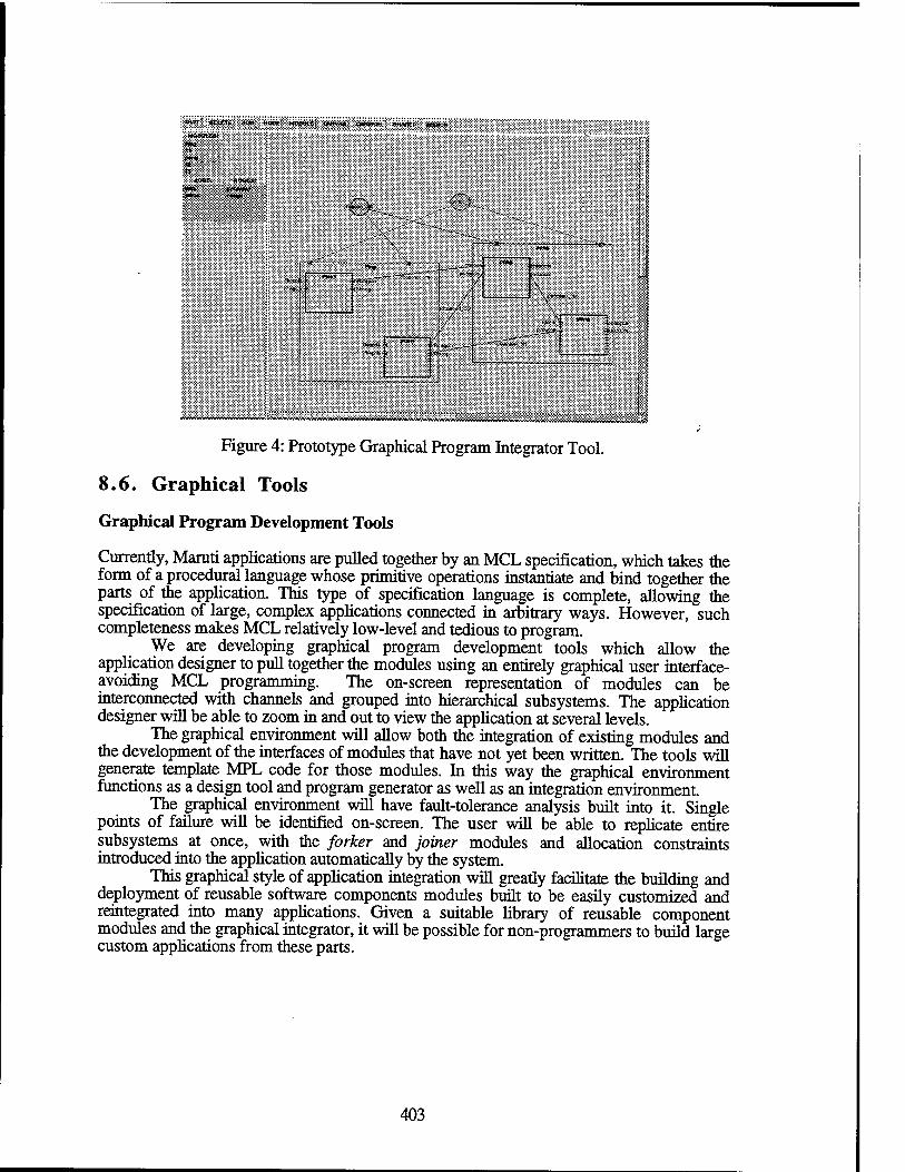
twr «.«TS <o» NOW' HVCVI' «*VM «HMRKC1 »WHO xnpcH

:;:»«»«US»S::

JO« HOW»

*iw«vwiw>«iwCOwv0iiwjjtf^uftjy«y»Y»Y>y«y.y»y/«y»yiy«y»w.y.y.y&^^^

Figure 4: Prototype Graphical Program Integrator Tool.

8.6. Graphical Tools

Graphical Program Development Tools

Currently, Maruti applications are pulled together by an MCL specification, which takes the form of a procedural language whose primitive operations instantiate and bind together the parts of the application. This type of specification language is complete, allowing the specification of large, complex applications connected in arbitrary ways. However, such completeness makes MCL relatively low-level and tedious to program.

We are developing graphical program development tools which allow the application designer to pull together the modules using an entirely graphical user interface- avoiding MCL programming. The on-screen representation of modules can be interconnected with channels and grouped into hierarchical subsystems. The application designer will be able to zoom in and out to view the application at several levels.

The graphical environment will allow both the integration of existing modules and the development of the interfaces of modules that have not yet been written. The tools will generate template MPL code for those modules. In this way the graphical environment functions as a design tool and program generator as well as an integration environment.

The graphical environment will have fault-tolerance analysis built into it. Single points of failure will be identified on-screen. The user will be able to replicate entire subsystems at once, with the forker and joiner modules and allocation constraints introduced into the application automatically by the system.

This graphical style of application integration will greatly facilitate the building and deployment of reusable software components modules built to be easily customized and reintegrated into many applications. Given a suitable library of reusable component modules and the graphical integrator, it will be possible for non-programmers to build large custom applications from these parts.

403

ft-* «■■€-*-■ 1*- 7JX» «r BLln 7i* «r "* IS- ^•ÄäfiiiäKiää®

...,» ■•'.•... ■ .»a :' (««o ;«W ftX> ,«»i««i«r

■IIBHIIIIJJ J! MIM lUiJil &31 ^■^■'■:-isii^^^^^-^ 1 mz

ffe$che0u$p ^&x?» .Jrt 1>eBh 3ocp» put G«*>h

&OT ;

Figure 5: Prototype Graphical Resource Scheduling Tool

Graphical Resource Management Tools

Along with the graphical software development tools, we are pursuing graphical resource management tools. These are a non-programmer's interface into the advanced Maruti scheduling technology. The Maruti allocator/scheduler works with the abstract concepts of schedulable entities, available resources, and various types of constraints on the placement of entities and resources. In the Maruti operating system, the scheduling entities are EUs, and the resources are CPUs, network, memory, and devices - but in fact any type of entity or resource can be manipulated by the allocator/scheduler.

A graphical resource management tool will allow the specification of these entities, resources, and constraints on screen in a way more oriented towards the general user. With this tool users should be able to use Maruti scheduling technology to schedule classes, busses, or projects, for example.

We have built a small prototype of the graphical resource manager. The prototype displays the EU graph input to the scheduler as well as the calendar output of the scheduler. The user can edit the EU graph and its constraints and reschedule with the click of a button. The resulting resource calendar is redisplayed.

9. Availability

We are pleased to announce the availability of the Maruti 3.1 Hard Real-Time Operating System and Development Environment.

With Maruti 3.1, we are entering a new phase of our project. We have an operating system suitable for field use by a wider range of users, and we are embarking on the integration of our time-based, hard real-time technology with industry standards and more traditional event-based soft- and non-real-time systems. For this, we are greatly interested in the feedback from users as to the direction of evolution of the system.

404

For the Maruti 3.1 project, we will be pursuing the integration of a POSIX interface for soft and non-real-time applications, the use of Ada for Maruti programming, support for asynchronous events and soft/non-real time schedulers within the time-based framework, and heterogeneous Maruti networks.

For this user-oriented phase of the project we will be making regular releases of our software available to allow interested parties to track and influence our development. To begin this phase we are making our current base hard real-time operating system and its development environment available. This is an initial test release.

. Maruti 3.1 will be made available to interested parties on request, via Internet ftp. Please send electronic mail to [email protected] for details. More information about the Maruti Project, as well as papers and documentation, are available via the World Wide Web at:

http://www.cs.umd.edu/projects/maruti/l

9.1. Runtime System

The Maruti 3.1 embeddable hard real-time runtime system for distributed and single-node systems includes the following features:

• The core Maruti runtime system is small -16 KB code for the single node core, 30 KB code for the distributed core.

• The core provides a calendar-based scheduler, threads, distributed message passing using Time Division Multiplexed Access (TDMA) over the network, and tight time synchronization between network nodes.

• Also included in the runtime system is a graphics library suitable for system monitoring displays as well as simulations.

• Maruti runs on PC-AT compatible computers using the Intel i386 (with i387 coprocessor), i486DX, or Pentium processors. Distributed operation currently requires a 3Com 3c507 ethernet card. The graphics library supports standard VGA and Tseng- Labs ET-4000-based Super-VGA. Support for other SVGA chipsets is forthcoming soon.

9.2. Development Environment

Maruti 3.1 includes a complete development environment for distributed embedded hard real-time applications. The development environment runs on NetBSD Unix and includes the following:

• d The Mamti/Virtual debugging environment - simulates the Maruti runtime system within the development environment. The system clock in this environment tracks virtual time, which can be sped up, slowed down in relation to the actual time, or single-stepped or stopped. This allows temporal debugging of the application. Within Marati/Virtual traces of the application scheduling and network traffic can be monitored in the debugging session.

405

•

•

•

•

The ANSI-C based Maruti Programming Language (MPL/C). MPL adds modules, message passing primitives, shared memory, periodic functions, message-invoked functions, and exclusion regions to ANSI C. MPL is processed by a version of the GNU C compiler which has been modified to recognize the new MPL features, and to output information about the resources used by the MPL program.

The Maruti Configuration Language (MCL). MCL allows the system designer to specify the placement, timing constraints, and interconnections of all the modules in an application. MCL is a powerful interpreted C-like language, allowing complex, hierarchical configuration specifications, including replication of components and installation-site specific sizing of the application. The MCL processor analyses the application graph for completeness, and type-checks all connections.

The Maruti Allocator/Scheduler. The Maruti allocation and schedulingtool analyses the information generated by the MPL compiler and the MCL integrator to find an allocation and scheduling of the tasks of a distributed application across the nodes of a Maruti network. All relative and global timing, exclusion, and precedence constraints are taken into account in finding a schedule, as are the network speed and scheduling parameters.

The Maruti Timing Trace Analyzer. The Timing Analyzer calculates worst-case computation times from timing files output by the runtime system. Computation times are calculated for each scheduling unit in the application, and these times can be fed back into the Allocator/Scheduler for more precise scheduling analysis.

The Maruti Runtime Binder (mbind). One of the features of Maruti is the late binding of an application to a particular runtime system. The same application binaries can be combined with different system libraries to build a binary customized for a particular application in a particular setting. Only those portions of the system library needed for that binding are included. Mbind manages this final step.

The Maruti Application Builder (mbuild). Mbuild automates the process of building an application by generating for the programmer a customizable makefile that manages the complete process of compiling, configuring, scheduling, and binding an application.

406

Final Report - Defense Technical Information Center

Documents

Transcript of Final Report - Defense Technical Information Center