2MWri\ 090 - Defense Technical Information Center
234
LU O : " mm W ^^ m 1M . N* CB 0) (0 o 0) OOC i US Army Corps of Engineers® Engineer Research and Development Center Nonfacility Particulate Matter Issues in the Army-A Comprehensive Review Michael R. Kemme, Joyce C. Baird, Dick L. Gebhart, Matthew G. Hohmann, Heidi R. Howard, David A. Krooks, and Jearldine I. Northrup June 2001 Approved for public release; distribution is unlimited. 2MWri\ 090
-
Upload
khangminh22 -
Category
Documents
-
view
3 -
download
0
Transcript of 2MWri\ 090 - Defense Technical Information Center

LU O
: ■" mm W ^^m 1M . ■N* CB
0) (0 o 0)
OOC i
US Army Corps of Engineers® Engineer Research and Development Center
Nonfacility Particulate Matter Issues in the Army-A Comprehensive Review Michael R. Kemme, Joyce C. Baird, Dick L. Gebhart, Matthew G. Hohmann, Heidi R. Howard, David A. Krooks, and Jearldine I. Northrup
June 2001
Approved for public release; distribution is unlimited. 2MWri\ 090

m >»
LU O
Ü -C
4- TO
(0 0) rol
O 0 O DC
..,';!
US Army Corps of Engineers® Engineer Research and Development Center
Nonfacility Particulate Matter Issues in the Army-A Comprehensive Review Michael R. Kemme, Joyce C. Baird, Dick L. Gebhart, Matthew G. Hohmann, Heidi R. Howard, David A. Krooks, and Jearldine I. Northrup
June 2001
Approved for public release; distribution is unlimited.

ERDC/CERLTR-01-50
Foreword
This study was conducted for Headquarters, U.S. Army Corps of Engineers un- der 622720A896, "Base Facilities Environmental Quality"; Work Unit number TJO, "Comprehensive Review of Particulate Matter Issues for DOD." The techni- cal monitor was Rochelle Williams, AFEN-EN, U.S. Army Forces Command.
The work was performed by the Environmental Processes Branch (CN-E) of the Installations Division (CN), Construction Engineering Research Laboratory (CERL). The CERL Principal Investigator was Michael Kemme. The technical editor was Linda L. Wheatley, Information Technology Laboratory — Cham- paign. Dr. Ilker Adiguzel is Chief, CN-E, and Dr. John Bandy is Chief, CN. The associated Technical Director was Gary W. Schanche, CVT. The Acting Director of CERL is Dr. Alan W. Moore.
CERL is an element of the U.S. Army Engineer Research and Development Cen- ter (ERDC), U.S. Army Corps of Engineers. The Director of ERDC is Dr. James R. Houston and the Deputy to the Commander is A. J. Roberto, Jr.
DISCLAIMER
The contents of this report are not to be used for advertising, publication, or promotional purposes. Citation of trade names does not constitute an official endorsement or approval of the use of such commercial products. All product names and trademarks cited are the property of their respective owners.
The findings of this report are not to be construed as an official Department of the Army position unless so designated by other authorized documents.
DESTROY THIS REPORT WHEN IT IS NO LONGER NEEDED. DO NOT RETURN IT TO THE ORIGINATOR.

ERDC/CERLTR-01-50
Contents
Foreword 2
List of Figures and Tables 9
1 Introduction 11
Background 11
Objective 13
Approach 13
Mode of Technology Transfer 14
Units of Weight and Measure 14
2 Chemistry and Physics of PM in the Atmosphere 15
Particle Size Distribution 15
Chemical Composition 17
Visibility 19
Atmospheric Particulate Removal Mechanisms 20
3 Review of the Environmental Protection Agency's Enforcement Strategy for Particulate Matter 21
Introduction 21
Regulatory Review 23
PM2.5 Standards 23
PM10 26
Regional Haze 33
New Source Review/Prevention of Significant Deterioration 39
Conformity 40
The Particulate Monitoring Program 41
Enforcement at DOD Facilities 42
Conclusions 44
4 Army Nonfacility PM Source Emission Estimation 47
Vehicles 49
Exhaust, Brake Wear, and Tire Wear. 49
Re-entrained Dust on Paved Roads 51
Re-entrained Dust on Unpaved Roads 51
Prescribed Burning 54

ERDC/CERLTR-01-50
Smokes and Obscurants Training 56
Artillery Practice and Weapons Impact Testing 57
Open Burning/Open Detonation of Munitions 59
Aircraft 61
Reliability of Emission Factors 63
Procedures for Submitting New or Revised Emission Factors 64
5 Atmospheric Modeling 67
Industrial Source Complex (ISC3) Model 70
Applicability of ISC3 to Army Nonfacility PM Sources 70
Required Inputs for ISC3 JQ
Steps and Level of Effort Required To Run ISC3 77
Special Training or Knowledge Required To Run ISC3 72
Outputs of ISC3 and How To Interpret the Results 72
Accuracy of ISC3 72
Advantages and Drawbacks of ISC3 73
Probability of the Results of ISC3 Being Accepted by Regulators 73
Procedure for Obtaining ISC3 and Its Costs 74
Climatological Dispersion Model (CDM 2.0) 74
Applicability of CDM to Army Nonfacility PM Sources 74
Required Inputs for CDM 74
Steps and Level of Effort Required To Run CDM. 75
Special Training or Knowledge Required To Run CDM 75
Outputs of CDM and How To Interpret the Results 75
Accuracy of CDM 75
Advantages and Drawbacks of CDM 75
Probability of the Results of CDM Being Accepted by Regulators 76
Procedure for Obtaining CDM and Its Cost. 76
Gaussian-Plume Multiple Source Air Quality Algorithm (RAM) 76
Applicability of RAM to Army Nonfacility PM Sources 76
Required Inputs for RAM 76
Steps and Level of Effort Required To Run RAM 77
Special Training or Knowledge Required To Run RAM. 77
Output of RAM and How To Interpret the Results 77
Accuracy of RAM 77
Advantages and Drawbacks of RAM 78
Probability of the Results of RAM Being Accepted by Regulators 78
Procedure for Obtaining RAM and Its Costs 78
Open Burning/Open Detonation Dispersion Model (OBODM) 78
Applicability of OBODM to Army Nonfacility PM Sources 78
Required Inputs for OBODM 79
Steps and Level of Effort Required To Run OBODM 79

ERDC/CERLTR-01-50
Special Training or Knowledge Required To Run OBODM 79
Output of OBODM and How To Interpret the Results 79
Accuracy of OBODM 79
Advantages and Drawbacks of OBODM. 80
Probability of the Results of OBODM Being Accepted by Regulators 80
Procedure for Obtaining OBODM and Its Costs 80
Second-order Closure Integrated Puff Model (SCIPUFF) 80
Applicability of SCIPUFF to Army Nonfacility PM Sources 80
Required Inputs for SCIPUFF 80
Steps and Level of Effort Required To Run SCIPUFF .81
Special Training or Knowledge Required To Run SCIPUFF 81
Output of SCIPUFF and How To Interpret the Results 81
Accuracy of SCIPUFF 81
Advantages and Drawbacks of SCIPUFF 81
Probability of the Results of SCIPUFF Being Accepted by Regulators 82
Procedure for Obtaining SCIPUFF and Its Costs 82
MESOPUFF 82
Applicability of MESOPUFF II to Army Nonfacility PM Sources 82
Required Inputs for MESOPUFF II 83
Steps and Level of Effort Required To Run MESOPUFF II 83
Special Training or Knowledge Required To Run MESOPUFF II 83
Output of MESOPUFF II and How To Interpret the Results 83
Accuracy of MESOPUFF II 84
Advantages and Drawbacks of MESOPUFF II 84
Probability of the Results of MESOPUFF II Being Accepted by Regulators 84
Procedure for Obtaining MESOPUFF II and Its Costs 84
CALPUFF 84
Applicability of CALPUFF to Army Nonfacility PM Sources 84
Required Inputs for CALPUFF 85
Steps and Level of Effort Required To Run CALPUFF 86
Special Training Required To Run CALPUFF 86
Outputs of the CALPUFF Model 87
Accuracy of the CALPUFF Model 87
Advantages and Drawbacks of the CALPUFF Model 87
Probability of the Results of CALPUFF Being Accepted by Regulators 87
Procedure for Obtaining CALPUFF and Its Cost 88
Electro-Optical Systems Atmospheric Effects Library (EOSAEL) and the Combined Obscuration Model for Battlefield Induced Contaminants (COMBIC) Module 88
Two Air Dispersion Models Proposed 88
6 Trajectory Models 90
Hybrid Single-Particle Lagrangian Integrated Trajectory (HYSPLIT4) Model 90

ERDC/CERLTR-01-50
Applicability of the HYSPUT4 Model to Army Nonfacility Sources 91
Required Inputs for HYSPLIT4 and How the Inputs Are Obtained 91
Steps and Level of Effort Required To Run the HYSPLIT4 Model 91
Special Training or Knowledge Required To Run the HYSPLIT4 Model 91
Output of the HYSPUT4 Model and How To Interpret the Results 92
Accuracy of the HYSPUT4 Model 92
Advantages and Drawbacks of the HYSPUT4 Model. 92
Probability of the Results of HYSPLIT Being Accepted by Regulators 92
Procedure for Obtaining the HYSPLIT4 Model and Its Costs 92
Center for Air Pollution and Trend Analysis (CAPITA) Monte Carlo Model 93
Applicability of the CAPITA Monte Carlo Model to Army Nonfacility Sources 93
Required Inputs for the CAPITA Model and How the Input Data Are Obtained. 93
Steps and Level of Effort Required To Run the CAPITA Model. 93
Special Training or Knowledge Required To Run the CAPITA Model 93
Output of the CAPITA Model and How To Interpret the Results 94
Accuracy of the CAPITA Model 94
Advantages and Drawbacks of the CAPITA Model 94
Probability of the Results of the CAPITA Model Being Accepted by Regulators 94
Procedure for Obtaining the CAPITA Model and Its Costs 94
7 Measurement of Paniculate Matter 95
Overview 95
Federal Reference and Equivalent Methods 95
Noncontinuous Filter-Based Mass Measurement Systems 100
Size-Selective Inlets 100
Flow Control 102
Filters 102
Sampling Artifacts, Interferences, and Limitations 103
Continuous and Semi-Continuous PM Measurement Systems 107
Mass and Particle Size 108
Visible Light Scattering no
Electrical Mobility 773
Visible Light Absorption 774
Chemical Speciation 775
Laboratory Techniques for Speciation 116
Elements 777
Ions 119
Carbonaceous Aerosols 120
Semivolatile Organic Aerosols 123
Opacity 123

ERDC/CERLTR-01-50
8 Dust Suppression and Soil Stabilization Technology 125
Background 125
Construction and Maintenance of Unpaved Roads and Trails 126
Good Construction and Maintenance Practices 127
Mechanical Stabilization 128
Physical Stabilization 129
Chemical Methods of Dust Suppression 130
Water-attracting Chemicals (Chlorides, Salts, and Brine Solutions) 131
Organic Nonbituminous Chemicals (Lignosulfonates, Sulphite Liquors, Tall Oil Pitch, Pine Tar, Vegetable Oils, and Molasses) 131
Petroleum-Based Binders and Waste Oils (Bitumen Emulsions, Asphalt Emulsions, and Waste Oils) 132
Electrochemical Stabilizers (Sulphonated Petroleum, Ionic Stabilizers, and Bentonite) 132
Polymers (Polyvinyl Acrylics and Acetates) 133
Enzyme Slurries 133
Cementitious Binders (Portland Cement, Lime, Fly Ash, and Bioenzymes) 133
Biological Methods of Dust Suppression 134
Vegetation Systems 135
Mulch Applications 137
Biological Crusts 138
9 Ranking of Army Nonfacility Paniculate Matter Sources/Installations 140
Identification of Installations 140
Activity Levels 144
Vehicles 147
Prescribed Burning 157
Smokes and Obscurants Training 159
Artillery and Other Main Rounds Practice 161
Weapons Impact Testing 164
Open Burning and Open Detonation 165
Helicopters 168
TSR PM10, and PM2.5 Emissions Inventory 170
Vehicles 170
Prescribed Burning 175
Smokes and Obscurants Training 179
Open Burning/Open Detonation During Field Exercises 179
Helicopters 180
Qualitative Ranking of TSP, PM10, and PM2.5 Contributions 181
Ranking the Emission Sources 181
Ranking the Installations 195
10 Summary and Conclusions 206

ERDC/CERLTR-01-50
Acronyms and Abbreviations 210
References 214
CERL Distribution 232
Report Documentation Page 233

ERDC/CERL TR-01-50
List of Figures and Tables
Figures
1
2
3
4
5
6
7
8
9
10
11
12
13
Tables
1
2
3
4
5
6
7
8
9
Representative mass size distribution with measured particle size fractions and dominant chemical components 16
PM10 nonattainment areas and non-ARNG installations 31
PM10 nonattainment areas and ARNG installations 32
Federal Class I areas and non-ARNG installations 36
Federal Class I areas and ARNG installations 37
Mean number of days with 0.01 inch or more of precipitation in United States 53
2.5-micron impactor assembly 97
Changes in particle size distribution after passing through PM2.5 and PM10 inlets 101
Flow diagram of filter processing and analysis activities for NAMS 118
Schematic of thermal-optical instrument 121
Thermogram for a sample containing organic, carbonate, pyrolytic, and elemental carbon (OC, CC, PC, and EC). The last peak is the methane calibration peak 122
Locations of major FORSCOM, TRADOC, and USAR installations 143
Locations of major ARNG installations 144
EPA-designated PM10 nonattainment and maintenance areas as of 10 August 1999 27
Installations within or adjacent to PM10 nonattainment areas 30
Non-ARNG installation proximity to Federal Class I areas 34
ARNG installation proximity to Federal Class I areas 35
Schedule for SIP development for regional haze 38
Impact of NAS report on PM2.5 monitoring network design 42
AP-42 PM emission factors for prescribed burning activities 55
PM10 emission factors for OB/OD of explosives/propellants 60
Average emission factors for OB/OD processes 61

10 ERDC/CERLTR-01-50
10 Helicopter engine paniculate emissions with JP-8 fuel 62
11 Emission factor ratings from AP-42 64
12 Applicability of dispersion models to Army nonfacility emission sources 69
13 List of designated reference and equivalent methods, 9 May 2000 99
14 FORSCOM, TRADOC, and USAR installations and PM-generating activity data -J42
15 HMMWV and Abrams tank activity at ARNG installations 143
16 TRADOC, FORSCOM, and USAR installations 146
17 Emission related vehicle characteristics 148
18 Vehicle activity at non-ARNG installations 149
19 Vehicle activity at ARNG installations 154
20 Installation characteristics related to prescribed burning emissions 158
21 1998 main gun activity 162
22 1998 distribution of main rounds fired 163
23 ATEC testing center activity 165
24 Artillery rounds fired 167
25 Artillery propellant used 167
26 Helicopter activity (hours) and engine parameters 169
27 PART5 emission factors (exhaust PM, brake wear, and tire wear) 171
28 1998 estimated PM emissions from vehicles at Army installations 172
29 Regional average fuel loading and emission factors for prescribed burning ....176
30 Estimated PM emissions from prescribed burning 177
31 PM10 emissions from open burning of munitions during field operations 180
32 Installation operational hours and emissions from helicopters 182
33 Rank of individual installation PM2.5 sources 183
34 Rank of individual installation PM10 sources 187
35 Rank of individual installation TSP sources 191
36 Frequency of nonfacility source rankings from 50 installations 195
37 Installation ranking by 1998 PM2.5 vehicle emissions 196
38 Installation ranking by 1998 PM10 vehicle emissions 198
39 Installation ranking by 1998 TSP vehicle emissions 200
40 Installation ranking by annual PM prescribed burning emissions 202
41 Open burning PM10 emissions 203
42 Installations ranked by 1998 helicopter exhaust emissions 203

ERDC/CERLTR-01-50 11
1 Introduction
Background
Particulate matter (PM) is the general term used to describe a mixture of solid particles and liquid droplets found in the air. These particles, found in a wide range of sizes, originate from many stationary, mobile, and natural sources. PM may be emitted directly by a source or formed in the atmosphere by the trans- formation of gaseous emissions. Their chemical and physical compositions vary depending on location, time of year, and meteorology.
Scientific studies show a link between PM and significant health effects. These health effects include premature death, and increased hospital admissions and emergency room visits. Other effects are increased respiratory symptoms and disease, decreased lung function, and alterations in lung tissue and structure and in respiratory tract defense mechanisms. Sensitive groups such as the eld- erly, children, and individuals with cardiopulmonary diseases such as asthma appear to be at greatest risk to these effects. In addition to health problems, PM is the major cause of reduced visibility in many parts of the United States. Air- borne particles also can soil and damage materials.
PM generated from Army nonfacility sources is a military-unique problem, and a significant source of air pollution. Army nonfacility sources include soil-based PM from training activities, prescribed burning, smokes and obscurants train- ing, artillery practice, weapons impact testing, and open burning/open detona- tion (OB/OD). A majority of these sources are found on troop-based installations. PM emissions may create legal, regulatory, ecological, and practical problems for the modern Army installation. It has the potential to limit or restrict time and frequency of training, to close ranges, or completely shut down training exercises due to the Clean Air Act Amendment of 1990 (CAA1990) or threatened and endangered species (TES) compliance requirements. Major Army Commands (MACOMs) primarily affected include the Forces Command (FORSCOM), Train- ing and Doctrine Command (TRADOC), Army Reserve Command (USARC), and the National Guard Bureau (NGB). These problems will worsen with mission realignments, new weapon systems, encroachment, and increasing urbanization.

12 . ERDC/CERLTR-01-50
Many other significant nonregulatory issues, however, are related to nonfacility PM sources. These issues include safety; health and welfare of troops; military vehicle maintenance requirements; tactical considerations; soil erosion and loss of training land soil resources; and fines, lawsuits, damage claims, and com- plaints. PM clouds generated from helicopter landing pads, tank trails, and smokes and obscurants training impair the visibility of military vehicle opera- tors, increasing the likelihood of accidents and injury. Excessive PM is a health hazard to military vehicle operators and is an air quality hazard when it drifts into nearby housing and administrative areas or onto adjacent highways and streets. Dust intruding into engine and turbine compartments, air filtering sys- tems, and other sensitive mechanical and electrical components causes excessive wear and tear on military vehicles and aircraft (Hass 1986). Continuous move- ment of training vehicles over training lands removes vegetation and reduces soil cohesion causing this soil to be much more susceptible to wind and water ero- sion. Finally, dust generated from helicopter and tank movement provides an unmistakable signature to enemy forces in a tactical scenario.
Although not directly related to the mission and training problems mentioned above, dust also adversely affects vegetation near helicopter pads, roads, and trails. A covering of dust on leaf surfaces increases leaf temperatures (Eller 1977; Hirano et al. 1995) and water loss (Ricks and Williams 1974; Fluckinger, Oertli, and Fluckinger 1979), while decreasing carbon dioxide (C02) uptake (Fluckinger, Oertli, and Fluckinger 1979; Thompson et al. 1984; Hirano et al. 1990, 1995). These physiological changes suggest that vegetation around heli- copter pads, roads, and trails is susceptible to chronic decreases in photosynthe- sis and growth, which may eventually lead to accelerated erosion problems from lack of adequate roadside vegetative stabilization.
The Army Environmental Requirements and Technology Assessments (AERTA) process generates user requirements that are used as guidance for environ- mental research and development within the Army. The requirements are or- ganized into the environmental pillars of cleanup, compliance, conservation, and pollution prevention, and then the requirements are ranked within each pillar. In the compliance pillar the number one ranked user requirement is numbered "A (2. Lb)" and is titled "Particulate Matter/Dust Control and Measurement Tools for Maneuver Training, Smokes/Obscurants Training, and Range and Road Maintenance." User requirement A (2.1.b) has three focus areas: • PM mitigation/soil stabilization technologies • Source and atmospheric characterization methods and models • Real-time measurement of PM emissions.

ERDC/CERLTR-01-50 13
The high ranking of this user requirement has led to the development of a re- search and development (R&D) program to provide useful technology for Army users affected by nonfacuity PM emission issues. The preparation of this review document is the first step of this R&D program.
Objective
The objective of the study was to develop a technical report that includes a re- view of previous work related to Department of Defense (DOD) nonfacility PM problems. The review will be used to determine the U.S. Environmental Protec- tion Agency's (EPA's) enforcement strategy for PM, to identify previous work in the area, and to determine the scope of the nonfacility PM problem at Army fa- cilities. The results of this review will be used to help focus an R&D program in this area. It is also hoped that this review will be a valuable source of informa- tion for others interested in this topic.
Approach
Researchers reviewed and described literature in the following areas: Atmospheric science of PM EPA's regulatory strategy Estimating PM emissions from nonfacility sources Dispersion modeling of PM emissions Transport modeling of PM emissions Measurement of atmospheric PM Dust suppression and soil stabilization technologies.
Each of these areas corresponds to a chapter in this report. Besides information obtained from the literature, these chapters also contain general knowledge per- taining to each of these areas.
In addition to the literature review, an attempt was made to relatively rank non- facility PM sources and the major Army installations containing these sources. The rankings were based on mass emissions of PM10 and PM2.5. The develop- ment of emission estimating techniques and PM rankings was aided by informa- tion developed by the Science Applications International Corporation (SAIC 2000).

14 ERDC/CERLTR-01-50
Mode of Technology Transfer
The final product will be transferred to troop MACOMs by technical report. The report will be available on the CERL website at: http://www.cecer.armv.mil. The information in this report will also be transferred to the field through pres- entations at appropriate symposiums and user group meetings.
Units of Weight and Measure
Some U.S. standard units of measure are used in this report. A table of conver- sion factors for Standard International (SI) units is provided below.
SI conversion factors
1 in. = 2.54 cm 1 mi = 1.61 km 1 lb = 0.453 kg

ERDC/CERLTR-01-50 15
2 Chemistry and Physics of PM in the Atmosphere
Atmospheric PM originates from a variety of sources and possesses a range of properties that affect its impact on human health and degradation of visibility in the atmosphere. Atmospheric PM contains inorganic ions and elements, EC, or- ganic, and crustal compounds. Some hygroscopic (absorbing moisture from the air) particles may contain particle-bound water. PM can be liquid droplets or solids that originate from a variety of natural and anthropogenic (manmade) sources. Atmospheric PM ranges in diameter from a few thousandths of a um to several hundred urn.
Atmospheric PM can be classified as primary or secondary. Primary PM is com- posed of material directly emitted into the atmosphere, while secondary PM forms because of chemical reactions involving gas-phase precursors. Examples of primary particles include wind-blown dust, sea salt, road dust, fly ash, and soot. Examples of secondary PM include ammonium sulfate and nitrate that form in the atmosphere. In urban atmospheres, secondary PM can exceed 50 percent of the total PM mass (Seinfeld 1986).
Particle Size Distribution
Atmospheric PM has traditionally been divided into fine-mode and coarse-mode particle categories with "coarse" particles defined as those larger than 2.5 urn and "fine" particles as those less than or equal to 2.5 urn. These modes not only correspond to different size ranges but also reflect differences in formation mechanism, chemical composition, sources, and exposure relationships. PM size distribution is dynamic since particles are constantly being formed, changed, and removed from the atmosphere. Figure 1 shows an idealized representation of the common size ranges of PM and the principle chemical components of the parti- cles found in these size ranges.

16 ERDC/CERLTR-01-50
0.1 1 10 Partide Aerodynamic Diameter (um)
Figure 1. Representative mass size distribution with measured particle size fractions and dominant chemical components (Watson et al. 1998).
As depicted in Figure 1, the fine particle category can sometimes be divided into two separate size ranges. The particles in the "nucleation" size range are smaller than 0.1 urn and are sometimes called ultra-fine particles. These parti- cles are formed either through direct emission from combustion sources or by condensation of gases near an emission source. Particles in the nucleation range normally have very short lifetimes in the atmosphere because they very rapidly either coagulate with larger particles or serve as condensation nuclei for the formation of water droplets. These ultra-fine particles, therefore, are normally found only near their emission sources. The "accumulation" range consists of particles with diameters between -0.1 and 2 urn. This size range of particles gets its name because particle removal mechanisms are not efficient in this range, and these particles have a tendency to accumulate in the atmosphere. Accumulation range particles consist of aerosols coagulated from ultra-fine par- ticles, aerosols emitted directly from combustion sources, gas-to-particle conver- sion, condensation of volatile species, and finely ground dust. The sizes of these particles can also be affected by the presence of water. When water-soluble par- ticles are present, the peak of the nucleation and accumulation mode will shift toward larger aerodynamic diameters as the humidity increases.
Coarse particles are created primarily from grinding activities and are domi- nated by material of geological origin. Windblown dust from soil, unpaved roads, construction, evaporation of sea spray, pollen, mold spores, and PM formed from

ERDC/CERLTR-01-50 17
the grinding of larger particles are predominantly in the coarse particle size range, with minor or moderate quantities in the fine fraction. Particles at the low end of the coarse size range also occur when cloud and fog droplets form in a polluted environment, then dry out after having scavenged other particles and gases (Jacob et al. 1986).
Chemical Composition
The major constituents of atmospheric PM are sulfates, nitrates, carbonaceous compounds (organic carbon [OC] and elemental carbon [EC]), geological materi- als, sodium chloride, and water. Chemical compositions vary with particle size, geographic location, and season. The relative abundances of chemical compo- nents in the atmosphere can provide evidence about the emission sources con- tributing to atmospheric PM. It is likely that PM chemical composition data will someday be used to establish a relationship between specific chemical compo- nents of PM and health effects.
Ammonium sulfate ((NH4)2S04), ammonium bisulfate (NH4HS04), and sulfuric acid (H2S04) are the most common forms of sulfate found in atmospheric PM. The sulfate compounds result from irreversible reactions between sulfuric acid and ammonia gas (NH3) (Watson et al. 1994a). These compounds are water- soluble and reside almost exclusively in the PM2.5 size fraction. Sodium sulfate (NajSC^) may be found in coastal areas where sulfuric acid has been neutralized by sodium chloride in sea salt. Though gypsum (Ca^C^,) and some other geologi- cal compounds contain sulfate, these are not easily dissolved in water for chemi- cal analysis. They are more abundant in the coarse fraction than in PM2.5, and are usually classified in the geological fraction.
Ammonium nitrate (NH4N03) is the most abundant nitrate compound, resulting from a reversible gas/particle equüibrium between ammonia gas (NH3), nitric acid gas (HN03), and particulate ammonium nitrate. Because this equilibrium is reversible, the concentration of ammonium nitrate particles will constantly change due to changes in temperature and relative humidity. Sodium nitrate (NaN03) is found in the PM2.5 and coarse fractions near seacoasts and salt pla- yas where nitric acid vapor irreversibly reacts with sea salt (Watson et al. 1994b). While most of the sulfur dioxide and oxides of nitrogen precursors of ni- trate and sulfate compounds originate from fuel combustion, most of the ammo- nia gas precursor is derived from animals, especially animal husbandry prac- ticed in dairies and feedlots.

— . ERDC/CERL TR-01 -50
The atmosphere contains particles with thousands of separate organic com- pounds that contain more than 20 carbon atoms. These particles are primarily found in PM2.5. Vehicle exhaust; residential, agricultural, and prescribed burn- ing, meat cooking, fuel combustion, road dust, and particle formation from heavy hydrocarbon (C8 to C20) gases are the major sources of organic carbon (OC) in PM2.5. Total OC found in PM is operationally defined by the sampling and analysis method used to measure these organic particles.
EC PM consists of dark organic particles referred to as soot. It contains pure, graphitic carbon, but also contains high molecular weight, dark-colored, non- volatile organic materials such as tar, biogenics, and coke. EC usually accompa- nies OC in combustion emissions such as diesel exhaust from vehicles. Total EC is also operationally defined by the sampling and analysis method for quantify- ing these types of organic particles.
Geological material-based PM consists mainly of oxides of aluminum, silicon, cal- cium, titanium, iron, and other metals oxides (Chow and Watson 1992). The precise combination of these minerals depends on the geology and the specific types of industrial processes found in the area. Geological material is mostly found in the coarse particle fraction and typically constitutes -50 percent of PM10 while only contributing 5 to 15 percent to PM2.5 (Chow et al. 1992; Watson et al. 1994b).
Sodium chloride is found in suspended particles near seacoasts, open playas, and roadways after de-icing materials are applied. Sodium chloride from deicing sand and re-entrained playa dust is usually in the coarse particle fraction and classified as geological material (Chow et al. 1996). However, sodium chloride PM formed from the evaporation of a suspended water droplet (as in sea salt or when resuspended from melting snow) is found mostly in the PM2.5 fraction. As mentioned above, sodium chloride can be neutralized by nitric or sulfuric acid in urban air where it is often encountered as sodium nitrate or sodium sulfate.
Soluble nitrates, sulfates, ammonium, sodium, other inorganic ions, and some organic material can absorb liquid water, especially when relative humidity ex- ceeds 70 percent (Tang and Munkelwitz 1993). Sulfuric acid absorbs some water at all humidities. Particles containing these compounds will grow in size and can become droplets as they continue to absorb water.
ERDC/CERL TR-01-50 19
Visibility
Visibility degrades as PM concentrations increase. Light reflected from an object is absorbed and scattered by the gases and particles in the air as the light trav- els toward an observer, thereby degrading visibility of the object. A measure- ment of the combined effects of scattering and absorption in the atmosphere is the extinction coefficient, which is often measured in units of Mm'1. The extinc- tion coefficient is the sum of the scattering coefficient and the absorption coeffi- cient. Typical extinction coefficients range from 10 Mm'1 for clean air to 1,000 Mm1 for air with high concentrations of PM (Trijonis et al. 1988). The inverse of the extinction coefficient corresponds to the distance at which the original inten- sity of transmitted light is reduced by about two-thirds.
Light is scattered when it is diverted from its path by some form of matter. Two predominant forms of light scattering in the atmosphere are Rayleigh and Mie scattering. For visible light, Rayleigh scattering is caused by particles corre- sponding to the size of atmospheric gases such as oxygen and nitrogen. Mie scat- tering is caused by particles with sizes similar to the wavelength of the electro- magnetic radiation. The visible light wavelength range is about 0.4 - 0.7 urn and particles of this general size are the most efficient at scattering light.
Rayleigh scattering accounts for visibility degradation in pollution-free air. Un- der typical atmospheric conditions the scattering coefficient for Rayleigh scatter- ing is -10 Mm"1. Rayleigh scattering is much stronger in the blue side of the visible spectrum. This accounts for the blue color of a clear sky because most of the visible light seen by an observer has been scattered by atmospheric gases. Light scattering caused by PM depends on the particles' sizes, shapes, and chemical compositions. Each \ig/m3 of ammonium sulfate or ammonium nitrate typically contributes 2-6 Mm'1 to the scattering coefficient. Each |ug/m3 of PM2.5 soil particles contributes ~1 Mm'1 while each \ig/m3 of particles >PM2.5 contribute ~0.5 Mm'1 to visible light extinction (White et al. 1994).
Light is absorbed in the atmosphere primarily by nitrogen dioxide (N02) and by EC particles. Absorption of light by N02 typically accounts for a few percent of the total light extinction in urban atmospheres and has a negligible effect in most remote areas. N02 absorbs blue light more strongly than other visible wavelengths, and contributes to the yellow or brown appearance of urban hazes. The great majority of light absorption by particles is caused by EC (Japar et al. 1986). Mass specific particle absorption efficiencies are usually in a range of 5 to 20 m7g (Jennings and Pinnick 1980). This corresponds to an absorption coeffi- cient contribution of 5 to 20 Mm'1 for each ng/m3 of EC particles.

— ERDC/CERLTR-01-50
Atmospheric Paniculate Removal Mechanisms
Atmospheric PM deposition occurs when PM is removed from the atmosphere and falls on the land or water. PM that is deposited in snow, fog, or rain is called wet deposition, while the deposition of dry particles is dry deposition. Acid rain is a combination of wet and dry deposition of acidic sulfate and nitrate species.
Dry deposition of PM occurs when it is transported to the surface of the earth and removed without the aid of precipitation. Atmospheric turbulence will con- tinually bring PM close to surfaces where it can be removed. Before PM can be removed by a surface, the particles must diffuse across a thin layer of quiescent air. Unlike gases, particles that encounter a surface normally are deposited on that surface since the particle does not have to be absorbed or adsorbed by the surface in order for deposition to occur. Dry deposition of particles is a strong function of particle size, atmospheric conditions, and terrain physiography. The existence of vegetation will increase the surface area available for particle dry deposition and increase deposition rates. Large particles (i.e., above 20 urn in diameter) deposit mainly by gravitational settling. Very small particles (i.e., less than 0.1 urn in diameter) behave much like gases — Brownian diffusion through the thin quiescent surface layer is the limiting dry deposition step. Particles in the 0.1 to 1.0 urn diameter range deposit the least rapidly since they are not large enough for gravitational settling to be important and they are too large for Brownian diffusion to predominate (Seinfeld 1986).
PM is scavenged in clouds when they serve as nuclei for the formation of cloud droplets (cloud condensation nuclei). This process is especially important for fine particles. PM is also scavenged below clouds when they are intercepted by fal- ling precipitation (e.g., rain, snow, etc.). This interception process is more impor- tant for coarse particles than fine particles. Because fine particles tend to follow air motions, they move out of the way and are not impacted by falling raindrops. The wet removal of particles depends on the air trajectories through clouds, the supersaturation to which the air mass is exposed, and the amount of time drop- lets are present before arriving at the ground.

ERDC/CERLTR-01-50 21
3 Review of the Environmental Protection Agency's Enforcement Strategy for Particulate Matter
Introduction
The United States Government has shown interest in regulating PM emissions since 1967, when the Air Quality Act was passed. The 1967 Act focused on the establishment of air quality standards, and these standards, in effect, set goals for a national air quality program. It was not until the Clean Air Act (CAA) of 1970, however, that achieving and maintaining compliance with standards be- gan to emerge as significant issues.
The 1970 Act authorized the EPA to set National Ambient Air Quality Standards (NAAQS), and these standards have become the backbone of air pollution control efforts in this country. The CAA of 1970 established two types of national air quality standards. Primary standards set limits to protect public health, includ- ing the health of "sensitive" populations such as asthmatics, children, and the elderly. Secondary standards set limits to protect public welfare, including pro- tection against decreased visibility, and damage to animals, crops, vegetation, and buildings.
The CAA of 1970 also established the list of criteria pollutants that is still used today: • Total suspended PM (regulated since 1 July 1987 as PM smaller than 10 um
[i.e., PM10]) • Sulfur dioxide (S02) • Nitrogen dioxide (N02) • Lead (Pb)
Thanks go to Vincoli (1993) and Brownell and Zeugin (1992) for their lucid presentations of the history of air quality
legislation in this country. See also http://www.epa.gov/oar/caa/overview.txt.

— . ERDC/CERLTR-01-50
• Carbon monoxide (CO) • Ozone (03)
The 1970 Act also set up the process for developing and implementing State Im- plementation Plans (SIPs), which are a principal means of enforcing NAAQS.
The CAA Amendments of 1977 left the Act of 1970 essentially intact but added new compliance dates and enforcement strategies. The 1977 Amendments also address both Prevention of Significant Deterioration (PSD) in areas that are in attainment of NAAQS (or that are unclassifiable) and the New Source Review (NSR). The NSR portion of the PSD/NSR program addresses both the construc- tion of new facilities and the modification of existing facilities in nonattainment areas.
CAA1990 significantly revised the air pollution control program that was estab- lished by the previous legislative efforts. The Army lives and works with the 1990 Amendments today, and so the CAA as amended in 1990 has important consequences for the present concerns with PM emissions. For example, Title I of the amended Act (Air Pollution Prevention and Control) includes classifica- tions for nonattainment areas, deadlines for achieving attainment, and control measures that must be implemented in nonattainment areas. Title V of the amended Act (Permits) sets up the air-related permitting procedures with which Army environmental managers are so familiar. Of these procedures, Vincoli (1983:86) says:
Under the new Act, SIPs will continue to be used by the states as planning documents to meet air quality objectives. However, permits issued by the states under the federal air permitting program are now the primary enforce- ment mechanism for the EPA. To ensure consistency in its enforcement, the EPA established minimum requirements for state plans. Hence, the permits will not replace the SEPs but will become the principal mechanism for detail- ing the specific requirements as they apply to individual emission sources.
Army activities encompass both stationary sources of PM (such as power plants and industrial processes) and area (nonfacility) sources, such as training activi- ties, prescribed burning operations, and OB/OD. Of these, training areas are of special concern to the Army. If the need to control particulate emissions results in restrictions on training activities, there is likely to be a direct effect on the troops' ability to carry out their assigned missions. Combat readiness could be negatively affected.

ERDC/CERL TR-01 -50 23
Regulatory Review
PM2.5 Standards
Monitoring of primary (directly emitted) particles suggests that fugitive dust, motor vehicles, and wood smoke are the major contributors to ambient PM sam- ples in the Western United States, while stationary combustion, motor vehicles, and fugitive dust are the major contributors in the East. For secondary particles (formed by atmospheric reaction), the major components in the West are nitrates and OC, while in the East sulfates and OC are the major secondary components.
Since 1990, and especially since 1997, there has been a great deal of activity by the EPA, environmental groups, and industry that has consequences for air pol- lution control efforts addressing PM emissions in this country. On 18 July 1997 the EPA released new air quality standards for PM (and ozone), but on 14 May 1999 the U.S. Court of Appeals for the District of Columbia (DC) ruled that the EPA had overstepped its constitutional authority in adopting the 1997 stan- dards. The EPA requested that the Court reconsider its ruling, but it rejected that request on 29 October 1999.
The U.S. Court of Appeals for DC ruled that the PM2.5 standards should remain in place, but the Court will allow parties to apply for the standards to be vacated if "the presence of this standard threatens a more imminent harm." The EPA states (EPA 1999b:2):
Presumably, the 'harm' refers to the burden on sources complying with the regulation. During remand, the legal status of the standards is as follows:
• The Court left the new ozone standards in place based on its determination that it "cannot be enforced."
• The Court vacated the revised coarse particle (PM 10) standards. The pre- existing PM10 standards continues (sic) to apply.
The summary goes on to say (EPA 1999b:2) that "EPA believes it can continue to move forward with other vital clean air programs... including...ensuring the air quality monitoring program continues and the PM2.5 monitors are put in place."
On 29 January 1999, the Department of Justice asked the U.S. Supreme Court to review the lower court's decision, and a number of other organizations (among them the American Lung Association, the American Trucking Association, and the National Chamber Litigation Center) also asked for review. On 22 May 2000, the Supreme Court announced its intention to hear the case. It is expected that a decision on whether EPA overstepped constitutional boundaries in prom- ulgating new NAAQS for ozone and PM will be handed down sometime in 2001.

i* . ERDC/CERLTR-01-50
Meanwhile, EPA is going forward with plans to implement the PM2.5 standards. That implementation plan involves the following activities: • Developing a monitoring network • Working with states to deploy the monitoring network • 3 years of data from the earliest monitors available by Spring 2001; 3 years of
data from all monitors in 2004
• First determinations about designation of nonattainment areas in 2002 (at the earliest)
• States have 3 years from being designated as nonattainment areas to develop pollution control plans (i.e., SIPs) and submit them to the EPA
• Areas then have up to 10 years from nonattainment designation to meet the PM2.5 standards (two 1-year extensions are possible).
On 18 November 1998, EPA issued draft guidance on implementing the PM2.5 standards, and that draft guidance has not been withdrawn since the Court rul- ing in May 1999. Recent developments suggest, however, that U.S. courts will not permit EPA to short-circuit standard rulemaking procedures. On 14 April 2000, the U.S. Court of Appeals for DC set aside EPA's guidance related to Title V permitting rules (Appalachian Power Co. v. EPA, D.C. Cir., No. 98-1512, 4/14/2000). The EPA's Periodic Monitoring Guidance for Title V Operating Per- mits required state permitting authorities to indicate that major industrial fa- cilities must periodically monitor their various pollution sources to ensure com- pliance with the provisions of their permits. The Court of Appeals' decision set aside this guidance entirely saying (as cited in Najor 2000a):
State permitting authorities.. .may not, on the basis of EPA's guidance... require in permits that the regulated source conduct more frequent monitoring of its emissions than that provided in the applicable state or federal standard, unless that standard requires no periodic testing, specifies no frequency, or requires only a one-time test.
Although no direct connection exists between the 14 April ruling and EPA's draft or proposed guidance related to other criteria pollutants, one might suspect that this niling will encourage the Agency to use guidance documents less aggres- sively in the future.
The EPA is moving forward to the extent that it can on the implementation of PM2.5 standards, and it also believes that the development of statewide emission inventories for ozone and PM and their precursors can go forward (EPA 1999a:3):
The implementation of the PM2.5 NAAQS will not occur until after the Clean Air Act Scientific Advisory Committee (CASAC) completes its review of the standard in 2002. However, because many of the same sources produce emis- sions that contribute to ozone and PM2.5 formation and visibility impairment,

ERDC/CERL TR-01-50 25
EPA encourages States to coordinate emission inventory planning and devel- opment efforts for ozone, regional haze, and PM2.5 as they develop their re- quired inventories for ozone. EPA believes that the States should take advan- tage of the opportunity to produce a PM emission inventory while they are collecting data and preparing their ozone precursor inventory.
Once an air quality standard has been put into effect, each state must develop its own plan for meeting those standards, and that plan is its SIP. SIPs must ad- dress specific topics: • Attaining the standard • Implementing control measures • Showing "reasonable further progress" toward attainment • Providing for contingency measures for failure to make progress or attain • Conducting NSR • Requiring conformity of transportation and air quality planning.
The process for developing an SIP is as follows: 1. EPA promulgates new or revises existing NAAQS. 2. After emission inventories, monitoring, and modeling are accomplished, the State
Governor submits to EPA a list of all areas in the State and a recommended air quality designation for each area.
3. EPA may modify recommended designations of the areas (or portions thereof) or boundaries of areas (or portions thereof).
4. EPA promulgates designations (NLT 1 year after recommendations are due) 5. SIPs for nonattainment areas must be submitted to EPA within three years of
promulgation of the new or revised NAAQS; requirements for the SIPs vary de- pending on whether the nonattainment area is classified as moderate or serious forPM2.5.
6. EPA approves/promulgates the SIP, which makes its provisions Federally en- forceable.
The EPA has not yet issued guidance to the States on how to develop their PM2.5 SIPs, but, if it turns out that the PM2.5 problem has a nature and an ex- tent similar to the ozone problem, it is reasonable to expect the guidance on SIPs to be like that for SIPs on ozone.
Broadly speaking, conformity means conformity to an implementation plan's purpose of eliminating or reducing the severity and number of violations of the NAAQS and achieving expeditious attainment of the standards. In addi- tion, Federal actions must not cause or contribute to violation of NAAQS, exacerbate existing violations, or inter- fere with timely attainment of NAAQS or required interim emissions reductions or other milestones.

*L ERDC/CERL TR-01-50
To summarize, there is a PM2.5 standard on the books now, and EPA is develop- ing a monitoring network for PM2.5 so it can make attainment designations un- der the new standard. Because PM2.5 is related to both ozone and regional haze issues, EPA is encouraging state officials to think about PM2.5 and regional haze as they begin work on emissions inventories for ozone. The PM2.5 standard cannot actually be implemented, however, until after the CASAC completes its review of the standard in 2002.
Meanwhile, the Supreme Court must rule on the constitutionality of EPA's ac- tions with regard to the 1997 NAAQS revisions. No one can foresee what that ruling will be or what consequences it will have for the regulated community. In addition, the opinion expressed by the District Court with respect to EPA's habit of rule-making by guidance rather than through the established notice-and- comment process adds another measure of uncertainty. When (or even if) PM2.5 standards will actually become compliance obligations is still an open question.
PM10
The attempt to revise the NAAQS for ozone also included an attempt to revise the existing NAAQS for PM10. As noted above, the DC District Court vacated the revised PM10 standard and left the existing PM10 standard in place. There- fore, the 1987 standards and their associated designations continue to be in ef- fect. Although the continued implementation of the 1987 PM10 standards was not part of EPA's plan for PM10 regulation, its continued enforcement helps to maintain PM air quality at current levels and assures continued public health protection until states have had the opportunity to assess the impacts of the PM2.5 NAAQS (based on ambient monitor data) in their areas.
The existing standards were set in July 1987 for two averaging times: 150 ug/m3
(24-hour average) with no more than one exceedance per year, and 50 ug/m3 (ex- pected annual arithmetic mean) averaged over 3 years. This standard necessi- tated complex data handling when the data set was not complete. In 1997, the 24-hour NAAQS for PM10 was retained at 150 ug/m3 for a 3-year period but in a 99th percentile form. Under this form, an exceedance is measured if the 99th per- centile value measured on a single day is over 150 ug/m3 (averaged over 3 years).
As of 10 August 1999, 77 areas over 79 counties were designated as nonattain- ment for the PM10 NAAQS. Additionally, seven areas were listed as PM10 maintenance areas (previous nonattainment areas). Faculties in nonattainment areas are subject to all applicable state permitting requirements, NSR program requirements, offset provisions for new or modified facilities, and control meas- ures for PM10. Best Available Control Measures (BACMs) are required for

ERDC/CERLTR-01-50 27
facilities in serious nonattainment areas, and Reasonably Available Control Measures (RACMs) must be implemented at facilities located in moderate nonattainment areas.
Table 1 reflects the areas designated as PM10 nonattainment as of 10 August 1999. The table includes the region name, state, classification (moderate or seri- ous), county/counties, and community designation. Facilities located in desig- nated nonattainment areas are subject to RACM or BACM policies and must meet offset provisions when modifying a permitted activity or introducing a new process. The PM10 maintenance areas are also included in Table 1.
Table 1. EPA-designated PM10 nonattainment and maintenance areas as of 10 August 1999.
State Area Classification Affected Location
Alaska Eagle River Moderate Part of Anchorage Ed, Community of Eagle River
Juneau Moderate Part of Juneau Ed, City of Juneau: Mendenhall Valley area
Arizona Ajo Moderate Part of Pima Co.
Douglas Moderate Part of Cochise Co.
Hayden/Miami Moderate Parts of Gila and Pinal counties
Mohave Co. Moderate Part of Mohave Co., Bullhead City
Nogales Moderate Part of Santa Cruz Co.
Paul Spur Moderate Part of Cochise Co.
Payson Moderate Part of Gila Co.
Phoenix Serious Parts of Maricopa and Pinal counties
Rillito Moderate Part of Pima Co.
Yuma Moderate Part of Yuma Co.
California Coachella Valley Serious Part of Riverside Co., Coachella Val- ley planning area
Imperial Valley Moderate Part of Imperial Co., Imperial Valley planning area
Los Angeles South Serious Parts of Los Angeles, Orange, River- Coast Air Basin side, and San Bernardino counties,
South Coast Air Basin
Mammoth Lake Moderate Maintenance Part of Mono Co.
Mono Basin Moderate Part of Mono Co., Hydrologie Unit 1809010
Owens Valley Serious Part of Inyo Co., Owens Valley plan- ning area Hydrologie Unit 18090103
Sacramento Co. Moderate Sacramento Co.
San Bernardino Co. Moderate Part of San Bernardino Co.
San Joaquin Serious Parts of Fresno, Kern, Kings, Valley Madera, San Joaquin, Stanislaus,
and Tulare counties, San Joaquin Valley planning area

28 ERDC/CERLTR-01-50
State Area Classification Affected Location
Searles Valley Moderate Parts of Inyo, Kern, and San Bernar- dino counties, Searles Valley plan- ning area Hydrologie Unit 18090205
Colorado Aspen Moderate Part of Pitkin Co. Canon City Moderate Part of Fremont Co. Denver Metro Moderate Denver, Douglas, and Jefferson
counties and parts of Adams, Arapa- hoe, and Boulder counties
Lamar Moderate Part of Prowers Co. Pagosa Springs Moderate Part of Archuleta Co. Steamboat Springs Moderate Part of Routt Co., Steamboat Springs Telluride Moderate Part of San Miguel Co.
Connecticut New Haven Co. Moderate Part of New Haven Co., City of New Haven
Idaho Bonner Co. (Sand- point)
Moderate Part of Bonner Co.
Fort Hall Moderate Parts of Bannock and Power coun- Reservation ties Pinehurst Moderate Part of Shoshone Co., City of Pine-
hurst Portneuf Valley Moderate Parts of Bannock and Power coun-
ties
Part of Shoshone Co. excluding Shoshone Co. Moderate Pinehurst
Illinois Granite City, Nameoki Township
Moderate Maintenance Part of Madison Co.
Lyons Township Moderate Part of Cook Co., Lyons Township Oglesby Moderate Maintenance Part of LaSalle Co. Southeast Chicago Moderate Part of Cook Co.
Indiana East Chicago Moderate Part of Lake Co., cities of Hammond, Whiting, and Gary
Vermillion Co. Moderate Maintenance Part of Vermillion Co., Clinton Town- ship
Maine Presque Isle Moderate Maintenance Part of Aroostook Co. Michigan Wayne Co. Moderate Maintenance Part of Wayne Co., Detroit Minnesota Olmsted Co. Moderate Maintenance Part of Olmsted Co.
Ramsey Co. Moderate Part of Ramsey Co., St. Paul Montana Butte Moderate Part of Silver Bow Co.
Columbia Falls Moderate Part of Flathead Co. Flathead Co.; Moderate Part of Flathead Co. Whitefish and Vicinity
Kalispell Moderate Part of Flathead Co. Lame Deer Moderate Part of Rosebud Co. Libby Moderate Part of Lincoln Co. Missoula Moderate Part of Missoula Co. Poison Moderate Part of Lake Co., Poison Ronan Moderate Part of Lake Co., Ronan

ERDC/CERLTR-01-50 29
State Area Classification Affected Location
Sanders Co. (part); Thompson Falls and vicinity
Moderate Part of Sanders Co.
Nevada Clark Co. Serious Part of Clark Co., Las Vegas plan- ning area Hydrographie Area 212
New Mexico Anthony Moderate Part of Dona Ana Co.
New York New York Co. Moderate New York Co.
Ohio Cuyahoga Co.
Jefferson Co.
Moderate
Moderate
Cuyahoga Co.
Part of Jefferson Co., Mingo Junction
Oregon Eugene-Springfield
Grants Pass
Klamath Falls
LaGrande
Lake Co.
Lane Co.
Medford-Ashland
Moderate
Moderate
Moderate
Moderate
Moderate
Moderate
Moderate
Part of Lane Co., Urban Growth Boundary
Part of Josephine Co., Urban Growth Boundary
Part of Klamath Co., Urban Growth Boundary
Part of Union Co., Urban Growth Boundary
Part of Lake Co., Lakeview (Urban Growth Boundary)
Part of Lane Co., Oakridge (Urban Growth Boundary)
Part of Jackson Co.
Pennsylvania Clairton and 4 boroughs
Moderate Part of Allegheny Co.
Puerto Rico Mun. of Guaynabo Moderate Part of Guaynabo Co.
Texas El Paso Co. Moderate Part of El Paso Co., City of El Paso
Utah Ogden
Salt Lake Co.
Utah Co.
Moderate
Moderate
Moderate
Part of Weber Co., City of Ogden
Salt Lake Co.
Utah Co.
Washington Kent
King Co.
Olympia, Tumwater, Lacey
Pierce Co.
Spokane Co.
Wallula
Yakima Co.
Moderate
Moderate
Moderate
Moderate
Moderate
Moderate
Moderate
Part of King Co.
Part of King Co., Seattle
Part of Thurston Co., Cities of Olympia, Tumwater, and Lacey
Part of Pierce Co., Tacoma
Part of Spokane Co.
Part of Walla Walla Co., Wallula
Part of Yakima Co.
West Virginia Follansbee
Weirton
Moderate
Moderate
Part of Brooke Co.
Parts of Brooke and Hancock counties, City of Weirton
Wyoming Sheridan Moderate Part of Sheridan Co., City of Sheridan, Trona Industrial Area

30 ERDC/CERLTR-01-50
Chapter 9 describes a process used to develop a list of U.S. Army troop-based in- stallations that are likely to be the largest emitters of PM from nonfacility sources. Once the list of troop-based installations was developed, the locations of the individual installations were examined to determine whether or not they are located in or near a PM10 nonattainment area. Air emission sources located in nonattainment areas are potentially subject to more stringent permitting and air emission control requirements. Table 2 presents troop-based installations that are near PM10 nonattainment areas. Figures 2 and 3 show the general location of PM10 nonattainment areas relative to Army National Guard (ARNG) and non- ARNG installations, respectively.
The EPA has not established nonattainment areas for PM2.5 and will not do so until 2005. Since sources of PM2.5 and characteristics of the pollutant are not the same as for PM10, it cannot be assumed that the future PM2.5 nonattain- ment areas will be related to the current PM10 nonattainment areas. In Decem- ber 1996, in fact, EPA projected that 166 counties would not meet the proposed PM2.5 standards compared with 41 counties that were not meeting the PM10 standards at that time (EPA 1996).
Table 2. Installations within or adjacent to PM10 nonattainment areas.
Installation County Area Classification
Fort Huachuca, AZ Cochise Douglas Moderate Fort Irwin, CA San Bernardino South Coast Basin Serious Fort Carson, CO Canon City Fremont Moderate Fort Bliss, TX El Paso El Paso Moderate Fort Lewis, WA Tacoma Pierce Moderate Yakima Training Center, WA Yakima Yakima Moderate

ERDC/CERLTR-01-50 31
w c o a S M C
a z <
I e O c
■o c a w CD CO
0) E c
1 eg c o c
S a.
£ 3 O)

32 ERDC/CERL TR-01-50
CO ■ tr
'.-« k- i5 m " t*«#*-o orSp ayS^ ~W^ Q.
E cö (0 O O
(0 c o
S «) c O z ac <
w a o>
c a> E c s a c o c
2 O)

ERDC/CERL TR-01-50 33
Regional Haze
Regional haze, also known as impaired visibility or visibility impairment, is caused by particles and gases in the atmosphere that scatter and absorb light. Such particles and gases are emitted by numerous source activities across the United States; their effect on visibility is understood to be cumulative. In addi- tion to impairing visibility, according to the EPA (65 Federal Register [FR] 35715), fine PM "(e.g., sulfates, nitrates, organic carbon, elemental carbon, and soil dust)...can cause serious health effects and mortality in humans, and con- tribute to environmental effects such as acid deposition and eutrophication."
The EPA released the final version of its Regional Haze Regulation on 1 July 1999. That regulation implements Section 169A of the Clean Air Act, which sets forth a national goal for visibility (65 FR 35717): "prevention of any future, and the remedying of any existing, impairment of visibility in Class I areas which impairment results from manmade air pollution."
There are 156 Class I areas across the country, including many well-known na- tional parks and wilderness areas, such as the Grand Canyon, Great Smokies, Shenandoah, Yellowstone, Yosemite, the Everglades, and the Boundary Waters. States and tribes are free, under the terms of the Clean Air Act, to designate Class I areas of their own, but the Regional Haze Regulation applies only to the 156 federally designated Class I areas.'
In addition to detennining whether an installation is located in a PM10 nonat- tainment area, the location of each installation was examined to determine its proximity to any protected Federal Class I visibility area. An installation near a Federal Class I area could be required to control emissions, including those from nonfacility sources, if they are believed to contribute to a visibility problem. Ta- bles 3 and 4 list the non-ARNG and ARNG troop-based installations and their
eotrophication: abundant accumulation of nutrients that support a dense growth of algae and other organisms in
lakes, the decay of which depletes the shallow waters of oxygen in summer.
1" The following states (and one territory) contain at least one mandatory Federal Class I Area (40 CFR 81.400«):
Alabama, Alaska, Arizona, Arkansas, California, Colorado, Florida, Georgia, Hawaii, Idaho, Kentucky, Louisiana,
Maine, Michigan, Minnesota, Missouri, Montana, Nevada, New Hampshire, New Jersey, New Mexico, North Caro-
lina, North Dakota, Oklahoma, Oregon, South Carolina, South Dakota, Tennessee, Texas, Utah, Vermont, Virgin
Islands, Virginia, Washington, West Virginia, and Wyoming. Also included is the Roosevelt Campobello Interna-
tional Park in New Brunswick, Canada. It is worth noting that the vast majority of these designated areas lie in the
western half of the United States.
34 ERDC/CERLTR-01-50
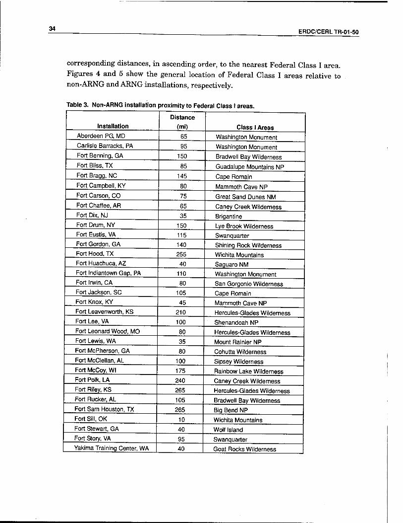
corresponding distances, in ascending order, to the nearest Federal Class I area. Figures 4 and 5 show the general location of Federal Class I areas relative to non-ARNG and ARNG installations, respectively.
Table 3. Non-ARNG installation proximity to Federal Class I areas.
Installation Distance
(mi) Class 1 Areas Aberdeen PG, MD 65 Washington Monument Carlisle Barracks, PA 95 Washington Monument Fort Benning, GA 150 Bradwell Bay Wilderness Fort Bliss, TX 85 Guadalupe Mountains NP
Fort Bragg, NC 145 Cape Romain
Fort Campbell, KY 80 Mammoth Cave NP
Fort Carson, CO 75 Great Sand Dunes NM Fort Chaffee, AR 65 Caney Creek Wilderness Fort Dix, NJ 35 Brigantine Fort Drum, NY 150 Lye Brook Wilderness Fort Eustis, VA 115 Swanquarter Fort Gordon, GA 140 Shining Rock Wilderness Fort Hood, TX 255 Wichita Mountains Fort Huachuca, AZ 40 Saguaro NM Fort Indiantown Gap, PA 110 Washington Monument Fort Irwin, CA 80 San Gorgonio Wilderness Fort Jackson, SC 105 Cape Romain Fort Knox, KY 45 Mammoth Cave NP Fort Leavenworth, KS 210 Hercules-Glades Wilderness Fort Lee, VA 100 Shenandoah NP
Fort Leonard Wood, MO 80 Hercules-Glades Wilderness Fort Lewis, WA 35 Mount Rainier NP Fort McPherson, GA 80 Cohutta Wilderness Fort McClellan, AL 100 Sipsey Wilderness Fort McCoy, Wl 175 Rainbow Lake Wilderness Fort Polk, LA 240 Caney Creek Wilderness Fort Riley, KS 265 Hercules-Glades Wilderness Fort Rucker, AL 105 Bradwell Bay Wilderness Fort Sam Houston, TX 265 Big Bend NP Fort Sill, OK 10 Wichita Mountains Fort Stewart, GA 40 Wolf Island Fort Story, VA 95 Swanquarter Yakima Training Center, WA 40 Goat Rocks Wilderness

ERDC/CERLTR-01-50 35
Table 4. ARNG installation proximity to Federal Class I areas.
Installation
Distance
(mi) Class I Areas
CampAtterbury, IN 145 Mammoth Cave NP
Camp Blanding, FL 45 Okefenokee
Camp Dodge, IA 345 Hercules-Glades Wilderness
Camp Edwards, MA 160 Lye Brook Wilderness
Camp Grafton, ND 170 Lostwood
Camp Grayling, Ml 125 Seney
Camp Guernsey, WY 110 Wind Cave NP
Camp Howze, TX 110 Wichita Mountains
Camp Parks, CA 50 Point Reyes NS
Camp Rapid, SD 35 Wind Cave NP
Camp Rilea, OR 90 Olympic NP
Camp Ripley, MN 150 Rainbow Lake Wilderness
Camp Roberts, CA 45 Ventana Wilderness
Camp Robinson, AR 90 Upper Buffalo Wilderness
Camp Shelby, MS 90 Breton
Camp Stanley, TX 255 Big Bend NP
Camp Williams, UT 140 Capitol Reef NP
The Regional Haze Regulation addresses "visibility impairment in its two princi- pal forms: 'reasonably attributable' impairment (i.e., impairment attributable to a single source/small group of sources) and regional haze (i.e., widespread haze from a multitude of sources which impairs visibility in every direction over a large area)" (40 CFR 51.300(a)). Although the provisions that address reasona- bly attributable impairment apply only to those states (and the one territory) that have mandatory Federal Class I areas, the provisions of the rule that ad- dress regional haze visibility impairment apply to all 50 states.
Concerned about the implications of the rule for farmers, the American Corn Growers Association filed a petition for review of the rule in the U.S. Court of Appeals for the DC Circuit {American Corn Growers Association v. EPA, D.C. Cir., No. 99-1348, 8/30/99). In addition, the Center for Energy and Economic De- velopment, a nonprofit organization that represents coal producers and electric utilities, also filed for review by the same court (CEED v. EPA, D.C. Cir., No. 99- 1359, 8/30/99). These two suits were consolidated on 1 September 1999; they as- sert that the EPA exceeded its statutory authority and violated procedures in promulgating the rule.

36 ERDC/CERL TR-01-50
CO c o
a CO c O z DC < ■ C o c
■o c a CO
CO
« O
£
2
O) il

ERDC/CERLTR-01-50 37
CO e o a I a z DC < c a to a £ CO
M M a U S a>
3
u.

38 ERDC/CERLTR-01-50
Interestingly, the State of West Virginia and the Sierra Club have joined the suit against the EPA, as have additional industry groups such as the Utility Air Regulatory Group, the National Mining Association, and the Midwest Ozone Group. As of this report the Court of Appeals has not spoken on the matter.
The Regional Haze Regulation requires all states to submit regional haze SIPs because it concluded (65 FR 35721) that "all States contain sources whose emis- sions are reasonably anticipated to contribute to regional haze in a Class I area." Each state must deliver its first regional haze SIP in accordance with the sched- ule shown in Table 5.
The following are the principal requirements that must be met by a state's re- gional haze SIP:
• Ensure reasonable progress toward the national goal of preventing any fu- ture, and remedying any existing, impairment of visibility in Class I areas where impairment results from manmade air pollution
• Long-term strategies addressing all types of sources and activities (including, but not limited to, major, minor, mobile, and area sources)
• Long-term strategies addressing best available retrofit technology for certain stationary sources put into operation between August 1962 and August 1977
• Tracking of "reasonable progress" (involves monitoring and tracking of both emissions and visibility improvement)
• Long-term coordination between states in developing strategies for meeting the national goal.
Table 5. Schedule for SIP development for regional haze.
For this case:
Areas designated as attainment or unclassifiable for PM2.5
Areas designated as nonattainment for PM2.5
States participating in multistate regional planning efforts for combined attainment and nonattainment areas
States following the recommendations of the Grand Canyon Visibility Transport Commission (contained in section 51.309 of the final rule)
States must submit the first regional haze SIPs no later than:
1 year after EPA publishes the designation (generally 2004-2006).
At the same time as PM2.5 SIPs are due under section 172 of the CAA. (That is, 3 years after EPA publishes the designation, generally 2006-2008.) In two phases:
Commitment to regional planning due 1 year after the EPA publishes the first designation for any area within the State, and Complete implementation plan due at the same time as PM2.5 SIPs are due under section 172 of the CAA. (That is, 3 years after EPA publishes the designation.) 31 December 2003

ERDC/CERLTR-01-50 39
Revisions of the SIP are required as the state evaluates its progress toward meeting the national goal by the year 2064. The goal is to reach natural back- ground conditions in Class I areas within 60 years and to prevent degradation in areas that currently have good visibility.
It will be noted, once again, that Army activities such as training, prescribed burning, OB/OD, and smokes and obscurants training could be of interest to state agencies developing regional haze SIPs. Indeed, DOD submitted comments in November 1997 on the proposed rule that preceded the final rule of 1 July 1999, saying {Defense Environment Alert, 14 July 1999):
We are concerned that the proposed regional haze rule will curtail training and range management activities because these activities occasionally produce lo- cally-visible airborne particulates, even though their impact on visibility in Class I areas is minimal.
The EPA, however, did not grant a specific exclusion for military activities, even though DOD had requested it. States may choose to address the issue in their SIPs, but EPA still has the authority to accept a proposed SIP or reject it. Once again, the ultimate outcome is unclear at present.
New Source Review/Prevention of Significant Deterioration
The NSR is a preconstruction permitting process. Sources in nonattainment and unclassifiable areas may have to undergo NSR if the construction of new facili- ties or the modification of existing facilities will result in increased emissions. NSR's companion program in attainment areas is the PSD. According to Inside EPA (14 January 2000):
New source review (NSR) rules require companies to install pollution control equipment when facility modifications increase emissions. But the program has been plagued by uncertainty over the requirements and stakeholder con- cerns that the program is too complex, costly and ineffective. EPA has been working for years on reforming the NSR rules, and is now considering regula- tory options that would allow certain industries to avoid the cumbersome rules in exchange for implementing pollution reductions. The agency has been considering a proposal that would include reductions of nitrogen oxides, sul- fur dioxide, CO2 and mercury .... But sources are now saying that a backlash against controlling CO2 and mercury could prevent EPA from even trying.
NSR/PSD issues are staggeringly complex in the present regulatory environ- ment; for example, determining whether or not a source counts as a major source for purposes of NSR is no easy or trivial task (see Seitz 1996). The fact that ef- forts to reform the NSR regulations have been underway since 1992 and are still

it) — . ERDC/CERLTR-01-50
far from complete also demonstrates this complexity. EPA's role in NSR/PSD is largely a matter of approving SIPs, and, once approved by EPA, a state's SIP be- comes federally enforceable. It is this that allows EPA to give notices of violation (NOVs) to entities whom it alleges have not complied with NSR/PSD require- ments.
Conformity
Because the DOD is a Federal agency, its actions and those of its components are subject to "conformity," of which there are two species: (1) general conformity and (2) transportation conformity. The following is one of the more lucid descrip- tions of general conformity (EPA 1997:1-2):
Prior to the 1990 Amendments [to the CAA], the [general] conformity provi- sions provided that no Federal department shall (1) engage in, (2) support in any way or provide financial assistance for, (3) license or permit, or (4) ap- prove any action which does not conform to a state implementation plan (SIP) after it has been approved or promulgated. Because the Act contained no spe- cific definition of conformity, some Federal agencies interpreted these provi- sions to mean that actions supported or approved by agencies had to conform only with the measures contained in a SIP. The 1990 Amendments clarified and expanded the conformity provisions by defining conformity to a SIP as conformity to the plan's purpose of attaining and maintaining the National Ambient Air Quality Standards (NAAQS) or emission reduction progress plans leading to attainment. Section 176(c)(1) of the 1990 Amendments fur- ther establishes that Federal agencies and departments cannot support or ap- prove an action that does any of the following:
• Causes or contributes to new violations of any standard in any area; • Increases the frequency or severity of any existing violation of any stan-
dard in any area; or • Delays timely attainment of any standard or any required interim emission
reductions or other milestones in any area.
EPA promulgated the general conformity regulations at 40 CFR Part 51, Sub- part W and 40 CFR Part 93, Subpart B on November 30, 1993 under the au- thority of CAA, as amended. 40 CFR 51.850 establishes that no instrumental- ity of the Federal Government shall "engage in, support in any way or provide financial assistance for, license or permit, or approve any action which does not conform to an applicable implementation plan."
The general conformity rule ensures that general Federal actions conform to the appropriate SIPs and sets forth the requirements a Federal agency must comply with to make a conformity determination. The general conformity re- quirements in Subpart W apply to those Federal actions in nonattainment or maintenance areas that satisfy one of the following two conditions:

ERDC/CERLTR-01-50 41
• The action's direct and indirect emissions have the potential to emit one or more of the six criteria pollutants at rates equal to or exceeding [specific limits] for Federal actions in nonattainment and maintenance areas... or
• The action's direct and indirect emissions of any criteria pollutant repre- sent 10 percent or more of a nonattainment or maintenance area's total emissions inventory for that pollutant.
Examples of Federal actions that may require a conformity determination in- clude leasing of Federal land, private construction on Federal land, reuse of military bases, and construction of Federal office buildings.
The second species of conformity — transportation conformity — is relevant to highway and transit projects only. In the words of Howitt and Moore (1999:17), at "the core of the conformity process are procedures intended to ensure that a state does not undertake federally funded or approved transportation projects, programs, or plans that are inconsistent with the state's obligation to meet and maintain the NAAQS." Transportation conformity is a matter for state and Fed- eral environmental and transportation authorities; it is of no direct interest to the Army and its concerns with PM emissions.
The Paniculate Monitoring Program
The EPA issued implementation guidance for the particulate monitoring pro- gram in March 1998. As implementation went on, it became clear that the states (who are largely responsible for implementation) were encountering problems. As a result of a congressional request, the U.S. General Accounting Office (GAO) reviewed a March 1998 report by the National Academy of Sciences (NAS) on EPA's plans for PM2.5 monitoring. As a result of the 1999 GAO report, EPA re- evaluated its monitoring plans and delayed the fielding of speciation monitors (used to measure separate components of PM) in order to ensure that they would be adequately tested prior to deployment.
In March 2000, EPA published Update: PM2.5 Monitoring Implementation (EPA 2000b), on which the following discussion is based.
The particulate monitoring network will consist of several different types of
monitoring sites: • Federal Reference Method (FRM) • Continuous sampling sites • Chemical speciation sites • Supersites
42 ERDC/CERLTR-01-50
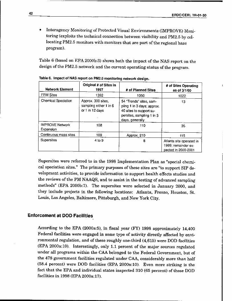
• Interagency Monitoring of Protected Visual Environments (IMPROVE) Moni- toring (exploits the technical connection between visibility and PM2.5 by col- locating PM2.5 monitors with monitors that are part of the regional haze program).
Table 6 (based on EPA 2000b:3) shows both the impact of the NAS report on the design of the PM2.5 network and the current operating status of the program.
Table 6. Impact of NAS report on PM2.5 monitoring network design.
Network Element Original # of Sites in
1997 # of Planned Sites # of Sites Operating
as of 3/1/00 FRM Sites 1392 1050 1022 Chemical Speciation Approx. 300 sites,
sampling either 1 in 6 or 1 in 12 days
54 "Trends" sites, sam- pling 1 in 3 days; approx. 40 sites to support su- persites, sampling 1 in 3 days, generally
13
IMPROVE Network Expansion
108 110 35
Continuous mass sites 100 Approx. 210 115 Supersites 4 to 9 8 Atlanta site operated in
1999; remainder ex- pected in 2000-2001
Supersites were referred to in the 1998 Implementation Plan as "special chemi- cal speciation sites." The primary purposes of these sites are "to support SIP de- velopment activities, to provide information to support health effects studies and the reviews of the PM NAAQS, and to assist in the testing of advanced sampling methods" (EPA 2000b:7). The supersites were selected in January 2000, and they include projects in the following locations: Atlanta, Fresno, Houston, St. Louis, Los Angeles, Baltimore, Pittsburgh, and New York City.
Enforcement at DOD Facilities
According to the EPA (2000a:5), in fiscal year (FY) 1998 approximately 14,400 Federal facilities were engaged in some type of activity directly affected by envi- ronmental regulation, and of these roughly one-third (4,615) were DOD facilities (EPA 2000a: 10). Interestingly, only 1.1 percent of the major sources regulated under all programs within the CAA belonged to the Federal Government, but of the 478 government facilities regulated under CAA, considerably more than half (58.4 percent) were DOD facilities (EPA 2000a:10). Even more striking is the fact that the EPA and individual states inspected 310 (65 percent) of those DOD facilities in 1998 (EPA 2000a:17).

ERPC/CERLTR-01-50 43
Statistics on multimedia inspections in FY98 show a strikingly similar picture. The number of multimedia inspections of DOD facilities conducted in FY98 was considerably smaller than the number (22) devoted to air quality (EPA 1999c:3). It is worth noting, however, that an overall total of only 30 multimedia inspec- tions were conducted at Federal facilities that year. Thus, DOD facilities ac- counted for slightly more than 73 percent of all multimedia inspections con- ducted at Federal facilities.
The statistics on both air-related and multimedia inspections suggest that DOD facilities are more likely than not to be the recipients of inspections conducted by the EPA and state/local regulators. It clearly behooves DOD facilities not just to have environmental compliance programs that include both audits and means for addressing the findings of noncompliance that may result from them, but also to have compliance programs that are robust and highly effective.
It is clear (see EPA 1999c:3) that NSR/PSD is a principal means by which EPA is addressing what it views as violations of the CAA. At EPA's request, the De- partment of Justice filed a number of lawsuits on 3 November 1999 against cer- tain electric utilities for violations of NSR regulations. The NSR regulations re- quire facilities that are major sources built prior to the 1977 CAA Amendments to obtain permits before making significant repairs and/or modifications. The government alleges that the companies named in the suit made such repairs and/or modifications (which had the effect of increasing emissions) without ob- taining the required permits. Further, an administrative order was filed against a federally operated power company (Tennessee Valley Authority [TVA]) and NOVs were issued against eight plants not named in the lawsuits. Four addi- tional NOVs were issued later that month. The government claims that in all these instances significant modifications were made but were treated (illegally) as routine maintenance not subject to permit requirements. It is further claimed that required pollution control equipment was not installed. A settlement in one of these suits was reached on 29 February 2000. However, the number of NOVs based on alleged violation of NSR provisions has continued to increase (for ex- ample, see Najor 2000b).
As noted above, the EPA is in the process of final rulemaking on NSR; a reform process that engages industry, state and local governments, and environmental public interest groups has been underway since 1992. From recent discussions of EPA's plans (for example, see Cook 2000), it can be expected that the enforce- ment effort against electric utilities will be extended to stationary sources in the petroleum and pulp and paper industries that EPA believes have attempted to circumvent permit requirements. In addition, EPA published a request for

— . ERDC/CERLTR-01-50
stakeholder comment on its preliminary national enforcement and compliance assurance priorities for FYs 2002 and 2003 on 28 September 2000 (65 FR 58273- 58275). Although a final list of priorities for FYs 2002 and 2003 will not be re- leased until April 2001, it is important to note that both pollution at Federal fa- cilities and PM pollution are on the list of suggested new areas for enforcement efforts.
Conclusions
DOD has raised concerns about the impact of the PM2.5 standards on its opera- tions. These concerns, as characterized by the EPA Administrator in a letter to SECDEF (Browner 1997), include:
1. Training and readiness impacts arising from potential restrictions on the use of ob- scurants, from the potentially mandated elimination or control of fugitive dust from field exercises, from design and operating restrictions on military mobile combustion sources incompatible with their mission, and from potential restric- tions on prescribed burning needed to sustain training areas and installation for- estry programs;
2. Potential for increased difficulty in meeting general conformity requirements and achieving DoD's goals for infrastructure consolidation, closed facility reuse, and operational realignments; and
3. Potential costs associated with Title V permits and for New Source Review and control requirements at additional military bases.
Ms. Browner addresses these concerns as follows (ibid.):
I want to make it clear that EPA does not see the need for Defense activities to be the target of control strategies designed to attain these new standards.
Specifically, EPA will take the following actions to address DoD concerns. Understanding that critical training using smoke or obscurants must continue to ensure the training and readiness of the military, I am directing my staff to work with DoD to develop a policy which ensures that a local area will not be redesignated to nonattainment solely on the basis of use of obscurants or smoke. While there is a need to ensure that the public is informed of viola- tions of the air quality standards, if any were to occur, there is no need to cur- tail the training or limit it to certain weather conditions. Additionally this pol- icy can encourage States not to look to restrictions on these activities to meet the revised air quality standards.
With respect to DoD's concerns with fugitive dust from training activities, EPA has been analyzing actual samples of fine (e.g., PM2.5) particles in the air to determine the sources of the particles. In so doing, it is clear that mili- tary training activities are actually among the smallest sources of PM2.5 in

ERDC/CERL TR-01-50 45
areas likely to have a fine particle problem. While military activities contrib- ute some primary PM2.5, secondary particles such as sulfates are by far the largest component of PM2.5. The major sources of fine particles include sul- fates from power plants and nitrate from power plants and other large combustion sources. We intend to work with States to target the PM2.5 monitoring program on urban areas with large populations.
If EPA does add a PM2.5 standard, I intend to issue guidance to the States to ensure that in meeting the standard they focus their control strategies on sources of fine, rather than coarse particles. Thus, if we establish a new PM2.5 standard, EPA would not recommend that States focus regulatory at- tention on military training and field exercises.
EPA has consistently recognized the unique needs of the military regarding mobile sources used for combat or combat training. Military aircraft engines are exempt from emission standards, and each EPA nonroad engine rule in- cludes provisions for combat and national security exemptions. EPA believes it is sensible to continue to include these military exemptions in any new rulemaking to implement the proposed standards. In addition, as pointed out by DoD, States have limited authority through in-use operating restrictions to regulate these nonroad engines. We understand that the needs for operation and readiness at military bases require operations at all hours of the day and we do not believe such operations generally need to be restricted to protect air quality. EPA will work with the States to ensure that their implementation plans do not impose unreasonable burdens on military tactical vehicles or equipment or their use.
With regard to DoD's concerns about possible restrictions on the use of pre- scribed burning resulting from any new standards, EPA is working with Fed- eral and State agencies to develop guidance for balancing air quality strategies and the need for prescribed burning. Recognizing that DoD is the third largest Federal Land Manager, EPA has included DoD in this Wildland Fire Issues Workgroup Steering Committee. EPA will also work closely with DoD to re- solve those prescribed burning issues specific to the Department such as ord- nance range fire prevention and safety.
EPA appreciates that the Clean Air Act conformity requirement has posed a special problem in executing the base closure process. To the extent the mili- tary realigns large numbers of mobile sources like aircraft or vessels, satisfy- ing conformity has been a significant challenge. EPA commits to work with DoD in the implementation of any new standards to assure that conformity is applied in an appropriate and beneficial manner for air quality and consistent with the goals of DoD for the cost-saving consolidation of the Defense infra- structure and the economic viability for civilian reuse of the former military bases.
Finally, I am directing my staff to continue to work with DoD on the pending revisions to both the Title V Permit Program and the New Source Review Program to assure equivalent treatment of military facilities.

46 — . ERDC/CERLTR-01-50
The EPA, however, issued the final regional haze rule without excluding military training activities from its scope.
Army installations need to be aware of their locations relative to federally man- dated Class I Areas. Those installations with training grounds (particularly those located west of the Mississippi and upwind of such areas) must be espe- cially aware and must be in close contact with their permitting authorities.
SIPs vary widely throughout the country. The number and nature of sources in a state and that state's geography are two factors that contribute to the variety of SIPs that we see in the United States. Because of the inherent complexity of NSR/PSD, and because of the essentially local character of SIPs, installations must work closely with their permitting authorities to determine whether they have any NSR/PSD issues and what precisely those issues might be.
Though the focus of NSR/PSD-related enforcement efforts has been on the indus- trial sector, the inspection statistics cited earlier suggest that DOD components will be well served by paying close attention to this area as well.
The requirements of general conformity also necessitate a close working rela- tionship between an installation and its permitting authority. Along with PM NAAQSs in general, regional haze, and NSR/PSD, general conformity, too, cru- cially involves the provisions of SIPs. The most useful advice is to know the pro- visions of your state's implementation plan and work closely with your permit- ting authority as you seek to comply with its provisions. As PM2.5 SIPs evolve, it is also advisable to work closely with state regulators to make sure that the Army's nonfacility sources are properly accounted for in the state's emission in- ventory and atmospheric modeling efforts.

ERDC/CERL TR-01 -50 47
4 Army Nonfacility PM Source Emission Estimation
This chapter discusses techniques for estimating emissions from the Army's non- facility PM sources. As discussed in Chapter 1, these PM sources include vehi- cles, prescribed burning, smokes and obscurants training, artillery practice, weapons impact testing, OB/OD, and aircraft.
Emission factors and models that provide estimations of emissions are never considered as accurate as data collected from good sampling techniques. Emis- sion estimation will normally produce more conservative results than source sampling. Large variability can exist among results from source tests on differ- ent sources of the same source type. EPA's AP-42 documentation (AP-42, 1998) discusses the variability of emissions and points out that emissions can vary by an order of magnitude or more, depending on the source characteristics.
The Army needs to estimate emissions because actual measurements at each in- stallation would be difficult to perform and cost-prohibitive. Emission factors have long been used as cost-effective alternatives to sampling. Federal and state air quality programs rely heavily on emission factors to support applicability de- terminations, permit applications, emission inventories, and modeling studies.
An emission factor relates the quantity of pollutants released from a source to some activity associated with those emissions. Emission factors are usually ex- pressed as the weight of pollutant emitted divided by a unit weight, volume, dis- tance, or duration of the activity emitting the pollutant (e.g., pounds of PM per vehicle mile traveled). Emission factors are used to estimate a source's emis- sions by the general equations:
E = AxEFx[l-(CE/100)] [Eq 1]
where E = the estimated emissions
A = the activity level EF = the uncontrolled emission factor CE = the control efficiency (expressed as a percentage).

i? _ ERDC/CERLTR-01-50
Emission factors are usually averages of available data that meet sampling ac- ceptability criteria and are generally assumed to be representative of long-term averages for all facilities in a source category. The available data on which a fac- tor is based often do not provide sufficient information to characterize the influ- ences of different operating scenarios, so emission factors may represent aggre- gate behavior and not be specific to a particular mode of operation.
EPA recognized the need for emission estimation methods and emission factors in order to implement the programs promulgated under the Clean Air Act. EPA's Compilation of Emission Factors (AP-42) has been published since 1972 as the primary source of emission factors. It contains emission factors and process information for more than 200 air pollution source categories. A source category is a specific industry sector or group of similar emitting sources. The emission factors have been developed and compiled from source test data, material bal- ance studies, and engineering estimates. AP-42 is a dynamic document that con- tinually has new factors added and established factors revised to reflect new scientific findings, changes in processes, and changes in emission control devices.
For regulatory purposes, EPA and states prefer that actual source emission test- ing results, conducted in accordance with EPA approved methods, be used to quantify source emissions. Recognizing the cost and time associated with collect- ing source data, the following estimation methods are accepted in the following order:
• Regulatory-approved emissions factors compiled in AP-42 • Emission factors based on source testing on similar equipment • Extrapolations of factors provided for similar types of source categories.
AP-42 and the emission factor development program have focused on emission factors for industrial and commercial activities and vehicles found in the private sector. Many of these source categories (e.g., boilers and solvent coating proc- esses) are identical to operations at Army installations. Little information, how- ever, has been developed on emission factors for many of the Army's nonfacility source categories. Combat and tactical equipment, smoke generators, and artil- lery are typically unique to the military.
When the PM10 NAAQS was promulgated, measurements of TSP emissions be- came less frequent and less important to reporting requirements. Therefore, TSP emissions are often not reported in the literature, and other parameters must serve as surrogates. The issues associated with PM and the characteriza- tions of PM emissions have become more focused in recent years. Until the PM2.5 NAAQS were issued in 1997, few measurements characterized the PM2.5

ERDC/CERLTR-01-50 49
emissions from processes. Distribution of the PM2.5 emissions monitors was ex- pensive; therefore, few emission factors for PM2.5 exist, especially for the fugi- tive processes examined in this study.
This chapter examines the emission estimation methods available for the source categories of this report. Methods approved by the EPA's Emission Factor and Inventory Group are noted and expected to be acceptable to meet reporting requirements for most states. Readers should, however, consult their state and local agencies to find out if alternative methods are recommended or available.
Most important to many states is that — for reporting purposes — the activity measurements are quantifiable. Environmental professionals at installations should find a quantifiable parameter that can be collected each year for an annual inventory. Some examples include: • Gallons/barrels of fog oil consumed • Vehicle miles traveled or fuel consumed by various vehicle types over various
road surfaces • Rounds fired outdoors • Number of acres burned through prescription and the fuel loading for the
burned land • Pounds of propellants/explosives disposed of through OB/OD.
Vehicles
The EPA guidance on the estimation of PM emissions from vehicles came in 1995 in EPA's PART5 model. The PART5 model calculates PM emissions from vehicle exhaust, brake wear, tire wear, paved road dust re-entrainment, and dust re- entrainment on unpaved road surfaces. Since that time, the EPA has revised its methods for calculating emissions from re-entrained dust on paved and unpaved roads (AP-42 Sections 13.2.1 and 13.2.2). Therefore, the methods are presented separately under the following three subsections.
Exhaust, Brake Wear, and Tire Wear
The PART5 model is the EPA's approved tool for determining particulate emis- sions from vehicles (http://www.epa.gov/oms/part5.htm). The user must supply the following information: 1. Total vehicle miles traveled (VMT) 2. Average vehicle speed (mph)

50 ERDC/CERLTR-01-50
Fraction of VMT to be attributed to each of the 12 vehicle classes: Light-duty gasoline vehicle
Light-duty gasoline truck under 6,000 lb gross vehicle weight (GVW) Light-duty gasoline truck from 6,001 to 8,500 lb GVW Heavy-duty gasoline truck over 8,500 lb GVW Motorcycle
Light-duty diesel vehicle under 6,000 lb GVW Light-duty diesel truck from 6,001 to 8,500 lb GVW Class 2B heavy-duty diesel vehicle from 8,501 to 10,000 lb GVW Light heavy-duty diesel vehicle from 10,001 to 19,500 lb GVW Medium heavy-duty diesel vehicle from 19,501 to 33,000 lb GVW Heavy heavy-duty diesel vehicle over 33,000 lb GVW Buses.
The model will also calculate emissions from re-entrained dust (with the specifi- cation of other input parameters), but EPA has issued new guidance on these calculations since PART5's creation.
The PART5 model will predict PM10 and PM2.5 emissions. To calculate TSP emissions, the PM size fractions from the California Emission Inventory Devel- opment and Reporting System (CEIDARS 1999) suggest that PM10 represents 96.43 percent of the TSP emissions from Diesel Vehicle Exhaust. The PM10 emissions should be divided by 96.43 percent to calculate TSP emissions.
The State of California uses MVEI7G software (documentation available at http://www.arb.ca.gov/msei/mvei/mvdocs.htm) to estimate pollutant emissions from vehicle tailpipes. Many of the emission factors and size distributions for this software are identical to those used for PART5 and based on the same stud- ies. Since exhaust PM, brake wear, and tire wear emissions are small compared with those from re-entrained dust, the differences between the emission factors of PART5 and MVEI7G will not have a considerable effect on the total PM emis- sions from vehicles.
The emission calculations discussed above consider only a fleet composed of gaso- line and diesel engines but ignore the use of vehicles powered by JP-8 fuel. This shortcoming is significant since most military vehicles use JP-8 as their primary fuel. The calculations discussed earlier also do not consider that most tracked military vehicles (such as tanks) use turbine engines.
In 1996 the JP-8 Aircraft Engine Emissions Characterization Program began testing aircraft engines to determine the emissions of criteria and hazardous air

ERDC/CERLTR-01-50 51
pollutants. The PM emissions from four aircraft turbine power plants are re- ported in the Aircraft Engine and Auxiliary Power Unit Emissions Testing Re- port (summary available at sg-www.satx.disa.mil/iera/rse/JP-8data.htm). Those emissions range from 0.48 to 2.60 lb TSP/1000 lb JP-8 fuel. Similarly, AP-42 Ta- ble 3.1-1 reports the PM2.5 and PM10 emissions from large, uncontrolled gas turbines as 1.3 lb/1000 lb distillate oil (using 5.9 MMBtu/bbl oil and 6.8 lb oil/gal). This emission information might be more appropriate for turbine engine land vehicles such as tanks.
The only information that would need to be tracked for emissions inventories would be the number of gallons of fuel used by those vehicles.
Re-entrained Dust on Paved Roads
The EPA AP-42 Section 13.2.1 document (Supplement D, October 1997) provides a method for calculating PM emissions from paved roads (http://www.epa.gov/ttn/chief/ap42cl3.html). The data necessary for emissions estimates are: 1. Average weight (W) of the vehicles traveling over the roads (tons) 2. Total VMT.
If the road surface silt loading (sL in g/m2) is also available, it should be used in the equation:
E = VMTxk(sL/2)065 (W/3)15 [Eq 2]
where E = the particulate emissions k = a particle size multiplier for paved roads.
The multiplier k has values of 0.0040 lb PM2.5/VMT, 0.016 lb PM10/VMT, and 0.082 lb TSP/VMT. Road surface silt loadings ranged from 0.02 to 400 g/m2 in EPA's tests. If no road surface silt loading value is available, the worst-case rec- ommended default silt loading value for public paved roads with low average daily travel (Table 13.22.1-2 of AP-42) can be used (3 g/m2). The worst-case con- dition was chosen to represent roads that have substantial mud/dirt carryout.
Re-entrained Dust on Unpaved Roads
The EPA AP-42 Section 13.2.2 document (Supplement E, September 1998) pro- vides a method for calculating PM emissions from unpaved roads

52 . ERDC/CERLTR-01-50
(http://www.epa.gov/ttn/chief/ap42cl3.htmlV The data necessary for emissions estimates are:
1. Average W of the vehicles traveling over the roads (tons) 2. Total VMT
3. Surface material silt content(s) of the road (%)
4. Mean number of days in a year with at least 0.01 inches precipitation (p) 5. Average vehicle speed (S) if less than 15 mph 6. Control efficiency (CE as a percentage) for processes such as placing gravel, wa-
tering, or chemical stabilization.
Before 1998, EPA's emission factors for re-entrained dust on unpaved roads also required the number of vehicle wheels to be used in calculations. However, the parametric analysis conducted for the revised factors in 1998 found no depend- ence on the number of wheels when vehicle weight was included as a parameter (EPA 1998). The 1998 analysis included newer references that had not been used in earlier versions of AP-42.
EPA testing showed surface silt contents that ranged from 1.2 to 35 percent. The mean number of days of precipitation can be estimated from AP-42 Figure 13.2.2- 1 (shown here as Figure 6) in the absence of better information. Additionally, the surface material moisture content under dry, uncontrolled conditions (1VL) can be used, but a default value of 0.2 percent may be used if no site-specific in- formation is available. If no emissions control measures are applied, the control efficiency is zero.
Control efficiencies vary based on the surface silt loadings, the strength and flexibility of suppressant material, exposure to weathering, and the number of vehicle passes (Gillies et al. 1999). After a single week, Gillies et al. found that suppressant efficiencies for PM10 varied from 33 to 100 percent for four suppres- sant types in the San Joaquin Valley, CA. After 8 to 12 months of exposure, the control efficiencies for PM10 emissions ranged from 0 to 95 percent. Chapter 8 of this report presents additional material related to dust suppression and soil sta- bilization technologies.
At Fort Campbell, KY, control efficiencies of suppression techniques were evalu- ated using oil-coated dust collection pans located approximately 5 meters from the roads (Gebhart and Hale 1997). Both wheeled and tracked vehicles used the roads, and dust control efficiencies ranged from 84 to 96 percent after application and from 38 to 87 percent after 80 days. These studies did not discriminate par- ticle size, so the control efficiencies for PM2.5, PM10, and TSP may vary consid- erably.

ERDC/CERLTR-01-50 53
eg I o.
< w
S tn
c o 3 a '5 P
o 2 o E
u c
o ©
•o
a> n E 3 C C a a> £
£ 3 O) U.

54 ERDC/CERLTR-01-50
Equations 3 to 5 are used to calculate PM2.5, PM10, and TSP emissions (Ep E
PMIO> a11^ ETSP' respectively).
EPM25 = (1-CE) x VMTx 0-38(s/12)-(W/3r x 365,0 [Eq 3] (Mdry)
03 365
xO-S/wm^A c ,1 ™~ ^-rr 2.6(s/12)u•8(W/3)u', 365-p EpMIo=(l-CE)xVMTx , ,n, *-Z7T- [Eq4]
'dry- (Mdrv)03 365
\0.8/AI7/'>X0.5
ETSP = (l-CE)x VMTx 'Wiy-y xjg^P [Eq5l
■•dry- (M^)04 365
Tracked vehicles are likely to emit more PM as they churn up the unpaved roads than are other vehicles traveling the same roads. It could be argued that, be- cause of the nature of the vertical disturbance to the soil, more appropriate emission factors for tracked vehicles would be those used for heavy construction activities (AP-42 Section 13.2.3). Emission tests have not been performed on any tracked vehicles in the EPA development of emission factors for unpaved roads. The need for emission testing of PM emissions from tracked vehicles is clear, al- though regulators may argue that the process of tracked vehicle movement along an unpaved road is a fundamentally different process than movement of wheeled vehicles and should not be estimated by the above equations.
Prescribed Burning
Under EPA-approved methods (AP-42 Section 13.1), the estimation of PM emis- sions from prescribed burning practices requires the following information: 1. Fuel loading (L) consumed (mass of forest fuel/acre burned) 2. Land area (A) burned (acres) 3. Fire configuration (broadcast logging slash, range fire, line fire, or logging slash
debris) 4. Fire phase (preheating, flaming, glowing, and smoldering phases) 5. Fuel characteristics (e.g., hardwood, conifers, or sagebrush).
The emissions (E) are calculated by:
E = EF x L x A [Eq 6]

ERDC/CERLTR-01-50 55
where EF represents the emission factor, a function of the pollutant (TSP, PM10, or PM2.5), fire configuration, fire phase, and fuel characteristics. The preheat- ing phase seldom emits significant PM emissions. Table 7 summarizes the emis- sion factors for prescribed burning from AP-42 Table 13.1-3 and covers the fac- tors that EPA approved.
Table 7. AP-42 PM emission factors for prescribed burning activities.
Fire Configuration
Fuel Characteristics Fire Phase
Emission Factors (lb/1000 lb fuel)
Percent Fuel in Fire
Phase PM2.5 PM10 TSP
Broadcast logging slash
Hardwood Flaming
Smoldering
Fire
6
13 11
7
14 12
13 20
18
33 67
Broadcast logging slash
Conifer - short needle
Flaming
Smoldering
Fire
7 14
12
8
15
13
12
19 17
33 67
Broadcast logging slash
Conifer - long needle Flaming Smoldering
Fire
6
16 13
6 17
13
9
25 20
33 67
Logging slash debris
Dozer piled conifer - no mineral soil
Flaming Smoldering
Fire
4
6 4
4
7 4
5 14
6
90
10
Logging slash debris
Dozer piled conifer — 10 to 30% mineral soil
Smoldering No data
No data
25 Not avail- able (NA)
Logging slash debris
Dozer piled conifer - 25% organic soil
Smoldering No data
No data
35 NA
Range tire Juniper slash Flaming Smoldering
Fire
7
12
9
8 13
10
11
18 14
8.2
15.6 12.5
Range fire Sagebrush Flaming Smoldering
Fire
15 13
13
16 15
15
23 23
23
NA
Range fire Chaparral shrub communities
Flaming
Smoldering
Fire
7
12
10
8
13 11
16
23 20
NA
Line fire Conifer-long needle (pine)
Heading
Backing
No data
40
20
50
20
NA
Line fire Conifer- palmetto/gallberry
Heading
Backing
Fire
No data
15
15 8-22
17
15
No data
NA
Line fire Chaparral Heading 8 9 15 NA
Line fire Grasslands Fire No data
10 10 NA

— . ERDC/CERLTR-01-50
In addition to the EPA method presented above, the National Forest Service dis- tributes computer models (http://fire.org/perytools.cgi) with specific applicability for predicting PM emissions from prescribed burning activities: CONSUME, EPM (Emissions Production Model), and FOFEM (First Order Fire Effects Model). CONSUME and EPM were developed specifically to predict emissions from prescribed fires in the Pacific Northwest, but FOFEM has nationwide ap- plicability. The FOFEM model predicts fuel loading (in tons/acre) and both PM10 and PM2.5 emission factors (in lb/acre). The model requires the following inputs:
1. Cover type of major species (also includes fire configuration) 2. Moisture 3. Dead fuel adjustment factor 4. Fire intensity 5. Tree crown loading 6. Herbaceous and shrub densities 7. Tree regeneration density 8. Season 9. Days since last precipitation 10. Fuel loadings 11. Duff depth.
FOFEM also offers default values for the above parameters. Since the FOFEM model covers a wider variety of vegetation cover (136 species) and fire configura- tions than the AP-42 tables, it would be the appropriate model to use when the species is not listed in the AP-42 tables or belongs to a mixed community. The natural resources personnel at each installation should be able to provide the detailed information about the past year's activities to calculate emissions.
Smokes and Obscurants Training
The following information is required to estimate PM emissions from smokes and obscurants: 1. Mass of obscurant consumed (lb/yr) 2. Size distribution of particles in the created fog.
The mass of obscurant brought onto the installation during a year should be tracked through the Hazardous Material Pharmacy at each installation. A mass balance is the preferred method for estimating the PM emissions from smokes and obscurants. The mass of obscurant consumed to create fog serves as a reli- able estimate of the total PM emitted. In some cases, additional information is

ERDC/CERLTR-01-50 57
available to make slight reductions to this estimate (e.g., only 95 percent of fog- oil smoke condenses into aerosol droplets (Dunn, Brown, and Policastro 1996). After the total PM is estimated, it is necessary to estimate the size distribution of particles in the smoke in order to convert the total PM emissions into TSP, PM10, and PM2.5 emissions.
For example, fog-oil smoke (the predominant obscurant used by the Army) has a log-mean diameter averaging 0.9 jim (microns). Dunn, Brown, and Policastro report a size distribution showing 99 percent of the particles from fog oil are less than 2.5 and 10 microns in size. If 10,000 lb of fog oil were consumed in a year, the TSP emissions (Erep) would be:
ETSP = [Fraction fog oil that condenses] x [Fog oil consumed] IE<1 7] = [0.95 lb TSP/lb fog oil] x 10,000 lb fog oil/yr = 9500 lb TSP/yr
The PM2.5 and PM10 emissions (EPM25 and EPM10, respectively) would be calcu- lated as
EPM2.5 = [Fraction PM2.5 in ETSP] x ETSP IE(181 = [0.99 lb PM2.5/lb TSP] x 9500 lb TSP/yr = 9400 lb PM2.5/yr
EPMIO = [Fraction PM10 in E^p] x E^p [Eq9]
= [0.99 lb PM10/lb TSP] x 9500 lb TSP/yr = 9400 lb PM10/yr
These estimates will yield the ground-level PM emissions to be used for regional emission inventories. The PM generated from fog oil should be characterized as organic aerosols in regional modeling efforts. To understand the opacity gener- ated locally, the Army's SMOKE dispersion model was to be designed to simulate smoke dispersion from military training exercises (Dunn, Brown, and Policastro 1996). The design parameters for the model were established, but the SMOKE dispersion model was never demonstrated.
Artillery Practice and Weapons Impact Testing
The EPA has not issued guidance in its AP-42 documents on the estimation of PM emissions from artillery practice or weapons impact testing. Few emissions data have been collected in this area, and it varies greatly among the different

-5L- ERDC/CERLTR-01-50
types of munitions, weapons, and ambient environments. The Firing Point Emissions Study (METDC 1999) has deemed these factors to be contributors to emission rates from firing point emissions:
Chemical composition of the primer, propellant, projectile, etc. Temperature of the munition item at the time of firing Weight of the projectile (for nonfixed ammunition) Amounts of energetic material consumed Length and diameter of the gun tube Gun bore tube characteristics (material, rifling, etc.)
Presence or lack of flash suppressor or muzzle brake (can affect muzzle flash) Temperature of gun tube (affected by ambient temperature, rate of fire, etc.) Presence or lack of bore evacuator
Blast reflectors near the muzzle of the gun Water content of the atmosphere Temperature of the atmosphere.
The DOD and National Aeronautical and Space Administration (NASA) models for munitions firing that are designed to predict the combustion products (e.g., Chemical Equilibrium and Applications [CEA], BLAKE, IBHVG2, IDEAL CBP GUN, PCAD, ADORA, POLU13, MERLIN, Shock and Detonation [SD], FAST3D- OAD/CT, NOVA, and CHEETAH) rely on a complete understanding of the chemical species and predict only hydrogen, nitrogen, carbon monoxide, carbon dioxide, water, and some minor combustion species (METDC 1999). Predictions of particulate emissions must rely on emissions testing and not on kinetics/ equilibrium model studies.
Phase I of the Firing Point Emissions Study reported PM10 emissions from an M16 Rifle as 4162 ± 291 \xglg propellant (Snelson et al. 1995). Although PM2.5 emissions were not measured in this study, the particulate emissions less than 2.1 microns were measured at 140 ± 82 ng/g propellant. The 2.1-micron meas- urement serves as a rough approximation of a PM2.5 emission factor. These emission factors may be sufficient to estimate PM2.5 and PM10 emissions (E;) from M16 rifles with the formula:
E( = NxMxEF. [Eq 10]
where N = the number of rounds fired M = the propellant mass per round EF = the pollutant emission factor.

ERDC/CERLTR-01-50 59
For example, if 1000 rounds of 5.56mm blank cartridges (7 grams propellant) are fired from M16 rifles, the associated PM2.5 and PM10 emissions would be calcu- lated as:
innn „ 7gpropellant 140±82gPM2.5 lgPM2.5 PM2.5 emissions = 1000 roundsx 6F F - & ~ 6
round g propellant 1E6 g PM2.5
PM2.5 emissions = 0.98 ± 0.57 g PM2.5
7 g propellant 4162±291gPM10 lgPMlO PM10 emissions = 1000 rounds x
round g propellant lE6gPM10
PM10 emissions = 29±2gPM10
When comparing emissions rates from an M16 rifle and a 105mm tank gun, Snelson et al. (1995) found similar emissions per gram propellant for carbon- containing species but no indication that these similarities could be extended to other pollutants.
Phase II of the Firing Point Emissions Study is sponsoring research to character- ize the PM2.5, PM10, and TSP emissions generated by representative U.S. Army munition classes at the weapon firing position. The U.S. Air Force has plans to begin testing emissions from weapon firing. The U.S. Army Environmental Cen- ter (AEC) is sponsoring the Characterization of Smoke and Pyrotechnic Emis- sions project to quantify emissions generated by smoke grenades, flares, and re- lated pyrotechnics. The AEC's Exploding Ordnance Emission Study will quantify emissions generated from the downrange functioning of munitions con- taining explosives or other energetic fills.
In the absence of other emission estimation techniques, it may be possible to roughly approximate PM emissions using the information for OB/OD activities listed in the next section.
Open Burning/Open Detonation of Munitions
OB/OD activities are used to destroy excess, obsolete, or unserviceable munitions and energetic materials. Open burning of munitions involves the combustion of propellants or explosive ordnance without the control of combustion, air, containment of the reaction, or the emissions. Open detonation is the uncon- fined, violent reaction of explosive ordnance without the control of combustion, air, containment of the reaction, or the emissions. Models have been developed

60 ERDC/CERLTR-01-50
to predict the emission products of OB/OD activities but have not focused on PM species other than those species formed during combustion (see Chapter 5).
The DOD established a program to develop emission factors for OB/OD activi- ties, and the results were compiled by the EPA (Mitchell and Suggs 1998). PM10 emission factors developed under this study for propellants and explosives are listed in Table 8 as a function of the mass of energetic material (MEM).
Table 8. PM10 emission factors for OB/OD of explosives/propellants
Propellant/Explosive PM10 Emission
Factor (g/g MEM) Charge MEM (g)
Diesel fuel and dunnage 5.40E-03 913 Manufacturer's waste - aluminized propellant with diesel 1.90E+00 1139 Propellant, ammonium perchlorate, aluminized 4.20E-01 1183 Propellant, ammonium perchlorate, nonaluminized 1.50E-02 2270 Propellant, double base 1.90E-02 2227 Propellant, M-3 8.60E-03 Propellant, M-43 (USN) 1.20E-03 1060 Propellant, M-9 1.60E-02 2406 Propellant, MK-23 5.90E-02 1030 Propellant, M31A1E1 9.10E-01 2276 Propellant, PBXN-110 4.90E-01 1064 Propellant, Smokey Sam 2.60E-01 273 Smokeless Powder (Hercules Unique) 1.80E-03 454 40 mm HEI Cartridge 4.70E-01 158 Amatol surrogate 1.90E-02 235 Amatol surrogate with water 3.20E-02 235 Cartridge, Impulse, ARD 446-1 8.30E-02 215 Cartridge, Impulse, BBU-36/B 1.80E-01 144 Cartridge, Impulse, MK 107 2.50E-01 208 Composition B surrogate 1.20E-02 235 Detonating train 3.60E-02 178 Flare, IR Countermeasure M206 5.50E-01 241 Fuze, Tail Bomb FMU-139 A/B 6.00E-01 172 Fuze, Tail Bomb FMU-54 A/B 3.30E-01 210 Gas Generator, GGU-2/A 9.30E-02 139 HBX surrogate 1.80E-01 220 Mine, Claymore, M18A1 2.30E-01 229 Signal, Illumination, Red Star AN-M43A2 4.50E-01 260 Signal, Illumination, Red Star M158 8.20E-02 239 T45E7 Adapter Booster 2.60E-01 193 TNT(ACC1) 7.30E-02 230 TNT(ACC2) 9.30E-02 230 Tritonal surrogate 3.70E-01 235 Tritonal surrogate with calcium stearate 2.60E-01 235 Tritonal surrogate with water 1.90E-01 235

ERDC/CERLTR-01-50 61
To calculate the PM10 emissions from OB/OD activities, the number of charges should be multiplied by the associated MEM and PM10 emission factor (from Table 8):
PM10 emissions (g) = (Number of charges) x (mass MEM/charge) x (PM10 Emission Factor)
[Eq 11]
For example, the emissions from the open detonation of 150 M18A1 Claymore mines would be calculated as:
PM10 emissions = 150 charges x (229 g MEM/charge) x (0.23 g PM10/g MEM) x (1 lb/454 g)
PM10 emissions = 17 lb
If complete information is not available on the specific energetic materials burned/detonated (or if materials are not listed in Table 8), Air Force guidance (IERA 1999) suggests an alternative method using the mean emission factors
presented in Table 9.
Table 9. Average emission factors for OB/OD processes.
Category PM10 Mean Emission
Factor (lb/lb MEM)
Open Detonation of Encapsulated Energetics 0.30
Open Detonation of Bulk Energetics 0.13
Open Burning of Ammonium Perchlorate-Based Energetics 0.15
Open Burning of Organic-Based Energetics 0.28
Lawrence Livermore National Laboratory is leading additional research at the Nevada Test Site to characterize the particulate emissions from the open detona- tion of 155mm, M107 projectiles. This research is also investigating the ways to optimize the open detonation procedure to minimize emissions and evaluating innovative instruments for characterizing open air events.
Aircraft
In 1996 the JP-8 Aircraft Engine Emissions Characterization Program began testing aircraft engines to determine the emissions of criteria and hazardous air pollutants. The program tested two types of helicopter engines (T700-GE-700 and T64-GE-100), and results were reported in an Aircraft Engine and Auxiliary Power Unit Emissions Testing Report (the executive summary can be found at

62 ERDC/CERLTR-01-50
sg-www.satx.disa.mil/ifira/rse/JP-8data.htm). The TSP emission factors appear in Table 10.
Table 10. Helicopter engine paniculate emissions with JP-8 fuel.
Engine/Condition Filterable Particulates Total Suspended Particulates
Ib/hr lb/1000 lb fuel Ib/hr lb/1000 lb fuel T700-GE-700 Ground Idle 0.07 0.51 0.20 1.48 Flight Idle 0.56 1.19 0.59 1.26 Flight Max 0.81 1.29 1.39 2.22 Overspeed 1.01 1.39 1.89 2.60
T64-GE-100 Ground Idle 0.06 0.22 0.70 2.36 75% Normal 1.43 1.52 1.85 1.97 Normal 1.24 0.73 2.73 1.61 Military 1.53 0.83 1.69 0.92
Therefore, the TSP emissions from an aircraft with T700-GE-700 engines can be calculated in the following equation:
TSP Emissions (lb TSP) = Time (hr) x No. Engines x
f Fraction time in GI mode x 0.20 lb/hr + Fraction time in FI mode x 0.59 lb/hr + Fraction time in FM mode x 1.39 lb/hr + Fraction time inOv mode x 1.89 lb/hr
[Eq 12]
According to the California Emission Inventory Development and Reporting Sys- tem (CEIDARS 1999), the PM10 fraction of TSP for aircraft burning jet fuel is 97.6 percent, and the PM2.5 fraction of TSP is 96.7 percent. Therefore, the PM10 and PM2.5 emissions can be calculated using the formulas:
PM10 Emissions = 97.6 % x TSP Emissions
PM2.5 Emissions = 96.7 % x TSP Emissions
[Eq 13]
[Eq 14]
In 1999 the Air Force began using a jet fuel additive (JP-8+100) that creates a cleaner burn and likely fewer particulate emissions. Emissions tests from the use of this fuel are still in the early stages, however, and no test results have yet been published to compare JP-8 and JP-8+100 fuels.
The above emission factors represent exhaust emissions and do not account for the fugitive dust re-entrained from the ground as a helicopter takes off, passes

ERDC/CERLTR-01-50 63
over (near the surface), or lands. The TSP, PM10, and PM2.5 emissions from the re-entrainment process will be specific to the soil characteristics at a particular landing zone and any dust suppression measures that have been applied. In- stead of helicopter operational hours, the activity levels for estimating emissions from dust re-entrainment should be expressed in terms of the number of land- ings and take-offs.
Reliability of Emission Factors
The EPA discusses the reliability of emission factors through its emissions factor rating system (http://www.epa.gov/ttn/chief/ap42pdf/c00s00.pdf). Five ratings may be assigned and their characteristics are presented below:
A - Excellent rating, indicating that the tests were based on sound methodolo- gies from manyxandomly chosen facilities in the industry
B - Above average rating, indicating that the tests were based on sound methodologies from a reasonable number of facilities in the industry
C - Average rating, indicating that the tests ranged from sound to un- proven/new methodologies, perhaps without sufficient background informa- tion on the tests, and that tests were made at a reasonable number of facili- ties in the industry
D - Below average rating, indicating that the tests ranged from sound to un- proven/new methodologies, perhaps without sufficient background informa- tion on the tests, and that tests were made at only a small number of facili- ties in the industry (with possible evidence of variability within the source population)
E - Poor rating, indicating that the tests were based on unproven/new or unac- ceptable methodologies, the tests may not represent a random sample of the industry, and that there may be evidence of variability within the source
category.
Table 11 presents the AP-42 emission factor ratings for the source categories dis- cussed in this chapter. The reader must be cautioned, however, that these emis- sion factor ratings require local inputs and are specific to the conditions under which they were tested. For example, the emissions factor rating for PM2.5 emissions from paved roads is B. When site-specific information on silt loading
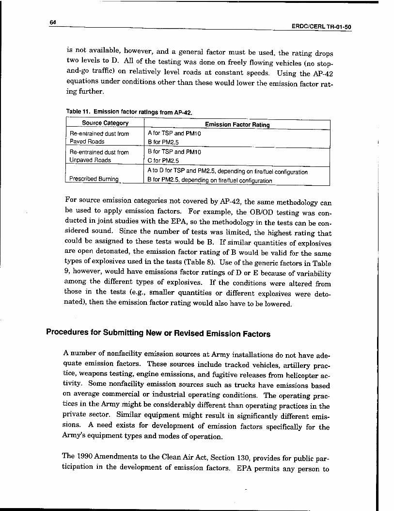
— —-________ ERPC/CERLTR-01-50
is not available, however, and a general factor must be used, the rating drops two levels to D. All of the testing was done on freely flowing vehicles (no stop- and-go traffic) on relatively level roads at constant speeds. Using the AP-42 equations under conditions other than these would lower the emission factor rat- ing further.
Table 11. Emission factor ratings from AP-42.
Source Category
Re-entrained dust from Paved Roads
Re-entrained dust from Unpaved Roads
Prescribed Burning
Emission Factor Rating AforTSPandPMIO B for PM2.5
BforTSPandPMIO C for PM2.5
A to D for TSP and PM2.5, depending on fire/fuel configuration B for PM2.5, depending on fire/fuel configuration
For source emission categories not covered by AP-42, the same methodology can be used to apply emission factors. For example, the OB/OD testing was con- ducted in joint studies with the EPA, so the methodology in the tests can be con- sidered sound. Since the number of tests was limited, the highest rating that could be assigned to these tests would be B. If similar quantities of explosives are open detonated, the emission factor rating of B would be valid for the same types of explosives used in the tests (Table 8). Use of the generic factors in Table 9, however, would have emissions factor ratings of D or E because of variability among the different types of explosives. If the conditions were altered from those in the tests (e.g., smaller quantities or different explosives were deto- nated), then the emission factor rating would also have to be lowered.
Procedures for Submitting New or Revised Emission Factors
A number of nonfacility emission sources at Army installations do not have ade- quate emission factors. These sources include tracked vehicles, artillery prac- tice, weapons testing, engine emissions, and fugitive releases from helicopter ac- tivity. Some nonfacility emission sources such as trucks have emissions based on average commercial or industrial operating conditions. The operating prac- tices in the Army might be considerably different than operating practices in the private sector. Similar equipment might result in significantly different emis- sions. A need exists for development of emission factors specifically for the Army's equipment types and modes of operation.
The 1990 Amendments to the Clean Air Act, Section 130, provides for public par- ticipation in the development of emission factors. EPA permits any person to

ERDC/CERLTR-01-50 65
demonstrate improved or new emissions estimation techniques. Following EPA approval of the measurements, they will be authorized for general use.
Section 130 requires public participation in developing emission factors for car- bon monoxide, nitrogen oxides, and volatile organic compounds. However, EPA intends to follow the same procedures for all criteria, toxic, and other air pollut- ants. This process is not a means for individual facilities to obtain EPA approval of site-specific emission factors or to determine the appropriateness of applying a published EPA factor to a specific installation. EPA does not approve site- specific factors or judge the appropriateness of its factors for specific facilities. The responsibility for such decisions continues to be that of the state or local regulating authority.
A request for revision or addition of an emissions-estimating technique or any other aspect of AP-42 should be submitted in writing to EPA. The request should be for a source that is not unique, and the emission estimation technique should be widely applicable to similar sources in order to be considered. Military tanks, for example, are unique to the U.S. Army but are found at numerous installa- tions across the country, so a general emission factor would be of interest to the EPA. An emission factor applicable to military tanks at only one installation would probably not be of interest.
The request will first be reviewed by EPA for completeness and applicability, and it has 30 days to complete the review. The review will ensure that the request adequately addresses all of the following:
Identification of the submitter with name, address, and phone information Contact name (if different than submitter) with name, address, and phone information Description of AP-42 section, guidance document, or database affected Description of emission source affected Estimation of the number of installations affected Estimation of the total emissions affected Description of the proposed change or addition New or marked-up text for the proposed revision to AP-42 section, guidance document, or database affected Description of the type and source of data Estimate of the range or uncertainty of the estimation technique Description of the effect on U.S. Army installations in terms of regulatory re- quirements An explanation of significant issues, such as "no existing test method"

66 ERDC/CERLTR-01-50
• All data and analyses necessary to support the request, test reports, material balances, data evaluations
• All the details of the test data, which should include: - Is the point tested clearly identified? - Were process parameters monitored and recorded? - Were process parameters within normal ranges? - Are upsets and deviations described and explained? - Are the test methods and procedures described? - Are the methods compatible with approved EPA methods? - Is there enough detail for EPA to validate the procedures? - Are deviations from the normal procedures identified? - Are original raw data and field data sheets included?
- Are quality assurance/quality control (QA/QC) procedures described?
If the request is determined to be complete and applicable, EPA will place a no- tice to the public describing the requested revision on the Clearinghouse for In- ventories and Emission Factors (CHIEF) area of the Office of Air Quality Plan- ning and Standards' (OAQPS) Technology Transfer Network bulletin board system (http://www.epa.gov/ttn/chief).
If the request is determined to be complete and applicable, EPA will also begin an internal review for technical acceptability. The review for technical accept- ability follows guidelines in Technical Procedures for Developing AP-42 Emission Factors and Preparing AP-42 Sections, EPA-45/B-93-050. EPA will issue its rec- ommendation to accept or reject the submitted revisions within 90 days of begin- ning the technical review. This initial recommendation will be described in a second notice to the public on the CHIEF bulletin board. Members of the public review group will submit their individual review comments to EPA within 90 days of receipt of the review package. The EPA will consider the review com- ments and issue a final decision via a third notice on the CHIEF bulletin board within 30 days. If accepted, this change will be reflected in the next possible up- date to AP-42 and affected EPA guidance documents and databases.

ERDC/CERLTR-01-50 67
5 Atmospheric Modeling
Airborne PM is a complex air pollutant to model because it results not only from direct emissions of particles, but also from emissions of gases that either con- dense as particles directly or undergo chemical transformation to a species that condenses as a particle.
Particles emitted directly from a source are referred to as primary PM and can encompass particles of all sizes. The main anthropogenic sources of primary PM are fuel combustion, roadway dust from vehicle traffic on both paved and un- paved roads, wind erosion of industrial storage piles, agricultural operations, construction, and fires.
Particles that result from chemical transformation and/or condensation are re- ferred to as secondary PM and are mainly PM2.5 particles (Seinfeld 1986). The fraction of PM2.5 to TSP can vary significantly based on geography, land use, and other factors. In the Los Angeles and New York City urban areas, for exam- ple, the PM2.5 is 40 to 60 percent of the TSP, while in Denver this percentage varies from 15 to 20 percent. Furthermore, secondary PM usually exceeds 50 percent of the fine PM fraction in urban areas (Seinfeld 1986). Major compo- nents of PM2.5 include sulfate, ammonium, nitrate, and condensed organic mat- ter from secondary sources, and lead- and carbon-containing material such as soot from primary sources. The main precursors that lead to secondary PM are sulfur dioxide, nitrogen oxides, ammonia, and organic compounds. These com- ponents can be from either anthropogenic sources such as combustion, or from natural sources such as wildfires, ammonia generated by animals, and oxidation of naturally occurring hydrocarbons.
Air quality models that address PM can vary significantly in their complexity depending on whether or not they account for secondary PM formation. The chemistry required to model secondary PM formation is closely tied to the chem- istry involved in modeling ozone formation. This is because nitrogen oxides and organic compounds are precursors for both the formation of ozone and the forma- tion of secondary PM. As a result, air quality models that most accurately ac- count for the formation and transport of secondary PM are complex ozone models that have been modified to also calculate secondary PM formation. At this point,

— ERDC/CERLTR-01-50
the formation of secondary PM is usually accounted for only in complex Eulerian models, and even for those models, there are insufficient data to determine if they are accurately modeling the formation of secondary PM (FACA 1997). Two of the more complex dispersion models, CALPUFF and MESOPUFF, however, include chemical transformations that lead to the formation of secondary PM.
Wet and dry deposition are mechanisms by which PM is removed from the at- mosphere. Dispersion and trajectory models can, to varying degrees, account for these mechanisms. Wet deposition occurs when a particle is absorbed into a droplet followed by the droplet being removed by precipitation. Accurate precipi- tation data, including precipitation type and intensity, are required for a model to account for wet deposition. Dry deposition occurs when a particle impacts the
Earth's surface. To accurately represent dry deposition, a model requires land- use data and site-specific data on canopy uptake of PM. These site-specific data are often not available and, if dry deposition is to be accounted for, assumptions must be made regarding the deposition velocity of particles.
One of the Army's objectives in conducting this review of dispersion models is to find models that are or are likely to be acceptable to regulatory agencies. In searching for dispersion models to include in this review, therefore, starting points and primary sources of information were the EPA Support Center for Regulatory Air Models (SCRAM) and the EPA Guideline on Air Quality Models (40 CFR Part 51, Appendix W). Some of the criteria used in selecting models for review in this chapter were: (1) that they be dispersion models rather than Eul- erian models, (2) that they not be categorized as screening models by EPA, and (3) that sufficient documentation is available. Additional models were included based on the applicability of specific models to Army nonfacility source activities and on the modeling experience and knowledge of the authors.
Models that are not already included as a preferred model in the EPA Guideline on Air Quality Models can always be submitted to EPA for inclusion in the Guideline. For a model to be considered, it must meet the following require- ments:
• It must be computerized and functioning in a common Fortran language suitable for use on a variety of computer systems
• It must be documented in a user's guide that identifies the mathematics of the model, data requirements, and program operating characteristics
• It must be accompanied by a complete test data set • It must be useful to typical users
• The model documentation must include a comparison with air quality data or other well-established analytical techniques

ERDC/CERLTR-01-50 69
• The developer must be willing to make the model available to users at a rea- sonable cost, and the model cannot be proprietary.
The process for evaluating models that meet these requirements includes statis- tical measures of model performance in comparison with measured air quality data, and scientific peer reviews. Models that receive favorable evaluations are proposed for inclusion as preferred models in future EPA Guideline revisions.
The remaining sections of this chapter address particular dispersion models. Within each section are subsections that address specific issues of interest to the U.S. Army. For each model, the paragraphs on applicability describe the condi- tions for which a model is applicable. Table 12 summarizes which models are applicable to emissions from specific activities.
Each model section includes a paragraph on accuracy. A quantitative measure of the accuracy of an air quality model, such as a comparison of model results to measured values, is only valid for the specific conditions in which the observa- tions were made. The paragraphs on accuracy, therefore, provide information on the characteristics of each model that contribute to or detract from the expected accuracy of a model. A model that accounts for dry deposition, for example, is more accurate than a model that does not.
Table 12. Applicability of dispersion models to Army nonfacuity emission sources.
Prescribed Burning Vehicles
Smokes and
Obscurants Artillery
Weapons Impact
Test OB/OD Helicopters
Point/Area Area Area Multi-point Area Area Point Area
Activity Duration Intermittent Continuous Intermittent Continuous Continuous Intermittent Continuous
Plume Buoyancy
X X
ISC X X X X
CDM X X X X
RAM X X X X
OBOD X
SCIPUFF X X
MESOPUFF X X X X X X X
CALPUFF X X X X X X X
EOSAEL
SIPM X X X X

— . ERDC/CERLTR-01-50
Industrial Source Complex (ISC3) Model
The ISC3 model is a steady-state Gaussian-plume model that can be used to as- sess pollutant concentrations from sources that are typically associated with an industrial source complex. ISC3 can account for point, area, and volume sources; settling and dry deposition of particles; downwash; plume rise as a function of downwind distance; separation of point sources; and limited terrain adjustments. In addition, ISC3 can be operated in either a long-term mode (ISCLT3) or a short-term mode (ISCST3). The primary source for the information provided here is the ISC3 User's Guide (ISC3 1995).
Applicability of ISC3 to Army Nonfacility PM Sources
The ISC3 model can be applied to point, area, and volume sources (and line sources can be defined as a subset of volume sources). According to the EPA Guideline on Air Quality Models (Revised), ISC3 is appropriate for the following applications: • Industrial source complexes • Rural or urban areas • Flat or rolling terrain (not complex terrain) • Transport distances less than 50 km • 1-hour to annual averaging times • Continuous emissions of primary pollutants.
Required Inputs for ISC3
For point sources, ISC3 requires the following data as model inputs: • Location • Emission rate • Physical stack height • Stack gas exit velocity • Stack inside diameter • Stack gas temperature.
Optional point source data include that can be accepted as model inputs are: • Source elevation • Building dimensions
• Particle size distribution with corresponding settling velocities • Surface reflection coefficients.

ERDC/CERLTR-01-50 71^
For volume sources, ISC3 requires the following data as model inputs: • Location • Volume emission rate • Release height • Lateral and vertical dimensions of the volume.
The area source algorithms of ISC3 are designed to model low-level or ground- level releases with no plume rise. The area source is defined by a rectangle that may be rotated to specify its orientation. The required inputs for an area source are: • Location (of the southwest corner of the rectangle) • Area emission rate • Release height • Length and with of the area • Orientation angle (optional) • Initial vertical dimension of the area source plume (optional).
In short-term mode, ISCST3 requires hourly surface meteorology data. The for- mat of the data can be provided as an ASCII file, or either the PCRAMMET or MPRM (Meteorological Processor for Regulatory Models) meteorology preproces- sors can generate the meteorology data using National Weather Service or onsite meteorological data respectively. The meteorology data required for the ISCST3 model are: • Year, month, day, hour • Flow vector (degrees) • Wind speed (m/s) • Ambient temperature (K) • Stability class (A through F) • Rural and urban mixing heights.
Additional parameters may be provided to account for dry and wet deposition.
Steps and Level of Effort Required To Run ISC3
The hardware requirements to run ISC3 are an IBM-compatible personal com- puter (PC-486 or higher) with 8 MB of memory. The model input files must be
American Standard Code for Information Interchange.

— - ■ ERDC/CERLTR-01-50
created as ASCII text files with a keyword/parameter format that is described in detail in the ISC user's guide. Alternatively, Global Positions, LLC (Limited Li- ability Company) has incorporated the ISC3 model into a graphical geographic information system (GIS) using Arc/Info.
Special Training or Knowledge Required To Run ISC3
No special training is required to use ISC3 other than to understand the user's guide. The user's guide anticipates that users of ISC3 will range from novice us- ers who are new to either ISC or dispersion modeling in general, to experienced users. The learning curve will be rather steep for the novice dispersion modeler, however.
Outputs oflSC3 and How To Interpret the Results
The output from ISC3 is an ASCII file with the model result data organized in tables. The output provided by ISC3 depends on options specified in input files. The user defines output values as either concentration or deposition at a recep- tor. According to the ISC3 User's Guide, the output from ISC3 can include: • Summaries of high values (highest, second highest, etc.) by receptor for each
averaging period and source group combination • Summaries of overall maximum values (e.g., the maximum 50) for each aver-
aging period and source group combination • Tables of concurrent values summarized by receptor for each averaging pe-
riod and source group combination for each day of data processed.
An additional module, called the ISC Short-Term Event model (ISCEV), can be used to determine the contribution of a particular source to an overall concentra- tion value.
Accuracy of ISC3
The following aspects of the ISC3 algorithm contribute to the overall accuracy of the model:
• The ISC3 model uses a steady-state Gaussian-plume equation to model emis- sions from point, area, and volume sources.
• The wind power law is used to estimate the wind speed at the height of an elevated source. Default urban wind profile exponents and rural wind profile exponents are used for each stability class (A through F).

ERDC/CERLTR-01-50 73
• Plume rise due to buoyancy and due to stack gas momentum are estimated. The Briggs plume rise equations are used to estimate the buoyancy of the plume (how high the plume will rise after exiting a stack).
• Stack-tip downwash can be accounted for if the stack gas velocity is less than 1.5 times the wind speed.
• Procedures are included to account for the aerodynamic wakes and eddies produced by buildings and structures in the path of the plume.
• Area sources can be modeled as rectangles and can be rotated around an axis to more accurately represent the area source. Irregularly shaped area sources can be represented by multiple rectangles.
• Dry deposition is modeled using the resistance method to calculate the depo- sition velocity as shown in the following equation:
vd = l/(ra + rd + rardvg) + vg [Eq 15]
where vd is the deposition velocity, ra is the aerodynamic resistance, rd is the deposition layer resistance, and vg is the gravitational settling velocity.
• A scavenging ratio approach is used to model the deposition of gases and par- ticles through wet deposition.
• Although ISC3 is designed to be most accurate in a simple terrain environ- ment, a complex terrain screening model, COMPLEX1, is incorporated to al- low ISC3 to provide a means for conducting screening estimates in complex terrain. This aspect of the model only applies to point source and volume source emissions.
Advantages and Drawbacks of ISC3
The ISC3 model can be used to assess pollutant concentrations from a wide vari- ety of sources. Other advantages are that it requires very few computing re- sources, and conforms to the EPA Guidelines on Air Quality Modeling. Some of its disadvantages are that it is only applicable to continuous sources, and it does not model the formation of secondary PM.
Probability of the Results of ISC3 Being Accepted by Regulators
The ISC3 model is included in Appendix A of the EPA Guidelines on Air Quality Modeling (40 CFR Part 51, Appendix W).

— . __ ERDC/CERLTR-01-50
Procedure for Obtaining ISC3 and Its Costs
The ISC3 model and user's guide are available free of charge from the EPA SCRAM web site (www.epa.gov/scram001/).
Climatological Dispersion Model (COM 2.0)
The CDM uses average emission rates from multiple point and area sources, and a joint frequency distribution for wind direction, wind speed, and stability to es- timate long-term (seasonal to annual) average pollutant concentrations. The pri- mary source of the information provided here is the CDM User's Guide (Irwin, Chico, and Catalano 1985).
Applicability of CDM to Army Nonfacility PM Sources
CDM can be used for up to 200 point sources, 2500 area sources, and an unlim- ited number of level receptors. The model is applicable to rural or urban areas, flat to gently rolling terrain, and transport of distances less than 50 km. If the goal of modeling is to estimate contributions to annual average PM concentra- tions, then CDM is a reasonable choice. Most Army nonfacility PM sources, however, have emissions of short duration and have their greatest effect on shorter duration air quality problems such as exceedances of the 24-hour NAAQS for PM10 and PM2.5.
Required Inputs for CDM
For each source, CDM requires the following data: • Location • Area source length (area sources only) • Average emission rate • Daytime and nighttime emission ratios • Source height • Stack diameter (point sources only) • Stack gas exit velocity (point sources only) • Stack gas temperature (point sources only).
The meteorological data required for CDM are: • Joint frequency function of wind direction, wind speed, and stability class
(the user has a choice between 16 and 36 wind direction sectors) • Average wind speed representing each of the six stability classes

ERDC/CERL TR-01-50 75
• Mean atmospheric temperature • Mixing heights for each of the six stability classes • Wind-profile exponents for each stability class.
For receptors, a location is required. Optional data for receptors include the ob- served concentration of each pollutant, and the height of a receptor above the
ground.
Steps and Level of Effort Required To Run CDM
CDM has been compiled to run on any IBM-compatible PC. Model input data files must be created as ASCII text files with a specific format described in the CDM user's guide. Anyone proficient with PCs can operate CDM.
Special Training or Knowledge Required To Run CDM
A general understanding of dispersion models is required to run CDM. Other required information regarding CDM operation can be found in the user's guide.
Outputs of CDM and How To Interpret the Results
The output of CDM can provide the total concentration at each receptor, the contribution of area and point sources for each receptor, the contribution of area and point sources by stability class, and the contribution of area and point sources by wind direction.
Accuracy of CDM
CDM is designed to estimate annual average concentrations, and therefore does not require the level of accuracy necessary for shorter averaging times. CDM does account for buoyancy-induced dispersion, stack-tip downwash, and gradual plume rise. It allows the user to specify a joint wind frequency function based on up to 36 wind direction sectors. Rather than accounting for wet and dry deposi- tion, a simple exponential decay model is available for pollutant removal.
Advantages and Drawbacks of CDM
CDM is a long-term model for evaluating the effects of multiple point and area sources within 25 km. It requires very little computational effort to determine

Z§ . . ERDC/CERLTR-01-50
annual average concentrations for multiple sources and receptors. For calculat- ing annual average concentrations, it may be much more efficient than simulat- ing an entire year with a more complex model.
Probability of the Results of CDM Being Accepted by Regulators
The CDM model is included in Appendix A of the EPA Guideline on Air Quality Modeling (40 CFR Part 51, Appendix W).
Procedure for Obtaining CDM and Its Cost
CDM and its user's guide are available free of charge from the EPA SCRAM web site (www.epa.gov/scram001/).
Gaussian-Plume Multiple Source Air Quality Algorithm (RAM)
RAM is a steady-state Gaussian-plume model for estimating concentrations of relatively stable pollutants over short averaging times (1 hour to 1 day) from point and area sources. The primary source for the information provided here is the RAM User's Guide (Catalano, Turner, and Novak 1987).
Applicability of RAM to Army Nonfacility PM Sources
RAM is applicable for multiple point and area sources, rural and urban areas, flat terrain, transport distances less than 50 km, and 1 hour averaging times.
Required Inputs for RAM
For each point source, RAM requires the following data: • Location • Emission rate • Stack height • Stack diameter • Stack gas exit velocity • Stack gas temperature.
For each area source, RAM requires the following data: • Location (of the southwest corner) • Source side length • Emission rate of the total area

ERDC/CERLTR-01-50 77
• Effective area source height • Area sources.
RAM requires the following meteorology data hourly: • Power-law wind profile exponents for each stability class • Anemometer height • Stability class at the hour of measurement • Wind speed • Air temperature • Wind direction • Mixing height.
As an alternative to providing an input file with hourly meteorology data, the results of RAMMET, a meteorology preprocessor for RAM, may be used for mete- orology input.
The user may specify the location of up to 180 receptors. Alternatively, up to five radial distances may be provided, in which case RAM generates 36 equally spaced receptors at each radial distance.
Steps and Level of Effort Required To Run RAM
RAM has been compiled to run on any IBM-compatible PC. Model input data files must be created as ASCII text files with a specific format described in the RAM user's guide. Anyone proficient with PCs would be able to operate RAM.
Special Training or Knowledge Required To Run RAM
Other than having a general understanding of dispersion models and reading the user's guide, no special training or knowledge is required to run RAM.
Output of RAM and How To Interpret the Results
The output of RAM includes 1-hour to 24-hour average concentrations at each receptor. Individual source contributions are also included in the output for sources that are labeled as significant in the input file.
Accuracy of RAM
The RAM algorithm is a steady-state Gaussian-plume dispersion model. The wind speed and direction are assumed to be constant for 1 hour. Plume rise is

— . . ERDC/CERLTR-01-50
accounted for with both buoyancy and momentum-based plume rise. The model does not explicitly treat either wet or dry deposition, and any removal of pollut- ants from the atmosphere is estimated by a simple exponential decay.
Advantages and Drawbacks of RAM
RAM is a useful model for estimating concentrations of relatively stable pollut- ants such as inert primary PM. It does not, however, account for chemical trans- formations (i.e., the formation of secondary PM). Also, RAM can only account for wet and dry deposition by using a simple exponential decay function.
Probability of the Results of RAM Being Accepted by Regulators
The RAM model is included in Appendix A of the EPA Guideline on Air Quality Modeling (40 CFR Part 51, Appendix W).
Procedure for Obtaining RAM and Its Costs
RAM and its user's guide are available free of charge from the EPA SCRAM web site (www.epa.gov/scram001/).
Open Burning/Open Detonation Dispersion Model (OBODM)
The OBODM is intended for use in evaluating the potential air quality impacts of the open-air burning and detonation of obsolete munitions and solid propel- lants. The OBODM is both an emissions model and a dispersion model. To pre- dict downwind air quality impacts of OB/OD operations, it is first necessary to determine the quantities of pollutants released. OBODM can use either theo- retical emission factors predicted by a products of combustion model, or empiri- cal emission factors. The dispersion part of the OBODM predicts downwind transport and dispersion of these pollutants using cloud rise and dispersion model algorithms based in part on the EPA's ISC dispersion model.
Applicability of OBODM to Army Nonfacility PM Sources
The OBODM is designed specifically to estimate emissions from OB/OD opera- tions and to predict the downwind transport and dispersion of these pollutants (including PM). The model is applicable to instantaneous (detonation) or quasi- continuous (open-burn) releases from point, volume, or line sources.

ERDC/CERLTR-01-50 79
Required Inputs for OBODM
The OBODM is a menu-driven model in which the user is presented with sepa- rate menus for entering receptor input data, meteorology input data, source in- put data, and program control data. The receptor menu requires the location of each receptor in Cartesian or polar coordinates and the height of the receptor. The meteorology menus require a data file that contains hourly meteorology data. Wind speed, wind direction, temperature, and the Pasquill Stability Cate- gory are required inputs. Other model inputs, such as relative humidity, have default values that can be changed. The meteorology data can be provided in a user-defined format or OBODM will accept meteorological data in an ISC, RAMMET, or MPRM preprocessed format. Source data required by OBODM in- clude the source location, source type (point, volume, line), emission type (instan- taneous or continuous), mass of material burned, material heat content, and ma- terial burn rate.
Steps and Level of Effort Required To Run OBODM
The OBODM is designed to run on an IBM-compatible PC with a minimum of 505 KB of free conventional memory. The user is required to follow the series of input menus to set up the model inputs and model configuration. The OBODM can be run by someone with moderate computer proficiency.
Special Training or Knowledge Required To Run OBODM
Other than reading the OBODM user's guide and having a general understand- ing of dispersion models, no special training or knowledge is required to run OBODM.
Output of OBODM and How To Interpret the Results
The output of an OBODM run provides peak concentrations, time-mean concentrations, time-integrated concentrations, and gravitational deposition of PM. The model also produces regulatory output tables with high and second- high data.
Accuracy of OBODM
For PM the OBODM accounts for gravitational deposition. It also allows the user to specify a particle size distribution.

on — ERDC/CERLTR-01-50
Advantages and Drawbacks of OBODM
The advantages of the OBODM are that it is designed specifically for OB/OD op- erations and that, in addition to acting as a transport and dispersion model, the OBODM is also an emissions model. A drawback is that the model does not es- timate secondary PM.
Probability of the Results of OBODM Being Accepted by Regulators
The OBODM model is not included in Appendix A of the EPA Guideline on Air Quality Modeling (40 CFR Part 51, Appendix W). The dispersion algorithms, however, are based upon the ISC model, which is an EPA-accepted dispersion model.
Procedure for Obtaining OBODM and Its Costs
The OBODM is available free of charge from the EPA SCRAM web site (http ://www. epa. gov/scramOO 1/).
Second-order Closure Integrated Puff Model (SCIPUFF)
The SCIPUFF model is an atmospheric dispersion model that uses a collection of Gaussian puffs to represent an arbitrary, three-dimensional, time-dependent concentration. The model uses a second-order turbulence closure theory, which relates the dispersion rate to velocity fluctuation statistics.
Applicability of SCIPUFF to Army Nonfacility PM Sources
The SCIPUFF model is appropriate for modeling both short- and long-range (greater than 50 km) transport, steady or nonsteady state emissions of primary pollutants, and buoyant or neutral sources using time-dependent meteorology data. SCIPUFF does not, however, allow for source types other than point sources.
Required Inputs for SCIPUFF
The SCIPUFF model uses a graphical user interface (GUI) to facilitate the speci- fication of model inputs. For each source, SCIPUFF requires the source location, stack height, emission rate, stack gas exit velocity, and stack gas temperature. A meteorology data file is required that contains hourly wind direction, wind
ERDC/CERLTR-01-50 81
speed, and temperature data. In addition, precipitation data and terrain data may be provided, if available. For modeling PM, the model allows the user to specify a particle size distribution.
Steps and Level of Effort Required To Run SCIPUFF
The SCIPUFF model is relatively straightforward to set up and run. Anyone proficient with Windows® can operate the model. SCIPUFF is designed to run on a PC, and typical scenarios can be run in less than an hour.
Special Training or Knowledge Required To Run SCIPUFF
The SCIPUFF User's Guide provides sufficient guidance on how to set up and run the SCIPUFF model.
Output of SCIPUFF and How To Interpret the Results
The output of the SCIPUFF model is a graphical representation of the plume dispersion spread across a user-defined domain that can be viewed in a number of different ways. In addition to the average concentration value, the model pro- vides a prediction of the statistical variance in the concentration field resulting from the random fluctuations in the wind field. This allows the user to view a visual representation of the probability that the concentration is greater than a specified value at all points within the modeled domain. An ASCII text file is also generated for each model run that contains the mean concentration and con- centration variance at each point in the modeled domain.
Accuracy of SCIPUFF
Several factors contribute to the accuracy of the SCIPUFF model. SCIPUFF al- lows for puffs to split when they grow too large for a single point of meteorology data to be representative. SCIPUFF accounts for wind shear effects, and dry and wet deposition. Optionally, the model can account for complex terrain ef- fects if the user provides terrain data.
Advantages and Drawbacks of SCIPUFF
Advantages of SCIPUFF are that (1) the graphical user interface makes the model easy to set up and run, and interpretation of the output simple; (2) the re- lationship between dispersion rate and velocity fluctuation statistics allows the model to estimate probability distributions for predicted concentration values.
®?_ ERDC/CERLTR-01-50
The primary drawback of the model for Army nonfacility sources is that the SCIPUFF model is only applicable to point sources.
Probability of the Results of SCIPUFF Being Accepted by Regulators
SCIPUFF has been recommended as an alternative model by the EPA, meaning that it may be used on a case-by-case basis for regulatory applications with ap- proval from a regulatory agency.
Procedure for Obtaining SCIPUFF and Its Costs
The SCIPUFF and user's guide are available free of charge from Titan Systems
(http://www.titan.com/svstems/scipuff.htm). The publicly available version of SCIPUFF is the same version that is incorporated into the Defense Threat Re- duction Agency's Hazard Prediction and Assessment Capability (HPAC).
MESOPUFF
MESOPUFF II is a Gaussian, variable-trajectory, puff superposition model de- signed to account for the spatial and temporal variations in transport, diffusion, chemical transformation, and removal mechanisms encountered on regional scales (hundreds of kilometers). The primary source of the information provided here is the MESOPUFF II User's Guide (MESOPUFF 1994).
Applicability of MESOPUFF II to Army Nonfacility PM Sources
MESOPUFF II is designed to model the transport and dispersion and to estimate a first-order chemical transformation of five chemical species: sulfur dioxide (S02), nitrogen oxides (NO and N02), ammonia (NH3), sulfate (S04) and nitrate (N03). Secondary fine PM, in the form of sulfate and nitrate aerosols, is among the products of the chemical transformation of these chemical species. The MESOPUFF II model is not applicable to primary PM, however. MESOPUFF II models short duration puffs of emissions rather than a continuous plume (al- though a continuous plume can be simulated by a series of discrete puffs). The model may be used for multiple point sources, and includes wet and dry deposi- tion and sedimentation. A sister model of MESOPUFF, called INPUFF (instan- taneous puff) has been used in the past by the Army to predict concentrations from OB/OD operations of short duration (less than 1 hour). INPUFF is not ap- plicable to area sources, however, which make up most of the source types for Army nonfacility operations.

ERDC/CERLTR-01-50 83
Required Inputs for MESOPUFFII
The input data required by MESOPUFF II are provided by several preprocessor programs: READ56, READ62, PXTRACT, PMERGE, and MESOPAC II. READ56 and READ62 are preprocessor programs that read and process the twice-daily upper-air wind and temperature sounding data available from the National Climatic Data Center (NCDC) for selected stations. READ56 extracts the data required by MESOPAC II from a TDF5600-formatted NCDC tape, and READ62 extracts the data from the more recent TD6201 NCDC data format. The output from either READ56 or READ62 is used in the MESOPAC II mete- orological processing program. PXTRACT extracts precipitation data from NCDC data files, and PMERGE processes and reformats the precipitation data for use in MESOPAC II. MESOPAC II is the meteorological processor program that computes the time and space interpolated fields of the meteorological vari- ables required by MESOPUFF II. MESOPAC II produces a single output file containing gridded meteorological fields, which serves as an input file to MESOPUFF II.
Steps and Level of Effort Required To Run MESOPUFF II
For most practical applications, MESOPUFF II can be run with a 486 PC with 4 MB of memory, 300 to 500 MB of hard disk space, and a tape backup unit. Typi- cal scenarios can require between 2 and 6 hours of processing time per month of simulation on a 486 PC. In addition to the computational time, several preproc- essing programs need to be run in order to prepare the meteorological data for MESOPUFF.
Special Training or Knowledge Required To Run MESOPUFF II
The MESOPUFF Users Guide provides limited guidance on how to set up and run the MESOPUFF II model. A background in meteorology or atmospheric modeling would be useful for setting up and running the MESOPUFF model.
Output of MESOPUFF II and How To Interpret the Results
MESOPUFF II creates three output files. PUFFOUT.DAT contains hourly concentration values for gridded as well as individual receptors (in g/m3). FLUXWET.DAT contains hourly gridded and nongridded wet deposition fluxes and FLUXDRY.DAT contains hourly gridded and nongridded dry deposition fluxes (in g/m2/s). A post-processor program called MESOFILE II can be used to summarize the raw output data.

-*? . . ERDC/CERLTR-01-50
Accuracy of MESOPUFFII
The MESOPUFF II model accounts for the formation of secondary PM using a first-order estimation of the chemical mechanisms involving S02, S04, NOx, HN03, and N03. The chemistry is simplified for use in a dispersion model by us- ing hourly chemical rate constants derived from photochemical model simula- tions. Dry deposition is treated with the resistance method, and deposition ve- locities are calculated using land use classification information. Wet deposition can be included if hourly precipitation data are provided.
Advantages and Drawbacks of MESOPUFF II
A significant advantage of MESOPUFF is that it estimates the formation of sec- ondary PM. A significant drawback, however, is that it is not applicable to pri- mary PM. The MESOPUFF model is also more complicated to set up and run.
Probability of the Results of MESOPUFF II Being Accepted by Regulators
The MESOPUFF II model is included in Appendix A of the EPA Guideline on Air Quality Modeling (40 CFR Part 51, Appendix W).
Procedure for Obtaining MESOPUFF II and Its Costs
MESOPUFF II and its user's guide are available free of charge from the EPA SCRAM web site (www.epa.gov/scram001/).
CALPUFF
CALPUFF is a multilayer, multispecies non-steady-state puff dispersion model that can simulate the effects of time- and space-varying meteorological condi- tions on pollutant transport, transformation, and removal. The primary source of the information provided here is the CALPUFF User's Guide (Scire, Stri- maitis, and Yamartino 1999).
Applicability of CALPUFF to Army Nonfacility PM Sources
CALPUFF can be applied to constant or variable emissions from multiple point, line, volume, and area sources. The model is suitable for pollutant transport dis- tances ranging from tens of meters to hundreds of kilometers. Averaging times can range from 1 hour to 1 year. CALPUFF can be applied to inert primary PM
ERDC/CERLTR-01-50 85
and pollutants subject to chemical conversion to secondary PM, and is also appli- cable for rough or complex terrain situations.
Required Inputs for CALPUFF
A GUI is available if CALPUFF is run on a PC. The GUI facilitates the process of specifying inputs for CALPUFF and running the model. The following is a summary of the data that must be provided to CALPUFF either through the GUI, input files generated by the user, or input files generated by other preproc- essing programs: • Control variables determining methods for treating chemistry, wet deposi-
tion, dry deposition, dispersion, plume rise, complex terrain, and near-field sampling methods
• A list of species names and flags for determining which species are modeled, advected, emitted, and dry deposited
• The geometric mass mean diameter and geometric standard deviation of the PM size distribution (used for dry deposition calculations)
• Other dry deposition parameters including ground resistances, reference pol- lutant reactivity, and vegetation state
• Wet deposition parameters including scavenging coefficients for each pollut- ant and precipitation type
• Dispersion and computational parameters: - vertical dispersion constants - dispersion rate above the boundary layer
crossover distance to time-dependent dispersion coefficients land use associated with urban dispersion site characterization parameters for single-point meteorological data files sampling constraints
- puff-splitting controls - plume path coefficients - wind speed power-law exponents - default temperature gradients - wind speed classes
• Point source parameters: location, elevation, stack parameters, emissions, units, building dimensions, and variable emission cycle
• Area source parameters: location, effective height, elevation, initial sigmas, emissions, units, and variable emission cycle
• Line source parameters: location, elevation, line length, buoyancy parame- ters, release height, emissions, units, variable emissions cycle
• Volume source parameters: location, elevation, effective height, initial size, emissions, units, variable emissions cycle
• Receptor locations and elevations.

86 ERDC/CERLTR-01-50
The CALPUFF modeling system includes a meteorology data processor called CALMET. CALMET is a meteorological model that develops hourly wind and temperature fields. CALMET can accommodate raw meteorology data from the NCDC. CALMET is also designed to optionally work with a number of meteorol- ogy data processing programs including MM4/MM5, the MESOPUFF II meteor- ology preprocessors, and the Colorado State University Mesoscale Model (CSUMM). Other preprocessing programs can optionally be used to incorporate U.S. Geological Survey (USGS) land use data and terrain elevation data.
Steps and Level of Effort Required To Run CALPUFF
CALPUFF can run on an IBM-compatible PC or can be compiled to run on a Unix platform for larger studies. A GUI is available on the PC platform to facili- tate setting up a model run. Typical studies require at least 32 MB of memory. The computational time can vary widely depending on the complexity of the study. For example, a model run involving two sources and 64 receptors re- quired less than 1 minute on a 500 MHz PC, while a more complex visibility study involving 218 sources and 425 receptors simulating a 1-year period re- quired approximately 9 hours of runtime for CALMET and 95 hours for CALPUFF.
In addition to running CALMET and CALPUFF, significant effort may be in- volved in compiling the required input files either manually or by running addi- tional preprocessing programs. Additional input files include terrain data files, emission data files, deposition velocity files, upper air and surface level meteor- ology data files, precipitation data files, and numerous others. Numerous proc- essing programs can be used to prepare various data files for CALMET and CALPUFF including an upper air data preprocessor (READ62), a surface mete- orology data preprocessor (SMERGE), a precipitation data preprocessor (PMERGE), an emissions preprocessor (EPM), and several others.
Special Training Required To Run CALPUFF
A background in meteorology or atmospheric modeling would be useful for set- ting up and running the CALPUFF model. The CALPUFF User's Guide pro- vides substantial information on how to set up and run the CALPUFF model. In addition, EarthTech, Inc. in Concord, MA, offers a 3-day training course.

ERDC/CERLTR-01-50 87
Outputs of the CALPUFF Model
The primary output files from CALPUFF contain either hourly concentrations or hourly deposition fluxes evaluated at selected receptor locations. CALPOST, the CALPUFF post-processing module, is used to process these files, producing tabu- lations that summarize the results of the simulation. The output summary pro- vided by CALPOST can be customized to analyze the data using different aver- aging times, or in other ways based on the application.
Accuracy of the CALPUFF Model
The CALPUFF model accounts for the formation of secondary PM using a first- order estimation of the chemical mechanisms involving S02, S04, NO, N02, HN03, and N03. The chemistry is simplified for use in a dispersion model by us- ing hourly chemical rate constants derived from photochemical model simula- tions. Dry deposition is treated with the resistance method, and deposition ve- locities are calculated using land use classification information. Wet deposition can be included if hourly precipitation data is provided.
Advantages and Drawbacks of the CALPUFF Model
The CALPUFF model can be used with a GUI to facilitate the setup and running of the model. The CALPUFF model can also interface with a number of meteor- ology and land-use preprocessor programs through the CALMET program. The disadvantage of the CALPUFF model is that it may be overly complex and re- source intensive for some applications.
Probability of the Results of CALPUFF Being Accepted by Regulators
The CALPUFF model has been improved over the past several years as part of work for the Interagency Workgroup on Air Quality Modeling (rWAQM), U.S. EPA, the U.S. Department of Agriculture (USDA) Forest Service, the Environ- mental Protection Authority of Victoria (Australia), and private industry in the United States and abroad. The rWAQM has recommended the use of CALMET and CALPUFF models for estimating air quality impacts relative to the NAAQS and PSD increments. The EPA has proposed that the CALPUFF modeling sys- tem be included as a guideline model in Appendix A of 40 CFR Part 51, Appendix W (EPA's Guideline on Air Quality Modeling). The EPA is primarily proposing that CALPUFF be used for modeling long-range transport of pollutants.

— . ERDC/CERLTR-01-50
Procedure for Obtaining CALPUFFand Its Cost
CALPUFF, supporting programs (e.g., CALMET), and user's guides are available free of charge from EarthTech, Inc. at (www.src.com/calpun7calpuffl.htm).
Electro-Optical Systems Atmospheric Effects Library (EOSAEL) and the Combined Obscuration Model for Battlefield Induced Contaminants (COMBIC) Module
EOSAEL is a collection of computer programs that mathematically describe as- pects of electromagnetic propagation in battlefield environments. The COMBIC
module simulates the production, transport, diffusion, and nonuniform structure of smoke and dust plumes produced on the battlefield. Specifically, COMBIC predicts the movement of smoke and dust raised by high-energy explosives, ve- hicular movement, phosphorus and hexachloroethane munitions, diesel oil fires, generator-disseminated fog oil and diesel fuel, and other screening aerosols. Once the plume is generated, COMBIC uses semi-empirical and first-principles physics to compute the influences of wind, humidity, temperature, and pressure on the aerosol yield, puff buoyancy, transport, and diffusion. The output of COMBIC, however, is a description of the extinction (transparency) of electro- magnetic propagation between points on a battlefield, which is not relevant for air quality modeling of PM. More information on COMBIC and other EOSAEL modules is available from the EOSAEL web site (www.eosael.com).
Two Air Dispersion Models Proposed
Two dispersion models for assessing ambient air pollution would be added to Appendix A of the EPA's Guideline on Air Quality Models under a 21 April 2000 proposal (65 FR 21,506). Appendix A identifies models and databases that EPA considers acceptable for estimating ambient levels of pollutants. It is used by public agencies and industry to prepare and review new source review permits and revisions to state implementation plans. EPA would replace the Industrial Source Complex (ISC3) model with the American Meteorological Society/ Environmental Protection Agency (AMS/EPA) Regulatory Model Improvement Committee (AERMIC) Model (AERMOD). AERMOD is designed to assess pol- lutant concentrations in urban and rural areas from a variety of sources. ISC3 would be revised by the addition of a new downwash algorithm (PRIME) and would be renamed ISC-PRIME. The other model, CALPUFF, would be a rec-

ERDC/CERLTR-01-50
ommended technique for assessing long-range transport of pollutants and their impacts on Federal Class I areas.

— ERDC/CERLTR-01-50
6 Trajectory Models
Trajectory modeling involves identifying the trajectories of air parcels between a source and a receptor. Both forward and reverse trajectories can be computed. Forward trajectory traces the path of emissions from source to receptor, and re- verse trajectory traces an air parcel from a receptor backward to where it origi- nated. Trajectories are estimated based on wind measurements at various levels in the atmosphere (Seinfeld 1986). For this review of trajectory models, two
models were identified. An intensive search of the Internet did not result in the identification of any additional trajectory models, although others are likely to exist. The two trajectory models that were identified (HYSPLIT and CAPITA) are discussed in the following sections.
Hybrid Single-Particle Lagrangian Integrated Trajectory (HYSPLIT4) Model
The HYSPLIT model is a mesoscale model for computing simple trajectories to complex dispersion and deposition simulations. For simple trajectory modeling, the HYSPLIT4 model can simulate both forward and backward trajectories. The model can compute air concentrations through either of two methods: using a puff model or using a particle model. In the puff method, the source is simulated by releasing pollutant puffs at regular intervals over the duration of the release. The puff is advected according to the trajectory of its center position while the size of the puff expands (both horizontally and vertically) in time to account for the dispersive nature of a turbulent atmosphere. In the particle method, the source can be simulated by releasing many particles over the duration of the re- lease. In addition to the advective motion of each particle, a random component is added to the motion at each time step according to the atmospheric turbulence at the time. Using this method, a cluster of particles released at the same point will expand in space and time simulating the dispersive nature of the atmos- phere. The model has the option of combining the puff and particle methods so that puff dispersion is used in the horizontal direction, and random particle ad- vection is used in the vertical direction. This "hybrid" method has been found by the model's developers to be the most accurate. The primary source of the in-

ERDC/CERLTR-01-50 91
formation provided here is the HYSPLIT4 User's Guide (Draxler and Hess 1998) available on the Air Resource Laboratory (ARL) website: www.arl.noaa.gov/data/models/hysplit4/win95/user_man.pdf.
Applicability of the HYSPLIT4 Model to Army Nonfacility Sources
The HYSPLIT4 model is well suited for quick calculations from pollutant point sources. It does not apply to area or line sources. The model is applicable to sin- gle point source emissions for forward trajectory modeling, or to a single receptor for backward trajectory modeling.
Required Inputs for HYSPLIT4 and How the Inputs Are Obtained
The meteorological input fields used by HYSPLIT4 are required to be in "ARL packed" format. Gridded meteorological data are available in this format on ARL's HYSPLIT4 web site at www.arl.noaa.gov/ss/models/hysplit.html. Mete- orological data that are not available from ARL can be obtained from NCDC. At a minimum, the model requires gridded meteorological data that includes hori- zontal wind components, temperature, height or pressure, and the pressure at the surface. Moisture and vertical motion are optional and, if wet deposition is to be included, then rainfall data are also required. The model also requires the location, height, and emission rate of the source.
Steps and Level of Effort Required To Run the HYSPLIT4 Model
The HYSPLIT4 model either can be downloaded from the ARL web site, or can be run over the Internet using a Java-enabled browser. The download version requires Windows® 95/98/NT and some additional graphical software (Tk/Tcl, and Ghostscript). Typical scenarios can be modeled in 1 to 3 minutes on a Pen- tium-class PC. The GUI allows scenarios to be set up and run very easily if the meteorology data for the scenario are available in the ARL format.
Special Training or Knowledge Required To Run the HYSPLIT4 Model
No special training or knowledge is required to run the model. The GUI guides the user through setting up and running the model. This model could be oper- ated by anyone who is proficient in Windows®.

— ERDC/CERLTR-01-50
Output of the HYSPLIT4 Model and How To Interpret the Results
The model provides concentration and deposition data for each time step (hourly) along the trajectory path. Animated graphical images of the results are also pro- vided and may be useful for visualizing the trajectory path.
Accuracy of the HYSPLIT4 Model
The HYSPLIT4 model accounts for dry deposition using either an explicitly de- fined deposition velocity or the resistance method for estimating deposition ve- locity. Wet deposition can also be accounted for if rainfall data are provided. The model allows wet particle removal to be defined by a scavenging ratio within the cloud and by a scavenging coefficient for pollutants below the cloud base. HYSPLIT trajectory predictions have been compared to balloon paths to test the advection calculations and have performed reasonably well, although a quantita- tive assessment of the accuracy is not available.
Advantages and Drawbacks of the HYSPLIT4 Model
The GUI and availability of preprocessed gridded meteorological data make the HYSPLIT4 model very easy to use. The model runs quickly and the graphical output makes the results easy to interpret. Drawbacks of the HYSPLIT model are that it only accounts for single-point sources and does not attempt to esti- mate the formation of secondary PM.
Probability of the Results of HYSPLIT Being Accepted by Regulators
Trajectory models are not included, nor are any being evaluated for inclusion, in the EPA Guidelines in Air Quality Modeling. The use of trajectory models is also discouraged in "Conceptual Model for Ozone and Particulate Matter," produced by EPA (Science and Technical Support Work Group 1997). HYSPLIT has been accepted, however, as a tool for evaluating regional haze in the Big Bend Na- tional Park.
Procedure for Obtaining the HYSPLIT4 Model and Its Costs
The HYSPLIT4 model is available free of charge from the ARL web site (www.arl.noaa.gov/ss/models/hvsplit.html). From the web site, the model can either be run within a web browser or be downloaded and run locally on a PC with Microsoft® Windows®.

ERDC/CERLTR-01-50 93
Center for Air Pollution and Trend Analysis (CAPITA) Monte Carlo Model
The CAPITA Monte Carlo model is a simulation of regional scale transport, transformation, and dry and wet deposition. Source emissions are treated as a collection of individual parcels of pollutants that are then subject to transport, transformation, and removal processes. Dispersion among the collection of par- cels arises from each parcel being independently subject to mean and random wind components. The model can be used as either a forward or backward tra- jectory model. The primary source of the information provided here is a report on the CAPITA Monte Carlo web site (Schichtel and Husar 1997).
Applicability of the CAPITA Monte Carlo Model to Army Nonfacility Sources
The CAPITA Monte Carlo model is applicable for modeling the regional effects of a single source of instantaneous or continuous emissions on a regional basis.
Required Inputs for the CAPITA Model and How the Input Data Are Obtained
The PC implementation of the CAPITA Monte Carlo model includes a Eulerian to Lagrangian transformer module to generate a Lagrangian air mass history data- base from more commonly available meteorology databases. The developers of the CAPITA model have used meteorology data from the National Meteorology Centers Nested Grid Model (NGM) and Colorado State University's Regional Atmospheric Modeling System (RAMS). A GUI in the CAPITA model facilitates the transformation of data to a Lagrangian database.
Steps and Level of Effort Required To Run the CAPITA Model
The model has low computational requirements and is not complicated to set up and run if an acceptable meteorology data file is available to a given application.
Special Training or Knowledge Required To Run the CAPITA Model
No special training or knowledge is required to run the CAPITA model. Profi- ciency with Windows® is all that is necessary to operate the model.

94 ERDC/CERLTR-01-50
Output of the CAPITA Model and How To Interpret the Results
Various visual interface screens can be used to interpret the results of the model. The GUI presents the location of the particles at a given time as well as a cross section of the map that displays the height and longitudinal positions of all the particles.
Accuracy of the CAPITA Model
The accuracy of the transport portion of the model is determined by the avail- ability of accurate meteorology data. The deposition mechanisms used in the CAPITA model are based on empirical rate constants derived from observed data.
Advantages and Drawbacks of the CAPITA Model
The model does include mechanisms to estimate chemical transformations, which can be used to model secondary PM. A GUI, visual presentation of results, and low computational requirements are also advantages. Drawbacks include the fact that the model has not been thoroughly evaluated, and the approxima- tion techniques used for chemical transformations (S02 to S04) may not be easily extendable to include other chemical mechanisms such as ozone formation or secondary PM formation.
Probability of the Results of the CAPITA Model Being Accepted by Regulators
The CAPITA Monte Carlo model has not been tested thoroughly enough at this point to be generally accepted by regulators.
Procedure for Obtaining the CAPITA Model and Its Costs
The CAPITA Monte Carlo Model: PC Implementation is available free of charge on the CAPITA web site (http://capita.wustl.edu/CAPITA/).

ERDC/CERLTR-01-50 95
7 Measurement of Particulate Matter
Overview
Army installations measure atmospheric PM for many reasons. The installa- tions may be required to perform measurements as part of an operating source permit condition, they may want to gather information showing their contribu- tion to local PM concentrations, or they may want to obtain measurements as an alternative to conservative source estimation methods used to develop their emission inventory.
Several commonly measured characteristics of PM are: • MassofPM(TSP,PM10,PM2.5) • Particle size distribution of PM • Chemical species contained in PM (sulfates, nitrates, metals, organic com-
pounds, ammonia, etc.) • Light reduction by PM (scattering, absorption).
The EPA has or is planning monitoring networks that perform most of these measurement tasks. These EPA-sponsored and -mandated networks were dis- cussed in Chapter 3. The subsequent sections in this chapter contain technical information and references related to available measurement technologies. These sections discuss both generally available technologies and promising re- search-based technologies.
Federal Reference and Equivalent Methods
The EPA has codified many requirements for PM2.5 and PM10 sampling equip- ment and methods. The two basic categories of PM samplers are Federal Refer- ence Method (FRM) and Federal Equivalent Method (FEM) samplers. 40 CFR Part 50, Appendix J describes the requirements for PM10 FRM samplers while 40 CFR Part 50, Appendix L describes the requirements for PM2.5 FRM sam- plers. In addition, 40 CFR Part 53 describes requirements for the classification of both FRM and FEM samplers for all criteria air pollutants including PM10 and PM2.5, and 40 CFR Part 58 contains criteria and requirements for quality

ÜÜ ERDC/CERLTR-01-50
assurance, siting, and operation of all criteria air pollutant samplers, including PM10 and PM2.5 samplers.
A PM10 FRM sampler is a device that draws air through a PM10 particle sepa- rator and then a filter, which collects the PM10 fraction. The specifications for PM10 FRM samplers include performance characteristics and operational re- quirements. These specifications include requirements for sampling filters and the sampler's range, precision, accuracy, flow rate, and operation. FEM PM10 samplers deviate from the PM10 FRM specifications while still producing results that are acceptable to regulators for determining compliance with the PM10 NAAQS. Usually the PM10 FEM samplers are continuous or semi-continuous devices capable of providing PM10 concentration information for averaging peri- ods of 1 hour or less. The operating principle of the most common continuous and semi-continuous PM samplers will be explained later in this chapter.
The specifications for PM2.5 FRM samplers are different in that they include not only performance characteristics and operational requirements but also design specifications. PM2.5 FRM samplers must be designed to collect PM for 24-hour sampling periods on Teflon-membrane filters using a controlled flow rate through the Well Impactor Ninety-Six (WINS) PM2.5 size-selective inlet. The inlet and PM size separation components, filter types, filter cassettes, and inter- nal configuration of the filter holder assemblies are specified by design, with drawings and manufacturing tolerances. Figure 7 is an example of one of these drawings showing the WINS PM2.5 size-selective inlet. Other sampler compo- nents and procedures including flow rate control, interface controls, exterior housing, and data acquisition are specified by performance characteristics with test methods to assess the performance.

ERDC/CERLTR-01-50 97
C| £
a e
1
$
a o
i
M
1 i
o CM
O in OC u. O
> 2 E
(0 a
& E c e o E i
in

Ü? ERDC/CERLTR-01-50
Equivalent methods for PM2.5 can significantly differ from the PM2.5 FRM sampler specification. These samplers are not required to be based on filter col- lection of PM; the idea is to allow the development of new types of PM2.5 meas- urement technologies capable of achieving the same performance as the FRM PM2.5 samplers. Equivalent methods must demonstrate both measurement ca- pabilities comparable to FRM measurements and similar PM2.5 measurement precision. The requirements that candidate samplers must meet to be desig- nated by EPA as FEM samplers are specified in 40 CFR 53. Three classes of equivalent methods have been established in 40 CFR 53 based on the differences between the candidate PM2.5 method and PM2.5 FRM requirements. All three classes of equivalent methods are acceptable for compliance-related PM2.5 moni- toring. However, not all types of equivalent PM2.5 methods may be equally suited to specific PM2.5 monitoring requirements or applications.
Class I equivalent methods are very similar to the PM2.5 FRM, with only minor deviations, and must meet nearly all of the FRM specifications and require- ments. Class I FEM requirements for flow rate, inlets, and temperature are identical to FRM requirements. The requirements for designation as a Class I FEM sampler are only slightly more extensive than the designation require- ments for PM2.5 FRM samplers. To qualify as a PM2.5 Class I FEM sampler, the sampler must meet the requirements of 40 CFR 53, Subparts C and E.
Class II FEM samplers are filter-based devices used for gravimetric analysis, but otherwise differ substantially from the FRM instruments. Dichotomous sam- plers (divided into two parts) and high-volume samplers are two types of PM measurement devices that would fall into the Class II designation. The re- quirements for designation as a Class II FEM sampler may be considerably more extensive than for reference or Class I equivalent methods, depending on the specific differences from the FRM sampler requirements. To qualify as a PM2.5 Class II FEM sampler, the sampler must meet the requirements of 40 CFR 53, Subparts C, E, and F.
Class III FEM samplers include any PM2.5 sampler that cannot qualify as an FRM sampler or a Class I or Class II FEM sampler. Class III FEM samplers have extensive differences from FRM samplers. This class encompasses con- tinuous and semi-continuous PM2.5 samplers and new PM2.5 measurement technologies. The requirements for designation as a Class III sampler are the most extensive but are not explicitly documented in 40 CFR 53. Test procedures and performance criteria will be specified on a case-by-case basis with equiva- lency to the FRM demonstrated over a wide range of particle size distributions, aerosol compositions, and environmental conditions.

ERDC/CERLTR-01-50 99
Whenever PM2.5 samplers achieve either FRM or FEM status, the EPA assigns it an FRM or FEM number and a notice is published in the Federal Register. The most current FRM and FEM list can be obtained from the EPA at http://www.epa.gov/ttn/amtic/criteria.html. Table 13 shows PM reference and equivalent methods as of 6 May 2000 (EPA 2000c).
Table 13. List of designated reference and equivalent methods, 9 May 2000.
Paniculate Matter- PM10 Andersen Model RAAS10-100 PM10 Single Channel PM10
Manual Reference Method: RFPS-0699-130
Andersen Model RAAS10-200 PM10 Single Channel PM10 Audit Sampler
Manual Reference Method: RFPS-0699-131
Andersen Model RAAS10-300 PM10 Multi Channel PM10 Sampler
Manual Reference Method: RFPS-0699-132
BGI Incorporated Model PQ100 Air Sampler Manual Reference Method: RFPS-1298-124
BGI Incorporated Model PQ200 Air Sampler Manual Reference Method: RFPS-1298-125
Graseby Andersen/GMW Model 1200 High- Volume Air Sampler
Manual Reference Method: RFPS-1287-063
Graseby Andersen/GMW Model 321 -B High- Volume Air Sampler
Manual Reference Method: RFPS-1287-064
Graseby Andersen/GMW Model 321-C High- Volume Air Sampler
Manual Reference Method: RFPS-1287-065
Graseby Andersen/GMW Models SA241 and SA241M Dichotomous Sampler
Manual Reference Method: RFPS-0789-073
Graseby Andersen/GMW Model FH621-N Beta Monitor
Automated Equivalent Method: EQPM-0990-076
Met One or Sibata Models BAM/GBAM 1020, BAM/GBAM 1020-1
Automated Equivalent Method: EQPM-0798-122
Oregon DEQ Medium Volume PM10 Sampler. (NOTE: This method is not now commercially available.)
Manual Reference Method: RFPS-0389-071
Rupprecht & Patashnick TEOM Series 1400/1400a PM10 Monitors
Automated Equivalent Method: EQPM-1090-079
Rupprecht & Patashnick Partisol Model 2000 Air Sampler
Manual Reference Method: RFPS-0694-098
Rupprecht and Patashnick Co. PartisoKB>-FRM Model 2000 PM10 Air Sampler
Manual Reference Method: RFPS-1298-126
Rupprecht and Patashnick PartisoKS>-Plus Model 2025 PM10 Seq. Air Sampler
Manual Reference Method: RFPS-1298-127
Wedding & Associates' or Thermo Environmental Instruments Inc. Model 600 PM10 High-Volume Sampler
Manual Reference Method: RFPS-1087-062
Wedding & Associates' or Thermo Environmental Instruments Inc. Model 650 PM10 Beta Gauge Automated Particle Sampler
Automated Equivalent Method: EQPM-0391-081

100 ERDC/CERLTR-01-50
Paniculate Matter- PM2.5
Andersen Model RAAS2.5-200 PM2.5 Ambient Audit Air Sampler
BGI Inc. Models PQ200 and PQ200A PM2.5 Ambi- ent Fine Particle Sampler
Graseby Andersen Model RAAS2.5-100 PM2.5 Ambient Air Sampler
Graseby Andersen Model RAAS2.5-300 PM2.5 Sequential Ambient Air Sampler
Rupprecht & Patashnick Partisol@-FRM Model 2000 Air Sampler
Rupprecht & Patashnick Partisol® Model 2000 PM2.5 Audit Sampler
Rupprecht & Patashnick Partisol®-Plus Model 2025 Sequential Air Sampler
Thermo Environmental Instruments, Incorporated Model 605 "CAPS" Sampler
URG-MASS100 Single PM 2.5 FRM Sampler
URG-MASS300 Sequential PM 2.5 FRM Sampler
Manual Reference Method: RFPS-0299-128
Manual Reference Method: RFPS-0498-116
Manual Reference Method: RFPS-0598-119
Manual Reference Method: RFPS-0598-120
Manual Reference Method: RFPS-0498-117
Manual Reference Method: RFPS-0499-129
Manual Reference Method: RFPS-0498-118
Manual Reference Method: RFPS-1098-123
Manual Reference Method: RFPS-0400-135
Manual Reference Method: RFPS-0400-136
Noncontinuous Filter-Based Mass Measurement Systems
Particle filtration samplers consist of size-selective inlets, filter media, filter holders, pumps, and flow controllers. These samplers are sometimes augmented with denuder systems and absorbing materials that capture gases associated with volatile species such as ammonium nitrate and some organic compounds. The dimensions, materials, and construction of these components affect the par- ticles that are measured.
Size-Selective Inlets
The vast majority of size selective inlets use either impactors or cyclones to sepa- rate particles at the desired cut-point. Since the NAAQS for PM regulate PM2.5 and PM10, these size-selective inlets are most often designed to separate parti- cles for these two size ranges. Figure 8 shows typical particle size distributions for atmospheric TSP, atmospheric PM10, atmospheric PM2.5, streams exiting a PM10 inlet, and streams exiting a PM2.5 inlet. Figure 8 shows the rather sharp cut-point of both the PM10 and PM2.5 size-selective inlets. The figure also shows the three major size range "modes" of particulates in the atmosphere that were discussed in Chapter 2.

ERDC/CERLTR-01-50 101
10
0.1 1 10 Particle Aerodynamic Diameter (urn)
I !"!">'
0.8 S i s
0.6 £
u s It
0.4 I c
I 0.2
f+0
100
Figure 8. Changes in particle size distribution after passing through PM2.5 and PM10 inlets (Chow and Watson 1998, fig 3-2).
Both impaction and cyclonic particle separation technologies are very sensitive to changes in flow rate. This sensitivity is the primary reason that precise flow control is required for PM samplers using this size separation technology. Flow rate requirements for impaction and cyclonic particle separation devices can range from about 1,000 L/min to <5 L/min. PM sampling devices are commonly categorized based on these flow rate ranges: high-volume (~ 1000 L/min); me- dium-volume (-100 L/min); low-volume (-10 to 20 L/min); and mini-volume (<5 L/min).
Direct impactor size-selective inlets consist of a series of openings called jets po- sitioned over an impaction plate. The PM contaminated air flows through the jets onto the impaction plate. Those particles that are small enough to follow the streamlines past the impaction plate are then directed to the PM sampler's filter. The larger particles collide with the impaction plate and are collected. Particles must adhere to the impaction plate to maintain sampling effectiveness. Particle re-entrainment from the impaction plates will seriously degrade the performance of impactors. For this reason the impaction plates are often oiled or greased to retain the particles, and the impaction surfaces need to be cleaned regularly.

— ERDC/CERLTR-01-50
Virtual impactors used in dichotomous PM samplers operate in a manner similar to direct impactors. Instead of an impactor plate, there is an opening that allows larger particles to follow one sampling line while the smaller particles follow the streamlines to another sampling line.
Cyclonic size-selective inlets use a cyclone to perform particle separation. A cy- clone forces an air stream into a circular motion within a cylinder. The motion of the gas stream forces larger particles toward the walls of the cylinder where they are collected. The collection occurs both at the wall surface, which normally has an oiled surface, and in a hopper located below the cylinder. The air stream con- taining the smaller particles continues toward the filter of the PM sampler. The wall of the cyclone must be cleaned regularly to prevent re-entrainment of parti- cles. Cyclones normally have higher loading capacities than direct impactors due to the larger collection wall area of the cylinder and the storage provided by the hopper.
Flow Control
As mentioned above, the size-selective inlets of PM samplers require carefully controlled flows to maintain the desired cut-point. Flow rates can vary with par- ticulate loading on the filter and changes of atmospheric temperature and pres- sure. It is important to note that it is the volumetric flow of air that must be controlled and not the mass flow. Flows are usually either controlled by the use of a critical orifice/critical throat design or by some type of feedback mechanism to adjust a pressure drop or pump speed. A critical orifice is simple and inexpen- sive but requires the pressure downstream of the orifice to be less than 50 per- cent of the upstream pressure. A PM sampling device using a critical orifice for flow control will require a larger pump. The critical throat design compensates for this somewhat by recovering some of the energy that is expended in back pressure behind a critical orifice (Wedding et al. 1987).
Filters
Particle sampling filters consist of a tightly woven fibrous mat or a plastic mem- brane that contains microscopic pores. When chemical analysis will accompany mass analysis of a filter, the filter characteristics must be chosen carefully. When several analyses will be done, it will sometimes be necessary to use more than one filter type for sampling. The following filter characteristics are impor- tant to consider when selecting filters for compliance measurements:

ERDC/CERLTR-01-50 103
• Particle sampling efficiency: Filters must be able to remove 99 percent of the particles drawn through them regardless of the particle size distribution or flow rate.
• Mechanical stability: Filters must be able to lie flat, remain in one piece, and provide a good seal with the sampling system to prevent leaks.
• Chemical stability: Filters should not chemically react with deposited parti- cles or absorb gases that are not intended to be collected.
• Temperature stability: Filters should retain their porosity and structure at the temperatures typical of the air stream being sampled.
• Blank concentrations: Filters should not contain significant or highly vari- able concentrations of the chemicals that the analysis is designed to measure.
• Flow resistance and loading capacity: Filters should allow enough air to flow through them to maintain size-selective inlet flow requirements and to obtain sufficient deposit of particles for analysis.
The most common filter materials are: • Polytetrafluoroethylene (PTFE; Teflon®) used for mass and element analyses • Nylon used for nitrate, sulfate, ammonium, sodium, and potassium analyses • Pre-fired quartz fiber used for total carbon, OC, EC, and carbonate analyses.
Sampling Artifacts, Interferences, and Limitations
This section discusses some of the general difficulties that may be encountered while making PM measurements. Particle and gas removal by inlet surface deposition, nitrate particle volatilization, adsorption of S02 and NOx, OC adsorp- tion and volatilization, liquid water content, electrostatic charge, passive deposi- tion and recirculation, and improper filter handling are all categories of prob- lems with PM sampling. In general, PM2.5 measurements will be more sensitive to these difficulties than PM10 measurements. Many of the biases can be avoided or counteracted with alternative sampling and filter handling tech- niques (EPA 1999).
Inlet surface deposition
The composition of inlets can negatively affect PM collection, especially when the sampled stream contains gases or volatile species such as ammonium nitrate that must be accounted for. Most samplers are manufactured from aluminum, plastic, or galvanized steel, due to the availability and economy of these materi- als. These materials can absorb some gases, especially nitric acid, and can change the equüibrium between volatile particles on a filter and the surrounding air.

— . ERDC/CERLTR-01-50
Nitric acid has a tendency to adhere to surfaces. Surfaces coated with perfluoro- alkoxy (PFA) Teflon® will allow the majority of nitric acid to pass. The alumi- num surfaces common to many samplers and inlets, however, have a large capac- ity (60 - 70 percent) for absorbing nitric acid vapor while transmitting particles with high efficiency (John, Wall, and Ondo 1988). If measurement of nitric acid is important to the sampling program, then coating of the inlet is necessary. In PM samplers designed for chemical speciation of PM, denuders are often used to remove gases that might interfere with the aerosol measurement.
Plastic surfaces can acquire static electrical charges that can attract suspended particles. For most PM samplers, the dimensions of the inlets are sufficiently large that the attraction through this mechanism is negligible (Rogers, Watson, and Mathai 1989).
Nitrate particle volatilization
Loss of nitrate during and after sampling is a well-known PM sampling problem. At temperatures greater than 30 °C, most nitrate will be in the gas phase as HN03 (nitric acid), while at temperatures lower than 15 °C, most nitrate will be in the particle phase as ammonium nitrate (NH, NO J. Amounts of HNO and NH4 N03 will vary between these two temperatures. Relative humidity and con- centrations of ammonia and nitric acid gases also affect this equilibrium, but temperature is by far the most important variable. When air temperature changes during sampling, some of the NH4N03 already collected on the filter can volatilize. Nitrate volatilization is minimized when ambient temperatures are low and with proper ventilation of the sampler housing.
Nitrate losses can also occur after sampling and prior to filter weighing or chemical analysis. Losses of nitrate, ammonium, and chloride from glass and quartz-fiber filters that were stored in unsealed containers at ambient air tem- peratures for 2 to 4 weeks prior to analysis exceeded 50 percent (Witz et al. 1990). Storing filters in sealed containers and under refrigeration will minimize these losses.
Filter media artifacts
A filter media artifact is a positive mass change caused by the oxidation of acid gases (e.g., S02, N02) or by retention of gaseous HN03 on the surface of alkaline (e.g., glass fiber) or other filter types. These biases can be greatly reduced by use of filters that pass the filter acceptance requirements for alkalinity of less than
ERDC/CERLTR-01-50 K»
25 micro-equivalents per gram typical of Teflon-membrane and quartz-fiber filter
materials.
Another effective mechanism for reducing filter artifacts is the use of an appro- priate denuder for acid gases in front of the filter. If the denuder is not properly maintained or replaced on a regular preventative schedule, however, acid gas breakthrough and the potential for artifact formation may occur.
Conversion of S02 on nylon filters has been shown to be highly variable and dependent on sampling conditions (Chan, Orr, and Chung 1986). The extent of the conversion of S02 to sulfate on Nylasorb nylon filters was found to depend on both the concentration of S02 and the relative humidity. The conversion was higher at lower S02 concentrations. More recent work done to test the sorption of S02 on various filter types has shown the artifact formation for Teflon® and quartz fiber filters to be insignificant (Batterman, Osak, and Gelman 1997).
Organic carbon adsorption and volatilization
The adsorption of organic gases onto filters during sampling can introduce posi- tive weight biases, while the volatilization of organic species collected on filters can introduce negative weight biases. Gas adsorption depends on both the filter material and the sampling environmental conditions (temperature, relative hu- midity, partial pressure of particle precursor gases, and flow rate). Volatilization depends more on sampling environmental conditions and not on filter media. It is not yet known which of these competing processes predominate under particu- lar sampling conditions.
The capability for determination of semivolatile organic aerosols will be added to the EPA's routine speciation program as the technology further develops and is validated for routine use. The approach to be used by a routine speciation pro- gram to correct for these artifacts during the collection of particulate OC, will be to incorporate the use of a diffusion denuder to remove the gas phase organic compounds (including volatile organic and semivolatile organic compounds) prior to the collection of particles on a single quartz filter. A post-filter sorbent mate- rial like XAD-4 will also be necessary to collect the gas phase semivolatile or- ganic compounds volatilized from the particulate and the filter medium. The candidate speciation samplers have been designed to accommodate the necessary components as they are developed (EPA 1999).

— . . ERDC/CERLTR-01-50
If the determination of semivolatile organics is required to fulfill the objectives of nonroutine sampling, the analysis of the gas-phase semivolatile organics col- lected by the denuder, in addition to the quartz filter and post-filter sorbent, will be necessary.
Sample moisture
The importance of liquid water content in ambient PM measurement has been recognized for a long time. As ambient relative humidity exceeds 70 percent, particle growth due to accumulation of moisture becomes significant. Theoreti- cal calculation or experimental measurement of aerosol liquid content is compli- cated because growth rates vary with aerosol composition, ambient relative hu- midity, and surface tension.
Both the current PM10 and PM2.5 FRMs require filter equilibrium at a low rela- tive humidity prior to weighing. This procedure represents a compromise be- tween minimizing the effects of humidity and the volatilization of semivolatile compounds on the PM collected on the filter surface.
Electrostatic charge
One potential problem with weighing filters on a microbalance is electrostatic charge buildup on the filter. Electrostatic charge is the accumulation of electri- cal charges on a nonconductive, dielectric surface such as the surface of a Tef- lon®-membrane or polycarbonate-membrane filter. The residual charge on a fil- ter can produce a force between the filter on the microbalance weighing pan and the metal casing of the microbalance. Since this force is independent of the weight of the filter and PM, this force can bias mass measurements (Feeney et al. 1984). As electrostatic charges build up during the weighing session, the readout of the microbalance can become increasingly unstable.
One method for minimizing the static charge during gravimetric analysis is the use of radioactive antistatic strips that are placed inside the microbalance cham- ber prior to weighing. Antistatic solutions can also be used to coat the interior and exterior nonmetallic surfaces of the weighing chamber. This coating in- creases surface conductivity and facilitates the draining of electrostatic charges from nonmetallic surfaces to metallic surfaces. Earth-grounded conductive mats should also be placed on the weighing table surface and beneath the analyst's feet to reduce electrostatic charge buildup.

ERDC/CERLTR-01-50 107
Passive deposition and recirculation
Passive deposition of PM is when windblown dust enters the PM sampling device and becomes deposited on the filter either before or after a sampling cycle. This unwanted deposition obviously will positively bias PM mass and chemical meas- urements. This deposition is normally minimal and depends on local conditions during the specific collection time. Passive deposition can be minimized by more frequent sample filter changing, preloading filters in the laboratory, and trans- porting unexposed and exposed filter cassettes in covered cassette holders. The magnitude of passive deposition can be estimated by using field blanks, which are filters placed in the sampling system without air being drawn through them.
Recirculation occurs when PM sampler exhaust becomes part of the atmosphere being sampled. The sampling pump exhaust should not have an effect on PM2.5 mass measurements. It can, however, affect carbon and trace metal speciation measurements when pump and armature wear are entrained in the exhaust. Filtering pump exhausts or ducting them away from nearby sampling inlets can minimize this contamination. Also, even though PM2.5 pump exhaust may be adequately filtered, nearby high volume samplers for PM10 or TSP can still af- fect the PM2.5 mass measurements and require filtration or ducting.
Contamination due to handling
Sampling and laboratory personnel can cause a gain or loss of the collected PM through faulty handling. The proper use of gloves and forceps, however, will greatly reduce the chance of biases introduced by improper handling.
Continuous and Semi-Continuous PM Measurement Systems
These samplers are defined by their ability to provide immediate atmospheric measurements for averaging periods of 1 hour or less. Samplers of this type are used to measure mass concentrations of PM, chemical composition of PM, and precursor gases of PM. When measuring PM, the sampling systems usually con- tain a size-selective inlet to introduce only the desired PM size category into the analytic portion of the system. These sampling systems range from low-cost/low- resolution devices to high-cost/high-resolution devices designed for research- oriented work.
Many of these devices require some conditioning of the sample stream (i.e., heat- ing, changing pressure, lowering humidity). Changing the temperature, pressure,

108 ERDC/CERLTR-01-50
or humidity can raise or lower the concentration of volatile and water-soluble spe- cies of PM and affect the results. A discussion of how atmospheric conditions af- fect PM concentrations and size distributions can be found in Chapter 2.
The continuous and semi-continuous samplers that measure PM concentration can be candidates for FEM status. Table 13 shows that some of the FEM sam- plers for PM10 are continuous. It is very likely that other continuous samplers for both PM10 and PM2.5 will be designated as FEM in the next several years.
Mass and Particle Size
Tapered element oscillating microbalance (TEOM)
The TEOM® collects PM on a filter mounted to the narrow end of a hollow ta- pered tube (Patashnick and Rupprecht 1991). The wide end of the tube is fixed and the narrow end oscillates in response to a constant electric field. The air sample flows through the filter where PM accumulates and then through the hol- low tube. The filter and tapered tube act as a simple harmonic oscillator and the angular frequency of the oscillation will vary with the collected PM according to the following equation:
co = (k/m)05 [Eq 16]
where: © = angular frequency k = restoring force constant m = the oscillating mass.
The restoring force constant k can be determined through calibrations with known masses and measured oscillating frequencies. After k is known, a meas- urement of the oscillating frequency can result in a calculation of the mass of PM.
Because the restoring force constant k is a function of temperature, the tempera- ture of the TEOM* is kept constant. The normal temperature used is 50 °C to prevent the measurement of particle-bound water. At 50 °C most of the NH4 N03
and some of the volatile organic species will volatilize leading to a negative mass bias. Because of the temperature conditioning, monitored locations and seasons where high levels of NH4 N03 or organic PM exist do not always show a high cor- respondence between the TEOM® and manual filter-based measurements (Allen et al. 1997).

ERDC/CERLTR-01-50 109
The TEOM® is capable of collecting no more than 10 mg of PM. It operates under flow rates of 0.5 to 5 L/min and has size-selective inlets for TSP, PM10, PM2.5, and PM1.0. It can provide averaging times from 5 minutes to 24 hours. The TEOM® has been designated as an FRM for PM10.
Piezoelectric microbalance
A piezoelectric microbalance uses piezoelectric crystals to measure the mass of PM deposited on the crystal. The resonant frequency of a piezoelectric crystal excited by the application of alternating voltage is well-defined and stable. These frequencies are a function of mass and are capable of measuring very small changes in mass. A piezoelectric microbalance compares the difference in frequency between a crystal with and one without deposited PM. This compari- son compensates for temperature effects on the resonant frequency.
A piezoelectric microbalance deposits particles on the crystal either by electro- static precipitation or impaction. The collection efficiency of the PM deposition process needs to be known for quantitative measurements. The sensitivity of the quartz crystals used in piezoelectric microbalances allows measurements of typi- cal PM atmospheric concentrations to within a few percent in less than 1 minute (Olin and Sem 1971). These devices are most often used for specialized projects within the R&D community.
Beta attenuation monitor (BAM)
A BAM measures the attenuation (reduction) of beta radiation as it penetrates a filter with PM deposits (Wedding and Weigand 1993). Particles are collected on a portion of filter tape. A beta radiation source emits beta particles toward the filter tape and a detector measures the amount of beta radiation passing through the tape. The intensity of the beta radiation is attenuated both by the filter and the PM deposited on the filter. The attenuation of the beta radiation is fairly proportional to mass; therefore, the measurement of this attenuation can be re- lated to the mass of PM on the filter tape. The amount of beta attenuation is re- lated to the composition of the PM, and if the calibration standard composition is greatly different than the ambient PM, a biased measurement could occur.
A typical BAM will use a 1-hour averaging period and sample PM at ambient temperatures and relative humidity. Sampling under these conditions will not cause the volatilization of ammonium nitrate and organic compounds, but it will favor the sampling of liquid water associated with water-soluble species at high

— . ERDC/CERL TR-01 -50
humidity. Under high humidity conditions, therefore, BAMs can have a positive mass bias. Several BAMs have been designated as FRMs for PM10 (EPA 2000c).
Pressure drop tape sampler
A continuous ambient mass monitor system (CAMMS) was recently developed at Harvard University (Babich et al. 2000). The CAMMS is based on measuring the pressure drop across a porous membrane filter (Fluoropore™, Millipore Cor- poration, Bedford, MA) and the pressure drop is linearly related to the mass of PM deposited on the filter. The monitor consists of a size-selective inlet, a Fluoropore™ filter tape, a filter tape transport system to allow several weeks of unattended sampling, a system to measure the pressure drop across the filter, a diffusion dryer to remove particle-bound liquid water, and an air sampling pump. The CAMMS is not commercially available.
Visible Light Scattering
Particle light scattering occurs when light is diverted from its path by its inter- action with matter. The amount of scattering due to PM in air is a function of the number of particles, the size of the particles, and the composition of the par- ticles. Chapter 2 contains a discussion of light scattering in the atmosphere. Several types of PM monitors that use light scattering are discussed in this sec- tion.
Nephelometer
Nephelometers measure light scattering of air samples in an optical chamber. The air sample is irradiated from one side with visible light, and the amount of light scattered is measured by one or more photomultiplier tubes. The light used is usually monochromatic and occasionally several monochromatic wavelengths are used. Most devices are designed to measure and integrate as much of the light scattered by gases and particles as possible. Usually calibration is achieved through the use of clean air and various dense gases with known Rayleigh scat- tering properties. Averaging periods vary from ~ 1 second to several minutes. A comprehensive review of nephelometer designs and applications can be found in a 1996 journal article (Heintzenberg and Charlson 1996).
Nephelometers are often used to indicate visibility. They provide a direct meas- urement of the scattering coefficient and can provide a measurement of PM re- lated scattering by subtracting the Rayleigh scattering component of the total measurement. When these instruments are used for visibility measurements, it

ERDC/CERLTR-01-50 111
is important to include the contribution of liquid water associated with particles and water molecules. It is important, therefore, to eliminate temperature and pressure changes in the air stream before scattering measurements are made.
Light scattering is often highly correlated with mass concentration of PM, and many integrated nephelometers use this correlation to report mass concentra- tions of PM. The exact nature of this correlation, however, depends on particle size, shape, and composition and will vary between locations and seasons. Un- der very humid conditions, light scattering by PM can be exaggerated as ultra fine, water-soluble particles absorb water and grow to sizes where they scatter light more efficiently. Therefore, sampling systems using a nephelometer to measure mass will often heat the air stream to remove liquid water from the hy- groscopic particles. In practice, the relationship between nephelometer readings and mass concentration of PM is often empirically determined by collocating nephelometers with filter-based samplers and comparing the measurements.
Optical particle counter (OPC)
OPCs measure light scattering properties of individual particles to detect the number and sizes of particles in a sample. OPCs illuminate a small sample of air with a visible light wavelength laser. Sensitive detectors measure the light scattered by individual particles. The detectors produce an electronic pulse with a magnitude that is proportional to the intensity of the scattered light. Since the intensity of light scattered by particles can be correlated with the size of a parti- cle, an OPC can not only count particles but also provide size information about all the particles that are counted. Typically OPCs can detect particles in the size range from 0.2 to 30 |mi. OPCs are commonly used for certification and meas- urement of particle contamination in cleanrooms and are not often used for rou- tine monitoring of PM in ambient air.
Calibration of OPCs is normally achieved by using National Institute of Stan- dards and Health (NIOSH) traceable polystyrene spheres of known diameter. The accuracy of OPCs depends on particle composition and shape (Buettner 1990). These issues have been discussed for atmospheric particles (Hindman et al. 1978; Hering and McMurry 1991). A NASA study reports large variations be- tween measurements of the same air sample by OPCs from different manufac- turers and broad, sometimes multimodal pulse height distributions for meas- urements of particles with very tight particle-size distributions (Mogan 1997).

112 — ERDC/CERLTR-01-50
Condensation nuclei counter (CNC)
CNCs count ultrafine particles by causing them to grow in size so they can be detected by light scattering of the enlarged particles (Sinclair and Hoopes 1975). Particles are enlarged by first passing the air stream through a heated chamber where a saturated atmosphere of alcohol vapors is created and then passing the air stream into a cooled chamber where the alcohol vapors condense onto the particles in the super-saturated atmosphere. After condensation has occurred, the particles are detected with an OPC. CNCs operate in two modes: counting and photometric modes. In the counting mode, each scattered light pulse is measured. When particle concentrations exceed about 1000 particles/cm3, how- ever, the ability of an OPC to distinguish individual particles degrades and the OPC then must use the photometric mode where the OPC measures the total scattering from all particles as an indicator of the particle count.
OPCs detect particles in the 0.003 to 1 um-diameter size range. They are the most practical instruments for determining a number concentration of ultrafine particles. They are not, however, useful for determining PM2.5 or PM10 mass concentration values because of their inability to size particles and their inability to be used for particles larger than 1 yxa. in diameter.
Aerodynamic particle sizer (APS)
The APS measures light scattering and time-of-flight of individual particles (Wil- son and Liu 1980). The APS accelerates the sampled air stream in a converging nozzle. Particles with higher mass reach lower velocities than those with lower mass. Each particle is detected by laser scattering at the start and end of a fixed path length. The time it takes the particle to complete this path is know as the "time-of-flight" and is proportional to the particle mass.
The APS measures particles with diameters of 0.5 to 30 urn. The aerodynamic diameter determined by the APS differs somewhat from the standard definition. This value can be adjusted, however, for particle density, ambient gas density, and ambient air viscosity (Baron 1986).
Older APS systems suffered from phantom particle counts and coincidence parti- cle counts where it was difficult to track a single particle because of higher parti- cle densities. These problems have been partially resolved using overlapping la- ser light paths that produce a single bimodal scattering pulse as a particle transverses these overlapping beams (TSI1996).

ERDC/CERLTR-01-50 113
Light detection and ranging (LIDAR)
LIDAR measures backscattering from a pulsed laser light source directed into the atmosphere (Grant 1995). LIDAR has many uses including vehicle speed de- tection, measurement of wind speed, measurement of atmospheric gases, and measurements of atmospheric aerosols. Aerosol LIDAR uses a single wavelength of light and measures the backscatter caused by air molecules and aerosols. The scattered light will arrive at the detector at different times corresponding to the distance where the backscattering occurred. The intensity of the backscattered light will indirectly correspond to the concentration of particles at different dis- tances. This results in a profile of aerosol distribution along the path of the laser light. The changes that occur between different pulses of light for the same dis- tance will indicate temporal changes of aerosols in the atmosphere. A complicat- ing factor of this technology is that the intensity of the backscattered radiation is a function of both the backscattering coefficient at the point of backscattering and the extinction coefficient of the entire atmosphere between the LIDAR and the point of backscattering. These two atmospheric parameters cannot be solved simultaneously without additional assumptions being made. Because the rela- tionship between backscatter intensity and particle concentration is not direct, aerosol LIDAR cannot be used to determine mass concentration of PM.
Electrical Mobility
Charged particles placed in an atmosphere with an applied voltage will have a force applied to them. Electrical mobility refers to the relative acceleration or terminal speed these particles can achieve. Smaller particles will achieve a greater speed (greater electrical mobility) than larger particles. This property of charged particles can be used to separate different sizes of particles in an electri- cal mobility analyzer.
An early design of an electrical mobility analyzer was the electrical aerosol ana- lyzer (EAA) (Liu, Whitby, and Pui 1974). EAAs were typically operated with around 10 size channels covering a particle diameter range of 0.01 to 1.0 (am. These devices would positively charge particles and then place them into a parti- cle classifier consisting of an inner and outer cylinder. The outer cylinder was grounded, and a negative voltage was applied to the inner cylinder. As the parti- cles traveled through the classifier, the smaller more mobile particles would de- posit on the inner cylinder. The remaining particles were usually detected by measuring the electrical current produced by the particles. Particle size ranges were measured by changing the voltage applied to the inner cylinder in steps.

— . ERDC/CERLTR-01-50
An improvement on the original EAA design was to configure the particle classi- fier so that only a distinct particle size range is detected. This is normally achieved by placing a slit partially down the inner cylinder of the classifier. In this design, smaller particles are deposited on the inner cylinder as in the EAA, but only a small size range of particles enter the slit with larger particles con- tinuing past. Different size ranges will be detected depending on the flow rate and the voltage applied between the two cylinders. This type of device is often called a differential mobility analyzer (DMA).
The use of DMAs allows a much larger number of particle size channels to be measured but also adds to the time needed to detect the particle current of each particle size range. For this reason, DMAs are sometimes combined with CNCs
to reduce the analysis time. In this configuration, particles are first classified by the DMA and then counted using a CNC. The CNC counting can reduce meas- urement times by an order of magnitude. Another recent improvement to reduce sampling times was achieved through scanning the inner cylinder voltage in- stead of discretely stepping through the voltage range (Wang and Flagan 1990).
Visible Light Absorption
Particles containing EC account for a large majority of the visible light absorbed by PM. These types of particles are generally dark in color and are sometimes referred to as soot. EC-bearing particles are most often generated from anthro- pogenic combustion sources. Chapter 2 contains more information about EC and light absorption in the atmosphere.
The amount of light absorbed by PM is primarily a function of the amount of EC found in the PM. Several PM monitors measure light absorption to indicate the amount of EC found in the atmosphere. There are two basic types of these moni- tors. One type of monitor measures changes in light attenuation through a filter containing a PM sample, while the other type uses the principles of photoacous- tic spectroscopy to measure absorption of visible light by PM.
Measurement of light attenuation through a filter has been used as an indicator of air pollution since the early 1950s. The coefficient of haze measurement sys- tem is a well-known example of this type of device (Lodge 1989). In the devices designed to measure light absorption by PM, both the light transmitted through the PM-contaminated filter and the light scattered by particles or by the filter are collected and measured. The difference between light measurements of clean and PM-contaminated filters is the light absorbed by the PM on the filter.

ERDC/CERLTR-01-50 115
Continuous versions of this type of sampler use a filter tape where the tape is occasionally moved so that different portions of the tape are exposed to PM at different times. The aethalometer, which continuously collects PM on a quartz filter tape, is an example of this type of device (Hansen, Rosen, and Novakov
1984).
Acoustic spectroscopy is another method for measuring visible light absorption by PM. Particles that absorb light will instantaneously produce heat that warms the surrounding gases. If the light is pulsed, then a sound wave of the same fre- quency as the light pulsations will be created, and this sound wave can be de- tected by a microphone (Pao 1977). This amplitude of the sound wave is related to the amount of light absorbed and therefore to the amount of light absorbing material. Although these devices have shown promise in the laboratory, they have not yet become practical enough to supplant devices such as the aethalome- ter for ordinary monitoring activities.
Chemical Speciation
Single particle mass spectrometers
Various configurations of continuous single particle mass spectrometers have been developed in the last decade (Mansoori, Johnston, and Wexler 1994; Mur- phy and Thomson 1994, 1995; Nordmeyer and Prather 1994; Prather, Nord- meyer, and Salt 1994; Carson et al. 1995; Johnston and Drexler 1995; Noble and Prather 1996, 1998). These devices are all capable of analyzing the size and composition of individual particles. Smaller and more portable instruments are being developed (Gard et al. 1997). A project funded by the Strategic Environ- mental Research and Development Program (SERDP) is looking at a single par- ticle mass spectrometer technology called the aerosol time-of-flight mass spec- trometer (ATOFMS) as a method for measuring PM emissions from DOD sources
(SERDP 2000).
In these instruments, particles are introduced into a vacuum where the presence of the particle is detected through scattering from a visible light laser beam. The scattering from the particle is also used to determine the size of the particle. The instrument will size the particle using OPC or APS techniques. When a par- ticle is detected, a high-energy laser pulse ablates and partially ionizes the parti- cle. The ions are detected and analyzed by a time-of-flight mass spectrometer. The particle is in the vacuum for only several microseconds; therefore, the effect of the vacuum on the particle's size or composition is minimized. These devices have just recently been made available through commercial vendors.

— ERDC/CERLTR-01-50
Carbon analyzer
In the laboratory, methods to determine OC and EC in PM based on their ther- mal and oxidative properties are common (Chow et al. 1993). The section later in this chapter on laboratory techniques covers these procedures for analyzing carbon content of PM. Continuous methods using these principles have been under development since the 1990s (Turpin, Cary, and Huntzicker 1990). Moni- tors of this type are available commercially.
Sulfur analyzer
Continuous sulfur monitors normally first remove gaseous sulfur compounds from the sampling stream and then analyze only the sulfur found in the PM (Huntzicker, Hoffman, and Ling 1978; Tanner et al. 1980). The sulfur content is measured by a flame photometric detector. The detector measures the chemilu- minescence of excited state S2* molecules that are produced when the sample is introduced into a hydrogen-air flame. Continuous sulfur monitoring devices are available commercially through several vendors. Some of these devices actually use the method described in the next paragraph for continuous nitrate analysis.
Nitrate analyzer
A relatively new method for continuous nitrate analysis has become available (Hering 1997). The Automated Particle Nitrate Monitor (APNM) collects parti- cles using a humidified impaction process that causes ultrafine hygroscopic ni- trate particles to grow and be collected along with larger particles. After a large enough sample of PM is collected, the cell where the particles were collected is purged with N2, and the PM is flashed through the application of a high current. The flashing process converts the nitrate to NOx, which is then analyzed with a chemiluminescent analyzer. This type of analyzer is commercially available for both nitrate and sulfate analysis.
Laboratory Techniques for Speciation
The amount of PM deposited on a filter during a sampling cycle is small. The typical mass loadings on filters from low and medium volume samplers are less than 5 mg, and many of the chemical species of interest must be measured when less than 1 ug is present in the deposit. If chemical speciation analyses are to be performed, the sampling durations and flow rates must be sufficient to collect enough PM for the intended analyses. The principles, procedures, and results

ERDC/CERLTR-01-50 117
from laboratory methods for speciation of PM are explained in several sources (Lodge 1989; EPA 1999d, 1999e).
The methods used for analyses of the filter media include gravimetry (electro- microbalance) for mass and various instrumental methods for determining the chemical composition of the particles. In addition to chemical analyses, special measurement needs may include determining particle size and morphology through optical and/or electron microscopy.
The EPA has a network of PM2.5 speciation samplers called National Air Moni- toring Stations (NAMS). This network is designed to track trends in the chemi- cal makeup of PM in the atmosphere and to collect samples for common speci- ation analyses. Figure 9 is a flow diagram of filter processing and analysis activities for the NAMS. Most of this section will be devoted to PM speciation analyses and methods related to the NAMS network.
The most commonly applied aerosol analyses methods can be divided into the following categories: mass, elements, ions, and carbon. It is possible to obtain several different analyses from the same substrate, but not possible to obtain all desired chemical species from a single substrate; therefore, the appropriate filter media, sampling hardware, and analysis methods must be combined. The actual chemical species analyses performed will depend on the study objectives and sources in an area. The following sections outline the filter analysis methods for the target chemical species categories of elements, ions, OC, and semi-volatile organic compounds.
Elements
X-ray fluorescence (XRF) is the method chosen to characterize the elemental composition of the aerosol deposits on PTFE filters for the routine PM2.5 NAMS chemical speciation program. Details of this method can be found in the EPA's Compendium of Method for the Determination of Inorganic Compounds in Ambi- ent Air as Method 10-3.3 (EPA 1999e). This method's strong points include a small PM mass requirement, little sample preparation time, and the fact that the sample is left virtually intact and can be submitted for further analysis by other methods. Typical XRF analyses, however, place the PM sample in a vac- uum where volatile organic and nitrate compounds may volatilize.

118 ERDC/CERLTR-01-50
Mas»
Elements
PTFE (Teflon)
I Acceptance
T*5ting
Equtltbrati on )
Pra-sampling Gravimetry
Field Sampling
Transfer to the Laboratory
I PTFE (Teflon) Quartz
Post-samplina Gravimetry
Mass
X-Rav Ftiiartmcnnna Aluminum -
Lead
Therm at Optical Analytl*
Total, Organic, Elemental, Carbonate
Carbon
(AIRS-AQS A
Nylon
Filter Extraction
Ion Chromatograph*
Ammonium, Sodium.
Potassium, Nitrate, Sulfate
Figure 9. Flow diagram of filter processing and analysis activities for NAMS (EPA 1999, fig 7-2).
In XRF the filter deposit is irradiated by high energy X-rays, which causes the ejection of inner shell electrons from the atoms in the sample. When a higher energy electron drops into the vacant lower energy orbital, a fluorescent X-ray photon is released. The energy of this photon is unique to each element, and the

ERDC/CERLTR-01-50 119
number of photons is proportional to the concentration of the element. Concen- trations are determined by comparing photon counts for a sample with those ob- tained from thin-film standards of known concentration.
The type of filter is important and thin membrane filters (PTFE) are required so that the background is low and penetration of particles into the matrix of the fil- ter is small. XRF provides rapid, simultaneous, and nondestructive detection of the target elements from aluminum to lead. Advantages of using XRF are the quantitative analysis of bulk elemental composition, the ability to perform trace level particulate analysis with sensitivity to ppm levels, and the availability of instrumentation.
The sensitivity of this method is on the order of a few ng/m3 for 24-hour samples (flow rates of 10-20 liters per minute). Even with this level of sensitivity, envi- ronmental samples often have elemental measurements below the detection limit of this method. Thus, analytical uncertainties can have a significant im- pact on the quality of the data analysis, such as for source apportionment stud- ies.
Ions
Aerosol ions refer to chemical compounds that are soluble in water. The water- soluble portion of PM associates itself with liquid water in the atmosphere when relative humidity increases, thereby changing the light scattering properties of these particles. Gaseous precursors can also be converted to their ionic counter- parts when they interact with chemicals impregnated on the filter material.
Polyatomic ions such as sulfate, nitrate, and ammonium are quantified by meth- ods such as ion chromatography (IC). Simple ions (e.g., chloride and fluoride) may also be measured by IC along with the polyatomic ions, although atomic ad- sorption spectrophotometry (AAS) and automated colorimetric analysis (AC) are often used also. IC is the method used for IMPROVE and chosen for the PM2.5 NAMS speciation program for the analysis of the target cations (ammonium, so- dium, and potassium) and anions (nitrate and sulfate).
IC can be used for anions (fluoride, phosphate, chloride, nitrate, sulfate) and cations (potassium, ammonium, sodium) by using separate columns. All ion analysis methods require a fraction of the filter to be extracted in deionized dis- tilled water and then filtered to remove insoluble residues prior to analysis. In IC, the sample extract passes through an ion-exchange column, which separates the ions for individual quantification, usually by an electroconductivity detector.

— . ERDC/CERLTR-01-50
The anions are separated when passed through a resin consisting of polymer beads coated with quaternary ammonium active sites. The separation is a result of the different affinities of the anions for these sites. After separation and prior to detection, the column effluent and anions enter a suppressor column where the cations are exchanged for H + ions. Species are then detected as their acids by a conductivity meter. The ions are identified by their elution/retention times and are quantified by the conductivity peak area or peak height. The IC is espe- cially desirable for particulate samples because it provides results for several ions with a single analysis, has low detection limits, and uses a small portion of the filter extract.
The cations are analyzed in the same manner except the sample extract passes
through a surface-sulfonated ion exchange resin where separation occurs. After separation and prior to detection, the cations enter a suppressor column where all the anions are exchanged for OH ions. The species are then detected as then- bases (hydroxides) by a conductivity meter. Concentrations of ions and cations are proportional to the conductivity changes.
Carbonaceous Aerosols
Three classes of PM carbon are typically measured: (1) organic, volatilized, or non-light absorbing carbon, (2) elemental or light-absorbing carbon, and (3) car- bonate carbon. Carbonate-source carbon (i.e., potassium carbonate [K,C03], so- dium carbonate [Na2C03], magnesium carbonate [MgC03], calcium carbonate [CaC03]) may be specifically determined from a second section of the filter after its acidification. Without acidification, the determination of carbonate carbon is not specific and is detected as either OC or EC.
Two thermal-optical methods currently in use for the analysis of carbonaceous aerosols are thermal/optical reflectance (TOR) and thermal optical analysis (TOA). The measurement principle is fundamentally the same, but the methods differ with respect to calibration, analysis time, temperature ramping and set- tings, types of carbon speciated, and pyrolysis correction technique.
For the NAMS chemical speciation program, total, organic, elemental, and car- bonate carbon will be determined by TOA instrumentation specified in NIOSH Method 5040 (NIOSH 1996). The thermal-optical method is applicable to non- volatile, carbon-containing species only. Thermal-optical analyzers are practical, economical, and are routinely used for environmental and occupational monitor- ing of carbonaceous aerosols.

ERDC/CERLTR-01-50 121
Figure 10 is a schematic of the thermal-optical analyzer evaluated by NIOSH researchers, and Figure 11 shows an example of the instrument's output, called a "thermogram." The traces appearing in the thermogram correspond to tempera- ture, filter transmittance, and detector response of the flame ionization detector. Thermal-optical analyzers operate by liberating carbon compounds under differ- ent temperature and oxidation environments. A small portion (or punch) is taken from a quartz-fiber filter sample and placed in the sample oven. The oven is purged with helium and the temperature is then stepped to a preset value. Volatilized compounds are converted to C02 in an oxidizer oven (Mn02 at 870 °C or higher), the C02 is subsequently reduced to methane (CH4) in a methanator (nickel-impregnated firebrick heated to ~550 °C in a stream of hydrogen), and CH4 is quantified by a flame ionization detector (FID). In the second part of the analysis, an oxygen-helium mix is introduced and the remaining carbon is re- moved through combustion and quantified in the same manner.
In general, thermal-optical methods classify carbon as "organic" or "elemental." OC is carbon that is volatilized in helium as the temperature is stepped to a pre- set maximum (850 °C). EC is light-absorbing carbon and any non-light absorb- ing carbon evolved after pyrolysis correction. EC is evolved in the second part of the analysis when the temperature is lowered, a 2 percent oxygen/98 percent he- lium mix is introduced, and the temperature is then stepped to a maximum of 940 °C. At the end of the analysis, a calibration gas standard (CH4) is injected.
FID
V = valve
Figure 10. Schematic of thermal-optical instrument (NIOSH 1996).

122 ERDC/CERLTR-01-50
Figure 11. Thermogram for a sample containing organic, carbonate, pyrolytic, and elemental carbon (OC, CC, PC, and EC). The last peak is the methane calibration peak (NIOSH 1996).
Depending on the sampling environment, carbonates [e.g., potassium carbonate (KjCOa)» sodium carbonate (Na^Oj), magnesium carbonate (Mg C03), calcium carbonate (Ca C03)] also may be present in the sample. NIOSH Method 5040 quantifies carbonate-source carbon as organic since carbonates decompose dur- ing the first part of the analysis when the sample is exposed to 850 °C in a he- lium-only atmosphere. To quantify carbonate carbon, a second portion of the fil- ter sample is analyzed after its acidification, which removes the carbonates from the filter. Carbonate is taken as the difference between the pre-and post- acidification results. Alternatively, carbonate carbon in a simple carbonate (i.e., not a bicarbonate) can be estimated by integrating the carbonate peak (typically the fourth peak in a thermogram). Typically, carbonate carbon is not speciated in environmental samples because it has been found to constitute less than 5 percent of the total carbon in most samples (Chow et al. 1993).
It is important to remember that EC and OC have meaning only in the opera- tional sense. That is, results reflect the method used and the appropriateness of a method depends on its purpose. Operational methods differ from those used for specific, identifiable analytes (e.g., sulfate or sulfur), where a well-defined entity is quantified and laboratory standards are available for its determination. Because EC and OC are defined operationally, the details of the measurement method must be rigorously described.
ERDC/CERLTR-01-50 123
Semivolatile Organic Aerosols
The EPA considers measurement of semivolatile organic aerosols as a non- routine and research-oriented activity. This type of PM speciation is not part of the specifications for the NAMS. Identification of the ideal denuder, filter com- bination, and sorbents and development of routine sampling and analytical methods is complicated due to the number and variety of semivolatile organic aerosol compounds in the atmosphere and their varying absorptive properties.
The collection of particulate organic matter can be accomplished using particu- late sampling instruments equipped with quartz fiber or Teflon®-impregnated glass fiber filters. However, since many organic compounds are distributed be- tween the gas and particle phases, additional sampling techniques are required to measure the particle phase semivolatile organics. This methodology is suscep- tible to both negative (desorption of semivolatile compounds from the particles on the filters) and positive (adsorption of gases by the filter material) artifacts. Considerable experimental and theoretical effort has been expended to under- stand and correct for these vaporization and adsorption effects. Denuder tech- nology has been used to provide a less artifact-encumbered approach for accurate determination of semivolatile species because the gas phase is removed prior to the particulate phase. A sorbent or denuder after the filter may also be used to collect any semivolatile material desorbed from the filter.
For quantifying individual organic compounds, the denuder, filter, and sorbent are extracted individually with a suitable organic solvent or combination of sol- vents. The extract is then analyzed by gas chromatography (GC) combined with mass spectrometry (MS) or with other specific detectors. Combined GC/Fourier transform infrared (FTIR)/MS techniques or high performance liquid chromatog- raphy (HPLCVMS techniques are also used.
Opacity
Opacity is the measurement of visible light extinction through the Earth's at- mosphere where 100 percent opacity means all visible light is extinguished and 0 percent opacity means that none of the light is diminished. This report uses the more restrictive definition of opacity, which describes the amount of light extinc- tion that can be attributed to a plume of PM emitted from a source. It is common for state regulations to limit the opacity from PM sources, since poor opacity of a plume is a surrogate indicator of high PM concentrations within the plume.

— . _____^ __ ERDC/CERLTR-01-50
The most common method of measuring opacity is EPA Method 9 (40 CFR 60, Appendix A). In this method, a qualified human observer assesses the opacity of the plume against the background of the sky. Although Method 9 is performed by individuals who have successfully completed "smoke school" training, the re- sults of this method are rather subjective since they are based entirely on human observation. There can be honest disagreements between source owners and regulatory personnel about Method 9 results.
Opacity from stationary sources with well-defined stacks can also be measured using a continuous monitoring device. This measurement technique is described in EPA Method 203 (40 CFR 60, Appendix B). The continuous opacity monitors use transmissometers to measure the extinction of light across a stack. There are many commercial vendors of these continuous opacity monitors.
There does not appear to be the same type of automated opacity monitors avail- able for PM plumes in the atmosphere. EPA does have an alternative promul- gated method to Method 9 using LIDAR to measure atmospheric plumes (40 CFR 60, Appendix A). The use of LIDAR is very complex, however, and perhaps this is why there seems to be no LIDAR-based system dedicated to the meas- urement of plume opacities.

ERDC/CERLTR-01-50 125
8 Dust Suppression and Soil Stabilization Technology
Background
Wind erosion describes the loss or movement of soil particles by several different processes including: saltation, surface creep, and suspension. This loss of soil material occurs either through the force of natural winds or turbulent air move- ments caused by the passage of vehicles and aircraft. Particles that can be lifted by the wind, but fall back to the surface after a short distance, are traveling by saltation. Soil aggregates and particles larger than -1000 jam cannot be picked up by the wind but tend to roll along the surface driven by wind forces and im- pacting grains. These grains move by surface creep. Suspension is the process whereby very fine particles (less than 100 urn in diameter) are lifted from the ground surface by saltation, then carried by wind forces higher into the air.
PM is generated primarily as a consequence of this final wind erosion process — suspension. Particles transported by suspension can travel thousands of kilome- ters. Although this process accounts for only a small fraction of the total soil moved by wind, it is significant because this soil fraction is the most important in soil fertility and water-holding relationships (Gillette et al. 1980; Fryrear 1985). PM generation is, to a lesser extent, a byproduct of the saltation compo- nent of wind erosion, whereby abrasion from saltating particles facilitates parti- cle detachment and transport by wind forces. In this process, the rate of PM generation depends on kinetic energy from saltating particles during the wind erosion process and the soil's PM potential (i.e., particle size distribution, aggre- gate cohesiveness, abrasion resistance).
Vehicle movements increase PM generations through several means. The vehi- cle's tires interact with the surface material, directly injecting particles into the atmosphere while at the same time pulverizing the material. Furthermore, the passage of the vehicle results in a wake that also entrains particulate matter. The intensity of this process will depend on many factors, such as: vehicle weight, number of wheels, tread design, tire footprint pressure, clearance height, and vehicle speed (EPA 1998).

-2*. ERDC/CERLTR-01-50
Since the 1940s, numerous products have been developed and used to control dust on unsurfaced landing zones, roads, and trails. The relative merits of vari- ous agents for controlling dust on helicopter landing pads, tank trails, and un- surfaced roadways have long been the subject of heated debate. At one time or another, nearly every conceivable material has been sprayed onto unsurfaced roadways in an attempt to control dust, stabilize the road surface, and reduce vehicle maintenance costs (Kirchner 1988). Some products (e.g., used motor oils, industrial manufacturing wastes, and other petroleum based derivatives) have damaging environmental effects, and their use is now prohibited.
Recent developments in dust control technology, however, have provided a num- ber of environmentally safe materials that are similar in cost, efficacy, durabil- ity, and maintenance requirements, especially on unimproved roadways where somewhat rougher terrain may make traditional road maintenance more diffi- cult and costly. Although chemical, physical, and biological methods to stabilize unsurfaced roads, trails, and landing zones have the potential to reduce traffica- bility, erosion, PM emissions, and maintenance requirements, these methods have not been fully investigated for military roads and trails.
Construction and Maintenance of Unpaved Roads and Trails
The main factors that lead to excessive PM generation are loose surface materi- als and turbulent air movement caused by strong winds and vehicle movement. Climatic factors, such as low rainfall and high temperatures, also contribute to PM problems as evidenced in arid and semi-arid regions of the United States. Loose road surface materials are easily removed through wind action, resulting in surface degradation and enhanced PM generation because smaller particles (fines) necessary for proper bonding and surface strength have been eliminated. This will eventually lead to excessive road subsurface wear, thereby accelerating further destabilization.
When a subgrade deteriorates, the road will require regrading, the addition of fines to promote surface bonding and strength, shaping, and compaction to cre- ate a hard surface layer and a properly crowned cross section. Frequently, only specific sections of roads, trails, and landing strips are problematic in terms of excessive PM generation and can be treated individually on an as-needed basis. Some examples include road/trail intersections, road/trail segments close to high speed paved roads or housing and administrative areas, and fuel and ammuni- tion supply routes. This approach specifically targets problem areas and assures

ERDC/CERLTR-01-50 127
that valuable personnel, equipment, and material resources are not wasted on areas with only marginal PM emission problems.
The best way to avoid PM emission problems is to ensure that proper mainte- nance is scheduled and implemented to include surface grading and shaping so that proper cross-sectional crowning is attained to prevent excessive road surface wearing and consequent dust generation (Brown and Elton 1994; Cleghorn 1992). Chemical dust suppressants are considered a secondary solution, to be used only when maintenance practices have been implemented to the greatest extent possible.
Good Construction and Maintenance Practices
Good construction and maintenance practices are fundamental in providing du- rable and erosion-resistant trafficked surfaces in dust prone areas. Properly crowned roadway cross sections (referred to as geometry), well-graded materials composed of sufficient fines for strength and durability, and adequate drainage are vital to maintaining a hard surface that reduces PM emissions. Existing PM emission problem areas should be assessed to ensure that poor construction and maintenance practices are not causing the emission problem.
The best way to provide long-term dust control is proper design and construction of new roads, trails, and landing zones. Special considerations should be given to the following: • Proper crown in the subgrade to assist in preserving a uniform thickness of
surface material across the trafficked area • Proper crown of the wearing surface to ensure effective drainage of the sur-
face to minimize loss of fines and potential leaching of chemical dust pallia- tives (suppressant)
• Compaction of the subgrade and pavement material to minimize particle movement.
The requirements for the various materials used in the construction of aggregate surfaced roads and airfields depend upon whether or not frost is a consideration in the design. The material should be sufficiently cohesive to resist abrasive ac- tion. It should have a liquid limit no greater than 35 and a plasticity index of 4 to 9. It should be graded for maximum density and minimum volume of voids in order to enhance optimum moisture retention while resisting excessive water intrusion. The gradation, therefore, should consist of the optimum combination of coarse and fine aggregates that will ensure minimum void ratios and maxi- mum densities. Such a material will then exhibit cohesive strength as well as

198 — ERDC/CERL TR-01 -50
intergranular shear strength. Where frost is a consideration, a layer system should be used. The percentage of fines should be restricted in all layers to fa- cilitate drainage and reduce the loss of stability and strength during thaw peri- ods.
Adequate surface drainage should be provided to minimize moisture damage. Expeditious removal of surface water reduces the potential for absorption and ensures more consistent strength and reduced maintenance. Drainage, however, must be provided in a manner to preclude damage to the aggregate surfaced road or airfield through erosion of fines or erosion of the entire surface layer.
Regular maintenance of existing roads and landing zones is the most cost- effective method to control dust emissions at a military installation. Mainte- nance activities should pay special attention to the following: • Use of well-graded aggregates having adequate cohesive binder (fines) • Retention of the crown to provide adequate drainage • Adequate drainage for rapid draining of the wearing surface, shoulder, and
verge
• Proper compaction of wearing surface following the addition of aggregate and grading — compaction increases the density and strength of the wearing sur- face and retention of larger aggregates
• Avoid maintenance grading during dry weather.
Roads require frequent maintenance because the environment and traffic dete- riorate the aggregate surface. Rain or water flow will wash fines from the ag- gregate surface and reduce cohesion, while traffic action causes displacement of surface materials. Maintenance should be performed at least every 6 months and more frequently if required. The frequency of maintenance will be high for the first few years of use but will decrease over time to a constant value (Za- niewski and Bennett 1989). The majority of the maintenance will consist of pe- riodic grading to remove ruts and potholes that will inevitably be created by the environment and traffic. Occasionally during the lifetime of a road or airfield, the surface layer may have to be scarified, additional aggregate added to in- crease the thickness to the original requirement, and the wearing surface com- pacted again to the specified density.
Mechanical Stabilization
Mechanical stabilization involves mixing substrate materials to ensure that the local soils have a wearing surface with the correct grading and plasticity. A sub- strate that considerably reduces dust generation is composed of well-graded

ERDC/CERLTR-01-50 129
gravel-sand mixtures with sufficient amounts of clayey (cohesive) fines to pro- mote surface bonding and wear resistance. Mechanical stabilization can be used under a variety of conditions and, once established, will reduce PM emissions for years when properly maintained.
When a gravel road resists lateral displacement during traffic, it is said to be mechanically stable. The natural forces of cohesion and internal friction that exist in the soil provide this resistance. Cohesion is mainly associated with the fine silt and clay particles of the material, while internal friction is characteristic of the coarser particles. For a soil to be mechanically stable, it must fulfill re- quirements with respect to shear strength, resistance to abrasion, rigidity, in- compressibility, and freedom from swelling, shrinkage, and frost action. Each of these requirements must be addressed within a mechanically stabilized road; however, the requirements will vary due to the soil material in the road and the loads applied to the road structure.
Mechanical stabilization is accomplished by mixing or blending soils of two or more gradations to improve certain properties of the soil. The blending may take place at the construction site, a central plant, or a borrow area. After the soil is blended, it is spread and compacted to required densities by conventional means.
Physical Stabilization
Physical stabilization is the implementation of best management practices for disturbed areas with temporary dust problems. These practices include the ap- plication of water, compaction, installation of temporary coverings, and pre- grading planning. Water should be used, when available, on areas with short duration dust events to properly maintain a 12 percent soil moisture level (Rule 403, 1999). Spraying water on a problem area usually provides immediate re- sults and is inexpensive for short-term dust control. Water surrounds and ad- heres to dust particles making movement more difficult. The effectiveness of wa- ter applications is short-lived, however, and it may cause the pumping of fines to the wearing surface under continual wetting conditions. In arid climates, con- servation of water may be regulated in such a way as to prohibit this method. Application of water is only recommended as a short-term solution to dust emis- sion problems.
Prior to excavation or construction activities, the area should be watered to en- sure a 12 percent moisture level to the anticipated depth of excavation. Mining and construction areas should be watered as necessary to reduce visible emis- sions. For disturbed surface areas, unpaved roads and graded areas, water once

-I?? ^ ^^ ERDC/CERL TR-01-50
an hour or at least twice a day to reduce emissions. Open storage piles of soil require 80 percent of the exposed surface area to be watered daily when there is evidence of wind driven fugitive dust.
Compaction of the soil by itself or in conjunction with water or amendments is a relatively nonresearched method for reduction of dust loads. Compacting the soil develops a hardened surface, which increases particle resistance to detachment. If compaction is taken a step further and amendments or water are added, the possibility for a long-life hardened surface increases. Fibers from paper and other industries would potentially provide a more cohesive bond within the com- pacted soil. The addition of water during the compaction phase would increase the soil's bulk density, resulting in a more hardened surface. Other proposed additives include, but are not limited to, polyacrylamide, enzyme slurries, and bentonite.
Temporary and permanent coverings include gravel, membranes, tarps, and mulches. Gravel should only be used in areas where paving, chemical stabiliza- tion, or frequent watering is not feasible. The gravel should be maintained at a depth of 4 inches in order to be an effective control measure (Rule 403, 1999). Open storage piles of soil should be covered with a tarp or membrane during high winds to reduce fugitive dust. Vehicles transporting soil need to have the entire surface area of hauled earth covered with a tarp; coverings need to be properly anchored to prevent removal of the tarp by wind.
Proper planning is critical for reductions in fugitive dust. Each phase of con- struction, grading, earth movement, and soil transportation should be planned with reduction in dust as a primary objective. Grading should be done sepa- rately, preferably not all at once, and timed to coincide with construction phases. If this is not feasible and grading of the entire project is necessary, application of chemical stabilizers, mulch, or ground cover to the graded areas will reduce fugi- tive dust. Finally, during high wind events, all activities for excavating, grading, or hauling soil should cease. -
Chemical Methods of Dust Suppression
Chemical dust palliatives (suppressants) should be considered an adjunct to the other dust control methods, especially if mechanical stabilization is cost prohibi- tive and high PM emissions persist. Chemical dust palliatives have a limited life span and require regular applications to maintain adequate dust control on a

ERDC/CERLTR-01-50 131
long-term basis. Tracked-vehicle traffic may reduce product performance stan- dards by an estimated 50 to 75 percent or more (Gebhart, Denight, and Grau 1999). Careful consideration should be given to the life-cycle management of chemical dust suppressants, since other dust control options may prove most cost-effective over time.
Chemical dust suppressants, however, do have their place in the management of PM emissions from unpaved surfaces. There are many types of suppressants and the selection of the correct material depends on local conditions such as soil type, soil moisture, and usage pattern for the road or trail. Chemical dust sup- pressants are classified in the following general categories: water-attracting chemicals, organic nonbituminous chemicals, petroleum-based binders and waste oils, electro-chemical stabilizers, polymers, enzyme slurries, and cementitious binders.
Water-attracting Chemicals (Chlorides, Salts, and Brine Solutions)
These chemicals have the ability to absorb moisture from the atmosphere or the road surface. Absorption of moisture causes a brine film to develop, which at- tracts dust particles. The hygroscopic properties also result in the retardation of evaporation off the road surface during the day. This category of dust palliatives provides the most satisfactory combination of application ease, durability, cost, and dust control for semi-arid, semi-humid, and humid climates (Addo and Sanders 1995; Aquin, Korgemagi, and Lynch 1986; Bassel 1992; Bergeson et al. 1995; Bolander 1989; Gebhart et al. 1996, 1997; Hass 1985, 1986; Hoover et al. 1981; Kolot 1984; Marshal 1997; Monlux 1993; Muleski and Cowherd 1987; Za- niewski and Bennett 1989).
Their effectiveness is limited and may not provide sufficient dust control for a second year. Subsequent applications may, however, be made at reduced rates due to residual effects. It should be noted that this product category is corrosive to metals and may not be an acceptable choice if vehicle exposure to corrosive materials is not advisable or if relatively frequent vehicle washing is not possi-
ble.
Organic Nonbituminous Chemicals (Lignosulfonates, Sulphite Liquors, Tall Oil Pitch, Pine Tar, Vegetable Oils, and Molasses)
These chemicals are able to either adhere to the soil particles or physically bind the soil particles together thereby increasing the mass of the particles. This category of dust palliative performs best under arid and semi-arid conditions,

132 . ERDC/CERLTR-01-50
but is less effective on igneous, crushed gravel, and medium-to-low fine materi- als (Addo and Sanders 1995; Apodaca and Huffmon 1990; Bennett and Gleeson 1995; Bolander 1989; Brown and Elton 1994; Boyd 1983a-b, 1986; Cleghorn 1992; Gebhart, Hale, and Busch 1996; Gebhart and Hale 1997; Grau 1993; Highway Extension Research Project 1992; Hoover et al. 1981; Kolot 1984; Son- towski and Vliet 1977; Tetteh-Wayoe 1982; Zaniewski and Bennett 1989). As with water attracting chemicals, the effectiveness of organic nonbituminous chemicals is limited and may not provide sufficient dust control for a second year, but subsequent applications may be made at reduced rates due to residual effects. Failures often occur following rains, because organic nonbituminous products have long curing times and are gradually leached out. Some of the commercial products in this category may be visually unappealing, odorous, or very sticky upon application, which may preclude their use depending on loca- tion of the area to be treated.
Petroleum-Based Binders and Waste Oils (Bitumen Emulsions, Asphalt Emulsions, and Waste Oils)
These suppressants are derived from petroleum. They are not soluble in water and generally form a sealant on the road surface. The sealed road surface is then able to hold the soil particles, thereby preventing dust generation. This category of dust palliative is the most effective suppressant for a variety of cli- matic conditions (Bassel 1992; Bolander 1989; Grau 1993; Marks and Petermeier 1997; Monlux 1993; Muleski and Cowherd 1987; Troedsson 1994; Unger 1990; Watson et al. 1996; Zaniewski and Bennett 1989). Unfortunately, waste oils can cause significant adverse environmental effects due to toxic materials and are not environmentally acceptable unless they have been processed to remove these materials. A number of asphalt emulsions, however, have been approved for use and, although relatively expensive compared with other product types, are con- sidered effective under a broad range of soil types and climates. As with the or- ganic nonbituminous product category, some of these commercial products may also be visually unappealing, odorous, or very sticky upon application. These factors may preclude their use depending on location of the area to be treated.
Electrochemical Stabilizers (Sulphonated Petroleum, Ionic Stabilizers, and Bentonite)
These stabilizers have negatively charged surfaces. When the stabilizer's elec- trically charged surfaces are exposed to fine particles with a positively charged surface, an ionic exchange takes place causing the fine particulates to bond with the stabilizer. These products work over a wide range of climatic conditions, are

ERDC/CERLTR-01-50 133
least likely to leach out, and are particularly effective on materials with clayey or sandy surfaces (Bergeson and Brocka 1995; Bergeson and Wahbeh 1990). A large variety of these materials are available to road construction and mainte- nance engineers and, when applied under highly specific trafficked surface and aggregate conditions, have been shown to produce dramatic reductions in dust generation. Unlike most traditional dust palliatives, these products have no standard laboratory tests for predicting their performance under field conditions and their use often results in either unqualified success or failure. Until stan- dard testing is developed for this product category, small-scale trials should be initiated and evaluated for effectiveness before large-scale applications.
Polymers (Polyvinyl Acrylics and Acetates)
These products bind surface soil particles together and form a semirigid film on the trafficked surface. Most of the polymer products are supplied in concen- trated form and require dilution with water before application. With slight variations in dilution and final application rates, polymers are generally suitable for use under a wide range of soil and climatic conditions (Gebhart, Hale, and Busch 1996; Gebhart and Hale 1997; Grau 1993; Monlux 1993; Muleski and Cowherd 1987; Styron, Hass, and Kelley 1985; Watson et al. 1996). Unlike some of the other product types, most polyvinyl acrylics and acetates are considered nontoxic and environmentally friendly when used according to manufacturers' recommendations. They are most effective on lightly trafficked surfaces such as helicopter landing surfaces in zones that receive between 8 and 40 inches of pre- cipitation per year.
Enzyme Slurries
Many enzymes are adsorbed by clay particles, resulting in a compression of the pore space, which aids in compaction and consequently reduces dust generation. As with the electrochemical stabilizer product category, these products have shown great success under highly specific trafficked surface and aggregate condi- tions (Gebhart, Denight, and Grau 1999). Without standard testing procedures to predict their performance under field conditions, small-scale trials should be initiated and evaluated for effectiveness before large-scale applications.
Cementitious Binders (Portland Cement, Lime, Fly Ash, and Bioenzymes)
These products agglomerate fine soil particles and harden over time through chemical reaction. The chemical reaction causes the fine soil particles to perma- nently cement together.

— . ERDC/CERLTR-01-50
Depending on which state the installation is located in, there may be limitations as to which product category can be used. Before actually applying any dust pal- liative, it is imperative to determine if there are any regulatory limitations con- cerning its usage. Most state Departments of Transportation, Environmental Quality, or Environmental Conservation can provide details concerning the ap- plication of specific dust palliatives. For example, the State of New York prohib- its the use of salts (calcium chloride, magnesium chloride) within 100 feet of regulated wetlands, and limits yearly application rates for nonwetland areas. It is, therefore, always advisable to obtain a record of environmental consideration or a similar document before purchasing and applying any dust palliative.
It is also important to note that similar products within a given product category
are not necessarily equal in terms of performance, durability, cost, and ease of application. Vendors capable of providing services to both supply and apply dust palliatives are also not necessarily equal in terms of reliability, timeliness, and adherence to application specifications. Because the mention of specific trade names could be perceived as exclusionary by competing vendors, it is the respon- sibility of the end user of these products to ascertain whether a given vendor or product trade name can provide high quality results or services.
Biological Methods of Dust Suppression
Although numerous studies have investigated how biological systems help to control wind erosion, few have explicitly investigated their effect on dust sup- pression. This is not entirely surprising given that only recently has attention been directed to air quality violations resulting from PM10. Previously, the driv- ing factor behind wind erosion studies has been focused on soil and nutrient loss.
Biological methods of wind erosion control and dust suppression specifically refer to methods that make direct use of living organisms (essentially vascular and nonvascular plants) or largely unprocessed by-products of living organisms. Consequently, the distinction from other dust suppressants, such as certain wood pulp- and dairy-based by-products, is to some extent artificial. The use of these other biologically related products, however, is primarily limited to im- proved/unimproved road surfaces, whereas biological methods are applied to nonroad areas (e.g., applied adjacent to a road to reduce wind velocity, thereby reducing dust generation). Chemical suppressants act directly on soil surface properties (e.g., surface strength and aggregate properties). Furthermore, chemical suppressants can hinder vegetative growth and can potentially limit the use of biological methods of dust suppression.

ERDC/CERLTR-01-50 135
Vegetation Systems
The role of vegetation in preventing loss of soil by wind erosion has long been known (Banzhaf et al. 1992; Wolfe and Nickling 1993; Bilbro and Fryrear 1994), but the ability of vegetation to mitigate PM emissions has not been as well inves- tigated (for a recent example, however, see Grantz, Vaughn, and Färber 1998). Successful uses of vegetation for wind erosion control include establishing wind- breaks, planting cover crops, and maintaining adequate cover of native vegeta- tion. Even senescent (aging) vegetation, whether planted or naturally estab- lished, can provide effective wind erosion control (Wolfe and NickHng 1993). The plant growth forms that have been used successfully for wind erosion control are as varied as annual grasses and trees (Fryrear 1963), and significant differences in relative performance exist among these vegetation types. The growth form used typically depends on the need and the ability of the soil and climate to sup- port the desired species.
Standing vegetation reduces wind erosion and dust generation through three mechanisms: raising the threshold wind speed, reducing shear stress at the soil surface, and intercepting salting particles (Armbrust and Bilbro 1997). These three mechanisms are largely influenced by vegetation characteristics including plant canopy cover, silhouette area (SA), and leaf area (Hagen and Armbrust 1994; van de Ven, Fryrear, and Spaan 1989; Lyles and Allison 1981). Nielsen and Aiken (1998), for example, showed that increasing the SA decreased wind speeds within standing vegetation and thereby reduced the potential for wind erosion. They showed that even sparse stands of sunflower stalks (SA index = 0.02 m2/m2) can reduce saltation discharge to 15 percent of what it would be for surfaces without vegetative cover. Their work also showed that more typical densities of standing sunflower stalks with SA indexes ranging from 0.035 to 0.045 m2/m2 can reduce saltation discharge to less than 5 percent of that pre- dicted for bare surfaces. In another study, Smika (1983) measured a 74 percent reduction in wind speed at the soil surface when standing wheat straw height was increased from 30 to 61 cm (12 to 24 in.).
Windbreaks (also known as shelterbelts) are the most common vegetation sys- tem used in wind erosion control efforts (e.g., Woodruff, Fryrear, and Lyles 1963). Consequently, many studies have focused on documenting and optimizing their effectiveness. Michels, Lamers, and Buerkert (1998) demonstrated that, within a distance of 20 m, strips (double rows, 1.5 m between rows, plants spaced 3 m apart) of perennial grass reduced total annual soil flux by 6 to 55 percent, and hedges (2 m high) reduced soil flux by 47 to 77 percent compared with un- sheltered control plots. This reduction in wind erosion was observed at distances

— ERDC/CERLTR-01-50
up to five times the height of the vegetation. In an effort to mitigate fugitive dust and PM10, Grantz et al. (1998) showed that a protocol of furrowing and di- rect seeding of three native perennial shrubs and a bunch grass helped reduce fugitive PM emissions in an area of the Mojave Desert by more than 95 percent. The work of Banzhaf et al. (1992) is another example where wind breaks were used for wind erosion control.
Windbreaks are typically planted perpendicular to prevailing winds to maximize their effectiveness. If soils are seasonally devoid of ground cover, or winds are excessive for only a portion of the year, windbreaks can satisfy a temporary need for erosion control (Woodruff et al. 1977). Vegetative windbreaks can also be po- sitioned along unimproved roads to reduce fugitive dust.
The width of a windbreak is not as important as its porosity or density (ca. 50 percent is ideal), since this variable largely determines the windbreak's effec- tiveness. Similarly, it is the height of the windbreak that determines the lee- ward distance that is protected. Ideally, the wind records for a given region would be examined prior to constructing a windbreak in order to choose the best design (Woodruff, Fryrear, and Lyles 1963).
Species composition is also important as it influences growth rate, vegetative characteristics, and shelterbelt life span. In areas with a large supply of unsta- bilized soil, it is important that lodging-resistant vegetation is used for the wind- break in order to prevent dune formation (Bilbro and Fryrear 1997).
Establishing and maintaining stands of native vegetation is a particularly effec- tive and cost-efficient method of soil stabilization and fugitive dust suppression. This method is less site-specific than use of shelterbelts and is usually less man- agement intensive than planting cover crops. Rehabilitating native vegetation represents an ecologically sustainable and long-term strategy. Native species will be better adapted to local ecological conditions (i.e., soils and climate) than non-native species, which are typical of cover crops, and require less mainte- nance. Moreover, Army Regulation (AR) 200-4 and Executive Order 13112 man- date the use of native plant species in revegetation efforts wherever possible.
Limitations in the use of vegetation for erosion control and dust suppression do exist, however. For example, in extremely arid regions where PM generation can be particularly problematic, establishing vegetation can be slow and uncertain (Call and Roundy 1991; Jackson, McAuliffe, and Roundy 1991; Grantz et al. 1998). Seed germination and seedling establishment associated with occasional episodes of abundant and/or well-timed rainfall occur only infrequently in these

ERDC/CERLTR-01-50 137
areas. Even when germination and establishment is successful, seedlings must also reach a stage that is able to tolerate drought or cold, and overcome competi- tion from rapidly developing annual species. Furthermore, vegetation planted along roadsides can become coated with dust, causing death or impaired growth.
Mulch Applications
Distinct from methods that rely upon standing senescent vegetation are methods that use mulches or flat plant residues. Typically, these plant materials are ap- plied to an area where wind erosion is known to be problematic. For example, areas lacking adequate vegetation cover and/or having soils that are prone to generating PM would be good candidates for mulch application. Like standing vegetation, these methods control wind erosion by increasing the threshold veloc- ity, reducing wind speed at the soil surface, or preventing wind from coming in contact with the soil (Fryrear and Bilbro 1994; Bilbro and Fryrear 1994, 1997).
Numerous studies have documented the efficacy of mulches for wind erosion and dust suppression (Chepil 1944). For example, Michels, Lamers, and Buerkert (1998) applied mulch (millet stover at a rate of 2 t ha'1), and found significant re- ductions in soil flux. Similarly, Michels, Allison, and Sivakumar (1995) showed that mulching (with crop residue and twigs) reduces wind erosion and traps blown soil. In another study, Sterk and Spaan (1997) tested the effectiveness of two levels of mulching for soil protection. Total mass transport rates were re- duced by 42.2 percent (from 325.1 to 188.0 gin1 s"1) with a cover of 1000 kg ha1 of crop residues, and by 63.6 percent (from 365.2 to 132.9 g m'V) with a soil cover of 1500 kg ha-1. Soil losses from the protected plot were significantly lower than from the unprotected plot. Linear regression indicated that the reduction in mass transport approached zero at wind speeds of 11.1 and 16.0 ms'1 for the 1000 and 1500 kg ha'1 covers, respectively. Using another form of mulch, De Vos (1996) showed that a compost slurry application was effective in reducing wind erosion on sandy wind-erosion-susceptible soils. The threshold velocity (i.e., wind speed needed to detach particles from soil surfaces) of the compost-treated soil was 12-14 ms'1, whereas the control soil had a threshold velocity of 6 ms1.
Mulch application is less effective than standing plant residue for controlling wind erosion, because it absorbs less of the wind's energy (Siddoway, Chepil, and Armbrust 1965) and is not secured to the soil like rooted vegetation. Being diffi- cult to implement in remote areas and labor intensive, mulch applications have limited practicality.

138 ERDC/CERLTR-01-50
Biological Crusts
Biological crusts (also known as cryptogamic, microphytic, or microbiotic crusts) are common in sparsely vegetated arid and semi-arid landscapes (West 1990; El- dridge and Greene 1994). In these landscapes biological crusts perform many of the ecological functions (e.g., nitrogen fixation) normally performed by vascular plants in more mesic regions (Evans and Johansen 1999). Biological crusts are formed by an association of lichen, bryophytes (mosses and liverworts), cyano- bacteria (blue-green algae), green algae, and fungi, in the uppermost layers of the soil (West 1990).
By binding soil particles together, biological crusts significantly increase soil sur- face stability, which reduces soil erosion potential (Mackenzie and Pearson 1979; Leys 1990; Eldridge and Greene 1994; Williams et al. 1995). Algal and fungal filaments form a network around soil particles (Durrell and Shields 1961; Bond and Harris 1964; Griffiths 1965) and extracellular polysaccharide and polypep- tide secretions from cyanobacteria bind soil particles together (Barclay and Lewin 1985; Bond and Harris 1964; Fletcher and Martin 1948; Belnap and Gardner 1993; Belnap 1995; McKenna-Neuman, Maxwell, and Boulton 1996). Schulten (1985), for example, found that cryptogam-covered soil was signifi- cantly more aggregated (67.8 percent of particles greater than 2000 urn) than bare sou (3.8 percent of particles larger than 2000 urn). The microtopography created by the surface of biological crusts also reduces wind erosion by disrupt- ing air currents and increasing surface friction (Leys 1990). Therefore, they are particularly important in arid and semi-arid regions where other vegetative cover is sparse.
In addition to providing direct benefits for erosion control and soil stabilization, biological crusts also provide numerous indirect benefits. The microtopography of the crust's surface, for example, aids in collecting organic matter and enhances water infiltration, which in turn increases the probability for site stabilization through enhanced seed germination and vascular plant establishment (St. Clair et al. 1984; Evans and Johansen 1999).
Numerous studies have documented the ability of biological soil crusts to reduce the wind erodibility of soil surfaces (e.g., Leys 1990; Mackenzie and Pearson 1979; Williams et al. 1995). Yet this ability is both variable and limited. For ex- ample, biological crusts provide more protection for sandy than for loamy soils, because sandy soils have inherently higher erodibility. Sandy soils almost to- tally rely on crusts for protection, whereas loamy soil benefits from both inher- ently higher clay contents and the effects of the crust (Leys and Eldridge 1998).

ERDC/CERLTR-01-50 139
One of the major limitations of relying wholly upon biological soil crusts to pro- vide protection against wind erosion and PM emissions is their high susceptibil- ity to disturbance, especially in soils with low aggregate stability such as sands (Belnap and Gardner 1993; Gillette et al. 1980; Wilshire 1983). Biological crusts are brittle when dry, and crush easily when subjected to trampling or vehicular traffic (Belnap 1995; Belnap and Gillette 1997). Leys and Eldridge (1998), for example, showed that crust disturbance lowered the threshold friction velocity of the soil — threshold wind velocities were approximately halved when the crust was severely disturbed. Crustal organisms are only metabolically active when wet, so crust re-establishment is slow in arid systems; therefore, frequent or se- vere disturbance results in limited crust development. Yet, even at an early stage of development (i.e., during initial colonization by cyanobacteria) biological crusts can offer some protection against wind erosion. Belnap and Gillette (1997), for example, found that crusts in different stages of development after a disturbance have different threshold velocities, with greater crust development conferring greater resistance to wind erosion.
Crust's ability to provide protection is compromised by abrasive materials. McKenna-Neuman, Maxwell, and Boulton (1996), for example, have shown that crusts on sandy soils are stable in wind velocities up to 19 ras'1, but with the ad- dition of saltation material in the air stream, the crust is abraded, physically de- stroying the polysaccharide bonds and destabilizing the soil surface.
Relatively undisturbed biological soil crust can contribute a great deal of stabil- ity to otherwise highly erodible soils. Unlike vascular plant cover, crustal cover is not diminished during droughts and is present year-round. Consequently, bio- logical crusts offer stability over time and in adverse conditions. These traits are often lacking in other soil surface protectors.
Although prospects remain largely unexplored, using biological crust species for reclamation, rehabilitation, and stabilization of disturbed soils in arid regions has been suggested by various authors (e.g., Ashley and Rushford 1984; Belnap 1993; Campell, Seeler, and Golubic 1989; Knutsen and Metting 1991; St. Clair, Johansen, and Webb 1986). Several studies have had limited success in develop- ing crustal inoculants (e.g., Buttars et al. in review; Howard and Warren 1998). Hopefully, greater success will be had by the U.S. Army Corps of Engineers ERDC/CERL in their ongoing research and development of cyanobacterial inocu- lants for arid land reclamation. Results of studies examining the relative effi- cacy of different delivery media and species mixes are due in 2001.

140 ERDC/CERLTR-01-50
9 Ranking of Army Nonfacility Paniculate Matter Sources/Installations
A study to rank Army nonfacility PM sources and installations was performed for CERL by Science Applications International Corporation (SAIC 2000). This study reviewed these Army nonfacility PM sources: dust training emissions, en- gine emissions, prescribed burning, smokes and obscurants, artillery test- ing/weapons impact testing, and OB/OD. These sources can also emit a wide va- riety of gaseous pollutants.
The PM emissions from nonfacility sources are not routinely quantified in emis- sion inventories associated with permit applications. Estimating PM emissions from nonfacility sources (e.g., artillery practice) is typically more difficult than preparing emission estimates for traditional facility sources, such as boilers and generators, for which there are usually good records in addition to well- documented and established emission factors. To prioritize troop-based installa- tions and source categories with respect to their likelihood of being affected by Federal or state ambient PM programs, this study needed to identify a list of in- stallations, their associated activity levels, and proximity to sensitive air quality areas. This chapter discusses: (1) the methodology for identifying the represen- tative list of installations to be included in the study, (2) the PM10 attainment status of the areas surrounding the installations, (3) the distance to the nearest Federal Class I areas, (4) the methodology for determining activity levels at each installation, (5) the characteristics and associated activity levels of each nonfacil- ity source, and (6) the estimated mass PM emissions from nonfacility PM sources.
Identification of Installations
The focus of the study was nonfacility PM emission sources at troop-based Army installations. The nonfacility PM emission sources identified for this study are vehicles, prescribed burning, smokes and obscurants training, artillery and ar- mored vehicle practice, weapons testing, OB/OD, and helicopter activity. Troop- based installations were selected because these nonfacility PM emission sources are typically associated with the training and readiness preparation of Army

ERDC/CERLTR-01-50 141
personnel. These troop-based Army installations therefore initially included all FORSCOM installations, all TRADOC installations, major continental United States (CONUS) ARNG training facilities, and major CONUS Army Reserve (USAR) training facilities.
A master list of troop-based Army installations was prepared by consulting with several military-related information sources. A principal source of installation information was a DOD Military Installations Properties list (http^/www. defense link.mil/pubs/installations). This list of U.S. military installations by state and service includes information on each installation's location, population, acreage, and major unit or activity. Limited information is also included for major ARNG/USAR training centers. This property list was cross-referenced with other lists (e.g., list of FORSCOM installations) to compile a list of troop-based Army installations in the United States. Table 14 presents the list of the 34 non- ARNG troop-based Army installations that were examined further in this study. Figure 12 shows the general location of these installations. Since information on individual ARNG installations was not available on a national basis and there are hundreds of ARNG installations across the country, the final list of ARNG troop-based installations used in this study was determined using a different methodology. The list of ARNG major training facilities in the DOD Properties List was compared to data in the Army's Operating and Support Management Information System (OSMIS), which is discussed in further detail later in the Activity Levels section. For purposes of this study, it was assumed that the ARNG installations with the greatest amount of reported vehicle travel would reasonably correspond to the installations with the greatest levels of field train- ing exercises. Therefore, the OSMIS was searched to determine which ARNG installations or "camps" reported vehicle miles for the High Mobility Multi- purpose Wheeled Vehicle (HMMWV) or the Abrams tank. OSMIS does not pro- vide the location of the installation/camp. Other references were used to identify the location. All camps determined to be in CONUS were selected as additions to the FORSCOM/TRADOC/USAR troop-based installations listed in Table 14 that were examined further in this study. Table 15 lists 17 ARNG camps that were identified and Figure 13 shows the general location of these ARNG installations.

142 ERDC/CERLTR-01-50
Table 14. FORSCOM, TRADOC, and USAR installations and PN l-generating activity data.
Installation MACOM 1998 Main
Rounds Fired 1998 Vehicle Activity (mi)
1998 Helicopter Activity (hr)
Carlisle Barracks, PA TRADOC 3,029 46,652 0 Fort Benning, GA TRADOC 211,447 7,419,807 4,095 Fort Bliss, TX TRADOC 31,848 7,152,474 0 Fort Bragg, NC FORSCOM 128,988 29,788,899 45,603 Fort Campbell, KY FORSCOM 226,969 15,602,466 50,241 Fort Carson, CO FORSCOM 251,535 10,138,277 11,560 Fort Chaffee, AR TRADOC 0 531,834 0 Fort Dix, NJ USAR 3 620,191 39 Fort Drum, NY FORSCOM 26,491 7,989,346 15,919 Fort Eustis, VA TRADOC 0 2,128,294 7,427 Fort Gordon, GA TRADOC 0 4,995,801 0 Fort Hood, TX FORSCOM 449,624 36,531,536 29,656 Fort Huachuca, AZ TRADOC 0 2,701,563 635 Fort Indiantown Gap, PA USAR 114 860,300 10,951 Fort Irwin, CA FORSCOM 225,570 15,618,902 8,066 Fort Jackson, SC TRADOC 0 1,527,644 0 Fort Knox, KY TRADOC 151,908 4,221,821 3,022 Fort Leavenworth, KS TRADOC 0 2,769,726 0 Fort Lee, VA TRADOC 0 1,630,952 0 Fort Leonard Wood, MO TRADOC 0 3,501,779 0 Fort Lewis, WA FORSCOM 28,197 20,149,067 8,801 Fort McClellan, AL TRADOC 0 2,246,072 0 Fort McCoy, Wl USAR 0 1,344,853 0 Fort McPherson, GA FORSCOM 0 949,396 30 Fort Polk, LA FORSCOM 13,705 9,194,198 5,437 Fort Riley, KS FORSCOM 137,898 10,057,202 2,652 Fort Rucker, AL TRADOC 143,930 244,899 140,085 Fort Sam Houston, TX TRADOC 0 1,299,997 0 Fort Sill, OK TRADOC 194,683 11,118,057 0 Fort Stewart, GA FORSCOM 344,115 15,315,867 19,369 Fort Story, VA TRADOC 0 627,946 0 Presidio of Monterey, CA TRADOC 0 4,701 0 Vancouver Barracks, WA FORSCOM 0 0 0 Yakima TC, WA FORSCOM 3,925 638,557 0

ERDC/CERLTR-01-50 143
Figure 12. Locations of major FORSCOM, TRADOC, and USAR installations.
Table 15. HMMWV and Abrams tank activity at ARNG installations.
ARNG Installation HMMWV Series
(mi) Abrams Tank
(mi)
Camp Atterbury, IN 5,793
Camp Blanding, FL 8,971 112
Camp Carroll, AK 151,959
Camp Dodge, IO 22,592 7,616
Camp Edwards, MA 391
Camp Grayling, Ml 13,300
Camp Guernsey, WY 321
Camp Howze, TX 85,878
Camp Parks, CA 5,896
Camp Rapid, SD 1,596
Camp Rilea, OR 1,596
Camp Ripley, MN 16,790 634
Camp Roberts, CA 136
Camp Robinson, AR 11,954
Camp Shelby, MS 17,758 119
Camp Stanley, TX 389,929
Camp Williams, UT 4,891
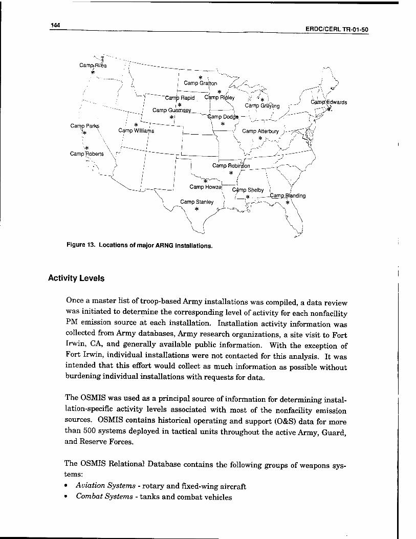
144 ERDC/CERLTR-01-50
CampbRiiea
Camp Parks
Camp^Roberts
Figure 13. Locations of major ARNG installations.
Activity Levels
Once a master list of troop-based Army installations was compiled, a data review was initiated to determine the corresponding level of activity for each nonfacility PM emission source at each installation. Installation activity information was collected from Army databases, Army research organizations, a site visit to Fort Irwin, CA, and generally available public information. With the exception of Fort Irwin, individual installations were not contacted for this analysis. It was intended that this effort would collect as much information as possible without burdening individual installations with requests for data.
The OSMIS was used as a principal source of information for determining instal- lation-specific activity levels associated with most of the nonfacility emission sources. OSMIS contains historical operating and support (O&S) data for more than 500 systems deployed in tactical units throughout the active Army, Guard, and Reserve Forces.
The OSMIS Relational Database contains the following groups of weapons sys- tems:
• Aviation Systems - rotary and fixed-wing aircraft • Combat Systems - tanks and combat vehicles

ERDC/CERLTR-01-50 145
• Artillery / Missile Systems - artillery weapons, artillery support vehicles, air defense artillery and missiles, surface-to-surface missiles, and detection sys- tems
• Tactical Systems - wheeled vehicles • Engineer / Construction Systems - engineer, construction, electrical power
generation, and floating equipment • Communications /Electronics Systems - radio receivers, teletypewriters and
terminal sets, switches, and communications and data processing systems, radar sets, and terminals.
OSMIS provided information that was used to characterize activity levels for all the nonfacility emission sources except prescribed burning. To focus the study on the installations with significant nonfacility emission sources, an initial screen was performed using OSMIS activity information. All FORSCOM, TRADOC, and USAR installations were ranked according to activity level for in- dividual source categories. These ranking were summed up to produce a com- bined ranking. Table 16 presents the results. Because of their low activity lev- els, the Presidio of Monterey and Vancouver Barracks were removed from further consideration.
As discussed later in this chapter in the Weapons Testing section, Aberdeen Proving Ground was identified as an installation with PM emissions-related ac- tivity from nonfacility sources, and it is included with the non-ARNG installa- tions evaluated in this study.
The selection of the ARNG installations was based only on HMMWV and Abrams Tank activity. There could be many other nonfacility emission sources at these installations that have yet to be considered. Therefore, all the ARNG installa- tions identified in Table 15 were included in the remainder of the study. The methodologies used to quantify the individual nonfacility source emissions are presented in the following paragraphs.

146 ERDC/CERLTR-01-50
Table 1 B. TRADOC, FORSCOM, and USAR installations (ranked by overall activity).
Overal Activity
Rank i
Installation State MACOM
1998 Activity Levels Ranking for
Individual Activity
Sum of Individual Rankings
Main Rounds
Fired
Vehicle Activity
(mi)
Helicoptei Activity
(hr) Rounds
Fired Vehicle Activity
Helicoptei Activity
1 Fort Hood TX FORSCOM 449,624 36,531,536 29,656 1 1 4 6 2 Fort Campbell KY FORSCOM 226,969 15,602,466 50,241 4 5 2 11 3 Fort Stewart GA FORSCOM 344,115 15,315,867 19,369 2 6 5 13 4 Fort Bragg NC FORSCOM 128,988 29,788,899 45,603 11 2 3 16 5 Fort Carson CO FORSCOM 251,535 10,138,277 11,560 3 8 7 18 6 Fort Irwin CA FORSCOM 225,570 15,618,902 8,066 5 4 10 19 7 Fort Lewis WA FORSCOM 28,197 20,149,067 8,801 13 3 9 25 8 Fort Drum NY FORSCOM 26,491 7,989,346 15,919 14 11 6 31 9 Fort Benning GA TRADOC 211,447 7,419,807 4,095 6 12 13 31 10 Fort Sill OK TRADOC 194,683 11,118,057 7 7 19 33 11 Fort Riley KS FORSCOM 137,898 10,057,202 2,652 10 9 15 34 12 Fort Polk LA FORSCOM 13,705 9,194,198 5,437 15 10 12 37 13 Fort Knox KY TRADOC 151,908 4,221,821 3,022 8 15 14 37 14 Fort Rucker AL TRADOC 143,930 244,899 140,085 9 31 1 41 15 Fort Bliss TX TRADOC 31,848 7,152,474 12 13 20 45 16 Fort Eustis VA TRADOC 2,128,294 7,427 20 20 11 51
17 Fort Indiantown Gap PA ARC 114 860,300 10,951 18 26 8 52
18 Fort Huachuca AZ TRADOC 2,701,563 635 21 18 16 55 19 Fort Gordon GA TRADOC 4,995,801 22 14 21 57
20 Fort Leonard Wood MO TRADOC 3,501,779 23 16 22 61
21 Fort Leavenworth KS TRADOC 2,769,726 24 17 23 64 22 Fort Dix NJ ARC 3 620,191 39 19 29 17 65 23 Fort McClellan AL TRADOC 2,246,072 25 19 24 68
24 Fort McPherson/ Fort Gillem GA FORSCOM 949,396 30 29 25 18 72
25 Fort Lee VA TRADOC 1,630,952 26 21 25 72
26 Yakima Training Center WA FORSCOM 3,925 638,557 16 27 29 72
27 Fort Jackson SC TRADOC 1,527,644 27 22 26 75 28 Fort McCoy Wl ARC 1,344,853 28 23 27 78 29 Carlisle Barracks PA TRADOC 3,029 46,652 17 32 32 81 30 Fort Sam Houston TX TRADOC 1,299,997 30 24 28 82 31 Fort Story VA TRADOC 627,946 31 28 30 89 32 Fort Chaffee AR TRADOC 531,834 32 30 31 93
33 Presidio of Monterey CA TRADOC 4,701 33 33 33 99
34 t
Vancouver Bar- acks WA 1 rORSCOM| 34 34 34 102|

ERDC/CERL TR-01-50 147
Vehicles
Vehicles generate PM from fiiel combustion (or tailpipe), and by traveling on paved and unpaved surfaces. Significant numbers of military vehicles are using both paved and unpaved roads at troop-based Army installations. Training op- erations at these installations involve a wide range of wheeled and tracked vehi- cles, and they are typically conducted in off-road areas. Tracked vehicles, in par- ticular, are usually operated on unpaved surfaces so as to avoid damage to any paved roadway surfaces. The HMMWV, in its variety of platforms, is the stan- dard light duty military truck used by all the installations. While the HMMWV and assorted cargo trucks are found at all installations, each installation's mix of vehicles reflects its unique military mission.
The OSMIS was searched to determine the types of vehicles used at each instal- lation as well as the extent of vehicle travel (i.e., VMT) associated with each ve- hicle type. The annual VMT reported for 1998 was used as the activity level for this report. Vehicle weight, speed, and number of wheels were extracted from other sources, in most cases the Internet. These vehicle specifications, except for number or wheels, relate directly to the emission factors discussed in Chapter 4. In earlier versions of fugitive emission factors, the number of wheels was consid- ered an important parameter; however, the latest factors referenced in Chapter 4 do not use number of wheels as an input. Tracked vehicles are described as 12- wheeled. Table 17 lists vehicle characteristics. When information was available, the gross weight used was the most common configuration with weapons and crew. If a specific configuration was not known, the gross weight for the weapon system was used. The maximum speed was used when available; otherwise, 55 mph was used as a default. These vehicles are all tactical vehicles. Activity lev- els for nontactical vehicles were not determined.
A total of 44 types of vehicles were reported at the 31 non-ARNG installations with a corresponding combined activity of 228 million VMT. The list of vehicles, identified by their Mission Design Series (MDS), includes armored vehicles, in- fantry personnel carriers, self-propelled mortars, HMMWVs, and 5-ton, 2-1/2- ton, and 3/4-ton trucks, among others.

148 ERDC/CERLTR-01-50
Table 17. Emission related vehicle characteristics.
MDS Vehicle Gross Weight
Maximum Speed
Wheels
AVLB Armored Vehicle Launch Bridge (AVLB) 113,000 30 M1009 Commercial Utility Cargo Vehicle (CUCV Series) 5,900 55 4 M1059 Smoke Generator 27,180 41 12 M1064A3 Personnel Carrier/ M113A FOV 28,240 40 12 M106A2 Self-propelled Mortar 23,360 40 12 M1070 Heavy Expanded Mobility Tactical Vehicle (HET) 91,000 45 20 M1078 Standard Cargo Truck 16,499 58 4 M1083 5-Ton Standard Cargo Truck 19,597 58 6 M1097 Heavy HMMWV 10,000 55 4 M109A5 Self-propelled Howitzer 55,000 35 12 M109A6 Paladin 62,000 35 12 M113A3 Armored Personnel Carrier (APC) 27,180 41 12 M1A1 Abrams 126,000 41.5 12 M1A2 Abrams with uranium armor 139,000 41.5 12 M1IP Abrams Tank 120000 45 12 M2A1 Bradley Infantry Fighting Vehicle (BFV) 66,000 42.1 12 M2A2 Bradley (BFV HS) 66,000 42.1 12 M35A2 2-1/2-Ton Truck (M35 Series) 13,530 55 6 M544A 5-Ton Truck (M54 Series) 19,597 58 6 M548A3 Cargo Carrier (M113 FOV) 27,180 41 12 M54A2 5-Ton Truck (M54 Series) 19,597 58 6 M551 Sheridan Airborne Assault Vehicle 34,000 45 12 M577A3 Command Post Carrier (M113 FOV) 27,180 41 12 M578 Light Armored Recovery Vehicle (LRV) 53,573 34 M728 Combat Engineer Vehicle (CEV) (M60A FOV) 120,000 30 12 M818 5-Ton Truck (M809 Series) 19,597 58 6 M88A1 Armor recovery vehicle 112,000 27 M9 Combat Earthmover (ACE) 54,000 30 M901A3 Improved Tow Vehicle (M113 FOV) 27,180 41 12 M911 HET 9100 45 20 M915A2 Truck Tractor (M915 Series) 50,000 55 6 M916 Tractor Truck 66,000 55 M917 Dump Truck (assumed 5-ton) 19,597 58 6 M918 DIST Bitumen Not Available 55 M919 Concrete Truck Not Available 55 M920 Tractor Truck 75,000 55 M923A2 5-Ton Truck (M939 Series) 19,597 58 6 M973A1 Small Unit Support Vehicle (SUSV) Not Available 55 12 M977 HEMTT Series 5,200 55 8 M981 Fire Support Team Vehicle (FIST-V/M113 FOV) 27,180 41 12 M992A2 Field Artillery Ammunition Support Vehicle 58,500 35 M997 HMMWV AMB 9,100 55 4 M998 HMMWV Series 7,700 55 4 MLRS Multiple Launch Rocket System Varies 55

ERDC/CERLTR-01-50 149
Table 18 lists the reported vehicles and their associated VMT at each non-ARNG installation as well as a sum total for all the installations. The HMMWV (M998) was responsible for over half the total VMT. Together, HMMWVs and the 5-ton, 2-1/6-ton, and %-ton trucks represented 95 percent of the VMT reported in 1998.
Table 18. Vehicle activity at non-ARNG installations (miles).
MDS Activity
(mi) Aberdeen
PG Carlisle
Barracks Fort
Benning
AVLB Armored Vehicle Launch Bridge (AVLB) 1,531,457 1,576 M1009 Commercial Utility Cargo Vehicle (CUCV Series) 10,415,377 288,528 2,273 346,089 M1059 Smoke Generator 61,833 M1064A3 Personnel Carrier/ M113A FOV 125,342 11,290 M106A2 Self-propelled Mortar 1,070,049 M1070 Heavy Expanded Mobility Tactical Vehicle (HET) 5,901,359 796 33 M1078 Standard Cargo Truck 4,441,218 19,040 110,703 M1083 5-Ton Standard Cargo Truck 3,104,606 10,374 M1097 Heavy HMMWV 3,679,795 243 M109A5 Self-propelled Howitzer 41,105 1,012 M109A6 Paladin 303,287 306 10,151 M113A3 Armored Personnel Carrier (APC) 1,122,906 13,201 29,924 M1A1 Abrams 1,008,768 7,861 17,501 M1A2 Abrams with uranium armor 48,814 345 M1IP Abrams Tank 12,675 M2A1 Bradley Infantry Fighting Vehicle (BFV) 180,927 510 3,288 M2A2 Bradley (BFV HS) 3,896,423 3,913 127,759 M35A2 2-1/2-Ton Truck (M35 Series) 14,685,234 51,286 14,331 976,826 M548A3 Cargo Carrier (M113 FOV) 56,373 332 1,128 M54A2 5-Ton Truck (M54 Series) 50,885 M551 Sheridan Airborne Assault Vehicle 404,255 M577A3 Command Post Carrier (M113 FOV) 360,708 194 16,871 M578 Light Armored Recovery Vehicle (LRV) 17,304 4,068 158 M728 Combat Engineer Vehicle (CEV) (M60A FOV) 589,310 M818 5-Ton Truck (M809 Series) 2,762,124 44,879 160,886 M88A1 Armor recovery vehicle 295,215 17,908 9,435 M9 Combat Earthmover (ACE) 100,605 5,880 M901A3 Improved Tow Vehicle (M113 FOV) 71,945 M911 HET 1,472,318 18 M915A2 Truck Tractor (M915 Series) 1,905,621 5,361 94,621 M916 Tractor Truck 1,087,859 3,195 228,125 M917 Dump Truck (assumed 5-ton) 20,258 6,228 M918 DIST BITUMIN 94 M919 Concrete Truck 120,331 M920 Tractor Truck 9,434,686 336 8,089 M923A2 5-Ton Truck (M939 Series) 23,980,816 146,573 1,315,005 M973A1 Small Unit Support Vehicle (SUSV) 5,384,095 M977 HEMTT Series 8,763,694 93,783 385,014
M981 Fire Support Team Vehicle (FIST-V/M113 FOV) 129,311 8,874
M992A2 Field Artillery Ammunition Support Vehicle 1,629,171 312 7,424
M997 HMMWVAMB 43,238,191 201,453
M998 HMMWV Series 75,683,872 174,361 28,510 3,335,233
MLRS Multiple Launch Rocket System 74,111,566 1,566
Total 303,301,782 888,520 46,652 7,419,807

150 ERDC/CERLTR-01-50
Table 18. Vehicle activity at non-ARNG installations (miles) (continued).
MDS Fort Bliss Fort Bragg Fort
Campbell Fort
Carson Fort
Chaffee Fort Dix Fort Drum Fort
Eustis AVLB 5,503 138 M1009 210,470 224,442 63,200 129,877 220,510 382,936 101,974 139,746 M1059 9,496 M1064A3 103 16,627 M106A2 69 M1070 228,264 37,829 64 M1078 53,360 3,768,811 1,257,773 182,234 525,307 M1083 1,502,628 745,190 2,229 7,423 9,504 M1097 49,037 1,080,501 824,656 174,195 742,055 M109A5 344 344 M109A6 39,577
M113A3 832 132 115,116 916 M1A1 125,553 614 M1A2 174,280 M1IP 176 519 M2A1 388 388 M2A2 8,807 188 188 M35A2 509,096 931,986 163,678 1,289,226 94,384 32,490 84,530 97,329 M548A3 1,166 8,261 660 M54A2 1,211 476 1,899 M551 11,234
M577A3 1,088 9,257 45,679 M578 144 44 280 M728 1,604 M818 96,802 99,485 169,919 69,944 7,211 16,420 104,910 18,313 M88A1 59 1,765 35,961 266 M9 1,472 M901A3 162 471 M911 1,261 1,261 1,261 M915A2 1,914 188,267 626,202 119,826 2,458 531,111 M916 12,398 116,389 3,230 201,134 1,645 42,259 13,688 M917 6,854 M918 4 M919 75 3 M920 97,372 8,573 1,080 11,803 1,172 M923A2 1,122,961 2,723,965 1,829,208 1,785,173 25,408 7,857 1,400,381 346,467 M973A1
M977 1,028,772 638,435 594,857 770,910 4,840 1,800 128,537 85,795 M981 210 17,817 210 M992A2 29,696 M997 158,468 605,216 311,977 59,043 4,889 3,285 279,281 19,123 M998 3,670,146 17,788,454 8,915,204 4,671,993 172,471 165,541 4,558,987 865,979 MLRS 13,790
Total 7,152,474 29,708,899 15,602,466 10,138,277 531,834 620,191 7,989,346 2,128,294

ERDC/CERLTR-01-50 151
Table 18. Vehicle activity at non-ARNG installations (miles) (continued).
MDS Fort
Gordon Fort Hood Fort
Huachuca
Fort Indiantown
Gap Fort Irwin Fort
Jackson Fort Knox
AVLB 15,003 14,656 1,880
M1009 998,418 710,364 666,564 361,550 195,039 403,603 993,762
M1059 16,201 17,708
M1064A3 33,559 23,367 174
M106A2 803,112 780
M1070 55,013 198 66
M1078 231,250 577,521 52,141 27,601
M1083 132,110 137 22,092 34,432
M1097 59,921 1,708,554 118,486 1,011,861
M109A5
M109A6 40,780 40,169 34
M113A3 1,122 217,290 1,357 280,744 27,427
M1A1 174,662 184,552 114,761
M1A2 45,093 2,681
M1IP 11,542
M2A1 408 163,075 3,687
M2A2 212,210 544 22,794
M35A2 626,043 3,780,100 450,212 174,034 1,626,707 155,159 436,426
M548A3 11,852 8,477 1,031
M54A2 19,899 9,508
M551 119 344,542
M577A3 60,048 146 492 51,437 1,470
M578 185 181 7,186 359
M728 204
M818 56,112 180,638 26,897 69,116 480,562 24,922 65,431
M88A1 55,738 133 74,034 29,704
M9 26,388 8,006
M901A3 67,838
M911
M915A2 4,662 8,922 22 32,538
M916 1,645 211,830 76,268 48,900
M917
M918 6
M919 105
M920 22,414
M923A2 893,627 7,325,115 444,362 1,600,874 229,562 32,131
M973A1 17,939
M977 2,623,302 13,814 553,342 122,220 137,335
M981 25,603 25,882
M992A2 27,424 43,646
M997 23,736 438,996 36,582 166,862 232,446
M998 1,967,036 17,107,968 920,482 156,462 8,564,123 497,409 2,047,492
MLRS 11,092
Total 4,995,801 36,531,536 2,701,563 860,300 15,618,902 1,527,644 4,221,821

152 ERDC/CERLTR-01-50
Table 18. Vehicle activity at non -ARNG installations (miles) (continued).
MDS
Fort Leaven- worth Fort Lee
Fort Leonard Wood Fort Lewis
Fort McClellan Fort McCoy
Fort McPherson
AVLB 3,588 7,467 M1009 361,008 97,916 831,433 447,151 382,396 774,377 251,891 M1059
M1064A3 12,710 M106A2
M1070 66 202 M1078 174,972 15 M1083 28,447 M1097 167,122 M109A5
M109A6 23,740 M113A3 297 30,118 91,611 2,805 592 M1A1 66,134 M1A2 M1IP
M2A1
M2A2 40,851 M35A2 142,787 174,995 87,271 1,211,923 152,406 160,727 46,116 M548A3 3,759 4,631 M54A2 400 132 1,284 M551
M577A3 42 3,161 30,865 1,716 M578 968 M728 5,958 M818 46,708 5,879 655,344 119,895 45,340 65,720 20,900 M88A1 1,143 11,590 M9 7,733 6,805 M901A3
M911
M915A2 11,484 153,478 481,253 183,752 11,982 M916 14,817 39,583 112,528 M917
M918 4 M919 75 1 M920 582 77,707 157 M923A2 1,385 674,721 837,863 3,248,696 276,167 27,963 147,854 M973A1
M977 13,580 175,298 730,518 7,565 M981 10,873 M992A2 25,200 M997 6,034 842 560,947 13,565 114,584 M998 2,217,099 630,944 670,131 12,462,628 1,386,957 108,934 354,353 MLRS
Total 2,769,726 1,630,952 3,501,779 20,162,433 2,246,072 1,344,853 949,396

ERDC/CERLTR-01-50 153
Table 18. Vehicle activity at non- ARNG installations (miles) (continued).
MDS Fort Polk Fort Riley Fort
Rucker Fort Sam Houston Fort Sill
Fort Stewart
Fort Story
Yakima TC
AVLB 6,557 7,575
M1009 672,444 403,494 96,617 926,363 131,094 42,066 21,441
M1059 8,886 2,308
M1064A3 16,974 26,581 618
M106A2
M1070 1,845 55,655
M1078 2,251 978,750
M1083 4,036 2,534
M1097 58,458 50,084 40,906 463,472
M109A5 516
M109A6 2,502 53,259 15,350
M113A3 15,942 156,226 256 118,267 9,560
M1A1 149,160 103,153 16,704
M1A2
M1IP 119 238
M2A1 388 388
M2A2 87,782 197,851
M35A2 190,892 1,291,704 82,517 1,552,308 1,010,643 12,159 267,575
M548A3 17,401 4,176
M54A2 266 1,232 6,287 643
M551 3,570
M577A3 55,429 100,843 33,966 3,560
M578 572 144 1,831 48
M728 144
M818 130,562 14,089 15,009 440,078 48,133 2,768 4,205
M88A1 473 30,378 25,487 35,037 2,683
M9 20,750 24,410
M901A3 162 162
M911 1,261 1,261
M915A2 69,719 813 290,623 165,648
M916 255,456 7,160 381 1,481 72,580 4,854 2,202
M917 1,570 12,456
M918 4 2
M919 75 75
M920 38,589 12,605 32,787
M923A2 1,830,603 25,057 138,546 846,195 3,632,148 304,991 1,378
M973A1 2,112,210
M977 115,484 843,467 241 1,694,599 1,234,927 968
M981 8,991 19,392
M992A2 28,508 37,099 18,276
M997 236,568 146,264 60,301 80,325 87,353 22,558
M998 5,642,936 4,488,531 23,845 749,050 5,098,228 6,657,496 260,140 119,734
MLRS 6,732 217,622 2,773
Total 9,194,198 10,057,202 244,899 949,378 11,118,057 15,315,867 627,946 638,557

154 ERDC/CERLTR-01-50
Table 19 lists the reported vehicles and their associated VMT at each selected ARNG camp as well as a sum total for all the camps. A total of 34 types of vehi- cles were reported at the 19 installations with a corresponding combined activity of 11 million VMT. At these ARNG installations, the Commercial Utility Cargo Vehicle (M1009) accounted for 32 percent of the VMT, while HMMWVs and 244- ton trucks accounted for 28 and 13 percent, respectively. Since these activity levels are all for tactical vehicles, it is likely that a large majority of the VMT oc- curred on unpaved surfaces.
Table 19. Vehicle activity at ARNG installations (miles).
MDS Vehicle Total VMT for MDS
Camp Atterbury
Camp Blanding
AVLB Armored Vehicle Launch Bridge (ALVB) 244 M1009 Commercial Utility Cargo Vehicle (CUCV Series) 3,567,986 25,471 240,292 M1059 Smoke Generator 0 M1064A3 Personnel Carrier Same as M113A 8,296 M106A2 Self-propelled Mortar 595 M1070 Heavy Expanded Mobility Tactical Vehicle (HET) 3,030 1,010 M1078 Standard Cargo Truck 0 M1083 5-Ton Standard Cargo Truck 0 M1097 Heavy HMMWV 138,138 195 M109A5 Self-propelled Howitzer 516 M109A6 Paladin 0 M113A3 Armored Personnel Carrier (APC) 22,095 339 M1A1 Abrams 866 M1A2 Abrams with uranium armor 0 M1IP Abrams 7,751 112 M2A1 BFV (Bradley Fighting Vehicle) 1,285 121 M2A2 BFV HS (Bradley) 76,134 M35A2 M35 Series (2-1/2-Ton Truck) 1,425,452 3,430 5,259 M544A M54 Series (5-ton Truck) 0 M548A3 Cargo Carrier (M113 Family) 178 M54A2 M54 Series (5-Ton Truck) 179,172 1,196 1,221 M551 Sheridan (Airborne Assault Vehicle) 0 M577A3 Command Post Carrier (M113 Family) 21,127 M578 Light Armored Recovery Vehicle (LRV) 481 73 M728 Combat Engineer Vehicle/M60AIFAV (CEV) 4,361 M818 M809 Series (5 Ton Truck) 599,347 56,376 7,037 M88A1 Armor Recovery Vehicle 9,862 913 M9 Combat Earthmover (ACE) 0 M901A3 Improved Tow Vehicle/Ml 13FAV 2,799 253 M911 HET (Values based on M1070) 45,366 1,261 M915A2 M915 Series Truck Tractor 580,272 3,100 M916 Tractor Truck 16,279 1,947 M917 Dump Truck (assumed 5 Ton Truck) 14,064 14,064 M918 DIST BITUMIN 37 M919 Concrete Truck 2,108 161 1,548 M920 Tractor Truck 61,301 49,271 M923A2 M939 Series (5-Ton Truck) 989,538 136,559 5,924 M973A1 Small Unit Support Vehicle (SUSV) 0 M977 HEMTT Series 234,329 1,085 4,343 M981 Fire Support Team Vehicle (FIST-V/M113FOV) 1,613 36 M992A2 Field Artillery Ammunition Support Vehicle 0
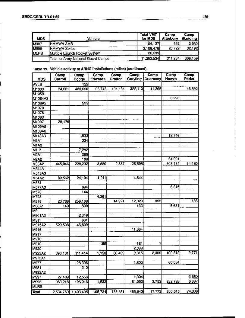
ERDC/CERL TR-01-50 155
MDS Vehicle Total VMT for MDS
Camp Atterbury
Camp Blanding
M997 HMMWVAMB 104,137 952 2,930 M998 HMMWV Series 3,108,476 20,722 32,192
MLRS Multiple Launch Rocket System 26,299
Total for Army National Guard Camps 11,253,534 311,234 308,159
Table 19. Vehicle activity at ARNG installations (miles) (continued).
MDS Camp Carroll
Camp Dodge
Camp Edwards
Camp Grafton
Camp Grayling
Camp Guernsey
Camp Howze
Camp Parks
AVLB 122 M1009 34,681 483,690 93,743 101,134 322,110 11,365 46,892
M1059 M1064A3 8,296 M106A2 595 M1070 M1078 M1083 M1097 28,176 M109A5 M109A6 M113A3 1,833 13,746 M1A1 334 M1A2 M1IP 7,282 M2A1 388 M2A2 188 64,901 M35A2 445,046 228,292 3,580 9,387 28,898 308,184 14,160 M544A M548A3 M54A2 89,562 24,194 1,211 4,844 M551 M577A3 694 6,615 M578 144 M728 4,361 M818 20,788 256,168 14,921 12,320 355 136 M88A1 140 808 133 5,681 M9 M901A3 2,319 M911 861 M915A2 529,538 46,899 M916 11,664 M917 M918 M919 156 161 1
M920 2,388 M923A2 396,131 111,414 1,150 60,409 9,315 2,300 100,312 2,771
M973A1 M977 28,398 1,800 60,084
M981 210 M992A2 M997 27,489 12,556 1,304 3,680
M998 963,218 196,016 1,533 61,003 3,752 232,726 6,667
MLRS
Total 2,534,769 1,403,405 105,734 185,851 455,940 17,773 800,545 74,306

156 ERDC/CERLTR-01-50
Table 19. Vehicle activity at ARNG installations (miles) (continued).
MDS Camp Rapid
Camp Rilea
Camp Ripley
Camp Roberts
Camp Robinson
Camp Shelby
Camp Stanley
Camp Williams
AVLB 122 M1009 160,558 13,638 633,017 331,767 281,240 721,224 67,164 M1059 M1064A3 M106A2
M1070 2,020 M1078
M1083 M1097 108,052 1,715 M109A5 516 M109A6
M113A3 5,822 355 M1A1 396 136 M1A2 M1IP 238 119 M2A1 388 388 M2A2 188 188 10,669 M35A2 133,534 10,214 82,694 57,437 67,621 27,716 M544A M548A3 178 M54A2 53,256 695 2,612 381 M551 M577A3 748 13,070 M578 144 120 M728 M818 27,874 56,652 11,323 50,741 71,952 7,758 4,946 M88A1 992 458 737 M9 M901A3 81 146 M911 38,533 4,125 586 M915A2 677 58 M916 2,668 M917 M918 37 M919 29 52 M920 3,009 4,671 1,962 M923A2 24,895 3,221 40,575 89,454 5,108 M973A1 M977 11,554 3,032 5,575 2,958 115,500 M981 105 1,262 M992A2 M997 7,743 20,377 2,130 2,103 6,008 14,732 2,133 M998 7,224 2,955 39,364 4 40,079 103,597 1,365,053 32,371 MLRS 26,2991 Total 175,525 44,496 1,023,704 363,513 473,960 1,012,827 1,820,588 141,205

ERDC/CERLTR-01-50 157
Prescribed Burning
Prescribed burning is the deliberate ignition of fire within specific, prepared ar- eas under controlled conditions. It is used as a land treatment to accomplish natural resources management objectives. The process produces PM and PM precursor emissions as products of combustion.
Prescribed fires are conducted within the limits of a fire plan that describes the acceptable range of weather, moisture, fuel, and fire behavior parameters, and the ignition method to achieve the desired effects. Prescribed burning is a cost- effective and ecologically sound tool for forest, range, and wetland management. Its use reduces the potential for destructive wildfires, removes logging residues, controls insects and disease, improves wildlife habitat and forage production, in- creases water yield, maintains natural succession of plant communities, and re- duces the need for pesticides and herbicides (AP-42/13.1). Prescribed burning is conducted at many of the Army troop-based installations for these reasons as well as to support military training objectives.
At Army installations, prescribed burns are usually managed by the Directorate of Public Works, Natural Resources Management and conducted by trained for- estry and natural resources personnel. OSMIS does not provide information on prescribed burning, and individual installations were not contacted during this study, so installation-specific activity levels were not available.
Because the woodland community growth rates vary depending on temperature and precipitation rates, some areas of the country require more frequent pre- scribed burning than others. A 1989 national inventory (Ward, Peterson, and Hao 1993) concluded that over 70 percent of the nation's prescribed burning oc- curred in the Southeast (Alabama, Florida, Georgia, Kentucky, Mississippi, North Carolina, South Carolina, and Tennessee). In 1998 Fort Carson, CO, was permitted to burn 9,035 acres of its total 373,300 acres of land (Dick Wold, Colo- rado Department of Public Health and Environment, telephone conversation, 9 December 1999). The prescribed burning took place on 2.4 percent of the land. In 1999 Range Control at Fort Bragg, NC, reported prescribed burning of 25,916 acres of its total 150,088 acres of land, or 17 percent of the land (Evelyn Watkins, Fort Bragg Range Control, Fort Bragg, NC, professional discussion). No pre- scribed burning occurs at Fort Irwin, CA. Instead the installation constructs fire lines to prevent wildfire spread (W.M. Quillman, Environmental Division, Fort Irwin, CA, professional discussion, 8 February 2000).

158 ERDC/CERLTR-01-50
Based on this information, it was assumed that the percentage of land burned • through prescription at the other installations west of 100° longitude (Forts Bliss, Huachuca, and Lewis, and Camps Guernsey, Park, Rilea, Rapid, Roberts, and Williams) matched that at Fort Carson (2.4 percent). All other installations were assigned burning percentages equal to that at Fort Bragg (17 percent). Then the land burned through prescription was estimated as the total land area of the installation times the burning percentage. This approach is very conser- vative because it does not account for developed or other nonforested areas on the installation (e.g., cantonment area, roadways).
The information that is needed to estimate PM emissions includes location (lati- tude and longitude), fuel load, and land area. For this study, fuel load informa- tion was obtained from Table 13.1-1 of EPA's AP-42, and land area, except for a few installations, was obtained from a DOD Military Installations Properties list. Table 20 lists these installation parameters.
Table 20. Installation characteristics related to prescribed burning emissions.
Installation Latitude Longitude Precipitation
Days Land Area
(acres) Aberdeen Proving Ground, MD 39.472500 76.130000 130 72,516 Carlisle Barracks, PA 40.200800 77.204200 135 403 Fort Benning, GA 32.352200 84.968900 115 184,051 Fort Bliss, TX 31.807500 106.422000 60 1,126,514 Fort Bragg, NC 35.138600 79.001100 110 150,088 Fort Campbell, KY 36.653600 87.459700 120 105,070 Fort Carson, CO 38.741900 104.782000 90 373,300 Fort Chaffee, AR 35.312200 94.305800 98 71,372 Fort Dix, NJ 40.005000 74.613100 135 30,997 Fort Drum, NY 44.053300 75.773900 160 107,712 Fort Eustis, VA 37.055300 76.291900 130 8,229 Fort Gordon, GA 33.417200 82.140800 110 56,497 Fort Hamilton, NY 40.618600 74.033600 135 166 Fort Hood, TX 31.133900 97.774200 80 217,345 Fort Huachuca, AZ 31.565000 110.323000 40 101,358 Fort Indiantown Gap, PA 40.341400 76.423300 135 17,902 Fort Irwin, CA 35.262800 116.684000 20 636,214 Fort Jackson, SC 34.039200 80.886400 110 52,301 Fort Knox, KY 37.890800 85.963100 120 109,210 Fort Leavenworth, KS 39.324400 94.923300 100 7,000 Fort Lee, VA 37.233300 77.330300 130 5,574 Fort Leonard Wood, MO 37.705300 92.158100 105 63,270 Fort Lewis, WA 47.106100 122.582000 180 91,174 Fort McPherson/Gillem, GA 33.707200 84.433600 120 350

ERDC/CERLTR-01-50 159
Installation Latitude Longitude Precipitation
Days Land Area
(acres)
Fort McClellan, AL 33.718900 85.790800 120 45,679
Fort McCoy, Wl 43.989700 90.503300 115 127,730
Fort Pickett, VA 37.078600 78.001700 130 45,160
Fort Polk, LA 31.046400 93.205300 102 198,894
Fort Richardson, AK 61.254400 149.688000 150 71,492
Fort Riley, KS 39.111900 96.815800 90 100,671
Fort Rucker, AL 31.343300 85.715300 115 63,271
Fort Stewart, GA 31.872500 81.610000 115 279,271
Fort Story, VA 36.739400 76.043600 130 1,452
Camp Stanley, TX 29.664722 98.628889 80 1,280
Camp Howze, TX 33.637222 97.150556 80
Camp Dodge, IA 41.685833 93.702222 105 4,000
Camp Shelby, MS 31.312778 89.306944 110 134,000
Camp Ripley, MN 46.166389 94.361667 110 30,720
Camp Grayling, Ml 44.657222 84.709444 135 147,000
Camp Robinson, AR 34.788333 92.255556 105 35,840
Camp Blanding, FL 29.946944 82.112222 120 67,200
Camp Parks, CA 37.715833 121.910000 70
Camp Atterbury, IN 39.352778 85.967500 120
Camp Williams, UT 40.476111 111.955556 90 28,800
Camp Rapid, SD 44.075278 103.232778 90
Camp Rilea, OR 46.170278 123.920833 180
Camp Edwards, MA 41.691111 70.637222 140 15,680
Camp Guernsey, WY 42.266389 104.744444 90
Camp Roberts, CA 35.751667 120.692222 40 32,000
Camp Grafton, ND 48.112778 98.874167 100 2,340
Smokes and Obscurants Training
The Army uses smokes and obscurants to mask troop movements and mecha- nized equipment and to defeat visual-range observation and tracking methods, including lasers. Four types of military smoke are currently used by the Army: fog-oil smoke, vehicle smoke, smoke pots, and smoke rounds. The generation of fog-oil smoke is the most widely used method and the only one for which activity data were obtained.
Fog oil is a mineral-oil-like liquid hydrocarbon that produces a very dense white smoke. Fog-oil smoke is produced by smoke generators that can create area- wide visual smoke screens. The smoke is produced by sending the fog oil through a pulse-jet engine. The oil is rapidly vaporized and then condenses into liquid drops when it comes in contact with the ambient air. The liquid drops

— ERDC/CERLTR-01-50
produce a thick, white cloud, which obscures visibility. Fog-oil smoke is ex- tremely effective as an obscurant because more than 95 percent of the oil con- denses to form liquid drops with a log-mean diameter of about 0.9 microns. The typical particle size distribution for a fog-oil smoke plume is 100 percent PM10 and 92 percent PM2.5 (Dunn, Brown, and Policastro 1996).
Field training with smoke is essential to ensure its successful use under actual battlefield conditions. Smokes and obscurants training occurs at many installa- tions as part of troop training activities and includes operating the equipment in full battlefield exercises. In addition, extensive specialized smoke generation training occurs at the Army Chemical School and the Military Police School, which were relocated from Fort McClellan, AL, to Fort Leonard Wood, MO. Smoke generation training at the schools' new location at Fort Leonard Wood began October 1999.
The major components of the M1059 are two M54A2 smoke generators, an air compressor assembly, a 120-gallon fog-oil tank, a fog-oil pump assembly, and a control panel. The M54A2 pulse jet engine burns any mid-viscosity fuel (diesel, JP4, JP8, etc.) to vaporize fog oil. Each M54A2 is capable of vaporizing 40 gal- lons of fog oil in a 1-hour mission. The fog-oil smoke generator may be operated from fixed locations or moving vehicles.
In November 1998 the new M56 Infrared and Visual Smoke System was de- ployed with the 82nd Airborne Division's 21st Chemical Company at Fort Bragg, NC. The new system can defeat infrared weapons systems. This is accomplished with ground-up graphite in the M56 smoke that absorbs thermal energy. Graph- ite is processed to emit flakes that are 70 percent PM10 and 15 percent PM2.5. Since the PM2.5 is included in the PM10, the 70 percent PM10 implies that 30 percent of the particles would be classified as TSP. Generation rates for graphite flakes are typically 60 lb/hr (Getlin et al. 1998).
The addition of ground particles to the fog oil will probably have some effect on the PM produced and the particle size distribution. Data were not provided on the effect, if any, that adding graphite to the fog oil has on the typical use rate for the fog oil. If there is not a significant effect, however, fog oil is typically used at 650 lb/hr (i.e., 100 gal/hr) and the graphite flakes are typically used at 60 lb/hr. In this proportion of less than 10 percent it is likely that the fog oil itself will still dominate the quantity and size distribution of the PM generated. The operation of a smoke generator will result in PM emissions from fugitive dust, obscurants, and vehicle and generator exhausts.

ERDC/CERLTR-01-50 161
Unfortunately, smoke generator activity is tracked in OSMIS in terms of miles of smoke generator activity for the M1059 Lynx Smoke Generator. This activity level is not very useful for two reasons. One reason is that smoke generation is not limited to this equipment. It appears that, when a smoke generating device is added as a specialized vehicle configuration, there is no way to identify that use in OSMIS. Smoke generation activity at places such as Forts Bragg and Lewis was not reported in OSMIS. The other important reason why this activity information is not useful is that there is no direct correlation between vehicle miles traveled and the amount of fog-oil smoke produced. Since almost all fog oil that is used is converted into PM, the most useful activity information is fog-oil usage.
Fog-oil usage information was obtained for Forts Irwin and Leonard Wood. In calendar year (CY) 1995, Fort Irwin reported using 6200 gallons of fog oil as smoke obscurant (Title V Applicability 1995). Fort Irwin uses approximately the same quantity of fog oil every year . The yearly usage level for Fort Leonard Wood is expected to be around 65,000 gallons. This value was obtained from the maximum gallons of fog oil allowed in Fort Leonard Wood's air quality operating permit (Rory McCarthy, Fort Leonard Wood, MO, telephone conversation, 23 February 2000 [hereafter referred to as McCarthy 2000]). Because of the Army Chemical School and the Military Police School at Fort Leonard Wood, it is by far the largest generator of fog-oil smoke. Other installations generating fog oil will likely use it at a rate much closer to Fort Irwin's than Fort Leonard Wood's.
Artillery and Other Main Rounds Practice
OSMIS provides installation-specific data on the number of main rounds fired from both artillery and armored vehicles. Separate statistics are provided on the number of ammunition rounds fired from both the weapon system's main gun and secondary guns. The level of activity for all main rounds fired was extracted from OSMIS.
Firing practice for artillery and other large caliber guns produces PM and PM precursor emissions from both the weapons firing process and the exploding ord- nance. Firing point emissions involve pollutants released from both the fuse and the propellant used to launch the projectile, and from the rapid movement of the
Walter Perry, Air Quality Program Manager, Fort Irwin, CA, professional discussion, 8 February 2000.

162 ERDC/CERLTR-01-50
weapon system across the earth's surface during firing. The down-range emis- sions are generated from the munitions-containing explosives or other energetic fills (e.g., flash compound) and the dust cloud from impact. The level of activity for all main rounds fired, which includes artillery practice, is presented in Table 21. Table 22 shows the distribution of ordnance comprising these main rounds.
Table 21. 1998 main gun activity.
Installation MACOM Main Rounds
Fired Carlisle Barracks, PA TRADOC 3,029
Camp Dodge, IA ARNG 6,417
Camp Howze, TX ARNG 60,678
Camp Ripley, MN ARNG 81
Camp Roberts, CA ARNG 690
Camp Shelby, MS ARNG 1
Camp Stanley, TX ARNG 31,463 Fort Benning, GA TRADOC 211,447
Fort Bliss, TX TRADOC 31,848 Fort Bragg, NC FORSCOM 128,988 Fort Campbell, KY FORSCOM 226,969 Fort Carson, CO FORSCOM 251,535 Fort Dix, NJ USAR 3 Fort Drum, NY FORSCOM 26,491
Fort Hood, TX FORSCOM 449,624
Fort Indiantown Gap, PA USAR 114
Fort Irwin, CA FORSCOM 225,570 Fort Knox, KY TRADOC 151,908 Fort Lewis, WA FORSCOM 28,197
Fort Polk, LA FORSCOM 13,705
Fort Riley, KS FORSCOM 137,898 Fort Rucker, AL TRADOC 143,930 Fort Sill, OK TRADOC 194,683
Fort Stewart, GA FORSCOM 344,115
Yakima Training Center, WA FORSCOM 3,925

ERDC/CERLTR-01-50 163
■o CD
CO ■o c 3 o c « E •^ o c o
£
W
■o
CO o
CM CM
.2
CD 1^- CO o •%—' CD r~- CO 00 CD in _ ■* ■<3- O CO P- m 00 O CO in in —■ CM T— h- 00 CD CM ■<* ■* 00 CD CO CD CM y— r- o CD o CD CO 00 ^~ CM 15 o -* CO_ CD CM_ ■* 00 OJ CD in Tf CD T— m CD T^ r-- CO CD CD ■?— CD
o CO CD o , T— y— Y— oo" CO y— CD CD in T— 00 co r~~ CO ■* ■* co" K CD CO y—
CM CO CM CM
CM in CM
CM ■*
■*
CM CM
m CM CO y—
■* CD CO
CM CO CD CO CD •* in CD CO CO T— t 00
CM T— m ** CM" o
s <J) o CD 1^ CO r^ ■* 00 ^ _
■* CM o CO CM OJ CM T-* CO CM O CM •* ■* r~- CD CD O CO y-m i^
5 o CM 00_ CD CD CO in i^- CD in [--._ in O co_ in co" •^-" T— CM" oo" K CM" •*" in" co" co" CM" ■*" o m T™ CO CM CO in CM T— CM ^~ CO T- T~
£ O CD 2 CD T—
2 CO
CM T^
in T~
o> CD CD 1^- 1— o ■* ■* CD •* _ CD 00 in 2 CD r^ in o CO CD o T— CO o CO CO 1-^ CM
2 CD t-~ CD CD ^~ in T— CD o CO CD_ in CD
o ■*" oo" o" co" in" T— CD" co" CM CM CM CD ^ ■<t CO CO
'"
2 CD CO
o 00
2 CD CO i>- o '"
o> r-~ O CD h- CM lO 2 CO T— CO rf in y—
5 CM CD CD CD CD_ T—
m •y— in" t" co" co" CO" o in m T— r~~ T—
CD ■>* O CD 00 o CO •o CM t-^ in T— CO o 2 y— 00 in T— 00 CD_ in
2 o" CM" o CM" t"-" co" o" o ■* CD ■* ^ ■* CM CO
o 2 CO in •* CO in in m CO in CD 00
o i>- o CO CM o ■r— ■* CD r~ 2 CD_ * r--_ ■<*• CO o CM C0_ o in CD~ •r" co" ^— oo" ■*" in CM" co" co" CM m CO 1-^
<p- CO h~ 00
CM in CO 00 in
CM
2 in CM
2 cx> in o in" CM
a O 2 2 CM co
o CD" o ■r"
t^
< 5
< i_r c 0. 52 o
"5 *•* CO e
co" o CO k_ k-
<
CD"
X 1- CD N
Z 2 si CD
< Ü CO tr CD
CO 2 Si .a
X H Si a)
< o c X
Ü Z
>
"05
O O c"
> z X H
Q. CO (3 c o < O
> < < _J
CO _1 < kj* CD
o 3
^
< O tf
c CD O O) c 'c CO
CO
CO m co
•a o Q
o X
a. be
O DC
CD
CO
c CO
05 c CD
co" CO CO
Q. E CO
o CO
CO E" ■a" o
o
c CO c" x"
o c
to"
> CD
^c" o
5i _CD
O CO
CD 55 CO Q. a Q. a. Q. a 00 m m O Ü Q X c ^ _l a. if cc CO E
i_ E E E E E E tr tr tr tr tr tr tr tr tr tr tr tr tr c tr tr ^ CO CO CO CO CO CO CO o o o o o o o o o o o o o o o o J° O O O O O Ü Ü LL LL. LL LL LL LL LL LL LL LL LL LL LL LL LL LL >
08
CM <
CD < CD O
< e.
CO
E £3
< •o c CO
CO
II CO t:
•o n» co 0. T3 c CO
00 CD
in < CD O
CO
o o _ 2 1 E T3 0)
Q. O
CD ^^ 9- c O CO
»L 2= CD
$ CO CO
§^ —~ CO
ü S3)
I I X <
^ a> x: ._ —.
o CO
5 CO JZ ^: o rt CO
CM < CM
CO X > LL CD ■o c CO
< CM
o
co B g>
LL SN
CO
< S5 Tf CD CO ^
u_ CD N CD
S3 O _ O CO
O > a. o < X
CO .O Ü "O CD
164 ERDC/CERLTR-01-50
The distribution of ordnance varies significantly between installations. Fort Sill, which is the site of the U.S. Army Field Artillery School and Field Artillery Cen- ter, has a high level of activity for Howitzers (M102, M109A5, M119A1, and M198) and Paladin Self Propelled Howitzers (M109A6) that fire 155mm ord- nance. Fort Irwin (the National Training Center) conducts combat operations to achieve proficiency in desert warfare. The main rounds fired at Fort Irwin are attributed to the Abrams Tank (M1A1), Bradley Fighting Vehicles (M2A1 and M2A2), and the Paladin (M109A6), which fire 120mm, 25mm, and 155mm ord- nance, respectively. The Abrams Tanks at Fort Irwin represent half the main rounds fired at that installation. Forts Benning and Riley are involved with in- fantry training, so the most frequent source of the main rounds fired is the Brad- ley Fighting Vehicle (M2M2) with its 25mm main guns.
With respect to PM emissions, therefore, a ranking based on main rounds fired will not provide a direct correlation to PM emission activity, because the size dis- tribution of ordnance fired at specific installations varies considerably, and PM estimates must account for these changes in ordnance distribution.
Weapons Impact Testing
The U.S. Army Test and Evaluation Command (ATEC) operates nine test centers for the evaluation and testing of weapon systems, munitions, and other equip- ment. At these test centers, which are located in a variety of climatic and geo- graphical environments, DOD is able to perform live-fire testing of weapon sys- tems to ensure their safety and reliability. The U.S. Army Developmental Test Command (DTC), a major subordinate command of ATEC, serves as the Army's premier materiel testing organization for weapons and equipment. Testing ca- pabilities include missile systems, weapons, munitions, aircraft, communications and electronics, as well as live-fire vulnerability and lethality testing.
Of particular interest to this study is ATEC's testing of artillery weapons and ammunition, missiles and rockets, mortar weapons and ammunition, and smart munitions. At the Aberdeen Test Center in Aberdeen, MD, for example, the Army conducts weapons proofing of all large caliber cannons before final ship- ment. Weapons proofing includes assembling the weapon and firing multiple test rounds to ensure that the gun system is safe to use in the field.
The test firing of cannons and other weapon systems is expected to produce the same types of air emissions as those produced during actual training exercises at troop-based installations. Similarly, the testing of weapon systems often

ERDC/CERLTR-01-50 165
involves the movement of motorized vehicles, which in turn produces additional emissions. Therefore, the OSMIS was searched to determine if any of the ATEC installations had reported data on the types and numbers of artillery rounds fired during 1998 as well as associated VMT.
Table 23 shows ATEC testing centers reported firing a total of only 250 rounds in 1998. All of these rounds were from tests of the 105mm lightweight towed how- itzer at Yuma Proving Ground. No main rounds were reported at the other ATEC testing centers that were likely to be involved in main gun firing. It was suspected that 1998 may have been unusually low; therefore, data were ex- tracted from OSMIS for a 5-year period (1994 - 98). Over that period of time, there was some additional activity at Aberdeen Proving Ground involving 586 rounds fired from Heavy HMMWVs (M1097) and Fire Support Team Vehicles (M981). Nonetheless, this level of activity is trivial when compared to the rounds fired at many troop-based installations. In 1998, for instance, 449,624 rounds were fired at Fort Hood, and an average of 135,472 rounds were fired at all non-ARNG installations reporting main-gun activity, and an average of 16,555 rounds were fired at all ARNG installations reporting main-gun activity. It was decided, therefore, that emissions from weapons impact testing at ATEC testing centers are insufficient for inclusion in this study. Aberdeen Proving Ground's vehicle activity of 888,520 VMT is comparable to other installations included in this study, so it will be added to the list of non-ARNG installations.
Table 23. ATEC testing center activity.
Installation 1998 1994 -1998
Main Rounds Vehicle Miles Main Rounds
Aberdeen PG, MD 0 888,520 586 (a)
Dugway PG, UT 0 3,946 0
Fort Greely, AK 0 0 0
Yuma PG AZ 250 (b) 0 1581 (b)
a M1097 - Heavy HMMWV (390 rounds) and
M981 - Fire Support Team Vehicle (196 rounds)
b M102 - 105mm Lightweight Towed Howitzer
Open Burning and Open Detonation
The DOD conducts OB/OD of certain munitions and explosives on ranges and other training areas as a way of safely disposing of these materials. Open burn- ing of munitions involves the combustion of propellants or explosive ordnance without the control of combustion or air, or the containment of the reaction or the emissions. Open detonation is the unconfined, violent reaction of explosive ordnance without the control of combustion or air, or the containment of the

166 . ERDC/CERLTR-01-50
reaction or the emissions. OB/OD operations are conducted in accordance with the EPA's Military Munitions Rule (62 FR 6621, February 12, 1997). This study addresses only the open burning of unused propellants that is conducted during field exercises at troop-based installations. This study does not address other OB/OD activities such as the permitted treatment of waste munitions at Army depots and open detonation of unexploded munitions during range clearing.
During live-fire training exercises, not all of the propellant charges or charge increments are always used. Propellant charges for a given round are packaged together in a set. The number of charges used depends on the desired firing dis- tance, so some of the charge increments in the set may not be used. In this case the propellant cannot be returned to munitions storage because it is an incom- plete set, and its future performance may have been compromised by handling or environmental conditions (e.g., high humidity). Unused propellant charges in the field represent an explosive safety hazard to the troops and a tactical threat in combat situations. The training of personnel in the safe management and ex- pedient destruction of unused propellant by open burning, therefore, is a re- quired element of military training and is not considered a waste management activity under the Resource Conservation and Recovery Act (RCRA).
Information was not available on the amount of unused propellant that is dis- posed of in the field by open burning. The number of artillery rounds fired at each installation is available in OSMIS, however, and emission factors have been developed for OB/OD activities on a pound propellant/round basis. As presented in Table 22, OSMIS reports the number of 105mm and 155mm rounds fired by howitzers and paladin artillery. Based on median values reported in Artillery Ammunition Round Charts prepared by the Army Materiel Command (USAMC 1985), it was determined that 105mm ordnance requires an average of 3.3 lb propellant/round fired and 155mm ordnance requires an average of 3.3 lb propel- lant/round fired. Based on input from the AEC, it was estimated that approxi- mately 40 percent of the 105mm and 155mm propellant ends up being destroyed by open burning (T. Clark, AEC, Aberdeen, MD, telephone conversation, 11 January 2000).
Table 24 shows the number of 105mm and 155mm rounds fired at 17 troop-based installations. Table 25 shows the corresponding amount of propellant that is as- sumed to be open burned.

ERDC/CERLTR-01-50 167
Table 24. Artillery rounds fired.
Installation
Weapon System/Ordnance
Total Rounds Fired
Howitzer Paladin
M119A1 M102 M109A5 M198 M109A6
105mm 105mm 155mm 155mm 155mm
Fort Hood, TX 200 706 31,642 32,548
Fort Campbell, KY 54,989 54,989
Fort Stewart, GA 30,872 30,872
Fort Bragg, NC 55,610 250 45 32,612 88,518
Fort Carson, CO 28,927 28,927
Fort Irwin, CA 54,771 54,771
Fort Lewis, WA 3,952 23,564 27,516
Fort Drum, NY 18,647 7,844 26,491
Fort Benning, GA 1,237 11,827 13,064
Fort Sill, OK 78,115 8,589 39,483 65,946 192,134
Fort Riley, KS 18,463 4,097 22,560
Fort Polk, LA 13,702 13,702
Fort Knox, KY 5,961 5,961
Carlisle Barracks, PA 3,029 3,029
Camp Dodge, IA 3,979 242 4,221
Camp Ripley, MN 4 3 2 10
Camp Roberts, CA 16 73 89
Table 25. Artillery propellant used (lb).
Installation
Weapon System/Ordnance
Total Propellant
Howitzer Paladin
M119A1 M102 M109A5 M198 M109A6
105mm 105mm 155mm 155mm 155mm
Fort Hood, TX 740 9,531 427,167 437,438
Fort Campbell, KY 203,459 203,459
Fort Stewart, GA 416,772 416,772
Fort Bragg, NC 205,757 926 613 440,263 647,560
Fort Carson, CO 390,515 390,515
Fort Irwin, CA 739,409 739,409
Fort Lewis, WA 14,622 318,114 332,736
Fort Drum, NY 68,994 105,894 174,888
Fort Benning, GA 4,578 159,660 164,238
Fort Sill, OK 289,027 31,778 533,023 890,275 1,744,103
Fort Riley, KS 249,245 55,315 304,560
Fort Polk, LA 184,977 184,977
Fort Knox, KY 80,474 80,474
Carlisle Barracks, PA 40,891 40,891
Camp Dodge, IA 14,722 3,267 17,989
Camp Ripley, MN 15 45 33 93
Camp Roberts, CA 59 981 1,040

— ERDC/CERLTR-01-50
Helicopters
Aircraft contributing to nonfacility PM emissions include fixed-wing aircraft and helicopters. Activity data for fixed-wing aircraft were not available in OSMIS. So consideration of aircraft was limited to helicopters.
The Army makes extensive use of a number of different types of tactical and non- tactical helicopters to support its mission and operations. Helicopters are used for a wide variety of applications that include the general transport of troops and equipment, reconnaissance, air assault, ground troop support, and medical evacuation. Principal Army helicopters are the Apache, Blackhawk, Chinook, Cobra, Huey, Kiowa, and Quick Fix. Helicopters produce particulate emissions from both fuel combustion and the generation of strong turbulent winds, which entrain dust particles, during takeoff and landings. AP-42 contains emission fac- tors for estimating PM emissions from fuel combustion. No emission factors, however, have been developed to estimate the amount of airborne dust generated by the wind forces associated with helicopter takeoff and landing, so this emis- sion source was not accounted for in this study.
OSMIS reports on the total hours of helicopter usage at each troop-based instal- lation. The hours are broken down by the type of helicopter (e.g., Apache, Black- hawk). As Table 26 shows, a total of 262,204 hours were logged at a total of 20 installations using 10 different types of helicopters. Fort Rucker, which serves as the Army's Helicopter Training Center, reported the highest number of hours (140,085).

ERDC/CERLTR-01-50 169
to CD
E 2 2. a> c
"5> c a>
■o c a
>
a. o o
X to CM
a>
3 a £
U a
CD
_J o to
1
X 3
CO
co CO
CD
CM"
5 00
in
in
CM"
CO O CO
co"
< o to X 3
IO CO o ■*"
LO C\l o co"
CD o in
OJ
CO OJ
CO CD CM_
CD o CO
CM CD OJ
CD CO CO
CM"
CO_
T—
OJ
CD
in
00 00
a> 3 X
X 1
X 3
•<* o
a> in CO
CD
CVI_
CT> CO CO in"
CO
CO
co"
CO
h-
t"
CX> CD
OJ
CM"
CM in co_ CM"
o CO CM
co" 0J
o CO
■r-»
co_ co"
ra 3 o 2
o oo in i
X o
o CO CO
co"
o in co"
o
m CM"
CO
co"
OJ CD
o CO
co"
Ü 00 in ■ X o
CO
CM"
o in 00
o CM"
CO
©
CO o>
co"
CO O
in
CM
< 00 IO ■ X o
co
X LI
o 3 o
< o to X LU
CM ID CT>
CM o m
CO
CO
CM in in
in CO CD
CM CD
CO in CM
o o c
o
Q
X ü
O CO CO
5- OJ
in CO 00 in
CM
co_
CO OJ m co"
CO CD
■*"
a>
u
<
< to i
X <
CO O in co"
CO in CM CM"
CO CO
CM CM O
co"
in OJ
o>"
in o co"
o 00
(0
n o Ü
<0
X <
o O CM
00 CO O CO
c o
n
S (0 c
< o d> c 'c c CD
CO ■c o
O z a> «
CO t: o
LL
>
"55 n Q. E CO
Ü •c o
LL
O O
c£ o u> i_ CO
O tr o Li.
>- Z
E" 3
a •e o
LL.
2 tn
to 3
LU
o LL
X h-
•o" o o I tr o
LL
N < CO" o 3 .c o (0 3 X •c o
LL
of d. (0 Ü c
o
CO
■o _c
tr o
LL
< Ü c
i tr o
LL
> x" O
tr o
LL
< CO
3 0) _1
■c o
LL
< a c" o 0) k_ CD
0_ o
tr o
LL
< _l
.*" o a. tr o
LL
CO
a>
if tr o
LL
_1 < o Ü 3
oc ■e o
LL
< o ■c CO
3 CD
CO tr o
LL
< CD" O)
■o o Q Q. E CO
ü
X 1-
CD" N 3 o X Q. E CO
O
CC < c" o 0) c [a o
CC a E CO
O
O o r^- LU
CO o o r-- 1-
CM
Ü o r^- LU
O o o H
CM
m CO
_J
CO in
^~
ct CO o
CO
ct CO o r^ l-1-
co CC,
CO o
Ü o t^.
LU
9 o o r-- H
CM
CM ■¥—
_1 in m H
CM
o p^.
LU (3 o o r^
CM
o •<t
LU a o o
CM
CD a.
CD C O) c
LU
CO CD C
'o> c
LU
O ^_ CD
E 3 Z
— . ERDC/CERLTR-01-50
TSP, PM10, and PM2.5 Emissions Inventory
PM emission levels were estimated using both activity data presented earlier in this chapter and the emission estimation methods in Chapter 4 to calculate "rough order-of-magnitude" emissions estimates for the nonfacility emission sources. These estimates are not based on information obtained directly from installations and generally would not be appropriate for regulatory purposes. They are described as rough order-of-magnitude because they did not include in- stallation-specific information such as:
• emission control programs (i.e., dust suppressants) • VMT distribution between paved and unpaved surfaces
• installation-specific parameters for calculating emissions, such as soil silt content, forest species, and precipitation
• accepted emission factors for tracked vehicles • installation-specific prescribed burning acreage • installation-specific fog oil usage.
The emissions estimates in this chapter are only designed to provide qualitative comparisons among troop-based installations that will provide some insights for prioritizing PM NAAQS concerns. Emissions are calculated in this chapter for vehicles, prescribed burning, smokes and obscurants training, OB/OD of muni- tions during field exercises, and helicopter engine exhaust. The source categories Artillery Practice and Weapons Impact Testing were not covered in this chapter since no emission factors had been published at the time that this report was prepared.
Vehicles
This section estimates vehicle emissions as a result of fuel combustion (i.e., tail- pipe), tire wear, brake wear, and vehicular travel over paved and unpaved road surfaces. Emissions are only calculated for tactical vehicles, since they are asso- ciated with training activities, and not the Army's General Services Administra- tion (GSA) fleet or other commercial or civilian activity on installations. The emission estimation methods for vehicles were not developed for military appli- cations, and the reader is cautioned that a high degree of uncertainty is associ- ated with emission factors developed for different sources. This is especially true for the application of these factors to tracked vehicles, but also applies to the dif- ferent modes of operation associated with military equipment (e.g., idle time, terrain, and travel distance) when compared with private sector use.

ERDC/CERLTR-01-50 171
Fugitive emissions on paved and unpaved surfaces differ by several orders of magnitude. Data were not available to allow proportioning the vehicle traffic between these two types of surfaces. The total VMT estimates were used to cal- culate emissions on both paved and unpaved roads; the emissions range between these categories should encompass the actual emissions from this travel. It is likely, however, that the majority of the VMT occurred on unpaved surfaces.
Tailpipe emissions, brake wear, and tire wear are estimated with the EPA PART5 model. The PAET5 model bases emissions on VMT for the diesel vehicle classes that are independent of vehicle speed and weight as shown in Table 27. These emission factors are all for diesel fueled vehicles.
Table 27. PART5 emission factors (exhaust PM, brake wear, and tire wear).
Vehicle Class Gross Vehicle
Weight (lb) PM10 Emission
Factor (g/mi VMT)
PM2.5 Emission
Factor (g/mi VMT)
Light-duty diesel vehicle Under 6,000 0.241 0.212
Light-duty diesel truck 6,001-8,500 0.271 0.240
Class 2B heavy-duty diesel vehicle 8,501-10,000 0.254 0.225
Light heavy-duty diesel vehicle 10,001-19,500 0.935 0.846
Medium heavy-duty diesel vehicle 19,501-33,000 0.791 0.718
Heavy heavy-duty diesel vehicle Over 33,000 0.932 0.834
To calculate the emissions from exhaust PM, brake wear, and tire wear for each vehicle class, the following formulas were used with the VMT information for the installations provided earlier in this chapter:
PM2.5 emissions = [PM2.5 Emission Factor] x VMT
PM10 emissions = [PM10 Emission Factor] x VMT
TSP emissions = [PM10 Emissions] / 0.9643
[Eq17]
[Eq 18]
[Eq 19]
Table 28 shows the resulting PM2.5, PM10, and TSP emissions from exhaust PM, brake wear, and tire wear. The average vehicle weight of the heavy-duty vehicles at more than half of the installations were more than 66,000 lb, twice the gross vehicle weight required to belong to that vehicle class. Therefore, the emission factors (as a function of VMT) may not accurately reflect the emissions from these heavy vehicles. The tailpipe emission calculations only consider a fleet composed of gasoline and diesel engines. However, the Army uses JP8 to fuel most of its land vehicles; therefore, these emission estimates may not accu- rately reflect the emissions from these vehicles.

172 ERDC/CERLTR-01-50
CO c o
,spBoy
paAedun
o o o 00 co
o o o CM T—
o o
o o o in CO
o
m
o o in
o o CO
o C\ CM
o o o CD CM
o
CD
o o CO
CM
o in 00
o o o c\
o o 00
o o a> in
o o o c\
o o o ■*'
CM
o o cv CM
00
d CM
o o o 1^ o
es O O
d CM
o o CD
d o
o o o d CO CD
o o o oo' 00 CM
o o o ■*'
o o CO
co"
CO c o
'5> CO
E LU Q. CO I-
,speoy paABd
o CO CM
o OS
CO CO
o
CO 1^ ■v— CO CD
O
CM
00
CO o CO
m CM CD
o O O CM
in
CO o o o CM'
o o CO
o o in •*'
o o
co"
o o CO
co'
CO in
CM CO
JB3M PUB isneqxg,
in
Ö CO
o o a> Ö o
V Ö
CM
Ö Ö V
CO
Ö © V
d V
d V
in
d d CM
d d d d d V
■* ■* CD 00 CO CM
d CM
d
"co c o
CO c o
'55 co
E tu o S Q.
»speoy paAedun
O O 00
o o CO
C\f
o o
o o CM
1»."
o CM
o ■<*
O O O
o o a» co"
o
CM
o co m
o o o CO
CM"
o o
o o CO
o o in CM"
o o
in
o co
q Ln
o o o CM" CM
o o o ■*"
CM
o o o CM" 00
o o o d CO Y—
o o o co" in
o o as CM"
o o
»speoy P9ABd
T— in
1^ CO
CO
CO
o CO
in ©
CO
CO r1
CO
©
CO in
co en m CM
CO CM
00 CO
00
CM CO o
CO
o
CO
o CD CO
o o CD
o
CO
T— CM
jea/w pue isneijxg
in
ö CO
o o 00 o ö
V ö
CM
Ö O V
CO
ö Ö V
d V
d V
m d d
CM
d d d d d V
TT CO in 00 CO CM
d CM
d
c o
CO c o
"55 CO
E LLI
in
£ Q.
,speoy paAedun
o o
T—
o
CO
o o CO
o o
00 o O m
i-~- o
m CO
in 00
in CM
o 00 CO
o in
o 00
o CO CO
o in
00 CO
CM CM
o o CM
co"
o o in
co"
o o o CM"
o o q
o o m oo"
o CO
o o CM
CO c
a
CO
,speoy paABd
CO CM
d in in
Ö in
CO ö CO CO
Ö in
d in
d CO
CD
CM CO
CO CO in d d
CO
d 00
1^ o CM CM
o in
o CO
CO CO
c
>. E < CO
JB3M PUB jsnenxg Ö
CM
Ö CD 00
Ö Ö V
o CM
© o V
m Ö Ö
V d V
d V
d d CM
d CO
d CO
d d d V
■<r CO CO (^ in CM
d CM
d
CO 0) _o !E CD >
E o
w c
i E I"5-0
o a o,
o CO
o CM
o CM
in o
o
Y-»
o o
in CO
o OS
o 00
o o CO
o 00
o o in o
o o 00
o OJ
o in o CD
o o CM
o a>
00 05
in CO
CO CO
E a> £ a -
o o w o CD
o in
o o o Y-»
o o CM
o CM
o CO
O CM
o co
o o CM
o CM
o CM
o CM
o CM
in CM
in CM
o CM
o CM
o CM
o CO
o o in
o CM
■o a> «5 E CO a>
CO
cö CM
a>
ß
c
« s CO c
Q 2
c5 0- c CO CO -o CO
<
Z
>; 3 n CD
< a E CO
ü
li-
es c
X3 c CO
m Q. E CO
Ü
< CO O)
T> o Q
Q. E CO
o
<
to
CO
3 "O LU
a E CO
O
Q z c o *; CO
o a. E CO
1 c
CO
O Q. E CO
O
>- 5 >; CO co c k- CD
o a E CO
O
X h-
co"
o X Q. E CO
< Ü
CO
k_ CO 0-
o. E CO
O
O CO
T3 a CO
tr Q. E CO
Ü
CC O
co" a>
if Q. E CO O
Z
Ss CO Q.
ic a. E CO
O
< Ü
to ■c
JB o
oc a. E CO
ü
CC < c" o CO c !a o
DC a. E CO
Ü
CO
;£ .o CO .c CO Q. E CO
O
X 1- Ss CO c: CO
CO a E CO
ü
h- =3
to E <o
i a. E CO
O
2 co _*: o CO
CO CO CO
CO
k_ CO
o
< O
d> c 'c c CD m ■c o
Li-
X (- co" CO
m ■e o
o z d> O) CO
m tr o
LL
>
"CD n a. E CO
Ü
•c
LL
O O
c" o CO 1-
co O t: o
CC < co" CO
CO JZ o ■c o
Li-
—3 z x" b tr o
Li-
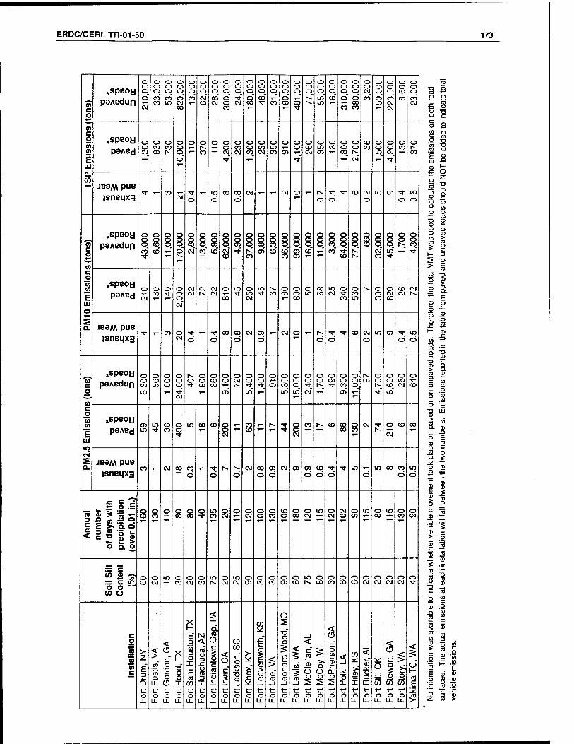
ERDC/CERLTR-01-50 173
in c o ** in c o
"35 in
I HI 0. co H
»speoy paABdun
o o o o
CM
o o o co" CO
O O o co" LO
o o o_ o CM 00
o o o co"
o o o CM" CO
o o o oo" CM
o o o o" o CO
o o o ■>*
CM
o o o o 00
o o o co"
o o o
CO
o o o o" CO
o o o
o o o Is-"
o o o LO" LO
o o o CO"
o o o o CO
o o o o 00 CO
o o CM_
co"
o o o o" LO
o o o co" CM CM
o o CO
oo"
o o o co" CM
»speoy peABd
o o CM
o CO
o CO
o o o o"
o o
CO
o o o CM
•<*"
o CO CM
o o C0_
o CO CM
o LO CO
o o o
■*"
o CO CM
o LO CO
o CO T—
o o 00
o o r^ CM"
CD CO
o o L0_
o o CM
■*"
o CO
o co
JB9M Pue
isneijxg ■* - CO CM Ö
T—
Ö CO 00
o CM - - CM o - 1^.
Ö Ö t CO CM
Ö LO <J>
Ö CD
o
"ST c o
m c o «5 0)
E HI O
E Q.
»speoti paABdun
o o o CO
o o CO
co"
o o o
o o o o
o o CO OJ
o o o co"
o o a> LO"
o o © CM" CO
o o a> ■*"
o o o CO
o o 00 a>"
o o CO
co"
o o o co" CO
o o o OJ CD
o o o co"
o o o o o CO
co"
o o o ■*"
CO
o o o r>-~
o CD CD
o o o CM" CO
o o o LO"
o o ■r—
o o CO
■*"
»speoy paABd
o CM
o CO
o o o o CM"
CM CM
CM CM CM
o CO
LO o LO CM
LO CD
o CO
o o 00
o LO
00 CO
LO CM
o CO
o CO LO
h~ o o CO
o CM 00
CD CM
CM
JB9M pue isneqxa
■* - CO o C\J Ö
- Ö
00 00 o
CM 05 Ö
- CM o - 1^
Ö Ö Tt CO CM
Ö LO a>
Ö LO
o
C o
w c o
'55 (0
E Ul m c>i E a
»speoa peAedun
o o CO
CO
o CD CT>
o o CD_
o o o "*" CM
o o o
o CO 00
o o
a>"
o CM 1^
o o LO"
o o o o o CO LO"
o o o LO"
o o
CM"
o o
o a> •<*
o o CO
o>
o o o o o ■*"
o o CD
co"
o CO CM
o CD
„speofc) paABd
o> in
LO CO CO
o •4-
LO CO co o o CM
- CO CO -
1^ ■*
■*
o o CM
CO h- (D CO 00
o CO
CM o
CM
CD 00
JB3AA PUB lsnei)X3
CO - CM CO CO o
- o
f- ©
CM 00 Ö Ö
CM o> a> CD
cp Ö
■* LO
Ö LO 00 CO
Ö LO o
Ann
ual
nu
mb
er
of
day
s w
ith
pre
cip
itat
ion
(o
ver
0.01
in.
)
o CO
o CO
o o 00
o 00
o in CO
o CM
o o CM
o o o CO
LO o o
00 o CM
LO o CM
CM o o CT> LO o 00
LO o CO
o CT>
Soi
l S
ilt
Co
nte
nt
(%) o
CO o CM
LO o CO
o CM
o CO
LO o CM
LO CM
o O)
o CO
o CO
o 05
o CD
LO f-.
o 00
o CO
o CO
o CO
o CM
o CM
o CM
o CM
o
c o
« S m c
> z E
Q tr o
LL
co
CO 3
LU
o LL
< (3 c" o
"O Ö o •c o LL
X H "d o o X c o LL
X \- c" o CO 3 o X E CO
CO ■c o LL
N < CO Ü 3 .c CJ CO 3
X t: o LL
d CO o c
o
CO
c
o LL
< Ü c"
1 tr o
LL
Ü CO
c o CO
o CO —> ■c o LL
>- it: x o c *:
■e o LL
CO
d ■c o 5 c CO > CO CD _l
■c o LL
2 CD _l
t: o
LL
o
o o § "S CO c o CD _l
•c o LL
<
CO
CD _l
t; o LL
_l < c" «
"05 o o
o LL
5 o Ü o
o LL
< o c" o CO L—
CD
a. o
■c o LL
< _l
^:" o a. ■c o LL
CO
a> if c o LL
_l
< CD ^. o 3 tr •c o LL
o CO t: o LL
< o tf CO
CD
m o
LL
o m ■c o LL
< § d H CO
E
CO ■n o m o CD
x: CO o
o T3 XJ c c o o w T3 [_ CD o T3 </> ■D to CO
F CD a) n
h- c o m z fo ■o
CJ o m CO o to o "O
CO T) o <D
w
CO ■D _) CD CO >
CO
5 a. c
H 3 > ■D
> c CO
3 o ■o CD
CD CO a. 4-1 E
(1> o o (1) CD
CD .a CO
H CD £:
en *■ '
r> c (T! o ■o
CD T1 ■c <I) o a. CO CD n *— c to 13 c c o o to
CO
o H TJ LU a> > CO CO Q. CD .a o t- (1) 3 C) CO o Cl ^ o CD n J=
CD u> CD b CD CD o .Q
h 15 CD o :^ c s CD
o CD CO
(1) CO .c CO s c CD JO
CJ o CO CD
c co o CO
CD o CO to
CO > fc CD
CO CO CO 3 co i c * o CD S o fo |E| h to CD o fi CD c CO .<->
■c ^ 3 CD
4^ CO >

174 — ERDC/CERLTR-01-50
Brake and tire wear included in the factors do not represent tracked vehicles. However, the contribution of tracked vehicles to total VMT is small. The emis- sions calculated for brake and tire wear will not have a significant impact on the overall estimates, so no adjustments were made for tracked vehicles' lack of tires and different braking systems.
To calculate the emissions from dust on paved roads, the EPA's recommended default silt loading of 3 g/m2 was used. The mean gross vehicle weight for each vehicle class in Table 27 was determined for each installation as an average of the specific vehicle weights (weighted based on VMT of the specific vehicles). No information was available to indicate whether travel took place on paved or on unpaved roads, so paved road calculations reflect the case if all of the travel oc- curred on paved roads. Using the total VMT for each vehicle class, the emissions from paved road dust were calculated with the following equations from Chapter 4:
EpM2.5,i = VMT x (0.0040 lb/VMT) (3/2)065 (W/3)" [Eq 20]
EpMio, i = VMT x (0.016 lb/VMT) (3/2)°M (W/3)" [Eq 21]
ETSP . = VMT x (0.082 lb/VMT) (3/2)°M (W/3)" [Eq 22]
where EPM25., EPM10., and ETSP. = the emissions from vehicle class i VMT; = the vehicle miles traveled by the vehicles in the class W. = the weighted average gross vehicle weight of the class at the instal-
lation.
The unpaved road dust emissions from all six vehicle classes were totaled to cal- culate the PM2.5, PM10, and TSP emissions at each installation and are pre- sented in Table 28.
To calculate the emissions from dust on unpaved roads, the surface material moisture content under dry, uncontrolled conditions was assumed to be 0.2 per- cent. Since information was not available on the long-term control efficiencies of dust suppression techniques at the installations, the control efficiencies were as- sumed to be negligible at all installations. Then the equations for dust from un- paved roads in Chapter 4 simplified to the following:
F VMT 0-38 (s/12 f W,/3f 365 -p E PM2.5, i = VMT ■ x > \—!—I— x *L [Eq 23] (0.2 )03 365

ERDC/CERLTR-01-50 175
_ VMT :2.6 (s/nrCW,^)» :, 365 -p
™" ' i (0.2)" 365 lq '
E„„. = VMT;X»0(s/12r(W,/3r x365 -p [Eq25] TSP, i (0.2 )04 365
where s = the surface material silt content of the road p = the number of days with precipitation over 0.01 in.
The values for surface material silt content were obtained from the soil datasets at Pennsylvania State University, State College, PA, (http://www.essc.psu.edu/ soil info/index.cgi?soil data&conus&data cov&fract&image), and the precipitation data from AP-42 Figure 13.2.2-1 (AP-42 1998). The unpaved road dust emissions from all six vehicle classes were totaled to calculate the PM2.5, PM10, and TSP emissions at each installation and are presented in Table 28. No information was available to indicate whether travel took place on paved or unpaved roads, so unpaved road calculations were made as if all of the travel occurred on un- paved roads. The unpaved road calculations also do not consider that some of the vehicle travel will occur over off-road surfaces. These unprepared surfaces may contain a vegetative cover that could significantly reduce PM emissions.
Prescribed Burning
This section provides estimates of PM emissions from prescribed burning at troop-based installations. PM emissions are a waste product of the combustion of wood and vegetation.
Detailed information about prescribed burning activities at the installations was not available for this report. Instead, regional profiles from EPA's AP-42 Section 13.1 (AP-42 1998) were used to characterize the various installations. The re- gional profiles provided data for average fuel loadings for the regions and aver- age emission factors for prescribed burning as shown in Table 29.
PM2.5 emission factors were not available outside the Pacific Northwest and Alaska. However, the ratios of PM2.5 to PM10 for a wide variety of fuel types (piled slash, Douglas fir/Western hemlock, mixed conifer, Ponderosa pine, hard- wood, underburning pine, and chaparral) were all between 0.8 and 1.0. It was assumed, therefore, that PM2.5 emission factors in the regions outside the Pa- cific Northwest and Alaska could be approximated by multiplying the PM10
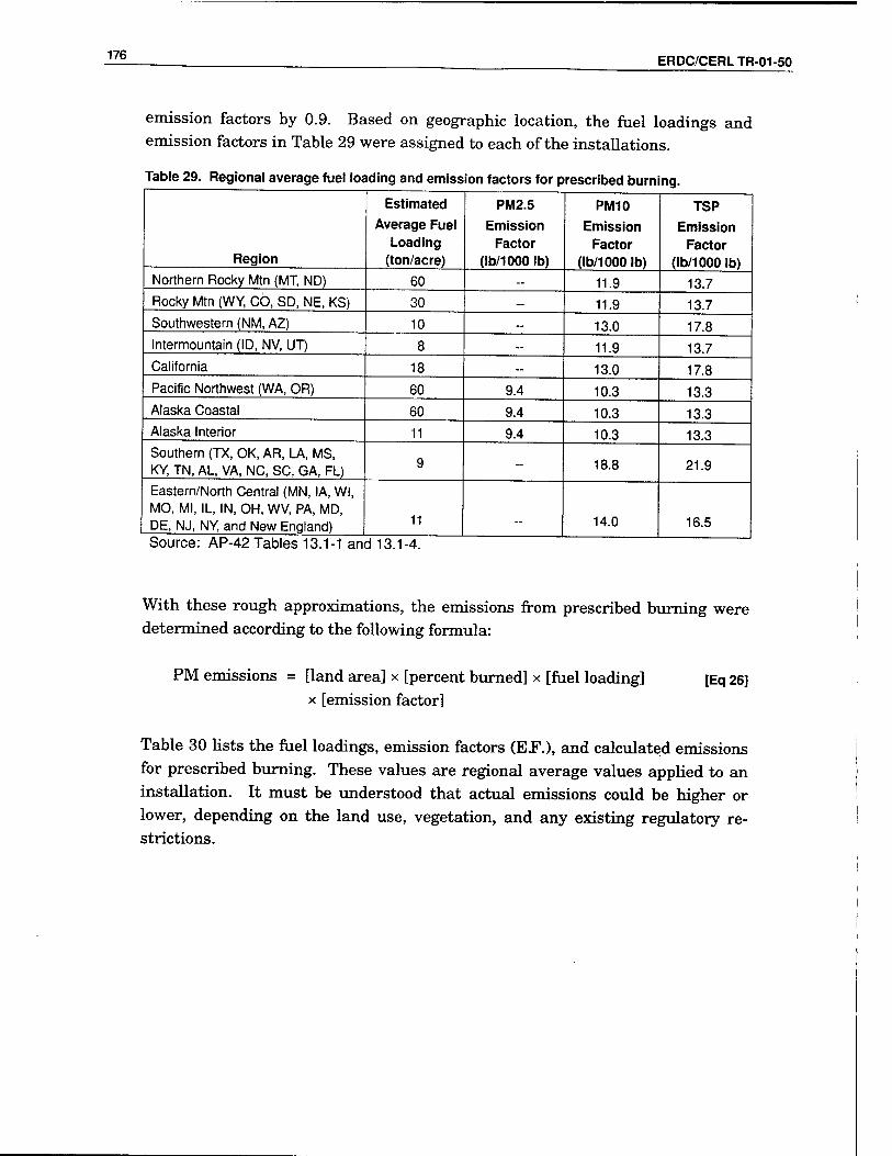
176 ERDC/CERLTR-01-50
emission factors by 0.9. Based on geographic location, the fuel loadings and emission factors in Table 29 were assigned to each of the installations.
Table 29. Regional average fuel loading and emission factors for prescribed burning.
Region
Estimated
Average Fuel Loading
(ton/acre)
PM2.5
Emission Factor
(lb/1000 lb)
PM10
Emission Factor
(lb/1000 lb)
TSP
Emission Factor
(lb/1000 lb) Northern Rocky Mtn (MT, ND) 60 — 11.9 13.7 Rocky Mtn (WY, CO, SD, NE, KS) 30 — 11.9 13.7 Southwestern (NM, AZ) 10 — 13.0 17.8 Intermountain (ID, NV, UT) 8 — 11.9 13.7 California 18 — 13.0 17.8 Pacific Northwest (WA, OR) 60 9.4 10.3 13.3 Alaska Coastal 60 9.4 10.3 13.3 Alaska Interior 11 9.4 10.3 13.3 Southern (TX, OK, AR, LA, MS, KY, TN, AL, VA, NC, SC, GA, FL) 9 - 18.8 21.9
Eastern/North Central (MN, IA, Wl, MO, Ml, IL, IN, OH, WV, PA, MD, DE, NJ, NY, and New England) 11 14.0 16.5
Source: AP-42 Tables 13.1-1 an d 13.1-4.
With these rough approximations, the emissions from prescribed burning were determined according to the following formula:
PM emissions = [land area] x [percent burned] x [fuel loading] x [emission factor]
[Eq26]
Table 30 lists the fuel loadings, emission factors (EF.), and calculated emissions for prescribed burning. These values are regional average values applied to an installation. It must be understood that actual emissions could be higher or lower, depending on the land use, vegetation, and any existing regulatory re- strictions.

ERDC/CERLTR-01-50 177
ra c
3 a
'C u (A CD
E o w *- (A C O
'35 (0
E V S a. ■o a> a E (A UJ
© CO 0)
TS
P
Em
issi
on
s (t
on
s)
© o CO
c\f
o CO
o OJ
o CO CO
o o CD
■*"
o o Cvl_
o o CO
■*"
•* ■*
CD CO o o CO
co"
O O ■<fr
■*"
O o
in
O O CD_
co"
O O
co"
O O
CM"
o
OJ
O O
co"
o 00 CVI
o o OJ_ 1"
m o o
o ■<!■
o CD in
-CO
o
PM
10
Em
issi
on
s (t
on
s) o
o o>
o o CM
o o o OJ
CO
O O O
o o a> co"
CO CO CO
^* o o
in"
O O CM
co"
o o
■*"
O O
co"
o o CM
co"
O O
CVl"
o CVJ oo
O O OJ
CM"
o
CVJ
o o
■* o o
co"
o CVJ CO
o 00 o
PM
2.5
Em
issi
on
s (t
on
s) o
o CD OJ
o CO CO
o CO CM
O O in co"
O
OJ
o o in cr>"
CO © CO
o o o CO
•*"
O O OJ CM
o o OJ
co"
O O CO
CM"
o o OJ CVl"
O O OJ_
o o o CD
CVI*
o CVJ CVl
o o in
■<* o o
in"
o OJ CVJ
o CO o
Land
Are
a (a
cres
) CO
in
CM"
o o o ■*"
o CO CD in
o
CO
CM"
o o o r-~."
o CO in" CO
o o o •*" CO
o CO CVJ_
o o CO
co" OJ
CO o in
o ■*"
CO
in co" CVI
00 00 o o" m
O (^ O in" o
o o CO
co"
CO
CM
CO OJ OJ
o" CO
CVJ
h-" O
OJ CVJ CM
co"
OJ
co" in
CD CO
in CO
CM
00 in co_
o
CM o OJ
h-"
Cvj co" CO CO
TS
P E
.F.
(lb
/100
0 Ib
)
in
CD
in
CD
in
CD CO in CD
OJ
cvi
a>
c\j
OJ CO
in
CD cvi
CO
r-»' OJ
CM
OJ
CM
1^;
CO
OJ
Cvj
in
CD
in
CD
OJ
cvj
OJ
CM
m CD t-"
OJ
CM
CO in CO
CO
PM
10 E
.F.
(lb/1
000
Ib)
o o OJ 1—
o CO
CO CO
cd CO
CO
en o CO
CO p CO
CO CO
00 CO
OJ CO o <*
o CO
CO 00 CO
o CO
CO
o CO
o o CO
d § in ©
CO CM
CO c\i
CO 0Ü Ö
CO
cvi OJ
CO
o> CO
OJ CO o
CD c\i
OJ CO
h~ OJ
CO OJ CD ö
OJ
CO
CO
cvi CD cvi
OJ
CD
OJ
CD
CO
cvi OJ
CO h-; CO
cvi
1^
Fuel
Loa
ding
(t
on
/acr
e)
■*"
,_ T" o CO
,_ CD OJ CD CO T— OJ OJ OJ OJ o CO
OJ ■*~
OJ OJ 'r" OJ o y~
CO
c o « B (0 c
o
X) c 3 o
Ü O) c
■>
o
CL
c CD CO T3 i_ CO
.Ct <
< CD"
O Q a E « O
<
CO
"E CO
UJ a. E CO
O
Q z c o
CO
<5 a E CO
O
I d> c
CO
Ö a E CO
O
cc < c" o CO c Id O
DC a E CO
O
CO 2
5". X) CD
SZ CO a E CO
O
X H >". CD
C CO
« CL
E CO
O
\- ID co E CO
i a E CO
Ü
SE co
o CO l_
CO CO CO
co l_
CO o
< O
d> c 'c c CO m tr o
LL
co co
CO
o LL
o Z
O) O) CO L_
CO ■e o
LL
>•
"5 JD a E CO
O
o LL
O O
c" o co CO
O •e o
LL
DC < co" CO s= CO
Ü
o LL
Z
x" b t; o
LL
>- z E" 3
Q c o
LL
to
UJ 3
UJ tr o
LL
< a c" o
■o o Ü •c o
LL
>- z c" o
I CO
t o
LL
1-
E o I ■c o
LL
5 CO" Ü 3 SI Ü CO 3
X •c o
LL
a. CO
o c 5 o c CO TJ _c
•c o
LL
< o c"
1 tr o
LL
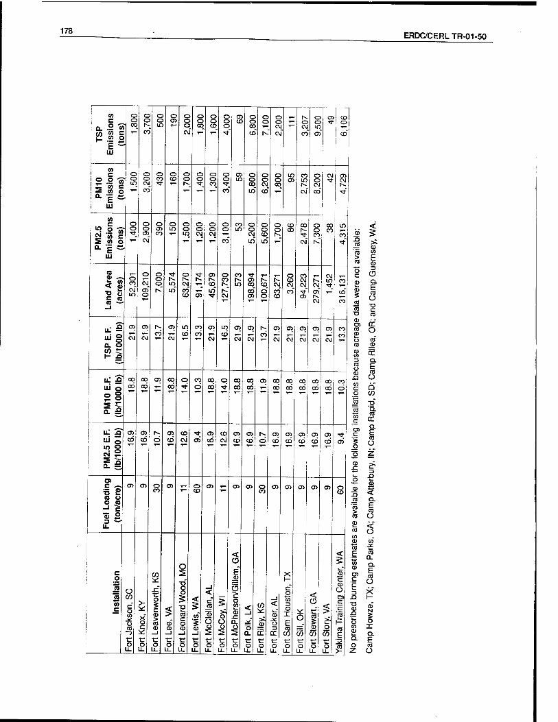
178 ERDC/CERLTR-01-50
TS
P
Em
issi
on
s ft
on
si
c c
o o
en
O o in
O CD
es o o CM
c c CC
T-
a CD
O o o
CD CO
o o CO
CD
o o
o O C\
CM
c o en
O O m CD
49
6,10
6
| o .2 « Ewe 2 co o o. gC
I
o '8
o o c\ CO
o CO
o CO
o o
o o
O O CO
o o
co'
CD in
o o CO
in"
o o c\ CD"
O o CC
in CD
CO m
CM
o o OJ
co'
CM CD CM
■*"
W
">. .2 w £i w c 5 « o eg c
tu
o o
o o CD
o CD CO
o in
o o in
o o
O o CM
o o r—
co"
CO in
o o CM
m"
o o CO
in
o o
CO co
CO I"-
Oj"
o o CO N."
co CO
in
CO
■*"
(0 CD —.
< cu •a Ö S3 _i
o CO
CM* in
o CM
CD" o
o o o in
in"
o OJ
co" CO
f-
CD
CD
CO
m"
o CO
CM
CO
in CD CO
co" CD
co_ o o
CM_
co" CD
o CD OJ. co"
CO CM OJ if CD
I-» OJ
CD"
CM
OJ in CO
co"
CO
ui § Q. O
1- £
CM
en
CM CO
CD
CM
m CO
CO
CO
CD
CM
m CO
CD
CM
CD
CM CÖ
CD
CM
CD
f— CM
CD
CM
<x>
CM
CD
CM
CO CO
UJ o CO
00 00
CO CD CO
CO o CO
Ö CO
c6 o CO
CO 00 CO
CD
T—
00
00 00
00 00 00
00 cri
00
00 CO
Ö
i I
u: S" ui o in ©
CM* ?
11
CD CD
CO o CD
CD CO
CM
Tj-
CD CD
CO CO
CM
CD
CO CD
CO
N.
Ö CD
CO
CD
CD
CD
CD CD
CD
CD
CD CD
c -^ =5 £ CO u O (0
-J c
ä> S 3 —
LL
OJ CD o CO
CD T-"
O CO
CD "r" CD CD O
CO CD <J> CD CD CD o
CO
! c o
(0 c
o CO
cr" o CO .* Ü CO -3
tr o
LL
>
X* o c
tr o
Li.
CO *:
tr o 5 c CD > CO CD _l
tr o
LL
2 CD"
CD _l
tr o li-
o 5 ■d o o §
'S CO c o CD _l
tr o u.
< 5 co
5 CD _l
tr o
LL.
_l < c « "5 O o
tr o
LL.
i >; o ü o
tr o
< a E"
Ö "£ o CO k_ CD xz 0. Ü
tr o
< _l
.*" o 0. tr o "-1
CO
CD
if tr o "-
< CD
Ü =3
tr tr o
LL
X \- t£ o to o I E CO
CO ■c o
LL
o CO tr o
LL
< Ü tr" CO
5 CD
do tr o
LL
o 55 c o
LL
<
2 c CD o c
'c
CO
CO
E XL
2
n TO CD
m CO > c CO CD
3 o c o n> a CD
5 h CO
o CO
T3 CO C o CO CD . . TO LL CO CD
O O CO CO CD
CD CO CC 3 n (0 o CD
E CO
J3 U CO r Q o U) CO ■a
m Q. CO
r tr — Q.
E 5 o
CO
O
o z CD >. .c ^.
3 L_ S3 o k_
CD CD ts
O < CO a cö E > CO CO O CD <f CO O CO „ CD 0)
CO
E CO a.
co CD
Q. F
U) CO C)
c 1_
7J X n H ■a CD N
5 o o CO I CD a Q. F O m z ü

ERDC/CERL TR-01 -50 179
Smokes and Obscurants Training
In CY 1995 Fort Irwin reported using 6,200 gallons of fog oil as smoke obscurant (Title V Applicability 1995). Since the density of fog oil is 7.5 lb/gal and 95 per- cent of fog-oil smoke condenses into aerosol droplets (99 percent of which are less than 2.5 microns in aerodynamic diameter), the emissions of fog oil can be calcu- lated using the sample method shown in Chapter 4:
ETSP = [Fraction fog oil that condenses] x [Fog oil consumed] [Eq 27] x [Density]
= [0.95 lb TSP/lb fog oil] x 6,200 gal/yr x 7.5 lb fog oil/gal = 44,000 lb TSP/yr = 22 ton TSP/yr
EPM25 = [Fraction PM2.5 in ETCP] x ETSP [Eq 28]
= [0.99 lb PM2.5/lb TSP] x 44,000 lb TSP/yr = 44,000 lb PM2.5/yr = 22 ton PM2.5/yr
EPMI0 = [Fraction PM10 in E^] x ETSP [Eq 29] = [0.99 lb PM10/lb TSP] x 44,000 lb TSP/yr = 44,000 lb PM10/yr = 22 ton PM10/yr
At Fort Leonard Wood, the state permit allows 65,000 gallons of fog oil to be used each year and up to 1200 gallons per day (under certain meteorological condi- tions). If Fort Leonard Wood used 65,000 gallons of fog oil in a single year, the TSP, PM10, and PM2.5 emissions would be calculated as 231, 229, and 229 tons, respectively.
Open Burning/Open Detonation During Field Exercises
Earlier in this chapter, activity levels were only reported for open burning of propellants generated during training exercises. No open detonation activity was quantified. Table 25 presents the amount of propellants disposed of by open burning during field operations. Two emission factors were available in Table 9 for open burning propellants 0.15 and 0.28 lb PM10/lb MEM, depending on the energetic composition. The larger one was chosen as a worst-case assumption for these calculations. The PM10 emissions were calculated from the activity infor- mation, using the following formula:
E (lb) = (mass propellant burned) x (PM10 Emission Factor) [Eq 30]

180 ERDC/CERLTR-01-50
Table 31 lists the PM10 emissions for open burning during field operations. No TSP or PM2.5 emission factors have yet been reported in the literature for OB/OD processes, so those calculations were not performed for this report. In the rankings provided later in this chapter, however, PM2.5 and TSP are re- ported as being less than the PM10 value for PM2.5 and more than the PM10 value for TSP.
Table 31. PM10 emissions from open burning of munitions during field operations.
Installation
PM10 Emissions
(tons)
Camp Dodge, IA 3.2
Camp Ripley, MN <0.1
Camp Roberts, CA 0.1
Carlisle Barracks, PA 2.3 Fort Benning, GA 9.2 Fort Bragg, NC 35 Fort Campbell, KY 10 Fort Carson, CO 22
Fort Drum, NY 9.4
Fort Hood, TX 25 Fort Irwin, CA 41
Fort Knox, KY 4.5
Fort Lewis, WA 19 Fort Polk, LA 10 Fort Riley, KS 17
Fort Sill, OK 100
Fort Stewart, GA 23
Helicopters
Helicopters were the only aircraft considered in this study. Helicopter activity levels at various installations were shown earlier in this chapter. Chapter 4 re- ports emission factors developed for only two types of helicopter engines (T700- GE-700 and T64-GE-100 models), so it was assumed that all 700 series engines had emissions similar to the T700-GE-700 power plant and that all others had the higher emissions associated with the T64-GE-100 engine. It was assumed that these aircraft used JP8 fuel and that the time spent in each of the four modes was divided evenly. Using the emission factors from Table 10 and the 4095 operational hours of Blackhawk helicopters at Fort Benning (shown in Table 26), the emissions from Fort Benning were calculated as:

ERDC/CERLTR-01-50 181
TSP Emissions (lb) = 4095 hr x 2 Engines x
'0.25 x 0.20 lb/hr+ ^
0.25 x 0.59 lb/hr +
0.25x1.39 lb/hr +
0.25 x 1.89 lb/hr j
= 8300 lbs TSP
PM10 Emiss. (lb) = 97.6 % x 8300 lb TSP = 8100 lb PM10 = 4.1 tons [Eq 31]
PM2.5 Emiss. (lb) = 96.7 % x 8300 lb TSP = 8100 lb PM2.5 = 4.0 tons [Eq 32]
The emissions from Fort Benning and the other installations were calculated us- ing the above method. The activity levels and the resulting emissions appear in Table 32.
Qualitative Ranking of TSP, PM10, and PM2.5 Contributions
This section presents a series of tables that rank the nonfacility PM sources and troop-based installations based on their emissions of TSP, PM10, and PM2.5 pollutants. Rankings are provided for the following nonfacility sources: vehicles (engine exhaust/tire wear/brake wear, re-entrained dust from paved roads, and re-entrained dust from unpaved roads), prescribed burning, smoke generators, open burning, and helicopter exhaust. The first part of this section presents the emissions from all the source categories for each individual installation. The second part presents the installation rankings by source category and by pollut- ant.
Ranking the Emission Sources
Table 33 lists all the installations and their respective emissions of PM2.5. The list is in alphabetical order by installation name. For each installation, the non- facility emission sources are listed in order of significance at that installation. Therefore, the order of source categories differs from installation to installation. Tables 34 and 35 present similar information for PM10 and TSP, respectively. Since no PM2.5 or TSP emissions were calculated from open burning activities, Tables 33 and 35 use the PM10 emissions as a surrogate placeholder in the charts.

182 ERDC/CERLTR-01-50
(0 m c o
'55 CM
2 Q.
tf lO O ^- 00
CO CO cp
Ö CO
CD
CO
CO
CM
CO CD Ö If) CO
CM
CM
O o CM
CD
Ö CO
CD CD tf
E O ,_ ,_ CM O CM CD CO co CO h- CM CM ^
Lf) CO O O CD CO CO 2 a.
tf CO o CD CD CO CD o CO CM - CM O O tf
£
UJ oo CO
a CM ,_ CO O <M ^ r^ co CO CO CO If) CO CO o CD CO 00 V) i-
tf *~ ' r-» 'i— o CD CO CO CD o CO CM CM O O tf
(OtOZ-30-OOZOAftj) a> CO _ if» I-»
109-Hn CO tf 00 tf If)
CO O 00
>|/\ABi|>pe|g CO CM tf CM CO
(OlOZ-39-OOZO/vu) lO CD
IT) CM
co o
1^ CO
0) co CO
•tf tf
05 ■tf
CO CO 1^.
CD 1*^
00 co
V09-HD o o in CM CM o CO CD CO CO LO 1^
>)MBLj>)0B|a tf CO CM Y™ h- CM CM CM
CM 'f—
(aei.-i-s9i9uo) tf a> in CO CD CO CO CD ■tf CM O O <_) tf CD T" CO l~- CD CO ■tf If) 00 m r^ Ht-Hn Y— r-~ ■^ CM CO 00 1^ CM CD CM CO
XanH If) CO ■tf CM CM CD
CM CO
((s-y) eoz-i 3uo) o CO
o tf o CO
■tf CM
tf 089-HO 00 If) in CD CO CO
BM0IV, CO 00 CM 00 tf CO
^ o X -5T ((e-y) eoz-i 9uo) tf O ^ CO tf CO 00 CD
UJ U) UJ CD ■tf CD n C\l CO c 089-HO r~ o O r~ 1^
9 ä BMOjV, CM CM ,_ 'r_ CO
LO '-
in CD
2 a> a. o ((e-y) eoz-i suo) r-~-
Q. O u
O a oo w V89-HO
CD
"35 en o> BM0l><
x: *~ E (OIOZ o -30-OOZi OMi)
CM w CD
C\J o IO
00 tf CO
CM in in
to CO CO
CM CD
CO If) CM
c o
'55 CO
I
V09-H3 xy >)0ino
(SIZ1-9910/VU) o _ If) CM CD CO
aZfr-HO CO CD
tf CM
00 CO if)
1^ CD
CM Lf)
CO
■a c n
^ooujuo ^ t^ T- ■""
CO tf
co 3 O
C
(lOZ-39-OOZlOAA}) CO tf 00 CM If) tf CD
Vfr9-HV aqoBdv
o lO
CO
CM co_
If) CM
CM"
00 CD
CM O
CO
CM tf CD"
LO O
CO
O CO
o
2 a>
d-Ofr-SO-OOZlOMj) r~- on ro Sl-HV
a> o
o CM
O CD
a. o Bjqoo T~
o «j
c
a CO
Ü (0 o c CZ
CO c « Q)
£1 c CO Ü 3
5 o
o CO
i— f <0 rn
CO N
o CO c
CM CO
eo c el a>
Ol O! CO
a E CO
o co k_
CO
E 3
co
w -) "8 o
Ü CO 3
c CO
T3 c
1 X o
CO
3 a. o n a)
a>
->
CO
5 0)
T3 O Q
o X
o oc
a> — j CO en (J O Q UJ I I ^ _j ^ CL oc rr CTJ Q. a. ca n I t: tr tr tr tr tr tr tr tr tr tr f t- ■r t* f f fc b b .w 1 o o o o o o o o o o o o o r> o o o CO CO CO I- 1 I LL Li. U-l LL| LL| LL| Li. Li. LL U-l Li. Li. LL. U. LL a. LL| ü O O

ERDC/CERLTR-01-50 183
Table 33. Rank of individual installation PM2.5 sources.
Installation Nonfacility Emission Sources (tons)
Aberdeen PG, MD
Prescribed Burning
Unpaved Roads
Paved Roads
Vehicle Exhaust
Smoke Generator
Helicopter Exhaust
OB/OD
1,735.5 1,100.0 13.0 0.4
Camp Atterbury, IN
Unpaved Roads
Paved Roads
Vehicle Exhaust
Prescribed Burning
Smoke Generator
Helicopter Exhaust
OB/OD
343.1 9.2 0.2
Camp Blanding, FL
Unpaved Roads
Paved Roads
Vehicle Exhaust
Prescribed Burning
Smoke Generator
Helicopter Exhaust
OB/OD
1,767.0 59.0 1.6 0.1
Camp Dodge, IA
Unpaved Roads
Prescribed Burning
Paved Roads
Helicopter Exhaust
Vehicle Exhaust
Smoke Generator
OB/OD
1,055.9 95.7 15.0 0.9 0.8
Camp Edwards, MA
Prescribed Burning
Unpaved Roads
OB/OD Paved Roads
Vehicle Exhaust
Smoke Generator
Helicopter Exhaust
375.3 18.2 <3.2 0.4 <.01
Camp Grafton, ND
Prescribed Burning
Unpaved Roads
Paved Roads
Vehicle Exhaust
Smoke Generator
Helicopter Exhaust
OB/OD
259.6 137.3 1.5 0.1
Camp Grayling, Ml
Prescribed Burning
Unpaved Roads
Paved Roads
Vehicle Exhaust
Smoke Generator
Helicopter Exhaust
OB/OD
3,518.1 149.1 3.1 0.2
Camp Guernsey, WY
Unpaved Roads
Paved Roads
Vehicle Exhaust
Prescribed Burning
Smoke Generator
Helicopter Exhaust
OB/OD
6.9 0.1 <.01
Camp Howze, TX
Prescribed Burning
Unpaved Roads
Paved Roads
Vehicle Exhaust
Helicopter Exhaust
Smoke Generator
OB/OD
735.2 572.5 13.2 0.5 0.3
Camp Parks, CA
Prescribed Burning
Unpaved Roads
Paved Roads
Vehicle Exhaust
Smoke Generator
Helicopter Exhaust
OB/OD
163.1 30.9 0.3 <-01
Camp Rapid, SD
Unpaved Roads
Paved Roads
Vehicle Exhaust
Prescribed Burning
Smoke Generator
Helicopter Exhaust
OB/OD
85.3 0.5 <.01
Camp Rilea, OR
Unpaved Roads
Paved Roads
Vehicle Exhaust
Prescribed Burning
Smoke Generator
Helicopter Exhaust
OB/OD
25.2 0.5 <.01
Camp Ripley, MN
Unpaved Roads
Paved Roads
Vehicle Exhaust
OB/OD Prescribed
Burning Smoke
Generator Helicopter Exhaust
383.1 6.3 0.4

184 ERDC/CERLTR-01-50
Installation Nonfacility Emission Sources (tons) U

ERDC/CERLTR-01-50 185
Fort Drum, NY
Unpaved Roads
Prescribed Burning
Paved Roads
Helicopter Exhaust
OB/OD Vehicle Exhaust
Smoke Generator
6,300.0 2,577.8 59.0 11.4 <5.9 3.0
Fort Eustis, VA
Unpaved Roads
Prescribed Burning
Paved Roads
Helicopter Exhaust
Vehicle Exhaust
Smoke Generator
OB/OD
960.0 216.4 45.0 6.8 1.0
Fort Gordon, GA
Unpaved Roads
Prescribed Burning
Paved Roads
Vehicle Exhaust
Smoke Generator
Helicopter Exhaust
OB/OD
1,600.0 1,485.6 36.0 2.0
Fort Hood, TX
Unpaved Roads
Prescribed Burning
Paved Roads
OB/OD Vehicle Exhaust
Helicopter Exhaust
Smoke Generator
24,000.0 5,715.0 490.0 <24.6 18.0 15.9
Fort Huachuca, AZ
Unpaved Roads
Prescribed Burning
Paved Roads
Vehicle Exhaust
Helicopter Exhaust
Smoke Generator
OB/OD
1,900.0 287.0 18.0 1.0 0.6
Fort Indiantown Gap, PA
Unpaved Roads
Prescribed Burning
Helicopter Exhaust
Paved Roads
Vehicle Exhaust
Smoke Generator
OB/OD
860.0 428.4 9.3 6.0 0.4
Fort Irwin, CA
Unpaved Roads
Paved Roads
Smoke Generator
Vehicle Exhaust
Helicopter Exhaust
Prescribed Burning
OB/OD
9,100.0 200.0 22.0 7.0 6.6 0.0 0.0
Fort Lewis, WA
Unpaved Roads
Prescribed Burning
Paved Roads
OB/OD Helicopter Exhaust
Vehicle Exhaust
Smoke Generator
15,000.0 1,244.6 200.0 <17.8 9.1 9.0

186 ERDC/CERLTR-01-50
Installation Nonfacility Emission Sources (tons)

ERDC/CERLTR-01-50 187
Table 34. Rank of individual installation PM10 sources.
Installation Nonfacility Emission Sources (tons)
Aberdeen PG, MD
Unpaved Roads
Prescribed Burning
Paved Roads
Vehicle Exhaust
Smoke Generator
Helicopter
Exhaust OB/OD
7,800.0 1,928.3 51.0 0.5
Camp Atterbury, IN
Unpaved Roads
Paved Roads
Vehicle Exhaust
Prescribed Burning
Smoke Generator
Helicopter Exhaust
OB/OD
2,347.3 36.9 0.3
Camp Blanding, FL
Prescribed Burning
Unpaved Roads
Paved Roads
Vehicle Exhaust
Smoke Generator
Helicopter Exhaust
OB/OD
1,963.3 404.0 6.3 0.1
Camp Dodge, IO
Unpaved Roads
Prescribed Burning
Paved Roads
OB/OD Helicopter Exhaust
Vehicle Exhaust
Smoke Generator
7,224.5 106.4 59.9 3.2 0.9 0.8
Camp Edwards, MA
Prescribed Burning
Unpaved Roads
Paved Roads
Vehicle Exhaust
Smoke Generator
Helicopter Exhaust
OB/OD
417.0 124.3 1.5 0.0
Camp Grafton, ND
Unpaved Roads
Prescribed Burning
Paved Roads
Vehicle Exhaust
Smoke Generator
Helicopter Exhaust
OB/OD
939.4 288.5 6.0 0.1
Camp Grayling, Ml
Prescribed Burning
Unpaved Roads
Paved Roads
Vehicle Exhaust
Smoke Generator
Helicopter Exhaust
OB/OD
3,908.9 1,020.4 12.5 0.2
Camp Guernsey, WY
Unpaved Roads
Paved Roads
Vehicle Exhaust
Prescribed Burning
Smoke Generator
Helicopter Exhaust
OB/OD
47.1 0.3 0.0
Camp Howze, TX
Unpaved Roads
Paved Roads
Vehicle Exhaust
Helicopter Exhaust
Prescribed Burning
Smoke Generator
OB/OD
3,916.8 53.0 0.6 0.3
Camp Parks, CA
Unpaved Roads
Paved Roads
Vehicle Exhaust
Prescribed Burning
Smoke Generator
Helicopter Exhaust
OB/OD
211.6 1.3 0.0
Camp Rapid, SD
Unpaved Roads
Paved Roads
Vehicle Exhaust
Prescribed Burning
Smoke Generator
Helicopter Exhaust
OB/OD
583.5 1.9 0.0
Camp Rilea, OR
Unpaved Roads
Paved Roads
Vehicle Exhaust
Prescribed Burning
Smoke Generator
Helicopter Exhaust
OB/OD
172.3 1.9 0.0
Camp Ripley, MN
Unpaved Roads
Prescribed Burning
Paved Roads
Vehicle Exhaust
OB/OD Smoke
Generator Helicopter Exhaust
2,621.1 816.9 25.1 0.5 0.0
Camp Roberts, CA
Unpaved Roads
Prescribed Burning
Paved Roads
Vehicle Exhaust
OB/OD Smoke
Generator Helicopter Exhaust
1,056.9 181.2 4.9 0.1 0.1

188 ERDC/CERLTR-01-50

ERDC/CERLTR-01-50 189
I Installation | Nonfacility Emission Sources (tons)
Fort Gordon, GA
Unpaved Roads
Prescribed Burning
Paved Roads
Vehicle Exhaust
Smoke Generator
Helicopter Exhaust
OB/OD
11,000.0 1,650.6 140.0 3.0
Fort Hood, TX
Unpaved Roads
Prescribed Burning
Paved Roads
OB/OD Vehicle Exhaust
Helicopter Exhaust
Smoke Generator
170,000.0 6,350.0 2,000.0 24.6 20.0 16.1
Fort Huachuca, AZ
Unpaved Roads
Prescribed Burning
Paved Roads
Vehicle Exhaust
Helicopter Exhaust
Smoke Generator
OB/OD
13,000.0 318.9 72.0 1.0 0.6
Fort Indiantown Gap, PA
Unpaved Roads
Prescribed Burning
Paved Roads
Helicopter Exhaust
Vehicle Exhaust
Smoke Generator
OB/OD
5,900.0 476.0 22.0 9.3 0.4
Fort Irwin, CA
Unpaved Roads
Paved Roads
Smoke Generator
Vehicle Exhaust
Helicopter Exhaust
Prescribed Burning
OB/OD
62,000.0 810.0 22.0 8.0 6.7 0.0 0.0
Fort Jackson, SC
Unpaved Roads
Prescribed Burning
Paved Roads
Vehicle Exhaust
Smoke Generator
Helicopter Exhaust
OB/OD
4,900.0 1,528.0 45.0 0.8
Fort Knox, KY
Unpaved Roads
Prescribed Burning
Paved Roads
OB/OD Helicopter Exhaust
Vehicle Exhaust
Smoke Generator
37,000.0 3,190.7 250.0 4.5 3.2 2.0
Fort Leavenworth, KS
Unpaved Roads
Prescribed Burning
Paved Roads
Vehicle Exhaust
Smoke Generator
Helicopter Exhaust
OB/OD
9,800.0 431.5 45.0 0.9
Fort Lee, VA
Unpaved Roads
Prescribed Burning
Paved Roads
Vehicle Exhaust
Smoke Generator
Helicopter Exhaust
OB/OD
6,300.0 162.9 67.0 1.0
Fort Leonard Wood, MO
Unpaved Roads
Prescribed Burning
Smoke Generator
Paved Roads
Vehicle Exhaust
Helicopter Exhaust
OB/OD
36,000.0 1,682.4 229.0 180.0 2.0
Fort Lewis, WA
Unpaved Roads
Prescribed Burning
Paved Roads
OB/OD Vehicle Exhaust
Helicopter Exhaust
Smoke Generator
99,000.0 1,363.7 800.0 17.8 10.0 9.2
Fort McClellan, AL
Unpaved Roads
Prescribed Burning
Paved Roads
Vehicle Exhaust
Smoke Generator
Helicopter Exhaust
OB/OD
16,000.0 1,334.6 50.0 1.0
Fort McCoy, Wl
Unpaved Roads
Prescribed Burning
Paved Roads
Vehicle Exhaust
Smoke Generator
Helicopter Exhaust
OB/OD
11,000.0 3,396.5 68.0 0.7
Fort McPherson, GA
Unpaved Roads
Prescribed Burning
Paved Roads
Vehicle Exhaust
Helicopter Exhaust
Smoke Generator
OB/OD
3,300.0 59.2 25.0 0.4 0.1
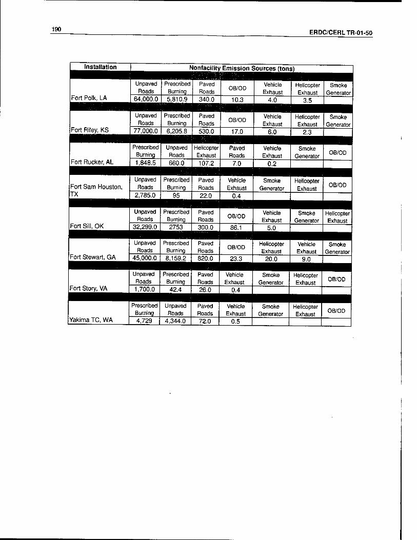
190 ERDC/CERLTR-01-50

ERDC/CERLTR-01-50 191
Table 35. Rank of individual installation TSF ' sources.
Installation Nonfacility Emission Sources (tons)
Aberdeen PG, MD
Unpaved Roads
Prescribed Burning
Paved Roads
Vehicle Exhaust
Smoke Generator
Helicopter Exhaust
OB/OD
38,000.0 2,272.6 260.0 0.5
Camp Atterbury, IN
Unpaved Roads
Paved Roads
Vehicle Exhaust
Prescribed Burning
Smoke Generator
Helicopter Exhaust
OB/OD
12,269.8 189.2 0.3
Camp Blanding, FL
Prescribed Burning
Unpaved Roads
Paved Roads
Vehicle Exhaust
Smoke Generator
Helicopter Exhaust
OB/OD
2,287.1 1,870.6 32.5 0.1
Camp Dodge, IA
Unpaved Roads
Paved Roads
Prescribed Burning
OB/OD Helicopter Exhaust
Vehicle Exhaust
Smoke Generator
35,292.5 306.8 125.4 >3.2 0.9 0.9
Camp Edwards, MA
Unpaved Roads
Prescribed Burning
Paved Roads
Vehicle Exhaust
Smoke Generator
Helicopter Exhaust
OB/OD
569.8 491.4 7.7 0.0
Camp Grafton, ND
Unpaved Roads
Prescribed Burning
Paved Roads
Vehicle Exhaust
Smoke Generator
Helicopter Exhaust
OB/OD
4,535.9 332.1 30.7 0.1
Camp Grayling, Ml
Unpaved Roads
Prescribed Burning
Paved Roads
Vehicle Exhaust
Smoke Generator
Helicopter Exhaust
OB/OD
4,792.2 4,607.0 64.1 0.2
Camp Guernsey, WY
Unpaved Roads
Paved Roads
Vehicle Exhaust
Prescribed Burning
Smoke Generator
Helicopter Exhaust
OB/OD
219.3 1.7 0.0
Camp Howze, TX
Unpaved Roads
Paved Roads
Vehicle Exhaust
Helicopter Exhaust
Prescribed Burning
Smoke Generator
OB/OD
19,600.9 271.5 0.6 0.3
Camp Parks, CA
Unpaved Roads
Paved Roads
Vehicle Exhaust
Prescribed Burning
Smoke Generator
Helicopter Exhaust
OB/OD
985.2 6.8 0.0
Camp Rapid, SD
Unpaved Roads
Paved Roads
Vehicle Exhaust
Prescribed Burning
Smoke Generator
Helicopter Exhaust
OB/OD
2,641.0 9.7 0.0
Camp Rilea, OR
Unpaved Roads
Paved Roads
Vehicle Exhaust
Prescribed Burning
Smoke Generator
Helicopter Exhaust
OB/OD
850.3 9.7 0.0
Camp Ripley, MN
Unpaved Roads
Prescribed Burning
Paved Roads
Vehicle Exhaust
OB/OD Smoke
Generator Helicopter Exhaust
12,369.6 962.8 128.5 0.5

192 ERDC/CERLTR-01-50
Installation Nonfacility Emission Sources (tons)

ERDC/CERLTR-01-50 193
Installation Nonfacility Emission Sources (tons)
Fort Drum, NY
Unpaved Roads
Prescribed Burning
Paved Roads
Helicopter Exhaust
OB/OD Vehicle Exhaust
Smoke Generator
210,000.0 3,375.7 1,200.0 11.8 >5.9 4.0
Fort Eustis, VA
Unpaved Roads
Paved Roads
Prescribed Burning
Helicopter Exhaust
Vehicle Exhaust
Smoke Generator
OB/OD
33,000.0 930.0 280.1 7.1 1.0
Fort Gordon, GA
Unpaved Roads
Prescribed Burning
Paved Roads
Vehicle Exhaust
Smoke Generator
Helicopter Exhaust
OB/OD
53,000.0 1,922.8 730.0 3.0
Fort Hood, TX
Unpaved Roads
Paved Roads
Prescribed Burning
OB/OD Vehicle Exhaust
Helicopter Exhaust
Smoke Generator
820,000.0 10,000.0 7,397.0 >24.6 21.0 16.5
Fort Huachuca, AZ
Unpaved Roads
Prescribed Burning
Paved Roads
Vehicle Exhaust
Helicopter Exhaust
Smoke Generator
OB/OD
62,000.0 436.7 370.0 1.0 0.6
Fort Indiantown Gap, PA
Unpaved Roads
Prescribed Burning
Paved Roads
Helicopter Exhaust
Vehicle Exhaust
Smoke Generator
OB/OD
28,000.0 561.0 110.0 9.6 0.5
Fort Irwin, CA
Unpaved Roads
Paved Roads
Smoke Generator
Vehicle Exhaust
Helicopter Exhaust
Prescribed Burning
OB/OD
300,000.0 4,200.0 22.0 8.0 6.8 0.0 0.0
Fort Jackson, SC
Unpaved Roads
Prescribed Burning
Paved Roads
Vehicle Exhaust
Smoke Generator
Helicopter Exhaust
OB/OD
24,000.0 1,780.0 230.0 0.8
Fort Knox, KY
Unpaved Roads
Prescribed Burning
Paved Roads
OB/OD Helicopter Exhaust
Vehicle Exhaust
Smoke Generator
180,000.0 3,716.8 1,300.0 >4.5 3.3 2.0
Fort Leavenworth, KS
Unpaved Roads
Prescribed Burning
Paved Roads
Vehicle Exhaust
Smoke Generator
Helicopter Exhaust
OB/OD
46,000.0 496.8 230.0 1.0
Fort Lee, VA
Unpaved Roads
Paved Roads
Prescribed Burning
Vehicle Exhaust
Smoke Generator
Helicopter Exhaust
OB/OD
31,000.0 350.0 189.7 1.0
Fort Leonard Wood, MO
Unpaved Roads
Prescribed Burning
Paved Roads
Smoke Generator
Vehicle Exhaust
Helicopter Exhaust
OB/OD
180,000.0 1,982.9 910.0 231.0 2.0
Fort Lewis, WA
Unpaved Roads
Paved Roads
Prescribed Burning
OB/OD Vehicle Exhaust
Helicopter Exhaust
Smoke Generator
481,000.0 4,100.0 1,760.9 >17.8 10.0 9.5

194 ERDC/CERLTR-01-50
Installation Nonfacility Emission Sources (tons)
Table 36 summarizes the rankings of the emission source categories at the in- stallations. As Table 36 shows, the most significant emission sources are (1) dust re-entrainment from unpaved roads and (2) prescribed burning. The emission estimates from these two source categories must be qualified: (1) the unpaved road emissions in Tables 33 - 35 assume that no travel is conducted on paved roads, and (2) the prescribed burning estimates at 26 installations were based on the activity data reported for 1 year at Fort Bragg and are likely to be high for

ERDC/CERLTR-01-50 195
installations outside the Southeast. Table 36 also shows that prescribed burning is more likely to be the number one source category for PM2.5 emissions than for TSP emissions. This observation reflects the smaller particle size associated with prescribed burning emissions than that associated with dust re- entrainment from road surfaces.
Table 36. Frequency of nonfacility source rankings from 50 installations.
Source Category Ranking
Frequency of Source Ranking
PM2.5 PM10 TSP
#1 Source Category
Dust Re-entrainment from Unpaved Roads 34 44 49
Prescribed Burning 16 6 1
#2 Source Category
Dust Re-entrainment from Paved Roads 8 8 16
Dust Re-entrainment from Unpaved Roads 15 6 1
Helicopter Engine Exhaust 1 0 0
Prescribed Burning 26 36 33
Ranking the Installations
The purpose of this section is to allow the reader to target installations that may have significant activities that generate PM emissions. The rankings in this sec- tion are based on the "rough order-of-magnitude" emissions estimates for the nonfacility emission sources. These estimates are not based on information ob- tained directly from installations and generally would not be appropriate for regulatory purposes. The emissions estimates in this section are only designed to provide qualitative comparisons among troop-based installations that will provide some insights for prioritizing PM NAAQS concerns.
Tables 37 through 42 display the order of installations based on their emissions of PM2.5, PM10, and TSP. Table 37 (PM2.5), Table 38 (PM10), and Table 39 (TSP) present the installation rankings based on emissions from vehicles (i.e., engine exhaust/tire wear/brake wear, dust from paved roads, and dust from un- paved roads). Table 40 ranks the installations based on PM2.5, PM10, and TSP emissions from prescribed burning. Table 41 presents the rankings of PM10 emissions from the open burning of propellant during field exercises, and Table 42 ranks the installations based on helicopter exhaust emissions. Installation ranking for smoke generation is not presented, although Fort Leonard Wood would clearly be the installation ranked number one in this category.

196 ERDC/CERLTR-01-50
Table 37. Installation ranking by 1998 PM2.5 vehicle emissions (tons).
Rank Installation Vehicle Exhaust Rank Installation
Paved Roads Rank Installation
Unpaved Roads
1 Fort Hood, TX 18.0 1 Fort Hood, TX 490.0 1 Fort Hood, TX 24,000.0 2 Fort Bragg, NC 13.0 2 Fort Bragg, NC 220.0 2 Fort Campbell, KY 19,000.0 3 Fort Lewis, WA 9.0 3 Fort Stewart, GA 210.0 3 Fort Lewis, WA 15,000.0 4 Fort Stewart, GA 8.0 4 Fort Irwin, CA 200.0 4 Fort Bragg, NC 12,000.0 5 Fort Campbell, KY 7.0 5 Fort Lewis, WA 200.0 5 Fort Riley, KS 11,000.0 6 Fort Irwin, CA 7.0 6 Fort Carson, CO 160.0 6 Fort Polk, LA 9,300.0 7 Fort Carson, CO 5.0 7 Fort Campbell, KY 150.0 7 Fort Irwin, CA 9,100.0 8 Fort Riley, KS 5.0 8 Fort Riley, KS 130.0 8 Fort Carson, CO 8,500.0 9 Fort Sill, OK 5.0 9 Fort Benning, GA 98.0 9 Fort Stewart, GA 6,600.0 10 Fort Benning, GA 4.0 10 Fort Polk, LA 86.0 10 Fort Drum, NY 6,300.0 11 Fort Polk, LA 4.0 11 Fort Bliss, TX 79.0 11 Fort Knox, KY 5,400.0 12 Fort Bliss, TX 3.0 12 Fort Sill, OK 74.0 12 Fort Leonard
Wood, MO 5,300.0
13 Fort Drum, NY 3.0 13 Fort Knox, KY 63.0 13 Fort Sill, OK 4,721.0 14 Fort Gordon, GA 2.0 14 Fort Drum, NY 59.0 14 Fort Bliss, TX 3,500.0 15 Fort Knox, KY 2.0 15 Fort Eustis, VA 45.0 15 Fort Benning, GA 3,200.0 16 Fort Leonard
Wood, MO 2.0 16 Fort Leonard
Wood, MO 44.0 16 Fort McClellan, AL 2,400.0
17 Fort Eustis, VA 1.0 17 Fort Gordon, GA 36.0 17 Fort Huachuca, AZ 1,900.0 18 Fort Huachuca, AZ 1.0 18 Fort Huachuca, AZ 18.0 18 Fort McCoy, Wl 1,700.0 19 Fort Lee, VA 0.9 19 Yakima TC, WA 18.0 19 Fort Gordon, GA 1,600.0 20 Fort McClellan, AL 0.9 20 Fort Lee, VA 17.0 20 Fort Leavenworth,
KS 1,400.0
21 Fort Leavenworth, KS
0.8 21 Fort McCoy, Wl 17.0 21 Aberdeen PG MD 1,100.0
22 Camp Dodge, IO 0.8 22 Camp Dodge, IA 15.0 22 Camp Dodge, IA 1,055.9 23 Fort Jackson, SC 0.7 23 Camp Howze, TX 13.2 23 Fort Eustis, VA 960.0 24 Fort McCoy, Wl 0.6 24 Aberdeen PG MD 13.0 24 Fort Lee, VA 910.0 25 Camp Stanley, TX 0.6 25 Fort McClellan, AL 13.0 25 Fort Indiantown
Gap, PA 860.0
26 Camp Howze, TX 0.5 26 Fort Jackson, SC 11.0 26 Camp Stanley, TX 751.2 27 Yakima TC, WA 0.5 27 Fort Leavenworth,
KS 11.0 27 Fort Jackson, SC 720.0
28 Camp Ripley, MN 0.4 28 Camp Stanley, TX 9.7 28 Yakima TC, WA 635.0 29 Aberdeen PG MD 0.4 29 Camp Atterbury, IN 9.2 29 Camp Howze, TX 572.5 30 Fort Indiantown
Gap, PA 0.4 30 Camp Ripley, MN 6.3 30 Fort McPherson,
GA 490.0
31 Fort McPherson, GA
0.4 31 Fort Indiantown Gap, PA
6.0 31 Fort Chaffee, AR 430.0
32 Camp Shelby, MS 0.3 32 Fort McPherson, GA
6.0 32 Fort Sam Houston, TX
407.0
33 Fort Sam Houston, TX
0.3 33 Fort Story, VA 6.0 33 Camp Ripley, MN 383.1
34 Fort Story, VA 0.3 34 Camp Shelby, MS 5.3 34 Camp Shelby, MS 363.3

ERDC/CERLTR-01-50 197
Rank Installation Vehicle Exhaust Rank Installation
Paved Roads Rank Installation
Unpaved Roads
35 Camp Atterbury, IN 0.2 35 Fort Sam Houston, TX
5.0 35 Camp Atterbury, IN 343.1
36 Camp Robinson, AR
0.2 36 Camp Robinson, AR
3.3 36 Fort Story, VA 260.0
37 Fort Chaffee, AR 0.2 37 Camp Grayling, Ml 3.1 37 Fort Dix, NJ 200.0
38 Fort Dix, NJ 0.2 38 Fort Chaffee, AR 3.0 38 Camp Robinson, AR
182.9
39 Camp Grayling, Ml 0.2 39 Fort Dix, NJ 3.0 39 Camp Roberts, CA 154.5
40 Fort Rucker, AL 0.1 40 Fort Rucker, AL 2.0 40 Camp Grayling, Ml 149.1
41 Camp Roberts, CA 0.1 41 Camp Blanding, FL 1.6 41 Camp Grafton, ND 137.3
42 Camp Grafton, ND 0.1 42 Camp Grafton, ND 1.5 42 Fort Rucker, AL 97.0
43 Camp Blanding, FL 0.1 43 Camp Roberts, CA 1.2 43 Camp Rapid, SD 85.3
44 Camp Williams, UT 0.1 44 Camp Williams, UT 0.7 44 Camp Williams, UT
67.5
45 Camp Rapid, SD 0.0 45 Camp Rilea, OR 0.5 45 Camp Blanding, FL
59.0
46 Camp Edwards, MA
0.0 46 Camp Rapid, SD 0.5 46 Camp Parks, CA 30.9
47 Camp Parks, CA 0.0 47 Camp Edwards, MA
0.4 47 Camp Rilea, OR 25.2
48 Camp Rilea, OR 0.0 48 Camp Parks, CA 0.3 48 Carlisle Barracks, PA
22.0
49 Camp Guernsey, WY
0.0 49 Camp Guernsey, WY
0.1 49 Camp Edwards, MA
18.2
50 Carlisle Barracks, PA
<.01 50 Carlisle Barracks, PA
<.01 50 Camp Guernsey, WY
6.9

198 ERDC/CERLTR-01-50
Table 38. Installation ranking by 1998 PM10 vehicle emissions (tons).
Rank Installation Vehicle Exhaust Rank Installation
Paved Roads Rank Installation
Unpaved Roads
1 Fort Hood, TX 20.0 1 Fort Hood, TX 2,000.0 1 Fort Hood, TX 170,000.0 2 Fort Bragg, NC 15.0 2 Fort Bragg, NC 890.0 2 Fort Campbell, KY 130,000.0 3 Fort Lewis, WA 10.0 3 Fort Stewart, GA 820.0 3 Fort Lewis, WA 99,000.0 4 Fort Stewart, GA 9.0 4 Fort Irwin, CA 810.0 4 Fort Bragg, NC 82,000.0 5 Fort Campbell, KY 8.0 5 Fort Lewis, WA 800.0 5 Fort Riley, KS 77,000.0 6 Fort Irwin, CA 8.0 6 Fort Carson, CO 640.0 6 Fort Polk, LA 64,000.0 7 Fort Carson, CO 6.0 7 Fort Campbell, KY 600.0 7 Fort Irwin, CA 62,000.0 8 Fort Riley, KS 6.0 8 Fort Riley, KS 530.0 8 Fort Carson, CO 58,000.0 9 Fort Sill, OK 5.0 9 Fort Benning, GA 390.0 9 Fort Stewart, GA 45,000.0 10 Fort Benning, GA 4.0 10 Fort Polk, LA 340.0 10 Fort Drum, NY 43,000.0 11 Fort Drum, NY 4.0 11 Fort Bliss, TX 310.0 11 Fort Knox, KY 37,000.0 12 Fort Polk, LA 4.0 12 Fort Sill, OK 300.0 12 Fort Leonard Wood,
MO 36,000.0
13 Fort Bliss, TX 3.0 13 Fort Knox, KY 250.0 13 Fort Sill, OK 32,299.0 14 Fort Gordon, GA 3.0 14 Fort Drum, NY 240.0 14 Fort Bliss, TX 24,000.0 15 Fort Knox, KY 2.0 15 Fort Eustis, VA 180.0 15 Fort Benning, GA 22,000.0 16 Fort Leonard Wood,
MO 2.0 16 Fort Leonard Wood,
MO 180.0 16 Fort McClellan, AL 16,000.0
17 Fort Eustis, VA 1.0 17 Fort Gordon, GA 140.0 17 Fort Huachuca, AZ 13,000.0 18 Fort Huachuca, AZ 1.0 18 Fort Huachuca, AZ 72.0 18 Fort Gordon, GA 11,000.0 19 Fort Lee, VA 1.0 19 Yakima TC, WA 72.0 19 Fort McCoy, Wl 11,000.0 20 Fort McClellan, AL 1.0 20 Fort McCoy, Wl 68.0 20 Fort Leavenworth,
KS 9,800.0
21 Fort Leavenworth, KS
0.9 21 Fort Lee, VA 67.0 21 Aberdeen PG MD 7,800.0
22 Camp Dodge, IA 0.8 22 Camp Dodge, IA 59.9 22 Camp Dodge, IA 7,224.5 23 Fort Jackson, SC 0.8 23 Camp Howze, TX 53.0 23 Fort Eustis, VA 6,600.0 24 Fort McCoy, Wl 0.7 24 Aberdeen PG MD 51.0 24 Fort Lee, VA 6,300.0 25 Camp Stanley, TX 0.7 25 Fort McClellan, AL 50.0 25 Fort Indiantown
Gap, PA 5,900.0
26 Camp Howze, TX 0.6 26 Fort Jackson, SC 45.0 26 Camp Stanley, TX 5,139.9
27 Aberdeen PG, MD 0.5 27 Fort Leavenworth, KS
45.0 27 Fort Jackson, SC 4,900.0
28 Yakima TC, WA 0.5 28 Camp Stanley, TX 38.7 28 Yakima TC, WA 4,344.0 29 Camp Ripley, MN 0.5 29 Camp Atterbury, IN 36.9 29 Camp Howze, TX 3,916.8 30 Fort Sam Houston,
TX 0.4 30 Fort Story, VA 26.0 30 Fort McPherson, GA 3,300.0
31 Fort Indiantown Gap, PA
0.4 31 Camp Ripley, MN 25.1 31 Fort Chaffee, AR 2,900.0
32 Fort McPherson, GA 0.4 32 Fort McPherson, GA
25.0 32 Fort Sam Houston, TX
2,785.0
33 Fort Story, VA 0.4 33 Fort Sam Houston, TX
22.0 33 Camp Ripley, MN 2,621.1

ERDC/CERLTR-01-50 199
Rank Installation Vehicle Exhaust Rank Installation
Paved Roads Rank Installation
Unpaved Roads
34 Camp Shelby, MS 0.4 34 Fort Indiantown Gap, PA
22.0 34 Camp Shelby, MS 2,485.8
35 Camp Williams, UT 0.4 35 Camp Shelby, MS 21.2 35 Camp Atterbury, IN 2,347.3
36 Camp Atterbury, IN 0.3 36 Camp Robinson, AR
13.0 36 Fort Story, VA 1,700.0
37 Camp Robinson, AR 0.2 37 Camp Grayling, Ml 12.5 37 Fort Dix, NJ 1,400.0
38 Fort Chaffee, AR 0.2 38 Fort Dix, NJ 12.0 38 Camp Robinson, AR 1,251.2
39 Fort Dix, NJ 0.2 39 Fort Chaffee, AR 11.0 39 Camp Roberts, CA 1,056.9
40 Fort Rucker, AL 0.2 40 Fort Rucker, AL 7.0 40 Camp Grayling, Ml 1,020.4
41 Camp Grayling, Ml 0.2 41 Camp Blanding, FL 6.3 41 Camp Grafton, ND 939.4
42 Camp Roberts, CA 0.1 42 Camp Grafton, ND 6.0 42 Fort Rucker, AL 660.0
43 Camp Grafton, ND 0.1 43 Camp Roberts, CA 4.9 43 Camp Rapid, SD 583.5
44 Camp Blanding, FL 0.1 44 Camp Williams, UT
2.8 44 Camp Williams, UT 461.6
45 Camp Rapid, SD <.01 45 Camp Rilea, OR 1.9 45 Camp Blanding, FL 404.0
46 Camp Edwards, MA <.01 46 Camp Rapid, SD 1.9 46 Camp Parks, CA 211.6
47 Camp Parks, CA <.01 47 Camp Edwards, MA
1.5 47 Camp Rilea, OR 172.3
48 Camp Rilea, OR <.01 48 Camp Parks, CA 1.3 48 Carlisle Barracks, PA
151.0
49 Camp Guernsey, WY <.01 49 Carlisle Barracks, PA
1.0 49 Camp Edwards, MA 124.3
50 Carlisle Barracks, PA <.01 50 Camp Guernsey, WY
0.3 50 Camp Guernsey, WY
47.1
Note: Installations in bold are located in or near PM nonattainment areas.

200 ERDC/CERLTR-01-50
Table 39. Installation ranking by 1998 TSP vehicle emissions (tons).
Rank Installation Vehicle Exhaust Rank Installation
Paved Roads Rank Installation
Unpaved Roads
1 Fort Hood, TX 21.0 1 Fort Hood, TX 10,000.0 1 Fort Hood, TX 820,000.0 2 Fort Bragg, NC 16.0 2 Fort Bragg, NC 4,500.0 2 Fort Campbell, KY 630,000.0 3 Fort Lewis, WA 10.0 3 Fort Irwin, CA 4,200.0 3 Fort Lewis, WA 481,000.0 4 Fort Stewart, GA 9.0 4 Fort Stewart, GA 4,200.0 4 Fort Bragg, NC 400,000.0 5 Fort Campbell, KY 8.0 5 Fort Lewis, WA 4,100.0 5 Fort Riley, KS 380,000.0 6 Fort Irwin, CA 8.0 6 Fort Carson, CO 3,300.0 6 Fort Polk, LA 310,000.0 7 Fort Carson, CO 6.0 7 Fort Campbell,
KY 3,100.0 7 Fort Irwin, CA 300,000.0
8 Fort Riley, KS 6.0 8 Fort Riley, KS 2,700.0 8 Fort Carson, CO 288,000.0 9 Fort Sill, OK 5.0 9 Fort Benning, GA 2,000.0 9 Fort Stewart, GA 223,000.0 10 Fort Benning, GA 4.0 10 Fort Polk, LA 1,800.0 10 Fort Drum, NY 210,000.0 11 Fort Bliss, TX 4.0 11 Fort Bliss, TX 1,600.0 11 Fort Knox, KY 180,000.0 12 Fort Drum, NY 4.0 12 Fort Sill, OK 1,500.0 12 Fort Leonard
Wood, MO 180,000.0
13 Fort Polk, LA 4.0 13 Fort Knox, KY 1,300.0 13 Fort Sill, OK 153,631.0 14 Fort Gordon, GA 3.0 14 Fort Drum, NY 1,200.0 14 Fort Bliss, TX 120,000.0 15 Fort Knox, KY 2.0 15 Fort Eustis, VA 930.0 15 Fort Benning, GA 107,000.0 16 Fort Leonard
Wood, MO 2.0 16 Fort Leonard
Wood, MO 910.0 16 Fort McClellan, AL 77,000.0
17 Fort Eustis, VA 1.0 17 Fort Gordon, GA 730.0 17 Fort Huachuca, AZ 62,000.0 18 Fort Huachuca, AZ 1.0 18 Fort Huachuca,
AZ 370.0 18 Fort McCoy, Wl 55,000.0
19 Fort Leavenworth, KS
1.0 19 Yakima TC, WA 370.0 19 Fort Gordon, GA 53,000.0
20 Fort Lee, VA 1.0 20 Fort Lee, VA 350.0 20 Fort Leavenworth, KS
46,000.0
21 Fort McClellan, AL 1.0 21 Fort McCoy, Wl 350.0 21 Aberdeen PG MD 38,000.0 22 Camp Dodge, IA 0.9 22 Camp Dodge, IA 306.8 22 Camp Dodge, IA 35,292.5 23 Fort Jackson, SC 0.8 23 Camp Howze,
TX 271.5 23 Fort Eustis, VA 33,000.0
24 Fort McCoy, Wl 0.7 24 . Aberdeen PG MD
260.0 24 Fort Lee, VA 31,000.0
25 Camp Stanley, TX 0.7 25 Fort McClellan, AL
260.0 25 Fort Indiantown Gap, PA
28,000.0
26 Camp Howze, TX 0.6 26 Fort Jackson, SC 230.0 26 Camp Stanley, TX 24,167.7 27 Yakima TC, WA 0.6 27 Fort Leaven-
worth, KS 230.0 27 Fort Jackson, SC 24,000.0
28 Aberdeen PQ MD 0.5 28 Camp Stanley, TX
198.2 28 Yakima TC, WA 22,589.0
29 Fort Indiantown Gap, PA
0.5 29 Camp Atterbury, IN
189.2 29 Camp Howze, TX 19,600.9
30 Camp Ripley, MN 0.5 30 Fort McPherson, GA
130.0 30 Fort McPherson, GA
16,000.0
31 Camp Shelby, MS 0.4 31 Fort Story, VA 130.01 31 Fort Chaffee, AR 14,000.0

ERDC/CERLTR-01-50 201
Rank Installation Vehicle Exhaust Rank Installation
Paved Roads Rank Installation
32 Fort Sam Houston, TX
0.4 32 Camp Ripley, MN 128.5 32 Fort Sam Hous- ton, TX
33 Fort McPherson, GA 0.4 33 Fort Sam Hous- ton, TX
110.0 33 Camp Ripley, MN
34 Fort Story, VA 0.4 34 Fort Indiantown Gap, PA
110.0 34 Camp Atterbury, IN
35 CampAtterbury, IN 0.3 35 Camp Shelby, MS
108.4 35 Camp Shelby, MS
36 Camp Robinson, AR 0.2 36 Camp Robinson, AR
66.7 36 Fort Story, VA
37 Fort Chaffee, AR 0.2 37 Camp Grayling, Ml
64.1 37 Fort Dix, NJ
38 Fort Dix, NJ 0.2 38 Fort Dix, NJ 62.0 38 Camp Robinson, AR
39 Fort Rucker, AL 0.2 39 Fort Chaffee, AR 56.0 39 Camp Roberts, CA
40 Camp Grayling, Ml 0.2 40 Fort Rucker, AL 36.0 40 Camp Grayling, Ml
41 Camp Roberts, CA 0.1 41 Camp Blanding, FL
32.5 41 Camp Grafton, ND
42 Camp Grafton, ND 0.1 42 Camp Grafton, ND
30.7 42 Fort Rucker, AL
43 Camp Blanding, FL 0.1 43 Camp Roberts, CA
24.9 43 Camp Rapid, SD
44 Camp Williams, UT 0.1 44 Camp Williams, UT
14.6 44 Camp Williams, UT
45 Camp Rapid, SD <0.1 45 Camp Rilea, OR 9.7 45 Camp Blanding, FL
46 Camp Edwards, MA <0.1 46 Camp Rapid, SD 9.7 46 Camp Parks, CA
47 Camp Parks, CA <0.1 47 Camp Edwards, MA
7.7 47 Camp Rilea, OR
48 Camp Rilea, OR <0.1 48 Carlisle Barracks, PA
7.0 48 Carlisle Barracks, PA
49 Camp Guernsey, WY
<0.1 48 Camp Parks, CA 6.8 49 Camp Edwards, MA
48 Carlisle Barracks, PA I
<0.1 49 Camp Guernsey, WY
1.7 50 Camp Guernsey, WY

202 ERDC/CERLTR-01-50
Table 40. Installation ranking by annual PM prescribed burning emissions (tons).
Rank Installation PM2.5 (tons) Installation
PM10 (tons) Installation
TSP (tons)
1 Fort Stewart, GA 7343 Fort Stewart, GA 8159 Fort Stewart, GA 9505 2 Fort Hood, TX 5715 Fort Hood, TX 6350 Fort Hood, TX 7397 3 Fort Riley, KS 5585 Fort Riley, KS 6206 Fort Riley, KS 7144 4 Fort Polk, LA 5230 Fort Polk, LA 5811 Fort Polk, LA 6769 5 Fort Benning, GA 4840 Fort Benning, GA 5377 Fort Benning, GA 6264 6 Yakima TC, WA 4315 Yakima TC, WA 4729 Yakima TC, WA 6106 7 Fort Bragg, NC 3946 Fort Bragg, NC 4385 Fort Bragg, NC 5108 8 Camp Shelby, MS 3523 Camp Shelby, MS 3915 Camp Grayling, Ml 4607 9 Camp Grayling, Ml 3518 Camp Grayling, Ml 3909 Camp Shelby, MS 4561 10 Fort McCoy, Wl 3057 Fort McCoy, Wl 3397 Fort Bliss, TX 4368 11 Fort Carson, CO 2903 Fort Carson, CO 3225 Fort McCoy, Wl 4003 12 Fort Knox, KY 2872 Fort Knox, KY 3191 Fort Knox, KY 3717 13 Fort Bliss, TX 2871 Fort Bliss, TX 3190 Fort Carson, CO 3713 14 Fort Campbell, KY 2763 Fort Campbell, KY 3070 Fort Campbell, KY 3576 15 Fort Drum, NY 2578 Fort Drum, NY 2864 Fort Drum, NY 3376 16 Fort Sill, OK 2478 Fort Sill, OK 2753 Fort Sill, OK 3207 17 Fort Chaffee, AR 1877 Fort Chaffee, AR 2085 Fort Chaffee, AR 2429 18 Camp Blanding, FL 1767 Camp Blanding, FL 1963 Camp Blanding, FL 2287 19 Aberdeen PG, MD 1735 Aberdeen PG MD 1928 Aberdeen PQ MD 2273 20 Fort Rucker, AL 1664 Fort Rucker, AL 1849 Fort Rucker, AL 2153 21 Fort Leonard Wood, MO 1514 Fort Leonard Wood, MO 1682 Fort Leonard Wood, MO 1983 22 Fort Gordon, GA 1486 Fort Gordon, GA 1651 Fort Gordon, GA 1923 23 Fort Jackson, SC 1375 Fort Jackson, SC 1528 Fort Jackson, SC 1780 24 Fort Lewis, WA 1245 Fort Lewis, WA 1364 Fort Lewis, WA 1761 25 Fort McClellan, AL 1201 Fort McClellan, AL 1335 Fort McClellan, AL 1555 26 Camp Robinson, AR 942 Camp Robinson, AR 1047 Camp Robinson, AR 1220 27 Fort Dix, NJ 742 Fort Dix, NJ 824 Fort Dix, NJ 971 28 Camp Ripley, MN 735 Camp Ripley, MN 817 Camp Ripley, MN 963 29 Fort Indiantown Gap, PA 428 Fort Indiantown Gap, PA 476 Fort Indiantown Gap, PA 561 30 Fort Leavenworth, KS 388 Fort Leavenworth, KS 432 Fort Leavenworth, KS 497 31 Camp Edwards, MA 375 Camp Edwards, MA 417 Camp Edwards, MA 491 32 Fort Huachuca, AZ 287 Fort Huachuca, AZ 319 Fort Huachuca, AZ 437 33 Camp Grafton, ND 260 Camp Grafton, ND 288 Camp Grafton, ND 332 34 Fort Eustis, VA 216 Fort Eustis, VA 240 Fort Eustis, VA 280 35 Camp Roberts, CA 163 Camp Roberts, CA 181 Camp Roberts, CA 248 36 Fort Lee, VA 147 Fort Lee, VA 163 Fort Lee, VA 190 37 Camp Dodge, IA 96 Camp Dodge, IA 106 Camp Dodge, IA 125 38 Fort Sam Houston, TX 86 Fort Sam Houston, TX 95 Fort Sam Houston, TX 111 39 Camp Williams, UT 60 Camp Williams, UT 66 Öamp Williams, UT 76 40 Fort McPherson, GA 53 Fort McPherson, GA 59 Fort McPherson, GA 69 41 Fort Story, VA 38 Fort Story, VA 42 Fort Story, VA 49 42 Camp Stanley, TX 34 Camp Stanley, TX 37 Camp Stanley, TX 44 43 Carlisle Barracks, PA 10 Carlisle Barracks, PA 11 Carlisle Barracks, PA 13 44 Fort Irwin, CA * 0 Fort Irwin, CA 0 Fort Irwin, CA 0 No prescribed burning estimates are available for the following installations because acreage data were not available: Camp Howze, TX; Camp Parks, CA; Camp Atterbury, IN; Camp Rapid, SD: Camp Rilea, OR; and Camp Guernsey, WY. Note: Installations in bold are located near PM10 nonattainment areas. * No burning conducted at Fort Irwin.

ERDC/CERLTR-01-50 203
Table 41 . Open burning PM10 emissions (tons).
Rank Installation Emissions 1 Fort Sill, OK 100.5
2 Fort Irwin, CA 0.0
3 Fort Bragg, NC 35.1 4 Fort Hood, TX 24.6
5 Fort Stewart, GA 23.2
6 Fort Carson, CO 21.8 7 Fort Lewis, WA 18.5
8 Fort Riley, KS 17.0
9 Fort Polk, LA 10.3
10 Fort Campbell, KY 10.2
11 Fort Drum, NY 9.4
12 Fort Benning, GA 9.2
13 Fort Knox, KY 4.5 14 Camp Dodge, IA 3.2 15 Carlisle Barracks, PA 2.3 16 Camp Roberts, CA 0.1 17 Camp Ripley, MN 0.0
Table 42. Installations ranked by 1998 helicopter exhaust emissions (tons).
Rank Installation PM2.5 PM10 TSP
1 Fort Rucker, AL 106.2 107.2 109.8
2 Fort Campbell, KY 51.2 51.7 53.0
3 Fort Stewart, GA 19.8 20.0 20.5
4 Fort Hood, TX 15.9 16.1 16.5
5 Fort Drum, NY 11.4 11.5 11.8
6 Fort Bragg, NC 10.6 10.7 11.0
7 Fort Carson, CO 10.0 10.1 10.4
8 Fort Indiantown Gap, PA 9.3 9.3 9.6
9 Fort Lewis, WA 9.1 9.2 9.5
10 Fort Eustis, VA 6.8 6.9 7.1
11 Fort Irwin, CA 6.6 6.7 6.8
12 Camp Robinson, AR 4.6 4.6 4.8
13 Fort Benning, GA 4.0 4.1 4.2
14 Fort Polk, LA 3.5 3.5 3.6
15 Fort Knox, KY 3.2 3.2 3.3
16 Fort Riley, KS 2.2 2.3 2.3
17 Camp Dodge, IA 0.9 0.9 0.9
18 Fort Huachuca, AZ 0.6 0.6 0.6
19 Camp Howze, TX 0.3 0.3 0.3
20 Fort McPherson, GA 0.1 0.1 0.1
— ERDC/CERLTR-01-50
Table 37 (PM2.5), Table 38 (PM10), and Table 39 (TSP) present rankings of all 50 installations for vehicle-related emissions. As shown in these tables, Fort Hood has the highest emissions of all three pollutants for each of the three vehi- cle emission categories; its emissions are at least 26 percent higher than those from the next highest installation.
It should also be noted in Tables 37 through 39 that the five facilities with the highest emissions in each list are not located in one geographic area of the coun- try. Instead, emissions are directly related to vehicle activity, so that seven of the nine installations with 1998 VMT over 10,000,000 miles appear in the top 5
rankings in these tables. Also note that the top 12 installations are responsible for 80 percent of the total emissions in each of the 9 lists. The installations that fall into the top 12 categories are Forts Benning, Bliss, Bragg, Campbell, Carson, Drum, Hood, Irwin, Knox, Leonard Wood, Lewis, Polk, Riley, Sill, and Stewart. FORSCOM installations dominate this list, and none of these are ARNG instal- lations.
Table 38 shows that the PM10 emissions from installations located near PM10 nonattainment areas are at least 60 times greater from dust on unpaved roads than from dust on paved roads. This significant difference suggests that an ef- fective PM10 emissions control strategy for these facilities would be to decrease emissions from unpaved roads through the use of dust control agents or through increased travel on paved roads.
Table 40 presents the ranking of estimated emissions of all three pollutants from prescribed burning at 44 installations. The order of the rankings is the same for all three pollutants, but the rankings may change from year to year depending on forestry program needs and plans and the occurrences of favorable meteoro- logical conditions. Fort Stewart is estimated to have the highest emissions fol- lowed by Fort Hood, Fort Riley, and four other installations in the Southeast. Generally installations located in the southeastern states were estimated to have the highest emissions from prescribed burning operations, and this finding is consistent with national studies that found that 70 percent of the prescribed burning in the United States occurs in southeastern states (Ward, Peterson, and Hao 1993).
A table is not shown for smoke generation rankings. However, PM emissions were estimated for Forts Leonard Wood and Irwin. Compared with the other nonfacility emission sources, PM emissions from smoke generators are small contributors. Even at Fort Leonard Wood, the permit levels for PM emissions (230 TPY TSP, 229 TPY PM10, 229 TPY PM2.5) will still only be 5 percent of the emissions from dust on unpaved roads as shown in Tables 37 - 39.

ERDC/CERLTR-01-50 205
Table 41 presents the ranking of 17 installations based on their estimated PM10 emissions from the open burning of unused propellant charges during field exer- cises. Fort Sill has the highest estimated emissions followed by Forts Irwin and Bragg. However, Forts Sill and Bragg did not even appear in the top 5 rankings of main rounds fired (Table 22). It can be concluded, therefore, that using the total number of main rounds fired is not sufficient to estimate open burning of propellant during field exercises; the counts of the main rounds must be muni- tions-specific.
Table 42 presents the ranking of 20 installations for their estimated emissions from helicopter engine exhaust for all three pollutants. The 1998 emissions of each pollutant at Fort Rucker, location of the Army's Helicopter Training Center, were more than double that at any other installation. The helicopter engine ex- haust emissions at Fort Rucker, however, still ranked only number two for non- facility sources for PM2.5 (Table 33) and number three for PM10 (Table 34) and TSP (Table 35). At other installations, the rankings were even lower, indicating that helicopter exhaust emissions are not responsible for a significant fraction of the PM emissions at the installations examined in this study.

— ERDC/CERLTR-01-50
10 Summary and Conclusions
The objective of the study was to develop a technical report that includes a re- view of previous work related to DOD nonfacility PM problems. The review was used to determine the EPA's enforcement strategy for PM, to identify previous
work in the area, and to determine the scope of the nonfacility PM problem at Army facilities. The results of this review will be used to help focus an R&D pro- gram in this area. It is also hoped that this review will be a valuable source of information for others interested in this area of study. The review contains chapters covering:
atmospheric science of PM (Chapter 2) EPA's regulatory strategy (Chapter 3) estimating PM emissions from nonfacility sources (Chapter 4) dispersion modeling of PM emissions (Chapter 5) transport modeling of PM emissions (Chapter 6) measurement of atmospheric PM (Chapter 7) dust suppression and soil stabilization technologies (Chapter 8) ranking of nonfacility PM sources/installations (Chapter 9).
Chapter 2 discussed the physics and chemistry of PM in atmosphere. A basic understanding of PM atmospheric science is essential to understanding PM health impacts, visibility impacts, regulations, and atmospheric modeling. Chapter 2 was divided into separate sections on particle size distribution, chemi- cal composition of PM, visibility impacts of PM, and particulate removal mecha- nisms. The particle size distribution section discussed the different "modes" of particle sizes that occur in the atmosphere and the origin of particles in these particle size classifications. The chemical composition section covered the ori- gins and behaviors of different chemical species that occur in PM. These species include sulfates, nitrates, organic carbon, elemental carbon, geologic material, and sodium chloride. The visibility section described how PM reduces visibility through visible light scattering and absorption. The final section discussed how the atmosphere removes PM through dry deposition (no precipitation) and wet deposition (particles trapped in precipitation) mechanisms.
Chapter 3 discussed the EPA's strategy for regulating PM emissions. This chap- ter contained a regulatory review of PM2.5, PM10, regional haze, NSR/PSD, and conformity. The reviews contain information about the current state of each of

ERDC/CERLTR-01-50 207
these regulatory areas and the mechanisms through which these national air quality standards and programs can ultimately restrict operations at Army in- stallations. The chapter also contained sections about the EPA's PM monitoring program, enforcement trends at DOD facilities, and general conclusions. The chapter made clear the importance of the Army following the development of new SIP components and PM regulations to ensure that Army sources of PM are rep- resented in an accurate and reasonable manner.
Chapter 4 covered PM estimation methods for nonfacility PM sources that are important to the Army. The chapter discussed PM estimation procedures for ve- hicles (exhaust, brake and tire wear, re-entrained dust on paved and unpaved surfaces), prescribed burning, smokes and obscurants training, artillery practice and weapons impact testing, OB/OD, and aircraft. For each of these source cate- gories, a review of available methods was presented along with details for calcu- lating TSP, PM10, and PM2.5 emissions. The chapter also discussed the reliabil- ity of emission factors and the procedure used to submit new emission factors. Many of the nonfacility sources do not have applicable emission estimation methods. For example, the existing engine emission methods do not consider JP8 fuel combustion and do not cover turbine engine emissions, tracked-vehicle dust emission estimation methods do not exist, nor do weapons testing and firing estimation methods for most munitions, or methods to estimate dust re- entrainment from aircraft landings and takeoffs.
Chapter 5 reviewed dispersion models that can be used to predict PM10 and PM2.5 concentrations resulting from nonfacility source emissions. The chapter e vie wed the following models:
ISC3 CDM 2.0 RAM OBODM SCIPUFF MESOPUFF II CALPUFF EOSAEL.
For each of these models, the chapter discussed the following attributes: • applicability to Army nonfacility PM sources • required inputs • steps and level of effort to run model • special training required to run the model • outputs of model • accuracy

208 ERDC/CERLTR-01-50
• advantages and drawbacks • probability of the results being accepted by regulators • the procedure for obtaining the model and its cost.
Chapter 6 was a review of trajectory models. These models predict the trajecto- ries of air parcels between a source and a far distant receptor. The review iden- tified HYSPLIT and the CAPITA model as the two most prevalent trajectory models. The same model attributes used in Chapter 5 were used to describe these two models in Chapter 6. During the review of trajectory models it was discovered that, for the most part, EPA discourages their use for regulatory pur- poses. For long-range modeling applications, the use of the CALPUFF disper- sion model is encouraged.
Chapter 7 reviewed atmospheric PM measurement technologies. The chapter includes sections on Federal reference and equivalent methods, filter-based non- continuous methods, continuous and semicontinuous methods, laboratory tech- niques for chemical speciation of PM, and plume opacity. Monitors are available that measure PM10 and PM2.5 mass concentrations, PM size distribution, visi- ble light scattering, visible light absorption, and chemical components of PM (ni- trates, sulfates, organics, etc.). Some of the measurement technologies are in everyday use while others are still limited to the R&D community.
Chapter 8 reviewed dust suppression and soil stabilization technologies. The chapter contained sections on physical preventative techniques, chemical dust suppressants, and biological methods of dust suppression. The chemical dust suppressants covered include water attracting chemicals, organic nonbituminous chemicals, petroleum-based binders and waste oils, electrochemical stabilizers, polymers, enzyme slurries, and cementitious binders. Biological methods in- clude the use of vegetative systems, mulch application, and biological crusts. Many of these technologies have not been studied in a systematic way to deter- mine their ability to control PM10 and PM2.5 over time. This area could also benefit from the development of technology selection criteria for users to apply to their unique dust suppression problems.
Chapter 9 presented the results of an effort to rank Army nonfacility PM sources and the installations that contain these sources. The rankings were developed by combining the PM emission estimation techniques discussed in Chapter 4 with the source characteristics and activity data required by each technique. Chapter sections described selection of 50 installations for this study, sources and data for nonfacility PM source activity, emission inventory values for the dif- ferent source types at applicable installations, and rankings for both source types and installations. The results of this study show that estimated mass

ERDC/CERLTR-01-50 209
emissions of PM10 and PM2.5 were greatest for dust emissions from unpaved roads and PM emissions from prescribed burning. Other source types had much smaller emissions at all installations. The installation ranking showed only FORSCOM facilities as the top 10 emitters of PM2.5. These installations were all ranked high because of the large number of VMT reported for its tactical ve- hicles.
This review presented a large amount of information related to Army nonfacility sources of PM. This research area is very dynamic and new technologies for modeling, measuring, and controlling PM are constantly being developed. CERL will continue to follow these trends along with regulatory changes with an eye toward improving the Army's ability to maintain training capabilities and mis- sion readiness by improving regulatory compliance, operating costs, land re- source losses, and safety.

210 ERDC/CERLTR-01-50
Acronyms and Abbreviations
AAS atomic adsorption spectrophotometry AC automated colorimetric ACE combat earthmover AEC Army Environmental Center
AERMIC AMS/EPA Regulatory Model Improvement Committee AERMOD AMS/EPA Regulatory Model
AERTA Army Environmental Requirements and Technology Assessments AMS/EPA American Meteorological Society/Environmental Protection Agency APC armored personnel carrier APNM Automated Particle Nitrate Monitor APS aerodynamic particle sizer ARL Air Resource Laboratory ARNG Army National Guard ASCII American Standard Code for Information Interchange ATEC Army Test and Evaluation Command ATOFMS aerosol time-of-flight mass spectrometer AVLB armored vehicle launch bridge BACM Best Available Control Measures BAM Beta Attenuation Monitor BFV Bradley infantry fighting vehicle CAA Clean Air Act CAMMS continuous ambient mass monitor system CAPITA Center for Air Pollution and Trend Analysis CASAC Clean Air Act Scientific Advisory Committee CDM Climatological Dispersion Model CEA Chemical Equilibrium and Applications CEED Center for Energy and Economic Development CEIDARS California Emission Inventory Development and Reporting System CERL Construction Engineering Research Laboratory CEV combat engineer vehicle CHIEF Clearinghouse for Inventories and Emission Factors CNC condensation nuclei counter COMBIC Combined Obscuration Model for Battlefield Induced Contaminants CONUS continental United States CSUMM Colorado State University Mesoscale Model CUCV commercial utility cargo vehicle

ERDC/CERLTR-01-50 211
CY calendar year DC District of Columbia DMA differential mobility analyzer DOD Department of Defense DTC Developmental Test Command EAA electrical aerosol analyzer EC elemental carbon EOSAEL Electro-Optical System Atmospheric Effects Library EPA Environmental Protection Agency EPM Emissions Production Model ERDC Engineer Research and Development Center FACA Federal Advisory Committee Act FEM Federal Equivalent Method FID flame ionization detector FOFEM First Order Fire Effects Model FORSCOM Forces Command FR Federal Register FRM Federal Reference Method FTIR Fourier transform infrared FY fiscal year GAO General Accounting Office GC gas chromatography GIS geographic information system GSA General Services Administration GUI graphical user interface GVW gross vehicle weight HET heavy expanded mobility tactical vehicle HMMWV High Mobility Multi-Purpose Wheeled Vehicle HPAC Hazard Prediction and Assessment Capability HPLC high performance liquid chromatography HYSPLIT4 Hybrid Single-Particle Lagrangian Integrated Trajectory IC ion chromatography IERA Institute for Environment, Safety, and Occupational Health Risk
Analysis IMPROVE Interagency Monitoring of Protected Visual Environments ISC3 Industrial Source Complex ISCEV Industrial Source Complex Short-Term Event ISCLT3 Industrial Source Complex long-term ISCST3 Industrial Source Complex short-term rWAQM Interagency Workgroup on Air Quality Modeling LID AR light detection and ranging

212 ERDC/CERLTR-01-50
LLC Limited Liability Company LRV* light armored recovery vehicle MACOM Major Commands MDS Mission Design Series MEM mass of energetic material
METDC Maryland Environmental Technology Demonstration Center MPRM Meteorological Processor for Regulatory Models MS mass spectrometry
NAAQS National Ambient Air Quality Standards NAMS National Air Monitoring Stations NAS National Academy of Sciences
NASA National Aeronautical and Space Administration NCDC National Climatic Data Center NGB National Guard Bureau NGM Nested Grid Model NIOSH National Institute of Standards and Health NOV notice of violation NSR New Source Review O&S operating and support OAQPS Office of Air Quality Planning and Standards OB/OD open burning/open detonation OBODM Open Burn/Open Detonation Dispersion Model OC organic carbon OPC optical particle counter OSMIS Operating and Support Management Information System PC personal computer PM particulate matter PSD Prevention of Significant Deterioration PTFE Polytetrafluoroethylene QA/QC quality assurance/quality control R&D research and development RACM Reasonably Available Control Measures RAMS Regional Atmospheric Modeling System RCRA Resource Conservation and Recovery Act SA silhouette area SAIC Science Applications International Corporation SCIPUFF Second-order Closure Integrated Puff Model SCRAM Support Center for Regulatory Air Models SD Shock and Detonation SERDP Strategic Environmental Research and Development Program SI Standard International

ERDC/CERLTR-01-50 213
SIP State Implementation Plan SUSV small unit support vehicle TEOM Tapered Element Oscillating Microbalance® TES threatened and endangered species TOA thermal optical analysis TOR thermal/optical reflectance TRADOC Training and Doctrine Command TSP total suspended particulates TTN Technology Transfer Network (EPA) USAR U.S. Army Reserve USARC U.S. Army and Reserve Command USD A U.S. Department of Agriculture USGS U.S. Geological Survey VMT vehicle miles traveled WINS Well Impactor Ninety-Six XRF x-ray fluorescence

— ERDC/CERLTR-01-50
References
AP-42, Compilation of Air Pollutant Emission Factors, AP-42, Volume I: Stationary Point and Area Sources, Fifth Edition (through Supplement E), downloaded from http://www.epa.gOv/ttn/chief/ap42.html#chapter. (U.S. Environmental Protection Agency (EPA), 1998).
Army Regulation 200-4. 1998. Cultural Resources Management. U.S. Army Publishing Agency, Washington, DC, October 1998.
Addo, J.Q. and T.G. Sanders. 1995. "Effectiveness and environmental impact of road dust sup- pressants," Mountain-Plains Consortium Report Number 95-28A, North Dakota State Univer- sity.
Allen, G.A., C. Sioutas, P. Koutrakis, R. Reiss, F.W. Lurmann, and P.T. Roberts. 1997. "Evalua- tion of the TEOM method for measurement of ambient particulate mass in urban areas." JAWMA 47:682-9.
Apodaca, M. and D. Huffmon. 1990. "Dust abatement review and recommendations." USDA For- est Service - Gifford Pinchot National Forest.
Aquin, R., P. Korgemagi, and DP. Lynch. 1986. "Evaluation of Tembind 35 Dust Palliative." On- tario Ministry of Transportation and Communications. Ml-83 Report.
Armbrust, D.V. and J.D. Bilbro. 1997. "Relating plant canopy characteristics to soil transport ca- pacity by wind." Agronomy Journal 89:157-162.
Ashley, J. and S.R. Rushford. 1984. "Growth of Soil Algae on Top Soil and Processed Oil Shale From the Uintah Basin, Utah, USA." Reclamation and Revegetation Research 3:49-63.
Babich, P., P. Wang, G. Allen, C. Sioutas, and P. Koutrakis. 2000. "Development and Evaluation of a Continuous Ambient PM2.5 Mass Monitor." Aerosol Science and Technology 32:4, April 2000.
Banzhaf, J., D.E. Leihner, A. Buerkert, and P.G. Serafini. 1992. "Soil tillage and windbreak ef- fects on millet and cowpea: I. Wind speed, evaporation, and wind erosion." Agronomy Jour- nal 84:1056-1060.
Barclay, W.R. and R.A. Lewin. 1985. "Microalgal polysaccharide production for the conditioning of agricultural soils." Plant and Soil 88:159-169.
Baron, P.A. 1986. "Calibration and use of aerodynamic particle sizer (APS 3300)," Aerosol Sei. Technol 5:55-67.
Bassel, J.R. 1992. "A demonstration of a dust palliative." USDA Forest Service, Technology and Development Program, Roads Tech Tips, May 1992.

ERDC/CERLTR-01-50 215
Batterman, S., I. Osak, and C. Gelman. 1997. "S02 Sorption Characteristics of Air Sampling Me- dia Using a New Laboratory Test," Atmospheric Environment 31:7, 1041-7.
Belnap, J. and J.S. Gardner. 1993. "Soil microstructure of the Colorado Plateau: the role of the cyanobacterium Microcoleus vaginatus." Great Basin Naturalist 53:40-47.
Belnap, J. 1993. "Recovery rates of cryptobiotic crusts: inoculant use and assessment methods." Great Basin Naturalist 53:89-95.
Belnap, J. 1995. "Surface disturbances: their role in accelerating desertification." Environmental Monitoring and Assessment 37:39-57.
Belnap, J. and D.A. Gillette. 1997. "Disturbance of Biological soil crust: impacts on potential wind erodibility of sandy desert soils in southeastern Utah." Land Degradation and Development 8:355-362.
Bennett, D.M. and K. Gleeson. 1995. "Performance evaluation oftall oil pitch emulsion for stabi- lizing unpaved forest road surfaces." Sixth International Conference on Low-Volume Roads, Transportation Research Board, pp 213-224.
Bergeson, K.L. and A.M. Wahbeh. 1990. "Development of an economic dust palliative for lime- stone-surfaced secondary roads." Final report. Iowa Department of Transportation, Research Project HR-297.
Bergeson, K.L. and S.G. Brocka. 1995. "Bentonite treatment for fugitive dust control." Sixth In- ternational Conference on Low-Volume Roads, Vol. 2, Transportation Research Board, Wash- ington, DC, National Academy Press.
Bergeson, K.L., J.W. Wadingham, S.G. Brocka, and R.K. Lapke. 1995. "Bentonite treatment for economical dust reduction on limestone-surfaced secondary roads." Highway Division, Iowa Department of Transportation and Iowa Highway Research Advisory Board, Project HR-351.
Bilbro, J.D. and D.W. Fryrear. 1994. "Wind erosion losses as related to plant silhouette and soil cover." Agronomy Journal 86:550-553.
Bilbro, J.D. and D.W. Fryrear. 1997. "Comparative performance of forage sorghum, grain sor- ghum, kenaf, switchgrass, and slat-fence wind barriers in reducing wind velocity."
Bolander, P. 1989. "Chemical additives for dust control." Transportation Research Record 1589:42-49.
Bond, R.D. and J.R. Harris. 1964. "The influence of the microflora on physical properties of soils. I. Effects associated with filamentous algae and fungi." Australian Journal of Soil Research 2:111-122.
Boyd, K.R. 1983a. "Evaluation of calcium lignosulfonate as a dust palliative," Report 1, Manitoba Department of Highways and Transportation, Canada.
Boyd, K.R. 1983b. "Evaluation of calcium lignosulfonate as a dust palliative," Report 2, Manitoba Department of Highways and Transportation, Canada.

— ERDC/CERLTR-01-50
Boyd, K.R. 1986. "Summary of the 1985 lignosulfonate evaluations," Manitoba Department of Highways and Transportation, Canada.
Brown, D.A. and D.J. Elton. 1994. Guidelines for dust control on unsurfaced roads in Alabama, Final report IR-94-02, Alabama Highway Research Center, Auburn University.
Brownell, F.W. and Lee B. Zeugin. 1992. Clean Air Handbook (Government Institutes, Inc.).
Browner, CM. Letter to Secretary of Defense William Cohen, dated 17 June 1997. Available to DENIX users at http://www.denix.osd.mil/denix/Public/Librarv/Air/CAA/brownerd.html
Buettner, H. 1990. "Measurement of the size distribution of fine nonspherical particles with a light-scattering particle counter," Aerosol Sei. Technol 12:413-21.
Buttars, S.M., L.L. St. Clair, J.R. Johansen, J.C. Sray, M.C. Payne, B.L. Webb, R.E. Terry, B.K. Pendleton, and S.D. Warren (in review). "Pelletized cyanobacterial soil amendments: labora- tory testing for survival, escapability, and nitrogen fixation." Arid Soil Research and Rehabili- tation.
Call, C.A. and B.A. Roundy. 1991. "Perspectives and processes in revegetation of arid and semi- arid rangelands." J. of Range Management 44:543-549.
Campbell, S.E., J.S. Seeler, and S. Golubic. 1989. "Desert crust formation and soil stabilization." Arid Soil Research and Rehabilitation 3:217-228.
Carson, P.G., K.R. Neubauer, M.V. Johnston, and AS. Wexler. 1995. "On-line chemical analysis of aerosols by rapid single-particle mass spectrometry," Aerosol Science and Technology 26535- 45.
Catalano, J.A., D.B. Turner, and J.H. Novak. 1987. User's Guide for RAM, Second Edition (Abridged), EPA-600/8-87-046 (EPA).
CEIDARS. 1999. PM Size Fractions from the California Emission Inventory Development and Reporting System at http://arbis.arb.ca.gov/emisinv/speciate/PMSIZEFRList.htm. last updated March 24,1999 (California Air Resources Board).
Chan, W.H., D.B. Orr, and D.H.S. Chung. 1986. "An Evaluation of Artifact S04 * Formation on Nylon Filters Under Field Conditions," Atmospheric Environment 20(12):2397-2401.
Chepil, W.S. 1944. "Utilization of crop residues for wind erosion control." Sei. Agric. 24:307-319.
Chow, J.C. and J.G. Watson. 1992. "Fugitive Emissions Add to Air Pollution," Environ. Protection 3:26-31.
Chow, J.C, J.G. Watson, D.H. Lowenthal, P.A. Solomon, K.L. Magliano, S.D. Ziman, and L.W. Richards. 1992a. PM10 source apportionment in California's San Joaquin Valley. Atmos. En- viron. 26A:3335-54.

ERDC/CERLTR-01-50 217
Chow, J.C., J.G. Watson, L.C. Pritchett, W.R. Pierson, and C.A. Frazier. 1993. "The DRI Ther- mal/Optical Reflectance Carbon Analysis System: Description, Evaluation, and Applications in U.S. Air Quality Studies," Atmospheric Environment, Vol. 27A, No. 8.
Chow, J.C., J.G. Watson, Z. Lu, D.H. Lowenthal, C.A. Frazier, P.A. Solomon, R.H. Thuillier, and K.L. Magliano. 1996. "Descriptive analysis of PM2.5 and PM10 at regionally representative locations during SJVAQS/AUSPEX." Atmospheric Environment 30:2079-112.
Chow, J.C. and J.G. Watson. 1998. "Guideline on Speciated Particulate Monitoring," prepared by the Desert Research Institute for the EPA, Office of Air Quality Planning and Standards (MD- 14), August 1998.
Cleghorn, HP. 1992. Dust Control and Compaction of Unpaved Roads —Field Trials. MAT-92- 02. Research and Development Branch, Ontario Ministry of Transportation, Canada.
Code of Federal Regulations (CFR), title 40, part 51, section 300.
CFR, title 40, part 51, section 850.
CFR, title 40, part 51, subpart W.
CFR, title 40, part 60, appendix A, Method 9, "Visual determination of the opacity of emissions from stationary sources."
CFR, title 40, part 60, appendix A, Alternate Method 1, "Determination of the opacity of emissions from stationary sources remotely by LIDAR."
CFR, title 40, part 60, appendix B, Method 203, "Determination of the opacity of emissions from stationary sources by continuous opacity monitoring systems."
Cook, S. 2000. "EPA Official Says Compliance Assistance, Air Act Enforcement Expansion Are Priorities." Daily Environment Report, Vol. 00, No. 025 (07 February 2000). Available at http://www.denix.osd.mil/denix/DOD/News/Pubs/DER/Q7Feb00/news der 07Feb00.html.
Defense Environment Alert, "EPA Issues Final Regional Haze Rule, Denying Military Training Ex- clusion," Vol. 7, no. 14 (14 July 1999). Available to DENK users at httpy/www.denix.osd.mil/denix/DOD/News/Pubs/DEA/14Jul99/news dea 14Jul99.html.
De Vos, J.A. 1996. Testing compost as an anti-wind erosion agent in a wind tunnel." Soil Tech- nology 9:209-221.
Draxler, R.R. and G.D. Hess. 1998. Description of the HYSPLIT_4 Modeling System (National Oceanic and Atmospheric Administration, Air Resources Laboratory, Silver Spring, MD).
Dunn, W.E., DF. Brown, and A.J. Policastro. 1996. Modeling of Fog Oil Smoke Dispersion in the Atmosphere Using the SMOKE Model, presented at the 1996 Real World Air Conference, available at http://chppm-www.apgea.armv.mil/air/airconf/AirConf 96 papers/modeling of fog oil smoke disper.htm. (University of Illinois).
— . ERDC/CERLTR-01-50
Durrell, L.W. and L.M. Shields. 1961. "Characteristics of soil algae relating to crust formation." Transactions of the American Microscopical Society 80:73-79.
EA1998. Environmental Assessment for Fielding of Generator, Mechanical, Smoke: For Dual- Purpose Units, M56; and Generator, Smoke, Mechanical: Mechanized Smoke Obscurant Sys- tem, M58. February 1998. Prepared by Steve Getlein and Mary A. Reed, Conservation Branch; Scott M. Farley, Office of Command Counsel; and Lawrence L. Webber, Compliance Branch, Army Environmental Center, Edgewood Area; and Mark S. Johnson, U.S. Army Center for Health Promotion and Preventive Medicine, Edgewood Area, Aberdeen Proving Ground, MD.
Eldridge, D.J. and R.S.B. Greene. 1994. "Microbiotic soil crusts: a review of their roles in soil and ecological processes in the rangelands of Australia." Australian Journal of Soil Research 32:389-415.
Eller, B.M. 1977. "Road Dust Induced Increase of Leaf Temperature," Environmental Pollution 13:99-107.
EPA. 1997. Supporting Statement For EPA Information Collection Request Number 1637.02: "General Conformity Of Federal Actions To State Implementation Plans," July 31,1997, pp 1- 2. Available at http://www.epa.gov/ttncaaal/tl/meta/metagen.html.
EPA. 1996. Counties Not Meeting the Current PM-10 Standards, Tables 3-5 (EPA, December 4 1996).
EPA. 1998. "Emission Factor Documentation for AP-42, Section 13.2.2, Unpaved Roads, Final Report," Office of Air Quality Planning and Standards Emission Factor and Inventory Group, EPA Purchase Order 7D-1554-NALX, September 1998.
EPA. 1999. "Particulate Matter (PM2.5) Speciation Guidance Document," Monitoring and Quality Assurance Group, Emissions, Monitoring, and Analysis Division, Office of Air Quality Plan- ning and Standards, Triangle Research Park, NC 27711, Third Draft, January 21, 1999.
EPA. 1999a. Emissions Inventory Guidance for Implementation of Ozone and Particulate Matter National Ambient Air Quality Standards (NAAQS) and Regional Haze Regulations, Office of Air Quality Planning and Standards, EPA-454/R-99-006, April 1999, p 3. Available at http://www.epa.gov/ttnchiel/txt/eidocfnl.pdf.
EPA. 1999b. 28 June 1999 Summary of the Decision in American Trucking Associates, Inc. v. EPA, Nos. 97-1440 and 97-1441 (D.C. Cir. May 14, 1999). Available at http://www.epa.gov/airlinks/ozpminfo.html.
EPA. 1999c. Enforcement and Compliance Assurance FY98 Accomplishments Report, EPA, Office of Enforcement and Compliance Assurance, June 1999. Available at http://es.epa.gov/oeca/98accomp.html.
EPA. 1999d. Compendium of Methods for the Determination of Toxic Organic Compounds in Am- bient Air - Second Edition, EPA, Office of Research and Development, (EPA/625/R-96/010b), January 1999.
EPA. 1999e. Compendium of Methods for the Determination of Inorganic Compounds in Ambient Air, EPA, Office of Research and Development, (EPA/625/R-96/010a), June 1999.

ERDC/CERLTR-01-50 219
EPA. 2000a. The State of Federal Facilities: An Overview of Environmental Compliance at Federal Facilities FY1997-98, EPA 300-R-00-002, (EPA, Office of Enforcement and Compliance Assur- ance, January 2000). Available at http://es.epa.gov/oeca/fedfac/soff9798.pdf.
EPA. 2000b. Update: PM2.5 Monitoring Implementation. March 2000. Available at http://www.epa.gov/ttnamtil/fiIes/ambient/pm25/workshop/execoo.pdf.
EPA. 2000c. "List of Designated Reference and Equivalent Methods," National Exposure Re- search Laboratory, Human Exposure & Atmospheric Sciences Division, May 9, 2000. Avail- able at http://www.epa.gov/ttn/amtic/criteria.html.
Evans, R.D. and J.R. Johansen. 1999. "Microbiotic crusts and ecosystem processes." Critical Re- views in Plant Sciences 18:183-225.
Executive Order 13112, "Invasive Species," 3 February 1999.
Federal Advisory Committee Act (FACA), Science/Technology Work Group. 1997. Conceptual Model for Ozone, Particulate Matter and Regional Haze, prepared by Science Applications In- ternational Corporation, under EPA Contract No. 68-D3-0030.
Feeney, P.J., T.A. Cahill, J. Olivera, and R. Guidara. 1984. "Gravimetric Determination of Mass on Lightly Loaded Membrane Filters," JAPCA 34:376-378.
Fletcher, J.E. and WP. Martin. 1948. "Some effects of algae and molds in the rain-crust of desert soils." Ecology 29:95-100.
Fluckinger, W., J.J. Oertli, and H. Fluckinger. 1979. "Relationship Between Stomatal Diffusive Resistance and Various Applied Particle Sizes on Leaf Surface," Z. Pflanzenphysiology 19:173- 175.
Fryrear, D.W. 1963. "Annual crops as wind barriers." Transactions of the American Society of Agricultural Engineers 6:340-342, 352.
Fryrear, D.W. 1985. "Soil cover and wind erosion." Transactions of the American Society of Agricultural Engineers 28:781-784.
Fryrear, D.W. and J.D. Bilbro. 1994. "Wind erosion control with residues and related practices," In P.W. Unger (ed) Managing Agricultural Residues, pp 7-17, Lewis Publishers, Inc., Chelsea, MI.
Gard, Eric, Joseph E. Mayer, Brad D. Morrical, Tas Dienes, David P. Fergenson, and Kimberly A. Prather. 1997. "Real-Time Analysis of Individual Atmospheric Aerosol Particles: Design and Performance of a Portable ATOFMS," Analytical Chemistry, Vol. 69 No. 20, October 15,1997.
Gebhart, D.L., M.L. Denight, and R.H. Grau. 1999. Dust Control Guidance and Technology Selec- tion Key, FY99, Technical Report SFIM-AEC-EQ-CR-99002 (U.S. Army Environmental Center [AEC], May 1999).
Gebhart, D.L. and T.A. Hale. 1997. Effectiveness of Dust Control Agents Applied to Tank Trails and Helicopter Landing Zones, FY97, Technical Report 97/69/ADA326039, U.S. Army Con- struction Engineering Research Laboratory (CERL), April 1997.

— ERDC/CERLTR-01-50
Gebhart, D.L., T.A. Hale, and K. Michaels-Busch. 1996. Dust Control Material Performance on Unsurfaced Roadways and Tank Trails, FY 96, Technical Report SFIM-AEC-EQ-CR-99002 (AEC, September 1996).
General Accounting Office (GAO). 1999. Air Pollution: EPA's Actions to Resolve Concerns with the Fine Particulate Monitoring Program, GAO, Resources, Community, and Economic Develop- ment Division, GAO/RCED-99-215 (August 1999).
Getlein, S., MA. Reed, S.M. Farley, L.L. Webber, et al. 1998. Programmatic Environmental As- sessment for Fielding of Generator, Mechanical, Smoke: For Dual-Purpose Units, M56;and Generator, Smoke, Mechanical: Mechanized Smoke Obscurant System, M58. U.S. Army Envi- ronmental Center, Aberdeen, MD.
Gillette, D.A., J. Adams, A. Endo, D. Smith, and R. Kihl. 1980. Threshold velocities for input of soil particles into the air by desert soils," J. of Geophysical Research 85:5621-5630.
Gillies, JA., J.G. Watson, CP. Rogers, D. DuBois, J.C. Chow, R. Langston, and J. Sweet. 1999. "Long term efficiencies of dust suppressants to reduce PM10 emissions from unpaved roads." The Journal of the Air and Waste Management Association 49:3-16.
Grant, W.B. 1995. "Lidar for atmospheric and hydrospheric studies," In Tunable Laser Applica- tions, F. Duarte, ed. (Marcel Dekker, NY), pp 213-305.
Grantz, D.A., D.L. Vaughn, R. Färber, B. Kim, M. Zeldin, T. Vancuren, and R. Campbell. 1998. "Seeding native plants to restore farmland and mitigate fugitive dust and PM." J. of Envi- ronmental Quality 1027(5):1209-1218, September/October 1998.
Grantz, David A., David L. Vaughn, and Robert J. Färber. 1998. "Wind barriers suppress fugitive dust and soil-derived airborne particles in arid regions." J. of Environmental Quality, v. 27(4): 946-952, July/August 1998.
Grau, R.H. 1993. "Evaluation of Methods for Controlling Dust." Technical Report GL-93-25/ ADA270527, U.S. Army Waterways Experiment Station (USAWES), Vicksburg, MS.
Griffiths, E. 1965. "Micro-organisms and soil structure." Biological Review 40:129-142.
Hagen, L.J. and D.V. Armbrust. 1994. "Plant canopy effects on wind erosion saltation." Transac- tions of the American Society of Agricultural Engineers 37:461-465.
Hansen, A.D.A., H. Rosen, and T. Novakov. 1984. "The aethalometer - an instrument for the real- time measurement of optical absorption by aerosol particles," Sei. Total Environ. 36,191.
Hass, Robert A. 1986. Dustproofing Unsurfaced Areas: Facilities Technology Application Test (FTAT) Demonstration, FY 85, Technical Report GL-86-20/ADA176861 (USAWES, December 1986).
Hass, Robert A. 1985. "Dustproofing Unsurfaced Tank Trails at Grafenwohr Training Area, Fed- eral Republic of Germany, June 15-29,1985," Miscellaneous Paper GL-86-40, USAWES.
Heintzenberg, J. and R.J. Charlson. 1996. "Design and application of the integrating nephelome- ter: a review," J. Atmos. Oceanic Technol. 13:987-1000.

ERDC/CERLTR-01-50 221
Hering, S.V. and P.H. McMurry. 1991. "Optical counter response to monodisperse atmospheric aerosols," Atmos. Environ. 25A:463-8.
Hering, S.V. 1997. "Automated, high-time resolution measurement of fine particle nitrate concen- trations for the Northern Front Range Air Quality Study," Final Report to EPRI, Palo Alto, CA.
Hindman, E.E., G.L. Trusty, J.G. Hudson, J.W. Fitzgerald, and CF. Rogers. 1978. "Field compari- sons of optical particle counters," Atmos. Environ. 12:1195-200.
Highway Extension Research Project: Indiana Counties and Cities. 1992. Purdue University, 10:10-11.
Hirano, T., M. Kiyota, Y. Kitaya, and I. Aiga. 1990. "The Physical Effects of Dust on Photosyn- thetic Rate of Plant Leaves," Journal of Agricultural Meteorology 46:1-7.
Hirano, T., M. Kiyota, Y. Kitaya, and I. Aiga. 1995. "The Physical Effects of Dust on Leaf Physiol- ogy of Cucumber and Kidney Bean Plants," Environmental Pollution 3:255-261.
Hoover, J.M., D.E. Fox, MT. Lustig, and J.M. Pitts. 1981. "Mission-oriented dust control and sur- face improvement processes for unpaved roads." Final Report, Iowa Highway Research Board Project, H-194.
Howard, G.L. and S.D. Warren. 1998. The Incorporation of Cyanobacteria Into Starch Pellets and Determination of Escapability Rates For Use in Land Rehabilitation. CERL Special Report 98/56/ADA341141, April 1998.
Howitt, A.M. and Elizabeth M. Moore. 1999. Linking Transportation and Air Quality Planning: Implementation of the Transportation Conformity Regulations in 15 Nonattainment Areas, A report to the EPA and the Federal Highway Administration, U.S. Department of Transporta- tion (EPA420-R-99-011), March 1999. Available at http://www.epa.gov/oms/transp/conform/fullrpt.pdf
Huntzicker, J.J., R.S. Hoffman, and C.S. Ling. 1978. "Continuous measurement and speciation of sulfur containing aerosols by flame photometry," Atmospheric Environment 12:83-8.
IERA. 1999. Air Emissions Inventory Guidance Document for Stationary Sources at Air Force In- stallations (Institute for Environment, Safety, and Occupational Health Risk Analysis, May 1999), available at http://sg- www.satx.disa.mil/iera/rse/docs/compliance articles/aie by section.htm.
Inside EPA, "EPA Faces Uphill Battle to Control C02 through New Source Review." Vol. 21, No 2 (14 January 2000), available to DENIX users at http://www.denix.osd.mil/denix/DOD/News/Pubs/EPA/14Jan00/news epa 14Jan00.html
Irwin, J.S., T. Chico, and J. Catalano. 1985. CDM2.0 -- Climatological Dispersion Model User's Guide (Abridged), EPA-600/8-85-029 (EPA).
ISC3. 1995. User's Guide for the Industrial Source Complex (ISC3) Dispersion Models, EPA- 454/B-95-003 (EPA; Office of Air Quality Planning and Standards; Emissions, Monitoring, and Analysis Division).

— . ERDC/CERLTR-01-50
Jackson, L.L., J.R. McAuliffe, and B.A. Roundy. 1991. "Desert restoration." Restoration Manage- ment Notes 9:71-80.
Jacob, DJ., J.M. Waldman, J.M. Munger, and M. Hoffman. 1986. The H,S04-HNO.,-NH, System at High Humidities and in Fogs. 2. Comparison of Field Data with Thermodynamics Calcula- tions," J. Geophysical Research 91(D1):1089.
Japar, S.M., W.W. Brachaczek, R.A. Gorse Jr., J.M. Norbeck, and W.R. Pierson. 1986. The Con- tribution of Elemental Carbon to the Optical Properties of Rural Atmospheric Aerosols. Atmos. Environ. 20:1281-1289.
Jennings, S.G. and R.G. Pinnick. 1980. "Relationship between visible extinction, absorption and mass concentration of carbonaceous smokes." Atmos. Environ. 14:1123-9.
John, W., S.M. Wall, and J.L. Ondo. 1988. "A New Method for Nitric Acid and Nitrate Aerosol Measurement Using the Dichotomous Sampler," Atmos. Environ. 22:1627-1635.
Johnston, M.V. and AS. Drexler. 1995. "MS of individual aerosol particles," Analytical Chemistry 67:721A-6A.
Kirchner, H.W. 1988. "Road Dust Suppressants Compared," Public Works, vol 119 no. 13, Decem- ber 1988.
Knutsen, G. and B. Metting. 1991. "Microalgal mass culture and forced development of biological crusts in arid lands" in J. Skujins, ed. Semiarid Lands and Deserts - Soil Resource and Rec- lamation, Marcel Dekker, Inc., pp 487-506.
Kolot, J.B. 1984. "Report on dust treatment test sections." Internal report, Saskatchewan High- ways and Transportation, Canada.
Leys, J.N. 1990. Soil crusts: their effect on wind erosion. Research Note 1/90, Soil Conservation Service of New South Wales, Australia.
Leys, JP. and D.J. Eldridge. 1998. "Influence of cryptogamic crust disturbance to wind erosion on sand and loam rangeland soils." Earth Surface Processes and Landforms 23:963-974.
Liu, B.Y.H., K.T. Whitby, and D.Y.H. Pui. 1974. "A portable electrical analyzer for size distribution measurement of submicron aerosols," JAPCA 24:1067-72.
Lodge, JP. 1989. Methods of Air Sampling and Analysis, 3rd ed., Lewis Publishers, Inc., Chelsea MI.
Lyles, L. and B.E. Allison. 1981. "Equivalent wind-erosion: the protective role of simulated stand- ing stubble." Transactions of the American Society of Agricultural Engineers 24:405-408.
Mackenzie, H.J. and H.W. Pearson. 1979. "Preliminary studies on the potential use of algae in the stabilization of sand wastes and wind blown situations," British Journal ofPhycology 14:126.
Mansoori, B.A., M.V. Johnston, and A.S. Wexler. 1994. "Quantitäten of ionic species in single microdroplets by on-line laser desorption/ionization," AraaZ.Chem. 66:3681-7.

ERDC/CERLTR-01-50 223
Marks, V.J. and G. Petermeier. 1997. "Let me shingle your roadway." Interim report, Iowa De- partment of Transportation, Research Project HR-2079.
McKenna-Neuman, C, CD. Maxwell, and J.W. Boulton. 1996. "Wind transport of sand surfaces with photoautotropic microorganisms." Catena 27:229-247.
MESOPUFF. 1994. A Revised User's Guide to MESOPUFFII Version 5.1, EPA-454/B-94-025 (EPA).
METDC. 1999. Final Report for Phase I of the Firing Point Emissions Study, prepared for the U.S. Army Environmental Center, Aberdeen Proving Ground, MD, TECOM Project No. l-CO-160- 000-193 (Maryland Environmental Technology Demonstration Center).
Michels, K.I., B.E. Allison, and M.V.K. Sivakumar. 1995. Wind erosion control using crop residue. I. Effects on soil flux and soil properties. Field Crops Research 40:101-110.
Michels, K.I., JP.A. Lamers, and A. Buerkert. 1998. "Effects of windbreak species and mulching on wind erosion and millet yield in the Sahel." Expl. Agric. 34:449-464.
Mitchell, W.J. and J.C. Suggs. 1998. Emission Factors for the Disposal of Energetic Materials by Open Burning and Open Detonation, EPA/600/R-98/103 (EPA, August 1998).
Mogan, P. 1997. "Issues Related to the Calibration of Aerosol Optical Particle Counters," National Aeronautics and Space Administration, Kennedy Space Center, Instrumentation and Controls Systems Division, April 1997, available at http://www- de.ksc.nasa.gov/dedev/labs/cml_lab/lpc_calibration_issues.html.
Monlux, S. 1993. "Dust Abatement Product Comparisons in U.S. Forest Service Region One." Internal Report, USFS, Region 2, Missoula, MT.
Muleski, G.E. and C. Cowherd. 1987. Evaluation of the Effectiveness of Chemical Dust Suppres- sants on Unpaved Roads. Midwest Research Institute EPA report number 600/2-87/102.
Murphy, D.M. and D.S. Thomson. 1994. "Analyzing single aerosol particles in real time," Aerosol Science and Technology 24:30-5.
Murphy, D.M. and D.S. Thomson. 1995. "Laser ionization mass spectroscopy of single aerosol par- ticles," Aerosol Science and Technology 22:237-49.
Najor, P. 2000a. "Appeals Court Sets Aside Guidance on Periodic Monitoring on Procedural Ba- sis." Daily Environment Report, Vol. 00, No. 074 (April 17, 2000). Available to DENIX users at http://www.denix.osd.miiydenix/DOD/News/Pubs/DER/17Apr00/news der 17AprQ0.html.
Najor, P. 2000b. "EPA Issues Notice of NSR Violations At Eight Plants Owned by Duke Energy Co." Daily Environment Report, Vol. 00, No. 094 (15 May 2000). Available at http://www.denix.osd.mil/denix/DOD/News/Pubs/DER/15MavQ0/news der 15Mav00.html.
National Academy of Sciences. 1998. Research Priorities for Airborne Particulate Matter: Imme- diate Priorities and a Long-Range Research Portfolio, Committee on Research Priorities for Airborne Particulate Matter, National Research Council, National Academy of Sciences (March 1998).

— ERDC/CERL TR-01 -50
Nielsen, D.C. and R.M. Aiken. 1998. "Wind speed above and within sunflower stalks varying in height and population," Journal of Soil and Water Conservation 53:347-352.
NIOSH. 1996. Elemental Carbon (Diesel Particulate): Method 5040, in: NIOSH Manual of Ana- lytical Methods, 4th ed. (2nd Supplement), P.M. Eller and M.E. Cassinelli, eds., National Insti- tute for Occupational Safety and Health, DHHS (NIOSH), Cincinnati, OH; Publication No 96- 135.
Noble, C.A. and K.A. Prather. 1996. "Real-time measurement of correlated size and composition profiles of individual atmospheric aerosol particles." Environmental Science and Technology 30:2667-80.
Noble, C.A. and K.A. Prather. 1998. "Air pollution: the role of particles." Phys. World 11:39-43.
Nordmeyer, T. and K.A. Prather. 1994. "Real-time measurement capabilities using aerosol time- of-flight mass spectrometry," Analytical Chemistry 66:3540-2.
Ohn, J.G. and G.J. Sem. 1971. "Piezoelectric microbalance for monitoring the mass concentration of suspended particles," Atmos. Environ. 5:653-68.
Pao, Y.H. 1977. Optoacoustic Spectroscopy and Detection, Academic Press, New York, NY.
Patashnick, H. and E.G. Rupprecht. 1991. "Continuous PM10 measurements using the tapered element oscillating microbalance," JAWMA 41:1079-83.
Perry, Walter, Fort Irwin, CA, professional discussion, 8 February 2000.
Prather, K.A., T. Nordmeyer, and K. Salt. 1994. "Real-time characterization of individual aerosol particles using time-of-flight mass spectrometry," Analytical Chemistry 66:1403-7.
Ricks, G.R. and R.J.H. Williams. 1974. "Effects of Atmospheric Pollution on Deciduous Woodland, II. Effects of Particulate Matter upon Diffusion Resistance in Leaves of Quercus petraea," En- vironmental Pollution 6:87-109.
Rogers, CF., J.G. Watson, and C.V. Mathai. 1989. "Design and Testing of a New Size Classifying Isokinetic Sequential Aerosol Sampler (SCISAS)," JAPCA 39:1569-1576.
Rule 403 Implementation Handbook. 1999. South Coast Air Quality Management District, Office of Planning and Policy. Diamond Bar, CA. January 1999.
Schanche, Gary W. and Martin J. Savoie. 1981. Fort Carson Dust Generation and Transport Study: Lessons Learned, Technical Report N-117/ADA110330, November 1981, CERL, Cham- paign, IL.
Schichtel, B.A. and R.B. Husar. 1997. "Regional Simulation of Atmospheric Pollutants with the CAPITA Monte Carlo Model," J. of the Air & Waste Management Assoc. 47: 331-343.
Schulten, J.A. 1985. Soil aggregation by cryptogams of a sand prairie. American J. of Botany 72:1657-1661.

ERDC/CERLTR-01-50 225
Science and Technical Support Work Group. 1997. Ozone and Particulate Matter National Ambi- ent Air Quality Standards, Federal Advisory Committee Act, Harvey Jeffries and Tom Helms, co-chairs, "Conceptual Model for Ozone, Particulate Matter and Regional Haze," EPA, Febru- ary 19, 1997.
Science Applications International Corporation (SAIC). 2000. "Problem Identification and Charac- terization Tools for Nonfacility Particulate Matter Emissions from Troop-Based Army Installa- tions." Prepared for the Construction Engineering Research Laboratory, March 31, 2000.
Scire, J.S., D.G. Strimaitis, and R.J. Yamartino. 1999. A User's Guide for the CALPUFFDisper- sion Model (Version 5.0) (Earth Tech, Inc.).
Seinfeld, J.H. 1986. Atmospheric Chemistry and Physics of Air Pollution (John Wiley & Sons).
Seitz, John S., Major Source Determinations for Military Installations Under the Air Toxics, New Source Review, and Title V Operating Permit Programs of the Clean Air Act, memorandum dated 02 August 1996.
Siddoway, F.H., W.S. Chepil, and D.V. Armbrust. 1965. "Effect of kind, amount and placement of residue on wind erosion control." Transactions of the American Society of Agricultural Engi- neers 8:327-331.
Sinclair, D. and G.S. Hoopes. 1975. "A continuous flow condensation nucleus counter," J. Aerosol Sei. 6:1-7.
Smika, D.E. 1983. "Soil water changes as related to position of wheat straw mulch on the soil sur- face." Soil Science Society of America Journal 47: 988-991.
Snelson, A., P. Ase, W. Eisenberg, S. Gordon, and K. Taylor. 1995. Propellant Combustion Product Analyses; an M16 Rifle and a 105mm Caliber Gun, AD-B099 710 (87-0189), pp 289-298 (Pre- sented at JANNAF Safety and Environmental Protection Subcommittee Meeting, Monterey, CA, 4-8 November 1995).
Sontowski, D. and L. Vliet. 1977. "Lignosulfonate Dust Palliative Evaluation." Geotechnical and Materials Branch, Ministry of Highways and Public Works, Victoria, British Columbia, Can- ada.
Sterk, G. and WP. Spaan. 1997. Wind erosion control with crop residues in the Sahel." Soil Sci- ence Society of America Journal 61: 911-917.
St. Clair, L.L., J.R. Johansen, and B.L. Webb. 1986. Rapid stabilization of fire-disturbed sites us- ing a soil crust slurry: inoculation studies." Reclamation and Revegetation Research 4:261- 269.
St. Clair, L.L., B.L. Webb, J.R. Johansen, and G.T. Nebeker. 1984. Cryptogamic soil crusts: en- hancement of seedling establishment in disturbed and undisturbed areas." Reclamation and Revegetation Research 3:129-136.
Strategic Environmental Research and Development Program (SERDP). 2000. "Characterization of Particulate Emission: Size Characterization and Chemical Speciation," SERDP Project Fact Sheet CP-1106. Available at http://www.serdp.org/research/Compliance.htmI.

— . ERDC/CERLTR-01-50
Styron, C.R., R.A. Hass, and K. Kelley. 1985. "Dustproofing unsurfaced areas; facilities technol- ogy application test demonstrations, FY84," Technical Report GL-85-11/ADA163161 USAWES, Vicksburg, MS.
Tang, I.N. and H.R. Munkelwitz. 1993. "Composition and Temperature Dependence of the Deli- quescence Properties of Hygroscopic Aerosols," Atmos. Environ. 27A(4):467.
Tanner, R.L., T. D'Ottavio, R.W. Garber, and L. Newmann. 1980. "Determination of ambient aerosol sulfur using a continuous flame photometric detection system. Part I, Sampling sys- tem for aerosol sulfate and sulfuric acid," Atmospheric Environment 14:121-7.
Tetteh-Wayoe, H. 1982. "Evaluation of M+F road stabilizer on gravel roads." Research and De- velopment Branch, Alberta Ministry of Transportation, Canada.
Thompson, J.R., P.W. Mueller, W. Fluckinger, and A.J. Rutter. 1984. "The Effects of Dust on Pho- tosynthesis and its Significance for Roadside Plants," Environmental Pollution Series A 34:171-190.
Title V Applicability (Fort Irwin, CA, 1995).
Trijonis, J.C., M. McGown, M.L. Pitchford, D.L. Blumenthal, P.T. Roberts, W.H. White, E.S. Marias, R.E. Weiss, A. Waggoner, J.G. Watson, J.C. Chow, R.G. Flocchini, "The RESOLVE project: Visibility Conditions and Causes of Visibility Degradation in the Mojave Desert of California," Santa Fe Research Corporation, Sante Fe, NM. Prepared for Naval Weapons Cen- ter/China Lake.
Troedsson, K. 1994. Hot on the Trail of a New Dust Control Product-Soybean Soapstock. Minne- sota Technology Exchange, University of Minnesota, 2, 3-4.
TSI, Inc. 1996. U.S. Patent 5,561,515, "Apparatus for Measuring Particle Sizes and Velocities," October 1,1996.
Turpin, B.J., R.A. Cary, and J.J. Huntzicker. 1990. "An in-situ, time-resolved analyzer for aerosol organic and elemental carbon," Aerosol Science and Technology 12:161-71.
Unger, M. 1990. "Investigation of Relationship of Visible Emissions to TSP/PM10 Control Effi- ciency," Indiana Department of Environmental Management/Indiana University Northwest.
U.S. Army Materiel Command (USAMC). 1985. Logistics- Complete Round Charts Artillery Am- munition, AMC Pamphlet AMC-P 700-3-3 (USAMC, November 1985).
Van de Ven, T.A.M., D.W. Fryrear, and WP. Spaan. 1989. Vegetation characteristics and soil loss by wind. Journal of Soil and Water Conservation 44:347-349.
Vincoli, JW. 1993. Basic Guide to Environmental Compliance (Van Nostrand Reinhold).
Wang, S.C. and R.C. Flagan. 1990. "Scanning electrical mobility spectrometer," Aerosol Sei. Tech- nol. 13:230-40.

ERDC/CERL TR-01 -50 227
Ward, D.E., J. Peterson, and W.M. Hao, "An Inventory of Particulate Matter and Air Toxic Emis- sions from Prescribed Fires in the USA for 1989," Proceedings of 1993 Annual Meeting and Exhibition (Air and Waste Management Association, June 1993).
Watson, J.G., J.C. Chow, F.W. Lurmann, and S. Musarra. 1994a. "Ammonium nitrate, nitric acid, and ammonia equilibrium in wintertime Phoenix, Arizona." JAWMA 44:405-12.
Watson, J.G., J.C. Chow, Z. Lu, E.M. Fujita, D.H. Lowenthal, and D.R. Lawson. 1994b. "Chemical mass balance source apportionment of PM10 during the Southern California Air Quality Study." Aerosol Sei. Technol. 21:1-36.
Watson, J.G., J.C. Chow, JA. Gillies, H. Moosmuller, CP. Rogers, D. DuBois, and J. Derby. 1996. Effectiveness Demonstration of Fugitive Dust Control Methods for Public Unpaved Roads and Unpaved Shoulders on Paved Roads. Final Report 685-5200.1F1, Desert Research Institute, Reno/Las Vegas, NV.
Watson J.G., J.C. Chow, H. Moosmüller, M. Green, N. Frank, and M. Pitchford. 1998. "Guidance for Using Continuous Monitors in PM2.5 Monitoring Networks," EPA-454/R-98-012 (Office of Air Quality Planning and Standards, May 1998).
Wedding J.B., M.A. Wiegand, Y.J. Kim, D.L. Swift, and JP. Lodge Jr. 1987. "A Critical Flow De- vice for Accurate PM10 Sampling and Correct Indication of PM10 Dosage to the Thoracic Re- gion of the Respiratory Tract," J. of the Air Pollution Control Assoc. 37:254-258.
Wedding, J.B. and M.A. Weigand. 1993. "An automatic particle sampler with beta gauging." Journal of the Air and Waste Management Association 43:475-9.
West, N.E. 1990. "Structure and function of microphytic soil crust in wildland ecosystems of arid and semi-arid regions." Advances in Ecological Research 20:179-223.
White, W.H., E.S. Marias, R.C. Nininger, and D.E. Schorran. 1994. "Size-resolved measurements of light scattering by ambient particles in the southwestern U.S.A." Atmospheric Environment 28:909-22.
Williams, J.D., JP. Dobrowolski, N.E. West, and DA. Gillette. 1995. "Microphytic crust influences on wind erosion." Transactions of the American Society of Agricultural Engineers 38:131-137.
Wilshire, H.G. 1983. "The impact of vehicles on desert soil stabilizers," pp 31-51 In R.H. Webb and H.G. Wilshire (eds.). Environmental Effects of Off Road Vehicles: Impacts and Manage- ment in Arid Regions. Springer-Verlag, New York.
Wilson, J.C. and B.Y.H. Liu. 1980. "Aerodynamic particle size measurement by laser-Doppler ve- locimetry." J. of Aerosol Science 11:139-50.
Witz, S., RW. Eden, M.W. Wadley, C. Dunwoody, RP. Papa, and K.J. Torre. 1990. "Rapid Loss of Particulate Nitrate, Chloride and Ammonium on Quartz Fiber Filters During Storage," J. of the Air and Waste Management Assoc. 40:53-61.
Wolfe, S.A. and W.G. Nickling. 1993. "The protective role of sparse vegetation in wind erosion." Progress in Physical Geography 17:50-68.

— - ERDC/CERL TR-01 -50
Woodruff, NP., D.W. Fryrear, and L. Lyles. 1963. "Reducing wind velocity with field shelterbelts.' Technical Bulletin 131 of the Kansas State University Agricultural Experiment Station Man- hattan, KS.
Woodruff, NP., L. Lyles, F.H. Siddoway, and DW. Fryrear. 1977. "How to control wind erosion." USDA-ARS, Agric. Inf. Bulletin. 354 Washington, DC: Government Printing Office.
Zaniewski, JP. and A.K. Bennett. 1989. "Consumers guide to dust control technologies." Center for Advanced Research in Transportation, College of Engineering and Applied Sciences, Ari- zona State University.
UNCITED REFERENCES
Auerbach, N.A., M.D. Walker, and DA. Walker. 1997. "Effects of roadside disturbance on sub- strate and vegetation properties in artic tundra." Ecological Applications 7(l):218-235, Febru- ary 1997.
Armstrong, Jeffery P., "Dustproofing Unsurfaced Areas: Facilities Technology Application Test (FTAT) Demonstration, FY 86," Miscellaneous Paper GL-87-19/ADA185185, USAWES August 1987.
Blank, R.R., J.A. Young, and F.L. Allen. 1999. "Aeolian dust in a saline playa environment, Ne- vada, U.S.A." Journal of Arid Environments 41:365-381.
Brooks, K. and M.J.R. Schwar. 1987. "Dust deposition and the soiling of glossy surfaces." Envi- ronmental Pollution 43:129-141, May 1987.
Chalfant, R.V. 1996. "Reducing fugitive dust," New Steel 12:81, May 1996.
Chang, Y.M., T.C. Chang, and W.K. Chen. 1999. "An estimation of overall emission rate of fugi- tive dust emitted from road construction activity." Environmental Engineering Science 16(5):375-388, September/October 1999.
Chepil, W.S., and NP. Woodruff NP. 1963. The physics of wind erosion and its control." Ad- vances in Agronomy 15:154-157.
Chow, J.C., J.G. Watson, and J.E. Houck. 1994. "A laboratory resuspension chamber to measure fugitive dust size distributions and chemical compositions," Atmospheric Environment (Oxford, England), 28(21):3463-81, December 1994.
Chow, J.C., J.G. Watson, and M.C. Green. 1999. "Middle- and neighborhood-scale variations of PM10 source contributions in Las Vegas, Nevada," Journal of the Air & Waste Management Association (1995). 49(6):641-54, June 1999.
Clairborn, C, A. Mitra, G. Adams, L. Bamesberger, G. Allwine, R. Kantamaneni, B. Lamb, and H. Westberg. 1995. "Evaluation of PM10 emission rates from paved and unpaved roads using tracer techniques," Atmospheric Environment 29(10):1075-1089.

ERDC/CERLTR-01-50 229
Colorado State University Local Technical Assistance Program. 1995. "Measuring and Controlling Dust." The Wheel: 1-3, March 1995.
Colorado State University Local Technical Assistance Program. 1993. "How Do You Measure Dust." The Wheel: 6, May 1993.
Committee on Research Priorities for Airborne Particulate Matter, National Research Council. 1998. Research Priorities for Airborne Particulate Matter: Immediate Priorities and a Long- Range Research Portfolio (National Academy Press, March 1998). Available at http://www.nap.edu/catalog/6131.html.
Countess, R.J. 1999. "Development of a PM2.5 emissions inventory for the South Coast Air Ba- sin," J. of the Air & Waste Management Association 49 (Special Issue SI) 125-132, September 1999.
Day, Robert W. 1993. "Accidents on interstate highways caused by blowing dust." J. of Perform- ance of Constructed Facilities 7:128-32, May 1993.
Edgerton S.A., X. Bian, J.C. Doran, J.D. Fast, J.M. Hubbe, E.L. Malone, W.J. Shaw, CD. White- man, S. Zhong, J.L. Arriaga, E. Ortiz, M. Ruiz, G. Sosa, E. Vega, T. Limon, F. Guzman, J. Archuleta, J.E. Bossert, S.M. Elliot, J.T. Lee, L.A. McNair, J.C. Chow, J.G. Watson, R.L. Coul- ter, and P.V. Doskey. 1999. "Particulate air pollution in Mexico City: A collaborative research project." J. of the Air & Waste Management Association 49(10):1221-1229, October 1999.
Eickelpasch, D. and H.G. Schecker. 1998. "Method to analyse fugitive dust emissions" [German]. Gefahrstoffe Reinhaltung der Luft 58(11-12):437-441, November/December 1998.
EPA. 1999. "Compliance with Permitting Critical to Clean Air Act Goals," Enforcement Alert, Vol. 2, Number 1 (January 1999), Office of Enforcement and Compliance Assurance. Available at http://es.epa.gov/oeca/ore/enfalert/1999eds.html.
Federal Register (FR), vol 65, 2000.
Forbes, B.C. 1995. "Tundra disturbance studies. 3 short-term effects of aeolian sand and dust, Yamal Region, Northwest Siberia." Environmental Conservation 22(4):335-344.
Gill, T.E. "Dust generation resulting from desiccation of playa systems: studies on Mono and Owen Lakes, California (Mono Lake, Owens Lake)." Dissertation Abstracts International Vol- ume 56-11, Section: B, p 6007.
Goossens, D. and Z.Y. Offer. 1994. "An evaluation of the efficiency of some eolian dust collectors." Soil Technology 7:25-35.
Hesketh, Howard E., El-Shobokshy, Muhammad S. 1985. Predicting & Measuring Fugitive Dust. Accession Number 01968310, Technomic Publishing Co., Lancaster, PA.
Hitzenberger, R.M., R.B. Husar, and H. Horvath. 1984. An intercomparison of measurements by a telephotometer and an integrating nephelometer. Atmos. Environ. 18:1239-42.

— ___ ERDC/CERLTR-01-50
Huckfeldt, U. and J.S. Morkowski. 1999. "An Estimation of the uncertainties of emission- measurements by "well-ordered assessment" - an alternative to comparative measurements" [German]. Gefahrstoffe Reinhaltung der Luft 59(3):79-85, March 1999.
Keller, J. and R. Lamprecht. 1995. "Road dust as an indicator for air pollution transport and deposition: an application of SPOT imagery." Remote Sens. Environment 54:1-12.
Lamoree, DP. and J.R. Turner. 1999. "PM emissions emanating from limited-access highways." J. of the Air & Waste Management Association 49 (Special Issue SI):85-94, September 1999.
Littmann, T. 1997. "Atmospheric input of dust and nitrogen into the Nizzana sand dune ecosys- tem, north-western Negev, Israel." J. of Arid Environments 36:433-457.
Marshall, S.C. 1997. "Effectiveness of calcium chloride on road dust suppression and effects on roadside water and soil." MA. thesis, University of Wyoming.
Matzka, J. and B.A. Maher. 1999. "Magnetic biomonitoring of roadside tree leaves: identification of spatial and temporal variations in vehicle-derived particulates." Atmospheric Environment 33(28):4565-4569, December 1999.
McCaleb, N.L. 1985. Soil Survey ofCoryell County, Texas, United States Department of Agricul- ture, Natural Resources Conservation Service, May 1985.
Miguel, A.G., G.R. Cass, M.M. Glovsky, and J. Weiss. 1999. "Allergens in paved road dust and airborne particles." Environmental Science & Technology 33(23):4159-4168 1, December 1999.
Mobley, H.L. and R.C. Brinlee. 1967. Soil Survey ofComanche County, Oklahoma. United States Department of Agriculture, Natural Resources Conservation Service, August 1967.
Nasyrov, A.R. and V.V. Sadchikov. 1994. "Doppler ranging of minor vehicles moving in a dust cloud." J. of Optical Technology 61(2):124-126.
Noguchi, I., T. Kato, M. Akiyama, H. Otsuka, and Y. Matsumoto. 1995. The effect of alkaline dust decline on the precipitation chemistry in Northern Japan." Water, Air, & Soil Pollution 85(4):2357-2362, December 1995.
Nord, M. 1991. "Shelter effects of vegetation belts-results of field measurements." Boundary- Layer Meteorology 54:363-385.
Ramsperger, B., L. Herrmann, and K. Stahr. 1998. "Dust Characteristics and source-sink rela- tions in eastern West Africa (SW-Niger and Benin) and South America (Argeninean Pampas)." Z. Planzenernahr. Bodenk 161:357-363.
Reheis, M.C. and R. Kihl. 1995. "Relations to climate, source area, and source lithology." J. of Geophysical Research Dust Deposition in Southern Nevada and California 1984-1989: 100(D5):8893-8918.
Sanders, T.G., J.Q. Addo, A. Ariniello, and WP. Heiden. 1997. "Relative effectiveness of road dust suppressants." J. of Transportation Engineering-ASCE 123(5):393-397, September/October 1997.

ERDC/CERLTR-01-50 231
Schwär, M.J.R. 1994. "A dust meter for measuring dust deposition and soiling of glossy surfaces." Clean Air 24:164-169.
Scott, W.D. 1993. "Wind erosion of residue waste, Part I: Using the wind profile to characterize wind erosion." Catena 21:519-532.
Scott, W.D. 1995. "Measuring the erosivity of the wind." Cantena 24:163-175.
Seitz, J.S. 1996. Major Source Determinations for Military Installations under the Air Toxics, New Source Review, and Title V Operating Permit Programs of the Clean Air Act, Memorandum of 02 August 1996. Available at http://www.epa.gov/ttn/oarpg/t5/memoranda/dodguid.pdf.
Shao, Y., G.H. McTainsh, JF. Leys, and M.R. Raupach. 1993. "Efficiencies of sediment samplers for wind erosion measurement." Aust J. Soil Res. 31:519-532.
Smith, D.J.T., E.C. Edelhauser, and R.M. Harrison. 1995. "Polynuclear aromatic hydrocarbon concentration in road dust and soil samples collected in the United-Kingdom and Pakistan." Environmental Technology 16(l):45-53, January 1995.
Stunder, B., J. Billman, and SP.S. Arya. 1988. "Windbreak effectiveness for storage pile fugitive dust control: a wind tunnel study." J. Air Pollution Control Assoc. 38:135-43, February 1988.
Termine, Frank and John R. Favilla. 1987. "Chemical methods reduce fugitive dust." Power En- gineering 91:26-29, January 1987.
Tsai, J.H. and Y.L. Wu. 1995. "Contributions of road dust resuspension to the airborne particle concentration in Taipei." Particulate Science & Technology 13(l):55-67, January-March 1995.
U.S. General Accounting Office, Resources, Community, and Economic Development Division. 1999. Air Pollution: EPA's Actions to Resolve Concerns with the Fine Particulate Monitoring Program, GAO/RCED-99-215 (August 1999). Available at http://www.gao.gov.
Vallack, H.W. and M.J. Chadwick. 1992. "A Field Comparison of Dust Deposit Gauge Performance at Two Sites in Yorkshire, 1987-1989." Atmospheric Environment 26:1445-1451.
Vallack, H.W. 1995. "A Field Evaluation of Frisbee-Type Dust Deposit Gauges." Atmospheric En- vironment 29:1465-1469.
Venkatram, A., D. Fitz, K. Bumiller, SM Du, M. Boeck, and C. Ganguly. 1999. "Using a dispersion model to estimate emission rates of particulate matter from paved roads." Atmospheric Envi- ronment 33(7): 1093-1102, March 1999.
Videen G. Optics. 1997. "Polarized light scattering from surface contaminants." Communications 143(4-6):173-178, November 1997.
Zobek, T.M. 1991. "Conservation soil properties affecting wind erosion." J. Soil and Water 46:112- 118.

— ERDC/CERLTR-01-50
CERL Distribution
Chief of Engineers ATTN: CEHEC-IM-LH (2)
Engineer Research and Development Center (Libraries) ATTN: ERDC, Vicksburg, MS ATTN: Cold Regions Research, Hanover, NH ATTN: Topographic Engineering Center, Alexandria, VA
Commander, U.S. Army Forces Command ATTN: AFEN-EN
Defense Tech Info Center 22304 ATTN: DTIC-O
7 5/01

REPORT DOCUMENTATION PAGE Form Approved OMB No. 0704-0188
Public reporting burden for this collection ol information is estimated to average 1 hour per response, including the time for reviewing instructions, searching existing data sources, gathering and maintaining the data needed, and completing and reviewing this collection of information. Send comments regarding this burden estimate or any other aspect of this collection of information, including suggestions for reducing this burden to Department of Defense, Washington Headquarters Services, Directorate for Information Operations and Reports (0704-0188), 1215 Jefferson Davis Highway, Suite 1204, Arlington, VA 22202- 4302. Respondents should be aware that notwithstanding any other provision of law, no person shall be subject to any penalty for failing to comply with a collection of information if it does not display a currently valid OMB control number. PLEASE DO NOT RETURN YOUR FORM TO THE ABOVE ADDRESS.
1. REPORT DATE (DD-MM-YYYY) 06-2001
2. REPORT TYPE Final
3. DATES COVERED (From • To)
4. TITLE AND SUBTITLE Nonfacility Paniculate Matter Issues in the Army: A Comprehensive Review
5a. CONTRACT NUMBER
5b. GRANT NUMBER
5c. PROGRAM ELEMENT NUMBER
6. AUTHOR(S) Michael R. Kemme, Joyce C. Baird, Dick L. Gebhart, Matthew G. Hohmann, Heidi R. Howard, David A. Krooks, and Jearldine I. Northrup
5d. PROJECT NUMBER 622720A896 5e. TASK NUMBER
5f. WORK UNIT NUMBER TJ0
7. PERFORMING ORGANIZATION NAME(S) AND ADDRESS(ES) U.S. Army Engineer Research and Development Center (ERDC) Construction Engineering Research Laboratory (CERL) P.O. Box 9005 Champaign, IL 61826-9005
8. PERFORMING ORGANIZATION REPORT NUMBER
ERDC/CERLTR-01-50
9. SPONSORING / MONITORING AGENCY NAME(S) AND ADDRESS(ES)
U.S. Army Corps of Engineers 441 G Street, NW. Washington, DC 20314-1000
10. SPONSOR/MONITOR'S ACRONYM(S)
11. SPONSOR/MONITOR'S REPORT NUMBER(S)
12. DISTRIBUTION / AVAILABILITY STATEMENT Approved for public release; distribution is unlimited.
13. SUPPLEMENTARY NOTES Copies are available from the National Technical Information Service, 5285 Port Royal Road, Springfield, VA 22161.
14. ABSTRACT
Particulate matter (PM) generated from Army nonfacility sources is a military-unique problem, and a significant source of air pollution. Army nonfacility sources include soil-based PM from training activities, prescribed burning, smoke and obscurant training, artillery prac- tice, weapons impact testing, and open burning/open detonation. PM emissions may create legal, regulatory, ecological, and practical prob- lems for the modern Army installation. It has the potential to limit or restrict time and frequency of training, to close ranges or completely shut down training exercises due to Clean Air Act Amendment of 1990 (CAA1990) or threatened and endangered species (TES) compli- ance requirements. These problems will worsen with mission realignments, new weapon systems, encroachment, and increasing urbaniza- tion.
This report reviews previous work in the areas of PM science, emission estimation, atmospheric modeling, atmospheric measurement, and dust control; investigates the U.S. Environmental Protection Agency's enforcement strategy for PM; and presents the results of a study to rank mass emissions of PM from U.S. Army nonfacility sources and installations. The results of this review will be used to help focus an R&D program in this area. It is also hoped that this review will be a valuable source of information for others interested in this area.
15. SUBJECT TERMS particulate matter (PM) military training
air pollution health effects
dust
16. SECURITY CLASSIFICATION OF:
a. REPORT Unclassified
b. ABSTRACT Unclassified
C. THIS PAGE Unclassified
17. LIMITATION OF ABSTRACT
SAR
18. NUMBER OF PAGES
234
19a. NAME OF RESPONSIBLE PERSON Michael R. Kemme
19b. TELEPHONE NUMBER (in- clude area code)
(217)373-4554 Standard Form 298 (Rev. 8-98) Prescribed by ANSI Std. 239.18