A&-010-504 - Defense Technical Information Center

A&-010-504

Ifjprs'

MANOEUVRE CONTROLLER DESIGN FOR AN F-l 11C FLIGHT DYNAMICS

MODEL

P.W. Gibbens

DSTO-RR-0129

] | APPROVED FOR PUBLIC RELEASE

© Commonwealth of Australia

«BPE"

DEPARTMENTOF DEFENCE

DEFENCE SCIENCE AND TECHNOLOGY ORGANISATION .

MANOEUVRE CONTROLLER DESIGN FOR AN F-111C FLIGHT DYNAMICS MODEL

P.W. Gibbens

Air Operations Division Aeronautical and Maritime Research Laboratory

DSTO-RR-0129

ABSTRACT

A manoeuvre controller program has been developed to fly an F-111C dynamic flight model through any number of prescribed manoeuvres. A selection of discrete manoeuvres is available which can be used as building blocks to represent most of those likely to be encountered in flight. Generalised manoeuvres can also be flown by providing reference flight trajectories generated by an external source. The dynamic model and manoeuvre controller have been developed to allow the realistic modelling of manoeuvres required by mission analyses, weapons delivery studies and systems assessments.

RELEASE LIMITATION

Approved for public release

DEPARTMENT OF DEFENCE ♦

DEFENCE SCIENCE AND TECHNOLOGY ORGANISATION

Published by

DSTO Aeronautical and Maritime Research Laboratory PO Box 4331 Melbourne Victoria 3001 Australia

Telephone: (03) 9626 7000 Fax: (03)9626 7999 © Commonwealth of Australia 1997 AR-010-504 April 1998

APPROVED FOR PUBLIC RELEASE


Executive Summary

In 1989, the Information Technology Division (ITD) of the then Electronics Research Laboratories (ERL) placed a research agreement with the Electrical and Computer Engineering Department at the University of Newcastle, for the development of a manoeuvre controller program to fly an F-111C flight dynamics model through a set of manoeuvres representative of typical operational flights. The program was to be based on the Air Operations Division (AOD) F-111C Flight Dynamics Model and the Mirage m-O Manoeuvre Controller Program previously developed by the Electrical and Computer Engineering Department at the University of Newcastle for the then Aerodynamics Division of AMRL. The resulting program, referred to as the F-111C Manoeuvre Controller Program formed one component of the ITD F-111C Pave Tack Simulation (FPTS). The F-111C Manoeuvre Controller Program has since undergone continued development in the Air Operations Division of DSTO, and has been used in support of the F-111C Avionics Update Program (AUP) and to assist in an accident investigation.

Since its inception, the development of the F-111C Manoeuvre Controller Program has been motivated by the need to determine the control inputs and aircraft dynamic motions which result in the aircraft following a desired reference trajectory. The approach is philosophically different from that which motivates the use of a pure flight dynamics model, where known control input sequences are specified and the resulting trajectories are evaluated on their own merits but are not intended to match any preconceived trajectories. The F-111C Manoeuvre Controller Program makes the F-111C flight dynamics model more useful for the analysis of aircraft dynamics and performance in an operational framework. The program can be used to simulate manoeuvres involved in navigation, terrain following, and operational and weapons delivery exercises, and to assess the mission effectiveness of aircraft systems and avionics and associated effects, including human factors, sensor performance and aircraft flight path and environmental effects.

The program allows a flight to be constructed in either of two ways. Firstly, the flight may be constructed as a sequence of discrete manoeuvres selected from a library which includes throttle movement, acceleration/deceleration, pull-up, push- over/pull-up, level turns, altitude changes, dive and climb, and altitude change with a turn. Alternatively, the flight may be specified as a generalised manoeuvre, with reference trajectories generated using an external source such as mission planning software or graphical data processing software, provided that these reference trajectories are aerodynamically and kinematically achievable by an F-111C. The program incorporates discrete control loops working independently to manipulate the throttle and control stick deflections as a function of the error between the reference

trajectories and the corresponding state variables generated by the dynamic aircraft model, such that the aircraft model tracks the reference trajectories.

This report describes the development of the F-111C Manoeuvre Controller Program. Each of the component parts is treated in detail, including the F-111C flight dynamics model, the discrete state variable control loops and their coordinating manoeuvre controller routines, and the manoeuvre generators. For each of the discrete manoeuvres, the manoeuvre design data required to define the manoeuvre are discussed together with the procedures for transforming these data into reference trajectories. For each of the three generalised manoeuvre options, the input trajectory variables are discussed together with the procedures used to transform them into controllable reference trajectories. A description of program architecture and operation is given along with example manoeuvres and a case study.

Author

Peter W. Gibbens

Air Operations Division

Peter Gibbens received the degree of Bachelor of Engineering in Aeronau- tical Engineering from the University of Sydney in 1983. From 1985 to 1988, he worked in the Aircraft Behaviour Studies - Fixed Wing group of the then Aeronautical Research Laboratories, where he was involved in aerodynamic parameter estimation and flight dynamics modelling for fixed wing aircraft operated by the Royal Australian Air Force. In 1993, he received the degree of Doctor of Philosophy in Electrical Engineering from the University of Newcastle, specialising in nonlinear control for manoeuvring aircraft. His research interests include aircraft flight dynamics and behaviour, robust nonlinear control, nonlinear system analysis, state and parameter estimation for aeronautical applications, and the effects of power on the aerodynamics ofpropellor driven aircraft.

CONTENTS

LIST OF TABLES iii

LIST OF FIGURES iv

NOTATION v

UNITS x

1 INTRODUCTION 1

2 F-111C FLIGHT DYNAMICS MODEL 3 2.1 Aircraft description 3 2.2 Aircraft mathematical model 4 2.2.1 Flight dynamics and kinematics 7 2.2.2 Pitch control system 8 2.2.3 Roll control system 11 2.2.4 Yaw control system 14 2.2.5 Propulsion model 16 2.3 Aircraft aerodynamics 18 2.4 System trimming 18

3 MANOEUVRE CONTROL 19 3.1 Control design methodology 20 3.2 Controller designs 22 3.2.1 Angle of attack controller 22 3.2.2 Altitude controller 23 3.2.3 Climb angle controller 24 3.2.4 Bank angle controller 25 3.2.5 Velocity controller 26 3.2.6 Normal acceleration control 26 3.3 Controller tuning 28 3.4 Manoeuvre controllers 30

4 THE DISCRETE MANOEUVRE SUITE 31 4.1 Level flight step change in throttle position 32 4.2 Level flight acceleration/deceleration 34 4.3 Push-over/pull-up 37 4.4 Pull-up 40 4.5 Level turns specified by normal acceleration or bank angle 42 4.6 Level turns specified by angle of attack 44 4.7 Altitude change 48 4.8 Dive and climb 50 4.9 Altitude change and turn 53 4.10 Hook turn 56

5 GENERAL MANOEUVRES 60 5.1 Specification by true airspeed, bank angle and altitude 62 5.2 Specification by true airspeed, bank angle and normal acceleration 62 5.3 Specification by Cartesian spatial coordinates 68 5.3.1 Ground track augmentation 70 5.3.2 Normal acceleration constraints 71

6 PROGRAM DESCRIPTION 72 6.1 Program organisation and flow 72 6.2 Program input and output 76 6.3 Database system 78 6.4 Program operation 79

7 CASE STUDY —VELOCITY BLEED-OFF DURING PULL-UP 79

8 CONCLUSION 81

REFERENCES 86

APPENDIX A: AIRCRAFT FLIGHT DYNAMICS STATE REPRESENTATION 91

APPENDIX B: ATMOSPHERE MODEL 94

APPENDIX C: FLIGHT CONTROL SYSTEM STATE REPRESENTATION 95

APPENDIX D: AERODYNAMIC AND PROPULSIVE DESCRIPTION 101

APPENDLX E: EXAMPLE PROGRAM EXECUTION 105

LIST OF TABLES

1 Fixed physical characteristics of the F-111C in its reference condition (A = 16°) ... 6 2 Variable physical characteristics of the F-l 11C 6 3 Control system pitch gain 11 4 Control system roll gain 14 5 Ziegler-Nichols closed loop gain design estimates 29 6 Closed loop controller gains 30 7 State variable controllers implemented by manoeuvre controllers 31 8 Throttle position step change manoeuvre specifications 33 9 Acceleration/deceleration manoeuvre specifications 36 10 Push-over/pull-up manoeuvre specifications 39 11 Pull-up manoeuvre specifications 40 12 Turns specified by normal acceleration manoeuvre specifications 44 13 Turn specified by angle of attack manoeuvre specifications 46 14 Altitude change manoeuvre specifications 50 15 Dive and climb manoeuvre specifications 53 16 Altitude change and turn manoeuvre specifications 56 17 Hook turn manoeuvre specifications 58 18 General manoeuvre generation specifications for a level turn followed by an altitude

change and turn 61 19 Case study: velocity bleed-off test matrix 81 Al Aircraft dynamics state variables 91 Cl Control system inputs 95 C2 Pitch control system state variables 96 C3 Roll control system state variables 97 C4 Yaw control system state variables 99 C5 Engine control system state variables 100 Dl Aerodynamics and propulsion database parameters 103

in

LIST OF FIGURES

1 F-111C manoeuvre flight envelope 4 2 Relationship between aircraft body axes and stability axes 5 3 F-111C pitch control system 9 4 F-111C roll and yaw control system 12 5 Typical thrust mapping in relation to throttle lever position 17 6 General control structure 20 7 Angle of attack controller 22 8 Altitude controller 23 9 Climb angle controller 24 10 Bank angle controller 25 11 Velocity controller 26 12 Typical open loop step response 28 13 Manoeuvre 1 — Step change in throttle lever position 34 14 Manoeuvre 2 — Acceleration/deceleration 36 15 Manoeuvre 3 — Push over/pull up 39 16 Manoeuvre 4 — Pull up 41 17 Manoeuvre 5 — Level turn specified by normal acceleration or bank angle 45 18 Manoeuvre 6 — Level turn specified by angle of attack 47 19 Manoeuvre 7 — Altitude change 51 20 Manoeuvre 8 — Dive and climb 54 21 Manoeuvre 9 — Altitude change and turn 57 22 Manoeuvre 10 — Hook Turn 59 23 General manoeuvre specified by true airspeed, bank angle and altitude 63 24 General manoeuvre specified by true airspeed, bank angle and normal acceleration,

with normal acceleration determined by the angle of attack controller 66 25 General manoeuvre specified by true airspeed, bank angle and normal acceleration,

with normal acceleration determined by longitudinal stick position prediction . . 67 26 General manoeuvre specified by Cartesian spatial coordinates and with an overall

normal acceleration limit of 4g 73 27 General manoeuvre specified by Cartesian spatial coordinates and with an overall

normal acceleration limit of 5g 74 28 F-111C Manoeuvre Controller Program flow chart 75 29 Case study: velocity bleed-off throttle profile cases 80 30 Case study: velocity bleed-off with climb angle during 4g pull-ups for cases 1,2 and 3 83 31 Case study: velocity bleed-off with climb angle during 4g pull-ups for cases 4,5 and 6 84 32 Case study: velocity bleed-off with climb angle during 4g pull-ups for cases 7, 8 and 9 85 Dl Un-trimmed lift dependent drag 104

IV

DSTO-RR-0129

NOTATION

Abbreviations

A/B After-burner AMRL Aeronautical and Maritime Research Laboratory ANSI American National Standards Institute AOD Air Operations Division ARDU Aircraft Research and Development Unit of the RAAF ASCII American Standard Code for Information Interchange ASL Above Sea Level AUP Avionics Update Program eg Centre of Gravity DSTO Defence Science and Technology Organisation ERL Electronics Research Laboratory FPTS F-111C Pave Tack Simulation HUD Head Up Display ITD Information Technology Division MC Mission Computer MIMO Multi-Input Multi-Output PD Proportional-Derivative PI Proportional-Integral PID Proportional-Integral-Derivative RAAF Royal Australian Air Force SISO Single-Input Single-Output TFR Terrain Following Radar UAV Unmanned Airborne Vehicle

Symbols

TO

a a a. an

0.nh

ax a. a. *ii

a Vfb

Vw

*ZW

Cdw Cdls

CdL

Cdmi,

Cdw

Cdie

Q

speed of sound (m/s) system normalised step response magnitude system step response magnitude normalising parameter normal acceleration (m/s2, expressed in multiples of g) horizontal component of the normal acceleration (m/s2, expressed in multiples of g) vertical component of the normal acceleration (m/s2, expressed in multiples of g) acceleration of the aircraft in the Xb direction (m/s2, expressed in multiples of g) acceleration of the aircraft in the xw direction (m/s2) lateral acceleration feedback signal (m/s2) acceleration of the aircraft in the yw direction (m/s2) acceleration of the aircraft in the zw direction (m/s2) reference wing span (m) reference mean aerodynamic chord (m) drag coefficient lower bound parameter drag coefficient upper bound parameter induced drag coefficient minimum drag coefficient drag coefficient increment due to the weapon load drag coefficient increment due to elevator deflection rolling moment coefficient (non-dimensional aerodynamic moment about the Xf, axis)

v

DSTO-RR-0129

Ci rolling moment derivative with respect to roll rate Cir rolling moment derivative with respect to yaw rate Cu rolling moment derivative with respect to sideslip Ci5 rolling moment derivative with respect to aileron Cis rolling moment derivative with respect to rudder CL static total lift coefficient dbr lift coefficient break point parameter Cxg lift coefficient derivative with respect to pitch rate Cxmin lift coefficient at minimum drag CL& lift coefficient derivative with respect to rate of change of angle of attack CLS =0 un-trimmed static lift coefficient Cm pitching moment coefficient (non-dimensional aerodynamic moment about y&

axis) Cmo static pitching moment coefficient Cmq pitching moment derivative with respect to yaw rate Cm& pitching moment derivative with respect to pitch rate Cn yawing moment coefficient (non-dimensional aerodynamic moment about the

Zb axis) Cnp yawing moment derivative with respect to roll rate CnT yawing moment derivative with respect to yaw rate Cn/3 yawing moment derivative with respect to sideslip Cns yawing moment derivative with respect to aileron Cns yawing moment derivative with respect to rudder CT

r thrust coefficient (CT = T/qS) Cx longitudinal force coefficient (non-dimensional aerodynamic force in the xs

direction) Cy lateral force coefficient (non-dimensional aerodynamic force in the ys direction) Cy side force derivative with respect to roll rate CyT side force derivative with respect to yaw rate Cy/3 side force derivative with respect to sideslip angle Cy. side force derivative with respect to rate of change of sideslip Cys side force derivative with respect to aileron deflection Cyg side force derivative with respect to rudder deflection Cz normal force coefficient (non-dimensional aerodynamic force in the zs direction) Co inertial coefficient (kg2.m4) C\ - Ci inertial coefficients (kg-1.m-2) Dig rolling moment increment due to spoiler DnSs yawing moment increment due to spoiler Dyg side force increment due to spoiler e natural logarithm basis (e = 2.7183...) fm factor to convert from feet to metres (0.3048 m/ft) g gravitational acceleration at mean sea level (9.807 m/s2) gm system step response magnitude Gp control system pitch gain GT control system roll gain Git i-1 -13 control system component transfer functions h altitude (ft) h0 altitude at which the turn begins in an altitude change and turn manoeuvre (ft)

VI

DSTO-RR-0129

Idw drag number (index) associated with the weapon load carried (Idw = Caw x 10~4) Ixx moment of inertia about Xb axis (kg.m2) Iyy moment of inertia about y& axis (kg.m2) Izz moment of inertia about Zb axis (kg.m2) Ixz product of inertia in Xb — Zb plane (kg.m2) ka induced drag constant kb induced drag constant h, i=i,2,3 exponential indices defined at sea level, 16 400 ft and 32 800 ft respectively,

determining static atmospheric pressure decrease with altitude (Pa) Kan empirical adjustment factor associated with normal acceleration KT empirical adjustment factor associated with thrust Ki pitch control system lag circuit gain (° / s / °) lt temperature lapse rate with altitude (K/ft) L coupled rolling moment (N.m) m aircraft mass (kg) rhf fuel flow rate (lb/h) M Mach number n degree of a dynamic system iV coupled yawing moment (N.m) p body axes roll rate (angular velocity about Xb axis) (rad/s) pw air-path axes roll rate (angular velocity about xw axis) (rad/s) P static atmospheric pressure (Pa) Pi, i=i,2,3 atmospheric pressure at sea level, 16400 ft and 32 800 ft (Pa) q body axes pitch rate (angular velocity about yj, axis) (rad/s) qfb pitch rate feedback signal (rad/s) qw air-path axes pitch rate (angular velocity about yw axis) (rad/s) q dynamic pressure (Pa) q threshold dynamic pressure (Pa) r body axes yaw rate (angular velocity about Zb axis) (rad/s) r<2 factor to convert from radians to degrees (180/7T ° /rad) rw air-path axes yaw rate (angular velocity about zw axis) (rad/s) R universal gas constant (286.7 m2s-2K-1) s the complex Laplace transform variable S reference wing area (m2) t simulation time (s) f 0 time delay at the start of a manoeuvre (s) t0 time delay before throttle movement (s) td total manoeuvre duration for a discrete or a generalised manoeuvre (s) tf fall time — time taken for a reference trajectory to return to its original value (s) th duration for which the dynamic part of a discrete manoeuvre is sustained (s) tL aircraft system step response time lag (s) tp flight time at which a pull-up commences (s) tT rise time — time taken for a reference trajectory to reach a new steady value (s) tTT throttle rise time (s) tss time for which a steady state turn is sustained during a discrete manoeuvre (s) T net thrust (N) Tfc static atmospheric temperature (K) Tr trim ratio u control input vector

vii

DSTO-RR-0129

Ui, z=i-io individual components of the control input vector x V true airspeed (m/s or ft/s) Vz climb rate (Vz = Vsm^f) (m/s) x state vector Zi, i=i-57 individual components of the state vector x Xb longitudinal body axis passing through the aircraft centre of gravity, fixed

relative to the fuselage in the forward direction and lying in the plane of symmetry

xe longitudinal Earth axis with the origin at the runway threshold and aligned to the North

xs longitudinal stability axis passing through the aircraft centre of gravity aligned in a forward direction coinciding with the projection of the true airspeed vector V in the plane of symmetry and offset from Xf, by the angle of attack a

xw longitudinal air-path axis passing through the aircraft centre of gravity aligned in the forward direction parallel to the true airspeed vector V and offset from xs

by the angle of sideslip ß Xacc offset distance in the Xb direction of the accelerometers from the aircraft centre of

gravity (m) Xcg centre of gravity position in the —Xb direction relative to the wing root chord

leading edge, expressed as a fraction of reference mean aerodynamic chord Xe northward location coordinate relative to a runway threshold, defined in Earth

axes and evaluated from the body axes orientation angles (m) Xew northward location coordinate relative to a runway threshold, defined in Earth

axes and evaluated from the air-path axes orientation angles (m) 2/6 lateral body axis passing through the aircraft centre of gravity, fixed relative to

the fuselage in the starboard direction perpendicular to the plane of symmetry 2/e lateral Earth axis with origin at the runway threshold and aligned to the East ys lateral stability axis passing through the aircraft centre of gravity, aligned in the

starboard direction perpendicular to the plane of symmetry (coincides with yb) yw lateral air-path axis passing through the aircraft centre of gravity, aligned toward

starboard and offset from ys toward xs by the angle of sideslip ß Ye eastward location coordinate relative to a runway threshold, defined in Earth

axes and evaluated from the body axes orientation angles (m) Yew eastward location coordinate relative to a runway threshold, defined in Earth

axes and evaluated from the air-path axes orientation angles (m) z system output vector Zb normal body axis passing through the aircraft centre of gravity, fixed relative to

the fuselage in the downward direction perpendicular to the plane of the aircraft ze normal Earth axis with origin at the runway threshold and aligned downward

toward the centre of Earth zs normal stability axis passing through the aircraft centre of gravity, aligned in a

downward direction relative to the fuselage in the plane of symmetry and offset from Zb away from xs by the angle of attack a

zw normal air-path axis passing through the aircraft centre of gravity, aligned in a downward direction relative to the fuselage (coincident with zs)

Zacc offset distance in the Zb direction of the accelerometer pack from the aircraft centre of gravity (m)

Zcg centre of gravity position in the -zb direction relative to the water line, expressed as a fraction of wing chord

viii

DSTO-RR-0129

Ze downward location coordinate relative to a runway threshold, defined in Earth axes and evaluated from the body axes orientation angles (m)

Zew altitude relative to a runway threshold, evaluated from the air-path axes orientation angles (ft)

Symbols (Greek)

a angle of attack (°) ß angle of sideslip (°) 7 climb angle (°) 7a ratio of specific heats for air 70 climb angle at the beginning of a dive or climb phase of a dive and climb manoeuvre (°) öion longitudinal stick position (fraction of travel, -1 to 0.64, fully aft to fully forward) 6iat lateral stick position (fraction of travel, -1 to 1, fully right to fully left) Srud rudder pedal position (fraction of travel, -1 to 1, fully right to fully left) Sti engine thrust line offset angle (°) 5a aileron (differential stabilator) deflection (°) Se elevator (symmetrical stabilator) deflection (°) 6hp port stabilator deflection (°) 5hs starboard stabilator deflection (°) <5r rudder deflection (°) 6S spoiler deflection (°) 5T throttle lever position (ranges from 1 at flight idle to 5 at maximum military thrust,

and in segments from 6 at minimum after-burner to 15 at maximum after-burner) Adn component of ground track error normal to the instantaneous ground track (m) Adt component of ground track error tangential to the instantaneous ground track (m) Ah change in altitude (ft) At simulation time integration step (s) AV change in true airspeed (%) AX component of the ground track error in the northerly direction (m) Ay component of the ground track error in the easterly direction (m) Aa change in angle of attack (°) AST increment in throttle lever position Aip change in heading angle (°) 6 pitch angle (°) 6W flight path (climb) angle (°) A wing sweep angle (°) p atmospheric air density (kg.m-3) Te engine time constant (s) TV time based parameter for ground track augmentation through true airspeed control (s) T$ time based parameter for ground track augmentation through bank angle control (s) <f> body axes bank angle (°) (f>w air-path axes bank angle (°) xp yaw angle (°) ipw heading angle (°) u)n filter natural frequency (rad/s) u}nan filter natural frequency based on a normal acceleration constraint (rad/s) u)n filter natural frequency based on a thrust constraint (rad/s)

IX

DSTO-RR-0129

Accents

denotes the derivative of the accented variable denotes a preliminary form of the accented variable, usually to receive further processing such as filtering denotes an augmented form of the accented variable; a threshold value of the accented variable, or a final value of the accented variable

Subscripts

b denotes a quantity defining or defined in body axes e denotes a quantity defining or defined in Earth axes lim denotes a limiting (maximum or minimum) value that the subscripted variable is to

reach max denotes the maximum value that the subscripted variable is to reach min denotes the minimum value that the subscripted variable is to reach rec denotes a quantity related to the recovery from a manoeuvre ref denotes reference trajectory s denotes a quantity defining or defined in stability axes ss denotes a steady state value of subscripted variable trim denotes the value of the subscripted variable when the aircraft is in a trimmed flight

condition turn denotes a quantity related to a turn manoeuvre w denotes a quantity defining or defined in air-path axes, or computed from state

variables defining or defined in air-path axes

UNITS

It has been an accepted standard for many decades for aircraft operators to express aircraft mass, altitude, rate of ascent or descent, and airspeed in imperial units, and range in navigational units. The software described in this report models an aircraft that is still operated in accordance with these standards. The software therefore allows the user to choose the units basis for specification and presentation of these quantities in order to either conform with this standard, or to do so based fully on SI units. This report therefore treats the relevant quantities either in imperial units or in both sets of units where pertinent. Altitude is always expressed in feet for input and output purposes. All quantities completely internal to the software are evaluated in SI units.

Normal acceleration is defined in this document in units of m/s2. However, to be consistent with aircrew practice it is expressed in multiples of g, for example 2g = 19.614 m/s2. This is also normal practice for the purposes of flight dynamics analysis and aircraft operations. Expression of normal acceleration in this manner is a conventional representation which is also referred to as the normal load factor.

DSTO-RR-0129

1 INTRODUCTION

With the development of aeronautics as a science and the ever increasing complexity and capabilities of aircraft has come the need to automate many of the tasks traditionally undertaken by the pilots of those aircraft. Initially this need led to the development of the classical autopilot, where in the interests of relieving pilot workload and increasing navigation accuracy the tasks of maintaining heading and altitude were automated. Subsequent development has realised a wealth of potential applications for autopilots, including landing and approach control [7], missile and Unmanned Airborne Vehicle (UAV) guidance [45, 36, 40], terrain following and avoidance [4], optimal manoeuvring [43], weapon delivery manoeuvring [26,38,41,24], flight test manoeuvring [15] for weapons clearance and aerodynamic parameter estimation, and systems assessment and development [19,5,20].

In aeronautical research it is often useful to investigate phenomena associated with aircraft flight by utilising accurate mathematical models of the flight dynamics of those aircraft. The practice of mathematical model development for military aircraft has become extensive in re- cent decades as improvements in computing power have enabled large scale simulations of aircraft dynamic behaviour. The reasons are numerous, not the least of these being the capability to analyse aircraft dynamics for problem solving, performance and handling assessment, control system research, and data analysis and reduction, all of which may be performed with considerable benefits over actual flight trials in terms of cost, time and safety. Often these models are necessary tools in investigations involving the assessment of onboard systems such as navigation computers, sensor systems, weapons delivery computers, and target designation systems. In addition, it is often useful in such studies to have the aircraft model track particular trajectories in space. This ability is particularly important in studies which investigate the behaviour of other subsystems such as the control activity required to fly the aircraft through such manoeuvres, to study the variation of state variables or other parameters through various manoeuvre phases, or to accurately predict or reconstruct flight behaviour, as in accident investigation studies [23]. Accordingly, a manoeuvre controller (often called a manoeuvre autopilot) is required to fly the aircraft model through the prescribed manoeuvres.

In Australia, the Defence Science and Technology Organisation (DSTO) has been involved in studies relating to the modelling and control of the General Dynamics F-111C aircraft operated by the Royal Australian Air Force (RAAF) [8]. In 1974, the Flight Dynamics Group of the Aero- nautical Research Laboratories (ARL) commenced the development a six degree-of-freedom dynamic model for the F-111C aircraft, which is geometrically different from the F-111A and F-111B aircraft operated by the services of the United States of America. The model is used directly and indirectly as a source of aerodynamics, mass, moment of inertia, and flight control system data to support RAAF operational investigations, aircraft development and strategic studies. Specifically, it has been utilised by Rockwell International in the Avionics Update Program (AUP) for the aircraft, and will also provide the aerodynamic database for the update of the F-111C flight simulator at RAAF Base, Amberley.

In 1984 a research agreement was placed by the Aerodynamics Division of the then Aeronautical Research Laboratories with the Electrical Engineering Department of the University of New- castle to develop a manoeuvre controller program for a mathematical model of the Mirage III-O aircraft, which was then in service with the RAAF. This program was written to aid in stability and control studies for the Mirage III-O aircraft, and as a proof of concept study for manoeuvre control of highly agile aircraft. The program allows the aircraft to be flown through any of a suite of ten manoeuvres, which may be sequenced to build a flight profile representative of

DSTO-RR-0129

operational flight manoeuvres.

In 1989, the Electronics Research Laboratories (ERL), Information Technology Division (ITD) placed a research agreement with the Electrical and Computer Engineering Department at the University of Newcastle, for the development of a manoeuvre controller program to fly an F- 111C dynamic model through a set of manoeuvres representative of typical operational flights. The program was to be based on the AOD F-111C Flight Dynamics Model and the Mirage III-O Manoeuvre Controller Program. The resulting program, referred to as the F-111C Manoeuvre Controller Program, was developed by the author [22] and forms a component of the ITD F-111C Pave Tack Simulation (FPTS). In this role it is used to define and simulate navigation, terrain following, and operational and weapons delivery manoeuvres required by the FPTS in assessing the mission effectiveness of the Pave Tack system, aircraft avionics, and associated effects including human factors, sensor performance and aircraft flight path and environmental effects [5,20].

The program has been used within AOD on two major studies to date. The first involved the determination of the rates of true airspeed bleed-off when the aircraft is performing 4g weapon delivery pull-up manoeuvres with various release climb angles and throttle positions. This work was carried out in support of the AUP to provide check data for the AUP MC ballistics prediction and weapon release condition algorithms. The second project required the reconstruction of the flight path of an F-111C during a practice weapon delivery manoeuvre which resulted in its crash [23]. The objective was to assist a RAAF accident investigation team to infer the sequence of events which occurred in the final 10 to 11 seconds prior to the crash, in order to determine the most likely cause of the accident.

In contrast to the AOD F-111C Flight Dynamics Model [8] which computes the aircraft response to a given set of control inputs, the F-111C Manoeuvre Controller Program takes a reference trajectory and implements control loops which, at every instant in a flight, compare the actual flight trajectory generated by its own internal model of the F-111C flight dynamics with the reference trajectory, to determine the control inputs necessary to make the flight dynamics model follow the reference trajectory. This makes it more suitable for use in the study of the aircraft behavioural aspects of F-111C operations, where the spatial trajectory required of the aircraft is generally known. In such cases, the program can be used to determine the behaviour of the aircraft in order to, for example, investigate the effects of the manoeuvres on the aircrew or flight systems, on the aerodynamics or performance of the aircraft, or to determine whether the aircraft can physically achieve the required manoeuvres.

The program has four overall options for specification of the reference trajectory for a flight. The first allows the user to build a flight trajectory by sequentially selecting discrete manoeuvres from a library which includes throttle movement, acceleration/deceleration, pull-up, push-over/pull-up, level turns (specified by either normal acceleration, bank angle or angle of attack), altitude changes, dive and climb, and altitude change with a turn. Most manoeuvres can be performed at either constant velocity or constant throttle position. In the remaining options, the program reads the trajectory information from an input file which specifies the trajectory in terms of either the true airspeed/bank angle/altitude triplet, the true airspeed/bank angle/normal acceleration triplet, or the Cartesian coordinates (Xe, Ye, Ze).

The program incorporates discrete control loops working independently to manipulate the throttle and control stick deflections as a function of the error between the respective reference trajectories and the controlled quantities. For example, the longitudinal stick position is manipulated by comparing either the altitude, angle of attack, or climb angle, to the respective

DSTO-RR-0129

reference trajectory. Similarly, the program utilises a control loop which compares the bank angle reference to the aircraft bank angle to determine lateral control stick movements required. When constant airspeed manoeuvres are requested, the throttle lever position is manipulated by a control loop which compares the true airspeed of the aircraft to the reference true airspeed. A further option is available which allows the specification of the magnitudes and timing of discrete throttle movements.

Once the manoeuvre references trajectories are specified, the program controls the aircraft model to track the references and provides additional important information including the pitch and climb angles, airspeed or Mach number, heading angle, angles of attack and sideslip, control deflections, stick movements, location and altitude, and other information detailing the aircraft dynamic response to the control inputs determined.

This Research Report describes the development and usage of the F-111C Manoeuvre Con- troller Program developed for ITD and subsequent versions used at AMRL for similar aircraft dynamics and system assessments. Section 2 describes the aircraft kinematics, dynamics, aerodynamics, propulsion, and its flight control systems. Section 3 describes the construction and tuning of the controllers and their combination relative to each of the modelled manoeuvres. Section 4 is concerned with the discrete manoeuvre capabilities of the program and describes the available manoeuvres, and their generation, while Section 5 describes the options for specifying a generalised manoeuvre. Section 6 details the architecture of the program, its database structure, and its input and output. An application case study is described in Section 7. Conclusions are drawn in Section 8.

2 F-111C FLIGHT DYNAMICS MODEL

The F-111C Manoeuvre Controller Program contains a six degree-of-freedom model of the flight dynamics of the F-111C utilising the wind tunnel and flight test validated F-111C aerodynamic databases developed within AOD [6]. The following sections describe the general characteristics of the F-111C and the various components of the flight dynamics model, including the flight control systems, the aerodynamics model, the propulsion model, and the system trimming methodology.

2.1 Aircraft description

The General Dynamics F-111C is a variable-sweep high-wing strike aircraft powered by two Pratt and Whitney TF30-P3 low by-pass jet engines. Initially designed to operate at subsonic and supersonic speed at both high and low altitudes, the aircraft is utilised in RAAF operations mainly at low altitudes and at subsonic speeds in a strike role. The level flight and manoeuvre envelope of the aircraft is illustrated in Figure 1 [1] for an F-111C with a gross mass of 55 000 lb. The operational gross mass of the aircraft has a useful range of between 49 800 lb and 90 000 lb (or equivalently a useful gross mass range, expressed in SI units, of between 22 600 kg and 40 800 kg) excluding any weapon load. The maximum military thrust rating of the aircraft is nominally 17700 lbf, and the maximum thrust with after-burner is nominally 34100 lbf.

The broad range in flight Mach number is achieved by the variable wing sweep feature of the aircraft, enabling the aircraft to fly as slowly as Mach 0.3 at sea level in clean configuration with wings swept to their forward-most position. With wings swept fully aft, the aircraft is

DSTO-RR-0129

capable of flight at a Mach number of 2.5 at high altitude. Figure 1 shows the angle of attack and horizontal stabiliser deflection limited manoeuvre boundaries for various values of normal acceleration. It also shows the maximum level flight speed boundaries for continuous operation imposed by dynamic pressure limits and engine operation limitations.

The empennage of the aircraft comprises a vertical tail and rudder combination for lateral directional control, and all moving horizontal tail control surfaces (stabilators) acting sym- metrically (herein termed elevator or symmetrical stabilator deflection) to give pitch control, and asymmetrically (termed aileron or differential stabilator deflection) to give roll control. Roll control is supplemented by wing spoilers when the wings are swept forward of 45° to overcome the additional wing rolling inertia, thus retaining maximum roll rate capability. The wings are also equipped with leading edge slats and trailing edge flaps for flight at low speeds in the take-off and landing phases.

The aircraft layout is illustrated in Figure 2. The overall size and geometric configuration of the aircraft are summarised in Table 1.

o o o

80

70

60

50-

40- u 3

•2 30

20-

10

0-

MAXIMUM SPEED FOR CONTINUOUS OPERATION

MAXIMUM HORIZONTAL STABILISER DEFLECTION LIMIT

ANGLE OF ATTACK LIMIT _ - "

1.2 1.6 2.0

Mach number

Figure 1: F-111C manoeuvre flight envelope

2.4 2.8

2.2 Aircraft mathematical model

The F-111C dynamics model contained in the F-111C Manoeuvre Controller Program has been constructed to represent the dynamic behaviour of the aircraft and its systems as completely and accurately as possible within the subsonic region of the flight envelope illustrated in Figure 1. No attempt has been made to model the aircraft in the takeoff and landing flight regimes. Accordingly, the effects of the lift augmentation devices installed on the aircraft, such as flaps and leading edge slats, have not been modelled.

Table 1 summarises geometric data defining the fixed physical characteristics of the F-111C

4

DSTO-RR-0129

Lift

Rolling moment

Sideforce

Xb>xs

Xs,Xj

Pitching moment 8e=0.5(8hs+o,p)

ns np -

Figure 2: Relationship between aircraft body axes, stability axes, and wind axes

DSTO-RR-0129

aircraft. The quantities described are used to non-dimensionalise the aerodynamic and propulsive forces and moments which govern the aircraft dynamic motion. The aerodynamic data which contribute to the total aerodynamic forces and moments that act upon the aeroplane are non-dimensionalised by the reference wing area S, the mean aerodynamic chord c, and the reference wing span b according to their nature. The aerodynamic data are non-dimensionalised with respect to these reference values (corresponding to a wing sweep of 16° [35]) for all wing sweep angles to give a simple standardised means of data storage and comparison, and to sim- plify the corrections that are made to account for centre of gravity (eg) movement. Although wing sweep is variable, and aerodynamic data are available in the program for the full range of wing sweeps, the current implementation of the F-111C Manoeuvre Controller Program is constrained to a single selected sweep throughout an execution. Table 2 lists those quantities of importance to the dynamics of the aircraft, that vary as fuel is burnt.

Quantity Description Value

S Reference wing area 51.1 m2

c Mean aerodynamic chord 2.68 m b Reference wing span 21.34 m A Wing leading edge sweep angle 16° to 72.5° Sti Thrust line offset

(positive downwards from nose) 0°

Te Engine time constant 2s ■X- ace Longitudinal offset of accelerometer pack 4.56 m ^acc Normal offset of accelerometer pack Om

Table 1: Fixed physical characteristics of the F-111C in its reference condition (A = 16°)

Quantity Description Units m Aircraft mass kg (lb)

J-XX Moment of inertia about longitudinal axis kg.m2

lyy Moment of inertia about lateral axis kg.m2

±zz Moment of inertia about normal axis kg.m2

Ixz Product of inertia in plane of longitudinal and normal axes

kg.m2

xcg Longitudinal centre of gravity position m zcg Normal centre of gravity position m

Table 2: Variable physical characteristics of the F-111C

The aircraft mathematical model comprises several parts. These are the dynamics and kinematics of the flying vehicle as a whole, the longitudinal flight control system, the lateral flight control systems, the propulsion system, the aircraft aerodynamic forces and moments, and the tiimming system which finds the equilibrium state of the component at a given steady level flight condition. These components are described in the following sections.

DSTO-RR-0129

2.2.1 Flight dynamics and kinematics

The flight dynamics and kinematics in the aircraft mathematical model are based on those developed in detail in [16], and on a generic flight dynamics simulation model developed for use within AOD by the author [22].

The system of equations used in the model is based on several moving axes systems. These are body axes (zf,, y&, zb), stability axes (xs, ys, zs), and air-path axes (xw, yw,zw)1. Their orientations with respect to the aircraft fuselage are indicated in Figure 2. In addition, the motions of these axes systems are referenced to an inertial reference frame called the Earth axes (xe,ye,ze) system, which is fixed with respect to Earth's surface. The differential equations of motion describe the changing relationships between these sets of axes with time. The state variables of the system interrelate the origin locations and orientations of the systems of axes at each point in time. Table Al in Appendix A lists the state variables of the flight dynamics and kinematics subsystem.

Aerodynamic forces and moments are traditionally measured in wind tunnel facilities in stability and body axes respectively. Figure 2 shows that these two axes systems are related by the angle of attack a. Stability axes are related to the air-path axes through the angle of sideslip /?. All three axes systems have their origin located at the aircraft centre of gravity. The aircraft rotation rates p, q, and r are defined about the body axes and describe the rotation of these axes relative to the Earth axes. A similar set of rotation rates pw, qw, and rw is defined about the air-path axes and describe the rotation of these axes relative to Earth axes.

The Earth axes xe, ye, and ze are orientated North, East and downward respectively. The origin is defined to be at a runway threshold. The coordinates Xe, Ye, and Ze define the location of the origins of the body, stability and air-path axes systems (and hence the location of the aircraft) with respect to the origin of the Earth axes system.

The body axes system is related to the Earth axes through the Euler orientation angles cp, 9, and ip which define the bank, pitch, and yaw angles respectively. Similarly, the air-path axes are related to the Earth axes through <{>W,6W, and ij>w, the roll angle, flight path (climb) angle, and heading angle respectively. The additional coordinates Xew, Yew, and Zew are computed from the air-path axes equations. These coincide with Xe, Ye, and Ze when there is no wind, except that Zew (or h) is computed as an altitude in feet, and is of course defined in an upward direction with respect to Earth's surface. The four axes systems are summarised more fully in [22]. The dynamic equations of motion are presented in detail in Appendix A. The equations use atmospheric quantities such as air pressure, temperature and density which are generated by the standard atmosphere model in Appendix B. This model also computes Mach number and dynamic pressure from the true airspeed.

There are a number of effects which have not been included in the flight dynamics model. Since the expected simulation time period of the model is short, and since the altitude is constrained to remain within the atmosphere of Earth, the model neglects effects due to the curvature of Earth's surface, the rotation of Earth, and the variation of gravity with altitude and latitude. Steady wind components have not been included in the model as their effects are generally small with respect to the speed range of the F-111C. They would, however, be simple to include given an application in which wind components are important. For example, in flight path reconstruction in support of accident investigations where inertial and

1 When the wind velocity components are zero, the air-path axes coincide with the flight-path axes or wind axes defined by Etkin [16]

DSTO-RR-0129

GPS measurement discrepencies indicate that steady winds components existed. Unsteady wind effects such as turbulence and wind shear have not been considered. No applications are currently envisaged which would benefit from the modelling of these phenomena due to their random characteristics.

2.2.2 Pitch control system

Due to its wide range in flight speeds and altitudes of operation, the F-111C aircraft has been fitted with stability augmentation systems to account for the changing dynamic behaviour with flight condition. The aim of these systems is to minimise the changes in the handling qualities of the aircraft with changes in flight condition and to maintain desirable damping characteristics in the dynamic motions, hence meeting military handling qualities specifications.

To maintain desirable dynamic pitch response characteristics, the control systems include automatic damping sensing and adaptive gain changing features. Due to the complexity of the system and its damping sensing methodology, the adaptive characteristics of the control systems have not been modelled. Instead, the gain changers have been replaced with scheduled gains which are interpolated as functions of the instantaneous true airspeed and altitude. The gains used in the schedule were obtained from [28] which presents the results of a flight test program performed by the Aircraft Research and Development Unit (ARDU) of the RAAF, to determine the steady state gains of the flight control systems across a matrix of test points covering the subsonic flight envelope. These tests did not extend to transonic and supersonic speeds and gain data are therefore not available for these speed ranges. Hence the control system gains for transonic and supersonic speeds were fixed at their Mach 0.9 values. Since the main purpose of the program is to model subsonic manoeuvres, and since the aircraft rarely performs demanding manoeuvres at supersonic speeds, this approximation is not considered important. It does however mean that the dynamic system model is not validated for flight at speeds beyond Mach 0.9.

A detailed description of the F-l 11C control systems is given in [39]2. A schematic representation of the pitch control system of the F-111C, as implemented in the F-111C Manoeuvre Controller Program, is given in Figure 3. This implementation has been developed from earlier work by Feik [18]. The full set of state space equations used in the mathematical model of the longitudinal control system is presented in Appendix C. It can be seen from Figure 3 that the longitudinal stick position influences the elevator deflection both through a direct mechanical link to the actuator, and through the pitch command augmentation loop. The longitudinal stick movement is limited to between 14° forward and 22° aft.

The pitch command augmentation loop induces aircraft pitch handling characteristics which are approximately uniform throughout the speed and altitude ranges in terms of stick force per g, and short period response frequency and damping. This is done by feeding back a signal which is a blend of normal acceleration (expressed in g) and pitch rate (expressed in °/s) in a ratio of 4g to l°/s. The feedback signal is effectively a composite pitch rate which is compared by the control system to the demanded pitch rate.

The pitch command augmentation loop feeds a composite pitch rate signal measured from the aircraft response through an inverse model. This transfer function represents the inverse of the ideal aircraft response. As the gain of the pitch command augmentation loop is increased,

2Reference [39] presents the control system for the F-111A aircraft, which has a control system identical to that oftheF-lllC

DSTO-RR-0129

J U < S K H < y co Z < >» ? «

o u

<

< z 5 3

5 z o J

W f-

2g a- >. u o s- a.

o z o

a. w

D. ? z B. < m Ol

c« OS

■*-J

>-. c«

C O

Ö o

öß

C3

es

X! o • l-H

U

b

en <D u, 3

•t-H

P-,

N +

FRO

M

AU

TO

PIL

OT

O

RT

FR

CIR

CU

ITS

;*

J3 o c > U CO

E .E o — o w oo a c o 03 T3

c ~ •3 »• 00 O ü > 3 _. OO

g"= TT ID

« ■£ Ms

p. ■'

'S

o =5 Z .5

= s "3 ü

?s-.l e Z V .2 o g ä|s g a-§

Ja - e

.a -g 2 c t £ 'S a e 8 ■§> M

■o "5 c a 4) -a ü m U -C JTj —

a £ c -2 ff ö o S

« ea K .5 w x: ra en X) o X) s

DSTO-RR-0129

the response of the aircraft approaches the ideal aircraft response characterised by the inverse model. The inverse model transfer function is

((f)2 + ^ + l) Gl(S)"(f + l)(^ + l)(^ + l)(^ + l) (1)

and is modelled in state space by Equations C21 to C24.

The longitudinal stick position is passed through a lag circuit having the transfer function

G2(s) = T^T (2)

where the gain Ki = 3.43 s_1. The resulting signal represents a composite pitch rate/normal acceleration demand. In the mathematical model the longitudinal stick movement is normalised by its full scale aft deflection of 22°, and therefore has a range of values between -1 (fully aft) and 0.64 (fully forward). The gain K\ is combined with the full scale longitudinal stick deflection of 22° to define a maximum demanded composite pitch rate of 75°/s.

A summing element determines the difference between the demand signal and the feedback signal, which is then passed through a structural filter to remove the effects of the dominant structural modes from the feedback component of the signal. The structural filter has the transfer function

This filter serves no real filtering purpose in the mathematical model as aircraft flexibility is not modelled. However, the filter has been included in the model as the time lag effects of the filter must still be included in the composite pitch rate feedback signal.

The feedback signal is then amplified by the system gain in the gain changer, before passing into a damper servo. The adaptive gain system employed on the F-111C comprises a damping sensor pre-filter, a damping sensor, control logic, and the gain changer. The overall function of these modules is to determine the damping of the adaptive mode response (see [39] for a full description of the adaptive mode dynamics) of the aircraft to a subliminal pitch control input. By measuring the number of zero crossings in the composite pitch rate signal in a fixed time, the frequency of the zero crossings, and the time for the response to settle within a given threshold level, and applying some control logic to the resulting parameters, the gain is automatically adjusted until the adaptive mode response has a damping ratio of 0.3. In the mathematical model developed in the F-111C manoeuvre controller program, the gain change system, shown in Figure 3 within the dashed polygon, has been replaced by the schedule of gains reported in [39] and checked by flight test in [28]. The schedule is listed in Table 3 as a function of Mach number and altitude for the subsonic region of the flight envelope. It can be seen from the table that the magnitude of the system gain is reduced in the high dynamic pressure region of the flight envelope, that is, during flight at high Mach number and low altitude.

Parallel pitch trimming and pitch damping is performed by the damper servo shown in Figure 3 in the forward path of the command augmentation loop. The pitch damper has the transfer function

Gi(s)-'WTW^- (4)

10

DSTO-RR-0129

Altitude (ft) Mach Number

0.4 0.5 0.6 0.7 0.8 0.9

0 -1.250 -1.084 -0.750 -0.588 -0.448 -0.349 5000 -1.250 -1.228 -0.925 -0.675 -0.508 -0.411 10000 -1.250 -1.250 -1.080 -0.794 -0.616 -0.478 20000 -1.250 -1.250 -1.250 -1.113 -0.865 -0.680 30000 -1.250 -1.250 -1.250 -1.250 -1.216 -0.984 40000 -1.250 -1.250 -1.250 -1.250 -1.250 -1.250 50000 -1.250 -1.250 -1.250 -1.250 -1.250 -1.250

Table 3: Control system pitch gain

In addition, a series trim actuator is included in the loop to provide continuous smooth subliminal trim changes with changes in flight condition. The series trim actuator acts upon the output of the pitch damper with an integral action. Its transfer function is

G5(s) = 3.6

«(Ä + 1)' (5)

The output of the series trim actuator is summed with the direct output of the pitch damper and the mechanically transmitted direct stick displacement to give an elevator demand signal.

The physical control system installed on the aircraft achieves control of the pitching motions of the aircraft through two horizontal control surface actuators, each of which controls the position of one of the two stabilators. The elevator demand signal is input equally to each of the stabilator actuators. These are equivalently modelled as a single elevator actuator having a transfer function which moves the horizontal tail surfaces simultaneously (i.e. the same transfer function as a single horizontal control surface actuator);

G6(s) = — + 1' 20 ^ x

(6)

It must be noted that in the F-111C aircraft, the pitch damper, series trim actuator, and the command augmentation can be selected by the pilot individually or in any combination, depending on the flight condition and operational circumstances. However, in subsonic flight the normal operating mode is to have all three subsystems engaged and operating. The longitudinal control system has therefore been included in the F-111C Manoeuvre Controller Program with these subsystems permanently engaged.

The state space equations in the model which represent the system transfer functions in Equa- tions 1 to 6 are given by Equations C10 to C24 in Appendix C. The longitudinal stick gearing inputs to the elevator actuator and to the command augmentation loop are given by Equa- tions Cl and C2.

2.2.3 Roll control system

The lateral control system models implemented in the F-111C Manoeuvre Controller Program have been developed from similar work by Martin [33]. Figure 4 is a schematic representation

11

DSTO-RR-0129

o +-» c« >-. CO

"o e o o

>> •a c c3

2 u

&

i-i 3 00

12

DSTO-RR-0129

of the F-111C lateral control systems. The roll control circuits are contained in the loops in the upper part of the figure. It can be seen from the figure that the roll control system is similar in structure to the pitch control system, having a similar set of primary components. It does, however, have some additional intricacies.

The roll control system determines the roll response of the aircraft to pilot and TFR inputs. The aircraft roll dynamics are excited primarily by differential stabilator movement, and additionally by wing spoilers which operate only when the wings are swept forward of 45° leading edge sweep.

The lateral stick movement enters the roll control system at three points. These comprise a direct link to the spoiler actuator, a direct mechanical link to the horizontal stabilator actuator input gearing, and an input to the roll command augmentation loop. Each of these input points is subject to a nonlinear gearing function associated with a detent at the half-way point in the lateral stick travel in both left and right directions. The forms of these gearing functions are indicated pictorially in Figure 4. The lateral stick input demands spoiler deflection through a quadratic relationship defined by Equations C5 and C8, reaching the extreme spoiler demands of -45° and 45° for stick deflections of-0.5 and 0.5 respectively. The spoiler demand is saturated at these extremes for stick positions between -0.5 and -1, and 0.5 and 1 respectively. The direct mechanical linkage to the horizontal stabilator actuators passes through a bilinear gearing defined by Equations C4 and C7. The roll rate demand is generated by a quadratic mapping defined by Equation C3 and C6, reaching an extreme roll rate demand of ±160°/s at the lateral stick detents, and saturating at ±160°/s roll rate demand for stick travel beyond the detents.

The roll rate command augmentation loop is incorporated in the system to produce uniform roll handling characteristics throughout the flight envelope. The roll rate command augmentation loop is driven by a roll rate signal fed back from the roll rate gyroscope installed in the aircraft. In the mathematical model, the roll rate state variable p is used as the feedback signal. This is passed into the inverse model, which, as in the case of the pitch control system, defines the desired dynamic characteristics which the command augmentation system attempts to emulate. The inverse system transfer function is given by

G'(S) = (§ + D(*++l) (Ä + ir <7)

The roll rate demand is passed through a lag circuit with transfer function

Gs(s) = y^-r (8) 2 "^ x

and is then compared with the output from the inverse model. The difference is passed through a structural filter with transfer function

rn(e\ - I U5/ ^ 45 ^ -1 \ I V78^ ^ 78 ^ L \ (Q\

in order to remove oscillations in the roll rate signal resulting from the dominant structural vibrational modes. Again, although no structural vibrations will be present in the feedback signal in the F-111C Manoeuvre Controller Program due to the assumption of rigid body dynamics, the structural filter is included in order to model its effects, such as time lag, on the closed loop control signal and hence the aircraft dynamic response.

13

DSTO-RR-0129

As with the pitch control system, the adaptive gain system shown in Figure 4 within the dashed polygon has not been modelled. In the mathematical model of the roll control system, this has been replaced by the gain schedule listed in Table 4. The amplified signal is passed through the roll damper servo to damp out undesirable roll oscillations. This servo has the characteristics

Gw(s) = (Är + 2(0.7)5

52 + 1 (10)

On the F-lllC, the output of the roll damper servo is then mechanically added to the direct mechanical differential stabilator position demand. The sum constitutes the total aileron or differential stabilator demand signal which is transmitted through a mechanical rod and bell- crank system to achieve differential input to the stabilator actuators (which is superimposed on the symmetric stabilator deflection demand). This system is modelled by a single aileron actuator which represents the two horizontal control surface actuators driven differentially by the aileron demand signal. This actuator has the same characteristic transfer function as the elevator actuator, as in Equation 6.

Altitude (ft) Mach Number

0.4 0.5 0.6 0.7 0.8 0.9 0 -0.500 -0.500 -0.460 -0.386 -0.312 -0.251

5000 -0.500 -0.500 -0.447 -0.426 -0.347 -0.284 10000 -0.500 -0.500 -0.500 -0.468 -0.388 -0.312 20000 -0.500 -0.500 -0.500 -0.500 -0.494 -0.418 30000 -0.500 -0.500 -0.500 -0.500 -0.500 -0.500 40000 -0.500 -0.500 -0.500 -0.500 -0.500 -0.500 50000 -0.500 -0.500 -0.500 -0.500 -0.500 -0.500

Table 4: Control system roll gain

Spoiler deflection demands are passed directly to the spoiler actuators, which also have the characteristic dynamics defined by Equation 6.

2.2.4 Yaw control system

The yaw control system on the F-lllC incorporates control of the rudder via direct pilot input from the rudder pedals to the rudder actuator via mechanical linkages, as well as through a yaw stability augmentation loop. A schematic representation of the system is given in the lower portion of Figure 4.

The yaw stability augmentation system comprises two feedback loops which act independently upon yaw rate and lateral acceleration feedback signals. The yaw rate loop takes the signal from the yaw rate gyro (the yaw rate state variable r in the mathematical model), and passes it through a washout filter and structural filter network with transfer function

Gn(s) = 1.59s

(« + i)(sfo + i) 2' (11)

This transfer function contains a second order critically damped structural filter with corner frequency 300 rad/s to damp out high frequency components in the yaw rate signal initiated by

14

DSTO-RR-0129

high frequency structural dynamics. The remaining component is a washout filter that prevents the yaw damper from opposing steady state yaw commands initiated by the pilot. Since the integration rate used in the implementation of the mathematical model is 60 Hz, the 300 rad/s (47.7 Hz) high frequency structural filter mode is not modelled in order to avoid aliasing effects and instability caused by its proximity to the integration frequency. Instead it is treated as a straight through connection. This presents no loss of accuracy since there will be no structure- induced high frequency signals to be filtered, and the time lags introduced by such a fast filter are insignificant compared to the frequency bands in which the control system dynamics and flight dynamics occur. The transfer function in Equation 11 was therefore approximated by

GnW-j^j.. (12)

This approximation was not necessary with previous filter transfer functions as their fastest modes are slow with respect to the integration frequency, and aliasing effects will not occur. It is also more important to retain the slower filters in the model as their time lags will be more significant.

In the F-111C, the lateral acceleration loop takes a signal from the lateral accelerometer which is located in the crew module. In the mathematical model, the lateral acceleration is formulated by computing the lateral acceleration arising due to the total side force acting on the aeroplane in the lateral body axis j/6, and compensating for the offset of the accelerometer from the aircraft centre of gravity by adding the component of lateral acceleration that arises due to yaw acceleration about the zt, axis. The sum is equivalent to the lateral acceleration that would be measured by the real accelerometer on the aircraft while in flight. The lateral acceleration signal is formulated in the model according to Equation C39.

The lateral acceleration loop filters have the transfer function

^JiMiiimm. (13, Uo "*" 1) / \ 20 ~*~V \ 300 "*" 1,

Again, because of stability problems induced by the integration rate of the model, the fast structural filter component of this transfer function is neglected without loss of accuracy. The transfer function is approximated in the model by

Gl2(s). (UML+l) ( ' ). (14) (& + 1) /U + 1.

Once filtered, the lateral acceleration and yaw rate feedback signals enter the yaw damper, which represents the primary yaw stability augmentation component. This damper has the transfer function

Gl3(s)=(ÄFTWTT (15)

with damping factor 0.7. The damper output is then added to the direct pilot yaw command from the rudder pedals, and then passed into the rudder actuator. Again, the rudder has the same actuation characteristics as the aileron and spoiler actuators, given by Equation 6.

The complete yaw control system is modelled by state space representations of Equations 12 to 14, given in Appendix C, Equations C38 to C42.

A fully detailed explanation of the control systems on the F-111C aircraft, including multiple redundancy systems, fail-safe modes, electrical circuitry, hydraulic circuitry, and switches and switching modes and sequences, can be found in [39].

15

DSTO-RR-0129

2.2.5 Propulsion model

The propulsive systems on the F-111C aircraft are represented by a simple model which envelops all the dynamics of the engine into a single first-order filter representing the engine spool-up lag, together with thrust and fuel flow data sourced from [3].

The thrust and fuel flow data in [3] are in tabulated form and are stored in a database which is interrogated by the program. The structure of the database and database access will be discussed in Section 6.3. The numerical values of thrust and fuel flow are determined by the current values of the flight altitude and Mach number, and the throttle lever position 6T. The data represent steady-state values of the variables at each flight condition. Therefore, in order to incorporate the effects of engine spool-up response, an intermediate throttle lever position ST is defined, which represents a lagged thrust demand variable. In other words, the spool-up response is modelled as a lagged throttle lever movement

^ = 1^1 (16)

where re = 2s is the engine time constant given in Table 1. This transfer function is modelled in state space by Equation C46. The thrust and fuel flow are then determined from the database as functions of the lagged throttle lever position, i.e. T = T(h, M, ST) and rhf = rhf(h, M, ST) respectively (see Appendix D), where the fuel flow is the rate of fuel burn, as indicated by the dotted differential notation.

The intermediate throttle lever position 5T is subject to a nonlinear mapping resulting from the behaviour of the after-burner ring lighting sequence. Throttle lever positions vary between 1 and 15 according to a set program. The value 0 is reserved for the idle position for which no data are available. A value of 1 indicates the 20% throttle position, and a value of 5 indicates the maximum dry (maximum military) thrust condition, with the values 2 to 4 corresponding to the intervening 20% increments. The thrust and fuel flow vary smoothly between these throttle positions. The after-burner on the F-111C consists of five individual rings which inject fuel into the turbine exhaust chamber according to the fuel pressure [1]. When the throttle lever is pushed past the after-burner engage detent, the first after-burner ring is supplied with fuel, with the fuel flow (and hence the thrust) increasing smoothly with fuel pressure until the ring is saturated. The throttle lever travel for the first after-burner ring corresponds with positions between 6 and 7. After the fuel pressure has increased past a certain set value, a valve opens to allow fuel to pass to the second after-burner ring, which has similar characteristics. This process continues until the fifth after-burner ring is fully supplied with fuel at a throttle lever position of 15. Figure 5 shows a typical mapping between thrust and intermediate throttle lever position (Mach 0.8 at sea level). The use of separate throttle position numbers to signify the end of one after-burner segment and the commencement of the next is necessary because minimum fuel flows to each after-burner ring mean that there is a jump in thrust and fuel flow between consecutive throttle lever positions corresponding to the lighting of an after-burner ring.

There is an obvious absence of any thrust or fuel flow information between throttle positions of 5 and 6, 7 and 8, etc. When the manoeuvre controllers are flying the aircraft model through manoeuvres which require thrust levels in the after-burner range, they will invariably demand values of throttle position which lie in these intermediate segments of the throttle position scale between valid after-burner zones. To solve this problem, values in these intermediate ranges have been resolved into neighbouring after-burner zones. The demanded throttle lever position is resolved into the lower after-burner zone if the demanded throttle lever position exceeds the

16

DSTO-RR-0129

4U -

Stage 5 /S 35 -

Stage 4/*

30-

8 25_ o S20-

1/3 3

S

Military range

Stage 3^/

Stage 2 /

tage l/

£15- After-burner range

10-

5 -

o- ' 1 1 1 1 1 1 1 1 1 1 1 1 1 1

0 1 2 3 4 5 6 7 8 9 10 11 12 13 14 15

Throttle lever position

Figure 5: Typical thrust mapping in relation to throttle lever position

upper limit of that zone by 0.2 or less. Otherwise it is resolved into the next zone up. For example a throttle lever position of 7.2 is resolved to 7, while a value of 7.3 is resolved to 8. This 20%/80% separation was chosen over a 50%/50% separation because speed is more difficult to gain than to lose in these circumstances. Due to the nonlinear nature of the concurrent changes in thrust which arise due to the sudden changes from one after-burner zone to another, limit cycle or chattering type behaviour can occur under the influence of the closed loop velocity controller. Some examples of this may be seen in the example manoeuvres of Sections 4 and 5.

In addition to the throttle lever mapping implementation described above, an additional limitation has been imposed on the throttle lever position. As the purpose of manoeuvre control is in a sense to mimic the control movements that would have to be made by a pilot to perform the same manoeuvre, it is realistic to place an upper limit on the speed of throttle lever movement. In essence this represents not only the physiological limitations of the pilot's arm movements, but also a control actuator acting upon a throttle lever with friction. Such an actuator would have a finite time response in moving the throttle. Accordingly, the maximum throttle lever position rate of change is limited to a rate commensurate with a full scale deflection (i.e. from 1 to 15) in 0.5 seconds (a maximum rate of 30/s). In reality, a pilot could not achieve such a rate through the after-burner range due to the throttle lever detents which must be negotiated. It should be noted that this limitation is placed on the throttle lever position demand. The engine lag associated with the intermediate throttle lever position determined from Equation 16 is assumed to cover effects such as lighting of successive after-burner rings.

The fuel flow rate is determined from the database in a similar manner to the thrust. Its principal role in the model is to evaluate the rate of change of the total aircraft mass, and is evaluated as in Equation A36. This effect may be important in longer manoeuvres, especially those performed at high thrust (and hence high fuel flow), where the effects of gross mass changes on the flight dynamics of the aircraft may become significant.

17

DSTO-RR-0129

2.3 Aircraft aerodynamics

The flight dynamics state equations presented in Appendix A are driven by the forces and moments which are externally applied to the aircraft. These include the propulsive force or thrust T as described in Section 2.2.5, and the aerodynamic forces and moments produced by the incident air flowing over the aircraft fuselage, the fixed aerodynamic surfaces, and the control surfaces.

The aerodynamic forces and moments are expressed in the stability and body axes systems respectively in order to retain consistency with conventional wind tunnel force and moment measurement techniques. Each aerodynamic force and moment is each comprised of a number of contributions arising from the influences of the aircraft fuselage, the fixed aerodynamic surfaces, and the control surfaces. The values of these contributions vary with the angle of attack a and the sideslip angle ß, the roll, pitch and yaw rotation rates p, q, and r, and the control surface deflection angles Se,6a, Sr and 6S.

Force and moment components are stored in an aerodynamics database in coefficient form. The coefficients represent forces, longitudinal moments, and lateral moments that have been non-dimensionalised by qS, qSc, and qSb respectively (see Appendices A and D). Of these coefficients, those which describe the influence of a, ß, the angular rates a,p,q, and r, and the control surface deflections 6e,6a, and 5T, are stored in linear derivative form, for example Cm& = ^§^- In addition, the longitudinal and lateral derivatives describing the influences of the angular rates ä and q, and p and r are further non-dimensionalised by ^7 and ^ respectively. Definitions of the derivatives can be found in Table 5.1 of [16] (page 176). The spoiler coefficients are not stored as derivatives due to the nonlinear nature of their influence. Instead they are stored as coefficient increments with the spoiler deflection being an independent variable.

Appendix D gives a detailed breakdown of the total force and moment coefficients. The component coefficients and derivatives are defined together with their parametric dependencies in Table Dl. This appendix also gives a detailed description of the formulation of the lift and drag coefficients from the aircraft drag polar information stored in the database.

There are currently two aerodynamic databases from which the program may draw information. The first database is a compilation of aerodynamic data determined from wind tunnel measurements made by General Dynamics Corporation [44,32]. The second database is a compilation of the results of a flight test and aerodynamic data identification program undertaken jointly by DSTO and ARDU to estimate the stability and control characteristics of the F-111C from flight recorded manoeuvres. This second database has been compiled from both the wind tunnel and flight test data and has been validated by comparing the responses of the DSTO F-111C Flight Dynamics Model to the flight test recorded control surface time histories, with the flight test dynamic aircraft responses [17, 9, 10, 13, 12, 14, 30, 31, 42]. A third database is in preparation which will also contain the flight test validated aerodynamic data, but with data structures modified to reflect the dependence of some of the aerodynamic coefficients and derivatives on the angle of attack [6]. This third database will be integrated into the F-111C Manoeuvre Controller Program in due course.

2.4 System trimming

At the commencement of program execution, the aircraft mass, wing sweep, and the desired flight Mach number and altitude are specified. To allow the flight manoeuvre simulation to

18

DSTO-RR-0129

begin smoothly, the dynamic equations in the F-111C dynamic model contained within the F-111C Manoeuvre Controller Program must be in equilibrium, and in a state which represents steady level flight. This requires a preliminary trimming procedure to find the equilibrium state for the configuration and flight conditions specified.

Since the flight control system has been modelled, the trirrtming procedure involves a two- stage process. The first stage involves determining the equilibrium state of the flight dynamic equations. The second stage determines the equilibrium state of the control system. This is achieved by use of the Newton-Raphson [29] iteration method for finding the equilibrium solution of a set of ordinary differential equations. This procedure is used to find the equilibrium state vector x and input vector u for which the state derivatives are all zero, that is, for which the right hand side of Equation Al is equal to zero.

Trimming the longitudinal flight dynamics equations involves finding the equilibrium angle of attack a, elevator angle Ser and thrust T (through the intermediate throttle lever position ST = X51) for which the right hand sides of Equations A3, A5 and A7 are simultaneously zero, subject to the restrictions that the pitch angle 9 = a in order to achieve level flight (flight path angle 7 = 0), and the pitch rate q is zero.

Since the characteristic nature of the pitch control system is essentially a normal acceleration demand system, the system automatically adjusts the longitudinal stick position to the neutral position in steady level flight (lg). The adjustment is performed by the series trim actuator (see Section 2.2.2, Equation 5). This allows the equilibrium elevator angle to change with flight condition while retaining the neutral stick position in steady level flight. The trimming requirement, therefore, is to determine the equilibrium value of the series trim actuator output state £23 for which the right hand side of Equation C19 is equal to zero. In addition, the equilibrium value of the throttle lever position 6T is determined such that the right hand side of Equation C46 is equal to zero.

No trimming of the lateral aerodynamic control surfaces or the lateral control systems is necessary due to the symmetry of the aircraft. The pilot's lateral control deflections are automatically trimmed to their neutral positions.

3 MANOEUVRE CONTROL

The manoeuvre control component of the F-111C Manoeuvre Controller Program consists of five fundamental state variable controllers, together with a set of coordinating routines, referred to as manoeuvre controllers, of which there is one for each of the discrete and general manoeuvre options. The manoeuvre controller routines govern the functions represented in Figure 6, which shows the general control structure of the program. These functions include the generation of the manoeuvre reference trajectories, the formulation of the trajectory tracking errors, and the selection and coordination of the state variable controllers relevant to the current manoeuvre. The three primary functional groups are a manoeuvre generators, the state feedback controllers, and the aircraft dynamics model discussed in Section 2. The manoeuvre generator governs the design of the manoeuvre reference trajectories which are to be tracked by the aircraft model. The set of reference trajectories to be tracked will be particular to the manoeuvre being performed, and therefore will be addressed for each individual manoeuvre in Sections 4 and 5.

The five state variable controllers are designed to independently control angle of attack, altitude, bank angle, climb angle, and true airspeed. No external control of sideslip has been

19

DSTO-RR-0129

implemented since zero sideslip is generally desirable in operational manoeuvres, and sufficient sideslip regulation is achieved by the natural damping action of the yaw control system. A number of the state variable controllers are implemented in unison by the relevant manoeuvre controller according to the requirements of the manoeuvre being flown. That is, the set of state variable controllers implemented corresponds to the set of reference trajectories that define the chosen manoeuvre.

MANOEUVRE

DESIGN -

PARAMETERS

MANOEUVRE

GENERATOR Zref

STATE

FEEDBACK

CONTROLLER

U AIRCRAFT

MATHEMATICAL MODEL

Z

i\

STATE FEEDBACK LOOP

X

Figure 6: General control structure

In this section the control design methodology used in the program is discussed. The five state variable controllers are described in detail, followed by a discussion of the method used to tune the state variable controllers. The resulting controller gains are then presented. The manoeuvre controllers are considered with emphasis on their implementation of the state variable controllers.

3.1 Control design methodology

The controller architecture employed is a cascaded linear single-input single-output (SISO) arrangement. Each system output3 is manipulated independently, via a SISO control loop, by the system input4 which has the most influence on it. There were two other primary alternatives that were considered for this task. The first was a multi-input multi-output (MIMO) linear controller in which the system outputs are each manipulated by all of the system inputs but to differing degrees, depending on the cross-coupling characteristics of the open loop system, through one large multivariable cross-coupled controller. The second was to implement a full nonlinear multivariable control strategy, such as the feedback linearisation method discussed by the author in [21]. This method is based on a knowledge of the nonlinear structure and coupling characteristics of the dynamic system being controlled.

There are particular advantages in utilising a SISO architecture to control a model of a manoeuvring F-111C aircraft. Firstly, it is a simple architecture for which tuning principles are well developed, especially for systems in which the magnitudes of the cross-coupling responses are small compared to the responses generated by the primary control input/output pairs. By comparison, the design, development, and tuning of a MTMO control system is complex and cumbersome [11], requiring the same effort for a system with little coupling as for one which is strongly coupled. Nonlinear methods such as feedback linearisation have the potential to remove nonlinearity and cross-coupling inherent in the open loop system from the closed

3The system outputs z are the state variables being controlled, see Equation A2 and Table Al. 4The system inputs u are the stick and throttle lever positions, see Equation Al and Table Cl.

20

DSTO-RR-0129

loop. However, nonlinear control theory is still in its infancy, and current methods rely on an accurate knowledge of the system structure and parametric description, and present a heavy computational burden. They are mainly aimed at decoupling strongly nonlinear systems. Their potential lies in their application to highly manoeuvrable aircraft [21] which can manoeuvre at high angle of attack where rotation about the velocity vector induces nonlinear aerodynamics and strongly coupled gyroscopic effects. In such circumstances the application of nonlinear methods to uncertain systems requires high gains to ensure robustness. The parametric components of the F-111C dynamic model that are subject to some uncertainty are the aerodynamic coefficients and performance data discussed in Section 2.3 and 2.2.5. Although the data contained in the databases have been validated against flight data and are considered to give a good representation of the aerodynamic characteristics of the aircraft, it cannot be assumed that the data are completely free from uncertainty when designing the control system. Since the intention of the program is to emulate a control system that might be built to control the real aircraft, it must be assumed that the flight dynamic system has some level of uncertainty, even if this only arises due to errors in measurement of Mach number and altitude on which the aerodynamic and propulsion data depend.

There were two primary reasons for choosing the cascaded SISO architecture in the development of manoeuvre controllers for the F-111C aircraft. Firstly, compared to aircraft with high angle of attack flight capability, the F-111C is not a highly manoeuvrable aircraft and therefore cross-coupling effects are not large. The implementation of a nonlinear approach with the associated computational overheads and lengthy development time was therefore judged to be unwarranted. Secondly, the cascaded SISO linear system has a high degree of inherent robustness with respect to uncertainties in the flight dynamics model and can be simply implemented.

It might be considered that the simplest way of controlling the aircraft would be to have the controllers manipulate the aerodynamic control surfaces and engine thrust directly. This may be true, and it was the way that the Mirage III-O Manoeuvre Controller [37,47] was designed. However, the disadvantage of this approach is that for an aircraft with elaborate control systems, the resulting aircraft responses would not be representative of those achievable by a pilot since the response lags introduced by the control system are not present in the response. Theoretically, the pilot's control movements necessary to achieve the resulting manoeuvre could be computed by inverting the mathematical representation of the control system. However, this would involve determination of multiple derivatives of the control surface time histories, which is mathematically undesirable. This process is also likely to produce control stick movements which would not be reproduceable by pilots due to their physiological speed and power limitations. These aspects were not particularly important for the Mirage III-O since it had a relatively unsophisticated control system, consisting primarily of control surface actuators driven by mechanical linkages from the pilot's controls through a pitch damper. However, the control system on the F-111C is one of the most elaborate yet developed for a military aircraft, and since one of the primary aims of the F-111C Manoeuvre Controller Program is to determine the control stick and throttle movements that would need to be made by the pilot in order to perform the required manoeuvre, the control strategy utilised in the program is to have the controllers manipulate the pilot's controls. If this were not the case, there would be little point in modelling the control systems at all. The one disadvantage of manipulating the pilot's controls is that the system being controlled is of a higher order, a factor which can potentially cause significant problems in control design with regard to stability and tuning of the closed loop system.

21

DSTO-RR-0129

3.2 Controller designs

3.2.1 Angle of attack controller

The angle of attack controller manipulates the longitudinal stick position to force the aircraft model to follow an angle of attack reference signal produced by a manoeuvre generator. The structure of the angle of attack controller is fundamentally that of a linear proportional-integral- derivative (PID) nature, being composed of conventional proportional-integral (PI) error feedback loops, with derivative action provided directly by the feedback of the rate of change of angle of attack ä.

Figure 7 shows the configuration of the angle of attack controller. Its input is the reference angle of attack, aref, produced by the relevant manoeuvre generator. This is compared with the angle of attack output from the aircraft mathematical model to produce the tracking error signal. This tracking error is acted upon by the proportional gain Kap, and an integrator with gainü:Qi.

*<* "

a

) '+ STICK LIMITER 5/o*

AIRCRAFT

MATHEMATICAL MODEL

<v -**c H +r a J *L

-i \ -n

s LM rrER

Figure 7: Angle of attack controller

The rate feedback loop passes ä from the aircraft mathematical model through the rate feedback gain Kad. The three feedback signals are then summed to give a longitudinal stick demand position. This demand is truncated by the stick limiter to keep the demanded longitudinal stick position within its valid range of -1 to 0.64. The resulting signal is used to drive the longitudinal motion of the aircraft mathematical model.

Because of the control input limitations, a phenomenon called integral wind-up can occur when the longitudinal stick demand is saturated at either of its limits. The stick demand may strike the limit due to the demanded manoeuvre being beyond the capabilities of the aircraft. As long as this situation prevails, the tracking error will be nonzero and will continue to be integrated by the integral gain Kai. This is called integrator wind-up, and if not curtailed, the result will be that an unrealistically large input will be demanded when the tracking error does eventually go to zero, resulting in a dramatic overshoot in aircraft angle of attack in the opposite direction. This is prevented by implementing a simple anti-integral windup procedure which involves placing saturation limits on the integrator state. This is represented in Figure 7 by the integrator limiter. In order to keep the effect of the integrator within the scale of the longitudinal stick position

22

DSTO-RR-0129

that it generates, the upper and lower saturation limits of the integrator are set to -j^ and ir- respectively, where the integral gain Kai is negative. These limits constrain the extreme control demands due to the integrator alone to be between the longitudinal stick position saturation limits, that is, between -1 and 0.64.

3.2.2 Altitude controller

The altitude controller forces the aircraft to follow an altitude reference trajectory through control of the longitudinal aircraft motion by manipulating the longitudinal stick position. The schematic representation of the controller in Figure 8 shows that it is of proportional-derivative (PD) type with climb angle feedback. The proportional and derivative gains Khv and Khd act upon the altitude error between the altitude reference signal and the altitude achieved by the aircraft model.

Kfly

\ < ,

1

1 —

STICK LIMITER 8/on AIRCRAFT

MATHEMATICAL

MODEL

href -A?— Kh+sKhi

+r 1 + h

COS §ref / -) l /

Figure 8: Altitude controller

The climb angle feedback loop with gain K^ is included to give additional damping during manoeuvres involving a change in altitude, while allowing the proportional gain to be increased to improve the speed of response without reducing the stability of the closed loop. Since the climb angle is approximately the rate of change of altitude divided by the true airspeed

(7 ~ pO' ^e feedback of this parameter provides consistent damping across a broad range of true airspeed, while the value of the gain remains essentially speed independent. The feedback signal is summed with the PD signal to form a preliminary control signal that is subject to further compensation to account for bank angle.

Use of an altitude controller which operates via the aircraft pitch motions is subject to a potential problem when the aircraft is performing turning manoeuvres. If a controller with fixed gains is used for all turning manoeuvres, the influence of the controller will diminish as the bank angle of the aircraft tends towards ±90°, since its axis of activity JZ& becomes orthogonal to the axis ze in which altitude is defined. This would result in progressively larger altitude errors as the steady state bank angle of a turn increases, until altitude is no longer controllable through the longitudinal stick position. To overcome this, an additional variable gain is introduced which amplifies the preliminary control signal by the factor -r-4—. This factor retains the same control influence for all commanded bank angles. Its validity has been established for reference bank angles up to 75.5°, corresponding to a 4g turn, throughout the subsonic flight envelope. It is unlikely that turns of normal acceleration greater than 4g would be required, and unlikely that they would be achievable by the aircraft. A maximum bank angle reference

23

DSTO-RR-0129

of 75.5° corresponds to a maximum gain multiple of 4.

The reference bank angle signal is used to formulate this gain in preference to the actual aircraft bank angle for two reasons. Firstly, if the flight bank angle was used, there could be a risk that the gain could become undesirably high if the aircraft roll response overshot to a bank angle between ±80° and ±90° {4> = ±90° would give infinite gain). Secondly, this would also subject the loop to additional nonlinear feedback effects, for which stability could not be guaranteed.

The demanded longitudinal stick movement is subject to the same truncation procedure as in the case of the angle of attack controller to keep it within its physical limits. However, anti-integral windup is not necessary in this case since there is no integral effect in the controller.

3.2.3 Climb angle controller

The climb angle controller manipulates the longitudinal stick position to force the aircraft model to follow a reference climb angle trajectory. The controller is of PI form with damping provided by feedback of the rate of change of the climb angle.

Figure 9 shows a schematic representation of the climb angle controller. The proportional and integral gains, Klp and K7i respectively, act upon the climb angle error signal, which is the difference between the reference climb angle signal and the climb angle fed back from the aircraft mathematical model. The integrator output is limited to prevent integral wind-up. The upper and lower limits of its output are =^- and ^- respectively, where K7i is negative. These values ensure that the integrator alone cannot demand a longitudinal stick position outside the physical limits of the longitudinal stick.

Ky-

Y

\ r. STICK LIMITER $lon

AIRCRAFT

MATHEMATICAL MODEL

'Ire}

-*C + r +

FILTER Y

J *-{. -i \ '/ i

■Kv

s - LIM ITER

Figure 9: Climb angle controller

Damping is achieved by direct feedback of the rate of change of climb angle from the aircraft model, through the gain K7i. The resulting signal is summed with the PI component to give a preliminary longitudinal stick position demand <5/0„. This preliminary demand signal is passed through a second order Butterworth filter to remove high frequency demands which would be

24

DSTO-RR-0129

beyond the dynamic capabilities of the F-111C in pitch. The filter has transfer function

,2

ölon{s) U„

S2 + 2<>n + ul Slon(s) (17)

where the natural frequency is un = 2ir and the damping factor ( = ^. This is implemented digitally at 60 Hz as

5lm(k) = 1.85224m(Jfc - 1) - 0.862Z5ion(k - 2) + 0.005217<5/on(A; - 1) + 0.0049664m (£ - 2) (18)

where the arguments k, k - 1 and k - 2 indicate the current and previous two values of the variables respectively. The output of the filter is further processed by a stick limiter to keep the longitudinal stick position within its physical limits. The resulting signal is used to drive the longitudinal motions of the aircraft model.

3.2.4 Bank angle controller

The bank angle controller in the Mirage III-O manoeuvre controller program [37, 47] was a PI based design with direct roll rate feedback to provide damping in the response. However, in the F-111C Manoeuvre Controller Program it was found that error derivative feedback provided faster, better damped, and more robust controller performance across the complete subsonic flight envelope. A straightforward PID design was therefore adopted for control of the bank angle. The controller schematic is shown in Figure 10.

Vref K^ + K^ + sK^ s

ST LIM

CK [TER Kt

AIRCRAFT

MATHEMATICAL MODEL

<i>

l

Figure 10: Bank angle controller

The instantaneous difference between the reference bank angle 4>ref and the aircraft mathematical model bank angle </> constitutes the tracking error. This is acted upon by the proportional gain K$ , an integrator with gain K^, and a differentiator with gain K^. The three components are summed to give a lateral stick position demand. This demand is passed through a stick limiter which truncates the demanded signal to conform with the physical range of the lateral stick position (-1 to 1). The resulting signal is used to drive the rolling motions of the aircraft model.

Although acting on a type 1 system5 [11], the chosen PID control structure acting on bank angle is essentially equivalent to a PI controller acting on roll rate (a type 0 system6) with additional external steady state control of bank angle. This induces similar well behaved tracking characteristics as achieved by the angle of attack controller.

5A type 1 system produces a steady state response in the derivative of the system output in response to a step input.

6 A type 0 system produces a steady state response in the system output in response to a step input.

25

DSTO-KR-0129

3.2.5 Velocity controller

The velocity, or more correctly, the true airspeed controller, is a PID design as shown in Figure 11. It controls the true airspeed of the aircraft model by manipulation of the throttle lever. A true airspeed tracking error is formulated by comparing the true airspeed of the aircraft model with the reference true airspeed signal. The tracking error is acted upon directly by the proportional gain KVp, its integral is acted upon by the integral gain KVi, and its derivative by the derivative gain KVd to form a throttle lever demand 6T.

Vr, ref ■*0 Ky^+Ky.+SKy^

8r THROTTLE

PROFILE

Z-

AIRCRAFT

MATHEMATICAL

MODEL

V

Figure 11: Velocity controller

The throttle lever demand 6T is resolved into a valid throttle lever position demand within the aircraft model by the process described in Section 2.2.5, which is represented in Figure 11 by the throttle profile. The throttle profile prevents the controller from demanding thrust levels from the engines which lie between the valid thrust ranges coinciding with the five after-burner rings. The throttle profile also implements the throttle rate limit discussed in Section 2.2.5.

The controller may give rise to chattering in the control demand due to the nonlinearity introduced by the throttle profiler. The resulting variations in throttle lever demand are small and are not filtered. In reality, such behaviour could be prevented by implementing a finite (time) hold on the throttle demand while in the after-burner range, based on some acceptability criterion relating the demanded throttle position to the held throttle position. Such a procedure would result in temporarily larger true airspeed tracking errors than will be achieved by the current implementation in the program. It could also result in limit cycle behaviour under the influence of the controller.

3.2.6 Normal acceleration control

Several of the manoeuvres discussed in Sections 4 and 5 are specified in terms of normal acceleration, and ideally a dedicated normal acceleration controller is desirable for controlling these manoeuvres. However, attempts to design a dedicated normal acceleration controller have so far failed to achieve the desired response speed with sufficient damping and stability.

This first attempt was intended to make use of the strong relationship between angle of attack and normal load factor. The approach taken was to adopt a control structure based on the angle of attack controller shown in Figure 7 with the proportional and integral gains scaled by the trim angle of attack, while retaining angle of attack derivative feedback. The control law

Sion(t) = KanpAan{t) + Kan. jAan(t)dt + Kan.a{t) (19)

was implemented with the gains computed as Karlp = banpKapatrim, Kan. = baniKaiatrim and KariA = bandKaa,-where the factors banp, ban. and barir! were included to allow empirical adjustment of the response characteristics. This approach was intended to give products in the normal

26

DSTO-RR-0129

acceleration control law which were of similar magnitudes and had similar properties to the equivalent products in the angle of attack controller control law. The resulting controller was successful. However the responses to the normal acceleration reference trajectories did not display sufficient speed, had significant overshoot, and were insufficiently damped. Adjustment of the responses through manipulation of banp, ban. and band failed to resolve these difficulties without inducing instability. The required response characteristics were not achievable via this control scheme since the inherent gain limit imposed by the unstable zero in the open loop transfer function between normal acceleration and longitudinal stick position prevents the use of high gains. This method was therefore not included in the program.

Two alternative indirect methods have been implemented for normal acceleration control. The desired method may be chosen when the program is executed. The first of these involves a steady state analysis of the pitch control system loop (Equations 1, 4, 5, and 6) to arrive at the following steady state relationship between normal acceleration and longitudinal stick position:

x n\ (a„re/(t) - cos7(t) cos <£(*)) / grd \ Slon(t) = ^ \A + W))' (20)

The cos j(t) cos <j)(t) component of this expression accounts for the diminishing effect of the gravity vector on the lift vector as the climb angle and bank angle approach ±90°, while the ffik component incorporates the steady-state pitch rate effect which is inherent in the pitch control system feedback signal.

Although open loop, this method gives excellent prediction of the ratio of longitudinal stick displacement per g in steady state and therefore gives accurate steady state response with no overshoots apart from those resulting from the natural dynamics of the aircraft. That is, there are no controller induced overshoots or lowly damped oscillations. However, because it is determined from a steady state analysis of the control system loop, it does not predict transient stick movements required to give fast tracking of trajectory transients and accordingly, results in transient response lags. These lags are associated with the rate of normal acceleration onset only and may or may not be significant, depending upon the manoeuvre. The transient lags have been counteracted for generalised manoeuvres by the introduction of a lead-lag filter. This feature is elaborated upon in Section 5.2.

The second alternative implements the angle of attack controller to track an angle of attack reference trajectory that is approximately equivalent to the desired normal acceleration reference trajectory. The angle of attack reference, aref, is computed from the relevant normal acceleration reference trajectory, a„re/, based on the assumption that the angle of attack and normal acceleration are linearly related. The approximate angle of attack reference trajectory is given by

«re/(<) = Onre/(*)(v^r)2(o;irim ~ Otzl) + °*-zl (21)

where azi = —0.6° is the approximate zero-lift angle of attack, and the multiplier involving the instantaneous true airspeed ratio ^vffi compensates for departures from the trim true airspeed. This second method has the advantage that it has a very fast and well damped response to the reference trajectory due to its use of the angle of attack controller, but has the disadvantage that the magnitude of the normal acceleration response only approximates the reference because of the intermediate angle of attack reference trajectory approximation. However, the inaccuracy is normally bearable. If greater accuracy is required, then the magnitude of the initial reference trajectory specification may be altered to produce an acceptable response.

27

DSTO-RR-0129

Further efforts to develop a dedicated normal acceleration controller may be made in future versions of the program using a different controller design.

3.3 Controller tuning

The aim of the tuning process for each of the controllers was to achieve the highest possible response speed (minimum response time lag), while retaining sufficient damping in the response to guarantee stability of the closed loop. Unrealistic aircraft responses are prevented by ensuring that reference trajectories are physically achievable by the aircraft.

To tune the controllers, the Ziegler-Nichols [48] method was used to give initial estimates of the gains, with further fine tuning achieved by simulating manoeuvres, until the responses were acceptable. The Ziegler-Nichols method gives estimates of the required gains based on the step response of the open loop system. Figure 12 shows a typical response of the aircraft model to a unit step input. The estimates of the closed loop gains are based on the response gain gm and the response parameters am and tL, where tL defines the response time lag, and am/tL is an indicator of the response speed.

Figure 12: Typical open loop step response

A normalised response magnitude a* = am/gm is introduced to nondimensionalise the response parameters if the response to a unit step input was not unitary. The Ziegler-Nichols estimates for the closed loop gains are given in Table 5 for several controller types.

The Mirage III-O manoeuvre controller program was designed with fixed controller gains. These were maintained for all flight conditions encountered by its aircraft mathematical model. In the F-111C Manoeuvre Controller Program, the controller gains have been scheduled, their values being dependent upon the wing sweep angle and the flight conditions prevailing at the commencement of the manoeuvre to be controlled. There are a number of reasons for

28

DSTO-RR-0129

Controller Type

Gain Kp Ki Kd

P a*

PI 09 a*

0.3 a'tL

PID L2 a*

0.6 a'tL

0Mh

a*

Table 5: Ziegler-Nichols closed loop gain design estimates

implementing such a scheme. Firstly, although the aircraft flight control systems are intended to produce relatively constant handling qualities as flight conditions change, there remains some variation in the handling qualities across the flight envelope, particularly as the dynamic pressure q increases. In addition, the natural dynamic modes of the airframe vary considerably. Secondly, having fixed gains means that if the controller performance is optimised at a particular flight condition, the controller performance at other flight conditions will be sub-optimal due to the variations in the aircraft dynamics. By scheduling the controller gains according to the prevailing flight conditions, the controllers can be tuned to achieve optimal performance at all flight conditions. Scheduling according to wing sweep also accounts for the variation in the aircraft dynamics due to reconfiguration of the airframe. Thirdly, because the order (degree) of the aircraft dynamic system including the control systems is high, closed loop stability is easier to ensure if the controllers are attuned to the prevailing flight conditions, and hence to the current dynamic characteristics of the system.

Although scheduled, the gains are fixed at their values determined according to the flight conditions prevailing at the commencement of each manoeuvre. This is done for two reasons. Firstly, if the gains were allowed to evolve as the flight condition changes, they would introduce additional dynamics into the system which may prove to be problematic. Secondly, significant additional computational effort would be required. This means that the controllers will perform slightly sub-optimally as the flight conditions vary during a manoeuvre. These variations are, however, usually small. The controllers have sufficient robustness to account for the flight condition variations encountered during typical manoeuvres. Nevertheless, manoeuvres involving large flight condition variations should be designed with care, and with these factors in mind. Manoeuvres that present problems in this regard may be broken into smaller manoeuvres to allow the controller gains to be reset to suit the new flight conditions.

Each of the controllers is scheduled with gains designed and tested for subsonic flight conditions. If supersonic flight is encountered, the gains will be extrapolated. Since the program is not intended to model manoeuvres accurately in the supersonic region of the flight envelope, the performance of the controllers in the supersonic region is not guaranteed.

The default closed loop controller gains, which may be overridden, are presented in Table 6. Parameters used to schedule the gains include the wing sweep angle, altitude (expressed in thousands of feet), Mach number and the dynamic pressure, q is the prevailing dynamic pressure at the commencement of the manoeuvre, while the factor q = 522A (Pa) is a threshold

29

DSTO-RR-0129

Gain Schedule criteria Gain schedule Effective range

- -0.306 -1.358 0.086

Khp

Khd

q > q (where q = 522A) otherwise

q>q otherwise

-0.004 -0.0Mq/q

-0.0104 0.012

0M2q/q

-0.004 to -0.00155

0.00465 to 0.012

A < 35°, M > 0.49 + 0.01A otherwise

A < 35°, M > 0.49 + 0.01A otherwise

-0.113M -5.65M2/(87.0 - 0.75A + M2h)

-5.65M2/(58.8 + M2h) 0.0493 - 0.00042A + 0.000565M2/i

0.0331+0.000565M2/i

-0.113 to -0.0452

-0.0961 to -0.0116

0.0331 to 0.06135 K

4>P

K4>d

- -0.025

-0.004/M -0.01

-0.01 to -0.004

Kvp

KVi Kvd

- 0.5 0.2

0.0001

Table 6: Closed loop controller gains

dynamic pressure beyond which the relevant gains are held constant. The value of q reflects a dynamic pressure below which the airframe responsiveness becomes more sluggish, warranting different controller gains. The dynamic pressure at which this occurs increases with wing sweep angle.

The gains relating to the velocity controller are highly tuned to give a true airspeed response perhaps more rapid than would be required of a pilot performing the same manoeuvre. This is because the response of the aircraft to throttle position changes is slow relative to other controller influences due mainly to the thrust to mass ratio being small compared to the lift to mass ratio, and to control limitations. The high performance tuning of this controller is partly responsible for the chattering behaviour discussed in Section 3.2.5.

3.4 Manoeuvre controllers

The manoeuvre controller components of the F-111C Manoeuvre Controller Program are routines which implement and coordinate the state variable controllers according to the manoeuvre being flown. They are responsible for the coordination of all the functions in the feedback loops illustrated in Figure 6, throughout the simulation of the manoeuvres with which they are associated. There is one manoeuvre controller for each discrete manoeuvre described in Section 4, and one for each of the generalised manoeuvres of Section 5. Each manoeuvre controller is tailored to the requirements of its particular manoeuvre, implementing only those state variable controllers associated with the reference trajectory variables defining the manoeuvre. The state variable controllers implemented by each of the manoeuvre controllers are set out in Table 7.

30

DSTO-RR-0129

The open circles indicate that the velocity controller implementation is optional and may be replaced with either a constant throttle position (valid in all cases) or a throttle input profile (only valid for some cases).

Manoeuvre Controller

a h 7 4> V

Step change in throttle position •

Acceleration/deceleration • •

Push-over/pull-up • 0

Pull-up • 0

Turn specified by an or <f> • • •

Turn specified by a • • •

Altitude change • 0

Dive and climb • 0

Altitude change and turn • • 0

Hook turn • • •

General manoeuvre specified by V, 4>, and an • • o

General manoeuvre specified by V, <f>, and h • • o

General manoeuvre specified by Xe, Ye, and h • • 0

• Controller implementation is fundamental

o Controller implementation is optional

Table 7: State variable controllers implemented by manoeuvre controllers

For discrete manoeuvres, the manoeuvre controllers contain the manoeuvre generators which generate the reference trajectory time history profiles from the manoeuvre design parameters specified by the user. These parameters include maximum and minimum values of the reference trajectories, timing of periods of change, rates of change in reference trajectory values, time delays before and between manoeuvres, and manoeuvre durations. The design of the reference trajectories and the parameters required will be addressed for each discrete manoeuvre in Sec- tion 4. Similar reference trajectory generation criteria are discussed for each of the generalised manoeuvres in Section 5.

4 THE DISCRETE MANOEUVRE SUITE

The contract placed by ITD required the development of software which included manoeuvre generators and controllers to fly the full six degree-of-freedom F-111C flight dynamics model through a number of predefined manoeuvres. The suite of available manoeuvres has been designed to allow the specification of manoeuvre sequences which truly represent the functional segments of any complete flight. The manoeuvres may be chosen and time sequenced at the beginning of program execution from a menu presented at the appropriate time during an on-line interactive session with the user.

The suite of discrete manoeuvres available is as follows:

1. level flight step change in throttle position,

31

DSTO-RR-0129

2. level flight acceleration/deceleration,

3. push-over/pull-up,

4. pull-up,

5. level turns specified by normal acceleration or bank angle,

6. level turns specified by angle of attack,

7. altitude change,

8. dive and climb,

9. altitude change and turn, and

10. hook turn — a 180° turn to reverse heading onto the initial ground track.

Each of these manoeuvres is described in detail in this section. The reference trajectories for any manoeuvre are either state variables or auxiliary variables, such as normal acceleration, as dictated by the objectives of the manoeuvre. These variables are described in section 2.2 which discusses the structural and parametric representation of the aircraft dynamic system. Normally the reference trajectories will be physical quantities such as true airspeed, altitude or others representing the orientation, attitude or location of the aircraft.

The design of the reference trajectories for each manoeuvre takes into account the physical limitations of the aircraft. Control limitations are imposed to prevent normal acceleration and speed (or Mach number) limits being infringed. Manoeuvres requiring a change in altitude have been designed so that thrust requirements do not exceed the performance capabilities of the aircraft. However, it is taken for granted that the user will be reasonably familiar with the capabilities of the aircraft, and accordingly, will not specify a manoeuvre that is not physically achievable, such as a constant speed climb at a climb angle at which the aircraft has insufficient thrust to maintain constant speed.

Depending on the degree (relative degree [21]) of the dynamic subsystem required to track the reference trajectory, the reference trajectory will normally be generated as a step or ramp function which may be filtered to a suitable degree in order to achieve sufficient smoothness.

If manoeuvres are sequenced, due consideration must be given to the transfer between manoeuvres at the specification stage. As a rule a new manoeuvre will commence at the flight condition at which the previous manoeuvre concluded. Therefore, in the specification of one manoeuvre, the user must design the end of the manoeuvre to place the aircraft in a suitable flight condition to commence the next manoeuvre. For example, if a climb/dive has been specified, the user must ensure that the aircraft is returned to level flight if the following manoeuvre is to involve a level flight acceleration/deceleration. If such factors are not taken into account, the results of transfers between particular manoeuvres (depending upon the circumstances) may not be smooth, and may excite harsh dynamic responses due to discontinuities in the reference trajectories or their derivatives at the changeover points.

4.1 Level flight step change in throttle position

This manoeuvre enables post-trim in-flight thrust changes in preparation for subsequent manoeuvres such as climb, dive or altitude change manoeuvres, in which a single pre-emptive

32

DSTO-RR-0129

throttle movement is preferred to active control of airspeed. The realistic modelling of pilot behaviour would be a typical circumstance requiring this manoeuvre to be invoked, where a discrete throttle movement may be made in preparation for say a weapon delivery, pull-up or climb. Step changes in throttle lever position may be specified in terms of either a percentage of the throttle position value at the commencement of the manoeuvre or as an absolute change in the throttle lever position. Level flight is maintained throughout the manoeuvre by the altitude controller described in section 3.2.2 which forms a control loop between the aircraft altitude and the reference altitude, this being the aircraft altitude at the commencement of the manoeuvre. Altitude control is achieved by manipulation of the longitudinal stick position, producing the required movement in the horizontal stabiliser position via the action of the pitch control system.

The design of the manoeuvre involves the specification of the following:

• whether an absolute or percentage change in throttle lever position is desired,

• the magnitude or percentage change in the throttle lever position A6T,

• the duration th (s) for which the new throttle lever position is to be maintained,

• the time delay t0 (s) before the throttle movement commences, and

• the manoeuvre duration i^ (s).

Figure 13 shows a manoeuvre that has been generated to illustrate the design of the manoeuvre, the nature of the aircraft response to the control inputs, and the performance of the altitude controller. The figure shows a typical throttle step movement together with the manoeuvre design parameters. The aircraft configuration, trim flight condition and manoeuvre design parameter values used in the example are listed in Table 8.

General data Option Aerodynamics database Flight test

Units SI Weapons drag index 0

Flight parameter Value m 30000 kg A 55°

Mtrim 0.8 fttrim 2000 ft

Manoeuvre parameter Value A5T 1.282 th 20 s to 5s td 50 s

Table 8: Throttle position step change manoeuvre specifications

The example illustrates the capability to return the throttle to its initial position after some specified hold time. If it is desired that the throttle change be permanent, this may be achieved

33

DSTO-RR-0129

o a, U >

Aircraft control inputs and response Reference trajectories

6.0

5.0

4.0

3.0

2.0

- 1 ' 1 1 ' 1

-

i A5T

1 ~ .

ln th ....^ ■ ld -

1 1 i i i , 0.0

265.0 0.0

10.0 20.0 30.0

Time (s)

40.0 50.0 1999.6

0.0 10.0 20.0 30.0 40.0 50.0

Time (s)

10.0 20.0 30.0

Time (s)

40.0 50.0 -0.0005

"0.0 10.0 20.0 30.0 40.0 50.0

Time (s)

Figure 13: Manoeuvre 1 — Step change in throttle lever position.

by specifying a hold time which extends beyond the total manoeuvre duration. It is interesting to note that sections of steady level flight may be achieved at any stage by specifying this manoeuvre with zero throttle movement, or with a manoeuvre duration shorter than the time delay before throttle movement (i.e. £<* < t0). The irregularities visible in the longitudinal stick position response in Figure 13 are due to the very small scale of the stick movements necessary to maintain the specified altitude. At this scale, the effects of the discrete updates of the aerodynamic parameters become apparent.

4.2 Level flight acceleration/deceleration

The level flight acceleration/deceleration manoeuvre is similar to the step change in throttle lever position manoeuvre in that it can be used to increase and/or decrease airspeed, but differs in that it is specified directly in terms of an airspeed change. This makes it a suitable intermediate manoeuvre for changing flight conditions between other manoeuvres, as well as being of particular use in flight test applications. In its entirety, the manoeuvre returns the aircraft to its initial airspeed. However, an option is available which allows the choice of an acceleration or deceleration only. A decrease in airspeed is achieved by specifying a negative percentage increase in airspeed.

The manoeuvre utilises the altitude controller to maintain level flight while the velocity controller described in section 3.2.5 is used to ensure that the true airspeed of the aircraft tracks as closely as possible a ramp-up/ramp-down speed profile. Once again, the altitude controller manipulates the longitudinal stick position to maintain the altitude at the value at which the

34

DSTO-RR-0129

manoeuvre commenced, while the velocity controller manipulates the throttle lever position to achieve the desired velocity profile.

The actual velocity reference trajectory is generated by the filter

Vref = (|^T) Vref (22)

where the preliminary reference function Vref is a ramp up/ramp down function of magnitude AV and duration th- The ramp up and ramp down segments are of equal duration. The above filter is implemented digitally at 60 Hz as

VTef{k) = 0.9917Vref{k) + 0.008ZVref(k). (23)

The resulting velocity profile is subject to the effects of full-scale deflection and rate limits of the throttle lever. This may result in an acceleration which is insufficient to achieve the required velocity increase due to insufficient thrust, or a deceleration which is insufficient because there is too little drag. Deployment of the speed brake is not possible to assist deceleration in the model as no aerodynamic data regarding its effectiveness are as yet available. Its effects have therefore not been included in the aircraft mathematical model. Where problems occur due to throttle saturation, the user may need to reconsider the design of the true airspeed reference trajectory to realistically reflect both the aircraft capabilities and the needs of the application at hand.


• whether an acceleration alone, or an acceleration/deceleration is desired,

• the duration th (s) of the acceleration or acceleration/deceleration,

• the percentage change in true airspeed AV,

• the time delay t0 (s) before commencing the acceleration/deceleration, and

• the manoeuvre duration td (s).

Figure 14 shows an example of an acceleration/deceleration manoeuvre, illustrating the manoeuvre design parameters, the reference trajectories produced by the manoeuvre generator, the aircraft responses, and the controller performance. The trim flight condition and manoeuvre design data are given in Table 9.

The example manoeuvre has been chosen to illustrate the result of throttle lever saturation. It will be noted that the true airspeed response of the aircraft model does not track the reference trajectory well during the deceleration phase of the manoeuvre. This is because there is insufficient drag acting upon the aeroplane to give the required deceleration at the prevailing flight condition with the engines at idle. It can be seen that the velocity controller has driven the throttle lever position to its minimum position. This situation may be avoided by specifying either a lower value of AST or a higher value of the hold time th to demand a lower acceleration and deceleration. However, the controller is robust to the saturation as shown by the rapid throttle lever deflection and true airspeed response when the true airspeed eventually catches up with the reference trajectory (after th), to settle once again at the trim true airspeed. This behaviour can therefore be merely tolerated or in fact used to advantage in manoeuvre design since high accelerations can be achieved while the deceleration is dominated by the aircraft drag.

35

DSTO-RR-0129

General data Option Aerodynamics database

Units Weapons drag index

Flight test SI 0

Flight parameter Value m A

Mtrim

25000 kg 45° 0.8

25000 ft Manoeuvre parameter Value

Accel/Decel mode th

AV to

td

Accel/Decel 34s 10% 10 s 80s

Table 9: Acceleration/deceleration manoeuvre specifications

280.0

u 1)

<

260.0

240.0


220.0

-

1 1 ' 1 '

- X^x A" / C\

\ N. AV / \ \

\ * .

V<J. l" j -

"« ld -

. 1 . i

o eu U >

25002.0

25001.0

•§ 25000.0

24999.0

24998.0 40.0

Time (s)

40.0 Time (s)

20.0 40.0 Time (s)

60.0

80.0

80.0

Figure 14: Manoeuvre 2 — Acceleration/deceleration

36

DSTO-KR-0129

4.3 Push-over/pull-up

The push-over/pull-up manoeuvre is normally used to define rapid pitch-up or pitch-down motions or both. This manoeuvre is principally of use in flight test applications such as those involving the identification of aerodynamic parameters.

This reference trajectories for this manoeuvre may be specified in terms of either a change in angle of attack or a normal acceleration profile. The manoeuvre may be performed either at constant speed, in which case the true airspeed controller computes the required throttle lever movements, or with either a step or a ramp throttle movement profile.

During the manoeuvre, the angle of attack of the aeroplane is forced to track the specified angle of attack reference trajectory by an angle of attack controller. This senses the departure of the aircraft from the given reference trajectory and generates a corrective input to the longitudinal stick, which in turn manipulates the stabilators through the pitch control system and the elevator demand. If the constant airspeed option is chosen, the true airspeed is controlled by the velocity controller by manipulation of the throttle lever position. Otherwise, the specified throttle lever input profile is followed.


• whether the manoeuvre is to be flown at constant true airspeed or with a discrete throttle movement. In the latter case, the following parameters must be specified;

- whether to use a step change or ramp change in throttle position,

- the magnitude of the change in throttle position AST,

- the time delay t0 (s) before throttle movement,

- the throttle rise time tTT (s) (minimum 0.5 seconds for a step change),

• whether the manoeuvre is to be specified in terms of a change in angle of attack or in terms of normal acceleration extremes,

• the positive (negative) change in angle of attack Ac* (°) or maximum (minimum) normal acceleration anmax (g) (anmin (g)) to be achieved in the push-over/pull-up (pull-up/push- over),

• the rate of change of angle of attack (°/s) or normal acceleration (g/s),

• the duration th (s) of each steady state offset in the reference angle of attack or normal acceleration profile,

• the time delay t0 (s) before commencing the push-over/pull-up, and

• the manoeuvre duration tj (s).

The manoeuvre specification involves the definition of a preliminary ramp doublet angle of attack reference signal aref composed of a constant rate ramp down to a steady value atrim — Aa which is held for the assigned hold time. This is then followed by a constant rate ramp up to a steady state value atrim + Aa which is maintained for the same hold time, before the angle of attack reference is returned to the trim value. The corner points of the ramp doublet are defined by the commencement time, the steady state elevated value of angle of attack, the hold time, and the rate of change of angle of attack.

37

DSTO-RR-0129

If the manoeuvre is specified in terms of normal acceleration, the resulting normal acceleration will only approximate the reference normal acceleration magnitude specified since the manoeuvre is actually flown by controlling angle of attack. A preliminary normal acceleration reference trajectory a„re/ is defined, from which a preliminary angle of attack reference trajectory is calculated from

&ref(t) =änref(t)atrimVt2rim/V(t)2. (24)

This incorporates compensation for the loss or gain in lift (normal acceleration) due to true airspeed variations. The preliminary normal acceleration reference trajectory anre/ is a ramp doublet composed of a constant rate ramp down to a steady value 1 — (aniim — 1) which is held for the assigned hold time. The value of aniim is set equal to the value of aUmax for a push-over/pull-up or a„min for a pull-up/push-over. This is followed by a constant rate ramp up to a steady state value aniim which is maintained for the same hold time, before the signal is returned to a value of 1. In this case the ramp doublet is defined by aniim, the hold time, and the rate of change of normal acceleration.

Since the reference trajectory determined in this manner is an approximation, the normal acceleration limits may therefore be exceeded. As a precautionary measure, upper and lower bounds are imposed on the longitudinal stick position. These bounds are formulated from the upper and lower normal acceleration limits according to the relationship

* m _ (Qniim-cos7(*)) (. grd \ ~-

Equation 25 is determined from a steady state analysis of the pitch control system augmentation loop, Equations 1,4,5, and 6, in the same manner as Equation 20.

It is desirable that the reference trajectory has a certain degree of smoothness to avoid undesirable overshoots at the corner points of the preliminary reference trajectory. Therefore, in order to generate the actual reference trajectory aref, the preliminary reference are/ is passed through a first order filter with a corner frequency of 2 rad/s:

2 aref = J^T2aref- (26)

This filter is implemented digitally at an integration frequency of 60 Hz as

aref(k) = 0.9672aref(k - 1) + 0.0328are/(A;) (27)

where the argument k denotes the value of the variable at the current instant in time, and k — 1 denotes its value at the previous discrete time instant.

The physical significance of each of the design parameters is illustrated in Figure 15, which shows a manoeuvre specified in terms of an angle of attack change. The design parameters anmax

and anmin for the equivalent manoeuvre specified by normal acceleration are also indicated. The design parameters specified for the example manoeuvre are given in Table 10. The example manoeuvre is shown in Figure 15, and was generated with a fixed throttle lever position. However, the design parameters associated with the specification of a throttle movement profile are described in Section 4.4 for the pull-up manoeuvre, for which the same manoeuvre design parameters are used.

38

DSTO-RR-0129




Mtrim 0.6 i^trim 15000 ft

Manoeuvre parameter Value Throttle control mode Constant throttle position

A<5T 0 (zero step input) 0s

tj-j. 0.5 s Aa 5.5° ä 3°/s th 4s to 2s td 20 s

Table 10: Push-over/pull-up manoeuvre specifications

15.0

10.0

5.0

o.o

-5.0 o.o 5.0 10.0 15.0

Time (s)

10.0 Time (s)


- i I i

- - k .Aa

/

lh *" \

i

V V ^r VJ

i , i

20.0

20.0

3.0 So

o 2.0

ü o <

0.0 - o Z

-1.0 0.0

220.0

_ an max

I

-

\ - - an .

min -

I . I I

5.0 10.0 15.0 Time (s)

20.0

5.0 10.0 15.0 Time (s)

20.0

Figure 15: Manoeuvre 3 — Push over/pull up

39

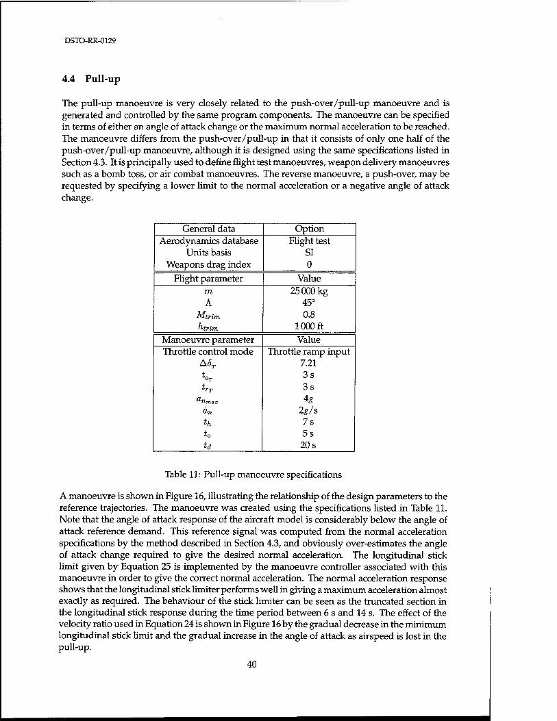
DSTO-RR-0129

4.4 Pull-up

The pull-up manoeuvre is very closely related to the push-over/pull-up manoeuvre and is generated and controlled by the same program components. The manoeuvre can be specified in terms of either an angle of attack change or the maximum normal acceleration to be reached. The manoeuvre differs from the push-over/pull-up in that it consists of only one half of the push-over/pull-up manoeuvre, although it is designed using the same specifications listed in Section 4.3. It is principally used to define flight test manoeuvres, weapon delivery manoeuvres such as a bomb toss, or air combat manoeuvres. The reverse manoeuvre, a push-over, may be requested by specifying a lower limit to the normal acceleration or a negative angle of attack change.


Units basis SI Weapons drag index 0


Mtrim 0.8 "-trim 1000 ft

Manoeuvre parameter Value Throttle control mode Throttle ramp input

AST 7.21

*0T 3s

tTT 3s Tlmax 4g an 2g/s th 7s to 5s td 20 s

Table 11: Pull-up manoeuvre specifications

A manoeuvre is shown in Figure 16, illustrating the relationship of the design parameters to the reference trajectories. The manoeuvre was created using the specifications listed in Table 11. Note that the angle of attack response of the aircraft model is considerably below the angle of attack reference demand. This reference signal was computed from the normal acceleration specifications by the method described in Section 4.3, and obviously over-estimates the angle of attack change required to give the desired normal acceleration. The longitudinal stick limit given by Equation 25 is implemented by the manoeuvre controller associated with this manoeuvre in order to give the correct normal acceleration. The normal acceleration response shows that the longitudinal stick limiter performs well in giving a maximum acceleration almost exactly as required. The behaviour of the stick limiter can be seen as the truncated section in the longitudinal stick response during the time period between 6 s and 14 s. The effect of the velocity ratio used in Equation 24 is shown in Figure 16 by the gradual decrease in the minimum longitudinal stick limit and the gradual increase in the angle of attack as airspeed is lost in the pull-up.

40

DSTO-RR-0129

a u _u "u o o < "as S o Z

6.0

4.0

2.0

0.0

-2.0

o

o u e <

0.0

-o 2 a •a.s s .ts o w

.2 .- gw E O Z

0.20

0.10 h

0.00

-0.10 |-

-0.20

-0.30

-0.40

0.0 5.0 10.0 15.0 Time (s)

5.0 10.0 15.0 Time (s)


-

I 1 1

- an max

lh - to : -

ld • ^ I 1 1 1

o

o > u

15.0

10.0

| 5"° o

20.0 0.0

I ' I ' I

Jv /■

i , i , i

0.0 5.0 10.0 Time (s)

IO.U ■ ■ i | i 1 ' 1

-

10.0 ^ ""*

\\ -

5.0 / \ -

n r\ i 1 , i

20.0 5.0 10.0 Time (s)

8000.0

0.0 5.0 10.0 15.0 Time (s)

10.0 Time (s)

15.0 20.0

20.0

20.0

Figure 16: Manoeuvre 4 — Pull up

41

DSTO-RR-0129

4.5 Level turns specified by normal acceleration or bank angle

In any realistic flight simulation, it is essential to have the capability to perform steady level turns. Such a manoeuvre is useful for general flight modelling, and more specifically for flight test and evaluation manoeuvres involving the collection of aerodynamic loading and drag data.

In this manoeuvre, turns are defined in terms of either the steady state normal acceleration anss

or steady state bank angle 4>ss. The difference is only cosmetic since a specified acceleration is converted to a bank angle for the turn via the relationship

4>ss = arccos ( I (28)

with the sign of <j>ss corresponding to the turn direction, that is, negative for left or positive for right. The criterion for termination of the turn can be either a desired duration of the turn, or a desired change in heading.

The design of the turn manoeuvre involves the specification of the following:

• whether a right or a left turn is required,

• whether the criterion for terminating the turn is the heading angle to be reached or the duration of the turn,

• the heading change Aip (°) during steady state banking or the banking duration tss (s),

• whether the turn is to be specified by bank angle or normal acceleration,

• the steady state bank angle <f>ss (°) or the steady state normal acceleration anss (g) at which to turn,

• the time delay t0 (s) before commencing the turn, and


Since the turn is steady and level, the true airspeed is held constant by a velocity controller which manipulates the throttle lever position. The normal acceleration, which was either specified or corresponds to the specified bank angle for the turn, is achieved by implementing an altitude controller, which manipulates the longitudinal stick position as a function of the departure of the aircraft altitude from the trimmed altitude at the commencement of the turn.

The bank angle is controlled by the bank angle controller by manipulation of the lateral stick position. The reference bank angle trajectory is generated by a second-order critically-damped filter. The natural frequency of the filter was chosen to give a maximum roll rate into or out of the turn which is consistent with both the maximum bank angle to be reached in the turn, and with the maximum roll rate capability of the aeroplane. The reference trajectory is given by

**w - (.^KL «,)**<•> (29)

where the natural frequency un = 1.5 rad/s. This filter is implemented digitally at 60 Hz integration frequency as

<j>ref(k) = 1.9506&e/(fc - 1) - O.95120re/(A; - 2) + 0.0003048<£re/(A; - 1) + 0.0003048<£re/(A; - 2). (30)

42

DSTO-RR-0129

The input 0re/ is a square wave input of two sequential steps coinciding with the roll into the turn and the roll out of the turn. A typical filtered reference trajectory is shown by the dashed bank angle time history in Figure 17.

If the turn is to be terminated when a prescribed change in heading is achieved, it is necessary for the program to predict the point at which to commence the roll recovery back to a wings level state which brings the aircraft onto the desired final heading after the turn is complete. As this phase is subject to the unpredictable coupled dynamics in the lateral motions of the aircraft, and since the whole turn is performed by depending on the altitude controller to give the correct normal acceleration and hence turn rate, the open loop nature of this task will rapidly lead to errors in heading both during and after the turn unless further closed loop augmentation is implemented. Accordingly, correction of heading drifts has been implemented by first generating an ideal reference heading function and then augmenting the bank angle reference trajectory to compensate for any departure from the ideal heading angle trajectory. The ideal reference heading function is modelled by

( rt

$ref =

y yfey tan <f>(t)dt while tp{t) <ip- 0.2r/vec

(31) ip thereafter

where the integrand in Equation 31 is the instantaneous turn rate, ip is the desired final heading angle, and iprec, the heading change predicted to occur during the roll recovery, is approximated by

^rec = Jo ^rtan(^M(c_WB* + *c"WB*))*, (32)

where the integrand is the instantaneous turn rate during the recovery, accounting for the exponentially reducing bank angle. The preliminary heading angle reference is then filtered to give the heading reference trajectory as

^'W = {s + Zls + uJ^{s) (33)

where that natural frequency u>n = 1.5 rad/s. This filter is implemented digitally at 60 Hz integration frequency as

il>ref(k) = 1.9506</Ye/(fc - 1) - 0.9512^re/(fc - 2) + 0.0003048^re/(A - 1) + 0.0003048^re/(fc - 2). (34)

Closed loop tracking of the heading angle is then achieved by empirically augmenting the bank angle reference trajectory

4>ref(t) = <f>ref(t) + 0.1 arctan(t/Ve/(*) - V'W) (35)

where the argument of the arctan function is evaluated in degrees. This augmented bank angle trajectory is then used as a reference to be tracked by the bank angle controller.

Equation 35 induces nonlinear augmentation of the bank angle reference with an increment of up to 9°. For example, a 1° heading error will induce a 4.5° of bank angle augmentation, while a 10° error will induce 8.4° of augmentation. The augmentation function was designed to have sufficient authority to correct departures from the heading reference without causing extreme bank angles which would make altitude tracking difficult, and without causing unrealistically

43

DSTO-RR-0129

high normal acceleration responses. All integrals are implemented using a fourth order Runge- Kutta integration algorithm.

Figure 17 shows an example manoeuvre and the reference trajectories used to generate it. The figure also relates the design parameters listed above to the shapes of the reference trajectories. The example manoeuvre was generated using the configuration, flight conditions, and design parameter data given in Table 12. The figure shows the reference heading angle trajectory used in the formulation of the bank angle augmentation. The effect of the augmentation can be seen in the bank angle trajectory, and its corrective action ensures that the specified final heading angle is achieved.




M-irim 0.8 "trim 1000 ft

Manoeuvre parameter Value Turn direction Right

Atp 90° anss 4g

to 3s td 30 s

Table 12: Turns specified by normal acceleration manoeuvre specifications

4.6 Level turns specified by angle of attack

Turns specified by angle of attack change are an unusual requirement, but are most likely to be needed in flight test situations for either aerodynamic analysis or systems assessment.


• whether a right or a left turn is required,

• the increase in angle of attack Ac* (°),

• the rise time tr (s) for the angle of attack to reach the steady state value for the turn and the fall time tf (s) taken to return to the trim value on completion of the turn (the fall time must not be less than the rise time),

• the hold time th (s) for which the steady state elevated angle of attack is to be maintained (excluding the rise and fall times),


44

DSTO-RR-0129

c a

pq

100.0

50.0

0.0

-50.0 0.0

c <

-a a u X

150.0

100.0 -

50.0

0.0

-50.0 0.0


/l^~

I I

<t>Ss -

If A -

' l«

-

. lo^ ■*'*" ld. .,. » "^ I i

1020.0

0.8

10.0 20.0 Time (s)

30.0

10.0 20.0 Time (s)

30.0 0.0

0.0 10.0 20.0 Time (s)

10.0 20.0 Time (s)

10.0 20.0 Time (s)

30.0

30.0

30.0

30.0

Figure 17: Manoeuvre 5 — Level turn specified by normal acceleration or bank angle

45

DSTO-RR-0129

• the duration tj (s) of the manoeuvre.

The manoeuvre involves increasing the angle of attack by the increment Aa at a specified rate, holding the new angle of attack for the specified hold time th, and then returning to the trim angle of attack cttrim- This preliminary angle of attack reference trajectory is passed through the first order filter defined in Equation 26 to achieve a suitable level of smoothness in the reference trajectory. The aircraft is forced to track the resulting angle of attack reference trajectory, aref, by the angle of attack controller, through manipulation of the longitudinal stick position. Meanwhile the true airspeed is held constant by the velocity controller.

The bank angle is forced (by the bank angle controller) to track a reference trajectory which is generated from

&trim \ (j)ref(t) = arccos aref(t)

(36)

where the ratio of the instantaneous reference angle of attack to the trim angle of attack is used to approximate the instantaneous normal acceleration. The true normal acceleration cannot be used to generate a bank angle reference trajectory because this would introduce additional nonlinear feedback for which stability could not be guaranteed.



Flight parameter Value 771 25000 kg A 26°

■M-trim 0.6 "trim 10000 ft

Manoeuvre parameter Value Turn direction Right

Aa 6.6° bf Is

*f 2s th 10 s to 3s td 20 s

Table 13: Turn specified by angle of attack manoeuvre specifications

A manoeuvre generated with the configuration, flight condition and manoeuvre design data in Table 13, is illustrated in Figure 18. This manoeuvre has an angle of attack increase of 6.6° during the turn above the trim angle of attack of 3.3°, representing a turn of approximately 3g. It can be seen from the figure that the normal acceleration reaches a steady-state value of only approximately 2.7g. This highlights the fact that the altitude response of the aircraft in this manoeuvre is open loop. The altitude decreases rapidly after an initial increase due to the steady state normal acceleration being less than sufficient to achieve a steady level turn. Although the nature and purpose of this manoeuvre do not necessarily require an accurate

46

DSTO-RR-0129


o

O

c <

00

u o

<:

o 0.0

0.0 5.0 10.0 Time (s)

10.0 Time (s)

15.0

100.0

50.0 b0 E < C a «

20.0 -50.0

a Ü a 0.5 es o ►J- T3 en u O 2 0i

0.0

la g co -0.5

20.0 -1.0

0.0

10100.0

10000.0 ID

■o s

20.0

9900.0

9800.0

o a. u > U

►J

o IM

20.0 0.0

5.0

5.0

10.0 Time (s)

10.0 Time (s)

15.0

15.0

20.0

20.0

20.0

20.0

Figure 18: Manoeuvre 6 — Level turn specified by angle of attack

47

DSTO-RR-0129

steady altitude response, this open loop nature needs to be borne in mind by the user when specifying this manoeuvre.

4.7 Altitude change

Altitude change manoeuvres allow smooth transitions between altitudes. The altitude change can be either an ascent or a descent with the user being responsible for the speed at which the change is made, as defined by the maximum or minimum normal acceleration at which to commence the pull-up or push-over into the climb or dive respectively.

The manoeuvre can be flown at either constant true airspeed or constant throttle lever setting. Constant airspeed is achieved by employing the velocity controller to regulate airspeed. The altitude change is achieved by using the altitude controller to force the aircraft to follow a specified altitude reference trajectory by manipulating the longitudinal stick position, subject to a number of constraints.

The altitude reference trajectory is generated by taking the step response of a second order critically damped filter, with the natural frequency tailored to give the specified normal acceleration at the commencement of the pull-up or push-over, subject to the limitation that there must be sufficient excess thrust available to achieve a constant velocity climb if that option was chosen. If the constant velocity altitude change option was chosen, then the natural frequency of the filter is chosen to conform with either the maximum available climb rate in the specified flight condition, or the requested normal acceleration, whichever is the limiting factor. The reference trajectory produces a response that asymptotically approaches the target altitude, while achieving 95% of the required altitude change within a realistic manoeuvre time. The manoeuvre realistically represents a true altitude change manoeuvre, reflecting both the normal load factor and the maximum climb rate capabilities of the aircraft.

The altitude reference trajectory is generated by the filter

n

where the preliminary reference href(s) = Ah/s is a step input of magnitude Ah, which is the desired change in altitude.

Two contenders are considered for the natural frequency of the filter, reflecting the potential limitations imposed by the normal load factor, and the maximum available climb rate. The former reflects the maximum vertical acceleration that will result during the reference altitude change. This is determined from the second derivative of the time domain response of the filter. The natural frequency is chosen such that the maximum (or minimum) vertical acceleration conforms with the specified limiting normal acceleration aniim (maximum for a climb or minimum for a descent) for the manoeuvre, as follows:

Kan {aniim - l)g Ah (38)

The natural frequency corresponding to the maximum climb rate limitation is formulated such that the first derivative of the time domain response of the filter conforms with the maximum available climb capability of the aircraft in the given flight condition. This is a function of the

48

DSTO-RR-0129

aircraft mass m, the excess thrust (the difference between the required thrust in trimmed flight Ttrim and the maximum available thrust Tmax at the current altitude), and the true airspeed V:

"-T * {-'■max ~ J-trim)e /OQ\

"T mgAh

The empirical adjustment factors Kan and KT are included to allow for the difference between the actual aircraft response (which is affected by response time lags and induced drag) and the ideal response required by the reference trajectory. Their values were determined via experimental simulations and assigned as follows:

Kan = 1.3 (40)

' 0.90 for h< 10000 ft 0.85 for 10 000 ft <h< 20 000 ft (41) 0.80 for h> 20 000 ft.

KT —

Once the two natural frequency contenders have been computed, the smaller value is chosen as the natural frequency for the filter, reflecting the slower response, commensurate with the relevant limiting factor.

With the reference trajectory as given in Equations 37 to 41, the normal acceleration limits should not be exceeded. However, as a precautionary measure, upper and lower bounds are imposed on the longitudinal stick position according to the Equation 25.


• the change in altitude Ah (ft) (negative for a descent),

• the maximum normal acceleration anmax (g) during the pull-up,

• the minimum normal acceleration anmin (g) during the push-over,

• whether the altitude change is to be performed at constant velocity or constant thrust (constant throttle position). If constant velocity:

- whether an upper limit is to be placed on the throttle lever position, and

- the value of the throttle position upper limit,

• the time delay t0 (s) before commencing the altitude change, and


If the manoeuvre is to be flown at constant true airspeed, that is, with the true airspeed controller engaged, then an option can be taken to place an upper limit on the throttle lever position to be achieved during the manoeuvre. This facility has been included because in normal operational flight, a pilot will generally restrict throttle movements to the military thrust range to minimise fuel burn. Accordingly, the user may specify a throttle position limit of 5 for military thrust, or any other desired limit (see Section 2.2.5). If an upper limit (other than the default maximum of 15) is placed on the throttle lever position, the altitude reference filter natural frequency contender associated with the available thrust, as formulated in Equation 39, is computed with a value of Tmax corresponding to the maximum available thrust at the specified throttle position upper limit.

49

DSTO-RR-0129

Figure 19 shows a typical altitude change manoeuvre, together with the altitude and true airspeed reference trajectories. The configuration, flight condition and manoeuvre design data used to specify this manoeuvre are listed in Table 14.



Flight test SI 0


■Mtrim

30000 kg 50° 0.8

1000 ft

Manoeuvre parameter Value Ah

Tlmax

On • nTnm

Throttle control mode Throttle lever limit

to td

4000 ft 4g 0g

Constant velocity Default (15)

4s 40 s

Table 14: Altitude change manoeuvre specifications

4.8 Dive and climb

This manoeuvre has been designed to allow the definition of individual dive or climb manoeuvres or combinations of both in either order. The manoeuvre differs fundamentally from the altitude change in that dives and/or climbs can be as long as desired, but defined by a steady state flight path (climb or dive) angle.

Dives and climbs are specified by the dive and/or climb angles and the maximum and minimum normal accelerations to be exerted during the pull-up and push-over. In addition, the extent of the dive and/or climb is defined by specifying the minimum and maximum altitudes to be flown during the manoeuvre. The manoeuvre generation accounts for altitude gained or lost in pull-ups and push-overs such that the minimum and maximum altitudes specified are achieved as closely as possible.


• whether the manoeuvre is to be flown at constant true airspeed or to use a throttle movement defined by the following:

- whether to use a step change or ramp change in throttle position,

- the magnitude AST of the change in throttle position,

- the time delay t0x (s) before throttle movement, and

50

DSTO-RR-0129

"O 3

C _o 08

U 13 o o <

o

5000.0

4000.0

3000.0

2000.0

1000.0

0.0

T3 3

c o

0.0


- I ' I i_

- - - - -

A Ah:

—

3*>* - - / /

V - -

I I ^ I

6.0

5.0

4.0

3.0

2.0

1.0

0.0

-1.0

-2.0 0.0

-0.40 0.0

10.0 20.0 30.0 Time (s)

10.0 20.0 30.0 Time (s)

10.0 20.0 30.0 Time (s)

40.0

• I ' 1 i - . -

/ \ "max -

I -

- ''min

- - - - i I

- 40.0

40.0

274.0

^ 272.0 E ^ 270.0

S 268.0

•I 266.0 - § 264.0

£ 262.0

260.0

J3

u "5b

E

0.0

o

u > u J

20.0

■5S 15.0 -

10.0

30.0

20.0

10.0

-10.0 0.0

10.0 20.0 Time (s)

30.0 40.0

20.0 Time (s)

40.0

10.0 20.0 Time (s)

30.0 40.0

Figure 19: Manoeuvre 7 — Altitude change

51

DSTO-RR-0129

- the throttle rise time tTT (s) (minimum 0.5 seconds for a step change),

• whether to perform a dive or climb or both,

- if both, whether to dive and then climb or vice versa,

• the dive angle jmin (°),

• the climb angle jmax (°),

• the minimum altitude hmin (ft) to be reached during the pull-up recovery from a dive,

• the maximum altitude hmax (ft) to be reached during the push-over recovery from a climb,

• the maximum normal acceleration anmax (g) to be experienced (during a pull-up),

• the rmnimum normal acceleration anmin (g) to be experienced (during a push-over),

• the time delay t0 (s) before commencing the initial climb or dive, and


The climb angle reference trajectory is generated by a second order critically damped filter. This results in the flight path angle exponentially approaching the specified steady-state climb and dive angles. The natural frequency of the filter is given by

^'(S) = Ä^^(S) (42)

where the preliminary reference %ef(s) consists of a step doublet for each of the climb and dive

segments, with magnitudes yma.x and 7min respectively. The natural frequency of the filter is chosen so that the maximum rate of change of the flight path angle (the first derivative of the time domain response of the reference trajectory filter defined in Equation 42) is consistent with the specified maximum and minimum normal load factors for the climb and dive respectively. For a climb segment of the manoeuvre, the natural frequency of the filter is computed as

W"-.3679F(7max-7o) ^

where % is the flight path angle which exists before the aircraft enters the climb. Similarly, for a dive, the natural frequency is computed as

= Kan{anTnin-l)g 0M79V(lmin-%Y ^

The empirical factor Kan =1.3 has been introduced to account for the natural time lags in the aircraft response, and to tune the response of the aircraft to meet the input specifications.

Bringing the aircraft back to steady wings-level flight at the end of the manoeuvre is performed by whichever of Equations 43 or 44 is relevant, with jmin or jmax replaced by zero.

At the end of a climb (dive), the dive (climb) or level-out that follows is commenced at a point Ahrec below (above) the specified maximum (minimum) altitude. The quantity Ahrec is given by

Aftrec=F^-COS^ (45)

52

DSTO-RR-0129

for recovery from a climb, or

£±">re.c. — V2(l COS7„

(46) (°nmin - l)g

for recovery from a dive. It represents the altitude gained or lost during the ensuing recovery to level flight or entry into the next dive or climb segment. Pre-empting this altitude increment ensures that the aircraft achieves the specified maximum and minimum altitudes as closely as possible.

Although the reference trajectory designed according to the above development will in theory generate the specified normal accelerations, an additional hard limit on the longitudinal stick position has been implemented according to Equation 25 to ensure that the specified normal acceleration limits are not violated.




"i-trim 0.8 "-trim 15000 ft

Manoeuvre parameter Value Throttle control mode Constant velocity

Throttle lever limit None Dive/climb mode Climb/dive

Tmin -25° 'Ymax 20° ftmin 20000 ft i^max 25000 ft anmax 4# anmin 0g

to 10 s td 100 s

Table 15: Dive and climb manoeuvre specifications

Figure 20 shows an example climb/dive manoeuvre designed with the configuration, flight condition and manoeuvre design data listed in Table 15. This also shows the relationships between the design parameters and the reference trajectories. The operation of the hard limits on the longitudinal stick position can be seen as the flat sections at the extremes of the longitudinal stick travel.

4.9 Altitude change and turn

The altitude change and turn manoeuvre allows the user to specify a single manoeuvre combin- ing the features of the altitude change manoeuvre of Section 4.7 and the level turn manoeuvre

53

DSTO-RR-0129


to c <

u -:

40.0

30.0

20.0

10.0

0.0

10.0

20.0

-30.0

-40.0

1 1 1 1 ' i • - -

- 'max

- j A . J \ - '/ A .

\\ . '/ .

_ \\ -— ,7 -

- h 7 ■ - min_

^ , 1 . 1 , 1 . 1 . ■—

0.0

oo

4> O o < e t-l o

6.0

4.0

2.0

0.0

-2.0

- 0.3

g>£ 0.0 o w

=s s -°-3

o 2

-0.6 0.0

30000.0

25000.0

•a 20000.0

< 15000.0

20.0 40.0 60.0

Time (s) 80.0 100.0

~i ' 1 ' 1 ' r

V

v V.

J . i_

1 D.

10000.0 c

320.0

300.0

0.0

u 280.0

1>

0.0 20.0 40.0 60.0 Time (s)

80.0 100.0

■t^ih o

OH

> ID

J2

260.0

240.0

220.0 C

20.0

15.0

10.0

5.0

0.0

. I ' i • I ' I '

- h max

- - - - h . ^

min

- i i.i. I

20.0 40.0 60.0 Time (s)

80.0 100.0

20.0 40.0 60.0 Time (s)

80.0 100.0

20.0 40.0 60.0 Time (s)

80.0 100.0 0.0

I I I I , I ' I '

A

I I.I,'

> \f- , I , I , i , i

0.0 20.0 40.0 60.0 Time (s)

80.0 100.0

Figure 20: Manoeuvre 8 — Dive and climb

54

DSTO-RR-0129

of Section 4.5. The only restriction regarding the phasing of the two components is that the turn must begin after the altitude change has commenced. Unlike level turns, this manoeuvre permits specification of a constant throttle position throughout the manoeuvre, consistent with the pure altitude change manoeuvre of Section 4.7.

The generation of the altitude reference trajectory is the same as for the altitude change manoeuvre. The bank angle or normal acceleration trajectory and the heading trajectory are as described in Section 4.5. Closed loop heading tracking is ensured by augmenting the bank angle reference trajectory as for the level turn (see Section 4.5).

Limits are imposed on the longitudinal stick position to ensure that the specified normal acceleration limits are not violated. This is done in a similar way to that described in Section 4.3 (Equation 25) except that the diminishing effect of the gravity vector on the longitudinal behaviour of the aircraft due to banking must be accounted for. The full expression of the longitudinal stick limit is

n\ - ^Hm -cos7(t) cos (/>(*)) / grd \ A'~ 75 V V(t)J "—w=—-—K K^mJ- (47)

Imposing these limits is especially important in the altitude change and turn manoeuvre because the specification of a banked turn which coincides with the pull-up phase of the altitude change can briefly cause a condition in which a higher normal acceleration is required to achieve the reference trajectories than is permitted by the specified normal acceleration limits. A throttle lever upper limit may be specified for this manoeuvre, as discussed in Section 4.7 for the altitude change manoeuvre, to constrain throttle lever travel if desired.

The design of the manoeuvre involves the specification of the following information which comprises the relevant components from each of the two separate manoeuvres:

• the altitude change Ah (ft),

• the maximum normal acceleration anmax (g) (during pull-up),

• the minimum normal acceleration anmin (g) (during push-over),

• whether the manoeuvre is to be flown at constant thrust (throttle position) or constant airspeed. If constant airspeed:

- whether an upper limit is to be placed on the throttle lever position, and - if so, the value of the throttle position upper limit,

• the altitude h0 (ft) to start the turn relative to the initial altitude (i.e. 0 < h0 < Ah),

• whether a right turn or a left turn is required,

• whether the criterion for terminating the turn is the heading angle to be reached or the duration of the turn,

• the heading change Aip (°) or the banking duration tss (s),

• whether the turn is to specified by bank angle or normal acceleration,

• the steady state bank angle 4>ss (°) or normal acceleration an3S (g) at which to turn. (Note: anss or equivalent^ ^^ must be less than anmax),



55

DSTO-RR-0129

Figure 21 shows an example manoeuvre which incorporates a 4g pull-up from trimmed flight to an altitude of 5 000 ft. The configuration, flight condition and manoeuvre design parameters are listed in Table 16. At an altitude of 2 000 ft, a 3g turn through 120° heading change is performed while climbing. The normal acceleration time history shows that the specified normal acceleration limits are satisfied. The longitudinal stick position time history shows that the stick limiting function has been activated accordingly.




Mtriro 0.8 f^trim 400 ft

Manoeuvre parameter Value Ah 4600 ft Tlmax 4g "'■mzn 0g

Throttle control mode Constant velocity Throttle lever limit None

K 1600 ft Turn direction Right

Aip 120° anss 3g t0 12 s td 80s

Table 16: Altitude change and turn manoeuvre specifications

4.10 Hook turn

The hook turn turn is a specialised manoeuvre, adapted from the Mirage III-O manoeuvre controller program, which attempts to reverse the direction of flight of the aircraft, while returning the aircraft to its initial path over the ground. This is achieved by commencing a turn at a specified normal acceleration or bank angle, and in a specified direction, left or right. The turning direction is reversed after a heading change of 90° is achieved, and is continued at the same normal acceleration or bank angle until a further heading change of 270° is achieved in the opposite direction to give a net heading change of 180°.

56

DSTO-RR-0129


6000.0

3

00

c _o

u

o ü <

o -2.0

0.0

0.30

■a

■g> o o.oo O 'tn

.52 !H -0-30 ion

o 2 -0.60

0.0

274.0

272.0 T3 <u D Ui 270.0 l-i

< 3 268.0 H

266.0

20.0 40.0 60.0 Time (s)

20.0 40.0 Time (s)

60.0

40.0 Time (s)

80.0

80.0

80.0

80.0

-40.0 0.0

"5b e < c

•5 cd eu X

150.0

100.0

50.0

0.0

-50.0 0.0

03 IM

C3 O 0? HJ'C

0) P 00 «i O-i

13 -0.2 :w

-0.4

-0.6 0.0

20.0

■3 15.0 o IM

> 10.0 -

o Ja

0.0

20.0 40.0 60.0 Time (s)

80.0

1 1 i [ i | i

T - / /

Ay / / ~ // - / /

L <y

I i.i.

20.0 40.0 60.0 Time (s)

20.0 40.0 Time (s)

20.0

80.0

60.0 80.0

40.0 60.0 Time (s)

80.0

Figure 21: Manoeuvre 9 — Altitude change and turn

57

DSTO-RR-0129


• whether the initial turn is to be to the left or to the right,

• whether the turn is to specified by bank angle or normal acceleration,

• the steady state bank angle 4>ss (°) or normal acceleration anss (g) at which to turn,



The bank angle reference is generated by the same filter used in the level turn manoeuvre, as defined in Equation 29, where the preliminary bank angle reference <j>ref is a step doublet of magnitude <f>ss. This is either the specified bank angle or is determined from the specified normal acceleration as in Equation 28. Each segment of the step doublet is terminated when the heading goals described above are achieved.

Due to the coupling effects excited in the lateral dynamics during recovery to wings level flight at the end of the manoeuvre, the final heading may not be precisely reversed. It would be possible to implement an augmented bank angle reference trajectory similar to that used in the turn manoeuvre of Section 4.5 (Equation 35) to close the loop on the final heading. However, no effort has been made to do so because this manoeuvre is the least used of the manoeuvre suite.

Figure 22 illustrates an example hook turn manoeuvre generated with the configuration, flight condition and manoeuvre specifications listed in Table 17.



Flight test SI 0


"•trim

30000 kg 35° 0.6

1000 ft Manoeuvre parameter Value

Turn direction anss

to td

Left 2g

10 s 100 s

Table 17: Hook turn manoeuvre specifications

58

DSTO-RR-0129


c < e es m

100.0

50.0

0.0

-50.0 -'

-100.0

1050.0

1000.0

-o

5j 950.0

0.0

6000.0

u cS 4000.0

's O o

r i 2000.0

'S es

0.0

-2000.0

204.0

•O 203 u u a.

.5

u 3

203.0

202.5

20.0 40.0 60.0 80.0 100.0 Time (s)

900.0 0.0 20.0 40.0 60.0 80.0

Time (s) 4.0

0.0 20.0 40.0 60.0 80.0 100.0 Time (s)

"0.0 4000.0 8000.0 12000.0 Northward Coordinate (m)

0.0 20.0 40.0 60.0 80.0 100.0 Time (s)

c o 3.0 es <u <ü ?0 o o <

C3 1 n b UH o Z 0.0

0.10 cs c

T3 oon 3 _ 'S c

'60 2 C *j -0.10 O en J o

-0.20 -S2 ^ ^ -0.30 Ui

O 2 -0.40

10.0 c o

■w 8.0 w o

OH 6.0 U > D -! 4.0 V

o Ü.U

|5 0.0

100.0

0.0 20.0 40.0 60.0 80.0 Time (s)

100.0

100.0

0.0 20.0 40.0 60.0 80.0 Time (s)

100.0

Figure 22: Manoeuvre 10 — Hook Turn

59

DSTO-RR-0129

5 GENERAL MANOEUVRES

In addition to the suite of in-built manoeuvres described in Section 4, three additional manoeuvre options are available which allow the user to specify a specialised manoeuvre in terms of generalised spatial reference trajectory coordinates. The three available options permit specification of the manoeuvre in terms of flight time and any one of three reference trajectory triplets:

true airspeed V (m/s), bank angle <f> (°), and altitude h (ft);

true airspeed V (m/s), bank angle <j> (°), and normal acceleration an {g); or

Northward Xe (m) and Eastward Ye (m) Cartesian spatial coordinates, and altitude h (ft).

The data are supplied to the program in the data file v track. dat' in four column free format. These manoeuvre specification options and the formulations of their reference trajectories are described in detail in the following sub-sections.

It is feasible that the reference trajectories may be obtained from any of several sources. Possi- ble sources of reference trajectory information include digitised flight plans, optimal trajectory algorithms, or previously recorded flight paths from actual F-111C flights or from flights performed in a simulator. In addition, previous output trajectories from the F-111C Manoeuvre Controller Program or from the AOD F-111C Flight Dynamics Model may be used as reference trajectories. Data may also be synthesised using interactive plotting packages (for example [46]). However, there is a requirement that the degree of smoothness of the reference data must be compatible with the degree (say n) of the dynamic subsystem that is required to track them, in order to avoid unrealistic control input demands. Therefore the reference trajectory that is created must have the dynamic characteristics of the output of an n th order system. In other words, the first n derivatives of the reference trajectory must be continuous. For instance, since the dynamic characteristics of the relationship between longitudinal stick position and altitude is of degree n = 3, the first three derivatives of the reference signal must be continuous. Sufficiently smooth reference trajectories can be created by passing raw data through a filter of sufficient order. Such signal processing capabilities are available in most data handling and graphics packages (see [46] for example).

An example manoeuvre has been designed to illustrate the relative performance of the manoeuvre controllers for each of the manoeuvre specification triplet options. The example consists of a level turn commanded by normal acceleration followed by an altitude change and turn. The manoeuvre was generated with the configuration, flight condition and manoeuvre specifications listed in Table 18. The manoeuvre was first generated as a sequence of the two discrete manoeuvres described in Sections 4.5 and 4.9. These manoeuvres are specified in terms of bank angle, altitude and true airspeed reference trajectories. Therefore the reference trajectories used to define the three manoeuvre options in the following sections used the reference trajectories generated for discrete manoeuvres where possible. In cases where the manoeuvre is specified in terms of other reference trajectory triplets, for instance Cartesian coordinates, the corresponding trajectories resulting from the simulation of the discrete manoeuvres are used as reference trajectories.

60

DSTO-RR-0129

General data Option Aerodynamics database Wind tunnel



M-trim 0.7 il'trim 400 ft

Manoeuvre 1 parameter Value Turn direction Right

*ss 18 s anss 3s

*o 2s td 30 s

Manoeuvre 2 parameter Value Ah 2000 ft

Umax 4g arimin 0g

Throttle control mode Constant velocity Throttle lever limit None

h0 1000 ft Turn direction Left

tss 18 s anSs 2g

to Is td 50 s

Table 18: General manoeuvre generation specifications for a level turn followed by an altitude change and turn

61

DSTO-RR-0129

5.1 Specification by true airspeed, bank angle and altitude

In the study of operational manoeuvres, the two foremost flight variables considered as candi- dates for manoeuvre definition are the true airspeed and altitude. In this manoeuvre, the true airspeed is controlled by the velocity controller by manipulation of the throttle lever position, while vertical motion is determined by the specification of an altitude reference trajectory and controlled by the altitude controller via manipulation of the longitudinal stick position. The lateral horizontal motions are determined by the specification of a bank angle reference trajectory to be tracked by the bank angle controller via lateral stick position movements.

Although this may be the most useful manoeuvre specification system for relatively gentle manoeuvres, it is subject to limitations, and may not be suitable for more vigorous manoeuvres. The first restricts the aircraft bank angles to the range -90° < <j> < 90° to avoid a singularity condition. This singularity limitation arises because the axes in which the altitude reference and the aircraft lift vector are defined are not always coincident, and are in fact orthogonal when <f> = ±90°. When this occurs, the lift vector, which is the primary manoeuvring force, no longer has any direct influence on the altitude. Manoeuvres which are likely to exceed these limitations, such as any that involve bank angles outside this range, may be better modelled by specification of the longitudinal motions in terms of normal acceleration as discussed in Section 5.2. In fact any manoeuvre for which \<p\ exceeds approximately 75° may reach a higher than desired normal acceleration due to the sensitivity of the altitude controller when |</>| is large. Accordingly, it is imperative that the user ensures that the reference altitude changes which occur while \<f>\ is high are not extreme, and are achievable. Secondly, if a reference trajectory is specified in terms of true airspeed, bank angle and altitude, the actual flight path response of the aircraft model in terms of the Cartesian coordinates is open loop. Therefore, the model is not guaranteed to reproduce any preconceived flight path. Any flight requiring closed loop flight path tracking may be better modelled by specifying the reference trajectories in terms of the Cartesian coordinates Xe, Ye, and h, and implementing closed loop ground track control as described in Section 5.3.

To illustrate a manoeuvre specified by true airspeed, bank angle and altitude, the reference trajectories defining the flight composed of the discrete manoeuvres described in Table 18 have been used. The control of the manoeuvre is performed as in the discrete manoeuvres, and by the same controllers, except that the reference trajectories are being read from a file instead of being generated concurrently. The responses shown in Figure 23 are therefore identical to the responses resulting from the simulation of the discrete manoeuvres.

It can be seen that the bank angle and true airspeed responses are good. The altitude graph shows that the maximum altitude error is of the order of 60 ft. The resulting ground track, defined in terms of Northward and Eastward coordinates, is used as a reference trajectory for the example manoeuvre of Section 5.3.

5.2 Specification by true airspeed, bank angle and normal acceleration

The specification of a general manoeuvre by true airspeed, bank angle and normal acceleration allows much more flexibility in the types of manoeuvres that can be performed in comparison to the manoeuvre specification described in Section 5.1. The three reference trajectory quantities in this manoeuvre specification system and the influences of their respective control effectors remain perfectly correlated under all circumstances and are therefore not subject to the same

62

DSTO-RR-0129


100.0

50.0

"So c < M B a

DO

-100.0

-50.0

0.0

0.40

1^ gw -0.20

-0.40 0.0

5000.0

-7500.0

3000.0

« 2000.0

3

^ 1000.0

20.0 40.0 60.0 Time (s)

80.0 0.0

I

0.0 20.0

20.0 40.0 Time (s)

60.0 80.0

6.0 00

5.0 B O 4.0 C3 3.0 <D

O 2.0 O < 1.0 a 0.0 fa o -1.0 V

-2.0 0.0 20.0

40.0 Time (s)

40.0 Time (s)

0.20

-5000.0 0.0 5000.0 10000.0 Eastward Coordinate (m)

15000.0 40.0 Time (s)

1)

D.

O & u > o _l

o

15.0

10.0

5.0

236.0 40.0 60.0

Time (s) 80.0

0.0 0.0 20.0 40.0

Time (s)

60.0 80.0

60.0 80.0

80.0

60.0 80.0

Figure 23: General manoeuvre specified by true airspeed, bank angle and altitude

63

DSTO-RR-0129

singularity conditions that occur when specifying the manoeuvre in terms of altitude. This means that the bank angle and climb angle are free to evolve throughout their complete ranges (-180° to 180°), thus allowing inverted and vertical flight, neither of which are possible when using altitude as a reference for controlling the longitudinal dynamics of the aircraft model (see the discussion in Section 5.1).

The bank angle is controlled via the bank angle controller. True airspeed may be controlled through the true airspeed controller, or alternatively an option is available which allows the specification of throttle step or ramp movements. Normal acceleration is determined indirectly via the angle of attack controller or by direct longitudinal stick position prediction as described in Section 3.2.6. If the normal acceleration is to be controlled via the angle of attack controller, the normal acceleration reference trajectory is converted via the approximation of Equation 21 into an angle of attack reference trajectory. The imprecise nature of the conversion means that the actual normal load factor achieved may not be quite as specified, although the angle of attack will accurately track the angle of attack reference trajectory. Accordingly, the approach normally taken when using this manoeuvre specification option is an iterative one. To achieve the desired normal acceleration profile, a reference trajectory is prepared with a data processing and presentation package such as Xmgr (Ace/gr) [46]. The program then simulates the flight with the proposed input trajectory and the resulting normal acceleration response is compared with the desired normal acceleration profile (as opposed to the reference trajectory). The reference trajectory is then redesigned by increasing or decreasing the normal acceleration values where necessary until the model response agrees with the desired response. The number of iterations will depend upon the complexity of the manoeuvre and the accuracy required by the user in matching the response to the desired normal acceleration profile.

Alternatively, if the normal acceleration is to be determined via the steady state longitudinal stick position prediction of Equation 20, the response will usually follow the desired normal acceleration magnitude with sufficient accuracy. However, insufficient transient response speed resulting from the lack of transient stick position prediction and the time lags inherent in the normal acceleration response of the aircraft, typically of the order of 0.6 s, may be of concern. In order to minimise these effects, the normal acceleration reference trajectory may have to be either advanced in time relative to the true airspeed and bank angle trajectories and/or the rate of change of the reference signal may have to be increased where transients occur. This can be done prior to program execution with a data processing package, or alternatively, options have been included in the software which allow the user to either invoke a lead-lag filter to increase the onset rates of the transients in the reference trajectory, or invoke a 0.6 s time advance on the normal acceleration reference trajectory, or both. The lead-lag filter is primarily intended to overcome the lack of transient prediction in Equation 20, while the time advance is intended to account for the aircraft response lag. The time advance is only necessary if the objective is to reproduce a previously flown or simulated manoeuvre accurately, since manoeuvres that have been completely synthesised will normally have been designed to account for or pre- empt the response time lag. However, accounting for the lack of transient prediction given by Equation 20 is necessary in both cases.

The lead-lag filter increases the rate of change of the normal load factor reference trajectory during rapid changes. Its effect reduces as the rate of change of the normal acceleration reference decreases. It does not, however, shift the reference signal forward in time. The trajectory specified in the input file ' track. dat' is treated as a preliminary reference trajectory an,.

64

DSTO-RR-0129

The new reference trajectory aUref is the output of a lead-lag filter with the transfer function

anref (s) = 7^-[ö<e/ (s) • (48)

This filter has been implemented digitally at 60 Hz as

anref(k) = 13.6667o„re/(A) - 13.0000a„re/ (k - 1) + 0.3333a„re/(fc - 1). (49)

In general, prediction of the required longitudinal stick position using Equation 20 is superior to controlling the normal acceleration indirectly through the angle of attack controller. The latter approach is more sensitive to variations in trim flight condition and changes in flight condition during the manoeuvre, while the former approach is relatively independent of the changes in the aerodynamics of the aircraft due to the influence of the pitch control system.

Whichever approach is used, the initial reference trajectory will usually generate a reasonably good normal acceleration response which may be acceptable. Otherwise only a few iterations should be necessary. If further iterations are necessary, a stepwise procedure should be employed, working along the manoeuvre in segments rather than making gross alterations to the complete profile. This is because changing the early part of the manoeuvre will change the latter parts due to the variations in instantaneous flight conditions. A profile which initially is not satisfactory in the latter parts of the manoeuvre may well become so after the early part of the manoeuvre has been refined.

If the manoeuvre to be modelled involves high bank angles thus forcing the manoeuvre to be specified in terms of normal acceleration, but is otherwise aimed at achieving an altitude profile or a ground track profile rather than a normal acceleration profile, then the iterative procedure may become more protracted. Altitude may be particularly sensitive to normal acceleration since small changes in normal acceleration, resulting in small changes in climb angle, can cause significant changes in altitude. This is due to the velocity controller attempting to achieve the specified reference velocity profile, hence altering the climb rate and altitude through the engine thrust.

Figure 24 illustrates the manoeuvre described in Table 18 specified in terms of true airspeed, bank angle and normal acceleration, where the normal load factor is controlled via the angle of attack controller. The figure shows that despite the imprecision of the manoeuvre specification method, the magnitudes of the specified reference trajectory and the actual response are effectively related by a scale factor very close to 1 (i.e. an = \anref where A ss 1). The scale factor will of course be dependent on the flight condition since the angle of attack per g varies with Mach number and altitude. The normal acceleration response from Figure 23 was used as an initial normal acceleration reference trajectory, with further iterations aimed at improving the altitude and ground track responses. Only slight alterations to the initial reference trajectory were necessary between 12 and 23 seconds, and between 40 and 46 seconds, requiring four further iterations. The normal acceleration, altitude and ground track responses compare well with those shown in Figure 23.

Figure 25 illustrates the same example manoeuvre with the same reference trajectories, but with the normal acceleration determined by the longitudinal stick position prediction of Equation 20. The manoeuvre was performed using both the 0.6 s time advance, and the lead-lag filter to pre-empt the aircraft normal acceleration response lag and to augment the transient normal acceleration response. The responses shown in Figure 25 resulted from the first attempt to perform the manoeuvre. Although further refinement of the input reference trajectories may

65

DSTO-RR-0129

c < c re

100.0

50.0

0.0

-50.0

-100.0 0.0

0.40

re 1| 0.20 •a '« oj o .22 &* 0.00

6-S -0.20 -

-0.40 0.0

f= 5000.0

1) re 2500.0

"a o o U

0.0

'S re -2500.0

4-1 -5000.0 o 2

-7500.0 -5(

239.0 /■—i

t 238.5

u 238.0

237.5

< 237.0

236.5

236.0 0.0

20.0

20.0

Aircraft control inputs and response ■ — Reference trajectories Original manoeuvre trajectories

-r 1 l 1 '

\

i '

i 1 I

(

- L i : id , i.i. i

3000.0

3

2000.0 -

< 1000.0 -

40.0 60.0 Time (s)

80.0

s _o re w

JZ "53 o o <c

o

40.0 60.0 Time (s)

80.0 -2.0

0.0 20.0 40.0 60.0 80.0 Time (s)

0.0 5000.0 10000.0 15000.0 Eastward Coordinate (m)

0.0 20.0 40.0 60.0 80.0 Time (s)

o OH

> ID

►J 4>

15.0

10.0

20.0 40.0 60.0 Time (s)

80.0

« 5.0

o J2

0.0 20.0 40.0 60.0 80.0

Time (s)

Figure 24: General manoeuvre specified by true airspeed, bank angle and normal acceleration, with normal acceleration determined by the angle of attack controller

66

DSTO-RR-0129

"ob c < c CO

pa

100.0

50.0

0.0

-50.0

-100.0 0.0

0.40

1 § 0-20

§ CL, 0.00

O ^ -0.20

-0.40 0.0

g 5000.0

os 2500.0

20.0 40.0

Time (s) 60.0

20.0 40.0 60.0

Time (s)

Aircraft control inputs and response Reference trajectories Original manoeuvre trajectories

:r— I ' 1 ' i '

LJ { t«.

, I,I. i

3000.0

80.0

80.0


15000.0

239.0

? 238.5

TT 238.0 a

& 237.5

< 3 H

237.0

236.5

236.0 0.0 20.0 40.0

Time (s) 60.0 80.0

80.0

80.0

80.0

80.0

Figure 25: General manoeuvre specified by true airspeed, bank angle and normal acceleration, with normal acceleration determined by longitudinal stick position prediction

67

improve the altitude performance, comparison of the the trajectory responses with those in Figure 24 suggests that further improvement may be unwarranted. Indeed experience has proven this approach to be preferable in terms of efficiency.

5.3 Specification by Cartesian spatial coordinates

Specification of a reference manoeuvre via its Cartesian spatial coordinates allows the user to define a flight or manoeuvre based on an intended ground track/altitude combination. Such an exercise might be required for instance in a mission planning application to investigate the aircraft behaviour associated with a particular route, or perhaps to repeat or reconstruct a previous flight based on a known ground track/altitude combination. The purpose of such an exercise might be to determine the evolution of aircraft states such as the attitude angles, rotation rates, airspeed, incidence angles (a and ß) and normal acceleration throughout the flight, as well as to determine the control stick and control surface movements and thrust variations required to achieve the desired manoeuvre.

The manoeuvre is specified as a generalised trajectory defined in terms of the Cartesian spatial coordinates Xere/(m) and Yere/(m), being the Northward and Eastward locations with respect to the starting point, together with the altitude /ire/(ft). The altitude is directly controllable through the altitude controller. However, in order to make this manoeuvre achievable, the preliminary reference trajectories Xeref and Yeref must first be converted into reference states which are directly controllable through the aircraft control system. Accordingly, Xeref, Y£ref

and href(m) (=/m/ire/) are used to formulate reference true airspeed and bank angle trajectories by first differentiating to give X€ref, Yeref and href. A preliminary true airspeed reference is then

Vref = ]/xlef + Y£ef + href. (50)

The objective in determining a bank angle reference trajectory is to align the net unbalanced force vector acting on the aircraft with the instantaneous radius of curvature of the reference flight path. This involves determination of the vertical and horizontal curvature components. Initially the instantaneous pitch angle and heading angle of the flight path are computed from consecutive points of the reference trajectories from

(51) Kef = arctan ( Kefjk)-href(k - 1) \((Xref(k) - Xref(k - 1))2 + (Yref(k) - Yref(k - l))*f2

and

j, f - arctan (*ref{k) - Xref{k - 1)\ 1W - arctan ^ y^(jfc) _ y^ _ ^ j (52)

where k denotes the current value, and k - 1 the previous value of each reference trajectory.

Differentiation then gives 9ref and rpref, the rates of change of the flight path pitch and heading angles respectively.

Due to the sensitivity of the differentiation process in determining the rates of change of both the ground track velocity components and the flight path pitch and heading angle rates, they are then passed through second-order Butterworth filters to smooth the irregularities in these

68

DSTO-RR-0129

signals. The filters are

ul Vref(s) = " 2 W«) (53)

ul sz + ^2u)ns + u)^

ul Aef(s) = _ " ^ 2 </Ve/(*) (55)

where u)n = -K has been used to give the required smoothness in the reference signals while minimising the time lag introduced by the filters. These filters are implemented digitally as

Vref(k) = 1.8523Vrre/(ifc-l)-0.8625Vr

re/(Ä;-2)+0.005100Fre/(A;-l)+0.005100Fre/(/i;-2), (56)

with similar expressions for 6ref(k) and ipref(k).

The instantaneous vertical and horizontal components of the normal acceleration are determined from their physical relationships to the flight path angular rates,

= OrefVrel + l

g

ah = ^SiM. (58) g

The reference bank angle is then computed from these components:

<t>ref = arctan f — j . (59)

It should be noted that this transformation is sensitive to small rapid variations in the Xref and Yref coordinates. This arises because a small variation in the lateral component of the resultant normal load factor may cause significantly large variations in the resultant bank angle reference trajectory due to the nonlinearity of the transformation in Equation 59. Care should therefore be taken when preparing the reference trajectories, to ensure that the reference trajectories are sufficiently smooth, and that the manoeuvre is attainable by the aircraft. The manoeuvre controller cannot force the aircraft model to follow a manoeuvre which the aircraft is not physically capable of achieving. It is suggested that if a flight path is to be built from discrete points along a ground track, the trajectories should be produced by using either a smooth tension spline fit to the data or a regression fit of suitable order, preferably the former. Alternatively, if a flight path from recorded flight data or from a previous simulation is used, the computed reference bank angles, and the aircraft response to them, will reach higher bank angle values than the aircraft behaviour that produced the reference flight path. It is generally true that normal acceleration responses resulting from altitude control at high bank angles will reach higher levels than those of the original flight or simulation. Thus this option of program operation should generally be restricted to relatively gentle manoeuvres which require a maximum normal acceleration no greater than 3g, in order to avoid exceeding the normal acceleration limits of the aircraft, unless constraints are placed on the normal acceleration. The placing of such constraints will be discussed in Section 5.3.2.

69

DSTO-RR-0129

5.3.1 Ground track augmentation

It should be noted that due to the transformation from Cartesian coordinates to bank angle and true airspeed reference trajectories, the ground track of the aircraft becomes open loop. That is, due to the difference between the bank angle and airspeed reference trajectories and the respective aircraft responses, the ground track is subject to integration errors. Therefore an option has been included which allows closed loop tracking of the ground track reference trajectory by augmenting the bank angle and airspeed reference trajectories with increments that are dependent upon the departure of the aircraft ground track from the reference ground track.

The augmentation functions are formulated from the Cartesian components AX and Ay of the error between the actual aircraft ground track and the reference ground track. These are converted into distance error components Adn and Adt normal to and tangential to the aircraft ground track respectively, through the coordinate transformations

Adn = -AXsiaxp + AYcxtsi/; (60)

Adt = AX costp + AY sin ip. (61)

Empirical augmentation functions have been devised based on a pseudo-true airspeed error and a pseudo-heading error defined as

AV = ** (62)

where TV and T^ are time based parameters, AV has units of m/s, and Atp is in degrees. The velocity and bank angle reference trajectories are augmented by

Vref = V;e/-|-0.05arctanAF (64)

4>ref = <Pref + 0-2 cos <f)ref arctan Aip. (65)

The reason for including the nonlinear arctangent functions is to weight the importance of a departure from the reference flight path. That is, large corrective inputs are only generated when this departure, represented by AV and Aip, appreciably exceeds a threshold level. The time based parameters TV and T^ in Equations 62 and 63 are both set to a value of 10 s. Their role is to set the threshold levels by, in the former case, normalising the tangential ground track error with respect to 10 s of flight to give a reference airspeed augmentation, and in the latter case, by normalising the normal ground track error with respect to the distance travelled by the aircraft in 10 s to give a reference heading augmentation. This behaviour mimics the behaviour of a pilot, who will not be concerned with the departure of the aeroplane from the intended ground track until the departure exceeds some unacceptable level, at which time he/she will take immediate and rapid corrective action.

The constant preceding the nonlinear term in Equation 64 is a weighting which sets the maximum airspeed reference trajectory augmentation to be 4.5 m/s. The constant preceding the nonlinear terms in Equation 65 is a weighting which sets the maximum bank angle reference trajectory augmentation to be 18° when the preliminary reference trajectory commands zero degrees bank. The first nonlinear term (cos2 (j)ref) in Equation 65 is designed to reduce the maximum bank angle augmentation as the value of the preliminary reference trajectory increases.

70

DSTO-RR-0129

This is necessary because the normal acceleration required to maintain altitude increases nonlinearly with the inverse of the cosine of the bank angle. The complete augmentation function is designed to give bank angle augmentation of ±1.125° in the vicinity of a nominal 75.5° (4g) bank, ±2° in the vicinity of a nominal 70.5° (3g) bank, and ±4.5° in the vicinity of a nominal 60° (2g) bank. In each case the augmentation limits are equivalent to ±0.33g increments in the normal acceleration.

5.3.2 Normal acceleration constraints

Characteristic lags and overshoots arise in the responses of the filters presented in Equations 54 and 55 that, if not curtailed, can lead to unrealistically high normal acceleration responses from the aircraft model for short periods. In particular this occurs during periods of rapid manoeuvring, principally during high-rate rolls to high bank angles. The extreme sensitivity in normal acceleration is due to the nonlinear relationship between normal acceleration and steady state bank angle (see Equation 28). If the overshoots are not curtailed, the temporary high bank angles provoke an extreme response from the altitude controller in an attempt to regain the altitude reference trajectory, resulting in unrealistically high normal load factors.

This behaviour has been dealt with by introducing an option selectable at the commencement of the program execution, which sets two normal acceleration limits. The first is a normal load factor limit anturn that is placed on turns. This limit is implemented in the form of a restriction on the reference bank angle

\<f>refmax I = arccos ( ) (66)

and is evaluated with a sign consistent with the turn direction, that is, with the same sign as anh. Whenever the absolute value of the filtered bank angle reference demand exceeds the specified value of \4>refmax 1/ the reference is truncated to have the same absolute value as \4>refmax I-

The second normal load factor limit anmax is an overall limit that is used to prevent the instantaneous normal acceleration from exceeding the specified value. This is implemented by formulating a limit Sioniim on the longitudinal stick position by steady state analysis of the pitch control system loop, as

A (A (anmax-cos j(t) cos 4>(t)) ( grd \ 6ionHm(t) = (4 + W) j . (67)

The value of this function, for any normal acceleration greater than cos j(t) cos (f>(t), is negative. If the instantaneous longitudinal stick position demanded by the altitude controller is less than this lower limit, the value of the stick demand is truncated upward to the value of the limit. The specified overall normal acceleration limit obviously should be higher than the specified turn normal acceleration limit (i.e. anmax > anturn).

In order to demonstrate this manoeuvre specification mode and its options, the example manoeuvre introduced in Section 5 has been repeated both with and without ground track augmentation, and with and without normal acceleration limits. This serves to highlight the effects of reference trajectory augmentation and normal acceleration limits both separately and concurrently. The part of the manoeuvre to be noted in particular is the high rate roll to 3g at the commencement of the manoeuvre, and the response of the aircraft model to the filtered bank angle references (with and without truncation) which is manifested in the normal acceleration and altitude responses.

71

DSTO-RR-0129

Figure 26 shows the initial Cartesian reference trajectories as well as the transformed reference trajectories Vref and <f>ref. The simulations in this figure were subject to a normal acceleration limit of 3g to limit the bank angle during turns, and an overall normal acceleration limit of Ag. Careful inspection of the bank angle reference trajectories shows the truncation of the overshoot. The responses of the aircraft model to the control inputs required to track the transformed reference trajectories show that the ground track achieved approximates the initial reference ground track well. However, the open loop nature is evident toward the end of the manoeuvre where the different heading angle results in the aircraft diverging from the intended ground track. The second simulation illustrated in Figure 26 was performed with ground track augmentation implemented. The augmented transformed Vref and <f>ref reference trajectories are shown, the differences arising from the augmentation being evident. The response of the aircraft to these reference trajectories shows that despite a small wandering of the ground track during the first turn (due to the larger truncation in the bank angle reference trajectory to allow for the reference bank angle increment introduced by augmentation), the overall ground track response is good, and the closed loop nature induced by reference trajectory augmentation is evident toward the end of the manoeuvre where the ground track response coincides with the reference ground track.

Figure 27 shows the same initial reference trajectories from the reference manoeuvre. In this case however the manoeuvre has been performed with both the turn and overall normal acceleration limits set to 5g (imposed only to avoid stall and infringement of manoevre envelope boundaries), and so the manoeuvre is effectively unconstrained. The responses of the aircraft model both with and without ground track augmentation show considerable departure from the reference ground track. This is principally because in responding to the bank angle reference trajectories (the initial 2>g turn had a maximum bank angle reference of 70.5°), the aircraft model bank angle overshoots to approximately 79°. The altitude controller then induces a normal acceleration in the region of 5g. The net result is that the curvature of the flight path in the horizontal plane at the commencement of the manoeuvre departs significantly from the intended track. Without ground track augmentation, the aircraft continues to depart with a fixed heading error from then on. However, with ground track augmentation, track correction is occurring via maximum bank angle increments. The response would eventually converge with the intended ground track.

This manoeuvre was specifically chosen to highlight the potential problems that can occur with this manoeuvre specification option. In general, with smoother manoeuvres and /or lower bank angles and lower roll rates into banked turns, these aspects of the manoeuvre behaviour would be less evident.

6 PROGRAM DESCRIPTION

6.1 Program organisation and flow

The F-111C Manoeuvre Controller Program has been written in ANSI Standard FORTRAN 77. The current state of the program sees it at the fourth recognisable version. Figure 28 illustrates the flow of program operations. The main program governs the flow and sequencing of the program operations. It acquires the basic input data governing options such as whether discrete or general spatial manoeuvres are to be flown, the databases to be used in determining the aerodynamic forces, the type of units to be used for input and output data, and the drag

72

DSTO-RR-0129

Aircraft control inputs and response to transformed reference trajectories Reference trajectories Transformed reference trajectories Aircraft control inputs and response to augmented reference trajectories Augmented transformed reference trajectories

JO "5b c < c CS

m

100.0

50.0

0.0

-50.0

-100.0

0.40

2 a °-20

'S p o.oo

5 m -0.20

-0.40 0.0

5000.0

% 2500.0 C3

*0 § o.o o U •O -2500.0 03

j= -5000.0 •c o ^ -7500.0

I ' I ' I

^'"~ 2000.0 / -

// •a 3

< 1000.0

1/ i!

-

n r»

I; — -■ ■■-.-■^'

i , i

-

I

0.0 20.0 40.0 60.0 Time (s)

80.0 0.0 20.0 40.0 Time (s)

60.0

6.0 00 5.0 c o 4.0

a 3.0 u u 2.0 u

< 1.0

CO 0.0 a O -1.0 z r> c\

20.0 40.0 60.0 Time (s)

80.0 0.0 20.0 40.0 Time (s)

60.0

. I

1 1 ' 1 '

. - / "

I

I \ - \ - - -

-

I 1 1

"

■a u <a a.


245.0

240.0

15000.0

235.0

230.0 20.0 40.0 60.0

Time (s) 80.0 5.0 20.0 40.0

Time (s) 60.0

80.0

1 1

■ f\

1 i ' i '

1 "

1,1,

80.0

80.0

80.0

Figure 26: General manoeuvre specified by Cartesian spatial coordinates and with an overall normal acceleration limit of 4g

73

DSTO-RR-0129

Aircraft control inputs and response to transformed reference trajectories Reference trajectories Transformed reference trajectories Aircraft control inputs and response to augmented reference trajectories Augmented transformed reference trajectories

100.0

50.0

0.0 - c <

| -50.0 h

-100.0 0.0

0.40

-0.40

5000.0

-7500.0 -5000.0

245.0

" y^^w

I ■ I

■

- / /

- I J if^*-—

i ■

■ ld

**=} ■

3000.0

2000.0

3

~ 1000.0

20.0 40.0 60.0 80.0

Time (s)

0.0

6.0 00

5.0 a o 4.0 ts 3.0 <u D 2.0 O O

< 1.0 ^^ ea 0.0

o -1.0 2

0.0 20.0 40.0 60.0 Time (s)

80.0 -2.0

0.0 20.0 40.0 60.0 Time (s)

•o 3 _ 0.00 ts c

oo 2 C 3 O '[«

►J o -0.20 -o&*

<U J4 cfl O

"155 -0.40

o Z n Rn

0.0 5000.0 10000.0 15000.0 Eastward Coordinate (m)

o CL,

240.0

235.0

230.0

I I i '

i. \ 'A

i

I;

I;

i

-

'

A - W ! /

I

<£ >

15.0

10.0

5.0

80.0

80.0

0.0 20.0 40.0 60.0 Time (s)

80.0 0.0

80.0

0.0 20.0 40.0 60.0 Time (s)

80.0

Figure 27: General manoeuvre specified by Cartesian spatial coordinates and with an overall normal acceleration limit of 5g

74

DSTO-RR-0129

( START )

Input manoeuvre type, databases used, units basis, weapons data

Input trim flight condition: mass, wing sweep, Mach number, altitude

Interrogate databases to determine

aerodynamic and propulsion data

Initialise and trim flight

dynamic equations

Acquire the sequence of discrete manoeuvres to be flown

and the design parameters for each discrete manoeuvre

Output trim flight condition data to visual display

Compute manoeuvre profile data

t = t+ At

Manoeuvre controllers: compute manoeuvre reference

and implement state variable controllers to determine

control inputs from feedback of aircraft state responses

Interrogate databases to determine

aerodynamic and propulsion data

Compute aircraft model response

to control inputs

Output aircraft response trajectory information to files

Output flight condition to visual display

at the conclusion of each manoeuvre

( STOP )

Figure 28: F-111C Manoeuvre Controller Program flow chart

75

DSTO-RR-0129

index of any weapon load to be carried. It also acquires the aircraft configuration and flight condition data with which to commence the simulation. These are the aircraft mass, wing sweep, trim Mach number and the trim altitude. These data are used to access the aerodynamic and propulsion databases to determine the aerodynamic and propulsive forces and moments acting on the aeroplane in the trim condition and to initialise and trim the flight dynamics equations according to the procedure detailed in Section 2.4. A routine is then invoked which generates menus which prompt the user for the discrete manoeuvres to be flown, and the correct sequence. For each discrete manoeuvre this routine prompts the user for the parameters required to define the shapes of the manoeuvre reference trajectories as discussed in Sections 4.1 to 4.10.

After writing the trim flight conditions and state variables to the visual display, the program enters a routine which flies each of the scheduled discrete manoeuvres in sequence, or flies a general manoeuvre if specified. The routine is accessed once for each manoeuvre. This routine coordinates all the activities associated with the simulation of a manoeuvre. It commences by computing general parameters used to define the reference trajectory such as filter natural frequencies, set points, signal maxima and minima, and their correct time sequences. A time incrementing loop is commenced which at each time step implements the manoeuvre controller routines, the state variable controllers, and the F-111C dynamic flight model. At each point in time the manoeuvre controller routines generate the next point in each of the manoeuvre reference trajectory time histories. The state variable controllers then compare the reference trajectories to the aircraft model response trajectory to generate the next point in each of the control stick and throttle command time histories. The F-111C dynamic flight model then integrates the state equations to determine the state variable responses to the control inputs determined. At each cycle through the loop, the dynamic flight model accesses the atmosphere model which determines the prevailing atmospheric conditions. In addition, routines are are called which interrogate the aerodynamics and propulsion databases to determine the forces and moments acting upon the aeroplane. A fourth order Runge-Kutta [29] procedure is implemented to integrate the system state equations and to compute the new state vector and output trajectories. These new states and outputs are then used in the next iteration of the integration loop to compute the control inputs at the next time instant. The state variables and outputs are written to output files at the end of each cycle.

At the conclusion of each manoeuvre, the state vector is written to the visual display for the user's information and to allow monitoring of the progress of the flight.

6.2 Program input and output

The primary input to and output from the program is the interactive communication via the computer keyboard and visual display. The only other input to the program, apart from the data obtained from the databases, is from the file * track. dat'. This file contains the flight time (beginning at zero) and the reference trajectory triplets used to define the general manoeuvres, as described in Section 5. The data are stored in ASCII form in a four column free format.

Output files generated by the program are:

f 111c .all : t,V, a, 7,6, an,ß, <f>, ip, XBw, Yew,h, 6T,Sion, 5taU Vref, href, aref,

flllc.ct : CT

76

DSTO-RR-0129

flllc.dat f111c.drag flllc.fpr

flllc.lat f111c.long f111c.mass flllc.xyz

a-x, 0, an,p, q, r, h, M, V, a, ß,p, q, r, 6, (f>, 5e, Sa, Sr, Ss, <5/on, 6lat, ST

t,Xew,Yew, Zew(it),ipw,6, <f>, a,ß, V (kn), Vz, an, -3<5,0„ (in), UM (in), 2Srud (in), SM76T (°), 8.667^r (°) t,^,ip,ß,Siat,(j)ref t,a,-y,9,6lon,an

t,m t,V,6T,Xe,Ye,h.

Of the output files listed, the most useful file for post-flight analysis and presentation of trajectory results is 'flllc.all', which contains time histories of all the state, control and output variables from a single execution of the program. Files ' f 111c. long', 'flllc.lat' and v f 111c .xyz ' contain the longitudinal, lateral and positional subsets of the state vector information in 'flllc.all', and are useful for longitudinal, lateral or navigational analyses respectively. The data in all files are in ASCII form in multi-column free format, and are amenable to graphical presentation via standard generic plotting packages such as Xmgr (Ace/gr) [46].

The file ' f 111c .mass' contains a time history of the aircraft mass, which reduces due to fuel burn. This feature was initially included to aid in Pave Tack system assessments [19, 5, 20], and has since proven to be an important capability when the program is used to simulate long complex missions. The files % f 111c. dat' and ' f 111c. ct' contain control input and response information that can be read by the AOD F-111C Flight Dynamics Model. This model can then simulate the responses of the aircraft to the control inputs, which can then be compared to those generated by the F-111C Manoeuvre Controller Program. These files were initially produced to check that the two models generated the same flight trajectories from the same control surface deflection and thrust coefficient time histories. The second parameter in the file x f 111c .dat' is set to zero, and replaces a measurand that the AOD F-111C Flight Dynamics Model program expects for comparison (for other purposes and from other sources), but which is not generated by the AOD F-111C Manoeuvre Controller Program. The drag and thrust data in file * f 111c. drag' were used to check the variation of thrust and drag during operational manoeuvres. This file also provides a means of comparing performance data with the AOD F-111C Flight Dynamics Model.

The data in file x f 111 c. f pr' may be used as input data to the AOD Graphical Replay Software (GRS) [25]. This software was developed within AOD as a tool for visualising aircraft flight trajectories, and is the primary tool used to visualise the trajectory results generated by the F-111C Manoeuvre Controller Program. It allows aircraft flight trajectory information to be displayed in real time as a three-dimensional animation. Images of the aircraft are displayed together with a ground plane (including a grid for motion reference), sky, and fixed objects such as buildings and runways. The aircraft flight can be observed from several viewpoints, including a fixed point in space, a moving viewpoint which views the aircraft from a fixed direction in space and remains a fixed distance from the aircraft centre of gravity, a wingman view which places the viewer in the pilot's seat of a chase plane, and a pilot's view which places the viewer in the pilot's seat of the manoeuvring aircraft. The viewpoint and magnification can be continuously updated by mouse or keyboard inputs while the program is running, without delaying image generation. Flight condition and orientation information is displayed via a representation of a HUD. Instruments displayed include an artificial horizon, turn and bank indicator, heading indicator, angle of attack and sideslip indications, and control stick and rudder pedal deflections. The flight variables contained in ' f 111 c. f pr' are used to define the

77

DSTO-RR-0129

movement and orientation of the aircraft image and the instrument indications on the HUD. The control deflections are used to drive the control stick, throttle and rudder position indicators. The conversion factors applied to Sion,Siat, 5rud and 6T in the output list for this file are used to convert these variables from their working units in the F-111C Manoeuvre Controller Program into the units basis expected by GRS. The GRS system is an invaluable tool for presenting the trajectory results generated by the F-111C Manoeuvre Controller Program.

6.3 Database system

The aerodynamic and propulsive force and moment coefficients and derivatives discussed in Section 2.3, and detailed in Appendix D, are extracted from database files at each time step during program execution. The values of each of the coefficients and derivatives are dependent upon a subset of the current values of the aircraft states, control surface and throttle positions, flight conditions, aircraft configuration and mass. The subset of independent variables depends on the nature of the particular coefficient or derivative concerned. These dependencies are detailed in Table Dl.

The databases accessed by the F-111C Manoeuvre Controller Program store data in the standard format used by AOD for all aircraft flight dynamics and performance models [27]. Data are stored in multi-dimensional arrays in ASCII form, which allows the data to be easily read by the user. The dimensions of an array correspond to the number of independent variables specified for the particular parameter. For example, the parameter Cmq = Cmq (A, h, M, a) is stored as a four dimensional array of data. The database software performs multi-dimensional linear interpolation to determine the required value.

The aerodynamic and propulsion database files are:

flllfueldb.fl8 : Thrust and fuel flow database sourced from [3], fllllatdb.fl8 : Lateral aerodynamics database containing data obtained

from wind tunnel measurements [44,32], fllllongdb.fl8 : Longitudinal aerodynamics database containing data

obtained from wind tunnel measurements [44,32], fllltoladb.fl8 : Take-off and landing aerodynamics database containing

data obtained from wind tunnel measurements [44,32] (not currently implemented),

flightlat.fl8 : Lateral aerodynamics database containing data extracted from flight test data analysis [17],

flightlong.fl8 : Longitudinal aerodynamics database containing data extracted from flight test data analysis [17].

The first of these files is the propulsion database, and contains data from the same source as the F-111C flight performance manual [2]. The second and third files constitute the wind tunnel database discussed in Section 2.3. The fifth and sixth files constitute the flight test validated database discussed in Section 2.3. The fourth file constitutes the wind tunnel determined take-off and landing database, which is not currently implemented.

78

DSTO-RR-0129

6.4 Program operation

At start-up, the F-111C Manoeuvre Controller Program prompts the user for the operation information, configuration information and trim flight condition data discussed in Section 6.1. Valid responses to each option are specified throughout the program. After the aircraft mathematical model has been trimmed, the user is given an opportunity to modify the state variable controller gains. The manoeuvre design data discussed in Section 4 are requested and entered interactively by the user in sequence with the chosen discrete manoeuvres. Once these data have been specified, the program enters its integration loops to simulate the specified flight. The simulation flight time in seconds is continually displayed on the computer screen during the integration of the flight path. In addition, flight condition reports are displayed on the computer screen at the end of each manoeuvre. These data are supplied to inform the user of the progress of the simulation, and to check that the intended flight path is being successfully achieved. It also indicates whether the manoeuvre design data specified represented achievable manoeuvres.

As an example of an interactive session, Appendix E contains a transcript of the program execution that was used to generate the reference trajectory for the example general manoeuvres presented in Sections 5.2,5.1 and 5.3.

7 CASE STUDY — VELOCITY BLEED-OFF DURING PULL-UP

In August 1992, DSTO was requested by the F-111C AUP Project Office to perform an analysis of the velocity bleed-off undergone by an F-111C during 4g weapon delivery pull-ups subject to a series of approach flight conditions, throttle profiles, and weapon release attitudes. This work was required to assist the AUP in updating the Mission Computer (MC) predictions of the true airspeed at the point of weapon release in order to improve weapon delivery accuracy. The task was aimed at predicting the true airspeed lost between the moment the pull-up is commenced and the time that the aircraft reaches the climb angle at which the MC is programmed to release the weapon. The sensitivity of the speed loss to variations in the gross aircraft mass m, the approach airspeed Vtrim (or Mach number Mtrim), and the drag index or equivalently the drag coefficient increment Cdw of the weapon load were assessed.

The aircraft configurations analysed all involved a wing sweep of 45° and an approach altitude of 200 ft ASL. The test matrix requested by the AUP Project Office covered the configurations given in Table 19. Each of the test points required simulation of the pull-up with each of the four throttle movement profiles shown in Figure 29, and denoted as A, B, C and D. These profiles involved movements in the throttle position prior to, at, and/or after the pull-up time tp as indicated. In reality, only those throttle cases indicated in Table 19 were possible. Those which are not included in Table 19 were not possible since the trim throttle setting required on the approach already exceeded the trim throttle setting limitations indicated in Figure 29.

The results of the investigation for cases 1,2 and 3 are presented in Figure 30. This figure shows the change in true airspeed as climb angle is increased during the pull-up for each of the throttle profiles listed in Table 19. For each approach airspeed the reduction in true airspeed loss is evident as the thrust is increased. For throttle profiles C and D, the effect of the pre-emptive 4 second advance of the throttle to minimum after-burner is seen as a rise in the true airspeed prior to any change in the climb angle. The initial increment of airspeed gained during this period is sustained throughout the remainder of the manoeuvre in each case. Equivalent true

79

DSTO-RR-0129

Throttle profile A 15

o a.

i 6i o

Throttle profile B 15

212

I 6 e £ 3

Throttle position 5: Military thrust Throttle position 6: Minimum A/B Throttle position 15: Maximum A/B

kary-thrust < Maximum military thrust |

Time (s)

Minimum A/B

< Minimum A/B

Time (s)

Throttle profile C 15

c .212 O Q

- f. Ö O o

tp-4

Maximum A/B

Minimum A/B /'^

< Minimum A/B j t

■ ;

► tp + 5 Time (s)

Throttle profile D 15

c .212

a. *

I 6 o

Maximum A/B

3"

Minimum A/B

< Minimum A/B ; '

'■ 1 h.

tp-4 Time (s)

Figure 29: Case study: velocity bleed-off throttle profile cases

80

DSTO-RR-0129

Case Approach configuration Throttle profiles analysed Aircraft mass (lb) Cdw Vtrim (kn) {Mtrim}

1 60000 0.0 600 {0.907} B,C,D 2 60000 0.0 540 {0.817} A,B,C,D 3 60000 0.0 480 {0.726} A,B,C,D

4 60000 0.01 600 {0.907} CD 5 60000 0.01 540 {0.817} B,C,D 6 60000 0.01 480 {0.726} A,B,C,D

7 80000 0.01 600 {0.907} CD 8 80000 0.01 540 {0.817} B,C,D 9 80000 0.01 480 {0.726} A,B,C,D

Table 19: Case study: velocity bleed-off test matrix

airspeed/climb angle trajectories are shown in Figure 31 for cases 4, 5 and 6, and in Figure 32 for cases 7,8 and 9. Comparisons between the three figures illustrate the effect on true airspeed loss during the pull-ups of increasing the drag due to the weapon load, and the effect of the increase in the gross aircraft mass. Overall, increasing the mass of the aircraft appears to have the most dramatic effect on the true airspeed lost during a pull-up.

8 CONCLUSION

The development of an F-111C Manoeuvre Controller Program has been described. The program includes a number of interacting components. The first is a mathematical model of the flight dynamics of the F-111C aircraft and its control systems, together with flight validated aerodynamics, and a model of the propulsion system. Collectively this model computes aircraft trajectories and dynamic responses to control stick and throttle movements. Secondly, a set of state variable controllers and associated coordinating manoeuvre controller routines perform closed loop control of the aircraft model, forcing it to track any number of manoeuvres which are either selected from a set of discrete manoeuvres defined via an interactive menu system, or generated by an external source. These routines compute the stick and throttle movements necessary to track the manoeuvre reference trajectories.

Technical descriptions have been given of the aircraft model dynamic equations and aerodynamic representation, as well as the state variable controller operation. A description of the manoeuvre reference trajectory generation equations has been given, detailing the manoeuvre definition data and their relationship to the form of each discrete manoeuvre. Generalised manoeuvres have been described together with procedures for transforming their input trajectory variables into controllable reference trajectories. An auxiliary external closed loop control has been formulated to augment tracking of input trajectory variables where they are not directly controllable.

81

DSTO-RR-0129

A description of the software, its architecture and its operation has been given. Examples have been given of each of the available manoeuvre options to illustrate their form, to aid in the design of new manoeuvres, and to exemplify the operation of the program. A case study has been presented to demonstrate a practical application of the software.

Due to limitations imposed by the nature of the relationship between normal acceleration and the longitudinal stick position of the aircraft, the design of a dedicated normal acceleration controller has to date proven fruitless. Further effort may be made in the future to design a normal acceleration controller via alternative methods. The indirect methods currently implemented in the program to control normal acceleration, although not optimal, do however give good performance.

The development of the F-111C Manoeuvre Controller Program has been motivated by a need to determine the control inputs and aircraft dynamic motions which result in the aircraft following a desired reference trajectory. The approach is philosophically different from that which motivates the use of a pure flight dynamics model where known input sequences are specified and the resulting trajectories are are not intended to match any preconceived trajectories. The F- 111C Manoeuvre Controller Program makes the F-111C flight dynamics model more amenable to the analysis of the aircraft dynamics and performance in an operational framework.

82

DSTO-RR-0129

660.0

600.0

540.0

a, c/5 u< eö

2 480.0 H

420.0

360.0

- Throttle profile A - Throttle profile B - Throttle profile C

Throttle profile D

Case 1

Case 2 U

Case 3

-15.0 0.0 15.0 30.0

Climb angle (°)

45.0

Figure 30: Case study: velocity bleed-off with climb angle during Ag pull-ups for cases 1,2 and 3

83

DSTO-RR-0129

660.0

600.0

c 540.0

T3 <u <IJ OH c« u.

• 1—t <n <D 3

H 480.0

- Throttle profile A - Throttle profile B - Throttle profile C

Throttle profile D

Case 4

Case 5

420.0 -

Case 6

360.0 -15.0 0.0 15.0 30.0

Climb angle (°)

45.0

Figure 31: Case study: velocity bleed-off with climb angle during Ag pull-ups for cases 4,5 and 6

84

DSTO-RR-0129

DDU.U 1 i 1 I 1 1

Throttle profile A — — Throttle profile B Throttle profile C

600.0 - Case7 ;~ "—•...

' "-x ■•...

's? 540.0 Case 8 —-^.^ M *"* ^ '""--. "*'■■.

^ ' "-•- """"■■-

T3 U *■"• ""**■-■» ""'* <U "*- ""-s

OH ""* X Vi- "'•• l» VH X ~v

rt <u "■--. X ^

3 IM 480.0 P Case9 u^\ "••■.... ss % H ^"^C*\?"*"■■••-..

\v Vv..^ '•.,

420.0

•aen n 1 . . 1 . . 1 . .

-15.0 0.0 15.0 30.0

Climb angle (°)

45.0

Figure 32: Case study: velocity bleed-off with climb angle during 4g pull-ups for cases 7,8 and 9

85

DSTO-RR-0129

REFERENCES

[1] Flight manual F-111C. Defence Instruction (Air Force) AAP 7214.003-1 (amendment AL112), Headquarters, Royal Australian Air Force, August, 1974 (amended January, 1989).

[2] Flight manual performance data F-111C. Defence Instruction (Air Force) AAP 7214.003-1-2, Headquarters, Royal Australian Air Force, February, 1973.

[3] R. F. Andres. Propulsion data substantiation regular flight manual F-111C. Technical Report FZM-12-5002, General Dynamics, Fort Worth Division, Fort Worth, Texas, USA, February, 1969.

[4] F. Barfield, J. Probert, and D. Browning. All terrain ground collision avoidance and manoeuvring terrain following for automated low level night attack. Proceedings of the IEEE/AIAA 11th Digital Avionics Systems Conference, Seattle, Washington, USA, pages 13-18, October 5-8, 1992.

[5] F. D. J. Bowden and M. Davies. The man-in-the-loop aspects of the F-111C Pave Tack simulation. Technical Report ERL-0658-RR, DSTO Electronics Research Laboratory, Salisbury, Australia, February, 1993.

[6] G. J. Brian. F-111C flight dynamic model aerodynamic database development. DSTO Technical Report (In preparation), DSTO Aeronautical Research Laboratories, Melbourne, Australia, 1995.

[7] J.R. Broussard. Design, implementation and flight testing of pif autopilots for general aviation aircraft. NASA Contractor Report 3709, Information and Control Systems Incor- porated, Hampton, Virginia, USA, July 1983.

[8] M. I. Cooper. A flight dynamics model of the F-111C using the simulation language ACSL. Aerodynamics Report 166, Aeronautical Research Laboratories, Melbourne, Australia, December, 1985.

[9] M. I. Cooper, J. S. Drobik, and C. A. Martin. F-111C flight data reduction and analysis procedures. ARL Flight Mechanics Report 187, Aeronautical Research Laboratories, Melbourne, Australia, December, 1990.

[10] M. I. Cooper, C. A. Martin, J. S. Drobik, and P. W. Gibbens. F-111C longitudinal aerodynamic flight data analysis for wing sweeps of 50° and 72.5°. ARL Flight Mechanics Report 183, Aeronautical Research Laboratories, Melbourne, Australia, January, 1991.

[11] J. J. D'Azzo and C. H. Houpis. Linear Control System Analysis and Design, Conventional and Modern. McGraw-Hill, New York, USA, 1988.

[12] J. S. Drobik, C A. Martin, and M. I. Cooper. F-111C lateral aerodynamic flight data analysis for wing sweeps of 35° and 45°. ARL Flight Mechanics Report 185, Aeronautical Research Laboratories, Melbourne, Australia, December, 1991.

[13] J. S. Drobik, C A. Martin, and M. I. Cooper. F-111C lateral aerodynamic flight data analysis for wing sweeps of 16° and 26°. ARL Flight Mechanics Report 184, Aeronautical Research Laboratories, Melbourne, Australia, January, 1992.

86

DSTO-RR-0129

[14] J. S. Drobik, C. A. Martin, M. I. Cooper, and P. W. Gibbens. F-111C lateral aerodynamic flight data analysis for wing sweeps of 50° and 72.5°. ARL Flight Mechanics Report 186, Aeronautical Research Laboratories, Melbourne, December, 1990.

[15] E.L. Duke, F.R Jones, and R.B. Roncoli. Development of a flight test manoeuver autopilot for a highly manoeuverable aircraft. Proceedings ofAAIA 21st Aerospace Sciences Meeting, AIAA-83-0061:l-20, January 10-13,1983.

[16] B. Etkin. Dynamics of Atmospheric Flight. John Wiley and Sons, Inc., New York, USA, 1972.

[17] R. W. Eustace, M. I. Cooper, and C. A. Martin. F-111C flight dynamic model aerodynamic data-base development and verification. Flight Mechanics Technical Memorandum 437, DSTO Aeronautical Research Laboratory, Melbourne, Australia, December, 1991.

[18] R. A. Feik. Some aspects of the stability and control in pitch of the F-111C aircraft. Aerodynamics Note 366, DSTO Aeronautical Research Laboratory, Melbourne, Australia, December, 1976 (Confidential).

[19] D. A. B. Fogg. F-111C flight models for combat systems performance studies. Technical Report WSRL-TR-6/91, DSTO Weapons Systems Research Laboratory, Salisbury, Australia, January, 1991.

[20] D. A. B. Fogg, M. Davies, F. D. J. Bowden, and R. Janus. A PC-based interactive simulation of the F-111C Pave Tack system and related sensor, avionics and aircraft aspects. Technical Report ERL-0656-RR, Electronics Research Laboratory, Salisbury, Australia, March, 1994.

[21] P. W Gibbens. Robust nonlinear control for flight manoeuvres. PhD thesis, Department of Electrical and Computer Engineering, The University of Newcastle, NSW, Australia, 1992.

[22] P. W Gibbens. A flight dynamic simulation program in air-path axes using ACSL. Aero- dynamics Technical Memorandum 380, DSTO Aeronautical Research Laboratories, Mel- bourne, Australia, June, 1986.

[23] P. W. Gibbens, J. S. Drobik, and G. J. Brian. Flight path reconstruction for F-111C A8- 127 accident. DSTO Technical Report 0138, DSTO Air Operations Division, Melbourne, Australia, 1995 (Confidential).

[24] F.W. Gordon, A.M. Johnston, and A.F. Barfield. Automated manoeuvring attack system safety design. Proceedings of the IEEE 1986 National Aerospace and Electronics Conference NAECON, pages 567-571,1986.

[25] P. Greenwell. Graphic replay software version 2.1 - user manual and technical report. Wackett Centre Report CR94/13, The Sir Lawrence Wackett Centre for Aerospace Design Technology, RMIT University, Melbourne, Australia, July, 1994.

[26] M.R. Griswold. AFTI/F-16 automated manoeuvring attack system - AMAS guidance and control. Proceedings of the IEEE 1986 National Aerospace and Electronics Conference NAECON, pages 560-566,1986.

[27] S. D. Hill. A database compiler for flight dynamic applications. DSTO Technical Report (In preparation), DSTO Air Operations Division, Melbourne, Australia, 1995.

[28] R. A. Howard and T. W Poynton. Determination of the pitch and roll gain limits for the F-111C automatic flight control system. Technical Note Aero 81, Aircraft Research and Development Unit, Royal Australian Air Force, Edinburgh, Australia.

87

DSTO-RR-0129

[29] E. Kreyszig. Advanced Engineering Mathematics. John Wiley and Sons, London, 1983.

[30] L. D. MacLaren, C. A. Martin, M. I. Cooper, and J. S. Drobik. F-111C longitudinal aerodynamic flight data analysis for wing sweeps of 16° and 26°. ARL Flight Mechanics Report 181, Aeronautical Research Laboratories, Melbourne, Australia, December, 1990.

[31] L. D. MacLaren, C. A. Martin, M. I. Cooper, and J. S. Drobik. F-111C longitudinal aerodynamic flight data analysis for wing sweeps of 35° and 45°. ARL Flight Mechanics Report 182, Aeronautical Research Laboratories, Melbourne, January, 1991.

[32] R. F. Marquardt and C. W. Smith. Aerodynamic data substantiation for standard aircraft characteristics charts and regular flight manual F-111C aircraft. Technical Report FZA-12- 5001, General Dynamics, Fort Worth Division, Fort Worth, Texas, USA, October, 1968.

[33] C. A. Martin. A sudy of the F-111C roll/yaw flight control system. Aerodynamics Note 382, DSTO Aeronautical Research Laboratory, Melbourne, Australia, December, 1978 (Confi- dential).

[34] B. W. McCormick. Aerodynamics, Aeronautics, and Flight Mechanics. John Wiley and Sons, Inc., New York, USA, 1979.

[35] C. B. Powell, D. P. Linn, L. N. Hammett, and R. Crawford. Final preliminary stability and control aerodynamic data for the F-111B airplane. Technical Report FZM-12-4207, General Dynamics, Fort Worth Division, Fort Worth, Texas, USA, November, 1966.

[36] C.F. Price. Application of optimal control techniques to tactical missile guidance. P. Kent, editor, AGARDograph 251 on Theory and Applications of Optimal Control in Aerospace Systems, NATO, 251:13.1-13.18,1980.

[37] Z. H. Qureshi, G. C Goodwin, and C. E. de Souza. Design of a manoeuvre autopilot - report no. 1. Technical Report EE8628, Department of Electrical and Computer Engineering, The University of Newcastle, Australia, July, 1986.

[38] J.K. Ramage and WS. Bennett. AFTI/F-16 automated manoeuvring attack system configuration development and integration. Proceedings of the IEEE 1986 National Aerospace and Electronics Conference, NAECON1986, pages 538-549,1986.

[39] J. L. Roberts and C E. Martin (Ed.). Final flight control subsystem engineering report for the F-111A aircraft. Technical Report FZM-12-13468, General Dynamics, Convair Aerospace Division, Fort Worth, Texas, USA, May, 1973.

[40] R.B. Roncoli. A flight test maneuver autopilot for a highly manoeuvrable aircraft, paper presented at the AAIA Region VI Student Conference, Irvine, California, USA, April 28 to May 1,1982.

[41] D.H. Ross. AFTI/F-16 program - phase ii overview: Automated manoeuvring attack system. Proceedings of the IEEE 1986 National Aerospace and Electronics Conference, NAECON 1986, pages 534-537,1986.

[42] T. D. Rundle. Validation of the F-111C flight dynamics mathematical model (U). ARDU Technical Report ARDU-TS-1691, Aircraft Research and Development Unit, Royal Aus- tralian Air Force, Edinburgh, Australia, August, 1988.

DSTO-RR-0129

[43] J. Shinar, A. Merari, D. Blank, and E.M. Medinah. Analysis of optimal turning manoeuvers in the vertical plane. AIAA Journal of Guidance and Control, 3(l):69-77, Jan-Feb, 1980.

[44] General Dynamics Corporation F-lll Stability and Control Group. Final preliminary stability and control aerodynamic data for the F-111A airplane. Technical Report FZM- 12-4198, General Dynamics Corporation, Fort Worth Division, Fort Worth, Texas, USA, October, 1965.

[45] M. Tahk, M.M. Briggs, and P.K. A. Menon. Applications of plant inversion via state feedback to missile autopilot design. Proceedings of the 27th IEEE Conference on Decision and Control, pages 730-735, December, 1988.

[46] P. J. Turner. Ace/gr user's manual — graphics for exploratory data analysis. Software Documentation Series SDS3, 91-3, Center for Coastal and Land-Margin Research, Oregon Graduate Institute of Science and Technology, Beaverton, Oregon, USA, 1993.

[47] V. Wertz, C. E. de Souza, G. C Goodwin, and M. J. Loveridge. Design of a manoeuvre autopilot - report no. 2. Technical Report EE8703, Department of Electrical and Computer Engineering, The University of Newcastle, Australia, January, 1987.

[48] J. G. Ziegler and N. B. Nichols. Optimum settings for automatic controllers. Transactions of the ASME, 64:759-768,1942.

DSTO-RR-0129

APPENDIX A: AIRCRAFT FLIGHT DYNAMICS STATE REPRESENTATION

Form of system equations

x = f{x)+g(x)u

z = h(x)

(Al) (A2)

Aircraft dynamics state variable sub-vector x

State variable Symbolic notation Description Units

Xi a Angle of attack 0

X2 ß Angle of sideslip 0

X3 V True airspeed m/s X\ P Roll rate about body axes rad/s X5 Q Pitch rate about body axes rad/s xe r Yaw rate about body axes rad/s x7 0 Bank angle 0

%8 e Pitch angle 0

Xg * Yaw angle 0

£10 Xe Northward coordinate m xu Ye Eastward coordinate m X\2 Ze Downward coordinate m X\3 an Normal acceleration 8 X\A 7 Climb angle 0

X52 4>w Bank angle 0

X53 @w Climb angle 0

X54 ifrw Heading angle 0

^55 Xew Northward coordinate m ^56 Yew Eastward coordinate m £57 Zew or h Altitude ft

Table Al: Aircraft dynamics state variables

Note: The state variables listed in Table Al are numbered according to their position in the state vector x as implemented in the F-111C Manoeuvre Controller Program. Of these, £13 and re 14 are not true states, that is, they are not integrated but are computed from other states as alternative sources of information. The remainder of the state vector is associated with the flight control systems and is discussed in Appendix C.

State equations

Angle of attack:

Xi = rd\—(cos £1 cos £7 cos £8 + sinrEi sina^/cosa^ \X3

qSCz-Tsia(xi-Sa) +X5 — (0:4 cos £1 + X6sina;i) tan £2 +

91

mxz cos X2 ) (A3)

DSTO-RR-0129

Angle of sideslip:

%2 = ?"d (—(cosxi sin £2 sin xs + cos £2 sin £7 cos xs — sinrri sin #2 sin £7 cos xs)

, / N , qS(Cy cosx2 - Cx sinx2) - Tcos(xi - Sa)\ .. t. + (X4 SinSi - X6 COSZi) + y —- — (A4) mxz )

The angle 5ti is the offset angle of the thrust line from the xt, axis, in the x6 - z\, plane (6ti = 0° for F-111C). Determination of T, the net thrust, is discussed briefly in Appendix D.

True airspeed:

^3 = g{— cosxi cosx2sinx8 + sinx2sinx7Cosx8 + sinxi cos £2 cos £7 cos xs) +(qS(Cx cos X2 + Cy sinx2) + T cos(xi — 5t{) cos x2)/m (A5)

Rotation rates:

ii = IZZL + IXZN (A6)

&h = (Ixz(x6X6 ~ X4X4) + {Izz - 4x)z4£6 + qScCm) / Iyy (A7)

x6 = IXXN + IXZL (A8)

where the coupling terms L and N are given by

L = C4x4x5 + (C2-C3)x5xe + qSbCi/Co (A9) N = -C4x5x6 + (Ci - C2)x4Z5 + qSbCn/C0 (A10)

and the following inertial coefficients are formulated from the moments and products of inertia introduced in Table 2:

Inertial coefficients:

Co = Ixxhz — Ixzlxz (All) Ci = Ixx/Co (A12)

C2 = Iyy fC0 (A13)

C3 = W<?o (A14) C4 = /„/Co (A15)

Orientation angles of body axes:

x7 — r<i(x4 + (x5 sin£7 + rr6 cos x7) tan x8) (A16)

*8 = rd(x5cosa;7-X6sina;7) (A17)

«9 = rd((x5sina:7 + a;6cosa;7)/cosa;8) (A18)

Location coordinates relative to a runway threshold:

iio = X3(cosxi cos £2 cos £8 cos £9 + sin £2 (sin X7 sin xs cos xg — cosxysinxg)

+ sin x\ cos X2 (cos xj sin xs cos xg + sin x-j sin xg)) (A19)

in = £3(cosxi cosx2Cosxgsmxg + smx2(sin£7sinx8sinx9 — cosx7COsxg) + sin x 1 cos £2 (cos £7 sin xs sin x% — sin £7 cos xg)) (A20)

^12 = Z3(— cosxicosx2sina;8 + sin x2 sin x7 cos xg + sinxi cosx2cosx7Cosx8) (A21)

92

DSTO-RR-0129

Rotation rates of air path axes:

pw = x\ cos^i cos £2 + (25 — ii/rd) sin £2 + ^6 sinxi cos £2 (A22)

qw = (x5 — xi/rd)cos x2 — £4 cos x\ sin 2:2 — x6 sinrri sin £2 (A23)

rw = Ä2/r"d — X4sino;i+a;6cosa;i (A24)

Orientation angles of air path axes:

£52 = rd(pw + qw sin X52 tan Z53 + r„, cos £52 tan £53) (A25)

Ä53 = rd(qw cos x52 -rwsinx52) (A26) Ä54 = rd(qw smx52+rw cos x52)/ cos x53 (A27)

Northward and eastward locations and altitude:

^55 = £3 COS £53 COS £54 (A28)

£56 = £3 cos Z53 sin 2:54 (A29)

£57 = x3sinx53//m (A30)

Auxiliary flight inf ormation

Aircraft accelerations along air path axes:

aXw = -(qSCx + Tcos{xi- 5ti))/(mcosx2) (A31) ayw = —qSCy/(m cos X2) (A32) azw = -(qSCz+Tsm(xi-öti))/(mcosx2) (A33)

Normal acceleration:

Xl3 = —(qS(Czcosxi + Czsinzi) + T sin i^;)/(7715 cos £2) (A34)

Climb angle: X14 — xs — x\ cos xr — X2 sin £7 (A35)

Aircraft mass change due to fuel burn:

m = -rh/ /7934.4 (A36)

where 771/ is the fuel flow in lb/h, and m is in kg.

In the preceding equations, the dynamic pressure q is computed by the model of the standard atmosphere in Appendix B, together with air pressure, temperature and density, and Mach number.

93

DSTO-RR-0129

APPENDIX B: ATMOSPHERE MODEL

The F-111C Manoeuvre Controller Program uses standard atmosphere conditions. The variation of pressure is computed from exponential curve fits to standard atmosphere data obtained from [34]. The atmosphere is segmented into three layers for the purpose of curve fitting to maximise curve fit accuracy. The air pressure is given by

For 0<h< 16400 ft: P = pie-

klh (Bl)

where Pi = 101325 Pa is the standard sea level pressure, and kx = 3.832 x 10~5 ft-1.

For 16400 <h< 32800 ft: P = p2e-k2(h-16400) (B2)

where Pi = 54056 Pa is the standard atmosphere pressure at 16400 ft, and k2 = 4.343 x 10~5

ft"1.

For h > 32 800 ft: p = p3e-k3(h-32800) (B3)

where P$ = 26 504 Pa is the standard atmosphere pressure at 32800 ft, and k3 = 4.774 x 10-5

ft"1.

The temperature is determined from the standard lapse rate for altitudes below the tropopause (36069 ft):

Tk = 288.16 - lth (B4)

where lt = -1.9805 x 10-3 K/ft is the temperature lapse rate. Above the tropopause, the temperature is constant at Tk = 216.67 K.

Air density at any altitude is computed from the temperature and pressure at that altitude using the universal gas law:

P = M (B5)

where the universal gas constant R = 286.7 m2s-2K_1.

Further information computed for use in the program includes the speed of sound, Mach number and dynamic pressure:

a = (7a-RT;fc)1/2 (B6) M = x3/a (B7)

q = \iaPM2 (B8)

respectively, where 7a = 1.4 is the ratio of specific heats for air.

94

DSTO-RR-0129

APPENDIX C: FLIGHT CONTROL SYSTEM STATE REPRESENTATION

Aircraft control vector u

The inputs to the control system state equations are the pilot's stick, rudder, and throttle movements, and the rate and control surface demands generated by the nonlinear gearing functions described in Sections 2.2.2,2.2.3 and 2.2.4 for the pitch, roll and yaw control systems respectively. The system inputs are summarised in Table Cl and the gearing functions are detailed in Equations Cl to C9.

Input Description Range (non-dimensional)

Ul Throttle position 5T ltol5 U<1 Longitudinal stick position <5;on -1 to 0.64 U3 Lateral stick position 5iat -Itol 144 Rudder pedal position 6rud -Itol

Input Description Units u5 Pitch rate demand °/s u6 Elevator demand 0

u7 Roll rate demand % U8 Aileron demand o

ug Spoiler demand o

uio Rudder demand 0

Table Cl: Control system inputs

Pitch control shaping:

us = 75u2

«6 = 22u2.

(Cl) (C2)

Roll control shaping is implemented nonlinearly in two stages. For |u3| < 0.5

U7 = 640u3 signu3

u8 = 4«3

UQ = 180u3 signu3.

(C3)

(C4)

(C5)

Otherwise

where signu3 = ^|j.

Yaw control shaping:

uj = 160 sign«3

u8 = |l2|u3| -4| sigim3

ug = 45 sign«3.

uio = 11.25^4.

(C6) (C7)

(C8)

(C9)

95

DSTO-RR-0129

Pitch Control System

State variable sub-vector x

The sub-vector of state variable vector x associated with the pitch control system equations described in Section 2.2.2 is summarised in Table C2. The state space forms of the pitch control system equations are given by Equations CIO to C24.

State variable Description

»15 Longitudinal stick lag circuit »16 Structural filter xn //

»18 //

»19 //

»20 Pitch damper servo »21

//

»22 Series trim actuator »23

//

»24 Elevator actuator »25 Inverse model »26

//

»27 //

»28 //

Table C2: Pitch control system state variables

State equations

Longitudinal stick lag circuit:

»15 = —2^15 + u5. (CIO)

Structural filter:

x16 = -lOOrcis - 2500x17 - - 4500x28 - 2xi5 (Cll)

»17 = »16 (C12) ii8 = -170xi8 - 7225^19 - - 95xi6 - 4500x28 - - 2xi5 (C13)

»19 = »18- (C14)

Pitch damper servo:

x20 = -72.8x20 - 2704.0x21 + Gp(-161.5xi8 - 95xi6 - 4500x28 - 2xi5) (C15)

»21 = »20- (C16)

The control system pitch gain Gp is determined by interpolating tabulated data extracted from

96

DSTO-RR-0129

[28]. The value of the pitch gain is dependent on the current flight altitude and Mach number. The data are summarised in Table 3 in Section 2.2.2.

Series trim actuator:

x22 = -18x22 + 2704x21

X23 = 222-

(C17)

(C18)

Elevator actuator:

£24 = -20^24 + 64.8X23 + 2704x2i + u6.

Longitudinal aerodynamic feedback - modified -pitch rate:

(C19)

o*o (V~\ XE*

qfb = 4— (x5 ) + 4—Xacc + rdx5. 8 rd g

(C20)

model:

X25 = —32X25 — 60X26 + Qfb (C21)

X26 = ^25 (C22)

X27 = -135X27 - 4500X28 - 96X25 - - 165x26 + 3.75^/6 (C23)

X28 = ^27- (C24)

Roll Control System



Z29 Lateral stick lag circuit X30 Structural filter X31

//

^32 //

^33 //

X34 Roll damper servo ^35

//

^36 Aileron actuator X37 Inverse model 2>38

//

£39 //

Table C3: Roll control system state variables

The sub-vector of state variable vector x associated with the roll control system equations described in Section 2.2.3 is summarised in Table C3. The state space forms of the roll control system equations are given by Equations C25 to C37.

97

DSTO-RR-0129

State equations

Lateral stick lag circuit:

Structural filter:

X2g = -2X29 + «7- (C25)

x30 = -90^30 - 2025x31 + -2x29 - 386.8x39

^31 = £30

X32 = —85.5x30 — 156x32 — 6084x33 — 2x2g - 386.8x39

^33 = 232 ■

(C26)

(C27)

(C28)

(C29)

(C30)

Roll damper servo:

X34 = -72.8x34-2704x35 +0^-85.5x30-148.2x32-2x29-386.8x39) (C31)

^35 = xS4. (C32)

The control system roll gain GT is determined by interpolating tabulated data extracted from [28]. The value of the roll gain is dependent on the current flight altitude and Mach number. The data are summarised in the Table 4 in Section 2.2.3.

Aileron actuator:

Spoiler actuator:

Lateral inverse model:

x36 = -20x36 + 2704x35 + u8.

X50 = -20x50 +U9-

(C33)

(C34)

^37 = -130x37 +X47-d

x38 = -45x38 - 124.5X37 + x4rd

£39 = -2x39 - 39.5x38 - 124.5x37 + x4rd.

(C35)

(C36)

(C37)

98

DSTO-RR-0129

Yaw Control System


The sub-vector of state variable vector x associated with the yaw control system equations described in Section 2.2.4 is summarised in Table C4. The state space forms of the yaw control system equations are given by Equations C38 to C45.


£40 Yaw rate feedback network x4i

//

Z42 tt

£43 Lateral acceleration feedback network X44

//

£45 //

X46 //

X47 Yaw damper servo £48

//

£49 Rudder actuator

Table C4: Yaw control system state variables

State equations

Yaw rate feedback network:

£40 = —£40 + £6^-

Lateral aerodynamic feedback (lateral acceleration at the centre of gravity):

ay/b = {xz{^2fd — sin £1X4 + XQ) — ZaccX4 + Xaccx§/g — cos xs sin £7.

Lateral acceleration feedback network:

(C38)

(C39)

Yaw damper servo:

£43 = —120X43 — 3600X44 + aytb

Z44 = X43

X45 = —20X45 - H4X43 + CLyfb-

(C40)

(C41)

(C42)

X47 = -72.8x47 - 2704x48 - 1.59x40 + 1.59x6rd + 20x45

X48 = X47.

(C43)

(C44)

99

DSTO-RR-0129

Rudder actuator:

£49 = -2OZ49 + 2704x48 + «10. (C45)

The missing states £41,2:42 and x^ are associated with the fast modes of the structural filters discussed in Section 2.2.4 and have not been modelled. They have instead been treated as straight through connections with their inputs being passed directly to the next element in the system.

Engine control system


The sub-vector of state variable vector x associated with the engine control system equations described in Section 2.2.5 is summarised in Table C5. The state space form of the engine control system equation is given by Equation C46.


X51 Engine lag (Lagged throttle lever 6T)

Table C5: Engine control system state variables

State Equation

Engine dynamics:

£51 = (-Z51 + ui)/re- (C46)

100

DSTO-RR-0129

APPENDIX D: AERODYNAMIC AND PROPULSIVE DESCRIPTION

The aerodynamic force and moment coefficients which govern the motions described by the aircraft dynamics state equations in Appendix A are comprised of various component coefficients and derivatives which are dependent upon the aircraft altitude, Mach number, aerodynamic flow angles a (*i) and ß (X2), and the elevator, aileron, rudder, and spoiler control surface deflections 6e, 6a, 6r and <5S respectively.

Control surface deflections:

Se = 20*24 (Dl)

8a = 20*36 (D2)

6r = 20*49 (D3)

<5, = 20*50- (D4)

Intermediate throttle lever position: ST=x51. (D5)

Total aerodynamic force and moment coefficients:

Cx = -Cdmin - CdL - CdSe - Cdw (D6)

Cy = Cy0X2 + (rdCy$X2+CypX4 + CyrXe)—+Cy6Ja + CySr8r+DySs (D7)

Cz = -CL-faCL^ + C^xa)^- (D8)

b_ '2*3

Ci = CiBx2 + {Clpx± + ClTx&)— + Ci58a + Ci58r + Dl (D9)

Cmo + {rdCm« xi + Cmq xb) £- (D10)

b_

'2x~3 Cn = Cn0X2 + {CnpX4 + CnrXQ)- \rCnSaSa + CnSr8T+DnSs. (Dll)

The component coefficients and derivatives in Equations D6 to Dll are extracted from the aerodynamics database [6]. Table Dl details the coefficients, derivatives and other parameters that are stored in the database, describing briefly their nature, and the independent variables that are used to recover their instantaneous values from the database. Corrections are applied to all static aerodynamic coefficients and dynamic derivatives to allow for the effects of aircraft flexibility and changes in centre of gravity position (Xcg, Zcg) as a function of fuel quantity [8, 6]. The contributions of the elevator deflection to the normal force and pitching moment coefficients do not appear explicitly in Equations D8 and D10 since their effects are stored in the database as implicit contributions to Cx and Cmo respectively. This can be seen in Table Dl by the dependency of these coefficients on Se.

In Equation D6, Cdw is a drag coefficient increment due to the weapon load being carried. This quantity is specified by the user at commencement of program execution as a drag index or drag number Idw. The equivalent drag coefficient increment is given by Cdw =10~AIdw.

CdSe is the drag coefficient increment due to the tailplane lift. This is the product of the proportion of the lift coefficient which is attributable to the tailplane, and the trim ratio Tr. The

101

DSTO-RR-0129

trim ratio data stored in the database were extracted from [32]. They quantify the relationship between tailplane lift coefficient increment and the drag due to tailplane lift. The contribution of the tailplane to the total lift coefficient is computed from the difference between the total static lift coefficient and the un-rrimmed static lift coefficient CLS _0 = Cx(A, h, M, 0, a) (i.e. with the elevator set at zero). Cds is then given by

Cd5e=(CL-CL5e=0)TT (D12)

The remaining drag coefficient components in Equation D6 are the minimum (or zero lift) drag coefficient Cdmin, and the induced drag coefficient CdL- The drag polar summarised in generalised form by Figure Dl gives the square root of CdL as a function of the total static lift coefficient. The graph indicates a bilinear relationship distinguished by the minimum drag lift coefficient CLmin, the break point lift coefficient Ci,br and the maximum lift coefficient of 0.9. The relationship is treated as two separate linear functions, indicated by regions a and b in Figure Dl, and delimited by two bounding parameters Cdlb and Cdls ■ For region a, CdL is determined from

CdL = ((CLie=0-CLmJka)2 (D13)

where the slope ka is given by

K = (77-% ) (D14) \ ^Lbr — ^Lmin )

and for region b

CdL = (Cdlb + (CLie=0 - CLJkbf (D15)

where the slope kf, is given by

The net thrust T (N) is computed from the net thrust data stored in a propulsion database according to T = 4.448T where f is stored in lbf. Fuel flow (ihf) data are stored in the propulsion database in lb/h. The instantaneous values of T and rhf are recalled from the database as functions of altitude, Mach number, and the engine state x5i (6T).

102

DSTO-RR-0129

Parameter Description

Cdlb=Cdlb(A,M) Cdls=Cdls(A,M) Cdmin=Cdmin(A,M) Tr=Tr(A,h,M,a,6e)

Drag coefficient lower bound parameter Drag coefficient upper bound parameter Minimum drag coefficient Trim ratio

Cyß=Cy0(A,h,M,a,5e) Cy0=Cy0(A,h,M)

Cyp=Cyp(A,h,M,a) CyT=Cyr(A,h,M,a)

CysT=CySr(A,h,M,a) DySs=DySs(A,h,M,a,8s)

Side force derivative with respect to sideslip Side force derivative with respect to rate of change of sideslip Side force derivative with respect to roll rate Side force derivative with respect to yaw rate Side force derivative with respect to aileron Side force derivative with respect to rudder Side force increment due to spoiler

CL=CL(A:h,M,6e,a) CLä=CLä(A,M)

CLq=CLq{A,h,M,a) CLbr=CLbr(A,M) CLmin=CLmin(A,M)

Static total lift coefficient Lift coefficient derivative with respect to rate of change of angle of attack Lift coefficient derivative with respect to pitch rate Lift coefficient break point parameter Minimum drag lift coefficient

Clß=Clß(A,h,M,a,6e) Clp=Clp(A,h,M,a,öe) Clr=Clr(A,h,M,a,6e) CiSa=CiSa(A,h,M,a,Se,6a) ClSr=ClSr(A,h,M,a) DiSs=Dks(A,h,M,a,6s)

Rolling moment derivative with respect to sideslip Rolling moment derivative with respect to roll rate Rolling moment derivative with respect to yaw rate Rolling moment derivative with respect to aileron Rolling moment derivative with respect to rudder Rolling moment increment due to spoiler

Cm0=Cmo(A,h,M,5e,a) Cmd=Cm<i(A,h,M,a) Cm?=Cm,(A,/i,M,a)

Static pitching moment coefficient Pitching moment derivative with respect to pitch rate Pitching moment derivative with respect to yaw rate

Cn/3=Cnß(A,h,M,a,öe) Cnp=Cnp(A,h,M,a) Cnr=Cnr(A,h,M,a) CnSa =CnSa (A, h, M, a, 6e,6a) CnsT=Cn5r(A,h,M,a,5r) DnSs=DnSs(A,h,M,a,6s)

Yawing moment derivative with respect to sideslip Yawing moment derivative with respect to roll rate Yawing moment derivative with respect to yaw rate Yawing moment derivative with respect to aileron Yawing moment derivative with respect to rudder Yawing moment increment due to spoiler

f = f{h,M,ST) rhf = rhf(h,M,ST)

Net thrust (lbf) Fuel flow rate (lb/h)

Table Dl: Aerodynamics and propulsion database parameters

103

DSTO-RR-0129

; G C, C=0.9 L8=0 Lbr LS=0 L

Figure Dl: Un-trimmed lift dependent drag

104

DSTO-RR-0129

APPENDIX E: EXAMPLE PROGRAM EXECUTION

> flllcpilot4

********* F111C Manoeuvre Controller - Version 4 **********

Do you want the aircraft to :

(1) Perform discrete manoeuvres to be specified later,

OR Track a spatial manoeuvre described in file TRACK.DAT and specified by:

(2) Time, true airspeed (m/s), bank angle (deg), normal acceleration (g) (3) Time, true airspeed (m/s), bank angle (deg), altitude (ft) (4) Time, Xe (m), Ye (m), Ze (ft) - Cartesian coordinates

Option : 1

Do you wish to use flight test validated database :n Do you wish to employ SI units (otherwise British) :y Are any weapons to be carried during the flight :n

*** TRIM CONDITIONS SPECIFICATIONS ***

Enter aircraft mass (22600 < Mass(kg) < 40800) Enter the wing sweep angle (16< Sweep <72.5 deg) Enter trim Mach number (0.4 < Mach < 2.5) Enter trim altitude in feet (10 < Alt < 50000)

Trim true airspeed : 237.74 (m/s)

Reading databases !

Trimming aircraft !

30000 26 0.7 400

105

DSTO-RR-0129

******** CONTROL CONSTANTS SELECTION ********

DEFAULT CONSTANTS ANGLE OF ATTACK CONTROLLER CONSTANTS ALTITUDE CONTROLLER CONSTANTS VELOCITY CONTROLLER CONSTANTS BANK ANGLE CONTROLLER CONSTANTS GAMMA CONTROLLER CONSTANTS EXIT : any integer > 5

Specify controller selection : 0

0) 1) 2) 3) 4) 5)

Longitudinal Thrust Lever

Stick : : 3

.00000

.08215 Elevator Thrust

(deg) : (N) :

.60120 40120.492

Alpha (deg) P (r/s) Phi (deg) Xe (m)

2.35325 .00000

.000 .0

Beta q Theta Ye

(deg) (r/s) (deg) (m)

.00000

.00000 2.353

.0

Vel (m/s) r (r/s) Psi (deg) Alt (ft)

237.744 .00000

.000 400.0

Specify the number of manoeuvres to be performed (<10)

****** MANOEUVRE OPTIONS ******

STEP CHANGE IN THRUST LEVEL FLIGHT ACCELERATION/DECELERATION PUSH-OVER PULL-UP PULL-UP TURNS - g FORCE OR BANK ANGLE SPECIFIED

- ANGLE OF ATTACK SPECIFIED ALTITUDE CHANGE DIVE AND CLIMB ALTITUDE CHANGE AND TURN SPECIAL TURN

1. 2. 3. 4. 5. 6. 7. 8. 9.

10.

Specify option for manoeuvre number 1

Turns

Specify right turn (1) or left turn (2) ? : 1 Specify yaw angle (1) or banking duration (2) ? : 2 Specify banking duration (s) : 18 Specify bank angle (1) or g-force (2) ? : 2 Specify g-force (must be positive) : 3 Specify the time delay before starting the manoeuvre Enter manoeuvre duration (s) : 30

(s) : 2

106

DSTO-RR-0129

****** MANOEUVRE OPTIONS ******

STEP CHANGE IN THRUST LEVEL FLIGHT ACCELERATION/DECELERATION PUSH-OVER PULL-UP PULL-UP TURNS - g FORCE OR BANK ANGLE SPECIFIED

- ANGLE OF ATTACK SPECIFIED ALTITUDE CHANGE DIVE AND CLIMB ALTITUDE CHANGE AND TURN SPECIAL TURN

1. 2. 3. 4. 5. 6. 7. 8. 9.

10.

Specify option for manoeuvre number 2

"** Altitude change and turn ***

Specify altitude change (in feet) : 2000 Specify maximum normal acceleration (in g) : 4 Specify minimum normal acceleration (in g) : 0 Constant thrust (1) or constant velocity (2) ? : 2 Do you want to impose a throttle setting limit ? : y 5: Mil Thrust, 6: Min Burner, 15: Max Burner. Enter the throttle setting upper limit: 13 Specify altitude to start the turn

(relative to the initial altitude - in feet) : 1000 Specify right turn (1) or left turn (2) ? : 2 Specify yaw angle (1) or banking duration (2) ? : 2 Specify banking duration (s) : 18 Specify bank angle (1) or g-force (2) ? : 2 Specify g-force (must be positive) : 2 Specify the time delay before starting the manoeuvre (s) Enter manoeuvre duration (in sees) : 50 Specify the number of samples/sec for output files (max 60) 10

F111C Manoeuvre Autopilot Mk IV » Simulation Time .1 s.

F111C Manoeuvre Autopilot Mk IV >> Simulation Time :

Manoeuvre 1 completed by flight time : 29.9833 s.

29.9 s.

Longitudinal Stick : .00010 Elevator (deg) : .62 699 Thrust Lever : 3.06828 Thrust (N) : 40656.422

Alphc i (deg) 2.32650 Beta (deg) .02825 Vel (m/s) 237.746 P (r/s) .00507 q (r/s) .00013 r (r/s) .00223 Phi (deg) .538 Theta (deg) 2.422 Psi (deg) 105.039 Xe (m) 2288.1 Ye (m) 4824.8 Alt (ft) 395.8

107

DSTO-RR-0129

F111C Manoeuvre Autopilot Mk IV » Simulation Time 30.1 s.

F111C Manoeuvre Autopilot Mk IV » Simulation Time 79.9 s.

Manoeuvre 2 completed by flight time 79.9667 s.

Longitudinal Stick : .00003 Thrust Lever : 3.05732

Elevator (deg) Thrust (N)

.51638 38030.055

Alpha (deg) P (r/s) Phi (deg) Xe (m)

2.45942 .00022

.123 5316.1

Beta (deg) q (r/s) Theta (deg) Ye (m)

.00325 -.00001 2.465

15339.7

Vel (m/s) r (r/s) Psi (deg) Alt (ft)

237.748 .00009 54.395 240:;.8

End of Main Program

108

DISTRIBUTION LIST

Manoeuvre Controller Design for an F-111C Flight Dynamics Model

P. W. Gibbens

AUSTRALIA

DEFENCE ORGANISATION

Task Sponsor COPS HQAC

S&T Program Chief Defence Scientist ] FAS Science Policy r shared copy AS Science Corporate Management J Director General Science Policy Development Counsellor Defence Science, London (Doc Data Sheet) Counsellor Defence Science, Washington (Doc Data Sheet) Scientific Adviser to MRDC Thailand (Doc Data Sheet) Director General Scientific Advisers and Trials/Scientific Adviser Policy and

Command (shared copy) Navy Scientific Adviser (Doc Data Sheet and distribution list only) Scientific Adviser - Army (Doc Data Sheet and distribution list only) Air Force Scientific Adviser Director Trials

Aeronautical and Maritime Research Laboratory Director

Air Operations Division Chief of Air Operations Division Research Leader - Avionics and Flight Mechanics Head - Air to Surface Operations Task Manager

J. S. Drobik Author

P. W. Gibbens Sydney University Department of Aeronautical Engineering

G. J. Brian B. A. Woodyatt A. D. Snowden K. L. Bramley

Airframes and Engine Division C. A. Martin S.D.Hill

Electronics and Surveillance Research Laboratory Director

Information Technology Division Dr D. A. Fogg Dr M. D. Davies F. D. J. Bowden

DSTO Library Library Fishermens Bend Library Maribyrnong Library Salisbury (2 copies) Australian Archives Library, MOD, Pyrmont (Doc Data sheet only)

Capability Development Division Director General Maritime Development (Doc Data Sheet only) Director General Land Development (Doc Data Sheet only) Director General C3I Development (Doc Data Sheet only)

Navy AMAFTU

Army ABCA Office, G-l-34, Russell Offices, Canberra (4 copies) SO (Science), DJFHQ(L), MILPO Enoggera, Queensland 4051 (Doc Data Sheet

only) NAPOC QWG Engineer NBCD c/- DENGRS-A, HQ Engineer Centre Liverpool

Military Area, NSW 2174 (Doc Data Sheet only) COMD (HQASG)

Air Force CDR SRG DDOFFOPS DFS-ADF

ARDU OC CO FTSQN STK2

RAAF Base Amberley 501 Wing Library

Intelligence Program DGSTA Defence Intelligence Organisation

Corporate Support Program (libraries) OIC TRS, Defence Regional Library, Canberra Officer in Charge, Document Exchange Centre (DEC), 1 copy *US Defence Technical Information Center, 2 copies *UK Defence Research Information Centre, 2 copies "Canada Defence Scientific Information Service, 1 copy *NZ Defence Information Centre, 1 copy National Library of Australia, 1 copy

UNIVERSITIES AND COLLEGES

Australian Defence Force Academy Library Head of Aerospace and Mechanical Engineering

Melbourne University Engineering Library

Monash University Hargrave Library

University of Newcastle Library Institute of Aviation Department of Electrical and Computer Engineering

Queensland University of Technology Library

Royal Melbourne Institute of Technology Department of Aerospace Engineering Library

Sydney University Engineering Library Department of Aeronautical Engineering

University of New South Wales Physical Sciences Library

OTHER ORGANISATIONS

NASA (Canberra) AGPS Civil Aviation Safety Authority

Library Bureau of Air Safety Investigations

Library

OUTSIDE AUSTRALIA

ABSTRACTING AND INFORMATION ORGANISATIONS INSPEC: Acquisitions Section Institution of Electrical Engineers Library, Chemical Abstracts Reference Service Engineering Societies Library, US Materials Information, Cambridge Scientific Abstracts, US Documents Librarian, The Center fo~ Research Libraries, US

INFORMATION EXCHANGE AGREEMENT PARTNERS Acquisitions Unit, Science Reference and Information Service, UK Library - Exchange Desk, National Institute of Standards and Technology, US National Aerospace Laboratory, Japan National Aerospace Laboratory, Netherlands

SPARES (10 copies)

Total number of copies: 85

Page classification: UNCLASSIFIED

DEFENCE SCIENCE AND TECHNOLOGY ORGANISATION DOCUMENT CONTROL DATA

2. TITLE


1. PRIVACY MARKING/CAVEAT (OF DOCUMENT)

3. SECURITY CLASSIFICATION (FOR UNCLASSIFIED REPORTS THAT ARE LIMITED RELEASE USE (L) NEXT TO DOCUMENT CLASSIFICATION)

Document Title Abstract

(U) (U) (U)

4. AUTHOR(S)

P.W. Gibbens

5. CORPORATE AUTHOR

Aeronautical and Maritime Research Laboratory PO Box 4331 Melbourne Vic 3001 Australia

6a. DSTO NUMBER DSTO-RR-0129

6b. AR NUMBER AR-010-504

6c. TYPE OF REPORT Research Report

7. DOCUMENT DATE May 1998

8. FILE NUMBER Ml/9/62

9. TASK NUMBER AIR 97/135

10. TASK SPONSOR COPS HQAC

11. NO. OF PAGES 128

12. NO. OF REFERENCES 48

13. DOWNGRADING/DELIMITING INSTRUCTIONS

Not Appliable

14. RELEASE AUTHORITY

Chief, Air Operations Division

15. SECONDARY RELEASE STATEMENT OF THIS DOCUMENT

Approved for public release

OVERSEAS ENQUIRIES OUTSIDE STATED LIMITATIONS SHOULD BE REFERRED THROUGH DOCUMENT EXCHANGE CENTRE, DIS NETWORK OFFICE, DEFT OF DEFENCE, CAMPBELL PARK OFFICES, CANBERRA ACT 2600 16. DELIBERATE ANNOUNCEMENT

No Limitations

17. CASUAL ANNOUNCEMENT Yes 18. DEFTEST DESCRIPTORS

Automatic Flight Control, Control, F-111C Aircraft, Flight Dynamics, Flight Manoeuvres, Flight Paths, Modelling

19. ABSTRACT

A manoeuvre controller program has been developed to fly an F-111C dynamic flight model through any number of prescribed manoeuvres. A selection of discrete manoeuvres is available which can be used as building blocks to represent most of those likely to be encountered in flight. Generalised manoeuvres can also be flown by providing reference flight trajectories generated by an external source. The dynamic model and manoeuvre controller have been developed to allow the realistic modelling of manoeuvres required by mission analyses, weapons delivery studies and systems assessments.

Page classification: UNCLASSIFIED

A&-010-504 - Defense Technical Information Center

Documents

Transcript of A&-010-504 - Defense Technical Information Center