NASA Contractor Report 175017

Satellite Voice BroadcastFinal ReportTechnical Volume

(NASA-CR-175017) SATIILITE VOICE BBOADCASI. , N86-24S76VOLUME 2: SYSTEM S10DI Fiaal Beport, Apr .1984 - Jun. ,1985 (Kartiii Marietta Aerospace)261 p HC A12/HF A01 CSCL, 17B Unclas

G3/32 43031

E. E. Bachtell, S. S. Bettadapur, J. V. Coyner,and C. E. Farrell

Martin Marietta Denver AerospaceDenver, CO 80201

Contract NAS3-24233

November 1985

NASANational Aeronautics andSpace Administration

Lewis Research CenterCleveland, Ohio 44135

1 Report No. 2. Government Accession No. 3 Recipient's Catalog No.

4. Title and Subtitle

SATELLITE VOICE- BROADCAST SYSTEM STUDY

5. Report Date

August 19856. Performing Organization Code

7 Author(s)

Eric E. Bachtell, Shailesh S. Bettadapur,John V. Coyner, and Curtis E. Farrell

8. Performing Organization Report No.

MCR-85-556

10. Work Unit No

9. Performing Organization Name and Address

Martin Marietta Denver AerospaceP. 0. Box 179Denver, CO 80201

11. Contract or Grant No.NAS3-24233

13 Type of Report and Period Covered

12. Sponsoring Agency Name and Address

Lewis Research CenterNational Aeronautics and Space AdministrationCleveland, OH 20546

14. Sponsoring Agency Code

15. Supplementary Notes

Study jointly sponsored by United States Information Agency and NASA.Agency

16. Abstract

Designs are synthesized for direct sound broadcast satellite systems for HF-,VHF-, L-, and Ku-bands. Methods are developed and used to predict satelliteweight, volume, and RF performance for the various concepts considered. Costand schedule risk assessments are performed to predict time and cost requiredto implement selected concepts. Technology assessments and tradeoffs aremade to identify critical enabling technologies that require development tobring technical risk to acceptable levels for full scale development.

17. Key Words (Suggested by Author(s)

Sound broadcast satellitesLarge space systemsLife cycle cost estimatingRisk assessment

18. Distribution Statement

19. Security Classif (of this report) 20. Security Classif (of this page) 21. No. of Pages 22. Price

For sale by the National Technical Information Service, Springfield, Virginia 22161

FOREWORD

This report was prepared by Martin Marietta Denver Aerospace underContract NAS3-24233. The contract was administered by the Lewis ResearchCenter (LeRC) of the National Aeronautics and Space Administration (NASA).The study was performed from April 1984 to June 1985 and the NASA-LeRC projectmanager was Mr. Grady Stevens.

The authors want to acknowledge the contributions of the followingindividuals to this program: Mr. T.A. Milligan and Dr. L.K. Desize for theirradio frequency analysis; Mr. B.C. Swanson and his team for their excellentorbit and coverage analysis; Mr. E. Linkbald and Mr. E.R. Zercher for theirdesign and analysis of the power subsystems; and Mr. T. Buna for his designand analysis of the thermal radiation subsystem.

11

CONTENTS

Paget

GLOSSARY xi

1.0 INTRODUCTION 2

1.1 Background 2

1.2 Program Objectives 2

1.3 Program Requirements 3

2.0 SURVEY OF NONTERRESTRIAL BROADCAST TECHNIQUES 7

2.1 Techniques and Coverage 82.1.1 Nonorbital Methods of Coverage 82.1.2 Orbital Methods of Coverage 132.1.3 Satellite State of the Art 17

2.2 Cost and Schedule 19

3.0 SATELLITE SYSTEM MISSION ANALYSIS 21

3.1 Orbital and Coverage Analysis 223.1.1 Orbital Constraints 223.1.2 Elliptical Orbits 233.1.3 Circular Orbits 273.1.4 Coverage Analysis 30

3.2 Propagation Analysis 473.2.1 Signal Strength Requirements 473.2.2 Propagation Parameters 49

3.3 Payload Capability Analysis 513.3.1 STS Capabilities 513.3.2 OTV Capabilities .* 523.3.3 Determination of Payload Capability 52

3.4 Technology Survey 563.4.1 Antenna Technology 583.4.2 Satellite Feed Link Technology 713.4.3 Satellite Signal Processing Technology 733.4.4 Transmitter Technology 733.4.5 Power Generation System Technology 753.4.6 Power Distribution Technology 803.4.7 Energy Storage Technology 813.4.8 Power Control Technology 823.4.9 Attitude Control, Stationkeeping, and Maneuvering Technology . 823.4.10 Telemetry, Tracking, and Command Technology 85

iii

3.4.11 Thermal Control Technology 863.4.12 Equipment Bay and Mechanisms Technology 88

3.5 Recommended Satellite Concepts 893.5.1 Ku-Band System 893.5.2 L-Band System 893.5.3 VHP-band System 903.5.4 HF-Band System 90

4.0 SATELLITE CONCEPTS SUBSYSTEM REQUIREMENTS DEFINITIONAND ANALYSIS 92

4.1 Subsystem Weight and Volume Estimating Method 934.1.1 Communication Subsystem Weight and Volume Estimating 934.1.2 Electrical Power Subsystem Weight and Volume Estimating .... 984.1.3 ACS, Stationkeeping, and Maneuvering Weight

and Volume Estimating 1074.1.4 TT&C Weight and Volume Estimating Ill4.1.5 Thermal Control Weight Estimating 1124.1.6 Equipment Bay and Mechanisms Weight Estimating 113

4.2 Technology Tradeoffs 1144.2.1 Communications Subsystem Technology Tradeoffs 1144.2.2 Electrical Power Subsystem Tradeoffs 1194.2.3 ACS/APS Technology Tradeoffs 125

4.3 Cost Estimating Procedure 1274.3.1 Communications Subsystem Cost Estimates ..... 1274.3.2 Electrical Power Subsystem Cost Estimates 1294.3.3 Attitude Control Subsystem Cost Estimates 1314.3.4 Auxiliary Propulsion Subsystem Cost Estimates 1314.3.5 TT&C Subsystem Cost Estimates 1324.3.6 Thermal Control Subsystem Cost Estimates 1324.3.7 Equipment Bay and Mechanisms Cost Estimates 1324.3.8 Other Program Costs 132

5.0 SATELLITE SYSTEM DESIGN AND ANALYSIS 136

5.1 Ku-Band System 1375.1.1 Ku-Band Weight and Volume Estimates 1375.1.2 Ku-Band Coverage Analysis 1415.1.3 Ku-Band RF Performance Analysis 1425.1.4 Ku-Band LCC Estimates 1445.1.5 Ku-Band Summary of Results 145

5.2 L-Band Systems 1465.2.1 L-Band Weight and Volume Estimates ... 1465.2.2 L-Band Coverage Analysis 1515.2.3 L-Band RF Performance Analysis 1545.2.4 L-Band LCC Estimates 1575.2.5 L-Band Summary of Results 161

iv

5.3 VHP-band Systems 1635.3.1 VHP-band Weight and Volume Estimates 1645.3.2 VHP-band Coverage Analysis 1695.3.3 VHP-band RF Performance Analysis 1705.3.4 VHP-band LCC Estimates 1715.3.5 VHP-band Summary of Results 172

5.4 HP-Band Systems 1745.4.1 HP-Band Weight and Volume Estimates 1745.4.2 HP-Band Coverage Analysis 1785.4.3 HP-Band RF Performance Analysis 1885.4.4 HP-Band LCC Estimates 1895.4.5 HP-Band Summary of Results 191

6.0 DVBS PLANNING SUPPORT 193

6.1 Critical Technology Development Plans 1946.1.1 Critical Technology Identification 1946.1.2 Critical Technology Plans 196

6.2 Satellite Systems Project Plan 1976.2.1 Functional Decomposition 1976.2.2 Risk Assessment Procedure 198

6.3 Critical Technology Risk Analysis 202

6.4 Satellite Systems Risk Analysis 207

7.0 CONCLUDING SECTION 2137.1 Summary of Results 2147.2 Conclusions 218

APPENDIX 220

REFERENCES 245

Figure

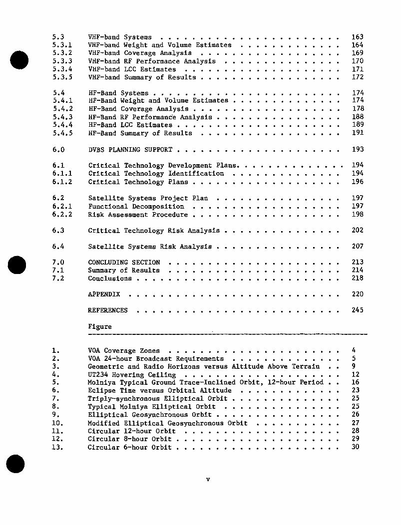
1. VOA Coverage Zones 42. VOA 24-hour Broadcast Requirements 53. Geometric and Radio Horizons versus Altitude Above Terrain . . 94. UT234 Hovering Ceiling 125. Molniya Typical Ground Trace-Inclined Orbit, 12-hour Period . . 166. Eclipse Time versus Orbital Altitude 237. Triply-synchronous Elliptical Orbit 258. Typical Molniya Elliptical Orbit 259. Elliptical Geosynchronous Orbit 2610. Modified Elliptical Geosynchronous Orbit 2711. Circular 12-hour Orbit 2812. Circular 8-hour Orbit 2913. Circular 6-hour Orbit 30

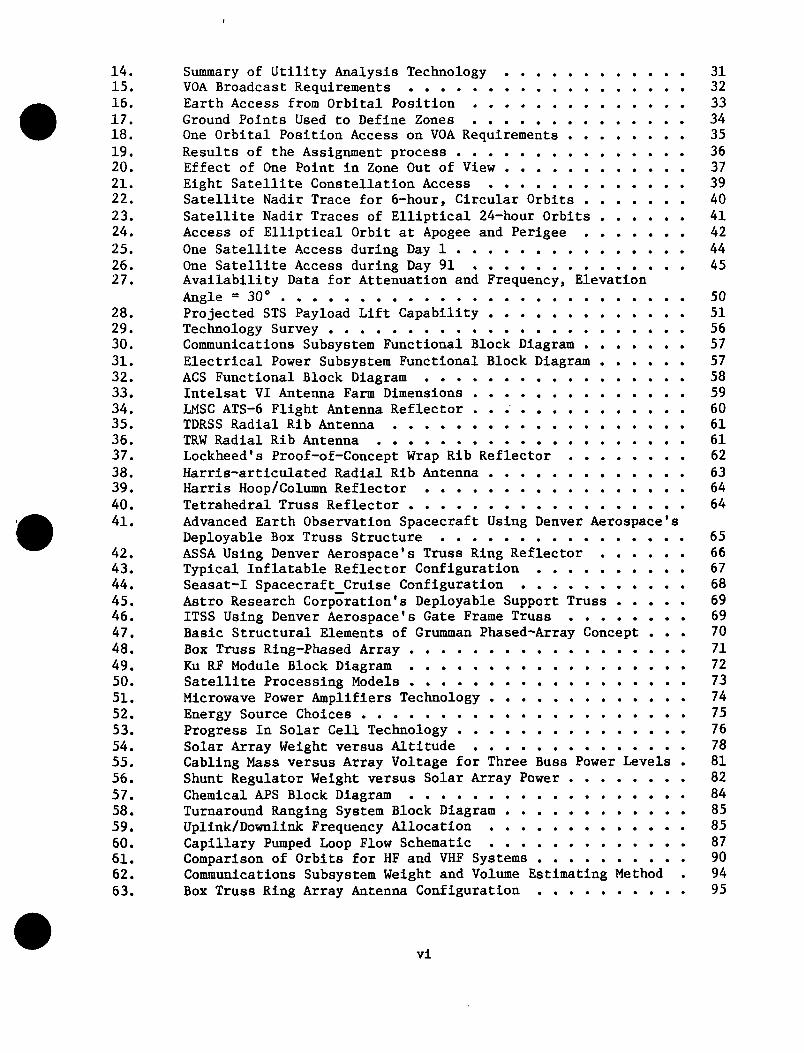
14. Summary of Utility Analysis Technology 3115. VOA Broadcast Requirements 3216. Earth Access from Orbital Position 3317. Ground Points Used to Define Zones 3418. One Orbital Position Access on VOA Requirements 3519. Results of the Assignment process 3620. Effect of One Point in Zone Out of View 3721. Eight Satellite Constellation Access 3922. Satellite Nadir Trace for 6-hour, Circular Orbits 4023. Satellite Nadir Traces of Elliptical 24-hour Orbits 4124. Access of Elliptical Orbit at Apogee and Perigee 4225. One Satellite Access during Day 1 4426. One Satellite Access during Day 91 4527. Availability Data for Attenuation and Frequency, Elevation

Angle = 30° 5028. Projected STS Payload Lift Capability 5129. Technology Survey 5630. Communications Subsystem Functional Block Diagram 5731. Electrical Power Subsystem Functional Block Diagram 5732. ACS Functional Block Diagram 5833. Intelsat VI Antenna Farm Dimensions 5934. LMSC ATS-6 Flight Antenna Reflector ... 6035. TDRSS Radial Rib Antenna 6136. TRW Radial Rib Antenna 6137. Lockheed's Proof-of-Concept Wrap Rib Reflector 6238. Harris-articulated Radial Rib Antenna 6339. Harris Hoop/Column Reflector 6440. Tetrahedral Truss Reflector 6441. Advanced Earth Observation Spacecraft Using Denver Aerospace's

Deployable Box Truss Structure 6542. ASSA Using Denver Aerospace's Truss Ring Reflector 6643. Typical Inflatable Reflector Configuration 6744. Seasat-I Spacecraft_Cruise Configuration 6845. Astro Research Corporation's Deployable Support Truss 6946. ITSS Using Denver Aerospace's Gate Frame Truss 6947. Basic Structural Elements of Grumman Phased-Array Concept ... 7048. Box Truss Ring-Phased Array 7149. Ku RF Module Block Diagram 7250. Satellite Processing Models 7351. Microwave Power Amplifiers Technology 7452. Energy Source Choices 7553. Progress In Solar Cell Technology 7654. Solar Array Weight versus Altitude 7855. Cabling Mass versus Array Voltage for Three Buss Power Levels . 8156. Shunt Regulator Weight versus Solar Array Power 8257. Chemical APS Block Diagram 8458. Turnaround Ranging System Block Diagram 8559. Uplink/Downlink Frequency Allocation 8560. Capillary Pumped Loop Flow Schematic 8761. Comparison of Orbits for HF and VHF Systems 9062. Communications Subsystem Weight and Volume Estimating Method . 9463. Box Truss Ring Array Antenna Configuration 95

vi

64, Power Distribution and Generation Calculation Flow 9965, Direct Energy Transfer System for Unregulated (+ 10%) Bus ... 9966, Solar Cell Radiation, Temperature, and Cover Slide Factors,

versus Altitude 10167, Shunt Regulator Weight Factor versus Array Power 10468, Allowable Depth of Discharge versus Charge/Discharge Cycles . . 10569, Reaction Control Weight Estimate 10770, Total Force Components versus Anomaly Angle 11071, Total Torque Components versus Anomaly Angle 11072, Representative Specific Mass and Area of Potential Power

Systems 11973, System Weight versus Distribution Loss 12274, Allowable Depth of Discharge versus Battery Discharge/Charge

Cycles 12475, Housekeeping Power System Weight versus Altitude 12576, Satellite System Design and Analysis Approach 13677, Ku-Band Satellite Design 13778, Constellation for Ku-Band-geostationary, Three Satellites . . 14279, Ku-Band Cumulative and Yearly Program Costs, 1984$ 14580, L-Band Satellite Design 14681, Constellation for High RF Power L-Band System—Geostationary.

Five Satellites 15282, Constellation for Low RF Power Option I L-Band System—

Geostationary, Five Satellites 15383, Constellation for Low RF Power Options II and III L-Band

System—geostationary, three satellites 15484, L-Band High Power System Program Cumulative and Yearly Costs . 15885, L-Band Option I System Program Cumulative and Yearly Costs . . 15986, L-Band Option II System Program Cumulative and Yearly Costs . . 16087, L-Band Option III System Program Cumulative and Yearly Costs . 16188, Typical VHF and HF Satellite 16389, Constellation for VHF System—24-hour, 30° Inclination,

Elliptical Four Satellite Clusters90, Constellation for VHF System—12-Hour, 45° Inclination,

Elliptical Four Satellite Clusters 16991, Small HF 6-Hour Satellite Weight and Signal Strength 17792, Small HF 8-Hour Satellite Weight and Signal Strength 17793, , Small HF 12-Hour Satellite Weight and Signal Strength 17794, Small HF 24-Hour Satellite Weight and Signal Strength 17795, Small HF GEO Satellite Weight and Signal Strength 17796, Small HF 'Triply-Synchronous Orbit Satellite Weight and

Signal Strength 17797, Constellation for HF System—6-Hour, 30 and 45° Inclination,

Circular, Eight Satellite Clusters 17998, Constellation for HF System—8-Hour, 45° Inclination, Circular,

Eight Satellite Clusters 18099, Constellation for HF System—12-Hour, 45° Inclination, Circular

Eight Satellite Clusters 181100, 6-Hour Orbital Satellite Coverage 182101, Small HF Satellite—12-Hour Orbital Satellite Coverage .... 183102, Small HF Satellite—24-Hour Elliptical Orbital Satellite

Coverage 184

vu

103. Small HF—Triply-Synchronous Satellite Coverage 185104. Small HF—Geostationary Satellite Coverage 186105. Small HF—8-Hour Orbital Satellite Coverage 187106. Small HF—8-Hour Orbit; 3-Month Sidereal Shift 188107. Small HF 6-Hour Satellite Costs 190108. Small HF 8-Hour Satellite Costs 190109. Small HF 12-Hour Satellite Costs 190110. Small HF 24-Hour Satellite Costs 190111. Small HF GEO Satellite Costs 190112. Small HF Triply-Synchronous Orbit Satellite Costs 190113. Communications and Electrical Power Subsystem Development Plans 196114. DVBS Planning Support—Satellite Systems Project Plan 197115. DVBS Project Plan —Top-Level Function 1.0, 2.0, 3.0, 4.0,

5.0, 6.0, 7.0 & 8.0 198116. Example of Risk Assessment Log 200117. Quantitative Risk Assessment Interpretation 201118. HF Small GEO Case Antenna Technology Development Cost Risk

Assessment 202119. HF Small GEO Case EPS Technology Development Cost Risk

Assessment 203120. HF Small GEO Case Transmitters Cost Risk Log 203121. Antenna Technology Development Schedule Risk Assessment .... 205122. Solid State Transmitter Technology Development Schedule

Risk Assessment 205123. Ku-Band Program Schedule Risk Assessment Results 211124. L-Band Program Schedule Risk Assessment Results 211125. HF and VHF Program Schedule Risk Assessment Results 212126. Ku-Band Satellite Concepts 215127. L-Band Satellite Concepts 216128. VHF and HF Satellite Concepts 217

Table

1. Program Outputs 32. Program Requirements—Ku-Band: 11.7 GHz 53. Program Requirements—L-Band: 1.5 GHz + 25 MHz 64. Program Requirements—VHP-band: 47 - 68 MHz 65. Program Requirements—HF-Band: 15.1 - 26.1 MHz 66. VOA Power Requirement Range (per Voice Channel) 87. Examples of Satellites in Circular, Subsynchronous,

Sun-Synchronous Orbits 168. Orbital and Nonorbital Concepts—Single Unit Cost and Schedule 199. Number of Vehicles Required for Zone 2010. Orbital and Nonorbital Concepts—Total LCC and Schedule $B . . 2011. Elliptical Orbits 2312. Circular Orbits 2713. Performance of the Satellite System 3614. Orbit Position Configurations and Requirements 3815. Effects of Satellite Eclipse on Coverage Efficiency 4316. Effect of Sidereal Shift on Coverage Efficiency 45

vui

17. VOA Transmission Requirements per Channel, Referred to Edgeof Coverage 47

18. Determination of Power Densities for L-Band System 4919. Propagation 4920. Orbit Transfer Vehicles 5221. Orbit Transfer Analysis for 6-Hour, 30° Inclination Orbit ... 5322. Orbit Transfer Analysis for Triply-Synchronous Elliptical

Orbit 5423. Orbit Transfer Results 5524. Allocated Satellite Bands for the U.S 7225. Transmitter Parametrics 7426. Silicon Solar Cell Tradeoff 7727. Gallium Arsenide Solar Cell Tradeoff 7728. Blanket Weight Comparisons for Various Solar Cell Designs ... 7729. SP-100 Description 7930. SP-100 Power Generation Tradeoff 8031. Microthruster Candidates 8332. Pulsed Plasma Thruster Data 8433. Thruster, Gimbal, and Beam Shield Unit 8434. Thermal Control Requirements 8735. Recommended Satellite Concepts 8936. Solar Array Weight and Volume Estimating Factors 10237. Attitude Control 10738. RCD Module Input Variables 10839. Satellite Model Input Variables 10840. RCD Module Output Summary 10941. VOA DVBS Auxiliary Propulsion System Requirements Ill42. TT&C Equipment List Ill43. Array versus Reflector PFD Comparison 11444. Number of Feeder Link Stations Required versus Satellite Height 11745. Power Generation Technology Tradeoffs 12046. Comparison of HF 8-Hour Baseline with 8- and 12-Mil SI Cells . 12047. Control Torque Actuator Summary 12648. APS Candidates Weight Tradeoff Results 12649. Cost Estimating Procedures for Communications Subsystem .... 12850. Planar Silicon Array Cost Data, 1984$M 12951. EPS Component Cost Fractions 12952. Cost Estimating Relationships for Other Subsystems 13153. Cost Estimating Relationships for Other Subsystems 13154. Ku-Band Satellite Weight and Volume Estimate 13855. Ku-Band Sizing Example 13856. RF Analysis for Ku-Band, Zone 9 14357. Ku-Band Antenna Design Summary 14458. Ku-Band Satellites LCC Estimates, 1984$ 14459. L-Band Satellites Weights and Volumes 14760. L-Band Sizing Example 14861. RF Analysis for High Power L-Band, Zone 9 15562. RF Analysis for Low RF Power L-Band, Option III Zones 4, 6, 7,

and 8 Combined 15563. High RF Power L-Band Antenna Design Summary 15664. Low RF Power L-Band Antenna Design Summary—Option I 15665. High RF Power L-Band Antenna Design Summary—Option II .... 157

IX

66. Low RF Power L-Band Antenna Design Summary—Option III .... 157b7. L-Band Systems' LCC Estimates, 1984$ 15868. Low RF Power L-Band Summary of Results 16269. High RF Power L-Band Summary of Results 16270. VHF Systems' Design Approach 16471. VHF Matrix of Design and Analysis Cases 16472. VHF Systems' Satellite Weight and Volume Estimates 16573. VHF Satellite Sizing Example 16674. VHF-Band Rf Performance Single-Satellite Capabilities 17175. VHF Systems' LCC Estimates, 1984$ 17276. Satellite Fabrication Learning Factors for VHF Systems .... 17277. VHF Systems' Design Summary 17378. VHF Summary of Results 17379. HF (26 MHz) System Design Approach 17480. HF Weight and Volume Estimates—6-Hour Orbit 17581. HF Weight and Volume Estimates—8-Hour Orbit 17582. HF Weight and Volume Estimates—12-Hour Orbit 17583. HF Inflatable Concept Weight and Volume Estimates 17884. HF System Maximum RF Performance Capabilities Summary for A

Single Satellite 18985. HF Fabrication Cost Learning Factors 18986. HF Systems' LCC Estimates 19187. HF System Design Summary 19188. HF-Matrix of Design and Analysis Cases (8 Hours) 19289. HF-Matrix of Design and Analysis Cases (6 Hours) 19290. DVBS Planning Support—Performance Risk Analysis 19491. Critical Technology Development Costs 19692. HF Small Satellite NRC Estimates 20093. DVBS Planning Support—Cost Risk Analysis Approach 20194. DVBS Planning Support—Schedule Risk Analysis Approach .... 20195. Tabular Output for HF Small GEO Case Antenna Technology and

EPS Cost Risk 20496. Critical Subsystem Technology Cost Risk 20497. Antenna Technology and Solid-State Transmitter Development

Schedule Risks 20698. Component and Subsystem Development Time Estimates from SDCM . 20699. Ku-Band System Cost Risk Assessment Results 207100. L-Band Systems Cost Risk Assessment Results, 1984$ 208101. VHF System Single Satellite Cost Risk Assessment Results,

1984$ 208102. HF-Band Systems Single Satellite Cost Risk Assessment 209103. Ku-, L-, HF-, and VHF-Band Project Function 3-Point Schedule

Estimates 210104. Summary of Program Results for Nonterrestrial Broadcast

Techniques 214105. Summary of Program Results for Ku-Band System 214106. Summary of Program Results for L-Band System 215107. Summary of Program Results for VHF System 216108. Summary of Program Results for HF System 217109. Summary of Program Results for Ku-, L-, VHF-, and HF-Bands . . 217110. LCCOST CER Input Parameters 224

GLOSSARY

A Antenna Array AreaACS Attitude Control SubsystemAM Amplitude ModulationAPS Auxiliary Propulsion SubsystemASSA Advanced Space Systems AnalysisATS-6 Applications Technology Satellite-6Ap Panel Area

Solar Array Area

BOL Beginning of LifeBS Broadcast SatelliteBW Beam Width

C Average Unit CostC/N Carrier-to-Noise RatioCDR Critical Design ReviewCER Cost Estimating RelationshipCMC Control Moment GyroCP Circular PolarizationGPL Capillary Pumped LoopCave Average Cost of Unitscul First Unit Fabrication CostCt Total Fabrication Cost

D/A Digital to AnalogA/D Analog to DigitalD Antenna Diameterdeg Degree(s)DOD Department of DefenseDSB Double SidebandDVBS Direct Voice Broadcast System

EOC Edge of CoverageEOL End of LifeEPS Electrical Power SubsystemESH Equivalent Solar HourETR Eastern Test Range

FM Frequency ModulationFjjV Battery Volume FactorFjjW Battery Weight FactorFc Solar Cell Cover Glass Thickness Weight FactorF<j Battery Depth of DischargeFr Radiation Degradation FactorFt Temperature Adjustment Factor

GEO Geostationary Earth Orbit

h Hour(s)HF High Frequency

XI

IFIRIUS

K

L/D

LLaRCLEOLCCLSS

LsLssl

m

MCCMeVMBGMSFC

NNASANRNRG

N"uNwrNWS

O&SOPDOTSOTV

Interface (Intermediate) FrequencyInfraredInertial Upper StageSpecific Impulse

Solar Array Sizing Constant (1123 W/m2)Solar Array Density Coefficient

Length-to-Diameter (Ratio)Structural Dimension RatioLength of Radiating DipoleLangley Research CenterLow-Earth OrbitLife-Cycle CostLarge Space SystemSpreading LossSpacecraft Stowed Launch Length

Slope of Learning CurveMeter(s)Miniature Cassegrainian ConcentratorMegaelectron Volt(s)Multiband GapMarshall Space Flight Center

Number of Radiating ElementsNational Aeronautics and Space AdministrationNonrecurringNonrecurring CostCharger EfficiencyDiode EfficiencyBattery EfficiencySolar Cell EfficiencyDistribution EfficiencyTotal Number of Units ProducedWire Efficiency (Source to Bus)Wire Efficiency (Bus to Load)

Operation and SupportOrbital Plane DayOff the ShelfOrbital Transfer Vehicle

PDRPFDPPTpsi

PesPiPisPS

Preliminary Design ReviewPower Flux DensityPulsed Plasma ThrusterPound(s) per Square InchEclipse Load PowerLoad PowerSun Load PowerPower from SourceTransmitter Power

xu

Q Radiative Heat

R Distance from Satellite to ReceiverRAMP Risk Assessment and Management ProgramRC Recurring CostRCD Rigid Body ControlRCS Reaction Control SystemRFC Regenerative Fuel CellRTG Radioisotope Thermoelectric Generator

s Second(s)S/C SpacecraftS/N Signal-to-Noise (Ratio)SAFE Solar Array Flight ExperimentSAR Synthetic Aperture RadarSCIAP Spacecraft Integrated Analysis ProgramSDCM System Design and Cost ModelSDR System Design ReviewSEMP Systems Engineering Management PlanSEP Solar Electric PropulsionSi SiliconSOA State of the ArtSOD Sidereal Orbital DaySOW Statement of WorkSRR System Requirements ReviewSSB Single SidebandSSPA Solid State Power AmplifierSIS Space Transportation System

TCOM Tethered Communications CorporationTOS/AMS Transfer Orbit Stage/Apogee Maneuvering StageTT&C Telemetry, Tracking, and CommandTWT Traveling-Wave TubeTWTA Traveling-Wave Tube AmplifierTc Temperature CollectorTC(j Component Development TimeTCq Component Qualification TimeIQ Time of EclipseTem Temperature EmitterTS(j Subsystem Development TimeTsq Subsystem Qualification TimeTsysq System Qualification TimeTs Time in Sun

UHF Ultrahigh FrequencyUSAF United States Air ForceUSIA United States Information AgencyUTC Universal Time Coordinated

VHF Very High FrequencyVOA Voice of AmericaVol Volume

Xlll

V|j Battery VolumeVe Equipment Bay VolumeVs Subsystem Hardware VolumeVsa Solar Array Volume

W WattsWa Antenna WeightWfc Battery WeightWjjC Battery Charger WeightW,j Power Distribution WeightWe Equipment Bay WeightWs Subsystem WeightWsa Solar Array WeightWsr Shunt Regulator WeightWsw Power Switching WeightWt Transmitter WeightWTR Western Test Rangea absorptivitye Emmissivityo Stefan-Boltzmann ConstantX Wavelength

xiv

SATELLITE VOICE BROADCAST SYSTEM STUDY

Eric E. Bachtell, Shailesh S. Bettadapur, John V. Coyner, and

Curtis E. Farrell

Martin Marietta Denver Aerospace

SUMMARY

The primary goal of this study was to develop technical, schedule, andcost data that can be used by the U.S. Information Agency to evaluate use ofsound broadcast satellite systems to meet future international sound broadcastneeds. Satellite systems launchable by the space shuttle were synthesized andanalyzed for broadcast at four frequencies: 26 MHz (HF-band); 47 MHz (VHF-band); 1.5 GHz (L-band); and 12.2 GHz (Ku-band). Broadcast requirements forthe study specified time of day, duration of broadcast, and ranges of groundsignal strength. Results showed that satellite systems can meet Ku-band re-quirements. L-band systems were designed that can meet lower signal strengthrequirements. Neither VHFnor HF-band requirements can be met by realisticsatellite systems. For these latter bands, the study results identified themaximum possible broadcast capabilities for each concept. Also, for HF-bandsystems, parametric relationships were derived to identify available signalstrength and satellite mass vs satellite output power. Time and cost to im-plement each system were estimated, and risk assessments performed to identify90 and 10% risk values of time and cost.

1.0 INTRODUCTION

The Satellite Voice Broadcast System Study was commissioned by NASA to in-vestigate the feasibility of a Direct Voice Broadcast System (DVBS) in space.The study evaluated potential operating systems in four frequency bands: 26MHz, 47 MHz, 1.5 GHz, and 12.2 GHz. Potential operational system conceptswere defined to a depth sufficient to determine the relative technical charac-teristics, performance, and costs (development, construction, and operating),and to develop schedules of selected system concepts. In addition, an assess-ment of the impact of and need for advanced technology for these system con-cepts was performed.

1.1 BACKGROUND

The use of satellites to provide sound broadcasting was examined by NASAas early as 1967 (ref. 1 and 2). More recently, this service has received in-creasing attention for both national and international broadcasting inter-ests. CCIR Report 955 (ref. 3) deals with the feasibility of sound broadcast-ing satellite systems operating in the range of 500 MHz to 2 GHz. The primaryapplication in Report 955 is broadcasting to automotive or portable receivershaving relatively low gain antennas; in this case rather large satellites arerequired due to large multipath fade margins.

An extension of this work by Chaplin, et al. considered only the ruralbroadcasting case and an improved receiver noise performance. Their analysesfor this special case (ref. 4) indicates that national broadcasting at 1 GHzis feasible with rather conventional size spacecraft. Phillips and Knight(ref. 5) explored the same subject at 26 MHz. None of these studies consid-ered the operational difficulties of worldwide sound broadcasting but confinedthemselves to restricted coverage, single satellite concepts.

The U.S. Information Agency (USIA)/Voice of America (VGA) is consideringsound broadcasting by satellite as part of a program to renovate, modernize,and expand the existing worldwide USIA/VOA broadcasting network. With suchcomprehensive coverage, new difficulties are introduced to satellite broad-casting. Therefore, it is appropriate to examine worldwide conceptual andoperational satellite sound broadcast systems to delineate these difficultiesand to continue to examine the practicality of worldwide sound broadcasting bysatellite. This will clarify the more subtle operational difficulties ofsatellite sound broadcasting and provide guidance to the more favorable broad-cast bands and technologies to use.

1.2 PROGRAM OBJECTIVE

The objective of this study was to provide the data necessary fcQ developtechnical, schedule, and cost data to aid in evaluating alternatives for sat-isfying future international sound broadcasting needs of the U.S. Government.

Conventional terrestrial broadcasting techniques were excluded from thisstudy. Satellite system concepts were synthesized and optimized for operationin each of four bands: 15.1-26.1 MHz, 47-68 MHz, 1.5 GHz, and 11.7-12.5 GHz.The technical and operating characteristics of the space segment were studiedin sufficient detail to demonstrate technologically feasible and cost-effec-tive launch, deployment, and operational capabilities; critical technologieswere identified; project plans were prepared defining tasks and providing es-timates of schedules and costs to construct and operate such systems. Projectplans were separately addressed for the technical, schedule, and cost elementsof development efforts required in each of the critical technology areas. Al-ternative approaches were developed that reduce risk and schedule associatedwith the development of these critical technologies. Systems costs (develop-ment, construction, implementation, and operation) and their associated fund-ing profiles were delineated in sufficient detail to separately facilitatelife-cycle and cost-effectiveness comparisons.

Also, the technical and operatingcharacteristics of the telemetry, TARJFI PKOCRAM nriTMTT*tracking, and control station and the TABLE L-PROGRAM OUTPUTSassociated feeder link were defined insufficient detail to develop estimatesof technical, schedule, and cost datafor this segment. Global service cov-erage combined with centralized systemcontrol and program feed from the U.S.or its territories is a desirable sys-tem feature.

Program outputs are summarized inTable 1.

1.3 PROGRAM REQUIREMENTS

The VOA requirements include specification of zones to be covered, univer-sal time coordinated (UTC) times and number of channels, frequency of opera-tion, and power flux density (PFD). A variety of options were also studied toprovide a broad data base to not only study system designs but also to provideinsight into optional system requirements.

Figure 1 pictorially describes the 15 zones of interest. The broadcastrequirements for the zones are presented in Figure 2. Times are presented in15-minute increments (UTC times) for a 24-hour day. For Ku-band, L-band, andHF-band, all zones were to be covered. As a baseline for VHF-band, only Zones9, 10, 12, and 14 were to be covered.

For several sets of operating requirements, what are the mostcost-effective satellite system concepts?What is the impact on selected systems concepts of variationsin the operating requirements?What critical technology must be developed for the varioussound DBS system options7 What are the estimated develop-ment costs & schedule?What are the cost & schedule risks in developing the soundDBS system options?What is the least costly implementation approach to each ofthe sound DBS system options7

ORIGINAL SSOF POOR

80180 W 140 100 60 20 0 20 60

Figure 1. - VOA coverage zones.100 140 180

ED

HDED

ffl Illlilllillllllll ffl iiniiiu

HD iiiiniiiirrm iniiiiniiiiniii

i i n i m n n i[rmm

EDrrm

CD iiiiniii

iiiiiiiniiiiiiiiiniininiiniimniiii

rnrm mn

EHUDrrm

nr i i i i i i i i i i i i i i i i • i > i i i •0 i 2 3 A 5 6 7 8 9 10 11 12 13 14 15 16 17 18 19 20 21 22 23 24

Legend Time, hQ Requirement

Zone in access

Figure 2. - VOA 24-hour broadcast requirements.

Table 2 presents the program requirements for Ku-band including frequencyof operation, zones, maximum simultaneous channels and signal strength. Nooptions were evaluated for the Ku-band system.

Table 3 presents the program requirements for L-band. Three signal levelswere initially specified, however, due to high power requirements on the sat-ellite for power levels P^ and ?3, emphasis was placed on the ?2 levelwith a high and low power requirement.

TABLE 2. - PROGRAM REQUIREMENTS-KU-BAND: 11.7 GHZ

Zone

No. of channels

1

2

2

2

3

2

4

2

5

11

6

3

7

4

8

2

9

6

10

3

11

4

12

2

13

6

14

2

15

1

- Signal level. -128dBW/m2/4 kHz (maximum)

TABLE 3. - PROGRAM REQUIREMENTS L-BAND 1.5 GHZ ± 25 MHZ

Zone

No of channels

1

2

2

2

3

2

4

2

5

11

6

3

7

4

8

2

9

6

10

3

11

4

12

2

13

6

14

2

15

1

- Signal level Pi,P2*,P3

Pt — Power flux density required to achieve an acceptable signal in a portable receiver or a receiver in an automobile Obtain(-91 2) this value as follows.

P! =107 + 20 LOGf + Mwhere M = 12.5 + 0.17f -0.170 + 1 65 [6 4 - 1 19f - 0.050]

f = Frequency in GHz0 = Elevation angle of satellite in degrees

Pi — Power flux density sufficient to achieve 49 dB demodulated S/N ratio with a receiver inside a single family dwelling making(-1036) use of an outside antenna.

?3 — Power flux density sufficient to achieve 49 dB demodulated S/N ratio with a receiver & antenna inside a single family(-92.6) dwelling having an 11 dB wall attenuation.

*P2 selected for satellite parametrics at two power levels (-103.6 dBW/m & a less conservative -116 1 dBW/m I Pl & Pj power levels notachievable

TABLE 4. -PROGRAM REQUIREMENTS —VHP-BAND 47-68MHZ

ZoneNo of channels

96

103

122

14

z|- Signal level: 250, 1000«, 5000* JUV/m FM

— Optional systems studied— Reduced channel requirements (selective reduction)- Reduced signal level. 150/LiV/m— Satellite using full orbiter

Table 4 presents the program re-quirements for VHP-band. Only Zones9, 10, 12, and 14 were specified forcoverage. Three power levels wereinitially specified (250, 1000, and5000 yV/m). The 1000 and 5000 yV/msignal levels were not achievable soprogram emphasis was placed on250 yV/m with a 150 yV/m option andreduced channel options. A single or-biter was specified as the baselinebut an option using a satellite in oneorbiter and a large Centaur-type stagein a second orbiter was also considered.

Table 5 presents the program requirements for HF-band. Three power levelswere initially specified: 300, 500, and, 1000 yV/m. The 500 and 1000 uV/msignal levels were not achievable so program emphasis was placed on 200 yV/mwith a 150 yV/m option. Reduced channel requirements and two reduced zonecoverages were also to be evaluated. Single spacecraft in six different or-bits were also evaluated at three signal levels for both double sideband (DSB)and single sideband (SSB). A full orbiter spacecraft was also investigated toprovide greater capability on a single satellite.

* 1000& 5000/JV/m were.not achieveable (150& 250/JV/m wereemphasized m program)

TABLE 5. - PROGRAM REQUIREMENTS HF-BAND 15.1-26.1 MHZ

Zone

No. of channels

1

2

2

2

3

2

4

2

5

11

6

3

7

4

8

2

9

6

10

3

11

4

12

2

13

6

14

2

15

1

- Signal levels: 300, 500*. & 1000* JUV/m double sideband (DSB)

— Optional systems studied— Reduced channel requirements (six-channel max, one-channel max, selective reduction)— Reduced signal level. 150 jUV/m- Small single spacecraft (DSB & single sideband [SSB]), 50, 150, 300 JUV/m- Reduce coverage to 40° N-& 15° S. Lat (at.- Reduce coverage to 40-70 IM. & 15-60 S. lat.- Satellite using full orbiter

*500 & 1000 JUV/m were not achievable (150 & 300 JUV/m were emphasized in program)

2.0 SURVEY OF NONTERRESTRIAL BROADCAST TECHNIQUES

This survey identified and described existing and planned nonterrestrialbroadcast techniques. Top-level analyses were performed on each technique todetermine its feasibility for use as a sound broadcasting system.

In this introduction, it is useful to say a few words about why nonterres-trial transmission methods are superior to terrestrial methods. Radio signalsin general propagate via a direct space wave out to a distance within theradio horizon, and via a surface wave considerably beyond this horizon. Forterrestrially located transmitters, however, the horizon is only on the orderof 65 km (40 miles) for tower or terrain elevations of up to 305 m (1000 ft).Although a reflected space wave can propagate over considerably greater dis-tances via reflection or "skip" conditions, coverage is not continuous overthe land, and varies considerably with time of day and sunspot activity. Onthe other hand the surface wave (also known as the ground wave) experiences aloss resulting from ground absorption in addition to its spreading loss ofspace wave propagation. This ground absorption loss increases with frequency,and therefore is not very useful for frequencies above 10 MHz. For example,over rich agricultural land with low hills, the absorption loss at 10 MHz andrange of 100 km (62 miles) is about 70 dB. At 20 km (12 miles) the loss isabout 90 dB (ref. 6).

If the antenna is elevated to heights available from balloons and poweredheavier-than-air aircraft, or even more so to heights available from satel-lites, the radio horizon distance is considerably increased, and propagationover substantial distances via the space wave is possible.

The studies for nonterrestrial techniques have shown that while variousnonorbital techniques can provide coverage, they suffer from some severe draw-backs. Most notably, they can only cover the edges of unfriendly territory,and many are required to cover an entire friendly zone. The number of indi-vidual signal sources raises the concern that there will be areas of interfer-ence where individual coverages overlap. Even in friendly territory, the needfor logistics support for each platform can make the system nonviable.

Existing orbital communication systems operate at geostationary altitude.Equivalent coverage at HF and VHP would require very large antenna apertures.Also, the high-power requirements for these HF and VHP systems would be largerthan any existing system. In the L-band, a DBSC satellite design could pro-vide adequate power for the low-end power requirement and would provide beamsizes of the correct order of magnitude. In the Ku-band, several satellitesdesigned for TV direct broadcast applications, (e.g, the Japan-Broadcastingsatellite, the Hughes HS394, and the DBSC satellites, could be used; however,some modifications to the spacecraft antenna would be required. Also, anSBS-type satellite could provide adequate power levels and the proper sizebeams for Ku-band operation.

2.1 TECHNIQUES AND COVERAGE

To obtain some idea of the power that will be required for the VGA appli-cation, the VGA specified edge of coverage signal level was converted into anequivalent power required, per voice channel, for each band, for the largestand smallest areas to be covered. These areas were, respectively, SouthAmerica (Zone 3) and the Eastern Europe region (Zone 9). This was done forvarious ground receive antenna, elevation angle of 20°. The approximate rangeof values for each band is summarized in Table 6.

The data contained in Table 6 assumes straight line propagation with noallowance for atmospheric or ionospheric losses. By the nature of theproblem, these power requirements are, except for atmospheric or ionosphericconsiderations, independent of transmitter altitude, and thus apply to bothnonorbital and orbital methods of coverage. It is obvious that with the ex-ception of the power requirement for the Ku-band, and the lower range ofL-band, no existing satellites can satisfy these power requirements. Discus-sion on what levels of power could be supplied by various techniques is insubsequent sections of this report.

TABLE 6. - VGA POWER REQUIREMENT RANGE(PER VOICE CHANNEL)

Banddesignation

HFVHPLKu

Frequencyrange

15 0 - 2 6 0 MHz47 0 - 68 0 MHz

1.5 GHz11.7- 127GHz»

Specified EOCsignal level

300 jUV/m250 JUWmP2-131 dBW/m2

Requiredpower range

5 9 kW - 29 5 kW4.2 kW - 20 9 kW450.0 W - 2.2 kW2.0 W- 10.0 W

'Maximum range per single transponder is 11.7 to 12.5 GHz.

2.1.1 Nonorbital Methods of Coverage

This section examines three nonorbital methods of providing nonterrestrialoriginated coverage. The three methods are:

1) Tethered lighter-than-air platforms,

2) Powered lighter-than-air platforms,

3) Powered heavier-than-air platforms.

2.1.1.1 Tethered Lighter-Than-Air Platforms

Low altitude (nonorbital) vehicles have an advantage over satellites inthat they are retrievable, and can thus be repaired, or have their payloadschanged. However, since they are susceptible to destruction in unfriendlyterritory, they are useful only in friendly territory. In addition, nonor-bital vehicles also have a much lesser broadcasting range than satellites, sothat many such vehicles must be used to cover one broadcast zone. The result-ing segmentation of coverage results in a potential for undesirable interfer-ence in the regions where signal strengths from two or more sources of thesame frequency are roughly equivalent. This could be a serious drawback to ahighly segmented system, and should be studied further if such a system is tobe considered.

The geometric line-of-sight coverage of low altitude platforms is, to afirst order approximation, a function of the square root of altitude or eleva-tion above the surrounding terrain. For radio frequencies in the approximaterange of 100 MHz to 20 GHz, however, the radio propagation range is about 15%further than the geometric line of sight because of atmospheric refraction ef-fects. These geometric line of sight and radio propagation distances (as afunction of altitude) are shown in Figure 3.

1000 r

900 -

800 -

Radio horizon (100 mHz to 20 GHz)

Note' For altitudes small relative to Earth's radius.

Geometric horizon, km = 3 57 t/altitude, m

Radio horizon, km = 4 124 (/altitude, m

100

10 20 50 6030 40Altitude, km

Figure 3. - Geometric and radio horizons versus altitude above terrain.

70

The tethered aerostat is a developed product, having already'been used inbroadcasting applications. Tethered aerostats can operate to altitudes ofabout 6000 m where they can carry payloads of 200 kg. At lower altitudes theycan carry significantly heavier payloads. At 4500 m, line-of-sight distanceis about 240 km (149 statute miles), as shown in Figure 3. To obtain reason-ably full coverage of a region, tethered aerostats at this altitude would haveto be placed in a grid with separations on the order of 500 km. For example,to cover a region such as Region 4 (Western Africa) which is roughly 4300 by2700 km, an array of aerostats roughly 8x6 (on the order of 50 aerostats)would be required. (Tethered aerostats range in size from about 1400 m^, 35m long to about 17,000 m^, 85 m long.)

The principal systems designer of tethered communications balloons isTethered Communications Corporation, (TCOM) a subsidiary of WestinghouseElectric Company. Their product line generally falls into two categories:

1) A small, trailer-based transportable system capable of lifting 100 kgto an altitude of about 760 m (2500 ft) above sea level (ref. 8).

2) A permanent, installation-type system capable of lifting about 100 kgto 1830 m (6000 ft), or about 1000 kg to 1525 m (5000 ft) (ref. 8).

The payload for a tethered aerostat is suspended beneath the aerostat in aseparate compartment. Systems built about ten years ago (refs. 9, 10, 11, 12)carried their own communications system power source, typically with the useof Sachs-Wankel rotary engines with a generating capacity of up to 5 kW.Under full-time use, fuel for the engines would typically last up to oneweek. More recently, power has been provided via the tether cable. This isaccomplished by carrying high voltage, so as to minimize resistance losses,and stepping it down at the aerostat.

For a communication system, the problem of antenna orientation stabiliza-tion can be solved basically in one of two ways. The first way is to elimi-nate the problem by having an antenna pattern that is symmetrical about thevertical axis. In this case, rotations of the aerostat, with changing windconditions, will not affect the coverage. The second method is to use an air-borne mechanical system consisting of a two-axis gimbal, an azimuth drive, anda slip ring assembly package. The gimbal assembly acts as a pivot at the bot-tom of the aerostat hull from which the entire airborne payload is suspendedin a pendulum fashion. Each axis is damped by a rotary viscous damper. Theupper linkage on the gimbal assembly is mounted to the aerostat through alightweight truss structure that distributes the airborne package weight andinertial loads throughout the balloon skin. The fixed shaft of the azimuthdrive (with respect to the aerostat) is attached below the lower gimbal link-age. The azimuth drive is the mechanical portion of the azimuth heading servoloop. The drive system receives an electrical signal from the servo elec-tronics and converts it into mechanical rotation of the payload package tomaintain proper heading with respect to north, as the aerostat moves. Theslip ring assembly incorporated into the airborne package allows unrestrictedazimuth motion between the payload and the aerostat. The ring is located atthe upper end of the azimuth drive where it is attached to the lower linkageof the gimbal. An azimuth positioning of + 0.5° pointing accuracy, controll-able in 0.1° increments, is achieved. The gimbal assembly isolates payloadmotion with respect to aerostat motion by a factor of 10 to 1.

10

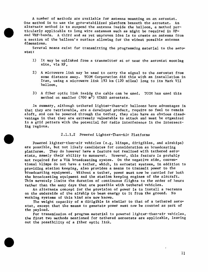
A number of methods are available for antenna mounting on an aerostat.One method is to use the gyro-stabilized platform beneath the aerostat. Analternate method is to suspend the antenna inside the balloon, a method par-ticularly applicable to long wire antennas such as might be required in HF-and VHF-bands. A third and as yet unproven idea is to create an antenna froma section of the balloon1s surface allowing for the widest possible antennadimensions.

Several means exist for transmitting the programming material to the aero-stat:

1) It may be uplinked from a transmitter at or near the aerostat mooringsite, via RF,

2) A microwave link may be used to carry the signal to the aerostat fromsome distance away. TCOM Corporation did this with an installation inIran, using a microwave link 193 km (120 miles) long to its Mark VIIballoon,

3) A fiber optic link inside the cable can be used. TCOM has used thismethod on smaller (700 nr) STARS aerostats.

In summary, although tethered lighter-than-air balloons have advantages inthat they are retrievable, are a developed product, require no fuel to remainaloft, and can be powered through the tether, they also have an obvious disad-vantage in that they are extremely vulnerable to attack and must be organizedin a grid pattern with the potential for radio interference in the intersect-ing regions.

2.1.1.2 Powered Lighter-Than-Air Platforms

Powered lighter-than-air vehicles (e.g, blimps, dirigibles, and airships)are possible, but not likely candidates for consideration as broadcastingplatforms. They do however have a feature not realized with tethered aero-stats, namely their ability to maneuver. However, this feature is probablynot required for a VGA broadcasting system. On the negative side, conven-tional blimps do not have a tether, which, in aerostat systems, in addition toproviding station keeping, also provides a means to transmit power to thebroadcasting equipment. Without a tether, power must now be carried for boththe broadcasting equipment and the station keeping engines of the aircraft.This severely limits the duration of continuous flights to the order of hoursrather than the many days that are possible with tethered vehicles.

An alternate concept for the provision of power is to install a rectennaon the underside of the airship to beam energy to it from the ground. Noworking systems of this kind are now known.

The weight capacity of a dirigible is similar to that of a tethered aero-stat, except that the means to generate power must now be counted as part ofthe payload.

For transmission of program material to powered lighter-than-air vehicles,the first two methods mentioned for tethered aerostats are applicable, leavingout the possibility of a fiber optic link.

11

In conclusion, powered lighter-than-air vehicles share many advantageswith tethered balloons, (e.g, retrievability and buoyancy) and have an addedadvantage in that they are maneuverable. Unfortunately, they also have allthe disadvantages found in tethered balloons (e.g vulnerability to attack andinterference between broadcast platforms, as well as having to generate re-quired power on board). Also important to consider is that although the tech-nology required to build dirigibles is available, only a limited number of de-signs have been developed, designs that may not suit payload capacity and ser-vice ceiling requirements.

2.1.1.3 Powered Heavier-Than-Air Platforms

The usefulness of powered heavier-than-air vehicles, including fixed-wingaircraft and helicopters have been investigated. The results are notpromising.

In this category, the helicopter has the advantage over fixed-wing air-craft in that it can operate without a landing strip, and can take off verti-cally and reach its desired position directly. This could be advantageous inremote mountainous coverage zones.

The largest helicopter on the market and also one of the most expensive isthe Boeing UT234. Starting at approximately $17M for the basic aircraft, theUT234 (ref. 13) will also cost an estimated $3800 per flight hour to run.This vehicle sports a fairly impressive range of payload and service ceilingcapabilities—from 7710 kg (17,000 Ib) at 4570 m (15,000 ft) to 12250 kg(27,000 Ib) at 2130 m (7,000 ft) as illustrated in Figure 4.

Another factor to keep in mindwhen considering helicopters is theclose relationship between helicopterperformance and air temperature. Dur-ing periods of warmer weather, thereis a notable decline in the serviceceiling due to variation in air den-sity. Figure 4 indicates that for aspecified service ceiling, a 20° var-iation in air temperature can cause upto a 16% decrease in payload capacity.

Fixed-wing aircraft generally havemuch higher load and altitude capabil-ity than helicopters. A wide varietyof midsized airplanes, from executivejets to propeller driven transportplanes, are easily capable of doingthe same job as the UT234 with powerto spare. The greatest drawback withairplanes is not payload weight capa-cities, but limits on the size andshape of the broadcast antenna. Thedrag created by a 10-m dish, for exam-ple, would cripple all but the largestof these aircraft. This problem has

4270

3660

3050

2440

1830

1220

610

Standardtemperature

Standardtemperature

+ 20°C

4.2 6.0 7.8 9.6 11.4Payload capacity, 1000 kg

13.2 15.0

Figure 4. - UT234 hovering ceiling.

12

given rise to creative antenna designs that reconcile aerodynamics and broad-cast efficiency. Examples of these are the disk-shaped antennas like thosemounted on the Boeing 707 AWACS planes, and long trailing antennas developedby Lockheed.

The Lockheed C-130, a 4-engine turboprop, can be ordered with a 457-m(1500 ft) trailing antenna designed for broadcasting an AM signal. Used ex-tensively in the past for broadcasting, this aircraft can carry up to 19500 kg(43,000 Ib) at well above 3050 m (10,000 ft) for six or seven hours (specifi-cation provided courtesy of Wallace Robby, Lockheed Corp.). No existing heli-copter can boast such impressive capabilities.

Helicopters and airplanes alike share one considerable limitation in thatthey can be flown only over friendly territory. Being easy targets for mis-sile or other anti-aircraft attack, a very large percentage of the proposedcoverage areas would be off limits to these vehicles. On the other hand,friendly territories can be serviced by radio towers (for years, the methodpreferred over airborne broadcast platforms).

Unlike lighter-than-air platforms, heavier-than-air platforms must contin-uously burn fuel to remain aloft. Fuel reserves set aside for this task wouldadd considerably to a payload already made heavy by power generating fuel andequipment.

It is difficult to escape the conclusion that although heavier-than-airbroadcast platforms are technically feasible, they do not represent an attrac-tive alternate to the satellite or other conventional systems. Their two ap-parent assets, retrievability and maneuverability, seem far outshadowed bytheir numerous shortcomings:

1) Vulnerability to attack,

2) Must expend fuel to remain airborne,

3) Must generate all power onboard,

4) Limited weight and hovering capabilities,

5) Can remain airborne for only short periods of time,

6) Can use only specialized broadcast antennas.

2.1.2 Orbital Methods of Coverage

Various classes of satellite orbits are useful as broadcast platforms.Among these, equatorial satellite orbits (e.g, geostationary, geosynchronous,nonsyaehronous, circular, or elliptical) form a special class in that theyhave no specific equator crossing, and hence no right ascension of their as-cending node. This means that systems using circular equatorial orbits neednot be concerned with precession of ascending node, as it does not exist.Elliptical equatorial orbits, however, would be concerned with the longitudi-nal location of the argument of perigee. All other satellite orbits are in-clined, and must consider ascending node right ascension and its drift.

We will consider the various classes of satellite orbits ana the charac-teristics that apply to VGA broadcasts, and give examples of existing orclose-to-existing technology that are applicable.

13

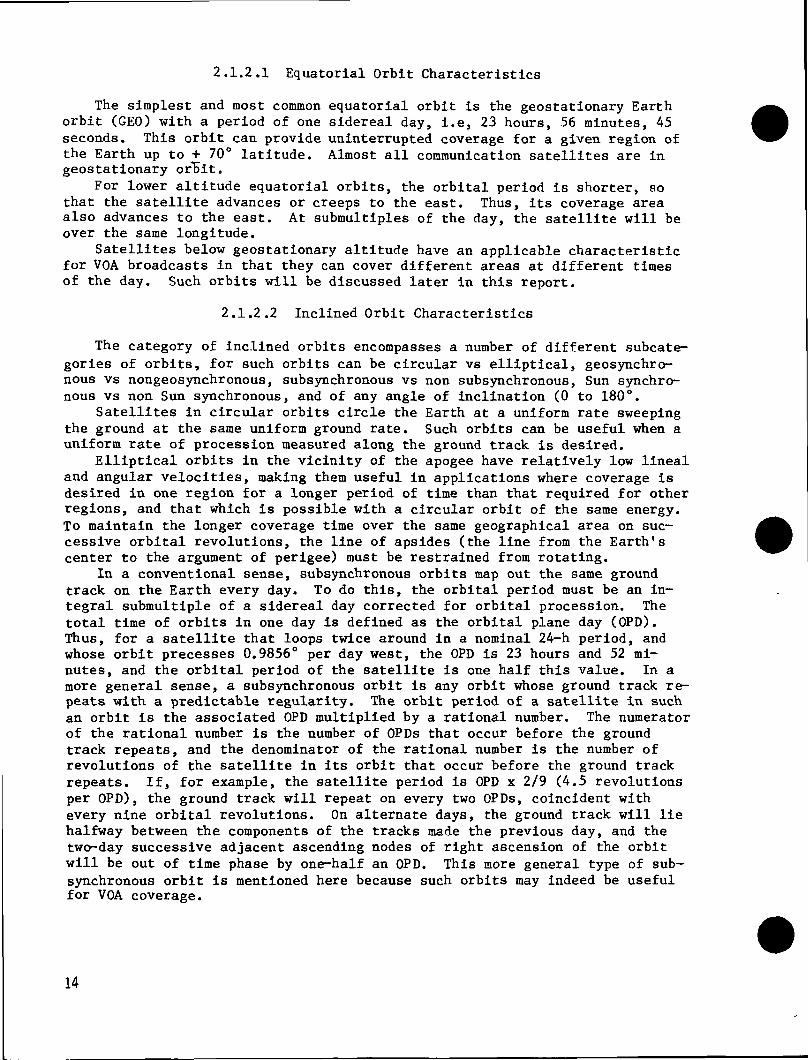
2.1.2.1 Equatorial Orbit Characteristics

The simplest and most common equatorial orbit is the geostationary Earthorbit (GEO) with a period of one sidereal day, i.e, 23 hours, 56 minutes, 45seconds. This orbit can provide uninterrupted coverage for a given region ofthe Earth up to + 70° latitude. Almost all communication satellites are ingeostationary orEit.

For lower altitude equatorial orbits, the orbital period is shorter, sothat the satellite advances or creeps to the east. Thus, its coverage areaalso advances to the east. At submultiples of the day, the satellite will beover the same longitude.

Satellites below geostationary altitude have an applicable characteristicfor VGA broadcasts in that they can cover different areas at different timesof the day. Such orbits will be discussed later in this report.

2.1.2.2 Inclined Orbit Characteristics

The category of inclined orbits encompasses a number of different subcate-gories of orbits, for such orbits can be circular vs elliptical, geosynchro-nous vs nongeosynchronous, subsynchronous vs non subsynchronous, Sun synchro-nous vs non Sun synchronous, and of any angle of inclination (0 to 180°.

Satellites in circular orbits circle the Earth at a uniform rate sweepingthe ground at the same uniform ground rate. Such orbits can be useful when auniform rate of procession measured along the ground track is desired.

Elliptical orbits in the vicinity of the apogee have relatively low linealand angular velocities, making them useful in applications where coverage isdesired in one region for a longer period of time than that required for otherregions, and that which is possible with a circular orbit of the same energy.To maintain the longer coverage time over the same geographical area on suc-cessive orbital revolutions, the line of apsides (the line from the Earth'scenter to the argument of perigee) must be restrained from rotating.

In a conventional sense, subsynchronous orbits map out the same groundtrack on the Earth every day. To do this, the orbital period must be an in-tegral submultiple of a sidereal day corrected for orbital procession. Thetotal time of orbits in one day is defined as the orbital plane day (OPD).Thus, for a satellite that loops twice around in a nominal 24-h period, andwhose orbit precesses 0.9856° per day west, the OPD is 23 hours and 52 mi-nutes, and the orbital period of the satellite is one half this value. In amore general sense, a subsynchronous orbit is any orbit whose ground track re-peats with a predictable regularity. The orbit period of a satellite in suchan orbit is the associated OPD multiplied by a rational number. The numeratorof the rational number is the number of OPDs that occur before the groundtrack repeats, and the denominator of the rational number is the number ofrevolutions of the satellite in its orbit that occur before the ground trackrepeats. If, for example, the satellite period is OPD x 2/9 (4.5 revolutionsper OPD), the ground track will repeat on every two OPDs, coincident withevery nine orbital revolutions. On alternate days, the ground track will liehalfway between the components of the tracks made the previous day, and thetwo-day successive adjacent ascending nodes of right ascension of the orbitwill be out of time phase by one-half an OPD. This more general type of sub-synchronous orbit is mentioned here because such orbits may indeed be usefulfor VGA coverage.

14

- - •A geostationary orbit Is a special case of a subsynchronous orbit, in

which the satellite period and the OPD are one sidereal day, the orbit is cir-cular, and the inclination is zero.

It is important to note that although subsynchronous orbits repeat theirground tracks, they do not, in general, repeat at the same time on correspond-ing revolutions. Sun-synchronous orbits (but more precisely, Sun stationaryorbits) are those that precess one revolution to the east per year. Thismaintains the plane of the orbit at a constant average angle relative to aline between the centers of the Earth and Sun, and the OPD when referred to aSun-synchronous orbit is exactly 24 hours. The term average allows for thenonuniform motion of the Earth about the Sun, described by the equation oftime. Sun-synchronous orbits, in themselves, do not require that their syn-chronous orbital period be a rational number multiple of the 24-h siderealorbital day (SOD). They may be of any period which, in combination with theother orbital parameters, results in an eastward precession of the ascendingnode of one revolution per year. Orbits that are both subsynchronous and Sunsynchronous may be useful for VOA applications.

Posigrade orbits are those whose satellite motion is to the east, the sameas the direction of the rotation of the Earth. The inclination angle of suchsatellites is between 0 and 90°. Because of Earth's motion, satellites insuch orbits require less energy for launch than do satellites in retrogradeorbits whose satellite motion is to the west, with the Earth is motion hinder-ing launch. Retrograde orbits have inclination angles between 90 and 180°.Orbits near 90° inclination are know as polar orbits. Their ground track ex-tends to the polar regions. Since VOA does not require polar coverage, andfurther, since coverage to high latitudes can be provided by satellites ofonly moderate inclination, they appear to be inefficient orbits. They do,howevers have a unique characteristic in that they can satisfy the conditionsfor circular, subsynchronous orbits. This is discussed further in the nextsection.

2.1,2.3 Some Special Orbits

1) An elliptical, subsynchronous orbit,

2) A class of circular, subsynchronous, Sun-synchronous orbits,

3) An elliptical, subsynchronous, Sun-synchronous orbit.

An elliptical, subsynchronous orbit. - An example of an elliptical, sub-synchronous orbit is provided by the Molniya series of Russian satellites.These satellites are in highly elliptical orbits that precess to the west, andhave a period of one-half of 23 hours, 56 minutes minus an allowance for pre-cession (one half an OPD). The satellites are in an inclined orbit of 63.4°.Tbe main characteristic of this angle and its complement of 116.6°, is thatthe line of apsides does not rotate. Thus, the irregular orbital pattern thatresults from the high eccentricity is held stationary in position, althoughnot in time, so that the relatively long dwelltime at apogee is maintainedover the same area of Earth. Figure 5 shows the ground track of a typicalMolniya type trajectory.

15

ORIGINAL PAGE ISOF POOR QUALITY

80

60 90 120 150 180 210 240 270 300 330Longitude

Figure 5. - Molniya typical ground trace—inclined orbit, 12-hour period.

30 60

Circular, subsynchronous, Sun-synchronous orbits. - An interesting classof orbits is the Sun synchronous, subsynchronous circular type. This classdiffers from mere subsynchronous orbits in that the ground track is repeatedat the same clocktime, making them geosynchronous. The class differs fromelliptical orbits in that there are no restraints on inclination angle, allow-ing rotation of the line of apsides. Without this restraint, there are anumber of orbits of interest.

Table 7 lists characteristics of various satellites that have beenlaunched.

TABLE 7. - EXAMPLES OF SATELLITES IN CIRCULAR, SUBSYNCHRONOUS, SUN-SYNCHRONOUS ORBITS

NOAA weather satellite

NOAA weather satellite

NIMBUS 6 weathertechnology

LANOSAT

NOAA-7

DMSP-F3

HCMM

METIOR 1-29

SOLWINO P78-1

UOSTAT

Revolutions persolar day

12.39

1259

1341

1397

14.13

1424

14.83

1491

1506

1508

Orbitalaltitudes

1510.0, km

1450.0

1106.0

905.0

848.0

811.0

6230

5950

5450

539.5

Inclinationangle

101.9. deg

101.4

998

98.8

989

98.6

97.6

979

97.6

978

Launch date

1976

1974

1975

1972

1981

1978

1978

1979

1979

1981

Mass

340 0 kg

340.0

8290

816.4

1405.0

513.0

134.0

38000

1331.0

520

16

Elliptical, subsynchronous, Sun-synchronous orbit. - The next class ofsatellite trajectories contains a number of potential subclasses that aresimilar to the Molniya subsynchronized class, but, in addition, are inSun-synchronous trajectories. To accomplish this, the inclination angle is116.6°, and the other orbital parameters are defined such that the orbitdrifts to the east one revolution per year, and the subsynchronous also be-comes Sun synchronous. It turns out, however, that of all the potential sub-classes of such orbits, only one is realizable.

2.1.3 Satellite State of the Art

This section looks at designs of some existing satellites, and some thatare presently in a design phase, to determine to what extent such technologycould reasonably satisfy VGA requirements. Before considering specific exam-ples, it is well to note a general limitation in terms of satellite mass re-quired per unit of primary power available. A survey of some satellites(other than experimental) shows a range of roughly 250 to 1400 grams perwatt. The broadcast type satellites tend to cluster in the range of 350 to475 grams per watt, while the fixed service satellites tend to cluster in therange of 600 to 1250 grams per watt.

2.1.3.1 The Applications Technology Satellite-6 (ATS-6)

The ATS-6 was launched in May 1974 to perform a number of experiments.One primary objective was to demonstrate the feasibility of deploying a 9.1 m(30 ft) parabolic reflector antenna. Its initial orbital mass in geostation-ary orbit was 1350 kg, and had 645 W of solar power for a relatively ineffi-cient mass to primary power ratio of 2093 grams per watt. Several trans-mitters at frequencies ranging from 860 MHz to 315 GHz (including a 40 Wtransmitter at 1.55 GHz) with RF powers of up to 80 W were employed with thelarge parabolic reflector.

If the full resources of an ATS-6-type satellite were converted to VOAapplications, the large parabolic reflector could provide the followingbeamwidths:

Frequency Beamwidth

15.0 MHz 154.80°26.0 MHz 88.8047.0 MHz 49.1068.0 MHz 33.901.5 GHz 4.0 (1/4 illumination of dish)1.5 GHz 1.54 (full illumination of dish)12.0 GHz 0.19

The beamwidths from 154.8° down through 33.9° clearly would not be effi-cient from geostationary altitudes, as the Earth extends only about 17° fromthis altitude.

If, in addition, the full primary resources were devoted to a singletransponder voice channel, it is estimated that about a quarter of the 645 Wavailable, or 160 W, could be available for transponder output. This would

17

not be sufficient to produce the power needed in HF-, VHF-, and L-bands re-gardless of satellite altitude. In Ku-band, the available power would be suf-ficient but the beam size would be too small at geostationary altitude, andthe antenna size would have to be reduced to meet coverage requirements. ForHF- and VHF-bands, the antenna size from geostationary orbit provides wholeEarth coverage. However, unless it is coupled with much higher power, the PFDon the ground would not meet the VGA requirements. Such higher power mightthen be able to power several channels simultaneously.

2.1.3.2 Japan Broadcasting Satellite

In April 1978, NASA launched for Japan a TV broadcast satellite (BS).This satellite has a mass of 678 kg, and a primary power of 1000 W (678kg/kW). It has two 100 W transponders to handle two simultaneous TV broad-casts. A more recent BS-2 has increased the primary power to 1780 W, for asomewhat more efficient mass-to-power ratio. The antennas on the BS were 1 by1.6 m, and produced a beam of approximately 2 by 1.4° at 12 GHz with 40.3 dBpeak gain.

Satellites with the above parameters, as in the case of the ATS-6 technol-ogy, do not have sufficient power to be of use in HF- and VHF-bands. With alarger antenna, the stated power would be sufficient for two L-band voicebroadcasts. However, the satellite would require significant redesign to becompatible with such an antenna. At Ku-band the antenna change could easilybe accomplished and the resulting satellite could broadcast 12 channels ormore.

2.1.3.3 Hughes DBS Satellites

Hughes Aircraft has introduced a high power DBS satellite (HS 394) capableof providing eight channels, each of 160 W output, with a total RF output inthe 1200 to 1500 W range. Primary power is 3-4 kW, with about 1050 kW inor-bit, for a mass-to-primary power ratio in the neighborhood of 300 kg/kW. Un-like conventional Hughes spin-stabilized satellites, the solar array is Sunstabilized, although the propulsion and attitude control section is spun. Theantenna is sized to cover one half of the Continental U.S. at 12 GHz, result-ing in a beam of about 3° in diameter, covering about three times the groundarea of the Japanese BS.

As in the case of the Japan BS, power is insufficient for HF- andVHF-bands. This satellite is large enough to accommodate a significantlysized L-band-deployable antenna. This coupled with the large power sourcecould provide several voice channels at L-band. In Ku-band, the 3° beam mightbe satisfactory from geostationary orbit for coverage of an area about halfthe size of Zone 8, (e.g, Saudi Arabia-Turkey). Therefore, a different anten-na would be needed at Ku-band and this could be easily accommodated.

18

2.2 COST AND SCHEDULE

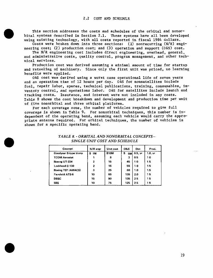
This section addresses the costs and schedules of the orbital and nonor-bital systems described in Section 2.1. These systems have all been developedusing existing technology, with all costs reported in fiscal 1984 dollars.

Costs were broken down into three sections: (1) nonrecurring (N/R) engi-neering cost; (2) production cost; and (3) operation and support (O&S) cost.

The N/R engineering cost includes direct engineering, overhead, general,and administrative costs, quality control, program management, and other tech-nical services.

Production cost was derived assuming a minimal amount of time for startupand retooling of machinery. Since only the first unit was priced, no learningbenefits were applied.

O&S cost was derived using a worst case operational life of seven yearsand an operation time of 12 hours per day. O&S for nonsatellites includefuel, repair labor, spares, technical publications, training, consumables, in-ventory control, and operations labor. O&S for satellites include launch andtracking costs. Insurance, and interest were not included in any costs.Table 8 shows the cost breakdown and development and production time per unitof five nonorbital and three orbital platforms.

For each coverage zone, the number of vehicles required to give fullcoverage is shown in Table 9. For nonorbital techniques, this number is in-dependent of the operating band, assuming each vehicle would carry the appro-priate antenna required. For orbital techniques, the number of vehicles isshown for a specific operating band.

TABLE 8. - ORBITAL AND NONORBITAL CONCEPTS-SINGLE UNIT COST AND SCHEDULE

Concept

Goodyear B-type blimp

TCOM Aerostat

Boeing UT-234

Lockheed C-130

Boeing 707 (AWACS)

Fairchild ATS-6

OBSC

SBS

N/R engr

$ 1M

1

2

2

3

10

15

10

Unit cost

$10M

8

15

15

25

65

90

75

O&S

$ 5M

3

45

55

80

135

135

125

Dev

0.5, yr

05

1 0

10

1.0

2.0

25

25

Prod.

1.0, yr1 0

1 5

1 5

1.5

1 5

1 5

1 5

19

TABLE 9 - NUMBER OF VEHICLES REQUIRED PERZONE

Zone

123456789

101112131415

Total

Blimp

219213719375469188

1000157163284344222844159406

5762

Tetheredballoon

7371

24012515663

333535495

11574

28153

135

1921

UT-234

7270

23612315461

328525393

11373

27652

133

1889

C-130

3635

119617731

1642727475636

1382667

947

707

252483435321

1141318323925961846

650

ATS-6(L-band)

87

2513167

3556

10128

296

14

201x05=100*

DBSC(L-band)

0606201 01 3053.00405081 00625041 0

16

SBS(Ku-band)

Approxsixtotal

'Assumes 50% reduction for a single satellite covering multiple zones

-Table 10 represents the total lifespecific concepts. The total cost in-cludes nonrecurring engineering, unit,and operations and support costs.Total schedule includes developmentand production schedules. Scheduleswere based on the assumptions of pro-duction rates of 14 aircraft per monthfor the winged aircraft and 20 air-craft per month for the other two non-orbital aircraft. A production rateof two spacecraft per month was as-sumed for orbital platforms.

cycle cost and schedule for each of the

TABLE 10. - ORBITAL AND NONORBITALCONCEPTS-TOTAL LCC AND SCHEDULE, $B

Concepts

Goodyear B-type blimpTCOM AerostatBoeing UT-234Lockheed C-130Boeing 707Fair-child ATS-6DBSCSBS

Quantity

576219211889947650100

166

Total cost

$ 8621

11366682041

Total schedule

25.5, yr95

1358.16495686.3

20

3.0 SATELLITE SYSTEM MISSION ANALYSIS

Mission analysis was performed to characterize various satellite concepts,performance parameters, and hardware implementation options applicable to theDVBS satellite service requirements. The final results were a set of candi-date satellite system concepts that satisfy the service requirements and arecompatible with STS payload weight and volume restrictions and the require-ments of an orbital transfer vehicle (OTV).

The analysis included an orbit and coverage analysis, a propagation analy-sis, a payload capability analysis, and a technology survey of subsystems forDVBS. The orbit and coverage analysis encompassed a wide range of orbits fromlow to high altitude for both elliptical and circular orbits. The propagationanalysis reviewed data available on propagation parameters and used the para-meter effects to yield the losses associated with transmission at each band.The payload analysis used projected STS payload capabilities and near-termOTV's to determine satellite limitations as to the total weight and volumethat could be delivered to each orbit. The technology survey of applicablesubsystems considered communication, power, ACS, stationkeeping and maneuver-ing, TT&C, thermal control, and the equipment bay (e.g, spacecraft body andsubsystems).

21

3.1 ORBIT AND COVERAGE ANALYSIS

The full range of possible orbits was examined systematically. Both el-liptical and circular orbits were considered. In recommending orbits forDVBS, the payload that can be placed into each orbit was considered along withthe orbital constraints (e.g, eclipse time, Van Allen belt radiation, and or-bit perturbations).

Additionally, orbits that provide repeatable ground tracks, repeatabletime schedules, and long coverage time over a particular area were desirableto meet the VGA coverage requirements. These requirements could be met by alarge number of satellites surrounding the globe. However, the number was re-duced by choosing orbits with repeatable ground tracks over the required cov-erage area. Also, the number was reduced further by assuring either the samesatellite or multiple satellites repeat the time schedule (e.g, the sameschedule to the same area everyday). Coverage time was increased by usingconstellations of trailing satellites or by using an elliptical orbit with ahigh apogee occurring over the target area.

In order to provide a measure of the degree at which each recommended or-bit met the VGA coverage requirements, a coverage analysis was performed usingrepresentative orbital positions. Each orbital position was assumed to have acapability to view the Earth to a 20° elevation angle for HF- and VHP-bandsand a 11.5° elevation angle for L- and Ku-bands. Depending on the requirednumber of voice channels and signal strength, the orbital position consistedof either a single satellite or a cluster of satellites.

3.1.1 Orbital Constraints

The orbital constraints that provided a basis to measure which orbits werepossible candidates for DVBS included eclipse time, Van Allen belt radiation,and orbital perturbations.

Power requirements for the HF-, VHF-, and L-band satellites were such thatthe satellite operating during eclipse would need large battery packs or thesatellite could not operate at all. In either case, minimizing eclipse timewas desirable. In general, the eclipse time decreases as the satellite alti-tude increases. As it turned out, having to operate during eclipse was such asevere requirement for battery power that satellites recommended for HF-,VHF-, and L-band do not operate during eclipse. Figure 6 shows the percent ofsunlight for a satellite vs the orbital altitude as orbit inclination isvaried.

In addition to eclipse time, the charged particles in the Van Allen beltscan cause serious deterioration of satellite solar panels and electronics.Providing the satellite operating in the Van Allen belts with enough end-of-life (EOL) solar power requires larger and heavier solar arrays than on asatellite outside of the Van Allen belts, and the weight of shielding neededfor the satellite electronics increases. It was therefore desirable to mini-mize or avoid the Van Allen belt regions as much as possible.

Orbital perturbations include effects due to oblateness of the Earth, dragof atmosphere, solar and lunar gravity, solar radiation pressure, and electro-magnetic drag. For the most part, all but the oblateness of the Earth are ef-fects that the satellite can easily compensate for by using the stationkeepingsystem on the satellite.

22

100 r

100 200 300 400 500Orbital altitude, nmi

600 700 800 900 1000

Figure 6. - Eclipse time versus orbital altitude.

The Earth's oblateness causes both periodic and steady (secular) changesin the orbital elements. The effects of Earth's oblateness were consideredfor each orbit and are included in the coverage analysis discussed later.

3.1.2 Elliptical Orbits

The orbital analysis conducted under this study looked at three types ofelliptical orbits: Molniya, geosynchronous, and a Sun-synchronous subgeosyn-chronous orbit called a triply-synchronous orbit.

Elliptical orbits are used to maximize the dwelltime over a coveragezone. However, elliptical orbits usually require higher delta-v capabilitiesthan circular orbits of the same orbital period. Consequently, there will bea reduction of the payload capability to the orbit.

Table 11 shows the four elliptical orbits studied under this contract.Two of the elliptical orbits are geosynchronous with different eccentricitiesand inclinations.

TABLE 11. -ELLIPTICAL ORBITS

Type

Tnply-synch

MolniyaGeosynch

Period

3.000 h

11 9672393423934

Eccentricity

0.3467

0.7720

0.60000.3000

Inclination

1166deg

63.460.0300

Altitude

Apogee Perigee

7,843 km 52139,375 1,000

61,085 10,48848,435 23,137

Payloadcapability3134kg

9575

80076544

23

The triply-synchronous elliptical orbit is retrograde and thus the orbitalplane drifts to the east at the rate of +0.9856 deg/day. This equals theaverage rate of motion of the Earth around the Sun. Therefore, the orbitalplane maintains a fixed orientation with respect to the Earth-Sun line. Thisallows the satellite to have nongimbaled solar arrays thereby reducing theweight and cost of the electrical power subsystem. Also, at the inclinationof 116.57 deg, the orientation of the orbit in its plane does not change andthus the position of the perigee relative to the orbit remains fixed. There-fore, the orbit has a fixed time schedule and a fixed ground track. At the3-hour period, the ground track repeats itself after eight revolutions in oneday. Figure 7 shows the ground tracks of the triply-synchronous orbit.

The main drawback of this orbit is the large delta-v required to obtainhigh inclination. Therefore, satellites that could be placed in this orbitwould be restricted to 3134 kg using a Centaur G as the orbital transfervehicle.

The Molniya elliptical orbit (named after a class of Russian satellites)is characterized by a highly eccentric elliptical 12-hour orbit whose line ofapsides does not precess. Satellites in this orbit would have long dwelltimesat apogee and short dwelltimes at perigee. For example, Figure 8 shows theground track of a typical Molniya orbit. It can be seen that on each 12-hourrevolution, 11 hours are spent in the northern hemisphere and only one hour inthe southern hemisphere. The ground track is constant because the orbitalperiod is adjusted to be exactly half a sidereal day corrected for the driftof right ascension. At an inclination of 63.4 deg, forces that produce therotation of the line of apsides are balanced, therefore the location of theapogee remains constant.

The one item that is not fixed in this orbit is the time schedule. Thesatellite arrives above a given point on Earth about four minutes earlier eachday.

The final elliptical orbit considered in this study was the ellipticalgeosynchronous orbit. The eccentricity used for the geosynchronous orbit de-signs were 0.6 and 0.3 for inclinations of 60 and 30°, respectively. This re-sulted in the ground trace becoming egg-shaped and provided an extensive peri-od of time that a satellite would remain above a given coverage area. Figures9 and 10 show the ground trace resulting from these two orbits. Both orbitsallow the line of apsides to drift thereby the apogee will progress with time,however, it is possible to compensate for this effect through use of multiplesatellites. The 60° inclination and 0.6 eccentricity orbit passes through theVan Allen radiation belt due to the low perigee altitude and therefore the 30°inclination and 0.3 eccentricity orbit is better suited for VGA applications.

24

ORIGINAL PAGE ISOF POOR QUALITY

330

BDA

ADO

30 60 90 120 150 180 210

Figure 7. - Triply-synchronous elliptical orbit.240 270

60 90 120 150 180 210 240 270 330 0

Figure 8. - Typical molniya elliptical orbit.

30 60

25

.12

150 180 210 240 270 300 330 0 30 60 90 120

Figure 9. - Elliptical geosynchronous orbit.

26

ORIGINAL PAGE ISOF POOR QUALmr

120 150 180 210 240 270 300 330 0 30

Figure 10. - Modified elliptical geosynchronous orbit.

3.1.3 Circular Orbits

60 go

TABLE 12. - CIRCULAR ORBITSThe circular orbits studied under

this contract consisted of threetypes: triply synchronous, geostation-ary, and subgeosynchronous (Table12). For the subgeosynchronous orbitsboth 30 and 45° inclination orbitswere examined to assess the impact oninclination vs coverage requirements.

The triply-synchronous circularorbit has characteristics similar tothe triply-synchronous elliptical,i.e., a fixed ground track, a fixedtime schedule and, a fixed orientation to the Sun. However, dwelltime over aparticular spot is drastically reduced and therefore, would require more sat-ellites to meet the same coverage requirements than the triply-synchronous el-liptical orbit. Also, the inclination required is increased to 125.3° therebyrequiring additional delta-v to achieve this orbit and restricting the payloadto orbit from 3134 kg for the elliptical case to 2127 kg. Due to these re-duced capabilities, the triply-synchronous circular orbit was not consideredfor full capability VOA applications.

Type

Triply synch

Geostationary

Subgeosynch

Period

3.000 h

23.934

11.967

7.978

5.984

Inclination

125.3deg

0.0

30.045030.045030045.0

Altitude

4,182km

35,786

20,194

13,892

10,355

Payloadcapability

2127 kg

4387

7236

8910

9993

27

The geostationary orbit is a standard for existing communication satel-lites. Satellites in geostationary orbits provide service to a wide coveragearea. Dwelltime is constant since the satellite in geostationary orbit ap-pears to be stationary to observers on Earth. However, the elevation anglefrom high altitude areas to a geostationary satellite will be low. Because ofthe high altitude, eclipse time is minimal.

The subgeosynchronous circular orbits studied ranged from approximately 12to 6-hour periods. The inclinations of 30 and 45° were chosen since coveragerequirements did not warrant higher inclinations and lower inclinations wouldproduce low elevation angles when covering high latitude zones. All of thecircular orbits studied had periods that were submultiples of one siderealday. This assured the ground tracks of the orbits remain fixed. However, thetime schedule was not fixed since the satellite will arrive over a given point4 minutes earlier each day after completing one ground track cycle. Becauseof this time shift, multiple satellites in different orbital planes that gen-erate the same ground track and follow one another were necessary to providecontinuous service.

As the circular orbits were reduced in period and thus altitude, the fol-lowing occurred: (1) the dwelltime of an individual satellite over a targetshortened, (2) the eclipse time increased, and (3) the payload capability in-creased. As discussed later, the low altitude circular orbits, i.e. the 6-and 8-hour orbit, proved advantageous for use at the HF frequency due to thisincreased payload capability. Figures 11, 12, and 13 show the ground tracksfor the 12-, 8-, and 6-hour orbits at 30° inclination respectively.

240 270 300 330 0 30 60 90

Figure 11 - Circular 12-hour orbit.

120 150 180 210

28

ORIGINAL PAGE BSOE POOR QUALITY

240 270 300 330 0 30 60 90

Figure 12. - Circular 8-hour orbit.120 150 160 210

29

60

30

180 210 240 120 150270 300 330 0 30

Figure 13. - Circular 6-hour orbit.

3.1.4 Coverage Analysis

After completing the orbital analysis, a coverage analysis was performedusing the orbits best suited for VGA applications in order to provide somemeasure of the utility of proposed VGA satellite systems. The goal of theanalysis was to measure the ability of alternative satellite systems to meetthe VGA requirements. Figure 14 diagrams the method and logic flow of thisanalysis.

The VGA requirements for satellite broadcast to the zones of interest weredescribed in matrix form in the statement of work (SOW). A graphical repre-sentation of the overall requirements (time vs zone) is shown in Figure 15.Note that this example is for the full HF broadcast requirements.

'A time-step simulation of satellite access to the zones of interest wasconducted using computer routines developed by the Martin Marietta DenverAerospace Operations Analysis Department. Since the requirements were statedin 15-min increments throughout the day, the simulations were run at that in-terval as well. The simulations were conducted for 24 hours, since the re-quirements repeated daily and since the orbital positions chosen for analysiswere reconfigured (that is, at their original positions relative to theEarth's surface) after 24 hours. (Exceptions to this 24-hour reconfigurationare discussed later in this section.)

30

The simulation routines look for access from the orbital position to geo-graphic points on the Earth's surface within grazing angle limits. (Grazingangle and elevation angle are synonymous in this context, depending only onthe point of reference; i.e., from the satellite or from the ground observer,respectively.) HF and VHP analyses assumed a minimum 20° elevation angle lim-it. For L- and Ku-band an 11.5° elevation angle was used. Figure 16 depictsaccess from two satellites. Each geographic zone of interest was simulated bymultiple latitude/longitude ground points. Figure 17 shows the set of pointsthat were used. Depending on the zone size, anywhere from three to six groundpoints were used to define each zone.

These access matrices were then compared, one orbital position at a time,to the requirements matrix. If a requirement to cover a zone existed and anorbital position had access to that zone, an assignment of orbital position tozone was made. Two possible transmit schemes were investigated. First, eachorbital position was allowed to cover only one zone at a time, even if it hadaccess to multiple zones. In the second scheme, each orbital position wasconsidered to consist of a cluster of spacecraft all with the same ascendingnode, which has the capability to cover all zones in access at that time.These two schemes provided lower and upper bounds respectively on the perform-ance capabilities of the systems examined.

Figure 18 shows an example of an orbital position's access overlaid on therequirements diagram from Figure 15. The scheme depicted here is that multi-ple zones can be covered at one time.

15 zonesofinterest

I65 groundpoints(3 to 6per zone)

( 24-h/15-mm time >L

(access vs time) \

,Broadcastrequirements(zone vstime)

/^ Assignmen

I zones as ap

\

\ Calculatior

I — all point^ — one-miss

i

.t of availableNrequired 1

propnate J

i of percent

sfit,ed-point fity'

Percent fit,less periods of «i —eclipse

Satellite

parameters

Day ofyear

i

I Eclipse 11 calculation 1

' Consider_ _^ __— . — regress

— rotatic

effects ofion of nodesin of apsidesil shift _j

Figure 14. - Summary of utility analysis methodology.

31

15

14

13

12

11

10

9

8

g 7o

IM6

5

4

3

2

1

m i m i i m i i m i i i IB rnnrm

ED I l l l l l l l l l l l l l l l l l l l l l l l lILB I l l l l l l l l l l l l l ITTTTm

iiiininiiiiiiinTTTTTTl LDiniinmiiimiiTTTTTn HD

mil rmrrm \ i inmnD LnmiD ID mmm i i i n i i n i i m m i i i i n i i i i i i i n

nm m niuiiiiiiiiii

m i m i i i i i i i i i i LnnDi i i m i i i nun LUD

T I | I I I I | I I I I I I I I I I I I I I I I

0 1 2 3 4 56 7 8 9 10 11 12 13 14 15 16 17 18 19 20 21 22 23 24Legend Time, hQ Requirement

^ Zone m access

Figure 15. - VOA broadcast requirements.

32

ORIGINAL PAGE ISOF POOR QUALITY

Critical grazing/elevation20° angle for broadcast reception for HF & VHP

1 Jan 198500.00-00

Figure 16. - Earth access from orbital position.

33

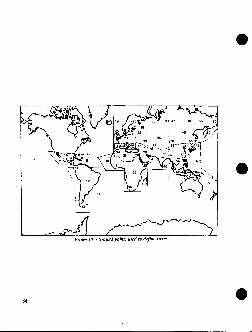
Figure 17. - Ground points used to define zones.

34

15

14

13

12

11

10

9

oN

Iffl

HEHD

Illllllll

\mmrnminnnnffflffli

ffl niiiiiiiIliiminmillllllim

flirmiiii ..... inn

mieiii i i i i i i i i i i i i i i i i im r n n u i i i i i i m i i i i i i i i i i i i i i i i i i ]

rnnn ffl iiiiiiiniiiiiiMiiliUiiliillillllU miiiiiimmirfTR-o

lUiiiliHHlTm

i l l l t i i U i l

r i i i \ \ i i i i i i i i r i i i i i r i i i0 1 2 3 4 56 7 8 9 10 11 12 13 14 15 16 17 18 19 20 21 22 23 24

Legend1 Time, hQ Requirement

^ Zone in access

Figure 18. - One orbital position access on VOA requirements.

The procedure for assigning orbital positions to zones was repeated foreach orbital position in the constellation. A resulting matrix was thenformed to show the results of the simulation. Figure 19 is an example of anoutput matrix showing information about orbital position assignments over timeand when, where, and why requirements were not met during the 24-hour period.

Once a broadcast assignment matrix was completed, system efficiency wascalculated. For cases with multiple orbital positions, the ratio of coverageprovided to the coverage required was calculated. That is, the denominatorwas the number of time period-to-zone combinations in the requirements matrixand the numerator was the number of time/zone assignments made. For singleorbit position concepts, very few of the requirements could be met. Conse-quently, coverage efficiency would not be meaningful. However, the fractionof time that a single satellite would be transmitting is useful. This parame-ter can be obtained from charts like Figure 18 and has been provided in Table13.

35

Time step

1234

UTC 1

0.00 80.15 80.30 8045 3

333$

6666

0000

0000

0000

0000

10 11

* 0* 0* 07 0

12 13 14 15

7 0 57 0 57 0 2$ 0 2

959697

23.30234524.00

* 4* 10 0

8 orbital planes—limit of one zone access per satellite (8 satellites).

* — Access required, cannot see zone$ — Access, but orbital position allocated to another zone.0 — No access required

Other numbers are individual orbital position numbers.

740

555.

Figure 19 - Results of the assignment process.

TABLE 13. - PERFORMANCE OF THE SATELLITESYSTEM

Case 1123456789

1011121314**15**16**17**

0.450.400.620.430.630.520.540.520.720330.580.690930.500.500.720.66

0.590.550.850.580.710680670680.840450650911 000560.580.76072

0.67 0.84 'Coverage efficiency criteria065 0810.83 0 97 1) Fraction of total requirements met0 50 0.67 — One zone per satellite0 73 0 80 - All of zone covered0 91 1 00 2) Fraction of total requirements met0 88 0.95 — One zone per satellite091 1 00 — Most of zone covered0 92 1 00 3) Fraction of total requirements met0.38 0 49 — Multizones per satellite0.72 0 76 — All of zone covered0 84 1 00 4) Fraction of total requirements met1.00 1.00 — Multizones per satellite0 74 0.81 — Most of zone covered0 76 0 82096 1.00 *'Hybrid constellations (geostationary/096 1.00 elliptical) Combined performance

calculated

Utilization factor for single satellites

18 0.5419 0.6920 0.7521 0.6722 0.9623 0.96Note

L-band & Ku-band at three geostationary positions (20W, 15E, 110E) provided100% coverage using 11.5° elevation

During the process of determining the coverage efficiency, it was foundthat many of the orbit positions covered all but a single ground point defin-ing a zone, i.e., effectively covering 80% of the required zone. Since thiswas the case, two different efficiencies were calculated. First, all pointsof the zone were required to be in view for an access to be generated in thematrix. In the second calculation, one point in the zone could be out ofview. Obviously, allowing one point in the zone to be out of access increases

36

the measured performance. The operational significance of this depends on theimpact of broadcasting to less than an entire zone. Figure 20 displays onesatellite access to one zone and demonstrates the effect of this modification.

The analyses were completed by taking into account orbital effects, i.e,satellite eclipse time and Earth's oblateness.

Satellite in 6-hour, circular orbit

Figure 20. - Effect of one point in zone out of view.

3.1.4.1 Orbital Positions

Determining the optimum orbit to provide space-to-Earth communications isa nontrivial problem. While high orbit altitudes provide wide area access,lower altitudes are generally cheaper because of lower transmitter power andorbital insertion energy requirements. For this analysis, 23 orbital configu-rations were investigated under various zone coverage requirements. Althoughthese configurations do not begin to exhaust the possible solutions, they doprovide a range of capabilities for comparisons. Table 14 lists the orbitalposition configurations and zone requirements analyzed.

37

TABLE 14. - ORBIT POSITION CONFIGURATIONS AND REQUIREMENTS

Case

123456789

10111213

14

15

16

17181920212223

Orbit parameters

6-h circular, 30-deg, eight orbital positions6-h circular, 45-deg, eight orbital positions6-h circular, 30-deg, eight orbital positions6-h circular, 30-deg, eight orbital positions6-h circular, 45-deg, eight orbital positions8-h circular, 45-deg, eight orbital positions12-h circular, 30-deg, eight orbital positions12-h circular, 45-deg, eight orbital positions12-h circular, 45-deg, eight orbital positions3-h elliptical, 117-deg, 0.347 eccen, eight orbital positions12-h circular, 30-deg, eight orbital positions12-h circular, 45-deg, three orbital positions24-h elliptical, 30-deg, 0.3 eccen, four orbital positio24-h geostationary, three orbital positions24-h elliptical, 30-deg, 0.3 eccen, three orbital positio24-h geostationary, three orbital positions24-h elliptical, 30-deg, 0.3 eccen, three orbital positio24-h geostationary, three orbital positions24-h elliptical, 30-deg, 0.3 eccen, six orbital positions24-h geostationary, three orbital positions24-h elliptical, 30-deg, 0.3 eccen, four orbitcal positio3-h elliptical, 1 17-deg, 0 347 eccen, one orbital positior6-h circular, 45-deg, one orbital position8-h circular, 45-deg, one orbital position12-h circular, 30-deg, one orbital positior24-h geostationary, one orbital position24-h elliptical, 30-deg, 0.3 eccen, one orbital positior

Zones of access

1-151-151-4,6-8,11,13,153,5,9, 10, 12, 143,5,9, 10, 12, 141-151-151-153,5,9,10,12,141-159, 10, 12, 149, 10, 12,149, 10, 12, 141-4,6-8,11,13,155,9,10,12, 141-4,6-8,11,13,155,9,10.12,141-4,6-8,11,13,155,9,10,12,141-4,6-8, 11, 13, 155,9,10,12,14

-15-15-15-15-15-15

Band

HFHFHFHFHFHFHFHFHFHFVHPVHPVHP

L»

L*

L*

Ku*HFHFHFHPHFHF

*Subsequent to this analysis, L and Ku-band orbits were changed to geostationary with a 1 1 5° minimum elevation <

Instantaneous access of eight orbital positions in circular orbit is shownin Figure 21 and represents Case 1. These eight orbital positions were con-figured in an eight-plane set in which all satellites pass the equator (andthen reach maximum latitudes) at the same time. The circles shown around eachnadir point represent a 20° grazing angle limit assumed in the analyses. Atthe 6-hour orbit period altitude of 10,350 km, Earth access is provided out to5450 km from the satellite nadir points. As seen in Figure 21, all of theareas of interest are in access 1 1/2 hours after the satellites cross theequator. If the one-zone-per-orbit position transmit scheme is being consid-ered however, only eight of the required zones may be covered at that time.

Figure 22 shows the satellite nadir traces for Case 1 and 2 constella-tions. The period and number of orbit positions chosen provides reconfigura-tions of the form of the constellation at 3-hour intervals. Every 24 hourseach orbit position is at its original position relative to the Earth'ssurface.

24-hour elliptical orbits (Cases 13-17 and 23) provide a different type ofaccess pattern. As shown in Figure 23, the combination of orbit position andEarth rotation results in a nadir point trace on the planet's surface in theshape of an oval. Note that the hourly interval marks in Figure 23 are closertogether in the northern regions; this is due to the placement of apogee atthe highest north latitude of the orbit. The resultant slower satellite ve-locity at the higher altitude maximizes the time viewing the higher latitudes.

38

20 elevation angle limit

AT EQUATORIAL CROSSING

20 elevation angle limit

IK HOURS AFTER EQUATORIAL CROSSING

Figure 21. - Eight satellite constellation access.

39

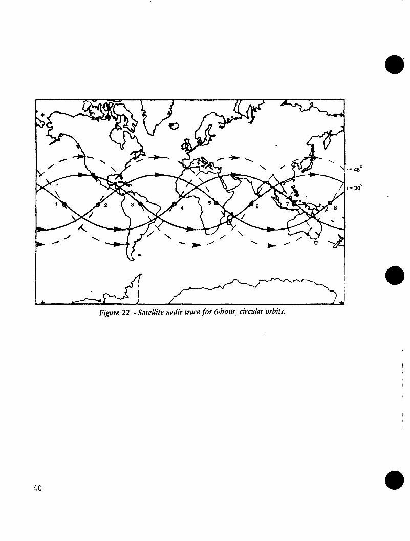
= 45"

= 30"

Figure 22. - Satellite nadir trace for 6-hour, circular orbits.

40

ORIGINAL PAGE ISOF POOR QUALITY

Figure 23. - Satellite nadir traces of elliptical 24-hour orbits.

The size of the access area for elliptical orbits varies throughout thesatellites' passage from perigee to apogee, again because of the difference inaltitude. Figure 24 shows the size of 20° grazing angle access areas at apo-gee and perigee for one of the satellites of Case 14.

The third type of satellite orbit considered was the geostationary config-uration. These are placed in equatorial orbit at an altitude (35,800 km) thatmatches satellite motion with Earth rotation, thus providing a stationarynadir point and continuous access to the same area of the Earth. While theseorbits are ideal for many communication applications, their disadvantages(that of vehicle payload limitations, high transmit power requirements andsize of antenna) are significant.

41

Figure 24. - Access of elliptical orbit at apogee and perigee.

3.1.4.2 Results of Analyses

A 24-hour simulation of the performance of the 23 combinations of satel-lite constellations and requirements listed in Table 14 provided the resultsshown in Table 13. The values shown are the coverage efficiencies describedin the methodology section.

3.1.4.3 Temporal Effects on Satellite System Performance

Four physical phenomena that affect Earth satellites were analyzed tomeasure the potential degradation of system efficiency over periods of time:

1) Eclipse - the period when the satellite is in Earth shadow. This isimportant in considering systems powered by solar arrays.

2) Sidereal shift - the phenomena relating to the difference between asolar and a sidereal day.

3) Regression of nodes - a shift of an orbit's longitude of ascending node.

42

4) Rotation of line of apsides - a change in the apogee and perigeepositions of an elliptical orbit.

Eclipse effects are dependent upon satellite altitude, inclination, andlongitude of ascending node. Another factor is the time of year, with falland winter eclipse periods being similar to spring and summer periods, re-spectively, because of the similarity in relative Earth/Sun/orbit-planeorientations.

Eclipse effects were examined forthe cases listed in Table 14. It wasassumed in this analysis that the VGAL-, VHF-, and HF-band satellitesystems would not be able to transmitduring a period of eclipse. For therelatively low altitude satellite

TABLE 15. - EFFECTS OF SATELLITEECLIPSE ON COVERAGE EFFICIENCY

Case

18

Orbit parameters

6-hr circular, 30°12-hr circular, 45°

W/O eclipse

0.450.52

Eclipse(spring)

0440.52

Eclipse(summer)

0.430.51

systems considered (such as the 6-hourcircular or- bits), the performanceefficiency was generally degraded by only a small amount. Table 15 providesan example of this. Higher altitude (geostationary and high elliptical)orbits are affected even less.

Sidereal shift is caused by the fact that the Earth rotates 360° in 23.934hours, approximately 4 minutes less than a solar (24-hour) day. This minordifference has the effect of causing a satellite in a repeating ground traceorbit to arrive over the same geographical spot 4 minutes earlier each daywhen measured on a local (solar) clock. Because the VOA broadcast require-ments are based on solar time, the sidereal time shift must be taken intoaccount.

The greatest impact of the phenomenon occurs in the single satellite case,such as Cases 19-23 from Table 14. The Day 1 coverage pattern for the 8-hourcircular orbit (Case 20) is shown in Figure 25. After 90 days, the accesspattern has shifted to an entirely new set of zones requiring coverage (Fig.26). After half a year, the trend begins to reverse itself and the satellitereturns to its original time/position relationship with the Earth a year later.

43

HD iiiiinii

LLLilillililliililliiilU

03 iiiimii

i i i iTff l i i i i i i i i i i n i i i nrrnm rrm f f l i i i i i m i i i i i i i

•iiiimmiiimm IIHIII iiiiiiii LLllliillU

i i i i i r i i i i i i i i i i r T i i i i i i0 1 2 3 4 5 6 7 8 9 10 11 12 13 14 15 16 17 18 19 20 21 22 23 24Legend. Time, h

jj Requirement

Zone in access

Figure 25. - One satellite access during Day 1.

44

15

14

13

12

11

10

9

8

§ 7

Q] iiiiiini

EDmi

ED i i i i i i n i irrm i i i i i i n iIllllllll miinii Q]

rrm

iiiiiniiiiiiiiiiiiiiiiiiimjiimin

MTTTTTTTmi nTmTTTTmWBTfHTminTTTI

rmm rrm

IllllllllIII 1 iiiiiiiiiiiiiinimrrrrm

rrmi I i i i i i n i i i i i i i i i i i i i i i P

0 1 2 3 4 5 6 7 8 9 10 11 12 13 14 15 16 17 18 19 20 21 22 23 24

Legend: Time, hQ Requirement

I Zone in access

Figure 26. - One satellite access during Day 91.

TABLE 16. - EFFECT OF SIDEREAL SHIFT ONCOVERAGE EFFICIENCY

Case

1

Orbit parameters

6-hr circular, 30°

Day

0.45

Day 15

0.44

Day 30

0.43

Day 45*

0.45

•Reconfiguration of satellite occurs

This effect is significantly re-duced in the multisatelllte constella-tions. In an eight satellite constel-lation, for example, satellite taskingcan be changed over periods of time sothat requirements met by one satelliteat one time are met by another afterthe sidereal shift begins to degradeperformance. In constellations in which satellites repeat ground traces, af-ter a time the relative satellite-Earth access patterns reconfigure. Table 16gives an example of the effect of sidereal shift on the Case 1 configuration.

Regression of nodes is a shift of the orbit plane because of Earth's ob-lateness. This shift is westerly for posigrade orbits (inclination less than90°) and easterly for retrograde orbits. The rate of regression of the as-cending and descending nodes is dependent on orbital inclination and period.For example, a 6-hour orbit at a 30° inclination will regress west approxi-mately 0.3° per day.

45

For the applications considered in this study, nodal regression does notpose a serious problem. The reason for this is that a change in orbital peri-od causes a change in ground trace that can be used to compensate for nodalregression. The west regression of 0.3° per day cited above, for instance,may be cancelled out by a slight decrease in orbital period. It should benoted however, that a decrease in orbital period in this case would increasethe time shift discussed in the preceding section on sidereal shift.

Rotation of the line of apsides, the line joining the apogee and perigeein an elliptical orbital plane, is another effect caused by the Earth's ob-lateness. The rate of rotation is also dependent on orbital inclination andperiod (or altitude.) Rotation is in the direction of satellite motion if in-clination is less than 63.4° or greater than 116.6°, and opposite betweenthose values. For the elliptical orbits considered in this study (Cases 13-17and 23), the rotation of the line of apside is approximately 8° per year inthe direction of satellite motion.

Three methods of eliminating or compensating for this effect are sug-gested. First, no apsidal rotation is incurred at exactly 63.4- or 116.6° in-clination. If these inclinations are suitable from other considerations, theproblem can be eliminated. Second, choice of initial placement of the line ofapsides can be made so that efficiency is maximized at" satellite midlife withlower performance accepted at beginning and end of life. Lastly, satellitestationkeeping with onboard thrusters or orbit maneuvering vehicles could bedone occasionally to return the orbital plane to its optimum orientation.

The triply-synchronous satellite orbit (Cases 10 and 18) is an interestingsolution to the effects discussed above. This orbit's inclination, period,and eccentricity are chosen such that:

1) The orbital plane retains the same fixed orientation with respect tothe Earth-Sun line by matching its retrograde orbit drift to the rateof motion of the Earth around the Sun (approximately 1° per day). ThisSun-synchronous orbit can be positioned to eliminate or minimizeeclipse, thus maximizing operation time of solar powered transmitters;

2) The satellite repeats its ground trace pattern daily;

3) The satellite repeats its time schedule each solar (24 hour) day; and

4) The apogee/perigee points (line of apsides) remain fixed.

46

3.2 PROPAGATION ANALYSIS

The propagation analysis consisted of determining the signal strength re-quirements and appropriate losses associated with transmission at each band ofoperation. Except for L-band, the exact signal strength requirements werespecified in the SOW. For L-band, an analysis was performed to determine anappropriate signal strength to meet the SOW requirements. The propagationparameters were determined by reviewing literature on operating direct broad-casting satellites. The propagation parameters included the following:

1) Path loss,

2) Ionosphere attenuation and refraction,

3) Atmospheric and ionospheric scintillation,»

4) Atmospheric refraction,

5) Atmospheric attenuation due to rain.

6) Spacecraft elevation,

7) Shadowing and/or attenuation due to buildings, trees and foliage.

3.2.1 Signal Strength Requirements

The four radio bands in the SOWand their specified signal or carrierlevels on the ground are shown inTable 17. For the HF-band, the threelower required levels are shown foreach modulation method; i.e., doublesideband/amplitude modulation (DSB/AM)and single sideband/amplitude modula-tion (SSB/AM). The DSB/AM-requiredlevels represent the carrier strengthon the ground. The SSB/AM-requiredlevels represent the signal strengthon the ground. For the HF- and VHF-bands, the two upper-level signal re-quirements proved too severe for real-istic DVBS applications, therefore aprogram decision was made to studyonly the lower levels. The L-band re-quirements were developed from a sig-nal to noise requirement of 40dB forthe PI power level and 49dB for theremaining signal levels. The PI sig-nal level represents the signal re-quired for portable or mobile re-

TABLE 17. - VOA TRANSMISSIONREQUIREMENTS PER CHANNEL, REFERRED

TO EDGE OF COVERAGE

Band

HF (26 MHz)

VHF (47 MHz!

L (1.5 GHz)

Ku (12.2 GHz)

Specified EOCsignal strength*

50/IV/m150/JV/m300/JV/m500/IV/m*

1000/UV/m"

35.4 /IV/m106.1 jUV/m212.1 MV/m

150 JUV/m250 jUV/m

1000jUV/m5000 MV/m

P1 ••P2-HighP2-LowP3 ••

5.5 /UV/m

Modulation

DSB/AMDSB/AMDSB/AMDSB/AMDSB/AM

SSB/AMSSB/AMSSB/AM

WBFMWBFMWBFMWBFM

WBFMWBFMWBFMWBFM

WBFM

Power density

•111.8dBW/m'i

-102.2-96.3-91.8-85.8

-114.8-105.3-99.2

-102.2-97.8•85.8•71.8

-91 2-103.6-116.1-100.1

-131 0

'Assuming that EOC signal level is 3 dB less than center ormaximum beam

* 'Power densities that were not studied due to severity ofpower requirement

47

ceivers using a whip receive antenna. The P2-low signal level requirementrepresents an average estimate as to the ground receiver and outside groundantenna used to receive the signal. The P2-high signal level requirement rep-resents a conservative estimate as to the ground receiver and outside groundantenna used to receive the signal. Finally, the P3 signal level representsan average receiver and inside receive antenna. The PI and P3 signal levelswere again too severe and were not studied. PI signal requirements were de-rived from the CCIR Study Group 10/11, Report 955 (ref. 14). Detailed analy-sis of the P2 and P3 requirements is discussed below. The Ku-band specifiedpower on the ground is in terms of power per 4 kHz, and is specified as a max-imum in order to minimize interference with ordinary licensed services. Alsoshown in Table 17 are the corresponding power flux densities (PFD) on theground. For all cases, the signal levels and PFD requirements are shown foredge of coverage.

3.2.1.1= L-band Analysis

The analysis performed for L-band system to determine the required PFD foreach of the three signal levels, used the following requirements:

1) The signal to noise (S/N) ratio must be better than 49 dB,

2) Top modulation, frequency (FM) is 15 kHz,

3) Peak deviation, D, is 75 kHz,

4) Preemphasis is 75 ys.

For the first signal level, the receiver carrier to noise ratio, C/N, re-quired to obtain a weighted S/N ratio of slightly better than 49 dB was esti-mated to be 19 dB in 250 kHz. This was conservatively estimated for a S/Nratio value of 40 dB corresponding to a C/N of 10 dB determined in CCIR Report955. However, the preemphasis used in the CCIR Report was 50 ys. For thesecond and third signal level requirements, the change in preemphasis from50 ys to 75 ys was also considered, which reduces the required C/N value tolOdB.

Additionally, the receiving antenna for each level was assumed to be 9dBi, 14 dBi and 6 dBi respectively, and for the inside antenna case, signallevel 3, an 11 dB building absorption loss was assumed.

To determine the flux density requirements, the first level assumed nomi-nal RF receiver characteristics and the second and third levels accounted forrecent improvements in receiver technology. A summary of results is shown inTable 18.

48

TABLE 18. - DETERMINATION OF POWER DENSITIES FOR L-BAND SYSTEM

Signal LevelApplicationAntenna gainTransmission line lossBuilding absorptionEquivalent system gainEquivalent antennaEffective area

Receiver system tempReceiver noise in 2SO kHz

Equivalent G/TRequired C/NRequired flux density*

P2-HighOutside antenna9dBi3dB

OdB

+6dBi0.013 m2 or-18.97 dB-m2

2000 K-141.6 dBW

•30 dB/K19 dB-103.6 dBW/m2

P2-LowOutside antenna14dBi

3dB

OdB

+11 dBi0.04 m2 or-13.97 dB-m2

700 K-146.1 dBW-20.5 dB/K16 dB-116.1 dBW/m2

P3

Inside antenna6dBiOdB

11 dB-SdBi0 001 m2 or-29.97 dB-m2

700 K-146.1 dBW-36.5 dB/K16 dB-100.1 dBW/m2

'Required flux density is for linear polarized signal A 3-dB polarization loss is included m the communications subsystem, assumingcircularly polarized transmission and linear reception.

3.2.2 Propagation Parameters

TABLE 19. - PROPAGATION LOSSESFor each radio band, propagation

parameters that cause transmissionlosses were determined using availableliterature. Table 19 summarizes theresulting losses per band for eachpropagation parameter considered.

Ionospheric refraction was neg-lected in this study since this effectis usually small. Even if it has asignificant effect, neglecting refrac-tion is conservative since the areaserved by the satellite will increasedue to refraction rather than decrease.

Atmospheric attenuation due torain was also neglected since thisloss is also small. Figure 27 showsatmospheric attenuation due to rain as a function of frequency and availabil-ity at a constant 30° elevation angle (ref. 15). The availability of 90% rep-resents the percent of time the satellite will be able to penetrate the rainif the loss associated with the availability curve is used in the link analy-sis. For the frequency range of interest in this study, 26 MHz to 12.2 GHz,it can be seen that rain attenuation has virtually no effect until the upperfrequency of 12.2 GHz. For the Ku-band, assuming a 90% availability, the rainattenuation results in a loss of less than 0.5 dB (Fig. 27).

~ — - — -^_ BandLoss — •— ^___

Ionospheric & atmos-pheric refractionIonospheric attenuationPolarizationAtmospheric attenuationdue to rainSpacecraft elevationAtmospheric & iono-spheric scintillation*Total loss

HF

Ni2dB

3dB

OdB

20°

Not co

VHP

jglected1 dB3dB

OdB

20°

isidered

L Ku

—

OdB

3dB

OdB

11.5°

OdB

5dB 4dB 3dB

OdB

OdB

<05dB115°

OdB

OdB

'Scintillation margin not included due to high powerrequirement.

49

50

40

00

§30

-20

10

99.9% availability

99.5%

10 20 30 40

Frequency, GHz

50 60

Figure 27. - Availability data for attenuation andfrequency, elevation angle = 30°.

Ionospheric attenuation for the HF- and VHF-bands was determined by usingthe results from the 1984 NTIA technical memorandum on HF/VHF direct broad-casting satellites (ref. 15). For L- and Ku-bands the ionosphere produces noloss of signal.

Atmospheric and ionospheric scintillation has not been included in theloss margin for HF- and VHP-bands due to the severity of the loss that canoccur. It is known that scintillation is essentially a nightime phenomenonand maximum losses up to 20 dB occur during maximum sunspot activity. The ir-regularities in the ionospheric electron density can cause rapid fading of thesignal of such magnitude to render the signal useless. Adding scintillationinto the link margin would have caused the power requirements to become ex-cessive. L- and Ku-band frequencies are not affected by scintillation.

An additional loss not shown in the above table was path loss or spreadingloss. Since spreading loss is dependant on the orbit and the satellite eleva-tion angle, the spreading loss was calculated during the RF performance analy-sis for each band. The equation describing spreading loss is:

L = G /4 7TRs p2 (3-1)

where Ls = spreading loss in per square metersGD = 1.0 for free-spaceR Distance from satellite to receiver station

The distance from the satellite to the ground station, R, is always maxi-mum at the minimum elevation angle of, for example 20 or 11.5° depending onthe operating frequency. The minimum elevation angle of 20° for HF and VHFfrequencies was chosen to assure signal penetration through the ionosphere 90%of the time.

50

3.3 PAYLOAD CAPABILITY ANALYSIS

In order to provide some measure as to which orbits were better candidatesfor VOA missions and to provide a basis for sizing the recommended satellitesystem concepts, a payload capability analysis was performed. Both the east-ern test range (ETR) and the western test range (WTR) as well as a variety ofOTVs were considered in the analysis.

3.3.1 STS Capabilities

As defined in the SOW, the STS shuttle was examined to determine the pro-jected lift capability for the 1990's. Although the lift capability of 29483kg (65000 Ib) has yet to be achieved, it is anticipated that by the mid 1990'ssuch a capability will exist.

The 29483 kg capability is not alift-off limit but rather an abortcondition limitation. Figure 28 showsthe lift-off capability for the shut-tle as a function of orbiter inclina-tion and altitude. For ETR launch,the reduction in lift-off capabilitydue to increased inclination can beoffset by reducing the orbiter alti-tude. As an example, launching into a45 deg, 370.4 km orbit the STS has alift capability of approximately 27000kg. However, by reducing the orbitaltitude to 255 km allows the full STScapability of 29483 kg to be used.For the VOA study, the STS was placedto assure the full 29483 kg capabilitywould be achieved. For WTR launches,

35

o30

I 25

20

• 185.2 km• 222.2 km

296.3 km370.4 km

444.5 km

185.2km (only)

ETR

20 90 10030 40 50 60 70 80STS initial orbit inclination, deg

* Design landing load limit of 29,483 kg

Figure 28. - Projected STS payload lift capability.

a reduction in lift capability occursafter 60° of inclination. The orbitaltitude of 185.2 km is generally con-sidered the minimum altitude the STSmust achieve.

An ETR launch was considered for any final payload orbit less than 57° in-clination. Additionally, the STS inclination matched the final orbital incli-nation when possible, e.g., for the 45°, 6-hour circular orbit, the STS wasplaced in a 45° inclination, 255-km orbit. This assured both maximum liftcapability for the STS and a minimum plane change delta-v requirement for theOTV, thereby maximizing the payload capability to final orbit.

WTR launches were considered for any final payload orbit above 57° incli-nation (e.g, the triply-synchronous elliptical orbit). Unlike ETR launches,matching the final orbital inclination with the STS inclination reduces thelift capability of the STS. Even though this would minimize the plane changedelta-v requirements on the OTV, it was not readily obvious that this was thebest solution. Therefore, for each WTR launch, a number of STS inclinationswere looked at to optimize the payload capability.

51

3.3.2 OTV Capabilities

In general, the present day OTVs, (PAM-D and IUS) do not have the payloadcapability from low-Earth orbit (LEO) that would be necessary for transferringproposed DVBS to final orbit. Therefore, this study looked at near-term ve-hicles that would provide such a capability, [e.g, the Transfer Orbit Stage/Apogee Maneuvering Stage (TOS/AMS) and the Centaur G]. In addition, a Centaurderivative, Centaur B, was also examined that could be used for multiple STSlaunches. The Centaur B uses the entire STS lift capability by carrying addi-tional fuel to provide a maximum capability to orbit. The satellite andCentaur B would be mated in orbit, thereby requiring a separate STS launch forthe satellite. Both the TOS/AMS and Centaur G are expected to be operationaltransfer stages by 1986. The Centaur G is a single-stage system that uses acyro-high energy thrust system while the TOS/AMS is a two-stage system withthe first stage using a solid rocket and the second stage a storable bipropel-lant thrust system. Table 20 summarizes the parameters of each of the aboveOTVs.

TABLE 20. - ORBIT TRANSFER VEHICLES

OTV

Stage length, m

Stage loaded wt, kg

Max main propel lantwt, kg

Effective 1 , s

Average thrust, N

Shuttle ASE wt, kg

Typ P/L to Synch-Equatorial, kg

TOS/AMS

46

15,665

9,705/4,007

293/315

11,787/195,712

1,893

2,900

Centaur G

6.1

17,015

13,808

4404

133,440

4,139.0

4,390

Centaur B

91

25,064

22,426

446.4

146,784

4,4150

9,570

3.3.3 Determination of Payload Capabilility

To determine the final payload capability, three Martin Marietta computerprograms were used. The first program determined the delta-v requirements toplace a payload into a circular orbit from an STS park orbit, using a two burntransfer. Burn 1 was a perigee burn to transfer to the final altitude and in-cludes a small plane change burn to minimize the total delta-v required. Burn2 was the apogee burn used to circularize the orbit and complete any planechange. The amount of delta-v required for both burns was determined using amodified classical minimum energy technique, i.e., Hohman transfer. The modi-fication was in a Newton-Raphson iteration technique that was used to computethe optimum amount of plane change that should occur during the first burn.

The second program was used to determine the delta-v requirements to placea payload into an elliptical orbit from an STS park orbit, again using a twoburn transfer. Burn 1 was a perigee burn used to put the spacecraft into thetransfer orbit. Burn 2 was an apogee burn to produce the final orbit and anyplane change and adjustment for the argument of perigee. The minimum delta-vrequired from both burns was determined by iterating on the latitude at whichthe second burn occurred', then back solving for the minimum energy cotangent-ial first burn.

52

The final program took the delta-v requirements from the previous programsand computed the payload-to-final-orbit capability using a specified OTV.This program automatically offloads fuel on the OTV to achieve the final orbitand meet shuttle lift capability.

Tables 21 and 22 show example outputs of the three programs. Table 21 isan example of the payload capability to the 6-hour, 30° inclination circularorbit. Table 22 is an example of the payload capability to the triply-synchronous elliptical orbit.

TABLE21. - ORBIT TRANSFER ANALYSIS FOR 6-HOUR, 30° INCLINATION ORBITPROGRAM--/ORBITC/

RUN DATE WAS: 02-05-1985 AT TIME:FOLLOWING IS A SUMMARY OF THE INPUT PARAMETERS:*** ORBIT TYPE - CIRCULAR ***INITIAL STS ORBIT INCLINATION = 30 degreesSTS PARK ORBIT = 407.44 kmFINAL P/L ORBIT INCLINATION = 30 degreesFINAL P/L ORBIT PERIOD = 6 hours

16:01:36

RESULTING CALCULATIONS:FINAL P/L ORBITAL ALTITUDE = 5607.594 n.miles1 ST BURN DELTA V = 1480.685 m/sec ( 4857.891 ft/sec)2 ND BURN DELTA V = 1174.493 m/sec ( 3853.325 ft/sec)TOTAL REQUIRED DELTA V = 2655.178 m/sec ( 8711.216 ft/sec)PLANE CHANGE (BURN II) IS:-9.999999E-06fff***tft*tt************»**ttt*t*»*****»***»»**t

PROGRAM--/PAYLOAD/RUN DATE WAS: 02-05-1985

*** DELTA V REQUIREMENTS ***Req, Delta-v Burn 1 = 4857.9 ft/sec

*»* Launch Site ETR *»*

tt» STS/ACC/OTV DATA «**ASE (ACC) Weight: 0,0 KgService Support Weight: 0,0 Kg

tt* STAGE 2 DATA ***Max Propellant Weight: 13810.8 KgHise Fluid (Res,He) Weight: 109,8 KgTrapped (Unusable) Prop: 198.7 KgMisc, Fluid Use Before Burn 2: 48.1 Kg

AT TIME: 16:02:01

Req. Delta-v Burn 2 = 3853.3 ft/sec

OTV NAME:CENTAURGASE (SB) Weight: 4139.6 KgSTS Lift Capability: 29484.0 Kg

Structural (Dry) Weight: 3097,2 KgPropellant Margin: 113,4 KgMisc, Fluid Use Before Burn 1: 9,1 KgMain Propellant Losses Burn 1: 132,5 Kg

Main Propellant Losses Burn 2: 180.1 Kg Effective ISP (Sec): 440,4Thrust: 133440 N

ttt STS CAPABILITIES **»STS Cargo Capability (STS Lift Wt - All ASE tt Adaptor): 25344,45 KgVehicle' Total Weight (Stages + P/L): 25344,4 Kg

Weight: 0,0 Kg Stage 1 Main Propel lant Weight:Stage IStage 2 Main Propel lant Weight: 12144,6 KgStage 2 Loaded Weight: 15351.6 Kg

Pay load Weight Delivered to Final Orbit: 9992.9 KgStage 1 Stage 2a Stage 2b Stage 2 Tot

DeltS'V (ft/sec) 0 4857.891 3853.325 8711.217(sec) 0 236.7428 136.0825 372.8253

0,0 Kg

53

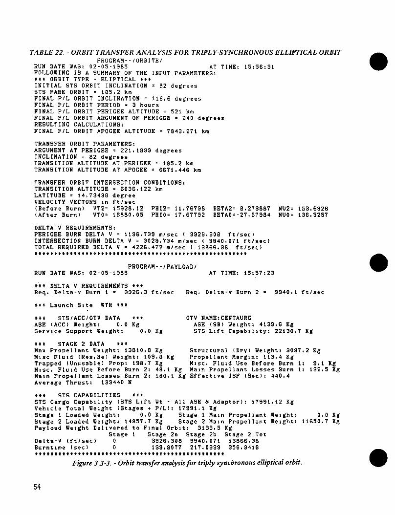
TABLE 22. - ORBIT TRANSFER ANALYSIS FOR TRIPLY-SYNCHRONOUS ELLIPTICAL ORBITPROCRAM--/ORBITE/

RUN DATE WAS: 02-05-1985 AT TIME: 15:56:31FOLLOWING IS A SUMMARY OF THE INPUT PARAMETERS:t«* ORBIT TYPE - ELIPTICAL **»INITIAL STS ORBIT INCLINATION = 82 degreesSTS PARK ORBIT = 185.2 kmFINAL P/L ORBIT INCLINATION = 116.6 degreesFINAL P/L ORBIT PERIOD = 3 hoursFINAL P/L ORBIT PERIGEE ALTITUDE = 521 kmFINAL P/L ORBIT ARGUMENT OF PERIGEE = 240 degreesRESULTING CALCULATIONS:FINAL P/L ORBIT APOGEE ALTITUDE = 7843.271 km

TRANSFER ORBIT PARAMETERS:ARGUMENT AT PERIGEE = 221.1899 degreesINCLINATION = 82 degreesTRANSITION ALTITUDE AT PERIGEE = 185.2 kmTRANSITION ALTITUDE AT APOGEE = 6671.446 km

TRANSFER ORBIT INTERSECTION CONDITIONS:TRANSITION ALTITUDE = 6036.122 kmLATITUDE = 14.73438 degreeVELOCITY VECTORS in ft/sec(Before Burn) VT2= 15928.12 PHI2= 11.76798(After Burn) VTO= 16880.05 PHIO= 17.67792

BETA2= 8.273887BETAO=-27.57984

NU2= 153.6926NUO= 136.5257

DELTA V REQUIREMENTS:PERIGEE BURN DELTA V = 1196.739 ro/sec ( 3926.308 ft/sec)INTERSECTION BURN DELTA V = 3029.734 m/sec ( 9940.071 ft/sec)TOTAL REQUIRED DELTA V = 4226.472 ro/sec ( 13866.38 ft/sec)»**«»»**»*»»»t»*tf»t»»tt*t**»*»**tit»ft»***»»»ttt»t*f*t»

PROGRAM--/PAYLOAD/RUN DATE WAS: 02-05-1985 AT TIME: 15:57:23

»** DELTA V REQUIREMENTS *«*Req. Delta-v Burn 1 = 3926.3 ft/sec Req. Delta-v Burn 2 = 9940.1 ft/sec

*** Launch Site WTR ***

*»* STS/ACC/OTV DATA ***ASE (ACC) Weight: 0.0 KgService Support Weight: 0.0 Kg

*** STAGE 2 DATA »**Max Propellant Weight: 13810.8 KgMisc Fluid (Res,He) Weight: 109.8 KgTrapped (Unusable) Prop: 198.7 KgMisc. Fluid Use Before Burn 2: 48.1 KgMain Propellant Losses Burn 2: 180.1 Kg Effective ISP (Sec): 440.4Average Thrust: 133440 N

OTV NAME:CENTAURGASE (SB) Weight: 4139.6 KgSTS Lift Capability: 22130.7 Kg

Structural (Dry) Weight: 3097.2 KgPropellant Margin: 113.4 KgMisc. Fluid Use Before Burn 1: 9.1 KgMain Propellant Losses Burn 1: 132.5 Kg

**« STS CAPABILITIES ***STS Cargo Capability (STS Lift Wt - All ASE «c Adaptor): 17991.12 KgVehicle Total Weight (Stages + P/L): 17991.1 KgStage 1 Loaded Weight: 0.0 Kg Stage 1 Main Propellant Weight: 0.0 KgStage 2 Loaded Weight: 14857.7 Kg Stage 2 Main Propellant Weight: 11650.7 KgPayload Weight Delivered to Final Orbit: 3133,5 Kg

Stage 1 Stage 2a Stage 2b Stage 2 TotDelta-V (ft/sec) 0 3926.308 9940.071 13866.38Burntime (sec) 0 139.8077 217.0339 356.3416f****t*******»*******tt****f*t*tt********t«******

Figure 3.3-3. - Orbit transfer analysis for triply-synchronous elliptical orbit.

54

For each orbit studied in section 3.1, a payload capability was per-formed. A summary of results is shown in Table 23. Table 23 shows the launchsite, shuttle orbit and OTV assumed for each orbital case along with thedelta-v requirements for each orbit. The table shows that the payload capa-bility increases as the orbital altitude decreases. Also, the payload capa-bility increased as the inclination decreased for the same orbital period.This is attributed to the fact that the STS park orbital altitude is higherfor the lower inclination. As an example, 7130 kg can be delivered to the12-hour, 45° inclination orbit using the Centaur G. For the 12-hour, 30° in-clination orbit, the payload capability is increased to 7236 kg. This is dueto the fact that the orbiter park altitude was increased from 287.1 km to407.4 km, thus reducing the delta-v requirements for the Centaur G.

TABLE 23. - ORBIT TRANSFER RESULTS

Triply-synchElliptical. 116.6

Molniya, 63.4°

Geosynch ellip0 6/60°0.3/30°

Triply-synch circular

Geostationary

Sub-geosynch12 h/45°

12 h/30°8 h/45°

8 h/30°6h/45°6 h/30°

STS park orbit

Altitude

185.2, km185.2

185.2

185.2370.4

185.2

444.5

287 1

4074287 1

407.4287.14074

Inclination

860°820

60.

59.030.0

850

28.5

450

30.0450

30.0450300

Launch -site

WTRWTR

WTR

WTRETR

WTR

ETR

ETR

ETRETR

ETRETRETR

Delta-V

Burn 1

1209, m/s1197

2463

27242571

1137

2411

2647

20111756

172015181481

Burn 2

2689 m/s3030

285

545992

3552

1781

1421

14031316

129511981175

OTV

TOS/AMSCentaur G

Centaur G O>

Centaur GCentaur GCentaur B

Centaur G

TOS/AMSCentaur GCentaur B

Centaur GCentaur BCentaur GCentaur GCentaur BCentaur GCentaur GCentaur GCentaur B

Payloadcapability

1,722kg3,134

llt 9,575

8,0076^44

13,054*

2,127

3,0134,3879^72*

7,13013,900*7,2368,745

17,195*8,91093049,993

21,770*

'Payload capability assumes separate STS launches for OTV & satellite.

55

3.4 TECHNOLOGY SURVEY

A survey was performed to assess the state-of-the-art (SOA) of subsystemtechnologies applicable to direct broadcast satellite systems. The surveysources included discussions with vendors in specific technology areas, datacontained in the NASA Space Systems Technology Model, the NASA Systems Costand Design Model, and information contained in the literature.

The objective of the survey was to identify applicable hardware that isspace-qualified hardware that is being built for space use, and hardware thatis or was intended for space application, but has not reached the qualifica-tion phase. The results of the technology survey were used to help identifycritical technology areas, to identify and define system and subsystem re-quirements, and to enhance the ability to estimate size and cost of systemsand subsystems. Figure 29 shows the scope of the technology survey and theinformation flow to other program tasks.

The technology survey was categorized by VOA satellite subsystem. Simpli-fied block diagrams of some of these subsystems appear in Figures 30 through32.

Subtask 2.1 &

Satellite cone(system rqmt:

iSubtask 2.3.1

Antenna subsystemsizing

1

\

2.2

)

*Subtask 2 3.2

Power subsystemsizing

*Subtask 2.3.1Antenna systemdata baseHardware concepts& extrapolationequations

i I

\

Subtask 2 3.3Transpondersubsystemsizing

*Subtask 2 3.2Power systemdata baseHardware concepts& extrapolationequations

L— '

Othersubsystemspay loadrqmts

-»•

N

Subtask 2.3.3Transponder databaseHardware concepts& extrapolat onequations

1

i

^XSTS ^N'V. compatible,

TN

./ Data base^

Y

" *Subtask 2.4Candidate conce

^ Y

Pt

^^exhausted .S'

figure 29. - Technology survey.

56

Ku uplink

Crosslink

uI

Ir *•

Ku RFmodule

Crosslinkmodule

1

| RFsw

J i

Signal processor

Wide band module

J

£ n transmitter

Commands tosubsystems

Data fromsubsystems

Figure 30. - Communications subsystem functional block diagram.

Power controlunit

Battery charger

Batteries

Power distributionunit

Powerbusses

Figure 31. - Electrical power subsystem functional block diagram.

Transmitters

Subsystems

57

Rate gyros j-

Star trackers

Command Receiver

Attitude/positiondeterminationsoftware

Coarse Sunsensors

Fine Sunsensors

Solar-drivetransducers

Solar array controlsoftware

Solar arraydrive electronics

Solar arraydrive

Antenna-drivetransducers

Auto trackreceiver

Antenna signalacquisitionsoftware

Antenna driveelectronics

Antenna drives

Figure 32. - ACS functional block diagram.

3.4.1 Antenna Technology

The antenna types considered in the VGA study fall into two classes: re-flectors and arrays. Each class had advantages and disadvantages for DVBS ap-plications, with the frequency of operation and aperture size of major impor-tance. Reflectors had a distinct advantage from a simplicity standpoint.However, when large amounts of RF power were required, e.g, for HF-, VHF-, andL-band systems, an array had the advantage of allowing a distribution of thepower over a number of element/transmitter pairs thus reducing the possibilityof any arcing and multipacting effects from the generation of high RF power inspace. This also proved to alleviate heat dissipation problems, and will pro-vide graceful degradation if a transmitter should fail. Arrays also proved tohave another advantage in that the pattern characteristics could be changed toscan the main beam and match the required coverage for the various zones. Forthis study, the aperture efficiency for any reflector system was considered tobe 50% while an array system had an aperture efficiency of 80% for nonscannedarray and 75% times the cosine of the scan angle for a scanned array. The 50%efficiency factor is generally used for reflector systems to account for thefeed mismatch and circular polarization (CP) conversion losses, spillover lossand the losses due to reflector surface accuracy. The 80% array efficiencyaccounted for the losses associated with array mismatch, amplitude and phasecontrol of the elements and CP conversion. For scanned arrays, an additional5% reduction in the maximum aperture efficiency was used to account for theadditional losses from phasors used to provide the scanning ability.

3.4.1.1 Parabolic Reflector Antennas

Parabolic reflector antennas in the 1-to 4-meter range are the most widelyused on existing broadcast systems and proved to be acceptable candidates forthe Ku-band system design. Antennas of this size are generally constructed of

58

a single rigid dish and either a single feed horn or a small feed array. Toincrease structural and thermal stability, the most recent systems have usedgraphite composites in the reflectors and antenna support structures. Anexample of this technology is Intelsat VI (Fig. 33) which uses four graphiterigid dish parabolic reflectors. The smaller reflectors are fed with conven-tional horn feeds, while the larger 2- to 3-meter reflectors are fed using ahoneycomb array feed.

For parabolic reflector antennas in the 4- to 20-meter size, two types ofantenna systems, wrap-rib antennas and radial rib antennas, are most widelyused. Because of aperature size, these reflectors are generally required tobe stowed for STS launch.

3.2mTransmit hemi/zonereflector \

Receive hemi/zonereflector

1.12mK-bandwest spot

Extendablesolar drum

Figure 33. -Intelsat VI antenna farm dimensions.

Wrap-rib antenna. - The first system, the wrap-rib design, has been devel-oped by Lockheed. The best known application is on the ATS-6 spacecraft,which uses a 9.1-meter parabolic, wrap-rib reflector antenna operating up toand above 8 GHz (Fig. 34). The ATS-6 antenna, made with aluminum ribs andconventional thermal blankets, represents a technology about 10 years old.Recent developments using this concept have resulted in a manufacturing capa-bility for wrap ribs using structural composite materials with low coeffi-cients of thermal expansion. New materials and manufacturing processes forreflector mesh have been developed recently, and the analytical capability forthe detail design of the structure has been improved recently. These develop-ments have made it possible to design, build, and predict antenna performancefor lighter and more stable wrap-rib structures.

59

Figure 34.LMSC ATS-6 flight antenna reflector.

Radial rib antenna. - The radial rib antenna has been used by both HarrisCorporation and TRW on recent satellite systems. TDRSS uses two 6-meter dia-meter radial-rib antennas built by Harris (Fig. 35). Harris has also devel-oped the radial-rib concept to the point of demonstrating that this technologyqualifies for flight applications of antennas up to 18.3 meters in diameterand operation up to K-band. TRW's radial-rib antenna has been used on theFLTSATCOM satellite. The FLTSATCOM antenna is 4.9 meters in diameter andoperates at 300 MHz. The reflector consists of a 2-meter diameter solid cen-ter dish and a deployable outer ring of rib-supported mesh (Fig. 36).

60

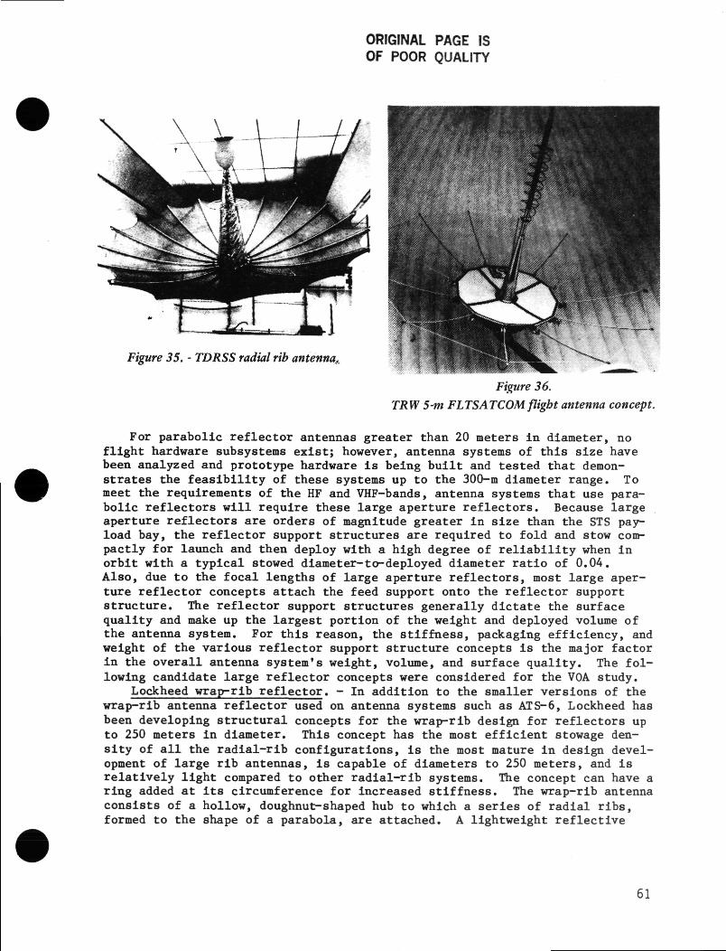
ORIGINAL PAGE ISOF POOR QUALITY

Figure 35. - TDRSS radial rib antenna.

Figure 36.TRW 5-m FITSATCOM flight antenna concept.

For parabolic reflector antennas greater than 20 meters in diameter, noflight hardware subsystems exist; however, antenna systems of this size havebeen analyzed and prototype hardware is being built and tested that demon-strates the feasibility of these systems up to the 300-m diameter range. Tomeet the requirements of the HF and VHP-bands, antenna systems that use para-bolic reflectors will require these large aperture reflectors. Because largeaperture reflectors are orders of magnitude greater in size than the STS pay-load bay, the reflector support structures are required to fold and stow com-pactly for launch and then deploy with a high degree of reliability when inorbit with a typical stowed diameter-to-deployed diameter ratio of 0.04.Also, due to the focal lengths of large aperture reflectors, most large aper-ture reflector concepts attach the feed support onto the reflector supportstructure. The reflector support structures generally dictate the surfacequality and make up the largest portion of the weight and deployed volume ofthe antenna system. For this reason, the stiffness, packaging efficiency, andweight of the various reflector support structure concepts is the major factorin the overall antenna system's weight, volume, and surface quality. The fol-lowing candidate large reflector concepts were considered for the VOA study.

Lockheed wrap-rib reflector. - In addition to the smaller versions of thewrap-rib antenna reflector used on antenna systems such as ATS-6, Lockheed hasbeen developing structural concepts for the wrap-rib design for reflectors upto 250 meters in diameter. This concept has the most efficient stowage den-sity of all the radial-rib configurations, is the most mature in design devel-opment of large rib antennas, is capable of diameters to 250 meters, and isrelatively light compared to other radial-rib systems. The concept can have aring added at its circumference for increased stiffness. The wrap-rib antennaconsists of a hollow, doughnut-shaped hub to which a series of radial ribs,formed to the shape of a parabola, are attached. A lightweight reflective

61

mesh is stretched between these ribs to form the parabololdal reflecting sur-face. Figure 37 shows four ribs of the 55 meter proof-of-concept hardware be-ing built by Lockheed.

Figure 37. - Lockheed's proof-of-concept wrap rib reflector.

Articulated radial-rib reflector. - This concept (Fig. 38) is a logicalextension of Harris' smaller radial-rib design, but has the flexibility to ac-commodate larger diameters and retain the same packaging efficiency. It con-sists of a central mast that supports the feed and to which rigid radial ribsare attached by privots at the base. Because of the antenna diameters underconsideration and the constraint of the limited stowed volume available, it isnecessary to put an articulation at the midspan of each rib. The ribs approx-imate a parabolic contour and have adjustable standoffs to which the reflec-tive mesh is attached. The surface is shaped between the ribs by the second-ary drawing surface technique. The concept is attractive from an experiencestandpoint, but there are serious packaging size limitations. The shorteststowed length with a single articulation in the ribs is one-quarter of the an-tenna diameter. For a 100-meter diameter antenna, this length would becomeprohibitive. Another articulation for each rib is possible, but the addedmechanical complexity and probable mesh handling problems negate any potentialadvantages.

62

Figure 38. - Harris-articulated radial rib antenna.

Hoop and column reflector. - Both Martin Marietta and Harris have hoop andcolumn reflector design concepts. The fundamental elements of the two con-cepts are similar but the mechanical design approaches are different. TheHarris Corporation hoop and column reflector concept for self-erectable struc-tures is intended for reflector design up to 250-meter diameter (Fig. 39).This concept has been developed to the point of a preliminary design for sizesup to 100-meter diameter; a 15-meter diameter conceptual demonstration modelhas been built. The fundamental elements of the support structure include thehoop and upper, lower, and center control stringers. The reflector consistsof the mesh, mesh shaping ties, secondary drawing surface, and mesh tensioningstringers. The basic antenna configuration is a type of may pole with aunique technique for contouring the RF reflective mesh.

63

Continguous truss reflector. - Two basic truss configurations, the MartinMarietta box truss, and the General Dynamics tetrahedral truss are the mostwidely used for designing contiguous truss reflectors. Components of the re-flector structure use the basic bay design regardless of the number of bays.The selection of the number of bays for a given antenna size and applicationis a function of cost, reliability, weight, and surface tolerance.

The tetrahedral concept is a basic building block used in numerous combi-nations to achieve the desired shape and size of an antenna structure (Fig.40). The basic element is a deployable tetrahedron hinged by spider links ateach corner. Each tetrahedron forms one truss bay, and the number of bays canvary in number from four to 10 more across the major diameter of the reflectorstructure. This configuration forms the support structure for the reflectivemesh. With tetrahedral trusses, the reflector outline is hexagonal ratherthan circular so the equivalent reflector diameter is about 10% less than themaximum point-to-point width.

Feed

Hoop

Telescoping feed support

Upper control stringers

HingeSpider

Secondarydrawing surface

Telescopingmast (extended)

Lowercontrolstringers

Meshshaping

Mesh ties

tensioningstringers

Figure 39 - Harris hoop/column reflector Figure 40 - Tetrahedral truss reflector.

Martin Marietta is developing a deployable box truss structural systemapplicable to parabolic antennas. Originally proposed for the Air Force's On-orbit Assembly program, we are currently developing the system with prototypebeam and truss segments. The system features compact stowage, step-by-stepdeployment, high deployed precision and reliability, and adaptability to awide variety of reflector sizes up 200-meter diameter. Figure 41 shows a re-cent concept of a 120x60-meter antenna system designed for NASA LaRC on theAdvanced Earth Observation Spacecraft contract.

Truss ring antenna reflector. - The Martin Marietta box truss has alsobeen used in box truss ring design. This box truss ring consists of box trusstrapezoids forming a circular or racetrack ring. Figure 42 shows a box trussring supporting an electrostatically controlled membrane mirror reflector.The application shown in the figure is a 100-meter diameter ring designed byMartin Marietta for the NASA LaRC Advanced Space Systems Analysis (ASSA)program. The box truss ring is a ultra-lightweight structure that has excel-lent stiffness. Stowed packaging is very efficient and allows packaging ofsubsystems in the center of the stowed truss.

64

ORIGINAL PAGE ISOF POOR QUALITY

Figure 41. - Advanced Earth observation spacecraft using Denver Aerospace's deploy able box

truss structure.

65

Figure 42. - ASS A using Denver Aerospace's truss ring reflector.

Inflatable reflectors. - Inflatable reflectors can offer low weight, com-pact stowage, reliable deployment, and adequate shape accuracy. L'Garde In-corporated and others are developing advanced antenna concepts using inflat-able, thin-film bodies. These bodies incorporate surfaces of revolution suchas a paraboloidal reflector capped by a cone (Fig. 43). Shape accuracies for

66

HF- and VHF-bands with 100-meter diameter apertures appear to be easilyachievable. By operating at very low pressures (e.g, 10~6 psi), the weightof inflatant gas lost through micrometeoroid holes can be kept within practi-cal bounds. A metallized surface forms the reflector and, to achieve adequatethermal control, the cone can be more than 90% metallized in a patchworkfashion; each patch being very small relative to the broadcast wavelength. Ingeostationary orbits, such reflectors could depressurize thermally and havedegraded shape accuracy only during two periods per year (equinoxes) and, dur-ing those periods, only for short period (less than 3 hours) bracketing localmidnight. It is also interesting to note that the feeds, with their high heatdissipation, can be located outside the inflatable body.

Metallized reflector film

Annular-shapedstabilizer(multi-ply offilms &yielded foils)

Film cone (can bepatchwork metallizedfor thermal control)

Feed location

Figure 43Typical inflatable reflector configuration.

3.4.1.2 Array Antennas

Similar to large reflector antenna concepts, array concepts require an ex-terior support structure. Unlike the lightweight reflective surface, the mostmature array antenna technology uses large rigid panels containing array ele-ments. For these systems, array panels dictate the weight and volume of theantenna system with the support structure accounting for only 10% of the totalsystem weight and volume. Due to the fact that the rigid arrays must stow byfolding, the array size is limited to moderate size apertures. Also, sincethe back surface of the panel is generally used as the ground plane, the panelthickness is dictated by the operating frequency of the array, i.e., gener-ally A/4 in thickness. This type of array proved acceptable for the L-bandsystem. The HF and VHF systems, because of their long wavelengths, required amore advanced, yet unproven array systems using lightweight film material withthin array elements. For these systems, the support structure again dominatesthe total antenna system's weight and volume. The following are the variousarray system concepts studied under this contract. The first two concepts,the synthetic aperature radar (SAR) antenna and the gate frame truss phased

67

array, are examples of technology that exist for the rigid panel type arraysystems. The remaining concepts show examples of membrane type array systems,capable of sufficiently separating the ground plane from the radiating surfaceallowing these concepts to be used for HF and VHF-band applications.

SAR antenna. - One of the key science instruments and a unique feature ofthe Seasat-I Spacecraft (launched during spring 1978) is the SAR antenna (Fig.44). This antenna is a planar-phased array that measures 10.7 by 2.2 metersin the deployed configuration and operates at 1.275 GHz. The planar arrayconsists of eight 1.3 by 2.16-meter rigid and structurally identical fiber-glass honeycomb panels. The panels are hinged together in series, but are in-dividually mounted to a deployable truss structure that provides support andalignment for the panels. The deployable truss, in turn, is supported by adeployable tripod structure whose function is to support and govern deploymentof the truss and panels (Fig. 45). The tripod was attached to a biaxial actu-ator mounted directly on the Agena spacecraft.

The SAR antenna subsystem was developed by Ball Brothers Research Corpora-tion. Lockheed Missiles and Space Company, was responsible for development ofthe flight hardware and integration of the SAR antenna with the Agena space-craft. .The weight of the antenna system is about 113.4 kg (250 Ib).

Gate frame truss phased array antenna. - Figure 46 shows the gate frametruss structural system under development at Martin Marietta. It is specifi-cally designed for compact stowage and high precision and stiffness when de-ployed with integral, rigid array panels. The support structure makes upabout 5% of the total system weight and about 15% of the stowed volume.

Figure 44. - Seasat-I spacecraft—cruise configuration.

68

ORIGINAL PAGE ISOF POOR QUALITY

V-shaped,2-member frame

Antenna panel

Diagonal\

Tubularlongerons

Control linkage

Figure 45. - Astro Research Corporation's deploy/able support truss forthe panels of the Seasat-I SAR antenna.

Figure 46. - ITSS using Denver Aerospace's gate frame truss.

69

Hoop and column phased-array antenna. - The Grumman space-fed, phased-array concept for self-deployable antennas is Intended for designs up to 300-meter diameter and operation at L-band or lower (Fig. 47). Grumman developedthis concept to the point of a preliminary design for a 60-meter diameter an-tenna and a 1.3-meter diameter mechanical model. The mechanical model wasused to demonstrate and evaluate the basic mechanical conceptual design. Theprimary limitation of this concept is the complicated deployment and the lowstructural vibration frequency of the deployed membrane.

The Grumman antenna concept is a planar array whose basic support struc-ture is a wire-wheel configuration. This concept development was centeredaround the design of 61-meter diameter and 300-meter diameter space-fed,phased-array antennas for operation at L-band. The phased array is composedof 32- to 72-gore panel assemblies and their tensioning devices.

Phased ArrayAntenna RimAssembly

Stays (32)16 fore & aft

Figure 47 - Basic structural elements of Grumman phased-array concept.

Box truss ring phased array. - Similar to the Martin Marietta box trussring reflector (see Fig. 42) a box truss ring phase array consists of boxtruss trapezoids forming a circular or racetrack ring. Instead of a membranemirror reflector, the radiating surface is stretched flat across the ring withflexible bow-tie radiating elements attached on the surface. The ground planeis a second stretched membrane on the back surface, with the box truss depthbeing adjusted to provide the correct spacing between surfaces. The back sur-face also acts as a support structure for the antenna transmitters. Figure 48illustrates this concept for an 80-meter array. This concept provides alightweight and efficient method for producing a phased array in which theground plane is required to be at a relatively large distance from the radiat-ing plane. Also, since stowage of the system does not require the box truss

70

ORIGINAL PAGE ISOF POOR QUALITY

to stow in depth, rigid coax can be used between the transmitters and radiat-ing elements. (Rigid coax is desirable when high power is to be transmit-ted.) Another desirable feature of this system is the distribution of thetransmitters over the back surface, providing a method to allow each transmit-ter to carry its own radiators to dissipate waste heat. This feature elimi-nates the need for a central radiator and a large and heavy system of heatpipes.

Figure 48. - Box truss ring-phased array.

3.4.2 Satellite Feeder Link Technology

The satellite uplink frequency bands allocated for the United States bythe 1979 World Administration are summarized in Table 24. Also shown are in-tersatellite frequency allocations and unallocated bands. Technology for up-link, either for realtime or delayed retransmission, is SOA. The LANDSAT-DKu-band technology will be adequate for VGA DVBS concepts. Figure 49 showsthe basic concept and components required for the satellite feeder link.Earth station transmission is typically provided by high powered amplifierssuch as traveling wave tubes (TWT) or Klystrons, again representing SOA tech-nology. The specific Earth station design will depend on the spacing ofsatellites and whether or not intersatellite links are used. A later discus-sion presents a tradeoff of use of multiple Earth stations vs intersatellitelinks.

71

TABLE 24. - ALLOCATED SATELLITE BANDS FOR THE U S.

C-band

X-band

Ku-band

Ka-band

V-bandQ-band

V-band

Frequency band

Uplink

5 9-6.4 GHz

79-84

140-145

27-3030-31

50-51

Downlink

3 7-4 2 GHz

7 25-7 75

11 7-12.2

17-2020-21

40-4141-43

54-5859-64

Major uses in U.S.

Fixed, point-to-point ground stations; nonmihtary

Mobile (ships, aircraft), radio relay, military only

Broadcast & fixed-point service; nonmihtary

(unassigned)

Fixed-point, nonmihtaryBroadcast, nonmihtary

IntersatelhteIntersatellite

Bandwidth

500 MHz

500 MHz

500 MHz

—

1 GHz2 GHz

3.9 GHz5 GHz

Ku uplinkantenna

Figure 49. - Ku RF module block diagram.

72

3.4.3 Satellite Signal Processing Technology

The onboard signal processing generates the carriers for the downlink.Figure 50 shows options for satellite signal processing. All are existing SOAtechnologies. The method to be used will depend on the specific DVBS, consid-ering band and number of carriers to be processed.

RFfront end t

Freqmult

»» IFfilter •*• Mod •

jFreqmult

. ,Y^ Power J

Oscillator

•*. IFfilter

»• Demod

Oscillator! •*

*

Freqmult

RFmod

l)

Poweramplifier

Figure 50. - Satellite processing models.

3.4.4 Transmitter Technology

The transmitter technology for Ku-band will use SOA TWTs. Figure 51 sum-marizes existing TWT technology. Power output levels on existing satellitesare found between 5 and 250 watts. Higher power levels are considered easilyattainable for use in space. Efficiencies of TWTs are typically about 35 to50%.

For the L-band, TWTs are applicable for output power levels below 250watts. Above these levels, solid state power amplifiers (SSPA) are an alter-native. When used in phased array systems, multiple SSPAs can be used.6-watt space qualified SSPAs exist in the L-band range. Terrestrial and air-borne SSPAs are available up to 1000 watts.

73

1000

10

15 (R) (S)

PPM coupledcavity TWT

Air cooled PPM)helix TWT

• Data from published results:

Hughes (H)Raytheon (R)Siemens (S)Thompson CSE (C)USSR (U)Varian (V)Watkms Johnson (W)

EIO

Figure

10 100Freq.GHz

51. - Microwave power amplifiers technology.

HF- and VHP-bands SSPAs will require new design approaches. Double-sidedprinted circuit boards are projected to provide packaging densities of 700kg/nr* or greater. To meet a 7-yr lifetime requirement, designs will includeinternal redundancy and modularity. Current technology bipolar transistorsare suitable for powers up to a 500 watts. A bipolar NPN transistor rated at200-watts at 300 MHz has been developed. A 600 watt SSPA for low UHF-band iscurrently under development for space use. The same design is projected forgrowth to 1000 watts with minimal redesign. A 400 watt SSPA for operationfrom 100 to 500 MHz has also been developed for airborne military applications.

TABLE 25. - TRANSMITTER PARAMETRICSUse of power MOSFETs will makepower levels of up to 20 kW possiblein the 1990fs. SSPAs using MOSFETtechnology will operate in a class-Dmode and use dual single-ended, push-pull stages for powers greater than1000 watts. A 200 Vdc power bus willbe sufficient for powers up to 1.5 kW,but for higher powers (up to 20 kW) ahigher bus (400 Vdc) will be required.

Predicted weights and volumes for SSPAs (including bipolar and MOSFETtechnologies) are summarized in Table 25. These weights and volumes assume adc voltage bus on a satellite that results in limited required power condi-tioning. By using a regulated bus and with projected advances, efficienciesof 65% are predicted for SSPAs for DVBS in the HF-, VHF-, or L-bands.

Transmitter power

SOW100200500750

10002000

Mass

5.10kg9.94

12.8116.2119.6123.0236.62

Volume

0.0105 m3

0.01770.01820.02190.0255002920.0439

74

3.4.5 Power Generation System Technology

Some VGA mission configurations considered require the energy source becapable of delivering power greater than 100 kW. The load power is a functionof antenna array size and orbit altitude and optimum power levels will be de-termined through detailed parametric analysis. To qualify as a viable energysource, it was assumed that the source must be capable of supplying at least100 kW, since the optimum power level will be near this value. All possibleenergy generation sources are diagrammed in Figure 52.

1Photc

Solai

1Planner

Solar

1woltaic Concentrator

1

array

1Concentrator

1Reactor

1

Nuclear

Radioisotope

IHeat

1

Stored1

1 1Thermal Chemical Mech

1 1

anical

1 1Fuel cell Battery Flywheel

1 1Thermoelectric Dyanmic

Figure 52. - Energy source choices.

Several choices may be eliminated immediately. All stored sources aresecondary energy sources and thus are not applicable since they require peri-odic energy input to replenish their capacity. Radioisotope sources, such asradioisotope thermal generators (RTG) or radioisotope dynamic sources such asorganic rankine cycles and brayton isotope power systems, have not been devel-oped to produce the high power levels required. Dynamic systems of the typementioned are promising sources (in the near term) in the 1 to 25 kW rangeonly. Solar concentrator/ thermoelectric and solar dynamic sources are underearly stages of development and although theoretically capable of high poweroutput, the technological risk is high in the near term. These sources willbe discussed further in Section 4.2, Technology Tradeoffs. Another sourcethat presents difficult design challenges is nuclear reactor. This may be theonly feasible source at some orbital altitudes (e.g., in the Van Allen belt).The most viable energy sources are solar photovoltaic. These latter twosources are discussed in Section 3.4.5.1.

3.4.5.1 Solar Photovoltaic Sources

Many advances have occurred in the photovoltaic field over the last 15years and consequently a wide variety of choices now exist in the design of asolar array. Figure 53 graphically summarizes these improvements in terms ofcost and efficiency. The types of solar cells currently available and underdevelopment are single crystal silicon cells, advanced vertical-junctioncells, gallium arsenide cells in a planar or concentrator array, multiband gap(MBG) cells, and three junction cascade cells. Advanced concepts under studyto improve solar cell performance are the high concentration (100 suns) ratiominiature cassegrainian concentrator (MCC) concept, metal interconnects be-tween cells, and the surface plasmon concept. The cell types together withthe advanced concepts will be discussed here and in Section 4.2 with the aimof selecting optimum energy sources for use in the power system parametricequations.

75

500

400

§300

tt8 200

u100

20

£10 u

1960 1970 1980 1990 2000

Figure 53. - Progress in solar cell technology.

Beginning with the FRUSA flight experiment in 1971 and the NASA developedsolar electric propulsion (SEP) array in the early 1970s, significant improve-ments have been made in single crystal silicon solar cell technology. In theSEP, a 66W/kg flexible foldout design capable of supplying 25 kW beginning oflife (BOL) was developed. A second generation SEP is currently under develop-ment and specific powers as high as 300 W/kg will likely be realized. Tanta-mount to achieving higher specific powers is the increase of the silicon cellconversion efficiency. Presently, state of the art efficiencies are near 14%for planar silicon arrays. It is not reasonable to expect efficiencies to in-crease much above this in the near future. Therefore, the use of higher effi-cient (up to 18%) gallium arsenide cells or concentrator arrays will be re-quired to demonstrate very high specific powers of 400 W/kg or more. Althoughspecific powers in the 300-400 W/kg range are not necessary to construct a 100kW array, they result in lower array area which reduces spacecraft drag anddecreases the propellent mass necessary for altitude maintenance.

Silicon solar cells have many advantages. They are flight proven, andrelatively lightweight; advances in the ultrathin (50 ym) cells using advancedcell processing techniques such as back surface fields and reflectors, plusfront surface texturing and multiple layer antireflection coatings, promise topush efficiencies to 15% by the mid-1990s. Silicon cells have the lowestcost; the use of larger cell sizes (6x6 cm and 8x8 cm) will reduce cost evenmore. Additionally, space station will probably use a planar nonconcentratedsilicon array and thus incur much of the developmental cost for a high power(> 50 kW) system. The ultrathin cells and large cells have experienced prob-lems with bowing but the use of a gridded pattern for the back contact config-uration appears to have eliminated this with the added benefit of reducingcell weight. Silicon cells have the disadvantage of possessing the lowest ef-ficiency of the new cell types, which means an array comprised of siliconcells will have the largest area. This translates into high inertias andhighest effect from drag or solar pressures, which gives the highest orbitmaintenance subsystem mass. Table 26 summarizes the advantages and disadvant-ages of silicon cell technology.

Gallium arsenide solar cells have been demonstrated to operate at effi-ciencies as high at 18% (20% with concentrators). This equates to a reductionof solar array area up to 30% of a silicon array. Also, gallium arsenidecells have a lower temperature coefficient than silicon cells and are moreradiation resistant. The lower temperature coefficient makes gallium arsenidecells ideal for operating with a concentrator and the cassegrainian concept

76

should demonstrate this. However, gallium arsenide cells are approximatelytwo to three times the weight of an equivalently sized silicon cell and arepresently expensive to manufacture. Reductions in cost and blanket weight arelikely to occur in the future and with projected efficiencies of 20%, galliumarsenide will become very attractive. However, considering that a gallium ar-senide array has yet to be flown, the technological risk and initial costwould be high to develop a gallium arsenide array for a mid-1990 launch.Table 27 summarizes the advantages and disadvantages of gallium arsenide celltechnology.

TABLE 26. - SILICON SOLAR CELLTRADEOFF

TABLE 27. - GALLIUM ARSENIDE SOLARCELL TRADEOFF

Plus

Flight proven15% Efficiencies possibleLightweightLow cell costLarge cell size possibleSmall development cost

MinusLarge array area — highest orbitSubsystem massArray stiffness may be an issue

Plus

Higher efficiencies vs Si

Compatible with concentrators

Lower temperature coefficient vs Si

Higher radiation resistance vs Si

Reduction in spacecraft inertias

Minus

High cost

Not flight proven

Higher weight vsSi

Higher weight may negatesmaller area

The most promising of the advanced cells are the three junction cascadecells with possible efficiencies of 30%. MBG cells, which use two materialswith different bandgaps to convert more of the solar spectrum into electrici-ty, show signs of full development in the near future. Vertical junctioncells possess high radiation resistance but this is offset by a high solar ab-sorptance that results in a higher operating temperature. Reaching higherspecific powers by reducing the blanket weight through using thinner coverglasses and thinner cells (2 mil) should reach maturity in the near term. Al-though these technologies will not be available without high risk by the mid-1990s, they promise a bright future in solar array development. Table 28gives a comparison of various solar cell designs.

TABLE 28. - BLANKET WEIGHT COMPARISONS FOR VARIOUS SOLAR CELL DESIGNS

Cell description

Cell efficiency, (% at25°C

Operating temp, °Ckg/m2

W/m2,BOLW/kg. BOL

Radiation degradation1x10ls equiv, 1 MeV e/cm2

Present

Si

2 mil

10.2

78

0.303

86

284

29%

Si

8 mil

14.9

73

0738

131

116

27%

Near Term

Si

2 mil

14

75

0.303

117

385

22%

Vertical

Jen

135

84

0.357

113

312

16%

GaAs

7 mil

17-18

65

1.060

135

252

20%

Far Term

GaAs

2 mil

18

68

0.411

201

493

20%

MBG

3 mil

22

66

0523

244

375

20%

3 Jen

Cascade

30

71

0.840

335

399

20%

3.4.5.2 Solar Array System Considerations

Some key issues that must be considered in designing a power generationsystem are mission duration, the existing and near-term technology, weight orsystem mass, radiation tolerance, size and interaction with spacecraft con- -trol, and orbital altitude. For solar photovoltaics, altitude is a key system

77

driver. Altitude affects radiation level and thus the degradation of thesolar cell performance. Altitude also determines the length of eclipse peri-ods and thus determines the amount of power expended during occulation whichmust be made up during sunlight. As a point of departure, transmitter opera-tion was constrained to be off during eclipse periods to avoid the large bat-tery and solar array size increases. The seven year life requirement will bedifficult to meet at some altitudes because high radiation levels will requirelarge amounts of shielding weight to be added.

Several solar array configurations are possible. The solar cells may bearranged on panels either in a rigid foldout planar configuration or in aflexible rollout blanket configuration. The blanket configuration uses kaptonas the flexible substrate and in addition to achieving high packaging densi-ties, it is relatively lightweight. The cells may also be mounted to thespacecraft body. For gallium arsenide cells a concentrator system may beused, although development of this system is still required and concentratorreflector life is questionable for a seven year mission. The effect of or-bital altitude on system weight for a silicon blanket array is shown in Figure54. Because the transmitter was constrained to be off during eclipse, the ef-fects of increased solar array size to account for power lost during eclipsewas not included in the figure. As can be seen a severe weight penalty willbe incurred with operation in the Van Allen belt.

O

Xo>

01

I|3

<

- 100kW EOL— Circular orbit- SI blankets

4 5 6 7

Altitude, km x 103

8 9 10 20 30 40

Figure 54. - Solar array weight versus altitude.

To fully use the power generation capability of the array, it must be Sunpointing. The technology now exists for solar arrays to track the Sun andmaintain the array plane normal to the solar flux within +2°. For a largepower system it is impractical to design an array that does not track the Sunbecause the array size is proportional to the cosine of the solar incidenceangle. A concentrator system also requires Sun tracking to direct the solarenergy into the reflector. The disadvantage to a Sun-pointing system is thatpower transfer from solar array to the distribution bus is more difficult, es-pecially at high voltage.

78

The technology with the lowest risk is the photovoltaic blanket plannerarray, utilizing silicon solar cells. If space station uses this technologyas planned, then much of the engineering development effort for a 100 kW powersystem will be complete, making this system even more attractive.

3.4.5.3 Nuclear Reactor Source

The only space nuclear reactor TARTF2Q <?P inn nFSCRJPTmNpower sources being developed is the TABLE 29. - SP-100 DESCRIPTIONSP-100 100 kW power plant. Table 29 Type .......... In-core thermiomcs

highlights the features of one design %£" " .;:::/ | " sCo™"' 1°° VdCconcept. The power System described Dimensions ......... 3.0 m diameter x 5. 76 m 'pngth

is a spacecraft power system that con- gSS.rT. '. . '. \ \ . \ \ ' SZfKZS.'S&.VertS the thermal output Of a nuclear density cannot be scaled down

reactor into electrical power for useby a Spacecraft System. The normal 'Exclusive of mounting boom and distribution cabling

output of the power system is 100 kW.The power system is compatible with launch in the STS. The power system con-sists of a reactor- converter subsystem, a heat transport subsystem, a powerconditioning and control subsystem, and a structure subsystem. The nuclear-converter subsystem converts the fuel to heat energy by means of nuclear fis-sion. The heat is converted directly to electrical power using in-core thermi-onic converters. Heat is removed from the reactor by the heat transport sub-system and transported to the radiator which rejects it to space. The rawelectrical output of the nuclear- converter subsystem is regulated by the powerconditioning and control subsystem and distributed to the spacecraft interface.

Thermionic conversion refers to a physical mechanism for the direct con-version of heat into electricity. A thermionic heat- to- electricity converteris an engine in which electrons are the thermodynamic working field. Elec-trons are emitted from a hot metallic surface (the emitter) maintained by nu-clear or other heat sources at a temperature Tem, and absorbed on a second,parallel surface ( the collector) . The voltage developed between the two sur-faces causes electrons to flow through an intervening electrical impedance,delivering electrical power to a load. The electrons also transport heat fromone surface to the other. The collecting surface is held at the desired tem-perature, Tem, by thermal contact with a coolant. The temperatures, Temand Tc, are approximately 1700 K and 1000 K respectively. Currently, thereis widespread debate about whether the thermionic converter can meet a sevenyear mission at these high temperatures. The collector cylinder is containedwithin an electrical insulating sheath, which is in turn contained within ametallic sheath in contact with the liquid-metal coolant.

79

TABLE 30. - SP-100 POWER GENERATIONTRADEOFF

Plus

— Produces power continuously

— Not as susceptible to Van Allenbelt

— Scales up readily

_ Low area and drag

- Potential first flight 1990-1992

Minus

Nonproven technology-highdevelopment risk

Nuclear thermal source

Does not scale down below100 kW

Safety considerations— placeslower limit

Onorbit altitude

The SP-100 power system is pro-jected for a demonstration flight byearly 1990. For power levels above100 kW and for orbits in high radia-tion belts the SP-100 system may bethe only viable candidate for a mid-1990 mission. The advantages and dis-advantages of this system are summar-ized in Table 30. There is still highdevelopment risk for this technology,making this system at present less at-tractive than solar photovoltaics. Ifdevelopment proceeds as planned how-ever, this system may become a highpower generation source of the future.

3.4.6 Power Distribution Technology

Power distribution involves the transfer of power from the power source tothe user loads. This entails selecting the type of cabling, the voltage leveland the voltage frequency (ac vs dc), and the type of regulation and switchingrequired. The voltage regulation or power conditioning is highly dependent onthe user loads and their requirements and should be defined later in a de-tailed system design. The power conditioning technology exists now to be com-patible with the power system selected. The issues that need to be addressedare cabling weight and type, voltage level, voltage frequency, and powertransfer from solar array to bus.

3.4.6.1 Cabling

The cabling weight is a significant portion of the power system weight.For constant power loss, cabling weight increases with the square of thelength and decreases with the square of the voltage. This relationship is notnecessarily valid however, for shorter cable runs where the cable weight maybe limited by the current carrying capabilities of the conductor. A.S can beseen, higher voltage levels can significantly reduce the cabling weight.

Several conductor types should be available in the near and far term. Be-sides the traditional copper conductors, aluminum conductors should be readyfor near-term applications and in the far term, intercalated carbon fibers andsodium conductors should be available. These conductor types will be dis-cussed further in Section 4.2.

3.4.6.2 Voltage Level

It was mentioned previously that high voltage levels can significantly re-duce cabling weight. For large space power systems it is impractical to uselow voltage levels. For example, a 100 kW system operating at 28 Vdc wouldproduce currents in excess of 3500 amps. With these large currents, switchand semiconductor losses and the resultant heat increase, the efficiency ofthe system goes down, and a larger and more expensive energy source is re-quired. Conversely, serious problems arise such as plasma charging and corona

80

discharge if the voltage is too high. Another factor requiring careful con-sideration is the paschen breakdown voltage of various gaseous elements thatmay surround the spacecraft cabling and electrical components. The potentialfor breakdown exists as gaseous pressures are reduced during the spacecraftlaunch and ascent phase. Outgassing from various spacecraft materials maycause the potential breakdown conditions to exist long after the spacecrafthas been placed in its orbit. Minimum breakdown voltages can occur at 300 V.In consideration of this, a safe upper limit of 250 Vdc should be selected.This is also below the voltage threshold where plasma arc discharging andpower losses due to plasma charging are a factor. The plasma effects are pri-marily seen in low-Earth orbit, where the electron densities are relativelyhigh. Figure 55 depicts the array cabling mass as a percent of total powersystem mass vs array voltage. This figure shows that for a 100 kW system,small weight savings is realized in increasing array voltage from 200 to 250Vdc. Thus, to provide an added margin of safety between the Paschen breakdownvoltage, a buss voltage of 200 Vdc would be optimum.

Buss power

100 400200 300Arrav voltage. V 5_°°

Figure 55. - Cabling mass versus array voltage forthree buss power levels.

3.4.7 Energy Storage Technology

Because the transmitters will be off during eclipse for L-, VHF-, and HF-bands, the function of the energy storage portion of the power system will beto maintain only critical power on the spacecraft during deployment operationsand during eclipse or occulation. The critical power load (primarily house-keeping loads) during eclipse has been assumed to be 500 W. This greatlysimplifies the selection of an energy storage system.

81

Options available for energy storage devices include the traditional meth-ods of nickel cadmium and nickel hydrogen batteries, and more creative methodssuch as regenerative fuel cells (RFC). To support housekeeping loads only,batteries are most effective. Regenerative fuel cells may be the only effec-tive system if transmission is required during eclipse periods and power lev-els greater than 10 kW are needed. Nickel hydrogen batteries have performedvery successfully on missions in GEO orbit and development programs are underway to qualify them for LEO applications. Nickel hydrogen batteries should beavailable at low risk for all applications by the early 1990's.

3.4.8 Power Control Technology

200

: ISO

100

so

10 20 30 40 50 60 80 100Solar array power, kW

200

Figure 56. - Shunt regulator weight versussolar array power.

The objective of power control isto regulate voltage variations causedby source and load changes, and todissipate excess power to prevent dam-age to the loads and electronicparts. The system must be capable ofdissipating all but critical loadpower. Conventional designs use ashunt regulator or shunt resistor bankto dissipate the excess power. Figure56 displays shunt regulator weight vssolar array power, the relationship isnot linear because as the array powerincreases, increasingly large portionsof the solar array can be controlledby single shunt regulator elements. The type of shunt regulator considered isan electronic regulator that shorts out solar array strings so that the poweris never generated. Shorting the array strings will not harm the solar cellsbecause short circuit current for a solar cell is typically only 5% aboveoperating current. A resistor bank would be used in conjunction with the reg-ulator to dissipate small amounts of power or fine tune the regulation. Thedesign challenge is developing switching devices capable of handling largecurrents at high voltage. This system should be scaleable to 100 kW powersystems at low risk.

3.4.9 Attitude Control, Stationkeeping and Maneuvering Technology

The attitude control subsystem (ACS) and auxiliary propulsion subsystem(APS) are considered together throughout the.study, primarily because attitudecontrol is performed by the APS system for most satellite concepts of inter-est. The requirement for multiple satellite and antenna beam steering in HF-,VHF-, and L-bands leads to a requirement for some degree of autonomous atti-tude control and orbit maintenance. Since adequate electrical power will beavailable during periods of no or lower RF transmission, electric propulsioncan be considered as a viable alternative to chemical propulsion.

The basic elements of the ACS for HF- and VHP-bands were shown previous-ly. Sun sensors, star trackers, and rate gyro units are all in use and spacequalified. The onboard control electronics represents a new design for eachsatellite application, but the technology is well understood and the required

82

components available. To meet the lifetime requirement for VOA DVBS, the de-signs should use high levels of redundancy and cross-strapping to enhance re-liability, fault-tolerant operation modes, and distributed ACS data processing.

Control moment gyros (CMS) are used for attitude control on most satellitesystems. Their technology is well understood, but for large antenna systemssuch as required for HF- and VHP-bands, they may not be desireable. Instead,electric thrusters can provide sufficient torque to counteract environment-ally-induced torques. The use of small electric thrusters is possible becauseof the large moment arms with the large antenna structure.

The size of thrusters that can be used with the HF and VHP antennas islimited by the small allowable loads for these large deployable antennas.Thus, small thruster technology was surveyed to identify candidates for VOADVBS. Table 31 contains a summary of small thrusters that might be appli-cable. Also shown is the status of each. Table 32 contains data for a pulsedplasma thruster (PPT) that might be used. Table 33 summarizes a mercury-ionthruster that has operating characteristics similar to the PPT. For geosta-tionary orbits, chemical systems for APS and CMGs or reaction wheels for ACShave been used for some time. For VOA satellites in geostationary orbit, theACS and APS technology is almost off the shelf (OTS). Figure 57 shows a blockdiagram representing a typical chemical APS.

TABLE31. -MICROTHRUSTER CANDIDATES

System ThrustChemical

Inert gasVaporizing liquidSubliming solidsHydrazine direct catalystBipropellant (storable)

10"4 to 1.0 N10": to 0.0510 to 10"2

005 to 1000005 to 10

'sp

35 to 275 s50 to 10040 to 80

100 to 225170 to 320

ElectricResistojetElectrolysisPulsed plasmaIon (mercury)Ion (noble gas)*MPD*Mass driver*

0.01 to 5 010^ to 5.0,10, to 10"3

10'J to OJ52.1 x 10";2.3 x10'2 t o 3 2 x 1010"5 to 10

175 to 860100 to 350

1000 to 50002000 to 90005500 to 64002000 to 9000104 to5x 104

*Not flight qualified.

-SL.

83

TABLE 32 - PULSED PLASMA THRUSTERDATA

Manufacturer

Status- Qualified.— Flown

Life— Total impulse— Total propSteady-state vacuum-specific impulsePropellant ...PowerWeight

Fairchild RepublicCompany

YesLES6, 8, &9, TIP2 & 3, NOVA

320 000 N-s15kg2200sTeflon170W/milli-lb23kg

TABLE 33. - THRUSTER, GIMBAL, ANDBEAM SHIELD UNIT

Thruster converts electrical power & propellant into thrust

Thrust level 4.98 x 10~3 NSpecific impulse 2700sWeight 3 88 kgSize— Beam diameter 8 cm— Gimbal adapter diameter. . . ... 7.6cm— External diameter 17cm— Length 22.6 cmPower to thruster 125 WElectrical efficiency 72%Propellant efficiency 77%Total efficiency 55%Beam current . 72 mANet acceleration voltage 1208 VThermal dissipation 35 WPropellant flow rate 0 7 g/h 0Temperature range -20 to 80 CDesign life 20,000 h

10,000 off/oncycles

Gimbal unit 0— Deflection in any azimuth 10— Motor steps per degree deflection. . . . 2421— Time from 10 to -10-deg deflection. . 120s— Motor drive power (max) 7 W- Mass* 15.0 kg— Size

Base 14 41 x 15.15 cmHeight 13 48 cm

'Includes mass of internal propellant feedlme and manifold.

Propellant distribution model

Databus

• Transducers

•If A! J i _ —I Dual thruster module |

Figure 57. - Chemical APS block diagram.

84

3.4.10 Telemetry, Tracking, and Command (TT&C) Technology

The TT&C subsystem must provide the information to permit continual moni-toring of satellite position and attitude. A turnaround ranging system is acommon approach. This approach has the satellite instantly return an uplinkranging waveform to the transmitting Earth station. A functional block dia-gram of such a system is shown in Figure 58. The satellite range from theEarth station is computed as a function of the time delay between transmissionand reception of the reflected waveform. The range computation is periodi-cally repeated and the position compared to the desired orbit position to de-termine corrective maneuvers to maintain the orbit. This technology is in useand applicable to VOA satellite.

The other functions of the TT&C subsystem are to receive commands and theprogram information from the Earth station, decode the information for use on-board, encode satellite subsystem data, and transmit satellite data to theEarth station. The allocated frequency bands shown previously include down-link bands. For VOA satellite, the Ku-band link will include the frequencyallocations shown in Figure 59. LANDSAT-D Ku-band hardware can be used forthe frequency bands. As shown, an uplink can contain information for up to6-HF or VHF satellites for clustered systems. Each satellite is assigned abandwidth of 80 MHz. Within the 80 MHz a 36-MHz bandwidth could be used forcommand data on the uplink. Program data could use a 40-MHz bandwidth withadditional separation for multiple channels. Each channel requires 450 KHzfor high quality music. The 80-MHz bandwidth with 36 MHz for command is cur-rently used on Intelsat systems.

For nonclustered systems, each satellite can make use of the entire uplinkor downlink. Thus, up to 11 channels, each with-40 MHz bandwidth, can be sup-ported per satellite. More channels could be provided by decreasing the band-width of each.

High quality music—450 kbs

Channelization

Uplink

I GHz

14.08 14.16 14.24 14.32

/C 2*HS/C 3*4* S/C

14.40 14.50

80MHz

[Command Program channels

_L_L

Ranging Earth Station

36 40 6036 MHz (same as Intelsat)

80

Figure 58. - Turnaround ranging system blockdiagram. Downlink

I I I117 11 78 11.86 11.94 12.02 12.10 12.2

Figure 59. - Uplink/downlink frequencyallocation

85

3.4.11 Thermal Control Technology

Thermal control of onboard components typically requires use of insula-tion, some means to transfer heat to and from components, and a heat dissipa-tion method. Insulation may be a single, homogeneous material such as a lowthermal conductivity foam or an evacuated, multilayer, insulation system inwhich each layer acts as a low conductance radiation shield and is separatedby low conductance spacers. Electric resistance heaters are commonly used tomaintain components above some minimum allowable temperature. Phase changematerial, such as electric salts, is used where components cycle on and off,storing heat when the component is on and providing heat when it is off. Theresult can be a relatively constant component temperature. Heat pipes havebeen used as a heat transfer method. Special radiative coatings have beendeveloped with high emissivity and low absorptivity to enhance heat dissipa-tion in space while decreasing heat absorbed from solar flux. Typical valuesof emissivity and absorptivity that can be expected are 0.8 and 0.2 respec-tively at satellite end of life. These technologies represent space-qualifiedand in-use methods and components.

Another heat transfer approach that may be useful for VGA HF and VHFsatellites is a GPL that is in the development stage. The CPL differs fromthe heat pipe in that it is a continuous loop in which both the vapor and liq-uid flow in the same direction and that the condenser section can be made ofsmooth wall tubing. In a heat pipe, vapor and liquid flow in opposite direc-tions, and the entire length of the pipe must be provided with a wick. Be-cause of its smooth-walled condenser section, the CPL can have a distinctweight and volume advantage. Also, with a CPL system, a single evaporator(requiring a wick) can feed several condenser tubes configured in parallel.

A simplified schematic of the CPL is shown in Figure 60. The capillarypumping head is provided by the evaporator, which is an integral part of thecold plate. The high velocity vapor leaving the evaporator is at slightlyhigher pressure than the subcooled liquid entering the evaporator. The vaporhead feeds the parallel condenser loops that correspond to an equal number ofradiative surfaces.

In the condenser, the liquid moves in three successive flow regimes: asan annular film covering the wall of the tube near the entrance to the con-denser; then, as a succession of slugs separated by condensing vapor bubbles,and finally, as an all-liquid phase. As indicated earlier, the fluid in theaccumulator will be in a subcooled state during normal operation. Details notshown in Figure 60 may include provisions for trapping noncondensable gas inthe system; and for priming the capillary in the evaporator by controlledflooding from the accumulator.

86

Condenser

I

ir r«a11111

-1 U

1 — .

1 1i j1 1J L

'"

1

1

1

j L"

Subcooled liquid

I Two-phasei flow

AR_

Vapor •e

H

, Evaporator (capillary pump)& cold plate

: Accumulator (reservoir), Main radiator panels

Small Earth-orientedradiator for reservoirtemperature controlPower-compensating heater

Reservoir thermal controlheater

/VVS/WV\

Figure 60. - Capillary pump loop flow schematic.

TABLE 34. - THERMAL CONTROLREQUIREMENTS

Heat dissipation. W- 237 or 457 (HF-band)- 253 or 421 (VHP-band)

Equipment temperature limits- -30 to -i- 55°C (functional)

Environmental criteria— Orbital environments per NASA SP-8067 & TMX-64627— Induced environments to include-

- Mutual radiation blockage by transmitters— Transmissivity of tricot mesh— Radiation from solar panels '

Orbital life- seven years

ConstraintsConsl- Wi'eight-limited S/C— Prescribed stowed dimensions— No power during occultations

Top-level requirements establishedfor the conceptual design of the SSPAthermal control subsystem are listed inTable 34. The similarity in their re-spective power levels indicates that asingle basic thermal design can satisfythe requirements of both HF and VHF ap-plications. The dual power levels implythe need for a large turndown ratio forthe thermal control subsystem. Thefunctional temperature limits of thetransmitters were assumed on the basisof available data on similar equipment.Because of their effect on sizing andturndown ratio requirements, considera-tion must be given to the nominal aswell as the limiting values of orbitalenvironmental parameters (Earth IR, albedo, and solar radiation). The radiantinteraction among transmitters and other elements of the system was evaluatedon a preliminary basis. Although relatively small, these effects vary signi-ficantly with the location of the individual transmitters.

The 7-yr orbital life when translated into equivalent solar hours (ESH)can result in significant degradation of some thermal coatings at the end ofthe mission. The solar absorptivity of silvered teflon, for example, couldincrease from 0.07 BOL to 0.23 EOL. A more stable coating, although withsomewhat higher beginning solar absorptivity would be preferred for this ap-plication. The 7-yr life also imposes constraints on the selection of thermalcontrol equipment, e.g, components with no moving parts are preferred. It is

87

assumed at the present that there will be no power available for thermal con-trol purposes during occultation. This represents a significant challenge forthe thermal designer, considering the high heat dissipation requirements dur-ing Sun-on operational modes, and the relatively long occultation periods ofsome of the proposed orbits.

3.4.12 Equipment Bay and Mechanisms Technology

The equipment bay is the structure that houses the electronics equipmentfor the various subsystems. The mechanisms for deployment, unstowing, andstowing of hardware other than the self-deployable antenna structure are alsoincluded in this subsystem.

The structure will use conventional aerospace materials and standard manu-facturing processes. The mechanisms include those for radiator panel deploy-ment, solar array stowage, uplink antenna boom stowage, and uplink antennastowage. Any other gimbaled mechanisms should also be included here. Remoteoperation of all mechanisms is required. The technology for structure andmechanisms is state of the art, and no problems are anticipated to develop.

83

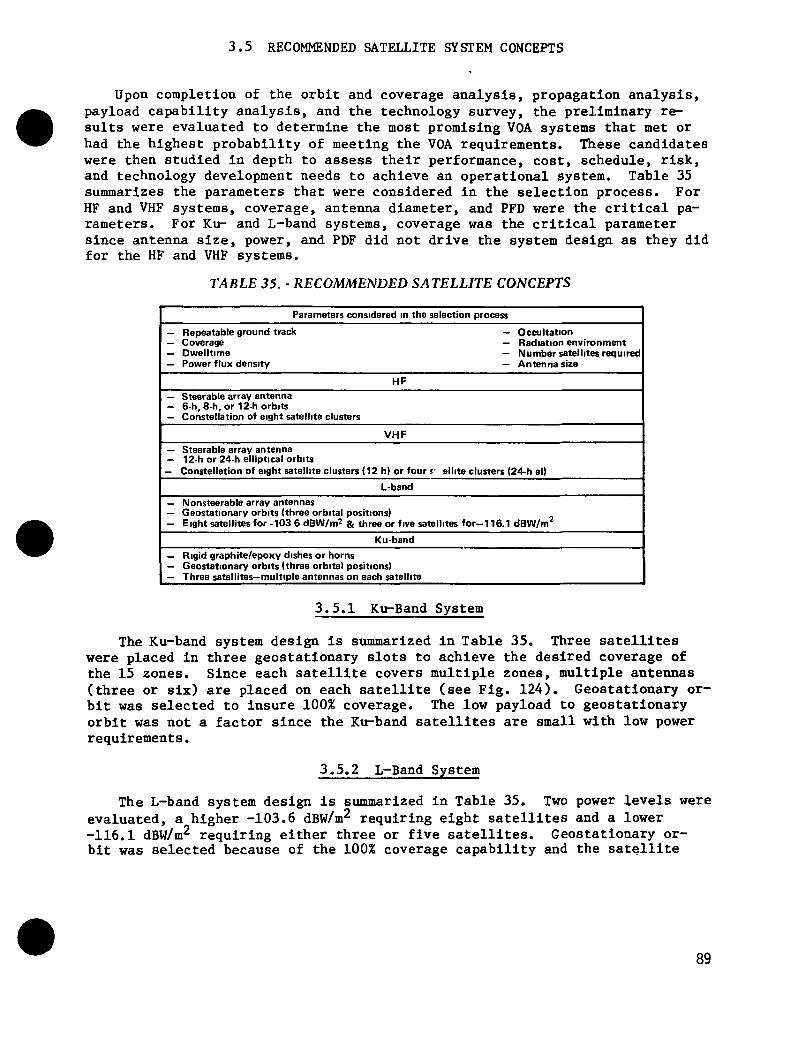
3.5 RECOMMENDED SATELLITE SYSTEM CONCEPTS

Upon completion of the orbit and coverage analysis, propagation analysis,payload capability analysis, and the technology survey, the preliminary re-sults were evaluated to determine the most promising VOA systems that met orhad the highest probability of meeting the VOA requirements. These candidateswere then studied in depth to assess their performance, cost, schedule, risk,and technology development needs to achieve an operational system. Table 35summarizes the parameters that were considered in the selection process. ForHF and VHP systems, coverage, antenna diameter, and PFD were the critical pa-rameters. For Ku- and L-band systems, coverage was the critical parametersince antenna size, power, and PDF did not drive the system design as they didfor the HF and VHF systems.

TABLE 35. - RECOMMENDED SATELLITE CONCEPTS

Parameters considered in the selection process

— Repeatable ground track— Coverage— Dwelltime— Power flux density

— Occupation— Radiation environment— Number satellites required— Antenna size

HF

— Steerable array antenna— 6-h, 8-h, or 12-h orbits— Constellation of eight satellite clusters

VHF

— Steerable array antenna— 12-h or 24-h elliptical orbits

— Constellation of eight satellite clusters (12 h) or four r ellite clusters (24-h el)

L-band

— Nonsteerable array antennas— Geostationary orbits (three orbital positions)- Eight satellites for -103 6 dBW/m? & three or five satellites for- 11 6.1 dBW/m

Ku-band

— Rigid graphite/epoxy dishes or horns— Geostationary orbits (three orbital positions)— Three satellites— multiple antennas on each satellite

3.5.1 Ku-Band System

The Ku-band system design is summarized in Table 35. Three satelliteswere placed in three geostationary slots to achieve the desired coverage ofthe 15 zones. Since each satellite covers multiple zones, multiple antennas(three or six) are placed on each satellite (see Fig. 124). Geostationary or-bit was selected to insure 100% coverage. The low payload to geostationaryorbit was not a factor since the Ku-band satellites are small with low powerrequirements.

3.5.2 L-Band System

The L-band system design is summarized in Table 35. Two power levels wereevaluated, a higher -103.6 dBW/m2 requiring eight satellites and a lower-116.1 dBW/m2 requiring either three or five satellites. Geostationary or-bit was selected because of the 100% coverage capability and the satellite

89

masses did not exceed payload capabilities to geostationary orbit. Also, an-tenna sizes were not excessive in order to achieve the desired spot sizes.The L-band satellites (see Fig. 125) were placed in three orbital slots.

3.5.3 VHF-Band System

The VHP-band system design is summarized in Table 35. A constellation ofeight satellites in a 12-hour circular orbit and a constellation of foursatellites in a 24-hour elliptical orbit were selected. These two systemswere selected for further study because both have their advantages and disad-vantages. The 12-hour orbit produces higher PFD and smaller antenna diame-ters, but has lower coverage efficiency and requires more satellites (Fig.61). The 24-hour orbit has higher coverage efficiency and fewer requiredsatellites, but has lower PFD and requires a larger antenna (Fig. 61). TheVHP-band satellite concept (see Fig. 126).

100

90

so

70

u.o.

1 50•sas

030

as

20

10

No. of S/C

Trip sync6h

Coverage

No. of S/C

5 OCO

8h

HF-bandZone 9: 6 channel: HF = 300 /M/m. VHP = 250jUV/m

12h GEO 12 h 24 h ELLVHP-band

10

Figure 61. - Comparison of orbits for HF and VHP systems.

3.5.4 HP-Band System

The HF-band system design is summarized in Table 35. A constellation ofeight orbital positions in the 6-, 8-, and 12-hour circular orbits were se-lected. Triply-synchronous elliptical and geostationary were eliminated be-cause of their low PFD capability. The 8-hour orbit (see Fig. 61) was the

90

most promising candidate. The 8-hour orbit had the same high coverage effi-ciency of the 12-hour orbit (higher than the 6-hour orbit). The 8-hour orbitalso had the same high PFD as the 6-hour orbit (higher than the 12-hour or-bit). Although the 8-hour orbit did look to be the best system, the 6- and12-hour orbits were also evaluated to ensure completeness of the study. TheHF-band satellite concept is shown in Figure 126.

91

4.0 SATELLITE CONCEPTS, SUBSYSTEM REQUIREMENTS DEFINITION, AND ANALYSIS

Each selected satellite system was evaluated to derive its specific systemand subsystem requirements. The system requirements were derived from themission (communications payload) requirements. A Martin Marietta Denver Aero-space computer program, Spacecraft Integrated Analysis Program (SCIAP) wasused to model satellites and analyze their requirements. The SCIAP subsystemsproperties module (ref. the Appendix) was used to size and trade off candidatesubsystem configurations. Methods were then developed to estimate weight andthe cost of the satellites, ground control stations cost, and launch cost.Weight and cost estimates were made for each subsystem broken down by the fol-lowing :

1) Communications subsystem:a) antenna system,b) transmitters,c) feeder link,d) signal processing,

2) Electrical power subsystem:a) power generation,b) power control,c) power distribution,d) energy storage,

3) Attitude control,

4) Auxiliary propulsion,

5) Telemetry, tracking and command,

6) Thermal control,

7) Equipment bay and mechanisms.

Following are discussions of the assumptions and methods used to estimateweight, volume, and cost of each of the subsystems. Also included are the as-sumptions and method used to estimate total program cost including satellitenonrecurring costs, recurring costs, launch costs, and ground control costs.

92

4.1 SUBSYSTEM WEIGHT AND VOLUME ESTIMATING METHOD

The first step in estimating subsystem weight and volume was to identify -each subsystem's configuration and components. Then, an evaluation was madeto determine if sufficient data was available to size components or subsystemsas a function of a specific performance parameter (e.g, power, diameter, ororbit altitude). The TT&C subsystem and electronics associated with attitudecontrol, communications uplink, and signal processing were felt to be rela-tively constant across the range of satellites to be analyzed. Thus, repre-sentative weights were obtained from components described in the NASA LaRCSystem Design and Cost Model (SDCM) data base. For all other subsystems andcomponents, parametric relationships were used for weight and volume estimates.

^

4.1.1 Communications Subsystem Weight and Volume Estimating

The communications subsystem weight and volume estimates were made forfour sets of components:

1) Antenna structure with reflector or array surfaces,

2) Transmitters,

3) Uplink/crosslink,

4) Signal processing.

The antenna structure and transmitters account for the majority of theweight and volume of the communication subsystem. Parametric sizing relation-ships were available or were developed to size the structures and solid statetransmitters. Uplink/crosslink and signal processing estimates were based onstate-of-the-art components described by the SDCM data base. Following aredescriptions of the method used to estimate weight and volume of communicationsubsystem components. The overall flow of the method is shown in Figure 62.

93

Selectantenna type

Input diameter

Input frequency

Input phasedarray element spacing

Input transmittersefficiency

Input number oftransmitter sizes

Input transmittersize & percentat each size

Input uplinkhardware weight& volume

Input signalprocessingweight & volume

Output communicationssubsystem summary

1 f

Figure 62. - Communications subsystem weightand volume estimating method.

94

4.1.1.1 Antenna Structure Weight and Volume Estimates

The antenna weight and volume estimates for HF and VHP satellites assumesa Martin Marietta box truss ring structure that has been studied previously(ref. 16). The transmitters and radiating elements are supported by a Kaptonweb and a tricot weave, gold plated molybdenum mesh ground plane as shown inFigure 63. The weight estimating relationship for this type of antenna struc-ture is:

W 1.26D + 0.02A + 0.266 x L x N (4-1)

where

WaD

A

L

N

0.02

0.266

antenna weight (kg)= antenna diameter (m)

2= antenna array area (m )

- length of radiating dipole element (m)

= number of radiating elements2

= area density of mesh ground plane (kg/m )

= combined area density of Kapton support and elements

Ground plane& support fortransmitters

(kg/m /element)

fRadiatingsurface

Box truss structure -

•COAX

V.,- Support for transmitters transmitter

Figure 63. - Box truss ring array antenna configuration.

The first term in the weight equation estimates the weight of the ringstructure. The second term gives the weight of the groundplane. The lastterm gives the weight of the two supporting surfaces of Kapton webs and theradiating elements, assuming a A/2 spacing between radiating elements.

95

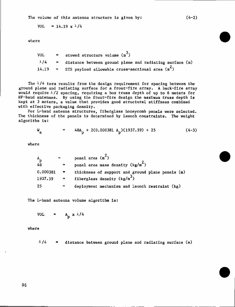
The volume of this antenna structure is given by: (4-2)

VOL = 14.19 x A/4

where

3VOL = stowed structure volume (m )

A/4 = distance between ground plane and radiating surface (m)2

14.19 = STS payload allowable cross-sectional area (m )

The A/4 term results from the design requirement for spacing between theground plane and radiating surface for a front-fire array. A back-fire arraywould require A/2 spacing, requiring a box truss depth of up to 6 meters forHF-band antennas. By using the front-fire design the maximum truss depth iskept at 3 meters, a value that provides good structural stiffness combinedwith effective packaging density.

For L-band antenna structures, fiberglass honeycomb panels were selected.The thickness of the panels is determined by launch constraints. The weightalgorithm is:

Wo = 48A + 2(0.000381 A X1937.59) + 25 (4-3)a P P

where

A = panel area (m )P 248 = panel area mass density (kg/m )

0.000381 = thickness of support and ground plane panels (m)

1937.59 - fiberglass density (kg/m3)

25 = deployment mechanism and launch restraint (kg)

The L-band antenna volume algorithm is:

VOL = A x A/4P

where

A/4 = distance between ground plane and radiating surface (m)

96

Ku-band antennas are assumed to be graphite epoxy parabolic reflectorssimilar to those used for LANDSAT-D. Each antenna has an estimated weight of12.7 kg, including the feed electronics.

4.1.1.2 Transmitters Weight and Volume Estimating

As discussed in Section 3.4.4, data points were identified relating theweight and volume of solid state power amplifiers to their output power lev-els. Upon performing a regression analysis on the data points, two relation-ships were established, one for power levels less than 100 watts, and one forpower greater than or equal to 100 watts. These relationships are:

Wt = 0.0136Pt + 9.41 (for Pfc <_ 100 watts) (4-4)

Wt = 0.097Pt + 0.253 (for Pt > 100 watts)

where

W = transmitter weight (kg)

P = transmitter output power (watts)

The expressions used to estimate solid state transmitter volume is:

VOL - 1.47 x 10~5P + 0.0145 (for P 100 watts) (4-5)/

VOL - 1.441 x 10 Pt + 0.003304 (for Pt 100 watts)

where

oVOL = transmitter volume (m )

For HF-, VHF-, and L-band satellites, many of the designs incorporate morethan one size (power output) of transmitter. The use of different sizes per-mits beam steering and shaping to optimize PFD to each zone that might beserved at different times by the satellite. This results in part-time opera-tion of transmitters in a backed-off mode that has the added advantages of in-creased lifetime and reliability. The weight and volume estimates for thesecases are based on the total number of transmitters required at each size.

97

For HF and VHF satellites, a nominal power per transmitter was identifiedassuming all transmitters operating simultaneously at the maximum availablepower consistent with power generator capability. Then, each required trans-mitter power level was used to determine a weight and volume per transmitter.Each weight and volume was then multiplied by the number of transmitters ofeach size to determine the total of transmitters' weight and volume. The pow-er levels and percent of transmitters for HF and VHF satellites were 1.5 timesthe nominal power, 45%; 2.5 times the nominal power, 15%; 4.0 times the nomi-nal power, 40%.

For L-band satellites, different transmitter sizes correspond to differentarray antennas. Thus, separate transmitter weight and volume estimates weremade for each array antenna.

For the Ku-band, travelling wave tube amplifiers (TWTA) were assumed tohave an average weight of 5.2 kg each. This value was obtained from the SDCMdata base. Two TWTAs are assumed for each channel, resulting in a totaltransmitter weight of 10.4 kg times the number of satellite antennas. A vol-ume of 0.05 m^ was assumed for each pair of TWTAs.

4.1.1.3 Uplink/Crosslink Weight and Volume Estimating

The uplink/crosslink hardware weight was approximated by assuming the sameweight as a LANDSAT-D Ku-band RF module (78 kg per ref. 17). The crosslinkhardware estimated weight was 43 kg, since smaller TWTAs would be required andsome of the original electronics would be used through switching and up/downconversion. Thus, the estimated weight for HF and VHF systems was 121 kg persatellite. The volume of the uplink/crosslink hardware was estimated at 0.5m^, much of which is from the reflectors, gimbal drives, and antenna booms.

For the Ku- and L-band satellites, the crosslink hardware would not be re-quired. Also, the gimbaling hardware would not be required for the uplinksystem. The total weight estimate for these system's link hardware is reducedto 24 kg per satellite. The volume estimate is reduced by the same percentageto 0.2 m3.

4.1.1.4 Signal Processing Weight Estimating

For HF and VHF satellites, the LANDSAT-D Ku-band wideband module weightand volume from ref. 18 are used (58 kg and 0.02 m respectively). For Ku-and L-band, the signal processing weight is assumed at 9.5 kg per downlink an-tenna. The volume estimate is 0.01 m3 per antenna.

4.1.2 Electrical Power Subsystem Weight and Volume Estimating

This section describes the space electrical power system from which powersystem sizing equations were derived. From load requirements for Sun andeclipse periods and distribution losses, required source power can be calcu-lated. Knowing source power, the size of the solar array can be calculated.Then, the weights and volumes of the power system components can be calcu-lated. Figure 64 summarizes the calculation flow of the power generation anddistribution model. The various calculations are supported by a data base ofperformance factors, weight densities, and specific densities. The calculatedpower system weights and volumes reflect the state of technology expected bythe early 1990 time period.

98

Data base

Inputs

— Power to load— Orbit parameters— Antenna size— Life requirement

Energybalancecalculation

S/Asizingcalculation(Asa>

Distribution lossTime of eclipseTime of SunCharger efficiencyStorage efficiencyS/AraddegS/A temp factorS/A const factorsS/A cell efficiencyWeight factorsVolume factorsAllowable bat.depth of discharge

Weight &volumecalculations

— Solar array— Shunt reg— Battery— Bat charger— Distribution— Switching

Figure 64. - Power distribution and generation calculation flow.'

4.1.2.1 Energy Balance Equationo

One simplification made in the power generation model is the assumption ofa direct energy transfer system. This is a realistic assumption since the ma-jority of spacecraft power systems use this form of energy transfer. Thissystem implies a dc distribution network (accurate ac distribution models haveyet to be developed) with an unregulated (+10%) bus and no conversion losses.Figure 65 illustrates a simplified direct energy transfer power system and al-so depicts the data base for the energy balance equation. Note that the dis-tribution loss, Nr, is the sum of the wire (Nws and Nwr) and diode(N,j) losses from source to bus and bus to load. Other energy transfer sys-tem approaches are possible; specifically, peak power tracking, a regulatedbus, distributed power switching, and distributed inverters with ac distribu-tion. These systems may have advantages over the system shown, however, thedirect transfer system is viewed as optimum for modeling purposes.

ws

_JNJ_

Nc = .85

N e = 8

Charger

11

Battery

L

N = 99wr 33

k .. AAAj

\N = QU"d •!)B Nr = Distrib

N =C

IMQ = S16

•MM

ution I

2Ndharger

orage

Loadswitching

oss (.94) = N +

efficiency ( 85)

discharge/charge.afficiency (.80)

Figure 65. • Direct energy transfer system for unregulated (± 10%) bus.

99

p pl"s N

r

T / i \"l i e 1 1 \1 ' T I N N !

s \ c e /

The energy balance equation converts power required at the load into powerrequired from the source. Because eclipse periods affect the size of solar-derived sources, the equation reflects the additional source power required toreplenish any power taken from an energy storage device. If the load power,P! is the same during Sun and eclipse periods then the energy balance equa-tion takes the form:

(4-6)

where

P = power from source

PI = load power

T = time of eclipse

T = time in SunsN , N , and N are as defined in Figure 4.1-4

For non-Sun power generation (e.g, SP-100), Te = 0. For those systemswhose transmitters are assumed to be off during eclipse, the Sun and eclipsepower levels will be different. In this case the appropriate balance equationis:

T> T>

(4-7)plPI

N

P1 "

Nr

TeTs

1N Ne c

where

P, = Sun load power

P, = eclipse load power

Once Ps is known the solar array may be sized.

4.1.2.2 Solar Array Sizing Equation

The solar array sizing equation takes into account the major variablesthat affect solar array area. The variables dependent on altitude are solarcell radiation degradation (Fr), the effects of temperature on cell perform-ance (Ffc), and cover slide thickness weight factor (Fc). Figure 66 is agraph of these variables vs altitude. The figure shows how the radiation fac-tor includes the benefits of increased cover slide thickness as the arraypasses through the Van Allen belt (centered about 4000 km). The weight ofthis increased shielding is reflected by Fc.

100

The variables (except solar cell efficiency) which are independent of al-titude are multiplied together to give a solar array sizing constant, K.These variables are:

Array Orientation Factor 98Solar Cell Packaging Factor 90Cover Slide Traasmissivity Loss 97Array Fabrication Loss 98Miscellaneous Loss Factor 99Solar Intensity 1353 W/m2

100

.96

.92

I-£84

1 .80T?aE 76

08co

§

68

'.6408

"•^.eo

.56

.52

.483 4 5 6 8 1 0

Altitude, km x 103

20

.4

.8

1.2

1.6

2.0

2.4

2.4

32

30 40

Su

oUI

u.

Figure 66. • Solar cell radiation, temperature, and cover slide factors, versus altitude.

101

The resulting value of K used to estimate area is 1123 W/m^. Solar cellefficiency is the remaining variable. The efficiencies assumed in the modelare 14% for 8-mil silicon and 18% for gallium arsenide. The array area sizingequation is:

sa (Fr)(Ft)(K)(Ni)(4-8)

where

P =power required from source (W)2

A =area of solar array (m )saF ^radiation degradation factor

F =temperature adjustment factor

N.=cell efficiency (14% or 18%)1 2K = sizing constant = 1123 W/m

4.1.2.3 Solar Array Weight and Volume Equations

Solar array weight and volume calculations rely heavily on the array panelweight and volume factors and the array structure factors shown in Table 36.Because the solar array can be such a large percentage of spacecraft weight,many studies and development programs have addressed means of reducing panelweight and volume. Table 36 reflects the results of these studies. Althoughthe weight factors shown have not been proven by direct flight experience andattaining the factors may present design challenges, the factors are seen asbeing achievable in the early to mid-1990s. The weight and volume of theSP-100 reactor system is provided for comparison.

TABLE 36. - SOLAR ARRAY WEIGHT AND VOLUMEESTIMATING FACTORS

Source type

Si blanket(8 Mil)

/

Si panel

Galliumarsenide panel

Body-mountedSi cells

SP-100 in-corethermionicgenerator

Panel wtfactor

0 75 kg/m2

2.6

4.4

26

3000 kg

Structure wtfactor

0.85 kg/m2

1.0

10

0

58.2 m3

Panel volumefactor

0.008 m3/m2

003

0.05

0

100kW netoutput EOL

Reference

SAFEMarshall's 25 -kWarrayGE's 10-WW arrayFrusaDORA (frusa type)Space Station

TRW FLTSATCOMTRW LRSAOTSLewisMartin Marietta

LewisMartin Marietta

102

The solar array weight and volume estimating equations are given below.

W = A [panel wt factor + structure wt factor + (4-9)sa sa y

cover slide factor (F )]

V = A (panel volume factor)Scl S3.

where

W = array weightS3

V = array volume

A - array areasa J

FC (determined from Fig. 66)

4.1.2.4 Battery Charger and Shunt Regulator Weight Equations

The battery charger and shunt regulator reflect state-of-the-art electri-cal design approaches. A battery charger weight factor was derived from cur-rent and near-term electronic power densities. Present power densities forlow power are 61-122 W/kg and near-term power densities for high-power devicesthat employ active cooling are 244-305 W/kg. From these values, a realisticnear-term power density of 175 W/kg was selected. This yields a chargerweight factor of 5.7 x 10~3 kg/W.

The shunt regulator weight factor is shown in Figure 67. This factor re-flects the material densities used in the construction of a shunt regulator.The weight factor is not linear because a sequential shunt regulator was as-sumed where increasingly large steps of array area can be shunted by a simpleswitch. The design challenge would be in the switching of large currents.The weight equations are:

W, - PP.. T / T~| ( 5.7 x 10~3 kg/W) (4-10)be 1 e slW = P x Fsr *1 x sr

where

W, = battery charger weight (kg)

PI = load power (W)

T = eclipse time (hr)

T = time in Sun (hr)sW = shunt regulator weight (kg)Si

F is determined from Figure 4.1-6

103

3.5

30

2.5

2.0

I 1-0

.5

10 20 50Solar array power, kW

100 200 500 1000

Figure 67. - Shunt regulator weight factor versus array power.

4.1.2.5 Battery Sizing Equations

Battery size is primarily dependent upon eclipse load power and orbitalparameters. Orbital parameters affect the size in two ways. First, altitudeand inclination affect the length (time) of eclipse (Te) which determinesbattery discharge time. Second, the orbit period determines the number ofdischarge cycles per year. Battery allowable depth of discharge is also animportant factor and depends upon the type of battery selected. Figure 68displays the allowable depth of discharge (F ) vs battery charge/dischargecycles for Nickel Cadmium and Nickel Hydrogen batteries.

104

90

80

70

CO

"I 50•6

I 40a0)•a0 30

J3a

1 20

10

Nickel Hydrogen

Nickel Cadmium

10 20 30 40 50

Battery discharge/charge cycles x 10

Figure 68. - Allowable depth of discharge versus charge/discharge cycles.

The remaining variables requiring definition to estimate battery weightand volume are energy densities and specific energies. Energy densities orbattery weight factors that are achievable with low risk for nickel cadmiumand nickel hydrogen batteries are 35 Wh/kg and 33 Wh/kg, respectively. Simi-larly, specific energies or battery volume factors achievable at low risk are70 kWh/nH for nickel cadmium and 25 kWh/m^ for nickel hydrogen. The bat-tery sizing equations are given below.

(Te) (Te) (4-11)

Fbv>

where

bw

bv

battery weight (kg)

allowable depth of discharge (from Figure 4.1.5)

weight factor (35 Wh/kg for nickel cadmium or 33 Wh/kg for

nickel hydrogen)3

battery volume (m )3

volume factor (70 kWh/m for nickel cadmium or 25

kWh/m for nickel hydrogen)

105

4.1.2.6 Switching and Distribution Weight Equations

The equations for distribution weight are based on aluminum wire for powerbus feeders. Handbook current ratings (70°C temperature rise) were used.These equations assume that cable weight is limited by the current rating ofthe wire rather than the allowable power loss. This is a valid assumption forshorter cable runs and may or may not be valid for longer cable runs, depend-ing on the cost (in weight) of generating the additional power lost in thecable. Other assumptions made are 200 Vdc bus, hybrid electromechanicalswitches, and distribution losses of 3% from both source to bus and -.bus toload. The switching and distribution sizing equations are defined below.

Solar array to bus distribution weight:

W, = (0.0243 kg/m2-W)(A )(P) (4-12)u sa s

where

A = solar array area (m )saP = power from source (W)S

Bus to transmitters distribution weight:

(0.0243 kg/W-m)(Ll + L2/2)(P1) (4-13)

where

LI, L2 = antenna dimensions (m) :

PI = power to load (W)

Power switching equipment weight and volume:

W - 2.18 kg +(0.23 kg/kW)(P1) (4-14)SW J- i

i

VOL - W i_ sw |

1200 kg/m3

106

4.1.3 ACS, Stationkeeping, and Maneuvering Weight and Volume Estimating

TABLE 37. - ATTITUDE CONTROL

Component

Fine-Sun sensorCoarse-Sun sensorStar trackerRate gyroElectronicsCabling/harness

Status

SOA/OTSSOA/OTSSOA/OTSSOA/OTSSO A/NEWSOA/NEW

Number

222211

Weight

0.1kg02

12.813.626.050

Total 57 7 kg

For nongeostationary orbits, theassumed onboard equipment for attitudedetermination is summarized in Table37. For geostationary orbits, therate gyros could be eliminated ascould most of the control electron-ics. Thus the ACS weight would besignificantly reduced (13.1 kg).

The weight and volume of the APSwas determined by running the SCIAPprogram. The inputs and outputs are summarized in Figure 69. When usingSCIAP, the first step is to create a satellite mass and geometry model usingan interactive model generator module. This data is then transferred automa-tically through the SCIAP data base to the mass properties module and then tothe rigid body controls (RCD) Module. The RCD module computes forces andtorques on the satellite as it travels around its orbit. The forces andtorques are integrated to compute the total linear and rotational impulse perorbit. Allowable locations for thrusters are entered along with a nominalthrust per thruster. The RCD module then determines the optimum number ofthrusters, thrusters' firing strategy, and the required propellant mass perorbit. The propellant per orbit is then extrapolated to the specified satel-lite lifetime. The RCD module permits definition of solar array orientationthrough the orbit, feathering of arrays in the occulted region of the orbit ifso desired, specifying satellite orientation, and selecting from differentdensity atmospheres. Effect of ACS limit cycle and maneuvers on propellantmass requirement are also included. The required propellant can be computedby assuming attitude control by either the APS thrusters or by momentum stor-age devices. In the latter case, the number of orbits between desaturation isan input and the propellant mass compulation includes propellant required fordesaturation.

Following is an example of SCIAP run results for the HF-band triply-synchronous orbit. The RCD module inputs are summarized in Table 38. The al-titude shown is the altitude at the start of the orbit. The orbit is actuallydefined later by interactive input of the orbit periapsis and apoapsis. Table39 shows the satellite mass properties created by the model generator thatwere fed in through the data base. The results of the analysis are summarizedin Table 40. Figures 70 and 71 show the total forces and torques on thesatellite as a function of orbit anomaly angle.

Orbit parameters ,

S/C parameters.

Mission parameters <

ACS characteristics -

RCS characteristics •

SCIAPrigidbodycontrolsmodule

Totalimpulse

Propellantmass

SCIAPsubsystempropertiesmodule

RCS mass

RCS power*

•Electric propulsion

Figure 69. - Reaction control weight estimate.

107

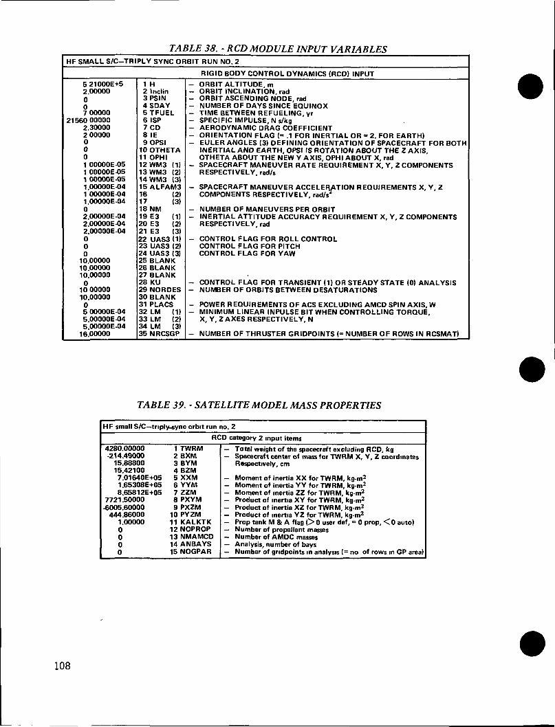
TABLE 38. - RCD MODULE INPUT VARIABLESHF SMALL S/C-TRIPLY SYNC ORBIT RUN NO. 2

RIGID BODY CONTROL DYNAMICS (RCD) INPUT5 21000E+52.00000007 00000

21560 000002.300002 000000001 OOOOOE-051 OOOOOE-051 OOOOOE-051.00000E-041 OOOOOE-041.00000E-0402.00000E-042.00000E-042.00000E-04000

10.0000010.0000010.000000

100000010.0000005 OOOOOE-045 OOOOOE-045.00000E-04

16.00000

1 H2 Inclin3 PSIN4SDAY5TFUEL6 ISP7 CD8 IE9OPSI

10 OTHETA11 OPHI12WM3 (1)13WM3 (2)14WM3 (3)15 ALFAM316 (2)17 (3)18 NM19 E3 (1)20 E3 (2)21 E3 (3)22 UAS3 (1)23 UAS3 (2)24 UAS3 (3)25 BLANK26 BLANK27 BLANK28 KU29 NORDES30 BLANK31 PLACS32 LM (1)33 LM (2)34 LM (3)35 NRCSGP

- ORBIT ALTITUDE, m- ORBIT INCLINATION, rad- ORBIT ASCENDING NODE rad- NUMBER OF DAYS SINCE EQUINOX- TIME BETWEEN REFUELING, yr- SPECIFIC IMPULSE, Ns/kg- AERODYNAMIC DRAG COEFFICIENT- ORIENTATION FLAG (= .1 FOR INERTIAL OR = 2. FOR EARTH)- EULER ANGLES (3) DEFINING ORIENTATION OF SPACECRAFT FOR BOTH

INERTIAL AND EARTH, OPSI IS ROTATION ABOUT THE Z AXIS,OTHETA ABOUT THE NEW Y AXIS, OPHI ABOUT X, rad

- SPACECRAFT MANEUVER RATE REQUIREMENT X, Y, Z COMPONENTSRESPECTIVELY, rad/s

- SPACECRAFT MANEUVER ACCELERATION REQUIREMENTS X, Y, ZCOMPONENTS RESPECTIVELY, rad/s

- NUMBER OF MANEUVERS PER ORBIT- INERTIAL ATTITUDE ACCURACY REQUIREMENT X, Y, Z COMPONENTS

RESPECTIVELY, rad

- CONTROL FLAG FOR ROLL CONTROLCONTROL FLAG FOR PITCHCONTROL FLAG FOR YAW

- CONTROL FLAG FOR TRANSIENT (1) OR STEADY STATE (0) ANALYSIS- NUMBER OF ORBITS BETWEEN DESATURATIONS

- POWER REQUIREMENTS OF ACS EXCLUDING AMCD SPIN AXIS, W- MINIMUM LINEAR INPULSE BIT WHEN CONTROLLING TORQUE,

X, Y, Z AXES RESPECTIVELY, N

- NUMBER OF THRUSTER GRIDPOINTS (= NUMBER OF ROWS IN RCSMAT)

TABLE 39. - SATELLITE MODEL MASS PROPERTIES

HF small S/C—triply-sync orbit run no. 2

RCD category 2 input items

4280.00000-214.49000

15.8880015.421007.01640E+051.65308E+058.65812E+05

7721.50000-6005.60000

444.860001.000000000

1 TWRM2BXM3 BYM4BZM5 XXM6 YYM7 ZZM8 PXYM9 PXZM10 PYZM11 KALKTK12 NOPROP13 NMAMCD14 ANBAYS15 NOGPAR

Total weight of the spacecraft excluding RCD, kgSpacecraft center of mass for TWRM X, Y, Z coordinatesRespectively, cm

Moment of inertia XX for TWRM, kg-m2

Moment of inertia YY for TWRM, kg-m2

Moment of inertia ZZ for TWRM, kg-m2

Product of inertia XY for TWRM, kg-m2

Product of inertia XZ for TWRM, kg-m2

Product of inertia YZ for TWRM, kg-m2

Prop tank M & A flag (>0 user def, = 0 prop, <0 auto)Number of propellant massesNumber of AMDC massesAnalysis, number of baysNumber of gridpoints in analysis (= no of rows in GP area)

108

TABLE 40. - RCD MODULE OUTPUT SUMMAR Y

HF small S/C— triply-synchronous orbit, run no. 2

Linear impulse per orbit to orbit keep, Newton-s =— X component m— Y component in

spacecraft coordinates =spacecraft coordinates =

— Z component in spacecraft coordinates =

2.115E+02-2.071E+02-9.519E-12-4.381E+00

Linear impulse needed per orbit for desaturation, N-s = —Linear impulse for life to orbit keep, N-s =— X component in spacecraft coordinates =*— Y component in spacecraft coordinates =— Z component in spacecraft coordinates =

.432E+07- .423E+07- .195E-06- .896E+05

Linear impulse needed per orbit for desaturation, N-s = —Linear impulse for life for attitude control, N-s =Linear impulse per orbit for attitude control. RCS only, N-s =Linear impulse per orbit for limit cycle, RCS only, N-s =

.290E+061.418E+012.995E-04

Linear impulse per orbit for maneuvering, RCS only, N-s = —Total linear impulse per orbit for RCS only, N-s =

Orbit radius, m =Orbit velocity, m/s =Orbit period, s =

Propellant mass fix ratio =Propellant mass, kg -

Spacecraft mass less

=

propellent, kg =— X distance to center of mass in frame 4, m =— Y distance to center of mass in frame 4, m =— Z distance to center of mass in frame 4, m =

Mass moment of inertia, kg-m Dis

7.016E+05-7.721E+036.006E+03

-7.721E+031 653E+05

-4.449E+02

6.006E+06-4449E+02 1.807E+008658E+05 2.130E+00

1.418E+01

6.899E+068.821E+031.080E+04

1.000E+002.141E+024.280E+03-2.145E+001.589E-011.542E-01

tance from center of gravityto center of pressure, m

-8 745E-02 2.744E-013.208E-01

-1.578E-01

Torque resulting from RCSMAT assuming all thrusters fire at nominal value

2.288E-01_-

1.934E-01-

_ _2.288E-01

Inverse matrix_ __ _— -

Eff radii for application of torque Spacecraft projected areas6 356E+00 1.075E+01 1.271E+01 | 4.200E+01 4.000E+01 8.922E+02

109

Ezffl"

2>oy

oa

0.5 r~

0.4

03

02

0.1

-0.3 —

-0.4 -

-0.560 120 180 240

Anomaly Angle, deg300 360

Figure 70. - Total force components versus anomaly angle.

osr

04

03

0.2|

3tr

I 0

g-0.1coaE5-0.2

-0.4

-0.5

Note

" YnAxis scale factor is 1/10Y range is +/-.0500

60 120 180 240Anomaly angle, deg

300 360

110

Figure 71. Total torque componentsversus anomaly angle.

Table 41 summarizes the required propellant mass for each satellite systemstudied during the program. The number and orientation of each requiredthruster was also determined for each case from the RCD module outputs. Fromthe number of thrusters, the dry APS weight was then determined. For HF-,VHF-, and L-band systems, PPTs were assumed with a dry weight of 23 kg eachand a volume of 0.275 m . A. minimum of eight thruster modules was assumedfor full 3-axis control and redundancy.

Ku-band satellites can use existing chemical thruster technology (e.g,hydrazine). The assumed dry weight of the chemical system is 91 kg. Thehigher propellant mass compared to electric propulsion makes the total weightcomparable to the total weight of a PPT system.

TABLE 41. - VOA DVBS AUXILIARY PROPULSION SYSTEM REQUIREMENTS

System

HF, 6-h orbitHF, 8-h orbitHF, 12-h orbitHF, multi-launch, 6-h orbitHF, multi-launch, 8-h orbitHF, multi-launch, 12-h orbitHF, inflatable reflector, array feedHF, Molmya orbitHF, small antenna, 6-h orbitHF, small antenna, 8-h orbitHF, small antenna, 12-h orbitHF, small antenna, GEOHF, small antenna, triply-synchHF , small antenna, 24-h ellip

VHP, 12-h orbitVHP, 24-h elhp orbitVHP, multi-launch, 24-h ellipVHP, inflatable reflector, 24-h ellip

L.GEO

Ku.GEO

Propellantmass

7yr

12kg434496

102104

107314612441265

21018

57160180

1200

32318

111

10 yr

17kg6363

137146149

1533209

17631793

30626

81229257

1714

Repositionallowable

70kg6250

142120868682706250312246

5046SO46

16152

62

Drymass*

184kg184184236236184368184184184184184276184

184236276368

18491

TotalAPS mass

7yr

266kg298269474458374

1527412266290256280510248

291442570

1614

232561

10 yr

271kg318288677654419

1987475271309261308708256

315511644

2128

'Mass of propulsion components only.

4.1.4 TT&C Weight and Volume Estimating

TABLE 42. - TT&C EQUIPMENT LISTThe TT&C subsystem includes the

hardware required to sense and commu-nicate satellite status and positioninformation1to a ground control sta-tion and to receive commands from aground station. For this study, real-time access is assumed for all sys-tems. Thus, no onboard data storageis required. The hardware assumed forHF- and VHP-bands TT&C subsystems issummarized in Table 42. The weight estimate used for HF and VHF systems was32.1 kg. A mass density of 1000 kg/or* was assumed to compute TT&C volume.For L- and Ku-bands, the autotrack module would be eliminated,' resulting in aweight of 26.4 kg.

Component

Onboard computerCommand receiverRemote interface unitComputer interfaceRedundancy managerAutotrack moduleCabling/harness

Status

SO A/NEWSOASOASOASOASOASOA

Number

(2)(2)(2)(2)(2)(2)(1)

Weight

8.36.62.11.02.75.75.7

111

4.1.5 Thermal Control Subsystem Weight Estimating

The thermal control weight estimates are based on algorithms contained inthe SCIAP subsystems properties module. Thermal control subsystem weight iscomputed as a function of radiative surface area using an assumed area massdensity of 4.88 kg/m^ (1 Ib/ft ). The required area is computed as afunction of the BTUs of heat to be radiated (Q), maximum allowable temperature(Tmax°R), end-of-life radiators emissivity (e), end-of-life radiators ab-sorptivity (a) , and orbit altitude. The equations used to compute the re-quired area are:

1) Altitudes below GEO:

Area = max- aQ Kmax xs

where

K is factor to account for orientation of radiators to Sun (0.707 for

45°)

a is Stefan-Boltzman constant -0.1714 x 10~? Btu/h ft2 R

Q is solar constant 1353 w/m2 (442 Btu/hr-ft2)

2) Altitudes at GEO or above:

2QmaxArea =max

The volume is computed by assuming a radiator equivalent thickness of 0.05meters (2 in.).

Usually, the heat to be rejected is computed automatically as the differ-ence between the power into the load and the useful power out. However, HFand VHF satellites' thermal control subsystems could not be sized automati-cally because of the different sized transmitters and the requirement of sometransmitters to be operated at different power levels depending on the zone tobe covered (as discussed previously in Section 4.1.1.2). The power levels ofthe transmitters were estimated to fall into three categories: 45% at 1.5times a nominal power, 15% at 2.5 times the nominal power, and 40% at 4 timesnominal power. Thus, the radiative surface area for each transmitter must beincreased appropriately. The weighted average of these transmitter size fac-tors is 2.65 requiring an effective radiative surface area 2.65 times that re-quired for the simple difference between maximum power available to the loadand maximum power out.

112

Weight of other thermal control components such as insulation, coldplates, and heaters are included in the weight estimate of individual subsys-tems or components.

4.1.6 Equipment Bay and Mechanisms Weight Estimating

The relationships to estimate weight and volume of the equipment bay weretaken from the SDCM. The equipment bay was assumed to be a conventionalsatellite structure applicable to a 3-axis stabilized spacecraft. The SDCMempirically derived weight estimate is:

W = K. W0<99(L/D)0'24 +0.1W ' (4-17)e d s s

where

W = equipment bay weight (kg)

W = subsystem components weight (kg)S

(L/D) = structural dimension ratio (1.0)

K = density coefficient (.129 for non-body-mounted solar

arrays)

The equipment bay volume estimated is computed from the relationship:

V = 4.95 V (4-18)e s

where

4.95 = average volume sizing factor for satellites with solar arrays

V = volume of subsystem hardware to be contained in equipment bayS

The mechanisms weight was estimated from data contained in the SDCM database. For HF-, VHF-, and L-bands, the mechanisms weight was estimated at 102kg. This includes the weight of all stowage and deployment mechanisms exceptfor the deployable antennas (e.g, box truss ring structure, honeycomb pan-els). For Ku-band satellites, the mechanism weight was assumed to be 51 kg,primarily to account for the deployment mechanisms for the solar arrays.

113

4.2 TECHNOLOGY TRADEOFFS

The objective of the subsystem technology tradeoffs was to identify sub-system technologies that might enhance VGA DVBS missions, even though-thesetechnologies might be in an early development phase. This section will dis-cuss why subsystem configurations were selected. The goals of the tradeoffswere to identify ways to minimize satellite weight, maximize reliability, in-crease lifetime, minimize cost, and reduce implementation time.

4.2.1 Antenna Structure Tradeoffs

The communications subsystem is the payload for VOA satellites and repre-sents a significant part of the total cost, time to develop, and weight.Thus, the selection of the configuration and components will be critical toVOA satellite program success. Presented here are alternatives for the com-munications subsystem mode of operation and for subsystem components.

4.2.1.1 Antenna Technology Tradeoffs

Present antenna systems for Ku-band applications use solid parabolic re-flectors in the order of 1- to 4-meter diameter. This technology is well es-tablished state of the art. However, larger antenna systems, particularly atthe RF power levels needed for HF-, VHF- and L-band applications are rela-tively new technologies. The antenna types that make up the larger antennasystems fall into two types: reflectors and arrays. To use a reflector insuch an application has the advantage of simplicity in the sense that the RFsubsystem is not very complex. By comparison, an array requires a rather com-plex RF subsystem to assure that each element in the array is properly fed andphased.

Structurally, both large arraysand large reflectors are quite simi- TABLE 43.-ARRAY VERSUS REFLECTORlar. Both must be stowable for STS ppo COMPARISONlaunch and deploy reliably and accur-ately. Table 43 presents a comparisonof maximum PFD available from an arrayand reflector for the same orbit andaperture. As shown, the PFD for thereflector is higher than for the array. In reality, the beamwidth of the re-flector would be larger for the same diameter. Thus, for the same ground spotcoverage, the PFD from the reflector would be still greater since a smallerreflector diameter would result in less weight for the structure. The reducedweight could be allocated to the EPS, increasing the available electricalpower and thereby increasing PFD to the ground.

The advantages of an array system, especially at the RF power levels andfor the coverage requirements for VOA applications, is that power can be dis-tributed over a number of element/transmitter pairs and the antenna patterncan be adjusted to meet coverage requirements. Distributing the power over anumber of element/transmitter pairs helps to alleviate any arcing and multi-pacting effects from the generation of high RF powers in space. Also, heatdissipation problems and the risk of a single point failure are reduced. Un-like reflectprs that require mechanical actuators to scan the antenna beam, an

Antenna

12 h-mflatable12 h—array

Aperture diameter

168m168m

PFD

290 /LtV/m244 /IV/m

114

array has the capability to scan electronically by adding phasors at each ra-diating element. In addition, by selectively turning transmitters off and on,the antenna beam pattern of an array can be broadened or narrowed to meet zonecoverage requirements. Combining phase control and selective activation al-lows an array to maximize power flux density on the ground and also providesextended coverage time for a given zone.

The above rationale was used in choosing an array over a reflector for theHF-, VHF- and L-band antenna systems. In the VHF-band system design that pro-posed a reflector (an inflatable reflector) an array was still used for thefeed. The inflatable reflector concept resulted in a feed array of 26 x 26meters and an inflatable aperture structure with extremely low mass. However,the large inflatable proved to have significant controllability problems andincreased APS propellant requirements. For the array antenna concepts forHF- and VHF-bands, the box truss ring array was used because it provided lowerweight and stowed volume than contiguous truss structures and provided a capa-bility to 'attach both the radiating surface and ground plane surface onto thestructure without adding additional structural elements. For the array an-tenna systems for the L-band, honeycomb panel arrays were used. These arraysare similar to existing technology which has been used in satellites such asthe synthetic aperture radar antenna.

4.2.1.2 Transmitter Technology Tradeoff

For the HF-band, the requirements for DSB-AM require linear amplificationif the carrier is modulated prior to uplinking and merely amplified in thesatellite. Solid state power amplifiers (SSPA) typically are designed as lin-ear devices while TWTAs have a nonlinear operating region. TWTAs requirehigher dc operating voltages than do SSPAs. While SSPAs can operate almostdirectly off a dc photovoltaic power bus, TWTAs require DC to DC conversionfor power, thus increasing weight and complexity of the electrical power sub-system. Also, TWTAs have lower lifetime reliability than SSPAs, particularlywhen operated in a cyclic mode as is anticipated for VGA satellites.

As discussed in Section 3.3.4, powers above 1000 watts will require SSPAsusing MOSFETs. Use of multiple SSPAs with array antennas will result in aweight penalty, but use of a transmitter per element provides high system re-liability since failure of a small percent of transmitters should not seri-ously degrade performance. Also, use of SSPAs results in simpler packagingand permits distributed thermal control. Finally, since TWTA gain is propor-tional to wavelength, a TWTA at HF or VHF frequencies would be orders of mag-nitude larger than TWTAs for L- or Ku-bands if the same gains are required.

For Ku-band, TWTAs are in use and are selected for VOA satellites, basedon their minimal required development cost and time and the availability ofpower levels needed for VOA satellites.

As an alternative to conventional space technology for the provision ofsingle very high-power devices, we look to the technology that has providedthe broadcast industry with high powered transmitters. This is the classicaltechnology of triodes and tetrodes. Varian, for example, has developed a newtube called a klystrode, that combines the features of a klystron and a tet-rode. It operates as a class-B linear amplifier in the manner of a tetrode,but with the reliability and high-power handling capability of the klystron.Such tubes have been operated in the 400 to 800 MHz region, and there are

115

plans to extend operation to L-band. Powers available are up to 28 kW, with30 kV beam voltage. The efficiency of this device when operating at fullpower can be 50%, and it has the unique feature that the dc power drawn is de-creased as the input level is decreased. This feature could be particularlydesirable for VGA operation, where power is at a premium. Peak power require-ments from the primary power source could be reduced by the use of energystorage devices that can be charged during periods of low modulation, and byexploiting the average statistics of several channels aboard the same satel-lite. The average power requirements could also be reduced, since the powerdrawn would be low during periods of low modulation percentage. Use of thisdevice would, of course, require a space qualification program, but mightprove useful for L- or Ku-band satellites.

4.2.1.3 Array Antenna Phase Control

Signal processing for array phase control for steerable beams can be ac-complished by splitting the signal from a common interface/intermediate fre-quency (IF) output through equal length and impedance cables to each transmit-ter. A separate phase shift circuit and command would then be used at eachtransmitter to perform shifting for steerable beams.

An alternative is to use minimum cable length to each transmitter, per-forming shifting in a separate IF stage for each transmitter. The shift foreach would then be commanded as a function of desired beam steering' with abuilt-in compensator relating the length of cable to the associatedtransmitter.

The common IF source approach has fewer electronics piece parts thatshould result in higher reliability and lower design and production complex-ity. The separate IF source approach requires less cable and therefore haslower weight (60 kg for largest satellite). However, for this approach, eachIF stage must be shifted differently to compensate for the different cablelengths to each transmitter, making each stage design different.

Cost comparison is difficult to address, since the common source approachIF stage(s) must have higher gain to provide the same input power to thetransmitters as the separate stage approach. This should result in highercost per stage, but with significantly fewer stages, overall cost will prob-ably be lower. Thus, the common IF source is recommended since it should beless complex, have higher reliability, and have lower cost.

116

4.2.1.4 Feeder Link Tradeoffs

TABLE 44. - NUMBER OF FEEDER 'LINK STATIONS REQUIRED VERSUS

SATELLITE HEIGHT

Satelliteheight

4,163, km4,1826,3927,843

10,35513,89220,18435,78639,58161,085

G reat circle degreesof coverage, diam

86.987.0

101.0107.6115.912391326142.9144.3149.3

No. of Earth stationsfor full coverage(assuming no overlap)

7.307.285.504.894.263.783.342.932.882.72

The principal choice to be made in the feeder link system design is wheth-er realtime uplink capability is required at all times. If so, then for loworbit satellites, up to perhaps seven or eight ground stations are required,spaced fairly evenly about the Earth. Higher orbits have greater visibility,and only two or three Earth stations are required. If realtime operation isnot required, fewer Earth stations may be used, since low-orbitsatellites will eventually pass overthe United States and the programmingmay be uplinked during that pass. Ifjamming is a considera-tion, burst andstore from the U.S. or nonhostile ter-ritory will provide protection. Fi-nally, an intersatellite link can helpto reduce the number of uplink sta-tions, as well as provide protectionagainst jamming. Although the relaysatellite option shown is based ondedicated satellites, it may be pos-sible to use the sound broadcast sat-ellites themselves as intersatellitelinks to one another.

Table 44 summarizes the number ofrequired ground stations vs orbit altitude. The recommended mode for HF- andVHP-bands systems is onboard*crosslinks. Since there will typically be clus-ters of satellites spaced around an orbit, there will always be a realtimewindow from a ground station to any specific satellite. Since up to fiveground stations would be required for some systems, the overall cost would becomparable to that for an intersatellite link. There would be an advantagewith the intersatellite link option in that only two stations would be re-quired, simplifying site acquisition and security.

As an example, Table 44 shows that four ground stations would be required"for the 8-hour orbit (altitude of 13892 km). The estimated cost of eachground station is $56,500,000 for a 24-satellite system and a 20-yr opera-tional lifetime. The estimated cost to develop the crosslink system is$9,000,000. The additional estimated first unit recurring cost per spacecraftfor the crosslink system is $3,360,000. The two additional ground stationswithout intersatellite capability would cost $113,000,000. The'estimated costof the crosslink capability for a 20-yr lifetime (72 satellites) would be$126,000,000. Thus, there is no significant difference in cost between thetwo approaches.

A significant goal of VGA should be the transmission of maximum intelligi-bility in speech broadcasts, within the confines of power and energy availablefrom the satellite. Techniques available can be used either to increase in-telligibility for the power and energy available, to decrease the power andenergy requirements for a fixed level of intelligibility, or to arrive at anintermediate compromise.

117

Intelligibility is increased with increased S/N ratio. One technique longused to increase the S/N ratio of voice transmission over the transmissionchannel is the use of compression and expanding, which may be applicable tothe HF-band DSB-AM VGA system. Companding reduces the dynamic range of thesignal carried over the transmission channel, so that high amplitude signalsare transmitted at a relatively higher level. There is an accompanying reduc-tion in quiet level noise and a notable increase in subjective or apparent S/Nratio. At the receiving end, the original dynamic range is restored, so thatthe listener receives a relatively faithful reproduction of the original.This restoration (as opposed to the compression alone) is particularly desir-able in broadcasts of classical music and other programs that have a wide dy-namic range, but even for voice it aids in maintaining natural sounding speech.

A disadvantage of conventional companding is that it requires a coopera-tive receiver with built-in expansion circuitry. Since the VOA system cannotdepend on the presence of a population of such receivers, it is useful to askwhether there is an advantage in a system with compression only, without ex-pansion at the receiver.

It turns out that there is such an advantage. By the amplitude compres-sion of the voice signal, a higher average S/N ratio can be achieved. This inturn may allow usable reception using a reduced carrier power, and in fact,with reduced tptal power. This could be a significant factor for VOA systemsthat have such large power requirements. In effect, more of the primary poweris diverted to the sidebands rather than to the carrier, which conveys no in-formation, but is just an artifact of the classical AM system. However, thecompression may also give the listener a feeling that what is heard is unin-teresting and unrealistic. If the compression is applied only to that rangeof frequencies that influences intelligibility most, the natural variation tothe lower and higher frequencies might convey the dynamics of a conventionaltransmission without defeating the objectives of compression.

The above technique increases not only the channel S/N ratio, but also theenvironmental or acoustic S/N ratio. This technique is somewhat similar tothat used in Dolby B audio systems intended for a cooperative receiver. Lis-teners to these systems have in fact noted increases in intelligibility withthe cooperative features of the receiver turned off.

Exploitation of the above and other power conservation methods demand thatthe system take all possible steps to maximize intelligibility. For example,attention must be given to ensuring an appropriate frequency response in thespeech channel and properly equalizing to match microphone response. Consid-eration should also be given to differing equalization curves for differentspeaker's ypices.

In addition, scrupulous attention must be given to the avoidance of non-linear distortion in the speech channel, since this can seriously eat into theintelligibility budget. Random noise and unplanned level shifts must also beminimized* Level lineup must be maintained over a range of sources, includingmicrophones, remote input channels, and prerecorded media. Operationally,this may call for more complete audition (medium preview) procedures thanwould ordinarily be required.

118

4.2.2 Electrical Power Subsystem Tradeoffs

4.2.2.1 Power Generation

Energy sources currently under development that possess the greatest po-tential for use in the spacecraft's power generation system are photovoltaicconcentrator arrays, nuclear (SP-100), and solar thermal dynamic (using Stir-ling, Brayton, or Rankine cycles). Section 3.4.2 discussed the solar concen-trator and nuclear sources. The solar dynamic source has many advantages, ascan be seen in Figure 72 which compares specific mass and area of potentialpower systems. Note that a system with a relatively low specific mass mayhave a relatively high specific area, such as the silicon flexible blanket ar-ray and regenerative fuel cells (RFC) system. The solar dynamic Stirling sys-tem has the advantage of possessing both the lowest specific mass and area ofthe systems considered. The solar dynamic systems also have the potential forlower cost and higher reliability vs a photovoltaic system, and, with effi-ciencies of 23-25%, the solar dynamic collector area would be 35% of a siliconsolar array. Table 45 summarizes the advantages and disadvantages of thepower generation systems described here. If development continues at the pre-sent rate then a solar dynamic system should prove a viable candidate for highpower applications in the far term. To ready this system for an early 1990flight however, would require substantial engineering effort and would be highrisk.

Development of 2-mil silicon cell technology would also result in improvedperformance of photovoltaic blankets. Table 46 shows the comparison of satel-lite subsystem weights, total power, and RF power for the maximum payload,8-hour, HF baseline system. The increase in power (0.87dB) results in a 10.5%increase in PFD with the 2-mil technology as shown for a sample of zones.

300

250

200

ISO

100

50

kg/kW 10 x (sq-m/kW)

Silicons— rigidnickel cadmium

Silicon - rigidRFC

Gallium arsenide/RFC

Silicon — flexibleRFC

Solar brayton

Solar org ranking

Solar Stirling

Figure 72. - Representative specific mass and area of potential power systems.

119

TABLE 45. - POWER GENERATION TECHNOLOGY TRADEOFFS

Technology Advantages Disadvantages

Photovoltaic planar solar array

Photovoltaic concentrator solar array

Nuclear

Solar thermal dynamic

Low riskPossible development by space stationLow cost

Lower area/dragBetter performance

No sun trackingNo energy storage requiredLowest area/dragContinuous operationDirect ac generation possible

Low area/dragNo chemical storageDirect ac generation possible

Large area/dragLow stiffnessCell degradation high at some altitudes

Development requiredReflector life questionableNeed gallium arsenide cells (high cost)

Safety implicationsHigh development cost/riskHigh-temperature concernsDynamic interaction concernsReentry considerations

Thermal storage concernsHigh development cost/riskReflector life concernsAccurate sun pointing requiredStartup problemsBearing life concerns

TABLE 46. - COMPARISON OF HF 8-HOURBASELINE WITH 8-AND 2-MIL SI CELLS

Type ofSolar Cell

8-mil Si2-mil Si

Total EPSPower

93.1 kW108.9

RFpower

58 kW70.8

PFD zone (one channel)

Zone 1

320/UV/m354

Zone 7

228 JiV/m252

Zone 10

282/UV/m312

120

Of the energy source technologies, a gallium arsenide concentrator arrayshould be the first to be space qualified. Section 3.4.5 discussed the rela-tive merits of this system and Figure 72 displays the savings in specific areavs silicon when paired with an RFC. Full development is not likely to occurby 1990 unless space station uses this technology, which is doubtful. Becausethe specific mass of a gallium arsenide concentrator is greater than a siliconflexible blanket array, this system may only be desirable for missions in or-bits that experience the greatest effect from solar pressures and atmosphericdrag. Table 45 compares this system to the other power systems.

In conclusion, the most viable near term (1990) energy source option isthe photovoltaic flexible blanket array using the advanced silicon solarcell. While a solar dynamic system will have lower specific mass and area,for an unmanned satellite it will not be practical from the standpoint ofmaintainability. A nuclear source becomes attractive for very large powersystems ( 200 kW) or for operation in areas of high radiation. If reductionsin cost and blanket weight can occur for gallium arsenide arrays then thatcell will be preferable to silicon for most applications.

4.2.2.2 Power Distribution

Areas in power distribution that will require optimization are cablingtype, voltage type (ac or dc), power transfer mechanism (from solar array toconductors), voltage level, and voltage regulation for a dc system. A voltagelevel of 200 Vdc was previously selected as optimum (ref. Sect. 3.4.6). Con-siderations for selecting cabling type, voltage type, and power transfer de-vices are presented here.

4.2.2.3 Cabling

For cabling material, the product of electrical resistivity and density isthe appropriate figure of merit for conductor lightness. For aluminum, theproduct is half that of copper (a 50% weight savings over copper can be real-ized). Some drawbacks of aluminum are its low tensile strength, poor flexi-bility, and poor crimp terminability. Poor crimp terminability can result increep, causing looseness in the connector, eventual arcing, and an open cir-cuit. Alloying aluminum with some other conductor such as copper should solvethese problems and make aluminum available for large power systems in the1990s.

Figure 73 illustrates the effects of increasing distribution voltage andtype of conductor wire (aluminum or copper) on the combined distribution andpower generation system weight. A 100 kW power level and 122 meter one-waylength were assumed. The graphs are representative of system weight variancefor a photovoltaic source. Also shown are the points for aluminum and copperwire at which the current in the wire exceeds its 70°C temperature rise lim-it. To further reduce conductor weight and thus increase distribution losswould drive the conductor to higher temperatures. The 70°C limit was used toprovide a benchmark, the actual temperature limit being a function of the in-sulator material. It should be noted that the weight difference betweencopper and aluminum decreases as distribution voltage increases.

121

6000 r

4000

2000

a5

1000

800

600

400

200

122 m length one way100 kW power level33W/kg source energy densityHandbook current limits &temp levels

300V AL

10 12 14Distribution loss, %

16 18 20 22 24 26 28

Figure 73. - System weight versus distribution loss.

Far-term options for conductor material are intercalated carbon fibers andsodium. A sodium conductor would be extremely lightweight, with a resist-ivity-density product 45% less than aluminum. The tensile strength of theconductor will depend upon the type of sheath used. The use of such a cablewould be best suited for high current or extremely long distributors. Thetechnological risk of sodium is high for the mid-1990s and it should not beconsidered as a viable option.

The application of intercalated carbon fibers is a possibility. Carbonfibers alone have a high resistivity (20 times that of copper), but doped withthe proper elements, carbon can become a good conductor. The projected re-sistivity-density product of intercalated carbon is comparable to that ofcopper, so the advantage of using carbon is strictly cost. This technology isstill experimental and should not be available by mid-1990.

i

*122

4.2.2.4 Voltage Type (ac versus dc)

The advantage of high frequency ac to dc voltage is primarily the weightreduction with increasing frequency of energy storage devices such as trans-formers, capacitors, and other magnetic components. Also, filter sizes inpower conditioning components decrease and voltage conversion is simpler andcompleted with fewer losses. With the development of high power switching andmagnetic devices for use in high frequency ac systems, large spacecraft powersystems will have the option of selecting an ac or hybrid ac/dc distributionand control network by 1990. Because cabling is not significantly affected byan ac system, the amount of weight savings realized may not be great enoughwhen compared to the total system mass to justify the risk of developing an acsystem. The type of voltage used, ac or dc is not seen'as design critical tothe power system.

4.2.2.5 Power Transfer

Power transfer assemblies currently in use have been designed for lowvoltage, low power satellite applications. They possess many design limita-tions that could prevent their use in high power, high voltage systems. Someof these limitations are a 200 V voltage limit due to critical pressure, alife limited by the brush wear in a vacuum environment, a current limited tothe power dissipation in the interfacing elements of the electrical transfermechanism, and a short circuit failure mode at wearout conditions. Alterna-tives to the conventional slip ring designs are roll rings, twist flex cables,and pressurized slip rings.

The roll ring is a new approach that incorporates a complex structure ofmechanical parts. The device has a significant reduction in friction that maylead to instability if not damped properly. The roll ring is still suscepti-ble to corona discharges at critical pressure, that could be significant con-sidering that the broad array of elements between adjacent channels would in-crease the electric field strength in the gas media between rings. A rollring would be an advantage in a high velocity control system that could bene-fit from the low friction.

The twist flex assembly has many attractive advantages. It is extremelysimple and lightweight. The assembly permits power transfer through insulatedwire bundles from one rotating disc to a second rotating disc, having a lim-ited rotating angle of +205°. The voltage carrying capability may be in-creased by increasing the dielectric strength of the wire and improved insula-tion can prevent corona discharge. Other advantages are minimal power loss,long lifetime and high reliability open circuit failure mode, and zero noisefor signal handling. The major disadvantage is the residual torque generatedby the twisted cables, which require additional power to overcome the loss.This is the preferred system assuming the Sun tracking requirement can be sat-isfied by the limited rotation.

For power systems with operating voltages greater than 250 Vdc, a pressur-ized slip ring assembly would be needed. A pressurized system can eliminatethe corona discharge problem at high voltage in addition to allowing an in-crease in power density with improved heat transfer. The disadvantage is itscomplex design and early development stage.

123

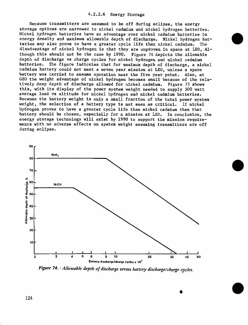
4.2.2.6 Energy Storage

Because transmitters are assumed to be off during eclipse, the energystorage options are narrowed to nickel cadmium and nickel hydrogen batteries.Nickel hydrogen batteries have an advantage over nickel cadmium batteries inenergy density and maximum allowable depth of discharge. Nickel hydrogen bat-teries may also prove to have a greater cycle life than nickel cadmium. Thedisadvantage of nickel hydrogen is that they are unproven in space at LEO, Al-though this should not be the case by 1990. Figure 74 depicts the allowabledepth of discharge vs charge cycles for nickel hydrogen and nickel cadmiumbatteries. The figure indicates that for maximum depth of discharge, a nickelcadmium battery could not meet a seven year mission at LEO, unless a sparebattery was carried to assume operation near the five year point. Also, atGEO the weight advantage of nickel hydrogen becomes small because of the rela-tively deep depth of discharge allowed for nickel cadmium. Figure 75 showsthis, with its display of the power system weight needed to supply 500 wattaverage load vs altitude for nickel hydrogen and nickel cadmium batteries.Because the battery weight is only a small fraction of the total power systemweight, the selection of a battery type is not seen as critical. If nickelhydrogen proves to have a greater cycle life than nickel cadmium then thatbattery should be chosen, especially for a mission at LEO. In conclusion, theenergy storage technology will exist by 1990 to support the mission require-ments with no adverse effects on system weight assuming transmitters are offduring eclipse.

Battery discharge/charge cycles x 103

Figure 74. - Allowable depth of discharge versus battery discharge/charge cycles..

124

180

160

140

120

~" 100o>

IE 80

I>M 60

40

20

Nickel Cadmium

SI battery solar arrayDistribution systemShunt regulatorBattery chargerBattery500 W load

I I

5 6 7

Altitude, km x 10

8 9,3

10 20 30 40

Figure 75. - Housekeeping power system weight versus altitude.

4.2.3 ACS/APS Technology Tradeoff

Table 47 summarizes advantages and disadvantages of candidate ACS/APSactuators. Table 48 shows the results of a tradeoff between APSs using chemi-cal blowdown, chemical bipropellant, and PPT. The results shown are repre-sentative of the propellant mass and APS weight required for an HF multiplelaunch case and are about one-half of what would be required for the small HFdesign in the triply-synchronous orbit. Except for the Ku-band satellites,electric propulsion will result in a weight advantage, although for someL-band concepts there is little difference. For these L-band systems, a smalladded weight for a chemical system might be offset by lower cost for the chem-ical system.

125

TABLE 47. - CONTROL TORQUE ACTUATOR SUMMARY

TorqueActuator

Thrusters

— Electric

— Chemical

Momentum exchangedevices reaction wheels&CMSs

Magnetic torquers

No cross-coupling with the vehicle motion to pro-duce undesirable torques for which compensationmust be made

High specific impulse, applicable to missions witha long lifetime

High thrust, low risk, lower dry weight

Ideal when disturbances are cyclic with respect toan inertia! reference frame & the secular component(bias torque) is small; could reduce the size &number of thrusters required for the mission

Used in conjunction with momentum exchangedevices for desaturation or momentum managementpurposes

Disadvantage

Low-thrust, high-power requirements; power alreadyavailable for most VOA satellite concepts; well-suitedfor distributed system

Low specific impulse, no applicable to missions with along lifetime; tankage volume & weight can be high;not well suited for distributed system, more complexthermal controlCross-coupling with the vehicle motion to produceundesirable torques that require compensation;requires a desaturation control law scheme; numberrequired could be prohibitive in terms of size, weight,& power required for large VOA antenna conceptsMagnetic field of Earth is time variant & stronglyaltitude dependent, at any instant torque can beproduced only along components normal to the localmagnetic field vector; practical limitations in powersupply & coil size make the generation of large torquesimpractical for VOA orbits

TABLE 48. -APS CANDIDATES WEIGHTTRADEOFF RESULTS

System

SlowdownBipropellantPPT

'sp

230s400

2200

Dryweight

220kg220184

Propellentfor 7 yr

1033kg594108

Total APSweight

1253 kg814292

126

4.3 COST ESTIMATING PROCEDURE

The cost estimating procedure developed and used identifies the costs ofeach subsystem, total satellite recurring and nonrecurring costs, launch costsand ground operations costs. The end results of the cost estimating procedureare satellite system and program life-cycle cost (LCC) which can be used toestimate LCC per channel hour.

The first step was to select or derive cost estimating relationships (CER)that are applicable to VOA DVBS. The Denver Aerospace documented LCC method-ology and cost analysis data base served as a starting point. We used themultiple independent cost estimating approach. This approach evaluates LCCestimates from several models, qualifying each by relation of hardware config-uration assumed by the model to configuration defined for the satellite. TheLCC estimating sources that were used included:

1) The Denver Aerospace 15-volume cost analysis data base;

2) the USAF Space Division model;

3) the NASA MSFC LSS model;

4) the NASA LeRC SDCM;

5) The U.S. Navy LCC Handbook.

In some cases, existing CERs were adjusted to reflect judgement as to ap-plicability to VOA satellite concepts. Finally, new CERs were developed frominformation contained in recent literature, specifically for costs associatedwith electrical power subsystems that produce more than 20 kW, electric pro-pulsion, and high power solid state power amplifiers. The CERs identified ascandidates for estimating LCC of VOA satellite concepts were included in acomputer program developed during this program. This program is documented inthe Appendix and is delivered as part of the contract.

The second step was to estimate the performance parameters required byeach CER. These estimates were obtained using the methods described in Sec-tion 4.1. Finally, a quantitative risk assessment method, including the riskassessment and management program (RAMP), was used to further qualify the LCCestimates obtained from the various CERs. The point LCC estimates presentedin Section 5 are defined as the 50/50 values obtained by running RAMP. Afurther discussion of the risk analysis method is presented in Section 6.Following is a discussion of the approach that was taken to derive the basecost estimates for each subsystem and the overall DVBS.

4.3.1 Communication Subsystem Cost Estimates

The communications subsystem is broken up into: (1) the antenna struc-ture, including array or reflector surface and ground plane; (2) the feederlink electronics and antenna(s); (3) the onboard signal processing; and (4)the payload transmitters. Since no prior data existed for LCC of antennasgreater than 20 meters in diameter or for space qualified amplifiers (trans-mitters) in the HF- and VHF-bands, new CERs had to be developed. The CERsused for the communications subsystem are listed in Table 49.

127

TABLE 49. - COST ESTIMATING PROCEDURES FOR COMMUNICATIONS SUBSYSTEM

Component

Box-ring truss planar array

Honeycomb fiberglass array

Graph ite/epoxy reflector

Solid-state transmitters

Uplink

Signal processing

Band

HF, VHP

L

Ku

HF, VHP

L

All

All

NRCCER

NRC = 0.013Wt

NRC = 0.013W t

NRC = 0.722W °-263

NRC = 0.746W, °'7n 7

NCR = 0.746W t

NRC = 0.373W °7

NRC = 0.373W t°'7

RCCER

RC = 0.002W

RC = 0.002Wt

RC = 0.0361 Wta65

RC = 0.06Nt

RC = 0.006N t

RC = 0.051Wt

RC = 0.057Wt

Source

MSFC, U S. Navymodel, judgement

Same

SDCM model

Space Division model

Vendor survey

Space Division model

Space Division model

Legend-

N Number of transmitters

4.3.1.1 Antenna Cost Estimates

For planar array antennas, the U.S Navy LCC handbook recurring cost esti-mate includes the structure, dipole elements, elevation network, and groundplane. In 1984 dollars the C£R for recurring cost is $4,900 to $9,800/m2.The MSFC model CER for graphite epoxy structures is $2,205/kg ($l,000/lb).For a 60-meter diameter, 1,000 kg box truss ring structure, the Navy CER pre-dicts a recurring cost of from $13.9 to $27.7M dollars while the MSFC CER pre-dicts $2.2M. Since the Navy CER assumes a continuous structure and the MSFCmodel is for graphite structures only, a compromise value of $4,4lO/kg($2,000/lb) was selected for array antenna recurring cost. For nonrecurringcost, the MSFC CER at $28,665/kg ($13,000/lb) was considered adequate. TheseCERs were also selected for the L-band honeycomb fiberglass panel arrayantennas.

The Ku-band reflector antenna costs were best fit by the SDCM model. How-ever, the SDCM data base also contains specific costs for graphite epoxy Ku-band reflectors used for the LANDSAT-D program. These costs were used for theVOA Ku-band systems. The total recurring cost from the SDCM data base is$790,000 while the nonrecurring cost is estimated at $1,700,000 for one anten-na or $850,000 per antenna for multiple antennas. There are up to eight re-flectors (two uplink and six downlink) for a single Ku-band satellite concept.

4.3.1.2 Feeder Link Electronics and Antennas

A Ku-band feed link is assumed for all systems, augmented by a V-bandcrosslink capability for HF and VHP concepts. The Space Division model CERfor communications electronics was used to estimate costs for all satellitesbased on the weight estimates described in Section 4.1. The costs for theL- and Ku-band satellites is considerably less than the HF- and VHF-sateilitessince no gimbaling, autotrack, or crosslink are required.

128

4.3.1.3 Signal Processing Cost Estimates

For all systems, the Space Division model communications electronics CERswere selected to estimate cost of onboard signal processing electronics. Theweights used for the CERs were obtained using the estimating procedure ofSection 4.1.

4.3.1.4 Transmitters Cost Estimates

The nonrecurring cost estimate for HF- and VHF-bands transmitters uses theSpace Division Model CER for communications electronics. For HF and VHPsatellites with different sized transmitters, the average transmitter weightwas used as the input to obtain nonrecurring cost. For each of the fourL-band systems, the largest transmitter size from all satellites in a systemwas used for the input to the CER.

The nonrecurring cost for the Ku-band system is based on a TWTA cost fromthe SDCM. TWTAs for Ku-band should require little development. A value of$37,500 was used for the development cost.

Recurring cost estimates for HF- and VHF-bands were obtained from a CERdeveloped after conversations with vendors. Estimated cost to produce solidstate amplifiers up to 1 kW was $60,000 per unit. For L-band, the Space Divi-sion model CER for communication electronics was selected. A learning factorincluded in the LCC estimating computer program reduces the overall averageunit cost based on the number of transmitters. To estimate the transmitter'stotal recurring cost for each L-band system, the computer program was run foreach complement of transmitter size and number. The total recurring cost foreach set of transmitters (corresponding to each unique array antenna) was ob-tained and summed to get the total recurring transmitter cost for the system.

The Ku-band recurring cost estimates use an average cost for a 20 wattTWTA of $790,000 as obtained from the SDCM data base. This value is reducedby an 80% learning factor for multiple TWTA's required on each of the Ku-bandsystem satellites. Thus the average unit cost is $632,000 per TWTA.

4.3.2 Electrical Power Subsystem (EPS) Cost Estimates

The EPS will provide power far in excess of that required for any existingsatellite system. For this reason, the CERs in existing LCC models were, con-sidered inadequate for estimating EPS costs for HF-, VHP- and L-band satel-lites. A brief literature search was conducted to identify cost estimates ofhigh power EPS. From information in ref. 17, 19, and 20, data points of costvs power were identified as shown in Table 50. From the MSFC model, typicalEPS components cost fractions were identified as shown in Table 51.

TABLE 50. - PLANAR SILICON ARRAYCOST DATA, 1984 $M

Source

Lockheed MSFCStudy (NAS8-32981)TRW LaRCStudy (NAS1 -17568)JSC space station study

Power

206 kW311

12.5

100

Nonrecurringcost

$21M2112

26

Recurringcost

$67 .2M85.522

54

TABLE 51. - EPS COMPONENTCOST FRACTIONS

Component

Solar arraysBatteriesDistributionControl

Nonrecurringcost fraction

MSFC0.2570.1260 1660451

VOA

[0.38]f?>.!Ql[<M71[0.4Q]

Recurringcost fraction

MSFC

0.6170.0910.1030 189

VOA

[0.70][0.05][010][0.15]

129

From the data of Table 50, expressions for nonrecurring (NRCsa) and re-curring (KCsa) cost of large solar arrays were developed as:

RC = 0.3P + 20 (4-19)saNRC = 0.094P + 16

sa

As indicated in Table 51, the solar arrays account for a fraction of theEPS cost. For conventional systems the fractions shown under the MSFC columnwould be used. However, for VGA high power satellites, the batteries willrepresent a very small part of the total EPS cost. For this reason, the newset of component cost fractions were identified for VOA high power satel-lites. Since the solar arrays are now assumed to account for 70% of EPS re-curring cost, a new EPS recurring CER is obtained by dividing the cost forsolar arrays by 0.7 resulting in:

RCeps = 0.43P + 28.5 (4-20)

Likewise, a new EPS nonrecurring CER is obtained by dividing the solar ar-rays development cost relationship by 0.38 resulting in:

0.247P + 42.1 (4-21)~-r~

where

RCe g = EPS recurring cost ($M 1984)

NRCe = EPS nonrecurring cost ($M 1984)

P = Required EPS power (kW)

A comparison of the MSFC and new VOA CERs at 20 kW shows good comparisonfor recurring costs ($35M and $37M respectively). However, the estimated non-recurring costs from the MSFC model is $102M while the corresponding VOA EPSCER results in $47M. The VOA CER is considered better since it takes into ac-count an economy of scale and, the MSFC model may include the multiplicativefactor of 2.5 to 3.0 used by MSFC to reflect increased development cost formanned vs unmanned spacecraft. The EPS CERs are summarized in Table 52.

130

TABLE 52. - COST ESTIMATING RELATIONSHIPS FOR OTHER SUBSYSTEMS

Subsystem

Electrical power >20 kW

<20kW

Attitude control

Auxiliary propulsion

Chemical blowdown

— N2H4 pressurant

- N2O4/MMH

- LO2/LH2

— H2 resistojet

— Cold gas

NCR CER

NCR = 42 1 + 0 247P

NCR = 143P0656

N RC = 2 923+ 0.2241 WT

NCR =0.661 +0.049WT

NRC = 0.36WT°-6242

NCR = 0.69WT °'545

NCR = 1.04W °'545

NCR = 3.2WT°-545

NCR = 1.64WT0'545

NCR = 0.144T W°-226

RCCER

RC = 28 5 + 0 043P

RC = 3.62P°757

RC = 0 0577WT

RC = 0 0085WT

RC = 0.0808WT ° 722

RC = 0 141WT ° 65

RC = 0211WT0'65

RC = 0.63WT ° ^

RC = 0 27WT ° 65

RC = 036v4°2°6

Source

Lockheed multi-kWstudy, NASA spacestation, Boeingelectric prop.NASA MSFC.

Space Division Model

Space Division model &Boeing electricpropulsion study

JPL (JPLD-972, 12/83)

Same

Same

Same

Same

Same

Legend:

P Power, kW

4.3.3 Attitude Control Subsystem (ACS) Cost Estimates

The satellite designs all use the reaction control system (RCS) for atti-tude control. Therefore, the attitude control subsystem consists of elec-tronics alone. For this reason, the Space Division LCC Model CER for attitudedetermination was considered the best choice for both recurring and nonrecurr-ing satellite costs. The ACS CERs are shown in Table 52.

4.3.4 Auxiliary Propulsion Subsystem (APS) Cost Estimates

The existing CERs are based on use of chemical APS, generally hydrazineblowdown or pressurized designs. For HF-, VHF-, and L-band satellites, elec-tric propulsion was considered a better design because of the higher specificimpulse and resulting lower propellant and subsystem mass. Proposed use ofelectric propulsion required development of a CER for electric propulsion.From ref. 21, a cost relationship was identified for recurring cost of anelectric propulsion subsystem. For nonrecurring cost, an assumption was madethat development costs would be about the same as for a chemical subsystem.As a result, the Space Division CER for nonrecurring cost was considered ade-quate. The CERs are shown in Table 53.

TABLE 53. • COST ESTIMATING RELATIONSHIPS FOR OTHER SUBSYSTEMS

Subsystem

Thermal control

TT&C

Equipment bay

NCR CER

NRC = 1.84+0.172WT066

NRC = 1 38 + 0063W' 0 fifi

NBC = 10.84 + 0.172WT

RCCER

RC = 00361WTa65

RC = 0.66 + 0 056W/T ° 93

RC = 0.36 1WT° 65

Source

Space Division model

Space Division model

Space Division model

•131

4.3.5 TT&C Subsystem Cost Estimates

The CERs contained in most LCC models should be adequate for estimatingTT&C subsystem costs. For consistency, the CERs from the Space Division modelwere selected. These CERs are shown in Table 53.

4.3.6 Thermal Control Subsystem Cost Estimates

The Space Division CERs were selected, again for consistency. The CERsare also shown in Table 53.

4.3.7 Equipment Bay and Mechanisms Cost Estimates

The equipment bay structure and the mechanisms for stowage and deploymentwill be similar to designs used on previous unmanned satellites. Thus, theSpace Division model CERs should be adequate. The CERs are also shown inTable 53.

4.3.8 Other Program Costs

The nonrecurring and recurring costs estimated by the subsystem CERs donot include other generic program costs. The other costs that were includedin the cost estimating approach follow:

1) Aerospace ground equipment costs;

2) Systems engineering, integration, and program costs;

3) Launch costs;

4) Ground operations costs.

4.3.8.1 Aerospace Ground Equipment Costs

These costs include tooling and investment costs for development, test,and production facilities. These costs are estimated by the Space DivisionModel at 11.3% of platform costs. Nonrecurring platform cost is the sum ofthe subsystem nonrecurring costs and likewise, recurring platform cost is thesum of subsystem recurring costs.

4.3.8.2 Systems Engineering, Integration, and Program Level Costs

Systems engineering and integration costs are expressed differently bydifferent LCC models. The SDCM model uses the following factors:

1) 32% of design cost,

2) 27% of development and test cost,

3) 32% of production engineering cost,

4) 22% of first unit fabrication cost.

132

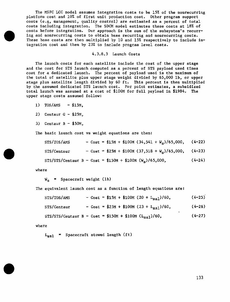
The MSFC LCC model assumes integration costs to be 15% of the nonrecurringplatform cost and 10% of first unit production cost. Other program supportcosts (e.g, management, quality control) are estimated as a percent of totalcosts including integration. The SDCM model estimates these costs at 18% ofcosts before integration. Our approach is the sum of the subsystem's recurr-ing and nonrecurring costs to obtain base recurring and nonrecurring costs.These base costs are then multiplied by 10 and 15% respectively to include in-tegration cost and then by 23% to include program level costs.

4.3.8.3 Launch Costs

The launch costs for each satellite include the cost of the upper stageand the cost for STS launch computed as a percent of STS payload used timescost for a dedicated launch. The percent of payload used is the maximum ofthe total of satellite plus upper stage weight divided by 65,000 Ib, or upperstage plus satellite length divided by 60 ft. This percent is then multipliedby the assumed dedicated STS launch cost. For point estimates, a subsidizedtotal launch was assumed at a cost of $100M for full payload in $1984. Theupper stage costs assumed follow:

1) TOS/AMS - $15M,

2) Centaur G - $25M,

3) Centaur B - $50M,

The basic launch cost vs weight equations are then:

STS/TOS/AMS - Cost = $15M + $100M (34,541 + Ws)/65,000, (4-22)

STS/Centaur - Cost = $25M + $100M (37,518 + Ws)/65,000, (4-23)

STS/STS/Centaur B - Cost = $150M + $100M (Wg)/65,000, (4-24)

where

Ws = Spacecraft weight (Ib)

The equivalent launch cost as a function of length equations are:

STS/TOS/AMS - Cost = $15M + JlOOM (20 + Lssl)/60, (4-25)

STS/Centaur - Cost = $25M + $100M (23 + Lgsl)/60, (4-26)

STS/STS/Centaur B - Cost = $150M + $100M (Lsgl)/60, (4-27)

where

= Spacecraft stowed length (ft)

133

The maximum launch costs were limited to the following:

STS/TOS/AMS - $115M,

STS/Centaur - fcl25M,

STS/STS/Centaur B - $250M.

4.3.8.4 Ground Operations Costs

The ground control costs include the costs to maintain the operational or-bit, to maintain the required satellite attitude, and to perform satellite on-orbit operations through the TT&C subsystem. The costs of a station includefacility fabrication, ground equipment, procurement, and manpower costs. Al-though manpower cost is spread over the station lifetime, it is lumped intothe total cost of each station. An eight person crew providing three shiftsof coverage is assumed for each station with tracking capability as requiredfor nongeostationary orbits. The eight persons include a working manager, twomaintenance personnel, and five mission operators/analysts. The rate assumedfor personnel was $75,000 per year. Total station cost for a 7-yr operationis $24,000,000, including manpower costs, equipment replacement, and spares.A further assumption is that the basic 8-person station can monitor and con-trol up to eight satellites using satellite cross links for both spacecraftcontrol and program feed. Each additional set of eight satellites will in-crease ground operations cost by $3.5M for each 7 years for three additionalpersonnel and additional tracking equipment. The total 7-yr ground operationscost for two stations for nongeostationary orbit systems is then expressed as:

Cost = $24M + $7.0M (n) (4-28)

where

n = number of additional sets or partial sets of eightsatellites

The cost of geostationary ground stations is estimated at $18,000,000 foriars of operation. The reduced cost results from requirement foreach seven years of operation. The reduced cost results from requirement for

fewer personnel and no tracking equipment. Also, none of the VGA geostation-ary systems have more than eight satellites; additional crews and equipmentwill not be required.

134

4.3.8.5 Learning Factor for Satellite Fabrication

To derive the total system life-cycle cost for multisatellite systems, alearning factor is assumed for satellite fabrication. The basic learningcurve equations are:

Cave = CulN-b (4-29)

where

b = log(m)/log(2)

C = average cost of N unitsave °C , = first unit fabrication cost

N = number of units to be fabricated

m = slope of learning curve (0.9 assumed)

The total fabrication cost (Ct) is then:

ct = cave N = cul N(1'b) (4-30)

The total system recurring cost, including launch cost, excluding infla-tion factors for phase acquisition, is then:

RCt = Ct + N'C! (4-31)

where

RC = total recurring cost

C- = cost per launch

135

5.0 SATELLITE SYSTEM DESIGN AND ANALYSIS

The system concepts and satellite design options for the four bands arepresented in this section. Satellite designs were generated and analysis per-formed to determine the key performance parameters of weight, volume, cost,and RF power flux density on the ground. These satellite designs were thencompared to the payload capability of the launch vehicle (Centaur G, TOS/AMS,and a hypothetical large Centaur) to ensure they were launch compatible.

For HF and VHF satellite designs, the channel requirements and PFD re-quirements were quite severe. Where these requirements could not be met usinga launch compatible satellite, the maximum capability satellite was determinedand its reduced capability was calculated. These reduced capabilities werethen compared to the VOA requirements to develop a system within reasonablecost parameters. Because the capabilities of satellites launched on a Centaurcould not achieve VOA requirements, a larger satellite design was developedthat would use a full orbiter bay and a hypothetical Centaur-type stage thatwould fill a second orbiter and produce a much greater capability on a singlesatellite.

The design and analysis flow used for the satellite system design andanalysis is presented in Figure 76. Subsystem selection was based on the de-sire to use as much off-the-shelf hardware as possible, but still achieve theVOA requirements. This was feasible for the Ku-band and L-band systems. Forthe VHF and HF systems, both the antenna and electric power subsystem wouldrequire advanced technology. The power subsystem technology could be derivedfrom space station development available in the early to mid 1990's.

Analysis was performed for all satellite system options to determine theability of a constellation of the proposed satellites to cover the 15 zones atthe VOA specified times.

Orbitanalysis& coverage

Selectionofapplicablespacecraftsubsystems

Spacecraftsubsystemparametrics

Paycap:

oadibility

RF analysispower &antenna size

i

Parametricspacecraftanalysis

i

Maximumoptimumspacecraftanalysis

i

Recmis

No '

Are thespacecraftlaunchcompatible

Yes

ucedsionlysis

Satellitedesignconcepts

Figure 76. - Satellite system design and analysis approach.

136

5.1 KU-BAND SYSTEM

For Ru-band operation, the satellite system design resulted in a singlepoint design to meet all VGA requirements. The system uses existing technol-ogy at reasonable power levels. The Ku-band system consists of three geosta-tionary satellites in three orbit slots. Each satellite consists of a farm ofoffset fed parabolic dish antennas attached to a central spacecraft bus. Thenumber of antennas per satellite varies depending on the number of zonescovered.

The parabolic dishes use graphite composite technology to provide enhancedstructural and thermal characteristics. Figure 77 illustrates the proposedsatellite design. The following sections describe the results of the variousdesign and analysis processes used to determine the satellite characteristics.

Figure 77. • Ku-band satellite design.

5.1.1 Ru-Band Systems Weight and Volume Estimates

The Ku-band satellites weight and volume are summarized in Table 54. Theelectric power subsystem requirements are based on a transmitter efficiency of35% and housekeeping power of 500 watts. Also, unlike systems designed forthe other bands, the Ku-band satellites are sized for operation during occul-tation. Table 55 shows the results of the sizing run for the first satelliteof the system. This satellite has three payload antennas while the other twosatellites each have six.

137

ORIGINAL PAGE ISOF POOR QUALFTY

TABLE 54. - KU-BAND SATELLITE WEIGHT AND VOLUME ESTIMATE

I

SYSTEM CONFIGURATION SUMMARY

Rf PayloadAuxi l i a ry Propulsion SuhsytemTelemetry, Tracking and CommandElectr ical Power SubsystemThermal Control SubsystemEquipment bay Structure

MAJ-SCKU) VOLUME<M A 3>

?28 2.0-.J?03.1 V. 2i><?6.4 .027?.08425 .31790244.6?'5708 4.736863E-0283.!!>8633 11.19356

TOTAL SYSTEM SUMMARY 617.7V63 15.84884

*»**«*»»»»**»***»******»*****»****»»»***********************

BYSTL-IM CnNFTUUKATION SUMMARY

Rf P ty I "<<dA u x i l i a r v fvooul SIOH Suhsyi em'( 13 1 pi»t»i ry . Ti%acki»y -old Comma n«iI!) HI t> 4< a I F'owtM !>u))'»s.">t »>m

MAS'UKI.) VOLUME<M"3>

'3'?9 3.1:'<>L« ,L 'S . 2 I,?6.4 .02

Kqu i hav !!tt i>(-5.A84232K-0?

103.6118 i\,:

TOTCH, rYSTIJM MIMMARY ' ) l t>.708l

SYSTEM CONFIGURATTOH SUMMARY

pf PayloadAuxiliary Propulsion SuhsytemT.elemeti-y, Tracking and CommandElectrical Cower SubsystemThermal Control Subsystemggiupment Pay Structure

MASS(KG) VOLUME(MA3)

40-5 3.1i'03.1 2.2126.4 .02/b.46364 .34363164.81073-5 4.92«33/E-Oi>104.2808 11.14387

TOTAL SYSTEM SLIMMARY MV.057] 16.868761806,021

138

TABLE 55. - KU-BAND SIZING EXAMPLE

EPS SUMMARY

Power required from source = 1.320852 KWPower at load, average = .76 KWOrbital altitude = 35786 KmOrbital period = 23.93445 hrsSpacecraft lifetime requirement = 7 yrsTotal eclipse time per orbit= 1.156897 hrsSolar array degradation factor due to radiation = .9538934Solar array thermal adjustment factor = .8943101Solar array cover slide weight factor = OAntenna Size = 1 m by 1 m

***** Power Generation Sizing *****

For Si Blanket ArrayArea required = 9.847787 m2Weight = 15.7564* Kg Volume = .0787823 m3

***** Shunt Regulator Sizing *****

Shunt Regulator Weight = 4.036412 KgShunt Regulator Volume = 4.576431E-03 mA3

***** Power Switching/Distribution Sizing *****

Power Switching Equip Wt. = 2.479833 KgPower Switching Equip Vol. = 2.811602E-03 m3

Distribution Weight; Source to Bus - .100516 KgDistribution Weight; Bus to Load = 3.2O3O65E-02 KgTotal Distribution Weight - .1325466 KgTotal Switching and Distribution Weight = 2.61238****** TOTAL SI SYSTEM WEIGHT W/0 BATTERIES<kg> = 22.4O525****** TOTAL SI SYSTEM VOLUME W/0 BATTERIES<M*3> = 8.617033E-02

***** Battery Sizing *****

For NiCd BatteriesBattery Capacity Required = 1051.725 UhBattery Weight - 29.81588 Kg Battery Volume = 1.489074E-02 m3

***** Battery Charger Sizing *****

For NiCd BatteriesBattery Charger Weight = .1675525 Kg Battery Charger Volume1 = 1.899688E-04 m3

TOTAL EPS MASS(ka) - 52.'38868TOTAL EPS VOLUME<MA3) - .10J251

139

«n •!•

TABLE 55. - CONTINUEDp a :-.«- > t ni i » I) f •»

THERMAL CONTROL SUBSYSTEM S[/ tNU 'SUMMARY

Max j mum tempt'rotured,) _>.>Maximum heat radiatod(W) 2150R«xr t ja tJVf» surf a< t» t innss>iV3ty fac lor .0Radiative 'surface? absorptivity factor .2Required radiator surface arpa(M*?> .94737?*

Thermal Control Subsystem mass (Kg)Thermal ' ontrol Gubsy^tem area <M"?>Thermal Control Subsystem Volume (11*3)

]R >

Lbs 10.199*9.947372*64./36863E-02

rtn g. *

KQUtPMENT BAY SUMMARY

Total mai,s> of e^qui pmenl bay<k<:)J ?>e.!>fl/>34 I.tas 1/J9.1629Mass of deployment/stowage mechan isms(kg) 2'5Total mas,s,<kg) 83.58633 (Lbs) 184.307VTotal volume of structure and niechanisms(mA3> 16.79034

Ku-band Sizing Example

SYSTEM CONFJGUKATION SUMMARY

Rf PayloadAuxj l iary F'ropu I j t>u SubsytemTelemetry/ Tracking and CommandF. I £••(. t>-3«. a 1 F'owt>r SubsystemTh <-ar ma 1 Con tr o 1 Subsy s ternKauipme>m H?\y Strurturp

MAGS (KG) VOI.UME(MA3)

226 2.05203.3 ?.2226.4 .02W. 38868 .i012514.62570Q 4.736Q63E-0?83. 8633 1J.1V3L»A

TOTAL SYSTf'.M SUMMARY !>90.1007 15.63?3 81316.812 (Lbs)

»**»**<»»**»* X ***»»»»#***»*****»* ****X >»*»*»*»!*»»*«•*»»»**»»)'

140

TABLE 55. - CONCLUDEDSi :z::

RF SUBSYSTEM SIZING SUMMARYData for Honeycomb Panel Array (Non-phased)

ANTENNA APERTURE AREA(M*2> 0TOTAL ANTENNA STRUCTURE MASS(KG) OTOTAL ANTENNA STRUCTURE VOLUME<MA3) 0WEIGHT OF UPLINK COMPONENTS(Kg) 119VOLUME OF UPLINK COMPONENTS(M*3> 2UEIGHT OF SIGNAL PROC. COMPONENTS(Kg) 1O9VOLUME OF SIGNAL PROC. COMPONENTS(MA3) .05

TOTAL RF SUBSYTEM MASS(KG) 228TOTAL RF SUBSYSTEM VOLUME(MA3) 2.05

ATTITUDE CONTROL, STATIONKEEPING AND MANEUVERING SUMMARY

Total ACS subsystem mass (Kg) 13.1 Ltas 28.8855Total ACS subsystem volume (MA3> .02Total RCS subsystem mass(Kg) 190 Lbs 418.95Total RCS subsystem volume(MA3> 2.2

Total RCS/ ACS subsystem mass (Kg) 203.1Total RCS/ ACS subsystem volume(M*3) 2.22

£> dL

TT&C SUBSYSTEM SUMMARY

Total TT&C subsystem mass(Kg) 26.4 Lbs 58.212Total TT&C subsystem voHime(M*3) .02

5.1.2 Ku-Band Coverage Analysis

To meet the coverage requirements In the SOW, the three satellites wereplaced in unique geostationary orbit slots. Figure 78 shows the location ofeach satellite. It was assumed that each satellite would carry multiple an-tennas targeted to the center of each zone to be covered. The first satellitewas placed at 70° W. longitude and provided coverage for Zones 1, 2, and 3.The next satellite was placed at 15° E. longitude and provided coverage forZones 4 through 9. The final satellite was placed at 110° E. longitude andprovided coverage for Zones 10 through 15. To assure coverage up to 70° lati-tude, (to cover Zones 9, 10, 12 and 14) a minimum satellite elevation angle of11.5° was required. The three geostationary satellites can provide 24 hourcontinuous service to each zone. Eclipse effects at geostationary orbit will

141

be maximum at spring and fall equinox resulting in slightly more than one hourof eclipse time when the satellites could not transmit if battery storage hadnot been provided.

Figure 78. - Constellation for Ku-band—geostationary, three satellites.

5.1.3 Ku-Band System RF Performance Analysis

For each zone covered, an RF performance analysis was performed to deter-mine the antenna size and power requirements needed to provide a PFD of-131 dBW/m^ at edge of coverage. The RF analysis took the servicing satel-lite location and zone size into account when determining antenna aperturesize. In addition, Ku-band reflector antennas were assumed to have a beam-width equal to:

BW70XD

(5-1)

where

BW = beamwidth, degreeX = wavelength, mD = reflector diameter, m

142

To determine the PFD on the ground, a 3-dB polarization loss was assumedfor circular polarization transmission and a linear polarized receiver.Spreading loss was calculated using the maximum slant range required for cov-ering the zone (the slant range being the distance from the satellite to theground). The maximum slant range occurs at the same point on the ground asthe minimum spacecraft elevation angle.

A computer program (RFANAL - ref. the Appendix) was written to performthese calculations quickly and efficiently. Table 56 shows an example of theprogram output for Zone 9. The propagation loss of 0 dB used in this analysisis discussed in Section 3.2. The aperture efficiency of 0.5 was used to ac-count for feed mismatch and circular polarization conversion loss, spilloverloss, and losses due to reflector surface accuracy. The power is shown inwatts required per channel for an EOC PFD of -131 dBW/m2.

After each zones' aperture and power requirement were determined, thezones common to a single satellite were combined to determine the satellite'speak power requirement by combining the service requirements (showing how manychannels for each zone are at any given UTC time were required to be transmit-ted) with the RF power required per zone per channel.

The results are shown in Table 57. Of the three geostationary satellites,the highest power requirement Is 159 watts occuring at UTC 415. This was theresult of simultaneously requiring 10 channels to operate in Zone 5, two chan-nels in Zone 6, four channels in Zone 7, one channel In Zone 8 and six chan-nels in Zone 9.

TABLE 56. - RF ANALYSIS FOR KU-BAND, ZONE 9

Zone covered Zone 9 GEO Ku-band at 35786Orbital altitude 35786 kmOperating frequency 12200 MHzSatellite location 0 tat. 15 Long.Zone size 37x70 Lat.. 20x53 Long.Polarization—ci rcu larAperture size 659 m x .334 m using Tapered illuminationAntenna EOC gain 29.5 dBiAntenna aperture efficiency 50%Antenna beamwidth 2.613 x 5.146°Ground coverage 3673.46 x 3673.46 km, 33 x 33°Antenna scan angle 0Polarization margin 3 dBPropagation loss 0 dBMin elevation angle 11.475Spreading loss 163.13 dBSlant range 40429.3 kmPower read/channel for EOC PFD of -131 dBW/m2 a61 WEOC EIRP at EOC PFD of -131 dBW/m2 35 13 dBW

143

TABLE 57 - KU-BAND ANTENNA DESIGN SUMMAR Y

Satellite ZonesAperturesize

No. ofchannels

Max powerper aperture

Satellite worst case design power at UTC 45 = 78 W

1 123

0.49x0.32 m0 42x0.260.17x0.17

222

9.7 W12.256.0

Satellite worst case design power at UTC 415 = 159 W

2 456789

0.37x0.250.55x0.240.66x0.230.18x0.240.35x0.360.66x0.33

2113426

15.966.413.562.611.121.7

Satellite worst case design power at UTC 1 100 = 129 W

3 101112131415

0.43x0.370.33x0.300.85x0.230.18x0 220.77X0.340.18x0 33

342621

14.830.78.2

103.56.1

12.7

5.1.4 Ku-Band System LCC Estimates

TABLE 58. - KU-BAND SATELLITES LCCESTIMATES, 1984 $

SystemSatellite

123

S/CNRC

$76M8

10

94

Recurringcost

$174M165120

459

Launchcost

$21 3M213210

636

Ground*cost

$17M1717

51

Totalcost

S480M403357

1240

*20 years operational lifetime

The Ku-band three-satellite systemLCCs are summarized in Table 58. Fig-ure 79 shows the total cumulative costas a linear function, and yearly cost,as a bar graph, for a 24-yr life cy-cle. Assuming four launches per yearcombined with a 7-yr satellite life-time, three sets of launches are re-quired starting after a 3-yr develop-ment program. This approach providesa 21-yr, full coverage Ku-band capa-bility. The costs shown during the periods between launches include only theground stations operating cost ($18M per seven years). The different recurr-ing cost for each satellite results from different sized apertures, differentpower requirements, and different numbers of downlink apertures for satellitenumber one (three, vs six for satellites one and two). The launch costs, de-termined from payload weight, are similar since most of the STS payload is dueto the TOS/AMS upper stage. Two ground stations are assumed for the system,although an intersatellite link using the middle satellite would permit real-time communication from a single ground station. The reduced cost for theground stations would be offset by increased nonrecurring and recurring costsfor the middle satellite. No learning factor was assumed in deriving thetotal cost.

Since the Ku-band satellites are capable of operation even during the oc-culted period of the orbit, the LCC per channel hour is easily computed fromtotal LCC divided by total channel hours.'

144

1200

1080

960

840

720

600

480

360

240

120

10 12 14Program time, yr

16 18 20 22 24

Figure 79. -Ku-band cumulative and yearly program costs, 1984 $M.

5.1.5 Ku-Band Summary of Results

The Ku-band system designed for VOA applications consisted of three satel-lites in geostationary orbit. Each satellite carried multiple parabolic dishantennas targeted to specific zones. This resulted in a 100% match in cover-age with the VOA requirements. The frequency of operation for the Ku-bandsystem was 12.2 GHz with sufficient RF power in each satellite to provide apower flux density of -131 dBW/m^ at the edge of coverage. The orbit trans-fer stage used to deliver each satellite into orbit was the TOS/AMS, resultingin a payload capability to orbit of 3113 kg. This provided sufficient growthmargin for satellites mass ranging from 618 to 819 kg.

Including a 3-yr development schedule, three sets of launches result in a24-yr life cycle for satellite lifetimes of seven years. Total estimated costfor three sets of satellites is $1,189M. Ground operations cost for 20 yearswould be fc51M. Thus, a 20-yr operational capability would cost $1,240M.Twenty years of operation would provide 2,184,523 channel hours resulting in acost of fe568 per channel hour. Since the system life is 21 years, one year ofproductive service is left after the 20-yr program.

145

5.2 L-BAND SYSTEM

For L-band operation, the satellite system design and analysis resulted ina single point design at the high RF power requirement and three system op-tions at the low RF power requirement. Each system design meets all VGA re-quirements with the high RF power system designed to meet the PFD requirementof -103.6 dBW/m^ and the low RF power systems designed to meet the PFD re-quirement of -116.1 dBW/m^. All designs use existing state-of-the-art"tech-nologies for communications, ACS, stationkeeping, TT&C, thermal control, andspacecraft structure.

Although the electrical power subsystem uses existing technology, the sizeof the system is larger than present day satellites and will require projectedimprovements in the state of the art, e.g, those demonstrated in the solararray flight experiment (SAFE). The communication subsystem is made up ofrigid honeycomb panel nonscanning arrays and solid state transmitters. Thistechnology is similar to the communication subsystem found on the Seasat-ISpacecraft, Section 3.4.1.2.

The high RF power L-band system consists of eight satellites. Each satel-lite consists of a farm of rigid panel arrays attached to a central spacecraftbus. The number of arrays per satellite varies depending on the number ofzones covered, with each array illuminating a single zone. Figure 80 illu-strates the proposed satellite design for the high RF power system.

The first option, Option I, for the low RF power L-band system consists offive satellites. Again each satellite consists of a farm of rigid panel ar-rays and each array illuminates a single zone. The next two low RF power op-tions consist of three satellites each. The first, Option II, has individualarrays per zone, while the second, Option III, has a single array for multiplezones. Option II of the three satellite systems has a lower power requirementthan Option III but is heavier due to the number of arrays on each satellite.

Figure 80. - L-band satellite design.

5.2.1 L-Band Systems Weight and Volume Estimates

Weights and volumes for the four L-band systems are summarized in Table59. For sizing the electrical distribution weight from the bus to the load,the total area of all array antennas was computed and an equivalent area de-fined for the antenna diameter input to the EPS sizing program. Table 60shows the sizing program results for satellite two of the high power system.

146

TABLE 59. - L-BAND SATELLITES WEIGHTSAND VOLUMES

System

High-power requirementdesign (-103.6 dBW/m2)(eight satellites required)

Low-power requirementoption 1 (-116.1 dBW/m2)(five satellites required)

Option II (-116.1 dBW/m2)(three satellites required)

Option III (-116.1 dBW/m2)(three satellites required)

Satellitenumber

1234567812345

123123

Weight3914. kg244437102981282133734249265113231472146017071176

125221502150106518931835

Volume26.323.324.521.722.423.228.49.4

18.019.019.2•22252

18.023.824.216.218.517.8

Note:

Satellite locations by satellite number are shown in Figures 81,82 & 83.

147

TABLE 60. - L-BAND SIZING EXAMPLEE_ --JK»i.xnnc-l E> i- TT.-\. n-cj TE -B/L »? (5 -103.* dH

RF SUBSYSTEM SIZING SUMMARYData for Honeycomb Panel Array (Non-phased)Data for antenna no4 1Antenna aperture (M) 2.B x 1.9

Power pertransmitter(uU

29,16667

Number oftransmitters

Output power(kw)

6.3

ANTENNA APERTURE AREA(MA2) 5.32TOTAL ANTENNA STRUCTURE MASS(KG) 63.6227TOTAL ANTENNA STRUCTURE VOLUME<M"3) ,266TOTAL RF TRANSMITTER MASS(KG) 672.4055TOTAL RF TRANSMITTER VQLUME(MA3) 1.621494Data for Honeycomb Panel Array (Non-phased)Data for antenna no. 2Antenna aperture (M) 4.1x1.8

Power pertr an«»m 111 er (w)

37.03704

Number oftransmitters

324

Output power (kiu)

12

ANTENNA APERTURE AREA(MA2) 7.38TOTAL ANTENNA STRUCTURE MASS(KG) 64.60817TOTAL ANTENNA STRUCTURE VOLUME(MA3) .369TOTAL RF TRANSMITTER MASS(KG) 1258.43?TOTAL RF TRANSMITTER VOLUME(MA3) 2.799696WEIGHT OF UPLINK COMPONENTS(Kg) 78VOLUME OF UPLCNK COMPONENTS(MA3) .5WEIGHT OF SIGNAL PROC. COMPONENTS(Kg) 67VOLUME OF SIGNAL PROC. COMPONENTS(MA3> .03

TOTAL RF SUBSYTEM MASS(KG) 2244.068TOTAL RF SUBSYSTEM VOLUME(MA3) 5.58619

148

TABLE 60. - CONTINUED

:z:dL v»<:|S/C *»2 0 -103.6 dB

EPS SUMMARY

Power required from source = 30,0774 KWPower at load/ average = 28.65385 KWOrbital altitude = 35786 KmOrbital period = 23.93445 hrsSpacecraft lifetime requirement = 7 yrsTotal eclipse time per ortait= 1.156897 hrsSolar array degradation factor due to radiation = .9538934Solar array thermal adjustment factor = .8943101Solar array cover slide weight factor = 0Antenna Size = 3.065372 m by 3.065372 m

***** power Generation Sizing *****

For Si Blanket ArrayArea required = 224.2461 m2Weight = 358.7937 Kg Volume •= 1,793969 m3

***** Shunt Regulator Sizing *****

Shunt Regulator Weight = 51.63594 KgShunt Regulator Volume = 5.854415E-02 m*3

***** Power Switching/Distribution Sizing *****

Power Switching Equip Wt. = 9.007568 KgPower Switching Equip Vol. = 1.021266E-02 m3

Distribution Weight; Source to Bus = 10,92231 KgDistribution Weight? Bus to Load = 2.235811 KgTotal Distribution Weight = 13.15812 KgTotal Switching and Distribution Weight = 22.16568****** TOTAL SI SYSTEM WEIGHT W/0 BATTERIES(kg) = 432.5953****** TOTAL SI SYSTEM VOLUME W/0 BATTERIES(MA3> = 1.862725

***** battery Sizing *****

For NiCd BatteriesBattery Capacity Required = 1051.725 WhBattery Weight = 29.81588 Kg Battery Volume = 1.489074E-02 m3

***** Battery Charger Sizing *****

For NiCd BatteriesBattery Charger Weight - ,1675525 Kg Battery Charger Volume = 1.899688E-04 m3

TOTAL EPS MASS (kg) = 462,5787TOTAL. EPS VOLUME<MA3> = 1.877806

149

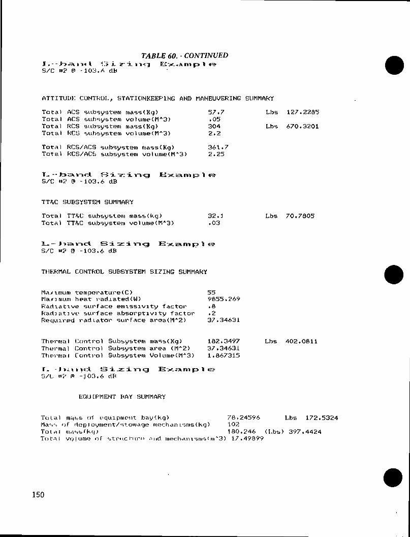
S .- - fr*^\ i -*i I 13 i_ a- it. iS/C **? P -103, A db

TABLE 60. - CONTINUEDK-J E£ -XL -tarn p> ll n-!-

ATTITUDK CONTROL, STATIONKEEP1NG AND MANEUVERING SUMMARY

Ltas 127,2285

Lbs 670.3201

Total ACS subsystem mass (Kg)Total ACS subsystem vo)ume(MA3>Total RCS subsystem mass(Kg)Total RCl> <bub&ystem volume(MA3)

Total RCS/ACS subsystem mass (Kg)Total RCS/ ACS subsystem volume (MA3>

57.7.053042.2

2,25

T - - - J:> 5sn v> N~l f> "JL -?: -JLS/C «2> P -103. A dB

Jfci -XL i-a. m

TTJiC SUBSYSTEM SUMMARY

Total TT'iC sub&y&lem mas>s>(kg)Total TTM: subsystem volume(MA3)

32.3.03

Lbs 70.7805

1_ — Jl SHU vid S ± zc. ±S/C **? (? -103.6 dB

13-xLEH.mi IT* 1 €=2-

THKRMAL CONTROL SUBSYSTEM SIZING SUMMARY

Maximum temperature(C) 55Maximum heat radiated(U) 9855.2*9Radiative surface emissivity factor .SRadiative surface absorptivity factor .2Required radiator surface area(M"2) 37.34631

The»rroal Control Subsystem mass (Kg) 1S2.3497Thermal Control Subsystem area (MA2> 37.34631Thermal Control Subsystem Volume(MA3) 1.8*7315

If * -1 •» 4. t 11 •! :l £•> -JL jz: 3. vt cj 13 >r. fa. m p> Tl e?S/L «»/' f° -103,6 dB

Lbs 402.0611

KQUCPMENT HAY SUMMARY

Tola) m?4t>s> of equipment bay (kg)Mass of deployment/stowage median isms (Kg)

Total volume of strut:

78.24596 Lbs 172.5324102180,246 (I.tas) 397.4424

/md mechanisms* m"3) 17,49899

150

TABLE 60. - CONCLUDED*M*«tt«*K«ttKKK«*«**»*«*tt«*tt*W«**««*«**«***«**tt«M«***ttM**tttt*tt«

L-band Sizing ExampleS/C «»2 (5 -103.6 dB

SYSTEM CONFIGURATION SUMMARY

MASS(KG) VOLUME<MA3>

Rf Pay loadAu> 1 I iary Propu 1 sion SubsytemTelemetry/ Tracking and CommandElectrical Power SubsystemThermal Control SubsystemEquipment Bay Structure

TOTAL SYSTEM SUMMARY

2244 ,O683*1.732.1462.5787182.3497180.246

3463.0427636.009

5.586192.25.031.8778061.8673151 1 . 66599

23.27731(Lbs)

5.2.2 L-Band System Coverage Analysis

To meet the VGA coverage requirements, satellites for each L-band systemwere placed in three geostationary orbit slots. Depending on the system, thenumber of satellites in any one slot varied from four for the high RF powersystem to one for the low RF power system. Figures 81, 82, and 83 show thesatellites locations for each system. The system designs call for each satel-lite to carry several array antennas with each antenna targeted to the centerof a specific area to be covered. In the Option III design, the covered areaconsisted of multiple zones.

The first constellation of satellites was placed at 70° W. longitude andprovided coverage for Zones 1, 2 and 3. The next satellite constellation wasplaced at 15° E. longitude and provided coverage for Zones 4 through 9. Thefinal satellite constellation was placed at 110° E. longitude and providedcoverage for Zones 10 through 15. To assure coverage up to 70° latitude forZones 9, 10, 12 and 14, a minimum satellite elevation angle of 11.5° was re-quired. The VOA coverage requirements were matched 100%.

151

Figure 81. - Constellation for high RFpower L-band system—geostationary, eight satellites.

152

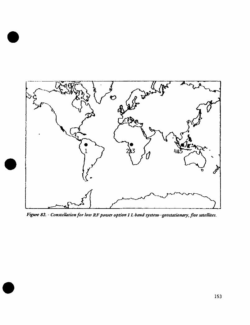
Figure 82. - Constellation for low RF power option I L-band system—geostationary, five satellites.

153

Figure 83. - Constellation for low RFpower options II and III L-band system-geostationary, three satellites.

5.2.3 L-Band System RF Performance Analysis

For each L-band system, an RF performance analysis was performed to deter-mine the antenna size and RF power requirements needed to provide the requiredPFD at edge of coverage. The RF analysis took the servicing satellite loca-tion and ground area to be covered into account when determining antenna aper-ture size. In addition, L-band nonscanning arrays were assumed to have abeamwidth equal to:

BW =65AD

(5-2)

where

BW = beamwidth, degreeA = wavelength, mand D = reflector diameter, m

To determine the PFD on the ground, a 3-dB polarization loss was assumedfor circular polarization transmission and linear polarized reception. Also,the spreading loss was calculated using the maximum slant range required for

154

ground coverage. The coverage area on the ground was equal to the zone cov-ered for all but the last system, In which multiple zones were covered with asingle aperture. A computer program was written to allow these calculationsto be done quickly and efficiently. Table 61 shows an example of the programresults for the high RF power system at Zone 9. Table 62 shows an example ofthe program results for Option III, the multiple zone per aperture case. Thepropagation loss of 0.0 dB used in the analysis is discussed in Section 3.2.The aperture efficiency of 0.8 was used to account for losses associated witharray mismatch, amplitude and phase control of array elements and circularpolarization conversion. The power per channel for the required PFD level isshown in watts.

TABLE 61. - RF ANALYSIS FOR HIGH POWER L-BAND, ZONE 9

Zone covered Zone 9 GEO L-Band at 35786Orbital altitude . 35786 kmOperating frequency 1500 MHzSatellite location 0 Lat 15 Long.Zone size 37x70 Lat, 20x53 Long.Polarization CircularAperture size 4.974 x 2.53 m using UNIFORM illuminationAntenna EOC gain 30.94 dBiAntenna aperture efficiency 80%Antenna beamwidth 2 613 x 5.146°Ground coverage 3673.46 x 3673.46 km, 33 x 33°Antenna scan angle 0Polarization margin 3 dBPropagation loss OdBMin elevation angle 11 47Spreading loss 163.126 dBSlant range 40429.3 kmPower read/channel for EOC PFD of -103.6 dBW/m2 1439.191 WPower reqd/channel for EOC PFD of -116.1 dBW/m2 80 93 WEOC EIRP at EOC PFD of -103.6 dBW/m2 ' . ' . ' . ' . ' . ' . ' ' . . . . . . . . . . 62.53 dBWEOC EIRP at EOC PFD of -116.1 dBW/m2 50.03 dBW

TABLE 62. - RF ANALYSIS FOR LOW RF POWER L-BAND, OPTION HIZONES 4, 6, 7, AND 8 COMBINED

Zone covered Zone 4,6, 7, & 8 GEO L-Band at 35786Orbital altitude 35786 kmOperating frequency 1500MHzSatellite location 0 Lat 15 LongZone size -35x44 Latitude, 40x60 LongitudePolarization - CircularAperture size 1.05 m x .893 m using UNIFORM illuminationAntenna EOC gam 19.67 dBiAntenna aperture efficiency 80%Antenna beamwidth 12.38 x 14 556°Ground coverage 8794.05 x 11131.71 km, 79 x 100°Antenna scan angle 0Polarization margin 3 dBPropagation loss 0 dBMm elevation angle 27.27Spreading loss 162 78 dBSlant range 38858.56 kmPower reqd/channel for EOC PFD of-103.6 dBM/m2 17814.22 WPower reqd/channel for EOC PFD of -116.1 dBM/m2 10001 767 WEOC EIRP at EOC PFD of -103.6 dBW/m2 62.18 dBWEOC EIRP at EOC PFD of -116 1 dBW/m2 46.68 dBW

After each zones' aperture and power requirement were determined, thezones common to a single satellite were combined to determine the satellitespeak pgwer requirement. This was accomplished by combining the service re-quirements (showing how many channels for each zone at any given UTC time were

155

required to be transmitted) with the RF power required per zone per channel.The results are shown in Tables 63 through 66. Table 63 gives the results ofthe high RF power L-band system made up of eight satellites. Table 64 givesthe results of the five satellite low RF power L-band system, Option I. Ta-bles 65 and 66 are the results of the three satellite low RF power L-band sys-tems , Options II and III.

TABLE 63. - HIGH RF POWER L-BAND ANTENNADESIGN SUMMARY

s/c*1

2

3

4

5

6

7

8

Zone

123

45567

89

10111214151313

Aperturesize

3.7x2.4 m3.2x1.91.25x1.242.8x1.94 1x1 84.1x185.0x1.71.4x1 826x275.0x2.53 3x2.82.5x2.36.4x1.75.8x2.61.4x2.51.4x1.71.4x1 7

No. ofchannels

22225

634

263422133

RF outputpower/zone3.8 kW4.8

223

6.312014.45.4

24.94.48.65.9

12.2332.45.1

20.620.6

Maximum S/C RFpower

31 0 kW-UTC 45

18 3-UTC 530

198-UTC530

24.9-UTC 41511.6-UTC430

16.2-UTC 300

25.7-UTC1100

20.6-UTC 1100

'Satellite mass range-2651 to 4349 kg

TABLE 64. - LOW RF POWER L-BAND ANTENNADESIGN SUMMAR Y-OPTIONI

s/c*1

2

3

4

5

Zone123456789

10111214

1315

Aperturesize

3.7x2 4 m3.2x1 91.25x1.242.8x1.94.1x1 85.0x1 7

1.4x1.82.6x2.75 0x2.5

3.3x2 82.5x2 36.4x1.75.8x2.5

14x1 71.4x2.5

No. ofchannels

2222

113

426

3422

61

RF outputpower/zone

0.22 kW0.271.25

0361.500.30

1.400.250.49

0.330.690.180.14

2.30.28

Maximum S/C RFpower

1.75kW-UTC45

2.14-UTC530

2 0-UTC 415

0 9-UTC 300

26-UTC 1100

•Satellite mass range—1176 to 1707 kg

156

TABLE 65. • HIGH RF POWER L-BAND ANTENNADESIGN SUMMAR Y-OPTIONII

s/c*1

2

3

Zone

123

456789

101112131415

Aperturesize

3.7x2.4 m3.2x1.91.25x1 24

2.8x1.94.1x1.85.0x1.71.4x1.82.6x2.75.0x25

3.2x2.82.5x2.36.4x1.71.4x1.75.8x2.51.4x2.5

No ofchannels

222

2113426

342621

R F outputpower/zone

0.22 kW0.271.25

0.361.500301.400250.490.330.690.182.300.140.28

Maximum S/C RFpower

1 75 kW-UTC 45

3.4-UTC 430

2.9-UTC 1100

•Satellite mass range-1251 to 2150 kg

TABLE 66. - LOW RF POWER L-BAND ANTENNADESIGN SUMMAR Y-OPTION III

s/c«1

2

3

Zone

1&235&94&6&7&S

10&1112&13&14&15

Aperturesize

3.75x1.2 m1.25x1.244.15x1.231.05x0.89

1.7x2.31.2x1.1

RF outputpower/aperture

0.84 kW1.253.29.0

1577.2

Maximum S/C RFpower

2.1 kW-UTC 45

10.2-UTC 430

7.5-UTC 1100

•Satellite mass range—1066 to 1893 kg

5.2.4 L-Band Systems LCC Estimates

Each satellite of the L-band systems Is generlcally the same. However,the unique coverage required from each results in different aperture sizes anddifferent subsystem sizes. To estimate system LCC, each satellite's nonrecur-ring and recurring costs were estimated first. The system nonrecurring devel-opment cost was then obtained by comparing the subsystem development costs foreach satellite, selecting the maximum for each subsystem and summing the maxi-mums. The individual satellites' recurring costs were summed to estimatetotal system recurring cost. Because the satellites within each system havedifferent antenna designs, different electrical power requirements, and dif-ferent thermal control requirements, no learning factor adjustment for cost offabrication was assumed. The LCC estimates for the L-band systems are summa-rized in Table 67.

157

TABLE 67. - L-BAND SYSTEMS' LCC ESTIMATES, 1984 $

System*

High power (-103 6 dBW/m2)Option 1 (-116.1 dBW/m2)Option II (-116 1 dBW/m2)Option III (-116.1 dBW/nV)

NRC

13098

113135

Groundcosts*

$51 M515151

RC

1968645441504

Launchcosts

S3000M1095666663

TotalLCC

S5149M188912731353

*20-yr operational lifetime

Figures 84 through 87 contain linear plots of total L-band system costas a function of time, and bar graphs showing phased yearly costs for the fourL-band concepts. The high-power option (Fig. 84) uses eight satellites, re-quiring six years for a full capability system (eight satellites), assumingfour STS launches per year starting after a 4-yr development phase. Thiswould provide full capability for 21 years, assuming 7-yr satellite lifetime.The other L-band options would also provide full capability for 21 years asshown on the graphs. The total L-band program length would be 25 years.

5400.—

4800

4200

3600

8 3000

Io 2400

Q_

1800

1200

600

8 10 12 14 16 18 20 22 24

Program time, yr

Figure 84. - L-band high power system program cumulative and yearly costs.

26

158

1500

135O

1200

1050

1900

E 750

eoot-

450

300

150

II i

i6

n! i

18 20 22 248 10 12 14

Program time, yr

Figure 85. - L-band option I system program cumulative and yearly costs.

26

159

1500

1350

1200

1050

900

750

600

450

300

150

n n

i ii

8 18 20 2210 12 14 16Program time, yr

Figure 86. - L-bcmd option II system program cumulative and yearly costs.

24 26

160

2000

1800

1600

1400

1200s

§1000

E

600

400

200

n i"!i i ! i

8 10 12 14 16 18 20 22 24 26Program time, yr

Figure 87. - L-band option III system program cumulative and yearly costs.

5.2.5 L-Band Summary of Results

The L-band systems designed for VOA applications consisted of four differ-ent system designs ranging from three to eight satellites in geostationary or-bit. The first system design was for a high RF power level and required eightsatellites in three geostationary orbit slots to achieve the required powerand channel requirements. The next three system designs were for a low RFpower level and require 5, 3 and 3 satellites. For the high RF power systemand the first two low power systems, each satellite carried multiple nonscan-ning rigid panel array antennas targeted at each zone required to be covered.The last system design carried array antennas that could cover multiplezones. The frequency of operation for all the L-band systems was 1.5 GHz. »

For the high RF power system, the orbit transfer stage used to delivereach satellite into orbit was the Centaur G, resulting in a payload capabilityto orbit of 4390 kg. The resulting satellite mass ranged from 2651 to 4349kg. For the low RF power systems, the orbit transfer stage used was theTOS/AMS, resulting in a payload capability to orbit of 3113 kg. This provideda sufficient growth margin for the satellites mass which ranged from 1176 to1707 kg, 1251 to 2150 kg and 1066 to 1893 kg for Option I, II, and III systemdesigns respectively. The satellite power requirements range from 20 to 50 kWfor the high RF power system and 2.5 to 17.2 kW for the low RF power systems.

161

For a 20-yr operational lifetime, ground operations would cost $51M. Atthe end of the 20-yr period, one year of full operating capability would beavailable with reduced capability available for up to three years depending onthe system concept.

Total life-cycle cost for 20 years operation, including launch and mainte-nance costs, ranged from a high of $5l49M for the high RF power system to alow of $1353M for the low RF power system, Option II. Tables 68 and 69 summa-rize the results for each L-band system design.

TABLE 68. - LOW RF POWER L-BANDSVMMAR Y OF RESULTS

L-band summary

Geostationary orbit-three slots (70W, 15E, 110E)Three and five satellite optionsTOS/AMS orbit transfer vehicle (payload—3113 kg)Array technology selected but reflectors could be considered dueto lower power requirements.Zones/channels-all/f ull VOACoverage efficiency—100%

Five-satellite design—option I

Individual arrays per zoneTwo, three, or four arrays on each satelliteSatellite mass range—1176 to 1707 kgSatellite power range—2 5 to 5.2 kWTotal LCC-$1889M (20-yr operational lifetime)*Total channel hours—2,184,526Cost per channel hour—$865

Three-satellite design—individual arrays per zone, option II

Three, six and, six arrays on three satellitesSystem has lower power but more array weight than other three-satellite designs.Satellite mass range—1251 to 2150 kgSatellite power range—3.8 to 6.5 kWTotal LCC-S1273M (20 years)*Cost per channel hour-$583

Three-satellite design—multiple zones per array, option III

Up to four zones covered by one large array spotSystem has only two arrays per satelliteSystem has lower array mass & overall mass but slightly higherpower than other three satellite designs.Satellite mass range-1066 to 1893 kgSatellite power range-4.4 to 17.2 kWTotal LCC-S1353M (20 years)*Cost per channel hour-$619

*1-yr full operational capability still available (total program life 20years plus 4 years development = 24 years)

TABLE 69. - HIGH RF POWER L-BANDSUMMAR Y OF RESULTS

— Geostationary orbit—three slots (70W, 15E, 110E)— Eight satellites are required to achieve power channel

requirements.— Each zone is illuminated by its own aperture.- Array technology was selected due to high power requirements.- Zone/channels-all/full VOA- Coverage eff iciency-100%- Centaur orbit transfer vehicle (payload—4390 kg)- Satellite mass range-2651 to 4349 kg- Satellite power range—20 by 50 kW- Total LCC-S5149M (20 years)*- Cost per channel hour—$2357

- 1-year full operation! capability still available (total program life20 years plus 4 years development = 24 years).

162

5.3 VHP-BAND SYSTEMS ORIGINAL PAGE ISOF POOR QUALITY

For VHF-band operation, two candidate orbits were selected, the 12-hourcircular orbit and the 24-hour elliptical orbit described in Section 3.2. Asan option, a 24-hour orbit design was also evaluated that would use one STSlaunch for the satellite and another launch for the upper stage (an expandedcapability Centaur design).

The basic design uses a deployable phased array configuration as illus-trated in Figure 88. State of the art technologies are used for attitude con-trol electronics, TT&C, signal processing, and communication uplink. Theelectric power system is state of the art with the exception of the solar ar-rays which must be larger than any flown experimentally or on operating satel-lites. However, space station requirements for large solar arrays will resultin development of arrays that will be directly applicable to VHF satellites.The VHP-band design approach is summarized in Table 70.

The areas requiring further development for VHF-band systems are solidstate power amplifiers using MOS-FET technology, thermal control for the am-plifiers, V-band crosslink electronics, and the deployable antenna structure.

Table 71 presents a summary of VHF-based full and reduced system designsthat meet VGA signal strength and channel capability requirements. As shown,the total number of satellite ranges from 4 to 16 for the various conceptsconsidered.

Figure 88. - Typical VHF and HF satellite.

163

TABLE 70. - VHP SYSTEMS'DESIGNAPPROACH

Antenna is deployable phased array.Power generation is by gimballed SI blanket solar array.Power distribution bus is at 200 VdcPower storage is provided by nickel cadmium batteries.Transmitters' thermal rejection is by integral radiator panels.Attitude control is by three-axis stabilizationStationkeeping and maneuvering are by electric propulsion(high lsp).Orbit transfer is by Centaur G.TT&C uses Ku-band uplink/downlink & V-band intersatellitelink.Orbits are 12-h period, 45-deg inclination, circular, & 24-hperiod, 30-deg inclination, elliptical.

TABLE 71. - VHP-MATRIX OF DESIGN AND ANALYSISCASES

Case

12

34

5678

Orbit

12 h, 45 deg, circ12 h, 45 deg, circ

12 h,45 deg, circ1 2 h, 45 deg, circ

24 h, 30 deg, ellip24 h, 30 deg, ellip24 h, 30 deg, ellip24 h, 30 deg, ellip

|UV/m

250150

250200

250(140- 150)250250

Channelrequired

6, 3, 2, 26, 3, 2, 2

3, 2, 2, 25, 3, 2, 2

6, 3, 2, 26, 3, 2, 22.1.1,16, 3, 2, 2

Zones

9, 10, 12, 149, 10, 12, 14

9, 10, 12, 149, 10, 12, 14

9,10,12,149,10,12,149, 10, 12, 149, 10, 12, 14

No ofS/C

168

88

12444"

'Full shuttle satellite—large Centaur-type stage brought up in second shuttle & matedto satellite.

5.3.1 VHP Band System Weight and Volume Estimates

Weight and volume estimates for the three VHP systems are summarized inTable 72. The output of the sizing program for the 24-hour orbit, single STSlaunch is shown in Table 73. Note in the RF subsystem sizing summary thethree different sizes of transmitters, the number of transmitters, and thetotal power for each set of transmitters. These total powers are for refer-ence only since the satellite design never has all transmitters operatingsimultaneously. The three transmitter powers are 1.5, 2.5, and 4.0 times anominal power level. This nominal power level times the total number oftransmitters is the load power used to determine EPS size. For this VHF casethe nominal transmitter power level was 180 watts.

164

TABLE 72. - VHP SYSTEMS SATELLITEWEIGHT AND VOLUME ESTIMATES

VHF stretched design-180 W/transmitter

Configuration summary

RF pay loadAuxiliary propulsion subsystemTelemetry, tracking & commandElectrical power subsystemThermal control subsystemEquipment bay structure

Total system summary

Mass, kg

4825.6507.7

32.1596.2335.1213.8

6510.6

Volume, m3

25.413.34.03

1303.43

17.12

51.25

VHF baseline cast at 370 w /transmitter

Configuration summary

RFpayloadAuxiliary propulsion subsystemTelemetry, tracking & commandElectrical power subsystemThermal control subsystemEquipment bay structure

Total system summary

Mass, kg

4204.1361.7

32.11374.6857.7206.7

7037.1

Volume, m3

26.942.25.03

5.438.78

12.00

55.45

VHF stretched design for full STS & max Centaur— 75.26 kW RF output

Configuration summary

RF payloadAuxiliary propulsion subsystemTelemetry, tracking & commandElectrical power subsystemThermal control subsystemEquipment bay structure

Total system summary

Mass, kg

6851.627.32.

2170.1321.290.

11293.

Volume, m

27583.35.03

7.1813.5317.69

69.38

165

TABLE 73. - VHP SATELLITE SIZING EXAMPLE'•J'B D]"" 1. i * •*-f l 4 >• li 1 :S i l . f c 1 - T I » H* ii s &< |i in-.* <^in y:* ll <t *Stretched Design -- L80 m/transm L ' ler

EF'S SUMMARY

F'owe>r required from sourer - ')1.3111 KWPower at load/ average = 29.854 KWOrbital altitude = 40000 KmOrbital period = 27.6108 hr<5Spacecraft Ijfetjme re'quirpment - 7 yrt>Total eclipse time per orbit = 1.212'>19 hrsSolar array degradation factor due to radiation - .v7ft77AtSolar array thermal adjustment factor • «8v6Solar array cover slide wt'ight factor - 0Antenna Sice - 168 m by 168 m

*»«*» F'ower Generation Gi?inq *****

For Si Blanket ArrayArea required - ??7.0603 m?Weight = 363.3284 Kg Volume ~ 1.816642 m3

**•*•«« Shmit Regulator Sizing *****

Shunt Regulator Weight = '>3.21464 KgShunt Regulator Volume = 6.033406E-0? mA3

*»*** Power Switching/Distribution Siting »*»)<«

F'ower Switching Fqui p Wt. - 9,287619 KgPower Switching Equip Vol. = 1,0'53018E-02 ml!

Distribution Weight; Source to Hits = ] 1.44194 KgDistribution Weight; Hus to Load - 127.5614 KgTotal Distribution Weight =• 139.0033 K<)Total Switching and Distribution Weight - 148.291*-*.*-*«» TOTAL SI SYSTEM WEIGHT W/H HATTFR] K&<Kq> = !>64.8341»*-»*•*» TOTAL ST SYSTEM VOLUME W/0 HATTERTES<IV3> = 1.887'507

«***« Battery £>i?ing ******

For Ni(d BatteriesBattery Capacity Reqiured 110/'.?V WhBattery Weight = 31.24937 Kg Battery Volume - 1 .'560666E-02 m3

***•*•* Battery (.hrxrger Sizing *****

For NiC'l Batterie-5Battery Phargei Weight .JMU>??I K'j Bai-terv Pharger Volume 1 .717V38E 04 m3

EPS MA'3b<kg> SvA,',?3r5

166

TABLE 73. - CONTINUED

1 I ±tr«=? JBi^cdL vt-cp E^-Eum p> 1 o-Stretched Design -- ISO w/transmitter

RF SUBSYSTEM SIZING SUMMARYData for Box Truss Ring Array (limit on diameter of 200 meters)Antenna diameter <M) 168

Power per Number of Output power<kw)transmitter(w) transmitters

720 42 30.24450 16 7.2270 48 12.9*

ANTENNA APERTURE AREA(MA2> 22167.08TOTAL ANTENNA STRUCTURE MASS(KG) 2964.033TOTAL ANTENNA STRUCTURE VQLUME(MA3> 22.63755TOTAL RF TRANSMITTER MASS(KG) 1701,954TOTAL RF TRANSMITTER VOLUME(MA3> 2.281131WEIGHT OF UPLINK COMPONENTS(Kg) 121VOLUME OF UPLINK COMPONENTS(MA3) .5WEIGHT OF SIGNAL PROC. COMPONENTS(Kg) 58VOLUME OF SIGNAL PROC. COMPONENTS(MA3> .02

TOTAL RF SUBSYTEM MASS(KG) 4844.987TOTAL RF SUBSYSTEM VOLUME(MA3> 25.43868

Ssate 1 1 i-tea- S3 i. rz: i. in<g Eix-sam p* 1 «=••Stretched Design -- 1QO w/transmitter

ATTITUDE CONTROL/ STATIONKEEPING AND MANEUVERING SUMMARY

Total ACS subsystem mass (Kg) 57.7 Lbs 127.2285Total ACS subsystem volume(M"3) .05Total RCS subsystem mass (Kg) 45O Lbs 992.2501Total RCS subsystem volume(MA3) 3.3

Total RCS/ ACS subsystem mass (Kg) 507.7Total RCS/ACS subsystem vo)ume(MA3) 3.35

1 1 TL-tr«~? SdLrse-Lvngi «S-x.H3i.innip "6Stretched Design -- 180 w/transmitter

TT&C SUBSYSTEM SUMMARY

Total TT^C subsystem mass < kg) 32.1 Ltas 70,7805Total TTM: subsystem volume(MA3) .03

167

TABLE 73. - CONCLUDED

Jt£-jr <~nrni » b 4 -••Stretched Do>siqn -- 180 w/transnutter

THL'KMAL CONTROL &UHSYSTHM HI ZING SUMMARY

Maximum fwrnpMaximum heat racliated(U) 27726RadiAtjve «»urfA(:i3 omisstvity f AC for .8Radiative^ surf a< o absorptivity factor .?Required radiator surface area(MA2) «8.82'59'5

Thermal Control Subsystem mass<Kg) 336.0544Thermal Control Subsystem area (M"2) 68.8259'5Thermal Control Sub&ystem Volume(MA3) 3.441P97

L (•_• *•:? £3 "JL H!_ JL •» n -eg] 80 lu/transmitter

I.bs 740.9V99

~-° -jf. -t.x it t f.> 11 «?.••

KQUTPMENT HAY SUMMARY

Totnl mass of et|ui pment bay (kg) 111.8368 Ltas 246,6003Mass of deployment/stowage mechamsms(kg) 102Total mass(kg) 213.8369 (Lbs) 47J.5103Total volume of structure and mechanisms(mA3) 25.68732

VHP Satellite Siting ExampleHtrrtched Drsogn - 180 Mi/transmitter

SYSTEM CONFIGURATLON SUMMARY

MASS(KG) VOLUME(MA3)

Rf Pay loadAuxjliary Propulsion Subsyl emTelemetry^ Tracking and CommandI! 1 t?r t r i r a 1 Power SubsystemThermal Control SubsystemL'qui pment I<ay Strut ture

4844 . 987507 . 732.1596 . 2>35336.0'544213.8369

25.438683.35.031 . V032853.44129717.1 ?48B

TOTAL SYSTEM SUMMARY 6530.9J4 51.2681514400.67 (Lbs)

168

5.3.2 VHP-Band System Coverage Analysis

The VHP-band coverage analysis considered both 12-hour circular and24-hour elliptical orbits. Figure 89 shows the satellite constellation andresulting ground trace for the 12-hour case. Eight satellite positions areshown, each position representing a satellite or satellites in one of eightunique orbital planes. For the 250 V/m requirement, each position shown musthave two satellites to provide the required ground coverage and signalstrength for full channel requirements. For reduced channels or signalstrength, only one satellite is required for each orbital plane.

The 24-hour elliptical system ground trace is shown in Figure 90. Here,there are four orbital planes using three satellites each to meet full cover-age requirements or one satellite each to provide reduced channel capabilityor signal strength.

Figure 89. • Constellation for VHP system-12-bour, 45° inclination, circular, eight satellite clusters.

169

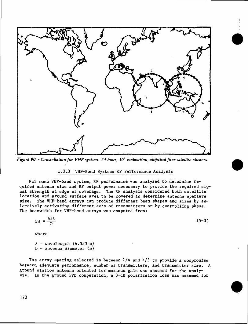
Figure 90. - Constellation for VHP system—24-hour, 30° inclination, elliptical four satellite clusters.

5.3.3 VHP-Band Systems RF Performance Analysis

For each VHP-band system, RF performance was analyzed to determine re-quired antenna size and RF output power necessary to provide the required sig-nal strength at edge of coverage. The RF analysis considered both satellitelocation and ground surface area to be covered to determine antenna aperturesize. The VHP-band arrays can produce different beam shapes and sizes by se-lectively activating different sets of transmitters or by controlling phase.The beamwidth for VHP-band arrays was computed from:

BW =65AD

(5-3)

where

A = wavelength (6.383 m)D = antenna diameter (m)

The array spacing selected is between A/4 and A/3 to provide a compromisebetween adequate performance, number of transmitters, and transmitter size. Aground station antenna oriented for maximum gain was assumed for the analy-sis. In the ground PFD computation, a 3-dB polarization loss was assumed for

170

TABLE 74. - VHF-BAND RF PERFORMANCESINGLE-SATELLITE CAPABILITIES

VHF system

12-h orbit

24-h elliptical orbit,single STS launch

24-h elliptical orbit,two STS launches

Zone 9

Ch

365

267

//V/m254185203243140258

Zone 10

Ch

UU

M

1

34

/jV/m256202202262146260

Zone 1 1

Ch

222126

AIV/m298298298

311220252

Zone 12

Ch

222125

pV/m275275275

295209262

circular polarization, along with a 1-dB propagation loss. For the 12-hourorbit, the antenna aperture size and beamwidth were calculated from nadirpointing to a 20° elevation angle. For the elliptical orbit, the size andbeamwidth were computed using specific satellite locations. In both cases,the antenna aperture efficiency was computed from:

efficiency =0.75 cos (a) (5-4)

where

a = scan angle

The resulting maximum singlesatellite performance capabilities ofthe VHF-band satellites are summarizedin Table 74. The table shows how manychannels can be transmitted with thecorresponding signal strength. Forexample, the first case shows thatthree channels at 254 uV/m can betransmitted to Zone 9, two channels at256 yV/m to Zone 10, two channels at298 yV/m to Zone 11, and two channels at 275 yV/m to Zone 12. Since the fullcapability calls for six channels at 250 yV/m to Zone 9, two satellites,transmitting simultaneously, would be required to provide the six channels.This leads to the requirement for 16 satellites, two in each of the eightorbital planes discussed in Section 5.3.2. The second case shows that eachsatellite can provide maximum signal strengths of 185 and 202 yV/m to Zone 9and 10 respectively when transmitting the required number of channels.

For the 24-hour, elliptical orbit and single STS launch, only two channelscan be broadcast to Zone 9 at 243 yV/m (slightly below the desired 250 yV/m).Thus, three satellites are required per orbital plane, or 12 satellites totalfor the system. The performance for full channel capability cannot provide250 yV/m in any zone and can provide the required number of channels at150 yV/m in Zones 11 and 12 only. As shown, the only satellite that can pro-vide full channel and signal strength capability is the 24-hour system usingtwo STS launches. To meet the ground coverage profile, four satellites wouldstill be required, one for each of the four orbital planes shown previously.

5.3.4 VHF Band Systems LCC Estimates

The first step in estimating LCC for the VHF systems was to estimate thetotal nonrecurring and recurring costs for each satellite configuration.Based on the use of a single design for all satellites within a system, learn-ing factors were then computed to derive an average recurring cost per satel-lite. Table 75 summarizes the costs for the VHF systems, using appropriatelearning factors for a slope of 0.9. Table 76 shows the factors as a functionof number of spacecraft for the VHF systems.

A further analysis of LCC could take Into account the time required tolaunch all satellites for a system and the percent of coverage provided duringthe phased launches. However, this level of analysis was considered beyond

171

the scope of the study. The basic objective was met: providing cost and per-formance data that would permit comparison between DVBS concepts and betweenDVBS and terrestrial broadcast methods.

TABLE 75. - VHP SYSTEMS'LCC ESTIMATES, 1984$

System*

VHP, case 1- 12-h orbit, 8S/C- 12-h, orbit, 12 S/C

VHP, ease 2— 24-h orbit, 4 S/C- 24-h orbit, 6 S/C- 24-h orbit, 12 S/C

VHP, case 3- 24-h orbit, 4 S/C

(multiple launch)

1st Unitcost

S156M156

136136136

178

No ofS/C

2436

121836

12

Averageunit cost

$ 97M90

948779

123

Averagewith launch

$222M215

219212204

373

TotalRC

$532SM7740

262838167344

4476

S/CNRC

$252M252

256256256

304

Groundcost

$71M92

717192

71

TotalNRC

S323M344

317348348

375

Total

S5651M8084

294541337692

4851

*20-yr operational lifetime (total program length is 20 years plus 6 years development = 26 years); 1-yr full capability remains

TABLE 76. - SATELLITE FABRICATIONLEARNING FACTORS FOR VHP SYSTEMS

Number ofsatellites

12182424. . . .

Learn ingfactor

0.690640.620.58

5.3.5 VHF-Band Summary of Results

The VHP-band systems designed for VOA applications consisted of three sys-tem designs using from four to 16 satellites to meet VOA broadcast require-ments. Each design uses a phased array and is capable of beam shaping andsteering through combined phase control and selectively turning transmitterson and off. The characteristics of the three systems are summarized in Table77.

Total estimated life cycle cost for a 20-yr operational lifetime plus a5-yr development cycle, and VHF system capability summaries are presented inTable 78. As shown, the LCC per channel hour for VHP-band systems that werestudied varies from a low value of $8,584 per hour to a high of |>28,050 perhour.

172

TABLE 77. - VHP SYSTEMS'DESIGN SUMMARY

Number of satellitesAntenna diameter, mAntenna mass, -kgTransmitter number/power, W

Total RF power, kWRequired EPS power (EOU, kWUpper stage

12-hcircular orbit

8 to 1662.57,03753/1480. 20/925.59/555494

785

Centaur

24-h elliptical orbitOne STS launch

4 to 12168

6.51143/720, 16/450.47/27019.131.3Centaur

Two STS launches4

168

11.29343/2840. 16/1775.47/106575.3120.4Large Centaurderivative

TABLE 78. - VHP SUMMARY OF RESULTS

Case

1

2

3

4

5

6

7»»

8"

Orbit12 h

12

12

12

24

24

24

24

/IV/m250

150

250

200

250

140-150250

250

Channelsrequired

6, 3, 2, 2

6. 3. 2, 2

3. 3. 2. 2

5, 3, 2, 2

6, 3. 2. 26,3.2.22,1,1, 16, 3, 2, 2

No. ofS/C

16

8

8

8

12

4

4

4

Coverageefficiency

84%

84

84

84

100

100

100

100

LCC

$8084M

5651

5651

5651

7692294529454851

Total channelhours

343,100 h

343,100

308,426

337,626

343,100343.100251,851

343,100

Cost perchannel hour$23,562*28,05016,470*19,60818,322*21,81216,737*19,92622,4198,584

11,69314,139

•Does not include coverage efficiency factor"Multiple launch—hypothetical Centaur

173

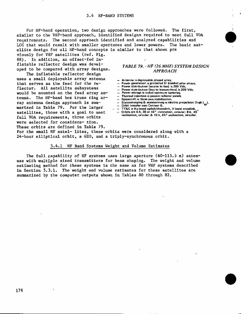
5.4 HF-BAND SYSTEMS

For HF-band operation, two design approaches were followed. The first,similar to the VHP-band approach, identified designs required to meet full VOArequirements. The second approach identified and analyzed capabilities andLCC that would result with smaller apertures and lower powers. The basic sat-ellite design for all HF-band concepts is similar to that shown previously for VHP satellites (ref. Fig.88). In addition, an offset-fed in- /flatable reflector design was devel- TARLE J9 _ Hf (26 MfJZ) SYSTEM DESIGNoped to be compared with array designs. APPROACH

The inflatable reflector designuses a small deployable array antenna _ Antenna 1S dep|0yable phased array.that serves as the feed for the re— — Power generation is gimballed SI blanket solar arrays.

flector. All satellite subsystems = *£\ ^ ««££±£would be mounted on the feed array an— - Power storage is nickel cadmium batteries.

tenna. The HF-band box truss ring ar- I a ^ T .11""11ray antenna design approach is SUm- — Stationkeeping & maneuvering is electric propulsion (high I ).

marized in Table 79. For the larger t ~ TT&C Is Ku^nTupH^k/dow'niink, v-band crosslink. 0Satellites, those With a goal tO meet - Orbits are 6-h, 30 or 45° inclination, circular; 8-h. 45,. .. _ T T _ . . . ., uji. inclination, circular, & 12-h, 45° inclination, circular.full VOA requirements, three orbitswere selected for considera- tion.These orbits are defined in Table 79.For the small HF satel- lites, these orbits were considered along with a24-hour elliptical orbit, a GEO, and a triply-synchronous orbit.

5.4.1 HF Band Systems Weight and Volume Estimates

The full capability of HF systems uses large aperture (60-115.5 m) anten-nas with multiple sized transmitters for beam shaping. The weight and volumeestimating method for these systems is the same as for VHF systems describedin Section 5.3.1. The weight and volume estimates for these satellites aresummarized by the computer outputs shown in Tables 80 through 82.

174

TABLE 80. - HF WEIGHT AND VOLUME

ESTIMATES-6-HOUR ORBITTABLE 81. - HF WEIGHT AND VOLUME

ESTIMATES-8-HOUR ORBIT

HF OSB 60-m antenna, 6-h orbit, single launchDSB carrier output power— 38.1 kWDSB or SSB total RF output power— 57.2 kW

System Configuration Summary

RF pay loadAuxiliary propulsion subsystemTelemetry, tracking, & commandElectrical power subsystemThermal control subsystemEquipment bay structure

Total system summary

Mass, kg

489032332

3405984208

984521710, Ib

Volume, m

46.182.25

.037.78

10.0812.10

7844

HF DSB 60-m antenna, 6-h orbit— multiple launchDSB carrier output power— 97.5 kWDSB or SSB total RF signal power- 146.3 kW

System Configuration Summary

RF pay loadAuxiliary propulsion subsystemTelemetry, tracking, & commandElectrical power subsystemThermal control subsystemEquipment bay structure

Total system summary

Mass, kg

8052631

3285972518

305

20137(44404 Ib)

Volume, m3

49564.45

0319.6225.782363

123.09

HF 80-m antenna, 8-h orbit, single launchDSB carrier output power— 38.7 kWDSB or SSB total RF output power- 58 kW

System Configuration Summary

RF pay loadAuxiliary propulsion subsystemTelemetry, tracking, & commandElectrical power subsystemThermal control subsystemEquipment bay structure

Mass, kg

532935532

17871021217

Volume, m

46.262.25

.037.03

10.4612.10

Total system summary 8743 78.14(19280 Ib)

HF 80-m antenna 8-h orbit— multiple launchDSB carrier power— 88.9 kWDSB or SSB total RF output power- 133.3 kW

System Configuration Summary

RF pay loadAuxiliary propulsion subsystemTelemetry, tracking, & commandElectrical power subsystemThermal control subsystemEquipment bay structure

Mass, kg

807065632

40402347308

Volume, m

49.204.45

.0315.9424.0423.55

Total system summary 15456 117.21(34081 Ib)

TABLE 82. - HF WEIGHT AND VOLUMEESTIMATES-12-HOUR ORBIT

HF 12-h orbit 115.5 m antenna— single launchDSB carrier output power— 20.3 kWDSB or SSB total RF output power- 30.5 kW

System configuration summary

RF payloadAuxiliary propulsion subsystemTelemetry, tracking, & commandElectrical power subsystemThermal control subsystemEquipment bay structure

Mass, kg

499532632

943536198

Volume, m

45.192.25.03

3.43549

11.81

Total system summary 7032 68.22(15506 Ib)

HF 12-h orbit 115.5 m antenna— multiple launchDSB carrier output power, 59.8 kWDSB or SSB total RF output power, 89.7 kW

System configuration summary

RF payloadAuxiliary propulsion subsystemTelemetry, tracking, & commandElectrical power subsystemThermal control subsystemEquipment bay structure

Mass, kg

715043132

26631579263

Volume, m

47.502.25.03

98616.1712.35

Total system summary 12120. 88.18(26726 Ib)

175

The next set of HF systems are the small satellite reduced size and powerconcepts. These systems assume a single size of transmitter as opposed tothree sizes assumed for the previous HF cases. For each of the applicable HFreduced size concepts, analyses were performed from 10 kW to the maximum powerattainable with a fully dedicated STS launch. Figures 91 through 96 show theestimated weight and field strength as a function of total RF output power foreach of the six orbits considered for small HF concepts. The field strengthshown is for Zone 1 only.

The last type of HF system studied was the inflatable reflector conceptwith an array antenna feed. The weight and volume of the inflatable structurewere obtained first, then the inflatable's mass was subtracted from the maxi-mum payload limit and the weights and volumes for the small feed array and therest of the subsystems were estimated. The total satellite weight is the sumof the two summaries shown in Table 83.

176

10000

8000o>je

36000E2£4000

Mass

Signal strength

400^

8ofsl

I200 f

s1

0 15 30 45 60 75 90 105 120Total RF output power, kW

Figure 91. -Small HF 6-hour satellite weigbt and signal strength.

10000

8000

°6000aCD

E 4000

S 2000

Mass

Signal strength

400

oNE

I

Itoc

CO

0 20 40 60 80 100 120 140 160Total RF output power, kW

Figure 92. -Small HF 8-hour satellite weight and signal strength.

lOOOOp

8000

s eoooi| 4000*o

& 2000

Signal strength

Mass

250^

8oN

E

I150 j-

5,

50

3to

0 20 40 60 80 100 120 140 160Total RF output power, kW

Figure 93. -Small HF 12-hour satellite weigbt

and signal strength.

10000

8000o>

JC

«6000

14000

1"2000

Signal strength

Mass

150

oco

-S«-•o>

gs

0 15 30 45 60 75 90 105 120Total RF output power, kW

Figure 94. -Small HF 24-hour elliptical orbit satellite weight

and signal strength.

5000

54000

isoooIP

S2000CO

1000

0

Mass

Signalstrength

150

oN

75

10 20 30 40 50 60 70 80Total RF output power, kW

5000

4000o>

| 3000E

I 2000

1000

Signal strength

Mass

300

coN

200 5

1004 8 12 16 20 24 28 32

Fiffure 95 - Total RF output power, kW

Small HFGEO satellite weight and signal strength. Figure 96. -6 6 Small H F triply-synchronous orbit satellite weigbtand signal strength

177

TABLE83. - HF INFLATABLE CONCEPTWEIGHT AND VOL UME ESTIMA TES

HF inflatable structure

RF Subsystem sizing summaryData for inflatable (limit on dia from 10 to 200 m)

Antenna aperture area, m2

Total antenna structure mass, kgTotal antenna structure volume, m3

Weight of uplink components, kgVolume of uplink components, m3

Weight of signal proc components, m3

Volume of signal proc components, m3

Total RF subsystem mass, kgTotal RF subsystem volume, m3

221671663

669

1663669

HF inflatable design 12-h orbitDSB carrier output power— 38 9 kWDSB or SSB total RF output power-58 4 kW

System configuration summary

RF pay loadAuxiliary propulsion subsystemTelemetry, tracking & commandElectrical power subsystemThermal control subsystemEquipment bay structure

Total system summary

Mass, kg

16971498

321549464161

5404(11916 Ib)

Volume, m

42.82665.03

6474.75.96

61.69

5.4.2 HF-Band Coverage Analysis

The coverage analysis for the large HF satellite concepts was similar tothat described for the VHP-band systems. Figures 97, 98, and 99 show the re-spective ground traces for the 6-, 8-, and 12-hour orbits. As shown in Figure97, the three solid line paths represent the coverage trace for 30° inclinedorbits while the dashed lines represent the trace for 45° inclined orbits.The complete system includes eight orbital planes with the number of satel-lites in each orbit dependent on the signal strength and channel capabilitiesof a satellite. The dots on the ground trace represent the relative satellitepositions resulting from the eight orbital planes. Figures 98 and 99 show theground traces and satellite positions for the 8- and 12-hour orbits. Again,eight orbital planes are used.

The five nongeostationary orbits for the small HF satellites were analyzedto determine the ground coverage that could be obtained from a single satel-lite. Figures 100 through 106 show typical coverages that could be obtained ineach zone as a function of universal time. Figure 106 compared to Figure 105shows the effect on ground coverage of the 4-minute daily sidereal shift overthree months for the 8-hour orbit. Similar time shifts would result for theother nongeostationary orbits.

178

Figure 97. -

Constellation for HF system—6-bour, 30 and 45° inclination, circular, eight satellite clusters.

179

Figure 98. - Constellation for HF system—8-hour, 45° inclination, circular, eight satellite clusters.

180 C-3

Figure 99. - Constellation for HF system—12-bour, 45° inclination, circular, eight satellite clusters.

181

15

13

12

10

m IIHIIIIIIIIIIIII ffl IllllllllmiMtmm

IIINIitHlilllllllllllll

ED inntUD i i i i i i n iI l l l l l l l l

Hllllllllliiiiiillllllll

frnrm

rnnHltlHIIIIIIIIIIIII

IllllllllmrniiniiHTflroini

iiiiiiiimriillllTnIIIIIIIIIIIIEIillllll

irm

;;:flBHHffl I l l l l l l l l l ITT1

<; MTTT11 iiiiiiiiiiiirMiriHini

i i i i i i i i i i m i m i i i i i i i i i i i iimiJimiii iiiiiiiiiiiiiiiiuHHiiniiiiiin

t ^ & > III

iiiiiiiimHiiiiiiii

iiiitJiiiiiiiiinii ^^ "^w

mrmLED

i i i i i i i i0 1 2 3 4 5 6 7 8

Legend:

Q Requirement

~ I I I I I I I I I I I I I I10 11 12 13 14 15 16 17 18 19 20 21 22 23 24

Time, h

Zone in access

Figure 100. -6-hour orbital satellite coverage.

182

oN

15

14

13

12

11

10

9

8

1

6

5

4

3

2

1

ED IIIMMIiIllllllll Illllllll

iiiiiiiiiiiiniiiiriirnrm rrm

i mmmmmmiim

f f l H l l l l l l i

niiinnininiifTTT] Illlllimiftlffffiffl

IIIIIIIIIIIIIIIIIHIHI rrm0 1 2 3 4 5 6 7 8 9 10 11 12 13 14 15 16 17 18 19 20 21 22 23 24Legend Time, hQ Requirement

H Zone m access

Figure 101. - Small HF satellite-12-bour orbital satellite coverage.

183

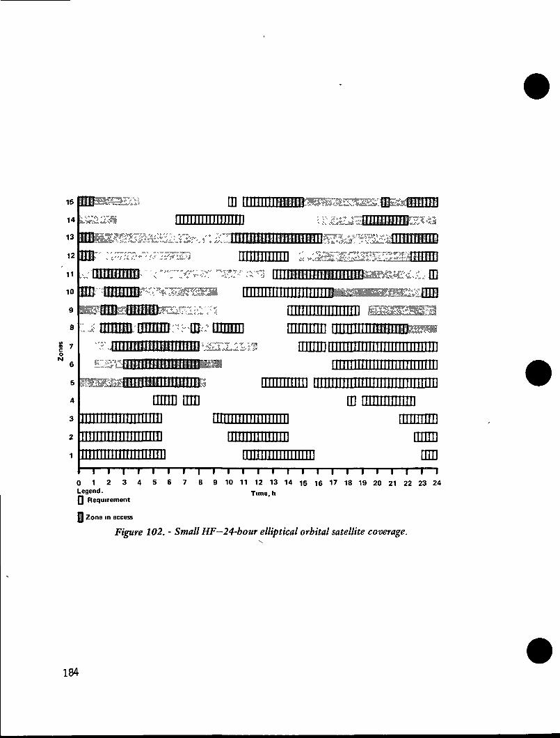
rTTTm rrmi i i i m m i r m n i m i

linn iiimmm

ID i i i i i i i n m i i i

mrmHID

I I I I I I I I I T I I I I I I I I I I I I T I0 1 2 3 4 5 6 7 8 9 10 11 12 13 14 15 16 17 18 19 20 21 22 23 24Legend. Time h

Q Requirement

y Zone in access

Figure 102. - Small HF—24-hour elliptical orbital satellite coverage.

184

15

14

13

12

11

10

9

8

I 7

6

5

4

3

2

1

m

mm

mmntfmiin ffl IliililMIIHifiill Illliii

I millliil II III!Hi

niniiiHrrm nnmniIllllliil iiiiinn

linn iiiiimiiiiii

rTTTTTTI

mrnn

ffl Illlllllliiiiimmiiiimimiiniiiimiim

iimiTTmnimmrrrnn mn

iHamiiiiiiriiinTi ninTrminiii i i i i iI I I I I I I I I I I I I I J U

mniiiiiiiiiiniiii r T i i i i i i i r T i r i i r i

0 1 2 3 4 5 6 7 8 9 10 11 12 13 14 15 16 17 18 19 20 21 22 23 24Legend. Time, hQ Requirement

|J Zone in access

Figure 103. - Small HF-triply-syncbronous satellite coverage.

185

15

14

13

12

11

10

9

8

7

6

5

4

3

2

1

no CD iiniiiiiiiiimi ID I l l l l l l l l

mrmED

1 I I I I I III I I I I I I I I I I I I I I I

0 1 2 3 4 56 7 8 9 10 11 12 13 14 15 16 17 18 19 20 21 22 23 24Legend. Time, h

Requirement

Zone in access

Figure 104. - Small HF—geostationary satellite coverage.

186

15

14

13

12

11

10

9

8

oN

ffl imniiiiiiiiiiimmr ii

I millliifiitiill

I liiill Hill ID immiii Minium

iiiiiini

IIIIIIIMIIIIIIIIIII

Illlillllllll llllilllllUllimiimilliHIIIII

01 iiiiiiiiiiiiiii

ffimilfllllll

Illlillllllll

0 1 2 3 4 56 7 8 9 10 11 12 13 14 15 16 17 18 19 20 21 22 23 24Legend. Time, hQ Requirement

Zone in access

Figure 105. - Small HF—8-hour orbital satellite coverage.

187

oN

15

14

13

12

11

10

9

8

6

5

4

3

2

1

Q] irmtittittmil ffl HIIIIIII

miED

ED i i i i i n i i iLED l l l l l l l l li i n i i i i i i i i i i i i i i Q ]

I M I I l l i n i l l l l l l l l l l l l

UiilllUiiiiiillilil

Illlllllill MllllllllllliUlllBnTTTTTIiiiiiiiiiimiitiitiiMflfmi

rrmn rrm

imiiniiininiTTlrrnrn

rimI I I I I I I I I I I I I I I I I I I I I I B I

0 1 2 3 45 6 7 8 9 10 11 12 13 14 15 16 17 18 19 20 21 22 23 24Legend Time, hQ Requirement

^ Zone in access

Figure 106. - Small HF—8-hour orbit: 3-month sidereal shift.

5.4.3 HF-Band Systems RF Performance Analysis

The approach taken to analyze HF-band satellites RF performance was simi-lar to that described for VHF-band satellites. The only differences were a2-dB propagation loss for HF instead of the 1 dB used for VHF, and elementspacing from A/3 to 3/4 A for HF arrays. Table 84 shows for a single satel-lite the maximum number of channels and signal strength available in each zonefor the large HF systems. Signal strength for the small HF satellites waspreviously shown as a function of RF power (Figs. 91 through 96) along withsatellite estimated weight.

188

TABLE 84. - HF SYSTEM MAXIMUM RF PERFORMANCE CAPABILITIES SUMMAR Y FORA SINGLE SATELLITE

System

8-h orbitsingle launch

8-h orbitMultiple launchc_h nrtlit

single launch

6-h orbitmultiple launch

1

1320

4-160

2-3461308

4-162

2-399

2j345

5-154

3-291

324

4-159

3-292

3D1

230

2-162

1-348

218

2-154

1-350

3L

1

259

2-183

1-393

257

2-182

2-291

4j301

4-152

2-327

294

3-165

2-334

5

298

4-149

2-320

293

4-147

2-332

6

325

4-163

2-352

308

4-154

2-350

Zoi

7

228

2-161

1-344

217

2-154

1 —

347

IBS

8

351

5-157

3-297

314

5-153

3-304

9

357

B-159

3-301

350

5-157

3-314

10

282

3-157

2-302

272

3-152

2-308

11

282

3-158

2-303

270

3-151

2-306

12

327

4-163

2-350

311

5-156

2-350

13

221

2-156

1-335

211

2-149

1-337

14

301

4-151

2-323

295

3-165

1-335

15

773

2-158

1-338

213

2-150

1-341

5.4.4 HF-Band Systems LCC Estimates

TABLE 85. - HF FABRICATION COSTLEARNING FACTORS

Number ofsatellites

24364872144264

Recurring costlearning factor

0.620.580.560520.470.43

The approach taken to estimate LCCfor the HP-band systems was similar tothat taken for VHP-band systems. A20-yr operational lifetime was assumedafter a 5-yr development cycle. Alaunch frequency was assumed thatwould result in a fully operationalsystem in two years after completionof development. Obviously, this as-sumption may be unrealistic for thosesystems using a large number of satel-lites. Table 85 shows the LCC breakdown for the 6- and 8-hour HF systems.The number of satellites shown is for three launch sets. The average unitcost includes the learning factor for the number of satellites shown. Thelaunch cost was $125M for the single STS launch cases and {5250M for the multi-ple launch cases. The increase in ground costs as a function of number ofsatellites was described previously in Section 4.3.8.4.

Figures 107 through 112 show satellite nonrecurring cost (NRG), recurringcost (RC), and total costs as a function of RF output power for each of thesmall HF concepts. Using a Centaur for the upper stage results in a dedicatedlaunch for each satellite. Use of a different upper stage might be possiblefor a low-power satellite.

Estimated launch cost and ground operations cost should be added to thesatellite costs shown in the figures to estimate a total system cost for thesmall satellite concepts. Also, use of multiple satellites would reduce re-curring cost by the factors shown in Table 86.

189

500

I 400^§*• 300

200

100

500

Total

0 15 30 45 60 75 90 105 120Total RF output power, kW

Figure 107. - Small HF 6-hour satellite costs

500

2 300

8 200|^>S 100

Total

2300

8 200o

100

Total

500

I 400«t

I 300VI

ts8 200

I 100

20 40 60 80 100 120 140 160Total RF output power, kW

Figure 108. -Small HF 8-hour satellite costs.

Total

20 40 60 80 100 120 140 160 0 15 30 45 60 75 90 105 120Total RF output power, kW Total RF output power,kW

Figure 109. • Figure 110.-Small HF 12-hour satellite costs. Small HF 24-hour elliptical orbit satellite costs.

300 r

240

22 180

a8 120

S 6°CO

. Total

.NRC

0 10" "?0 30 40 50 60 70Total RF output power,kW

Figure 111,' Small HF GEO satellite costs.

80

i«t?fi8

i?&

300

240

180

120

60

0

-

Total

p—p NRC

-

RC-

i i f i t i i8 12 16 20 24Total RF output power, kW

28

Figure 112. -Small HF triply-synchronous orbit satellite costs.

190

I

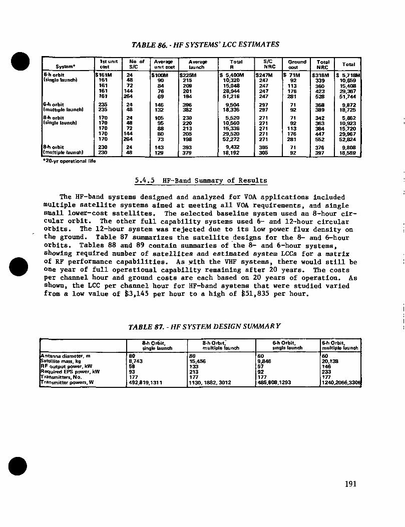
TABLE 86. - HF SYSTEMS' LCC ESTIMATES

System*

6-h orbit(single launch)

6-h orbit(multiple launch)8-h orbit(single launch)

8-h orbit(multiple launch)

1st unitcost

S161M161161161161

235235

170170170170170

230230

No ofS/C

244872

144264

2448

244872

144264

2448

Averageunit cost

S100M90847669

146132

10595888073

143129

Averagelaunch

$225M215209201194

396382

230220213205198

393379

TotalR

$ 5.400M10,32015,04828,94451.216

9,50418,3365,520

10,56015,33629,52052.2729,432

18,192

S/CNRC

S247M247247247247

297297

271271271271271

305305

Groundcost

$ 71M92

113176281

7192

7192

113176281

7192

TotalNRC

$318M339360423528

368389

342363384447552

376397

Total

$ 5,7 18M10.65915.40829.36751,744

9.87218,725

5,86210,92315,72029,96752,8249,808

18.589*20-yr operational life

5.4.5 HF-Band Summary of Results

The HF-band systems designed and analyzed for VGA applications includedmultiple satellite systems aimed at meeting all VQA requirements, and singlesmall lower-cost satellites. The selected baseline system used an 8-hour cir-cular orbit. The other full capability systems used 6- and 12-hour circularorbits. The 12-hour system was rejected due to its low power flux density onthe ground. Table 87 summarizes the satellite designs for the 8- and 6-hourorbits. Tables 88 and 89 contain summaries of the 8- and 6-hour systems,showing required number of satellites and estimated system LCCs for a matrixof RF performance capabilities. As with the VHF systems, there would still beone year of full operational capability remaining after 20 years. The costsper channel hour and ground costs are each based on 20 years of operation. Asshown, the LCC per channel hour for HF-band systems that were studied variedfrom a low value of fc3,145 per hour to a high of £51,835 per hour.

TABLE 81. - HF SYSTEM DESIGN SUMMAR Y

Antenna diameter, mSatellite mass, kgRF output power, kWRequired EPS power, kWTransmitters, No.Transmitter powers, W

8-h Orbit,single launch

808,7435893177492,819,1311

8-h Orbit,multiple launch

8015,4561332131771130, 1882,3012

6-h Orbit,single launch

609,8465792177485,808,1293

6-h Orbit,multiple launch6020.1381462331771240,2066,3306

191

TABLE 88. - HF-MATRIX OF DESIGN AND ANALYSIS CASES (8 HOURS)

Case

1-82-8

3-8

4-8

5-8

6-8

7-8

8-8

9-8

Required yV/m

300"300*

300»

300*

150

150

150

300

300

No. of channels

- FullVOA— Six ch max

— One ch max

- Two S/C percluster

- FullVOA

- Two S/C percluster

— One S/C percluster

- Two S/C percluster

- One S/C percluster

Zones

AllAll

All

All

All

All

All

All

All

No. of S/C

8848

8

16

24

16

8

16**

8*«

LCC

S52.824M29,967

5,862

10,923

15,720

10,923

5,862

18,589

9,808

Cost/channel hour

$24,181/h14,440

5,082

6,268

7,195

5,168

3,225

9,451

6,086

•Cannot achieve 300 jUV/m for single channel Zones 3D, 3L, 7, 10, 11, 13, 15**Full shuttle satellite—large Centaur-type stage in second orbiter

TABLE 89. - HF-MATRIX OF DESIGN AND ANALYSIS CASES (6 HOURS)

Case

1-62-6

3-6

4-6

5-6

6-6

7-6

8-6

9-6

10-6

11-6

Required JL(V/m

300*300*

300*

300*

300*

300*

150

150

150

300

300

No. of channels

- FullVOA— Six ch max

— One ch max

- Two S/C percluster

— Six ch max

— Six ch max

- FullVOA

— Two S/C percluster

- One S/C percluster

- Two S/C percluster

— One S/C percluster

Zones

AllAll

All

All

1,2, 3U,4,6,7,8,11,13,15

3L,5, 9, 10, 12,14

All

All

All

All

All

No. of S/C

8848

8

16

48

48

24

16

8

16**

8**

LCC

$51,744M29,367

5,718

10,659

29,367

29,367

15,408

10,659

5,718

18,725

9,872

Cost/channel hour

$23,686/h14,140

4,957

6,116

51,835

34,831

7,053

5,044

3,145

9,942

6,127

•Cannot achieve 300 /UV/m for single-channel Zones 3U, 3L, 7,10, 11,13, 15'•Full shuttle satellite—large Centaur-type stage in second orbiter

192

6.0 DVBS PLANNING SUPPORT

The objectives of this part of the study were to provide information forthe selected satellite concepts that will identify the following:

1) What needs to be done to implement a DVBS satellite system,

2) What technologies need to be advanced to reduce technical risks or en-hance DVBS satellite performance,

3) The cost and schedule risks that would be encountered in criticaltechnology development plans,

4) The cost and schedule risks that would be encountered for completeDVBS satellite programs.

Following are discussions detailing the approach taken to meet these ob-jectives and the results of analyses.

193

6.1 CRITICAL TECHNOLOGY DEVELOPMENT PLANS

The first step taken was to analyze performance risks for the four fre-quency bands of interest. The set of generic risks shown in Table 90 were se-lected and the risk level assessed for satellite systems, using the results ofthe technology survey described in Section 3.4, the technology tradeoffs de-scribed in Section 4.2, and analyses performed during the study. The risk as-sessment was expressed in qualitative terms as shown in the table. Using thisrisk assessment as a baseline, specific technologies were identified that mustbe addressed to reduce risk for VGA satellite systems.

TABLE 90. - DVBS PLANNING SUPPORT-PERFORMANCE RISK ANALYSIS

Risk

State-of-the-art advancePhysical propertiesMaterial propertiesRadiation propertiesMaterial availabilityTesting/modeling validityIntegration/interface (utilities)Program personnelSoftware designSafetySecurityCritical failure modesEnergy/environmental impacts

Ku

LowLowLowLowLowLowLowLowLowLowMediumLowLow

L

MediumMediumLowLowLowLowMediumLowLowLowMediumLowLow

VHP

HighMediumLowMediumMediumHighHighLowLowLowMediumMediumLow

HF

HighMediumLowMed/highMediumHighHighLowLowLowMediumMediumLow

6.1.1 Critical Technology Identification

The HF and VHF satellite concepts require large deployable structures toprovide the required aperture sizes for optimum performance. Since there areno deployable antennas developed or under development in the size rangesrequired for HF or VHF systems, a development program must be established toreduce uncertainty surrounding use of these types of structures. The objec-tives of this program follow:

1) To demonstrate the capability of the structure to deploy itself andthe communication subsystem payload;

2) To demonstrate the capability of the deployed structure to withstandenvironmentally and internally induced stresses, forces, and torques;

3) TQ demonstrate the capability of the undeployed structure to tolerateground handling, system integration, packaging, STS, and upper-stagelaunch loads;

4) To satisfactorily demonstrate structural element and overall structuralfabrication methods;

5) To demonstrate applicability and validity of modeling, simulation, andanalysis techniques to analyze large deployable structures.

194

Space qualified SSPAs are not presently available at the power levels re-quired from the results of this study. Thus a transmitter development programis recommended to:

1) Demonstrate the capability of SSPAs to operate efficiently at powersof at least one kW at the HF- and VHF-bands, and up to 300 watts inL-band;

2) Demonstrate the ability of SSPAs to operate over the desired 7-yrlifetime for the duty cycles and operating environment projected forL, HF, and VHP systems;

3) Demonstrate capability of designing SSPAs to meet packaging and stow-age requirements;

4) Demonstrate capability to manufacture SSPAs in the quantities thatwould be required for L, HF, and VHP satellites.

Another aspect of the HF-, VHF-, and to a lesser degree, L-band systemsthat involves uncertainty is the array antenna RF performance. A program isrecommended to perform the following:

1) Demonstrate the capability to shape and steer beams using phase con-trol at the high powers and over the long distances associated with HFand VHP satellites;

2) Demonstrate satisfactory performance of an array antenna with high-power radiating elements, both with respect to signal at the groundand noninterference with TT&C functions for HF-, VHP-, and L-bands;

3) Evaluate the potential of multipacting in the vacuum of space.

Thermal control for HF-, VHF-, and high-power L-band concepts requires adistributed approach such as the GPL described previously. A program paral-leling SSPA development is recommended to:

1) Develop and qualify the GPL technology;

2) Demonstrate the capability to integrate a GPL thermal control system(or other thermal control technique) with the SSPAs and antenna sup-port system, meeting thermal dissipation, packaging, and deploymentrequirements.

The last critical technology area is solar array technology. The highpowers required for HF-, VHF-, and L-band concepts exceed any of currentsatellites. However, development under the space station program should beapplicable to VGA satellite systems. If not, some development will be re-quired to demonstrate the capability to package and deploy solar arrays cap-able of generating powers of 100 kW and greater; demonstrate the capability toefficiently fabricate the large solar arrays; and to demonstrate the capabil-ity of an EPS to regulate and control large powers in cyclic operating modes.

195

A final technology that is applicable to Ku-band satellites is the devel-opment of TWTA technology that decreases operating degradation when operatedin a cyclic mode. Work is under way in this area and should be monitored forapplicability to VOA Ku-band satellites that will probably operate in a cyclicrather than steady state output mode.

6.1.2 Critical Technology Plans

To meet the technology development goals and reduce uncertainty for anten-nas, SSPAs, thermal control, and electric power generation, the activitiesshown in Figure 113A & B should be started early in a VOA program. A flighttest of deployable large structures has been proposed by other studies to ver-ify deployment, test flexible body control approaches, and validate analysistechniques. The times shown in these two figures are considered reasonableestimates although they are subjective. As will be shown later, they are con-sistent with estimates obtained from the NASA SDCM data base. The estimatedcosts for critical technology development shown in Table 91 are based on CERsdiscussed in Section 4.3, with the cost range due to the range of CER inputparameter values for the various satellite concepts.

© COMMUNICATIONS PLANMonths from go-ahead

0 4 8 12 16 20 24 28 32

4.1.1 Deployable antenna technology— Deployment mechanism design & test— Prototype structure fabrication- Flight test— Modeling development/verification— Fabrication & handling method development

4.1.4 Transmitters development— Solid state amplifier design & test— Phased array prototype design & fab— Phased array prototype performance tests— Transmitter stow/deploy deisgn & test

4.6 Transmitter thermal control design & test

B lELECTRICAL POWER PLAN

4.2.1 Solar array prototypes fabricationSolar array stowage/deployment testsSolar array production method designPower bus regulation tests

Months from go-ahead

0 4 8 12 16 20 24 28 32

Figure 113. - Communications and electrical power subsystem development plans.

TABLE 91. - CRITICAL TECHNOLOGYDEVELOPMENT COSTS

4.1 1

4.1.4

4.6

4.2

Deployable antenna technologyHF-band $6 - $10M (+$25M for flight test)VHP-band $10M -$13M(+$25M for flight test)

Transmitters developmentHF- & VHF-bands $12 - $20M

Transmitter thermal control developmentHF- & VHF-bands $4-$10M

Electrical power subsystem technologyH F-, VH F-, & L-bands $3 - $35M

196

6.2 SATELLITE SYSTEMS PROJECT PLANS

The set of top-level functions shown In Figure 114 were identified for ageneric DVBS program. Also, the existence of a functional breakdown is re-quired to facilitate a cost and schedule risk analysis using the MartinMarietta risk analysis methodology.

0.0

DVBS Iprogram I

|

10 2.0 3.0 I 4.0 5.0 6.0 7.0 8.0

Allocatemission/systemrqmts

[ SRR

Define DVBSconfiguration

LSDR

Developsubsystemrqmts

|PDR

Developdetaileddesign

[COR

Integrate& fabricate

Deliver& deploy

Operate"& maintain

Provideprogramsupport

Figure 114. - DVBS planning support-satellite systems project plan.

6.2.1 Functional Decomposition

As an aid to developing estimates of cost and time required to perform thetop-level functions, each was decomposed to identify the scope of activitiesor subfunctions under it. These subfunctions are shown in Figure 115. Pro-gram milestones, indicated where applicable, are: (1) System requirements re-view (SRR), (2) System design review (SDR), (3) Preliminary design review(PDR), (4) Critical design review (CDR).

197

20

[Define VOA DVBS system]

Define mission rqmtsDecompose functionsDerive system rqmts

t Draft system engineering mgmt plan (SEMP)Draft A spec

SRR

System modelingTradeoff studiesSubsystem allocationDesign baselineConfiguration drawingsInterface definitionsPreliminary B specFinal A specDraft B spec

-A SDR

30 4.0

Develop subsystem rqmts I

CommunicationsElectrical powerAttitude controlAuxiliary propulsionTelemetry, tracking & commandThermal controlEquipment bay & mechanismsPrimary propulsionGround controlProgram feedPerform trade studiesUpdate interface definitionsPerform subsystem prototype testsDraft C specPrepare final B specUpdate SEMP

-A PDR

Develop detailed design I

Communications subsystemElectrical powerAttitude controlAuxiliary propulsionTT&CThermal controlEquipment bay & mechanismsPrimary propulsionGround controlProgram feedContinue trade studiesPrepare final interface control documentMaintain configuration controlDraft flight operations planPerform system modeling & testingPrepare facilities plansPrepare final C spec

5.0 6.0

I Integrate & fabrication I Deliver & deploy satellite I

Build & test components/subsystemsBuild & test satelliteBuild & test ground stationsPrepare final payload integration planPerform system acceptance tests

Integrate with upper stageInstall in STS & checkoutLaunch & separateTransfer to operational orbitSelf deploy & checkout (HF & VHF systems)

7.0 8.0

Operate & maintain

Perform onorbit functionsFeed programsMonitor satellite healthMonitor satellite attitude& position •Maintain attitude & orbit

I Provide program support [

Systems engineeringFinancial mgmtSchedule mgmtRisk mgmtContract administrationQuality control

- Documentation

Figure 115. - DVBS project plan-top-level functions1.0, 2.0, 3.0, 4.0, 5.0, 6.0, 7.0& 8.0.

6.2.2 Risk Assessment Procedure

The risk assessment procedure uses a quantitative risk assessment method-ology developed at Martin Marietta in an IR&D project during 1982 and 1983.The method has been used on several programs to predict and monitor technical,schedule, and cost risks. The basic approach is not unique, using a MonteCarlo simulation approach. However, the method of implementation represents

198

an advantage over approaches used by others within the industry and the gov-ernment. The advantage lies in an easily used computer program, RAMP devel-oped to facilitate management of risk data and to simplify access to the MonteCarlo simulation software. The steps involved in the RAMP-augmented riskanalysis procedure follow:

1) Obtain risk data estimates (for VGA, low, most likely, and highvalues) that are used as values of a probability density function;

2) Document the rationale for the estimates;

3) Document the source of the estimates;

4) Enter the estimates and program identifiers into a RAMP data baseunique to the program being evaluated;

5) Compute a cumulative probability function for the risk parameter ofinterest (e.g, cost, months).

Figure 116 shows a risk assessment form' containing the three point antennastructure development cost estimate for the small HF design for geostationaryorbit. The nonrecurring cost estimates for this satellite, as obtained fromthe LCC program are shown in Table 92. As indicated on the assessment form,the cost predicted by the LCC model is taken as the highest cost that mightoccur. Since this is a relatively small satellite (26-meter diameter) workcurrently in process or planned for deployable box truss structures should re-sult in less required development. Based on past experience with this type ofstructure, estimates of the most likely cost are predicted to be $2,000 perpound and could conceivably be as low as $1,000 per pound.

Risk assessment can be performed assuming that program functions are in-dependent of or dependent on each other. In the context of quantitative riskanalysis, dependence between functions means that if one function occurs at aworst-case value then all dependent functions will also occur at their worst-case values. When functions are independent, the level of one function has noinfluence on the expected level of others. Since the objective of breaking upa program into a set of functions is to establish a set of relatively indepen-dent activities, this independence should be considered when estimating totalcost or time to complete. Unfortunately, the practice of summing estimates isfrequently used, resulting in over-conservative estimates of cost or timerequired.

The difference between risks resulting from the two methods is illustratedin Figure 117. For a given parameter value, the risk will be higher for ananalysis that assumes dependence. The cost and schedule risk assessments pre-sented here were performed assuming independence. However, a degree of de-pendence is automatically built in by summing values of recurring, nonrecurr-ing, launch, and ground operations at the fixed risk values of interest (90,50, and 10%). The steps for the cost risks performed in the study are out-lined in Table 93. The steps for schedule risk assessment are listed in Table94.

199

RISK ASSESSMENT LOG

Program: VOA small HF.GEO

Risk Analyst:

WBS/Function No 4 1 1

WBS/Function Title- Communications antenna development

Date:

CostRisk Type-

Risk Description- The cost predicted by the MSFC planar array antenna and Navy graphite structure derived CER is considered thehighest that might occur It is assumed that DDTE programs for deployable graphite structures will precede VOA satellite programsThus, the most likely cost is predicted to be $2000 per Ib with the lowest at $1000 per IbRisk Parameter: $M-Nonrec (nonrecurring cost)

Most Likely Value/LevelHighest PossibleLowest PossibleR isk Weighting FactorSecondary Effects.

1.6510.7083

DistributionType Triangular

Mitigation Approach:

Data Source MSFC CER, Navy LCC handbook CER, engineering judgement

Figure 116.- Example of risk assessment log.

TABLE 92. - HF SMALL SATELLITENRC ESTIMATES

Nonrecurring design & development cost

Subsystem

Structure (equipment bay)

Thermal Control

Electrical power

Communications antenna

Communications uplink

Signal processor

Communications transmitter

Attitude determination

Attitude reaction

Propulsion

TT&C

Aerospace ground equipment

Total nonrecurring

Cost,1984$

10.04 $M

22.21

66.18

10.74

13.69

11.13

15.19

3.55

20.54

0.00

5.05

6.58

184.91

Cost source

Space Division CER

Space Division CER

VOA CER

Planar array antenna CER

Space Division CER

Space Division CER

Solid state transmitter CER

Space Division CER

Elect propulsion CER

Throughput

Space Division CER

Space Division CER

200

0 1

la£•0

Risk parameter cumulative value

Figure 117.- Quantitative risk assessmentinterpretation.

TABLE 93. - DVBS PLANNING SUPPORT-COST RISK ANAL YSIS APPROACH

LCC estimating program for point estimates

Three point estimates using values from LCC model as startingpoint— Most likely cost— Highest potential cost— Lowest potential cost

Obtain cumulative functions— Nonrecurring spacecraft cost— Recurring spacecraft cost (with learning factor)— Aerospace ground equipment, integration, system engineer-

ing, & program cost factors— Launch costs— Ground operations cost

Compute total cost risk— Sum four cumulative function results

TABLE 94. - DVBS PLANNING SUPPORT-SCHEDULE RISK ANALYSIS APPROACH

Identify program critical path— Estimates of components/subsystem design + test + quali-

fication times- Select longest time for critical path

Estimate program top function times including decision lagsbetween phases

Compute quantitative schedule risk

201

6.3 CRITICAL TECHNOLOGY RISK ANALYSIS

The cost risk assessment cumulative probability functions shown in Figures118 and 119 are for the HF small design for geostationary orbit. The data es-timates used for the antenna development include the estimate for antenna(ref. Fig. 116) and the 3-point estimate for transmitters development de-scribed in the risk assessment form of Figure 120. The output plots of Fig-ures 116 and 117 are accompanied by a tabular risk printout (Table 95A & B).These tables identify the cost values corresponding to probability of suc-cess. For antenna technology development for this satellite design, therewould be a 10% probability that the development would cost $10.8M or less,corresponding to a 90% risk if only $10.8M were allocated for development.The 90, 50, and 10% cost risks for antenna and EPS development, for thissatellite, are shown in Table 96, along with the similar costs for the con-cepts selected as best for the HF-, VHF-, and L-bands. The Ku-band system isnot included since it uses existing technology.

The corresponding schedule risk for antenna structure and transmittertechnologies is summarized in Figures 121 and 122 and Table 97A & B. Thetimes shown are considered reasonable across the range of satellite conceptsstudied. The list of component, subsystem, and system development times shownin Table 98 is presented for reference. These times were taken from SDCM doc-umentation, and represent times required on previous satellite developmentprograms.

i.o

v,8o

0.5

I

Cost, $M

Figure 118. - HF small GEO case antenna technology development cost risk assessment.

202

1.0p

a

I

.aCOJJo

I J_6 14 22 30 40 48 58

Cost.SM

Figure 119. - HF small GEO case EPS technology development cost risk assessment.

66

RISK ASSESSMENT LOG

Program. VOA small HF.GEO

Risk Analyst-

WBS/Function No. 41.4

Date:

WBS/Function Title: Transmitter development

Risk Type: Cost

Risk Description: The value predicted by the Space Division LCC model is used as the most likely value. Because higher powers aretypically required than for other systems, the highest possible is assumed at 100% over the most likely value. The lowest value is taken tobe 10% below the most likely value

Risk Parameter- $M-Nonrec (nonrecurring cost)

Most Likely Value/Level 7.6Highest Possible 15.2Lowest PossibleRisk Weighting FactorSecondary Effects:

DistributionType Triangular

Data Source: Space division LCC model, judgement

Mitigation Approach

Figure 120. - HF small GEO case transmitters cost risk log.

203

TABLE 95. - TABULAR OUTPUT FOR HF SMALL GEO CASE ANTENNATECHNOLOGY AND EPS COST RISK

Probability

00050100.150200250300350.400.450500550600650.700.750800850900951.00

Parameter

7.6300009.973318

10.7871111.1890511.8188612.0886512.6983113.0154413.2691313.7753314.0441314.5032914.8828415.1555815.5718116 1219916.7669317.5604418.3651120.1393325 90000

0'ANTENNA TECHNOLOGY COST RISK

Probability

00.050.100.150200.250.300350400.450500.550.600.650.700.750800.850.900.951.00

Parameter

6.6000008.1091049.658474

11.2515112.8921414.5848816.3350618.1498420.0340321.9994524.0564326.2191028.5056530.9401633.5557336.3999939.5460743.1170247.3528152.8730266.20000

Antenna technology development cost, 1984, $M— Risk parameter, $M—antenna development— Independent risks

— Number of passes, 200— Number of intervals, 20

B) EPS COST RISK

EPS technology development cost, 1984 $M— Risk parameter, SM-EPS development— Dependent risks

— Number of passes, 200— Number of intervals, 20

TABLE 96. - CRITICAL SUBSYSTEMTECHNOLOGY COST RISK

System

HF small GEOHF,8hVHF,24hL-band. option IIL-band, option III

Antenna technologycost risk

90%

10818825.270

10.6

50%

14.028245.217512.1

10%

18.440.973.334.314.3

EPS technologycost risk

90%

978682

12.413.6

50%

24.125.018.715933.8

10%

47448.935.7181663

204

Development time, mo

Figure 121. - Antenna technology development schedule risk assessment.

1.0

co

Ia

S. oso

oa.

16Development time, mo

Figure 122. - Solid state transmitter technology development schedule risk assessment.

205

TABLE 97.-ANTENNA TECHNOLOGY AND SOLID-STATETRANSMITTER DEVELOPMENT SCHEDULE RISKS

©

Probability00050.100.150.200.250300350.400450.500.550.600.650.700.750.800850.900.951.00

Parameter17.0000021.4822921 .9055222.0370222.4364722.7492022 9723123 3245623.5677823.9957424.0753424.4129724.6409524.7999525.0282225.3134825.6826226.0019326.3316927 1457532.00000

Probability00.050.100 150200250300.350.400450500.550.600.650.700750800.850.900.951.00

Parameter

16 0000023.093123.9305625.0438325.7178726.1315626.8143227.4317627 6551228.0893028.4945629.0066729.5054929.8471330.5866230 7915231.6291532.1907432.7216533.4420840.00000

ANTENNA TECHNOLOGY

Deployable array antenna schedule time, months— Risk parameter, antenna months— Independent risks

— Number of passes, 200— Number of intervals, 20

LID-STATE TRANSMITTER

Solid-state transmitter development time, months— Risk parameter, SSPA months— Independent risks

— Number of passes, 200- Number of intervals, 20

TABLE 98. - COMPONENT AND SUBSYSTEMDEVELOPMENT TIME ESTIMATES FROM

SDCM

Subsystem

Communications— Antenna— Transmitters- Feed link— Signal procElectrical powerThermal controlAttitude controlAuxiliary propulsionTT&C

Tcd*

_

9.29.48.0

14010.01195.7

10.5

V—5.04.55030303.02.520

Tsd*

2.8

—1 48.38.23.0

V30

1002930301 0

sysq

2.9

10910019410.32.7

*TC(J — Component development time

T — Component qualification time

T^ — Subsystem development time

T — Subsystem qualification time

T — System qualification time

206

6.4 SATELLITE SYSTEMS COMPOSITE RISK ANALYSIS

The final set of analyses are the cost and schedule risk assessments forthe satellite systems studied over the course of the contract. Tables 99through 102 summarize the cost risks for each systems' satellites (L-band usesan average cost per satellite as described in Section 4.3). In the tables,the 10/90 heading is a 90% risk level, while the 90/10 heading is a 10% risklevel. All costs are in millions of 1984 dollars.

Table 103A, B & C, along with the corresponding Figures 123, 124, and 125summarize the schedule risk assessment from phase B onward for the varioussystems. The 3-point time estimates shown in the tables are identified by thetop-level function numbers described earlier. The similarities between the HFand VHP systems make it reasonable to use the same assessment for each. Tosummarize from the figures, the schedule risk values in months, starting withfunction 3.0 (Phase B) follow:

Ku-band systemL-band systemHF/VHF-band system

10/9037.0 months50.559.4

50/5039.954.663.5

90/1043.361.469.1

TABLE 99. - KU-BAND SYSTEM COST RISKASSESSMENT RESULTS

System

Satellite No. 3Launch No. 3Ground operations

Totals No. 3

Satellite No. 2Launch No. 2Ground operations

Totals No. 2

Satellite No. 1Launch No 1

Totals No. 1

System totals

Nonrecurring costs

10/90

$ 64 M

6

70

6

6

12

8

8

90

50/50

$ 76 M

9

85

8

9

17

10

10

112

90/10

$ 94 M

12

106

13

12

25

15

15

146

Recurring costs

10/90

$ 51 M50

101

4750

97

3650

86

284

50/50

$ 58 M62

120

5562

117

4062

102

339

90/10

$ 68 M155

223

61155

216

44155

199

638

207

TABLE 100. - L-BAND SYSTEMS COST RISKASSESSMENT RESULTS, 1984$

System

Eight SIC at -103.6dBW— Launches— Ground

operations— Totals

Option I (5 S/C)— Launches— Ground

operations- Totals

Option II (3 S/C)— Launches— Ground

operations- Totals

Option III (3 S/C)— Launches— Ground

operations- Totals

Nonrecurring costs

10/90

$107 M—

12119

82—

1294

90—

12102

104—

12116

50/50

$130 M—

18148

98—

18116

113—

18131

135—

18153

90/10

$169 M—

24193

119—

24143

144—

24168

190—

24214

Recurring costs

10/90

$ 568 M840

—1408

195292

—487

132187

—319

150150

—300

50/50

$ 656 M1000

«—

1656

215365

_580

147222

—369

168221

—389

90/10

$ 760 M1400

—2160

245510

—756

168311

—479

178310

—488

TABLE 101. - VHP SYSTEM SINGLE SATELLITE COST RISKASSESSMENT RESULTS, 1984$

System

12-h orbitLaunch

24-h orbitLaunch

24-h orbit,multiple launchLaunch

Nonrecurring costs

10/90$218 M

217

242

50/50

$252 M

258

304

90/10

$306 M

336

384

Recurring costs

10/90

$138M105

121105

153210

50/50

$156 M125

136125

178250

90/10

$187 M250

162250

220500

208

TABLE 102. - HF-BAND SYSTEMS SINGLE SATELLITE COSTRISK ASSESSMENT RESULTS, 1984$

System

6-h orbit

6-h orbit, multlaunch

8-h orbit

8-h orbit, multlaunch

12-h orbit, multlaunch

6-h small maxpyld

6-h small 50 kWDSB

6-h small 50 kWSSB

8-h small maxpyld

8-h small 50 kWDSB

8-h small 50 kWSSB

12-h small maxpayload

12-h small, 50 kWDSB

12-h small 50 kWSSB

Triply synchronousorbit small maxpayload

Geostationary or-bit small, maxpayload

24-h elliptical orbsmall, max payload

24-h, 50 kW DSB

24-h, 50 kW SSB

Nonrecurring costs

10/90$207 M

237

228

244

234

220

206

197

227

208

200

206

195

180

186

194

209

194

180

50/50

$247 M

297

271

305

285

265

239

231

267

241

227

247

225

210

209

222

245

225

199

90/10

$301 M

376

338

382

358

332

279

270

331

291

259

300

268

249

241

258

293

265

246

Recurring costs

10/90

$138 M

201

153

185

162

140

129

115

166

127

112

105

130

116

94

124

149

130

117

50/50

$161 M

235

170

230

190

170

150

133

199

147

126

142

152

131

105

141

172

151

134

90/10

$195 M

276

217

290

233

221

178

159

250

176

154

199

182

151

122

171

217

179

157

209

©

TABLE 103. - KU-, L-, HF-, AND VHP-BAND PROJECTFUNCTION 3-POINT SCHEDULE ESTIMATES

KU-BAND

Function/activity

1.0 Allocate mission/system requirements (SRR)Decision

2.0 Define DVBS configuration (SDR)Decision

3.0 Develop subsystem requirements (PDR)Decision

4.0 Develop detailed design (CDR)Decision

5.0 Integrate & fabricate6.0 Deliver & deploy

Estimates, months

Low

3061919163

Most likely

4161

102

12194

High

5192

123

182

125

B ) L-BAND

Function/activity

1.0 Allocate mission/system requirements (SRR)Decision/RFP

2 0 Define DVBS configuration (SDR)Decision/RFP

3.0 Develop subsystem requirements (PDR)Decision

4.0 Develop detailed design (CDR)Decision

5.0 Integrate & fabricate6.0 Deliver & deploy

Estimates, months

Low

306191

151

123

Most likely

4162

102

181

154

High

5193

153

302

185

HF-AND VHP-BANDS

Function/activity

1.0 Allocate mission/system requirements (SRR)decision/RFP

2.0 Define DVBS configuration (SDR)decision/RFP

3.0 Develop subsystem requirements (PDR)decision

4.0 Develop detailed design (CDR)decision

5.0 Integrate & fabricate6.0 Deliver & deploy

Estimates, months

Low

3061

121

181

153

Most likely

4162

122

201

204

High

5194

183

302

245

210

1.0

I"5.

o 0.5

a2Sa.

J_29 40

_L45 50

Required program time, mo

Figure 123. - Ku-band program schedule risk assessment results.

1.0 •-

c_oS"5.

i•505

o

41 50 60Required program time, mo

Figure 124. - L-band program schedule risk assessment results.

70

211

10

cos"EIu•50.5

o£

50 60 70Required program time, mo

Figure 125. - HF and VHP program schedule risk assessment results.

so

212

7.0 CONCLUDING SECTION

Section 7.0 summarizes the key results of the Satellite Voice BroadcastSystem study which investigated the feasibility of direct voice broadcastingfrom space. Also presented are some conclusions that can be drawn from theresults. It is anticipated that in the future as the results are studiedfurther, additional conclusions will be drawn.

213

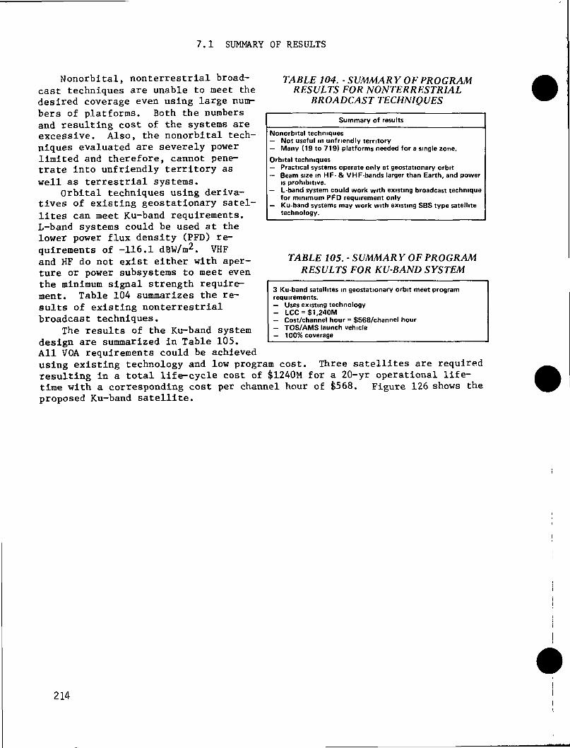
7.1 SUMMARY OF RESULTS

TABLE 104. - SUMMARY OF PROGRAMRESULTS FOR NONTERRESTRIAL

BROADCAST TECHNIQUES

Summary of results

Nonorbital techniques— Not useful in unfriendly territory— Many (19 to 719) platforms needed for a single zone.

Orbital techniques— Practical systems operate only at geostationary orbit— Beam size in HF- & VHP-bands larger than Earth, and power

is prohibitive.— L-band system could work with existing broadcast technique

for minimum PFD requirement only— Ku-band systems may work with existing SBS type satellite

technology.

Nonorbital, nonterrestrial broad-cast techniques are unable to meet thedesired coverage even using large num-bers of platforms. Both the numbersand resulting cost of the systems areexcessive. Also, the nonorbital tech-niques evaluated are severely powerlimited and therefore, cannot pene-trate into unfriendly territory aswell as terrestrial systems.

Orbital techniques using deriva-tives of existing geostationary satel-lites can meet Ku-band requirements.L-band systems could be used at thelower power flux density (PFD) re-quirements of -116.1 dBW/m2. VHFand HF do not exist either with aper-ture or power subsystems to meet eventhe minimum signal strength require-ment. Table 104 summarizes the re-sults of existing nonterrestrialbroadcast techniques.

The results of the Ku-band systemdesign are summarized in Table 105.All VOA requirements could be achievedusing existing technology and low program cost. Three satellites are requiredresulting in a total life-cycle cost of $1240M for a 20-yr operational life-time with a corresponding cost per channel hour of J>568. Figure 126 shows theproposed Ku-band satellite.

TABLE 105. - SUMMARY OF PROGRAMRESULTS FOR KU-BAND SYSTEM

3 Ku-band satellites in geostationary orbit meet programrequirements.— Uses existing technology- LCC = $1.240M— Cost/channel hour = $568/channel hour- TOS/AMS launch vehicle- 100% coverage

214

Figure 126. - Ku-band satellite concept.

The results of the L-band systemdesign are summarized in Table 106.This design option uses the lowerpower requirement of -116.1 dBW/m*.Each of three satellites has two an-tenna array apertures that cover mul-tiple zones with one large spot. AllVOA requirements could be achievedusing existing technology and low pro-gram cost. The 17-kW power subsystemwould require the use of SAFE arraytechnology that was demonstrated by NASA,operational lifetime cost of $1353M and aother low-power options and one high-power127 shows the proposed L-band satellite.

TABLE 106. - SVMMAR Y OF PROGRAMRESULTS FOR L-BAND SYSTEM

3 L-band satellites in geostationary orbit meet programrequirements.— Uses existing technology for -116.1 dBW/m2

- LCC=$1,353M— Cost/channel hour—$619/channel hour— Requires 17 kW on satellite— Two array antennas per satellite- TOS/AMS launch vehicle— 100% coverage

The three satellites have a 20-yrcost per channel hour of t>619. Twooption were also studied. Figure

215

Figure 127. - L-band satellite concept.

TABLE 107. - SUMMAR Y OF PROGRAMRESULTS FOR VHP SYSTEM

Four VHP-band satellites in a 24-h elliptical orbit can meet140-150 MV/m requirement— New technology for 168 m array & transmitters- 31.3 kW satellite power existing technology (SAFE)- LCC = $2945— Cost/channel hour—$8584/channel hour— Centaur G launch vehicle— 100% coverage

The results of the VHF-band systemdesign are summarized in Table 107. Afour satellite constellation in a24-hour elliptical orbit provides140-150 yV/m performance at the mini-mum cost. The 12-hour orbit had ahigher PFD (250 yV/m) but requiredeight satellites and had lower cover-age efficiency. A deployable scanningarray is used for the aperture arid adeployable 31.3 kW solar array flight experiment (SAFE) type solar array wasused. The four satellites have a 20-yr operational lifetime cost of &2945Mwith cost per channel hour of $8584. Figure 128 shows a proposed VHF-bandsatellite.

The results of the HF-band system showed that excessively large numbers ofsatellites are required (88) to meet all zone and channel requirements at300 yV/m. By reducing requirements to 150 uV/m a constellation of eightsatellites can provide the number of channels shown in Table 108. New tech-nology is required for both the array antenna and the power subsystem. It isanticipated that space station will develop the technology for a 100 kW solarpower system. The eight satellites have a 20-yr operational lifetime cost of{35862M and a cost per channel hour of J33225M. Although the total program costfor the HF system is the highest, the cost per channel is lower than the VHPsystem and only four times the cost of the Ku- or L-band systems. Figure 128shows a proposed HF-band satellite.

Table 109 presents a cost comparison of the four systems. The HF systemhas the highest LCC, even at the reduced power level and reduced channel capa-bility. The VHP system has the highest cost per channel hour due to the re-duced zones being covered. The VHP spacecraft have the lowest satellite uti-lization factor.

216

ORIGINAL PAGE ISOF POOR QUALHTY

Figure 128.- VHP and HF satellite concepts.

TABLE 108. - SUMMARY OF PROGRAM RESULTS FOR HF SYSTEM

Eight HF-band satellites in an 8-h circular orbit can meet 150 /JV/m— New technology for 80 m array & transmitters— 93.1 kW satellite power requires space station technology

Zone

No. of channels

1

4

2

5

3

1

4

4

5

4

6

4

7

2

8

5

9

6

10

3

11

3

requirement with reduced channel capability.

12

4

13

2

14

415

2

- LCC = $5,862 m- Cost/channel hour-$3,225/h— Centaur G launch vehicle— 68% coverage frequency

TABLE 109. - COST COMPARISON FOR KU-, L-,VHF-, & HP-BANDS

Ku-band

L-band ,<-116.1dBW/m2)

VHF-band(140-150/^V/m)

HF-band< 150 tlV/m, reducedchannel capability)

HF-band1 300 JUV/m, full VGA)

No. ofspacecraft

3

3

4

8

88

LCC

$ 1.240M

1,353

2,945

5,862

52,824

Cost/channel hour

$ 568/h

619

8,584

3.225

24,181

217

7.2 CONCLUSIONS

The study conclusions are based only on this system study and do not in-clude other significant considerations being evaluated by NASA LeRC and VGA(e.g, receiver population and distribution).

1) Terrestrial systems have the advantage of coverage over nonorbital, non-terrestrial systems because the high power and resulting signal skips forterrestrial systems is more significant in expanding coverage than raisingaltitude (increasing line of sight) to expand coverage. It is difficultif not impossible to achieve 100-500 kW power levels on either lighter-than-air or heavier-than-air vehicles. The nonorbital, nonterrestrialsystem does have potential to provide local coverage where existing fixedsights do not exist.

2) Orbital systems can expand coverage for VGA beyond existing terrestrialsystems. Orbital systems can be used as an augmentation to the terres-trial system or as a potential replacement. Costs become significant whena full capability orbital replacement system for the HF terrestrial systemis considered.

3) Cost of the system increases as the operation frequency decreases.

4) HF is desirable due to high ground receiver population, but antenna sizeis large and transmit power levels are high. Because of high power re-quirements at greater than 300 yV/m, future tests are desirable to deter-mine if a reduced level (150 yV/m) could be received on the ground withadequate S/N ratio.

5) Both HF and VHP systems require technology development for both the powersubsystem and the array antenna. The Ku-band system uses OTS technology.The L-band system uses OTS technology except for the array antenna and de-ployable solar array which are SOA.

6) HF and VHF array antennas have many advantages over reflectors includinglow power per transmitter, simple thermal control, electronic beam steer-ing, higher reliability (graceful degradation if transmitter fails).

7) Parametric performance studies showed that power generation using deploy-able photovoltaic solar arrays were superior to other systems based onspecific weight (kW/kg) packing volume (kW/stowed volume).

8) Optimizing the HF and VHF VOA coverage requirements for the selected orbitcoverage characteristics can improve satellite utilization factors andprovide more operational hours and thus reduce cost per channel hour.Also reducing the peak multichannel requirements can improve both thesatellite utilization factor and cost per channel hour. Tasking of asatellite to cover more than one zone simultaneously with multiple beams(when satellite power and channel capability is available after coveringfirst zone) can improve both coverage and satellite utilization factorsproducing lower cost per channel hour.

218

9) For subsynchronous orbits with multiple satellites, the use of two groundstations with satellite cross linking was more cost effective than addi-tional ground stations and no satellite cross linking.

10) Two smaller HF systems: (1) two satellites in an 8-hour, 0° inclinationorbit or (2) two satellites in a triply-synchronous orbit can provide VGAprogramming with reduced signal strengths but with repeating ground cover-age times. This system has significantly lower cost than the full capa-bility system and could be used as a low-cost startup system to augmentthe terrestrial system.

219

APPENDIX - COMPUTER PROGRAM DOCUMENTATION

This appendix contains descriptions of and user instructions for computerprograms developed and used during the study of direct broadcast satellitesystems. The first, life-cycle cost (LCC) estimating program (LCCOST), pro-vides estimates of satellite LCCs. The second, RFANAL, performs calculationsto estimate RF performance. A third set of programs is also provided althoughthey were not developed during the study. These programs include SUBSIZ Voiceof America (VOA), EPSSIZ VGA, and RFSIZ VGA. Together they provide estimatesof weight and volume for satellite subsystems. These estimates and other par-ametric data can be used to automatically interface with LCCOST to estimateLCC. The three programs are derivatives of Martin Marietta Denver Aerospaceprograms that have been modified to reflect assumptions made for sizing VOAsatellites as discussed in Sections 3 and 4 of the Satellite Voice BroadcastFinal Report.

LCCOST

Following is a description of the LCC estimating program developed for usein the VOA satellite study. The LCCOST program was developed to run in astandalone mode or interface with outputs from SUBSIZ. This document discus-ses the standalone capabilities of LCCOST as provided to NASA.

The objective of the program is to provide an efficient means to estimateand tradeoff LCC of spacecraft concepts. LCC estimates are broken out by sub-system for:

1) Attitude control (attitude determination),

2) Stationkeeping and maneuvering reaction control system (RCS),

3) Primary propulsion,

4) Communication payload,

5) Electrical power subsystem,

6) Thermal control,

7) Telemetry, tracking, and command (TT&C),

8) Structure (equipment bay).

Following are descriptions of the LCC estimating approach for each of thesubsystems required for VOA direct broadcast satellite systems. The LCC esti-mating algorithms and cost estimating relationships (CER) have been coded andtested on an IBM PC. This program provides an efficient tool for trading offdifferent subsystems and for determining sensitivity of LCC to weight, stowedvolume, and electric power for different system requirements.

220

LCC Estimating Procedure Overview

In the standalone mode, LCC estimates for each spacecraft configurationare determined from subsystem-specific input data obtained from some data basesource (such as the NASA LaRC system design and cost model (SDCM) or IDEASprograms) and input manually. The input data are applied to user-selectedCERs. The CERs contained in the program were described in Section 4. TheseCERs are used to compute cost at the subsystem level, with subsystem costssummed to provide total spacecraft nonrecurring cost and recurring first unitcost. Additional CERs are included to permit estimation of launch, groundsupport, and project management costs.

The output of the LCC program is a breakout of nonrecurring, recurring,launch, and ground costs by subsystem, by combinations of subsystems, or for atotal system. In the standalone mode, sensitivity of cost to spacecraft de-sign parameters is determined by manual input of new values for CER input pa-rameters.

To estimate LCC for multiple spacecraft, it is necessary to determine anaverage unit cost (C) by using a learning factor. A commonly used approachuses the expression:

c = Cul/i£ (i)

where: b = Log(m)/Log(2)

m is a learning factor slope expressed in %;

C , is estimated first unit cost;

N is total number of units to be produced

For spacecraft, a conservative value for m is 0.95, with an optimisticvalue of 0.8. The total recurring cost can then be obtained by multiplying Ctimes N.

The CERs used to estimate spacecraft LCC include data obtained and/or re-fined during the VGA study contract and CERs based on cost data from the NASASDCM, the NASA MSFC LCC data base, the REDSTAR LCC data base, and the USAFSpace Division LCC data base. The CER contained in these models vary at thesubsystem level primarily because of different assumed subsystem configura-tions in the different LCC models. The LCC program therefore includes thecapability to select different CERs for different subsystems. Selection of theCER for a subsystem is at the discretion of the user. By using different CERson subsequent runs, an estimate of cost estimating uncertainty can be obtainedby comparing the differences in subsystem and system LCC estimates. If de-sired, the different results can be averaged to compute an average cost. Theresults can also be weighted manually to reflect the similarity (or dissimi-larity) of each CER's subsystem configuration to the VGA satellite subsystemconfiguration.

221

Subsystem LCC Estimating Descriptions

Following are brief discussions of strategies for CER inputs recommendedfor specific subsystems and program activities.

1) Communication Subsystem—The communication subsystem includes the communi-cations antenna(s), uplink components, signal processing components, anddownlink components. For large space system (LSS) antennas, the downlinkcomponents are identified as the transmitters. If conventional (non-LSS)spacecraft costs are being estimated, downlink component weight should bedistributed into the uplink and signal processing components. This is al-so the case if a passive LSS antenna (e.g. radiometer) is being con-sidered. The VOA CERs for transmitters' recurring cost were obtained fromdiscussions with potential vendors and are considered better for solid-state electronics than any of the other model CERs included in programLCCOST. A learning factor is built into the program to account for mul-tiple transmitter assemblies for a single planar array antenna.

2) Electric Power Subsystem—For spacecraft requiring more than 10 kW fromthe source, the VOA CER should be used. For power requirements less than10 kW, the CER derived from the MSFC LCC model may be better. Also, theVOA CER assumes a much smaller proportion of cost for batteries than iscommon for current spacecraft.

3) Reaction Control Subsystem (RCS)—The CER derived from the Space Divisionmodel should be used if the RCS uses chemical thrusters. If electric pro-pulsion is used, the derived electric propulsion CER is applicable. ThisCER was obtained from results of electric propulsion studies found in theliterature and by studies performed at the Denver Aerospace company.

4) Other Subsystems—For all other spacecraft subsystems, the Space Divisionmodel subsystem configuration assumptions are considered to provide thebest fit with VOA or most other spacecraft. Thus, if CERs are used to es-timate costs, the Space Division CERs are recommended. However, consid-erable data exists defining costs for the more common subsystem configura-tions. If costs of subsystem components are known from prior programs,the best approach is to use the throughput option of LCCOST.

5) Launch Costs—Launch costs are separated into STS launch cost and orbittransfer (upper stage) cost. The STS launch cost algorithm assumes non-subsidized costs, and computes cost as a function of required weight orvolume fraction of the STS payload. The STS launch cost is computed asfollows:

222

Cost = (dedicated launch cost + user fee + escalated user fee) timespayload charge factor

where charge factor is smaller of 1.0 or load factor divided by0.75; Load factor is larger of [spacecraft (S/C) + upper stagelength] divided by 60 ft or (S/C + upper stage weight) dividedby 65000 Ib; dedicated launch cost is $210M; user fee is '$4.3M; escalated user fee is $37M

For subsidized STS launch costs, a throughput value can be obtained by as-suming $20,000 per pound for a Centaur G upper stage, or $19,000 per poundusing a TOS/AMS upper stage.

6) Ground Costs—Aerospace ground cost, a nonrecurring cost, accounts forspecial tools, facilities, and test equipment necessary to support produc-tion and is computed as a function of total spacecraft weight. Ground op-erations cost includes the ground control station facility cost, a non-recurring cost, and operations cost, which depends on the number of space-craft to be monitored. No CER was identified that adequately representsthis cost category. Therefore, use of the throughput option is recom-mended.

7) Other Costs—Program-level costs not directly associated with a specificsubsystem must be included to account for such activities as program man-agement, systems engineering, quality control, contract management, fi-nance management, etc. The LCCOST program computes these costs as a userdefined percentage of total nonrecurring and recurring costs. The lastcost category included in the overall cost estimate is the program fee,again computed as a user defined percentage of total cost.

LCCOST User Instructions

The LCCOST program has two different execution modes. It can be linked tothe executive program SUBSIZ and run automatically, or it can be run as astandalone program. When linked to SUBSIZ, all of the input parameters forthe spacecraft CERs are input automatically. When run as a standalone pro-gram, these parameters must be entered manually in response to a prompt suchas:

ENTER COMMUNICATIONS ANTENNA WEIGHT (LB): 2035.5

The required input parameters are summarized in Table 110.

223

TABLE 110. - LCCOST CER INPUTPARAMETERS

CER

Structure (equipment bay)Thermal controlElectrical powerCommunication antennaCommunication signal processorCommunication transmitterAttitude determinationAttitude reactionPrimary propulsionTT&CNumber of transmittersTotal S/CTotal S/CGround operations

Parameter

weight, Ibweight, Ibpower, Wweight, Ibweight, Ibweight, Ibweight, Ibweight, Ibimpulse, Ib-sweight, Ibunitlessweight, Iblength, ftlife, yr

An input of zero for any subsystem parameter will result in skipping costcomputation for that subsystem. After parameter input is complete, the pro-gram will prompt for the CER source by displaying the available options forthe subsystem. For example, the prompt for a communications antenna will be:

COST SOURCE FOR COMMUNICATIONS ANTENNA

0 : THROUGH PUT1 : USER DEFINED CER2 : SPACE DIVISION CER3 : VGA CER

SOURCE SELECTION — ?

COST SOURCE FOR COMMUNICATIONS UPLINK

0 : THROUGH PUT1 : USER DEFINED CER2 : SPACE DIVISION CER

SOURCE SELECTION — ?

COST SOURCE FOR SIGNAL PROCESSOR

0 : THROUGH PUT1 : USER DEFINED CER2 : SPACE DIVISION CER

SOURCE SELECTION — ?

COST SOURCE FOR COMMUNICATIONS TRANSMITTER

0 : THROUGH PUT1 : USER DEFINED CER2 : SOLID STATE CER

SOURCE SELECTION — ?

When a CER is chosen, the parameter value input previously for that ele-ment is used to calculate the cost. This process repeats for each subsystem ,in turn.

224

The throughput option allows direct input of recurring and nonrecurringcost without requiring an input parameter. The prompts for the throughput op-tion have the form:

How Many Recurring Cost Elements for COMMUNICATIONS UPLINK? 1

Recurring Element Cost ( 1 of 1 ) ? 3.1

The user-defined CER option allows the user to define recurring and non-recurring CER having the form:

A + B x (parameter)C

The prompts for the user-defined CER mode have the form:

ENTER A : ?ENTER B : ?ENTER C : ?

The user-defined CER then uses the previously input value of the CER pa-rameter to calculate costs. The CER is not, however,' retained after the modulehas terminated execution.

Exceptions to the above cost source input format are shuttle launch cost,program level, and fee. Program level and fee are input as decimal percent-ages. Program level is a percentage of the spacecraft total platform cost,and fee is a percentage of the program subtotal cost. Cost options for shut-tle launch are either throughput or the shuttle launch algorithm described inSection 4. The algorithm requires information such as upper-stage weight,length, and cost (in FY 1984 $M).

Prompts for output options appear after calculations are complete. If themodel is run as a standalone program a prompt will request an output title.This title is printed on paper printouts only. The next option is for displayof the results on the screen or on the printer. After output is complete theuser is given the option of printing again. A 'Y' response will return theprogram to the beginning of the output menu. A 'N1 response results in pro-gram termination. The following three pages show an example of program LCCOSToutput.

225

MONkECURRIMf, DESIGN OEVKUiF'MrNT f ObT

SUBSYSTEM

THERMAL CONTROL

ELECTRICAL F'OUER

coMMUNi CAT r ONS ANTENNA

COMMUNICATIONS UF'LINK

SIGNAL PROCESSOR

LOMMUN i HAT r ONS TR ANSM r TTER

ATT[TUDE DETERM[NAT[ON

ATTITUDE REACTION

PRDI-'ULblON (AKI1)

TTJiC

AEK'OSI-'ACE GROUND EQUIPMENT

F'RUGRAM LEVEL

FEE

T(JTAI. NONRECURRING

COST(^M)in 1VA4 '!>

cn<rr

A,4A C>r-ACE D I V I S I O N Clik

v,?? SPACy; DLVT51UN CER

4/'«i i VOA U:R

48,47 SPACE DIVISION CEK

io,A? SPACE pivj j j f iN cr.R

U * 13 SPACE D CM IS TON CEk

7,7V SOLID <VTATE TRANr-MJTTER

?'>/•>•> ^PACE DIVISION CJ-JR

33.43 ELECT. r'Rdl'ULtOON (,ER

0.00 THRnUJM PUT

f>.A3 f>F'ACE DIVJMON r'ER

7.99 SI-1 AC)-. D [VLSI ON CER

]3«75

33.24

226

SUBSYSTEM

RI-CURRI'NU PRODUCTION CURT

COST(*M)j n 1 V04 '

STRUCTURE (ENUTPMENT HAY)

THERMAL CONTROL

EI.ECTRJCAL POWER

COMMl IN [ CAT IONG ANTENNA

COMMlJN1CATTONS UF'I.] NK

SIGNAL PROCESSOR

COMMUN1CAT FONS TRANSM LTTERI

ATT fTUOE DETERITENATLON

ATTITUDE REAfTfON

PROPULSION <AKM)

TT8.C

PROGRAM LEVF.L

f'EE

TOTAL RECURRING

COST SOURCE

1 .3?

1.46

11.03

7.34

5. 6&

0.00

13.00

143.01

SPACE D1VJSJUN CER

SPACE D[V[SION CER

VOA CER

SPACE DEVES EON CER

SPACE DIVJSFnN CER

SPACE DIVES[ON CER

GOLJD STATE TRANSMITTER CKR

SPACE DIVES FUN CKR

ELECT. PROPULSION CER

TMROUlrl I PUT

SF'ACE DIVISION CER

227

VGA TOTAL IJFI: CYCI.F: COST

228

COST CATEGORY Cm JVfl4 *

TOTAL NUNRLCUKKJNG 1*63.64

TOTAL RED JRR F NG 1 43 * 0 I

J>TL» I.AUNril ?5I .60

UPI'CR STAGE 2'5.00

J?.00

TUTAI. COST 7V /.?'-•>

RF PERFORMANCE PROGRAM (RFANAL)

Following is a description of the RF performance program developed for usein the VOA satellite study (contract NAS3-24233). The program, RFANAL, wasdesigned to prompt the user for all necessary data required to run the pro-gram. The following are the program prompts and explanatory comments abouteach.

1) ENTER ORBITAL ALTITUDE IN km?

2) ENTER OPERATING FREQUENCY IN MHz?

The program was designed to run in three separate bands of operatingfrequencies.

a) 15 - 68 MHz,b) 1100 - 1300 MHz,c) 11000 - 13000 MHz.

The user has the option of choosing any frequency within one of thesethree bands.

3) IS FEED SYSTEM CIRCULARLY OR LINEARLY POLARIZED (C/D?

The user should input a "C" for a circular polarized feed or "L" for alinear polarized feed. By inputting a "C" the program will add theappropriate 3 dB loss to the RF analysis.

4) ENTER SPACECRAFT LAT., LONG. POINT—SOUTHERN LAT. AND WESTERN LONG.ARE NEGATIVE?

Enter the starting position of the satellite with respect to the cov-erage zone of interest. Southern latitudes and Western longitudes aredefined as negative numbers. Therefore, latitudes are limited to +90° and longitudes are limited to + 180°.

5) ENTER INCREMENT FOR LAT. LOCATION OF SPACECRAFT—ENTER 0 TO KEEPSATELLITE STATIONARY?

This is used to allow the user to move the satellite along a constantlongitudinal line at the increment specified. For each incrementalstep, the program will print out the RF analysis results. This willterminate when either the minimum elevation angle of 20° or the space-craft's latitude limit (orbit inclination) is reached. This processwill not be performed if the user inputs 0 for the increment.

6) ENTER INCREMENT FOR LONG. LOCATION OF SPACECRAFT—ENTER 0 TO KEEPSATELLITE STATIONARY?

229

This is similar to the above input, however the satellite will movealong a constant latitude line. The program will again print out theRF analysis results for each incremental step. This will terminatewhen the minimum elevation angle of 20° is reached. This process willnot be performed if the user inputs 0 for the increment.

7) ENTER SPACECRAFT LAT. LIMIT—I.E., THE INCLINATION OF THE ORBIT?

This is used above to determine when the spacecraft has reached thelatitude limit. This prompt will not appear if the user has entered 0for prompt number 5.

8) ENTER NAME OF ZONE (LIMIT 80 CHARACTERS)?

The user can input any combination of letters and numbers that will beused to title the output.

9) ENTER LOWER LAT. AND WESTERN LONG. OF SPOT—SOUTHERN LAT. AND WESTERNLONG. ARE NEGATIVE?

Enter the lower most and left most boundaries of the zone. As withthe spacecraft lat., long, point (prompt number 4) Southern latitudesand Western longitudes are defined as negative numbers.

10) ENTER UPPER LAT. AND EASTERN LONG. OF SPOT—SOUTHERN LAT. AND WESTERNLONG. ARE NEGATIVE?

Enter the upper most and right most boundaries of the zone. As withthe spacecraft lat., long, point (prompt number 4) Southern latitudesand Western longitudes are defined as negative numbers.

11) ENTER REFLECTOR DIAMETER LIMIT IN METERS?

This is used to let the program know what the maximum size of the re-flector can be. If the zone is too small requiring an antenna reflec-tor larger than the user's defined limit, the program will flag theuser and determine the actual zone covered by using the reflector di-aineter limit.

12) ENTER TOTAL TRANSMIT POWER IN WATTS?

This is the end of the program prompts. After each question has been an-swered the program will calculate and print out the RF analysis results. Thefollowing page shows an example of the program outputs.

230

*»* USER [NPUTS »»**70NK COVERED - - EXAMPLE 70NKTOTAL TRANSMIT POWER - 10000 WATTS 40 dBWORBITAL ALTITUDE = 10355 KmOPERATING FREQUENCY - 26 MH^SATELLITE LOCATION =• 30 LAT 30 LONG/.ONE SIZE -=-20 X 50 LATITUDE

-20 X 50 LONGITUDEPOLARIZATION -- CIRCULAR*w* PROGRAM OUTPUTS ***APERTURE SI7E = 22.9884 m X 22.9684 m using UNIFORM IlluminationANTENNA EOC GAIN = 11.66537 dBiANTENNA APERTURE EFF = .7473356ANTENNA BEAMWIDTH = 32.625 dog X 32.625 degGROUND COVERAGE =- 7792.19 Km X 7792.19 Km

70 deg X 70 degANTENNA SCAN ANGLE =4,63EOC EIRP = 51.66537 dHWPOLARIZATION MARGIN = 3 dBPROPAGATION LOSS = 2 dBMIN ELEVATION ANGLE - 18.85A4]SPREADING LOSS = 153.6273 dBSLANT RANGE = 13545.17 KmEOC POWER FLUX DENSITY IN dBW/sq. m.NO. OF CHANNELS 1 ? 3 4 5 A 7

-106.97 -107.97 -111.74 -112.yy -113.VA -114,75 -1L5.4?EOC SIGNAL STRENGTH IN uV/m.N O . O F CHANNELS 1 2 1 4 5 6 7

87.100 61.588 48.579 43.550 38.952 35.559 32.921

*** USER INPUTS »**»ZONE COVERED -- EXAMPLE ZONETOTAL TRANSMIT POWER •= 10000 WATTS 40 dBWORBITAL ALTITUDE = 10355 KmOPERATING FREQUENCY = 26 MHzSATELLITE LOCATION - 30 LAT 30 LONGZONE SIZE -=-20 X 50 LAT [TUBE

-20 X 50 LONGITUDEPOLARIZATION -- CIRCULAR««* PROGRAM OUTPUTS *«»APERTURE SI7E ~ 22.9884 m X 22.9884 m usimj UNIFORM IlluminationANTENNA EOC GAIN - 11.66537 dBiANTENNA APERTURE EFF = ,7473356ANTENNA BEAMWIDTH - 32.625 de<j X 32,625 deaGROUND COVERAGE - 7792.19 Km X 7792.19 Km

70 cleg X 70 deepANTENNA SCAN ANGLE = 4.83EOC EIRP = 51.66537 dBWPOLARIZATION MARGIN = 3 dBPROPAGATION LOSS - 2 dBMIN ELEVATION ANGLE = 18,85641SPREAD[NG LOSS - 153.6278 dBSLANT RANGE - 13545.17 KmEOC POWER FLUX DENSITY IN dBW/<sq. m.NO. Or CHANNELS 1 2 3 4 5 A 7

-106.97 -109,97 -111.74 -112.99 -113.96 -114.75 -115,42EOC SIGNAL STRENGTH JN uV/m,NO, OF CHANNELS 1 ? 3 4 5 6 7

87.100 61.588 48,579 43.550 38.952 35.559 32.921

231

PROGRAM ASSUMPTIONS

The program was designed to provide the necessary data for the VOA study.Therefore, the program automatically assumes certain RF parameters. First,for frequency bands 15-68 MHz and 1100-1300 MHz, the program calculates theantenna beamwidth using the following equation:

BW = 65 x >/ D (2)

where BW = antenna beamwidth, deg65 = 65° uniform illumination factorA = wavelength, mD = reflector diameter, m.

For the frequency band of 11000-13000 MHz, the program calculates the an-tenna beamwidth by using:

BW = 70 x A/ D (3)

where BW = antenna beamwidth, deg70 = 70° tapered illumination factorA = wavelength, mD = reflector diameter, m.

The difference in the two equations results because the first two fre-quency bands assume a phased array reflector system with uniform illumination,while the third frequency band uses a reflector dish and feed system with ta-pered illumination.

The next RF parameter built into the program is the aperture efficiency.For the first band, 15-68 MHz, the program uses:

Eff = 0.75 x cos(0 )

(4)

where Eff = aperture efficiency

G = antenna scan angle off boresight

This equation assumes that the phased array antenna used for the firstband design is an electronically steerable array. For the second band, theaperture efficiency is a constant 0.8, and for the third band, the apertureefficiency is a constant 0.5. These numbers assume a nonsteerable phased ar-ray and a dish reflector and feed, respectively.

The final parameter automatically calculated by the program is the propa-gation loss due to transmission from space. The program assumes a propagationloss of 2 dB if operating at less than 35 MHz, 1 dB if operating between 35MHz and 68 MHz, and 0 dB for all other frequencies.

232

Program Listing

The following is the program lasting for the rf performanceprogram (RFANAL).

10 DIM PHI(4)15 T*=STRING*<73,42>20 CLSsINPUT "ENTER ORBITAL ALTITUDE IN KM";OT30 INPUT "ENTER OPERATING FREQUENCY IN MHz";OF40 INPUT "IS FEED SYSTEM CIRCULARLY OR LINEARLY POLARIZED <C/L>";A*50 IF A*="C" OR A*="c" THEN PM=3sGOTO 8060 IF A*="L" OR A*="1" THEN PM=OsGOTO 8070 GOTO 408O INPUT "ENTER SPACECRAFT LAT,LONG POINT -- SOUTHERN LAT. AND WESTERN

LONG. ARE NEGATIVE";LATSC,LONGSC90 INPUT "ENTER INCREMENT FOR LAT LOCATION OF SPACECRAFT - ENTER 0 TO

KEEP SATELLITE STATIONARY";;SCLATINC100 INPUT "ENTER INCREMENT FOR LONG LOCATION OF SPACECRAFT - ENTER 0 TO

KEEP SATELLITE STATIONARY";SCLONGINC110 LATSCI*LATSCsLOOP=OsLONGSCI=LONGSCsLATLIMIT=90120 IF SCLATINCOO THEN INPUT "ENTER SPACECRAFT LAT LIMIT --- I.E.,THE

INCLINATION OF THE ORBIT";LATLIMIT130 INPUT "ENTER NAME OF ZONE (LIMIT 80 CHARACTERS)";NAM*140 INPUT "ENTER LOUER LAT AND WESTERN LONG OF SPOT -- SOUTHERN LAT. AND

WESTERN LONG. ARENEGATIVE";LAT1,LONG1

150 INPUT "ENTER UPPER LAT AND EASTERN LONG OF SPOT -- SOUTHERN LAT. ANDWESTERN LONG. ARE

NEGATIVE";LAT2,LONG2160 IF LAT1*LATSC THEN LAT1=LAT1-.0001170 IF LAT2=LATSC THEN LAT2=LAT2-,0001180 IF LONG1-LONGSC THEN LONG1=LONG1-.O001190 IF LONG2=LONGSC THEN LONG2=LONG2-.O001200 OLAT1=LAT1:OLAT2»LAT2:OLONG1»LONG1sOLONG2=LONG2211 PHIL=90220 INPUT "ENTER REFLECTOR DIAMETER LIMIT IN METERS";DIAL230 INPUT "ENTER TOTAL TRANSMIT POWER IN WATTS";TTP240 LAT1-OLAT1:LAT2=OLAT2:LONC1=OLONC1:LONG2°OLONG2sFL=0250 SCAN=OiTAPER=0:ILLUM=652AO IF OF>110OO AND OF<13000 THEN TAPER=lsILLUM=70270 WL=3E+O8/<OF«100OOOO!>280 AWLIM=ILLUM«WL/DIAL290 TP*10*LOG<TTP)/LOG<10)300 GC1=TAN«LAT1-LATSC)»3.1415927««/180)»*(COS((LAT1-

LATSC>*3.1415927»/180)*A378)310 GC2=TAN«LAT2-LATSC)*3.1415927«»/180)*(COS«LAT2-

LATSC)*3.1415927«/180)«A378>320 GC3=TAN«LONG1-LDNGSC>*3.1415927»/180>*<COS< (LONG1-

LONGSC)*3.1415927«/180 > «6378)330 GC4=TAN< <LONG2-LONGSC)»3.1415927M/180>»(COS<(LONG2-

LONGSC)«3.1415927M/180)«A378)340 ALPHAl=ATN(GCl/<OT+<6378-COS«LATl-LATSC)*3.1415927«/180)«6378))>350 ALPHA2=ATN<GC2/(OT+ <6378-COS< < LAT2-LATSC)*3.1415927t«/180>«6378) ) )360 ALPHA3*ATN<GC3/<OT+<637e-COS«LONGl-LONGSC>«3.1415927«*/180>*&378> ))

233

370 ALPHA4=ATN<GC4/<OT+<6378-COS«LONG2-LONGSC)*3.1415927*»/180>*6378»>380 IF OF>15 AND OF<68 THENSCAN1=ABS< ALPHA1+ALPHA2)/2:SCAN2=ABS(ALPHA3+ALPHA4)/2 sIF SCAN2 >SCAN1THEN SCAN=SCAN2sEFF=COS<SCAN2)*.75 ELSE SCAN=SCAN1:EFF=COS<SCAN1)*.75390 IF OF>11OO AND OF<3000 THEN EFF=.8400 IF OF>11OOO AND OF<13000 THEN EFF=.5420 ABW1=ALPHA2-ALPHA15ABW1=ABWl*180/3.1415927**43O ABW2=ALPHA4 - ALPHAS s ABW2=ABW2* 180/3.1415927**44O IF ABWKAWLIM THEN FL=lsGOSUB 1210450 IF ABU2<AWLIM THEN FL=lsGOSUB 1350460 Al=ILLUM*WL/ABW15A2=ILLUM*WL/ABW2470 ATG=(1O*LOG<EFF*9.869605*A1*A2/<WL*WL)>/LOG(10)) -3480 GCD1*LAT2-LAT1490 GCD2*LONG2-LONG1500 EIRP=TP+ATG510 IF OF>=35 AND OF<68 THEN PL=1 ELSE PL=0520 IF OF<35 THEN PL=254O PHIT*ABS<LATl~LATSC)5PHKl)=90-PHIT-ABS<ALPHAl*180/3.1415927**)550 PHIT=ABS<LAT2-LATSC)5PHK2)=90~PHIT-ABS<ALPHA2*180/3.1415927**)5*0 PHIT=ABS<LONGl-LONGSC)sPHI(3)=90-PHIT-ABS(ALPHA3*180/3.1415927**)57O PHIT=ABS<LONG2-LONGSC)5PHI(4)=90-PHIT-ABS<ALPHA4*180/3.1415927**)580 FOR 1=1 TO 4590 IF PHKIXPHIL THEN PHIL=PHI(I)600 NEXT I610 IF PHIL<0 THEN PRINT "»**« ALL OF ZONE CAN NOT BE SEEN FROM

SATELLITE «**«"sGOTO 1160620 IF PHIL<20 THEN PRINT "**** CAUTIONs ELEVATION ANGLE LESS THAN 20

DEGREES **»*"630 PHID=PHIL*3.1415927**/180640 SR=SQR< <6378*SIN<PHID>)A2+2*6378*OT+OT*OT)-6378*SIN<PHID>650 SL - -10»LOG < 1 / (12.566371 *»*SR*SR* 1000000! ) ) /LOG < 10 >660 PFD•(TP+ATG>-< SL+PL+PM)670 SS= <SQR< 10A<PFD/10»»19.4165)/.000001671 SS=INT(SS*100)/100672 PFD=INT<PFD*10O)/1OO680 IF FL=1 THEN PRINT ••****#*###»**********#*#*»#****"690 IF FL=1 THEN PRINT "* ANALYSIS IS LIMITED BY »"7OO IF FL=1 THEN PRINT "* USER INPUT MAXIMUM REFL. *"71O IF FL=1 THEN PRINT "* DIAMETER *"720 IF FL=1 THEN PRINT750 PRINT "APERTURE SIZE ="?Al?"ro X<i;A2;"m"760 LPRINT "»** USER INPUTS »***770 IF FL-1 THEN LPRINT780 IF FL=1 THEN LPRINT "* ANALYSIS IS LIMITED BY *"790 IF FL=1 THEN LPRINT "* USER INPUT MAXIMUM REFL. *"80O IF FL=1 THEN LPRINT "* DIAMETER *"810 IF FL=1 THEN LPRINT "*»«»«M«w«»«**«KK*w«*4(M«»*MW»«»"820 LPRINT "ZONE COVERED -- ";NAM*830 LPRINT "TOTAL TRANSMIT POWER =";TTP5"WATTS "sTPVdBW840 LPRINT "ORBITAL ALTITUDE =";OT;tlKmil

85O LPRINT "OPERATING FREQUENCY =1<;OF5"MHz"860 LPRINT "SATELLITE LOCATION ="?LATSC;" LAT";LONGSC;" LONG"870 LATl=INT(LATl*100)/100sLAT2=INT<LAT2*100)/100

5LONGl=INT<LONGl*100)/100sLONG2=INT<LONG2»100)/100880 LPRINT "ZONE SIZE =";LAT1;" X "5LAT2;" LATITUDE

234

890 LPRINT " ";LONG1;" X ";LONG2;" LONGITUDE900 IF Pn*3 THEN LPRINT "POLARIZATION -- CIRCULAR" ELSE LPRINT

"POLARIZATION -- LINEAR"910 LPRINT "*** PROGRAM OUTPUTS *«*"920 LPRINT "APERTURE SIZE =";Al;"ro X";A2;"m";930 IF TAPER=0 THEN LPRINT " using UNIFORM 11 1 urnination"940 IF TAPER=1 THEN LPRINT " usinq TAPERED inuminatrion"950 LPRINT "ANTENNA EOC GAIN =";ATG;"dBi"960 LPRINT "ANTENNA APERTURE EFF =";EFF970 ABWl=INT<ABWl*10OO>/10OOsABU2=INT<ABW2*1000>/1000980 LPRINT "ANTENNA BEAMUIDTH =";ABWl;"deg X";ABW2;"deg"990 LPRINT "GROUND COVERAGE =";

INT<10O*ABS<LATl-LAT2>*3.1415927i**12756/360>/100;"Km X";INT<100*ABS<LONGl-LONG2>*3.1415927«*»12756/360>/100;"Km"

1000 LPRINT TAB<17) GCDl;"de<g X";GCD2;"deg"1010 LPRINT "ANTENNA SCAN ANGLE = ";INT<100*SCAN*180/3.1415927t*>/100102O LPRINT "EOC EIRP =";TP+ATG;"dBW"1030 LPRINT "POLARIZATION MARGIN =";PM;"dB"1040 LPRINT "PROPAGATION LOSS =";PL;"dB"1050 LPRINT "MIN ELEVATION ANGLE =";PHIL1060 LPRINT "SPREADING LOSS =";SL;"dB"1070 LPRINT "SLANT RANGE =";SR;"Km"1080 LPRINT "EOC POWER FLUX DENSITY IN dBU/sq. m."1081 LPRINT "NO* O F CHANNELS 1 2 3 4 5

6 7"1082 LPRINT TAB<19>;sLPRINT USING "mum.w«*";PFD;1083 LPRINT TAB<27);sLPRINT USING "ttmw.m*1

1084 LPRINT TAB<35);sLPRINT USING "«««**,.««*•1085 LPRINT TAB<43);sLPRINT USING "MINIM. MM" ;PFD-6.021001;1086 LPRINT TAB(51);sLPRINT USING "NMMN. *m";PFD-6.9897;1087 LPRINT TAB<59);sLPRINT USING "««»i»»».«i»";PFD-7.78151;1088 LPRINT TAB<67>;sLPRINT USING "t»i«i««i..it«";PFD-8.4511090 LPRINT "EOC SIGNAL STRENGTH IN uV/m."1091 LPRINT ""NO. O F CHANNELS 1 2 3 4 5

6 7"1092 LPRINT TAB<19);sLPRINT USING "««*«*.mm";SS;1093 LPRINT TAB<27);sLPRINT USING "«i»i».i»»««" ;SS**7071;1094 LPRINT TAB<35);sLPRINT USING "*»*.***" ;SS«.557735;1095 LPRINT TAB(43);sLPRINT USING "***,»**" ;SS*.5;1096 LPRINT TAB<51);sLPRINT USING "t»t»«.i«».i»";SS«.44721;1097 LPRINT TAB(59);sLPRINT USING "««ti».i»»ti»";SS*.40825;1098 LPRINT TAB<67);sLPRINT USING "«««.««»«";SS».3779641100 LPRINT T*111O IF LOOP=2 THEN GOTO 11401120 IF PHIL<20 OR ABS(LATSC»=ABS(LATLIMIT) THEN

LOOP=2sLATSC=LATSCIsLONGSC=LONGSCI+SCLONGINC5PHIL=90sGOTO 2401130 IF SCLATINCO 0 THEN LATSC=LATSC+SCLATINCsPHIL=905GOTO 2401132 IF SCLONGINC=0 THEN GOTO 11511133 LOOP=2sLATSC=LATSCIsLONGSC=LONGSCI+SCLONGINC5PHIL=905GOTO 2401140 IF PHIL<20 THEN GOTO 11511150 IF SCLONGINCO 0 THEN LONGSC=LONGSC+SCLONGINC:PHIL=90sGOTO 240 ELSE

GOTO 11511151 LPRINT T*sLPRINT CHR*(12)1200 GOTO 201210 DELTA=AWLIM-ABW1

;PFD-3;;PFD-4.771001;

235

ALPHA2=ALPHA2+DELTAALPHA1=ALPHA1-DELTA

DELTA = DELT A*3 .141 5927»/ 1 80IF ABS<LAT1-LATSC»ABS<LAT2-LATSC> THENIF ABS<LAT1-LATSCXABS<LAT2-LATSC> THENIF ABS<LAT1-LATSO=ABS<LAT2-LATSC> THENALPHA 1 = ALPHA 1 - DELTA/2 ! ALPH A2 = ALPH A2+DELT A/2K 1 = ( OT*TAN < ALPHA 1 > + 6378*T AN ( ALPHA 1 ) ) /6S78K2 « ( OT*TAN < ALPHA2 > +6378»TAN < ALPHA2 ) ) / 6378C1=TAN<ALPHA1) sC2=TAN(ALPHA2)D1P= < 2*K1*C1+SQR< 4*K1»K1*C1»C1 -4# ( 1+C1*C1 ) *

<K1*K1-1»)/<2*<1+C1*C1»D2P = < 2*K2*C24-SQR < 4*K2*K2*C2*C2 - 4« < 1 +C2*C2 > *

<K2*K2-1> ) >/<2«<l+C2*C2> >LATlP=<1.570796-ATN<DlP/SaR<l-DlP#DlP>»*lSO/3.1415927«**

ALPHA1/ABS( ALPHA1 )+LATSCLAT2P= ( 1 .570796 -ATN(D2P/SQR( 1-D2P*D2P) ) >*180/3. 1415927«»

ALPHA2/ ABS < ALPHA2 ) +LATSCLATl=LATlPsLAT2=LAT2PABWl=AWLIMsRETURNDELTA=AWLIM-ABW2DELTA=DELTA*3.1415927«/180IF ABS<LONG1-LONGSC»ABS<LONG2-LONGSC)IF ABS < LONG 1-LONGSCX ABS (LONG2-LONGSC)IF ABS<LONG1-LONGSO=ABS<LONG2-LONGSC>

ALPHA4 = ALPHA4+DELT A/2REM PRINT ALPH A3, ALPH A4Kl =<OT*TAN< ALPHAS )+6378*TAN( ALPHAS) >/6378K2=(OT»TAN(ALPHA4)+6378»TAN(ALPHA4) )/6378Cl=TAN(ALPHA3)sC2=TAN(ALPHA4)D1P=<2«K1*C1+SQR(4*K1*K1»C1*C1-4*(1+C1*C1)*(K1*K1-1»)/

1 220123012401250

1 2601 27012801290

1 3OO

1310

1320

133013401350136O13701380139O

14001410142014301440

1450 D2P = <2*K2*C2+SQR< 4*K2*K2*C2*C2-4* <1+C2*C2 > * < K2*K2-1> »/<2»<1+C2*C2»

146O LONGlP=<1.570796-ATN<DlP/SQR<l-DlP«DlP>»*180/3.1415927***ALPHA3/ABS < ALPHAS)+LONGSC

1470 LONG2P = (1.570796 - ATN < D2P/SQR < 1 - D2P*D2P ») * 180/3.1415927***ALPHA4/ABS<ALPHA4)+LONGSC

1480 LONGl=LONGlPsLONG2=LONG2P1490 ABW2=AWLIM:RETURN

THENTHENTHEN

ALPHA4=ALPHA4+DELTAALPHAS=ALPHA3-DELTAALPHA3=ALPHA3-DELTA/2;

236

WEIGHT AND VOLUME ESTIMATING PROGRAM (SUBSIZ,EPSSIZ,RFSIZ)

The algorithms contained in the weight and volume estimating program weredescribed in Section 4.0. The software provided uses these algorithms. Fol-lowing is a summary of assumptions used to perform sizing for all subsystems,including those that were originally sized using other programs (e.g. SCIAP,SDCM).

1) Antenna sizing (RFSIZ):a) transmitter efficiency = 0.65 for frequencies > 3 GHz, where solid

state power amplifiers (SSPA) are applicable;b) transmitter efficiency = 0.36 for frequencies _1 3 GHz, where

traveling-wave tube antennas (TWTA) are applicable.

2) Feeder link electronics (RFSIZ):a) 121 kg for nongeostationary Earth orbits (GEO), where crosslinks are

assumed;b) 78 kg for GEOs, where crosslinks are not required.

3) Signal processing electronics (RFSIZ):a) 58 kg for all cases.

4) Auxiliary propulsion (SUBSIZ):a) dry weight = 184 kg for non-GEOs (electric propulsion);b) dry weight = 91 kg for GEOs (chemical propulsion);c) fuel weight = 120 kg for both cases.

5) Attitude determination (SUBSIZ):a) weight = 57.7 kg for non-GEO cases;b) weight = 13.6 kg for GEO cases.

6) TT&C (SUBSIZ):a) weight = 32.1 kg for non-GEO cases;b) weight = 26.4 kg for GEO cases.

7) Thermal control (SUBSIZ)a) maximum temperature = 55°Cb) minimum temperature = -12°Cc) end-of-life absorptivity = 0.2d) end-of-life emissivity = 0.8

The EPS (program EPSSIZ) and equipment bay structure (SUBSIZ) sizes arecomputed from user Inputs and outputs from the other subsystem sizings. Theequipment bay structure sizing must not be performed until sizing is completedfor all other subsystems.

Subsystem Sizing Example and User Instructions

The module, SUBSIZ, serves as the executive control, chaining to EPSSIZ,RFSIZ, or LCCOST as necessary in a mode completely transparent to the user.Subsystem sizing is started inserting the program diskette into the defaultdrive and by typing:

237

BASICA SUBSIZ.VOA

or, if already in BASICA:

LOAD "SUBSIZ.VOA"RUN

The following example shows the user inputs and resulting outputs for siz-ing an HF concept in an 8-hour circular orbit. First the main menu is dis-played, listing the subsystems that can be sized.

IHI-'UT TJTI.I-: FOK Til LG ANALYSIS•' HF 6 hoi.ir orbit u/amploFnput i?r n<l l i w 1 1 nP6»rU*rtv

Input 3rd lino if nor.rU~.rtvEM bl/IHU I1AJM MJCNU

L - ^ntfonna/rf sub*:>vt(?m? i\u/3 1 xnrv propn'l t> i on sub* y«->tpm"?• - primary p ropu ln ion subsy^i'pin4 TTJiCL> •• fH t * t tn tH) p(nufrT 'juJ^'-iy^i om6 \ h or ma I c 01 1 tr o I si i hsvs'f^m7 • eqm pmnnt )^ay «,ivi.n<ift - A nV - Stop t?*f%c ut J on

Your choice-'-1 I

The choice made, 2, results in display of the menu from the antenna and RFsizing module. The choice made here, 12, is for the HF and VHF baseline de-sign concept described in the report. Now the RF frequency, phased array ele-ment spacing, modulation mode (prompted only for HF cases), transmitter char-acteristics, and orbit class are defined by the user as shown.

238

D-IIJI" f\ D TI <• TH in"1 4 MH-J:.ii "H -fl. o*-.x_nil iron n"ii 1 i).--*

RF SUKbY&TEM '3 [ZING SUMMARY

Se I ect antenna ^trur t ura 1 i ype

t - Wrap Radial Rih (Lockheed's)? Hoop and Column (Grumman's)3 - Hoop -awl Column (Harris'''4 • I<ox Truss R i nq (Mart in' <•>)'5 - I n f l a t a J D l o <L' Garde's)6 - Pox. Tru«:>£ Rff I PC t or (Mart 3 n' K>/ - Ca)D l e Catenary Re f I oc tor (TRW' i»)^ Telrnhe^dral Tru<:>u Reflet Lor <GI)'<_,)v - Umbrella Radial Rib <.Harris' )10 - Articulated Umbrella R?\d.j a I F-;ib <lb\r>M<>')it - Honeycomb Panel Solid Reflector (Ford Aoro«>J/? • Hox Tru<>'> RURJ Arr<\y iMartiri <>)13 - Honeycomb Pan(?l Array (Non -phased)Your choice'* 1?Enter anfonna diamoter (m)'? AO

Data for Boy Tru«.c> Rinci Array (Ijnut on diame-ter of 2*00 meters)

For a reflector antenna^ ontor a 0 for tran'snut frequency*For a phased ttrr?xy^ enter the iransnu «>«» i on frequeiuv in Ghz«

FREQUENCY (OR 0)'? ,026

Enter the^ s>pacn.nti between phe\s>t.-d array element?,as a dec i ma 1 f r ac t i on o f m i <»<» i on w<> ve 1 engt I)Fraction'-* .73Calculated transmitter «pat.jnq - 8.6!!>3847 iv this> correct (Y/N)'? y

Select modulation mode; DPP<I» or Bf>I'<(H) v <:,[nput number of transmitter potuur levels? t

TRANSMITTER TYF'E 3Enter power per transmi L ter (uO/:> 2'50Input % (if i_ram>mj tterti c>l t h i <••-. power? 3tnpui number of channels per transmitter? I

239

The eleraeat spacing input, 0.75 in the example, is used by the program tocompute the number of transmitters as well as the number of radiating ele-ments, assuming one transmitter for each element. However, for many designsit may be desireable to have multiple transmitters feeding a single element.In this case, the spacing must be defined to result in the desired number oftransmitters. The required spacing to be input is computed from:_

spacing = 4/ZL. A (5)V 2^R_K-l

where R = antenna diameter (m)N = number of transmitters requiredX = wavelength f(m)

For example, for 177 transmitters on a 40-meter antenna at 26 MHz, the re-quired spacing (as a fraction of wavelength) would be:

spacing - y^/ 11.538 . , 0.463 «>

The user prompts and inputs would be:

Enter the spacing between phased array elementsas a decimal fraction of mission wavelength.Fraction? 0.463

Computed spacing from program is xxxx.xx. Isthis correct (Y/N)? Y

The last prompt, "DO YOU WANT TO SIZE ANOTHER ANTENNA SUBSYSTEM(Y/N)?"transfers back to the executive after a "NO" input.

Main menu choices 2 or 4 result in the prompt to select the orbit cate-gory, either non-GEO or GEO. Depending on the choice, the appropriate weightand volume values are selected by the program.

SPECIFY ORBIT TYPE: 1 - GEO2 - NON-GEO

YOUR CHOICE? 2

Main menu choice 5 results in the prompts and interaction necessary to se-lect the EPS configuration and to then compute weights and volumes of EPS com-ponents. In the example, the required power is fed in automatically from theRF sizing section. If the EPS were sized first, a prompt would appear to in-put the required peak load power. The prompt for housekeeping power is forthe average power required during occultation. The next inputs define the or-bital altitude, lifetime, power generation component, and battery type. Thelast prompt permits another EPS sizing or transfers control back to the execu-tive as for the antenna and RF sizing.

240

Input S/C housekeeping e lec t r ica l power required for subsystems E > x c ) u d j n g F<f subsystem ( K m ) 7 ? .'5Input orbit aitJtude (km)' 13692Input Spacecraft lifetime requirement in YRS' 7

SELECT POWER GENERATION TYPE

I Silicon blanket2-S] I icon panel3-Existing Carts panel4-Near term GaA& panel"5-Future(1 ong term) GaAs panel6-SF'lOO

YOUR CHOICE'? L

SELECT PATTKF<Y TYF'F

t -NiCd? - N g H

YOUR CHOICE-? L

Main menu choice 6 results in thermal control subsystem sizing. In the ex-ample, the difference between the power in and out of the load (transmitters)is shown and the user prompted to use this value or to input another. Theuser then selects an orbit category as shown, and further defines the thermalcontrol subsystem configuration.

DIFFERENCE KF.TWEKN POWER TO LOAD AND PUWEK OUT IS V. 135254 Kw.

DO YOU WANT TO USE THES VALUE TO SCZE THE THERMAL CONTROL SYSTEM(Y/N)? yInput nmxjnmm operating temperature1 (C)'? 55Input minimum temperature(C)'? -12

SELECT S/C OF'KRATl ONAL ALTITUDE CLASS

1 - GEO or greater? - 926 Km(500 Nm) to GF.O3 - less than 926 Km (LHO)

YOUF< CHOICE' 2

Is phase change* material included an the Thermal Control Subsystem(Y/N)'? n

Main menu choice 7 does not result in any further user interaction sinceequipment bay structure sizing is based on the weight of components sized forother subsystems.

Selection of main menu choice 9 results in output of the system weight andvolume summary and display of a prompt to estimate life-cycle cost. If LCCestimates are desired, program LCCOST will automatically be executed.

The following three pages contain the sizing program outputs for the exam-ple inputs shown here.

241

ORIGINAL PAGE ISOF POOR QUALFTY

J1 'I. B ll 4 M t| H ' ,| » H ' S I" B 1 •• , , _l! STlTl II J> ll it !!' i| . , H. ' , 4

f<r MlKbY'nTM < i l / I N C f.UMMAKYL>' i is i lor t<<i/ IV' i«.-' KI IKI AD \y ( I i in i i < > i i <( i<\i iu>i"f>i oi '/'OOAm 'MUM (I i <.inu>i t>r ".I"!; t\()

Tof A I 03 r< Output Rf f.arrmi I •uuior(kw' t I/To ta l Uui|)ul F^f :>ici i i ix l T'cnunrdMn) I/

r |)'">r Nuinhor ol To I'M I Kf potu'Tin i L l er ' »*) i i an- in i it <-ir<,2'50 Afl L /

ANTKNNA STRUCTUKETOTAL ANTIINNA STRUt/CUUi: yfn.UMJX I'f'O 40,Vi' I /;>TOTAL RF TRANSIIFTTER l1A'^(Kf;) rt/V./'?00TOTAL KV TKANMvIITTi:r<wj;if;nT or UPLTHK ruiiVOI.UMI: or UPLINK iTiNF iUNL ihn i<;<riA:<jwr.iuirr ui- 'SIGNAL PROC, coiriPQNiKrs(K<4>

i: or MUNAL PRO(\ u

TOTAL Kl' SUHSYTKII I'lA'^SfKlP 2W I ,',J?v.lJMi:(l1A;O 4/ '»A/ / i |v

U II II " .I'D. B ll i| hM 1 h - 4 H b - ( » L H ' i . Hlbb || » H H ? .1 - , H •• , H '•

ATTITUDL CONTFs'OL, <>TATJ ONKFIIF'I NC AMD I'lANIIWIIR I N(; bUI'lhAFvY

' i f*/ Lbs

IB." j1 Tl. I 14 > * .q. t • 'i i> i - J > i. Q r a i .x g uii H * ll <r .-

C; f>uBi>Y^Ti:iTi NUMMARY

242

44 fri c~jn. nv~ c.Tn-Jj:ii -it. *» v-n.m g s H *;? cz: vu.- ..

EPS SUMMARY

Power required from source = P8.06J61 KWPower at 1 oad > average = 26.65385 KUOrbital altitude ~ 3369? KmOrbital period = 7.977999 hrsSpacecraft lifetime requirement - 7 yrsTotal eclipse time per orbit- .812874 hr<>Golar array degradation factor due to radjatjon = .784776?Solar array thermal adjustment f AC for - .87994'53Solar array cover r>ljde> weight factor - 0Antenna Size = 80 m by 80 m

***** F'cnuer Generation Giving *****

For Si Blanket ArrayArea required - 2f>8.4f>4? m2Weight = 413.5267 Kg Volume - 2.067634 m3

***** Shunt Regulator Sizing *****

Shunt Regulator Weight = 49.00938 KgShunt Regulator Volume = b.">!>66lvF:-0? m"3

***** Power Switching/Distribution Sizing *»««x

Power Switching Equip Wt. - 8.349986 KgPower Switching Equip Vol. = 9.69386IE-03 m3

Distribution Weight; Source to Bus. = 10,93997 KgDistribution Weight; Bus to Load - 54.439'52 KgTotal Distribution Weight = 65.37949 KgTotal Switching and Distribution Weight - 73.92948****** TOTAL SI SYSTEM WKTGHT W/f) PATTER!ES(kg) - 536,4/ 6****** TOTAL SI SYSTEM VOLUME W/0 BATTER[ES<MA3> = 2.132894

***** Hattery Sizing *****

For NiCd Batteriesbattery Capacity Required = 1063.564 WhBattery Weight - 30.15152 Kg Battery Volumo = 1.505837E-02 m3

%***** Battery Charger Sizing *****

For NiCd BatteriesBattery Charger Weight = ,5386365 Kg Battery Charger Volume - 6.10699E-04 m3

TOTAL EPS MASS (kg) - 567.1'557TOTAL EPS VOLUME<"MA3) •- ?. 148563

243

IE -" k t ii 4Jt k • > k •- P > 5_ Pr « » i TI UTk H 1> "6 it :>•

THKKMAI, CONTROL MIKSY&TKM HJZJNK SUMMARY

Ma * x mi ini t em pnra tur o (C >M^x i mum heat rad i ate»d (W)Rad x <? (. i vc1 <-ji i r f AC G em i s i v i ty f AC l"orF<aci i at j v*> -Airftxre ahs>orpti vj ty factorRoquircM radiator surface ar<?a(l1A2> 27*69343

Control Sub^vsC^m are^ <I1A2^Thermal fonfrol Bub«->y&t-pm Volume <M*LO

27, 6d .384671

HAY NUMMARY

Total rnasn of ^(|in pmpiH b<xy<kq) 43.42271Mas'i of dep i ovmi:?ni"/<5towage rne'"htinif»m<»(K<j) 71.4Tot-O nrnfa-:,(k<j) " 114.02P7Total vuluiw? of structure and mGi:hani<5m<5(mA3) .7711403

Lb«» 9f>. 74708

> 25'J.J041

HF 8 hour orbit sample cast?

CONI'TGURATION SUMMARY

R f Pay1oadAuxi l iary Propulsion Suta«»ycemTelemetry, Tracking and CommandE l f ^c t r j ca l F'oiuer f5ubs>y<:>tt>mThermal Control Suta'sy«>ternEquipment !<ay btrocture

MASS (KG) VOLUMF:<MA3)

2321.229 42.67819241.7 ?.2r>32.1 .03567.1^>7 ?.1485A3135.2178 1.384671J14.B227 ,

TOTAL SYSTEM SUMMARY7'523,9'56

244

References

1. Voice Broadcast Mission Study, Volume II—Study Report. General ElectricMissile and Space Division. NASA CR-98711, July 1967.

2. Voice Broadcast Mission Study. RCA Astro-Electronics, NASA CR-95491, May1967.

3. Satellite Sound Broadcasting with Portable Receivers and Receivers inAutomobiles. Report 955 of the XVth Plenary Assembly of the InternationalRadio Consultative Committee (CCIR), Geneva, 1982.

4. Chaplin, J., et al.: Satellite Sound Broadcasting Direct to Portable andVehicle Receivers. Telecommunications Journal, Vol. 52, 1/1985.

5. Phillips, G. J., Knight, P.: Use of the 26 MHz Band for SatelliteBroadcasting. EBU Technical Review, No. 170, August 1978, pp. 173-178.

6. Saveskie, Peter N.: Radio Propagation Handbook, Chapter 1, 1980.

7. Kase, Charles: Satellite Voice Broadcast Study Preliminary SpacecraftAntenna and Power Considerations, June 6, 1984.

8. TCOM Aerostats Systems Notes, TCOM Corps, Columbia, Maryland.

9. Lighter, R. A. and Moghadam, A. A.: A Revolutionary Telecommunicationsand Broadcast System. TCOM Corp., Rockville, MD, Proceedings of 4thIranian Congress of Electrical Engineering, Shirag, Iran, May 12-16, 1974.

10. Menke, James A., Manager Tethered Aerostat Systems: A Revolutionary andOperational Tethered Aerostat System Illustrating New LTA Technology,Sheldahl, Inc., Northfield, Minn.

11. Tethered Aerostats used in TCOM Corporation. Proceedings of AIAA 13thAnnual Meeting, Washington, DC, January 10-13, 1977.

12. Reed, Harold E.: Tethered Aerostats—Technology Improvements. PanAmerican Airways Aerostat Systems, Patrick AFB, FL, 1977.

13. 1984 Helicopter Annual, Helicopter Association International, 1110 VermontAve. N.W., Washington, DC.

14. Satellite Sound Broadcasting with Portable Receivers and Receivers inAutomobiles. CCIR Report 955, 1982.

s

15. Rush, C. M.: Some Considerations on the Operation of an HF/VHF DirectBroadcasting Satellite Service. NTIA-TM-84-105, USDC, 1984.

16. Brook, A., et al: Conceptual Design and Analysis of a Large AntennaUtilizing Electrostatic Membrane Management. NASA CR-3522, May 1982.

245

17. Mann, A., et al: Study of Multi-kW Solar Array for Earth OrbitApplication. Final Report, Contract NAS8-32981, April 1980.

18. Riel, F. D. : Space Platform Subsystem Description and Component Data BaseStudy. NASA Contract Final Report, NAS1-17600, January 1984.

19. NASA LeRC SDCM Data Base.

20. Conceptual Design and Evaluation of Selected Space Station Concepts.December 1983, NASA JSC.

« 521. Smith, W., et al: Study of Auxiliary Propulsion Requirements for Large

Space Systems. NASA CR-168193, September 1983.

246