CEFF Technical Report Version 1.0 (Draft Final), March 2021

California Environmental Flows Framework

California Environmental Flows Working Group, a committee of the California Water Quality Monitoring Council

Funded by:

State Water Resources Control Board, Division of Water Rights

March 2021

Technical Report version 1.0

DRAFT FINAL

i

Draft Final Report, March 31, 2021

Suggested Citation:

California Environmental Flows Working Group (CEFWG). 2021. California Environmental

Flows Framework Version 1.0. California Water Quality Monitoring Council Technical Report

65 pp.

For more information, please see:

https://mywaterquality.ca.gov/monitoring_council/environmental_flows_workgroup/index.html

https://ceff.ucdavis.edu/


https://ceff.ucdavis.edu/

ii


ACKNOWLEDGEMENTS

This work was funded by the State Water Resources Control Board under contract No. 16-062-

300. The product reflects extensive discussion and input from all members of the California

Environmental Flows Workgroup who provided countless hours to this effort. This collaborative

effort would not have been possible without the dedication of the workgroup members, but it

does not reflect any official policy of any of the participating agencies.

Members of the California Environmental Flows Framework Technical Team (in alphabetical

order):

Alyssa Obester – California Department of Fish and Wildlife

Amber Villalobos – California Department of Fish and Wildlife

Belize Lane – Utah State University

Bronwen Stanford – California Department of Fish and Wildlife

Daniel Schultz – State Water Resources Control Board

Eric Stein – Southern California Coastal Water Research Project

Jeanette Howard – The Nature Conservancy

Julie Zimmerman – The Nature Conservancy

Kris Taniguchi-Quan – Southern California Coastal Water Research Project

Robert Holmes – California Department of Fish and Wildlife

Rob Lusardi – CalTrout

Samuel Sandoval Solis – UC Davis and UC Agriculture and Natural Resources

Samuel Cole – State Water Resources Control Board

Sarah Yarnell – UC Davis

Theodore Grantham – UC Berkeley and UC Agriculture and Natural Resources

iii


CORRESPONDENCE

For correspondence regarding California Environmental Flows Framework coordination with

agency requirements and actions:

State Water Board – Dan Schultz ([email protected])

California Department of Fish and Wildlife – Robert Holmes

([email protected])

Natural Flows database – Julie Zimmerman ([email protected])

https://rivers.codefornature.org

mailto:[email protected]



https://rivers.codefornature.org/

iv


TABLE OF CONTENTS

Acknowledgements ..................................................................................................................... ii

Correspondence ........................................................................................................................ iii

Table of Contents ....................................................................................................................... iv

Appendices ................................................................................................................................ vi

Introduction to the California Environmental Flows Framework .................................................. 1

Background ............................................................................................................................ 1

Framework overview and purpose .......................................................................................... 2

Framework approach and organization................................................................................... 3

Section A – Identify ecological flow criteria using natural functional flows .................................14

Overview ...............................................................................................................................14

Step 1: Define ecological management goals ........................................................................17

Outcome of Step 1 .............................................................................................................18

Step 2: Obtain natural ranges for functional flow metrics .......................................................20

Outcome of Step 2 .............................................................................................................21

Step 3: Evaluate whether the natural ranges of function flow metrics will support functions needed to achieve ecological management goals .................................................................23

Outcome of Step 3 .............................................................................................................24

Step 4: Select ecological flow criteria ....................................................................................26

Outcome of Step 4 .............................................................................................................26

Outcome of Section A ............................................................................................................29

Section B – Develop ecological flow criteria for focal flow components requiring additional consideration ............................................................................................................................32

Overview ...............................................................................................................................32

Step 5: Develop detailed conceptual model relating focal flow components to ecological management goals ................................................................................................................33

Outcome of Step 5 .............................................................................................................36

Step 6: Quantify flow-ecology relationships ...........................................................................37

Incorporating flow-ecology relationships from existing flow criteria .....................................38

Developing flow-ecology relationships from new and/or existing data ................................38

Developing flow-ecology relationships by expert opinion ....................................................40

Outcome of Step 6 .............................................................................................................41

Step 7: Define ecological flow criteria for focal flow components ...........................................42

Outcome of Step 7 .............................................................................................................42

Outcome of Section B ............................................................................................................44

Section C – Developing environmental flow recommendations .................................................45

Overview ...............................................................................................................................45

v


Step 8: Identify management objectives ................................................................................47

Clarify the decision context ................................................................................................47

Identify management objectives and measures .................................................................48

Outcome of Step 8 .............................................................................................................48

Step 9. Assess flow alteration ................................................................................................49

Compare present-day conditions to ecological flow criteria ................................................49

Identify likely causes of alteration .......................................................................................53

Outcome of Step 9 .............................................................................................................53

Step 10. Evaluate management scenarios and assess tradeoffs ...........................................54

Propose and simulate alternative management scenarios .................................................54

Identify non-flow management actions ...........................................................................54

Identify flow-based management actions ........................................................................55

Evaluate consequences and assess management tradeoffs ..............................................55

Quantify tradeoffs ...........................................................................................................55

Outcome of Step 10 ...........................................................................................................55

Step 11. Define environmental flow recommendations ..........................................................58

Outcome of Step 11 ...........................................................................................................58

Step 12. Develop an implementation plan .............................................................................60

Implementation and adaptive management ........................................................................60

Monitoring ..........................................................................................................................61

Outcome of Step 12 ...........................................................................................................62

Outcome of Section C ...........................................................................................................62

References ...............................................................................................................................63

vi


APPENDICES

A: A functional flows approach to selecting ecologically relevant flow metrics for environmental

flow applications

B: California natural streamflow classification

C: Functional flows metrics calculation

D: Predicting natural functional flow metrics

E: State data sources

F: Geomorphic classification for California

G: Regional method for hydraulic response relationships

H: California umbrella fish species

I: Flow alteration biological condition assessment

J: Assessing flow alteration

K: Functional flows calculator user's guide

L: Decision support system for developing environmental flow regimes

M: CEFF case study metadata documentation templates

N: Impaired stream classification

1


INTRODUCTION TO THE CALIFORNIA ENVIRONMENTAL FLOWS FRAMEWORK

Background

Multiple local, regional, and State agencies share responsibility for managing environmental

flows, defined as the water required to protect the ecological health of California streams while

balancing human uses and other water management objectives. The process of developing

environmental flow recommendations is complex, often involving multi-component technical

studies and lengthy public discussions that can take years to complete. Although many

environmental flow assessment tools exist, managers are often constrained to using either time-

intensive, site-specific studies or a limited set of rapid desktop and regional approaches that have

not been tailored to California. Furthermore, environmental flow assessments have not always

been consistently designed and implemented in a way that allows data to be aggregated and

shared, making it difficult to accelerate learning and improve the effectiveness of environmental

flows in supporting the ecological health of California’s rivers and streams. Water managers

need a consistent statewide approach that can help transform complex environmental data into

scientifically defensible, easy-to-understand environmental flow recommendations that support a

broad range of ecosystem functions1 and preserve the multitude of benefits provided by healthy

rivers and streams. Having a consistent statewide approach would also improve statewide data

compatibility and promote coordinated regional flow assessments that would benefit multiple

agency programs working to improve the scale and pacing at which environmental flow

protections can be extended to rivers and streams across the state.

For decades, hydrologists have been working to understand the quantity, quality, and timing of

flows needed to sustain the health of stream ecosystems. This work has helped advance the field

toward more holistic approaches for setting flows that recognize the importance of flow

variability and ecosystem functions. While it has long been known that changes in flows can

have direct, predictable impacts on ecological condition, researchers increasingly have

recognized the role of other factors in mediating the relationship between flow and ecology,

including the physical form and structure of the stream channel, impairments to water quality,

and biological interactions among species. As a result, scientists have been able to understand at

a more holistic level how flows support physical, chemical, and biological functions of streams

that, in turn, sustain ecosystem health. Despite these scientific advances, implementing

environmental flows in a holistic manner faces significant obstacles. In most rivers, ecosystem

water needs must be balanced with legal and regulatory requirements, public health and safety

requirements, and social values and priorities for water, including other human uses. It is

essential both to recognize these sociopolitical dimensions in the process of developing

environmental flow recommendations, and also to clearly distinguish sociopolitical

considerations from the underlying scientific process of assessing ecosystem water needs.

In 2017, a collaborative team of agency personnel, academic researchers, and non-governmental

organization scientists from across the state formed an Environmental Flows Workgroup and

began working on a common framework for determining ecosystem water needs that can be used

to inform the development of environmental flow recommendations statewide. The goal of the

workgroup was to develop a common, scientifically defensible approach that would enable

1 Ecosystem functions or processes are the dynamic actions supporting the biologic composition (individual species, communities), physical habitat (geomorphology and hydraulics), and water quality of a river (see Table 1.1).

2


managers from different agencies to incorporate their existing flow management tools and

strategies, and that would be flexible enough to be used statewide. In 2018, the California Water

Quality Monitoring Council recognized the workgroup as an official Council subgroup, which

will help to ensure the framework is optimally positioned for adoption and use by the California

agencies and other stakeholders. The California Environmental Flows Framework—as described

in this report—should be viewed as a “living document” that will be updated periodically.

Framework overview and purpose

The California Environmental Flows Framework (hereafter the Framework) is a management

approach that provides technical guidance to help managers efficiently develop scientifically

defensible environmental flow recommendations that balance human and ecosystem needs for

water. The Framework was developed to help managers improve the speed, consistency,

standardization, and technical rigor in establishing environmental flow recommendations

statewide. There are 12 steps in the Framework, which are divided into three main sections and

encompass multiple tools and standardized methodologies. The key objectives of the Framework

are to:

● Standardize, streamline, and improve transparency of environmental flow assessments

● Provide flexibility to accommodate diverse management goals and priorities

● Improve coordination and data sharing among management agencies and other

stakeholders

The first two sections of the Framework support development of consistent, scientifically-

supported ecological flow criteria – i.e., quantifiable metrics that describe ranges of flows that

must be maintained within a stream and its margins to support the natural functions of healthy

ecosystems. Upon this scientific foundation, users are then able to develop environmental flow

recommendations that take human uses and other water management objectives into

consideration. These environmental flow recommendations are expressed as a “rule set” of flow

requirements that are informed by ecological flow criteria that satisfy ecosystem water needs, but

also other water management objectives. Because the management contexts in which

environmental flows may be established can vary substantially between sites, specific strategies

for implementing recommendations are not prescribed by the Framework. Rather, general

guidelines around best practices are offered to support successful implementation.

The expected user of the Framework is an individual or organization tasked with defining

ecological flow criteria to inform environmental flow recommendations for a stream, watershed,

or region. Thus, this Framework is intended to be used by scientists, agency personnel, non-

governmental organizations, and local stakeholders working to develop environmental flow

recommendations for streams in California. It may also be helpful in planning and prioritizing

stream flow enhancement projects and environmental flow recovery efforts. The Framework

does not establish, replace, or modify any specific agency requirements set forth under existing

regulations.


http://ceff.ucdavis.edu/

3


Framework approach and organization

The technical approach of the Framework rests upon the scientific concept of functional flows –

i.e., distinct aspects of a natural flow regime that sustain ecological, geomorphic, or

biogeochemical functions, and that support the specific life history and habitat needs of native

aquatic species (Yarnell et al. 2015). Most California streams have five functional flow

components:

● Fall pulse flow: First major storm event at the end of dry season

● Wet-season peak flows: Coincides with the largest storms in winter

● Wet-season baseflow: Sustained by overland and shallow subsurface flow in the periods

between winter storms

● Spring recession flow: Represents the transition from the wet to dry season and is

characterized by a steady decline of flows over a period of weeks to months

● Dry-season baseflow: Sustained by groundwater inputs to rivers

Managing for these five functional flow components preserves essential patterns of flow

variability within and among seasons, but it does not mandate either the restoration of full natural

flows or maintenance of historical ecosystem conditions. Furthermore, a functional flows

approach is not focused on the habitat needs of a particular species, but rather, is focused on

identifying and preserving key ecosystem functions—such as sediment movement, water quality

maintenance, and environmental cues for species migration and reproduction—that are necessary

to maintain ecosystem health and that are broadly supportive of native freshwater plants and

animals, including listed species.

The Framework is divided into three main sections that guide users through 12 steps (Figure

1.1). The first two sections lead to the identification of scientifically defensible ecological flow

criteria in support of user-defined ecological management goals. The third section guides

development of environmental flow recommendations using these flow criteria in combination

with consideration of human water needs and other non-ecological management objectives:

● SECTION A (Steps 1-4): Identify ecological flow criteria using natural functional flows

Key question: What are natural functional flows for my location of interest? What are the

corresponding ecological flow criteria?

Section A provides ecological flow criteria for a study area (e.g., river, watershed, or

region) based on predictions of the natural ranges of flow metrics (i.e., expected values in

the absence of human activities) for each of five functional flow components (Table 1.1).

It also provides guidance for determining if non-flow impairments – such as altered

physical habitat, poor water quality, or invasive species – require further consideration

because the natural range of functional flow metrics may fail to support desired functions.

● SECTION B (Steps 5-7): Develop ecological flow criteria for each flow component

requiring additional consideration

4


Key question (as applicable): How do I use additional information to develop ecological

flow criteria that accommodate physical and biological constraints?

Section B provides guidance for determining ecological flow criteria for functional flow

components that may be affected by non-flow impairments. This involves development

of conceptual models, compiling data and information, and quantitative analyses to assess

the relationship between functional flow components and ecosystem responses relevant to

ecological management goals. The outcomes of the assessment are used to develop

ecological flow criteria for functional flow components that were not addressed in

Section A.

● SECTION C (Steps 8-12): Develop environmental flow recommendations

Key question: How do I reconcile my ecological flow criteria with non-ecological

management objectives to create environmental flow recommendations?

Section C provides guidance on balancing ecological flow criteria with competing

management objectives to develop a final set of environmental flow recommendations.

This involves assessing flow alteration to inform management strategies and balancing

ecological and non-ecological management objectives through tradeoff analyses.

Additional guidance is provided for adaptively managing environmental flows,

monitoring outcomes, and implementing environmental flow recommendations.

5


Figure 1.1. An overview of three sections and 12 steps of the California Environmental Flows Framework, with the key questions that get answered by the end of each section.

6


Table 1.1. List of functional flow metrics associated with each of the five natural functional flow components for California. Functional flow metrics describe the magnitude, timing, duration, frequency, and/or rate of change of flow for each of the functional flow components.

Functional Flow Component Flow Characteristic Functional Flow Metric

Fall pulse flow

Magnitude (cfs) Peak magnitude of fall season pulse event (maximum daily peak flow during event)

Timing (date) Start date of fall pulse event

Duration (days) Duration of fall pulse event (# of days start-end)

Wet-season baseflow

Magnitude (cfs)

Magnitude of wet season baseflow and median flow (the 10th and 50th percentile of daily flows, respectively, during the wet season, including peak flow events)

Timing (date) Start date of wet season

Duration (days) Wet season baseflow duration (# of days from start of wet season to start of spring season)

Wet-season peak flows

Magnitude (cfs) Peak flow magnitude (annual peak flows for 2-, 5-, and 10-year recurrence intervals)

Duration (days) Duration of peak flows over wet season (number of days in which a given peak-flow recurrence interval is exceeded in a year)

Frequency

Frequency of peak flow events over wet season (number of times in which a given peak-flow recurrence interval event occurs in a year)

Spring recession flow

Magnitude (cfs) Spring peak magnitude (daily flow on start date of spring recession-flow period)

Timing (date) Start date of spring recession (date)

Duration (days) Spring flow recession duration (# of days from start of spring to start of summer base flow period)

Rate of change (%) Spring flow recession rate (percent decrease per day over spring recession period)

Dry-season baseflow

Magnitude (cfs)

Magnitude of dry season baseflow and high baseflow (the 50th and 90th percentile of daily flows, respectively, during the dry season)

Timing (date) Dry season start timing (start date of dry season)

Duration (days) Dry season baseflow duration (# of days from start of dry season to start of wet season)

The hypothesis underlying Section A is that natural ranges of flow metrics for each of the five

functional flow components will support multiple ecosystem functions (described in the “Primer

on Functional Flows in California Rivers” section and Table 1.2 below) and satisfy the habitat

needs of native freshwater and riparian species. Therefore, the natural ranges of functional flow

metrics are used as the starting point for defining ecological flow criteria. However, certain

forms of physical habitat alteration, water quality impairment, and biological interactions may

make natural ranges for these flow metrics less effective in supporting ecosystem functions. For

example, natural peak flows may not inundate floodplains if the channel is deeply incised, and

thus the functions associated with floodplain inundation (e.g., fish breeding and riparian seed

dispersal) may not be supported. Similarly, high stream temperatures resulting from riparian

vegetation loss may limit the functionality of a summer baseflow for fish rearing if the

7


temperatures exceed suitability thresholds. In such cases, affected functional flow components

are subject to further analysis in Section B, resulting in potential revisions to ecological flow

criteria that take into account the altered stream condition and thus may deviate from natural

ranges of functional flow metrics. When these criteria from Section B are combined with the

ecological flow criteria developed in Section A, the user obtains a full set of ecological flow

criteria for all five functional flow components.

For planning applications, or where non-flow limiting factors are not a concern, the user may

only need to implement the steps in Section A to obtain ecological flow criteria for their study

area. The Section A ecological flow criteria can be readily translated into environmental flow

recommendations in Section C and, in many cases, will help avoid resource-intensive, site-

specific flow studies. In areas with non-flow limiting factors, such as altered water quality and/or

physical conditions, Section B of the Framework offers a structured approach for developing a

consistent, scientifically defensible set of ecological flow criteria for translation into

environmental flow recommendations in Section C. Section C then provides general guidelines

for how to develop environmental flow recommendations and implementation strategies.

A Primer on Functional Flows in California Rivers

River ecosystems are shaped by the dynamic interaction between flowing water and the

landscape. As flows rise and fall in response to seasonal rainfall and snowmelt runoff,

rivers expand and contract, temporarily inundating banks and adjacent floodplains and

then receding back into their channels. High and moderate flows move sediment and

wood, modifying stream channels and creating structural complexity that supports

numerous plant and animal species. As flows recede into the dry season, waters warm and

become more productive, stimulating plant growth and creating food for insects, fish, and

birds. These predictable seasonal changes in flows also provide cues to native aquatic and

riparian species for migration, breeding, rearing, and seed dispersal. Functional flows are

those aspects of the flow regime that support stream processes and collectively maintain

stream ecosystem health (Grantham et al. 2020).

The functionality of flows—the ability of streamflow to provide discrete ecosystem

functions—is mediated by three principal factors: physical habitat, water quality, and

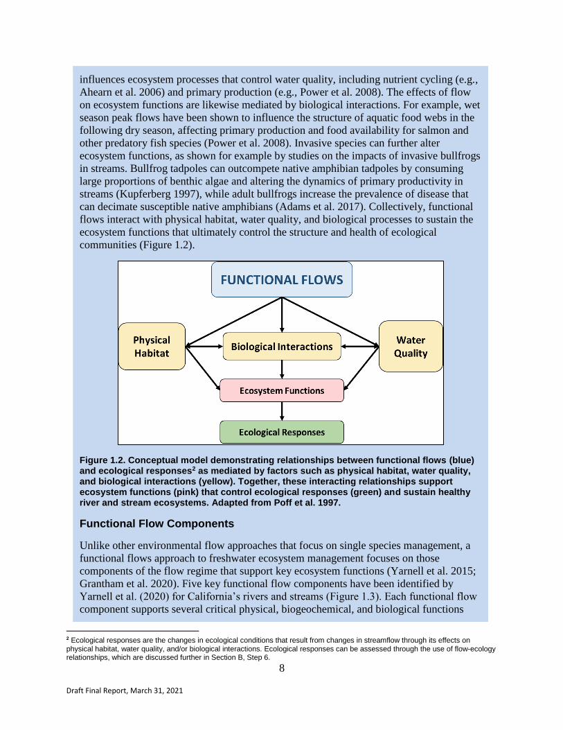
biological interactions (Figure 1.2). Flow interacts with the stream channel morphology

(i.e., channel type, size, shape, slope, and substrate) to create and maintain a nested

hierarchy of physical habitats (Frissell et al. 1986) through geomorphic processes such as

sediment transport, scour, deposition, and floodplain connectivity (Escobar-Arias and

Pasternack 2010; Wohl et al. 2015). Together with flow, physical habitat provides the

stream conditions necessary for native species to survive, grow, migrate, and reproduce.

Water quality also affects the health of aquatic ecosystems and impacts the number and

distribution of species in a stream (Nilsson and Renöfält 2008; Vidon et al. 2010). Flow

has a dominant influence on temperature, dissolved oxygen, and concentrations of

sediment and chemical constituents, including salts, nutrients, and contaminants, which

directly affect the health and survival of aquatic species (Yarnell et al. 2015). Flow

8


influences ecosystem processes that control water quality, including nutrient cycling (e.g.,

Ahearn et al. 2006) and primary production (e.g., Power et al. 2008). The effects of flow

on ecosystem functions are likewise mediated by biological interactions. For example, wet

season peak flows have been shown to influence the structure of aquatic food webs in the

following dry season, affecting primary production and food availability for salmon and

other predatory fish species (Power et al. 2008). Invasive species can further alter

ecosystem functions, as shown for example by studies on the impacts of invasive bullfrogs

in streams. Bullfrog tadpoles can outcompete native amphibian tadpoles by consuming

large proportions of benthic algae and altering the dynamics of primary productivity in

streams (Kupferberg 1997), while adult bullfrogs increase the prevalence of disease that

can decimate susceptible native amphibians (Adams et al. 2017). Collectively, functional

flows interact with physical habitat, water quality, and biological processes to sustain the

ecosystem functions that ultimately control the structure and health of ecological

communities (Figure 1.2).

Figure 1.2. Conceptual model demonstrating relationships between functional flows (blue) and ecological responses2 as mediated by factors such as physical habitat, water quality, and biological interactions (yellow). Together, these interacting relationships support ecosystem functions (pink) that control ecological responses (green) and sustain healthy river and stream ecosystems. Adapted from Poff et al. 1997.

Functional Flow Components

Unlike other environmental flow approaches that focus on single species management, a

functional flows approach to freshwater ecosystem management focuses on those

components of the flow regime that support key ecosystem functions (Yarnell et al. 2015;

Grantham et al. 2020). Five key functional flow components have been identified by

Yarnell et al. (2020) for California’s rivers and streams (Figure 1.3). Each functional flow

component supports several critical physical, biogeochemical, and biological functions

2 Ecological responses are the changes in ecological conditions that result from changes in streamflow through its effects on physical habitat, water quality, and/or biological interactions. Ecological responses can be assessed through the use of flow-ecology relationships, which are discussed further in Section B, Step 6.

9


that maintain stream ecosystem health and satisfy life history requirements of native

species. These ecosystem functions are briefly summarized below (see Table 1.1 for more

detailed descriptions of the ecosystem functions supported by each of the five functional

flow components):

● The fall pulse flow flushes fine sediment and organic material from stream

channels, increases river corridor connectivity, and rewets riparian zones. As the

hyporheic zone (the stream channel bed and underlying sediments) is reactivated,

exchange of nutrients occurs both vertically and laterally, increasing nutrient

cycling. Water quality conditions are improved with reduced temperatures and

increased dissolved oxygen, while lower salinity in estuaries and increased

streamflow signal native fish species to migrate upstream or spawn.

● Wet-season peak flows maintain and restructure river corridors by scouring the

river channel bed and banks and transporting substantial volumes of sediment and

large wood. Inundation of the floodplain recharges groundwater increases nutrient

cycling and the exchange of nutrients between the river channel and floodplain,

and provides breeding and rearing habitat for native fish. These flood disturbances

within the channel and floodplain reset riparian succession and limit the

establishment of non-native species, increasing native plant biodiversity through

time.

● The wet-season baseflow supports longitudinal connectivity through the river

network for fish migration and replenishes shallow groundwater in the riparian

zone. Higher wet season baseflows support increased hyporheic exchange and

salmonid egg incubation within riverbed gravels.

● The spring recession flow prolongs lateral and longitudinal connectivity into the

dry season, recharging groundwater, redistributing sediment within the river

channel, and maintaining cooler water temperatures. The gradual reduction in flow

creates a shifting mosaic of hydraulic conditions that supports high habitat

diversity and resulting aquatic species diversity. The spring recession further

provides reproductive and migratory cues for both aquatic and riparian species,

such as cues for amphibian spawning, fish outmigration, and riparian plant seed

dispersal and germination.

● The dry-season baseflow is critical for maintaining aquatic habitat for native

species through the summer period, not just in perennial streams, but also in

intermittent streams where contracted habitat conditions support native predators

and limit non-native species less tolerant of naturally low warm flows or periods of

no flow in the dry season.

10


Figure 1.3. Functional flow components for California depicted on a representative hydrograph. Blue line represents median (50th percentile) daily discharge. Gray shading represents 90th to 10th percentiles of daily discharge over the period of record.

Although the five natural functional components of flows are the same for all of

California’s rivers, their flow characteristics – magnitude, timing, frequency, duration, and

rate of change – vary regionally. For example, the spring recession flow component will

have a larger magnitude and longer duration for rivers in the Sierra Nevada than for rivers

in the South Coast. Characteristics of the functional flow components also vary by water

year type (e.g., wet, moderate, dry conditions). Thus, the functional flow components can

be quantified by a suite of functional flow metrics—quantitative measures of the flow

characteristics of each of the five functional flow components—that reflect the natural

diversity in flow characteristics throughout the state (Table 1.2; Yarnell et al. 2020;

Appendix A).

Based on a natural streamflow classification for California that categorizes the diversity of

flow regimes throughout the state (Lane et al. 2018; Appendix B), functional flow metrics

can be calculated for any annual hydrograph using algorithms developed by Patterson et

al. (2020; Appendix C).

11


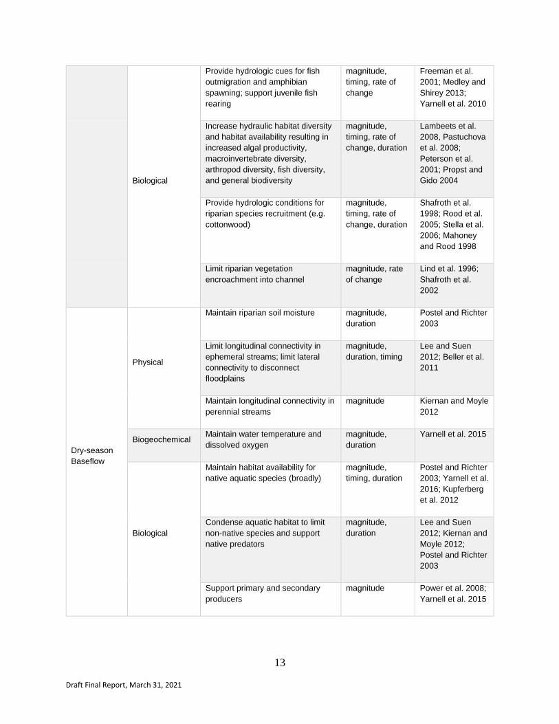
Table 1.2. Descriptions of the ecosystem functions that are supported by each of the five components of functional flows and the corresponding references in the scientific literature. References listed specifically link the associated flow characteristic with the ecosystem function.

Functional

Flow

Component

Type of

Ecosystem

Function

Supported Ecosystem Function

Associated

Flow

Characteristic

References

Fall Pulse

Flow

Physical

Flush fine sediment and organic

material from substrate

magnitude Postel and Richter

2003; Kemp et al.

2011

Increase longitudinal connectivity magnitude,

duration

Grantham 2013

Increase riparian soil moisture magnitude,

duration

Stubbington 2012

Biogeochemical

Flush organic material downstream

and increase nutrient cycling

magnitude,

duration

Ahearn et al. 2006

Modify salinity conditions in

estuaries

magnitude,

duration

Postel and Richter

2003

Reactivate exchanges/connectivity

with hyporheic zone

magnitude,

duration

Stubbington 2012

Decrease water temperature and

increase dissolved oxygen

magnitude,

duration

Yarnell et al. 2015

Biological

Support fish migration to spawning

areas

magnitude,

timing, rate of

change

Sommer et al.

2011; Kiernan et

al. 2012

Wet-season

Baseflow

Physical

Increase longitudinal connectivity magnitude,

duration

Grantham 2013;

Yarnell et al. 2020

Increase shallow groundwater

(riparian)

magnitude,

duration

Vidon et al. 2010

Biogeochemical Support hyporheic exchange magnitude,

duration

Stubbington 2012

Biological

Support migration, spawning, and

residency of aquatic organisms

magnitude Grantham 2013

Support channel margin riparian

habitat

magnitude Vidon et al. 2010

Wet-season

Peak Flows Physical

Scour and deposit sediments and

large wood in channel and

floodplains and overbank areas.

magnitude,

duration,

frequency

Ward 1998;

Florsheim and

Mount 2002;

Escobar-Arias and

12


Encompasses maintenance and

rejuvenation of physical habitat.

Pasternack 2010;

Wheaton et al.

2010; Senter et al.

2017

Increase lateral connectivity magnitude,

duration

Ward 1998,

Cienciala and

Pasternack 2017

Recharge groundwater

(floodplains)

magnitude,

duration

Opperman et al.

2017

Biogeochemical

Increase nutrient cycling on

floodplains

magnitude,

duration

Ahearn et al. 2006

Increase exchange of nutrients and

organic matter between floodplains

and channel

magnitude,

duration

Ahearn et al. 2006

Biological

Support fish spawning and rearing

in floodplains and overbank areas

magnitude,

duration, timing

Jeffres et al. 2008;

Opperman et al.

2017

Support plant biodiversity via

disturbance, riparian succession,

and extended inundation in

floodplains and overbank areas

magnitude,

duration,

frequency

Ward 1998;

Shafroth et al.

1998; Opperman

et al. 2017

Limit vegetation encroachment and

non-native aquatic species via

disturbance

magnitude,

frequency

Petts and Gurnell

2013; Kiernan and

Moyle 2012; Poole

and Berman 2001

Spring

Recession

Flow

Physical

Sorting of sediments via increased

sediment transport and size

selective deposition

magnitude, rate

of change

Hassan et al.

2006; Ashworth

1996; Madej 1999

Recharge groundwater

(floodplains)

magnitude,

duration

Opperman et al.

2017

Increase lateral and longitudinal

connectivity

magnitude,

duration

Ward and

Stanford 1995

Biogeochemical

Decrease water temperatures and

increase turbidity

duration, rate of

change

Leland 2003

Increase export of nutrients and

primary producers from floodplain

to channel

magnitude,

duration, rate of

change

Bowen et al. 2003;

Ward and

Stanford 1995

13


Biological

Provide hydrologic cues for fish

outmigration and amphibian

spawning; support juvenile fish

rearing

magnitude,

timing, rate of

change

Freeman et al.

2001; Medley and

Shirey 2013;

Yarnell et al. 2010

Increase hydraulic habitat diversity

and habitat availability resulting in

increased algal productivity,

macroinvertebrate diversity,

arthropod diversity, fish diversity,

and general biodiversity

magnitude,

timing, rate of

change, duration

Lambeets et al.

2008, Pastuchova

et al. 2008;

Peterson et al.

2001; Propst and

Gido 2004

Provide hydrologic conditions for

riparian species recruitment (e.g.

cottonwood)

magnitude,

timing, rate of

change, duration

Shafroth et al.

1998; Rood et al.

2005; Stella et al.

2006; Mahoney

and Rood 1998

Limit riparian vegetation

encroachment into channel

magnitude, rate

of change

Lind et al. 1996;

Shafroth et al.

2002

Dry-season

Baseflow

Physical

Maintain riparian soil moisture magnitude,

duration

Postel and Richter

2003

Limit longitudinal connectivity in

ephemeral streams; limit lateral

connectivity to disconnect

floodplains

magnitude,

duration, timing

Lee and Suen

2012; Beller et al.

2011

Maintain longitudinal connectivity in

perennial streams

magnitude Kiernan and Moyle

2012

Biogeochemical Maintain water temperature and

dissolved oxygen

magnitude,

duration

Yarnell et al. 2015

Biological

Maintain habitat availability for

native aquatic species (broadly)

magnitude,

timing, duration

Postel and Richter

2003; Yarnell et al.

2016; Kupferberg

et al. 2012

Condense aquatic habitat to limit

non-native species and support

native predators

magnitude,

duration

Lee and Suen

2012; Kiernan and

Moyle 2012;

Postel and Richter

2003

Support primary and secondary

producers

magnitude Power et al. 2008;

Yarnell et al. 2015

14


SECTION A – IDENTIFY ECOLOGICAL FLOW CRITERIA USING NATURAL

FUNCTIONAL FLOWS

Overview

The goal of Section A is to identify ecological flow criteria—expressed as metrics describing the

magnitude, timing, duration, frequency, and/or rate-of-change for five functional flow

components—that must be maintained to support healthy stream ecosystems in California

(Figure 2.1). These ecological flow criteria are based on functional flow metric values expected

to occur in the absence of existing and historic human activities (see Table 1.1 for an overview of

the functional flow metrics). The predicted, natural values of functional flow metrics can be

obtained from the California Natural Flows Database for locations of interest in any stream or

river in the state. Stakeholders—referred to as “the user” hereafter—then evaluate whether the

range of natural values for each functional flow component may fail to support ecosystem

functions due to the alteration of physical, biological, or water quality factors. The outcome of

that analysis determines whether the user selects ecological flow criteria for the five flow

components based on predicted natural flows and proceeds to Section C to develop

environmental flow recommendations, or proceeds to Section B to develop ecological flow

criteria for the subset of functional flow components for which natural flows are unlikely to

support essential ecosystem functions.

Figure 2.1. Steps in Section A of the California Environmental Flows Framework.

15


Section A has four steps (Figure 2.1). In Step 1, the user defines the study area and locations of

interest (LOIs) for establishing flow criteria, specifies ecological management goals, and

identifies the specific ecosystem functions that must be supported by ecological flow criteria to

satisfy those goals. In Step 2, the user characterizes natural functional flows at their LOIs by

obtaining predictions of the natural ranges of flow metrics from the California Natural Flows

Database or locally calibrated hydrologic model. In Step 3, the user evaluates whether there are

any physical, biological, or water quality factors that may limit the ability of natural functional

flows to support ecosystem functions. If non-flow factors may limit the effectiveness of the

natural range of flow metrics to support ecosystem functions for any flow component, further

analysis is required in Section B to define ecological flow criteria for these focal flow

components. In Step 4, the user selects ecological flow criteria based on the predicted natural

flow ranges for the functional flow components that do not require additional consideration. A

sample worksheet is provided in Figure 2.2 to illustrate what types of information are gathered in

Section A and how the information is linked in each step.



16


Figure 2.2. Sample worksheet providing a conceptual overview of the key pieces of information that are gathered during each step of Section A. An example of a completed worksheet is provided at the end of Section A (Figure A.4).

17


Step 1: Define ecological management goals

Objective: To identify ecological management goals for the study area and the corresponding

ecosystem functions that must be supported by ecological flow criteria to satisfy those goals

First, the user identifies their study area, which should be defined by watershed boundaries and

could include multiple watersheds, a single watershed, or a subwatershed.3 Ecological

management goals, which can be broad or qualitative in nature, for the study area should then be

specified. An assumption under the Framework is that the protection of general stream

ecosystem health will always be an overarching ecological management goal and that

maintenance of ecosystem functions associated with each of the functional flows components

will be required. However, ecological management goals can also express more specific

objectives that ecological flow criteria are intended to achieve. For example, goals may include

supporting the habitat and life history requirements of native fish species or maintaining

freshwater macroinvertebrate communities in good condition. When developing goals, the user

should also address legal requirements for listed species, water quality, or other biological

objectives expressed in applicable policies and regulations.

Next, the user identifies LOIs on which subsequent analyses will be performed. The Framework

requires that LOIs be specified at the stream-reach scale, defined by the USGS National

Hydrography Dataset Plus, medium resolution, version 2 (NHD). The NHD is a representation of

California’s stream network that includes over 100,000 unique stream reaches. Stream reaches

vary in size but are, on average, 2 km long. The LOIs selected by the user might include

locations with:

● a monitoring station, such as a streamflow gage

● the outlet of a river basin

● an infrastructure feature, such as point of diversion, discharge, or dam outlet

● a zone of ecological sensitivity, such as spawning reaches or critical habitat for listed

species

The selected LOIs might also include a set of reaches that are a representative sample of stream

classes within the study area (Lane et al. 2017; see also Appendix B). At the end of Step 1, the

user creates a study area map, depicting watershed boundaries, the stream network, and all LOIs.

Finally, the user identifies the specific ecosystem functions that must be supported by ecological

flow criteria to achieve ecological management goals. Table 1.2 documents a wide variety of

physical, biogeochemical, and biological functions associated with each functional flow

component, such as maintenance of fish spawning and rearing habitat, hydrologic connectivity,

sediment mobilization, and suitable dissolved oxygen and temperature levels. Under the

Framework, all functional flow components must be maintained to achieve ecological

management objectives. Therefore, the user should identify at least one ecosystem function in

3 We use the terms watershed and sub-watershed throughout this document to refer to discrete portions of the landscape that drain to a common water body or river. These terms are used interchangeably with basin and sub-basin, and do not refer to a specific size or scale.

https://nhdplus.com/NHDPlus/

18


Table 1.2 for each of the five functional flow components that are relevant to their ecological

management goals. This will help to ensure that the assessment considers the many functions

that flows support throughout the year to maintain ecosystem health.

Outcome of Step 1

A well-defined study area accompanied by a written description and map with watershed

boundaries, the stream network, and LOIs (stream reaches)

A list of LOIs with a short description of why they were selected

A list of ecological management goals

A list of ecosystem functions (associated with each functional flow component) that must

be supported by ecological flows to achieve ecological management goals

Example: Coastal Watershed in Northern California

In this hypothetical example, the study area encompasses a watershed in northern California

(Figure A.1). The watershed is 150 km2 in area and encompasses a stream network that is 200

km in total length. Two locations of interest have been identified in the study area, including

one located at a long-term flow gage (Figure A.1; Table A.1). Another LOI was selected at the

outlet of a tributary stream that is known to support high-quality salmon spawning and rearing

habitat.

Figure A.1. Map of hypothetical study area in a north coast California watershed, highlighting two locations of interest (red stream segments) and a flow gage.

19


Table A.1. Locations of interest for study area.

Location of Interest Reason for Selecting

1 Stream reach on tributary to mainstem river known to support high-quality salmon spawning and rearing habitat

2 Stream reach with long-term flow gage at which flow alteration can be assessed and environmental flow implementation monitored

The overall ecological management goal for the study area is to preserve stream health to

sustain salmon populations. Specific goals are to maintain juvenile salmon rearing habitat and

to protect passage flows for adult migration and smolt outmigration (Table A.2).

Table A.2. Ecological management goals.

Goals

Maintain stream ecosystem health

Maintain suitable habitat conditions for juvenile salmon rearing

Preserve passage flows during adult salmon migration and smolt outmigration

Using Table 1.2, a set of ecosystem functions needed to achieve ecological management goals

was selected from each of the five functional flow components (Table A.3).

Table A.3. Ecosystem functions that must be supported by ecological flows to satisfy ecological management goals in the study area.

Functional Flow Component Ecosystem Function(s)

Fall pulse flow Flush fine sediment and organic material from substrate, increase longitudinal hydrologic connectivity, increase nutrient cycling, decrease water temperature and increase dissolved oxygen, trigger fish migration

Wet-season baseflow Maintain longitudinal hydrologic connectivity, support hyporheic exchange, support riparian habitat along channel margins, support fish migration and spawning

Wet-season peak flows Scour and deposit sediment and large wood in channel and overbank zones, increase lateral hydrologic connectivity, support riparian vegetation diversity and health through disturbance and overbank inundation, limit non-native species and in-channel vegetation encroachment through disturbance and displacement

Spring recession flow Provide hydrologic cues for fish spawning and out-migration, support juvenile fish rearing, maintain hydraulic habitat diversity that supports diversity of aquatic plants and animals

Dry-season baseflow Limit warming of water, concentration of contaminants, and low dissolved oxygen, support algal growth and primary productivity, maintain habitat availability and connectivity for aquatic species

20


Step 2: Obtain natural ranges for functional flow metrics

Objective: To download natural functional flow metrics and characterize natural functional

flow components at locations of interest

Natural functional flow metrics can be viewed and downloaded at the California Natural Flows

Database for any stream segment in the state. Metrics are quantified as a range of values

expected to occur at LOIs under natural conditions over a long-term period of record (10 or more

years). The range of predicted metric values is defined by quantiles (the 10th, 25th, 50th, 75th, and

90th percentiles below which predicted values fall). In addition to reporting the expected range of

values for each metric across all years, predictions are also provided for wet, moderate and dry

water year types.4

How the California Natural Flows Database was developed

Statewide models have been developed to predict natural functional flows (Table 1.1) for all

stream reaches in California. The models rely on streamflow data from reference gages in

California located on streams with minimal disturbance to natural hydrology and land cover

(Falcone et al. 2010). Functional flow metrics were calculated at each reference gage from

daily flow values, using algorithms described by Patterson et al. (2020; Appendix C) based on

the natural streamflow classification for California (Lane et al. 2018; Appendix B). Separate

statistical models were then developed for each functional flow metric, using machine

learning methods to relate functional flow metric values to watershed characteristics,

following the approach described by Zimmerman et al. (2018). Additional details of the

modeling approach, input data, and performance evaluation are provided in Appendix D.

Once downloaded, the natural functional flow metrics should be summarized by flow

component. In the example below, natural flow metrics at a location of interest indicate that the

fall pulse flow is an event in which flows reach between 30 and 180 cfs for a period 2 to 7 days

between October 7 and October 28 (Table A.4). At this location, the natural dry season baseflow

period starts around June 20 (June 5-July 7), lasts for 151 (121 - 183) days and has a magnitude

of 10 (7-15) cfs. It may be helpful to plot predicted component ranges in relation to hydrographs

from a reference gage at or near LOIs (Figure A.2).5

If the user has a hydrologic model for their watershed, it may be preferable to calculate natural

functional flow metrics from the locally calibrated model. Functional flow metrics can be

calculated from time series of simulated daily flow timeseries of natural stream flow using the

functional flow calculator (Appendix K). Predicted values of the functional flow metrics should

be compiled in a format similar to that provided by the California Natural Flows Database before

proceeding to Step 3.

4 Water year types have been defined for all years between 1950-2015 at all stream segments by partitioning the range of predicted natural mean annual flow into terciles, reflecting dry (lower 33% of values), moderate (34%-65% of values), and wet (upper 33% of values) conditions. 5 Tools for exploring and visualizing flow data from California reference gages are available at https://eflows.ucdavis.edu

https://rivers.codefornature.org/#/home

https://rivers.codefornature.org/#/home

https://doi.org/10.1890/09-0889.1

https://doi.org/10.1016/j.jhydrol.2020.124787

https://doi.org/10.1111/fwb.13058

https://eflows.ucdavis.edu/

21


Outcome of Step 2

A table of natural functional flow metric values associated with each functional flow

component for each LOI, downloaded from the California Natural Flows Database or

calculated from a locally calibrated hydrologic model.


In Step 2, natural functional flow metric predictions are obtained for LOIs within the study

area. These data should be downloaded at rivers.codefornature.org and compiled in a table

for each LOI (Table A.4). These data can also be visualized graphically (Figure A.2).

Table A.4. Example of predicted flow metric values for five functional flow components (at location of interest 2), obtained from the California Natural Flows Database. Note: 16 of 24 natural functional flow metrics are included here for simplicity.

Flow Component Flow Metric

Predicted Range at LOI 1

median (10th - 90th percentile)

Predicted Range at LOI 2


Fall pulse flow

Fall pulse magnitude 9 (3 - 40) cfs 62 (30-180) cfs

Fall pulse timing Oct 19 (Oct 7 - Oct 29) Oct 20 (Oct 7 - Oct 28)

Fall pulse duration 3 (2 - 7) days 3 (2 - 7) days

Wet-season baseflow

Wet-season baseflow 34 (21 - 54) cfs 324 (260 - 410) cfs

Wet-season timing Nov 15 (Nov 1 - Dec 13) Nov 13 (Nov 3 - Nov 30)

Wet-season duration 162 (115 - 192) days 168 (145 - 184) days


5-year peak flow magnitude 870 (500 - 1000) cfs 3790 (3000 - 4800) cfs

5-year peak flow duration 3 (1 - 6) days 3 (1 - 6) days

5-year peak flow frequency 1 (1-3) events 1 (1-3) events


Spring recession magnitude 90 (34 - 267) cfs 520 (300 - 980) cfs

Spring timing Apr 25 (Mar 25 - May 20) Apr 28 (Apr 6 - May 14)

Spring duration 46 (29 - 98) days 50 (36 - 66) days

22


Spring rate of change 6 (3 - 10) % decline per day

6 (3 - 10) % decline per day

Dry-season baseflow

Dry-season baseflow 1 (0.5 - 2.5) cfs 10 (7 - 15) cfs

Dry-season timing June 17 (May 13 - Jul 20)

June 20 (June 5 - July 7)

Dry-season duration 160 (115 - 218) days 151 (121 - 183) days

Figure A.2. A hydrograph representing the range of daily flows observed at a flow gage in the study area and the start timing and magnitude of wet-season baseflow. The dark line represents the median gaged daily flow, the grey lines are the gaged daily flows for all years. The vertical blue bands show the range of variation (10th, 25th, 50th, 75th and 90th percentile) in wet-season start timing and the horizontal blue band shows the range of variation (10th, 25th, 50th, 75th and 90th percentile) in wet-season baseflow magnitude.

23


Step 3: Evaluate whether the natural ranges of function flow metrics will support functions needed to achieve ecological management goals

Objective: To perform an evaluation of factors that may limit the ability of the natural range of

functional flow metrics to support essential ecosystem functions

Maintaining functional flows within their natural range is hypothesized to support ecosystem

functions and sustain healthy ecosystem conditions for native freshwater species under natural

watershed conditions. However, historical and ongoing land- and water-management activities

have the potential to degrade the physical, chemical, and biological conditions of rivers and

streams, such that the natural ranges of functional flow metrics may be less effective in

supporting essential ecosystem functions. For example, channel widening may make it less likely

that natural baseflows can support in-channel pools that provide refugia for juvenile fish.

In this step, the user evaluates historical and ongoing land- and water-management activities that

may limit the effectiveness of the natural range of functional flow metrics in supporting

ecosystem functions (Table 2.1). The evaluation should focus on the potential influence of

physical habitat, water quality, and biological interactions on the relationship between natural

functional flows and ecosystem functions, identified in Step 1, that are essential to achieving

ecological management goals. The direct effects of flow alteration on ecosystem functions from

land and water management activities are not considered in this step, but are addressed in Section

C.

Table 2.1. Examples of land- and water-management impacts that may limit the effectiveness of the natural range of functional flow metrics in supporting ecosystem functions.

Mediating factor Example Land- and Water-Management Impacts

Physical habitat Altered sediment supply, channel incision, channelization, levees, bank stabilization, bed armoring, impoundments, barriers

Water quality Altered temperature patterns, low dissolved oxygen, high conductivity, high concentrations of contaminants, excess fine sediment, excess nutrients

Biological interactions Non-native species predation or competition, parasitism, limited food supply, vegetation encroachment, altered wood supply

This step does not require a rigorous quantitative analysis, but rather encourages the user to

appraise if alteration of non-flow conditions may undermine ecological management goals. For

example, consider a stream reach below a large dam that has modified both the physical

conditions of the river channel and downstream water temperatures. By blocking sediment

movement and altering the downstream flow regime, the dam has changed the shape of the river

from a shallow, meandering, wide channel, with flows often connected to the floodplain, to a

deep, incised, narrow channel, now disconnected from the floodplain. In this case, the ecosystem

functions that depend upon floodplain inundation – controlled by wet season peak flows – are

compromised by channel incision. Thus, the channel may need higher magnitude peak flows

than estimated under natural conditions to access the floodplain. Similarly, the temperature

regime of the river may have been modified as a result of water releases from the reservoir. For

24


example, dam releases during the dry season may be higher or lower than natural temperatures,

depending on the depth of where water is drawn from the reservoir. In this case, the magnitude

of the natural dry-season baseflow may be inadequate for sustaining temperatures within the

tolerance range of species of concern (e.g., juvenile salmon). Flow releases above or below the

natural range may be required to sustain desired temperatures.

There may also be circumstances in which additional flow metrics may be needed to ensure that

ecological management goals are satisfied. For example, hydropeaking operations at a dam may

result in sub-daily alteration of river flow that can impact ecological function but not be captured

by the functional flow metrics. In this case, the user should work through Section B to evaluate

the appropriate functional flow component(s) and construct one or more conceptual models and

flow-ecology relationships that address additional flow metrics (e.g., coefficient of variation of

daily flow, Richards-Baker flashiness index).

The evaluation of natural functional flows in relation to ecosystem functions should be

performed as a high-level exercise, in which potential limiting factors are considered for each

target function. In the dammed river example described above, the user would evaluate the

specific ecosystem functions for each component and may determine that the natural range of

flows are expected to support functions associated with the fall pulse flow, wet-season baseflow,

and spring flow recession. However, downstream channel incision may limit the effectiveness of

natural wet season peak flows in supporting floodplain functions and temperature alteration may

limit the effectiveness of natural dry season baseflows in supporting fish rearing habitat.

Therefore, further investigation should be performed (in Steps 5-7 of Section B) to develop

ecological flow criteria for wet-season peak flows and dry season baseflow. Since current

conditions at the sites are not expected to impair the functions of the fall pulse flow, wet-season

baseflow, and the spring flow recession, the natural range of functional flow metrics for those

components can be selected as ecological flow criteria (in Step 4).

In many cases, it will not be possible to directly assess the current condition of mediating factors

and their potential to alter the relationship between flows and ecosystem functions. However, an

evaluation of land use within the watershed can provide indirect evidence of impairment from

non-flow factors. For example, urbanization is frequently associated with stream channelization,

riparian vegetation removal, and water quality impairment, while agriculture often increases fine

sediment inputs to streams, limits floodplain connectivity, and impairs water quality from runoff

containing fertilizers, pesticides, herbicides, and manure. Lands subject to intensive grazing are

prone to soil compaction, mass wasting, erosion, increased nutrient loads, and declines in

riparian and instream habitat quality and diversity. Because of these known associations between

land use and river ecosystem impacts, assessing land use patterns can help identify potential

limiting factors to ecosystem functions and those focal components that warrant additional

consideration in Section B.

Outcome of Step 3

Identification of functional flow components where there is evidence that their natural

range of flow metrics will not be supportive of ecological management goals, and a list of

associated limiting factors and potentially affected ecosystem function(s); these focal

components will be subject to further investigation in Section B to develop their

corresponding ecological flow criteria.

25



This step involves a high-level evaluation of factors that can alter the relationships between

natural functional flows and ecosystem functions. For the North Coast stream example, no

limiting factors are identified for the ecosystem functions associated with the five functional

flow components for LOI 1. However, one potential limiting factor is identified for the dry

season baseflow component in LOI 2 (Table A.5). Specifically, altered stream morphology

from intensive logging activity in the upper watershed is identified as a potential limiting

factor to juvenile salmonid habitat for rearing in the dry season. Logging activity has

increased sedimentation, reduced riparian cover, and decreased woody debris recruitment

which has resulted in decreased channel complexity, wider stream channels, and reduced

riparian vegetation cover downstream. Natural dry season baseflows may not be adequate to

protect water temperature and provide depths suitable for rearing under these altered

conditions. As a result, further investigation is needed (in Section B) to assess the dry season

baseflows that will support ecosystem functions at LOI 2 to achieve ecological management

objectives.

Table A.5. The potential limiting factors that may alter the relationship between the natural range of functional flow metrics and their intended functions for each functional flow component at locations of interest.

Functional Flow Component Potential Limiting Factor Affected Ecosystem Function(s)

Fall pulse flow None identified None

Wet-season baseflow None identified None

Wet-season peak flows None identified None

Spring recession flow None identified None

Dry-season baseflow

Altered channel morphology and riparian vegetation condition from historic logging activity (at LOI 2)

Potential warming of water and limited habitat availability for juvenile salmonid rearing

26


Step 4: Select ecological flow criteria

Objective: To select ecological flow criteria for all functional flow components (unless it is

determined in Step 3 that further assessment is required for one or more components) to support

ecological management goals using natural functional flow metrics

Ecological flow criteria are selected for all functional flow components for which the natural

range of metrics is expected to support ecosystem functions. These ecological flow criteria are

defined by a median and bounded range of metric values for each flow component. The median

represents the long-term value around which a metric is expected to center. The 10th to 90th

percentiles represent the lower and upper bounds, respectively, in which the metric is expected to

vary. For example, ecological flow criteria for the dry-season baseflow would be specified by

median, 10th, and 90th percentile values of flow magnitude, timing, and duration. The annual

values of these metrics are expected to vary under natural conditions, but over many years, are

expected to be distributed around the predicted median value. The 10th and 90th percentiles of the

ecological flow criteria represent an interval between which annual values of a metric are

expected in fall in most years. This interval is accounts for both inter-annual variation in the

metric as well as model prediction uncertainty.

Ecological flow criteria can be defined for all water years, or by water year type. The median,

10th, and 90th percentile values of flow metrics have been calculated for dry, moderate, and wet

water year types. Once selected, ecological flow criteria should be organized by flow component

and compiled in a table for each LOI in the study area (Table A.6). Note that ecological flow

criteria will not be selected for those functional flow components identified in Step 3 that require

additional consideration; criteria for those components will be developed in Steps 5-7 in Section

B.

If the user desires greater certainty that ecological flow criteria will support ecological

management goals when they are established as environmental flow recommendations (Section

C), actions to monitor their effectiveness should be included in the Implementation Plan (Step

12).

Outcome of Step 4

Ecological flow criteria values for functional flow components where the natural range of

functional flow metrics are expected to support ecological management goals

27



Following the assessment in Step 3, ecological flow criteria based on the natural functional

flow metrics are selected for all five functional flow components for LOI 1 and for all

components except dry-season baseflow for LOI 2 (Table A.6, Figure A.3). At LOI 2, altered

geomorphic and water quality conditions may limit the ecosystem functions associated with

natural dry season baseflows (Table A.5). Therefore, the dry-season baseflow component for

LOI 2 requires further investigation in Section B before ecological flow criteria can be

specified.

Table A.6. Ecological flow criteria for functional flow components at locations of interest.

Flow Component Flow Metric

Ecological Flow Criteria at LOI 1


Ecological Flow Criteria at LOI 2


Fall pulse flow




Wet-season baseflow




Wet-season peak flows 5-year peak flow magnitude

870 (500 - 1000) cfs 3790 (3000 - 4800) cfs


5-year flood frequency 1 (1-3) event 1 (1-3) event

28



Spring recession magnitude

90 (34 - 267) cfs 520 (300 - 980) cfs





Dry-season baseflow

Dry-season baseflow 1 (0.5 - 2.5) cfs To be determined in Section B

Dry-season timing June 17 (May 13 - Jul 20) To be determined in Section B

Dry-season duration 160 (115 - 218) days To be determined in Section B

Figure A.3. Ecological flow criteria for functional flow components at LOI 2, displayed in blue, plotted against a median gaged water year (black line) and displaying mean daily flow over the

29


entire gaged period of record (shaded gray). Dry season baseflow is shown in orange. Ecological flow criteria for this functional flow component will be developed in Section B.

Outcome of Section A for North Coast Example

At the end of Section A, ecological flow criteria are selected for LOI 1 based on the range of

natural functional flows (Table A.6). The natural range of functional flows are also used to

establish ecological flow criteria at LOI 2, with the exception of criteria for dry-season

baseflow. The dry-season baseflow requires further evaluation in Section B because of the

potential for physical habitat and water quality degradation to alter the relationship between

flow and ecosystem functions in the dry season.

For an overview of all of the information obtained in Section A for this North Coast

watershed, see Figure A.4.

Outcome of Section A

After completing Steps 1 to 4 in Section A, the user will have defined ecological management

goals for their study region and identified the ecosystem functions needed to achieve them. The

outcome of Section A will be a set of ecological flow criteria derived from natural functional

flow metrics that characterize the natural variability in flow that supports essential ecosystem

functions. The user will also have evaluated whether there are non-flow mediating factors that

could limit the effectiveness of the natural range of functional flow metrics in supporting

ecosystem functions. If limiting factors are identified for one or more flow components, the user

should proceed to Section B to develop ecological flow criteria for those focal component(s).

30


STEP 1: What are my location(s)

of interest (LOI) and my

rationale for selection?

Hypothetical north coast watershed LOI 2: Stream reach with long-term flow gage at which flow alteration can be assessed and

environmental flow implementation monitored. This LOI has been affected by historical logging activity which may reduce its suitability

for salmon rearing and migration

STEP 1: What are the ecological

management goals at my LOI?

1. Maintain stream health needed to support salmon populations 2. Maintain suitable habitat conditions for juvenile salmon rearing 3. Preserve passage flows during adult salmon migration and smolt outmigration

STEP 1: Which ecosystem

functions do I need to support to

achieve my ecological

management goals?

Five functional flow components for my LOI

Fall pulse flow Wet-season baseflow Wet-season peak flows Spring recession flow Dry-season baseflow

Flush fine sediment

and organic material

from substrate,

increase longitudinal

hydrologic connectivity,

increase nutrient

cycling, decrease water

temperature and

increase dissolved

oxygen, trigger fish

migration

Maintain longitudinal


support hyporheic

exchange, support

riparian habitat along

channel margins, support

fish migration and

spawning

Scour and deposit

sediment and large wood

in channel and overbank

zones, increase lateral


support riparian

vegetation diversity and

health through

disturbance and

overbank inundation, limit

non-native species and

in-channel vegetation

encroachment through

disturbance and

displacement

Provide hydrologic cues

for fish spawning and

out-migration, support

juvenile fish rearing,

maintain hydraulic

habitat diversity that

supports diversity of

aquatic plants and

animals

Limit warming of water,

concentration of

contaminants, and low

dissolved oxygen,

support algal growth

and primary

productivity, maintain

habitat availability and

connectivity for aquatic

species

STEP 2: What are the natural

ranges for functional flow

components (i.e., functional

flow metrics) at my LOI?

Fall pulse magnitude

62 (30-180) cfs

Fall pulse timing

Oct 20 (Oct 7 - Oct 28)

Fall pulse duration

3 (2 - 7) days

Wet-season baseflow

324 (260 - 410) cfs

Wet-season timing

Nov 13 (Nov 3 - Nov 30)

Wet-season duration 168

(145 - 184) days

5-year peak flow

magnitude

3790 (3000 - 4800) cfs

5-year peak flow duration

3 (1 - 6) days

5-year peak flow

frequency

1 (1-3) events

Spring recession

magnitude

520 (300 - 980) cfs

Spring timing

Apr 28 (Apr 6 - May 14)

Spring duration

50 (36 - 66) days

Dry-season baseflow

10 (7 - 15) cfs

Dry-season timing

June 20 (June 5 - July

7)

Dry-season duration

151 (121 - 183) days

31


Spring rate of change 6

(3 - 10) % decline per

day

STEP 3: What are the functional

flow components for which

ecosystems functions may not

be supported by the natural

range of functional flows due to

alterations of physical, biological

or water quality factors?

None identified None identified None identified None identified

Potential Limiting

Factor

Altered channel

morphology and

riparian vegetation

condition from historic

logging activity

Affected Ecosystem

Function

Potential warming of

water and limited

habitat availability for

juvenile salmonid

rearing

STEP 4: What are the ecological

flow criteria for the functional

flow components that do not

require additional consideration?

Fall pulse magnitude

62 (30-180) cfs

Fall pulse timing

Oct 20 (Oct 7 - Oct 28)

Fall pulse duration

3 (2 - 7) days

Wet-season baseflow

324 (260 - 410) cfs

Wet-season timing

Nov 13 (Nov 3 - Nov 30)

Wet-season duration 168

(145 - 184) days

5-year peak flow

magnitude

3790 (3000 - 4800) cfs

5-year peak flow duration

3 (1 - 6) days

5-year peak flow

frequency

1 (1-3) events

Spring recession

magnitude

520 (300 - 980) cfs

Spring timing

Apr 28 (Apr 6 - May 14)

Spring duration

50 (36 - 66) days

Spring rate of change 6

(3 - 10) % decline per

day

(to be determined in

Section B)

Figure A.4. The sample worksheet shown in Figure 2.2, filled in with the information for the Example watershed.

32


SECTION B – DEVELOP ECOLOGICAL FLOW CRITERIA FOR FOCAL FLOW

COMPONENTS REQUIRING ADDITIONAL CONSIDERATION

Overview

Section B is necessary if the ecological management goals (identified in Step 1) would not be

expected to be met by the natural ranges of flow metrics for one or more flow components. If the

user determines in Section A that the natural ranges of flow metrics can be used to develop

ecological flow criteria for all five functional flow components, the user skips Section B and

proceeds to Section C. However, where alteration of non-flow factors (e.g., physical habitat,

water quality, or biologic conditions) limit the ability of the natural ranges for flow metrics to

support desired ecological functions and achieve ecological management goals (Step 3), further

analysis for these functional flow component(s) is completed in Section B.

In Section B, the user performs a detailed analysis of the linkages between flow, physical habitat,

water quality, and biological interactions to develop ecological flow criteria for the functional

flow components requiring additional consideration. At the end of Section B, these criteria are

combined with those developed in Section A to define a full set of ecological flow criteria

associated with all functional flow components (Figure 3.1).

Section B begins with developing a conceptual model that links the functional flow components

requiring additional consideration—referred to as focal functional flow components—to

ecological management goals (Step 5). This involves specifying the direct and indirect pathways

in which changes in flow metrics can affect ecological responses. Next, the various pathways

within the conceptual model are quantified using either existing flow-ecology relationships or

analytical methods that rely on existing data or data generated from site-specific studies (Step 6).

The outcome of Step 6 is one or more flow-ecology relationships that quantify how changes in

functional flow components and associated flow metrics affect ecological responses of interest,

accounting for mediating factors such as water quality, physical habitat, and biological

interactions. In Step 7, the user evaluates the flow-ecology relationships to identify a targeted

range of flow metrics and define ecological flow criteria for the focal functional flow

components. These ecological flow criteria are then combined with those defined in Section A to

establish a full set of ecological flow criteria for all five functional flow components required to

achieve ecological management goals.

Section B requires general knowledge of the ecology and hydrology of the study area and

familiarity with the technical methods used to quantify flow-ecology relationships. General

guidance on constructing and quantifying conceptual models is included in Steps 5 and 6;

however, these steps do not provide specific guidance on which mediating factors and ecosystem

functions should be included in conceptual models, which tools should be used to quantify

relationships, or how simple or complex of a model is appropriate for a given location. Decisions

on how to structure the conceptual models and apply tools and quantitative methods will have a

significant influence on the quality and nature of the results, and as such, should be developed

through an open, collaborative process informed by experts and multiple stakeholders.

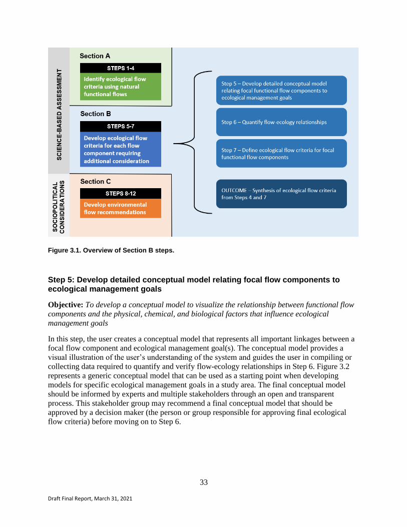
33


Figure 3.1. Overview of Section B steps.

Step 5: Develop detailed conceptual model relating focal flow components to ecological management goals

Objective: To develop a conceptual model to visualize the relationship between functional flow

components and the physical, chemical, and biological factors that influence ecological

management goals

In this step, the user creates a conceptual model that represents all important linkages between a

focal flow component and ecological management goal(s). The conceptual model provides a

visual illustration of the user’s understanding of the system and guides the user in compiling or

collecting data required to quantify and verify flow-ecology relationships in Step 6. Figure 3.2

represents a generic conceptual model that can be used as a starting point when developing

models for specific ecological management goals in a study area. The final conceptual model

should be informed by experts and multiple stakeholders through an open and transparent

process. This stakeholder group may recommend a final conceptual model that should be

approved by a decision maker (the person or group responsible for approving final ecological

flow criteria) before moving on to Step 6.

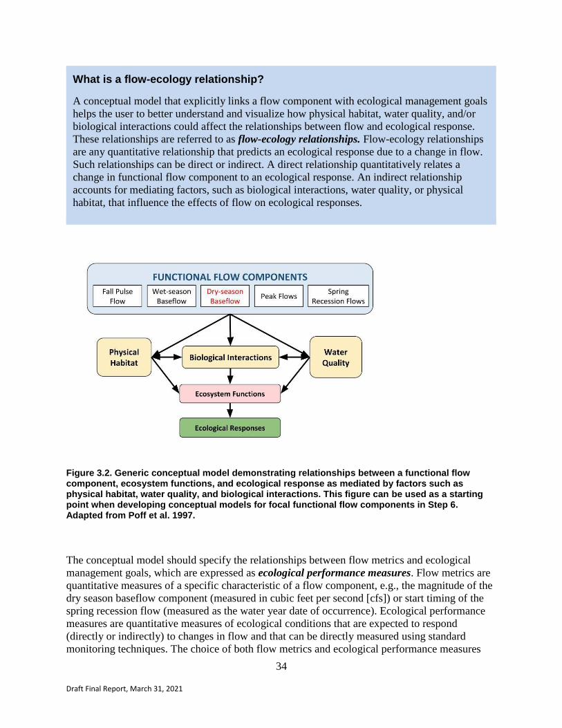
34


What is a flow-ecology relationship?

A conceptual model that explicitly links a flow component with ecological management goals

helps the user to better understand and visualize how physical habitat, water quality, and/or

biological interactions could affect the relationships between flow and ecological response.

These relationships are referred to as flow-ecology relationships. Flow-ecology relationships

are any quantitative relationship that predicts an ecological response due to a change in flow.

Such relationships can be direct or indirect. A direct relationship quantitatively relates a

change in functional flow component to an ecological response. An indirect relationship

accounts for mediating factors, such as biological interactions, water quality, or physical

habitat, that influence the effects of flow on ecological responses.

Figure 3.2. Generic conceptual model demonstrating relationships between a functional flow component, ecosystem functions, and ecological response as mediated by factors such as physical habitat, water quality, and biological interactions. This figure can be used as a starting point when developing conceptual models for focal functional flow components in Step 6. Adapted from Poff et al. 1997.

The conceptual model should specify the relationships between flow metrics and ecological

management goals, which are expressed as ecological performance measures. Flow metrics are

quantitative measures of a specific characteristic of a flow component, e.g., the magnitude of the

dry season baseflow component (measured in cubic feet per second [cfs]) or start timing of the

spring recession flow (measured as the water year date of occurrence). Ecological performance

measures are quantitative measures of ecological conditions that are expected to respond

(directly or indirectly) to changes in flow and that can be directly measured using standard

monitoring techniques. The choice of both flow metrics and ecological performance measures

35


should be guided by the ecological management goal, knowledge of the study area, and available

data. For example, if an ecological management goal for a study area is the maintenance of a

healthy macroinvertebrate community, biological indicators such as the California Stream

Condition Index (CSCI) can be used as an ecological performance measure. The CSCI is a

statewide biological scoring index that is applied to samples of macroinvertebrates, which are

regularly collected in streams as part of a statewide monitoring program. The CSCI translates

information about benthic macroinvertebrates living in a stream into an overall measure of

stream health (Rehn et al. 2015), enabling ecological performance measures to be specified as a

range of desired CSCI values. Performance measures for listed species might be measured by

population targets or recruitment rates. Ecological performance measures could also be specified

for intermediate links in the conceptual model, such as geomorphic processes or water quality

parameters including dissolved oxygen, temperature, and contaminants. However, performance

measures for intermediate links should be paired with measures for ecological responses.

The conceptual model should also include mediating factors that are likely to influence the

relationship between flow metrics and ecological performance measures (identified in Section A,

Step 3). These may include, but are not limited to, physical habitat factors, water quality

conditions, and biological interactions (see box). This conceptual model is intended to illustrate

flow ecology relationships, not the possibility of implementing non-flow actions (e.g., habitat

restoration). Trade-offs between implementing flow and non-flow actions can be explored in

Section C, if appropriate.

Mediating factors in flow-ecology relationships

Flow metrics and ecological performance measures often have one or more mediating factors

that influence the flow-ecology relationship. These mediating factors can be categorized by

physical habitat conditions, water quality, or biological interactions (Figure A.5).

The physical form and structure of rivers and floodplains interacts with flow to influence

ecological responses. In particular, channel morphology (i.e., channel type, size, shape, slope,

and substrate) determines how flow is expressed as hydraulic conditions (water depth and

velocity). Many species have distinct preferences for depths and velocities (Bovee 1986) as

well as tolerance thresholds (e.g., related to the swimming ability of tadpoles (Kupferberg et

al. 2012) or juvenile salmon (Katzman et al. 2010)). Hydraulic habitat preferences may differ

at different life stages (e.g., Gard 2006; Yarnell et al. 2016). However, hydraulic tolerances

and preferences often hold across different stream types, flow regimes, and geomorphic

conditions, and thus can be useful for evaluating habitat suitability within and across diverse

geographic areas (Nestler et al. 2019).

Water quality affects the health of aquatic ecosystems by controlling the condition, survival,

and distribution of freshwater species. Many water quality parameters that species are

sensitive to are influenced by flows. These include water temperature, salinity (often

measured by specific conductance), nutrients, dissolved oxygen (DO), and dissolved organic

carbon (DOC) (Nilsson and Renöfält 2008). Therefore, it may be necessary to include these or

https://paperpile.com/c/aVQYgy/xeir

https://paperpile.com/c/aVQYgy/juMH

https://paperpile.com/c/aVQYgy/juMH

https://paperpile.com/c/aVQYgy/9L92

https://paperpile.com/c/aVQYgy/fvhV+RPE4

https://paperpile.com/c/aVQYgy/E2gZ

36


other water quality parameters in conceptual models that link changes in flow to ecological

responses.

Biological interactions also have the potential to influence ecological responses to changes in

flow. For example, the presence of non-native species could affect the response of native

species to streamflow through competition, predation, or habitat alteration (Doubledee et al.

2003; Adams et al. 2017). Biological interactions can also directly influence ecosystem

functions, such as primary production, which can have a significant influence on the growth,

survival and health of target species (e.g., Kupferberg 1997).

Additional information on suggested data sources, tools, and methods for determining flow-

ecology relationships are provided in Step 6 and Appendix E.

Outcome of Step 5

A detailed conceptual model for each LOI (or study area, if it includes multiple LOIs that

can be addressed by the same conceptual model) that illustrates the flow-ecology

relationships that influence ecological responses and management goals expressed as

ecological performance measures. A separate conceptual model is required for each

functional flow component that is addressed in Section B.


Continuing the example from Section A, altered stream morphology from intensive logging

activity in the upper watershed was identified as a potential limiting factor to juvenile

salmonid habitat for rearing during the dry season at LOI 2. The effects of physical habitat

alteration on rearing salmon were expressed through two mediating factors. First, stream

channel widening and degradation of riparian vegetation has increased solar radiation to the

channel, potentially increasing water temperatures beyond the tolerance limits of juvenile

salmon. Second, logging activity has widened the stream channel such that natural dry season

baseflows may not be adequate to provide depths suitable for rearing juvenile salmon.

The user determined that the two mediating factors would only influence one characteristic of

dry-season baseflow: flow magnitude. Mediating factors were not expected to alter the

relationship between dry-season duration or timing and ecological management goals;

therefore, the natural ranges of duration and timing were specified for these two flow

characteristics (with values obtained from Section A). The user examined the life history

stages and timing for salmon and determined that only the juvenile life history stage would be

affected by dry season baseflow magnitude. The user chose juvenile salmon growth and

survival rates as two ecological performance measures relevant to the ecological management

goal of supporting healthy salmon populations.

https://paperpile.com/c/aVQYgy/Q1gj+M6Kr

https://paperpile.com/c/aVQYgy/Q1gj+M6Kr

37


The conceptual model for the system captures the effects of the two mediating factors by

linking (1) dry-season baseflow magnitude to water temperature and salmon physiology, and

(2) dry-season baseflow magnitude to water depths and velocities and juvenile salmon

hydraulic habitat preferences (Figure A.5). Both pathways ultimately affect growth and

survival of juvenile salmon.

Figure A.5. Conceptual model linking the focal flow component in a coastal watershed in Northern California (dry-season baseflow) with mediating factors, ecosystem functions (as defined in Table A.3), and ecological performance measures that relate to the ecological management goal of healthy salmon populations.

Step 6: Quantify flow-ecology relationships

Objective: To quantify flow-ecology relationships in the conceptual model using provided

guidance on data sources and methods for defining these relationships

Using the conceptual model as a guide, the user collects any existing flow criteria and data from

previous studies (i.e., site-specific studies conducted for the LOI or comparable watersheds) that

might provide insights into flow-ecology relationships for the study area. The user first evaluates

any existing flow criteria or documented ecological relationships and determines whether they

are applicable for the study area. If not available, the user then compiles existing data for

components of the conceptual model. Suggested datasets and repositories are provided in

Appendix E. If relationships in the conceptual model cannot be quantified using existing data,

the user may choose to quantify the relationship by designing a study to collect new data. If

38


resources are not available to collect new data, the user may choose to quantify relationships

based on expert knowledge that is elicited following standard methodologies (see below).

Incorporating flow-ecology relationships from existing flow criteria

Flow criteria may exist for the user’s study area or LOI. For example, for streams that have been

identified as high priority for the State (e.g., through the California Water Action Plan or Public

Resources Code 10000), the California Department of Fish and Wildlife (CDFW) has conducted

studies to develop flow criteria (CDFW 2020). Current and completed instream flow studies and

recommended ecological flow criteria can be found on CDFW’s Instream Flow Studies page.

When reviewing existing flow criteria, the user ensures that they will be adequate to achieve

desired ecological management goals or address additional management concerns. Specifically,

the user considers whether the criteria:

● consider one or more of the focal functional flow components

● are conceptually linked to ecosystem functions in streams and ecological management

goals

● have been developed in a comparable physical setting or watershed context to the study

area and/or LOI

For example, an instream flow study might focus on winter spawning flow needs, which

correspond to the wet-season baseflow functional flow component. Findings of the flow study

could be used to establish ecological flow criteria for wet-season baseflow magnitude, but other

sources of information and/or data analysis may be required to develop ecological flow criteria

for other baseflow characteristics (timing, duration) or other focal flow components addressed in

Section B.

Developing flow-ecology relationships from new and/or existing data

Whether relying on new or existing data, there are a wide variety of approaches that can be used

to quantify flow-ecology relationships; these methods have been extensively described, reviewed

and categorized (e.g., Arthington 2012; Williams et al. 2019). Although many methods do not

specifically address functional flows, some approaches may help to develop ecological flow

criteria from some functional flow components and/or characteristics. There are three key

guiding principles for selecting methods for developing flow-ecology relationships:

● The methods should be appropriate for, and relevant to, assessing the relationship

between ecological management goals defined in Step 1 and functional flow components.

● The methods should be chosen based on the conceptual model of the relationships

between each flow component and ecological performance measures. In the case that

there are many mediating factors important to a flow-ecology relationship, two or more

complementary methods may be needed.

https://paperpile.com/c/aVQYgy/hMV6

https://www.wildlife.ca.gov/Conservation/Watersheds/Instream-Flow/Studies

39


● The final method (or set of methods) should quantify each link in the conceptual model.

An example of flow-ecology relationships with geomorphology and hydraulics as

mediating factors is shown in Appendix G.

40


Developing flow-ecology relationships by expert opinion

If existing flow criteria or data are not available, and resources are not sufficient to collect new

data, the user may quantify flow-ecology relationships using expert elicitation. Expert elicitation

is often used in conservation decision-making (Martin et al. 2012) and can be rigorous if

information is elicited using established methods (Burgman 2016). The most frequently used

method is the Delphi process (Runge et al. 2011; Mukherjee et al. 2015), which is a structured

approach to identifying experts, eliciting quantitative values independently, allowing for

discussion and revision of initial values, and applying statistical methods to calculate means and

confidence intervals across experts.

Tools for quantifying indirect flow-ecology relationships

While there are countless methods available for quantifying and evaluating flow-ecology

relationships that include mediating factors, certain categories of tools will be frequently used.

Physical form and structure: When stream hydraulics (variation in depth and velocity) have

a significant effect on ecological responses, models are used to simulate changes in hydraulics

over a range of flows. Such models require topographic data of the channels, as well as

measurements of water level (or stage) across a range of flows for model training and

validation.6 Hydraulic model outputs are then paired with assessments of hydraulic habitat

preferences for one or more species (or life history stage) to predict how habitat suitability

changes in response to flow7. Hydraulic models can also be coupled with sediment transport

models to simulate physical processes that create and redistribute habitat for target species.

Often, such physical habitat assessments identify an optimal flow value that maximizes

suitable habitat for a given life stage for the species of interest, such as salmon spawning

habitat. However, to link physical habitat to ecological performance measures, additional

work may be needed. For example, if performance metrics are juvenile salmon growth and

survival, additional analytical steps may be needed to assess how stream hydraulics affect

food resources (e.g., using bioenergetics models).

Water-quality parameters: Water quality parameters that influence ecological responses

include temperature, turbidity/clarity, DO, contaminants, and others. When water quality is a

mediating factor, modeling the response of the water quality metric to a range of flows is

necessary. For example, low flows are often associated with high temperatures that may be

detrimental to ecological management goals. In this case, a temperature model is necessary to

determine how water temperature is expected to respond to a change in flow conditions. The

results of a water quality model can then be compared to physiological temperature

thresholds, such as those published by USEPA (2003), to quantify ecological responses.

Biological species interactions: Biological conditions that may mediate flow-ecology

relationships include food supply (instream or in off-channel habitat), predator-prey

interactions, and abundance of non-native species that may compete with natives for habitat

6 Appendix F provides a geomorphic classification for several regions of the State of California. This information can be used to develop hydraulic response relationships, as described in Appendix G. 7 Appendix H provides functional flow requirements for umbrella fish species that represent native fish communities across regions in California. Appendix I describes functional flow metrics that are best correlated with stream health condition as quantified by the California Stream Conditions Index. This information can be used in developing flow-ecology relationships.

https://paperpile.com/c/aVQYgy/5YQ5a

https://paperpile.com/c/aVQYgy/SIv7

https://paperpile.com/c/aVQYgy/Lhetk+tq9ki

41


and food. For example, the relative abundance of non-native fish to native species often

changes in response to flow (Feyrer and Healey 2003; Kiernan et al. 2012), and these

relationships should be incorporated in the conceptual model using statistical methods to

predict ecological responses.

Outcome of Step 6

Quantitative flow-ecology relationships that relate focal functional flow components to

ecological responses


In Step 6, it was determined that there were no flow criteria from previous studies that can be

used to relate dry season baseflow to juvenile growth and survival; however, resources were

available to conduct site-specific hydraulic and temperature modeling (Figure A.6). For the

first conceptual model pathway, a temperature model was used to evaluate changes in weekly

maximum and weekly mean temperatures over the same flow range as evaluated by the

hydraulic model. Optimal temperature ranges for juvenile salmon growth and survival

depends on food supply. Optimal range is 13०-20०C for unlimited food and 10०-16०C with

limited food (USEPA 2003). Data were lacking on food supply, so a target of 13०-16०C was

chosen to overlap the two food supply states. Results from the temperature model showed that

a dry-season baseflow magnitude of at least 22 cfs would be required to achieve optimal

temperature conditions.

For the second conceptual model pathway, a hydraulic model was used to evaluate changes in

water depth and velocity over a wide range of dry season baseflow scenarios, and then habitat

suitability criteria were applied to the modeling results to estimate salmon rearing habitat

availability over the flow range. Using a model that was developed to link rearing habitat

availability to juvenile growth and survival, it was determined that dry-season baseflow

magnitude in the range of 17-23 cfs would provide habitat conditions that would achieve

ecological management goals.

The two modeling efforts resulted in different flow criteria to achieve desired levels of

juvenile growth and survival. However, the results suggest that a dry-season baseflow

magnitude of 22-23 cfs during the period that juvenile salmon are rearing would satisfy both

temperature and physical habitat requirements.

https://paperpile.com/c/aVQYgy/cTUK3

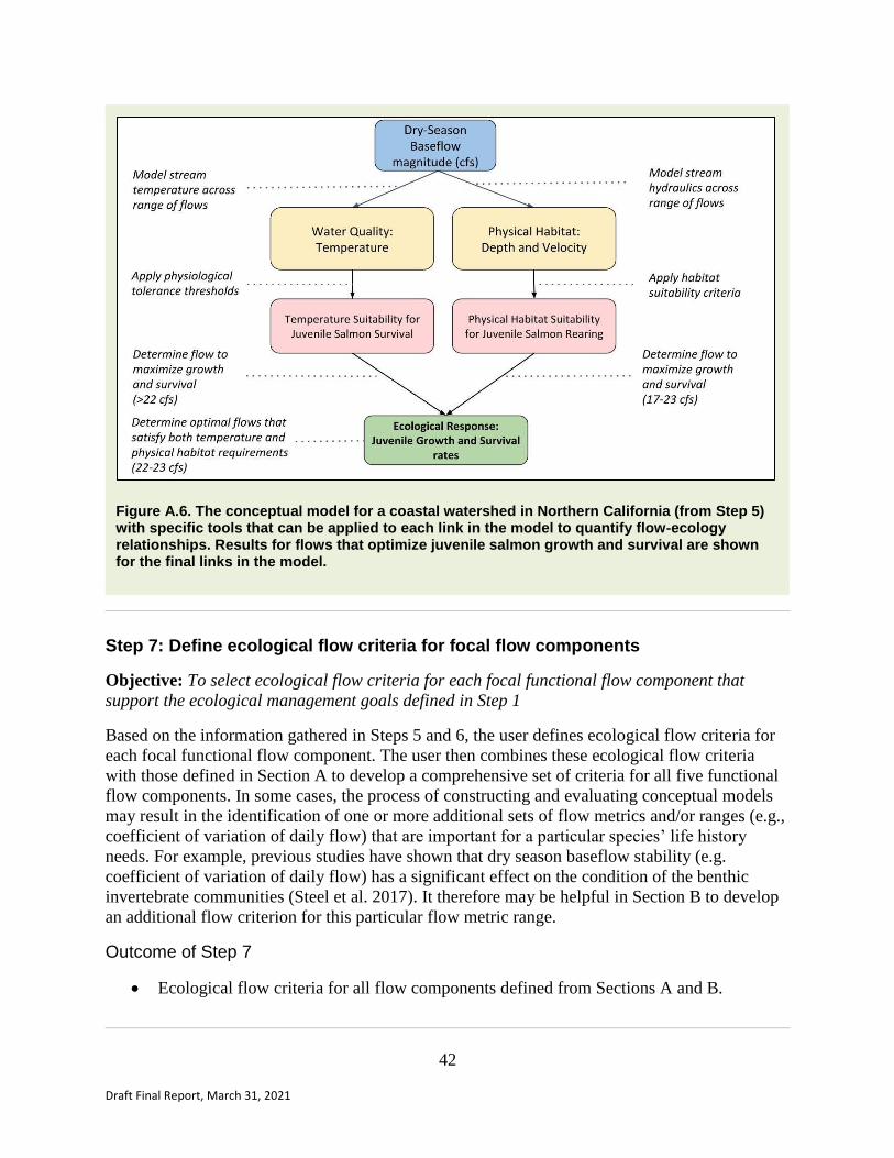
42


Figure A.6. The conceptual model for a coastal watershed in Northern California (from Step 5) with specific tools that can be applied to each link in the model to quantify flow-ecology relationships. Results for flows that optimize juvenile salmon growth and survival are shown for the final links in the model.

Step 7: Define ecological flow criteria for focal flow components

Objective: To select ecological flow criteria for each focal functional flow component that

support the ecological management goals defined in Step 1

Based on the information gathered in Steps 5 and 6, the user defines ecological flow criteria for

each focal functional flow component. The user then combines these ecological flow criteria

with those defined in Section A to develop a comprehensive set of criteria for all five functional

flow components. In some cases, the process of constructing and evaluating conceptual models

may result in the identification of one or more additional sets of flow metrics and/or ranges (e.g.,

coefficient of variation of daily flow) that are important for a particular species’ life history

needs. For example, previous studies have shown that dry season baseflow stability (e.g.

coefficient of variation of daily flow) has a significant effect on the condition of the benthic

invertebrate communities (Steel et al. 2017). It therefore may be helpful in Section B to develop

an additional flow criterion for this particular flow metric range.

Outcome of Step 7

Ecological flow criteria for all flow components defined from Sections A and B.

43



Using the results of Step 6, the range of 22-23 cfs was defined as an ecological flow criterion

for dry-season baseflow magnitude.8 Natural functional flow metric values for dry-season

timing and duration were accepted as flow criteria in Step 5. The full table (Table A.7) of

ecological flow criteria for all five functional flow components and a corresponding

ecological flow regime (Figure A.7) is shown below.

Table A.7. Example of ecological flow criteria for all functional flow components (at locations of interest 1 and 2). All flow criteria were selected from the natural range of flow metrics identified in Section A, except for the dry-season baseflow magnitude that was determined in the Section B site-specific analyses.

Flow Component Flow Metric Ecological Flow Criteria

at LOI 1

median (10th - 90th

percentile)

Ecological Flow Criteria

at LOI 2

median (10th - 90th

percentile)

Fall pulse flow




Wet-season baseflow




Wet-season peak flows 5-year peak flow

magnitude

870 (500 - 1000) cfs 3790 (3000 - 4800) cfs


5-year peak flow

frequency

1 (1-3) event(s) 1 (1-3) event(s)


Spring recession

magnitude

90 (34 - 267) cfs 520 (300 - 980) cfs



Spring rate of change 6 (3 - 10) % decline per

day

6 (3 - 10) % decline per

day

Dry-season baseflow 1 (0.5 - 2.5) cfs 22-23 cfs

8 Note that the values differ from the predicted natural functional flow range of 7-15 cfs and a median of 10 cfs

44


Dry-season baseflow Dry-season timing June 17 (May 13 - Jul 20) June 20 (June 5 - July 7)

Dry-season duration 160 (115 - 218) days 151 (121 - 183) days

Figure A.7. Ecological flow regime developed from the ecological flow criteria presented in Table A.7. Note that only dry-season baseflow magnitude was determined in Section B, while all other criteria were selected from the natural range of functional flow metrics identified in Section A.

Outcome of Section B

The outcome of Section B is a full set of ecological flow criteria that include the natural ranges

of flow metrics for some functional flow components (Section A) and ecological flow criteria

developed in this section for the focal functional flow components evaluated in Steps 5-7. Flow

criteria will be defined for all LOIs within a study area, with their specific values compiled in

tables and visualized as ecological flow regimes.

45


SECTION C – DEVELOPING ENVIRONMENTAL FLOW RECOMMENDATIONS

Overview

Section C outlines a process for developing environmental flow recommendations that balance

ecological management goals with other non-ecological water management objectives, such as

those prioritized for human use. This section represents a transition from a scientific process in

which ecological flow criteria are developed (Sections A and B) to a process that incorporates

social values, and other management needs, including human uses of water, public health and

safety needs, and legal and regulatory requirements (Figure 4.1). In Section C, the user should be

continuing to engage stakeholders (including traditionally underrepresented groups) to guide the

development of a final set of environmental flow recommendations, along with an

implementation plan for their study area, in collaboration with agency partners.

Section C follows a structured decision-making process. Structured Decision Making (Figure

4.2) and, in general, the field of Multi-Criteria Decision Analysis (e.g., Gregory and Keeney

2002; Runge et al. 2011) offer a systematic framework to guide development of environmental

flow recommendations that are characterized by trade-offs and uncertainty. Section C begins

with defining specific and quantifiable management objectives and the legal, regulatory and

social context in which environmental flow recommendations are to be developed (Step 8). This

section also evaluates existing flow conditions relative to ecological flow criteria to understand

the changes in management that may be required (Step 9). Next, a set of management

alternatives hypothesized to satisfy all management objectives are developed, and the

consequences of each alternative—including trade-offs among objectives—are assessed (Step

10). Then, a preferred management alternative is selected, and environmental flow

recommendations defined (Step 11). Finally, an implementation plan is developed (Step 12). The

plan should include feedback mechanisms to guide future refinement of environmental flow

recommendations, following an adaptive management approach (Figure 4.2).

Because users must take into account numerous sociopolitical considerations that are often site-

specific and non-scientific, Section C provides less prescriptive guidance than Sections A and B.

Instead, Section C is intended to offer a conceptual framework, including suggested tools, to help

the user appropriately balance ecological and non-ecological management objectives to develop

a set of environmental flow recommendations. These recommendations should consider all

relevant regulatory requirements and stakeholder priorities. Implementation guidelines will be

developed in the future in response to specific issues and based on lessons learned from early

applications of the Framework.

46


Figure 4.1. Overview of Section C steps.

Figure 4.2. A Structured Decision-Making process for developing and implementing environmental flow recommendations, adapted from Failing et al. (2013). Associated Framework Steps 8-12 are indicated in blue.

47


Step 8: Identify management objectives

Objective: To identify the full set of management objectives that should be considered in

determining environmental flow recommendations, including both ecological management goals

(from Step 1) and non-ecological management goals, in addition to any regulatory requirements

Clarify the decision context

Consideration of relevant federal, statewide, and local laws and policies related to beneficial

uses, streamflow and ecological conditions is important in helping the user understand how

existing policy and legal conditions may be used to support the implementation of environmental

flow recommendations. In California, existing laws, policies and processes focused on water

quality, water supply, and habitat often also relate to environmental flows. Some, but not all,

regulations that should be considered include:

State and federal Endangered Species Acts, which prohibit unauthorized “take” of

threatened and endangered species through factors including habitat and hydrologic

alteration

Federal Clean Water Act and State Porter Cologne Act, which establish the beneficial use

for fish and wildlife preservation and enhancement, and the procedure to apply for a

water right for instream use

The Federal Energy Regulatory Commission (FERC) relicensing process, which provides

the opportunity to negotiate dam operations to facilitate ecological flows for species of

interest

California Fish and Game Code 5937, which requires that dam operators release

sufficient water to keep fish below dams in good condition

Sustainable Groundwater Management Act (SGMA) - which require consideration of

“undesirable results” associated depletions of interconnected surface water that have

significant and unreasonable adverse impacts on beneficial uses of the surface water

caused by groundwater conditions occurring throughout the basin, such as effects on the

ability to support priority species.

Recycled Water Policy - encourages the safe use of recycled water from wastewater

sources in a way that meets state and federal water quality laws, protects public health

and the environment, such as making sure to substitute the use of surface

water/groundwater sources with recycled water, and reassuring that the reduction in the

wastewater treatment discharge does not affect the water quantity or quality that support

freshwater ecosystems.

State water rights law (including Water Code Section 106), which may affect

environmental flows recommendations due to competing or senior water rights

48


Other local ordinances that may constrain environmental flow implementation (e.g.,

stormwater management, wastewater discharge requirements)

Identify management objectives and measures

The ecological flow criteria developed in Sections A and B support the ecological management

goals for a study area. Development of environmental flow recommendations, however, also

requires consideration of non-ecological management goals, which may broadly include meeting

municipal and agricultural water demands, generating hydropower, flood management,

eliminating or reducing nuisance dry weather flows, discharging wastewater outflow, and

providing water for recreational purposes. When identifying specific and quantifiable non-

ecological management objectives, the user also identifies the responsible agencies or

stakeholders associated with these objectives within their geographic area, and the requirements

that the agencies must fulfill. These agencies or stakeholders should be involved in the objective-

setting process, with the user expressing management objectives as a desired outcome that

includes associated performance measures (i.e., the same strategy used in Step 6 for ecological

management goals). Specific agency mandates and regulations should be considered when

developing management objectives; however, consistency and compliance with these regulations

will be determined by each relevant agency.

Outcome of Step 8

● A full set of management objectives, that incorporate both ecological and non-ecological

water management goals, and associated performance measures

● Relevant regulatory requirements necessary to evaluate management objectives

● List of key stakeholders and a process for ongoing stakeholder engagement


Continuing the example from Sections A and B, it was determined that LOI 1 had no non-

ecological water management goals, and that the ecological flow criteria at this location are

accepted as environmental flow recommendations. However, there are competing

management objectives for LOI 2 – specifically, satisfying the water needs of domestic and

agricultural water users in the watershed (Table A.8).

Table A.8. Non-ecological Water Management Goals for LOI 2.

Non-ecological Management Goal Performance Measure

Meet domestic and agricultural surface water use needs in the area of interest

Proportion of monthly water demand satisfied for domestic and agricultural water users

49


It was also determined that the following regulations should be considered when developing

environmental flow recommendations for LOI 2:

● Lake and Streambed Alteration Agreement (LSA): Agreements would be

necessary for the construction of diversion structure.

● Federal and California Endangered Species Act (ESA) authorization: Review and

authorization under federal and State ESA would be required if diversions may affect

species or habitats protected under the Acts.

● Section 404 and 401 Clean Water Act permits: Federal Clean Water Act permits

would be required for construction and maintenance of diversion structures.

As part of Step 8, the following stakeholders were also identified for inclusion in the process

of developing environmental flow recommendations:

● Local landowners

● Local irrigation district

● Local environmental NGOs

● California Department of Fish and Wildlife

● Local Resource Conservation District

Step 9. Assess flow alteration

Objective: To evaluate whether flow conditions at the location(s) of interest (LOI) are likely

unaltered, likely altered, or indeterminate by comparing present-day ranges of functional flow

metrics for functional flow components to the ecological flow criteria defined in Step 7

Compare present-day conditions to ecological flow criteria

First, the user compares current hydrologic conditions at the LOI to ecological flow criteria to

assess whether current conditions are likely altered, likely unaltered, or indeterminate. If current

conditions are altered relative to flow conditions in the absence of all human activity, the user

proceeds to Steps 10-12, including evaluating opportunities to modify existing management

practices to reduce alteration (Step 10), developing environmental flow recommendations that

consider the need to balance ecological and non-ecological management objectives (Step 11),

and identifying mitigation measures to reduce the effects of altered flow (Steps 11 and 12). For

detailed methods on this analysis, see Appendix J.

The assessment consists of the following steps (which are intended for non-peak flow metrics

only):

50


1. Obtain the list of ecological flow criteria for each functional flow metric range at the

LOI (outputs of Sections A and B, defined in Step 7)

2. Obtain current, daily flow data at each LOI from gage stations or hydrologic models

3. Quantify values for functional flow metrics based on current conditions using the

functional flow calculator at https://eflows.ucdavis.edu/hydrology (Appendix K)

4. Assess hydrologic alteration to identify which metrics do not currently meet the

ecological flow criteria and quantify the direction and degree of alteration. This can be

done for all years combined or by water year type if there is sufficient data.

Then, the user evaluates whether local observed flow conditions are likely unaltered, likely

altered, or indeterminate by comparing present-day functional flow metric ranges to the

ecological flow criteria defined in Step 7. A flow alteration assessment approach has been

developed for applications in which a user compares observed ranges of flow with predicted,

natural ranges of functional flow metrics obtained from the California Natural Flows Database

(Appendix J). In such cases, flow alteration status is determined according to the following rules

(Figure 4.3):

● Current conditions are likely unaltered if the median observed value falls within the 10th

to 90th percentile range of the ecological flow criteria and greater than 50% of the

observations fall inside of the 10th to 90th percentile range.

● Current conditions are likely altered if the median observed value falls outside the 10th to

90th percentile range of the ecological flow criteria.

● Alteration is indeterminate if the median observed value falls within the 10th to 90th

percentile range of the ecological flow criteria but less than 50% of observed values fall

within the 10th to 90th percentile range.

Figure 4.3. Alteration assessment determination for a functional flow metric. Predicted natural ranges for functional flow metrics (in red) represent the ecological flow criteria at a LOI against which observed values (in blue) are compared. The box and whiskers plots represent the range

https://eflows.ucdavis.edu/hydrology


51


(10th, 25th, 50th, 75th, and 90th percentiles) of predicted and observed values for the functional flow metric.

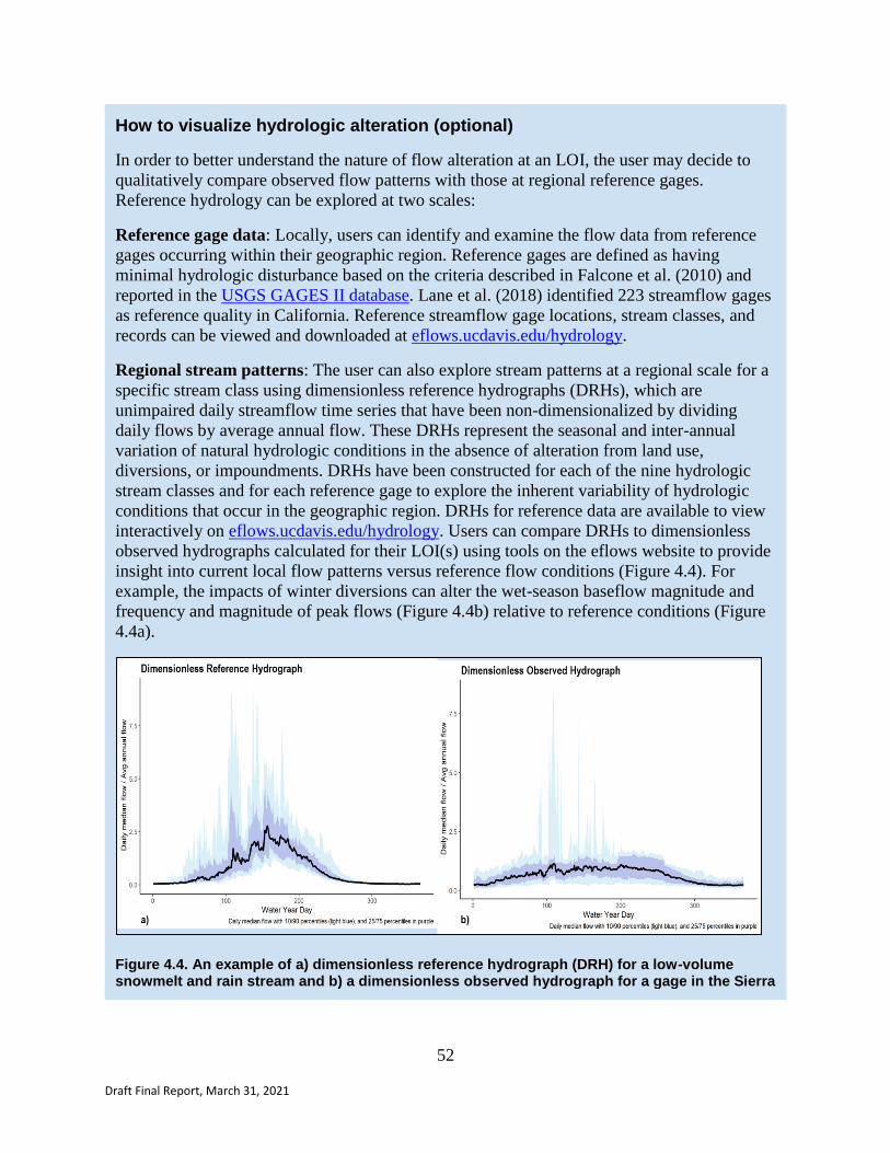
52


How to visualize hydrologic alteration (optional)

In order to better understand the nature of flow alteration at an LOI, the user may decide to

qualitatively compare observed flow patterns with those at regional reference gages.

Reference hydrology can be explored at two scales:

Reference gage data: Locally, users can identify and examine the flow data from reference

gages occurring within their geographic region. Reference gages are defined as having

minimal hydrologic disturbance based on the criteria described in Falcone et al. (2010) and

reported in the USGS GAGES II database. Lane et al. (2018) identified 223 streamflow gages

as reference quality in California. Reference streamflow gage locations, stream classes, and

records can be viewed and downloaded at eflows.ucdavis.edu/hydrology.

Regional stream patterns: The user can also explore stream patterns at a regional scale for a

specific stream class using dimensionless reference hydrographs (DRHs), which are

unimpaired daily streamflow time series that have been non-dimensionalized by dividing

daily flows by average annual flow. These DRHs represent the seasonal and inter-annual

variation of natural hydrologic conditions in the absence of alteration from land use,

diversions, or impoundments. DRHs have been constructed for each of the nine hydrologic

stream classes and for each reference gage to explore the inherent variability of hydrologic

conditions that occur in the geographic region. DRHs for reference data are available to view

interactively on eflows.ucdavis.edu/hydrology. Users can compare DRHs to dimensionless

observed hydrographs calculated for their LOI(s) using tools on the eflows website to provide

insight into current local flow patterns versus reference flow conditions (Figure 4.4). For

example, the impacts of winter diversions can alter the wet-season baseflow magnitude and

frequency and magnitude of peak flows (Figure 4.4b) relative to reference conditions (Figure

4.4a).

Figure 4.4. An example of a) dimensionless reference hydrograph (DRH) for a low-volume snowmelt and rain stream and b) a dimensionless observed hydrograph for a gage in the Sierra

https://water.usgs.gov/GIS/metadata/usgswrd/XML/gagesII_Sept2011.xml

http://eflows.ucdavis.edu/hydrology

http://eflows.ucdavis.edu/hydrology

53


Nevada where flows are altered due to a diversion dam. Both figures were calculated and output from eflows.ucdavis.edu/hydrology.

If different hydrologic models are used to assess current and predicted, natural flows, the user

may develop alternative rule sets to classify alteration status. However, in all cases, a functional

flow component should be considered altered if any of its functional flow metrics are likely

altered.

Identify likely causes of alteration

Once patterns of alteration are assessed, the user identifies potential causes of alteration that can

be addressed by management interventions. Sources of alteration may be near the LOI or further

upstream, and can include factors such as physical alteration of the stream channel, controlled

discharges, diversions, impoundments, groundwater withdrawals, or land use practices. Users

may consult the State Water Board’s eWRIMS water rights database and consult with local

agency staff regarding sources of diversions. For each potential source of alteration, the user

should identify the potential mechanisms responsible for altered flow. Understanding the

relationship between the source of alteration, the effect on functional flow components, and

related effects on ecosystem functions will support evaluation of measures to reduce impacts and

assess tradeoffs between ecological and non-ecological management objectives. To the extent

possible, this analysis should also attempt to account for anticipated changes in future flows

associated with climate change based on the best available local projections and models.

Outcome of Step 9

● Determination of which functional flow metrics and functional flow components are

altered

● Comparison of current and reference annual hydrology using dimensionless hydrographs

(optional)

● Identification of likely causes of hydrologic alteration


An alteration assessment was conducted on all functional flow components at LOI 2. It was

determined that only dry-season baseflow was altered. Current summer baseflow magnitudes

were found to be substantially lower (5-7 cfs) than the ecological flow criteria (22-23 cfs)

(Table A.9). It was further determined that the difference between current conditions and the

criteria was the result of stream widening and sparse vegetation (caused by historic logging

activity), such that higher flows are needed to maintain desired temperatures. The impacts of

upstream diversions were also impacting streamflow in the dry season by depleting dry season

baseflows.

https://eflows.ucdavis.edu/hydrology

54


Table A.9. Results of alteration assessment for LOI 2. All components were found to be likely unaltered except the dry-season baseflow. Note: The natural range of functional flows for dry-season baseflow magnitude at LOI 2 was estimated to be 7-15 cfs.

Flow

Component Flow Metric

Ecological

Flow Criteria

Current

Conditions

Alteration

Status

Likely Source

of Alteration

Dry-season

baseflow

Dry-season

baseflow

22-23 cfs

(determined in

Step 7) 5 - 7 cfs likely altered

stream

widening

creates need

for higher

baseflow;

upstream

diversions

reduce flow

magnitude

Dry-season

timing

June 20 (June 5

- July 7)

June 10 - July

15 indeterminate

uncertain

source of

alteration

Dry-season

duration

151 (121 - 183)

days 125 - 185 days likely unaltered not applicable

Step 10. Evaluate management scenarios and assess tradeoffs

Objective: To explore non-flow and flow-based strategies to satisfy ecological flow criteria,

quantify the ecological consequences of failing to satisfy ecological flow criteria, and propose

mitigation measures to offset impacts, if any

Environmental flow recommendations incorporate multiple competing objectives for water and

may require balancing of competing uses. There is rarely a single, optimal set of flow

recommendations that will satisfy all needs, or equally distribute impacts. Ecological flow

criteria represent one possible environmental flow recommendation that achieves ecological

management objectives but that potentially disregards other management needs. Environmental

flow recommendations that deviate from ecological flow criteria may satisfy other management

needs, but risk failure in achieving ecological management objectives. There are countless

possible environmental flow recommendations that entail different tradeoffs among management

objectives; however, there is likely to be a discrete set of scenarios that are potentially acceptable

to stakeholders and require detailed evaluation.

Propose and simulate alternative management scenarios

Identify non-flow management actions

The user, in coordination with agency staff and local stakeholders, identifies a set of non-flow

actions that have the potential to satisfy all management objectives for the study area, including

55


both ecological and non-ecological management goals. These actions may include direct channel

modifications, changes in land use, or riparian revegetation, among others, that will make it

possible to achieve ecological flow criteria while satisfying other management needs.

Identify flow-based management actions

If non-flow actions cannot satisfy ecological flow criteria, flow-based management alternatives

should also be considered. In this case, the user identifies flow-management strategies that

minimize deviance from the ecological flow criteria. These strategies include changes to existing

water management practices (e.g., reservoir re-operations, adjusted wastewater releases,

diversion scheduling, etc.) that attempt to satisfy ecological flow criteria while minimizing or

avoiding adverse effects to other non-ecological management objectives.

If proposed changes to management practices allow users to meet ecological flow criteria while

satisfying other non-ecological management objectives, then the environmental flow

recommendations will be the same as ecological flow criteria. However, if proposed actions do

not allow users to satisfy ecological flow criteria without significantly compromising other non-

ecological management objectives, alternative environmental flow recommendations that deviate

from ecological flow criteria should be identified.

Evaluate consequences and assess management tradeoffs

Any environmental flow recommendation may have consequences for both ecological and non-

ecological management goals. For example, adoption of ecological flow criteria from Section B

could require consideration of alternative flow diversion practices to meet agricultural water

needs. Many quantitative tools, including mechanistic models, statistical relationships, water

allocation models, cost-benefit analyses, life-cycle models, infrastructure planning, or social

(system dynamics) models among others, may be used to predict the outcomes and consequences

of implementing alternative management scenarios for each management objective. As part of

the Framework, we do not recommend or advocate for any specific approach; the choice of

approach is case-specific and should be made as part of the stakeholder process. Similarly, it is

beyond the scope of this document to provide a comprehensive review of available tradeoff

approaches.

Quantify tradeoffs

Once alternative environmental flow scenarios have been assessed, the user assesses tradeoffs

among management objectives for each alternative. Multi-Criteria Decision Analysis (MCDA)

provides a useful approach for quantifying tradeoffs and can include simple checklists, tradeoff

curves, optimization models, and other quantitative predictions. Tradeoff assessment should

consider options for maximizing certain benefits during specific times of the year or under

specific climatic conditions (i.e., wet years vs. dry years). Appendix L describes one example of

a decision support system and collaborative MCDA modeling approach to assist managers and

stakeholders in assessing tradeoffs and developing environmental flow recommendations that

achieve an acceptable balance among competing management objectives.

Outcome of Step 10

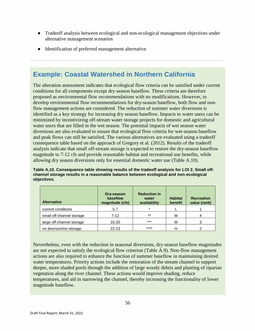
56


● Tradeoff analysis between ecological and non-ecological management objectives under

alternative management scenarios

● Identification of preferred management alternative


The alteration assessment indicates that ecological flow criteria can be satisfied under current

conditions for all components except dry-season baseflow. These criteria are therefore

proposed as environmental flow recommendations with no modifications. However, to

develop environmental flow recommendations for dry-season baseflow, both flow and non-

flow management actions are considered. The reduction of summer water diversions is

identified as a key strategy for increasing dry season baseflow. Impacts to water users can be

minimized by incentivizing off-stream water storage projects for domestic and agricultural

water users that are filled in the wet season. The potential impacts of wet season water

diversions are also evaluated to ensure that ecological flow criteria for wet-season baseflow

and peak flows can still be satisfied. The various alternatives are evaluated using a tradeoff

consequence table based on the approach of Gregory et al. (2012). Results of the tradeoff

analysis indicate that small off-stream storage is expected to restore the dry-season baseflow

magnitude to 7-12 cfs and provide reasonable habitat and recreational use benefits, while

allowing dry season diversions only for essential domestic water use (Table A.10).

Table A.10. Consequence table showing results of the tradeoff analysis for LOI 2. Small off-channel storage results in a reasonable balance between ecological and non-ecological objectives.

Alternative

Dry-season baseflow

magnitude (cfs)

Reduction in water

availability Habitat benefit

Recreation value (rank)

current conditions 5-7 * L 1

small off-channel storage 7-12 ** M 4

large off-channel storage 15-20 *** M 3

no diversion/no storage 22-23 **** H 2

Nevertheless, even with the reduction in seasonal diversions, dry-season baseflow magnitudes

are not expected to satisfy the ecological flow criterion (Table A.9). Non-flow management

actions are also required to enhance the function of summer baseflow in maintaining desired

water temperatures. Priority actions include the restoration of the stream channel to support

deeper, more shaded pools through the addition of large woody debris and planting of riparian

vegetation along the river channel. These actions would improve shading, reduce

temperatures, and aid in narrowing the channel, thereby increasing the functionality of lower

magnitude baseflow.

57


58


Step 11. Define environmental flow recommendations

Objective: To select a preferred management alternative set of environmental flow

recommendations in collaboration with stakeholders and agency partners based on the results

from the previous 10 steps, and then to develop the final set of environmental flow

recommendations

In Step 11, the user defines final environmental flow recommendations that account for both

human and ecological objectives. For some functional flow metrics, the environmental flow

recommendations and the ecological flow criteria will be the same, but they may differ in cases

where management trade-offs cannot be avoided. As mentioned previously, balancing among

management objectives is a process driven by social values and interpretation of regulatory

requirements, and it will need to account for ecological, economic, social, and public safety

considerations, among others. Multiple stakeholders, including relevant State agencies, should be

involved in selecting final environmental flow recommendations.

Final environmental flow recommendations should also include measures that enhance the

effectiveness of flow in support of ecosystem functions and habitat for target species, especially

when recommendations deviate from ecological flow criteria. Mitigation measures might include

riparian revegetation to reduce temperature through shading, channel grading to reconnect

floodplains and off-channel habitats, or invasive species control. Mitigation measures should be

included in the implementation plan developed in Step 12.

Outcome of Step 11

● Final set of environmental flow recommendations

● List of measures to enhance the effectiveness of environmental flows or mitigate adverse

effects (if final recommendations deviate from ecological flow criteria)


In Step 7, it was determined that dry-season baseflow should be 22-23 cfs to meet

temperature, water depth, and velocity needs of salmonids under current conditions. However,

it is not possible to increase dry season baseflows over the natural reference range via

diversion restrictions. A range of 7-12 cfs is established as the environmental flow

recommendation for dry-season baseflow magnitude. In addition, the stream restoration

measures identified in Step 10 are recommended to improve habitat conditions for salmonids

by narrowing the channel, deepening pools, and recovering riparian vegetation to enhance the

functionality of the lower baseflow magnitude.

Table A.11 summarizes the environmental flow recommendations for LOI 2. Ecological flow

criteria are used to establish flow recommendations for LOI 1 because there are no non-

ecological management goals for this LOI. For most components and metrics at LOI 2, the

environmental flow recommendations and the ecological flow criteria (defined in Step 7) are

59


the same, but they differ for dry-season baseflow magnitude based on the results from Steps

8-10.

Table A.11. Environmental Flow Recommendations for LOI 2. Note that environmental flow recommendations are the same as ecological flow criteria for all but dry-season baseflow magnitude.

Functional Flow Component Flow Characteristic Ecological Flow Criteria

Environmental Flow Recommendation

Fall pulse flow

Fall pulse magnitude 62 (30-180) cfs 62 (30-180) cfs



Wet-season baseflow


Wet-season timing Nov 13 (Nov 3 - Nov 30) Nov 13 (Nov 3 - Nov 30)



5-year peak flow magnitude 3790 (3000 - 4800) cfs 3790 (3000 - 4800) cfs


5-year peak flow

frequency

1 (1-3) event(s) 1 (1-3) event(s)


Spring recession magnitude 520 (300 - 980) cfs 520 (300 - 980) cfs

Spring timing Apr 28 (Apr 6 - May 14) Apr 28 (Apr 6 - May 14)




Dry-season baseflow

Dry-season baseflow 22-23 cfs 7 - 12 cfs

Dry-season timing June 20 (June 5 - July 7) June 10 - July 15

Dry-season duration 151 (121 - 183) days 125 - 185 days

60


Step 12. Develop an implementation plan

Objective: To develop an implementation plan that includes an adaptive management plan and

monitoring strategy that will guide implementation of environmental flow recommendations,

including the associated mitigation measures

Implementation and adaptive management

Once environmental flow recommendations are developed, an implementation plan and an

adaptive management plan are developed by the local agencies responsible for managing flows.

The implementation plan should identify:

a) What management actions or strategies should be implemented in order to achieve

environmental flow recommendations

b) Where and when management actions should be implemented

c) Who is responsible for implementing different management actions (Implementation

responsibility may be shared among different entities based on jurisdiction, location in

the watershed, or mission. When implementation is shared, a coordination mechanism

should be developed to facilitate ongoing cooperation during the implementation phase

and to reduce redundancy.)

d) What resources are necessary over what timeframes to support implementation (This will

require a consideration of the timeframe of implementation. For example, are

management measures temporary, permanent, seasonal, etc.?)

e) What the ongoing operations and maintenance requirements of various management

measures should be, and who is responsible for conducting the maintenance (In many

cases, it may be necessary to develop a dedicated maintenance plan that provides details

on maintenance responsibilities and how they will be supported. Long-term funding

mechanisms for ongoing maintenance and monitoring must also be considered.)

f) How the outcomes of management actions will be assessed and provide feedback that

guides future management actions (i.e., adaptive management)

The implementation plan should be closely related to the maintenance and monitoring strategy

(see below) in that it should include performance measures that assess how well management

measures are working and what adaptive management measures may be appropriate if

performance is less than desired. Example implementation plans and resources can be found on

the USEPA’s Wetlands website and on the California Water Quality Monitoring Council’s State

Wetland and Riparian Monitoring Program website.

The California Environmental Flows Framework and its approach to establishing environmental

flow recommendations is relatively new and, like all environmental flow approaches, is

associated with uncertainty regarding actual ecological impacts. As such, monitoring and

adaptive management are critical to evaluating the efficacy of the overall approach and

performance in specific locations. These efforts will provide critical data that can be used to

further refine flow-ecology relationships and conceptual models in each study area. Adaptive

https://www.epa.gov/wetlands/examples-state-and-local-wetland-volunteer-monitoring-programs

https://mywaterquality.ca.gov/monitoring_council/wetland_workgroup/docs/2010/tenetsprogram.pdf

https://mywaterquality.ca.gov/monitoring_council/wetland_workgroup/docs/2010/tenetsprogram.pdf

61


management is defined as learning by doing and modifying future actions (adapting) based on

information that is learned (Walters and Holling 1990). However, adaptive management is not

the same as trial and error. It is a systematic approach to learning and improving decision making

over time, and it is appropriate when there are alternative hypotheses about best management

actions to achieve desired outcomes. Adaptive management should have a systematic learning

component and an explicit plan for future actions that will be taken under each different

monitoring outcome (Williams and Brown 2012; Runge 2011).

Monitoring

Monitoring is a crucial component of adaptive management, because monitored ecological

responses are used to determine future implemented actions. Monitoring results should be

closely coupled to the implementation plan so that measured indicators can be used to determine

if performance measures are being met or if adaptive management measures need to be

implemented. Performance measures should generally meet the following criteria:

● Clear and unambiguous

● Defensible and science-based

● Readily quantifiable with known levels of confidence

● Descriptive and inclusive of the set of management objectives

● Can be used as pre-defined triggers in the adaptive management plan

Like all monitoring programs, monitoring of environmental flow implementation should be

question-driven and modular. USEPA provides general guidance on the elements of a good

monitoring program that can be consulted in preparing a monitoring plan. Typical questions that

should be addressed through a monitoring program include:

1. Question #1 (Performance assessment): How effective are specific management

measures/strategies?

2. Question #2 (Effectiveness assessment): How effective is the overall flow management

program at achieving regional or watershed management objectives?

3. Question #3 (Trends assessment): Are conditions getting better or worse over time?

4. Question #4 (Causal assessment): What are the predominant factors that affect

performance of management measures and overall program effectiveness?

Monitoring design should be catered to each question. For example, Question #1 (performance

assessment) may be addressed through targeted monitoring of key locations where management

measures have been applied, along with relevant comparator or reference sites. Question #2

(effectiveness assessment) may be addressed through a combined probabilistic and targeted

design. Question #3 (trends assessment) may be best addressed by monitoring sentinel sites or

repeat visit sites. The state of California Framework for Developing Hydromodification

Monitoring Programs (Stein and Bledsoe 2013) provides a useful example for developing flow-

ecology monitoring.

https://archive.epa.gov/water/archive/web/html/elements.html

62


A multi-indicator approach should generally be used that includes continuous hydrologic

monitoring along with seasonal monitoring of geomorphology, water quality, and biology. In all

cases, the ecological outcomes being managed for and associated performance measures

(identified in Step 8) should be included to both directly assess whether the desired ecological

responses have been achieved and to help provide data to improve flow-ecology relationships

and reduce uncertainties for future application. The monitoring program should include detailed

quality control procedures, including standard operating procedures and data quality objectives

for every parameter being measured. Data templates should also be included to facilitate efficient

data management and dissemination of information to agency staff, stakeholders, and the public.

It is important to keep in mind that if the monitoring program only measures ecological

management objectives, then the adaptive management plan can only inform aspects of the

environmental flow recommendation designed to provide desired ecological responses. It cannot

inform decisions regarding how well a flow recommendation balances competing management

objectives or achieves ecological or non-ecological management goals. For adaptive

management to inform all aspects of an environmental flow regime, the monitoring plan should

be inclusive of metrics that describe outcomes for all management objectives.

Implementing a flow management program will require ongoing monitoring, management, and

adaptation. Changing land use and water use practices, climate change, and effects of mitigation

and management measures will result in a dynamic situation that requires periodic assessment

and potentially adjusting environmental flow recommendations. This process will be most

successful if coordinated through established workgroups that include experts on ecological,

social, and policy issues within the study area.

Outcome of Step 12

● Implementation plan that includes mitigation measures and adaptive management

● Monitoring strategy that informs adaptive management

● Schedule for assessing performance and determining if adaptive management is

necessary

Outcome of Section C

In completing all 12 steps of the Framework, the user develops environmental flow

recommendations necessary to support the broad suite of ecological functions and human water

needs associated with their locations of interest. These will include articulation of the physical,

biogeochemical, and biological factors that should also be addressed through enhancement and

mitigation measures to ensure that all ecosystem functions are met. At the end of Section C, the

development of an implementation plan and monitoring strategy that incorporate adaptive

management principles increases the likelihood that environmental flow recommendations will

achieve desired management objectives.

63


REFERENCES

Adams, A.J., S.J. Kupferberg, M.Q. Wilber, A.P. Pessier, M. Grefsrud, S. Bobzien, V.T.

Vredenburg, and C.J. Briggs. 2017. Extreme drought, host density, sex, and bullfrogs influence

fungal pathogen infection in a declining lotic amphibian. Ecosphere 8:e01740.

Ahearn, D.S., J.H. Viers, J.F. Mount, and R.A. Dahlgren. 2006. Priming the productivity pump:

Flood pulse driven trends in suspended algal biomass distribution across a restored floodplain.

Freshwater Biology 51: 1417–1433.

Arthington, A. 2012. Environmental Flows: Saving Rivers in the Third Millennium. University

of California Press. Oakland. DOI: 10.1525/california/9780520273696.001.0001

Ashworth, P.J. 1996. Mid-channel bar growth and its relationship to local flow strength and

direction. Earth Surface Processes and Landforms 21: 103–123.

Beller, E.E., R.M. Grossinger, and M.N. Salomon. 2011. Historical ecology of the lower Santa

Clara River, Ventura River, and Oxnard Plain: An analysis of terrestrial, riverine, and coastal

habitats. San Francisco Estuary Institute (SFEI). SFEI Publication no. 641.

Bovee, K.D. 1986. Development and evaluation of habitat suitability criteria for use in the

Instream Flow Incremental Methodology. Instream Flow Information Paper 21. U.S. Fish and

Wildlife Service Biological Report 86(7). 235 pp.

Bowen, Z.H., K.D. Bovee, and T.J. Waddle. 2003. Effects of flow regulation on shallow-water

habitat dynamics and floodplain connectivity. Transactions of the American Fisheries Society

132: 809–823.

Burgman, M.A. 2016. Trusting Judgements: How to Get the Best out of Experts. Cambridge

University Press.

CDFW. 2020. Instream flow regime criteria on a watershed scale: Ventura River, Version 2.

California Department of Fish and Wildlife, Instream Flow Program (CDFW).

Cienciala, P., and G.B. Pasternack. 2017. Floodplain inundation response to climate, valley form,

and flow regulation on a gravel-bed river in a Mediterranean-climate region. Geomorphology

282:1-17. DOI: 10.1016/j.geomorph.2017.01.006

Doubledee, R.A., E.B. Muller, and R.M. Nisbet. 2003. Bullfrogs, Disturbance Regimes, and the

Persistence of California Red-Legged Frogs. The Journal of wildlife management 67:424–438.

Escobar-Arias, M.I., and G.B. Pasternack. 2010. A Hydrogeomorphic Dynamics Approach to

Assess In-Stream Ecological Functionality Using the Functional Flows Model, Part 1- Model

Characteristics. River Research and Applications 26: 1103-1128. DOI: 10.1002/rra.1316.

Failing, L., R. Gregory, and P. Higgins. 2013. Science, uncertainty, and values in ecological

restoration: a case study in structured decision‐making and adaptive management. Restoration

Ecology 21(4): 422-430.

http://paperpile.com/b/aVQYgy/M6Kr




http://paperpile.com/b/aVQYgy/SIv7

http://paperpile.com/b/aVQYgy/SIv7

http://paperpile.com/b/aVQYgy/hMV6

http://paperpile.com/b/aVQYgy/hMV6

http://paperpile.com/b/aVQYgy/Q1gj

http://paperpile.com/b/aVQYgy/Q1gj

64


Falcone, J.A., D.M. Carlisle, D.M. Wolock, and M.R. Meador. 2010. GAGES: A stream gage

database for evaluating natural and altered flow conditions in the conterminous United States:

Ecological archives E091‐045. Ecology 91(2): 621-621.

Feyrer, F., and M.P. Healey. 2003. Fish community structure and environmental correlates in the

highly altered southern Sacramento-San Joaquin Delta. Environmental biology of fishes 66:123–

132.

Freeman, M.C., Z.H. Bowen, K.D. Bovee, and E.R. Irwin. 2001. Flow and habitat effects on

juvenile fish abundance in natural and altered flow regimes. Ecological Applications 11: 179–

190.

Frissell, C.A., W.J. Liss, C.E. Warren, and M.D. Hurley. 1986. A hierarchical framework for

stream habitat classification: Viewing streams in a watershed context. Environmental

Management 10(2): 199-214.

Florsheim, J.L., and J.F. Mount. 2002. Restoration of floodplain topography by sand-splay

complex formation in response to intentional levee breaches, Lower Cosumnes River, California.

Geomorphology 44: 67–94.

Gard, M. 2006. Modeling changes in salmon spawning and rearing habitat associated with river

channel restoration. International Journal of River Basin Management 4:201–211.

Grantham, T.E. 2013. Use of hydraulic modelling to assess passage flow connectivity for salmon

in streams. River Research and Applications 29(2): 250–267.

Grantham, T.E., J.F. Mount, E.D. Stein, and S.M. Yarnell. 2020. Making the most of water for

the environment: a functional flows approach for California Rivers. Public Policy Institute of

California [release expected August 25, 2020].

Gregory, R., L. Failing, M. Harstone, G. Long, T. McDaniels, and D. Ohlson. 2012. Structured

decision making: a practical guide to environmental management choices. John Wiley & Sons.

Gregory, R.S., and R.L. Keeney. 2002. Making smarter environmental management decisions

JAWRA Journal of the American Water Resources Association 38(6): 1601-1612.

Hassan M.A., R. Egozi, and G. Parker. 2006. Experiments on the effect of hydrograph

characteristics on vertical grain sorting in gravel bed rivers. Water Resources Research 42:

W0940. doi:10.1029/2005WR004707

Jeffres, C.A., J.J. Opperman, and P.B. Moyle. 2008. Ephemeral floodplain habitats provide best

growth conditions for juvenile Chinook salmon in a California river. Environmental Biology of

Fishes 83: 449–458.

Katzman, S.M., J. Greathouse, J.M. Roessig, J. Graham, D.E. Cocherell, and J.J. Cech. 2010.

Water velocity preferences of Coho Salmon during the parr-smolt transformation. Environmental

biology of fishes 88:79–84.

Kemp, P., D. Sear, A. Collins, P. Naden, and I. Jones. 2011. The impacts of fine sediment on

riverine fish. Hydrological Processes 25: 1800–1821.

http://paperpile.com/b/aVQYgy/iX3P



http://paperpile.com/b/aVQYgy/fvhV

http://paperpile.com/b/aVQYgy/fvhV

http://paperpile.com/b/aVQYgy/9L92



65


Kiernan, J.D., and P.B. Moyle. 2012. Flows, droughts, and aliens: Factors affecting the fish

assemblage in a Sierra Nevada, California, stream. Ecological Applications 22: 1146–1161.

Kiernan, J.D., P.B. Moyle, and P.K. Crain. 2012. Restoring native fish assemblages to a

regulated California stream using the natural flow regime concept. Ecological Applications 22:

1472–1482.

Kupferberg, S.J. 1997. Bullfrog (Rana catesbeiana) invasion of a California river: The role of

larval competition. Ecology 78(6): 1736-1751.

Kupferberg, S.J., W.J. Palen, A.J. Lind, S. Bobzien, A. Catenazzi, J.O.E. Drennan, and M.E.

Power. 2012. Effects of flow regimes altered by dams on survival, population declines, and

range-wide losses of California river-breeding frogs. Conservation biology: the journal of the

Society for Conservation Biology 26:513–524.

Lambeets, K., M.L. Vandegehuchte, J.P. Maelfait, and D. Bonte. 2008. Understanding the

impact of flooding on trait-displacements and shifts in assemblage structure of predatory

arthropods on river banks. Journal of Animal Ecology 77: 1162–1174.

Lane, B.A., H.E. Dahlke, G.B. Pasternack, and S. Sandoval‐Solis. 2017. Revealing the diversity

of natural hydrologic regimes in California with relevance for environmental flows applications.

JAWRA Journal of the American Water Resources Association 53(2): 411-430.

Lane, B.A., S. Sandoval-Solis, E.D. Stein, S.M. Yarnell, G.B. Pasternack, and H.E. Dahlke.

2018. Beyond metrics? The role of hydrologic baseline archetypes in environmental water

management. Environmental Management 62(4): 678-693.

Lee, P.Y., and J.P. Suen. 2012. Niche partitioning of fish assemblages in a mountain stream with

frequent natural disturbances: An examination of microhabitat in riffle areas. Ecology of

Freshwater Fish 21: 255–265.

Leland, H.V. 2003. The influence of water depth and flow regime on phytoplankton biomass and

community structure in a shallow, lowland river. Hydrobiologia 506: 247–255.

Lind, A.J., H.H. Welsh, and R.A. Wilson. 1996. The effects of a dam on breeding habitat and

egg survival of the foothill yellow-legged frog (Rana boylii) in northwestern California.

Herpetological Review 27: 62–67.

Madej, M.A. 1999. Temporal and spatial variability in thalweg profiles of a gravel-bed river.

Earth Surface Processes and Landforms 24:1153–1169.

Mahoney, J.M., and S.B. Rood. 1998. Streamflow requirements for cottonwood seedling

recruitment: An integrative model. Wetlands 18: 634–645.

Martin, T.G., M.A. Burgman, F. Fidler, P.M. Kuhnert, S. Low-Choy, M. McBride, and K.

Mengersen. 2012. Eliciting expert knowledge in conservation science. Conservation biology: the

journal of the Society for Conservation Biology 26:29–38.

http://paperpile.com/b/aVQYgy/juMH




http://paperpile.com/b/aVQYgy/5YQ5a



66


Medley, C.N., and P.D. Shirey. 2013. Review and reinterpretation of Rio Grande silvery minnow

reproductive ecology using egg biology, life history, hydrology, and geomorphology

information. Ecohydrology 6: 491–505.

Mukherjee, N., J. Hugé, W.J. Sutherland, J. McNeill, M. Van Opstal, F. Dahdouh‐Guebas, and

N. Koedam. 2015. The Delphi technique in ecology and biological conservation: applications

and guidelines. Methods in ecology and evolution - British Ecological Society 6:1097–1109.

Nestler, J.M., R.T. Milhous, T.R. Payne, and D.L. Smith. 2019. History and review of the habitat

suitability criteria curve in applied aquatic ecology. River Research and Applications 35:1155–

1180.

Nilsson, C., and B.M. Renöfält. 2008. Linking flow regime and water quality in rivers: a

challenge to adaptive catchment management. Ecology and Society 13.

Opperman, J.J., P.B. Moyle, E.W. Larsen, J.L. Florsheim, and A.D. Manfree. 2017. Floodplains:

Processes and Management for Ecosystem Services. University of California Press. Oakland.

Pastuchova, Z., M. Lehotsky, and A. Greskova. 2008. Influence of morphohydraulic habitat

structure on invertebrate communities (Ephemeroptera, Plecoptera and Trichoptera). Biologia

63: 720–729.

Peterson, C.G., H.M. Valett, and C.N. Dahm. 2001. Shifts in habitat templates for lotic

microalgae linked to interannual variation in snowmelt intensity. Limnology and Oceanography

46: 858–870.

Patterson, N.K., B.A. Lane, S. Sandoval-Solis, G.B. Pasternack, S.M. Yarnell, and Y. Qiu. 2020.

A hydrologic feature detection algorithm to quantify seasonal components of flow regimes.

Journal of Hydrology 585: 124787. DOI: 10.1016/j.jhydrol.2020.124787

Petts, G.E., and A.M. Gurnell. 2013. Hydrogeomorphic effects of reservoirs, dams, and

diversions. Pages 96–114 in Shroder JF, James LA, Harden CP, Clague JJ, eds. Treatise on

Geomorphology. Academic Press.

Poff, N.L., J.D. Allan, M.B. Bain, J.R. Karr, K.L. Prestegaard, B.D. Richter, R.E. Sparks, and

J.C. Stromberg. 1997. The natural flow regime. BioScience 47:769–784.

Poole, G.C., and C.H. Berman. 2001. An ecological perspective on in-stream temperature:

Natural heat dynamics and mechanisms of human-caused thermal degradation. Environmental

Management 27(6): 787–802.

Postel, S., and B. Richter. 2003. Rivers for life: Managing water for people and nature. Island

Press. Washington, D.C.

Power, M.E., M.S. Parker, and W.E. Dietrich. 2008. Seasonal reassembly of a river food web:

Floods, droughts, and impacts of fish. Ecological Monographs 78: 263–282.

Propst, D.L., and K.B. Gido. 2004. Responses of native and nonnative fishes to natural flow

regime mimicry in the San Juan River. Transactions of the American Fisheries Society 133: 922–

931.

http://paperpile.com/b/aVQYgy/Lhetk



http://paperpile.com/b/aVQYgy/E2gZ

http://paperpile.com/b/aVQYgy/E2gZ

67


Rehn, A.C., R.D. Mazor, and P.R. Ode. 2015. The California stream condition index (CSCI): a

new statewide biological scoring tool for assessing the health of freshwater streams. Sacramento,

CA: Surface Water Ambient Monitoring Program (SWAMP).

Rood, S.B., G.M. Samuelson, J.H. Braatne, C.R. Gourley, F.M.R. Hughes, and J.M. Mahoney.

2005. Managing river flows to restore floodplain forests. Frontiers in Ecology and the

Environment 3: 193–201.

Runge, M. C. 2011. An introduction to adaptive management for threatened and endangered

species. Journal of Fish and Wildlife Management 2(2): 220-233.

Runge, M.C., S.J. Converse, and J.E. Lyons. 2011. Which uncertainty? Using expert elicitation

and expected value of information to design an adaptive program. Biological conservation

144:1214–1223.

Senter, A.E., G.B. Pasternack, H. Piégay, M.C. Vaughan, and J.S. Lehyan. 2017. Wood export

varies among decadal, annual, seasonal, and daily scale hydrologic regimes in a large,

Mediterranean climate, mountain river watershed. Geomorphology 276: 164-179.

Shafroth, P.B., G.T. Auble, J.C. Stromberg, and D.T. Patten. 1998. Establishment of woody

riparian vegetation in relation to annual patterns of streamflow, Bill Williams River, Arizona.

Wetlands 18: 577–590.

Shafroth, P.B., J.C. Stromberg, and D.T. Patten. 2002. Riparian vegetation response to altered

disturbance and stress regimes. Ecological Applications 12: 107–123.

Sommer, T., M. Nobriga, L.F. Grimaldo, F. Feyrer, and F. Mejia. 2011. The spawning migration

of delta smelt in the upper San Francisco Estuary. San Francisco Estuary and Watershed Science

9: 1–16.

Stein, E.D., and B.P. Bledsoe. 2013. Framework for developing hydromodification monitoring

programs. Technical Rep, (752). Southern California Coastal Water Research Project.

Steel, A.E., R.A. Peek, R.A. Lusardi, and S.M. Yarnell, S. M. 2017. Associating metrics of

hydrologic variability with benthic macroinvertebrate communities in regulated and unregulated

snowmelt-dominated rivers. Freshwater Biology 63: 844–858.

Stella, J.C., J.J. Battles, B.K. Orr, and J.R. McBride. 2006. Synchrony of seed dispersal,

hydrology and local climate in a semi-arid river reach in California. Ecosystems 9: 1200–1214.

Stubbington, R. 2012. The hyporheic zone as an invertebrate refuge: A review of variability in

space, time, taxa, and behaviour. Marine and Freshwater Research 63: 293–311.

USEPA. 2003. EPA Region 10 Guidance for Pacific Northwest State and Tribal Temperature

Water Quality Standards. Environmental Protection Agency, Seattle, WA.

Vidon, P., C. Allan, D. Burns, T.P. Duval, N. Gurwick, S. Inamdar, R. Lowrance, J. Okay, D.

Scott, and S. Sebestyen. 2010. Hot spots and hot moments in riparian zones: Potential for

improved water quality management. Journal of the American Water Resources Association 46:

278–298.

http://paperpile.com/b/aVQYgy/xeir



http://paperpile.com/b/aVQYgy/tq9ki



http://paperpile.com/b/aVQYgy/cTUK3

http://paperpile.com/b/aVQYgy/cTUK3

68


Walters, C.J., and C.S. Holling. 1990. Large‐scale management experiments and learning by

doing. Ecology 71(6): 2060–2068.

Ward, J.V. 1998. Riverine landscapes: Biodiversity patterns, disturbance regimes, and aquatic

conservation. Biological Conservation 83: 269–278.

Ward, J.V. and J.A. Stanford. 1995. Ecological connectivity in alluvial river ecosystems and its

disruption by flow regulation. Regulated Rivers-Research and Management 11: 105–119.

Wheaton, J.M., J. Brasington, S. Darby, J.E. Merz, G.B. Pasternack, D.A. Sear, and D. Vericat.

2010. Linking geomorphic changes to salmonid habitat at a scale relevant to fish. River Research

and Applications 26:469-486.

Williams, B. K., and E. D. Brown. 2012. Adaptive Management: The U.S. Department of the

Interior. Applications Guide. Adaptive Management Working Group.

Williams, J.G., P.B. Moyle, J.A. Webb, and G.M. Kondolf. 2019. Environmental flow

assessment: Methods and applications. John Wiley & Sons Ltd. Hoboken.

Wohl, E.E., B.P. Bledsoe, R.B. Jacobson, N.L. Poff, S.L. Rathburn, D.M. Walters, and A.C.

Wilcox. 2015. The natural sediment regime in rivers: Broadening the foundation for ecosystem

management. BioScience 65: 358–371.

Yarnell, S.M., J.H. Viers, and J.F. Mount. 2010. Ecology and management of the spring

snowmelt recession. BioScience 60: 114–127.

Yarnell, S.M., G.E. Petts, J.C. Schmidt, A.A. Whipple, E.E. Beller, C.N. Dahm, P. Goodwin, and

J.H. Viers. 2015. Functional flows in modified riverscapes: Hydrographs, habitats and

opportunities. Bioscience 65(10): 963–972. DOI: 10.1093/biosci/biv102.

Yarnell, S.M, R.A Peek, G. Epke, and A. Lind. 2016. Management of the Spring Snowmelt

Recession in Regulated Systems. Journal of the American Water Resources Association 52:723–

736.

Yarnell, S.M., E.D. Stein, J.A. Webb, T.E. Grantham, R.A. Lusardi, J. Zimmerman, R.A. Peek,

B.A. Lane, J.K. Howard, and S. Sandoval-Solis. 2020. A functional flows approach to selecting

ecologically relevant flow metrics for environmental flow applications. River Research &

Applications. DOI: 10.1002/rra.3575

Zimmerman, J.K., D.M. Carlisle, J.T. May, K.R. Klausmeyer, T.E. Grantham, L.R. Brown, and

J.K. Howard. 2018. Patterns and magnitude of flow alteration in California, USA. Freshwater

Biology 63(8): 859-873.

http://paperpile.com/b/aVQYgy/RPE4



CEFF Technical Report Version 1.0 (Draft Final), March 2021

Documents

Transcript of CEFF Technical Report Version 1.0 (Draft Final), March 2021