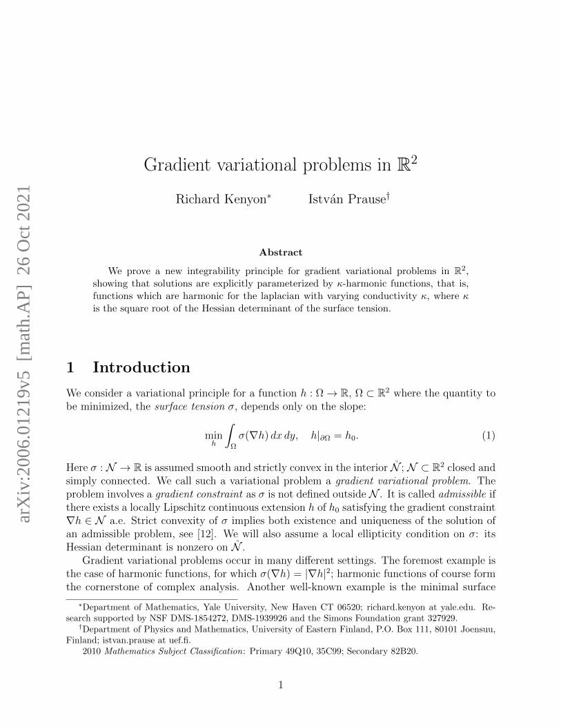
Gradient variational problems in R2

Richard Kenyon∗ Istvan Prause†

Abstract

We prove a new integrability principle for gradient variational problems in R2,showing that solutions are explicitly parameterized by κ-harmonic functions, that is,functions which are harmonic for the laplacian with varying conductivity κ, where κis the square root of the Hessian determinant of the surface tension.

1 Introduction

We consider a variational principle for a function h : Ω→ R, Ω ⊂ R2 where the quantity tobe minimized, the surface tension σ, depends only on the slope:

minh

∫Ω

σ(∇h) dx dy, h|∂Ω = h0. (1)

Here σ : N → R is assumed smooth and strictly convex in the interior N ; N ⊂ R2 closed andsimply connected. We call such a variational problem a gradient variational problem. Theproblem involves a gradient constraint as σ is not defined outside N . It is called admissible ifthere exists a locally Lipschitz continuous extension h of h0 satisfying the gradient constraint∇h ∈ N a.e. Strict convexity of σ implies both existence and uniqueness of the solution ofan admissible problem, see [12]. We will also assume a local ellipticity condition on σ: itsHessian determinant is nonzero on N .

Gradient variational problems occur in many different settings. The foremost example isthe case of harmonic functions, for which σ(∇h) = |∇h|2; harmonic functions of course formthe cornerstone of complex analysis. Another well-known example is the minimal surface

∗Department of Mathematics, Yale University, New Haven CT 06520; richard.kenyon at yale.edu. Re-search supported by NSF DMS-1854272, DMS-1939926 and the Simons Foundation grant 327929.

†Department of Physics and Mathematics, University of Eastern Finland, P.O. Box 111, 80101 Joensuu,Finland; istvan.prause at uef.fi.

2010 Mathematics Subject Classification: Primary 49Q10, 35C99; Secondary 82B20.

1

arX

iv:2

006.

0121

9v5

[m

ath.

AP]

26

Oct

202

1

equation, where σ(∇h) =√

1 + |∇h|2. Other important examples are the dimer model(or stepped surface model), see Figure 1, and its variants, and other models of statisticalmechanics. Up until now these problems have been studied in an ad hoc way. The presentwork provides a unified approach which applies to all variational problems of this type.

For a positive real function κ : R2 → R, called conductance, a κ-harmonic function is afunction u satisfying

∇ · κ∇u = 0.

This is the inhomogeneous-conductance Laplace equation, or κ-Laplace equation. Our mainresult, Theorem 3.2 below, is that graphs of solutions to any gradient variational problem(1) are envelopes of κ-harmonically moving planes in R3. Here κ =

√det Hess(σ).

We identify a large class of surface tensions for which this allows us to give explicitsolutions. We say that σ has trivial potential if its Hessian determinant is the fourth powerof a harmonic function of the intrinsic coordinate (see definition below). We show that inthis case one can solve (1) in a very concrete sense, called Darboux integrability : one canfind explicit parameterizations of all solutions in terms of analytic functions.

We discuss several representative examples, including the dimer model of [14], the “en-harmonic laplacian” σ(s, t) = − log st of [1], and the p-laplacian σ(s, t) = (s2 + t2)p/2 andother isotropic surface tensions. An important example with trivial potential, the 5-vertexmodel [11], is discussed and worked out in detail in [17].

Probabilistic applications. While our results apply to any gradient variational problem,this work was originally motivated by probabilistic applications. “Limit shapes” for severalprobability models are known (or conjectured) to be minimizers of gradient variational prob-lems. Let us briefly recall the limit shape problem, see Figure 1 for an example, and [7].Many well-known statistical mechanical models such as the plane partition model, the dimermodel and the five- or six-vertex models, are models of random discrete Lipschitz functionsfrom Z2 to Z. The limit shape problem is to understand the shape of the random functionwith fixed Dirichlet boundary conditions in the scaling limit, that is, in the limit when thelattice spacing tends to zero. In quite general situations the random surface concentrates, inthe scaling limit, onto a nonrandom continuous surface, which is obtained by minimizing agradient variational problem, where the surface tension function encodes the “local entropy”of the probability model.

For many determinantal models, the exact surface tension is known, see [7, 15] for thedimer model and [21] for random Young tableaux. These have the property that κ is con-stant and hence κ-harmonic functions are simply harmonic. In this situation we obtain asurprisingly simple representation of limit shapes: they are envelopes of harmonically mov-ing planes in R3, see Corollary 4.2. The advantage of this representation compared to thosebased on complex Burgers equation [14, 3] is that it makes the problem of matching a limitshape to given boundary values much more feasible and systematic, since often there is noneed to guess the frozen boundary [16]. We illustrate this by two examples in Section 6.

2

Figure 1: A uniform random sample of a large “Boxed Plane Partition” (shown here for abox of size n = 50). This is a stepped surface spanning six edges of an n× n× n cube. Forn large a random sample lies (with probability tending to 1 as n→∞) near a certain fixedsmooth surface, which was first computed by Cohn, Larsen and Propp in [8].

An essential novelty of our work lies in the fact that it also applies to non-determinantalmodels. Our prime example of a surface tension with trivial potential is in fact the surfacetension arising in the five-vertex model. As far as we know, the five-vertex model [11] andits genus-zero generalisation [17] are the only examples beyond determinantal models wherethe exact surface tension has been derived. With the help of the trivial potential propertyall limit shapes of these models can be explicitly parametrised [17].

In the current paper we borrow some terminology from the probability setting such asfree energy, liquid region and amoeba; see their definitions for general gradient models below.

As a final note, it would be interesting to compare the “tangent plane method” of thepresent work and [16] to the tangent (line) method of [10] introduced in the context of thesix-vertex model.

Acknowledgements. We thank Robert Bryant for discussions and hints on Ampere’stheorem and Darboux integrability. We thank Filippo Colomo and Andrea Sportiello fordiscussions on arctic curves and the tangent method. We are grateful to the referees fortheir comments, suggestions and careful reading of the manuscript.

2 Intrinsic coordinate

Let (s, t) be coordinates for N ⊂ R2.

3

Free energy. The Legendre dual F (X, Y ) to the surface tension σ is defined for every(X, Y ) ∈ R2 as

F (X, Y ) = sup(s,t)∈N

(sX + tY − σ(s, t)) .

In probabilistic settings F is called the free energy. We define the amoeba1 A = A(F ) ⊂ R2

of F to be the closure of the set where F is strictly convex. The gradient map ∇σ : N → Agives a one-to-one correspondence between the interiors N and A. By the Wulff construction[13], F is a volume-constrained minimizer for σ, that is, a minimizer of the surface tensionfunctional (1) under the additional constraint of having fixed volume under the graph of h,and for appropriate boundary conditions at ∞.

Isothermal coordinates and complex structure. The Hessian matrix of σ, Hσ, ispositive definite and so determines a Riemannian metric on N

g = σss ds2 + 2σst ds dt+ σtt dt

2.

There is likewise a metric on A determined by the Hessian of F ; the map ∇σ : N → A ishowever an isometry for these metrics.

Let z = u + iv = u(s, t) + iv(s, t) be a conformal (also known as isothermal) coordinatesystem for g, that is, g = eΦ(du2 + dv2) for some function Φ = Φ(u, v). To match withthe usual definitions for the dimer model, we will choose z to be an orientation reversinghomeomorphism to some uniformizing domain, which we can choose to be either H, theupper half-plane2 or C. We call z the intrinsic coordinate.

To find z, following Gauss (see e.g. [19]), we solve the Beltrami equation

∂z

∂z=

12(zs + izt)

12(zs − izt)

=1

µσ, (2)

where µσ is the Beltrami coefficient

µσ =σss − σtt + 2iσst

σss + σtt + 2√σssσtt − σ2

st

.

Equivalently, define the Gauss map (or “complex slope”) γ on N to be

γ :=−σst − i

√σssσtt − σ2

st

σss=

σtt

−σst + i√σssσtt − σ2

st

, (3)

1It is generally not an algebraic amoeba; the terminology is motivated by analogy with the dimer model.2In the dimer model σ is smooth on N except at a finite number of points, where it has conical singularities;

these singularities lead to holes in A. It is then natural to parameterize A with a multiply-connected domain[15]. For our purposes here, however, A is assumed simply connected.

4

then z satisfies the following equation

zszt

= −1

γ. (4)

The local ellipticity of σ implies that |µσ| < 1 and uniformly bounded away from 1 on com-pact subsets of N which guarantees the existence of the solution for the Beltrami equationin (2) [4].

We can equivalently work on A and define z by the equation

zXzY

= γ. (5)

Since zXXz + zY Yz = 0, and zssz + zttz = 0, equations (4) and (5) lead to

γ = − YzXz

=sztz. (6)

With this setup X, Y and s, t are all functions of the intrinsic coordinate z, and satisfy(6).

Proposition 2.1. The following statements are each equivalent to ζ being an intrinsic co-ordinate

(i)Xζtζ

+Yζsζ

= 0,

(ii)sζtζ

= −σst−i√

detHσσss

,

and when either of these holds we necessarily have

Xζ

tζ= −i

√detHσ = −Yζ

sζ, (7)

Proof. Define γ by γ =sζtζ

. Since Xζ = (σs)ζ = σsssζ + σsttζ we can writeXζtζ

= σssγ + σst.

Similarly,Yζsζ

= σtt1γ

+ σst. Now (i) is equivalent to the equation

σssγ2 + 2σstγ + σtt = 0,

which has two solutions

γ =−σst ± i

√detHσ

σss.

Because ζ is assumed to be orientation reversing, Imγ < 0 and thus we have the minus signabove. This leads to

Xζtζ

= −i√

detHσ = −Yζsζ

. Thus (i), (ii) are equivalent (and imply (7)).

On the other hand by definition the intrinsic complex variable ζ is an orientation-reversinghomeomorphism ζ : N → H solving (4); this is equivalent to (ii) in terms of the inversemapping.

5

Intrinsic Euler-Lagrange equation. Consider a minimizer h of the variational problem(1). A priori regularity results for the minimizer are established in [12]. The liquid regionL ⊂ Ω is defined to be the subset where ∇h is in the interior of N and thus σ is smooth.On the liquid region h satisfies the associated Euler-Lagrange equation

div(∇σ ∇h) = 0, (8)

or simply Xx + Yy = 0. Ampere showed that, combined with the fact that ∇h is curl-freewe get a single complex equation for z : L → C:

Theorem 2.2 (Ampere [2]). We have

Xzzx + Yzzy = 0 (x, y) ∈ L. (9)

In an equivalent form,zxzy

=sztz

= γ.

Proof. Observe that

Xx − i√

detHσtx = Xzzx +Xz zx − i√

detHσ (tzzx + tz zx)

=(Xz − i

√detHσtz

)zx +

(Xz + i

√detHσtz

)zx = 2Xzzx

in view of Proposition 2.1. Similarly,

Yy + i√

detHσsy = 2Yzzy.

Thus the Euler-Lagrange equation Xx + Yy = 0 together with the curl-free conditiontx = sy combine to a single complex equation

Xzzx + Yzzy = 0.

Remark 1. We can make a volume-constrained problem by fixing the volume under the graphof h. The volume constrained Euler-Lagrange equation is 2Xzzx + 2Yzzy = c, where c ∈ R isthe Lagrange multiplier for the volume, see [14].

Complex structure on the liquid region. There is a canonical mapping from the liquidpart L of the minimizer to the Wulff shape, defined in terms of the corresponding tangentplanes. In planar coordinates, (x, y) ∈ L 7→ (∇σ ∇h)(x, y) ∈ A. Composed with theisothermal coordinate, z : L → C gives an intrinsic complex structure to L with

zxzy

= γ. (10)

Thus in the intrinsic complex structure the map L → A is holomorphic. For surface tensionsarising from the dimer model, equation (10) is equivalent to the complex Burgers equationsof [14], or to the Beltrami equations studied in [3].

6

3 κ-harmonic functions

We call a (sufficiently smooth) solution w to the conductivity equation in a domain D ⊂ R2

∇ · κ∇w = 0 (11)

a κ-harmonic function3. The conductivity κ : D → (0,∞) in our setting is smooth, indeed weset κ(z) =

√detHσ. That is, we consider the Hessian determinant of σ (in (s, t)-coordinates)

as a function of the intrinsic coordinate z ∈ D. Here D is H or C. For later purposes, wealso introduce the fourth root

ψ(z) := 4√

detHσ = κ(z)1/2 > 0. (12)

We interpret Proposition 2.1 in real notation as follows. Recall that z = u+iv and the Hodgestar operator acts as a (counterclockwise) rotation by 90 degrees, i.e. ∗∇ = ∗(∂u, ∂v) =(−∂v, ∂u),

∇X = ∗κ∇t and ∇(−Y ) = ∗κ∇s. (13)

Since the Hodge star operator transforms curl-free fields into divergence-free fields, it followsthat

∇ · κ∇t = 0 and ∇ · κ∇s = 0, (14)

and thus t and s are both κ-harmonic functions in D. Equation (13) shows that by definitionX and −Y are the respective conjugate functions. These are in turn 1/κ-harmonic functions.

Reduction to Schrodinger equation. A standard technique is to reduce (11) to theSchrodinger equation

(−∆ + q)(w) = 0, (15)

with potential q = ∆ψψ

. Indeed, with the substitution w = wψ satisfies (15). Define real-

valued functions φ, φ∗ as φ = sψ and φ∗ = tψ. From (14) and the above reduction

ψ∆φ− φ∆ψ = 0 and ψ∆φ∗ − φ∗∆ψ = 0, (16)

which can also be verified directly from Proposition 2.1.

The intercept function. Consider next the intercept function h− (sx+ ty) in the liquidregion (x, y) ∈ L, where h is the minimizer, and (s, t) = ∇h(x, y). We will also view thisfunction as a function of the intrinsic coordinate z; now however this function is multi-valued, as (x, y) 7→ z is generally many-to-one. Alternatively, we can consider the interceptfunction as a single-valued function in the liquid region in its intrinsic complex structure. Thenext theorem shows that the intercept function is κ-harmonic with respect to this intrinsicvariable.

3the conventional terminology is σ-harmonic but we reserve σ for the surface tension. See e.g. Chapter16 of [4] for more on κ-harmonic functions.

7

Theorem 3.1. The functions s, t and h− (sx+ ty) are all κ-harmonic in the liquid regionwith the respect to the intrinsic coordinate z.

Proof. The statement for s and t is just a repetition of (14). We also record from (16)

(sψ)zz = φzz = sψzz = 0 and (tψ)zz = φ∗zz = tψzz = 0. (17)

Consider next(h− (sx+ ty))ψ.

Let us take the ∂z derivative, and remembering that ∇h = (hx, hy) = (s, t)

(ψ(h− (sx+ ty)))z = ψz(h− (sx+ ty))− ψ(szx+ tzy)

= ψz(h− (sx+ ty)) + (sψz − φz)x+ (tψz − φ∗z)y.

Take now the ∂z derivative and observe a number of cancellations

(ψ(h− (sx+ ty)))zz =ψzz(h− (sx+ ty))− ψz(szx+ tzy) + szψzx+ tzψzy

+ (sψzz − φzz)x+ (tψzz − φ∗zz)y + (sψz − φz)xz + (tψz − φ∗z)yz=ψzz(h− (sx+ ty))− ψ(szxz + tzyz).

We now apply Theorem 2.2 (the intrinsic Euler-Lagrange equation) for the inverse relation –away from critical points – z 7→ (x, y) in the form −yz/xz = zx/zy = sz/tz to find altogether

((h− (sx+ ty))ψ)zz = (h− (sx+ ty))ψzz. (18)

This means that (h − (sx + ty))ψ is a solution to (15), in other words, h − (sx + ty) is asolution to (11), i.e. it is κ-harmonic.

Envelopes. The graph of the minimizer h is a surface in R3. Over a point (x, y) ∈ L thereis a tangent plane to the minimizer which has slope (s, t) = ∇h(x, y) and it intersects thevertical axis at the point h(x, y)− (sx + ty). That is, using (x, y, x3) ∈ R3 coordinates, thetangent plane is Pz = x3 = sx + ty + c where c = h − (sx + ty). Theorem 3.1 says thatall the coefficients s, t, c of these tangent planes are κ-harmonic with respect to z. In otherwords, we have shown:

Theorem 3.2. The minimizer is an envelope of κ-harmonically moving planes in R3.

In circumstances where we can determine a priori the values of z along the boundary ofΩ, and where we can solve the κ-laplace equation with these boundary values, this allows usto solve the problem (1).

8

4 Trivial potential

We say that the surface tension σ has trivial potential if ψ = κ1/2 in (12) is a harmonicfunction of z. In this case, the potential q ≡ 0 in (15) and thus κ-harmonic functions areratios of harmonic functions with a common denominator ψ. This leads to the followingtheorem.

Theorem 4.1. If σ has trivial potential then s, t and h−(sx+ ty) are all ratios of harmonicfunctions (in z) in the liquid region with the common denominator ψ(z).

For the dimer model, the Hessian determinant is constant, hence the surface tension hastrivial potential.

Corollary 4.2. Minimizers in the dimer model are envelopes of harmonically moving planes.

Proof. By Theorem 5.5 of [15], detHσ ≡ π2 for the dimer model. It means that for thenormalized surface tension 1

πσ, κ ≡ 1 and we have harmonic dependence for each coefficient.

Remark 2. For statistical mechanical models, π/κ is known in the physics literature as theLuttinger parameter, see e.g. [5, 20]. For free fermionic systems, like the dimer model, theLuttinger parameter is the constant 1.

The five-vertex model [11] is not free-fermionic and the Hessian determinant is not con-stant. Nevertheless, its surface tension, as well that of its generalization, the genus-zerofive-vertex model, has trivial potential, see [17].

Theorem 4.1 leads to an algorithm for matching a minimizer for (certain) extremal bound-ary values, namely, those for which the boundary tangent planes are determined. This isdiscussed in [16]; see Section 6 below for an illustration of the method.

Solving the Euler-Lagrange equation. According to Theorem 4.1 if σ has trivial po-tential then

G(z) = ψ(h− (sx+ ty)) (19)

is a (possibly multi-valued) harmonic function. We now describe how to parametrize solu-tions in terms of this harmonic function. We have

hz = sxz + tyz = (sx+ ty)z − szx− tzy

from which we getszx+ tzy + (h− (sx+ ty))z = 0,

orszx+ tzy + (G/ψ)z = 0. (20)

9

The functions s, t and ψ are functions of z depending only on the surface tension σ whileG depends on the boundary conditions of h. The equation (20) describes a complex linethrough (x, y) ∈ R2 with three complex coefficients. Since the complex slope sz

tz= γ is not

real (as Imγ < 0), this defines uniquely (x, y) in terms of z,

x(z) = −Im(t−1

z (Gψ

)z)

Im(γ), y(z) = −

Im(s−1z (G

ψ)z)

Im(γ−1). (21)

Finally, the solution h(x, y) = sx+ ty +G/ψ is also a function of z

h(z) =G

ψ−

Im(stz

(G/ψ)z

)Imγ

−Im(tsz

(G/ψ)z

)Im(γ−1)

(22)

This gives an explicit solution to the Euler-Lagrange equation for an arbitrary harmonicfunction G(z). Typically, however, matching G(z) with the desired Dirichlet boundaryconditions on h is a nontrivial problem. It is also worth noting that for a general G, (21)and (22) will solve the Euler-Lagrange equation locally ; it may globally correspond to aself-intersecting surface and/or have ramification points.

5 Examples of gradient variational problems

Trivial potential example. For a first example, let

σ(s, t) =2

3(s−2 + t−2)

for s, t ∈ (0,∞). Then Hσ =

(4s−4 0

0 4t−4

), and z = s−1 − it−1 is a conformal coordinate.

We have detHσ = 16(st)−4 so ψ(z) = −Im(z2) is harmonic. Also sz = −2(z+z)2

and tz = 2i(z−z)2 .

In the simplest case when G is constant, G ≡ C, we get

(x, y, h) = (C

2Imz,− C

2Rez,

C

Im(z2)),

or equivalentlyh(x, y) = (−2/C)xy.

Young tableaux. The surface tension for random Young tableaux was derived in [21]:

σ(s, t) = −(1 + log(cos πs

πt

))t

where

(s, t) ∈ (−1

2,1

2)× (0,∞).

10

This is obtained from a certain limit of the dimer model.We have

Hσ =

(π2t sec2(πs) π tan(πs)π tan(πs) 1

t

)with detHσ ≡ π2, thus σ has trivial potential. A conformal coordinate is

z = −πt(tan(πs)− i).

Now γ = − ztzs

= 1z

and equation (9) becomes

zx −zyz

= 0

which is the complex Burgers equation. Using zxxz + zyyz = 0, this becomes yz + 1zxz = 0,

and integrating

y +x

z+ f(z) = 0

for an arbitrary analytic function f . Alternatively, solutions are envelopes of harmonicallymoving planes.

Enharmonic functions. In this case σ(s, t) = − log(st) where s, t ∈ [0,∞), see [1]. Wehave

Hσ =

(1s2

00 1

t2

).

A conformal coordinate is z = u + iv = log s − i log t. Then ψ = 1√st

= e(−u+v)/2 and the

potential is q = ∆ψψ

= 12, a constant.

Ampere’s equation (9) becomes

xz + ie−u−vyz = 0. (23)

Equivalently,∇y = ∗eu+v∇x,

that is, x is eu+v-harmonic with conjugate y. This leads to

∆x+ xu + xv = 0.

Solutions to this are linear combinations of x = eau+bv where a2 + b2 + a + b = 0. For thiselementary solution the corresponding conjugate y is y = − b

a+1e(a+1)u+(b+1)v. We then have

hz = sxz + tyz = euxz + e−vyz = (1 + i)(a+ ib)e(a+1)u+bv

whence

h =(a− b)a+ 1

e(a+1)u+bv.

11

Thus a general solution to the variational problem can parameterized as a linear combinationof

(x, y, h) = (eau+bv,− b

a+ 1e(a+1)u+(b+1)v,

(a− b)a+ 1

e(a+1)u+bv)

where (a, b) run over solutions to a2 + b2 + a+ b = 0.

The p-laplacian. Here σ(s, t) = (s2 + t2)p/2 = rp. A conformal coordinate is z = rαe−iθ

where reiθ = s+ it and α =√p− 1. Also detHσ = p2(p− 1)|z|(2p−4)/α and

q =∆ψ

ψ=

(p− 2)2

4(p− 1)|z|2=

C

|z|2.

To solve (∆ − q)w = 0, use separation of variables: write z = Re−iθ and look for solutionsof the form w(z) = A(R)B(θ). The equation is

(∂2

∂R2+

1

R

∂

∂R+

1

R2

∂2

∂θ2− C

R2)A(R)B(θ) = 0,

soA′′(R) + 1

RA′(R)− C

R2A(R)

A(R)/R2= −B

′′(θ)

B(θ).

Setting both sides to a constant c gives the solution

B(θ) = C1ei√cθ + C2e

−i√cθ

A(R) = c1R√C−c + c2R

−√C−c.

Other isotropic surface tensions (surface tensions depending only on r =√s2 + t2) can

be dealt with in the same way: a conformal coordinate can be chosen of the form z = f(r)eiθ,and ψ is a function of r only. The Euler-Lagrange equation can then be solved by separationof variables.

6 Limit shape examples

We demonstrate applications of Section 4 to limit shapes in probability. We consider twoconcrete illustrative boundary value problems for domino tilings. More complex examples,with a more systematic treatment, are discussed in [16] and [18]. See also Section 4.3–4.4of [17] for explicit examples of limit shapes for staggered 5-vertex models. These non-determinantal examples go well beyond the framework of [14, 3] and are essentially basedon Theorem 4.1 above.

12

π s

2

π t

2

zw

zw

10 1

Figure 2: When 1 + z + w − zw = 0 (and z ∈ H), the convex quadrilateral with sides1, z,−zw,w is cyclic. The values s, t are obtained from the angles of the extended sides asshown.

6.1 Domino tilings of the Aztec diamond

We start by revisiting the classic arctic circle limit shape for domino tilings of the Aztecdiamond, first derived in [6]. For domino tilings (tilings of regions in Z2 with 2 × 1 and1× 2 rectangles) there are two natural conformal coordinates z ∈ H and w ∈ H, related bythe “characteristic polynomial” 1 + z + w − zw = 0, as discussed in [14]. The relationshipbetween (s, t) and (z, w) is given in Figure 2: it is

(s, t) =2

π(arg z − argw − π, arg z + argw),

and (s, t) ∈ N = cvx(2, 0), (0, 2), (−2, 0), (0,−2); see [7].The Aztec diamond of order n is the region of Figure 3, left panel. In the limit n→∞,

the height function limit shape has facetted regions near each corner, where the limit shapeis linear with slope at a corner of N . The liquid region is a disk tangent to each of thesides of the limiting polygon. (We do not actually assume the exact shape of the liquidregion, this will be found a posteriori.) The situation is as shown in Figure 3, right panel:the height function along the boundary determines the linear equations of the limit shapenear each corner. In this example the z values run once around R∪ ∞ as the point (x, y)runs around the boundary of the liquid region. The slopes and intercepts (in blue in thefigure) are piecewise constant functions of z as z runs over the real axis, as indicated in thefollowing table. Recall that by Corollary 4.2 we may assume that ψ ≡ 1 in (19).

13

(1,0,1)

(0,1,-1)

(-1,0,1)

(0,-1,-1)

01

∞ -1

2 x - 1

1 - 2 y

-2 x - 1

2 y + 1

Figure 3: The Aztec diamond region of order n = 5, and in the limit n→∞, the limitingheights of the facets (blue) and z values at the tangency points (red). The black values arethe positions of the vertices in R3; the height (third coordinate) is linear along each boundarysegment, and determines the intercepts of the linear functions on the facets.

z < −1 −1 < z < 0 0 < z < 1 1 < zs 0 2 0 −2t 2 0 −2 0G 1 −1 1 −1

Because G is a harmonic function of z, we can find it from the harmonic extension of itsboundary values on H, given by the last line in the above table; we have

G =2

π(−π

2+ arg(z − 1)− arg(z) + arg(z + 1)).

The equation for the limit shape (the envelope of the moving planes) is obtained bysolving the linear system, see (20)

sx+ ty +G = x3

szx+ tzy +Gz = 0 (24)

for x, y, x3 as functions of z. See Figure 4.By calculating the ∂z-derivatives, (24) takes the explicit form(

1

z+

1

z − 1− 1

z + 1

)x+

(1

z− 1

z − 1+

1

z + 1

)y +

1

z − 1− 1

z+

1

z + 1= 0.

Taking real and imaginary parts, we find x and y to be

x =1− 2 Rez − |z|2

2(1 + |z|2)and y =

1 + 2 Rez − |z|2

2(1 + |z|2).

14

Figure 4: Aztec diamond limit shape (with contour lines for the height function).

Inverting these relations

z(x, y) =y − x+ i

√1− 2(x2 + y2)

1 + x+ y.

The height function can be written down explicitly with the help of the introduced functionsas

x3(x, y) = s(z)x+ t(z)y +G(z), x2 + y2 <1

2.

We emphasize that in deriving the limit shape the only a priori assumption we made isthat it has four facetted regions in the four corners. This assumption is justified rigorously(for this case and in similar settings with more sides) in [14] and [3]. The boundary conditionsdictate the equations for these four planes and their harmonic extension in terms of the z-variable give the entire family of tangent planes. The exact form of the frozen boundary isthen found a posteriori from the envelope construction.

6.2 Domino tilings of L-shape

We consider domino tilings of an L-shaped Aztec diamond from [9]. Again the techniquesof [14] and [3] apply to this setting. However, it is highly nontrivial to find either the Q0

function of [14, Corollary 1] or the Blaschke product/holomorphic factor pair (B, γ) of [3,Theorem 5.2] from the given boundary conditions. Indeed, [9] proceeds with the (not fullyrigorous) tangent method to find the frozen boundary. We show here that the full limitsurface can be obtained from Corollary 4.2 with minimal difficulty.

See Figure 5. The z values are marked in red, and facet equations are in blue; thereare 8 facets. Let u ∈ H parameterize the liquid region; u is a double cover of z, that is,

15

(1,0,1)(-1,0,1)

(0,-1,-1)

(a,1-a,2a-1)(-a,1-a,2a-1)

(0,1-2a,4a-1)

01

∞ -1

∞-1

10

2 x - 1

-2y+1-2y+1

-2 x - 1

2 y + 1

-2x+4a-12x+4a-1

2y+8a-3

Figure 5: Boundary data for domino tilings of an L shaped region.

z = z(u) is a rational function of degree 2. We can normalize so that u sends 0 and ∞ to∞. Let a1 < a2 < a3 < 0 < a4 < a5 < a6 be the points that u sends to −1, 0, 1,−1, 0, 1respectively. Without loss of generality (after a Mobius transformation) set a3 = −1. Then

z = z(u) has the form z = A(u−a2)(u−a5)u

where, solving, the constants A, a4, a5, a6 are rationalfunctions of a1, a2.

P1 P2 P3 P4 P5 P6 P7 P8

u (−∞, a1) (a1, a2) (a2, a3) (a3, 0) (0, a4) (a4, a5) (a5, a6) (a6,∞)z (−∞,−1) (−1, 0) (0, 1) (1,∞) (−∞,−1) (−1, 0) (0, 1) (1,∞)s 0 2 0 −2 0 2 0 −2t 2 0 −2 0 2 0 −2 0G 1 −1 1 4a− 1 8a− 3 4a− 1 1 −1

There is one more nontrivial necessary condition, which is that Gu vanishes at the branchpoint of u. This is necessary for the local single-valuedness of the surface. This conditionuniquely determines (a1, a2) in the relevant range, and therefore all of a1, . . . , a6. For exam-

ple, when a = 10−3√

216

, we have

(a1, a2, a3, a4, a5, a6) = (−4,−4 +3√2,−1,

−1 + 9√

2

7,8 + 12

√2

7,−4 + 36

√2

7).

At this point it is straightforward to find the harmonic extension of G as in the previousexample, and solve the linear system (24) to get the equation of the surface; the explicit

16

formulas are a little bulky to include here. The resulting surface is shown in Figure 6 fora = .3 (the feasible range of a values is 0 ≤ a < 1/2; at a = 1/2 the surface breaks into twocomponents).

Figure 6: The limit shape, showing height contours.

References

[1] Aaron Abrams and Richard Kenyon. Fixed-energy harmonic functions. Discrete Anal.,2017. Paper No. 18.

[2] A.M. Ampere. Memoire contenant l’application de la theorie exposee dans le XVII.e Cahier du Journal de l’Ecole polytechnique, a l’integration des equations auxdifferentielles partielles du premier et du second ordre. De l’Imprimerie royale, 1819.

[3] Kari Astala, Erik Duse, Istvan Prause, and Xiao Zhong. Dimer models and conformalstructures, 2020, arXiv:2004.02599.

[4] Kari Astala, Tadeusz Iwaniec, and Gaven Martin. Elliptic partial differential equationsand quasiconformal mappings in the plane, volume 48 of Princeton Mathematical Series.Princeton University Press, Princeton, NJ, 2009.

[5] Yannis Brun and Jerome Dubail. The Inhomogeneous Gaussian Free Field, with ap-plication to ground state correlations of trapped 1d Bose gases. SciPost Phys., 4:37,2018.

17

[6] Henry Cohn, Noam Elkies, and James Propp. Local statistics for random domino tilingsof the Aztec diamond. Duke Math. J., 85(1):117–166, 1996.

[7] Henry Cohn, Richard Kenyon, and James Propp. A variational principle for dominotilings. J. Amer. Math. Soc., 14(2):297–346, 2001.

[8] Henry Cohn, Michael Larsen, and James Propp. The shape of a typical boxed planepartition. New York J. Math., 4:137–165, 1998.

[9] Filippo Colomo, Andrei G. Pronko, and Andrea Sportiello. Arctic curve of the free-Fermion six-vertex model in an L-shaped domain. J. Stat. Phys., 174(1):1–27, 2019.

[10] Filippo Colomo and Andrea Sportiello. Arctic curves of the six-vertex model on genericdomains: the tangent method. J. Stat. Phys., 164(6):1488–1523, 2016.

[11] Jan de Gier, Richard Kenyon, and Samuel S. Watson. Limit shapes for the asymmetricfive vertex model, 2018, arXiv:1812.11934.

[12] Daniela De Silva and Ovidiu Savin. Minimizers of convex functionals arising in randomsurfaces. Duke Math. J., 151(3):487–532, 2010.

[13] R. Dobrushin, R. Kotecky, and S. Shlosman. Wulff construction, volume 104 of Trans-lations of Mathematical Monographs. American Mathematical Society, Providence, RI,1992. A global shape from local interaction, Translated from the Russian by the authors.

[14] Richard Kenyon and Andrei Okounkov. Limit shapes and the complex burgers equation.Acta Mathematica, 199(2):263–302, 2007.

[15] Richard Kenyon, Andrei Okounkov, and Scott Sheffield. Dimers and amoebae. Annalsof Mathematics, pages 1019–1056, 2006.

[16] Richard Kenyon and Istvan Prause. Limit shapes from envelopes. in preparation.

[17] Richard Kenyon and Istvan Prause. The genus-zero five vertex model, 2021,arXiv:2101.04195.

[18] Istvan Prause. Random Young tableaux and harmonic envelopes. in preparation.

[19] Michael Spivak. A comprehensive introduction to differential geometry. Vol. IV. Publishor Perish, Inc., Wilmington, Del., second edition, 1979.

[20] Jean-Marie Stephan. Extreme boundary conditions and random tilings, 2020,arXiv:2003.06339.

[21] Wangru Sun. Dimer model, bead model and standard young tableaux: finite cases andlimit shapes, 2018, arXiv:1804.03414.

18