Variational Principles of Continuum Mechanics
590
-
Upload
khangminh22 -
Category
Documents
-
view
2 -
download
0
Transcript of Variational Principles of Continuum Mechanics


Interaction of Mechanics and Mathematics
For further volumes:www.springer.com/series/5395

Victor L. Berdichevsky
Variational Principlesof Continuum MechanicsI. Fundamentals
With 79 Figures
123

IMM Advisory Board
D. Colton (USA) . R. Knops (UK) . G. DelPiero (Italy) . Z. Mroz (Poland) .M. Slemrod (USA) . S. Seelecke (USA) . L. Truskinovsky (France)
IMM is promoted under the auspices of ISIMM (International Society for theInteraction of Mechanics and Mathematics).
Author
V.L. BerdichevskyProfessor of MechanicsDepartment of Mechanical EngineeringWayne State UniversityDetroit, MI [email protected]
ISSN 1860-6245 e-ISSN 1860-6253ISBN 978-3-540-88466-8 e-ISBN 978-3-540-88467-5DOI 10.1007/978-3-540-88467-5Springer Heidelberg Dordrecht London New York
Library of Congress Control Number: 2008942378
c© Springer-Verlag Berlin Heidelberg 2009This work is subject to copyright. All rights are reserved, whether the whole or part of the material isconcerned, specifically the rights of translation, reprinting, reuse of illustrations, recitation, broadcasting,reproduction on microfilm or in any other way, and storage in data banks. Duplication of this publicationor parts thereof is permitted only under the provisions of the German Copyright Law of September 9,1965, in its current version, and permission for use must always be obtained from Springer. Violationsare liable to prosecution under the German Copyright Law.The use of general descriptive names, registered names, trademarks, etc. in this publication does notimply, even in the absence of a specific statement, that such names are exempt from the relevant protectivelaws and regulations and therefore free for general use.
Cover design: WMXDesign GmbH, Heidelberg
Printed on acid-free paper
Springer is part of Springer Science+Business Media (www.springer.com)

Our mind is frail as our senses are; it wouldlose itself in the complexity of the world ifthat complexity were not harmonious; likethe short-sighted, it would only see details,and would be obliged to forget each of thesedetails before examining the next because itwould be incapable of taking in the whole.The only facts worthy of our attention arethose which introduce order into thiscomplexity and so make it accessible to us.
H. Poincare, Science and Method

Preface
There are about 500 books on variational principles. They are concerned mostly withthe mathematical aspects of the topic. The major goal of this book is to discuss thephysical origin of the variational principles and the intrinsic interrelations betweenthem. For example, the Gibbs principles appear not as the first principles of thetheory of thermodynamic equilibrium but as a consequence of the Einstein formulafor thermodynamic fluctuations. The mathematical issues are considered as long asthey shed light on the physical outcomes and/or provide a useful technique for directstudy of variational problems.
The book is a completely rewritten version of the author’s monograph VariationalPrinciples of Continuum Mechanics which appeared in Russian in 1983. I have beenpostponing the English translation because I wished to include the variational prin-ciples of irreversible processes in the new edition. Reaching an understanding of thissubject took longer than I expected. In its final form, this book covers all aspects ofthe story. The part concerned with irreversible processes is tiny, but it determines theaccents put on all the results presented. The other new issues included in the bookare: entropy of microstructure, variational principles of vortex line dynamics, vari-ational principles and integration in functional spaces, some stochastic variationalproblems, variational principle for probability densities of local fields in compositeswith random structure, variational theory of turbulence; these topics have not beencovered previously in monographic literature. Other than that, the scope of the bookis the same though the text differs considerably due to many detailed explanationsadded to make the level of the book suitable for graduate students.
Grass Lake, Michigan V.L. Berdichevsky
vii

Acknowledgements
This book has been affected by many influences. The most essential one was thatof my teacher, L.I. Sedov, who set up the standards of scholarly work. My latefriend P.P. Mosolov, the most knowledgeable expert in variational calculus I knew,explained to me the notion of “feeling the constraints” (Sect. 5.5). He insisted thatthe first 30 pages of any good scientific book must be written at a level undergrad-uate students can comprehend. His point influenced the way the beginning of thebook is written; it seems that the limit suggested is exceeded. One short chat withV.I. Arnold in the 1980s advanced considerably my understanding of thermody-namics for ergodic Hamiltonian systems. Further work on this topic has resulted ina series of my papers on the subject; an overview of the “derivation of thermody-namics from mechanics” is given in Chap. 2. I learned the asymptotics in homoge-nization of periodic structures from N.S. Bakhvalov (Sect. 17.2), its generalizationto random structures from S. Kozlov (Sect. 17.4), and conditions of elastic phaseequilibrium from M. Grinfeld (Sect. 7.4).
The last but not the least: two decisive contributions to the book were madeby my daughter Jenia and my former student Partha Kempanna. Jenia translated theRussian edition into English, and Partha prepared the Tex file and shaped the outlookof the book. At the final phase of the work I received help from Maria Lipkovich.The advice of Vlad Soutyrine at each stage of this work was, as always, very helpful.Dewey Hodges, Le Khanh Chau and Lev Truskinovsky read the manuscript andmade valuable comments. I had many discussions of the issues considered herewith Boris Shoykhet.
The usual words of gratitude can hardly convey my special feelings towardeveryone mentioned.
ix

Contents - I. Fundamentals
Part I Fundamentals
1 Variational Principles . . . . . . . . . . . . . . . . . . . . . . . . . . . . . . . . . . . . . . . . . . 31.1 Prehistory . . . . . . . . . . . . . . . . . . . . . . . . . . . . . . . . . . . . . . . . . . . . . . . . 31.2 Mopertuis Variational Principle . . . . . . . . . . . . . . . . . . . . . . . . . . . . . . 111.3 Euler’s Calculus of Variations . . . . . . . . . . . . . . . . . . . . . . . . . . . . . . . 151.4 Lagrange Variational Principle . . . . . . . . . . . . . . . . . . . . . . . . . . . . . . . 201.5 Jacobi Variational Principle . . . . . . . . . . . . . . . . . . . . . . . . . . . . . . . . . 261.6 Hamilton Variational Principle . . . . . . . . . . . . . . . . . . . . . . . . . . . . . . . 261.7 Hamiltonian Equations . . . . . . . . . . . . . . . . . . . . . . . . . . . . . . . . . . . . . 321.8 Physical Meaning of the Least Action Principle . . . . . . . . . . . . . . . . 36
2 Thermodynamics . . . . . . . . . . . . . . . . . . . . . . . . . . . . . . . . . . . . . . . . . . . . . . 452.1 Thermodynamic Description . . . . . . . . . . . . . . . . . . . . . . . . . . . . . . . . 452.2 Temperature . . . . . . . . . . . . . . . . . . . . . . . . . . . . . . . . . . . . . . . . . . . . . . 472.3 Entropy . . . . . . . . . . . . . . . . . . . . . . . . . . . . . . . . . . . . . . . . . . . . . . . . . . 512.4 Entropy and Probability . . . . . . . . . . . . . . . . . . . . . . . . . . . . . . . . . . . . 592.5 Gibbs Principles . . . . . . . . . . . . . . . . . . . . . . . . . . . . . . . . . . . . . . . . . . . 592.6 Nonequilibrium Processes . . . . . . . . . . . . . . . . . . . . . . . . . . . . . . . . . . 602.7 Secondary Thermodynamics and Higher Order Thermodynamics . . 64
3 Continuum Mechanics . . . . . . . . . . . . . . . . . . . . . . . . . . . . . . . . . . . . . . . . . 673.1 Continuum Kinematics . . . . . . . . . . . . . . . . . . . . . . . . . . . . . . . . . . . . . 673.2 Basic Laws of Continuum Mechanics . . . . . . . . . . . . . . . . . . . . . . . . . 933.3 Classical Continuum Models . . . . . . . . . . . . . . . . . . . . . . . . . . . . . . . . 983.4 Thermodynamic Formalism . . . . . . . . . . . . . . . . . . . . . . . . . . . . . . . . . 112
4 Principle of Least Action in Continuum Mechanics . . . . . . . . . . . . . . . . 1174.1 Variation of Integral Functionals . . . . . . . . . . . . . . . . . . . . . . . . . . . . . 1174.2 Variations of Kinematic Parameters . . . . . . . . . . . . . . . . . . . . . . . . . . . 121
xi

xii Contents - I. Fundamentals
4.3 Principle of Least Action . . . . . . . . . . . . . . . . . . . . . . . . . . . . . . . . . . . 1254.4 Variational Equations . . . . . . . . . . . . . . . . . . . . . . . . . . . . . . . . . . . . . . 1284.5 Models with High Derivatives . . . . . . . . . . . . . . . . . . . . . . . . . . . . . . . 1344.6 Tensor Variations . . . . . . . . . . . . . . . . . . . . . . . . . . . . . . . . . . . . . . . . . . 136
5 Direct Methods of Calculus of Variations . . . . . . . . . . . . . . . . . . . . . . . . . 1495.1 Introductory Remarks . . . . . . . . . . . . . . . . . . . . . . . . . . . . . . . . . . . . . . 1505.2 Quadratic Functionals . . . . . . . . . . . . . . . . . . . . . . . . . . . . . . . . . . . . . . 1635.3 Existence of the Minimizing Element . . . . . . . . . . . . . . . . . . . . . . . . . 1675.4 Uniqueness of the Minimizing Element . . . . . . . . . . . . . . . . . . . . . . . 1685.5 Upper and Lower Estimates . . . . . . . . . . . . . . . . . . . . . . . . . . . . . . . . . 1725.6 Dual Variational Principles . . . . . . . . . . . . . . . . . . . . . . . . . . . . . . . . . . 1785.7 Legendre and Young-Fenchel Transformations . . . . . . . . . . . . . . . . . 1815.8 Examples of Dual Variational Principles . . . . . . . . . . . . . . . . . . . . . . . 2015.9 Hashin-Strikman Variational Principle . . . . . . . . . . . . . . . . . . . . . . . . 2165.10 Variational Problems with Constraints . . . . . . . . . . . . . . . . . . . . . . . . 2245.11 Variational-Asymptotic Method . . . . . . . . . . . . . . . . . . . . . . . . . . . . . . 2435.12 Variational Problems and Functional Integrals . . . . . . . . . . . . . . . . . . 2705.13 Miscellaneous . . . . . . . . . . . . . . . . . . . . . . . . . . . . . . . . . . . . . . . . . . . . 278
Part II Variational Features of Classical Continuum Models
6 Statics of a Geometrically Linear Elastic Body . . . . . . . . . . . . . . . . . . . . 2856.1 Gibbs Principle . . . . . . . . . . . . . . . . . . . . . . . . . . . . . . . . . . . . . . . . . . . 2856.2 Boundedness from Below . . . . . . . . . . . . . . . . . . . . . . . . . . . . . . . . . . . 2896.3 Complementary Energy . . . . . . . . . . . . . . . . . . . . . . . . . . . . . . . . . . . . 2936.4 Reissner Variational Principle . . . . . . . . . . . . . . . . . . . . . . . . . . . . . . . 2946.5 Physically Linear Elastic Body . . . . . . . . . . . . . . . . . . . . . . . . . . . . . . 2946.6 Castigliano Variational Principle . . . . . . . . . . . . . . . . . . . . . . . . . . . . . 2986.7 Hashin-Strikman Variational Principle . . . . . . . . . . . . . . . . . . . . . . . . 3066.8 Internal Stresses . . . . . . . . . . . . . . . . . . . . . . . . . . . . . . . . . . . . . . . . . . . 3186.9 Thermoelasticity . . . . . . . . . . . . . . . . . . . . . . . . . . . . . . . . . . . . . . . . . . 3216.10 Dislocations . . . . . . . . . . . . . . . . . . . . . . . . . . . . . . . . . . . . . . . . . . . . . . 3236.11 Continuously Distributed Dislocations . . . . . . . . . . . . . . . . . . . . . . . . 328
7 Statics of a Geometrically Nonlinear Elastic Body . . . . . . . . . . . . . . . . . 3417.1 Energy Functional . . . . . . . . . . . . . . . . . . . . . . . . . . . . . . . . . . . . . . . . . 3417.2 Gibbs Principle . . . . . . . . . . . . . . . . . . . . . . . . . . . . . . . . . . . . . . . . . . . 3507.3 Dual Variational Principle . . . . . . . . . . . . . . . . . . . . . . . . . . . . . . . . . . . 3557.4 Phase Equilibrium of Elastic Bodies . . . . . . . . . . . . . . . . . . . . . . . . . . 369
8 Dynamics of Elastic Bodies . . . . . . . . . . . . . . . . . . . . . . . . . . . . . . . . . . . . . 3758.1 Least Action vs Stationary Action . . . . . . . . . . . . . . . . . . . . . . . . . . . . 375

Contents - I. Fundamentals xiii
8.2 Nonlinear Eigenvibrations . . . . . . . . . . . . . . . . . . . . . . . . . . . . . . . . . . 3778.3 Linear Vibrations: The Rayleigh Principle . . . . . . . . . . . . . . . . . . . . . 3798.4 The Principle of Least Action in Eulerian Coordinates . . . . . . . . . . . 381
9 Ideal Incompressible Fluid . . . . . . . . . . . . . . . . . . . . . . . . . . . . . . . . . . . . . . 3899.1 Least Action Principle . . . . . . . . . . . . . . . . . . . . . . . . . . . . . . . . . . . . . . 3899.2 General Features of Solutions of Momentum Equations . . . . . . . . . . 3929.3 Variational Principles in Eulerian Coordinates . . . . . . . . . . . . . . . . . . 3969.4 Potential Flows . . . . . . . . . . . . . . . . . . . . . . . . . . . . . . . . . . . . . . . . . . . 4059.5 Variational Features of Kinetic Energy in Vortex Flows . . . . . . . . . . 4089.6 Dynamics of Vortex Lines . . . . . . . . . . . . . . . . . . . . . . . . . . . . . . . . . . 4149.7 Quasi-Two-Dimensional and Two-Dimensional Vortex Flows . . . . . 4279.8 Dynamics of Vortex Filaments in Unbounded Space . . . . . . . . . . . . . 4339.9 Vortex Sheets . . . . . . . . . . . . . . . . . . . . . . . . . . . . . . . . . . . . . . . . . . . . . 4449.10 Symmetry of the Action Functional and the Integrals
of Motion . . . . . . . . . . . . . . . . . . . . . . . . . . . . . . . . . . . . . . . . . . . . . . . . 4469.11 Variational Principles for Open Flows . . . . . . . . . . . . . . . . . . . . . . . . . 453
10 Ideal Compressible Fluid . . . . . . . . . . . . . . . . . . . . . . . . . . . . . . . . . . . . . . . 45510.1 Variational Principles in Lagrangian Coordinates . . . . . . . . . . . . . . . 45510.2 General Features of Dynamics of Compressible Fluid . . . . . . . . . . . 45710.3 Variational Principles in Eulerian Coordinates . . . . . . . . . . . . . . . . . . 46110.4 Potential Flows . . . . . . . . . . . . . . . . . . . . . . . . . . . . . . . . . . . . . . . . . . . 46810.5 Incompressible Fluid as a Limit Case of Compressible Fluid . . . . . . 470
11 Steady Motion of Ideal Fluid and Elastic Body . . . . . . . . . . . . . . . . . . . . 47311.1 The Kinematics of Steady Flow . . . . . . . . . . . . . . . . . . . . . . . . . . . . . . 47311.2 Steady Motion with Impenetrable Boundaries . . . . . . . . . . . . . . . . . . 47511.3 Open Steady Flows of Ideal Fluid . . . . . . . . . . . . . . . . . . . . . . . . . . . . 47911.4 Two-Dimensional Flows . . . . . . . . . . . . . . . . . . . . . . . . . . . . . . . . . . . . 48311.5 Variational Principles on the Set of Equivortical Flows . . . . . . . . . . . 48411.6 Potential Flows . . . . . . . . . . . . . . . . . . . . . . . . . . . . . . . . . . . . . . . . . . . 49011.7 Regularization of Functionals in Unbounded Domains . . . . . . . . . . . 493
12 Principle of Least Dissipation . . . . . . . . . . . . . . . . . . . . . . . . . . . . . . . . . . . 49512.1 Heat Conduction . . . . . . . . . . . . . . . . . . . . . . . . . . . . . . . . . . . . . . . . . . 49512.2 Creeping Motion of Viscous Fluid . . . . . . . . . . . . . . . . . . . . . . . . . . . . 49812.3 Ideal Plasticity . . . . . . . . . . . . . . . . . . . . . . . . . . . . . . . . . . . . . . . . . . . . 50212.4 Fluctuations and Variations in Steady Non-Equilibrium Processes . 505
13 Motion of Rigid Bodies in Fluids . . . . . . . . . . . . . . . . . . . . . . . . . . . . . . . . . 50913.1 Motion of a Rigid Body in Creeping Flow of Viscous Fluid . . . . . . 50913.2 Motion of a Body in Ideal Incompressible Fluid . . . . . . . . . . . . . . . . 51413.3 Motion of a Body in a Viscous Fluid . . . . . . . . . . . . . . . . . . . . . . . . . . 521

xiv Contents - I. Fundamentals
Appendices . . . . . . . . . . . . . . . . . . . . . . . . . . . . . . . . . . . . . . . . . . . . . . . . . . . . . . . . 531A. Holonomic Variational Equations . . . . . . . . . . . . . . . . . . . . . . . . . . . . 531B. On Variational Formulation of Arbitrary Systems of Equations . . . . 538C. A Variational Principle for Probability Density . . . . . . . . . . . . . . . . . 543D. Lagrange Variational Principle . . . . . . . . . . . . . . . . . . . . . . . . . . . . . . . 549E. Microdynamics Yielding Classical Thermodynamics . . . . . . . . . . . . 553
Bibliographic Comments . . . . . . . . . . . . . . . . . . . . . . . . . . . . . . . . . . . . . . . . . . . . 557
Bibliography . . . . . . . . . . . . . . . . . . . . . . . . . . . . . . . . . . . . . . . . . . . . . . . . . . . . . . . 563
Index . . . . . . . . . . . . . . . . . . . . . . . . . . . . . . . . . . . . . . . . . . . . . . . . . . . . . . . . . . . . . 577
Notation . . . . . . . . . . . . . . . . . . . . . . . . . . . . . . . . . . . . . . . . . . . . . . . . . . . . . . . . . . . 583

Contents - II. Applications
Part III Some Applications of Variational Methods to Development ofContinuum Mechanics Models
14 Theory of Elastic Plates and Shells . . . . . . . . . . . . . . . . . . . . . . . . . . . . . . . 58914.1 Preliminaries from Geometry of Surfaces . . . . . . . . . . . . . . . . . . . . . . 59014.2 Classical Shell Theory: Phenomenological Approach . . . . . . . . . . . . 59814.3 Plates . . . . . . . . . . . . . . . . . . . . . . . . . . . . . . . . . . . . . . . . . . . . . . . . . . . . 62014.4 Derivation of Classical Shell Theory from Three-Dimensional
Elasticity . . . . . . . . . . . . . . . . . . . . . . . . . . . . . . . . . . . . . . . . . . . . . . . . 62614.5 Short Wave Extrapolation . . . . . . . . . . . . . . . . . . . . . . . . . . . . . . . . . . . 64014.6 Refined Shell Theories . . . . . . . . . . . . . . . . . . . . . . . . . . . . . . . . . . . . . 64214.7 Theory of Anisotropic Heterogeneous Shells . . . . . . . . . . . . . . . . . . . 66514.8 Laminated Plates . . . . . . . . . . . . . . . . . . . . . . . . . . . . . . . . . . . . . . . . . . 67914.9 Sandwich Plates . . . . . . . . . . . . . . . . . . . . . . . . . . . . . . . . . . . . . . . . . . . 68814.10 Nonlinear Theory of Hard-Skin Plates and Shells . . . . . . . . . . . . . . . 701
15 Elastic Beams . . . . . . . . . . . . . . . . . . . . . . . . . . . . . . . . . . . . . . . . . . . . . . . . . 71515.1 Phenomenological Approach . . . . . . . . . . . . . . . . . . . . . . . . . . . . . . . . 71515.2 Variational Problem for Energy Density . . . . . . . . . . . . . . . . . . . . . . . 72515.3 Asymptotic Analysis of the Energy Functional
of Three-Dimensional Elasticity . . . . . . . . . . . . . . . . . . . . . . . . . . . . . 741
16 Some Stochastic Variational Problems . . . . . . . . . . . . . . . . . . . . . . . . . . . 75116.1 Stochastic Variational Problems . . . . . . . . . . . . . . . . . . . . . . . . . . . . . . 75116.2 Stochastic Quadratic Functionals . . . . . . . . . . . . . . . . . . . . . . . . . . . . . 75616.3 Extreme Values of Energy . . . . . . . . . . . . . . . . . . . . . . . . . . . . . . . . . . 76116.4 Probability Distribution of Energy: Gaussian Excitation . . . . . . . . . 76816.5 Probability Distribution of Energy: Small Excitations . . . . . . . . . . . 77116.6 Probability Distribution of Energy: Large Excitations . . . . . . . . . . . . 78916.7 Probability Distribution of Linear Functionals of Minimizers . . . . . 79716.8 Variational Principle for Probability Densities . . . . . . . . . . . . . . . . . . 801
xv
xvi Contents - II. Applications
17 Homogenization . . . . . . . . . . . . . . . . . . . . . . . . . . . . . . . . . . . . . . . . . . . . . . . 81717.1 The Problem of Homogenization . . . . . . . . . . . . . . . . . . . . . . . . . . . . . 81717.2 Homogenization of Periodic Structures . . . . . . . . . . . . . . . . . . . . . . . . 81817.3 Some Non-asymptotic Features of Homogenization Problem . . . . . 83317.4 Homogenization of Random Structures . . . . . . . . . . . . . . . . . . . . . . . 84017.5 Homogenization in One-Dimensional Problems . . . . . . . . . . . . . . . . 84917.6 A One-Dimensional Nonlinear Homogenization Problem: Spring
Theory . . . . . . . . . . . . . . . . . . . . . . . . . . . . . . . . . . . . . . . . . . . . . . . . . . 85617.7 Two-Dimensional Structures . . . . . . . . . . . . . . . . . . . . . . . . . . . . . . . . 86217.8 Two-Dimensional Incompressible Elastic Composites . . . . . . . . . . . 87517.9 Some Three-Dimensional Homogenization Problems . . . . . . . . . . . . 88317.10 Estimates of Effective Characteristics of Random Cell Structures
in Terms of that for Periodic Structures . . . . . . . . . . . . . . . . . . . . . . . 892
18 Homogenization of RandomStructures: a Closer View . . . . . . . . . . . . . . . . . . . . . . . . . . . . . . . . . . . . . . . 89918.1 More on Kozlov’s Cell Problem . . . . . . . . . . . . . . . . . . . . . . . . . . . . . . 89918.2 Variational Principle for Probability Densities . . . . . . . . . . . . . . . . . . 91818.3 Equations for Probability Densities . . . . . . . . . . . . . . . . . . . . . . . . . . . 92218.4 Approximations of Probability Densities . . . . . . . . . . . . . . . . . . . . . . 92718.5 The Choice of Probabilistic Measure . . . . . . . . . . . . . . . . . . . . . . . . . 93118.6 Entropy of Microstructure . . . . . . . . . . . . . . . . . . . . . . . . . . . . . . . . . . 93418.7 Temperature of Microstructure . . . . . . . . . . . . . . . . . . . . . . . . . . . . . . . 93918.8 Entropy of an Elastic Bar . . . . . . . . . . . . . . . . . . . . . . . . . . . . . . . . . . . 943
19 Some Other Applications . . . . . . . . . . . . . . . . . . . . . . . . . . . . . . . . . . . . . . . 96119.1 Shallow Water Theory . . . . . . . . . . . . . . . . . . . . . . . . . . . . . . . . . . . . . . 96119.2 Models of Heterogeneous Mixtures . . . . . . . . . . . . . . . . . . . . . . . . . . . 96619.3 A Granular Material Model . . . . . . . . . . . . . . . . . . . . . . . . . . . . . . . . . 97619.4 A Turbulence Model . . . . . . . . . . . . . . . . . . . . . . . . . . . . . . . . . . . . . . . 978
Bibliographic Comments . . . . . . . . . . . . . . . . . . . . . . . . . . . . . . . . . . . . . . . . . . . . 987
Bibliography . . . . . . . . . . . . . . . . . . . . . . . . . . . . . . . . . . . . . . . . . . . . . . . . . . . . . . . 991
Index . . . . . . . . . . . . . . . . . . . . . . . . . . . . . . . . . . . . . . . . . . . . . . . . . . . . . . . . . . . . . 1005
Notation . . . . . . . . . . . . . . . . . . . . . . . . . . . . . . . . . . . . . . . . . . . . . . . . . . . . . . . . . . . 1011

Introduction
A variational principle is an assertion stating that some quantity defined for all pos-sible processes reaches its minimum (or maximum, or stationary) value for the realprocess. Variational principles yield the equations governing the real processes. Theequations following from a variational principle possess a very special structure.The major feature of this structure is the reciprocity of physical interactions: actionof one field on another creates an opposite and, in some sense, symmetric reaction.All equations of microphysics possess such a structure. Perhaps this is the mostfundamental law of Nature revealed up to now.
Macrophysics operates with the averaged characteristics of microfields. Thevariational structure of microequations affects the structure of macroequations. Inparticular, for equilibrium processes, the variational structure of microequationsbrings up the classical equilibrium thermodynamics. In the case of non-equilibriumreversible processes the variational structure of microequations yields a variationalstructure of macroequations. The governing equations of irreversible processes alsopossess a special structure. This structure, however, is not purely variational.
The above-mentioned explains the fundamental role of the variational princi-ples in modeling physical phenomena. If the interactions between various fieldsare absent or simple enough, then one does not need the variational approach toconstruct the governing equations. However, if the interactions in the system arenot trivial (e.g. nonlinear and/or involving high derivatives, kinematical constraints,etc.) the variational approach becomes the only method to obtain physically sensiblegoverning equations.
Another important use of the variational principles is the direct qualitative andquantitative analysis of real processes which is based solely on the variationalformulation and does not employ the governing equations. Such analysis is veryadvanced for solids while for fluids the major developments are still ahead.
The book aims to review the two above-mentioned sides of the variationalapproach: the variational approach both as a universal tool to describe physicalphenomena and as a source for qualitative and quantitative methods of studyingparticular problems. In addition, a thorough account of the variational principles
xvii

xviii Introduction
discovered in various branches of continuum mechanics is given, and some gaps arefilled in.1
The book consists of three parts. Part I presents basic knowledge in the area,including variational principles for systems with a finite number of degrees offreedom, “the derivation of thermodynamics from mechanics,” a review of basicconcepts of continuum mechanics and general setting of variational principles ofcontinuum mechanics. Part I also contains an exposition of the direct methods ofcalculus of variations. The major goal here is to prepare the reader to understandand to speak the “energy language,” i.e. to be able to withdraw the necessary infor-mation directly from energy without using the corresponding differential equations.An important component of the energy language is the ability to work with energydepending on a small parameter. A way to do that (variational-asymptotic method)is discussed in detail. Another important component, duality theory, is also coveredin detail. The variational-asymptotic method and duality theory are widely usedthroughout the book. Part II gives an account of variational principles for solids andfluids. Part III is concerned with applications of variational methods to shell andplate theory, beam theory, homogenization of periodic and random structures, shal-low water theory, granular media theory and turbulence theory. The considerationof random structures is preceded by a review of stochastic variational problems.Some interesting variational principles that are beyond the main scope of the bookare placed in Appendices. The details of some derivations that can be skipped with-out detriment for understanding of further material are also put in the appendices.By publisher’s suggestion, the book is published in two volumes with volume 1containing the first two parts of the book.
It is assumed that the reader knows the basics of calculus and tensor analysis.The latter, though, is not absolutely necessary as all tensor notations used are brieflyoutlined. Part I was used by the author as notes for the course Fundamentals ofMechanics, some chapters of Parts II and III were used in courses on elasticitytheory and advanced fluid mechanics. Every effort was made to unify the notationfor the broad range of the subjects considered. The notation is summarized at theend of each volume.
1 Following the tradition, variational principles are named after their author; the references aregiven in Bibliographical Comments at the end of the book. Most of the variational principles withno name attached appeared first in the previous edition of this book.

Part IFundamentals
Chapter 1Variational Principles
1.1 Prehistory
Mechanics is a branch of physics studying motion. The history of mechanics, aswell as the history of other branches of science, is a history of attempts to explainthe world by means of the smallest possible number of universal laws and gen-eral principles. The most successful and fruitful attempts stem from the idea thatthe observable events are extreme in their character and that the general principlessought are variational, i.e. they assert that certain parameters obtain their maximumor minimum values in realizable physical processes.
This idea seems to endow Nature with some goal and appeared a long time ago.Aristotle (384–322 B.C.) claimed in his Physics, which served as the major sourcefor natural philosophers for over 2000 years, that in all its manifestations, Naturefollows the easiest path that requires the least amount of effort. However, this ideais, perhaps, even older. As Euler mentioned [99], “. . .It seems, Aristotle borrowedthis dogma from his predecessors rather than invented it independently.” It wasa long way from Aristotle’s vague assertion to a precise quantitative formulation.The major breakthrough occurred in the seventeenth century along with other keyadvances in mathematics and physics.1
The figures whose contributions are most closely related to our considera-tion have been Galileo (1564–1642), Descartes (1596–1650), Fermat (1601–1665),Newton (1643–1727), Leibnitz (1646–1716), R. Hooke (1635–1703) andJ. Bernoulli (1667–1748).
Galileo discovered the universal features of motion which formed the experi-mental basis of Newtonian mechanics: acceleration of a falling body does not de-pend on its mass; pendulum vibration frequency does not depend on the mass ofthe pendulum; a falling body passes distances proportional to the second powerof time. Galileo also introduced the two principles which later became the cor-nerstones of Newtonian mechanics: the invariance of the laws of mechanics withrespect to change of inertial frames, and the inertia principle – motion of a body
1 As B. Russell put it, we would live in a quite different world if in the seventeenth century 100scientists were killed in their childhood.
V.L. Berdichevsky, Variational Principles of Continuum Mechanics,Interaction of Mechanics and Mathematics, DOI 10.1007/978-3-540-88467-5 1,C© Springer-Verlag Berlin Heidelberg 2009
3

4 1 Variational Principles
which does not interact with other bodies will remain uniform indefinitely in anunbounded space. Note that both principles, being in complete accord with thespirit of Euclidian geometry, were purely a mind game: they cannot be checkedexperimentally because there are neither isolated bodies nor inertial frames, not tomention that one can hardly justify the unboundedness of our space. Galileo wasalso known for his experiments with telescopes and astronomical observations. Hereis Lagrange’s appreciation [168] of Galileo’s achievements:
. . .To discover the satellites of Jupiter, the phases of Venus, the spots on the Sun, etc., oneneeds only a telescope and a power of observation, but an exceptional genius is neededto establish the laws of Nature for phenomena which were in everyone’s plain sight, but,nevertheless, escaped the attention of philosophers.
Another giant of the seventeenth century, Descartes, introduced the analyticalapproach to geometry and emphasized the method of orthogonal coordinates whichallows one to study geometrical objects in terms of equations. Thus, for example, anellipse, considered before Descartes as a cross-section of a cone, becomes a solutionof an algebraic equation of second order.
Newton formulated the basic laws of dynamics and created the theory of grav-itation. In particular, he introduced the concept of mass, a characteristic of bod-ies which is different from weight; discovered the key dynamic law: mass ×acceleration = force; gave the general formulation of the principle of the par-allelogram of forces, and formulated the law of action and reaction.2
Discovery of the laws of mechanics is inseparable from development of the dif-ferential calculus by Leibnitz and Newton.
And, finally, it was Fermat who set up the beginning of the story which is thesubject of this book.
One of the topics widely discussed at the time was reflection and refraction oflight. It was known for centuries that the beam of light hitting a mirror at some angleα reflects from the mirror at the same angle (Fig. 1.1).
Fig. 1.1 The law of lightreflection
2 Interestingly, all the laws of statics were known to Archimedes (287–212 B.C.). It took about 19centuries before the next step was made.

1.1 Prehistory 5
Fig. 1.2 The law of lightrefraction
It was also established experimentally that if a beam of light falls on the interfaceof two transparent media at some incidence angle α1 from the side of medium 1, itpenetrates into medium 2 at a different angle, α2 (Fig. 1.2).
It is remarkable that, for any two media 1 and 2, the ratiosin α1
sin α2remains the
same for all incidence angles α1:
sin α1
sin α2= n = constant. (1.1)
This ratio, n, depends only on the materials (for example water and air, or glassand air). Moreover, the ratio remains the same if the direction of light is reversed:the beam of light falling on the interface from the side of the medium 2 at angle α2
penetrates the medium 1 at the angle α1 determined by the formula (1.1). This lawwas established by working up the experimental data by Snell in 1621.
The challenge for theoreticians was to find some underlying reasons for the pecu-liar behavior of light. The first attempt was made by Descartes. Descartes envisionedlight as a set of small elastic balls and attempted to derive the diffraction law fromthe laws of elastic collisions. He obtained the correct answer. Descartes’ derivationassumed, however, that light propagates in a denser medium, say, water, faster thanin a less dense one, like air. Experimental verification of such features was beyondthe technical possibilities at the time: methods for determining the speed of lightappeared much later.
The proposition about faster light propagation in a denser medium seemed quitequestionable for Fermat, and he attempted to consider diffraction from another per-spective. As the basis for his derivation, he used the following postulate: Naturetakes the easiest and most accessible paths. However, what is the measure of “easi-ness of path”? The simplest candidate is the length of the path. Consider whether itworks in the reflection phenomenon.
Let light go from point A to point B reflecting from the mirror at some point(Fig. 1.3). Let C be the point for which the incidence angle is equal to the reflectionangle. Consider two light trajectories, one reflects from the mirror at the point C,
another at some point C ′. The length of the path AC ′B is greater than the length

6 1 Variational Principles
Fig. 1.3 The principle ofminimum distance
of the path ACB. To see that, we3 introduce the mirror image of point B, point B ′.Obviously, the lengths of lines ACB′ and AC ′B ′ are equal to the lengths of linesACB and AC ′B, respectively. Since the line AC B ′ is straight, the length of AC ′B ′ isgreater than the length of ACB′, and, correspondingly, the length of AC ′B is greaterthan that of ACB. We arrived at the simplest example of a variational principle: lightmoving from point A to a mirror and then to point B chooses a trajectory such as tominimize the distance traveled.
This example contains the two major “entries” of any variational principle: the setof admissible trajectories, in this case all lines connecting the starting point A withthe reflection point C and the destination point B, and the quantity to be minimized,in this case the length of the trajectory. Note that the minimizing trajectory is highlysensitive to the choice of admissible paths. If, for example, we choose as admissibleall the paths connecting the point A and the point B, then the minimizing trajectoryis the straight line connecting A and B which is not the correct answer for the initialphysical problem.
The principle of minimum distance works for reflection, but does not work forrefraction: if point B is on the other side of the interface plane, then the minimumdistance corresponds to the straight line, i.e. α1 = α2, in contradiction to the exper-imental observations.
Fermat suggested that the experimentally observed refraction law corresponds tothe principle of minimum time: light moving from point A to point B chooses thetrajectory for which the travel time is minimum.
Let us derive the Snell law (1.1) from the Fermat principle. To proceed, we haveto introduce the speeds of light in both media, c1 and c2, and distances from pointsA and B to the interface, h1 and h2 (Fig. 1.2).
We are looking for point C such that the travel time from A to B is minimum.In each medium, 1 and 2, the trajectory of light is straight, because, for constantvelocity, minimum travel time between two points, A and C or C and B, correspondsto the paths with minimum lengths, i.e. to the straight segments AC and C B. Let A0
and B0 be the orthogonal projections of points A and B onto the interface. Denote
3 Here and in what follows “we” means “the reader and the author.”

1.1 Prehistory 7
the distances A0C and A0 B0 by x and a, respectively. The distance x is unknownwhile the distance a is given. The travel time from A to B is a function of x :
f (x) =√
h21 + x2
c1+√
h22 + (a − x)2
c2.
We consider this function on the segment [0, a] and seek the value of x whichdelivers the minimum value to this function. Note that the second derivative of f (x),
d2 f (x)
dx2= h2
1
c1(h2
1 + x2) 3
2
+ h22
c2(h2
1 + (a − x)2) 3
2
,
is positive. Therefore, f (x) is a convex function4 and has the form shown in Fig. 1.4.
Fig. 1.4 Qualitativedependence of the travel timeon the position of point C
It is seen that f (x) has only one minimum. This minimum is achieved at the
point x whered f (x)
dx= 0, i.e.
x
c1
√h2
1 + x2− a − x
c2
√h2
2 + (a − x)2= 0. (1.2)
The ratiox√
h21 + x2
is equal to sin α1. Similarly,a − x
c2
√h2
2 + (a − x)2= sin α2.
Equation (1.2) becomes
sin α1
c1= sin α2
c2. (1.3)
4 Here we rely on the reader’s knowledge of calculus. The notion of a convex function and itsrelations to variational problems will be discussed in detail later in Chap. 5.

8 1 Variational Principles
Equation (1.3) yields the Snell law (1.1) because, as expected, c1 and c2 dependonly on the material properties. Equation (1.3) also contains additional information:the material constant n can be expressed in terms of the speeds of light in bothmedia:
n = c1
c2. (1.4)
It was established experimentally that n ≈ 0.75 if the first medium is water andthe second medium is air. This is why we see stones at the bottom of the river closerthan they are in reality (Fig. 1.5).
Fig. 1.5 Refraction in waterand air
According to (1.4), the speed of light in water is about 3/4 of that in air. Thiscontradicts the Descartes claim that the speed of light is greater in denser media.
Descartes’ conclusion was supported by Leibnitz. Like Fermat, he based hisconsideration on a variational principle. But he suggested that Nature chooses theeasiest path defined as a path of least resistance. The resistance to light propagationis different in different media. Leibnitz introduced the notion of “difficulty” whichis equal to the product of time and resistance, and postulated that light chooses thetrajectory for which the sum of all difficulties is minimum. Eventually, he arrivedat the Snell law. According to Leibnitz, the denser the medium, the greater its re-sistance. This fact, he argued, yields a greater velocity of light in denser media: thedispersion of light is smaller, hence the beam of light is more compressed alongits way, and, similar to water in a narrow river-bed, moves faster. Apparently, heenvisioned the light flux as a flow of some medium.
It became clear much later that in this controversy Fermat was right.Successful applications of the variational ideas to optics encouraged the search
for analogies in mechanics. In 1696, in Leipzig journal Acta Eruditorum, JohannBernoulli published the following note:
Two points, A and B, are given in a vertical plane (see Fig. 1.6). Find the trough AMB,which minimizes the travel time of a body moving from point A to point B by the forceof its own weight. To arouse the interest of amateurs in such matters and to encouragetheir enthusiasm in attempting to obtain the solution, I will say that solving this problemis not a pure intellectual speculation deprived of any practical application whatsoever, as itmay seem. Actually, this problem is of great practical interest and not just in the subject

1.1 Prehistory 9
Fig. 1.6 Bernoulli’s problem
of mechanics, but also in other disciplines, which may seem unbelievable. By the way(I am mentioning the following fact in order to avert a possible misjudgment), althoughthe segment AB is the shortest distance between points A and B, the time it takes for thebody to travel this distance is not the shortest possible, and there exists the (minimum time)curve AMB well known to geometers. I will disclose what this curve is if, during the courseof the year, nobody else announces the answer.
Bernoulli sent his solution to Leibniz, in order for Leibniz to publish it in a year.This, as Leibnitz put it, “such wonderful and hitherto unheard problem” which “en-tices by its beauty just as the apple enticed Eve,” attracted the attention of manyscholars. In particular, it is believed that some anonymous solutions were given byJacob Bernoulli and Isaac Newton. The notorious curve turned out to be a cycloid,a curve “well known to geometers.”
Bernoulli’s problem is much more difficult than Fermat’s problem since the func-tion to be minimized depends on the curve connecting the points A and B, i.e. onan infinite number of variables. Such functions are now called functionals.
If y = y (x) is the equation of the curve connecting points A and B, then the timeof motion along this curve, I , depends only on the function y (x). One writes
I = I (y (x))
and says that I is a functional of y (x). In Bernoulli’s problem,
I (y (x)) =l∫
0
√√√√1+(
dydx
)2
2gy (x)dx . (1.5)
where g is the acceleration of gravity.To see that, we note that motion of the body is frictionless; therefore, the total
energy of the particle is conserved. Energy is the sum of kinetic energy K andpotential energy U . Kinetic energy is the mass m times half of the squared velocity,(
dx
dt
)2
+(
dy
dt
)2
. Since the point moves along the curve y = y (x),

10 1 Variational Principles
K = m
2
((dx
dt
)2
+(
dy
dx
)2 (dx
dt
)2)= m
2
(1+
(dy
dx
)2)(
dx
dt
)2
.
The potential energy is (remember that the positive direction of the y-axis isdown, therefore the smaller y the bigger U )
U = −mgy.
Initial value of energy, K +U, is zero; therefore at all times
m
2
(1+
(dy
dx
)2)(
dx
dt
)2
− mgy = 0.
Hence,
dx
dt=√√√√ 2gy
1+(
dydx
)2 . (1.6)
The travel time is
I =l∫
0
dxdxdt
. (1.7)
Formula (1.5) follows from (1.7) and (1.6).The functional (1.5) must be minimized on the set of curves y (x) which satisfy
the following conditions:
y (0) = 0, y (l) = yB . (1.8)
The first condition fixes the choice of the origin, the second prescribes they-coordinate of the given point, B.
The solutions obtained at the time did not provide a general method of inves-tigating this type of problem. It was found 50 years later by a student of JohannBernoulli, Leonard Euler, who laid down the cornerstones of modern calculus ofvariations.
In addition to the constraints (1.8) the admissible functions y(x) should obeysome other restrictions which we have not mentioned explicitly yet. For example,the integrand in (1.5) contains the derivative dy/dx , and therefore the admissiblefunction must be differentiable at least.
If we accept for consideration all non-negative functions y(x) with piecewisecontinuous derivatives, then the integral (1.5) makes sense. Note that for some func-tions, e.g., quadratic functions, y(x) = const x2, the integral is equal to +∞. Such

1.2 Mopertuis Variational Principle 11
functions are automatically sorted out because we seek the minimum value of thefunctional (1.5).
The insights of Fermat and Bernoulli imparted a new importance to the ques-tion of whether some goal parameter obtains its minimum in realizable motion ofbodies or, in the language of the time, whether the body, moving from one point toanother chooses such a way that the payment, if the body is to pay for its motion, isminimized.
1.2 Mopertuis Variational Principle
The first formulation of the variational principle in mechanics was made by PierreMopertuis in 1744. According to Mopertuis’ principle, in real motion, the productof the mass of the body, its speed and the distance it has traveled, is minimum. Thisquantity,
I = mvs, (1.9)
Mopertuis, following Leibniz, called action.An important testing ground for Mopertuis was the law of collision of elastic
balls. Let us first show that Mopertuis’ principle yields the correct law of reflectionof a rigid ball from the wall when the ball moves along the normal line to the wall.To emphasize an analogy with the Fermat principle, we consider a trajectory of theball in the two-dimensional space-time plane (see Fig. 1.7).
If at the instants t = 0 and t = θ the ball was at the points A and B, andcorrespondingly, h1, h2 are the distances from these points to the wall, and tc is thetime of the collision, then the action is
I = mh1
tch1 + m
h2
θ − tch2. (1.10)
Fig. 1.7 Reflection of the ballfrom the wall

12 1 Variational Principles
Note that the initial and final positions of the ball and the total time of motionθ are assumed to be given, so action I is a function of one variable, tc, I = I (tc).Function I (tc) is defined on the segment [0, θ ]. The second derivative of this func-tion,
d2 I
dt2c
= 2mh2
1
t3c
+ 2mh2
2
(θ − tc)3 ,
is positive. Thus, the function, I (tc) , is convex and has only one minimum. Theminimum is achieved at the point where the first derivative of I (tc) vanishes, i.e.
−mh2
1
t2c
+ mh2
2
(θ − tc)2 = 0.
This equation means that the velocity of the ball after the collision,h2
θ − tc, is
equal to the velocity of the ball before the collision,h1
tc, in full compliance with the
experimentally established law of elastic collisions. The reader may check that thecorrect law of elastic collisions follows from Mopertuis’ principle for an inclinedcollision with a flat wall (Fig. 1.8a) or a collision with a curved wall (Fig. 1.8b).
Fig. 1.8 Elastic collision ofthe ball with a flat and acurved wall
Collision with a curved wall is actually a more delicate problem. It turns out thatmultiple collision points are possible, and some collision points could correspondto the maximum value of action.
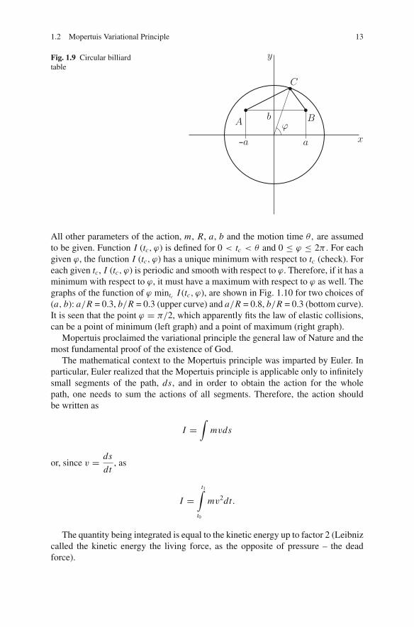
To clarify this issue, consider the following model problem. Let points A and Bbe inside a circular billiard table of radius R (see Fig. 1.9). The coordinates of pointsA and B are (−a, b) and (a, b), respectively. The point of possible reflection fromthe wall is denoted by C , as before. Point C has coordinates (R cos ϕ, R sin ϕ). Theaction is a function of two variables: collision time tc and angle ϕ:
I (tc, ϕ) = m(R cos ϕ + a)2 + (R sin ϕ − b)2
tc+m
(R cos ϕ − a)2 + (R sin ϕ − b)2
θ − tc.
1.2 Mopertuis Variational Principle 13
Fig. 1.9 Circular billiardtable
All other parameters of the action, m, R, a, b and the motion time θ, are assumedto be given. Function I (tc, ϕ) is defined for 0 < tc < θ and 0 ≤ ϕ ≤ 2π . For eachgiven ϕ, the function I (tc, ϕ) has a unique minimum with respect to tc (check). Foreach given tc, I (tc, ϕ) is periodic and smooth with respect to ϕ. Therefore, if it has aminimum with respect to ϕ, it must have a maximum with respect to ϕ as well. Thegraphs of the function of ϕ mintc I (tc, ϕ), are shown in Fig. 1.10 for two choices of(a, b): a/R = 0.3, b/R = 0.3 (upper curve) and a/R = 0.8, b/R = 0.3 (bottom curve).It is seen that the point ϕ = π/2, which apparently fits the law of elastic collisions,can be a point of minimum (left graph) and a point of maximum (right graph).
Mopertuis proclaimed the variational principle the general law of Nature and themost fundamental proof of the existence of God.
The mathematical context to the Mopertuis principle was imparted by Euler. Inparticular, Euler realized that the Mopertuis principle is applicable only to infinitelysmall segments of the path, ds, and in order to obtain the action for the wholepath, one needs to sum the actions of all segments. Therefore, the action shouldbe written as
I =∫
mvds
or, since v = ds
dt, as
I =t1∫
t0
mv2dt.
The quantity being integrated is equal to the kinetic energy up to factor 2 (Leibnizcalled the kinetic energy the living force, as the opposite of pressure – the deadforce).

14 1 Variational Principles
Fig. 1.10 Functionmintc I (tc, ϕ) of ϕ for twovalues of (a, b) : a/R = 0.3,b/R = 0.3 (upper curve),a/R = 0.8, b/R = 0.3(bottom curve). The pointϕ = π/2 can be a point ofminium (left) and a point ofmaximum (right)
In the 1750s the letters claimed to have been written by the late Leibniz werepublished, from which one may conclude that Leibniz knew about the extreme prop-erties of action. Besides, it was asserted that the action can achieve in a real processnot only some minimum, but also maximum value. This publication provoked greatcontroversy which, in turn, raised some philosophical, moral and priority issues. Itwas a rare event when a purely scientific issue became a matter of public interest.Philosophers, writers, kings and their courts, took part in heated debates. One of theechoes of these debates reached us in the form of Voltaire’s pamphlet “Histoire dudocteur Akakia et du natif de Saint-Malo” (1752).
Finally, the following point of view crystallized: for some motions, the actionreaches its minimum value, while for the others it may have the maximum value; or,in the language of the time, “Nature is a thrifty mother, who manages with the leastpossible, if she can do so; but, if not, she pays honestly and as much as possible, soas not to be reputed a miser”.5
Although it was understood from the very beginning that action may have eitherminimum, maximum or stationary value, historically the term “principle of least
5 From a letter by Kraft to Euler (1753).

1.3 Euler’s Calculus of Variations 15
action” gained a foothold. We will follow the tradition and use this term, thoughone should bear in mind that in some cases the term “principle of stationary action”might be more appropriate.
1.3 Euler’s Calculus of Variations
The discovery of the least action principle made obvious the necessity of a techniqueto deal with the so-called integral functionals,
I (x (t)) =t1∫
t0
L
(x (t) ,
dx
dt, t
)dt. (1.11)
This technique was developed by L. Euler. The first question to answer was: if x (t)is the minimizing function of the functional (1.11), which equation must it obey?The key role in establishing such an equation is played by the variation, δ I, of thefunctional I. To define δ I, consider infinitesimally small variations, δx (t) , of somefunction, x (t), and the difference,
I (x (t)+ δx (t))− I (x (t)) . (1.12)
The difference (1.12) in which one keeps only terms of the first order with respectto δx (t) and neglects all terms of higher orders is called the variation δ I of thefunctional I (x (t)). The variation δ I is a functional of two arguments, x (t) andδx (t). To underline that δ I is a functional of two functions, x (t) and δx (t), onealso uses the notation
δ I = I ′ (x (t) , δx) . (1.13)
Here the prime emphasizes the similarity with usual derivative.Since all the terms of higher orders are omitted in the difference (1.12), δ I de-
pends on δx linearly, i.e. for any two functions δx1 and δx2,
I ′ (x (t) , δx1 + δx2) = I ′ (x (t) , δx1)+ I ′ (x (t) , δx2) , (1.14)
and for any number λ,
I ′ (x (t) , λδx) = λI ′ (x (t) , δx) . (1.15)
Functions, x (t) , may be subject to some constraints. Then δx (t) are not arbitrarybecause x (t) + δx must obey the constraints. Functions x (t) and δx obeying theconstraints are called admissible.

16 1 Variational Principles
If x (t) is the minimizing element of the functional, I (x (t)), then the variationof the functional, I (x (t)) , computed at the function, x (t) , must vanish for anyadmissible variations, δx (t),
δ I = I ′ (x (t) , δx) = 0. (1.16)
Indeed, assume the opposite: δ I �= 0 for some δx0 �= 0. Then, there is δx1, forwhich δ I < 0: if I ′ (x (t) , δx0) < 0, we put δx1 = δx0; if I ′ (x (t) , δx0) > 0, weput δx1 = −δx0 and, due to linearity of δ I with respect to δx, I ′ (x (t) , δx1) =I ′ (x (t) ,−δx0) = −I ′ (x (t) , δx0) < 0. For sufficiently small δx1, I (x (t)+ δx1)−I (x (t)) ≈ δ I , and δ I being negative means that the value of the functional I (x (t))on the function x (t) + δx1 is smaller than that on the function x (t). We arrive at acontradiction. Hence, (1.16) holds true. This equation is sometimes called the Eulerequation for the functional I .
Let us find the variation of the functional (1.11). Since
I (x (t)+ δx (t))− I (x (t)) =
=t1∫
t0
L
(x (t)+ δx,
d
dt(x (t)+ δx) , t
)dt −
t1∫
t0
L
(x (t) ,
dx
dt, t
)dt
=t1∫
t0
(L
(x (t)+ δx,
d
dt(x (t)+ δx) , t
)− L
(x (t) ,
dx
dt, t
))dt,
computing of δ I is reduced to keeping the linear terms with respect to δx in theintegrand. We have
δ I =t1∫
t0
(�L
�xδx + �L
�x
dδx
dt
)dt. (1.17)
Here and in what follows dot denotes the time derivative.Now we have to draw the consequences from (1.11),
δ I =t1∫
t0
(�L
�xδx + �L
�x
dδx
dt
)dt = 0. (1.18)
Consider first a simpler issue: let for some function A (t) and for any continuousfunction δx (t)
t1∫
t0
A (t) δx (t) dt = 0. (1.19)

1.3 Euler’s Calculus of Variations 17
What can one say about the function A (t)? If the function A (t) is continuousthen
A (t) = 0. (1.20)
This is obvious: if at some point t∗, A (t∗) �= 0, then A (t) is not zero and doesnot change its sign in some small vicinity, V, of the point t∗. Choosing δx (t) zerooutside V and positive inside V we obtain
t1∫
t0
A (t) δx (t) dt =∫
V
A (t) δx (t) dt.
This integral is not equal to zero because A (t) δx (t) does not change the signinside V, and we arrive at a contradiction with (1.19).
The statement made is called the main lemma of calculus of variation.We may strengthen the main lemma: Equation (1.20) remains valid if we narrow
the admissible functions δx (t) in (1.19) by the functions δx vanishing at any finitenumber of points of the segment [t0, t1] including the end points. Indeed, from theprevious reasoning A (t) = 0 at all points excluding the points where δx (t) = 0. Bycontinuity, A (t) = 0 on the entire segment [t0, t1].
This extension of the main lemma yields an important consequence: if
t1∫
t0
A (t) δx (t) dt + B0δx (t0)+ B1δx (t1) = 0, (1.21)
for any function δx (t) , then
A (t) = 0, B0 = 0, B1 = 0. (1.22)
Indeed, considering (1.21) for δx (t0) = δx (t1) = 0, we obtain from the exten-sion of the main lemma, that A (t) = 0. Then, from (1.21) for arbitrary δx (t0) andδx (t1),
B0δx (t0)+ B1δx (t1) = 0. (1.23)
Setting first δx (t1) = 0 and δx (t0) arbitrary, we find from (1.23) that B0 = 0. Thisequation along with (1.23) yield, for arbitrary δx (t1) , B1 = 0.
If we have a number of functions, A1 (t) , . . . , An (t) and a number of variations,δx1 (t) , . . . , δxn (t), and
t1∫
t0
(A1 (t) δx1 (t)+ . . .+ An (t) δxn (t)) dt = 0, (1.24)

18 1 Variational Principles
for any choice of functions δx1 (t) , . . . , δxn (t) , then
A1 (t) = 0, . . . , An (t) = 0. (1.25)
This statement can be derived from the main lemma: first we set δx2 = . . . =δxn = 0. Then (1.24) transforms to (1.19), and we obtain A1 = 0. Puttingδx3 = . . . = δxn = 0 we transform (1.24) to the equation
t1∫
t0
A2 (t) δx2 (t) dt = 0.
Hence, A2 (t) = 0. Continuing this procedure, we obtain (1.25).Formally, (1.18) has the form (1.24) with
A1 = �L
�x, δx1 = δx, A2 = �L
�x, δx2 = dδx
dt.
We cannot conclude, however, that �L/�x and �L/�x are zero, because the varia-tions δx and dδx/dt are not independent: for the prescribed δx1 = δx, the variationδx2 = dδx/dt is determined completely.
To put (1.18) into the form suitable for the application of the main lemma weintegrate the second term by parts
t1∫
t0
(�L
�xδx + �L
�x
dδx
dt
)dt =
=t1∫
t0
(�L
�xδx + d
dt
(�L
�xδx
)− δx
d
dt
�L
�x
)dt = (1.26)
=t1∫
t0
(�L
�x− d
dt
�L
�x
)δxdt + �L
�xδx
∣∣∣∣t=t1
− �L
�xδx
∣∣∣∣t=t0
= 0.
Since the function δx (t) is arbitrary, from (1.26) we obtain for the minimizingfunction the ordinary differential equation
�L
�x− d
dt
�L
�x= 0, (1.27)
and the boundary conditions
�L
�x
∣∣∣∣t=t1
= 0,�L
�x
∣∣∣∣t=t0
= 0. (1.28)

1.3 Euler’s Calculus of Variations 19
If �L/�x does depend on x, (1.27) is an equation of second order. Supplementingthis equation with the two boundary conditions (1.28), we obtain a sensible bound-ary value problem.
Equations (1.27) and (1.28) are called Euler equations of the minimization prob-lem. Their equivalent form is the equation I ′ (x (t) , δx) = 0.
The admissible functions in variational principles may obey some kinematic con-straints. For example, the values of the admissible functions at the ends, t0 and t1,can be given:
x (t0) = x0, x (t1) = x1. (1.29)
Then, since the varied functions, x (t)+ δx (t), must obey the same conditions,
x (t0)+ δx (t0) = x0, x (t1)+ δx (t1) = x1,
the variations must vanish at the ends:
δx (t0) = 0, δx (t1) = 0.
The last two terms in (1.26) become zero, and the only consequence of (1.26) is(1.27). It must be accomplished with the two boundary conditions (1.29). We haveagain a sensible boundary value problem. We observe here a general feature of thevariational approach: in a generic case, the number of equations it provides is asmany as necessary to solve the problem.
The integral functional of many functions, x1 (t) , . . . , xn (t),
I (x1 (t) , . . . , xn (t)) =t1∫
t0
L (x1, . . . , xn, x1, . . . , xn, t) dt,
is considered similarly. We have
δ I =n∑
i=1
t1∫
t0
(�L
�xiδxi + �L
�xi
dδxi
dt
)dt =
=n∑
i=1
⎛⎝
t1∫
t0
(�L
�xi− d
dt
�L
�xi
)δxi dt +
[�L
�xiδxi
]t1
t0
⎞⎠ .
If xi (t) are the minimizing functions, then they satisfy the equation
�L
�xi− d
dt
�L
�xi= 0. (1.30)

20 1 Variational Principles
A few words about terminology. When dealing with functions of a finite numberof variables, f (x1, . . . , xn) , it is convenient to use a geometrical language consid-ering x1, . . . , xn as coordinates of a point x in some n-dimensional space. Accord-ingly, every time when it cannot cause confusion, we suppress indices and writef (x) instead of f (x1, . . . , xn) or f (xi ). We keep the notation f (x1, . . . , xn) orf (xi ) only if it is worth emphasizing that f is a function of many variables. Themajor feature of the x-space used is the linearity of the space: for any number λ
and the point x , the space contains the point λx (its coordinates are λx1, . . . , λxn),and for any two points x ′ and x ′′ the space contains their sum x ′ + x ′′ (if x ′1, . . . , x ′nand x ′′1 , . . . , x ′′n are the coordinates of the points x ′ and x ′′, respectively, then, bydefinition, the coordinates of the point x ′ + x ′′ are x ′1 + x ′′1 , . . . , x ′n + x ′′n ).
Similarly, considering a functional I (x (t)) , it is convenient to think of itsargument as a point in some space of functions. The space of functions (or func-tional space) is linear because for each number λ and each function x (t) the func-tion, λx (t) , is defined, and for each two functions, x1 (t) and x2 (t), the functionsx1 (t)+ x2 (t) is defined. In accordance with such a view, the point of the functionalspace at which δ I = 0 is called the stationary point of the functional, and the valueof the functional at this point the stationary value. We will also use the followingnotation: the point of maximum of the functional I (x (t)) is marked by “hat”, x (t) ,
the point of minimum by the “check” sign, x (t) , and the stationary point by the
cross sign,×x (t). Of course, the points of minimum and maximum are also the sta-
tionary points, and the notation×x is used if we seek a stationary point or if we are
not certain about the type of the stationary point.
1.4 Lagrange Variational Principle
The development of the least action principle was completed by Lagrange. Topresent his final version of the principle in modern terms we first consider the notionof generalized coordinates.
The construction of any mathematical model of a mechanical system begins witha description of its kinematics, i.e. a description of all possible configurations. To dothis, one has to specify a set of numbers, q1, . . . , qn , which determine the configu-ration of the system. Then motion of the system is described by functions of time t ,q1(t), . . . , qn(t). “To know motion” means “to know the functions q1(t), . . . , qn(t).”The n-dimensional space Q of points q with coordinates q1, . . . , qn is called theconfiguration space , or Q-space. The coordinates, q1, . . . , qn, are called the gen-eralized coordinates if they are independent in the sense that any curve in Q-spacerepresents some motion. The number n is called the number of degrees of freedom.
Example 16 The position of a particle on a line is given by one number q – thecoordinate of the point on the line. The motion of a particle is described by the
6 Examples are numbered separately within each section.

1.4 Lagrange Variational Principle 21
function q(t). The coordinate space is the line. If the particle moves between twowalls with coordinates 0 and a, the admissible values of q are the numbers between0 and a (Fig. 1.11).
Fig. 1.11 Particle movingalong the line between thetwo walls
Example 2. The position of a pendulum (Fig. 1.12a) in a plane is given by onenumber, q, the angle between the rod and the vertical axis. So, the pendulum isa system with one degree of freedom. The angle q can take any value between 0 and2π . Two values of q, 0 and 2π , correspond to the same position of the pendulum.Combining these two points of the segment, one gets a circle, so one can say that theQ-space is a circle. The Cartesian coordinates of the position of the pendulum x, yare not generalized coordinates because they are dependent: they obey the equationx2 + y2 = �2, where � is the length of the rod.
Fig. 1.12 Generalizedcoordinate and Q-space for apendulum
Example 3. Each position of a double pendulum (Fig. 1.13) in a plane is specified bytwo angles, q1 and q2. This is an example of a system with two degrees of freedom.Each angle can have any value between 0 and 2π , and the Q-space is a square(Fig. 1.14a).
The points on the segments O A (by O we denote the origin) and BC with thesame q2 coordinate correspond to the same position of the pendulum. Combiningthese two segments, one gets a cylinder (Fig. 1.14b); the position of the pendu-lum corresponds to the points on the lateral surface of the cylinder. The pointson the top and the bottom circles of the cylinder in Fig. 1.14b also correspond tothe same q2 positions of the pendulum. Combining these circles one gets a torus(Fig. 1.14c). There is a one-to-one correspondence between points of the torus andpositions of the pendulum. One can say that the Q-space of the double pendulumis the torus. Any motion of the double pendulum is displayed by a curve on thetorus.

22 1 Variational Principles
Fig. 1.13 Generalizedcoordinates for a doublependulum
Example 4. A particle in three-dimensional space is, obviously, a mechanical systemwith three degrees of freedom. The generalized coordinates q1, q2, q3 coincide withthe Cartesian coordinates of the particle in space. N particles in three-dimensionalspace form a system with 3N degrees of freedom.
Consider a mechanical system which is described by a finite number of general-ized coordinates q1, . . . , qn . The set of coordinates qi (i = 1, . . . , n) will be denotedby q. Each motion of the system corresponds to a trajectory q = q (t) in the config-urational space Q.
Inertial properties of the system are characterized by a function of q and q ,K (q, q), which is called kinetic energy. By definition, in an inertial observer’sframe, the kinetic energy is one-half of the sum of the products of the masses andsquared velocities of all parts of the mechanical system. Usually, velocities dependon qi linearly, and kinetic energy is quadratic with respect to qi :
K = 1
2
∑i, j
mi j qi q j . (1.31)
Fig. 1.14 Q-space of a double pendulum; small circles and squares mark the points in Q-spacewhich correspond to the same position of the pendulum and should be identified

1.4 Lagrange Variational Principle 23
Kinetic energy may be considered as a primary characteristic of mechanical sys-tems. Then masses can be defined, as was suggested by H. Poincare, as coefficientsof this quadratic form. Formula (1.31) is valid only in inertial frames. In all furtherconsiderations, the observer’s frame is assumed to be inertial. The correspondingresults in non-inertial frames are obtained by change of coordinates.
In the Lagrange variational principle, it is not essential that K is a quadratic form;kinetic energy can be any positive-valued function K (q, q) homogeneous of secondorder with respect to q . Homogeneity means that for any λ,
K (q, λq) = λ2 K (q, q) . (1.32)
Homogeneous functions of the second order obey the identity
∑i
qi�K
�q i= 2K (q, q) . (1.33)
This identity follows from (1.32) by differentiation of (1.32) with respect to λ andsetting λ = 1. Obviously, quadratic forms obey both (1.32) and (1.33).
Formulas (1.31) and (1.33) can be written shorter if we employ notation fromtensor analysis: repeated indices in a formula implies summation over these indices.This convention allows us to drop the summation sign in (1.31) and (1.33) to write
K = 1
2mi j qi q j , qi
�K
�q i= 2K (q, q) . (1.34)
Summation over repeated indices is always assumed throughout the book.Another notation from tensor analysis which we will employ is the use of low
and upper indices. The reader who is not familiar with tensor analysis may assumethat quantities with upper and lower indices coincide, for example, q1 = q1. Thisis always true in Cartesian coordinates. The differences appear only in curvilinearcoordinates. The summation rule in invariant7 form requires the summation to betaken over repeated one upper and one low indices. For example, an invariant formof the first Equation (1.34) is
K = 1
2mi j q
i q j . (1.35)
The reader may ignore these nuances and identify the quantities with upper andlow indices until Chap. 3, where an adequate treatment of continuum mechanicsrequires the invariant tensor language. We also prefer to write all the equations formechanical systems with a finite number of degrees of freedom in an invariant form.
Internal interactions in a mechanical system are characterized by its internal en-ergy, a function U (q). For any isolated system the law of conservation of energyholds:
7 I.e. independent of the choice of the coordinate system.

24 1 Variational Principles
K (q, q)+U (q) = E = const. (1.36)
Consider two points, q0 and q1, in the configurational space Q and the trajecto-ries, q = q (t), which begin at a point q0 at time t0 and end at a point q1 at time t1(see Fig. 1.15):
q (t0) = q0, q (t1) = q1. (1.37)
We denote the set of such trajectories by M.
The law of conservation of energy (1.36) does not put constraints on the possibletrajectories: for any trajectory, q (t), connecting the points q0 and q1, one can requirethat (1.37) holds. This equation will determine the rate of passing the trajectory, and,thus, the time, t1, of arrival at the point q1.
Indeed, according to (1.32), we can write
K (q, q) = K (q, dq)
dt2.
Therefore, for a given constant E ,
dt =√
K (q, dq)√E −U (q)
, (1.38)
and the time of arrival at the point q is determined by the integral over the trajectorygoing from q0 to q:
t = t0 +q∫
q0
√K (q, dq)
E −U (q).
Accordingly, the arrival time at the point q1 is
Fig. 1.15 Admissibletrajectories in theconfigurational space Q

1.4 Lagrange Variational Principle 25
t1 = t0 +q1∫
q0
√K (q, dq)
E −U (q).
The arrival time depends on the trajectory.Let us introduce action as the time integral of kinetic energy:
I =t1∫
t0
K (q, q) dt. (1.39)
Lagrange variational principle. The true motion is a stationary point of the actionfunctional (1.39) on the set M narrowed by an additional constraint: energy isconserved along each path.
Note that in the Lagrange variational principle the time at which the system ar-rives at the point q1 is not fixed. This time is determined by the trajectory. The arrivaltime is varied when one varies the trajectory.
We will see that the equations, determining the true trajectory, are
�L
�qi− d
dt
�L
�q i= 0, (1.40)
where L is the difference of kinetic and potential energies,
L = K −U. (1.41)
The left hand side of (1.40) is usually denoted by the symbol,
δL
δqi≡ �L
�qi− d
dt
�L
�q i,
which is called the variational derivative of the function L (q, q, t) , while L (q, q, t)is called Lagrange function or Lagrangian.
The equations of the type (1.40) are the basic equations of classical mechanics.They are called Lagrange equations.
The derivation of (1.40) from Lagrange variational principle is given inAppendix D. Equation (1.40) will be obtained further from the Hamilton variationalprinciple which requires fewer technicalities.
The principle of least action was not explained very clearly in Lagrange’s An-alytical Mechanics. As Jacobi pointed out in his Lectures on Dynamics [140],“This principle is presented in almost all textbooks, even in the best ones, likePoisson’s, Lagrange’s and Laplace’s, in such a way that, in my opinion, it is be-yond comprehension.” The derivation given in Appendix D was published 3 yearsafter Lagrange’s death by Rodrigues [257]. The obscurities instigated Hamilton,

26 1 Variational Principles
Ostrogradsky, Jacobi, and Poincare to examine the subject further. This brought upa number of modifications of the principle of least action.
1.5 Jacobi Variational Principle
Jacobi proposed to eliminate time from the variational principle by means of theenergy equation. Indeed, using relation (1.38), one can write the action functionalin the form
I =t1∫
t0
K dt =q1∫
q0
√E −U (q)
√K (q, dq). (1.42)
Here integration is taken over a path connecting the points q0 and q1. We arrive atJacobi variational principle. The true motion is the stationary point of functional(1.42) on the set of all trajectories which begin at point q0 and end at point q1 andwhich satisfy the law of conservation of energy (1.36).
The action functional taken in the form (1.42) does not depend on the rate withwhich the path is passed. The rate is controlled by the energy equation.
The Jacobi principle takes an especially beautiful form in the case when internalenergy does not depend on q. Then, up to a constant factor,
I =q1∫
q0
√2K (q, dq),
(the factor 2 is put in for convenience). For a quadratic function, 2K (q, q) =gi j (q) q i q j , and
I =q1∫
q0
√gi j (q) dqi dq j .
If one measures distances in Q-space by means of kinetic energy form, i.e. thesquared distance between the points q and q+dq is set equal to gi j (q) dqi dq j , thenthe principle of least action states that true motion corresponds to geodesic lines inQ-space, i.e. the shortest paths connecting the points q0 and q1.
1.6 Hamilton Variational Principle
Hamilton put the principle of least action in the form which is used nowadays mostwidely. He noticed that it is not necessary to take into account the law of conserva-tion of energy if the action functional is taken in the form

1.6 Hamilton Variational Principle 27
I =t1∫
t0
L (q, q, t) dt. (1.43)
L (q, q, t) = K (q, q, t)−U (q, t) .
It turns out that energy will be conserved automatically due to Euler equationsfor the functional (1.43) if K and U do not explicitly depend on time. An advantageof this modification of the least action principle is the possibility to consider time t1fixed and to avoid the energy constraint (1.36) on the trajectories.Hamilton variational principle. The true motion is the stationary point of thefunctional (1.43) on the set of all paths beginning at point q0 and instant t0 andending at point q1 at instant t1.
Somewhat later, and independently of Hamilton, Ostrogradsky arrived at thesame statement.
Hamilton variation principle yields the dynamical equations of mechanics (1.40):this follows from (1.30). Consider these equations for the above-mentioned examples.
Example 1 of Sect. 1.58 (continued) Denote the mass of the particle by m. Then
K = 1
2mq2.
Potential energy contains only the particle-wall interaction energy; denote it by�ε(q). So,
L = 1
2mq2 −�ε(q). (1.44)
Substituting (1.44) into (1.40) we get the equation of particle motion:
mq + d�ε (q)
dq= 0. (1.45)
If the function �ε(q) is of the form shown in Fig. 1.16a, i.e. it is equal to zeroon the segment [ε, a − ε] and grows to infinity in the vicinities of the points q = 0and q = a, then (1.45) describes elastic collisions of the particle and the walls.That means, by definition, that the particle, moving toward a wall with velocity v,has the velocity −v after collision. Indeed, (1.45) admits the reduction of the order:multiplying it by q we have
d
dt
(1
2mq2 +�ε(q)
)= 0
or
1
2mq2 +�ε(q) = E (1.46)
8 The section number is mentioned only when we refer to the examples from a different section.

28 1 Variational Principles
Fig. 1.16 Particle-wall interaction energy
where E is a constant, depending on the initial conditions. Consider a particle, mov-ing toward the wall q = a (q > 0). When q is outside the particle-wall interactionregion, �ε(q) = 0, and, as follows from (1.46), the velocity of the particle is con-stant. As soon as the particle comes into the interaction zone [a − ε ≤ q ≤ a], theparticle velocity begins to change. As the particle penetrates the interaction zone,the interaction energy grows and, as follows from (1.46), the velocity decreases. Atpoint B on Fig. 1.16b, where the interaction energy �ε is equal to the initial energyof the particle E , the velocity q is equal to zero in accordance with (1.46). However,this point is not an equilibrium point because, as follows from (1.45), the accelera-
tion q is not equal to zero at B. Sinced�ε (q)
dq< 0 at B, the particle starts moving
in the opposite direction. The particle’s velocity grows because �ε(q) decreases;and, when the particle escapes the interaction zone, the velocity becomes equal tothe initial velocity with the opposite sign. So, the function �ε(q) really describes anelastic collision. In the limit ε→ 0, function �ε (q) becomes the function
�(q) ={
0 if 0 ≤ q ≤ a
+∞ if q < 0 or q > a(1.47)
Every time we use this function we should bear in mind a smoothed function�ε(q) with a parameter ε, which is much smaller than any characteristic length ofthe problem. Note that the functions �ε(q) and �(q) depend on the position of thewall a. If one of the walls moves, a depends on time. Then, the potential energyand, thus, the Lagrange function explicitly depend on time.
If the particle is attached to a spring, and the spring is stress-free when q = q0,
then
U (q) = 1
2k(q − q0)2,

1.6 Hamilton Variational Principle 29
k being the spring rigidity. The Lagrange function of the particle on a spring is
L = 1
2mq2 − 1
2k(q − q0)2,
and the Lagrange equations of motion (1.40) transform to the usual dynamical equa-tion of an oscillator:
mq + k(q − q0) = 0.
Now we proceed to a less elementary case.
Example 2 of Sect. 1.5 (continued) Let us find the Lagrange function of a pendulum.We refer the motion of the pendulum to Cartesian coordinates (x, y), shown inFig. 1.17. Assume that the rod is massless and the mass m is concentrated at theend of the rod. If x(t), y(t) are the coordinates of the mass point, then the kineticenergy is
K = 1
2m(x2 + y2
). (1.48)
From Fig. 1.17 we have
x = � sin q, y = � cos q. (1.49)
Let us suppose that the length � can also change with time; this corresponds, forinstance, to the case of a mass on a rope, which could be pulled up through a hole(Fig. 1.18). The dependence of � on time is supposed to be given. Differentiating(1.49), we get
x = � sin q + � cos q q, y = � cos q − � sin q q. (1.50)
Substituting (1.50) into (1.48), we find the kinetic energy:
K = 1
2m(�2 + �2q2
). (1.51)
Fig. 1.17 To calculation ofthe kinetic energy of apendulum

30 1 Variational Principles
Fig. 1.18 The case when ldepends on time
l
Suppose that gravity is the only force acting on the pendulum. The gravitationalpotential energy is equal to the product of the mass m, the gravity acceleration con-stant g, and the height of the mass above some fixed level. One can choose thebottom position of the pendulum as the level of zero potential energy. Then, it isseen from Fig. 1.17 that
U = mg(�− � cos q).
So,
L = 1
2m�2 + 1
2m�2q2 − mg�(1− cos q). (1.52)
The Lagrange equation of motion takes the form
d
dt
(m�2q
)+ mg� sin q = 0. (1.53)
The variation of the first term in (1.52) is zero because �(t) is given.If � is constant, then (1.53) is reduced to the equation of a “mathematical pendu-
lum”:
q + g
�sin q = 0. (1.54)
Note that (1.54) does not contain the mass of the pendulum. This yields theremarkable feature of pendulum vibrations: the frequency of vibration does notdepend on the pendulum mass. This property was first experimentally observed byGalileo and was a cornerstone of Newtonian mechanics.
If � is not constant, then an additional “force” enters the governing equation:
q + g
�sin q = −2q
�
�.
It is quite cumbersome to obtain these equations from the “force concept.”

1.6 Hamilton Variational Principle 31
Example 3 of Sect. 1.5 (continued). The reader can check that the double pendulumhas the following Lagrange function:
L = m1 + m2
2�2
1q21 +
m2
2�2
2q22 + m2�1�2q1q2 cos(q1 − q2)
+(m1 + m2)g�1 cos q1 + m2g�2 cos q2.
The notation is shown in Fig. 1.19; �1, �2 are assumed constant.
Fig. 1.19 Notation for thedouble pendulum
Example 4 of Sect. 1.5 continued. The Lagrange function of a particle in a box is
L = 1
2m(x2 + y2 + z2)−�(x)−�(y)−�(z),
where � is the function (1.47). The set of N particles with masses m1, . . . , m N hasthe Lagrange function
L = 1
2m1
(x2
1 + y21 + z2
1
)+ · · · + 1
2m N
(x2
N + y2N + z2
N
)− (1.55)
−�(x1)−�(y1)−�(z1)− · · · −�(xN )−�(yN )−�(zN ).
Note that the particles interact in this case only with the walls, and two or moreparticles are allowed to be at the same space point. The model of spherical particleswith some finite radius a, experiencing elastic collisions, is more realistic. In thiscase one has to include in (1.55) the particle-particle interaction energy:
∑α<β
�(|rα − rβ |).
Here, Greek indices run through the values 1, 2, . . . , N ; rα is the position vector ofthe center of the αth sphere, |rα| is the length of the vector, rα , and the function �

32 1 Variational Principles
is shown in Fig. 1.20a. As before, in dealing with function �, one should bear inmind a smoothed function �ε (Fig. 1.20b) and consider the limit ε → 0. In somephysical models an attraction of particles at long distances is added (Fig. 1.20c).
Fig. 1.20 Particle-particle interaction energy
For Hamilton, the formulation of the variational principle was a by-product of thestudy on integration of dynamical equations. He considered the action functional asa function of initial and final points of the trajectory, I = I (q1, q2), and derivedthe partial differential equation for I (q1, q2) which is equivalent to dynamical equa-tions. This construction was used later by Schrodinger in motivations for the basicequation of quantum mechanics.
1.7 Hamiltonian Equations
The equations of mechanics (1.40) form a system of n ordinary differential equa-tions of second order. Usually, it is more convenient to deal with a system of 2nordinary differential equations of first order. Let us put the equations of motion(1.40) into this special form.
First, consider the systems with one degree of freedom and the Lagrange function
L = 1
2mq2 −U (q).
The equation of motion (1.40) is the second-order equation
d
dt(mq)+ �U (q)
�q= 0. (1.56)

1.7 Hamiltonian Equations 33
To rewrite it as a system of two equations of first order, one has to introduce a newrequired function, the momentum p = mq. Then (1.56) can be written as a systemof two ordinary differential equations of the first order,
q = 1
mp, p = −�U
�q.
To make a similar transformation in the general case we introduce the new un-known functions, the momenta, by the relations
pi =�L
(qk, qk, t
)
�q i. (1.57)
Suppose that we can solve (1.57) with respect to qk :
qk = Ak(qi , pi , t). (1.58)
If L is a quadratic function of q , then (1.57) is a system of linear equations withrespect to q , and velocities, q, depend on momenta p linearly. This is the usual case.There are, however, mechanical systems for which L is not a quadratic function ofvelocities (see Sects. 9.6 and 9.7). Therefore, we proceed without the assumptionthat (1.57) is a linear system of equations.
Using (1.58) one can rewrite Lagrange equations (1.40) as a system of the first-order equations,
qk = Ak(q, p, t), pk = �L (q, q, t)
�qk
∣∣∣∣q=A(q,p,t)
. (1.59)
It is implied that the expression of q in terms of p and q is substituted in the secondequation (1.59).
It turns out that equations (1.59) take an especially elegant form if they are writtenin terms of a function of the variables p and q, defined by the relation
H (p, q, t) = pi qi − L(qi , q i , t). (1.60)
To calculate H one has to substitute in the right-hand side of (1.60) the expressionsof q in terms of p and q (1.58), found from (1.57). The function H obtained inthis way is the Legendre transformation of the Lagrange function with respect tothe generalized velocities qi ; the Legendre transformation is considered in detail inChap. 5.

34 1 Variational Principles
The functions Ak can be written in terms of function H in a simple form:
qk = Ak = �H (p, q, t)
�pk. (1.61)
Indeed, differentiating (1.60) with respect to pk and taking into account that qi
in the right-hand side of (1.60) are functions of p and q found from (1.57), we have
�H
�pk= qk + pi
�q i
�pk− �L
�q i
�q i
�pk. (1.62)
The two last terms in (1.62) are equal, due to (1.57), and we see that (1.61) holdstrue. Similarly, differentiating (1.60) with respect to qk we obtain
�L
�qk= − �H
�qk.
So, the equation of motion can be rewritten in the form
qk = �H (p, q, t)
�pk, pk = −�H (p, q, t)
�qk. (1.63)
These equations and function H were introduced by Hamilton [123]. They arecalled the Hamiltonian equations and Hamilton function (or Hamiltonian).
If the Lagrange function is the difference between the kinetic energy K and thepotential energy U , and K is quadratic with respect to qi , then H can be interpretedas the total energy:
H = K + U. (1.64)
The reader is invited to check (1.64).The derivative of the Hamiltonian function with respect to time along a trajectory
of the system can be found by using (1.63) and is equal to
d H
d t≡ �H
�qk qk + �H
�pkpk + �H
�t= �H (p, q, t)
�t. (1.65)
As follows from (1.60), the partial derivatives of H and L are linked as
�H (p, q, t)
�t= −�L(q, q, t)
�t.
The explicit dependence of H and L on time appears if some external objects acton the system (such as in Example 2 where this dependence is due to the change of� with time). If the system is isolated and does not interact with its surroundings,

1.7 Hamiltonian Equations 35
H and L do not depend on time explicitly. Then (1.65) transforms into the law ofconservation of energy:
d H (p(t), q(t))
dt= 0 or H (p(t), q(t)) = E = const. (1.66)
Example 5 of Sect. 1.5 (continued). The Lagrange function of the pendulum is
L = 1
2ml2q2 − mgl(1− cos q).
Therefore, the generalized momentum, p, is given by
p = �L
�q= ml2q. (1.67)
From (1.60) we find the Hamilton function
H (p, q) = pq − L = p2
2ml2+ mgl(1− cos q). (1.68)
The Hamilton function is the total energy (the sum of the kinetic and potential ener-gies). The equations of motion in Hamiltonian form are
p = −�H
�q= −mgl sin q, q = �H
�p= p
ml2.
If l changes with time due to external action, the Hamilton function depends ontime explicitly through l.
Poincare constructed a different version of the least action principle, in which theaction functional is defined on the trajectories in the phase space – the space of gen-eralized coordinates q1, . . . , qn and momenta p1, . . . , pn . To obtain the expressionfor the action functional one can plug in (1.43) function L determined from (1.60):
I =t1∫
t0
(pi q
i−H (p, q))dt. (1.69)
It is easy to check that the stationary points of functional (1.43) are also thestationary points of functional (1.69) on the set of all functions q (t) , p (t) whichsatisfy the conditions q (t0) = q0, q (t1) = q1. Requiring the variation of functional(1.69) to vanish yields the Hamiltonian equations.

36 1 Variational Principles
The functional
A =t1∫
t0
pi qi dt,
is sometimes called the shortened action.In physics, the methods of derivation of equations using functional (1.43) and
functional (1.69) are called the Lagrangian and Hamiltonian formalisms, respec-tively.
Both versions of the least action principle enjoyed the most popularity, and incurrent literature, the versions of Lagrange and Jacobi are rarely encountered.
1.8 Physical Meaning of the Least Action Principle
Forces vs energy. Usually, the laws of mechanics are formulated in an alternativeway using the notion of force. To discuss the differences, consider motion of a par-ticle of mass m. In Cartesian coordinates xi , i = 1, 2, 3, motion of the particle isdescribed by the dependence of its coordinates on time: xi = xi (t). According toNewton’s second law, mass times acceleration of the particle is equal to the force,Fi , acting on the particle:
md2xi (t)
dt2= Fi . (1.70)
The right-hand-side of this equation, force, represents the external action on theparticle. If there are no external actions, the right-hand-side of (1.70) is zero. Thisfact has important consequences. First, (1.70) incorporates Galileo’s principle: anisolated particle moves with constant velocity. Second, the frame of reference usedin writing (1.70) is inertial; an inertial frame is a frame of reference in which motionof a free mass is uniform.
From an experimentalist’s point of view, (1.70) is nothing but a definition offorce. To find the force one has to measure the mass of the particle and its accelera-tion, then the force is their product. Remarkably, in many cases, the force determinedin this way turns out to be a universal function of the position of the particle, xi , and
its velocity,dxi
dt. Then (1.70) becomes an ordinary differential equation of second
order. It allows one to find motion if the initial position and initial velocity of theparticle are given. The possibility to prescribe arbitrarily initial position and initialvelocity is another remarkable feature of our world (consider, for example, throwinga stone: one can choose any starting point and any velocity, then the further pathof the stone is determined uniquely). The force is not necessarily a function of xi
and x i : it may depend on the entire prehistory of motion (e.g. a body sinking inwater; see Sect. 13.3).

1.8 Physical Meaning of the Least Action Principle 37
Compare (1.70) with the Lagrange equation,
�L
�xi− d
dt
�L
�x i= 0. (1.71)
We set Lagrange function to be the difference between kinetic and potential energy:
L = 1
2m
dxi
dt
dxi
dt−U (x, t) . (1.72)
By x, as usual, we denote the set of three coordinates, x1, x2 and x3. The governingdynamic equation (1.71) takes the form
md2xi (t)
dt2= −�U (x, t)
�xi.
We see that the force corresponding to the Lagrange equation is always potential:
Fi = −�U (x, t)
�xi. (1.73)
Such a property may seem to be too strong a constraint on possible forces encoun-tered in Nature. The striking feature of our world is that all physical laws do followthe potentiality rule at the microlevel. At least until now no experimental evidencehas been found to contradict (1.73) (see also further comments in Sect. 2.6). Per-haps the principle of least action brings an adequate theory of micromotion. Atthe macrolevel some additional (dissipative) terms may appear in (1.73). Furtherdiscussion of this issue is given in Chap. 2.
Admitting that (1.73) holds we state that energy always exists. Then one caneliminate forces from consideration and discuss the physical properties of the sys-tem directly in terms of energy. This is a way which is accepted in modern physics.
Reciprocity of interactions. Existence of energy puts very strong constraints onpossible interactions in the system. We discuss these constraints for two examples.
Consider a two-dimensional motion of a mass particle attached to a set of springs(Fig. 1.21). We choose the origin of the Cartesian coordinate system (x, y) at theequilibrium position of the particle. Let the deviations of the particle from the equi-librium position, x and y, be small. Then the potential energy of the system, U , maybe expanded over x and y in the vicinity of the point x = y = 0. Let us ignore termsof the third and higher degrees in x and y:
U = U0 + ax x + ay y + 1
2kx x2 + kxy xy + 1
2ky y2. (1.74)

38 1 Variational Principles
Fig. 1.21 Sketch for the firstexample
Then the forces acting on the particle in the axis directions, Fx and Fy , are
Fx = −(ax + kx x + kxy y
), (1.75)
Fy = −(ay + kxy y + ky y
).
Note right away the feature which will be used further without mention: linear rela-tions between forces and displacements correspond to the quadratic dependence ofenergy on displacements.
Since the particle position x = y = 0 is equilibrium, force must be zero atx = y = 0. Thus, ax = ay = 0, i.e. the linear terms in energy are zero. The additiveconstant U0 does not affect the equations of motion. Due to this, one usually saysthat energy is defined up to a constant. This is true for the case under consideration.Later on we will encounter the situation where an additive constant may play animportant role (see Sect. 7.4). So, forces are linked to displacements by the relations
Fx = −kx x − kxy y, (1.76)
Fy = −kxy y − ky y.
Such types of relations are usually called constitutive equations. The coefficients in(1.76) are called rigidities of the system.
The term −kx x in (1.76) describes the force making the particle move to theequilibrium position: if x > 0, the force −kx x is negative; if x < 0, the force −kx xis positive; this, of course, assumes that the coefficient kx is positive. The force−ky yhas a similar meaning. The most important for our discussion are the interactionforces −kxy y and −kxy x . The force −kxy y is the force in the x-direction caused bythe vertical deflection of y. The force −kxy x is the force in the y-direction causedby the horizontal deflection of x . In general, these two forces may be expected tohave different rigidities, say,−k1 y and−k2x . The existence of energy implies that k1

1.8 Physical Meaning of the Least Action Principle 39
Fig. 1.22 Sketch for thesecond example
must be equal to k2. Remarkably, this is a well-supported experimental fact providedthat all springs can be considered as purely elastic.
The existence of energy brings more sophisticated constraints on the admissibleconstitutive equations in a nonlinear situation. Consider, for simplicity, the case ofthe system which is symmetric with respect to the reflection x → −x , like thesystem shown in Fig. 1.22. Due to the symmetry, energy U must be an even functionof x : the system gains the same energy as the particle is deflected in the x-directionfor x or −x . The rigidity kxy must be zero for all such systems. Let us write downenergy keeping the terms of the third order. There are four terms of the third order:x3, x2 y, xy2 and y3. The terms x3 and xy2 cannot appear due to the evenness ofenergy with respect to x . The term y3 brings a small correction to the quadratic termy2. Thus, the only interesting effect may be expected from the interaction term x2 y.So,
U = 1
2kx x2 + 1
2ky y2 + Ax2 y. (1.77)
For forces, we have
Fx = − (kx x + 2Axy) , (1.78)
Fy = −(
Ax2 + ky y).
We see that the deflection in the x-direction causes a vertical force proportionalto the squared deflection, while the deflection in the y-direction causes a horizontalforce proportional to the product of the deflections in both directions. Moreover,the rigidity in the horizontal force is twice that in the vertical force. It would behard to anticipate such a peculiar behavior of the system staying entirely within theforce concept; it is caused only by the existence of energy. Remarkably, constitutiveequations of the form (1.78) are supported experimentally in a similar phenomenon

40 1 Variational Principles
of the torsion-extension interaction in isotropic elastic beams, the so-called Poyntingeffect.
Inertial reciprocities. Accepting Lagrange equations as the basic governing equa-tions of mechanics assumes more than just the existence of energy. We, in fact,claim the existence of the Lagrange function. The Lagrange function contains thecomplete information on the physical properties of the system. The special formof Lagrange equations (1.71) indicates that another kind of reciprocity appears ifmass depends on generalized coordinates. Such a situation is encountered, for ex-ample, for rigid bodies moving in ideal fluids (see Sect. 13.3). In this case, Lagrangefunction coincides with the total kinetic energy of the system, which is the sum ofkinetic energy of the rigid body and kinetic energy of fluid. The latter is proportionalto squared velocity of the body; the coefficient, called the attached (or apparent)mass of the body, depends on the geometry of the flow region and, thus, on theposition of the body. Consider, for example, a body moving toward (or away from)the wall (Fig. 1.23). Kinetic energy of the body is 1
2 m0(dy/dt)2. Kinetic energyof the fluid motion caused by the motion of the body is proportional to (dy/dt)2.
The coefficient, 12 ma, depends on the distance between the body and the wall, y:
ma = ma(y), ma(y) being the attached mass.
Fig. 1.23 Sketch for the thirdexample
The Lagrange function of the system is
L = 1
2(m0 + ma (y))
(dy
dt
)2
,
The dynamical equation (1.71) takes the form
d
dt(m0 + ma (y))
dy
dt− 1
2
dma (y)
dy
(dy
dt
)2
= 0.
We see that the force acting on the body is quite peculiar:

1.8 Physical Meaning of the Least Action Principle 41
F = − d
dt
(ma (y)
dy
dt
)+ 1
2
dma (y)
dy
(dy
dt
)2
=
= −mad2 y
dt2− 1
2
dma (y)
dy
(dy
dt
)2
It requires quite an effort to obtain this relation without the variational approach.
Action and reaction. Consider two bodies, A and B, with masses m A and m B . Thebodies move in unbounded space. We model the bodies by point masses and denotetheir coordinates by xi and yi , respectively. The bodies interact, and therefore thepotential energy of the system is a function of xi and yi : U = U (xi , yi ), while theLagrange function is
L = 1
2m A
dxi
dt
dxi
dt+ 1
2m B
dyi
dt
dyi
dt−U (xi , yi )
To determine the interaction forces between the bodies, we write down the dy-namical equations of the system:
m Ad2xi
dt2= Fi
AB = −�U (xi , yi )
�xi, m B
d2 yi
dt2= Fi
B A = −�U (xi , yi )
�yi
Here FiAB is the force acting on the body A from the body B, and Fi
B A the forceacting on B from A. In general, these two forces are different.
Assume that the translation of both bodies for an arbitrary vector, ci , does notchange the potential energy:
U (xi + ci , yi + ci ) = U (xi , yi ) (1.79)
Then the potential energy is a function of only the difference, xi−yi (it is enoughto set ci = −yi in (1.79), then U (xi , yi ) = U (xi − yi , 0)). Denote this function by�(zi ) :
U (xi , yi ) = �(xi − yi )
Plugging this relation into the formulas for the forces we obtain
FiB A = −Fi
AB,
i.e. the force acting on the body B from the body A is equal in magnitude andopposite in direction to the force acting from the body B on the body A. This is theinteraction law suggested by Newton. We see that this law has a simple underlyingcause in the energy terms.

42 1 Variational Principles
Meaning of the term “Hamiltonian structure”. Hamiltonian form of the gov-erning equations implies quite essential features of physical interaction. We need,however, make one important addition to the definition of the terms “Hamiltonianform” and “Hamiltonian structure.” If these terms are understood “naively” as away to write a system of ordinary differential equations in the form of Hamiltonianequations,9 then a system possessing a Hamiltonian structure is not a special onebecause any system of ordinary differential equations can be written in Hamiltonianform. Indeed, consider a system of ordinary differential equations:
dqi
dt= Qi (q) , i = 1, . . . , n. (1.80)
Let us introduce the additional required functions, pi (t), and determine pi (t)from the equations,
dpi
dt= −pk
�Qk (q)
�qi. (1.81)
Equations (1.80) and (1.81) form a Hamiltonian system of equations with the Hamil-tonian,
H (p, q) = pk Qk (q) .
This emphasizes that the term “Hamiltonian structure” must also include fixingthe phase space of the system. By Hamiltonian structure of a mechanical systemwe mean that the mechanical system is characterized by certain generalized coor-dinates, q, and certain generalized momenta, p, and their dynamics is governed byHamiltonian equations. Stating that, we imply that the characteristics chosen, p andq, are linked by the “Hamiltonian reciprocities.”
Lagrange function vs energy. Lagrange function is the difference of kinetic energyand potential energy,
L = K −U.
Such a difference appears only in the least action principle and is not encounteredin other relations of classical mechanics. This causes some perplexity: what meaningcould one associate with minimization of the time integral of L? Here is an excerptfrom Principles of Mechanics by H. Hertz [130]:
9 Hamiltonian form of the equations is also often understood as a formal structure based on Pois-son’s brackets. Such a structure captures the features of differential equations related to integra-bility. We do not dwell on these issues here because they are not used further in the book. Thecorresponding theory can be found in [5, 328].

1.8 Physical Meaning of the Least Action Principle 43
. . . The Hamilton principle . . . does not only make the present events dependent on thefuture outcome, supposing the existence of intentions in Nature, but, which is worse, itsupposes the existence of meaningless intentions. The integral, the minimum of which theHamilton principle requires, does not have any simple physical meaning; what is more,Nature’s purpose in achieving the minimum in a mathematical expression or making thevariation of this expression equal to zero seems unintelligible. . ..
An answer to the question on “Nature’s intention” was found after the creation ofthe relativity theory. If a particle with the rest mass m0 is considered in a force fieldcreating the potential energy U (q), then the total energy of the particle is m0c2 +U (q), c being the speed of light. Let t be the observer’s time. Then the properparticle time t∗ is linked to the observer’s time by the relation
dt∗ =√
1− v2
c2dt.
Consider the integral of total energy over the proper time,
I =∫
(m0c2 +U (q))dt∗ =t1∫
t0
(m0c2 +U (q)
)√1− v2
c2dt.
If we take into account that
v
c<< 1,
U (q)
m0c2<< 1,
and keep only the leading terms in the integrand,
(m0c2 +U (q)
)√1− v2
c2≈ m0c2
(1+ U (q)
m0c2
)(1− v2
2c2
)≈
≈ m0c2 +U (q)− m0v2
2,
then, after neglecting the additive constant m0c2, we get the Lagrange function (withan opposite sign).
The quantity m0c2 + U (q) is the rest energy of the particle. Therefore, the ac-tion has a clear physical meaning: it is a sum over the particle’s proper time of thequantity which is the total rest energy of the particle. The “strange” expression forthe Lagrange function as the difference of the kinetic and the potential energies isthe Newtonian limit in the observer’s frame.
Nonlocal nature of the least action principle. Another perplexity is caused by thenonlocal character of the least action principle: the particle trajectory is selected byprescribing the initial and final positions of the particle instead of initial positionand initial velocity, as is done in the usual form of Newtonian mechanics. Here is anexcerpt from H. Poincare [242]:

44 1 Variational Principles
. . .There is something unacceptable to the intellect in the way the least action principle isphrased. To reach one point from another, a molecule not acted upon by any forces but con-strained to a surface will move along the geodesic line, i.e. along the shortest possible path.This molecule is moving as though it knows the point where it is supposed to go, foreseesthe time it will take to reach that point taking one or another path, and then chooses themost appropriate one. The way the principle is stated presents the molecule as an animatedbeing exercising free will. It is clear that it would be better to rephrase the formulation ofthe least action principle by less striking on, in which, as philosophers say, the final goalsdo not seem to be replacing the actual causes.
Perhaps, nonlocality of the least action principle has its roots in quantum me-chanics. In quantum mechanics all particle trajectories are possible. The key char-acteristics of the particle motion is the probability of transition from one point toanother. A link between this probability and Lagrange function was found by R.Feynman. He considered the quantity
� (t1, q1; t0, q0) =∑
all trajectories
eih
t1∫t0
L(
q(t), dq(t)dt
)dt
(1.82)
where h is Plank’s constant,10 the sum is taken over all possible trajectories connect-ing the initial position of the system q0 and the final position q1. Of course, sometechnical difficulties must be overcome in order to provide a mathematical meaningof such a sum. It turns out that �, as a function of t1 and q1, obeys the Schrodingerequation , while |�|2 is the probability of transition of the system from the state q0 atinstant t0 to state q1 at instant t1. If the magnitude of the action is much larger than h,then the major contribution to the sum (1.82) is provided by the trajectory on whichaction is stationary (one can apply the method of stationary phase to the sum). Sucha case corresponds to classical (non-quantum) motion of the system. Quantum lawsbecome essential if the action is of the order of h. Plank’s constant is very small;therefore, motion of all systems with a large mass (in particular macroscopic bodies)is governed by the least action principle.
Minimum action vs stationary action. The most important outcome of the leastaction principle is that the governing equations possess a very special form which wewill call the Hamiltonian structure. From this perspective, it is not essential whetherthe action functional has a minimum value or a stationary value; only the structureof the governing equations matters. In the formulation of the variational principle,one can always choose the final time, t1, close to the initial time, t0. Then, as willbe seen in Sect. 8.1, in typical cases the action functional is minimum on the truetrajectory for systems with a finite number of degrees of freedom. Therefore, theterm “least action principle” is precise for sufficiently small t1 − t0.
10 Note that Plank’s constant has the dimension of action = dimension of energy × time; thus, theexpression in the exponent is dimensionless.

Chapter 2Thermodynamics
2.1 Thermodynamic Description
In some cases, mechanical systems with many degrees of freedom admit a simplerdescription using a small number of parameters. Consider, for example, modeling ofa gas in a vessel. The vessel is closed with a piston to which some force P is applied.The force compresses the gas (Fig. 2.1). The gas is envisioned as a system of a largenumber of rigid balls representing its molecules. The balls move inside the vesselcolliding elastically with the walls and the other balls. Usually one is not interestedin knowing the molecule motion. It is of interest to determine how the volume oc-cupied by the gas depends on the applied force. This is a typical “thermodynamic”question: one is concerned with some integral characteristics of the system and therelations between them. The characteristics used for the reduced description of thesystem are called thermodynamic parameters. Traditionally, thermodynamics is pre-sented as a field which is logically and conceptually independent of mechanics. Insuch treatments, the central notion of thermodynamics, entropy, remains vague; andachieving an understanding of thermodynamics is a similar process to that in quan-tum mechanics, where, by Feynman’s words, “to understand” means “to get used toand learn how to apply.” In fact, thermodynamics may be derived from mechanics.Such a derivation makes clear the notions used and provides the conditions whichare necessary for the basic thermodynamical laws to be true. “The mechanical view”on thermodynamics is outlined in this chapter. We focus only on the basic ideas andskip a derivation if it is lengthy. For more details the reader is referred to [46, 50].
The reason why some universal thermodynamic relations may exist was uncov-ered by Boltzmann and Helmholtz: the rate of change of the thermodynamic pa-rameters is much smaller than the rate of change of the generalized coordinatesand momenta of the system. In the system of enclosed gas forced by the piston, athermodynamic description is possible if the piston velocity is much smaller thanthe average molecule velocity. If the velocity of the piston is on the order of theaverage molecule velocity, thermodynamic description fails: the relation betweenthe force and the gas volume becomes dependent on the details of the moleculemotion.
The gas-piston system may be viewed as a mechanical system consisting of theballs and the piston. Mass of the piston is much greater than the molecule masses:
V.L. Berdichevsky, Variational Principles of Continuum Mechanics,Interaction of Mechanics and Mathematics, DOI 10.1007/978-3-540-88467-5 2,C© Springer-Verlag Berlin Heidelberg 2009
45

46 2 Thermodynamics
Fig. 2.1 Gas under piston
this is the reason why the coordinate of the piston, y, changes slowly.1 In case ofelastic collisions, the system is Hamiltonian. One may say that the thermodynamicdescription of the system “gas under piston” corresponds to elimination of the fastdegrees of freedom from the governing Hamiltonian equations. In fact, this situationis generic: classical thermodynamics is a theory of slow variables for a Hamiltoniansystem which governs micromotion.
Thermodynamics is concerned with systems possessing at least two well sep-arated time scales and, thus, characterized by fast and slow variables. Thermody-namic theory is a theory of slow variables for such systems – this was a majorBoltzmann’s insight. One can say that thermodynamic equations are the equationsthat are obtained by elimination of fast variables from the governing equations.
Why should macromotion obey the first and second laws of thermodynamics?Clearly, this must be caused by some special features of microdynamics. It turnsout that these features are ergodicity, mixing and the Hamiltonian structure of theunderlying microdynamics. The meaning of the terms ergodicity and mixing is dis-cussed in the next section. The absence of ergodicity or Hamiltonian structure wouldprevent the existence at macrolevel temperature and entropy. The absence of mixingwould yield the violation of the second law.2
We call the laws of thermodynamics obtained by elimination of fast degrees offreedom from Hamiltonian equations primary thermodynamics. The characteristicfeatures of primary thermodynamics are the appearance of two new slow variables,temperature and entropy, and the dissipation of energy of slow variables (the totalenergy of fast and slow variables is conserved in isolated systems).
The first and the second laws of thermodynamics are the constraints which mustbe obeyed by any macroscopic theory. There are additional independent constraints,
1 In fact, the slow change of y is accompanied by fast oscillations of small magnitude due to thecollisions of the piston with the molecules. In thermodynamic description, these oscillations canbe neglected. They are studied in the theory of thermodynamic fluctuations (Sect. 2.4).2 These statements will be rectified further in one respect: in fact, to have the laws of thermody-namics on macrolevel, the microequations might possess slightly more general structure than theHamiltonian one.

2.2 Temperature 47
which are sometimes called the third law of thermodynamics, Onsager’s reciprocalrelations (they are considered further in Sect. 2.6). Are there other constraints of asimilar level of universality? Yes, there are. It turns out that, if dissipation is negli-gible, the governing equations of some slow variables must possess a Hamiltonianstructure. That indicates the existence of quite peculiar “Hamiltonian reciprocities”in macrophysical interactions.
The dissipative equations of primary thermodynamics can also possess two wellseparated time scales. Elimination of fast degrees of freedom in primary thermo-dynamics yields the equations of secondary thermodynamics. If the fast variablesin primary thermodynamics perform some chaotic motion then, after elimination offast degrees of freedom and transition to the secondary thermodynamics, two newslow variables appear, “secondary entropy” and “secondary temperature.” It is quiteplausible that the secondary entropy possesses the features which are similar to thefeatures of the usual thermodynamic entropy.
We touch upon all these issues in this chapter and further in Chap. 17.
2.2 Temperature
If a mechanical system is governed by Hamiltonian equations, and its motion issufficiently chaotic, one can introduce the notion of temperature. First, the term“sufficiently chaotic” must be explained.
Consider a Hamiltonian system with Hamiltonian H (p, q). Function H (p, q)does not change in the course of motion; its value is called the energy of the system.Let energy have the value E . Any trajectory of the system lies on a surface in phasespace defined by the equation
H (p, q) = E .
This surface is called an energy surface. It is assumed that energy surfaces boundfinite regions in phase space.
The system is called ergodic if (almost) any trajectory covers the entire energysurface. That means the following. Let a trajectory start at some point A. Considera point B with some vicinity of this point �B. For ergodic systems, sooner or later,the trajectory will pass through the vicinity, �B, of the point B for any choice ofB and �B (Fig. 2.2). Since �B can be chosen as small as we wish, the trajectorywill be passing closer and closer to B. The time of the next passage can, however,be very large. Such a behavior is observed for almost any trajectory in the sensethat the set of points A for which trajectories behave differently has zero area onthe energy surface. For example, there might be periodic trajectories on the energysurface of an ergodic Hamiltonian system, but the area covered by such trajectoriesis zero.
Intuitively, ergodicity is a feature of chaotic motion. There is another feature ofchaotic motion, mixing. To define mixing one has to view the trajectories of theHamiltonian system on an energy surface as the trajectories of particles of some

48 2 Thermodynamics
Fig. 2.2 A sketch for thedefinition of ergodicity;shadowed region is �B
media. One can put an ink spot on the energy surface and observe its evolution inthe course of motion (Fig. 2.3). If the spot tends to cover densely the entire energysurface, the system is called mixing. It turns out that every mixing system is ergodic.Ergodic systems are not necessarily mixing. Equilibrium thermodynamics discussedin Sects. 2.2–2.5 holds true for ergodic systems. In order the laws of nonequilibriumthermodynamics to be true the underlying Hamiltonian system must be also mixing.The notion of temperature and entropy is based on ergodicity only.
Consider the time average of some function, ϕ(p, q), of generalized coordinatesand momenta along a trajectory p(t), q(t):
〈ϕ〉 = limθ→∞
1
θ
θ∫
0
ϕ (p(t), q(t)) dt.
Fig. 2.3 A sketch for the definition of mixing: an initial small spot �B is being spread by thephase flow to cover densely the entire energy surface
As was discovered by Boltzmann, for ergodic systems this time average is thesame for (almost) all trajectories on the same energy surface. Moreover, this timeaverage can be computed without knowing the particular trajectory by the formula
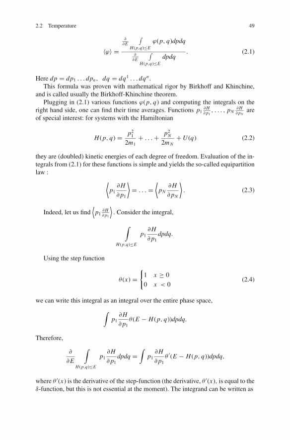
2.2 Temperature 49
〈ϕ〉 =�
�E
∫H (p,q)≤E
ϕ(p, q)dpdq
��E
∫H (p,q)≤E
dpdq. (2.1)
Here dp = dp1 . . . dpn, dq = dq1 . . . dqn .
This formula was proven with mathematical rigor by Birkhoff and Khinchine,and is called usually the Birkhoff-Khinchine theorem.
Plugging in (2.1) various functions ϕ(p, q) and computing the integrals on theright hand side, one can find their time averages. Functions p1
�H�p1
, . . . , pN�H�pN
areof special interest: for systems with the Hamiltonian
H (p, q) = p21
2m1+ . . .+ p2
N
2m N+U (q) (2.2)
they are (doubled) kinetic energies of each degree of freedom. Evaluation of the in-tegrals from (2.1) for these functions is simple and yields the so-called equipartitionlaw :
⟨p1
�H
�p1
⟩= . . . =
⟨pN
�H
�pN
⟩. (2.3)
Indeed, let us find⟨p1
�H�p1
⟩. Consider the integral,
∫
H (p,q)≤E
p1�H
�p1dpdq.
Using the step function
θ (x) ={
1 x ≥ 0
0 x < 0(2.4)
we can write this integral as an integral over the entire phase space,
∫p1
�H
�p1θ (E − H (p, q))dpdq.
Therefore,
�
�E
∫
H (p,q)≤E
p1�H
�p1dpdq =
∫p1
�H
�p1θ ′(E − H (p, q))dpdq,
where θ ′(x) is the derivative of the step-function (the derivative, θ ′(x), is equal to theδ-function, but this is not essential at the moment). The integrand can be written as

50 2 Thermodynamics
p1�H
�p1θ ′(E − H (p, q)) = −p1
�
�p1θ (E − H (p, q))
= − �
�p1(p1θ (E − H (p, q)))+ θ (E − H (p, q)) . (2.5)
The integral of the first term in the right hand side over the entire phase space isequal to zero due to the divergence theorem and vanishing of θ (E − H (p, q)) atinfinity (H (p, q) > E at infinity). Therefore,
�
�E
∫
H (p,q)≤E
p1�H
�p1dpdq =
∫θ (E − H (p, q))dpdq. (2.6)
The result (2.6) does not depend on the choice of a particular component of mo-menta, p1, . . . , pn, and the same answer we get for integrals of p2
�H�p2
, . . . , pn�H�pn
.
Then the equipartition law follows from (2.1) and (2.6)For the systems with Hamiltonians (2.2) equipartition law means that the aver-
aged values of kinetic energies of all degrees of freedom are the same. The commonvalue (2.3) is denoted by T and called absolute temperature. We drop the adjectiveand call it temperature because no other temperatures will appear in our considera-tion.
The integral in the right hand side of (2.6) is called the phase volume,
�(E) =∫
θ (E − H (p, q))dpdq =∫
H (p,q)≤E
dpdq.
The denominator in (2.1) is the derivative of the phase volume, d�(E)/d E,
which will also be denoted for brevity �E (E).Finally, temperature can be expressed explicitly in terms of the phase volume
�(E):
T = �(E)
d�(E)/d E. (2.7)
As follows from (2.7), temperature has the dimension of energy. Traditionally,temperature is measured in degrees. The two numbers are linked by Boltzmann’sconstant k: if T ◦ is the value of temperature in degrees Kelvin, then
T = kT ◦.
The constant k is very small:
k = 1.38× 10⁻¹⁶ erg/ deg .

2.3 Entropy 51
Fig. 2.4 A sketch of energysurface for a two-temperaturesystem
i.e. one degree Kelvin corresponds to energy of about 10−16 g cm2/ s2. Temper-ature becomes on the order of unity if measured in electron-volts. (1 eV is theenergy which an electron gains accelerating between the points with the differ-ence of electric potential equal to 1 V; this energy is very small due to the smallmass of an electron). Room temperature corresponds to about 1/40 eV. Energyunits for temperature are convenient in all theoretical treatments and will be usedhere; Boltzmann’s constant appears only at the stage of comparing theory andexperiments.
Ergodicity is necessary to introduce temperature. If the system is not ergodic,temperature may not exist. For example, consider the system for which the energysurface contains two parts such that trajectory started in one part always remainsin that part (see Fig. 2.4). For such systems, formula (2.1) does not hold, and theequipartition law is not true. Under some additional conditions, one may say thatthe system has two temperatures corresponding to each part of the energy surface,but such a situation is beyond the scope of classical thermodynamics.
Ergodicity yields immediately irreversibility of macromotion. This is seen fromthe equipartition law. Consider, for example, the gas-piston system. Let the pistonbe given some initial velocity. After some time, the equipartition of energy sets upin the system. This means that the average kinetic energy of the piston is equal tothe average kinetic energy of a molecule. Since the mass of the piston is much largerthan the mass of molecules, the velocity of the piston becomes very small, i.e. thepiston comes to rest. This clearly demonstrates the irreversible character of piston’smotion in spite of reversibility of the underlying microdynamics.
2.3 Entropy
Entropy is a characteristic of slow processes in ergodic Hamiltonian systems.3
3 The term “entropy” is widely explored now in many different senses. What we mean here byentropy is, precisely, the thermodynamic entropy introduced by Clausius. The meaning of Clausius’entropy for ergodic Hamiltonian systems was determined by J.W. Gibbs and P. Hertz.

52 2 Thermodynamics
To explain what entropy is, consider first the gas-piston system. Let the positionof the piston, y, be changed slowly by some “hard device.” This means that weprescribe the function, y(t). Changing y we do some work. Therefore energy of thesystem changes. To find the dependence of energy on time we note that Hamiltonianof the system,
H (p, q, y) = p21
2m+ . . .+ p2
n
2m+U (q1, . . . , qn, y), (2.8)
depends explicitly on time through the dependence of potential energy on y. Theenergy rate is
d E
dt= d H (p, q, y)
dt= �H
�pi
dpi
dt+ �H
�qi
dqi
dt+ �H
�y
dy
dt= �H (p, q, y)
�y
dy
dt. (2.9)
The two terms in (2.9) are canceled due to Hamiltonian equations (1.63). Thederivative �H/�y has the meaning of force which one has to apply in order to makethe piston move along the path y(t).4
If we know the trajectory of the systems, p(t), q(t), we could find the energy attime t by integrating (2.9):
E(t)− E(t0) =t∫
t0
�H (p(τ ), q(τ ), y(τ ))
�y(τ )
dy(τ )
dτdτ. (2.10)
In principle, one obtains different values of energy at time t for different trajecto-ries p(τ ), q(τ ) and different piston paths y(τ ). Remarkably, for ergodic Hamiltoniansystems and a slow change of the parameter y, the final value of energy depends onlyon the final value of the parameter y, the initial values of energy, E0 = E(t0) and theinitial value of the parameter y, y0 = y(t0), and depends neither on the trajectories,p (τ ) , q (τ ) , nor on the path, y (τ ):
E(t) = function(y(t), y0, E0). (2.11)
Moreover, the dependence of the final value of energy, E (t) , on y0 and E0
is “degenerated”: the parameters y0 and E0 enter (2.11) only through a combina-tion S(E0, y0), where S(E, y) is some function which is determined uniquely byHamilton function H (p, q, y) :
E (t) = E(y (t) , S0 (E0, y0)). (2.12)
4 For the gas-piston system the factor �H (p, q, y)/�y does not depend on p due to (2.8), but thisis not essential in our reasoning and we proceed in a more general setting.

2.3 Entropy 53
Derivation of (2.12) is quite simple. First, we note that on the right hand side of(2.10) dy/dτ changes slowly. Therefore, �H/�y may be substituted by its averageover the energy surface H (p, q, y(τ )) = E(τ ),
E(t)− E(t0) =t∫
t0
⟨�H
�y
⟩dy
dτdτ,
or, after differentiation with respect to t,
d E
dt=⟨
�H
�y
⟩dy
dt. (2.13)
The average value 〈�H/�y〉 can be computed using the Birkhoff-Khinchinetheorem (2.1) as
⟨�H
�y
⟩=
�
�E
∫H (p,q,y)≤E
�H
�ydpdq
�
�E
∫H (p,q,y)≤E
dpdq. (2.14)
Introducing the phase volume bounded by the energy surface H (p, q, y) = E,
�(E, y) =∫
H (p,q,y)≤E
dpdq =∫
θ (E − H (p, q, y))dpdq, (2.15)
and differentiating (2.15) with respect to y we find
��(E, y)
�y= −
∫θ ′(E − H (p, q, y))
�H (p, q, y)
�ydpdq
= − �
�E
∫θ (E − H (p, q, y))
�H (p, q, y)
�ydpdq (2.16)
= − �
�E
∫
H (p,q,y)≤E
�H (p, q, y)
�ydpdq.
From (2.14) and (2.16)
⟨�H
�y
⟩= − ��(E, y)/�y
��(E, y)/�E. (2.17)
Plugging (2.17) into (2.13) we obtain
��(E, y)
�E
d E
dt+ ��(E, y)
�y
dy
dt= 0. (2.18)

54 2 Thermodynamics
Hence, the phase volume does not change in time, which is also true of anyfunction of the phase volume, S(�).
Let us specify function S(�) by the condition that
�S(� (E, y))
�E= 1
T. (2.19)
Since
�S(�(E, y))
�E= d S
d�
��
�E,
and according to (2.7), T = � (��/�E)−1 , we obtain for S(�) the differentialequation
d S
d�= 1
�,
the only solution of which is
S(E, y) = ln �(E, y)+ const. (2.20)
This function is called thermodynamic entropy.Entropy does not change in the process under consideration. Hence,
S(E, y) = S0, S0 = S(E0, y0). (2.21)
If T > 0, then �S/�E > 0 and we can solve (2.21) with respect to E . We seethat energy is determined by the current value of y, while the initial values of energyand y enter in this dependence only through the combination S0 = S0(E0, y0), i.e.we arrive at (2.12).
In terms of entropy, equation (2.17) for the force, 〈�H/�y〉 , takes the form
⟨�H
�y
⟩= −T
�S(E, y)
�y. (2.22)
Obviously, our derivation remains valid if the system has a number of slowparameters, y1, . . . , ym . In this case, y in all previous equations denotes the sety = (y1, . . . , ym) while (2.22) is replaced by the equation
⟨�H
�yμ
⟩= −T
�S(E, y)
�yμ, (2.23)
where μ runs through values 1, . . . , m.
Equations (2.19) and (2.23) link temperature, T, and generalized forces,〈�H/�yμ〉 , with the slow characteristics of the system, E and yμ. They are called

2.3 Entropy 55
constitutive equations. The constitutive equations are specified as soon as entropyis known as a function of E and yμ. For a given Hamiltonian of the system,H (p, q, y) , one can determine the phase volume computing the integral (2.15),and then find entropy S (E, y) from (2.20).
Constitutive equations (2.19) and (2.23) take a simpler form in the terms offunction E(y, S) :
T = �E(y, S)
�S,
⟨�H
�yμ
⟩= �E(y, S)
�yμ. (2.24)
Indeed, the equation
S (E (S, y) , y) = S (2.25)
must be an identity for all values of parameters S and y. Differentiating (2.25) withrespect to S and yμ, we obtain
�S
�E
�E(S, y)
�S= 1,
�S
�E
�E(S, y)
�yμ+ �S
�yμ= 0. (2.26)
Equations (2.24) follow from (2.19), (2.23) and (2.26).It is worthing emphasize that, if the system were not ergodic or the parameters y
were not slow, then the energy at time t computed from differential equation (2.9)depends on the initial values of the generalized coordinates and momenta p0, q0,
and the entire trajectory y(τ ), τ < t . Therefore, the constitutive equations obtaineddo not make sense.
Formulas (2.12), (2.19), (2.21), (2.23) and (2.24) are valid for any ergodic Hamil-tonian system no matter how many degrees of freedom it has. For example, onecan speak of entropy and temperature of a pendulum, which has just one degreeof freedom. In this case the energy surfaces are closed curves in the phase space(for sufficiently small E). Each trajectory covers the entire energy surface, thus thesystem is ergodic. Assuming for definiteness that the length of the pendulum is aslow parameter, one can find entropy of the pendulum from (1.68): in the limit ofsmall energies, S = ln(E
√l/g)+ const.
Example. Let us find entropy of a gas occupying volume V . We model the gas bya Hamiltonian system of N rigid spheres of radii a and of equal masses m. Eachball has three translational degrees of freedom, so the total number of degrees offreedom, n, is 3N . Hamilton function is a sum of kinetic energy K and particle-particle and particle-wall interaction energy U :
H = K +U,
K = p21
2m+ . . .+ p2
n
2m, U = U (q1, . . . , qn). (2.27)
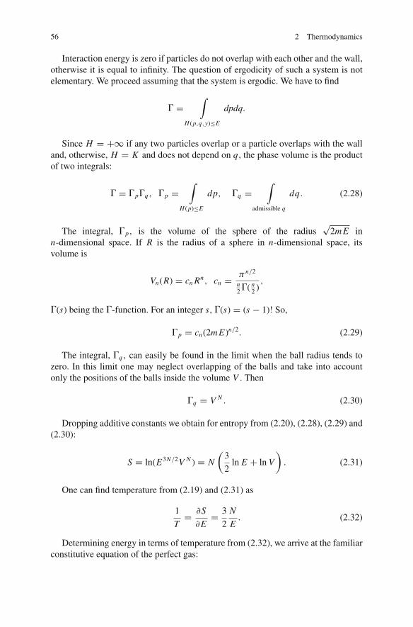
56 2 Thermodynamics
Interaction energy is zero if particles do not overlap with each other and the wall,otherwise it is equal to infinity. The question of ergodicity of such a system is notelementary. We proceed assuming that the system is ergodic. We have to find
� =∫
H (p,q,y)≤E
dpdq.
Since H = +∞ if any two particles overlap or a particle overlaps with the walland, otherwise, H = K and does not depend on q, the phase volume is the productof two integrals:
� = �p�q , �p =∫
H (p)≤E
dp, �q =∫
admissible q
dq. (2.28)
The integral, �p, is the volume of the sphere of the radius√
2m E inn-dimensional space. If R is the radius of a sphere in n-dimensional space, itsvolume is
Vn(R) = cn Rn, cn = πn/2
n2 �( n
2 ),
�(s) being the �-function. For an integer s, �(s) = (s − 1)! So,
�p = cn(2m E)n/2. (2.29)
The integral, �q , can easily be found in the limit when the ball radius tends tozero. In this limit one may neglect overlapping of the balls and take into accountonly the positions of the balls inside the volume V . Then
�q = V N . (2.30)
Dropping additive constants we obtain for entropy from (2.20), (2.28), (2.29) and(2.30):
S = ln(E3N/2V N ) = N
(3
2ln E + ln V
). (2.31)
One can find temperature from (2.19) and (2.31) as
1
T= �S
�E= 3
2
N
E. (2.32)
Determining energy in terms of temperature from (2.32), we arrive at the familiarconstitutive equation of the perfect gas:

2.3 Entropy 57
E = 3
2N T . (2.33)
An important consequence of formula (2.31) is an unbounded growth of entropywhen the gas volume increases. Such a behavior of entropy changes if a force, P,
acts on the piston. Then the Hamiltonian of the system acquires an additional term:5
H = K +U + Py. (2.34)
Calculation of entropy of the system (2.34) is reduced to the previous one for thesystem (2.27) by changing E to E − Py :
S = N
(3
2ln(E − Py)+ ln V
).
Taking into account that V is a linear function of y: V = y�, � being the areaof the piston, and dropping unessential constants, we obtain
S(E, y) = N ln
[3
2ln(E − Py)+ ln(y�)
]
= N ln
[Py
E
(1− Py
E
)3/2]+ const.
A graph of the entropy per particle, S/N , as a function of the dimensionlessdistance y∗ = Py/E is shown in Fig. 2.5.
The remarkable feature of this graph is that entropy reaches its maximum value.The point where entropy is maximum corresponds to the equilibrium state of thesystem the reader is invited to check this fact. It turns out that this property of en-tropy, reaching its maximum value at equilibrium, is generic. The physical origin ofthis property is explained in Sect. 2.5.
So far we have considered the case when all external forces act only on slowvariables as is seen from the energy equation (2.9). Such processes are called adia-batic. If there are some external forces, Fi , acting on the fast coordinates, qi , thenthe energy equation gets the additional term
5 Formula (2.34) becomes obvious if one writes first the energy of the entire system “gas+piston”endowing the piston with some mass M :
H = K +U + Py + Y 2
2M,
where Y is the momentum of the piston. In (2.34) we dropped the kinetic energy of the pistonwhich is negligible because, due to the equipartition of energy over all degrees of freedom, nearequilibrium it is on the order of kinetic energy of one molecule, K/N . The sign + at Py correspondsto the negative direction of the force acting on the piston for P ≥ 0 (indeed, the Lagrange functionof the piston corresponding to the Hamilton function chosen is L = 1
2 M y2−Py, thus M y = −P).

58 2 Thermodynamics
–2
–4
–6
–8
0 0.2 0.4 0.6 0.8 1
Fig. 2.5 S/N , as a function of the dimensionless distance between the piston and the bottom,y∗ = Py/E
d E
dt= �H
�yμ
dyμ
dt+ �H
�qiFi .
Averaging over time and taking into account that E and y change slowly, we have
d E
dt=⟨
�H
�yμ
⟩dyμ
dt+ d Q
dt,
d Q
dt=⟨
�H
�qiFi
⟩. (2.35)
The additional work of external forces denoted by d Q is called heat supply. Heatsupply causes entropy to change. The process is called quasi-equilibrium, if theconstitutive equations (2.28) remain valid for d Q �= 0. Then, we have from energyequation (2.35)
�E(y, S)
�yμ
dyμ
dt+ �E(y, S)
�S
d S
dt=⟨
�H
�yμ
⟩dyμ
dt+ d Q
dt. (2.36)
The first terms on both sides of (2.36) cancel out due to (2.24), and (2.36)becomes a link between entropy, temperature and heat supply:
d Q
dt= T
d S
dt. (2.37)
If d Q �= 0, entropy may either increase or decrease depending on whether energyis pumped to the system (d Q > 0) or taken from the system (d Q < 0).
Comparing the two characteristics of the system, energy and entropy, one maysay that energy is a more fundamental one: energy makes sense for any system whileentropy can be introduced only for slow processes in ergodic systems.
We have seen that the Hamiltonian structure of the equations of micromechanicsyields the laws of equilibrium thermodynamics. One may wonder how important

2.5 Gibbs Principles 59
it is that the equations of micromechanics are Hamiltonian. In other words: couldnon-Hamiltonian equations of microdynamics yield the equations of classical equi-librium thermodynamics? It turns out that the class of such equations is indeedslightly wider than the class of Hamiltonian equations (see Appendix E).
2.4 Entropy and Probability
Slow parameters y fluctuate near the equilibrium values. For example, in the system“gas under piston” the distance between the piston and the bottom, y, varies slightlydue to the collisions of the piston with the molecules. One may wonder what is theprobability density of y, f (y)? The answer was found by Einstein: the probabilitydensity of slow variables fluctuating near the equilibrium values is determined onlyby the equilibrium properties of the system, namely, by the function S(E, y), and isgiven by the formula
f (y) = const eS(E,y). (2.38)
Formula (2.38) has an asymptotic nature and holds for systems with a very largenumber of fast degrees of freedom, n. There is a generalization of this formula forsystems with any finite n [43, 46].
According to (2.38), the most probable values of y are the values for whichentropy takes its maximum value. Since entropy is usually proportional to thenumber of fast degrees of freedom (for a gas this is seen from (2.31)) which islarge, maximum is very sharp and, in fact, the slow variables just fluctuate slightlyaround the equilibrium values.
2.5 Gibbs Principles
Gibbs suggested use of the maximum property of entropy as the first principle inany modeling of thermodynamic equilibrium.The first Gibbs principle. In a state of thermodynamic equilibrium, the entropy Sof an isolated system attains its maximum on all possible states of the system with agiven energyE.
The Gibbs principle differs considerably from the variational principles of ana-lytical mechanics. In mechanics, only the particle positions are subject to change,but in the Gibbs principles virtually all characteristics of equilibrium are varied.In the consideration of phase equilibrium, for example, the interphase surface andthe masses of both phases are subject to change. An example of the application ofthe Gibbs principles to the equilibrium of elastic media will be given in Sect. 7.4.Consider here another example.
Let us show that temperatures of two contacting systems are equal if the systemsare in thermodynamical equilibrium and isolated from the environment. Denote
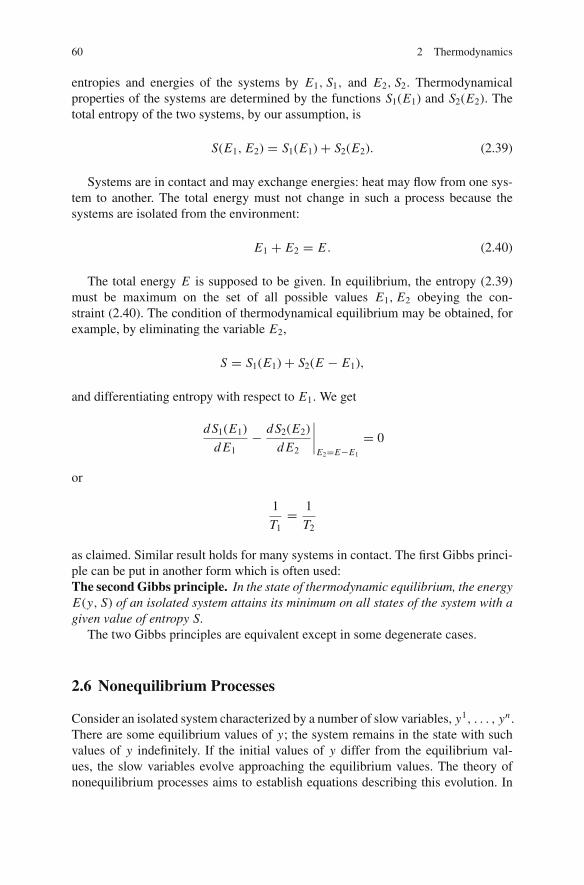
60 2 Thermodynamics
entropies and energies of the systems by E1, S1, and E2, S2. Thermodynamicalproperties of the systems are determined by the functions S1(E1) and S2(E2). Thetotal entropy of the two systems, by our assumption, is
S(E1, E2) = S1(E1)+ S2(E2). (2.39)
Systems are in contact and may exchange energies: heat may flow from one sys-tem to another. The total energy must not change in such a process because thesystems are isolated from the environment:
E1 + E2 = E . (2.40)
The total energy E is supposed to be given. In equilibrium, the entropy (2.39)must be maximum on the set of all possible values E1, E2 obeying the con-straint (2.40). The condition of thermodynamical equilibrium may be obtained, forexample, by eliminating the variable E2,
S = S1(E1)+ S2(E − E1),
and differentiating entropy with respect to E1. We get
d S1(E1)
d E1− d S2(E2)
d E2
∣∣∣∣E2=E−E1
= 0
or
1
T1= 1
T2
as claimed. Similar result holds for many systems in contact. The first Gibbs princi-ple can be put in another form which is often used:The second Gibbs principle. In the state of thermodynamic equilibrium, the energyE(y, S) of an isolated system attains its minimum on all states of the system with agiven value of entropy S.
The two Gibbs principles are equivalent except in some degenerate cases.
2.6 Nonequilibrium Processes
Consider an isolated system characterized by a number of slow variables, y1, . . . , yn .There are some equilibrium values of y; the system remains in the state with suchvalues of y indefinitely. If the initial values of y differ from the equilibrium val-ues, the slow variables evolve approaching the equilibrium values. The theory ofnonequilibrium processes aims to establish equations describing this evolution. In

2.6 Nonequilibrium Processes 61
this section we discuss the situation when the governing equations of the evolutionto equilibrium are ordinary differential equations.
Clausius found from phenomenological reasoning that entropy of an isolated sys-tem may not decrease in the path to equilibrium. This is the so-called second law ofthermodynamics. For Hamiltonian systems this feature of entropy was establishedby Kubo [163]. Hamiltonian systems possess such a feature if the phase flow is mix-ing. In summary, the first and the second laws of thermodynamics are observed onlyfor one reason: the equations governing micromotion are Hamiltonian and mixing.6
If micromotion is not Hamiltonian or mixing, one can construct examples showingthat the first and/or the second laws are violated.
The governing equations of nonequilibrium thermodynamics are purely phe-nomenological. They must obey the constraint of the second law: if the system isisolated, its entropy may not decrease. To construct the evolution equations oneusually chooses as the main idea that entropy has a maximum value at equilibrium.Then the simplest system of equations warranting the approach to equilibrium is
dyμ
dt= Dμν(y)
�S(E, y)
�yν, (2.41)
where Dμν(y) is some positive semi-definite matrix. Indeed, entropy of the systemgrows along each trajectory y(t) of the system (2.41):
d S (E, y (t))
dt= �S(E, y)
�yμDμν(y)
�S(E, y)
�yν� 0. (2.42)
We assumed here that the system is isolated, so the energy remains constant.According to (2.42), Dμν(y) have the meaning of dissipation coefficients, i.e. thecoefficients controlling the entropy growth.
If y(t) are close to the equilibrium values, one can use a linearized version of(2.41). To write down the linearized equations (2.41) we accept that the equilib-rium corresponds to the zero values of y. Then, expanding S in a Taylor series withrespect to y in vicinity of equilibrium, we have
S = const− 1
2aμν yμyν,
where aμν is a non-negative symmetric matrix. In linear approximation the coeffi-cients Dμν are some constants, Dμν = Dμν(0). The governing equations take theform a system of linear differential equations,
dyμ
dt= −Dμν(0)aλν yλ. (2.43)
6 Up to some refinements of this statement like that made at the end of Sect. 2.3, which, mostprobably, are of little physical significance.

62 2 Thermodynamics
Equations (2.41) are more a concept than a “Law of Nature”: in modeling theevolution to equilibrium, one may try equations of the form (2.41), but, in fact, thephysically adequate dynamical equations may have a different form: all one mustnot violate is the evolution of entropy to its maximum value.
Are there other constraints to the governing equations, which are additional to thefirst and the second laws of thermodynamics? Yes, there are. They are caused by theHamiltonian structure of microdynamics. The first such constraint was discoveredby Onsager [236]: the dissipative coefficients, Dμν(0), are not arbitrary. They mustobey the reciprocal relations
Dμν(0) = Dνμ(0). (2.44)
Onsager’s reciprocal relations follow from reversibility of micromotion. The lat-ter takes place if Hamilton function is an even function of momenta, p. There aresystems for which Hamilton function is not an even function, like, for example,the systems under action of external constant magnetic field, B: Hamilton functioncontains the terms of the form, pB, which change the sign if time is reversed . Forsystems in a magnetic field, the coefficients Dμν may also depend on the magneticfield, and Onsager’s reciprocal relations are replaced by
Dμν(0, B) = Dνμ(0,−B).
Note that the coefficients of the linear differential equations (2.43), the productof two symmetric matrices, are not necessarily symmetric.
Onsager’s reciprocal relations are independent of the first and the second laws ofthermodynamics. They are sometimes called the third law of thermodynamics.
There are also other constraints [44, 50]: if the slow variables are the coordinatesand momenta of the underlying Hamiltonian microdynamics, and the dissipationis negligibly small, the equations of slow evolution must possess a Hamiltonianstructure with some effective Hamilton function, Heff (y, S) ,
dyμ
dt= ωμν �Heff(y, S)
�yν. (2.45)
Here ωμν is the constant tensor defining the Hamiltonian structure
ωμν =⎧⎨⎩
1 μ ≥ n + 1, ν = μ
−1 μ ≤ n, ν = n + μ
0 otherwise.
The effective Hamilton function, Heff(y, S), can be calculated explicitly in terms ofthe phase volume of the Hamiltonian system. This calculation shows that it has themeaning of the total energy of the system. Entropy in (2.45) is a given constant. Inmany models of continuum mechanics, the kinematic variables can be viewed as theslow variables of the underlying Hamiltonian system. Therefore, if the dissipation is

2.6 Nonequilibrium Processes 63
neglected, the governing dynamics is Hamiltonian, and the corresponding principleof least action must exist.7 This implies that only quite special interactions with spe-cific “variational reciprocal relations” are possible in continuum mechanics. Mostconsiderations in this book are based on that point.
In general, if the dissipative terms are taken into account, then the slow evolutionis governed by the equations
dyμ
dt= ωμν �Heff(y, S)
�yν− 1
TDμν(y, S)
�Heff(y, S)
�yν
d S
dt= 1
T 2Dμν(y, S)
�Heff(y, S)
�yμ
�Heff(y, S)
�yν, T = �Heff(y, S)
�S. (2.46)
In these equations, the dissipative processes are characterized by the dissipativecoefficients, Dμν (y, S). The dissipative coefficients must be symmetric:
Dμν(y, S) = Dνμ(y, S). (2.47)
Equation (2.47) may be viewed as an extension of Onsager’s relations to thenon-linear case.
Equations (2.46) form a system of ordinary differential equations for unknownfunctions yμ(t) and S(t). The model is specified by the effective Hamiltonian,Heff(y, S), and the dissipative coefficients, Dμν(y, S). The effective Hamiltonianis determined by the equilibrium properties of the system since it can be expressedin terms of its phase volume. In contrast, the dissipative coefficients are the char-acteristics of the nonequilibrium behavior; they describe the mixing properties ofthe underlying Hamiltonian system. The dissipative coefficients are independent ofequilibrium properties: one may envision the systems with the same equilibriumproperties but different laws of evolution to equilibrium.
Energy of the system, Heff(y, S), is conserved in the course of evolution toequilibrium:
Heff(y, S) = E = const, (2.48)
as it must be for an isolated system. Indeed,
d Heff(y, S)
dt= d Heff(y, S)
�yμ
dyμ
dt+ d Heff(y, S)
�S
d S
dt, (2.49)
and the right hand side of (2.49) vanishes due to (2.46).The energy conservation allows us to reduce the order of the system. The re-
sulting equations take a simple form if expressed in terms of the function, S(E, y),
7 The fact that (2.45) holds for isolated systems is not a constraint in consideration of continuummedia: the isolation requirement just specifies the boundary conditions and does not affect thedifferential equations.
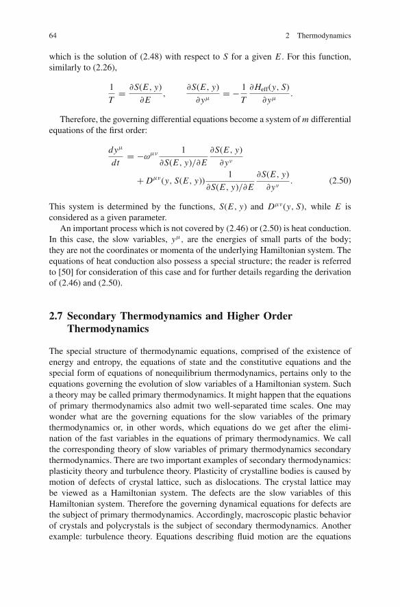
64 2 Thermodynamics
which is the solution of (2.48) with respect to S for a given E . For this function,similarly to (2.26),
1
T= �S(E, y)
�E,
�S(E, y)
�yμ= − 1
T
�Heff(y, S)
�yμ.
Therefore, the governing differential equations become a system of m differentialequations of the first order:
dyμ
dt= −ωμν 1
�S(E, y)/�E
�S(E, y)
�yν
+ Dμν(y, S(E, y))1
�S(E, y)/�E
�S(E, y)
�yν. (2.50)
This system is determined by the functions, S(E, y) and Dμν(y, S), while E isconsidered as a given parameter.
An important process which is not covered by (2.46) or (2.50) is heat conduction.In this case, the slow variables, yμ, are the energies of small parts of the body;they are not the coordinates or momenta of the underlying Hamiltonian system. Theequations of heat conduction also possess a special structure; the reader is referredto [50] for consideration of this case and for further details regarding the derivationof (2.46) and (2.50).
2.7 Secondary Thermodynamics and Higher OrderThermodynamics
The special structure of thermodynamic equations, comprised of the existence ofenergy and entropy, the equations of state and the constitutive equations and thespecial form of equations of nonequilibrium thermodynamics, pertains only to theequations governing the evolution of slow variables of a Hamiltonian system. Sucha theory may be called primary thermodynamics. It might happen that the equationsof primary thermodynamics also admit two well-separated time scales. One maywonder what are the governing equations for the slow variables of the primarythermodynamics or, in other words, which equations do we get after the elimi-nation of the fast variables in the equations of primary thermodynamics. We callthe corresponding theory of slow variables of primary thermodynamics secondarythermodynamics. There are two important examples of secondary thermodynamics:plasticity theory and turbulence theory. Plasticity of crystalline bodies is caused bymotion of defects of crystal lattice, such as dislocations. The crystal lattice maybe viewed as a Hamiltonian system. The defects are the slow variables of thisHamiltonian system. Therefore the governing dynamical equations for defects arethe subject of primary thermodynamics. Accordingly, macroscopic plastic behaviorof crystals and polycrystals is the subject of secondary thermodynamics. Anotherexample: turbulence theory. Equations describing fluid motion are the equations
2.7 Secondary Thermodynamics and Higher Order Thermodynamics 65
of primary thermodynamics. In the case of a chaotic fluid motion, turbulence, themotion is characterized by fast and slow variables. Elimination of fast variables andconstruction of the equations governing the slow variables is the major goal of tur-bulence theory. For both examples of secondary thermodynamics, the developmentof a theory of slow variables has not been completed yet. In particular, it is notknown whether the equations of secondary thermodynamics must possess a specialstructure, as do the equations of primary thermodynamics. Most probably, there areno statements of the same level of generality as for primary thermodynamics. In par-ticular, in turbulence theory different flow geometries may yield quite different sys-tems of equations for slow variables. One feature of secondary thermodynamics canbe quite general though. If the equations of primary thermodynamics exhibit chaoticbehavior, then a new entropy can enter the theory. As in primary thermodynamics, itsmeaning is two fold: the new entropy characterizes fluctuations of the slow variablesand the information on the system lost in the elimination of fast degrees of freedom.In the case of materials with random microstructures, this new characteristic calledentropy of microstructure is introduced and studied in Sect. 18.5−18.8. In contrastto thermodynamic entropy, entropy of microstructure should decrease in an isolatedsystem.8 This feature is caused by the appearance of attractors in the phase space:the phase volume shrinks when the system approaches the equilibrium state.
One may envision the situations when a secondary thermodynamics model pos-sesses two well-separated time scales. Then the elimination of the fast variablesyields the equations of tertiary thermodynamics, etc. What will be common for alllevels of thermodynamics is the existence of energy and entropy equations as longas energy and entropy remain slow variables. Besides, thermodynamic entropy, onceappeared, will remain an increasing function for closed systems.
The existence of entropy is intimately related to the Hamiltonian structure ofmicrodynamics. Such a structure is guaranteed by the classical approximation inquantum mechanics. However, if the quantum mechanics problem has two well-separated time scales, the elimination of the fast variables may yield the dissipa-tive equations already at the level of the quantum mechanics description. On thenext level, the classical mechanics description, one would have a system that isnot Hamiltonian but instead a system with dissipation. Presumably, entropy canstill be introduced, but such a consideration seems not have been pursued yet. Thecontinuum mechanics level of description will then correspond at least to secondarythermodynamics.
8 An exception is the case of unstable systems. For such systems entropy of microstructure can begenerated without external actions.

Chapter 3Continuum Mechanics
3.1 Continuum Kinematics
Continuum kinematics. A continuum is a system consisting of an infinite numberof particles. More precisely, a continuum is defined as a set of particles which isin a one-to-one correspondence with a set of points of some region V in three-dimensional space R3. Each particle can be assigned its “name”: the coordinatesof its counterpart in region V . We denote these coordinates by capital Latin let-ters X1, X2, X3, in contrast to the coordinates of the observer’s frame, which aredenoted by x1, x2, x3. The latter are called Eulerian coordinates, while the coor-dinates X1, X2, X3 are usually referred to as Lagrangian coordinates or materialcoordinates.
Positions of the particles at any instant t are described by the functions
xi = xi(X1, X2, X3, t
).
We use the small Latin indices i, j, k, l for numbering Eulerian coordinates,while for Lagrangian coordinates another group of indices, a, b, c, d is employed.We will call these indices observer’s indices and Lagrangian or material indices,respectively. The reason for such a distinctive notation will be explained later. So,for the particle trajectories we write
xi = xi(Xa, t
)(3.1)
or, if the indices are suppressed,1
x = x (X, t) .
Distinguishing the points of the continuum and assigning each one a “name,” Xa ,is a key point in the definition of continuum. For, if we do not identify particles, we
1 We do not strictly maintain this order of the arguments throughout the book and, in cases whenthe dynamic effects are of primary concern, we write x = x(t, X ).
V.L. Berdichevsky, Variational Principles of Continuum Mechanics,Interaction of Mechanics and Mathematics, DOI 10.1007/978-3-540-88467-5 3,C© Springer-Verlag Berlin Heidelberg 2009
67

68 3 Continuum Mechanics
Fig. 3.1 Lagrangian and Eulerian coordinates
are not able to introduce such notions, as, say, velocity (defining velocity, one hasto say velocity of which object is considered).
Region V is usually identified with the initial position of the continuum. The cur-rent position of the continuum is denoted by V (Fig. 3.1). If we wish to emphasizethat the region V changes in time, we write V (t) instead of V .
For a given observer’s space point x and a given instant t , one can consider (3.1)as a system of three (non-linear) equations with respect to Lagrangian coordinates.In principle, this system of equations can be solved, and one can write
Xa = Xa(xi , t) or X = X (x, t) . (3.2)
Equations (3.2) show which particle arrives at the space point x at the time t .We will call the functions x(X, t) the particle trajectories, and, in case of statics,
when these functions do not depend on time, the particle positions. The inversefunctions, X (x, t) will be called the Lagrangian coordinate flow.
In addition to functions x (X, t), behavior of continuum may need to be charac-terized by other functions u (X, t), some “internal degrees of freedom,” like temper-ature, plastic deformations, concentration of chemical species, etc. Selection of theproper set of characteristics is the first step in continuum modeling.
Tensor character of continuum mechanics equations. We have introduced twocoordinate frames, the observer frame with the Eulerian coordinates xi , and the ma-terial frame with the Lagrangian coordinates Xa . Even if Eulerian coordinates areCartesian, Lagrangian coordinates are, in general, curvilinear (Fig. 3.2). Therefore,the technique of curvilinear coordinates appears naturally. Besides, all the relationswe consider must not depend on the choice of Eulerian and Lagrangian coordinates.Thus, tensor analysis must be employed. In order to make the text approachablefor the reader who is not familiar with tensor analysis and the theory of curvilinearcoordinates, the following simplifications are made. First, the text is written in such

3.1 Continuum Kinematics 69
Fig. 3.2 Curvilinear nature ofLagrangian coordinates:material frame in the initialand the current states
a way that all remarks concerning tensor character of the relations derived can beomitted without detriment to understanding the key part of the material. Second,though all equations in the book are written in a proper tensor form distinguishingupper and lower indices, the reader may decline making a difference between upperand lower Eulerian indices i, j, k, l, accepting that the observer frame is Cartesian.Therefore, for example, one can identify x1 (Xa, t) and x1 (Xa, t). Such identifica-tion, however, cannot be made for quantities with Lagrangian indices; for example,Xa and Xa must be treated as different quantities. If a quantity with Lagrangianindices is used with upper and lower indices we always provide the link betweenthe two. Third, we use the Cartesian coordinates for the observer’s frame; thereforethe covariant derivatives do not appear, and the space derivatives with respect toEulerian coordinates are just �/�xi . The subsections concerned with the issues ontensor features of continuum mechanics are furnished with the sign ∗ which indi-cates that the subsection can be omitted by an uninterested reader. The only tensornotation which the reader is supposed to know is the summation convention overrepeated indices introduced in Sect. 1.4. One simple statement from tensor analysis,the sum ai j bi j is zero if ai j is symmetric and bi j is anti-symmetric, is also used.Perhaps, the only part of the book where the knowledge of tensor analysis cannotbe avoided is the shell theory (Chap. 14) where the coordinate system on the shellmiddle surface is inevitably curvilinear.
Distortion. Derivatives
xia =
�xi (X, t)
�Xa
are called distortions (the term deformation gradient is often used as well). Deriva-tives
Xai =
�Xa (x, t)
�xi
are called inverse distortions.They obey the equations
xia Xa
j = δij , xi
a Xbi = δb
a , (3.3)
where δij is Kronecker’s delta: δi
j = 1 if i = j and δij = 0 if i �= j .

70 3 Continuum Mechanics
The first equation (3.3) can be obtained from the identity
xi (X (x, t) , t) = xi , (3.4)
which expresses the fact that functions X (x, t) are solutions of (3.1). Differentiating(3.4) with respect to x j and using the chain rule, we obtain
�xi (X (x, t) , t)
�x j= �xi (X (x, t) , t)
�Xa
�Xa (x, t)
�x j= xi
a Xaj =
�xi
�x j= δi
j ,
i.e. the first equation (3.3) holds. The second equation (3.3) is derived similarly fromthe identity
Xa (x (X, t) , t) = Xa .
Matrices will be denoted by double bars:∥∥xi
a
∥∥means the matrix with the compo-nents xi
a . Equations (3.3) mean that the matrix∥∥Xa
i
∥∥ is inverse to the matrix∥∥xi
a
∥∥.Indeed, let the upper indices number the columns, while the lower indices numberthe rows. Then (3.3) can be written as
∥∥xia
∥∥ · ∥∥Xaj
∥∥ = ∥∥δij
∥∥ ,∥∥Xa
i
∥∥ · ∥∥xib
∥∥ = ∥∥δab
∥∥ ,
i.e. Xai are the components of the inverse matrix. This explains the term “inverse
distortion” for Xai .
Velocity. Time derivative when Lagrangian coordinates are kept constant is denotedby d/dt and called material time derivative. By definition, the particle velocity is
vi = dxi (X, t)
dt.
As has been mentioned, velocity cannot be defined if Lagrangian coordinates arenot introduced explicitly: vi (X, t) is the velocity of the particle with the Lagrangiancoordinate X.
Velocity and distortion obey the compatibility relation
�vi
�Xa= dxi
a
dt. (3.5)
Inverse matrix. Let the determinant of matrix∥∥∥ai
j
∥∥∥ ,
a = det∥∥ai
j
∥∥ ,
be not equal to zero and a(−1)ij be the components of the matrix which is inverse to
the matrix∥∥∥ai
j
∥∥∥ :

3.1 Continuum Kinematics 71
∥∥aij
∥∥ ·∥∥∥a(−1) j
k
∥∥∥ =∥∥δi
k
∥∥ .
To write this equation in the index form we accept a convention that the upper andthe lower indices are the numbers of the row and the column, respectively. Thena(−1)i
j obey to the system of equations
aij a
(−1) jk = δi
k, (3.6)
Equations (3.6) may be considered as a system of n linear equations with respect toa(−1) j
k assuming that aij are given. It follows from (3.6) that a(−1)i
j obeys also to asystem of equations,
aij a
(−1)ki = δk
j . (3.7)
In equation (3.6) the lower index of aij is involved in summation; in equation (3.7)
the upper index does. Equations (3.7) is an index form of the matrix equation,
∥∥∥a(−1)ki
∥∥∥ ·∥∥ai
j
∥∥ = ∥∥δkj
∥∥ .
To prove (3.7) one can first check that, due to (3.6),
(aij a
(−1)ki − δk
j )amk = 0. (3.8)
(opening brackets in (3.8) we arrive at an identity, amk − am
k = 0). Since det∥∥∥ai
j
∥∥∥ �=0, equation (3.7) follows from (3.8).Metric tensor. The distance ds between the points with coordinates xi and xi +dxi
is, by definition,
ds2 = gi j dxi dx j , (3.9)
where gi j = g ji are called the covariant components of metric tensor. Determinantof the matrix
∥∥gi j
∥∥ is denoted by g :
g = det∥∥gi j
∥∥ . (3.10)
In Cartesian coordinates gi j are constant and equal to Kronecker’s delta δi j whileg = 1.
Contravariant components of metric tensor, gi j , are, by definition, the compo-nents of the matrix inverse to the matrix
∥∥gi j
∥∥:
gi j gk j = δik .
In Cartesian coordinates, gi j = gi j = δi j .

72 3 Continuum Mechanics
Similarly, the distance between the two material points Xa and Xa + d Xa is
ds2 = gabd Xad Xb, (3.11)
where gab are the Lagrangian components of the metric tensor.Comparing (3.9) and (3.11) and using the equality
dxi = xiad Xa,
we obtain the expression of the metric tensor in Lagrangian coordinates in terms ofdistortion:
gab = gi j xia x j
b . (3.12)
Contravariant components of metric tensor in Lagrangian coordinates, gab, arethe components of the inverse matrix to the matrix ‖gab‖. The reader is invited tocheck that
gab = gi j Xai Xb
j , Xai = gi j g
abx jb . (3.13)
The Levi-Civita symbol. A system of numbers ei jk = eki j = ei jk where
e123 = e312 = e231 = 1, e213 = e321 = e132 = −1,
and all other ei jk are equal to zero is called the three-dimensional Levi-Civita sym-bol. The Levi-Civita symbol is used for explicitly writing determinants and vector
products. For any tensor aij , the determinant of the matrix
∥∥∥aij
∥∥∥ is
det∥∥ai
j
∥∥ = ei jkai1a j
2 ak3 . (3.14)
Note also the following relations:
ei jkail a j
makn = det
∥∥aij
∥∥ elmn, (3.15)
det∥∥ai
j
∥∥ = 1
3!ei jkai
l a jmak
nelmn . (3.16)
In Cartesian coordinates the vector with the components ei jkai b j is called thevector product of the vectors with components ai and b j . An important role inoperations with vector products is played by the identities
ei jkelmk = δli δ
mj − δm
i δlj , ei jkel jk = 2δl
i . (3.17)
In Cartesian coordinates the Levi-Civita symbol coincides with the Levi-Civitatensor, εi jk, defined in the next subsection.

3.1 Continuum Kinematics 73
The Levi-Civita tensor*. It is easy to derive from (3.15) that the quantities εi jk
which are equal to√
gei jk in coordinate systems of one orientation and to −√gei jk
in coordinate systems of the opposite orientation form the components of a covarianttensor of the third order. This tensor is called the Levi-Civita tensor.
One can introduce two Levi-Civita tensors setting ε123 = 1 or ε123 = −1 in adextral Cartesian coordinate system (i.e. at right handed orientation). Accordingly,there are two ways to introduce a vector product. The two vector products differ bya sign. In what follows, we assume ε123 = √g in a dextral coordinate system.
Appearance of the Levi-Civita symbol in a theory indicates that left handed andright handed coordinate systems are not equivalent.2
Note the relation for contravariant components of the Levi-Civita tensor:
εi jk = gii ′g j j ′gkk ′εi ′ j ′k ′ = 1√g
ei jk . (3.18)
The identities (3.17) yield the corresponding identities for the Levi-Civita tensor:
εi jkεlmk = δl
i δmj − δm
i δlj , εi jkε
l jk = 2δli . (3.19)
In a Cartesian coordinate system, εi jk = εi jk = ei jk .
Formula for inverse matrix. We will employ a useful explicit formula for the com-ponents of the inverse matrix in terms of the determinant a.
The determinant a is a certain function of the matrix components: a = a(
aij
).
The components of the inverse matrix a(−1) ij are the derivatives of ln a:
a(−1) ji =
1
a
�a
�aij
= � ln a
�aij
. (3.20)
The reader can easily check the validity of (3.20) for two-dimensional matricesby direct inspection. Since this formula will be used further on many occasions, wegive here its proof for 3 × 3 matrices; the proof in general case is similar. From(3.14),
�a
�ai1
= ei jka j2 ak
3 .
Hence,
1
a
�a
�ai1
ai1 = 1,
1
a
�a
�ai1
ai2 = ei jkai
2a j2 ak
3 = 0.
2 The exceptions are the cases when εi jk are contained in products such as εi jkεlmn which are
invariant with respect to the sign change of εi jk .

74 3 Continuum Mechanics
Here we used that summation of object, ei jk , which is anti-symmetric over i j , andthe tensor ai
2a j2 , which is symmetric over i j, is zero. Similarly,
1
a
�a
�ai1
ai3 = 0.
Therefore, the term 1/a �a/�ai1 obeys (3.7) with
a(−1)1i = 1
a
�a
�ai1
.
Other relations (3.7) are verified in the same way.
Jacobian of transformation from Lagrangian to Eulerian variables and relatedformulas. Denote by � the Jacobian of transformation from Lagrangian to Eulerianvariables:
� = det∥∥xi
a
∥∥ .
The following useful consequences of (3.15) hold:
ei jk xia x j
b xkc = �eabc, eabc Xa
i Xbj Xc
k =1
�ei jk, (3.21)
eabcxia x j
b xkc = �ei jk, ei jk Xa
i Xbj Xc
k =1
�eabc.
Contracting the second equation (3.21) with xia x j
b we obtain:
eabc Xck =
1
�ei jk xi
a x jb . (3.22)
Further contraction of (3.22) with eabc and use of the second formula (3.17)yields
Xck =
1
2�ei jk xi
a x jb eabc. (3.23)
The same result can be obtained from relation (3.20) by differentiation ofJacobian,
Xai =
1
�
��
�xia
. (3.24)
An equivalent form of (3.23) is obtained by contraction of (3.23) with Levi-Civitasymbol, ei ′ j ′k, and use of (3.17):
Xckei jk = 1
�xi
a x jb eabc.

3.1 Continuum Kinematics 75
Similarly to (3.23), distortion can be expressed in terms of inverse distortion:
xkc =
1
2 det∥∥Xa
i
∥∥ei jk Xai Xb
j eabc. (3.25)
Lagrangian components of metric tensor and Levi-Civita tensor. The determi-nant of the matrix det‖gab‖ will be denoted by g. According to (3.20), the con-travariant Lagrangian components of metric tensor are related to g by the formula
gab = 1
g
�g
�gab. (3.26)
For Lagrangian components of the Levi-Civita tensor we have
εabc =√
geabc, εabc = 1√g
eabc.
Note that
g = g�2. (3.27)
Therefore formulas for Lagrangian components of the Levi-Civita tensor can bewritten also as
εabc = √g�eabc, εabc = 1√g�
eabc. (3.28)
The initial position/initial state. Consider the position of continuum at some initialinstant t0:
xi = xi(Xa, t0
) = x i(Xa). (3.29)
Lagrangian coordinates can be always chosen to coincide with the Eulerian co-ordinates at the initial instant. Then the functions (3.29) become
x1(Xa) = X1, x2
(Xa) = X2, x3
(Xa) = X3. (3.30)
Transformations of Lagrangian coordinates change functions (3.30). Therefore,in order to maintain the ability to keep the invariance of all the relations with respectto the transformations of the Lagrangian coordinates, we will describe the initialposition of the system by functions (3.29) of general form.
The components of the metric tensor in the initial state are
gab = gab (X, t0) = gi j xia x j
b, gab = gi j X ai X b
j .
Here,
x ia =
�x i
�Xa, X a
i =1
�
��
�x ia
, � = det∥∥x i
a
∥∥ .
All the initial values are furnished with the symbol ◦.

76 3 Continuum Mechanics
Transformation from Eulerian to Lagrangian coordinates. Let f (x, t) be ascalar function of Eulerian coordinates and time. From this function, two differentfunctions of Lagrangian coordinates, f (x (X ) , t) and f (x (X, t) , t), can be con-structed. In what follows, if not noted otherwise, we use the second way, i.e. thetransformation from Eulerian to Lagrangian coordinates and back is done by meansof the particle trajectories x (X, t) and the Lagrangian coordinate flow X (x, t).
Two groups of transformations∗. Continuum mechanics equations have a tensorcharacter with respect to the two groups of transformation: the group of Euleriancoordinate transformations,
x ′i = x ′i (x j ), (3.31)
and the group of Lagrangian coordinate transformations,
X ′a = X ′a(Xb). (3.32)
Now we can give a precise distinction between Eulerian indices which wedenoted by the group of letters i, j, k, l and Lagrangian indices for which the let-ters a, b, c, d were reserved. The group (3.31) causes the transformation of Eu-lerian indices while the objects with Lagrangian indices are not affected by thisgroup and behave as scalars. Similarly, the group (3.32) yields the transformationsof the objects with Lagrangian indices leaving the objects with Eulerian indicesunchanged.
The examples are: velocity, vi , a vector with respect to the group (3.31) and aset of three scalars with respect to the group (3.32); the metric tensor gab, a set ofsix scalars with respect to the group (3.31) and a tensor of the second order withrespect to the group (3.32); distortion xi
a , a set of three vectors with respect to thegroup (3.31) and a set of three vectors with respect to the group (3.32).
Using the first letters of the Latin alphabet a, b, c, d for Lagrangian coordinatesis a tribute to the tradition of the nineteenth century to denote the three Lagrangiancoordinates by the first letters of the Latin alphabet a, b, c.
Juggling with indices. Indices are moved up and down by the following rule: Foran object with upper index, T i , by definition,
Ti = gi j Tj .
Accordingly,
T i = gi j Tj .
Since we agreed to deal with Cartesian observer’s frame, gi j = gi j = δi j , wehave T i = Ti . Nevertheless, in order to have all the relations in tensor form, wekeep the metric tensor when necessary.

3.1 Continuum Kinematics 77
For the objects with the Lagrangian indices, keeping the metric tensor while jug-gling with the indices is always necessary because in Lagrangian coordinates wehave two different metric tensors, gab and gab, and, to avoid ambiguities, we haveto specify which one is used for juggling.
Strain measures. Distortion xia (X, t) describes an affine deformation of an in-
finitesimally small element of the continuum in the neighborhood of a point X .There are two ways of extracting strain from the distortion. Strain is a part of affinedeformation not affected by the rotation of the element. The first way uses the metrictensor in the Lagrangian coordinate system. It is apparent that the tensor gab mea-suring the distances does not depend on the rotation of the material element. Thetensor
εab = 1
2
(gab − gab
) = 1
2
(gi j x
ia x j
b−gab
)(3.33)
can be used as a measure of strain.The second way of defining strain is based on splitting the matrix
∥∥xia
∥∥ into theproduct of a symmetric positive matrix3 with the components |x |ab and an orthogo-nal matrix with the components λib,
xia = |x |ab λib. (3.34)
The orthogonality of the matrix∥∥λib
∥∥ means that
gi jλibλ jc = gbc, gbcλ
ibλ jc = gi j . (3.35)
Formula (3.34) corresponds to presenting the affine deformation as a superpo-sition of extensions in three directions and orthogonal rotation. Indeed, by rotatingcoordinates one can put a symmetric matrix, |x |ab , into diagonal form. The fibersdirected along the axes of the new coordinate system (along the principal directionsof the tensor |x |ab) elongate or contract depending on whether the correspondingeigenvalue of the tensor |x |ab is greater or smaller than unity. The final distortionis obtained by rotation of the deformed fibers. Presentation of matrices in the form(3.34) is called the polar decomposition.
Tensors |x |ab and gab are related as
gab = gi j xia x j
b = gcd |x |ac |x |bd . (3.36)
According to (3.36), gab and |x |ab can be made diagonal by the same orthogonal(with respect to the metric gab) transformation.
Formula (3.36) provides a one-to-one correspondence between gab and |x |ab . In-deed, if |x |ab is known then gab is determined by (3.36). The principal coordinates oftensors |x |ab and gab (the coordinates in which |x |ab and gab are diagonal) coincide
3 Positiveness of a symmetric matrix means that its eigenvalues are positive.

78 3 Continuum Mechanics
according to (3.36). If gab is known, then, to find |x |ab, one makes an orthogonaltransformation which diagonalizes gab. Since |x |ab are diagonal in the same coordi-nate system and the principal values are positive, we have (for gab = δab)
|x |11 =√
g11, |x |22 =√
g22, |x |33 =√
g33.
Since the tensor |x |ab is a “square root” of the metric tensor, it is called thedistortion modulus.
The tensor |x |ab depends on the distortion semilinearly, i.e. if the distortion ismultiplied by a positive constant, |x |ab acquires the same factor.
The tensor λib can be expressed in terms of xia as
λib = |x |(−1)ba xia,
where |x |(−1)ba is the inverse of the tensor |x |ab:
|x |ab |x |(−1)bc = δca .
In the system of coordinates in which the tensor |x |ab is diagonal,
|x |(−1)11 = 1
|x |11, |x |(−1)22 = 1
|x |22, |x |(−1)33 = 1
|x |33.
Therefore, |x |ab and λib are uniquely determined in terms of the distortion xia .
Using the tensor |x |ab, we can construct a second strain measure:
γab = |x |ab − gab. (3.37)
Note that
|x |ab ≡ |x |ab|t=t0 = gab.
This equality can be checked by transforming tensor |x |ab into its principal axes.According to (3.36) and (3.37), the strain tensors εab and γab are related as
εab = γab + 1
2gcdγacγbd . (3.38)
Strain measures εab and γab are useful if the deviations of gab from their initialvalues, gab, are small. Otherwise, it is more convenient to use gab as the primarycharacteristics of deformations.
A representation of three-dimensional orthogonal matrices. The matrix with thecomponents λia , orthogonal in sense of (3.35), can be orthogonal in the usual senseif it is multiplied by matrix
∥∥x ia
∥∥, αi j = x iaλ
ja . Indeed from (3.35) we find that thematrix
∥∥αi j
∥∥ is inverse to itself:
αi jαk j = δik αi jαik = δ
jk . (3.39)

3.1 Continuum Kinematics 79
A characteristic feature of the orthogonal transformation in three-dimensionalspace is that an orthogonal transformation keeps one line, the axis of rotation, im-mobile. Denote the axis of rotation by C and the unit vector directed along it by ci .Since the transformation does not change ci ,
αi j c j = ci .
Due to the orthogonality of αi j we can also write
αi j ci = c j .
The orthogonal transformation can be given by vector ci and the angle θ ofcounterclockwise (if observed from the end of ci ) rotation around the line C . Thecouples (ci , θ ) and (−ci ,−θ ) define the same transformation. The components ofthe orthogonal matrix, αi j , are expressed in terms of ci and θ as
αi j = cos θgi j + (1− cos θ ) ci c j − sin θεi jkck . (3.40)
This can be checked by writing down (3.40) in an orthogonal coordinate system oneof the axes of which coincides with C .
Inversely, if the components of matrix αi j are known, the angle θ is found bymeans of the formula
cos θ = 1
2
(αi
i − 1), (3.41)
It follows from (3.40) by contraction over indices i, j. Then the vector ci is com-puted by contracting (3.40) with εi jk and using (3.19)2 :
ck = − 1
2 sin θεi jkα
i j .
The analogous expression for the orthogonal matrix with the determinant equalto −1 is
αi j = cos θgi j − (1+ cos θ ) ci c j − sin θεi jkck . (3.42)
Space and time derivatives. The derivatives with respect to time with Eulerian co-ordinates held constant will be denoted in several ways depending on convenience:
�t ≡ (·),t ≡ (·)t ≡�
�t.
Similarly, for spatial derivatives with respect to Eulerian coordinates we use thenotation
�
�xi≡ �i ≡ (·),i

80 3 Continuum Mechanics
while spatial derivatives with respect to Lagrangian coordinates are denoted as
�
�Xa≡ �a ≡ (·),a .
Obviously, for any function of Eulerian coordinates and time, u(x, t),
du
dt= du(x(X, t), t)
dt= �u
�t+ �u
�xi
dxi
dt= �u
�t+ vi �u
�xi.
The order of differentiation with respect to time and space coordinates, �t and�i , can be changed:
�
�xi
�
�t= �
�t
�
�xi.
Similarly,
�
�Xa
d
dt= d
dt
�
�Xa.
However,
�
�xi
d
dt�= d
dt
�
�xi,
�
�Xa
�
�t�= �
�t
�
�Xa.
The operator �t applied to the components of a tensor with Eulerian indices re-sults in tensor components with a similar index structure. The same is true for theoperator d/dt applied to tensor components with Lagrangian indices.
The material time derivative of tensor components with Eulerian indices does notyield a tensor. For example,
dxia
dt= �
�Xa
dxi
dt= �vi
�Xa= xk
a
�vi
�xk. (3.43)
Quantities dxia/dt do not transform by tensor rules since they are expressed in terms
of partial (not covariant) derivatives of velocity.
The strain rate tensor. The components of the strain rate tensor in the Lagrangiancoordinate system are defined as
eab = dεab
dt.
Differentiating (3.33) with respect to time, we get
2eab =(
gi j�vi
�Xax j
b
)+ (a ↔ b) . (3.44)

3.1 Continuum Kinematics 81
By (a ↔ b) we denote the previous term in brackets with index a changed to band index b changed by a.
Equation (3.44) can be rewritten as4
2eab = xia x j
b
(�vi
�x j +�v j
�xi
). (3.45)
Contracting (3.45) with inverse distortions Xai Xb
j , we obtain the following ex-pression for the strain rate tensor in the Eulerian coordinate system, ei j = Xa
i Xbj eab:
ei j = �(iv j) ≡ 1
2
(�vi
�x j +�v j
�xi
). (3.46)
The parentheses in indices stand for symmetrization:
a(i j) ≡ 1
2
(ai j + a ji
).
Let us emphasize that the time derivatives of Eulerian components of the straintensor, εi j = Xa
i Xbj εab, are not equal to ei j :
ei j �= dεi j
dt.
Rigid motion. Consider the motion of the system when the distortion xia does not
depend on the Lagrangian coordinates. In this case, the particle trajectories are
xi = r i (t)+ αia (t) Xa . (3.47)
Functions xi = r i (t) define the trajectory of the particle with the zero Lagrangiancoordinates.
The motion (3.47) is called homogeneous deformation. It is called rigid if thedistortion, xi
a = αia, is an orthogonal matrix, i.e.
gi jαiaα
jb = gab, gabαi
aαjb = gi j . (3.48)
4 In curvilinear Euler’s coordinates one has to differentiate in (3.44) the metric tensor as well. Thatyields an additional term dgi j
dt x ia x j
b in (3.45). Since
dgi j(xk (Xa, t)
)
dt= dgi j
dxkvk ,
�gi j
�xk= gmj �
mik + gmi �
mjk ,
where �mik are Kristoffel’s symbols, (3.45) gets a tensor form
2eab = xia xi
b
(∇iv j + ∇ j vi).
where ∇i is the covariant space derivative in Eulerian coordinates.

82 3 Continuum Mechanics
For gi j = δi j , gab = δab, the matrix αia is orthogonal in the usual sense.
Note that the second equation (3.48) follows from the first one, and vice versa.Indeed, denote gabαi
aαjb by gi j . Contracting the first equation (3.48) with gacαk
c , weget the relation gi j gikα
jb = αk
b which, due to the non-degeneracy of the matrix∥∥αi
a
∥∥,implies that gi j gik = δk
j . Therefore gik = g(−1)ik = gik , as claimed; similarly, onecan prove that the first equation (3.48) follows from the second one.
In rigid motion, according to the first equation (3.48), the strain tensor is equalto zero. The inverse statement is also true, i.e. if the strain tensor is equal to zero atevery point of the continuum, the particle trajectories are given by formulas (3.47)where αi
a is an orthogonal matrix. Hence, the rigid motion can be defined as a motionfor which the distance between any two points of the continuum does not changeover time.
The continuum which performs only rigid motions is called a rigid body. Thevelocities of the particles of the rigid body can be found by differentiating (3.47):
vi(Xa, t
) = ui (t)+ dαia (t)
dtXa, ui ≡ dr i
dt. (3.49)
Here ui is the velocity of the point with the zero Lagrangian coordinates.Let us find the velocity field vi as a function of Eulerian coordinates. In order
to do this, we first need to express the Lagrangian coordinates in terms of Euleriancoordinates from (3.47):
Xa(xi , t
) = α ja (t)(x j − r j (t)
). (3.50)
It does not matter which metric tensor, gab or gab, is used to lift the index in αia
because gab=gab for a rigid motion. Substituting (3.50) into (3.49), we get
vi(xk, t
) = ui (t)+ ω j i (t)(x j − r j (t)
). (3.51)
where we introduced the notation
ω j i = α ja (t)dαi
a
dt. (3.52)
Tensor ω j i is antisymmetric with respect to i, j . Indeed, differentiating the sec-ond equation (3.48) with respect to t and using the definition (3.52), we obtain
d
dt
(αi
aαjb gab
)= ωi j + ω j i = 0.
Antisymmetric tensors of the second order, ωi j , in a three-dimensional space arein one-to-one correspondence with vectors, ωk , such that
ωi j = εi jkωk, ωk = 1
2εki jω
i j . (3.53)

3.1 Continuum Kinematics 83
Relations (3.53) follow from (3.19). The vector
ωk = 1
2εki jα
ia dαja
dt, (3.54)
is called the angular velocity vector of a rigid body, ωi j the tensor of angular veloc-ity, ωi j dt the tensor of infinitesimally small rotation, and dϕi = ωi dt the angle ofinfinitesimally small rotation. The kinematic relation (3.51) in terms of the vectorof angular velocity takes the form
vi(xk, t
) = ui (t)+ εik jωk(x j − r j (t)
). (3.55)
Time derivative of Lagrangian coordinates. By the definition of the material timederivative,
d Xa
dt= 0. (3.56)
If one plugs into (3.56) the dependence of Xa on Eulerian coordinates, one gets
d Xa(t, x)
dt= d Xa(t, x(t, X ))
dt= �Xa(t, x)
�t+ �Xa
�xi
dxi
dt= 0
or
�Xa
�t+ vi �Xa
�xi= 0. (3.57)
Equations (3.57) may be considered as a system of three linear equations withrespect to velocity. Contracting (3.57) with x j
a and using the first equation (3.3) weobtain
vi = −xia
�Xa
�t(3.58)
Equation (3.58) presents velocity in terms of time and space derivatives of theLagrangian coordinate flow Xa(t, x) because xi
a may be viewed as some functionsof the derivatives of Xa(t, x), Xa
i .
Time derivative of the inverse distortion. Let us show that
d Xaj
dt= −Xa
i
�vi
�x j. (3.59)
Indeed, differentiating (3.57) with respect to x j , we have
�
�t
�Xa
�x j+ vi �
�xi
�Xa
�x j+ �vi
�x j
�Xa
�xi= 0. (3.60)
Since the sum of the first two terms in (3.60) is d Xaj /dt, we arrive at (3.59).

84 3 Continuum Mechanics
Invariant integration. In an Eulerian coordinate system, the volume element dV is
dV = √gdx1dx2dx3 (3.61)
where g is the determinant (3.10). After the coordinate transformation, x → X,
dV = √g |�| d X1d X2d X3,
where � is the Jacobian of transformation. Since, due to (3.27),
√g = √g |�| , (3.62)
the volume element in Lagrangian coordinates in the current state is
dV =√
gd X1d X2d X3. (3.63)
Similarly, in the initial state,
dV =√
gd X1d X2d X3, g = det ‖gab‖ . (3.64)
It can be proved that dV and dV are scalars with respect to transformationsof Lagrangian coordinates which do not change the orientation of the coordinatesystem.
Integrals
∫
V
�dV,
∫
V
�dV
have the same form in all Lagrangian coordinate systems, Xa, if � is a scalar withrespect to transformations of Lagrangian coordinates.
The following equality holds:
∫
V
�√
gd X1d X2d X3 =∫
V
�√
gdx1dx2dx3, (3.65)
where V is the region occupied by the system in the current state. Equation (3.65)allows one to convert the integrals over Eulerian variables to the integrals overLagrangian variables and vice versa.
The continuity equation. Denote by ρ the mass density. Then the mass of thematerial occupying the volume element dV is ρdV . We assume that the mass ofeach volume element does not change in the course of motion, i.e.
ρdV = ρ0dV , (3.66)

3.1 Continuum Kinematics 85
where ρ0 is the mass density in the initial state. Then, from (3.63), (3.64), and (3.66),it follows the so-called continuity equation in Lagrangian variables:
ρ√
g = ρ0
√g. (3.67)
In the initial state, the mass density ρ0 and the metric tensor are some given func-tions of Xa . For given particle trajectories, one can find g; therefore, the continuityequation can be considered as an equation allowing one to find the mass density, ρ,
if the continuum motion is known:
ρ = ρ0
√g√
g. (3.68)
In terms of the determinant of distortion, �, according to (3.62),
ρ = ρ0
√g√
g
1
|�| . (3.69)
Hence, the mass density is a function of distortion, xia . Further we assume that
� > 0, and the sign of the absolute value in (3.69) can be dropped: at the initialstate � > 0, and, in order to change the sign, � must become zero at some spacepoint; vanishing of � would mean a collapse of a material volume to a point or asurface – we exclude such cases from consideration.
In many cases it is convenient to consider mass density as a function of Euleriancoordinates. As such, mass density obeys the equation
dρ
dt+ ρ
�vi
�xi= 0. (3.70)
To derive (3.70) we differentiate (3.69) with respect to time while keeping theLagrangian coordinates constant and use (3.24) and (3.43):
dρ
dt= − ρ0
√g√
g�2
��
�xia
dxia
dt= −ρXa
i
dxia
dt= −ρXa
i
�vi
�Xa= −ρ
�vi
�xi .
The formula for mass density (3.68) may be considered as the solution of thedifferential equation (3.70) for mass density.
Note the relation for the time derivative of the distortion determinant, �, whichfollows from (3.69) and (3.70):
d�
dt= �
�vi
�xi. (3.71)
Equation (3.66) allows one to convert easily the integrals of densities per unitmass over the Eulerian variables into the integrals over the Lagrangian variables;

86 3 Continuum Mechanics
for example, in the case of the internal energy density per unit mass, U , one canwrite
∫
V
ρUdV =∫
V
ρ0UdV . (3.72)
Derivative of the Jacobian with respect to parameters. Formula (3.71) is a specialcase of a more general relation. Consider a coordinate transformation, X → x,
which depends of parameters yμ, μ = 1, ..., m :
xi = xi(Xa, yμ
).
Let � be the Jacobian of this transformation:
� = det
∥∥∥∥�xi
�Xa
∥∥∥∥ .
Then
��
�yμ
∣∣∣∣X=const
= ��
�xi
�xi (X, y)
�yμ. (3.73)
Indeed,
��
�yμ
∣∣∣∣X=const
= ��
�xia
�xia
�yμ= �Xa
i
�
�Xa
�xi (X, y)
�yμ= �
�
�xi
�xi (X, y)
�yμ.
Some identities. Consider an arbitrary coordinate transformation, x = x(X ). Forthe Jacobian of this transformation an identity holds
�
�x j
1
�x j
a = 0. (3.74)
It can be checked by direct inspection:
x ja
�
�x j
1
�= −x j
a
1
�2
��
�xib
�
�x jxi
b
= −x ja
1
�Xb
i
�xib
�x j= − 1
�Xb
i
�xib
�Xa
= − 1
�Xb
i
�xia
�Xb= − 1
�
�xia
�xi.

3.1 Continuum Kinematics 87
The identity (3.74) yields another form of (3.71), which employs the Lagrangiancomponents of velocity, va = Xa
i vi ,
d�
dt= ��va
�Xa. (3.75)
Replacing in the identity (3.75) x by X and X by x and taking into account thatdet ‖�X/�x‖ = 1/�, we obtain another identity,
�
�Xa
(�Xa
�xi�
)= 0. (3.76)
Divergence form of (3.73). Note another form of equation (3.73):
��
�yμ
∣∣∣∣X=const
= − �
�Xa
(�Xa
�yμ�
). (3.77)
It is obtained from (3.73) using the relation,
− �xi (X, y)
�yμ= xi
a
�Xa(x, y)
�yμ, (3.78)
which follows from differentiation of the identity
xi(Xa
(xk, y
), y) = xi
with respect to yμ. Plugging (3.78) in (3.73) we have
��
�yμ
∣∣∣∣X=const
= −��
�xixi
a
�Xa
�yμ.
Employing (3.74) we obtain
��
�yμ
∣∣∣∣X=const
= −��
�xi
1
�xi
a
�Xa
�yμ� = −xi
a
�
�xi
�Xa
�yμ� = − �
�Xa
�Xa
�yμ�
as claimed.
An identity. In transformations of equations of continuum mechanics the followingidentity proves to be useful:
�(ρx ja)
�x j= ρ
ρ0
√g
�(ρ0
√g)
�Xa. (3.79)

88 3 Continuum Mechanics
For homogeneous continuum, when ρ0 = const, and for Cartesian Lagrangian co-ordinates in the initial state (with g = 1), the identity (3.79) simplifies to
�(ρx ja)
�x j= 0. (3.80)
Formulas (3.79) and (3.80) are written in Cartesian coordinates x . In curvilinearcoordinates partial derivatives with respect to xi must be replaced by covariantderivatives.
Formula (3.79) follows from (3.68) and (3.74):
�ρx ja
�x j= �
�x j
ρ0
√g
�x j
a =1
�x j
a
�
�x jρ0
√g
= 1
�
�ρ0
√g
�Xa= ρ
ρ0
√g
�(ρ0
√g)
�Xa.
An identity similar to (3.79) holds for the inverse distortion,
�
�Xa
1
ρXa
i = −1
ρρ0
√g
�(ρ0
√g)
�xi. (3.81)
To prove (3.81) we note that
�
�Xa
1
ρXa
i = x ja
�
�x j
1
ρXa
i =1
ρ
(�
�x jρx j
a
1
ρXa
i −1
ρXa
i
�
�x jρx j
a
)= − 1
ρ2Xa
i
�
�x jρx j
a .
Plugging here (3.79) we arrive at (3.81). In homogeneous media referred to Carte-sian Lagrangian coordinates,
�
�Xa
1
ρXa
i = 0. (3.82)
The divergence theorem. In this subsection, several versions of the divergence the-orem that will be used later are introduced.
The divergence theorem is a multi-dimensional generalization of Newton’s for-mula: for any function of one variable, f (x),
∫ b
a
d f (x)
dxdx = f (b)− f (a).
This formula means that the integral of d f/dx does not depend on the value off inside the integration region, it is determined only by the end values of f. The
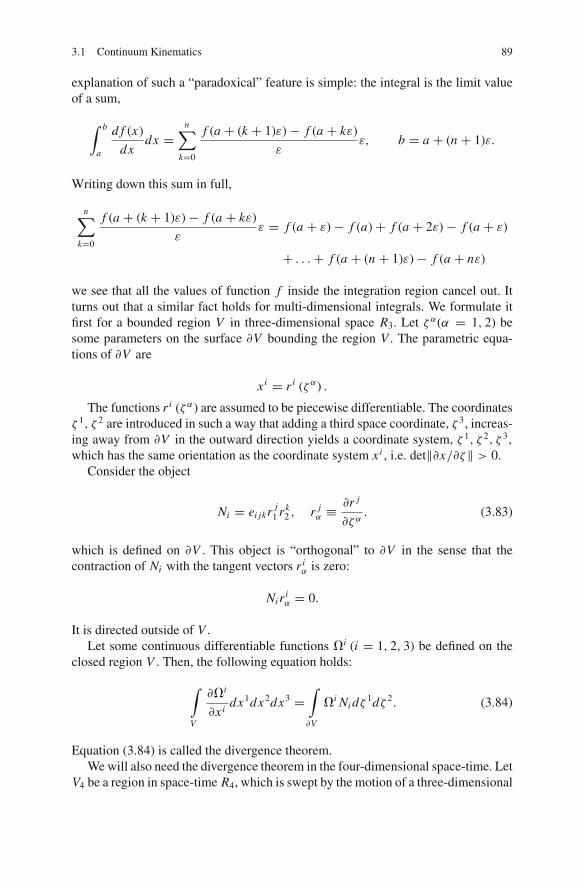
3.1 Continuum Kinematics 89
explanation of such a “paradoxical” feature is simple: the integral is the limit valueof a sum,
∫ b
a
d f (x)
dxdx =
n∑k=0
f (a + (k + 1)ε)− f (a + kε)
εε, b = a + (n + 1)ε.
Writing down this sum in full,
n∑k=0
f (a + (k + 1)ε)− f (a + kε)
εε = f (a + ε)− f (a)+ f (a + 2ε)− f (a + ε)
+ . . .+ f (a + (n + 1)ε)− f (a + nε)
we see that all the values of function f inside the integration region cancel out. Itturns out that a similar fact holds for multi-dimensional integrals. We formulate itfirst for a bounded region V in three-dimensional space R3. Let ζ α(α = 1, 2) besome parameters on the surface �V bounding the region V . The parametric equa-tions of �V are
xi = r i (ζ α) .
The functions r i (ζ α) are assumed to be piecewise differentiable. The coordinatesζ 1, ζ 2 are introduced in such a way that adding a third space coordinate, ζ 3, increas-ing away from �V in the outward direction yields a coordinate system, ζ 1, ζ 2, ζ 3,
which has the same orientation as the coordinate system xi , i.e. det‖�x/�ζ‖ > 0.Consider the object
Ni = ei jkr j1 rk
2 , r jα ≡
�r j
�ζ α. (3.83)
which is defined on �V . This object is “orthogonal” to �V in the sense that thecontraction of Ni with the tangent vectors r i
α is zero:
Niriα = 0.
It is directed outside of V .
Let some continuous differentiable functions �i (i = 1, 2, 3) be defined on theclosed region V . Then, the following equation holds:
∫
V
��i
�xidx1dx2dx3 =
∫
�V
�i Ni dζ 1dζ 2. (3.84)
Equation (3.84) is called the divergence theorem.We will also need the divergence theorem in the four-dimensional space-time. Let
V4 be a region in space-time R4, which is swept by the motion of a three-dimensional

90 3 Continuum Mechanics
Fig. 3.3 Motion of athree-dimensional region V3
in four-dimensionalspace-time
region V3 in R3 (Fig. 3.3). Denote as before the parameters on the boundary, �V3,
of the region V3 by ζ 1, ζ 2. Then the “time” part of the boundary �V4 of the regionV4 is described by the parametric equations
xi = r i(ζ 1, ζ 2, t
), x4 = t, (3.85)
where small Latin indices correspond to the projections on the space coordinate axesand the index 4 marks the projection on the time axis. Denote the quantities definedby (3.83) by Ni , where r i
α are derivatives of the function (3.85) with respect to ζ α .For any continuous differentiable functions, �, �i , in the closed region V4, the
following equality holds:
∫
V4
(��
�t+ ��i
�xi
)dx1dx2dx3dt =
=t∫
t0
∫
�V3
(�i −�r i
t
)Ni dζ 1dζ 2dt +
⎡⎣∫
V3
�dx1dx2dx3
⎤⎦
t1
t0
. (3.86)
where r it ≡ �r i/�t
∣∣ζ α=const .
Invariant form of the divergence theorem*. Equation (3.84) can be written in the“invariant” form if we put in (3.84) �i = √gωi , where ωi are the components ofsome vector field. In order to do that, we use the relation for the covariant5 diver-gence of the vector ωi ,
∇iωi = 1√
g
�√
gωi
�xi, (3.87)
5 The reader who is not familiar with the notion of covariant derivatives can find the necessarydefinitions in Sect. 4.6.
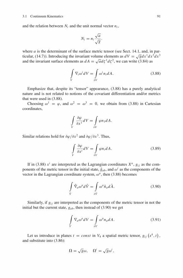
3.1 Continuum Kinematics 91
and the relation between Ni and the unit normal vector ni ,
Ni = ni
√a√g.
where a is the determinant of the surface metric tensor (see Sect. 14.1, and, in par-ticular, (14.7)). Introducing the invariant volume elements as dV = √gdx1dx2dx3
and the invariant surface elements as d A = √adζ 1dζ 2, we can write (3.84) as
∫
V
∇iωi dV =
∫
�V
ωi ni d A. (3.88)
Emphasize that, despite its “tensor” appearance, (3.88) has a purely analyticalnature and is not related to notions of the covariant differentiation and/or metricsthat were used in (3.88).
Choosing ω1 = ϕ, and ω2 = ω3 = 0, we obtain from (3.88) in Cartesiancoordinates,
∫
V
�ϕ
�x1dV =
∫
�V
ϕn1d A.
Similar relations hold for �ϕ/�x2 and �ϕ/�x3. Thus,
∫
V
�ϕ
�xidV =
∫
�V
ϕni d A. (3.89)
If in (3.88) xi are interpreted as the Lagrangian coordinates Xa , gi j as the com-ponents of the metric tensor in the initial state, gab, and ωi as the components of thevector in the Lagrangian coordinate system, ωa , then (3.88) becomes
∫
V
∇aωadV =
∫
�V
ωanad A. (3.90)
Similarly, if gi j are interpreted as the components of the metric tensor in not theinitial but the current state, gab, then instead of (3.90) we get
∫
V
∇aωadV =
∫
�V
ωanad A. (3.91)
Let us introduce in planes t = const in V4 a spatial metric tensor, gi j(xk, t
),
and substitute into (3.86):
� = √gω, �i = √gωi ,

92 3 Continuum Mechanics
dV = √gdx1dx2dx3, d A = √adζ 1dζ 2,
where ωi are the components of a spatial vector field. Then (3.86) takes the form
∫
V4
(1√g
�ω√
g
�t+∇iω
i
)dV dt =
=t1∫
t0
∫
�V3
(ωi − ωr i
t
)ni d Adt +
⎡⎣∫
V3
ωdV
⎤⎦
t1
t0
. (3.92)
The quantity r it ni means the surface velocity component in the direction of the
normal to the surface.Identifying in (3.92) the coordinates, x, with the Lagrangian coordinates, and the
metric tensor, gi j ,with the initial metric tensor, gab, we get
∫
V3×[t0,t1]
(dω
dt+ ∇aω
a
)dV dt =
=t1∫
t0
∫
�V3
(ωa − ωra
t
)nad Adt +
⎡⎢⎣∫
V3
ωdV
⎤⎥⎦
t1
t0
. (3.93)
The quantity rat na can be interpreted as the velocity of the boundary, �V3, of the
region V3 over the particles.If in (3.92) the coordinates, x, are identified with the Lagrangian coordinates, X,
while gi j are set to be the current Lagrangian metric tensor, gab, then (3.92) becomes
∫
V4
(1√g
d
dtω√
g + ∇aωa
)dV dt =
=t1∫
t0
∫
�V3
(ωa − ωra
t
)nad Adt +
⎡⎣∫
V3
ωdV
⎤⎦
t1
t0
. (3.94)
Another useful form of the divergence theorem is obtained if one substitutes ω
in (3.94) by ρω. Then, using the continuity equation (3.67), one can write (3.94) as
∫
V4
(ρ
dω
dt+∇aω
a
)dV dt =
=t1∫
t0
∫
�V3
(ωa − ρωra
t
)nad Adt +
⎡⎣∫
V3
ρωdV
⎤⎦
t1
t0
. (3.95)

3.2 Basic Laws of Continuum Mechanics 93
In particular, when ωa = 0, (3.95) takes the form
∫
V4
ρdω
dtdV dt = −
t∫
t0
∫
�V3
ρωrat nad Adt +
⎡⎣∫
V3
ρωdV
⎤⎦
t1
t0
. (3.96)
3.2 Basic Laws of Continuum Mechanics
Momentum equation. The second Newton law for one particle reads: the rate ofmomentum, mvi , is equal to the external force acting on the particle
d
dtmvi = Fi .
What is an analogy of this law for a continuum? The answer is not self-evident andfor the classical continuum models is as follows.
Consider a piece of continuum, some region V in the space of Lagrangian coor-dinates. For an observer, this piece occupies some moving region V (t). It consists ofthe same material particles. Momentum of an infinitesimally small piece of material,dV , is, by definition, the product of the mass of the particle, ρdV, and the particlevelocity, vi . We postulate that the momentum of the entire piece of continuum is thesum of momenta of all its infinitesimally small parts:
momentum =∫
V (t)
ρvi dV .
Denote by Fi the total force acting on the material in region V . Then we acceptthe following continuum version of the second Newton law:
d
dt
∫
V (t)
ρvi dV = Fi . (3.97)
The total force, Fi , can be split into the sum of the surface force and the bodyforce:
Fi = Fisur f ace + Fi
body . (3.98)
Both forces are assumed to possess a force density:
Fisur f ace =
∫
�V
f i d A, Fibody =
∫
V
ρgi dV . (3.99)

94 3 Continuum Mechanics
The body force per unit mass, gi , is a function of x and t ; in most applications,the only body force is gravity; the vector gi , the gravity acceleration, is constant.The surface force per unit area, f i , can depend not only on the space point of theboundary and time, but also on the geometrical characteristics of the surface �V .The crucial assumption of classical continuum mechanics is that the surface forcedensity depends linearly on the normal vector to �V :
f i = σ i j n j, (3.100)
and “the coefficients” σ i j are some functions of x and t only. These coefficients arecalled the stress tensor. The unit normal vector n j is directed, by our convention,outside of the region V . Surface force density may depend on the geometry of thesurface in a more complex way as we will see later in Sect. 4.5, but for all classicalmodels formula (3.100) holds true.
In principle, the stress tensor may be non-symmetric, but it is assumed symmetricin all classical models:
σ i j = σ j i . (3.101)
Equations (3.97), (3.98), (3.99) and (3.100) constitutes the integral form of momen-tum equation for classical models of continuum media.
Differential form of momentum equation. Let us show that (3.97), (3.98), (3.99)and (3.100) are equivalent to the following equation:
ρdvi
dt= �σ i j
�x j+ ρgi . (3.102)
Consider the momentum equation (3.97). We would like to move the time deriva-tive under the integral, but then some additional terms must appear because thelimits of integration depend on time. To get around this complication, we write theintegral in terms of Lagrangian coordinates by means of (3.66):
∫
V (t)
ρvi dV =∫
V
ρ0vi d V . (3.103)
The limits of integration in the right hand side of (3.103) do not depend on time;thus we can move the time derivative under the integral:
d
dt
∫
V (t)
ρvi dV =∫
V
ρ0dv
dt
i
dV .
Returning back to Eulerian coordinates by means of (3.66) we obtain

3.2 Basic Laws of Continuum Mechanics 95
d
dt
∫
V (t)
ρvi dV =∫
V (t)
ρdv
dt
i
dV . (3.104)
The total force (3.98) can also be written as a volume integral due to (3.100):
Fi =∫
V
(�σ i j
�x j+ ρgi
)dV . (3.105)
Here we used the divergence theorem. Equating (3.104) and (3.105) we have
∫
V
(ρ
dvi
dt− �σ i j
�x j− ρgi
)dV = 0. (3.106)
Since the region V is arbitrary and all functions involved are assumed to be con-tinuous, the integrand must be identically equal to zero, otherwise one can find aregion V for which the left hand side of (3.106) is not zero. We thus arrive at themomentum equation (3.102).
Piola-Kirchhoff stress tensor. Stress tensor σ i j is also called Cauchy’s stress ten-sor. The projection of this tensor over the second index to Lagrangian coordinateswith a factor, ρ0/ρ,
pia = ρ0
ρσ i j Xa
j ,
is usually called Piola-Kirchhoff stress tensor. The Piola-Kirchhoff stress tensor hasone observer’s and one Lagrangian index, i.e. it behaves as a triad of vectors undertransformation of observer’s frames and a triad of vectors under transformation ofLagrangian frames. There is convention in tensor analysis to keep the same coreletter for the components of the tensor in different coordinate systems. Therefore,one can write for Piola-Kirchhoff stress tensor
pia = ρ0
ρσ ia
or
σ ia = ρ
ρ0pia .
Note also here the relation between the Lagrangian and Eulerian components ofthe stress tensor:
σ ab = σ i j Xai Xb
j .

96 3 Continuum Mechanics
Momentum equation in Lagrangian coordinates. Momentum equation in La-grangian coordinates takes a simple form if we use the Piola-Kirchhoff stress tensor6
ρ0dvi
dt= �pia
�Xa+ ρ0gi . (3.108)
Another form of this equation,
ρ0�2xi (t, X )
�t2= �pia
�Xa+ ρ0gi , (3.109)
emphasizes that the independent variables in this equation are Lagrangian coordi-nates and time.
To derive (3.108) from (3.102) one can plug into (3.102) the expression ofCauchy’s stress tensor in terms of Piola-Kirchhoff’s stress tensor,
σ i j = ρ
ρ0pia x j
a ,
and use the identity (3.73).
Energy equation. Consider the total energy of material contained in some regionV (t). As we discussed in Chap. 2, energy is a primary characteristic of a mechanicalsystem which always exists. Continuum is an approximate description for mechan-ical systems consisting of a large number of material particles. Energy is definedas the total energy of these particles. Total energy can be presented as a sum of thekinetic energy of the macroscopic motion,
∫
V (t)
ρv2
2dV
and the remainder, which is called internal energy. The latter is assumed to havesome energy density. The internal energy density per unit mass is denoted by U . So,
6 Here we assume that the Lagrangian coordinates are Cartesian in the initial state, and g = 1.
Otherwise, the momentum equation is
ρ0dvi
dt= 1√
g
�
�Xa
(√g pia
)+ ρ0gi , (3.107)
or, in terms of the covariant derivative in the initial state,
ρ0dvi
dt= ∇a pia + ρ0gi .
Note that the covariant derivative ∇a “acts” only on the Lagrangian index of Piola-Kirchhoff tensor.

3.2 Basic Laws of Continuum Mechanics 97
total energy =∫
V (t)
ρv2
2dV +
∫
V (t)
ρUdV .
The energy rate is caused by the work of external forces
d
dt
∫
V (t)
ρ
(v2
2+U
)dV = P + d Q
dt. (3.110)
Here P is the power of external forces (the work of external forces per unit time)
P =∫
�V (t)
σ i j n jvi d A +∫
V (t)
ρgivi dV, (3.111)
and heat supply d Q is the work additional to the work of external forces. Heat sup-ply is the work done on “microscopic degrees of freedom” as discussed in Chap. 2.
It is assumed in classical continuum models that the heat supply is due only tosome energy flux through the surface, and there is a heat supply surface density, q,such that
d Q
dt=∫
�V
q d A. (3.112)
Moreover, the dependence of the heat supply surface density, q, on the geometry ofthe surface is similar to (3.100):
q = −qi ni , (3.113)
where qi are some functions of the space points and time. The vector qi is called theheat flux vector. The minus sign in (3.113) is caused by the convention that energyshould decrease if the vector qi is directed outside of the region V and increaseotherwise.
Combining (3.110), (3.111), (3.112) and (3.113) and repeating the reasoning thatyields the momentum equation in differential form (3.102) we obtain the energyequation in differential form:
ρd
dt
(v2
2+U
)= �(σ i jvi )
�x j+ ρgivi − �qi
�xi. (3.114)
This equation may be simplified. Note that the momentum equation (3.102)yields an equation for the kinetic energy rate: contracting (3.102) with vi we have
ρd
dt
v2
2= �σ i j
�x jvi + ρgivi . (3.115)

98 3 Continuum Mechanics
Deducting (3.115) from (3.114) we obtain the equation for the internal energy rate:
ρdU
dt= σ i j �vi
�x j− �qi
�xi. (3.116)
Entropy equation. If the processes in the system are sufficiently slow, one canintroduce S, the entropy of the system. We assume that entropy of the system is thesum of entropies of all subsystems, i.e. the entropy density per unit mass, S, exists:
S =∫
V
ρSdV .
Entropy density has the dimension (mass)−1 if the total entropy is taken as dimen-sionless.
The second law of thermodynamics claims that for an isolated system the totalentropy does not decrease:
dSdt=∫
V
ρd S
dtdV ≥ 0. (3.117)
Every continuum model must obey this constraint.
3.3 Classical Continuum Models
All continuum models can be roughly split into two categories. The first is com-prised of the models that have as the primary characteristics only the particle posi-tions x(t, X ) and the entropy S(t, X ). Functions x(t, X ) and S(t, X ) are analogousto the generalized coordinates of classical mechanics. Note that the “generalizedcoordinates” of continuum mechanics include, in addition to the functions x(t, X ),which are a direct analogy of the particle coordinates in classical mechanics, anadditional “coordinate” S(t, X ). The second type of model is formed by the mod-els which have some additional primary characteristics like plastic deformations,concentrations of chemical species, etc. We call these additional characteristics theinternal degrees of freedom. We consider first the models which do not have internaldegrees of freedom.
All classical continuum models are based on the assumption that internal energydensity, U , is a function of distortion and entropy density only:
U = U (xia, S). (3.118)
Function U (xia, S) specifies the physical properties of the media. To close the
system of three momentum equations (3.102) and energy equation (3.115), onehas to prescribe the constitutive equations which link the remaining unknowns in
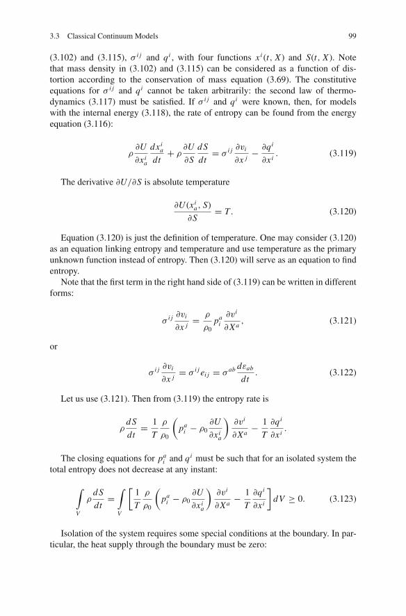
3.3 Classical Continuum Models 99
(3.102) and (3.115), σ i j and qi , with four functions xi (t, X ) and S(t, X ). Notethat mass density in (3.102) and (3.115) can be considered as a function of dis-tortion according to the conservation of mass equation (3.69). The constitutiveequations for σ i j and qi cannot be taken arbitrarily: the second law of thermo-dynamics (3.117) must be satisfied. If σ i j and qi were known, then, for modelswith the internal energy (3.118), the rate of entropy can be found from the energyequation (3.116):
ρ�U
�xia
dxia
dt+ ρ
�U
�S
d S
dt= σ i j �vi
�x j− �qi
�xi. (3.119)
The derivative �U/�S is absolute temperature
�U (xia, S)
�S= T . (3.120)
Equation (3.120) is just the definition of temperature. One may consider (3.120)as an equation linking entropy and temperature and use temperature as the primaryunknown function instead of entropy. Then (3.120) will serve as an equation to findentropy.
Note that the first term in the right hand side of (3.119) can be written in differentforms:
σ i j �vi
�x j= ρ
ρ0pa
i
�vi
�Xa, (3.121)
or
σ i j �vi
�x j= σ i j ei j = σ ab dεab
dt. (3.122)
Let us use (3.121). Then from (3.119) the entropy rate is
ρd S
dt= 1
T
ρ
ρ0
(pa
i − ρ0�U
�xia
)�vi
�Xa− 1
T
�qi
�xi.
The closing equations for pai and qi must be such that for an isolated system the
total entropy does not decrease at any instant:
∫
V
ρd S
dt=∫
V
[1
T
ρ
ρ0
(pa
i − ρ0�U
�xia
)�vi
�Xa− 1
T
�qi
�xi
]dV ≥ 0. (3.123)
Isolation of the system requires some special conditions at the boundary. In par-ticular, the heat supply through the boundary must be zero:

100 3 Continuum Mechanics
qi ni = 0 at �V .
Integrating the last term of the integral in (3.123) by parts, we put the second lawof thermodynamics in the form
∫
V
(1
T
ρ
ρ0
(pa
i − ρ0�U
�xia
)�vi
�Xa+ qi �
�xi
1
T
)dV ≥ 0. (3.124)
The consequences of the inequality (3.124) depend on the further assumptions forthe stresses and the heat flux.
Heat conductivity. Consider first the case when the continuum does not move. Thenthe only process remaining is the heat conduction. It is described by the equation
ρdU
dt= −�qi
�xi. (3.125)
To close this equation, we need the constitutive equation for the heat flux. It mustsatisfy the second law of thermodynamics (3.124). Now (3.125) takes the form
∫
V
qi �
�xi
1
TdV ≥ 0. (3.126)
The simplest relation to obey this inequality is the Fourier heat conduction law:
qi = κ
�
�xi
1
T, (3.127)
with some positive parameter, κ, the coefficient of heat conductivity.Let us choose the function U (Xa, t) as the independent thermodynamic variable,
and describe the thermodynamic properties of the material by the function S =S0 (U ) . Then the temperature is linked to U by the formula
1
T= d S0 (U )
dU. (3.128)
Equations (3.125), (3.128) and (3.127) form a closed system of equations for heatconductivity.
Fourier law is often written in a slightly different form,
qi = −γ�T
�xi,
It has an advantage that the coefficient γ = κ/T 2 only slightly depends on temper-ature for many materials.
To demonstrate the importance of the inequality (3.126) consider an improve-ment of heat conductivity theory suggested by Cattaneo. One can derive from the

3.3 Classical Continuum Models 101
equations obtained that the heat propagates with an infinite velocity. To get rid ofthis paradox, Cattaneo proposed to replace (3.127) by the equation
qi + αdqi
dt= κ
�
�xi
1
T, (3.129)
The energy equation (3.125) along with equations (3.128) and (3.129) form aclosed system of equations. However, these equations contradict the inequality ofthe second law of thermodynamics (3.126). Indeed, in Cattaneo’s theory, qi andU can be given independently for the initial instant since the energy equation andthe equation for qi (3.129) contain the first derivatives of qi and U with respect totime. By a specific choice of the initial values, the integrand in (3.126) and, hence,the integral (3.126) can be made negative. Therefore, all the formulas of Cattaneo’stheory cannot be left unchanged. The question arises whether it is possible to choosesuch equations of state for entropy that entropy increases in an isolated system. Thenegative answer to this question would mean that (3.129) is not consistent with thelaws of thermodynamics. It turns out that a modification of the equation of statedoes exist. One has to change only the constitutive equation for entropy:
S = S0 (U )− α
2κ
qi qi ,
1
T=d S0 (U )
dU.
The reader can check that the total entropy of the system does increase. The negativesign in the equation for the entropy has a clear meaning: the heat flux induces someorder, and the entropy density decreases.
Elastic body. Theory of elasticity is based on the assumption that pai and qi may
depend only on distortion, entropy (or temperature) and temperature gradient.Besides, these relationships are universal, i.e. they are valid for any values of xi
a ,T and �T/�xi . Let us take first T = const . Then inequality (3.124) simplifies to
∫
V
1
T
ρ
ρ0
(pa
i − ρ0�U
�xia
)�vi
�XadV ≥ 0. (3.130)
The momentum equation contains the time derivative of the velocity field. There-fore, the initial data for velocity must be provided. The initial velocity field can bechosen arbitrarily. Applying inequality (3.130) to the initial instant and using thefact that pa
i and �U/�xia do not depend on velocity field, we see that the expression
in parenthesis must vanish and thus
pai = ρ0
�U
�xia
. (3.131)
Otherwise, one can choose the velocity field in such a way that entropy rate isnegative (the reasoning is similar to that of the main lemma of calculus of variationin Chap. 1). Since at the initial instant any distributions of distortion and entropy

102 3 Continuum Mechanics
can be taken, and the dependence pai (x j
b , S) is universal, (3.131) gives the requiredconstitutive equations for the stress tensor.
Consider now an arbitrary temperature field. Because of (3.131), inequality(3.124) is now a constraint for the heat flux vector (3.126). Any dependence ofqi on the temperature gradient satisfying to (3.126) is possible, in principle. Thesimplest is the Fourier law, which we write for the general anisotropic case as
qi = Di j �
�x j
1
T. (3.132)
The heat conductivities, Di j , must be positive definite:
Di jξiξ j ≥ 0 for any ξi .
The heat conductivities may depend on temperature and distortion. It can beshown that Onsager’s relations for heat conduction imply the symmetry of tensorDi j ,
Di j = D ji .
The momentum (3.108), energy (3.116), continuity (3.68) and constitutive equa-tions (3.120), (3.131) and (3.132) form the closed system of equations for elasticheat conducting body. The model is specified by prescribing the internal energyU (xi
a, S) and the heat conductivities Di j .
Stress-strain relations for elastic body. The constitutive equations (3.131) can befurther specified if we note that internal energy must be invariant with respect torigid rotations of an elastic body. If a body with the particle positions xi (t, X ) isrotated, the new particle positions, x ′i (t, X ), are
x ′i (t, X ) = αij x j (t, X )
where αij are the components of an orthogonal matrix. Therefore, the distortion in
the new position is
x ′ia = αij x
ja .
Internal energy must be the same in both states for any orthogonal matrix αij and
any initial distortion xia :
U(αi
j xj
a , S) = U
(x j
a , S). (3.133)
One can show that to satisfy (3.133), function U may depend on distortion onlythrough the metric tensor gab = gi j x i
a x ja , or, equivalently, through the strain tensor
εab = 12 (gab − gab). Since
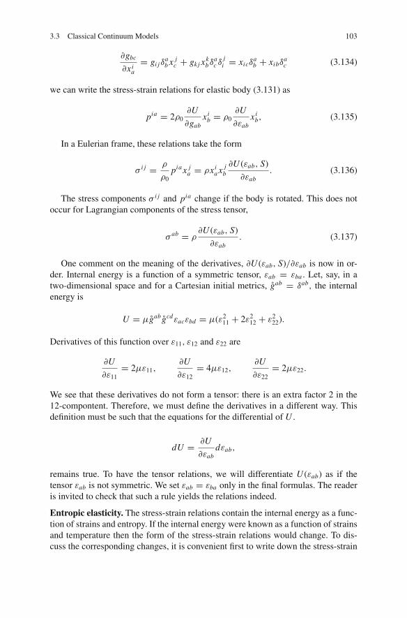
3.3 Classical Continuum Models 103
�gbc
�xia
= gi jδab x j
c + gk j xkbδa
c δji = xicδ
ab + xibδ
ac (3.134)
we can write the stress-strain relations for elastic body (3.131) as
pia = 2ρ0�U
�gabxi
b = ρ0�U
�εabxi
b, (3.135)
In a Eulerian frame, these relations take the form
σ i j = ρ
ρ0pia x j
a = ρxia x j
b
�U (εab, S)
�εab. (3.136)
The stress components σ i j and pia change if the body is rotated. This does notoccur for Lagrangian components of the stress tensor,
σ ab = ρ�U (εab, S)
�εab. (3.137)
One comment on the meaning of the derivatives, �U (εab, S)/�εab is now in or-der. Internal energy is a function of a symmetric tensor, εab = εba . Let, say, in atwo-dimensional space and for a Cartesian initial metrics, gab = δab, the internalenergy is
U = μgabgcdεacεbd = μ(ε211 + 2ε2
12 + ε222).
Derivatives of this function over ε11, ε12 and ε22 are
�U
�ε11= 2με11,
�U
�ε12= 4με12,
�U
�ε22= 2με22.
We see that these derivatives do not form a tensor: there is an extra factor 2 in the12-compontent. Therefore, we must define the derivatives in a different way. Thisdefinition must be such that the equations for the differential of U .
dU = �U
�εabdεab,
remains true. To have the tensor relations, we will differentiate U (εab) as if thetensor εab is not symmetric. We set εab = εba only in the final formulas. The readeris invited to check that such a rule yields the relations indeed.
Entropic elasticity. The stress-strain relations contain the internal energy as a func-tion of strains and entropy. If the internal energy were known as a function of strainsand temperature then the form of the stress-strain relations would change. To dis-cuss the corresponding changes, it is convenient first to write down the stress-strain

104 3 Continuum Mechanics
relations in terms of entropy as the primary thermodynamic potential. Entropy is afunction of internal energy and strains,
S = S(U, εab). (3.138)
For a given dependence of internal energy on strain and entropy, U = U (εab, S),function (3.138) may be viewed as a solution of the equation
U (εab, S) = U.
Therefore, the derivatives of U (εab, S) and S(U, εab) are linked. To find the corre-sponding relationships, we differentiate the identity
U (εab, S(U, εab)) = U, (3.139)
with respect to εab and U :
�U (εab, S)
�εab+ �U
�S
�S(U, εab)
�εab= 0,
�U (εab, S)
�S
�S(U, εab)
�U= 1.
Hence,
�U (εab, S)
�εab= −T
�S(U, εab)
�εab,
�S(U, εab)
�U=(
�U (εab, S)
�S
)−1
= 1
T. (3.140)
In terms of the thermodynamics function S(U, εab), the stress-strain relations takethe form
σ ab = −ρT�S(U, εab)
�εab. (3.141)
Experiments show that some materials, such as rubbers or polymers, exhibit thefollowing feature: their internal energy is a function of temperature only and, prac-tically, does not depend on strain:
U = U0(T ).
Equivalently, temperature is some function of internal energy:
T = T0(U ).
According to the second equation (3.140), in this case
�S(U, εab)
�U= 1
T0(U ). (3.142)
The general solution of (3.142) is

3.3 Classical Continuum Models 105
S(U, εab) = S0(U )+ S1(εab). (3.143)
where S0(U ) is the solution of the ordinary differential equation
d S0(U )
dU= 1
T0(U ).
Finally, for the stress-strain relations we have from (3.141) and (3.143)
σ ab = −ρT�S1(εab)
�εab. (3.144)
To see some qualitative peculiarities of such stress-strain relations, consider theone-dimensional case when the stress and strain tensors have just one component,σ and ε. According to (3.144),
σ = −ρT�S1(ε)
�ε.
Let the dependence of stresses on strains be linear, i.e.
S1 = −1
2λε2. (3.145)
Here λ is the material rigidity, λ > 0; the negative sign in (3.145) roots in Gibbs’variational principle: in equilibrium, i.e. at ε = 0, entropy must be maximum. So,
σ = ρT λε.
We see that the rigidity of material increases if temperature is raised. This is oppositeto typical behavior of metals for which the rigidity decreases when temperaturerises.
Another outcome of our consideration is that the material properties are uniquelydefined only if the internal energy is given in terms of their “native arguments”, εab
and S. If one uses as an argument temperature instead of entropy, then an uncertaintyappears in the costitutive equations. The uncertainty can be fixed by providing anadditional information about entropy, like (3.140).
The class of elasticity models (3.143) is sometimes called entropic elasticity.
Ideal compressible fluid. The special case of an elastic body when the internalenergy depends on distortion through the mass density only,
U = U (ρ, S), (3.146)
is called an ideal fluid. To derive the constitutive equations in this case we need therelation
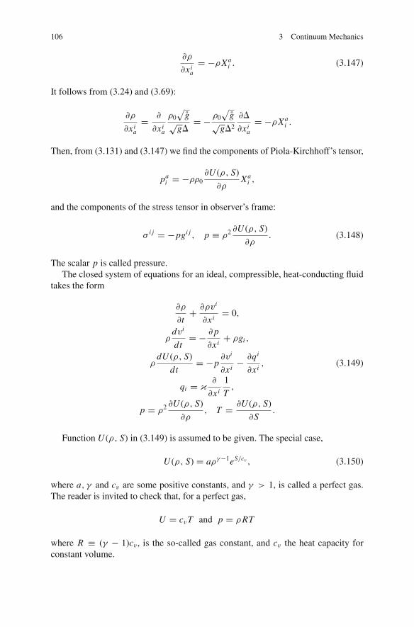
106 3 Continuum Mechanics
�ρ
�xia
= −ρXai . (3.147)
It follows from (3.24) and (3.69):
�ρ
�xia
= �
�xia
ρ0
√g√
g�= − ρ0
√g√
g�2
��
�xia
= −ρXai .
Then, from (3.131) and (3.147) we find the components of Piola-Kirchhoff’s tensor,
pai = −ρρ0
�U (ρ, S)
�ρXa
i ,
and the components of the stress tensor in observer’s frame:
σ i j = −pgi j , p ≡ ρ2 �U (ρ, S)
�ρ. (3.148)
The scalar p is called pressure.The closed system of equations for an ideal, compressible, heat-conducting fluid
takes the form
�ρ
�t+ �ρvi
�xi= 0,
ρdvi
dt= − �p
�xi+ ρgi ,
ρdU (ρ, S)
dt= −p
�vi
�xi− �qi
�xi, (3.149)
qi = κ
�
�xi
1
T,
p = ρ2 �U (ρ, S)
�ρ, T = �U (ρ, S)
�S.
Function U (ρ, S) in (3.149) is assumed to be given. The special case,
U (ρ, S) = aργ−1eS/cv , (3.150)
where a, γ and cv are some positive constants, and γ > 1, is called a perfect gas.The reader is invited to check that, for a perfect gas,
U = cvT and p = ρRT
where R ≡ (γ − 1)cv , is the so-called gas constant, and cv the heat capacity forconstant volume.

3.3 Classical Continuum Models 107
The constant a in (3.150) is nonessential: by changing a one only shifts entropyby a constant. The model for an ideal gas contains two physical characteristics, cv
and γ.
Incompressible ideal fluid. If “the fluid rigidity” with respect to the volume changetends to infinity, then the variations of the density become negligibly small. One canaccept that in the first approximation the density is constant. Then the system of(3.149) splits into two subsystems: the first serves to find velocities and pressure(density ρ is a given constant),
�vi
�xi= 0, (3.151)
ρ�vi
�t= − �p
�xi+ ρgi ,
and the second allows one to determine temperature distribution when fluid motionis known from (3.151):
ρdU (S)
dt= −�qi
�xi, qi = κ
�
�xi
1
T, T = dU (S)
d S. (3.152)
Equations (3.151) are called Euler equations.
Viscous compressible fluid. For a compressible fluid internal energy is, as before,a function of density and entropy. What changes is the assumption made regardingthe stress tensor: for viscous fluid the stress tensor depends on the velocity field.Consider again the inequality of the second law of thermodynamics (3.124). We putit in the form
∫
V
(1
T
(σ i j + ρ2 �U (ρ, S)
�ρgi j
)�vi
�x j+ qi �
�xi
1
T
)dV ≥ 0. (3.153)
Let us define tensor τ i j by the equation
σ i j = −ρ2 �U (ρ, S)
�ρgi j + τ i j . (3.154)
Tensor τ i j is symmetric since σ i j and gi j are symmetric. Due to the symmetry ofτ i j , the sum τ i j �vi/�x j can also be be written as
τ i j �vi
�x j= τ i j ei j (3.155)
where ei j is the strain rate tensor (3.46). So,
∫
V
(1
Tτ i j ei j + qi �
�x j
1
T
)dV ≥ 0. (3.156)

108 3 Continuum Mechanics
In principle, any dependence of τ i j and qi on ei j and the temperature gradientwhich does not violate the inequality (3.156) is acceptable. The simplest one is alinear dependence of τ i j on ei j :
τ i j = μi jklekl (3.157)
with a positive tensor μi jkl (μi jklei j ekl ≥ 0 for any ei j ), and Fourier’s law for qi
(3.132). This case is called a Newtonian fluid.For an isotropic Newtonian fluid,
τ i j = λekk gi j + 2μei j . (3.158)
In general, one usually assumes that the dissipation, D, defined as
D = τ i j ei j + T qi �i T−1, (3.159)
is a function7 of ei j and T−1,i :
D = D(ei j , �i T
−1) ,
and the closing relations are
τ i j = λ�D
�ei j, T qi = λ
�D
�(�i T−1
) . (3.160)
Here λ is the parameter determined from (3.159) and (3.160)
λ
(�D
�ei jei j + �D
�(�i T−1
)�i T−1
)= D. (3.161)
Newtonian fluids correspond to a quadratic function D. In this case, the parameterλ is equal to 1/2.
Incompressible viscous fluid. If the fluid is incompressible then, as for incompress-ible ideal fluids, the determination of the temperature field separates from the deter-mination of fluid motion. The closed system of equations for fluid motion consistsof four equations for four unknowns, velocity vi and pressure p:
�vi
�xi= 0 (3.162)
7 Dissipation may also depend on temperature and mass density, but this is not emphasized in thenotation.

3.3 Classical Continuum Models 109
ρdvi
dt= − �p
�xi+ μ�vi .
Here � is Laplace’s operator:
� = �2
�x21
+ �2
�x22
+ �2
�x23
.
Equations (3.162) are called Navier-Stokes equations.Temperature is determined from the energy equation after velocity field has been
found from Navier-Stokes equations:
ρdU (S)
dt= 2μei j e
i j − �
�xiκ
�
�xi
1
T. (3.163)
The first term in the right hand side of (3.163) describes heating of fluid caused byviscosity.
Plastic bodies. Among a wide class of continuum models with internal degrees offreedom we consider the models of classical plasticity theory. They endow the mate-rial with additional degrees of freedom – the tensor field of plastic deformation ε
(p)ab .
Internal energy of a plastic body depends on elastic deformation ε(e)ab = εab − ε
(p)ab ,
plastic deformation ε(p)ab and entropy:
U = U(ε
(e)ab , ε
(p)ab , S
). (3.164)
Following the same line of reasoning as for elastic bodies, we first determine theentropy rate from the energy equation (3.116):
ρTd S
dt=(
σ ab − ρ�U
�ε(e)ab
)dεab
dt+(
ρ�U
�ε(e)ab
− ρ�U
�ε(p)ab
)dε
(p)ab
dt− �qi
�xi,
and then write the inequality of the second law of thermodynamics as
∫ [1
T
(σ ab − ρ
�U
�ε(e)ab
)dεab
dt+ 1
T
(ρ
�U
�ε(e)ab
− ρ�U
�ε(p)ab
)dε
(p)ab
dt+ qi �
�xi
1
T
]dV ≥ 0.
(3.165)
Consider, for simplicity, the cases when heat flux, qi , can be neglected. If thetensor σ ab does not depend on strain rates then it necessarily follows from (3.165)that
σ ab = ρ�U
(ε
(e)ab , ε
(p)ab , S
)
�ε(e)ab
. (3.166)

110 3 Continuum Mechanics
The closing equations for plastic deformation are chosen in such a way that
(ρ
�U
�ε(e)ab
− ρ�U
�ε(p)ab
)dε
(p)ab
dt≥ 0. (3.167)
If the internal energy does not depend explicitly on plastic deformations theninequality (3.167) simplifies to
σ ab dε(p)ab
dt≥ 0.
Denote the expression from (3.167) in parenthesis by τ ab, so that
τ ab = ρ�U
�ε(e)ab
− ρ�U
�ε(p)ab
= σ ab − ρ�U
�ε(ρ)ab
. (3.168)
The dissipation in plastic flow is
ρTd S
dt= D = τ abε
(p)ab , ε
(p)ab ≡
dε(p)ab
dt. (3.169)
If one assumes that the dissipation is a function of the plastic strain rate,8
D = D(ε
(p)ab
),
then, similarly to (3.160), one postulates that
τ ab = λ�D
�ε(p)ab
. (3.170)
The parameter λ is determined from (3.169) and (3.170):
λ = D
/�D
�ε(p)ab
ε(p)ab .
If τ i j and e(p)i j are the components of the tensors τ and the plastic strain rate in an
Eulerian frame,
τ i j = xia x j
b τ ab, e(p)i j = Xa
i Xbj ε
(p)ab ,
then, obviously,
8 Dissipation may depend on distortion as well.

3.3 Classical Continuum Models 111
τ i j = λ�D
�e(p)i j
. (3.171)
For metals, plastic deformation is usually incompressible and
gi j e(p)i j = 0.
Therefore, dissipation depends only on the deviator part of the plastic strain rate
e′(p)i j = e(p)
i j −1
3e(p)k
k gi j .
One can then obtain from (3.171) that the trace of the tensor τ i j is zero:
τ ii = 0,
while the deviator part of the tensor τ, τ ′i j = τ i j − 1/3τ kk gi j , is
τ ′i j = λ�D
�e′(p)i j
.
The behavior of many metals is well described by the model
D = k(
e′(p)i j e′(p)i j
) 12 (1+ 1
m ). (3.172)
It contains two material characteristics, k and m. The dimensionless parameter,m, is usually very large. In the limit m → ∞, this model transforms into the vonMises model, where
D = k√
e′(p)i j e′(p)
i j . (3.173)
For the von Mises model, λ = 1, and
τ ′i j = ke′(p)
i j√e′(p)
mn e′(p)mn
. (3.174)
If e′(p)i j �= 0, i.e. the material is deforming plastically, then, from (3.174),
τ ′i jτ ′i j = k2. (3.175)
This equation defines a surface in the six-dimensional space of variables τi j . Theplastic flow occurs only if the stresses lie on this surface.

112 3 Continuum Mechanics
If there is no plastic deformation, e′(p)i j = 0, then (3.174) contain an indetermi-
nacy of the type 0/0. The analysis of the non-degenerated model (3.172) shows thatfor e′(p)
i j = 0 the tensor τ ′i j lies inside the surface (3.175).Usually, elastic deformation is much smaller than plastic deformation, and one
can equate the total and plastic strains. Accordingly, one can identify the total strainrate ei j with the plastic strain rate, e(p)
i j . Then we obtain for von Mises dissipation:
D = k√
e′i j e′i j . (3.176)
If, additionally, the internal energy depends only on elastic deformations, then
σ ′i j = τ ′i j = ke′i j
√e′mne′mn
. (3.177)
Equations (3.176) and (3.177) characterize the material called an ideal plastic body.A remarkable feature of the von Mises dissipation is the independence of the
total dissipation on the rate of the process. Namely, for the deformation path, εi j (t) ,
starting at the strain state, ε1i j , and ending at the strain state, ε2
i j , the integral
ε2i j∫
ε1i j
Di j(e′i j
)dt
depends only on the path, εi j (t) , and does not depend on the rate with which thispath is passed. Such a feature is characteristic for many materials.
3.4 Thermodynamic Formalism
In this section we briefly describe what is called the thermodynamic formalism inderivation of governing equations. For simplicity, we assume that continuum doesnot move, and there is no heat conductivity. To incorporate continuum motion andheat conduction one needs to complicate the treatment in accordance with what wassaid in the previous section.
So, let the state of the continuum be characterized by some fields, uκ (X, t),κ = 1, . . . , m. For example, these could be plastic deformation (or plastic distor-tion), concentrations of chemical species, etc. We assume that internal energy den-sity is some function of uκ , their spatial derivatives and entropy:
U = U(uκ, uκ
,a, S). (3.178)
This is a crucial assumption. In fact, when we have chosen some set of param-eters to model the state of a material, we can never be sure a priori that energy is

3.4 Thermodynamic Formalism 113
completely determined by these parameters, and there are no additional “hidden”parameters which affect the value of energy. The validity of (3.178) can be checkedonly experimentally either by direct measurements of energy, entropy and otherparameters involved or by inspecting the validity of the consequences of (3.175). Tomake further relations simpler, we include the factor, ρ0, in U, so, in this section Umeans the internal energy per unit volume of the initial state.
Let V be some piece of the material. The energy of the material confined inregion V is
E =∫
V
U(uκ, uκ
,a, S)
dV . (3.179)
Let the material be adiabatically isolated. Then the first law of thermodynamicsstates that the energy rate is equal to the power of external forces (recall that, as wehave just assumed, heat fluxes are neglected)
d
dt
∫
V 0
U(uκ, uκ
,a, S)
dV = P. (3.180)
The structure of the power is controlled by the form of energy. We have seenin Sections 3.2 and 3.3 that formula for the power (3.108) is consistent with theassumption that energy density depends on the first derivatives of displacements.Similarly, we set in the general case
P =∫
�V
σ aκ
duκ
dtnad A +
∫
V
gκ
duκ
dtdV . (3.181)
Here σ aκ
and gκ are some “generalized stresses” and “generalized body force”.Transforming the surface integral (3.181) into a volume integral by means of di-vergence theorem, we write the first law of thermodynamics as
∫
V
[�U
�SS +
(�U
�uκ
− �aσaκ− gκ
)uκ +
(�U
�uκ
,a
− σ aκ
)uκ
,a
]dV = 0.
Since the region V is arbitrary, this equation may be satisfied only if the integrandis zero identically. Employing the notation, T, for the derivative, �U/�S, we have
ρ0T S +(
�U
�uκ
− �aσaκ− gκ
)uκ +
(�U
�uκ
,a
− σ aκ
)uκ
,a = 0. (3.182)
Let us rewrite (3.182) in the form,

114 3 Continuum Mechanics
ρ0T S = τκ uκ + τ aκ
uκ
,a, (3.183)
where we introduced the notation
τκ ≡ �aσaκ− ρ0
�U
�uκ
+ gκ, τ aκ≡ σ a
κ− ρ0
�U
�uκ
,a
. (3.184)
The generalized forces,τκ and τ aκ, control the entropy rate and, thus, describe the
non-equilibrium features of the model. If τκ = 0 and τ aκ= 0 and U
(uκ, uκ
,a, S)
is given, then (3.184) form a closed system of equations for uκ . Remarkably, thissystem of equations has a variational form:
�a�U
�uκ
,a
− �U
�uκ
+ gκ = 0,
Using the variational derivative,
δU
δuκ
= �U
�uκ
− �a�U
�uκ
,a
,
we can write this system of equations as
δU
δuκ
= gκ .
To obtain a closed system equations for uκ in general case, one can, in additionto specifying function U
(uκ, uκ
,a, S), prescribe the dependence of τκ, τ a
κ, and gκ
on uκ and their derivatives. Then, eliminating σ aκ
from (3.184), we arrive at thefollowing system of equations for uκ :
τκ = �a
(ρ0
�U
�uκ
,a
+ τ aκ
)− ρ0
�U
�uκ
+ gκ. (3.185)
As to gκ, usually, there are no “body forces” working on the change of the internalparameters, uκ, i.e. gκ = 0. We accept this in what follows.
The only constraint for the admissible dependencies of τ aκ
and τκ on uκ and theirderivatives is the condition that entropy does not decay (or dissipation, D, the righthand side of (3.183) is non-negative):
D ≡ τκ uκ + τ aκ
uκ
,a ≥ 0. (3.186)
It is often supposed that there exists a function of uκ, uκ, and uκ
,a, D, such that
τκ = �D�uκ
, τ aκ= �D
�uκ
,a
. (3.187)

3.4 Thermodynamic Formalism 115
Function D is called the dissipation potential. The potential law is not a “law ofNature”, but rather a way to obtain a model with simply controlled mathematicalfeatures.
In case of the potential law (3.187) the governing equations (3.185) take espe-cially simple “variational” form:
δU
δuκ
= − δDδuκ
. (3.188)
Here δD/δuκ is the variational derivative:
δDδuκ
= �D�uκ
− �a�D�uκ
,a
.
The dissipative potential, D, is simply related to dissipation if D is a homoge-neous function, i.e. for any λ and some number, m,
D(λuκ, λuκ
,a
) = λmD(uκ, uκ
,a
). (3.189)
According to Euler’s identity for homogeneous functions,
uκ�D�uκ
+ uκ
,a
�D�uκ
,a
= mD(uκ, uκ
,a
),
the dissipative potential differs from the dissipation by the factor, m :
D = mD. (3.190)
In linear theory, D and D are quadratic functions and m = 2. For ideal-plasticity-typemodels, m = 1.

Chapter 4Principle of Least Action in ContinuumMechanics
As we discussed in Sect. 2.6, for reversible processes the governing equations ofmechanics must have a Hamiltonian structure, and accordingly a principle of leastaction must exist. In another extreme case, when the inertial effects and the internalinteractions described by the internal energy can be ignored, variational principlesalso exist, but they are due to the special structure of the models rather than to thelaws of Nature. In this chapter we consider the principle of least action in continuummechanics of reversible processes and some related issues. The variational princi-ples for dissipative processes are presented in the second part of the book along withthe other variational features of the classical continuum models.
4.1 Variation of Integral Functionals
Let a continuum be characterized by some functions uκ(xi , t), κ = 1, . . . , m, i =1, 2, 3. In what follows the number of the variables xi is not essential; besides, timedoes not play a special role. Therefore, we include time in the set of independentvariables and write uκ = uκ(x) assuming that x = {
x1, . . . , xn}
is a point ofn-dimensional space. We write, for brevity, u(x) for the set
{u1 (x) , . . . , um (x)
},
when this cannot cause confusion.Let a functional, I (u), be given, i.e. there is a rule which allows one to compute
the number, I (u), for each u(x). The major example of such a functional for us is anintegral functional
I (u) =∫
V
L(xi , uκ, uκ
,i)dn x, uκ
,i≡ �uκ
�xi, (4.1)
where V is some region in n-dimensional space of x-variables. For such function-als, function L is called Lagrangian. The case when Lagrangian depends on higherderivatives will be considered further in Sect. 4.4.
We assume that region V is compact to avoid the technicalities caused by theunboundedness of V ; some peculiarities of the variational problems for an un-bounded domain are considered in Sect. 11.7. All functions involved are assumed
V.L. Berdichevsky, Variational Principles of Continuum Mechanics,Interaction of Mechanics and Mathematics, DOI 10.1007/978-3-540-88467-5 4,C© Springer-Verlag Berlin Heidelberg 2009
117

118 4 Principle of Least Action in Continuum Mechanics
to be sufficiently smooth to make the derivation of the final equations meaningful.In particular, the boundary �V of region V is piecewise smooth, and Lagrangian isa smooth function of its arguments.
Physical reasoning to be considered later sets some constraints on the admissiblefunction u(x). A typical constraint is prescribing the values of u(x) at a piece of theboundary, �Vu , of the boundary �V :
u (x) = ub (x) at �Vu . (4.2)
Here ub(x) are the given boundary values of functions u(x).The constraints specify the set of admissible functions u(x). We denote this set
by M. A description of the set M also includes the characterization of smoothnessof the admissible functions. In order for the integral (4.1) to be sensible, it is suf-ficient to include in the set M the functions u(x) which are continuous along withtheir derivatives in the closed region V . The physically important case of piecewisedifferentiable functions will be treated in Sect. 7.4.
A variational principle usually states that the true process (or, in statics, the equi-librium state) of a continuum is a stationary point of the functional I (u) on the setM, i.e. variation of this functional, δ I, vanishes for all admissible variations δu.
Let u(x) be a stationary point of the functional I (u) and u(x) = u(x)+ δu(x) bea small disturbance of the function u(x). Keeping only the leading small terms inthe difference I (u + δu)− I (u), we find the variation of the functional, I (u) ,
δ I =∫
V
(�L
�uκ
δuκ + �L
�uκ
,i
(δuκ),i
)dn x . (4.3)
Functions δuκ and (δuκ),i are not independent because (δuκ),i are completelydetermined by δuκ . To put (4.3) in the form which contains only independent terms,we integrate the second term in the integrand by parts:
δ I =∫
V
((�L
�uκ
− �
�xi
�L
�uκ
,i
)δuκ + �
�xi
(�L
�uκ
,i
δuκ
))dV
=∫
V
δL
δuκ
δuκdn x +∫
�V
�L
�uκ
,i
δuκni d A. (4.4)
Here d A is the area element at �V, ni the unit normal vector at �V and a notationfor the variational derivative of L is introduced,
δL
δuκ
= �L
�uκ
− �
�xi
�L
�uκ
,i
. (4.5)
Note that
δu = 0 at �Vu

4.1 Variation of Integral Functionals 119
due to the boundary conditions (4.2). Therefore, the surface integral in (4.4) is, infact, an integral over �V − �Vu .
The terms in (4.4) are independent because the value of δuκ inside the region Vand at its boundary can be changed independently of each other.
Formula (4.4) is the sought expression for the variations of functional I (u) . Wewill often encounter this expression in that or in a similar form. Further, the deriva-tions will be given only in cases when they do not repeat the above one; otherwise,only the result will be stated.
The main lemma of calculus of variations. For the case under consideration themain lemma of calculus of variations takes the form: if
∫
V
Fκ uκdn x = 0, (4.6)
where Fκ are some continuous functions of coordinates which are independent ofuκ, and uκ are arbitrary smooth functions which are zero on the boundary �V ofregion V , then
Fκ = 0 in V .
This lemma can be proved in the same way as in Sect. 1.3.Note the following consequence: if
∫
V
Fκ uκdn x +∫
�V
fκ uκdn−1x = 0, (4.7)
where F and f are continuous functions of coordinates which are independent ofuκ, and uκ are arbitrary smooth functions, then
Fκ = 0 in V, fκ = 0 on �V . (4.8)
To obtain the first equation (4.8) one should consider functions uκ which areequal to zero at �V ; then the first equation (4.8) follows from the main lemma ofcalculus of variations. Thus, the first term in (4.7) is zero. Then the second term in(4.7) is also zero and, applying again the main lemma of calculus of variations, onegets the second equation (4.8).
At the stationary point,
δ I = 0. (4.9)
From (4.9), (4.4) and the main lemma of variational calculus it follows that thestationary points of the functional (4.1) satisfy the equations
δL
δuκ
≡ �L
�uκ
− �
�x
�L
�uκ
,i
= 0 in V, (4.10)

120 4 Principle of Least Action in Continuum Mechanics
and the boundary conditions
�L
�uκ
,i
ni = 0 on �V − �Vu . (4.11)
Equations (4.10), (4.11) and (4.2) form a closed system of equations and bound-ary conditions to find the stationary point. As has been already mentioned on asimilar occasion in Sect. 1.3, the remarkable feature of the variational approach isthat one always1 gets a proper number of boundary conditions to solve the partialdifferential equations (4.10).
Note that the inhomogeneous boundary conditions,
�L
�uκ
,i
ni = fκ at �V − �Vu,
where fκ are some prescribed functions at �V − �Vu, are obtained if the surfaceintegral
∫
�V−�Vu
fκuκd A
is added to the functional (4.1).In our consideration, variations δu(x) are the infinitesimally small disturbances
of the stationary point u. In calculus of variations one sometimes uses a slightly dif-ferent language which proves to be useful for non-smooth variational problems. Oneconsiders a curve in the functional space, u = u(ε), i.e. a set of functions, u (x, ε),smoothly depending on parameter ε. The curve passes through the stationary point atε = 0. Along this curve the functional becomes a function of one variable, I (u(ε)).The derivative of this function must vanish at the stationary point
d
dεI (u(ε)) = 0 for ε = 0.
One can easily check that
d
dεI (u(ε)) = I ′
(u(ε),
du
dε
).
The notation I ′(u, du
dε
)is similar to that in (1.13); in the case under consideration
I ′ (u, δu) = δ I. For infinitesimally small dε, then one can set
1 With the exception of some degenerated cases; further discussion of this issue the reader will findin Sect. 5.5 in connection with the notion of “feeling the constraints.”

4.2 Variations of Kinematic Parameters 121
δu = du
dε
∣∣∣∣ε=0
dε. (4.12)
Various variations, δu, correspond to different curves passing through the sta-tionary point. The idea of considering the functional on some curves (or on somesurfaces) in the functional space is quite fruitful; in fact, the entire finite elementideology is based on this concept. For the purpose of the derivation of equations forthe stationary point, the “variation language” is enough, and we will abide with it.
Energy-momentum tensor. For any function, L(xi , uκ, uκ
,i
), the following iden-
tity holds:
�
�x j
(�L
�xκ
, j
uκ
,i − Lδji
)= − δL
δuκ
uκ
,i − �i L . (4.13)
Here �i L are the partial derivatives of the function, L(xi , uκ, uκ
,i
), with respect
to xi , while �/�x j in the left hand side of (4.13) mean the “full derivative,” i.e. thederivative taking into account the dependence of all functions involved, includinguκ and uκ
,i , on xi .The identity (4.13) can be checked by direct inspection.If the Lagrangian does not depend explicitly on the coordinates, i.e. L =
L(uκ, uκ
,i
), then any solution of Euler equations (4.10) also satisfies the equations
�
�x j
(�L
�uκ
, j
uκ
,i − Lδji
)= 0. (4.14)
If index i runs through four values, three marking the spatial coordinates and onethe time, the corresponding equations are the momentum equations and the energyequation, as the inspection shows for various models. The tensor
P ji =
�L
�uκ
, j
uκ
,i − Lδji (4.15)
is called the energy-momentum tensor. For some field variables,−P ji has the mean-
ing of the energy-momentum tensor.The facts mentioned have a deep origin in the invariance of the action functional
with respect to translations, but we do not dwell on these issues here.Now we turn to discussion of the principle of least action in continuum mechanics.
4.2 Variations of Kinematic Parameters
In this section the relations for the variations of key kinematic characteristics of thecontinuum motion are summarized.

122 4 Principle of Least Action in Continuum Mechanics
Variation of velocity. If uκ are some functions of Lagrangian coordinates and time,uκ = uκ (Xa, t) , then the variations, δuκ, were defined as derivatives with respectto an auxiliary parameter ε,
δuκ = �uκ (Xa, t, ε)
�ε
∣∣∣∣ε=0
dε. (4.16)
Therefore, the operator δ commutes with the operators d/dt and �/�Xa . Theinterchangeability of the operators δ and d/dt implies that
δvi = dδxi
dt.
If δxi are considered as functions of the Eulerian coordinates and time, then
δvi = �δxi
�t+ vk �δxi
�xk. (4.17)
Variation of the Jacobian �. Using the equation for the components of the inversematrix (3.24) and the interchangeability of the operators δ and �/�Xa , we have
δ� = ��
�xia
δxia =
��
�xia
�δxi
�Xa= �Xa
i
�δxi
�Xa. (4.18)
Consider now the variations of the particle trajectories, δxi (Xa, t), as functionsof the Eulerian coordinates. Then, the right hand side of (4.18) may be viewed asthe chain rule for differentiation of δxi with respect to xi :
�Xai
�δxi
�Xa= �
�Xa
�xi
�δxi
�Xa= �
�δxi
�xi.
Finally, for the variation of the determinant of the distortion we obtain
δ� = ��δxi
�xi. (4.19)
Variation of mass density. Taking the variation of (3.69), we find
δρ = −ρ
�δ�.
Using equation (4.19), we get
δρ = −ρ�δxi
�xi. (4.20)

4.2 Variations of Kinematic Parameters 123
Variation of the strain tensor. From (3.33), we have
δεab = 1
2δgab = 1
2δ(
gi j xia x j
b
)= 1
2gi j
(xi
a
�δx j
�Xb+ �δxi
�Xax j
b
). (4.21)
Consider δxi in (4.21) as functions of Eulerian coordinates, and substitute�δxi/�Xa by xk
a �δxi/�xk . Equation (4.21) take the form
δεab = 1
2gi j
(xk
a x jb + xk
b x ja
) �δxi
�xk= 1
2xi
a x jb
(�iδx j + � jδxi
) = xia x j
b �(i δx j).
(4.22)
Variation of inverse distortion. The variations Xai are most easily found from the
definition of Xai as the components of the inverse of matrix xi
a . Taking the variationof the equation x j
b Xbi = δ
ji , we get
x jb δXb
i + Xbi δx j
b = 0. (4.23)
Let us contract (4.23) with Xaj with respect to index j . Since x j
b Xaj = δa
b , theequality (4.23) becomes
δXai = −Xa
j Xbi δx j
b . (4.24)
If we use the interchangeability of the operators δ and �b and consider δx j asfunctions of the Eulerian coordinates, we obtain
δXai = −Xa
j
�δx j
�xi. (4.25)
Variation of contravariant components of Lagrangian metrics. The contravari-ant components of the metric tensor are the components of the inverse matrix tothe matrix ‖gab‖ . Therefore, as in computation of inverse distortion, we vary theequation gabgbc = δa
c . Similarly to (4.24),
δgab = −gacgbdδgcd = −2gacgbdδεcd . (4.26)
From the relations (4.26) and (4.22) we get
δgab = Xai Xb
j
(�iδx j + � jδxi
). (4.27)
Variations of particle trajectories of a rigid body. The motion of the rigid bodyis described by functions r i (t) and αi
a (t) (see (3.47)). If there are no additional con-straints on the motion, the functions r i (t) can change independently while functionsαi
a (t) change in such a way as to satisfy the orthogonality condition (3.48). Takingthe variation of the second relation (3.48), we get

124 4 Principle of Least Action in Continuum Mechanics
δ(
gabαiaα
jb
)= αiaδα j
a + α jaδαia = 0. (4.28)
Equation (4.28) means that infinitesimally small tensor δϕi j = αiaδαja is anti-
symmetric with respect to indices i, j , but otherwise is arbitrary. The variation ofthe particle trajectories is
δxi = δr i (t)+ (x j − r j (t))δϕ j i . (4.29)
If the vector δϕk corresponding to the antisymmetric tensor δϕ j i is defined as
δϕk = 1
2εi jkδϕ
i j , δϕi j = εi jkδϕk,
then (4.29) can be written as
δxi = δr i + εi jkδϕ j (xk − rk (t)) . (4.30)
Note that δϕi j and δϕ j are some infinitesimally small quantities which are notvariations of any characteristics of motion. The tensor δϕi j is analogous to the tensorof an infinitesimally small rotation, and δϕ j is analogous to an infinitesimally smallangle of rotation.
If variation δ coincides with the time increment, d, along the real trajectory,(4.29) and (4.30) transform to (3.51) and (3.55).
Variation of a function of Eulerian coordinates. Functions uκ can be consideredas functions of the Eulerian coordinates. Then the corresponding set of the trialfunctions is uκ (x, t, ε). The quantity
�uκ = �uκ (x, t, ε)
�ε
∣∣∣∣ε=0, x=const
dε
is the variation with the Eulerian coordinates held constant; it is denoted by thesymbol �. The variation δ (for constant Xa) and the variation � (for constant x) arerelated as
δuκ = �
�εuκ
(xi(Xa, t, ε
), t, ε
)∣∣∣∣ε=0,Xa=const
dε = �uκ + δxi �uκ
�xi. (4.31)
The operator � commutes with the operators �/�xi and �/�t and does not com-mute with the operators �/�Xa and d/dt .
The formulas establishing the relations between �d/dt , ��/�Xa and d�/dt ,��/�Xa are easily obtained by the means of (4.31). For an arbitrary function F ,

4.3 Principle of Least Action 125
�d
dtF = δ
d
dtF − δxi �
�xi
d
dtF = dδF
dt− δxi �
�xi
d F
dt=
= d
dt�F + d
dt
(δxi �F
�xi
)− δxi �
�xi
d F
dt,
��
�XaF = δ
�
�XaF − δxi �
�xi
�
�XaF =
= �
�Xa�F + �
�Xaδxi �
�xiF − δxi �
�xi
�
�XaF.
Here are some formulas for the variations when the Eulerian coordinates are heldconstant.
Eulerian variation of velocity. Applying (4.31) we get
�vi = δvi − δxk �vi
�xk= dδxi
dt− δxk �vi
�xk. (4.32)
Eulerian variation of mass density. Using (4.20) and (4.31), we get
�ρ = δρ − δxi �ρ
�xi= −ρ�iδxi − δxi �ρ
�xi= −�i
(ρδxi
). (4.33)
Variation of Lagrangian coordinates. Writing the condition for the variation δ
being equal to zero in the Lagrangian coordinates,
δXa = �Xa + δxi �Xa
�xi= 0,
we obtain, for the variation of the Lagrangian coordinates at constant x
�Xa = −Xai δxi . (4.34)
4.3 Principle of Least Action
Continuum mechanics aims to model the behavior of a large number of particles.Dynamics of particles is governed by the principle of least action with the actionfunctional of the form
t1∫
t0
(Lagrange function) dt
In the continuum description, Lagrange function possesses a density, the Lagrangian, L ,

126 4 Principle of Least Action in Continuum Mechanics
Lagrange function =∫
V
L dV (4.35)
where V is the region occupied by the continuum in the initial state. The summationover particles is made in two steps: first, LdV is the total Lagrange function ofparticles which are in the volume dV ; second, summation over particles from dif-ferent parts of the region V is replaced by integration over V . The latter procedureassumes that the interaction between particles from different parts of the region Vis negligible, and the total Lagrange function is approximately equal to the sum ofLagrange functions of small parts of the region V .
As in classical mechanics, L is the difference of kinetic and potential energies.Denoting the kinetic and potential energies per unit mass by K and U , we have
L = ρ0 (K −U ) . (4.36)
The classical continuum models correspond to the assumption that the key kine-matic characteristics of motion are the particle trajectories, xi (Xa, t) , and en-tropy, S,
K = 1
2viv
i , U = U(xi
a, S). (4.37)
Internal energy for inhomogeneous media may depend on Lagrangian coordi-nates, but we do not mention this explicitly.
Finally, the action functional is
I (x (X, t) , S (t, X )) =t1∫
t0
∫
V
ρ0
(1
2viv
i −U(xi
a, S))
dV dt. (4.38)
The action functional can also be written as an integral over the current state, themoving region, V (t) . According to (3.72),
I =t1∫
t0
∫
V (t)
ρ
(1
2viv
i −U(xi
a, S))
dV dt. (4.39)
Let the dissipation be negligible. Then in each particle, entropy, S, does notchange and becomes a certain function of Lagrangian coordinates, S = S (X ) ,
known from the initial conditions. Thus, entropy drops out of the set of unknownfunctions.
Suppose that, as in Hamilton variational principle, the initial and the final posi-tions of the particles are prescribed:

4.3 Principle of Least Action 127
x (t0, X ) = 0x (X ) , x (t1, X ) = 1
x (X ) . (4.40)
Let us show that then the following variational principle holds.Principle of least action. The true motion of continuum is a stationary point of theaction functional (4.38) on the set of all particle trajectories obeying the constraint(4.40).
The action functional (4.38) has the form (4.1) with x and u replaced by (X, t)and x (X, t) , respectively. Thus, we may apply the formulas of Sect. 4.1. If functionL is an arbitrary function of vi and xi
a , vi and xia being derivatives of xi (X, t) with
respect to t and Xa , then from (4.10),
d
dt
�L
�vi+ �
�Xa
�L
�xia
= 0. (4.41)
For the function
L = ρ0
(1
2viv
i −U(xi
a, S))
these equations take the form
ρ0d
dtvi = �
�Xaρ0
�U
�xia
(4.42)
or, recalling the definition of the Piola-Kirchhoff tensor (3.131),
ρ0d
dtvi = �
�Xapa
i . (4.43)
For Cauchy’s stress tensor, σ i j = ρ
ρ0x j
a pia, (4.43), as shown in Sect. 3.2, takesthe usual form of the momentum equations
ρdvi
dt= �σ i j
�x j. (4.44)
Constraints (4.40) vanish the variations of x (X, t) at the initial and finite times.The variations of x (X, t) at the boundary of the body are arbitrary. Therefore, theboundary conditions of Sect. 4.1, (4.11), read
pai na = 0 (4.45)
where na are the Lagrangian components of the unit normal vector of the surface�V .
These formulas can be derived directly from the principle of least action usingthe relationships for variations from Sect. 4.2.

128 4 Principle of Least Action in Continuum Mechanics
To include boundary tractions, one has to add into the action functional the sur-face integral
t1∫
t0
∫
�V
fi (X, t) xi (X, t) d Adt. (4.46)
To take into account the body forces, the volume integral must be added:
t1∫
t0
∫
V
ρ0gi (X, t) xi (X, t) dV dt. (4.47)
Accordingly, (4.42) and (4.45) change to
ρ0d
dtvi = �
�Xaρ0
�U
�xia
+ ρ0gi , pai na = fi at �V . (4.48)
The origin of the additional terms (4.46) and (4.47) is apparent: on the microlevel,the external forces act on the particles and cause the terms in Hamiltonian functionslike fi qi ; (4.46) and (4.47) are the homogenized form of these contributions.
4.4 Variational Equations
In general, the equations of continuum mechanics cannot be obtained from a varia-tional principle. But they can always be derived from a variational equation, i.e. thestatement that the variation of the action functional is equal not to zero but to somefunctional, δA, which is a linear functional of variations:
δ I = δA. (4.49)
Variational equations lose the major feature of the variational principle, the spe-cial structure of the governing equations, because any equation can be obtainedfrom the variational equation, unless the possible functionals δA are somehow con-strained. Indeed, let I be functional of a required function u, while δA has the form
δA =∫
V
Fδudn x .
Then it follows from the variational equation that
δL
δu= F. (4.50)

4.4 Variational Equations 129
Any equation for function u, G = 0, can be written in the form (4.50): it is enoughto set F = G + δL/δu. Therefore, the information on the admissible forms of thefunctional δA is what actually defines the variational equation. Here is a brief reviewof the suggestions made.
The principle of virtual displacements. Historically, the first variational equa-tion was the “golden rule” of mechanics – the principle of virtual displacement.Its formulation for a lever was given in Aristotle’s “Physics” (fourth century BC).Further significant development of the principle was made by Stevin and Galileo.The modern form of the principle was essentially obtained by Johann Bernoulli. Theformulation of the principle of virtual displacement for a system of material pointsthat is subject to some kinematical constraints is as follows. Let x(s) be the positionvector of particle s, F(s) the force acting on particle s, and δx(s) the infinitesimallysmall displacements compatible with the constraints.2 The constraints are assumedto be “ideal”; this term will explained later. The system is in equilibrium if and onlyif the total work of all forces on possible displacements is zero:
∑s
F(s) · δx(s) = 0. (4.51)
If there are no kinematic constraints, the assertion (4.51) is “trivial,” since it isequivalent to equalities F(s) = 0. “Nontrivial” conditions arise as a result of con-straints.
In the papers of the nineteenth century, the principle of virtual displacements wasalso called the principle of virtual work or principle of virtual velocities or princi-ple of virtual powers (the latter two terms are related to the possibility to replaceδx(s) by kinematically admissible velocities; up to an infinitesimally small factor,the velocities take the same values as δx(s)).
The d’Alambert principle and the energy equation for virtual displacements.In dynamics, the variational equation (4.51) remains true if the inertial forces areadded to F(s):
∑s
(F(s) − m(s)a(s)
) · δx(s) = 0, (4.52)
where m(s) is the mass and a(s) is the acceleration of the particle s. Equation (4.52)is called the d’Alambert principle.
If there are no interactions between particles, (4.52) yields the second Newton’sLaw. In the presence of the interaction forces, (4.52) becomes “nontrivial.”
In the d’Alambert principle the inertial forces are in some sense as importantas the other forces: for the derivation of the basic equations one has to includein the static equation one more force, the force related to the particle acceleration
2 The indices of non-tensor nature are put in parentheses.

130 4 Principle of Least Action in Continuum Mechanics
with respect to the inertial frame of reference. Note that in the co-moving frame ofreference, i.e. a non-inertial deforming frame where all the particles are at rest, theNewton’s equations can be considered as equilibrium equations for the system offorces including the inertial forces.
The d’Alambert variational equation (principle) can be taken as the primary pos-tulate of the mechanics of systems with a finite number of degrees of freedom.
L.I. Sedov suggested the idea that the variational equation of mechanics is, infact, the energy equation written for virtual displacements. Let us show how totransform the d’Alambert principle into the energy equation for virtual motions.
The quantity∑
sF(s)δx(s) apparently represents the work done by the external
forces through the virtual displacements, δx(s); we denote this quantity by δA(e):
δA(e) =∑
s
F(s) · δx(s).
Consider the expression
ma·δx = mdvdt·δx.
Let us add and subtract the term mvδv in the right-hand side of this expression. Then
ma·δx = δ
(1
2mv2
)+ m
dvdt·δx− mv·δ dx
dt, v2 ≡ v·v
Define the kinetic energy as
K =∑
s
1
2m(s)v2
(s),
and functional δ� as
δ� = −∑
s
(m(s)
dv(s)
dt·δx(s) − m(s)v(s) · δ dx(s)
dt
). (4.53)
Then the d’Alambert principle takes the form
δK = δA(e) + δ�. (4.54)
It is seen from (4.53) that the functional δ� has the following property: for realmotion it is equal to zero, i.e. replacing the admissible variation δ by the incrementin the real process, d, causes δ� to vanish, i.e.
δ�|δ=d = 0.

4.4 Variational Equations 131
For real motion the variational equation (4.54) becomes the energy equation,
dK = dA(e).
Variational equation (4.54) can be considered as the first law of thermodynamicsfor the virtual displacements in the case of a system with a finite number of degreesof freedom. For the virtual displacements, the energy equation has an additionalcontribution δ� which is not present in the equation for the real displacements.
Now we can explain the meaning of the term “ideal constraints” used in theformulation of the principle of virtual displacements. As is apparent in (4.54), thevariational equation does not include the energy contribution from dissipation. Inthis case the constraints are called ideal. For non-ideal constraints the variationalequation would contain the additional dissipation term.
A variational version of the first law of thermodynamics. Let us move on to theconsideration of the variational equation in the context of continuum mechanics. Ina real process, the equation of the first law of thermodynamics is
d E = dA(e) + dQ (4.55)
where E is the energy of the system, dA(e) is the work done by the external macro-scopic forces, and dQ is the energy supply caused by heat and, possibly, by otherforms of energy.
If the increment d of the real process in (4.55) is replaced by an increment δ ofthe arbitrary admissible process,3 (4.55) will, generally speaking, not hold. Denotingthe arising “discrepancy” by δ�, we can write
δE = δA(e) + δQ+ δ�. (4.56)
Functional δ� is equal to zero for real variations,
δ�|δ=d = 0. (4.57)
If the functionals E , δA(e), δQ and δ� are defined, then (4.56) becomes the vari-ational equation equivalent to the first law of thermodynamics for the admissiblevirtual variations. Functional δE is by definition the variation of functional E .Functional δA(e) is also easy to define: usually, dA(e) is the linear functionalof increments duκ , and therefore δA(e) means the value of functional dA(e) onδuκ .
3 Here and in what follows we will assume that the increments of the parameters in real processesbelong to the set of all admissible variations.

132 4 Principle of Least Action in Continuum Mechanics
Let dQ be the heat supply. In order to define functional δQ, we need to considerthe definition of δQ based on the second law of thermodynamics:
dQ =∫
V
ρT d SdV − dQ′, (4.58)
where dQ′ is the so-called uncompensated heat. In classical models dQ′ is the linearfunctional of increments duκ . Therefore, the heat supply as defined by (4.58) is alsoa linear functional of duκ . Consequently, the heat supply for any admissible processcan be defined as the value of this functional at δuκ, and
δQ =∫
V
ρT δSdV − δQ′. (4.59)
Variational equation of the first law of thermodynamics becomes
δE = δA(e) +∫
V
ρT δSdV − δQ′ + δ�. (4.60)
Note that in the variational statement of the first law of thermodynamics (4.60)the second law of thermodynamics in the form (4.59) was used.
Sedov’s variational equation. In the variational equation (4.60) not all function-als are independent: only some terms can be given, while others are determinedfrom (4.60). To distinguish the two kinds of terms, let us first set for definitenessthat
E =∫
V
ρ
(1
2v2 +U
)dV,
δ� =∫
V
ρ
(vi
dδxi
dt− dvi
dtδxi
)dV,
and express the work done by external forces by the sum of surface and body forces:
δA(e) = δA(e)body + δA(e)
sur f .
Then the variational equation can be written as
δ
∫
V
ρ
(1
2viv
i −U
)dV − d
dt
∫
V
ρviδxi dV + δA(e)body + δA(e)
sur f+
+∫
V
ρT δSdV − δQ′ = 0.

4.4 Variational Equations 133
Let us integrate this equation over an arbitrary interval [t0, t1] . Using the notation
L = ρ
(1
2viv
i −U
),
δW = −⎡⎣∫
V
ρviδxi dV
⎤⎦
t1
t0
+t1∫
t0
δA(e)sur f dt,
δW ∗ =t1∫
t0
⎛⎝∫
V
ρT δSdV − δQ′ + δA(e)body
⎞⎠dt,
we get
δ
t1∫
t0
∫
V
LdV dt + δW ∗ + δW = 0. (4.61)
Variational equation (4.61) holds for an arbitrary volume V and an arbitrary timeinterval [t0, t1], and, therefore, is equivalent to the variational energy equation in the“local” (for any time instant) form.
The functional δW is an integral over the boundary of a four-dimensional regionV × [t0, t1] of the linear combination of variations of the parameters involved.
The function L and the functional δW ∗ are prescribed, while the functional δWcan be found from the variational equation (4.61).
The relation between functional δW ∗ and the uncompensated heat δQ′ and thepostulates of thermodynamics of irreversible processes can be used to prescribeδW ∗.
It is clear that the variational equation (4.61) can be also interpreted as the secondlaw of thermodynamics for the virtual processes. Then, U should be consideredas an independent thermodynamic variable and S a known function of U and thethermodynamical parameters. The energy equation completes the closed system ofequations.
The variational equation (4.61) has two distinctive features. First, it is writ-ten not for the entire region occupied by the continuum, but for any arbitrarypart of this region; this makes the variational equation very close to the energyequation. Arbitrariness of the region leads to the appearance of the functionalδW in the variational equation. This functional describes the interactions of thepiece of the material with its surroundings and is also determined by this equa-tion. The calculation of δW corresponds to establishing the equations of state.Second, the variational equation contains the contributions of irreversible pro-cesses.
In essence, the variational equation (4.61) expresses in a compact form the lawsof thermodynamics if these laws are taken into account in construction of the func-tional δW ∗.

134 4 Principle of Least Action in Continuum Mechanics
4.5 Models with High Derivatives
In classical continuum models, energy density depends on distortion, the first spacederivatives of x (X, t) . If energy density depends on higher derivatives, the con-tinuum acquires some new interesting features which we discuss in this section.These features are common in statics and dynamics, therefore we focus here onthe static case. We consider a general setting when the state of continuum isdescribed by some field variables, uκ (x) , κ = 1, . . . , m. We accept for sim-plicity that the process is adiabatic, and entropy drops out from the set of re-quired functions. The internal energy is assumed to be a function of uκ, uκ
,i anduκ
,i j :
U = U(uκ, uκ
,i , uκ
,i j
).
By U in this section we mean the energy per unit volume, therefore the totalenergy is
E =∫
V
U(uκ, uκ
,i , uκ
,i j
)dV . (4.62)
Let is find the variation of energy. We have
δE =∫
V
[�U
�uκ
δuκ + �U
�uκ
,i
�δuκ
�xi+ �U
�uκ
,i j
�2δuκ
�xi �x j
]dV . (4.63)
To extract the independent variations in the integrand we do, as before, integra-tion by parts. Integrating by parts the last term in (4.63) we have
δE =∫
V
[�U
�uκ
δuκ + δU
δuκ
,i
�δuκ
�xi
]dV +
∫
�V
�U
�uκ
,i j
�δuκ
�xin j d A. (4.64)
Here δU/δuκ
,i is the variational derivative:
δU
δuκ
,i
≡ �U
�uκ
,i
− �
�x j
�U
�uκ
,i j
.
Integrating by parts the last term in the volume integral we obtain
δE =∫
V
δU
δuκ
δuκdV +∫
�V
(δU
δuκ
,i
δuκni + �U
�uκ
,i j
�δuκ
�xin j
)d A. (4.65)
Here

4.5 Models with High Derivatives 135
δU
δuκ
= �U
�uκ
− �
�xi
δU
δuκ
,i
= �U
�uκ
− �
�xi
�U
�uκ
,i
+ �2
�xi �x j
�U
�uκ
,i j
.
Now we see the most distinctive feature of the models with high derivatives: inaddition to the usual work of surface forces on variations δuκ, some new surfaceforces appear, which work on the gradient of variations. The variations in the surfaceintegral are still dependent, and we need to make an additional transformation todefine the surface forces uniquely. To put the surface integral to a suitable form wesplit the gradient, �/�xi into the sum of normal derivative and tangent derivatives.Let xi = r i (ξα) be the parametric equations of the surface, �V, ξα being the param-eters on the surface; Greek indices run through the values 1, 2. Then r i
α ≡ �r i/�ξα
are the components of the two tangent vectors. We introduce two other vectors, rαi ,
by the relation
r iαrα
j = δij − ni n j .
The explicit formulas for rαi are given further (see (14.5) and (14.15)). Then the
following decomposition of the gradient holds true:
�
�xi= rα
i
�
�ξα+ ni
�
�n,
�
�n≡ ni
�
�xi. (4.66)
Its derivation is given in Sect. 14.1 (see (14.17)).Note that for a smooth surface and smooth two-dimensional vector, vα, the di-
vergence theorem has the form
∫
�
vα;αd A =
∫
��
vαναds (4.67)
where a semi-colon in indices denotes covariant surface derivative (its definition isgiven in Sect. 14.1), να is the normal unit vector to the curve, ��, which is tangentto �, and s is the arc length along ��.
If the surface � is a closed smooth surface, and vα a smooth vector field on �,
then , as follows from (4.67),
∫
�
vα;αd A = 0. (4.68)
Using (4.66) and (4.68) we can rewrite (4.65) as
δE =∫
V
δU
δuκ
δuκdV +∫
�V
(Pκδuκ + Qκ
�δuκ
�n
)d A (4.69)

136 4 Principle of Least Action in Continuum Mechanics
where
Pκ = δU
δuκ
,i
ni −(
�U
�uκ
,i j
rαi n j
)
;α
, Qκ = �U
�uκ
,i j
ni n j . (4.70)
Obviously, δuκ and �δuκ/�n are independent of �V .
For adiabatic processes variation of energy must be balanced with the work ofexternal forces, δA :
δE = δA. (4.71)
Equation (4.69) suggests that the work of external forces should have the form
δA =∫
V
FκδuκdV +∫
�V
(fκδuκ + gκ
�δuκ
�n
)d A. (4.72)
The work contains additional “higher order” surface forces, gκ . If the external“body forces,” Fκ, and “surface forces,” fκ and gκ, are given we obtain from (4.71)a closed system of equations and boundary conditions for uκ :
δU
δuκ
= Fκ in V, (4.73)
δU
δuκ
,i
ni −(
�U
�uκ
,i j
rαi n j
)
;α
= fκ,�U
�uκ
,i j
ni n j = gκ on �V
There are three major differences from the equations of classical continuum mod-els. First, the equations are of higher order, and, therefore, require more boundaryconditions. Second, in classical continuum models the surface forces work only oninfinitesimally small displacements. In models with the second derivatives an ad-ditional surface force appears which works on normal derivatives of infinitesimallysmall “displacements,” �δuκ/�n. Third, as we see from (4.73), the “usual surfaceforce,” fκ, depends on the surface derivatives of the normal and tangent vectors,and, thus, on the geometry of the surface. In classical continuum models, the sur-face force is linear with respect to the normal vector of the surface (see (3.100)).In models with high derivatives it is not linear and depends on curvatures of thesurface. An example of models with high derivatives, theory of elastic plates andshells, will be considered in Chap. 14.
4.6 Tensor Variations
In derivation of the governing equations from the least action principle we didnot use the tensorial nature of the characteristics involved. Remarkably, if theLagrangian is a scalar and its arguments are tensors, the resulting governingequations automatically have the tensor form. This section explains that point, and,additionally discusses an alternative way of deriving the governing equations based

4.6 Tensor Variations 137
on the notion of tensor variations. We begin with a reminder of the basic facts oftensor analysis.
Basic vectors. Consider in a Euclidian three-dimensional space a coordinate sys-tem with coordinates, xi . This system is, in general, curvilinear. Let r (x) be theposition vector of the point x . Then the basic vectors of the coordinates system, ei ,
are defined as
ei = �r�xi
. (4.74)
The scalar products of the basic vectors are the covariant components of themetric tensor,
gi j = ei · e j . (4.75)
while the components of the matrix inverse to∥∥gi j
∥∥ are the contravariant compo-nents of the metric tensor, gi j . The basic vectors with upper indices are introducedby the formula
ei = gi j e j . (4.76)
An alternate definition of ei follows from (4.76) and (4.75):
ei · e j = δji . (4.77)
If the point x is shifted to x + dx , the basic vectors get the increments dei . Theincrements are proportional to the shift, dx . Expanding the increments over the basicvectors, one can write
dei = �ki j dx j ek . (4.78)
The coefficients �ki j are called Christoffel’s symbols of the coordinate frame. It
follows from (4.74) and (4.78) that Christoffel’s symbols are symmetric over lowindices:
�ki j = �k
ji .
The expression for Christoffel’s symbols in terms of metric tensor can be foundby differentiating (4.75) and solving the resulting system of equations with respectto Christoffel’s symbols. One gets:
�ki j =
1
2gkm
(�gmi
�x j+ �gmj
�xi− �gi j
�xm
). (4.79)

138 4 Principle of Least Action in Continuum Mechanics
Contracting (4.79) over j, k and using the equality
gi j = 1
g
�g
�gi j, g = det
∥∥gi j
∥∥ ,
which follows from (3.20), we obtain an important identity:
�ji j =
1
2g
�g
�xi= 1√
g
�√
g
�xi. (4.80)
Differentiating (4.77), one obtains for the differentials of ei :
dei = −�ik j dx j ek (4.81)
Tensors. Consider a new coordinate system, x ′i = x ′i(x j). It is convenient to mark
a new coordinate system by putting the prime sign not at the root letter, but at theindex: xi
′ = xi′ (
x j). The basic vectors of new coordinate system, ei ′ , differ from
ei . From (4.74),
ei ′ =�r
�xi ′= �r
�x j
�x j
�xi ′. (4.82)
Accordingly,
gi ′ j ′ = ei ′ · e j ′ = gi j�xi
�xi ′�x j
�x j ′.
One can check by direct inspection that, for the inverse matrix,
gi′j′ = gi j �xi
′
�xi
�x j′
�x j
and
ei′ = gi
′j′e j ′ =
�xi′
�xiei .
The set of functions T i1...ikj1... jm
form the components of a tensors, if in any coordinate
system, xi′, the new components T
i ′1...i′k
j ′1... j ′mobey the equality
T = Ti ′1...i
′k
j ′1... j ′mei ′1 . . . ei ′k e j ′1 . . . e j ′m = T i1...ik
j1... jmei1 . . . eik e j1 . . . e jm .
Covariant derivatives. Consider the tensor T = T i1...ikj1... jm
ei1 . . . eik e j1 . . . e jm . By def-inition, the result of an infinitesimal parallel transport of T from point x + dx topoint x is the tensor T = T (x + dx) in which the basic vectors ei (x + dx) and

4.6 Tensor Variations 139
e j (x + dx) are replaced by ei (x)+�ki j dx j ek (x) , e j (x)−�
jikdxi ek (x) , respectively
and only the infinitesimally small terms of the first order are retained. Covariantderivatives ∇i T
i1...ikj1... jm
are defined by the equation
T− T (x) = ∇i Ti1...ikj1... jm
ei1 . . . eik e j1 . . . e jm dxi .
Hence, for example, for vector T i ei , we have
∇ j Ti = �T i
�x j+ �i
jk T k .
Lagrangian covariant derivatives. Let ea, ea and ea, ea be the basic vectors of theLagrangian coordinate system in the initial and current states:
ea = xiaei , ea = Xa
i ei , ea = x iaei , ea = X a
i ei ,
and �cab and �c
ab be the respective Christoffel’s symbols:
dea = �cabd Xbec, dea = −�a
cbd Xbec,
d ea = �cabd Xbec, d ea = −�a
cbd Xbec.
Christoffel’s symbols �cab and �c
ab can be expressed in terms of gab and gab bymeans of formulas analogous to (4.79). Also note that �c
ab can be written in termsof the particle trajectories as
�cab = �k
i j xia x j
b Xck +
�2xi
�Xa�XbXc
i . (4.83)
It is seen from (4.83) that �cab are not zeros even if Christoffel’s symbols of
observer’s frame, �ki j , are zeros.
Consider quantities with the Lagrangian indices, T b. Using T b, we can constructtwo vectors:
T = T beb and T = T beb.
Accordingly, we may introduce two operators of covariant differentiation,∇a and∇a :
�T�Xa= ∇aT beb,
�T�Xa= ∇aT beb.
In the case of tensors of higher orders, the number of possibilities to define co-variant differential growth drastically. We will use the covariant derivatives ∇a and∇a corresponding to the differentiation of the tensor

140 4 Principle of Least Action in Continuum Mechanics
T a1...akb1...bm
ea1 . . . eak eb1 . . . ebm and T a1...akb1...bm
ea1 . . . eak eb1 . . . ebm .
For the operator ∇a , the parallel transport occurs by means of Christoffel’s sym-bol �c
ab, while for ∇a by means of �cab. In particular,
∇aT b = �Tb
�Xa+ �b
acT c, ∇aT b = �Tb
�Xa+ �b
acT c.
Covariant derivatives of metric tensors with respect to the corresponding paralleltransport, as one can check by direct inspection, are zero:
∇agbc = 0, ∇a gbc = 0, ∇k gi j = 0. (4.84)
Differentiating the tensors with both Eulerian and Lagrangian indices, we willinclude the parallel transport over each index. For example,
∇bxia =
�xia
�xb+ �i
jk x ja xk
b − �cabxi
c.
Using (4.83), one can check by inspection that
∇bxia = 0.
Time derivatives. The tensor time derivative for the constant Lagrangian coordi-nates, d/dt, is defined as follows. Let uκi1...in
j1... jmbe the components of a tensor where
κ stands for some set of the Lagrangian indices. Define V κ as
V κ = uκi1...inj1... jm
ei1 . . . eik e j1 . . . e jm .
Derivatives dV κ/dt transform as a tensor with Lagrangian indices κ. To calcu-late dV κ/dt we note that
dei
dt= �ei
�xk vk = �likelv
k,dei
dt= −�i
lkelvκ .
Hence,
dV κ
dt=
=(
duκi1...inj1... jm
dt+ uκli1...in
j1... jm�i
lkvk + . . .− uκi1...in
j1... jm−1l�ljm kv
k
)ei1 . . . eik e j1 . . . e jm =
= duκi1...inj1... jm
dtei1 . . . eik e j1 . . . e jm .

4.6 Tensor Variations 141
It follows from the last equality that duκi1...inj1... jm
/dt are the components of a tensor.For example, the tensor time derivative of the distortion is
dx ia
dt= dxi
a
dt+ �i
lk xlav
k = xka
�vi
�xk+ �i
kl xkavl = xk
a∇kvi .
The usual rules for differentiation of sums and products hold for d/dt . In differ-entiation of the contractions, like ai bi , the derivatives d/dt and d/dt coincide:
d
dt
(ai b
i) = dai
dtbi + ai dbi
dt= dai
dtbi + ai dbi
dt= d
dt
(ai b
i). (4.85)
Tensor �cab. Christoffel’s symbols �c
ab and �cab are not tensors. The difference �c
ab =�c
ab − �cab is a tensor. It follows from the formula
�cab =
1
2gcd
(∇bgad + ∇agbd − ∇d gab
). (4.86)
The covariant derivative ∇a can be expressed in terms of the covariant deriva-tive ∇a and tensor �c
ab. For example, for the covariant derivatives of a vector thecorresponding relation is
∇aT b = ∇aT b + �bacT c.
The tensor �cab can be expressed in terms of gradients of the strain tensor εab :
from (4.86) and (4.84)
�cab = gcd
(∇bεad + ∇aεbd − ∇dεab
). (4.87)
Here tensor gcd can be considered as a function of gab and εab.
Direct tensor notation. This is a widely used notation when, for example, for avector, one writes v, implying that v =vi ei . Unfortunately, the attractive simplicityof the direct notation is accompanied by some shortcomings. Dealing with the com-ponents of a vector we do not know the vector. This is emphasized by the formulav =vi ei : to prescribe a vector one needs to specify both the components, vi , and theframe, ei . For the same components of, say, the strain tensor (4.2), one can definethree different tensors,
ε1 = εabeaeb, ε2 = εabea eb, ε3 = εabea eb.
We are interested in the dependence of energy on the components of the straintensor, not on the entire tensor itself: it does not matter whether the strain tensoris the tensor ε1, ε2 or ε3. If we, nevertheless, write U = U (ε1), we introduce intoenergy the extra arguments, the basic vectors, on which energy, in fact, does not

142 4 Principle of Least Action in Continuum Mechanics
depend. Mathematically, nothing is wrong: function may be independent on some ofthe arguments, but physically, this complication does not seem reasonable. Anothershortcoming of the formula U = U (ε1) is that one has to list all other arguments ofenergy, and the form of the arguments not mentioned by writing U = U (ε1) mayaffect the actual value of energy. For example, in the case of an isotropic mediathe additional argument is just a tensor of the second order formed from the metrictensor. We have, however, a number of possibilities:
g1 = gabeaeb, g2 = gabeaeb, g3 = gabea eb,
not to mention a few more. The models with energies, say, U = U (ε1, g1) andU = U (ε1, g2) are different. For example, in the case of the linear dependence ofenergy on the strains,
U (ε1, g1) = const gabεab, U (ε1, g2) = const gabεab.
These are two different functions. Without specifying the additional argumentsin energy, the model remains undetermined. Of course, after all necessary special-izations, the direct tensor notation makes sense; however, such specializations areneeded only because we introduced the artificial argument into energy, the basicvectors. This is why the index notation is employed in the book: it avoids any ambi-guities.
The tensor variations. The rules of transformation of required functions and theirvariations under coordinate transformations are, generally speaking, different. Con-sider, for example, the particle trajectories, xi (Xa, t). Functions xi (Xa, t) do nottransform by the tensor rules. In a different coordinate frame, x ′i = f i
(x j), the
particle trajectories are given by the function
x ′i(Xa, t
) = f i(x j(Xa, t
)).
However, the variations of particle trajectories form the vector components. Indeed,
δx ′i(Xa, t
) = δ f i(x j(Xa, t
)) = �x ′i
�x jδx j .
The Christoffel’s symbol of the Lagrangian coordinate system, �cab, is not a ten-
sor, while its variation, δ�cab, is a tensor of the third order: from (4.86) and (4.26)
δ�cab = δ�c
ab = −gce�dabδged + 1
2gcd
(∇bδgad + ∇aδgbd − ∇dδgab
)
= 1
2gcd (∇bδgad +∇aδgbd − ∇dδgab) (4.88)
Equation (4.25) shows that the opposite is also true: the variations of the com-ponents of a tensor are not necessarily a tensor. In general, this does not cause any

4.6 Tensor Variations 143
complications, because, as will be explained further, the final equations automati-cally possess a tensor nature. Nevertheless, it is worth knowing how to modify thedefinition of variations in order to deal with tensors at each step of the derivation ofthe governing equations.
Let uκ be the components of a tensor, where the multi-index κ corresponds to aset of the Lagrangian indices. The variations δuκ are the components of the tensorwith the index structure similar to that of the tensor uκ because the transformationmatrix �X
′a/�Xb can be taken outside the variation operator.Consider a tensor with the components uκi
j where the multi-index κ still cor-responds to a set of Lagrangian indices, and i, j are the observer’s indices. Thevariation δuκi
j defined in the same way as before is no longer a tensor since thetransformation matrix �x ′ j/�xi depends on xi and cannot be taken outside the vari-ation operator.
Define V κ as
V κ = uκij ei e j . (4.89)
V κ have only the Lagrangian indices, so δV κ transform in the same way as thecomponents of the tensor V κ . Let us find the relation between δV κ and δuκi
j . Since
δei = �ei
�xkδxk = �
jike jδxk, δe j = −�
jikeiδxk,
taking the variation of (4.89) we obtain
δV κ = (δuκi
j + �ilkuκl
j δxk − �ljkuκi
l δxk)
ei e j . (4.90)
Formula (4.90) shows that quantities
δuκij = δuκi
j + �ilkuκl
j δxk − �ljkuκi
l δxk (4.91)
are the components of a tensor with respect to both the transformations of theLagrangian coordinate system and the Eulerian coordinate system. Equation (4.91)can be generalized for the tensors with an arbitrary structure of the Eulerian indices.The variation δ (4.91) is called the tensor variation.
The tensor variation δ can also be defined in terms of derivatives with respectto an auxiliary parameter ε like in (4.12). In order to do this, the trial functionsuκi
j (Xa, t, ε) should be replaced by uκij (Xa, t, ε) where the tilde stands for a paral-
lel transport of the tensor uκij with the Eulerian indices from the point xi (Xa, t, ε)
to the point xi (Xa, t):
δuκij =
�uκij
�ε
∣∣∣∣∣ε=0
dε. (4.92)
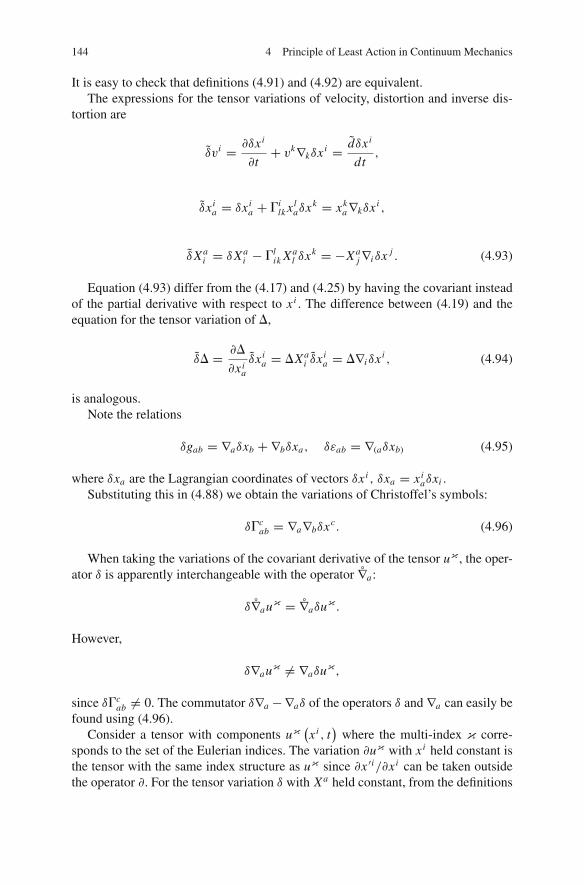
144 4 Principle of Least Action in Continuum Mechanics
It is easy to check that definitions (4.91) and (4.92) are equivalent.The expressions for the tensor variations of velocity, distortion and inverse dis-
tortion are
δvi = �δxi
�t+ vk∇kδxi = dδxi
dt,
δxia = δxi
a + �ilk xl
aδxk = xka∇kδxi ,
δXai = δXa
i − �lik Xa
l δxk = −Xaj∇iδx j . (4.93)
Equation (4.93) differ from the (4.17) and (4.25) by having the covariant insteadof the partial derivative with respect to xi . The difference between (4.19) and theequation for the tensor variation of �,
δ� = ��
�xia
δxia = �Xa
i δxia = �∇iδxi , (4.94)
is analogous.Note the relations
δgab = ∇aδxb +∇bδxa, δεab = ∇(aδxb) (4.95)
where δxa are the Lagrangian coordinates of vectors δxi , δxa = xiaδxi .
Substituting this in (4.88) we obtain the variations of Christoffel’s symbols:
δ�cab = ∇a∇bδxc. (4.96)
When taking the variations of the covariant derivative of the tensor uκ , the oper-ator δ is apparently interchangeable with the operator ∇a :
δ∇auκ = ∇aδuκ .
However,
δ∇auκ �= ∇aδuκ,
since δ�cab �= 0. The commutator δ∇a −∇aδ of the operators δ and ∇a can easily be
found using (4.96).Consider a tensor with components uκ
(xi , t
)where the multi-index κ corre-
sponds to the set of the Eulerian indices. The variation �uκ with xi held constant isthe tensor with the same index structure as uκ since �x ′i/�xi can be taken outsidethe operator �. For the tensor variation δ with Xa held constant, from the definitions

4.6 Tensor Variations 145
of the operators δ and � we have
δuκ = �uκ + δxi∇i uκ . (4.97)
In particular, equation. (4.97) implies that the tensor variation of the metric tensorδgi j is equal to zero, since �gi j = 0 and ∇k gi j = 0. Recall that the variation
δgi j = �gi j
�xkδxk
in a curvilinear system of coordinates is not zero.The variation � commutes with the covariant derivative ∇i ,
�∇i uκ = ∇i �uκ, (4.98)
since ��ki j = 0.
The variation δ does not commute with ∇i :
δ∇i uκ = �∇i u
κ + δxk∇k∇i uκ = ∇i �uκ + δxk∇k∇i u
κ == ∇i
(δuκ − δxk∇kuκ
)+ δxk∇k∇i uκ =
= ∇i δuκ − ∇kuκ∇iδxk + δxk (∇k∇i uκ −∇i∇kuκ) . (4.99)
In a space where the curvature tensor is equal to zero, ∇k∇i uκ = ∇i∇kuκ , and(4.99) becomes
δ∇i uκ = ∇i δuκ − ∇kuκ∇iδxk . (4.100)
The variation of a scalar function. Let the scalar L be a function of a set of tensorswith components uκ , L = L (uκ), where κ corresponds to a set of the observer’sindices and the Lagrangian indices. The following equality holds:
δL = δL (4.101)
or, more explicitly,
�L
�uκ
δuκ = �L
�uκ
δuκ . (4.102)
Indeed, since L does not change in a parallel transport of uκ from the pointxi (Xa, t, ε) to the point xi (Xa, t), we can write
L (uκ (x (X, t, ε) , ε)) = L (uκ (x (X, t, ε) , ε)) , (4.103)
where the tilde above uκ stands for the parallel transport with respect to the Eulerianindices. Differentiating (4.103) with respect to ε and setting ε = 0, we get (4.102).

146 4 Principle of Least Action in Continuum Mechanics
Here is an example illustrating (4.102). Let the internal energy density, U, bea function of the distortion component xi
a . Since one cannot form a scalar onlyfrom xi
a , U must depend also on other tensors with the Eulerian and Lagrangianindices. They characterize the properties of the material and the observer’s frame.Assume that the properties of the material are characterized by some tensor with theLagrangian indices, K κ, and K κ are given function of the Lagrangian coordinates.Then, δK κ = δK κ = 0. Also assume that the metric tensor gi j is the only tensorwith the Eulerian indices in U . Then
δU = �U
�gi jδgi j + �U
�xia
δxia . (4.104)
where δgi j = gi j,kδxk . On the other hand, since δgi j = δxk∇k gi j = 0,
δU = �U
�xia
δxia . (4.105)
According to (4.102), variations (4.104) and (4.105) must coincide. Let us derivethe equality (4.105) directly from (4.104). The derivation is based on the identity
�U
�xia
xka = 2
�U
�gmkgmi , (4.106)
which follows from the scalar nature of U. To obtain it we consider the transforma-tion of the Eulerian coordinates xi → x ′i , xk = bk
i x ′i , x ′i = b(−1)ik xk . Function U,
as a scalar, does not change:
U(g′i j , x ′ia , K κ
) = U(gi j , xi
a, K κ
), (4.107)
where g′i j = gmnbmi bn
j , x ′ia = b(−1)ij x j
a . Differentiating (4.107) with respect to bij
and setting bij = δi
j , we arrive at (4.106).As follows from (4.106),
�U
�gmk=1
2
�U
�xia
xka gim . (4.108)
Note an important consequence of this relation: its left hand side is symmetricwhile the right hand side can be written in terms of the stress tensor:
�U
�gmk= 1
2ρσ mk
Therefore, the stress tensor in such models is necessarily symmetric
σ mk = σ km .

4.6 Tensor Variations 147
Consider (4.104). We have
δU = �U
�gmkgmk,sδxs + �U
�xia
δxia .
We may replace gmk,s by gmk,s + gsm,k − gsk,m because the addition, gsm,k −gsk,m, is anti-symmetric over mk and, thus, its contraction with a symmetric tensor,�U/�gmk, is zero. Substituting �U/�gmk by the right hand side of (4.108),
δU = 1
2
�U
�xia
xka gim(gmk,s + gsm,k − gsk,m)δxs + �U
�xia
δxia,
we recognize in the first term Christoffel’s symbols (see (4.79)). Thus,
δU = �U
�xia
xka �i
ksδxs + �U
�xia
δxia =
�U
�xia
δxia,
as claimed.So, depending on convenience, one can use either the usual variation operator δ
or the tensor variation operator δ.

Chapter 5Direct Methods of Calculus of Variations
The variational principles allow one to investigate the properties of the minimizing/stationary elements without the use of differential equations. Such methods ofstudying the solutions are called direct. The direct methods are especially effec-tive in cases when the functional of the variational problem has only one station-ary point, and this stationary point is either the maximum or the minimum of thefunctional.
There are many direct methods of constructing the approximate solutions, andthere are also some direct methods of qualitative analysis, like the analysis of theexistence and uniqueness of the solution or the derivation of a priori estimates. Thischapter will cover some ideas that form the basis of the direct qualitative methods.As all other reasonings based on the notion of energy, they are simple and almostobvious. However, their application to particular problems often calls for inventive-ness, certain skills, and some subtle mathematical techniques.
We begin with the consideration of the existence and uniqueness theory. Fromthe perspective of an engineer or a physicist, it may seem an infringement in extra-neous territory as this subject is a classical topic of mathematics. In fact, however,one can hardly understand in depth such issues of mechanics as loss of stabilityor the proper choice of boundary conditions without being exposed to the simpleideas underlying the existence and uniqueness theory. Such understanding is cer-tainly necessary for everyone involved in construction of new models of continuummedia.
The next topic is the deep and powerful theory of dual variational problems. Itis based on the notions of convexity and Young-Fenchel transformation, which arediscussed in detail.
Another important tool of the direct methods is the asymptotic analysis of thefunctionals depending on small parameters. We discuss the general scheme andconsider a number of examples while most of the applications are spread over therest of the book.
In this chapter we establish also a link between minimization problems andintegration in functional spaces. This relationship is used in Part III for studyingsome stochastic variational problems. The chapter is concluded with a discussion ofseveral useful tricks, which help to work with variational problems.
V.L. Berdichevsky, Variational Principles of Continuum Mechanics,Interaction of Mechanics and Mathematics, DOI 10.1007/978-3-540-88467-5 5,C© Springer-Verlag Berlin Heidelberg 2009
149

150 5 Direct Methods of Calculus of Variations
5.1 Introductory Remarks
Setting of variational problems. Consider a functional I (u) defined on a set Mof elements u. In continuum mechanics, u are some functions of space variablesand, in dynamical problems, time. Since, the sum of two functions, u1 and u2, andthe multiplication of a function, u, by a real number, are defined, one says that theu-space is a linear space; denote it by R. The space R is also called a functionalspace as it is a set of functions. The set M in which the functional I (u) is definedis a subset of the space R. In continuum mechanics, the set M is usually specifiedby the characterization of smoothness of u and the choice of boundary conditions.There is an important special case when the set M is also linear, i.e. for any twoelements of M, u1 and u2, the sum u1 + u2 belongs to M and the product of anyelement u of M by a number λ is also an element of M. An example of such a setM is a set of continuous functions u(x), defined in a bounded region V, which havezero values on the boundary �V of region V :
u(x) = 0 at �V . (5.1)
Obviously, if u1(x) and u2(x) obey (5.1), then u1(x) + u2(x) and λu1(x) do too. Ifthe boundary conditions are inhomogeneous,
u(x) = u(b)(x) at �V, (5.2)
then the set has the following structure: any element u of M can be presented in aform
u = u0 + u′
where u0 is some function satisfying the boundary condition (5.2), and u′ a functionwith zero boundary values, i.e. an element of a linear set M′.
Another example of M is a cone: the set M is called a cone if, for any element uof M, it also contains the element λu for all positive λ. Cones appear in variationalproblems with unilateral constraints such as
u(x) � 0.
We consider the variational problems of the following type: find the minimumvalue of the functional I (u) on a given set M. For such a problem we write
I (u)→ minuεM
or minuεM
I (u) or minM
I (u).
The minimum and maximum values of I (u) on M are denoted by I and I ,respectively:
I = minuεM
I (u) , I = maxuεM
I (u).

5.1 Introductory Remarks 151
If the set M is selected by an equation like, for example, vanishing of admissiblefunctions at the boundary �V of region V ,
u = 0 on �V, (5.3)
we also use the notation
I = minu∈(5.3)
I (u),
or, if the constraint is a short equation,
I = minu∈ u|�V=0
I (u) .
A search for the maximum value of I (u) is equivalent to a search for the mini-mum value of the functional −I (u); therefore we focus mostly on the minimizationproblem. In minimization problems we may admit that the functional I (u) takes atsome elements of the set M the positive infinite value: I = +∞ (if it would takealso negative infinite values, the solution of the minimization problem is obvious:I = −∞). That is equivalent to the elimination of such elements from the set M.This way of operating with the inadmissible elements is quite convenient. For ex-ample, we may write the original variational problem as a minimization problem fora functional I (u) defined on the entire linear space
I (u) ={
I (u) uεM+∞ uεM
Then
I = minuεR
I (u).
Usually we are interested to find not only the minimum value of the functionalI (u) but also the element, u, on which this value is achieved, i.e. such u that
I (u) = I . (5.4)
Such an element is called the minimizing element or the minimizer. There mightbe many minimizing elements (example: min−∞<u<+∞ sin u = −1, u = −π
2 + 2πn,
n = 0,±1,±2, . . .). On the other hand, the element u may not exist (example:min
0<u<+∞1u = 0, while 1/u > 0 at any point). Mathematicians like to emphasize in
notation the possibility of non-existence of the minimizing elements. For example,they write inf I (u) if it is not known whether the existence of the minimizing elementis guaranteed and min
MI (u) only in the case when the minimum value is achieved on

152 5 Direct Methods of Calculus of Variations
M (and, accordingly, sup I (u) instead of max I (u)). We choose rather to use onlythe symbols min and max; in the usual mathematical notation they correspond to infand sup.
In variational problems of continuum mechanics the existence of the minimizingelement is usually guaranteed by the physics of the problem. Therefore, the varia-tional problem will be called correctly posed (or, briefly, correct) if a minimizingelement does exist. For the variational problems of non-physical nature, like theproblems of optimal control theory, such terminology is not appropriate because ina typical situation, the minimizing element does not exist. We will not encountersuch problems in this book.
On the geometry and dimension of functional spaces. Functional spaces areinfinite-dimensional. This means the following. Consider a smooth function of onevariable, u(x). It can be approximated by a piece-wise linear function which has atsome nodes, xk , the same values as u(x) (Fig. 5.1). The approximation is determineduniquely by the values of the function at the nodes, u(xk). To describe the functionu(x) completely one has to tend the number of nodes, N , to infinity. In the limitfunction u(x) is said to have an infinite number of degrees of freedom.
Another way to introduce the “degrees of freedom” of a function is to expand itinto a series. For example, a continuous function of one variable u(x), defined on asegment −a ≤ x ≤ a, can be presented as the Fourier series
u(x) =∞∑
k=0
ak cosπkx
a+∞∑
k=1
bk sinπkx
a. (5.5)
Hence, each function u(x) is specified by an infinite sequence of numbers{a0, a1, a2, . . . , b1, b2, . . .}. To select a function, u(x), one has to prescribe thesenumbers. There is a one-to-one correspondence between all continuous functions
Fig. 5.1 A finite-dimensionaltruncation in the functionalspace

5.1 Introductory Remarks 153
u(x) and all sequences1 {a0, a1, a2, . . . , b1, b2, . . .} . In the spirit of vector analysis,one can consider u(x) as a vector in an infinite-dimensional space, with the coordi-nates {a0, a1, a2, . . . , b1, b2, . . .}. The vector u(x) has these coordinates in the basisformed by the vectors (functions)
1, cosπx
a, cos
2πx
a, . . . , sin
πx
a, . . . .
The same function, u(x), may also be presented in terms of the Taylor series:
u(x) =∞∑
k=0
ck xk . (5.6)
The coefficients {c0, c1, . . .} may be viewed as the coordinates of functionu(x) in the basis
{1, x, x2, . . .
}. The coordinates {a0, a1, a2, . . . , b1, b2, . . .} and
{c0, c1, c2, . . .} are linked by a linear transformation which can be derived from(5.5) and (5.6).
A functional, I (u), is a function of an infinite number of arguments,a0, a1, a2, . . . , b1, b2, . . . , or c0, c1, c2, . . . . In some cases this functional can becomputed explicitly. For example,
I (u) ≡a∫
−a
u2(x)dx = a
π
π∫
−π
( ∞∑0
ak cos kt +∞∑1
bk sin kt
)2
dt =
= a[2a2
0 + a21 + a2
2 + . . .+ b21 + b2
2 + . . .]. (5.7)
Here we used the following property of the harmonic functions:
π∫
−π
cos kt cos mt dt =π∫
−π
sin kt sin mt dt = πδkm,
π∫
−π
cos kt sin mt dt = 0.
One important point is now in order. The infinite dimensionality of the func-tional space in static problems of continuum mechanics is, in fact, an unnecessarycomplication. In each application of models of continuum mechanics there is alwayssome characteristic length, l∗, such that the model does not make sense for functionschanging on distances less than l∗. For example, if a crystal lattice is modeled bya continuum elastic body, then one can disregard the change of displacements ondistances less than the interatomic distance. In terms of the Fourier coefficients,ignoring the changes of the function u(x) on distances less than l∗ means drop-ping in the Fourier series (5.5) all terms with the wavelengths, a/k, smaller thanl∗, i.e. keeping only a finite number of coordinates a0, a1, . . . , aN , b1, . . . , bN with
1 Which decay fast enough; we do not go into mathematical details.

154 5 Direct Methods of Calculus of Variations
N � a/ l∗. Such a dimensional truncation is possible in all problems of continuummechanics. However, it is also always interesting to see if the results obtained do notdepend on the truncation and admit the limit transition N →∞. The results derivedfor infinite-dimensional functional spaces may be perceived from this perspective:these results do not depend on the value of the characteristic length l∗ and may beviewed as the result corresponding to the limit l∗ → 0 (or N →∞). The idea thatthe space R can be considered as finite-dimensional is quite fruitful: then, withoutloss of any physical feature of the problem, the functional I (u) becomes a functionof a finite number of variables.
Linear and quadratic functionals. Two classes of functionals play a very specialrole in continuum mechanics: linear functionals and quadratic functionals.
Functional l(u) is called linear if, for any u, v and a number λ,
l(λu) = λl(u), l(u + v) = l(u)+ l(v).
This is an example of a linear functional:
l(u) =∫
V
a(x)u(x) dV .
Here a(x) is a given smooth function, and u(x) is any integrable function.Functional E(u, v) is called bilinear if it is linear with respect to each argument,
u and v.Functional E(u) is called quadratic if there is a bilinear symmetric functional,
E(u, v) = E(v, u), such that
E(u) = E(u, u). (5.8)
Boundedness from below. A functional I (u) is called bounded from below on Mif there exists a constant, c, such that for all elements u of M,
I (u) ≥ c.
The fact that functional I (u) has a finite value at a minimizer, u, implies thatfunctional I (u) is bounded from below on M in a correct variational problem. Thereare two reasons why a variational problem may not be correct: either the functionalis not bounded from below on M, or it is bounded from below but its minimumis not reached at M, i.e. there is no element u for which I (u) = I . To determinewhether the problem is correct, it is natural to start from the investigation of theboundedness from below of the functional on M. Here are some examples.
Example 1. Linear functional, l(u), is always unbounded on a linear set M unless itis equal to zero identically. Indeed, if l(u) �= 0 for some u, then l(λu) = λl(u) couldbe made as large or as small as we wish by the appropriate choice of λ.

5.1 Introductory Remarks 155
Example 2. Let M be a set of differentiable functions of one variable, defined onthe segment [0, a]. Consider the functional on M,
E (u) = 1
2
a∫
0
A (x)
(du
dx
)2
dx, (5.9)
where A(x) is a positive function. Functional E(u) is obviously quadratic since itcan be obtained from a bilinear symmetric functional,
E(u, v) = 1
2
a∫
0
A(x)du
dx
dv
dxdx .
Functional E(u) is non-negative, and thus, bounded from below by zero.
The functional (5.9) is defined, if u(x) is a differentiable function such that theintegral of A (x) (du/dx)2 exists. In what follows we skip such details and use avague term “smooth function”, which assumes that all operations on this function,which are involved in our consideration, are meaningful.
Example 3. Consider the functional
I (u) = E(u)− l(u), (5.10)
where E(u) is the functional (5.9), and
l (u) =a∫
0
g (x) u (x) dx + fau (a)− f0u (0) . (5.11)
We assume that functions A (x) and g (x) are smooth, and function A (x) is positiveand separated from zero, i.e.
A (x) ≥ A0 = const > 0. (5.12)
Functional E (u) is bounded from below by zero. Functional l (u) is linear, and,thus, unbounded. The sum E (u) − l (u) can be bounded from below because thelinear growth of l (u) is accompanied by the quadratic growth of E (u) and the lattercan suppress the negative contribution of l(u). Such “suppression” may not occur ifthere are functions u for which l(u) �= 0 while E(u) = 0. Then I (λu) = −λI (u)and, choosing λ, one can tend I (λu) to −∞. Functional E (u) is equal to zero forfunctions u = const. This suggests that the necessary condition for the boundednessfrom below of functional I (u) is
l (u) = 0 (5.13)

156 5 Direct Methods of Calculus of Variations
for all u ≡ const. The equality (5.13) is equivalent to the following constraint onthe entries, g, fa, f0, of the functional l(u) :
a∫
0
g (x)dx + fa − f0 = 0. (5.14)
To understand the meaning of the constraint (5.14), let us write down the Eulerequations for the functional (5.10) assuming that minimizer, u (x), is twice continu-ously differentiable on [0, a]:
d
dxA (x)
du
dx+ g (x) = 0, 0 ≤ x ≤ a, (5.15)
Adu
dx
∣∣∣∣x=0
= f0, Adu
dx
∣∣∣∣x=a
= fa . (5.16)
The boundary value problem (5.15) and (5.16) is not always solvable. To obtaina necessary condition of its solvability, let us integrate (5.15) on [0, a]. Using theboundary condition (5.16), we arrive at (5.14). So, the necessary condition of theboundedness from below of the functional I (u) coincides with the necessary condi-tion of the solvability for the boundary value problem (5.15) and (5.16).
The physical meaning of the constraint (5.14) is simple: if the variational problemis interpreted as the equilibrium problem for extension of an elastic beam, and thus,g(x) is the body force while fa, f0 are the end forces, the condition (5.14) meansthat at equilibrium the sum of all forces acting on the body must be zero.
Let us show that the condition (5.14) is also the sufficient condition for bound-edness from below, i.e. if the linear functional l(u) satisfies (5.14), then I (u) isbounded from below.
First, let us note that, if (5.14) holds, functional I (u) is invariant with respect toshifts of u by a constant, u, since E(u + u) = E(u) and l(u + u) = l(u). Therefore,the minimizing element of the functional I (u) cannot be determined uniquely: if uis a minimizing element then u + u is also a minimizing element. We may add aconstraint eliminating the shifts for a constant. As such we take, for definiteness,
a∫
0
u (x)dx = 0. (5.17)
Now we need the following inequality: for smooth functions u(x) satisfying theconstraint (5.17),
λ2u2 (x) ≤ a
a∫
0
(du
dx
)2
dx, (5.18)

5.1 Introductory Remarks 157
where λ is some constant. The factor, a, is included in the right hand side of (5.18)to make the constant λ dimensionless.
The proof is simple. Consider the identity
u (x)− u (y) =x∫
y
du (z)
dzdz.
Let us integrate it with respect to y from 0 to a. Using (5.17), we get
au (x) =a∫
0
dy
x∫
y
du (z)
dzdz. (5.19)
We square (5.19)
a2u2 (x) =⎡⎣
a∫
0
⎛⎝1 ·
x∫
y
du (z)
dzdz
⎞⎠ dy
⎤⎦
2
and apply the Cauchy inequality: for any two functions, f (x) and g(x),
(∫f (x)g(x)dx
)2
≤∫
f 2(x)dx∫
g2(x)dx (5.20)
For further references, note that inequality (5.20) holds true for integrals overmulti-dimensional regions as well.2 We get, using twice the Cauchy inequality,
a2u2(x) ≤a∫
0
12dy
a∫
0
⎡⎣
x∫
y
1 · du
dzdz
⎤⎦
2
dy ≤ a
a∫
0
⎡⎣
x∫
y
12dz
x∫
y
(du
dz
)2
dz
⎤⎦dy.
(5.21)Substituting the integration limits, x and y, in (5.21) by 0 and a, respectively, andconsequently increasing the value of the right-hand side, we obtain
a2u2 (x) ≤ a3
a∫
0
(du
dz
)2
dz. (5.22)
2 The Cauchy inequality follows from the positiveness for any α, β of the quadratic form,
α2∫
f 2dx + 2αβ
∫f gdx + β2
∫g2dx =
∫(α f + βg)2dx ≥ 0.
Clearly, the equality is achieved only when f and g are proportional.

158 5 Direct Methods of Calculus of Variations
Hence, the inequality (5.18) holds with the constant λ equal to at least unity (the“best” value for λ, i.e. the largest value of λ for which the inequality (5.18) remainstrue, is greater than unity).
The following inequalities are the obvious consequences of (5.18):
λ2u2 (0) ≤ a
a∫
0
(du
dx
)2
dx, λ2u2 (a) ≤ a
a∫
0
(du
dx
)2
dx, (5.23)
μ2
a∫
0
u2dx ≤ a2
a∫
0
(du
dx
)2
dx . (5.24)
with a constant μ which is not less than unity. Inequality (5.24) is also called theWirtinger inequality.
The elimination of shifts in u(x) by a constant is essential for the inequalities(5.23) and (5.24) to be true: if one ignores the constraint (5.17), then, putting u(x) =const, we get zero in the right hand sides and non-zero in the left hand sides. Theshift can be excluded by different constraints. The values of the best constants, λ
and μ, in (5.23) and (5.24) depend on the choice of the constraint.The best constant in the Wirtinger inequality is a solution of the following varia-
tional problem:
μ2 = minu(x)∈(5.17)
a2a∫
0
(dudx
)2dx
a∫0
u2dx.
One can find (for example, by expanding u(x) in Fourier series) that the bestvalue for μ is 2π . Similarly, the best constant λ can be defined by the corre-sponding variational problem. We will see in Sect. 8.3 that the best constants inthe Wirtinger-type inequalities relate to the minimum eigen-frequencies of somemechanical systems.
The best constants depend on the constraints imposed to eliminate the shift. Ifthe constraint (5.17) is replaced by the constraint
u (0) = 0 or u (0) = u (a) = 0, (5.25)
then the best value for μ becomes π/2 and π , respectively.Let us return to proving the sufficiency of conditions (5.14) for the boundedness
from below of the functional (5.10). Using the inequality
|u + v| ≤ |u| + |v|

5.1 Introductory Remarks 159
and the Cauchy inequality (5.20), we get the following estimate of the linearfunctional l(u)
|l(u)| =∣∣∣∣∣∣
a∫
0
g(x) u (x)dx + fau (a)− f0u (0)
∣∣∣∣∣∣≤
≤∣∣∣∣∣∣
a∫
0
g(x) u (x)dx
∣∣∣∣∣∣+ | fau (a)| + | f0u (0)| ≤
≤∣∣∣∣∣∣
a∫
0
a√A0
g (x)
√A0
au (x)dx
∣∣∣∣∣∣+ | fau (a)| + | f0u (0)| ≤
≤
√√√√√a∫
0
a2
A0g2dx
√√√√√a∫
0
A0
a2u2dx +
√a | fa|√
A0
√A0u2 (a)
a+
+√
a | f0|√A0
√A0u2 (0)
a. (5.26)
Let us increase the right-hand side of (5.26) by means of (5.23), (5.24), and(5.12). We see that the linear functional does not exceed
√E(u):
|l(u)| ≤ c√
E (u), (5.27)
with a constant c equal to
c =√
2
⎛⎜⎝ 1
μ
√√√√√a∫
0
a2
A0g2dx +
√a (| f0| + | fa|)
λ√
A0
⎞⎟⎠ . (5.28)
The inequality (5.27) allows us to complete the estimate of I (u) :
I (u) = E (u)− l (u) ≥ E (u)− |l(u)| ≥ E (u)− c√
E (u)
=(√
E (u)− c
2
)2.
− c2
4≥ −c2
4
This justifies the boundedness of the functional I (u) from below.Equation (5.28) shows that the integrability of g2 (x) is sufficient for boundedness
from below.In the example considered, there is a group of transformations, G, acting on
M, such that application of the transformation g from G to each element of Mgives again the set M, gM = M, g ∈ G (in the example G is the group ofshifts of u by a constant). This group leaves the functional E unchanged, E (gu) =

160 5 Direct Methods of Calculus of Variations
E (u) , g ∈ G, u ∈M. If the group G contains more elements than just the identitytransformation, the functional E is said to have a kernel. In statics, E is usually theenergy, and G is the transformation group corresponding to the rigid motions of thebody.
In the same way, as in Example 3, the following statement can be proven: Letthe invariance group of E(u), G, be a group of translations with respect to u, gu =u + ug , and the set K of elements ug is a cone, i.e. for every element u ε K andany positive constant λ, λu ε K. Let the functional I (u) of the form (5.10) alsobe bounded from below. Then for all u ∈ K the linear functional must satisfy theinequality
l (u) ≤ 0, (5.29)
If the cone K contains with every element u the element −u, then, as followsfrom (5.29), the necessary condition for the boundedness from below of thefunctional E (u)− l (u) is
l (u) = 0 (5.30)
for all u ∈ K.The property of E (u) of having a kernel depends on the set on which it is
considered. This is illustrated by the following example.
Example 4. Consider the set M of smooth functions u (x) which consists of all dif-ferentiable functions on [0, a] , satisfying the condition
u (0) = 0. (5.31)
In this case, the functional E (u) (5.9) does not have a kernel: shifts for a constantare forbidden by the condition (5.31). The functional I (u) is bounded from belowfor any g (x) and fa , since on the set of functions satisfying (5.31), the inequality(5.18) and, consequently, the inequality (5.27) hold true.
The physical interpretation of this fact for an elastic beam is as follows: if oneend of the beam is clamped, the equilibrium exists for any forces, not only for forceswith the zero resultant.
In the next example, the functional does not have a kernel.
Example 5. Let us change the functional E (u) (5.9) by adding the integral of u2:
E (u) = 1
2
a∫
0
(A (x)
(du
dx
)2
+ B (x) u2
)dx, B (x) ≥ B0 > 0. (5.32)
The functional E (u) (5.32) is not invariant with respect to shifts. FunctionalE (u) − l (u) is bounded from below. The proof of the boundedness from below isthe same as in Example 3, except that instead of inequalities (5.23), the inequalities
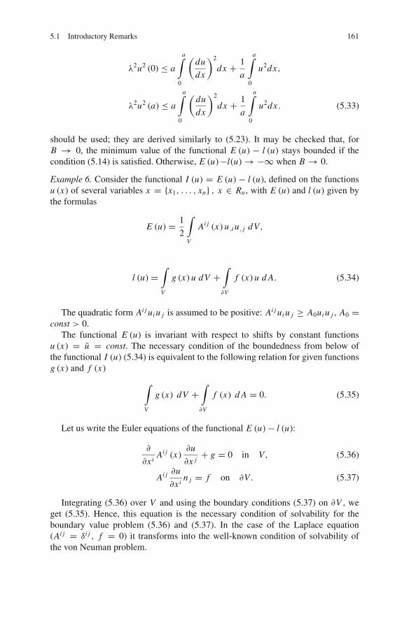
5.1 Introductory Remarks 161
λ2u2 (0) ≤ a
a∫
0
(du
dx
)2
dx + 1
a
a∫
0
u2dx,
λ2u2 (a) ≤ a
a∫
0
(du
dx
)2
dx + 1
a
a∫
0
u2dx . (5.33)
should be used; they are derived similarly to (5.23). It may be checked that, forB → 0, the minimum value of the functional E (u) − l (u) stays bounded if thecondition (5.14) is satisfied. Otherwise, E (u)−l(u)→−∞ when B → 0.
Example 6. Consider the functional I (u) = E (u) − l (u), defined on the functionsu (x) of several variables x = {x1, . . . , xn} , x ∈ Rn , with E (u) and l (u) given bythe formulas
E (u) = 1
2
∫
V
Ai j (x) u,i u, j dV,
l (u) =∫
V
g (x) u dV +∫
�V
f (x) u d A. (5.34)
The quadratic form Ai j ui u j is assumed to be positive: Ai j ui u j ≥ A0ui u j , A0 =const > 0.
The functional E (u) is invariant with respect to shifts by constant functionsu (x) = u = const. The necessary condition of the boundedness from below ofthe functional I (u) (5.34) is equivalent to the following relation for given functionsg (x) and f (x)
∫
V
g (x) dV +∫
�V
f (x) d A = 0. (5.35)
Let us write the Euler equations of the functional E (u)− l (u):
�
�xiAi j (x)
�u
�x j+ g = 0 in V, (5.36)
Ai j �u
�xin j = f on �V . (5.37)
Integrating (5.36) over V and using the boundary conditions (5.37) on �V , weget (5.35). Hence, this equation is the necessary condition of solvability for theboundary value problem (5.36) and (5.37). In the case of the Laplace equation(Ai j = δi j , f = 0) it transforms into the well-known condition of solvability ofthe von Neuman problem.

162 5 Direct Methods of Calculus of Variations
The proof of the sufficiency of the condition (5.35) for the boundedness frombelow of the functional I (u) is based on the Poincare-Steklov-Fridrichs-Erlichinequalities
λ2∫
�V
u2d A ≤∫
V
u,i u,i dV, μ2
∫
V
u2dV ≤∫
V
u,i u,i dV . (5.38)
It is obtained in the same way as in Example 3. The equation
∫
V
udV = 0 (5.39)
Minimizing sequences. Let the functional I (u) be bounded from below on M.Then there exist sequences {un} in M such that I (un) → I when n → ∞. Theyare called the minimizing sequences.
Example 7. Let M be a set of smooth functions u (x) of one variable defined on[0, a] which take the unity value at x = 0: u (0) = 1. Consider the functional
I (u) =a∫
0
u2dx .
on M. The functional is bounded from below by zero. Let us show that min I (u) =0. Consider a sequence of functions un (x) which are linear on the segment [0,a/n] ,
take the values unity and zero at the points x = 0 and x = a/n, respectively, andequal to zero outside the segment (Fig. 5.2). It is also obvious that I (un)→ 0 whenn → ∞. Hence, the constructed sequence is minimizing. It is obvious that thereis no minimizing element on the set of continuous functions because there is nocontinuous function which is equal to unity at the point x = 0 and for which theintegral of u2 is equal to zero.
Fig. 5.2 Minimizing sequence in Example 7

5.2 Quadratic Functionals 163
As was already mentioned, the incorrectness of the variational problems causedby the absence of the minimizing element is encountered in applications. To solvesuch a problem means to find I and to construct a minimizing sequence. In thevariational problems of physics and mechanics the minimizing element usually doesexist.3
5.2 Quadratic Functionals
Quadratic functionals, E(u), were defined as functionals which can be presented inthe form
E(u) = E(u, u),
where E(u, v) = E(v, u) is a bilinear symmetric functional. An immediate conse-quence of this definition is a “quadratic expansion”:
E(u + v) = E(u)+ 2E(u, v)+ E(v). (5.40)
Besides, the quadratic functionals grow quadratically along the lines,4 u = λu0 :
E(λu0) = λ2 E(u0).
An identity. The quadratic functionals, as follows from (5.40), obey a usefulidentity:
E
(u + v
2
)+ E
(u − v
2
)= 1
2(E(u)+ E(v)) . (5.41)
Alternative notation. As we have already discussed, in physical problems withoutloss of generality, the functional space can be replaced by a finite-dimensional space,Rm, of a large dimension, m. Then u becomes a vector in Rm , E(u) a quadraticfunction in Rm , and l(u) a linear function. Any linear function in Rm can be viewedas a scalar product of some vector, l, and vector u : l(u) = (l, u). By (l, u) wedenote the scalar product in Rm : if li and ui are the components of the vectors, land u,
(l, u) = li ui .
3 There are some exceptions such as the problem of thermodynamic equilibrium of two-phasematerials when one neglects the interface energy. However, the absense of the minimizer is causedby an oversimplification of the energy functional. To some extent, the situation is similar to theappearance of paradoxes in fluid mechanics when viscosity is neglected.4 For a given element u0, the equation u = λu0 may be interpreted as the parametric equation ofthe line in R passing through the origin and the point u0.

164 5 Direct Methods of Calculus of Variations
A quadratic function, E(u), may be presented as a scalar product of two vectors,Au and u, where Au is the product of a m × m matrix, A, and the vector, u :
E(u) = (Au, u).
The bilinear form, E(u, v), is, obviously, (Au, v). If m → ∞, Au transformsinto an operator acting on u. In what follows we will use for quadratic and linearfunctionals both notations introduced: E(u) = (Au, u) and l(u) = (l, u).
Example. Let E(u) be a functional,
E(u) =∫
V
�u
�xi
�u
�xidV,
where V is a region in an n−dimensional space, and u is a smooth function vanish-ing on �V . Integrating by parts we can write
E(u) =∫
V(−� u) udV,
where � is Laplace operator. Setting the scalar product of two functions, u andv, as
(u, v) ≡∫
VuvdV,
we see that in this example A = −� . Note that the operator, −�, is positive in thesense that (Au, u) ≥ 0 for any u.
Linear problems. Many linear problems of continuum mechanics can be formu-lated as the minimization problems for a functional which is a sum of quadratic andlinear functionals:
I (u) = E(u)− l(u)→ minM
(5.42)
Variations of such functionals can easily be found:
δE(u) = E(u + δu)− E(u) = E(u + δu, u + δu)− E(u)
= 2E(u, δu)
δl(u) = l(u + δu)− l(u) = l(δu)
δ I (u) = 2E(u, δu)− l(δu) (5.43)
The minimizing element, u, must obey the equation:
δE(u) = δl(u)

5.2 Quadratic Functionals 165
for any admissible δu. Thus, for any admissible δu,
2E(u, δu) = l(δu). (5.44)
Another form of this equation is obtained if we assume that l(u) is a scalar prod-uct of some element, l, and u : l(u) = (l, u), while E(u) = 1
2 (Au, u). Then theEuler equation is
Au = l.
If the solution of this equation is unique, it can be written as
u = A−1l,
where A−1 is the inverse operator. The inverse operator can be considered as theinfinite-dimensional limit of the inverse symmetric matrix, A−1
m , where Am is anm×m-matrix corresponding to an m−dimensional truncation of the quadratic func-tional, (Au, u).
Clapeyron theorem. If the set M is linear, then δu = u′ − u belongs to M. We canchoose, in particular, δu = uε, ε being an infinitesimally small number. Plugging itin (5.44) we arrive at the so-called Clapeyron’s theorem:
2E(u) = l(u). (5.45)
An important consequence of Clapeyron’s theorem is the link between theminimum value of the functional and the value of the quadratic functional at theminimizing element,
I (u) = −E(u), (5.46)
which follows from (5.42) and (5.45). Another useful form of this equation is
I (u) = −1
2l(u). (5.47)
Various forms of the minimization problem for quadratic functionals. Theminimization problem for the functional I = E (u) − l (u) may be presented ina number of equivalent forms that are sometimes useful.
Let the kernel of the quadratic functional E (u) be eliminated. One can assign toeach element, u, its “length,”
√E (u). Then the unit sphere in the functional space
is defined by the equation E (u) = 1.
Let us assign to every element of the functional space, u, an element on the unitsphere, v:

166 5 Direct Methods of Calculus of Variations
v = u√E (u)
, E (v) = 1.
The functional space can be split into rays, u = λv, 0 ≤ λ < +∞. The func-tional I (u) can be considered as a function of two arguments, v and λ. The minimumof the functional I (u) can be searched successively, by first finding the minimumalong each ray u = λv, and then finding the minimum on the sphere E (v) = 1.The search for the minimum along each ray is reduced to minimizing the functionλ2 − λl (v) of one variable, λ (v is fixed). The minimum is equal to − 1
4 (l(v))2.Minimizing this expression with respect to v is equivalent to maximizing the linearfunctional l (v) on the unit sphere, and we arrive at the variational problem
I = −1
4l2
, l = maxE(v)=1
l (v) . (5.48)
The variational problem (5.48) can be written in two other equivalent ways: as amaximization problem of the linear functional on a ball:
l = maxv: E(v)≤1
l (v) , (5.49)
or as a maximization problem over the entire space of a functional of the zerothorder of homogeneity:
l = maxu
l(u)√E (u)
. (5.50)
The equivalence of (5.48) and (5.49) can be justified by the following reasoning.Let us expand the set of the admissible elements in the variational problem for l,(5.48), allowing all elements inside the unit ball, E(v) ≤ 1. The maximum can onlyincrease:
maxv: E(v)≤1
l (v) ≥ maxv: E(v)=1
l (v) . (5.51)
Suppose that (5.51) is a strict inequality:
maxv: E(v)≤1
l (v) > maxv: E(v)=1
l (v) ≡ l.
Then there exists a sequence {vn} such that l (vn) > l and E (vn) ≤ 1. Define thenumbers λn by the equations: E (λnvn) = 1. Since E(λnvn) = λ2
n E(vn) = 1and E(vn) ≤ 1, the numbers λn are not less than unity. Therefore, l (λnvn) =λnl(vn) > λnl ≥ l, i.e. l (λnvn) > l. This contradicts the definition of l (5.48),because the sequence {λnvn} lies on the sphere E (v) = 1. Thus, only the equalitysign is possible in (5.51).

5.3 Existence of the Minimizing Element 167
Equation (5.50) follows from the fact that the functional l(u)�√
E(u) does notchange along the rays u = λv.
5.3 Existence of the Minimizing Element
In calculus of variations the theorems warranting the existence of the minimizingelement are usually the generalizations to the infinite-dimensional case of the the-orem which states that a continuous function in a finite-dimensional space reachesboth its maximum and minimum values on any closed set M. The analysis of thistheorem shows that it is based on three elements: the notion of the convergence ofthe elements on M, the notion of the continuity of the function (functional) on Mand the structure of the set M: any infinite sequence of elements from M has tocontain a subsequence that converges to an element of M.
The notion of the continuity of the functional (the functional is continuous atpoint u0 if for any sequence {un} converging to u0, I (un) converges to I (u0)), andthe above-mentioned property of the set M, which is called compactness, are bothbased on the way in which the convergence of elements of M is introduced.
For given functional I (u) and a set M the convergence of elements of M canbe defined differently. With respect to some convergences functional I (u) can becontinuous and the set M – compact; with respect to the other ones, this may not betrue. If it is possible to introduce such convergence of the elements that the set Mis compact and the functional I (u) is continuous with respect to that convergence,then I (u) has a minimizing element on M. This statement is proven similarly to thecorresponding theorem for a function of one variable in calculus.
One can check that the assumption of the functional continuity can be relaxedto a weaker assumption of its semi-continuity below. The functional is called semi-continuous below at point u0 if for any sequence {un} converging to u0, for whichthe sequence {I (un)} converges,
I (u0) ≤ limn→∞ I (un) .
The key types of the convergence of elements in M are as follows. Usually, theset M can be considered as a subset of a Banach space. A Banach space is a linearspace B, for which a norm, a non-negative functional, ‖u‖ , is defined, where ‖u‖is homogeneous (‖λu‖ = |λ| ‖u‖), non-degenerate (‖u‖ = 0 if and only if u = 0),convex (‖u + v‖ ≤ ‖u‖+‖v‖) functional, and the space B is complete with respectto the norm. The latter means that any fundamental sequence {un} (i.e. the sequencewith ‖un − um‖ → 0 as n, m →∞) converges to an element of B.
For a Banach space, the notion of convergence with respect to the norm arisesnaturally; it is also called strong convergence. One says that the sequence {un}strongly converges to u0 if ‖un − u0‖ → 0 as n → ∞. Strong convergence is notvery useful for theorems of the existence of the minimizing element since boundedclosed sets in functional spaces (i.e. closed sets contained in a ball ‖u‖ ≤ R of a

168 5 Direct Methods of Calculus of Variations
finite radius R) turn out to be non-compact. However, the bounded closed sets ina Banach space can be compact with respect to the so-called weak convergence:the sequence {un} weakly converges to u0 if for any linear continuous functional5
l (u), l (un) → l (u0) as n → ∞. Such Banach spaces are often encountered inapplications; they include Hilbert spaces (linear spaces for which the scalar product(u, v) is defined, and the norm is introduced as ‖u‖ = (u, u)1/2).
So the existence of the minimizing element is warranted for functionals I (u)which are semi-continuous below with respect to weak convergence on a boundedclosed set in the Banach space. The case of the unbounded set M (for example,when M is a cone) reduces to the case of the bounded set if the functional I (u)satisfies an additional condition of I (u)→+∞ when ‖u‖ → ∞.
One can prove that the functional ‖u‖ is semi-continuous below with respectto the weak convergence. This property warrants the existence of the minimizingelement for the functionals I (u) of the form
I (u) = E (u)− l (u)
if for some α, 0 < α < 1, the functional [E (u)]α has the properties of the norm6
and l (u) is a linear functional. For quadratic functionals, α = 1/2.
The functional space with the norm ‖u‖ = √E(u) plays a special role in varia-tional problems with quadratic functionals. It is called energy space because E(u)usually has the meaning of energy. To make the energy space a Banach space, onehas to include in this space the limits of all fundamental sequences {un} , i.e. suchsequences that ‖un − um‖ =
√E(un − um) → 0 for n, m → ∞. The minimizing
element is an element of the energy space.In the examples considered above E (u) does not have the properties of the norm
since it has a kernel (i.e. it is equal to zero for u �= 0). However, by eliminatingthe kernel by means of the constraints like (5.17) or (5.25),
√E (u) acquires the
properties of the norm, and the minimizing element does exist.The elements of the energy space do not have the smoothness expected of the
solution of physical problems. Hence, an independent problem of studying thesmoothness properties of the minimizing element arises. It is not as simple as theproblem of the existence of the minimizing element in the energy space.
5.4 Uniqueness of the Minimizing Element
The fundamental criterion for the uniqueness of the minimizing element is based onthe notion of convexity. We begin its consideration with the definition of convex sets.
5 Continuity of linear functionals with respect to strong convergence is implied.6 This condition can be weakened by replacing it by the conditions that the functional E (u) beconvex (see below), continuous with respect to some norm ‖u‖, and coercive, i.e. E (u) / ‖u‖ → ∞when ‖u‖ → ∞.

5.4 Uniqueness of the Minimizing Element 169
Fig. 5.3 The segmentconnecting the points u and v
For any two points of a finite-dimensional space, u and v, the sum 12 (u + v) is
the center of the segment connecting the points u and v, while any point of thissegment can be presented in the form αu + (1− α) v, 0 ≤ α ≤ 1. The ends of thesegment, u and v, correspond to α = 1 and α = 0, respectively (Fig. 5.3). We applythis terminology to the functional spaces calling the one-parametric set of elements,αu + (1− α) v, 0 ≤ α ≤ 1, the segment connecting the elements u and v.
The set M is called convex, if, for any two elements u and v, it contains thesegment αu + (1− α) v, 0 ≤ α ≤ 1 connecting those two elements.
The functional I (u) defined on the convex set M is called convex if, for any twoelements u and v in M and any 0 ≤ α ≤ 1,
I (αu + (1− α) v) ≤ α I (u)+ (1− α) I (v) . (5.52)
The functional is strictly convex, if for u �= v,
I (αu + (1− α) v) < α I (u)+ (1− α) I (v) , 0 ≤ α ≤ 1.
Sometimes, in the definition of convex functionals one uses the inequality
I
(u + v
2
)≤ 1
2(I (u)+ I (v)) . (5.53)
It follows from (5.52) for α = 12 . One can show that the conditions (5.52) and (5.53)
are equivalent for functionals which are semi-continuous below. The geometricalmeaning of the conditions (5.52) and (5.53) can be seen from Fig. 5.4.
Example 1. Consider the integral functional
I (u) =∫
V
L
(xi , uκ,
�uκ
�xi
)dV .
We are going to show that this functional is convex (strictly convex) if L is aconvex (strictly convex) function of uκ and �uκ/�xi . Indeed,

170 5 Direct Methods of Calculus of Variations
Fig. 5.4 Definition of theconvex functional
I (αu + (1− α) v) =
=∫
V
L
(xi , αuκ + (1− α) vκ, α
�uκ
�xi+ (1− α)
�vκ
�xi
)dV ≤
≤∫
V
[αL
(xi , uκ,
�uκ
�xi
)+ (1− α)L
(xi , vκ,
�vκ
�xi
)]dV =
= α I (u)+ (1− α) I (v) ,
as claimed.
A strictly convex functional cannot have more than one minimizing element ona convex set. Indeed, suppose that a strictly convex functional has two minimizingelements, u and v, on M. Then I (u) = I (v) = I . The element 1
2 (u + v) belongs toM due to the convexity of the set. According to the strict convexity of the functionalI (u), its value at the point 1
2 (u + v) is less than the minimum value on M,
I
(u + v
2
)<
1
2(I (u)+ I (v)) = I ,
which contradicts the definition of the minimum value.Any linear functional obeys (5.52):
l(αu + (1− α)v) = αl(u)+ (1− α)l(v),
and, thus, is convex. The sum of a convex functional and a linear functional isobviously convex. Moreover, the sum of any two convex functionals is convex.

5.4 Uniqueness of the Minimizing Element 171
Positive quadratic functionals with zero kernel are strictly convex. Indeed,consider the identity (5.41):
E
(u + v
2
)+ E
(u − v
2
)= 1
2(E (u)+ E (v)) . (5.54)
By our assumption, functional E(u) has zero kernel, i.e. E(u) = 0 only for u = 0.
Therefore, for u �= v, E(
u−v2
)> 0. Dropping E
(u−v
2
)in (5.54), we decrease the
left hand side and arrive at the inequality
E
(u + v
2
)<
1
2(E (u)+ E (v))
which indicates the strict convexity of E(u).
Examples 2–5 of Sect. 5.1 (continued). The quadratic functionals E (u) in Exam-ples 2–5 are positive. Thus, if the kernels are excluded, these functionals are strictlyconvex, and the functional I (u) = E (u) − l (u) is strictly convex as well. The setM in Examples 1–4 is convex. Hence, there is only one minimizing element in thecorresponding variational problems.
A convex, but not necessarily strictly convex, functional can have several mini-mizing elements (the corresponding example is illustrated in Fig. 5.5: the set of theminimizing points of the function is the straight segment).
The set of minimizing elements of a convex functional is convex. Indeed, if uand v are two minimizing elements, I (u) = I and I (v) = I , then
I (αu + (1− α) v) = I
because
I ≤ I (αu + (1− α) v) ≤ α I (u)+ (1− α) I (v) = I .
Consequently, all the points on the segment αu + (1− α) v, 0 ≤ α ≤ 1, are theminimizing elements of I (u).
Fig. 5.5 Convex functionalwith many minimizingelements

172 5 Direct Methods of Calculus of Variations
5.5 Upper and Lower Estimates
In many problems, the information about the minimum value of the functional I (u)is very important. Sometimes it is of the primary interest (many examples are givenfurther). In particular, the minimum value may be related to the energy of the system.
The estimates of the minimum value are usually based on some auxiliary varia-tional problems which are easier to investigate than the initial variational problem.In constructing the auxiliary problem, either the set M or the functional I (u) arechanged.
Changing the set of the admissible functions. Consider two sets, M1 and M2,such that M2 ⊂M ⊂M1. Suppose that the functional I (u) can be defined on theset M1. Denote by I1 and I2 the minimum values of the functional I (u) on M1 andM2, respectively. It is obvious that
I1 ≤ I ≤ I2. (5.55)
If one takes as the set M2 an element, u, of M, one gets an estimate
I ≤ I (u) (5.56)
In the case of the quadratic functionals of the form E(u) − l(u), minimized ona linear set, an upper estimate of the minimum value, according to the Clapeyrontheorem (5.46), corresponds to an estimate of energy from below, while a lowerestimate of the minimum value gives an upper energy estimate.
The Rayleigh-Ritz method. The most common method of obtaining an approxi-mate solution of a variational problem is the Rayleigh-Ritz method. The method isas follows. One selects a k-dimensional subset, Mk, of the set M. It is comprisedof the elements of the form a1u1+ . . .+ akuk , where u1, . . . , uk are some fixed ele-ments of M, while a1, . . . , ak are numerical parameters. The functional I becomesa function of k variables, a1, . . . , ak . Denote by a1, . . . , ak the minimizer of thisfunction, and by uk the element a1u1 + . . .+ akuk . This element can be consideredas an approximation of the minimizing element of the functional I on M; moreover,I ≤ I (uk), and if uk is the minimizing element of I on Mk , this estimate is the bestamong all elements of the set Mk .
Increasing the dimensionality of the subset Mk , M1 ⊂ M2 ⊂ M3 ⊂ . . ., weobtain better and better approximations of the minimizing elements and the mini-mum value. The convergence of this process is proved for a large class of variationalproblems.
The method of constraint unlocking. Let the set M be defined by some system ofequations or inequalities. By dismissing some of those equations, we obtain a larger

5.5 Upper and Lower Estimates 173
set M1, and I1 ≤ I . This way of making the lower estimates is called the methodof constraint unlocking.
Changing the functional. Another way of making estimates employs a change ofthe functional. One constructs the functionals I1 and I2 in such a way that I1 < I <
I2 on M. Then
I1 ≤ I ≤ I2. (5.57)
This method is effective if the minimum values I1 and I2 of the functionals I1 andI2 can be found on M.
Let, for example, the functional I be a sum of two functionals:
I = I ′ + I ′′
where I ′ and I ′′ are both bounded from below on M and their minimum values canbe found. Then one can take as a functional I1 the functional
I1 = I ′ +minM
I ′′
The low estimate (5.57) takes the form
minM
I ′ +minM
I ′′ ≤ minM
I. (5.58)
Example. Consider the minimization problem for the functional
I (u) = E (u)− l (u) , E (u) =∫
V
L
(xi , uκ,
�uκ
�xi
)dV,
l (u) =∫
V
gκ (x) uκdV +∫
�V f
fκ (x) uκd A,
where �V f is a part of the boundary �V where the “external surface forces,” fκ, aregiven. The minimum is sought over all functions uκ , taking the assigned values, onthe surface �Vu = �V − �V f :
uκ = uκ
(b). (5.59)
Let us divide the region V into two subregions V ′ and V ′′ by the surface �. Thesurface � divides each of the surfaces �Vu and �V f into two parts, �V ′u and �V ′′u ,and �V ′f and �V ′′f ; see Fig. 5.6. In this figure the part of the boundary with “hard”boundary conditions, i.e. the conditions that yield zero variations of the required

174 5 Direct Methods of Calculus of Variations
Fig. 5.6 Notation toinequality (5.62)
functions, is shadowed. The boundary of the surface V ′ comprises surfaces �V ′f ,�V ′u and �, and the boundary of the surface V ′′ comprises �V ′′u , �V ′′f , and �. Let usdefine on � some functions pκ (x) and define the functionals
I ′ (u) = E ′ (u)− l ′ (u) , I ′′ (u) = E ′′ (u)− l ′′ (u) ; (5.60)
E ′ (u) =∫
V ′
LdV, E ′′ (u) =∫
V ′′
LdV,
l ′ (u) =∫
V ′
gκuκdV +∫
�V ′f
fκuκd A +∫
�
pκuκd A,
l ′′ (u) =∫
V ′′
gκuκdV +∫
�V ′′f
fκuκd A −∫
�
pκuκd A, (5.61)
Obviously,
I ′ + I ′′ = I.
According to (5.58), for I we get the estimate
I ′ + I ′′ ≤ I . (5.62)
If the minimum value of the functional I (u) is related to the energy of the system,the inequality (5.62) provides an estimate of energy in terms of energies of its parts.
Essential and inessential constraints. The estimates of the minimum value areclosely related to the important notion of essential and inessential constraints. Theconstraints removing of which does not change the minimum value of the functionalare called inessential. Otherwise, the constraint is essential. We discuss this notionfor the following example.
Consider the minimization problem for the functional
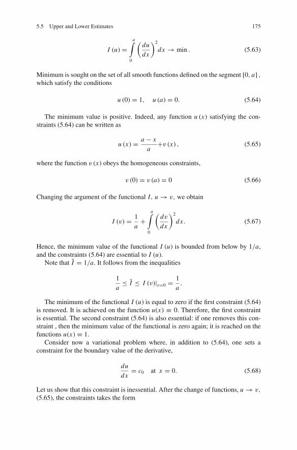
5.5 Upper and Lower Estimates 175
I (u) =a∫
0
(du
dx
)2
dx → min . (5.63)
Minimum is sought on the set of all smooth functions defined on the segment [0, a] ,
which satisfy the conditions
u (0) = 1, u (a) = 0. (5.64)
The minimum value is positive. Indeed, any function u (x) satisfying the con-straints (5.64) can be written as
u (x) = a − x
a+v (x) , (5.65)
where the function v (x) obeys the homogeneous constraints,
v (0) = v (a) = 0 (5.66)
Changing the argument of the functional I, u → v, we obtain
I (v) = 1
a+
a∫
0
(dv
dx
)2
dx . (5.67)
Hence, the minimum value of the functional I (u) is bounded from below by 1/a,and the constraints (5.64) are essential to I (u).
Note that I = 1/a. It follows from the inequalities
1
a≤ I ≤ I (v)|v=0 =
1
a.
The minimum of the functional I (u) is equal to zero if the first constraint (5.64)is removed. It is achieved on the function u(x) ≡ 0. Therefore, the first constraintis essential. The second constraint (5.64) is also essential: if one removes this con-straint , then the minimum value of the functional is zero again; it is reached on thefunctions u(x) ≡ 1.
Consider now a variational problem where, in addition to (5.64), one sets aconstraint for the boundary value of the derivative,
du
dx= c0 at x = 0. (5.68)
Let us show that this constraint is inessential. After the change of functions, u → v,
(5.65), the constraints takes the form

176 5 Direct Methods of Calculus of Variations
v(0) = 0, v(a) = 0,dv
dx
∣∣∣∣x=0
= c ≡ c0 + a−1. (5.69)
We assume, for definiteness, that c > 0. Consider a sequence of functions {vn (x)} ,
vn (x) =
⎧⎪⎨⎪⎩
cx, 0 ≤ x ≤ anc
−cx + 2an,anc ≤ x ≤ 2an
c
0, 2anc ≤ x ≤ a
where {an} is a sequence of positive numbers converging to zero (see Fig. 5.7).Functions vn (x) satisfy the constraints (5.69), and I (vn) = 1/a + 2can → 1/a
as n → ∞. Therefore, the minimum value of the functional I (u) does not changeif one prescribes the value of the derivative of u(x) at the boundary: it is still equalto 1/a.
One may say that the functional itself chooses the constraints which it cannotviolate (essential constraints) and which it ignores (inessential constraints). Thefunctional “feels” the essential constraints and does not feel the inessential con-straints.
It is also instructive to consider in the above example the case a = +∞. Then,the second constraint (5.64) is replaced by the condition u (x)→ 0 for x →∞.
If a = ∞, the constraints (5.64) become inessential. To make sure that it is the case,consider the sequence un (x) (Fig. 5.8):
un (x) ={
1− an x, 0 ≤ x ≤ 1an
0, 1an≤ x
{an} → 0 for n→∞.
For this sequence, I (un) = an → 0 as n → ∞. Hence, the minimum value is thesame as if there are no constraints at all.
Estimates of the closeness of the minimizing element and its approximations.Let a sufficiently narrow fork,
a ≤ I ≤ b,
Fig. 5.7 Minimizingsequence in the variationalproblem with constraints(5.69)

5.5 Upper and Lower Estimates 177
Fig. 5.8 Minimizingsequence for a = ∞
be constructed for the minimum value I of a strictly convex functional I (u), and letan element u be found such that the value of the functional for this element is alsowithin the same fork:
a ≤ I (u) ≤ b.
What can be said of the closeness of the element u to the minimizing elementu? The difference between u and u can be estimated in the case of strongly convexfunctionals. Functional I (u) is called strongly convex if there exists such a positivefunctional B (u) that for any two elements, u and v,
I
(u + v
2
)+ B
(u − v
2
)≤ 1
2(I (u)+ I (v)) . (5.70)
Quadratic positive functionals are strongly convex due to the identity (5.41). Itfollows from this identity that B (u) = E(u).
In the case of strongly convex functionals, the closeness of the elements u andu can be characterized in terms of the functional B (u). Indeed, putting in (5.70),v = u, we have
I
(u + u
2
)+ B
(u − u
2
)≤ 1
2(I (u)+ I (u)) . (5.71)
We can reduce the left-hand side of (5.71) substituting I(
u+u2
)by the smaller
number, I (u). We obtain
B
(u − u
2
)≤ 1
2(I (u)− I (u)) . (5.72)
Hence, if the values of the functional for an approximate solution, u, and forthe minimizer are within the same fork, and the fork is narrow, then measure of thedifference between the approximate and the exact solution, B
(u−u
2
), is small:
B
(u − u
2
)≤ b − a
2. (5.73)

178 5 Direct Methods of Calculus of Variations
For a quadratic functional, B(
u−u2
) = E(
u−u2
), and (5.73) provides the energy
estimate for the error of the approximate solution:
E
(u − u
2
)≤ b − a
2.
5.6 Dual Variational Principles
The general scheme. It has long been known that the same system of differen-tial equations can be the system of Euler equations for different functionals. Forexample, the equations of analytical mechanics for the systems with a finite num-ber of degrees of freedom can be obtained by means of two different variationalprinciples, the Hamilton principle in the phase space and the Lagrange principle.In other areas of mechanics, different principles were also proposed for the samesystem of equations: the Dirichlet and the Thompson principles in the mechanicsof ideal incompressible fluid and in electrostatics, the Lagrange, Castigliano andReissner principles in the elasticity theory, the Pontrjagin maximum principle in thevariational problems with constraints, etc. It turns out that one simple common idea,the idea of duality, lies in the basis of all such principles. This section is concernedwith the discussion of this idea.
Consider the minimization problem for the functional I (u) on a set M,
I = minu∈M
I (u) . (5.74)
Suppose that it is possible to construct a functional, � (u, v) , of two variables, uand v, u being an element of M, and v an element of some other set N , such that
I (u) = maxv∈N
� (u, v) . (5.75)
Then the initial variational problem can be stated as a minimax problem:
I = minu∈M
maxv∈N
� (u, v) . (5.76)
Assume that the order of computing of the maximum and minimum values in(5.76) can be changed,7
7 If we search the minimum of a function of two variables, �(u, v), we can first minimize thefunction over u for each fixed v, and then search the minimum of the result over v; or we cansearch minimum over v for each fixed u and then minimize the result over u. The answer is,obviously, the same:
minu
minv
�(u, v) = minv
minu
�(u, v).

5.6 Dual Variational Principles 179
I = maxv∈N
minu∈M
� (u, v) . (5.77)
Suppose also that the functional � (u, v) is chosen in such a way that minu∈M
� (u, v)
can be easily found. Denote it by J (v):
J (v) = minu∈M
� (u, v) . (5.78)
Then the initial minimization problem is equivalent to the maximization problemfor the functional J (v) on the set N :
I = maxv∈N
J (v) . (5.79)
The variational problem (5.79) is called dual to the initial variational problem(5.74).
It is possible to construct various dual variational problems, choosing variousfunctionals � (u, v) and sets N . This choice is limited by the two conditions. First,the possibility to change the order of minimization and maximization:
minu∈M
maxv∈N
� (u, v) = maxv∈N
minu∈M
� (u, v) . (5.80)
Second, it must be possible to find the functional J (v) (5.78) explicitly. In the vari-ational principles mentioned in the beginning of this section, the latter condition issatisfied by choosing the functional � (u, v) linear with respect to v.
For the validity of (5.80), various conditions of different degrees of generalitywere suggested. However, it is sometimes easier to check directly whether the or-der of maximization and the minimization can be changed. Usually, (5.80) can bechecked in the following way.
First, let us show that for any functional � (u, v) and for any non-empty sets, Mand N ,
maxv∈N
minu∈M
� (u, v) ≤ minu∈M
maxv∈N
� (u, v) . (5.81)
Indeed,
minu∈M
� (u, v) ≤ � (u, v) . (5.82)
In minimax problems the change of the order of minimization and maximization cannot be alwaysdone. This is seen, for example, for a function, �(u, v) = −u2 + uv, |u| ≤ 1, |v| ≤ 1 :
min|u|≤1
max|v|≤1
[−u2 + uv] = min|u|≤1
[−u2 + |u|] = 0,
max|v|≤1
min|u|≤1
[−u2 + uv] = max|v|≤1
min{−1+ v,−1− v} = −1.

180 5 Direct Methods of Calculus of Variations
If an element u on the right-hand side of (5.82) is fixed, then the inequality (5.82)means that the functional of v, min
u∈M� (u, v) , is not greater than the functional of v,
� (u, v). Therefore,
maxv∈N
minu∈M
� (u, v) ≤ maxv∈N
� (u, v) . (5.83)
According to (5.83), the functional of u, maxv∈N
� (u, v) is bounded from below by
a constant, maxv∈N
minu∈M
� (u, v). Consequently, its minimum value, minu∈M
maxv∈N
� (u, v),
is also bounded from below by this constant, and the inequality (5.81) holds true.The inequality (5.81) can also be written as
maxv∈N
J (v) ≤ minu∈M
I (u) . (5.84)
Denote the minimizing element of the initial variational problem (5.74) by u, andthe element v for which
maxv∈N
� (u, v)
is achieved by v. Using (5.84), we get an estimate:
J (v) ≤ maxv∈N
J (v) ≤ minu∈M
I (u) = I (u) . (5.85)
In many cases it is possible to compare J (v) and I (u), and, if it turns out thatJ (v) = I (u), then max
v∈NJ (v) = I .
It is essential that the dual variational principle (5.79) allows one easily to obtainthe lower estimates of I . Remember that getting the upper estimates of I is trivial;it is sufficient to calculate the value of functional I (u) at any element of the set M:
I ≤ I (u) .
If a dual variational problem is constructed, then obtaining the lower estimatesof I is just as trivial. It is sufficient to calculate the value of the functional J (v) atany element of the set N :
J (v) ≤ I .
So, we get a fork
J (v) ≤ I ≤ I (u) .
If one can find the elements u and v such that the numbers I (u) and J (v)are close, one gets an approximation for the minimum value without solving anyequations.

5.7 Legendre and Young-Fenchel Transformations 181
In some cases, it is hard to find a functional � (u, v) that would satisfy (5.75),but one can construct a functional � (u, v) that obeys the inequality
maxv∈N
� (u, v) ≤ I (u) .
Then,
maxv∈N
J (v) ≤ I .
So, because, as follows from (5.81),
maxv∈N
J (v) = maxv∈N
minu∈M
�(u, v) ≤ minu∈M
maxv∈N
�(u, v) ≤ minu∈M
I (u) = I ,
the ability to obtain the lower estimates of I is retained.An essential role in construction of the functional � (u, v) is played by the
Young-Fenchel transformation and other notions of convex analysis to discussionof which we proceed.
5.7 Legendre and Young-Fenchel Transformations
Convex functions. Consider a function f(x1, . . . , xn
)which takes on either a finite
value or the value +∞ at the points of n-dimensional space Rn . The set of pointsin the (n + 1)-dimensional space Rn+1 with coordinates x1, . . . , xn, y defined bythe condition y ≥ f
(x1, . . . , xn
), is called the epigraph of the function f (x) and
is denoted by epi f (Fig. 5.9). The set of the point in Rn for which f (x) < +∞ iscalled the effective domain of the function f (x) and is denoted by dom f . We willassume that the set dom f is a non-empty subset of Rn , that for all points in dom fthe function f (x) is continuous and that f (x) is bounded from below on dom f .
Fig. 5.9 Definition of theepigraph of function f (x)

182 5 Direct Methods of Calculus of Variations
The conditions that epi f is convex and that f (x) is a convex function are equiv-alent. The continuity of f (x) implies that epi f is a closed set. If f (x) is a convexfunction, then dom f is a convex set.
If a convex function is defined on some convex set V ⊂ Rn , then it can be ex-tended on the whole set Rn preserving its convexity, setting f (x) = +∞ outside V .
Example 1. The functions |x | , x2, eαx , linear function ai xi , positive definitequadratic form ai j x i x j , homogeneous function of the first order
√ai j x i x j , functions
f (x) ={
log 1x , 0 < x,
+∞, x ≤ 0
f (x) ={
x p, 0 ≤ x, 1 ≤ p ≤ +∞+∞, x < 0
are all convex.
There are operations on convex functions, which preserve the convexity of thosefunctions:
• The linear combination a1 f1 (x)+. . .+am fm (x) of convex functions f1 (x) , . . . ,
fm (x) with positive coefficients is a convex function.• The superposition, ϕ ( f (x)), of a non-decreasing convex function of one variable,
ϕ (y) , and a convex function, f (x) , is a convex function.• The function
f (x) = minx=x1+...+xm
( f1 (x1)+ . . .+ fm (xm))
where f1 (x) , . . . , fm (x) are convex functions and x ∈ Rn , is also convex. It iscalled the convolution of f1, . . . , fm .
• The point-wise maximum of several convex functions,
f (x) = max { f1 (x) , . . . , fm (x)} ,
is a convex function. Note that point-wise minimum of several convex functions
g(x) = min { f1(x), f2(x), . . . , fm(x)}
is not necessarily convex (see Fig. 5.10).A convenient criterion for convexity is the following statement: a differentiable
function f (x), x ∈ Rn , is convex if and only if for any two points, x1 and x2, theinequality holds:
0 ≤(
� f
�xi
∣∣∣∣x1
− � f
�xi
∣∣∣∣x2
)(xi
1 − xi2
). (5.86)

5.7 Legendre and Young-Fenchel Transformations 183
Fig. 5.10 Point-wise maximum of two convex functions, f (x), is always convex; point-wise min-imum, g(x), may be not convex
In the proof of this statement, we will assume that the function f is twice contin-uously differentiable. Consider first a convex, twice differentiable function of onevariable, ϕ (τ ),
ϕ
(τ1 + τ2
2
)≤ 1
2(ϕ (τ1)+ ϕ (τ2)) . (5.87)
Denote τ ≡ 12 (τ1 + τ2) , �τ ≡ 1
2 (τ2 − τ1). Assuming that �τ is infinitesimallysmall, we expand the right hand side with respect to �τ , retaining the terms of theorder �τ and �τ 2 :
ϕ (τ ) ≤ 1
2
(ϕ (τ )− dϕ
dτ�τ + 1
2
d2ϕ
dτ 2(�τ )2+
+ϕ (τ )+ dϕ
dτ�τ + 1
2
d2ϕ
dτ 2(�τ )2
)= ϕ (τ )+1
2
d2ϕ
dτ 2(�τ )2
.
Hence, 0 ≤ d2ϕ/dτ 2. Therefore, the derivative of a convex function, ϕ (τ ) , ismonotonously increasing.
Consider now the function ϕ (τ ) = f(xi + τ yi
)of one variable τ . The function
ϕ (τ ) is convex. Since
dϕ
dτ
∣∣∣∣τ=0
≤ dϕ
dτ
∣∣∣∣τ=1
,
we have
� f
�xi
∣∣∣∣x
yi ≤ � f
�xi
∣∣∣∣x+y
yi . (5.88)

184 5 Direct Methods of Calculus of Variations
Setting in (5.88), x = x1, y = x2 − x1 we arrive at (5.86). Now we assume that(5.86) is true and prove that function f (x) is convex. For some 0 < α < 1, considerthe expression
� = α f (x)+ (1− α) f (y)− f (αx + (1− α) y) .
The argument, αx + (1− α) y, can be put in various forms:
αx + (1− α) y = y + α (x − y) = x + (1− α) (y − x) .
Subtracting from � the function α f (x + (1− α) (y − x)) and adding the samefunction written as α f (y + α (x − y)) , we rewrite � as
� = α ( f (x)− f (x + (1− α) (y − x)))+ (1− α) ( f (y)− f (y + α (x − y))) .
Applying the Lagrange formula for finite increments, we get
� = −α� f
�xi
∣∣∣∣x+τ1(1−α)(y−x)
(1− α)(yi − xi
)−
− (1− α)� f
�xi
∣∣∣∣x+τ2α(x−y)
α(xi − yi
)
where 0 ≤ τ1 ≤ 1, 0 ≤ τ2 ≤ 1. We set x1 = x + τ1 (1− α) (y − x) and x2 =y + τ2α (x − y). Since x1 − x2 = (x − y) [(1− τ1) (1− α)+ (1− τ 2) α] and theexpression in the square brackets is positive,
� [(1− τ1) (1− α)+ (1− τ2) α] = α (1− α)
(� f
�xi
∣∣∣∣x1
− � f
�xi
∣∣∣∣x2
)(xi
1 − xi2
),
and � ≥ 0 due to (5.86). This proves the convexity of f (x).The condition of the strict convexity of the differentiable function f (x) is equiv-
alent to the validity of the strict inequality
0 <
(� f
�xi
∣∣∣∣x1
− � f
�xi
∣∣∣∣x2
)(xi
1 − xi2
)for |x1 − x2| �= 0. (5.89)
For applications, another criterion of convexity is also useful: a function, f (x),possessing continuous second derivatives is convex in some convex region, if andonly if the quadratic form of the variables x i ,
�2 f (x)
�xi �x jx i x j ≥ 0, (5.90)
is nonnegative at every point x in this region.

5.7 Legendre and Young-Fenchel Transformations 185
This statement follows from (5.86). Setting xi2 = xi
1 + εx i in (5.86) and tendingε to zero, we get that (5.90) is a necessary condition for convexity. Conversely, let(5.90) be valid. Then
1∫
0
�2 f(xk + t x k
)
�xi �x jx i x j dt ≥ 0.
This integral can be written as
0 ≤1∫
0
d
dt
(� f
(xk + t x k
)
�xix i
)dt =
(� f
(xk + x k
)
�xi −� f(xk)
�xi
)x i . (5.91)
Putting in (5.91), x i = xi2 − xi
1, xi = xi1, we obtain (5.86), and, thus, convexity of
f (x).
The Legendre transformation. We have already considered the Legendre trans-formation in Sect. 1.7 when we derived the Hamiltonian equations. Now we discussit in more detail in the general case.
Let f (x) be a twice continuously differentiable function. Consider a system ofnon-linear equations with respect to xi :
� f (x)
�xi= x∗i (5.92)
where x∗i are given. If for some values of x∗i the solution of the system of (5.92)
is xi and at the point xi the Hessian∣∣∣ �2 f
�xi �x j
∣∣∣ is not zero, then, according to the
implicit function theorem, there exists a neighborhood O of this point, for whichthere is a one-to-one continuously differentiable correspondence between xi andx∗i :
xi = xi(x∗k). (5.93)
Define the quantity
f × = x∗k xk − f (x) . (5.94)
Let xi in (5.94) be expressed in terms of x∗k by means of (5.93). Then f × becomesa function of x∗k . It is called the Legendre transformation of the function f (x).The arguments of the Legendre transformation, x∗k , are called dual variables toxk .
Example 2. Let us find the Legendre transformation of a quadratic function, f (x) =12 ai j x i x j . The system of (5.92) takes the form

186 5 Direct Methods of Calculus of Variations
� f
�xi= ai j x
j = x∗i . (5.95)
For a given x∗i , this is a system of linear equations with respect to xi . Assuming thatdet∥∥ai j
∥∥ �= 0, we can write the solution of (5.95) as
xi = a(−1)i j x∗j ,
a(−1)i j being the components of the inverse matrix to the matrix∥∥ai j
∥∥. For f × (x∗),we obtain
f ×(x∗) = x∗i x i − 1
2ai j x
i x j = 1
2x∗i x i = 1
2a(−1)i j x∗i x∗j .
We see that the Legendre transformation of the quadratic function is also aquadratic function. One can show that the quadratic function is the only functionwhich possesses such a property.
Example 3. Let x be a number, and
f (x) = 1
r|x |r , r > 1.
It is easy to check that
f ×(x∗) = 1
s
∣∣x∗∣∣s
where
1
r+ 1
s= 1.
The case r = 2 corresponds to quadratic functions. In this case the Legendre trans-formation is also a quadratic function: s = 2. If 1 < r < 2, then s > 2. If r > 2,
then 1 < s < 2. For a similar function with a coefficient, a,
f = a
r|x |r , a > 0,
its Legendre transformation is
f ×(x∗) = 1
sas−1
∣∣x∗∣∣s = a
s
∣∣∣∣x∗
a
∣∣∣∣s
.
A function in n-dimensional space,
f (x) = a
r
(xi x
i) r
2 ,

5.7 Legendre and Young-Fenchel Transformations 187
has the Legendre transformation,
f ×(x∗) = 1
sas−1
(x∗i x∗i
) s2 .
For a function,
f (x) = 1
r
(ai j x
i xj) r
2,
the Legendre transformation is
f ∗(x∗) = 1
s
(a−1i j x∗i x∗j
) s2.
The Legendre transformation is defined only in a small neighborhood of the pointx . However, if the function is strictly convex on Rn , then the Legendre transforma-tion can be found for all points in Rn . Indeed, in this case there is a one-to-onecorrespondence between � f/�xi and xi (otherwise, if there are two different pointsx1 and x2, for which � f/�xi are equal, then
((� f
�xi
)∣∣∣∣x1
−(
� f
�xi
)∣∣∣∣x2
)(xi
1 − xi2
) = 0,
which contradicts to (5.89)).
Example 2 shows that the function f (x) can be non-convex, but the Legendretransformation
′is defined on the entire space Rn : such is a quadratic function with
the coefficients ai j which have both positive and negative eigenvalues. There arefunctions for which the Legendre transformation is meaningless.
Example 4. Consider the function f (x) = |x |. Equation (5.92) becomes
±1 = x∗
and does not have a solution for all x∗, except x∗ = ±1. The Legendre transformation′
is meaningless for the function |x |.A generalization of this example is as follows.
Example 5. The Legendre transformation′
is not defined for an arbitrary functionof the first order of homogeneity (i.e. function possessing the property f (λx) =|λ| f (x)) since for this function identically,
det
∥∥∥∥�2 f
�xi �x j
∥∥∥∥ = 0.

188 5 Direct Methods of Calculus of Variations
Indeed, for the homogeneous functions of the first order Euler identity holds:
� f
�xixi = f.
Differentiating the Euler identity with respect to xi , we get
�2 f
�xi �x jx j = 0. (5.96)
Equation (5.96) means that the rows of the matrix∥∥∥ �2 f
�xi �x j
∥∥∥ are linearly dependent
and thus det∥∥∥ �2 f
�xi �x j
∥∥∥ = 0.
For the homogeneous function of first order,
f =√
xi xi ,
the absence of solvability of (5.92) can be seen directly from that equations. Indeed,for this function,
� f
�xi= xi
√xk xk
= x∗i . (5.97)
Equation (5.97) implies that x∗i lies on the surface of the sphere of unit radiusx∗i x∗i = 1, and therefore xi and x∗i cannot be uniquely related.
The difficulty demonstrated by Examples 4 and 5 is resolved by the Young-Fenchel transformation.
The Young-Fenchel transformation. Consider a function f (x) on Rn and definethe function f ∗ (x∗) as
f ∗(x∗) = max
x
(x∗i x i − f (x)
). (5.98)
The function f ∗ (x∗) is called the Young-Fenchel transformation of the functionf (x). Since for any function ϕ,
max ϕ = −min (−ϕ) ,
the definition (5.98) can also be written as
− f ∗(x∗) = min
x
(f (x)− x∗i x i
). (5.99)
Equation (5.99) has a simple geometric interpretation. Consider in Rn+1 thegraph of the function f (x), y = f (x) , and the graph of the linear functiony = x∗i x i (Fig. 5.11). The quantity, − f ∗ (x∗) , is the minimum vertical distancebetween these two functions.

5.7 Legendre and Young-Fenchel Transformations 189
Fig. 5.11 Geometricalinterpretation of theYoung-Fenchel transform,f ∗, of function f
Let the function f (x) be strictly convex and differentiable. Then, due to convex-ity, the minimum in (5.99) is reached at only one point, and at this point
f ∗ = x∗i x i − f (x) ,� f
�xi= x∗i .
Hence, for strictly convex differentiable functions the Young-Fenchel transfor-mation coincides with the Legendre transformation. However, the Young-Fencheltransformation is also valid for functions for which the Legendre transformation ismeaningless.
Example 6. Consider the Young-Fenchel transformation for the function f (x) =|x |. Let us find
minx
(|x | − x∗x).
It is seen from Fig. 5.12 that minx
(|x | − x∗x) = 0 for −1 < x∗ < 1; it is reached
at x = 0. For x∗ = ±1, minx
(|x | − x∗x) = 0; it is reached on the positive semi-axis
for x∗ = 1 and on the negative semi-axes for x∗ = −1. For x∗ < −1 and x∗ > 1,the function |x | − x∗x is not bounded from below; it tends to −∞ for x → −∞and x →+∞. So,
f ∗(x∗) =
{0, |x∗| ≤ 1
+∞, 1 > |x∗| .
A symbolic graph of this function is shown in Fig. 5.13.

190 5 Direct Methods of Calculus of Variations
Fig. 5.12 Computation of theYoung-Fenchel transform offunction |x |
Fig. 5.13 A symbolic graphof the Young-Fencheltransform of the function |x |
Example 7. The Young-Fenchel transformation for the homogeneous function of thefirst order of the form f =
√xi xi is calculated similarly:
f ∗(x∗) =
{0, x∗i x∗i ≤ 1
+∞, 1 > x∗i x∗i
The Young-Fenchel transformation has a number of remarkable properties.For any function f (x), its Young-Fenchel transformation is convex. To justify
this statement, consider the function f ∗(αx∗ + (1− α) y∗
), where 0 ≤ α ≤ 1.
According to the definition (5.98),
f ∗(αx∗ + (1− α) y∗
) = maxx
[(αx∗i + (1− α) y∗i
)xi − f (x)
] == max
x
[α(x∗i x i − f (x)
)+ (1− α)(y∗i x i − f (x)
)].
Using the inequality
max ( f + g) ≤ max f +max g,

5.7 Legendre and Young-Fenchel Transformations 191
we get
f ∗(αx∗ + (1− α) y∗
) ≤ α maxx
(x∗i x i − f (x)
)+ (1− α) maxx
(y∗i x i − f (x)
) == α f ∗
(x∗)+ (1− α) f ∗
(y∗),
i.e. f ∗(x∗), is convex.
Example 8. In this example we illustrate the notion of the Young-Fenchel transfor-mation by applying it to thermodynamic functions. Consider the thermodynamicpotentials of the ideal compressible gas. The model of the ideal compressible non-heat-conducting gas is specified by its internal energy density, U (ρ, S). Assumethat the Cauchy problem for the system of equations of the ideal compressible gasis correct, i.e. small disturbances of initial conditions yield small variations of thesolution. It is known that the system of equations possesses such a property if itis hyperbolic. It is not difficult to check that hyperbolicity holds when pressure,p = ρ2 �U (ρ, S) /�ρ, increases if the density increases. Hence, the internal energydensity has to satisfy the condition,
�
�ρρ2 �U (ρ, S)
�ρ> 0. (5.100)
There are two possible interpretations of the inequality (5.100). Define the spe-cific volume as ϑ = 1/ρ. Multiplying (5.100) by ρ2, we can write (5.100) in termsof the derivative with respect to ϑ as
�2U (ϑ, S)
�ϑ2> 0. (5.101)
The inequality (5.101) means that the function U (ϑ, S) is a convex function ofthe specific volume ϑ for every fixed value of S. The inequality (5.100) can also bewritten as
�2
�ρ2ρU (ρ, S) > 0. (5.102)
Here we used an identity which holds for any function f (ρ):
1
ρ
d
dρρ2 d f (ρ)
dρ= d2
dρ2ρ f (ρ) .
According to the inequality (5.102), the function ρU (ρ, S) is convex with respectto ρ for every fixed value of entropy S.
As an example, let us take the internal energy density of the ideal gas,
U = aργ−1eS/cv , (5.103)
where a, γ, cv are positive constants and γ > 1. Entropy in gas dynamics is deter-mined up to an additive constant. Therefore, the factor a can be eliminated. We keep

192 5 Direct Methods of Calculus of Variations
it, however, for dimension reasoning. Function (5.103) is not convex with respect toρ for γ < 2, because
�2U
�ρ2= a(γ − 1)(γ − 2)ργ−3eS/cv < 0 for γ < 2.
However, the function ρU (ρ, S) is a convex function of ρ for all γ > 1.
In terms of variables ϑ, S the internal energy density of a ideal gas is
U = a1
ϑγ−1eS/cv
It is a convex function of ϑ , as any function of the form b/xr , for r > 0, b >
0, x > 0.It is natural to require that energy increases monotonously with increase of S (that
is equivalent to positiveness of absolute temperature T = �U/�S), and temperatureincreases monotonously with increase of S (�T/�S = �2U/�S2 > 0). Then, forevery fixed ϑ , U will be a convex function of S. Without loss of generality onecan assume that entropy is non-negative. The region on which ϑ and S change is aconvex set, ϑ ≥ 0, S ≥ 0. One can extend U to all ϑ , S preserving the convexityproperty and prohibiting the negative values of ϑ and S by setting
U (ϑ, S) ={
U (ϑ, S) , ϑ ≥ 0, S ≥ 0,
+∞ otherwise
Let us define the free energy F (ϑ, T ) as
F (ϑ, T ) = minS≥0
(U (ϑ, S)− T S) .
This definition can also be written in terms of minimum of the function U overall values of S:
F (ϑ, T ) = minS
(U (ϑ, S)− T S
).
Denote the Young-Fenchel transformation of the function U (ϑ, S) with re-spect to S by U ∗ (ϑ, S∗), the Young-Fenchel transformation with respect to ϑ byU ∗ (ϑ∗, S), and the Young-Fenchel transformation with respect to ϑ and S byU ∗ (ϑ∗, S∗). The thermodynamic potentials are expressed in terms of these func-tions as follows. The free energy differs from the Young-Fenchel transformation ofinternal energy with respect to entropy by the sign:
F (ϑ, T ) = −U ∗(ϑ, S∗
)∣∣S∗=T
.

5.7 Legendre and Young-Fenchel Transformations 193
Therefore F (ϑ, T ) is a concave8 function of temperature. An important conse-quence of this fact is that in the increment of free energy, �F, resulting from anincremental growth of temperature, �T , the coefficient at (�T )2 must be negativedue to the concavity of F . In the case of the ideal gas, the free energy is
F (ϑ, T ) = cvT(
1− ln(cv
aϑγ−1T
)).
This function is convex with respect to specific volume ϑ and concave with respectto temperature, hence its graph in the neighborhood of every point is a saddle.
The enthalpy is defined by the formula
i (p, S) = minϑ
(U (ϑ, S)+ pϑ
).
This is “almost” the Young-Fenchel transformation: pressure differs from thedual variable to specific volume by the sign, while enthalpy is negative Young-Fenchel transformation of internal energy:
i (ρ, S) = −U ∗(ϑ∗, S
)∣∣ϑ∗=−p .
Since U is usually a decreasing function of ϑ and ϑ∗ = �U/�ϑ < 0, pressurep = −�U/�ϑ is positive. According to its definition, enthalpy is a concave functionof pressure. For the ideal gas,
i (ρ, S) = γ
(γ ′
γ
) 1γ ′ (
aeS
cv
) 1γ
p1γ ′ ,
1
γ+ 1
γ ′= 1.
and enthalpy is convex with respect to S. So, in the vicinity of each point the graphof enthalpy is a saddle.
The Gibbs thermodynamic potential (chemical potential) is defined as
μ (p, T ) = minϑ,S
(U (ϑ, S)+ pϑ − T S
). (5.104)
Chemical potential also differs by the sign from the Young-Fenchel transformationof internal energy:
μ (p, T ) = −U ∗(ϑ∗, S∗
)∣∣S∗=Tϑ∗=−p
.
Chemical potential is a concave function with respect to both p and T . In the caseof the ideal gas,
8 The function f (x) is concave if the negative of this function, − f (x), is convex.

194 5 Direct Methods of Calculus of Variations
μ (p, T ) = cvT
{ln
[a
cvT
(p
cvT
)γ−1]+ γ − (γ − 1) ln (γ − 1)
}.
If function F (ϑ, T ) is strictly convex with respect to ϑ , pressure p = −�F/�ϑ
is in one-to-one correspondence with the specific volume, ϑ, for every value of thetemperature T . There is an important class of models in which non-convex functionsF (ϑ, T ) appear. These are the models which describe the phase transitions. In suchmodels, one value of p can correspond to several values of ϑ . A typical example:the van der Waals gas, for which
F (ϑ, T ) = f (T )− c
ϑ− RT ln
(ϑ
b− 1
),
where c, R, b are positive constants, and f (T ) is some function of temperature. Asketch of the free energy of the van der Waals gas is shown in Fig. 5.14. For largevalues of T , the free energy is convex with respect to ϑ and �2 F/�ϑ2 > 0 (thetop curve). If temperature is decreased, then, for some value of temperature Tcr ,
these appears an inflection point A, at which the derivative Fϑϑ is equal to zero(the middle curve). For T < Tcr the free energy is non-convex, and, dependingupon the value of pressure p, there are one or three corresponding values of ϑ.
The left part of the curve (to the left of point C) on Fig. 5.15 corresponds to theliquid phase, and the right part of the curve (to the right of point D) to the fluidphase. The state corresponding to the segment C D of the curve is in some sense notrealized.
We continue the consideration of the properties of the Young-Fenchel transfor-mation.For any function f (x) and any x and x∗, the following inequality holds:
Fig. 5.14 A sketch of freeenergy of the van der Waalsgas

5.7 Legendre and Young-Fenchel Transformations 195
Fig. 5.15 Dependence ofpressure on specific volumefor van der Walls gas
x∗i x i ≤ f (x)+ f ∗(x∗)
(5.105)
This inequality follows directly from the definition (5.98). It is called the Young-Fenchel inequality.
The Young-Fenchel transformation of f ∗ (x∗) is a function of the dual variableto x∗, i.e. x . Denote this function by f ∗∗ (x).For any function f (x) the following inequality holds:
f ∗∗ (x) ≤ f (x) . (5.106)
The proof is simple: the definition of f ∗∗ (x) in terms of f (x) can be written as
f ∗∗ (x) = maxx∗
(xi x∗i − f ∗
(x∗)) = max
x
[xi x∗i +min
z
(f (z)− x∗i zi
)]
If we increase minz
by substituting it by the value of the function f (z)− x∗i zi at the
point zi = xi , we get
f ∗∗ (x) ≤ maxx∗
f (x) = f (x)
as claimed.The equality
f ∗∗ (x) = f (x) (5.107)
holds if and only if the function f (x) is convex and semi-continuous below.We will prove this statement for the case of continuous functions f (x). If
f ∗∗ (x) = f (x), then f (x) is a convex function as the Young-Fenchel transfor-
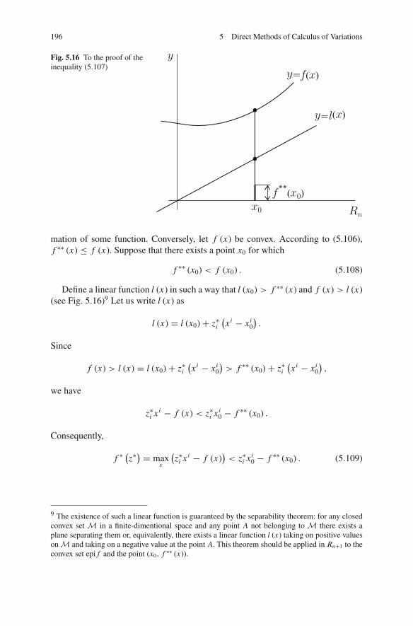
196 5 Direct Methods of Calculus of Variations
Fig. 5.16 To the proof of theinequality (5.107)
mation of some function. Conversely, let f (x) be convex. According to (5.106),f ∗∗ (x) ≤ f (x). Suppose that there exists a point x0 for which
f ∗∗ (x0) < f (x0) . (5.108)
Define a linear function l (x) in such a way that l (x0) > f ∗∗ (x) and f (x) > l (x)(see Fig. 5.16)9 Let us write l (x) as
l (x) = l (x0)+ z∗i(xi − xi
0
).
Since
f (x) > l (x) = l (x0)+ z∗i(xi − xi
0
)> f ∗∗ (x0)+ z∗i
(xi − xi
0
),
we have
z∗i x i − f (x) < z∗i x i0 − f ∗∗ (x0) .
Consequently,
f ∗(z∗) = max
x
(z∗i x i − f (x)
)< z∗i x i
0 − f ∗∗ (x0) . (5.109)
9 The existence of such a linear function is guaranteed by the separability theorem: for any closedconvex set M in a finite-dimentional space and any point A not belonging to M there exists aplane separating them or, equivalently, there exists a linear function l (x) taking on positive valueson M and taking on a negative value at the point A. This theorem should be applied in Rn+1 to theconvex set epi f and the point (x0, f ∗∗ (x)).

5.7 Legendre and Young-Fenchel Transformations 197
Fig. 5.17 DoubleYoung-Fencheltransformation, f ∗∗(x), of anon-convex function f (x)
The inequality (5.109) contradicts the Young-Fenchel inequality for the functionsf ∗ and f ∗∗:
x∗i x i ≤ f ∗(x∗)+ f ∗∗ (x) .
Therefore, the initial assumption (5.108) is false and f ∗∗ (x) = f (x) for all x .For an arbitrary (not necessarily convex) function f (x), the function f ∗∗ (x) is themaximum convex function which is not greater than f (x).
The maximum convex function can be found as follows: consider the epigraph,epi f, of the function f (Fig. 5.17, the epigraph is shaded), and construct the smallestpossible convex set in the (y, Rn)-space containing epi f ; it will be the epigraph ofthe maximum convex function not greater than f . This set is obtained by “fillingout” of all the concave regions of the epigraph of the function f (x). This set is theepigraph of the function f ∗∗ (x) .
The proof will be given again only for a continuous function, f (x). Denote themaximum convex function not greater than f by f (x). Let us show that f ∗ = f ∗.Let us fix an arbitrary point x∗. Since f (x) ≤ f (x), we have f ∗ (x∗) ≥ f ∗ (x∗).Consequently, if f ∗ (x∗) = +∞, then f ∗ (x∗) = +∞ and f ∗ (x∗) = f ∗ (x∗) . Nowlet the value of the function f ∗ at a point x∗ be finite. By definition,
− f ∗(x∗) = min
x
(f (x)− x∗i x i
).
Denote the point at which the minimum is reached10 by x0. Then
− f ∗(x∗) = f (x0)− x∗i x i
0. (5.110)
10 There can be many such points.

198 5 Direct Methods of Calculus of Variations
It follows from the Young-Fenchel inequality, x∗i x i − f ∗ (x∗) ≤ f (x) , and(5.110) that
x∗i(xi − xi
0
)+ f (x0) ≤ f (x) . (5.111)
We wish to show that f (x0) = f (x0). Suppose the contrary,
f (x0) < f (x0) (5.112)
According to (5.112), the value of the function f (x) at x0 is less than the valueof the function x∗i
(xi − xi
0
) + f (x0) at this point. Therefore, there exists a regionD in which f (x) < x∗i
(xi − xi
0
) + f (x0) , and outside of this region f (x) ≥x∗i(xi − xi
0
)+ f (x0). Define a convex function
˜f (x) ={
x∗i (xi − xi0)+ f (x0), xεD
f (x), x εD
Inequality (5.111) and the inequality f (x) ≤ f (x) imply that ˜f (x) ≤ f (x).Moreover, f (x) < ˜f (x) on D. This contradicts the fact that f is the maximumconvex function not greater than f . The proof that the graph of the function f (x)cannot be below the line y = x∗i
(xi − xi
0
)+ f (x0) is analogous.Since
− f ∗ = minx
(f (x)− x∗i x i
) ≥ minx
(x∗i(xi − xi
0
)+ f (x0)− x∗i x i)
= f (x0)− x∗i x i = − f ∗(x∗),
and
− f ∗ = minx
(f (x)− x∗i x i
) ≤ minx
(f (x)− x∗i x i
) = − f ∗(x∗)
we have
f ∗(x∗) = f ∗
(x∗)
Applying the Young-Fenchel transformation to this equality, we get f ∗∗ = f =f ∗∗, which completes the proof.
Example 9. Consider a mixture of liquid and its vapor bubbles. The liquid and thevapor are two states of the same matter. This matter is characterized by the freeenergy F (ϑ, T ), which is non-convex with respect to ϑ , or by the correspondingfunction p (ϑ, T ), which is shown in Fig. 5.18a for a fixed value of T . The mixturecan also be modeled by a continuum. Thus the macro-continuum could be in threestates, pure liquid, pure vapor or a mixture of liquid with vapor bubbles. For suchmacro-continuum, Maxwell proposed the following rule for determining the depen-dence of the pressure on the specific volume: on the graph of the “true” dependence

5.7 Legendre and Young-Fenchel Transformations 199
Fig. 5.18 The Maxwell rule
of p on ϑ , Fig. 5.18a, a straight line AB should be drawn in such a way, that theshaded areas ACO and ODB are equal; then, the graph p (ϑ, T ) for the mixtureconsists of three branches EA, AB and B F (Fig. 5.18b). They correspond to pureliquid, mixture of liquid with vapor bubbles and vapor bubbles, respectively.
Let us show that the Maxwell rule is equivalent to the following statement: thefree energy of the mixture is equal to F∗∗ (ϑ, T ).
The function F (ϑ, T ) is shown qualitatively in Fig. 5.19. The function F∗∗ (ϑ, T )coincides with F (ϑ, T ) for ϑ < a and ϑ > b; for a ≤ ϑ ≤ b, it is linear. Due to thesmoothness of F (ϑ, T ), the line AB is tangent to the graph of the function F (ϑ, T ).Therefore,
�F
�ϑ
∣∣∣∣ϑ=a
= �F
�ϑ
∣∣∣∣ϑ=b
.
Fig. 5.19 The Maxwell rulein terms of theYoung-Fencheltransformation

200 5 Direct Methods of Calculus of Variations
The figure shows that
F (b, T )− F (a, T ) = �F
�ϑ
∣∣∣∣ϑ=a
(b − a) .
Besides,
F (b, T )− F (a, T ) =b∫
a
�F
�ϑdϑ.
Since p = −�F/�ϑ , we have
b∫
a
pdϑ = p|ϑ=a (b − a) . (5.113)
The integral in (5.113) represents the area under the curve p (ϑ, T ) on the seg-ment [a, b] and p|ϑ=a (b − a) represents the area of the rectangle with its top sidebeing AB. Therefore, (5.113) is equivalent to the Maxwell rule.
The Young-Fenchel transformation allows one to present the convex functionf (x) as
f (x) = maxx∗
(x∗i x i − f ∗
(x∗))
. (5.114)
If f (x) is non-convex, then the Young-Fenchel transformation provides the best lowestimate of f (x) in terms of a convex function
f (x) ≥ f ∗∗ (x) = maxx∗
(xi x∗i − f ∗
(x∗))
. (5.115)
Let the variables y = (y1, . . . , ym) be the parameters of function f , f = f (x, y).Then its Young-Fenchel transformation with respect to x will also depend on param-eters, y: f ∗ = f ∗ (x∗, y). What can be said about the dependence of f ∗ on y?If the function f = f (x, y) is linear with respect to y, then the Young-Fencheltransformation of this function with respect to x is a convex function of y.
This statement follows from a chain of inequalities:
f ∗(x∗, αy1 + (1− α) y2
) = maxxi
[x∗i x i − f (x, αy1 + (1− α) y2)
] == max
xi
[x∗i x i − α f (x, y1)− (1− α) f (x, y2)
] == max
xi
[α(x∗i x i − f (x, y1)
)+ (1− α)(x∗i x i − f (x, y2)
)] ≤≤ α f ∗
(x∗, y1
)+ (1− α) f ∗(x∗, y2
),
as claimed.

5.8 Examples of Dual Variational Principles 201
This almost obvious property of the Young-Fenchel transformation implies somenon-trivial consequences.
Example 10. Let us show that for positive matrices, the diagonal components of theinverse matrix are convex functions of the original matrix components. Consider apositive quadratic form f = 1
2 ai j x i x j . Then f ∗ (x∗) = 12 a(−1)i j x∗i x∗j where a(−1)i j
are the components of the inverse matrix. Function f depends linearly on the pa-rameters ai j . As it has been established, f ∗ is a convex function of ai j . Let us setx∗1 = 1, x∗2 = 0, . . . , x∗n = 0. Then, 2 f ∗ = a(−1)11 is a convex function of ai j .Similarly, a(−1)22, . . . , a(−1)nn , as well as all linear combinations of a(−1)i j whichare obtained by choosing various x∗i , are convex functions of ai j .
Our next topic is the construction of the dual variational problems by means ofYoung-Fenchel transformations.
5.8 Examples of Dual Variational Principles
The Dirichlet and von Neuman problems. Consider the minimization problemfor the so-called Dirichlet functional,
E (u) =∫
�
1
2
[(�u
�x
)2
+(
�u
�y
)2]
dxdy, (5.116)
on the set of all functions of two variables u (x, y) defined on some two-dimensionalregion � with piece-wise smooth boundary �� and taking on the assigned values atthe boundary:
u (x, y)|�� = g (s) . (5.117)
Here g (s) is a continuous function of the arc length, s, along ��. The minimizingelement of the variational problem (5.116), (5.117) is the solution of the Dirichletproblem
�2u
�x2+ �2u
�y2= 0 in �, u|�� = g (s) . (5.118)
We are going to construct a dual variational problem. Let us write the integrandin the Dirichlet functional in the form
1
2
[(�u
�x
)2
+(
�u
�y
)2]= max
px ,py
[px
�u
�x+ py
�u
�y− 1
2
(p2
x + p2y
)].
Using this relation we can rewrite the initial variational problem as a minimaxproblem:

202 5 Direct Methods of Calculus of Variations
min E (u) = minu∈(5.117)
∫
�
maxpx ,py
[px
�u
�x+ py
�u
�y− 1
2
(p2
x + p2y
)]dxdy.
Recall that the notation u ∈(5.117) means that u satisfies the constraint (5.117).In the integral, maximum over px and py is taken at each point (x, y). The max-
imum can be moved outside the integral, if we perform maximization over arbitraryfunctions of two variables, px (x, y) and py(x, y) :
min E (u) = minu∈(5.117)
maxpx (x,y),py (x,y)
∫
�
[px
�u
�x+ py
�u
�y− 1
2
(p2
x + p2y
)]dxdy.
(5.119)
Further, for brevity, we use for this maximum the notation maxpx ,py
,implying that this is
maximization over the functions px (x, y) and py(x, y).Let us change the order of maximization and minimization in (5.119). According
to the inequality (5.81),
maxpx ,py
minu∈(5.117)
∫
�
[px
�u
�x+ py
�u
�y− 1
2
(p2
x + p2y
)]dxdy ≤ min
u∈(5.117)E (u) . (5.120)
The minimum value in the left hand side of (5.120) can be found explicitly. Sup-pose that the functions px , py are continuously differentiable and continuous on theclosed region �. Integrating by parts (5.120), we obtain
∫
�
[px
�u
�x+ py
�u
�y− 1
2
(p2
x + p2y
)]dxdy (5.121)
=∫
��
(px nx+pyny)uds−∫
�
(�px
�x+ �py
�y
)udxdy−
∫
�
1
2
(p2
x + p2y
)dxdy.
Here, nx , ny are the components of the outward unit normal vector on �� (Fig. 5.20).Note that function u in the first integral in the right hand side of (5.121) can bereplaced by g(s) according to the boundary condition (5.117).
For the integrals in the right hand side of (5.121), we will use the notations
E∗ (p) =∫
�
1
2
(p2
x + p2y
)dxdy
and
� (u, p) = −∫
�
(�px
�x+ �py
�y
)udxdy+ l (p) ,
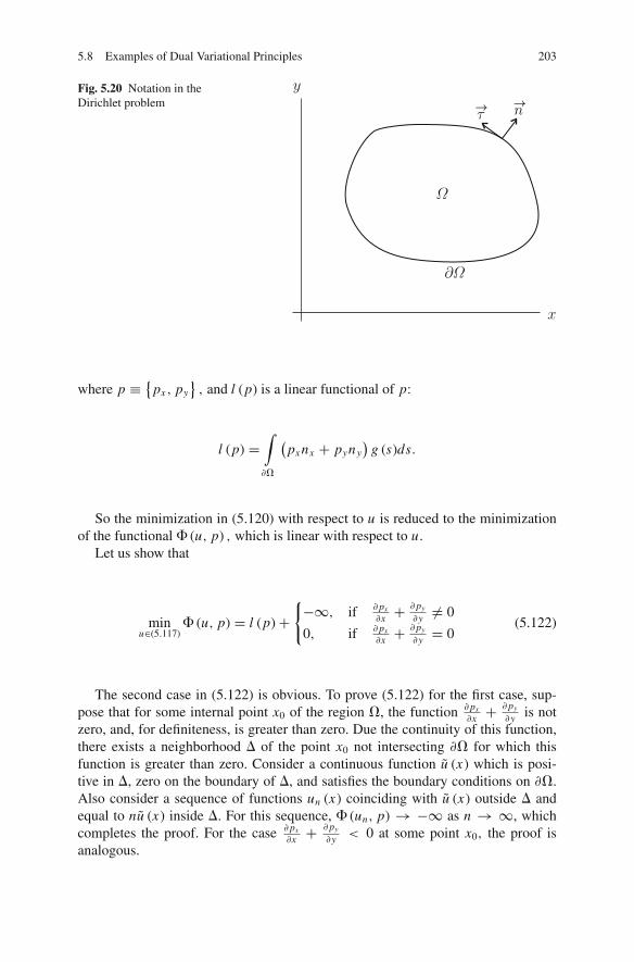
5.8 Examples of Dual Variational Principles 203
Fig. 5.20 Notation in theDirichlet problem
where p ≡ {px , py
}, and l (p) is a linear functional of p:
l (p) =∫
��
(px nx + pyny
)g (s)ds.
So the minimization in (5.120) with respect to u is reduced to the minimizationof the functional � (u, p) , which is linear with respect to u.
Let us show that
minu∈(5.117)
� (u, p) = l (p)+{−∞, if �px
�x +�py
�y �= 0
0, if �px
�x +�py
�y = 0(5.122)
The second case in (5.122) is obvious. To prove (5.122) for the first case, sup-pose that for some internal point x0 of the region �, the function �px
�x +�py
�y is notzero, and, for definiteness, is greater than zero. Due the continuity of this function,there exists a neighborhood � of the point x0 not intersecting �� for which thisfunction is greater than zero. Consider a continuous function u (x) which is posi-tive in �, zero on the boundary of �, and satisfies the boundary conditions on ��.Also consider a sequence of functions un (x) coinciding with u (x) outside � andequal to nu (x) inside �. For this sequence, � (un, p) → −∞ as n → ∞, whichcompletes the proof. For the case �px
�x +�py
�y < 0 at some point x0, the proof isanalogous.

204 5 Direct Methods of Calculus of Variations
From (5.121) and (5.122), we get
minu∈(5.117)
∫
�
[px
�u
�x+ py
�u
�y− 1
2
(p2
x + p2y
)]dxdy =
=⎧⎨⎩
l (p)− E∗ (p) , if �px
�x +�py
�y = 0
−∞, if �px
�x +�py
�y �= 0
After finding the minimum in (5.120), the maximum is to be found. Therefore,all values of px , py for which the minimum is equal to−∞ should be excluded. So,
maxp
(l(p)− E∗ (p)
) ≤ E, (5.123)
where the maximum is calculated over all functions px , py satisfying the conditions
�px
�x+ �py
�y= 0 in �. (5.124)
Let us show that, actually, there is the equality sign in (5.123):
maxp
(l(p)− E∗ (p)
) = E .
To this end, consider the functions
px = �u
�x, py = �u
�y, (5.125)
where u is the solution of the boundary value problem (5.118).11 Due to the firstequation (5.118), the functions (5.125) satisfy the constraint (5.124) and, hence, arethe admissible functions. Therefore,
l ( p)− E∗ ( p) ≤ maxp
(l(p)− E∗ (p)
)
and, according to (5.123),
l ( p)− E∗ ( p) ≤ maxp
(l(p)− E∗ (p)
) ≤ E = E (u) . (5.126)
The numbers l ( p)− E∗ ( p) and E (u) are equal:
11 We are assuming that u is a smooth function and, in particular, the derivatives (5.125) are de-fined. This assumption makes the proof of the coincidence of the maximum value of l (p)− E∗ (p)and the minimum value of E (u) almost trivial; a complete proof requires a more sophisticatedtechnique.

5.8 Examples of Dual Variational Principles 205
l ( p)− E∗ ( p) =∫
��
(px nx+ pyny
)uds − 1
2
∫
�
(p2
x+ p2y
)dxdy
=∫
�
[� ( px u)
�x+�( py u)
�y
]dxdy − 1
2
∫
�
(p2
x+ p2y
)dxdy
= 1
2
∫
�
[(�u
�x
)2
+(
�u
�y
)2]
dxdy = E (u) .
Here we transformed the integral over �� into an integral over � by means of thedivergence theorem and used (5.124).
Since l ( p)− E∗ ( p) = E (u), (5.126) implies that
l ( p)− E∗ ( p) = maxp
(l(p)− E∗ (p)
) = E (u) .
Hence, the order of maximization and minimization in (5.119) can indeed bechanged, and we obtain the dual variational problem:
E = maxpε(5.124)
(l(p)− E∗(p)).
The dual variational problem can be presented in a different form if we note thatthe general solution of (5.124) can be easily written:
px = �ψ
�y, py = −�ψ
�x. (5.127)
Here ψ (x, y) is an arbitrary function. In a simply connected region, ψ (x, y) mustbe single-valued; in a multiply connected region it might be multi-valued. For now,we will only consider simply connected regions �.
To write down the linear functional l(p) in terms of function ψ , we note that thetangent vector to ��, →τ , has the components
τx = −ny, τy = nx . (5.128)
We choose the arc length increasing counter-clockwise; therefore
τx = dx (s)
ds, τy = dy (s)
ds(5.129)
where x = x (s) , y = y (s) are the parametric equations of ��. Hence, we have
px nx + pyny = �ψ
�yτy + �ψ
�xτx = �ψ
�x
dx
ds+ �ψ
�y
dy
ds= dψ
ds. (5.130)

206 5 Direct Methods of Calculus of Variations
The linear functional, l (p) , becomes a functional of ψ :
l (ψ) =∫
dψ
dsg(s)ds.
Finally, the dual variational problem is the maximization problem for the func-tional
J (ψ) = l (ψ)− E∗ (ψ) =∫
��
dψ
dsgds−
∫
�
1
2
((�ψ
�x
)2
+(
�ψ
�y
)2)
dxdy (5.131)
on the set of all functions ψ .The duality means that
maxψ
J (ψ) = minu∈(5.117)
E (u) .
The functional J (ψ) can be put in a slightly different form by integrating by partsin the first integral in (5.131):
J (ψ) = −∫
��
ψdg
dsds −
∫
�
1
2
((�ψ
�x
)2
+(
�ψ
�y
)2)
dxdy.
The maximizing element of the dual variational problem is the solution of thevon Neuman problem
�ψ = 0,dψ
dn= −dg
ds.
The functional J (ψ) is invariant with respect to shifts of the function ψ for aconstant because function g (s) is continuous. For the same reason the necessarycondition for the solvability of this problem,
∫
��
�ψ
�nds = 0,
is satisfied.One can say that the von Neuman problem is dual to the Dirichlet problem.Discontinuity conditions. Solutions of the Dirichlet problem (5.118) are smooth,
if �� and g(s) are smooth. Therefore, in the dual variational problem the trial fields,px and py, can be assumed smooth. However, for more complex energy functionals,like, for example, the functional of a heterogeneous medium,

5.8 Examples of Dual Variational Principles 207
E(u) =∫
�
1
2a(x, y)
[(�u
�x
)2
+(
�u
�y
)2]
dxdy,
with the material characteristics, a(x, y), that is discontinuous on some line, �, theminimizer may be non-smooth. If the functional is minimized on the set of func-tions, u(x, y), which are continuous on � but may have discontinuous derivatives on�, then the variation of the functional gets a contribution,
∫
�
([a
�u
�x
]nx +
[a
�u
�y
]ny
)δu ds,
where [ϕ] denotes the jump of a function, ϕ, on �,
[ϕ] = ϕ+ − ϕ−,
and indices ± mark the limit values of ϕ on two sides of �; nx , ny are the compo-nents of the unit normal vector on � directed from the side − to the side +. Hence,the minimizer should obey the additional condition,
[a
�u
�x
]nx +
[a
�u
�y
]ny = 0 on �.
In the dual variational principle, one should admit the discontinuous trial func-tions, px and py . Therefore, integrating by parts in (5.121), one obtains the addi-tional term
∫
�
([px ] nx +
[py]
ny)
ud s.
Accordingly, the trial discontinuous functions in the dual variational principle,px and py, must obey the condition
[px ] nx +[
py]
ny = 0 on �. (5.132)
The Dirichlet and Thompson principles
Let V be a region in three-dimensional space which is an exterior of some boundedregion with the boundary � (Fig. 5.21). For a smooth function, u(x), the Dirichletfunctional, E (u) , is defined as
E (u) = 1
2
∫
V
u,i u,i dV .
For the Dirichlet functional, consider a minimization problem on the set of func-tions, u
(xi), selected by the conditions

208 5 Direct Methods of Calculus of Variations
Fig. 5.21 Notation for theDirichlet and Thompsonprinciples
u = 1 on �,
u ∼ c1
r+ c2
r2+ . . . as r →∞, r2 = xi x
i . (5.133)
The quantity
1
2πmin
u∈(5.133)E (u) ,
has the physical meaning of the electric capacity of the surface �. The formulatedvariational principle for the electric capacity is called the Dirichlet principle. Theminimizing function u (x) satisfies the Laplace equation in the region V ,
�u = 0 in V, (5.134)
and the boundary conditions (5.133).Note that the condition at infinity, u → 0 as r → ∞, is essential: without
this condition the minimizing function would be just u ≡ 1, and E(u) = 0. Thefunctional E(u) feels the condition at infinity, as can be seen from the followingreasoning. Denote the spherical coordinates in region V by r, ϕ, θ ; r ≥ R(ϕ, θ ),r = R(ϕ, θ ) being the parametric equation of the surface �. Suppose u(r, ϕ, θ )tends to some limit value, u∞, as r →∞.
Then, for each ray ϕ = const, θ = const,
u∞ − u|r=R(ϕ,θ) = u∞ − 1 =∞∫
R
u,r dr =∞∫
R
ru,r1
rdr.
Applying the Cauchy inequality (5.20) to the latter integral, we get
(u∞ − 1)2 ≤∞∫
R
r2u2r dr
∞∫
R
dr
r2= 1
R
∞∫
R
r2u2,r dr.

5.8 Examples of Dual Variational Principles 209
Since in spherical coordinates
(∇u)2 = u2,r +
1
r2u2
,θ +1
r2 sin2 θu2
,ϕ,
we have
u2,r ≤ (∇u)2.
Therefore,
(u∞ − 1)2 ≤ 1
Rmin
∞∫
R
r2∇u2dr (5.135)
where Rmin is the minimum distance from � to the origin. Integrating (5.135) overϕ and θ with the weight of the spherical coordinates, sin θ, we obtain
4π (u∞ − 1)2 ≤ 1
Rmin2E(u).
Hence, the change of u∞ affects the minimum value of the functional.In the case when u(r, ϕ, θ ) tends to different values, u∞(ϕ, θ ), along different
rays, the inequality (5.135) is replaced by the inequality
2π∫
0
π∫
0
(u∞(ϕ, θ )− 1)2 sin θ dϕdθ ≤ 1
Rmin2E(u).
We see that energy feels the limit values of u at infinity for each ray.The electric capacity of surface � corresponds to u∞ = 0.
Let us find the variational principle dual to the Dirichlet principle. Writing theintegrand in the Dirichlet functional in the form
1
2u,i u
,i = maxp
(pi u,i − 1
2pi pi
),
we present the initial variational problem as a minimax problem:
E = minu∈((5.133))
1
2
∫
V
u,i u,i dV = min
u∈((5.133))max
p
∫
V
(pi u,i − 1
2pi pi
)dV . (5.136)
Following the general scheme, we change the order of calculating the maximum andminimum values and calculate the minimum with respect to u.

210 5 Direct Methods of Calculus of Variations
Suppose the functions pi are continuously differentiable and continuous on theclosed region V and tend to zero as r →∞. Suppose also that pi can be expandedin Taylor series with respect to 1/r as
p ∼ a2
r2+ a3
r3+ . . . for r →∞. (5.137)
For a slower decay, the integral of pi pi in (5.136) would diverge.Integrating by parts, and using (5.133) and (5.137), for the integral in (5.136) we
obtain
∫
V
(pi u,i − 1
2pi pi
)dV = � (u, p)− E∗ (p) , (5.138)
E∗ (p) = 1
2
∫
V
pi pi dV, � (u, p) = l (p)− 1
2
∫
V
pi,i udV, l (p) =
∫
�
pi ni d A.
Minimization of the functional (5.138) with respect to u is reduced to minimizingthe linear functional � (u, p) . As in the previous example,
minu∈(5.133)
� (u, p) = l (p)+{−∞, if pi
,i �= 0
0, if pi,i = 0
. (5.139)
Combining (5.139) and (5.138), we have
minu∈(5.133)
∫
V
(pi u,i − 1
2pi pi
)dV =
{l (p)− E∗ (p) , if pi
,i = 0
−∞, if pi,i �= 0
.
Since we need to calculate the maximum value after calculating the minimumvalue with respect to u, all functions p for which min
uis equal to −∞ should be
dropped and only functions pi satisfying the equation
pi,i = 0 in V, (5.140)
should be retained.As in the previous example, one can check that the order of maximization and
minimization in the minimax problem (5.136) can be changed and we arrive at thefollowing dual variational problem:
E = maxpε(5.140)(5.137)
(l(p)− E∗ (p)
). (5.141)
5.8 Examples of Dual Variational Principles 211
So the dual variational problem is the maximization problem for the functionall (p) − E∗ (p) over all vector field satisfying the “incompressibility” condition(5.140).
At first glance, the formulation of the dual variational problem is surprising: wehave seen that the quadratic functional of the form
b∫
a
u2dx
does not feel the values of the function u(x) at the boundary (and, in fact, at anyfixed point of the segment [ab]). Similarly, the functional
∫
V
pi pi dV
should not feel the values of pi at �V and, thus, the values of the linear functional,l(p) = ∫
�
pi ni d A. The resolution of this “paradox” is in the constraints (5.140) and
(5.137): the admissible functions pi (x) are not arbitrary. Due to these constraints,the linear functional l(p) can be presented as
l(p) =∫
V
pi g,i dV
with some smooth function g, which is equal to unity at �� and decays at infinityas 1/r.
Therefore,
|l(p)|2 ≤∫
V
pi pi dV∫
V
g,i g,i dV ≤ const E(p),
i.e. energy does feel the values of the functional l(p).According to (5.141) and (5.50), the dual variational problem can also be stated
as the maximization problem of the functional
[l(p)]2
4E∗ (p).
The variational principle
maxp∈(5.140)
(5.137)
[l(p)]2
4E∗ (p)= E
is called the Thompson principle.

212 5 Direct Methods of Calculus of Variations
The case of general integral functional. Consider the functional I (u) of the formI (u) = E (u)− l (u)
E (u) =∫
V
L(xi , uκ, uκ
,i
)dV, uκ
,i ≡�uκ
�xi
l (u) =∫
V
gκuκdV +∫
�V f
fκuκd A, (5.142)
where uκ are smooth functions of the variables x1, . . . , xn , in a closed boundedregion V in Rn , �V f is a part of the boundary �V of the region V , and gκ andfκ are given functions in V and on �V f . The energy density L is a strictly convexfunction of the variables uκ and uκ
,i .The original minimization problem is to find the minimum of the functional I (u)
on the set of all functions uκ which take on the assigned values on the surface�Vu = �V − �V f :
uκ = uκ
(b) on �Vu . (5.143)
To construct the dual variational problem, we present L(xi , uκ, uκ
i
)using the
Young-Fenchel transformation as
L(xi , uκ, uκ
,i
) = maxp
(pκuκ+pi
κuκ
,i−L∗(xi , pκ, pi
κ
)). (5.144)
Here maximization is done over all p = {pκ, pi
κ
}, and L∗
(xi , pκ, pi
κ
)is the
Young-Fenchel transformation of the function L(xi , uκ, uκ
,i
)with respect to the
variables uκ and uκ
,i :
L∗(xi , pκ, pi
κ
) = maxuκ ,uκ
,i
(pκuκ+pi
κuκ
,i−L(xi , uκ, uκ
,i
)).
Rewriting the initial variational problem as a minimax problem by means of(5.144), we have
I = minu∈(5.143)
maxp
⎡⎣∫
V
(pκuκ+pi
κuκ
,i − L∗(xi , pκ, pi
κ
))dV − l (u)
⎤⎦ . (5.145)
Reversing the order of maximization and minimization in (5.145) yields the relation,
maxp
minu∈(5.143)
(� (u, p)− E∗ (p)
) ≤ I . (5.146)

5.8 Examples of Dual Variational Principles 213
Here,
� (u, p) =∫
V
(pκuκ + pi
κuκ
,i − gκuκ
)dV −
∫
�V f
fκuκd A,
E∗ (p) =∫
V
L∗(xi , pκ, pi
κ
)dV . (5.147)
Let us present uκ as a sum of some fixed smooth function hκ , taking on thevalues uκ
(b) on �Vu , and the function u′κ , which is equal to zero on �Vu :
uκ = hκ + u′κ, u′κ = 0 on �Vu . (5.148)
Then, � (u, p) can be written as
� (u, p) = l (p)+�(u′, p
),
where l (p) is a linear functional on the set of functions p defined by the equation
l (p) = � (h, p) .
Calculation of minu
in (5.146) is reduced to calculation of minu′
�(u′, p
):
minu∈(5.143)
� (u, p) = minu′∈(5.148)
(l (p)+�
(u′, p
)) == l (p)+ min
u′∈(5.148)�(u′, p
).
Since � (u, p) is linear with respect to u,
minu′∈(5.148)
�(u′, p
) = 0,
if for any u′
�(u′, p
) = 0, (5.149)
and
minu′∈(5.148)
�(u′, p
) = −∞ (5.150)
if �(u′, p
) �= 0 for at least one element u′. This can be proved in the same wayas (5.122). Since we need to find the maximum over p, we have to exclude fromconsideration all functions p for which min
uis equal to −∞. As a result, we arrive

214 5 Direct Methods of Calculus of Variations
at the maximization problem for the functional l (p)− E∗ (p) on the set of all func-tions p which satisfy the constraint (5.149). Due to (5.149), the values of the linearfunctional l (p) do not depend on the specific choice of functions hκ .
If pκ and piκ
are differentiable and continuous functions in the region V , thenthe constraint (5.149) is reduced to
pκ = �piκ
�xi+ gκ in V, pi
κni = fκ on �V f , (5.151)
and the functional l (p) is
l (p) =∫
�Vu
piκ
ni uκ
(b)d A. (5.152)
Equation (5.146) takes the form,
maxp∈(5.151)
(l(p)− E∗ (p)
) ≤ I . (5.153)
Suppose that the functions uκ
(xi)
which minimize the functional I (u) are twicecontinuously differentiable. Then, we are going to show that
maxp∈(5.151)
(l(p)− E∗ (p)
) = I . (5.154)
Define
pκ = �L
�uκ
∣∣∣∣uκ=uκ
, piκ= �L
�uκ
i
∣∣∣∣uκ=uκ
.
The Euler equations of the initial variational problem,
�L
�uκ
= �
�xi
�L
�uκ
i
+ Fκ in V,�L
�uκ
ni = fκ in �V,
imply that the functions pκ and piκ
satisfy the constraints (5.151) and, consequently,are the admissible functions. Therefore,
l ( p)− E∗ ( p) ≤ maxp∈(5.151)
(L(p)− E (p)) . (5.155)
On the other hand,
l ( p)− E∗ ( p) = I .
Indeed,

5.8 Examples of Dual Variational Principles 215
l ( p)− E∗ ( p) =∫
�Vu
piκ
ni uκ
(b)d A −∫
V
L∗(xi , pκ, pi
κ
)dV =
=∫
V
[�(
piκ
uκ
)
�xi− L∗
(xi , pκ, pi
κ
)]
dV −∫
�V f
piκ
ni uκd A =
=∫
V
[� pi
κ
�xiuκ+ pi
κuκ
,i−(
pκ uκ+ piκ
uκ
,i−L(xi ,uκ,uκ
,i
))]dV−
−∫
�V f
fκ uκd A =∫
V
L(xi ,uκ,uκ
,i
)dV −
∫
V
gκ uκdV −∫
�V f
fκ uκd A = I . (5.156)
Therefore (5.154) holds true.So, the maximization problem for the functional l (p) − E∗(p) on the set of
functions (5.151) is dual to the initial variational problem.Consider the specific case, when L does not depend on uκ . Denote by L∗
(xi , pi
κ
)the Young-Fenchel transformation of the function L
(xi , uκ
,i
)with respect to uκ
,i :
L∗(xi , pi
κ
) = maxu
(pi
κuκ
,i − L(xi , uκ
,i
)).
Function L∗(xi , pκ, pi
κ
)introduced in the beginning of this section is linked to
L∗(xi , pi
κ
)as
L∗(xi , pκ, pi
κ
) = maxu
(pκuκ + pi
κuκ
,i − L(xi , uκ
i
)) =
={
L∗(xi , pi
κ
)for pκ = 0
+∞ for pκ �= 0
If L∗(xi , pκ, pi
κ
) = +∞, then l (p) − E∗ (p) is equal to −∞. So in the dualvariational problem all non-zero functions pκ should be excluded from the set ofadmissible functions. For pκ = 0, (5.151) becomes
�piκ
�xi+ gκ = 0 in V, pi
κni = fκ on �V f . (5.157)
The dual variational principle (5.154) will be considered further for a number ofcontinuum models.
The Legendre and Young-Fenchel transformation can be used for constructingthe “dual” variational problems even in the cases when the functional is not convex.An example is the Hamilton variational principle in the phase space (Sect. 1.6).

216 5 Direct Methods of Calculus of Variations
Lower estimates of non-convex functionals by means of the dual problem. Con-sider the minimization problem for the integral functional of the form (5.142) on theset of functions (5.143). Let L
(xi , uκ, uκ
,i
)be a non-convex function of uκ and uκ
,i .Let us calculate L∗∗
(xi , uκ, uκ
,i
)– the second Young-Fenchel transformation of the
function L(xi , uκ, uκ
,i
)with respect to uκ, uκ
,i . We know that
L∗∗(xi , uκ, uκ
,i
) ≤ L(xi , uκ, uκ
,i
). (5.158)
Therefore, for all fields uκ ,
I ∗∗ (u) =∫
V
L∗∗dV − l (u) ≤∫
V
LdV − l (u) = I (u) .
Consequently,
I ∗∗ ≤ I . (5.159)
Since the functional I ∗∗ (u) is convex,
maxp
⎛⎝l (p)−
∫
V
L∗(xi , pκ, pi
κ
)dV
⎞⎠ = I ∗∗. (5.160)
Computing the functional in (5.160) on the admissible elements p, one obtainsthe lower estimates of I ∗∗ and, therefore, I . For some problems with non-convexfunctionals I ∗∗ coincides with I (see [95]).
5.9 Hashin-Strikman Variational Principle
Linear case. As we have seen in Sect. 5.8, the trial fields of the dual variationalproblems must obey some differential constraints and, possibly, the discontinuityconditions. While the differential constraints can be easily resolved, the disconti-nuity conditions are not so easy to deal with if the geometry of discontinuities iscomplex. Hashin and Strikman suggested a trick, which allows one to overcomethis difficulty. They obtained a dual variational principle with the admissible fieldsthat must not obey the differential constraints. We explain the trick first for a simplecase of the variational problem
E(u) =∫
V
1
2ai j (x)
�u
�xi
�u
�x jdV → min
u, (5.161)

5.9 Hashin-Strikman Variational Principle 217
where ai j (x) may have discontinuities on surfaces with a complex geometry, and theminimum is sought over all functions, u(x), with the prescribed boundary values,
u = u(b) on �V . (5.162)
Further we consider more general cases.Let us rewrite E(u) by adding and deducting the quadratic functional
∫
V
1
2a0
�u
�xi
�u
�xidV,
where ao is a constant. We have
E(u) =∫
V
1
2a0(x)
�u
�xi
�u
�xidV +
∫
V
1
2
(ai j − a0δ
i j) �u
�xi
�u
�x jdV .
Let us choose ao in such a way that the quadratic form
1
2
(ai j − a0δ
i j)
u,i u, j ,
(u,i ≡ �u
�xi
)
be positive definite. Then it can be presented as the Young-Fenchel transformationof the dual quadratic form
1
2
(ai j − a0δ
i j)
u,i u, j = maxpi
[pi u,i − 1
2bi j pi p j
], (5.163)
where bi j is the inverse tensor to ai j − a0δi j ,
(ai j − a0δ
i j)
b jk = δik, (5.164)
and the quadratic form, bi j pi p j , is positive definite. Hence, E(u) is the maximumvalue in the variational problem
E(u) = maxpi (x)
∫
V
[1
2a0u,i u
,i + pi (x)u,i − 1
2bi j (x)pi (x)p j (x)
]dV . (5.165)
The original variational problem takes the form
minu=u(b) at �V
maxpi (x)
∫
V
[1
2a0u,i u
,i + pi (x)u,i − 1
2bi j (x)pi (x)p j (x)
]dV .

218 5 Direct Methods of Calculus of Variations
The order of minimization and maximization can be changed (we do not pauseto prove that; it can be done in the same way as for Dirichlet and Neuman problemsin Sect. 5.8). We arrive at the relation
minu=u(b) at �V
E(u) = maxpi (x)
[J (p)−
∫
V
1
2bi j (x)pi (x)p j (x)dV
], (5.166)
where
J (p) = minu=u(b) at �V
∫
V
(1
2a0u,i u
,i + pi (x)u,i
)dV . (5.167)
So, we get a dual variational principle with the dual variables, pi (x), which arenot constrained. The cost is that the functional J (p) appears which is to be com-puted. Formula for J (p) can be simplified a bit. Denote by u(x) be the minimizer inthe variational problem,
minu=u(b) at �V
∫
V
1
2a0u,i u
,i dV . (5.168)
Let E0 be the minimum value in (5.168):
E0 = 1
2
∫
Va0u,i u
,i dV .
We set in (5.167)
u = u + u′,u′ = 0 on �V . (5.169)
Then
J (p) = E0 +∫
Vpi (x)u,i (x)dV + J (p),
J (p) ≡ minu′=0 at �V
∫
V
(1
2a0u′,i u
′,i + pi (x)u′,i
)dV (5.170)
The variational problem (5.170) is well-posed: the functional is obviouslybounded from below:
∫
V
(1
2a0u,i u
,i + pi u,i
)dV =
∫
V
1
2a0(u,i + pi
) (u,i + pi
)dV−
−∫
V
1
2a0 pi pi dV � −1
2a0
∫
Vpi pi dV . (5.171)

5.9 Hashin-Strikman Variational Principle 219
As we see from (5.171), it is enough for the boundedness from below that pi (x)be square integrable functions. In particular, they can be piece-wise continuous func-tions. We will further obtain the explicit dependence of J on pi (x). Irrespectivelyon the explicit form of J (p), we get.
Hashin-Strikman variational principle. The minimum value, E, of E(u) can befound by solving the variational problem
E = E0 +maxpi (x)
[∫
V
(pi (x)u,i (x)− 1
2bi j (x)pi (x)p j (x)
)dV +J (p)] . (5.172)
Here pi (x) do not obey any constraints.
Explicit form of J (p) for smooth p. Let us now find the dependence of J on pi (x).First, we assume that pi (x) are some smooth functions. Then the minimizer in u′
(5.170) obeys the boundary value problem,
a0�u′ = −�pi
�xi, u′ |�V = 0 (5.173)
Its solution can be written in terms of Green’s function, G(x, y), defined as thesolution of the boundary value problem
�x G(x, y) = −δ(x − y), G(x, y)|y∈�V= 0. (5.174)
Here δ(x) is the three-dimensional delta-function and �x Laplace’s operator actingon x-variables. We take for granted that the solution of this problem is symmetricwith respect to x, y,
G(x, y) = G(y, x), (5.175)
non-negative,
G(x, y) � 0,
and smooth everywhere except at the point x = y where it has the singularity of theform
G(x, y) = 1
4π |x − y| + bounded function as y → x .
Multiplying (5.174) by �pi/�yi and integrating over y, we obtain
�x
∫
VG(x, y)
�pi (y)
�yidVy = −
∫
Vδ(x − y)
�pi (y)
�yidV = −�pi (x)
�xi. (5.176)
Comparing (5.173) and (5.176) we see that

220 5 Direct Methods of Calculus of Variations
u′(x) = 1
a0
∫
VG(x, y)
�pi (y)
�yidVy . (5.177)
The singularity in (5.177) is integrable. To deal further with discontinuous func-tions, pi , we move the derivative from pi (y) to G(x, y) by integrating by parts.The singularity becomes stronger because �G(x, y)/�yi � 1/ |x − y|2 but is stillintegrable. To weaken the singularity of the integrand, before integrating by partsin (5.177), we replace pi (y) by pi (y) − pi (x). That, obviously, does not change(5.177). After integration by parts, we obtain
u′(x) = − 1
a0
∫
V
�G(x, y)
�yi
(pi (y)− pi (x)
)dVy . (5.178)
The differentiation of (5.178) with respect to xi yields an integral with absolutelyintegrable singularity; therefore the differentiation is possible and we obtain thederivatives of the minimizer 12:
�u′(x)
�xi= − 1
a0
∫
V
�2G(x, y)
�xi �y j
(p j (y)− p j (x)
)dVy. (5.179)
Finally, from Clapeyron’s theorem (5.47),
J (p) = 1
2
∫
Vpi (x)u′,i dV =
= − 1
2a0
∫
V
∫
Vpi (x)
�2G(x, y)
�xi �y j
(p j (y)− p j (x)
)dVx dVy . (5.180)
Formula (5.180) can also be written in a more symmetric form:
J (p) = 1
4a0
∫
V
∫
V
�2G(x, y)
�xi �y j
(pi (x)p j (x)+ pi (y)p j (y)− 2pi (x)p j (y)
)dVx dVy .
(5.181)Indeed, from (5.175):
�2G(x, y)
�xi �y j= �2G(y, x)
�y j �xi. (5.182)
12 The contribution to the derivative that is due to differentiation of pi (x),
1
a0
∫
V
�G(x, y)
�y j
�p j (x)
�xidVy,
is equal to1
a0
∫
�VG(x, y)n j d Ay
�p j (x)
�xi,
and is zero because G(x, y) = 0 when y ∈ �V .

5.9 Hashin-Strikman Variational Principle 221
Fig. 5.22 Notation for thevariational problem
Therefore, changing in (5.180) x by y, y by x, i by j and j by i, and taking intoaccount (5.182), we get
J (p) = − 1
2a0
�p j (y)
�2G(y, x)
�yi �x j
(pi (x)− pi (y)
)dVx dVy . (5.183)
Due to (5.182) the kernels in (5.180) and (5.183) coincide. Summing up (5.180) and(5.183) we obtain (5.181).
Explicit form of J (p) for discontinuous p. Let us show that (5.181) also holds forpiece-wise smooth functions that may have discontinuities on some surfaces. To thisend we need an auxiliary statement. Let S be a surface bounding some subregion,B, of V (Fig. 5.22). Consider a variational problem,
∫
V
1
2u,i u
,i dV −∫
SσudA→ min
u:u=0 at �V(5.184)
where σ is some function on S. The admissible functions, u, are supposed to becontinuous on S : [u] = 0. It is shown further in Example 11 of Sect.5.11 that theminimizer of this problem is
u(x) =∫
SG(x, y)σd A. (5.185)
Consider now the variational problem (5.170) for functions pi (x) that have adiscontinuity on S. The functional can be rewritten as
∫
V
1
2a0u,i u
,i dV −∫
V
�pi
�xiudV−
∫
S
[pi]
ni udA.
The minimizer, u, is the solution of the boundary value problem
a0�u = −�pi
�xiin V, u = 0 on �V, a0 [u,i ] ni = − [pi
]ni on S.
Here �pi/�xi is a piece-wise smooth function. The solution is a sum of two func-tions, u1 and u2, which are the solutions of the following boundary value problems:

222 5 Direct Methods of Calculus of Variations
a0�u1 = −�pi
�xiin V, u1 = 0 on �V,
[�u1
�xi
]ni = 0 on S,
a0�u2 = 0 in V, u2 = 0 on �V,
[�u2
�xini
]= − [pi
]ni on S.
The function of x ,
1
2a0
∫
VG(x, y)
�pi (y)
�yidVy,
has continuous first derivatives at S if �pi/�yi is piece-wise continuous.13 Thus,
u1(x) = 1
a0
∫
VG(x, y)
�pi (y)
�yidVy .
Function u2 is equal to the function (5.185) with the factor, 1/a0 and σ =[pi]
ni . So
u(x) = 1
a0
∫
VG(x, y)
�pi (y)
�yidVy + 1
a0
∫
SG(x, y)
[pi]
ni d A. (5.186)
Integrating by parts in the volume integral, we see that the surface terms cancelout:
u(x) = − 1
a0
∫
V
�G(x, y)
�yipi (y)dVy .
This formula can also be written as
u(x) = − 1
a0
∫
V
�G(x, y)
�yi
(pi (y)− pi (x)
)dVy,
because∫
V
�G(x, y)
�yidVy = 0,
due to the boundary condition, G(x, y) = 0 at �V .
The derivatives of the minimizer can be found by differentiating (5.186): for apoint, x, which is strictly inside B or V − B,
�u
�xi= 1
a0
∫
V
�G(x, y)
�xi
�p j (y)
�y jdVy + 1
a0
∫
S
�G(x, y)
�xi
[p j]
n j d A.
13 See, e.g., [81], vol. 2, p. 245.

5.9 Hashin-Strikman Variational Principle 223
Putting �(
pi (y)− p j (x))/�y j instead of �p j (y)/�y j and integrating by parts we
arrive at (5.179) for discontinuous pi . Hence, (5.181) also holds for discontinu-ous pi .
Minimum principle. One remark is now in order. If the parameter, a0, is so bigthat the quadratic form,
(ai j − a0δ
i j)
u,i u, j is negative definite, then we introducetensor bi j as the inverse tensor to a0δ
i j −ai j , and formula (5.163) is replaced by therelation
1
2
(ai j − a0δ
i j)
u,i u, j = minpi
[1
2bi j pi p j − pi u,i
].
Therefore,
E(u) = minpi (x)
∫
V
[1
2a0u,i u
, j − pi u,i + 1
2bi j pi p j
]dV,
and the Hashin-Strikman principle takes the following form.Hashin-Strikman variational principle. The minimum value, E, of E(u) can befound by solving the variational problem
E = E0 +minpi (x)
[∫
V
(−pi (x)u,i + 1
2bi j (x)pi (x)p j (x)
)dV + J (p)
].
Emphasize that the Hashin-Strikman variational principle holds for any value ofthe parameter, a0. If one makes estimates by plugging trial fields, then the estimatesinvolve a0, and an additional optimization of the estimates over a0 can be done.
Nonlinear case. This construction is easily extended to arbitrary convex functionals,
E(u) =∫
VL(x, u,i )dV,
in the cases when the function
(x, u,i ) = L(x, u,i )− 1
2a0u,i u
,i
is convex for some a0. Then (x, ui ) can be presented in terms of its Young-Fencheltransformation, ∗(x, pi ),
(x, u,i ) = maxpi
[pi u,i − ∗(x, pi )
],
and
E(u) = maxpi
∫
V
(1
2a0u,i u
,i + pi u,i − ∗(x, pi )
)dV .
From the same line of reasoning we obtain the following

224 5 Direct Methods of Calculus of Variations
Hashin-Strikman variational principle. If function, (x, u,i ), is strictly convex,then the variational problem
E = minu∈(5.162)
∫
VL(x, u,i )dV (5.187)
is equivalent to the variational problem
E = E0 +maxpi (x)
[∫
V
(pi u,i − ∗(x, pi )
)dV + J (p)
]
where E and u are the minimum value and the minimizer in the variational problem(5.168), and J(p) is the functional (5.181).
If (x, u,i ) is not convex, but the function
1(x, ui ) = 1
2a0u,i u
,i − L(x, ui )
is strictly convex, then
1
2a0u,i u
,i − L(x, ui ) = maxpi
[pi u,i − ∗(x, pi )
] = −minpi
[∗(x, pi )− pi u,i
],
and the original variational problem is equivalent to the variational problem
E = E0 +minpi
∫
V
(∗(x, pi (x))− pi (x)u,i
)dV + J (p).
Similar reasoning holds for functionals depending on many required functions.We will discuss this in the case of elastic bodies in Sect. 6.7.
For some functions, like, e.g., L = (aui ui
) 12 , neither L− 1
2 a0ui ui nor 12 a0ui ui−
L are convex. Therefore, the transformation of the variational problems to theHashin-Strikman form is not possible. For functions which vanish at some subregionof V like L = 1
2 a(x)ui ui with a(x) = 0 somewhere inside V , L− 12 a0ui ui is not con-
vex for all x , while 12 a0ui ui − L can be convex. In such cases, the Hashin-Strikman
transformation yields only the minimization problem.
5.10 Variational Problems with Constraints
Lagrange multipliers. Usually, the set of admissible functions is defined by theconstraints written in the form of equations or inequalities. Some of those con-straints, like the boundary conditions, are easy to satisfy, and they do not causeany difficulties in solving the variational problem. For non-local constraints or con-straints containing derivatives it is sometimes difficult to find a sufficiently large set

5.10 Variational Problems with Constraints 225
of admissible functions. “Getting rid” of such constraints is possible by means ofso-called Lagrange multipliers. We explain the idea of Lagrange multiplier methodby the following example. Consider the minimization problem for the functional
I (u) =∫
V
L
(xi , uκ,
�uκ
�xi
)dV
with the constraint
F (u) =∫
V
F
(xi , uκ,
�uκ
�xi
)dV = 0. (5.188)
It is assumed that there exists at least one element u which satisfies the constraint(5.188), besides the value of the functional I (u) is finite on this element.
Consider the following minimax problem:
minu
maxλ
[I (u)+ λF(u)] . (5.189)
Here, the minimum is sought over all functions u, while the maximum is soughtover all real numbers λ.
Let us show that the problem (5.189) is equivalent to the initial one. Indeed,consider the element u for which F (u) �= 0. For definiteness, let F (u) > 0. Then,tending λ to +∞, we get
maxλ
[I (u)+ λF(u)] = +∞. (5.190)
If F (u) < 0, then tending λ→−∞, we also arrive at (5.190). Therefore, for allu for which F (u) is not equal to zero, (5.190) holds. After calculating the maximumvalue over λ, the minimum value must be found. The elements u for which thefunction I (u) is finite and F (u) = 0 exist by our assumption. Hence, when themaximum value is sought, all u for which (5.190) holds should be excluded and
minu∈(5.188)
I (u) = minu
maxλ
[I (u)+ λF(u)] . (5.191)
The auxiliary variable in the minimax problem, λ, is called the Lagrange multiplierfor the constraint (5.188).
Suppose that the order of calculation of the maximum and minimum values in(5.191) can be changed:
minu∈(5.188)
I (u) = maxλ
minu
[I (u)+ λF(u)] . (5.192)
The problem
minu
[I (u)+ λF(u)] (5.193)

226 5 Direct Methods of Calculus of Variations
does not have any constraints for u. However, instead of one variational problemwith a constraint, a one-parametric set of variational problems depending on theparameter λ needs to be solved. The minimum value in (5.193) is a function of λ.Denote it by J (λ). The problem of finding the maximum value of J (λ) with respectto λ is the dual one to the initial variational problem:
minu∈(5.188)
I (u) = maxλ
J (λ) .
Suppose that the variational problem (5.193) has a unique minimizing elementu (λ), and the function J (λ) has a unique maximizing element λ, and that the deriva-tives of I (u) and F(u) with respect to u and the derivatives of J (λ) and u (λ) withrespect to λ exist. Let us show that the solution of the initial variational problem isu(λ). By definition,
J (λ) = I (u (λ))+ λF (u (λ)) . (5.194)
The function J (λ) is defined in a line, −∞ < λ < +∞. According to our assump-tion, it is differentiable and reaches its maximum at the point λ. Consequently,
d J (λ)
dλ
∣∣∣∣λ=λ
= I ′(
u (λ) ,du
dλ
)∣∣∣∣λ=λ
+ λF ′(
u (λ) ,du
dλ
)∣∣∣∣λ=λ
+ F(u(λ)) = 0.
(5.195)Due to the Euler equations of the variational problem (5.193),
I ′ (u (λ) , u)+ λF ′ (u (λ) , u) = 0 (5.196)
for any λ and any function u. In particular, putting λ = λ and u = du/dλ in (5.196),we get
I ′(
u (λ) ,du
dλ
)+ λF ′
(u (λ) ,
du
dλ
)∣∣∣∣λ=λ
= 0. (5.197)
It follows from (5.195) and (5.197) that the function u(λ)
satisfies the constraint(5.188):
F(u(λ)) = 0.
Choosing λ and u(λ)
as the trial elements of the dual and the initial variationalproblems, we get the estimate
J(λ) ≤ max
λJ (λ) = min
u∈(5.188)I (u) ≤ I
(u(λ))
.
According to (5.194), J(λ) = I
(u(λ))
. Hence the upper and the lower esti-mates coincide, and we obtain,
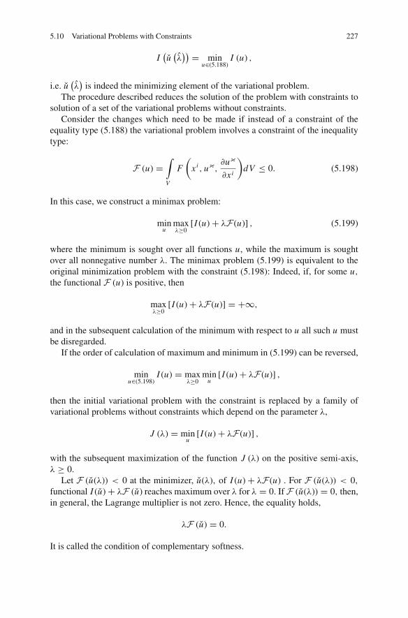
5.10 Variational Problems with Constraints 227
I(u(λ)) = min
u∈(5.188)I (u) ,
i.e. u(λ)
is indeed the minimizing element of the variational problem.The procedure described reduces the solution of the problem with constraints to
solution of a set of the variational problems without constraints.Consider the changes which need to be made if instead of a constraint of the
equality type (5.188) the variational problem involves a constraint of the inequalitytype:
F (u) =∫
V
F
(xi , uκ,
�uκ
�xi
)dV ≤ 0. (5.198)
In this case, we construct a minimax problem:
minu
maxλ≥0
[I (u)+ λF(u)] , (5.199)
where the minimum is sought over all functions u, while the maximum is soughtover all nonnegative number λ. The minimax problem (5.199) is equivalent to theoriginal minimization problem with the constraint (5.198): Indeed, if, for some u,
the functional F (u) is positive, then
maxλ≥0
[I (u)+ λF(u)] = +∞,
and in the subsequent calculation of the minimum with respect to u all such u mustbe disregarded.
If the order of calculation of maximum and minimum in (5.199) can be reversed,
minu∈(5.198)
I (u) = maxλ≥0
minu
[I (u)+ λF(u)] ,
then the initial variational problem with the constraint is replaced by a family ofvariational problems without constraints which depend on the parameter λ,
J (λ) = minu
[I (u)+ λF(u)] ,
with the subsequent maximization of the function J (λ) on the positive semi-axis,λ ≥ 0.
Let F (u(λ)) < 0 at the minimizer, u(λ), of I (u)+ λF(u) . For F (u(λ)) < 0,
functional I (u)+ λF (u) reaches maximum over λ for λ = 0. If F (u(λ)) = 0, then,in general, the Lagrange multiplier is not zero. Hence, the equality holds,
λF (u) = 0.
It is called the condition of complementary softness.

228 5 Direct Methods of Calculus of Variations
In the case of the point-wise constraints, the minimax problem is constructed byan analogous scheme. Suppose, functions uκ obey to s equations,
fα
(xi , uκ,
�uκ
�xi
)= 0, α = 1, . . . , s, (5.200)
and m inequalities
gβ
(xi , uκ,
�uκ
�xi
)≤ 0, β = 1, . . . , m. (5.201)
Then the Lagrange multipliers, λα and μβ, are functions of x , and
minu∈(5.200),(5.201)
I (u) =
= minu
maxλα (x),μβ (x)≥0
⎧⎨⎩I (u)+
∫
V
[λα (x) fα
(xi , uκ,
�uκ
�xi
)+ μβ gβ
(xi , uκ,
�uκ
�xi
)]dV
⎫⎬⎭ .
One proceeds further in the same way as in the previous case by changing the orderof minimum and maximum and obtaining an unconstrained variational problem.
In cases when one searches not the minimum but the stationary points of thefunctional I (u) with some constraints, the general rule of the Lagrange multipliers isas follows: the functional � (u, λ) is constructed, the varying of which with respectto λ provides the given constraints, while � (u, λ) = I (u) if those constraints aresatisfied. Hence, the search of the stationary points of the functional I (u) is reducedto the search of the stationary points of the functional � (u, λ). For example, for theconstraints of the type (5.200), the functional � (u, λ) is
� (u, λ) = I (u)+∫
V
λα (x) fα
(xi , uκ,
�uκ
�xi
)dV .
Consider how the Lagrange multiplier method works in the following example.Example: The minimum drag body in a hypersonic flow. Consider a body in
a hypersonic gas flow in a Cartesian coordinate system, x, y, z (Fig. 5.23). The gasis moving along the z axis in the negative z-direction. The boundary of the body inthe half-space z ≥ 0 (the head part of the body) is given by the equation
z = u (x, y) .
The force exerted by the flow on the body is given by the Newton formula14
14 Here is a brief derivation of this formula. In the case of hypersonic flow, the shock wave is veryclose to the body. If the body has a smooth shape, then the shock wave practically repeats the form

5.10 Variational Problems with Constraints 229
Fig. 5.23 Notation to thehypersonic flow problem
F (u) =∫
�
2
1+ u2x + u2
y
dxdy, (5.202)
� being the cross-section of the body by the plane z = 0, and ux , uy denote partialthe derivatives ux = �u/�x, uy = �u/�y. The region � is assumed to be simplyconnected. We will also assume that the function u (x, y) is continuous and almosteverywhere differentiable, and that
u (x, y) = 0 on �. (5.203)
The problem is to find a function u (x, y) for which the drag force F (u) takes itsminimum value.
of the body (at least near the head part of the body). According to the conservation of momentumon the shock wave in the ideal gas,
[p + ρv2
n
] = 0, where [ϕ] denotes the difference of the valuesof the function ϕ on the two sides of the shock wave, vn is the normal velocity on the shock wave.Due to the impermeability condition at the body, vn ≈ 0 after the shock wave. Therefore, from themomentum conservation the pressure at the body surface is p = p1 + ρ1v
2n1 (index 1 marks the
values before the shock wave). We assume that ρ1 = const, vn1 = vnz , where v, the gas speedfar away from the body, is a constant, and nz is the projection of the normal on the z-axis. Theprojection of the force on the z-axis is
∫pnzd A =
∫p1nzd A + ρ1
∫v2
n1nzd A.
The first term (under some conditions) is balanced by the pressure in the tail part of the body. Thesecond term, divided by the constant ρ1v
2/2 coincides with (5.202) if we take into account therelations linking nz and the area element d A with the shape of the body:
nz =(1+ u2
x + u2y
)− 12 , d A = (
1+ u2x + u2
y
)− 12 dxdy.
This derivation contains an assumption on the closeness of the shock wave and the body surface.This assumption is acceptable not for all body shapes, and, thus, imposes some implicit constraintson the shape of the body. These constraints are hard to formalize. In what follows we ignore theseconstraints and consider the minimization problem for the functional (5.202) as a pure mathemati-cal problem.

230 5 Direct Methods of Calculus of Variations
If the functional F (u) reaches its minimum value F for a smooth functionu (x, y), then, according to (5.202), F is greater than zero. Therefore, it makes senseto call the minimization problem for the functional F (u) correctly posed, if thereexits such a positive constant c, that
F (u) ≥ c. (5.204)
The minimization problem for the functional F (u) as stated is not correctlyposed. Indeed, consider a conic surface of the height h,
u = h
(1− r
ρ (θ )
), (5.205)
where r, θ are polar coordinates in the x-y plane, and r = ρ (θ ) is the parametricequation of the contour �. The functional F (u) for the functions (5.205) becomes
F (u) = 1
h2
2π∫
0
ρ4
1+ ρ2
h2+ ρ2θ
ρ2
dθ ≤ 1
h2
2π∫
0
ρ4
1+ ρ2θ
ρ2
dθ, (5.206)
where ρθ ≡ dρ/dθ . It follows from (5.206) that, along with the increase of theheight h of the cone, the force on the cone decreases to zero.
To exclude the loss of correctness caused by the possible increase of the size ofthe body, it is natural to bound above one of the parameters: the surface area of thebody
∫
�
√1+ u2
x + u2ydxdy ≤ S, (5.207)
the height of the body
max�
u (x, y) ≤ h, (5.208)
or the volume of the body
∫
�
u (x, y)dxdy ≤ V . (5.209)
Consider first the minimization problem on the set of all bodies with the boundedsurface area. This problem can be presented as a minimax problem:

5.10 Variational Problems with Constraints 231
F = minu∈(5.207),(5.203)
F (u) =
= minu∈(5.203)
maxλ≥0
⎡⎣∫
�
2
1+ u2x + u2
y
dxdy+ λ
⎛⎝∫
�
√1+ u2
x + u2ydxdy− S
⎞⎠⎤⎦ .
Let us reverse the order of minimization and maximization. According to (5.81),this cannot increase the result:
maxλ≥0
minu∈(5.203)
⎡⎣∫
�
2
1+ u2x + u2
y
dxdy+ λ
⎛⎝∫
�
√1+ u2
x + u2y dxdy− S
⎞⎠⎤⎦ ≤ F .
(5.210)Let us define the function σ (x, y) by the equation,
σ (x, y) =√
1+ u2x + u2
y, u|� = 0, (5.211)
and rewrite (5.210) as
maxλ≥0
minσ∈(5.211)
⎡⎣∫
�
2
σ 2dxdy+ λ
⎛⎝∫
�
σdxdy− S
⎞⎠⎤⎦ ≤ F . (5.212)
The notation σ ∈(5.211) means that for any admissible function σ (x, y) there existsa function u (x, y) satisfying (5.211). Let us expand the set of admissible functionsσ (x, y), replacing the constraint (5.211) by σ ≥ 0. The minimum in (5.212) canonly decrease:
maxλ≥0
minσ≥0
⎡⎣∫
�
2
σ 2dxdy+ λ
⎛⎝∫
�
σdxdy− S
⎞⎠⎤⎦ ≤ F . (5.213)
The minimum in (5.213) can easily be found. Its determination is reduced to miniza-tion of the function
ϕ (σ ) = 2
σ 2+ λσ for σ ≥ 0.
The function ϕ (σ ) for σ ≥ 0 is strictly convex and has only one minimum. Solvingthe equation dϕ/dσ = 0, we get σ = (4/λ)
13 ; ϕ (σ ) = min ϕ (σ ) = 3
2 (2λ)23 . Hence,
J (λ) = minσ
⎡⎣∫
�
(2
σ 2+ λσ
)dxdy− λS
⎤⎦ = 3
2(2λ)
23 |�| − λS.

232 5 Direct Methods of Calculus of Variations
The function J (λ) is strictly concave, and its maximum is reached at the uniquepoint λ; from the equation
(d Jdλ
)∣∣λ=λ= 0, we find λ: λ = 4 |�|3 /S3, J
(λ) =
2 |�|3 /S2. So we obtain a lower estimate for the minimum drag force,
2|�|3S2≤ F . (5.214)
This estimate demonstrates that the minimization problem for F (u) on the set of allbodies with bounded surface area is correctly posed.
Let us find an upper estimate of the drag force. For the extremum value of
the parameter λ, λ = 4 |�|3 /S3, the function σ (x, y) is constant and is equal
to(4/λ
) 13 = S/ |�|. Consider the function u (x, y), which is the solution of the
boundary value problem
u2x + u2
y =S2
|�|2 − 1, u|� = 0. (5.215)
It is obtained by substituting σ = S/ |�| into (5.211). The boundary value problemis meaningful because S > |�|.
For the solution u (x, y) of the boundary value problem (5.215), we have
∫
�
√1+ u2
x + u2ydxdy = S,
and therefore, u (x, y) belongs to the set of admissible functions and
F ≤ F (u) .
The value of the functional F for the function u is easily calculated and we arrive atthe estimate
F ≤ 2|�|3S2
. (5.216)
It follows from (5.214) and (5.216) that
F = 2|�|3S2
. (5.217)
The minimum drag shape of the body is defined by the solution of the boundaryvalue problem (5.215).
The solutions of (5.215) have the following structure: the lines, u = const, areparallel to the contour �, and the derivative �u/�n along the normal to the con-
tour line of the function u (x, y) takes on the values ±√
S2
|�|2 − 1. It is possible

5.10 Variational Problems with Constraints 233
to construct many solutions of (5.215), choosing between various contour lines�u�n = +
√S2
|�|2 − 1 or �u�n = −
√S2
|�|2 − 1. The solutions for which �u/�n changes
its sign are not meaningful, since the Newton equation for the force (5.202) is notapplicable to such bodies. Therefore, we can single out the unique solution of theboundary problem (5.216) by means of an additional condition �u/�n ≥ 0.
If � is a circle then, among all shapes having � as a base and having a surfacearea not greater than S, the least drag shape is the cone with the surface area S. Theminimum drag shape in the case of � being an ellipse is shown in Fig. 5.24; it lookslike a screwdriver head.
The minimum drag force F is determined only by the area of the base |�| andthe surface area S, and does not depend on the shape of the base (the minimumdrag shape does, of course, depend on the shape of the base). Hence, we also solvedanother problem: we found the minimum drag shape with the condition that thecross-section area of the body is |�|, and the head surface area is not greater than S.The above-mentioned implies that this problem has many solutions (at least one forevery region �), and the least possible drag force is given by (5.217).
Consider two cones of the same height and the same base area (and therefore,of the same volume), where the shape of the base of one cone is a circle, and ofthe other a star (Fig. 5.25). Then the star-shaped cone provides less drag than thecircular one.
Indeed, the surfaces of both cones are the solutions of (5.215), and (5.217) holds.It only remains to note that the surface area of the star-shaped cone is greater thanthat of the circular one. It follows, for example from the solution of the followingvariational problem: among all contours r = ρ (θ ), bounding the regions with agiven area |�|,
2π∫
0
1
2ρ2 (θ )dθ = |�| ,
Fig. 5.24 The minimum dragbody when the base is anellipse

234 5 Direct Methods of Calculus of Variations
Fig. 5.25 Star-shaped coneprovides less drag than acircular cone
find the contour for which the cone of the height h having this region as a base, hasthe minimum surface area
1
2
2π∫
0
√h2 + ρ2 (θ )ρ (θ )dθ → min .
Here is the solution to this problem. Introducing the Lagrange multiplier λ, we ob-tain the functional
1
2
2π∫
0
[ρ (θ )
√h2 + ρ2 (θ )− λ
(ρ2 (θ )− |�|
π
)]dθ.
Its Euler equation for the function ρ (θ ) is α + α−1 = 2λ, α ≡ ρ/√
h2 + ρ2.Consequently, ρ ≡ const, and the stationary value is reached for the cone withthe circular base of area |�| and height h. The stationary point is unique since thecircular cone is uniquely defined by h and |�|. It only remains to show that thisis the minimum point. Adding an increment ερ (θ ) to ρ, let us calculate the areachange up to the terms of order ε2,
1
2
(h2+ρ2
) (α2 + 1
) 2π∫
0
ερdθ + 1
2
(h2+ρ2
) [1
2α (1− α)+ α
] 2π∫
0
ε2ρ2dθ.
The first integral is equal to zero due the constraint for the area of the base, whilethe second integral is positive since α < 1. Therefore, the circular cone has theminimum surface area among the cones with the same height and the same basearea.
The above results can easily be generalized to the case of the region � boundedby two closed parallel contours � and �′. Let the function u (x, y) be equal to zeroon � and

5.10 Variational Problems with Constraints 235
Fig. 5.26 Minimum drag body with the base bounded by contours � and �′
u (x, y) = u0 = const on �′.
As in the case of the simply connected region, it can be proven that the soughtsurface obeys (5.215). The drag force is given by (5.217).
In the case of the circular base, the solution is constructed from conic surfacesand is shown in Fig. 5.26 for different ratios of u0 and S.
Let us move on the minimization problem for the functional F (u) with con-straints on the height (5.208) and volume (5.209) of the body. First, let us show thatthis problem is incorrectly posed in the absence of additional conditions. Consideran axis-symmetric body, the cross-section of which in the plane θ = const. is shownin Fig. 5.27. We will assume that the width of each tooth is ρ/n, where n is aninteger, and the height of the prong is equal to ε. Then, |�u/�r | = 2εn/ρ, and thefunctional has the value
F (u) =ρ∫
0
2π∫
0
2r
1+ u2r
dθdr = 2πρ2
1+ 4 ε2n2
ρ2
. (5.218)
Therefore, F (u)→ 0 as n→∞.
Fig. 5.27 A minimizingsequence for F (u)

236 5 Direct Methods of Calculus of Variations
By appropriately choosing the constants, a and ε, we can make the height andthe volume of the body satisfy the constraints. If the parameter ε is considered tobe dependent on n and tends to zero, then the sequence of surfaces will convergeto a cylinder closed by a flat cover z = a. If we apply an additional constraint ofεn→∞ as n→∞, then, according to (5.218), the corresponding drag force tendsto zero.
The existence of a sequence of surfaces for which F → 0 shows that the mini-mization problem for the functional F (u) on the set of bodies with limited heightand volume is incorrectly posed.
On the other hand, bounding the surface area of the body makes the problemcorrectly posed, as we have obtained. Therefore, it makes sense to narrow down theset of admissible functions u (x, y) in such a way that for this set the boundednessof the height or the volume of the body would imply the boundedness of the headsurface area. That means that on the set of admissible functions, the inequality
∫
�
√1+ u2
x + u2ydxdy−� ≤ l max
�u (x, y) (5.219)
holds in the case of the bounded height or the inequality
∫
�
√1+ u2
x + u2ydxdy−� ≤ k
∫
�
udxdy (5.220)
holds in the case of the bounded volume.The inequalities (5.219) and (5.220) are true, for example, for concave functions
u (x, y) (the head part of the body is convex). Indeed, for a concave function u (x, y),the surface area of its graph, z = u (x, y) , can be estimated above by the surfacearea of a cylinder with the cross-section � and the height max
�u (x, y). The constant
l in (5.220) can be interpreted as the length of contour �.The inequality (5.220) for concave functions can be proved as follows. Consider
the cone K , obtained by connecting the farthest point of the body from the planez = 0 with the points on the contour �. Due to the convexity of the body, the coneK is completely inside the body. The volume of the cone K , 1
3 � max�
u (x, y), is the
lower estimate of the body’s volume,
1
3� max
�u (x, y) ≤
∫
�
udxdy (5.221)
The inequality (5.220) where k is equal to 3l/� follows from the inequalities (5.221)and (5.219).
Due to (5.219) and (5.220), the problem of finding the shape of a convex bodyhaving a minimum drag in hypersonic flow is correctly posed on the set of all bodies

5.10 Variational Problems with Constraints 237
with bounded height or bounded volume. The solutions of these problems can beobtained only numerically.
Pontrjagin’s maximum principle. Consider the variational problem
I (x, u) =t1∫
t0
L(t, xi (t) , uκ (t)
)dt → min (5.222)
with the constraints
dxi
dt= f i
(t, xi (t) , uκ (t)
), i = 1, . . . , n, κ = 1, . . . , m, (5.223)
xi (t0) = xi0, (5.224)
uκ (t) ∈ U, (5.225)
where U is a set in Rm . The variational problem (5.222), (5.223), (5.224) and (5.225)has differential constraints (5.223). If the functions uκ (t) satisfying the condition(5.225) are given, then the system of differential equations (5.223) with the initialvalues (5.224) will determine the functions xi (t). Having xi (t) and uκ (t), we cancalculate the value of the functional I (x, u). The minimization of the functionalI (x, u) means its minimization with respect to all admissible functions uκ (t).
The variational problem with the constraints (5.223), (5.224) and (5.225) is anexample of the problems in optimal control theory. Let us find the dual variationalproblem in that case.
First, we rewrite the variational problem by introducing the Lagrange multipliers,pi (t), as
I = minx∈(5.224)u∈(5.225)
maxp
t1∫
t0
[L(t, xi , uκ
)+ pi (t)
(dxi
dt− f i
(t, x j , uκ
))]dt.
Suppose that the order of the minimization and maximization can be reversed:
I = maxp
minx∈(5.228)u∈(5.229)
t1∫
t0
[L(t, xi , uκ
)+ pi (t)
(dxi
dt− f i
(t, x j , uκ
))]dt. (5.226)
Now the minimization problem in (5.226) does not contain differential constraints.Consider the function
H (t, p, x, u) = pi f i(t, x j , uκ
)− L(t, xi , uκ
)
which is called the Pontrjagin function. In terms of this function (5.226) takes theform
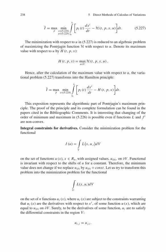
238 5 Direct Methods of Calculus of Variations
I = maxp
minx∈(5.224)u∈(5.225)
t1∫
t0
[pi (t)
dxi
dt−H (t, p, x, u)
]dt. (5.227)
The minimization with respect to u in (5.227) is reduced to an algebraic problemof maximizing the Pontrjagin function H with respect to u. Denote its maximumvalue with respect to u by H (t, p, x):
H (t, p, x) = maxu∈U
H (t, p, x, u) .
Hence, after the calculation of the maximum value with respect to u, the varia-tional problem (5.227) transforms into the Hamilton principle:
I = maxp
minx∈(5.224)
t1∫
t0
[pi (t)
dxi
dt− H (t, p, x)
]dt.
This exposition represents the algorithmic part of Pontrjagin’s maximum prin-ciple. The proof of the principle and its complete formulation can be found in thepapers cited in the Bibliographic Comments. It is interesting that changing of theorder of minimum and maximum in (5.226) is possible even if functions L and f i
are non-convex.
Integral constraints for derivatives. Consider the minimization problem for thefunctional
I (u) =∫
V
L(x, u,i
)dV
on the set of functions u (x), x ∈ Rn , with assigned values, u(b), on �V . Functionalis invariant with respect to the shifts of u for a constant. Therefore, the minimumvalue does not change if we replace u(b) by u(b)+ const. Let us try to transform thisproblem into the minimization problem for the functional
∫
V
L(x, ui )dV
on the set of n functions ui (x), where ui (x) are subject to the constraints warrantingthat ui (x) are the derivatives with respect to xi , of some function u (x), which areequal to u(b) on �V . Surely, to be the derivatives of some function, ui are to satisfythe differential constraints in the region V :
ui, j = u j,i .

5.10 Variational Problems with Constraints 239
However, we are interested in constraints of another type - the integral constraints.Namely, we are going to show that ui (x) are the derivatives of some function u (x)equal to u(b) + const on the boundary �V of some simply connected region V , ifand only if the following equality holds:
∫
V
pi ui dV =∫
�V
pi ni u(b)d A, (5.228)
where pi (x) is any smooth field satisfying the equation
pi,i = 0. (5.229)
In other words, the following variational principle holds:Variational principle. Minimization of the functional
∫
V
L(x, u,i
)dV
on the set of functions u(x) taking the boundary values u(b) + const is equivalentto the minimization problem for the functional
∫
V
L(x, ui )dV
on the set of functions ui (x) satisfying the constraint (5.228).Clearly, this is a version of the dual variational principle.First we show that (5.229) holds if and only if there exist twice continuously
differentiable functions ψ i j (x) such that
pi = � jψi j , ψ i j = −ψ j i . (5.230)
We prove this fact for the case of V = Rn . It is obvious that (5.229) followsfrom (5.230). Now, let us show that (5.230) follows from (5.229). For any functionspi (x) satisfying (5.229), there exists the solution ψ i (x) of equations
�ψ i (x)− �i � jψ j (x) = pi (x) . (5.231)
Indeed, applying the Fourier transformation to (5.231), we get
− k2ψ i (k)+ ki k jψ j (k) = pi (k) , k2 ≡ ki ki (5.232)

240 5 Direct Methods of Calculus of Variations
where pi (k) , ψ i (k) are the Fourier transformations15 of the functions pi (x) andψ i (x), respectively, and ki are the wave numbers (the Fourier transformation param-eters). Equations (5.232) form a system of linear equations for ψ i (k). The rank ofthe matrix of this system
∥∥−k2δi j + ki k j∥∥ is equal to n−1. The necessary condition
of the solvability of (5.232) is pi (k) ki = 0 and it is satisfied due to (5.229). From(5.232), we find that ψ i (k) = −k−2 pi (k) + ψ (k) ki , where ψ (k) is an arbitraryfunction. Hence, for any functions pi (k) there exists a function ψ i (k) satisfying(5.231). Equations (5.231) transform to (5.230) for ψ i j = � jψ i − �iψ j .
To prove (5.228) we note that, if ui = u,i , and u = u(b) + const on �V , then(5.228) is satisfied. Now, let (5.228) holds for any solutions of (5.229). Accordingto (5.230), the equality (5.228) can be written as
∫
V
ui � jψi j dV =
∫
�V
u(b)ni � jψi j d A.
Integrating by parts, we get
∫
V
ψ i j u[i, j]dV =∫
�V
(u(b)ni � jψ
i j − uiψi j n j
)d A. (5.233)
The square brackets in the indices denote the alteration a[i, j] ≡ 12
(ai j − a ji
).
Let xi = r i (ξα) , α = 1, . . . , n − 1, be the equations of the surface �V . Usingthe notation introduced for the surfaces in R3 (see Sect. 14.1) and the decompositionof the gradient (14.17), the contraction ni � jψ
i j is
ni � jψi j = nir
αj ψ
i j,α. (5.234)
Hence, the contraction (5.234) contains only the derivatives ψ i j along the sur-face �V . Assume that ψ i j = 0 on �V . Then the integral on the right-hand side of(5.233) is zero. Due to the arbitrariness of ψ i j , applying the main lemma of calculusof variations to (5.233), we find that ui, j = u j,i in V . Consequently, there existsfunction u (x) such that ui = u,i . Due to continuity, this also holds at �V .
For any functions u (x) and ψ i j (x) = −ψ j i (x), the identity
∫
�V
(u,iψ
i j − uψj i,i
)n j d A = 0. (5.235)
holds. It can be checked by transforming this integral to the volume integral bymeans of the divergence theorem. Thus, from (5.233) and (5.235),
15 The basic features of Fourier transformation are considered further in Sect. 6.7.

5.10 Variational Problems with Constraints 241
∫
�V
(u(b)−u
)ni � jψ
i j d A = 0 (5.236)
for any functions ψ i j on �V . The contraction nirαj ψ
i j,α is
nirαj ψ
i j,α =
(nir
αi ψ i j
)|α (5.237)
where the vertical bar in indices denote the surface covariant derivative along �V .This follows from the equalities
(nir
αj
)|α =
(n jr
αi
)|α (5.238)
which can be established by means of (14.33) and (14.31). Therefore, u(b) =u + const.
Unlocking the integral constraints. Let us retain a finite number of constraints cor-responding to some set of particular solutions pi
(1), . . . , pi(m) of (5.229), discarding
the rest. Then the set of admissible functions will expand, and the minimum of thefunctional will decrease. The minimum can be found by introducing the Lagrangemultipliers λ1, . . . , λm ; we get the following variational problem:
minui
maxλ1,...λm
∫
V
(L(x, ui )−
(λ1 pi
(1) + . . .+ λm pi(m)
)ui)dV+
+∫
�V
(λ1 pi(1) + . . .+ λm pi
(m))ni u(b)d A ≤ I .
after reversing the order of calculating of maximum and minimum, finding the min-imum with respect to ui is reduced to calculating the Young-Fenchel transformationof the function L with respect to ui . Therefore,
maxλ1,...λm
⎛⎝
∫
�V
pi ni u(b)d A−
∫
V
L∗ (x, pi )dV
⎞⎠ ≤ I ,
where pi denotes the sum λ1 pi(1) + . . .+ λm pi
(m).We see that relaxing of integral constraints is equivalent to the Rayleigh-Ritz
method for the dual problem, and the integral constraint method is based on thesame ideas as the duality theory methods.
The above consideration is easily generalized to the integral functional of theform

242 5 Direct Methods of Calculus of Variations
∫
V
L(xi , u
κ
, uκ
i
)dV . (5.239)
using the following statement:For the functions uκ (x) and uκ
i (x) to satisfy the relations uκ
i = uκ
,i and uκ =uκ
(b) on �Vu , it is necessary and sufficient that the relation
∫
V
(pκuκ + pi
κu
κ)dV =
∫
�Vu
piκ
ni uκ
(b)d A (5.240)
holds for all the solution of the equations
pκ − piκ,i = 0 in V, pi
κni = 0 on �V f = �V − �Vu . (5.241)
This statement becomes obvious if using (5.241) we write the equality (5.240) as
∫
V
(pi
κ,i uκ + pi
κu
κ)dV =
∫
�Vu
piκ
ni uκ
(b)d A (5.242)
and take into account that piκ
(x) are arbitrary vector fields with zero normal com-ponents on �V f .
So, the minimization problem for the functional (5.239) can be written also asthe minimization problem for the functional
∫
V
L(xi , uκ, u
κ
i
)dV
on the set of all functions uκ (x) and uκ
i (x) satisfying the relations (5.240).
The cross-section principle. In the problems without constraints, it is sometimesuseful to introduce constraints by means of the following construction.
Let us present the set M of elements u as a union of non-intersecting subsetsMv , M = ∪Mv , where v are elements of some set N . The subsets Mv will becalled the cross-sections of the set M.
The minimization problem for functional I (u) on M can be solved in two steps.First, the minimum of the functional I (u) is sought on the set Mv . The minimumvalue J of the function I (u) on Mv depends on v:
J (v) = minu∈Mv
I (u) .
Then the minimum of the functional J (v) on N is sought. One may expect that
I = minv∈N
J (v) . (5.243)

5.11 Variational-Asymptotic Method 243
Let us prove (5.243). Denote minJ (v) by J . Obviously, for any v, I ≤ J (v).Suppose that I < J . By the definition of the minimum value, there exists a sequenceun , for which I (un)→ I . Denote by vn the element v, for which un ∈Mv . SinceI ≤ J (vn) ≤ I (un), J (vn)→ I . This refutes the supposition.
The statement (5.243) is called the cross-section principle.
5.11 Variational-Asymptotic Method
In many problems of mechanics and physics there are small and large parameters.These can be geometric parameters like the thickness of a plate or a shell, thediameter of a beam cross-section, the average crystallite size in a polycrystal, themagnitude of deformation or displacements of a continuum, the wave length, thenumber of gas molecules in a container, or they can be physical parameters: theviscosity or heat conductivity of a fluid, the oscillation frequency of a rigid body,etc. To investigate properly such problems various asymptotic approaches were de-veloped. It is clear that for the problems which allow a variational formulation and,consequently, possessing a special structure, there should exist a direct variationalapproach based on direct asymptotic analysis of the corresponding functionals. Itshould automatically take into account the variational structure of the equations andthose properties of the solutions, which are dictated by this structure.
A method of asymptotic analysis of functionals will be considered in this sec-tion. This method is of heuristic character. It does not have a strict mathematicalfoundation. However, for problems admitting exact solutions or studied by differentmethods, there is a complete accordance of the results.
The method of asymptotic analysis of functionals, which will be called thevariational-asymptotic method, allows one to consider the minimization problemsfor functions of a finite number of variables and the problems for differential equa-tions possessing the variational structure from a common point of view.
When applied to differential equations, the variational-asymptotic method has anumber of advantages compared to the widely used asymptotic approaches mainlydue to the simplicity of analysis, which is more noticeable as the complexity ofthe system of differential equations increases. The reason for this is that in thevariational-asymptotic method only one function, the Lagrangian – instead of asystem of differential equations, is the subject of the investigation.
Another advantage of the variational-asymptotic method is that the approximateequations always possess a variational structure while the direct asymptotic analysisof differential equations may yield the approximate equations that do not have sucha structure. This can be seen from the analysis of a system of two linear algebraicequations, involving a small parameter, ε:
x + ε (x − y) = 1, y + ε (y − x) = 0.
This system can be interpreted as the equilibrium equations of two interactingsprings: x and y are the displacements of the springs from the equilibrium position,

244 5 Direct Methods of Calculus of Variations
and the first spring is subject to the external force of unit magnitude. The interactionis characterized by parameter ε. Let us pose the following problem: for ε → 0,
construct an approximate system of equations the solution of which coincides withthe solution of the original system in terms of the order of 1 and ε. Since x ≈ 1 andy ≈ ε, the only possible “simplification” is disregarding the term εy, which is ofthe order of ε2. We have
x + εx = 1, y − εx = 0.
The initial system of equations is a system of equations of variational type: theleft-hand sides of the equations are derivatives of the function
f (x, y, ε) = 1
2
(x2 + ε (x − y)2 + y2
),
and the equilibrium equations are the equations for the minimizing point of thefunction f (x, y, ε) − x . For the approximate system of equations, this is not true,there is no function g (x, y, ε) , such that
�g (x, y, ε)
�x= x + εx,
�g (x, y, ε)
�y= y − εx
because
�
�y(x + εx) �= �
�x(y − εx) .
This situation is typical in asymptotic analysis of differential equations withsmall parameters. The violation of the variational structure of the approximate equa-tions may result in even qualitatively wrong results. For example, the exact self-conjugated equations possess only real eigenvalues, while the approximate equa-tions acquire complex eigenvalues, i.e., physically, the system in an approximatedescription may become unstable while it is stable in the exact description.
The variational approach in asymptotic analysis of partial differential equationsis important also due to the necessity of short-wave extrapolation. This issue will bediscussed further in Sect. 14.5.
The variational-asymptotic method is based on the idea of neglecting the smallterms in energy. This idea is often used in physics. However, to apply it in a system-atic way one has to learn how to recognize small terms, how to treat the situationswhen neglecting small terms results in the loss of the uniqueness or the existence ofthe solution, and, moreover, understand how the small terms affect the next approx-imations and how the iteration procedure could be settled.
The variational-asymptotic method will be formulated as a set of rules, the ap-plication of which will be illustrated for a number of examples. Other applicationswill be encountered in later chapters.

5.11 Variational-Asymptotic Method 245
Let the functional I (u, ε) be defined on some set of elements M and dependon small parameter ε. We will assume that the functional I (u, ε) has a finite or acountable number of stationary points. The stationary points will be denoted by u,and, in order to avoid cumbersome notation, will not be numbered. The stationarypoints u are functions of ε. This will be emphasized by placing ε in the index, uε.
Let uε tend to u0 for ε→ 0. The following questions arise: how can we constructa functional which has u0 as stationary points? How can we construct an approx-imate functional, the stationary points of which are the approximations of uε of agiven accuracy?
It is clear that the answers to these questions are related to the simplification ofthe functional by disregarding small insignificant terms. It is natural to start with in-vestigation of the functional from which all small terms dropped, i.e. the functionalI0 (u) = I (u, 0). The following situations may be encountered:
1. I0 (u) has the isolated stationary points2. I0 (u) has the non-isolated stationary points3. I0 (u) does not have the stationary points or it is meaningless, i.e. the functional
I (u, ε) is not defined for ε = 0
Let us begin with the first case.
Case 1: I0 (u) has the isolated stationary pointsIt could be expected that the stationary points of the functional I0 (u) are the firstapproximations of the stationary points of the initial functional.
Example 1. Consider the behavior of the stationary points of the function of onevariable,
f (u, ε) = u2 + u3 + 2εu + εu2 + ε2u, (5.244)
for ε → 0. The function f0 (u) = u2 + u3 has two stationary points, u = 0 andu = − 2
3 . It is not difficult to check that they are indeed the limits for ε→ 0 for thestationary points of the function f (u, ε).
The second asymptotic term will be sought in the following way. Let us presentu as u = u0 + u′, where u0 is a stationary point of the functional I0 (u), and u′ → 0for ε → 0. We will also keep the leading terms containing u′ in the functionalI(u0 + u′, ε
). Thus we obtain the functional I1
(u′, ε
). We expect that the stationary
point with respect to u′ of this functional is the next asymptotic term.
Example 1 (continued). Consider the stationary point of the function (5.244) in aneighborhood of zero. Thus u is to be small. Let us keep only the leading terms withrespect to u in f (u, ε). Since εu2 and u3 are small compared to u2, and ε2u is smallcompared to 2uε, we have
f1 (u, ε) = u2 + 2εu.
Terms u2 and 2uε need to be kept since there are no terms in comparison withwhich they could be neglected. The function f1(u, ε) has the stationary point u =

246 5 Direct Methods of Calculus of Variations
−ε. Hence, the asymptotic approximation of the stationary point of the functionf (u, ε) in the neighborhood of zero is
uε = −ε + o (ε) .
At this point the function f (u, ε) is the same as f1 (u, ε), i.e. it has a minimum.Consider the stationary point of the function f (u, ε) in the neighborhood of the
point u = −2/3. Setting u = − 23 + u′ and keeping the leading terms with respect
to u′ in the function f(− 2
3 + u′, ε), we arrive at the function16
f1 (u, ε) = −u′2 + 2
3εu′.
Its stationary point is u′ = 13ε and the asymptotic approximation of the second
stationary point is
uε = −2
3+ 1
3ε + o (ε) ;
the function f (u, ε) has a local maximum at this point.The next asymptotic terms are constructed analogously. For example, for the
stationary point of f (u, ε) in the neighborhood of zero, we seek u in the formu = −ε + u′′, u′′ = o (ε). Keeping only the leading terms with respect to u′′ in thefunction
f (u, ε) = (−ε + u′′)2+(−ε + u′′
)3+2ε(−ε + u′′
)+ε(−ε + u′′
)2+ε2(−ε + u′′
),
we get the function
f2 (u, ε) = u′′2 + 2ε2u′′.
Therefore, u′′ = −ε2 and
uε = −ε − ε2 + o(ε2).
Note that the order of the “smallness” of u′ is not supposed a priori, but is deter-mined.
Also note that the terms that were insignificant in constructing the leading termof the asymptotic expansion may become important in determining the next termsof the asymptotic expansion.
The example considered demonstrates that the main issue in asymptotic analysisof functionals is to recognize the leading terms and the negligible ones. Usually,
16 From now on, additive constants will be disregarded without mentioning.

5.11 Variational-Asymptotic Method 247
this is the most important and the most difficult point of the analysis. However,there are cases when the recognition of the negligible terms does not cause difficul-ties. Here are two conditions upon satisfying which the terms may be considerednegligible.
Let the functional I (u, ε) includes a sum of two terms, A (u, ε) and B (u, ε), and
limε→0
maxu∈M
∣∣∣∣B (u, ε)
A (u, ε)
∣∣∣∣ = 0. (5.245)
Then B (u, ε) is negligible in comparison with A (u, ε) for all stationary points. Wewill call such terms globally secondary terms.
Let uε → 0 for ε→ 0, and for any sequence {un} converging to u = 0:
limn→∞ε→0
∣∣∣∣B (un, ε)
A (un, ε)
∣∣∣∣ = 0. (5.246)
Then the term B (u, ε) is negligible compared to A (u, ε) for the stationary point uε.The convergence un → 0 is understood in the same sense as the convergence ofuε → 0. The term B (u, ε) will be called locally secondary compared to A (u, ε).The case of uε → u0, u0 �= 0 is reduced to the case of uε → 0 by the substitutionu → u′: u = u0 + u′.
In the definitions (5.245) and (5.246), the additive constants in A (u, ε) are to beexcluded. This can be done, for example, by setting the condition
A (0, ε) = 0.
In Example 1, the term εu2 is globally secondary with respect to u2, ε2u is glob-ally secondary with respect to 2εu while u3 is locally secondary with respect to u2
in the neighborhood of the point u = 0.
Example 2. Consider the function
f (u, ε) = ln (1+ 2u)− 1+ 2u
1+ 2u2+ εu, 1+ 2u > 0. (5.247)
The function
f0 (u) = ln (1+ 2u)− 1+ 2u
1+ 2u2
has a stationary point at u = 0. The first terms of expansion f0 (u) with respect to uare −1+ 20
3 u3. The other terms are locally secondary with respect to u3. Therefore,the investigation of the function f (u, ε) can be replaced by the investigation of thefunction 20
3 u3 + εu in the first approximation. It has two stationary points ±√− ε20
for ε ≤ 0 and does not have any stationary points for ε > 0. Consequently, thefunction f (u, ε) has the same behavior in the neighborhood of zero.

248 5 Direct Methods of Calculus of Variations
For any secondary term, B (u, ε), of the type (5.245) or (5.246), there exists aterm of the functional, A (u, ε) , compared to which B (u, ε) is small. Along withsuch terms, the functional may have terms which cannot be easily pinpointed assmall because the corresponding “large” terms are not present in the functional.Consider, for example, the function
f (u, ε) = u3 + εu2 + ε3u. (5.248)
The function f0(u) = f (u, 0) = u3, and one may expect that all stationary pointsof the function f (u, ε) are in the vicinity of u = 0. Could we neglect the term ε3u?This is not clear because we do not know the order of uε. If, for example, uε ∼ ε,then the first two terms are of the same order, ε3, while the third, of the order ε4,
may be neglected. If uε is, say, of the order ε2, then the last two terms must be kept(they are both of the order ε5) while the second one, which is of the order ε6, may bedropped. If we cannot say about a term whether it is the leading one or negligible,we call such a term doubtful. All the terms of function (5.248) are doubtful.
A recipe for studying a functional with doubtful terms is simple: let the sta-tionary points of the functional be hard to find, but the corresponding problem forthe functional I with the dropped doubtful terms admits investigation. Then westudy the stationary points of the functional I and evaluate the doubtful terms atthese stationary points. If the doubtful terms are smaller (in the asymptotic sense)than the kept ones, then I provides the leading asymptotics of the stationary points.Otherwise, the doubtful terms should be kept.
Example 3. Consider the stationary points of the function (5.248) in the neighbor-hood of zero. There are no clear indications that any one of the terms is smallcompared to another.
Let us first drop the last term. We obtain the function u3 + εu2, the stationarypoints of which are u = 0 and u = − 2
3ε. At u = 0 it is not clear whether or not thelast term can be disregarded. At u = − 2
3ε it can be done, since the first two termsare of order ε3, while the last one is of order ε4.
Let us now discard the second term. We obtain the function u3+ε3u, which doesnot have any stationary points for ε > 0, while for ε ≤ 0, the stationary points are
±√− 1
3ε3. The first and third terms are of the order of ε92 , while the second is much
larger, of the order of ε4. Therefore, the second term cannot be discarded.Let us drop the first term. The function εu2 + ε3u has one stationary point at
− 12ε2. The first term is of the order of ε6 and is much smaller than the two retained,
which are of the order of ε5. Therefore, discarding the first term makes sense.So in the neighborhood of zero we found two stationary points, uε = − 2
3ε+o (ε)and uε = − 1
2ε2 + o(ε2). Since the function (5.248) has only two real stationary
points, all the stationary points have been found.
Example 4. Newton’s polygon rule. To find the leading asymptotic term for thestationary points of the function of the form

5.11 Variational-Asymptotic Method 249
f (u, ε) =N∑
m,n
amnεmun,
which tend to zero for ε → 0, one can use the method proposed by Newton17. Wedescribe this method for the case of the function
g (u, ε) = u3 + εu2 + εu3 + ε2u4 + ε3u + ε5u5.
For each term, define a point on a two-dimensional integer lattice with the x-coordinate equal to the order of ε and the y-coordinate equal to the order of u. Weget a set of points. For the function g (u, ε) this set is shown in Fig. 5.28. Then wedraw a maximum convex polygon with the vertices from this set, which includes allpoints of the set. According to Newton’s polygon rule, in constructing the leadingasymptotic term of the stationary points, it is necessary to keep only those terms thecorresponding points of which lie on the sides of the polygon. For ε→ 0, it is onlynecessary to keep the terms corresponding to the points in the part of the polygonbeginning at point A (see Fig. 5.28) and continuing to the right and down and endingat the point C, where the line turns upward. This part of the polygon is shown by asolid line in Fig. 5.28.
Let us derive Newton’s polygon rule for the function g (u, ε) using the generalpropositions made above. Consider the terms with the power of ε ≥ 0 and the powerof u ≥ 3. Since the asymptotic u → 0 is being considered, all the terms except u3
can be discarded: they correspond to the terms which are locally secondary com-pared to u3. For the same reason, among all the terms with the power of ε ≥ 1 andthe power of u ≥ 2 only εu2 should be kept – the corresponding terms are locallysecondary with respect to εu2. Thus, points A, B, and C remain. They correspondto the function (5.248) considered in Example 3. It has two stationary points, andfor the construction of the asymptotics of these points the terms corresponding tothe points on the edges AB and BC of Newton’s polygon should be used.
The derivation of Newton’s polygon rule for the general polygon is analogous tothe above one.
Case 2: I0 (u) has the non-isolated stationary pointsLet us move on to a more interesting for physical applications case when discardingthe secondary terms results in appearance of non-isolated stationary points.
A typical finite-dimensional situation can be shown for the function of two vari-ables (u = {x, y}) of the form
f (x, y, ε) = f0 (x)+ εg (x, y) , −∞ < x < +∞,−∞ < y < +∞, (5.249)
17 Newton’s polygon rule concerns the asymptotic behavior of the roots of polynomials; here it isconsidered in terms of the problem of finding the stationary points of function f (u, ε), which isan integral of a polynomial function.

250 5 Direct Methods of Calculus of Variations
Fig. 5.28 Newton’s rule
where the function f0 (x) has some stationary points x0.If the presumably small term εg (x, y) is dropped, we get the function f0 (x)
which has in the (x, y)-plane continuum of stationary points (x0, y), −∞ < y< +∞.
Before formulating the general rules for dealing with such cases, let us first con-sider some examples.
Example 5. Let us find the asymptotic for ε → 0 of the stationary points of thefunction
f (x, y, ε) = cos (x − y)+ ε
(1
x+ y
), −∞ < x < +∞, −∞ < y < +∞.
If 1xε+ yε is bounded for ε→ 0, then the second term is secondary, and f0 (x, y) =
cos (x − y). Denote the set of stationary points of the function f0, y = x +πk, −∞ < x < +∞, k = 0,±1,±2, . . ., by M0. Consider the functionf (x, y, ε) on M0. The function f (x, y, ε) on M0 becomes the function of onevariable x (and a number, k): f = cos πk + ε
(1x+x + πk
). The stationary points
of f on M0 with respect to x are x = ±1. It should be expected that the stationarypoints of function f (x, y, ε) converge to (±1,±1+ πk) for ε → 0. The validityof this proposition can be checked directly: it is sufficient to perform the change ofvariable, y → z: y = x + z, and the function f will become a sum of functionswhich depend only on x and z,

5.11 Variational-Asymptotic Method 251
f = cos z + εz + ε
(1
x+ x
),
for which the proposition made is obviously true.
The described procedure of constructing the stationary points made withoutsome precautions can provide wrong results. This is demonstrated in the followingexample.
Example 6. Let us find the stationary point of the quadratic form
f (x, y, ε) = x2 − 2x + 4ε (x − 1) y + ε2 y2 + 2ε2 y.
The set M0 of the stationary points of the function f0 (x, y) = x2−2x is the line,(1, y). The function f (x, y, ε) is a function of y on M0 : f = 1+ε2
(y2 + 2y
). This
function has a stationary point at y = −1. By analogy with the previous examplewe could assume that the stationary point of the function f (x, y, ε) tends to thepoint (1,−1) for ε → 0. This, however, is not true. Indeed, writing the stationarycondition for the function f (x, y, ε)
x − 1+ 2εy = 0, 2 (x − 1)+ εy + ε = 0,
we find the stationary points: xε = 1 − 23ε, yε = 1
3 . Why did we get the wronganswer?
Let us fix some point of the set M0 (defined by assigning a value to y). Thesearch for the stationary point will be carried out by first finding the stationary pointwith respect to x for a fixed y (the corresponding stationary value of f becomesa function of y only), and then finding the stationary point over all y. Since wesuspect that the stationary point is in the neighborhood of set M0, it is sufficientto consider not all values of x but only those x = 1 + x ′ for which x ′ are small.Keeping only the terms important with respect to x ′ in the function f
(1+ x ′, y, ε
),
we obtain the function x ′2 + 4εx ′y. Consequently, x ′ = −2εy. So, we have toconsider the function f (1− 2εy, y, ε) = −1− 3ε2 y2 + 2ε2 y but not f (1, y, ε) onM0. This yields y0 = 1
3 , in compliance with the correct result. It follows from theabove consideration that the stationary point is a saddle point – the function f ismaximum with respect to y and minimum with respect to x .
The difference between Examples 5 and 6 is the following. In Example 5, letus fix y and denote the stationary point of the function f0 (x, y) for fixed y byx0 (x0 = y + πk). Let x ′ be the first correction to x0. It is easy to check that thefunctions f
(x0 + x ′, y, ε
)and f (x0, y, ε) will differ in terms of the order of ε2,
while to calculate y we need to keep the terms of the order ε. In Example 6, functionsf(x0 + x ′, y, ε
)and f (x0, y, ε) also differ for terms of the order ε2. However, to
calculate y we need to keep the terms of the order ε2.Now we are ready to formulate the general rules for searching the stationary
points.

252 5 Direct Methods of Calculus of Variations
Let M0 be the set of stationary points of the functional I0 (u) and any elementu ∈M can be uniquely presented as u = u0 + u′, u0 ∈M0, u′ ∈M′. Fixing u0
and considering u′ to be small, we keep the leading terms with u′ in the functionalI(u0 + u′, ε
). We obtain a functional I1
(u0, u′, ε
). Let us find the stationary points
of I1 with respect to u′. They will depend on u0.Suppose that u′ is uniquely determined by u0, u′ = u′ (u0, ε). Representing u as
u = u0 + u′ (u0, ε) + u′′, where u0 ∈M0, u′′ ∈M′′ and u′′ is smaller than u′ inthe asymptotic sense, and keeping the leading terms with respect to u′′, we find u′′,and so on.
Consider the functionals I (u0, ε) and I(u0 + u′ (u0, ε) , ε
)on M0. If their sta-
tionary points do not differ significantly, then we can expect that the leading approxi-mation of the stationary points of the initial functional are the stationary points of thefunctional I (u0, ε) on M0. If the stationary points of the functionals I (u0, ε) andI(u0 + u′ (u0, ε) , ε
)differ significantly, but the stationary points of the functionals
I(u0 + u′ (u0, ε) , ε
)and I
(u0 + u′ (u0, ε)+ u′′ (u0, ε) , ε
)do not, then the leading
approximation are the stationary points of the functional I(u0 + u′ (u0, ε) , ε
). If the
stationary points of the functionals I(u0 + u′ (u0, ε) , ε
)and I
(u0 + u′ (u0, ε)+ u′′
(u0, ε) , ε) differ greatly, then the next approximations should be considered.After the leading term of the asymptotic expansion is found, the next terms are
constructed as described above.The application of this scheme is sometimes hindered by the following obstacle:
u′ may be not uniquely determined by u0, and for fixed u0, runs through someset M1.
Let M1 be such that any element u ∈ M and be uniquely presented asu = u0+u′+u′′, where u0 ∈M0, u′ ∈M′, u′′ ∈M′′. We fix u0 and u′ and, assum-ing u′′ � u′, we apply the previous scheme to find u′′. Usually, after a finite numberof steps, no additional variables appear and the expansion u = u0 + u′ + u′′ + . . .
can be written as u = v+w (v, ε)+w′ (v, ε), where v is an element of some set N ,and the subsequent terms of w,w′, . . . are uniquely determined by v. If the station-ary points of the functional I (v + w (v, ε) , ε) and the functional I (v, ε) on N areclose, then the stationary points of I (v, ε) are the leading terms of the asymptoticexpansion of the stationary points of the initial functional. If the stationary pointsof the functional I (v + w (v, ε) , ε) significantly differ from the stationary points ofthe functional I (v, ε) but not significantly differ from the stationary points of thefunctional I
(v + w (v, ε)+ w′ (v, ε) , ε
), the leading term is given by the station-
ary points of the functional I (v + w (v, ε) , ε). Otherwise, the next approximationsshould be considered.
Usually, in order to estimate the order of the difference of the two stationarypoints, it is sufficient to compare the values of the functionals at those points: ifthe values of the functionals do not differ significantly, their stationary points are inclose proximity to each other; corresponding estimates for strictly convex function-als were given in Sect. 5.5.

5.11 Variational-Asymptotic Method 253
Before considering more examples we need to introduce the notion of character-istic length.
Notion of characteristic length. To evaluate various terms in the functionals weoften need to determine the magnitude of derivatives of required functions. This isclosely related to the notion of the characteristic length. The term “characteristiclength” may have many different meanings. We will use it in the following sense.
Consider the function f (x) which is defined on the segment [a, b] and can bedifferentiated a sufficient number of times. Denote the amplitude of the function’soscillation on [a, b] by f :
f = maxx ′,x ′′∈[a,b]
∣∣ f(x ′)− f
(x ′′)∣∣ .
For sufficiently small l, the following inequality holds:∣∣∣∣d f
dx
∣∣∣∣ ≤f
l. (5.250)
The “best” constant in the inequality (5.250) – the greatest l for which the in-equality (5.250) holds – will be called the characteristic length of this function. Thisdefinition is convenient because the statements about the characteristic length implythe upper estimates of the function’s derivatives. Obviously, the characteristic lengthdoes not exceed the size of the region:
l ≤ b − a.
Indeed,
∣∣ f(x ′)− f
(x ′′)∣∣ =
∣∣∣∣∣∫ x ′′
x ′
d f
dxdx
∣∣∣∣∣ ≤∫ x ′′
x ′
∣∣∣∣d f
dx
∣∣∣∣ dx ≤∫ b
a
∣∣∣∣d f
dx
∣∣∣∣ dx .
Therefore,
f ≤∫ b
a
∣∣∣∣d f
dx
∣∣∣∣ dx ≤ f
l(b − a),
which yields the statement made.If we need to estimate higher derivatives, then the corresponding terms are in-
cluded in the definition of l, and the characteristic length is the best constant in thesystem of inequalities
∣∣∣∣d f
dx
∣∣∣∣ ≤f
l,
∣∣∣∣d2 f
dx2
∣∣∣∣ ≤f
l2, . . . ,
∣∣∣∣dk f
dxk
∣∣∣∣ ≤f
lk. (5.251)
If the derivative of the function changes significantly on [a,b], the number l mightbe a two rough characteristic, and a more appropriate one is the local characteristic

254 5 Direct Methods of Calculus of Variations
length, l (x) , the best constant in the inequalities (5.251) written for the point x , butnot for all points of the segment [a, b].
The definition of the characteristic length of a function of many variables issimilar.
Example 7. Derivation of the Bernoulli-Euler beam theory from Timoshenko’sbeam theory. In classical theory of beam bending developed by Bernoulli and Eu-ler, the energy is a functional of the lateral displacement of the beam, u (x),
EB−E (u) = 1
2
l∫
0
Eh4
(d2u
dx2
)2
dx (5.252)
where E is a coefficient depending on the elastic moduli of the material and onthe geometry of the cross-section, h is the diameter of the cross-section, and l isthe length of the beam. If, for definiteness, the kinematic boundary conditions aregiven:
u = du
dx= 0 at x = 0; u = ul ,
du
dx= −ψl at x = l, (5.253)
the true displacement provide minimum to the functional (5.252) on the set of func-tions u (x) selected by the conditions (5.253).
Timoshenko proposed a more precise beam theory, in which the kinematics ofthe beam is described by two functions – the displacement, u (x) , and the rotationof the cross-section, ψ (x). Function ψ (x) has the meaning of the angle betweenthe beam cross-sections in the deformed and undeformed states. In Timoshenko’stheory, the energy is
ET (u) = 1
2
l∫
0
[Eh4
(dψ
dx
)2
+ Gh2
(ψ + du
dx
)2]
dx, (5.254)
where G > 0 is a coefficient determined by the shear modulus of the material andthe geometry of the cross-section.
The kinematic conditions corresponding to (5.253) in Timoshenko’s theory are
u = 0, ψ = 0 at x = 0, u = ul , ψ = ψl at x = l. (5.255)
The true displacements u (x) and rotations of the cross-section ψ (x) providesminimum to the functional (5.254) on the set of functions u (x) , ψ (x) selected bythe constraints (5.255).
Let us show that Bernoulli-Euler theory can be considered as the first approxima-tion of Timoshenko’s theory for h → 0. We assume that the boundary values ul andψl and the moduli E and G do not depend on h. We also assume that the minimizingfunctions have the characteristic length which is much larger than h. This means, in

5.11 Variational-Asymptotic Method 255
particular, that h2(
dψ
dx
)2<< ψ2. Since Eh4
(dψ
dx
)2<< Gh2ψ2, the leading term
of Timoshenko’s functional is
E0 (u, ψ) = 1
2
l∫
0
Gh2
(ψ + du
dx
)2
dx .
Minimizing the functional E0 (u, ψ) and taking into account the conditions(5.255), we obtain that the minimum is equal to zero, and it is reached on thefunctions u and ψ linked by the relation
ψ = −du
dx. (5.256)
Consequently, the set M0 is a set of pairs (u, ψ), where u (x) are arbitraryfunctions taking on the boundary values (5.253) (due to (5.255) and (5.256)). Thefunctions ψ (x) are calculated from u (x) by means of (5.256).
The relation (5.256) has a simple geometric interpretation. It means that, thecross-section of the beam remains perpendicular to the deformed center line of thebeam after the deformation.
If the conditions of the general scheme (u′ is uniquely defined by u0 andI (u0, ε) − I
(u0 + u′ (u0, ε) , ε
)is small) are satisfied, then the functional E (u, ψ)
can be minimized on M0 in the first approximation. Timoshenko’s energy func-tional and Bernoulli-Euler energy functional coincide on M0:
ET = EB−E .
Therefore, in the first approximation, the calculation of u in Timoshenko’s theory isreduced to the calculation of u by Bernoulli-Euler theory.
Let us check whether or not these conditions are satisfied. For the followingcalculations it is convenient to make a change of variables and, instead of ψ , use thefunction ϕ = ψ + du/dx . The function ϕ is the shear angle, the angle between thedeformed cross-section and the cross-section normal to the deformed center line. Interms of u and ϕ, Timoshenko’s energy functional can be written as
ET (u) = 1
2
l∫
0
[Eh4
(d2u
dx2
)2
− 2Eh4 d2u
dx2
dϕ
dx+ Eh4
(dϕ
dx
)2
+ Gh2ϕ2
]dx .
(5.257)
Fixing the function u (x) (element of the set M0), we can find the dependence ofϕ on u. To do this, we keep the leading term in the functional containing ϕ
(Gh2ϕ2
),
and the term containing both u and ϕ, −2Eh4 d2u
dx2
dϕ
dx. The term Eh4
(dϕ
dx
)2
can
be dropped because h2
(dϕ
dx
)2
<< ϕ2. For determining function ϕ we get the
functional

256 5 Direct Methods of Calculus of Variations
1
2
l∫
0
(−2Eh4 d2u
dx2
dϕ
dx+ Gh2ϕ2
)dx . (5.258)
After integrating the first term by parts and applying the boundary conditionsto ϕ,
ϕ = du
dxfor x = 0, ϕ = ψl + du
dxfor x = l, (5.259)
the functional (5.258) becomes
1
2
l∫
0
(2Eh4 d3u
dx3ϕ + Gh2ϕ2
)dx−
−2Eh4 d2u
dx2
(ψl + du
dx
)∣∣∣∣x=l
+ 2Eh4 d2u
dx2
du
dx
∣∣∣∣x=0
. (5.260)
The non-integral terms are known (since u is given). Therefore, the minimization ofthe functional (5.260) is reduced to the minimization of the integrand over ϕ,
ϕ = − Eh2
G
d3u
dx3. (5.261)
Consequently, ϕ is uniquely defined by u. Moreover, ϕ is of the order h2, andthe terms related to ϕ make only a small contribution to the energy compared toBernoulli-Euler energy (ET − EB−E is small). Hence, Bernoulli-Euler theory is in-deed the first approximation of the Timoshenko’s theory18.
The example considered makes the physical meaning of the iteration schemeabsolutely transparent. In the first step, the “leading” term of energy is being min-imized. If ψ �= −du/dx , the total energy would be of the order of h2. This is notenergetically advantageous since upon satisfying (5.256) the energy is on the orderof h4.
18 Note also how (5.59) is made consistent with the boundary condition (5.259). Denote the so-lution of the problem in Bernoulli-Euler’s theory by u0. Similarly to the way the function ϕ wasfound, the first correction u′ to u0 can be found, u = u0 + u′ + . . .. It turns out that u′ ≈ h2u0.Then, in the first approximation,
ϕ = − Eh2
G
d3u0
dx3,
and the boundary conditions will be satisfied due to the fact that the function u′ (x) is subject toconstraints
ϕ = − Eh2
G
d3u0
dx3= du′
dxfor x = 0, l
at the ends of the beam.

5.11 Variational-Asymptotic Method 257
It is easy to construct the exact solution of the considered problem accordingto Timoshenko’s theory and to check that the results obtained by the asymptoticanalysis of energy correspond to the expansion of the solution of the differentialequations in h2.
Example 8. Dynamics of systems with non-holonomic constraints. For some dy-namical systems not every trajectory in the phase is admissible. Consider, for ex-ample, an ice-skate on a plane. The position of the ice-skate can be described bythree numbers, the two coordinates of the point of contact, x and y, and the anglebetween the ice-skate and x-axis, θ. For given x, y and θ , the velocity components,x and y, cannot be arbitrary because the velocity of the point of contact is directedalong the ice-skate. Therefore,
x sin θ − y cos θ = 0. (5.262)
If this condition had the form
d
dtϕ(x, y, θ ) = 0 or ϕ(x, y, θ ) = const, (5.263)
we would be able to eliminate one of the coordinates using the equation ϕ(x, y, θ ) =const to obtain a system with two degrees of freedom. Such a constraint is calledholonomic. However, (5.262) is not holonomic: it cannot be presented in the form(5.263).
Consider a mechanical system with a non-holonomic constraint:
ai (q)q i = 0. (5.264)
Let the system have the kinetic energy K (q, q) and potential energy U (q). At firstglance, to derive the governing dynamical equations of a non-holonomic mechanicalsystem, one has to seek the stationary points of the action functional,
I (q) =∫ t2
t1
L(q, q)dt, L(q, q) = K (q, q)−U (q),
on the set of trajectories selected by the constraint (5.264). In mechanics, however,another recipe was developed: at the real trajectory, δ I = 0 for all variations satis-fying the equation
ai (q)δqi = 0. (5.265)
The resulting equations are different: in the first case, one obtains the equations
�L
�qi− d
dt
�L
�q i= λ
�ak(q)
�qiqk − d
dt(λai ), (5.266)

258 5 Direct Methods of Calculus of Variations
λ being the Lagrange multiplier for the constraint (5.264), while in the second casethe governing equations are
�L
�qi− d
dt
�L
�q i= λ′ai , (5.267)
where λ′ is the Lagrange multiplier for the constraint (5.265). Which equations arecorrect? It turns out that they are both correct but correspond to different physicalsituations. Equations (5.266) appear if, in a more detailed description, Lagrangefunction of the system is
L(q, q) = K (q, q)−U (q)+ α(ai (q)q i )2,
where α is a large parameter. According to the general scheme of the variational-asymptotic method, one has to minimize first the leading term. We arrive at theconstraint (5.264), and then consider the stationary points of the action functionalon the constrained set.
Equations (5.267) appear in another limit: if a system has a dissipative poten-tial, D,
D = 1
2μ(ai (q)q i )2,
and the governing equations are
�L
�qi− d
dt
�L
�q i= μ(ak(q)qk)ai ,
then (5.267) correspond to the limit of infinite dissipation, μ → ∞. Justificationof this statement is beyond the scope of this book (see further details in [149–152,252]).
Example 9. Pendulum with vibrating suspension point. Consider a pendulum thesuspension point of which is vibrating in a vertical direction. Lagrange function ofsuch a pendulum can be found in the same way as in Example 2 of Sect. 1.6. Insteadof (1.49) one has to use the equations
x (t) = l sin q (t) , y (t) = l cos q (t)+ a (t) ,
where a (t) is the given y-coordinate of the suspension point. We have
L = 1
2ml2q2 − ml sin qqa + mgl cos q. (5.268)
Here we keep only the terms depending on q (t) .
The “interaction term” between q and a can also be written as

5.11 Variational-Asymptotic Method 259
−ml sin qqa = mld cos q
dta = −ml cos qa + d
dtml cos qa.
The last term, as a full derivative, does not affect the governing equations, and canbe dropped. Thus,
L = 1
2ml2q2 + ml (g − a) cos q.
So, the vibration of the suspension point results in the change of gravity acceleration,g, by the relative acceleration, g − a. For our purposes, it will be more convenientto work with the Lagrange function (5.268).
Let the suspension point oscillate very fast. That means that the function a (t)can be written as a periodic function of an auxiliary variable, τ,
a = a (τ ) , τ = ωt
with a large parameter, ω. In physical terms, “large ω” means that ω is much greaterthan the characteristic frequency of pendulum,
√g/ l. By an appropriate scaling,
function a (τ ) may be viewed as a 2π -periodic function. Since the Lagrange func-tion depends only on derivatives of a, one can set
〈a〉 ≡ 1
2π
2π∫
0
a (τ ) dτ = 0. (5.269)
The variable τ is called fast time.We assume that the amplitude of oscillations is small and put
a = 1
ωA (τ )
where A (τ ) is a smooth function of order unity. Then the velocity of the suspensionpoint is of order unity as well:
a = Aτ (τ ) , Aτ (τ ) ≡ d A (τ )
dτ, (5.270)
while acceleration is large:
a = ωAττ (τ ) , Aττ (τ ) ≡ d2 A (τ )
dτ 2.
If we plug (5.270) in the action functional, we obtain a problem with a large pa-rameter, ω, and we are going to investigate it by the variational-asymptotic method.

260 5 Direct Methods of Calculus of Variations
Our starting point is the assumption that the large parameter, ω, enters in functionq (t) through fast time, τ, i.e.,
q = q (t, τ )
and, the dependence of q (t, τ ) on τ is periodic. Function q (t, τ ) may also dependon a small parameter, 1/ω, but we do not emphasize this in our notation.
So,
q = qt + ωqτ , qt ≡ �q (t, τ )
�t, qτ ≡ �q (t, τ )
�τ. (5.271)
Plugging (5.271) in (5.268) we obtain
1
mlL = 1
2l (qt + ωqτ )2 − sin q (qt + ωqτ ) Aτ + g cos q. (5.272)
To compute the action functional, we have to integrate over time the function oftwo variables, t and τ = ωt :
I =t1∫
t0
L dt.
For any function of two variables, ϕ (t, ωt) , for large ω,
t1∫
t0
ϕ (t, ωt) dt ≈t1∫
t0
〈ϕ〉 dt
where 〈·〉 is the average over τ (5.269). Therefore,
I =t1∫
t0
〈L〉 dt. (5.273)
For ω→∞, the leading term of the Lagrange function (5.272) is
1
mlL = 1
2lω2q2
τ .
Hence, in the first approximation we have to minimize
ml2ω2
2
⟨q2
τ
⟩
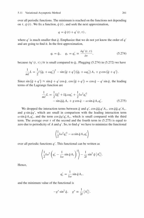
5.11 Variational-Asymptotic Method 261
over all periodic functions. The minimum is reached on the functions not dependingon τ, q (t) . We fix a function, q (t) , and seek the next approximation,
q = q (t)+ q ′ (t, τ ) ,
where q ′ is much smaller that q . Emphasize that we do not yet know the order of q ′
and are going to find it. In the first approximation,
qt = qt , qτ = q ′τ ≡�q ′ (t, τ )
�τ, (5.274)
because �q ′ (t, τ ) /�t is small compared to qt . Plugging (5.274) in (5.272) we have
1
mlL = 1
2l(qt + ωq ′τ
)2 − sin(q + q ′
) (qt + ωq ′τ
)Aτ + g cos
(q + q ′
).
Since sin(q + q ′
) ≈ sin q + q ′ cos q, cos(q + q ′
) = cos q − q ′ sin q, the leadingterms of the Lagrange function are
1
mlL = 1
2lq2
t + lqtωq ′τ +1
2lω2q ′2τ
− sin qqt Aτ + g cos q − ω sin q Aτ q ′τ . (5.275)
We dropped the interaction terms between q and q ′, cos qqt q ′Aτ , cos qqτ q ′Aτ ,
and g sin qq ′, which are small in comparison with the leading interaction termω sin q Aτ q ′τ , and the term cos qq ′q ′τ Aτ , which is small compared with the thirdterm. The average over τ of the second and the fourth term in (5.275) is equal tozero due to periodicity of A and q ′. So, to find q ′ we have to minimize the functional
⟨1
2lω2q ′2τ − ω sin q Aτ q ′τ
⟩
over all periodic functions q ′. This functional can be written as
⟨1
2lω2
(q ′τ −
1
lωsin q Aτ
)2⟩− 1
2lsin2 q
⟨A2
τ
⟩.
Hence,
q ′τ =1
lωsin q Aτ ,
and the minimum value of the functional is
−g∗ sin2 q, g∗ ≡ 1
2l
⟨A2
τ
⟩.

262 5 Direct Methods of Calculus of Variations
Fig. 5.29 Graphs of function1− cos q + k sin2 q fork = π/2 and k = π/10
Finally,
1
ml〈L〉 = 1
2lq2
t + g cos q − g∗ sin2 q. (5.276)
This is the “effective” Lagrange function of the pendulum. The fast vibrationof the suspension point results in the change of the gravitation potential energyg (1− cos q) by an effective potential energy, g
(1− cos q + k sin2 q
), k = g∗/g.
The graph of this potential energy is shown in Fig. 5.29. For small k, the vibrationsare qualitatively similar to vibrations of the usual pendulum, for large k the behaviorchanges: the potential energy gets an additional local minimum at q = π, i.e. theupper equilibrium position of the pendulum becomes stable19.
Example 10. Whitham’s method. Consider a linear homogeneous differential equa-tion with partial derivatives:
P
(�
�t,
�
�x
)u = 0, (5.277)
where P (r, s) is a polynomial of r, s. This equation always has a solution of theform
u = aei(kx−ωt), (5.278)
where a, k, ω are some possibly complex constants. For the function aei(kx−ωt) tobe the solution of (5.277), it is necessary and sufficient for k and ω to satisfy thepolynomial equation
P (−iω, ik) = 0. (5.279)
19 Mathematical justifications and a review can be found in papers by V.I. Yudovich [325] andV. Vladimirov [302].

5.11 Variational-Asymptotic Method 263
Solutions of the type (5.278) are called harmonic waves, a the amplitude, k thewave number, ω the frequency, θ = kx − ωt the phase (for Im a = 0), and (5.279)the dispersion equation. Harmonic waves are fundamental to the theory of linearequations (5.277), particularly due to the fact that any solution of (5.277) can bepresented as a superposition of harmonic waves. The dispersion equation containsall the information about the differential equation and can be used to reconstructuniquely the differential operator.
The following question arises: what is the analogy of the harmonic waves andthe dispersion equation for the non-linear case?
It turns out that the non-linear generalization of the harmonic wave type solu-tions is
u = ψ (a, θ ) , (5.280)
where a, θ are some functions of x, t ,
a = a(x, t), θ = θ (x, t),
and ψ (a, θ ) is a periodic (with a period of 2π ) function of θ . Besides, the character-istic lengths of functions a(x, t), θ,x (x, t), θ,t (x, t) are much greater20 than that ofθ (x, t). The functions a(x, t) corresponds to the amplitude, θ,x to the wave number,and θ,t to the frequency.
Now we construct the equations to determine the functions ψ , a, and θ , if thegoverning equation (5.277) is Euler equation of some functional. More specifically,we take (5.277) as the Euler equation of the functional
∫
�
L(u, ux , ut )dxdt (5.281)
and look for the solutions of this equation of the form
u = ψ (θ, x, t) , (5.282)
where θ is some function of x and t , ψ is a periodic (with a period of 2π ) functionof θ and the characteristic lengths L and T for change of the functions θ,x , θ,t andψ (θ, x, t)|θ=const over x and t are much greater than the characteristic lengths, l andτ, of the phase θ .
The lengths l and τ can be thought of as the largest constants in the inequalities
∣∣θ,x
∣∣ ≤ 2π
l,
∣∣θ,t
∣∣ ≤ 2π
τ. (5.283)
20 For harmonic waves, the quantities a, θ,x , θ,t are constant. Therefore, their corresponding char-acteristic lengths are infinite.

264 5 Direct Methods of Calculus of Variations
The definition of l and τ implies the meaning of the function θ as of oscillationphase: the phase increases on 2π on the lengths of the order of l and the time of theorder of the oscillation period, τ .
The lengths l and τ and the amplitude ψ are defined as the largest constants inthe inequalities
∣∣θ,xx
∣∣ ≤ 2π
ll,
∣∣θ,xt
∣∣ ≤ 2π
l τ,
∣∣θ,xt
∣∣ ≤ 2π
τ l,
∣∣θ,t t
∣∣ ≤ 2π
τ τ,
|�xψ | ≤ ψ
l, |�tψ | ≤ ψ
τ,
∣∣ψ,θ
∣∣ ≤ ψ, (5.284)
where �xψ and �tψ are the partial derivatives, �ψ/�x and �ψ/�t, when θ is keptconstant.
So, the problem contains two small parameters, l/ l and τ/τ .Let us find the derivatives u,x , and u,t ,
u,x = �xψ + ψ,θ θ,x , u,t = �tψ + ψ,θ θ,t .
Due to the estimates (5.283) and (5.284), in the first approximation
u,x = ψ,θ θ,x , u,t = ψ,θ θ,t .
Keeping only the leading terms in the functional, we obtain
∫ ∫
�
L(ψ,ψ,θ θx , ψ,θ θt
)dxdt. (5.285)
Let us cover the region � by the strips, 2πk ≤ θ ≤ 2π (k + 1) , k = 0, 1, 2, . . . .The integral over � can be replaced by the sum of integrals over the strips,
∫ ∫
�
Ldxdt =∑strips
∫ ∫L(ψ,ψθθx , ψθθt )κdθdζ, (5.286)
where ζ is the coordinate along the lines θ = const, κ is the Jacobian of the trans-formation from the variables x, t to the variables θ, ζ . In the first approximation,since θ,x and θ,t change slowly, we may assume that on every strip θ,x , θ,t do notdepend on θ . Therefore, in the first step of the variational-asymptotic method weobtain the same problem for every strip: find the stationary points of the functional
2π∫
0
L(ψ,ψθθ,x , ψθθ,t
)dθ (5.287)
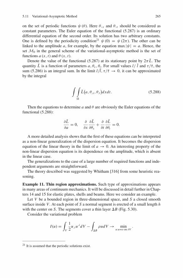
5.11 Variational-Asymptotic Method 265
on the set of periodic functions ψ (θ ). Here θ,x and θ,t should be considered asconstant parameters. The Euler equation of the functional (5.287) is an ordinarydifferential equation of the second order. Its solution has two arbitrary constants.One is defined by the periodicity condition21 ψ (0) = ψ (2π ). The other can belinked to the amplitude a, for example, by the equation max |ψ | = a. Hence, theset M0 in the general scheme of the variational-asymptotic method is the set offunctions a (x, t) and θ (x, t).
Denote the value of the functional (5.287) at its stationary point by 2π L . Thequantity L is a function of parameters a, θx , θt . For small values l/ l and τ/τ , thesum (5.286) is an integral sum. In the limit l/l, τ/τ → 0, it can be approximatedby the integral
∫ ∫
�
L(a, θ,x , θ,t
)dxdt. (5.288)
Then the equations to determine a and θ are obviously the Euler equations of thefunctional (5.288):
�L
�a= 0,
�
�x
�L
�θx+ �
�t
�L
�θt= 0.
A more detailed analysis shows that the first of these equations can be interpretedas a non-linear generalization of the dispersion equation. It becomes the dispersionequation of the linear theory in the limit of a → 0. An interesting property of thenon-linear dispersion equation is its dependence on the amplitude, which is absentin the linear case.
The generalizations to the case of a large number of required functions and inde-pendent arguments are straightforward.
The theory described was suggested by Whitham [316] from some heuristic rea-soning.
Example 11. Thin region approximations. Such type of approximations appearsin many areas of continuum mechanics. It will be discussed in detail further in Chap-ters 14 and 15 for elastic plates, shells and beams. Here we consider an example.
Let V be a bounded region in three-dimensional space, and S a closed smoothsurface inside V . At each point of S a normal segment is erected of a small length hwith the center on S. The segments cover a thin layer �B (Fig. 5.30).
Consider the variational problem
I (u) =∫
V
1
2u,i u
,i dV −∫
�BρudV → min
u:u=o on �V.
21 It is assumed that the periodic solutions exist.

266 5 Direct Methods of Calculus of Variations
Fig. 5.30 Notation forexample 11.
We assume that function ρ is constant along the normal to S and, thus, determinesby its values on S. We are going to find the limit solution as h → 0, if ρ tends toinfinity as
ρ = σ
h
where σ is a function on S.
Denote by u+ and u− the values of u on the two sides of �B. Let us seek min-imum of the functional I (u) in two steps, first minimizing I (u) over all u with theprescribed values of u+ and u−, and then minimizing over u+,u−. We split I (u) intothe sum of two functionals,
I (u) = I1(u)+ I2(u),
I1(u) =∫
V−�B
1
2u,i u
,i dV,
I2(u) =∫
�B
(1
2u,i u
,i − ρu
)dV .
For given u+ and u− these functionals can be minimized separately. We considerfirst the minimization of the functional I2.
We make an assumption that it is enough to consider only smooth functionsu+,u− with the characteristic length l that is much bigger than h. Moreover,the minimizer of I2 has the same characteristic length along S as u+ and u−.Then in the first term of the integrand, 1/2u,i u,i , the derivatives along S can beneglected in comparison with the derivative along the normal, which is of theorder 1/h.
Denote the coordinate along the normal by z,−h/2 � z � h/2. Then in theleading approximation the variational problem for I2 is
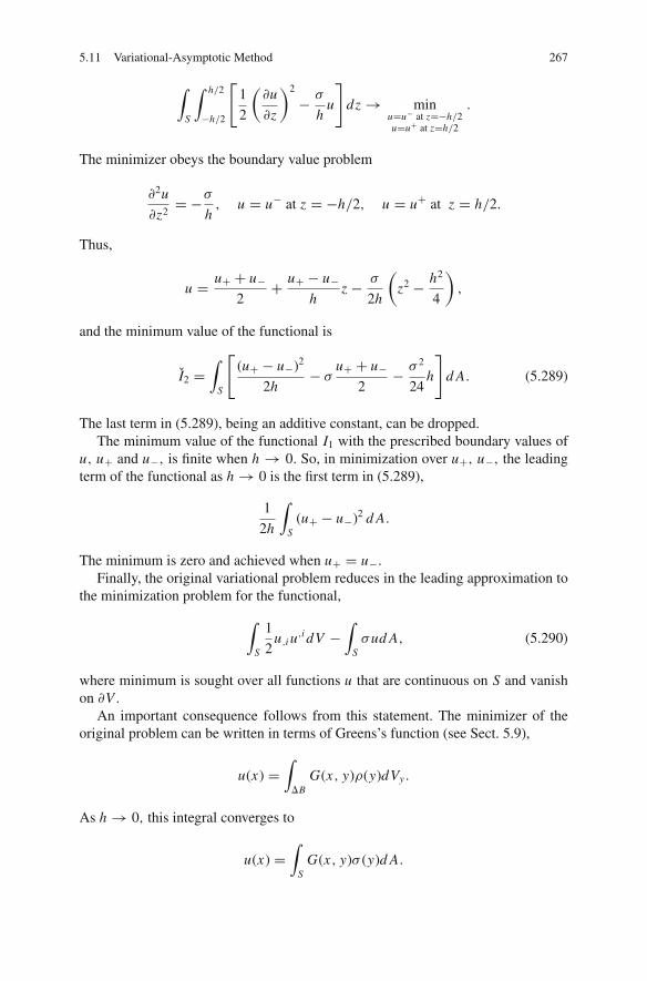
5.11 Variational-Asymptotic Method 267
∫
S
∫ h/2
−h/2
[1
2
(�u
�z
)2
− σ
hu
]dz→ min
u=u− at z=−h/2u=u+ at z=h/2
.
The minimizer obeys the boundary value problem
�2u
�z2= −σ
h, u = u− at z = −h/2, u = u+ at z = h/2.
Thus,
u = u+ + u−2
+ u+ − u−h
z − σ
2h
(z2 − h2
4
),
and the minimum value of the functional is
I2 =∫
S
[(u+ − u−)2
2h− σ
u+ + u−2
− σ 2
24h
]d A. (5.289)
The last term in (5.289), being an additive constant, can be dropped.The minimum value of the functional I1 with the prescribed boundary values of
u, u+ and u−, is finite when h → 0. So, in minimization over u+, u−, the leadingterm of the functional as h→ 0 is the first term in (5.289),
1
2h
∫
S(u+ − u−)2 d A.
The minimum is zero and achieved when u+ = u−.Finally, the original variational problem reduces in the leading approximation to
the minimization problem for the functional,
∫
S
1
2u,i u
,i dV −∫
Sσud A, (5.290)
where minimum is sought over all functions u that are continuous on S and vanishon �V .
An important consequence follows from this statement. The minimizer of theoriginal problem can be written in terms of Greens’s function (see Sect. 5.9),
u(x) =∫
�BG(x, y)ρ(y)dVy .
As h → 0, this integral converges to
u(x) =∫
SG(x, y)σ (y)d A.

268 5 Direct Methods of Calculus of Variations
This must be the minimizer of the variational problem (5.290). On the other hand,the minimizer of the (5.290) obeys the equation on S
[u,i]
ni = −σ.
We arrive at a well-known property of Green’s function:
[∫
S
�G(x, y)
�xiσ (y)d A
]ni = −σ (x).
Now let us move on to the construction of the next approximations. In physicalapplications, they are usually referred to as the refined theories. Refined theoriesare needed in cases when the first approximation is too crude; this can happen ifthe actual values of the small parameter ε are not sufficiently small. The method ofconstructing the refined theories consists of two steps: First, a functional is derivedwhich allows one to obtain the corrections to the solution of the next order of mag-nitude. Second, this refined functional is extrapolated to all, even not small, valuesof ε.
Usually, to construct a refined theory which takes into account the corrections onthe order of α (ε), one should keep in the functional all the terms on the order ofα (ε) compared to unity. We illustrate this statement by the minimization problemfor quadratic functional
I (u, ε) = E (u, ε)− l (u, ε) ,
where E(u, ε) is obtained from a positive symmetric bilinear form E(u, v, ε)
E(u, ε) = E(u, u, ε)
and
E (u, v, ε) = E0 (u, v)+ α (ε) E1 (u, v)+ α′ (ε) E2 (u, v)+ . . .
l (u, v) = l0 (u)+ α (ε) l1 (u)+ α′ (ε) l2 (u)+ . . . , α′ = o (α) , α (ε)→ 0 as ε→ 0.
The functional is minimized on a linear space M. The limit bilinear form E0 (u, v)is obviously positive. The first approximation u0 is the minimum point of thefunctional I0 = E0 (u, u)− l0 (u). The element u0 satisfies the Euler equation
2E0 (u0, u)− l (u) = 0. (5.291)
Equation (5.291) is valid for any element u ∈M.Let us present u as u = u0+u′. Keeping the leading terms containing u′ in I (u, ε)
and using the equality 2E0(u0, u′
) − l(u′) = 0, which follows from (5.291), we
obtain for determining u′ the minimization problem

5.11 Variational-Asymptotic Method 269
I1(u0, u′, ε
) = E0(u′, u′
)+ α (ε) E1(u0, u′
)− α (ε) l1(u′)→ minu′ .
After the substitution u′ → w: u′ = α (ε) w, it becomes the minimization problemfor the functional
α′−2 I1 = E0 (w,w)− 2E1 (u0, w)− l1 (w) ,
which does not depend on small parameter ε. Therefore, u′ ∼ α (ε), and, to incor-porate the corrections of the order α (ε), all terms of the functional of the functionalof the order α (ε) should be kept.
The construction of refined theories will be considered in detail in Chap. 14where the problem of the refinement of the classical shell theory is discussed.
So far, in all cases the functional I0 (u) had the stationary points. It remains todiscuss the cases when the functional I0 (u) does not have stationary points or it ismeaningless.
Case 3: I0 (u) does not have the stationary points or I0 (u) meaninglessSuch a case is not unusual. For example, the function of one variable
f (u, ε) = u + εu2 + sin εu, (5.292)
is such a case, because f0 (u) does not have stationary points.Another example is the minimization problem for the functional
∞∫
ε
1
r
(u2 + u2
,r
)dr (5.293)
on the set of functions u (r ) which are equal to 1 for r = ε. This variational problemarises in the modeling of incompressible flow along an axis-symmetric thin body.The integral (5.293) diverges for ε = 0.
The boundary layer problems also usually belong to this case.In general, there are no recipes for these cases, except, probably, for the following
one: an attempt should be made to reduce these problems to the problems of the typeconsidered earlier by means of a change of the required functions or some othertransformations. For example, for the function (5.292), the substitution: u → v :εu = v, f → g : ε f = g, yields the function
g(v, ε) = v + v2 + ε sin v
which may be studied by the method which has been discussed.As for the boundary layer problems, the applications of the variational methods
are not sufficiently elementary to be presented in an introductory treatment of thesubject (the interested reader is referred to [30]).

270 5 Direct Methods of Calculus of Variations
5.12 Variational Problems and Functional Integrals
In some variational problems, minimization can be replaced by integration. This isa useful trick in studying the stochastic variational problems as will be discussed inChap. 16. Here we explain the relation between minimization and integration.
First, we need a number of auxiliary facts. Consider in some finite-dimensionalspace, Rm, a quadratic form,
(Au, u) = Ai j ui u j . (5.294)
The form is assumed to be positive:
(Au, u) > 0 if u �= 0.
Then the Gauss formula holds true:
∫
Rm
e−12 (Au,u)du = 1√
det A. (5.295)
Here
det A ≡ det∥∥Ai j
∥∥ , du = du1√2π
. . .dum√
2π.
The Gauss formula can be proved by changing the variables, u → u,
ui = λij u
j , det∥∥λi
j
∥∥ = 1,
u j being the coordinates in which the tensor Ai j is diagonal,
(Au, u) = Ai jλii ′λ
jj ′ u′i u′ j = A1
(u1)2 + . . .+ Am
(um)2
. (5.296)
In the new variables,
∫
Rm
e−12 (Au,u)du =
∫
Rm
e− 1
2
(A1(u1)2+...+Am (um )2
)du
= 1√A1 . . . Am
= 1√det A
.

5.12 Variational Problems and Functional Integrals 271
Here we used that22
+∞∫
−∞e−
12 x2
dx =√
2π. (5.297)
The Gauss formula admits the following generalization: for any linear functionof u, (l, u) = li ui ,
√det A
∫
Rm
e−12 (Au,u)+(l,u)du = e
12 (A−1l,l) (5.298)
where A−1 is the inverse matrix to the matrix A. Formula (5.298) follows from(5.295) and the identity
1
2(Au, u)− (l, u) = 1
2
(A(u − A−1l
),(u − A−1l
))− 1
2
(A−1l, l
). (5.299)
Plugging (5.299) in (5.298), changing the variables of integration, u → u+A−1l,and using (5.295), we obtain the right hand side of (5.298).
Consider a quadratic function of a finite number of variables:
I (u) = 1
2(Au, u)− (l, u) , (5.300)
(Au, u) = Ai j ui u j , (l, u) = li u
i . (5.301)
The minimum value of this function is
I = −1
2
(A−1l, l
)(5.302)
and therefore, formula (5.298) can also be written as
e−min
uI (u) =
√det A
∫e−I (u)du. (5.303)
22 Note a witty trick suggested by Poisson to find the value of the integral (5.297):⎛⎝+∞∫
−∞e−
12 x2
dx
⎞⎠
2
=+∞∫
−∞e−
12 x2
dx
+∞∫
−∞e−
12 y2
dy =+∞∫
−∞
+∞∫
−∞e−
12 x2
e−12 y2
dxdy
=+∞∫
−∞
+∞∫
−∞e−
12 (x2+y2)dxdy =
+∞∫
0
2π∫
0
e−12 r2
rdrdθ = 2π
+∞∫
0
e−12 r2
d1
2r2 = 2π.

272 5 Direct Methods of Calculus of Variations
We see that the computation of the minimum value is reduced to integration.Since any quadratic functional in variational problems of continuum mechanicsadmits a finite-dimensional truncation, one can write formula (5.303) for a finite-dimensional truncation, and then consider the limit when the dimension of the trun-cation tends to infinity. In the limit, in the right hand side of (5.303) we obtain whatis called the functional integral. We include
√det A in the definition of the “volume
element” in the functional space,
DAu =√
det Adu (5.304)
and write (5.303) as
emin
uI (u) =
∫e−I (u)DAu. (5.305)
The notation, DAu, emphasizes that the volume element depends on the operator A.
We will need various generalizations of (5.305) involving non-positive quadraticfunctionals and complex-valued functionals. We consider them first in the one-dimensional case.
Formula (5.298) in one-dimensional case,
√A
+∞∫
−∞e−
12 Ax2+lx dx√
2π= e
12
l2
A , (5.306)
remains valid if the number l is complex. Indeed, the integral (5.306) may be con-sidered as an integral in the complex z-plane, z = x + iy, along the real axis,
√A
+∞∫
−∞e−
12 Az2+lz dz√
2π.
The change of variable, z → z1, z = z1 + A−1l, transforms this integral into theintegral over the line in z1-plane, −∞ < x <∞, y = y∗ ≡ − Im
(A−1l
):
√A
+∞∫
−∞e−
12 Az2+lz dz√
2π=√
A
+∞+iy∗∫
−∞+iy∗
e−12 Az2
1dz1√
2πe
l2
2A . (5.307)
The integral of exp[− 1
2 Az2]
over the line [−∞+ iy∗,+∞+ iy∗] is equalto the integral over the real axis [−∞,+∞] . Indeed, compare the integrals ofexp
[− 12 Az2
]over the segments BC and AD (Fig. 5.31). Since the integral of an
analytic function, exp[− 1
2 Az2]
over a closed contour ABCD is zero, the differenceof these integrals is equal to the sum of integrals of exp
[− 12 Az2
]of the segments

5.12 Variational Problems and Functional Integrals 273
Fig. 5.31 To the proof of(5.306) for complex l
AB and C D. The latter tend to zero as these segments are moved to infinity because∣∣∣e− 12 Az2
∣∣∣ on these segments tends to zero. Hence, the right hand side of (5.307) is
equal to exp[
12A l2
], and (5.306) holds true.
Two forms of (5.306) will be needed further: one is obtained by replacing l by il(with real l):
√A
+∞∫
−∞e−
12 Ax2+ilx dx√
2π= e−
12A l2
(5.308)
and another by replacing l by i√
zl with real l and any complex number z:
√A
+∞∫
−∞e−
12 Ax2+i
√zlx dx√
2π= e−z 1
2A l2, (5.309)
In this and all further formulas the argument of a complex number, z = |z| eiθ , isconstrained by the condition−π ≤ θ ≤ π, and the square root of a complex numberis understood as
√z = |z|1/2 eiθ/2. In particular, if z lies in the right half-plane,
Re z ≥ 0, then Re√
z ≥ 0.
A useful form of (5.304) is obtained if we change the variable of integration,x → v : v = i x and integrate over the imaginary axes, [−i∞,+i∞]:
√A
+i∞∫
−i∞e
12 Av2+√zlv dv√
2π i= e−z 1
2A l2. (5.310)
Changing l by −l, one can also write (5.310) in the form
√A
+i∞∫
−i∞e
12 Av2−√zlv dv√
2π i= e−z 1
2A l2. (5.311)
For Re z > 0, one can put (5.311) in the form

274 5 Direct Methods of Calculus of Variations
√Az
+i∞∫
−i∞ez( 1
2 Av2−lv) dv√2π i= e−z 1
2A l2. (5.312)
To prove (5.312) we get rid of the linear term in the exponent by making thechange, v → v + l
A . The line of integration can be moved back to imaginary axessimilarly to the move of the line of integration in proving (5.306). It remains to showthat
√Az
+i∞∫
−i∞e
12 z Av2 dv√
2π i= 1 (5.313)
for complex z, Re z > 0. Denote Argz by θ ; |θ | < π/2 since Re z > 0. Let usmake the change of variables, v→ w = ξ + iη : w = v
√z. The line of integration
in w-plane is the line passing through the points A, B shown in Fig. 5.32; denote itby L . We have
√Az
+i∞∫
−i∞e
12 z Av2 dv√
2π i=√
A∫
L
e12 Aw2 dw√
2π i. (5.314)
The integral over the segment C B is estimated as
Fig. 5.32 To the proof(5.313)

5.12 Variational Problems and Functional Integrals 275
∣∣∣∣∣∣
∫
C B
e12 A(ξ 2−η2+2iξη)dξ
∣∣∣∣∣∣≤ e−
12 Aη2
η tan(θ/2)∫
0
e12 Aξ 2
dη ≤
≤ ηe−12 A(η2−η2 tan2(θ/2)). (5.315)
Since |tan (θ/2)| < 1, the right hand side of (5.315) tends to zero as the segmentC B moves to infinity. Similarly, the integral over AD tends to zero as well. Thus,integral over L in (5.314) can be replaced by integral over the imaginary axis, andwe arrive at (5.313).
It is essential for what follows that z in (5.312) can also be taken as pure imagi-nary: Re z = 0, z �= 0. For pure imaginary z the integral (5.312) does not convergeabsolutely and needs to be defined. We define it as the following limit:
√Az
+i∞∫
−i∞ez( 1
2 Av2−lv) dv√2π i= lim
ε→+0
√A(z + ε)
+i∞∫
−i∞e(z+ε)( 1
2 Av2−lv) dv√2π i
.
Since
limε→+0
√A(z + ε)
+i∞∫
−i∞e(z+ε)( 1
2 Av2−lv) dv√2π i= lim
ε→+0e−(z+ε) 1
2A l2 = e−z 12A l2
,
we see that (5.312) holds for pure imaginary z as well.23
If Re z < 0, then (5.312) can be replaced by the equation
√−Az
+∞∫
−∞ez( 1
2 Au2−lu) du√2π= e−z 1
2A l2,
where integration is conducted over real u. This equation follows from (5.312) bychanging the integration variable v→ u : v = iu, and replacing l → il, z→−z.
23 Putting in (5.312) A = 1, l = 0, z = i, v = i x we obtain
√i
+∞∫
−∞e−i 1
2 x2 dx√2π= 1,
which yields the well-known relations
+∞∫
−∞cos
1
2x2dx = √π,
+∞∫
−∞sin
1
2x2dx = √π.

276 5 Direct Methods of Calculus of Variations
Another useful form of (5.312) is obtained if we replace z by 1/z (Re z−1 ≥ 0 ifRe z ≥ 0, so such a replacement is legitimate) and l by lz :
√1
zA
+i∞∫
−i∞e
12z Av2−lv dv√
2π i= e−z 1
2A l2. (5.316)
The finite-dimensional forms of (5.308), (5.309), (5.310), (5.311), (5.312) and(5.316) are:
√det A
∫
Rm
e−12 (Au,u)+i(l,u)du = e−
12 (A−1l,l), (5.317)
√det A
∫
Rm
e−12 (Au,u)+i
√z(l,u)du = e−
12 z(A−1l,l), (5.318)
√det A
+i∞∫
−i∞e
12 (Av,v)+√z(l,v)dv = e−
12 z(A−1l,l), (5.319)
√det A
+i∞∫
−i∞e
12 (Av,v)−√z(l,v)dv = e−
12 z(A−1l,l), (5.320)
√zm det A
+i∞∫
−i∞ez( 1
2 (Av,v)−(l,v))dv = e−12 z(A−1l,l), (5.321)
√1
zmdet A
+i∞∫
−i∞e
12z (Av,v)−(l,v)dv = e−
12 z(A−1l,l). (5.322)
For brevity, the imaginary unity is included in the “volume element”:
dv = dv1√2π i
dv2√2π i
. . .dvm√2π i
.
These relations are proved by transforming the coordinates to the principal coor-dinates of the tensor Ai j .
For Re z < 0, the similar relation is
√(−z)m det A
∞∫
∞ez( 1
2 (Av,v)−(l,v))dv = e−12 z(A−1l,l). (5.323)

5.12 Variational Problems and Functional Integrals 277
Tending the dimension to infinity, we find the following formulas linking theminimum values of quadratic functionals with integration in functional spaces: forarbitrary z,
emin
uI (u) =
∫e−
12 (Au,u)+i(l,u)DAu, (5.324)
ez min
uI (u) =
∫e−
12 (Au,u)+i
√z(l,u)DAu, (5.325)
ez min
uI (u) =
+i∞∫
−i∞e
12 (Av,v)+√z(l,v)DAv, (5.326)
for Re z > 0,
ez min
uI (u) =
+i∞∫
−i∞ez[ 1
2 (Av,v)−(l,v)]Dz Av =+i∞∫
−i∞ezI (v)Dz Av, (5.327)
ez min
uI (u) =
+i∞∫
−i∞e
12z (Av,v)−(l,v)D 1
z Av, (5.328)
for Re z < 0,
ez min
uI (u) =
∞∫
−∞ez[ 1
2 (Au,u)−(l,v)]D−z Au =∞∫
−∞ezI (u)D−z Au. (5.329)
In (5.327), (5.328) and (5.329) the parameter, z, is also included in the volumeelement: for m−dimensional truncation,
Dz Av = √zm det Adv,D 1z Av = √z−m det Adv,D−z Au =
√(−z)m det Adu.
In the right hand sides of (5.324)-(5.328) l can be replaced by −l because the lefthand sides remain the same for such change.
Let now the functional (Au, u) be non-convex, i.e. it can take negative values forsome u. Formula (5.327) still holds if we assume that (Au, u) is a non-degeneratedfunctional ( i.e. (Au, u) �= 0 for any u �= 0), and, thus, the functional I (u) =12 (Au, u) − (l, u) has a unique stationary point. Then, denoting by S.V.I (u)24 the
24 S.V. stands for stationary value.

278 5 Direct Methods of Calculus of Variations
value of I (u) at the stationary point and admitting in (5.327) only pure imaginary zwe get
ezS.V.I (u) =+i∞∫
−i∞ezI (v)Dz Av. (5.330)
The usefulness of such relations will be illustrated in Vol. 2.
5.13 Miscellaneous
In this section we collect some simple facts which help in working with variationalproblems.
Euler equations in curvilinear coordinates. In physical problems, the action func-tional is invariant with respect to the choice of coordinate system. This allows oneto write easily the equations for the minimizer in curvilinear coordinates. We illus-trate that by the following example. Let x, y be Cartesian coordinates. Consider thefunctional of functions of two variables, u(x, y),
I (u) = 1
2
∫
V
((�u
�x
)2
+(
�u
�y
)2)
dxdy. (5.331)
The Euler equation of this functional is Laplace’s equation,
� u = 0.
We wish to write this equation in polar coordinates, r, θ. To this end, we rewritethe functional in polar coordinates. Since
(�u
�x
)2
+(
�u
�y
)2
=(
�u
�r
)2
+(
1
r
�u
�θ
)2
, dxdy = rdrdθ,
we have
I (u) = 1
2
∫
V
(r
(�u
�r
)2
+ 1
r
(�u
�θ
)2)
drdθ.
This functional must be stationary with respect to u(r, θ ) at the minimizer. Thus,
�
�rr
�u
�r+ �
�θ
1
r
�u
�θ= 0.

5.13 Miscellaneous 279
This is the equation required. Derivation in other cases is similar.
Evenness and oddness of the minimizer. Let the admissible functions of a varia-tional problem be defined in a symmetric domain V , i.e. the domain, which containswith each point x the point −x . Then one can introduce the notion of evenness andoddness: function u(x) is even if
u(−x) = u(x),
and odd if
u(−x) = −u(x).
Each function may be uniquely presented as a sum of an even and an odd func-tions:
u(x) = u′(x)+ u′′(x), u′(−x) = −u′(x), u′′(−x) = u′′(x). (5.332)
Indeed, u′(x) and u′′(x) can be found uniquely in terms of u(x) from (5.332):
u′(x) = 1
2(u(x)− u(−x)), u′′(x) = 1
2(u(x)+ u(x)).
If the functional I (u) splits in the sum of functionals I (u′) + I (u′′) and the con-straints on admissible functions can be formulated as constraints to their odd andeven parts, then the entire variational problem splits into two independent simplerproblems for u′(x) and u′′(x). For example, if the region, V , in (5.331) is symmetric,then
I (u) = I (u′)+ I (u′′),
because ∇u′ and ∇u′′ are even and odd vector fields, respectively,25 therefore∫ ∇u′∇u′′dxdy = 0. If the boundary values of u are prescribed, and they are even,then the boundary values of u′ are zero, and minimization over u′ yields u′ = 0. So,it is enough to perform minimization only over even functions. Similar argumentshold if the region is symmetric only with respect to one variable.
Divergence terms. If Lagrangian contains a divergence term, e.g.,
L
(u,
�u
�xi
)= L0
(u,
�u
�xi
)+ �
�xiPi
(u,
�u
�xi
),
then this term does not contribute to Euler equation. That follows from the diver-gence theorem,
25 I.e. ∇u′∣∣−x= ∇u′
∣∣x
and ∇u′′∣∣−x= − ∇u′′
∣∣x.

280 5 Direct Methods of Calculus of Variations
∫
VL
(u,
�u
�xi
)dV =
∫
VL0
(u,
�u
�xi
)dV +
∫
�VPi
(u,
�u
�xi
)ni d A.
We see that the divergence term contributes only to the boundary conditions.
Derivative of minimum value with respect to parameter. Consider a variationalproblem, the functional of which depends on a parameter, r :
I = minu
I (u, r ).
The minimizer, u, depends on the parameter, u = u(r ), and so does the minimumvalue: I = I (u(r ), r ). The following formula holds true:
d I
dr= �I (u, r )
�r
∣∣∣∣u=u(r )
. (5.333)
The proof is simple:
d I (u(r ), r )
dr=(
δ I
δu
∣∣∣∣u=u(r )
,du(r )
dr
)+ �I (u, r )
�r
∣∣∣∣u=u(r )
.
The first term in the right hand side is zero, because u(r ) is the minimizer.
A modification of variational problems. Let the functional I (u, v) have a station-ary point, u∗, v∗, and v∗ can be explicitly computed in terms of u∗ : v∗ = �(u∗),where �(u∗) is a function or an operator. Then u∗ is a stationary point of the func-tional
I (u) = I (u, �(u)). (5.334)
Indeed,
δ I (u) =(
δ I (u, v)
δu
∣∣∣∣v=�(u)
, δu
)+(
δ I (u, v)
δv
∣∣∣∣v=�(u)
,δ�(u)
δu· δu
).
After substitution u = u∗ in the left hand side both terms vanish, thus δ I (u) = 0 asclaimed. Note that the substitution may result in appearance of additional stationarypoints, for which δ I (u, v)/δv|v=�(u) �= 0. We will use this point in transformationsof variational principles of fluid mechanics.
Stationary points of complex-valued functionals and Cauchy-Riemann equa-tions. Let S(v) be a complex-valued functional of complex-valued functions, v. Wedenote their real and imaginary parts by S1, S2 and v1, v2 :
S = S1(v1, v2)+ i S2(v1, v2), v = v1 + iv2.

5.13 Miscellaneous 281
Suppose that the functional S(v) is smooth, i.e. its variation, δS, is a linear functionalof δv, which we denote by
(δS
δv, δv
).
The scalar product (A, δv) is supposed to obey the two conditions: first, it is linearwith respect to both arguments on the set of complex numbers, i.e. for any complexnumbers, c1 and c2,
(c1 A1 + c2 A2, δv) = c1(A1, δv)+ c2(A2, δv),
(A, c1δv1 + c2δv2) = c1(A, δv1)+ c2(A, δv2);
second, if (A, δv) = 0 for any δv, then A = 0. Therefore, if the equation
(δS
δv, δv
)= (A, δv)
holds for any δv, then
δS
δv= A.
Under these assumptions the following generalized Cauchy-Riemann equationshold:
δS1
δv1= δS2
δv2,
δS2
δv1= −δS1
δv2. (5.335)
Indeed, let us vary v1. Then variation of the functional S(v) is
(δS1(v1, v2)
δv1, δv1
)+(
iδS2(v1, v2)
δv1, δv1
).
On the other hand, since S is a functional of v, the same variation is
(δS
δv, δv
)= (ξ + iη, δv1) ,
δS
δv≡ ξ + iη,
where ξ and η are some real-valued operators. Equating both expressions and usingarbitrariness of variations, we obtain the relations,
δS1
δv1= ξ,
δS2
δv1= η.
Similarly, if we vary v2, we have for the variation of S(v)

282 5 Direct Methods of Calculus of Variations
(δS1(v1, v2)
δv2, δv2
)+(
iδS2(v1, v2)
δv2, δv2
).
This must be equal to
(δS
δv, δv
)= (ξ + iη, iδv2) .
Hence,
δS1
δv2= −η,
δS2
δv2= ξ.
So we arrived at (5.335).If S = S1+i S2 is a complex-valued functional of complex-valued functions, v =
v1 + iv2, then, varying v1 and v2, we obtain the system of Euler equations for thestationary points:
δS1(v1, v2)
δv1= 0,
δS2(v1, v2)
δv1= 0,
δS1(v1, v2)
δv2= 0,
δS2(v1, v2)
δv2= 0.
At first glance we have four equations for two functions, v1 and v2. In fact,however, due to (5.335), only two of these equations are independent. As such,we can take the equations, obtained by varying only the real part of the functional,S1(v1, v2) :
δS1(v1, v2)
δv1= 0,
δS1(v1, v2)
δv2= 0. (5.336)
Part IIVariational Features of Classical
Continuum Models
In continuum mechanics, many seemingly unrelated variational principles have beeninvented. What follows is an attempt to present these variational principles system-atically, point out their interrelations, and fill in some gaps. Usually, the variationalprinciples have several equivalent forms; the form depends on the choice of argu-ments of the action functional. The initial formulation of the variational principles,which directly follows from the principle of least action, employs the particle trajec-tories x (X, t) as arguments of the action functional. Such a formulation is usuallyconvenient in mechanics of solids. As a rule, the problems of fluid mechanics arebetter suited for being stated and investigated when the arguments of the actionfunctional are the functions of Eulerian coordinates. Such variational principlesare derived from initial “Lagrangian coordinate” formulations by the correspondingchange of sought functions. Further transformations are based on the idea of duality.The chapters related to the mechanics of solids and to fluid mechanics can be readindependently.
283

Chapter 6Statics of a Geometrically Linear Elastic Body
6.1 Gibbs Principle
Gibbs principle. Equilibrium of elastic bodies is governed by Gibbs variationalprinciples. We will use as a starting point the second Gibbs principle. We assumethat the positions of the boundary particles are given at some part of the boundary,�Vu,
x (X ) = x(b) (X ) for X ∈ �Vu, (6.1)
while on the remaining part of the boundary, �V f , the surface forces, fi , are known.Gibbs variational principle. Equilibrium states of elastic body correspond to theminimum of the functional
I (x (X ) , S (X )) =∫
V
ρ0U(xi
a, S)
dV −∫
�V f
fi xi (X ) d A (6.2)
on the set of all functions xi (Xa) obeying the boundary conditions (6.1) and func-tions S (Xa) subject to the constraint
∫
V
ρ0SdV = S0. (6.3)
Strictly speaking, Gibbs variational principle selects the stable equilibrium states.There might be unstable equilibrium states which correspond to the stationary pointsof the functional (6.2). Functional (6.2) is called energy functional.
Minimization with respect to entropy can be carried out explicitly by introducingthe Lagrange multiplier, T, for the constraint (6.3). One has to minimize over S thefunctional
∫
V
ρ0U(xi
a, S)
dV − T
⎛⎜⎝∫
V
ρ0SdV − S0
⎞⎟⎠−
∫
�V f
fi xi (X ) d A.
V.L. Berdichevsky, Variational Principles of Continuum Mechanics,Interaction of Mechanics and Mathematics, DOI 10.1007/978-3-540-88467-5 6,C© Springer-Verlag Berlin Heidelberg 2009
285

286 6 Statics of a Geometrically Linear Elastic Body
Introducing free energy,
F(xi
a, T) = min
S
[U(xi
a, S)− T S
], (6.4)
we have
minS
I (x (X ) , S (X )) =∫
V
ρ0 F(xi
a, T)
dV −∫
�V f
fi xi (X ) d A + T S0. (6.5)
The parameter T has the meaning of absolute temperature at which the equilib-rium is achieved.
The functional (6.5) in which the additive constant T S0 is dropped will be de-noted by I (x (X )). We arrived at the following version of Gibbs principle.Gibbs variational principle. Equilibrium states of an elastic body correspond tothe minimum of the energy functional
I (x (X )) =∫
V
ρ0 F(xi
a, T)
dV −∫
�V f
fi xi (X ) d A (6.6)
on the set of all functions xi (Xa) satisfying the boundary conditions (6.1).Note that for inhomogeneous elastic bodies, internal energy and, correspond-
ingly, free energy depend explicitly on Lagrangian coordinates but, for brevity, theyare not mentioned explicitly among the arguments.
Free energy density F(xi
a, T)
is invariant with respect to rigid rotation. There-
fore, the distortion enters into F only in combinations, εab = 12
(gijx i
a x jb − gab
):
F = F (εab, T ) .
If the elastic material is also subject to the body forces with the force per unitmass gi , then an additional term must be included in the energy functional
I (x (X )) =∫
V
ρ0 F (εab, T ) dV −∫
V
ρ0gi xi (X ) dV −
∫
�V f
fi xi (X ) d A. (6.7)
Geometrically linear deformation. By geometrically linear deformation one meansthe case when the displacements
ui = xi(Xa)− x i
(Xa)
and their gradients are small. The gradients of displacements are dimensionless,denote their order by ε. In geometrically linear theory one neglects the terms on theorder of ε in comparison with unity. This yields several simplifications. First, thestrain tensor becomes a linear function of the displacement gradients:

6.1 Gibbs Principle 287
εab = 1
2(gab − gab) = 1
2
(gij
(�x i
�Xa+ �ui
�Xa
)(�x j
�Xb+ �u j
�Xb
)− gab
)=
= 1
2gij
(x i
a
�u j
�Xb+ x j
b
�ui
�Xa
). (6.8)
For Cartesian Eulerian coordinates coinciding with the Lagrangian coordinates inthe initial state, gij = δij, x i
a = δia, and (6.8) becomes
εab = 1
2
(�ua
�Xb+ �ub
�Xa
). (6.9)
Second, the derivatives with respect to Eulerian coordinates and Lagrangian co-ordinates coincide:
�
�Xa= xi
a
�
�xi=(
x ia +
�ui
�Xa
)�
�xi= x i
a
�
�xi= �
�xa.
Third, the components of tensors in Eulerian coordinates and the Lagrangiancoordinates coincide within the accuracy accepted because
xia = x i
a +�ui
�Xa≈ x i
a = δia .
Hence, only Eulerian indices can be used. In particularly, (6.9) will be written as
εij = 1
2
(�ui
�x j+ �u j
�xi
)= u(i, j). (6.10)
Fourth, due to smallness of displacements, one does not need to distinguish theinitial region occupied by the body, V , and the final region, V . Accordingly, theregions of integration in the energy functional (6.7) can be taken coinciding withthe corresponding regions in the deformed state. Therefore, one can drop the index0 in the region notation in (6.7). Fifth, the densities in the deformed and undeformedstates differ by terms of the order ε. Densities enter in all relations as factors atsmall terms. Thus, distinguishing the initial and final densities would yield onlysmall corrections. Therefore, in linear theory densities in the initial and the deformedstates can be identified. Further we drop index 0 in ρ0 in (6.7) and assume that ρ isthe given initial density. We will include the factor ρ in free energy density, so inwhat follows F means the free energy per unit volume. Besides, we will not mentionexplicitly temperature as an argument of F. Finally, replacing in (6.7) the particlepositions, xi (Xa) , by the displacement vector, ui (x) , and dropping the additiveconstants we obtain for the energy functional of elastic body in case of geometricallylinear deformation the following formula:

288 6 Statics of a Geometrically Linear Elastic Body
I (u) =∫
V
F(εij)
dV − l (u) , (6.11)
l (u) =∫
V
ρgi ui dV +
∫
�V f
fi ui d A.
Minimum of the energy functional is sought on the set of displacements whichhave the prescribed values on �Vu :
ui (x) = u(b)i on �Vu . (6.12)
Obviously, the minimum is achieved at the stress field,
σ i j = �F(εi j )
�εi j,
satisfying the equations,
�σ i j
�x j+ ρgi = 0 in V, σ i j n j = f i on �V f .
Without loss of generality, the energy density F may be assumed to possess theproperties:
F |εi j=0 = 0,�F
�εi j
∣∣∣∣εi j=0
= 0. (6.13)
If (6.13) were not held, one can replace F by F = F − F0 − σi j0 εi j , where F0 =
F |εi j=0 , σi j0 = �F/�εi j
∣∣εi j=0, and replace also gi and fi by gi = gi + σ
i j0, j , fi =
fi − σi j0 n j . However, such a replacement would change the physical meaning of
gi and fi as densities of the external body and surface forces. In what follows, weprefer to keep this original meaning. A continuum model with the energy func-tional (6.11) is called physically nonlinear and geometrically linear elastic body.Physically and geometrically linear elastic body corresponds to quadratic functionF(εi j ).
Physical meaning of energy functional. If an elastic body is deformed by the pre-scribed boundary displasments, then the energy functional coincides with the freeenergy of the body, and its minimum value is the free energy at equilibrium. Ifthe prescribed boundary displacements are zero, and the body is deformed by anexternal force, then, in linear theory, according to the Clapeyron theorem (5.46),the minimum value of the functional is equal to negative energy. If the body isdeformed by both the prescribed non-zero displacements and external forces, thensuch simple interpretations of the minimum value of the energy functional are lost.

6.2 Boundedness from Below 289
The question arises: What is the physical meaning of the energy functional to beminimized to determine the equilibrium states? The answer can be sought by study-ing a microscopical system that is described at the macro-level by the model of anelastic body. One can expect that the energy functional is the average of the Hamil-tonian of the microsystem. The first term of the energy functional, energy, is theresult of averaging of the energy of the microsystem. To interpret the second term,a linear functional, we recall that the action of an external force, f, on a particlewith a generalized coordinate, q, is described by the term in Hamiltonian, − f q.
Therefore, the linear functional l (u) may be thought of as the average value of allterms in the micro-Hamiltonian of the form f q.
The issue on the physical meaning of the energy functional becomes especiallyimportant, when one complicates the elasticity model by taking into account addi-tional phenomena, like cracks, dislocations or an interaction with electro-magneticfield. The guiding principle in a proper construction of the energy functional is thatthe energy functional has the meaning of the averaged micro-Hamiltonian of thesystem.
Consider now the conditions under which the minimization problem for the en-ergy functional (6.11) is well posed.
6.2 Boundedness from Below
Uniqueness. First let no kinematic constraints be imposed (i.e. the surface tractionsare prescribed everywhere on �V , and �V = �V f ). Then the elastic energy has akernel: it becomes zero on the infinitesimally small rigid motions:
ui = ci + eijkϕj xk . (6.14)
According to the necessary condition for the boundedness from below (5.30), thelinear part of the functional I (u) must vanish on the fields (6.14):
∫
V
ρgi dV +∫
�V
fi d A = 0, eijk
⎛⎝∫
V
ρg j xkdV +∫
�V
f i xkd A
⎞⎠ = 0. (6.15)
Equations (6.15) mean that the resultant and the total moment of the external forcesacting on the body are equal to zero.
Let us assume that the conditions (6.15) are satisfied. Then the energy functionalis invariant with respect to rigid motions (6.14), and the minimizing element is notuniquely determined. To single out a unique solution, one has to impose additionalconstraints which exclude rigid motions. As such one can take the condition of zeroaverage displacement,

290 6 Statics of a Geometrically Linear Elastic Body
∫
V
ui dV = 0 (6.16)
and zero average rotation
eijk∫
V
ui x j dV = 0. (6.17)
Let the elastic properties be non-degenerated in the sense that, for some positiveconstant μ and for any εij,
μεijεi j ≤ F
(εij). (6.18)
Then the conditions (6.15) are also sufficient conditions for the boundedness frombelow of the energy functional. In order to see that, we need the inequality
l (u) ≤ c
√√√√∫
V
F(u(i, j)
)dV . (6.19)
If the inequality (6.19) holds, the boundedness from below is obtained in the sameway as in Example 3 in Sect. 5.1.
The proof of the inequality (6.19) is based on one of the key inequalities of theelasticity theory, the Korn inequality:
∫
V
ui, j ui, j dV ≤ K
∫
V
εijεi j dV . (6.20)
For the Korn inequality to be valid the additional conditions, excluding the rota-tions of the body, must be imposed; otherwise, for the rotations, the left hand sideof (6.19) is positive while the right hand side is equal to zero. Usually, either thecondition (6.17) or the condition
∫
V
(ui, j − u j,i
)dV = 0
is used.The Korn inequality can be written in a more impressive form by splitting the
displacement gradient into the sum of the deformation and the rotation parts:
ui, j = εij + eijkϕk, ϕk = 1
2eijkui, j .
In terms of εij and ϕi the Korn inequality takes the form

6.2 Boundedness from Below 291
∫
V
ϕiϕi dV ≤ K − 1
2
∫
V
εijεi j dV .
This means that for any deformation of the body, the average value of the squaredangle of rotation never exceeds the average value of the squared strains times auniversal coefficient, K−1
2 , which depends only on the geometry of the region. Theproof of the Korn inequality can be found in the works cited in the bibliographiccomments.
To prove (6.19) we also need the inequalities
λ2∫
�V
ui ui d A ≤
∫
V
ui, j ui, j dV, μ2
∫
V
ui ui dV ≤
∫
V
ui, j ui, j dV . (6.21)
These inequalities are obtained by summing the inequalities (5.38) written for eachcomponent of the displacement vector. Inequalities (6.21) are valid if the transla-tional motions are excluded by, for example, conditions (6.16).
Let us derive (6.19). From (6.18), (6.20), (6.21), and the Cauchy inequality, wehave
|l (u)| ≤√√√√∫
V
ρgi gi dV
√√√√∫
V
ui ui dV +√√√√∫
�V
fi f i d A∫
�V
ui ui d A ≤
≤ c
√√√√∫
V
ui, j ui, j dV ≤ c
√√√√K∫
V
εijεi j dV ≤ c
√K
μ
√√√√∫
V
F(εij)
dV .
Here,
c = 1
μ
√√√√∫
V
ρgi gi dV + 1
λ
√√√√∫
�V
fi f i d A. (6.22)
So, the energy functional is bounded from below if the squared surface forces areintegrable on the surface while the body forces are integrable in the volume.
In the case when the displacements are given on a part of the boundary, the energyfunctional is bounded from below for any functions, gi and fi , including those whichhave non-zero total force and non-zero total moment. Let us outline the proof whenthe displacements are given on the entire boundary �V .
Consider the integral
2∫
V
εijεi j dV =
∫
V
(ui, j u
i, j + ui, j uj,i)dV .
Integrating the second term by parts twice, we get

292 6 Statics of a Geometrically Linear Elastic Body
2∫
V
εijεi j dV =
=∫
V
(ui, j u
i, j + (ui,i
)2)
dV +∫
�V
(ui u
j,i n j − ui ni uk,k
)d A. (6.23)
The surface integral depends only on the displacements at the boundary. Indeed,expanding the derivative along the normal and tangent directions (see Sect. 14.1),we have
ui uj,i n j − ui ni u
k,k = uir
iαu j,αn j − ui ni u
k,αrα
k
Hence, the surface integral is known due to the boundary conditions; we will de-noted it by B. Dropping in the identity (6.23) the integral of
(ui
,i
)2which is non-
negative, we obtain the inequality
∫
V
ui, j ui, j dV ≤ 2
∫
V
εijεi j dV − B,
which is a version of the Korn inequality. Analogous changes appear in the inequal-ities (6.21). Further steps are the same as in the case of given surface forces.
The boundedness from below of the energy functional shows that Gibbs principleis well-posed for the energy functional. The existence of the minimizing element inthe energy space is established following the general scheme of Sect. 5.3.
Let the free energy density be a strictly convex function of the components of thestrain tensor. The physical interpretation of this assumption can be seen from theinequality (5.89). Writing this inequality for function F , we have
0 < �σ i j �εij. (6.24)
Here,
σ i j = �F
�εij
are the components of the stress tensor, �εij is the difference between any two valuesof the strain tensor, and �σ i j is the difference between the corresponding values ofthe stress tensor. Inequality (6.24) means that there is a one-to-one correspondencebetween the values of the stress tensor and the strain tensor. Besides, the stressesmonotonously increase with increasing strains in the following sense. In the princi-pal coordinate system of the tensor �εij the inequality (6.24) becomes
0 < �σ 11�ε11 + �σ 22�ε22 + �σ 33�ε33.

6.3 Complementary Energy 293
Consequently, the stress increment �σ 11 (for ε22 = ε33 = 0) has the same sign asthe strain increase ε11 for any (not necessarily small) �ε11.
For strictly convex function, F(εij), the energy functional is a strictly convex
functional on the set of displacements with excluded rigid motions. As shown inSect. 5.4, it has the only minimizing element.
6.3 Complementary Energy
Consider the Young-Fenchel transformation of function F(εij)
with respect to εij:
F∗(σ i j
) = maxεij
[σ i jεij − F
(εij)]
. (6.25)
Here, σ i j are the components of a symmetric tensor. The function F∗(σ i j
)is called
the complementary energy. This term was motivated by the following geometricalinterpretation of F∗. Consider the constitutive equation of a one-dimensional elasticbody, σ = σ (ε). The dependence σ = σ (ε) is shown in Fig. 6.1. Since σ = �F/�ε,
F (ε) =ε∫
0
σ (ε) d ε.
Hence, the energy F (ε) is equal to the area beneath the curve σ = σ (ε) inFig. 6.1; this area is vertically shaded. The number F∗ (σ ) = σε − F (ε) is equalto the area of the figure horizontally shaded. This area “complements” F (ε) tothe area of the rectangle, σε. In a multi-dimensional case, this simple geometricinterpretation is lost.
Fig. 6.1 For one-dimensionaldeformation, energy is equalto the area covered by thevertical shade, while thecomplementary energy isequal to the area shadowedby the horizontal lines

294 6 Statics of a Geometrically Linear Elastic Body
6.4 Reissner Variational Principle
Let us represent the free energy density by means of its Young-Fenchel transforma-tion:
F(εij) = max
σ i j
[σ i jεij − F∗
(σ i j
)]. (6.26)
Reissner variational principle. The true state of an elastic body is a stationarypoint of the functional
I (σ, u) =∫
V
(σ i j ui, j − F∗
(σ i j
))dV −
∫
V
ρgi ui dV −
∫
�V f
fi ui d A (6.27)
on the set of all symmetric tensor fields, σ i j (x), and the fields,ui (x), obeying theconstraints
ui (x) = u(b)i on �Vu .
This statement follows from the general duality theory because
minu∈(6.12)
I (u) = minu∈(6.12)
maxσ
I (σ, u) . (6.28)
The solution of the minimax problem for the functional (6.27) is a saddle point,i.e. at this point I (σ , u) has maximum with respect to functions σ i j and the mini-mum with respect to functions ui . Sometimes this variational principle is also calledthe mixed variational principle.
6.5 Physically Linear Elastic Body
Assume that there is a stress-free state of the body. We choose the initial state of thebody coinciding with the stress-free state. Then,
σ i j = �F(εij)
�εij= 0 at εij = 0.
Expanding F(εij) over εij near the point εij = 0 and keeping only the leadingterms, we have
F(εij) = F(0)+ 1
2Cijklεijεkl . (6.29)
Elastic material with energy (6.29) is called physically linear. For physically lin-ear elastic material, the stresses σ i j depend linearly on strains:
σ i j = Cijklεkl . (6.30)

6.5 Physically Linear Elastic Body 295
Since εij is a symmetric tensor, the antisymmetric parts of Cijkl with respect toindices i j , kl and with respect to the transposition of the index couples (i, j) and(k, l) do not contribute to energy. Therefore, without loss of generality, one canaccept the symmetry properties for the elastic moduli:
Cijkl = Cjikl, Cijkl = Ci jlk, Cijkl = Cklij. (6.31)
The inverse tensor, i.e. the tensor defined by the equations
C (−1)ijkl Cklmn = δ
(mi δ
n)j , (6.32)
is called the tensor of elastic compliances. This tensor, by definition, possesses thesame symmetry properties as Cijkl :
C (−1)ijkl = Cjikl, C (−1)
ijkl = C (−1)i jlk , C (−1)
ijkl = C (−1)klij . (6.33)
Contracting (6.30) with the tensor of elastic compliances, one find strains interms of stresses:
εij = C (−1)ijkl σ kl . (6.34)
For physically linear material the complementary energy coincides with energyexpressed in terms of stresses:
F∗(σij) = 1
2C (−1)
ijkl σ i jσ kl .
In the one-dimensional case, this has a simple geometric interpretation: for phys-ically linear material the stress-strain curve is the straight line dividing the rectanglein Fig. 6.1 into two parts with equal areas.
In general, the tensor of elastic moduli depends on the tensors characterizingmaterial symmetry.1 In the particular case of isotropic material, the only tensorwhich is invariant with respect to all rotations is the metric tensor gi j . Thus, Cijkl
are functions of gi j . The only independent tensors of fourth order which can beconstructed from gi j are gi j gkl, gik g jl, gil gk j (the index i in gi j may appear onlyin combination with either with j or k or l). Therefore, the general form of elasticmoduli in the isotropic case is
Cijkl = λgi j gkl + μ1gik g jl + μ2gil gk j (6.35)
where λ, μ1 and μ2 are some scalars. Tensor (6.35) must satisfy the symmetryrequirements (6.31). This yields μ1 = μ2 ≡ μ. Finally,
1 The corresponding theory can be found in [269].
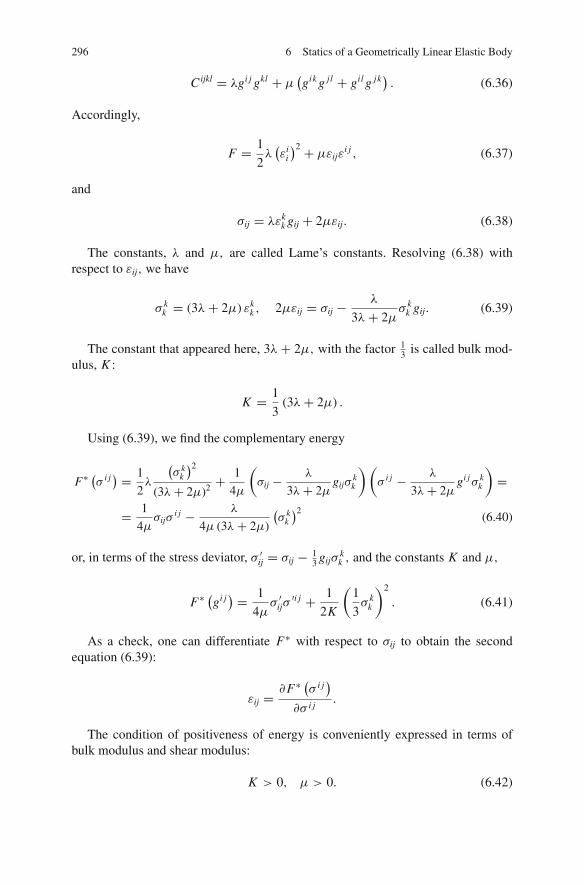
296 6 Statics of a Geometrically Linear Elastic Body
Cijkl = λgi j gkl + μ(gik g jl + gil g jk
). (6.36)
Accordingly,
F = 1
2λ(εi
i
)2 + μεijεi j , (6.37)
and
σij = λεkk gij + 2μεij. (6.38)
The constants, λ and μ, are called Lame’s constants. Resolving (6.38) withrespect to εij, we have
σ kk = (3λ+ 2μ) εk
k , 2μεij = σij − λ
3λ+ 2μσ k
k gij. (6.39)
The constant that appeared here, 3λ + 2μ, with the factor 13 is called bulk mod-
ulus, K :
K = 1
3(3λ+ 2μ) .
Using (6.39), we find the complementary energy
F∗(σ i j
) = 1
2λ
(σ k
k
)2
(3λ+ 2μ)2 +1
4μ
(σij − λ
3λ+ 2μgijσ
kk
)(σ i j − λ
3λ+ 2μgi jσ k
k
)=
= 1
4μσijσ
i j − λ
4μ (3λ+ 2μ)
(σ k
k
)2(6.40)
or, in terms of the stress deviator, σ ′ij = σij − 13 gijσ
kk , and the constants K and μ,
F∗(gi j) = 1
4μσ ′ijσ
′i j + 1
2K
(1
3σ k
k
)2
. (6.41)
As a check, one can differentiate F∗ with respect to σij to obtain the secondequation (6.39):
εij =�F∗
(σ i j
)
�σ i j.
The condition of positiveness of energy is conveniently expressed in terms ofbulk modulus and shear modulus:
K > 0, μ > 0. (6.42)

6.5 Physically Linear Elastic Body 297
To derive (6.42) we note that the components of strain deviator
ε′ij = εij − 1
3gijε
kk ,
(ε′kk = 0
)
and the strain trace, εkk , can be changed independently. Replacing εij in (6.37) by the
sum, ε′ij + 13εk
k gij, we have
F = 1
2K(εi
i
)2 + με′ijε′i j .
Obviously, F > 0 for εij �= 0 if and only if (6.42) holds.Instead of K , λ and μ, one often uses other two characteristics of isotropic elastic
bodies, Young’ modulus, E, and Poisson’s coefficient, ν:
E ≡ μ (3λ+ 2μ)
λ+ μ= 2 (1+ ν) μ, ν ≡ λ
2 (λ+ μ).
In terms of these characteristics the complementary energy is
F∗ = 1+ ν
2E
[σijσ
i j − ν
1+ ν
(σ k
k
)2]
.
Accordingly,
εij =�F∗
(σ i j
)
�σ i j= 1+ ν
E
(σij − ν
1+ νσ k
k gij
).
The constant λ+ μ is always positive:
λ+ μ = 3λ+ 3μ
3= 1
3K + μ > 0.
Therefore, E > 0. Poisson’s coefficient, ν, may be negative, but since E =2 (1+ ν) μ > 0, it is bounded from below:
ν > −1.
As follows from its definition, Poisson’s coefficient does not exceed 12 and ap-
proaches 12 when λ� μ.

298 6 Statics of a Geometrically Linear Elastic Body
6.6 Castigliano Variational Principle
Castigliano principle. In this section, we construct a variational principle dual toGibbs principle. The dual variational principle can be derived directly from thegeneral formulation given for the integral functionals (5.142), however we first re-peat the general scheme for constructing the dual principles taking into accountthe distinctive feature of the energy functional, its invariance with respect to rigidmotions. This feature has already been incorporated implicitly in the Young-Fencheltransformation (6.26) which used only symmetric tensors σ i j .
As in the general case, commuting the order of calculation of maximum andminimum in (6.28), we obtain
minu∈(6.12)
I (u) = maxσ
[J (σ )+ min
u∈(6.12)� (σ, u)
],
J (σ ) =∫
�Vu
σj
i n j ui(b)dσ −
∫
V
F∗(σ i j
)dV,
� (σ , u) = −∫
V
(σ
ji, j+ρgi
)ui dV −
∫
�V f
(fi − σ
ji n j
)ui d A. (6.43)
If the tensor field σ i j satisfies the equations
σj
i, j + ρgi = 0 in V, (6.44)
σj
i n j = fi on �V f , (6.45)
then � (σ, u) = 0. If σ i j does not satisfy these equations, minu
� (σ, u) = −∞.
Therefore,
minu∈(6.12)
I (u) = maxσ∈(6.44),(6.45)
J (σ ) .
In the general case, one can show that the maximizing field σ i j coincides withthe stresses computed for the minimizing displacements. We arrive at the followingCastigliano variational principle. The true stresses maximize the functional J (σ )on the set of all stress fields σ i j obeying the constraints (6.44) and (6.45).
Now, let us show how to derive the Castigliano principle from the dual variationalprinciple for the general integral functional (5.142). It follows from the generaltheory that the dual functional J (σ ) has the form (6.43); however F∗ in (6.43)represents not the function (6.25) but the Young-Fenchel transformation of F withrespect to displacements gradients ui, j :
F∗1 = maxui, j
(σ i j ui, j − F
(εij))
. (6.46)

6.6 Castigliano Variational Principle 299
Accordingly, in (6.46), and also in (6.44) and (6.45), the tensor σ i j is not necessarilysymmetric.
Let us rewrite (6.46), separating symmetric and antisymmetric components ofthe stresses and displacement gradients:
F∗1 = maxui, j
[σ (i j)εij + σ [i j]u[i, j] − F
(εij)]
.
Since F(εij)
does not depend on the antisymmetric components of the displacementgradients u[i, j], then F∗1 = +∞ for σ [i j] �= 0, and, consequently, if for some subre-gion of region V, σ [i j] �= 0, then the dual functional becomes equal to −∞. There-fore, all non-symmetric stress tensors should be excluded. For σ [i j] = 0 the functionF∗1 coincides with the function (6.25), and the variational principle is equivalent tothe general dual variational principle constructed for the functional (5.142).
Castigliano principle for stress functions. The general solution of the equilibrium(6.44) can easily be found. For simplicity, we consider only the case of zero exter-nal volume forces and simply-connected region V . We will show that the generalsolution of the equilibrium equations is
σ i j = eiklejmnψkm,ln , (6.47)
where ψkm is an arbitrary symmetric tensor field.Indeed, the general solution of the equation
Ai,i = 0 (6.48)
is
Ai = eijk B j,k,
where Bk are arbitrary functions of xi . Functions Bk are not uniquely determined byAi : adding to Bk an arbitrary potential vector field ψ,k does not change Ai .
Equilibrium equations for an elastic body have the divergence form (6.48), and,therefore their solution is
σ i j = e jkl Bik,l . (6.49)
Functions ψ i,k can be added to Bi
k without changing the components of the stresstensor. In particular, one can choose ψ i to make the trace of tensor Bi
k equal to zero:
Bii = 0. (6.50)
In order for the function (6.49) to be the solution to the equilibrium equations,the symmetry conditions for stresses has to be satisfied as well. Contracting (6.49)with ei js and using (3.19), we get

300 6 Statics of a Geometrically Linear Elastic Body
σ i j ei js = Bis,i = 0. (6.51)
Since (6.51) again has the form (6.48), the tensor Bis can be written as
Bis = eimnψsm,n .
The gradient of an arbitrary vector ϕs can be added to the tensor ψsm . Let uschoose ϕs in such a way that ψsm be symmetric, i.e. if ψsm were not symmetric weadd the gradient of the vector field ψs to obtain
eism(ψsm + ψs,m
) = 0. (6.52)
Denote by ψ and f the vector fields with the components ψs and eismψsm . Then,in direct vector notation, (6.52) reads
curl ψ = −f (6.53)
The vector field f has zero divergence: from (6.52) and (6.50)
div f = (eismψsm),i = eismψsm,i = Bs
s = 0
As known from calculus, for any vector field f with zero divergence, (6.53) issolvable. Hence, one can always choose the tensor ψmn to be symmetric.
Components of the symmetric tensor ψij are called the stress functions.It is clear that (6.47) has some extra degrees of freedom: on the left hand side of
(6.47) there are six functions connected by the three equilibrium equations, i.e. thereare three functional degrees of freedom; on the right hand side of (6.47) there are sixfunctional degrees of freedom. Thus, three more constraints can be imposed on ψkm .Of course, these additional constraints should not prevent the functions (6.47) fromcovering all possible solutions of the equilibrium equations. It is most convenient toselect the additional restrictions on the stress functions for each particular problem,using the simplifications related to the specifics of the problem.Castigliano variational principle for stress functions. The true stress functionsdeliver the maximum value to the functional
J (ψ) =∫
�Vu
eiklejmnψkm,lnu(b)i n j d A −
−∫
V
F∗(eiklejmnψkm,ln
)dV (6.54)
on the set of all stress functions obeying the boundary conditions
e jklψkm,lsejmsn j = f i on �V f . (6.55)

6.6 Castigliano Variational Principle 301
This variational principle does not determine the stress functions uniquely, butthis does not affect the uniqueness of the stress state.
One may wonder how to simplify the energy expression, and, thus, the governingequations by imposing the constraints on the stress functions. Consider an isotropicphysically linear homogeneous elastic body with the complementary energy (6.40).According to (3.19),
σ i jσij = eiklejmnψkm,lneik ′l ′e jm ′n′ψk ′m ′,l ′n′ =
= (δk
k ′δll ′ − δk
l ′δlk ′) (
δmm ′δ
nn′ − δm
n′δnm ′)ψkm,lnψ
k ′m ′,l ′n′ = (6.56)
= ψkm,lnψkm,ln − 2ψkm,lnψ
lm,kn + ψkm,lnψln,km,
σ kk =
(gkm gln − glm gkn
)ψkm,ln = �ψk
k − ψkm,km .
It is seen from (6.56) that by setting the three conditions
ψi j, j = 0, (6.57)
we make vanish the last term in the second equation (6.56) and put the last twoterms in the first equation (6.56) into divergence form:
−2ψkm,lnψlm,kn + ψkm,lnψ
ln,km == −2
�
�xl
(ψkm,nψ
lm,kn)+ �
�xn
(ψkm,lψ
ln,km)
Thus, they do not affect the equations for ψ i j .
Up to the divergence terms, the free energy becomes
∫
V
F∗dV =∫
V
1
4μ
(ψkm,lnψ
km,ln − ν
1+ ν
(�ψk
k
)2)
dV,
with � being Laplace’s operator. Hence, Euler equations for the stress functions are
�2ψ i j − ν
1+ ν�2ψk
k gi j = 0.
Note that the divergence terms may contribute to the boundary conditions.
Castigliano variational principle and compatibility of strains. Euler equationsfor the functional (6.54) read: in region V,
eiklejmn�l�n�F∗
�σ i j= 0. (6.58)
Since the derivatives of F∗ are the components of strain tensor

302 6 Statics of a Geometrically Linear Elastic Body
�F∗
�σ i j= εij,
(6.58) can be also written as
eiklejmn�l�nεij = 0. (6.59)
It is proved in differential geometry that these equations are the necessary andsufficient conditions for the existence of a vector field, ui (x), such that
εij = 1
2(ui, j + u j,i ). (6.60)
In other words, (6.59) gives the conditions of the existence of a displacementvector field such that the strain in the deformed state is generated by displacementfrom some undeformed state. One says that such strain is compatible.
On the other hand, stresses can be viewed as reactions to the compatibility con-straints (6.60). Indeed, one can consider the strain in Gibbs variational principleas an arbitrary field such that (6.60) holds. Then the governing equations can beobtained by introducing Lagrange multipliers for the constraints (6.60), σ i j , i.e. byadding to the energy functional the integral
∫
Vσ i j
(1
2(ui, j + u j,i )− εij
)dV .
The reader can check that the Lagrange multipliers σ i j have the meaning ofstress components. If, instead of (6.60), the compatibility conditions are taken inthe form (6.59), then the corresponding Lagrange multipliers have the meaning ofstress functions.
Two-dimensional plane problems. Castigliano principle for stress functions takesa considerably simpler form in two-dimensional plane problems because in this caseonly one stress function is needed.
Let � be a bounded simply connected region in a two-dimensional plane, andx, y be some Cartesian coordinates in the plane. The boundary �� of the region �consists of two parts, ��u and �� f ; the displacement components, ux and uy, areprescribed on ��u :
ux = u(b)x (s), uy = u(b)
y (s) on ��u,
s being the arc length along ��, while at �� f the external force{
fx (s) , fy (s)}
isknown.
Then Castigliano principle states:

6.6 Castigliano Variational Principle 303
Castigliano variational principle. The true stresses give the maximum value to thefunctional,
J (σ ) =∫
�� f
[u(b)
x (s)(σxx nx + σxyny
)+ u(b)y (s)
(σxynx + σyyny
)]ds −
−∫
�
F∗(σxx , σxy, σyy
)dxdy, (6.61)
on the set of all functions σxx , σxy = σyx , and σyy , which satisfy the constraints
�σxx
�x+ �σxy
�y= 0,
�σyx
�x+ �σyy
�y= 0 in �, (6.62)
σxx nx + σxyny = fx , σyx nx + σyyny = fy on �� f . (6.63)
Equations (6.62) mean that there exist functions �1 and �2 such that
σxx = ��1
�x, σxy = −��1
�x, σyx = ��2
�y, σyy = −��2
�x.
Since σxy = σyx ,
��1
�x+ ��2
�y= 0.
Therefore, there exists a function ψ such that
�1 = �ψ
�y, �2 = −�ψ
�x.
Thus, the general solution of the equilibrium equations is
σxx = �2ψ
�y2, σxy = − �2ψ
�x�y, σyy = �2ψ
�x2. (6.64)
The function ψ is called the Airy function. If the components of the stress tensorare known, function ψ can be determined up to a linear function of x and y. Thearbitrariness can be removed by setting
ψ = �ψ
�x= �ψ
�y= 0 (6.65)
at some point C on �� f . It is convenient to measure the arc length on �� startingfrom the point C . The arc length is assumed to increase in a counter-clockwisedirection.

304 6 Statics of a Geometrically Linear Elastic Body
The boundary conditions (6.63) take a simple form in terms of the Airy function.They are obtained by substitution (6.64) in (6.63) and taking into account (5.128)and (5.129):
σxx nx + σxyny = τy�2ψ
�y2+ τx
�2ψ
�x�y= d
ds
�ψ
�y= fx (s) ,
σyx nx + σyyny = −τy�2ψ
�x�y− τx
�2ψ
�x2= − d
ds
�ψ
�x= fy (s) . (6.66)
Consequently, the boundary conditions define the value of derivatives of the stressfunctions on the contour �� f :
�ψ
�y=
s∫
0
fx (s)ds,�ψ
�x= −
s∫
0
fy (s)ds. (6.67)
The boundary conditions (6.67) are equivalent to prescribing at �� the functionψ and its normal derivative:
�ψ
�n≡ nx
�ψ
�x+ ny
�ψ
�y.
If the surface forces are prescribed on the entire boundary, then the boundaryconditions (6.67) are also reduced to prescribing at the boundary function ψ andits normal derivative. To justify this statement we have to check that the boundaryconditions (6.67) written for the entire boundary define a single-valued function ψ .Indeed, the necessary condition for the correctness of the variational problem in thiscase is vanishing of the total force and the total moment:
l∫
0
fx (s)ds = 0,
l∫
0
fy (s)ds = 0,
l∫
0
(x fy (s)− y fx (s)
)ds = 0. (6.68)
Here, l is the length of the contour ��. The first two equations (6.68) mean thatformulas (6.67) define on the contour �� two single-valued functions �ψ/�x and�ψ/�y. Consequently, �ψ/�n and �ψ/�s ≡ τx �ψ/�x + τy�ψ/�y are also uniquelydefined. Let us find the boundary value of the Airy function, ψ (s). We have
ψ (s) =s∫
0
dψ
dsds =
s∫
0
(�ψ
�x
dx
ds+ �ψ
�y
dy
ds
)ds =
s∫
0
(�ψ
�xdx + �ψ
�ydy
)=
=(
x�ψ
�x+ y
�ψ
�y
)∣∣∣∣s
0
−s∫
0
(x
d
ds
�ψ
�x+ y
d
ds
�ψ
�y
)ds.

6.6 Castigliano Variational Principle 305
Using (6.66), we obtain
ψ (s) =(
x�ψ
�x+ y
�ψ
�y
)∣∣∣∣s
+s∫
0
(x fy − y fx
)ds. (6.69)
Here, we take into account that ψ and derivatives of ψ are zero at s = 0. Due to(6.68), formula (6.69) defines a single-valued function ψ (s) on ��.
Substituting (6.64) into the functional (6.61), we get the followingCastigliano variational principle for stress functions. The maximum of the func-tional∫
��u
(u(b)
x (s)d
ds
�ψ
�y− u(b)
y (s)d
ds
�ψ
�x
)ds −
∫
�
F∗(
�2ψ
�y2,− �2ψ
�x�y,
�2ψ
�x2
)dxdy
on the set of all functions ψ , satisfying the boundary conditions
ψ = f1 (s) ,dψ
dn= f2 (s) on �� f
is achieved at the true stress function.Functions f1 (s) and f2 (s) are calculated from fx (s) and fy (s) by means of
(6.67) and (6.69).
Anti-plane problems. The problems in which the component of displacements ina Cartesian coordinates, u3, is a function of x1 = x and x2 = y, while two othercomponents are zero, are called anti-plane problems. In this case, the body is acylinder with a cross-section �, {x, y} ∈ �. In anti-plane deformation, only twocomponents of strain are non-zero:
2ε13 = �u
�x, 2ε23 = �u
�y, u3 ≡ u(x, y).
Gibbs variational principle. The true displacement field provides minimum to thefunctional
I (u) =∫
�
F
(�u
�x,
�u
�y
)dxdy−
∫
�� f
f u ds
on the set of all u(x, y) obeying the condition
u = u(b)(s) at ��u .
Following the general scheme, one obtains the dual variational principle.

306 6 Statics of a Geometrically Linear Elastic Body
Dual variational principle. The true stresses provide minimum to the functional∫
�
F∗(σx , σy)dxdy−∫
��u
(σx nx + σyny)u(b)(s)ds
on the set of all fields, σx , σy, obeying the constraints
�σx
�x+ �σy
�y= 0 in �, σx nx + σyny = f (s) on �� f .
In anti-plane problems, the stress function, ψ, is introduced by the relations
σx = �ψ
�y, σy = −�ψ
�x.
The dual variational principle in terms of the stress function takes the form:
Dual variational principle. The true stress function provides minimum to the func-tional
∫
�
F∗(
�ψ
�y,−�ψ
�x
)dxdy−
∫
��u
dψ
dsu(b)(s)ds
on the set of all functions, ψ(x, y), obeying the boundary condition
dψ
ds= f (s) on �� f .
In the case when the displacements are given at all points of the boundary, mini-mum is taken over all functions, ψ(x, y).
In elasticity theory, there are other boundary value problems of interest besidesthose already considered. For example, on a part � of the boundary, only onecomponent of displacement, u1 can be prescribed and the “complementary” com-ponents of external forces, f2 and f3, are also given. Then the energy functional ofGibbs principle will include the integral over � of f2u2 + f3u3. The correspondingchanges in the Castigliano and the Reissner principles are straightforward.
6.7 Hashin-Strikman Variational Principle
In this section we formulate Hashin-Strikman variational principle for a linear inho-mogeneous body. The free energy density of the body is
F(εij) = 1
2Cijkl(x)εijεkl .
If the displacements are prescribed on the boundary

6.7 Hashin-Strikman Variational Principle 307
ui = ui(b) on �V, (6.70)
then the true displacement field minimizes the functional
I (u) =∫
V
1
2CijklεijεkldV (6.71)
on the set of displacements with the prescribed boundary values (6.70). We select ahomogeneous elastic body with the free energy
F0 = 1
2Cijkl
0 εijεkl . (6.72)
It is convenient to choose this body isotropic, i.e.
Cijkl0 = λ0gi j gkl + μ0
(gik g jl + gil g jk
). (6.73)
Suppose that the quadratic form, F − F0, is positive definite:
F − F0 = 1
2
(Cijkl − 1
2Cijkl
0
)εijεkl > 0 for εij �= 0.
Then F − F0 can be presented by means of Young-Fenchel transformation:
F − F0 = maxpi j
[pi jεij − 1
2Hijkl pi j pkl
], (6.74)
where Hijkl is the inverse tensor:
Hijkl(Cklmn − Cklmn
0
) = δ(mi δ
n)j . (6.75)
Repeating the line of reasoning of Sect. 5.9, we have:
I (u) =∫
V
[1
2Cijkl
0 εijεkl + 1
2
(Cijkl − Cijkl
0
)εijεkl
]dV =
= maxpi j
∫
V
[1
2Cijkl
0 εijεkl + pi jεij − 1
2Hijkl pi j pkl
]dV .
Therefore,
I = minuε(6.70)
I (u) = minuε(6.70)
maxpi j (x)
∫
V
[1
2Cijkl
0 εijεkl + pi jεij−
− 1
2Hijkl(x)pi j pkl
]dV .

308 6 Statics of a Geometrically Linear Elastic Body
Changing the order of minimum and maximum, we have
I = maxpi j (x)
[J (p)−
∫
V
1
2Hijkl(x)pi j pkldV
](6.76)
where
J (p) = minuε(6.70)
∫
V
(1
2Cijkl
0 εijεkl + pi j (x)εij
)dV . (6.77)
Let ui be the minimizer in the following variational problem for the homoge-neous body:
E0 = minuε(6.70)
∫
V
1
2Cijkl
0 εijεkldV .
We present displacements in (6.77) as the sum
ui = ui + u′i , u′i |�V = 0. (6.78)
Then
J (p) = E0 +∫
Vpi j εijdV + J (p), (6.79)
J (p) = minu′ε(6.78)
∫
V
(1
2Cijkl
0 ε′ijε′kl + pi jε′ij
)dV, ε′ij ≡ u′(i, j). (6.80)
The term ∫Cijkl
0 εijε′ijdV,
vanished due to the Euler equations for the minimizer, ui , and the zero boundaryconditions for u′i . Plugging (6.79) in (6.76), we obtain the followingHashin-Strikman variational principle. The true energy of the body, I , can becomputed from the variational problem
I − E0 = maxpi j (x)
[∫
V
(pi j (x)εij − 1
2Hijkl(x)pi j (x)pkl(x)
)dV + J (p)
]. (6.81)
The rest of this section is concerned with determining an explicit form of J (p).To find an explicit dependence of J (p) on pi j (x) one has to solve the boundaryvalue problem2
2 Writing (6.82) we used the symmetry of Cmnrs0 with respect to indices r, s, and therefore
Cmnrs0 εrs = Cmnrs
0 �r us .

6.7 Hashin-Strikman Variational Principle 309
�n(Cmnrs
0 �r us) = −�n pmn(x), us |�V = 0. (6.82)
Here pmn(x) are assumed to be some smooth functions. If pmn(x) are piece-wisesmooth and have a jump on some surface, S, while us(x) remain continuous on S,then additionally,
[Cmkrs
0 ur,s + pmk]
nk = 0 on S. (6.83)
As usual, [ϕ] denotes the jump of ϕ on S. To get the solution of the boundaryvalue problem (6.82) and (6.83) in an explicit form, we have to employ, as in thescalar case considered in Sect. 5.9, Green’s function, which, for elasticity problems,is a tensor.
Green’s tensor. Consider the variational problem
∫
V
(1
2Cmnrs
0 �mun�r us − us f s(x)
)dV → min
us :us=0 at �V. (6.84)
Its minimizer obeys the boundary value problem
�nCmnrs0 �r us = − f m(x), us |�V = 0. (6.85)
Let f m(x) be sufficiently smooth, e.g., piece-wise continuous. If we discretize(6.85), they become a system of linear algebraic equations. Solving this system, wefind the value of us at each point, x , as a linear function of the values of f m at allpoints of the discretization grid. In continuum limit, us becomes a linear functionalof f m of the form
us(x) =∫
VGsm(x, x ′) f m(x ′)dV ′. (6.86)
The kernel, Gsm(x, x ′), is called Green’s tensor. The operator of the linearproblem (6.85) is symmetric, therefore its inversion, the operator (6.86), is alsosymmetric, i.e.
Gsm(x, x ′) = Gms(x ′, x). (6.87)
As follows from (6.85) and (6.86), Green’s tensor is a solution of the boundaryvalue problem,
�nCmnrs0 �r Gst (x, x ′) = −δm
t δ(x − x ′), (6.88)
Gst (x, x ′) = 0 if x ∈ �V . (6.89)
By δ(x − x ′) we mean the delta-function in three-dimensional space:
δ(x − x ′) = δ1(x1 − x ′1)δ1(x2 − x ′2)δ1(x3 − x ′3),

310 6 Statics of a Geometrically Linear Elastic Body
where δ1(ξ ) is the usual “one-dimensional” delta-function of one variable, and xi ,
x ′i the components of the vectors, x and x ′, respectively.The δ-function in the right hand side of (6.88) causes Green’s tensor to have a
singularity at x = x ′. To find the character of this singularity we solve (6.88) in thecase of unbounded region.
Green’s tensor for unbounded region. We are going to show that Green’s tensorfor unbounded region is
Gst (x, x ′) = 1
16πμ0(1− ν0) |x − x ′| ((3− 4ν0) gst + nsnt ) (6.90)
where μ0 and ν0 are the shear modulus and Poisson’s coefficient of the homoge-neous elastic body, and ns the unit vector:
ns = xs − x ′s|x − x ′| . (6.91)
For a bounded region, Green’s tensor is a sum of the tensor (6.90) and a tensorthat is bounded as x → x ′.
Green’s tensor for unbounded region can be found by applying to (6.88) Fouriertransformation. First, we recall the basic features of Fourier transformations.
Fourier transformations. By Fourier transformations of a function, u(x), onemeans the function of a “dual variable,” k, defined by the relation
u(k) =∫
u(x)e−ik·x d3x . (6.92)
Here k · x means the scalar product of two three-dimensional vectors, k and x, andthe integration is conducted over the entire three-dimensional space. As is oftendone in physical literature, we keep for Fourier transformation of function, u(x),the same notation, u, but with the other argument, k. This emphasizes that u(x) andu(k) are different presentations of the same function. Both u(x) and u(k) can becomplex-valued. Integral (6.92) is converging if u(x) decays at infinity fast enough.In this case, it can be shown that formula (6.92) can be inverted and yields
u(x) = 1
(2π )3
∫u(k)eik·x d3k. (6.93)
Besides, for any two functionals, u(x) and v(x), which decay fast enough atinfinity, an important Parseval’s equation holds:
∫u(x)v∗(x)d3x = 1
(2π )3
∫u(k)v∗(k)d3k. (6.94)
We are going to apply Fourier transformation not only to fast decaying func-tions but also to the generalized functions, like δ(x − x ′), in (6.88). This is not

6.7 Hashin-Strikman Variational Principle 311
an elementary step, and we just mention here that Fourier transformation can beextended to the generalized functions. In particular, for the delta-function one has touse the following formal rules:
δ(k) =∫
δ(x)e−ik·x d3x = 1, (6.95)
δ (x) = 1
(2π )3
∫eik·x d3k. (6.96)
Parseval’s equality (6.94) holds not only for fast decaying functions, but alsofor functions u and v, one of which is generalized, and another one is “usual” (fastdecaying). Note that (6.93) and (6.94) can easily be obtained using (6.95) and (6.96).For example, multiplying (6.92) by eik·x and integrating over k we have
∫u(k)eik·x d3k =
∫u(x ′)e−ik·x ′d3x ′eik·x d3k =
∫u(x ′)
∫eik·(x−x ′)d3kd3x ′
=∫
u(x ′)(2π )3δ(x − x ′)d3x ′ = (2π )3u(x).
For a fast decaying function, u(x), Fourier transformation of its derivatives
us(k) =∫
�u(x)
�xse−ik·x d3x
is computed in terms of u(k) by integration by parts:
us(k) = −∫
u(x)�
�xse−ik·x d3x = iks
∫u(x)e−ik·x d3x = iksu(k).
The same formula remains true for generalized functions.
Derivation of (6.90). Denote by Gst (k, k ′) the Fourier transformation of Green’stensor:
Gst (k, k ′) =∫
Gst (x, x ′)e−i(k·x−k ′ ·x ′)d3xd3x ′. (6.97)
The sign at k ′ is chosen for convenience. Due to the symmetry of Green’s tensor(6.87), its Fourier transformation possesses a symmetry:
Gst (k, k ′) =∫
Gst (x, x ′)e−i(k·x ′−k ′ ·x)d3xd3x ′
=∫
Gts(x, x ′)e−i(k ′ ·x−k·x ′)d3xd3x ′ = Gts(−k ′,−k). (6.98)

312 6 Statics of a Geometrically Linear Elastic Body
Multiplying (6.97) by ei(k·x−k ′ ·x ′), integrating over k and k ′ and using (6.96) weobtain the inversion of (6.97):
∫Gst (k, k ′)ei(k·x−k ′ ·x ′)d3kd3k ′ =
=∫
Gst (x, x ′)e−i(k·x−k ′·x ′)d3 xd3 x ′ei(k·x−k ′ ·x ′)d3kd3k ′ =
=∫
Gst (x, x ′)eik·(x−x)+ik ′ ·(x ′−x ′)d3kd3k ′d3 xd3 x ′ =
(2π )6∫
Gst (x, x ′)δ(x − x)δ(x ′ − x ′)′d3 xd3 x ′ = (2π )6 Gst (x, x ′) (6.99)
To find Gst (k, k ′) we multiply both sides of (6.88) by ei(k·x−k ′ ·x ′) and integrateover x and x ′. Since
∫δ(x ′ − x ′)ei(k·x−k ′ ·x ′)d3xd3x ′ =
∫e−i(k−k ′)·x d3x = (2π )3 δ(k − k ′)
and
∫�n�r Gst
(x, x ′
)e−i(k·x−k ′ ·x ′)d3xd3x ′ =
=∫
Gst(x, x ′
)�n�r e−i(k·x−k ′ ·x ′)d3xd3x ′ = −knkr Gst
(k, k ′
),
we obtain for Gst(k, k ′
)a system of linear equations:
Cmnrs0 kr knGst
(k, k ′
) = (2π )3 δmt δ
(k − k ′
). (6.100)
In the case of an isotropic body, when Cmnrs0 are given by (6.73), these equations
take the form
(λ0 + μ0) kmks Gst(k, k ′
)+ μ0 |k|2 Gmt (k, k ′) = (2π )3 δm
t δ(k − k ′
). (6.101)
Here
|k|2 ≡ ksks.
Contracting (6.101) with km , we get
(λ0 + 2μ0) ks Gst(k, k ′
) = (2π )3 kt
|k|2 δ(k − k ′
).
Plugging this result back in (6.100) we finally obtain

6.7 Hashin-Strikman Variational Principle 313
Gmt (k, k ′) = (2π )3
μ0 |k|2(
δst −
λ0 + μ0
λ0 + 2μ0
kskt
|k|2)
δ(k − k ′
). (6.102)
Obviously this tensor obeys the symmetry condition (6.98). Green’s tensor inx-coordinates is obtained from (6.99):
Gst(x, x ′
) = 1
(2π )3
∫1
μ0 |k|2(
gst − λ0 + μ0
λ0 + 2μ0
kskt
|k|2)
eik·(x−x ′)d3k. (6.103)
The integral here can be computed explicitly. We have
∫1
|k|2 eik·τ d3k =∫ ∞
0
∫
Sei(ν·n)ρ|τ |dρd2ν, ρ ≡ |k| .
By ν and n we denote the unit vectors: ν = k/ |k|, n = τ/ |τ | , and by d2ν thearea element on the unit sphere, S. Changing ρ by ρ/ |τ | we obtain
∫1
|k|2 eik·r d3k = c
|τ |
where c is a constant,
c =∫ ∞
0
∫
Sei(ν·n)ρdρd2ν.
Choosing n to be the north pole of the unit sphere, S, and θ, ϕ to be the sphericalcoordinates, we can write
∫ei(ν·n)ρd2ν =
∫ π
0
∫ 2π
0eiρ cos θdθdϕ = −2π
∫ π
0eiρ cos θd cos θ = 4π
sin ρ
ρ.
Since3
∫ ∞0
sin ρt
ρdρ = π
2sgn t , (6.104)
we obtain
c =∫ ∞
0
∫
Sei(ν·n)ρdρd2ν = 2π2. (6.105)
So,
3 sgn t = 1 for t > 0, sgn t = 0 for t = 0, sgn t = −1, for t < 0.

314 6 Statics of a Geometrically Linear Elastic Body
∫1
|k|2 eik·τ d3k = 2π2
|τ | . (6.106)
Comparing (6.106) with (6.93), we conclude that the Fourier transformation of1/4π |x | is 1/ |k|2 .
To find the integral
∫1
|k|4 kskt eik·τ d3k =
∫ ∞0
∫
Sνsνt e
i(ν·n)ρ|τ |dρd2ν,
we change the variable, ρ → ρ/ |τ | , to obtain
∫1
|k|4 kskt eik·τ d3k = 1
|τ |Nst (6.107)
where the notation is introduced
Nst =∫ ∞
0
∫
Sνsνt e
i(ν·n)ρdρd2ν.
The tensor, Nst , is a function of the unit vector, ns . A general form of suchdependence is
Nst = αgst + βnsnt . (6.108)
To determine the values of the constants α and β we contract (6.108) with gst
and nsnt to obtain a system of two linear equations with respect to α and β:
3α + β = N ss =
∫ ∞0
∫
Sei(ν·n)ρdρd2ν (6.109)
α + β = Nst nsnt =
∫ ∞0
∫
S(ν · n)2ei(ν·n)ρdρd2ν. (6.110)
According to (6.105), the right hand side in (6.109) is 2π2. The right hand sidein (6.110) is zero. Indeed,
∫ ∞0
∫
S(ν · n)2ei(ν·n)ρdρd2ν = 2π
∫ ∞0
∫ π
0cos2 θeiρ cos θ sin θdθdρ. (6.111)
Changing the variable of integration, θ → t, t = cos θ, we have for the integralover θ,

6.7 Hashin-Strikman Variational Principle 315
∫ π
0cos2 θeiρ cos θ sin θdθ =
∫ 1
−1t2eiρt dt =
∫ 1
−1t2 cos ρtdt = 1
ρ
∫ 1
−1t2d sin ρt = 2
sin ρ
ρ− 2
∫ 1
−1
sin ρt
ρtdt. (6.112)
Integrals over ρ of both terms in the right hand side of (6.112) are equal due to(6.104). Therefore, the integral (6.111) is zero. Then, the solution of (6.109) and(6.110) is α = −β = π2, and
Nst = π2 (gst − nsnt ) . (6.113)
Collecting the results, (6.106), (6.107) and (6.113), and using the relation
λ0 + μ0
λ0 + 2μ0= 1
2(1− ν0), (6.114)
we arrive at (6.90).
Explicit form of J (p). We are going to show that the functional J (p) (6.80) can bewritten in terms of Green’s tensor, as
J (p) = 1
4
∫
V
∫
V
�2Gij(x, x ′)�xk�x ′m
(pim(x)p jk(x)+ pim(x ′)p jk(x ′)−
− 2pim(x)p jk(x ′))
dV dV ′. (6.115)
The derivation of (6.115) is similar to that of the scalar case given in Sect. 5.9.First, we consider smooth functions, pi j (x). Then, from Clapeyron’s theorem (5.47),
J (p) = 1
2
∫
Vui, j pi j dV, (6.116)
where ui is the solution of the boundary value problem (6.82). According to (6.85),this solution can be written as
ui (x) =∫
VGij(x, x ′)
�p jk(x ′)�x ′k
dV ′. (6.117)
Green’s tensor has an integrable singularity, 1/∣∣x − x ′
∣∣ . Replacing �p jk(x ′)/
�x ′k
by �(p jk(x ′)− p jk(x))/
�x ′k and integrating by part, we have
ui (x) = −∫
V
�Gij(x, x ′)�x ′k
(p jk(x ′)− p jk(x)
)dV ′. (6.118)
If we differentiate (6.118) over xm ; then the singularity is still absolutely inte-grable; therefore, the differentiation is possible. We get

316 6 Statics of a Geometrically Linear Elastic Body
�ui (x)
�xm= −
∫
V
�2Gij(x, x ′)�xm�x ′k
(p jk(x ′)− p jk(x)
)dV ′. (6.119)
Derivative with respect to xm of the last term in (6.118),
∫
V
�Gij(x, x ′)�x ′ j
dV ′�p jk(x)
�xm=∫
�VGij(x, x ′)n j (x
′)d A�p jk(x)
�xm,
is equal to zero because Gij(x, x ′) = 0 for x ′ε�V .
From (6.116) and (6.119),
J (p) = −1
2
∫ ∫�2Gij(x, x ′)
�xm�x ′kpim(x)
(p jk(x ′)− p jk(x)
)dV dV ′. (6.120)
The symmetry of Green’s tensor yields a symmetry of its derivatives:
�2Gij(x, x ′)�xm�x ′k
= �2G ji (x, x ′)�x ′k�xm
. (6.121)
Let us change in (6.120) i ↔ j, m ↔ k, x ↔ x ′. We obtain
J (p) = −1
2
∫ ∫�2G ji (x ′, x)
�x ′k�xmp jk(x ′)
(pim(x)− pim(x ′)
)dV dV ′. (6.122)
Summing up (6.120) and (6.122) and using (6.121) we arrive at (6.115).Now let pi j (x) have a discontinuity on some surface, S. As in the scalar case of
Sect. 5.9, one can show that the minimizer of the variational problem,
∫
V
1
2Cijkl
0 � j ui �kuldV −∫
Sσi u
i d A→ minu:u=0 at �V
, (6.123)
where minimum is sought over all functions ui (x) vanishing on �V , is given by theformula
ui (x) =∫
SGij(x, x ′)σ j (x ′)d A′.
Therefore, the solution of the boundary value problem (6.82) and (6.83) is
ui (x) =∫
VGij(x, x ′)
�p jk(x ′)�x ′k
dV ′ +∫
SGij(x, x ′)
[p jk
]nkd A′.

6.7 Hashin-Strikman Variational Principle 317
That yields, after integration by parts, (6.118). For any point, x , which does notbelong to S, we may differentiate (6.118) to obtain (6.119). After that the derivationof (6.115) proceeds in the same way as for smooth pi j (x).
The case of negative F–F0. If the constants, λ0 and μ0, are so large that
F0 − F = 1
2
(Cijkl
0 − Cijkl)
εijεkl > 0 for εij �= 0,
then, denoting by Hijkl the inverse tensor for Cijkl0 − Cijkl,
Hijkl
(Cijkl
0 − Cijkl)= δ
(mi δ
n)j ,
we can write
F0 − F = maxpi j
[pi jεij − 1
2Hijkl pi j pkl
]
or
F − F0 = minpi j
(1
2Hijkl pi j pkl − pi jεij
).
Then
I (u) = minpi j
∫
V
[1
2Cijkl
0 εijεkl + 1
2Hijkl pi j pkl − pi jεij
]dV
and
I = minuε(6.70)
I (u) = minpi j
[∫
V
1
2Hijkl pi j pkl + J (p)
]
where
J (p) = minuε(6.70)
∫
V
(1
2Cijkl
0 εijεkl − pi jεij
)dV =
= E0 −∫
Vpi j εijdV + J (p),
J (p) = minuε(6.78)
∫
V
(1
2Cijkl
0 ε′ijε′kl − pi jε′ij
)dV .
Formula for J (p) (6.115) remains unchanged, since it is invariant with respect tothe substitution, pi j →−pi j . We arrive at the followingHashin-Strikman variational principle. The true energy of the body, I , can becomputed from the variational problem

318 6 Statics of a Geometrically Linear Elastic Body
I − E0 = minpi j (x)
[∫
V
(1
2Hijkl pi j pkl − pi j εij
)dV + J (p)
].
The variational principles formulated hold for any choice of the parameters, Cijkl0 .
6.8 Internal Stresses
Elasticity theory considered in the previous sections was based on the assumptionthat there exists a global stress-free state of the body. The displacements in that the-ory are the displacements from the stress-free state to the deformed state. There aresituations for which such an assumption is not physically adequate, though “elastic-ity,” the way in which energy depends on strains, still holds. Consider, for example,a polycrystal. In general, even for zero tractions at the boundary of the polycrystal,the stresses are not zero: if we cut off a grain and set it free, it deforms into afree-stress state. Moreover, if we cut the polycrystal over all grain boundaries andlet each grain to deform to a stress-free state, then, in general, the unstressed grainscannot be put together to form a continuous body without gaps and overlapping.This motivates a modification of the previous theory, which we consider first withina general nonlinear framework and then make simplifications specific to geometricallinearity. We begin with an example.
Consider a stress-free material (matrix) with a cavity (Fig. 6.2a) and a piece ofother material (inclusion). The inclusion is shown in its stress-free state in Fig. 6.2b.After some deformation of the inclusion it fits the cavity. We put the inclusion intothe cavity and glue it to the cavity surface (Fig. 6.2d). We obtain a material withnonzero stresses: the matrix is unstressed, while the inclusion, being deformed,has nonzero stresses. To keep such a system in equilibrium, some forces must beapplied at the interface surface. If the external forces are removed, then the systemcomes to a new equilibrium state (Fig. 6.2e). The stresses in this state are nonzero.They are usually referred to as internal stresses. The example considered provides aphysically adequate model for various defects in solids: precipitates and inclusionsof various nature, voids, vacancies and interstitials in crystal lattices.
Fig. 6.2 Internal stressescaused by inclusion

6.8 Internal Stresses 319
Fitting this example to the general continuum mechanics scheme, we can identifythe current state with the state in Fig. 6.2e and the initial state with the state inFig. 6.2d. There is a displacement field which transforms the initial state into thecurrent state. The initial state is not, however, stress-free. To have a stress-free state,we have to cut off the inclusion. That yields the stress-free states of the two pieces(Fig. 6.2a and b). These two pieces cannot be put together without overlapping. Tocharacterize the transition from the initial state to a stress-free state quantitatively,first we introduce a Lagrangian smooth coordinate system, Xa, in the initial state. Itcan always be chosen Cartesian. The metric tensor in the initial state we denote asbefore by gab. Cutting off a small piece of material in the vicinity of point X and itsunloading lead to deformation to a stress-free state. The metric tensor in the stress-free state differs from gab, and we denote it by g∗ab. In our example, g∗ab coincideswith gab inside the matrix, and differs from gab in the inclusion. The deformationoccurring in the transition from the initial to the stress-free state is characterized bythe tensor
ε∗ab =1
2
(g∗ab − gab
).
It is called eigen-strain tensor, or just eigen-strain. In general, the eigen-strain,ε∗ab, cannot be obtained by a smooth displacement field from the initial state. Onesays that the eigen-strain is incompatible.
Since g∗ab corresponds to a stress-free state, the elastic strain tensor is
ε(e)ab =
1
2
(gab − g∗ab
).
Here, gab is the metric tensor in the current state,
gab = gijxia x j
b , xia =
�xi (X )
�Xa,
xi (X ) being the position of the particle X in the current state. As before, the totalstrain, εab, is, by definition, the strain associated with the transition from the initialto the current state:
εab = 1
2(gab − gab) .
Obviously,
εab = ε(e)ab + ε∗ab.
The total strain is compatible, the elastic strain and the eigen-strain are not.A typical problem of the internal stress theory is to find the stress field if the
eigen-strain field is known. The internal stresses can be found from the following

320 6 Statics of a Geometrically Linear Elastic Body
Gibbs variational principle. The true internal stress field provides minimum to thefunctional
I =∫
VF(ε(e)
ab )dV,
over all particle positions in the current state.In geometrically linear theory,
ε(e)ij =
1
2
(�i u j + � j ui − g∗ij
).
Therefore the functional simplifies to
I =∫
VF
(1
2
(�i u j + � j ui − g∗ij
))dV .
The tensor g∗ij is compatible if there exists a vector field, u∗i (x), such that
g∗ij = �i u∗j + � j u
∗i . (6.124)
The vector field, u∗i , can be interpreted as a displacement field from the initial tothe stress-free state. If F(ε(e)
ab ) has the only minimum for zero ε(e)ab , and stresses
σ i j = �F(ε(e)ij )
�ε(e)ij
,
are zero for ε(e)ij = 0, then the minimum is achieved for ui = u∗i , i.e. in the stress-free
state. Internal stresses appear only for incompatible g∗ij.In physically and geometrically linear theory,
F(ε(e)ij ) = 1
2Cijklε
(e)ij ε
(e)kl .
To obtain the dual variational principle in this case, we present F(ε(e)ij ) as
F(ε(e)ij ) = max
σ i j
(σ i j 1
2
(�i u j + � j ui − g∗ij
)− 1
2C (−1)
ijkl σ i jσ kl
).
Following the general scheme we arrive at
Dual variational principle. The true stress state of the body provides minimum tothe functional
J =∫
V
1
2C (−1)
ijkl σ i jσ kldV + l(σ ), l(σ ) = 1
2
∫
Vσ i j g∗ijdV, (6.125)

6.9 Thermoelasticity 321
on the set of all stress fields obeying the constraints
�σ i j
�x j= 0 in V, σ i j n j = 0 on �V . (6.126)
If g∗ij are compatible, i.e. (6.124) holds, then l(σ ) = 0 due to (6.126), and theminimizing stress is zero.
As we discussed in Sect. 6.6, in order to be compatible, g∗ij must satisfy (6.59):
eiklejmn�l�ng∗ij = 0.
Therefore, the tensor
ηi j = 1
2eiklejmn�l�ng∗ij
is a measure of the incompatibility of the eigen-strain.The linear functional, l(σ ), can be expressed in terms of ηi j , if we eliminate
stresses by introducing the stress functions, ψij. Plugging in l(σ ) (6.125) the expres-sion of stresses in terms of stress functions (6.47), integrating by parts and assuming,for simplicity, that g∗ij and their derivatives vanish at the boundary, we have
l(ψ) = 1
2
∫
Vσ i j g∗ijdV = 1
2
∫
Veiklejmsψkm,ls g∗ijdV =
∫
VψkmηkmdV .
Denote by F(ψkm,ls) the function which is obtained from 12 C (−1)
ijkl σ i jσ kl whenone replaces the stress tensor σ i j by its expression in terms of stress functions,eiklejmsψkm,ls . We obtainDual variational principle for stress functions. The true stress functions provideminimum to the functional
J (ψ) =∫
VF(ψkm,ls)dV +
∫
VψkmηkmdV
on the set of all stress functions obeying the boundary condition
eiklejmsψkm,lsn j = 0 on �V .
Here the incompatibility measure, ηkm, is assumed to be known.
6.9 Thermoelasticity
In the previous consideration temperature was assumed to be the same in the de-formed and undeformed state. If the temperature changes from the initial value, T0,

322 6 Statics of a Geometrically Linear Elastic Body
in the stress-free state to a value, T, in the deformed state, then some additionalstresses develop caused by the temperature difference, T − T0. Accordingly, aninteraction term between the strains and the temperature difference appears in thefree energy. In linear theory, expanding F
(εi j , T
)in Taylor series with respect to
small εi j and T − T0, we get
F(εi j , T
) = F0(T )− β i jεi j (T − T0)+ 1
2Ci jklεi jεkl
where F0(T ) is the free energy of the undeformed material. Then the stresses are
σ i j = �F
�εi j= Ci jklεkl − β i j (T − T0) . (6.127)
The meaning of the coefficients β i j is simple: −β i j (T − T0) are the stresses de-veloped in a homogeneous deformation of the material clamped at the boundary.For isotropic materials, −β i j = βgi j . Usually, β > 0, i.e. the material is undercompression, when temperature raises, and under tension when temperature dropes.
One can introduce the temperature expansion coefficients, αi j , by the relation:
εi j = αi j (T − T0) when σi j = 0.
From (6.127)
αi j = C−1i jklβ
kl .
In case of isotropic body,
σ i j = λεkk gi j + 2μεi j − βgi j (T − T0) .
Therefore,
αi j = αgi j , α = β
3λ+ 2μ,
and the free energy of isotropic thermoelastic body has the form
F(εi j , T
) = F0(T )+ 1
2λ(εi
i
)2 + μεi jεi j − (3λ+ 2μ) α (T − T0) εk
k .
In general case of anisotropic body, the free energy of the thermoelastic body canbe written as
F(εi j , T
) = 1
2Ci jkl
(εi j − αi j (T − T0)
)(εkl − αkl (T − T0))+ F1(T ), (6.128)
where

6.10 Dislocations 323
F1(T ) = F0(T )− 1
2Ci jklαi jαkl (T − T0)2 .
Comparing the free energy of thermoelastic bodies (6.128) with the free energy ofelastic bodies with internal stresses (Sect. 6.8), we see that the thermoelastic body isa special case of elastic bodies with internal stresses when the eigenstrains are equalto αi j (T − T0) .
6.10 Dislocations
Elasticity theory gives an adequate description of internal stresses caused by defectsof perfect crystal lattices. In such modeling of a discrete system, the displacementfield of a continuum is viewed as a smooth extrapolation of the displacements of thenodes of the crystal lattice. In this section we consider variational principles for theinternal stresses caused by one type of the crystal defects, dislocations.
The mechanism of plastic deformation in crystals (at not very high temperatures)is as follows. Let a shear force is applied to a crystal (Fig. 6.3a).
If the force is small, the crystal lattice is just slightly deformed. If the force islarge enough, it can cause an irreversible deformation of the crystal which remainsafter unloading (Fig. 6.3b). To move a crystal to state b from state a would requirea very large force. However, such transformation can be achieved by a smaller forceif a defect is introduced in the crystal, a dislocation, shown in Fig. 6.3c. When thisdefect passes the crystal, the crystal is transformed from state a to state b. The crys-tal lattice is deformed in a vicinity of dislocation. Thus, there are internal stressesin the body. We are going to formulate a mathematical problem describing thesestresses.
As the initial stress-free state we take the perfect lattice. It is assumed to be mod-eled by some elastic continuum. It is shown in Fig. 6.4a. There is another stress-freestate obtained as a result of plastic deformation (Fig. 6.4b). The total displacement,ui , of material particles from state a to state b has a discontinuity on a slip plane �.
The jump of displacements, bi = [ui ] is constant on �. It is called Burgers vector.The Burgers vector is tangential to the slip plane �. The magnitude of the Burgers
Fig. 6.3 A mechanism of plastic deformation in crystals. The grid nodes corresponds to positionsof atoms

324 6 Statics of a Geometrically Linear Elastic Body
Fig. 6.4 Continuum model of a dislocation
vector is equal to the interatomic distance. In the intermediate state from a to b, thestate with a dislocation, the displacements have a jump on the slip plane � shownin Fig. 6.4b.
The transition from state a to state b results in some plastic deformation. Thisplastic deformation is compatible: there is a displacement vector, u(p)
i , from state ato state b. Assuming the geometric linearity, we can write
ε(p)ij =
1
2
(�u(p)
i
�x j+ �u(p)
j
�xi
). (6.129)
The plastic displacement vector, u(p)i , is discontinuous. For example, for the case
shown in Fig. 6.4b,
u(p)1 = bθ (x2 − h) , u(p)
2 = 0
where θ (x2) is the step function. Thus
ε(p)12 =
1
2bδ (x2 − h) , (6.130)
while all other components of the plastic strain tensor are zero. As we will see,for a state with dislocations one can introduce plastic strains, but they will not becompatible, i.e. there are no plastic displacement fields satisfying (6.129). The totaldisplacements, i.e. the displacements from the state a to the state c do exist and havea jump on �.
Generalizing this picture, we consider an elastic body which contains a surface�, on which displacements have a given jump,
bi = u+i − u−i . (6.131)

6.10 Dislocations 325
The signs, ±, mark the values at the two sides of �. The Burgers vector, bi , istangential to � and its magnitude is equal to the interatomic distance.4 The crystallattice remains perfect inside �; however at the boundary of �, �, the positions ofthe atoms are far from the position of the perfect lattice. The distorted region canbe viewed as a thin rod with the central line �. The material inside the rod is in astate similar to the state of a melted crystal. � is called the dislocation line, or justdislocation.
Modeling the slip plane by a mathematical surface, �, and the dislocation by acurve, �, make sense, because we are going to consider the stresses far away fromthe dislocation. The numerical simulations of crystal lattices have shown that suchan approximation fails to predict the correct stress field only in a small vicinity ofthe dislocation line of the size of a few interatomic distances.
So, the only difference from the usual elasticity theory is to allow the displace-ments to have a given jump, bi , at some surface, �, with the vector, bi , tangentto that surface. To accord this kinematic picture with the theory of the previoussections, we note that the initial state is identified here with the stress-free state.Usually, � is a plane or piece-wise plane surface, and the vector, bi , is constant on�. However, in further consideration this is not essential, and the surface � can beviewed as an arbitrary smooth surface. The constancy of bi would cause a stress statewith singularities at �. In order to avoid singularities, the jump of displacementscould be smoothed from a constant value, bi , inside � to zero at �. Smoothingshould be made only in a small vicinity of � on the order of the interatomic distance.This region can be viewed as corresponding to the dislocation core.
Note that the “true” difference of the displacements on the two sides of the slipsurface “in a crystal” is equal to the Burgers vector plus a small vector on the orderof elastic strain. Such correction is negligibly small and will be ignored.
In physically and geometrically linear theory the internal stresses caused by adislocation is determined fromGibbs variational principle. The true displacement field of an unloaded crystalprovides the minimum value to the functional
I (u) =∫
V
1
2CijklεijεkldV, εij ≡ 1
2
(�i u j + � j ui
),
on the set of all displacement fields with a prescribed jump on � (6.131).Since, according to (6.131), the variations of displacements are continuous on �,
[δui ] = 0,
(remember that [ϕ] denotes the difference of the boundary values of function, ϕ, atthe two sides of discontinuity surface, [ϕ] = ϕ+ − ϕ−) the minimum is achieved atthe continuous surface forces at � :
4 There are crystal defects, of which the magnitude of Burger’s vector is not equal to the inter-atomic distance. They are called partial dislocations and not considered here. Partial dislocationspossess an additional energy distributed over the slip surface.

326 6 Statics of a Geometrically Linear Elastic Body
[σ i j ]n j = 0.
For definiteness, the normal vector on � is chosen directed from the side “−” tothe side “+”; in addition, the positive direction on the contour � is taken in sucha way that moving along � in positive direction one sees the surface � on the left(Fig. 6.5).
If some external surface forces, fi , act at the boundary of the crystal, the func-tional to be minimized changes to
I (u) =∫
V
1
2CijklεijεkldV −
∫
�Vfi u
i d A. (6.132)
Let us construct the dual variational principle. Following the general scheme,
minu∈(6.131)
I (u) =
= minu∈(6.131)
maxσ i j
[∫
V
(σ i j ui, j − 1
2C (−1)
ijkl σ i jσ kl
)dV −
∫
�Vfi u
i d A
]
= maxσ i j
minu∈(6.131)
[∫
�V(σ i j n j − f i )ui d A +
∫
�
(σ i j− n j u
−i − σ
i j+ n j u
+i )d A
−∫
V(� jσ
i j )ui dV −∫
V
1
2C (−1)
ijkl σ i jσ kldV
]. (6.133)
Changing the order of minimum and maximum in (6.133), replacing u+i by u−i + bi
and using the arbitrariness of ui in V and on �V and u−i on �, we obtainDual variational principle. The true stress state of the body with a dislocationprovides minimum to the functional
Fig. 6.5 Notations for asingle dislocation

6.10 Dislocations 327
J (σ ) =∫
V
1
2C (−1)
ijkl σ i jσ kldV + l(σ ), (6.134)
l(σ ) =∫
�
σ i j n j bi d A (6.135)
on the set of all stress fields obeying the constraints
�σ i j
�x j= 0 in V, [σ i j ]n j = 0 on �, σ i j n j = f i on �V . (6.136)
The boundary values of σ i j are, in principle, different on the two sides of �,
but it does not matter which boundary values are used in (6.135) because σ i j n j arecontinuous.
As we discussed in Section 6.1, the energy functional I (u) has the meaning ofaveraged micro-Hamiltonian. Its minimum value, denote it by H, depends on theposition of dislocation. Derivative of H with respect to that position is called theforce acting on dislocation. If H takes the minimum value for some dislocationposition, the force is zero, and the system is in equilibrium. Let us find the force.According to (6.133),
H = − minσ∈(6.136)
J (σ ). (6.137)
To find the variation of H caused by an infinitesimally small variation of the disloca-tion line, we note that, though the stresses depend on the position of the dislocation,and the stress variations are not zero, these variations do not contribute in δH be-cause the variation of J (σ ) with respect to stresses is zero. This is quite similar tothe differentiation of the minimum value of a functional with respect to parameters(Section 5.13). Thus, to find the variation of H , one has to find the variation of thelinear functional, l(σ ), caused by the variation of �. We consider infinitely smalldisplacements of � which lie in the tangent plane to � : for such displacementsno change of volume occurs during plastic deformation. In general, dislocationscan move in the direction normal to the slip plane as well, such motion is calledclimbing. However, for such motion the atomic half plane, bounded by the dislo-cation line, shrinks or grows and, accordingly, consumes or emits vacancies and/orinterstitials. The proper energy balance for such case should include the contributionfrom additional fields describing vacancies and interstitial, and we do not dwell onthis issue here.
Let νi be the unit vector orthogonal to � and to the normal vector of the slipplane, ni . Vector νi looks outside �. Denoting by δν the displacement of � in thedirection νi , we have from (6.135) and (6.137),
δH = −∫
�
σ i j n j biδνds. (6.138)
The expression

328 6 Statics of a Geometrically Linear Elastic Body
f = −σ i j n j bi
may be interpreted as the component of the force acting on the dislocation in thedirection of νi .
An additional analysis shows that out of slip plane displacements at some point sdo not involve the volume change (or, in physical terms, the flux of vacancies and/orinterstitials), if the Burgers vector of the dislocation is tangent to � at this point. Inthis case, n j in (6.138) is the normal vector to the increment of the slip surface.Thus, if δxi is the virtual displacement of the dislocation line with the magnitudeδν, then ni = eijkδx jτk/δν, τk being the tangent vector to �. Hence, the force is
fm = −σ ikbi ekmsτs .
This formula makes sense only if bi = bτi . Therefore, in particular, the sphericalpart of the stress tensor, pressure does not contribute to the force.
The relations obtained hold for a set of dislocations as well: this case correspondsto the slip surface, �, consisting of several disjoined pieces.
6.11 Continuously Distributed Dislocations
Crystals contain a huge number of dislocations. A typical total length of disloca-tion lines is on a cosmic scale: about 1014 m in 1 m3. Therefore, it makes sense toconsider a continuum theory which mimics some features of dislocation networks.Remarkably, it can be done in such a way that the continuum theory transforms inthe theory of single dislocations presented in the previous section by concentratingthe continuum characteristics of dislocation networks on dislocation lines. In thissection we describe this continuum theory and the corresponding variational princi-ples.
Plastic strains. Let us introduce the δ-functions associated with the slip surface,�. We will need the usual three-dimensional δ-function, which we denote here byδ3(x):
δ3(x) = δ(x1)δ(x2)δ(x3),
the δ-function of �
δ(�) =∫
�
δ3(x − x�)d A,
and δ-function of �

6.11 Continuously Distributed Dislocations 329
δ(�) =∫
�
δ3(x − x�)ds.
Here x� and x� denote the points on � and �, respectively.These δ – functions are linked by Kunin’s identity:5
e jkl�k(nlδ(�)) = τ jδ(�). (6.139)
Each dislocation causes some plastic deformation of the crystal. We are going tomotivate the following formula: a plastic strain, associated with a dislocation, is6
ε(p)ij = b(i n j)δ(�). (6.140)
Indeed, by plastic deformation one usually means the residual deformation,which remains in material after unloading. The residual deformation is measuredusing the values of displacements at the boundary of the material. Let loading ofthe material from a stress-free state create a dislocation inside the material. Afterunloading the displacements at the boundary are not zero due to the presence of thedislocation. By displacements we mean here the displacements from the state thatcorresponds to the perfect lattice. We define the plastic strain of a specimen in termsof the boundary values of displacements as
ε(p)ij =
1
|V |∫
�Vu(i n j)d A. (6.141)
For example, if there is just shear of the two sides of the boundary, S+ and S−,like the one shown in Fig. 6.6, then the only non-zero component of the displace-ment vector at the boundary is u1, and (6.141) yields a meaningful result: all thecomponents of plastic strain are zero except ε
(p)12 :
ε(p)12 =
1
2
1
|V |(u+1 S − u−1 S
) = 1
2
u+1 − u−1h
.
5 Indeed, for any smooth function, ϕ(x),∫
ϕ(x)e jkl �k (nlδ(�))d3x = −∫ ∫
�
�kϕ(x)e jkl nlδ(x − x�)d3xd A
= −∫
�
�kϕ(x�)e jkl nl d A = −∫
�
�kϕ(x�)εαβr jαrk
βd A
= −∫
�
�ϕ
�ζ βεαβr j
αd A = −∫
�
∇β (ϕεαβr jα )d A = −
∫
�
ϕεαβνβr jαds =
∫
�
ϕτ j ds.
Here we used (14.10), (14.13), (14.37), (14.28) and (14.21).6 This formula transforms into (6.130) for the special case of Fig. 6.3b.

330 6 Statics of a Geometrically Linear Elastic Body
Fig. 6.6 Notation to themotivation of formula (6.141)
Another point in favor of the definition (6.141) is that, for a homogeneous defor-mation inside the specimen, ui = aijx j , the integral in the right hand side of (6.141)is equal to a(i j) (due to the divergence theorem (3.89)), as it should be.
Let the specimen contain a dislocation with a slip surface, �. The strains in-side the specimen, by assumption, can be computed within the framework of linearelasticity. The elastic moduli are assumed to be constant over the specimen. We aregoing to show that the plastic strain of the specimen (6.141) is equal to
ε(p)ij =
1
|V |∫
�
b(i n j)d A. (6.142)
We have from (6.141):
ε(p)ij =
1
|V |(∫
�Vu(i n j)d A −
∫
�
b(i n j)d A
)+ 1
|V |∫
�
b(i n j)d A
= 1
|V |∫
Vu(i, j)dV + 1
|V |∫
�
b(i n j)d A. (6.143)
The first integral in (6.143) is equal to
1
|V |∫
Vu(i, j)dV = 1
|V |C(−1)ijkl
∫
Vσ kldV . (6.144)
On the other hand,
∫
Vσ kldV =
∫
�Vσ ksns xld A,
because, due to momentum equations,
∫
�Vσ ksns xld A =
∫
V
�(σ ks xl )
�xsdV =
∫
V
(�σ ks
�xsxl + σ ks �xl
�xs
)dV =
∫
Vσ kldV .

6.11 Continuously Distributed Dislocations 331
The presence of a surface of discontinuity, �, does not change the result becauseσ ksns are continuous on �. Since at the boundary the surface force is zero, so doesthe volume average of the stress. Thus, the integral (6.144) is zero, and (6.142) holdstrue.
So the plastic strain of a body with a dislocation is given by (6.142). This formulacan be written as the volume average of functions (6.140):
ε(p)ij =
1
|V |∫
Vb(i n j)δ(�)dV . (6.145)
This relation holds true when � consists of several disjointed pieces, i.e. for a setof dislocations. So, if we associate with each dislocation the plastic strain (6.140),then the total plastic deformation of the specimen is the volume average of “local”plastic deformations (6.140). That shows a feasibility of (6.140).
Plastic distortion and dislocation density tensor. The volume average of the char-acteristics of dislocation networks (6.140) is the macroscopic plastic strain. If weconstruct a theory of internal stresses in which ε
(p)ij can be smooth functions, ad-
mitting a limit transition to the δ-function (6.140), we embed the case of discretedislocation in a continuum theory. At first glance, we can take the smooth func-tions, ε
(p)ij , as the primary characteristics of dislocation networks. Here, however,
we face a difficulty. Plastic strain (6.140) depends on the slip surface, �. Theslip surface is determined by the history of dislocation motion. Thus, the plas-tic strain depends on the history of motion. The physical state of the materialis affected only by the current positions of the dislocations (if dislocations moveslow). Therefore, there should be no dependence of thermodynamic functionals onplastic strains. The first gradients of plastic strains do not help: they are history-dependent as well. The resolution of this difficulty is the following: instead of plasticstrain, one introduces the plastic distortion as the primary characteristics of plasticdeformation
βij = bi n jδ(�). (6.146)
Plastic strain is the symmetric part of the plastic distortion,
ε(p)ij = β(i j).
Plastic distortion contains three additional degrees of freedom, the plastic rota-tion, β[i j]. Now one can form the characteristics which are history-independent andassociated only with the current position of the dislocation line:
αji = e jkl�kβil . (6.147)

332 6 Statics of a Geometrically Linear Elastic Body
Indeed, due to the identity (6.139),
αji = biτ
jδ(�). (6.148)
Tensor αij is called the dislocation density tensor.7
The plastic distortion and the dislocation density tensor can now be taken as con-tinuous. In the special case (6.146), we return to the kinematic relation for discretedislocations (6.148).
The dislocation density tensor obeys the identity
� jαji = 0.
It follows from (6.147).The dislocation density tensor can be interpreted as a measure of incompatibility
of plastic deformation: according to (6.147), αji = 0 if and only if there exists a
smooth field of plastic displacements, u(p)i , such that the plastic distortion is the
gradient of plastic displacements:
βij = � j u(p)i .
In case of dislocations, αji �= 0, and the plastic displacements, u(p)
i , do not exist.The dislocation density tensor being determined by only the current positions of
dislocations is a proper argument of thermodynamic functions.
Elastic distortion and lattice rotation. Along with the plastic distortion, βij, onecan introduce the elastic distortion, β
(e)ij , by the relation
βij + β(e)ij =
�ui
�x j
where ui is the displacement from the state corresponding to the perfect lattice. Asfollows from this definition,
e jkl�kβil + e jkl�kβ(e)il = 0.
Therefore, the dislocation density tensor can be also written as
αji = −e jkl�kβ
(e)il . (6.149)
The symmetric part of the elastic distortion, β(e)ij , is the elastic strain, ε
(e)ij ; the
anti-symmetric part, ωij, describes the rotation of the crystal lattice. Typically, for
7 Historically, the dislocation density tensor was introduced from other reasoning. It was first usedas a measure of the lattice curvature by Nye [234]. Later Bilby and Kroner constructed its contin-uous version that involves all nine degrees of freedom of plastic distortions.

6.11 Continuously Distributed Dislocations 333
metals ε(e)ij ∼ 10−4 and ωij ∼ 10−2; therefore ε
(e)ij can be dropped in (6.149), and α
ji
is determined by the lattice rotation only:
αji = −e jkl�kωil . (6.150)
The lattice rotations can be measured experimentally, and formula (6.150) is usedto estimate the values of the dislocation density tensor.
Functional l(σ ). To specify a dislocation network, one can prescribe the tensorβij. In terms of this tensor, the linear functional (6.135) can be written as
l(σ ) =∫
Vσ i jβijdV .
The symmetry of the stress tensor allows us to write l(σ ) in terms of plastic defor-mation only:
l(σ ) =∫
Vσ i jε
(p)ij dV . (6.151)
Formula (6.151) is exact in the sense that it remains true if the smooth functions ε(p)ij
are replaced by the singular ones, (6.140).In fact, l(σ ) depends only on the derivatives of ε
(p)ij (or βij), because in (6.151)
σ i j is not an arbitrary tensor but a tensor satisfying the equilibrium equations. Thiscan be seen explicitely if we replace the stress tensor by the stress functions from(6.47):
l(σ ) =∫
Veiklejmsψkm,lsβijdV .
Here ψkm is a symmetric tensor field. Assume, for simplicity, that βij are zero insome vicinity of the boundary. Integrating by parts we obtain the linear functionalin terms of dislocation density tensor:
l(σ ) =∫
Veiklψkm,lα
mi dV . (6.152)
Formula (6.152) shows that the functional l(σ ), in fact, does not depend on thehistory of dislocation motion. Accordingly, energy of the body does not depend onthe history of dislocation motion as well.
Further integration by parts in (6.152) yields the equation
l(σ ) =∫
VψkmηkmdV,

334 6 Statics of a Geometrically Linear Elastic Body
where ηkm is the incompatibility measure
ηkm = 1
2
(eilkejsm + eilmejsk
)βi j,ls = 1
2
(ekilαm
i,l + emilαki,l
). (6.153)
The incompatibility ηkm is taken symmetric over k, m because ψkm is symmet-ric. Interestingly, the incompatibility depends only on the symmetric part of plasticdistortion, the plastic strain:8
ηkm = eilkejsmε(p)i j,ls . (6.154)
On the other hand, according to (6.152) the incompatibility can be expressed interms of the dislocation density tensor and, therefore, is history-independent. Hence,the combinations of second derivatives of plastic strain (6.154) are also history-independent and can serve as the characteristics of the current physical state of thecrystal.
Dislocation networks. In crystals, dislocations form a random network.9 It can becharacterized by random fields βi j (x, ω), ε
(p)i j (x, ω), αi j (x, ω) or ηi j (x, ω). Denote
by bar the mathematical expectations of these fields, e. g.,
ε(p)i j (x) = Mε
(p)i j , βi j (x) = Mβi j , αi j (x) = Mαi j ,
and by prime the fluctuations:
ε′(p)i j = ε
(p)i j − ε
−(p)i j , β ′i j = βi j − βi j , α′i j (x) = αi j − αi j .
We assume that βi j and αi j are some smooth fields, while β ′i j and α′i j may be singu-lar. Since the operations of mathematical expectation and differentiation commute,
αji = e jkl�k βil , α
′ ji = e jkl�kβ
′il .
We are going to split the variational problem for the energy functional into twovariational problems, one is for the averaged characteristics, and another one forfluctuations.
Let σ i j be the minimizer of the functional (6.134) in which l(σ ) is computed onthe averaged plastic strains,
8 Indeed, changing the dummy indices, i ↔ j, l ↔ s, we can write
eilmejskβ[i j],ls = ejsmeilkβ[ j i],sl = −eilkejsmβ[i j],ls .
Thus, the antisymmetric part of the plastic distortion disappears in (6.153).9 This part of the Section uses the notion of random fields introduced further in Chapter 16. Thereaders, who are not familiar with this notion, are advised to look at the definitions and the corre-sponding notations in Section 16.1.

6.11 Continuously Distributed Dislocations 335
l(σ ) =∫
Vσ i j ε
(p)i j dV .
Our goal is to prove the followingVariational principle. Let I (u) be the energy functional of an elastic body with theeigen-strains ε
(p)i j ,
I (u) =∫
V
1
2Ci jkl
(u(i, j) − ε
(p)i j
) (u(k,l) − ε
(p)kl
)dV −
∫
�Vfi u
i d A,
and σ i j the stress field of the minimizer of I (u). Then
minu
I (u) = minu
I (u)+ E(α′)−
∫
Vσ i jε
′(p)i j dV, (6.155)
where E(α′)
is the elastic energy of the dislocation network with the dislocationdensity tensor α′i j and zero tractions at the boundary.
The proof proceeds as follows. We present the plastic strains in (6.151) as thesum of averaged plastic strains and fluctuations,
l(σ ) =∫
Vσ i j ε
(p)i j dV +
∫
Vσ i jε
′(p)i j dV .
Then the functional (6.134) takes the form
J (σ ) =∫
V
1
2C−1
i jklσi jσ kldV +
∫
Vσ i j ε
(p)i j dV +
∫
Vσ i jε
′(p)i j dV . (6.156)
If we drop the last term and minimize over admissible σ i j , we get
J (σ ) = minσ i j∈(6.136)
[∫
V
1
2C (−1)
i jkl σ i jσ kldV +∫
Vσ i j ε
(p)i j dV
]. (6.157)
The constraints (6.136) can be written in a weak form: for smooth functions, ui ,
∫
Vσ i j ui, j dV =
∫
�Vfi u
i d A. (6.158)
Interpreting ui as the Lagrange multipliers, we can write (6.157) as
J (σ ) = minσ i j
maxui
[∫
V
(1
2C−1
i jklσi jσ kl + σ i j ε
(p)i j − σ i j u(i, j)
)dV +
∫
�Vfi u
i d A
].
Changing the order of maximization and minimization and computing minimumover symmetric tensors σ i j , we get

336 6 Statics of a Geometrically Linear Elastic Body
J (σ ) = maxui
[∫
�Vfi u
i d A − 1
2Ci jkl
(u(i. j) − ε
(p)i j
) (u(k,l) − ε
(p)kl
)dV
]
= −minui
[∫
V
1
2Ci jkl
(u(i. j) − ε
(p)i j
) (u(k,l) − ε
(p)kl
)dV −
∫
�Vfi u
i d A
]. (6.159)
Let us present any admissible stress field in the minimization problem for thefunctional J (σ ) (6.156) as a sum
σ i j = σ i j + σ ′i j . (6.160)
The field σ ′i j must obey the constraints that follow from (6.136):
�σ ′i j
�x j= 0 in V,
[σ ′i j
]n j = 0 on �, σ ′i j n j = 0 on �V . (6.161)
Recall that � denotes the set of slip planes of all dislocations in the body. Plugging(6.160) in (6.155) we obtain
J (σ ) =∫
V
1
2C (−1)
i jkl σ i j σ kldV +∫
V
1
2C (−1)
i jkl σ ′i jσ ′kldV +∫
V
1
2C (−1)
i jkl σ i jσ ′kldV
+∫
Vσ i j ε
(p)i j dV +
∫
Vσ ′i j ε
(p)i j dV +
∫
Vσ i jε
′(p)i j dV +
∫
Vσ ′i jε
′(p)i j dV . (6.162)
Note that for any tensor field σ ′i j , obeying the constraints (6.161),
∫
V
(C (−1)
i jkl σ i j + ε(p)kl
)σ ′kldV = 0.
This is Euler’s equation for the variational problem (6.157). Therefore, the sum ofthe third and the fifth terms in (6.162) vanishes. The sum of the first and the fourthterms in (6.162) is J (σ ). Thus,
J (σ ) = J (σ )+∫
V
1
2C (−1)
i jkl σ ′i jσ ′kldV +∫
Vσ ′i jε
′(p)i j dV +
∫
Vσ i jε
′(p)i j dV . (6.163)
Let ψkm be the stress functions for the stress tensor σ ′i j ,
σ ′i j = eikle jmnψkm,ln.
According to (6.161), ψkm obey the conditions,
[eikle jmnψkm,ln
]n j = 0 on �, eikle jmnψkm,lnn j = 0 on �V . (6.164)

6.11 Continuously Distributed Dislocations 337
Denote by U (ψ) the elastic energy,
∫
V
1
2C (−1)
i jkl σ ′i jσ ′kldV,
computed as a functional of ψkm . Then, using (6.152), we have
min J (σ ) = J (σ )+ minψkm∈(6.164)
[U (ψ)+
∫
Veiklψkm,lα
′mi dV
]+∫
Vσ i jε
′(p)i j dV .
(6.165)
The second term in (6.165) is negative energy of the dislocation network with thedislocation density tensor α
′ ji and zero surface forces, −E(α′). Recalling that
min I (u) = −min J (σ ),
we obtain from (6.165) formula (6.155).
The case of prescribed displacements at the boundary. If the displacements aregiven at some part �Vu of the boundary of the solid,
ui = ui(b) on �Vu, (6.166)
then the previous formulas change in the following way: the functional l(σ ) gets anadditional term,
l(σ ) =∫
Vσ i jε
(p)i j dV −
∫
�Vu
σj
i n j ui(b)d A;
tensor σ i j becomes the minimizer of the variational problem
J (σ ) = minσ i j∈(6.136)
[∫
V
1
2C−1
i jklσi jσ kldV +
∫
Vσ i j ε
(p)i j dV −
∫
�Vu
σj
i n j ui(b)d A
];
the weak form of the constraints for σ i j becomes∫
Vσ i j ui, j dV =
∫
�V f
fi ui d A +
∫
�Vu
σj
i n j ui(b)d A,
where ui are smooth functions taking at �Vu the boundary values ui(b), equation
(6.159) is replaced by the equation
J (σ ) = − minu∈(6.166)
[∫
V
1
2Ci jkl
(u(i, j) − ε
(p)i j
) (u(k,l) − ε
(p)kl
)dV −
∫
�V f
fi ui d A
];
the last of the constraints (6.161) is replaced by

338 6 Statics of a Geometrically Linear Elastic Body
σ ′i j n j = 0 on �V f ;
the constraints (6.164) are replaced by
[eikle jmnψkm,ln
]n j = 0 on �V, (6.167)
eikle jmnψkm,lnn j = 0 on �V f .
Variational principle. The minimum value of the energy functional can be pre-sented in terms of solutions of two variational problems:
minu∈(6.166)
I (u) = minu∈(6.166)
I (u)+ E(α′)−∫
Vσ i jε
′(p)i j dV, (6.168)
−E(α′) = minψ∈(6.167)
[U (ψ)+
∫
Veiklψkm,lα
′mi dV
].
The functional E(α′) has the meaning of elastic energy of the dislocation networkwith zero tractions at �V f and zero displacements at �Vu .
Formula for energy of a crystal with dislocations. The variational principle for-mulated yields important consequence, a formula for energy of a crystal with dislo-cations. For simplicity, we consider the case of zero tractions at �V f . Then min I (u)has the meaning of total energy of the crystal. Functional I (u) is the elastic energyof the crystal, a quadratic functional of elastic strains, ε
(e)i j = u(i, j) − ε
(p)i j ,
∫
V
1
2Ci jklε
(e)i j ε
(e)kl dV .
Let us assume that the random fields ε′(p)i j and α′i j have a correlation radius, a,
which is much smaller than the characteristic size of region V . Assume also that thefield ε
′(p)i j is ergodic, i.e. its volume integral coincides with mathematical expectation
and, thus, equal to zero (the size of the volume must be much bigger than a). Then
∫
Vσ i jε
′(p)i j dV � 0.
Let us divide V in a large number of boxes, B1, ..., BN , the size of which is muchbigger than a. Then α′mi can be considered statistically independent in differentboxes. The linear functional,
∫
Veiklψkm,lα
′mi dV,

6.11 Continuously Distributed Dislocations 339
becomes a sum of statistically independent linear functionals with zero mean value,
∫
Veiklψkm,lα
′mi dV =
N∑a=1
∫
Ba
eiklψkm,lα′mi dV .
Then the mathematical expectation of energy is equal to the sum of mathematicalexpectations of energies of each box (see footnote in Section 16.6). Hence,
ME =∫
VUmdV
where Um�V is the energy of the box. To find Um, one has to remove all dislocationsoutside the box and find energy of the system assuming that the displacements at �Vu
are zero. Since E is a sum of a large number of energies of boxes, it coincides withME as N → ∞, and we arrive at the following formula for the total energy of thecrystal, E ,
E = minu∈(6.166)
∫1
2Ci jkl
(u(i, j) − ε
(p)i j
) (u(k,l) − ε
(p)kl
)dV +
∫
VUmdV . (6.169)
Here an addition to elastic energy appears, the energy of microstructure, Um, theenergy of crystal defects. It is essential that for calculation Um one has to use not thetrue dislocation density, α
ji , but its fluctuations, α
′ ji . Note that our derivation holds
true, if the tensor of elastic moduli depends on coordinates. Therefore, (6.169) holdsfor polycrystals as well.

Chapter 7Statics of a Geometrically NonlinearElastic Body
In the geometrically nonlinear case, displacements and their gradients are not small.The major new feature which that brings into the theory is non-convexity of theenergy functional.
7.1 Energy Functional
Free energy. In elasticity theory, the free energy density F is a known function ofdistortion xi
a and temperature. Due to invariance of energy with respect to rotations,distortion can enter in F in combinations like gab, |x |ab , γab, or εab (see (3.33),(3.34), (3.35), (3.36) and (3.37)). The function F also depends on the physical con-stants – the components of some fixed tensors with Lagrangian indices, which donot change in the process of deformation and characterize the elastic properties.Physical constants of inhomogeneous bodies are some functions of material points,and through such functions the free energy explicitly depends on Lagrangian coor-dinates. This is not emphasized in notation, and only significant (i.e. depending onmotion) variables are written as the arguments of F . In the first three sections of thischapter we mean by F
(xi
a
)the free energy per unit volume of the undeformed state,
so the total free energy of the body is
∫
V
FdV .
We take zero as the “reference point” of free energy and assume that there are nostresses in the initial state. Then F satisfies the conditions
F = 0,�F
�εab= 0 for εab = 0. (7.1)
There are two significantly different cases in modeling of elastic bodies: the caseof small deformations and the case of finite deformations. Deformations are calledsmall if they are negligible in comparison with unity. Otherwise, the deformations
V.L. Berdichevsky, Variational Principles of Continuum Mechanics,Interaction of Mechanics and Mathematics, DOI 10.1007/978-3-540-88467-5 7,C© Springer-Verlag Berlin Heidelberg 2009
341

342 7 Geometrically Nonlinear Elasticity
are called finite. In the theory of small deformations, either the tensor εab or thetensor γab can be used as the measure of deformation, depending on convenience.According to formula (3.37), for small deformations these two tensors coincide.
In the theory of small deformations, the function F can be taken as a quadraticform with respect to the strain tensor:
F = 1
2Cabcdεabεcd . (7.2)
We consider here only isothermal equilibrium processes, and therefore the termsdepending on temperature are dropped.
Since any elastic deformation of the body involves an accumulation of energy,the quadratic form (7.2) must be positive:
1
2μεabε
ab ≤ F, μ = const > 0. (7.3)
Remember that the juggling of indices is done by means of the metric of the unde-formed state gab.
Formula (7.2) defines a physically linear material. The only difference from thephysically linear material considered in the previous section is that distortion xi
amay differ considerably from x i
a .
In the case of an isotropic material (i.e. a material for which F (εab)= F(εcdα
caα
db
)for any orthogonal matrix with the components αc
a), there are two material charac-teristics, λ and μ, and
F = 1
2λ(εa
a
)2 + μεabεab. (7.4)
The quadratic form (7.2) can be considered as the first term of Taylor’s expansionof the free energy with respect to εab. The next terms are cubic in strains:
F = 1
2Cabcdεabεcd + 1
3!Caba′b′cdεabεa′b′εcd .
If the components of tensors Cabcd and Caba′b′cd are of the same order of magnitudeand the deformations are small, then in statics the cubic form can be ignored. Thereare, however, the materials for which the components of the tensor Caba′b′cd aremuch greater than the components of the tensor of elastic moduli. For such materi-als, the cubic terms may be of the same order as the quadratic ones and must be takeninto account. In dynamics, the cubic terms, even being small, bring qualitatively neweffects.
In what follows, by the theory of small elastic deformations we mean the theoryin which F is given by the formula (7.2) or by an equivalent formula

7.1 Energy Functional 343
F = 1
2Cabcdγabγcd . (7.5)
In the range of finite deformations, expressions (7.2) and (7.5) are not equiva-lent. The model with the energy density (7.5) is called the semi-linear elastic body.The name is due to the fact that the tensor |x |ab used to construct the deformationmeasure γab depends semi-linearly on distortion (see Sect. 3.1).
Formulas (7.2) and (7.5) can be used in the case of finite but not very largedeformations. Indeed, consider, for example, a homogeneous collapse of a bodyinto a point. In this case, the stress tensors εab and γab change from zero to − 1
2 gab
and from zero to −gab, respectively. If the energy is defined by formulas (7.2) or(7.5) for any finite deformations, then the energy change for the collapse is finite.Consequently, to collapse a body into a point one has to perform finite work. Be-sides, the external forces are finite because the stresses are on the order of μ at thecollapse. Experiments show that solids cannot be compressed to a point by finiteforces.
For finite strains, it is natural to use the components of tensor gab or tensor |x |ab
as the strain measures, since their deviations from initial values are not small andthe role of εab and γab as the measures of deviation from the initial values is lost.
In the construction of the elastic energy in the case of finite deformations, thefact that the energy has to tend to infinity when the continuum is being compressedto a point or infinitely expanded has to be taken into account. When an element ofthe continuum is compressed to a point, the contravariant components of the metrictensor, gab, tend to infinity; for an infinite expansion, the covariant components ofthe metric tensor, gab, tend to infinity. For an isotropic material the simplest expres-sion satisfying the condition of infinite energy in the cases of infinite compressionor infinite expansion can be constructed from the contractions gabgab and gabgab:
F = c1gabgab + c2gabgab. (7.6)
The function (7.6) is to be corrected to satisfy the conditions (7.1), and to coin-cide with the function (7.4) for small deformations. After addition of the necessaryadditive constant and inclusion of another possible term, g/g, one obtains
F = μ
4
[(1+ c)
(gabgab − 3
)+ (1− c)(gabgab − 3
)]− μc
2
(g
g− 1
). (7.7)
where μ is the shear modulus for small deformations, and c is the second materialconstant.
In the theory of finite deformations of incompressible materials, the last term in(7.7) is zero and the free energy density becomes
F = μ
4
[(1+ c)
(gabgab − 3
)+ (1− c)(gabgab − 3
)]. (7.8)

344 7 Geometrically Nonlinear Elasticity
Expression (7.8) was suggested by Moony. The Moony material has one constantc experimentally determined for large deformations (the coefficient μ is the shearmodulus for small deformations).
For c = 1, the Moony formula reduces to the formula derived by Treloar forrubbers from statistical reasoning,
F = 1
2μ(gabgab − 3
). (7.9)
Instead of contractions gabgab and gabgab, the contractions gab |x |ab and gab
|x |(−1)ab can be used in constructing the free energy (|x |(−1)ab is the inverse tensor oftensor |x |ab). Then the Moony and Treloar formulas are replaced by the expressions
F = μ
4
[(1+ c)
(gab|x |ab − 3
)+ (1− c)(gab |x |(−1)ab − 3
)],
F = 1
2μ(gab |x |ab − 3
).
There exists a number of other suggestions on the dependence of the free energyon the deformation measures; we restrict the exposition by the examples given.
External forces. In principle, the body and the surface external forces may dependon the displacements and their gradients, and the work of external forces
δA = δAbody + δAsurf,
δAbody =∫
V
ρ0giδxi dV , δAsurf =∫
�V f
fiδxi d A, (7.10)
may be non-holonomic, i.e. not-admitting the functional, l (x (X )) , such that δA isequal to variation of l (x (X )) . In this case, the variational equation of the first lawof thermodynamics,
δF = δA,
is not reduced to a variational principle. The conditions on the external forces forwhich a functional l (x (X )) exists can be obtained by the approach outlined inAppendix C (vol. 2). Here we summarize the results. The work of the body forcesis holonomic if and only if, a function � of particle positions exists, such that
gi = −�� (x (X ))
�xi.

7.1 Energy Functional 345
Fig. 7.1 A “dead” surfaceforce
Then δAbody is a variation of the following functional:
δAbody = −δ
∫
V
ρ0�dV = −δ
∫
V
ρ�dV . (7.11)
An important example is the gravity force:
� = −gi xi(Xa),
where gi ≡ const is the gravity acceleration.A surface load is called “dead” if the surface force per unit area in the unde-
formed state depends only on Lagrangian coordinates, i.e. in (7.10) fi = fi (Xa).In the process of deformation, the “dead” loads conserve their magnitude and thedirection in space at every fixed point of the body’s boundary (Fig. 7.1). As a rule,the loads caused by gravity are “dead.”
In the case of “dead” loads, the work of the surface forces has the potential∫
�V f
f i (X ) xi (X ) d A.
Another case of holonomic work of surface forces is the hydrostatic load. It ap-pears when elastic bodies interact with ideal fluid. Then the surface forces per unitarea in the deformed state, fi , are directed along the normal vector to the deformedsurface,
fi = pni , (7.12)
p being fluid pressure. Pressure may be considered as a known function of Euleriancoordinates, and, therefore, of x (X ),
p = p (x (X )) .
Then the work of surface forces has the following potential:
δAsurf = δ
⎡⎣∫
V
p (x)dV .
⎤⎦ (7.13)

346 7 Geometrically Nonlinear Elasticity
Fig. 7.2 Hydrostatic loadacting on an elastic shell
In particular, for a body under constant external hydrostatic pressure,
δAsurf = pδ (|V |) .
Inhomogeneous hydrostatic load appears, for example, in the problems on thedeformation of elastic shells containing fluid (see Fig. 7.2).
If at every boundary point of the body the direction of the vector fi is linked tothe direction of the normal vector of the surface, the load is called following. Thesimplest example of the following load is a surface force which, at every boundarypoint, is normal to the surface, i.e. which is defined by the formula (7.12). Thedifference from the hydrostatic load is that p is not a universal function of Eule-rian coordinates, but can also depend on the Lagrangian coordinates of the surfacepoints. Such cases are encountered in some problems on deformation of shells andbeams. For example, for the load shown in Fig. 7.3, p = const �= 0 at the end of thebeam and p = 0 on the lateral surface of the beam. The work of following loads isusually non-holonomic.
Fig. 7.3 An example offollowing load

7.1 Energy Functional 347
The issue of the holonomicity of the work of external forces is of importancein the problems of vibrations of elastic bodies. For holonomic external loads, theirtotal work per one cycle of vibrations is equal to zero, and it can be expected thatthe amplitude of vibrations will not increase. If the work of external forces is notholonomic, then the total work during one cycle depends on the path. There mightexist such cycles on which the total work is positive, and the amplitude of vibrationsgrows.
Non-convexity of free energy. The geometrically nonlinear theory of elasticitycould be studied by means of general methods of variational calculus set forth inChap. 5 if the free energy density F were a convex function of the distortion xi
a .However, the invariance of F with respect to rigid motion practically excludes sucha possibility. Let us discuss this issue in more detail.
Consider the quadratic form
�F = 1
2
�2 F
�xia�x j
b
x ia x j
b .
In order for F to be convex, it is necessary and sufficient for the quadratic form�F to be positively definite (see (5.90)). Let us take gab = xi
a xib as the argumentsof F . Since
�gdc
�xia
= xicδad + xidδ
ac ,
we have
�F
�xia
= 2�F
�gacxic,
�2 F
�xia�x j
b
= 4�2 F
�gac�gbdxicx jd + �F
�gabgi j . (7.14)
Denote x ia xib by xab. The quadratic form �F becomes
�F = 2�2 F
�gac�gbdxac xbd + 1
2
�F
�gabgcd xac xbd . (7.15)
The tensor xac can be presented as the sum of its symmetric and antisymmetricparts
xac = εac + eachωh . (7.16)
Here,
ωh = 1
2eachxac, εab = x(ab).

348 7 Geometrically Nonlinear Elasticity
Substituting (7.16) into the expression for �F and using the notation for theLagrangian components of stress tensor,1
σ ab = ρ
ρ0
�F
�εab= 2
ρ
ρ0
�F
�gab,
we obtain
�F = 1
2C′abcdεabεcd + ρ0
ρσ abgcd εacebdhω
h
+ ρ0
2ρσ abgcdeach′ebdhω
hωh′ . (7.17)
Here,
Cabcd = 4�2 F
�gab�gcd
is the tensor of the instantaneous elastic moduli (for a physically linear material theycoincide with the similarly denoted quantities in (7.2)), and
C′abcd = Cabcd + ρ0
2ρσ acgbd + ρ0
2ρσ ad gbc. (7.18)
If we set ωh = 0, then the convexity condition becomes
�F = 1
2C′abcdεabεcd ≥ 0. (7.19)
For small deformations, Cabcdμ, σ abμε, ε being the magnitude of strain, thelast two terms in (7.18) are much smaller than the first one and can be neglected.Then (7.19) is warranted by the validity of (7.3).
Let us now set εab = 0. It follows from the formula (7.17) that for the convexityof F it is necessary that
σ abgcdeachebdh′ ωhωh′ ≥ 0 for any ωh . (7.20)
Since, according to (3.19),
gcdeachebdh′ =1
ggcdεachεbdh′ =
1
g(gabghh′ − gah′gbh) ,
the inequality (7.20) can be written as
1 Recall that by F we denoted in this section free energy per unit initial volume.

7.1 Energy Functional 349
(σ c
c gab − σab)ωaωb ≥ 0. (7.21)
Here, the indices are juggled by means of the metric gab.Consider the Lagrangian coordinate system for which the metric tensor, gab, co-
incides with δab, while the stress tensor is diagonal. The inequality (7.21) meansthat in this coordinate system, the sum of any two diagonal elements of the stresstensor must be non-negative:
σ 11 + σ 2
2 ≥ 0, σ 11 + σ 3
3 ≥ 0, σ 22 + σ 3
3 ≥ 0. (7.22)
The inequalities (7.22) are necessary for convexity of energy. It is clear that the stressstate for which the inequalities (7.22) are not satisfied can always be realized (forexample, hydrostatic pressure). Hence, the elastic energy is not a convex functionof distortion.
The non-convexity of F can also be made obvious by a concrete example of aphysically linear material: we set x1 = x (X ) , X= X1, x2 = X2, x3= X3, g11= 1,
and take
F = 1
2Cε2, ε = 1
2
((dx
d X
)2
− 1
).
The graph of the function F (dx/d X ) is shown in Fig. 7.4. The non-convexity of Fis obvious.
In this example, F is convex in a neighborhood of the undeformed state, andbecomes non-convex for finite deformations. It turns out that for three-dimensionaldeformations the situation is more complex: the function F is non-convex in anysmall vicinity of the undeformed state. Indeed, consider the nine-dimensional spaceof variables xi
a . The undeformed state corresponds to the point xia = x i
a . Since inthe undeformed state σ ab = 0, the quadratic form �F (7.17) computed at the pointx i
a is
1
2Cabcdεabεcd ≥ 0, Cabcd = Cabcd
∣∣εab=0 .
Fig. 7.4 Free energy as afunction of distortion forone-dimensional deformation

350 7 Geometrically Nonlinear Elasticity
Therefore, the convexity condition at the point x ia coincides with the condition (7.3):
energy is accumulated for any small deformations. The condition of the strict con-vexity of F is not satisfied: �F = 0 for any ωh . If at the point x i
a the condition ofstrict convexity were held, then there would be a neighborhood of the point x i
a forwhich the condition of strict convexity would be satisfied, and the convexity of Fcould be guaranteed in this neighborhood. However, for any infinitesimally smallshift from the point x i
a the quadratic form �F ceases to be positive. In order to seethat, consider the expression (7.17) for small deformations. The components of thetensor C
′abcd differ by quantities on the order of ε from the components of the tensorCabcd. Since the quadratic form Cabcdεabεcd is positive definite, the replacement of
the first term in (7.17) by 12 C
abcdεabεcd cannot result in the change of the sign of
�F . Similarly, gcd can be replaced by gcd , and ρ0/ρ by 1 in the second and thethird terms of (7.17). The expression for �F becomes
�F = 1
2Cabcdεabεcd + σ abεd
a ebdhωh + 1
2
(σ c
c gab − σab)ωaωb. (7.23)
The quadratic form �F has the following structure:
�F = ai j xi x j + 2biαxi yα + cαβ yα yβ,
where the variables xi and yα represent εab and ωa , respectively, the coefficientsai j are on the order of μ, and the coefficients biα and cαβ are small quantities onthe order of με. In such a quadratic form the interaction term, 2biαxi yα, in the firstapproximation, does not affect the positiveness of the form. Indeed, the form can bewritten as
�F = ai j(
xi + a(−1)ik bkα yα
)(i → j)+ cαβ yα yβ − a(−1)
i j biαb jβ yα yβ.
The last term is small compared to the previous one, and in the first approximationcan be ignored. Therefore the quadratic form �F is positive definite if and onlyif ai j xi x j ≥ 0 and cαβ yα yβ ≥ 0. The first of these inequalities is the condition ofenergy accumulation, while the second is the inequality (7.21). In any infinitesimallysmall neighborhood of the undeformed state there are points for which the inequality(7.21) is not satisfied. So, energy of the elastic body is not convex.
7.2 Gibbs Principle
In what follows, we assume the external forces to be “dead” and given on a partof the boundary, �V f , while the position of the other part of the boundary, �Vu, isgiven:
xi (X ) = xi(b)(X ) on �Vu . (7.24)

7.2 Gibbs Principle 351
Gibbs principle. Equilibrium states are the stationary points of the functional,
I (x (X )) =∫
V
F(xi
a
)dV − l,
l =∫
V
ρ0gi (X ) xi (X )dV +∫
�V f
fi (X ) xi (X )d A, (7.25)
on the set of functions x (X ) satisfying the conditions (7.24).The stationary points of the functional I (x (X )) are the solutions of the equilib-
rium equations
∇a pai + ρ0gi = 0, pa
i ≡�F
�xia
,
with the boundary conditions on �V f ,
pai na = fi ,
and the boundary conditions (7.24) on �Vu .
The constitutive equations. The form of constitutive equations depends on thechoice of the arguments of F . If F is a function εab or gab, then the Piola-Kirchhofftensor is linked to the strain by the equations
pai = 2
�F
�gabxib = �F
�εabxib.
Here we used (7.14). We see that Piola-Kirchhoff tensor depends not only on strainbut also on rotation of material elements. To derive the constitutive equations for thecase when F is a function of γab or |x |ab, we need to find the derivatives � |x |bc /�xi
a .By definition, |x |bc are determined by the conditions that the distortion, xi
a, can bepresented as the product of a symmetric non-negative matrix |x |bc and an orthogonalmatrix λic : xi
b = |x |bc λic. Recall that the orthogonality conditions are
gi jλiaλ jb = gab, gabλ
iaλ jb = gi j . (7.26)
Juggling of Eulerian and Lagrangian indices is done by means of the metrics gi j andgab, respectively. Therefore, the orthogonality conditions can also be written as
λiaλib = δab , λiaλ ja = δi
j .
Let δxib be an infinitesimally small increment of distortion. Varying the equality
xib = |x |bc λic, we have

352 7 Geometrically Nonlinear Elasticity
λicδ |x |bc + |x |bc δλic = δxib. (7.27)
Contracting (7.27) with a non-degenerated matrix, λid , we obtain an equivalentsystem of equations:
δ |x |bd + |x |cb λidδλic = λidδxi
b. (7.28)
The tensor λidδλic is antisymmetric with respect to d, c. This can be seen from vary-
ing the orthogonality condition (7.26): λidδλic + λicδλ
id = 0. Therefore, the tensor
λidδλic is in one-to-one correspondence with a three-dimensional vector δλb,
λidδλic = edchδλ
h, δλh ≡ 1
2edchλidδλ
ic. (7.29)
Equation (7.28) contains nine equalities. First we write down the three of themwhich are obtained by contracting (7.28) with ebda. Since, according to (3.19),
|x |cb λidδλicebda = |x |cb edchδλ
hebda = |x |cb(δa
c δbh − δb
c δah
)δλh,
such contraction yields a system of three equations with respect to vector δλh :
(|x |bb δah − |x |ah
)δλh = λidδxi
bedba. (7.30)
In the principal coordinate system of the tensor |x |ab, the tensor |x |bb δah − |x |ah is
diagonal and its diagonal components are equal to |x |22+|x |33 , |x |33+|x |11 , |x |11+|x |22.The numbers, |x |11 , |x |22 , and |x |33 are positive. Thus, the inverse tensor yh
c can beintroduced by the equation
yhc
(|x |bb δah − |x |ah
) = δac .
In the principal coordinate system of the tensor |x |ab, the components of thetensor yh
c are
y11 =
(|x |22 + |x |33)−1
, y22 =
(|x |33 + |x |11)−1
, y33 =
(|x |11 + |x |22)−1
.
The solution to (7.30) is given by the formula
δλh = yhc edbcλidδxi
b. (7.31)
From the first equality (7.29) and (7.31) we have,2
λidδλic = edch yh
c′ed ′bc′λid ′δxi
b. (7.32)
2 In substituting (7.31) into (7.29), one has to re-denote the dummy summation indices d andc. Since, by our convention, only the first few letters of the Latin alphabet are reserved for theLagrangian indices, we increase the number of “admissible letters” by using the letters with aprime.

7.2 Gibbs Principle 353
Substitution of (7.32) into (7.28) yields an expression for δ |x |bd in terms of δxia :
δ |x |bd = λidδxib − |x |cb edch yh
c′ed ′b′c′λid ′δxi
b′ . (7.33)
Each of the two terms on the right hand side of (7.33) is non-symmetric with respectto b, d; however, it is easy to verify that their difference is symmetric. From (7.33)we find that
� |x |bd
�xia
= λidδab − |x |cb edch yh
c′ed ′ac′λid ′ . (7.34)
Therefore, if F is considered as a function of |x |bd or γbd , the expression for thePiola-Kirchhoff tensor is
pai =
�F
� |x |adλid − �F
� |x |bd|x |cb edch yh
c′ed ′ac′λid ′ =
= �F
�γadλid − �F
�γbd|x |cb edch yh
c′ed ′ac′λid ′ . (7.35)
The condition of local minimum. The functional I (x (X )) is not convex because Fis a non-convex function of xi
a . Physically, this is natural: if the functional I (x (X ))were convex, then, according to the uniqueness theorem (Sect. 5.4) it would haveonly one stationary point, an apparent contradiction to the experimentally observedinstability of elastic bodies, i.e. to the existence of several equilibrium states for agiven load.
An important characteristic of the stationary point x (X ) is the second variationof I (x (X )):
�I = limσ→0
I (x (X )+ σ x (X ))−I (x (X ))
σ 2.
Recall that the first variation,
limσ→0
I (x (X )+ σ x (X ))−I (x (X ))
σ,
computed at a stationary point is equal to zero for all admissible x (X ).The functional �I is a quadratic functional with respect to x (X ). If the functional
�I is positive, then small disturbances of external forces will result in small changesof the minimizer.
Let us obtain the formula for the second variation. It is obvious that
�I =∫
V
�FdV .
where �F is given by (7.17), with xac = xic�x i/�Xa .

354 7 Geometrically Nonlinear Elasticity
The expression for �F admits significant simplifications if the deformations aresmall enough to omit not only the terms on the order of deformations, ε, but alsothe terms on the order of
√ε. Indeed, consider the second term in (7.23). According
to the inequality∣∣xi yi
∣∣ ≤ 12
(λ−1xi xi + λyi yi
), which holds for any xi , yi , (i =
1, . . . , r ), and λ > 0, we have
∣∣2σ abebdhωh εd
a
∣∣ ≤ 1
λσ abebdhω
hσ b′a ed
b′hωh + λεabε
ab.
Stresses are on the order με. If we choose λ = μ√
ε, then the above expressionis on the order μ
√ε(εabε
ab + ωhωh). So, neglecting the terms on the order of
√ε
compared to unity, we obtain
�I = 1
2
∫
V
(Cabcdεabεcd +
(σ c
c gab − σab)ωaωb
)dV .
Consider the condition of local convexity, �I ≥ 0. Choose the Lagrangian co-ordinate system in such a way that xi
a = δia . Then, denoting xa = xia x i (X ), we
get
εab = 1
2
(�xa
�Xb+ �xb
�Xa
), ωa = 1
2eabc
(�xb
�Xc− �xc
�Xb
). (7.36)
The functions xa are equal to zero on �Vu . Thus, the equilibrium state is the pointof local minimum of the functional I (x (X )), if for any functions xa equal to zeroon �Vu , the inequality holds:
1
2
∫
V
CabcdεabεcddV ≥ −1
2
∫
V
(σ c
c δab − σab)ωaωbdV , (7.37)
where εab and ωa are expressed through xa by means of (7.36). Note that for anisotropic body, the tensor Cabcd does not “feel” the transition to the coordinate sys-tem chosen above within the accepted accuracy. For an isotropic body, the localconvexity condition has the form
1
2
∫
V
(λ(εa
a
)2 + 2μεabεab)
dV ≥ −1
2
∫
V
(σ c
c δab − σab)ωaωbdV . (7.38)
If the tensor σ ccδab−σ ab is positive at every point of the body (i.e. the quadratic
form(σ c
c δab − σab)ωaωb is positive for ωa �= 0), then the inequality (7.37) holds
true, and the equilibrium state is the point of local minimum of the functionalI (x (X )). If the tensor σ c
c δab − σab is negative, or if in some parts of the body the

7.3 Dual Variational Principle 355
tensor σ cc δab − σab is positive while in others it is negative, then the investigation of
the inequality (7.37) is a difficult problem.The inequality (7.37) is similar in structure to the Korn inequality, and simple
sufficient conditions can be given in terms of the Korn constant K for satisfying theinequality (7.37).
For generic boundary conditions non-convexity yields non-uniqueness of the sta-tionary points. There is a special case, so-called “hard device” boundary conditions,when the particle positions are prescribed everywhere at the boundary. In this case,the minimum value may be unique even for non-convex energy. There is a vastliterature on this subject, some papers are cited in bibliographic comments.
7.3 Dual Variational Principle
In this section a generalization of the Castigliano principle for the geometricallynonlinear case is given.
In constructing the Castigliano principle in geometrically linear theory, we pre-sented F in terms of its Young-Fenchel transformation
F(εi j) = max
pi j
(pi jεi j − F∗
(εi j))
. (7.39)
In the geometrically nonlinear theory the formula analogous to (7.39) would be
F(xi
a
) = maxpa
i
[pa
i xia − F∗
(pa
i
)]. (7.40)
Equation (7.40), however, does not hold since the function F is not convex, andit can only be asserted that
F(xi
a
) ≥ maxpa
i
[pa
i xia − F∗
(pa
i
)](7.41)
where F∗(
pai
)is the Young-Fenchel transformation of the function F
(xi
a
):
F∗(
pai
) = maxxi
a
[pa
i xia − F
(xi
a
)].
Therefore, we will try to construct the Legendre transformation of the functionF(xi
a
), the function F×
(pa
i
), which is not necessarily single-valued everywhere,
but is such that the function pai xi
a−F×(
pai
)at its stationary points over pa
i coincideswith the function F
(xi
a
). We assume that free energy F is a convex function of |x |ab.
Its Young-Fenchel transformation will be denoted by G(nab
):
G(nab
) = max|x |ab
(nab |x |ab − F (|x |ab)
).

356 7 Geometrically Nonlinear Elasticity
Here, the maximum is computed over all symmetric positive tensors |x |ab, andachieved at such |x |ab that nab = �F/�|x |ab . Note that for small deformationsnab = 2σ ab. For finite deformations this is not true; the corresponding relation canbe obtained using (3.38) or from further relations of this section.
Let us show that for an isotropic material:1. The function F× is given by the equation
F×(
pai
) = G(|p|ab sc
b
), (7.42)
where |p|ab is the “modulus” of the Piola-Kirchhoff tensor defined by the polarexpansion: pa
i = |p|ab μib (μib are the components of an orthogonal matrix). Thefunction F× has several branches, each of which is defined by the choice of thematrix sc
b . In the principal coordinate system of the tensor |p|ab, the matrix scb has
eight possible values:
∥∥∥∥∥∥1 0 00 1 00 0 1
∥∥∥∥∥∥,
∥∥∥∥∥∥1 0 00 −1 00 0 −1
∥∥∥∥∥∥,
∥∥∥∥∥∥−1 0 00 1 00 0 −1
∥∥∥∥∥∥,
∥∥∥∥∥∥−1 0 00 −1 00 0 1
∥∥∥∥∥∥, (7.43)
∥∥∥∥∥∥−1 0 00 1 00 0 1
∥∥∥∥∥∥,
∥∥∥∥∥∥1 0 00 −1 00 0 1
∥∥∥∥∥∥,
∥∥∥∥∥∥1 0 00 1 00 0 −1
∥∥∥∥∥∥,
∥∥∥∥∥∥−1 0 00 −1 00 0 −1
∥∥∥∥∥∥. (7.44)
Matrix∥∥sc
b
∥∥ is one of the matrices (7.43) if det∥∥pa
i
∥∥ > 0, and one of the matrices(7.44) if det
∥∥pai
∥∥ < 0.2. For given xi
a , the point at which the function �(
pai , xi
a
) = pai xi
a − F×(
pai
)is stationary with respect to pa
i is uniquely defined; moreover, the branch of thefunction F×, for which �
(pa
i , xia
)has a stationary point, is determined by the values
of xia . At the stationary point, the following equality holds:
pai xi
a − F×(
pai
) = F(xi
a
). (7.45)
To prove the first assertion, we need to calculate F× = pai xi
a − F(xi
a
), where xi
amust be found by given pa
i from the equation
pai =
�F(xi
a
)
�xia
. (7.46)
Denote by X the set in the space of variables xia defined by the condition det
∥∥xia
∥∥ >
0, and by P the set run by pai = �F/�xi
a when xia take on the values in the set X .
Note that, in general, pai cannot take on any prescribed values. This can be seen,
for example, from Fig. 7.4 for dx/d X > 0: the stress,
p = 1
2C
dx
d X
((dx
d X
)2
− 1
),

7.3 Dual Variational Principle 357
can take on any positive values, while its possible negative values are bounded frombelow. In the one-dimensional case, the minimum value of stresses has a simpleinterpretation for semi-linear material. In this case, p1
1 = C (|x |11 − 1), and, since|x |11 ≥ 0, p1
1 ≥ −C . At the value p11 = −C the material element collapses into a
point.Considering pa
i , a known element of the set P , we seek the solutions of thesystem of equations (7.46) from the set X . According to (7.35), these equations canbe written as
pai =
�F
� |x |adλid − �F
� |x |bd|x |cb edch yh
c′ed ′ac′λid ′ . (7.47)
For an isotropic material, the tensors |x |ab and �F/� |x |ab are coaxial, and there-fore the tensor |x |cb �F/� |x |bd is symmetric with respect to c, d. In the last term of(7.47) this tensor is contracted with an antisymmetric object edch. Therefore, thisterm vanishes, and the system of equations (7.47) becomes
pai = nabλib, nab = �F
� |x |ab. (7.48)
Let us introduce the polar decomposition of the tensors pai and nab:
pai = |p|ab μib, nab = |n|ab′ sb
b′ .
In the principle coordinate system of the tensor nab, the non-diagonal elements ofthe matrix sa
b are equal to zero, while the diagonal elements are equal to either+1 or−1, depending on whether the eigenvalue of the tensor nab is positive or negative.3
Hence, in the principal coordinate system of the tensor |n|ab,∥∥sa
b
∥∥ is one of thematrices (7.43) and (7.44).
In terms of the polar decomposition, the system of equations (7.48) can be writtenas
|p|ab μib = |n|ab sdb λid .
Due to the uniqueness of the polar decomposition,
|p|ab = |n|ab , μib = λib′sb′b . (7.49)
The relations (7.49) determine how the solution of (7.46) should be obtained. First,the polar decomposition of the tensor pa
i is constructed. That gives us the tensors|p|ab and μib. Since the tensors |p|ab and |n|ab are equal, the matrix
∥∥sab
∥∥ has the
3 The case being considered is the generic one with det∥∥|n|ab
∥∥ �= 0. The case when some of theeigenvalues of |n|ab are equal to zero is obtained by the limit transition.

358 7 Geometrically Nonlinear Elasticity
form (7.43) or (7.44) in the principal coordinate system of the tensor |p|ab. If we fixthe matrix
∥∥sab
∥∥, then nab = |p|ab′ sbb′ are specified. For known nab, we find |x |ab
from the equation
nab = �F
� |x |ab.
Finally, the “orthogonal part” of distortion is found from (7.49): λib = μib′sb′b . So,
each solution corresponds to some choice of the matrix∥∥sa
b
∥∥ .
It follows from (7.49) and the condition det∥∥λi
d
∥∥ = +1 that det∥∥μi
a
∥∥ =det
∥∥scb
∥∥. Therefore, for det∥∥μi
a
∥∥ = +1, scb are the components of one of the matri-
ces (7.43) and for det∥∥μi
a
∥∥ = −1, and scb are the components of one of the matrices
(7.44).Since
|x |ab =�G
�nab, xi
a = |x |ab λib, (7.50)
the distortion is reconstructed using the components of the Piola-Kirchhoff tensorby the formula
xia =
�G
�nab
∣∣∣∣nab=|p|ab′ sb
b′
μib′sbb′ . (7.51)
For every Piola-Kirchhoff tensor pai , we have eight solutions corresponding to eight
different choices of the matrices∥∥sa
b
∥∥.
Note that the formula for the second variation F (7.23) shows that det∥∥∥ �2 F
�xia �x j
b
∥∥∥is zero in a small vicinity of the planes p1
1 + p22 = 0, p2
2 + p33 = 0, p3
3 + p11 = 0,
and for other values of xia , this determinant is nonzero. Therefore, the bifurcations
of the solutions of (7.46) are possible only in a small vicinity of these planes.The branch corresponding to the first matrix (7.43) can be obtained by the
following invariant condition:
x iaλ
ai > 1. (7.52)
The other branches do not satisfy the condition (7.52). Indeed, let λab be the pro-
jection of λai on the initial basis. The matrix, λa
b = x ibλ
ai = x i
bμci sa
c , is orthogonal:
gabλaa′λ
bb′ = gab x i
a′λai x j
b′λbj = gi j x
ia′ x
jb′ = ga′b′ .
Denote by λa1b the rotational part of distortion corresponding to the first matrix∥∥sa
b
∥∥ (7.43), and by λa2b the rotational part of distortion corresponding to any other
choice of the matrices (7.43) . Since λab = x i
bμci sa
c , and x ibμ
ci is fixed by the choice
of the Piola-Kirchhoff tensor, the sum λa1a + λa
2a , according to the construction of

7.3 Dual Variational Principle 359
sac is equal to double the value of one of the diagonal elements of the matrix λa
1bin the principal coordinate system of the tensor |p|ab. Since the components of theorthogonal matrix are less than or equal to 1,
λa1a + λa
2a ≤ 2.
Consequently, if λa1a satisfies the condition (7.52), then λa
1a does not.It can be proved analogously that the branch corresponding to the fourth matrix
(7.44) is selected by the invariant condition
x iaλ
ai < −1.
The condition (7.52) has a simple geometric interpretation. Let us use the repre-sentation of orthogonal matrices (3.40). It follows from (3.41) that λa
a = 1+2 cos θ ,where θ is the angle of rotation around the rotation axis. According to (7.52),cos θ > 0, and the inequality (7.52) means that the unique solution of (7.46) can beselected by the condition that the material filaments do not rotate for angles greaterthan π/2.
Let us calculate the function pai xi
a − F(xi
a
)at its stationary points. From (7.51)
we have
F×(
pai
) = pai xi
a − F(xi
a
) = pai
�G
�nab
∣∣∣∣nab=|p|ab′ sb
b′
μib′sbb′ − F =
= |p|ab′ sbb′
�G
�nab
∣∣∣∣nab=|p|ab′ sb
b′
− F =(
nab �G
�nab
)∣∣∣∣nab=|p|ab′ sb
b′
− F = G(|p|ab′ sb
b′
).
(7.53)
The function F× has several possible values at every point pai , depending on the
choice of the matrix∥∥sa
b
∥∥.Let us prove the second assertion. Consider the expression
�(
pai , xi
a
) = pai xi
a − F×(
pai
) = pai xi
a − G(|p|ab sd
b
)
as a function of pai ; we seek its stationary points with respect to pa
i when xia are
fixed. The function � has several branches, each of which is determined by thechoice of the matrix
∥∥sab
∥∥. Having chosen some matrix∥∥sa
b
∥∥, let us calculate thederivatives of �
(pa
i , xia
)with respect to pa
i . Using the formula (7.34), written forthe derivatives of |p|ab with respect to pa
i , as the stationarity condition we get thesystem of equations for pa
i :
xia −
�F×
�pai
= xia −
�G
�nab
∣∣∣∣nab=|p|ab′ sb
b′
sbb′μ
ib′ = 0. (7.54)

360 7 Geometrically Nonlinear Elasticity
It is taken into account here that, due to material isotropy, the tensor sbb′�G/�nab
is coaxial with the tensor nab; therefore, its contractions with the terms in the ex-pression � |p|bd /�pa
i , analogous to the second term in (7.34), are zero. Introducingthe polar decomposition for xi
a into (7.54), we get
|x |ad λid = �G
�nab
∣∣∣∣nab=|p|ab′ sb
b′
sbb′μ
ib′ .
The tensor �G/�nab is symmetric. Besides, it is positive for every nab as followsfrom (7.50). Consequently, due to the uniqueness of the polar decomposition,
|x |ab =�G
�nab
∣∣∣∣nab=|p|ab′ sb
b′
, λid = μibsdb .
Hence,
|p|ab′ sbb′ = nab, μib = λid sb
d , (7.55)
where nab is calculated by |x |ab from the formula nab = �F/� |x |ab.Consider the first equation (7.55) in the principal coordinate system of the tensor
|x |ab (and nab). This equation suggests that the tensor |p|ab is diagonal and
|p|1 s1 = n1, |p|2 s2 = n2, |p|3 s3 = n3. (7.56)
Here and further, |p|1 , |p|2 , |p|3 , s1, s2, s3, and n1, n2, n3 are the diagonal com-ponents of the tensors |p|ab , sd
b and nab in the principal coordinate system. Since|p|1 , |p|2 and |p|3 are positive, (7.56) with known n1, n2 and n3 uniquely define|p|1 = |n1|, |n|2 = |n2|, |p|3 = |n3|, and
s1 = sgn n1, s2 = sgn n2, s3 = sgn n3. (7.57)
Subsequently, μia are calculated from the second equation (7.55).Equation (7.57) uniquely define the matrix
∥∥sab
∥∥ by matrix∥∥xi
a
∥∥ (in the principalcoordinate system of the tensor |x |ab, s1, s2, s3 are given by the formulas (7.57)).Hence, (7.54) have solutions with respect to pa
i only in the case when the choiceof xi
a and sdb is coordinated in such a way as to satisfy the equalities (7.57). Conse-
quently, despite the function �(
pai , xi
a
)being non-single-valued, its branch which
has a stationary point with respect to pai is picked out uniquely. At this stationary
point, the function �(
pai , xi
a
)has the value
pai xi
a − F×(
pai
) = �F
� |x |ab|x |ab − G (n)|n=�F/�|x | = F (|x |ab) .

7.3 Dual Variational Principle 361
Based on the equality (7.45), Gibbs principle can be rewritten as
δxδp J = 0,
J =∫
V
(pa
i xia − F×
(pa
i
))dV −
∫
V
ρ0gi xi dV −
∫
�V f
fi xi d A. (7.58)
The symbols δx and δp mean variations with respect to xi (Xa) and pai , respectively.
Let us find first the conditions for the functional to be stationary with respect toxi (Xa). It is easy to see that these are the equilibrium equations and the boundaryconditions on �V f :
∇a pai + ρ0gi = 0 in V , pa
i na = fi on �V f . (7.59)
Now, instead of taking the variation with respect to all pai , let us take the variation
only with respect to those functions pai which satisfy (7.59). For such functions pa
i ,the functional J will take the form
J (p) =∫
�Vu
pai na xi
(b)d A −∫
V
F×(
pai
)dV .
We obtainPrinciple of complementary work. The true stress state of the isotropic elasticbody is the stationary point of the functional J (p) on the set of all functions pa
iwhich are the solutions of the equilibrium equations (7.59).
Small deformations of anisotropic bodies. Constructing the principle of comple-mentary work in geometrically nonlinear theory, we used isotropy of the body onlyonce–in replacing (7.46) by (7.48). Such a replacement was possible because thesecond term of the formula (7.35) for the Piola-Kirchhoff tensor is zero for isotropicbodies. For anisotropic bodies, this term is not equal to zero; however, in the case ofsmall deformations it is on the order of ε compared to the first term:
�F
� |x |bd|x |cb edch yh
c ed ′ac′λid ′ = �F
� |x |bdγ c
b edch yhc ed ′ac′λid ′ ∼ με2.
Therefore, in the theory of small deformations, the considered construction remainsvalid for anisotropic bodies as well, and the principle of complementary work for-mulated above is still applicable.
The extended dual variational principle. It is possible to avoid the difficultiesassociated with using a multi-valued functional if, along with the variation of thePiola-Kirchhoff tensor, we retain the variation of the orthogonal part of distortion,λi
a . The corresponding expanded principle of complementary work is constructed inthe following way.

362 7 Geometrically Nonlinear Elasticity
Gibbs principle can be reformulated as a statement on stationarity of thefunctional
∫
V
F (|x |ab)dV −∫
V
ρ0gi xi(Xa)dV −
∫
�V f
fi xi(Xa)d A, (7.60)
over all positive symmetric tensors |x |ab and the functions xi (Xa) satisfying theboundary conditions xi = xi
(b) on �Vu and compatibility conditions: for each |x |ab
and xi (Xa) there exists an orthogonal matrix, λib, such that the constraints hold:
�xi
�Xa− |x |ab λib = 0. (7.61)
The energy density is considered to be strictly convex function of |x |ab; the elasticbody can be anisotropic.
Let us introduce the Lagrange multipliers, pai , for the constraints (7.61) and
rewrite the functional (7.60) as
∫
V
(pa
i
(�xi
�Xa− |x |ab λib
)+ F (|x |ab)
)dV−
∫
V
ρ0gi xi(Xa)dV−
∫
�V f
fi xi(Xa)d A.
(7.62)Functions pa
i , |x |ab, xi (Xa), and λib are varied independently in the functional(7.62). Varying xi (Xa), we get (7.59) for pa
i . The functional (7.62) is strictly convexwith respect to |x |ab. Therefore, varying |x |ab can be replaced by minimization over|x |ab. As a result, taking into account (7.59), for the functional (7.62) we get
J (p, λ) =∫
�Vu
pai na xi
(b)d A −∫
V
G(
pai λib
)dV .
Here, as before, G(nab
)is the Young-Fenchel transformation of F (|x |ab) with re-
spect to |x |ab.The true stress states are the stationary points of the functional J (p, λ) on the
set of all pai satisfying the equilibrium equations and the boundary conditions (7.59)
and on the set of all orthogonal matrices λia .The stationarity condition for J (p, λ) over λi
a have the form
�G
�nab
∣∣∣∣nab=pa
i λib
pai λb
j =�G
�nab
∣∣∣∣nab=pa
i λib
paj λ
bi . (7.63)
Equation (7.63) has a simple meanings. Since �G/�nab = |x |ab , while |x |ab pai
λbj = pi j are the components of the Cauchy stress tensor, (7.63) are the symme-
try conditions for the Cauchy stress tensor and, thus, are the angular momentumequations.

7.3 Dual Variational Principle 363
The minimization problem. Since F is bounded from below, it is natural to posethe minimization problem for the functional I (x (X )) . If the positions of the par-ticles are given at the entire boundary, and the body forces are absent, then thefunctional I (x (X )) is bounded from below by zero, and posing the minimizationproblem is possible. Let us consider the other extreme case when the kinematicconstraints are absent while, the functional I (x (X )) has the form (7.25). The energyhas a kernel as it is invariant with respect to the rigid motions:
F(x ′ (X )
) = F (x (X )) , x ′i(Xa) = ci + αi
j xj(Xa). (7.64)
Here, x ′ (X ) is the position of the particles after translation of the deformed statex (X ) for a constant vector, ci , and rotation with an orthogonal matrix, αi
j . Thetranslations form a cone in the functional space, and according to (5.30) for theboundedness from below of I (x (X )) it is necessary that the work of external forcesbe equal to zero at any translation. This condition is equivalent to vanishing theresultant of external forces:
∫
V
ρ0gi dV +∫
�V
fi d A = 0. (7.65)
The work of external forces on rotations is
αi j
⎛⎜⎝∫
V
ρ0gi xj dV +
∫
�V
f i xj d A
⎞⎟⎠ . (7.66)
Unlike the geometrically linear case, this work is not necessarily equal to zerobecause the orthogonal transformations do not form a cone. Hence, the total mo-mentum of the prescribed external forces does not need to be equal to zero forthe existence of a minimizer. The mechanical interpretation of this fact is simple.Consider an example shown in Fig. 7.5. For an arbitrary chosen position of a solidthe “dead” forces applied are not in equilibrium (Fig. 7.5a). Nevertheless, the bodydoes have the equilibrium states; they are shown in Fig. 7.5b,c.
Fig. 7.5 “Dead” load can begiven in such a way that thetotal moment is not zero (a);nevertheless, the equilibriumpositions exist (b)

364 7 Geometrically Nonlinear Elasticity
The functional (7.66) is bounded from below due to boundedness of the com-ponents of orthogonal matrices. If xi (Xa) is a stationary point, then variation of(7.66) with respect to rotations yields vanishing of the total moment computed atthe stationary point:
ei jk
⎛⎜⎝∫
V
ρ0g j xk(Xa)
dV +∫
�V
f j xk(Xa)
d A
⎞⎟⎠ = 0. (7.67)
Suppose that external forces acting on the body are such that there exists a solu-tion f a
i of the equilibrium equations,
∇a f ai + ρ0gi = 0 in V , f a
i na = fi on �V , (7.68)
with a finite integral,
‖ f ‖2L2≡∫
V
f ai f i
a dV < +∞.
Assume also that free energy is bounded from below by a quadratic form
1
2μγabγ
ab ≤ F.
Then, the functional I (x (X )) is also bounded from below. Indeed,
l =∫
V
f ai x i
adV =∫
V
f ai λib |x |abdV =
∫
V
f ai λi
adV +∫
V
f ai λibγabdV .
Using the Cauchy inequality, we get
|l| ≤ ‖ f ‖L2
√3∣∣∣V∣∣∣+ ‖ f ‖L2
√∫
Vγabγ abdV .
The remaining part of the proof is similar to that considered in Sect. 5.1.Analogously investigated is the case of mixed boundary conditions. So, the func-
tional I (x (X )) is bounded from below and posing the minimization problem for theenergy functional is meaningful.
Let us construct the corresponding dual variational problem. Due to the non-convexity of I (x (X )) it is difficult to presuppose the existence of a functional I ∗,such that max I ∗ = min I . However, it is possible to construct the functional I ∗ forwhich

7.3 Dual Variational Principle 365
max I ∗ ≤ min I. (7.69)
The construction of the functional I ∗ is based on the calculation of the Young-Fenchel transformation of F .
The Young-Fenchel transformation of free energy. Let us denote by F(xi
a
)the
function
F(xi
a
) ={
F(xi
a
), det
∥∥xia
∥∥ > 0
+∞, det∥∥xi
a
∥∥ ≤ 0
and by F∗(
pai
)– its Young-Fenchel transformation,
F∗(
pai
) = max[
pai xi
a − F(xi
a
)] = maxxi
a ,det‖xia‖>0
[pa
i xia − F
(xi
a
)].
In order to calculate F∗(
pai
)we will need the following two assertions.
1. Let qab be an arbitrary tensor and let μab be the components of an orthogonalmatrix with positive determinant:
gabμacμbd = gcd , det ‖μab‖ = +1.
Then
maxμab
qabμab = |q|1 + |q|2 + |q|3 sgn det∥∥qab
∥∥ . (7.70)
Here, |q|1 , |q|2 , |q|3 are the eigenvalues of the tensor |q|ab arranged in decreasingorder.
To prove (7.70) consider first the case when det∥∥qab
∥∥ > 0. Let us present qab
in terms of its polar decomposition: qab = |q|ac λbc , λb
c being the components of anorthogonal matrix. Since det ‖q‖ab > 0, we have det
∥∥λbc
∥∥ = +1. The matrix withthe components λb
cμab belongs to the set of the orthogonal matrices with positivedeterminant; therefore,
maxμab
qabμab = maxμab
|q|ab μab.
Taking as a trial matrix ‖μab‖ the unit matrix, we get the low bound
|q|1 + |q|2 + |q|3 ≤ maxμab
qabμab. (7.71)
In the principal coordinate system of the tensor |q|ab, the contraction |q|ab μab hasthe form |q|1 μ11 + |q|2 μ22 + |q|3 μ33. Since the components of the orthogonalmatrix do not exceed unity,

366 7 Geometrically Nonlinear Elasticity
maxμab
|q|ab μab ≤ |q|1 + |q|2 + |q|3 . (7.72)
Low and upper bounds coincide and yield (7.70).Consider now the case det
∥∥qab∥∥ < 0. In the polar decomposition of the tensor
qab, the matrix∥∥λb
c
∥∥ has a determinant equal to −1; therefore,
maxμab
det‖μab‖=+1
qabμab = maxμab
det‖μab‖=−1
|q|ab μab, (7.73)
and we have to prove that this maximum (7.70) is equal to |q|1 + |q|2 − |q|3.Let us use the representation of the orthogonal matrices (3.42). In the principal
coordinate system of the tensor |q|ab, we have
|q|ab μab = cos θ[|q|1
(1− c2
1
)+ |q|2(1− c2
2
)+ |q|3(1− c2
3
)]
− |q|1 c21 − |q|2 c2
2 − |q|3 c23.
The expression in square brackets is non-negative because c21 + c2
2 + c23 = 1.
Therefore, the maximum is reached at θ = 0. After substituting c23 by 1 − c2
1 − c22,
we need to seek the maximum over c1, c2 (c21 + c2
2 ≤ 1) of the expression
|q|1 + |q|2 − |q|3 − 2(|q|1 − |q|3
)c2
1 − 2(|q|2 − |q|3
)c2
2.
It is equal to |q|1 + |q|2 − |q|3 which is what was claimed. If det∥∥qab
∥∥ = 0, then|q|3 = 0, and, as easy to see, (7.70) still holds.
Formula (7.70) can be presented in a form which does not employ the orderingof the eigenvalues:
maxμab
qabμab = maxsab
{|q|ab sab},
where the maximum is calculated over the tensors sab, which have the form (7.43)in the principal coordinate system of the tensor |q|ab if det
∥∥qab∥∥ > 0 and the form
(7.44) if det∥∥qab
∥∥ < 0.2. For an isotropic material, the point at which the function pa
i xia−F
(xi
a
)reaches
its maximum value over xia is the point at which the tensor |x |ab is coaxial with the
tensor |p|ab.Indeed, if the maximizing element of the function pa
i xia − F
(xi
a
)is an internal
point of the set X , then this statement follows from the formula (7.49). If the max-imizing element is on the boundary of the set X , i.e. det
∥∥xia
∥∥ = 0, then, xia is the
solution of the system of equations
pai =
�F
�xia
+ κ
�
�xia
det∥∥xi
a
∥∥ = �F
� |x |abλib + κea′b′c′λ
a′i |x |b
′b |x |c
′c eabc,
where κ is the Lagrange multiplier for the constraint det∥∥xi
a
∥∥ = 0. Hence,

7.3 Dual Variational Principle 367
|p|ac μicλid = �F
� |x |ad+ κed
·b′c′ |x |b′
b |x |c′
c eabc. (7.74)
The two terms on the right side of (7.74) are coaxial to the tensor |x |ab and aresymmetric with respect to a, d. Therefore, they are coaxial with the tensor |p|ac,and the tensors |p|ab and |x |ab are coaxial.
Now everything is prepared to derive the following formula: for an isotropicelastic material, in the framework of the theory of finite deformations:
F∗(
pai
) = maxxi
a
(pa
i xia − F
(xi
a
)) =⎧⎨⎩
G(|p|ab
), det
∥∥pai
∥∥ > 0
maxsc
b
{G(|p|ab sc
b
)}, det
∥∥pai
∥∥ < 0
(7.75)where the maximum is calculated over the matrices sc
b , which have the form (7.44)in the principal coordinate system of the tensor |p|ab.
Indeed, in searching for the maximum, max(
pai xi
a − F(xi
a
)), one can con-
sider only such xia for which the tensor |x |ab is coaxial to the tensor |p|ab. Then,
pai xi
a = |p|ab μib |x |ac λic = qabνab, where the tensor qab = |p|ac |x |bc is symmetricbecause the tensors |p|ac and |x |bc are coaxial, while νab are the components of theorthogonal matrix with det ‖νbc‖ = +1 for det
∥∥pai
∥∥ = +1, and det ‖νbc‖ = −1 fordet
∥∥pai
∥∥ = −1. One can seek for maximum over xia successively, first finding the
maximum over λia and then over |x |ab. Finding the maximum over λi
a is equivalentto maximization of qabνab. According to (7.70), we have:
for det∥∥pa
i
∥∥ > 0,
F∗(
pai
) = maxνab,|x |ab
det‖νab‖=+1
[|p|ab |x |cb νbc − F (|x |ab)] =
= max|x |ab
[|p|ab |x |ab − F (|x |ab)] = G
(|p|ab),
for det∥∥pa
i
∥∥ < 0,
F∗(
pai
) = maxνab,|x |ab
det‖νab‖=+1
[|p|ab |x |cb νbc − F (|x |ab)] =
= max|x |ab
[max
{|p|ab |x |cb sac}− F (|x |ab)
],
where the inner maximum is taken over the matrices sbc, which have the form (7.44)in the principal coordinate system of the tensor |p|ab. Changing the order of themaximization over sac and |x |ab, we obtain (7.75).
Note that in the case when the maximizing element of the function pai xi
a−F(xi
a
)is an internal point of the set X , the assertion of the (7.75) follows directly from theformula for the value of the function F× = pa
i xia−F
(xi
a
)at the points stationary
with respect to xia (7.53).
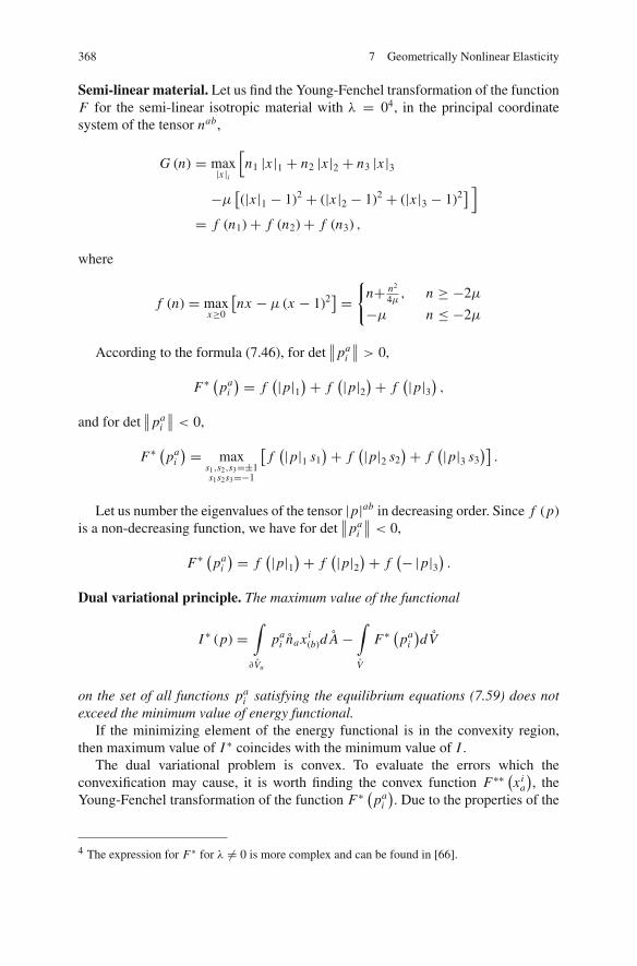
368 7 Geometrically Nonlinear Elasticity
Semi-linear material. Let us find the Young-Fenchel transformation of the functionF for the semi-linear isotropic material with λ = 04, in the principal coordinatesystem of the tensor nab,
G (n) = max|x |i
[n1 |x |1 + n2 |x |2 + n3 |x |3
−μ[(|x |1 − 1)2 + (|x |2 − 1)2 + (|x |3 − 1)2] ]
= f (n1)+ f (n2)+ f (n3) ,
where
f (n) = maxx≥0
[nx − μ (x − 1)2
] ={
n+ n2
4μ, n ≥ −2μ
−μ n ≤ −2μ
According to the formula (7.46), for det∥∥pa
i
∥∥ > 0,
F∗(
pai
) = f(|p|1
)+ f(|p|2
)+ f(|p|3
),
and for det∥∥pa
i
∥∥ < 0,
F∗(
pai
) = maxs1,s2,s3=±1s1s2s3=−1
[f(|p|1 s1
)+ f(|p|2 s2
)+ f(|p|3 s3
)].
Let us number the eigenvalues of the tensor |p|ab in decreasing order. Since f (p)is a non-decreasing function, we have for det
∥∥pai
∥∥ < 0,
F∗(
pai
) = f(|p|1
)+ f(|p|2
)+ f(− |p|3
).
Dual variational principle. The maximum value of the functional
I ∗ (p) =∫
�Vu
pai na xi
(b)d A −∫
V
F∗(
pai
)dV
on the set of all functions pai satisfying the equilibrium equations (7.59) does not
exceed the minimum value of energy functional.If the minimizing element of the energy functional is in the convexity region,
then maximum value of I ∗ coincides with the minimum value of I .The dual variational problem is convex. To evaluate the errors which the
convexification may cause, it is worth finding the convex function F∗∗(xi
a
), the
Young-Fenchel transformation of the function F∗(
pai
). Due to the properties of the
4 The expression for F∗ for λ �= 0 is more complex and can be found in [66].

7.4 Phase Equilibrium of Elastic Bodies 369
Young-Fenchel transformation, F∗∗ ≤ F , and, if F∗∗ does not differ considerablyfrom F , it can be expected that the solutions of the dual convex problem and theinitial non-convex problem are close, at least in energy norm. The calculations forthe two-dimensional case, not reproduced here, result in
F∗∗ ={
μ(γ 2
1 + γ 22
)for γ1 + γ2 ≥ 0
12μ (γ1 − γ2)2 for γ1 + γ2 ≤ 0
where γ1, γ2 are the eigenvalues of the tensor γab. Consequently, if the true strainsγ1 = |x |1 − 1, and γ2 = |x |2 − 1 along the axes X1, X2 are such that γ1 + γ2 ≥ 0,then F = F∗∗, and the solutions of the initial and the dual problems coincide. Ifthe true strain happens to be in the region γ1 + γ2 < 0, then, generally speaking,the solutions of the initial and the dual problems differ. The energy measure of theerrors is controlled by the difference
F(xi
a
)− F∗∗(xi
a
) ={
0 for γ1 + γ2 ≥ 012μ (γ1 − γ2)2 for γ1 + γ2 ≤ 0
7.4 Phase Equilibrium of Elastic Bodies
The variational approach considered so far dealt with only mechanic deformationsof an elastic body. Gibbs variational principles are deeper; in particular, they alsocontrol the thermodynamic equilibrium of two-phase elastic bodies in which thephases can transform one into another (for example, the equilibrium of a metal withits melt). In this section we derive the conditions of the phase equilibrium from thesecond Gibbs principle.
Let two phases of a solid occupy some region V . Subregions of V occupied byeach phase are denoted by V1 and V2 and their common boundary by � (Fig. 7.6).Let U1
(xi
a, S)
and U2(xi
a, S)
be the internal energy densities of two phases per unitmass. The quantities corresponding to the two phases are supplied by the indices 1and 2.
The motion of the surface � over the particles corresponds to transformation ofone phase into another. For definiteness, on the boundary of region V , the particlepositions are assumed to be given while the system is adiabatically isolated.
Fig. 7.6 Notation inconsideration of phaseequilibrium

370 7 Geometrically Nonlinear Elasticity
According to the second Gibbs principle, in thermodynamical equilibrium thefunctional
U =∫
V1
ρU1(xi
a, S)dV +
∫
V2
ρU2(xi
a, S)dV (7.76)
takes the minimum value on the set of all functions xi (Xa) , S (Xa) and surfaces �that satisfy the conditions
∫
V1
ρSdV +∫
V2
ρSdV = S0 = const (7.77)
xi(Xa) = xi
(b)
(Xa)
on �V, (7.78)
and an additional condition on continuity of particle positions on �
[xi(Xa)] = 0 on �. (7.79)
As before, [ϕ] denotes the difference of the limit values of function ϕ on thetwo sides of the surface �: [ϕ] = ϕ1 − ϕ2. Equation (7.79) excludes appearance ofvoids and slipping of the two sides of �. The derivatives of the functions xi (Xa)and the entropy S (Xa) can be discontinuous on �. To include into considerationthe inhomogeneous solids, we have to take into account that energy density maydepend on Lagrangian coordinates, Xa, through the dependence on Xa the physicalcharacteristics, some tensors K B with a set of Lagrangian indices denoted by B.
Denote by pai and μa
b the tensors
pai = ρ0
�U
�xia
, μab = −ρ0
�U
�xia
xib + ρ0 (U − T S) δa
b .
We are going to show that the conditions of thermodynamical equilibrium are
∇a pai = 0,
�U
�S= T = const in V, (7.80)
[pa
i
]na = 0 on �, (7.81)
[μa
b
]na = 0 on �. (7.82)
where ∇a is the covariant derivative in the undeformed state with respect to La-grangian coordinates; without loss of generality, it may be considered coincidingwith the partial derivatives, �/�Xa . The first two equations are the conditions of themechanical equilibrium. The third equation is the condition of the phase (chemical)equilibrium.
Indeed, let us find the variation of the functional U . Let xi (Xa) be a stationarypoint of U , and let xi (Xa, ε) be close particle positions. The space derivatives of

7.4 Phase Equilibrium of Elastic Bodies 371
the particle positions, xi (Xa, ε) , may be discontinuous on some surface �ε whichis close to �. As in the derivation of the Lagrange equations (see Appendix A), itis convenient to introduce the mapping V → V : X ′a = X ′a
(Xb, ε
)for which the
surface � transforms into the surface �ε. Due to the proximity of � and �ε, we canwrite X ′a = Xa + δXa , where δXa are some smooth functions in V . The functionsδXa are zero on �V .
Let us denote by δxi and δS the full variations of xi and S, i.e.
δxi = xi(X ′a, ε
)− xi(Xa), δS = S
(X ′a, ε
)− S(Xa).
The full variations δxi , according to (7.78) and (7.79), satisfy the constraints
δxi = 0 on �V,[δxi
] = 0 on �. (7.83)
Let us show that the constraint on the variations δS which follow from (7.77)have the form
∫
V
[ρ0δS + S∇a
(ρ0δXa
)]dV = 0. (7.84)
Indeed, keeping the small terms of the first order with respect to dε, we have forthe volume element5
ρ0(X ′)√
g (X ′)d3 X ′ =[ρ0 (X )
√g (X )+ �ρ0
√g
�XaδXa
] ∣∣∣∣�X ′
�X
∣∣∣∣ d3 X =
= ρ0
√g
[1+ 1
ρ0
√g
�ρ0
√g
�XaδXa
][1+ �δXa
�Xa
]d3 X =
= ρ0
√g
[1+ 1
ρ0
√g
�ρ0
√gδXa
�Xa
]d3 X
= ρ0
[1+ 1
ρ0∇a(ρ0δXa
)]dV . (7.85)
Therefore,
5 In (7.85), the formulas were used,
∇c Ac = 1√g
�√
g Ac
�Xc, ρdV = ρ0dV .

372 7 Geometrically Nonlinear Elasticity
δ
∫
V1
ρSdV =∫
V ′1
ρ0(X ′)
S(X ′)√
g (X ′)d3 X ′−
−∫
V1
ρ0 (X ) S (X )√
g (X )d3 X =∫
V1
[ρ0δS + S∇a
(ρ0δXa
)]dV .
Formula (7.84) follows from the last equation and a similar equation written for theregion V2.
Analogously to (7.84), we get the relation
δU =∫
V1
[ρ0δU1 +U1∇a
(ρ0δXa
)]dV +
∫
V2
[ρ0δU2 +U2∇a
(ρ0δXa
)]dV .
Consider the quantity δU . In calculating δU , the operator δ should be appliedto the tensor with the Lagrangian indices – the distortion xi
a and the characteristics ofthe medium, K B . We will assume that the operator δ includes the parallel transportover the Lagrangian indices in the initial state. Then, δ K B = δXa∇a K B . For δxi
a ,we have
δxia =
�x ′i(X ′b, ε
)
�X ′a− �b
acδXcxib −
�xi(Xb)
�X ′a= �δxi
�Xa− xi
b∇aδXb.
After integration by parts, the equation δU = 0 becomes
∫
V
[−δxi ∇ pa
i + ρ0δS
(�U
�S− T
)+
+ δXa
(−∇bμ
ba + (U − T S) ∇aρ0 + ρ0
�U
�K B∇a K B
)]dV +
+∫
�
([pa
i
]n
aδxi + [μa
b
]naδXb
)dσ = 0. (7.86)
Here, T is the Lagrange multiplier for the constraint (7.84). The equilibrium condi-tions (7.80), (7.81) and (7.82) follow from (7.86).
There is an additional equation, which must be satisfied in equilibrium:
− ∇bμba + (U − T S) ∇aρ0 + ρ0
�U
�K B∇a K B = 0 in V, (7.87)
However, one can check that (7.87) is a consequence of (7.80).Equations (7.80) are the conditions of thermodynamic equilibrium obtained in
Sect. 7.2.Equations (7.81) shows that the necessary condition of thermodynamic equilib-
rium is the equality of forces acting on the two sides of the surface �.
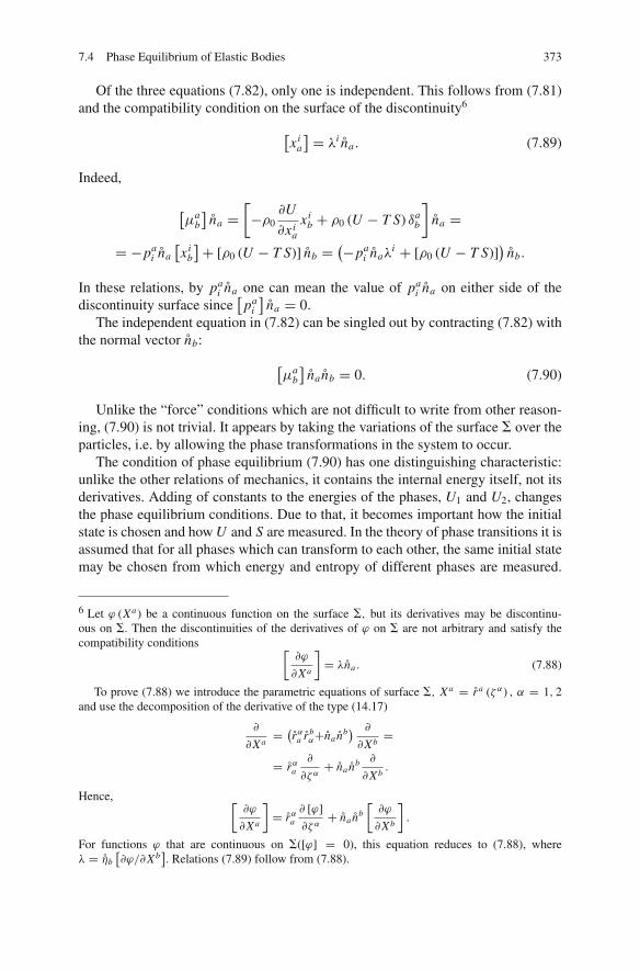
7.4 Phase Equilibrium of Elastic Bodies 373
Of the three equations (7.82), only one is independent. This follows from (7.81)and the compatibility condition on the surface of the discontinuity6
[xi
a
] = λi na . (7.89)
Indeed,
[μa
b
]na =
[−ρ0
�U
�xia
xib + ρ0 (U − T S) δa
b
]na =
= −pai na
[xi
b
]+ [ρ0 (U − T S)] nb =(−pa
i naλi + [ρ0 (U − T S)]
)nb.
In these relations, by pai na one can mean the value of pa
i na on either side of thediscontinuity surface since
[pa
i
]na = 0.
The independent equation in (7.82) can be singled out by contracting (7.82) withthe normal vector nb:
[μa
b
]na nb = 0. (7.90)
Unlike the “force” conditions which are not difficult to write from other reason-ing, (7.90) is not trivial. It appears by taking the variations of the surface � over theparticles, i.e. by allowing the phase transformations in the system to occur.
The condition of phase equilibrium (7.90) has one distinguishing characteristic:unlike the other relations of mechanics, it contains the internal energy itself, not itsderivatives. Adding of constants to the energies of the phases, U1 and U2, changesthe phase equilibrium conditions. Due to that, it becomes important how the initialstate is chosen and how U and S are measured. In the theory of phase transitions it isassumed that for all phases which can transform to each other, the same initial statemay be chosen from which energy and entropy of different phases are measured.
6 Let ϕ (Xa) be a continuous function on the surface �, but its derivatives may be discontinu-ous on �. Then the discontinuities of the derivatives of ϕ on � are not arbitrary and satisfy thecompatibility conditions [
�ϕ
�Xa
]= λna . (7.88)
To prove (7.88) we introduce the parametric equations of surface �, Xa = r a (ζ α) , α = 1, 2and use the decomposition of the derivative of the type (14.17)
�
�Xa= (
rαa r b
α+na nb) �
�Xb=
= rαa
�
�ζ α+ na nb �
�Xb.
Hence, [�ϕ
�Xa
]= rα
a
� [ϕ]
�ζ α+ na nb
[�ϕ
�Xb
].
For functions ϕ that are continuous on �([ϕ] = 0), this equation reduces to (7.88), whereλ = ηb
[�ϕ/�Xb
]. Relations (7.89) follow from (7.88).

374 7 Geometrically Nonlinear Elasticity
Due to this assumption, the initial values of energy, entropy, density and other phasecharacteristics turn out to be continuous on the phase boundary.
In order to clarify the meaning of the condition (7.90), let us consider a specialcase of elastic bodies, a liquid, when the internal energy depends on distortion onlythrough the density ρ = ρ0
√g/√
g�, � = det∥∥xi
a
∥∥. Since �ρ/�xia = −ρXa
i , thetensor μa
b is spherical:
μab = ρ0μδa
b , μ = U − T S + p
ρ.
Here, p = ρ2�U/�ρ is the pressure. Since [ρ0] = 0, it follows from (7.90) that[μ] = 0. The quantity μ is the chemical potential (see (5.104)), and the condition[μ] = 0 is the necessary condition for the thermodynamic equilibrium of two liquidphases, established by Gibbs. Accordingly, the tensor μa
b can be called the chemicalpotential tensor of an elastic medium.

Chapter 8Dynamics of Elastic Bodies
8.1 Least Action vs Stationary Action
The extrapolation to dynamics of the minimization principles formulated above en-counters difficulties, the essence of which can be observed for systems with onedegree of freedom.
Consider the harmonic oscillator – a material point on a spring. The deviationof the point from the equilibrium position is denoted by x (t); the kinetic energy isequal to 1
2 mx2, and the energy of the spring is 12 kx2. According to the Hamilton
principle, the true trajectory is the stationary point of the functional
I = 1
2
�t∫
0
(mx2 − kx2)dt
on the set of functions, x (t), which take at the initial and final moments the givenvalues
x (0) = x0, x (�t) = x1.
The question is: does the true trajectory provide the minimum for the functionalI ? In order to investigate this question, it is convenient to use instead of functionsx (t) the functions u (t) which are equal to zero in the initial and final moments:
x → u : x (t) = vt + x0 + u (t) , v = (x2 − x1) /�t = const, u (0) = u (�t) = 0.
The constant, v, has the meaning of the average velocity. The functional I (u)takes the form (additive constant is omitted)
I (u) = J (u)+ l (u) ,
J (u) = 1
2
�t∫
0
(mu2 − ku2
)dt, l (u) = −k
�t∫
0
(vt + xo) udt.
V.L. Berdichevsky, Variational Principles of Continuum Mechanics,Interaction of Mechanics and Mathematics, DOI 10.1007/978-3-540-88467-5 8,C© Springer-Verlag Berlin Heidelberg 2009
375

376 8 Dynamics of Elastic Bodies
Posing the minimization problem is possible if the functional I (u) is boundedfrom below. For this to be true, it is necessary that the functional J (u) be boundedfrom below.1 For every function u (x), the set of admissible functions contains thefunction λu (x) (with any λ); therefore, for the quadratic functional to be boundedfrom below it is necessary and sufficient that it is non-negative. Let us write downthis condition. It is convenient to use a new argument τ = 2π
�t t . From the inequalityJ (u) ≥ 0, it follows that, for any functions u (τ ) such that u (0) = u (2π ) = 0, theinequality
2π∫
0
(du
dτ
)2
dτ ≥ c
2π∫
0
u2dτ, c = k (�t)2
4π2m(8.1)
should hold. We arrive at the Wirtinger inequality (5.24). The inequality (8.1) holdsfor all c ≤ 1/4. Moreover, for c < 1/4 the functional J (u) will be strictly convex,as a quadratic positive functional. For c > 1/4, the functional J (u) is not boundedfrom below. Indeed, 1/4 is the best constant in the Wirtinger inequality for zerovalues of the function at the ends; therefore, for c > 1/4 there exists at least onefunction u0 for which J (u0) < 0, while l (u0) has a finite value. Thus, for thesequence {λu0}, λ→∞, J (λu0)→−∞.
So, posing the minimization problem is possible only for sufficiently small �t ,�t < π
√m/k.
For continuous media, the problem is more complicated. Let us consider, forexample, the action functional of the wave equation
I (u) = 1
2
�t∫
0
π∫
−π
(u2
,t − u2,x
)dxdt
and set the kinematic boundary conditions u (0, x) = u0 (x), u (�t, x) = u1 (x),u (t,−π ) = u (t, π ) = 0. Let the functions u0 (x) and u1 (x) be odd, so that we willonly need odd admissible functions u (x).2 Functions u (x) can be presented in theform of the Fourier series:
u (t, x) =∞∑
k=1
uk (t) sin kx . (8.2)
Substituting (8.2) into I (u), we get
I (u) =∞∑
k=1
Ik, Ik = π
2
�t∫
0
(u2
k − k2u2k
)dt.
1 Indeed, if there exists a sequence {un} for which J (un) → −∞, while l (un) ≤ const, thenI (un)→−∞. If l (un)→+∞, then for the sequence {−un}, we have I (un)→−∞.2 See Sect. 5.13.

8.2 Nonlinear Eigenvibrations 377
Since the functions uk (t) are independent, the boundedness from below of eachfunctional Ik is necessary for the boundedness from below of the functional I (u).For this, as shown above, it is necessary that for each k
k2�t2 ≤ π2.
It is impossible to satisfy these inequalities for all k. Therefore the functionalI (u) is not bounded from below, however small is �t . Apparently, posing the min-imization problem is possible for a quasi-continuum [164], for which short waves(with large k) are excluded.
The noted difficulty is related to the fact that the Hamilton principle in essenceyields a Dirichlet-type problem, but this problem is ill-posed for hyperbolicequations.
The noted difficulty is closely related to ill-posedness of hyperbolic equations forthe Dirichlet-type problems.
A well-posed dynamical problem is the Cauchy problem, when one prescribesthe initial values of the required function and its time derivative. The Hamil-ton principle can be rendered in the form which corresponds to a problem withthe prescribed initial value of the required function and the average value of itstime derivative over some interval �t. Indeed, instead of fixing u (�t, x) , one canprescribe
u (�t, x)− u (0, x)
�t= 1
�t
t+�t∫
t
u,t dt.
This assertion, however, has the same peculiarity as the Hamilton principle: theminimization problem is ill-posed unless the short waves are excluded.
8.2 Nonlinear Eigenvibrations
The above pertains to general dynamic problems for continua. However, there isan important class of dynamic problems for which the setting of the variationalproblems is very close to that for static problems. These are the so-called naturalvibrations. By natural one means periodic vibrations which occur without action ofexternal forces. On the boundary of the continuum, homogeneous boundary condi-tions are assumed (clamped boundaries, zero external surface forces, etc.). Naturalvibrations may occur only at some special values of frequencies called eigenfre-quencies. Let us construct the variational principle for determining the eigenfre-quencies and the modes of vibration.

378 8 Dynamics of Elastic Bodies
Let the true motion of a continuum be a stationary point of the functional
t1∫
t0
∫
V
L(x, uκ, uκ
,t , uκ
,i
)dV dt.
For definiteness, we will assume the clamped boundaries conditions
uκ = 0 on �V . (8.3)
Natural vibration with a frequency ω is a stationary point of the functional
πω∫
− πω
∫
V
L(x, uκ, uκ
,t , uκ
,i
)dV dt
on the set of functions uκ satisfying the condition (8.3) and the periodicity condition
uκ
(x,−π
ω
)= uκ
(x,
π
ω
).
In the variational problem, it is convenient to make a change of the independentvariable t → θ : ωt = θ,−π ≤ θ ≤ π . Then, the eigenvibrations are the stationarypoints of the functional
π∫
−π
∫
V
L(x, uκ, ωuκ
,θ , uκ
,i
)dV dθ (8.4)
on the set of functions uκ satisfying the condition (8.3) and the periodicity condition
uκ (x,−π ) = uκ (x, π ) . (8.5)
One can assume that 2π is the smallest period of the functions uκ (x, θ ) .
The variational problem (8.3), (8.4) and (8.5) admits an interesting interpretationif the Lagrangian L is the difference of the kinetic energy and the free energy,
L = K(x, uκ, uκ
,t
)− F(x, uκ, uκ
,i
),
where K and F are nonnegative, and K is a homogeneous function of the secondorder with respect to uκ
,t , i.e. for any ω > 0,
K(x, uκ, ωuκ
,t
) = ω2 K(x, uκ, uκ
,t
).

8.3 Linear Vibrations: The Rayleigh Principle 379
In order to simplify further consideration, we will also assume that K and F arestrictly convex and equal to zero for uκ ≡ 0.
Let us show that in this case the variational problem (8.3), (8.4) and (8.5) isequivalent to the following one: find stationary points of free energy functional
π∫
−π
∫
V
F(x, uκ, uκ
,i
)dV dθ (8.6)
on the set of function uκ , satisfying the constraints (8.3) and (8.5) and the condition
π∫
−π
∫
V
K(x, uκ, uκ
,θ
)dV dθ = A2, (8.7)
where A is some given constant.Indeed, introducing the Lagrange multiplier for the constraint (8.7), the func-
tional of the problem can be written as
π∫
−π
∫
V
FdV dθ − λ
⎛⎝
π∫
−π
∫
V
K dV dθ − A2
⎞⎠ . (8.8)
The Lagrange multiplier λ is nonnegative: for λ < 0, the functional (8.8) isstrictly convex and has the only stationary point, uκ = 0. Therefore, each stationarypoint of the variational problem (8.3), (8.5), (8.6) and (8.7) is the stationary point ofthe initial problem with ω2 = λ.
Conversely, each stationary point of the initial problem is the stationary point ofthe variational problem (8.3), (8.5), (8.6) and (8.7) for some A; it is sufficient tocalculate the value of A, corresponding to the stationary point being considered, bymeans of formula (8.7).
In the variational problem (8.3), (8.5), (8.6) and (8.7), the Lagrange multiplierfor the constraint (8.7) has the meaning of the squared frequency, and the constantA is a measure of the amplitude of the vibrations.
As a rule, for any value of A there exists a countable number of stationary pointsand the corresponding values of eigenfrequencies. They continuously change as thevalue of A is changed.
8.3 Linear Vibrations: The Rayleigh Principle
For A → 0, the amplitude of vibrations tends to zero. If F and K are smoothfunctions and K becomes zero for uκ
,t = 0, then for infinitesimally small amplitudes,F can be replaced by a quadratic form with respect to uκ, uκ
,i , and K can be replaced

380 8 Dynamics of Elastic Bodies
by a quadratic form with respect to uκ, uκ
,i , and K can be replaced by a quadraticform with respect to uκ
θ : 2K = ρκκ′uκ
θ uκ′
θ . It is easy to check that the stationarypoints have the form uκ = vκ (x) cos θ or uκ = vκ (x) sin θ . After integrating overθ , the variational principle (8.3), (8.5)–(8.7), becomesRayleigh principle.The modes of eigenvibrations are the stationary points of thefree energy functional 3
F =∫
V
F(x, vκ, vκ
,i
)dV, (8.9)
on the set of functions vκ vanishing on �V and having a given value of kineticenergy
K =∫
V
1
2ρκκ
′vκvκ′dv = A2. (8.10)
The change of the constant A corresponds to multiplying vκ by a constant; there-fore, without loss of generality we can set A = 1 in (8.10).
The Rayleigh variational principle is equivalent to the assertion of the stationarityof the so-called Rayleigh quotient,
R = FK =
∫V
F(x, vκ, vκ
,i
)dV
∫V
12ρκκ
′vκvκ′dV
.
Indeed, the Rayleigh quotient does not change if the function vκ is multipliedby a constant; in particular, this constant can be chosen in such a way as to makeK = 1 and thus R = F .
The non-convexity, which is characteristic for the variational problems of dy-namics, is preserved for eigenvibrations as well: the constraint K = const extracts anon-convex set in the functional space – a sphere (in an appropriate norm).4
If the function F is not smooth at zero, then the variational principle (8.3),(8.5), (8.6) and (8.7), generally speaking, does not transform to the Rayleighprinciple even in the case of infinitesimally small amplitudes. As an example,note the problem of eigenvibrations when continuum has different moduli foru,κ > 0 and u,κ < 0; e.g., in the one-dimensional case, 2F = αu2
,x + βu,x
∣∣u,x
∣∣ ,
3 It is easy to check that the stationary points of the functional (8.6) do not change if the samefactor, k , is included in the left-hand sides of (8.6) and (8.7), and the constant A2 is replacedby k A2. In transition from (8.6), (8.7) to (8.9), (8.10) the coefficient k = 1/π is introduced; theconstant A2 in (8.10) differs from the constant A2 in (8.7) by the same factor.4 If the condition K = A2 could be changed by the condition K ≤ A2, then the problem would beconvex. In the variational principle formulated, it is possible only to replace the condition K = A2
by the inequality K ≥ A2 which selects a non-convex set.

8.4 The Principle of Least Action in Eulerian Coordinates 381
α + β > 0, α − β > 0. For such elastic body, due to non-linearity, of the problem,the eigenfunctions cannot be presented as the product of a function depending on θ
and a function depending on x .
8.4 The Principle of Least Action in Eulerian Coordinates
The principle of least action for an elastic body in Lagrangian coordinates was for-mulated in Sect. 4.3. Sometimes it is of interest to formulate it also in Euleriancoordinates. Although it involves only rewriting the action functional in differentterms, there are a number of technical details deserving consideration.
In Eulerian coordinates, it is convenient to define the action functional on dis-placements, ui (x, t):
ui (x, t) = xi (X, t)−x i (X )∣∣
X=X (x,t) = xi − x i (X (x, t)) .
The displacements are uniquely related to the particle trajectories. The domainof displacements, ui (x, t), is the region, V (t) , occupied by the continuum at thetime t .
Assigning the particle positions in the initial and the final times corresponds toassigning the displacements,
ui (x, t0) = 0, ui (x, t1) = ui1 (x) . (8.11)
The functions ui1 (x) are defined in the region
1V = V (t1). The points with the
coordinates xi − ui1 (x) for x ∈
1V are in the region V = V (t0). The corresponding
mapping of1V onto V is one-to-one.
Let us express the arguments of the Lagrangian in terms of the displacementsand their derivatives. We begin with the Lagrangian coordinates Xa . The relationbetween the Lagrangian and the Eulerian coordinates at the initial instant is
Xa = X a (x)
where x i are the Eulerian coordinates of the points in V . Since x i = xi − ui(xk, t
),
the dependence of the Lagrangian coordinates on the Eulerian coordinates at anyinstant has the form
Xa = X a(xi − ui (x, t)
). (8.12)
Here, X a(xi)
are the known functions, the inverse of the functions x i (Xa) . Inparticular, if the Lagrangian and the Eulerian coordinates coincide at the initial time,then Xi = x i and Xi
(xi , t
) = xi−ui (x, t). However, as has been noted, a particularchoice of Lagrangian coordinates at the stage of deriving the equations excludes the

382 8 Dynamics of Elastic Bodies
possibility to check the invariance of all relations with respect to transformations ofthe Lagrangian coordinates; therefore, we use the general formula (8.12).
Assigning the particle positions at the boundary of the body corresponds to as-signing a part of the boundary � (t) of the region V (t) and the values of the dis-placement vector at this part:
ui = ui(b) (x, t) on � (t) . (8.13)
These values are not arbitrary. They satisfy the condition
X a(xi − ui
(b) (x, t)) ∈ � for x ∈ �.
(� is the part of the boundary of the body in the space of Lagrangian coordinatesfor the points of which the displacements are given).
Let us find the relation between the distortion and the displacement gradient.Differentiating (8.12) with respect to xi we have5
�Xa
�xi= �X a
�xk
(δk
i − uki
), uk
i =�uk
�xi.
Hence,
det
∥∥∥∥�Xa
�xi
∥∥∥∥ = det
∥∥∥∥∥�X a
�xi
∥∥∥∥∥ · det∥∥δk
i − uki
∥∥ . (8.14)
Equation (8.14) shows that the matrix∥∥δk
i − uki
∥∥ is non-singular. Therefore, it ispossible to introduce the tensor si
j , which is the inverse of the tensor δki − uk
i :
sij
(δ
jk − ui
k
)= δi
k . (8.15)
The distortion xia is given by the equation
xia = x k
a sik . (8.16)
This can be checked by direct inspection:
xia Xa
j = x ka si
k X am
(δm
j − umj
) = δij .
Here, the formulas (8.15) and (8.16) are used.In terms of the displacement gradient, the density ρ, according to (8.14) is
5 Remember that the observer’s coordinate system is Cartesian.
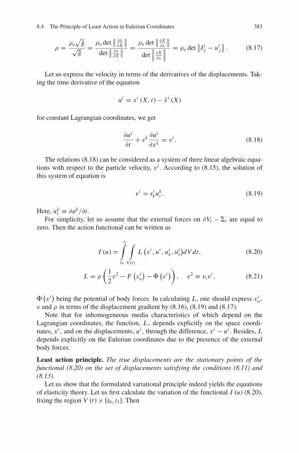
8.4 The Principle of Least Action in Eulerian Coordinates 383
ρ = ρo
√g√
g= ρo det
∥∥ �x�X
∥∥det
∥∥ �x�X
∥∥ =ρo det
∥∥ �X�x
∥∥det
∥∥∥ �X�x
∥∥∥= ρo det
∥∥δij − ui
j
∥∥ . (8.17)
Let us express the velocity in terms of the derivatives of the displacements. Tak-ing the time derivative of the equation
ui = xi (X, t)− x i (X )
for constant Lagrangian coordinates, we get
�ui
�t+ vk �ui
�xk= vi . (8.18)
The relations (8.18) can be considered as a system of three linear algebraic equa-tions with respect to the particle velocity, vi . According to (8.15), the solution ofthis system of equation is
vi = sikuk
t . (8.19)
Here, ukt ≡ �uk/�t .
For simplicity, let us assume that the external forces on �Vt – �t are equal tozero. Then the action functional can be written as
I (u) =t1∫
t0
∫
V (t)
L(xi , ui , ui
k, uit
)dV dt, (8.20)
L = ρ
(1
2v2 − F
(xi
a
)−�(xi))
, v2 ≡ vivi , (8.21)
�(xi)
being the potential of body forces. In calculating L , one should express xia,
v and ρ in terms of the displacement gradient by (8.16), (8.19) and (8.17).Note that for inhomogeneous media characteristics of which depend on the
Lagrangian coordinates, the function, L , depends explicitly on the space coordi-nates, xi , and on the displacements, ui , through the difference, xi − ui . Besides, Ldepends explicitly on the Eulerian coordinates due to the presence of the externalbody forces.
Least action principle. The true displacements are the stationary points of thefunctional (8.20) on the set of displacements satisfying the conditions (8.11) and(8.13).
Let us show that the formulated variational principle indeed yields the equationsof elasticity theory. Let us first calculate the variation of the functional I (u) (8.20),fixing the region V (t)× [t0, t1]. Then

384 8 Dynamics of Elastic Bodies
δ I (u) =t1∫
t0
∫
V (t)
�LdV dt =
=t1∫
t0
∫
V (t)
(�L
�ui�ui + �L
�uik
��ui
�xk+ �L
�uit
��ui
�t
)dV dt = 0. (8.22)
As before, the symbol � denotes the variation at constant Eulerian coordinates.First, let �ui = 0 on V (t). Integrating by parts, we get
δ I (u) =t1∫
t0
∫
V (t)
�ui δL
δuidV dt = 0,
δL
δui= �L
�ui− �
�xk
�L
�uik
− �
�t
�L
�uit
. (8.23)
From (8.23) the equations follow
δL
δui= 0. (8.24)
These equations are equivalent to the momentum equations of the elasticity the-ory. Indeed, due to the non-singularity of the matrix
∥∥δki − uk
i
∥∥, the system of equa-tions (8.24) is equivalent to the system of equations
δL
δuk
(δk
i − uki
) = 0. (8.25)
Note the identity
− uki
δL
δuk= �i L − �L
�xi+ �
�xm
(�L
�ukm
uki
)+ �
�t
(�L
�ukt
uki
)(8.26)
which can be checked by direct inspection. Here, the partial derivative of the func-tion L
(xi , ui , ui
k, uit
)with respect to xi is denoted by �i L , in contrast to �L/�xi
which means “full” derivative with respect to xi , i.e. the derivative taking into ac-count the dependence of all the arguments of L on xi .
From (8.25) and (8.26) we find that

8.4 The Principle of Least Action in Eulerian Coordinates 385
δL
δuk
(δk
i − uki
) = δL
δui− uk
i
δL
δuk= �L
�ui− �
�xm
�L
�uim
−
− �
�t
�L
�uit
+ �i L − �L
�xi+ �
�xm
(�L
�ukm
uki
)+ �
�t
(�L
�ukt
uki
)=
= �i L + �L
�ui− �
�xm
[�L
�ukm
(δk
i − uki
)+ Lδmi
]− �
�t
[�L
�ukt
(δk
i − uki
)]. (8.27)
Since the free energy depends on the Eulerian coordinates only through the dif-ference xi − ui ,
�i L + �L
�ui= −ρ
��
�xi. (8.28)
In order to calculate the other terms in (8.27), we need the formulas
(δk
i − uki
) �ρ
�ukm
= −ρδmi ,
�sij
�ukm
= siksm
j . (8.29)
The first follows from the equalities (3.20) and (8.17), the second is derived inthe same way as (4.24). Due to (8.29), we have
(δk
i − uki
) �
�ukt
(1
2ρv2
)= ρvi ,
(δk
i − uki
) �
�ukm
v2
2= viv
m . (8.30)
Therefore,
�L
�ukm
(δk
i − uki
)+ Lδmi = ρvmvi − σ m
i . (8.31)
Here, we introduced the notation
σj
i = ρ(δk
i − uki
) �F
�ukj
= ρ�F
�uij
− ρ�F
�ukj
uki . (8.32)
Using (8.29) and (8.16), it is easy to see that
σj
i = ρ�F
�xia
x ja .
Therefore, σj
i has the meaning of the components of the Cauchy stress tensor.From the relations (8.29), (8.30), (8.31) and (8.32) follow the known momentum
equations
�ρvi
�t+ �
�xm
(ρviv
m − σ mi
)+ ρ��
�xi= 0. (8.33)

386 8 Dynamics of Elastic Bodies
The constitutive equations (8.32) are sometimes written in the form which takesinto account the fact that the free energy depends on the components of the strain
tensor with the observer’s indices εi j = εab Xai Xb
j . Since εab = 12 gi j
(xi
a x jb − x i
a x jb
),
the quantities εi j are expressed through the displacement gradient as
εi j = 1
2
(gi j−xm
a xmb Xa
i Xbj
) = 1
2
(gi j −
(δk
i − uki
) (gk j − uk j
)) = u(i j) − 1
2uk
kuk j .
Consequently, for F = F(εi j), from (8.32) we have
σ i j = ρ�F
�εi j− 2ρ
�F
�εikε
jk .
This relation is called Murnagan’s equation. Note that this formula, unlike for-mula (8.32), is valid only for isotropic media because the free energy of anisotropicbody depends not only on the components of the strain tensor εi j but also on thedisplacement gradient. This can be checked by considering the example of a physi-cally linear material with 2F = Cabcdεabεcd . Switching to the components with theobserver’s indices, we have 2F = Cabcdxi
a x jb xk
c xldεi jεkl . Hence, F depends not only
on εi j , but also – through xia – on ui
j .Now let the displacement variations and the variations of the part of the boundary
S (t) = �V (t)− � (t) be non-zero. The calculation of δ I results in
δ I =t1∫
t0
∫
S(t)
[�ui
(�L
�uik
nk − �L
�uit
cx
)+ Lδn
]dσdt. (8.34)
Here, (3.92) is used, and it is taken into account that due to the momentum equa-tions (8.24) the volume integral is equal to zero; cx is the velocity of the surface S (t)along its normal in the observer’s coordinate system, δn is the virtual displacementof the surface S (t) in the direction of the normal.
Let us rewrite the integrand in (8.34) using the relations (8.30) and (8.31):
�ui
(�L
�uis
ns − �L
�uit
cx
)+ Lδn = �u j sk
j
(δi
k − uik
) ( �L
�uis
ns − �L
�uit
cx
)+ Lδn =
= �u j skj
[(ρvsvk − σ s
k − Lδsk
)ns − ρvkcx
]+ Lδn == �u j sk
j ρvk(vsns − cx
)+ L(δn − �u j sk
j nk)− �u j sk
j σsk ns . (8.35)
The first term in the right hand side of (8.35) is equal to zero: the differencevsns − cx has the meaning of the surface velocity over the particles, and it is equalto zero since S (t) does not move over the particles. The second term is also equalto zero. Indeed, the equality is valid:
δxk = δuk = skj �u j . (8.36)

8.4 The Principle of Least Action in Eulerian Coordinates 387
It follows from the relation (4.31), written for the displacements:
δu j = �u j + u jkδuk . (8.37)
The solution of (8.37), considered as a system of linear equations with respectto δuk , is given by the formulas (8.36). In terms of the variations with constantLagrangian coordinates, the condition that the boundary particles remain on theboundary yields
δn = δxknk . (8.38)
From (8.38) and (8.36),
δn − �u j skj nk = 0,
thus the second term in the right hand side of (8.35) vanishes. We obtain for thevariation of the action functional,
δ I = −t1∫
t0
∫
S(t)
�ui skj σ
sk nsdσdt = 0.
Due to the arbitrariness of �ui and the non-singularity of the matrix skj , the natural
condition on S (t) are σ sk ns = 0.

Chapter 9Ideal Incompressible Fluid
9.1 Least Action Principle
Consider a continuum in some vessel, V . Continuum occupies the entire vessel atthe initial instant, t0. Let us prescribe the initial and the final positions of each pointof the continuum,
x (t0, X ) = x (X ) , x (t1, X ) = 1x (X ) , (9.1)
and find the trajectories which minimize the action functional,
I (x (t, X )) =t1∫
t0
∫
V
1
2ρ
dxi (t, X )
dt
dxi (t, X )
dtdV dt, (9.2)
with ρ being a constant. Such a variational problem corresponds to motion of non-interacting particle. The particles are driven only by inertia. Obviously, the trajec-tory of each particle is a straight line in four-dimensional time-space connecting theinitial and final positions (Fig. 9.1). Such motion of continuum is compressible. Be-sides, the mapping, x (t, X ) , is not a one-to-one mapping because trajectories mayintersect. Let us complicate this inertial motion by imposing the incompressibilitycondition
det
∥∥∥∥�x (t, X )
�X
∥∥∥∥ = det
∥∥∥∥�x (X )
�X
∥∥∥∥ . (9.3)
Then mapping, x (t, X ) , becomes a one-to-one mapping, at least locally.Continuum model which incorporates two features, inertia of particles and in-
compressibility of motion, is called ideal incompressible fluid. Motion of ideal in-compressible fluid is a stationary point in the following variational principle.Least action principle. The true motions of ideal incompressible fluid are the sta-tionary points of the action functional (9.2) on the set of all motions extracted bythe constraints (9.1) and (9.3).
V.L. Berdichevsky, Variational Principles of Continuum Mechanics,Interaction of Mechanics and Mathematics, DOI 10.1007/978-3-540-88467-5 9,C© Springer-Verlag Berlin Heidelberg 2009
389

390 9 Ideal Incompressible Fluid
Fig. 9.1 Minimizer of thevariational problem (9.1) and(9.2)
In this formulation particles are allowed to detach from the wall. One can alsoimpose an additional condition that the boundary particles remain on the wall all thetime:
x (t, X ) ∈ �V (t) if X ∈ �V , (9.4)
where the current position of the vessel, V (t) , is prescribed and may not coincidewith the initial position, V .
To derive the equations governing the motion of ideal incompressible fluid fromthe least action principle, we get rid of the constraint (9.3) by introducing a Lagrangemultiplier, p. The expanded functional is
t1∫
t0
∫
V
[1
2ρ
dxi
dt
dxi
dt+ p
(det
∥∥ �x�X
∥∥det
∥∥ �x�X
∥∥ − 1
)]dV dt,
and for its variation we obtain
t1∫
t0
∫
V
[ρvi
dδxi
dt+ p
�δxi
�xi
]dV dt =
=
⎡⎢⎣∫
V
ρviδxi dV
⎤⎥⎦
t1
t0
+t1∫
t0
∫
V
pδxi ni d Adt −t1∫
t0
∫
V
δxi
(ρ
dvi
dt+ �p
�xi
)dV dt. (9.5)
Here we used (4.19). The first term in (9.5) vanishes due to (9.1): δxi = 0 att = t0, t1. If particles do not detach from the wall, δxi ni = 0 at �V , and the secondterm vanishes as well. Therefore, equating (9.5) to zero we obtain the equations
ρdvi
dt= − �p
�xi, (9.6)

9.1 Least Action Principle 391
which are the momentum equations of ideal incompressible fluid. Pressure in thefluid is the Lagrange multiplier for the incompressibility condition. This was the waywhich was used by Lagrange to derive these equations [168]. Momentum equationsmust be complimented by the incompressibility condition which is usually taken inthe differential form:
�vi
�xi= 0. (9.7)
If fluid is allowed to detach from the wall in the course of motion, and some freesurface forms, then, due to arbitrariness of δxi ni ,
p = 0 (9.8)
on the free surface.To model the fluid evaporation or other physical mechanisms by which a non-
zero pressure develops inside the cavity, formed by the detached fluid, one has totake into account the work of pressure on the free surface displacements. Then theaction functional gains an additional term,1
∫
Vc
p0dVdt,
where p0 is the pressure in the cavity, Vc. Accordingly the boundary condition (9.8)is replaced by the condition
p = p0 (9.9)
at the free surface.All the equations obtained remain valid if the fluid is inhomogeneous, i.e. its
density depends on Lagrangian coordinates: ρ = ρ (X ). Another modification of theaction functional appears if there are body forces with the potential � (x) , actingon the fluid. The action functional becomes
t1∫
t0
∫
V
[1
2ρ
dxi
dt
dxi
dt− ρ� (x (t, X ))
]dV dt. (9.10)
If the fluid is homogeneous and does not detach from the wall, then the secondterm in (9.10) is not essential because it does not depend on fluid motion:
t1∫
t0
∫
V
ρ� (x (t, X )) dV dt =t1∫
t0
∫
V (t)
ρ� (x) dV dt
1 See (7.13).

392 9 Ideal Incompressible Fluid
If the fluid is inhomogeneous and/or has free surfaces this term is essential. We willencounter its contributions later in Sect. 13.2.
9.2 General Features of Solutions of Momentum Equations
Momentum equations of ideal incompressible homogenous fluid (9.6) can be “in-tegrated” in the following sense. Let us project these equations on the Lagrangianframe:
ρxia
dvi
dt= −xi
a
�p
�xi= − �p
�Xa. (9.11)
Denoting by va the Lagrangian components of velocity,
va = xiavi ,
and using the fact that
xia
dvi
dt= dva
dt− vi
dxia
dt= dva
dt− vi
�vi
�Xa=
= dva
dt− 1
2
�
�Xav2, v2 ≡ viv
i , (9.12)
we have
dva
dt= �
�Xa
(− p
ρ+ v2
2
).
Let us introduce a function, ϕ, by the equation
dϕ
dt= − p
ρ+ v2
2. (9.13)
Then the momentum equations can be written as
d
dt
(va − �ϕ
�Xa
)= 0.
Hence, the Lagrangian covariant components of velocity, va differ from �ϕ/�Xa
only by some field, va, which does not depend on time:
va = �ϕ
�Xa+ va (X ) , (9.14)
or, in Eulerian coordinates,

9.2 General Features of Solutions of Momentum Equations 393
vi = �ϕ
�xi+ Xa
i va (X ) . (9.15)
Function ϕ can be chosen arbitrarily at the initial instant. If ϕ is set to be equalto zero initially, then va (X ) have the meaning of the initial Lagrangian velocitycomponents.
Equation (9.14) determines the general structure of solutions of Euler equations:the Lagrangian components of velocity, va, may depend on time only through thepotential part, �ϕ/�Xa .
There are other forms of this statement. As follows from (9.14) the antisymmetricpart of the gradient of velocity does not depend on time:
�[avb] = �[a vb] (X ). (9.16)
The antisymmetric tensor �[avb] is in one-to-one correspondence with the vector:
ωc ≡ εabc�[avb] = 1√g
eabc�[avb], �[avb] = 1
2
√geabcω
c.
Due to the incompressibility condition, the determinant of the metric tensor, g, canbe set equal to unity.
The vector with the contravariant Lagrangian components, ωa, is called the vor-ticity vector. In Eulerian coordinates, the vorticity vector has the components
ωi = eijk �vk
�x j, (9.17)
and, due to the law of transformation of vector components,
ωi = xiaω
a . (9.18)
Conversely,
ωa = Xai ωi .
According to (9.16), the contravariant Lagrangian components of vorticity, ωc,
do not change in time at each fluid particle:
dωa
dt= 0. (9.19)
Note that the covariant components of vorticity, ωb = gbaωa, may change in time.
Another form of (9.14) is obtained by differentiation of (9.18) with respect totime at constant Lagrangian coordinates. Using the independence of ωa on time andformula the time defivative of distortion (3.43), we obtain the evolution equationsfor Eulerian components of vorticity,

394 9 Ideal Incompressible Fluid
dωi
dt= �vi
�xkωk . (9.20)
This equation can also be written in a different form where summation over k isconducted with another index of the velocity gradient,
dωi
dt= �vk
�xiωk . (9.21)
This follows from the identity
(�vk
�xi− �vi
�xk
)ωk = 0. (9.22)
The identity follows from the inversion of (9.17) (similarly to (3.53)):
�vk
�xi− �vi
�xk= eikmωm,
and vanishing of the sum, eikmωkωm = 0.
Conservation of vorticity is often stated in the integral form: for any closed con-tour, �, the circulation of velocity over this contour,
∮vi dxi , does not change in
time. This statement is equivalent to the conservation of the Lagrangian contravari-ant components of vorticity, ωa . Indeed, a moving fluid contour � is the image ofa contour, �, which is stationary in Lagrangian coordinates. Therefore, the circula-tion of velocity can be presented as the circulation of velocity over this stationarycontour:
C ≡∫
�
vi dxi =∫
�
vi xiad Xa =
∫
�
vad Xa .
Transferring the integral over � to the integral over a surface S which has the bound-ary �, we have
C =∫
�
vad Xa =∫
S
�[avb]d Xa ∧ d Xb.
Since �[avb] do not depend on time, C also does not depend on time. The arbi-trariness of the contour � yields the equivalence of the conservation of velocitycirculations and the conservation of ωa .
Let us return to (9.14). In this equation, one can set ϕ = 0 at the initial instantand consider va (X ) as the functions known from the initial conditions. Then theparticle trajectories can be sought from a system of equations of the first order,

9.2 General Features of Solutions of Momentum Equations 395
�xi (t, X )
�Xa
�xi (t, X )
�t= va (X )+ �ϕ (t, X )
�Xa. (9.23)
The incompressibility condition,
det
∥∥∥∥�x
�X
∥∥∥∥ = det
∥∥∥∥�x
�X
∥∥∥∥ , (9.24)
closes this system of equations for xi (t, X ) and ϕ (t, X ) . Pressure can be computedfrom (9.13) after the potential ϕ and velocity are found.
Equation (9.23) can be resolved with respect to time derivative, �xi (t, X ) /�t :using (3.23) we have
�xi (t, X )
�t= Xa
i
(va (X )+ �ϕ (t, X )
�Xa
)= 1
2eijkx j
a xkb eabc
(vc (X )+ �ϕ (t, X )
�Xc
).
It is an attractive idea to eliminate ϕ and obtain a system of equations of the firstorder with respect to only the particle positions, xi (t, X ) . This is done further in aformulation of ideal fluid dynamics as the dynamics of vortex lines.
Note some other versions of (9.14). The three-dimensional vector, va, can bepresented2 (at least, locally) in terms of three potentials, α (X ) , β (X ) and ϕ0 (X ) as
va = �ϕ0
�Xa+ α
�β
�Xa.
It is convenient to redefine ϕ, denoting by ϕ the sum ϕ + ϕ0. Equation (9.14)takes the form
va = �ϕ
�Xa+ α
�β
�Xa. (9.25)
The scalars, ϕ, α and β are called Clebsch’s potentials. In Eulerian coordinates,(9.25) is
vi = �ϕ
�xi+ α
�β
�xi. (9.26)
Note that Clebsch’s potentials are not defined uniquely for a given velocity field.For example, for any constant k the change α → kα, β → β/k does not alter thevelocity field.
2 This follows from the theorem on the canonical presentation of differential forms, d A =A1dx1 + . . . + Andxn : for an even n, n = 2s, there are independent functions,p1 (x) , . . . , ps (x) , q1 (x) , . . . , qs (x) such that d A = p1dq1 + . . . + psdqs , while for an oddn, n = 2s + 1, there are independent functions, H (x) , p1 (x) , . . . , ps (x) , q1 (x) , . . . , qs (x) ,
such that d A = p1dq1 + . . .+ psdqs − d H.

396 9 Ideal Incompressible Fluid
Equation (9.26) must be complemented by the conditions that the potentials α
and β do not change along the particle trajectories:
dα
dt= �α
�t+ vi �α
�xi= 0,
dβ
dt= �β
�t+ vi �β
�xi= 0. (9.27)
Equation (9.13) for the potential ϕ in Eulerian coordinates is
�ϕ
�t+ vi �ϕ
�xi− v2
2+ p
ρ= 0. (9.28)
Using (9.26) and (9.27) we can also put it in the form
�ϕ
�t+ α
�β
�t+ v2
2+ p
ρ= 0. (9.29)
For potential flows, either α or β is zero. Then (9.29) transforms into the Cauchy-Lagrange integral
�ϕ
�t+ v2
2+ p
ρ= 0.
9.3 Variational Principles in Eulerian Coordinates
Instead of the particle trajectories x (X, t), the action functional may be consideredas a functional of functions of Eulerian coordinates: the Lagrangian coordinatesX (x, t), displacements, density and velocity, Clebsch potentials, etc. Doing so, aone-to-one correspondence of the new characteristics with the particle trajectoriesshould be maintained; otherwise, some “degrees of freedom” may appear or disap-pear.
Consider the changes in the variational formulations caused by various choicesof the action functional arguments.
Variation of the Lagrangian coordinates. Let X (x, t) be the arguments of theaction functional. The functions X (x, t) are defined in the region V (t) occupied bythe fluid at the instant t .
Let us find Lagrangian L in terms of the functions X (x, t). According to (3.58),velocity is function of time and space derivatives of X (t, x) :
vk = −xka
�Xa
�t. (9.30)
Here xka are viewed as the components of the matrix which is inverse to the matrix∥∥�Xa/�xi∥∥. Using (3.25), we can write that explicitly:

9.3 Variational Principles in Eulerian Coordinates 397
vk = − 1
2 det∥∥Xa
i
∥∥eijk Xbi Xc
j eabc�Xa
�t. (9.31)
So,
L = 1
2ρ (X ) gi j x
ia x j
b
�Xa
�t
�Xb
�t. (9.32)
Here we allow density to be a function of X . This function, ρ (X ) , is assumed tobe known.
The incompressibility condition is a constraint on the space derivatives of X (x, t) :
det
∥∥∥∥�Xa
�xi
∥∥∥∥ = 1 (9.33)
(for simplicity, we set∥∥∥X a
i
∥∥∥ = 1). The values of the functions Xa(xi , t
)at the
initial instant are known:
Xa(xi , t0
) = X a(xi). (9.34)
Besides, the values of the function Xa(xi , t
)at the finial instant are also given:
Xa(xi , t1
) = 1Xa
(xi). (9.35)
The functions X a(xi)
are defined in the region V = V (t0), and1Xa
(xi)
in the
region1V = V (t1). It is assumed that there exists a mapping V →
1V , for which the
functions X a(xi)
and1Xa
(xi)
coincide.If the equation of the boundary of the region V at the initial moment is
f (X ) = 0,
then the non-detachment of the fluid particles from the boundary means that theequation,
f (X (x, t)) = 0, (9.36)
is the equation of the boundary of the given region V (t).Consider the functional
I =t1∫
t0
∫
V (t)
LdVdt (9.37)
where L is the function (9.32).

398 9 Ideal Incompressible Fluid
Least action principle. The true motion of the ideal incompressible fluid is a sta-tionary point of the functional (9.37) with Lagrangian (9.32) on the set of all func-tions X (x, t), satisfying the constraints (9.33), (9.34), (9.35) and (9.36).
Let us show the validity of this principle by direct calculation. Indeed, denotingfurther by L the function (9.32) with the added Lagrange multiplier term,
−p
(det
∥∥∥∥�Xa
�xi
∥∥∥∥− 1
),
we have
δ I =t1∫
t0
∫
V (t)
δL
δXa�XadV dt +
t1∫
t0
∫
�V (t)
�Xa
(�L
�Xai
ni − �L
�Xat
cx
)d Adt = 0. (9.38)
Here Xat ≡ �Xa/�t. For �Xa = 0 on �V (t) it follows from (9.38) that
δL
δXa= �L
�Xa− �
�xk
�L
�Xak
− �
�t
�L
�Xat= 0. (9.39)
Equation (9.39) can be transformed into the usual form of the momentum equa-tions for ideal incompressible fluid. To do that we contract (9.39) with the compo-nents of the non-singular matrix Xa
i :
Xai
δL
δXa= Xa
i
�L
�Xa− �
�xk
(Xa
i
�L
�Xak
)− �
�t
(Xa
i
�L
�Xat
)+ �L
�Xak
�Xak
�xi+ �L
�Xat
�Xat
�xi=
= −�i L − �
�xk
(Xa
i
�L
�Xak
− Lδki
)− �
�t
(Xa
i
�L
�Xat
)= 0. (9.40)
As before, �i L is the derivative of the function L(xi , Xa, Xa
i , Xat , p
)with re-
spect to xi with Xa, Xai , Xa
t , p held constant. Note that �L/�p = 0. Then,
�i L = 0, Xai
�L
�Xak
− Lδki = −ρviv
k − pXai
�
�Xak
det∥∥Xa
k
∥∥− Lδki =
= −ρvivk − pδk
i ,�L
�Xat
Xai = −ρvi . (9.41)
Substituting (9.41) into (9.40) yields momentum equations of ideal incompressiblefluid (9.6).
The surface integral in (9.38) is equal to zero due to the non-detachment condi-tion (cx − vi ni = 0) and the constraint on the variations
� f
�Xa�Xa = � f
�xixi
a�Xa = 0 (or ni xia�Xa = 0),
which is obtained by varying (9.36).

9.3 Variational Principles in Eulerian Coordinates 399
Variations of velocity. In hydrodynamics of ideal incompressible fluid, one usuallyuses a closed system of equations in terms of velocity. Therefore, the variationalfeatures of the velocity field are especially interesting. Is it possible to vary velocityindependently? At first glance the answer is positive: the velocity is the first deriva-tive of the particle trajectories xi (Xa, t), and there is a one-to-one correspondencebetween the functions xi (Xa, t) and vi = dxi (Xa, t) /dt (with an additional initialcondition, e.g., xi (Xa, t0) = x i (Xa)). However, in such reasoning, one point ismissed, which we explain by the following example.
Consider the minimization problem for the functional
t1∫
t0
(dx
dt
)2
dt → min (9.42)
with the constraints
x (t0) = x0, x (t1) = x1. (9.43)
The function providing the minimum is obviously a linear function of t :
x (t) = x0 + x1 − x0
t1 − t0(t − t0) .
Let us try to reformulate the variational problem (9.42) and (9.43) in terms of veloc-ity v (t) = dx (t) /dt . Due to the end conditions (9.43), the function v (t) satisfiesthe constraint
t1∫
t0
v (t)dt = x1 − x0. (9.44)
It is easy to check that the minimization problem for the functional
t1∫
t0
v2dt (9.45)
over all functions v (t) satisfying the condition (9.44 ) is equivalent to the originalone, and yields the same solution:
v (t) = x1 − x0
t1 − t0= const.

400 9 Ideal Incompressible Fluid
If in the minimization problem the value of x (t) is given only at one end, then in thetransformed problem the function v (t), apparently, must not satisfy the constraint(9.44), and the functional (9.45) should be minimized over all functions v (t). Theminimum value of the functional is zero and achieved at v (t) ≡ 0, We obtain thesame solution by minimizing the functional (9.42) with the one end constraint.
This example shows that velocity can be varied independently only in the absenceof the constraint for the particle trajectories at the final instant, t1. If the positionsof the particles at t = t1 are given, then the velocity must satisfy an additionalconstraint similar to (9.44).
The formulation of constraints for velocity in integral form, like (9.44), in caseof continuum is difficult. However, such constraints can be given in the differentialform.
Assigning the particle positions at the initial and final instants means that for anyadmissible velocity field there exist functions Xa
(xi , t
)(Lagrangian coordinates),
which are the solution of the system of equations
�Xa
�t+ vk �Xa
�xk= 0 (9.46)
with the initial conditions and final conditions (9.34) and (9.35), and for all t and xthe incompressibility condition (9.33) holds. The non-detachment of the flow at theboundary means that
vi ni = cx on �V (t) . (9.47)
Lin variational principle. The stationary points of the functional
t1∫
t0
∫
V (t)
1
2ρviv
i dVdt (9.48)
on the set of functions vi(xi , t
)and Xa
(xi , t
), satisfying the conditions (9.33),
(9.34), (9.35), (9.46) and (9.47) are the solutions of the momentum equations ofideal incompressible homogeneous fluid.
Here, the incompressibility constraint (9.33) can also be used in its differentialform, vi
,i = 0.The differential constraints make this variational problem similar to some prob-
lems of the optimal control theory.The Lin variational principle is in essence a reformulation of the least action
principle for function Xa(xi , t
), since velocity can be expressed only through the
functions Xa(xi , t
)from (9.46).
The expansion of the set of admissible functions. In the least action principle, itis necessary that the admissible functions xi (Xa, t) take on the assigned values atthe initial and the final instants. Otherwise, varying the action functional, we obtainan additional term:

9.3 Variational Principles in Eulerian Coordinates 401
⎡⎢⎣∫
V (t)
ρviδxi dV
⎤⎥⎦
t1
t0
.
For arbitrary δxi at t = t0, t1, the least action principle yields a quite special flowwith vi = 0 for t = t0 and t = t1. However, we may weaken the conditions δxi = 0at t = t1, t2 in such a way that the least action principle yields some sensible classesof flows.
Suppose that for the initial and final instants, some system of hypersurfaces is
fixed in regions V and1V . The hypersurfaces are the level surfaces of some function
0β (x) in V and function
1β (x) in
1V . Now assume that for any admissible motion of
the continuum, the hypersurfaces0β (x) = c become the hypersurfaces
1β (x) = c
(see Fig. 9.2). This means that there exists a function, β (x, t), such that
dβ
dt= �β
�t+ vk �β
�xk= 0,
β (x, t0) = 0β (x) , β (x, t1) = 1
β (x) . (9.49)
The motion of the fluid is incompressible:
�vi
�xi= 0, (9.50)
and, since V (t) is a given region, the normal component of velocity is a knownfunction on �V (t):
vi ni = cx . (9.51)
Fig. 9.2 Weakenedconstraints at the initial andfinal instants

402 9 Ideal Incompressible Fluid
Variational principle. On the set of velocity fields, vi (x, t), which is selected by theconstraints (9.49), (9.50) and (9.51), the minimizing element of the kinetic energyfunctional
t1∫
t0
∫
V (t)
1
2ρvivi dVdt
satisfies the momentum equations of the ideal incompressible homogeneous fluid.Indeed, introducing the Lagrange multipliers ρα and ρϕ for the constrains (9.49)
and (9.50), respectively, we obtain the functional
ρ
t1∫
t0
∫
V (t)
[v2
2+ ϕvi
,i − α
(�β
�t+ vi �β
�xi
)]dVdt.
Variation of the functional with respect to α gives (9.49); variation with respect to ϕ
results in (9.50); variation with respect to vi yields the velocity expression in termsof the Clebsch potentials,
vi = �ϕ
�xi+ α
�β
�xi; (9.52)
finally, varying β we obtain the constancy of α for every particle:
dα
dt= 0. (9.53)
The integral that appeared in the integration by parts is equal to zero due to thevelocity constraint (9.51) and the constraints for β for (9.49).
Fluid motion with a free surface. Now, let the fluid have a free unknown surface� (t), while the other part of the boundary, S (t), is given and fluid does not detachfrom S (t). Let the external body forces with the potential � (x) also be acting onthe fluid. In this case, the following variational principle holds:Variational principle. The true motion of the ideal incompressible homogeneousfluid with a free surface is the stationary point of the functional
t1∫
t0
∫
V (t)
ρ
(v2
2−� (x)
)dV dt (9.54)
on the set of all velocity fields which satisfy the constraints (9.49) , (9.50) , theconditions (9.51) at the wall, and on the set of regions V (t) with the boundaryS (t)+ � (t) , which satisfy the conditions,

9.3 Variational Principles in Eulerian Coordinates 403
volume of V (t) = volume of V , V (t0) = V , V (t1) =1V . (9.55)
Let us introduce the Lagrange multipliers ρα and ρϕ for the constraints (9.49) and(9.50), respectively, and replace the functional (9.54) by the functional
ρ
t1∫
t0
∫
V (t)
[v2
2−� (x)+ ϕvi
,i − α
(�β
�t+ vi �β
�xi
)]dVdt. (9.56)
The variation of the functional (9.56) with respect to ϕ and α results in (9.49)and (9.50). The variation of vi , β and the boundary yields the equation
ρ
t1∫
t0
∫
V (t)
[�vi
(vi − ϕ,i − αβ,i
)+ �β(α,i + �i
(αvi
))]dVdt+
+ρ
t1∫
t0
∫
�V (t)
(α�β
(cx − vi ni
)+ ϕ�vi ni)dAdt+ ρ
t1∫
t0
∫
�(t)
(v2
2−�
)δndAdt = 0.
(9.57)
Here, δn is the distance by which the surface � (t) is displaced in the normal direc-tion, when its position is varied.
First, let the variations �vi , �β and δn be equal to zero on �V (t). Then (9.52) and(9.53) follow from (9.57). For nonzero values of �vi , �β and δn on �V (t), (9.57) isreduced to the relation
ρ
t1∫
t0
∫
�(t)
[α�β
(cx − vi ni
)+ ϕ�vi ni +(
v2
2−�
)δn
]dAdt = 0. (9.58)
Here, we used the fact that cx = vi ni and �vi ni = 0 on �V (t)− � (t).Let us first set �vi and δn equal to zero on � (t). There are two possible cases:
β = a = const on �V and β �= const on �V . In the first case, due to the condi-tion (9.49), the boundary equation of the region V (t) is of the form β (x, t) = a.Consequently, the variation �β on �V (t) is equal to zero, and the equality (9.58) issatisfied identically for �vi = δn = 0. In the second case,3 the variations �β arearbitrary on �V (t) and (9.58) yields (9.51) on the free surface.
To derive the boundary conditions following from (9.58) for nonzero variations�vi and δn, we need the following relation:
3 For simplicity, we will assume that the surfaces β (x, t) = const transversely cross the surface�V (t).

404 9 Ideal Incompressible Fluid
t1∫
t0
∫
�(t)
ϕ�vi ni dAdt = −t1∫
t0
∫
�(t)
dϕ
dtδndAdt+
⎡⎢⎣∫
�(t)
ϕδnd A
⎤⎥⎦
t1
t0
. (9.59)
The proof of (9.59) proceeds as follows. Let xi = r i(ζ 1, ζ 2, t
)be the parametric
equations of the surface � (t), and let ζ 1, ζ 2 be the Lagrangian coordinates of thepoints on the surface � (t) such that vi = r i
,t on � (t). Then, denoting the variationwith ζ α held constant by δ, we can write
δvi = �vi + δrkvi,k = δr i
,t .
Hence,
�vi ni = niδr i,t − δrkniv
i,k . (9.60)
Note the formulas
dni
dt= −r iαnkv
k,α,
1√a
d√
a
dt= rα
i vi,α, (9.61)
where a is the determinant of the metric tensor aαβ on the surface � (t), r iα =aαβr i
β , r iβ ≡ r i
,β . The first one is obtained from the formula for the variation of thenormal vector (14.47), in which δni and δxi should be replaced by dni and vi dt ,respectively. The second relation (9.61) follows from (3.20) and the definition ofthe surface metric tensor (14.3):
1√a
d√
a
dt= 1
2a
�a
�aαβ
daαβ
dt= 1
2aαβ d
dtr iαriβ = rα
i vi,α.
By means of (9.60) and (9.61), we get
ϕ�vi ni d A = ϕnidδr i
dtd A − ϕδrkniv
i,kd A =
= d
dt
(ϕniδr i√a
)dζ 1dζ 2 − dϕ
dtniδr i d A + ϕδrir
iαnkvk,αd A−
−ϕniδr irαk vk
,αd A − ϕδrknivi,kd A. (9.62)
Since niδr i = δn, and according to the decomposition of Kronecker’s delta(14.15), δ
ji = ni n j + rα
i r jα , we have
δrk · nivi,k = δrk · niv
i, jδ
jk = δrk · niv
i, j
(n j nk + rα
k r jα
)
= (δrk · nk
)ni n
jvi, j + δrk · rα
k nivi,α.
The last three terms in (9.62) sum up to zero (it should be taken into account that
vi,i = vi
, jδji = vi
, j
(n j ni + r j
αrαi
)= ni n jvi
, j + r jαrα
i vi, j = 0). So, the equality holds,
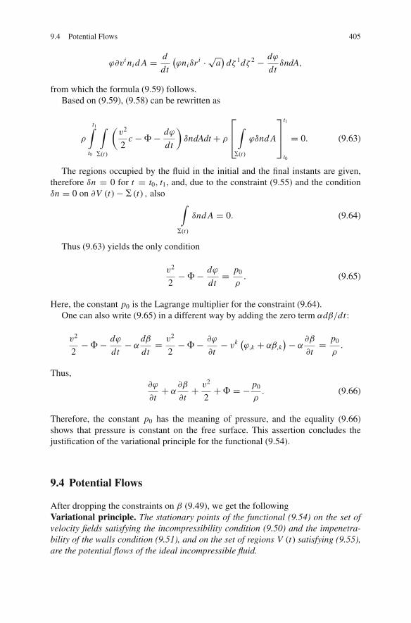
9.4 Potential Flows 405
ϕ�vi ni d A = d
dt
(ϕniδr i · √a
)dζ 1dζ 2 − dϕ
dtδndA,
from which the formula (9.59) follows.Based on (9.59), (9.58) can be rewritten as
ρ
t1∫
t0
∫
�(t)
(v2
2c −�− dϕ
dt
)δndAdt+ ρ
⎡⎢⎣∫
�(t)
ϕδnd A
⎤⎥⎦
t1
t0
= 0. (9.63)
The regions occupied by the fluid in the initial and the final instants are given,therefore δn = 0 for t = t0, t1, and, due to the constraint (9.55) and the conditionδn = 0 on �V (t)− � (t) , also
∫
�(t)
δnd A = 0. (9.64)
Thus (9.63) yields the only condition
v2
2−�− dϕ
dt= p0
ρ. (9.65)
Here, the constant p0 is the Lagrange multiplier for the constraint (9.64).One can also write (9.65) in a different way by adding the zero term αdβ/dt :
v2
2−�− dϕ
dt− α
dβ
dt= v2
2−�− �ϕ
�t− vk
(ϕ,k + αβ,k
)− α�β
�t= p0
ρ.
Thus,�ϕ
�t+ α
�β
�t+ v2
2+� = − p0
ρ. (9.66)
Therefore, the constant p0 has the meaning of pressure, and the equality (9.66)shows that pressure is constant on the free surface. This assertion concludes thejustification of the variational principle for the functional (9.54).
9.4 Potential Flows
After dropping the constraints on β (9.49), we get the followingVariational principle. The stationary points of the functional (9.54) on the set ofvelocity fields satisfying the incompressibility condition (9.50) and the impenetra-bility of the walls condition (9.51), and on the set of regions V (t) satisfying (9.55),are the potential flows of the ideal incompressible fluid.
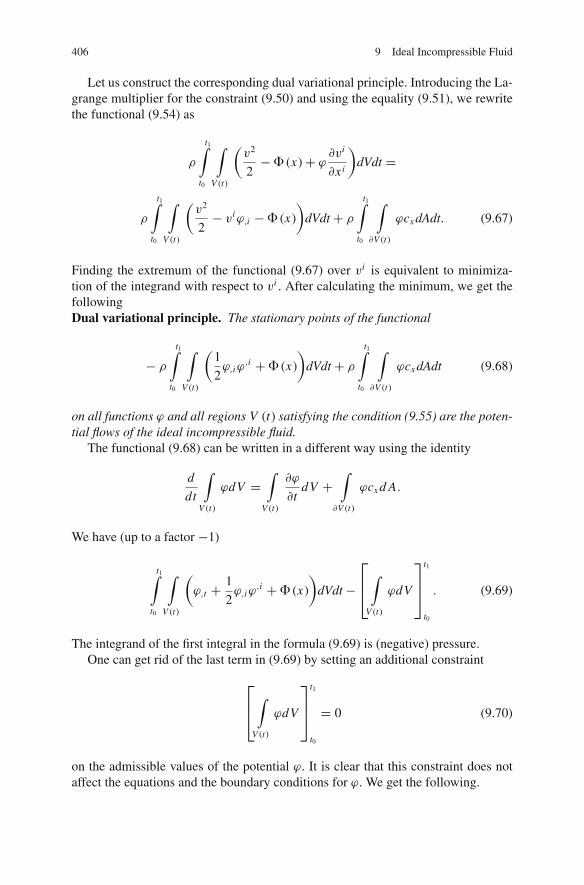
406 9 Ideal Incompressible Fluid
Let us construct the corresponding dual variational principle. Introducing the La-grange multiplier for the constraint (9.50) and using the equality (9.51), we rewritethe functional (9.54) as
ρ
t1∫
t0
∫
V (t)
(v2
2−� (x)+ ϕ
�vi
�xi
)dVdt =
ρ
t1∫
t0
∫
V (t)
(v2
2− viϕ,i −� (x)
)dVdt+ ρ
t1∫
t0
∫
�V (t)
ϕcx dAdt. (9.67)
Finding the extremum of the functional (9.67) over vi is equivalent to minimiza-tion of the integrand with respect to vi . After calculating the minimum, we get thefollowingDual variational principle. The stationary points of the functional
− ρ
t1∫
t0
∫
V (t)
(1
2ϕ,iϕ
,i +� (x)
)dVdt+ ρ
t1∫
t0
∫
�V (t)
ϕcx dAdt (9.68)
on all functions ϕ and all regions V (t) satisfying the condition (9.55) are the poten-tial flows of the ideal incompressible fluid.
The functional (9.68) can be written in a different way using the identity
d
dt
∫
V (t)
ϕdV =∫
V (t)
�ϕ
�tdV +
∫
�V (t)
ϕcx d A.
We have (up to a factor −1)
t1∫
t0
∫
V (t)
(ϕ,t + 1
2ϕ,iϕ
,i +� (x)
)dVdt−
⎡⎢⎣∫
V (t)
ϕdV
⎤⎥⎦
t1
t0
. (9.69)
The integrand of the first integral in the formula (9.69) is (negative) pressure.One can get rid of the last term in (9.69) by setting an additional constraint
⎡⎢⎣∫
V (t)
ϕdV
⎤⎥⎦
t1
t0
= 0 (9.70)
on the admissible values of the potential ϕ. It is clear that this constraint does notaffect the equations and the boundary conditions for ϕ. We get the following.

9.4 Potential Flows 407
Variational principle. The stationary points of the functional
ρ
t1∫
t0
∫
V (t)
(ϕ,t + 1
2ϕ,iϕ
,i +� (x)
)d3xdt (9.71)
on all functions ϕ and in all regions V (t) satisfying the constraints (9.70) and(9.55), respectively, are the potential flows of ideal fluid.
Consider a particular case of motion of the ideal incompressible fluid over theplane �. Denote the hight of the fluid by h (xα, t). The variational principle for thefunctional (9.71) becomesLuke variational principle. The potential flows of the ideal incompressible homo-geneous fluid over a plane are the stationary points of the functional
ρ
t1∫
t0
∫
�
h(xα,t)∫
0
(ϕ,t + 1
2ϕ,iϕ
,i +� (x)
)dx1dx2dx3dt (9.72)
on the set of all functions ϕ and h, satisfying the constraints
∫
�
[h (xα, t)− h0 (xα)
]dx1dx2 = 0,
⎡⎣∫
�
h∫
0
ϕdx1dx2dx3
⎤⎦
t1
t0
= 0,
h (xα, t0) = h0 (xα) , h (xα, t1) = h1 (xα) . (9.73)
The first constraint (9.73) can be disregarded if we include the Lagrange multiplierfor this constraint in the potential of the external body forces (or, after some redefi-nition of ϕ, in the potential, ϕ).
Consider now the flows without free surfaces.Kelvin variational principle. On the set M of velocity fields, selected by the con-straints (9.50) and (9.51), the minimizing element of the kinetic energy functional
I (v) =t1∫
t0
∫
V (t)
1
2ρvivi dV dt
corresponds to the potential flow of ideal incompressible fluid.The set M is convex. The kinetic energy, as a positive quadratic functional, is
strictly convex. Therefore, the minimizing element of the kinetic energy functionalis unique.
Constructing the dual variational principle, we get

408 9 Ideal Incompressible Fluid
Dirichlet principle. On all functions ϕ, the maximizing element of the functional
J =t1∫
t0
ρ
⎡⎢⎣∫
V (t)
cxϕd A − 1
2
∫
V (t)
�ϕ
�xi
�ϕ
�xidV
⎤⎥⎦dt
the velocity potential of the flow of the ideal incompressible fluid which satisfies theboundary condition (9.51) and
maxϕ
J = minv
I. (9.74)
Time is just a parameter in the Kelvin and Dirichlet principles. Therefore, theminimization problem for the functional I can be replaced by the minimizationproblem for the functional
K =∫
V (t)
1
2ρv2dV (9.75)
with the constraints (9.50) and (9.51), at each instant while the maximization prob-lem for the functional J corresponds to maximization of the functional
K∗ = ρ
∫
�V (t)
cxϕd A − 1
2ρ
∫
�V (t)
�ϕ
�xi
�ϕ
�xidV (9.76)
on all functions ϕ.
9.5 Variational Features of Kinetic Energy in Vortex Flows
There is a one-to-one correspondence between velocity and vorticity. Thereforekinetic energy can be considered as a functional of vorticity. It turns out that thisfunctional is the minimum value in a variational problem to which we proceed.
First we have to show that velocity and vorticity are in one-to-one correspon-dence indeed. Consider a velocity field, vi , in a closed bounded region V . Thevelocity field is incompressible:
�ivi = 0 (9.77)
and satisfies the impermeability condition:
vi ni = 0 on �V . (9.78)
For a known velocity field, one can find the corresponding vorticity field:

9.5 Variational Features of Kinetic Energy in Vortex Flows 409
ωi = eijk� jvk . (9.79)
The vorticity field is divergence-free:
�iωi = 0. (9.80)
Let now a divergence-free vorticity field be given. Then (9.77), (9.78) and (9.79)define a unique velocity field. Indeed, assume the opposite, that there are two solu-tions of (9.77), (9.78) and (9.79), vi
1 and vi2. Then the difference vi = vi
1− vi2 obeys
(9.77) and (9.78) and the equation
eijk� jvk = 0.
The latter means that the velocity field is potential, vi = �iϕ. According to (9.77)and (9.78) the potential is subject to the boundary value problem,
�ϕ = 0,�ϕ
�n
∣∣∣∣�V
= 0,
which has the solution, ϕ = const, and, hence, vi = 0, vi1 = vi
2. The one-to-one correspondence, ωi ⇐⇒ vi , holds true also if vi ni at �V is given and notnecessarily equal to zero.
If we do not impose on the velocity fields the constraints (9.77) and (9.78) thenthe one-to-one correspondence is lost: there are many velocity fields which satisfy(9.79) for a given ωi . It turns out that (9.77) and (9.78) are Euler equations in thefollowingVariational principle. The true dependence of kinetic energy of vorticity providesthe minimum value to the functional
∫
V
1
2ρvivi dV
on the set of all velocity fields selected by the constraints (9.79).To derive Euler equations, we introduce Lagrange multipliers for the constraints
(9.79), ρψi . The functional to be minimized becomes
ρ
∫
V
[1
2vivi − ψi
(eijk� jvk − ωi
)]dV (9.81)
410 9 Ideal Incompressible Fluid
or, after integration by parts,
ρ
∫
V
[1
2vivi + � jψi e
ijkvk + ψiωi
]dV − ρ
∫
�V
ψ i eijkn jvkd A. (9.82)
Euler equations are
vi = eijk� jψk in V, (9.83)
ψ i eijkn j = 0 on �V. (9.84)
Equation (9.77) follows from (9.83). Let us show that boundary condition (9.84)yields (9.78). Indeed, using Greek indices for vector projections on the tangentplanes, we can write (9.84) as
ψα = 0. (9.85)
On the other hand, denoting by r i (ξα) the position vector of �V, ξα being coor-dinates on �V, and using (14.7), we have
nivi = 1√
aeimnrm
1 rn2 eijk� jψk = 1√
a
(δ j
mδkn − δk
mδ jn
)rm
1 rn2 eijk� jψk
= 1√a
(rm
1 rn2 �mψn − rn
1 rm2 �mψn
) = 1√a
(rn
2 �1ψn − rn1 �2ψn
)(9.86)
= 1√a
(�1ψ2 − �2ψ1) = εαβψβ|α, ψα ≡ rmα ψm .
Here rmα ≡ �rm/�ξα , the vertical bar in indices denotes the covariant surface deriva-
tive (see Sect. 14.1 for the definition). The boundary condition (9.78) follows from(9.86) and (9.85).
After minimization with respect to velocity fields the functional (9.81) is equal to
− ρ
∫
V
[1
2
(curl−→ψ)2− −→ψ · −→ω
]dV. (9.87)
According to the general scheme of construction the dual variational principles,to obtain kinetic energy of the flow one has to maximize the functional (9.87)with respect to all fields,
−→ψ , which satisfy the constraint (9.84). We arrive at the
followingDual variational principle. The dependence of kinetic energy on vorticity can befound from the variational problem
−K = min−→ψ ε(9.84)
ρ
∫
V
[1
2
(curl−→ψ)2− −→ψ · −→ω
]dV . (9.88)

9.5 Variational Features of Kinetic Energy in Vortex Flows 411
The vector field,−→ψ , is called stream vector field; in case of two-dimensional flows
(v1, v2 �= 0, v3 = 0) , it has the only non-zero component, ψ3, which is calledstream function.
Note that the functional in (9.88) is invariant with respect to shifts−→ψ →−→ψ +∇ϕ
where the potential, ϕ, is constant at the boundary.4 Therefore, its minimum valueis achieved at many fields. To select a unique minimizing element, one can set anadditional constraint
�iψi = 0 (9.89)
which obviously, eliminates gradient invariance.Euler equations in the variational problem (9.88) are
�ψi − �i � jψj = −ωi . (9.90)
If the constraint (9.89) is set, Euler equations simplify to
�ψi = −ωi . (9.91)
The three equations (9.91) are not independent: the divergence of (9.91) is iden-tically zero.
The variational principles formulated can be extended to the case of non-zeronormal velocity at the boundary. To do that, consider the function, vn = vi ni ,
at �V . We introduce a two-dimensional vector, χα, on �V such that its “surfacedivergence” is equal to vn:
vn = −χα|α. (9.92)
Since the velocity field is divergence-free,
∫
�V
vndA = 0,
4 For such a shift the functional gets an increment
−ρ
∫
V
ωi �i ϕdV
which is equal, due to (9.80) to
−ρ
∫
�V
ωi ni ϕdA.
Since ϕ is a constant, c, on �V,
−ρ
∫
�V
ωi niϕdA = −ρc∫
�V
ωi ni dA = −ρc∫
V
�i ωi dV = 0.

412 9 Ideal Incompressible Fluid
the necessary condition for solvability of (9.92) is satisfied. For a given vn , one canobtain a solution of (9.92) assuming that the field χα is potential,χα = χ |α. So weassume that the vector field, χα, is known on �V .Variational principle. For a given vorticity, the true velocity field provides mini-mum to the functional
∫
V
1
2vivi dV−
∫
�V
vαχαd A. (9.93)
Here vα are the tangent components of velocity on �V .
To obtain Euler equations for the functional (9.93) we introduce Lagrange mul-tipliers for the constraint (9.79):
∫
V
[1
2vivi − ψi
(eijk� jvk − ωi
)]dV−
∫
�V
vαχαd A. (9.94)
The only difference from (9.81) is that after integration by parts we have to vanishfor all vi the surface integral
∫
�V
(−ψi eijkn jvk − vαχα
)d A.
Since, due to (14.10),
ψi eijkn jvk = −ψivkε
αβr iαrk
β = −εαβψαvβ ,
this surface integral is zero for
εαβψα = χβ
or
ψα = εαβχβ. (9.95)
Hence, inside the region V we find as before (9.83), while at the boundary weobtain using (9.86), (14.6) and (9.83),
vi ni = εαβψβ|α = εαβ(εβγ χγ
)|α = −χ
γ
|γ ,
i.e. the prescribed boundary value of normal velocity.Computation of the functional (9.94) on the minimizing velocity field yields the
followingDual variational principle. The true stream vector field is the maximizer of thefunctional

9.5 Variational Features of Kinetic Energy in Vortex Flows 413
−∫
V
[1
2
(curl−→ψ)2− ψiω
i
]dV (9.96)
on the set of all stream vector fields satisfying the boundary condition (9.95).For χα = 0, the maximum value of the functional (9.96) is kinetic energy of the
flow. The maximizer is a linear functional of ωi :
ψi =∫
VRi j (x, x ′)ω j (x ′)d3x ′.
Accordingly, kinetic energy is a quadratic functional of vorticity:
K = 1
2ρ
∫
V
∫
VRi j (x, x ′)ωi (x)ω j (x ′)d3xd3x ′.
If vorticity depends on time, then the variational principles hold at each instant.The variational principles formulated have pure mathematical origin as can be
seen from the following reasoning.Consider a divergence-free vector field →
v in a closed region V . Then, for agiven →
v,
min→ψ
1
2
∫
V
∣∣∣→v − curl→ψ
∣∣∣2
dV = 0, (9.97)
because there exists a vector field →χ such that →v = curl
→χ, and minimum is achieved
on→ψ = →
χ +∇ϕ, ϕ is an arbitrary function.Let additionally the normal component of →
v vanishes at the boundary. Ifxi = r i (ξα), α = 1, 2, are the parametric equations of the boundary, then
vi ni = ni ei jk� jχk = r j
1 rk2 (� jχk − �kχ j ) = �χ2
�ξ 1− �χ1
�ξ 2= 0, (9.98)
where χα = r iαχi are the tangent components of vector →χ on the boundary. Accord-
ing to (9.98), the surface vector, χα, is a potential vector: there is a function on theboundary, �(ξα), such that χα = ��(ξα)/�ξα. Taking any function, ϕ, which hasthe boundary value �(ξα), and replacing →
χ by →χ −∇ϕ, we obtain the stream vector
field with the zero tangent components at the boundary. Therefore, if we narrow the
admissible vector fields→ψ in (9.97) by the vector fields with the vanishing tangent
components at the boundary,
→ψ × →
n = 0 on �V, (9.99)
minimum in (9.97) remains equal to zero:

414 9 Ideal Incompressible Fluid
min−→ψ ∈(9.99)
[1
2
∫
Vviv
i dV −∫
Vvi e
ijk� jψkdV + 1
2
∫
V
∣∣∣curl−→ψ
∣∣∣2
dV
]= 0. (9.100)
The second term in (9.100) can be written as
−∫
Vvi e
ijk� jψkdV = −∫
�Vvi e
ijkn jψkdV +∫
Vψkeijk� jvi dV . (9.101)
The boundary integral vanishes because of (9.99), while the volume integral isequal to
∫
Vψkeijk� jvi dV = −
∫
Vψkω
kdV . (9.102)
Since, for a given velocity field, vorticity is known, minimum over−→ψ in (9.100)
yields the variational principle for the energy functional (9.88). According to(9.100), the minimum value of the energy functional is equal to negative kineticenergy of the flow.
Our derivation shows that variational principle for energy functional (9.88) alsoholds true for vorticity fields with non-zero normal component at the boundary.
Energy functional (9.88) is invariant with respect to transformations,−→ψ →−→ψ +
∇ϕ, where ϕ is constant at the boundary (see footnote in this section).Therefore, an additional constraint can be set on
−→ψ without changing the minimum
value of the functional.
9.6 Dynamics of Vortex Lines
Setting the problem. The governing equations of ideal incompressible fluid possessan infinite number of integrals of motion, which are additional to energy, thecirculations of velocity over closed fluid contours. As we have seen in Sect. 2.2,in statistical mechanics one usually deals with a Hamiltonian system which has theonly integral, energy. Therefore to develop statistical mechanics of ideal fluid oneneeds to eliminate all degrees of freedom which are “driven” due to the integrals ofmotion and keep only the independent degrees of freedom. Conservation of veloc-ity circulations reduces the number of independent degrees of freedom drastically.For example, ideal fluid in a container with an embedded rigid body is, in general,an infinite-dimensional system. However, if the circulations of velocity over anyfluid contour is zero, i.e. the fluid flow is potential, then the number of independentdegrees of freedom is only six: they are the degrees of freedom of the rigid body

9.6 Dynamics of Vortex Lines 415
(see Sect. 13.2 for details). It turns out that the dynamics of only “essential degreesof freedom” is dynamics of vortex lines. It is the subject of this section.
Governing equations of vortex line dynamics. Consider a flow of ideal fluid in abounded vessel, V, which is at rest in some inertial frame. The fluid neither pene-trates through nor detaches from the wall, �V .
Conservation of velocity circulations over fluid contours is equivalent to conser-vation of the Lagrangian components of vorticity:
ωa = ωa(Xb). (9.103)
The material lines tangent to ωa, i.e. the lines determined by the parametricequations,
d Xa(σ )
dσ= λωa(Xb),
are called vortex lines. Any vortex line consists of the same fluid particles becauseof the independence of ωa on time. Two cases should be distinguished: ωana = 0at �V and ωana �= 0 at �V (recall that na are the Lagrangian components of theunit normal vector at the boundary in the initial state). In the first case, vortex linesdo not end at the boundary, in the second they do (an example of the second caseis tornado). We consider in this section the first case. The necessary modificationsfor non-zero normal vorticity are made in the next section for quasi-two-dimensionalflows. In three-dimensional space a vortex line that does not end at the boundary canbe either closed or fill out some subregion of V . Strictly speaking, the term “dynam-ics of vortex lines” is meaningful for the case of closed vortex lines; for dense vortexlines it is more appropriate to deal with dynamics of “vortex particles”. The latteris beyond the scope of our consideration. We focus on the case when a Lagrangiancoordinate system can be attached to vortex lines. One of the coordinates, say, X3,
is directed along the vortex lines. We use for this coordinate the notation η ≡ X3.
The couple of other coordinates, Xμ, μ = 1, 2, marks different vortex lines; thecouple
{X1, X2
}is denoted in this section by X. In the coordinate system chosen
only one component of vorticity, ω3, is not zero.In Lagrangian coordinates, the condition that the vorticity field is divergence-free
at the initial instant takes the form
�
�Xa
√gωa = 0,
√g ≡ det
∥∥∥∥�xi (0, Xa)
�Xa
∥∥∥∥ . (9.104)
Hence, in the vortex line coordinate system,
�
�η
√gω3 = 0,
416 9 Ideal Incompressible Fluid
and√
gω3 is constant along each vortex line but may change from one vortex lineto another. We denote this function by ω. It measures the intensity of vortex lines.Function ω (Xμ) is assumed to be known from the initial conditions.
Due to incompressibility,
� ≡ det
∥∥∥∥�xi (t, Xa)
�Xa
∥∥∥∥ =√
g, (9.105)
and one can also put ω = ω3�.
The position vector of the points of vortex lines will be denoted further byr i (t, η, X ) . Vorticity field is determined by r i (t, η, X ) and ω (X ): according to(9.12) and (9.103)
ωi = �r i (t, η, X )
�ηω3 = �r i (t, η, X )
�η
ω (X )√g
. (9.106)
The independence of the Lagrangian component of vorticity, ω3, on time deter-mines the dynamics of vortex lines. Indeed, let ω3 and the positions of vortex lines,r i (t, η, X ), be known at some instant, t . Then we know at this instant the vorticityfield from (9.106) and can find velocity, vi (t, x), solving the kinematic problem ofthe previous section:
�ivi = 0, eijk� jvk = ωi (t, x), vi n
i∣∣�V = 0. (9.107)
This problem determines velocity as a functional of the positions of vortex lines;denote it by V i ( t, x | r (t, η, X )). Then, we can find the positions of the vortex linesat the instant t + �t by putting
r i (t + �t, η, X ) = r i (t, η, X )+ V i ( t, x | r (t, η, X ))∣∣x=r (t,η,X ) �t. (9.108)
Knowing the new positions of the vortex lines, we repeat the procedure, thus deter-mining the dynamics of vortex lines.
Equation (9.108) means that r i (t, η, X ) are sought from the system of equations
�r i (t, η, X )
�t= V i ( t, x | r (t, η, X ))
∣∣x=r (t,η,X ) . (9.109)
We have to show that fluid dynamics so defined obeys momentum equations ofideal fluid. To this end we have to check the equality
curl
(d→v
dt
)= 0,

9.6 Dynamics of Vortex Lines 417
where velocity is the solution of (9.107). We have5
eijk� jdvk
dt= eijk� j
(�vk
�t+ vm�mvk
)=
= d
dtωi + eijk� jv
m�mvk .
Note that
eijk� jvm�mvk = eijk
(� jvm − �mv j
)�mvk (9.110)
because eijk�mv j �mvk ≡ 0 due to symmetry of �mv j �
mvk over indices j, k. Besides,� jvm−�mv j = e jmsω
s , and, using (3.19) and (9.22) and incompressibility condition,�iv
i = 0, we have
eijk� jvm�mvk = −ωk�kv
i .
Therefore,
eijk� jdvk
dt= dωi
dt− ωk�kv
i . (9.111)
From (9.106) dωi/dt = ωk�kvi . Thus, the right hand side of (9.111) vanishes,
and the particle trajectories, r i (t, η, X ) , obey the momentum equations of idealincompressible fluid.
Setting (9.106), (9.107) and (9.109), we automatically obtain an incompressiblemotion of particles. Remarkably, we can reformulate the equations of vortex linedynamics as dynamics of geometrical lines when motion of particles over the vortexlines is ignored. This is done in the following way. Let us admit to considerationany motions, r i (t, η, Xμ), including the compressible ones. Equation (9.106) is nolonger true. For compressible motion, i.e. for � �= √
g, we replace (9.106) with theequation
ωi = 1
�
�r i (t, η, X )
�ηω (X ) . (9.112)
5 For any function, ϕ, we define dϕ/dt as
dϕ
dt= �
�tϕ(t, r (t, η, X ))|η,X=const .
Thus,dϕ
dt= �ϕ
�t+ V i ( t, x | r (t, η, X ))�i ϕ.

418 9 Ideal Incompressible Fluid
That means that ω (X ) is expressed in terms of the only non-zero Lagrangiancomponent of vorticity, ω3, as
ω (X ) = ω3�.
The vortex intensity does not depend on η, and therefore the vector field (9.112)is divergence-free:
�iωi = 1
�
�
�Xa
(�
�Xa
�xiωi
)= 1
�
�
�η
(ω3�
) = 1
�
�
�η(ω) = 0. (9.113)
Besides, ω does not depend on time. For compressible motion, the only non-zeroLagrangian component of vorticity, ω3 = ω/�, may depend on time.
Instead of (9.109), we set for r i (t, η, X ) the differential equations
�r i (t, η, X )
�t= V i ( t, x | r (t, η, X ))+ λωi
∣∣x=r (t,η,X ) , (9.114)
where V i is determined by the vorticity field from (9.107) and (9.112), and λ is anarbitrarily prescribed function of coordinates and time. The parameter λ controls theparticle velocity over vortex lines.
Equation (9.114) can also be written in the form
eijk
(�r i (t, η, X )
�t− V i ( t, x | r (t, η, X ))
∣∣x=r (t,η,X )
)ωk = 0 (9.115)
which emphasizes that in (9.114) only the velocity normal to the vortex line is es-sential.
Both (9.109) and (9.115) give the same velocity normal to vortex lines. There-fore, (9.115) describe the dynamics of vortex lines correctly. We are going to showthat (9.115) forms a Hamiltonian system of equations.
Variational principles. All possible motions can be split into “equivortical sheets”;each sheet is the set of motions r (t, η, X ) with the same vortex intensity ω. Eachsheet contains the true motions, i.e. motions obeying (9.115), and the motions thatare not realized. For a given vortex intensity, the total kinetic energy of the flow be-comes a functional of r i (t, η, X ), because, as we have seen in the previous section,there is one-to-one correspondence between velocity and vorticity, and vorticity isexpressed in terms of r i (t, η, X ) by (9.112):
K = K(r i (t, η, X )
) = 1
2ρ
∫
V
Vi ( t, x | r (t, η, X ))V i ( t, x | r (t, η, X ))d3x . (9.116)
The dynamics of vortex lines is governed by the following

9.6 Dynamics of Vortex Lines 419
Variational principle. The true motion of the vortex lines, r (t, η, X ), is a stationarypoint of the functional
J =t1∫
t0
[A−K] dt, (9.117)
A = 1
3ρ
∫
V
eijkrj (t, η, X )
�r i (t, η, X )
�t
�rk (t, η, X )
�ηω (X ) d2 Xdη, (9.118)
on the set of all motions with the prescribed vortex intensity, which have the sameinitial and final positions:
r (t0, η, X ) = r (t0, η, X ), r (t1, η, X ) = r (t1, η, X ). (9.119)
Here d2 X ≡ d X1d X2, and V is the region run by Lagrangian variables.If vortex lines occupy some subregion, V ′, of V then the integrand in (9.118)
must be integrated over this region, V ′ (ω = 0 outside of V ′). If V ′ = V, then
niδr i = 0 at �V, (9.120)
δr i being the variation of r i (t, η, X ). If V ′ is strictly inside V , niδr i are arbitraryat �V ′.
The functional does not depend on the choice of parameter along the vortexlines. This yields the above-mentioned peculiarity of the vortex line dynamics: thisis dynamics of geometrical lines. That means that a vortex line has not three buttwo functional degrees of freedom. For example, if the vortex line crosses eachplane x3 = const at one point, then its dynamics is completely determined by twofunctions xα = rα
(t, x3
), α = 1, 2.
Another feature of the variational principle is that, in contrast to Lagrange vari-ational principle, the motion, r i (t, η, X ) , is compressible, while the motion of theideal fluid under consideration is not.
The functional A is an analogue of the shortened action in classical mechanics.We will derive the variational principle formulated from another one which is
easier to justify.First, we set up a one-to-one correspondence between vi and ψk, imposing the
following constraints on ψk :
�kψk = 0 in V, (9.121)
−→ψ ×−→n = 0 on �V . (9.122)
As we discussed in the previous section, the condition (9.122) means the imperme-ability of the boundary.

420 9 Ideal Incompressible Fluid
Consider a functional
I (ψ) = 1
2(Aψ,ψ)− (l, ψ) (9.123)
(Aψ,ψ) ≡ ρ
∫
V
(curl−→ψ)2
dV, (l, ψ) = ρ
∫
V
−→ω · −→ψ dV .
For a given divergence-free vorticity field, we seek the minimum value of thefunctional I (ψ) with respect to all vector fields
−→ψ subject to the constraints (9.121)
and (9.122).
Functional I(−→
ψ)
is a quadratic functional being minimized on a linear set.
According to the dual variational principle of the previous section, its minimumvalue coincides with the negative kinetic energy of the flow:
min−→ψ ∈(9.121),(9.122)
I(−→
ψ)= −1
2ρ0
∫
V
−→v ·−→v dV = −1
2ρ0
∫
V
−→ω ·−→ψ dV, −→v = curl−→ψ .
(9.124)
The minimization problem for the functional I(−→
ψ)
determines the kinetic en-
ergy as a functional of vorticity, and in accordance with (9.112) as a functional ofthe vortex line positions. Substituting (9.124) into (9.117) we arrive at the followingVariational principle. The true trajectory of vortex line dynamics, r i (t, η, X ) , is astationary point of the functional
I (r (t, η, X ) , ψ (t, x)) =t1∫
t0
dtρ
⎡⎢⎣1
3
∫
V
ei jkr j �r i
�t
�rk
�ηωd2 Xdη + 1
2
∫
V
(curl
→ψ)2
dV
−∫
V
ψk (t, r )�rk
�ηωd2 Xdη
⎤⎥⎦ (9.125)
on the set of all motions, r i (t, η, X ) , of vortex lines, having the same vortexintensity the same initial and final positions (9.119), and the set of all vector fields,ψ i
(t, rk
), with vanishing tangent components on the boundary.
Motion of vortex lines, r i (t, η, X ) , in (9.125) is allowed to be compressible. TheJacobian � enters explicitly in the second integral (9.125) if we write the secondintegral as an integral over Lagrangian variables6:
∫
V
(curl−→ψ)2
�d2 Xdη.
6 Recall that volume element, dV, is equal to �d2 Xdη in Lagrangian coordinates.
9.6 Dynamics of Vortex Lines 421
The third integral can also be written, according to (9.112), as
∫
V
ψk (t, r )�rk
�ηωd2 Xdη =
∫
V
ψkωkdV .
Then minimization over ψk is equivalent to the variational problem for the func-tional (9.123). One obtains the same equations for ψk when all integrals are writtenin Lagrangian variables.
When varying r i (t, η, X ), the variation of the second integral is zero, becausefor fixed ψ i
(t, rk
)the second integral does not depend on r i (t, η, X ) . So, varying
the functional I with respect to r i (t, η, X ) , it is enough to vary only the first andthe third integral. For the variation of the first integral we have
δ
∫
V
1
3eijkr
j �r i
�t
�rk
�ηω (X ) d2 Xdη
=∫
V
(1
3eijkδr j �r i
�t
�rk
�η+ 1
3eijkr
j �δr i
�t
�rk
�η+ 1
3eijkr
j �r i
�t
�δrk
�η
)ω (X ) d2 Xdη
=∫
V
(1
3eijkδr j �r i
�t
�rk
�η− 1
3eijkδr i �
�t
(r j �rk
�η
)− 1
3eijkδrk �
�η
(r j �r i
�t
))ω (X ) d2 Xdη
+ �
�t
∫
V
1
3eijkr
jδr ir kη ω (X ) d2 Xdη =
∫
V
eijkδr j �r i
�t
�rk
�ηω (X ) d2 Xdη
+ �
�t
∫
V
1
3eijkr
jδr ir kη ω (X ) d2 Xdη. (9.126)
The divergence terms over η vanish due to closedness of the vortex lines. Thevariation of the third integral is
δ
∫
V
ψk (t, r )�rk
�ηω (X ) d2 Xdη =
∫
V
(�iψkδr i �rk
�η+ ψk
�δrk
�η
)ω (X ) d2 Xdη
=∫
V
(� jψk − �kψ j
)δr j �rk
�ηω (X ) d2 Xdη (9.127)
or
δK =ρ
∫
V
ei jkδr j(
curl→ψ)i �rk
�ηω (X ) d2 Xdη = ρ
∫
V
ei jkδr j(
curl→ψ)i
ωkdV .
(9.128)

422 9 Ideal Incompressible Fluid
So, for the variation of the action functional we obtain
1
ρδI =
∫
V
ei jkδr j
(�r i
�t−(
curl→ψ)i)
�rk
�ηω (X ) d2 Xdη+
+ �
�t
∫
V
1
3ei jkr jδr ir k
η ω (X ) d2 Xdη. (9.129)
The divergence term over time vanishes due to (9.119). Finally, one obtains theequations of vortex line dynamics:
eijk
(�r i
�t−(
curl−→ψ)i)
ωk = 0. (9.130)
Here curl−→ψ is assumed to be presented in terms of vorticity, and vorticity is ex-
pressed in terms of vortex line positions, r i (t, η, X ) , according to (9.112). We arriveat (9.115).
Derivation from the least action principle. In Hamiltonian mechanics, eliminationof the integrals of motion occurs by means of the following procedure: one makesa change of variables (p, q) → (p′, q ′, I, ϕ), where I1(p, q), . . . , Is(p, q) is theset of integrals, ϕ1, . . . , ϕs the dual variables, p′, q ′ the remaining variables, inorder to put the Lagrange function in the form: p′q ′ + I ϕ − H (p′, q ′, I ).7 Thenconservation of I1, . . . , Is follows from the independence of Hamilton function onϕ. It is not clear how to perform such a procedure for ideal fluid flow. Originally,the above-formulated variational principle with the eliminated integrals of motionwas found as a remarkable feature of dynamics of vortex lines without reference toa general algorithm. The existence of such algorithm for fluid flow is still an openissue. It became clear, however, how to derive the variational principle of vortexline dynamics from the least action principle of Sect. 9.1. It is especially interesting,because one has to explain the appearance in the action functional “strange” com-pressibility of the originally incompressible flow and a “strange” factor 1/3. Weconclude this section with that derivation.
Consider the action functional (9.2), which we write in the form
I (x (t, X )) = ρ
t1∫
t0
∫
V
1
2xi
t xit � d3 X dt, xit ≡
dxi (t, X )
dt.
Here, for simplicity, we set g0 = 1 and assume that fluid is homogeneous,ρ0 = const. Besides, to reduce technicalities, we accept that the vessel is at rest
7 This procedure is discussed in [4].

9.6 Dynamics of Vortex Lines 423
and fluid does not detach from the wall of the vessel. To enforce the incompress-ibility condition, we introduce in the action functional the corresponding Lagrangemultiplier:
I (x (t, X ) , ϕ(t, X )) = ρ
t1∫
t0
∫
V
(1
2xi
t xit �− ϕ�
)d3 X dt, ϕ ≡ dϕ(t, X )
dt.
(9.131)Here and in what follows we are concerned only with Lagrangian and ignore theboundary terms; otherwise we should add in (9.131) the integral
⎡⎢⎣ρ
∫
V
ϕd3 X
⎤⎥⎦
t1
t0
.
One can check by direct inspection that the stationary points of the functional(9.131) are the solutions of equations of ideal incompressible fluid: variation over ϕ
yields incompressibility condition:
d�
dt= 0,
while variation over xi (t, X ) and use of (4.19) results in the equation
d
dtρ�xit + �
�xiρ�
(1
2xk
t xkt − ϕ
)= 0.
This is the momentum equation, in which pressure is
p = ρ�
(1
2xk
t xkt − ϕ
). (9.132)
The stationary points of the functional (9.131) are also the stationary points ofthe functional J (x (t, X ) , ϕ(t, X ), v(t, X )):
J (x (t, X ) , ϕ(t, X ), v(t, X )) = (9.133)
ρ
t1∫
t0
∫
V
(vi (t, X )xi
t �− 1
2vi (t, X )vi (t, X )�− ϕ�
)d3 X dt.
At the stationary point, vi (t, X ) coincides with velocity:
vi (t, X ) = xit . (9.134)

424 9 Ideal Incompressible Fluid
Comparison of (9.132) and (9.134) with (9.13) and (9.15) shows that at thestationary point,
vi (t, X ) = �ϕ
�xi+ Xa
i va(X ). (9.135)
Here va(X ) can be considered as functions known from the initial conditions. Nowwe employ a note on the functional modification (5.334) and plug (9.135) into thefunctional (9.133). We obtain the functional that depends on x (t, X ) and ϕ(t, X )only:
t1∫
t0
∫
V
(Xa
i va(X )xit −
1
2gi j (�iϕ + Xa
i va(X ))(� jϕ + Xaj va(X ))− �ϕ(t, x)
�t
)� d3 X dt.
(9.136)Here we used the fact that ϕ = �ϕ/�t + ϕ,i x i
t .
We are going to show that the functional (9.136) is identical to the functional ofvortex line dynamics. The substitution (9.135) increased the set of stationary points,and this is how the incompressible fluid motions become compressible motions ofvortex dynamics.
To transform the functional (9.136), we first note that the last term can be pre-sented as a boundary integral:
ρ
t1∫
t0
∫
V
�ϕ(t, x)
�t� d3 X dt = ρ
t1∫
t0
∫
V
�ϕ(t, x)
�td3x dt =
⎡⎣ρ
∫
V
ϕ d3x
⎤⎦
t1
t0
,
and, thus, does not affect the differential equations. Therefore, the search of thestationary point with respect to ϕ is reduced to minimization of the functional,
K (ϕ, x(t, X )) = ρ
∫
V
1
2gi j (�iϕ + Xa
i va(X )) (� jϕ + Xaj va(X ))� d3 X , (9.137)
over ϕ at each instant. In this functional, Xaj va(X ) are considered as known; denote
them by ui . Transforming (9.137) to Eulerian variables, we obtain the variationalproblem
K(x(t, X )) = minϕ
∫
V
1
2ρ(�iϕ + ui )(�
iϕ + ui ) d3x . (9.138)
Any vector field, ui , can be presented as a sum of a divergence-free vector field,u′i , obeying the boundary condition u′i n
i = 0, and potential vector field, �iχ . Hence,the minimizing function, ϕ, is the solution of the boundary value problem

9.6 Dynamics of Vortex Lines 425
�(ϕ + χ ) = 0 in V,�(ϕ + χ )
�xini = 0 on �V .
Obviously, ϕ = −χ + const, and the minimum value in the variational problem(9.138) is
∫
V
1
2ρu′i u
′i d3x .
As we discussed, u′i are uniquely determined by vorticity,
ωi = eijk� j u′k = eijk� jvk = eijk Xb
j Xak �bva(X )
= 1
�xi
cecba�bva(X ) = 1
�xi
cωc(X ).
So, we arrived at the above-considered problem of calculation of kinetic energy interms of vorticity.
The first term in the functional (9.136) is transformed by means of (3.23):
ρ
t1∫
t0
∫
V
Xai va(X )xi
t � d3 X dt = ρ
t1∫
t0
∫
V
1
2eijkxi
a x jb eabcvc(X )xk
t d3 X dt. (9.139)
For further transformation we need the easily verifiable identities
eijkxia x j
b eabcvc(X )xkt = �b
(eijkxi
a x j eabcvc(X )xkt
)
−eijkxia x j eabc�bvc(X )xk
t − eijkxia x j eabcvc(X )
dxkb
dt,
2eijkxia x j eabcvc(X )
dxkb
dt= d
dteijkx i
a x j eabcvc(X )xkb − eijkxi
a x jt eabcvc(X )xk
b ,
which yield
3
2eijkxi
a x jb eabcvc(X )xk
t = �b(eijkxi
a x j eabcvc(X )xkt
)− 1
2
d
dteijkx i
a x j eabcvc(X )xkb
+eijkx j x it xk
a eabc�bvc(X ). (9.140)
The integral of the first term,
� =t1∫
t0
∫
V
�b(eijkxi
a x j eabcvc(X )xkt
)dV dt,
in general is not zero; however its variation is zero. Indeed,

426 9 Ideal Incompressible Fluid
δ� = δ
t1∫
t0
∫
�V
eijkx ia x j eabcvc(X )xk
t nbd Adt,
where d A is the area element, and nb the normal vector in the initial state. Let ξμ beparameters on �V , Greek indices run values 1,2, and Xa = r a(ξμ) the parametricequations of �V , r a
μ ≡ �r a/�ξμ ≡ �μr a . The identity holds true:
δ(eijkxia x j eabcvc(X )xk
t nb) = 3eijkδx j r cμxi
νeμνvcxkt − �μ(eijkδxi r c
ν x j eμνvcxkt )
+�t (eijkxia x j eabcvcδxknb), (9.141)
where �μ denotes the covariant derivative over the boundary in the initial state. Tocheck the validity of (9.6) we use the fact that eabcnb = 1√
aeμν r a
ν r cμ, a being the
determinant of the surface metric tensor; then
√aδ(eijkxi
a x j eabcvc(X )xkt nb) = δ(eijkxi
νx j vcrcμxk
t eμν) = eijkxiν vcr
cμeμνxk
t δx j
+eijkx j vcrcμxk
t eμν�νδxi + eijkxiνx j vcr
cμeμν(δxk)t =
3eijkxiν vcr
cμeμνxk
t δx j + �ν(eijkx j vcrcμxk
t eμνδxi )+ (eijkxiνx j vcr
cμeμνδxk)t
−eijkx j vc,ar cν r c
μxkt eμνδxi − eijkx j vcr
cμxk
t,νeμνδxi − eijkxiν,t x
j vcrcμeμνδxk .
The last two terms cancel out, the term eijkx j vc,ar cν r c
μxkt eμνδxi is zero because, as
we assumed, the normal component of vorticity, vc,ar aμeμν r c
ν , is zero, and, takinginto account (14.38), we arrive at (9.6).
The integral of the second term in the right hand side of (9.6) is zero, integralof the third term goes to the time ends and does not affect equations and boundaryconditions. Hence,
δ� =t1∫
t0
∫
�V
3eijkδx j r cμxi
νeμνvcxkt d Adt. (9.142)
The integrand in (9.142) is proportional to the volume of the parallelogramformed by three vectors, δx j , xi
ν and xkt . At the boundary, all these vectors are
tangent to the boundary, therefore the volume is zero, and, thus, δ� = 0 as claimed.So, up to the time end terms and constant terms,
ρ
t1∫
t0
∫
V
Xai va(X )xi
t � d3 X dt = ρ
t1∫
t0
∫
V
1
3eijkx j x i
t xka
ωa
�d3 X dt. (9.143)
We arrived at the action functional of the vortex line dynamics.

9.7 Quasi-Two-Dimensional and Two-Dimensional Vortex Flows 427
9.7 Quasi-Two-Dimensional and Two-Dimensional Vortex Flows
We call a flow quasi-two-dimensional if each vortex line crosses the plane x3 =const. at one point (Fig. 9.3). In such a flow rotational motion occurs mostly in the(x1, x2
)-plane.
The variational principles formulated cannot be applied to quasi-two-dimensionalflows because the vortex lines are not closed: if η = 0 and η = l are the values ofthe parameter η for the points lying in cross-sections x3 = 0 and x3 = L , thenr3 (t, l, X )− r3 (t, 0, X ) = L �= 0, and the divergence terms vanished for the closedvortex lines are no longer zero. Due to that the functional A must be modified8:
A = 1
3ρ
∫
V
ei jkr j �r i
�t
�rk
�ηωd2 Xdη + L
6ρ
∫eαβrβ (t, 0, X )
�rα (t, 0, X )
�tωd2 X
(9.144)
The variation of the second integral in (9.144) cancels the divergence terms whichappear in variation of the first integral.
Formula (9.144) can be simplified by a special choice of the parameter on thevortex lines. Identifying η with x,
x = r3 (t, η, X ) ≡ η,
we describe the positions of vortex lines by two functions xα = rα (t, x, X ) . Weconsider the flows in cylindrical domain � × [0, L] which are periodic in thex- direction with the period L . Then functions rα (t, x, X ) are periodic:
Fig. 9.3 Quasi-two-dimensional flow
8 Greek indices run values 1, 2 and mark projections on axes x1 and x2.

428 9 Ideal Incompressible Fluid
rα (t, 0, X ) = rα (t, L , X ) . (9.145)
The functional A takes the form
A = 1
3ρ
∫
V
(−eαβ
�rα
�t
�rβ
�ηx + eαβrβ �rα
�t
)ω (X ) d2 Xdx
+ L
6ρ
∫eαβrβ (t, 0, X )
�rα (t, 0, X )
�tωd2 X. (9.146)
Note the identity
eαβ
�rα
�t
�rβ
�ηx = −1
2eαβrβ �rα
�t+ �
�x
(1
2eαβrβ �rα
�tx
)− �
�t
(1
2eαβrβ �rα
�xx
).
(9.147)
Plugging (9.147) to (9.146) and dropping the divergence term
∫�
�t
(1
2eαβrβ �rα
�xx
)ω (X ) d2 Xdx,
we obtain the final expression for A :
A = 1
2ρ
∫
V
eαβrβ (t, x, X )�rα (t, x, X )
�tω (X ) d2 Xdx . (9.148)
Note the different factors: 1/2 in (9.148) and 1/3 in (9.118).The variational principle for kinetic energy must also be modified because the
condition used for closed flows at the boundary, −→v · −→n = 0, does not hold on theplanes x = 0 and x = L .
Denote by v, vα, ω, ωα and ψ,ψα the axial and the transversal components ofvelocity, vorticity, and stream function vector, respectively, and by [ϕ] the differenceof the values of function ϕ at x = L and x = 0 :
[ϕ] ≡ ϕ (L , yα)− ϕ (0, yα) .
We assume that the stream function vector and the axial component of vorticityare periodic in the axial direction and the normal component of vorticity at �� ×[0, L] is zero:
[ψ] = [ψα
] = 0, (9.149)
ωαnα = 0 on ��× [0, L] , [ω] = 0. (9.150)
Since v = eαβ�αψβ, the axial component of velocity is also periodic:
[v] = 0. (9.151)

9.7 Quasi-Two-Dimensional and Two-Dimensional Vortex Flows 429
The transversal components of velocity are not required to be periodic on the setof the admissible flow fields but, as we will see, they are periodic for the minimizingflow.
Due to the special geometry of the flow, it is convenient to change slightly theconstraints (9.121) and (9.122) for the stream vector field. We set the constraints
�αψα = 0, (9.152)
ψαnα = 0 on ��× [0, L] , (9.153)
∫
��
ψds = 0 0 ≤ x ≤ L . (9.154)
These constraints provide a one-to-one correspondence between velocity andstream vector field. Indeed, according to (9.152) and (9.153), the potential field,ϕ,k , which can be added to ψk without changing the velocity field, should obey theboundary-value problem
�ϕ = 0 in ��× [0, L] ,�ϕ
�n= 0 on ��× [0, L] .
Here � is the two-dimensional Laplace’s operator. Hence, ϕ can be an arbitraryfunction of x . This function affects only the third component of the stream vector,ψ . The constraint (9.154) yields �xϕ = 0. Thus, the gradient invariance is elimi-nated.
The dual variational principle (9.156) takes the form
−K = minψ,ψα∈(
9.149),(9.152
)−(9.154
)ρ
∫ [1
2
(curl−→ψ)2−−→ψ · −→ω
]dV .
It is easy to see that the minimizer satisfies the equations
�2ψ
�xα�x− �3ψα = ωα, −�ψ = ω, (9.155)
�3 being the three-dimensional Laplace’s operator. Equations (9.155) can also bewritten as
eαβ
(�β
(curl−→ψ)
3− �
�x
(curl−→ψ)
β
)= ωα, eαβ
(�β
(curl−→ψ)
α
)= ω.
(9.156)Equations (9.156) indicate that curl
−→ψ can be identified with velocity.
Note that the one-to-one correspondence between vorticity and velocity estab-lished for closed domains, does not hold for periodic flows: one can add arbitrary
430 9 Ideal Incompressible Fluid
constant axial velocity without changing the vorticity field. The constraints imposedselect a unique stream vector and, thus, a unique velocity field. One can show thatthis corresponds to a special choice of the inertial frame, namely the frame in which,for a given vorticity field, kinetic energy is minimum.
One remark is now in order. First, the constraints (9.152) and (9.153) mean thatthe functions ψα can be expressed in terms of one function, χ ,
ψα = eαβ�βχ, (9.157)
and
�χ
�n= 0 on ��. (9.158)
The velocity is determined by two functions, ψ and χ :
vα = eαβ(�βψ − �xψβ
) = eαβ�βψ + �α�xχ, v = eαβ�αψβ = −�χ.
The impermeability condition simplifies to dψ/ds = 0, and without loss ofgenerality, for simply connected region �, due to (9.154),
ψ = 0 on ��. (9.159)
Remarkably, the interaction terms between ψ and χ in kinetic energy vanishes:
∫
�
L∫
0
(v2 + vαvα
)d2ydx =
=∫
�
L∫
0
(�αψ�αψ + �α�xχ�α�xχ + (�χ )2
)d2ydx. (9.160)
Function χ is determined up to an arbitrary function of x . One can eliminate thisarbitrariness by putting additionally
∫
�
χd2 y = 0, 0 ≤ x ≤ L . (9.161)
In the case of two-dimensional flows functions rα (t, x, X ) do not depend on x,
and the functional A becomes
A = ρL
2
∫
V
eαβrβ (t, X )�rα (t, X )
�tω (X ) d2 X.
Up to divergence terms, it can also be written as

9.7 Quasi-Two-Dimensional and Two-Dimensional Vortex Flows 431
A = ρL∫
V
r2 (t, X )�r1 (t, X )
�tω (X ) d2 X. (9.162)
Further we drop the factor L in A and K.To compute the kinetic energy we note that only one component of stream vector,
ψ3 ≡ ψ, is not zero and
vα = eαβψ,β . (9.163)
At the boundary, ψ = 0. The dual variational principle I (ψ) takes the form
−K = minψ∈(9.159)
ρ
⎡⎣1
2
∫
�
�αψ�αψd2x −∫
�
ψωd2x
⎤⎦ , (9.164)
and kinetic energy can be expressed in terms of the corresponding Green’s function:
K = ρ
2
∫
V
G(x, x ′
)ω (x) ω
(x ′)
d2xd2x ′.
We arrive at the followingVariational principle. The true two-dimensional vortex motion of ideal incom-pressible fluid is a stationary point of the action functional
I =t1∫
t0
[A−K] dt,
A =ρ
∫
�
r2 (t, X )�r1 (t, X )
�tω (X ) d2 X, (9.165)
K =1
2ρ
∫
�
∫
�
G(r (t, X ) , r
(t, X ′
))ω (X ) ω
(X ′)
d2 Xd2 X ′.
Let vorticity be concentrated in small vicinities, �1, . . . , �N , of points, X1, . . . ,
X N . In Lagrangian coordinates, without loss of generality these vicinities can beviewed as circles of small radius ε. For ε → 0, in the leading approximation theshortened action A transforms into the sum
A =N∑
s=1
ργ(s)r2(s) (t)
dr1(s) (t)
dt,
where

432 9 Ideal Incompressible Fluid
rα(s) (t) = rα (t, Xs)
and
γ(s) =∫
�s
ω (X ) d2 X.
This suggests that the dynamics of the system can be described by the motionin the region � of N points, r(1), . . . , r(N ). To justify such an expectation, we haveto check that the kinetic energy also becomes a function only of r(1), . . . , r(N ) asε→ 0. For kinetic energy we have the double sum:
K =1
2ρ
N∑s=1
N∑m=1
∫
�s
∫
�m
G(r (t, X ) , r
(t, X ′
))ω (X ) ω
(X ′)
d2 Xd2 X ′.
As ε → 0, the terms of the sum with s �= m are approximated by a function of r(s)
and r(m):
1
2γ(s)γ(m)G
(r(s) (t) , r(m) (t)
).
Such approximation assumes that the points r(s) (t) and r(m) (t) remain on the dis-tances much bigger than ε in the course of motion. To obtain an approximation ofthe terms with s = m we note that, as
∣∣r − r ′∣∣→ 0,
G(r, r ′) = 1
2πln
1
|r − r ′| + 2g(r ),
where g(r ) is a smooth function uniquely determined by the region �. Therefore,
1
2
∫
�s
∫
�s
G(r (t, X ) , r
(t, X ′
))ω (X ) ω
(X ′)
d2 Xd2 X ′ = γ 2(s)g(r(s))
+1
2
∫
�s
∫
�s
1
2πln
1
|r (t, X )− r (t, X ′)| ω (X ) ω(X ′)
d2 Xd2 X ′. (9.166)
The integral in the right hand side of (9.166) is on the order γ 2(s) ln 1
ε, and, in
fact, much bigger than the other terms. However, it depends only on the details ofthe motion inside the vortex blob �s and does not feel translations being thus in-dependent on r(s). Therefore, the dynamics which involves only the positions of thevortex blobs, r(1), . . . , r(N ), is self-consistent. It is called point vortex dynamics. Theself-energy of the mth point vortex (9.166) is infinite in the limit ε → 0; howeverthe “infinite term” does not depend on the translational motion of the vortex.
Collecting all the essential terms of the action functional, we obtain the following.

9.8 Dynamics of Vortex Filaments in Unbounded Space 433
Variational principle. The true motion of point vortices is a stationary point of theaction functional
I =t1∫
t0
[A−K] dt,
A =N∑
s=1
ργ(s)r2(s) (t)
dr1(s) (t)
dt, (9.167)
K =∑s �=m
1
2ργ(s)γ(m)G
(r(s) (t) , r(m) (t)
)+N∑
s=1
ργ 2(s)g(r(s)(t)).
Note that function g(r ) tends to −∞ as the point r approaches the boundary ofregion �, and therefore the vortices never reach the boundary. The functional Kin (9.167) differs from the true kinetic energy by a large positive self-energy term.Not surprisingly, it can take the negative values. If one takes into account the shapechange of the vortex blobs, then the additional terms characterizing the dynamics ofthe shape enter the action functional and the kinetic energy.
Sometimes it is convenient to deal with positive energy and keep the self-energyterms. This can be done, for example, by including in energy higher derivatives witha small parameter, ε:
−K = minψ∈(9.159)
ρ
[∫
�
(1
2�αψ�αψ + 1
2ε2�αβψ�αβψ
)d2x −
N∑s=1
·γ(s)ψ(r(s))]
.
Then one can show that kinetic energy is finite and converges to the true energy asε → 0. The parameter, ε, plays the role of the size of the vortex core. The resultsobtained for such a model are meaningful if they do not depend on ε.
9.8 Dynamics of Vortex Filaments in Unbounded Space
Vortex line dynamics deals only with the necessary degrees of freedom of fluidmotion eliminating the “slave” degrees of freedom of potential flow. As an example,consider dynamics of a vortex filament, a thin fluid tube such that vorticity is negli-gible outside of this tube while inside the tube it is predominantly directed along itsaxis. If the size of the cross-section is much smaller than the characteristic radius ofthe tube, R, then the motion of the vortex filament can be modeled by motion of acurve, �. Accordingly, the degrees of freedom of the system are the functions
xi = r i (t, η), (9.168)

434 9 Ideal Incompressible Fluid
which determine the current position of �. It seems natural to identify � with thecenter line of the vortex tube and take the vortex intensity of the filament , ω(X ), asa δ-function,
ω(X ) = γ δ(X − X0), (9.169)
X0 being the Lagrangian coordinates of �. That certainly makes sense in computa-tion of the shortened action, A, which is meaningful for δ-type vorticity:
A = ργ
3
∫
V
ei jkr j (t, η)�r i (t, η)
�t
�rk (t, η)
�ηdη. (9.170)
However, there is an obstacle: kinetic energy is infinite for the δ-type vorticities.Moreover, as we will see, the “infinite term” is principally different from that forpoint vortices: the infinite self-energy of a point vortex does not affect its transla-tional motion while for the vortex filament the self-energy of a filament segmentprovides the leading contribution to its translational velocity. Therefore, a more del-icate analysis is needed. We start with a more adequate description of the filamentkinematics.
Kinematics of vortex filament. Let s(t, η) and τ i (t, s) be the arc length along thefilament,
�s(t, η)
�η=√
r i,ηri,η, r i
,η ≡�r i (t, η)
�η, (9.171)
and the unit tangent vector,
τ i = �r i (t, s)
�s= r i
,η√rk,ηrk,η
. (9.172)
We endow the line � with a couple of unit vectors, τ i1(t, η) and τ i
2(t, η), whichform together with the unit tangent vector to � an orthonormal triad:
τ iτi = 1, , τiτiμ = 0, τ i
μτiν = δμν. (9.173)
Greek indices run values 1, 2 and mark the vectors τ i1 and τ i
2. The local basis{τ i , τ i
1, τi2} is Cartesian, and therefore the tensor components with upper and lower
indices i, j, k and μ, ν coincide.We assume that the vortex filament has a circular cross-section, the radius of
which, a, does not change over � but may depend on time: a = a(t).Consider motion of vortex lines of a special form:
xi (t, X, η) = r i (t, η)+ a(t)τ iμ(t, η)Xμ. (9.174)
Here Lagrangian coordinates, Xμ, change within a unit circle,
9.8 Dynamics of Vortex Filaments in Unbounded Space 435
Xμ Xμ ≤ 1.
The vectors, τ iμ(t, η), in (9.174) will be chosen in a special way. To describe
it we first note the relations for the derivatives of the triad over � in terms of thecurvatures of �, κμ, κ :
�τ i
�s= κ
μτ iμ,
�τ iμ
�s= −κμτ i + κe·νμ·τ
iν, (9.175)
κμ ≡ τ iμ
�τi
�s, κ ≡ 1
2eμντ i
ν
�τiμ
�s.
The derivation of these relations can be found further in Chap. 159 where theyare used to characterize the deformations of elastic beams. Similarly to (9.175),differentiating the triad over time, one can write
�τ i (t, η)
�t= �μτ i
μ,�τ i
μ(t, η)
�t= −�μτ i +�e·νμ·τ
iν, (9.176)
where
�μ ≡ τ iμ
�τi
�t, � ≡ 1
2eμντ i
ν
�τiμ
�t.
If the rate of rotation, �, and the positions of �, r i (t, η), are known, then the sec-ond equation (9.176) may be considered as a system of partial differential equationsto determine τ i
μ(t, η):
�τ iμ(t, η)
�t= −
(�τ j (t, η)
�tτ jμ
)τ i (t, η)+�(t, η)e·νμ·τ
iν . (9.177)
Here τ i (t, η) are expressed in terms of r i (t, η) by (9.172). For given initial positionsof τ i
μ and a given motion of �, the further evolution of the vectors, τ iμ(t, η), is
defined by (9.177) uniquely. We make a special choice of τ iμ as follows. First, we
choose some initial vectors, τ iμ(0, η), and specify the evolution of τ i
μ by setting� = 0. We denote these uniquely defined vectors by τ i
μ(t, η). Then we introducethe vectors τ i
μ(t, η) which differ from τ iμ by a rotation on the same angle at each
point of �:
τ iμ(t, η) = oν
μ(t)τ iν(t, η). (9.178)
Here oνμ(t) is an orthogonal matrix.
9 See (15.4); we need to employ here other notation for curvatures because the letter ω is beenused for vorticity.

436 9 Ideal Incompressible Fluid
The rate of rotation, �, of vectors τ iμ is constant over �. Indeed,
� = 1
2eμντ i
ν
�τiμ
�t= 1
2eμνoλ
ν τiλ
�
�toσ
μτiσ = 1
2eμνoλ
ν τiλ(oσ
μτiσ + oσμ
�τiσ
�t)
= 1
2eμνoνσ oσ
μ +1
2eσλτ i
λ
�τiσ
�t= 1
2eμνoνσ oσ
μ.
Here we used the fact that the rate of rotation of τ iν is zero.
A two-dimensional orthogonal matrix, oνμ(t), has one degree of freedom, the
angle of rotation of the cross-section, ϕ(t):
∥∥oνμ
∥∥ =∥∥∥∥
cos ϕ − sin ϕ
sin ϕ cos ϕ
∥∥∥∥.
It is easy to check that10
� = dϕ
dt. (9.179)
So, in addition to r i (t, η), the vortex filament is endowed with two degrees offreedom, the cross-sectional radius, a(t), and the angle of rotation of the filamentcross-sections, ϕ(t).
Note the following relations for variations (they are similar to (15.12)):
δϕ = 1
2eμντiνδτ
iμ =
1
2eμνoνσ δoσ
μ, δτ iμ = −(τ jμδτ j )τ i + e·νμ·τ
iνδϕ. (9.180)
In what follows we assume that the radius of the filament cross-section is muchsmaller than the total length of the filament, L , and the characteristic radius of cur-vature of the filament, R, which is defined as
R =(
maxs
√κμκ
μ + κ2
)−1
.
So, the small parameters of the problem are
a
L� 1,
a
R � 1, aκ � 1, aκ1 � 1, aκ2 � 1.
To transform the integrals from Lagrangian to Eulerian variables we need theformula for the determinant of the transformation,
� = eijk�xi
�η
�x j
�X1
�xk
�X2= a2(1+ aκμ Xμ)
�s
�η.
10 Here the upper and low indices of oνμ are interpreted as the row and colomn numbers, respec-
tively (i.e. o12 = − sin ϕ, o2
1 = sin ϕ). Otherwise, the sign in (9.179) is negative.

9.8 Dynamics of Vortex Filaments in Unbounded Space 437
In the leading approximation,
� = a2 �s
�η. (9.181)
According to (9.106) and (9.181), vorticity in leading approximation is
ωi = �r i (t, η, X )
�η
ω (X )
�= τ i ω (X )
a2.
On the other hand, the circulation of velocity, γ, is linked to vorticity in theleading approximation as
τ iωiπa2 = γ.
Hence, inside the vortex tube,
ω (X ) = γ /π, (9.182)
and ω (X ) = 0 beyond the tube.
Kinetic energy. We assume that the flow is unbounded and fluid is at rest at infinity.To determine the kinetic energy of the flow we solve (9.91). Since vorticity, ωi , isnot equal to zero only in some bounded region V , and Green’ function of Laplace’soperator is 1/4π
∣∣x − x ′∣∣ :11
ψ i (x) =∫
V
ωi (x ′)d3x ′
4π |x − x ′| . (9.183)
For a vortex filament, ωi ni = 0 at �V, and therefore functions ψ i (x) (9.183)automatically satisfy the conditions �iψ
i = 0 :
�iψi (x) =
∫
Vωi (x ′)
�
�xi
1
4π |x − x ′|d3x ′ = −
∫
Vωi (x ′)
�
�x ′i1
4π |x − x ′|d3x ′
=∫
V
1
4π |x − x ′|�ωi (x ′)
�x ′id3x ′ = 0.
We find the kinetic energy of the flow in terms of vorticity from Clapeyron’stheorem (5.45) and (9.183):
K =1
2ρ
∫
Vψi (x)ωi (x)d3x = 1
2ρ
∫
V
∫
V
ωi (x)ωi (x ′)4π |x − x ′| d
3xd3x ′. (9.184)
11 We suppress in this subsection the dependence on time.

438 9 Ideal Incompressible Fluid
Further we consider only the case of uniform vorticity, when τ iωi is constantover the filament cross-sections up to terms of the order a/R; the same accuracywill be maintained in all further relations.
We are going to show that for any ε, which is much larger than a and muchsmaller than the characteristic radius of �, kinetic energy considered on motions(9.174) is the following functional of r i (t, η) and a(t) :
K =ργ 2
8π
∮
�
∮
�
τ i (s)τi (s ′)|� r | + ε
dsds ′ + ργ 2
8π
(2 ln
2ε
a+ 1
2
)L . (9.185)
Here and in what follows the logarithmic terms are treated as the terms of orderunity. The length of the filament in (9.185), L , is a functional of r i (t, η) :
L =∮
�
√r i,ηri,ηdη, r i
,η ≡�r i (η, t)
�η. (9.186)
To prove (9.185) we split the integral (9.184) into the sum of two integrals:
K =ρ
2
∫
V
∫
V
ωi (x)(ωi (x ′)− ωi (x))
4π |x − x ′| d3xd3x ′ + ργ 2
2(πa2)2
∫
V
∫
V
d3xd3x ′
4π |x − x ′| .(9.187)
The first integral in (9.187) is not singular. As a→ 0, it converges to
ργ 2
2
∮
�
∮
�
τ i (s)(τi (s ′)− τi (s))
4π |� r | dsds ′,
where
|� r | ≡√
� r i � ri , � r i ≡ r i (s, t)− r i (s ′, t).
The second integral we again split into a sum of two: for some � such that a � ��R, we present the second integral in the form:
ργ 2
2(πa2)2
∫
V
∫
V, ρ(s ′,s)≥�
d3xd3x ′
4π |x − x ′| +ργ 2
2(πa2)2
∫
V
∫
V, ρ(s ′,s)≤�
d3xd3x ′
4π |x − x ′| , (9.188)
where ρ(s ′, s) the shortest distance along � between the points s ′ and s. The firstintegral in (9.188) is not singular as a→ 0 and converges to
ργ 2
2
∮
�
∮
ρ(s ′,s)≥�
dsds ′
4π |� r | .
The second integral in (9.188), after transformation to Lagrangian coordinates, is

9.8 Dynamics of Vortex Filaments in Unbounded Space 439
ργ 2
8π3
∮
�
ds∫
Xμ Xμ≤1
∫
X ′μ X ′μ≤12∫ �
0
dξd2 Xd2 X ′√a2(Xμ − X ′μ)(Xμ − X ′μ)+ ξ 2
.
Integrating over ξ and using that �� a, we have for this integral
ργ 2
8π3
∮
�
ds∫
Xμ Xμ≤1
∫
X ′μ X ′μ≤12 ln
2�
a |X − X ′|d2 Xd2 X ′
= ργ 2
8π3
∮
�
ds2(π2 ln2�
a+ J ), J ≡
∫
Xμ Xμ≤1
∫
X ′μ X ′μ≤1ln
1
|X − X ′|d2 Xd2 X ′.
The number, J, as easy to see12, is equal to π2/4 . Collecting the results, we obtain,
K = ργ 2
2
∮
�
∮
�
τ i (s)(τi (s ′)− τi (s))
4π |� r | dsds ′
+ργ 2
2
∮
�
∮
ρ(s ′,s)≥�
dsds ′
4π |� r | +ργ 2
8π
(2 ln
2�
a+ 1
2
)L
12 There are several ways to compute J. Perhaps, the simplest one is to use that G(X, X ′) =1
2πln 1|X−X ′ | is Green’s function of Laplace’s operator: �G(X, X ′) = −δ(X − X ′). First, we write
J in the form:
J =∫
Xμ Xμ≤1
∫
X ′μ X ′μ≤1ln
1
|X − X ′|1
4
�2
�X ′μ�X ′μ
(X ′μ X ′μ − 1
)d2 Xd2 X ′
Integrating by parts twice we have,
J = 1
2
∫
Xμ Xμ≤1
∫
|X ′ |=1ln
1
|X − X ′|ds ′
+∫
Xμ Xμ≤1
∫
X ′μ X ′μ≤1
1
4
(X ′μ X ′μ − 1
) �2
�X ′μ�X ′μln
1
|X − X ′|d2 Xd2 X ′.
The integral of ln 1|X−X ′ | over the unit circle is zero: this can be checked by writing this integral in
terms of complex variable,∫
|X ′ |=1ln
1
|X − X ′|ds ′ =∫
|z′ |=1ln
1
|z − z′|dz′
i z′= − Im
∫
|z′ |=1ln
1
z − z′dz′
z′,
and transforming the contour of integration to a contour surrounding the singular point, z′ = 0,
and a contour going around the singular point, z′ = z. Thus,
J =∫
Xμ Xμ≤1
1
4
(1− Xμ Xμ
)2πd2 X = π2
4.

440 9 Ideal Incompressible Fluid
or, equivalently,
K = ργ 2
8π
∮
�
∮
ρ(s ′,s)≥�
τ i (s)τi (s ′)|� r | dsds ′ + ργ 2
8π
∮
�
∮
ρ(s ′,s)≤�
τ i (s)(τi (s ′)− τi (s))
|� r | dsds ′
+ργ 2
8π
(2 ln
2�
a+ 1
2
)L
The second integral is zero within the accepted accuracy. Thus,
K =ργ 2
8π
∮
�
∮
ρ(s ′,s)≥�
τ i (s)τi (s ′)|� r | dsds ′ + ργ 2
8π
(2 ln
2�
a+ 1
2
)L (9.189)
On the other hand, for ε � �,
ργ 2
8π
∮
�
∮
�
τ i (s)τi (s ′)|� r | + ε
dsds ′ = ργ 2
8π
∮
�
∫
ρ(s ′,s)≥�
τ i (s)τi (s ′)|� r | + ε
dsds ′
+ργ 2
8π
∮
�
∫
ρ(s ′,s)≤�
τ i (s)τi (s ′)|� r | + ε
dsds ′
In the first integral ε can be dropped. In the second integral, expanding τi (s ′) inTaylor series in vicinity of the point s, we see that only the first term of the expansionprovides a noticeable contribution. Therefore,
ργ 2
8π
∮
�
∮
�
τ i (s)τi (s ′)|� r | + ε
dsds ′ = ργ 2
8π
∮
�
∫
ρ(s ′,s)≥�
τ i (s)τi (s ′)|� r | dsds ′ + ργ 2
8πL2 ln
�
ε
(9.190)Comparing (9.189) and (9.190) we arrive at (9.185).
Functional A. Computation of the functional A on the motions (9.174) is a cumber-some task. A simpler way is to use the relation (9.126), which holds for any motion,r i (t, η, X ) :
δ
t1∫
t0
Adt = ρ
t1∫
t0
∫
V
ei jkδr j (t, η, X )�r i (t, η, X )
�t
�rk(t, η, X )
�ηω (X ) d2 Xdηdt.
In particular, for the motion (9.174),

9.8 Dynamics of Vortex Filaments in Unbounded Space 441
δ
t1∫
t0
Adt = ρω
∫
Vei jk(δr j + δ(aτ j
μ)Xμ)(r i,t + (aτ i
ν),t X ν)(rk,t + (aτ k
λ ),η Xλ)d2 Xdη
Using here (9.180) and (9.182) along with the formula,
∫
Xμ Xμ≤1Xμ X νd2 X = π
4δμν,
we have
δ
t1∫
t0
Adt = ργ
t1∫
t0
⎡⎣∮
�
(ei jk
�r i
�tτ k + �a2
4
dτ j
ds
)δr j ds + 1
4
d(a2 L)
dtδϕ
− 1
2
dϕ
dtaLδa
]dt. (9.191)
Functional A can be restored from (9.191) up to divergence terms:
A =ργ
3
∫
V
ei jkr j (t, η)�r i (t, η)
�t
�rk (t, η)
�ηdη − ργ a2
4L
dϕ
dt. (9.192)
Dynamical equations of vortex filament. The action functional considered onthe vortex motions (9.174) becomes a functional of positions of �, r i (t, η), andfunctions a(t) and ϕ(t) : I = I (r i (t, η), a(t),ϕ(t)). Assume that these functionsare given at initial and final instants. Then the following variational principleholds:Variational principle. The true motion of the vortex filament is a stationary pointof the action functional,
t1∫
t0
[A−K] dt.
To derive the corresponding dynamical equations we find the variation of kineticenergy (9.185),
δ
t1∫
t0
Kdt =t1∫
t0
⎛⎝∮
�
δKδr j
δr j ds − ργ 2L
4πaδa
⎞⎠ dt. (9.193)

442 9 Ideal Incompressible Fluid
Here we introduced the notations,
δKδr j= ργ ei jkv
iτ k − ργ 2
8π
dτ j
ds
(2 ln
2ε
a+ 1
2
),
vi ≡ γ
4πei jk
∮
�
τ j (t, s ′) � rk
(|� r | + ε)2 |� r |ds ′. (9.194)
The derivative, dτ j/ds, can be also written as
dτ j
ds= −ei jkbiτ k
R(9.195)
where bi is binormal and R curvature. Therefore,
δKδr j= ργ ei jk
[vi + γ
8π
bi
R
(2 ln
2ε
a+ 1
2
)]τ k .
Equating (9.191) and (9.193), we obtain the governing equations of the vortex fila-ment dynamics:
ei jk
[�r i (t, η)
�t− vi − γ
8π
bi
R
(2 ln
2ε
a+ 1
2
)− a2
4
dϕ
dt
bi
R
]τ k = 0. (9.196)
dϕ
dt= γ
2πa2,
d
dta2L = 0. (9.197)
The first equation (9.197) determines the angular velocity of cross-sections, thesecond one means conservation of the filament volume,
πa2L = V , (9.198)
V being the initial volume of the filament. If a and dϕ/dt are eliminated from(9.196) by means of (9.198), then (9.196) along with the expression of L in termsof r i (t, η) (9.186) become a closed system of equations for the filament positions.One can check that this system is asymptotically equivalent to the one derived bythe asymptotic analysis of Euler equations.
An interesting question arises: Is there a variational principle on the set of fila-ment positions only? The answer is positive due to a very simple structure of theequations for a and ϕ. Indeed, the last term in the functional A (9.192) can beinterpreted as the one generated by Lagrange multiplier, γ ϕ/4π, for the constraint

9.8 Dynamics of Vortex Filaments in Unbounded Space 443
(9.198) after integration by parts. Therefore, the following variational principleholds:Variational principle. The true motion of the vortex filament is a stationary pointof the action functional,
t1∫
t0
⎛⎝ργ
3
∫
V
ei jkr j (t, η)�r i (t, η)
�t
�rk (t, η)
�ηdη −K(r i (t, η))
⎞⎠ dt,
where K(r i (t, η)) is the functional,
K(r i (t, η))=ργ 2
8π
∮
�
∮
�
τ i (s)τi (s ′)|� r | + ε
dsds ′ + ργ 2
8π
(ln
4πε2 L
V+ 1
2
)L , (9.199)
and L is the functional (9.186).The functional (9.199) is obtained from the functional (9.185) by eliminating a
by means of the incompressibility condition (9.198).
Self-induction approximation. In kinetic energy, the logarithmic term may bedominant. Then, neglecting in (9.199) the terms of the order unity, one obtains forkinetic energy the expression,
K =ργ 2
8πL ln
4πε2 L
V. (9.200)
Variation of such kinetic energy is
t1∫
t0
Kdt = −t1∫
t0
ργ 2
8π
(ln
4πε2 L
V+ 1
)dτ j
dsδr j ds,
We keep here unity near logarithm for consistency of the model “forgetting” thatthe terms of the same order where neglected to obtain the simple formula (9.200).Using (9.195), we have
t1∫
t0
Kdt =t1∫
t0
ργ 2
8π
(ln
4πε2 L
V+ 1
)ei jkbiτ k
Rδr j ds.
Hence, the dynamical equations are:
ei jk
[�r i (t, η)
�t− γ
8π
bi
R
(ln
4πε2 L
V+ 1
)]τ k = 0.

444 9 Ideal Incompressible Fluid
Another form of these equations is
�r i (t, η)
�t= γ
8π
bi
R
(ln
4πε2 L
V+ 1
)+ λτ i , (9.201)
where λ is an arbitrary function.The length of the filament is conserved in the self-induction approximation:
d L
dt=∮
τidr i
,t
dsds = −
∮r i,t
dτi
dsds = 0. (9.202)
The integrand in (9.202) is zero because dτi/ds is proportional to the normal of thecurve, �, while, according to (9.201), r i
,t is orthogonal to the normal.Due to the conservation of the filament length, L , the cross-sectional radius, a,
does not change as well. Therefore, kinetic energy (9.200) may be written in anasymptotically equivalent form,
K =ργ 2
4πL ln
L
a,
where L is a functional (9.186), and a is a constant. The corresponding dynamicequations are:
�r i (t, η)
�t= γ
4π
bi
R
(ln
L
a+ 1
)+ λτ i .
They are called the equations of the self-induction approximation.
9.9 Vortex Sheets
Another case where the presence of a geometrical small parameter yields consid-erable simplifications is the dynamics of vortex sheets. A vortex sheet is a thinregion of non-zero vorticity, a vicinity of some surface, �, with the thickness ofthe region, h, being much smaller than the characteristic radius of the surface, R;besides, vorticity, up to small corrections of order h/R, is tangent to �. Motionof the vortex sheet is modeled by the motion of the surface, �. The derivation ofthe governing variational principle in this case is simpler than for vortex filamentsbecause the singularities are weaker. We begin with a more precise setting of theproblem.
Denote the Lagrangian coordinates of the fluid particles in the vortex region byξα, ξ, Greek indices run values 1, 2, ξα ∈ �, −h/2 ≤ ξ ≤ h/2. Motion of thesurface, �, is described by the functions

9.9 Vortex Sheets 445
xi = r i (t, ξα).
We present the positions of the particles in the vortex region in the form
xi (t, ξα, ξ ) = r i (t, ξα)+ x ′i (t, ξα, ξ ), (9.203)
without loss of generality, we can set the condition
∫ h/2
−h/2x ′i (t, ξα, ξ )dξ = 0. (9.204)
Assume that vorticity has only two non-zero components, ωα, and these com-ponents do not depend on ξ : ωα = ωα(ξβ). Since ω3 = e3αβ�αvβ is zero, vβ isa potential vector: vβ = �βχ, which can be vanished by the redefining function ϕ
in (9.14). Hence, only the third component of vector va is not zero; denote it by�(ξα)/h. The non-zero Lagrangian components of vorticity are
ωα = eαβ�β�/h. (9.205)
Accordingly, for the Eulerian components of this vector we have
ωi = r iαeαβ�β�/h, r i
α ≡�r i (t, ξα)
�ξα. (9.206)
We are going to show that, under some additional assumptions formulated fur-ther, dynamics of a vortex sheet in unbounded space is governed by
Migdal variational principle. The true motion of a vortex sheet is a stationarypoint of the functional
I (r (t, ξ )) =∫ t1
t0
(A−K)dt, (9.207)
A =ρ
∫
�
ei jkr i1r j
2 rkt �d2ξ, (9.208)
K = ρ
8π
∫
�
∫
�
r iαeαβ�β�r ′iα′e
α′β ′�β ′�′d2ξd2ξ ′
|r − r ′| . (9.209)
Here the prime marks the auxiliary variables of integration, ξ ′α, and r ′ ≡ r (t, ξ ′α),�′ ≡ �(ξ ′α), �β ′ ≡ �/�ξ ′β.
To derive this variational principle from the variational principle of dynamics ofvortex lines we use the identity (9.140). According to this identity, dropping the fulltime derivative, which does not affect the equations, we can write for A,

446 9 Ideal Incompressible Fluid
A =∫
V
1
2ρei jk xi
a x jb eabcvcxk
t dξ 1dξ 2dξ + integrals over �V .
For vortex sheets, the integrals over the vortex sheet faces vanish, because the vector,vc, has only one non-zero component, v3, and on the faces the factors, eabcvcnb, iszero. If the vortex sheet is closed, then there are no other boundary contributions.If the sheet is not closed, then, in general, there is an additional integral over ��.
For simplicity, we make this integral equal to zero by an additional assumption thatv3 = 0 at the edge of the vortex sheet. Since only v3 is not equal to zero,
A =ρ
∫
Vei jk x i
1x j2 xk
t v3dξ 1dξ 2dξ
= ρ
∫
Vei jk(r i
1 + x ′i1 )(r j2 + x ′ j2 )(rk
t + x ′kt )v3dξ 1dξ 2dξ. (9.210)
Due to (9.204), the functional (9.210) differs from the functional (9.208) by quadraticand cubic terms with respect to derivatives of x ′i (t, ξα, ξ ). An implicit conditionof applicability of the Migdal variational principle is smallness of these terms incomparison with (9.208). Formula for kinetic energy (9.209) follows from (9.184)in the limit h→ 0.
9.10 Symmetry of the Action Functional and the Integralsof Motion
In this section the groups of symmetries of the action functional of ideal incom-pressible fluid are found. They give rise to the integrals of fluid motion. We beginour consideration by showing that the conservation of the velocity circulations stemsfrom the invariance of kinetic energy with respect to the relabeling group of trans-formations.
Relabeling group. Consider the Hamilton variational principle: the true motion ofan ideal incompressible fluid is a stationary point of the action functional,
I (x, t, X ) =∫ t1
t0
∫
V
1
2ρ
�xi (t, X )
�t
�xi (t, X )
�td3 X, (9.211)
on the set of all functions x(t, X ) such that their initial and final values are pre-scribed,
x(t0, X ) = x0(X ), x(t1, X ) = x1(X ), (9.212)
the fluid does not detach from or penetrate through the wall,

9.10 Symmetry of the Action Functional and the Integrals of Motion 447
x(t, X ) ∈ V if X ∈ V, (9.213)
and the motion is incompressible,
det
∥∥∥∥�x
�X
∥∥∥∥ = 1. (9.214)
Let us rename the particles: X → Y (X ), and, for a given motion,
x = x(t, X )
consider another motion,
x = x ′(t, X ) ≡ x(t, Y (X )). (9.215)
Condition that (9.213) is obviously satisfied. To satisfy (9.214) we set
det
∥∥∥∥�Y
�X
∥∥∥∥ = 1. (9.216)
The new motion (9.215) does not obey (9.212), but this is not necessary for ourpurposes.
The action functional has the same values for both motions, x = x(t, X ) andx = x ′(t, X ). Indeed,
I (x ′(t, X )) =t1∫
t0
∫
V
1
2ρ
�x ′i (t, X )
�t
�x ′i (t, X )
�td3 X =
=t1∫
t0
∫
V
1
2ρ
�xi (t, Y (X ))
�t
�xi (t, Y (X ))
�td3 X =
=t1∫
t0
∫
V
1
2ρ
�xi (t, Y )
�t
�xi (t, Y )
�tdet
∥∥∥∥�X
�Y
∥∥∥∥ d3Y. (9.217)
Taking into account (9.216) and changing the notation for the integration vari-ables from Y to X we see that the integral (9.217) coincides with (9.211). Therefore,
δ I = I (x ′(t, X ))− I (x(t, X )) ≡ 0. (9.218)
Let the relabeling be infinitesimal, i.e. Y = X + δX . Then
δxi = x ′i (t, X )− xi (t, X ) = �xi
�XaδXa . (9.219)

448 9 Ideal Incompressible Fluid
The variation of functional (9.211) is
δ I =t1∫
t0
∫
V
ρvidδxi
dtd3 X =
=⎡⎣∫
V
ρviδxi d3 X
⎤⎦
t1
t0
−t1∫
t0
∫
V
[d
dtρvi (t, X )
]δxi d3 X. (9.220)
Assume that the motion x(t, X ) obeys the momentum equations. Then the lastintegral in (9.220) is zero because
t1∫
t0
∫
V
[d
dtρvi (t, X )
]δxi d3 X =
t1∫
t0
∫
V
(− �p
�xiδxi
)dV =
= −t1∫
t0
∫
�V
pδxi ni d A = 0. (9.221)
Here we used (9.6) and, integrating by parts, took into account that
�δxi
�xi= 0 in V, and δxi ni = 0 on �V,
due to (9.214), (9.213), (9.215) and (9.216). Hence,
δ I =⎡⎣∫
V
ρviδxi d3 X
⎤⎦
t1
t0
= 0,
and this equation holds for any t0, t1. Thus, for any t0, t1,
∫
V
ρviδxi d3 X
∣∣∣∣∣∣t=t0
=∫
V
ρviδxi d3 X
∣∣∣∣∣∣t=t1
,
or
∫
V
ρvi�xi
�XaδXad3 X
∣∣∣∣∣∣t=t0
=∫
V
ρvi�xi
�XaδXad3 X
∣∣∣∣∣∣t=t1
. (9.222)
The functions δXa are not arbitrary. Due to (9.216) they obey the equation

9.10 Symmetry of the Action Functional and the Integrals of Motion 449
�δXa
�Xa= 0.
This equation is satisfied if δXa is a vector field concentrated on any line γ
with a constant projection on this line (that is similar to conservation of Lagrangiancomponents of vorticity considered in Sect. 9.6). Denoting a parameter along theline by η one obtains from (9.222)
∫
γ
ρvi�xi
�ηdη
∣∣∣∣∣∣t=t0
=∫
γ
ρvi�xi
�ηdη
∣∣∣∣∣∣t=t1
=∫
γ
ρvi dxi ,
i.e. the conservation of the velocity circulation along any closed fluid contour.
Isovorticity group in 2D. The variational principles for the functionals (9.165)and (9.117) differ from the least action principle by the elimination of many sym-metries and, consequently, many integrals of motion (the velocity circulations).Nevertheless, certain symmetries (and integrals of motion) still remain. For ex-ample, Euler equations of the functional (9.165) yield incompressibility of motion(at each material point X , det ‖�x/�X‖ = const). The question arises: what arethe underlying symmetry groups for these integrals? Here we show that, for thetwo-dimensional case, this is the group relabeling the particles with the same vor-ticity. We call it the isovorticity group. More precisely, consider the action functionalfor two-dimensional flows:
I (r ) =t1∫
t0
dt
⎡⎣ρ
∫
V
y (t, X )�x (t, X )
�tω (X )d2 X−K
⎤⎦
K = 1
2ρ
∫
V
∫
V
G(r (t, X ) , r
(t, X ′
))ω (X ) ω
(X ′)
d2 Xd2 X ′ (9.223)
Let us show that the action functional has the same value for two motions x =r (t, X ) and x = r ′(t, X ) if
r ′(t, X ) = r (t, Y (X )) ,
and the relabeling X → Y (X ) conserves the vorticity:13
13 Equation (9.224) can also be written in the form
ω(X )d2 X = ω(Y )d2Y
emphasizing the vorticity conservation as a measure.
450 9 Ideal Incompressible Fluid
ω(X ) = ω(Y (X ))
∣∣∣∣�Y
�X
∣∣∣∣ ,∣∣∣∣�Y
�X
∣∣∣∣ ≡ det
∥∥∥∥�Y
�X
∥∥∥∥ . (9.224)
Incompressibility of motion follows from this symmetry group. Indeed, the ki-netic energy is an invariant under this transformation:
K(r ′(t, X )) = 1
2ρ
∫
V
∫
V
G(r ′(t, X ), r ′(t, X ))ω(X )ω(X )d2 Xd2 X =
= 1
2ρ
∫
V
∫
V
G(r (t, Y (X )), r (t, Y (X ))ω(X )ω(X )d2 Xd2 X =
= 1
2ρ
∫
V
∫
V
G(r (t, Y (X )), r (t, Y (X )))ω(Y (X ))ω(Y (X ))
∣∣∣∣�Y
�X
∣∣∣∣∣∣∣∣�Y
�X
∣∣∣∣ d2 Xd2 X =
= 1
2ρ
∫
V
∫
V
G(r (t, Y ), r (t, Y ))ω(Y )ω(Y )d2Y d2Y = K(r (t, X ))
The first integral in (9.223) is also invariant:
∫
V
y′(t, X )�x ′(t, X )
�tω(X )d2 X =
∫
V
y(t, Y (X ))�x(t, Y (X ))
�tω(X )d2 X =
∫
V
y(t, Y (X ))�x(t, Y (X ) )
�tω(Y (X ))
∣∣∣∣�Y
�X
∣∣∣∣ d2 X =∫
V
y(t, Y )�x(t, Y )
�tω(Y )d2Y.
In the same way as for the least action principle we obtain that
∫
V
y(t, X )δx(t, X )ω(X )d2 X =∫
V
y(t, X )�x(t, X )
�XμδXμω(X )d2 X = const.
(9.225)
The functions δXμ in (9.225) obey the constraint which follows from (9.224):
ω(X ) = ω(X + δX )
∣∣∣∣�(X + δX )
�X
∣∣∣∣ =(
ω(X )+ �ω
�XμδXμ
)(1+ �δXμ
�Xμ
).
Keeping only the leading terms we obtain
�ωδXμ
�Xμ= 0.

9.10 Symmetry of the Action Functional and the Integrals of Motion 451
Thus,
ωδXμ = eμν �χ (X )
�X ν, (9.226)
where χ is an arbitrary function. Therefore, the function χ is constant at the bound-ary. The vector, δXμ, is tangent to the boundary. Assuming that V is a simplyconnected region, we set χ = 0 at the boundary. Plugging (9.226) into (9.225)and integrating by parts we obtain
∫
V
eμν �y(t, X )
�Xμ
�x(t, X )
�X νχ (X )d2 X = const.
The factor at χ is the Jacobian of transformation from Lagrangian to Eulerian coor-dinates. Since χ (X ) is an arbitrary function, the Jacobian is constant at each particle,as was claimed.
Isovorticity group in 3D. The symmetry group of the functional (9.117) is a rela-beling group (i.e. the group of transformation (9.215)) which conserves vorticity inthe following sense:
ωa(X )√
g(X )�Y b(X )
�Xa= ωb(Y (X ))
√g(Y (X ))
∣∣∣∣�Y
�X
∣∣∣∣ . (9.227)
This can be checked by inspection. For an infinitesimal transformation, the ad-missible variations δXa = Y a − Xa obey the equation14
�
�Xa
[√g(ωaδXb − ωbδXa
)] = 0. (9.228)
The general solution of this equation is
ωaδXb − ωbδXa = 1√g
eabc �χ (X )
�Xc. (9.229)
14 Indeed, from (9.227)
ωa (X )√
g (X )�(Xb + δXb
)
�Xa= ωb
(Xa + δXa
)√g (Xa + δXa)
(1+ �δXa
�Xa
).
Keeping the terms of the first order, we obtain in the left hand side,
ωa (X )√
g (X )�δXb
�Xa= �
�Xa
(ωa (X )
√g (X )δXb
),
and in the right hand side
�√
gωb
�XaδXa + ωb
√g
�δXa
�Xa= �
�Xa
(ωb (X )
√g (X )δXa
).
That yields (9.228).

452 9 Ideal Incompressible Fluid
Equation (9.229) can be solved with respect to �χ/�Xc:
�χ
�Xc=√
g eabcωaδXb. (9.230)
If δXa is proportional to ωa , i.e. one relabels the particles on the same vortexlines, then �χ/�Xc ≡ 0. We consider the symmetries with respect to the relabelingof the neighboring vortex lines, i.e. δXa �= λωa at all points.
Both vectors ωa and δXa are tangent to the boundary. Projecting (9.230) on thetangent directions to the boundary we find that χ is constant at the boundary, and,without loss of generality, can be set equal to zero. It also follows from (9.230) thatthe vectors �χ/�Xc and ωc are orthogonal:
ωc �χ
�Xc= 0. (9.231)
Therefore, χ is constant along the vortex lines. In the same way as in the previoustwo cases, from the invariance of the action functional we obtain
∫eijkxi (t, X ) δx j (t, X )
�xk (t, X )
�Xaωa (X )
√gd3 X = const.
Here
δx j = �x j
�XbδXb.
Hence,
∫eijkxi �x j
�Xa
�xk
�XbδXbωa
√gd3 X =
∫eijkxi �x j
�Xa
�xk
�Xb
1
2
(ωaδXb − ωbδXa
)√gd3 X
=∫
eijkxi �x j
�Xa
�xk
�Xbeabc �χ
�Xcd3 X.
Integrating by parts, we obtain the following expression for this integral:
−∫
eijk�xi
�Xc
�x j
�Xa
�xk
�Xbeabc χ (X ) d3 X = −3!
∫ ∣∣∣∣�x
�X
∣∣∣∣χ (X ) d3 X.
In the vortex line coordinate system χ is constant along the vortex lines. Thefunction χ is arbitrary as a function of the vortex line. Thus, for each vortex line,the integral
∫ ∣∣∣∣�x
�X
∣∣∣∣ dη (9.232)
remains unchanged in the course of the motion.

9.11 Variational Principles for Open Flows 453
The existence of this invariant of motion can be derived directly from (9.130).Indeed, let us take this equation in the form (9.114). Computing the divergence of(9.114) and using the fact that velocity and vorticity fields are divergence-free wehave
�r i
�xi= ωi �λ
�xi. (9.233)
The left hand side of (9.233) is time derivative of ln � (see (3.71)). Thus, inLagrangian coordinates,
d�
dt= �ω3 �λ
�η. (9.234)
The product �ω3 is a function of only X . Integrating (9.234) over a closed vortexline we obtain the integrals of motion: for each vortex line,
d
dt
∫ ∣∣∣∣�x
�X
∣∣∣∣�η = 0. (9.235)
The integrals (9.235) mean that the volume of any vortex tube comprised of vortexlines does not change in the course of motion, as it must be for incompressible fluid.Note that the integrals (9.235) do not constrain the motion of any finite number ofvortex lines.
The invariance of the action functional with respect to relabeling of the particleson the same vortex line yields a “degeneracy” of (9.130): contraction of (9.130) withthe vorticity vector is an identity.
9.11 Variational Principles for Open Flows
To obtain an extension of the least action principle to open flows, consider motionin four-dimensional space-time. A symbolic picture of motion in a closed containeris shown in Fig. 9.4a. Each trajectory connects the given initial and final positionsof a fluid particle. A typical open flow is shown in Fig. 9.4b. Each trajectory also
Fig. 9.4 Geometry of theparticle trajectories inspace-time for closed (a) andopen (b) flows

454 9 Ideal Incompressible Fluid
connects the initial and final positions, but now some of the initial positions are atthe inlet of the flow, while part of the final positions is at the outlet of the flow. Inclosed flows, the most natural choice of Lagrangian coordinates is an identificationof Lagrangian coordinates with Eulerian ones at the initial instant, X1
(xi , t0
) =x1, X2
(xi , t0
) = x2, X3(xi , t0
) = x3. In open flows, it is natural to identify one ofthe Lagrangian coordinates with the moment of the appearance of the particle in thecontainer, while the two others can be the coordinates of the point at the inlet, wherethe particle appears for the first time.
Consider now the initial and the final positions of the fluid particles at the inletand outlet as given. The stationary points of the action functional are sought on theset of functions Xa
(xi , t
), which satisfy constraints (9.33), (9.34) and (9.35) along
with the following conditions at the inlet and the outlet:
Xa(xi , t
) = Xain
(xi , t
)at the inlet
Xa(xi , t
) = Xaout
(xi , t
)at the outlet
(Xain and Xa
out are some prescribed functions). Then, the second term in (9.38) van-ishes even if there is a flow through �V . Thus, the action functional has a stationarypoint at the real motion of an ideal fluid.

Chapter 10Ideal Compressible Fluid
Ideal compressible fluid can be considered as an elastic body the internal energyof which depends only on the mass density of the body. Therefore, the variationalprinciples formulated for elastic bodies are valid for compressible fluids as well.However, they deserve special consideration because, due to a simplified energystructure, they are enriched by new interesting features.
10.1 Variational Principles in Lagrangian Coordinates
Consider a vessel filled with ideal compressible fluid. The region occupied by thevessel is denoted by V . If the wall of the vessel deforms with time, then we writeV (t). The motion of the vessel is given. Moving fluid may detach from the wall ofthe vessel, i.e. the region, V (t), occupied by the fluid, in general, does not coincidewith the region V (t). We consider such a case later, and begin with the discussionof non-detaching flows, when V (t) = V (t). The initial and final particle positionsare given.
The functions x (X, t) are assumed to be twice continuously differentiable (thus,the shock waves are excluded from consideration). The entropy of the particles is aknown function of the Lagrangian coordinates, X . The internal energy, U, is a givenfunction of mass density, entropy and Lagrangian coordinates: U = U (ρ, S, X ) .
The explicit dependence of U on Lagrangian coordinates can be caused by hetero-geneity of the fluid. For homogeneous fluid, U = U (ρ, S) . If the flow is isentropic,i.e. entropy does not change over particles, internal energy may be considered as afunction of density only, U = U (ρ) . For the general case of inhomogeneous fluidwe write U = U (ρ, X ) , implying that the dependence of entropy on Lagrangiancoordinate is incorporated in this function. The external mass forces are assumed topossess a potential, � (x).Least action principle. The true motion of ideal compressible fluid is a stationarypoint of the functional
V.L. Berdichevsky, Variational Principles of Continuum Mechanics,Interaction of Mechanics and Mathematics, DOI 10.1007/978-3-540-88467-5 10,C© Springer-Verlag Berlin Heidelberg 2009
455

456 10 Ideal Compressible Fluid
I (x (X, t)) =t1∫
t0
∫
V
ρ
(1
2
�xi (t, X )
�t
�xi (t, X )
�t−U (ρ, X )−� (x (X, t))
)dV dt,
(10.1)on the set of functions, x (X, t) , which satisfy the conditions
xi(Xa, t
) = x i(Xa), xi
(Xa, t1
) = 1xi(Xa),
xi(Xa, t
) ∈ �V (t) for Xa ∈ �V . (10.2)
This statement is equivalent toMopertuis-Lagrange variational principle. The true motion of ideal compressiblefluid is a stationary point of the kinetic energy functional,
t1∫
t0
∫
V
1
2ρ
�xi (t, X )
�t
�xi (t, X )
�tdV dt,
on the set of all trajectories satisfying the conditions (10.2) and the law of conser-vation of energy,∫
V
ρ
(1
2
�xi (t, X )
�t
�xi (t, X )
�t+U (ρ, X )+� (x (X, t))
)dV = E = const. (10.3)
In the Mopertuis-Lagrange principle, the instant t1 at which the fluid arrives atits finial state is not fixed and must be varied.
The equivalence of the two variational principles can be proven in the same wayas in the mechanics of the systems with a finite number of degrees of freedom.
From the energy equation (10.3),
∫
V
1
2ρ
�xi (t, X )
�t
�xi (t, X )
�tdV = E −
∫
V
ρ[U (ρ, X )+� (x (X, t))
]dV,
one can find the “time differential”,
dt =
√12
∫V
ρdxi dxi dV
√E − ∫
Vρ[U (ρ, X )+� (x (X, t))
]dV
.
Here dx (X ) is the differential along a path in the space of functions x (X ) . Replac-ing integration over time in the action functional by the integration along a path inthe space of functions x (X ) , we put the Mopertuis-Lagrange principle in the formof the Jacobi variational principle:
10.2 General Features of Dynamics of Compressible Fluid 457
Jacobi variational principle. The true motion of ideal compressible fluid starting
from the state, x (X ) , and the finishing at the state,1x (X ) , is a stationary point of
the functional,
1x(X )∫
x(X )
√√√√E −∫
V
ρ[U (ρ, X )+� (x (X, t))
]dV
√√√√1
2
∫
V
ρdxi dxi dV , (10.4)
on the set of all trajectories satisfying the law of energy conservation (10.3).
10.2 General Features of Dynamics of Compressible Fluid
Modifications of the least action principle considered further employ the remarkablestructure of solutions of the equations of ideal compressible fluid, to a discussion ofwhich we proceed. This structure is, in essence, similar to that of incompressiblefluid reviewed in Sect. 9.2.
The closed system of equations of ideal compressible fluid consists of momentumequations,
dvi
dt= − 1
ρ
�p
�xi− �� (x)
�xi, (10.5)
the constitutive equation for pressure,
p = ρ2 �U (ρ, X )
�ρ, (10.6)
and the continuity equation in Lagrangian form,
ρ√
g = ρ0√
g0,√
g = � = det∥∥xi
a
∥∥ ,
or in the differential form,
�ρ
�t+ �ρvi
�xi= 0. (10.7)
We are going to show that the following statements hold:
1. If fluid is homogeneous and the flow is isentropic, then, at each fluid particle,the contravariant Lagrangian components of vorticity, ωa, divided by mass density,do not change in time:
ωa
ρ= ωa
ρ0. (10.8)

458 10 Ideal Compressible Fluid
In particular, this means that
a. Each vortex line consists of the same fluid particlesb. The vorticity cannot be generated or vanished in the course of motionc. A fluid region, where the flow was potential initially, moves with a potential
velocity field
2. If fluid is inhomogeneous, then vorticity may be generated:
d
dt
ωa
ρ= 1
ρ0
√g
eabc�b
(�U (ρ, X )
�Xc
∣∣∣∣ρ=const
). (10.9)
In particular, if the fluid is homogeneous, i.e. the dependence of internal energy onLagrangian coordinates is caused only by the dependence of entropy on X : U =U (ρ, S) , S = S (X ) , and entropy is not constant, then, as follows from (10.9),generation of vorticity is governed by the equation:
d
dt
ωa
ρ= 1
ρ0
√g
eabc�b
(T
�S
�Xc
)= 1
ρ0
√g
eabc �T
�Xb
�S
�Xc. (10.10)
In an observer’s frame this equation takes the form:
d
dt
ωi
ρ− ωk
ρvi
,k =1
ρei jk T, j S,k .
So, vorticity may develop only if the gradients of temperature and entropy are notcollinear.
3. In isentropic flows of homogeneous fluids the covariant Lagrangian compo-nents of velocity can be written as
va = �ϕ(t, X )
�Xa+ va(X ).
where ϕ is some function of coordinates and time while va depend only on theLagrangian coordinates. Accordingly, in an observer’s frame,
vi = �ϕ
�xi+ Xa
i va(X ) (10.11)
4. In case of homogeneous fluids, any solution of (10.5), (10.6) and (10.7) can beexpressed in terms of four scalar functions, ϕ, α, β and μ,
vi = �ϕ
�xi+ α
�β
�xi+ μ
�S
�xi, (10.12)

10.2 General Features of Dynamics of Compressible Fluid 459
which satisfy the equations
dα
dt= 0,
dβ
dt= 0, (10.13)
dμ
dt= T ≡ �U
�S. (10.14)
Pressure can be found from a generalized Cauchy-Lagrange integral :
dϕ
dt= −
(p
ρ+U +�− v2
2
)(10.15)
The derivation of these statements proceeds as follows. Let us contract the mo-mentum equations (10.5) with xi
a , i.e. project these equations onto the axes of theLagrangian coordinate system. On the right hand side, taking into account the con-stitutive equation (10.6), we get
− 1
ρ
(�p
�xi+ ρ
��
�xi
)xi
a = −(
1
ρ
�p
�Xa+ ��
�Xa
)=
= −(
�
�Xa
(p
ρ+�
)+ p
ρ2
�ρ
�Xa
)= − �
�Xa
(p
ρ+U +�
)+ �aU.
By �aU, we denote the derivative,
�aU = �U (ρ, Xa)
�Xa
∣∣∣∣ρ=const
.
The left hand side of momentum equation is transformed using (9.12). We obtain
dva
dt= − �
�Xa
(p
ρ+U + ϕ − v2
2
)+ �aU. (10.16)
Let us introduce the function ϕ by (10.15). Denoting the difference va−�ϕ/�Xa
by χa ,
va = �ϕ
�Xa+ χa, (10.17)
we can write the momentum equations as
dχa
dt= �aU. (10.18)
Any solution of the momentum equations can be written in the form (10.15),(10.16), (10.17) and (10.18), and, conversely, for any functions ϕ and χa satisfyingthe (10.15) and (10.18), the velocity va (10.17) satisfies the momentum equations.
According to (10.17), the curls of va and χa coincide:
eabc�bvc = eabc�bχc. (10.19)
460 10 Ideal Compressible Fluid
On the other hand,
eabc�bvc =√
gεabc�bvc =√
gωa = ρ0
√gωa
ρ. (10.20)
Equation (10.9) follows from (10.18), (10.19) and (10.20).Equation (10.9) is obtained from (10.10) by contraction of (10.10) with xi
a andthe use of the first formula (10.7) and the relation,
ei jk = 1√g
x ia x j
b xkc eabc.
For the homogeneous fluid,
�aU = T�S
�Xa,
and (10.18) takes the form
dχa
dt= T
�S
�Xa. (10.21)
We define a function μ by (10.14). Since S does not depend on time, the solutionof (10.21) is
χa = va (X )+ μ�S
�Xa,
where va are some function of the Lagrangian coordinates. For isentropic flows thisequation along with (10.17) yield (10.11).
According to the theorem on the canonical presentation of linear differentialforms (see Sect. 9.2), for a linear differential form, vad Xa, in three-dimensionalspace, there exist functions ϕ, α and β, such that vad Xa = dϕ + αdβ, or
va = �ϕ
�Xa+ α
�β
�Xa.
Since va are function of the Lagrangian coordinates, the functions ϕ, α, and β
also depend only on the Lagrangian coordinates. Denote the sum ϕ+ ϕ by ϕ. Then,the equation for ϕ (10.15) does not change, while the Lagrangian components ofvelocity (10.17) become
va = �ϕ
�Xa+ α
�β
�Xa+ μ
�S
�Xa. (10.22)
Projecting (10.22) onto the observer’s frame (i.e. contracting it with Xai ), we
obtain (10.12). The dependence of α and β only on the Lagrangian coordinates isexpressed by (10.13).
Note that, according to the above-mentioned theorem on the canonical pre-sentation of the linear differential form, the velocity vi can also be written as

10.3 Variational Principles in Eulerian Coordinates 461
vi = ϕ,i + αβ,i . In such presentation, however, ϕ, α and β are, generally speaking,functions of both time and Lagrangian coordinates.
For isentropic flows of compressible fluids, as for incompressible fluid, the ve-locity is presented in terms of Clebsch’s potentials:
vi = �ϕ
�xi+ α
�β
�xi. (10.23)
In terms of the Clebsch’s potentials, the generalized Cauchy-Lagrange integral(10.15) can be written in several equivalent forms:
dϕ
dt+ p
ρ+U +�− v2
2= dϕ
dt+ α
dβ
dt+ p
ρ+U +�− v2
2=
= �ϕ
�t+ α
�β
�t+ vk
(�ϕ
�xk+ α
�β
�xk
)+ p
ρ+U +�− v2
2=
= �ϕ
�t+ α
�β
�t+ v2
2+ p
ρ+U +� = 0. (10.24)
For potential flows (α or β is zero), the relations (10.24) become the Cauchy-Lagrange integral
�ϕ
�t+ v2
2+ p
ρ+U +� = 0.
If U = 0 for ρ = 0, then the sum p/ρ +U can also be written as
p
ρ+U =
ρ∫
0
dp
ρ.
Isentropic flows belong to a larger class of the so-called barotropic flows – theflows for which pressure is a function of density only. It is easy to see that forbarotropic flows (10.23), (10.13) and (10.24) remain valid if the function U is inter-preted as the function U defined by the equation p (ρ) = ρ2dU/dρ. In particular,U = U for isentropic flows and U = F for isothermal flows (i.e. the flows withT ≡ const). In further consideration of the barotropic flows we keep the formulasobtained for the isentropic flows without changes, supposing that U in this formulasmeans not the internal energy but the function U .
10.3 Variational Principles in Eulerian Coordinates
Variation of Lagrangian coordinates. There is a straightforward way to obtain avariational form of the governing equations of ideal compressible fluid: the actionfunctional,

462 10 Ideal Compressible Fluid
I =t1∫
t0
∫
V (t)
LdV dt (10.25)
L = ρ
(v2
2−U (ρ, X (x, t))−� (x)
), (10.26)
must be considered on the set of functions, X (x, t). Then in (10.26) mass density isgiven by the formula
ρ = ρ0(Xa
(xi , t
)) det∥∥ �Xa
�xi
∥∥det
∥∥ �Xa
�x i
∥∥ , (10.27)
while velocity is defined in terms of X (x, t) by (9.30) (or (9.31)). The initial and
final values of X (t, x), X (x) and1X (x) are given.
The functions X (x) and1X (x) are defined in the regions V = V (t0) and
1V =
V (t1) , respectively. It is assumed that there exists a mapping V →1V , for which
the functions X a(xi)
and1
Xa(xi)
coincide.The equation of the region V at the initial moment can be written as
f (X ) = 0.
The impermeability of the wall means that the equation
f (X (x, t)) = 0 (10.28)
is the equation of the boundary of the given region, V (t).Least action principle. The true motion of ideal compressible fluid is a stationarypoint of the functional (10.25) on the set of admissible functions X (x, t).
This variational principle is justified in the same way as in Sect. 9.3; one needsonly to modify (9.41):
�i L = −ρ��
�xi, Xa
i
�L
�Xak
− Lδki = −ρviv
k + ρ�L
�ρδk
i − Lδki =
= −ρvivk − ρ2 �U
�ρδk
i ,�L
�Xat
Xai = −ρvi . (10.29)
Substituting (10.29) into (9.40) yields the momentum equations of ideal compress-ible fluid (10.5).Variations of density and velocity. In variational principles in Lagrangian coordi-nates, the density is a dependent field. It is defined in terms of the particle trajectoriesfrom the continuity equation. In Eulerian coordinates, density is linked to velocityby the continuity equation

10.3 Variational Principles in Eulerian Coordinates 463
�ρ
�t+ �ρvi
�xi= 0. (10.30)
Admissible velocity fields satisfy the condition that there exist functions Xa(xi , t
)(Lagrangian coordinates), which are a solution of the system of equations
�Xa
�t+ vk �Xa
�xk= 0 (10.31)
with the initial conditions
Xa(xk, t0
) = X a(xk), (10.32)
such that they take on the assigned values at the time t = t1,
Xa(xk, t
) = 1Xa
(xk), (10.33)
and for all t and xk ,
det
∥∥∥∥�Xa
�xk
∥∥∥∥ �= 0. (10.34)
The definition of density (10.27) and the constraints (10.32) and (10.33) showthat the density fields at the initial and final instants should be considered as known:1
ρ(xi , t0
) = ρ0(xi), ρ
(xi , t1
) = ρ1(xi). (10.35)
By our assumption, the flow does not detach from the wall. Thus,
vi ni = cx on �V (t) , (10.36)
where cx is the normal velocity of the wall in the observer’s frame.Lin variational principle. The stationary points of the functional
t1∫
t0
∫
V (t)
ρ
(v2
2−U (ρ, X )−� (x)
)dV dt (10.37)
on the set of functions ρ(xi , t
), vi
(xi , t
), and Xa
(xi , t
), satisfying the conditions
(10.30), (10.31), (10.32), (10.33), (10.34), (10.35) and (10.36), are the solutions ofthe momentum equations of ideal compressible fluid.
1 In fact, one can consider density ρ1 as determined by the mapping V →1V .

464 10 Ideal Compressible Fluid
To justify this variational principle, we get rid of the constraints by means of theLagrange multipliers. Denoting the Lagrange multipliers for the constraints (10.30)and (10.31) by ϕ and ρχa , respectively, we obtain the functional
I(ρ, vi , ϕ, χa
) =t1∫
t0
∫
V (t)
[ρ
(v2
2−U (ρ, X )−� (x)
)+
+ϕ
(�ρ
�t+ �ρvi
ρxi
)+ ρχa
(�Xa
�t+ vk �Xa
�xk
)]dV dt. (10.38)
This functional should be varied with the constraints (10.32), (10.33), (10.35) and(10.36). The constraint (10.34) is not essential in the sense that it provides sufficientfreedom for variations of the functions involved, if it is satisfied at the stationarypoint.
Varying the functional (10.38) with respect to ϕ and ψa gives the continuity equa-tion and (10.31). Taking the variation with respect to ρ we obtain the generalizedCauchy-Lagrange integral (10.15):
v2
2−U − ρ
�U
�ρ−�− dϕ
dt= 0.
Taking the variation with respect to vi yields the expression for velocity throughthe “potentials” (10.17):
vi = �ϕ
�xi+ χa
�Xa
�xi,
while the variation with respect to Xa gives (10.18):
−�aU + dχa
dt= 0.
The surface integrals that appear in integration by parts are equal to zero due tonon-detachment condition and the initial/final instant constraints.
Weakening of time end conditions. At the initial and final instants let some sys-
tem of hypersurfaces be fixed in regions V and1V . The hypersurfaces are the level
surfaces of some function β (x) in V and function1β (x) in
1V . The hypersurfaces
1β (x) = c are considered as the positions of the hypersurfaces β (x) = c at the finalinstant; besides, in the initial and final instants density takes same given values,ρ0 (x) and ρ1 (x).

10.3 Variational Principles in Eulerian Coordinates 465
According to (4.33), the variations δxi satisfy the relations
�(ρ0δxi
)
�xi= 0, δxi �β
�xi= 0 for t = t0,
�(ρ1δxi
)
�xi= 0, δxi �
1β
�xi= 0 for t = t1.
The stationarity of the action functional yields the equations
vi = �ϕ
�xi+ α
�β
�xifor t = t0,
vi =1
�ϕ
�xi+ 1
α
1�β
�xifor t = t1,
where ϕ and ρα with indices are the corresponding Lagrange multipliers.The condition that the hypersurfaces β (x) = c transform to the hypersurfaces
1β (x) = c in the course of motion can be formulated in the following way: thereexists a function, β (x, t), such that
�β
�t+ vk �β
�xk= 0, (10.39)
β|t=t0 = β, β|t=t1 =1β. (10.40)
Equations (10.39) and (10.40) are the constraints on the admissible velocityfields. Remarkably, for barotropic flows, the following variational principle, whichwe shall formulate in the Eulerian coordinates, is valid.Variational principle. The stationary points of the functional,
t1∫
t0
∫
V (t)
ρ
(v2
2−U (ρ, X )−� (x)
)dV dt, (10.41)
on the set of functions ρ (x, t) , vi (x, t) selected by the constraints (10.30), (10.35),(10.36), (10.39) and (10.40), satisfy the momentum equations of ideal compressiblefluid.
Indeed, introducing the Lagrange multipliers ϕ and ρα for the constraints (10.30)and (10.39), respectively, we obtain the functional
t1∫
t0
∫
V (t)
[ρ
(v2
2−U (ρ)−� (x)
)+ ϕ
(�ρ
�t+ �ρvi
ρxi
)− ρα
(�β
�t+ vk �β
�xk
)]dV dt.
(10.42)
Varying with respect to ϕ and α results in (10.30) and (10.39); varying withrespect to ρ yields the Cauchy-Lagrange integral

466 10 Ideal Compressible Fluid
v2
2−U (ρ)− ρ
�U
�ρ−� (x)− dϕ
dt= 0;
varying with respect to vi results in the expression of velocity in terms of theClebsch potentials,
vi = �ϕ
�xi+ α
�β
�xi;
varying with respect to β gives the conservation of α along the particle trajectories
dα
dt= �α
�t+ vk �α
�xk= 0. (10.43)
These equations describe a barotropic flow of compressible fluid.The surface integrals are equal to zero due to the boundary condition (10.36) and
the relations
�ρ = �β = 0 for t = t0, t1, (10.44)
which follow from (10.35) and (10.40).Until the end of the section, we will consider the barotropic flows only.
Bateman principles. Let us integrate by parts the second term in (10.42). We get
t1∫
t0
∫
V (t)
[ρ
(v2
2−U (ρ)−� (x)
)− ρ
(�ϕ
�t+ vk �ϕ
�xk
)− ρα
(�β
�t+ vk �β
�xk
)]dV dt+
+∫
1V
ρ1ϕdV −∫
V
ρ0ϕdV . (10.45)
It is easy to check that variation of the functional (10.45) with respect to ϕ, yieldsnot only the continuity equation but also the non-detachment condition (10.36).Therefore, we getFirst Bateman variational principle. The stationary points of the functional (10.45)on the set of functions ρ (x, t) , vi (x, t) , ϕ (x, t) , α (x, t) , β (x, t), satisfying theconditions (10.35) and (10.40) are the solutions of the continuity equation and themomentum equations which obey the non-detachment conditions (10.36).
According to the Cauchy-Lagrange integral (10.15), the integrand of the four-dimensional integral in (10.45), P , coincides with pressure at the stationary points;it differs from the integrand of the original action functional by a divergent term,
�
�t(ρϕ)+ �
�xi
(ρviϕ
).

10.3 Variational Principles in Eulerian Coordinates 467
The integrand, P , is a convex function of vi and does not contain derivatives ofvi . Therefore, finding the extremum over vi is equivalent to minimization of P withrespect to vi . The calculations result inSecond Bateman variational principle. The stationary points of the functional
t1∫
t0
∫
V (t)
[−ρ
(v2
2+U (ρ)+� (x)+ �ϕ
�t+ α
�β
�t
)]dV dt+
∫
1V
ρ1ϕdV−∫
V
ρ0ϕdV,
(10.46)where
vi = �ϕ
�xi+ α
�β
�xi, (10.47)
on the set of functions ρ (x, t) , ϕ (x, t) , α (x, t) , β (x, t), satisfying the conditions(10.35) and (10.40), are the solutions of the continuity and momentum equationswith the boundary condition (10.36).
The integrand of the four-dimensional integral in (10.46) will be denoted by Pas well:
P = −ρ
(v2
2+U (ρ)+� (x)+ �ϕ
�t+ α
�β
�t
).
As in the first Bateman’s principle, it coincides with pressure at the stationary points.The integrand P depends algebraically on ρ. Therefore, finding the extremum of
the functional (10.46) with respect to ρ is equivalent to calculating the extremumover ρ of the function
P(ρ∗, ρ
) = ρ∗ρ − ρU (ρ) .
Here, we introduced the notation
− ρ∗ = v2
2+� (x)+ �ϕ
�t+ α
�β
�t. (10.48)
The function ρU (ρ) is a strictly convex function of ρ (see Example 8 inSect. 5.7). For any fixed ρ∗, the function P (ρ∗, ρ) is strictly concave with respectto ρ and has a unique maximum. The extremum of P (ρ∗, ρ) can only be the maxi-mum. Denote the maximum of P (ρ∗, ρ) with respect to ρ by P (ρ∗) :
P(ρ∗) = max
ρ≥0
(ρ∗ρ − ρU (ρ)
). (10.49)
So, P (ρ∗) is the Young-Fenchel transformation of the function ρU (ρ).After calculating P (ρ∗), we get

468 10 Ideal Compressible Fluid
Dual Bateman variational principle.2 The stationary points of the functional
t1∫
t0
∫
V (t)
P(ρ∗)dV dt +
∫
1V
ρ1ϕd3x −∫
V
ρ0ϕdV, (10.50)
−ρ∗ ≡ 1
2(�iϕ + α�iβ)
(�iϕ + α�iβ
)+ �ϕ
�t+ α
�β
�t+� (x) .
on the set of functions ϕ (x, t) , α (x, t) , β (x, t) selected by the constraints (10.40)satisfy the continuity equations, the momentum equations, and the non-detachmentcondition.At the extremals, P (ρ∗) coincides with the pressure of the fluid.
Function P (ρ∗) can be explicitly found for isentropic flows of the ideal gas. Inthis case it is a power function:
P(ρ∗) = k
(ρ∗) γ
γ−1 , (10.51)
k being a constant. Indeed, for an ideal gas,
U (ρ) = Aργ−1
γ − 1,
where the constant A is related to the initial state of the gas, while γ is a character-istic of the gas. We have
p = ρ2 �U
�ρ= Aργ , ρ∗ = d
dtρU (ρ) = Aγργ−1
γ − 1, P
(ρ∗ (ρ)
) = Aργ = p.
Hence, P (ρ∗) is given by (10.51), where
k = A
(γ − 1
γ A
) γ
γ−1
.
10.4 Potential Flows
Let us expand further the set of admissible functions by discarding one of the con-straints on β (x, t) (10.40). Then the constraint (10.39) becomes unessential. Wearrive at
2 The term “dual variational principle” is due to the fact that in this principle, only the Lagrangemultipliers are varied.

10.4 Potential Flows 469
Kelvin variational principle. The stationary points of the functional
t1∫
t0
∫
V (t)
ρ
(v2
2−U (ρ)−� (x)
)dV dt,
on the set of functions ρ (x, t) and vi (x, t) satisfying the continuity equation (10.30),the boundary condition (10.36) and the initial-final conditions (10.35) are the po-tential flows of the fluid.
Kelvin principle is equivalent to the variational principle for the functional(10.41), in which one of the constraints is dropped. In this case �β becomes arbitraryeither at t = t0 or at t = t1. That yields α = 0 for t = t0 or for t = t1, which, togetherwith (10.43), shows that α is equal to zero identically. The corresponding extremalsare potential flows.Dual variational principle. On the set of all functions ϕ (x, t), the stationary pointsof the functional (10.50), for which
− ρ∗ = 1
2
�ϕ
�xi
�ϕ
�xi+ �ϕ
�t+� (x) , (10.52)
satisfy the continuity equation, the momentum equations, and the non-detachmentcondition, if density, velocity and pressure are defined in terms of the potential, ϕ,
by the formulas
ρ = �P(ρ∗)�ρ∗
, vi = �ϕ
�xi, p = P
(ρ∗). (10.53)
The first formula is a consequence of the definition of the function P (ρ∗) (10.49).The variational principle follows from dual Bateman variational principle be-
cause, after dropping the constraints on β (x, t) at one of the time ends, function α
becomes zero at the stationary value of the action functional. This variational prin-ciple can also be obtained directly from Kelvin principle using the general schemeof constructing the dual variational principles considered in Sect. 5.6.
Motion of the fluids with free surfaces. If the region V (t) , occupied by thefluid, does not coincide with the region V (t) , then V (t) should be varied sub-ject to the constraint V (t) ⊂ V (t) . Let us consider as an example, a general-ization of Luke variational principle for compressible fluids moving over a plane.Denote the Cartesian coordinates in the plane by xα, and the distance from thefree surface to the plane at the point xα by h (xα, t) . Let the fluid be in a vesselV = {xα, x : xα ∈ �, 0 ≤ x < +∞} , where � is some bounded region in the plane{x1, x2
}.
Variational principle. The true potential flow of ideal compressible barotropic fluidover a plane is a stationary point of the functional

470 10 Ideal Compressible Fluid
t1∫
t0
∫
�
h(xα,t)∫
0
(P(ρ∗)− p (t)
)dxdx1dx2dt +
∫
�
⎛⎝
h(xα,t)∫
0
ρ1ϕdx −h0(xα )∫
0
ρ0ϕdx
⎞⎠ dx1dx2,
(10.54)where
−ρ∗ = 1
2
�ϕ
�xi
�ϕ
�xi+ �ϕ
�t+� (x) ,
on the set of functions ϕ (xα, x, t) and h (xα, t) selected by the constraints
h (xα, t0) = h0 (xα) , h (xα, t1) = h1 (xα) , h ≥ 0. (10.55)
Here P (ρ∗) is the function (10.49), p (t) is a given pressure on the free surface,ρ0 and ρ1 are the given density distributions at the instants t0 and t1, respectively. Ifthe values of the potential at times t0 and t1 are given, then the last term in (10.54)is an additive constant.
10.5 Incompressible Fluid as a Limit Case of Compressible Fluid
The ideal incompressible fluid can be considered as the limit in a sequence of themodels of compressible fluids, for which U (ρ, S) → +∞ if at every ρ exceptthe point ρ0, where the internal energy is finite. In this section, we derive the leastaction variational principle for incompressible fluid by the asymptotic analysis ofthe action functional of compressible fluid. We will use the Lagrangian coordinatesas independent variables.
The action functional of the ideal compressible fluid is
I =t1∫
t0
∫
V
ρ
(1
2viv
i −U (ρ, S)−� (x)
)dV dt. (10.56)
The admissible functions xi (Xa, t) take on the assigned values at the initial andfinal instants,
xi(Xa, t0
) = x i(Xa), xi
(Xa, t1
) = 1xi(Xa), (10.57)
and satisfy the non-detachment condition
xi(Xa, t
) ∈ �V (t) for Xa ∈ �V , (10.58)
where for each t , V (t) is a given space region. Mass density, ρ, is expressed interms of the functions, xi (Xa, t) , as

10.5 Incompressible Fluid as a Limit Case of Compressible Fluid 471
ρ = ρ0(Xa) det
∥∥∥ �x i
�Xa
∥∥∥det
∥∥∥ �xi
�Xa
∥∥∥, (10.59)
where U (ρ, S), � (x), ρ0 (X ), and S (X ) are given functions of their arguments, Vis a fixed region in the space of Lagrangian variables, X .
According to the least action principle, the true trajectories are the stationarypoints of the functional (10.56) on the set of functions selected by the constraints(10.57) and (10.58).
For definiteness, let us take the function U in the form
U = 1
2a2 (ρ − ρ0)2
ρ20
, a2 = const.
The constant, a, has the meaning of the speed of sound. We consider motions forwhich velocity is much smaller than a. Formally, one can treat it as a limit,3 a →+∞.
The leading (in the asymptotic sense) term of the action functional is
t1∫
t0
∫
V
1
2a2 (ρ − ρ0)2
ρ0dV dt. (10.60)
The minimum of the functional (10.60) is equal to zero. The minimum is reachedat the function, ρ = ρ0 (X ), or, according to (10.59), for
det
∥∥∥∥�xi
�Xa
∥∥∥∥ = det
∥∥∥∥�x i
�Xa
∥∥∥∥ . (10.61)
The given values of the functions xi (Xa, t) at the initial and final instants shouldbe consistent with the condition (10.61):
det
∥∥∥∥∥∥�
1xi
�Xa
∥∥∥∥∥∥= det
∥∥∥∥�x i
�Xa
∥∥∥∥ . (10.62)
3 The general scheme of the variational-asymptotic method deals with the functionals dependingon small parameters. For a verbatim application of the general scheme, a small parameter, ε = 1/a,
should be used, and, instead of the functional, I, the functional
1
a2I =
t1∫
t0
∫
V
ρ
(1
2a2vi v
i − 1
2
(ρ − ρ0)2
ρ20
− 1
a2� (x)
)dV dt,
should be considered. In this section, we employ a natural reformulation of the variational-asymptotic method for the case of large parameters.

472 10 Ideal Compressible Fluid
We assume that (10.62) holds true.The stationary points of the leading term of the functional are functions xi (Xa, t)
satisfying the constraints (10.57), (10.58) and (10.61). These functions comprise theset M0 in the general scheme of the variational-asymptotic method.
At the next step of the variational-asymptotic method, we present the particletrajectories as a sum:
xi(Xa, t
) = x i(Xa, t
)+ x ′i(Xa, t
)
where x i (Xa, t) ∈M0 and x ′i are small. Accordingly,
ρ = ρ0 + ρ ′, ρ ′ = −ρ0�i x′i .
Keeping in the functional the leading terms containing the functions, x ′i , we get
t1∫
t0
∫
V
ρ0
[(vi + v′i )
dx ′i
dt− 1
2a2(�i x′i)2 −�,i x
′i −(
1
2vk vk −�
)�i x′i]
dV dt,
vi ≡ dx i (Xa, t) /dt, v′i ≡ dx ′i (Xa, t) /dt. The leading terms must have the sameorder, therefore
(the magnitude of x ′i ) ∼ v
a�,
v and � being the characteristic length and characteristic velocity of the problem,respectively.4 Consequently, if the functional I is considered on the set M0, thecorrections will be small (on the order of a−2) and, in the first approximation, thevariational problem is reduced to minimizing the functional
t1∫
t0
∫
V
ρ0
(1
2vi v
i −� (x)
)dV dt, (10.63)
on the set of functions x i (Xa, t) satisfying the constraints (10.57), (10.58) and(10.61). This is indeed the least action principle for the ideal incompressible fluidin Lagrangian coordinates considered in Sect. 9.1. Writing down the next approxi-mation, one obtains the variational principle of the theory of sound waves. We leavethis as an exercise for the reader.
4 We assume that ∇� ∼ ∇vivi .

Chapter 11Steady Motion of Ideal Fluid and Elastic Body
All the preceding variational formulations, including those in Eulerian coordinates,dealt with the case when the flow region, V (t) , contains the same particles. If thisregion does not move in the observer’s frame and its boundaries are penetrable tothe media (i.e. some particles leave the region while other particles enter it), thenthe variational principles considered are not true. However, one may expect thatthe same functionals, perhaps, modified by additional terms describing the energyflux through penetrable parts of the boundary, have the stationary value on the truemotion. Such expectation is supported by the variational principles for open flowsof Sect. 9.11. In this chapter we show that this is indeed the case for steady openflows of the ideal fluids and elastic bodies. We also consider simplifications causedby steadiness of the flow in variational principles for closed flows.
11.1 The Kinematics of Steady Flow
The flows all the characteristics of which, including velocity and density, do notchange in time at every space point are called steady flows. For steady flows, theparticle trajectories, xi (Xa, t) , are the solutions of the system of ordinary differen-tial equations,
dxi (Xa, t)
dt= vi (xk). (11.1)
The system of equations is autonomous, i.e. its right hand side does not dependon time. Therefore, motion occurs over a two-parametric family of stream lines, thelines that are tangent to the velocity field. In three-dimensional space, the streamlines of a divergence-free vector field can be either closed or cover densely someregions. We consider further only the case when the stream lines can be describedby parametric equations,
xi = r i (Xμ,ζ ) ,
V.L. Berdichevsky, Variational Principles of Continuum Mechanics,Interaction of Mechanics and Mathematics, DOI 10.1007/978-3-540-88467-5 11,C© Springer-Verlag Berlin Heidelberg 2009
473
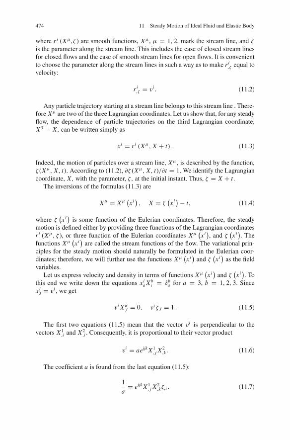
474 11 Steady Motion of Ideal Fluid and Elastic Body
where r i (Xμ,ζ ) are smooth functions, Xμ, μ = 1, 2, mark the stream line, and ζ
is the parameter along the stream line. This includes the case of closed stream linesfor closed flows and the case of smooth stream lines for open flows. It is convenientto choose the parameter along the stream lines in such a way as to make r i
,ζ equal tovelocity:
r i,ζ = vi . (11.2)
Any particle trajectory starting at a stream line belongs to this stream line . There-fore Xμ are two of the three Lagrangian coordinates. Let us show that, for any steadyflow, the dependence of particle trajectories on the third Lagrangian coordinate,X3 ≡ X, can be written simply as
xi = r i (Xμ, X + t) . (11.3)
Indeed, the motion of particles over a stream line, Xμ, is described by the function,ζ (Xμ, X, t). According to (11.2), �ζ (Xμ, X, t)/�t = 1. We identify the Lagrangiancoordinate, X, with the parameter, ζ, at the initial instant. Thus, ζ = X + t.
The inversions of the formulas (11.3) are
Xμ = Xμ(xi), X = ζ
(xi)− t, (11.4)
where ζ(xi)
is some function of the Eulerian coordinates. Therefore, the steadymotion is defined either by providing three functions of the Lagrangian coordinatesr i (Xμ, ζ ), or three function of the Eulerian coordinates Xμ
(xi), and ζ
(xi). The
functions Xμ(xi)
are called the stream functions of the flow. The variational prin-ciples for the steady motion should naturally be formulated in the Eulerian coor-dinates; therefore, we will further use the functions Xμ
(xi)
and ζ(xi)
as the fieldvariables.
Let us express velocity and density in terms of functions Xμ(xi)
and ζ(xi). To
this end we write down the equations xia Xb
i = δba for a = 3, b = 1, 2, 3. Since
xi3 = vi , we get
vi Xα,i = 0, viζ,i = 1. (11.5)
The first two equations (11.5) mean that the vector vi is perpendicular to thevectors X1
,i and X2,i . Consequently, it is proportional to their vector product
vi = aeijk X1, j X2
,k . (11.6)
The coefficient a is found from the last equation (11.5):
1
a= eijk X1
, j X2,kζ,i . (11.7)

11.2 Steady Motion with Impenetrable Boundaries 475
For steady flows density ρ does not change at any space point. In particular,on some surface P intersecting the stream lines, ρ is a function only of Xμ: ρ =ρ (Xμ). Let us show that at any space point, ρ is given by the formula
ρ = σ (Xμ) eijk X1, j X2
,kζ,i (11.8)
where the function σ (Xμ) is defined by the density values on the surface P:
σ (Xμ) = ρ (Xμ)eijk X1, j X2
,kζ,i onP. (11.9)
Indeed, due to (11.6), (11.7) and (11.8), the mass flux ρvi can be written as
ρvi = σ (Xμ) eijk X1, j X2
,k .
Therefore, the function ρ (11.8) satisfies the continuity equation,
(ρvi
),i =
(σ (Xμ) eijk X1
, j X2,k
),i= 0.
The solution of the continuity equation which takes on given values on P is unique,as is easy to see.
If a coordinate transformation Xμ → X ′μ is made, the coefficient σ acquires afactor det
∥∥�Xμ/�X ′ν∥∥ . Therefore, it can be made equal to unity by an appropriate
choice of the coordinates Xμ. Further, we assume that σ = 1, and that
ρvi = eijk X1, j X2
,k, ρ = eijk X1, j X2
,kζ,i . (11.10)
The steady flows have an important feature: the components of the inverse dis-tortion, Xa
i , and, consequently, the components of the distortion, xia, and its deter-
minant, �, do not depend on time at each point. This follows from the formulas(11.4).
In the course of motion, the particles cross the surface P . As the initial values ofparticle’s characteristics, one can take their values at P . In particular, let us define x i
aby the equality x i
a= xia on P . We will assume x i
a to be known functions of Xμ. Notethat such a definition of x i
a differs from the definition used in Chaps. 3 and 4: x ia
= xia for t = t0. We accept it to preserve the property of x i
a to have zero variations:δ x i
a = 0. The variations of the object xia
∣∣t=0 do not equal to zero when the stream
lines are varied.
11.2 Steady Motion with Impenetrable Boundaries
Consider a steady motion of continua in some region V . The particles do not enteror leave the region, and vi ni = 0 everywhere on �V .
The particles which are on the boundary move over the boundary. In terms of thefunctions Xμ
(xi), this condition can be written in the following way: there exists a
function f (Xμ), such that for xi ∈ �V

476 11 Steady Motion of Ideal Fluid and Elastic Body
f(Xμ
(xi)) = 0. (11.11)
The equation f (Xμ) = 0 defines the boundary of the region �V in the Lagrangiancoordinates.
According to the least action principle in Eulerian coordinates, the followingequality takes place:
∫ (�L
�Xat
�
�t�Xa + �L
�Xai
�
�xi�Xa + �L
�Xa�Xa
)dV dt = 0, (11.12)
where
L = ρ
(v2
2−U
(Xa
i , Xa)−�
(xi))
.
Recall that the symbol � means the variation at a fixed space point.Functions U and L do not depend explicitly on X, otherwise, they would change
with time at a fixed space point, but U and L may depend on Xμ.According to (10.29),
�L
�Xat= −ρvi x
ia
and, since for the steady flow ρ, vi and xia do not depend on time for every space
point, and �Xa = 0 at t = t0, t1, the first term in (11.12) is equal to zero. Theother two terms contain only �Xa and their derivatives with respect to the spatialcoordinates. Therefore, the integral (11.12) is not affected by the constraints on �Xa
for t = t0, t1, and, at every instant, the equation holds:
∫
V
(�L
�Xa�Xa + �L
�Xai
�Xai
)dV = 0. (11.13)
Now, note that in varying the functions (11.4), �Xa do not depend on time, whilethe dependence of �Xa on space coordinates can be arbitrary. If we limit the admis-sible variations by the variations �Xμ and �ζ , for which �Xμ = 0, �x i
a = 0 on P ,then δgab = 0, δρ0 = 0, and the left hand side of (11.13) represents the variation ofthe integral of L . Besides, as follows from (10.29), the equations
�L
�Xa− �
�xi
�L
�Xai
= 0 (11.14)
are the equations of the steady flow of the compressible fluid. Therefore, the follow-ing variational principle is valid.Variational principle. Consider the functional

11.2 Steady Motion with Impenetrable Boundaries 477
∫
V
ρ
(1
2viv
i −U (ρ, Xμ)−� (x)
)dV, (11.15)
where ρ and vi are expressed through Xμ (x) and ζ (x) according to the formulas(11.10). The stationary points of this functional on the set of all functions Xμ
(xi)
and ζ(xi)
obey the condition
� det∥∥Xa
i
∥∥ = 0 onP (11.16)
and the constraint (11.11), satisfy the momentum equations of ideal compressiblefluid.
Let us give a direct derivation of the momentum equations. It is convenient towrite the integrand as
L = L(
pi , ρ, Xμ, x) = pi pi
2ρ− ρU (ρ, Xμ)− ρ� (x) , pi ≡ ρvi ,
because the momentum, pi = ρvi , is expressed in terms of the field variables bysimple relations (11.10). We have1
δ I =∫
V
(�L
�pi
(eijk
(�X1
), j X2
,k + eijk X1, j
(�X2
),k
)+ �L
�ρ
(eijk
(�X1
), j X2
,kζ ,i+
+eijk X1, j
(�X2
),kζ ,i + eijk X1
, j X2,k (�ζ ),i
)− ρT
�S
�Xμ�Xμ
)dV . (11.17)
We have for the derivatives of Lagrangian:
�L
�pi= vi ,
�L
�ρ= −
(v2
2+U + ρ
�U
�ρ+�
).
Denote �L/�ρ by −R. Varying ζ , we obtain the equation
eijk (R),i X1, j X2
,k = 0.
It shows that the determinant of the matrix of the derivatives of the functions R, X1,and X2 is equal to zero. That means that R is a function of X1 and X2 only:
R = R(X1, X2
). (11.18)
1 The fluid is assumed to be homogeneous; thus,
�U
�Xμ = T�S
�Xμ .

478 11 Steady Motion of Ideal Fluid and Elastic Body
The coefficient at �ζ in the surface integral, which is obtained after integrationby parts, is equal to zero because the vector eijk X1
, j X2,k is equal to the velocity and
is, consequently, orthogonal to the normal vector.Using (11.18) and the equality vi eijk X1
, j X2,k = ρv2, which follows from (11.10),
the equations resulting from variations of X1 and X2 can be written as
(−vi, j eijkζ ,i
(R, j − T S, j
))X2
,k = 0,(−vi,keijkζ ,i(R,k − T S,k
))X1
, j = 0.
These equations show that the vector in the parenthesis is proportional to velocity.Denoting the corresponding factor by μ, we can write
− vi, j eijk + eijk
(R, j − T S, j
)ζ,i = μvk . (11.19)
The three equations (11.19), in fact, contain the two equations for the requiredfunctions while the third one serves to determine μ. The coefficient μ can be ex-cluded by projecting (11.19) on a plane perpendicular to the velocity, i.e. by con-tracting (11.19) with ekrsv
r . Using (3.19) and the equalities viζ,i = 1, vi R,i = 0,vi S,i = 0, we get the equations
vi, jvj − �i
(v2
2
)+ R,i − T S,i = 0,
which, as can be seen from the definition of R,
R = v2
2+U + ρ
�U
�ρ+�, (11.20)
are the momentum equation of the compressible fluid.At the variation, �X1, on the boundary of region V , the coefficient is
vi ei jkn j X2
,k − Rei jkn j X2,kζ,i .
Since the normal vector ni is proportional to � f�X1 X1
,i + � f�X2 X2
,i , this coefficient is
of the form a � f�X1 . The coefficient at the variation, �X2, is of the form a � f
�X2 . Since� f
�X1 �X1 + � f�X2 �X2 = 0 on �V , the variation Xα on �V does not give additional
relations.Let us formulate the analogous variational principle for the ideal incompressible
homogeneous fluid (it can be derived, from the considered one, by the variational-asymptotic method).
Let the density be a constant: ρ = ρ0 = const . Then the functions Xμ and ζ
satisfy the constraint
ei jk X1, j X2
,kζ,i ≡ const. (11.21)

11.3 Open Steady Flows of Ideal Fluid 479
Based on (11.10) and (3.19), the kinetic energy is
ρv2
2= 1
2ρ
[X1
,i X1,i X2, j X2, j − (X1
,i X2,i)2].
The integral of � over the given region V plays a role of an additive constantand, thus, can be dropped. Therefore, the following variational principle is true.Variational principle. The stationary points of the functional
1
2ρ0
∫
V
[X1
,i X1,i X2, j X2, j − (X1
,i X2,i)2]
dV
on the set of functions X1(xi), X2
(xi), and ζ
(xi)
subject to the constraints (11.11)and (11.21), satisfy the momentum equations of ideal incompressible fluid.
A similar variational principle is valid for elastic bodies.Variational principle. The stationary points of the functional
∫
V
ρ
(v2
2−U −� (x)
)dV (11.22)
(where ρ and vi are expressed in terms of functions, Xμ (x) and ζ (x) , according tothe formulas (11.10), and U is a known function of Xμ
,i , ζ,i , and Xμ) on the set offunctions Xμ (x) and ζ (x), subject to the constraints
onP : Xμ = Xμ (x) , ζ = ζ (x) , niζ,i = a (x) , ni Xμ
,i = aμ (x)
and the constraint (11.11), satisfy the momentum equations of the steady motionof the elastic body inside the volume V and zero boundary conditions for tangentcomponents of the surface force.
The constraints on the surface P are set forth in order to have zero variationsof x i
α and to make the left hand side of (11.13) a variation of the integral of L . Inderiving the equations, one should take into account that the constitutive equationsfor the Cauchy stress tensor in terms of functions Xa
(xi)
have the form
σ ij = −ρ
�U
�Xai
Xaj .
11.3 Open Steady Flows of Ideal Fluid
Now let a part of the boundary, S, of the region V be penetrable to the particles(Fig. 11.1). In this case, the variation of the functional (11.15) is not equal to zero.It is natural to postulate the following variational equation:

480 11 Steady Motion of Ideal Fluid and Elastic Body
Fig. 11.1 An open flow
δ
∫
V
ρ
(v2
2−U (ρ, Xμ)−� (x)
)dV =
∫
S
(λ�ζ+λμ�Xμ
)d A. (11.23)
The functional on the right hand side of (11.23) should be given.In what follows, we consider the case when the functions Xμ (x) on S are known:
Xμ (x) = aμ (x) on S. (11.24)
If the parts of the boundary through which the particles enter and leave V aredenoted by S+ and S−, respectively, the condition (11.24) means that a mappingS+ → S− is given: the starting point of the stream line on S+ maps to the end ofthis line on S−. According to (11.24), �Xμ = 0 on S.
The functional on the right-hand side of (11.23) is specified by prescribing eitherζ (x) on S :
ζ (x) = a (x) on S, (11.25)
or the coefficient λ. Since the functional (11.15) is invariant with respect to theshifts ζ → ζ + ϕ (Xμ), where ϕ is an arbitrary function of its argument, withoutloss of generality one can set ζ (x) = 0 on S−. Then, assigning ζ (x) on S+ fixes thevelocity with which the particles go over the stream lines.
To figure out the physical meaning of λ, consider the coefficient at �ζ on theboundary. As follows from (11.17), it has the value
− Rei jkni X1, j X2
,k . (11.26)
It includes the derivatives of Xμ only over S; therefore, assigning λ with known Xμ
on S is equivalent to assigning R on S as a given function of Xμ:
R = R (Xμ) on S. (11.27)
If Xμ and ζ are given on S, then the right-hand side of (11.23) is equal to zero,and we get the following

11.3 Open Steady Flows of Ideal Fluid 481
Variational principle. The steady motion of ideal compressible fluid is a stationarypoint of the functional
δ
∫
V
ρ
(v2
2−U (ρ, Xμ)−� (x)
)dV
on the set of functions Xμ(xi)
and ζ (x), satisfying the conditions (11.24) and(11.25) on S, and the condition (11.11) on �V − S.
If Xμ and λ are given on S, then the functional on the right-hand side of (11.23)is holonomic and we have the followingVariational principle. The steady motion of ideal incompressible fluid is a station-ary point of the functional
∫
V
ρ
(v2
2−U (ρ, Xμ)−� (x)
)dV +
∫
S
Rei jkni X1, j X2
,kζd A (11.28)
on the set of functions Xμ (x) and ζ (x), satisfying the condition (11.24) on S andthe condition (11.11) on �V − S.
The surface integral in (11.28) can be written as
∫
S+
(R+ (Xμ)ζ+ − R− (Xμ)ζ−
)d X1d X2,
where the indices + and − mark the quantities on S+ and S−, respectively. Thevolume integral in (11.28) is invariant with respect to shifts of ζ by an arbitraryfunction of Xμ. Therefore, in order for the variational problem to be well-posed, thesurface integral has to be equal to zero for all functions ζ+ = ζ− = ϕ (Xμ). Thus,there is a necessary condition which has to be satisfied by the given functions:
R+ (Xμ) = R− (Xμ) .
Using the first equation (11.10), the surface integral in (11.28) can be written as
∫
S
ρvi ni Rζd A.
The function R can be extended on the entire region V by setting R = R (Xμ (x)).Then, taking into account that vi ni = 0 on �V−S,
(ρvi
),i = 0, vi R,i = 0, viζ,i = 1,
the surface integral in (11.28) can be rewritten as
∫
S
ρvi ni Rζd A =∫
�V
ρvi ni Rζd A =∫
V
ρ RdV .

482 11 Steady Motion of Ideal Fluid and Elastic Body
Note that now varying ζ is equivalent to varying the density, ρ: although ρ de-pends on the derivative of ζ along the stream line, the values of ζ are not given atthe boundary, and this derivative (or the density ρ) can be chosen as a new indepen-dent function (see the discussion of a similar issue on the independent variation ofvelocity in Sect. 9.3). Since pi = ρvi do not depend on ζ , we getGiese-Kraiko variational principle. The steady flow of ideal compressible fluid isa stationary point of the functional
∫
V
(pi pi
2ρ− ρU (ρ, Xμ)− ρ� (x)+ρ R (Xμ)
)dV (11.29)
on the set of all functions ρ (x) and Xμ (x) satisfying the constraints (11.24) on Sand the constraints (11.11) on �V − S.
In (11.29), pi = ρvi are expressed through Xμ according to the formulas (11.10).Varying with respect to ρ yields an algebraic problem of calculating the station-
ary value of the function
pi pi
2ρ− ρU (ρ, S)− ρ
(�− R
).
The stationary value of ρ is found from the equation
pi pi
2ρ2+U + ρ
�U
�ρ+� = R, (11.30)
which has the meaning of the Bernoulli integral.After excluding pi = ρvi and ρ by means of (11.30) and (11.10), the integrand
in (11.30) becomes a function of Xμ and the derivatives of Xμ only, and, as easy tosee, it is equal to ρv2 + p. Therefore, we obtainGiese variational principle. The steady flow of ideal compressible fluid is a sta-tionary points of the functional,
∫
V
(ρv2 + p
)dV, (11.31)
on the set of all functions Xμ (x) satisfying the constraints (11.24) on S and theconstraints (11.11) on �V − S.
As an example, let us calculate the functional (11.31) for a barotropic motion ofthe ideal gas, when
U = Aργ−1
γ − 1.
Equation (11.30) becomes

11.4 Two-Dimensional Flows 483
pi pi
2ρ2+ γ A
γ − 1ργ−1 = R −�.
From this equation we find ρ as a function of the velocity
ρ =(
γ − 1
γ A
) 1γ−1
(R −�− v2
2
) 1γ−1
(11.32)
Therefore,
ρ2v2 =(
γ − 1
γ a
) 2γ−1
(R −�− v2
2
) 2γ−1
v2.
On the other hand, from the first equation (11.10),
ρ2v2 = ρviρvi = X1,i X1,i X2
, j X2, j − (X1,i X2,i
)2.
Equating both exptressions for ρ2v2, we get a nonlinear equation which determinesv2 as a function of Xμ
,i :
(γ − 1
γ a
) 2γ−1
(R −�− v2
2
) 2γ−1
v2 = X1,i X1,i X2
, j X2, j − (X1,i X2,i
)2. (11.33)
From (11.32) and the constitutive equation p = aργ , up to a constant factor, theintegrand in (11.31) has the form
L =(
R∗ −�− v2
2
) 1γ−1
+ a
(R∗ −�− v2
2
) γ
γ−1
where v2 is the solution of the equation (11.33) .
11.4 Two-Dimensional Flows
Consider in the Cartesian coordinate system x, y, z two-dimensional flows , i.e. theflows for which X1 = ψ (x, y), X2 = z, ζ = ζ (x, y).
Equation (11.10) becomes
ρvx = ψ,y, ρvy = −ψ,x , vz = 0.

484 11 Steady Motion of Ideal Fluid and Elastic Body
All variational principles formulated above can be applied for two-dimensionalflows. For example, in the case of the isoenergetic motion,2 the Giese-Kraiko prin-ciple transforms toLin-Rubinov variational principle. Steady two-dimensional flow of ideal gas is astationary point of the functional
∫
V
[1
2ρ
(ψ2
,x + ψ2,y
)− aργ
γ − 1+ Rρ
]dxdy
on the set of functions ψ (x, y), which are constant on �V − S and take on theassigned values on S.3
Analogously, the variational principles for axis-symmetric flows can be obtained:one has to take into account that in the cylindrical coordinate system r, ϕ, z: X1 =ψ (r, z) , X2 = ϕ, ζ = ζ (r, z).
11.5 Variational Principles on the Set of Equivortical Flows
All the variational principles for steady flows considered above are “true variationalprinciples” in the sense that the set of admissible functions is fixed and does notdepend on a stationary point. The variational principles of this section stand apart:they are concerned with the variational features of stationary points on the sets thatare determined by the stationary points. Such variational principles are closer to thenon-holonomic variational problems: for each element u, its own set of admissiblevariations, δu, is introduced.
We begin from the consideration of incompressible fluids. First, note that theLagrangian components of vorticity do not change over the stream lines: from (9.15)and (11.2), vc = r i
cri,ζ − �cϕ, therefore,
ωa(Xμ, X ) = eabc�bvc = eabcr icrib,ζ . (11.34)
Differentiating this relation over time we get
0 = eabcr icrib,ζ ζ .
On the other hand, the derivative of ωa over X3, is
ωa,3 = eabcr i
crib,ζ ζ .
Hence, ωa,3 = 0.
2 Isoenergetic is the motion for which R ≡ const.3 Here, V is a region in the plane x, y, and S is a part of its boundary.

11.5 Variational Principles on the Set of Equivortical Flows 485
For a steady motion and a given vorticity, ωa , kinetic energy is a functional ofr (X, ζ ),
K(r (X, ζ )) = ρ0
∫
V
1
2V i ( x | r (X, ζ ))Vi ( x | r (X, ζ ))d3x . (11.35)
Velocity does not depend on time, and so does kinetic energy.Consider the functional A on steady motion,
A = 1
3ρ0
∫
V
eijkrj (Xμ, X + t) r i
ζ (Xμ, X + t) rka (Xμ, X + t) ωa (Xμ) d3 X.
Transforming the integral to Eulerian variables,
A = 1
3ρ0
∫
V
eijkrjr i
ζ rka ωa (Xμ(x))
1
�d3x,
we see that A does not depend on time. Consider the functional
J = A−K, (11.36)
A =1
3ρ0
∫
V
eijkrj (Xμ, ζ ) r i
ζ (Xμ, ζ ) rka (Xμ, ζ ) ωa (Xμ) d2 Xdζ. (11.37)
For a given vorticity, ωa, J is a functional of diffeomorphisms that map the set ofLagrangian coordinates, V , to a given region, V .
Variational principle. The true stream lines of the steady vortex flow are the sta-tionary points of the functional (11.36) on the set of all compressible diffeomor-phisms V → V .
We check the validity of this statement by direct derivation. We have
δ[eijkr
jr iζ rk
a ωa (Xμ)]
= eijkδr jr iζ rk
a ωa (Xμ)+ eijkrj (δr i )ζ rk
a ωa (Xμ)+ eijkrjr i
ζ (δrk)aωa (Xμ)
= eijkδr jr iζ rk
a ωa (Xμ)+ (eijkrjδr ir k
a ωa (Xμ))ζ − eijkrjζ δr ir k
a ωa (Xμ)
−eijkrjδr ir k
a,ζ ωa (Xμ) (eijkr
jr iζ δrkωa (Xμ))a − eijkr
ja r i
ζ δrkωa (Xμ)
−eijkrjr i
ζ,aδrkωa (Xμ)− eijkrjr i
ζ δrkωa,a
= 3eijkδr jr iζ rk
a ωa (Xμ)+ (eijkrjδr ir k
a ωa (Xμ))ζ + (eijkrjr i
ζ δrkωa)a .
Here we used that ωa,a = 0. Integral of the divergence terms vanish (recall that
ωana = 0 at the boundary, and the stream lines are closed). Finally,

486 11 Steady Motion of Ideal Fluid and Elastic Body
δA =ρ0
∫
V
eijkδr jr iζ rk
a ωa (Xμ) d2 Xdζ. (11.38)
Variation of kinetic energy is (see (9.128))
δK =− ρ0
∫
V
eijkδr j V ir ka ωa (Xμ) d2 Xdζ. (11.39)
We obtain the equation
eijk(r iζ − V i )ωk = 0. (11.40)
This is equivalent to the equation of steady flows,
eijk� j (vm�mvk) = 0,
where by vk we mean the field Vk( x | r (X, ζ )). Indeed, (11.40) can be written as
r iζ = V i + λωi , (11.41)
where λ is an arbitrary function. The curl of acceleration is
eijk� j (vm�mvk) = vm�mωi + eijk� jv
m�mvk .
From (9.110),
eijk� j (vm�mvk) = vm�mωi − ωk�ivk + ωi �kvk . (11.42)
Divergence of velocity, �kvk , is zero because velocity field is found from thekinematic problem of Sect. 9.5 (note that divergence of r i
ζ is, in general, non-zero).For the first term in the right hand side of (11.42) we have
vm�mωi = (rmζ − λωm
)�m
(r i
a(Xμ, ζ )ωa(Xμ)
�
)= �
�ζr i
a(Xμ, ζ )ωa(Xμ)
�
−λωm�mωi = r iζ,a
ωa(Xμ)
�− ωi
�
��
�ζ− λωm�mωi = (V i + λωi ),mωm − ωi
�
��
�ζ
−λωm�mωi = = vi,mωm + λ,mωiωm − ωi
�
��
�ζ.
The derivative of the determinant can be expressed in terms of derivatives of r iζ :
��
�ζ= ��
�r ia
�r ia
�ζ= �
�Xa
�xi
�r iζ
�Xa= �
�r iζ
�xi.

11.5 Variational Principles on the Set of Equivortical Flows 487
According to (11.41),
�r iζ
�xi= ωi �λ
�xi.
Thus
vm�mωi = vi,mωm,
and the right hand side of (11.42) vanishes, i.e. momentum equations hold true atthe stationary points as claimed.
The idea to consider equivortical flows, i.e. the flows with the same vorticity, ωa,
as a set of admissible functions, was suggested by V.I. Arnold.Arnold variational principle. The true stream lines of the steady vortex flow arethe stationary points of kinetic energy (11.35) on the set of all incompressible dif-feomorphismsV → V .
This result follows from (11.39): for incompressible flows,
�δr i
�xi= 0,
and therefore there are functions, χk, such that
δr i = eijk� jχk or eijkδr i = � jχk − �kχ j . (11.43)
Hence,
δK =ρ0
∫
V
(v jωk − vkω j
)� jχkd2 Xdζ,
and, due to arbitrariness of χk,
(v jωk − vkω j
), j = 0. (11.44)
The left hand side of (11.44) is the curl of the momentum equations of ideal incom-pressible fluid. The boundary terms are zero due to conditions v j n j = ω j n j = 0.
Comparison of Arnold variational principle and the variational principle for thefunctional J suggests that the following statement holds:Variational principle. Let xi = r i (Xμ, ζ ) be the parametric equations of streamlines of an incompressible steady ideal fluid flow with vorticity, ωa(Xμ), and theparameter ζ be chosen in such a way that r i
ζ is fluid velocity. Then r i (Xμ, ζ ) is astationary point of the functional A (11.37) on the set of all incompressible diffeo-morphisms V → V .
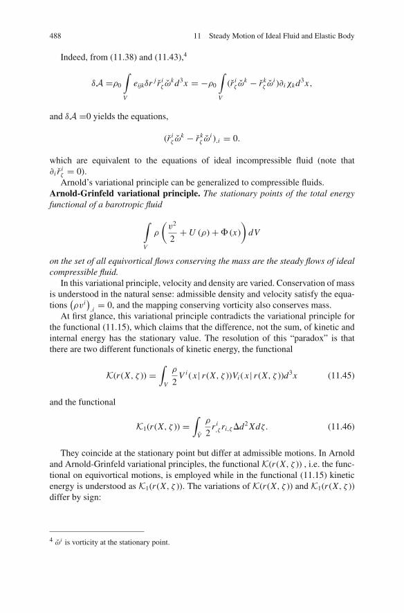
488 11 Steady Motion of Ideal Fluid and Elastic Body
Indeed, from (11.38) and (11.43),4
δA =ρ0
∫
V
eijkδr j r iζ ω
kd3x = −ρ0
∫
V
(r iζ ω
k − r kζ ωi )�iχkd3x,
and δA =0 yields the equations,
(r iζ ω
k − r kζ ωi ),i = 0.
which are equivalent to the equations of ideal incompressible fluid (note that�i r i
ζ = 0).Arnold’s variational principle can be generalized to compressible fluids.
Arnold-Grinfeld variational principle. The stationary points of the total energyfunctional of a barotropic fluid
∫
V
ρ
(v2
2+U (ρ)+� (x)
)dV
on the set of all equivortical flows conserving the mass are the steady flows of idealcompressible fluid.
In this variational principle, velocity and density are varied. Conservation of massis understood in the natural sense: admissible density and velocity satisfy the equa-tions
(ρvi
),i = 0, and the mapping conserving vorticity also conserves mass.
At first glance, this variational principle contradicts the variational principle forthe functional (11.15), which claims that the difference, not the sum, of kinetic andinternal energy has the stationary value. The resolution of this “paradox” is thatthere are two different functionals of kinetic energy, the functional
K(r (X, ζ )) =∫
V
ρ
2V i ( x | r (X, ζ ))Vi ( x | r (X, ζ ))d3x (11.45)
and the functional
K1(r (X, ζ )) =∫
V
ρ
2r i,ζ ri,ζ �d2 Xdζ. (11.46)
They coincide at the stationary point but differ at admissible motions. In Arnoldand Arnold-Grinfeld variational principles, the functional K(r (X, ζ )) , i.e. the func-tional on equivortical motions, is employed while in the functional (11.15) kineticenergy is understood as K1(r (X, ζ )). The variations of K(r (X, ζ )) and K1(r (X, ζ ))differ by sign:
4 ωi is vorticity at the stationary point.

11.5 Variational Principles on the Set of Equivortical Flows 489
δK(r (X, ζ )) = −δK1(r (X, ζ )). (11.47)
This is why the functional (11.15) is the difference of kinetic and potential energies,while the variational principle on the set of equivortical flows claims stationarity ofthe total energy.
To prove (11.47), we note that
δK1(r (X, ζ )) = δ
∫
V
ρ0
2r i,ζ ri,ζ
√gd2 Xdζ =
∫
Vρ0ri,ζ (δr i ),ζ
√gd2 Xdζ,
and, due to closedness of stream lines and independence of the product, ρ0
√g = σ ,
on ζ (see (11.8)):
δK1 = −∫
V(ρ0
√gvi ),ζ δr i d2 Xdζ = −
∫
Vρvi, j r
j,ζ δr i dV = −
∫
Vρvi, jv
jδr i dV .
(11.48)For variation of K(r (X, ζ )) we have
δK(r (X, ζ )) = δ
∫
V
ρ
2V i ( x | r (X, ζ ))Vi ( x | r (X, ζ ))d3x
= δ
∫
V
ρ0
2V i ( x | r (X, ζ ))Vi ( x | r (X, ζ ))
√gd2 Xdζ
=∫
Vρ0ViδV i
√gd2 Xdζ =
∫
VρViδV i dV .
Variation δV i is caused by variation of vorticity:
δωi = δ
(r i
a
ωa
�
)= (δr i ),a
ωa
�− r i
a
ωa
�
�δrk
�xk= (δr i ),kω
k − ωi (δrk),k .
Hence, the variation of Eulerian components of vorticity at a space point, �ωi , are
�ωi = δωi − δxkωi,k = (δr i ),kω
k − ωi (δrk),k − δxkωi,k = (δr iωk − ωiδrk),k .
Variation of velocity at a space point, �V i = δV i −δxk V i,k, are linked to �ωi as
eik j �k�Vj = �ωi = (δr iωk − ωiδrk),k .
The general solution to this equation, �Vj , is a sum of the partial solution,eikjδr iωk, and an arbitrary potential field, ϕ, j :
�Vj = eikjδr iωk + ϕ, j .

490 11 Steady Motion of Ideal Fluid and Elastic Body
Hence,
δK(r (X, ζ )) =∫
VρV j (eikjδr iωk + ϕ, j + δxk Vj,k)dV =
∫
VρV j
[−δr i (Vj,i − Vi, j )+ � jϕ + δxk Vj,k]
dV =∫
VρV j
[δr i Vi, j + ϕ, j
]dV .
(11.49)
The last term in (11.49) vanishes because at the true motion (ρV j ), j = 0, andρV j n j = 0. Finally,
δK(r (X, ζ )) =∫
VρV j Vi, jδr i dV . (11.50)
At the stationary point,5 vi = V i , and (11.47) follows from (11.48) and (11.50).This reasoning yields the following variational principle for elastic bodies.
Variational principle. Let xi = r i (Xμ, ζ ) be the parametric equations of streamlines of a steady motion of homogeneous elastic body. Then r i (Xμ, ζ ) is a stationarypoint of the functional of total energy,
K(r (X, ζ ))+∫
V
ρ0(U(r i
a
)+� (r (X, ζ ))
dV , (11.51)
on the set of all mappings, V → V, that have the same vorticity as r i (Xμ, ζ ).If there are external forces at the boundary, then the corresponding linear func-
tional must be added to (11.51).
11.6 Potential Flows
This section is concerned with the extremal features of the steady potential flows ofthe compressible fluid. For such flows, the closed system of equations comprises thecontinuity equation
�ρvi
�xi= 0 in V, (11.52)
the potentiality condition
vi = �ϕ
�xi, (11.53)
5 For admissible motions, vi �= V i .

11.6 Potential Flows 491
the Cauchy-Lagrange integral
1
2v2 + d (ρU (ρ))
dρ+�
(xi) = k = const, (11.54)
and the boundary condition
ρvi ni = h on �V . (11.55)
It is necessary for the consistency of the system of equations that the total bound-ary mass flux, h, vanishes
∫
�V
hd A = 0. (11.56)
Denote by ρ∗ the function of ∇ϕ and x :
ρ∗ ≡ k − 1
2v2 −� (x) , vi = �ϕ
�xi.
Here k is the constant from the Cauchy-Lagrange integral. The Cauchy-Lagrangeintegral can be viewed as the relation following from maximization of ρ∗ρ−ρU (ρ)with respect to ρ. The corresponding maximum value has the meaning of pressure.As before, we denote it by P (ρ∗).Bateman-Dirichlet variational principle. On the set of all functions ϕ (x), the sta-tionary points of the functional
J =∫
V
P(ρ∗)
dV +∫
�V
ϕhd A (11.57)
satisfy the equations of steady potential flows of compressible gas (11.52) and(11.55).
The Cauchy-Lagrange integral is automatically valid due to the definition ofP (ρ∗).
The function, P (ρ∗) , is a convex function of ρ∗ as the Young-Fenchel transfor-mation of the convex function, ρU (ρ). The same cannot be said of the dependenceof P on the potential gradient, ϕi ≡ �ϕ/�xi . Indeed, let us calculate the secondderivatives of P with respect to ϕi :
�P�ϕi= �P
�ρ∗�ρ∗
�ϕi= −ρϕi ,
�2P�ϕi �ϕ j
= −ρδi j − dρ
dp
�P�ϕ j= −ρ
(δi j − 1
c2ϕiϕ j
).

492 11 Steady Motion of Ideal Fluid and Elastic Body
Here, c denotes the speed of sound: c2 = dp/dρ. The matrix∥∥∥ �2P
�ϕi �ϕ j
∥∥∥ is negative
for the subsonic flows (v2 < c2) and positive for supersonic flows (v2 > c2). Thesubsonic flow can be selected by replacing in (11.57) P (ρ∗) by P (ρ∗) :
P(ρ∗) =
{P (ρ∗) , v2 ≤ c2
−∞ v2 > c2
The function P (ρ∗) is apparently a strictly concave function of ϕi . Therefore, aftersubstituting P (ρ∗) by P (ρ∗) in (11.57), the corresponding functional has a uniquestationary point, and at this stationary point the functional reaches its maximum.
The solvability condition of the boundary value problem (11.56) apparently co-incides with the necessary condition for the functional to be bounded from above. Itis obtained by considering the shifts of ϕ for a constant.
Let us construct the dual variational principle. Denote the Young-Fenchel trans-formation of the function-P , which is convex with respect to ϕi , by P∗
(pi):
P∗(
pi) = max
ϕi
(piϕi + P (ϕi )
).
The dual variables have the meaning of momentum. If the flow corresponding to agiven momentum pi is subsonic, then P∗ is equal to p + ρ v2
2 expressed in terms ofmomentum pi .
For the dual principle, we have
maxϕ
⎡⎣∫
V
P(ρ∗)
dV+∫
�V
ϕhd A
⎤⎦ = −min
ϕ
⎡⎣−
∫
V
P(ρ∗)
dV −∫
�V
ϕhd A
⎤⎦ =
−minϕ
maxpi
⎡⎣∫
V
(piϕi − P∗
(pi))
dV −∫
�V
ϕhd A
⎤⎦ =
−maxpi
minϕ
⎡⎣∫
V
(piϕi − P∗
(pi))
dV −∫
�V
ϕhd A
⎤⎦ =
−maxpi
⎡⎣−
∫
V
P∗(
pi)
dV
⎤⎦ = min
pi
⎡⎣−
∫
V
P∗(
pi)dV
⎤⎦ . (11.58)
The minimum in (11.58) is calculated over all pi satisfying the constraints
�pi
�xi= 0 in V, pi ni = h on �V . (11.59)
Thus, we get

11.7 Regularization of Functionals in Unbounded Domains 493
Bateman-Kelvin variational principle. The minimizing element of the functional,
∫
V
P∗(
pi)dV,
considered on the set of vector fields, pi , satisfying the constraints (11.59), corre-sponds to a subsonic flow of the compressible gas.
11.7 Regularization of Functionals in Unbounded Domains
As a rule, the flows in unbounded regions have diverging energy functionals. Inorder to make the variational principles sensible, it is necessary to modify (to reg-ularize) the energy functional without changing Euler equations. We describe theregularization method for an example of a two-dimensional potential flow of com-pressible gas following Shiffman [277].
Consider subsonic steady potential flow of a compressible gas in two-dimensionalplane, R2. The gas flows around some body, B. The velocity potential, ϕ, is a func-tion of two variables, x and y, defined in the exterior, R2 − B, of the body, B. TheLagrangian of the problem, L , is a function of ϕx = �ϕ/�x and ϕy = �ϕ/�y. LetL(ϕx , ϕy
)be a strictly convex function of ϕx and ϕy satisfying the condition
kai ai ≤ �2L
�ϕi �ϕ jai a j ≤ K ai a
i (11.60)
for any ai and all ϕx and ϕy . Here, k and K are constants, and, for brevity, thenotation ϕ1 = ϕx and ϕ2 = ϕy is used. One can check that the function L =−P (ρ∗) satisfies this condition in the case of the subsonic flows.
At infinity, velocity is supposed to tend to some limit values, ϕ∞i . We formulatethis condition by subjecting the admissible functions, ϕ, to the constraint
� =∫
R2−B
(ϕi − ϕ∞i
) (ϕi − ϕi∞)dxdy < +∞. (11.61)
The integral (11.61) converges only if ϕi → ϕ∞i at infinity. Note that condition(11.61) excludes non-zero circulation of velocity around the body B: for nonzerocirculation ϕi − ϕ∞i ∼ 1/r, and the integral (11.61) diverges.
The functional ∫
R2−B
L(ϕx , ϕy
)dxdy
is obviously diverging for any admissible field. We need to replace it by anotherfunctional, which yields the same Euler equations and remains meaningful forϕi → ϕ∞i at infinity. Consider the variational problem

494 11 Steady Motion of Ideal Fluid and Elastic Body
I =∫
R2−B
[L(ϕx , ϕy
)− L(ϕ∞x , ϕ∞y
)− Lϕx
(ϕ∞x , ϕ∞y
) (ϕx − ϕ∞x
)−
−Lϕy
(ϕ∞x , ϕ∞y
) (ϕy − ϕ∞y
)]dxdy→ min .
This problem yields the same Euler equations. At the same time, the functionalI is bounded from above and below, because
I =1∫
0
Lϕi ϕ j
∣∣ϕ∞i +τ(ϕi−ϕ∞i )
(ϕi − ϕ∞i
) (ϕ j − ϕ∞j
)(1− τ )dτdxdy. (11.62)
From (11.62) and (11.60), it follows that
1
2k� ≤ I ≤ 1
2K �.
Therefore, the minimization problem for the functional I is well-posed.Regularization in other variational problems is based on the same idea.

Chapter 12Principle of Least Dissipation
The variational principles of ideal fluid and elastic body are all based on ignoring thedissipation. If the dissipation is not negligible, the governing equations do not have avariational structure, they possess a quasi-variational structure (see Sect. 2.6). In theanother extreme case, when the dissipation plays the key role while the inertia andthe internal energy effects are negligible, the variational structure of the governingequations appears again, but this is the variational structure of the non-equilibriumprocesses. This chapter is concerned with the corresponding variational principles.As has been mentioned in Sect. 2.6, these variational principles, in contrast to theleast action principle, reflect the special features of the models used rather than thelaws of Nature.
12.1 Heat Conduction
Consider an adiabatically isolated body, V . The heat propagation in the body isgoverned by the following system of equations: the first law of thermodynamics,linking the internal energy rate with the heat flux,
→q ,
ρ�U
�t= −div
→q, (12.1)
the constitutive equation
U = U (S) , (12.2)
and Fourier law
qi = Di j �
�x j
1
T, T = dU (S)
d S(12.3)
Due to Onsager’s relations,
Di j = D ji . (12.4)
V.L. Berdichevsky, Variational Principles of Continuum Mechanics,Interaction of Mechanics and Mathematics, DOI 10.1007/978-3-540-88467-5 12,C© Springer-Verlag Berlin Heidelberg 2009
495

496 12 Principle of Least Dissipation
For adiabatically isolated body, there is no heat flux through the boundary:
qi ni = 0 on �V . (12.5)
In linear non-equilibrium thermodynamics one assumes that temperature deviatesslightly from a constant value, T0 :
T = T0 + T ′, T ′ � T0.
Therefore, Fourier law in linear approximation can be written as
qi = −Di j0
T 20
� j T′, Di j
0 = Di j∣∣T=T0
(12.6)
while for time derivative of internal energy we have
ρ�U
�t= ρ
dU
dT
∣∣∣∣T=T0
�T ′
�t= cv
�T ′
�t, cv ≡ ρ
dU
dT
∣∣∣∣T=T0
.
Finally, the first law of thermodynamics transforms into a linear equation for T ′ :
cv
�T ′
�t= �i
(Di j
0
T 20
� j T′)
.
This equation contains Di j0 , the values of Di j at T = T0. What follows pertains
to the case of linear non-equilibrium thermodynamics and to the special models ofnon-equilibrium thermodynamics when temperature may change considerably, but,as in the linear case, heat conductivities, Di j , do not depend on temperature.
Let us find the total dissipation1 in the continuum at an instant t :
D = d
dt
∫
V
ρSdV =∫
V
ρ�S
�tdV =
∫
V
1
Tρ
�U
�tdV
=∫
V
1
Tdiv
→q dV =
∫
V
→q∇ 1
TdV =
∫
V
Di j �
�xi
1
T
�
�x j
1
TdV . (12.7)
Here we used (12.1), (12.2), (12.3), (12.4) and (12.5). In terms of coldness, β ≡1/T, the dissipation is
D =∫
V
Di j �iβ� jβ dV . (12.8)
1 Another term used for this quantity is the dissipation rate.

12.1 Heat Conduction 497
In (12.8) the coefficients may depend on space points but do not depend on β, andthe quadratic form, Di jξiξ j , is non-negative. In thermodynamic equilibrium, β ≡const and dissipation is equal to zero. Since dissipation is non-negative, one can saythat dissipation is minimum in thermodynamic equilibrium. It is remarkable thatdissipation is also minimum in a non-equilibrium steady process when we maintaintemperature in some part of the body.Least dissipation principle. If temperature is maintained in a part, V2, of regionV , then dissipation considered as a functional of temperature (or coldness) attainsits minimum value for steady heat conduction in region V1 = V − V2.
Indeed,
D =∫
V1
Di j �iβ� jβ dV +∫
V2
Di j �iβ� jβ dV . (12.9)
The second integral is known. Varying the first integral with respect to β, weobtain the equation of steady heat conduction,
�i qi = 0, (12.10)
where qi are given by (12.3). The admissible temperature fields are assumed to besmooth. The values of β, given in the region, V2, also determine the values of β onthe surface, �, separating V1 and V2. Since the first integral in (12.9) feels the valuesof β at the boundary of V1, the values of β on � must be considered as known. Onthe surface �V1 − � the admissible functions, β (x), are arbitrary. This yields theboundary condition of adiabatic isolation, qi ni = 0 at �V1 − �.
The second integral (12.9) plays the role of an additive constant and may be omit-ted. Dropping also index 1 at the region V we arrive at the minimization problemfor the functional
D (β) =∫
V
Di j �iβ� jβ dV
on the set of all functions β taking the prescribed values on � :
β = β(b) on �.
Applying the general scheme of construction of the dual variational principles,we obtain the followingDual variational principle. The true heat flux gives the maximum value to the func-tional
2∫
�
qi niβ(b)d A −∫
V
D−1i j qi q j dV (12.11)

498 12 Principle of Least Dissipation
on the set of all vector fields, qi , selected by (12.10).Here D−1
i j is the inverse tensor to Di j . The maximum value of the functional(12.11) is equal to dissipation.
Note that the minimum dissipation principle does not hold if heat conductivitiesdepend on temperature. This emphasizes its restricted physical meaning.
If the heat flux is given on the surface �, then the true coldness field providesminimum to the functional
∫
V
Di j �iβ� jβ dV − 2∫
�
qnβd A. (12.12)
This functional can be obtained from the dissipation functional (12.9) in the fol-lowing way. Let us fix β on �. Then the true β-field gives minimum to the secondterm in (12.9). Presenting this term by means of the dual variational problem wehave
D =∫
V1
Di j �iβ� jβ dV + 2∫
�
qi niβd A −∫
V2
D−1i j qi q j dV . (12.13)
It remains to note that the unit normal vector in (12.13) looks outside V2, and,therefore, qn in (12.12) is qn = −qi ni . Therefore, the variational principle forthe functional (12.12) can be also interpreted as the minimum dissipation principlewhen the heat flux vector in V2 is fixed (it must be admissible, i.e. satisfy (12.10) inV2).
12.2 Creeping Motion of Viscous Fluid
Consider a slow flow of viscous fluid in a container, V . The velocity is assumed tobe so small that inertia forces are negligible compared to the friction forces. Thevelocity of the fluid is prescribed on the boundary,
vi = vi(b) on �V . (12.14)
The flow is incompressible,
�vi
�xi= 0, (12.15)
while the fluid is homogeneous and isotropic. Then the velocity field is the solutionof the Stokes’ equations,
− �p
�xi+ μ�vi = 0 in V, (12.16)

12.2 Creeping Motion of Viscous Fluid 499
with the boundary conditions (12.14). The dependence of the velocity field on timeappears if the boundary values, or the boundary itself, slowly depend on time. Thenthe following variational principle holds.Least dissipation principle. The true motion of viscous fluid delivers the minimumvalue to the total dissipation
D = 2∫
V
μv(i, j)v(i, j)dV (12.17)
on the set of all velocity fields selected by the constraints (12.14) and (12.15).Indeed, introducing the Lagrange multiplier, p, for the constraint (12.15) we get
the functional∫
V
(2μv(i, j)v
(i, j) − pvi,i
)dV .
Its Euler equations with respect to velocity is (12.16).The functional D differs from the true dissipation by the factor in the integrand:
the dissipation is
2∫
μ
Tv(i, j)v
(i, j)dV .
We will assume in this and the next section that temperature is constant and, writingthe dissipation, drop the factor 1/T .
The minimum property of dissipation is a characteristic of the model rather than amanifestation of a deep physical feature of nonequilibrium processes. This becomesespecially clear if we consider a class of models of viscous flow with non-linear po-
tential stress-strain rate relations. For such models, a dissipation potential, D(
e′i j
),
exists such that2
σ ′i j = �D
�e′i j
, ei j ≡ v(i, j) = 1
2
(�vi
�x j+ �v j
�xi
). (12.18)
The momentum equations are
− �p
�xi+ � jσ
′i j = 0. (12.19)
These equations can be obtained by minimization of the functional
∫
V
D(v(i, j)
)dV (12.20)
2 Primes denote tensor deviators: σ ′i j = σ i j − 13 σ k
k δi j , e′i j = ei j − 13 ek
kδi j .

500 12 Principle of Least Dissipation
on the set of incompressible velocity fields obeying the boundary conditions (12.14).If D is a quadratic form,
D = μe′i j e′i j , (12.21)
then the functional (12.20) differs from the total dissipation
∫
V
σ ′i j e′i j dV
by a factor, i.e. the minimum dissipation principle holds. The same is true for anyhomogeneous function like, for example, a function
D = μ(e′i j e′i j) 1
2 (1+ 1m )
considered in plasticity theory. However, if the dissipative potential is not ahomogeneous function, like, for example, the dissipative potential of visco-plasticmedium,
D = k√
e′i j e′i j + μe′i j e
′i j
then the functional to be minimized, (12.20), differs from the total dissipation.Further, we consider the case of the media with general constitutive equations
(12.18). We assume that the dissipative potential D is a strictly convex function ofthe strain rate tensor, ei j .
Let the boundary of region V comprises two surfaces, S and �; surface forces,fi , are given on S, while velocities are given on �:
vi = vi(b) on �. (12.22)
Besides, some body forces, Fi , acts on the fluid.Variational principle. The true motion provides the minimum value to the func-tional
I (v) =∫
V
D(ei j)
dV − l (v) , (12.23)
l (v) =∫
V
Fivi dV +
∫
S
fivi d A (12.24)
on the set of all velocity fields satisfying the constraints (12.15) and (12.22),If there are no kinematic constraints (12.22) (� = ∅ and S = �V ), then the
functional (12.23) has a kernel – the set of all velocity fields corresponding to the

12.2 Creeping Motion of Viscous Fluid 501
rigid motions. For such fields, D = 0. The necessary condition for the functionalI (v) to be bounded from below is the vanishing of the resultant and the total momentof the forces acting on the fluid:
∫
V
Fi dV +∫
�V
fi d A = 0,
∫
V
ei jk Fj xkdV +∫
�V
ei jk f j xkd A = 0. (12.25)
The sufficiency of the condition (12.25) or (12.22) for boundedness below canbe proven in the same way as for elastic bodies. The uniqueness theorem followsfrom the strict convexity of the dissipative potential and the convexity of the set ofthe admissible functions.
Now we construct the dual variational principle. Denoting the dual variables, thecomponents of the viscous stress tensor, by τ i j and the Young-Fenchel transforma-
tion of the function D(
e′i j
)by D∗
(τ i j)
(in the space of the deviators of the strain
rate tensor),
D∗(τ i j) = max
e′i j
(τ i j e′i j − D
(e′i j
)),
we can write
D(e′i j
) = max(τ i j e′i j − D∗
(τ i j))
.
The maximum is calculated over all τ i j of the deviator space,
τ i j = τ j i , τ ii = 0. (12.26)
Rewriting the variational principle as the minimax principle
I = minv∈(12.22),
(12.15)
maxτ i j∈(12.26)
⎛⎝∫
V
(τ i j e′i j − D∗
(τ i j))
dV − l (v)
⎞⎠ .
and getting rid of the constraint (12.15) by introducing a Lagrange multiplier, thepressure p (x), we have
I = minv∈(12.22)
maxp,τ∈(12.26)
⎛⎝� (v, p, τ )−
∫
V
D∗(τ i j)
dV
⎞⎠ .
Here,
� (v, p, τ ) =∫
V
(−pgi j + τ i j) �vi
�x jdV − l (v) .

502 12 Principle of Least Dissipation
Following to the general scheme of Sect. 5.8, one can check that the order ofcalculation of maximum and minimum can be changed, and, if
− �p
�xi+ �τ i j
�x j+ Fi = 0 in V,
(−pgi j+τ i j)
n j = f i on S, (12.27)
then
minvi∈(12.22)
� (v, p, τ ) =∫
�
(−pδ
ji + τ
ji
)n jv
i(b)dσ ≡ l∗ (p, τ ) .
If p and τ i j does not satisfy the constraints (12.27), then
minvi∈(12.22)
� (v, p, τ ) = −∞.
After minimization over vi , we need to find maximum with respect to p, andτ i j . Therefore, all fields p, τ i j which do not satisfy the constraints (12.27) shouldbe excluded. Thus, we getDual variational principle. The true stress field provides the maximum for the func-tional
J (p, τ ) = l∗ (p, τ )−∫
V
D∗(τ i j)
dV
on all fields p and τ i j satisfying the constraints (12.27). Moreover,
max J (p, τ ) = min I (v) .
12.3 Ideal Plasticity
In metals, elastic deformation is usually negligible compared to plastic deformation(on the order of 10−4 compared to, say, 10−2). Therefore, one may identify theplastic strain rate with the total strain rate
ε(p)i j = ei j = 1
2
(�vi
�x j+ �v j
�xi
). (12.28)
Since the plastic deformation usually preserves the volume, motion is incom-pressible:
�vi
�xi= 0. (12.29)

12.3 Ideal Plasticity 503
For slow motion, one may ignore the inertia effects, and momentum equationsbecome
�σ i j
�x j= 0. (12.30)
Besides, for slow motion heat conduction makes temperature constant over thespecimen and equal to the ambient temperature. Thus,
ρTd S
dt= σ i j ei j ≡ D.
In ideal plasticity, D is assumed to be a homogeneous function of first order
with respect to e′i j : D = D(
e′i j
); D
(λe′i j
)= |λ| D
(e′i j
). The total dissipation
becomes a functional of the velocity field:
D =∫
V
σ i j ei j dV =∫
V
D(ei j)
dV . (12.31)
If velocity is prescribed on the boundary,
vi = vi(b) on �V, (12.32)
then the variational principle holds:Least dissipation principle. The true velocity field provides the minimum value tothe dissipation functional on the set of all incompressible velocity fields with theprescribed boundary values.
At the minimizer, the stresses
σ i j = −pδi j + σ ′i j , σ ′i j = �D
�e′i j
satisfy the equilibrium equations, p being the Lagrange multiplier for the incom-pressibility condition (12.29).
Ideal plastic body is a special case of non-linear viscous media. For an idealplastic body the dissipation is a homogeneous function of the first order. This featureof dissipation makes an ideal plastic body drastically different from viscous fluid.To see that, let us construct the dual variational principle. By the definition of theYoung-Fenchel transformation of the dissipation density, D:
D∗(σ ′i j
) = maxe′i j
(σ ′i j e′i j − D
(e′i j
)). (12.33)
First, we compute D∗ for von Mises model, when
D = k√
e′i j e′i j .

504 12 Principle of Least Dissipation
We have to find
D∗(σ ′i j
) = maxe′i j
(σ ′i j e′i j − k
√e′i j e′i j)
.
Any element in the strain rate space can be presented as a product of an element,e′i j , on the unit sphere
e′i j e′i j = 1
and a positive number, λ :
e′i j = λe′i j .
Therefore, the maximization problem can be split into the succession of the twoproblems
D∗(σ ′i j
) = maxλ≥0
maxe′i j
λ(σ ′i j e′i j − k
). (12.34)
Maximum of a linear function, σ ′i j e′i j , on the sphere is achieved when e′i j isproportional to σ ′i j : the linear function is the scalar product of a unit vector, e′,and a given vector, σ ′, in a five-dimensional space of deviator tensors; it reaches itsmaximum when the angle between the two vectors is equal to zero:
e′i j = κσ ′i j , κ2σ ′i jσ
′i j = 1
Hence,
D∗(σ ′i j
) = maxλ≥0
λ(√
σ ′i jσ′i j − k
).
Obviously, D∗ may have only two values, 0 and +∞, depending on whether√σ ′i jσ
′i j − k smaller or greater than zero:
D∗(σ ′i j
) ={
0 if σ ′i jσ′i j ≤ k2
+∞ if σ ′i jσ′i j > k2
. (12.35)
According to the general scheme of Sect. 5.6 the dual functional is
∫
�V
(−pδi j + σ ′i j)
n jvi(b)d A −∫
V
D∗(σ ′i j
)dV .

12.4 Fluctuations and Variations in Steady Non-Equilibrium Processes 505
We have to maximize this functional, and thus all stress fields for which D∗ =+∞ must be excluded. Therefore, we admit only the stress field such that
σ ′i jσ′i j ≤ k2.
The surface σ ′i jσ′i j = k2 is called yield surface. We arrive at
Dual variational principle. The true stress field provides the maximum value to thelinear functional
∫
�V
(−pδi j + σ ′i j)
n jvi(b)d A
on the set of all stress fields which obey the equilibrium equations and lie inside theyield surface.
For a general homogeneous convex function of the first order, D∗(
e′i j
), which
is smooth everywhere (except the origin where such a function is always singular),Young-Fenchel transformation is similar to (12.35):
D∗(σ ′i j
) ={
0 if f(σ ′i j
) ≤ 0
+∞ if f(σ ′i j
)> 0
where f(σ ′i j
), the yield function, is some smooth convex function. Accordingly, in
the dual variational principle the admissible stresses obey the condition f(σ ′i j
) ≤0. In ideal plasticity theory some non-smooth convex functions are also used; suchcases can be treated as limits in a sequence of smooth dissipation functions.
12.4 Fluctuations and Variations in Steady Non-EquilibriumProcesses
We have seen in Chap. 2 a deep relationship between fluctuations and variations:Einstein’s formula for probability density of macroscopic variables (2.38) showsthat in thermodynamic equilibrium the most probable state corresponds to the max-imum value of entropy, i.e. it yields the first Gibbs principle. The question ariseswhether a similar fact is true for non-equilibrium processes. In this section we givesome arguments in favor of the positive answer.
Consider a steady non-equilibrium process in some region, V . The major ex-ample will be heat conduction. Let the process be characterized by a finite set ofvariables, y = (y1, . . . , ym). In case of heat conduction we partition the region in alarge number of small subregions and characterize the process in each subregion bya finite number of variables. The variables, y, fluctuate and have some probabilitydensity function, f (y). We define entropy of the non-equilibrium process by theformula

506 12 Principle of Least Dissipation
f (y) = const eS(y). (12.36)
Since the system is macroscopic, fluctuations of y are small. Besides, it isobserved a certain macroscopic state, y. The most probable values of y providemaximum to S(y). Therefore, there must be a universalVariational principle. The true values of the characteristics of a steady non-equilibrium process correspond to the maximum value of the non-equilibriumentropy.
Unfortunately, we do not have a reason to state that there is a universal functionof y, S(y), which does not depend on boundary conditions. In principle, for differenttrue states, y, the non-equilibrium entropy could be different: S = S(y, y). FunctionS(y, y) must have a maximum over y at y = y. If S(y, y) does not depend on y, wewould have a “true” variational principle.
Let us try to construct the non-equilibrium entropy for heat conduction. Firstof all, we accept that the non-equilibrium entropy coincides with the equilibriumone for an equilibrium process. The equilibrium entropy for two bodies being inthermal contact was considered in Sect. 2.5. The thermodynamic state of the bodyis characterized by its energy. Denote the equilibrium entropies of the two bodiesby S1(E1) and S2(E2), E1 and E2 being the energies of the bodies. The total energy,E = E1+E2, is conserved because the system, body 1+body 2, is isolated. The totalequilibrium entropy, S(E1, E2), is the sum of equilibrium entropies of the bodies:
S(E1, E2) = S1(E1)+ S2(E2).
The energies, E1 and E2, fluctuate. Their probability density function is
f (E1, E2) = const δ(E − E1 − E2) eS1(E1)+S2(E2). (12.37)
The most probable values of energies correspond to the maximum of entropy,S1(E1)+ S2(E2), under the constraint E1 + E2 = E . As we have seen in Sect. 2.5,this yields the equality of the temperatures of the bodies at equilibrium.
Expanding this reasoning to a continuum, we choose as the characteristic of thethermodynamic state of the system the field of the density of internal energy per unitmass, U (x). The equilibrium entropy density per unit mass is denoted, as before,by S. The thermodynamic properties of the system are described by the function,S = S(U ). Internal energy fluctuates. The fluctuations occur in the functional spaceof the functions, U (x). The corresponding probability density is a functional, f (U ).Generalizing (12.37) we can write
f (U ) = const δ
(E −
∫
VρUdV
)eS(U ), (12.38)
S(U ) =∫
VρS(U )dV . (12.39)
Again, maximum of entropy under constraint,

12.4 Fluctuations and Variations in Steady Non-Equilibrium Processes 507
∫
VρUdV = E,
corresponds to constant temperature over the body, as it must be in thermodynamicequilibrium.
Let the process now be non-equilibrium. We characterize it by the two fields,energy density, U (x), and the heat flux, qi (x). For definiteness, let the heat flux beprescribed at the boundary,
qi ni
∣∣�V= q(b). (12.40)
We wish to construct a functional, S(U, q), which has the maximum value at thesolution of the boundary value problem,
�i qi = 0, q i = κ�i 1
T,
1
T≡ �S(U )
�U, q i ni
∣∣�V = q(b). (12.41)
Besides, for isolated bodies, i.e. for q(b) = 0, the non-equilibrium entropy, S(U, q),should coincide with the equilibrium one (12.39). We will consider the general case,when the heat conductivity, κ, depends on temperature, or, for our choice of primarythermodynamic characteristic, on energy, κ = κ(U ). Then, as was mentioned inSect. 12.1, the least dissipation principle is not valid, while we expect to obtain ameaningful variational principle for such a case.
Fluctuations of energy and the heat flux are not arbitrary; they are linked by theenergy equation:
ρ�U
�t= −�qi
�xi. (12.42)
Let the initial value of U be U , and �t be so small that qi can be viewed aspractically constant during this time interval. Denote by δU and δqi the differences,
δU = U − U , δqi = qi − q i .
Then from (12.42),
ρδU = −�δqi
�xi�t. (12.43)
We see that the fluctuations of energy are completely determined by the fluctuationsof the heat flux.

508 12 Principle of Least Dissipation
Consider the functional
S(U, q) =∫
V
(ρS(U )− ρ
2κ(U )qi qi�t
)dV . (12.44)
For qi = 0 it transforms to the functional (12.39). We consider the functional(12.44) in a small vicinity of the field, q i , which is divergence-free. Variations ofheat flux, δqi , are not divergence-free. The non-zero divergence of δqi yields thevariation of energy. At the boundary δqi ni = 0. The dependence of S(U, q) on thetrue fields, U and q i , enters through the small deviations of U and qi from U and q i .
Variation of the functional, S(U, q), is
δS(U, q) =∫
Vρ
(1
TδU − 1
κ(U )qiδqi�t
)dV . (12.45)
Plugging in (12.45) the expression of δU in terms of δqi (12.43), and setting δS =0for arbitrary δqi , we arrive at the equations of steady heat conduction. Similarly, thevariational principles for other non-equilibrium processes can be formulated.
The variational principle described is not a “true” variational principle: the func-tional depends on the stationary point. This makes it similar to the variational prin-ciples for vortex flows of Sects. 9.6 and 11.5.

Chapter 13Motion of Rigid Bodies in Fluids
13.1 Motion of a Rigid Body in Creeping Flow of Viscous Fluid
Consider in some vessel, V, a linearly viscous isotropic incompressible fluid. Thefluid occupies the entire vessel and contains a rigid body which can move in the fluid(Fig. 13.1). At some instant, the body occupies a region B and has a translationalvelocity, ui :
vi = ui on �B. (13.1)
At the walls of the vessel, the fluid does not slip:
vi = 0 on �V . (13.2)
If the region V is unbounded, then the no-slip condition at the boundary is re-placed by the condition that the fluid is at rest at infinity.Least dissipation principle. The true fluid motion minimizes the dissipation
D (v) =∫
V−B
2μei j ei j dV, ei j = 1
2
(�vi
�x j+ �v j
�xi
), (13.3)
on the set of all incompressible velocity fields,
�vi
�xi= 0, (13.4)
satisfying the boundary conditions (13.1), (13.2).The minimizing element, vi , obeys the momentum equation,
�σ i j
�x j= 0, σ i j = − pgi j + μ
(�i v j + � j vi
), (13.5)
where p is the Lagrange multiplier for the incompressibility constraint (13.4).
V.L. Berdichevsky, Variational Principles of Continuum Mechanics,Interaction of Mechanics and Mathematics, DOI 10.1007/978-3-540-88467-5 13,C© Springer-Verlag Berlin Heidelberg 2009
509

510 13 Motion of Rigid Bodies in Fluids
Fig. 13.1 Notation formotion of rigid body in avessel
The system of equations for the minimizer, the so-called Stokes approximation,is linear. Therefore vi depends linearly on ui . Hence, the minimum value, D, ofdissipation D (v) is a quadratic function of ui :
D = Di j ui u j .
To determine the meaning of the coefficients of this quadratic form we note that,due to (13.1), (13.2), (13.4) and (13.5),
D =∫
V−B
2μv(i, j)v(i, j)dV =
∫
V−B
σ i j vi, j dV =∫
�B
σ i j n j vi d A = Fi ui .
Here we introduced the notation,
Fi ≡∫
�B
σ i j n j d A. (13.6)
The normal vector in (13.6) looks outside the region occupied by the fluid, andtherefore Fi are the components of the force with which the body acts on the fluid.The negative force, −Fi , is the force acting on the body. Since Fi is linear withrespect to ui ,
Fi = Di j u j .
The force is potential,
Fi = �D
�ui,
with the dissipative potential, D, equal to
D = 1
2D.
The estimates of the minimum value of dissipation yield the estimates of theforce. Consider a few elementary consequences of the least dissipation principle.

13.1 Motion of a Rigid Body in Creeping Flow of Viscous Fluid 511
1. For a steady flow of the viscous fluid, the force found within the Stokes approx-imation gives a low bound for the force calculated by means of the Navier-Stokesequations.
Indeed, the value of dissipation on any velocity field, including the velocity fieldfound from the Navier-Stokes equations, is greater than that for the velocity fieldminimizing the functional D (v) and corresponding to the Stokes theory. It remainsto show that for steady flow, Fi ui coincides with dissipation in the framework ofthe Navier-Stokes theory. If vi is a solution of the Navier-Stokes equations and Fi
N Sis the force computed from the Navier-Stokes theory, then
∫
V−B
2μv(i, j)v(i, j)dV =
∫
V−B
(2μv(i, j) − pδi j
)vi, j dV
= FiN Sui −
∫
V−B
(2μv(i, j) − pδi j
), jvi dV = FiN Sui −
∫
V−B
ρv jvi, jvi dV
= FiN Sui −
∫
V−B
1
2(ρv jv2), j dV = Fi
N Sui −∫
�B
1
2ρu j u2n j d A.
Here we used the boundary conditions of the Navier-Stokes theory: vi = ui on �B.The last integral is, obviously, zero. Thus, the dissipation is equal to Fi
N Sui .
2. The dissipation, and, consequently, the force increases as the size of the bodyincreases.
Indeed, let a body B ′ be added to the body B. Denote by DB (v) and DB+B ′ (v)the dissipations corresponding to the bodies B and B ′, respectively, and by vi
B+B ′
the velocity field of the fluid motion around the body B + B ′.Consider the velocityfield
vi ={
viB+B ′ , x ∈ V − (B + B ′
)ui x ∈ B ′
The velocity field vi is defined outside the body B and satisfies the conditions on�B and �V . Consequently, it is admissible in the minimization problem for the func-tional DB (v). We have
DB ≤ DB (v) = DB+B ′ ,
as claimed.An immediate consequence of that feature is the following statement.3. The force acting on the body in the Stokes flow increases if any additional
body is placed in the flow and kept at rest.If the rigid body, B, moves arbitrarily, then
vi = ui + eijkωj(xk−rk
)on �B, (13.7)

512 13 Motion of Rigid Bodies in Fluids
where rk are the coordinates of the point of the body with the velocity ui , and ω j
the angular velocity. It can be checked that D is the quadratic form with respect toui and ωi , and the derivatives
Fi = 1
2
�D�ui
, Mi = 1
2
�D�ωi
, (13.8)
have the meaning of the resultant and the moment of the forces with which thebody acts on the fluid. The moments have the same variational features as thosementioned for the resultants.
The inversion of formulas (13.8) is
ui = �D∗(F, M)
�Fi , ωi = �D∗(F, M)
�Mi , (13.9)
where D∗(F, M) is the Legendre transformation of D/2 with respect to ui and ωi .
Clearly, D∗ also depends on the position vector of the rigid body, rk, and on the or-thogonal matrix, αi
a, specifying the orientation of the body. Therefore, we write fur-ther D∗ = D∗(r, α, F, M). Let us derive the variational formula for D∗(r, α, F, M).
Consider the variational principle dual to the least dissipation principle. Follow-ing the general scheme of Sect. 5.6 we have
D = minvi∈(13.7),(13.2),(13.4)
maxσ ′i j=σ ′ j i
∫
V−B
(σ ′i j �iv j − 1
4μσ ′i jσ ′i j
)dV
= minvi∈(13.7),(13.2)
maxσ ′i j=σ ′ j i ,p
∫
V−B
((σ ′i j − pδi j )�iv j − 1
4μσ ′i jσ ′i j
)dV,
where p is the Lagrange multiplier for the constraint (13.4). Denoting the sum, σ ′i j−pδi j , by σ i j , and switching the order of computation of minimum and maximum,we obtain
D = maxσ i j
minvi∈(13.7),(13.2)
∫
V−B
(σ i j �iv j − 1
4μσ ′i jσ ′i j
)dV .
Hence, the admissible fields, σ i j , obey the constraints,
�σ i j
�x j= 0, (13.10)
and
D = maxσ i j∈(13.10)
(∫
�Bσ im(ui + ei jkω
j(xk−rk
))nmd A −
∫
V−B
1
4μσ ′i jσ ′i j dV
).
(13.11)
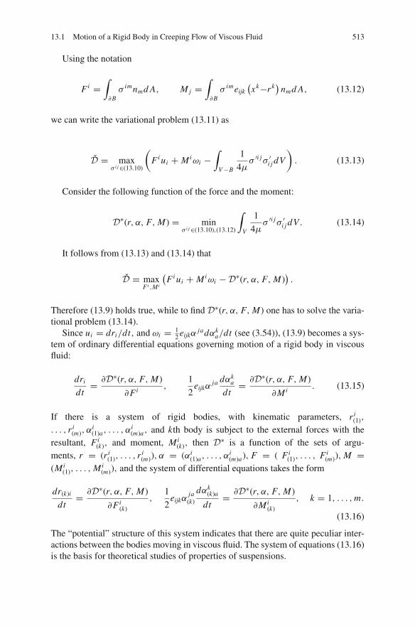
13.1 Motion of a Rigid Body in Creeping Flow of Viscous Fluid 513
Using the notation
Fi =∫
�Bσ imnmd A, M j =
∫
�Bσ imeijk
(xk−rk
)nmd A, (13.12)
we can write the variational problem (13.11) as
D = maxσ i j∈(13.10)
(Fi ui + Miωi −
∫
V−B
1
4μσ ′i jσ ′i j dV
). (13.13)
Consider the following function of the force and the moment:
D∗(r, α, F, M) = minσ i j∈(13.10),(13.12)
∫
V
1
4μσ ′i jσ ′i j dV . (13.14)
It follows from (13.13) and (13.14) that
D = maxFi ,Mi
(Fi ui + Miωi −D∗(r, α, F, M)
).
Therefore (13.9) holds true, while to find D∗(r, α, F, M) one has to solve the varia-tional problem (13.14).
Since ui = dri/dt, and ωi = 12 eijkα
jadαka/dt (see (3.54)), (13.9) becomes a sys-
tem of ordinary differential equations governing motion of a rigid body in viscousfluid:
dri
dt= �D∗(r, α, F, M)
�Fi ,1
2eijkα
ja dαka
dt= �D∗(r, α, F, M)
�Mi . (13.15)
If there is a system of rigid bodies, with kinematic parameters, r i(1),
. . . , r i(m), α
i(1)a, . . . , α
i(m)a, and kth body is subject to the external forces with the
resultant, Fi(k), and moment, Mi
(k), then D∗ is a function of the sets of argu-ments, r = (r i
(1), . . . , r i(m)), α = (αi
(1)a, . . . , αi(m)a), F = ( Fi
(1), . . . , Fi(m)), M =
(Mi(1), . . . , Mi
(m)), and the system of differential equations takes the form
dr(k)i
dt= �D∗(r, α, F, M)
�Fi(k)
,1
2eijkα
ja(k)
dαk(k)a
dt= �D∗(r, α, F, M)
�Mi(k)
, k = 1, . . . , m.
(13.16)
The “potential” structure of this system indicates that there are quite peculiar inter-actions between the bodies moving in viscous fluid. The system of equations (13.16)is the basis for theoretical studies of properties of suspensions.

514 13 Motion of Rigid Bodies in Fluids
13.2 Motion of a Body in Ideal Incompressible Fluid
The Thomson-Tait equations. Constructing the equations governing the motionof a deformable body in a potential flow of ideal incompressible fluid is a non-elementary issue if the starting point is momentum equations. The derivation isconsiderably simplified if the variational approach is used.
We assume that the body occupies region B (t) at time t , B will denote the regionrun by the Lagrangian coordinates of the body, Xa . The motion and the deformationof the body are described by a finite number of parameters qk (t) (k = 1, . . . , n):
xi(Xa, t
) = χ i(Xa, qk
)for Xa ∈ �B; qk = qk (t) .
The velocity of the boundary points depends linearly on qk :
x i(Xa, t
) = �χ i
�qkqk for Xa ∈ �B. (13.17)
The characteristics of the rigid motion of the body, r i (t) and αia (t) , are included
in the set of parameters qk .Suppose that the fluid occupies a moving and possibly deforming vessel V (t)
and in the process of motion does not detach from the walls of the vessel and theboundary of the body. The deformation and the motion of the vessel is also givenby a finite number of parameters, bk (t); the velocity of the vessel wall dependslinearly on bk . The sets of the parameters, qk and bk , will be denoted by q and b,respectively.
Let � (x) be the potential of the external body forces, KB and UB the kinetic andthe internal energies of the body, and KB = KB (q, q) , UB = UB (q).Least action principle. The true motion of the body and the fluid is a stationarypoint of the functional
t1∫t0
( ∫V (t)−B(t)
(12ρvivi − ρ� (x)
)dV+KB − UB
)dt (13.18)
on the set of functions x(X, t) and q (t) with the prescribed initial and final values.Assigning the initial positions of the fluid particles fixes the choice of the La-
grangian coordinates. Assume that the final positions of the fluid particles are chosenin such a way as to cause a potential flow in the vessel. The possibility of such achoice is guaranteed by the solvability of the corresponding problems.
For potential flow, the velocity field of the fluid at each instant is defined by thegeometry of the regions V (t) and B (t), i.e. by the values of the parameters q andb and the velocities of the fluid on �V (t) and �B (t), i.e. by q and b. The kineticenergy of the fluid, KF , is found by solving the variational problem

13.2 Motion of a Body in Ideal Incompressible Fluid 515
KF = minv
∫
V (t)−B(t)
1
2ρvivi dV, (13.19)
where the minimum is sought over all the velocity fields satisfying the conditions
�ivi = 0, vi ni
∣∣�B(t) =
�χ i
�qkqkni , vi ni
∣∣�V (t) = ckbk, (13.20)
where ckbk is the normal component of the velocity of the fluid on �V (t). Thekinetic energy of fluid motion is a function of q, q, b, b: KF = KF (q, q, b, b).
Suppose that the variational problem (13.19) and (13.20) is solved and the func-tion KF
(q, q, b, b
)is found. Then the functional (13.18) becomes
t1∫t0
L(q, q, b, b
)dt, (13.21)
where
L = KF +KB − UB − � (q, b) ,
� (q, b) =∫
V (t)−B(t)
ρ� (x) dV .
The least action principle yields the equations of motion
�L
�qk− d
dt
�L
�qk= 0. (13.22)
For the case of motion of rigid bodies, these equations were established by Thom-son and Tait [293]. Consider some examples.
Example 1. Consider the motion of a rigid body in an unbounded fluid being at restat infinity. The position of the body is defined by the position vector r i (t) and anorthogonal matrix αi
a (t). The constraints (13.20) become
vi,i = 0 in R3 − B (t) , vi ni =
(r i + eijkω j (xk − rk)
)ni on �B (t) , (13.23)
where ωk = 12 eklmαl
aαma . The kinetic energy of the fluid is finite only if vi → 0 as
x → ∞; therefore, the condition that the fluid is at rest at infinity is automaticallyincluded in the variational formulation and does not need to be mentioned explicitly.
Let Xa be Cartesian coordinates rigidly linked to the body. The constraints(13.23) become
va,a = 0 in R3 − B, vana =
(ua + eabcωb Xc
)na, (13.24)

516 13 Motion of Rigid Bodies in Fluids
where ua = αai r i , ωb = 1
2 ebacαci α
a , and B is the region in which the Lagrangiancoordinates of the body particles change. The kinetic energy of the fluid is quadraticwith respect to ua and ωa is
KF = 1
2
(Mabuaub + 2Rabuaωb + J abωaωb
). (13.25)
The coefficients Mab, Rab, and J ab depend only on the geometry of the region B.The kinetic energy of the rigid body also has the form (13.25). The coefficients ofthe quadratic form K = KF + KB will be denoted by Mab, Rab, and J ab. Theexplicit dependence of K on the characteristics of motion is:
K= 1
2
(Mabαi
aαjb ri r j+ Rabαi
aαjb ri e jklα
kc α
lc + 1
4J abαi
aαjb eimnα
mc αnce jm ′n′α
m ′c′ α
n′c′)
.
Euler equations for the action functional are the equations of motion of a freerigid body with the effective characteristics Mab, Rab, J ab.
If Lab and Mab are diagonal,
Mab = m(a)δab, Mab = Mδab
and m is the mass of the body, then
M = m + m(a).
This looks like an effective increase of the mass of the body; the parameter m(a)
is called the attached mass. In general case, the tensor Mab is called the tensor ofattached mass, and its trace, 1
3 Maa , the averaged attached mass.
Example 2. In the previous example, the kinetic energy did not depend on the posi-tion of the body. This is caused by the invariance of the kinetic energy with respectto translations, which, in turn, appears due to the absence of the external boundariesof the flow. Let us consider a problem where the flow has an external boundary.
Let the fluid occupy the half-space x ≥ 0 and a ball of radius a move in thefluid along the x axis. The system has one degree of freedom – the distance q fromthe center of the ball to the plane x = 0. The flow potential , ϕ, is defined by theboundary value problem
�ϕ = 0,�ϕ
�n= 0 for x = 0,
�ϕ
�n= qnx on the ball surface.
At infinity ∇ϕ = 0 because kinetic energy of the fluid is finite.In the absence of the wall, ϕ is the dipole potential:
ϕ = 1
2a3q
�
�x
1
|r − r0| .

13.2 Motion of a Body in Ideal Incompressible Fluid 517
Here, r and r0 are the position vectors of a space point and the center of the ball,respectively, and |r | the magnitude of vector, r . For large q/a, the harmonic function
ϕ = 1
2a3q
�
�x
(1
|r − r0| −1
|r + r0|)
(13.26)
satisfies the boundary condition at the wall and approximately satisfies the boundarycondition on the ball. One can show that (13.26) is the leading term of the expansionwith respect to a small parameter a/q . We will use only this term. Then kineticenergy is
KF = πρa3
3
(1+ 3
8
a3
q3
)q2. (13.27)
In particular, it follows from (13.27) that for a ball in an unbounded fluid flow, thetensor of attached mass is spherical and has the value, Mab = 2
3ρπa3δab.According to (13.22), the motion equation for a ball of mass m is governed by
the equation
d
dt
[m + 2πa3
3ρ
(1+ 3
8
a3
q3
)]q + 3πρa6
8q4q2 = 0.
It takes much more effort to derive this equation considering the balance of forces.
Example 3. The body B may consist of several simply connected components. Then(13.22) describes the interactions of the bodies in fluids. For example, let us considertwo balls moving in an unbounded fluid which is at rest at infinity. The system hassix degrees of freedom r i
1 (t) and r i2 (t) – the coordinates of the centers of the balls. In
order to calculate the kinetic energy of the fluid, KF , we have to solve the boundaryvalue problem
�ϕ = 0 in R3 − B1 − B2,�ϕ
�n= r i
1ni on �B1,�ϕ
�n= r i
2ni on �B2 (13.28)
with the condition that kinetic energy of the fluid is finite. Kinetic energy is aquadratic form:
KF = 1
2
(M1
r i1r j
1 + 2Ni j ri1r2 + M
2r i
2r j2
)(13.29)
The equations (13.28) are invariant with respect to translations, therefore, in thequadratic form (13.29) the coefficients, M
1i j , Ni j and M
2i j , depend only on the dif-
ference, r i1 − r i
2.The exact solution of the problem (13.28) can be obtained in the form of series;
however, the corresponding expressions for the coefficients in (13.29) are so com-plicated that they can hardly help in the analysis of the motion of the balls. We give

518 13 Motion of Rigid Bodies in Fluids
here the first terms of an asymptotic expansion when the ratios of the radii of theballs, a1, a2, to the distance between their centers, R = |r1 − r2| , are small. In thefirst approximation, the balls do not interact, and
M1
i j = 2πρ
3a3
1δi j , Ni j = 0, M2
i j = 2πρ
3a3
2δi j .
The approximation which takes into account corrections on the order of (a1/R)3,(a2/R)3, is as follows: the expressions for M
1i j and M
2i j do not change, while Ni j
becomes
Ni j = πρa31a3
2
R3
(δi j − 3
R2Ri R j
), Ri = r i
1 − r i2.
Polia-Shiffer’s theorem. Even in the case of the bodies moving in unbounded fluid,KF was found analytically only for ellipsoids. Therefore, for bodies with a morecomplex shape and any bodies in bounded regions, the approximation methods areused.
As an example of application of the variational formula for the kinetic energy,consider an elegant statement hypothesized by Polia and proved by Shiffer:
The averaged attached mass of the body moving in an unbounded fluid beingat rest at infinity is not smaller than the attached mass of the sphere of the samevolume.
Actually, a stronger statement holds: each eigenvalue of the tensor of attachedmass is not smaller than the attached mass of the sphere; it yields the assertion onthe averaged attached mass.
Denote the region occupied by the body by B and the exterior of B by V .According to the Dirichlet principle,
KF = maxϕ
K∗ (ϕ) ,
1
ρK∗ (ϕ) =
∫
�B
ϕui ni dσ − 1
2
∫
V
�ϕ
�xi
�ϕ
�xidV .
The unit normal vector is directed outward of the fluid.Choosing various functions ϕ, we get low estimates of KF :
K∗ (ϕ) ≤ KF . (13.30)
Let us take ϕ as
ϕ = ai �χ
�xi, (13.31)
where χ is the gravity potential of the body B,

13.2 Motion of a Body in Ideal Incompressible Fluid 519
χ =∫
B
d3x ′
|x − x ′| ,
and ai are some constants. We will choose ai later to optimize the estimate. Wecan expect that the trial functions (13.31) provide a good estimate, because for anappropriate choice of constants ai , formula (13.31) gives the exact solution for fluidmotion past an ellipsoid.
Substituting the trial functions (13.31) in the functional, K∗ (ϕ) , and integratingby parts we obtain
1
ρK∗ (ϕ) =
∫
�B(e)
ϕ
(ui − 1
2
�ϕ
�xi
)ni d A. (13.32)
The index (e) emphasizes that in computation of the integral (13.32) the limit of theintegrand is taken when �B is approached from the exterior side of the body, thefluid side. In deriving (13.32), it is taken into account that the integral over V ofϕ�ϕ is equal to zero since ϕ is a harmonic function.
Let us replace the limit value of the integrand from the exterior of B by the limitvalue from the interior of B in order to reduce the surface integral to an integral overthe region B by means of the divergence theorem. We have to take into account thatthe function ϕ = aiχ,i is continuous on �B, while the derivatives, �ϕ/�xi , have adiscontinuity, and
�ϕ
�xk
∣∣∣∣(e)
− �ϕ
�xk
∣∣∣∣(i)
= 4πnkn j a j . (13.33)
The index (i) denotes the limit values at �B from the interior side of the body.Replacing in (13.32) the limit values of the functions from the fluid side by the
limit values of the functions from the body side, we get
1
ρK∗ (ϕ) =
∫
�B(i)
ϕ
(ui − 2πni n
j a j − 1
2
�ϕ
�xi
)ni d A. (13.34)
Applying to (13.34) the divergence theorem, we find
1
ρK∗ (ϕ) =
∫
B
[− �ϕ
�xiui + 2πai �ϕ
�xi+ 1
2
�ϕ
�xi
�ϕ
�xi
]dV .
The term ϕ�ϕ = ϕak ��xk �χ is equal to zero in B, since the gravity potential χ
satisfies the equation �χ = const. in the region B.

520 13 Motion of Rigid Bodies in Fluids
Let us decrease the last term using the Cauchy inequality (5.20):1
1
|B|∫
B
�ϕ
�xidV
∫
B
�ϕ
�xidV ≤
∫
B
�ϕ
�xi
�ϕ
�xidV . (13.35)
Introducing the notation
Ai j = −∫
B
χ,i j dV,
we get the estimate
1
ρK∗ (ϕ) ≥ Ai j u
i a j − 1
2
(4π Ai j − 1
|B| Aim Amj
)ai a j . (13.36)
It is important that for an ellipsoid, �ϕ/�xi are constant in B; therefore in (13.35),and, consequently, in (13.36) (for ai which maximize the right hand side) the equal-ity is attained.
Let us choose a system of coordinates xi oriented along the principle axes of thetensor Ai j . Then
1
ρK∗ (ϕ) ≥ A1u1a1 + A2u2a2 + A3u3a3 − 1
2
(4π A1 − 1
|B| A21
)a2
1−
−1
2
(4π A2 − 1
|B| A22
)a2
2 −1
2
(4π A3 − 1
|B| A23
)a2
3, (13.37)
A1 ≡ A11, A2 ≡ A22, A3 ≡ A33. In this system of coordinates, the maximum ofthe right hand side is attained for
a1 = u1
4π − A1|B|
, a2 = u1
4π − A2|B|
, a3 = u1
4π − A3|B|
.
Therefore,
1
ρK∗ (ϕ) ≥ 1
2
(A1
4π − A1|B|
u21 +
A2
4π − A2|B|
u22 +
A3
4π − A3|B|
u23
).
1 We set in (5.20) g = 1 to obtain⎛⎝∫
B
f dV
⎞⎠
2
≤ |B|∫
B
f 2dV,
then apply this inequality to each component of the vector ∇ϕ, and take the sum of the threeinequalities such obtained.

13.3 Motion of a Body in a Viscous Fluid 521
The following inequality holds:
A1
4π − A1|B|+ A2
4π − A2|B|+ A3
4π − A3|B|≥ A1 + A2 + A3
4π − A1+A2+A33|B|
. (13.38)
Indeed, the function
f (x) = x
4π − x|B|
is strictly convex because, for 0 ≤ x ≤ |B| , �2 f/�x2 > 0. Let us consider theminimum of the strictly convex function f (A1)+ f (A2)+ f (A3) with the constraintA1 + A2 + A3 = const = c. Introducing the Lagrange multiplier, we see that theminimum is reached for A1 = A2 = A3. Consequently, at the minimum point
A1 = A2 = A3 = c
3, f (A1)+ f (A2)+ f (A3) = 3 f
( c
3
)= c
4π − c3|B|
.
For arbitrary A1, A2, A3 this yields, (13.38).From the definition of Ai j it follows that
A1 + A2 + A3 =∫
B
�χdV = 4π |B| .
Therefore,
1
ρK∗ (ϕ) ≥ 3
4|B| (u2
1 + u22 + u2
3
),
and each eigenvalue of the tensor of the attached mass is not smaller than 32ρ |B| ,
i.e. the attached mass of the sphere. In particular,
1
3Mi
i ≥1
2|B| = 1
3Mi
i(ball).
13.3 Motion of a Body in a Viscous Fluid
The equations for forces and moments acting on the body moving in a potentialflow of the ideal incompressible fluid and in Stokes flow of a viscous fluid possessa variational structure, as has been shown in the two preceding sections. The forceacting on the body in ideal fluid, is2
2 Since in this section the kinetic energy of the body does not appear and only the kinetic energyof the fluid is encountered, the corresponding index at kinetic energy is omitted.

522 13 Motion of Rigid Bodies in Fluids
Fi = �K�r i− d
dt
�K�r i
, (13.39)
while in viscous fluid
Fi = −�D
�r i. (13.40)
In these equations, K and D are functions of the instantaneous characteristics of themotion only.
The following question arises: is there a universal relation between the general-ized forces acting on the body with the kinetic energy of the fluid K and the dissi-pative potential D, when they depend not only on the instantaneous characteristicsof the motion, but also on the “history” of the motion?
It turns out that, with some assumptions (which shall be introduced further), ageneralization of (13.39) and (13.40) is the variational equation
Qkδqk = δK − d
dtδ.K − δ.D. (13.41)
Here, the generalized coordinates qk characterize the motion and the deformation ofthe body, Qk are the corresponding generalized forces, K and D are the functionalsof the motion history. The dependence of K and D on the motion history can bedescribed by the two groups of variables (separated by a semi-colon)3:
K = Kτ=tτ=0 (q (τ ) ; q (τ )) , D = D
τ=tτ=0 (q(τ ) ; q (τ )) .
The actual method of distinguishing the two groups of variables is describedbelow. In (13.41), δ is the variation operator with respect to both variables, and δ.is the operator which performs the variation with respect to the second group ofarguments and subsequently substitutes δq by δq.
If K is a function of r i (t) and r i (t) only: K = K(r i ; r i
)and D = 0, then (13.39)
follows from (13.41):
Fiδr i = �K�r i
δr i + �K�r i
δr i − d
dt
�K�r i
δr i =(
�K�r i− d
dt
�K�r i
)δr i .
If K = 0 and D = D
(r i ; r i
), then (13.40) follows from (13.41) as well.
The variational equation (13.41) defines n functionals Q1, . . . , Qn through thetwo functionals K and D.
Let us prove (13.41). Let V and B be regions in the space of variables Xa whichare run by the Lagrangian coordinates of the fluid and the body, respectively. The
3 The symbol Kτ=tτ=0 (q) denotes the functionals of functions q (τ ) defined on the segment 0 ≤
τ ≤ t .

13.3 Motion of a Body in a Viscous Fluid 523
fluid is assumed to be viscous and incompressible, and the boundary of the vesselV does not move. For given particle positions of the body and the fluid at the initialand final instants, and given motion of the boundary of the region V , we have thevariational equation
t1∫
0
⎛⎝δ
∫
V−B
ρ
2viv
i dV +∫
�B
Piδxi d A−∫
V
�D
�ei j� jδxi dV
⎞⎠dt = 0,
where Pi are the components of the surface force acting on the fluid from the body,D is the density of the fluid dissipative potential (the fluid does not have to beNewtonian).
The variational equation can be written as an equality valid at any time t
t∫
0
⎛⎝δ
∫
V−B
ρv2
2dV +
∫
�B
Piδxi d A −∫
V
�D
�ei j� jδxi dV
⎞⎠dt −
∫
V−B
ρviδxi dV
∣∣∣∣∣∣t
= 0.
(13.42)
Let us prescribe some motion of the body, q = q (t). Then, the motion of thefluid can by found from the system of equations
ρdvi
dt= −�i p + � j
�D
�ei j, (13.43)
det
∥∥∥∥�xi
�Xa
∥∥∥∥ = det
∥∥∥∥�x i
�Xa
∥∥∥∥ , (13.44)
which are supplemented by the boundary conditions
xi(Xa, t
) = ∗xi(Xa)
on �V, xi(Xa, t
) = χ i(Xa, qk
)on �B. (13.45)
Assume that the body and the fluid are at rest at the initial instant:
xi(Xa, 0
) = x i(Xa), vi
(Xa, 0
) = 0. (13.46)
For the consistency of the initial and the boundary conditions on �B at t = 0, werequire that
qk (0) = 0.
We assume that the system of equations (13.43), (13.44), (13.45) and (13.46)determines uniquely the fluid motion on the considered time interval. Then, in prin-ciple, one can find the particle trajectories of the fluid, and, for each Xa and t, theyare some functionals of the motion history of the body B, i.e. of q (τ ) for 0 ≤ τ ≤ t .

524 13 Motion of Rigid Bodies in Fluids
The variational equation (13.42) is an identity due to (13.43), (13.44) and (13.45)and the equality,
(−pδ
ji +
�D
�eij
)n j = Pi on �B,
for arbitrary δxi vanishing at t = 0 and on �V × [0, t] . In particular, the particletrajectories for the fluid, satisfying (13.43), (13.44), (13.45) and (13.46), can besubstituted into (13.42), and δxi can be interpreted as its variation caused by aninfinitesimally small variation of the body motion. Then the variations δxi are somefunctionals of q (τ ) and δq (τ ) at every point X, t for 0 ≤ τ ≤ t , which are linearwith respect to δq (τ ). Let us write this as follows:
δxi =τ=t
l i
τ=0(X, t |q (τ ) ; δq (τ )) .
At the boundary of the body,
δxi = �χ i
�qkδqk .
The variational equation (13.42) becomes
t∫
0
⎡⎣δK−Qkδqk−
∫
V
�D
�ei j� jδxi
⎤⎦dV −
∫
V−B
ρviδxi dV
∣∣∣∣∣∣t
= 0, (13.47)
where K, the kinetic energy of the fluid calculated for the solutions of the problem(13.43), (13.44), (13.45) and (13.46), is some functional of q (τ ), δ is the variationof the body motion, and Qk are the generalized forces:
Qk = −∫
�B
Pi�χ i
�qkd A.
It remains to check the relation
vi (X, t) =τ=t
l i
τ=0(X, t |q (τ ) ; q (τ )) , (13.48)
to finish the proof. Indeed, if the equality (13.48) is true, then the functionals
K =∫
V−B
ρ
2vivi dV, D =
∫
V
D(�(i v j)
)dV,

13.3 Motion of a Body in a Viscous Fluid 525
which are calculated for the velocity (13.48), become the functionals of the twogroups of variables.
Let us introduce the operator δ. which takes the variation with respect to the sec-ond group of variables and subsequently substitutes δq (τ ) by δq (τ ). If follows from(13.48) that
δ.vi = δxi .
The operator δ. , as the operator of taking the variation with respect to q, commuteswith the differential operators:
δ.�iv j = �iδ.v j = �iδx j .
Therefore, the variational equation (13.47) can be written as
t∫
0
[δK−Qkδqk − δ.D
]dt − δ.K = 0. (13.49)
Taking the derivative of (13.49) with respect to time results in (13.41).So, we have to prove the relation (13.48). Let us take the variation of (13.43)
and (13.44). We get some system of equations for δxi in the region V − B. Let uswrite it as Lδx = 0. The operator L is a linear differential operator with variablecoefficients. Taking the variation of the initial conditions results in
δxi = 0,dδxi
dt= 0 in V − B for t = 0. (13.50)
At the boundary of the fluid,
δxi = 0 on �V, δxi = �χ i
�qkon �B. (13.51)
The equations, Lδx = 0, together with the initial and the boundary conditions
(13.50) and (13.51) define the functionalsτ=t
l i
τ=0(X, t |q (τ ) ; δq (τ )).
Let us differentiate (13.43), (13.44) and (13.45) with respect to time. We get theequations Lv = 0 with the boundary conditions
vi = 0 on �V, vi = �χ i
�qkqk on �B, (13.52)
and the initial conditions
vi = 0 at t = 0.

526 13 Motion of Rigid Bodies in Fluids
Let qk = 0 for t = 0. Then,
dvi
dt= 0 for t = 0. (13.53)
Indeed, it follows from (13.43) that curl dv/dt = 0 for t = 0. Differentiatingthe continuity equation vi
,i = 0 with respect to time and setting t = 0, we getdiv dv/dt = 0. Consequently, dv/dt = gradϕ and �ϕ = 0. On the boundary of thefluid, taking the derivative of (13.52), we have dv/dt = gradϕ = 0 at �V and �Bfor t = 0. Therefore, ϕ = const and (13.53) holds.
The assumption that the motion starts from rest is essential, because otherwise(13.48) is not valid.
It is easy to check that the above reasoning can be applied verbatim for vis-coelastic fluid, for which the internal energy is a function of the distortion. Then theinternal energy U , which is a functional of the previous motion of the body, must beincluded in the variational equation as well:
Qkδqk = δ (K−U)− d
dtδ.K − δ.D. (13.54)
The problem of calculating forces and moments acting on the rigid body inviscous fluid is extremely difficult. Therefore, it is sensible to use the variationalequation (13.41) to determine forces and moments, by postulating the functionals Kand D from phenomenological reasonings. Note that there is a universal dependencebetween K and D due to which they cannot be prescribed arbitrarily. Indeed, let usset δqk = 0 at time t in (13.41). Then, for any functions δqk (τ ) which, along withtheir first and second derivatives, are equal to zero at the initial time and time t , thefollowing relation holds:
− δK + d
dtδ.K + δ.D = 0. (13.55)
If K and D are some functions of q, q , then (13.55) is automatically satisfied. How-ever, if memory is taken into consideration, the relation (13.55) puts the constrainton the possible functionals, K and D.
Consider some examples.Translational unsteady motion of a sphere. Consider a sphere of radius a in anunbounded flow of viscous incompressible fluid. For t = 0, the fluid and the ballare at rest. Then the sphere begins to move along a line with the velocity u (t).Let us find the force acting on the sphere, supposing that the nonlinear terms inthe momentum equations for the fluid can be ignored. Let R, θ, ϕ be the sphericalcoordinates rigidly connected to the ball, vR, vθ , vϕ the velocity components relativeto an inertial system projected on R, θ and ϕ−axes, and the velocity of the sphereis directed along the ray θ = 0. The solution of the problem is of the form [172]

13.3 Motion of a Body in a Viscous Fluid 527
vR = − 1
R2 sin θ
�ψ
�θ, vθ = 1
R sin θ
�ψ
�R, vϕ = 0,
ψ = 1
2π i
σ+i∞∫
σ−i∞
au (s)
2
{3e−(R−a)
√sν
(√s
ν+ ν
sa
)− 1
R
(a2 + 3a
√ν
s+ 3ν
s
)
est sin2 θ}ds,
u (s) =+∞∫
0
u (t) est dt, ν = μ
ρ,
p = ρa3u′ (t)2R2
+ 3a2ρ√
νπ
2R2
t∫
0
u′ (τ ) dτ√t − τ
+ 3μa
2R2u (t) .
where u′ (t) = du (t) /dt . Calculations yield the following expressions for the ki-netic energy and the dissipative potential:
K = ρπa3
3u2 (t)+ 3
2ρ√
πνa2
t∫
0
t∫
0
u (t − τ ) u (t − ξ )
(τ + ξ )32
dξdτ,
D = 3πμau2 (t)+ 3ρ√
πνa2
t∫
0
t∫
0
u′ (t − τ ) u′ (t − ξ )
(τ + ξ )12
dξdτ. (13.56)
Since in the system of coordinates attached to the sphere, the geometry of the regiondoes not change, K and D do not depend on the first group of variables. It is easyto check that the functionals (13.56) satisfy the equality (13.55). From (13.41) and(13.56) follows the known equation for the force acting on the sphere (Basset’sformula):
F = −6πμau (t)− 2
3πρa3u′ (t)− 6ρ
√πνa2
t∫
0
u′ (t − τ )√τ
dτ.
Bubble vibrations. Consider a spherical cavity of radius a in an unbounded viscousincompressible non-heat-conducting fluid. There is a surface tension on the surfaceof the cavity with the coefficient of the surface tension, σ . The radius of the cavitymay change with time. The cavity is filled with a gas, and its energy density per unitmass is denoted by Ug
(ρg, S
). The motions of the gas in the cavity is assumed to be
adiabatic, while the change of the gas density, ρg, over the cavity negligibly small.There is no exchange of mass between the gas and the fluid, hence the total mass ofthe gas does not change with time

528 13 Motion of Rigid Bodies in Fluids
4
3πa3ρg = m = const. (13.57)
Let us derive the equation describing the change of the bubble radius a with timefrom the variational equation for the fluid-bubble system:
δ
∫ t1
t0
⎡⎣∫
V−B
ρ
(viv
i
2−U
)dV − 4πa2σ −
∫
�
pδxi ni d A + δ.
∫
V
DdV
⎤⎦dt = 0,
(13.58)
where V is the volume bounded by a sphere, �, of a large radius (further, we willtend it to∞), p is the pressure given at � (in the limit, p becomes p∞); the variationsare assumed to be equal to zero for t = t0, t1.
Let us calculate the functionals in the variational equation. Due to the incom-pressibility and symmetry, the motion of the fluid is determined by the continuityequation
vi = −aa2 �
�xi
1
r, r =
√xi xi .
Therefore, after integration of K and D over the exterior of the bubble, we get
K = 2πa3ρa2, D = 8πμaa2.
The kinetic energy of the gas, as well as the change in the entropy of the fluid,related to the viscous dissipation of the gas, will be ignored. The internal energy ofthe gas in the bubble is
UB = 4
3πa3ρgUg
(ρg).
For the motion of the fluid corresponding to the bubble expansion,
δxi = −(
a2 �
�xi
1
r
)δa.
Therefore,
∫
�
pδxi ni d A = p4πa2δa
and the integral over � in (13.58) does not depend on the radius of the sphere �.Tending the radius of the sphere to infinity, we see that the work of the externalforces at infinity is

13.3 Motion of a Body in a Viscous Fluid 529
p∞4πa2δa = δ
(4
3πa3 p∞
).
Finally, the variational equation becomes
δt1∫
t0
(2πa2ρa2 − 4
3πa3(ρgUg
(ρg)+p∞
)− 4πa2σ)dt − δ.
t1∫t0
(8πμa2a2
)dt = 0.
(13.59)
Varying with respect to a, and taking into account (13.57), we obtain the equation
aa + 3
2a2 = 1
ρ
(pg − p∞ − 2σ
a− 4μa
a
), (13.60)
where pg = ρ2g�Ug/�ρg is the pressure inside the bubble. This equation governs the
bubble vibrations. It was first derived from other reasoning by Rayleigh. Note thatfor a moving bubble, the kinetic energy of the fluid caused by translational motionof the bubble with velocity u, 1
3πa3ρu2, must be included in the total kinetic energyof the system. Accordingly, the term− 1
4 u2 appears in the right hand side of (13.60).It describes the interaction between the translational and vibrational motions of thebubble.

Appendices
Appendices A, B, C contain some interesting variational principles that are beyondthe main scope of the book. Appendices D and E provide some details to the issuesthat have been considered.
A. Holonomic Variational Equations
Consider a functional, δ�, of two variables, u and δu, which is linear with respectto δu. The equation
δ� = 0, (A.1)
is called variational equation. The variational equation is holonomic if δ� is thevariation of some functional I (u). The question arises, what are the conditions underwhich the variational equation is holonomic? In this appendix such necessary andsufficient conditions are formulated and discussed.
Let us start with the finite-dimensional case. A “finite-dimensional model” of δ�is a linear differential form of the type Fκ (u) δuκ , where u = {uκ} ∈ Rn :
δ� = Fκ (u) δuκ .
The usual mathematical notation for such forms is � (δ) ; we prefer the “ther-modynamic notation” δ�. The question is: what are the conditions for δ� to be avariation of some function ϕ (u), δ� = δ (ϕ), or, equivalently, what are the condi-tions for the vector, Fκ (u) , to be potential, Fκ = �ϕ/�uκ?
Let functions Fκ (u) be continuous and differentiable in some region A in Rn .Define in A two infinitesimally small fields δuκ and δ′uκ . Denote by δ′δ� thevariation of δ� along the field δ′uκ . By definition, δ′δ� is
δ′δ� = Fκ
(u + δ′u
)δuκ − Fκ (u) δuκ, (A.2)
where one keeps only the terms of leading order. Thus,
δ′δ� = �Fκ (u)
�uκ′ δ′uκ
′δuκ . (A.3)
531

532 Appendices
The following theorem holds: in order for δ� to be a variation of some functionin the region A, it is necessary and sufficient that the equation
δ′δ� = δδ′� (A.4)
is satisfied at every point of the region. It follows from (A.3) and (A.4), the well-known conditions for the potentiality of the vector field, Fκ (u),
�Fκ (u)
�uκ′ =
�Fκ′ (u)
�uκ
. (A.5)
The conditions (A.5) are local, i.e. compliance with those conditions in a neigh-borhood of a certain point guarantees the existence in this neighborhood of such afunction, ϕ (u) , that δ� = δ (ϕ). The extension of ϕ (u) onto the whole region is notnecessarily unique. The uniqueness is guaranteed only if A is simply-connected.
The idea of the proof of (A.4) is the following. In order for δ� to be a variationof some function, it is necessary and sufficient for the integral of δ� over any closedcurve � in A to be zero:
∮
�
δ� = 0. (A.6)
Suppose that in A, every closed curve is a boundary of some two-dimensionalsurface, �. At every point of �, we take two linearly independent vectors contin-uously changing along �. Denote the infinitesimally small increments along thesevectors by δuκ and δ′uκ . According to the Stokes theorem,
∮
�
δ� =∫
�
(δ′δ�− δδ′�
). (A.7)
Due to the arbitrariness of the curve � and the surface �, it follows from (A.6)and (A.7) that δ� is holonomic if and only if (A.4) holds at any point, uκ, for anyinfinitesimally small increments δuκ and δ′uκ .
It turns out that this statement can be generalized to infinite-dimensional spaces[298, 299], and (A.4) is the criterion that the functional δ� is holonomic.
Example 1. Consider the functional δ� of the form
δ� =∫
V
F(x, u, ui , ui j
)δudn x, (A.8)
where x = {xi} ∈ Rn, ui ≡ u,i , ui j ≡ u,i j , and F is a twice continuously
differentiable function with respect to its arguments. The function F(x, u, ui , ui j
)can be considered as an operator acting on u (x). Operator F is called potential

Appendices 533
if δ� is a variation of some functional. Let us obtain the conditions for δ� to beholonomic, or, equivalently, for the operator, F, to be potential. For simplicity wewill assume that the admissible functions are zero on �V :
δu = 0 on �V . (A.9)
The variation of the functional δ� is
δ′δ� =∫
V
(�F
�uδ′u + �F
�ui
(δ′u
),i +
�F
�ui j
(δ′u
),i j
)δudn x .
According to (A.4), the following equality holds:
∫
V
(�F
�uδ′u + �F
�ui
(δ′u
),i +
�F
�ui j
(δ′u
),i j
)δudn x
=∫
V
(�F
�uδu + �F
�ui(δu),i +
�F
�ui j(δu),i j
)δ′udn x . (A.10)
Let us put the left-hand side of (A.10) into the same form as the right-hand side.To this end, we need to move derivatives from δ′u to δu using integration by parts.Taking into account that the integrals over the boundary of V are zero due to (A.9),we can write
∫
V
�F
�ui
(δ′u
),i δudn x = −
∫
V
(�F
�uiδu
)
,i
δ′udn x,
∫
V
�F
�ui j
(δ′u
),i j
δudn x =∫
V
(�F
�ui jδu
)
,i j
δ′udn x . (A.11)
Due to the arbitrariness of δ′u in V , it follows from (A.10) and (A.11) that theequality is true:
�F
�uδu −
(�F
�uiδu
)
,i
+(
�F
�ui jδu
)
,i j
=
= �F
�uδu + �F
�ui(δu),i +
�F
�ui j(δu),i j . (A.12)
This equality holds at any point of the region V for an arbitrary function δu. Atevery point, δu and all derivatives of δu can be considered independent. Therefore,the coefficients at δu, (δu),i , and (δu),i j should vanish. The coefficient at (δu),i j isequal to zero identically. Setting the coefficient at (δu),i equal to zero, we get thecondition

534 Appendices
�F
�ui− �
�x j
�F
�ui j= 0. (A.13)
The coefficient at δu is equal to zero due to (A.13). So, the necessary and suffi-cient condition for the functional (A.8) to be holonomic is (A.13). It is easy to checkthat when F = δL/δu, where L = L (x, u, ui ), the condition (A.13) is satisfiedidentically.
It follows from (A.13) that when F = F (x, u), functional (A.8) is always holo-nomic, and when F = F (x, u, ui ) (�F/�ui ≡/ 0) it is always non-holonomic.
Let us show that in the holonomic case F can depend on the second derivativesonly linearly. Indeed, a more detailed version of (A.13) is
�F
�ui− �2 F
�x j �ui j− �2 F
�u�ui ju j − �2 F
�uk�ui juk j − �2 F
�ui j �uklukl j = 0.
The third derivatives of u are present only in the last term, and, since u and thederivatives of u can take on arbitrary values at any given point,
�2 F
�ui j �ukl= 0,
which proves the statement made.
Holonomic integral functionals. Similarly, one can investigate when the function-als of the form
δ� =∫
V
Fκ
(xi , uκ, uκ
i , . . . , uκ
i1...iN
)δuκdn x (A.14)
are holonomic. In (A.14),
uκ
i1...ik≡ �kuκ
�xi1 . . . �xik,
and Fκ are functions of uκ and their derivatives up to the order N , differentiablethe necessary number of times.
We assume that uκ on �V satisfy the conditions
u|�V = uκ
0 ,�uκ
�n
∣∣∣∣�V
= uκ
1 ,�2u
κ
�n2
∣∣∣∣�V
= uκ
2 , . . . (A.15)
where �/�n is the normal derivative on �V . The number of given derivatives de-pends on N . When N is even, this number is N/2 (including the derivative ofthe zeroth order), and when N is odd, the number is (N + 1) /2. The boundaryconditions (A.15) are equivalent to prescribing on �V functions, uκ , and the corre-sponding number of their derivatives. Therefore,
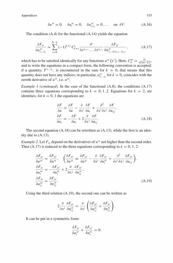
Appendices 535
δuκ = 0, δuκ
i = 0, δuκ
i1i2= 0, . . . on �V . (A.16)
The condition (A.4) for the functional (A.14) yields the equation
�Fκ
�uκ′
i1...ik
=N−k∑s=0
(−1)k+s Csk+s
�s
�xik+1 . . . �xik+s
�Fκ′
�uκ
i1...ik ik+1...ik+s
, (A.17)
which has to be satisfied identically for any functions uκ
(xi). Here, Cm
k = k!m!(m−k)! ,
and to write the equations in a compact form, the following convention is accepted:if a quantity, T i1...ik , is encountered in the sum for k = 0, that means that thisquantity does not have any indices; in particular, uκ
i1...ikfor k = 0, coincides with the
zeroth derivative of uκ , i.e. uκ .
Example 1 (continued). In the case of the functional (A.8), the conditions (A.17)contains three equations corresponding to k = 0, 1, 2. Equations for k = 2, areidentities; for k = 0, 1 the equations are
�F
�u= �F
�u− �
�xi
�F
�ui+ �2
�xi �x j
�F
�ui j,
�F
�ui= − �F
�ui+ 2
�
�x j
�F
�ui j. (A.18)
The second equation (A.18) can be rewritten as (A.13), while the first is an iden-tity due to (A.13).
Example 2. Let Fκ depend on the derivatives of uκ not higher than the second order.Then (A.17) is reduced to the three equations corresponding to k = 0, 1, 2:
�Fκ
�uκ′ =
δFκ′
δuκ
,
(δFκ
′
δuκ
≡ �Fκ′
�uκ
− �
�xi
�Fκ′
�uκ
i
+ �2
�xi �x j
�Fκ′
�ui j
),
�Fκ
�uκ′
i
= −�Fκ′
�uκ
i
+ 2�
�x j
�Fκ′
�uκ
i j
,
�Fκ
�uκ′
i j
= �Fκ′
�uκ
i j
. (A.19)
Using the third relation (A.19), the second one can be written as
2�
�xi
�Fκ′
�uκ
i j
= �
�xi
(�Fκ
′
�uκ
i j
+ �Fκ′
�uκ
i j
).
It can be put in a symmetric form:
δFκ
δuκ′
i
+ δFκ′
δuκ
i
= 0.

536 Appendices
Here we used the notation for the variational derivative,
δF
δui= �F
�ui− �
�xi
�F
�ui j.
Similarly transforming the first equation (A.19), we get the following holonomic-ity conditions:
�Fκ
�uκ′
i
− �Fκ′
�uκ
i
= 1
2
�
�xi
(δFκ
δuκ′
i
− δFκ′
δuκ
i
),
δFκ
δuκ′
i
+ δFκ′
δuκ
i
= 0,
�Fκ
�uκ′
i j
− �Fκ′
�uκ
i j
= 0. (A.20)
Note that the general holonomicity conditions (A.17) can be written more com-pactly by means of the following construction. Consider uκ as functions of n + 1variables, xi (i = 1, . . . , n) and an auxiliary variable, τ
(uκ
(xi) ≡ uκ
(xi , τ
)for
τ = 0). Let us introduce the “Lagrangian”:
L = Fκ
(xi , uκ, uκ
i , . . .) �uκ
�τ.
Then (A.17) are equivalent to
δL
δuκ
= 0, (A.21)
where the variational derivative is taken with respect to the functions uκ
(xi , τ
), and
then τ is set equal to zero.
The potential. If the conditions for the functional δ� to be holonomic are satisfied,then the “potential,” I (u) , can be found from by the equation
I (u) =u∫
u0
δ�,
where the integral is taken over some path in the functional space connecting afixed element, u0, with the current element, u. Usually, the potential of holonomicfunctionals is easy to guess. The holonomicity condition is useful in cases when theexistence of the potential is not obvious.
Expanding the functional space. Some functionals can be made holonomic byexpanding the set of functions on which they are considered. A number of examples

Appendices 537
of this kind will be given in the next appendix. Here we consider one commonindication for such a possibility.
Let two continua occupy regions V1 and V2, respectively. These two regions havea common piece of boundary, �.
The variational equation for the first continuum has the form
δ (I1)+ δA1 = 0.
We need to decide whether this variational equation is holonomic. Let the varia-tional equation for the second continuum and for the system “continuum 1 + con-tinuum 2” be
δ (I2)+ δA2 = 0, δ (I1 + I2)+ δA12 = 0.
The functional, δA12, describes the action of the surrounding on the system “con-tinuum 1 + continuum 2.” From these variational equations,
δA12 = δA1 + δA2.
If the functional, δA12, is holonomic, then the variational equation for the first con-tinuum is also holonomic, since
δA1 = δA12 + δ (I2) .
The holonomicity is achieved by expanding the set of field variables by includingin this set the field variables of the second continuum.
The variational equation for the first continuum is holonomic, in particular, forδA12 = 0. This is true, for example, in the case of an isolated system “continuum1 + continuum 2,” or in the case when the boundary of the second continuum isclamped.
Example 3. Consider an elastic body which has a common piece of boundary, �,
with a rigid body, T . We assume that the elastic body is “glued” to T along �. Therest of the boundary of the elastic body could be subjected to external surface force.
The virtual work of forces, acting from the rigid body on the elastic body,
δA =t∫
t0
∫
�
f iδxi dσdt, (A.22)
can be expressed in terms of work on the infinitesimally small displacements androtations of the rigid body, δr i and δϕi (see (3.47)):

538 Appendices
δA =t∫
t0
(Fiδr i + Miδϕ
i)dt (A.23)
where Fi and Mi are the total resultant and total moments of forces acting on theelastic body:
Fi =∫
�
fi dσ, Mi = εi jk
∫
�
f j(xk − rk (t)
)dσ.
If Fi and Mi are some prescribed functions of parameters, r i (t) and αia (t) ,
defining the motion of the rigid body, δA is, in general, non-holonomic. However,if the rigid body does not experience other external actions than those from theelastic body, then δA is holonomic on the expanded set of variables, including thefunctions, r i (t) and αi
a (t), because the following variational equation holds:
δ
t1∫
t0
KT dt −t∫
t0
(Fiδr i + Miδϕ
i)dt = 0,
where KT is the kinetic energy of the rigid body, a known function of dr i/dt, αia
and dαia/dt . The potential of δA is the action of the rigid body.
This is an example of the expansion of the functional space suggested by aphysical reasoning. Using “non-physical” expansions, one can put any system ofequations in the form of Euler equations of some functional. An example of thatwas given in Sect. 1.8.
B. On Variational Formulation of Arbitrary Systemsof Equations
Consider a system of equations and boundary conditions,
Fκ
(xi ,
�uκ
�xi,
�2uκ
�xi �x j, . . .
)= 0 in V,
fκ
(xi ,
�uκ
�xi, . . .
)= 0 on �V . (B.1)
We are going to discuss the following question: in which cases this system ofequations is Euler system of equations for some functional?
There is a certain difficulty in getting the answer caused by the possibility oftransforming the system of equations by, e.g., multiplication on some functions ofxi , uκ , �uκ/�xi , or by substitution of the required functions. As a result, the systemmay lose (or acquire) the property of being Euler system of equations.

Appendices 539
Example. Consider on the segment [0, a] the boundary value problem
F ≡ p (x)d2u
dx2+ q (x)
du
dx+ r (x) u + f (x) = 0, (B.2)
u (0) = u (a) = 0. (B.3)
We form the functional
δ� =a∫
0
Fδudx . (B.4)
If this functional is holonomic on the set of functions selected by the conditions(B.3), then (B.2) are the Euler equations.
From the holonomicity conditions (A.13) for the functional (B.4), we have
q (x)− d
dxp (x) = 0. (B.5)
If the functions, p (x) and q (x) , do not satisfy (B.5), then the functional (B.4) isnot holonomic and (B.2) cannot be the Euler equation for a functional of the form
a∫
0
L
(x, u,
du
dx
)dx .
Let us show that (B.2) can be transformed in such a way, that it becomes a Eulerequation. Let us make the substitution u → v:
u (x) = b (x) v (x) .
The equation takes the form
pd2
dx2bv + q
d
dxbv + rbv + f = 0. (B.6)
Now we choose b (x) in such a way that (B.6) satisfy the criterion (A.13). Thenb (x) must satisfy the equation
d
dx[b (x) p (x)] = 2
db (x)
dxp (x)+ q (x) b (x) .
This equation has the following solution:
b (x) = cp (x) e−
x∫0
q(x)dxp(x)
, c = const. (B.7)
For definiteness, we set c = 1.

540 Appendices
The equations and boundary conditions for the function v (x) become
G ≡ d
dx(b (x) p (x))+ rv (x)+ f (x) = 0, r ≡ rb + p
d2b
dx2+ q
db
dx, (B.8)
v (0) = v (a) = 0. (B.9)
The functional
a∫
0
Gδvdx
is holonomic on the set of functions satisfying (B.9). It is easy to guess the functionalfor which (B.8) is the Euler equation:
a∫
0
(b (x) p (x)
(dv
dx
)2
−rv2 − 2 f (x) v
)dx . (B.10)
The holonomicity was achieved by a change of the required function.It could also be obtained by multiplying (B.2) by 1/b (x) where b (x) is the func-
tion (B.7). Then, (B.2) becomes
d
dx
(p
b
du
dx
)+ r
bu + f = 0.
It is the Euler equation for the functional
a∫
0
[p
b
(du
dx
)2
− r
bu2 − 2 f u
]dx . (B.11)
The functional (B.11) becomes the functional (B.10) after the substitutionu → v: u = bv.
Another complication is related to a hardly formalized requirement that the vari-ational principle sought has some physical meaning. Without such a requirement, itis easy to construct various “non-physical” variational principles, which are of littleor no interest. For example: the solution of (B.1) minimizes the functional
∫
V
Fκ Fκdv +∫
�V
fκ f κd A.

Appendices 541
There are no sensible answers to the posed question. However, the search forthese answers lead to the formulation of a number of nontrivial “non-physical” vari-ational principles.
Morse-Feshbach principle. Consider the Cauchy problem for the heat conductiv-ity equations
ut = k�u + f, (B.12)
u|�V = 0, u|t=0 = 0. (B.13)
in a four-dimensional region V × [0, T ].It is easy to obtain from (A.17) that there are no functionals of the form
T∫
0
∫
V
L
(xi , t,
�u
�t,
�u
�xi
)dVdt
for which (B.12) would be the Euler equation.Let us introduce the adjoint boundary value problem
−vt = k�v + g, (B.14)
v|�V = 0, v|t=T = 0. (B.15)
and consider (B.12), (B.13), (B.14) and (B.15) as a system of equations for twofunctions, u and v.
Then, (B.12) and (B.13) are the Euler equations for the functional
T∫
0
∫
V
(utv + ku,iv
,i − f v − gu)
dVdt (B.16)
with the constraints (B.13) and (B.15).
Generalization. Let u, v be elements of some Hilbert space, H , (u, v) the scalarproduct in H , L – the linear operator acting from H to H , L∗ – the conjugateoperator, i.e. the operator which is defined by the equality
(Lu, v) = (u, L∗v
)
which holds for any u and v.Then the equations
Lu = f, L∗v = g (B.17)
are the stationary points of the functional
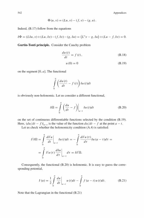
542 Appendices
� (u, v) = (Lu, v)− ( f, v)− (g, u) .
Indeed, (B.17) follow from the equations
δ� = (Lδu, v)+ (Lu, δv)− ( f, δv)− (g, δu) = (L∗v − g, δu
)+ (Lu − f, δv) = 0.
Gurtin-Tonti principle. Consider the Cauchy problem
du (t)
dt= f (t) , (B.18)
u (0) = 0 (B.19)
on the segment [0, a]. The functional
a∫
0
(du (t)
dt− f (t)
)δu (t)dt
is obviously non-holonomic. Let us consider a different functional,
δ� =a∫
0
(du
dt− f
)∣∣∣∣a−t
δu (t)dt (B.20)
on the set of continuous differentiable functions selected by the condition (B.19).Here, (du/dt − f )|a−t is the value of the function du/dt − f at the point a − t .
Let us check whether the holonomicity condition (A.4) is satisfied:
δ′δ� =a∫
0
dδ′udt
∣∣∣∣a−t
δu (t)dt = −a∫
0
dδ′u (τ )
dτδu (a − τ )dτ =
=a∫
0
δ′u (τ )dδu
dτ
∣∣∣∣a−τ
dτ = δδ′�.
Consequently, the functional (B.20) is holonomic. It is easy to guess the corre-sponding potential,
I (u) = 1
2
a∫
0
du
dt
∣∣∣∣a−t
u (t)dt −a∫
0
f (a − t) u (t)dt. (B.21)
Note that the Lagrangian in the functional (B.21)
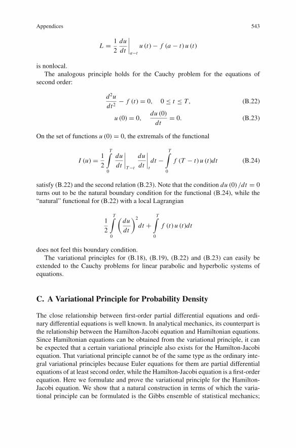
Appendices 543
L = 1
2
du
dt
∣∣∣∣a−t
u (t)− f (a − t) u (t)
is nonlocal.The analogous principle holds for the Cauchy problem for the equations of
second order:
d2u
dt2− f (t) = 0, 0 ≤ t ≤ T, (B.22)
u (0) = 0,du (0)
dt= 0. (B.23)
On the set of functions u (0) = 0, the extremals of the functional
I (u) = 1
2
T∫
0
du
dt
∣∣∣∣T−t
du
dt
∣∣∣∣t
dt −T∫
0
f (T − t) u (t)dt (B.24)
satisfy (B.22) and the second relation (B.23). Note that the condition du (0) /dt = 0turns out to be the natural boundary condition for the functional (B.24), while the“natural” functional for (B.22) with a local Lagrangian
1
2
T∫
0
(du
dt
)2
dt +T∫
0
f (t) u (t)dt
does not feel this boundary condition.The variational principles for (B.18), (B.19), (B.22) and (B.23) can easily be
extended to the Cauchy problems for linear parabolic and hyperbolic systems ofequations.
C. A Variational Principle for Probability Density
The close relationship between first-order partial differential equations and ordi-nary differential equations is well known. In analytical mechanics, its counterpart isthe relationship between the Hamilton-Jacobi equation and Hamiltonian equations.Since Hamiltonian equations can be obtained from the variational principle, it canbe expected that a certain variational principle also exists for the Hamilton-Jacobiequation. That variational principle cannot be of the same type as the ordinary inte-gral variational principles because Euler equations for them are partial differentialequations of at least second order, while the Hamilton-Jacobi equation is a first-orderequation. Here we formulate and prove the variational principle for the Hamilton-Jacobi equation. We show that a natural construction in terms of which the varia-tional principle can be formulated is the Gibbs ensemble of statistical mechanics;

544 Appendices
the varied functional is the mathematical expectation of the action of analytical me-chanics, while the Hamilton-Jacobi equation is the Euler equation corresponding tovarying the probability density function.
Consider a mechanical system with generalized coordinates q1, q2, . . . , qn, mo-menta p1, . . . , pn, and the Hamiltonian H (p, q, t), p = {p1, . . . , pn}, q ={q1, . . . , qn
}. Let us take an ensemble of such systems with the probability density
function f (p, q, t). In this ensemble the velocities, p, q, of the points representingthe system in the phase space, R, can be viewed as functions of p, q, t . The functionf (p, q, t) then satisfies the continuity equation
� f
�t+ �
(q i f
)
�qi+ � ( pi f )
�pi= 0. (C.1)
All indices run through the values 1, . . . , n.We introduce some “Lagrangian coordinates” of the system’s trajectories – the
functions πa (p, q, t) (a = 1, . . . , n) which are conserved along the trajectories:
�πa
�t+ q i �πa
�qi+ pi
�πa
�pi= 0. (C.2)
Consider the functional
I =t1∫
t0
∫
R
[pi q
i (p, q, t)− H (p, q, t)]
f (p, q, t) dpdqdt −∫
R
ϕ (q, π ) f (p, q, t1) dpdq.
(C.3)
Here ϕ (q, π ) is considered to be a given function of the arguments qi and πa andf (p, q, t) for each t is assumed to be decaying in R at infinity with a rate sufficientfor the convergence of the integrals.
The first term in (C.3) has the meaning of the mathematical expectation of theaction functional of analytical mechanics; the second term, as will be seen, is relatedto the momentum flux at t = t1.
Consider the stationary points of the functional (C.3) on a set of the functionsf (p, q, t), pi (p, q, t), q i (p, q, t), and πa (p, q, t), subject to constraints (C.1),(C.2), and the initial conditions
f = ψ (q, π )
∣∣∣∣�π
�p
∣∣∣∣ for t = t0, (C.4)
where ψ (q, π ) is a given function, and |�π/�p| is the determinant of the matrix‖�πa/�pi‖.Variational principle. At the stationary points of functional (C.3), the functions pi ,
qi satisfy Hamiltonian equations; the Lagrange multiplier for the constraint (C.1)satisfies the Hamilton-Jacobi equation.

Appendices 545
Indeed, let us write down Euler equations of functional (C.3). Denote by α andθa f the Lagrange multipliers for the constraints (C.1) and (C.2). Euler equations arethen found by varying the functional
t1∫
t0
∫
R
[(
pi qi − H
)f + α
(� f
�t+ �
(q i f
)
�qi+ � ( pi f )
�pi
)
+ θa f
(�πa
�t+ q i �πa
�qi+ pi
�πa
�pi
)]dpdqdt −
∫
R
ϕ (q, π ) f (p, q, t1) dpdq.
In R we obtain the following equations: by variation of q i (p, q, t),
�α
�qi+ θa �πa
�qi= pi , (C.5)
by variation of pi (p, q, t) ,
�α
�pi− θa �πa
�pi= 0, (C.6)
by variation of f (p, q, t) ,
pi qi − H − �α
�t− q i �α
�qi− pi
�α
�pi+ θa
(�πa
�t+ q i �πa
�qi+ pi
�πa
�pi
)= 0, (C.7)
by variation of πa (p, q, t) ,
� (θa f )
�t+ �
(θaqi f
)
�qi+ � (θa pi f )
�pi= 0. (C.8)
The variation of α and θa yields (C.1) and (C.2). The equations hold in a regionof space R where f > 0.
By virtue of the arbitrariness of the variations δ f and δπa at t = t1, we obtain theadditional relations
α = ϕ (q, π ) at t = t1, (C.9)
θa − �ϕ
�πa= 0 at t = t1. (C.10)
Variations at t = t0 yield the equality
∫
R
(αδ f + θa f δπa
)∣∣t=t0
dpdq = 0. (C.11)

546 Appendices
It will be shown further that equality (C.11) is fulfilled automatically by virtue of(C.4) and (C.6).
We now proceed to the analysis of (C.5)–(C.10). Equation (C.7) can be re-writtenby using (C.5) and (C.6) in a simpler form:
�α
�t− θa �πa
�t+ H (p, q, t) = 0. (C.12)
Suppose that functions π (p, q, t) at each q, t determine a one-to-one mapping p↔π so that p can be considered as functions of t , q, π : p = p (π, q, t) and
|�π/�p| �= 0. (C.13)
Then all the functions of p, q, and t can also be considered as functions of π , qand t . In particular, α = α (π, q, t). Equations (C.5) and (C.6) in terms of α (π, q, t)take a simpler form:
�iα = pi , (C.14)
�aα = θa . (C.15)
By �iα and �aα we denoted the partial derivatives of α with respect to qi and πa , atconstant π , t and q, t , respectively. Equations (C.14) and (C.15) define a canonicaltransformation of p, q → π , θ (see [4]).
By virtue of (C.14) and (C.15), (C.12) can be rewritten as a Hamilton-Jacobiequation for the function α (π, q, t) :
�tα + H(�iα, qi , t
) = 0. (C.16)
Here �tα is the time derivative of α at constant π, q.Equation (C.16) together with the initial condition (C.9) form the Cauchy prob-
lem for the function α.Note that the assumption (C.13) is satisfied if the determinant of the matrix∥∥�2ϕ/�qi �πa
∥∥ is nonzero and t1 − t0 is sufficiently small. Indeed, for small t1 − t0and smooth ϕ and H , one can guarantee the unique existence of a smooth solutionto the Cauchy problem (C.16) and (C.9) (see §47 in [4]). By virtue of (C.14), thedeterminant of the matrix ‖�pi/�πa‖ coincides with the determinant of the matrix∥∥�2α/�qi �πa
∥∥ ; due to (C.9), at t = t1 it coincides with the determinant of thematrix
∥∥�2ϕ/�qi �πa
∥∥. By continuity, it will be nonzero over a sufficiently smalltime interval.
Let us show now that at a stationary point the Hamiltonian equations hold:
pi = −�H
�qi, q i = −�H
�pi. (C.17)

Appendices 547
We will need the auxiliary equations
�θa
�qi
�πa
�q j− �θa
�q j
�πa
�qi= 0,
�θa
�pi
�πa
�p j− �θa
�p j
�πa
�pi= 0,
�θa
�p j
�πa
�qi− �θa
�qi
�πa
�p j= δ
ji . (C.18)
These equations can be obtained by differentiating (C.5) and (C.6) with respect topi , qi :
�2α
�qi �q j+ �θa
�q j
�πa
�qi+ θa �2πa
�qi �q j= 0,
�2α
�qi �p j+ �θa
�p j
�πa
�qi+ θa �2πa
�p j �qi= δ
ji ,
�2α
�qi �p j− �θa
�qi
�πa
�p j− θa �2πa
�qi �p j= 0,
�2α
�pi �p j− �θa
�pi
�πa
�p j− θa �2πa
�pi �p j= 0.
In the first equation we eliminate α and πa by alternating over i , j . That gives thefirst equation (C.18). Similarly, from the last equation we obtain the second equation(C.18). Subtraction of the second and the third equations yields the third equation(C.18).
Let us differentiate (C.12) with respect to p and q. Making use of (C.6) and (C.7)we have
�πa
�qi
�θa
�t− �θa
�qi
�πa
�t= −�H
�qi,
�πa
�pi
�θa
�t− �θa
�pi
�πa
�t= −�H
�pi.
Substituting here �πa/�t in terms of p, q from (C.2) and �θa/�t from the equation
�θa
�t+ q i �θa
�qi+ pi
�θa
�pi= 0
which follows from (C.8) and (C.1), and making use of (C.18), we obtain the Hamil-tonian equations (C.17).
Equation (C.1), by virtue of Hamiltonian equations (C.17), is transformed intothe Liouville equation
� f
�t+ �H
�pi
� f
�qi− �H
�qi
� f
�pi= 0.

548 Appendices
The system of equations obtained can be solved as follows. First we solve theCauchy problem (C.16) and (C.9). From its solution α (π, q, t), we find from (C.14)the functions πa (π, q, t). The values of these functions are substituted into the initialdata (C.4), and the initial value f (p, q, t0) of the function f is found. The Cauchyproblem is then solved for Liouville equation (C.1) and (C.16). The functions θa arereconstructed from α (π, q, t) using (C.15).
If ϕ = qiπi , then “the Lagrangian coordinates” πa , by virtue of (C.14) have themeaning of momenta at the final time point t = t1, and ψ (q, π ) have the meaningof the density of the simultaneous distribution of the initial coordinates and the finalmomenta.
Equation (C.10) is satisfied as an identity due to (C.15) and (C.9). We will showthat (C.11) is also satisfied as an identity.
Let us find the variation of the function f at t = t0. To this end we need theequality
δ
∣∣∣∣�π
�p
∣∣∣∣ =∣∣∣∣�π
�p
∣∣∣∣�δπa
�πa, (C.19)
which is obtained in the same way as (4.19).According to the initial condition (C.4) and formula (C.19), we have for the vari-
ation of the function f ,
δ f = �ψ
�πaδπa
∣∣∣∣�π
�p
∣∣∣∣+ ψ
∣∣∣∣�π
�p
∣∣∣∣�δπa
�πa=∣∣∣∣�π
�p
∣∣∣∣� (ψδπa)
�πa.
Therefore
∫
R
αδ f dpdq =∫
R
α
∣∣∣∣�π
�p
∣∣∣∣� (ψδπa)
�πadpdq =
=∫
R
α� (ψδπa)
�πadπdq = −
∫
R
ψ�aαδπadπdq = −∫
R
f �aαδπadpdq. (C.20)
From equality (C.20) it follows that relation (C.11) is satisfied identically by virtueof (C.15). This completes the proof of the variational principle stated.
Note that the constraint (C.2) could be replaced by the constraint
� (πa f )
�t+ � (πaqi f )
�qi+ � (πa pi f )
�pi= 0,
in which case the Lagrange multiplier for constraint (C.1) would have the meaningof Legendre transformation of the function α (π, q, t) with respect to πa, and wouldbe a function of θ , q, t .
If the function ψ (q, π ) is chosen as the δ-function, then the variational principlebecomes the Hamilton principle for a mechanical system with given coordinates q

Appendices 549
at t = t0. The values of momenta at t = t1 are obtained as the natural boundarycondition. One can modify the variational principle for the case when the positionsof the particles at t = t0 and t = t1 are given. Then, instead of n “Lagrangiancoordinates” πa , 2n Lagrangian coordinates should be introduced, half of whichtake the given values at t = t0 and the other half at t = t1.
D. Lagrange Variational Principle
To derive (1.40) we have first to find the variation of the action functional. To thisend, it is convenient to get rid of the constraint (1.36) by means of a Lagrangemultiplier. We consider an auxiliary variational problem which contains an extraunknown function, λ (t), and has a modified action functional,
I =t1∫
t0
(K+λ (t) (K+U−E))dt. (D.1)
We denote the integrand by L :
L (q, q, λ) ≡K+λ (t) (K+U−E).
Note that this function is not necessarily equal to K−U.
At the stationary trajectory the variation of functional I must vanish for all ad-missible variations δq, δt1 and δλ.
We will work with a more general functional,
I (q (t) , t1) =t1∫
t0
L (q, q, t)dt, (D.2)
not assuming that L =K+λ (K+U−E). The difference from the Hamilton varia-tional principle is that the upper limit of the integral is also varied.
Let us give infinitesimally small variation to the trajectory and the arrival time,
q ′ (t) = q (t)+ δq (t) , t ′1 = t1 + δt1,
and consider the difference,
I(q ′ (t) , t ′1
)− I (q (t) , t1) =t ′1∫
t0
L
(q + δq,
d (q + δq)
dt, t
)dt−
t1∫
t0
L
(q,
dq
dt, t
)dt.
(D.3)

550 Appendices
To obtain δ I we have to keep only the terms of the first order in (D.3). Note thatthe domain of integration of the first integral in (D.3) differs from that of the secondintegral. To perform the calculation it is convenient to write down the first integralin (D.3) as an integral over the segment [t0, t1]. Therefore, we consider a mappingof [t0, t1] onto
[t0, t ′1
]:
t ′ = t ′ (t) = t + δt.
Here δt is an infinitesimally small smooth function of time which is zero at t = t0and equal to δt1 at t = t1. Thus,
I(q ′ (t) , t ′1
) =t ′1∫
t0
L
(q(t ′)+ δq
(t ′),
d(q(t ′)+ δq
(t ′))
dt ′,t ′)
dt ′ (D.4)
=t1∫
t0
L
(q(t ′ (t)
)+ δq(t ′ (t)
),
d(q(t ′ (t)
)+ δq(t ′ (t)
))
dt ′,t ′ (t)
)dt ′
dtdt.
Let us introduce the total variation of q (t), δq, as the difference of the valuesof the function, q ′ = q + δq, at the shifted point, t ′ (t), and the function, q, at thepoint t :
δq = q ′(t ′ (t)
)− q (t) .
Obviously, up to the terms of higher order,
δq = q ′ (t + δt)− q (t) = δq + dq
dtδt.
The operator δ commutes with the operatord
dt,
δdq
dt= dq ′
dt− dq
dt= d (q + δq)
dt− dq
dt= d
dtδq. (D.5)
The operator δ does not possess such a property: δd
dtand
d
dtδ are different and
linked by the relation
δdq
dt= d
dtδq − dq
dt
dδt
dt. (D.6)
This relation follows from a chain of equalities:

Appendices 551
δdq
dt= dq ′
(t ′)
dt ′
∣∣∣∣∣t ′=t ′(t)
− dq (t)
dt
= d(q + δq
)
dt
dt
dt ′− dq
dt=(
dq
dt+d δq
dt
)(1+ dδt
dt
)−1
− dq
dt
=(
dq
dt+ d δq
dt
)(1− dδt
dt
)− dq
dt= d δq
dt− dq
dt
dδt
dt.
Let us show that the variation of the functional I is
δ I =t1∫
t0
[δL
δqiδqi − δL
δqiqiδt + d
dt
(�L
�q iδqi − Hδt
)]dt (D.7)
where the function H is defined as
H = �L
�q iq i − L . (D.8)
Indeed, expanding the integrand in (D.4), we have
I(q ′ (t) , t ′1
) =t1∫
t0
L
(q (t)+ δq,
dq
dt+ δ
dq
dt, t + δt
)(1+ dδt
dt
)dt
=t1∫
t0
[L
(q,
dq
dt, t
)+ �L
�qiδqi + �L
�q iδ
dqi
dt+ �L
�tδt
](1+ dδt
dt
)dt
= I (q (t) , t1)+t1∫
t0
[�L
�qiδqi + �L
�q i
(d δqi
dt− q i dδt
dt
)+ �L
�tδt + L
dδt
dt
]dt.
Integrating the second term in the integrand by parts, we find
δ I =t1∫
t0
[δL
δqiδqi+ d
dt
(�L
�q iδqi
)+�L
�tδt − H
dδt
dt
]dt. (D.9)
It may be checked by inspection that there is an identity,
d H
dt≡ − δL
δqiqi − �L
�t, (D.10)

552 Appendices
where�L
�tis the partial derivative of L (q, q, t) with respect to t (with q and q held
fixed) andd
dtis the derivative which takes into account the change of all arguments
with time. Substituting�L
�tfound from (D.10) into (D.9), we obtain (D.7).
After moving the terms with time derivative to the boundary, (D.7) takes the form
δ I =t1∫
t0
[δL
δqiδqi − δL
δqiqiδt
]dt +
[�L
�q iδqi − Hδt
]t1
t0
. (D.11)
The admissible variations δq must be zero at the ends of the integration domain,
δq = 0 at t = t0, t1, (D.12)
because q (t) are prescribed at the ends: both q (t) and q (t) + δq (t) must be equalto q0 and q1 at t = t0 and t = t1, respectively. Actually, the possibility of writingthe constraints for variations in such a simple form is the major motivation for usingthe variation δq instead of the variation δq. For zero δq at the ends, the third termin (D.11) vanishes.
Variation δt must be zero at t = t0. At all other points of the segment [t0, t1] thevariation δt is arbitrary.
Let us first take δt ≡ 0. Then, from the equality δ I = 0, the expression forδ I (D.7) and the main lemma of calculus of variations, we obtain the system ofequations
δL
δqi= 0. (D.13)
Now allow δt to be non-zero. The first two terms of (D.11) are zero due to (D.13).Therefore, the equation, δ I = 0, yields the condition
H = 0 for t = t1. (D.14)
The equations obtained are valid for an arbitrary (smooth) function L . Let usreturn now to the Lagrange function of the Lagrange variational principle,
L = K + λ (t) (K+U−E) . (D.15)
We have a closed system of equations for n+ 1 functions qi (t) , λ (t) comprisingthe energy equation (1.36), (D.13) and the boundary conditions (1.37) and (D.14).Let us show that the function λ (t) can be found explicitly. From (D.15), and thedefinition of H (D.8),

Appendices 553
H = �K
�q i (1+ λ) q i − K − λ (K +U − E) .
Using the homogeneity of kinetic energy, (1.33), and the energy equation (1.36),we see that
H = (1+ 2λ) K .
According to (D.13) and the identity (D.10),
d H
dt= −�L
�t.
The explicit dependence of L on time is due only to the the dependence of L onλ, and therefore
�L
�t= �L
�λ
dλ
dt= (K+U−E)
dλ
dt.
Therefore, in addition, d H/dt = 0, and H = (1+ 2λ) K = const. The bound-ary condition (D.14) shows that this constant is equal to zero. Since K �= 0, wehave 1+2λ = const. So, function λ (t) is constant and is equal to− 1
2 . For λ = − 12 ,
function L , up to a constant, is half of the difference of the kinetic and the potentialenergy,
L = 1
2(K−U )+ 1
2E . (D.16)
For the function L (D.16), (D.13) are equivalent to Lagrange equations (1.40).Apparently, the factor 1
2 and the additive constant 12 E are not essential in writ-
ing down the dynamical equations, and one can replace function L (D.16) by thefunction (1.41).
E. Microdynamics Yielding Classical Thermodynamics
As we have seen, the Hamiltonian structure of the equations of micro-mechanicsyields the laws of equilibrium thermodynamics. The question arises: How impor-tant it is that the equations of micro-mechanics are Hamiltonian? In other words:Could non-Hamiltonian equations of microdynamics yield the equations of classicalequilibrium thermodynamics? It turns out that the class of such equations is indeedslightly wider than the class of Hamiltonian equations.
To formulate the answer, it is convenient to introduce coordinates xμ(μ =1, . . . , 2n) in the phase space, x1 = p1, . . . , xn = pn, xn+1 = q1, . . . , x2n = qn
and write down the Hamiltonian equations (1.63) in the form

554 Appendices
xμ = ωμν �H (x)
�xν. (E.1)
where ωμν is a constant antisymmetric tensor:
ωμν =⎧⎨⎩
1 μ ≥ n + 1, ν = μ
−1 μ ≤ n, ν = n + μ
0 otherwise
Tensor ωμν has a non-zero determinant. Therefore, one can introduce an inversetensor, i.e. the tensor obeying the equations
�νμωμλ = δλν , (E.2)
with δλν being Kronecker’s tensor:
δλν =
{1 if λ = ν
0 if λ �= ν
Tensor �νμ is antisymmetric. Contracting (E.1) with �νμ and using (E.2) we obtainanother form of the Hamiltonian equations,
�νμ xμ = �H (x)
�xν. (E.3)
If one makes a general coordinate transformation then �νμ and ωμλ transform inaccordance with the tensor laws. If the Hamiltonian equations are written in arbitrarycoordinates, the tensors ωμν and �μν are certain functions of those coordinates.These functions are not arbitrary because there are special coordinates {p, q} forwhich (E.3) takes (locally) the form of the usual Hamiltonian equations (1.63). Itturns out [5] that the sufficient and necessary condition for the system (E.3) to beHamiltonian is
��νμ
�xλ+ ��λν
�xμ+ ��μλ
�xν= 0. (E.4)
Equations (E.4) are equivalent to the existence of functions Pμ(x) such that
�μν = �Pμ(x)
�xν− �Pν(x)
�xμ.
The coordinate system in which equations (E.3) takes the form (1.63) is the systemwhere the differential expression Pμ(x)dxμ takes the canonical form p1dq1+ . . .+pndqn . Some natural reasonings on the features of micromotion show that equa-tions of micromotion should have the from (E.1) with ωμν being functions of phase

Appendices 555
coordinates. These equations yield the laws of equilibrium thermodynamics if thetensor ωμν obeys the condition [50]
�
�xμ
(1√ω
ωμν
)= 0 (E.5)
where ω ≡ det ‖ωμν‖ . This condition is weaker than (E.4): one can show that (E.5)follows from (E.4) but not vice versa.

Bibliographic Comments
The diversity of topics considered makes it impossible to give a comprehensiveliterature review. The bibliographic comments given here are based on the paperswhich turned out to be in the view field of the author, and make no pretence atcompleteness.
Chapter 1
The history of variational principles can be learned from the collection of theoriginal papers [248]. It is considered also in the books by E. Mach [195], A.Mayer [207], F. Klein [149], C. Lanczos [170], and H. Goldstine [116]. There aremany excellent books to master in Hamiltonian mechanics; we mention just a few:Arnold [4], Arnold, Kozlov and Neistadt [6], Landau and Lifshits [171], and Licht-enberg and Liberman [182].
Chapter 2
There is a tremendous wealth of literature on thermodynamics. The key contri-butions to the “derivation of thermodynamics from mechanics” were made byBoltzmann, Gibbs, P. Hertz, Birkhoff, Khinchine and Kubo. The treatment of ther-modynamics in this chapter closely follows the author’s monograph [46], where ahistoric review and the references to the original papers can be found. A gener-alization of the Einstein formula for finite-dimensional Hamiltonian systems wasobtained in [43], the quasi-Hamiltonian structure of equations of macrophysics wassuggested in [44] and later justified in [50] where the notion of the secondary andthe higher order thermodynamics was also introduced. A proposition that entropy insecondary thermodynamics is decaying in isolated stable systems was made in [54].
Chapters 3 and 4
The contents of these chapters is standard. As an additional reading one can usethe text books by L.I. Sedov [268, 269], I.M. Gelfand and S.V. Fomin [110], A.J.McConnell [208], S.R. de Groot and P. Mazur [87] and a paper by L.I. Sedov [270].A key point used in the development of models with high derivatives, a proper
557

558 Bibliographic Comments
transformation of surface integrals, was made by Kirchhoff. It was applied in the1960s to the construction of refined elastic models by Mindlin [215].
Chapter 5
Additional readings: S.G. Mikhlin [209, 210, 211, 212], A.D. Ioffe and V.M.Tikhomirov [138], I. Ekeland and R. Temam [95], R. Rockafellar [256], L.C. Young[320], J.L. Synge [290], L.S. Pontrjagin [249], R.E. Bellman and R.E. Kalaba [20],and K.A. Lurie [190]. See regarding inequalities [18, 124, 138, 238, 240], dual vari-ational principles [7, 26, 81, 95, 131, 138, 232, 250, 274, 290] error estimates ofapproximate solutions [151, 209, 220, 221, 250, 280, 290], method of constraintunlocking [222], and Rayleigh-Ritz’s method [81, 117, 209, 210, 211, 253]. Thetreatment of the dual variational problems in the book follows [26]. The idea toeliminate differential constraints in the dual variational principle was suggested byHashin and Strikman in [126]. The treatment of this topic in the book is slightly dif-ferent from [126] and the studies that followed. The variational-asymptotic methodwas formulated in the author’s papers [28, 31]. It was further applied to variousproblems in [35, 37, 62, 68, 134, 173]. Nowadays, it is being actively developed theso-called �-convergence method (see [74, 75]), which is, in fact, a version of thevariational-asymptotic method. Some exact results in variational problems with asmall parameter were obtained by E.S. Levitin [178, 179, 180, 181]. A link betweenthe minimization and the integration in functional spaces was mentioned and usedin [48]. Its further applications can be found in [49, 52, 53, 56, 61, 65, 174]. In thebook we do not consider various modifications of the notion of convexity. Besides,the minimization of non-convex functionals has not been discussed.1 This can belearned from [12, 13, 14, 15, 16, 73, 74].
Chapter 6
There are many modifications of variational principles of linear elasticity the-ory. Our treatment is focused on three major statements: Gibbs principle, its dualversion – Castigliano principle, and the corresponding minimax principle –Reissner principle. These three assertions are enough for most applications. TheHashin-Strikman variational principle is used to obtain the bounds for effectivecharacteristics of micro-inhomogeneous bodies (see [126, 127, 318] and a review[214]). Regarding Korn’s inequality [153] see [105, 137, 162, 210, 217, 241, 279].
Chapter 7
Dual variational principle in geometrically nonlinear elasticity was discussed in[30, 90, 176, 189, 203, 225, 226, 227, 228, 235, 237, 287, 288, 289, 312, 313, 314,333, 334, 335, 336].
1 An exception is the dual variational principle in nonlinear elasticity considered in Chap. 7.
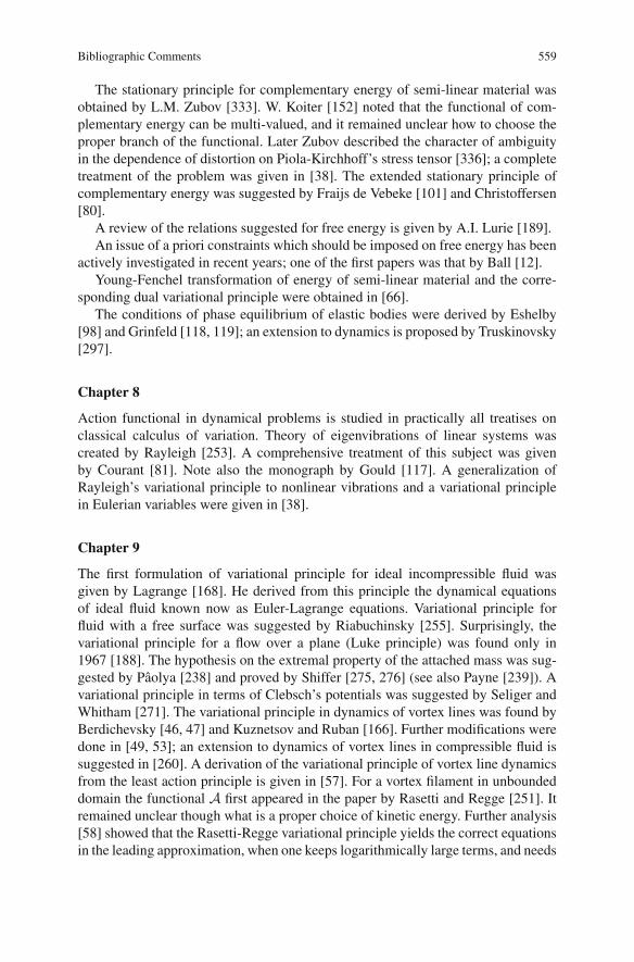
Bibliographic Comments 559
The stationary principle for complementary energy of semi-linear material wasobtained by L.M. Zubov [333]. W. Koiter [152] noted that the functional of com-plementary energy can be multi-valued, and it remained unclear how to choose theproper branch of the functional. Later Zubov described the character of ambiguityin the dependence of distortion on Piola-Kirchhoff’s stress tensor [336]; a completetreatment of the problem was given in [38]. The extended stationary principle ofcomplementary energy was suggested by Fraijs de Vebeke [101] and Christoffersen[80].
A review of the relations suggested for free energy is given by A.I. Lurie [189].An issue of a priori constraints which should be imposed on free energy has been
actively investigated in recent years; one of the first papers was that by Ball [12].Young-Fenchel transformation of energy of semi-linear material and the corre-
sponding dual variational principle were obtained in [66].The conditions of phase equilibrium of elastic bodies were derived by Eshelby
[98] and Grinfeld [118, 119]; an extension to dynamics is proposed by Truskinovsky[297].
Chapter 8
Action functional in dynamical problems is studied in practically all treatises onclassical calculus of variation. Theory of eigenvibrations of linear systems wascreated by Rayleigh [253]. A comprehensive treatment of this subject was givenby Courant [81]. Note also the monograph by Gould [117]. A generalization ofRayleigh’s variational principle to nonlinear vibrations and a variational principlein Eulerian variables were given in [38].
Chapter 9
The first formulation of variational principle for ideal incompressible fluid wasgiven by Lagrange [168]. He derived from this principle the dynamical equationsof ideal fluid known now as Euler-Lagrange equations. Variational principle forfluid with a free surface was suggested by Riabuchinsky [255]. Surprisingly, thevariational principle for a flow over a plane (Luke principle) was found only in1967 [188]. The hypothesis on the extremal property of the attached mass was sug-gested by Paolya [238] and proved by Shiffer [275, 276] (see also Payne [239]). Avariational principle in terms of Clebsch’s potentials was suggested by Seliger andWhitham [271]. The variational principle in dynamics of vortex lines was found byBerdichevsky [46, 47] and Kuznetsov and Ruban [166]. Further modifications weredone in [49, 53]; an extension to dynamics of vortex lines in compressible fluid issuggested in [260]. A derivation of the variational principle of vortex line dynamicsfrom the least action principle is given in [57]. For a vortex filament in unboundeddomain the functional A first appeared in the paper by Rasetti and Regge [251]. Itremained unclear though what is a proper choice of kinetic energy. Further analysis[58] showed that the Rasetti-Regge variational principle yields the correct equationsin the leading approximation, when one keeps logarithmically large terms, and needs

560 Bibliographic Comments
a correction, reproduced here, if the terms on the order of unity are also retained.Note that the Hamiltonian structure of the dynamical equations of a vortex filamentin unbounded region, when one keeps only logarithmically large terms, was firstestablished by Marsden and Weinstein [202] (see also a review in [5], Sect. 6.3B).The variational principle for open flows was formulated in [46]. Some exact resultson minimization of the action functional of ideal incompressible fluid were obtainedby Shnirelman [278].
Chapter 10
Variational principles in fluid mechanics were discussed in [76, 79, 88, 89, 91, 92,94, 97, 135, 139, 141, 165, 175, 184, 186, 194, 198, 226, 242, 272, 273, 283, 285,291, 292, 310, 311, 326, 327]. The Hamilton principle for ideal compressible fluid inLagrangian variables was studied by G. Zemplen [329]; he also obtained the discon-tinuity conditions. A detailed treatment is given in the monograph by L. Lichtenstein[183]. Variational principles in Eulerian coordinates when the field functions are La-grangian variables were constructed by Davydov [84], Mauersberger [204, 205, 206]and Rogula [258]. Herivel [128] noted that by varying velocity, density and entropyas functions of Eulerian coordinates subjected to continuity equation and the conser-vation of entropy in fluid particle, one obtains from the Hamilton principle the quasi-potential flows (vi = �iϕ + μ�i S). Lin variational principle was suggested in [185].Earlier, Davydov [84] noticed that instead of three constraints (10.31) one can useone constraint (10.39), thus obtaining the correct expression of velocity in terms ofClebsch’s potentials. However, since the set of admissible functions was not clearlyintroduced the necessity to set the constraint (10.31) or (10.39), as was mentioned in[271], seemed puzzling. The extension of the set of admissible functions describedin the text makes transparent the link between these two variational principles. Aswas mentioned by Moffat [218] (see also [76]), presentation of velocity in termsof Clebsch’s potentials, though possible locally, yields some integral constraints onvelocity.
Pressure as Lagrangian appears for the first time, perhaps, in Hargreave’s paper[125]; a detailed study was given by Bateman [17].
The variational principle for the functional (10.54) [38] generalizes for com-pressible case the Luke principle (an attempt of such generalization in [304] wasnot successful).
Derivation of discontinuity conditions from variational principles was consideredin [161, 165, 183, 186, 192, 193, 330, 331].
Chapter 11
Arnold’s variational principle was suggested in [3], its generalization to compressiblefluids in [120], other variational principles of Sect. 11.5 in [57], Giese variationalprinciple in [112], Giese-Kraiko variational principle in [112, 161], Lin-Rubinovvariational principle in [186], variational principles for potential compressible flowsin [17], and other variational principles of this chapter in [38].

Bibliographic Comments 561
Chapter 12
Regarding the principle of least dissipation see, e.g., Rayleigh [252]. A recent reviewof variational principles of ideal plasticity is given by Kamenjarzh [145]. The ideathat variations in variational principles are closely related to fluctuations in physicalsystems was suggested by Glansdorff and Prigogine [114], but they did not pursueit to obtain quantitative statements.
Chapter 13
Theory of motion of bodies in fluids was developed by Thompson and Tait [293]. Itis discussed in detail by Lamb [169] and Milne-Thomson [213], where many exam-ples of calculation of kinetic energy are given, and by Birkhoff [71]. Kirchhoff [148]found a number of exact solutions of equations of motion of rigid body in potentialflows. Generalizations to vortex flows are given in [243, 244, 303]. Section 13.3follows the paper [36]. An example with Basset force was prepared by S. Utkina.
Appendices
The proof of (A.4) in functional spaces can be found in monographs by Vainberg[298, 299]. Holonomicity condition (A.17) was obtained independently by Tonti[294] and the author [23]. Holonomicity condition (A.21) was suggested by B.Kupershmidt (see [197]). Holonomicity condition (A.20) was found in the case offunctions of one variable by Helmholtz. “Non-physical” variational principles areconsidered in [121, 122, 133, 196, 259, 295]. Appendix C follows paper [40].

Bibliography
1. H.G. Allen. Analysis and design of structural sandwich panels. Pergamon Press, New York,1969.
2. S.A. Ambartsumjan. General theory of anisotropic shells. Nauka, Moscow, 1974.3. V.I. Arnold. A variational principle for three-dimensional stationary flows of the ideal fluid.
Journal of Applied Mathematics and Mechanics (PMM), 29(5):846–851, 1965.4. V.I. Arnold. Mathematical methods of classical mechanics. Springer-Verlag, Berlin, 1989.5. V.I. Arnold and B.A. Khesin. Topological methods in hydrodynamics. Springer, New York,
1998.6. V.I. Arnold, V.V. Kozlov, and A.I. Neistadt. Mathematical aspects of classical and celestial
mechanics, volume 3 of Encycl. of Math. Sciences. Springer, 1988.7. A.M. Arthurs. Complementary variational principles. Clarendon Press, Oxford, 1980.8. I.B. Babuska. Solution of interface problems by homogenization. SIAM Journal of Mathe-
matical Analysis, 7:603–645, 1976.9. N.S. Bakhvalov. Average characteristics of bodies with periodic structure. Soviet Mathemat-
ics – Doklady, 218(5):1046–1048, 1974.10. N.S. Bakhvalov. Homogenization of partial differential operators with rapidly oscillating co-
efficients. Soviet Mathematics – Doklady, 16:351–355, 1975.11. N.S. Bakhvalov and G. Panasenko. Homogenisation: averaging processes in periodic media.
Kluwer-Academic Publishers Group, Norwell, MA/Dordrecht, 1989.12. J.M. Ball. Constitutive inequalities and existence theorems in nonlinear elastostatics. In
R.J. Knops, editor, Nonlinear analysis and mechanics, Heriot Watt Sympoisum, pp. 187–241.Pitman, London, 1977.
13. J.M. Ball. Convexity conditions and existence theorems in nonlinear elsticity. Archive forRational Mechanics and Analysis, 63:337–403, 1977.
14. J.M. Ball. Strict convexity, strong ellipticity, and regularity in the calculus of variations. Pro-ceedings of Cambridge Philosophical Society, 87:501–513, 1980.
15. J.M. Ball. Discontinuous equilibrium solutions and cavitation in nonlinear elasticity. Philo-sophical Transactions of Royal Society London, 306(ser. A):557–611, 1982.
16. J.M. Ball. The calculus of variations and material science. Quarterly of Applied Mathematics,56:719–740, 1998.
17. H. Bateman. Partial differential equations of mathematical physics. Cambridge Univ. Press,Cambridge, 1959.
18. E.F. Beckenbach and R.E. Bellman. Inequalities. Springer, Berlin, 1961.19. A.Yu. Beliaev. Homogenization in the problems of filtration theory. Nauka, Moscow, 2004.20. R.E. Bellman and R.E. Kalaba. Dynamic programming and modern control theory. Academic
Press, New York, 1965.21. A. Bensoussan, J.L. Lions, and G. Papanicolaou. Surquelques phenomenes asymptotiques
stationares. Comptes Rendus de l’Academie des Sciences Paris, 281:89–94, 1975.
563

564 Bibliography
22. A. Bensoussan, J.L. Lions, and G. Papanicolaou. Asymptotlc analysis for periodic structures.North Holland Publ., Amsterdam, 1978.
23. V.L. Berdichevsky. Variational equation of continuum mechanics. In Problems of SolidMechanics V. Novozhilov 60th birthday anniversary volume. Sudostroenie, Leningrad, 1970.
24. V.L. Berdichevsky. Equations describing transverse vibration of thin elastic plates. Mechan-ics of Solids, (6):138–141, 1972.
25. V.L. Berdichevsky. Dynamic theory of thin elastic plates. Mechanics of Solids, (6):86–96,1973.
26. V.L. Berdichevsky. A variational principle. Soviet Physics – Doklady, 19(4):188–190, 1974.27. V.L. Berdichevsky. Spatial averaging of periodic structures. Soviet Physics – Doklady,
20(5):334–335, 1975.28. V.L. Berdichevsky. Equations of the theory of anisotropic inhomogeneous rods. Soviet
Physics – Doklady, 21(5):286–288, 1976.29. V.L. Berdichevsky. High-frequency long-wave plate vibrations of plates. Physics Dokladi,
22(4):604–606, 1977.30. V.L. Berdichevsky. Variational-asymptotic method of constructing the nonlinear shell theory.
In G.K. Mikhailov W.T. Koiter, editor, Proceedings of IUTAM Symposium on Shell Theory,Tbilisi, pp. 137–161. North Holland Company, Amsterdam, 1979.
31. V.L. Berdichevsky. Variational-asymptotic method of constructing the shell theory. Journalof Applied Mathematics and Mechanics (PMM), 42(4):711–736, 1979.
32. V.L. Berdichevsky. Mechanical equations for fluids with particles. In Problems of averagingand development of continuum models, pp. 10–35. Moscow University Publishing, Moscow,1980.
33. V.L. Berdichevsky, V.A. Misiura. On interaction effect between extension and bending ofcylindrical shells. In Proceedings of XIII Conference on Plate and Shell Theory, pp. 165–171.Erevan, 1980.
34. V.L. Berdichevsky and K.C. Le. High-frequency long-wave shell vibrations. Journal of Ap-plied Mathematics and Mechanics. 44:737–744, 1980.
35. V.L. Berdichevsky. On the energy of an elastic beam. Journal of Applied Mathematics andMechanics (PMM), 45(4):518–529, 1981.
36. V.L. Berdichevsky. On the force acting on a body in viscous fluids. Journal of Applied Math-ematics and Mechanics (PMM), 45(4):628–631, 1981.
37. V.L. Berdichevsky. Variational principles in the problem of averaging random structures.Soviet Physics – Doklady, 26(11):1053–1055, 1981.
38. V.L. Berdichevsky. Variational principles of continuum mechanics. Nauka, Moscow, 1983.39. V.L. Berdichevsky. Heat conduction of checkerboard structures. Moscow University Mechan-
ics Bulletin, 40:15–25, 1985.40. V.L. Berdichevsky. On a variational principle of statistical mechanics. Moscow University
Mechanics Bulletin, 42:8–14, 1987.41. V.L. Berdichevsky. On turbulence theory. In L.I. Sedov 80th birthday anniversary volume,
pp. 106–110. Moscow University Publishing, Moscow, 1987.42. V.L. Berdichevsky. The problem of averaging random structures in terms of distribution func-
tions. Journal of Applied Mathematics and Mechanics (PMM), 51(6):704–710, 1987.43. V.L. Berdichevsky. A connection between thermodynamic entropy and probability. Journal
of Applied Mathematics and Mechanics (PMM), 52(6):947–957, 1988.44. V.L. Berdichevsky. Law of evolution to equilibrium in nonlinear thermodynamics. Interna-
tional Journal of Engineering Science, 28(7):697–704, 1990.45. V.L. Berdichevsky. Statistical mechanics of point vortices. Physical Review E, 51(5):4432–
4452, 1995.46. V.L. Berdichevsky. Thermodynamics of chaos and order. Addison Wesley Longman, 1997.47. V.L. Berdichevsky. Statistical mechanics of vortex lines. Physical Review E, 57(3):2885–
2905, 1998.48. V.L. Berdichevsky. Distribution of minimum values of weakly stochastic functionals. In
V.L. Berdichevsky, V.V. Jikov, and G. Papanicolaou, editors, Homogenization, pp. 141–186.World Scientific, Singapore, 1999.

Bibliography 565
49. V.L. Berdichevsky. On statistical mechanics of vortex lines. International Journal of Engi-neering Science, 40(123–129), 2002.
50. V.L. Berdichevsky. Structure of equations of macrophysics. Physical Review E,68(066126):26, 2003.
51. V.L. Berdichevsky. Distribution of functionals of solutions in some stochastic variationalproblems. Izvestia Vuzov, Yudovich anniversary volume, pp. 56–59, 2004.
52. V.L. Berdichevsky. Homogenization in micro-plasticity. Journal of Mechanics and Physicsof Solids, 53:2459–2469, 2005.
53. V.L. Berdichevsky. Averaged equations of ideal fluid turbulence. Continuum Mechanics andThermodynamics, 19:133–175, 2007.
54. V.L. Berdichevsky. On entropy of microstructure and secondary thermodynamics. InD. Jeulin and S. Forest, editors, Continuum Models and Discrete Systems, Proceeding ofCMDS, pp 25–29. Mines Paris, Paris Tech, 2008.
55. V.L. Berdichevsky. Distribution of minimum values of stochstic functionals. Networks andHeterogeneous Media, 3(3):437–460, 2008.
56. V.L. Berdichevsky. On statistical mechanics of vortex lines. In Proc. IUTAM Symposiumon Hamiltonian Dynamics, Vortex Structures and Turbulence, pp. 205–210. Springer-Verlag,Berlin, 2008.
57. V.L. Berdichevsky. On variational features of vortex flows. Continuum Mechanics and Ther-modynamics, 20:219–229, 2008.
58. V.L. Berdichevsky. A variational principle in dynamics of vortex filaments. Physical ReviewE, 78(3):036304, 2008.
59. V.L. Berdichevsky. An asymptotic theory of sandwich plates. International Journal of Engi-neering Science, 2009.
60. V.L. Berdichevsky. Nonlinear theory of hard-skin plates and shells. International Journal ofEngineering Science, 2009.
61. V.L. Berdichevsky. Entropy of microstructure. Journal of Mechanics and Physics of Solids,doi:10.1016/j.jmps.2007.07.004, 2007.
62. V.L. Berdichevsky, E. Armanios, and A. Badir. Theory of anisotropic thin-walled closed-cross-section beams. Composites Engineering, 2(5–7):411–432, 1992.
63. V.L. Berdichevsky, V.V. Jikov, and G. Papanicolaou, editors. Homogenization. World Scien-tific, Singapore, 1999.
64. V.L. Berdichevsky and S. Kvashnina. On equations describing the transverse vibrations ofelastic bars. Journal of Applied Mathematics and Mechanics (PMM), 40(1):104–118, 1976.
65. V.L. Berdichevsky and K.C. Le. A theory of charge nucleation in two dimensions. PhysicalReview E, 66:026129, 2002.
66. V.L. Berdichevsky and V. Misyura. On a dual variational principle in geometrically nonlinearelasticity theory. Journal of Applied Mathematics and Mechanics (PMM), 43(2):343–351,1979.
67. V.L. Berdichevsky and V. Misyura. Effect of accuracy loss in classical shell theory. Journalof Applied Mechanics, 59(2 Pt. 2):5217–5223, 1992.
68. V.L. Berdichevsky and V.G. Soutyrine. Problem of an equivalent rod in nonlinear theory ofsprings. Journal of Applied Mathematics and Mechanics (PMM), 47(2):197–205, 1983.
69. L.V. Berlyand. Asymptotic stress-strain distribution function for crystal with random pointdefects. In V.L. Berdichevsky, V.V. Jikov, and G. Papanicolaou, editors, Homogenization,pp. 179–192. World Scientific, Singapore, 1999.
70. A.S. Besicovitch. Almost periodic functions. Cambridge University Press, Cambridge, 1932.71. G. Birkhoff. Hydrodynamics: a study in logic, fact, and similitude. Princeton University
Press, Princeton, N.J., second edition, 1960.72. H. Bohr. Almost periodic functions. Chelsea Pub. Co., New York, 1947.73. A. Braides. Loss of polyconvexity by homogenization. Archive for Rational Mechanics and
Analysis, 127:183–190, 1994.74. A. Braides and A. Defranceschi. Homogenization of multiple integrals. Oxford University
Press, Oxford, 1998.75. A. Braides and L.M. Truskinovsky. Asymptotic expansions by Gamma-convergence. Con-
tinuum Mechanics and Thermodynamics, 20:21–62, 2008.

566 Bibliography
76. F.P. Bretherton. A note on Hamilton’s principle for perfect fluids. Journal of Fluid Mechan-ics, 44:19–31, 1970.
77. B. Budiansky and J.L. Sanders. On the “best” first order linear shell theory. In Progressin Applied Mechanics, The Prager anniversary volume, pp. 129–140. Macmillan Comp.,Norway, 1963.
78. L.J. Campbell and K. O’Neil. Statistics of two-dimensional point vortices and high-energyvortex states. Journal of Statistical Physics, 65:495–529, 1991.
79. P. Casal. Principles variationnels en fluide compressible et en magnetodynamique. Rev. Mec.Gren. Anyl., XI:40, 1965.
80. J. Christoffersen. On Zubov principle of stationary complementary energy in the non-lineartheory of elasticity. DCAMM Report, 44:31, 1973.
81. R. Courant and D. Hilbert. Methods of mathematical physics, volume I. Interscience Pub-lisher Inc., New York, 1953.
82. H. Cramer and M.R. Leadbetter. Stationary and related stochastic processes, volume I. JohnWiley & Sons Inc., New York, London, Sydney, 1967.
83. V.M. Darevsky. On basic relations in the theory of thin shells. Journal of Applied Mathemat-ics and Mechanics (PMM), 25(3):768–790, 1961.
84. B. Davydov. Variational principle and canonic equations for ideal fluid. Soviet Physics –Doklady, 69(1), 1949.
85. E. De Giorgi. Sulla convergenza di alcvune succesioni do integrali del tipo dell’ area. Rendi-conti Naturali, 6:277–294, 1975.
86. E. De Giorgi and S. Spagnolo. Sulla convergenze delli integrali dell energia per operatorielliptici del secondo ordine. Bollettino della Unione Mathematica Italiana, 8:391–411,1973.
87. S.R. De Groot and P. Mazur. Non-equilibrium thermodynamics. North-Holland Publ. Co.,Amsterdam, 1962.
88. I. Deval. Sur la dynamique des fluids perfaits et le principles d’Hamilton. Bulletin del’Academie de Belgique (Classe des Sciences), t.37:386–390, 1951.
89. Th. de Donder and F.H. Van der Dungen. Sur les principles variationnelles des milieuxcontinus. Bulletin de l’Academie de Belgique (Classe des Sciences), 35:841–846, 1949.
90. S. Dost and B. Tabarrok. Application of Hamilton principle to large deformation and flowproblems. Transactions on ASME, Journal of Applied Mechanics, 2(2):285–290, 1979.
91. S. Drobot and A. Rybarski. A variational principle of hydrodynamics. Archive of RationalMechanics and Analysis, 11:393–401, 1958.
92. V.T. Dubasov. Application of variational methods to solution of aerodynamic problems. TrudiMATI, 42:5–30, 1959.
93. A.M. Dykhne. Conductivity of two-phase two-dimensional system. Journal of Experimentaland Theoretical Physics, 59(7):110–115, 1970.
94. E. Eckart. Variational principles of hydrodynamics. Physics of Fluids, 3:421–427, 1960.95. I. Ekeland and R. Temam. Convex analysis and variational problems. North-Holland Pub.
Co., Amsterdam, New York, 1976.96. R.S. Ellis and J.S. Rosen. Asymptotic analysis of Gaussian integrals. I. Isolated minimum
points. Transactions of American Mathematical Society, 273:447–481, 1982.97. H. Ertel. Uber ein allgeneines Variationprinzip der Hydrodynamik. Abhandlungen preussiche
Akademie der Wissenschaften Physical Mathematics Klasse, 7:S:30–41, 1939.98. J.D. Eshelby. Energy relations and the energy-momentum tensor in continuum mechanics. In
M.F. Kanninen, W.F. Adler, A.R. Rosenfield, and R.I. Jaffee, editors, Inelastic behaviour ofsolids, pp. 77–115. McGraw-Hill, New York, 1970.
99. L. Euler. Dissertatio de principio minimae action is una cum examine objection Cl. Prof.Koenigii contra hoe principium factarum. Berlin, 1753.
100. R. Feynman and A. Hibbs. Quantum mechanics and path integrals. McGraw-Hill, New York,1965.
101. B. A. Fraijs de Vebeke. New variational principle for finite elastic displacements. Interna-tional Journal of Engineering Science, 10:745–763, 1972.

Bibliography 567
102. M.I. Freidlin. Dirichlet problem for equation with periodic coefficients depending on smallparameter. Theory of Probability and its Applications, 9(1):133–139, 1964.
103. M.I. Freidlin. Functional integration and partial differential equations, Princeton UniversityPress, Princeton, N.J., 1985.
104. M.I. Freidlin and A.D. Wentzel. Random perturbations of dynamical systems. Springer-Verlag, Berlin, 1984.
105. K.O. Friedrichs. On the boundary-value problems of the theory of elasticity and Korn’s in-equality. Annals of Mathematics, 48(2):441–471, 1947.
106. S.L. Gavrilyuk. Acoustic properties of a multiphase model with micro-inertia. EuropeanJournal of Mechanics B/Fluids, 24:397–406, 2005.
107. S.L. Gavrilyuk and R. Saurel. Mathematical and numerical modeling to two-phase compress-ible flows with microinertia. Journal of Computational Physics, 175:326–360, 2002.
108. S.L. Gavrilyuk and V.M. Teshukov. Generalized vorticity and flow properties for bubblyliquid and dispersive shallow water equations. Continuum Mechanics and Thermodynamics,13:365–382, 2001.
109. S.L. Gavrilyuk and V.M. Teshukov. Drag force acting on a bubble in a cloud of compress-ible spherical bubbles at large Reynolds number. European Journal of Mechanics B/Fluids,24:468–477, 2005.
110. I.M. Gelfand and S.V. Fomin. Calculus of variations. Prentice-Hall, Englewood Cliffs, N.J.,1963.
111. V.L. German. Some theorems on anisotropic media. Soviet Physics – Doklady, 48(1), 1945.112. J.H. Giese. Stream functions for threedimensional flows. Journal of Mathematical Physics,
30(I):1, 1951.113. I.I. Gihman and A.V. Skorokhod. The theory of stochastic processes. Springer-Verlag, Berlin,
1980.114. P. Glansdorff and I. Prigogine. Thermodynamic theory of structure, stability and fluctuations.
Wiley-Interscience, London, New York, 1971.115. A.L. Goldenveizer. Theory of elastic thin shells. Pergamon Press, New York, 1961.116. H.H. Goldstine. A history of the calculus of variations from the 17th through the 19th century.
Springer-Verlag, Berlin, 1980.117. S.H. Gould. Variational methods for eigenvalue problems; an introduction to the Wein-
stein method of intermediate problems. Toronto University Press; Oxford University Press,Toronto London, 2nd edition, 1966.
118. M.A. Grinfeld. On thermodynamic stability of materials. Doklady Academii Nauk SSSR,253(6):1349–1353, 1980.
119. M.A. Grinfeld. On the two types of heterogeneous phase-equilibria. Doklady Akademii NaukSSSR, 258(3):54–57, 1981.
120. M.A. Grinfeld. Variational principles for steady flows of ideal fluid. Doklady Akademii NaukSSSR, 262(1):54–57, 1982.
121. M.E. Gurtin. Variational principles for linear elastodynamics. Archive for Rational Mechan-ics and Analysis, 13:179–191, 1963.
122. M.E. Gurtin. Variational principles for linear initial-value problems. Quarterly Applied Math-ematics, XXII(3):252–256, 1964.
123. W.R. Hamilton. Second essay on a general method in dynamics. Philosophical Transactionsof Royal Society, (1):95–144, 1835.
124. G.H. Hardy, J.E. Littlewood, and G. Paolya. Inequalities. The University Press, Cambridge,1934.
125. R. Hargreaves. A pressure-integral as kinetic potential. Philosophical Magazine, 1908.126. Z. Hashin and S. Strikman. A variational approach to the theory of the behaviour of poly-
crystals. Journal of the Mechanics and Physics of Solids, 10:343–352, 1962.127. Z. Hashin and S. Strikman. A variational approach to the theory of the elastic behaviour of
multiphase materials. Journal of the Mechanics and Physics of Solids, 11:127–140, 1963.128. J.W. Herivel. The derivation of equations of motion of an ideal fluid by Hamilton’s principle.
Proceedings of the Cambridge Philosophical Society, 51:344–349, 1955.

568 Bibliography
129. C. Hermann. Tensoren und Kristallsymmetric. Zeitschrift fur Kristallographic, Band 89(H. 1):37–51, 1934.
130. H. Hertz. The principles of mechanics, presented in a new form. Dover Publications, NewYork, 1956.
131. R. Hill. New horizons in the mechanics of solids. Journal of the Mechanics and Physics ofSolids, 5(1):66–74, 1956.
132. R. Hill. Elastic properties of reinforced solids: some theoretical principles. Journal of theMechanics and Physics of Solids, 11(5):357–382, 1963.
133. I. Hlavacek. Variational principles for parabolic equations. Aplikace Mathematics, Chekoslov.Akad. Ved., 14(4):278–293, 1969.
134. D.H. Hodges. Nonlinear composite beam theory. AIAA, New York, 2006.135. E. Holder. Klassische und relativistische Gasdynamik Variations-problem. Mathematical
Nachrichten, Band 4:366–371, 1950.136. J. Holtsmark. Uber die Verbreitung von Spektrallinien. Annalen der Physik, Band 58:
577–630, 1919.137. O. Horgan and J.K. Knowles. Eigenvalue problems associated with Korn inequalities.
Archive for Rational Mechanics and Analysis, 40(5):130–141, 1971.138. A.D. Ioffe and V.M. Tikhomirov. Theory of extremal problems. North-Holland Pub. Co.,
Amsterdam, New York, 1979.139. H. Ito. Variational principle in hydrodynamics. Progress in Theoretical Physics, 9(2):117–
131, 1953.140. C.G.J. Jacobi. Gesammelte Werke, Suppl. G. Reimer, Berlin, 1884.141. H. Jeffreys. What is Hamilton principle? Quarterly Journal of Mechanics and Applied Math-
ematics, 7:335–337, 1954.142. V.V. Jikov, S.M. Kozlov, and O.A. Oleinik. Homogenization of differential operators and
integral functionals. Springer-Verlag, Berlin, 1994.143. F. John. Estimates for derivatives of the stresses in a thin shell and interior equations. Com-
munications of Pure and Applied Mathematics, 12:235–267, 1965.144. M. Kac. Probability and Related Topics in Physical Sciences. Interscience, New York, 1957.145. J.A. Kamenjarzh. Limit analysis of solids and structures. CRC Press, Boca Raton, 1996.146. J.B. Keller. A theorem on the conductivity of composite medium. Journal of Mathematical
Physics, 5:548–549, 1964.147. A. Khinchine. Korrelationstheorie der stationaren stochastischen Prozesse. Mathematische
Annalen, 109(4):604–615, 1934.148. G. Kirchhoff. Vorlesungen uber mathematische Physik. Mechanik. B.G. Teubner, Leipzig,
1876.149. F. Klein. Vorlesungen uber die Entwicklung der Mathematik. Verlag von Julius Springer,
Berlin, 1927.150. W.T. Koiter. A consistent first approximation in the general theory of thin elastic shells. In
Proceedings of IUTAM symposium on theory of thin elastic shells, pp. 12–33, 1960.151. W.T. Koiter. On the mathematical foundations of shell theory. In Proceedings of the interna-
tional congress on mathematics Nice 1970, volume 3, pp. 123–130. Gauthier-Villars, Paris,1971.
152. W.T. Koiter and J.G. Simmonds. Foundation of shell theory. In Theoretical and applied me-chanics, Proceedings of the 13th international congress on theoretical and applied mechanics(Moscow, 1972), Springer, Berlin, 1973.
153. A. Korn. Uber einige Ungelichyngen, welche in der Theorie der elastischen und Schwingun-gen eine Rolle spiellen. Bull. internal. cracovic akad. umiedet., Classe des sciences mathe-matiques et naturelles, pp. 705–724, 1909.
154. S.M. Kozlov. Averaging of differential equations with almost periodic rapidly oscillatingcoefficients. Soviet Mathematics – Doklady, 236(5):1323–1326, 1977.
155. S.M. Kozlov. Averaging of random structures. Soviet Mathematics – Doklady, 241(5), 1978.156. S.M. Kozlov. Conductivity of two-dimensional random media. Russian Mathematical Sur-
vey, 34(4):168–169, 1979.

Bibliography 569
157. V.V. Kozlov. Dynamics of the systems with non-integrable constraints. i. Moscow UniversityMechanics Bulletin, 37(3):92–100, 1982.
158. V.V. Kozlov. Dynamics of the systems with non-integrable constraints. ii. Moscow UniversityMechanics Bulletin, 37(4):70–76, 1982.
159. V.V. Kozlov. Dynamics of the systems with non-integrable constraints. iii. Moscow Univer-sity Mechanics Bulletin, 37(3):102–111, 1983.
160. V.V. Kozlov. Dynamics of the systems with non-integrable constraints. iv. Moscow UniversityMechanics Bulletin, 37(5):76–83, 1987.
161. A.N. Kraiko. Variational principles for perfect gas flows with strong discontinuities expressedin Eulerian variables. Journal of Applied Mathematics and Mechanics (PMM), 45(2):184–191, 1981.
162. A.L. Krylov. Justification of the Dirichlet principle for the first boundary value problem ofnonlinear elasticity. Soviet Mathematics – Doklady, 146(1), 1962.
163. R. Kubo. Journal of the Physical Society of Japan, 12:570, 1957.164. I.A. Kunin. Elastic media with microstructure, volume I,II. Springer-Verlag, Berlin, New
York, 1982.165. B.G. Kuznetsov. On the second Bateman variational principle. Proceedings of Tomsk U.,
144:117–124, 1959.166. E.A. Kuznetsov and V.P. Ruban. Hamiltonian dynamics of vortex lines in hydrodynamic-type
systems. JETP Letters, 67:1067–1081, 1998.167. P. Ladeveze. On the validity of linear shell theories. In W.T. Koiter and G.K. Michaile, edi-
tors, Theory of Shells, pp. 369–343. North Holl. Publ., Amsterdam, 1980.168. J.L. Lagrange. Mecanique analytique. Ve Courcier, Paris, 1811.169. H. Lamb. Hydrodynamics. Dover Publications, New York, 6th edition, 1945.170. C. Lanczos. The variational principles of mechanics. University of Toronto Press, Toronto,
1962.171. L.D. Landau and E.M. Lifshits. Mechanics. Pergamon Press, Oxford, New York, 1976.172. L.D. Landau and E.M. Lifshits. Fluid mechanics. Pergamon Press; Addison-Wesley Pub. Co.,
London Reading, Mass., 1987.173. K.C. Le. Vibrations of shells and rods. Springer-Verlag, Berlin, New York, 1999.174. K.C. Le and V.L. Berdichevsky. Energy distribution in a neutral gas of point vortices. Journal
of Statistical Physics, 104:883–890, 2001.175. C.M. Leech. Hamilton’s principle applied to fluid mechanics. The Quarterly Journal of Me-
chanics and Applied Mathematics, XXX(Pt. I):107–130, 1977.176. M Levinson. The complementary energy theorem in finite elasticity. Journal of Applied Me-
chanics, 32:826–828, 1965.177. B.M. Levitan and V.V. Zhikov. Almost periodic functions and differential equations. Cam-
bridge University Press, Cambridge, New York, 1982.178. E.S. Levitin. On differential features of the optimum value of parametric problems in math-
ematical programming. Soviet Mathematics – Doklady, 15(2):603–607, 1974.179. E.S. Levitin. On the local perturbation theory of a problem of mathematical programming in
a Banach space. Soviet Mathematics – Doklady, 16(5):1354–1356, 1975.180. E.S. Levitin. On the perturbation theory of non-smooth extremal problems with constraints.
Soviet Mathematics – Doklady, 16(5):1389–1393, 1975.181. E.S. Levitin and R.R. Tichatschke. On smoothing of generalized max-functions via epsilon-
regularization. Trier : Univ., Mathematik/Informatik, 1996.182. A.J. Lichtenberg and M.A. Liberman. Regular and chaotic dynamics. Springer-Verlag,
Berlin, 1992.183. L. Lichtenstein. Grundlagen der Hydrodynamik. Springer-Verlag, Berlin, 1929.184. C.C. Lin. A new variational principle for isenergetic flow. Quarterly Applied Mathematics,
9(4):421–423, 1952.185. C.C. Lin. Liquid helium. In International school of physics course, volume XXI, Academic
Publisher, New York, 1963.186. C.C. Lin and S.L Rubinov. On the flow behind curved shocks. Journal of Mathematical
Physics, 27(2):105 – 129, 1949.

570 Bibliography
187. A.E.H. Love. A treatise on the mathematical theory of elasticity. Dover Publications, NewYork, 4th edition, 1944.
188. J.C. Luke. A variational principle for a fluid with a free surface. Journal of Fluid Mechanics,27(2):375–397, 1967.
189. A.I. Lurie. Theory of elasticity. Springer-Verlag, Berlin, 2005.190. K.A. Lurie. Applied optimal control theory of distributed systems. Plenum Press, New York,
1993.191. K.A. Lurie and A.V. Cherkaev. G-closure of the set of anisotropic conductors in two dimen-
sions. Soviet Physics – Doklady, 26(7):657–659, 1981.192. M.V. Lurie. Application of variational principle for studying discontinuities in continuum
media. Journal of Applied Mathematics and Mechanics (PMM), 30(4):855–869, 1966.193. M.V. Lurie. Application of variational principle for studying the propagation of discon-
tinuities in continuum media. Journal of Applied Mathematics and Mechanics (PMM),33(4):586–592, 1969.
194. P.E. Lush and T.M Cherry. The variational method in hydrodynamics. Quarterly Journal ofMechanics and Applied Mathematics, 9(1):6–21, 1956.
195. E. Mach. The science of mechanics. Open Court Publishing Company, La Salle, I., London,5th edition, 1942.
196. F. Magri. Variational formulation for every linear equation. International Journal of Engi-neering Science, 12:537–549, 1974.
197. Yu.I. Manin. Algebraic aspects of non-linear differential equations. Journal of Soviet Mathe-matics, 11:1–122, 1979.
198. A.R. Manwell. A variational principle for steady homoenergic compressible flow with finiteshocks. Wave Motion, 2(1):83–90, 1980.
199. P. Marcellini and C. Sbordone. Sur quelques de G-coverergense et d’homogenneisation nonlineaire. Comptes Rendus de l’Academie des Sciences Paris, 284:121–125, 1977.
200. V.A. Marchenko and E.I. Khruslov. A boundary value problems for micro-inhomogeneousboundaries. Nauk. Dumka, Kiev, 1974.
201. V.A. Marchenko, E.I.A. Khruslov, M. Goncharenko, and D. Shepelsky. Homogenization ofpartial differential equations, Birkhauster, Boston, 2006.
202. J. Marsden and A. Weinstein. Coadjoing orbits, vortices, and Clebsh variables for incom-pressible fluids. Physica D, 7:305–323, 1983.
203. E.F. Masur and C.H. Popelar. On the use of the complementary energy in the solution ofbuckling problems. International Journal of Solids Structure, 12(3):203–216, 1976.
204. P. Mauersberger. Erweitertes Hamiltonisches Prinzip in der Hydrodynamik. Gerlands Be-traege Geophysics, 75(5):396–408, 1966.
205. P. Mauersberger. Variablentausch in Hamiltonischen Prinzip. Monatsberiehte DeutschesAkademie der Wissenschaften zu Berlin, 8(S.):289–298, 1966.
206. P. Mauersberger. Uber die Berucksichtigung freier Oberflachen in einer lokallen Fassung desHamiltonischen Prinzip. Monatsberiehte Deutsches Akademie der Wissenschaften zu Berlin,8(12):873–877, 1976.
207. A. Mayer. Geschichte des Princips der Kleinsten Aktion. Leipzig, 1877.208. A.J. McConnell. Application of tensor analysis. Dover Publications, New York, 1957.209. S.G. Mikhlin. Variational methods in mathematical physics. Macmillan, New York, 1964.210. S.G. Mikhlin. The problem of the minimum of a quadratic functional. Holden-Day, San Fran-
cisco, 1965.211. S.G. Mikhlin. The numerical performance of variational methods. Wolters-Noordhoff Pub-
lishing, Groningen, 1971.212. S.G. Mikhlin. Constants in some inequalities of analysis. B.G. Teubner; Wiley, Stuttgart
Chichester, New York, 1986.213. L.M. Milne-Thomson. Theoretical hydrodynamics. Dover Publications, New York, 5th edi-
tion, 1996.214. G.W. Milton. The theory of composites. Cambridge University Press, Cambridge, New York,
2002.

Bibliography 571
215. R.D. Mindlin. Second gradient of strain and surface tension in linear elaticity. InternationalJournal of Solids and Structures, 1:417–438, 1965.
216. B.A. Misiura. Loss of accuracy of the classical theory of shells. Soviet Physics – Doklady,27(5):423–425, 1982.
217. V.P. Mjasnikov and P.P. Mosolov. A proof of the Korn inequality. Soviet Physics – Doklady,201(1), 1971.
218. H.K. Moffat. The degree of knottedness of tangled vortex lines, Journal of Fluid Mechanics,35:117, 1969.
219. A.S. Monin and Yaglom A.M. Statistical hydromechanics. U.S. Dept. of Commerce, Wash-ington, 1967.
220. D. Morgenstern. Herleitung der Plattentheorie aus der dreidimensionalen Elastizitats-theorie.Archive for Rational Mechanics and Analysis, 4(2):82–91, 1959.
221. P.P. Mosolov and V.P. Mjasnikov. Variational methods in theory of visco-ideal plastic bodies.MGU Publishing, Moscow, 1971.
222. P.P. Mosolov and V.P. Mjasnikov. Mechanics of ideal plastic media. Nauka, Moscow, 1981.223. N.I. Muskhelishvili. Some basic problems of the mathematical theory of elasticity; funda-
mental equations, plane theory of elasticity, torsion, and bending. P. Noordhoff, Groningen,1963.
224. P.M Naghdi. Foundations of elastic shell theory. Progress in Solid Mechanics, 4:1–90, 1963.225. I.G. Napolitano. On the functional analysis derivation and generalization of hybrid varia-
tional method. Meccanica, 10(3):188–193, 1975.226. I.G. Napolitano and C. Golia. Dual variational formulation of non-linear problem in fluid
dynamics. In 23 Congr. naz. assoc. ital. mecc. teor: ed appl. (Cagliari, 1976), sez. 43,Bologna, 1976.
227. S. Nemat-Nasser. General variational methods for elastic waves in composites. Journal ofElasticity, (2):73–90, 1972.
228. S. Nemat-Nasser. A note on complementary energy and Reissner principle in non-linear elas-ticity. Iranian Journal of Science and Technology, 6:95–101, 1977.
229. S. Nemat-Nasser, editor. Variational methods in the mechanics of solids. Proceedings ofIUTAM symposium on variational methods in the mechanics of solids. Pergamon Press, NewYork, 1980.
230. R.I. Nigmatullin. Foundations of mechanics of heterogeneous mixtures. Nauka, Moscow,1978.
231. F.l. Niordson. A consistent refined shell theory. 1980.232. B. Noble and M.J. Sewell. On dual extremum principles in applied mathematics. Journal of
Institute of Mathematical Applications, 9(2):123–193, 1972.233. V.V. Novozhilov. Thin shell theory. P. Noordhoff, Groningen, 2d augm. and rev. edition,
1964.234. J.F. Nye. Some geometrical relations in dislocated crystals. Acta Metallurgica, 1:153–162,
1953.235. R.W. Ogden. A note on variational theorems in non-linear elastostatics. Mathematical Pro-
ceedings of the Cambridge Philosophical Society, 77:609–615, 1975.236. I. Onsager. Reciprocal relations in irreversible processes. Physical Review, 31:405–416,
1931.237. C. Oran. Complementary energy method for buckling. Journal of Engineering Mechanics
Division, ASCE, 93(EMI):57–75, 1967.238. G. Paolya and G. Szegio. Isoperimetric inequalities in mathematical physics, volume 27.
Princeton University Press, Princeton, 1951.239. I.E. Payne. Isoperimetric inequalities and their applications. SIAM Review, 9(3):453–488,
1967.240. I.E. Payne and H.F. Weinberger. New bounds for solutions of second order elliptic partial
differential equations. Pakistan Journal of Mathematics, 8:551–573, 1958.

572 Bibliography
241. L.E. Payne and H.F. Weinberger. On Korn inequality. Archive for Rational Mechanics andAnalysis, 8(2):17–31, 1961.
242. P. Penfield. Hamilton’s principle for fluids. Journal of Physical Fluids, 9(6):1184–1194,1966.
243. A.G. Petrov. Reactions acting on a small body in two- dimensional vortex flow. SovietPhysics – Doklady, 23(1):18–19, 1978.
244. A.G. Petrov. Hamilton variational principle for motion of a contour of variable form intwo-dimensional vortex flow. Mechanics of Inhomogeneous Continua. Dynamics of continua,(52):88–108, 1981.
245. W. Pietraszkiewicz. Introduction to the non-linear theory of shells. Ruhr-UniversitatBochum, 1977.
246. V.I. Piterbarg and V.R. Fatalov. Laplace method for probabilistic measures in Banach spaces.Uspekhi Materiaux Nauk, 50:57–150, 1995.
247. A. Poincare. Hertz’s ideas in mechanics. In addition to H. Hertz, Die Prizipien der Mechanikin neuem Zusammenhange dargestellt. 1894.
248. L.S. Polak, editor. Variational principles of mechanics. Fizmatgiz, Moscow, 1959.249. L.S. Pontrjagin. The mathematical theory of optimal processes. Wiley, New York, 1962.250. W. Prager and J.L. Synge. Approximations in elasticity based on the concept of function
space. Quarterly Applied Mathematics, 5(3):1–21, 1947.251. M. Rasetti and T. Regge. Vortices in He II, current algebras and quantum nots. Physica A,
80:217, 1975.252. J.W. Rayleigh. Philosophical Magazine, 26:776, 1913.253. J.W.S. Rayleigh. The theory of sound. Dover, New York, 1945.254. E. Reissner. The effect of transversal shear deformation on the bending of elastic plates.
Journal of Applied Mechanics, 12(2):67–77, 1945.255. D. Riabouchinsky. Sur un probleme de variation. Comptes Rendus de l’Academie des Sci-
ences Paris, 185:84–87, 1927.256. R. Rockafellar. Convex analysis. Princeton University Press, Princeton 1970.257. O. Rodrigues. De la maniere d’employer le principe de a moindre action, pour obtenir
les equations du mouvement rapportees aux variables independentes. Correspondences surl’Ecole Polytechnique, 3(2):159–162, 1816.
258. D. Rogula. Variational principle for material coordinates as dependent variables. applicationin relativistic continuum mechanics. Bulletin of the Academy of Polish Sciences; Services inSciences and Technology, 8(10):781–785, 1970.
259. P. Rosen. On variational principles for the solution of differential equations. Journal of Chem-ical Physics, 21:1220–1227, 1953.
260. V.P. Ruban. Variational principle for frozen-in vorticity interacting with sound waves. Phys-ical Review E, 68(047):302, 2003.
261. V.V. Rumiantsev. On the Hamilton principle for nonholonomic systems. Journal of AppliedMathematics and Mechanics, 42(3):387–399, 1978.
262. M.Y. Ryazantseva. Flexural vibrations of symmetrical sandwich plates. Mechanics of Solids,20(3):152–158, 1985.
263. M.Y. Ryazantseva. High-frequency vibrations of symmetrical sandwich plates. Mechanics ofSolids, 24(5), 1989.
264. E. Sanchez-Palencia. Equation aux derivees partielles dans un type de millieux heterogenes.Comptes Rendus de l’Academie Sciences Paris, 272(Ser. A):1410–1413, 1971.
265. E. Sanchez-Palencia. Comportaments local et macroscopique d’un type de milieux physiquesheterogenes. International Journal of Engineering Science, 12:331–351, 1974.
266. E. Sanchez-Palencia. Non-homogeneous media and vibration theory. Lecture Notes inPhysics, 127, Springer-Verlag, N.Y., 1980.
267. J.L. Sanders. An improved first order approximation theory of thin shells. NASA Report, 24,1959.
268. L. I. Sedov. Introduction to the mechanics of a continuous medium. Addison-Wesley Pub.Co., Reading, Mass., 1965.
269. L. I. Sedov. A course in continuum mechanics. Wolters-Noordhoff, Groningen, 1971.

Bibliography 573
270. L.I. Sedov. Some problems of designing new models of continuum medium. In 11 Interna-tional Congress of Applied Mechanics (Munich, 1964), pp. 23–41. Springer-Verlag, Berlin,Heidelberg and New York, 1966.
271. R.I. Seliger and G.B. Whitham. Variational principles in continuum mechanics. Proceedingsof Royal Society, 305(ser. A):1–25, 1968.
272. J. Serrin. Mathematical principles of classical fluid mechanics, volume VIII/I of Handbuchder physik. Berlin-Gottingen-Heidelberg, 1959.
273. M.J. Sewell. On reciprocal variational principle for perfect fluids. Journal of Mathematicsand Mechanics, 12(4):495–504, 1963.
274. M.J. Sewell. On dual approximation principles and optimization in continuum mechanics.Philosophical Transaction Royal Society of London, Series A, 265(1162):319–351, 1969.
275. M. Shiffer. Sur les raports entre jes solutions des problems interieurs et celles des problemesexterieurs. Comptes Rendus de l’Academie des Sciences Paris, 244(22):2680–2683, 1957.
276. M. Shiffer. Sur la polarisation et la masse virtuelle. Comptes Rendus de l’Academie desSciences Paris, 244(26):3118–3120, 1975.
277. M. Shiffman. On the existence of subsonic flows of a compressible fluid. Journal of RationalMechanics and Analysis, 1(4):605–621, 1952.
278. A. Shnirelman. Lattice theory and the flows of an ideal fluid. Russian Journal of Mathemati-cal Physics, 1:105–114, 1993.
279. B.A. Shoykhet. Existence theorems in linear shell theory. Journal of Applied Mathematicsand Mechanics (PMM), 38(3):527–553, 1974.
280. B.A. Shoykhet. An energy identity in physically non-linear elasticity theory and error es-timates of the plate equations. Journal of Applied Mathematics and Mechanics (PMM),40(2):291-301, 1976.
281. B. Simon. Functional integration and quantum physics. Academic Press, New York, 1979.282. A.V. Skorokhod. Integration in Hilbert space. Springer-Verlag, Berlin; New York, 1974.283. D.A. Smith and C.V. Smith. When is Hamiltons principle an extremum principle. AIAA Jour-
nal, 12(11):1573–1576, 1974.284. V.G. Soutyrine. Equations of the theory of springs. Soviet Physics – Doklady, 25(9):773–775,
1980.285. J.J. Stephens. Alternate forms of the Herivel-Lin variational principle. Physics of Fluids,
10(1):76–77, 1967.286. B.M. Strunin. Internal-stress distribution for a random positioning of dislocation. Soviet
Physics – Solid State, 9:630, 1967.287. H. Stumpf. Dual extremum principle and error bounds in the theory of plates with large
deflection. Archives of Mechanics and Stosowone, 27(3):17–21, 1975.288. H. Stumpf. Generating functionals and extremum principles in nonlinear elasticity with appli-
cations to nonlinear plate and shallow shell theory. In Lecture notes in mathematics, volume503, pp. 500–510. Springer-Verlag, Berlin, 1976.
289. H. Stumpf. The principle of complementary energy in nonlinear plate theory. Journal ofElasticity, 6:95–104, 1976.
290. J.L. Synge. The hypercycle in mathematical physics. Cambridge University Press, 1957.291. B. Tabarrok and J.Z. Johnston. Some variational principles for isentropic and isothermal gas
flows. Transaction on C.S.M.E., 3:187–192, 1975.292. A. Taub. Hamilton’s principle for perfect compressible fluids. In Symposium in Applied
Mathematics of American Mathematical Society, volume 1, pp. 148–157, 1949.293. W. Thomson and P.G. Tait. Elements of natural philosophy. London, 1867.294. E. Tonti. Variational formulation of nonlinear differential equations. Academie Royal de
Belgique Bulletin de la classe des Sciences, 55(I):137–165, 1969.295. E. Tonti. On the variational formulation for linear initial value problems. Annals of Mathe-
matics in Pure Applied, Series 4, 95:331–359, 1973.296. S. Torquato. Random heterogeneous materials: Microstructure and macroscopic properties,
volume 16. Springer-Verlag, New York, 2002.

574 Bibliography
297. L.M. Truskinovsky. Equilibrium phase interphases. Soviet Physics – Doklady, 27(7):551–553, 1982.
298. M.M. Vainberg. Variational methods for the study of nonlinear operators. Holden-Day, SanFrancisco, 1964.
299. M.M. Vainberg. Variational method and method of monotone operators in the theory of non-linear equations. Wiley, New York, 1974.
300. A.M. Vaisman and M.A. Goldshtik. Deformation of a granular media. Soviet Physics –Doklady, 25(5):364–366, 1980.
301. R.S. Varahdan. Large deviations and applications. SIAM, New Delhi, 1984.302. V.A. Vladimirov. On vibrodynamics of pendulum and submerged solid. Journal of Mathe-
matical Fluid Mechanics, 7:397–412, 2005.303. O.V. Voinov and A.G. Petrov. Lagrangian of a gas bubbles in nonuniform flow. Soviet
Physics – Doklady, 18(6):372–374, 1973.304. K.I. Voljak. Variational principle for compressible fluid. Soviet Physics – Doklady,
22(10):562–563, 1977.305. V.V. Volovoi and D.H. Hodges. Theory of anisotropic thin-walled beams. Journal of Applied
Mechanics, 67(3):453–459, 2000.306. V.V. Volovoi and D.H. Hodges. Single- and multi-cell composite thin-walled beams. AIAA
Journal, 40(5):960–965, 2002.307. V.V. Volovoi, D.H. Hodges, V.L. Berdichevsky, and V.G. Soutyrine. Dynamic dispersion
curves for non-homogeneous, anisotropic beams with cross sections of arbitrary geometry.Journal of Sound and Vibration, 215(5):1101–1120, 1998.
308. V.V. Volovoi, D.H. Hodges, V.L. Berdichevsky, and V.G. Soutyrine. Asymptotic theory forstatic behavior of elastic anisotropic I-beams. International Journal of Solids and Structures,36:1017–1043, 1999.
309. I.I. Vorovich. Some results and problems in asymptotic theory of plate and shells. In Pro-ceedings of the First Allunion school on theory and numerical methods in shell and platetheory, pp. 51–150. Tbilisi State University, Tbilisi, 1975.
310. C.T. Wang. A note on Bateman’s variational principle for compressible fluid flow. QuarterlyApplied Mathematics, 9:99–101, 1951.
311. C.T. Wang and G.V.R. Rao. A study of the non-linear characteristic of compressible flowequations by means of variational method. Journal of Aerosol Science, 17:343–348, 1950.
312. K. Washizu. Variational methods in elasticity and plasticity. Pergamon Press, Oxford, 1968.313. K. Washizu. A note on the principle of stationary complementary energy in nonlinear elas-
ticity. Mechanics Today, 5:509–522, 1980.314. G. Wempner. Complementary theorems of solid mechanics. pp. 127–135. In [229], 1980.315. D.R. Westbrook. A linear theory for anysotropic shells. In 3rd Canadian Congress on Applied
Mechanics, pp. 259–260, Calgary, 1971.316. G. B. Whitham. Linear and nonlinear waves. Wiley, New York, 1974.317. O.E. Widera. An anisotropic theory of plates. Journal of Engineering Mathematics, 3(3):7–
21, 1969.318. J.R. Willis. Bounds and self-consistent estimates for the overall properties of anisotropic
composites. Journal of the Mechanics and Physics of Solids, 25:185–202, 1977.319. A.M. Yaglom. Some classes of random fields in n-dimensional space similar to stationary
random processes. Theory of Probability and its Applications, 2:292–337, 1957.320. L.C. Young. Lectures on the calculus of variations and optimal control theory. Saunders,
Philadelphia, 1969.321. W.B. Yu, D.H. Hodges and V. Volovoi. Asymptotic construction of Reissner-like composite
plate theory with accurate strain recovery. International Journal of Solids and Structures,39(20):5185–5203, 2002.
322. W.B. Yu, D.H. Hodges and V. Volovoi. Asymptotic generalisation of Reissner-Mindlin the-ory: accurate three-dimensional recovery for composite shells. Computer Methods in AppliedMechanics and Engineering, 191(44):5087–5109, 2002.

Bibliography 575
323. W.B. Yu, D.H. Hodges and V. Volovoi. Asymptotically accurate 3-D recovery from Reissner-like composite plate finite elements, Computers & Structures, 87(7):439–454, 2003.
324. W.B. Yu and D.H. Hodges. Asymptotic approach for thermoelastic analysis of laminatedcomposite plates. Journal of Engineering Mechanics-ASCE, 130(5):531–540, 2004.
325. V.I. Yudovich. Vibrodynamics and vibrogeometry of mechanical systems with constraints.Uspekhi Mekhaniki, N3:26–74, 2006.
326. V.E. Zakharov. Hamiltonian formalism for hydrodynamical models of plasma. Journal ofExperimental and Theoretical Physics, 60(5):1714–1726, 1971.
327. V.E. Zakharov. The Hamiltonian formalism for waves in nonlinear media having dispersion.Radiophysics and Quantum Electronics, 17(4):326–343, 1974.
328. V.E. Zakharov and E.A. Kuznetsov. Hamiltonian formalism for nonlinear waves. Physics-Uspekhi, 40:1087–1116, 1997.
329. G. Zemplen. Kriterien fur die physikalische Bedutung des unstetigen Losungen der hydro-dynamischen Bewegungsgleichungen. Mathematical Annalen, 61:437–449, 1905.
330. V.A. Zhelnorovich. Toward the theory of constructing the continuum mechanics models.Soviet Physics – Doklady, 176(2), 1967.
331. V.A. Zhelnorovich and L.I. Sedov. On the variational method of derivation of the equationsof state for a material medium and a gravitational field. Journal of Applied Mathematics andMechanics (PMM), 42(5):827–838, 1978.
332. V.M. Zolotarev and B.M. Strunin. Internal-stress distribution for a random distribution ofpoint defects. Soviet Physics – Solid State, 13, 1971.
333. L.M. Zubov. The stationary principle of complementary work in nonlinear theory of elastic-ity. Journal of Applied Mathematics and Mechanics (PMM), 34(2):228–232, 1970.
334. L.M. Zubov. Variational principles of nonlinear theory of elasticity. Journal of Applied Math-ematics and Mechanics (PMM), 35(3):369–372, 1971.
335. L.M. Zubov. Variational principles of nonlinear elasticity theory, the case of compositionsmall and finite deformations. Journal of Applied Mathematics and Mechanics (PMM),35(5):802–806, 1971.
336. L.M. Zubov. The representation of the displacement gradient of isotropic elastic body interms of the Piola stress tensor. Journal of Applied Mathematics and Mechanics (PMM),40(6):1012–1019, 1976.

Index
Aalmost periodic functions, 900
spectrum, 902
Bbarotropic flow, 461basic vectors, 137beam theory
Bernoulli-Euler, 254energy density, 725governing equations, 720kinematics, 716Kirchhoff-Clebsch, 723linear, 722nonlinear effects, 723phenomenology, 715physically linear, 722Timoshenko, 254
Bernoulli problem, 8Birkhoff-Khinchine theorem, 49
CCauchy-Lagrange integral, 459characteristic length, 253, 633chemical potential, 193
tensor, 374Christoffel’s symbols, 137Clapeyron theorem, 165Clebsch’s potentials, 395, 461compatibility
detailed gradient, 807gradient, 805, 815strain, 302surface quadratic forms, 597velocity-distortion, 70
configurational space, 20constitutive equation, 55
geometrically nonlinear elastic body, 351perfect gas, 56
constraintessential/inessential, 174non-holonomic, 257unlocking, 241
coordinatesEulerian, 67, 76Lagrangian, 67, 76
cross-section principle, 242
Dd’Alambert principle, 129
energy form, 130D’Arcy law, 832deformation
geometrically linear, 286derivative
covariant, 138surface, 594
Lagrangian covariant, 139material time, 80normal vector, 597of inverse distortion, 83of Lagrangian coordinates, 83space, 79time, 79, 140
direct tensor notations, 141discontinuity condition, 207, 373distortion, 69
identity for derivatives, 87inverse, 70inverse, identity for derivatives, 88
divergence theorem, 88invariant form, 90two-dimensional, 598
Eeffective characteristics, 871, 880, 892effective coefficients, 833
577

578 Index
eigenvibrationslinear, 379nonlinear, 377
elastic moduli, 295bulk modulus, 296inverse, 295isotropic body, 295Lame’s constants, 296Poisson’s coefficient, 297symmetry conditions, 295, 668Young’s modulus, 297
energy, 191complementary, 293
isotropic elastic body, 296conservation, 23, 35equivalent beam, 861extreme values, 761free
elastic body, 286geometrically nonlinear elastic body,
341ideal compressible gas, 192non-convex, 347
internal, 23kinetic, 22particle-wall interaction, 27perfect gas, 191shell theory, 599, 613spring, 28, 859
energy surface, 47energy-momentum tensor, 121enthalpy, 193entropy, 51
elastic bar, 943gas, 55maximum, 57microstructure, 934perfect gas, 57
entropy functional, 773equation
Codazzi, 597conservation of mass, Eulerian form, 85conservation of mass, Lagrangian form, 84energy, 96entropy, 98equilibrium equation
general solution, 299Euler
in curvilinear coordinates, 278Gauss, 597Hamilton-Jacobi, 544internal energy rate, 98momentum, differential form, 94
momentum, general features, 392, 457momentum, in Lagrangian coordinates, 96momentum, integral form, 93Parseval, 310, 901
equipartition law, 49, 940ergodic system, 47ergodicity, 51estimate
changing the functional, 173changing the set of admissible functions,172closeness of minimizer and itsapproximation, 176constraint unlocking, 172non-convex functional, 216Reuss-Hill, 840Voigt-Hill, 839
Euler equation, 16excitation
Gaussian, 758, 797probability distribution of energy, 768
large, 758, 801probability distribution of energy, 789
small, 757, 799probability distribution of energy, 771
Fformula
Basset, 527Dykhne, 873Einstein, 59Gauss, 270
functionconcave, 193convex, 181stress, 299
functionalbilinear, 154boundedness from below, 154
elasticity, 291necessary condition, 160
complex-valued, 280convex, 169derivative of minimum value, 280Dirichlet, 201linear, 154
probability distribution, 797quadratic, 154, 163
identity, 163stochastic, 756
regularization, 493symmetry, 446

Index 579
functional integralLaplace’s asymptotics, 766
Ggeneralized coordinates, 20generalized momenta, 33Green’s function, 219Green’s tensor, 309
unbounded region, 310
HHamilton function, 33, 34Hamiltonian equations, 34Hamiltonian structure, 42, 47heat supply, 58, 97homogeneous function, 23
identity, 23homogenization, 817
layered composites, 853mixture of elastic phases, 889mixture of ideal fluids, 883one-dimensional, 849periodic structures, 818random structures, 842two-dimensional, 862two-dimensional elastic composites, 875
Iindices
Eulerian , 76juggling, 76Lagrangian , 76symmetrization, 81
inequalityCauchy, 157Korn, 290Poincare-Steklov-Fridrichs-Erlich, 162Wirtinger, 158
integrationfunctional, 277invariant, 84
isentropic flow, 461isovorticity group, 449
JJacobian, 74, 84
material time derivative, 85
KKolmogorov’s theorem, 802Kronecker’s delta, 69
decomposition, 592
LLagrange equations, 25Lagrange function, 25, 42
divergence terms, 279double pendulum, 31particle in a box, 31pendulum, 30
vibrating suspension point, 258spring, 29
Lagrange multipliers, 224Laplace’s asymptotics, 763least action principle, 127, 375
ideal compressible fluid, 455, 462ideal incompressible fluid, 389, 398in Eulerian coordinates, 381minimum action, 44nonlocal nature, 43rigid body in ideal fluid, 514vortex line dynamics, 422
least dissipation principleheat conduction, 497plastic body, 503viscous flow, 499, 500
Levi-Civita symbolidentity, 72three-dimensional, 72
Levi-Civita tensorLagrangian components, 75three-dimensional, 73two-dimensional, 591
Mmain lemma of calculus of variations, 17, 119mass, 23
attached, 40, 518mass density, 85matrix
inverse , 71, 73orthogonal, 78orthogonal , 77
Maxwell rule, 199metric tensor, 71
contravariant components, 71contravariant Lagrangian components, 72Lagrangian components, 72, 75
minimizing sequence, 162mixing, 48model
Cattaneo, 101dislocations, 323
continuously distributed, 328elastic body, 101
geometrically linear, 285

580 Index
geometrically nonlinear, 341Moony, 343physically linear, 294semi-linear, 368Treloar, 344
entropic elasticity, 103granular material, 976heat conductivity, 100heterogeneous mixtures, 966ideal compressible fluid, 105ideal compressible gas, 191
perfect, 191incompressible ideal fluid, 107internal stresses, 318perfect gas, 106plastic body, 109, 502
von Mises, 111shallow water, 961turbulent flow, 978van der Waals gas, 194viscous compressible fluid, 107viscous incompressible fluid, 108with high derivatives, 134
NNewton’s polygon rule, 249
Pparticle
positions, 67phase equilibrium
elastic body, 369liquids, 374
phase transition, 194phase volume, 50, 56Plank’s constant, 44polar decomposition, 77Polia-Shiffer’s theorem, 518position
current , 68initial, 68
principle of virtual displacements, 129problem
cell, 825, 875dual, 826, 876elasticity, 915random structure, 848
Dirichet, 201Kozlov’s cell, 844, 899, 905linear, 164von Neuman, 161, 206
processadiabatic, 57
dissipative, 63nonequilibrium, 60
Rrandom field
Gaussian, 759homogeneous, 903probability densities, 802
Rayleigh-Ritz method, 172reciprocity
inertial, 40of interactions, 37Onsager, 62
relabeling group, 446rigid motion, 81
SSchrodinger equation, 44set
convex, 169shell theory
anisotropic heterogeneous, 665bending measures, 607boundary conditions, 604energy, 613geometric relations, 589geometrically linear, 607isotropic shell, 613linear, 612, 620low frequency vibrations, 677membrane, 624phenomenology, 598physically linear, 606small parameters, 627strain measures, 599von Karman, 622
short wave extrapolation, 640, 966Snell law, 5, 6spring theory, 856step function, 49strain
measures, 77tensor, 77, 78
strain rate tensorEulerian components, 81Lagrangian components, 80
stress tensor, 94Piola-Kirchhoff, 95
surface geometryarea element, 592compatibility conditions, 597covariant derivatives, 594curvatures, 597divergence theorem, 598

Index 581
metric tensor, 590normal vector, 591
derivatives, 597second quadratic form, 595surface tensors, 590
Ttemperature, 47, 50
gas, 56torsional rigidity, 733transformation
Fourier, 240, 310Legendre, 185Young-Fenchel, 188
free energy of geometrically nonlinearelastic body, 365
quadratic form, 201transverse shear, 671
Vvariation
and fluctuations, 505beam strain measures, 719contravariant components of Lagrangianmetrics, 123density, 462Eulerian of mass density, 125Eulerian of velocity, 125integral functional, 117inverse distortion, 123Jacobian, 122Lagrangian coordinates, 125, 396, 461mass density, 122particle trajectories of rigid body, 123strain tensor, 123surface characteristics, 601tensor, 142
scalar function, 145velocity, 122, 399, 462
variational derivative, 25variational equation, 128, 531
d’Alambert, 129holonomic, 531Sedov, 132virtual displacements, 129
variational principlepotential flows, 405Arnold, 487Arnold-Grinfeld, 488Bateman, 466, 467Bateman-Dirichlet, 491Bateman-Kelvin, 493beam energy density, 725, 727bubble vibration, 527
Castigliano, 298for stress functions, 299, 300two-dimensional problems, 302
cell problem, 916Dirichlet, 408dual
anti-plane problem, 306Bateman, 467Dirichlet problem, 201dislocation, 326general integral functional, 212general scheme, 178geometrically nonlinear elastic body,
355, 361heat conduction, 497internal stresses, 320kinetic energy of vortex flow, 410, 412plastic body, 505potential flows, 406, 469semi-linear elastic body, 368stress function, 321viscous flow, 502
elastic body, 626steady flow, 490
Fermat, 4Gibbs, 59, 60
anti-plane problem, 305dislocation, 325elastic body, 285geometrically nonlinear elastic body,
351internal stresses, 320
Giese, 482Giese-Kraiko, 482Gurtin-Tonti, 542Hamilton, 27, 215Hashin-Strikman, 216
elastic body, 306, 317ideal compressible fluid, 465
free surface, 469open steady flow, 481steady flow, 476
ideal fluid with free surface, 402ideal incompressible fluid, 402
open steady flow, 481steady flow, 479
Jacobi, 26, 457Kelvin, 407, 469kinetic energy of vortex flow, 409, 412Kozlov’s cell problem, 906Lagrange, 25, 549Lin, 400, 463Lin-Rubinov, 484

582 Index
Luke, 407Migdal, 445Mopertuis, 11Mopertuis-Lagrange, 456Morse-Feshbach, 541non-equilibrium processes, 506open flows, 453point vortices, 433Pontrjagin, 237potential flows, 407probabilities densities, 801, 809probability densities, 920probability density, 544Rayleigh, 380Reissner, 294shell theory, 600steady vortex flow, 485, 487two-dimensional vortex flow, 431vortex filament, 441, 443vortex line dynamics, 419, 420
variational problemand functional integrals, 270existence of minimizer, 167extreme values, 761minimax, 179minimum drag body, 228modification, 280quadratic functional
various forms, 165
setting, 150stochastic, 751uniqueness of minimizer, 168with constraints, 224
integral constraints for derivatives, 238variational-asymptotic method, 243
beam theory, 742compressible flow, 472homogenization of periodic structures, 827homogenization of random structures, 844shallow water, 961shell theory, 631
vector product, 72velocity, 70
angular , 83volume element
in Lagrangian coordinates, 84in Eulerian coordinates, 84in initial state, 84
vortex filament, 434kinetic energy, 437self-induction approximation, 443
vortex gas, 766, 786, 792vortex line, 415vortex sheet, 444vorticity, 393, 408, 458
WWhitham’s method, 262

Notation
x a point in three-dimensional space, xi are its coordinates. Indices, i , j , k, l, m, runthrough values 1, 2, 3.
In consideration of mathematical issues, x is a point in n-dimensional space,xi are its coordinates, and small Latin indices, i , j , k, l, m, run through values1, 2, . . . , n.
Usually, writing the arguments of a function, the indices are suppressed, and thenotation, f (x), is used for function f (x1, . . . , xn). The notation, f (xi ), is used if itdesirable to emphasize that f is a function of several arguments.
Summation is always conducted over repeated low and upper indices. Indices ofvectors and tensors are written as low or upper indices depending on convenienceand in accordance with the rule of summation over repeated low and upper index.
Indices, which do not have tensor nature are put usually in parentheses; forexample, the boundary values of a function, u, is denoted by u(b).
t timeRn n-dimensional spaceR3 three-dimensional Euclidean spaceR4 four-dimensional space-timeXa Lagrangian coordinatesa, b, c, d small Latin indices run through values 1, 2, 3 and correspond to pro-
jections on Lagrangian axesα, β, γ, δ small Greek indices run through values 1, 2 and correspond to projec-
tions on a two-dimensional coordinate framegi j , gi j components of the metric tensor in observer’s framegab, gab components of the metric tensor in Lagrangian frame∥∥ai j
∥∥ matrix with the components, ai j∣∣ai j
∣∣ determinant of the matrix with the components ai j
g determinant of the matrix with the components gi j
g determinant of the matrix with the components gab
ˆ this symbol marks quantities in Lagrangian coordinates in cases whenan ambiguity appears without such a mark; it also marks a maximizer –the particular meaning is seen from the context.
583
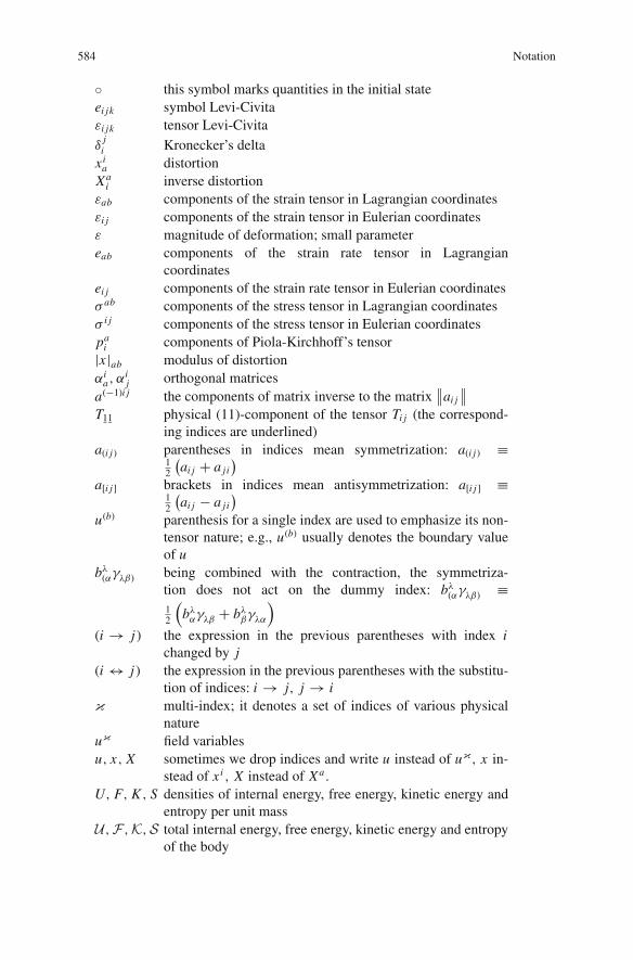
584 Notation
◦ this symbol marks quantities in the initial stateei jk symbol Levi-Civitaεi jk tensor Levi-Civitaδ
ji Kronecker’s delta
xia distortion
Xai inverse distortion
εab components of the strain tensor in Lagrangian coordinatesεi j components of the strain tensor in Eulerian coordinatesε magnitude of deformation; small parametereab components of the strain rate tensor in Lagrangian
coordinatesei j components of the strain rate tensor in Eulerian coordinatesσ ab components of the stress tensor in Lagrangian coordinatesσ i j components of the stress tensor in Eulerian coordinatespa
i components of Piola-Kirchhoff’s tensor|x |ab modulus of distortionαi
a, αij orthogonal matrices
a(−1)i j the components of matrix inverse to the matrix∥∥ai j
∥∥T1
¯1¯
physical (11)-component of the tensor Ti j (the correspond-ing indices are underlined)
a(i j) parentheses in indices mean symmetrization: a(i j) ≡12
(ai j + a ji
)a[i j] brackets in indices mean antisymmetrization: a[i j] ≡
12
(ai j − a ji
)u(b) parenthesis for a single index are used to emphasize its non-
tensor nature; e.g., u(b) usually denotes the boundary valueof u
bλ(αγλβ) being combined with the contraction, the symmetriza-
tion does not act on the dummy index: bλ(αγλβ) ≡
12
(bλ
αγλβ + bλβγλα
)
(i → j) the expression in the previous parentheses with index ichanged by j
(i ↔ j) the expression in the previous parentheses with the substitu-tion of indices: i → j, j → i
κ multi-index; it denotes a set of indices of various physicalnature
uκ field variablesu, x, X sometimes we drop indices and write u instead of uκ, x in-
stead of xi , X instead of Xa .U, F, K , S densities of internal energy, free energy, kinetic energy and
entropy per unit massU ,F ,K,S total internal energy, free energy, kinetic energy and entropy
of the body

Notation 585
ρ mass density�t ≡ �
�t ≡ (·)t = (·),t time derivative at constant Eulerian coordinates, xddt time derivative at constant Lagrangian coordinates, X
�i ≡ ��xi = (·),i partial space derivative in Eulerian variables
∇i covariant space derivatives in Eulerian coordinates�a ≡ �
�Xa = (·),a partial space derivatives in Lagrangian variables∇a Lagrangian covariant space derivatives in the deformed
state∇a Lagrangian covariant space derivatives in the initial
state� the Jacobian of transformation from Lagrangian to Eu-
lerian coordinatesδ variation at constant Xδ(x) δ-function; if x is a point in n-dimensional space, then
δ(x) is the product of n one-dimensional δ-functionsθ (x) the step function: θ (x) = 0 for x < 0, θ (x) = 1 for
x ≥ 0V usually a region in three-dimensional space�V boundary of region V|V | volume of region VdV volume element� usually a surface|�| area of the surface �
� usually a curve|�| length of curve �
�V f , �Vu parts of the boundary of elastic body in which one pre-scribes forces and displacements, respectively
dn x = dx1 . . . dxn volume element in Rn
d3x volume element in R3 in Cartesian coordinatesd A area elementI, J usually functionalsI usually action functionalI minimum value of the functionalI maximum value of the functionalL Lagrange function or Lagrangianφ symbol of empty setu ∈(1.1) function u satisfies the constraint (1.1)∗ usually the symbol of Young-Fenchel transformation;
complex conjugation in consideration of Fouriertransformation
× symbol of Legendre transformation≡ this sign is usually used for definitions

586 Notation
[ϕ] difference of values of function ϕ on the two sides of the discontinuitysurface
[ϕ]t1t0 difference of values of function ϕ at the instant t1 and t0