Molecular Mechanics and Dynamicsof Biomolecules Using a SolventContinuum Model

F. FOGOLARI,1 G. ESPOSITO,2 P. VIGLINO,2 H. MOLINARI1

1Dipartimento Scientifico e Tecnologico, Universita’ di Verona, Ca’ Vignal 1, Strada Le Grazie 15,37134 Verona, Italy2Dipartimento di Scienze e Tecnologie Biomediche, Universita’ di Udine, P.le Kolbe 4, 33100 Udine, Italy

Received 25 January 2001; accepted 18 May 2001

ABSTRACT: An easy implementation of molecular mechanics and moleculardynamics simulation using a continuum solvent model is presented that isparticularly suitable for biomolecular simulations. The computation of solvationforces is made using the linear Poisson–Boltzmann equation (polar contribution)and the solvent-accessible surface area approach (nonpolar contribution). Thefeasibility of the methodology is demonstrated on a small protein and a smallDNA hairpin. Although the parameters employed in this model must be refinedto gain reliability, the performance of the method, with a standard choice ofparameters, is comparable with results obtained by explicit water simulations.© 2001 John Wiley & Sons, Inc. J Comput Chem 22: 1–13, 2001

Keywords: molecular dynamics; solvent-accessible surface area;Poisson–Boltzmann; continuum electrostatics; implicit solvent

Introduction

A vailable computer power and methodologyrefinements have led in recent years to im-

pressive achievements in biomolecular dynamicssimulations.1 – 3 Unfortunately, most of the time isspent in simulating solvent molecules that servemostly to provide proper screening of electrosta-tic interactions and self potentials, and an effective

Correspondence to: F. Fogolari; e-mail: fogolari@sci.univr.itContract/grant sponsor: MURST

force towards removal from solvent exposure of ap-olar groups.

Continuum solvent representations, which havebeen implemented in molecular simulation by anumber of different algorithms, avoid the explicitsampling of solvent configurations, at the obviousprice of the loss of detail in the description of inter-facial solute–solvent interactions.4

It has been known for a long time5, 6 that classi-cal electrostatics for inhomogeneous media is ableto explain and predict semiquantitatively solva-tion free energies, pKa shifts in proteins and ionicstrength dependence for binding constants in manybiomolecular complexes.7, 8

Journal of Computational Chemistry, Vol. 22, No. 0, 1–13 (2001)© 2001 John Wiley & Sons, Inc.

FOGOLARI ET AL.

For nonpolar compounds it has been noted thatthe free energy of transfer between water and vac-uum or alkane phases are linearly related to thesolvent exposed surface area of the compound.9, 10

The polar and nonpolar contributions to the freeenergy of transfer are often assumed to be additive,and by using a restricted set of parameters solva-tion free energies for a large number of compoundscould be well reproduced.11

The statistical mechanical foundations for im-plicit treatment of the solvent (based on potentialof mean force12) have been reviewed recently,4, 13

although the linkage between the theoretical equa-tions and the semiempirical formulae is far frombeing clear.

For most of the continuum solvent methodolo-gies that compute electrostatic and hydrophobicinteractions by fast algorithms, the reference meth-odology has been the Poisson–Boltzmann solvent-accessible surface area (PB-SASA) model,11, 14 al-though there has been no consensus on theparameters to be employed in this model.

The PB equation (PBE) has become in recent yearsa standard tool to describe many physico-chemicalproperties of biomolecules.7, 8, 15

Electrostatic properties are computed under theassumption that a biomolecule in solution may bedescribed as a low dielectric cavity, with embeddedpartial charges, immersed in a high dielectric con-tinuum. Electrostatics for such model system obeysthe Poisson equation or, if ions in solutions are mod-eled through a Boltzmann distribution according tothe electrostatic potential, the PBE.

The solution of the PBE equation, which is ob-tained by different numerical methods,7 offers adetailed description of the electrostatic potentialoutside the molecule and also inside, provided thatself-potential effects are properly treated.15 Based onclassical expressions for electrostatic energy16 andfor thermodynamic free energy (e.g., see ref. 17),it is possible to exploit the solution of the PBE tocompute the free energy change for the hypotheti-cal process of charging the biomolecule in an ionicatmosphere.18 – 20 Applications of this methodologyinclude the computation and the display of elec-trostatic surface properties, the computation of pKashifts in proteins, the prediction of environmentaleffects on biomolecular stability, and the Browniandynamics simulation of encounter rates for smallligands with a biomolecule.15

Although quite popular and successful, the PBEapproach to biomolecular physical chemistry suf-fers from two major weaknesses: (1) the electrostaticpotential of mean force, even if all assumptions im-

plicit in the PBE should hold, is computed for asingle static molecular structure. This may be notrepresentative of the ensemble of conformationsthat a molecule may assume; (2) the macroscopicconcept of a dielectric constant is hardly suitableto describe the biomolecule–solvent interface wherecontacting solvent molecule reorientation is hin-dered and orientational preferences depend on thesurface shape, so that a more detailed treatment inthe continuum should be devised.

Both these difficulties may be partially circum-vented by semiempirical approaches like, for in-stance, scaling partial charges and atomic radii11

and molecular dielectric constant to fit experimentalobservations.21

To cope explicitly with molecular flexibility, anensemble of conformations [either experimentallydetermined or generated by standard molecular dy-namics (MD) or Monte Carlo simulations] has oftenbeen considered, and the same PBE computationhas been repeated on each conformer, and usu-ally predictions closer to experimental observationswere obtained (e.g., see ref. 22).

The inclusion of PB and other solvent forces intostandard MD algorithms, which would be a nat-ural extension of the methodology, has been veryscarcely explored,23 – 28 probably for the computa-tional burden leading to too little advantage incomputing time when compared to standard, moreinformative, explicit solvent simulations.

It is worth noting, however, that there are somepeculiar advantages when performing simulationsin implicit rather than explicit solvent:

1. Because MD is often used to generate a re-alistic conformational ensemble or conforma-tional pathways, rather than to follow the timedevelopment of biomolecular movement,29

implicit solvent simulations are expected tobe much faster due to lack of solvent vis-cosity. Therefore, even if the time requiredto compute a trajectory should be the same,conformational sampling with implicit solventsimulation is expected to be more efficientthan with explicit solvent simulation. For in-stance, it has been reported that the unfoldingof Chimotrypsin Inhibitor 2 takes place sev-eral times faster in high temperature implictsolvent simulations30 than in explict solventsimulation.31

2. The possibility of varying at will the sol-vent macroscopic properties, like surfacing di-mension, dielectric constant, surface tension,salt composition, and temperature allows one

2 VOL. 22, NO. 0

DYNAMICS OF BIOMOLECULES USING A SOLVENT CONTINUUM MODEL

to perform all possible ideal simulation ex-periments. For instance, the hypothesis thatelectrostatic or hydrophobic effects are the“driving forces” in many processes could beassayed by changing solvent dielectric con-stant or solute–solvent interface surface ten-sion. Also unfolding reactions at very hightemperatures can be easily performed main-taining room temperature solvent properties,thus providing a more appropriate compari-son with experimental data.

As a last remark we note that molecular dy-namics with PB and SASA forces would consti-tute a benchmark for comparison with other muchfaster implicit solvent models.28 The latter are notreviewed here, but in most of these, both electro-static forces and hydrophobic forces are calculatedusing computationally cheap approximations to atreatment based on the PBE and on the solvent ac-cessible surface area.4, 32, 33 It is, therefore, importantto probe the reliability of the reference methodology.

It is the purpose of this article to describe an easyimplementation suitable for any MM/MD standardpackage, to explore the application of the PB-SASAmodel to biomolecular simulations, and to test com-monly used estimates for continuum parameters onreal bimolecular systems. Although the goal of thepresent work is not to provide detailed simulations,for which suitable forcefields must still be devel-oped (e.g., see ref. 11), it is seen that the resultsobtained on model systems are comparable to thoseobtained with explicit solvent MD simulations.

Theory

A SOLVENT CONTINUUM MODEL

A continuum model for solvent effects simula-tion finds its rationale in the different time scaleson which solvent and biomolecular motions takeplace.29 In this respect it seems reasonable to as-sume that solvent effects are effectively averaged.Moreover, statistical thermodynamics shows that,if continuum properties reproduce correctly solva-tion potential of mean force, solute thermodynamicproperties are correctly computed.12, 13 Interfacialwater molecules with long residence times, thatmight play a relevant role in biomolecular func-tion (e.g., see ref. 34) are obviously not properlytaken into account in this approach, and should berepresented explicitly. Nevertheless, free energies ofsolvation for a large class of small organic molecules

are well reproduced by a solvent continuum model.Application of continuum methods to biomolecularthermodynamics has proven accurate and computa-tionally efficient on small systems (e.g., see refs. 35and 36). Following the lines of previous works, wewill consider separately intramolecular interactionsand all different solvent effects, namely electrosta-tic effects, hydrophobic effects, and coupling effects.Although dissection of free energy into componentshas been challenged, rigorous conditions for its fea-sibility have been formulated.37

ELECTROSTATIC FREE ENERGIES ANDMEAN FORCES

Electrostatic interactions are treated within theframework of the PBE.7, 8, 15 The biomolecule istreated as a low dielectric cavity with atomic partialcharges and the solvent as a high dielectric con-tinuum medium. Inner dielectric constants in therange 1–20 have often been used. The electrostaticpotential for this model obeys the Poisson equationfor nonhomogeneous media. Salts are considered,assuming that their average density in each pointfollows a Boltzmann distribution with the ion en-ergy computed from its valency and the averageelectrostatic potential.

The resulting Poisson–Boltzmann equation forthe average electrostatic potential allows one to cal-culate the average electrostatic potential in spaceand the free energy of charging the system. Thelinearized form of the Poisson–Boltzmann (LPB),usually reported in c.g.s., reads as follows:

�∇[ε( �r ) �∇ψ( �r )

] = −4πρ( �r )+4π∑

i c∞i z2

i q2ψ( �r )kT

(1)

where ρ( �r ) includes only molecular charges, c∞i is

the concentration of ion i at an infinite distancefrom the molecule, zi is its valency, q is the pro-ton charge, k is the Boltzmann constant, and T isthe temperature. This appears to be a satisfactoryapproximation for most proteins in physiologicalconditions.38 The program UHBD39 uses the finitedifferences method to solve the Poisson–Boltzmannequation. In practice, the dielectric map, the atomicpoint charges of the solute, and the salt accessib-lity map need to be discretized onto a grid, andthe Poisson–Boltzmann equation is converted ina set of finite difference equations (one for eachpoint of the grid), which is solved via an iterativeprocedure.15, 40, 41 The result is the electrostatic po-tential on each point of the grid.

The electrostatic potential within the molecule isstrongly dependent on the discretization procedure.

JOURNAL OF COMPUTATIONAL CHEMISTRY 3

FOGOLARI ET AL.

These effects may be circumvented, in principle,by taking the difference between two calculationswhere the solvent dielectric constant is set to itsproper value and to the molecule inner dielectricconstant, respectively. This subtraction allows oneto obtain the solvent reaction field. The Green’sfunction approach proposed by Luty et al.42 couldnot be applied in the present work due to repeatedfocussing steps and too large mesh leading to er-rors.

Electrostatic free energies are computed from thefollowing equation:

�Ges =∑i>j

qiqj

εrij+�Gsolv,es (2)

where subscripts i and j run on all atoms, qi is thepartial charge on atom i, rij is the distance betweenatoms i and j, ε is the inner molecular dielectricconstant, and �Gsolv,es is the electrostatic contribu-tion to the free energy of transferring the moleculeto solution from a phase possessing its inner diele-cric constant.�Gsolv,es is obtained by subtracting theLPB free energy obtained in a phase with uniforminner dielectric constant from that obtained in sol-vent.

It has been shown that the derivative of elec-trostatic free energy with respect to atom coordi-nates (in the linear approximation of the Poisson–Boltzmann equation) entails three terms:43

�Feli = qi �Ei −

∫S

18π

∣∣�E∣∣2 �∇iε( �r ) −∫

S

18πε( �r )ψ2k2

D�∇iλ( �r )

(3)where �Ei is the electric at atom i and λ( �r ) is the sol-vent accessibility. In this equation the second andthird terms represent electrostatic and ionic pres-sure, and are integrated over molecular surface S.

In all our calculations ionic pressure, which is ex-pected to be much smaller than other contributions,is neglected.43

HYDROPHOBIC FREE ENERGIES ANDMEAN FORCES

Although the concept of hydrophobic forces isstill subject to debate, it has been established thatthe free energy cost of transferring an alkane froman alkane or gas phase to water is roughly propor-tional to its solvent-accessible surface area A:

�Ghyd = γ SASAA (4)

The microscopic surface tension coefficient γ SASA

between alkane and water has been estimated closeto 0.05 kcal/mol Å2 for protein shapes,9, 10, 44 al-

though quite different values have been reportedand used in the literature. It is worth noting, how-ever, that alkane-to-water transfer free energy data(from which a rather high surface tension has beenderived) are not related in a straightforward man-ner to the present calculations. The assumption ismade here that solvent nonaccessible surface area(i.e., surface area exposed to the inner environmentof the solute) is in an alkane-like environment. Webelieve this choise is more representative than thealternative choice of an inner vacuum-like environ-ment, which would justify the use of a much lowersurface tension coefficient. Another issue concernsvan der Waals forces among atoms explicity repre-sented, which favor atomic association. Due to thiseffect, it is likely that the surface tension coefficientto emplopy for SASA forces must be lowered toavoid a sort of double counting “hydrophobic inter-actions.”

Although there are several algorithms able tocompute solvent accessible surface areas, the com-putation of their derivatives with respect to atomiccoordinates is not straightforward. We have usedthe algorithm of Sridharan et al.45 to calculate sur-face area derivatives and, consequently, to definea “hydrophobic” free energy. It is worth mention-ing here that although the free energy varies withcontinuity when atoms move, the correspondingmean force may have abrupt changes. This is evi-dent when one considers two isolated atoms withradii r1 and r2 in a solvent with radius rw. In thiscase, the hydrophobic free energy as a function oftheir distance r12 [for r12 ≤ (r1 + rw) + (r2 + rw)] isgiven by:

�Ghyd = γ SASA2π(r1 + rw)

×(

r1 + rw + (r1 + rw)2 − (r2 + rw)2 + r212

2r12

)

+ γ SASA2π(r2 + rw)

×(

r2 + rw + (r2 + rw)2 − (r1 + rw)2 + r212

2r12

)

(5)

The solvent-accessible surface area does notchange when atoms move in a direction perpen-dicular to the distance vector. The gradient of thefree energy, i.e., the mean hydrophobic force Fhyd, isdirected along the vector joining the atoms and isgiven by the following equation [for r12 ≤ (r1 +rw)+(r2 + rw)]:

Fhyd = −γ SASAπ(r1 + rw)

×(

(r2 + rw)2 − (r1 + rw)2 + r212

r212

)

4 VOL. 22, NO. 0

DYNAMICS OF BIOMOLECULES USING A SOLVENT CONTINUUM MODEL

− γ SASAπ(r2 + rw)

×(

(r1 + rw)2 − (r2 + rw)2 + r212

r212

)(6)

It can be seen that when (r1 + rw)2 ≈ (r2 + rw)2,the hydrophobic mean force is constant for r12 ≤(r1 + rw) + (r2 + rw):

�Fhyd = −γ SASAπ(r1 + rw) − γ SASAπ(r2 + rw) (7)

and drops to zero for larger interatomic distances. Itis likely that for reliable application of this method-ology a smoother potential should be employed.The implementation presented here partly remedi-ates to this behavior, by letting interactions decaywith a half life time of 50 fs, although the introduc-tion of a memory in forces does not guarantee thatcorrect conformational distributions are obtained(vide infra).

DYNAMICAL SOLUTE–SOLVENTCOUPLING EFFECTS

The issue of the coupling between solvent andsolute atoms is particularly intricate. At a very basicphysical level, for instance, when using the PBE tocompute electrostatic forces one implicitly assumesthat the reaction field by water and ions follows in-stantaneously changes in the solute, which is knownto be not true. For instance the dielectric relaxationtime of water is ca. 10 ps,46 and for ions, larger re-arrangement and averaging times are expected. Atthe atomic level the random tumbling of solventmolecules on solute will result in random forces ap-plied on the solute surface atoms with consequentviscous drag. To simulate this effect the Langevinequation has often been employed in implicit sol-vent simulations, using random forces with uniformstochastic properties over all solute atoms and a sin-gle viscous coefficient.47 Still at a higher level thecorrelated motion of many water particles resultsin hydrodynamic interactions difficult to modelin detail.48 As mentioned in the introduction, ourgoal is not to provide a detailed molecular dynam-ics algorithm to reproduce biomolecular dynamicswith realistic trajectories, but rather to use molecu-lar dynamics for efficiently sampling biomolecularconformational space according to the potential ofmean forces provided by the implicit treatment ofsolvent. For this purpose it is necessary to includein the simulation random forces, as a source ofenergy fluctuations, and a way to damp motions.Although this might not be self-evident, randomforces provide an efficient fluctuation source, thusallowing energy barrier hopping and better confor-

mational sampling, but, on the other hand, corre-lated motions take longer times to build up, dueto the randomizing effect of the same forces. Oftena compromise between these two conflicting issuesis sought, rather than a realistic model for solvent–solute random collisions.

In the present work numerical inaccuracies ofboth the LPBE solver and the molecular dynamicsalgorithm have been accepted to provide fluctua-tions. In the molecular dynamics simulations per-formed with the software Discover from MSI (SanDiego, CA), the temperature of the system wasrescaled every time it exceeded by more than a con-stant value, related to the number of atoms in thesystem, the target value. Although this might seema rather rough procedure, the trajectories obtainedare reasonable ones. The tolerance value was chosenin such a way that the kinetic energy fluctuations inthe (N, V, T) ensemble of the system could be in theproper range expected from statistical mechanics:12

〈�Ek〉2 = 3N2

(kT)2.

No Langevin dynamics has been performed to takeadvantage of the lack of solvent viscosity. Thisscheme does not, therefore, reproduce dynamicalfeatures of biomolecules in solution, but is expectedto efficiently generate statistical ensembles.

Materials and Methods

IMPLEMENTATION OF PB-SASA FORCES INSTANDARD MD PACKAGES

As mentioned in the introduction, solving thePBE on a grid for a large system is by far moretime consuming than any molecular dynamics step,and therefore, it is convenient to update reactionforces as seldom as possible. On one hand, the longdielectric relaxation time of water46 would allowa low-frequency update, but on the other hand,it should be remembered that, especially in viewof the simplified representation involved, MD isused to generate a statistically significant ensem-ble of conformations, rather than a realistic trajec-tory. For this purpose reaction forces should followmolecular movements. We have checked (vide in-fra) that for random atomic movements in a lysineresidue of about 0.3 Å the root-mean-square de-viation of computed reaction electrostatic forces isabout 0.5 kcal mol−1 Å−1, which appears acceptable.The choice of 0.3 Å movement before updating hasalso been adopted by other authors.25, 26 Instead ofchecking for atom movements we have estimated

JOURNAL OF COMPUTATIONAL CHEMISTRY 5

FOGOLARI ET AL.

that such movement is reached on average for afolded protein in more than 50 fs and, therefore,we update reaction and hydrophobic forces every50 fs.

As mentioned in the Theory section, hydropho-bic forces can undergo sudden changes as atomsmove apart. Partly for this reason and partly toavoid numerical errors in reaction forces due tothe rather largely spaced grid used for finite differ-ences PBE solution, computed forces at any step aremixed with those computed at a previous step. Thisguarantees that sudden changes in forces do not oc-curr and provide an overall stabilization mechanismagainst errors in reaction force computation. Onthe other hand, such moving average procedure isexpected to result in artifacts like, for example, dis-sipative forces, as can be easily seen by consideringa harmonic oscillator obeying the simple equation

mx = −k1x(t) + k2

(x(t) + x(t +�t)

2

)

where oscillations are damped by an exponentialfactor

k2�t4m

.

Solvation forces, computed as described later, areread into the MD algorithm in the form of templateforces. In practice, a template is created where atomsare displaced by an amount corresponding to

�F2kh

where �F is the computed force, and kh is the har-monic constant for template forcing. This is conve-nient because it avoids the necessity of modifiyingthe code, and is suited to most MD simulation pack-ages. The harmonic constant kh must be such thatduring a 50-fs MD run harmonic template forces donot change appreciably, and second, it must avoidthe problem that atoms that experience vanishingforces are template forced to their actual position.For these reasons a small constant of 0.05 kcalmol−1 Å−2 has been used, so that, with the updat-ing protocol described above, atoms for which thesolvation force is zero are not perturbed. Artifacts,however, may arise because of this force updatingscheme, and there is no guarantee that this will notbe in phase with some of the modes of the molecule(similar to the example of the harmonic oscillator).

The implementation scheme is therefore the fol-lowing:

1. A starting structure is taken (e.g., from thePDB).

2. Electrostatic reaction forces and hydrophobicforces are computed; if this is not the firststep in the protocol, newly computed forcesare mixed with previous computed forces, andthe corresponding template forcing structurecreated. Continuum reaction field energy andSASA energy are printed.

3. Template-forced energy minimization (EM) orMD is performed (50 minimization steps or 501-fs dynamics steps). Kinetic and potential en-ergy is printed.

4. The output structure from step 3 is used asinput at step 2.

The procedure is repeated for a fixed number oftimes.

Use of C-shell scripts is made to generate all in-put files and the script file containing all commandsto implemement the scheme depicted above.

BIOMOLECULAR SYSTEMS

Continuum models have been shown to repro-duce well solvation energies for a large number ofsmall organic compounds, but the suitability of themodel and the parameters usually employed hasbeen much less tested on larger biomolecules. Manytested predictions refer to static molecular models,and are limited to few aspects of their behavior,such as free energy of solvation and pH and salt de-pendence of thermodynamic properties. Therefore,testing the methodology on energy minimizationand molecular dynamics of small biomolecules thatretain some of the complexity of larger biologicalsystems, appears preliminary to any useful applica-tion on larger molecules employing the same algo-rithms.

We have chosen the small alanine dipeptide as asmall compound for gross testing atomic and sol-vent parameters. For this system much theoreticalwork already exists (e.g., see refs. 25, 26, and 49 –51), and it is sufficiently simple to obtain detailedfree energy maps in few hours on a PC.

As an example of protein structure we havechosen Viscotoxin A3, whose structure has beenrecently solved in our laboratory by NMR spec-troscopy (pdb id. 1ed0, model 1).52 This protein hashigh similarity with crambin, which has been usedin many modeling studies. The presence of threedisulfide bridges makes this protein very stable;therefore, it cannot be considered a typical proteinstructure, but, on the other hand, it should not be toosensitive on inadequacies of parameters employed.

6 VOL. 22, NO. 0

DYNAMICS OF BIOMOLECULES USING A SOLVENT CONTINUUM MODEL

We have finally considered as an example ofsmall but highly charged system an 11 nucleotideDNA hairpin.53 It is well known that accurate sim-ulation of nucleic acid is quite a difficult task dueto high electrostatic repulsion between backbonecharges. It is crucial for any MD algorithm to be ableto reproduce efficiently solvent screening effects.

ELECTROSTATIC CALCULATIONS

All electrostatic calculations have been per-formed using the program UHBD.15, 39 Atomiccharges have been taken from the AMBER force-field54 except for the alanine dipeptide for whichcharges from the CHARMM forcefield55 (v27b) havebeen used. For atomic radii we have tested a num-ber of different parameters. We report here resultsobtained using a set of rather large radii correspond-ing to the minima of the Lennard–Jones curves inthe CHARMM forcefield (version 22) for the smallprotein Viscotoxin A3. For DNA we report resultsobtained using a set of smaller radii correspondingto the value of 0.6 kcal/mol in the Lennard–Jonesenergy curve in the AMBER forcefield. For the ala-nine dipeptide simulation we used the radii setPARSE proposed by Sitkoff et al.11 Results do notdepend too heavily, at least at this stage of approxi-mation, on the parameter set employed.

A large grid was set up to enclose the systemunder simulation with a mesh of 2.5 Å, with Debye–Hückel boundary conditions. Then the LPBE wassolved for regions focussed on single residues withboundary conditions from the large grid computedon the whole molecule. The focussing steps em-ployed a mesh of 0.6 Å for molecular dynamicssimulations and 0.375 Å for the potential of meanforce minimization simulations, except where indi-cated. The inner and outer dielectric constant were 1to 8 (depending on the system under study) and 80,respectively. The ionic strength was 100 mM. Theconvergence required for the finite difference solu-tion algorithm to stop was 10−2 kcal mol−1 q−1. Notethat the algorithm execution time scales approxi-mately with the number of residues of the systemto be simulated.

These parameters have been properly estimatedby running a few simulations on the N-terminalresidue of lysine of Viscotoxin A3, and comparingcomputed reaction field forces with a reference cal-culation. Note that this test is more sensitive withrespect to a test on the solvation free energy alone,where differences can average out, and it is directlyrelated to the implementation described in the fol-lowing. The reference simulation was run with the

following parameters: grid dimensions (dime) 60 ×60 × 60, grid mesh (grid) 0.25 Å, number of points(nsph) for each sphere for surfacing algorithm 800,ionic strength (ions) 100 mM, inner dielectric con-stant (pdie) 4.0, solvent dielectric constant (sdie)80.0, ionic radius (rion) 2.0 Å, surfacing probe radius(nmap) 1.4 Å, and convergence required (conv) 10−6

kcal/q. The mean square deviation between refer-ence forces and those computed with changes to thisscheme have been tested. In practice, all force com-ponents obtained in a test simulation were plottedagainst the reference simulation values and linearregression was performed. The results are summa-rized in Table I.

SOLVENT-ACCESSIBLE SURFACE AREA ANDDERIVATIVES CALCULATIONS

All SASA and SASA derivative calculations havebeen performed using the program UHBD v. 6X,where the algorithm of Sridharan et al.45 is imple-mented. Several values of protein–solvent surfacetension coefficient have been tested as describedlater.

FORCEFIELD SIMULATIONS

Forcefield simulations have been performed us-ing either academic software CHARMM (version27b2)55 or the commercial software package Dis-cover v.3.0 (MSI, CA) employing the AMBERforcefield.54 In the latter case one to four interactionshave been scaled by a factor 0.5, and the older hy-drogen bonding potential has been retained becauseof the use of a dielectric constant larger than 1.0.Scaling one to four electrostatic interactions maylead to inconsistencies because in the computationof the reaction field on to four interactions cannotbe separated by all other electrostatic interactions.A test run on the dynamics of the DNA hairpin (seebelow), without scaling electrostatic one to four in-teractions, gives, however, the same results as therun with the scaling factor applied. Therefore, wepreferred to retain the scaling for internal consis-tency of the forcefield. No cutoff has been imposedon interactions. For the purpose of analysis internal(Ei), van der Waals (Evdw), hydrogen bonding (Ehb),and electrostatic (Eel) energy components have beenprinted out separately every 50 fs.

All dynamics simulations have been performedat constant temperature (298 K), with a 1-fs timestep and the Verlet velocity integration scheme.56

The temperature is controlled in a very rough wayby the program that rescales all velocities when the

JOURNAL OF COMPUTATIONAL CHEMISTRY 7

FOGOLARI ET AL.

TABLE I.Effect of Grid Parameters on Reaction Forces—Effect of Grid Parameters on Computed Reaction Field Forces.

Changes to Reference Simulation (nsph = 800, grid =0.25 Å, dime = 603, conv = 10−6 kcal mol−1q−1,ions = 100 mM, pdie = 4.0, sdie = 80)

Mean Square Deviation (ms) in Reaction Forces inkcal q−1 Å−1 mol−1, Correlation Coefficient (cc), Slope(sl), and Intercept (in)

nsph = 400 ms = 0.04, cc = 0.99, sl = 1.00, in = 0.0nsph = 200 ms = 0.06, cc = 0.98, sl = 1.01, in = 0.01nsph = 100 ms = 0.28, cc = 0.92, sl = 0.98, in = 0.0conv = 10−3 kcal mol−1 q−1 ms = 0.00, cc = 1.00, sl = 1.00, in = 0.0dime = 403, grid = 0.375 Å ms = 0.01, cc = 1.00, sl = 1.00, in = −0.01dime = 273, grid = 0.55 Å ms = 0.07, cc = 0.98, sl = 1.01, in = 0.0dime = 403, grid = 0.375 Å, nsph = 400 ms = 0.05, cc = 0.99, sl = 1.00, in = −0.01dime = 273, grid = 0.55 Å, nsph = 400 ms = 0.05, cc = 0.98, sl = 1.02, in = 0.02dime = 403, grid = 0.375 Å, nsph = 200 ms = 0.06, cc = 0.98, sl = 1.00, in = 0.03dime = 273, grid = 0.55 Å, nsph = 200 ms = 0.19, cc = 0.95, sl = 0.99, in = −0.01dime = 403, grid = 0,375 Å, nsph = 100 ms = 0.23, cc = 0.93, sl = 0.97, in = 0.0dime = 273, grid = 0.55 Å, nsph = 100 ms = 0.72, cc = 0.85, sl = 1.06, in = 0.01dime = 403, grid = 0.375 Å, conv = 10−3 kcal/q ms = 0.01, cc = 1.00, sl = 1.00, in = 0.01dime = 273, grid = 0.55 Å, ms = 0.07, cc = 0.98, sl = 1.01, in = 0.01

conv = 10−3 kcal mol−1 q−1

conv = 10−2 kcal mol−1 q−1 ms = 0.00, cc = 1.00, sl = 1.00, in = 0.0conv = 10−1 kcal mol−1 q−1 ms = 2.44, cc = 0.57, sl = 0.84, in = 0.02dime = 303, grid = 0.6 Å, nsph = 100, ms = 1.3, cc = 0.75, sl = 0.99, in = −0.01

conv = 10−1 kcal mol−1 q−1

dime = 303, grid = 0.6 Å, nsph = 100, ms = 0.67, cc = 0.84, sl = 1.01, in = −0.03conv = 10−2 kcal mol−1 q−1

different centering of the grid ms = 0.01, cc = 1.00, sl = 0.99, in = 0.01random movements of the atoms with ms = 0.28, cc = 0.90, sl = 0.89, in = −0.01

a RMSD = 0.28 Årandom movements of the atoms with ms = 0.60, cc = 0.78, sl = 0.77, in = 0.0

a RMSD = 0.47 Årandom movements of the atoms with ms = 0.99, cc = 0.59, sl = 0.57, in = −0.01

a RMSD = 0.94 Åions = 1000, sdie = 1000 ms = 0.00, cc = 1.00, sl = 1.03, in = 0.0

Nsph is the number of points per sphere defining atomic solvent accessible surface, grid is the spacing between nodes of thegrid, conv is the convergence criterion in kcal q−1mol−1, ions is ionic strength, pdie and sdie are molecular and solvent dielectricconstants, respectively.

difference between the target and actual tempera-ture exceed a tolerance value. This value has beenset such as to provide proper kinetic energy fluctu-ations (see above). Discover v.3.0 (MSI, CA) is alsonot able to separate internal motions from over-all translation and rotation, which would greatlyreduce movement of internal degrees of freedomwhile keeping the temperature constant. For thisreason four connected atoms in the center of thesimulated systems have been fixed to their originalposition. No procedure like this is needed if an ef-ficient control on overall motion is available, like inCHARMM.

Results

RAMACHANDRAN PLOTS

The alanine dipeptide has been chosen as a modelmolecule for peptide backbone potential of meanforce maps. Ramachandran maps have been gen-erated using different values for the dielectric con-stant (1, 2, 4, 8, and 20). Maps have been gener-ated using AMBER charges, as implememented inDiscover v.3.0 (MSI) with the CHARMM 22 radiiset, and CHARMM charges with Parse3 parame-

8 VOL. 22, NO. 0

DYNAMICS OF BIOMOLECULES USING A SOLVENT CONTINUUM MODEL

(a) (b)

FIGURE 1. Ramachandran map for the alanine dipeptide. (a) Total potential of mean force obtained with innerdielectric constant 1.0 and protein–solvent surface tension coefficient 0.01 kcal−1 mol−1 Å−2; (b) Total energy in vacuo.

ter set11 radii or the minimum in the correspondingLennard–Jones potential, with comparable results(judged from the location and depth of minima).The choice of CHARMM 22 radii, which are some-what larger than both AMBER and Parse3 radii, hasbeen adopted in this first test based on our previ-ous experience35 and because larger radii reduce themagnitude of reaction field on interfacial atoms.

Using different protein water surface tension co-efficients has minor effects on this model moleculebecause the solvent accessible surface area variesbetween 330 and 360 Å2 and, therefore, the widelyaccepted constant of 0.01 kcal mol−1 Å−2 was used.The solvent-accessible surface area does not changesignificantly after minimization, even using contin-uum forces, and for this reason it has been assumedthat a change in this parameter does not affect,on this small molecule, the following discussion.Maps are generated by restraining backbone an-gles ϕ and ψ to their target values with a harmonic

potential (force constant 100 kcal mol−1 deg−1) andsampling the torsional space of each angle in stepsof 10 degrees. Different contributions to the poten-tial of mean force can be appreciated by the hybridcontinuum/atomistic proposed here. The study ofsmall molecules, therefore, appears a viable tool toestimation of the parameters suitable for this contin-uum approach to molecular dynamics. In Figure 1the Ramachandran map of the potential of meanforce is shown and compared to the same map fora phase with a dielectric constant equal to the mole-cule inner one (1.0) and vanishing surface tensioncoefficient). The capabilities of the approach, evenwith nonoptimized parameters to reproduce solva-tion effects on conformational maps, is apparent.The PB-SASA solvation free energy is reported forthe sake completeness in Figure 2, together with theSASA contribution alone.

These results are much in line with similar stud-ies by other authors,25, 26, 49 – 51 although the detailed

(a) (b)

FIGURE 2. Ramachandran map for the alanine dipeptide. (a) Solvation contribution to the potential of mean force;(b) solvent accessible surface area contribution to the potential of mean force (γ SASA = 0.01 kcal−1 mol−1 Å−2).

JOURNAL OF COMPUTATIONAL CHEMISTRY 9

FOGOLARI ET AL.

features of the map (in particular, the relative depthof the upper right and lower right quadrant min-ima) depend on the parameters employed.

It is remarkable that solvation effects are similarto what expected on the basis of simulations usingsolvent explicit representation (e.g., see ref. 49). Thelimited contribution of the hydrophobic effect to thesolvation free energy is apparent from the same fig-ure.

A 1-ns Langevin dynamics at high temperature(with a friction coefficient 10 ps−1 and temnperature900 K) using the program CHARMM and straight-forward reading in of continuum solvation forceshas been performed to check the agreement be-tween the theoretical potential of the mean forcemap and statistical conformational distribution re-sulting from MD trajectories. The Langevin schemewas necessary to provide energy fluctuations in asmall system like the alanine dipeptide. The result-ing distribution agrees with the theoretical maps,with the system exploring mostly the two lowestpotential minima, but also the other local minimumregion of the map reported in Figure 1a, correspond-ing to positive values of ϕ angle.

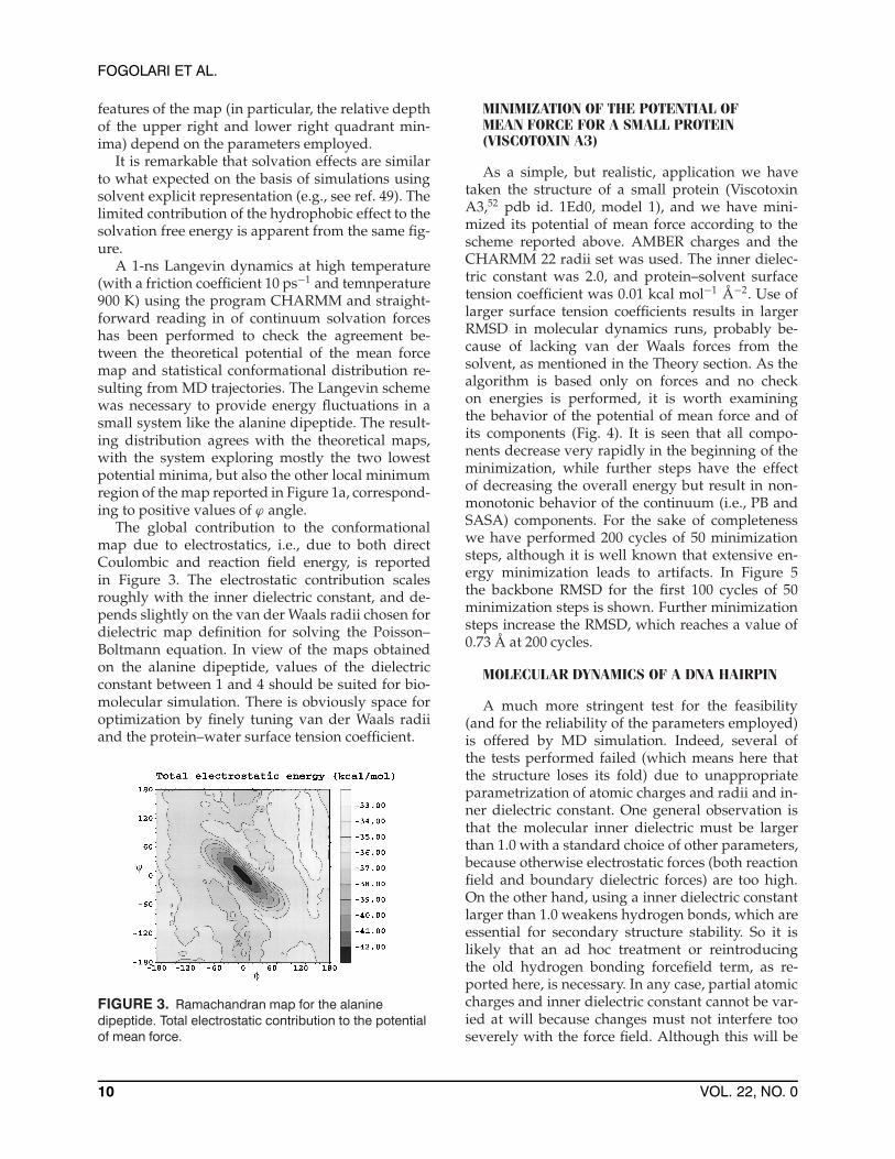
The global contribution to the conformationalmap due to electrostatics, i.e., due to both directCoulombic and reaction field energy, is reportedin Figure 3. The electrostatic contribution scalesroughly with the inner dielectric constant, and de-pends slightly on the van der Waals radii chosen fordielectric map definition for solving the Poisson–Boltmann equation. In view of the maps obtainedon the alanine dipeptide, values of the dielectricconstant between 1 and 4 should be suited for bio-molecular simulation. There is obviously space foroptimization by finely tuning van der Waals radiiand the protein–water surface tension coefficient.

FIGURE 3. Ramachandran map for the alaninedipeptide. Total electrostatic contribution to the potentialof mean force.

MINIMIZATION OF THE POTENTIAL OFMEAN FORCE FOR A SMALL PROTEIN(VISCOTOXIN A3)

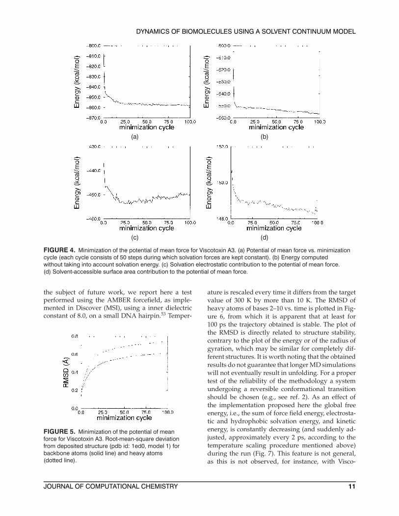
As a simple, but realistic, application we havetaken the structure of a small protein (ViscotoxinA3,52 pdb id. 1Ed0, model 1), and we have mini-mized its potential of mean force according to thescheme reported above. AMBER charges and theCHARMM 22 radii set was used. The inner dielec-tric constant was 2.0, and protein–solvent surfacetension coefficient was 0.01 kcal mol−1 Å−2. Use oflarger surface tension coefficients results in largerRMSD in molecular dynamics runs, probably be-cause of lacking van der Waals forces from thesolvent, as mentioned in the Theory section. As thealgorithm is based only on forces and no checkon energies is performed, it is worth examiningthe behavior of the potential of mean force and ofits components (Fig. 4). It is seen that all compo-nents decrease very rapidly in the beginning of theminimization, while further steps have the effectof decreasing the overall energy but result in non-monotonic behavior of the continuum (i.e., PB andSASA) components. For the sake of completenesswe have performed 200 cycles of 50 minimizationsteps, although it is well known that extensive en-ergy minimization leads to artifacts. In Figure 5the backbone RMSD for the first 100 cycles of 50minimization steps is shown. Further minimizationsteps increase the RMSD, which reaches a value of0.73 Å at 200 cycles.

MOLECULAR DYNAMICS OF A DNA HAIRPIN

A much more stringent test for the feasibility(and for the reliability of the parameters employed)is offered by MD simulation. Indeed, several ofthe tests performed failed (which means here thatthe structure loses its fold) due to unappropriateparametrization of atomic charges and radii and in-ner dielectric constant. One general observation isthat the molecular inner dielectric must be largerthan 1.0 with a standard choice of other parameters,because otherwise electrostatic forces (both reactionfield and boundary dielectric forces) are too high.On the other hand, using a inner dielectric constantlarger than 1.0 weakens hydrogen bonds, which areessential for secondary structure stability. So it islikely that an ad hoc treatment or reintroducingthe old hydrogen bonding forcefield term, as re-ported here, is necessary. In any case, partial atomiccharges and inner dielectric constant cannot be var-ied at will because changes must not interfere tooseverely with the force field. Although this will be

10 VOL. 22, NO. 0

DYNAMICS OF BIOMOLECULES USING A SOLVENT CONTINUUM MODEL

(a) (b)

(c) (d)

FIGURE 4. Minimization of the potential of mean force for Viscotoxin A3. (a) Potential of mean force vs. minimizationcycle (each cycle consists of 50 steps during which solvation forces are kept constant). (b) Energy computedwithout taking into account solvation energy. (c) Solvation electrostatic contribution to the potential of mean force.(d) Solvent-accessible surface area contribution to the potential of mean force.

the subject of future work, we report here a testperformed using the AMBER forcefield, as imple-mented in Discover (MSI), using a inner dielectricconstant of 8.0, on a small DNA hairpin.53 Temper-

FIGURE 5. Minimization of the potential of meanforce for Viscotoxin A3. Root-mean-square deviationfrom deposited structure (pdb id: 1ed0, model 1) forbackbone atoms (solid line) and heavy atoms(dotted line).

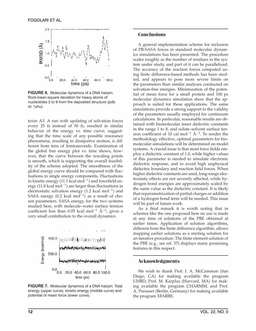
ature is rescaled every time it differs from the targetvalue of 300 K by more than 10 K. The RMSD ofheavy atoms of bases 2–10 vs. time is plotted in Fig-ure 6, from which it is apparent that at least for100 ps the trajectory obtained is stable. The plot ofthe RMSD is directly related to structure stability,contrary to the plot of the energy or of the radius ofgyration, which may be similar for completely dif-ferent structures. It is worth noting that the obtainedresults do not guarantee that longer MD simulationswill not eventually result in unfolding. For a propertest of the reliability of the methodology a systemundergoing a reversible conformational transitionshould be chosen (e.g., see ref. 2). As an effect ofthe implementation proposed here the global freeenergy, i.e., the sum of force field energy, electrosta-tic and hydrophobic solvation energy, and kineticenergy, is constantly decreasing (and suddenly ad-justed, approximately every 2 ps, according to thetemperature scaling procedure mentioned above)during the run (Fig. 7). This feature is not general,as this is not observed, for instance, with Visco-

JOURNAL OF COMPUTATIONAL CHEMISTRY 11

FOGOLARI ET AL.

FIGURE 6. Molecular dynamics of a DNA hairpin.Root-mean-square deviation for heavy atoms ofnucleotides 2 to 9 from the deposited structure (pdbid: 1zhu).

toxin A3. A run with updating of solvation forcesevery 25 fs instead of 50 fs, resulted in similarbehavior of the energy vs. time curve, suggest-ing that the time scale of any possible resonancephenomena, resulting in dissipative motion, is dif-ferent from tens of femtoseconds. Examination ofthe global free energy plot vs. time shows, how-ever, that the curve between the rescaling pointsis smooth, which is supporting the overall feasibil-ity of the scheme adopted. The smoothness of theglobal energy curve should be compared with fluc-tuations in single energy components. Fluctuationsin kinetic energy (11.1 kcal mol−1) and forcefield en-ergy (11.8 kcal mol−1) are larger than fluctuations inelectrostatic solvation energy (1.2 kcal mol−1) andSASA energy (0.2 kcal mol−1) as a result of cho-sen parameters. SASA energy, for the two systemsstudied here, with molecule–water surface tensioncoefficient less than 0.05 kcal mol−1 Å−2, gives avery small contribution to the overall dynamics.

FIGURE 7. Molecular dynamics of a DNA hairpin. Totalenergy (upper curve), kinetic energy (middle curve) andpotential of mean force (lower curve).

Conclusions

A general implementation scheme for inclusionof PB-SASA forces in standard molecular dynam-ics simulations has been presented. The procedurescales roughly as the number of residues in the sys-tem under study, and part of it can be parallelized.The accuracy of the reaction forces computed us-ing finite difference-based methods has been stud-ied, and appears to pose more severe limits onthe parameters than similar analyses conducted onsolvation-free energies. Minimization of the poten-tial of mean force for a small protein and 100 psmolecular dynamics simulation show that the ap-proach is suited for these applications. The samesimulations provide a strong support to the validityof the parameters usually employed for continuumcalculations. In particular, reasonable results are ob-tained with biomolecular inner dielectric constantsin the range 1 to 8, and solute–solvent surface ten-sion coefficient of 10 cal mol−1 Å−2. To render themethodology effective, optimal parameters for bio-molecular simulations will be determined on modelsystems. A crucial issue is that most force fields em-ploy a dielectric constant of 1.0, while higher valuesof this parameter is needed to simulate electronicdielectric response, and to avoid high unphysicaldielectric boundary and reaction field forces. Whenhigher dielectric constants are used, long-range elec-trostatic effects are not severely affected, while hy-drogen bond energies are approximately scaled bythe same value as the dielectric constant. It is likelythat reparametrization of partial charges or additionof a hydrogen bond term will be needed. This issuewill be part of future work.

As a final remark it is worth noting that inschemes like the one proposed here no use is madeat any time of solutions of the PBE obtained atearlier times. Application of solution algorithms,different from the finite difference algorithm, allowsmapping earlier solutions as a starting solution foran iterative procedure. The finite element solution ofthe PBE (e.g., see ref. 57) displays many promisingfeatures in this respect.

Acknowledgments

We wish to thank Prof. J. A. McCammon (SanDiego, CA) for making available the programUHBD, Prof. M. Karplus (Harvard, MA) for mak-ing available the program CHARMM, and Prof.A. Preusser (Berlin, Germany) for making availablethe program XFARBE.

12 VOL. 22, NO. 0

DYNAMICS OF BIOMOLECULES USING A SOLVENT CONTINUUM MODEL

References

1. Daggett, V. Curr Opin Struct Biol 2000, 10, 160.

2. Daura, X.; Jaun, B.; Seebach, D.; van Gunsteren, W. F.; Mark,A. E. J Mol Biol 1998, 280, 925.

3. Duan, Y.; Kollman, P. A. Science 1998, 282, 740.

4. Roux, B.; Simonson, T. Biophys Chem 1999, 78, 1.5. Born, M. Zeit Phys 1920, 1, 45.

6. Kirkwood, J. G. J Phys Chem 1934, 2, 351.

7. Davis, M. E.; McCammon, J. A. Chem Rev 1990, 97, 509.8. Honig, B.; Nicholls, A. Science 1995, 268, 1144.

9. Sharp, K. A.; Nicholls, A.; Friedman, R.; Honig, B. Biochem-istry 1991, 30, 9686.

10. Sharp, K. A.; Nicholls, A.; Fine, R. F.; Honig, B. Science 1991,252, 106.

11. Sitkoff, D.; Sharp, K. A.; Honig, B. J Phys Chem 1994, 98,1978.

12. Hill, T. L. An Introduction to Statistical mechanics; DoverPublications Inc.: New York, 1956.

13. Given, J. A.; Gilson, M. K.; Bush, B. L.; McCammon, J. A.Biophys J 1994, 72, 1047.

14. Honig, B.; Sharp, K. A.; Yang, A.-S. J Phys Chem 1993, 97,1101.

15. Madura, J. D.; Davis, M. E.; Gilson, M. K.; Wade, R.; Luty,B. A.; McCammon, J. A. Rev Comput Chem 1994, 5, 229.

16. Jackson, J. D. Classical Electrodynamics; John Wiley & Sons:New York, 1962.

17. Marcus, R. A. J Chem Phys 1955, 23, 1057.18. Sharp, K. A.; Honig, B. J Phys Chem 1990, 94, 7684.

19. Zhou, H.-X. J Chem Phys 1994, 100, 3152.

20. Fogolari, F.; Briggs, J. M. Chem Phys Lett 1997, 281, 135.

21. Antosiewicz, J.; McCammon, J. A.; Gilson, M. K. J Mol Biol1994, 238, 415.

22. Fogolari, F.; Ragona, L.; Licciardi, S.; Romagnoli, S.;Michelutti, R.; Ugolini, R.; Molinari, H. Proteins Struct FunctGenet 2000, 39, 317.

23. Sharp, K. A. J Comput Chem 1991, 12, 454.

24. Niedermeier, C.; Schulten, K. Mol Simul 1992, 8, 361.25. Gilson, M. K.; McCammon, J. A.; Madura, J. D. J Comput

Chem 1995, 16, 1081.

26. Smart, J. L.; Marrone, T. J.; McCammon, J. A. J ComputChem 1997, 18, 1750.

27. Smart, J. L.; McCammon, J. A. Biopolymers 1999, 49, 225.28. David, L.; Luo, R.; Gilson, M. J Comput Chem 2000, 21, 295.

29. McCammon, J. A.; Harvey, S. C. Dynamics of Proteins andNucleic Acids; Cambridge University Press: Cambridge,1987.

30. Lazaridis, T.; Karplus, M. Science 1997, 278, 1928.

31. Li, A.; Daggett, V. J Mol Biol 1996, 257, 412.32. Still, W. C.; Tempczyk, A.; Hawley, R. C.; Hendrickson, T.

J Am Chem Soc 1990, 112, 6127.

33. Lazaridis, T.; Karplus, M. Proteins Struct Funct Genet 1991,35, 133.

34. Billeter, M.; Guntert, P.; Luginbuhl, P.; Wuthrich, K. Cell1996, 85, 1057.

35. Misra, V. K.; Sharp, K. A.; Friedman, R. A.; Honig, B. J MolBiol 1994, 238, 245.

36. Baginski, M.; Fogolari, F.; Briggs, J. M. J Mol Biol 19xx, 274,253.

37. Mark, A. E.; van Gunsteren, W. F. J Mol Biol 1994, 240, 167.38. Fogolari, F.; Zuccato, P.; Esposito, G.; Viglino, P. Biophys J

1999, 76, 1.39. Madura, J. D.; Briggs, J. M.; Wade, R. C.; Davis, M. E.; Luty,

B. A.; Ilin, A.; Antosiewicz, J.; Gilson, M. K.; Bagheri, B.;Scott, L. R.; McCammon, J. A. Comput Phys Commun 1995,91, 57.

40. Warwicker, J.; Watson, H. C. J Mol Biol 1982, 157, 671.41. Gilson, M. K.; Sharp, K. A.; Honig, B. J Comput Chem 1987,

9, 327.42. Luty, B. A.; Davis, M. E.; McCammon, J. A. J Comput Chem

1992, 13, 768.43. Gilson, M. K.; Davis, M. E.; Luty, B. A.; McCammon, J. A.

J Phys Chem 1993, 97, 3591.44. Nicholls, A.; Sharp, K. A.; Honig, B. Proteins Struct Funct

Genet 1991, 11, 281.45. Sridharan, S.; Nicholls, A.; Sharp, K. A. J Comput Chem

1995, 16, 1038.46. Harvey, S. C. Proteins 1989, 5, 78.47. Friedman, H. L. A Course in Statistical Mechanics; Prentice-

Hall: Englewood Cliffs, NJ, 1985.48. Aris, R. Vectors, Tensors and the Basic Equations of Fluid

Mechanics; Dover Publications Inc.: New York, 1969.49. Anderson, A. G.; Hermans, J. Proteins Struct Funct Genet

1998, 3, 262.50. Brooks, C. L.; Case, D. A. Chem Rev 1993, 93, 2487.51. Marrone, T. J.; Gilson, M. K.; McCammon, J. A. J Phys Chem

1996, 100, 1439.52. Romagnoli, S.; Ugolini, R.; Fogolari, F.; Schaller, G.;

Urech, K.; Giannattasio, M.; Ragona, L.; Molinari, H.Biochem J 2000, 350, 569.

53. Zhu, L.; Chou, S. H.; Xu, J.; Reid, B. R. Nat Struct Biol 1995,2, 1012.

54. Cornell, W. D.; Cieplak, P.; Bayly, C. I.; Gould, I. R.; Merz, Jr.,K. M.; Ferguson, D. M.; Spellmeyer, D. C.; Fox, T.; Caldwell,J. W.; Kollman, P. A. J Am Chem Soc 1995, 117, 5179.

55. MacKerell, A. D. Bashford, D.; Bellott, Jr., M.; Dunbrack,R. L.; Evanseck, J. D.; Field, M. J.; Fischer, S.; Guo, H.; Gao, J.;Ha, S.; Joseph–McCarthy, D.; Kuchnir, L.; Kuczera, K.; Lau,F. T. K.; Mattos, C.; Michnick, S.; Ngo, T.; Nguyen, D. T.;Prodhom, Jr., B.; Reiher, W. E.; Roux, B.; Schlenkrich, M.;Smith, J. C.; Stote, R.; Straub, J.; Watanabe, M.; Wiorkiewicz–Kuczera, J.; Yin, D.; Karplus, J. J Phys Chem B 1998, 102,3586.

56. Verlet, L. Phys Rev 1967, 159, 98.57. You, T. J.; Harvey, S. C. J Comput Chem 1993, 14, 484.

JOURNAL OF COMPUTATIONAL CHEMISTRY 13