arX

iv:0

805.

3284

v1 [

cond

-mat

.mtr

l-sc

i] 2

1 M

ay 2

008

Line creep in paper peeling

Jari Rosti, Juha Koivisto, Xavier Illa, and Mikko J. Alava

Department of Engineering Physics, Helsinki University of Technology,

FIN-02015 HUT, email: firstname.secondname@tkk.fi

Paola Traversa and Jean-Robert Grasso

Universite Joseph Fourier, CNRS, LGIT, BP 53, 38041 Grenoble, France

Abstract

The dynamics of a ”peeling front” or an elastic line is studied under creep (constant load) condi-

tions. Our experiments show an exponential dependence of the creep velocity on the inverse force

(mass) applied. In particular, the dynamical correlations of the avalanche activity are discussed

here. We compare various avalanche statistics to those of a line depinning model with non-local

elasticity, and study various measures of the experimental avalanche-avalanche and temporal cor-

relations such as the autocorrelation function of the released energy and aftershock activity. From

all these we conclude, that internal avalanche dynamics seems to follow ”line depinning” -like be-

havior, in rough agreement with the depinning model. Meanwhile, the correlations reveal subtle

complications not implied by depinning theory. Moreover, we also show how these results can be

understood from a geophysical point of view.

PACS numbers:

1

I. INTRODUCTION

Creep is one of the fascinating topics in fracture for a physicist: the deformation and final

fracture of a sample follow empirical laws with a rich phenomenology. It is expected that

there are similarities and differences with ”static” fracture encountered in brittle materials

such that so-called ”time-dependent rheology” is not relevant [1]. However, the phenomenon

of creep is visible in most any setting regardless of whatever a tensile test might indicate

about the typical material response. A particular scenario where one can study creep is

the advancement of a single crack under a constant driving force. One can study this in

simple paper sheets, and for quite some time it has been noticed that this involves statisti-

cal phenomena, an intermittent response which could be characterized by ”avalanches”, in

particular of acoustic emission (AE) events [2, 3, 4, 5].

A particular experiment we analyze in this work is related to the dynamics of a crack

line as it moves through a sample, largely constrained on a plane. This can be achieved in

the case of paper in the so-called Peel-In-Nip (PIN) geometry (see below for a description).

The tensile case has been already reported in Ref. [6] and an early account of the creep

results published as Ref. [7]. The mathematical description of the line is a crack position

h(x, t), where h is the position coordinate along the direction of line propagation and x is

the coordinate perpendicular to h. On the average, the crack moves with the creep velocity

v (h = vt).

The problem has here, as in other such examples (the Oslo plexiglass experiment [9, 10]),

three important ingredients: randomness in that the peeling line experiences a disordered

environment coming from the fiber network structure, a driving force Keff or a stress in-

tensity factor, and the self-coupling of the interfacial profile h. In this particular problem,

it takes place via a long-range elastic kernel [11], expected to scale as 1/x or as k in Fourier

space.

For a constant force Keff the dynamics exhibits a depinning transition, of non-equilibrium

statistical mechanics. This implies a phase diagram for v(Keff). The crack begins to move

(v > 0) at a critical value Kc of Keff such that for Keff > Kc. In the proximity of Kc

the line geometry is a self-affine fractal with a roughness exponent ζ . The planar crack

problem [12, 13] has been studied theoretically via renormalization group calculations and

numerical simulations, and via other experiments as noted above. The roughness exponent

2

of theory ζtheory ∼ 0.39 has traditionally been considered to be absent from experiments

[8, 9, 10, 14], but recent results of Santucci et al. imply that the regime might be visible upon

coarse-graining. Imaging experiments prove in that case that as expected the line moves in

avalanches, and the avalanche size s distribution seems to have the form P (s) ∼ s−1.6···−1.7

[9, 10].

Here we look at the scenario of creep for the PIN geometry. This subject is such that

ordinary ”fracture creep” and the particular scenario related to depinning transitions coin-

cide. The creep of elastic lines becomes important for Keff ≤ Kc since thermally assisted

movement due to fluctuations takes place with a non-zero temperature [15, 16, 17]. In usual

depinning, it is assumed that thermal fluctuations nucleate “avalanches’ which derive their

properties from zero-temperature depinning, and the avalanches then translate into a finite

velocity vcreep > 0. There are two interesting differences in the fracture line creep to other

such in depinning. First, the line elasticity is non-local, and second, in materials (such as

paper here) where there is no healing, the line motion is irreversible, there are no fluctuations

in metastable states as in the case of magnetic domain walls, for instance.

In this scenario, the creep velocity becomes a function of the applied stress intensity factor

and the temperature, vcreep = vcreep(Keff , T ). As creep takes place via nucleation events

over energy barriers [15], the description of those barriers is of fundamental importance. One

can show by scaling arguments and more refined renormalization group treatments that the

outcome has the form of the following creep formula

vcreep ∼ exp (−C/Kµeff ). (1)

This gives the relation to the driving force Keff using the creep exponent, µ. The value of

the exponent depends on the elastic interactions and the dimension of the moving object (a

line), and we expect

µ = θ/ν =1 − α + 2ζ

α − ζ. (2)

The exponents θ, ν, and ζ denote the energy fluctuation, correlation length, and equilibrium

roughness exponents. All these exponents are functions of α, the k-space decay exponent of

the elastic kernel. For long range elasticity, one would assume α = 1.

The fundamental formula of Eq. (2) has been confirmed in the particular case of 1+1-

dimensional domain walls and other experiments [18, 19]. We have ourselves reported on

results, which show an inverse exponential dependence of vcreep(m) ∼ exp (−1/m), where

3

m is the applied mass in the experiment (see below), as is appropriate for non-local line

elasticity with an equilibrium roughness exponent of ζ = 1/3. In the current work we go

further by two important steps. First, we consider creep simulations of an appropriate non-

local line model and compare the avalanche statistics and v(m) to those from the experiments

(see Fig. 1 for an example of the activity timeseries from an experiment and a simulation).

Then, we ask the fundamental question: what can be stated of the correlations? This relates

to the timeseries of released energy, to aftershock rates and we present extensive evidence.

The experimental signatures show subtle correlations that are rather different from what one

would expect from the (depinning) creep problem with non-existing avalanche to avalanche

correlations.

50 60 70 80 90 100t [s]

100

102

104

106

E [

arb.

uni

ts]

80000 85000 90000 95000t

100

102

104

S(t)

(a)

(b)

FIG. 1: Activity as a function of time inside a given time window (a) for the creep experiment

with 410g load, and (b) for simulations with f = 1.87 and Tp = 0.002. In both cases we neglect

the duration of the avalanche and we only take into acount the starting time and the size of each

avalanche, obtaining a data series {ti, Ei} for the experiments and {ti, Si} for simulations (definition

of Si is given in Section IIB)

The structure of the rest of the paper is as follows. In the next Section, we discuss

the experimental setup and the simulation model. Section III shows results on v(m) both

from experiment and simulation. In Section IV we present data on avalanche statistics

again comparing the two cases. Section V offers an extensive analysis of correlations by

using a number of techniques to look at the experiment. Finally, Section VI finishes with

4

Conclusions and a Discussion.

II. METHODS

A. Experiment

In Figure 2 we show the apparatus [6]. The failure line can be located along the ridge, in

the center of the the Y-shaped construction formed by the unpeeled part of the sheet (below)

and the two parts separated by the advancing line. Diagnostics consist of an Omron Z4D-F04

laser distance sensor for the displacement, and a standard plate-like piezoelectric sensor [6].

It is attached to the setup inside one of the rolls visible in Fig. 2, and the signal is filtered and

FIG. 2: Experimental setup for peeling experiment. The paper (white) is peeled between two

cylinders (copper) separated by a few millimeters. The driving force is generated by a larger

hanging weight (black). A smaller weight adjusts the peeling angle. The AE and distance data are

collected by piezo transducer (red) and a laser sensor (gray).

amplified using standard techniques. The data aquisition card gives us four channels at 312.5

kHz per channel. We finally threshold the AE data. The displacement data is as expected

highly correlated with the corresponding AE, but the latter turns out to include much less

noise and thus convenient to study. For paper, we use perfectly standard copy paper, with

an areal mass or basis weight of 80 g/m2. Industrial paper has two principal directions,

called the “Cross” and “Machine” Directions (CD/MD). The deformation characteristics

are much more ductile in CD than in MD, but the fracture stress is higher in MD [20]. We

5

tested a number of samples for both directions, with strips of width 30 mm. The weight used

for the creep ranges from 380 g to 450 g for CD case and from 450 g to 533 g for MD case.

The mechanical (and creep) properties of paper depend on the temperature and humidity.

In our setup both remain at constant levels during experiments, and the typical pair values

for environment is 40 rH and 26 oC.

B. Simulations

We want to simulate the evolution of a discrete long-range elastic line of size L in a

disordered media. The line is characterized by a vector of integer heights {h1, . . . hL} with

periodic boundary conditions, although the experiment does not present periodic bound

conditions.

The long-range elastic force [21] acting on a string element is given by

f elastici = ko

(π

L

)2L

∑

j=1j 6=i

hj − hi

sin(xj−xi

Lπ) , (3)

where all forces on all sites can be computed in a L log L operations using a fast-Fourier-

transform (FFT) algorithm [22]. Simulations are done using ko = 0.01 and L = 1024.

The random force due to the quenched disorder may be obtained from a standard normal

distribution, i.e a Gaussian distribution with zero mean and a variance of one f randomi =

N(0, 1). Then, the total force acting in a given element of the string is fi = f elastici +

f randomi + f , where f is the external applied force.

At this point, we need to introduce a dynamics which mimic the experiment evolution.

A basic characteristic of the experiment is that it is completely irreversible, so the dynamics

has to include this important feature. We consider a discrete time evolution and the discrete

dynamical rule [22] is given by:

hi(t + 1) − hi(t) = vi(t) = θ [fi] t = 0, 1, 2 . . . (4)

where θ is the Heaviside step function. Then we apply the following procedure:

1. Start at t = 0 with a flat line located at h = 0 setting hi = 0 ∀i.

2. Compute the local force (fi) at each site and using the dynamical rule (Eq. 4) compute

the local velocity of each site. We can define the velocity of the string for this time,

as v(t) = 1L

∑L

i=1 vi(i).

6

3. Advance the sites according their local velocities vi.

4. Generate new random forces for those sites that have been advanced.

5. Go to step (2) and advance the simulation time by one unit.

This evolution shows a depinning transition at fc ∼ 1.88 in which the velocity of the line

v(t → ∞) > 0 when f > fc and v(t → ∞) = 0 when f < fc.

In order to simulate the creep evolution of the string we use an external force below the

depinning threshold, and when the line gets stuck we let thermal fluctuations play a role.

We scan all the sites and set vi(t) = 1 with a probability p = exp(

fi

Tp

)

and vi(t) = 0 with

a probability 1− p, where Tp is proportional to temperature. This can trigger an avalanche

which will have a finite duration T since the system is below the depinning treshold. We

define the avalanche size as S =∑

T v(t). If we consider small enough temperatures com-

pared to the typical internal forces, the avalanche needs some time to be triggered, which is

defined as the waiting time τ . We define this waiting time as the time between the end of

an avalanche and the starting time of the next one.

90800 90900 91000 91100t

100

102

v(t)

τiTi

Si

FIG. 3: Velocity of the long-range elastic string as a function of simulation time (dotted line). The

vertical and solid lines represents the signal S(t) ploted in figure 1(b). Avalanche properties are

also shown: τi is the waiting time, Ti is the avalanche duration duration, and Si is the avalanche

size.

In summary, this long-range elastic line model in the creep regime has an avalanche-like

behaviour. Each avalanche is characterized by three quantities: Waiting time τ , duration

7

T , and size S (see Fig. 3). Moreover, we observe that for long times, when the steady state

is reached, durations are small compared to waiting times, for that reason we can simplify

the signal just taking into account the starting time of the avalanche and its size.

III. CREEP VELOCITY

The main data about both simulations and experiment on the creep velocity are shown

in Figure 4. The prediction of Eq. (1) is that the velocity is exponential in the effective

driving force. In the case of the experiments at hand, we face the problem that we do not

know the average fracture toughness 〈K〉 empirically. It depends on the loading geometry,

and on the material at hand. There are estimates for similar papers in the literature in the

mode I case (see e.g. Ref. [23]) which indicate that the value of 〈K〉 is lower by at least

a factor of two compared with the actually used loads. One can try to work around the

problem by guessing 〈K〉 and checking how that affects the apparent functional relationship

of v vs. the reduced mass meff = m−〈K〉. In the range of physically sensible values of 〈K〉

the velocity exponential behaviour does not change and thus we can take meff = m .

0.0021 0.0022 0.0023 0.0024 0.0025 0.0026

1/meff

-6.0

-4.0

-2.0

0.0

2.0

4.0

6.0

8.0

10.0

Log

(v)

0.7 0.8 0.9 11/f

-14

-13

-12

-11

Log

(v)

T=0.0020T=0.0040

FIG. 4: The creep velocity vs. the inverse of the applied force or mass, meff = m. Inset: creep

velocity vs. f for the simulation model for two different temperatures.

From the figure we may conclude that the effective creep exponent µ ∼ 1, though there

is variability among the data sets. One of the data sets (black circles) shows some slight

8

curvature. The main finding, interpreted via Eq. (2) then indicates that the effective

roughness exponent ζ ∼ 1/3, which is the expected equilibrium value for a long-range elastic

problem with α = 1 [7].

The numerical simulation data agree qualitatively with the exponential decay except very

close to the depinning transition. According to the creep formula (see e.g. [17]), we should

expect that the velocity of the long-range string was

v(f, Tp) ∼ exp

[

−C

Tp

(

1

f

)µ]

. (5)

However, it appears that slope as a function of the temperature is not exactly the expected

one. One reason is that the model is simplified: we only let thermal fluctuations act when

the string gets stuck so avalanche nucleation during an avalanche is neglected. This may be

of importance very close to fc and for long avalanches.

100

101

102

v/<v>

10-6

10-4

10-2

100

P(v/

<v>

)

CD 400 gCD 404 gCD 409 gCD 415 gCD 420 gCD 425 gCD 430 gMD 487 gMD 502 gMD 518 gMD 533 gslope 2.3

FIG. 5: Histogram of a normalized velocity obtained from discretized distance data. Velocity, v,

is an average in a 0.5 s time window. < v > is an average over experiments with same weights.

The exponential average creep velocity can most directly be compared with the measured

velocities from the distance sensor over short time-spans. Figure 5 shows the probability

distributions P (v) for a very large number of different experiments, for the v = ∆h/∆t with

∆t = 0.5 s. The general trend shows clear stick-slip characteristics in the sense that the local

velocities vary with a power-law -like fashion. The typical slope of the data is about -2.3

though a more detailed look indicates that there is a tendency for the exponent to change

with m and with ∆t (increasing both decreases the slope). It is an interesting question

9

of how this locally time-averaged velocity is related to the average creep velocity, and the

avalanches that contribute to it, somewhat hindered by the relative large fluctuations in the

distance sensor - for which reason we resort in the detailed avalanche dynamics studies to

the AE.

IV. STATISTICAL DISTRIBUTIONS

Next we consider the statistics of the AE timeseries from the experiments as signatures

of the intermittent avalanche activity in the system during creep. In our setup, we face

the problem that direct imaging of the front dynamics is if not impossible then difficult to

realize. Thus we take the AE data up to be scrutinized as detailed information. It can be

studied from the viewpoint of the correlations of the creep avalanche activity but the finer

details thereof are left to the next Section. Here, we consider the averaged distributions of

three quantities: i) AE energy E in experiments and avalanche size in simulations assuming

that the avalanche energy is proportional to its size E ∼ S ii) waiting times τ both for

experiments and simulations and iii) avalanche durations T only for simulations, because

experimental avalanches have very short durations and can be neglected.

100

101

102

103

104

105

106

E

10-12

10-10

10-8

10-6

10-4

10-2

100

P(E

)

Tensile ExperimentCreep Experiment 410gSimulations f=1.87 T

p=0.002

FIG. 6: Energy distributions for the tensile experiment (circle), for the creep experiment (square),

and for the simulations (triangle up). For the simulations we are ploting the histogram of the

avalanches sizes {Si}. We can consider that the energy of an avalanche is proportial to its size, so

Si ∼ Ei}.

10

10-6

10-4

10-2

100

τ [s]

10-6

10-4

10-2

100

102

104

P(τ)

Tensile ExperimentCreep Experiment 410gSimulations f=1.87 Tp=0.002

10-4

10-2

100

102

τ/<τ>

10-6

10-4

10-2

100

102

P(τ/

<τ>) 380g

399g401g404g409g410g415g419g424g429g430g486g533g

(b)

(a)

FIG. 7: (a) Waiting time distributions for the tensile experiment (circle), for creep experiment

with 410g (squares), and for the simulations with f = 1.87 and T = 0.0020 (triangles up). (b)

Normalized waiting times for different creep experiments.

Figure 6 shows three cases of the avalanche size distributions. We compare the creep data

for one mass m to a similar dataset for a tensile experiment done at a constant average front

velocity [6]. Moreover data is included from the creep model for the parameters shown in the

caption. The normalization of the data for the experiments is such that the Emin has been

scaled to unity. Recall that the events are restricted in size from below by a thresholding

applied to the original AE amplitude signal A(t), from which the events are reconstructed.

We can observe that the effective power-law exponents of the experimental data are ∼ 1.6

for the creep and ∼ 1.8 for the tensile cases, respectively. These are very close to each other,

while the simulation data results imply ∼ 1.4 not very far from the experimental values.

We also can observe that there is no evident cutoff in any of them (the bending in the

11

simulations case is a finite size effect). These data can be compared with the Oslo plexiglass

experiment where for the avalanche size distribution the value of β = 1.6 ± 0.1 has been

found [9, 10].

100

101

102

103

104

105

106

T

10-12

10-10

10-8

10-6

10-4

10-2

100

P(T

)

f=1.85 T=0.002f=1.87 T=0.002f=1.89 T=0.002

FIG. 8: Avalanche duration distributions for Tp = 0.002 and three different forces. For the case

with f = 1.89 we are above the depinning treshold.

The waiting times are reported in Fig. 7. For all the three cases P (τ) is broad. In the

tensile case, it is known that there appears to be a ”bump” in the distribution, or a typical

timescale. This is absent from the creep one. It is interesting to note that here the simulation

model agrees rather well with the creep case. For larger m it is possible that the waiting

times start to look more like the tensile case. We also present the scaled distributions for

all the experiments. Later, in the next section, we discuss the attempt to link this to a

background plus correlated, triggered activity.

Finally, in Fig. 8 we show the avalanche durations from the simulations. In the case of

the experiment this is more complicated due to the fact that the actual amplitude signal

is convoluted via the preprocessing electronics and the response function of the piezos with

which the AE is measured. Later we present some examples of the outcome, but here we

just discuss the clear-cut case of the simulations also since they give an idea about what one

might see in the experiment, ideally. The main points that one learns from the Figure are

that a true power-law-like P (T ) ensues only at the proximity of the fc. For values higher

or lower than that the shape of the distribution changes, in particular such that not only a

cut-off appears but also the clear power-law character starts to disappear.

12

V. MEASURES OF CORRELATED DYNAMICS

A. Correlations

Next we look at the detailed temporal structure of the AE signal. The main question is

whether the creep activity exhibits interesting features that would in particular differ from

the theoretical expectations - based on elastic line depinning the inter-avalanche correlations

should be expected to be negligible.

FIG. 9: The autocorrelation function of the averaged event energy in paper peeling under creep

and tensile loading modes. Comparisons to the randomized data are also included. The numerical

data and the corresponding randomized data are not distinguishable.

In Figure 9 we show the autocorrelation function R(t) of the event energy time series.

The autocorrelation function is defined as:

R(u) =1N

∑N

t=1 EtEt+u − 〈E〉2

〈E2〉 − 〈E〉(6)

where Et is the energy of the AE signal at time t and 〈E〉 is the average value of the energy.

Et is defined as a sum of squared amplitudes of the AE signal in the time interval [t, t+∆t].

The length of the interval ∆t is chosen to be 10−3s in the tensile and 10−5s in the creep

peeling experiment in order to capture the correlations in both cases.

When compared to paper peeling experiments under a constant strainrate, the correlation

decays at a much faster rate than in creep peeling experiments. In that case, the existence

13

of a slow decay might be taken to be connected to the fact that there is a typical scale

in the waiting time distribution which is not the case for creep, seemingly. The functional

form of the shown case of a logarithmically decreasing autocorrelation function is R(t) =

−0.3 − 0.08ln(t). The data are also compared to a randomized timeseries, and one can see

that the correlations disappear. For the simulated data the autocorrelation function shows

no difference to a randomized signal. All in all these results imply that there are contrary

to theoretical models temporal correlations, albeit in creep on a very short timescale.

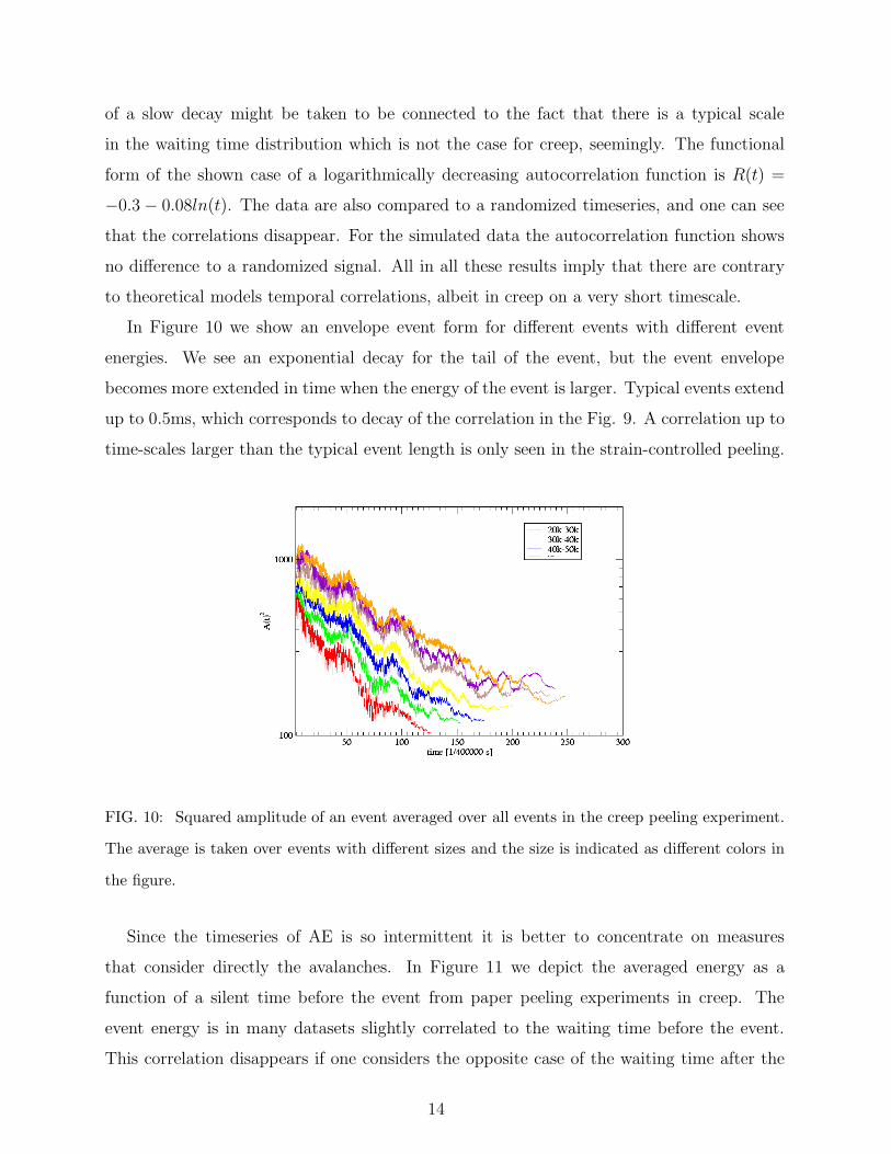
In Figure 10 we show an envelope event form for different events with different event

energies. We see an exponential decay for the tail of the event, but the event envelope

becomes more extended in time when the energy of the event is larger. Typical events extend

up to 0.5ms, which corresponds to decay of the correlation in the Fig. 9. A correlation up to

time-scales larger than the typical event length is only seen in the strain-controlled peeling.

FIG. 10: Squared amplitude of an event averaged over all events in the creep peeling experiment.

The average is taken over events with different sizes and the size is indicated as different colors in

the figure.

Since the timeseries of AE is so intermittent it is better to concentrate on measures

that consider directly the avalanches. In Figure 11 we depict the averaged energy as a

function of a silent time before the event from paper peeling experiments in creep. The

event energy is in many datasets slightly correlated to the waiting time before the event.

This correlation disappears if one considers the opposite case of the waiting time after the

14

event. The suggested interpretation is that the elastic fracture line apparently as a physical

system ages before a large event, while there is no real dependence of the waiting time on

the energy dissipated in the previous event.

FIG. 11: Averaged energy as a function of silent time before the event with weight 410g.

The difference in the autocorrelation between the creep and tensile peeling experiments

might be attributed to the forcing the line to move in the latter, which induces a “fiber-

scale” to results. This is also supported by observing the waiting time distribution, where

the pdf deviates from a power-law.

In paper peeling we study the clustering of events by computing the correlation integral

C(∆T ), that is the probability that two events are separated smaller time than ∆T . The

correlation integral is given by:

C(∆T ) =2

N(N − 1)

∑

i<j

θ [∆T − (tj − ti)] , (7)

where N is number of events in the experiment and ti is the event occurrence time.

Correlation integrals [24] are shown in the Fig. 12 for the peel creep experiment. If the

probability of the event occurrence is equal for every time interval, then one can assume that

correlation integral increases as C(∆T ) ∼ ∆T . We see a power law ∆T 0.9 in sufficiently

large times, but when the distance of events approaches the experiment length we see small

deflection in the curve. At temporal scales of the order of 10−2s we see deviation from the

power law behaviour, which indicates event clustering.

15

10-3

10-2

10-1

100

101

102

103

∆T [s]

10-6

10-5

10-4

10-3

10-2

10-1

100

C(∆

T)

399g404g419g430gC~∆T

FIG. 12: Correlation integrals for the creep in peeling experiment.

B. Seismicity - cascading occurrences as a model for the experimental data

In this part we will show how fracture in heterogeneous material, such as line creep

in paper peeling, behaves, in time, similarly to the rupture at the Earth scale, e.g. the

earthquakes driven by plate tectonic deformation.

From seismology it is known that seismicity can be described by two processes: the

background seismicity and the triggered events. The first one is modelled as a homogeneous

Poisson process, while the second one as a power law decay of seismic rate following the

occurrence of any event, e.g. the Omori’s law [25, 26, 27]:

R = µ0 +∑

t<ti

λi(t) (8)

The first term in the right hand side of Eq. 8 is the background seismicity, while the second

term is the correlated part of the seismicity, that is, the superposition of time-dependent

series of triggered seismicity following any event. The triggering process of the latter is

reproduced by models of cascading effect for earthquake interactions, i.e. ETAS (Epidemic

Type Aftershock Sequence) model [25, 26, 28]. This stochastic point process is based on

the Gutenberg-Richter law for energy distribution and Omori’s law for time distribution of

seismicity rate. According to this model, the rate of aftershocks triggered by an earthquake

occurring at time ti with magnitude Mi is given by:

λi(t) =K0

(c + t − ti)p10α(Mi−mc), (9)

16

where K0, α, c and p are constants and mc is the completeness magnitude of the catalogue.

The total earthquake rate of Equation (8) is therefore the sum of all preceding earthquakes

(triggered directly by the background events or indirectly by previous triggered events) and

the constant background rate µ0. This model reproduces most of the statistical properties

of earthquakes, including aftershock and foreshocks distributions in time, space and energy

[27].

Figure 13 illustrates the average acoustic event rate following any event for the peel creep

experiments (load m = 409g). It is reminiscent of Omori’s law for tectonic seismicity, where

we can observe the power law decay representing the cascade of aftershocks following an

event. For times greater than 10−2 seconds, the event rate keeps constant, at the background

rate level. The exponent of the power law decay of event rate is equal to 1.5 ± 0.1. This is

fairly close to what would fit the experimental P (τ) demonstrated in Fig. 7.

10-3

10-2

10-1

100

time after mainshock [s]

100

101

102

103

104

even

t rat

e [1

/s]

average aftershock rate4.25.7

FIG. 13: Event rate following events in paper peel creep experiments with m = 409g. Time t = 0

is the target event occurrence. Aftershock rates are averaged within each magnitude class of target

event (blue line: 4.2− 5.72; red line 5.72− 7.2). We compute the magnitude class M = log10(EM )

where EM is the energy of the target event. All magnitude classes are averaged together (thick black

line). Correlation between events is characterized by a power law decay of the activity after the

target event. The time for which events are correlated is a function of the target event magnitude,

as well as the number of triggered events (see Equations (8) and (9)). The observed duration of

the aftershock sequence is bounded by the level of the background uncorrelated constant rate.

The AE, triggered by line creep in paper peeling, is characterized by power law distri-

17

bution on energy (Fig. 6) and power law relaxation of aftershock rate (Fig. 13). ETAS

style models reproduce these macroscopic patterns, including foreshocks as aftershocks of

conditional mainshocks [28]. Corral [29] shows that the inter-event time probability density

for such kind of ETAS model for event occurrences follows a gamma distribution, according

to:

p(τ) = Cτγ−1 exp(−τ/β) (10)

where τ is the normalized inter-event time obtained by multiplying the inter-event time δt

with the earthquake rate λ, that is τ = δtλ.

Molchan [30] showed that, in agreement with Equation (10), the distribution decays

exponentially for large inter-event times and that the value 1/β is the fraction of mainshocks

among all seismic events. According to Hainzl et al. [31], 1/β is a regional quantity, allowing

for non-parametric estimate of the background rate in a specific process. In order to simulate

the AE properties of the creep fracture experiment (m = 409g), we tuned an ETAS model to

fit the estimated percentage of background activity of real data. One must notice that robust

inversion of ETAS model parameters is not yet available. Figure 14 shows the comparison

between inter-event time distributions of a synthetic catalogue generated by ETAS model.

Both, simulations and data inter-event time distributions fit a gamma distribution. Other

possible data fittings are possible [32], but this lies outside our aim of comparison between

data from paper peeling and ETAS simulations. The fit may underestimate here (see also

Fig. 7b) slightly the exponent of the power-law part of the waiting-time distribution. In

any case, the relevant exponent here is definately smaller than in the case of rock fracture

[33] (p = 1.4).

To summarize, line creep in paper peeling at a scale of ∼ 10−1m and ∼ 102s triggers

brittle creep damage that seems to share the same generic temporal properties than the ones

observed for tectonic seismicity at scales of ∼ 106m, ∼ 102 years. These properties can be

reduced to a rough constant seismicity rate with bursts of correlated activity, contemporary

to power law distribution of event sizes and (short-time) inter-event times. Estimates of

Omori’s law exponent suggest a faster relaxation for the paper peeling case than for Earth

crust response to tectonic loading, p equal to 1.4 and 1 respectively [26]. The portion of

uncorrelated events suggests a slightly lower triggered event rate in paper peeling than in

the Earth crust deformation. Estimations of the background portion of AE did not show

any sensitive dependence on the applied loading. Whether the difference between paper

18

10-4

10-2

100

102

normalized interevent time (∆ t λ)

10-4

10-2

100

102

norm

aliz

ed p

roba

bilit

y de

nsity

(pd

f / λ

)creep exp. load 409gETAS cataloggamma distr (24.7% uncorrelated activity)gamma distr. (23.2% uncorrelated activity)

FIG. 14: Inter-event time probability distribution for experimental dataset (thin red curve) and

synthetic catalogue generated by ETAS model (thin black curve). Dotted thick curves are gamma

distribution fits to data and ETAS model (red dotted line for the real data and black dotted

curve for ETAS). Estimations of background fraction of events according to Hainzl et al. (2006)

technique are close together (23 − 25%) for both data and simulation. ETAS parameters are:

p = 1.4, Ko = 0.09, α = 0.9 (n = 0.9), b = 1, c = 0.001s.

experiments and earthquakes come from experimental conditions or fracturing mode (i.e.

tensile, creep or compression) remains an open question. For earthquakes no change in

relative portions of background and triggered activity is resolved for compression, extensional

or shear tectonic settings.

VI. CONCLUSIONS

We have overviewed a simple creep experiment which uses paper and can be studied to

investigate planar crack propagation in a disordered medium. The information that one can

obtain and then compare to relevant theory extends from the average front velocity to details

of the spatiotemporal dynamics. We have also for a comparison studied a classical non-local

elastic line model under creep conditions. This shows similar features to the experiment: an

exponential dependence of the creep velocity on the applied force or mass or stress-intensity

factor.

The typical statistical distributions are power-law -like in particular for the event en-

19

ergy/size. It is perhaps useful to recall that the waiting time distribution is quite broad.

There is currently no understanding as to why, in particular one should note that the current

experimental setup allows to study this issue in a steady-state unlike in most other fracture-

related creep tests. In general as such distributions are regarded the line creep model agrees

at least qualitatively with the experimental data. Our results are also in line with other sim-

ilar planar crack data (though these are obtained usually in the constant-velocity ensemble,

not in creep [9, 10, 34]).

Looking in more detail at the correlations of the activity, differences transpire however.

The experimental AE events show subtle correlations via the autocorrelation function, via

the waiting times before events, and via the Omori’s law. All these measure different aspects

of the avalanche activity, and in all the cases the model differs in its behavior. Here, we lack

completely theoretical understanding, in particular as regards such a quantitative measure

as the Omori exponent. It is interesting to note that geophysics -oriented analysis methods

produce results in agreement with observations from tectonic activity. Here again the steady-

state character of the experiment at hand is of utility.

In the future such experiments and such comparisons can be used to study several different

aspects of avalanching systems, creep fracture, and models for line depinning. A particularly

pertinent question is for instance whether rate-dependent processes in the material at hand

modify the kinetics of the creep in some suitable way that still maintains the creep vs. force

-relation intact. We shall ourselves attempt a more careful study of the creep model, and

analyze how its correlation patterns could be matched with the experiment.

Acknowledgements - The authors would like to thank for the support of the Center of

Excellence -program of the Academy of Finland, and the financial support of the Euro-

pean Commissions NEST Pathfinder programme TRIGS under contract NEST-2005-PATH-

COM-043386. MJA is grateful for the hospitality of the Kavli Institute of Theoretical

Physics, China in Beijing, where the work at hand was to a large degree completed. Dis-

cussions with Lasse Laurson (Helsinki), Stephane Santucci (Oslo), Daniel Bonamy (Saclay),

and Stefano Zapperi (Modena) are also acknowledged.

[1] M. J. Alava, P. K. V. V. Nukala, and S. Zapperi, Adv. Phys. 55, 349 (2006).

[2] J. P. Sethna, K. A. Dahmen, and C. R. Myers, Nature 410, 242 (2001).

20

[3] J. Kertesz, V. K. Horvath, and F. Weber, Fractals 1, 67 (1993).

[4] L. I. Salminen, A. I. Tolvanen, and M. J. Alava, Phys. Rev. Lett. 89, 185503 (2002).

[5] S. Santucci, L. Vanel, and S. Ciliberto, Phys. Rev. Lett. 93, 095505 (2004).

[6] L. I. Salminen, J. M. Pulakka, J. Rosti, M. J. Alava, and K. J. Niskanen, Europhys. Lett. 73,

55 (2006).

[7] J. Koivisto, J. Rosti, and M. J. Alava, Phys. Rev. Lett. 99, 145504 (2007).

[8] A. Rosso and W. Krauth, Phys. Rev. E 65, 025101(R) (2002).

[9] J. Schmittbuhl and K. J. Maløy, Phys. Rev. Lett. 78, 3888 (1997).

[10] K. J. Maløy, S. Santucci, J. Schmittbuhl, and R. Toussaint, Phys. Rev. Lett. 96, 045501

(2006).

[11] D. S. Fisher, Phys. Rep. 301, 113 (1998).

[12] S. Ramanathan and D. S. Fisher, Phys. Rev. Lett. 79, 877 (1997).

[13] J. Schmittbuhl, S. Roux, J. P. Vilotte, and K. J. Maløy, Phys. Rev. Lett. 74, 1787 (1995).

[14] A. Rosso and W. Krauth, Phys. Rev. Lett. 87, 187002 (2001).

[15] T. Nattermann, Europhys. Lett. 4, 1241 (1987); L. B. Ioffe and V. M. Vinokur, J. Phys. C

20, 6149 (1987); T. Nattermann, Y. Shapir, and I. Vilfan, Phys. Rev. B 42, 8577 (1990).

[16] P. Chauve, T. Giamarchi, and P. Le Doussal, Phys. Rev. B 62, 6241 (2000).

[17] A. B. Kolton, A. Rosso, T. Giamarchi, and W. Krauth, Phys. Rev. Lett. 94, 047002 (2005).

[18] S. Lemerle, J. Ferre, C. Chappert, V. Mathet, T. Giamarchi, and P. Le Doussal, Phys. Rev.

Lett. 80, 849 (1998).

[19] Th. Braun, W. Kleemann, J. Dec, and P. A. Thomas, Phys. Rev. Lett. 94, 117601 (2005); T.

Tybell, P. Paruch, T. Giamarchi, and J.M. Triscone, Phys. Rev. Lett. 89, 097601 (2002).

[20] M. J. Alava and K. Niskanen, Rep. Prog. Phys 69, 669 (2006)

[21] A. Tanguy, M. Gounelle, and S. Roux, Phys. Rev. E 58, 1577 (1998).

[22] O. Duemmer and W. Krauth, J. Stat. Mech. P01019 (2007).

[23] Y. Yu and P. Karenlampi, J. Mat. Sci. 32, 6513 (1997).

[24] J. Weiss and D. Marsan, Science 299, 89 (2003).

[25] Y. Y. Kagan and L. Knopoff, J. Geophys. Res. 86 (B4), 2853 (1981).

[26] T. Utsu, Y. Ogata, and S. Matsuura, J. Phys. Earth 43, 1 (1995).

[27] A. Helmstetter, D. Sornette, Phys. Rev. E 66, 061104 (2002).

[28] A. Helmstetter, D. Sornette and J.R. Grasso, J. Geophys. Res. 108 (B1), 2046 (2003).

21

[29] A. Corral, Phys. Rev. Lett. 92, 108501 (2004).

[30] G. Molchan, Pure Appl. Geophys. 162 1135 (2005).

[31] S. Hainzl and Y. Ogata, J. Geophys. Res. 110 (B05), S07 (2002).

[32] A. Saichev and D. Sornette, J. Geophys. Res. 112 (B04), 313 (2007).

[33] J. Davidsen, S. Stanchits, and G. Dresen, Phys. Rev. Lett. 98, 125502 (2007).

[34] D. Bonamy, L. Ponson, S. Prades, E. Bouchaud, and C. Guillot, Phys. Rev. Lett. 97, 135504

(2006).

22