An Exterior Ballistics Primer

with

Applications to 9mm Handguns

Peter Fortune Ph. D. Harvard University

www.fortunearchive.com

2014

revised 2018

ii

Page Intentionally Left Blank

iii

Table of Contents

Topic Page

Motivation 1 Exterior Ballistics in a Vacuum 3 Shooting on a Slope: The Rifleman’s Rule 11 The Effect of Atmospheric Drag 15 So How Far Does a 9mm Bullet Carry? 29 Conclusions 35 Addendum 1: Units and Conversions 37 Addendum 2: The Mathematics of Ballistics in a Vacuum 39 Addendum 3: The Euler-Wade EXCEL Spreadsheet 41 References 43

iv

Page Intentionally Left Blank

Motivation

I first developed an acquaintance with guns as an Indiana teenager. Starting with

the boy’s standard first rifle, a .22 caliber Remington used mostly for target practice and

sometimes for hunting, I added a .22 Ruger revolver and, as a collector’s item, an 1878

Sharps .45-70 rifle like the one later highlighted in the movie Quigley Down Under— a

lethally gorgeous very long range rifle; regrettably, doubts about its integrity and the lack

of ammunition kept me from firing it. When I enlisted in the Marine Corps in 1961,

these guns were sold (I hope they’re not on the Detroit streets, especially the Sharp) and

guns became an occupational tool. At that time I learned the difference between my rifle

and my gun, the only lasting knowledge my drill instructor passed on.

In the early 1960s the USMC used the clunky and reliable M1 Garand Rifle as its

training weapon. The M1 had been replaced by the M14—virtually identical except with

a magazine—as a field weapon in 1957, and the M14 was soon to be replaced by the

M16—the workhorse of Viet Nam and the prototype of the civilian AR15 that haunts

school hallways today. In Advanced Training after Boot Camp, I was required to

“qualify” with the M1 at intervals of 250, 300, and 500 yards after a period of zeroing in

at 100 yards. The result could be Marksman, Sharpshooter, or Expert. My first attempt

was a dismal failure marked by rapid waves of Maggie’s Drawers—the red flag that

target managers wagged to inform you of a complete miss; I didn’t even achieve

Marksman status. My drill instructor, remarkably excited by this deficiency, sent me to

the ophthalmologist, where I discovered the meaning of myopia. After being fitted out

with the pink-rimmed glasses du jour that the Corps issued then (someone in Purchasing

had a sense of humor), I returned to the firing line and qualified as an Expert.

After the Corps I had no contact with guns: there was no time for them, and they

were not socially acceptable for an economics professor teaching in Massachusetts. But

on retiring and moving to the high-caliber-friendly state of Florida, I re-established my

acquaintance. The initial reason was that I developed a love of the water and bought a

boat. There are places you don’t want to be in a boat without defensive equipment, so I

2

acquired two Walther 9mm pistols (a P99 and a PPS) and a Mossberg 500 shotgun; and I

returned to target practice.

Now, one can do target practice on the cheap from a boat: simply throw an object

overboard (choose one that floats) and bang away. This has the advantages that no other

shooters are around to damage your ears, and that you learn to shoot on an unstable

platform. But it can create safety concerns for other boaters. As a result, I became

interested in the question. “What is the maximum range of my 9mm handguns?”

This is a matter of “Exterior Ballistics,” the forces on and motions of a bullet after

it exits the barrel. Initially I simply looked up the answer—about 2,300 yards. But then

the question took on a life of its own—in my many years of research I’ve repeatedly

encountered instances where the published word was wrong because mistakes crept in.

So I decided to see for myself. This primer is the result of that research. I hope someone

finds it useful.

The following analysis uses some specific language. The units of measurement

are in the English PFS (pound-foot-second) units rather than the Metric KMS (kilogram-

meter-second) units most commonly used in physics. Addendum 1 defines the units and

the fundamental definitions used here.

Words like “range” and “distance” refer to horizontal distance, “slant range” is

the direct line-of-sight distance to a target when it is above or below the shooter. The

word “velocity” refers to velocity along the bullet’s path (tangent to the arc at the bullet’s

position); when referring to the up-down or in-out motion we refer to “vertical velocity”

or “horizontal velocity.” “Mass” and “weight” are synonyms unless otherwise stated (as

in atmospheric density measurements where the pound-mass (lbm) is used to specifically

indicate mass).

A note for those less mathematically inclined. I have laid out the details of the

mathematical analysis, and after the first equation your eyelids will begin to flutter. Not

to worry: just ignore the math and scan the text. There will still be a lot to learn about

basic exterior ballistics.

If you see a need for corrections or have any polite suggestions, please let me

know at webmaster@fortunearchive.com.

3

Exterior Ballistics in a Vacuum

When a bullet is fired the trigger releases a hammer or a firing pin that slams into

the base of the cartridge, where a small amount of highly explosive matter—the primer—

is stored. The primer’s explosion ignites the powder just forward of the cartridge base

and the ignited powder releases gases that expand rapidly and push the bullet out of its

cartridge, accelerating the bullet from dead stop to perhaps 4,000 feet per second in just a

few inches. The pressure of the released gases as they exit the muzzle pushes on air

molecules and creates a “blast.” If the muzzle velocity is supersonic (greater than about

1,125 feet per second) a pressure wave is created and the blast is accompanied by the

“crack” of a sonic boom.

The activity of the bullet before it exits the muzzle is a matter of the “Interior

Ballistics” of the weapon. What happens once the bullet is released is the focus of

“Exterior Ballistics.” We begin with Figure 1 demonstrating the parameters underlying

the analysis, the Marksman’s Setup shown in Figure 1.

Figure 1

The Marksman’s Setup

Height (h)

LOB

h*

θ h0

GROUND (0) R

Distance (x) x*

Bul

let D

rop

@ R

LOS

4

The analysis that follows is in three stages: “first approximation” that is, ballistics in a

vacuum with no gravity; “second approximation,” that is, ballistics in a vacuum with

gravity; and “third approximation,” that is, ballistics in an atmosphere with both gravity

and aerodynamic drag.

First Approximation: Bullet Path in a Vacuum

A projectile is launched at velocity v0 feet/second at an angle of θ° (the launch

angle) from a height h0 feet above the ground to hit a target at the shooter’s elevation and

at horizontal distance R (the range). In this picture the Line-of-Sight (LOS) from shooter

to target is horizontal. The shooter elevates his weapon so that the Line-of-Bore (LOB)

exceeds the LOS. We know he does this because of gravity, but for the moment let’s

ignore both gravity and air resistance (“drag”).

In the absence of gravity the bullet will proceed forever along the LOB at constant

velocity v0 (the “muzzle velocity”). Obviously the target will be missed—after t seconds

of travel the bullet will be at distance v0t along the LOB, always above the LOS. If the

shooter really thought there was no gravity he should choose a zero-degree angle of reach,

aiming at the target directly along the LOS.

The bullet’s velocity can be decomposed into vertical motion at velocity vh and

horizontal motion at velocity vx, both of which are constant. These velocities will

conform to the equation v0 = √(vh2 + vh

2). It turns out that the vertical and horizontal

velocities will be vh = v0sinθ and vx = v0cosθ so the height of the projectile along the LOB

is h(t) = h0 + v0(sinθ)t and the projectile’s horizontal distance on the LOB is

x(t) = v0(cosθ)t.

Second Approximation: Bullet Path in a Vacuum with Gravity

When gravity is introduced the trajectory is no longer a straight line—it is a

parabola, an arc along which the height of the bullet and any horizontal distance x is the

height of the LOB at x less the bullet drop at x due to gravity. The bullet drop is at any

moment t after launch is – ½gt2 so the bullet’s height is now h(t) = h0 + v0t – ½gt2. This

5

can be converted to a drop at distance x by using the fundamental equation relating t and

x, that is, x(t) = v0(cosθ)t. Note that the projectile’s velocity on the arc (at any point

tangent to the arc) remains v0 throughout the bullet’s path, but the division between

velocity’s vertical and horizontal components changes along the flight path.1

This information is shown in Figure 1 above. There are two forces operating on

the projectile. The first is the force of the initial propulsion; this sends the projectile

along the LOB starting at h0 , traveling at muzzle velocity v0 at angle θ. At any time after

firing, the distance traveled along the LOB line is v0t, the height above the shooter is

h(t) = (v0sinθ)t and the horizontal distance from the shooter is (v0cosθ)t.

The height of the bullet above the ground and the horizontal distance travelled are

(1) a. ℎ 𝑡 = ℎ! + 𝑣!𝑠𝑖𝑛𝜃 𝑡 − !!𝑔𝑡!

b. x(t) = v0(cosθ)t Using these fundamental equations we can write height as a function of horizontal

distance travelled:

(1’) h(x) = h0 + (tanθ)x – ½[g/(v0cosθ)2]x2

The maximum height (also called “maximum trajectory” or “maximum ordinate”)

of the bullet, denoted as h*, occurs at time t* and horizontal distance x*, described by the

three equations in system (2)2

(2) a. 𝑥∗ = !!(𝑣!)𝑠𝑖𝑛2𝜃

b.3 ℎ∗ = ℎ! + 𝑡𝑎𝑛𝜃 𝑥∗ − !![ !(!!!"#!)!

]𝑥∗!

c. 𝑡∗ = !∗

(!!!"#$)

1 Recall that force equals mass times acceleration, i.e. F = ma. For an object subject to gravity and a gravitational constant of g we have F = -mg. Eliminating mass from both sides we get simply a = -g. Mass “disappears” and gravitational force tells us that for a falling body acceleration is negative (i.e., in the downward direction); the bullet’s acceleration is a constant determined solely by the gravitational force g—the bullet’s mass doesn’t matter. 2 The maximum height occurs when dh/dx = 0, (or, equivalently, dh/dt = 0). Readers not acquainted with basic calculus can directly solve equation (1’) for its two roots using the quadratic formula. Equation (2a) employs the identity sinθcosθ = ½ sin2θ.

6

The trajectory also has terminal conditions—values of time, distance, energy,

velocity, and so forth at the moment when the bullet hits the target. The range (R) and

the time (T) of impact are essential to this analysis. To find the range, substitute R for x in

equation (1’) and find the value of R for which h(R) = 0; this will be the solution to the

quadratic equation (3a). Once R is found, T can be found by setting x = R in equation

(1b); this gives the terminal time as shown in equation 3b.

(3) a. 0 = ℎ! + 𝑡𝑎𝑛𝜃 𝑅 − !![ !(!!!"#!)!

]𝑅!

b. 𝑇 = 𝑅/(𝑣!𝑐𝑜𝑠𝜃)

Finally, we have the concept of “bullet drop,” to be distinguished from the “bullet

path” (also called the “bullet trajectory).” Bullet path is the arc taken by the bullet and it

includes distances above and below the shooter—when shooting at an upward angle the

bullet path numbers begin as positive numbers because they are above the LOS, then they

shift to negative numbers as gravity pulls the bullet down below the shooter’s line of

sight. Bullet drop is often obtained from manufacturer’s information based on standard

conditions. It is also available in ballistics software used to adjust the launch angle 𝜃 so

the shooter can “come up” or “come down” the correct amount when the distance to the

target differs from the distance for which the weapon is zeroed. The bullet drop at

distance x is the vertical distance from the point on the LOB at distance x to the bullet’s

height at that distance (see Figure 1 above for bullet drop at range R). Denoting the bullet

drop as D(x), the equation for bullet drop at each distance x is

(4) 𝐷(𝑥) = 𝑣!𝑠𝑖𝑛𝜃 𝑥 − ℎ(𝑥)

that is, the drop at distance x is the height of the LOB less the bullet’s height above the

LOS at that distance.

Conversely, if you know the launch angle 𝜃 and the bullet drop 𝐷(𝑥) at any range,

you can use (4) to calculate the bullet’s height at that range. Drop is usually measured in

7

inches, though we will use yards and convert to inches when convenient. Minutes of

Angle (MOA) and Mil-dots are also used to measure drop.4

It is important to emphasize that this scenario excludes any consideration of

“drag,” that is, air resistance due to atmospheric or other factors creating drag (air density,

temperature, humidity, turbulence at the projectile, pitch and yaw of the projectile). Drag

will dramatically reduce the maximum height, range, and both the average and terminal

velocity of the projectile.

Addendum 2 summarizes the equations of motion used in exterior ballistics

calculations without drag.

Two important aspects of this exercise are noteworthy—we will alter these when

we consider ballistic drag.

• The mass of the projectile does not enter into the bullet’s motion. The reason is that in the absence of drag, mass affects neither the velocity along the flight path nor (as Galileo showed) the gravitational characteristics encountered by the projectile. • The velocity of the projectile is always equal to the muzzle velocity, v0. However, velocity is decomposed into vertical velocity (vh) and horizontal velocity (vx) using the equation v = √(vx

2 + vyh2 ). Along the projectile’s trajectory the

composition of velocity changes but velocity itself remains constant.

Table 1 below reports the results for our sample bullet used throughout this study:

a 124 grain 9mm Luger with a muzzle velocity of 1,110 feet per second. For these

calculations we have set the shooter’s elevation at ground level and equal to the elevation

of the target (that is, h0 = h1 = 0); the spreadsheets below show the results at different

launch angles.

The range-maximizing launch angle is 45° at which the maximum range of over

12,755 yards (7.25 miles) is achieved and the maximum height of 9,566 yards (5.4 miles)

is reached in 24½ seconds; and the bullet impacts the ground in 49 seconds. At a 90°

launch angle, when the bullet is shot straight up and all of its motion is vertical, the bullet

reaches a height of almost 7 miles, travels no horizontal distance, and returns to Earth in

4 Minute of Angle (MOA) is a measure of the number of degrees in the vertical rotation of the LOB: One MOA is 1/60 of a degree and translates to a 1” impact shift per 100 yards of distance to the target. A Mil-dot is a military unit equal to (roughly) one inch over a 100-yard distance.

8

69 seconds. Note that the bullet’s path is a perfect parabola: it leaves at launch angle θ°,

it peaks at horizontal distance x* = ½R , and it hits the earth at distance R = 2x* at an

impact angle θ°.

Most shooters don’t want to set a launch angle and calculate the range. Instead,

they want to find the launch angle that makes the bullet hit a target at a specified

horizontal and vertical point; this launch angle is called the Angle of Reach. For example,

zeroing a rifle to hit the center of a target 6 feet tall at, say, 200 yards, requires finding the

launch angle that leads to impact at the target’s middle—three feet above ground—at a

distance of exactly 200 yards. Having found that angle of reach, the sights are set so that

the LOB is elevated above the direct line of sight (LOS) at exactly that angle. The shooter

can then put the crosshairs directly on a target 200 yards away, knowing that the launch

angle is adjusted correctly to hit the target. A shot at any other distance will require some

sight readjustment.

Table 2 reports the angle of reach at different horizontal distances for our sample

bullet. There are two launch angles that will reach any given distance: the higher launch

angle, exceeding 45°, allows the bullet to arch high and then descend to the target. The

lower launch angle, below 45°, gives a gentler parabolic arc upward toward the target.

For example, our bullet will hit a target ½-mile distant using a launch angle of either

88.0° or 2.0°.

Don’t rush out and use these data unless you are operating in a vacuum with no

drag. Your chances of hitting a target 7¼ miles away using a 9mm Luger bullet are

absolutely zero—when drag resistance is factored in, that target is way out of range.

9

!!!!!!!!!!!!!!!!!!!!!!!!!!Table!1

!!!!!!!!!!!!!!!!!!!!!!!!!!!!!!!!!!!!!!!!!!!!!!!!!!!!!!!Bullet!Trajectories!at!various!Launch!Angles,!without!Drag!!!!!!!!!!!!!!!!!!!Sample!Bullet:!MagTech!124!Grain!Full!Metal!Jacket!9mm!Luger

Datah0 0 is!shooter's!height!relative!seal!level!(feet)v0 1,110 is!muzzle!velocity!(ft/sec)g 32.2 is!the!gravitational!constant!(ft/sec/sec)h1 0 is!height!of!the!target!relative!to!sea!level)(feet)

!!!!!!!!!!!!!!!!!!!!!!!!!!!!!!!!!!!!!!Maximum!Height!States!!!!!!!!!!!!!!!!!!!!!!!!!!!!!!!!!!!!!!!!!!!!!!!!!!!!!!!!!!!!!!!!!!!!!!!!!!Terminal!States!(at!time!T)!!!!!!!!!!!!!!!!!!!!!!!!!!!!!!!!!!!!!!!!!!!!!!!!!!!!Range!and!Flight!Time Maximum Time!of Distance!at Horizontal Vertical Angle!of

!!!!!!!!!!!!!!!!!!!!!!!!!Launch!Angle Range Range Range Flight!Time Height Max!Height Max!Height Velocity!* Velocity Velocity Impact(Degrees) (Radians) (feet) (yards) (miles) (seconds) (feet) (seconds) (feet) (ft/sec) (ft/sec) (ft/sec) (degrees)

'25 '0.4363 0 0 0 0 0 0.00 0 1,110 1,110 0 '25.00'20 '0.3491 0 0 0 0 0 0.00 0 1,110 1,110 0 '20.00'15 '0.2618 0 0 0 0 0 0.00 0 1,110 1,110 0 '15.00'10 '0.1745 0 0 0 0 0 0.00 0 1,110 1,110 0 '10.00'5 '0.0873 0 0 0 0 0 0.00 0 1,110 1,110 0 '5.000 0.0000 0 0 0 0 0 0.00 0 1,110 1,110 0 0.005 0.0873 6,644 2,215 1.26 6.01 145 3.00 3,322 1,110 1,106 97 5.0010 0.1745 13,087 4,362 2.48 11.97 577 5.99 6,544 1,110 1,093 193 10.0015 0.2618 19,132 6,377 3.62 17.84 1,282 8.92 9,566 1,110 1,072 287 15.0020 0.3491 24,596 8,199 4.66 23.58 2,238 11.79 12,298 1,110 1,043 380 20.0025 0.4363 29,312 9,771 5.55 29.14 3,417 14.57 14,656 1,110 1,006 469 25.0030 0.5236 33,138 11,046 6.28 34.47 4,783 17.24 16,569 1,110 961 555 30.0035 0.6109 35,956 11,985 6.81 39.54 6,294 19.77 17,978 1,110 909 637 35.0040 0.6981 37,683 12,561 7.14 44.32 7,905 22.16 18,841 1,110 850 713 40.0045 0.7854 38,264 12,755 7.25 48.75 9,566 24.38 19,132 1,110 785 785 45.0050 0.8727 37,683 12,561 7.14 52.81 11,227 26.41 18,841 1,110 713 850 50.0055 0.9599 35,956 11,985 6.81 56.48 12,838 28.24 17,978 1,110 637 909 55.0060 1.0472 33,138 11,046 6.28 59.71 14,349 29.85 16,569 1,110 555 961 60.0065 1.1345 29,312 9,771 5.55 62.48 15,715 31.24 14,656 1,110 469 1,006 65.0070 1.2217 24,596 8,199 4.66 64.79 16,894 32.39 12,298 1,110 380 1,043 70.0075 1.3090 19,132 6,377 3.62 66.59 17,850 33.30 9,566 1,110 287 1,072 75.0080 1.3963 13,087 4,362 2.48 67.90 18,555 33.95 6,544 1,110 193 1,093 80.0085 1.4835 6,644 2,215 1.26 68.68 18,987 34.34 3,322 1,110 97 1,106 85.0090 1.5708 0 0 0.00 68.94 19,132 34.47 0 1,110 0 1,110 90.00

*!Note:!!Velocity!is!constant!at!v0!in!the!absence!of!drag,!though!the!mix!between!vertical!and!horizontal!components!changes!as!the!bullet!travels!!!!!!!!!!!!!!!!Mass!does!not!affect!the!trajectory!in!the!absence!of!drag

!Source:!http://en.wikipedia.com/wiki/Trajetory_of_a_projectile

!!!!!!!!!!!!!!!!Table!2

!!!!!!!!!!!!!!!!!!!!!!!!!!!!!!!Angle!of!Reach!at!Various!Horizontal!!Distances

DistanceXFeet 660 1,320 2,640 5,280 10,560 15,840 21,120 26,400 31,680 36,960Yards 220 440 880 1,760 3,520 5,280 7,040 8,800 10,560 12,320Miles 1/8!mile 1/4!mile 1/2!mile 1!mile 2!miles 3!miles 4!miles 5!miles 6!miles 7!miles

Angle!!!!XX!High 89.5 89.0 88.0 86.0 82.0 77.8 73.2 68.2 62.1 52.5!!!!!!!!!!!!!!!XX!Low 0.5 1.0 2.0 4.0 8.0 12.2 16.8 21.8 27.9 37.5

!Source:!http://en.wikipedia.com/wiki/Trajetory_of_a_projectile

10

Page Intentionally Left Blank

11

Shooting on a Slope: The Rifleman’s Rule

Most shooters spend their time shooting on nearly level ground at targets either at

rest or moving at the same elevation, as is shown in Figure 1. Under those circumstances,

two things are noteworthy: first, the distance along the LOS (the Slant Range, denoted as

RS) is equal to the horizontal distance to the target (the Range, denoted as R); the reason

is, of course, that the angle of reach is zero forcing RS and R to be equal.

But what about a shooter who is above or below his target? There is a scene in the

movie True Grit when Rooster Cogburn (John Wayne or Jeff Bridges, depending on the

version) shoots from a high mesa downward at a sharp angle to hit a horseman riding

slowly along on the plain far below. This was well before the iPhone and ballistics apps

would do the calculations for him. Even so, he hits the target—it’s a movie—and I’m

sure that most folks in the audience were impressed, perhaps applauding at such fine

marksmanship. But if they knew the difficulties of shooting on a slope, they would have

awarded Rooster a Nobel Prize in Marksmanship.

Figure 2 Bullet Drop and Marksmanship h LOB A

Drop at RH

τ° RS θ° 0 R x

LOS

12

In Figure 2 above the target is at horizontal distance R but the target is elevated

above the shooter; The LOS is tilted upward at angle θ. The distance to the target along

the LOS is called the slant range and is denoted by RS. The shooter’s task is to determine

the “come-up” angle, τ, by which he must elevate the LOB above the LOS angle to make

the bullet drop at range R exactly the value that intersects the LOS at the target.

Knowing the drop at R, he then aims directly at point A, allowing gravity to bring the

bullet down to the target.

Consider a simple situation where the slant range is 300 yards and the target is

elevated 100 yards relative to the shooter—a real Rooster Cogburn shot. The old-

fashioned way to address this was to consult a bullet drop table to compute the distance

below the LOB the bullet will be at the target’s range. For example, a 150-grain .30-06

bullet will drop about 23 inches at 300 yards and about 20 inches at 285 yards (normal

atmospheric conditions). The shooter who recognizes that “range” and “slant range” are

very different concepts will compute the correct target line-of-sight angle (it is 19.47º)

and then calculate the range as RS•cos(19.47º), about 283 yards. He will shoot so that the

bullet drops by 20 inches at 283 yards, intersecting the bull’s eye on the target.

Suppose the shooter confuses the slant range with the range. He notes that the

slant range is 300 yards but forgets that the horizontal range is less than that—and that it

is horizontal range that determines both the time to impact and the associated horizontal

range. Thus, he correctly sees the LOS angle as 19.47º but thinks the target is 17 yards

farther out on the LOS. Consulting his drop table he will find a 23-inch drop at 300 yards

so he will aim for a point 23 inches above the bulls eye. The true drop at 283 yards is 20

inches, not 23 inches, so he will hit the target at a point 3 inches higher than his point of

aim. For many purposes this isn’t a problem, but for a hunter a hit 3 inches high could be

the difference between a clean kill and a long walk after a wounded animal.

The fundamental Rifleman’s Rule is simple: Don’t be a Dope, Shoot Low on a

Slope. But by how much should the shooter compensate? The exact answer lies in some

more trigonometry, now provided by hand-held ballistics computers. Anecdotal evidence

suggests that less experienced hunters, having heard the Rifleman’s Rule, tend to

overcompensate, coming down too much and shooting low. This suggests that experience

is the answer to correct implementation of the rule.

13

Consider a bullet fired at a zero-degree launch angle (called “flat-fire”). The only

vertical force on the bullet is gravity and the drop at any moment is - ½[g/(v0cosθ)2]x2 or

-½gt2, depending on whether you want to relate the drop to elapsed time or horizontal

distance. As we see later in Table 6, drag induces lower bullet drop as LOB angle

increases, so shooters most prone to shooting high are those who confuse slant range with

horizontal range and use flat-fire bullet drop data that overstates drop.

A more accurate Rifleman’s Rule, called the Improved Rifleman’s Rule, makes a

simple scale adjustment to the slant range: the slant range is multiplied by some fraction

to derive the correct distance (range) for bullet drop. The correct scale adjustment is to

multiply the slant range by the cosine of the angle-of-sight along the LOS; in our

example, this gives 300cos(19.47°), or 282.84 yards. We’ve seen this number before—it

is the target’s actual horizontal range! The scale adjustments made are given in Table 3.

Thus, at a 20° LOS angle the 300-yard slant rage is multiplied by .940 to give a range of

282 yards; the precise adjustment factor for 19.47° is .9428, for a range of 282.84 yards.

Table 3

Slant Range and Cosine Adjustment

Many shooters are not versed in trigonometry, some perhaps not in multiplication.

For them the Rifleman’s Rule is sometimes stated in a looser form. For example, John

Plaster, a retired Army sniper, suggests a version gleaned from the FBI practice book: if

the LOS angle is between 30° and 45°, aim for 90% of the slant range; if it is below 30°,

14

aim for 70% of the slant range; if it is below 10° shoot flat. This applies regardless of the

slope’s direction.

Yet another variation uses a bullet drop table for the particular ammunition used;

this table is typically provided by the manufacturer. It’s steps are: first, calculate the LOS

angle θ and the horizontal range as RS•cos(θ); second, determine from the bullet

manufacturer’s published drop tables the flat-fire bullet drop at the target’s horizontal

range; and finally, calculate the come-up angle as 𝜏 = 𝑎𝑟𝑐𝑡𝑎𝑛 [!∆(!)!].5 This can be

modified to become 𝜏 = 𝑎𝑟𝑐𝑡𝑎𝑛 [!(!"#!)∆(!!)!!

] as the come-up. Of course, by the time

you’ve done the calculation the target has moved on!

5 Drop Tables are reported in inches. Brian Litz’s Point Mass Ballistics Solver gives a drop of 114.71 inches, or 3.19 yards, at a 280 yard range

15

The Effect of Atmospheric Drag

We have discussed exterior ballistics in a vacuum with gravity; now we look at

the bullet path when atmospheric drag is added. This is our third approximation model of

ballistics. We also discuss arcane force-like effects like the Coriolis Effect and the

Magnus Effect that can affect projectiles over long distances but are not an integral part

of our third approximation model.

Forces and Effects inducing Ballistic Drag

Ballistic drag—deceleration of a projectile while in flight—and other “forces” or

“effects”—dramatically alter a projectile’s trajectory. Exterior Ballistics—the forces

affecting the projectile after launch—combine with other factors to make projectile

dynamics extremely complex

• The bullet’s shape: drag is related to the shape of the bullet, particularly its cross-sectional area (the area of the circle that the bullet presents to it flight path) and the shape at its stern. Bullets with larger cross-sectional area encounter greater air resistance and greater deceleration; bullets with stern shapes like a boat-tail generate less wake turbulence and lower resistance than flat-based bullets; bullets with pointed noses have less resistance than flat nosed bullets like hollow-points. • The bullet’s mass: given its cross-sectional area, greater mass reduces bullet drag as mass punches through the drag. Mass is typically measured in grains, once associated with the weight of a grain of wheat: 7,000 grains per Imperial pound. A common 9mm bullet’s mass is in the range 115-147 grains (7.5 – 9.5 grams); the WWII M1 Garand’s ,30-0 cartridge had a bullet weighing 150 grains. .45 caliber bullets can run up to 400 grains.

• The bullet’s stability: a bullet in flight does not stay exactly “on target.” Rather, it is subject to yaw (horizontal wobble), pitch (vertical wobble), and precession (circular nose wobble due to both pitch and yaw). If these are too great the bullet can tumble in flight, greatly increasing its drag. To counter these, the bore is rifled to cause the bullet to rotate in flight, creating angular velocity that reduces wobble. The rifling is calculated to achieve an optimal “twist rate” at which the stabilizing properties of rotation and its energy-using effects are balanced. Every gun is designed with this in mind. For example, the four-inch barrel on a Walther P99 induces a twist rate of one rotation every ten inches of travel; this is the standard “twist rate” for handguns.

16

• Muzzle velocity: This is particularly important when it exceeds the speed of sound, about 1,125 feet per second. At supersonic velocities air resistance and drag are considerably greater than at subsonic velocities. As a bullet advances, its velocity falls, so if the muzzle velocity is supersonic, drag decreases sharply as it becomes subsonic. Muzzle velocity is typically determined by barrel length and by the quantity and quality of the powder used as a propellant. The M-16 military rifle has a 5.56x45mm bullet. This is only .22 caliber bullet, the same as the standard match or varmint pistol, but the M-16 bullet is longer (more stable), more massive, and, propelled through a long barrel by more propellant; it achieves a muzzle velocity of 3,110 feet per second, much higher than the standard .22 caliber bullet or than the long-retired M1 Garand bullet. The 150-grain M2 Ball cartridge used in the Garand remains supersonic for more than 1,000 yards so I never gets to the transonic zone after which drag drops sharply.

• Air density: air density is a complex combination of air pressure, altitude (typically lower drag at higher altitudes), humidity (greater drag at higher water vapor content per unit of air), and air temperature (higher temperature generally means lower density and less drag).

A variety of other “effects” affect a bullet’s path. The Coriolis Effect is related to

the Earth’s rotation. It is the reason that winds moving northward from the equator arch

toward the east in the northern hemisphere. Suppose that a shooter is interested in a target

at higher latitude (say, he is on the equator aiming directly north toward Chicago). As the

Earth rotates, Chicago will always be directly north of his position, that is, the longitude

remains unchanged. But, because of the Earth’s spherical shape, his speed of travel

(rotational velocity) is greater than Chicago’s: at the equator he is rotating (relative to,

say, the sun) at 480 meters per second or approximately 1,000 mph, but Chicago, at

latitude 41° 51’N, is rotating at roughly 500 mph. In effect, the shooter must recognize

that his bullet will travel eastward relative to Chicago because Chicago is moving

westward relative to him; he must lag the target. In contrast, a Chicago shooter aiming at

our equatorial shooter must lead his target. Clearly, the Coriolis Effect is important for

long-range bullets, particularly ballistic missiles. But it can be of some concern for long-

range rifles as well.

Every golfer knows the Magnus Effect: a “slice” sends the ball veering to the right

because the ball is rotating clockwise relative to the vertical plane, reducing the air

pressure in the direction of the spin; the differential pressures on the right and left of the

flight path create lift that pushes the ball to the right. While the professional golfer can

17

control that motion, the shooter cannot—bullet rotation is required for stability. For

example, a Walther 9mm pistol has a right-handed rotation as it exits the barrel. This

right-handed spin is relative to the vertical plane, and, like the sliced golf ball, the bullet

is deflected to the right. The response of a professional shooter is to adjust for this,

aiming a bit leftward to compensate.

Measuring Ballistic Drag: The Ballistic Coefficient

A central concept in ballistic drag analysis is the “standard” bullet, used to

calibrate the drag of a specific “sample” bullet. To measure the drag coefficient of a

sample bullet, a standard bullet is chosen whose drag we know. Then the sample bullet’s

drag is measured and the ratio of the two drags, called the “form factor,” is calculated.

This form factor is used in measuring a sample bullet’s ballistic coefficient.

The earliest model of ballistic drag was based on the “G1” definition of the

standard bullet, developed in 1881 by Krupp, the German arms manufacturer, and used,

with modifications, by James Ingalls in his seminal 1883 book on exterior ballistics.

Though very simple by the standard of modern ballistics, the G1 model is a reasonable

standard for pistols using flat-based subsonic bullets. Other models are more appropriate

for long-range boat-tailed ammunition; the drag coefficient of supersonic military bullets

is typically drawn from a G6 or G7 standard bullet.

At present there are at least six standard bullets, labeled G1 through G8 (there is

no G3 or G4); other standards exist but are infrequently used. Each is based on a

different set of standard bullet dimensions. For example, the G1 standard bullet (the

original Krupp-Ingalls standard) is a flat-based cylindrical bullet 3.28 inches long with a

one-inch diameter, a weight of one pound (454 grams), and an “ogive” (sharp nose)

having a .02 inch “meplat” (nose-point diameter). By definition, the G1 bullet’s

“sectional density” is 1.0 and its drag scale factor is 1.0, giving it a ballistic coefficient

(defined below) of 1.0.

The G1 serves as the standard for short-range handguns. The most frequently

used alternative, used for long-range rifles, is the G7 standard bullet. The G7 is 4.28

inches long, weighing one pound with a one-inch diameter, with a boat-tail stern .6

inches long angled inward at 7.5°, and a slightly blunted nose with a .13 inch meplat; it

18

also has, by definition, a ballistic coefficient of 1.0. In fact, all standard bullets are

designed with unit values for their BC.

The Ballistic Coefficient of a bullet is essential to the bullet’s ballistics.

Developed in 1870, the BC measures the bullet’s resistance to air resistance, so a higher

value means less air resistance and, therefore, less drag. A bullet’s BC is based on its

Sectional Density (SD) and its Drag Scale Factor (DSF). These are6

(6) a. 𝑆𝐷 = !!!

b. 𝐷𝑆𝐹 = !"!"!

where d is the sample bullet’s maximum diameter in inches, m is its mass (assumed equal

to weight) in pounds, SD is the “sectional density” of the sample bullet7 and SDG is the

sectional density of the standard bullet. Because both numerator and denominator are in

the same units (pounds per square inch, or kilograms per square meter), the drag scale

factor (DSF) is a pure number. As noted above, sectional density is greater the higher the

mass (a heavy bullet resists drag better than a light bullet), and is lower the greater the

area facing the flight path (greater area means greater air resistance).

A sample bullet’s Ballistic Coefficient is defined as

(7) 𝐵𝐶 = !"!

Note that the form factor, denoted by f—has been introduced. This is a direct

measure of the bullet’s drag coefficient relative to that of the standard bullet. In fact, f is

defined as cS/cG, the ratio of the sample bullet’s drag coefficient to the standard bullet’s

drag coefficient.

Ingalls’ original work assumed that all sample bullets were scale models of the

G1 standard bullet; this is equivalent to setting f = 1 so BC is entirely defined by sectional 6 SD is a measure of mass relative to the cross-sectional area that the bullet presents to its flight path. The cross-sectional area is properly measured as πd2/4, but for historical reasons it is measured as simply d2 in ballistics calculations.

19

density. But it soon became obvious that actual drag results differed from Ingalls’

predictions because actual bullets rarely conformed precisely to the G1 shape. The

solution was to introduce a factor (f) to capture these differences: each bullet comes with

its own form factor, which, in turn, depends on the specific standard bullet used. For

example, the same bullet will have a higher form factor when compared to a “sleek” G7

model than when compared to a “blunt” G1 standard bullet.

The form factor is defined as the ratio of a sample bullet’s drag coefficient, cS, to

the standard bullet’s drag coefficient, cG. Substituting this above, we get the following

description of the Form Factor:

(8) f ≡ cS/cG = 𝑆𝐷𝐵𝐶

All bullets experience increased drag as velocity increases. Table 4 shows the

relationship between a bullet’s velocity and its drag coefficients (cG) for the two primary

standard bullets: the G1 and the G7.

The calculations in this document are for a specific sample bullet: a MagTech 124

grain 9mm Parabellum8 bullet with mass of .0177 pounds, diameter (caliber) of .355, SD

= .141 lb./in2, f = .73 (relative to the G1 bullet), a BC of .192 lb/in2, and a muzzle

velocity of 1,110 feet/sec (at the edge of supersonic). The dimensions of this sample

bullet are shown below in Table 5 and its associated image. Some terms need to be

defined: the base diameter is the width of the narrow base just forward of the cartridge’s

stern; this is the width of the bullet’s stern. The caliber is the width of the bullet in

inches at the base, where it connects with the cartridge; the nose diameter is the width of

the meplat. The meplat is large for blunt-nosed hollow-point bullets, small for the

standard rounded point bullet, or very small for supersonic military bullets.

8 The 9mm Parabellum is also called the 9x19mm Luger bullet; the first number is the diameter, the second number is the bullet’s length. There are other 9mm bullets, for example, the Russian 9x18 Makarov pistol bullet, or the Russian 9x39mm rifle bullet. Georg Luger developed the 9x19mm Parabellumin in 1901 and it became famous as the standard pistol issued to German officers in WWI and WWII. It has become the worldwide bullet of choice for military and police use because it is an excellent compromise between weight, accuracy and stopping power.

20

The ogive, or nose, is the portion of the bullet jutting out from the cartridge; it is

called the ogive because it has a curved shape. The ogive length is the length from the tip

of the bullet to the cartridge. The ogive radius is a measure of the bullet’s pointedness.

Table 4

Velocity and Drag Coefficients Mach G1 G7

0.00 .263 .120

0.50 .203 .119

0.60 .203 .119

0.70 .217 .120

0.80 .255 .124

0.90 .342 .146

0.95 .408 .205

1.00 .481 .380

1.05 .543 .404

1.10 .586 .401

1.20 .639 .388

1.30 .659 .373

1.40 .663 .358

1.50 .657 .344

1.60 .647 .332

1.80 .621 .312

Table 5 Dimensions of a 9mm Luger Bullet

Metric English

Nose Base Diameter (D) Width of Bullet at Cartridge

(Caliber)

9.03mm 0.355in

Bullet Weight Mass 124 grains 8.04 grams

. 0177lbs .2863ozs

Ogive Length (L) Length for Bullet Tip to Cartridge 10.54mm .415in

Ogive Tip Diameter (T) Flatness of Nose (Meplat) .30mm .012in

Ogive (Nose) Radius (R) Nose Pointedness 1.67 1.67

Total Length (Nose +

Cartridge)

Length of Entire Assembly 29.69mm 1.169 in

Cartridge Length Length of Unit Holding Propellant 19.15mm 0.754 in

21

Dimension Characteristic (mm) (inches)

The drag coefficient depends upon all of these dimensions and more. Analytical

calculations of drag coefficients are extremely difficult, so most reported drag coefficient

values are derived from field measurements by using sound sensors to calculate the

velocity decrease between any two points, then comparing that to the velocity decrease

for the standard bullet—the ratio of the two is the form factor. If a bullet’s velocity

decreases by, say, half of the standard bullet’s decrease between 250 and 500 yards, then

for that interval the form factor for the sample bullet is .50—its drag coefficient is half of

the standard bullet’s drag coefficient We’ve seen that in the absence of drag the only forces affecting a bullet are its

initial propulsion and gravity. Throughout the trajectory, velocity remains at muzzle

velocity, though the split between vertical and horizontal motion changes. But

aerodynamic drag is proportional to the square of velocity, so as velocity decreases

during a bullet’s flight, drag decreases exponentially. The decrease in drag is not at a

constant rate: an initially supersonic bullet will first experience an increase in drag as its

velocity slows, but the drag coefficient plunges as the bullet enters subsonic velocities.

The slight initial drag increase occurs because the slower-moving bullet loses heat,

cooling the air around it and increasing the local air density. The plunge at transonic

Cartridge Base Diameter Width of Cartridge Base 8.79mm 0.347in

22

speeds is because the drag-increasing sonic wave disappears. In contrast, the drag for a

subsonic bullet is relatively constant.9

This pattern is shown below in Figure 3 for a .308 caliber 210-grain VLD (Very-

Low-Drag) rifle bullet, compared to nine standard bullets. For velocities up to 90 percent

of the speed of sound (Mach .9) the .308 caliber’s drag coefficient rises slightly from .263

to .342, it then jumps to .588 at Mach 1.1, after the transonic range is passed; then it rises

slightly to Mach 1.4 and finally falls as Mach 2 is approached. Precise drag analysis

requires consideration of this drag vs. velocity relationship.

Figure 3 Drag Coefficients of A Rifle Bullet According to Different Standards

9 As an object goes supersonic velocities air cannot get out of the way fast enough, creating a pressure increase showing as a pressure (“shock”) wave. As the bullet passes, air flows back to fill the vacuum at supersonic speed creating a sonic boom that is heard downrange as the “crack” of the bullet.

23

Drag, Drop, and Velocity

We saw that in a vacuum a bullet’s mass plays no role in its trajectory: the bullet’s

velocity is constant, though the division between vertical and horizontal velocity changes,

and its drop relative to the LOB after t seconds is -½gt2. Atmospheric drag changes this:

as noted above, as the bullet proceeds its total velocity slows by an amount proportional

to the square of velocity; this increases the time taken by the bullet to travel a given

distance, thus increasing the time gravity has to work and the drop. It also alters the split

between vertical and horizontal velocity.

To demonstrate the effect of drag on bullet drop we have used a readily-available

ballistics program to calculate the effects at different launch angles. Table 6 summarizes

the results for our Magtech 124-grain 9mm bullet with 1,100 fps muzzle velocity.

Table 6

Bullet Drop with and without Drag

280-yard Horizontal Range

Launch

Bullet Drop Angle Drag No Drag Difference

0° -137.90” -110.11” -27.79”

5° -137.69” -109.90” -27.79”

10° -136.41” -108.85” -27.56”

15° -134.09” -106.06” -27.13”

20° -130.72” -104.23” -26.49”

24

Source: Author’s calculations; Brian Litz, Point Mass Ballistics Solver

The first column shows the launch angle, the second shows the bullet drop cum

drag, the third column shows the bullet drop without drag, and the final columns shows

the effect of drag on bullet drop10 We see that at any launch angle drag induces a greater

bullet drop, and that drop decreases as launch angle rises.

Because published bullet drop tables play an important role in a shooter’s life, it’s

worth investigating the accuracy of the tables, most of which are produced by

manufacturers. There are two broad reasons for this question. First, tables are often

produced under “flat fire” conditions, which, as Table 6 shows, will give larger drops

than shots taken on a slope.

Second, bullet makers are in a competitive environment and a high ballistic

coefficient is a marketing tool. Thus, there is a financial incentive to find ways to report a

high BC. There is some evidence supporting biased BC’s and drop tables. Courtney and

Courtney evaluated the ballistic coefficients reported by several manufacturers for a

small sample of bullets, concluding that there was a clear tendency to overstate the BCs

(hence understate drag); one bullet’s BC was overstated by twenty-five percent. How

might this bias arise? One method is to choose a standard bullet that has high drag, like

the G1 bullet; this makes the sample bullet’s drag appear lower when computing the BC.

Another way is to fiddle with atmospheric parameters by, say, basing density

estimates on choosing standard atmospheric conditions like ICAO that assume zero

humidity instead of “RMY Standard Metro” conditions that assume 78% relative

humidity; the dryer air has less density and imparts less drag. In fact, our sample bullet,

10 Drag is computed using air density of .0747 pounds per cubic feet, consistent with 29.92 inches of mercury barometric press, temperature = 68° and 70 percent relative humidity. With no drag the air density is, of course, zero.

25° -126.32” -100.69” -25.63”

30° -120.94” - 96.36” -24.58”

25

produced by MagTech, might have an overstated BC: MagTech reports it’s BC as .192

but 9mm Luger bullets produced by other manufacturers report BCs around .150.

In summary, increased drag increases bullet drop at any horizontal range. There is

evidence suggesting that Bullet Drop Tables provided by ammunition manufacturers tend

to understate drag and thus understate bullet drop. A shooter relying on published drop

tables might well learn to make the Rifleman’s Rule adjustments, then shoot even higher

to compensate for understated drag.

It is clear that bullet drop is greater with drag. As we shall soon see, the reason is

not that drag affects the bullet only in one direction: it affects the bullet in all directions

and its effect is the same in all directions. What drag does is to slow the bullet, its rate of

rise and fall, and its rate of forward progress. By slowing the bullet’s velocity gravity

more time to pull the bullet down at any horizontal distance the bullet travels.

To delve more deeply into the effects of drag, we derive the bullet’s equations of

motion. Aerodynamic drag is arises from a force that is directly proportional to air

density and to the square of the projectile’s velocity, as seen in equation (9):

(9) 𝐹! = − !!𝑐!𝜌𝑓𝐴𝑣!

where 𝜌 is air density in pounds per square inch and A is sectional density. Noting that

drag deceleration, ∆ is !!!, we can rewrite (9) as (9’)

(9’) ∆ = − !!𝑐!

!!"

𝑣!

The negative acceleration (i.e. deceleration) of velocity due to drag is proportional to the

square of velocity with the constant of proportionality depending directly on air density

and inversely on its ballistic coefficient. Thus, as the velocity along the bullet path

diminishes, the drag force diminishes by the square of that change—a halving of velocity

cuts the drag force by 75 percent. Note that the velocity referred to is measured along the

direction of travel, that is, at a point tangent to the bullet’s direction of travel on the arc

we call its trajectory.

26

Drag acceleration in two dimensions is described by equation system (10).

(10) a. µ = !!

!!!!"

b. ∆x = −µ𝑣𝑣x

c. ∆y = −µ𝑣𝑣h

where µ is the retardation coefficient, based entirely on air density and bullet

characteristics, v is the instantaneous velocity along the direction of travel, vx is

horizontal velocity, and vh is vertical velocity. Note that µ is a constant while v, vx, and vh

are functions of time.

Equation system (11) describes the complete system of equations of motion: (11a)

defines total velocity as the square root of the sums of squared horizontal and vertical

components; (11b) describe horizontal and vertical velocities as functions of the

retardation coefficient (µ), of the level and components of velocity (v, vx and vh) and of

the gravitational constant, g; Equations (11c) state the initial conditions for the trajectory

derived from muzzle velocity (v0) and launch angle (θ).

a. v = √[vx2 + vh

2]

(11) b. !"!!"= −Δ𝑣𝑣! !"!

!"= −𝑔 − Δ𝑣𝑣!

c. 𝑣 0 = 𝑣! 𝑣! 0 = 𝑐𝑜𝑠𝜃 𝑣! 𝑣! 0 = 𝑠𝑖𝑛𝜃 𝑣!

These differential equations have no closed form solution—there is no

mathematically exact solution for the trajectory. This is an inherent difficulty in ballistics

analysis—even through we know the equations, there is no precise solution. Numerical

approximation methods are used to compute discrete approximations to (11). These

methods consist of taking the bullet’s initial position at the end of the launch and using

the equations (11) to update the position in the next nanosecond, then use that second

position with (11) to update the calculation to the third nanosecond, and so on.

27

There are a number of numerical methods that can be used.11 Euler’s Updating

Equation is among the most straightforward. Let Δt be a discrete change in time (a

“nanosecond”) and F(t) be any function of time whose first derivative, F’(t) is known.

Then the following relationship approximates the exact result:

(12) F(t + Δt) ≈ F(t) + F’(t)Δt

The approximation improves as Δt becomes smaller, approaching the exact

solution as Δt becomes infinitesimally small. Each of the state variables in (11)—x, h, v,

and so on—can be updated using this equation if given suitable initial conditions.

Before proceeding to our third approximation ballistics model, it is worth noting

the contributions of Arthur Pesja to trajectory analysis. Unhappy with the mathematical

state of ballistics in the late 1940s, Pesja set out to find a way to make mathematically

precise trajectory calculations. To do this he subjected the equations of motion to

algebraic approximations that ultimately resulted in a closed form solution that could be

easily calculated and that, he believed, were accurate approximations to real data. Pesja’s

1953 classic, Modern Practical Ballistics, applies line-fitting techniques to empirical drag

data to model drag characteristics. A prominent ballistics software package called

ColdBore, available at Patagonia Ballistics, uses Pesja’s methods.

That program is sui generis, a black black box. Brian Litz says of the Pesja

method:

The simplicity of the Pesja solution method is only shifted onto the bullet description, which the shooter is burdened to establish for himself for each bullet at all velocities. Litz, Bryan. Applied Ballistics for Long-Range Shooting, p. 104

The lesson is that the Pesja method—or any method using approximations to

obtain closed solutions, does not eliminate complexity, it simply relocates it. Pesja’s

method requires measurement of bullet characteristics well beyond the ability of normal

11 A closer approximation often incorporated is ballistics software is the Runge-Kutta method.

28

shooters. The search for a closed form solution is like shifting deck chairs on HMS

Titanic as the iceberg looms—the fundamental problem remains unchanged, only the

view changes.

Amanda Wade and others have used Euler’s Equation to derive trajectory

information. The results are approximations—as are all numerical simulations—but they

have several advantages. First, they are transparent—the user knows exactly how the

calculations were done; what I call the Euler-Wade model is not a black box where the

user has no idea what happens between the inputs and the outputs. Second, the Euler-

Wade model is simple and straightforward in its implementation—it can be written as an

Excel spreadsheet that can easily be shared and modified as the user sees fit.

We have adapted Wade’s approach by modifying her Excel spreadsheet applying

Euler’s method to (12). The results are reported in the next section. Addendum 3 shows

the formulas in the EXCEL spreadsheet. We experimented with the launch angle using

the Euler-Wade model, finding that the range-maximizing launch angle for our sample

9mm bullet (MagTech 124-grain) is anywhere between 32° and 34° – at each of those

angles the maximum range is 2,311 yards. Note that this is spot-on with the 2,300-yard

range reported by the National Rifle Association Firearms Source Book, and is consistent

with the 2,130-yard range given by the National Law Enforcement and Corrections

Technology Institute (See Table 7).12

Recall that without drag the maximum range is exactly twice the range at which

height is maximum, and the terminal angle of impact is equal to the angle of launch. This

is not true with drag. For example, at a 33° launch angle the Euler-Wade model says the

maximum height (639 yards) is achieved at a horizontal range of 1,462 yards; this is

roughly 63 percent of the 2,311-yard maximum range. Also, the 33° launch angle results

in a -64° impact angle. This is consistent with the results of the other ballistics programs

used in the next section, excluding the CordBore program which, by using equations of

motion derived from linear approximations to the data, simply repeats the shape of the

trajectory implicit in a second-approximation model.

12 The NRA and NLECTC sources might have used an Euler-Wade-like model to derive their results; if so, this is not independent verification of Euler-Wade approach.

29

So How Far Does a 9mm Bullet Carry? Answers from Ballistics Software

The complexity of ballistics models is typically described in terms of the “degrees

of freedom” of the model, that is, the number of dimensions of a bullet’s path. There are a

total of six dimensions, three spatial and three rotational. The three spatial dimensions

capture the bullet’s flight path—forward-backward, up-down, and right-left—called

direction, elevation and drift. The three rotational dimensions are rotational velocity,

pitch, and yaw. The most complex model is a 6-DOF mode, while the least complex is a

2-DOF model. For a very stable bullet that doesn’t change its attitude as it follows the

flight path, a 3-DOF model is “good enough for government work. This, the choice of a

2-DOF model is highly accurate as long as there is no drift.

In the previous section we laid out the basic equations of motion with

aerodynamic drag in a 2-DOF ballistics model—the Euler-Wade model. We then used

this to simulate the trajectory for our sample 9mm bullet. We found that 2,311 yards was

the estimated maximum range. This is consistent with other published reports, but this

might not be an independent estimate—if those published reports used the same

estimation method—the Euler-Wade model—we have not found independent verification

of their conclusions; rather, we have simply found what method they used to get them.

Now we turn to applying a variety of commercial software programs to answer

our basic question. Before moving on, it’s worth asking not what is the maximum range

of a 9-mm bullet but what is the maximum effective range. This, of course, is a question

about the shooter as well as about the handgun and bullet used. The longest effective use

of a 9mm bullet from a handgun is a mighty 1,000 yards, a shot by Jerry Miculek, who

holds world records in pistol marksmanship. This was not in formal competition.

As noted above, advances in computer technology and numerical approximation

methods have greatly increased the precision of ballistics calculations. The field is now

the province of experts in that technology, among them the late R. L. McCoy, author of

Modern Exterior Ballistics. This technology has diffused from the military arena to the

realm of the laptop computers and PDAs of everyday shooters.

30

To get the answer to our fundamental question we use the Euler-Wade model,

described above, as well as several readily available ballistics software programs, under

identical drag-related assumptions (atmospherics, drag coefficients, etc.). We compute

trajectories of our sample bullet at several launch angles: 15°, 30°, and 45°, and, where

possible, the range maximizing launch angle. Note that the 15° launch angle is the most

realistic for handguns: rarely will a pistol shooter want to fire at a higher angle. The

other angles are included just to get a sense of their influence on horizontal range.

The ballistics programs we use are all point mass trajectory calculators. This

means that the bullet is treated as an infinitesimally small point with mass and that

rotational dimensions are ignored. In short, they are 3-DOF models in which windage

(right-left) is considered as well as forward-backward and up-down. More complicated

programs, such as those used for artillery trajectories, treat the shell as an object with

both size and rotation. At the top of the ballistics model hierarchy are 6-DOF models that

incorporate the three spatial dimensions and three rotational dimensions: spin that causes

drift (the Magnus Effect), yaw, and pitch. These models are very accurate and are

typically incorporated in analyses of ballistic missile trajectories and in very long range

sniper shots.

Consider the following scenario. A shooter uses a 9mm handgun with a four-inch

barrel and a ten-inch twist rate—my Walther P99. His load is a MagTech 124 grain Full

Metal Jacket round nose bullet with the dimensions reported in Table 6. The shooter is at

sea level, the terrain in front of him is flat, and there is no wind. He fires his weapon at a

chosen launch angle and calculates the bullet’s trajectory as would the program

designer—the designer is the man in the black box. After each experiment he gets the

results for the entire trajectory—flight time, velocity, energy, height, bullet drop, and

horizontal distance—at each moment until impact on the ground. Bullet drop is then

used to compute the height of the bullet as the height on the LOB at each range less the

bullet drop reported from the black box.

Our shooters in this exercise are:

• The Euler-Wade Model, as modified by this author

• JBM Ballistics, a free online ballistics calculator

• Point Mass Ballistics Solver, a free Mac program developed by Brian Litz

31

• Sierra Infinity Suite v6, a commercial PC program ($40) from Sierra Bullets

• Ballistics Explorer, a commercial PC program ($70)

• ColdBore, a Pesja-based commercial PC program ($85).

Because ballistics programs are designed to help practical shooters—hunters and

target shooters—none are designed to extend out to the far distances involved in

calculating a bullet’s range to impact at high launch angles (above, say, 15°); after all, a

2,000-yard shot will be an extremely rare event and wildly uncertain. Thus, for some of

the programs the longest reported range can end in mid-flight, well before impact or even

before maximum height is reached; in this case we record the range as na. In the former

case, when the reported trajectory ends with a descending bullet, we estimate the range

by taking the height and flight angle at the last reported bullet position, estimating an

average angle of descent from that point to the ground, calculating the extra yardage to

impact, and adding this to the last reported yardage; when this is done the results are

marked with †. The parameters used in all of our calculations are reported in Table 7.

Table 7 Parameters Used In Calculations Symbol Definition Value

*The ogive radius O is reported in units of length, but is typically discussed in terms of O/d – length divided by bullet diameter. In the latter form it measures a bullet’s pointedness —higher values are more pointed; O/d of .5 is least pointed.

m Bullet Mass .01773 lbs 8.04x10-3 kg

d Bullet Diameter 0.355 in 9.02x10-3mtr

A Cross-Sectional Area, 0.141 in2 1.24x10-5mtr2

O <O/d> * Ogive Radius <O/d> .196 in <1.67> 4.9784 mm

cG1 G1 Drag Coefficient .22

f Relative Drag (!!!!!!!

) .73

c9mm 9mm Drag Coefficient .1601

BC Ballistic Coefficient .192

T Temperature 68F° 21C°

H Relative Humidity 70%

P Air Pressure 29.92 inHg 101.325 kPa (1Atm)

ρ Air Density .07493 lbm/ft3 1.2003kg/mtr3

32

We should point out that JBM Ballistics is the only program that directly

calculates maximum range; all others allow the user to do it as we do—by experimenting

with the launch angle. There is no other way to address the question of maximum range

without letting the software tell its story.

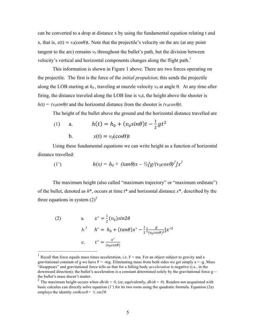
Table 8 reports the results generated by each program. The first column reports

the program used, the second reports the launch angle used and (when available) the

angle of impact. The final two columns show the maximum height and the range to

impact, in yards. For the Euler-Wade model and JBM Ballistics program we also include

the results at a range-maximizing launch angle.

The Euler-Wade program is the only program generating results at above 15° for

ranges extending out to impact. Thus, it provides impact angles for all launch angles. As

expected, these impact angles exceed the launch angles by a substantial margin. The

Euler-Wade maximum range results also conform reasonably well to the results of other

programs (excluding ColdBore). Because of its transparency, it ease of use, and the high

correlation of its results with the other programs, we consider Euler-Wade the most

useful of the programs reviewed, at least for purposes of maximum range estimation.

ColdBore claims to be the most comprehensive program: it has a large bullet

library, it allows several bullets to be simultaneously compared, it is rich in ballistics

information, and its user manual is outstanding. I can not judge how accurate it is for

hunters, marksmen, and military shooters, but I can assess how well it performs at the

long distances my purpose requires. The answer is, “not very well.” ColdBore’s

distances to impact reported in Table 8 are far greater than found for any other program,

and its angle of impact at 15°launch angle is only -16°; this is way too low—as if it

dramatically understates the drag coefficient by mimicking the parabolic arch associated

with no drag. Perhaps the reason is that it is based on Pesja’s work using approximations

that might induce greater error at longer distances. Whatever the reasons, we exclude

ColdBore from our range assessments, though we leave the ColdBore results in Table 9

so the reader can be aware of the issue.13

13 In communications with Patagonia Ballistics I was warned that ColdBore is designed for military and police use; it is not intended for use at the long ranges in which I am interested. Thus, ColdBore’s deficiencies at long ranges are no reason to discount its utility for its intended users. However, if you plan

33

Table 8 Estimates of Maximum Range 9mm MagTech 124 Grain Bullet Launch Angle Max Height Max Distance*

Source <Impact Angle> (yards) (yards) NRA Sourcebook 24° - 34° na 2,130

NLECTC* na na 2,300

Euler-Wade Solution (available in this paper) $0

15° <-33°> 30° <-60°> 33° <-64°> 45° <-74°>

205 560 639 950

1,960 2,305 2,310 2,195

Point Mass Solver (Applied Ballistics LLC)

$0

15° <-37°> 30° < na > 45° < na >

196 615

1,280

1,820 1,905† 1,855†

JBM Calculator (JBM Ballistics, Online)

$0

15° <-37°> 30° < na > 35° <-65°> 45° < na >

200 625

na na

1,850 2,260†

2,250 na

Sierra Infinity Suite (Sierra Bullets)

$40

15° <-37°> 30° < na > 45° < na >

230 510 845

1,830 2,035†

2,155† Ballistics Explorer

(Oehler Research)

$70

15° <-32°> 30° < na > 45° < na >

205 715

na

2,025 2,725†

na ColdBore 1.0

(Patagonia Ballistics)

$85

15° <-16°> 30° < na > 45° < na >

217 690

na

2,945 2,990†

na Results in blue font are direct estimates of the maximum range given by the program * NLECTC is the National Law Enforcement and Corrections Technology Center † Program does not allow a trajectory to impact. The maximum range is estimated using an estimate of the angle of descent from the bullet’s last reported position.

to imitate the 3,800-yard record for a sniper kill, you should not use ColdBore. And probably none of these programs would serve that need.

34

Page Intentionally Left Blank

35

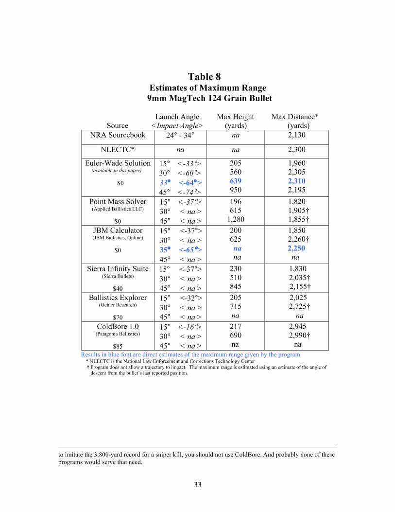
Conclusions

This paper began with a simple question: what is the maximum range of a bullet,

particularly a 9mm Luger handgun bullet? To derive an answer we first applied the

mathematics of trajectories without drag, in which trajectories are easily calculated as

parabolas with maximum range equal to twice the range at which the bullet reaches its

maximum height, and with an angle of impact always equals the angle of launch. The

maximum range, achieved with a 45° launch angle, is over seven miles, clearly an

unrealistic distance even for Rooster Cogburn.

Then we added aeronautical drag to the analysis, delving into the plumbing and

wiring behind drag. We reviewed the history of drag-related concepts like drag

coefficients and ballistic coefficients, and, having developed the basic foundations, we

used several different methods to calculate trajectories of a specific 9mm Luger bullet at

various launch angles. A rough summary of the results (excluding ColdBore) is shown

below.

Table 9 Summary Estimates of Maximum Range 9mm MagTech 124 Grain Bullet

Launch ___Range_____ Angle Min Max Mean

The first approach, dubbed the Euler-Wade method, uses the equations of motion

for projectiles with drag in a 2-DOF space: the two dimensions are vertical and horizontal,

there being no wind or other cross-range forces and no consideration of rotational forces.

This required inputs for bullet and atmospheric characteristics, as well as initial

15°

30°

45°

1790 2025

1905 2725

1850 2200

1865

2225

2005

36

conditions. These results are embedded in an EXCEL spreadsheet summarized in

Addendum 3.

The Euler-Wade method gives a 2,310-yard maximum range, achieved at a 33°

launch angle. This is close to the 2,130-yard maximum range reported by the National

Rifle Association (at launch angles of 24°-34°), and identical to the 2,300-yard range

reported by the National Law Enforcement and Corrections Technology Center,

An advantage of the Euler-Wade method is that we know precisely what goes into

the results. This is not true of the results from the use of “black box” ballistics software.

We have applied several different ballistics programs to our task: the Point Mass

Ballistics Solver, developed by Brian Litz, ballistician for Berger Bullets; the JBM

Ballistics Calculator, available online at JBM Ballistics; the Sierra Infinity Suite version

6, a commercial product of Sierra Bullets; and the ColdBore ballistics program from

Patagonia Software.

With the exclusion of ColdBore, the results generally confirm those from Euler-

Wade. A 9mm Luger-style handgun has a maximum range in windless conditions of

about 2,300 yards, or 1.3 miles. And, of course, the range is less at the lower launch

angles normally used.

Shoot Away!

37

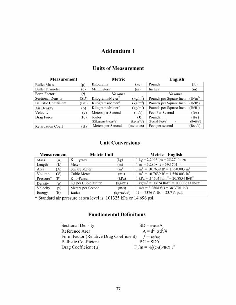
Addendum 1

Units of Measurement Measurement Metric English Bullet Mass (µ) Kilograms (kg) Pounds (lb) Bullet Diameter (d) Millimeters (m) Inches (in) Form Factor (f) No units No units Sectional Density (SD) Kilograms/Meter2 (kg/m2) Pounds per Square Inch (lb/in2) Ballistic Coefficient (BC) Kilograms/Meter2 (kg/m2) Pounds per Square Inch (lb/ft2) Air Density (ρ) Kilograms/Meter3 (kg/m3) Pounds per Square Inch (lb/ft3) Velocity (v) Meters per Second (m/s) Feet Per Second (ft/s) Drag Force (Fd) Joules (J)

(Kilogram-Meter/2s2 (kg•m2/s2) Poundal (ft/s) (Pound-Feet/s2

δ (lb•ft/s2)

Retardation Coeff (∆) Meters per Second (meters/s) Feet per second (feet/s) Unit Conversions Measurement Metric Unit Metric - English

Mass (µ) Kilo-gram (kg) 1 kg = 2.2046 lbs = 35.2740 ozs Length (L) Meter (m) 1 m = 3.2808 ft = 39.3701 in Area (A) Square Meter (m2) 1 m2 = 10.7639 ft2 = 1,550.003 in2 Volume (V) Cubic Meter (m3) 1 m3 = 10.7639 ft3 = 1,550.003 in3 Pressure* (P) Kilo-Pascal (kPa) 1 kPa = .14504 lb/in2 = 20.8854 lb/ft2

Density (ρ) Kg per Cubic Meter (kg/m3) 1 kg/m3 = .0624 lb/ft3 = .00003613 lb/in3

Velocity (v) Meters per Second (m/s) 1 m/s = 3.2808 ft/s = 38.3701 in/s Energy (E) Joules (kg•m2/s2) 1J = .7376 ft-lbs = 23.7 ft-pdls

* Standard air pressure at sea level is .101325 kPa or 14.696 psi. Fundamental Definitions Sectional Density SD = mass/A Reference Area A = d2 πd2/4 Form Factor (Relative Drag Coefficient) f = cS/cG Ballistic Coefficient BC = SD/f Drag Coefficient (µ) Fd/m = ½[(cG(ρ/BC)]v2

38

Page Intentionally Left Blank

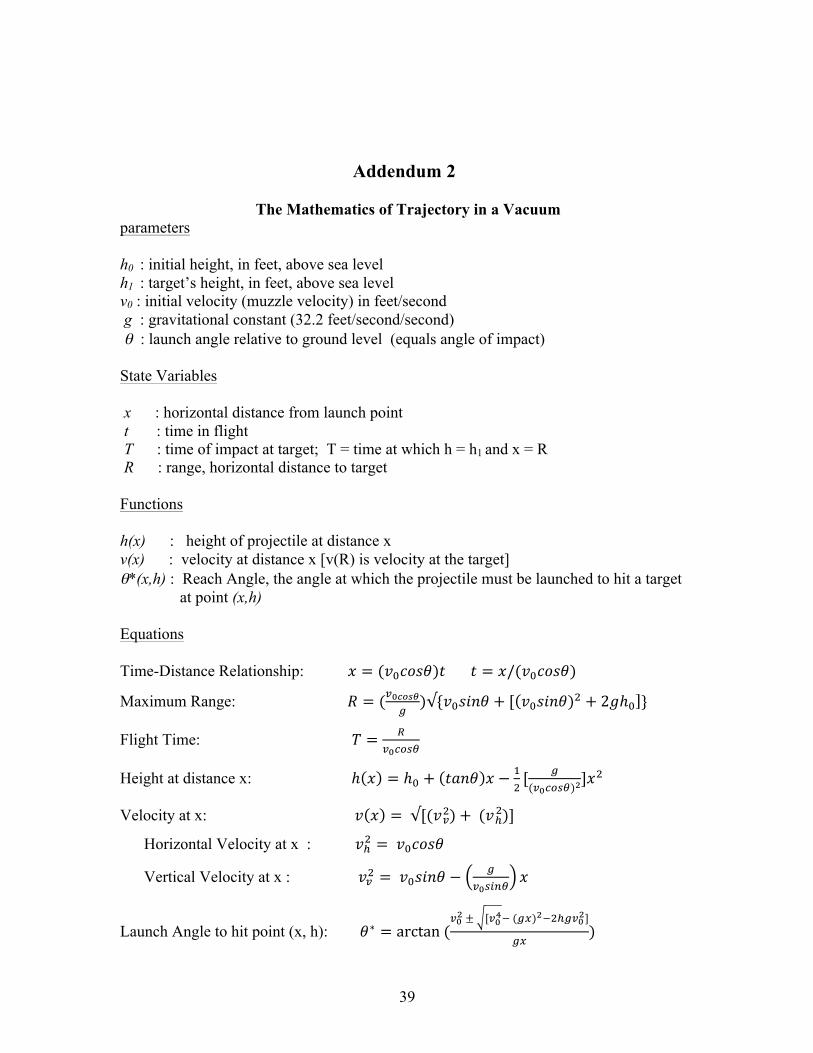
39

Addendum 2 The Mathematics of Trajectory in a Vacuum parameters h0 : initial height, in feet, above sea level h1 : target’s height, in feet, above sea level v0 : initial velocity (muzzle velocity) in feet/second g : gravitational constant (32.2 feet/second/second) θ : launch angle relative to ground level (equals angle of impact) State Variables x : horizontal distance from launch point t : time in flight T : time of impact at target; T = time at which h = h1 and x = R R : range, horizontal distance to target Functions h(x) : height of projectile at distance x v(x) : velocity at distance x [v(R) is velocity at the target] θ*(x,h) : Reach Angle, the angle at which the projectile must be launched to hit a target at point (x,h) Equations Time-Distance Relationship: 𝑥 = (𝑣!𝑐𝑜𝑠𝜃)𝑡 𝑡 = 𝑥/(𝑣!𝑐𝑜𝑠𝜃)

Maximum Range: 𝑅 = (!!!"#$!)√{𝑣!𝑠𝑖𝑛𝜃 + [ 𝑣!𝑠𝑖𝑛𝜃)! + 2𝑔ℎ! }

Flight Time: 𝑇 = !!!!"#$

Height at distance x: ℎ 𝑥 = ℎ! + 𝑡𝑎𝑛𝜃 𝑥 − !![ !(!!!"#$)!

]𝑥!

Velocity at x: 𝑣 𝑥 = √[(𝑣 )!! + (𝑣 )!! ]

Horizontal Velocity at x : 𝑣!! = 𝑣!𝑐𝑜𝑠𝜃

Vertical Velocity at x : 𝑣!! = 𝑣!𝑠𝑖𝑛𝜃 −!

!!!"#$𝑥

Launch Angle to hit point (x, h): 𝜃∗ = arctan (!!! ± [!!!! (!!)!!!"!!!!]

!")

40

Page Intentionally Left Blank

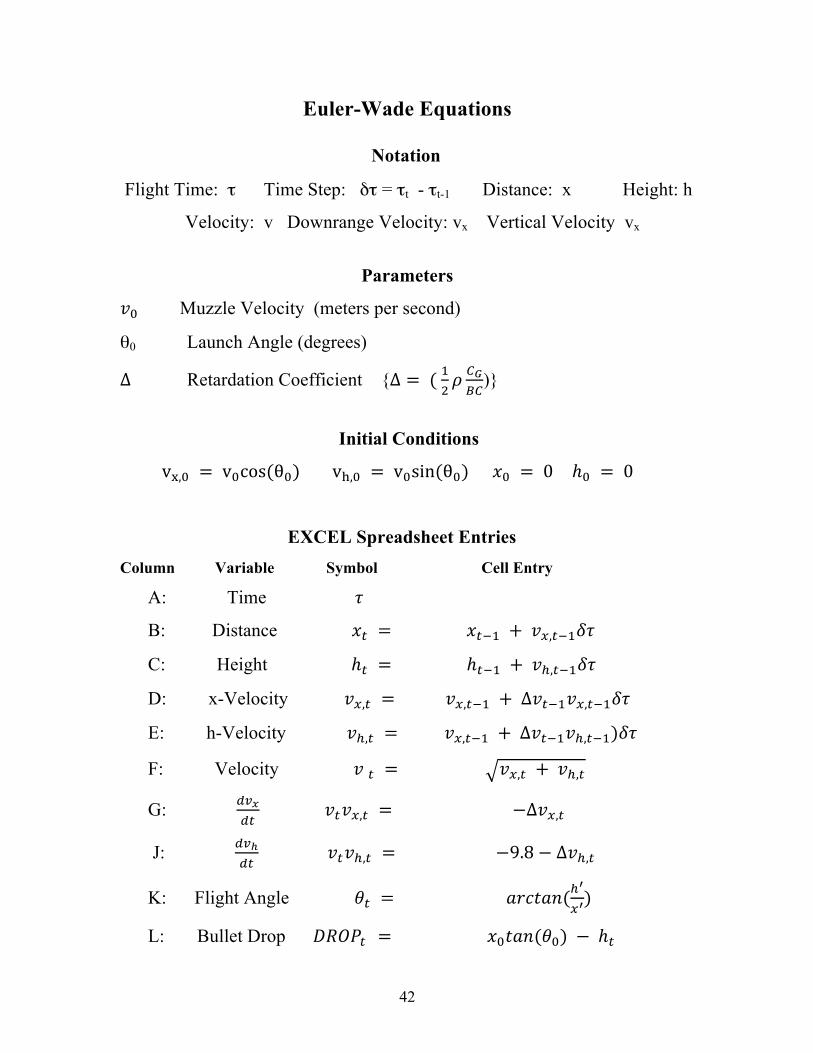
41

Formula View

Addendum 3 Euler-Wade EXCEL Spreadsheet Values View

42

Euler-Wade Equations Notation

Flight Time: τ Time Step: δτ = τt - τt-1 Distance: x Height: h

Velocity: v Downrange Velocity: vx Vertical Velocity vx

Parameters

𝑣! Muzzle Velocity (meters per second)

θ0 Launch Angle (degrees)

Δ Retardation Coefficient {Δ = ( !!𝜌 !!!"

)}

Initial Conditions

v!,! = v!cos(θ!) v!,! = v!sin(θ!) 𝑥! = 0 ℎ! = 0

EXCEL Spreadsheet Entries Column Variable Symbol Cell Entry

A: Time 𝜏

B: Distance 𝑥! = 𝑥!!! + 𝑣!,!!!𝛿𝜏

C: Height ℎ! = ℎ!!! + 𝑣!,!!!𝛿𝜏

D: x-Velocity 𝑣!,! = 𝑣!,!!! + ∆𝑣!!!𝑣!,!!!𝛿𝜏

E: h-Velocity 𝑣!,! = 𝑣!,!!! + ∆𝑣!!!𝑣!,!!!)𝛿𝜏

F: Velocity 𝑣 ! = 𝑣!,! + 𝑣!,!

G: !"!!"

𝑣!𝑣!,! = −Δ𝑣!,!

J: !"!!"

𝑣!𝑣!,! = −9.8 − Δ𝑣!,!

K: Flight Angle 𝜃! = 𝑎𝑟𝑐𝑡𝑎𝑛(!!

!!)

L: Bullet Drop 𝐷𝑅𝑂𝑃! = 𝑥!𝑡𝑎𝑛(𝜃!) − ℎ!

43

References

Books and Articles

Aboelkhir, M.S. and H. Yakout. 2013. Effect of Projectile Shape on the Power of Fire in Personal Defense Hand Held Weapons, Studies in System Science, Vol. 1 Issue 1, March, pp. 9-17. Bussard, Michael E. And S.L. Wormley. NRA Firearms Sourcebook, National Rifle Association, Fairfax VA. Courtney, Michael and A. Courtney. 2009. “Inaccurate Specifications of Ballistic Coefficients,” Varmint Hunter Magazine, January. Litz, Bryan. 2011. Applied Ballistics for Long-Range Shooting, Applied Ballistics LLC, Cedar Springs WI. McCoy, R.L. 2009. Modern Exterior Ballistics: The Launch and Flight Dynamics of Symmetric Projectiles, Schiffer Publishing, Atglen PA, 2009. Pesja, Arthur J. 2001, Modern Practical Ballistics, Kenwood Publishing, Minneapolis MN. Plaster, Major John L. www.milletsights.com/dowloads/ShootingUphillandDownhill.com Wade, Amanda. 2011. Going Ballistic: Bullet Trajectories, Undergraduate Journal of Mathematical Modeling: One and Two, Vol 5, Issue 1, Article 5. Weinacht, Paul, G.R. Cooper, and J.F. Newell. Analytical Prediction of Trajectories for High-Velocity Direct-Fire Munitions, Army Research Laboratory ARL-TR-3567, Aberdeen Proving Ground, MD. August 2005. Software Ballistic Explorer v6, Oehler Research Inc. (MS Windows) JBM Ballistics Calculator, www.jbmballistics.com Point Mass Ballistics Solver 2.0, Advanced Ballistics LLC (Apple OSX) Sierra Infinity Suite v6 Software, Sierra Bullets (MS Windows) ColdBore1, from Patagonia Ballistics (MS Windows)