Mixed discriminants

MIXED DISCRIMINANTS

EDUARDO CATTANI, MARIA ANGELICA CUETO, ALICIA DICKENSTEIN,SANDRA DI ROCCO, AND BERND STURMFELS

Abstract. The mixed discriminant of n Laurent polynomials in n variables is the irre-ducible polynomial in the coefficients which vanishes whenever two of the roots coincide.The Cayley trick expresses the mixed discriminant as an A-discriminant. We show that thedegree of the mixed discriminant is a piecewise linear function in the Plucker coordinates ofa mixed Grassmannian. An explicit degree formula is given for the case of plane curves.

Dedicated to the memory of our friend Mikael Passare (1959–2011)

1. Introduction

A fundamental topic in mathematics and its applications is the study of systems of npolynomial equations in n unknowns x = (x1, x2, . . . , xn) over an algebraically closed field K:

(1.1) f1(x) = f2(x) = · · · = fn(x) = 0.

Here we consider Laurent polynomials with fixed support sets A1, A2, . . . , An ⊂ Zn:

(1.2) fi(x) =∑a∈Ai

ci,axa (i = 1, 2, . . . , n).

If the coefficients ci,a are generic then, according to Bernstein’s Theorem [3], the number ofsolutions of (1.1) in the algebraic torus (K∗)n equals the mixed volume MV(Q1, Q2, . . . , Qn)of the Newton polytopes Qi = conv(Ai) in Rn. However, for special choices of the coef-ficients ci,a, two or more of these solutions come together in (K∗)n and create a point ofhigher multiplicity. The conditions under which this happens are encoded in an irreduciblepolynomial in the coefficients, whose zero locus is the variety of ill-posed systems [18, §I-4].While finding this polynomial is usually beyond the reach of symbolic computation, it isoften possible to describe some of its invariants. Our aim here is to characterize its degree.

An isolated solution u ∈ (K∗)n of (1.1) is a non-degenerate multiple root if the n gradientvectors ∇xfi(u) are linearly dependent, but any n−1 of them are linearly independent. Thiscondition means that u is a regular point on the curve defined by any n− 1 of the equationsin (1.1). We define the discriminantal variety as the closure of the locus of coefficients ci,a forwhich the associated system (1.1) has a non-degenerate multiple root. If the discriminantalvariety is a hypersurface, we define the mixed discriminant of the system (1.1) to be theunique (up to sign) irreducible polynomial ∆A1,...,An with integer coefficients in the unknownsci,a which defines it. Otherwise we say that the system is defective and set ∆A1,...,An = 1.

In the non-defective case, we may identify ∆A1,...,An with an A-discriminant in the senseof Gel’fand, Kapranov and Zelevinsky [12]. A is the Cayley matrix (2.1) of A1, . . . , An. This

2010 Mathematics Subject Classification. 13P15, 14M25, 14T05, 52B20.Key words and phrases. A-discriminant, degree, multiple root, Cayley polytope, tropical discriminant,

matroid strata, mixed Grassmannian.1

arX

iv:1

112.

1012

v1 [

mat

h.A

G]

5 D

ec 2

011

2 E. CATTANI, M. A. CUETO, A. DICKENSTEIN, S. DI ROCCO, AND B. STURMFELS

matrix has as columns the vectors in the lifted configurations ei ×Ai ∈ Z2n for i = 1, . . . , n.The relationship between ∆A1,...,An and the A-discriminant will be made precise in Section 2.

In Section 3 we focus on the case n = 2. Here, the mixed discriminant ∆A1,A2 expressesthe condition for two plane curves f1 = 0 and f2 = 0 to be tangent at a common smoothpoint. In Theorem 3.3 we present a general formula for the bidegree (δ1, δ2) of ∆A1,A2 . Innice special cases, to be described in Corollary 3.15, that formula simplifies to

(1.3)δ1 = area(Q1 +Q2)− area(Q1)− perim(Q2),

δ2 = area(Q1 +Q2)− area(Q2)− perim(Q1),

where Qi is the convex hull of Ai and Q1+Q2 is their Minkowski sum. The area is normalizedso that a primitive triangle has area 1. The perimeter of Qi is the cardinality of ∂Qi ∩ Z2.

The formula (1.3) applies in the classical case, where f1 and f2 are dense polynomials ofdegree d1 and d2. Here, ∆A1,A2 is the classical tact invariant [17, §96] whose bidegree equals

(1.4) (δ1, δ2) =(d22 + 2d1d2 − 3d2, d

21 + 2d1d2 − 3d1

).

See Benoist [2] and Nie [15] for the analogous formula for n dense polynomials in n vari-ables. The right-hand side of (1.3) is always an upper bound for the bidegree of the mixeddiscriminant, but in general the inequality is strict. Indeed, consider two sparse polynomials

(1.5) f1(x1, x2) = c10 + c11xd11 + c12x

d12 and f2(x1, x2) = c20 + c21x

d21 + c22x

d22 ,

with d1 and d2 positive coprime integers, then the bidegree drops from (1.4) to

(1.6)(d22 + 2d1d2 − 3d2 ·mind1, d2, d21 + 2d1d2 − 3d1 ·mind1, d2

).

In Section 4 we prove that the degree of the mixed discriminant, in the natural Zn-grading,is a piecewise polynomial function in the coordinates of the points in A1, A2, . . . , An.

Theorem 1.1. The degree of the mixed discriminant cycle is a piecewise linear function inthe Plucker coordinates on the mixed Grassmannian G(2n, I). It is linear on the tropicalmatroid strata of G(2n, I) determined by the configurations A1, . . . , An. The formula on eachmaximal stratum is unique modulo the linear forms on ∧2nRm that vanish on G(2n, I).

Here, the cycle refers to the mixed discriminant raised to a power that expresses the indexin Zn of the sublattice affinely spanned by A1∪ · · ·∪An. The mixed Grassmannian G(2n, I)parameterizes all 2n-dimensional subspaces of Rm that arise as row spaces of Cayley matri-ces (2.1) with m =

∑ni=1 |Ai| columns, and I is the partition of 1, . . . ,m specified by the n

configurations. This Grassmannian is regarded as a subvariety in the exterior power ∧2nRm,via the Plucker embedding by the maximal minors of the matrix (2.1). See Definition 4.2 fordetails. The mixed Grassmannian admits a combinatorial stratification into tropical matroidstrata, and our assertion says that the degree of the mixed discriminant cycle is a polyno-mial on these strata. The proof of Theorem 1.1 is based on tropical algebraic geometry, andspecifically on the combinatorial construction of the tropical discriminant in [7].

MIXED DISCRIMINANTS 3

2. Cayley Configurations

Let A1, . . . , An be configurations in Zn, defining Laurent polynomials as in (1.2). We shallrelate the mixed discriminant ∆A1,...,An to the A-discriminant, where A is the Cayley matrix

(2.1) A = Cay(A1, . . . , An) =

1 0 · · · 00 1 · · · 0...

.... . .

...0 0 · · · 1A1 A2 · · · An

.

This matrix has 2n rows and m =∑n

i=1 |Ai| columns, so 0 = (0, . . . , 0) and 1 = (1, . . . , 1)denote row vectors of appropriate lengths. We introduce n new variables y1, y2, . . . , yn andencode our system (1.1) by one auxiliary polynomial with support in A, via the Cayley trick :

φ(x, y) = y1f1(x) + y2f2(x) + · · · + ynfn(x).

We denote by ∆A the A-discriminant as defined in [12]. That is, ∆A is the unique (up tosign) irreducible polynomial with integer coefficients in the unknowns ci,a which vanisheswhenever the hypersurface (x, y) ∈ (K∗)2n : φ(x, y) = 0 is not smooth. Equivalently, ∆A

is the defining equation of the dual variety (XA)∨ when this variety is a hypersurface. Here,XA denotes the projective toric variety in Pm−1 associated with the Cayley matrix A. If(XA)∨ is not a hypersurface, then no such unique polynomial exists. We then set ∆A = 1and refer to A as a defective configuration. It is useful to keep track of the lattice index

i(A) = i(A,Z2n) =[Z2n : Z·A

],

where Z·A is the Z-linear span of the columns of A. The discriminant cycle is the polynomial

∆A = ∆i(A)A .

The same construction makes sense for the mixed discriminant and it results in the mixeddiscriminant cycle ∆A1,...,An . The exponents i(A) will be compatible in the following theorem.

Theorem 2.1. The mixed discriminant equals the A-discriminant of the Cayley matrix:

∆A1,...,An = ∆A.

This result is more subtle than it may seem at first glance. It implies that (A1, . . . , An) isdefective if and only if A is defective. The two discriminantal varieties can differ in that case.

Example 2.2. Let n = 2 and consider the Cayley matrix

A =

1 00 1A1 A2

=

1 1 1 0 0 00 0 0 1 1 10 1 2 0 0 00 0 0 0 1 2

The corresponding system (1.1) consists of two univariate quadrics in different variables:

f1(x1) = c10 + c11x1 + c12x21 = 0 and f2(x2) = c20 + c21x2 + c22x

22 = 0.

This system cannot have a non-degenerate multiple root, for any choice of coefficients cij, sothe (A1, A2)-discriminantal variety is empty. On the other hand, the A-discriminantal varietyis non-empty. It has codimension two and is defined by c211 − 4c10c12 = c221 − 4c20c22 = 0. ♦


Proof of Theorem 2.1. We may assume i(A) = 1. Let u ∈ (K∗)n be a non-degeneratemultiple root of f1(x) = · · · = fn(x) = 0. Our definition ensures the existence of a unique(up to scaling) vector v ∈ (K∗)n such that

∑ni=1 vi∇xfi(u) is the zero vector. The pair (u, v) ∈

(K∗)2n is a singular point of the hypersurface defined by φ(x, y) = 0. By projecting into thespace of coefficients ci,a, we see that the (A1, . . . , An)-discriminantal variety is contained inthe A-discriminantal variety. Example 2.2 shows that this containment can be strict.

We now claim that ∆A 6= 1 implies ∆A1,...,An 6= 1. This will establish the propositionbecause ∆A1,...,An is a factor of ∆A, and ∆A is irreducible, so the two discriminants areequal. Each point (u, v) ∈ (K∗)2n defines a point on XA. If ∆A 6= 1, the dual variety (XA)∨

is a hypersurface in the dual projective space (Pm−1)∨. Moreover, see e.g. [13], a generichyperplane in the dual variety is tangent to the toric variety XA at a single point.

Consider a generic point on the conormal variety of XA in Pm−1×(Pm−1)∨. It is representedby a pair

((u, v), c

), where (u, v) ∈ (K∗)2n and c is the coefficient vector of a polynomial

φ(x, y) such that (u, v) is the unique singular point on φ(x, y) = 0. The coefficient vectorc defines a point on the (A1, . . . , An)-discriminantal variety unless we can relabel such thatthe gradients of f1, . . . , fn−1 are linearly dependent at u. Assuming that this holds, we let

n−1∑i=1

ti∇xfi(u) = 0

be the dependency relation and set t = (t1, . . . , tn−1, 0) 6= 0. The point((t + u, v), c

)lies

on the conormal variety of XA. This implies that the generic hyperplane defined by c istangent to XA at two distinct points (u, v) 6= (t + u, v), which cannot happen. It followsthat ∆A1,...,An 6= 1, as we wanted to show. This concludes our proof.

Example 2.3. Let n = 2 and A1 = A2 = (0, 0), (1, 0), (0, 1), (1, 1), a unit square. Then

f1(x1, x2) = a00 + a10x1 + a01x2 + a11x1x2,

f2(x1, x2) = b00 + b10x1 + b01x2 + b11x1x2.

The Cayley configuration A is the standard 3-dimensional cube. The A-discriminant isknown to be the hyperdeterminant of format 2×2×2, by [12, Chapter 14], which equals

∆A1,A2 = a200b211 − 2a00a01b10b11 − 2a00a10b01b11 − 2a00a11b00b11

+4a00a11b01b10 + a201b210 + 4a01a10b00b11 − 2a01a10b01b10

−2a01a11b00b10 + a210b201 − 2a10a11b00b01 + a211b

200.

Theorem 2.1 tells us that this hyperdeterminant coincides with the mixed discriminant of f1and f2. Note that the bidegree equals (δ1, δ2) = (2, 2), and therefore (1.3) holds. ♦

We now shift gears and focus on defective configurations. We know from Theorem 2.1 that(A1, . . . , An) is defective if and only if the associated Cayley configuration A is defective.While there has been some recent progress on characterizing defectiveness [7, 10, 14], theproblem of classifying defective configurations A remains open, except in cases when thecodimension of A is at most four [6, 8] or when the toric variety XA is smooth or Q-factorial[4, 9]. Recall that XA is smooth if and only if, at each every vertex of the polytope Q =conv(A), the first elements of A that lie on the incident edge directions form a basis for thelattice spanned by A. The variety XA is Q-factorial when Q is a simple polytope, that is,when every vertex of Q lies in exactly dim(Q) facets. Note that smooth implies Q-factorial.


We set dim(A) = dim(Q), and we say that A is dense if A = Q ∩ Zd. A subset F ⊂ A iscalled a face of A, denoted F ≺ A, if F is the intersection of A with a face of the polytopeQ. We will denote by sn the standard n-simplex and by σn the configuration of its vertices.

When A is the Cayley configuration of A1, . . . , An ⊂ Zn, the codimension of A is m− 2n.This number is usually rather large. For instance, if all n polytopes Qi = conv(Ai) arefull-dimensional in Rn then codim(A) > n · (n − 1), and thus, for n > 3, we are outsidethe range where defective configurations have been classified. However, if n = 2 and theconfigurations A1 and A2 are full-dimensional we can classify all defective configurations.

Proposition 2.4. Let A1, A2 ⊂ Z2 be full-dimensional configurations. Then, (A1, A2) isdefective if and only if, up to affine isomorphism, A1 and A2 are both translates of p · σ2,for some positive integer p.

Proof. Let A = Cay(A1, A2). Both A1 and A2 appear as faces of A. In order to prove that Ais non-defective, it suffices to exhibit a 3-dimensional non-defective subconfiguration (see [5,Proposition 3.1] or [10, Proposition 3.13]). Let u1, u2, u3 be non-collinear points in A1 andv1, v2 distinct points in A2. The subconfiguration u1, u2, u3, v1, v2 of A is 3-dimensionaland non-defective if and only if no four of the points lie in a hyperplane or, equivalently, ifthe vector v2 − v1 is not parallel to any of the vectors uj − ui, j 6= i. We can always findsuch subconfigurations unless A1 and A2 are the vertices of triangles with parallel edges. Inthe latter case, we can apply an affine isomorphism to get A1 = p · σ2 and A2 a translate of±q ·σ2, where p and q are positive integers. The total degree of the mixed discriminant equals

deg(∆p·σ2,q·σ2) = (p2 + q2 + pq − 3 minp, q2)/gcd(p, q)2,

deg(∆p·σ2,−q·σ2) = (p+ q)2/gcd(p, q)2.

The first formula follows from (1.6) and it is positive unless p = q. The second formula willbe derived in Example 3.10. It always gives a positive number. This concludes our proof.

Similar arguments can be used to study the case when one of the configurations is one-dimensional. However, it is more instructive to classify such defective configurations fromthe bidegree of the mixed discriminant. This will be done in Section 3.

Corollary 2.5. Let A1 and A2 be full-dimensional configurations in Z2. Then the mixeddiscriminantal variety of (A1, A2) is either a hypersurface or empty.

Remark 2.6. The same result holds in n dimensions when the toric variety XA is smooth andA1, . . . , An are full-dimensional configurations in Zn. Under these hypotheses, (A1, . . . , An)is defective if and only if each Ai is affinely equivalent to p · σn, with p ∈ N. In particular,the mixed discriminantal variety of (A1, . . . , An) is either a hypersurface or empty. The “if”direction is straightforward: we may assume i(A) = 1 and p = 1 by replacing Zn with thelattice spanned by pe1, . . . , pen. Then, the system (1.1) consists of linear equations, and itis clearly defective. The “only-if” direction is derived from results in [9]: (A1, . . . , An) isdefective if and only if the (2n − 1)-dimensional polytope Q = conv(A) is isomorphic to aCayley polytope of at least t + 1 ≥ n + 1 configurations of dimension k < t that have thesame normal fan. As we already have a Cayley structure of n configurations in dimension n,we deduce t = n and k = n− 1. Then, we should have Q ' sn−1 × sn ' sn × sn−1. After anaffine transformation, all n polytopes Qi are standard n-simplices and all Ai are translatesof sn. This shows that A has an ”inverted” Cayley structure of n+ 1 copies of σn−1.


We expect Proposition 2.4 to hold in n dimensions without the smoothness hypothesisin Remark 2.6. Clearly, whenever the mixed volume of Q1, . . . , Qn is 1, then there are nomultiple roots and we have ∆A1,...,An = 1. The following result gives a necessary and sufficientcondition for being in this situation: up to affine equivalence, this is just the linear case.

Proposition 2.7. If A1, . . . , An are n-dimensional configurations in Zn then the mixed vol-ume MV(Q1, . . . , Qn) is 1 if and only if, up to affine isomorphism, A1 = · · · = An = σn.

Proof. We shall prove the “only-if” direction by induction on n. Suppose MV(Q1, Q2, . . . , Qn) =1. By the Aleksandrov-Fenchel inequality, we have vol(Qi) = 1 for all i, where the volumeform is normalized so that the standard n-simplex has volume 1. Since the mixed volumefunction is monotone in each coordinate, for any choice of edges li in Qi we have

0 6 MV(l1, l2, . . . , ln) 6 MV(l1, Q2, . . . , Qn) 6 MV(Q1, . . . , Qn) = 1.

Since all polytopesQi are full-dimensional, we can pick n linearly independent edges l1, . . . , ln.Therefore MV(l1, . . . , ln) > 0 and MV(l1, l2, . . . , ln) = MV(l1, Q2, . . . , Qn) = 1. In particular,the edge l1 has length one. After a change of coordinates we may assume that l1 = en, then-th standard basis vector. Denote by π the projection of Zn onto Zn/Z·en ' Zn−1 and thecorresponding map of R-vector spaces. We then have MV(π(Q2), . . . , π(Qn)) = 1.

By the induction hypothesis, we can transform the first n−1 coordinates so that π(A2) =· · · = π(An) = σn−1. This means that Ai ⊂ σn−1 × Z·en. Now, let ai be a point in Ai notlying in the coordinate hyperplane xn = 0. Then 1 6 vol(conv(σn−1, ai)) 6 vol(Qi) = 1, andwe conclude that Qi = conv(σn−1, ai). But, since vol(Qi) = 1, it follows that ai = bi ± en,for some bi ∈ σn−1. By repeating this process with an edge of A1 containing the point a1,we see that all bi’s are equal and that the sign of en in all ai’s is the same. This shows that,after an affine isomorphism, we have A1 = · · · = An = σn, yielding the result.

3. Two Curves in the Plane

In this section we study the condition for two plane curves to be tangent. This conditionis the mixed discriminant in the case n = 2. Our primary goal is to prove Theorem 3.3,which gives a formula for the bidegree of the mixed discriminant cycle of two full-dimensionalplanar configurations A1 and A2. Remark 3.11 addresses the degenerate case when one of theAi is one-dimensional. Our main tool is the connection between discriminants and principaldeterminants. In order to make this connection precise, and to define all the terms appearingin (3.3), we recall some basic notation and facts. We refer to [10, 12] for further details.

Let A ⊂ Zd and Q the convex hull of A. As is customary in toric geometry, we assume thatA lies in a rational hyperplane that does not pass through the origin. This holds for Cayleyconfigurations (2.1). Given any subset B ⊂ A we denote by Z ·B, respectively R ·B, thelinear span of B over Z, respectively over R. For any face F ≺ A we define the lattice index

i(F,A) :=[R·F ∩ Zd : Z·F

].

We set i(A) = i(A,A) = [Zd : Z·A]. We consider the A-discriminant ∆A and the principalA-determinant EA. They are defined in [12] under the assumption that i(A) = 1. If i(A) > 1then we change the ambient lattice from Zd to Z·A, and we define the associated cycles

EA = Ei(A)A and ∆A = ∆

i(A)A .

The expressions on the right-hand sides are computed relative to the lattice Z·A.


Remark 3.1. The principal A-determinant of [12, Chapter 10] is a polynomial EA in thevariables cα, α ∈ A. Its Newton polytope is the secondary polytope of A, and its degree is(d+ 1) vol(conv(A)), where vol = volZ·A is the normalized lattice volume for Z·A. We alwayshave deg(EA) = (d+ 1) volZd(conv(A)), where volZd is the normalized lattice volume for Zd.

We state the factorization formula of Gel’fand, Kapranov and Zelevinsky [12, Theorem1.2, Chapter 10] for the principal A-determinant as in Esterov [10, Proposition 3.10]:

(3.1) EA = ±∆A ·∏F≺A

∆u(F,A)F .

The product runs over all proper faces of A. The exponents u(F,A) are computed as follows.Let π denote the projection to R·A/R·F and Ω the normalized volume form on R·A/R·F .This form is normalized with respect to the lattice π(Zd), so that the fundamental domainwith respect to integer translations has volume (dim(R·A)− dim(R·F ))!. We set

u(F,A) := Ω(conv(π(A)) \conv(π(A\F ))

).

Remark 3.2. The positive integers u(F,A) are denoted cF,A in [10]. If i(A) = 1 then u(F,A)is the subdiagram volume associated with F , as in [12, Theorem 3.8, Chapter 5].

We now specialize to the case of Cayley configurations A = Cay(A1, A2), where A1, A2 ⊂Z2 are full-dimensional. Here, A is a 3-dimensional configuration in the hyperplane x1+x2 =1 in R4. Note that i(A,Z4) = i(A1 ∪A2,Z2). The configurations A1 and A2 are facets of A.

We say that F is a vertical face of A if F ≺ A but F 6≺ Ai, i = 1, 2. The vertical facetsof A are either triangles or two-dimensional Cayley configurations defined by edges e ≺ A1

and f ≺ A2. This happens if e and f are parallel and have the same orientation, that is, ifthey have the same inward normal direction when viewed as edges in Q1 and Q2. We callsuch edges strongly parallel and denote the vertical facet they define by V (e, f).

Let Ei denote the set of edges of Ai and set

P = (e, f) ∈ E1 × E2 : e is strongly parallel to f.

We write `(e) for the normalized length of an edge e with respect to the lattice Z2. Forv ∈ A1 we define

(3.2) mm(v) = MV(Q1, Q2)−MV(conv(A1\v), Q2),

and similarly for v ∈ A2. This quantity is the mixed multiplicity of v in (A1, A2).

Theorem 3.3. Let A1 and A2 be full-dimensional configurations in Z2. Then

δ1 := degA1(∆A1,A2) = area(Q2) + 2 MV(Q1, Q2)

−∑

(e,f)∈P

minu(e, A1), u(f, A2) `(f) −∑

v∈VertA1

mm(v).(3.3)

δ2 := degA2(∆A1,A2) = area(Q1) + 2 MV(Q1, Q2)

−∑

(e,f)∈P

minu(e, A1), u(f, A2) `(e) −∑

v∈VertA2

mm(v).


Theorem 3.3 is the main result in this section. We shall derive it from the following formula(which is immediate from (3.1)) for the bidegree of our mixed discriminant:

(3.4) bideg(∆A1,A2) = bideg(EA) −2∑

k=1

∑F≺Ak

u(F,A) bideg(∆F ) −∑F≺A

vertical

u(F,A) bideg(∆F ).

Note the need for the cycles ∆A1,A2 , EA and ∆F in this formula. We shall prove Theorem 3.3by studying each term on the right-hand side of (3.4), one dimension at a time. A series oflemmas facilitates the exposition.

Lemma 3.4. The bidegree bideg(EA) of the principal A-determinantal cycle EA equals

(3.5) (3 area(Q1) + area(Q2) + 2 MV(Q1, Q2), area(Q1) + 3 area(Q2) + 2 MV(Q1, Q2)).

Proof. By [12], the total degree of EA is 4 vol(Q). From any triangulation of A we can see

vol(Q) = area(Q1) + area(Q2) + MV(Q1, Q2).

Examining the tetrahedra in a triangulation reveals that the bidegree is given by (3.5).

Any pyramid is a defective configuration; hence, the vertical facets of Q that are trianglesdo not contribute to the right-hand side of (3.4) and can be safely ignored from now on. Inparticular, we see that the only non-defective vertical facets are the trapezoids V (e, f) for(e, f) ∈ P . The following lemma explains their contribution to (3.4).

Lemma 3.5. Let V (e, f) be the vertical facet of A associated with (e, f) ∈ P. Then

(1) bideg(∆V (e,f)) = (`(f), `(e)),

(2) u(V (e, f), A) = minu(e, A1), u(f, A2).

Proof. The configuration V (e, f) is the Cayley lift of two one-dimensional configurations. Itsdiscriminantal cycle is the resultant of two univariate polynomials of degree `(e) and `(f),so (1) holds. In order to prove (2), we note that u(V (e, f), Q) equals the normalized lengthof a segment in R3/R·V (e, f) starting at the origin and ending at the projection of a point inA1 or A2. This image is the closest point to the origin in the line generated by the projectionof Q. Thus, the multiplicity u(V (e, f), A) is the minimum of u(e, A1) and u(f, A2).

We next study the horizontal facets of A given by A1 and A2.

Lemma 3.6. The discriminant cycle of the plane curve defined by Ai has total degree

deg(∆Ai) = 3 area(Qi)−

∑e∈EdgesAi

u(e, Ai) deg(∆e) −∑

v∈VertAi

u(v, Ai),

where u(v,Ai) = area(Qi)− area(conv(Ai\v)).

Proof. This is a special case of (3.4) because deg(EAi) = 3 · area(Qi) and deg(∆v) = 1 for

any vertex v ∈ Ai. The statement about u(v, Ai) is just its definition.

Next, we consider the edges of A. The vertical edges are defective since they consist ofjust two points. Thus we need only examine the edges of A1 and A2.

Lemma 3.7. Let e be an edge of Ai. Then u(e, A) = u(e, Ai).


Proof. Consider the projection π : Qi → R2/R ·e. The image π(Qi) is a segment of lengthM1 = max`([0, π(m)]) : m ∈ Ai, while conv(Ai\e) projects to a segment of length M2 =max`([0, π(m)]) : m ∈ (Ai\e). Thus u(e, Ai) = M1 −M2. Next, consider the projectionQ→ R3/R·e. The images of A and conv(A\e) under this projection are trapezoids in R3/R·e.Their set-theoretic difference is a triangle of height 1 and base M2 −M1.

Lemma 3.8. Let v be a vertex of Ai. Then u(v,A) = u(v,Ai) + mm(v).

Proof. Suppose v ∈ A1. The volume form Ω is normalized with respect to the lattice Z3.The volume of our Cayley polytope Cay(A1, A2) equals area(Q1) + area(Q2) + MV(Q1, Q2),and the analogous formula holds for conv(A\v) = Cay(A1\v, A2). We conclude

u(v,A) = vol(Cay(A1, A2))− vol(Cay(A1\v,A2))

= area(Q1)− area(conv(A1\v) + MV(Q1, Q2)−MV(conv(A1\v), Q2))

= u(v,A1) + mm(v).

Proof of Theorem 3.3. By symmetry, it suffices to prove (3.3). We start with the A1-degreeof the principal A-determinantal cycle EA given in (3.5). In light of (3.1), we subtract theA1-degrees of the various discriminant cycles corresponding to all faces of A. Besides thecontribution from A1, having u(A1, A) = 1 and given by Lemma 3.6, only the vertices andthe vertical facets contribute. Using Lemmas 3.7 and 3.8, we derive the desired formula.

At this point, the reader may find it an instructive exercise to derive (1.4) and (1.6) fromTheorem 3.3, and ditto for (δ1, δ2) = (2, 2) in Example 2.3. Here are two further examples.

Example 3.9. Let A1 and A2 be the dense triangles (d1s2) ∩ Z2 and (−d2s2) ∩ Z2. Here,i(A) = 1 and ∆A1,A2 = ∆A1,A2 . We have MV(d1s2,−d2s2) = 2d1d2 and P = ∅. Computationof the mixed areas in (3.2) yields mm(v) = d2 for vertices v ∈ A1 and mm(v) = d1 forvertices v ∈ A2. We conclude

bideg(∆A1,A2) =(d22 + 4d1d2 − 3d2, d

21 + 4d1d2 − 3d1

). ♦

Example 3.10. Let A1 = d1σ2 and A2 = −d2σ2. This is the sparse version of Exam-

ple 3.9. Now, i(A) = g2, where g = gcd(d1, d2), and ∆A1,A2 = ∆g2

A1,A2. We still have

MV(d1s2,−d2s2) = 2d1d2 and P = ∅, but mm(v) = d1d2 for all v ∈ A. Hence

bideg(∆A1,A2) =1

g2(d22 + d1d2, d

21 + d1d2

). ♦

Remark 3.11. From (3.4) we may also derive formulas for the bidegree of the mixed dis-criminant in the case when one of the configurations, say A2, is one-dimensional. The maindifferences with the proof of Theorem 3.3 is that now we must treat A2 as an edge, ratherthan a facet, and that it is enough for an edge e of Q1 to be parallel to Q2 in order to have anon-defective vertical facet of Q. Clearly, there are at most two possible edges of Q1 parallelto Q2. The A2-degree of the mixed discriminant cycle now has a very simple expression:

(3.6) δ2 = area(Q1)−∑e||Q2

u(e, A1)`(e),

where the sum runs over all edges e of Q1 which are parallel to Q2.In particular, if no edge of Q1 is parallel to Q2, then δ2 > 0 and (A1, A2) is not defective.

If only one edge e of Q1 is parallel to Q2 then δ2 = 0 if and only if area(Q1) = u(e, A1)`(e)but this happens only if there is a single point of A1 not lying in the edge e. This means that


A = Cay(A1, A2) is a pyramid and hence is defective. Finally, if there are two edges e1 ande2 of Q1 parallel to Q2 then δ2 = 0 if and only if area(Q1) = u(e1, A1)`(e1) + u(e2, A1)`(e2).This can only happen if all the points of A1 lie either in e1 or e2. In this case, A is the Cayleylift of three one-dimensional configurations, and it is defective as well.

Our next goal is to provide a sharp geometric bound for the sum of the mixed multiplicities.We start by providing a method to compute such invariants by means of mixed subdivisions.

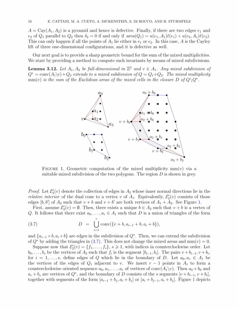
Lemma 3.12. Let A1, A2 be full-dimensional in Z2 and v ∈ A1. Any mixed subdivision ofQ∗ = conv(A1\v)+Q2 extends to a mixed subdivision of Q = Q1+Q2. The mixed multiplicitymm(v) is the sum of the Euclidean areas of the mixed cells in the closure D of Q\Q∗.

va3

a0

a1

a2

b0

b1

b2

v + b0

v + b1

v + b2

a3 + b2

a0 + b0

a1 + b0

a2 + b0

a2 + b1

a2 + b2

Figure 1. Geometric computation of the mixed multiplicity mm(v) via asuitable mixed subdivision of the two polygons. The region D is shown in grey.

Proof. Let E ′2(v) denote the collection of edges in A2 whose inner normal directions lie in therelative interior of the dual cone to a vertex v of A1. Equivalently, E ′2(v) consists of thoseedges [b, b′] of A2 such that v + b and v + b′ are both vertices of A1 + A2. See Figure 1.

First, assume E ′2(v) = ∅. Then, there exists a unique b ∈ A2 such that v + b is a vertex ofQ. It follows that there exist a0, . . . , ar ∈ A1 such that D is a union of triangles of the form

(3.7) D =r⋃i=1

conv(v + b, ai−1 + b, ai + b),

and ai−1+b, ai+b are edges in the subdivision of Q∗. Then, we can extend the subdivisionof Q∗ by adding the triangles in (3.7). This does not change the mixed areas and mm(v) = 0.

Suppose now that E ′2(v) = f1, . . . , fs, s > 1, with indices in counterclockwise order. Letb0, . . . , bs be the vertices of A2 such that fi is the segment [bi−1, bi]. The pairs v+ bi−1, v+ bi,for i = 1, . . . , s, define edges of Q which lie in the boundary of D. Let a0, ar ∈ A1 bethe vertices of the edges of Q1 adjacent to v. We insert r − 1 points in A1 to form acounterclockwise oriented sequence a0, a1, . . . , ar of vertices of conv(A1\v). Then a0 + b0 andar + bs are vertices of Q∗, and the boundary of D consists of the s segments [v+ bi−1, v+ bi],together with segments of the form [ai−1 + bj, ai + bj] or [ai + bj−1, ai + bj]. Figure 1 depicts


the case r = 3, s = 2. Given this data, we subdivide D into mixed and unmixed cells. Theunmixed cells are triangles v+ bj, ai+1 + bj, ai+ bj coming from the edges [ai+ bj, ai+1 + bj]of Q∗. The mixed cells are parallelograms v + bj, v + bj+1, ai + bj+1, ai + bj built from theedges [ai + bj, ai + bj+1] of Q∗. This subdivision is compatible with that of Q∗.

We write E ′1 for the set of all edges of A1 that are not strongly parallel to an edge of A2.The set E ′2 is defined analogously.

Proposition 3.13. Let A1, A2 ∈ Z2 be two-dimensional configurations. Then

(1) The sum of the lengths of all edges in the set E ′j is a lower bound for the sum of themixed multiplicities over all vertices of the other configuration Ai. In symbols,∑

v∈VertAi

mm(v) >∑e∈E ′j

`(e) for j 6= i.

(2) If E ′j = ∅ then∑

v∈VertAi

mm(v) = 0.

(3) If i(A1) = i(A2) = 1 and the three toric surfaces corresponding to A1, A2 and A1+A2

are smooth then the bound in (1) is sharp.

Proof. We keep the notation of the proof of Lemma 3.12. Recall that the set E ′2 is theunion of the sets E ′2(v), where v runs over all vertices in A1. By Lemma 3.12, the mixedmultiplicity mm(v) is the sum of the Euclidean areas of the mixed cells in D. Each mixedcell is a parallelogram v+ bk−1, v+ bk, ai + bk−1, ai + bk, so its area is `([bk−1, bk]) · `([v, ai]) ·|det(τk−1, ηi)|, where τk−1 and ηi are primitive normal vectors to the edges [bk, bk+1] and [v, ai].Thus mm(v) >

∑e∈E ′2(v)

`(e). Since E ′2 is the disjoint union of the sets E ′2(v), summing over

all vertices v of A1 gives the desired lower bound. Part (2) also follows from Lemma 3.12,as E ′2 = ∅ implies that the subdivision of D has no mixed cells.

It remains to prove (3). The assumption that XA1 is smooth implies that the segment[a0, a1] is an edge in conv(A1\v). Therefore, all mixed cells in D are parallelograms withvertices v + bk−1, v+ bk, ai + bk−1, ai + bk for i = 0, 1, k = 1, . . . , s. This parallelogram hasEuclidean area |det(ai − v, bk − bk−1)|, but, since XA1+A2 is smooth, we have:

|det(ai − v, bk − bk−1)| = `([v, ai]) · `([bk−1, bk]) = 1 · `([bk−1, bk])Since E ′2(v) = [b0, b1], . . . , [bs−1, bs], this equality and Lemma 3.12 yield the result.

Remark 3.14. The equality∑

v∈VertAimm(v) =

∑e∈E ′j

`(e) in case i(A1) = i(A2) = 1 and

the toric surfaces of A1, A2 and A1 + A2 are smooth, can be interpreted and proved withtools form toric geometry. Indeed, in this case, let X1, X2 and X be the associated toricvarieties. Then, there are birational maps πi : X → Xi defined by the common refinementof the associated normal fans, i = 1, 2. The map π1 is given by successive toric blow-ups offixed points of X1 corresponding to vertices v of A1 for which E ′2(v) 6= ∅. The lenghts of thecorresponding edges occur as the intersection product of the invariant (exceptional) divisorassociated to the edge with the ample line bundle associated to A2, pulled back to X.

If Ai is dense, then it is immediate to check that u(e, Ai) = 1 for all edges e ≺ Ai. Weconclude with a geometric upper bound for the bidegree of the mixed discriminant.

Corollary 3.15. Let A1 and A2 be full-dimensional configurations in Z2. Then:

(1) The bidegree satisfies degAi(∆A1,A2) 6 area(Qj) + 2 MV(Q1, Q2)−perim(Qj) , j 6= i.


(2) Equality holds in (1) if i(A1) = i(A2) = 1 and the three toric surfaces of A1, A2 andA1 + A2 are smooth.

(3) Equality holds in (1) if Q1, Q2 have the same normal fan and one of A1 or A2 is dense.

Proof. Assume i = 1. Statement (1) follows from (3.3) and∑(e,f)∈P

minu(e, A1), u(f, A2) `(f) +∑v∈A1

mm(v) >∑

f∈E2\E ′2

`(f) +∑f∈E ′2

`(f) = perim(A2).

Statement (2) follows from Theorem 3.13 (3) and the fact that the smoothness conditionimplies u(e, A1) = u(f, A2) = 1 for all edges e ≺ A1, f ≺ A2. Finally, if Q1 and Q2 have thesame normal fan then E ′1 = E ′2 = ∅, and, by Theorem 3.13 (2), all mixed multiplicities vanish.Density of A1 or A2 implies minu(e, A1), u(f, A2) = 1 for every pair (e, f) ∈ P . Hence∑

(e,f)∈P

minu(e, A1), u(f, A2) `(f) = perim(Q2).

Corollary 3.15 establishes the degree formula (1.3). We end this section with an examplefor which that formula holds, even though conditions (2) and (3) do not. It also shows that,unlike for resultants [7, §6], the degree of the mixed discriminant can decrease when removinga single point from A without altering the lattice or the convex hulls of the configurations.

Example 3.16. Consider the dense configurations A1 := (0, 0), (1, 0), (1, 1), (0, 1) andA2 := (0, 0), (1, 3), (−1, 2), (0, 1), (0, 2). The vertex v = (0, 0) of A2 is a singular point.However, its mixed multiplicity equals 1, so it agrees with the lattice length of the associatededge [(0, 0), (1, 0)] in A1. Theorem 3.3 implies that the bidegree of the mixed discriminant∆A1,A2 equals (δ1, δ2) = (12, 8). If we remove the point (0, 1) from A2, the mixed multiplicityof v is raised to 2 and the bidegree of the mixed discriminant decreases to (12, 7). ♦

4. The Degree of the Mixed Discriminant is Piecewise Linear

Theorem 3.3 implies that the bidegree of the mixed discriminant of A1, A2 ⊂ Z2 is piecewiselinear in the maximal minors of the Cayley matrix A = Cay(A1, A2). In this section we proveTheorem 1.1 which extends the same statement to arbitrary Cayley configurations, and wedescribe suitable regions of linearity. Theorem 1.1 allows us to obtain formulas for themultidegree of the mixed discriminant by linear algebraic methods, provided we are ableto compute it in sufficiently many examples. This may be done by using the ray shootingalgorithm of [7, Theorem 2.2], which has become a standard technique in tropical geometry.We start by an example in dimension 3, which was computed using Rincon’s software [16].

Example 4.1. Consider the following three trinomials in three variables:

f = a1 x+ a2 yp + a3 z

p,

g = b1 xq + b2 y + b3 z

q,

h = c1 xr + c2 y

r + c3 z.

Here p, q and r are arbitrary integers different from 1. By the degree we mean the triple ofintegers that records the degrees of the mixed discriminant cycle ∆(f, g, h) in the unknowns


(a1, a2, a3), (b1, b2, b3), and (c1, c2, c3). It equals the following triple of piecewise polynomials:(2pqr + q2r + qr2 − q − r − 1− pminq, r,2pqr + p2r + pr2 − p− r − 1− qminr, p,2pqr + p2q + pq2 − p− q − 1− rminp, q

)These three polynomials are linear functions in the 6× 6-minors of the 6× 9 Cayley matrixA that represents (f, g, h). The space of all systems of three trinomials will be defined as acertain mixed Grassmannian. The 6× 6-minors represent its Plucker coordinates. ♦

Givenm ∈ N with n 6 m, consider a partition I = I1, . . . , In of the set [m] = 1, . . . ,m.Let G(d,m) denote the affine cone over the Grassmannian of d-dimensional linear subspacesof Rm, given by its Plucker embedding in ∧dRm. Thus G(d,m) is the subvariety of ∧dRm cutout by the quadratic Plucker relations. For instance, for d = 2,m = 4, this is the hypersurfaceG(2, 4) in ∧2R4 ' R6 defined by the unique Plucker relation x12x34 − x13x24 + x14x23 = 0.

Definition 4.2. The mixed Grassmannian G(d, I) associated to the partition I is definedas the linear subvariety of G(d,m) consisting of all subspaces that contain the vectors eIj :=∑

i∈Ij ei for j = 1, . . . , n. Here “linear subvariety” means that G(d, I) is the intersection of

G(d,m) with a linear subspace of the(md

)-dimensional real vector space ∧dRm.

The condition that a subspace ξ contains eIj translates into a system of n(m− d) linearlyindependent linear forms in the Plucker coordinates that vanish on G(d, I). These linearforms are obtained as the coordinates of the exterior products ξ ∧ eIj for j = 1, . . . , n.

We should stress one crucial point. As an abstract variety, the mixed GrassmannianG(d, I) is isomorphic to the ordinary Grassmannian G(d−n,m−n), where the isomorphismmaps ξ to its image modulo span(eI1 , . . . , eIn). However, we always work with the Pluckercoordinates of the ambient Grassmannian G(d,m) in ∧dRm. We do not consider the mixedGrassmannian G(d−n,m−n) in its Plucker embedding in ∧d−nRm−n.

Our mixed Grassmannian has a natural decomposition into finitely many strata whosedefinition involves oriented matroids. On each stratum, the degree of the mixed discriminantcycle is a linear function in the Plucker coordinates. In order to define tropical matroid strataand to prove Theorem 1.1, it will be convenient to regard the mixed discriminant as the A-discriminant ∆A of the Cayley matrix A. In fact, we shall consider ∆A for arbitrary matricesA ∈ Zd×m of rank d such that e[m] = (1, 1, . . . , 1) is in the row span of A. Then, A represents apoint ξ in the Grassmannian G(d, [m]). This is the proper subvariety of G(d,m) consistingof all points whose subspace contains e[m].

In what follows we assume some familiarity with matroid theory and tropical geometry.We refer to [7, 11] for details. Given a d ×m-matrix A of rank d as above, we let M∗(A)denote the corresponding dual matroid on [m]. This matroid has rank m− d. A subset I =i1, . . . , ir ⊆ [m] is independent in M∗(A) if and only if e∗i1 , . . . , e

∗ir are linearly independent

when restricted to ker(A), where e∗1, . . . , e∗n denotes the standard dual basis. The flats of the

matroid M∗(A) are the subsets J ⊆ [m] such that [m]\J is the support of a vector in ker(A).Let T (ker(A)) denote the tropicalization of the kernel of A. This tropical linear space

is a balanced fan of dimension m − d in Rm. It is also known as the Bergman fan ofM∗(A), and it admits various fan structures [11, 16]. Ardila and Klivans [1] showed thatthe chains in the geometric lattice of M∗(A) endow the tropical linear space T (ker(A)) withthe structure of a simplicial fan. The cones in this fan are span(eJ1 , eJ2 , . . . , eJr) where


J = J1 ⊂ J2 ⊂ · · · ⊂ Jr runs over all chains of flats of M∗(A). Such a cone is maximalwhen r = m − d − 1. Given any such maximal chain and any index i ∈ [m], we associatewith them the following m×m matrix:

M(A,J , i) := (AT , eJ1 , eJ2 , . . . , eJm−d−1, ei).

Its determinant is a linear expression in the Plucker coordinates of the row span ξ of A:

det(M(A,J , i)) = ξ ∧ eJ1 ∧ eJ2 ∧ · · · ∧ eJm−d−1∧ ei.

Definition 4.3. Let A and A′ be matrices representing points ξ and ξ′ in G(d, [m]). Thesepoints belong to the same tropical matroid stratum if they have the same dual matroid, i.e.,

M∗(A) = M∗(A′),

and, in addition, for all i ∈ [m] and all maximal chains of flats J in the above matroid, thedeterminants of the matrices M(A,J , i) and M(A′,J , i) have the same sign.

Remark 4.4. Dickenstein et al. [7] gave the following formula for the tropical A-discriminant:

(4.1) T (∆A) = T (ker(A)) + rowspan(A).

This is a tropical cycle in Rm, i.e. a polyhedral fan that is balanced relative to the multiplic-ities associated to its maximal cones. The dimension of T (∆A) equals m− 1 whenever A isnot defective. It is clear from the formula (4.1) that T (∆A) depends only on the subspaceξ = rowspan(A), so it is a function of ξ ∈ G(d, [m]). The tropical matroid strata are thesubsets of G(d, [m]) throughout which the combinatorial type of (4.1) does not change.

Example 4.5. We illustrate the definition of the tropical matroid strata by revisiting theformulas in (1.6) and Example 3.10. The Cayley matrix of the two sparse triangles equals

A = Cay(A1, A2) =

1 1 1 0 0 00 0 0 1 1 10 d1 0 0 d2 00 0 d1 0 0 d2

.

The matroid M∗(A) has rank 2, so every maximal chain of flats in M∗(A) consists of a singlerank 1 flat. These flats are J1 = 1, 4, J2 = 2, 5, and J3 = 3, 6. The 6×6-determinantsdet(M(A,J , i)) obtained by augmenting A with one vector eJk and one unit vector ei are 0,±d1(d1 − d2), or ±d2(d1 − d2). This shows that d1 > d2 > 0 and d1 > 0 > d2 are tropicalmatroid strata, corresponding to (1.6) and to Example 3.10 with d2 replaced by −d2. ♦

Remark 4.6. The verification that two configurations lie in the same tropical matroid stratummay involve a huge number of maximal flags if we use Definition 4.3 as it is. In practice, wecan greatly reduce the number of signs of determinants to be checked, by utilizing a coarserfan structure on T (ker(A)). The coarsest fan structure is given by the irreducible flats andtheir nested sets, as explained in [11]. Rather than reviewing these combinatorial details forarbitrary matrices, we simply illustrate the resulting reduction in complexity when M∗(A) isthe uniform matroid. This means that any d columns of A form a basis of Rd. Then, M∗(A)has (m− d− 1)!

(m

m−d−1

)maximal flags J1 ⊂ J2 ⊂ · · · ⊂ Jm−d−1 constructed as follows. Let

I = i1, . . . , im−d−1 be an (m−d−1)-subset of [m] and σ a permutation of [m−d−1]. Then,we set Jk := [m]\iσ(1), . . . , iσ(k). It is clear that the sign of det(AT , eJ1 , eJ2 , . . . , eJm−d−1

, ek )is completely determined by the signs of the determinants

det(AT , ei1 , ei2 , . . . , eim−d−1, ek ),


where i1 < i2 < · · · < im−d−1. Hence, we only need to check(

mm−d−1

)conditions.

Recall that the A-discriminant cycle ∆A = ∆i(A)A is effective of codimension 1, provided

A is non-defective. The lattice index i(A) is the gcd of all maximal minors of A.

Theorem 4.7. The degree of the A-discriminant cycle is piecewise linear in the Pluckercoordinates on G(d, [m]). It is linear on the tropical matroid strata. The formulas onmaximal strata are unique modulo the linear forms obtained from the entries of ξ ∧ e[m].

In both Theorem 1.1 and Theorem 4.7, the notion of “degree” allows for any grading thatmakes the respective discriminant homogeneous. For the mixed discriminant ∆A1,...,An we areinterested in the Nn-degree. Theorem 1.1 will be derived as a corollary from Theorem 4.7.

Proof of Theorem 4.7. The uniqueness of the degree formula follows from our earlier remarkthat the entries of ξ ∧ e[m] are the linear relations on the mixed Grassmannian G(d, [m]).We now show how tropical geometry leads to the desired piecewise linear formula.

From the representation of the tropical discriminant in (4.1), Dickenstein et al. [7, Theorem5.2] derived the following formula for the initial monomial of the A-discriminant ∆A withrespect to any generic weight vector ω ∈ Rm. The exponent of the variable xi in the initialmonomial inω(∆A) of the A-discriminant ∆A is equal to

(4.2)∑J∈Ci,ω

| det(AT , eJ1 , . . . , eJm−d−1, ei) | .

Here, Ci,ω is the set of maximal chains J of M∗(A) such that the rowspan ξ of A has non-zerointersection with the relatively open cone R>0

eJ1 , . . . , eJm−d−1

,−ei,−ω

.It now suffices to prove the following statement: if two matrices A and A′ lie in the same

tropical matroid stratum, then there exists weight vectors ω and ω′ such that Ci,ω = Ci,ω′ .This ensures that the sum in (4.2), with the absolute value replaced with the appropriatesign, yields a linear function in the Plucker coordinates of ξ for the degree of ∆A and ∆A′ .

The condition J ∈ Ci,ω is equivalent to the weight vector ω being in the cone

R>0

eJ1 , . . . , eJm−d−1

,−ei

+ ξ.

Hence, it is convenient to work modulo ξ. This amounts to considering the exact sequence

0 −−−→ Rd AT

−−−→ Rk β−−−→ W −−−→ 0.

Choosing a basis for ker(A), we can identify W ' Rm−d. The columns of the matrix βdefine a vector configuration B = b1, . . . , bm ⊂ Rm−d called a Gale dual configuration of A.Projecting into W , we see that Ci,ω equals the set of all maximal chains J such that β(ω)lies on the cone R>0

β(eJ1), . . . , β(eJm−d−1

),−β(ei)

. It follows that

J ∈ Ci,ω if and only if β(ω) =m∑j=1

wjbj ∈ R>0

σJ1 , . . . , σJm−d−1

,−bi,

where σJ := β(eJ ) =∑

j∈J bj.We can also restate the definition of the tropical matroid strata in terms of Gale duals.

Namely, there exists a non-zero constant c, depending only on d, m and our choice of Galedual B, such that, given a maximal chain of flats J in the matroid M∗(A), we have:

(4.3) det(AT , eJ1 , eJ2 , . . . , eJm−d−1, ei ) = c · det(σJ1 , σJ2 , . . . , σJm−d−1

, bi ).


Hence, the tropical matroid strata in G(d, [m]) are determined by the signs of the deter-minant on the right-hand side of (4.3). If J ∈ Ci,ω for generic ω ∈ Rm, then the vectorsσJ1 , . . . , σJm−d−1

, bi in Rm−d are linearly independent. Let M(J , B, i) be the matrix whosecolumns are these vectors. Then, J ∈ Ci,ω if and only if the vector x = M(J , B, i)−1β(ω)has positive entries. By Cramer’s rule, those entries are

(4.4)

xk =

det(σJ1 , . . . , σJk−1, β(ω), σJk+1

, . . . , σJm−d−1,−bi)

det(M(J , B, i))for 0 6 k < m− d,

xm =det(σJ1 , σJ2 , . . . , σJm−d−1

, β(ω))

det(M(J , B, i)).

Suppose now that A and A′ are two configurations in the same tropical matroid stra-tum. Let B and B′ be their Gale duals. Then M∗(A) = M∗(A′) and the denominatorsdet(M(J , B, i)) and det(M(J , B′, i)) in (4.4) have the same signs. On the other hand,let us consider the oriented hyperplane arrangement in Rm−d consisting of the hyperplanesHJ ,B,k,i = 〈σJ1 , . . . , σJk−1

, σJk+1, . . . , σJm−d−1

, bi〉, for 1 6 k 6 m− d− 1, i 6∈ Jm−d−1, as wellas the hyperplane HJ = 〈σJ1 , . . . , σJm−d−1

〉, for all maximal chains J ∈ M∗(A) such thatσJ1 , . . . , σJm−d−1

are linearly independent. The signs of the numerators in (4.4) are deter-mined by the oriented hyperplane arrangement just defined. Since M∗(A) = M∗(A′), wecan establish a correspondence between the cells of the complements of these arrangementsthat preserves the signs in (4.4) for both A and A′, given weights ω and ω′ in correspondingcells. This means that Ci,ω = Ci,ω′ as we wanted to show.

We note that the conclusion of Theorem 4.7 is also valid on tropical matroid strata whereA is defective. In that case the A-discriminant ∆A equals 1, and its degree is the zero vector.We end this section by showing how to obtain our main result on mixed discriminants.

Proof of Theorem 1.1. Suppose that A is the Cayley matrix of n configurations A1, . . . , Anand let I = I1, . . . , In be the associated partition of [m]. It follows from (4.2) that

degAk(∆A) =

∑i∈Ik

∑J∈Ci,ω

| det(AT , eJ1 , . . . , eJm−d−1, ei) | .

By the same argument as in the proof of Theorem 4.7, we conclude that the above expressiondefines a fixed linear form on ∧dRm for all matrices A in a fixed tropical matroid stratum.

In closing, we wish to reiterate that combining Theorem 1.1 with Rincon’s results in [16]leads to powerful algorithms for computing piecewise polynomial degree formulas. Here isan example that illustrates this. We consider the n-dimensional version of the system (1.5):

fi = ci0 + ci1xdi1 + ci2x

di2 + · · ·+ cinx

din for i = 1, 2, . . . , n,

where 0 6 d1 6 d2 6 · · · 6 dn are coprime integers. The Cayley matrix A has 2n rowsand n2 +n columns. Using his software, Felipe Rincon computed the corresponding tropicaldiscriminant for n = 4, while keeping the di as unknowns, and he found

degAi(∆A1,...,An) = d1 · · · di−1di+1 · · · dn ·

(di + (−n)d1 + d2 + d3 + · · ·+ dn

).

Thus, we have a computational proof of this formula for n 6 4, and it remains a conjecture forn > 5. This shows how the findings of this section may be used in experimental mathematics.


Acknowledgments: MAC was supported by an AXA Mittag-Leffler postdoctoral fellowship(Sweden) and an NSF postdoctoral fellowship DMS-1103857 (USA). AD was supportedby UBACYT 20020100100242, CONICET PIP 112-200801-00483 and ANPCyT 2008-0902(Argentina). SDR was partially supported by VR grant NT:2010-5563 (Sweden). BS wassupported by NSF grants DMS-0757207 and DMS-0968882 (USA). This project started atthe Institut Mittag-Leffler during the Spring 2011 program on “Algebraic Geometry with aView Towards Applications.” We thank IML for its wonderful hospitality.

References

[1] F. Ardila and C. J. Klivans. The Bergman complex of a matroid and phylogenetic trees. J. Combin.Theory Ser. B, 96(1):38–49, 2006.

[2] O. Benoist: Degres d’homogeneite de l’ensemble des intersections completes singulieres, Annales del’Institut Fourier, to appear, arXiv:1009.0704.

[3] D. N. Bernstein. The number of roots of a system of equations. Funkcional. Anal. i Prilozen., 9(3):1–4,1975.

[4] C. Casagrande and S. Di Rocco. Projective Q-factorial toric varieties covered by lines. Commun. Con-temp. Math., 10(3):363–389, 2008.

[5] E. Cattani, A. Dickenstein, and B. Sturmfels. Rational hypergeometric functions. Compositio Math.,128(2):217–239, 2001.

[6] R. Curran and E. Cattani. Restriction of A-discriminants and dual defect toric varieties. J. SymbolicComput., 42(1-2):115–135, 2007.

[7] A. Dickenstein, E. M. Feichtner, and B. Sturmfels. Tropical discriminants. J. Amer. Math. Soc.,20(4):1111–1133, 2007.

[8] A. Dickenstein and B. Sturmfels. Elimination theory in codimension 2. J. Symbolic Comput., 34(2):119–135, 2002.

[9] S. Di Rocco. Projective duality of toric manifolds and defect polytopes. Proc. London Math. Soc. (3),93(1):85–104, 2006.

[10] A. Esterov. Newton polyhedra of discriminants of projections. Discrete Comput. Geom., 44(1):96–148,2010.

[11] E. M. Feichtner and B. Sturmfels. Matroid polytopes, nested sets and Bergman fans. Port. Math. (N.S.),62(4):437–468, 2005.

[12] I. M. Gel′fand, M. M. Kapranov, and A. V. Zelevinsky. Discriminants, resultants, and multidimensionaldeterminants. Mathematics: Theory & Applications. Birkhauser Boston Inc., Boston, MA, 1994.

[13] N. Katz. Pinceaux de Lefschetz: theoreme d’existence. Expose XVII in Groupes de Monodromie enGeometrie Algebrique (SGA 7 II), Lect. Notes Math. 340, 212–253, Springer, 1973.

[14] Y. Matsui and K. Takeuchi. A geometric degree formula for A-discriminants and Euler obstructions oftoric varieties. Adv. Math., 226(2):2040–2064, 2011.

[15] J. Nie: Discriminants and non-negative polynomials, J. Symbolic Comput. 47 (2012) 167–191.[16] E. F. Rincon. Computing tropical linear spaces. arXiv:1109.4130, 2011.[17] G. Salmon. A treatise on the higher plane curves: intended as a sequel to “A treatise on conic sections”.

3rd ed. Hodges & Smith, Dublin, 1852.[18] M. Shub and S. Smale. Complexity of Bezout’s theorem. I. Geometric aspects. J. Amer. Math. Soc.,

6(2):459–501, 1993.

Authors’ e-mail: [email protected], [email protected],

[email protected], [email protected], [email protected]

arXiv:1109.4130

Mixed discriminants

Documents

Transcript of Mixed discriminants