Fluid-Structure Interaction in Viscous DominatedFlows

byLonghua Zhao

A dissertation submitted to the faculty of the University of North Carolina at ChapelHill in partial fulfillment of the requirements for the degree of Doctor of Philosophy inthe Department of Computer Science.

Chapel Hill2010

Approved by:

Roberto Camassa, Advisor

Richard M. McLaughlin, Advisor

M. Gregory Forest, Committee Member

Laura Miller, Committee Member

Richard Superfine, Committee Member

Leandra Vicci, Committee Member

c© 2010

Longhua Zhao

ALL RIGHTS RESERVED

ii

ABSTRACTLONGHUA ZHAO: Fluid-Structure Interaction in Viscous Dominated

Flows.(Under the direction of Roberto Camassa and Richard M. McLaughlin.)

Theoretical, numerical and experimental studies for several flows in the Low Reynolds

number regime are reported in this thesis. It includes the flow structure and blocking

phenomena in linear shear or rotation flow past an embedded rigid body, and flows

induced by a slender rod precessing a cone to imitate the motion of nodal cilia are

studied with the singularity method.

The first subject is to explore interesting phenomena emerging in the fundamental

problem of shear flow past rigid obstacles. An analytical and computational study of

Lagrangian trajectories for linear shear flow past a sphere or spheroid at low Reynolds

numbers is presented. Using the exact solutions available for the fluid flow in this ge-

ometry, we explore and analyze blocking phenomena, local bifurcation structures and

their influences on dynamical effects arising in the fluid particle paths. In particular,

based on the work by Chwang and Wu who established a blocking phenomenon in two-

dimensional flows, whereby a cylinder placed in a linear shear prevents an unbounded

region of upstream fluid from passing the body, we show that a similar blocking exists

in three-dimensional flows. For the special case when the sphere is centered on the

zero-velocity plane of the background shear, the separatrix streamline surfaces which

bound the blocked region are computable in closed form by quadrature. With such

analytical results, we study the foliation of the physical material streamline surfaces,

identify the separation in the flow, and measure the blocked flow. When the sphere’s

center is out of the zero-velocity plane of the background shear, closed form expressions

appear unavailable due to the broken up-down mirror symmetry. In this case, com-

putations provide evidences for the persistence of the blocking region. Furthermore,

a complex bifurcation structure in the particle trajectories is documented. We com-

pute analytically the emergence of different critical points in the flow and characterize

the global streamline topology associated with these critical points, which includes the

iii

emergence of a three-dimensional bounded eddy. Additionally, we study the case of

a sphere embedded at a generic position in a rotating background flow, with its own

prescribed rotation including fixed and freely rotating. Exact closed form solutions for

fluid particle trajectories, stagnation points on the sphere, and critical points in the

interior of the flow are derived.

We extend our results further to spheroids as well, where similar blocking results are

documented. The broken symmetry offered by a tilted spheroid geometry induces new

three-dimensional effects on the streamline deflection, which can be viewed as effective

positive or negative suction in the horizontal direction orthogonal to the background

flow depending on the tilt orientation. We close this study with results of a spheroid

embedded in a rotating background flow, with its own prescribed tilt orientation. Net

fluid transport is observed in this flow, where the direction of transport depends on the

direction of the background rotation and the tilt orientation of the spheroid.

The study in the second part of this thesis is motivated by the intriguing properties

of airway surface liquids in ciliated tissues, and in particular we aim at detailed under-

standing and theoretical prediction of certain aspects of the fluid dynamics arising in

developing embryos. The fluid motion induced by spinning cilia is fundamental to many

living organisms. Under some circumstances it is appropriate to approximate cilia as

slender rigid rods. We study the effects of shape and orientation of these idealized

cilia upon flow structures in a Stokes fluid. In this topic, we model the cilia-induced

flow with the slender body theory and imitate the rotary motion of an isolated cilium

by spinning a slender rod in highly viscous fluids. By utilizing the slender body the-

ory and the image method, an asymptotic solution is constructed for a slender body

attached to a no-slip plane and rotating about its base to sweep out a cone. With

fully 3D stereoscopic images for the table-top experiment, 3D experimental particle

tracking is constructed. We explore the complex flow structures and present quantified

comparisons with the theoretical predictions. Intriguing short, intermediate and long

time phenomena of particle trajectories are documented, and the intricacies of their

theoretical modeling reported.

iv

ACKNOWLEDGMENTS

In this acknowledgements, I would like to thank those persons who help me to make

this thesis possible.

I would like to express my deep gratitude to my advisor Dr. Roberto Camassa who

introduced me into the world of fluid mechanics and helped me with his deep insight

to the problems. I also want to offer sincere appreciation to my co-advisor Dr. Richard

M. McLaughlin for his in-depth guidance and great inspiration during the development

of this work. Without their kind help, encouragement and support, this dissertation

would not have being possible. Their helpful advice and careful guidance are invaluable

for me beyond this dissertation work.

Faculty members at the Carolina Institute of the Interdisciplinary Applied Mathe-

matics (CIIAM) at UNC are very helpful and friendly to me, and I want to express my

appreciation to them. My special thanks go to Dr. M. Gregory Forest whose instructive

and stimulating suggestions are always of great help to me, and it is a great pleasure

to learn from him. I would also acknowledge my gratitude to Dr. David Adalsteisson

for his patience and assistance with many technological challenges during my study

and his DataTank software. I thank Dr. Jingfang Huang, who is always kind and

helpful in answering my questions and giving me useful suggestions. I want to thank

Dr. Laura Miller for agreeing to be on my dissertation committee and her support for

my job hunting. I also want to thank Dr. Peter Mucha for the nice discussions about

optimization and swimmer.

To the Rotation Mixing Group known as RMX, it has been fortunate to be part of

you. I am extremely grateful to Leandra Vicci for her support and what I learned from

her through our collaboration. Her engineering expertise is invaluable to our group

and makes the experiment part of my thesis work possible. I thanks Dr. Richard

Superfine for his support over years and being my committee. I am also grateful to

Herman Towles, without whose help we will suffer more about camera issues in our

experiment. I also thanks Dr. Russell M. Taylor II for his video spot tracker software

v

and his effort to track RMX videos. I thank David Holz, whom we met at the right

time and brought us the ideal tools, for his program to track the pin in the experiments

and all the discussions we have had.

This thesis has been greatly improved with helpful comments and suggestions from

my advisors and other committee members. I sincerely appreciate their time and efforts.

I also would like to thank the staff in the Mathematics Department, specially Brenda

Bethea for her assistance throughout my graduate years.

My friends at the Department of Mathematics have always offered a friendly atmo-

sphere and I am really happy for those years of study. A special acknowledgement goes

to all my officemates at UNC. I wish them the best in their future.

I will be grateful to CIIAM at UNC and the National Science Foundation. Specif-

ically, credits are due to the NSF DMS-0509423, NSF NIRT 0507151, and NSF RTG

DMS-0502266 grants that provided the equipment and manpower for this research work.

Finally, I acknowledge, appreciate, and return the love of my family, without whom

I would be lost. They have been my emotional anchors through not only the vagaries of

graduate school, but my entire life. I thank my parents and sisters for their continuous

and unconditional support of all my undertakings. And I want to thank my husband,

Lingxing, for his untiring encouragement, great care, and support, for cheering me on

throughout, commiserating with my frustrations, and sharing in my excitements.

vi

Contents

List of Figures xiii

List of Tables xix

1 Introduction: basic concepts, methodology and organization 1

I Theoretical studies of linear shear or rotation Stokes flow

past a sphere or spheroid 8

2 Lagrangian blocking in highly viscous shear flows past a sphere 9

2.1 Formulation of problem . . . . . . . . . . . . . . . . . . . . . . . . . . . 12

2.2 Linear shear flow past a sphere whose center is in the zero-velocity plane

of the background flow . . . . . . . . . . . . . . . . . . . . . . . . . . . 13

2.2.1 Exact quadrature formulae for the fluid particle trajectories . . 14

2.2.2 Blocking phenomenon . . . . . . . . . . . . . . . . . . . . . . . 16

2.2.3 Stagnation points on the sphere . . . . . . . . . . . . . . . . . . 21

2.2.4 Critical points on the y-axis . . . . . . . . . . . . . . . . . . . . 24

2.2.5 Stagnation lines . . . . . . . . . . . . . . . . . . . . . . . . . . . 26

2.2.6 Cross-sectional area of the blocking region . . . . . . . . . . . . 31

2.3 Linear shear flow past a sphere whose center off the zero-velocity plane

of the primary shear flow . . . . . . . . . . . . . . . . . . . . . . . . . . 41

2.3.1 Bifurcation of streamlines and stagnation points on the sphere . 42

vii

2.3.2 Stagnation points and critical points in the interior of the flow . 47

2.4 Linear shear flow past a freely rotating sphere . . . . . . . . . . . . . . 54

3 Linear shear flow past a fixed spheroid 59

3.1 Linear shear flow past an upright spheroid . . . . . . . . . . . . . . . . 59

3.2 Stagnation points on the spheroid . . . . . . . . . . . . . . . . . . . . . 61

3.3 Characterization of stagnation stream lines on the surface of the spheroid 63

3.4 Linear shear flow past a tilted spheroid . . . . . . . . . . . . . . . . . . 64

3.4.1 The velocity field for an extensional flow past a spheroid . . . . 66

3.4.2 Stagnation points on the tilted spheroid . . . . . . . . . . . . . 69

3.4.3 Cross sections of the blocked regions . . . . . . . . . . . . . . . 72

4 A sphere or spheroid embedded in a rotation flow 75

4.1 A sphere embedded in a rotating flow . . . . . . . . . . . . . . . . . . . 75

4.1.1 A fixed sphere in the rotating flow . . . . . . . . . . . . . . . . 76

4.1.2 A self-rotating sphere in the rotating flow . . . . . . . . . . . . 80

4.2 A spheroid embedded in a rotation flow . . . . . . . . . . . . . . . . . . 85

4.2.1 The velocity field . . . . . . . . . . . . . . . . . . . . . . . . . . 89

4.2.2 Fluid particle trajectories . . . . . . . . . . . . . . . . . . . . . 91

II Experimental, theoretical and numerical study of flows

induced by a slender body 96

5 Experiments for a rod sweeping out a cone above a no-slip plane 97

5.1 Experimental setup . . . . . . . . . . . . . . . . . . . . . . . . . . . . . 98

5.2 3D camera calibration . . . . . . . . . . . . . . . . . . . . . . . . . . . 102

5.3 Image processes and 3D data construction . . . . . . . . . . . . . . . . 108

viii

6 A straight rod sweeping a tilted cone above a no-slip plane 111

6.1 A straight rod sweeping out an upright cone . . . . . . . . . . . . . . . 113

6.2 A straight rod sweeping a tilted cone . . . . . . . . . . . . . . . . . . . 114

6.3 Fluid particle trajectories . . . . . . . . . . . . . . . . . . . . . . . . . 118

6.4 Far field behaviors . . . . . . . . . . . . . . . . . . . . . . . . . . . . . 121

6.5 Fluid transport . . . . . . . . . . . . . . . . . . . . . . . . . . . . . . . 128

6.6 Experimental and numerical trajectory . . . . . . . . . . . . . . . . . . 130

7 A bent rod sweeping out a cone above a no-slip plane 135

7.1 Model . . . . . . . . . . . . . . . . . . . . . . . . . . . . . . . . . . . . 135

7.2 Fluid particle trajectories . . . . . . . . . . . . . . . . . . . . . . . . . 140

7.3 Time reversibility . . . . . . . . . . . . . . . . . . . . . . . . . . . . . . 144

7.4 Drag and torque on the bent rod . . . . . . . . . . . . . . . . . . . . . 148

7.5 Experimental study . . . . . . . . . . . . . . . . . . . . . . . . . . . . . 154

7.5.1 Toroidal structure . . . . . . . . . . . . . . . . . . . . . . . . . . 154

7.5.2 Quantitative comparison . . . . . . . . . . . . . . . . . . . . . . 156

7.5.3 List of issues . . . . . . . . . . . . . . . . . . . . . . . . . . . . 161

7.5.4 Effect of thermal convection . . . . . . . . . . . . . . . . . . . . 163

8 A swimming related application of the slender body theory in Stokes

flows 166

8.1 The problem . . . . . . . . . . . . . . . . . . . . . . . . . . . . . . . . . 166

8.2 The velocity field for each step . . . . . . . . . . . . . . . . . . . . . . . 168

8.2.1 Phase 1: from step (a) to step (b) . . . . . . . . . . . . . . . . . 169

8.2.2 Phase 3: from step (c) to step (d) . . . . . . . . . . . . . . . . . 172

8.2.3 Phase 2: from step (b) to step (c) . . . . . . . . . . . . . . . . 174

8.2.4 Phase 4: from step (d) to step (e) . . . . . . . . . . . . . . . . . 179

ix

8.3 Fluid particle trajectories . . . . . . . . . . . . . . . . . . . . . . . . . 181

8.4 The far field . . . . . . . . . . . . . . . . . . . . . . . . . . . . . . . . . 183

8.4.1 Uniform transition . . . . . . . . . . . . . . . . . . . . . . . . . 183

8.4.2 Rotation . . . . . . . . . . . . . . . . . . . . . . . . . . . . . . . 189

8.5 Flux through a vertical plane at y = y0 . . . . . . . . . . . . . . . . . . 197

8.5.1 Flux during the horizontal shift . . . . . . . . . . . . . . . . . . 197

8.5.2 Flux during the longitudinal translation . . . . . . . . . . . . . 199

9 Conclusions and future work 201

A Fundamental singularities and the slender body theory 205

A.1 Singularities . . . . . . . . . . . . . . . . . . . . . . . . . . . . . . . . . 205

A.2 Canonical results of the slender body theory . . . . . . . . . . . . . . . 206

B Error analysis of the velocity field when approximating a prolate

spheroid in the flow with a slender body 211

B.1 Uniform flow past a spheroid or slender body . . . . . . . . . . . . . . . 212

B.1.1 Uniform flow past a spheroid . . . . . . . . . . . . . . . . . . . . 212

B.1.2 Uniform flow past a slender body . . . . . . . . . . . . . . . . . 215

B.1.3 Error analysis with uniform background flow . . . . . . . . . . . 217

B.2 A spheroid or slender body sweeping out a double cone . . . . . . . . . 219

B.2.1 A spheroid sweeps out a double cone . . . . . . . . . . . . . . . 221

B.2.2 A slender body sweeps out a double cone . . . . . . . . . . . . . 225

B.2.3 Error in the velocity field of the slender body theory . . . . . . 226

C Higher order asymptotic solutions for flows past a spheroid 237

C.1 Uniform background flow . . . . . . . . . . . . . . . . . . . . . . . . . . 238

C.2 Linear shear flow past a slender body . . . . . . . . . . . . . . . . . . . 239

x

C.3 Shear flow Ωzex past an upright spheroid above the x-y plane . . . . . 239

C.4 A prolate spheroid sweeping a single cone in free space . . . . . . . . . 240

C.5 Exact solution for the spheroid sweeping a single cone . . . . . . . . . . 244

D Slender body theory for a partial torus 250

D.1 Uniform flow (0, 0, U3) past the partial torus . . . . . . . . . . . . . . . 252

D.2 Uniform flow (U1, 0, 0) past the partial torus . . . . . . . . . . . . . . . 255

E The far-field velocity for the flow induced by a slender body’s trans-

lation or rotation 266

E.1 Uniform transition . . . . . . . . . . . . . . . . . . . . . . . . . . . . . 266

E.2 Rotation . . . . . . . . . . . . . . . . . . . . . . . . . . . . . . . . . . . 273

F Matlab scripts 278

F.1 Matlab script for the straight rod case . . . . . . . . . . . . . . . . . . 278

F.2 Matlab script for the bent rod case . . . . . . . . . . . . . . . . . . . . 290

G Terminal velocity of falling spheres, spheroids or slender bodies 299

G.1 Terminal velocity of a sphere in Stokes flow . . . . . . . . . . . . . . . 299

G.2 Terminal velocity of a spheroid . . . . . . . . . . . . . . . . . . . . . . 300

G.2.1 Terminal velocity of a prolate spheroid . . . . . . . . . . . . . . 300

G.2.2 Terminal velocity of an oblate spheroid . . . . . . . . . . . . . . 302

G.3 Terminal velocity of a slender body . . . . . . . . . . . . . . . . . . . . 303

G.4 A sphere vs a spheroid . . . . . . . . . . . . . . . . . . . . . . . . . . . 306

G.4.1 A sphere with half mass vs a spheroid . . . . . . . . . . . . . . 306

G.4.2 A sphere vs an oblate spheroid . . . . . . . . . . . . . . . . . . 306

G.4.3 A sphere vs a prolate spheroid . . . . . . . . . . . . . . . . . . . 310

G.5 A sphere vs a cylindrical slender rod . . . . . . . . . . . . . . . . . . . 312

xi

G.6 Terminal velocity of two spheres . . . . . . . . . . . . . . . . . . . . . . 313

G.6.1 Two widely separated spheres . . . . . . . . . . . . . . . . . . . 313

G.6.2 Two equal spheres . . . . . . . . . . . . . . . . . . . . . . . . . 315

G.7 Two unequal spheres . . . . . . . . . . . . . . . . . . . . . . . . . . . . 317

G.7.1 Two spheres as a sequence . . . . . . . . . . . . . . . . . . . . . 318

G.7.2 Numerical results for two spheres falling one after the other . . 321

G.7.3 Hydrodynamic force on a small sphere in flow induced by a sphere

moving uniformly . . . . . . . . . . . . . . . . . . . . . . . . . . 323

Bibliography 326

xii

List of Figures

2.1 Flow past a fixed sphere x2 + y2 + z2 = a2. . . . . . . . . . . . . . . . . 11

2.2 Streamlines in the y = 0 plane. . . . . . . . . . . . . . . . . . . . . . . 18

2.3 Separation surfaces generated by separatrix lines in the flow. . . . . . . 20

2.4 Streamlines on separation surfaces close to the sphere. . . . . . . . . . . 21

2.5 “Footprint” of stagnation surfaces on the sphere. . . . . . . . . . . . . . 24

2.6 Eigenvectors of matrix A at x = 0, y0 = 5, z = 0. . . . . . . . . . . . . 25

2.7 The front view of the cross section of the blocking region at x =∞. . . 31

2.8 Fluid particle trajectories passing the sphere or blocked. . . . . . . . . 43

2.9 Trajectories of fluid particles starting from those black dots when U = 3. 44

2.10 Bifurcation diagram below the sphere. . . . . . . . . . . . . . . . . . . 46

2.11 Circulation near the elliptical and hyperbolic critical points. . . . . . . 54

2.12 Different views of circulation below the sphere. . . . . . . . . . . . . . . 55

2.13 Closed and open streamlines below the sphere. . . . . . . . . . . . . . . 55

2.14 Streamlines in the symmetry plane when shear flow past a freely rotatingsphere. . . . . . . . . . . . . . . . . . . . . . . . . . . . . . . . . . . . 57

3.1 A linear shear flow past a fixed prolate spheroid. . . . . . . . . . . . . 60

3.2 Streamlines in the symmetry plane for a linear shear past an uprightspheroid. . . . . . . . . . . . . . . . . . . . . . . . . . . . . . . . . . . . 63

3.3 “Footprint” of stagnation surfaces on the spheroid surface from differentviewpoints. . . . . . . . . . . . . . . . . . . . . . . . . . . . . . . . . . 64

3.4 Blocked streamlines near the separation surface. . . . . . . . . . . . . . 70

3.5 Similar to Figure 3.4, blocked streamlines near the separation surface. . 71

xiii

3.6 Cross sections of the blocked region at x = −5 fixed. . . . . . . . . . . 73

4.1 Trajectories in the x-y symmetry plane. . . . . . . . . . . . . . . . . . . 78

4.2 3D view o f trajectories in the x-y symmetry plane when L > 2. . . . . 79

4.3 Critical points in the flow when a fixed sphere is embedded in a rotatingbackground flow. . . . . . . . . . . . . . . . . . . . . . . . . . . . . . . 81

4.4 Same as Figure 4.3 but for the case of the sphere freely self-rotating ina rotating background flow (γ = −1). . . . . . . . . . . . . . . . . . . 83

4.5 Trajectories in the x-y symmetry plane with a freely-rotating sphere. . 84

4.6 Trajectories out of the x-y symmetry plane when the sphere is freelyrotating and L = 4. . . . . . . . . . . . . . . . . . . . . . . . . . . . . . 84

4.7 Same as Figure 4.3 and 4.4 but with a unit sphere self-rotating in anopposite direction with respect to the background flow (γ = 1). . . . . 86

4.8 Trajectories in the x-y symmetry plane when the sphere is self-rotatingin an opposite direction with respect to the background flow. . . . . . . 87

4.9 Trajectories out of the x-y symmetry plane when the sphere is self-rotating in an opposite direction with respect to the background flow. . 87

4.10 A rotating flow past an upright spheroid with ω = 1 and different valuesof L. . . . . . . . . . . . . . . . . . . . . . . . . . . . . . . . . . . . . . 93

4.11 Fluid particle trajectories in the rotation flow past a tilted spheroid. . . 94

4.12 A fluid particle trajectory in the rotation flow past a tilted spheroid. . . 95

5.1 Setup of the tank, cameras, diffusers, and lighting. . . . . . . . . . . . . 99

5.2 Configuration of a bent rod sweeping out an upright cone. . . . . . . . 99

5.3 Bent pins used in our experiments. . . . . . . . . . . . . . . . . . . . . 100

5.4 The main calibration toolbox window. . . . . . . . . . . . . . . . . . . 102

5.5 Images for the calibration. . . . . . . . . . . . . . . . . . . . . . . . . . 103

5.6 Extracted corners on one image and reprojected corners after calibration. 104

xiv

5.7 Extrinsic parameters. . . . . . . . . . . . . . . . . . . . . . . . . . . . . 105

5.8 Extrinsic parameters with the camera on. . . . . . . . . . . . . . . . . . 105

5.9 Reprojection error. . . . . . . . . . . . . . . . . . . . . . . . . . . . . . 106

5.10 The stereo calibration window. . . . . . . . . . . . . . . . . . . . . . . . 107

5.11 Extrinsic parameters for the 3D stereo calibration. . . . . . . . . . . . . 108

5.12 Snapshot of tracking. . . . . . . . . . . . . . . . . . . . . . . . . . . . . 109

6.1 A fluid particle trajectory within 10 revolutions of the straight rod sweep-ing out an upright cone. . . . . . . . . . . . . . . . . . . . . . . . . . . 119

6.2 Fluid particle trajectories. . . . . . . . . . . . . . . . . . . . . . . . . . 120

6.3 Fluid particle trajectories. . . . . . . . . . . . . . . . . . . . . . . . . . 122

6.4 Similar to Figure 6.3 but with the tilt angle λ = π6. . . . . . . . . . . . 123

6.5 Open fluid particle trajectories. . . . . . . . . . . . . . . . . . . . . . . 124

6.6 Positions of the rod from tracked data. . . . . . . . . . . . . . . . . . . 130

6.7 Tracked angles for the experiment of Figure 6.6. . . . . . . . . . . . . . 131

6.8 Experimental trajectories compare to numerical trajectories. . . . . . . 133

6.9 Different numerical trajectories. . . . . . . . . . . . . . . . . . . . . . . 134

7.1 Configuration of a bent rod sweeping out an upright cone. . . . . . . . 136

7.2 Four extreme statuses of the cone. . . . . . . . . . . . . . . . . . . . . . 136

7.3 A short-time fluid particle trajectory created by a bent rod sweeping outan upright cone above a no-slip plane. . . . . . . . . . . . . . . . . . . 140

7.4 Trajectory generated by spinning a bent rod vs a straight rod. . . . . 141

7.5 A long-time particle trajectory in the lab frame. . . . . . . . . . . . . . 142

7.6 The cross section of the trajectory in Figure 7.5 in the x-z plane. . . . 142

7.7 Sketch of the Poincare map in the body frame. . . . . . . . . . . . . . . 143

xv

7.8 Poincare map of fluid particle trajectories with a straight rod. . . . . . 143

7.9 Time to complete a full torus. . . . . . . . . . . . . . . . . . . . . . . . 145

7.10 Poincare maps for buoyant particles. . . . . . . . . . . . . . . . . . . . 147

7.11 The torque at the origin as functions of the scooping angle β or the coneangle κ. . . . . . . . . . . . . . . . . . . . . . . . . . . . . . . . . . . . 153

7.12 Comparisons of each component of the torque with different values ofthe cone angle κ. . . . . . . . . . . . . . . . . . . . . . . . . . . . . . . 153

7.13 A torus captured with red dye and a torus created with the model in thelab frame. . . . . . . . . . . . . . . . . . . . . . . . . . . . . . . . . . . 155

7.14 An experimental trajectory tracked from two camera-views in pixel co-ordinates. . . . . . . . . . . . . . . . . . . . . . . . . . . . . . . . . . . 156

7.15 Tracked trajectories when the rod is scooping and rotating clockwisefrom top view (opposite to the motion for Figure 7.14). . . . . . . . . . 156

7.16 Comparison of the experimental trajectory with a numerical one. . . . 157

7.17 Long-time comparison of the experimental trajectory (red) with the nu-merical trajectory (blue) in Figure 7.16. . . . . . . . . . . . . . . . . . . 158

7.18 Comparison of the Poincare map of experimental and numerical trajec-tories. . . . . . . . . . . . . . . . . . . . . . . . . . . . . . . . . . . . . 158

7.19 Tracked trajectories in the silicone oil when the rod is scooping androtating clockwise from the top view. . . . . . . . . . . . . . . . . . . . 159

7.20 3D tracked trajectory and a few positions of the rod . . . . . . . . . . . 159

7.21 Tracked trajectories in silicone oil when the rod is scooping and rotatingclockwise from top view. . . . . . . . . . . . . . . . . . . . . . . . . . . 160

7.22 Comparison of numerical trajectory with experimental trajectory. . . . 161

7.23 Fluid particle trajectories . . . . . . . . . . . . . . . . . . . . . . . . . 164

7.24 Fluid particle trajectories with a straight rod sweeping out a double conein free space. . . . . . . . . . . . . . . . . . . . . . . . . . . . . . . . . 165

8.1 Swimmer. . . . . . . . . . . . . . . . . . . . . . . . . . . . . . . . . . . 167

xvi

8.2 Configuration of the periodic motion of the slender body in the x-y plane.168

8.3 Two groups of fluid particle trajectories. . . . . . . . . . . . . . . . . . 172

8.4 Three groups of fluid particle trajectories with longitudinal translationof the body. . . . . . . . . . . . . . . . . . . . . . . . . . . . . . . . . . 174

8.5 Fluid particle trajectories in the flow introduced by the counter-clockwiserotation of the slender body. . . . . . . . . . . . . . . . . . . . . . . . 177

8.6 Fluid particle trajectories within one counter-clockwise rotation of thebody. . . . . . . . . . . . . . . . . . . . . . . . . . . . . . . . . . . . . . 178

8.7 Numerical trajectories in the velocity field introduced by the anti-clockwiserotation of the slender body with ` = 0.5, U = 1 and T1 = 2. . . . . . 178

8.9 Two groups of fluid particle trajectories and part of imprints of theperiodic motion of the slender body. . . . . . . . . . . . . . . . . . . . . 182

8.8 Fluid particle trajectories within one period. . . . . . . . . . . . . . . 182

8.10 Two groups of fluid particle trajectories in the x-y plane. . . . . . . . 183

8.11 Contour plot for exact solution (8.17) of the far-field trajectory. . . . . 186

8.12 Contour plot for the exact solution (8.18) of the far-field trajectory. . . 189

8.13 Contour plot for (8.20). . . . . . . . . . . . . . . . . . . . . . . . . . . . 191

8.14 Contour plot for exact solution (8.20) (purple) of the far-field trajectoryand the averaged trajectory from (8.23) (green). . . . . . . . . . . . . . 196

8.15 Zoom in on Figure 8.14. . . . . . . . . . . . . . . . . . . . . . . . . . . 196

B.1 Fluid particle trajectories. . . . . . . . . . . . . . . . . . . . . . . . . . 234

B.2 Compare the exact fluid particle trajectories (black) with the slenderbody approximation (red) with ε = 1

log( 2`r

). . . . . . . . . . . . . . . . . 235

B.3 Similar to Figure B.2, but with the initial position x = −0.7, y = 0, andz = 0.4 . . . . . . . . . . . . . . . . . . . . . . . . . . . . . . . . . . . . 235

B.4 Trajectories in flows generated by a spheroid and a slender body sweepingout a double cone in free space. . . . . . . . . . . . . . . . . . . . . . . 236

xvii

B.5 Trajectories with different definitions of ε in the slender body theory. . 236

C.1 Comparison of fluid particle trajectories. . . . . . . . . . . . . . . . . . 249

G.1 Comparison of terminal velocity of a sphere with a horizontal oblatespheroid . . . . . . . . . . . . . . . . . . . . . . . . . . . . . . . . . . . 307

G.2 The ratio of terminal velocities fb(1, b) in (G.9) . . . . . . . . . . . . . . 308

G.3 Ratio fa(1, a) in (G.10) . . . . . . . . . . . . . . . . . . . . . . . . . . . 309

G.4 A sphere vs a slender body. . . . . . . . . . . . . . . . . . . . . . . . . 312

G.5 Coefficients in the terminal velocities of one single sphere vs two spheres. 317

G.6 The distance between centers of two unequal spheres while the smallsphere above the large sphere. . . . . . . . . . . . . . . . . . . . . . . . 322

G.7 The distance between centers of two unequal spheres while the smallsphere below the large sphere. . . . . . . . . . . . . . . . . . . . . . . . 322

G.8 Similar to Figure G.7 with a different initial distance. . . . . . . . . . . 322

xviii

List of Tables

2.1 Critical points in the interior of the flow in the x = 0 plane and stream-

lines in the y = 0 symmetry plane. . . . . . . . . . . . . . . . . . . . . 52

2.2 Continue of Table 2.1. . . . . . . . . . . . . . . . . . . . . . . . . . . . 53

5.1 Physical properties of Karo light corn syrup. . . . . . . . . . . . . . . . 101

5.2 Physical properties of Silicone Oil 12500 cst. . . . . . . . . . . . . . . . 101

7.1 Poincare maps in the body frame as varying the scooping angle β and

the cone angle κ. . . . . . . . . . . . . . . . . . . . . . . . . . . . . . . 144

xix

Chapter 1

Introduction: basic concepts,

methodology and organization

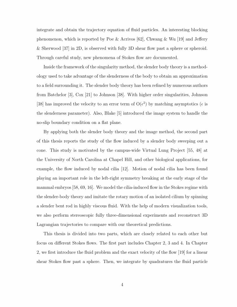
Studies of highly viscous flows past rigid obstacles and fluid flows induced by rigid

bodies with small spatial scales are fundamental in fluid mechanics. These flows play an

important role in particle entrainment, sediment transport, micro-fluidic mixing, micro-

organism locomotion and many other areas of geophysical and biophysical interests. In

these studies, an important class of problems concerns scales where inertia plays a

subdominant role to viscous forces, which is the case for many biophysical applications.

The Stokes approximation becomes relevant in such cases, despite its limitations in

governing fluid motion far from the body. Numerous studies have addressed these

Stokes problems in the literature.

The simplest Stokes flows with objects embedded are uniform flow and linear shear

flow past an infinite cylinder, a sphere, or an ellipsoid. For 2D uniform flow past a

cylinder with its axis perpendicular to the stream, there is no solution in the Stokes

regime, which is well-known as the Stokes paradox. For 3D uniform flow past a sphere,

the first order approximation of the velocity is obtained to satisfy the no-slip boundary

condition on the surface of the sphere and asymptotic to the uniform background flow

at infinity. However, a second approximation Stokes solution for uniform flow past

a sphere does not exist, known as Whitehead’s paradox [24]. Another version of the

Stokes paradox of this 3D flow is reflected on the energy carried by the sphere or the

drifting volume if we consider the flow at rest and the sphere is moving with a constant

velocity. Oseen correction of uniform flow past a cylinder or sphere has already been

well studied [24]. Using the matched asymptotic expansions, uniform flow past an

elliptic cylinder has also been studied by Shintani et al. [68].

For a linear shear flow past an infinite cylinder, the velocity field and stream function

can be found in Robertson & Acrivos [65], Poe & Acrivos [62], Kossack & Acrivos

[42], and Chwang & Wu [19], and the Oseen correction for this 2D flow is derived by

Bretherton [11]. In three-dimension, a general solution, the velocity field of an ellipsoid

immersed in a linear Stokes flow, can be found back to Jefferey [36]. For a linear shear

flow past a sphere, Saffman [66] worked out the Oseen correction for the force acting

on the sphere instead of the usual stream functions. The force is governed by one ODE

for this 3D flow. A good review is referred to Leal [45]. For most studies about these

Stokes flow past a rigid obstacle [44, 22, 47, 41], the focus is the velocity field, the force

acting on the flow [66], and sometimes the motion of the suspension in the fluid [36].

Despite the long history of research in Stokes flows, considerable attention to the

Stokes flow is continually drawn due to its medical, micro-biological and geological

applications. Studies of these applications can lead to better medical approaches for

many aliments, better strategies of environmental issues, and deep understanding of

the nature of life in the low Reynolds number regime [55], [26] [34]. For these appli-

cations, not only the flow motion but also the structure of the flow plays important

roles to completely understand the properties of the flow. Understanding of the flow

patterns for the fundamental problems will help to predict the streamlines of flow in

more complicated geometries.

However, few studies have presented or discussed the flow patterns. Even less has

2

investigated the flow from Lagrangian viewpoint, which is effective to show the flow

structure. Therefore, this thesis focuses on the structure and interaction of the flow in

the Lagrangian viewpoint. If the flow is 2D, a single valued continuous stream function

can be assumed to find the streamlines. For uniform flow past a sphere in 3D, due

to the axis symmetry, the flow can reduce to a 2D flow in the spherical coordinates.

Jeffrey & Sherwood [37] have studied the streamline pattern for 2D Stokes shear flow

around a rotating cylinder, where the flow is governed by one stream function. For a

linear shear flow or rotating flow past a sphere or spheroid, the flow is fully 3D, which is

much more complicated and 3D Oseen correction is extremely difficult. Acrivos’ group

[1, 65, 42, 62] has studied the shear flow past a sphere experimentally and numerically.

Cox, Zia & Mason [23] reported the streamline functions in integral form with a freely

rotating sphere in a linear shear background flow. Beyond the Stokes regime, a few

papers [72] [57] studied the flow structure numerically, considering the inertial effect

for this flow. As we know, there is no report about the stream functions of a linear

shear flow past a fixed sphere in the literature.

We study the flow problems with the singularity method seen in Chwang & Wu

[19], Kim & Karrila [41], Pozrikidis [63], and Leal [47]. This method has been used

widely in research and is especially suitable for these Stokes’ problems with regular or

complicated boundary geometries. The pioneering work about the singularity method

can be tracked back to Lorentz [51], Oseen [60], and Burges [13] as Chwang & Wu cited

[19] (see a review [50]). The vital components for this method are to identify the type of

singularities, determine the distribution and strength of the singularity, and construct

the velocity eventually. The singularities are usually distributed inside the obstacle, so

that the resulted velocity field is regular.

Based on Chwang and Wu’s work [19], we study the shear flow or rotating flow

past a sphere or spheroid in the first part of this thesis. Using the velocity field, we

3

integrate and obtain the trajectory equation of fluid particles. An interesting blocking

phenomenon, which is reported by Poe & Acrivos [62], Chwang & Wu [19] and Jeffery

& Sherwood [37] in 2D, is observed with fully 3D shear flow past a sphere or spheroid.

Through careful study, new phenomena of Stokes flow are documented.

Inside the framework of the singularity method, the slender body theory is a method-

ology used to take advantage of the slenderness of the body to obtain an approximation

to a field surrounding it. The slender body theory has been refined by numerous authors

from Batchelor [3], Cox [21] to Johnson [38]. With higher order singularities, Johnson

[38] has improved the velocity to an error term of O(ε2) by matching asymptotics (ε is

the slenderness parameter). Also, Blake [5] introduced the image system to handle the

no-slip boundary condition on a flat plane.

By applying both the slender body theory and the image method, the second part

of this thesis reports the study of the flow induced by a slender body sweeping out a

cone. This study is motivated by the campus-wide Virtual Lung Project [55, 48] at

the University of North Carolina at Chapel Hill, and other biological applications, for

example, the flow induced by nodal cilia [12]. Motion of nodal cilia has been found

playing an important role in the left-right symmetry breaking at the early stage of the

mammal embryos [58, 69, 16]. We model the cilia-induced flow in the Stokes regime with

the slender-body theory and imitate the rotary motion of an isolated cilium by spinning

a slender bent rod in highly viscous fluid. With the help of modern visualization tools,

we also perform stereoscopic fully three-dimensional experiments and reconstruct 3D

Lagrangian trajectories to compare with our theoretical predictions.

This thesis is divided into two parts, which are closely related to each other but

focus on different Stokes flows. The first part includes Chapter 2, 3 and 4. In Chapter

2, we first introduce the fluid problem and the exact velocity of the flow [19] for a linear

shear Stokes flow past a sphere. Then, we integrate by quadratures the fluid particle

4

equations when the sphere’s center is in the zero-velocity plane (see the first case in

Figure 2.1). In particular, we study in detail the stagnation points with their associated

surfaces, as these provide the framework for the blocked region geometry, and the mode

of divergence of the blocked regions’ cross-sectional area is calculated. Then, we turn

to the second case shown in Figure 2.1, when the center of the sphere is out of the zero-

velocity plane of the primary shear. Numerical results demonstrate the persistence

of the blocked regions. Complicated global bifurcations are found analytically in the

flow field with special ratios related to the shear rate, the radius of the sphere, and

the distance from the zero velocity plane of the primary shear to the sphere’s center.

Furthermore, we show information about the linear shear flow past a freely rotating

sphere. Analytical particle trajectory formulas are obtained similarly. There are closed

orbits in the flow and the height of the closed orbit near the sphere is convergent.

In Chapter 3, we report the primary results about linear shear flow past a spheroid

with the analytical velocity field in the Stokes regime. Numerical results illustrate the

blocking phenomenon. Using the explicit formula of the stagnation points, we show

the impact of the eccentricity of the spheroid on the positions of stagnation points.

When the spheroid is tilted in the symmetry plane, we construct the velocity and find

the explicit condition for the stagnation points. In this case, the blocking phenomenon

shows new features with respect to the spherical case, including deformation of fluid

particle trajectories in a positive and negative suction pattern. The positive or negative

suction depends on the orientation of the spheroid with respect to the background shear.

In Chapter 4, we continue to complete the information about a sphere or spheroid

embedded in a rotating flow. From the velocity field, we find the explicit fluid particle

trajectory equations for either a fixed or self-rotating sphere embedded in a rotating

background flow. Similarly, analytical formula for stagnation points on the sphere and

critical points in the interior of the flow are derived. With prescribed self-rotating rate

5

of the sphere, new phenomena appear in the structure of the flow. The analytical and

numerical results for rotating flow past a spheroid are presented at the end of this

chapter. When a spheroid is tilted in a direction tangential to the rotation background

flow, fluid transport is observed.

The second part of this thesis includes Chapter 5, 6, 7 and 8, whose main objects

are flows induced by a slender rod. We study the flow using experimental, theoretical

and numerical tools. In Chapter 5, the experimental setup and various tools involved in

the experiment are introduced. In Chapter 6, we study the flow induced by a rotating

straight rod above a no-slip plane. When a straight rod sweeps out an upright cone, the

flow has been studied by Leiterman [48] and Bouzarth et al.[9]. When the straight rod

sweeps out a tilted cone, new phenomena are introduced. The fluid particles no longer

only move along periodic trajectories as in the upright cone case. As the tilt angle

increases, the trajectories deform more and open trajectories are observed numerically.

There is net transport based on the flux through a vertical plane. The far field of the

flow has been checked for better understanding of the flow structure. In Chapter 7, we

study the flow induced by a bent rod sweeping out a cone above a no-slip plane. When

the slender rod is bent, there are rich structures of the fluid particle trajectories. One

appealing phenomenon is the toroidal structure of the trajectories introduced by the

bending. Using Poincare map, we show how the well-ordered nested tori are influenced

by the configuration of the rod. With fully 3D experimental abilities, we carefully go

through experimental and theoretical comparison. For the straight rod case, our model

shows excellent agreements with the experimental data. For the bent rod, qualitatively,

both the model and the experiments capture the toroidal structure. Quantitatively, the

predictions of the model show good agreement with many, but not all, observations from

experimental studies. The discrepancy especially shows up in long-time comparison.

Possible contributions to the discrepancies in both the model and the experiments are

6

discussed. In Chapter 8, a swimming related application of slender body theory is

documented. We focus on the flow induced by a periodic motion of a slender body.

Supplemental information of this thesis is provided in the appendices. In Appendix

A, we briefly summarize the fundamental singularities applied in this thesis without

derivation and the slender body theory with the canonical results of a uniform flow past

a slender body. These have been well documented in Chwang & Wu [19], Pozrikidis [63],

and Leiterman [48]. The purpose of the repetition is to make the thesis self-contained.

In Appendix B, the error analysis is reported if the flow past or induced by a prolate

spheroid is studied with the slender body theory, i.e., the spheroid is approximated

by a slender body in the flow. In the Stokes regime, the exact velocity field exists for

a uniform or linear shear flow past a spheroid. Improved slender body theory results

for several basic flows and the exact solution of a prolate spheroid sweeping out a

single cone are reported in Appendix C. In Appendix D, the leading order slender body

results for uniform flow past a partial torus are documented. In Appendix E, the details

about the non-dimensionalization of the farfield velocity field for the flow in Chapter 8

are supplied. Matlab scripts for a straight rod sweeping out a tilted cone and a bent

rod sweeping a cone above a no-slip plane are provided. Appendix G summarizes the

terminal velocity for one rigid body or two spheres falling in Stokes flow .

7

Part I

Theoretical studies of linear shear

or rotation Stokes flow past a

sphere or spheroid

8

Chapter 2

Lagrangian blocking in highly

viscous shear flows past a sphere

Fluid flow over a rigid body in the Stokes’ regime is a fundamental problem and has

received attention over more than a century. While the case of uniform flows and its

ensuing far-field paradoxes in two and three dimensions are well known, features associ-

ated with (spatially) non-uniform fluid flows at the far field have received comparatively

less attention in the literature.

For far-field linear flows, some experimental and analytical results have been pre-

sented in [36, 23, 65, 42, 62, 19]. In particular, Jeffery [36] provided the solutions for

both fluid and body motion for the case of an ellipsoid free to move under the fluid-body

forces in an imposed far-field linear flow. Even when the velocity field is analytically

available, the Lagrangian viewpoint of the fluid particle motion is seldom studied and

general solutions are naturally not available. Interestingly, for a freely rotating sphere

with its center fixed at the zero-velocity (horizontal, say) plane of a background linear

shear, Cox, Zia & Mason [23] computed fluid particle trajectories in closed form by

quadratures. For a fixed body, there are even fewer results for particle trajectories.

Bretherton [11], and later Chwang & Wu [19], presented an expression for the stream-

function for the 2D flow around a fixed disk with its center on the zero-velocity line in a

linear shear. (In this thesis, we use the terminology “disk” to refer to an infinitely long

cylinder whose axis is perpendicular to the background stream, i.e. an inherently two-

dimensional setup). These authors noted an interesting blocking phenomenon which

was observed numerically and experimentally by Acrivos’ group [65, 62]. This blocking

behaviour is a strong modification of the particle trajectories from situations without

and with a fixed disk: in the absence of the body, particles are swept by the shear flow

on straight horizontal lines, never crossing the zero-velocity horizontal line. When the

disk is placed into the flow, two regions of fluid emerge in which particles cross the

zero-velocity line as they approach the disc in either forward or backward time. Parti-

cles initially within these regions are confined to them, and will never pass through the

vertical line through the disk’s center orthogonal to the background shear flow. One of

the focuses of this chapter is to analyse this kind of phenomenon in more general 3D

flows associated with a sphere or spheroid.

Generally, the regions where blockage occurs are bounded by separation ‘stream-

surfaces’. In the 2D case involving linear shear flow past a disk, the height of these

separation streamlines becomes infinite far from the disk, an effect which was observed

by Bretherton [11] and Chwang & Wu [19] and was conjectured not to persist in 3D

shear flow past a fixed sphere. This case appears to not have been studied in detail,

although particle trajectories are sketched in the symmetry plane by Robertson &

Acrivos [65] and Leal [47].

Most of the existing literature seems to concentrate on the flow velocity field and on

the forces acting on the sphere, see for example, [36], [66], [19], [63], [57] and [41]. Here

we demonstrate that the blocking phenomenon persists in the 3D flows for the simple

linear shear flow past a fixed sphere, and obtain explicit expressions for the blocking

regions, such as the bounding stream-surfaces and asymptotic estimates for the blocked

regions in the far field.

10

Figure 2.1: Flow past a fixed sphere x2 + y2 + z2 = a2. Without lost of generality,assume Ω ≥ 0 and U ≥ 0.

In this chapter, we thoroughly study the blocking phenomenon for shear flow past

a fixed, rigid sphere and document related results. In section 2.1, we introduce the

problem and the exact velocity of the flow [19]. In section 2.2, we deduct the trajectory

equations of fluid particles, in the closed integral form, for an unbound linear shear

flow past a fixed sphere, when the sphere’s center is in the zero-velocity plane of the

shear flow (see the first case in Figure 2.1). We illustrate the blocking phenomenon

in the flow using streamlines in the symmetry plane and separation streamlines. To

study the geometry of the blocked flow, we discuss the stagnation lines in detail and

compute the area of the cross section of the blocked flow. In section 2.3, we examine

the second case shown in Figure 2.1, when the center of the sphere is out the zero-

velocity plane of the primary shear. Numerical results indicate the existence of the

blocked flow. Complicated bifurcations are found analytically in the flow field with

special ratios related to the shear rate, the radius of the sphere, and the distance from

the zero velocity plane of the primary shear to the center of the sphere.

11

2.1 Formulation of problem

We study the motion of an unbounded linear shear flow U = Ωzex+Uex of constant

density ρ and dynamic viscosity µ, past a fixed sphere

x2 + y2 + z2 = a2. (2.1)

Since the fluid is incompressible, the continuity equation is

div u = 0, (2.2)

where u is the fluid velocity. In this thesis, we assume that the inertial terms in the

Navier-Stokes equations can be neglected. Thus, the equations of motion are

µ∇2u = ∇p, (2.3)

where p denotes the fluid pressure. The condition for (2.3) to hold is that Re =

Ωa2ρ/µ 1. The boundary conditions are that u = 0 on the solid boundary, and u is

asymptotic to the basic shear flow at large distances from the rigid body.

Schematics of the problems are shown in Figure 2.1. Case 1 on the left is the

shear flow Ωzex past a fixed sphere at the origin. Case 2 on the right is the shear

Ωzex +Uex past the sphere, where the sphere’s center is out of the zero-velocity plane

of the background shear.

The exact velocity field is constructed by employing Stokes doublets associated with

the base vector ex and ey and potential quadrupole. More details about fundamental

singularities can be found in [19]. The velocity field u for a fixed sphere in the linear

12

shear is

u = Ω

(zex −

5a3

6

3xzx

r5+a3

2

ey × x

r3− a5

6∇ ∂2

∂x∂z

1

r

)+U

ex −

3a

4

[exr

+(ex · x)x

r3

]+a3

4∇ ∂

∂x

1

r

, (2.4)

where x = (x, y, z), r = |x| =√x2 + y2 + z2, ex, ey and ey are unit vectors along x, y,

and z direction, respectively. The force acting on the fixed sphere is F = 6πµUex and

the torque at the origin is T = −4πµΩ a3ez [19].

Let x′ = xa, u′ = u

aΩand U ′ = U

aΩ, nondimensionalizing the equations (dropping the

primes), the non-dimensional velocity field is

u = zex −5

2

xzx

r5+

ey × x

2r3− 1

6∇ ∂2

∂x∂z

1

r

+U

[ex −

3

4

(exr

+(ex · x)x

r3

)+

1

4∇ ∂

∂x

1

r

]. (2.5)

From now on, we use the non-dimensional variables unless stated otherwise.

2.2 Linear shear flow past a sphere whose center

is in the zero-velocity plane of the background

flow

In this section, we first derive closed formulae for the fluid particle trajectories in

the case of an unbounded linear shear past a fixed unit sphere, whose center lies in the

zero-velocity plane of the background shear flow. Then, we investigate the blocking

phenomena based on the trajectory equations. We report results about the flow’s

structure on the y = 0 symmetry plane followed by results out of this symmetry plane,

and compare these results with the 2D flow around an infinitely long cylinder. We

13

analytically calculate the stagnation points, the 3D separatrix, and the measurement

of blocking regions. Additionally, we analyze the structure of the flow near the sphere.

For this case, the center of the sphere is in the zero-velocity plane of the background,

and the velocity field is a simplified form of equation (2.5)

u = zex −5

2

xz x

r5+

ey × x

2r3− 1

6∇ ∂2

∂x∂z

1

r. (2.6)

2.2.1 Exact quadrature formulae for the fluid particle trajec-

tories

Here, streamlines may be constructed as the intersection of two stream surfaces for

a 3D flow. Of course, it is not always possible to find explicit formulas of streamlines

for a flow field, and we show how particle trajectories may be computed in closed form

for the complex flow under study in this chapter.

Based on the special geometry of this problem, we change the coordinates from

rectangular coordinates to spherical coordinates (r, φ, θ). Using the explicit fluid flow,

we may immediately write the particle trajectory equations in spherical coordinates as:

drdt

= cos(θ) sin(2φ)3−5r2+2r5

4r4 ,

dθdt

= sin(θ) cot(φ)1+r2−2r5

2r5 ,

dφdt

= cos(θ)cos(2φ)(r5−1)+r5−r2

2r5 ,

(2.7)

where r =√x2 + y2 + z2 (1 ≤ r <∞), φ = arccos

(zr

)(0 ≤ φ ≤ π), and θ = arctan

(yx

)(0 ≤ θ ≤ 2π).

Since ODE system (2.7) is an autonomous system, we eliminate time t and use the

14

radius r as a new independent variable giving a system for dφdr

and dθdr

:

dθ

dr=

(1 + r2 − 2r5) tan(θ)

(3r − 5r3 + 2r6) sin2(φ),

dφ

dr=

−r2 + r5 + (r5 − 1) cos(2φ)

r(3− 5r2 + 2r5) cos(φ) sin(φ).

Next, changing the variable y = r sin(θ) sin(φ) and taking the derivative of y with

respect to r, yields:

dy

dr= sin(θ) sin(φ) + r cos(θ) sin(φ)

dθ

dr+ r sin(θ) cos(φ)

dφ

dr.

Substituting dθdr

and dφdr

into the above equation and replacing sin(θ) sin(φ) with yr, we

get

dy

dr=

−5(1 + r) sin(θ) sin(φ)

(r − 1)(3 + 6r + 4r2 + 2r3)=

−5(1 + r)y

r(r − 1)(3 + 6r + 4r2 + 2r3). (2.8)

Similarly, take derivative of z = r cos(φ) with respect to r and substitute dφdr

into the

resulting formula,

dz

dr= cos(φ)− r sin(φ)

dφ

dr=

(1 + r)(3 + 5(2 cos2(φ)− 1))

(6 + 6r − 4r2 − 4r3 − 4r4) cos(φ).

Replacing cos(φ) with z/r, the above equation becomes

dz

dr=

(r + 1) (r2 − 5z2)

r(r − 1) (3 + 6r + 4r2 + 2r3) z. (2.9)

The obtained ODEs dydr

and dzdr

decouple.

Using separation of variables, ODE (2.8) can be solved analytically. The analytic

15

solution is,

y3 = C1r5

(r − 1)2 (3 + 6r + 4r2 + 2r3). (2.10)

The ODE in equation (2.9) is not exact, and hence not immediately separable, nonethe-

less an integrating factor may be found. We rewrite it as

(1 + r)(r2 − 5z2)

(r − 1)r(3 + 6r + 4r2 + 2r3)dr − zdz = 0.

Notice that multiplying this equations by the integrating factor (3−5r2+2r5)23

r103

yields an

exact equation which is solved in closed integral form:

∫ 1r (1 + s)(1− s) 1

3

(2 + 4s+ 6s2 + 3s3)13

ds− (3− 5r2 + 2r5)23

2 r103

z2 = C2. (2.11)

Here C1 and C2 are constants determined by the initial values r0, y0, and z0.

Equations (2.10) and (2.11) describe the fluid particle trajectories. If r0 6= 1, (2.11)

can be rewritten to read:

z2 =2 r

103

(3− 5r2 + 2r5)23

∫ 1r0

1r

(1 + s)(1− s)(2− 5s3 + 3s5)

13

ds+ z20

(r

r0

) 103(

3− 5r20 + 2r5

0

3− 5r2 + 2r5

) 23

. (2.12)

This equation expresses the height, z, of the fluid particle trajectory in terms of r.

These trajectory equations provide rigorous tools to study the blocking phenomenon.

2.2.2 Blocking phenomenon

Here we analyze the blocking phenomena which occurs in this flow. This blocking

behavior is a strong modification of the particle trajectories from situations without

and with a fixed solid sphere present in the flow: In the absence of a solid sphere,

16

particles released in the shear flow (starting, say, above the z = 0 plane) will be swept

from large negative x values, to large positive x values as time progresses. However,

when the fixed, solid sphere is introduced into the flow, a large measure of particle

trajectories lose this streaming property. Namely, blocked particles starting with large

negative x values do not pass the sphere as time progresses, but rather, limit back to

large negative x values as time progresses. The regions where this behavior occurs in

three dimensional space are defined to be the “blocked regions” of the flow. See Figure

2 which depicts this blocking region when the flow is restricted to the two dimensional

symmetry plane. We note that this type of behavior has been observed for the case

of an infinitely long cylinder immersed in a linear shear flow by Chwang & Wu [19];

however, they conjectured that this behavior would not persist for situations involving

a sphere (instead of a cylinder). Here, we show that in fact for the case of the sphere,

the blocking region persists, and moreover, we analytically compute the geometry of

this region, and show that it has infinite cross-sectional area. With the exact, closed

form expressions for the particle trajectories given in equations (2.10) and (2.12), we

may proceed directly to computing the geometry of the blocked regions.

Blocking phenomenon in the y = 0 symmetry plane

In the y = 0 plane, the velocity field is

u(x, 0, z) = z

(1− 1

2r3− 5x2

2r5− z2 − 4x2

2r7

),

v(x, 0, z) = 0,

w(x, 0, z) = x

(1

2r3− 5z2

2r5− x2 − 4z2

2r7

),

and r =√x2 + y2 + z2 =

√x2 + z2. Notice that one velocity component v vanishes.

Particles initially on this plane never leave this plane, i.e. y = 0 for the particle

17

Figure 2.2: Streamlines in the y = 0 plane with the linear shear flow zex past a fixedsphere. The four black points on the sphere are stagnation points in this symmetryplane. Note that the separatrix height limits to approximately 0.88207 and is rigorouslyless than unity.

trajectory. Fluid particles in this plane are thus described by the closed integral formula

equation (2.12) with r20 = x2

0 + z20 and r2 = x2 + z2. The streamlines in the y = 0

symmetry plane shown in Figure 2.2 explicitly depict the blocking region. The fully

3D structure of the blocking region will be described below.

The four dots on the sphere in Figure 2.2 are stagnation points. They are (x, y, z) =

(± 2√5, 0,± 1√

5) in rectangular coordinates. Two other stagnation points on the sphere

are located at (0,±1, 0), which are out of this symmetry plane. Stagnation points are

special among the fixed points that comprise a no-slip boundary. We define a point

on such boundaries to be stagnation points if, for any neighborhood of one such point,

there exists a subset of material fluid points of the neighborhood that never leave

the neighborhood in backward (for a repelling stagnation point) or forward (for an

attracting stagnation point) infinite time. We remark that this definition is in fact valid

for classifying any fixed point in the flow, not necessarily those on the boundary. The

calculation of these fixed points, as well as the explicit calculation of the separatrices

will be presented in the following two subsections.

18

From figure 2.2, it is clear that there are blocking regions. For example, the flow

is separated by the stagnation line in the second quadrant. Below that stagnation line

the flow is trapped on the left side of the sphere.

It is worth comparing this case with that of the analogous 2D flow: For the 2D

flow in the case of an infinitely long cylinder immersed in a linear shear flow with the

cylinder axis perpendicular to the lines of constant shear [37], the stream function is

φ(x, z) =1

2z2

(1− 1

r2

)2

+1

4

(1− 1

r2

)− 1

2log r

see Chwang & Wu [19] for more details. Here r2 = x2 + z2, and the radius of the

cylinder is unity. The stagnation points on the cylinder are (±√

32,±1

2). Notice that

the separatrix is totally explicit in this case. Moreover, as x → ±∞, the height |z| of

separatrix goes to∞. This peculiar behavior is in some sense similar to the well-known

Stokes Paradox in 2D uniform flow past a cylinder. Our results below show that the

limiting height of the separatrix is finite in the case involving a fixed, rigid sphere, in

sharp contrast with the 2D case.

Blocking phenomenon off the y = 0 plane

By continuity, it is expected that the blocking phenomenon extends outside the

y = 0 symmetry plane. Our analytic results not only show the existence of this 3D

blocking region, but further establish that the height of the blocking region is bounded

by a constant less than the sphere radius, and dependent upon the distance off the

symmetry plane. (We will compute explicitly the 3D geometry of the blocked region in

subsection 2.2.5 and 2.2.6.)

19

Figure 2.3: Separation surfaces generated by separatrix lines in the flow.

Recall equations (2.10) and (2.12) with initial value (x0, y0, z0):

y = y0r

53 (r0 − 1)

23 (3 + 6r0 + 4r2

0 + 2r30)

13

r530 (r − 1)

23 (3 + 6r + 4r2 + 2r3)

13

,

z2 =2 r

103

(3− 5r2 + 2r5)23

∫ 1r0

1r

(1 + s)(1− s) 13

(2 + 4s+ 6s2 + 3s3)13

ds+ z20

r103

r103

0

(3− 5r2

0 + 2r50

3− 5r2 + 2r5

) 23

,

where r0 =√x2

0 + y20 + z2

0 . Particle trajectories are determined by simultaneously

solving (intersecting these surfaces) these equations to obtain a curve relating (x, y, z).

Figure 2.3 shows the separation surfaces in the flow. As shown in this figure, there

is a region off the x-z plane between the separation surfaces, where the flow is blocked.

The vertical plane in this figure shows the cross section of the blocking region. The

cross-sectional area in the limit of x→ ±∞ will be discussed in subsection 2.2.6.

Figure 2.4a and 2.4b show the stagnation lines close to the sphere and how they

connect to the critical points in the flow off the sphere. In this case, the critical points,

i.e. fixed points in the flow, are the y-axis outside of the sphere. This line of fixed

points is a subset of the original z = 0 plane of fixed points present in the absence of

20

(a) Streamlines close to the sphere. (b) Zoom in the cube near the y-axis.

Figure 2.4: Streamlines on separation surfaces close to the sphere.

the rigid sphere. From Figure 2.4b, it is easy to see that they are hyperbolic critical

points.

2.2.3 Stagnation points on the sphere

Since all points on a solid boundary are fixed points of the flow, special care is

needed to define stagnation points which reside on a solid boundary. This degeneracy

on solid boundaries may be split by computing those points on the boundary for which

the linearization of the velocity vector field vanishes. These will define the stagnation

points on the rigid boundary. Streamlines in the fluid which end at any stagnation

point (whether in the fluid or on the boundary) are referred to as stagnation lines.

Stagnation lines ending on the boundary are not necessarily perpendicular to the no-

slip, rigid boundary. For 2D flow, the angle between the stagnation line and the rigid

surface can be computed, as seen in Pozrikidis [63].

To find the stagnation points on the sphere, we linearize and rescale the velocity

equation near the surface of the sphere. When the velocity field in spherical coordinates

21

are linearized with respect to radius r at 1, the expansions are

dr

dt= O((r − 1)2),

dθ

dt= −4 cot(φ) sin(θ)(r − 1) +O((r − 1)2),

dφ

dt=

3 + 5 cos(2φ)

2cos(θ)(r − 1) +O((r − 1)2).

After rescaling time τ = t(r − 1) and neglecting the higher order, we reduce the ODE

system to

dr

dτ= 0,

dθ

dτ= −4 cot(φ) sin(θ), (2.13)

dφ

dτ=

3 + 5 cos(2φ)

2cos(θ).

The steady state of the above ODE system provides the stagnation points, yielding the

following conditions:

cot(φ) sin(θ) = 0, 2 cos(θ)(5 cos2(φ)− 1) = 0.

Since 1 ≤ r ≤ ∞, 0 ≤ φ ≤ π, 0 ≤ θ < 2π, six stagnation points on the sphere are

r = 1,

θ = 0, π,

φ = arccos(

1√5

), arccos

(− 1√

5

);

and

θ = π2, 3π

2;

φ = π2

.

Rewritten in rectangular coordinates, these points are located at

(0,±1, 0) ,

(± 2√

5, 0,± 1√

5

)(2.14)

(the last ones in the y = 0 symmetry plane are plotted in Figure 2.2).

22

The rescaled velocity field provides an imprint of the particle trajectory pattern

just off the sphere surface which mathematically reduces to heteroclinic connections

between the stagnation points. These connections can be found from the ODE system

(2.13),

dθ

dφ= −8 cot(φ) tan(θ)

3 + 5 cos(2φ),

and the solution is

sin(θ)2 = C4 cos2(φ)− sin2(φ)

sin2(φ)= C

5 cos2(φ)− 1

sin2(φ), (2.15)

where C is a constant depending on the initial value of r, θ, and φ. When r = 1, using

the stagnation points as initial conditions, we get the equation of the trajectories on

the sphere in rectangular coordinates:

(x, y, z) =(±2 cos(φ),±

√1− 5 cos2(φ),± cos(φ)

),(

arccos(

1/√

5)< φ < π/2

).

Or, r = 1 and cos(θ) = ±2 cot(φ) in the spherical coordinates. These trajectories

connect the stagnation points in the rescaled flow field, and demonstrate the topolog-

ical structure on the sphere (see Figure 2.5). From these trajectories, in the rescaled

coordinates, we classify these stagnation points on the sphere as four nodal points (in

the symmetry plane) and two hyperbolic points (on the y-axis). We emphasize that

the rescaled flows are a projection onto the sphere, and all of these fixed points in the

rescaled system correspond to higher order (quadratic) hyperbolic points in the original

system.

23

Figure 2.5: “Footprint” of stagnation surfaces on the sphere.

2.2.4 Critical points on the y-axis

Beside the stationary points on the surface of the sphere, we further remark that

the entire y-axis exterior to the sphere is a line of fixed points. For finite y values along

this line, they are hyperbolic points (in the x-z plane) with orientation depending upon

the distance from the sphere. Infinitely far from the sphere along the y-axis, these fixed

points lose their hyperbolic structure, with the flow becoming a simple shear flow (the

background flow). In this limit, the orientation angle tends to zero. In the opposite

limit, approaching the sphere, this line of hyperbolic points tend to the higher order

hyperbolic fixed point on the sphere, with the orientation angle depicted by the geodesic

curves in Figure 2.5, with tangent value 4/3, which can also be verified by the local

analysis near the critical points on the y-axis.

Without loss of generality, we assume y0 > 1 (the radius of the unit sphere). Near

24

-15 -10 -5 5 10 15x

-1.0

-0.5

0.5

1.0z

Figure 2.6: Eigenvectors of matrix A at x = 0, y0 = 5, z = 0.

a point on the y-axis (0, y0, 0), the linearized velocity field is

dxdt

dydt

dzdt

=

0 0

2y50−y2

0−1

2y50

0 0 0

y20−1

2y50

0 0

x

y

z

.

This shows that the flow near (0, y0, 0) can be reviewed as 2D flow in the x-z plane,

dxdt

dzdt

=

02y5

0−y20−1

2y50

y20−1

2y50

0

x

z

≡ A

x

z

.

Eigenvalues of matrix A are ±(y0−1)

q(1+y0)(1+y0+2y2

0+2y30+2y4

0)2y5

0, and the corresponding

eigenvectors are

±√1 + y0 + 2y20 + 2y3

0 + 2y40

1 + y0

, 1

.

Figure 2.6 shows the eigenvectors at the point (0, 5, 0). As y0 →∞, the angle between

the eigenvectors goes to zero. When y0 → 1, the eigenvectors are (±2, 1), i.e., the

tangent value of the angle between these two eigenvectors is 4/3.

25

2.2.5 Stagnation lines

The precise mathematical definition of the blocking region requires some care to set

up. Clearly, the unblocking and blocking regions are divided by the separation surfaces

created by stagnation lines in the interior of the fluid as depicted in Figures 2.2 and

2.3. These regions may be succinctly defined as follows: We define the set of unblocked

trajectories to be the set of initial points whose particle trajectories intersect the x = 0

plane off of the y-axis in finite or infinite time. This set of points is topologically open.

The complement of this set (thus closed), we define to be the blocking region. Notice

that the boundary of this set defines the separation surface. This connected surface

contains the separating surface in the fluid, the y-axis, and the sphere surface.

To calculate this separation surface, we first identify the stagnation lines using the

explicit formulae for the trajectory equations given in (2.10) and (2.12), then study

their properties on and off the y = 0 symmetry plane. Through this analysis, we will

prove that the height |z| of stagnation lines is finite as x→ ±∞ and y fixed.

Stagnation lines in the y = 0 symmetry plane

Since one velocity component vanishes in this plane, streamlines are only governed

by equation (2.12)

z2 =1(

32r5 − 5

2r3 + 1) 2

3

∫ 1r (1 + s)(1− s) 1

3(1 + 2s+ 3s2 + 3

2s3) 1

3

ds+ C

,

where C is determined by the initial value (x0, 0, z0).

As we know from the previous subsection, four stagnation points on the sphere in

this symmetry plane are (± 2√5, 0,± 1√

5). We use these points as the initial value and

26

get the equation of the stagnation line in this plane

z2 =1(

32r5 − 5

2r3 + 1) 2

3

∫ 1

1r

(1 + s)(1− s) 13(

1 + 2s+ 3s2 + 32s3) 1

3

ds.

A few remarks regarding this stagnation line may be made. First, the height of the

stagnation line, |z|, is bounded. This is easily seen by replacing the denominator in

the integrand by unity, and evaluating the integral. This gives a constant slightly

bigger than the unit sphere radius. Second, this bound may be improved substantially

through dividing the integral into subintervals and further integrand estimates. In fact,

this ultimately establishes very tight upper and lower bounds for the limiting height

value of the stagnation line in the limit x → ∞. This upper bound is less than unity,

with value 0.8831, and the lower bound is 0.8811. Numerically, we find

|zmax| ≈ 0.88207 as r →∞.

Integral estimates for the height of the stagnation line

In the y = 0 symmetry plane, the height of the stagnation lines |z| satisfies the

following equation

z2 =1(

32r5 − 5

2r3 + 1)2/3

∫ 1

1r

(1 + s)(1− s)1/3(1 + 2s+ 3s2 + 3

2s3)1/3

ds.

Let ε = 1r, then

z2 =1(

32ε5 − 5

2ε3 + 1

)2/3

∫ 1

ε

(1 + s)(1− s)1/3(1 + 2s+ 3s2 + 3

2s3)1/3

ds.

As the stagnation line is far from the sphere, ε→ 0 in the above equation.

27

When ε < 110

,

∫ 1

ε(1+s)(1−s)1/3

(1+2s+3s2+ 32s3)

1/3 ds < z2 <(

1 + 5ε3

3

) ∫ 1

ε(1+s)(1−s)1/3

(1+2s+3s2+ 32s3)

1/3 ds <

601600

∫ 1

ε(1+s)(1−s)1/3

(1+2s+3s2+ 32s3)

1/3 ds <601600

∫ 1

0(1+s)(1−s)1/3

(1+2s+3s2+ 32s3)

1/3ds, (2.16)

since 1 < 1

( 32ε5− 5

2ε3+1)

2/3 < 1 + 5ε3

3< 601

600.

When ε < 11000

,

∫ 1

ε

(1 + s)(1− s)1/3(1 + 2s+ 3s2 + 3

2s3)1/3

ds >

∫ 1

0

(1 + s)(1− s)1/3(1 + 2s+ 3s2 + 3

2s3)1/3

ds− ε

>

∫ 1

0

(1 + s)(1− s)1/3(1 + 2s+ 3s2 + 3

2s3)1/3

ds− 1

1000.

Substitute the above lower bound into (2.16), the height of the stagnation line |z| is

bounded as

∫ 1

0

(1 + s)(1− s)1/3(1 + 2s+ 3s2 + 3

2s3)1/3

ds− 1

1000< z2 <

601

600

∫ 1

0

(1 + s)(1− s)1/3(1 + 2s+ 3s2 + 3

2s3)1/3

ds.

(2.17)

Next, we break the integral interval into two subintervals [0, 12] and [1

2, 1] and estimate

the integrand on each subintervals.

When 0 ≤ s ≤ 12,

L1 ≡(

1− s2 + 5s3

6− 4s5

3+ 25s6

18+ s7

2− 55s8

18

)< (1+s)(1−s)1/3

(1+2s+3s2+ 32s3)

1/3 (2.18)

<(

1− s2 + 5s3

6− 4s5

3+ 25s6

18+ s7

2

)≡ H1, (2.19)

28

and when 12≤ s ≤ 1,

L2 =(

215

)1/3(1− s)1/3

[2 + 1

10(1− s)

]< (1+s)(1−s)1/3

(1+2s+3s2+ 32s3)

1/3 (2.20)

<(

215

)1/3(1− s)1/3

[2 + (1−s)

9+ (1−s)2

81− 347(1−s)3

10935− 4261(1−s)4

98415

]= H2. (2.21)

Evaluate the integrals with the lower or upper bounds in (2.18)-(2.21),

∫ 12

0

L1 ds =1089251

2322432,

∫ 12

0

H1 ds =121199

258048,

∫ 1

12

L2 ds =7132/3

28051/3,

and

∫ 1

12

H2 ds =1164154073

1528450560151/3.

Keep four decimal places and substitute these estimations into (2.17), the estimates for

z2 are 0.7764 < z2 < 0.7799. Eventually, the bounds for the height of the stagnation

lines far from sphere r →∞ are

0.8811 < |z| < 0.8831 .

Stagnation lines off the y = 0 symmetry plane

We next calculate the stagnation surface out of the symmetry plane. As shown in

subsection 2.2.4, the set of critical points which are detached from the sphere is the

y-axis. Thus any stagnation line not in the symmetry plane must contain a unique

point on the y-axis (as shown in Figure 2.3 and Figure 2.4 which demonstrate this

fact). We use these critical points as the initial conditions r0 = y0 > 1, z0 = 0, and

substitute them into the parametric equations for the fluid particle trajectory to obtain

29

stagnation lines lying outside of the symmetry plane

y = y0r

53 (y0 − 1)

23 (3 + 6y0 + 4y2

0 + 2y30)

13

y530 (r − 1)

23 (3 + 6r + 4r2 + 2r3)

13

, (2.22)

z2 =2 r

103

(3− 5r2 + 2r5)23

∫ 1y0

1r

(1 + s)(1− s) 13

(2 + 4s+ 6s2 + 3s3)13

ds. (2.23)

This provides the equations for the stagnation lines out the symmetry plane.

Notice that the stagnation line in the symmetry plane terminates on the sphere

at a point which is not on the y-axis. So next we investigate how the points on the

separation surface close to the symmetry plane topologically connect stagnation lines

intersecting the y-axis with the stagnation line in the symmetry plane. (Due to the

symmetry of the flow, we only consider the case of y0 close to +1. )

Using the y coordinate of the stagnation lines crossing the y-axis given in equation

(2.22), with initial condition (0, 1 + δ, 0) (δ 1), we have

y =

(δ2 (15 + 20δ + 10δ2 + 2δ3)

2(1 + δ)2

) 13(

1− 1

r

)− 23(

1 +2

r+

3

r2+

3

2r3

)− 13

.

The initial condition specifies a point close to (0, 1, 0). In the limit of r → ∞, this

limits to (15

2

) 13

δ23

(1 + 4δ

3+ 2

3δ2 + 2

15δ3) 1

3

(1 + δ)23

,

and as δ → 0, the leading order approximation is(

152

) 13 δ

23 . This shows that the out of

the symmetry plane stagnation line crossing the critical point (0, y0, 0), which is suffi-

ciently close to the stagnation point (0, 1, 0) on the sphere, asymptotically approaches

the stagnation line in the y = 0 plane as r → ∞ (we note that the z value given in

equation (2.23) trivially converges in this limit to the limiting height computed above).

This property guarantees that the blocking region at x =∞ is completely characterized

by the separation lines which intersect the y-axis. This will be very useful in measuring

30

Figure 2.7: Light gray area is the front view of the cross section of the boundedblocking region at x =∞.

the cross-sectional area of the blocking region.

2.2.6 Cross-sectional area of the blocking region

We next study the geometry of this blocking region far from the sphere. We do this

by examining its cross-sectional structure (as in Figure 2.3 and Figure 2.7).

Unfortunately, at finite distances from the body, this cross-sectional region of in-

tersecting the plane x = L with the stagnation surface is not readily provided by the

equations in (2.22) and (2.23) as they are parametrized by the spherical radius. Fortu-

nately, we can overcome this difficulty by working with L→∞ since r ∼ x in this limit.

In this limit, the formulae in equations (2.22) and (2.23) provide (y, z) coordinates for

the curves bounding the blocking region, shown for large, but finite L, in Figure 2.7).

While from this figure it is clear that the height z = z(y) will decay to zero as y →∞,

the limiting procedure yields a parametric representation (with parameter y0) for this

curve. To obtain the decay rate of z(y) as y →∞ (which is critical to determine if the

cross-sectional area is infinite) requires further analysis.

31

From the equations of the stagnation lines (2.22) and (2.23), we get

y ∼ y0

(1− 1

y0

) 23(

1 +2

y0

+3

y20

+3

2y30

) 13

, (2.24)

z2 ∼∫ 1

y0

0

(1 + s)(1− s) 13(

1 + 2s+ 3s2 + 32s3) 1

3

ds = (z∞)2, (2.25)

as r → ∞ by taking x → ∞, where z∞ > 0. Here y0, a point on the y-axis, is the

initial value in the trajectory equations for y, and z. This parametric representation

for the curve z = z(y) may be viewed as an image of the y axis under the flow after

infinite time, which we may use to derive an explicit expression for the cross-sectional

area. To whit, the Jacobian matrix for this mapping is

dy

dy0

=

(1 +

3

2y50

− 5

2y30

) 13

+5 (1 + y0)

2y40

(1− 1

y0

) 13(

2 + 4y0

+ 6y20

+ 3y30

) 23

.

The area of the blocking flow is noted as A,

A

4=

∫ ∞0

z(y) dy =

∫ ∞1

z∞ (y0)dy

dy0

dy0

=

∫ ∞1

z∞

(1 +

3

2y50

− 5

2y30

) 13

dy0 +

∫ ∞1

z∞5 (1 + y0)

2y40

(1− 1

y0

) 13(

2 + 4y0

+ 6y20

+ 3y30

) 23

dy0

= Part1 + Part2.

For integral Part2, the leading order of the integrand 5(1+y0)

2y40

“1− 1

y0

” 13„

2+ 4y0

+ 6

y20

+ 3

y30

« 23

is 5

2(2)23 y3

0

as y0 → ∞. Notice that integrand in equation (2.25) is bounded. Consequently, an

upper bound for the decay of z∞ is√

1y0

as y0 → ∞. Thus, the integral Part2 is

bounded.

32

We next show that integral Part1 diverges:

Part1 =

∫ ∞1

z∞

(1− 5

2y30

+3

2y50

) 13

dy0 .

Substitute z∞(y0) in equation (2.25) into the integrand

Part1 =

∫ ∞1

∫ 1y0

0

(1 + s)(1− s) 13(

1 + 2s+ 3s2 + 32s3) 1

3

ds

12 (

1− 5

2y30

+3

2y50

) 13

dy0,

As y0 →∞,

(1− 5

2y30

+3

2y50

) 13

→ 1.

Using the following result to estimate the integral in the kernel (which follows directly

through straightforward Taylor expansion),

∫ η

0

(1 + s)(1− s) 13(

1 + 2s+ 3s2 + 32s3) 1

3

ds = η − η3

3+O

(η4),

This establishes the following asymptotic expansion:

∫ 1y0

0

(1 + s)(1− s) 13(

1 + 2s+ 3s2 + 32s3) 1

3

ds ∼ 1

y0

as y0 →∞.

So, the integrand of Part1 is asymptotic to√

1y0

as y0 →∞. With such a decay rate the

integral∫∞

1

√1y0dy0 = ∞ is divergent. Since the integrand is sign definite, this result

shows that Part1 is divergent. Consequently, the total area of the cross-section of

the blocking region is infinite when the plane x = x0 →∞.

In the y-z plane (i.e. x = 0), the blocking region is the y-axis , i.e. the area of the

cross section is zero. This is in sharp contrast with the calculation just presented above,

33

where it was shown that at x =∞, the cross section of the blocking region is infinite.

Since the explicit, closed form formula for the area at an arbitrary distance from the

sphere is not available, we study its behavior by analyzing the integrand involved here

under different asymptotic limits. We will see a continuous connection between zero

cross-sectional blocking area at x = 0, to diverging cross-sectional blocking area as

x→∞.

The separation surface is generated by the stagnation lines cross the critical points

(0, y0, 0) on the y-axis, where |y0| > 1. If we take the cross section of the blocking region

at x0, then y2 + z2 = r2 − x20. Based on the trajectory equation (2.22) and (2.23),

(3

2

1

r5− 5

2

1

r3+ 1

)2/3 (r2 − x2

0

)=

∫ 1y0

1r

(s+ 1)(1− s)1/3(32s3 + 3s2 + 2s+ 1

)1/3ds (2.26)

+y20

(3

2

1

y50

− 5

2

1

y30

+ 1

) 23

.

From the above equation, we find the mapping from r to y0 with x0 fixed. With such

a mapping, the boundary of the cross section of the blocking area can be written as

parametric functions

y = y (r (y0) , y0)

z = z (r (y0) , y0)(2.27)

at x = x0 fixed. The leading order asymptotic solution to (2.26) is

r ∼√y2

0 + x20 as y0 →∞ and x0 fixed. (2.28)

If ~a = (0, z) and ~n is the outer normal direction of the cross section,

~a.~n =z(y0) dy

dy0

| dydy0|.

34

By the Divergence theorem or Gauss’ theorem, the cross section of the blocking area I

is an explicit integral:

I

4=

∫Ω

dA =

∫Ω

div~a dA =

∫∂Ω

~a.~n ds =

∫ ∞1

(z(y0)

dy

dy0

)dy0 . (2.29)

From the asymptotic result (2.28) and several applications of the implicit function

theorem to obtain derivative asymptotics (we relegate these technical details to the next

subsection), we find that for finite x0, the integrand decays as x0√2y

3/20

when y0 → ∞,

which yields a finite cross-sectional blocking area.

To study the behavior for the blocking area as x0 increases, we take the cross section

at x0 = yε0, where ε > 0 is a constant.

• When 0 < ε < 1, from equation (2.26), we find r ∼√y2

0 + y2ε0 as y0 →∞. Substi-

tute this into the integrand for the blocking area, the integrand for the blocking

area is asymptotic to 1√2

1

y3/2−ε0

. When 0 < ε < 12, the integral is convergent.

Otherwise, 12< ε < 1, the integral is divergent.

• If the cross section is taken at x0 = yε0 (ε ≥ 1), then r ∼√y2ε

0 + y20 as y0 → ∞.

In this case, the integrand of equation (2.29) for the blocking area decays as 32√y0

with y0 →∞.

This illustrates an unreported property about the solution of the Stokes flow but

physically not observed. Since, at large distances, the characteristic length used in

the Reynolds number need to be redefined, the inertia terms ignored in Navier-Stokes

equation are not negligible.

If ~a = 12(y, z), similar results are hold. Then,

~a.~n =1

2

z(y0) dydy0− y(y0) dz

dy0√(dzdy0

)2

+(dydy0

)2.

35

Similarly, by the Divergence theorem or Gauss’ theorem, the cross section of the block-

ing area I is an explicit integral:

I

4=

∫Ω

dA =

∫Ω

div~a dA =

∫∂Ω

~a.~n ds =1

2

∫ ∞1

(z(y0)

dy

dy0

− y(y0)dz

dy0

)dy0.

We find that for finite x0, the integrand decays as x0√2y

3/20

when y0 →∞, and

• When 0 < ε < 1, from equation (2.26), the integrand for the blocking area is

asymptotic to 18√

21

y3/2−ε0

.When 0 < ε < 12, the integral is convergent. Otherwise,

12< ε < 1, the integral is divergent.

• If the cross section is taken at x0 = yε0 (ε ≥ 1), the integrand of equation (2.30)

for the blocking area decays like 32√y0

as y0 → ∞, which leads to the divergence

of the integral.

Details of asymptotics of the integrand for the cross-sectional area

In this subsection, we provides the details about the decay rate of the integrand

used to compute the cross-sectional area of the blocking region. When the integrand

decays fast enough, the integral is convergent, which implies that the cross section of

the blocking area is finite. Otherwise, the integral is divergent and the cross-sectional

area of the blocking region is infinite.

The closed integral form trajectory equations (2.22) and (2.23) of the fluid particles

are

y = y0

(

1− 1y0

)2 (32

1y30

+ 3 1y20

+ 2 1y0

+ 1)

(1− 1

r

)2 (32

1r3 + 3 1

r2 + 21r

+ 1)

1/3

, (2.30)

z2 =1(

1 + 32r5 − 5

2r3

)2/3

∫ 1y0

1r

(s+ 1)(1− s)1/3(32s3 + 3s2 + 2s+ 1

)1/3ds. (2.31)

36

Substituting y and z in the originally ODE system used to derive the trajectory equa-

tions, we have

dy

dr=

5(

1r

+ 1)y

(1− r) (3 + 6r + 4r2 + 2r3)

=5y0

(1r

+ 1)

(1− r) (3 + 6r + 4r2 + 2r3)

(

1− 1y0

)2 (32

1y30

+ 3 1y20

+ 2 1y0

+ 1)

(1− 1

r

)2 (32

1r3 + 3 1

r2 + 21r

+ 1)

13

(2.32)

dz

dr=

(1 + r)(

5r2 z

2 − 1)

3 + 3r − 2r2 − 2r3 − 2r4

r

z

=

(1 + r)r

(5

r2( 32

1r5− 5

21r3

+1)23

∫ 1y0

1r

(s+1)(1−s)13

( 32s3+3s2+2s+1)

13ds− 1

)

(3 + 3r − 2r2 − 2r3 − 2r4)

1

( 32

1r5− 5

21r3

+1)23

∫ 1y0

1r

(s+1)(1−s)13

( 32s3+3s2+2s+1)

13ds

12

(2.33)

All these four equations are in terms of r and y0.

If x = x0, from x2 = r2 − y2 − z2, we derive the following constraint

(1− 5

2r3+

3

2r5

) 23 (r2 − x2

0

)=

∫ 1y0

1r

(s+ 1)(1− s) 13(

32s3 + 3s2 + 2s+ 1

) 13

ds+ y20

(1− 5

2y30

+3

2y50

) 23

.

Taking implicit differentiation, we have

dr

dy0

=2y5

0 − y20 − 1

y40(1− 5

2r3 + 32r5 )2/3(1− 5

2y30

+ 32y5

0)1/3

/ (

1− 1r

) (1 + 1

r

)r2(1− 5

2r3 + 32r5

) +10y2

0(1 + r)

r(r − 1)(3 + 6r + 4r2 + 2r3)

(1 + 3

2y50− 5

2y30

1− 52r3 + 3

2r5

) 23

+2r − 5 (1− r2)

r6(1− 5

2r3 + 32r5

) 53

∫ 1y0

1r

(s+ 1)(1− s) 13(

32s3 + 3s2 + 2s+ 1

)1/3ds

.

37

Also, from the trajectory equation, we get

∂y (r, y0)

∂y0

= − (y50 − 1)

y50

(1− 5

2r3 + 32r5

)1/3(

1− 52y3

0+ 3

2y50

)2/3, (2.34)

∂z (r, y0)

∂y0

= −

(1− 1

y0

)(1 + 1

y0

)2y2

0

(∫ 1y0

1r

(s+1)(1−s)1/3

( 32s3+3s2+2s+1)

1/3 ds

)1/2

(1− 5

2r3 + 32r5

)−1/3(1 + 3

2y50− 5

2y30

)1/3. (2.35)

Now all the components involved in the integrals for the cross-sectional area are pre-

pared in terms of r and y0.

If ~a = (0, z), then

~a · ~n =z dydr√(

dzdr

)2+(dydr

)2, ds =

√(dz

dr

)2

+

(dy

dr

)2

dr,

or

~a · ~n =z dydy0√(

dzdy0

)2

+(dydy0

)2, ds =

√(dz

dy0

)2

+

(dy

dy0

)2

dy0.

Note the area of the 2D cross section as I. By the divergence theorem, the area of the

2D cross section of the blocked region is

I

4=

∫Ω

dA =

∫Ω

div~adA =

∫∂Ω

~a.~nds =

∫ ∞1

zdy

dr

dr

dy0

dy0 =

∫ ∞1

z

(∂y

∂r

∂r

∂y0

+∂y

∂y0

)dy0.

We will analyze the integrand involved in the cross-sectional area of the blocked region

z

(∂y

∂r

∂r

∂y0

+∂y

∂y0

),

38

to study the property the cross-sectional area of the blocking region.

Substitute all the components (2.30)-(2.35) into the integrand, we write the inte-

grand as function of r and y0,

z

(∂y

∂r

∂r

∂y0

+∂y

∂y0

)=

1(1− 5

2r3 + 32r5

) 23

(∫ 1y0

1r

(1 + s)(1− s)1/3(32s3 + 3s2 + 2s+ 1

)1/3ds

) 12

(

1− 1y50

)(

1− 52y3

0+ 3

2y50

) 23

−5(1 + 1

r

) (1 + 1

y20− 2y3

0

)y0(1− r) (3 + 6r + 4r2 + 2r3)

(1− 5

2r3 + 32r5

) 23

/2r −

1022/3y20

(1 + 3

2y50− 5

2y30

)2/3

r(1− r) (3 + 6r + 4r2 + 2r3)+

1− 1r2

r2(1− 5

2r3 + 32r5

)− 5 (1− r2)

r6(1− 5

2r3 + 32r5

)5/3

∫ 1y0

1r

(s+ 1)(1− s)1/3(32s3 + 3s2 + 2s+ 1

)1/3ds

). (2.36)

If x0 is a fixed finite number, from the constraint (2.34), we get the asymptotic solution

r ∼√y2

0 + x20. Substitute this solution to the above equation (2.36). The asymptotic

result of the integrand is

z

(∂y

∂r

∂r

∂y0

+∂y

∂y0

)∼ x0√

2y3/20

as y0 →∞.

At a finite distance |x0| from the sphere, the cross-sectional area of the blocked region

depends on x0 and is finite.

If the cross section is taken at infinite x0 =∞, then

y ∼ y0

((1− 1

y0

)2(1 +

3

2y30

+3

y20

+2

y0

))1/3

,

z2 ∼∫ 1

y0

0

(s+ 1)(1− s)1/3(32s3 + 3s2 + 2s+ 1

)1/3ds.

39

The cross-sectional area I is computed as

I

4=

∫Ω

dA =

∫Ω

div~adA =

∫∂Ω

~a.~nds =

∫ ∞1

zdy

dy0

dy0.

The integrand decays as

zdy

dy0

∼

(∫ 1y0

0

(s+ 1)(1− s)1/3(32s3 + 3s2 + 2s+ 1

)1/3ds

)1/222/3 (−1 + y5

0)(

y50

3−5y20+2y5

0

)2/3

y50

∼ 1√y0

+5

3

(1

y0

)7/2

when y0 →∞.

With such a decay rate, the integral is divergent. This demonstrates that far enough

from the sphere the cross-sectional area is infinite .

To understand the growth of the area, we assume x0 = yε0 (ε > 0). Then, from

the constraint (2.34), we get the asymptotic solution r ∼√y2

0 + y2ε0 . Substituting this

solution into the integrand (2.36) and computing the asymptotic as y0 →∞, we have:

• when 0 < ε < 1, as y0 →∞, the leading order of the integrand (2.36) is

z

(∂y

∂r

∂r

∂y0

+∂y

∂y0

)∼ −y

− 32

+ε

0√2

as y0 →∞.

As y0 →∞, the integrand decays like y− 3

2+ε

0 . Consequently, when 0 < ε < 12, the

integral is convergent. When ε ≥ 12, the integral is divergent.

• when ε ≥ 1, as y0 →∞, the leading order of the integrand (2.36) is

z

(∂y

∂r

∂r

∂y0

+∂y

∂y0

)∼ − 3

2√y0

as y0 →∞.

In this case, the cross-sectional area of the blocking region is infinite.

40

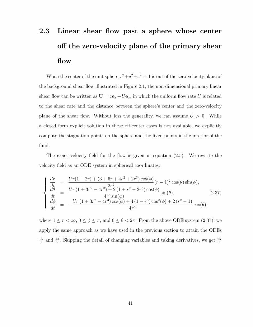
2.3 Linear shear flow past a sphere whose center

off the zero-velocity plane of the primary shear

flow

When the center of the unit sphere x2+y2+z2 = 1 is out of the zero-velocity plane of

the background shear flow illustrated in Figure 2.1, the non-dimensional primary linear

shear flow can be written as U = zex+Uex, in which the uniform flow rate U is related

to the shear rate and the distance between the sphere’s center and the zero-velocity

plane of the shear flow. Without loss the generality, we can assume U > 0. While

a closed form explicit solution in these off-center cases is not available, we explicitly

compute the stagnation points on the sphere and the fixed points in the interior of the

fluid.

The exact velocity field for the flow is given in equation (2.5). We rewrite the

velocity field as an ODE system in spherical coordinates:

dr

dt=

Ur(1 + 2r) + (3 + 6r + 4r2 + 2r3) cos(φ)

2r4(r − 1)2 cos(θ) sin(φ),

dθ

dt=

Ur (1 + 3r2 − 4r3) + 2 (1 + r2 − 2r5) cos(φ)

4r5 sin(φ)sin(θ),

dφ

dt= −Ur (1 + 3r2 − 4r3) cos(φ) + 4 (1− r5) cos2(φ) + 2 (r2 − 1)

4r5cos(θ),

(2.37)

where 1 ≤ r <∞, 0 ≤ φ ≤ π, and 0 ≤ θ < 2π. From the above ODE system (2.37), we

apply the same approach as we have used in the previous section to attain the ODEs

dydr

and dzdr

. Skipping the detail of changing variables and taking derivatives, we get dydr

41

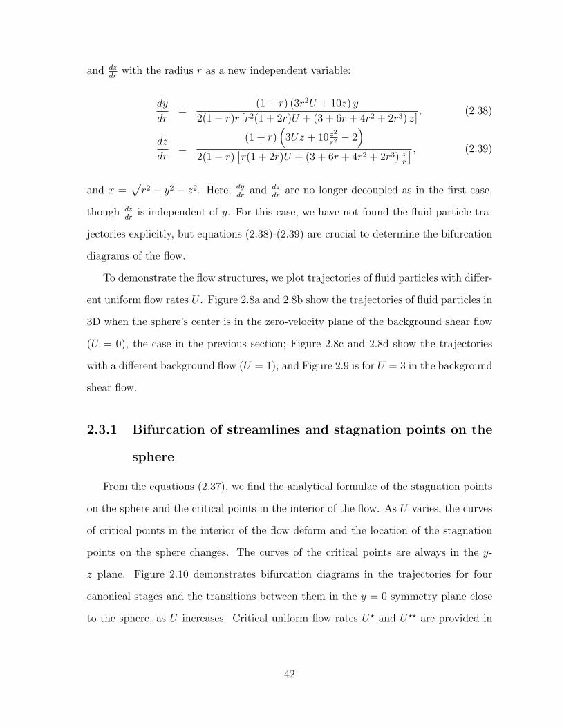
and dzdr

with the radius r as a new independent variable:

dy

dr=

(1 + r) (3r2U + 10z) y

2(1− r)r [r2(1 + 2r)U + (3 + 6r + 4r2 + 2r3) z], (2.38)

dz

dr=

(1 + r)(

3Uz + 10 z2

r2 − 2)

2(1− r)[r(1 + 2r)U + (3 + 6r + 4r2 + 2r3) z

r

] , (2.39)

and x =√r2 − y2 − z2. Here, dy

drand dz

drare no longer decoupled as in the first case,

though dzdr

is independent of y. For this case, we have not found the fluid particle tra-

jectories explicitly, but equations (2.38)-(2.39) are crucial to determine the bifurcation

diagrams of the flow.

To demonstrate the flow structures, we plot trajectories of fluid particles with differ-

ent uniform flow rates U . Figure 2.8a and 2.8b show the trajectories of fluid particles in

3D when the sphere’s center is in the zero-velocity plane of the background shear flow

(U = 0), the case in the previous section; Figure 2.8c and 2.8d show the trajectories

with a different background flow (U = 1); and Figure 2.9 is for U = 3 in the background

shear flow.

2.3.1 Bifurcation of streamlines and stagnation points on the

sphere

From the equations (2.37), we find the analytical formulae of the stagnation points

on the sphere and the critical points in the interior of the flow. As U varies, the curves

of critical points in the interior of the flow deform and the location of the stagnation

points on the sphere changes. The curves of the critical points are always in the y-

z plane. Figure 2.10 demonstrates bifurcation diagrams in the trajectories for four

canonical stages and the transitions between them in the y = 0 symmetry plane close

to the sphere, as U increases. Critical uniform flow rates U? and U?? are provided in

42

(a) U = 0 (b) U = 0

(c) U = 1 (d) U = 1

Figure 2.8: 3D fluid particle trajectories passing the sphere or blocked with different Uin the background shear flow.

43

x

z

Figure 2.9: Trajectories of fluid particles starting from those black dots when U = 3.

the next subsection, after the general formula of critical points are derived.

For Stage 1, Figure 2.10a shows the diagram of streamlines in the symmetry plane

below the sphere when U < U?. The stagnation line bounding the blocking region

moves downward with the stagnation points on the sphere, as the center of the sphere

moves upwards from the zero-velocity plane of the background shear. There is no

critical point in the interior of the flow in this symmetry plane for this stage. The

critical points in the interior of the flow are on two curves in the y-z plane.

The transition from stage 1 to stage 2 appears when U = U?, when a cubic parabolic

critical point (a cusp point) emerges in the symmetry plane (Figure 2.10b). In stage

2 (U? < U < U??), this cubic parabolic critical point deforms into a pair of critical

points, one elliptical critical point and one hyperbolic critical point, in the symmetry

plane. Surrounding the elliptical critical point, there are closed orbits in the symmetry

plane plotted in Figure 2.10c.

The transition from stage 2 to stage 3 occurs when U = U??. With this critical value,

the stagnation lines separating the blocking region also form a separatrix distinguishing

44

the open trajectories from the closed trajectories below the sphere. These stagnation

lines cross the hyperbolic critical point and end on the stagnation point on the sphere.

Above the hyperbolic critical point, streamlines are closed; below it, the streamlines

are open and fluid particles pass the sphere from the right to the left. There is no flow

past the sphere from the left to the right below the sphere in this symmetry plane.

In stage 3 (U?? < U < 83) as Figure 2.10e, the elliptical critical point moves toward

the sphere. The stagnation lines ending on the hyperbolic critical points are no longer

separation lines of the elliptical critical points. The closed orbits around the elliptical

critical point are above the blocking region in this symmetry plane. There are open

streamlines between the elliptical critical point and the hyperbolic point. Fluid par-

ticles along the open streamlines pass the sphere from the left to the right above the

hyperbolic critical points.

Stage 4 begins at U = 83, when the elliptic critical point, the two stagnation points

in the symmetry plane on the sphere, and two stagnation points out of the symmetry

plane vanish or collapse simultaneously at the open dot shown in the Figure 2.10f.

After these four stagnation points on the sphere and the elliptical critical point in the

interior of the flow collapse, the flow structure remains the same as shown in Figure

2.10f, with only two stagnation points on the sphere.

A brief discussion regarding dynamical system theory is merited. For example,

there is a criterion (Poincare-Bendixson) which states that a 2D non-divergence free

vector field may posses periodic particle trajectories only if the divergence of the flow

changes sign. In the symmetry plane, we have a 2D compressible flow for all values of

the parameter U . For some values of this parameter, we just document the existence

of closed orbits in the symmetry plane. A quick inspection of the divergence of the

45

(a) Stage 1 (U < U?) (b) Stage 1-2 (U = U?)

(c) Stage 2 (U? < U < U??) (d) Stage 2-3 (U = U??)

(e) Stage 3 (U?? < U < 83 ) (f) Stage 4 (U ≥ 8

3 )

Figure 2.10: Bifurcation diagram below the sphere in the y = 0 symmetry plane as theuniform flow rate U increases. The gray regions are portions of the sphere. Black dotsindicate stagnation points on the sphere or critical points in the interior of the flow.Arrows show the direction of the flow along the trajectories.

46

velocity field

(u(x, 0, z), w(x, 0, z)) =x(x2 + z2 − 1) [3U(x2 + z2) + 10z]

4(x2 + z2)72

shows that indeed it does change sign, in the agreement with the Poincare-Bendixson’s

criterion. Moreover, using the generalized Poincare-Hopf index definition by Ma &

Wang [52], the index of the flow is also shown to be preserved, with the caveat that

fixed points on the boundary are indexed with selected weight one half.

2.3.2 Stagnation points and critical points in the interior of

the flow

Next, we provide the explicit formula for the stagnation points on the sphere when

its center is out of the zero-velocity plane of the primary background shear flow. After

linearizing, rescaling τ = t(r − 1) and neglecting the higher order terms in the ODE

system (2.37), we get

dr

dτ= 0,

dθ

dτ= −3U csc(φ) + 8 cot(φ)

2sin(θ),

dφ

dτ=

3U cos(φ) + (3 + 5 cos(2φ))

2cos(θ).

Based on the conditions for stagnation points on the sphere,

dθ

dτ= 0 and

dφ

dτ= 0, (2.40)

the explicit formula for stagnation points on the sphere are obtained as:

47

• When 0 ≤ U < 83, there are six solutions of (2.40)

θ = 0, π;

φ = arccos(−3U±

√9U2+80

20

),

and

θ = π2, 3π

2;

φ = arccos(−3U

8

) . In rectangular coordinates, these six points are :

(±(

1− (√

9U2+80−3U20

)2) 1

2, 0, ±

√9U2+80−3U

20

), and

(0,±

√1−

(3U8

)2,−3U

8

).

As U → 83, four of the stagnation points at the lower part of the sphere approach

each other; at U = 83, they collapse and disappear, and there are two stagnation

points(±2√

65, 0, 1

5

)left on the sphere.

• When U ≥ 83, there are only two solutions of (2.40)

θ = 0, π;

φ = arccos(√

9U2+80−3U20

)representing two stagnation points

(±(

45

+3U(√

9U2+80−3U)200

) 12

, 0,√

9U2+80−3U20

)on the sphere in rectangular coordinates.

Besides the stagnation points on the sphere, we find the explicit formula for all the

critical points in the interior of the flow. In the spherical case where the center of the

sphere is in the zero-velocity plane of the primary shear flow, i.e. U = 0 in the primary

flow, the critical points are on the y-axis. When U 6= 0, the curves for critical points

still only appear in the y-z plane but are no longer restricted to the y-axis. The critical

points in the interior of the flow are found as functions of r and U from equations (2.38)

and (2.39)

x(r, U) = 0,

z(r, U) = −Ur2(1+3r2−4r3)2(1+r2−2r5)

,

y(r, U) = ±√r2 − z2(r, U) = ±

√r2 −

(Ur2

2(1+3r2−4r3)(1+r2−2r5)

)2

.

(2.41)

48

If 0 < U < U?, the critical points are on two curves. Each of them ends on one

of the stagnation points

(±(

1− (3U+√

9U2+80)2

400

)1/2

, 0,−√

9U2+80+3U20

)on the sphere.

Far away from the sphere, these two curves are asymptotic to line (0, y,−U), which is

in the zero-velocity plane of the background linear shear. On the other hand, closer

to the sphere, as U increases, these two distinct curves of fixed points deform and

intersect at a critical value of U = U?, as shown in the second column and row in Table

2.1. Before this critical value a few other transitions in the graph of these curves are

noteworthy. When U ≤ 169

√2, the curves of critical points in the y-z plane can be

written as functions of y. When U = 169

√2 < U?, the curve (y(r, U), z(r, U)) has a

vertical tangent line at the stagnation point on the sphere.

The critical ratio U? equals to2(1+s2−2s5)s(1+3s2−4s3)

, in which s is the smallest positive real

root of the following polynomial

8s6 + 4s5 − 4s3 − 11s2 − 2s− 1 = 0. (2.42)

derived from the equation (2.41). At this critical ratio U?, the two pieces of curves join

at a cusp critical point in the symmetry plane.

As U(U? ≤ U < 83) increases further, these two curves of critical points bifurcate into

two new curves. One of the new curves has no end point on the sphere, and all points

on this curve are hyperbolic critical points. The other curve is a finite length curve

whose end points are two stagnation points on the sphere. Along this finite length

curve, the critical points change properties as they move away from the stagnation

points on the sphere: near the two stagnation points on the sphere, i.e. near the two

end points of the curve of critical points, the curve consists of hyperbolic critical points;

a bit further down the curve, at a critical position these points become two degenerate

critical points with three vanishing eigenvalues; finally, moving still further away from

the sphere and close to the y = 0 symmetry plane, the points on this curve become

49

elliptical critical points and no further transition is observed through the symmetry

plane. These properties are determined by the sign of the following function

F (r, U) = 2[1 + r + 2r2(1 + r + r2)

]3(2.43)

+U2r4(5 + 3r + 24r2 − 48r3 − 84r4 − 60r5 − 44r6 + 36r7 + 24r8

)and the equation (2.41). This function, F (r, U), is derived through a standard eigen-

analysis. For given U and r, if F (r, U) > 0, the corresponding point (x, y, z) from the

equation (2.41) is a hyperbolic critical point. If F (r, U) < 0, and the point (x, y, z)

satisfying (2.41) is an elliptical critical point. Otherwise, when F (r, U) = 0, the point

of (2.41) is a higher order critical point with all three eigenvalues being zero.

When U = 83, the finite curve shrinks into a point and collapses with the four

stagnation points on the sphere, and all the critical points in the interior of the flow

are now on the infinite length curve. After U ≥ 83, critical points in the interior of the

flow are always on such a curve.

The quantified streamline plots shown in Table 2.1 document the qualitative bifur-

cation diagram sketched in Figure 2.10. In Table 2.1, we show critical point curves in

the flow and the flow structure in the x-z symmetry plane with given U . Notice that

the critical points are plotted in the y-z plane, since the critical points in the flow are

only in the y-z plane. In the table, the first column shows the different values of U

studied, and in the second column are plots for curves of critical points from equation

(2.41) (the gray area indicates the sphere). The third column are streamlines patterns

obtained numerically in the x-z symmetry plane, i.e., the lateral view.

The first value U = 169

√2 < U? is picked corresponding to stage 1 in the bifurcation

diagram Figure 2.10. In this case, as shown in the second column, critical points are on

two infinite length curves, each of whose end point is a stagnation point on the sphere.

50

With this special value, the curves of critical points in the y-z plane have infinite slopes

at the stagnation point. With the second value U = 2.64837 ≈ U?, a cubic parabolic

(cusp) critical point appears. In the third row U? < U = 2.64912 < U??, the critical

points in the flow are on two new curves. Both end points of the finite length curve

are stagnation points on the sphere, and the curve with infinite length is asymptotic

to a line in the zero-velocity plane of the background shear flow. With the fourth

value U = 2.65059 ≈ U??, the critical points in the flow are still on two curves. The

stagnation lines in the streamline plot in the symmetry plane connect the hyperbolic

critical point in the flow with the stagnation points on the sphere, and separate the

closed orbits around the elliptical critical point from the open trajectories. For U??,

we do not have an explicit formula for this value and use the numerical approximation

2.65059. For the fifth U?? < U = 2.65287 < 83, the elliptical critical points moves up

as U increases, and there are fluid particles which pass the sphere from the left to the

right between the elliptical critical point and the hyperbolic critical point. The last

case U = 83

shows that critical points are on one curve in the flow.

These numerical results clearly show the existence of the blocking regions when the

sphere is out of the zero-velocity plane of the primary shear flow. The streamlines

plots in the y = 0 plane show the interesting bifurcation appearing in the fluid particle

trajectories.

When U? < U < 83, streamlines show a 3D eddy near the elliptical critical points

below the sphere. Figure 2.11 shows the circulation near the elliptical critical points

below the sphere when U = 2.6514. Figure 2.11a is the front view of fluid particles’

trajectories, and Figure 2.11b is the lateral view of the same trajectories. From Figure

2.11b, it is clear that these are closed trajectories circulating around the elliptical

critical points on the finite length critical point curve in the symmetry plane and out

of the symmetry plane. From the front view Figure 2.11a and Figure 2.12a, we see the

51

Fix points in y-z plane streamlines in x-z symmetry plane

U=

16√

29

<U?

-3 -2 -1 0 1 2 3-2

-1

0

1

y

z

U=

2.64

837≈U?

-3 -2 -1 0 1 2 3-2

-1

0

1

y

z

U?<U

=2.

6491

2<U??

-3 -2 -1 0 1 2 3-2

-1

0

1

y

z

Table 2.1: Critical points in the interior of the flow in the x = 0 plane and streamlinesin the y = 0 symmetry plane for different U . The thick dash lines in the streamlinepatterns indicate the zero-velocity plane of the primary background shear flow. Thegray area is the sphere.

52

U=

2.65

069≈U??

-3 -2 -1 0 1 2 3-2

-1

0

1

y

z

U=

2.65

287>U??

-3 -2 -1 0 1 2 3-2

-1

0

1

y

z

U=

8/3

-3 -2 -1 0 1 2 3-2

-1

0

1

y

z

Table 2.2: Continue of Table 2.1.

53

(a) Front view (b) Lateral view

Figure 2.11: Circulation near the elliptical and hyperbolic critical points below thesphere. The gray surface is a portion of the surface of the sphere.

trajectories are further deformed when they are close to the surface of the sphere and

approaching the hyperbolic fixed point on the finite length critical point curve.

Figure 2.12 and Figure 2.13 show streamlines in the y < 0 half space below the

sphere. In Figure 2.12, the streamlines are only closed orbits near the critical points

on the finite length curve (here, we take U = 2.6514). Figure 2.12a is the front view,

Figure 2.12b is the lateral view, and Figure 2.12c is the 3D view. These orbits are

selected so that they are around the elliptical points, but near the sphere they are close

to the hyperbolic critical points on the finite length critical point curve. Figure 2.13

shows both closed and open streamlines near the critical points.

2.4 Linear shear flow past a freely rotating sphere

When non-dimensional shear flow U = zex past a freely rotating sphere [62], the

governing equations are Stokes equations

∇2u = ∇p, (2.44)

div u = 0. (2.45)

54

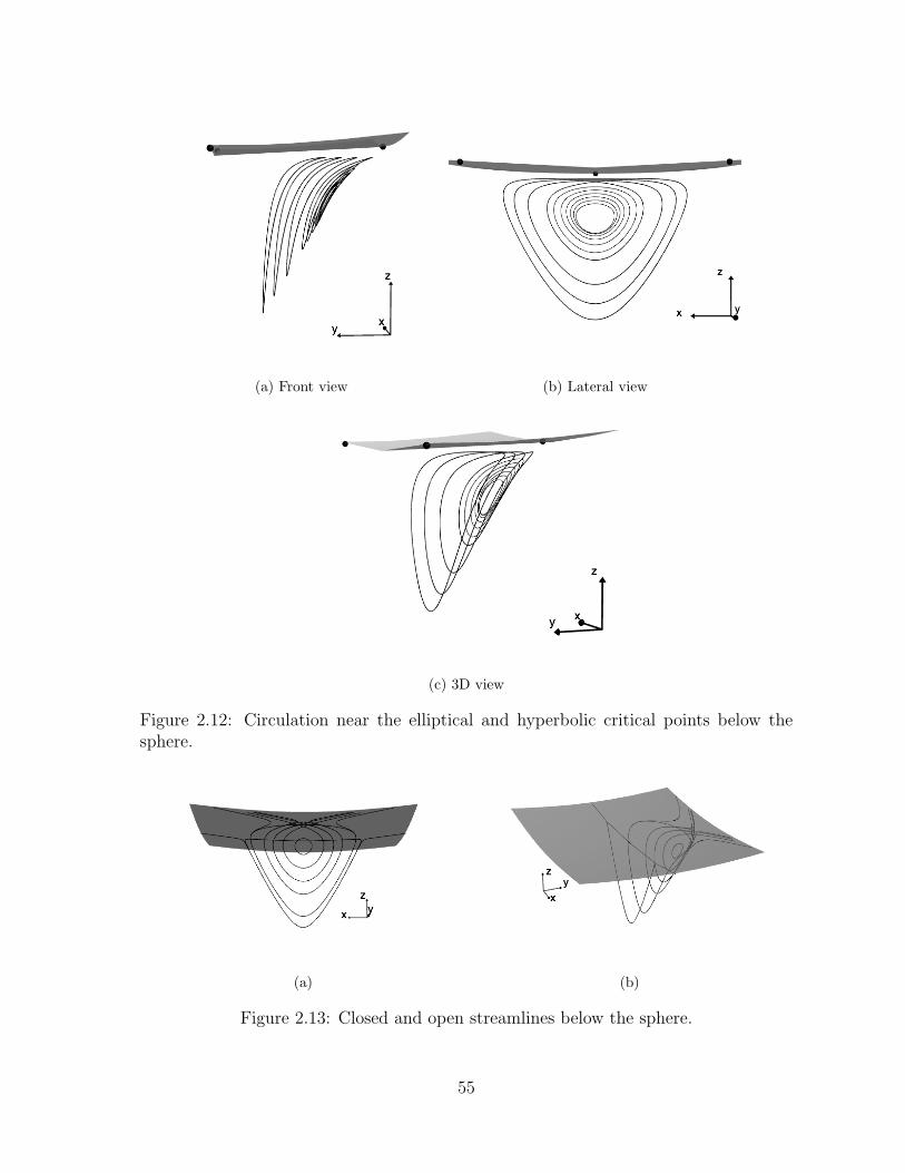
(a) Front view (b) Lateral view

(c) 3D view

Figure 2.12: Circulation near the elliptical and hyperbolic critical points below thesphere.

(a) (b)

Figure 2.13: Closed and open streamlines below the sphere.

55

The boundary conditions are changed to

u = (0, ω, 0)× x at |x| = 1 on the surface of the sphere,

u ∼ U = zex as |r| → ∞,

where ω is the angular velocity of the sphere. Since the background shear flow is

prescribed, the direction of the sphere rotation has been specified. When the sphere

is freely rotating, ω = 12

is determined by the condition of no force or torque on the

sphere.

The velocity of the flow is

u = zex −5

6USS(x, ez, ex)−

1

6

∂

∂xUD(x, ez). (2.46)

The pressure is

p(x) = − 5xy

(x2 + y2 + z2)52

.

This velocity field is adopted from the velocity formula from Chwang & Wu [19]. In

detail, it is

u(x) = z

[1− 1

2(x2 + y2 + z2)52

− 5x2

2(x2 + y2 + z2)52

(1− 1

x2 + y2 + z2

)],

v(x) = − 5xyz

2(x2 + y2 + z2)52

(1− 1

x2 + y2 + z2

),

w(x) = x

[− 1

2(x2 + y2 + z2)52

− 5z2

2(x2 + y2 + z2)52

(1− 1

x2 + y2 + z2

)].

From the velocity, the critical points in the interior of the flow is the y-axis out of the

sphere.

With the same techniques we use for the fixed sphere embedded in a linear shear,

56

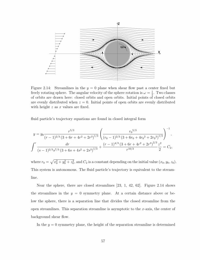
x

z

ω

Figure 2.14: Streamlines in the y = 0 plane when shear flow past a center fixed butfreely rotating sphere. The angular velocity of the sphere rotation is ω = 1

2. Two classes

of orbits are drawn here: closed orbits and open orbits. Initial points of closed orbitsare evenly distributed when z = 0. Initial points of open orbits are evenly distributedwith height z as x values are fixed.

fluid particle’s trajectory equations are found in closed integral form

y = y0r5/3

(r − 1)2/3 (3 + 6r + 4r2 + 2r3)1/3

(r0

5/3

(r0 − 1)2/3 (3 + 6r0 + 4r02 + 2r0

3)1/3

)−1

,

∫ r dr

(s− 1)2/3s7/3 (3 + 6s+ 4s2 + 2s3)1/3+

(r − 1)4/3 (3 + 6r + 4r2 + 2r3)2/3

r10/3

z2

2= C2,

where r0 =√x2

0 + y20 + z2

0 , and C2 is a constant depending on the initial value (x0, y0, z0).

This system is autonomous. The fluid particle’s trajectory is equivalent to the stream-

line.

Near the sphere, there are closed streamlines [23, 1, 42, 62]. Figure 2.14 shows

the streamlines in the y = 0 symmetry plane. At a certain distance above or be-

low the sphere, there is a separation line that divides the closed streamline from the

open streamlines. This separation streamline is asymptotic to the x-axis, the center of

background shear flow.

In the y = 0 symmetry plane, the height of the separation streamline is determined

57

by the following integral equation

∫ r

1

1

(s− 1)2/3s7/3(3 + 6s+ 4s2 + 2s3)1/3ds+

(r − 1)4/3(3 + 6r + 4r2 + 2r3)2/3

r10/3

z2

2= 0.

It is independent of the shear rate. Numerically, we find the critical height is |z| ≈

1.155645 for the unit sphere.

58

Chapter 3

Linear shear flow past a fixed

spheroid

When a linear shear flow past a fixed sphere, complicated flow structures and in-

teresting blocking phenomenon are explored. The simple modification of a sphere in

the flow is a spheroid. We study the flow structure and blocking phenomena for a

prolate spheroid embedded in a linear shear flow in this chapter. With respect to the

spherical case, the spheroid orientation relative to the background shear enriches the

phenomena, some of which will be examined here. The literature on this setup has

concentrated mostly on forces and torques [7], while some experimental investigations

of three-dimensional separation structures for flows past spheroids can be found in the

high Reynolds regime [76].

3.1 Linear shear flow past an upright spheroid

First, we report results about the shear flow Ωzex past an upright spheroid. The

spheroid sits with its center on the zero-velocity plane with its major axis upright (as

shown in Figure 3.1),

x2 + y2

b2+z2

a2= 1 ,

xy

zPrimary shear flow (Ωz, 0, 0)

Figure 3.1: A linear shear flow past a fixed prolate spheroid. The major axis of thespheroid is perpendicular to the direction of the shear flow (an upright spheroid).

where a > b are the major and minor semi-axis, respectively, and the half focal length

c and the eccentricity e are defined as c = (a2 − b2)1/2 = e a. From [19], the exact

velocity field in this case is

u(x) = Ωzex −∫ c

−c

(c2 − ξ2

)(αUSS (x− ξ; ez, ex) + γUR (x− ξ; ey)) dξ

−β∫ c

−c

(c2 − ξ2

)2∂zUD (x− ξ; ex) dξ, (3.1)

where USS, UR and UD are the fundamental singularities of stresslet, rotlet and dou-

blelet, located at ξ,

USS (x− ξ; ez, ex) =3 ((x− ξ) · ez) ((x− ξ) · ex)

R5(x− ξ),

UR (x− ξ, ey) =(x− ξ)× ey

R3,

UD (x− ξ, ex) = − exR3

+3(x− ξ) · ex

R5(x− ξ) ,

with R =√x2 + y2 + (z − ξ)2, and ξ = ξez. Here, α, β and γ are known constants,

α = β4e2

1− e2= γ e2 −2e+ (1− e2)Le

2e (2e2 − 3) + 3 (1− e2)Le, γ =

Ω

−2e+ (1 + e2)Le,

60

and Le = log(

1+e1−e

). Numerical results show the existence of blocking regions in the

flow as Figure 3.2, where the streamlines are plotted in the y = 0 symmetry plane.

3.2 Stagnation points on the spheroid

From the velocity field (3.1), we find the stagnation points on the spheroid. Sim-

ilar to the spherical case, we first rewrite the velocity field in the prolate spherical

coordinates x = a e sinh(µ) sin(ν) cos(φ)

y = a e sinh(µ) sin(ν) sin(φ)

z = a e cosh(µ) cos(ν) ,

where acosh(1e) ≤ µ ≤ ∞, 0 ≤ ν ≤ π, and 0 ≤ φ ≤ 2π. Next, we rescale time

τ =(µ− acosh(1

e))t, and expand the velocity field near the no-slip boundary of the

spheroid where µ = arccosh(1e), ignoring higher order terms of order

(µ− arccosh(1

e))2

.

The linearized ODE system for the trajectory of fluid particle near the surface of the

spheroid reduces to

dµ

dτ= 0,

dν

dτ= 4ω e3 cos(φ)

e2 + e2 cos(2ν)− 2

k(e)

d(e),

dφ

dτ= 4ω e3 [2e (3− e2) + (e4 + 2e2 − 3)Le]

d(e)

cot(ν) sin(φ)

1− e2,

(3.2)

where

d(e) ≡ 12e2 − 8e4 + 4e(e4 + e2 − 3

)Le − 3

(e4 − 1

)L2e ,

61

and

k(e) ≡ 2e(6− e2

)+(e4 + 3e2 − 6

)Le + e2 cos(2ν)

((1 + e2

)Le − 2e

).

The conditions for stagnation points on the boundary

dµ

dτ= 0,

dν

dτ= 0, and

dφ

dτ= 0, (3.3)

define six stagnation points on the upright prolate spheroid in the prolate spherical

coordinates

a(

arccosh(1/e) ,π

2,π

2

), a

(arccosh(1/e) ,

3π

2,π

2

),

a

(arccosh(1/e) , 0 , arccos

(±(

6e− (3− e2)Le2e3 − e2 (1 + e2)Le

)1/2))

,

and

a

(arccosh(1/e) , π , arccos

(±(

6e− (3− e2)Le2e3 − e2 (1 + e2)Le

)1/2))

.

In the original rectangular coordinates, the latter stagnation points lie in the y = 0

symmetry plane

a

(±√

1− e2

(1− 6e− (3− e2)Le

2e3 − e2 (1 + e2)Le

)1/2

, 0 ,±(

6e− (3− e2)Le2e3 − e2 (1 + e2)Le

)1/2),

while the other two are on the y-axis at (0,±a√

1− e2, 0).

The location of the stagnation points in the y = 0 symmetry plane migrate towards

the spheroid’s “tips” with increasing eccentricity e at fixed a. The four points merge

into two at the tips in the “needle” limit of eccentricity e → 1, while for the opposite

limit of a sphere (e→ 0) we retrieve the spherical result (2.14). Like for the spherical

case, the zero-velocity plane of the background shear flow collapses to the y-axis for

62

x

z

Figure 3.2: Streamlines in the y = 0 symmetry plane for a linear shear past a fixedupright spheroid. The four points mark the stagnation points on the spheroid.

the upright spheroid whose center is on this zero-velocity plane.

3.3 Characterization of stagnation stream lines on

the surface of the spheroid

As for the case of the sphere, the rescaled velocity field provides an imprint of the

particle trajectory pattern just off the spheroid surface which mathematically reduces

to heteroclinic connections between the stagnation points, see Figure 3.3.

From the rescaled velocity field ODE (3.2), we obtain the governing equation of the

fluid particle imprint on the spheroid

dν

dφ=

(1− e2) cot(φ) tan(ν)k(e)

(e2 cos(2ν) + e2 − 2) [2e (3− e2) + (e4 + 2e2 − 3)Le].

The solution for the above equation is

sin(φ) sin(ν) = C (k(e))p(e) , (3.4)

63

Figure 3.3: “Footprint” of stagnation surfaces on the spheroid surface from differentviewpoints.

where the constant C is determined by the initial conditions, and the constant p(e) is

p(e) ≡ 2e+ (e2 − 1)Le(1− e2) ((1 + e2)Le − 2e)

. (3.5)

Substituting the stagnation points into (3.4) yields the trajectories

x2 =(1− e2

) (a2 − z2

)− y2 = a2

(1− e2

)sin2(ν)− y2,

y = a√

1− e2 sin(ν) sin(φ) = a√

1− e2 C (k(e))p(e) ,

z = a cos(ν).

in the first octant (x, y, z positive), which can be extended by the symmetry of the flow

to the whole space.

3.4 Linear shear flow past a tilted spheroid

When the major axis of the spheroid is tilted with an angle κ, defined as the angle

between the positive z-axis and the major axis of the spheroid in the x-z plane (see

64

Figure 3.4a and Figure 3.5a), the y = 0 plane is still a symmetry plane of the flow.

However, the up-down symmetry of the fluid-body setup is broken. The tilted prolate

spheroid is

(x cos(κ)− z sin(κ))2 + y2

b2+

(x sin(κ) + z cos(κ))2

a2= 1 (a > b > 0). (3.6)

(The upright spheroid case is recovered with κ = 0.)

The solution of Stokes equations for this tilted case can be efficiently obtained

from the general results of Chwang & Wu [19] and Jeffery [36] in the body frame. In

this frame, the spheroid’s major axis is on the x-axis, and the background flow can be

decomposed into two simple shear flows xey and yex, and an elongational flow xex−yey.

The velocity field uL(xL) in the laboratory frame can be obtained from the velocity field

u(x) in the body frame with the transformation between these two reference frames

uL(xL) = Ru(RTx),

where the transformation matrix

R =

cos(κ) 0 sin(κ)

0 1 0

− sin(κ) 0 cos(κ)

.

For two shear background flows, the velocity field in the body frame for the shear

flow xey is given by changing coordinates of (3.1), and the velocity field in the body

65

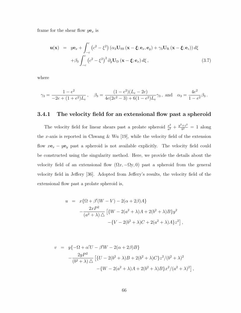
frame for the shear flow yex is

u(x) = yex +

∫ c

−c

(c2 − ξ2

)(α3USS (x− ξ; ex, ey) + γ3UR (x− ξ; ez)) dξ

+β3

∫ c

−c

(c2 − ξ2

)2∂yUD (x− ξ; ex) dξ , (3.7)

where

γ3 =1− e2

−2e+ (1 + e2)Le, β3 =

(1− e2)(Le − 2e)

4e(2e2 − 3) + 6(1− e2)Leγ3 , and α3 =

4e2

1− e2β3 .

3.4.1 The velocity field for an extensional flow past a spheroid

The velocity field for linear shears past a prolate spheroid x2

a2 + y2+z2

b2= 1 along

the x-axis is reported in Chwang & Wu [19], while the velocity field of the extension

flow xex − yey past a spheroid is not available explicitly. The velocity field could

be constructed using the singularity method. Here, we provide the details about the

velocity field of an extensional flow (Ωx,−Ωy, 0) past a spheroid from the general

velocity field in Jeffery [36]. Adopted from Jeffery’s results, the velocity field of the

extensional flow past a prolate spheroid is,

u = xΩ + β′(W − V )− 2(α + 2β)A

− 2xP 2

(a2 + λ)4[W − 2(a2 + λ)A+ 2(b2 + λ)By2

−V − 2(b2 + λ)C + 2(a2 + λ)Az2],

v = y−Ω + α′U − β′W − 2(α + 2β)B

− 2yP 2

(b2 + λ)4[U − 2(b2 + λ)B + 2(b2 + λ)Cz2/(b2 + λ)2

−W − 2(a2 + λ)A+ 2(b2 + λ)Bx2/(a2 + λ)2],

66

w = zβ′V − α′U − 2(α + 2β)C

− 2zP 2

(b2 + λ)4[V − 2(b2 + λ)C + 2(a2 + λ)Ax2/(a2 + λ)2

−U − 2(b2 + λ)B + 2(b2 + λ)Cy2/(b2 + λ)2].

Next, all the variables used in the above equation are provided in detail.

First, 4 = (a2 + λ)12 (b2 + λ), so the velocity field can be rewritten as

u = xΩ + β′(W − V )− 2(α + 2β)A

− 2xP 2

(a2 + λ)32 (b2 + λ)3

[W − 2(a2 + λ)A+ 2(b2 + λ)By2

−V − 2(b2 + λ)C + 2(a2 + λ)Az2],

v = y−Ω + α′U − β′W − 2(α + 2β)B

− 2yP 2

(a2 + λ)12 (b2 + λ)2

[U − 2(b2 + λ)B + 2(b2 + λ)Cz2/(b2 + λ)2

−W − 2(a2 + λ)A+ 2(b2 + λ)Bx2/(a2 + λ)2],

w = zβ′V − α′U − 2(α + 2β)C

− 2zP 2

(a2 + λ)12 (b2 + λ)2

[V − 2(b2 + λ)C + 2(a2 + λ)Ax2/(a2 + λ)2

−U − 2(b2 + λ)B + 2(b2 + λ)Cy2/(b2 + λ)2].

Here, λ is the positive root of x2

a2+λ+ y2+z2

b2+λ= 1, i.e.

λ =1

2

(x2 + y2 + z2 − a2 − b2

+√

(x2 + y2 + z2 − a2 − b2)2 + 4a2(y2 + z2 − b2) + b2x2),

67

and

P 2 =

(x2

(a2 + λ2)2+

y2 + z2

(b2 + λ)2

)−1

.

The explicit harmonic functions included in the velocity field are

α =

∫ ∞λ

1

(a2 + λ)32 (b2 + λ)

dλ = − 2

(a2 − b2)√a2 + λ

−log(√

a2+λ−√a2−b2√

a2+λ+√a2−b2

)(a2 − b2)3/2

,

β =

∫ ∞λ

1

(b2 + λ)2√

(a2 + λ)dλ =

√a2 + λ

(a2 − b2) (b2 + λ)+

log(√

a2+λ−√a2−b2√

a2+λ+√a2−b2

)2 (a2 − b2)3/2

,

α′ =

∫ ∞λ

1

(b2 + λ)3√

(a2 + λ)dλ

=

√a2 + λ (2a2 − 5b2 − 3λ)

4 (a2 − b2)2 (b2 + λ)2 −3 log

(√a2+λ−

√a2−b2√

a2+λ+√a2−b2

)8 (a2 − b2)5/2

,

β′ =

∫ ∞λ

1

(a2 + λ)32 (b2 + λ)2

dλ

=a2 + 2b2 + 3λ

(a2 − b2)2√a2 + λ (b2 + λ)

+3 log

(√a2+λ−

√a2−b2√

a2+λ+√a2−b2

)2 (a2 − b2)5/2

,

α′′ =

∫ ∞λ

λ

(b2 + λ)3√

(a2 + λ)dλ = β − b2α′ =

√a2 + λ

(a2 − b2) (b2 + λ)

−b2 (2a2 − 5b2 − 3λ)

√a2 + λ

4 (a2 − b2)2 (b2 + λ)2 +(4a2 − b2) log

(√a2+λ−

√a2−b2√

a2+λ+√a2−b2

)8 (a2 − b2)5/2

,

and

β′′ =

∫ ∞λ

λ

(a2 + λ)32 (b2 + λ)2

dλ = α− b2β′

= − (b2λ+ a2 (3b2 + 2λ))

(a2 − b2)2√a2 + λ (b2 + λ)

−(2a2 + b2) log

(√a2+λ−

√a2−b2√

a2+λ+√a2−b2

)2 (a2 − b2)5/2

.

68

The constants A through W are

A =Ω

6β′′0, B = Ω

−2β′′0 − α′′06β′′0 (β′′0 + 2α′′0)

, C = Ω−α′′0 + β′′0

6β′′0 (β′′0 + 2α′′0),

U = − Ωb2

2α′′0 + β′′0, V =

Ωb2(β′′0 − α′′0)

3β′′0 (β′′0 + 2α′′0)− Ωa2

3β′′0, W =

Ωa2

3β′′0+

Ωb2(2β′′0 + α′′0)

3β′′0 (β′′0 + 2α′′0),

where α′′0 = 3−e24a3e4(1−e2)

− (e2+3)Le8a3e5

and β′′0 = −6e+(3−e2)Le2a3e5

are α′′ and β′′ evaluated at

λ = 0, respectively.

3.4.2 Stagnation points on the tilted spheroid

As for the other cases we have discussed, six stagnation points on the tilted spheroid

are obtained by rescaling the velocity field in prolate spherical coordinates and lineariz-

ing it near the surface of the spheroid. Two of the stagnation points are located at

(0,±b, 0), while the location of the other four are defined by the solutions of the fol-

lowing equation in prolate spheroid coordinates

cos(2κ) cos(2ν)

3(1− e2)Le + 2e (2e2 − 3)

− 22e3 − 18e+ (9− 14e2 + 5e4)Le sin(2κ) sin(2ν)

2√

1− e2 (6e+ (e2 − 3)Le)(2e (5e2 − 3) + 3 (e2 − 1)2 Le

) (3.8)

+12e− 8e3 − 6(1− e2)Le + (6e+ (e2 − 3)Le) e

2 cos(2κ)

e2 (3(1− e2)Le + 2e (2e2 − 3)) ((1 + e2)Le − 2e)= 0 .

Use notation T = tan(ν), then

e2 cos(2κ) (1− T 2)

3(1− e2)Le + 2e (2e2 − 3)− e2 (5e4Le + 22e3 − 14e2Le − 18e+ 9Le) sin(2κ)T√

1− e2 (6e+ (e2 − 3)Le)(2e (5e2 − 3) + 3 (e2 − 1)2 Le

)+

(−6Le+ 2e (6− 4e2 + 3eLe) + e2 (6e+ (e2 − 3)Le) cos(2κ))

(3Le + e (4e2 − 3eLe − 6)) (Le + e(eLe − 2))

(1 + T 2

)= 0.

69

(a) Configuration (b) Streamlines

Figure 3.4: Blocked streamlines near the separation surface in the y < 0 half space whenthe spheroid is tilted toward the shear with κ = −π

4. Particles initially distributed on

a curve within the blocked region move downwards while being attracted toward thebody as indicated by the perspective arrow to the right.

This equation yields two values of the angle ν between 0 and π, corresponding to two

stagnation points on the spheroid in the y = 0 symmetry plane. In the original rectan-

gular coordinates, where the spheroid is tilted in the shear flow, these two stagnation

points are defined by substituting such solutions ν into

xs

ys

zs

= a

− sin(κ) cos(ν)−

√1− e2 cos(κ) sin(ν)

0

cos(κ) cos(ν)−√

1− e2 sin(κ) sin(ν)

. (3.9)

Using the specular symmetry of the setup with respect to the origin in the y = 0 plane

locates the other two stagnation points.

Figure 3.4 and 3.5 are plots of numerically evaluated streamlines from the above

exact velocity field in the laboratory frame which illustrate the main features of the

flow. When the spheroid is tilted in the x-z plane, the portion of the y-axis in the fluid

turns into a stagnation streamline, as opposed to a line of fixed points for the upright

case, i.e., points on the y-axis move in the y-direction. However, the y-axis keeps its

70

(a) Configuration

(b) Streamlines

Figure 3.5: Similar to Figure 3.4, blocked streamlines near the separation surface inthe y < 0 half space, when the spheroid is tilted along the shear with κ = π

4.

71

feature of being the intersection of separation surfaces bounding the blocked region of

fluid. For a given spheroid, the maximum speed on the y-axis streamline is achieved

at a certain finite location on this axis for the tilt corresponding to the angle κ = ±π4.

The speed along the y-axis is zero on the body and at infinity.

• When the spheroid is tilted toward the background linear shear (κ < 0), on the

y-axis, the flow pushes the fluid particles toward to the spheroid. Figure 3.4a

shows the configuration of the linear shear and the tilted spheroid with κ = −π4,

and Figure 3.4b shows the positive suction of the fluid particles when the particle

trajectories are close to the separation surface.

• When the spheroid is tilted along the background linear shear (κ > 0), on the y-

axis, the flow pushes the fluid particles away from the spheroid. The configuration

of the linear shear and the tilted spheroid with κ = π4

is shown in Figure 3.5a,

and the negative suction of the fluid particles is illustrated with the blocked fluid

particles trajectories close to the separation surface in Figure 3.5b.

3.4.3 Cross sections of the blocked regions

For the cross section of the blocked region, when the spheroid is upright or horizon-

tal, i.e. when its major axis is aligned along the z or x axis, respectively, the up-down

symmetry (reflections with respect to the x-y plane) of the setup is preserved; in this

case, the cross section is symmetric as shown in Figure 3.6a. This is similar to the

spherical case in Figure 2.7, but notice that corners develop on the bounding surfaces

along the y = 0 plane. The cross section height is a decreasing function of y. When

the spheroid is tilted in the x-z plane, the up-down symmetry of the cross section is

also broken: when the spheroid is tilted against the background stream (κ < 0), both

boundaries of the cross section are concave upward near y = 0; when the spheroid is

tilted along the background linear shear (κ > 0), both boundaries of the cross section

72

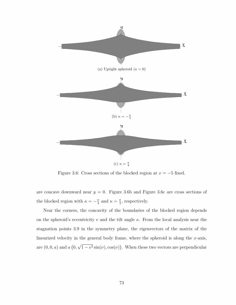
y

z

(a) Upright spheroid (κ = 0)

y

z

(b) κ = −π4

y

z

(c) κ = π4

Figure 3.6: Cross sections of the blocked region at x = −5 fixed.

are concave downward near y = 0. Figure 3.6b and Figure 3.6c are cross sections of

the blocked region with κ = −π4

and κ = π4, respectively.

Near the corners, the concavity of the boundaries of the blocked region depends

on the spheroid’s eccentricity e and the tilt angle κ. From the local analysis near the

stagnation points 3.9 in the symmetry plane, the eigenvectors of the matrix of the

linearized velocity in the general body frame, where the spheroid is along the x-axis,

are (0, 0, a) and a(0,√

1− e2 sin(ν), cos(ν)). When these two vectors are perpendicular

73

to each other, i. e. the eccentricity e and the tilt angle κ satisfy

12e− 8e3 − 6(1− e2)Le + (6e+ (e2 − 3)Le) e2 cos(2κ)

e2 (3(1− e2)Le + 2e (2e2 − 3)) ((1 + e2)Le − 2e)

− cos(2κ)

3(1− e2)Le + 2e (2e2 − 3)= 0,

the concavity of the blocked region changes.

74

Chapter 4

A sphere or spheroid embedded in

a rotation flow

To further explore the flow past a rigid obstacle, we consider the flow with a sphere

or spheroid embedded in rotating flows in this chapter.

4.1 A sphere embedded in a rotating flow

First, we consider the flow with a sphere embedded in rotating flows. The center

of the sphere is set at the origin of the coordinate system. The background flow is

a rigid body rotation in the x-y plane with the rotation axis parallel to the z-axis

and translated a fixed distance L from the origin. In this case, the x-y plane is the

symmetry plane of the flow. The planar linear shear case with the sphere’s center at

some distance off the zero-velocity plane may be viewed as an extreme case of this

rotating background flow in that at large distances L, the curvature of rigid body

rotation streamlines over regions of sphere radius scales becomes negligible. However,

there are important differences with respect to the planar case in the interpretation

of blocking regions for the case of rotating background flow past a sphere, as in this

case the definition of blocking itself becomes fundamentally different. We will study

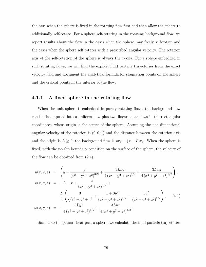
the case when the sphere is fixed in the rotating flow first and then allow the sphere to

additionally self-rotate. For a sphere self-rotating in the rotating background flow, we

report results about the flow in the cases when the sphere may freely self-rotate and

the cases when the sphere self rotates with a prescribed angular velocity. The rotation

axis of the self-rotation of the sphere is always the z-axis. For a sphere embedded in

such rotating flows, we will find the explicit fluid particle trajectories from the exact

velocity field and document the analytical formula for stagnation points on the sphere

and the critical points in the interior of the flow.

4.1.1 A fixed sphere in the rotating flow

When the unit sphere is embedded in purely rotating flows, the background flow

can be decomposed into a uniform flow plus two linear shear flows in the rectangular

coordinates, whose origin is the center of the sphere. Assuming the non-dimensional

angular velocity of the rotation is (0, 0, 1) and the distance between the rotation axis

and the origin is L ≥ 0, the background flow is yex − (x + L)ey. When the sphere is

fixed, with the no-slip boundary condition on the surface of the sphere, the velocity of

the flow can be obtained from (2.4),

u(x, y, z) =

(y − y

(x2 + y2 + z2)3/2+

3Lxy

4 (x2 + y2 + z2)3/2− 3Lxy

4 (x2 + y2 + z2)5/2

),

v(x, y, z) = −L− x+x

(x2 + y2 + z2)3/2+

L

4

(3√

x2 + y2 + z2+

1 + 3y2

(x2 + y2 + z2)3/2− 3y2

(x2 + y2 + z2)5/2

), (4.1)

w(x, y, z) = − 3Lyz

4 (x2 + y2 + z2)5/2+

3Lyz

4 (x2 + y2 + z2)3/2.

Similar to the planar shear past a sphere, we calculate the fluid particle trajectories

76

for this velocity field and obtain the explicit formulae in terms of r,

x =r2(5 + 4r)

8L(1− r)+r2(

27√

2 log(2√r +

√2(1 + 2r))− 8C1

)16L(1− r)

√r(1 + 2r)

,

z2 =C2r

3

(r − 1)2(1 + 2r),

y2 = r2 − x2 − z2,

where C1 and C2 are constant determined by the initial condition of the fluid particle.

To present the structure of the flow, we plot fluid particle trajectories with different

L in the x-y symmetry plane.

• When L = 0, trajectories are shown as in Figure 4.1a. In this case, it is easy to

verify from the velocity field (4.1) that there is no motion in the z-direction and

all velocity components vanish along the z-axis (x = y = 0).

• When 0 < L < 2, trajectories are illustrated in Figure 4.1b with a specified value

L = 1. There are two stagnation points on the sphere and they are in the x-z

plane, shown in Figure 4.3b when we show the stagnation points on the sphere.

• When L = 2, trajectories are shown in Figure 4.1c. There is one stagnation point

on the sphere at (−1, 0, 0).

• When L > 2, trajectories are plotted as Figure 4.1d with L = 3. There are two

stagnation points on the sphere. Figure 4.2 is the 3D view of Figure 4.1d.

As Figure 4.1 and 4.2 show, the stagnation points on the sphere depend on the

distance L. For a unit sphere, there are two stagnation points (−L2, 0,

√4−L2

2) and

(−L2, 0,

√4−L2

2) on the sphere if 0 ≤ L < 2. When L = 2, there is only one stagnation

point (−1, 0, 0) on the sphere. When L > 2, there are two stagnation points on the

77

(a) L=0 (b) L=1

(c) L=2 (d) L=3

Figure 4.1: Trajectories in the x-y symmetry plane.

78

Figure 4.2: 3D view o f trajectories in the x-y symmetry plane when L > 2.

sphere at (− 2L,√L2−4L

, 0) and (− 2L,−√L2−4L

, 0), but they are in the x-y symmetry plane

instead of the x-z plane for the L < 2 cases.

Furthermore, we get the formula for critical points in the interior of the flow, which

are always in the x-z plane. The implicit formula for critical points in the flow is

L+ 4x

4 (x2 + z2)3/2= L+ x− 3L

4√x2 + z2

.

In parametric formulae, they are

x = −L4

1 + s+ 4s2

1 + s+ s2,

z = ±√s2 − x2 = ±

√16s2(1 + s+ s2)2 + L2(1 + s+ 4s2)2

4(1 + s+ s2),

where |s| ≥ 1. When L ≤ 2, critical points in the interior of the flow connect to

the two stagnation points (−L2, 0,

√4−L2

2) and (−L

2, 0,

√4−L2

2) on the sphere as shown in

Figure 4.3a and Figure 4.3b. Black dots on the sphere are stagnation points in Figure

79

4.3. Since critical points in the flow are only in the x-z plane, plots in Figure 4.3 are

restricted in the x-z plane. The black curve in Figure 4.3a shows where critical points

are when L = 0. Figure 4.3b shows the location of critical points when L = 1. For the

special case L = 2 shown in Figure 4.3c, the curve connects to the unique stagnation

point (−1, 0, 0) on the sphere. Otherwise, for L > 2, as in Figure4.3d (L = 3), critical

points are on a curve that is still in the x-z plane but is away from the sphere. All the

curves are asymptotic to the rotation axis of the background flow as |z| → ∞. Notice

the analogy of these curves of fixed points with those identified off the x-z plane by

the analysis of the linear planar shear case in Table 2.1 in Chapter 2. The force acting

on the fixed sphere is F = −6πµLey and the torque at the origin is T = −8πµey in

dimensionless formulae.

4.1.2 A self-rotating sphere in the rotating flow

If the sphere self-rotates in the rotating background flow, imposing the no-slip

boundary condition on the rotating sphere requires the velocity on the surface of the

sphere to be U′ = −γyex + γxey. Here, γ is the angular velocity of the sphere’s self-

rotation in the z direction. For the special torque free case involving a sphere freely

self-rotating at the origin, the angular velocity of the self-rotation is set to γ = −1, as

the calculation shows. The exact velocity field is

u(x, y, z) = y +3Lxy

4 (x2 + y2 + z2)3/2− 3Lxy

4 (x2 + y2 + z2)5/2− (γ + 1)y

(x2 + y2 + z2)3/2,

v(x, y, z) = −L− x+3L

4√x2 + y2 + z2

+4x(γ + 1) + L(1 + 3y2)

4 (x2 + y2 + z2)3/2

− 3Ly2

4 (x2 + y2 + z2)5/2,

w(x, y, z) =3Lyz

4 (x2 + y2 + z2)3/2− 3Lyz

4 (x2 + y2 + z2)5/2.

80

-2 0 2

-2

0

2

x

z

(a) L = 0

-2 0 2

-2

0

2

xz

(b) L = 1

-2 0 2

-2

0

2

x

z

(c) L = 2

-2 0 2

-2

0

2

x

z

(d) L = 3

Figure 4.3: Critical points in the flow when a fixed sphere is embedded in a rotatingbackground flow. L is the distance from the rotation center of the background flow tothe center of the unit sphere.

81

And the equation of fluid particles is the following parametric system

x =r3

2L√

(r − 1)2r3(1 + 2r)

− 1

24√

(1 + 2r)

[64γ√

3(1 + 2r)arctanh

(√3r

1 + 2r

)+3(

2√r(5 + 14r + 8r2

)+ 27

√2(1 + 2r) log

(2√r +

√2(1 + 2r)

))]− C1

,

z2 =r3

C2(r − 1)2(1 + 2r),

y2 = r2 − x2 − z2,

where constants C1 and C2 depend on initial values.

Critical points in the interior of the flow are

x = L4(γ+1−r3)

(4r3 − 3r2 − 1),

z2 = r2 − x2.(4.2)

The slope of the critical-point curve as depicted in Figure 4.4 is 2γ3L

at the top of the

sphere (0, 0, 1). For the degenerate cases L = 0 and γ > −1, the velocity does not

only vanish on the curve prescribed by (4.2) in the x-z plane but also on the shell

x2 + y2 + z2 = (1 + γ)23 . For the special case γ = 0 (with the fixed sphere), the location

of stagnation points on the sphere depends on L as shown in Figure 4.3. Figure 4.4

shows the critical points in the x-z plane for different L when the sphere is freely

self-rotating in the rotating background flow.

Figure 4.5 shows the freely self-rotating case’s fluid particle trajectories in the x-y

symmetry plane for different L. Figure 4.6 shows trajectories of fluid particles out of

the x-y symmetry plane, when L = 4 and the sphere is freely rotating.

When the orientation of the sphere’s self-rotation is opposite and equal to that of

the background flow, Figure 4.7 shows critical points in the x-z plane and Figure 4.8

shows the trajectories of fluid particles in the x-y symmetry plane with different values

of L and γ = 1. Figure 4.9 show the structure of the fluid particle trajectories out of

82

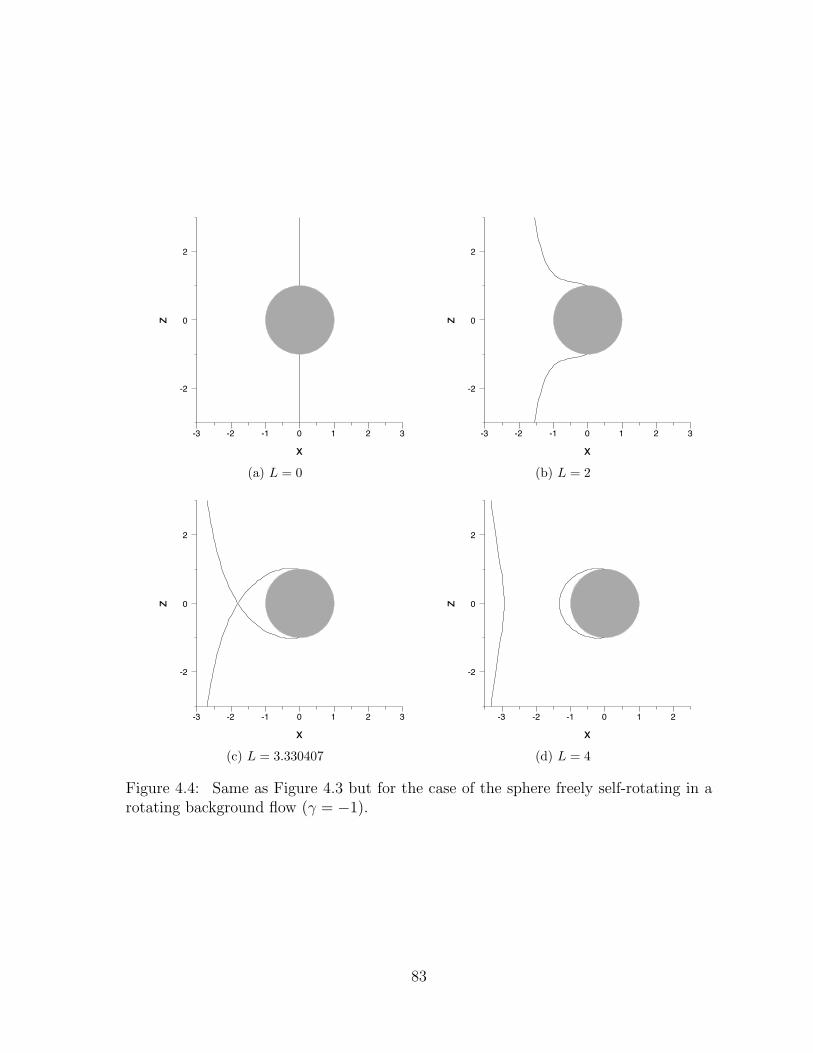
-3 -2 -1 0 1 2 3

-2

0

2

x

z

(a) L = 0

-3 -2 -1 0 1 2 3

-2

0

2

xz

(b) L = 2

-3 -2 -1 0 1 2 3

-2

0

2

x

z

(c) L = 3.330407

-3 -2 -1 0 1 2

-2

0

2

x

z

(d) L = 4

Figure 4.4: Same as Figure 4.3 but for the case of the sphere freely self-rotating in arotating background flow (γ = −1).

83

(a) L=0 (b) L=2

(c) L=3.330407 (d) L=4

Figure 4.5: Trajectories in the x-y symmetry plane with a freely-rotating sphere.

Figure 4.6: Trajectories out of the x-y symmetry plane when the sphere is freely rotatingand L = 4.

84

the symmetry plane when L = 3.

Comparisons between Figures 4.4-4.6 and Figures 4.7-4.9 show locations of the hy-

perbolic fixed points may be at either the left or the right side of the sphere, depending

upon parameters L, ω and γ.

4.2 A spheroid embedded in a rotation flow

As for the linear shear flow case, we generate our results to the prolate spheroid

embedded in the rotating flow in this section. The major axis of the spheroid could be

parallel to the axis of the background rotation, or oriented with a tilt angle κ 6= 0. The

tilt angle (−π2≤ κ < π

2) is defined as the angle between the major axis of the spheroid

and the axis of the rotation.

The background flow is purely rotating flow in the x-y plane with a constant angular

velocity (0, 0, -ω). If ω >0, the flow rotates clockwise, otherwise, the background flow

rotates counter-clockwise. The distance between the center of the spheroid to the center

of the rotation is noted as L. We specify the center of the spheroid at the origin, and

the axis of the rotation of the background flow at (−L, 0, z). In this coordinates, the

linear velocity of the background flow is

U = ~ω × ~r = yL ω ex − (xL + L)ω ey =

0 ω 0

−ω 0 0

0 0 0

xL

yL

zL

−

0

ωL

0

.

It is a uniform flow plus shear flows in both x direction and y direction.

If the major axis of the spheroid is parallel or perpendicular to the rotation axis of

the background flow, the flow is similar to a sphere embedded in a rotation flow. The

exact velocity can be constructed with the components for uniform flows and shear

85

-3 -2 -1 0 1 2 3

-2

0

2

x

z

(a) L = 0

-3 -2 -1 0 1 2 3

-2

0

2

xz

(b) L = 0.02

-3 -2 -1 0 1 2 3

-2

0

2

x

z

(c) L = 1

-3 -2 -1 0 1 2 3

-2

0

2

x

z

(d) L = 3

Figure 4.7: Same as Figure 4.3 and 4.4 but with a unit sphere self-rotating in anopposite direction with respect to the background flow (γ = 1).

86

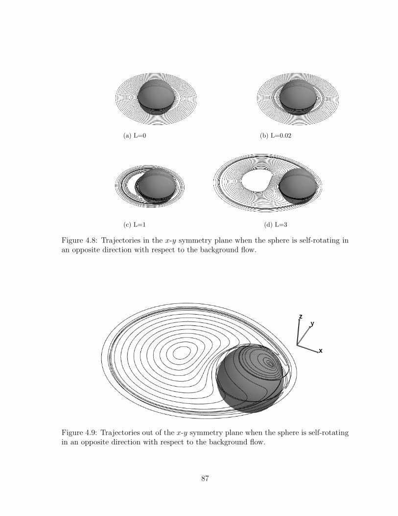
(a) L=0 (b) L=0.02

(c) L=1 (d) L=3

Figure 4.8: Trajectories in the x-y symmetry plane when the sphere is self-rotating inan opposite direction with respect to the background flow.

Figure 4.9: Trajectories out of the x-y symmetry plane when the sphere is self-rotatingin an opposite direction with respect to the background flow.

87

flows in Chwang & Wu [19], if their the velocity field is viewed as the velocity field in

the body frame. In that body frame, the major axis of the prolate spheroid is along

the x-axis and the center of the spheroid is at the origin of the coordinates, which is

referred as the “general” body frame in this thesis. When the spheroid is tilted in

the radial direction of the rotation (L = 0), it is the flow when a spheroid sweeps out

an upright cone in one of its body frame as defined in (4.3), which can be similarly

obtained from the flow in the general body frame [14].

We consider that the spheroid is tilted in the plane tangential to the rotating back-

ground flow, and the angle κ between the major axis of the spheroid and the rotation

axis of the background is between −π2

and π2. Then any tilt direction can be decom-

posed into radial and tangential directions to the rotation. When κ = 0, the upright

spheroid case is automatically recovered. In the laboratory frame (xL, yL, zL), the tilted

prolate spheroid is

x2L + (yL cos(κ)− zL sin(κ))2

b2+

(yL sin(κ) + zL cos(κ))2

a2= 1, (a > b). (4.3)

We construct the velocity field of the flow in the general body frame, where the spheroid

is along the x-axis. Then, the equation of the spheroid isx2b

a2 +y2b+z2

b

b2= 1.

The transformation matrix between the laboratory frame (xL, yL, zL) and the gen-

eral body frame (xb, yb, zb) is

R =

0 0 1

sin(κ) − cos(κ) 0

cos(κ) sin(κ) 0

. (4.4)

88

So,

(xL yL zL

)T= R

(xb yb zb

)T(4.5)

The background flow in the general body frame is

Ub(xb) = RTU(Rxb) = ω

− sin(κ)zb

cos(κ)zb

sin(κ)xb − cos(κ)yb

+ ωL

− sin(κ)

cos(κ)

0

, (4.6)

which consists of a uniform flow −ωL sin(κ)ex + ωL cos(κ)ey in x and y directions and

four shear flows −ω sin(κ)zbex, ω cos(κ)zbey, ω sin(κ)xbez and −ω cos(κ)ybez.

4.2.1 The velocity field

From (4.7), the velocity field for the uniform flow −ωL sin(κ)ex + ωL cos(κ)ey

past a prolate spheroidx2b

a2 +y2b+z2

b

b2= 1 is

u1(xb) = −ωL sin(κ)ex + ωL cos(κ)ey −∫ c

−c[α1uS (xb − ξ; ex) + α2uS (xb − ξ; ey)] dξ

+

∫ c

−c

(c2 − ξ2

)[β1uD (xb − ξ; ex) + β2uD (xb − ξ; ey)] dξ , (4.7)

where ξ = ξez,

α1 =2e2

1− e2β1 =

−ωL sin(κ)e2

−2e+ (1 + e2)Le, α2 =

2e2

1− e2β2 =

2ωL cos(κ)e2

2e+ (3e2 − 1)Le,

and Le = log(

1+e1−e

).

The velocity field for the shear flow −ω sin(κ)zbex past the spheroidx2b

a2 +y2b+z2

b

b2= 1

is not provided directly in Chwang & Wu [19]. However, by changing coordinates, the

89

velocity field is obtained as

u2(xb) = −ω sin(κ)zbex +

∫ c

−c

(c2 − ξ2

)[α3uSS (xb − ξ; ex, ez)− γ3uR (xb − ξ; ey)] dξ

+β3

∫ c

−c

(c2 − ξ2

)2 ∂

∂zuD (xb − ξ; ex) dξ , (4.8)

where

γ3 =−ω sin(κ)(1− e2)

−2e+ (1 + e2)Le, and α3 =

4e2

1− e2β3 =

2e2(Le − 2e)

2e(2e2 − 3) + 3(1− e2)Leγ3 .

The velocity field for the shear flow ω cos(κ)zbey past the spheroidx2b

a2 +y2b+z2

b

b2= 1

is provided directly in Chwang & Wu [19]

u3(xb) = ω cos(κ)zbey +

∫ c

−c

(c2 − ξ2

)[α4uSS (xb − ξ; ey, ez) + γ4uR (xb − ξ; ex)] dξ

+β4

∫ c

−c

(c2 − ξ2

)2 ∂

∂zuD (xb − ξ; ey) dξ , (4.9)

where

γ4 =ω cos(κ)(1− e2)

4e− 2(1− e2)Le, and α4 =

4e2

1− e2β4 =

2ω cos(κ)e2(1− e2)

2e(3− 5e2)− 3(1− e2)2Le.

The velocity field for the shear flow ω sin(κ)xbez past the spheroidx2b

a2 +y2b+z2

b

b2= 1

can be adopted from the results in Chwang & Wu [19]

u4(xb) = ω sin(κ)xbez −∫ c

−c

(c2 − ξ2

)[α5uSS (x− ξ; ex, ez)− γ5uR (x− ξ; ey)] dξ

−β5

∫ c

−c

(c2 − ξ2

)2 ∂

∂xuD (x− ξ; ez) dξ , (4.10)

90

where

γ5 =ω sin(κ)

−2e+ (1 + e2)Le, and α5 =

4e2

1− e2β5 =

−2e+ (1− e2)Le2e(2e2 − 3) + 3(1− e2)Le

e2γ5 .

The velocity field for the shear flow −ω cos(κ)ybez past a spheroidx2b

a2 +y2b+z2

b

b2= 1

can be obtained from the results in Chwang & Wu [19]

u5(x) = −ω cos(κ)ybez +

∫ c

−c

(c2 − ξ2

)[α6uSS (x− ξ; ey, ez) + γ6uR (x− ξ; ex)] dξ

+β6

∫ c

−c

(c2 − ξ2

)2 ∂

∂yuD (x− ξ; ez) dξ , (4.11)

where

γ6 =−ω cos(κ)

−2e+ (1 + e2)Le, and α6 =

4e2

1− e2β6 =

−2e+ (1− e2)Le2e(2e2 − 3) + 3(1− e2)Le

e2γ6 .

Totally, the velocity field in the body frame is

u(xb) = u1(xb) + u2(xb) + u3(xb) + u4(xb) + u5(xb).

The singularities involved in the above velocity fields are provided in Appendix A and

explicitly integrable. The tedious formulae are curtailed.

4.2.2 Fluid particle trajectories

When an upright prolate spheroid embedded in the rotation flow, as stated at the

beginning of this section, the flow structure is similar to a sphere embedded in the

rotation flow. Both the y = 0 and z = 0 planes are the symmetry planes of the flow.

In the z = 0 plane, the vertical velocity component vanishes. So, the fluid particle will

stay in the plane. The separation of the flow depends on the distance of the center of

91

the sphere to the rotation axis of the background flow.

Figure 4.10 shows the fluid particle trajectories near the spheroid. When L = 0, the

flow is rotating around the spheroid as Figure 4.10a. As L increases, the fluid particle

trajectories deform but are still closed orbits around the spheroid as Figure 4.10b for

L = 0.5. When L increases more, there are fluid particles trajectories that separate

and wrap around the spheroid slowly as shown in Figure 4.10c for L = 2. In these

plots, the shear rate ω = 1, the semimajor axis a = 1, and the semiminor axis b = 1/2.

On the surface of the spheroid, the no-slip boundary condition is always preserved.

Nevertheless, the fluid particle trajectories are closed periodic orbits.

When the spheroid’s center is coincident with the center of the rotation (L = 0)

and tilted with a tilt angle κ, the flow can be viewed as the flow generated by the

spheroid sweeping out a double cone in free space in a body frame. Figure 4.11 shows

particle trajectories for such a tilted spheroid in the rotating flow. These fluid particles

are initialized at same height z = 0.275 or z = −0.275. When they move close to the

spheroid, the particles are separated by the spheroid and wrap the spheroid. Similar

trajectories have been reported in Leiterman [48].

When the tilted spheroid is embedded in a purely rotating background flow with

a tilt angle κ 6= 0 and the spheroid’s center is away from the rotation axis of the

background flow (L 6= 0), there is net flow transport as shown in Figure 4.12. Neither

y = 0 nor z = 0 is the symmetry plane of the flow. In Figure 4.12, the fluid particle

moves from the upper half space to the lower half space when the spheroid is tilted with

κ = π6. The distance from the center of the rotation background to the spheroid’s center

is L = 2. For a specified rotation of the background flow, the tilt angle determines the

direction of the transport. This phenomenon is essentially different from those observed

in the spherical cases or the upright spheroid cases.

Further analysis about the stagnation points on the spheroid in the rotation flow

92

(a) L = 0 (b) L = 0.5

(c) L = 2

Figure 4.10: A rotating flow past an upright spheroid 4(x2 + y2) + z2 = 1 with ω = 1and different values of L.

93

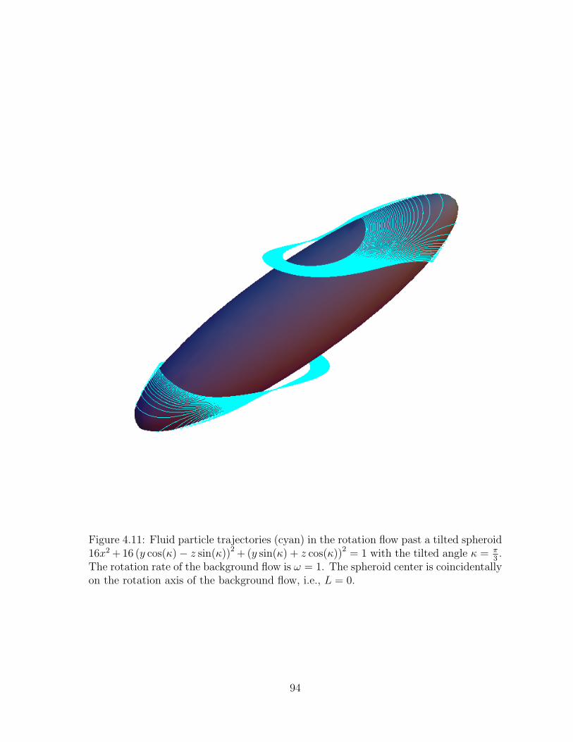
Figure 4.11: Fluid particle trajectories (cyan) in the rotation flow past a tilted spheroid16x2 + 16 (y cos(κ)− z sin(κ))2 + (y sin(κ) + z cos(κ))2 = 1 with the tilted angle κ = π

3.

The rotation rate of the background flow is ω = 1. The spheroid center is coincidentallyon the rotation axis of the background flow, i.e., L = 0.

94

xy

z

(a) View 1

x y

z

(b) View 2

Figure 4.12: Two views of a fluid particle trajectory in the rotation flow past a tiltedspheroid 4x2 + 4 (y cos(κ)− z sin(κ))2 + (y sin(κ) + z cos(κ))2 = 1. Here ω = 1, L = 2and κ = − π

16. The red dots indicate the initial position.

and the “imprint” on the surface will be interested. This information will be pursued

in the future study.

95

Part II

Experimental, theoretical and

numerical study of flows induced by

a slender body

96

Chapter 5

Experiments for a rod sweeping out

a cone above a no-slip plane

Study of flows induced by nodal cilia in the Stokes regime plays an important role in

fluid dynamics. Learning the flow structure will improve understanding of the fluid flow

in a ciliated system [9, 25]. For example, numerous left-right asymmetries in the internal

organs of the vertebrates are established during embryogenesis. Advanced results about

flow generated by nodal cilia on the embryo can help to verify the evidences of the left-

right symmetry breaking [58, 16, 32]. A review about the study of left-right symmetry

is referred to Hamada [29]. A few studies have been reported from the fluid mechanics

view [69]. But, as we know, there is no experimental work compared with the model in

the Lagrangian view. Because of its practical significance, experimental and theoretical

investigations are carried out on this Stokes problem. For the experimental study, it

can validate the mathematical theory and allow for direct comparison of experimental

data with theoretical observations.

In this chapter, the table-top experimental work with Rotation and Mixing eXper-

iment (RMX) is reported. This chapter focuses on the experimental setup and the

procedures. Experimental data are reported in Chapter 6 and Chapter 7, when we

compare the experimental trajectories with the theoretical predictions.

5.1 Experimental setup

Table-top experiments are conducted in a 30cm cubical, clear plexiglass tank filled

with approximately 10cm height highly viscous fluid. Figure 5.1 shows the tank, lighting

and camera setup on a kinematic mount. The two 1024×768 black and white PointGray

Dragonfly cameras are put in front of the tank and at the left side of the tank, referring

as side camera and front camera. With fiber optical illuminator light source through

the diffusers (white glass on the two sides), rods and the tracer in the fluid cast shadows

to each camera, in silhouette.

Above the horizontal planar bottom of the tank, a magnetically permeable rod

precesses in a cone (as Figure 5.2). The rod is driven by a 3000 G permanent magnet

mounted on a motorized turntable underneath the tank. Both straight and bent rods are

manufactured with body length ` = 1cm and cross-sectional radius r ∼ 0.038±0.002cm.

The curvature of the bent rod is about 0.40± 0.01cm−1. Figure 5.3a and 5.3b show a

batch of bent pins used in our experiments and an individual one. At least one end of

the rod is sharped to provide a well-defined pivot point to precess. Ideally, the pivot

point is the rotation axis of a motor driven turnable.

The configuration of the cone is shown in Figure 5.2. For a straight rod, the rod

will be the red chord. For a bent rod, the sharp tip at the apex of the cone is bent off

the plane of the rod and causes a scooping angle which is defined as the angle between

the plane of the rod and the vertical plane through the cone axis and the rod’s chord as

angle β shown in Figure 5.2. The cone angle κ is defined as the angle between the chord

of the rod and the cone axis. It is determined by the offset of the magnet underneath

the tank from the rotation center of the turning table.

We use two different fluids, Karo corn syrup and silicone oil. The Karo light corn

syrup’s density is approximately 1.36 g/cc and its dynamic viscosity is about 32 Poise.

A thin layer of baby oil is put on the top of the corn syrup to prevent evaporation. The

98

diffusers

Figure 5.1: Setup of the tank, cameras, diffusers, and lighting.

Figure 5.2: Configuration of a bent rod sweeping out an upright cone above a no-slipplane. Cone angle κ is the angle between the rod’s chord and the positive z-axis (thecone axis). Scooping angle β is the angle between plane “a” and plane “b” in whichthe rod lies.

99

(a) A batch of uniformly bent pin with onesharped tip.

(b) One individual pin

Figure 5.3: Bent pins used in our experiments.

silicone oil is with density 0.92 g/cc and kinematic viscosity 12500 Cst (about 95 Poise

for dynamic viscosity). The magnet turntable is engaged and adjusted so that the pin

precesses conically at a ω = 0.2 Hz rate.

The fluid viscosities and precession frequencies are selected so that a Reynolds

number Re and SrRe of 10−3 are not exceeded, where the Reynolds number is Re=

ρω `2 sin(κ)µ

, the Strouhal number is Sr= ω `U

= ω `ω ` sin(κ)

= 1sin(κ)

and U = ω ` sin(κ). So,

SrRe= ω`2

ν. When Re 1 and Sr Re 1, the fluid flow is in the Stokes’ regime.

The details of the parameters of the flow are listed in Table 5.1 and Table 5.2. If

the cone angle is about 30 degrees and the characteristic length is the radius of the rod,

then Re and Sr Re ≈ 10−3 for the corn syrup. If the cone angle is about 30 degree and

the characteristic length is the radius of the rod, then Re≈ 10−4 and Sr Re ≈ 10−3 for

the silicone oil.

From Cartwright et al. [16], the Reynolds number of the cilia flow Re = v Lν

is of

order 10−3. Here the characteristic length L is the size of the nodal cilia, v is the flow

100

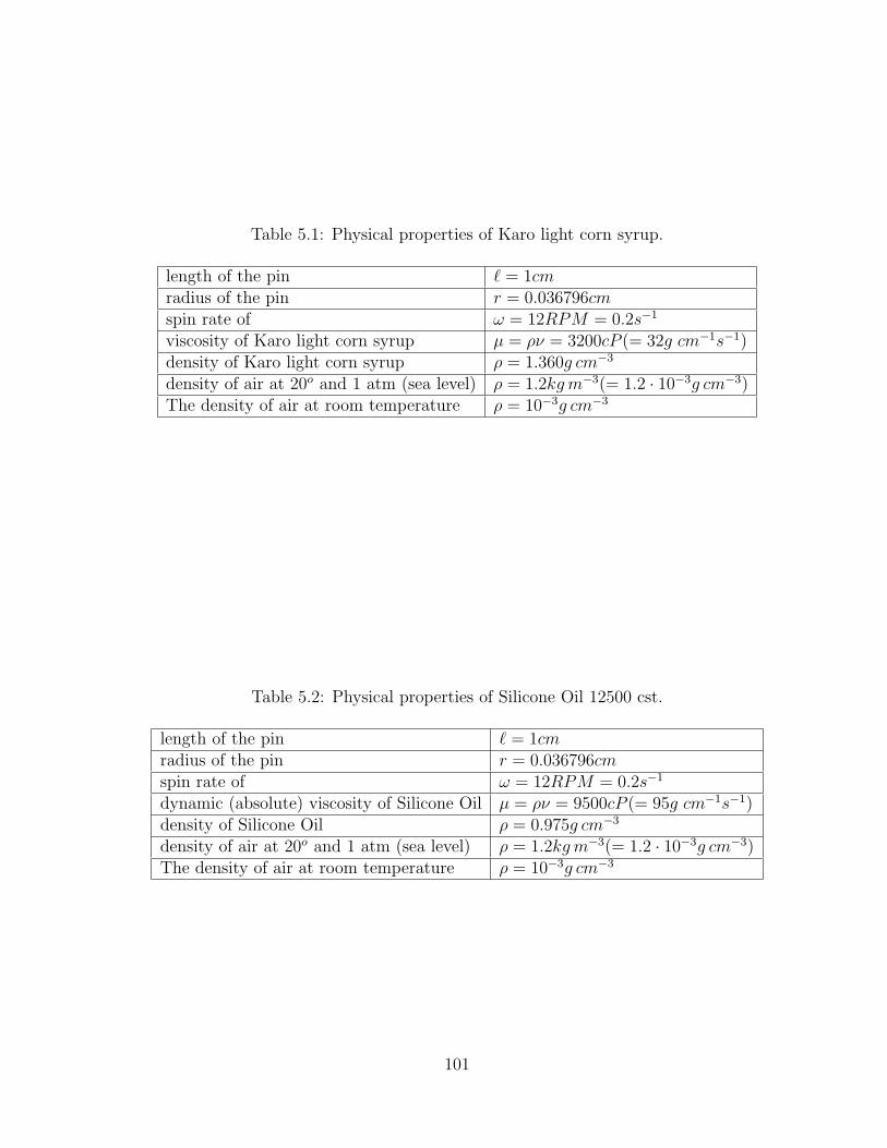
Table 5.1: Physical properties of Karo light corn syrup.

length of the pin ` = 1cmradius of the pin r = 0.036796cmspin rate of ω = 12RPM = 0.2s−1

viscosity of Karo light corn syrup µ = ρν = 3200cP (= 32g cm−1s−1)density of Karo light corn syrup ρ = 1.360g cm−3

density of air at 20o and 1 atm (sea level) ρ = 1.2kg m−3(= 1.2 · 10−3g cm−3)The density of air at room temperature ρ = 10−3g cm−3

Table 5.2: Physical properties of Silicone Oil 12500 cst.

length of the pin ` = 1cmradius of the pin r = 0.036796cmspin rate of ω = 12RPM = 0.2s−1

dynamic (absolute) viscosity of Silicone Oil µ = ρν = 9500cP (= 95g cm−1s−1)density of Silicone Oil ρ = 0.975g cm−3

density of air at 20o and 1 atm (sea level) ρ = 1.2kg m−3(= 1.2 · 10−3g cm−3)The density of air at room temperature ρ = 10−3g cm−3

101

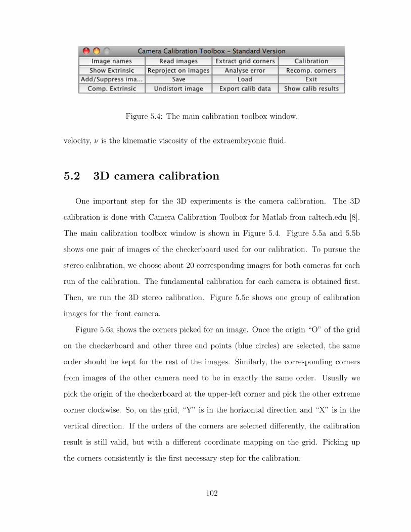
Figure 5.4: The main calibration toolbox window.

velocity, ν is the kinematic viscosity of the extraembryonic fluid.

5.2 3D camera calibration

One important step for the 3D experiments is the camera calibration. The 3D

calibration is done with Camera Calibration Toolbox for Matlab from caltech.edu [8].

The main calibration toolbox window is shown in Figure 5.4. Figure 5.5a and 5.5b

shows one pair of images of the checkerboard used for our calibration. To pursue the

stereo calibration, we choose about 20 corresponding images for both cameras for each

run of the calibration. The fundamental calibration for each camera is obtained first.

Then, we run the 3D stereo calibration. Figure 5.5c shows one group of calibration

images for the front camera.

Figure 5.6a shows the corners picked for an image. Once the origin “O” of the grid

on the checkerboard and other three end points (blue circles) are selected, the same

order should be kept for the rest of the images. Similarly, the corresponding corners

from images of the other camera need to be in exactly the same order. Usually we

pick the origin of the checkerboard at the upper-left corner and pick the other extreme

corner clockwise. So, on the grid, “Y” is in the horizontal direction and “X” is in the

vertical direction. If the orders of the corners are selected differently, the calibration

result is still valid, but with a different coordinate mapping on the grid. Picking up

the corners consistently is the first necessary step for the calibration.

102

(a) From front camera (b) From side camera

Calibration images

(c) One group images from front camera

Figure 5.5: Images for the calibration.

103

X

YO

The red crosses should be close to the image corners

100 200 300 400 500 600 700 800 900 1000

100

200

300

400

500

600

700

(a) Extract corners

X

YO

Image 3 − Image points (+) and reprojected grid points (o)

100 200 300 400 500 600 700 800 900 1000

100

200

300

400

500

600

700

(b) Reprojected corners

Figure 5.6: Extracted corners on one image and reprojected corners after calibration.

After extracting the corners, click “calibration” to run the calibration with all cor-

ners from the images. Figure 5.6b shows the reprojected corners as green circles after

calibration, as compared to the extracted corners. The arrows show the magnitude

and the direction of the difference. Figure 5.7 shows the reconstructed 3D grid on

the checkerboard from the 20 images selected here, with camera-centered view and

world-centered view.

Figure 5.8 shows the grids and the position of the camera. Since the camera is

placed outside the tank, the distance between the camera and the checkerboard is

much larger than the size of the checkerboard. The calibrated data are in the camera-

view coordinates. Notice the orientation of the coordinates (Xc,Yc,Zc) and the origin

“O” are different from the coordinates defined in our model. The coordinate system for

our model is the cone-centered view as in Figure 5.2. Rotation and translation must be

applied to the experimental data to make the coordinates consistent with each other.

During the calibration, press the button “Analysis error” to check the reprojection

error. For example, Figure 5.9 shows the reprojection errors are within 5 pixels for the

calibration images showed in Figure 5.5. Reprojection errors within 10 pixels are with

104

−20

0

20260

280300

−10

0

10

20

Zc

18172019161314128

15711

Extrinsic parameters (camera−centered)

654312910

Xc

<−

− Y

c

−500

50100

0

100

200

0

50

100

150

200 1781820

131412

15167

Yworld

111196352

49

Extrinsic parameters (world−centered)

10

Xworld

Zw

orld

Figure 5.7: Extrinsic parameters.

−20 020 050

100150

200250

300

−20

0

20

1817208191613141215711654312910

Extrinsic parameters (camera−centered)

Xc

Zc

Yc

Oc

Figure 5.8: Extrinsic parameters with the camera on.

105

−2 −1.5 −1 −0.5 0 0.5 1 1.5

−1

−0.5

0

0.5

1

1.5

Reprojection error (in pixel)

x

y

(a) For images from the front camera

−1.5 −1 −0.5 0 0.5 1 1.5

−2

−1.5

−1

−0.5

0

0.5

Reprojection error (in pixel) − To exit: right button

x

y

(b) For images from the side camera

Figure 5.9: Reprojection error.

a reasonable range for our images. Running a few iterations of “Recomp·corners” and

“Add/Suppress images” is helpful to reduce the reprojection error.

For details of calibration toolbox, refer to the website of the calibration tool [8].

Here are a few tips to produce a good calibration for our experiments. We should

always be aware of the blockage of the corners of the grid by any object, for example,

air bubbles in the fluid, tracers or the rod. If this happens, the stereo calibration data

may not be produced. Missing a corner sometimes can cause such severe problems

that the calibration for that camera itself could fail. Also the images selected for the

calibration should not be too close to each other, otherwise, the ill-condition in the

data can fail the calibration. Thirdly, when the calibration fails, go to “Analysis error”

in the camera calibration tool and click the “+” with a large pixel error to check which

image and which corner on that image produces that error. For example, if the error

information is following:

Selected image: 1

Selected point index: 8

Pattern coordinates (in units of (dX,dY)): (X,Y)=(7,11)

106

Figure 5.10: The stereo calibration window.

Image coordinates (in pixel): (776.94,627.15)

Pixel error = (2.64628,7.82514)

Window size: (wintx,winty) = (8,8)

It means the clicked pixel error (2.64628,7.82514) is caused by the corner with index 8

on image 1. In the calibration grid, that corner is at (x, y) = (7, 11) in the unit of grid,

and (776.94,627.15) in pixel. The window size used to picked up corners is (8,8) pixels.

Also, set the camera perpendicular to the wall of the tank to avoid extreme distortions.

In this case, a single distortion coefficient automatically selected by the toolbox will

be sufficient. Otherwise, call manual corner extraction.m after the standard corner

extraction and choose the appropriate distortion model with help of isualize distortions.

When the calibration data for both camera are saved, run “stereo gui” for 3D stereo

calibration. The stereo calibration toolbox window is shown in Figure 5.10. Load

the calibration for the two cameras in order and then press “Run stereo calibration”

to get the 3D stereo calibration. Figure 5.11 shows the extrinsic parameters for the

stereo calibration with the left camera corresponding to the side camera and the right

camera corresponding to the front camera for our experiment. Since the scale of the

checkerboard is much small compare to dimensions of the tank, the grids are compressed

at the center on the figure. However, this figure demonstrates the relative positions of

our cameras very well. Finally, save the data for 3D calibration. Based on the stereo

calibration data, 3D trajectory is constructed with function stereo triangulation.

107

0

100

2000

100200

300

−20−10010

XY

Right CameraZ

Extrinsic parameters

21616381203406145638618996176161815311572711568581690760816

ZXYLeft Camera

Figure 5.11: Extrinsic parameters for the 3D stereo calibration.

5.3 Image processes and 3D data construction

To visualize the motion of the fluid, visible markers of the order of 100 microns are

placed at the desired locations in the fluid with a syringe to enable optical tracking of

their Lagrangian trajectories. Two synchronized PointGray Dragonfly digital cameras

are set up at the sides of the tank to capture videos with the program Ladybugrecord

[20] as shown in Figure 5.1.

Main image analyses involved in the experiments are raw video processes and the

3D calibration, which has been documented in detail in the 3D calibration section. The

raw image processes and the 3D data reconstruction are reported in this section.

The captured videos are originally saved as raw data files which can previewed by

“rawplayer” and read by “raw2ppm” associated with Ladybugrecord. Each raw file

includes 450 frames. At the current 15fps (frame per second) speed for our cameras,

each file contains data for a 30-second movie. Every 100 raw files will be written to one

folder. The first 100 raw files in folder “dir0”, and the second 100 files in folder “dir1”,

etc. But the frame number is sequentially saved. Run “raw2txt” script to extract the

information of these raw files and check if there are fames dropped during the filming.

The raw files are then compressed into an AVI container from Matlab and processed

108

Figure 5.12: Snapshot of tracking.

with program Video Spot Tracker [73]. Video Spot Tracker program can read AVI video

stream or one raw file with current version v06.02. Figure 5.12 is a snapshot of tracking

with Video Spot Tracker program. The yellow trajectory is the trace of the marker.

The red dot numbered with “0” is the tracker which is overlapped with the maker.

After tracking the marker from both cameras, based on the calibration data, we

construct the 3D trajectory with the function “stereo triangulation” in the calibration

toolbox. The parameters of the rod are tracked with the tracking program in Matlab

from David Holz [35] with the calibration information.

The units of the output data from the calibration are consistent with the units

imputed during the calibration. For the 7×11 checkerboard used in our experiment, the

grid size is 5mm× 5mm. If we enter 5mm for the size of each square, the reconstructed

3D trajectories of our tracer are in the units of mm. The origin of the reconstructed

data is in the camera-centered coordinates. Proper rotation and translation are applied

109

to the experimental trajectories to compare with the theoretical trajectories.

110

Chapter 6

A straight rod sweeping a tilted

cone above a no-slip plane

A prolate spheroid or a straight slender rod sweeping out a cone or double cone in

Stokes flow draw scientists’ attention due to its biological applications to flows gener-

ated by spinning cilia [58, 69, 16]. Such fluid motions are fundamental to many living

organisms. One important example is the left-right symmetry breaking in the early

development of mammals, where primary nodal cilia exhibit canonical rotatory move-

ment [16, 12]. Effectively, it is appropriate to approximate nodal cilia as rigid slender

rods. We build a model to study the flow generated by a slender rod and compare the

theoretical prediction to the experimental data. Such direct comparisons have not been

found in the literature yet.

In free space, the exact velocity field for a spheroid sweeping out a double cone has

been reported in Camassa et al. [14]. (In the appendix, we provide the error analysis

of the velocity field if the spheroid is approximated with a slender body.) When the

slender body precesses an upright cone above a no-slip plane, the velocity field and

the properties of the fluid particle trajectories have been studied with the slender body

theory and the image method [48, 9]. The velocity field is constructed in the body

frame, where the rod is fixed and there is rotating background flow. In this frame, a

fundamental singularity Stokeslet is distributed along the center-line of the slender rod.

Since the slender rod is sweeping out an upright cone, the distance between a point on

the rod and the no-slip plane is fixed. So, the center-line of the rod and its image with

respect to the no-slip plane have no time dependence in the body frame. Ultimately,

the velocity field in the body frame is independent of time and can be constructed

with Blakelet [5]. By applying the transformation between the body frame and the

laboratory frame, the velocity in the laboratory frame is obtained from the velocity

field in the body frame.

When the cone is tilted, the distance from a point on the rod to the no-slip plane

varies while the rod sweeps. In such situations, the flow is fully time dependent in

both the body frame and the laboratory frame. To construct the velocity field, we

have to carry time information either in the body frame (to identify the position of

the no-slip plane over time) or in the lab frame. The simplification in the body frame

is no longer available, compared to the upright cone case. The tilt of the cone makes

the construction of the flow velocity field complicated. The tilted cone is especially

interesting, since most cilia sweep out tilted cones or extensive tilted cones in reality

and the cilia themselves are bent. Results for bent cilia sweeping out a cone will be

reported in the next chapter, which is much more complicated.

This chapter will continue with a brief review of results about the straight rod

sweeping out an upright cone, and then focus on the straight rod sweeping a tilted

cone above a no-slip plane. For a rod sweeping a tilted cone, we construct the velocity

directly in the laboratory frame and show the properties of the flow with fluid particle

trajectories. Distinct phenomena for a rod sweeping a tilted cone are deformations

of the Lagrangian fluid particle trajectories and directional fluid transport induced

by the rod. Since our model is flexible about the configuration of the cone, we run

the model with tracked cone angle from the experiment and compare the numerical

112

trajectories with the experimental trajectories. Our model shows good agreement with

the experimental data.

6.1 A straight rod sweeping out an upright cone

For a straight rod sweeping out an upright cone above a no-slip plane, Leiterman

[48] has studied the flow in the Lagrangian view point with the slender body theory. To

construct the velocity field for the flow, three different types of fundamental singularities

are used, i.e. Stokeslet, Stokes doublet, and potential doublet (also known as dipole).

The special combination of these three different singularities is Blakelet. It is a Stokeslet

with its image system introduced by Blake [5] to satisfy the no-slip boundary condition

in the flow. Leiterman [48] has reviewed these singularities and written the formula

conveniently applied here. The velocity field satisfying

µ∇2uB + 8πµαδ(x− s) = ∇p,

∇ · uB = 0,

uB|z=0 = 0,

in the upper half space x = (x, y, z) ∈ R3|z ≥ 0 is given as the Blakelet uB(x−s;α),

which is a collection of singularities

uB(x− s;α) = uS(x− s;α) + uS(x− s′;−α) (6.1)

+uSD(x− s′; ez, 2hα′) + uD(x− s′;−2h2α′)

where s = (s1, s2, s3) is the location of the Stokeslet, s′ = (s1, s2,−s3) is the location of

the image system, α = (α1, α2, α3) is the strength of the Stokeslet, α′ = (α1, α2,−α3),

and h = s3 is the distance from the point-force (Stokeslets) in the flow field to the

113

no-slip plane.

When a slender rod with radius r and length ` sweeps out an upright cone with the

cone angle κ defined as the angle between the cone axis and the rod, the angular velocity

of the rod is (0, 0, ω). If ω > 0, then the rod sweeps out a cone counter-clockwise. If

ω < 0, then the rod sweeps out a cone clockwise. The introduced velocity by a slender

body sweeping out an upright cone in the body frame is

u(x) = U(x) +

∫ `

0

(uS(x− xs;α(s)) + uS(x− x′s;−α(s))

+uSD(x− x′s; ez, 2zsα′(s)) + uD(x− x′s;−2z2

sα′(s))

)ds

= U(x) +

∫ `

0

[α(s)

|x− xs|+

(x− xs) ((x− xs) ·α(s))

|x− xs|3(6.2)

−(α(s)

|x− x′s|+

(x− xS′(s)) ((x− x′s) ·α(s))

|x− x′s|3

)+

+2zs

(−zα(s)′

|x− x′s|3+

(x− x′s)× ez ×α(s)′

|x− x′s|3+

3z(x− x′s) ((x− xs) ·α(s)′)

|x− x′s|5

)]ds.

Here, U(x) = (ωy,−ωx, 0) is the background rotating flow in the body frame, xs =

(s sin(κ), 0, s cos(κ)), x′s = (s sin(κ), 0,−s cos(κ)), and α(s) = α(s)′ = ωε sin(κ)2

(0, s, 0).

The slenderness ε is defined as ε = log−1( `r).

6.2 A straight rod sweeping a tilted cone

Similarly, to study the flow induced by a straight rod sweeping out a tilted cone, we

utilize the slender body theory and the image method to construct the velocity field.

This inquires the information about types of the singularities, locations of singularities,

and the strength of the singularities. Stokeslet is distributed along the center-line of

the slender rod to achieve the leading order approximation, and the image system is

added to satisfy the no-slip boundary condition.

114

Positions of the singularities

The singularities are distributed along the center-line of the rod. To find the posi-

tions of the singularities, it is essential to find the center-line of the slender rod. This

requires that we analyse the motion of the rod and configuration of the cone. The

slender rod sweeps out a tilted circular cone with a tilt angle λ, which is defined as

the angle between the cone axis and the positive z-axis. Without loss of generality, we

always choose the coordinate system that the tilt of the cone is in the x-z plane. If the

axis is tilted to the positive x-axis, λ > 0. Otherwise, λ < 0. When λ = 0, the cone is

upright. The cone angle κ is still the angle from the axis of the cone to the center-line

of the slender rod. The rod rotates counter-clockwise with an angular velocity ω in the

cone axis direction in the laboratory frame. To find the expression of the center-line,

we consider the cone as tilting the rod with angle κ first, then rotate the rod with the

angular velocity ω, and finally tilt the cone itself. Following this procedure, we get the

center-line of the rod as

xs = RλRωRκ(s, 0, 0)T = s

sin(κ) cos(ωt) cos(λ) + cos(κ) sin(λ)

sin(κ) sin(ωt),

− sin(κ) cos(ωt) sin(λ) + cos(κ) cos(λ)

, (6.3)

where 0 ≤ s ≤ `,

Rκ =

sin(κ) 0 − cos(κ)

0 1 0

cos(κ) 0 sin(κ)

, Rω =

cos(ωt) − sin(ωt) 0

sin(ωt) cos(ωt) 0

0 0 1

,

115

and

Rλ =

cos(λ) 0 sin(λ)

0 1 0

− sin(λ) 0 cos(λ)

.

We obtain the position of the center-line of the rod xs as a function of the rod’s arc-

length s in (6.3), which provides the location of the Stokeslet. The location of the

image system is determined accordingly.

Strength of singularities for a tilted cone

The strength of the singularities is obtained by imposing the no-slip boundary con-

dition on the surface of the slender rod. As the canonical slender body theory, the

strength of the singularity is in proportion to the velocity. The ratios are different from

the tangential direction to the normal and binormal directions of the rod. With the

prescribed velocity of the rod and the ratios from the slender body theory, the strength

of the Stokeslet is determined as

α1 = −ε ω2

sin(κ) sin(ωt) cos(λ),

α2 =ε ω

2sin(κ) cos(ωt), (6.4)

α3 =ε ω

2sin(κ) sin(ωt) sin(λ),

where ε = log−1( `r) is the slenderness defined in the previous section.

With the location and strength of the singularity and the relation of the image

116

system with the Stokeslet, the velocity field is finally found as

u(x) =

∫ `

0

uB(x− xs;α)ds

=

∫ `

0

[uS(x− xs;α) + uS(x− x′s;−α) (6.5)

+uSD(x− xs; ez; 2hα′) + uD

(x− xs;−2h2α′

)]ds

=

∫ `

0

[α

|x− xs|+

(x− xs)((x− xs) ·α)

|x− xs|3− α

|x− x′s|− (x− x′s)((x− x′s) ·α)

|x− x′s|3

+2zs

(−zα′

|x− x′s|3+

(x− x′s)× ez ×α′

|x− x′s|3+

3z(x− x′s)[α′ · (x− x′s)]

|x− x′s|5

)]ds.

Three components of the velocity field are:

u1(x, y, z) =

∫ `

0

α1

|x− xs|+

(x− xs) ((x− xs)α1 + α2(y − ys) + (z − zs)α3)

|x− xs|3(6.6)

− α1

|x− xs|− (x− xs) ((x− xs)α1 + α2(y − ys) + (z + zs)α3)

|x− x′s|3 + 2zs

[−zα1

|x− x′s|3

+(x− xs)α3

|x− x′s|3 +

3z(x− xs) (α1(x− xs) + α2(y − ys)− α3(z + zs))

|x− x′s|5

]ds,

u2(x, y, z) =

∫ `

0

α2

|x− xs|+

(y − ys) ((x− xs)α1 + α2(y − ys) + (z − zs)α3)

|x− xs|3(6.7)

− α2

|x− x′s|+

(y − ys) ((x− xs)α1 − α2(y − ys) + (z + zs)α3)

|x− x′s|3 + 2zs

[−zα2

|x− x′s|3

+(y − ys)α3

|x− x′s|3 +

3z(y − ys) (α1(x− xs) + α2(y − ys)− α3(z + zs))

|x− x′s|5

]ds,

117

u3(x, y, z) =

∫ `

0

α3

|x− xs|+

(z − zs) ((x− xs)α1 + α2(y − ys) + (z − zs)α3)

|x− xs|3

− α3

|x− x′s|− (z + zs) ((x− xs)α1 + α2(y − ys) + (z + zs)α3)

|x− x′s|3 (6.8)

+2zs

[zα3

|x− x′s|3 +

(y − ys)α2 + (x− xs)α1

|x− x′s|3

+3z(z + zs) (α1(x− xs) + α2(y − ys)− α3(z + zs))

|x− x′s|5

]ds,

where

|x− xs| =[(x− xs)2 + (y − ys)2 + (z − zs)2

]1/2and

|x− x′s| =[(x− xs)2 + (y − ys)2 + (z + zs)

2]1/2

.

As xs given by (6.3) and α in (6.4) are dependent of time and the geometry of cone,

the velocity field is fully 3D and time dependent. From the analytical velocity field, we

study the fluid particle trajectory numerically.

6.3 Fluid particle trajectories

When a straight rod sweeps out a cone above a no-slip plane, the trajectory of the

fluid particle is computed numerically from the velocity field equation (6.2) or (6.5).

The upright cone case can be recovered from (6.5) by setting the tilt angle λ = 0.

Since this upright cone case has been studied before [48, 9], we simply provide one

fluid particle trajectory with two views in Figure 6.1 to show the main properties of fluid

particle trajectories. While the rod rotates, the fluid particle moves along a slow, large,

periodic orbit surrounding the cone, and small epicycles with time scale proportional

to one revolution of the rod. Except for a periodic fluctuation during each epicycle, the

fluid particle stays at a fixed z-level. This property is illustrated clearly from the side

118

(a) Top view (b) Side view

Figure 6.1: A fluid particle trajectory starts at (0.6, 0, 0.5) within 10 revolutions of thestraight rod sweeping out an upright cone. The cone angle κ = 40o, the length of therod is ` = 1, and the radius is r = 0.038.

view of the trajectory in Figure 6.1b.

When the rod sweeps out a tilted cone, the symmetry of the cone with respect to

the no-slip plane is broken, which introduces new phenomena in the flow. Figure 6.2

shows fluid particle trajectories at one fixed initial position with different values of the

tilt angle λ, with the other parameters in the model held fixed for these trajectories.

The larger the tilted angle is, the more the trajectory is deformed. In Figure 6.2, the

fluid particle trajectory seems changed from a closed orbit to an open orbit when λ = π4

(the cone is always above the no-slip plane).

With the same geometry of the rod, Figure 6.3 and 6.4 show tilt effects with the

fluid particle trajectories initially on a line perpendicular to the cone axis. If the cone is

upright, such particles will stay at almost the same level. As the tilt angle λ increases,

the motion in the cone axis direction is enhanced. Initial positions on the plots are

marked with filled green circles. The cone angle for both cases is κ = π6. The tilt angle

λ is π12

for Figure 6.3, and λ equals π6

for Figure 6.4. The geometry of the rod in Figure

119

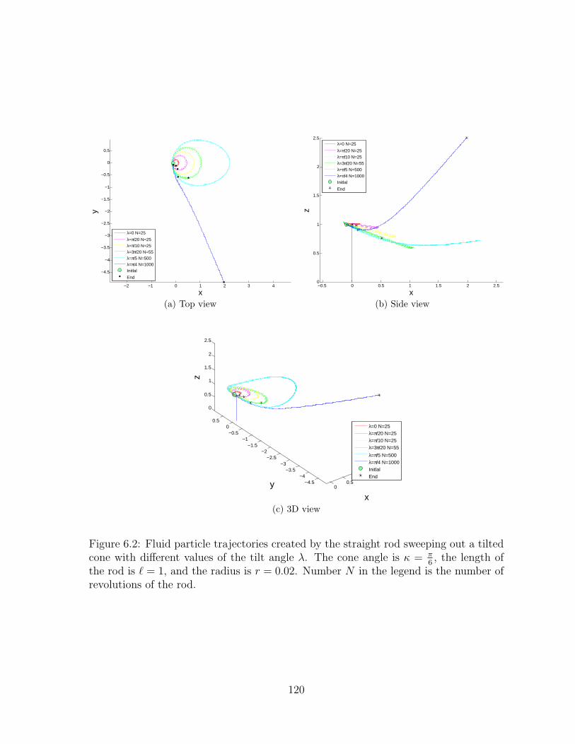
−2 −1 0 1 2 3 4

−4.5

−4

−3.5

−3

−2.5

−2

−1.5

−1

−0.5

0

0.5

x

y

λ=0 N=25

λ=π/20 N=25λ=π/10 N=25λ=3π/20 N=55λ=π/5 N=500λ=π/4 N=1000Initlal

End

(a) Top view

−0.5 0 0.5 1 1.5 2 2.50

0.5

1

1.5

2

2.5

x

z

λ=0 N=25

λ=π/20 N=25λ=π/10 N=25λ=3π/20 N=55λ=π/5 N=500λ=π/4 N=1000Initlal

End

(b) Side view

00.5

11.5

2

−4.5−4

−3.5−3

−2.5−2

−1.5−1

−0.50

0.5

0

0.5

1

1.5

2

2.5

xy

z

λ=0 N=25λ=π/20 N=25λ=π/10 N=25λ=3π/20 N=55

λ=π/5 N=500λ=π/4 N=1000InitlalEnd

(c) 3D view

Figure 6.2: Fluid particle trajectories created by the straight rod sweeping out a tiltedcone with different values of the tilt angle λ. The cone angle is κ = π

6, the length of

the rod is ` = 1, and the radius is r = 0.02. Number N in the legend is the number ofrevolutions of the rod.

120

6.3 and 6.4 is kept the same as in Figure 6.2.

Figure 6.5 shows another group of fluid particle trajectories within the same number

of revolutions N of the rod. The initial positions are at the opposite side of the x-axis

compared to the tilted cone axis. In another word, the cone axis is tilted to the x > 0

side, but x < 0 for the fluid particle initial positions. The cone angle is κ = π6

and the

tilt angle is λ = π4. The geometry of the rod is the same as in Figure 6.2. These fluid

particle trajectories are not closed orbits around the tilted cone. As this figure shows,

they are open trajectories. Since these are numerical trajectories, further theoretical

study is required to verify this.

As the fluid particle trajectories indicate, the tilted cone creates net transport. The

trajectories are periodic closed orbits near the cone, but there are open trajectories

away from the cone. Especially, some fluid particle trajectories are similar to the

streamlines of flow past a Stokeslet as shown in Figure 6.5. This is a new phenomenon

never observed with a straight rod sweeping out an upright cone.

6.4 Far field behaviors

To understand the open trajectories in the flow induced by the straight rod sweeping

out a tilted cone, it is worthwhile to check the flow far from the body. In the far field,

the flow motion could be captured by the leading order of the non-dimensionalized

velocity field.

To examine the velocity field as the observation point x gets far from the force

distribution, the non-dimensional formulae are introduced. Let

x = x/R, s = s/`, α′ = α/U, (6.9)

where R is a scalar parameter with the dimensions of length assumed to be large and

121

−0.50

0.51

1.5

−1

−0.5

0

0.5

1

0

0.5

1

1.5

xy

z

(a) 3D view (b) Cone axis view

−0.5 0 0.5 1 1.5 2

−1

−0.8

−0.6

−0.4

−0.2

0

0.2

0.4

0.6

0.8

1

x

y

(c) Top view

−0.5 0 0.5 1 1.5

0

0.2

0.4

0.6

0.8

1

1.2

1.4

1.6

1.8

x

z

(d) Side view

Figure 6.3: Fluid particle trajectories within the same number of revolutions N = 1000of the rod. The initial positions are distributed on a line perpendicular to the coneaxis in the x-z plane, indicated by the green points. The cone angle κ = π

6and the tilt

angle λ = π12

. The geometry of the rod is same as in Figure 6.2.

122

0

1

2

3

−2.5−2

−1.5−1

−0.50

0.5

0

0.5

1

1.5

2

2.5

3

xy

z

(a) 3D view (b) Cone axis view

−0.5 0 0.5 1 1.5 2 2.5 3 3.5−2.5

−2

−1.5

−1

−0.5

0

0.5

x

y

(c) Top view

−0.5 0 0.5 1 1.5 2 2.5 3 3.50

0.5

1

1.5

2

2.5

3

x

z

(d) Side view

Figure 6.4: Similar to Figure 6.3 but with the tilt angle λ = π6.

123

−6 −4 −2 0 2 4−5

−4

−3

−2

−1

0

1

2

3

4

5

x

y

(a) Top view

−3 −2.5 −2 −1.5 −1 −0.5 0 0.5

−0.5

0

0.5

1

1.5

2

xz

(b) Side view

−3−2

−10

−5

0

5

0

1

x

κ=π/6,λ=π/4

y

z

InitialEnd

(c) 3D view

Figure 6.5: Fluid particle trajectories created within the same number of revolutionsof the straight rod with κ = π

6and λ = π

4. The geometry of the rod is kept the same

as in Figure 6.2.

124

U = ω` is a characteristic velocity. The velocity field written as function of the non-

dimensional variables in (6.9) becomes

u′1(x, y, z) =

∫ `

0

[Uα1

R∣∣x− `

Rxs∣∣

+U(x− `

Rxs)((x− `

Rxs)α1 + (y − `

Rys)α2 + (z − `

Rzs)α3

)R∣∣x− `

Rxs∣∣3

− Uα1

R∣∣x− `

Rxs∣∣ − U(x− `

Rxs)((x− `

Rxs)α1 + α2(y − `

Rys) + (z + `

Rzs)α3

)R∣∣x− `

Rx′s∣∣3

+2`zs

(−zUα1U

R2∣∣x− `

Rx′s∣∣3 +

(x− `Rxs)Uα3

R2∣∣x− `

Rx′s∣∣3

+3Uz(x− `

Rxs)(α1(x− `

Rxs) + α2(y − `

Rys)− α3(z + `

Rzs))

R2∣∣x− `

Rx′s∣∣5

)]ds,

u′2(x, y, z) =

∫ `

0

[Uα2

R∣∣x− `

Rxs∣∣

+U(y − `

Rys)((x− `

Rxs)α1 + (y − `

Rys)α2 + (z − `

Rzs)α3

)R∣∣x− `

Rxs∣∣3

− Uα2

R∣∣x− `

Rx′s∣∣ +

U(y − `Rys)((x− `

Rxs)α1 − α2(y − `

Rys) + (z + `

Rzs)α3

)R∣∣x− `

Rx′s∣∣3

+2`zs

(−zUα2

R2∣∣x− `

Rx′s∣∣3 +

(y − `Rys)Uα3

R2∣∣x− `

Rx′s∣∣3

+3Uz(y − `

Rys)(α1(x− `

Rxs) + α2(y − `

Rys)− α3(z + `

Rzs))

R2∣∣x− `

Rx′s∣∣5

)]ds,

125

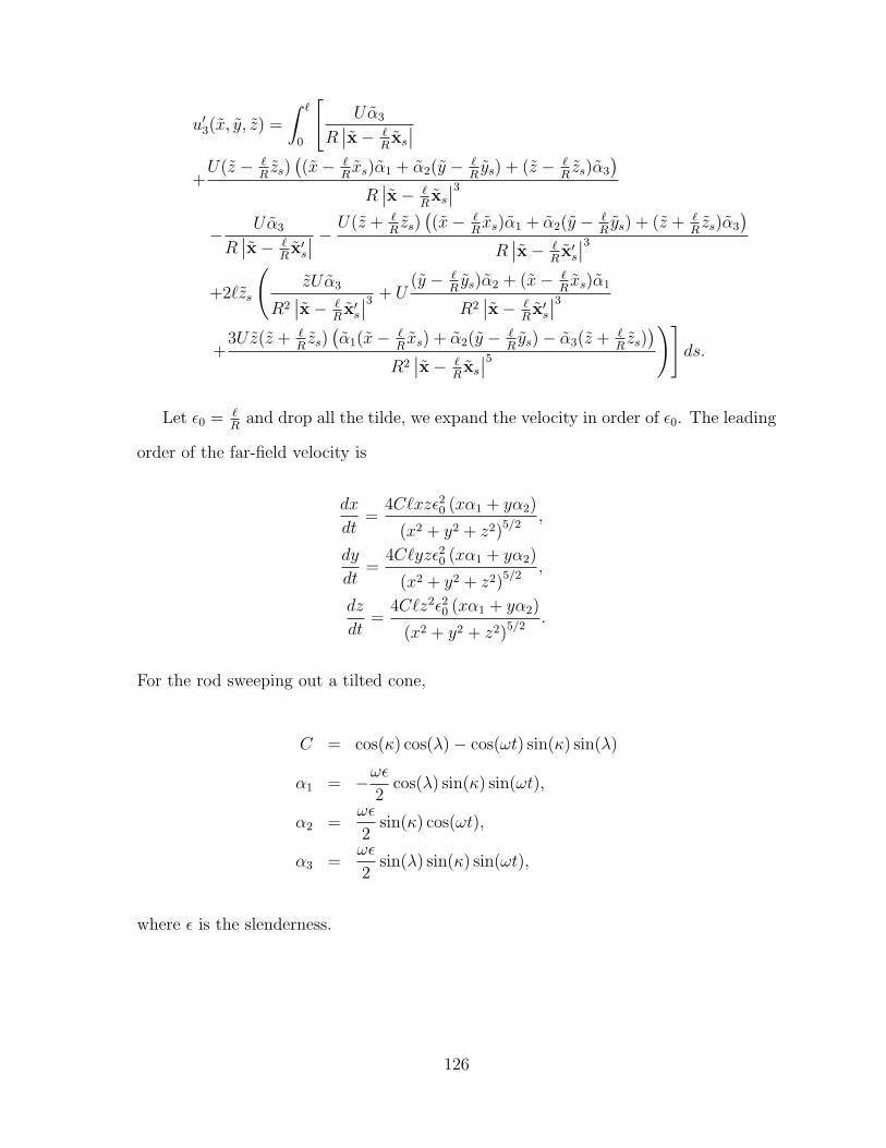
u′3(x, y, z) =

∫ `

0

[Uα3

R∣∣x− `

Rxs∣∣

+U(z − `

Rzs)((x− `

Rxs)α1 + α2(y − `

Rys) + (z − `

Rzs)α3

)R∣∣x− `

Rxs∣∣3

− Uα3

R∣∣x− `

Rx′s∣∣ − U(z + `

Rzs)((x− `

Rxs)α1 + α2(y − `

Rys) + (z + `

Rzs)α3

)R∣∣x− `

Rx′s∣∣3

+2`zs

(zUα3

R2∣∣x− `

Rx′s∣∣3 + U

(y − `Rys)α2 + (x− `

Rxs)α1

R2∣∣x− `

Rx′s∣∣3

+3Uz(z + `

Rzs)(α1(x− `

Rxs) + α2(y − `

Rys)− α3(z + `

Rzs))

R2∣∣x− `

Rxs∣∣5

)]ds.

Let ε0 = `R

and drop all the tilde, we expand the velocity in order of ε0. The leading

order of the far-field velocity is

dx

dt=

4C`xzε20 (xα1 + yα2)

(x2 + y2 + z2)5/2,

dy

dt=

4C`yzε20 (xα1 + yα2)

(x2 + y2 + z2)5/2,

dz

dt=

4C`z2ε20 (xα1 + yα2)

(x2 + y2 + z2)5/2.

For the rod sweeping out a tilted cone,

C = cos(κ) cos(λ)− cos(ωt) sin(κ) sin(λ)

α1 = −ωε2

cos(λ) sin(κ) sin(ωt),

α2 =ωε

2sin(κ) cos(ωt),

α3 =ωε

2sin(λ) sin(κ) sin(ωt),

where ε is the slenderness.

126

Type of singularity

The leading term in the far-field expansion of linear distribution of Blakelet is

u =2C`z(x ·α)

(x2 + y2 + z2)5/2x +

2C`z(x ·α′)(x2 + y2 + z2)5/2

x .

So,

u (x) ∼ uSD

(x; (α1, α2, 0),

4

3ε20C`ez

)= 4ε20C`z

(αT · xT

)x

|x|5. (6.10)

While the leading term in the far-field expansion of a uniform distribution of Stokeslets

is a single Stokeslet, the leading term in the farfield expansion of linear distribution of

Stokeslet is a Stokeslet doublet as (6.10).

Trajectory

From the far-field velocity (6.10), we rewrite the governing equations of the fluid

particle trajectory as

dy

dx=y

x,

dz

dx=z

x.

Let yx

= constant = η and zx

= constant = ζ, then y = ηx and z = ζx. Fluid particles

move along straight lines in the far field.

Computing the mean farfield velocity over one rotation of the rod, we get

u =ω

2π

∫ 2 πω

0

u (x, t) dt,

which is

127

dx

dt= −`ε

3ω sin2(κ) sin(λ)

(x2 + y2 + z2)5/2

xyz,

dy

dt= −`ε

3ω sin2(κ) sin(λ)

(x2 + y2 + z2)5/2

y2z,

dz

dt= −`ε

3ω sin2(κ) sin(λ)

(x2 + y2 + z2)5/2

yz2.

The above mean velocity field also shows the trajectories are straight lines.

6.5 Fluid transport

When a straight rod spins an upright cone, there is no net flux through a plane per-

pendicular to the no-slip plane over one rod revolution, due to the symmetry property

of the rotation. When the cone is tilted, the symmetry is broken. As the cone axis is

tilted in the x-z plane, there is net flux through a semi-infinite plane parallel to the x-z

plane. The flux is computed as an integral of velocity component v in the y-direction.

The mean flux is computed as a double integral of the velocity over the semi-infinite

plane and over one revolution.

From the velocity field (6.7), we first compute the integral over the spacial variables.

Then, the integral is over the semi-infinite plane at fixed y, parallel to the x-z plane,

and above the z = 0 plane. We notice the flux is contributed by the Stokeslet with

point force pointing perpendicular to this semi-infinite. In terms of the strength in

(6.4), they are velocity components associated with α2.

We first analyze the flux induced by a Blakelet uB(x−Csez;α2ey) through the semi-

infinite plane. The flux induced by either one Stokeslet uS(x − Csez;α2ey) or a pair

of Stokeslets uS(x−Csez;α2ey) + uS(x +Csez;−α2ey) in the Blakelet is infinite. The

Stokes doublet and the point source dipole in the Blakelet are higher order singularities

128

for the spatial coordinates, compared to the Stokeslet, and their contribution to the

velocity field decays faster at inifinity. However, seen from large distances, the pair

of Stokeslets contributes at leading order the same rate of decay as that of the Stokes

doublet and dipole, and hence there can be a cancellation that makes the flux induced

by a Blakelet uB(x− Csez;α2ey) is finite, as can be easily checked.

Based on the above information, we switch the order of integral to simplify the

integrals. The instantaneous flux through the semi-infinite plane perpendicular to the

y-axis is

∫ ∞0

∫ ∞−∞

v(x, y, z)dxdz =

∫ `

0

∫ ∞0

∫ ∞−∞

vB(x, y, z)dxdzds (6.11)

=

∫ `

0

8[cos(κ) cos(λ)− cos(ωt) sin(κ) sin(λ)] sin(κ) cos(ωt)ωε

2s2ds,

where vB(x, y, z) is the velocity component of a Blakelet in the y-direction. The average

flux over one revolution of the rod is

Flux =ω

2π

∫ 2πω

0

(∫ ∞0

∫ ∞−∞

v(x, y, z)dxdz

)dt (6.12)

=ω

2π

∫ 2πω

0

dt

∫ `

0

4ω ε(cos(κ) cos(λ)− cos(ωt) sin(κ) sin(λ)) sin(κ) cos(ωt)s2ds

=ω

2π

∫ 2πω

0

4`3ε ω

3cos(ωt) sin(κ)[cos(κ) cos(λ)− cos(ωt) sin(κ) sin(λ)]dt

= −2

3`3ε ω sin2(κ) sin(λ).

This is consistent with the result from Smith et al. [69], which is in terms of the

resistance coefficient and computed with the far-field velocity. The negative sign is

due to the prescribed counter-clockwise rotation of the rod and the definition of the

tilt angle λ. If the cone is tilt to the positive x-axis direction and the rod is sweeping

counter-clockwise with angular velocity ω, then the flux past a plane at y > 0 is

129

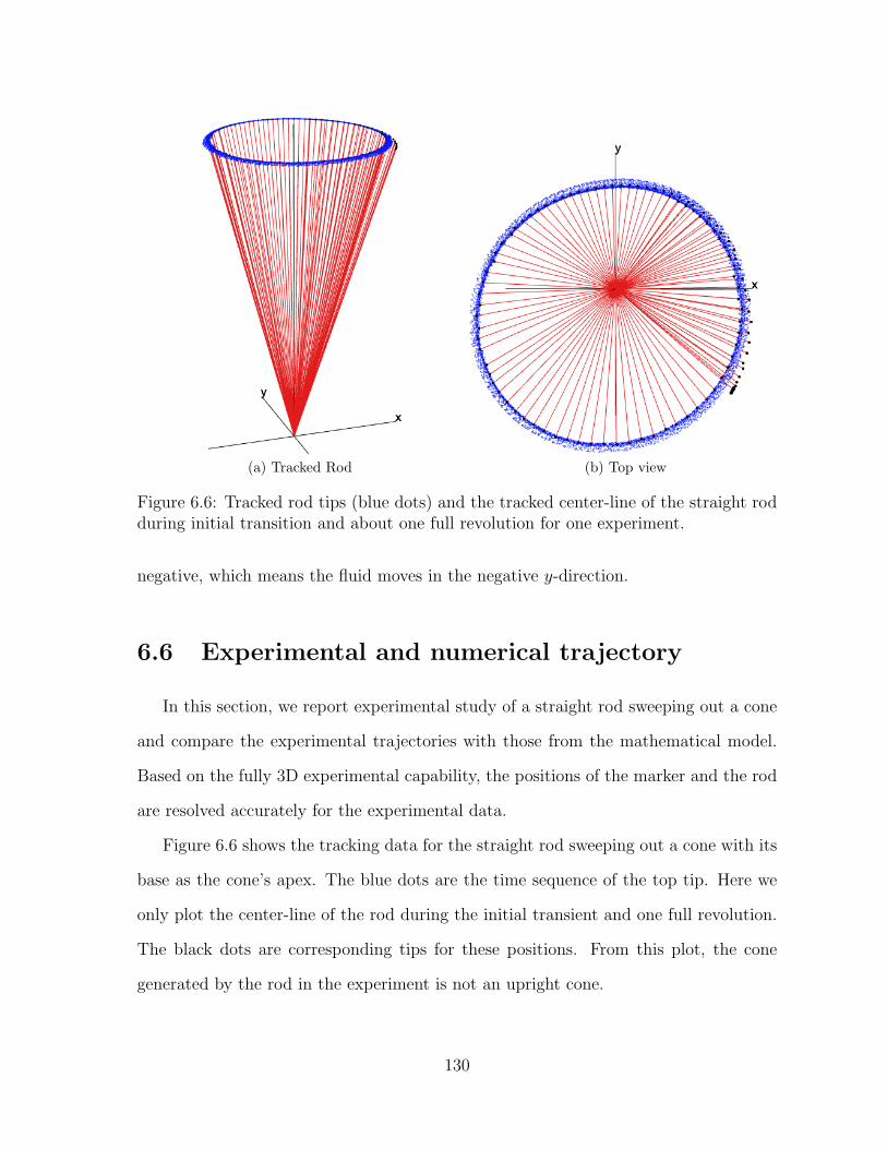
(a) Tracked Rod (b) Top view

Figure 6.6: Tracked rod tips (blue dots) and the tracked center-line of the straight rodduring initial transition and about one full revolution for one experiment.

negative, which means the fluid moves in the negative y-direction.

6.6 Experimental and numerical trajectory

In this section, we report experimental study of a straight rod sweeping out a cone

and compare the experimental trajectories with those from the mathematical model.

Based on the fully 3D experimental capability, the positions of the marker and the rod

are resolved accurately for the experimental data.

Figure 6.6 shows the tracking data for the straight rod sweeping out a cone with its

base as the cone’s apex. The blue dots are the time sequence of the top tip. Here we

only plot the center-line of the rod during the initial transient and one full revolution.

The black dots are corresponding tips for these positions. From this plot, the cone

generated by the rod in the experiment is not an upright cone.

130

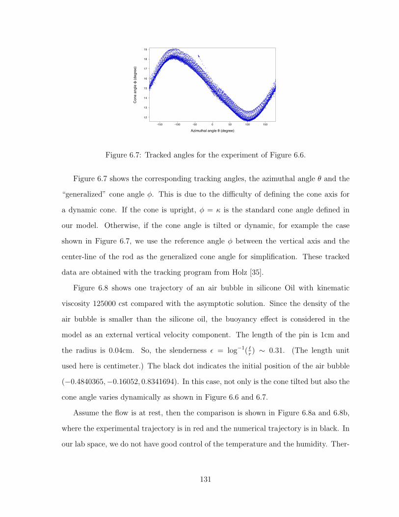
-150 -100 -50 0 50 100 150

12

13

14

15

16

17

18

19

Azimuthal angle θ (degree)C

one

angl

e ϕ

(deg

ree)

Figure 6.7: Tracked angles for the experiment of Figure 6.6.

Figure 6.7 shows the corresponding tracking angles, the azimuthal angle θ and the

“generalized” cone angle φ. This is due to the difficulty of defining the cone axis for

a dynamic cone. If the cone is upright, φ = κ is the standard cone angle defined in

our model. Otherwise, if the cone angle is tilted or dynamic, for example the case

shown in Figure 6.7, we use the reference angle φ between the vertical axis and the

center-line of the rod as the generalized cone angle for simplification. These tracked

data are obtained with the tracking program from Holz [35].

Figure 6.8 shows one trajectory of an air bubble in silicone Oil with kinematic

viscosity 125000 cst compared with the asymptotic solution. Since the density of the

air bubble is smaller than the silicone oil, the buoyancy effect is considered in the

model as an external vertical velocity component. The length of the pin is 1cm and

the radius is 0.04cm. So, the slenderness ε = log−1( `r) ∼ 0.31. (The length unit

used here is centimeter.) The black dot indicates the initial position of the air bubble

(−0.4840365,−0.16052, 0.8341694). In this case, not only is the cone tilted but also the

cone angle varies dynamically as shown in Figure 6.6 and 6.7.

Assume the flow is at rest, then the comparison is shown in Figure 6.8a and 6.8b,

where the experimental trajectory is in red and the numerical trajectory is in black. In

our lab space, we do not have good control of the temperature and the humidity. Ther-

131

mal instability is observed in the tank, even though the convection is slow and observed

in a very large time scale. In Figure 6.8c and 6.8d, the blue numerical trajectories are

obtained with optimized shear background flow (−1.050−4,−7.283 × 10−4, 0)z cm/s.

The optimized background flow is considered on the magnitude and direction of the

measured velocity of the air bubble without the motion of the rod for this experiment.

The shear flow instead of uniform background flow is input to avoid the invalidation of

no-slip boundary condition on the flat plane. These figures show that our model and

experiment have good agreement.

One mysterious result is the black trajectory shown in Figure 6.9. It is a numerical

trajectory if the background shear flow is directly added to the velocity field generated

by the rotating rod. In such a situation, the strength of the Stokeslet distributed along

the center-line of the rod should be adjusted properly to satisfy the no-slip boundary

condition on the surface. However, this trajectory with shear flow (5×10−6, 4×10−5, 0)z

directly added to the flow field has an excellent agreement with the trajectory with the

right velocity field, even though at the end of the trajectory very small discrepancy

shows up from the side view.

132

(a) Top view (b) Side view

(c) Top view (d) Side view

Figure 6.8: Experimental trajectories compare to numerical trajectories when a straightrod sweeps out a cone. The red trajectory is from experimental data. The blacktrajectory is from the numerical simulation without considering the convection in thefluid. The blue trajectory is the numerical trajectory with a shear background flow.The velocity of the background flow is based on the convection velocity measured inthe tank.

133

(a) Top view (b) Side view

Figure 6.9: The numerical trajectory with the shear background flow compared with anumerical trajectory with an invalid shear background flow. The blue trajectory is thenumerical trajectory in Figure 6.8c by correctly adding the background shear flow inthe fluid problem. The black trajectories is the trajectory with the invalid backgroundshear. In the numerical simulation, the background shear is added directly to the flowfield generated by spinning a rod in a stationary background flow instead of consideringthe shear flow as the background flow and justifying the singularities on the rod.

134

Chapter 7

A bent rod sweeping out a cone

above a no-slip plane

Following the study of flows generated by a straight rod sweeping out a cone in the

previous chapter, we study the flow induced by a bent rod, which precesses conically

above a no-slip plane in a highly viscous fluid. When a straight rod sweeps out an

upright cone, the flow preserves symmetry properties. When the rod is bent, symmetry

breaking induced by the bend creates new phenomena over a long time scale. A family

of nested tori appears in the fluid particle trajectories. Similar to the straight rod

case, we use experiment, theory and numerics to investigate and understand the flow

generated by a bent rod sweeping out a cone.

7.1 Model

The configuration of the motion of a bent rod is shown in Figure 7.1, which has been

briefly discussed in the experiment setup in Chapter 5. The rod stands above a no-slip

plane and sweeps out a cone with its lower tip as the pivot point. For the bent rod case,

the cone angle is defined as the angle between the chord of the rod and the axis of the

cone, and an extra scooping angle β is introduced. As the bent rod is in plane “b” in

Figure 7.1: Configuration of a bentrod sweeping out an upright cone.Cone angle κ is the angle betweenthe chord of the rod and the positivez-axis. Scooping angle β is the an-gle between plane “a” and plane “b”where the rod is.

Figure 7.1, the scooping angle β is defined as the angle from plane “a”, where the chord

and the axis of cone are, to plane “b”. To make the scooping angle unique for each

rod position, angle β is defined from plane “a” outside the cone to plane “b” clockwise.

Figure 7.2 shows four extreme situations of the rod sweeping out a cone. When β = 0,

we call it belly out; when β = π, we call it belly in; β = π2

and β = 3π2

for scooping and

anti-scooping, respectively, when the rotation is counter-clockwise as views from above.

−0.5

0

0.5

−0.5

0

0.50

0.2

0.4

0.6

0.8

1

xy

z

(a) Belly out (β = 0)−0.5

0

0.5

−0.5

0

0.50

0.2

0.4

0.6

0.8

1

xy

z

(b) Belly in (β = π)

−0.5

0

0.5

−0.5

0

0.50

0.2

0.4

0.6

0.8

1

xy

z

(c) Scoop (β = π2 )

−0.5

0

0.5

−0.5

0

0.50

0.2

0.4

0.6

0.8

1

xy

z

(d) Anti-scoop (β = 3π2 )

Figure 7.2: Four extreme statuses of the cone.

A model based on the slender-

body theory is developed to study the

induced flow above the infinite no-slip

plane. The essence is to express the

solutions in terms of a collection of

fundamental singular solutions to the

Stokes equations, and then to com-

pute the strength of the selected sin-

gularities in order to satisfy the far

field and no-slip boundary conditions.

The image system for the Stokeslet de-

rived by Blake [5] is utilized to handle

136

the no-slip boundary condition on the

flat plane upon which the apex of the cone rests.

The details about the velocity field for a bent rod precessing in an upright cone are

provided here. For the experimental verification, we extend our model to the tilted

cone case as necessary. Since the tilted cone for the bent rod is similar to the straight

rod case in the previous chapter, we skip those details to avoid redundancies.

In the body frame, when the rod sweeps out an upright cone, the rod and the no-slip

plane are relatively fixed and there is rotation background flow in the body frame. In

this frame, we construct an asymptotic solution in closed form using the slender body

theory. As for the straight rod case, Blakelets are distributed along the center-line of

the bent rod. In the body frame, the center-line of the bent rod is fixed and can be

written as a parametric function of its arc-length s. With prescribed scooping angle β

and cone angle κ, the center-line xb = (xb(s), yb(s), zb(s))T is

xb = −2a cos(β) cos(κ) sin(`− s

2a) sin(

s

2a) + 2a sin(κ) cos

(`− s

2a

)sin(

s

2a), (7.1)

yb = −2a sin(β) sin(`− s

2a) sin(

s

2a), (7.2)

zb = 2a cos(κ) cos(`− s

2a) sin(

s

2a) + 2a cos(β) sin(κ) sin

(`− s

2a

)sin(

s

2a), (7.3)

(0 ≤ s ≤ `), where ` is the body length and K = 1a

is the local non-dimensional

curvature of the body center-line with respect to the body length.

The strength of the Stokeslet in the Blakelet

α = Rdiag(ε

4,ε

2,ε

2)R−1U (7.4)

is determined from the linear background velocity U in the local coordinates of the bent

rod. In the body frame, U = ω×xb = (0, 0, ω)× (xb, yb, zb) is the rotation background

137

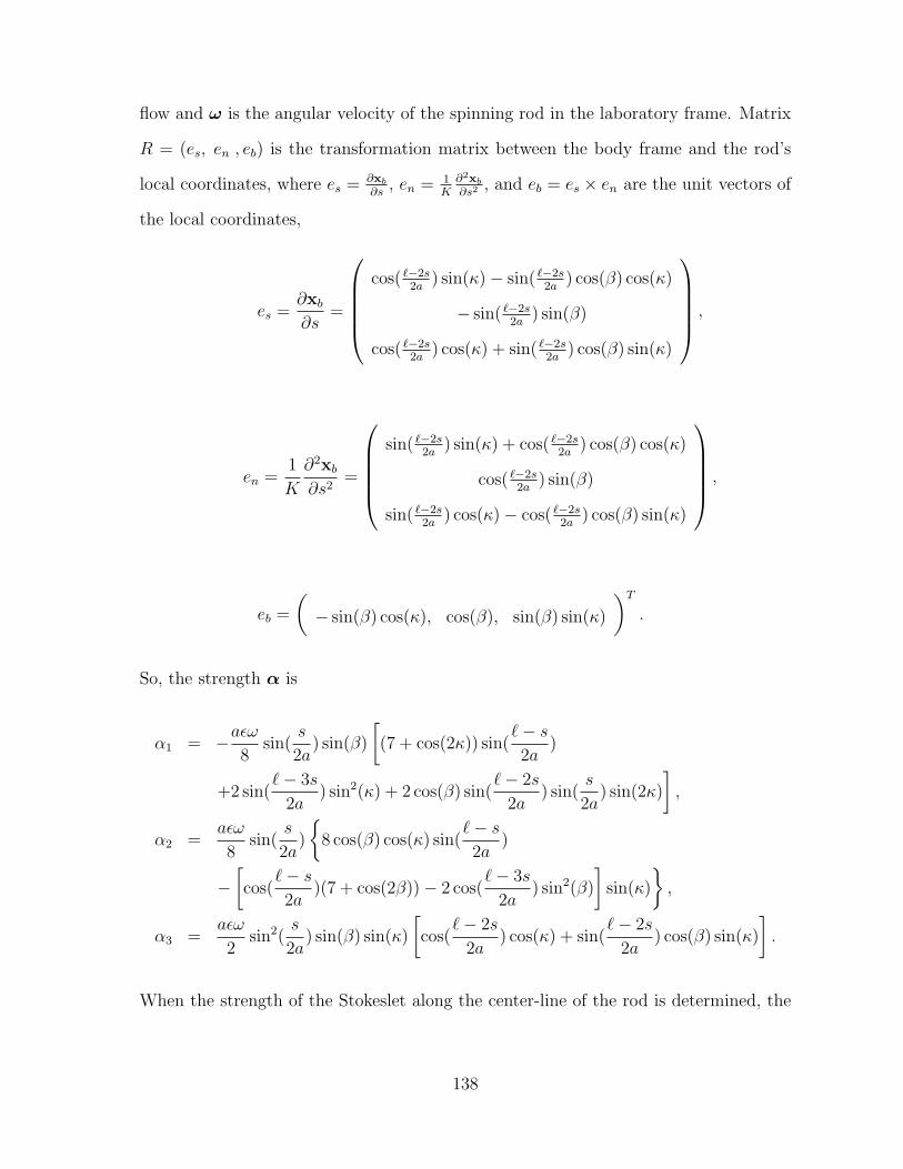
flow and ω is the angular velocity of the spinning rod in the laboratory frame. Matrix

R = (es, en , eb) is the transformation matrix between the body frame and the rod’s

local coordinates, where es = ∂xb∂s

, en = 1K∂2xb∂s2

, and eb = es × en are the unit vectors of

the local coordinates,

es =∂xb∂s

=

cos( `−2s

2a) sin(κ)− sin( `−2s

2a) cos(β) cos(κ)

− sin( `−2s2a

) sin(β)

cos( `−2s2a

) cos(κ) + sin( `−2s2a

) cos(β) sin(κ)

,

en =1

K

∂2xb∂s2

=

sin( `−2s

2a) sin(κ) + cos( `−2s

2a) cos(β) cos(κ)

cos( `−2s2a

) sin(β)

sin( `−2s2a

) cos(κ)− cos( `−2s2a

) cos(β) sin(κ)

,

eb =

(− sin(β) cos(κ), cos(β), sin(β) sin(κ)

)T.

So, the strength α is

α1 = −aεω8

sin(s

2a) sin(β)

[(7 + cos(2κ)) sin(

`− s2a

)

+2 sin(`− 3s

2a) sin2(κ) + 2 cos(β) sin(

`− 2s

2a) sin(

s

2a) sin(2κ)

],

α2 =aεω

8sin(

s

2a)

8 cos(β) cos(κ) sin(

`− s2a

)

−[cos(

`− s2a

)(7 + cos(2β))− 2 cos(`− 3s

2a) sin2(β)

]sin(κ)

,

α3 =aεω

2sin2(

s

2a) sin(β) sin(κ)

[cos(

`− 2s

2a) cos(κ) + sin(

`− 2s

2a) cos(β) sin(κ)

].

When the strength of the Stokeslet along the center-line of the rod is determined, the

138

strength of the singularities for the image system is automatically specified. With the

strength and the location of the singularities, the velocity field of the flow is

u = U−∫ `

0

uB (x− xb;α) ds, (7.5)

where U = ω × xb is the rotation background flow and Blakelet uB (x− xb;α) is

uB(x− xb;α) = uS(x− xb;α) + uS(x− x′b;−α) + uSD(x− xb; ez; 2hα′)

+uD (x− xb;−2h2α′)

=(

α|x−xb|

+ (x−xb)((x−xb)·α)|x−xb|3

)−(

α|x−x′b|

+(x−x′b)((x−x′b)·α)

|x−x′b|3

)+2zb

(−zα′

|x−x′b|3+

(x−x′b)×ez×α′

|x−x′b|3+

3z(x−x′b)[α′·(x−x′b)]

|x−x′b|5

).

(7.6)

In the above equation, xb is the location of the Stokeslet along the center-line of the

rod, x′b = (xb(s), yb(s),−zb(s))T is the location of the image system, α is the strength

of Stokeslet, and α′ = (α1, α2,−α3). This velocity field is in the body frame. Since

singularities are located outside the domain of the flow, the velocity field is regular.

From the velocity field (7.6), the induced fluid motion is time independent in the

body frame, if the angular velocity ω = (0, 0, ω) is a constant vector. If ω = (0, 0, ω(t))

depends on time, the bent rod sweeps out an “upright” cone but with time-varying

angular velocity. Then, the velocity field in the body frame is still time independent

in the sense that the time information only applying to the strength with the angular

velocity and the transformation matrix. This conclusion is similar to the straight rod

spinning an upright cone case. However, the velocity field in the lab frame is fully

three-dimensional and time-varying for any cones.

139

(a) Top view (b) Side view

Figure 7.3: A short-time fluid particle trajectory created by a bent rod sweeping outan upright cone above a no-slip plane.

7.2 Fluid particle trajectories

Using the velocity field (7.6), we compute the numerical trajectories with the Runge-

Kutta method. We provide theoretical predictions of the fluid particle’s behavior as a

function of its spatial location, investigate complicated effects of the cilium’s geometry

on the flow, and compare numerical results with experimental data.

Figure 7.3 shows one fluid particle trajectory when a uniformly bent rod sweeps out

an upright cone. The initial position of the fluid particle is (0.6, 0, 0.5). The bent rod’s

length is 1, its radius is 0.038, and the curvature is 0.395604. The scooping angle of

the rod is β = 58o and the cone angle is κ = 40o. The lengths here are always in units

of cm, unless otherwise specified.

If we keep the rod body length, the cross-sectional radius of the rod, the cone angle,

the initial position of the particle the same for both a straight rod case and a bent

rod case, Figure 7.4 shows the fluid particle trajectories with the bent rod (in red) and

with the straight rod (in blue). If the cylindrical rod is straight, the fluid particle is

140

(a) Top view (b) Side view

Figure 7.4: Trajectory generated by spinning a bent rod vs a straight rod. The initialposition of the fluid particle, the body length, the cross-sectional radius of the rod, thecone angle are the same values for both case. The blue trajectory is corresponding tothe straight rod, and the red one is to the bent rod.

observed to follow a fast epicyclic motion with a period roughly commensurate with

one rod rotation. Over a longer time scale, it follows a slow orbit around the cone at

a fixed height. These properties have been documented in the fluid particle trajectory

section in Chapter 6.

From the comparison in the side view in Figure 7.4b, a vertical motion induced by

the bend is clearly illustrated. For the straight rod, except the small fluctuation during

each epicycle, the particle moves on a periodic trajectory and stays at a relatively fixed

height. When the rod is bent, not only the fast epicycles and the slow orbits in Figure

7.4a occurs, but also toroidal flow structures over much longer times are exhibited in

the fluid particle trajectory as shown in Figure 7.5. Figure 7.6 is the cross section of

this trajectory in the x-z plane.

To visualize the toroidal structure of the fluid particle trajectory, we use Poincare

maps of the fluid particle trajectories in the body frame. A Poincare map is the

141

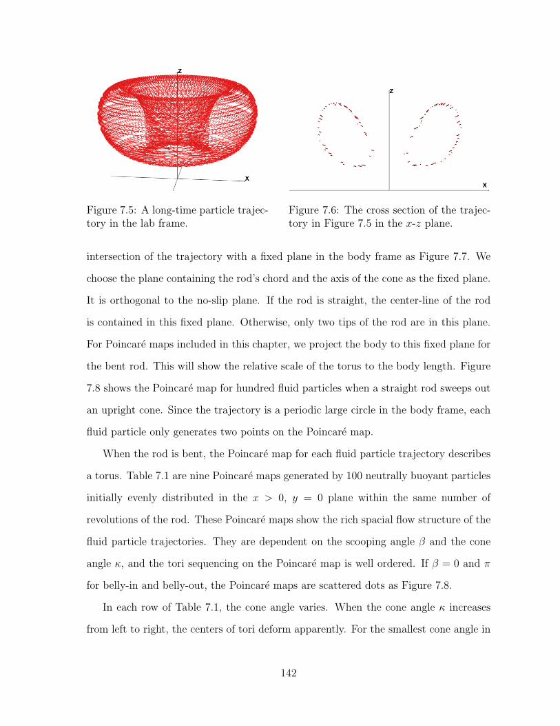
Figure 7.5: A long-time particle trajec-tory in the lab frame.

Figure 7.6: The cross section of the trajec-tory in Figure 7.5 in the x-z plane.

intersection of the trajectory with a fixed plane in the body frame as Figure 7.7. We

choose the plane containing the rod’s chord and the axis of the cone as the fixed plane.

It is orthogonal to the no-slip plane. If the rod is straight, the center-line of the rod

is contained in this fixed plane. Otherwise, only two tips of the rod are in this plane.

For Poincare maps included in this chapter, we project the body to this fixed plane for

the bent rod. This will show the relative scale of the torus to the body length. Figure

7.8 shows the Poincare map for hundred fluid particles when a straight rod sweeps out

an upright cone. Since the trajectory is a periodic large circle in the body frame, each

fluid particle only generates two points on the Poincare map.

When the rod is bent, the Poincare map for each fluid particle trajectory describes

a torus. Table 7.1 are nine Poincare maps generated by 100 neutrally buoyant particles

initially evenly distributed in the x > 0, y = 0 plane within the same number of

revolutions of the rod. These Poincare maps show the rich spacial flow structure of the

fluid particle trajectories. They are dependent on the scooping angle β and the cone

angle κ, and the tori sequencing on the Poincare map is well ordered. If β = 0 and π

for belly-in and belly-out, the Poincare maps are scattered dots as Figure 7.8.

In each row of Table 7.1, the cone angle varies. When the cone angle κ increases

from left to right, the centers of tori deform apparently. For the smallest cone angle in

142

Figure 7.7: Sketch of thePoincare map in the bodyframe.

Figure 7.8: Poincare map of fluid particle trajecto-ries with a straight rod.

this table, the torus centered inside the cone is close to the z-axis. As the cone angle

increases, the centers of these tori move away the z-axis. Additionally, the centers of

tori, which is outside the cone, are pushed toward the no-slip plane.

In each column, the scooping angle β varies. From these plots, the torus of a

fluid particle at the same initial position does not change much as the scooping angle

decreases from β = 900 (complete scooping) to β = 50(close to belly out). However,

the time for the same particle to create a full torus grows when the scooping angle

β decreases. In another word, the time for a fluid particle at a given initial position

to complete a torus is highly dependent on the scooping angle if the cone angle is

fixed. When the scooping angle β varies from belly out to complete scooping, more

of the torus is completed during the same mount of time. Figure 7.9 shows the result

about time to complete a torus with fixed initial positions, fixed cone angle κ and fixed

angular velocity but varying scooping angle β. The time is presented by the number

of rod’s revolutions N . The plot on the right side in Figure 7.9 is the loglog plot of the

left one to show the growth rate.

As the torus sequencing is well ordered, its orientation depends on the scooping

143

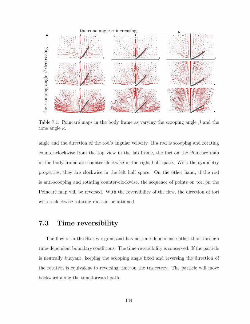
the

scoop

ing

angl

eβ

dec

reas

ing

-

the cone angle κ increasing -

Table 7.1: Poincare maps in the body frame as varying the scooping angle β and thecone angle κ.

angle and the direction of the rod’s angular velocity. If a rod is scooping and rotating

counter-clockwise from the top view in the lab frame, the tori on the Poincare map

in the body frame are counter-clockwise in the right half space. With the symmetry

properties, they are clockwise in the left half space. On the other hand, if the rod

is anti-scooping and rotating counter-clockwise, the sequence of points on tori on the

Poincare map will be reversed. With the reversibility of the flow, the direction of tori

with a clockwise rotating rod can be attained.

7.3 Time reversibility

The flow is in the Stokes regime and has no time dependence other than through

time-dependent boundary conditions. The time-reversibility is conserved. If the particle

is neutrally buoyant, keeping the scooping angle fixed and reversing the direction of

the rotation is equivalent to reversing time on the trajectory. The particle will move

backward along the time-forward path.

144

0 20 40 60 80 1000

2000

4000

6000

8000

10000

12000

β (in degree)

N

p1=(0.9, 0, 0.8)p2=(0.9, 0, 1.1)p3=(0.9, 0, 1)

100 101 102102

103

104

105

p1=(0.9, 0, 0.8)p2=(0.9, 0, 1.1)p3=(0.9, 0, 1)y∼ x−1

Figure 7.9: Time (in the number of rod’s revolutions N) to complete a torus for a fluidparticle at three different positions pi (i = 1, 2, 3)with different scooping angle β. Theright plot is the loglog plot to show the decay rate.

Since the induced flow is nonlinear, the torus exists even if the particle is buoyant.

The reversibility, however, is no longer conserved for buoyant particles. If the buoyant

force raises the particle, the center of the torus will shift downward. Otherwise the

center moves upward, compared to the center of the torus of a neutrally buoyant parti-

cle. With neutrally buoyant particles, Poincare maps with different scooping angles are

similar in the sense that the difference is in small scale as shown in each column of Table

7.1. When the time reversibility is broken by the buoyancy effect, buoyancy introduces

a new phenomenon to the Poincare maps when changing the scooping angle. If adding

a The non-negligible, constant buoyant velocity into the system, Poincare maps are

noticeably changed with different scooping angles.

Such conclusions can be drawn from the velocity field for buoyant particles. The

governing equation for the Stokes flow is a linear differential equation. When a particle

is not neutrally buoyant, the velocity for this tracking particle can be written as u′ =

u + Qez, where Q is the velocity due to the buoyant force in the vertical direction ez.

When min(w) < Q < max(w), the z component of the location of the zero vertical

145

velocity in the spatial locations is modified by Q. Then, the height of the torus’ center

in the flow is changed. Therefore, the center of the torus is shifted. For example, when

the rod rotates counter-clockwise and Q > 0, the buoyant force raises the particle. The

original equilibrium position (x0, y0, z0) is shifted to where the velocity is w(x1, y1, z1) =

−Q, which is above the original center of the torus from the monotonic properties of

the velocity component w(x, y, z). Notice that if the velocity in the vertical direction

w +Q does not change sign, then z on the buoyant particle trajectory either increases

or decrease over time. In such cases, the buoyant force is so strong that the particle

will either rise and escape or descend to the no-slip bottom. These buoyant particles

are not able to create any full tori regardless their initial positions in the flow.

Figure 7.10 shows Poincare maps of the buoyant particles with different Q and two

different scooping angles. In each column, the buoyant force gets stronger from the

top to the bottom but with the same cone angle and scooping angle. The stronger the

buoyant force is, the more to the torus is changed. For a neutrally buoyant particle,

the torus will always be closed even though the time to complete the torus grows. For

a buoyant particle, the buoyant velocity can be dominant part of the total velocity

comparing to the velocity induced by the rod. In such situations, the particle will rise

and escape on an open trajectory if it is already far from the cone. In each row, the two

Poincare maps show the difference from complete scooping (on the left) to complete

anti-scooping (on the right) with the same buoyant force, which raises the particles.

Especially, as we have plotted here, the rod is spinning counter-clockwise and anti-

scooping, the tori on the Poincare maps will break earlier than those with the bent rod

scooping based on the orientation of the tori.

146

x

z

(a) Q = 0.00001, κ ≈ 27o and β = 90o

x

z

(b) Q = 0.00001, κ ≈ 27o and β = −90o

x

z

(c) Q = 0.001, κ ≈ 27o and β = 90o

x

z

(d) Q = 0.001, κ ≈ 27o and β = −90o

x

z

(e) Q = 0.01, κ ≈ 27o and β = 90o

x

z

(f) Q = 0.01, κ ≈ 27o and β = −90o

Figure 7.10: Poincare maps for buoyant particles. Q is the constant vertical velocitydue to buoyancy.

147

7.4 Drag and torque on the bent rod

With the singularities distributed along the centerline of the slender rod, we have

obtained the velocity field of the flow generated by the rod. With these information, we

further compute the force and torque exerted on the bent slender rod in the body frame,

where the bent rod is tilted in the x-z plane with a cone angle κ. The hydrodynamic

force applied to the body is important to understand the stability of the motion, and

such information can help to design the experimental instruments.

The hydrodynamic force exerted on the slender body from the fluid is given by

f(x) = −σ · n = − (σ1knk, σ2knk, σ3knk) , (7.7)

where x is any point on the surface of the body, n is the outward normal at x, and

σik = −pδik + µ

(∂ui∂xk

+∂uk∂xi

)

is the stress tensor associated with a fluid motion with the velocity u. p denotes the

pressure field, and δik is the Kronecker delta function. With the properties of the delta

function, the total hydrodynamic force exerted on the rod is

F =

∫Sc

(−σ · n) dS =

∫v

(OpS − µO2uS

)dv =

∫v

fSdv

= 8πµ

∫v

α(s)δ(x− xs)dv = 8πµ

∫ `

0

α(s)ds.

Since the strength of the singularity is known, each component of the drag on the body

148

is

F1 = 8πµ

∫ `

0

α1 ds

= −πµaεω4

−2` cos(

`

2a)(7 + cos(2κ)) sin(β) + 2a sin(

3`

2a) sin(β) sin2(κ)+

sin(`

2a)

[a(25 + 7 cos(2κ)) sin(β) +

(−`+ a sin(

`

a)

)sin(2β) sin(2κ)

],

F2 = 8πµ

∫ `

0

α2 ds

= −πµ2aεω

8` cos2(β) sin(

`

2a) sin(κ)− 16a cos(β) cos(κ) sin(

`

2a)

+

(6` sin(

`

2a)− a cos(

3`

2a)

)sin2(β) sin(κ)

+ cos(`

2a)(8` cos(β) cos(κ) + a sin2(β) sin(κ)

),

F3 = 8πµ

∫ `

0

α3 ds

=πµ

2aεω sin(β) sin(κ)

− cos(κ)

[2` cos(

`

2a) + a

(sin(

3`

2a)− 7 sin(

`

2a)

)]−

2 cos(β) sin(`

2a)

(`− a sin(

`

a)

)sin(κ)

.

The torque on the sender body at the origin equals∫S

x× fds, where x is any point

on the body and f is the hydrodynamic force exerted on the slender bent rod. Given

the flow field, the hydrodynamic force is f = −σ · n in (7.7). The pressure field and

the velocity field for a Stokeslet at y with the strength α is

pS(x,y;α) = 2µα · (x− y)

|x− y)|3,

uS(x,y;α) =α

|x− y)|+

(α · (x− y)))(x− y))

|x− y)|3.

149

With the divergence theorem, it is found that

T (0)i = −∫ν

εijkxj∂σkm

∂xmdv.

So,

T (0)1 = −∫ν

(ε12kx2

∂σkm

∂xm+ ε13kx3

∂σkm

∂xm

)dv = −

∫ν

(x2(Div(σ))3 − x3(Div(σ))2) dv,

T (0)2 = −∫ν

(x3(Div(σ))1 − x1(Div(σ))3) dv,

T (0)3 = −∫ν

(x1(Div(σ))2 − x2(Div(σ))1) dv.

Utilizing the divergence of the stress tensor to determine the total force on a slender

bent rod, we find that Div(σ) = −8πµαδ(x− y). Then, the torque on the rod is

T (0)1 =

∫ν

(x28πµα3δ(x− y)− x38πµα2δ(x− y)) dv

= 8πµ

∫ `

0

(x2(s)α3(s)− x3(s)α2(s)) ds,

T (0)2 =

∫ν

(x38πµα1δ(x− y)− x18πµα3δ(x− y)) dv

= 8πµ

∫ `

0

(x3(s)α1(s)− x1(s)α3(s)) ds,

T (0)3 =

∫ν

(x18πµα2δ(x− y)− x28πµα1δ(x− y)) dv

= 8πµ

∫ `

0

(x1(s)α2(s)− x2(s)α1(s)) ds.

150

Consequently,

T (0)1 = 8πµ

∫ `

0

[−2a sin(

`− s2a

) sin(s

2a) sin(β)

] [1

2aεω sin2(

s

2a) sin(β)

sin(κ)

(cos(

`− 2s

2a) cos(κ) + cos(β) sin(

`− 2s

2a) sin(κ)

)]−[

2a cos(`− s

2a) cos(κ) sin(

s

2a) + 2a cos(β) sin(

`− s2a

) sin(s

2a) sin(κ)

][−aεω

4sin(

s

2a)

(4 cos(

`− s2a

) cos2(β) sin(κ)− 4 sin(`− s

2a) cos(β) cos(κ)

+

(cos(

`− 3s

2a) + 3 cos(

`− s2a

)

)sin2(β) sin(κ)

)]ds

=a2πεµω

4

[−16a cos(β) cos(2κ) + 8` cos(β) cos(2κ) sin(

`

a)+(

2a(3 + cos(2β)) sin(`

a) + (2`− a sin(

2`

a)) sin2(β)

)sin(2κ) +

2 cos(`

a) (8a cos(β) cos(2κ)− `(3 + cos(2β)) sin(2κ))

],

T (0)2 = 8πµ

∫ `

0

[2a cos(

`− s2a

) cos(κ) sin(s

2a) + 2a cos(β) sin(

`− s2a

) sin(s

2a) sin(κ)

][−1

4aεω sin(

s

2a) sin(β)

(4 cos2(κ) sin(

`− s2a

) + 2 cos(β) cos(κ)

sin(`− 2s

2a) sin(

s

2a) sin(κ) +

(sin(

`− 3s

2a) + 3 sin(

`− s2a

)

)sin2(κ)

)]−[

2a cos(`− s

2a) sin(

s

2a) sin(κ)− 2a cos(β) cos(κ) sin(

`− s2a

) sin(s

2a)

]aεω

2sin2(

s

2a) sin(β) sin(κ)(

cos(`− 2s

2a) cos(κ) + sin(

`− 2s

2a) cos(β) sin(κ)

)ds

=1

2a2πεµω sin(β)

[4 cos(κ)

(−2a+ 2a cos(

`

a) + ` sin(

`

a)

)+

cos(β)

(−2`− 4` cos(

`

a) + 4a sin(

`

a) + a sin(

2`

a)

)sin(κ)

],

151

and

T (0)3 = 8πµ

∫ `

0

sin(

s

2a)

[−2a cos(β) cos(κ) sin(

`− s2a

) + 2a cos(`− s

2a) sin(κ)

][−1

4aεω sin(

s

2a)

(−4 cos(β) cos(κ) sin(

`− s2a

) + 4 cos(`− s

2a) cos2(β)

sin(κ) +

(cos(

`− 3s

2a) + 3 cos(

`− s2a

)

)sin2(β) sin(κ)

)]−

2a sin(`− s

2a) sin(

s

2a) sin(β)

aεω

4sin(

s

2a) sin(β)

[4 cos2(κ) sin(

`− s2a

)+

cos(β) sin(`− 2s

2a) sin(

s

2a) sin(2κ)

+

(sin(

`− 3s

2a) + 3 sin(

`− s2a

)

)sin2(κ)

]ds

=1

16a2πεµω

−68`− 8` cos(

`

a) + 8` cos(

`

a) cos(2β) + 4` cos(2β)+

72a sin(`

a) + 2a sin(

2`

a)− 4a sin(

`

a− 2β)− a sin(

2`

a− 2β) + 2 cos(2κ)[

−4(3 + cos(2β))

(` cos(

`

a)− a sin(

`

a)

)+ 2

(2`− a sin(

2`

a)

)sin2(β)

]−

a sin(2`

a+ 2β)− 4a sin(

`

a+ 2β) +

64 cos(β) sin(`

2a)

(−` cos(

`

2a) + 2a sin(

`

2a)

)sin(2κ)

.

Figure 7.11 is a group of plots about the torque at the base of the bent rod (the

apex of the cone) with different scooping angle β and cone angle κ. The curvature

of the bent rod is 0.4cm−1, the rod’s body length is ` = 1, ω = 2π5

radian/second,

the radius of the cross-section of the bent rod is r = 0.0375cm. So, the slenderness

ε = 1log(1/0.03750)

∼ 0.30. The dynamic viscosity of the fluid is µ = 3200cP . The torque

is in the dimensions of force times distance, using the unit dyne centimeter (g· cm2/s2)

in the cgs unit system.

Figure 7.11a shows the three components of the torque at the base of the rod in the

body frame as functions of the scooping angle β for the cone angle κ = π6. Similarly,

152

ΠΠ

2

3 Π

2

Β

-1000

1000

2000

Torque

TH0L3

TH0L2

TH0L1

(a) κ = π6

ΠΠ

2

3 Π

2

Β

-1000

1000

2000

Torque

TH0L3

TH0L2

TH0L1

(b) κ = π4

Π

12

Π

6

Π

4

Π

3

Κ

-3000

-2000

-1000

1000

2000

Torque

TH0L3

TH0L2

TH0L1

(c) Belly out β = 0

Π

12

Π

6

Π

4

Π

3

Κ

-3000

-2000

-1000

1000

2000

Torque

TH0L3

TH0L2

TH0L1

(d) Scoop β = π2

Figure 7.11: The torque at the origin as functions of the scooping angle β or the coneangle κ.

ΠΠ

2

3 Π

2

Β

2300

2500

TH0L1

(a) T (0)1

ΠΠ

2

3 Π

2

Β

-200

-100

100

200

TH0L2

(b) T (0)2

0 ΠΠ

2

3 Π

2

Β

-3500

-2500

-1500

TH0L3

Κ=

Π

3

Κ=

Π

4

Κ=

Π

6

(c) T (0)3

Figure 7.12: Comparisons of each component of the torque with different values of thecone angle κ.

153

Figure 7.11b shows the components with κ = π4. When the rod is belly in or belly out,

these figures show the second component (in the y-direction) vanishes. Figure 7.11c

and 7.11d show the three components of the torque at the base of the rod as functions

of the cone angle κ for two different scooping angle β = 0 and β = π2, respectively.

These two figures show the variation of torque with respect to the cone angle κ. Figure

7.12 shows the comparisons of individual components of the torque at the base of the

rod as functions of the scooping angle κ for three different values of the cone angle

κ = π6, π

4and π

3.

7.5 Experimental study

To study the flow, we build a mathematical model with the slender body theory

and provide theoretical predictions. Besides numerical simulation, we have conducted

experimental studies for both the straight rod and the bent rod cases to examine the

flows. In this section, we provide the experimental data for the bent rod sweeping out

a cone above a no-slip plane, and compare them with our model’s predictions. The

experimental verification has two purposes: first, the experimental data help to verify

our model and demonstrate the order of our asymptotic results; second, based on our

theoretical model we explore the flow experimentally.

7.5.1 Toroidal structure

When a fluid particle moves in the flow generated by a bent rod sweeping out a cone,

but not belly in or belly out, a toroidal structure appears in the particle trajectories.

Figure 7.13 shows the toroidal structure captured in Karo corn syrup with injected

red food dye. The torus on the lower left corner is a fluid particle trajectory from the

model. Both the experiment and the model capture the closed torus near the bent rod.

154

Figure 7.13: A torus captured with red dye and a torus created with the model in thelab frame.

Besides this qualitative comparison, we pursue a quantitative comparison between the

model and the experimental data.

The flow not only has a rich parameter space but also shows complicated spatial

structure. Therefore, the trajectory is very sensitive to the location of the fluid particle.

The initial 2D experiments we carried out are helpful to capture the properties of the

fluid. However, it is very difficult to obtain a fair comparison based on approximated

initial positions. With fully 3D experimental capability, we explore the complex flow

structure and quantitatively compare the experimental data with theoretical predic-

tions.

We take videos from two cameras, one of which is in front of the tank (front view)

and the other is on the left side of the tank (side view), then track the particle trajectory

from these videos. Figure 7.14 shows 2D tracking trajectories in pixel coordinates from

both cameras, when the rod is rotating counter-clockwise and scooping. The purpose

of the color on the trajectory is to show the overlap structure in 2D. The particle goes

downward in the center and come up in the outer layer. Figure 7.15 is 2D tracking

trajectory for the same particle and the same setup of the rod, but the rod is rotating

clockwise. To the flow, it is equivalent to the rod counter-clockwise rotating and anti-

155

460 480 500 520 540 560 580 600 620

130

140

150

160

170

180

190

200

(a) Front view

400 420 440 460 480 500 520 540 560

90

100

110

120

130

140

150

160

(b) Side view

Figure 7.14: An experimental trajectory tracked from two camera-views in pixel coor-dinates. The rod is scooping and rotating counter-clockwise from the top view.

480 500 520 540 560 580150

160

170

180

190

200

210

220

230

240

250

260

270

(a) Front view

420 440 460 480 500 520110

120

130

140

150

160

170

180

190

200

210

220

230

(b) Side view

Figure 7.15: Tracked trajectories when the rod is scooping and rotating clockwise fromtop view (opposite to the motion for Figure 7.14).

scooping. The experimental trajectories verify the prediction of the direction of the

torus, even though based on results for a buoyant particle. Here, the particle trajectory

starts with blue and progresses to dark red.

7.5.2 Quantitative comparison

Figure 7.16 shows short-time comparison of the particle trajectories with experi-

mental data in red and the theoretical prediction in blue. One position of the rod is

plotted to demonstrate the scale. From this plot, the model and experiment have good

156

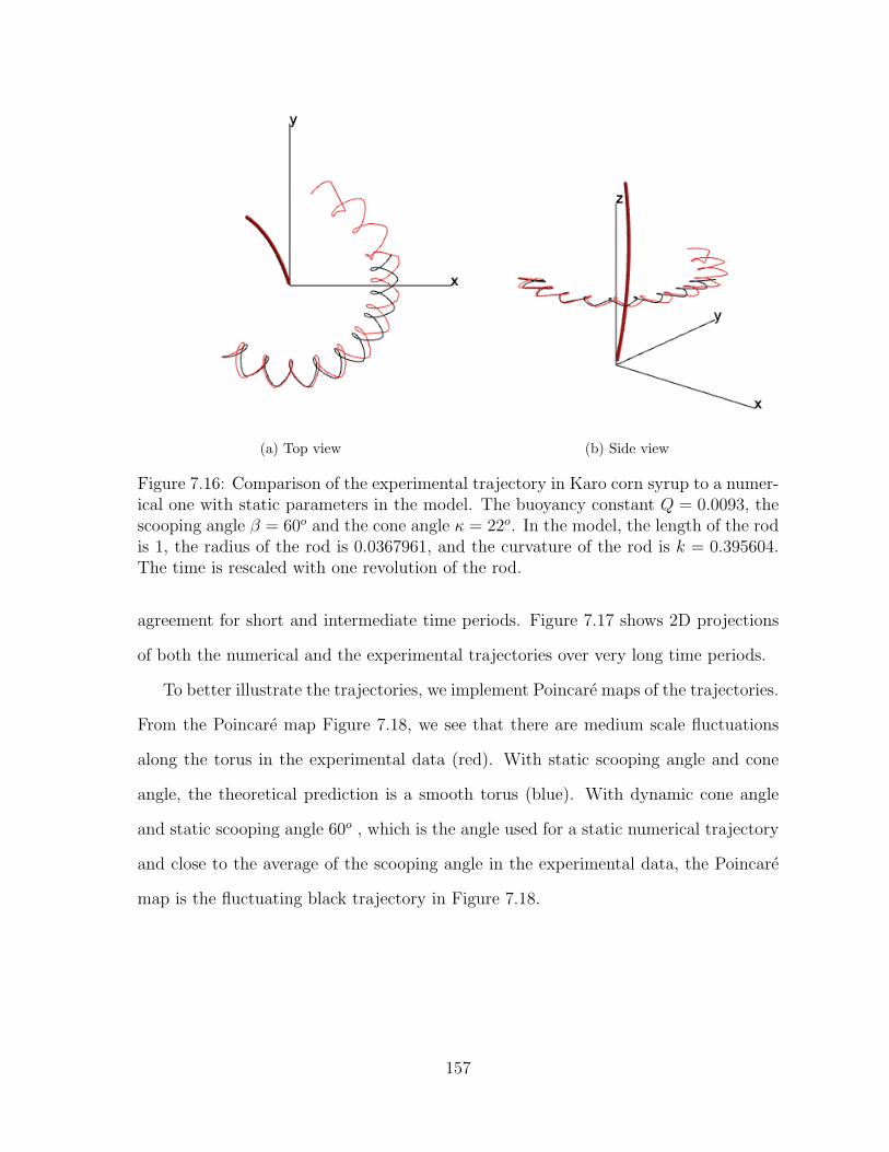
(a) Top view (b) Side view

Figure 7.16: Comparison of the experimental trajectory in Karo corn syrup to a numer-ical one with static parameters in the model. The buoyancy constant Q = 0.0093, thescooping angle β = 60o and the cone angle κ = 22o. In the model, the length of the rodis 1, the radius of the rod is 0.0367961, and the curvature of the rod is k = 0.395604.The time is rescaled with one revolution of the rod.

agreement for short and intermediate time periods. Figure 7.17 shows 2D projections

of both the numerical and the experimental trajectories over very long time periods.

To better illustrate the trajectories, we implement Poincare maps of the trajectories.

From the Poincare map Figure 7.18, we see that there are medium scale fluctuations

along the torus in the experimental data (red). With static scooping angle and cone

angle, the theoretical prediction is a smooth torus (blue). With dynamic cone angle

and static scooping angle 60o , which is the angle used for a static numerical trajectory

and close to the average of the scooping angle in the experimental data, the Poincare

map is the fluctuating black trajectory in Figure 7.18.

157

(a) Top view (b) 3D view

Figure 7.17: Long-time comparison of the experimental trajectory (red) with the nu-merical trajectory (blue) in Figure 7.16.

Figure 7.18: Comparison of the Poincare map of experimental and numerical trajecto-ries. The red dots are generated by the experimental trajectory. For the blue trajectory,the cone angle κ = 23o is static. For the black numerical trajectory, the cone angleκ = 25o−2o sin(2πt

75)+sin(4πt) is dynamic. For both numerical trajectories, the buoyant

velocity constant Q = 0.0093, the scooping angle β = 60o, and the number of revolutionis N = 200. The blue dot indicates the initial position for these trajectories.

158

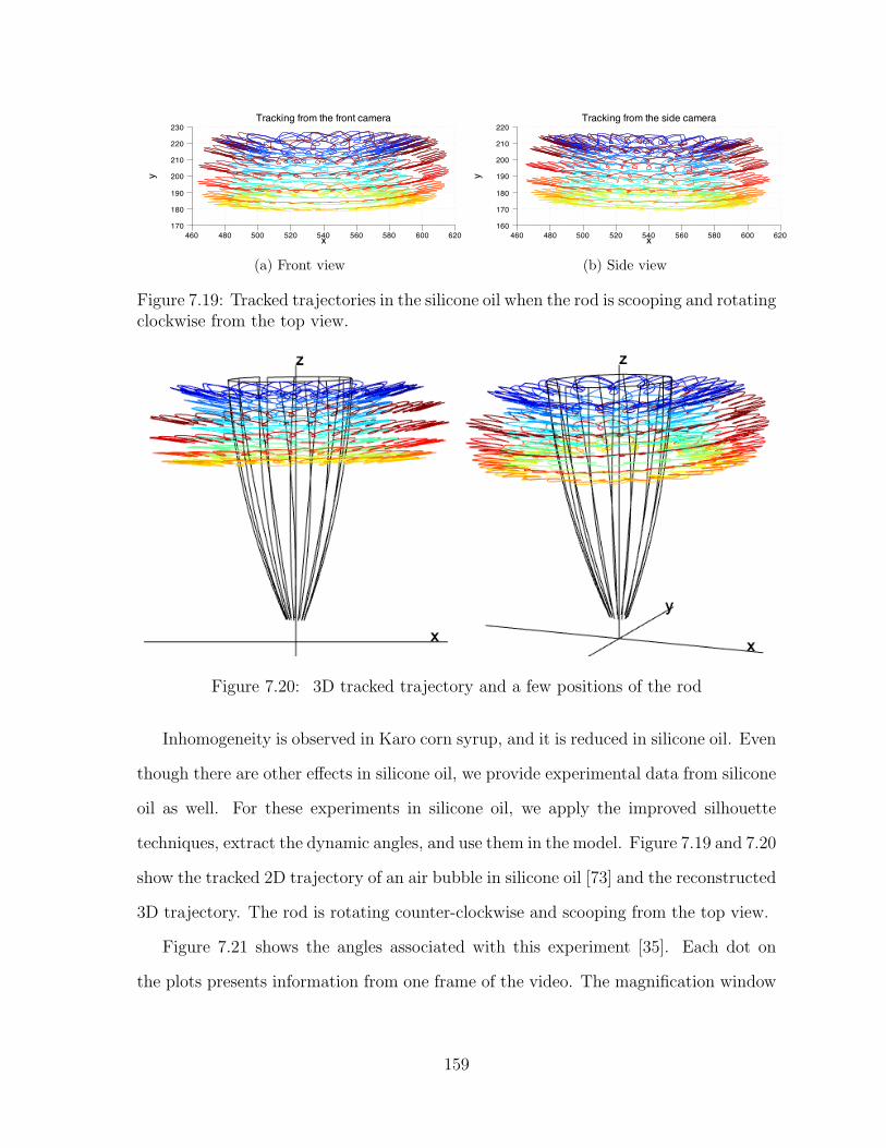
460 480 500 520 540 560 580 600 620170

180

190

200

210

220

230Tracking from the front camera

x

y

(a) Front view

460 480 500 520 540 560 580 600 620160

170

180

190

200

210

220Tracking from the side camera

x

y

(b) Side view

Figure 7.19: Tracked trajectories in the silicone oil when the rod is scooping and rotatingclockwise from the top view.

Figure 7.20: 3D tracked trajectory and a few positions of the rod

Inhomogeneity is observed in Karo corn syrup, and it is reduced in silicone oil. Even

though there are other effects in silicone oil, we provide experimental data from silicone

oil as well. For these experiments in silicone oil, we apply the improved silhouette

techniques, extract the dynamic angles, and use them in the model. Figure 7.19 and 7.20

show the tracked 2D trajectory of an air bubble in silicone oil [73] and the reconstructed

3D trajectory. The rod is rotating counter-clockwise and scooping from the top view.

Figure 7.21 shows the angles associated with this experiment [35]. Each dot on

the plots presents information from one frame of the video. The magnification window

159

(a) Cone angle VS azimuthal angle (b) Scooping angle VS azimuthal angle

Figure 7.21: Tracked trajectories in silicone oil when the rod is scooping and rotatingclockwise from top view.

shows a small portion of the clouds of dots. There are a few dots scattered above

the clouds when the azimuthal angle θ is between 0o and 180o. This is due to the

transient when we start the motor. Figure 7.21a shows the generalized cone angle φ

over time as a function of the corresponding azimuthal angle. Figure 7.21b shows the

dynamic scooping angles versus the azimuthal angles. The azimuthal angles and the

cone angles specify the rod’s positions on the cone, and the scooping angles determine

the orientation of the rod at each position. From these two plots, the rod sweeps out

a dynamic tilted cone. We use these angles in the model to run the simulation.

For the simulation, we not only consider the tracked dynamic angles in the model

but also the buoyancy effect of the air bubble. Figure 7.22 shows two views of the

experimental trajectory (red) and the numerical trajectories (gray). One rod posi-

tion is plotted to show the relative scale. The initial position of the trajectories is

(0.0652893,−0.378317, 0.659856). The length of the rod is 1, the cross-sectional ra-

dius is r = 0.3750, and the curvature is K = 1/2.419. So, the slenderness parameter

ε = 1log(`/r)

∼ 0.30. Epicycles on the numerical trajectory appear smaller than the

experimental epicycles.

160

(a) 3D view (b) Top view

Figure 7.22: Comparison of numerical trajectory (grey) with experimental trajectory(red), which is in the silicone oil when the rod is scooping and rotating clockwise fromthe top view.

7.5.3 List of issues

From the comparisons between the experimental data and the theoretical prediction,

we see that there are agreements between the model and the experiment, but also

discrepancies. Qualitatively, the epicycles, the large orbits and the toroidal structure in

the experimental trajectories are in agreement with the theoretical prediction. However,

there are quantitative discrepancies between the experimental Lagrangian trajectory

and the theoretical trajectory, especially over long time scale. We list and discuss the

possible issues with the model and the experimental data.

For the model,

1. The velocity field obtained using the slender body is a leading order approxi-

mation. We provide the error analysis of the slender body theory for a straight

rod sweeping out a double in free space in Appendix B. From those analysis, the

discrepancies in the fluid particle trajectory would be expected with the slender-

ness for our experiments. Also, the slender body theory is invalid within a radius

distance from the tips of the slender body. Such close encounter has happened

both in the experiment and the model.

161

2. Besides the systematic error due to the leading order approximation of the velocity

field, the numerical error for the model is accumulated from the ODE solver.

However, this numerical error can be reduced by choosing small time steps. In

our numerical trajectories such effects are negligible.

3. The higher order asymptotics are not necessary, if there is no chaos in the fluctu-

ating system. Then the slender body orbit is accurate far from the boundaries.

If there is chaos, then both the experiment and the model will observe wildly

different phenomena. Estimation for the differences of the orbit in terms of the

slenderness ε is helpful to understand the discrepancy.

For experiments,

1. From Poincare maps of the experimental trajectories and videos, we learn that

rotation rate of the rod is not constant. The fluctuation in the rotation rate is

not a problem because the Reynolds number is still small enough to keep the flow

in the Stokes’ regime. However, this will effect the azimuthal angles in the model,

especially when we feed the tracking data into the model.

2. From the experiment data shown in Figure 7.14-7.18, the base of the rod slides

within a small circle of an approximate radius 0.15mm. Such motion will con-

tribute to an inaccuracy of the cone angle, for which it could be reasonable to add

or subtract one degree to the cone angle. Now we take the center of this small

circle as the center of the cone. The sliding needs to be considered in the model,

which will be including in the future work.

3. Without thermal control of the experiment, the slow convection detected in the

tank. Such background flow will influence the particle trajectory, more apparently

on the long-time trajectory.

162

4. Dynamic scooping angle and cone angle are measured in the experiments, which

generate zigzagging trajectories.

5. For the experiments, inhomogeneity in fluid, density stratification, oil laying

above Karo corn syrup to prevent evaporation complicate the fluid.

6. The solubility rate of air bubbles in silicone oil varies over time. The Faxen

correction is very small based on the small radius of the bubbles and the velocity

field. However, the buoyant force is also changed. The nonlinearity of the system

makes the influence hard to predict over long time scale.

7. Based on the 3D calibration, the error due to the alignment of cameras is mini-

mized, if the vertical of the cameral view is parallel to gravity and perpendicular

to the no-slip flat bottom of the tank.

7.5.4 Effect of thermal convection

The discrepancies between the experimental trajectory and the numerical prediction

may be explained by taking account of the approximation of the slender body theory,

the dynamics of the experiments, the buoyancy effect, and thermal effects in highly

viscous fluids. However, the thermal effect is not controlled in our experiment. In this

section, we briefly study the thermal effects with a simplified situation.

When the Rayleigh number exceeds some critical value, the background flow is no

longer stationary. The convection is a very slow motion. For the experiments, thermal

effect convection was indeed detected in our highly viscous fluids. Unfortunately, it is

hard to measure globally. Fortunately, our model has the ability to handle any given

background flow, even if time dependent. To better understand the thermal effect,

we check the flow with a straight rod sweeping out a double cone with a uniform

background flow in free space.

163

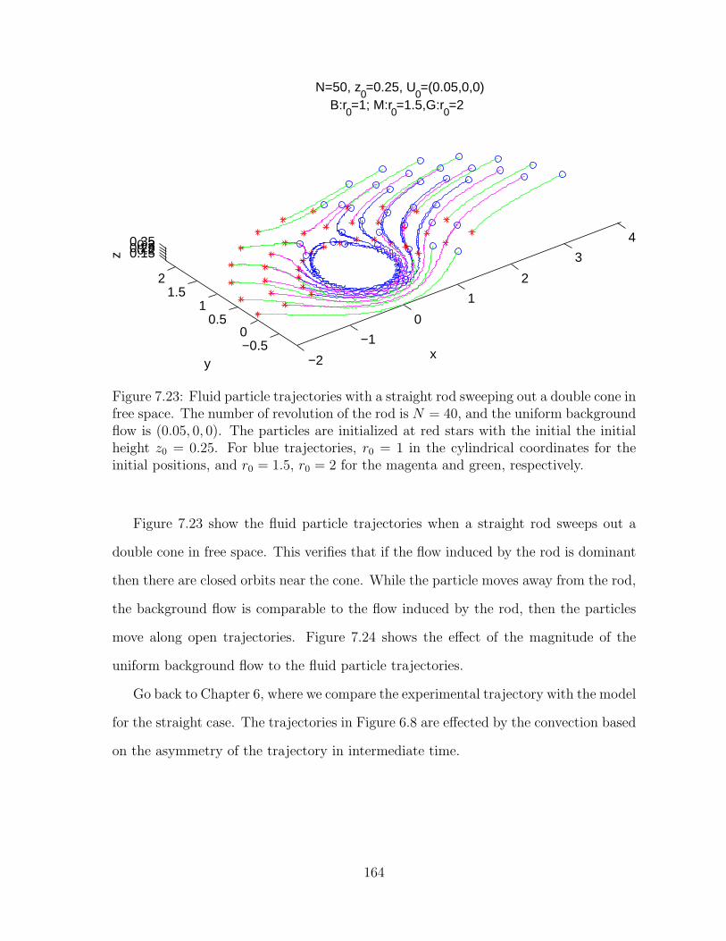
−2

−1

0

1

2

3

4

−0.50

0.51

1.52

0.150.20.250.30.35

x

N=50, z0=0.25, U

0=(0.05,0,0)

B:r0=1; M:r

0=1.5,G:r

0=2

y

z

Figure 7.23: Fluid particle trajectories with a straight rod sweeping out a double cone infree space. The number of revolution of the rod is N = 40, and the uniform backgroundflow is (0.05, 0, 0). The particles are initialized at red stars with the initial the initialheight z0 = 0.25. For blue trajectories, r0 = 1 in the cylindrical coordinates for theinitial positions, and r0 = 1.5, r0 = 2 for the magenta and green, respectively.

Figure 7.23 show the fluid particle trajectories when a straight rod sweeps out a

double cone in free space. This verifies that if the flow induced by the rod is dominant

then there are closed orbits near the cone. While the particle moves away from the rod,

the background flow is comparable to the flow induced by the rod, then the particles

move along open trajectories. Figure 7.24 shows the effect of the magnitude of the

uniform background flow to the fluid particle trajectories.

Go back to Chapter 6, where we compare the experimental trajectory with the model

for the straight case. The trajectories in Figure 6.8 are effected by the convection based

on the asymmetry of the trajectory in intermediate time.

164

Figure 7.24: Fluid particle trajectories with a straight rod sweeping out a double conein free space. The fluid is at rest for the black trajectories. The uniform backgroundflow is (0.0005, 0, 0), (0.005, 0, 0), and (0.05, 0, 0) for the blue, yellow, and red trajectory,respectively.

165

Chapter 8

A swimming related application of

the slender body theory in Stokes

flows

The slender body theory has been developed for a long time [75, 21, 74, 3, 39]. It

provides a good asymptotic solution for flows generated by a slender body, if ignoring

the end effect. The end effects can be attained with higher order singularities [38].

In this chapter, we report a swimming-related application of the slender body theory.

We study the velocity field, the fluid particle trajectory and the flux introduced by

the periodic motion of a slender body. This study may shade light on the efficiency of

swimming or propelling in the low-Reynolds-number regime.

8.1 The problem

The cylindrical slender body (red) is attached to a fuselage (gray) by a fine wire and

moves along the track (green) on the fuselage as shown in Figure 8.1. In the fuselage’s

body frame, the cylindrical slender body moves periodically in a plane. Assume in

the fuselage’s body frame the surrounding fluid is stationary, the configuration of the

(a) (b) (c) (d)

Figure 8.1: Swimmer.

periodic motion of the rigid slender body is show in Figure 8.2. We examine on the

flow induced by the slender body in this chapter. Study of the effect of the fuselage

and the whole system will be pursued in the future work.

The body moves periodically from step (a) to step (e), divided into 4 phases con-

sidering its motion and direction. After one revolution, the body returns to its original

position in the fuselage frame. If the fuselage is fixed and the surrounding fluid is at

rest, the background flow in the fuselage frame is stationary. If the fuselage is free in a

stationary fluid, the background flow in the fuselage frame depends on the motion of

the system. We focus on the case when the background flow in the fuselage frame is

at rest, and refer the fuselage frame as the lab frame in the rest of this chapter. Since

the flow is in the Stokes regime, inertia effect is negligible and transient is neglect. We

focus on the steady Stokes flow for each phase. Generally, two types of motion are

considered, uniform translation and pure rotation.

The half length of the cylindrical slender body ` is much large compared with its

cross-sectional radius r ( r `). We study the flow induced by the slender body when

it moves periodically in the laboratory frame, which is selected that the slender body

is always in the x-y plane. Beside the laboratory frame (the fuselage frame), another

important reference frame used here is the body frame, which is a moving frame. The

167

(a) (b) (c) (d)

(e=a)(a) (b) (c) (d)

(e)

Figure 8.2: Configuration of the periodic motion of the slender body in the x-y plane.

velocity field is presented with explicit formulae using the slender body theory.

8.2 The velocity field for each step

In this section, we provide the velocity field of the flow induced by the cylindrical

slender body in each step of the periodic motion. Phase 1 is the first step from (a)

to (b) in Figure 8.2, Phase 2 is from (b) to (c), etc. During phase 1 and phase 3, the

slender body moves uniformly. During phase 2 and phase 4, the body purely rotates

either clockwise or counter-clockwise in the fluid. We first consider the flow induced by

the cylindrical slender body when it moves with uniform velocity in phase 1 and phase

3, then switch to the rotating flow in phase 2 and phase 4.

168

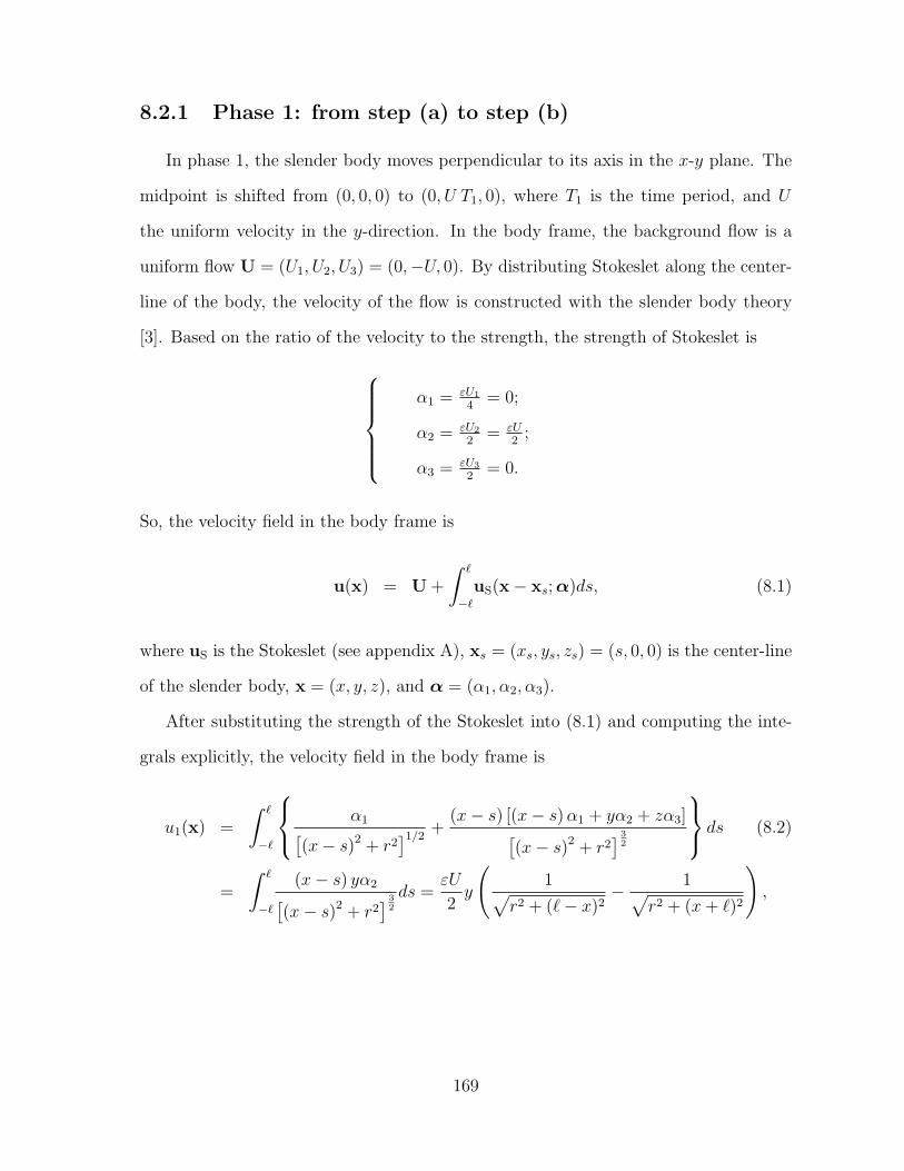
8.2.1 Phase 1: from step (a) to step (b)

In phase 1, the slender body moves perpendicular to its axis in the x-y plane. The

midpoint is shifted from (0, 0, 0) to (0, U T1, 0), where T1 is the time period, and U

the uniform velocity in the y-direction. In the body frame, the background flow is a

uniform flow U = (U1, U2, U3) = (0,−U, 0). By distributing Stokeslet along the center-

line of the body, the velocity of the flow is constructed with the slender body theory

[3]. Based on the ratio of the velocity to the strength, the strength of Stokeslet is

α1 = εU1

4= 0;

α2 = εU2

2= εU

2;

α3 = εU3

2= 0.

So, the velocity field in the body frame is

u(x) = U +

∫ `

−`uS(x− xs;α)ds, (8.1)

where uS is the Stokeslet (see appendix A), xs = (xs, ys, zs) = (s, 0, 0) is the center-line

of the slender body, x = (x, y, z), and α = (α1, α2, α3).

After substituting the strength of the Stokeslet into (8.1) and computing the inte-

grals explicitly, the velocity field in the body frame is

u1(x) =

∫ `

−`

α1[(x− s)2 + r2

]1/2 +(x− s) [(x− s)α1 + yα2 + zα3][

(x− s)2 + r2] 3

2

ds (8.2)

=

∫ `

−`

(x− s) yα2[(x− s)2 + r2

] 32

ds =εU

2y

(1√

r2 + (`− x)2− 1√

r2 + (x+ `)2

),

169

u2(x) = −U +

∫ `

−`

α2[(x− s)2 + r2

]1/2 +y [(x− s)α1 + yα2 + zα3][

(x− s)2 + r2] 3

2

ds

= −U +

∫ `

−`

α2[(x− s)2 + r2

]1/2 +y2α2[

(x− s)2 + r2] 3

2

ds

= −U +εU

2log

`+√r2 + (`− x)2 − x

−`+√r2 + (`+ x)2 − x

(8.3)

+εU

2

y2

r2

`− x√r2 + (`− x)2

− −`− x√r2 + (`+ x)2

,

u3(x) =

∫ `

−`

α3[(x− s)2 + r2

]1/2 +z [(x− s)α1 + yα2 + zα3][

(x− s)2 + r2] 3

2

ds (8.4)

=

∫ `

−`

yzα2[(x− s)2 + r2

] 32

ds =εU

2

yz

r2

(`− x√

r2 + (x− `)2− −`− x√

r2 + (x+ `)2

),

where r2 = y2 + z2, since

∫1[

(x− s)2 + r2]1/2ds = log

(s+

√r2 + (s− x)2 − x

),∫

1(x− s)2 + r2

32

ds =s− x

r2

√r2 + (s− x)2

,

∫(x− s)[

(x− s)2 + r2] 3

2

ds =1√

r2 + (s− x)2.

If y2 + z2 ≤ r2 and −` ≤ x ≤ `, then the fluid particle is on or inside the slender

body, which is outside the fluid. If y2 + z2 ≤ r2 and |x| > `, then the fluid particle is

along the slender body. Especially, if y2 + z2 = 0 (y = z = 0) and |x| ≥ `, then the

170

fluid particle is along the longitudinal of the slender body,

u1(x) = yα2

∫ `

−`

(x− s)[(x− s)2 + r2]

32

ds = 0,

u3(x) = yzα2

∫ `

−`

1

[(x− s)2 + r2]32

ds = 0,

u2(x) = −U + α2

∫ `

−`

1[(x− s)2 + r2

]1/2ds+ y2α2

∫ `

−`

1[(x− s)2 + r2

] 32

ds

= −U + α2

∫ `

−`

1

|x− s|ds+ y2α2

∫ `

−`

1

|x− s|3ds

= −U − sgn(x)α2 log(`− x`+ x

).

The above velocity field is in the moving body frame. To obtain the velocity field in

the lab frame, we apply the transformation between these two frames.

From the lab frame (xL, yL, zL) to the moving body frame (x, y, z):

x = xL,

y = yL − U t,

z = zL.

So, the velocity field in the lab frame

uL(xL) =dxLdt

=dx

dt+ Uey = Uey + u(x− Utey). (8.5)

Figure 8.3 shows two groups of fluid particle trajectories in the x-y plane in the labora-

tory frame. The initial positions of the fluid particle are either at y = −0.1 or y = 0.6.

While the cylindrical slender body moves from y = 0 to y = 1 with uniform velocity

(0, 1, 0), the fluid particles moves with the same direction. When the slender body

passes some fluid particles (green) initially in front of the slender body, these particles

have been pushed aside. The blue thick horizontal lines indicate the initial and end

171

−0.6 −0.4 −0.2 0 0.2 0.4 0.6

0

0.2

0.4

0.6

0.8

1

x

y

Figure 8.3: Two groups of fluid particletrajectories in the flow introduced by atranslation of the cylindrical slender bodyperpendicular to its axis. The length of theslender body is 1, i.e., ` = 0.5 in the model,U = 1, and T1 = 1. The blue thick linesindicates the initial and the end positionsof the body. The particles are in the x-yplane and will not leave the plane due tothe symmetry of the flow. The green tra-jectories are for particles initially in frontof the body. The magenta particles are fol-lowing the body.

positions of the slender body.

8.2.2 Phase 3: from step (c) to step (d)

In phase 3, the flow is induced by the longitudinal translation of the slender body.

The midpoint of the slender body moves from (0, U T1, 0) to (0, 0, 0) with uniform veloc-

ity (0,−U, 0) in the laboratory frame. To be consistent with the frame transformation

in phase 1, we choose the body frame where the slender body is along the y-axis. The

Stokeslets are distributed over the portion −` ≤ y ≤ `. Similarly as in phase 1, the

strength of the Stokeslet is a uniform vector.

Applying the ratio of the velocity to the strength of the singularity, we find the

strength of the Stokeslet is

α1 = εU1

2= 0,

α2 = εU2

4= εU

4,

α3 = εU3

3= 0.

172

The velocity field in the body frame is

u(x) = U +

∫ `

−`uS(x− xs;α)ds.

After evaluating the integrals, the velocity is

u1(x) =εU

4

x√r2 + (`− y)2

− x√r2 + (`+ y)2

, (8.6)

u2(x) = U +εU

4

2 log

`+√r2 + (`− y)2 − y

−`+√r2 + (`+ y)2 − y

− `− y√

r2 + (`− y)2− `+ y√

r2 + (`+ y)2

, (8.7)

u3(x) =εU

4

z√r2 + (`− y)2

− z√r2 + (`+ y)2

, (8.8)

where r2 = x2 + z2.

Since the body moves along the positive y-axis with constant velocity U , the trans-

formation between the fixed lab frame (xL, yL, zL) and the moving body frame (x, y, z)

is

x = xL, y = yL − Ut, z = zL.

The velocity field in the lab frame is derived from the velocity field (8.6)-(8.8) in the

body frame with (8.5).

Figure 8.4 shows three groups of fluid particle trajectories when the body longitu-

dinal translates with its center from (0, 0, 0) to (0, 2, 0). The uniform velocity in the

lab frame is (0, 1, 0). Here the body moves along an opposite direction compared to

the periodic motion sketched in Figure 8.2. The purpose is to show the fluid flow in

173

−1.5 −1 −0.5 0 0.5 1 1.5−0.5

0

0.5

1

1.5

2

2.5

x

y

Figure 8.4: Three groups of fluidparticle trajectories when the cylin-drical body longitudinal translatesfrom the bottom to the top positionsindicating by the thick blue lines.The geometry of the body is keptthe same as in Figure 8.3, U = 1 andT1 = 2. The initial positions of thesethree groups of the fluid particles aredistributed on three horizontal lines.

each phase first. When we combine the motions together, the proper direction will be

set. From these trajectories, we see particles move along the direction of the body’s

motion. From the magenta trajectories, the fluid particles are pushed aside when the

body passes the particles and move toward the center after the body passes them.

Also, the particles initially close to the tip (0, 0.5, 0) go inside the body, which is due

to neglecting of the end effect and the first approximation of the slender body solution.

The no-slip boundary condition is approximated.

8.2.3 Phase 2: from step (b) to step (c)

In phase 2 and phase 4, the cylindrical slender body rotates counter-clockwise or

clockwise. When the slender body rotates counter-clockwise in the laboratory frame

from step (b) to step (c) in Figure 8.2, the rod is fixed along the x-axis and the

background flow is the clockwise rotating flow in the body frame. The body rotates

about its midpoint with constant angular velocity ω in the x-y plane.

• One end of the slender body moves from (`, UT1, 0) to (0, UT1 + `, 0).

• The other end of the slender body moves from (−`, UT1, 0) to (0, UT1 − `, 0).

174

• If the rotation time period is T2, the angular velocity is ω = π2T2

.

In the body frame, with linear distribution of Stokeslet along the center-line, the velocity

field is

u(x) = U +

∫ `

−`uS(x− xs;α(s))ds,

where xs = (xs, ys, zs) = (s, 0, 0) is the center-line of the slender body, x = (x, y, z),

and α = (α1, α2, α3) = ω ε2

(0, s, 0). The velocity field is

u1(x) = ωy +ωε

2

∫ `

−`

(x− s)ys[(x− s)2 + y2 + z2]3/2

ds

= ωy +ωεy

2

∫ `

−`

(x− s)s[(x− s)2 + y2 + z2]3/2

ds,

u2(x) = −ωx+ωε

2

∫ `

−`

s

[(x− s)2 + y2 + z2]1/2+

y2s

[(x− s)2 + y2 + z2]32

ds

= −ωx+ωε

2

∫ `

−`

s

[(x− s)2 + y2 + z2]1/2ds+

ωεy2

2

∫ `

−`

s

(x− s)2 + y2 + z232

ds,

u3(x) =ωε

2

∫ `

−`

yzs

[(x− s)2 + y2 + z2]32

ds =ωεyz

2

∫ `

−`

s

[(x− s)2 + y2 + z2]32

ds.

Since

∫s

[(x− s)2 + r2]1/2ds =

√(x− s)2 + r2 + x log

(s− x+

√(x− s)2 + r2

),∫

s

[(x− s)2 + r2]32

ds =(s− x)x− r2

r2√

(x− s)2 + r2,∫

(x− s)s[(x− s)2 + r2]3/2

ds =s√

(x− s)2 + r2− log

(s− x+

√(x− s)2 + r2

),

175

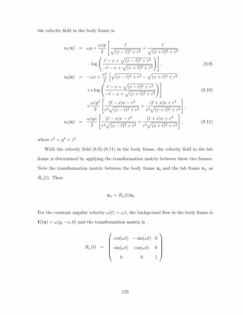
the velocity field in the body frame is

u1(x) = ωy +ωεy

2

[`√

(x− `)2 + r2+

`√(x+ `)2 + r2

− log

(`− x+

√(x− `)2 + r2

−`− x+√

(x+ `)2 + r2

)], (8.9)

u2(x) = −ωx+ωε

2

[√(x− `)2 + r2 −

√(x+ `)2 + r2

+x log

(`− x+

√(x− `)2 + r2

−`− x+√

(x+ `)2 + r2

)](8.10)

+ωεy2

2

[(`− x)x− r2

r2√

(x− `)2 + r2+

(`+ x)x+ r2

r2√

(x+ `)2 + r2

],

u3(x) =ωεyz

2

[(`− x)x− r2

r2√

(x− `)2 + r2+

(`+ x)x+ r2

r2√

(x+ `)2 + r2

], (8.11)

where r2 = y2 + z2.

With the velocity field (8.9)-(8.11) in the body frame, the velocity field in the lab

frame is determined by applying the transformation matrix between these two frames.

Note the transformation matrix between the body frame xb and the lab frame xL as

Rω(t). Then

xL = Rω(t)xb.

For the constant angular velocity ω(t) = ω t, the background flow in the body frame is

U(x) = ω(y,−x, 0) and the transformation matrix is

Rω(t) =

cos(ωt) − sin(ωt) 0

sin(ωt) cos(ωt) 0

0 0 1

.

176

−0.6 −0.4 −0.2 0 0.2 0.4 0.6

−0.5

−0.4

−0.3

−0.2

−0.1

0

0.1

0.2

0.3

0.4

0.5

x

y

(a) Two fluid particle trajectories (green and ma-genta) initially outside the blue circle.

−0.6 −0.4 −0.2 0 0.2 0.4 0.6−0.5

−0.4

−0.3

−0.2

−0.1

0

0.1

0.2

0.3

0.4

0.5

x

y

(b) Two fluid particle trajectories (green and red)initially inside the blue circle.

Figure 8.5: Fluid particle trajectories in the flow introduced by the counter-clockwiserotation of the slender body in the x-y plane. Here, ` = 0.5. The blue circle is theimprint of the slender body’s tips.

The velocity field in the lab frame is

uL(xL) =dxLdt

=d(Rωxb)

dt=

.

RωRTωxL +Rωu

(RTωxL

)

= ω

0 −1 0

1 0 0

0 0 0

xL

yL

zL

+

cos(ωt) − sin(ωt) 0

sin(ωt) cos(ωt) 0

0 0 1

u(RTωxL

).

Figure 8.5a shows two fluid particle trajectories when the slender body rotates coun-

terclockwise at the center of the lab frame within 15 revolutions of the slender body.

Figure 8.5b shows two fluid particle trajectories in the x-y plane when their initial

positions are close to the tip of the slender body. These two fluid particles are inside

the blue orbit of the slender body tips.

177

0.4 0.45 0.5 0.55 0.6 0.650

0.05

0.1

0.15

0.2

x

y

−0.2 −0.15 −0.1 −0.05 0 0.05

0.45

0.5

0.55

0.6

0.65

x

y

Figure 8.6: Two fluid particle trajectories within one revolution of the counter-clockwise rotation of the slender body (` = 0.5). The fluid particle trajectories areindicated by different colors for each quarter of the rotation. The blue trajectory is theimprint of the tips of the slender body.

−0.6 −0.4 −0.2 0 0.2 0.4 0.6 0.8 1

−0.4

−0.2

0

0.2

0.4

0.6

0.8

x

y

Figure 8.7: Numerical trajectories in the velocity field introduced by the anti-clockwiserotation of the slender body with ` = 0.5, U = 1 and T1 = 2.

178

Since the slender body has been shifted horizontally in phase 1 before its rotation,

the following transformation is applied the coordinates

x′ = x, y′ = y − U T1, z′ = z.

We ignore the above translation for the study of this phase itself. Such translation will

be considered when we examine the whole period of the slender body motion.

8.2.4 Phase 4: from step (d) to step (e)

In phase 4, the slender body clockwise rotates about its midpoint (0, 0, 0) with

constant angular velocity ω in the x-y plane in the lab frame.

• One end of the slender body moves from (0, `, 0) to (`, 0, 0);

• The other end of the slender body moves from (0,−`, 0) to (−`, 0, 0);

• The rotating time period is T2, so the frequency is ω = π2T2

.

Similar to the velocity (8.9)-(8.11) constructed in phase 2, we linearly distribute

Stokeslets along the center-line of the slender body, which is along the y-axis (−` ≤

y ≤ `) in the body frame. Since the slender body rotates clockwise in the lab frame,

the background flow in the body frame is counter-clockwise rotation flow. The velocity

179

field in the body frame is

u1(x) = −ωy +ωε

2

∫ `

−`

s

[(y − s)2 + r2]1/2ds+

ωεx2

2

∫ `

−`

s

[(y − s)2 + r2]32

ds

= −ωy +ωε

2

√(y − `)2 + r2 −

√(y + `)2 + r2

+y log

(`− y +

√(y − `)2 + r2

−`− y +√

(y + `)2 + r2

)

+ωεx2

2

[(`− y)y − r2

r2√

(y − `)2 + r2− (−`− y)y − r2

r2√

(y + `)2 + r2

],

u2(x) = ωx+ωεx

2

∫ `

−`

(y − s)s[(y − s)2 + r2]3/2

ds

= ωx+ωεx

2

`√

(y − `)2 + r2− −`√

(x+ `)2 + r2

− log

(`− y +

√(y − `)2 + r2

−`− x+√

(y + `)2 + r2

),

u3(x) =ωεxz

2

∫ `

−`

s

[(y − s)2 + r2]32

ds

=ωεxz

2

[(`− y)y − r2

r2√

(y − `)2 + r2− (−`− y)y − r2

r2√

(y + `)2 + r2

],

where r2 = x2 + z2.

If x2 + z2 = 0 and |y| > `, then the fluid particle is along the axis of the slender

body. The velocity field is

u1(x) = −ωy +ωε

2

∫ `

−`

s

|y − s|ds+

ωεx2

2

∫ `

−`

s

|y − s|3ds

= −ωy − ωε

2sign(y)

(2`+ y log

∣∣∣∣`− y`+ y

∣∣∣∣) ,u2(x) = u3(x) = 0.

In phase 2, the body is along the x-axis in the body frame. However, the body is

along y-axis in the body frame for phase 4. Before applying the transformation matrix

180

in phase 2, we need change the coordinates

xL =

1 0 0

0 −1 0

0 0 1

x′L,

where xL is in the laboratory frame and x′L is the coordinates in the laboratory frame

in phase 2, then rotate the slender body in the x-y plane. For constant angular velocity

ω(t) = ωt, the background flow is u(x) = ω(y,−x, 0).

Due to the time reversibility of the Stokes flow, the fluid particle trajectories in this

phase is easily to understand with the fluid particle trajectories in phase 2. We skip

fluid particle trajectory in this phase and illustrate the flow with the whole periodic

motion of the slender body.

8.3 Fluid particle trajectories

With the velocity field for the fluid motion during each step, we examine the fluid

particle trajectories when the slender body moves periodically as shown in Figure 8.2.

During each period, the proper transformation matrix is applied from the body frame

to the lab frame. A relation for the uniform translation velocity and the rotation rate

is selected to make the linear velocity of the tips equal between two phases.

In Figure 8.8, the magenta curves are fluid particle trajectories during one period at

different locations. The blue curves and red lines are part of the imprint of the slender

body’s tips. The half length of the slender body is ` = 0.5, and U = 1. The uni-

form translation is in the y-direction. The slender body rotates clockwise at the origin,

and rotates counter-clockwise at (0, 2, 0). From these trajectories, the motion gener-

ated by the rotation of the slender body contribute less than the uniform translation.

181

−6 −4 −2 0 2 4 6

−2

−1

0

1

2

3

4

5

x

y

Figure 8.9: Two groups of fluid particle trajectories and part of imprints of the periodicmotion of the slender body. All the particles move upward over time. Here the halfbody length is ` = 0.5, U = 1, and T1 = 2.

−1 −0.8 −0.6 −0.4 −0.2 0 0.2 0.4 0.6 0.8 1

−0.5

0

0.5

1

1.5

2

2.5

3

x

y

Figure 8.8: Fluid particle tra-

jectories within one period.

Figure 8.9 and 8.10 shows the fluid particle tra-

jectories when the slender body moves periodically as

shown in Figure 8.2. All the trajectories are in the

x-y plane. From these trajectories, there are direc-

tional fluid transport due to the periodic motion of

the slender body. The transport is along the transver-

sal translation direction (opposite to the longitudinal

translation) of the slender body. The comparison be-

tween Figure 8.10a and 8.10b shows the transport is

stronger if the uniform motion last longer when the

uniform velocity is fixed.

182

−3 −2 −1 0 1 2 3

−1

0

1

2

3

4

x

y

(a) T1 = 1.

−6 −4 −2 0 2 4 6

−2

−1

0

1

2

3

4

5

6

7

8

x

y

(b) T1 = 2.

Figure 8.10: Two groups of fluid particle trajectories in the x-y plane. Their initialpositions are at y = −1.5 or −2.5. Here, ` = 0.5, U = 1 and different values of T1.Part of the imprint of the tips are plotted at the center of these plots.

8.4 The far field

To examine the flow transport, it is worth checking the flow in the far field. In

this section, we study the asymptotic solution of the far-field velocity field for the flow

induced by the slender body in each step. For convenience, parentheses are drops for

trigonometry functions.

8.4.1 Uniform transition

Consider a distribution of Stokeslets over the portion −` < s < ` of the x-axis with

strength α(s) = (α1(s), α2(s), α3(s)), the velocity field u = (u1, u2, u3) at x due to this

183

force distribution is

u1(x;α) =

∫ `

−`

α1(s)[(x− s)2 + r2

]1/2 +(x− s) [(x− s)α1(s) + yα2(s) + zα3(s)][

(x− s)2 + r2] 3

2

ds,

u2(x;α) =

∫ `

−`

α2(s)[(x− s)2 + r2

]1/2 +y [(x− s)α1(s) + yα2(s) + zα3(s)][

(x− s)2 + r2] 3

2

ds,

u3(x;α) =

∫ `

−`

α3(s)[(x− s)2 + r2

]1/2 +z [(x− s)α1(s) + yα2(s) + zα3(s)][

(x− s)2 + r2] 3

2

ds,

where r2 = y2 + z2.

As the observation point x is far from the body, we examine the far-field velocity.

Hence, a non-dimensional formulation is introduced. Let

x′ =x

R, s′ =

s

`, α′ =

α

U(8.12)

in which R is a characteristic length assumed to be large and U is a characteristic

velocity. Note r as the non-dimensional radius, r2 = (y′)2 + (z′)2, and

ε0 =`

R0

(8.13)

as the small parameter for the far-field velocity. The details for the far-field velocity

are provided in Appendix E. Since the far-field limit of the velocity field is of interest,

we examine ε0 → 0 in the limit of R0 → 0.

Consider the velocity field due to a line distribution of uniform Stokeslets with

184

strength

α1(s) = εU1

4;

α3(s) = εU2

2;

α2(s) = εU3

2.

From the leading order of the far-field velocity

u1(x;α) = ε0

[2

|x|α1 +

2x2

|x|3α1 +

2xy

|x|3α2 +

2xz

|x|3α3

]+O(ε30) (8.14)

u2(x;α) = ε0

[2

|x|α2 +

2xy

|x|3α1 +

2y2

|x|3α2 +

2yz

|x|3α3

]+O(ε30) (8.15)

u3(x;α) = ε0

[2

|x|α3 +

2xz

|x|3α1 +

2yz

|x|3α2 +

2x23

|x|3α3

]+O(ε30) (8.16)

The far-field velocity of the induced velocity in Phase 1 Since the slender

body moves in the x-y plane and for phase 1

α1 = α3 = 0, and α2 =εU

2,

the leading order of the far-field velocity field for the induced flow is

dx

dt= ε0

2xy

|x|3α2 +O(ε30),

dy

dt= ε0

[2

|x|α2 +

2y2

|x|3α2

]+O(ε30),

dz

dt= ε0

[2yz

|x|3α2

]+O(ε30).

If the particle’s initial position is in the x-y plane, then z = 0 is always true on the

185

-4 -2 0 2 4

-4

-2

0

2

4

Figure 8.11: Contour plot for exact solution (8.17) of the far-field trajectory.

fluid particle trajectory

dx

dt= 2ε0α2

xy

(x2 + y2)32

+O(ε30),

dy

dt= 2ε0α2

[1√

x2 + y2+

y2

(x2 + y2)32

]+O(ε30),

dz

dt= O(ε30).

From the velocity field, we find the fluid particle trajectory equation in the x-y plane,

dy

dx=

x2 + 2y2

xy,=⇒ 1

x2+y2

x4= constant. (8.17)

Since the slender body moving in the x-y plane and for phase 1 with background

186

flow (0,−U, 0) and

α1 = α3 = 0, and α2 = −εU2,

the far-field velocity field in the body frame is

dx

dt= ε0

2xy

|x|3α2 +O(ε30),

dy

dt= −U + ε0

[2

|x|α2 +

2y2

|x|3α2

]+O(ε30),

dz

dt= ε0

[2yz

|x|3α2

]+O(ε30).

If the particle’s initial position is in the x-y plane, then

dx

dt= 2ε0α2

xy

(x2 + y2)32

+O(ε30),

dy

dt= −U + 2ε0α2

[1√

x2 + y2+

y2

(x2 + y2)32

]+O(ε30),

dz

dt= O(ε30).

From the above velocity field,

dx

dy=

xy

(x2+y2)32

− U2ε0α2

+

[1√x2+y2

+ y2

(x2+y2)32

] ,=⇒

− U

2ε0α2

+

[1√

x2 + y2+

y2

(x2 + y2)32

]dx− xy

(x2 + y2)32

dy = 0.

187

Applying the integral factor µ(x, y) = x,

− Ux

2ε0α2

+

[x√

x2 + y2+

xy2

(x2 + y2)32

]dx− x2y

(x2 + y2)32

dy = 0

d

[− Ux2

4ε0α2

+√x2 + y2 − y2√

x2 + y2

]= 0

d

[− Ux2

4ε0α2

+x2√x2 + y2

]= 0

−Ux2 + 4ε0α2x2√x2 + y2

= constant. (8.18)

Equation (8.18) is the fluid particle trajectory equation in the body frame. As the

velocity component in the z-direction vanishes for any fluid particle initially in the x-y

plane, we only need check the fluid particle trajectory in the x-y plane in the lab frame.

In the laboratory frame (x′, y′),

x′ = x

y′ = y + Utand

x = x′

y = y′ − Ut.

So, the particle trajectory equation is

− Ux2 + 4ε0α2x2√

x2 + (y − Ut)2= constant. (8.19)

The far-field velocity in phase 3 can be obtained similarly from (8.14)-(8.16) with

corresponding background flow.

188

-1.5 -1 -0.5 0.5 1 1.5

-2

-1

1

2

Figure 8.12: Contour plot for the exact solution (8.18) of the far-field trajectory.

8.4.2 Rotation

During phase 2 and phase 4, the body rotates about its midpoint with constant

angular velocity ω in the (x, y) plane. In the body frame, the velocity field is

u1(x) = ωy +ωε

2

∫ `

−`

(x− s)ys[(x− s)2 + y2 + z2]3/2

ds,

u2(x) = −ωx+ωε

2

∫ `

−`

s

[(x− s)2 + y2 + z2]1/2+

y2s

[(x− s)2 + y2 + z2]32

ds,

u3(x) =ωε

2

∫ `

−`

yzs[(x− s)2 + y2 + z2

] 32

ds.

Non-dimensionalize the velocity as for the uniform translation in the previous sub-

section, the far-field velocity field is

u1(x) = ωRy +ωε`y

2

[(3x2

|x|5− 1

|x|3

)2

3ε20 +O(ε40)

],

u2(x) = −ωRx+ωε`

2

[x

|x|32ε203

+O(ε40)

]+ωε`y2

2

[3x

|x|52

3ε20 +O(ε40)

],

u3(x) =ωε`yz

2

[3x

|x|52

3ε20 +O(ε40)

].

189

More details about the non-dimensionalization are provided in Appendix E. If the high

order terms are negligible, the fluid particle trajectory is governed by

dx

dt= ωRy +

ωε`y

3

(3x2

|x|5− 1

|x|3

)ε20 +O(ε40),

dy

dt= −ωRx+

ωε`x

3 |x|3ε20 +

ωε`xy2

|x|5ε20 +O(ε40),

dz

dt= ωε`yz

x

|x|5ε20 +O(ε30).

If the fluid particle is in the x-y plane initially, i.e., z = 0 and |x| =√x2 + y2, keep

the leading order of the far field velocity

dx

dt= ωRy +

ωε`y

3

2x2 − y2

(x2 + y2)5/2ε20 +O(ε40),

dy

dt= −ωRx+

ωε`x(x2 + 4y2)

3(x2 + y2)5/2ε20 +O(ε40),

dz

dt= 0.

If the fluid particles is in the x-y plane, they will be restricted in that plane. For the

ODE system in the x-y plane in the body frame

dx

dt= ωRy +

ωε`y(2x2 − y2)

3(x2 + y2)5/2ε20,

dy

dt= −ωRx+

ωε`x(x2 + 4y2)

3(x2 + y2)5/2ε20.

Rewrite the equations and apply the integrating factor µ(x, y) = 3√x2 + y2,

[3ωRy

√x2 + y2 +

ωε`ε20y(2x2 − y2)

(x2 + y2)2

]dy

+

[3ωRx

√x2 + y2 − ωε`ε20x(x2 + 4y2)

(x2 + y2)2

]dx = 0

=⇒ d

(ωR(x2 + y2)

32 − ωε`ε20

2

(log(x2 + y2) +

3x2

x2 + y2

))= 0.

190

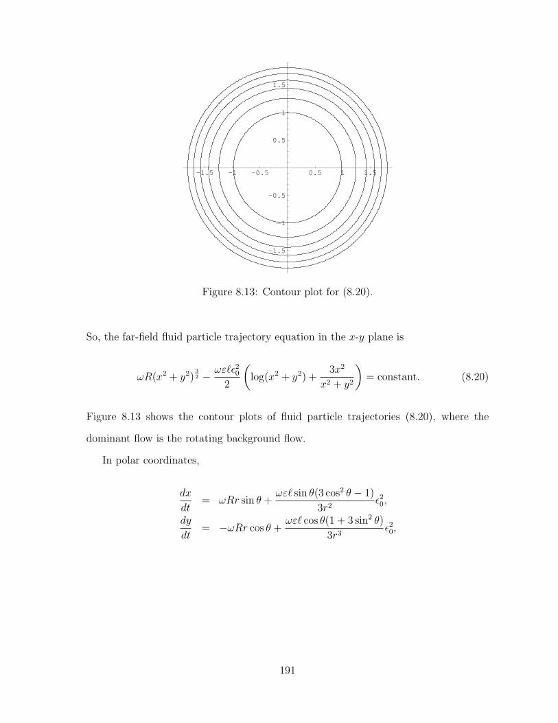
-1.5 -1 -0.5 0.5 1 1.5

-1.5

-1

-0.5

0.5

1

1.5

Figure 8.13: Contour plot for (8.20).

So, the far-field fluid particle trajectory equation in the x-y plane is

ωR(x2 + y2)32 − ωε`ε20

2

(log(x2 + y2) +

3x2

x2 + y2

)= constant. (8.20)

Figure 8.13 shows the contour plots of fluid particle trajectories (8.20), where the

dominant flow is the rotating background flow.

In polar coordinates,

dx

dt= ωRr sin θ +

ωε` sin θ(3 cos2 θ − 1)

3r2ε20,

dy

dt= −ωRr cos θ +

ωε` cos θ(1 + 3 sin2 θ)

3r3ε20,

191

and

dθ

dt=

∂θ

∂x

dx

dt+∂θ

∂y

dy

dt= −sin θ

r

dx

dt+

cos θ

r

dy

dt= −ωR +

ωε`

3r3ε20,

dr

dt=

∂r

∂x

dx

dt+∂r

∂y

dy

dt= cos θ

dx

dt+ sin θ

dy

dt=ωε`ε20 sin θ cos θ

r2.

Thus

dθ

dt= −ωR +

ωε`

3r3ε20,

dr

dt=

ωε`ε20 sin θ cos θ

r2.

The far-field fluid particle trajectory in the polar coordinates in the body frame is

ωRr3 − ωε`ε20 log(r)− 3ωε`ε202

cos 2θ = C = constant. (8.21)

Rewriting (8.21), we get

cos 2θ = 2ωRr3 − ωε`ε20 log(r)− C

3ωε`ε20. (8.22)

Substitute the above equation into drdt

,

dr

dt= ±ε20

ωε`

√1− 4

(ωRr3−ωε` log(r)−C

3ωε`ε20

)2

2r2.

The equation shows the change in the radial direction can be captured only with higher

order solutions, which verifies the results demonstrated with the contour plots.

192

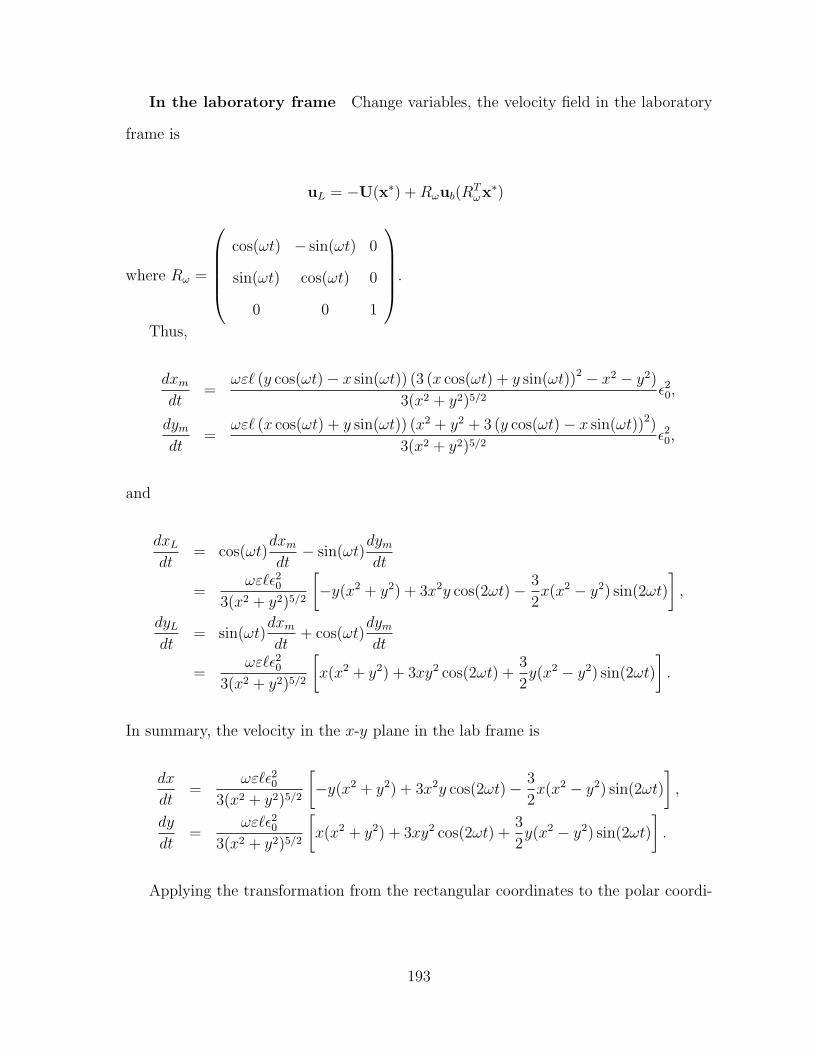
In the laboratory frame Change variables, the velocity field in the laboratory

frame is

uL = −U(x∗) +Rωub(RTωx∗)

where Rω =

cos(ωt) − sin(ωt) 0

sin(ωt) cos(ωt) 0

0 0 1

.

Thus,

dxmdt

=ωε` (y cos(ωt)− x sin(ωt)) (3 (x cos(ωt) + y sin(ωt))2 − x2 − y2)

3(x2 + y2)5/2ε20,

dymdt

=ωε` (x cos(ωt) + y sin(ωt)) (x2 + y2 + 3 (y cos(ωt)− x sin(ωt))2)

3(x2 + y2)5/2ε20,

and

dxLdt

= cos(ωt)dxmdt− sin(ωt)

dymdt

=ωε`ε20

3(x2 + y2)5/2

[−y(x2 + y2) + 3x2y cos(2ωt)− 3

2x(x2 − y2) sin(2ωt)

],

dyLdt

= sin(ωt)dxmdt

+ cos(ωt)dymdt

=ωε`ε20

3(x2 + y2)5/2

[x(x2 + y2) + 3xy2 cos(2ωt) +

3

2y(x2 − y2) sin(2ωt)

].

In summary, the velocity in the x-y plane in the lab frame is

dx

dt=

ωε`ε203(x2 + y2)5/2

[−y(x2 + y2) + 3x2y cos(2ωt)− 3

2x(x2 − y2) sin(2ωt)

],

dy

dt=

ωε`ε203(x2 + y2)5/2

[x(x2 + y2) + 3xy2 cos(2ωt) +

3

2y(x2 − y2) sin(2ωt)

].

Applying the transformation from the rectangular coordinates to the polar coordi-

193

nates x = r cos θ

y = r sin θ

∂r∂x

= cos θ

∂r∂y

= sin θ

∂θ∂x

= − sin θr

∂θ∂y

= cos θr

,

we have

dx

dt=

ωε`ε203r2

[− sin θ + 3 cos2 θ sin θ cos(2ωt)− 3

2cos θ(cos2 θ − sin2 θ) sin(2ωt)

],

dy

dt=

ωε`ε203r2

[cos θ + 3 cos θ sin2 θ cos(2ωt) +

3

2sin θ(cos2 θ − sin2 θ) sin(2ωt)

].

For the polar coordinates,

dθ

dt=

∂θ

∂x

dx

dt+∂θ

∂y

dy

dt= −sin θ

r

dx

dt+

cos θ

r

dy

dt

=ωε`ε20r3

[1

3+

1

4sin 4θ sin(2ωt)

],

dr

dt=

∂r

∂x

dx

dt+∂r

∂y

dy

dt= cos θ

dx

dt+ sin θ

dy

dt

=ωε`ε203r2

[3

2sin 2θ cos(2ωt)− 3

2cos2 2θ sin(2ωt)

].

Define the average as f(·) = 1T

∫ T0f(·, t)dt, then the average equations for the fluid

motion are dθdt

=ωε`ε203r3

drdt

= 0=⇒

θ =ωε`ε203r(0)3 t

r = r(0). (8.23)

From the averaged equation, the radial component of the fluid particle trajectory is a

constant. The azimuthal angle is a monotonic function of time t.

194

From the equation of fluid particle trajectory in the body frame (8.20)

ωR(x2 + y2)32 − ωε`ε20

2

(log(x2 + y2) +

3x2

x2 + y2

)= constant,

and the relations:

From body frame to lab frame,xL

yL

zL

=

cos(ωt) − sin(ωt) 0

sin(ωt) cos(ωt) 0

0 0 1

xb

yb

zb

=

xb cos(ωt)− yb sin(ωt)

yb cos(ωt) + xb sin(ωt)

zb

From the lab frame to the body frame,

xb

yb

zb

=

cos(ωt) sin(ωt) 0

− sin(ωt) cos(ωt) 0

0 0 1

xL

yL

zL

=

xL cos(ωt) + yL sin(ωt)

yL cos(ωt)− xL sin(ωt)

zL

,

the equation of trajectory in the laboratory frame is

ωR(x2 + y2)32 − ωε`ε20

2

(log(x2 + y2) +

3(x cos(ωt) + y sin(ωt))2

x2 + y2

)= constant.

Sometime (x, y, z) are used in both the body frame and the lab frame without sub-

scription, if we specify the frame. In polar coordinates, it is

ωRr3 − ωε`ε202

(log(r2) + 3(cos θ cos(ωt) + sin θ sin(ωt))2

)= constant,

ωRr3 − ωε`ε20 log(r)− 3ωε`ε202

cos2(θ − ωt) = constant.

Figure 8.14 and 8.15 show the comparison of the far-field fluid particle trajectories with

the averaged trajectory.

195

−1 −0.5 0 0.5 1

−0.8

−0.6

−0.4

−0.2

0

0.2

0.4

0.6

0.8

x

y

Figure 8.14: Contour plot for exact solution (8.20) (purple) of the far-field trajectoryand the averaged trajectory from (8.23) (green).

0.99 0.995 1 1.0050

0.002

0.004

0.006

0.008

0.01

0.012

0.014

0.016

0.018

0.02

x

y

0.9 0.95 1 1.050

0.02

0.04

0.06

0.08

0.1

0.12

0.14

0.16

0.18

0.2

x

y

Figure 8.15: Zoom in on Figure 8.14.

196

8.5 Flux through a vertical plane at y = y0

To better under the flow induced by the slender rod, we study the flux through a

vertical plane at y = y0 far from the body. During one period of the slender body

motion, the rotation of the slender body in phase 2 can be viewed as the reverse of

rotation in phase 4. Due to reversibility of the Stokes flow, the total flux introduced by

these two phases equals to each other by neglecting the different of the distance. Thus,

we only compute the flux during the uniform translations, which is the dominant part

of the total flux.

The equation of flux F at an instantaneous time t through the vertical plane (x, z) ∈

(−L,L)× (−H,H) at y = y0 is

F =

∫ H

−Hdz

∫ L

−Ldx

dy

dt

∣∣∣∣y=y0

.

8.5.1 Flux during the horizontal shift

In phase 1, the slender body shift perpendicular to its axis. During this horizontal

shift, the velocity component dydt

in the body frame at y = y0 is

dy

dt

∣∣∣∣y=y0

= −U + α2 log

`− x+√r2 + (`− x)2

−`− x+√r2 + (`+ x)2

+y2α2

r2

`− x√r2 + (`− x)2

− −`− x√r2 + (`+ x)2

,

197

where r2 = y20 + z2. In the laboratory frame, it is

dy

dt|y=y0 = α2

log

`+√

(y0 − Ut)2 + z2 + (`− x)2 − x

−`+√

(y0 − Ut)2 + z2 + (`+ x)2 − x

+

(y0 − Ut)2

r2

`− x√(y0 − Ut)2 + z2 + (`− x)2

+`+ x√

(y0 − Ut)2 + z2 + (`+ x)2

.Flux during phase 1 through the plane at y = y0 is

Flux1(α2, L, y,H, U, `, t) =∫ H−H dz

∫ L−L dx

dydt|y=y0

= α2

∫ H−H dz

∫ L−L dx log

(`+√

(y0−Ut)2+z2+(`−x)2−x

−`+√

(y0−Ut)2+z2+(`+x)2−x

)+α2

∫ H−H dz

∫ L−L dx

(y0−Ut)2

r2

(`−x√

(y0−Ut)2+z2+(`−x)2+ `+x√

(y0−Ut)2+z2+(`+x)2

)= α2

2H(√

H2 + (`− L)2 + (y − Ut)2 −√H2 + (`+ L)2 + (y − Ut)2

)+ ((`− L)2 + (y − Ut)2) log

(−H+√H2+(`−L)2+(y−Ut)2

H+√H2+(`−L)2+(y−Ut)2

)− ((`+ L)2 + (y − Ut)2) log

(−H+√H2+(`+L)2+(y−Ut)2

H+√H2+(`+L)2+(y−Ut)2

)−2H(`− L) log

(`−L+√H2+(`−L)2+(y−Ut)2

−`+L+√H2+(`−L)2+(y−Ut)2

)+ 2H(`+ L) log

(`+L+√H2+(`+L)2+(y−Ut)2

−`−L+√H2+(`+L)2+(y−Ut)2

).

As y →∞,

Flux1(α2, L, y,H, U, `, t) ∼16α2H`L

y.

When x→∞,

Flux1(α2, L, y,H, U, `, t) ∼ 8α2H` (log(L) + 1) + 4α2H` log

(4

H2 + (y − Ut)2

).

198

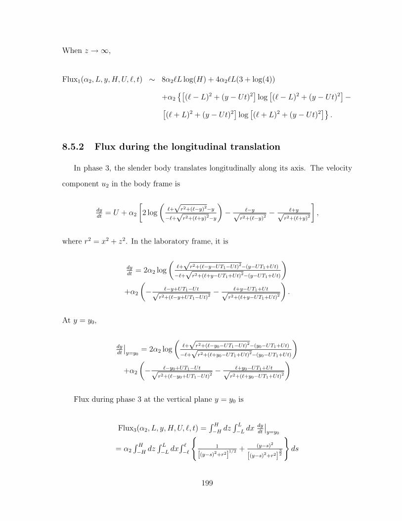
When z →∞,

Flux1(α2, L, y,H, U, `, t) ∼ 8α2`L log(H) + 4α2`L(3 + log(4))

+α2

[(`− L)2 + (y − Ut)2

]log[(`− L)2 + (y − Ut)2

]−[

(`+ L)2 + (y − Ut)2]

log[(`+ L)2 + (y − Ut)2

].

8.5.2 Flux during the longitudinal translation

In phase 3, the slender body translates longitudinally along its axis. The velocity

component u2 in the body frame is

dydt

= U + α2

[2 log

(`+√r2+(`−y)2−y

−`+√r2+(`+y)2−y

)− `−y√

r2+(`−y)2− `+y√

r2+(`+y)2

],

where r2 = x2 + z2. In the laboratory frame, it is

dydt

= 2α2 log

(`+√r2+(`−y−UT1−Ut)2−(y−UT1+Ut)

−`+√r2+(`+y−UT1+Ut)2−(y−UT1+Ut)

)+α2

(− `−y+UT1−Ut√

r2+(`−y+UT1−Ut)2− `+y−UT1+Ut√

r2+(`+y−UT1+Ut)2

).

At y = y0,

dydt

∣∣y=y0

= 2α2 log

(`+√r2+(`−y0−UT1−Ut)2−(y0−UT1+Ut)

−`+√r2+(`+y0−UT1+Ut)2−(y0−UT1+Ut)

)+α2

(− `−y0+UT1−Ut√

r2+(`−y0+UT1−Ut)2− `+y0−UT1+Ut√

r2+(`+y0−UT1+Ut)2

)

Flux during phase 3 at the vertical plane y = y0 is

Flux3(α2, L, y,H, U, `, t) =∫ H−H dz

∫ L−L dx

dydt

∣∣y=y0

= α2

∫ H−H dz

∫ L−L dx

∫ `−`

1

[(y−s)2+r2]1/2 + (y−s)2

[(y−s)2+r2]32

ds

199

Explicitly,

Flux3(α2, L, y,H, U, `, t)

= −2α2

2L2

[arctan

(H(`−y)

L√H2+L2+(y−`)2

)+ arctan

(H(`+y)

L√H2+L2+(`+y)2

)]+2H2

[arctan

(L(`−y)

H√H2+L2+(y−`)2

)+ arctan

(L(`+y)

H√H2+L2+(`+y)2

)]+L(`− y) log

(−H+√H2+L2+(y−`)2

H+√H2+L2+(y−`)2

)+H(`− y) log

(−L+√H2+L2+(y−`)2

L+√H2+L2+(y−`)2

)−L(`+ y) log

(H+√H2+L2+(`+y)2

−H+√H2+L2+(`+y)2

)−H(`+ y) log

(L+√H2+L2+(`+y)2

−L+√H2+L2+(`+y)2

)+4HL log

(−`−y+

√H2+L2+(`+y)2

`−y+√H2+L2+(y−`)2

).

As y →∞,

Flux3(α2, L, y,H, U, `, t) ∼16α2H`L

y.

When x→∞,

Flux3(α2, L, y,H, U, `, t)

∼ 8α2H` log(L)− 2Hα2

−8`+ 2H

[arctan

(`− yH

)+ arctan

(`+ y

H

)]+(`− y) log

(H2 + (y − `)2

4

)− (`+ y) log

(4

H2 + (`+ y)2

).

As z →∞,

Flux3(α2, L, y,H, U, `, t)

∼ 8α2L` log(H)− 2Lα2

−8`+ 2L

[arctan

(`− yL

)+ arctan

(`+ y

L

)]+(`− y) log

(L2 + (y − `)2

4

)− (`+ y) log

(4

L2 + (`+ y)2

).

200

Chapter 9

Conclusions and future work

This thesis reports mainly as two parts about flow patterns and flow and rigid

obstacles interactions in the Stokes regime. The first part focuses on the analytical

and numerical study of Stokes linear shear or rotating flow past a sphere or spheroid.

In the second part, the rigid bodies in the flow are irregular compared to spheres or

spheroids. We experimentally and theoretically study the flow induced by a slender

rod either straight or bent sweeping out a cone above a no-slip plane.

In the first part, based on the velocity field of a rigid sphere immersed in a linear

shear flow, we have derived the fluid particle trajectory equations in closed quadrature

when the sphere’s center is in the zero-velocity of the background linear shear. Us-

ing the trajectory equations, we have obtained the explicit formula for the stagnation

points on the sphere and explored the blocking phenomenon in the streamlines. The

cross-sectional area of the blocked flow at infinity equals infinity, which is a physically

unobserved property of the Stokes flow. With linearized velocity field near the surface

of sphere, we have found the explicit formula for the imprint on the sphere, where the

no-slip boundary is imposed.

If the sphere’s center is out of the zero-velocity plane blocking phenomenon is cap-

tured numerically. Starting from the velocity field, we find the analytical results for

the stagnation points and the critical points in the interior of the flow. Complicated

bifurcation structures are studied in terms of the dimensionless distance, U , from the

center of the sphere to the zero-velocity plane of the background linear shear. A 3D

eddy appears with special values of U . With linearized velocity near the surface of the

sphere, the trajectory of the imprint is also achieved.

If the sphere is fixed in the linear shear flow, there is no closed streamline emerged

in contrast to the well-known closed orbits for the linear shear past a freely rotating

cylinder or sphere [23, 1, 42, 62, 53, 77, 54]. We have reviewed the linear shear past a

freely rotating sphere and estimate the height of the closed streamline near the sphere,

when the sphere’s center is in the zero-velocity plane. When the sphere is embedded

in purely rotating background flows, the explicit fluid particle trajectory equation and

stagnation points in the flow are obtained.

When the embedded rigid body becomes a prolate spheroid, we study the case when

the center of the spheroid is in the zero-velocity plane of the background shear. The

orientational spheroid is either upright or tilted in the symmetry plane of the flow,

along or against the background streamline. Even though the trajectory equation is

not available explicitly, the blocking phenomenon has been illustrated numerically. We

have found the critical points in the interior of the flow, and derived the formula of

the stagnation points on the spheroid. We have also checked how stagnation points

migrate as the eccentricity of the spheroid changes.

If the major axis of the spheroid is perpendicular to the background stream (up-

right), the flow structure is similar to the spherical case. When the spheroid is tilted, the

broken symmetry offered by a tilted spheroid geometry induces new three-dimensional

effects on streamline deflection. The deflection can be viewed as effective positive or

negative suction in the horizontal direction orthogonal to the background flow depend-

ing on the tilt orientation.

While our findings have led to improved understanding about shear flows past an

202

obstacle, they have been limited to the Stokes flow regime. It will be useful to improve

the physical description of the flow if we can include the Oseen correction into the

governing equations, thus take into account the inertial effects of real fluids. This

would lead to finding a correction for the blockage area we computed in the Stokes

limit, possibly making it finite. We also want to design an experiment based on these

theoretical studies. This will allow for the assessment of effects of boundary conditions

at a finite range. Moreover, the investigation of general linear unsteady Stokes flows

past rigid bodies will be interesting. Such problems have natural implications in the

rheology of complex fluids and fluid-solid mixtures, applications to micro-fluidic mixing

devices and their biological counterparts.

In the second part of this thesis, we have aimed to understand flows induced by a

slender rod precessing in a cone that mimics the motion of primary nodal cilia. We

have studied the flow with the 3D experiment, theoretical modeling and numerics. For

the straight rod case, we study the flow generated by the straight rod sweeping out a

tilted cone, which carries time information both in the laboratory frame and in the body

frame. Near the cone, the fluid particle follows a small time scale epicycle corresponding

to almost one revolution of the rod and a long time orbit surround the cone, which is

similar to the trajectory with an upright cone. Due to the tilt, depending on the scale of

the large orbit, the trajectory is deformed dramatically with respect to the no-slip plane.

For the upright cone, except the fluctuation during each epicycle, the trajectory stays

at the relatively fixed level. Both closed periodic trajectories and open trajectories are

observed, which is a new phenomena introduced by the tilt. Flux through a vertical

plane parallel to the cone axis is evaluated to show the fluid transport. Using the

dynamic cone angle and approximate convection detected from the experiments, the

experimental and theoretical data show excellent agreement.

For the bent rod sweeping a cone above the no-slip plane, a toroidal structure

203

has been captured. In a short or intermediate time, the fluid particle trajectories are

similar to the straight rod case. Over very long time scale, the particle trajectory

stay on the surface of a torus. Using the Poincare map as an effective tool, we have

examined the multiple parameters that have influences on the tori. Both our model and

the experiment have verified this toroidal structure in the fluid particle trajectories.

With fully 3D experimental ability, we quantitatively compare the model with the

experiment. However, the discrepancies show up in a short time comparison of the

trajectories. Possible issues have been discussed. We have reported the relative studies

for simplified flows.

We have only studied the flow generated by rigid rods. However, our model is

feasible to extend to flexible cilia with small curvatures. In the future, we want to

study the flexible rod with small curvatures. It will be interesting to further model

flows induced by multiple cilia, study hydrodynamic interactions between separated

cilia, and assess wall effects in the flow in the future work. Increased fidelity of the

models could be achieved by investigating non-Newtonian effects naturally existing in

biological contexts.

204

Appendix A

Fundamental singularities and the

slender body theory

The fundamental singularities used in this thesis are listed without the details about

the derivation and their components. Details could be referred to Chwang & Wu [19]

and Leiterman [48]. In addition, the slender body theory is briefly summarized with

emphasis on the strength ratio with respect to the velocity field [3]. The purpose of

the repetition is to make the thesis self-contained.

A.1 Singularities

For Stokes flows, fundamental singular solutions are available, which are useful for

constructing solutions for more complicated boundary conditions. The Stokeslet uS is

a fundamental solution of the Stokes equation for a single point force,

µ∇2u + fS = ∇p,

∇ · u = 0, (A.1)

where fS = 8πµαδ(x), and

uS(x;α) =α

|x|+

(x ·α)x

|x|3

pS(x;α) = −2µx ·α|x|3

.

205

Here α is the strength of the singularity located at the origin, x = (x, y, z) and |x| =√x2 + y2 + z2. Due to the linear property of the Stokes equations, a derivative of any

order of uS and pS(x;α) is also a solution of (A.1) with corresponding derivative of fS.

The Stokes doublet is

uSD(x;α,β) = −(β · ∇)uS(x;α) =(β ×α)× x

|x|3− (α.β)x

|x|3+ 3

(α · x)(β · x)x

|x|5.

The symmetric component of a Stokes doublet is a stresslet

uSS(x;α,β) =1

2[uSD(x;β,α) + uSD(x;α,β)] = −(α · β)x

|x|3+

3(α · x)(β · x)x

|x|5.

The antisymmetric component of a Stokes doublet is Rotlet or couplet

uR(x;γ) =1

2[uSD(x;β,α)− uSD(x;α,β)] =

1

2∇× uS(x;γ) =

γ × x

|x|3,

where γ = α× β.

A potential doublet is

uD(x; δ) =1

2∇2 × uS(x; δ) = − δ

|x|3+

3(δ · x)x

|x|5,

where δ is the doublet strength.

A.2 Canonical results of the slender body theory

Many important applications of Stokes flow involves elongated particles, such as

slender rods and glass and carbon fibres. However, analytical solutions exist for a

limited range of particle shapes, for example, sphere and spheroid. Consider the body

is slender, i.e., its length 2` is much larger than its radius r0, asymptotic solutions

206

to the equation of fluid flow can be constructed by slender-body theory, which is first

developed by Burgers [13].

The velocity field due to the presence of the body is approximated by a distribution

of Stokeslets along the center-line of the body,

u(x) =

∫ `

−`uS(x− xs;α)ds, (A.2)

where x is the observation position and xs is the location of the Stokeslet depending

on s. If the body is along the x-axis and Stokeslets are distributed over the portion

−` ≤ x ≤ ` of the x axis, the canonical results for uniform flow (U1, U2, U3) past a rigid

cylindrical body are restated here.

Assume the strength of the Stokeslet α is uniform, a constant vector, then the total

velocity field is

u1(x) = U1 − α1

∫ `

−`

1√(x− s)2 + y2 + z2

ds− α1

∫ `

−`

(x− s)2

((x− s)2 + y2 + z2)32

ds

−(α2y + α3z)

∫ `

−`

(x− s)((x− s)2 + y2 + z2)

32

ds,

u2(x) = U2 + α2

∫ `

−`

1√(x− s)2 + y2 + z2

ds− α1y

∫ `

−`

(x− s)((x− s)2 + y2 + z2)

32

ds

−(α2y2 + α3yz)

∫ `

−`

1

((x− s)2 + y2 + z2)32

ds,

u3(x) = U3 − α3

∫ `

−`

1√(x− s)2 + y2 + z2

ds− α1z

∫ `

−`

(x− s)((x− s)2 + y2 + z2)

32

zds

−(α2yz + α3z2)

∫ `

−`

1

((x− s)2 + y2 + z2)32

zds,

To determine the strength α, we impose the no-slip boundary condition on the surface

207

of the slender body y20 + z2

0 = r20 and −` ≤ x0 ≤ `.

0 = U1 − α1

∫ `

−`

1√(x0 − s)2 + r2

0

ds− α1

∫ `

−`

(x0 − s)2

((x0 − s)2 + r20)

32

ds

−(α2y0 + α3z0)

∫ `

−`

(x0 − s)((x− s)2 + r2

0)32

ds,

0 = U2 − α2

∫ `

−`

1√(x0 − s)2 + r2

0

ds− α1y0

∫ `

−`

(x0 − s)((x0 − s)2 + r2

0)32

ds

−(α2y20 + α3y0z0)

∫ `

−`

1

((x− s)2 + r20)

32

ds,

0 = U3 − α3

∫ `

−`

1√(x0 − s)2 + r2

0

ds− α1z0

∫ `

−`

(x0 − s)((x0 − s)2 + r2

0)32

z0ds

−(α2y0z0 + α3z20)

∫ `

−`

1

((x0 − s)2 + r20)

32

zds,

Away from the ends of the slender body, as the radius of the body r0 → 0,

∫ `

−`

1√(x0 − s)2 + r2

0

ds = log

(s+

√r2

0 + (s− x0)2 − x0

)|s=`s=−`

= log

√(

r0`

)2+(1− x0

`

)2+(1− x0

`

)√(r0`

)2+(1 + x0

`

)2 −(1 + x0

`

) ∼ log

(1− x0

`

)+

( r0` )2

2(1−x0` )

+(1− x0

`

)(1 + x0

`

)+

( r0` )2

2(1+x0` )−(1 + x0

`

)

= log

2(1− x0

`

)2(1 + x0

`

)+

( r0` )2

(1−x0` )

(1 + x0

`

)(r0`

)2

∼ log

(4(1− x0

`

) (1 + x0

`

)(r0`

)2

)= 2 log

(2`

r0

)+ log

(1−

(x0

`

)2)

Note ε = log(

2`r0

)−1

as the slenderness parameter, then

∫ `

−`

1√(x0 − s)2 + r2

0

ds ∼ 2

ε

208

Also,

∫ `

−`

1

((x0 − s)2 + r20)

3/2ds =

s− x0

r20

√r2

0 + (s− x0)2

∣∣∣∣∣s=`

s=−`

=`− x0

r20

√r2

0 + (`− x0)2+

`+ x0

r20

√r2

0 + (`+ x0)2

=1

r20

1− x0

`√(r0`

)2+(1− x0

`

)2+

1 + x0

`√(r0`

)2+(1 + x0

`

)2

∼ 1

r20

(2− 1

2

(`2

(`− x0)2+

`2

(`+ x0)2

)(r0

`

)2)

So, the leading order is

∫ `

−`

1

((x0 − s)2 + r20)

3/2ds ∼ 2

r20

, as r0 → 0.

Since

∫ `

−`

(x0 − s)((x0 − s)2 + r2

0)3/2ds =

1√r2

0 + (s− x0)2

∣∣∣∣∣s=`

s=−`

=1√

r20 + (`− x0)2

− 1√r2

0 + (`+ x0)2

=1

`

1√(r0`

)2+(1− x0

`

)2− 1√(

r0`

)2+(1 + x0

`

)2

∼ 1

`

(1

1− x0

`

− 1

1 + x0

`

+

(− 1

2(`− x0)3+

1

2(`+ x0)3

)(r0

`

)2),

the leading order of this integral is

∫ `

−`

(x0 − s)((x0 − s)2 + r2

0)3/2ds ∼ 1

`− x0

− 1

`+ x0

.

209

From the above results,

∫ `

−`

(x0 − s)2

((x0 − s)2 + r20)

3/2ds =

∫ `

−`

1√(x0 − s)2 + r2

0

ds−∫ `

−`

r20

((x0 − s)2 + r20)

3/2ds

∼ 2

ε

In summary, the boundary conditions are

0 = U1 − α12

ε− α1

2

ε,

0 = U2 − α22

ε,

0 = U3 − α32

ε.

So, the strength α is determined as

α1 =U1 ε

4in the direction parallel to the body’s axis,

α2 =U2 ε

2and α3 =

U3 ε

2in the direction perpendicular to the body’s axis.

Notice the factor 2 of α1 compared to α2 and α3.

Be ware that the slender-body asymptotic velocity is accurate for small slenderness

ε = log−1(

2`r0

)away from the ends of the body.

For other flow past a slender body, an asymptotic solution can be found by applying

the same mechanism.

210

Appendix B

Error analysis of the velocity field

when approximating a prolate

spheroid in the flow with a slender

body

Slender body theory is a good approximate for the arbitrary cross section body

immersed in stokes flow, if the body is slender. It gives a first order approximation and

not accurate near the ends of the body. In this appendix, we provide the error analysis

for approximating a prolate spheroid with a slender body. In both cases, we check the

velocity fields and compute the error, since the velocity field is exact Stokes solution

for a prolate spheroid case.

In the first section, we check the error when a uniform flow past a spheroid compare

to the approximation of uniform flow past a slender body. In the second section, we

check the error for slender body theory when the body sweeps out a double cone.

211

B.1 Uniform flow past a spheroid or slender body

B.1.1 Uniform flow past a spheroid

Based on the singularity method, by employing a line distribution of Stokeslets and

potential doublets between the foci x = −c and c, the exact velocity of uniform fluid

flow U1ex + U2ey past a prolate spheroid is given by [19]

u(x) = U1ex + U2ey −∫ c

−c(uS (x− s;α1ex) + uS (x− s;α2ey)) ds

+

∫ c

−c

(c2 − s2

)(uD (x− s; β1ex) + uD (x− s; β2ey)) ds, (B.1)

in which

α1 =2β1e

2

1− e2=

U1e2

−2e+ (1 + e2)Le,

α2 =2β2e

2

1− e2=

2U2e2

2e+ (3e2 − 1)Le,

are the strength of the singularities with Le = log(

1+e1−e

)(e is the eccentricity). In

component format, the velocity field is

u1(x) = U1 −∫ c

−c

α1

(x− s)2 + r21/2ds−

∫ c

−c

(x− s)2α1

(x− s)2 + r232

ds

−∫ c

−c

(x− s)yα2

(x− s)2 + r232

ds−∫ c

−c

β1 (c2 − s2)

(x− s)2 + r23/2ds (B.2)

+

∫ c

−c

(c2 − s2

) 3(x− s)2β1

(x− s)2 + r252

ds+

∫ c

−c

(c2 − s2

) 3(x− s)yβ2

(x− s)2 + r252

ds

= U1 − α1I1 − α1I2 − α2yI3 − β1I5 + 3α2yI8 + 3β1I9,

212

u2(x) = U2 −∫ c

−c

α2

(x− s)2 + r21/2ds−

∫ c

−c

y(x− s)α1

(x− s)2 + r232

ds

−∫ c

−c

y2α2

(x− s)2 + r232

ds−∫ c

−c

β2 (c2 − s2)

(x− s)2 + r23/2ds (B.3)

+

∫ c

−c

(c2 − s2

) 3y(x− s)β1

(x− s)2 + r252

ds+

∫ c

−c

(c2 − s2

) 3y2β2

(x− s)2 + r252

ds

= U2 − α2I1 − α1yI3 − α2y2I4 − α2I5 + 3α2y

2I6 + 3β1yI8,

u3(x) = −∫ c

−c

z(x− s)α1

(x− s)2 + r232

ds−∫ c

−c

yzα2

(x− s)2 + r232

ds (B.4)

+

∫ c

−c

(c2 − s2

) 3z(x− s)β1

(x− s)2 + r252

ds+

∫ c

−c

(c2 − s2

) 3yzβ2

(x− s)2 + r252

ds

= −α1zI3 − α2yzI4 + 3α2yzI6 + 3β1zI8.

Here, these definite integrals are defined as following and can be integrated explicitly,

I1 =

∫ c

−c

1

((x− s)2 + r2)1/2ds, I2 =

∫ c−c

(x−s)2

((x−s)2+r2)3/2 ds, I3 =

∫ c

−c

(x− s)(x− s)2 + r2

32

ds,

I4 =

∫ c

−c

1

((x− s)2 + r2)3/2ds, I5 =

∫ c−c

(c2−s2)

((x−s)2+r2)3/2ds, I6 =

∫ c

−c

(c2 − s2)

((x− s)2 + r2)5/2ds,

I7 =

∫ c

−c

(c2 − s2)(x− s)((x− s)2 + r2)3/2

ds, I8 =∫ c−c

(c2−s2)(x−s)((x−s)2+r2)5/2ds, I9 =

∫ c

−c

(c2 − s2)(x− s)2

((x− s)2 + r2)5/2ds.

After substituting these integral into the velocity field (B.2)-(B.4), the velocity field

213

in detail is

u1(x) = U1 −2e2U2y

2e+ (3e2 − 1)Le

(1√

(x− c)2 + r2− 1√

(x+ c)2 + r2

)

+2 (1− e2)U2y

(2e+ (3e2 − 1)Le) r2

(x2 + r2 + cx√(x+ c)2 + r2

− x2 + r2 − cx√(x− c)2 + r2

)

− (1− e2)U1

2 (−2e+ (1 + e2)Le)

[(x+ c)

√(x− c)2 + r2 + (c− x)

√(x+ c)2 + r2

r2

+2 log

(x+ c+

√(x+ c)2 + r2

x− c+√

(x− c)2 + r2

)]

+(1− e2)U1

2 (−2e+ (1 + e2)Le) r2

(−(x+ c)2(x− c) + (3c− x)r2√

(c+ x)2 + r2

+(x− c)2(x+ c) + (3c+ x)r2√

(c− x)2 + r2

)− 2e2U1

(1 + e2)Le − 2elog

(x+ c+

√(x+ c)2 + r2

x− c+√

(x− c)2 + r2

)

− e2U1

−2e+ (1 + e2)Le

(x− c√

(x− c)2 + r2− x+ c√

(x+ c)2 + r2

),

214

u2(x) = U2 −e2U1y

−2e+ (1 + e2)Le

(1√

(x− c)2 + r2− 1√

(x+ c)2 + r2

)

+(1− e2)U1y

(−2e+ (1 + e2)Le) r2

(x2 + r2 + cx√(x+ c)2 + r2

− x2 + r2 − cx√(x− c)2 + r2

)

− 2e2U2y2

(2e+ (3e2 − 1)Le) r2

(x+ c√

(x+ c)2 + r2− x− c√

(x− c)2 + r2

)

+2 (1− e2)U2y

2

(2e+ (3e2 − 1)Le)r4

(−(x+ c)2(x− c)− xr2√

(x+ c)2 + r2+

(x− c)2(x+ c) + xr2√(x− c)2 + r2

)

− (1− e2)U2

2e+ (3e2 − 1)Le

((x+ c)

√(x− c)2 + r2 + (c− x)

√(x+ c)2 + r2

r2

)

+(1− 3e2)U2

2e+ (3e2 − 1)Lelog

(x+ c+

√(x+ c)2 + r2

x− c+√

(x− c)2 + r2

),

u3(x) = − e2U1z

−2e+ (1 + e2)Le

(1√

(x− c)2 + r2− 1√

(x+ c)2 + r2

)

+(1− e2)U1z

r2 (−2e+ (1 + e2)Le)

(x2 + r2 + cx√(x+ c)2 + r2

− x2 + r2 − cx√(x− c)2 + r2

)

− 2e2U2yz

(2e+ (3e2 − 1)Le)r2

(x+ c√

(x+ c)2 + r2− x− c√

(x− c)2 + r2

)

+2 (1− e2)U2yz

(2e+ (3e2 − 1)Le)r4

((x− c)2(x+ c) + xr2√

(x− c)2 + r2− (x+ c)2(x− c) + xr2√

(x+ c)2 + r2

),

in which r2 = y2 + z2.

B.1.2 Uniform flow past a slender body

Based on the slender body theory, the velocity of uniform fluid flow U1ex+U2ey past

a slender body by employing a line distribution of Stokeslets between the centerline of

the slender body x = −` and ` given by (the length of the body is 2` and the radius of

the body is r0)

v(x) = U1ex + U2ey −∫ `

−`(uS (x− s;α1ex) + uS (x− s;α2ey)) ds

215

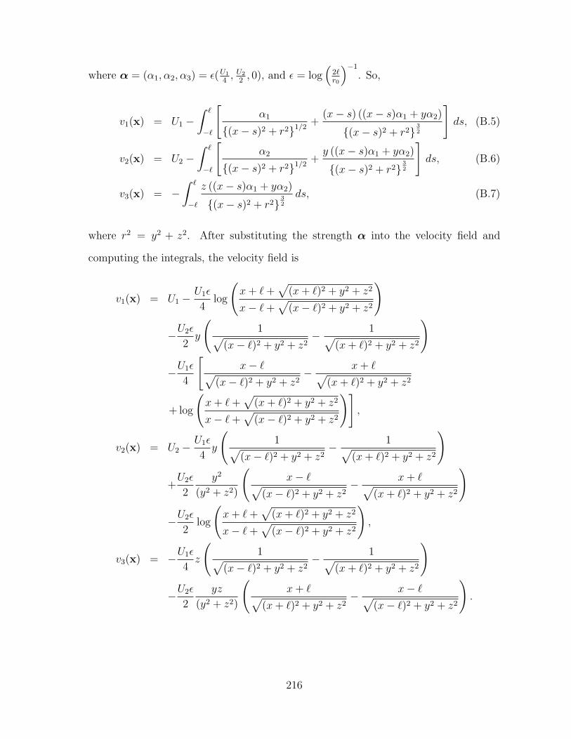
where α = (α1, α2, α3) = ε(U1

4, U2

2, 0), and ε = log

(2`r0

)−1

. So,

v1(x) = U1 −∫ `

−`

[α1

(x− s)2 + r21/2+

(x− s) ((x− s)α1 + yα2)

(x− s)2 + r232

]ds, (B.5)

v2(x) = U2 −∫ `

−`

[α2

(x− s)2 + r21/2+y ((x− s)α1 + yα2)

(x− s)2 + r232

]ds, (B.6)

v3(x) = −∫ `

−`

z ((x− s)α1 + yα2)

(x− s)2 + r232

ds, (B.7)

where r2 = y2 + z2. After substituting the strength α into the velocity field and

computing the integrals, the velocity field is

v1(x) = U1 −U1ε

4log

(x+ `+

√(x+ `)2 + y2 + z2

x− `+√

(x− `)2 + y2 + z2

)

−U2ε

2y

(1√

(x− `)2 + y2 + z2− 1√

(x+ `)2 + y2 + z2

)

−U1ε

4

[x− `√

(x− `)2 + y2 + z2− x+ `√

(x+ `)2 + y2 + z2

+ log

(x+ `+

√(x+ `)2 + y2 + z2

x− `+√

(x− `)2 + y2 + z2

)],

v2(x) = U2 −U1ε

4y

(1√

(x− `)2 + y2 + z2− 1√

(x+ `)2 + y2 + z2

)

+U2ε

2

y2

(y2 + z2)

(x− `√

(x− `)2 + y2 + z2− x+ `√

(x+ `)2 + y2 + z2

)

−U2ε

2log

(x+ `+

√(x+ `)2 + y2 + z2

x− `+√

(x− `)2 + y2 + z2

),

v3(x) = −U1ε

4z

(1√

(x− `)2 + y2 + z2− 1√

(x+ `)2 + y2 + z2

)

−U2ε

2

yz

(y2 + z2)

(x+ `√

(x+ `)2 + y2 + z2− x− `√

(x− `)2 + y2 + z2

).

216

B.1.3 Error analysis with uniform background flow

To compare the velocity fairly, we set the semimajor axis of the spheroid and the

half body length of the slender body ` be the unit, and the semiminor axis of the

spheroid and the radius of the slender body be r0. Then, from the slender body theory

ε = log(

2r0

)−1

. Since we are especially interested in the uniform flow perpendicular

to the centerline of the body, the uniform flow is U2ey. The error of the velocity with

background flow in the other direction can be obtained similarly. The absolute error is

computed by subtracting the exact velocity (B.2)-(B.4) by the slender body approxi-

mation (B.5)- (B.7). The leading order of the absolute error due to approximating the

spheroid with a slender body is

U2ε2

4

y2

(1√

(x+1)2+y2+z2− 1√

(x−1)2+y2+z2

)y2

y2+z2

(1−x√

(x−1)2+y2+z2+ 1+x√

(x+1)2+y2+z2

)+ log

(x+1+√

(x+1)2+y2+z2

x−1+√

(x−1)2+y2+z2

)yz

(y2+z2)

(x−1√

(x−1)2+y2+z2− x+1√

(x+1)2+y2+z2

)

In summary, when a uniform flow U2ey past a spheroid x2

`2+ y2+z2

r20

= 1 compare the

flow past a slender body along the x-axis with ` = 1 and radius r0, the leading order

of the absolute error is ε2 for all the components. The relative error of the velocity is

trivial because of the background flow. It is the same order as the absolute error. The

relative error of the induced velocity is in the order of ε, which verifies that the velocity

field of the slender body theory is asymptotic to the exact velocity field as ε→ 0.

To approximate the spheroid with a slender body, the slender body result can be

improved if the slenderness ε = 1log( 2`

r)− 1

2

, which is the limit observed from the strength

217

of the Stokeslet for the spheroid. Then, the error is in higher order

err1 =U2yr

2

1 + 2 log(

2r

) x

(y2 + z2)

[1 + x√

(x+ 1)2 + y2 + z2+

1− x√(x− 1)2 + y2 + z2

]

−1 + 3 log

(2r

)1 + 2 log

(2r

) [ 1√(x− 1)2 + y2 + z2

− 1√(x+ 1)2 + y2 + z2

]

+1

2

[1 + x

((x+ 1)2 + y2 + z2)32

− 1− x((x− 1)2 + y2 + z2)

32

],

err2 =U2r

2(1 + 2 log

(2r

)) − y2

2 (y2 + z2)

[(−1 + x)2

((x− 1)2 + y2 + z2)32

+(1 + x)2

((x+ 1)2 + y2 + z2)32

− x√(x− 1)2 + y2 + z2

+x√

(x+ 1)2 + y2 + z2

− 1

1 + 2 log(

2r

) ( 1− x√(x− 1)2 + y2 + z2

+1 + x√

(x+ 1)2 + y2 + z2

)]

+y2

(y2 + z2)2

[1− x2 + x3 + x (−1 + y2 + z2)√

(x− 1)2 + y2 + z2

−−1 + x2 + x3 + x (−1 + y2 + z2)√(x+ 1)2 + y2 + z2

]−

1

2

((1 + x)

√(x− 1)2 + y2 + z2

y2 + z2−

(−1 + x)√

(x+ 1)2 + y2 + z2

y2 + z2

− log

[1 + x+

√(x+ 1)2 + y2 + z2

−1 + x+√

(x− 1)2 + y2 + z2

])+

1

2(1 + 2 log

(2r

)) [( 1√(x+ 1)2 + y2 + z2

+1√

(x− 1)2 + y2 + z2

)(

1 + 2 log

(2

r

))− 2 log

(2

r

)log

[1 + x+

√(x+ 1)2 + y2 + z2

−1 + x+√

(x− 1)2 + y2 + z2

]],

218

err3 =U2yz

2 (y2 + z2)2

r2(1 + 2 log

(2r

)) (y2 + z2)

[x

(1√

1− 2x+ x2 + y2 + z2− 1√

1 + 2x+ x2 + y2 + z2

)

− (x+ 1)2

((x+ 1)2 + y2 + z2)32

− (x− 1)2

((x− 1)2 + y2 + z2)32

+1(

1 + 2 log(

2r

)) ( 1− x√(x− 1)2 + y2 + z2

+1 + x√

(x+ 1)2 + y2 + z2

)]

+2

[(x− 1)2√

(x− 1)2 + y2 + z2+

(x+ 1)2√(x+ 1)2 + y2 + z2

]+2x

[√(x− 1)2 + y2 + z2 −

√(x+ 1)2 + y2 + z2

].

In these equations, we set ` = 1.

B.2 A spheroid or slender body sweeping out a dou-

ble cone

In this section, we document the velocity field of a prolate spheroid sweeping out

a double cone in free space and the flow induced by the cylindrical slender body. We

compare the velocity field of these two cases by taking the same length and radius of

the bodies as the previous section. In both cases, the flow is time independent in the

body frame, where the body is stationary and the background can be decomposed as

several simple linear shear. For linear shear flows past a prolate spheroid, the exact

solution has been obtained based on the exact solution [19]. Applying their results, we

provide the velocity field consistent with the notation in [48].

In the lab frame, the prolate spheroid or the slender body sweeps a cone with angular

velocity (0, 0, ω) and the background flow is at rest. The cone angle κ is defined from

219

the axis of the cone to the centerline of the body. In the body frame, we assume the

spheroid and the cylindrical slender body is along the x-axis. For the spheroid,

x2

`2+y2 + z2

r20

= 1.

So, the half foci length c =√`2 − r2

0 = e`. For the slender body, y2 + z2 = r20 when

−` ≤ x ≤ `.

In this body frame, we distribute the singularity along the x-axis. For the spheroid,

the singularities are distributed between two foci. For the slender body, Stokeslets are

linearly distributed between two ends x = −` and `. From the lab frame xL to the

body frame x,

x = RTκR

TωxL,

where

Rω =

cos(ωt) − sin(ωt) 0

sin(ωt) cos(ωt) 0

0 0 1

and Rκ =

sin(κ) 0 − cos(κ)

0 1 0

cos(κ) 0 sin(κ)

.

The relation of the velocity between the lab frame uL(xL) and the velocity in the body

frame u(x) can be derived from the transformation of the frames. The velocity field in

the lab frame is

uL(xL) =dxLdt

=d(RωRκx)

dt= RωRκx +RωRκ

dx

dt

= RωRκx +RωRκu(x) = RωRTωxL +RωRκu(RT

κRTωxL).

220

Similarly,

u(x) =dx

dt= RT

κ RTωxL +RT

κRTωuL(xL) = RT

κ RTωRωRκx +RT

κRTωuL(RωRκx).

If the background flow is at rest in the lab frame,

U0(x) = RTκ R

TωRωRκx = ω

y sin(κ)

z cos(κ)− x sin(κ)

−y cos(κ)

(B.8)

is the background flow in the body frame.

After obtaining the velocity in the body frame, we compare the velocity field in the

body frame directly. The error in the lab frame will be the same order by changing

frames.

B.2.1 A spheroid sweeps out a double cone

When a spheroid sweeping out a double cone in free space, from the exact solution

for shear flow past a prolate spheroid in [19], the exact solution [48] the solution of

potential flow past a prolate spheroid based on the singularity method, is constructed

by employing a line distribution of stresslet, rotlet, and potential doublets between the

foci −c and c given by

u(x) = U0(x) + ω sin(κ)

(∫ c

−c

(c2 − ξ2

)(αuSS (x− ξ; ex, ey) + γ1uR (x− ξ, ez))dξ

+β

∫ c

−c

(c2 − ξ2

)2∂yuD (x− ξ; ex) dξ

)+

ωγ2 cos(κ)

∫ c

−c

(c2 − ξ2

)uR (x− ξ; ex) dξ,

221

where

α =e2

−2e+ (1 + e2)Le, β =

1− e2

4 (−2e+ (1 + e2)Le),

γ1 =2− e2

−2e+ (1 + e2)Le, γ2 =

1− e2

2e− (1− e2)Le.

In detail, the velocity field is

u1(x) = ωy sin(κ) + ω sin(κ)

[∫ c

−c

(c2 − ξ2

)(3αy(x− ξ)2

R5− γ1y

R3

)dξ

+β

∫ c

−c

(c2 − ξ2

)2(− 3y

R5− 15y(x− ξ)2

R7

)dξ

](B.9)

= ωy sin(κ) + ω sin(κ)y(3α I1 − γ1 I2 − 3β I3 − 15β I4),

u2(x) = −ωx sin(κ) + ωz cos(κ) +

ω sin(κ)

(∫ c

−c

(c2 − ξ2

)(3α(x− ξ)y2

R5+γ1(x− ξ)

R3

)dξ

+β

∫ c

−c

(c2 − ξ2

)2(−15y2(x− ξ)

R7+

3(x− ξ)R5

)dξ

)(B.10)

+ωγ2 cos(κ)

∫ c

−c

(c2 − ξ2) z

R3dξ

= −ωx sin(κ) + ωz cos(κ) +

ω sin(κ)(3αy2 I5 + γ1 I7 − 15y2β I6 + 3β I8) + ωγ2 cos(κ)z I2,

u3(x) = −ωy cos(κ) + ωγ2 cos(κ)

∫ c

−c

(c2 − ξ2) y

R3dξ (B.11)

+ω sin(κ)

(∫ c

−c

(c2 − ξ2

) 3α(x− ξ)yzR5

dξ − β∫ c

−c

(c2 − ξ2

)2 15yz(x− ξ)R7

dξ

)= −ωy cos(κ) + ω sin(κ)(3αyz I5 − 15βyz I6) + ω cos(κ)γ2y I2,

222

where

I1 =

∫ c

−c

(c2 − ξ2) (x− ξ)2

R5dξ, I2 =

∫ c

−c

(c2 − ξ2)

R3dξ,

I3 =

∫ c

−c

(c2 − ξ2)2

R5dξ, I4 =

∫ c

−c

(c2 − ξ2)2

(x− ξ)2

R7dξ,

I5 =

∫ c

−c

(c2 − ξ2

) (x− ξ)R5

dξ, I6 =

∫ c

−c

(c2 − ξ2

)2 (x− ξ)R7

dξ,

I7 =

∫ c

−c

(c2 − ξ2) (x− ξ)R3

dξ, I8 =

∫ c

−c

(c2 − ξ2

)2 (x− ξ)R5

dξ,

and R2 = (x− ξ)2 + y2 + z2.

For each of these integrals, we integrate explicitly as the following equations.

I1 = − x+ c

3 ((x− c)2 + y2 + z2)1/2− (x+ c)(x− c)2 − 2(2c+ x) (y2 + z2)

3 (y2 + z2)√

(x− c)2 + y2 + z2

+x− c

3 ((x+ c)2 + y2 + z2)12

− (x− c)(x+ c)2 + 2(2c− x) (y2 + z2)

3 (y2 + z2)√

(x+ c)2 + y2 + z2

− log

(c+ x+

√(x+ c)2 + y2 + z2

−c+ x+√

(x− c)2 + y2 + z2

).

I2 =(x+ c)

√(x− c)2 + y2 + z2

(y2 + z2)−

(x− c)√

(x+ c)2 + y2 + z2

(y2 + z2)

− log

(c+ x+

√(x+ c)2 + y2 + z2

−c+ x+√

(x− c)2 + y2 + z2

).

223

I3 = − 1

3 (y2 + z2)2

√(c− x)2 + y2 + z2

[2(x+ c)2(x− c) + (5x+ 3c)

(y2 + z2

)]+√

(x+ c)2 + y2 + z2[−2(x− c)2(x+ c)− (5x− 3c)

(y2 + z2

)]+ log

(c+ x+

√(x+ c)2 + y2 + z2

−c+ x+√

(x− c)2 + y2 + z2

).

I4 =1

15

(2(c− x)3(x+ c)2

(y2 + z2)2√

(c− x)2 + y2 + z2+

2(c− x)2(c+ x)3

(y2 + z2)2√

(x+ c)2 + y2 + z2

−5c3 − 7c2x+ c (−17x2 + 15 (y2 + z2)) + x (19x2 + 17 (y2 + z2))

(y2 + z2)√

(c− x)2 + y2 + z2

−5c3 + 7c2x+ c (−17x2 + 15 (y2 + z2))− x (19x2 + 17 (y2 + z2))

(y2 + z2)√

(x+ c)2 + y2 + z2

)

+ log

(c+ x+

√(x+ c)2 + y2 + z2

−c+ x+√

(x− c)2 + y2 + z2

).

I5 = − 2 (−cx+ x2 + y2 + z2)

3 (y2 + z2)√

(x− c)2 + y2 + z2+

2 (cx+ x2 + y2 + z2)

3 (y2 + z2)√

(x+ c)2 + y2 + z2.

I6 =8(

15 (y2 + z2)2 ((c− x)2 + y2 + z2) ((x+ c)2 + y2 + z2))(√

(c− x)2 + y2 + z2 −√

(x+ c)2 + y2 + z2)

(c4x2 +

(x2 + y2 + z2

)3+ c2

(−2x4 − x2

(y2 + z2

)+(y2 + z2

)2))

+cx(c4 − 2c2x2 +

(x2 + y2 + z2

)2)

(√(c− x)2 + y2 + z2 +

√(x+ c)2 + y2 + z2

).

I7 = 2√

(x− c)2 + y2 + z2 − 2√

(x+ c)2 + y2 + z2

+2x log

(c+ x+

√(x+ c)2 + y2 + z2

−c+ x+√

(x− c)2 + y2 + z2

).

224

I8 =4√

(x+ c)2 + y2 + z2 (cx− x2 + 2 (y2 + z2))

3 (y2 + z2)+

4√

(c− x)2 + y2 + z2 (cx+ x2 − 2 (y2 + z2))

3 (y2 + z2)

−4 log

(c+ x+

√(x+ c)2 + y2 + z2

−c+ x+√

(x− c)2 + y2 + z2

).

When r2 = y2 + z2 = 0, the above formulae are not valid. However, these integrals

reduce to even simpler cases, which can be integrated easily.

B.2.2 A slender body sweeps out a double cone

When the body is tilted in the x-z plane and sweeps a double cone with the cone

angle κ, the velocity in the body frame is constructed by distribution of Stokeslet along

the centerline of the body. In the body frame, the body is along the x-axis (−` ≤ x ≤ `).

The strength of the Stokeslet is a linear function of the arc-length α = εω sin(κ)2

(0, s, 0).

225

The velocity field in detail is

v1(x) = ωy sin(κ) +

∫ `

−`

(x− ξ) yα2ξ(x− ξ)2 + r2

32

dξ

= ωy sin(κ) +ε ω sin(κ)y

2

[`√

(x+ `)2 + r2+

`√(x− `)2 + r2

(B.12)

− log

(x+ `+

√(x+ `)2 + r2

x− `+√

(x− `)2 + r2

)],

v2(x) = ωz cos(κ)− ωx sin(κ) +

∫ `

−`

α2ξ√(x− ξ)2 + r2

dξ +

∫ `

−`

x22α2ξ

(x− ξ)2 + r2 3

2

dξ

= ωz cos(κ)− ωx sin(κ) +εω sin(κ)y2

2r2

((x+ `)x+ r2√

(x+ `)2 + r2− (x− `)x+ r2√

(x− `)2 + r2

)

+εω sin(κ)

2

[−√

(x+ `)2 + r2 +√

(x− `)2 + r2 (B.13)

+x log

(x+ `+

√(x+ `)2 + r2

x− `+√

(x− `)2 + r2

)],

v3(x) = −ωy cos(κ) +

∫ `

−`

zyα2ξ(x− ξ)2 + r2

32

dξ (B.14)

= −ωy cos(κ) +εω sin(κ)yz

2r2

((x+ `)x+ r2√

(x+ `)2 + r2− (x− `)x+ r2√

(x− `)2 + r2

),

where r2 = y2 + z2.

B.2.3 Error in the velocity field of the slender body theory

Since the relation from the body frame to the lab frame holds for both the spheroid

and the slender body, to analysis the error by approximating the spheroid with the

slender body, we compare the velocity field in the body frame. Similar to the velocity

field, the error in the lab frame can be obtained by the transformation of the error in

the body frame. In the body frame, the velocity field for the background flow (B.8)

226

past a prolate spheroid

x2

`2+y2 + z2

r20

= 1

is u(x) in (B.9)-(B.11). The velocity field for the flow past a cylindrical slender body

y2 + z2

r20

= 1 (−` ≤ x ≤ `)

is v(x) in (B.12)-(B.14). (From the above equations of bodies, the major axis of

spheroid or the axis of the slender body is along the x-axis in the body frame.) Since

the velocity field u(x) for the spheroid is exact Stokes solution. If we approximate the

body with a slender body, the error due to the slender body is the velocity difference

u(x) − v(x), which can be computed explicitly from (B.9)-(B.11) and (B.12)-(B.14).

The leading order of the difference, the error from the slender body theory, is

erru1 = −yε2ω sin(κ)

4

− 1√

(x− 1)2 + y2 + z2− 1√

(x+ 1)2 + y2 + z2

+ log

(1 + x+

√(x+ 1)2 + y2 + z2

−1 + x+√

(x− 1)2 + y2 + z2

),

erru2 =ε2ω sin(κ)

−4 (y2 + z2)

(x(y2 + 2z2)

(1√

(x− 1)2 + y2 + z2+

1√(x+ 1)2 + y2 + z2

)

+(y2 + z2 +(x2 + y2 + z2

)z2)

(1√

(x+ 1)2 + y2 + z2− 1√

(x− 1)2 + y2 + z2

)

−x(y2 + z2

)log

(1 + x+

√(x+ 1)2 + y2 + z2

−1 + x+√

(x− 1)2 + y2 + z2

)),

erru3 =ε2ω sin(κ)yz

4(y2 + z2)√

(x− 1)2 + y2 + z2√

(x+ 1)2 + y2 + z2

((x2 + y2 + z2 + x)√

(x− 1)2 + y2 + z2 − (x2 + y2 + z2 − x)√

(x+ 1)2 + y2 + z2).

227

From the above error analysis, the error of the slender body theory is in the order of

O(ε2). In the body frame, the background flow is not zero, which makes the asymptotics

always hold. To the verify the velocity induced by the slender body is asymptotic to the

exact solution, we check the induced velocity of the body by subtracting the background

flow in the velocity formulae. When the background flow is subtracted, the induced

velocities for both case decay zero as ε→ 0. And the leading order of the relative error

of the induced velocity is in the order of O(ε), which confirms that the slender body

theory result is a valid asymptotic solution.

Similar to the uniform flow, we observe that with the slenderness ε = 1log( 2`

r)− 1

2

the

asymptotic solution is improved. With ε = 1log( 2`

r)− 1

2

in the slender body result and

228

` = 1, the error in the velocity field is

err1 =yω sin(κ)r2

8

−4

(y2 + z2)(1− 2 log

(2r

))(1− x√

(x− 1)2 + y2 + z2+

1 + x√(x+ 1)2 + y2 + z2

)

+4(1− 3 log

(2r

))(1− 2 log

(2r

))2

[(1 + x)

√(x− 1)2 + y2 + z2

y2 + z2+

(1− x)√

(x+ 1)2 + y2 + z2

y2 + z2

− log

(1 + x+

√(x+ 1)2 + y2 + z2

−1 + x+√

(x− 1)2 + y2 + z2

)]+

1

(1− 2 log(

2r

)) (y2 + z2)2[(√

(x+ 1)2 + y2 + z2 +√

(x− 1)2 + y2 + z2) (

2− 2x2 − 3y2 − 3z2)

+(√

(x+ 1)2 + y2 + z2 −√

(x− 1)2 + y2 + z2)x(2x2 + 5y2 + 5z2 − 2

)]+

3

1− 2 log(

2r

) log

(1 + x+

√(x+ 1)2 + y2 + z2

−1 + x+√

(x− 1)2 + y2 + z2

)− 1

(y2 + z2)2 (1− 2 log(

2r

))[(1√

(x+ 1)2 + y2 + z2− 1√

(x− 1)2 + y2 + z2

)(−2x5 + x3

(4− 19y2 − 19z2

)− x

(2 + 17y4 − 7z2 + 17z4 + y2

(−7 + 34z2

)))+

(1√

(x+ 1)2 + y2 + z2+

1√(x− 1)2 + y2 + z2

)(−2− 2x4 + 15y4 + 5z2 + 15z4 + x2

(4− 17y2 − 17z2

)+ 5y2

(1 + 6z2

))−15

(y2 + z2

)2log

(1 + x+

√(x+ 1)2 + y2 + z2

−1 + x+√

(x− 1)2 + y2 + z2

)]+

2

(y2 + z2) ((x− 1)2 + y2 + z2)3/2 ((x+ 1)2 + y2 + z2)3/2 (1− 2 log(

2r

))2[2(1− 2 log(

2

r))(

(1 + x)3((x− 1)2 + y2 + z2)32 + (1− x)3((x+ 1)2 + y2 + z2)

32

)+((x− 1)2 + y2 + z2

) ((x+ 1)2 + y2 + z2

)(−2 + 2 log

(2

r

))(x(−1 + x2 + y2 + z2

) (√(x− 1)2 + y2 + z2 −

√(x+ 1)2 + y2 + z2

)+(−1 + x2 − 3y2 − 3z2

) (√(x− 1)2 + y2 + z2 +

√(x+ 1)2 + y2 + z2

)229

+3(y2 + z2

)√(x− 1)2 + y2 + z2

√(x+ 1)2 + y2 + z2

log

(1 + x+

√(x+ 1)2 + y2 + z2

−1 + x+√

(x− 1)2 + y2 + z2

))],

230

err2 =r2

2ω

cos(κ)

[(1 + x)

√(x− 1)2 + y2 + z2

y2 + z2+

(1− x)√

(x+ 1)2 + y2 + z2

y2 + z2

− log

(x+ 1 +

√(x+ 1)2 + y2 + z2

x− 1 +√

(x− 1)2 + y2 + z2

)]

+

[y2

y2 + z2

(−1

1− 2 log(

2r

) (3(−1 + x) (−x+ x2 + y2 + z2)

((x− 1)2 + y2 + z2)3/2

+2 (−x+ x2 + y2 + z2)√

(x− 1)2 + y2 + z2+

3(1 + x) (x+ x2 + y2 + z2)

((x+ 1)2 + y2 + z2)3/2− 2 (x+ x2 + y2 + z2)√

(x+ 1)2 + y2 + z2

+−6x2 − 3x3 − 2 (y2 + z2)− 3x (1 + y2 + z2)

((x+ 1)2 + y2 + z2)3/2

+6x2 − 3x3 + 2 (y2 + z2)− 3x (1 + y2 + z2)

((x− 1)2 + y2 + z2)3/2

)

+2 log

(2r

)(1− 2 log

(2r

))2

((x2 + y2 + z2 + x)√(x+ 1)2 + y2 + z2

− (x2 + y2 + z2 − x)√(x− 1)2 + y2 + z2

))

+2y2

(y2 + z2)2 (−1 + 2 log(

2r

))(x3 + x4 + x (−1 + y2 + z2) + (y2 + z2)

2+ x2 (−1 + 2y2 + 2z2)

)√

(x+ 1)2 + y2 + z2

−

(−x3 + x4 − x (−1 + y2 + z2) + (y2 + z2)

2+ x2 (−1 + 2y2 + 2z2)

)√

(x− 1)2 + y2 + z2

+

1

1− 2 log(

2r

) ( 1√(x− 1)2 + y2 + z2

− 1√(x+ 1)2 + y2 + z2

)

+−2 + 6 log

(2r

)(1− 2 log

(2r

))2

(√(x− 1)2 + y2 + z2 −

√(x+ 1)2 + y2 + z2

+x log

(x+ 1 +

√(x+ 1)2 + y2 + z2

x− 1 +√

(x− 1)2 + y2 + z2

))− 1

(y2 + z2)(1− 2 log(2

r)) ((x2 − 2

(y2 + z2

)+ x)√

(x− 1)2 + y2 + z2

−(x2 − 2

(y2 + z2

)− x)√

(x+ 1)2 + y2 + z2

−3x(y2 + z2

)log

(x+ 1 +

√(x+ 1)2 + y2 + z2

x− 1 +√

(x− 1)2 + y2 + z2

))]sin(κ)

,

231

err3 =yzωr2

2

cos(κ)

[(1 + x)

√(x− 1)2 + y2 + z2

y2 + z2−

(−1 + x)√

(x+ 1)2 + y2 + z2

y2 + z2

− log

(x+ 1 +

√(x+ 1)2 + y2 + z2

x− 1 +√

(x− 1)2 + y2 + z2

)]+[((

y2 + z2) (((

y2 + z2 + 2(x4 + (y2 + z2)2 + x2(3 + 2y2 + 2z2)))

(((x+ 1)2 + y2 + z2)

32 − ((x− 1)2 + y2 + z2)

32

)−2(3x3 + x(1 + 3y2 + 3z2)

) (((x+ 1)2 + y2 + z2)

32 + ((x− 1)2 + y2 + z2)

32

))(−1 + 2 log

(2

r

))/((

(x− 1)2 + y2 + z2)3/2 (

(x+ 1)2 + y2 + z2)3/2)

+

(− −x+ x2 + y2 + z2√

(x− 1)2 + y2 + z2+

x+ x2 + y2 + z2√(x+ 1)2 + y2 + z2

)2 log

(2

r

))−2((x6 +

(y2 + z2

)2 (1 + y2 + z2

)+ x4

(−2 + 3y2 + 3z2

)+x2

(−1− 3y4 + z2 − 3z4 + y2

(1− 6z2

)))(√

(x− 1)2 + y2 + z2 −√

(x+ 1)2 + y2 + z2)

+(x(

1 + x4 + 2x2(−1 + y2 + z2

)+(y2 + z2

)2))

(√(x− 1)2 + y2 + z2 +

√(x+ 1)2 + y2 + z2

)) (−1 + 2 log

(2

r

))/((

(x− 1)2 + y2 + z2) (

(x+ 1)2 + y2 + z2)))] sin(κ)(

(y2 + z2)2 (1− 2 log(

2r

))2) .

Figure B.1-B.4 are comparisons of the fluid particle trajectories from flows induced

by a spheroid with a slender body in the laboratory frame. In these figures, the black

trajectories are from the exact Stokes solution in the flow generated by a spheroid; the

red trajectories are from the asymptotic solution by approximating the spheroid with

a cylindrical slender body with the slenderness ε = 1log( 2`

r)− 1

2

; the purple trajectories are

from the asymptotic solution with ε = 1log( 2`

r). The half length of the slender body `

equals to the semimajor axis of the spheroid a = 1 and the radius of the slender body r

equals to the semiminor axis of the spheroid b, i.e., the spheroid inscribes in the slender

232

body. The comparison is made for different radius of the slender body by varying the

eccentricity e =√

1− b2/a2.

Figure B.1 shows trajectories with an initial location (−0.46, 0, 0.4) with eccentricity

e = 0.995, 0.9995 and 0.99995. Only side view of Figure C.1b is provided here, since

the top view is the better view of the comparison. From this group of plots, we find

trajectories with the slenderness ε = 1log( 2`

r)− 1

2

in the asymptotic solution converges well

to the exact solution. Figure B.2 shows the comparison of the exact solution to the

asymptotic solution with ε = 1log( 2`

r)− 1

2

with e = 0.9995.

Figure B.3 shows trajectories starting from a different initial location (−0.7, 0, 0.4)

with eccentricity e = 0.995, 0.9995 and 0.99995. Only top view of these trajectories

are plotted here. Similarly to the previous plots, the black trajectories are from the

exact spheroid solution and the red trajectories are from the asymptotic solution with

ε = 1log( 2`

r)− 1

2

. These trajectories are consistent with the conclusion that the velocity

with the slender body theory for a slender body is asymptotic to the exact solution of

a spheroid when the slenderness ε→ 0.

Finally, Figure B.4 shows the comparison of fluid particle trajectories in the free

space with initial position selected in the straight rod above a no-slip plane experiment

shown in Figure 6.8.

When a = 1, for these eccentricities e = 0.995, 0.9995, 0.99995, the semiminor axis

b is 0.1, 0.032, and 0.01, respectively. The corresponding slenderness ε = log−1(2`r

) is

0.33, 0.24, 0.19. The slenderness ε = 1log( `

r)− 1

2

is 0.40, 0.27,0.21.

233

(a) Top view (e = 0.995) (b) Top view (e = 0.9995)

(c) Top view (e = 0.99995) (d) Side view of (b) (e = 0.9995)

Figure B.1: Fluid particle trajectories from initial position x = −0.46, y = 0, andz = 0.4 . The black trajectories are the exact solution for the spheroid case, the purpletrajectories are the slender body result with the slenderness ε = 1

log( 2`r

), and the red

trajectories are with ε = 1log( 2`

r)− 1

2

. The spheroid is inscribed in the cylindrical slender

body. e is the eccentricity of the prolate spheroid.

234

(a) Top view (e = 0.9995) (b) Side view (e = 0.9995)

Figure B.2: Compare the exact fluid particle trajectories (black) with the slender bodyapproximation (red) with ε = 1

log( 2`r

). The initial position of trajectories is x = −0.46,

y = 0, and z = 0.4 .

(a) Top view (e = 0.995) (b) Top view (e = 0.9995) (c) Top view (e = 0.99995)

Figure B.3: Similar to Figure B.2, but with the initial position x = −0.7, y = 0, andz = 0.4 .

235

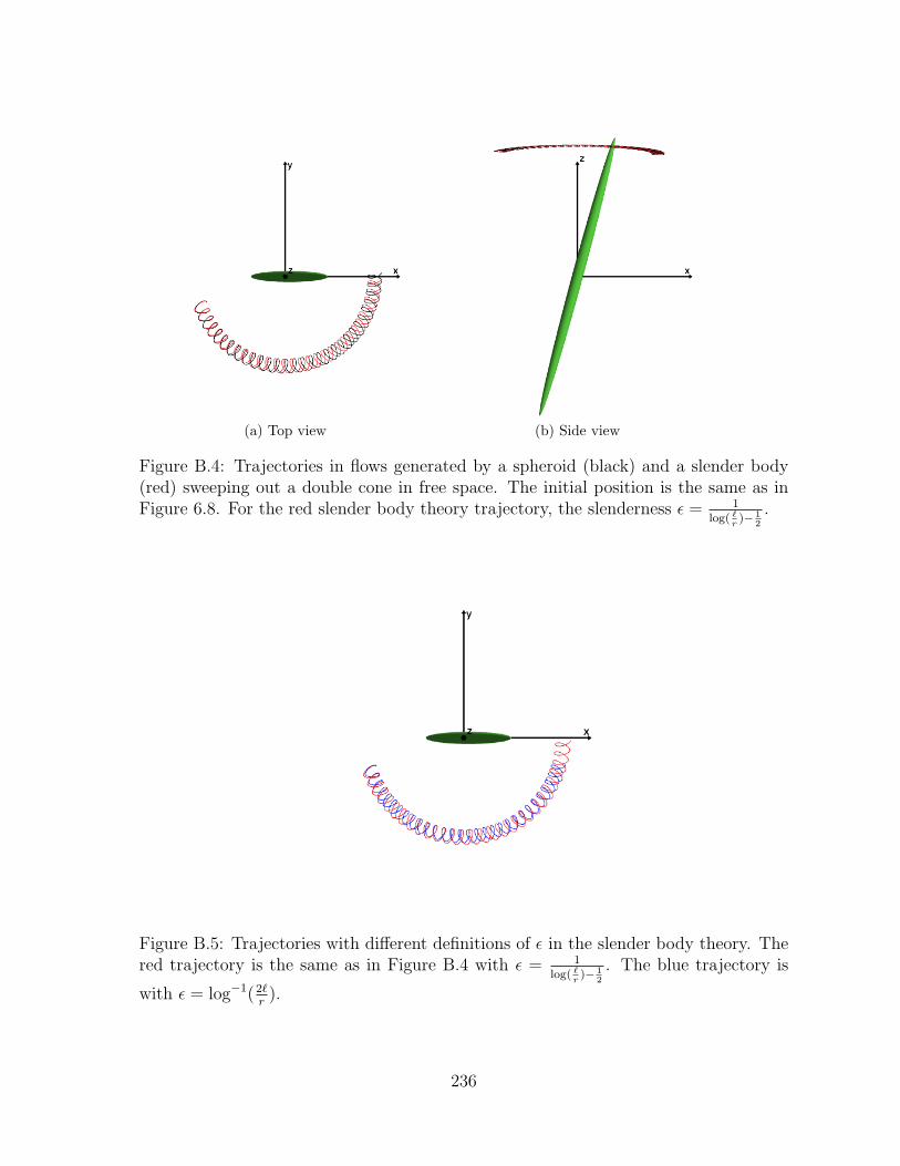
(a) Top view (b) Side view

Figure B.4: Trajectories in flows generated by a spheroid (black) and a slender body(red) sweeping out a double cone in free space. The initial position is the same as inFigure 6.8. For the red slender body theory trajectory, the slenderness ε = 1

log( `r

)− 12

.

Figure B.5: Trajectories with different definitions of ε in the slender body theory. Thered trajectory is the same as in Figure B.4 with ε = 1

log( `r

)− 12

. The blue trajectory is

with ε = log−1(2`r

).

236

Appendix C

Higher order asymptotic solutions

for flows past a spheroid

For linear flow past a spheroid in free space, there are exact solutions available [36,

19, 41]. With the slender body theory, asymptotic solutions can be found when using

a cylindrical slender body to approximate the spheroid. The leading order asymptotic

solutions have been studied well with analytical error in O(ε2) [21, 3, 48] , where ε is the

slenderness parameter. The error analysis are documented in Appendix B for uniform

flow past a spheroid and improved slender body results for a slender rod sweeping out

a double cone in free space. For a slender body approximating the spheroid, we provide

the leading order slender body results and the higher order results for several basic flows

in this appendix. The spheroid is inscribed to the cylindrical slender body. The major

axis of the spheroid 2a equals the length of the slender body 2`, and the semi-minor

axis of the spheroid b equals to the cross-sectional radius of the slender body r.

If the exact solution has been reported in this thesis before, we concisely document

the slender body results for both leading order approximation or higher order results.

Beside the asymptotic solutions, we derive the exact solution for the spheroid for the

spheroid sweeping a single cone.

237

C.1 Uniform background flow

When a uniform flow U1ex +U2ey past a prolate spheroid, the flow is approximated

with the uniform flow past a cylindrical slender body. Assuming the slender body along

the x- axis from x = −` to x = `, the asymptotic velocity field is

u(x) = U1ex + U2ey −∫ `

−`(US (x− ξ;α1ex) + US (x− ξ;α2ey)) dξ, (C.1)

where x− ξ = (x− ξ, y, z).

From the canonical slender body theory, the constants in the strength of the Stokeslet

are

α1 =U1

4

1

log(

2`r

)and α2 =

U2

2

1

log(

2`r

)for the leading order asymptotic solution. The error for the velocity is O(ε2), where

ε = 1log( 2`

r)

is the slenderness parameter.

Comparing with the exact solution for the uniform flow past a spheroid (B.1), we

find that the asymptotic velocity is accurate to O((

r`

)2)

with the following modified

constants

α1 =U1

4

1

log(

2`r

)− 1

2

,

α2 =U2

2

1

log(

2`r

)+ 1

2

.

Notice the difference between the tangential direction and the normal direction.

238

C.2 Linear shear flow past a slender body

Similar to the uniform flow, when shear flow Ωxey past a spheroid along the x-axis

(−` ≤ x ≤ `), the asymptotic velocity field is

u(x) = Ωxey −∫ `

−`US(x− ξ;α2ξey)dξ, (C.2)

where x − ξ = (x − ξ, y, z). We use a cylindrical slender body to approximate the

spheroid. The velocity is obtained with linear distributed Stokeslet along the center-

line.

From the slender body theory, the leading order asymptotic solution with

α2 =Ωε

2=

Ω

2

1

log(

2`r

) .With

α2 =Ω

4

1

log(

2`r

)− 1

2

,

the asymptotic velocity is accurate to O((

r`

)2)

.

C.3 Shear flow Ωzex past an upright spheroid above

the x-y plane

For shear flow Ωzex past an upright spheroid above the x-y plane, we approximate

the flow with the shear flow past a slender body. Then, the slender body is to approx-

imate the spheroid x2+y2

b2+ (z−a)2

a2 = 1 or x2+y2

r2 + (z−`)2

`2= 1. The exact solution for the

spheroid can be attained from (B.1) and (3.1) by moving the origin to the center of the

spheroid.

Based on the slender body theory, the velocity of shear flow Ωzex past a slender

239

body by employing a linear distribution of Stokeslets between the centerline of the

slender body z = 0 and 2` is given by (the length of the body is 2`)

u(x) = Ωzex −∫ 2`

0

US(x− ξ;α1ξex)dξ, (C.3)

where x− ξ = (x, y, z − ξ) and α1 = Ωε2

= Ω

2 log( 2`r )

for the leading order solution.

Since the background flow is not symmetric with respect to the center of the

spheroid, we decompose the background flow into a shear flow plus a uniform flow

to achieve the higher order asymptotic solution. Then, both flows are symmetric with

respect to the center of the body.

The higher order velocity field is

u(x) = Ωzex +

∫ 2`

0

US(x− ξ; (β1 − α1) ex)dξ −∫ 2`

0

US(x− ξ; β1ξex)dξ, (C.4)

where x− ξ = (x, y, z − ξ), α1 = Ω`

2(log( 2`d )+ 1

2)and β1 = Ω

2(log( 2`d )− 1

2).

C.4 A prolate spheroid sweeping a single cone in

free space

When a spheroid or a slender body sweeps out a single cone above the x-y plane in

free space, we derive the exact solution for the spheroid and asymptotic solutions for

the slender body in the body frame. There are two body frames. In one body frame

xb = (xb, yb, zb), the body is titled in the x-z plane and the cone is above the x-y plane.

Such a body frame is convenient when we add the no-slip boundary on the x-y plane.

In this frame, the slender body is an approximation of the titled spheroid above the

240

x-y plane

(xb sin(κ) + zb cos(κ)− a)2

a2+

(−xb cos(κ) + zb sin(κ))2

b2= 1 (C.5)

or (xb sin(κ)+zb cos(κ)−L)2

`2+ (−xb cos(κ)+zb sin(κ))2

r2 = 1, where κ is the cone angle. The back-

ground in this titled spheroid body frame is (ωyb,−ωxb, 0), in which ω is the angular

velocity of the spheroid. The transformation between the body frame xb to the lab

frame xL is

xL = Rωxb, (C.6)

where Rω =

cos(ωt) − sin(ωt) 0

sin(ωt) cos(ωt) 0

0 0 1

. The leading order asymptotic solution is

given directly in this tilted spheroid body frame.

The other body frame is the general body frame where the spheroid and the slender

body are along the x-axis. The origin is the center of the rigid body. The transformation

between the tilted spheroid body xb and the general body frame x is

xb

yb

zb

=

sin(κ) 0 − cos(κ)

0 1 0

cos(κ) 0 sin(κ)

x+ `

y

z

.

From the background flow in the tilted spheroid body frame (ωyb,−ωxb, 0), the back-

ground flow in the general body frame is

U =

yω sin(κ)

−ω(−z cos(κ) + (`+ x) sin(κ))

−yω cos(κ)

. (C.7)

241

The higher order asymptotic solution is derived in the general body frame and trans-

formed into the tilted spheroid body frame. The exact solution for a spheroid is derived

in this general frame in the next section.

Employing a linear distribution of Stokeslets between the centerline of the slender

body (the length of the body is 2`), the leading order asymptotic solution is

u(x) = ybωex − ωxbey +

∫ 2`

0

US(xb − ξ;α2ξey)dξ, (C.8)

where xb − ξ = (xb − ξ sin(κ), yb, zb − ξ cos(κ)) and α2 = ω sin(κ)

2 log( 2`r ).

To get the higher order approximation, we first consider the flow in the general

body frame, where the background flow is

yω sin(κ)

−ω(−z cos(κ) + (`+ x) sin(κ))

−yω cos(κ)

. The

velocity field is

u(x) = ωy sin(κ)ex + ωz cos(κ)ey − ωy cos(κ)ez − ω` sin(κ)ey − ωx sin(κ)ey

+

∫ `

−`US (x− ξ;α1ey) dξ +

∫ `

−`US (x− ξ; β1ξey) dξ (C.9)

where x− ξ = (x− ξ, y, z) and

α1 =ω` sin(κ)

2(log(

2`r

)+ 1

2

) ,and

β1 =ω sin(κ)

2(log(

2`r

)− 1

2

) .Rewriting the higher order velocity field (C.9) in the tilted spheroid body frame,

242

we get

ub (xb) = ybωex − ωxbey +

∫ 2`

0

US(xb − s; (α1 − β1`) ey)ds+

∫ 2`

0

US(xb − s; β1ξey)ds,

(C.10)

where xb − s = (xb − s sin(κ), yb, zb − s cos(κ)).

In detail,

ub1 (xb) = ybω +

∫ 2`

0

(α1 − β1`) yb(xb − s sin(κ))

(xb − s sin(κ))2 + y2b + (zb − s cos(κ))2

32

ds

+

∫ 2`

0

β1ybs(xb − s sin(κ))

(xb − s sin(κ))2 + y2b + (zb − s cos(κ))2

32

ds,

ub2 (xb) = −xbω +

∫ 2`

0

(α1 − β1`

(xb − s sin(κ))2 + y2b + (zb − s cos(κ))2

12

+

(α1 − β1`) y2b

(xb − s sin(κ))2 + y2b + (zb − s cos(κ))2

32

)ds

+

∫ 2`

0

(β1s

(xb − s sin(κ))2 + y2b + (zb − s cos(κ))2

12

+β1y

2bs

(xb − s sin(κ))2 + y2b + (zb − s cos(κ))2

32

)ds,

ub3 (xb) =

∫ 2`

0

(α1 − β1`) yb(zb − s cos(κ))

(xb − s sin(κ))2 + y2b + (zb − s cos(κ))2

32

ds

+

∫ 2`

0

β1ybs(zb − s cos(κ))

(xb − s sin(κ))2 + y2b + (zb − s cos(κ))2

32

ds.

For the higher order asymptotic solution, the induced velocity is due to uniformly

distributed Stokeslet on the center-line with strength (0, (α1 − β1`) , 0) and linear dis-

tributed Stokeslet with strength (0, β1, 0).

243

C.5 Exact solution for the spheroid sweeping a sin-

gle cone

When a spheroid sweeps out a single upright cone above the x-y plane, the back-

ground flow in the tilted spheroid body frame is (ωyb,−ωxb, 0) and the background flow

in the general body frame is ωy sin(κ)ex + ωz cos(κ)ey − ωy cos(κ)ez − ωa sin(κ)ey −

ωx sin(κ)ey. Since the spheroid is along the x-axis, x−ξ = (x− ξ, y, z) in the following

formulae.

For uniform flow −ωa sin(κ)ex past a spheroid, the exact velocity field is [19]

u(x) = U2ey −∫ c

−cα2US (x− ξ, ey) dξ +

∫ c

−c

(c2 − ξ2

)β2UD (x− ξ, ey) dξ, (C.11)

where

U2 = −ωa sin(κ), α2 = 2β2e2

1−e2 = 2U2e2

2e+(3e2−1)Le, β2 =

U2 (1− e2)

2e+ (3e2 − 1)Le,

and Le = log(

1+e1−e

).

For shear flow yω sin(κ)ey past a spheroid, the exact velocity field is [19]

u(x) = Ω3yex +

∫ c

−c

(c2 − ξ2

)(α3USS(x− ξ; ex, ey) + γ3UR (x− ξ; ez))dξ

+β3

∫ c

−c

(c2 − ξ2

)2 ∂

∂yUD (x− ξ; ex) dξ, (C.12)

244

where Ω3 = ω sin(κ) and

γ3 = Ω31− e2

−2e+ (1 + e2)Le,

α3 =4e2

1− e2β3 = 2e2γ3

−2e+ Le2e (2e2 − 3) + 3 (1− e2)Le

= 2Ω3e2 1− e2

−2e+ (1 + e2)Le

−2e+ Le2e (2e2 − 3) + 3 (1− e2)Le

,

β3 =Ω3

2

(1− e2)2

−2e+ (1 + e2)Le

−2e+ Le2e (2e2 − 3) + 3 (1− e2)Le

.

For shear flow ωz cos(κ)ey past a spheroid, the exact velocity field is [19]

u(x) = Ω1zey +

∫ c

−c

(c2 − ξ2

)(α4USS(x− ξ; ey, ez) + γ4UR (x− ξ; ex))dξ

+β4

∫ c

−c

(c2 − ξ2

)2 ∂

∂zUD (x− ξ; ey) dξ, (C.13)

where

Ω1 = ω cos(κ), γ4 =Ω1

2

1− e2

2e− (1− e2)Le,

α4 =4e2

1− e2β4 =

2Ω1e2 (1− e2)

2e (3− 5e2)− 3 (1− e2)2 Le,

β4 =Ω1

2

(1− e2)2

2e (3− 5e2)− 3 (1− e2)2 Le.

For shear flow −ωx sin(κ)ey past a spheroid, the velocity field is [19]

u(x) = Ω′3xey −∫ c

−c

(c2 − ξ2

)(α′3USS(x− ξ; ex, ey) + γ′3UR (x− ξ; ez)) dξ

−β′3∫ c

−c

(c2 − ξ2

)2 ∂

∂xUD (x− ξ; ey) dξ, (C.14)

245

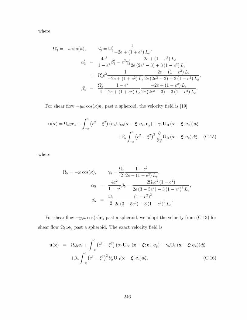
where

Ω′3 = −ω sin(κ), γ′3 = Ω′31

−2e+ (1 + e2)Le,

α′3 =4e2

1− e2β′3 = e2γ′3

−2e+ (1− e2)Le2e (2e2 − 3) + 3 (1− e2)Le

= Ω′3e2 1

−2e+ (1 + e2)Le

−2e+ (1− e2)Le2e (2e2 − 3) + 3 (1− e2)Le

,

β′3 =Ω′34

1− e2

−2e+ (1 + e2)Le

−2e+ (1− e2)Le2e (2e2 − 3) + 3 (1− e2)Le

.

For shear flow −yω cos(κ)ez past a spheroid, the velocity field is [19]

u(x) = Ω5yez +

∫ c

−c

(c2 − ξ2

)(α5USS(x− ξ; ez, ey) + γ5UR (x− ξ; ex))dξ

+β5

∫ c

−c

(c2 − ξ2

)2 ∂

∂yUD (x− ξ; ez) dξ, (C.15)

where

Ω5 = −ω cos(κ), γ5 =Ω5

2

1− e2

2e− (1− e2)Le,

α5 =4e2

1− e2β5 =

2Ω5e2 (1− e2)

2e (3− 5e2)− 3 (1− e2)2 Le,

β5 =Ω5

2

(1− e2)2

2e (3− 5e2)− 3 (1− e2)2 Le.

For shear flow −ybω cos(κ)ez past a spheroid, we adopt the velocity from (C.13) for

shear flow Ω1zey past a spheroid. The exact velocity field is

u(x) = Ω5yez +

∫ c

−c

(c2 − ξ2

)(α5USS (x− ξ; ez, ey)− γ5UR(x− ξ; ex))dξ

+β5

∫ c

−c

(c2 − ξ2

)2∂yUD(x− ξ; ez)dξ, (C.16)

246

where

Ω5 = −ω cos(κ), γ5 =Ω5

2

1− e2

2e− (1− e2)Le,

α5 =4e2

1− e2β5 =

2Ω5e2 (1− e2)

2e (3− 5e2)− 3 (1− e2)2 Le,

β5 =Ω5

2

(1− e2)2

2e (3− 5e2)− 3 (1− e2)2 Le.

In summary, the velocity field is

u(x) = −ωa sin(κ)ey + ω sin(κ)yex + ω cos(κ)zey − ω sin(κ)xey − ω cos(κ)yez

−∫ c

−cα2US (x− ξ, ey) dξ +

∫ c

−c

(c2 − ξ2

)β2UD (x− ξ, ey) dξ

+

∫ c

−c

(c2 − ξ2

)(α1USS(x− ξ; ex, ey) + γ1UR (x− ξ; ez) + γ2UR(x− ξ; ex))dξ

+β1

∫ c

−c

(c2 − ξ2

)2 ∂

∂yUD (x− ξ; ex) dξ, (C.17)

where

α1 =e2ω sin(κ)

−2e+ (1 + e2)Le,

α2 =−2ωa sin(κ)e2

2e+ (3e2 − 1)Le,

β1 =(1− e2)ω sin(κ)

4 (−2e+ (1 + e2)Le),

β2 =−ωa sin(κ) (1− e2)

2e+ (3e2 − 1)Le,

γ1 =(2− e2)ω sin(κ)

−2e+ (1 + e2)Le,

γ2 =(1− e2)ω cos(κ)

2e+ (−1 + e2)Le.

To get the exact solution (C.17), we have applied the following identities to the velocity

247

field,

USS (x− ξ; ey, ez) = USS (x− ξ; ez, ey) ,

∂

∂xUD (x− ξ; ey) =

∂

∂yUD (x− ξ; ez) ,

∂

∂yUD (x− ξ; ex) =

∂

∂xUD (x− ξ; ey) .

Figure C.1 shows fluid particle trajectories from two initial positions. For each posi-

tion, there are three trajectories based on different velocity field. The black trajectory

is from the exact solution when a spheroid sweeps out a single cone in free space. The

red trajectory is the higher order slender body result and the blue trajectory is the

leading order slender body result. These trajectories verify the improvement of the

higher order asymptotic solutions. The dashed circle in the top view indicates the top

of the cone.

248

(a) 3D view

(b) Top view

Figure C.1: Fluid particle trajectories from the two initial positions with the exactsolution for a spheroid sweeping a single cone, the leading order slender body approxi-mation, and the higher order slender body approximation.

249

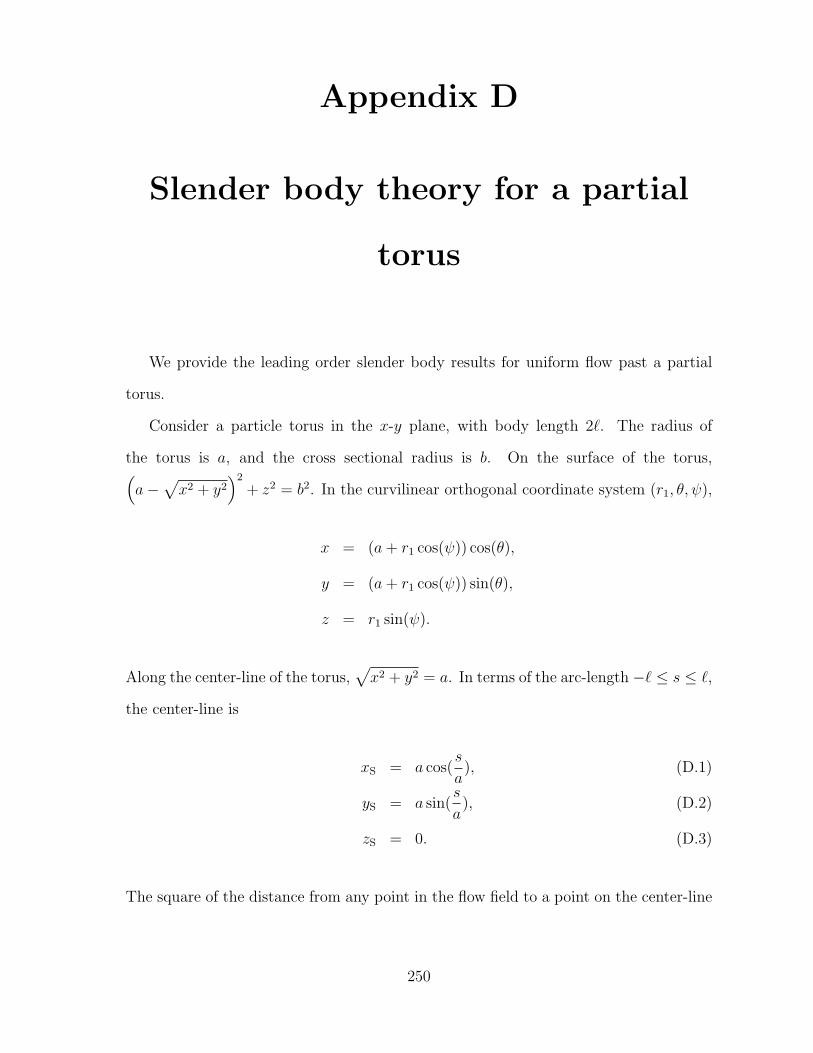
Appendix D

Slender body theory for a partial

torus

We provide the leading order slender body results for uniform flow past a partial

torus.

Consider a particle torus in the x-y plane, with body length 2`. The radius of

the torus is a, and the cross sectional radius is b. On the surface of the torus,(a−

√x2 + y2

)2

+ z2 = b2. In the curvilinear orthogonal coordinate system (r1, θ, ψ),

x = (a+ r1 cos(ψ)) cos(θ),

y = (a+ r1 cos(ψ)) sin(θ),

z = r1 sin(ψ).

Along the center-line of the torus,√x2 + y2 = a. In terms of the arc-length −` ≤ s ≤ `,

the center-line is

xS = a cos(s

a), (D.1)

yS = a sin(s

a), (D.2)

zS = 0. (D.3)

The square of the distance from any point in the flow field to a point on the center-line

250

is

(x−xS)2+(y−yS)2+(z−zS)2 =(

2a2(

1 +r1

acos(ψ)

)(1− cos

(θ − s

a

))+ r2

1

). (D.4)

The onsatz is the flow induced by the partial torus can be constructed with Stokeslet

uniformly distributed along the center-line and the strength of the singularity is pro-

portional to the local velocity at the center line. In the rectangular coordinates, the

strength of the Stokeslet is noted as (α1, α2, α3)T , the strength of the Stokeslet in

the local coordinate is (ατ , αn, αb)T . ατ , αn, αb are for tangential, normal and bi-

normal, respectively. The basis of the local coordinates are the tangential direction

eτ =(∂xS

∂s, ∂yS

∂s, ∂zS∂s

)T, the normal direction en = a

(∂2xS

∂s2, ∂

2yS

∂s2, ∂

2zS∂s2

)T, and the binormal

direction eb = eτ × en = (0, 0, 1)T . So,

α1

α2

α3

=

(eτ en eb

)ατ

αn

αb

=

∂xS

∂sa∂

2xS

∂s20

∂yS

∂sa∂

2yS

∂s20

∂zS∂s

a∂2zS∂s2

1

ατ

αn

αb

=

− sin

(sa

)− cos

(sa

)0

cos(sa

)− sin

(sa

)0

0 0 1

ατ

αn

αb

≡ R

ατ

αn

αb

.

From the onsatz,

ατ

αn

αb

=

c1 0 0

0 c2 0

0 0 c3

Uτ

Un

Ub

.

For the uniform flow past the partial torus (U1, U2, U3)T , the local velocity is (Uτ , Un, Ub)T =

RT (U1, U2, U3)T .

251

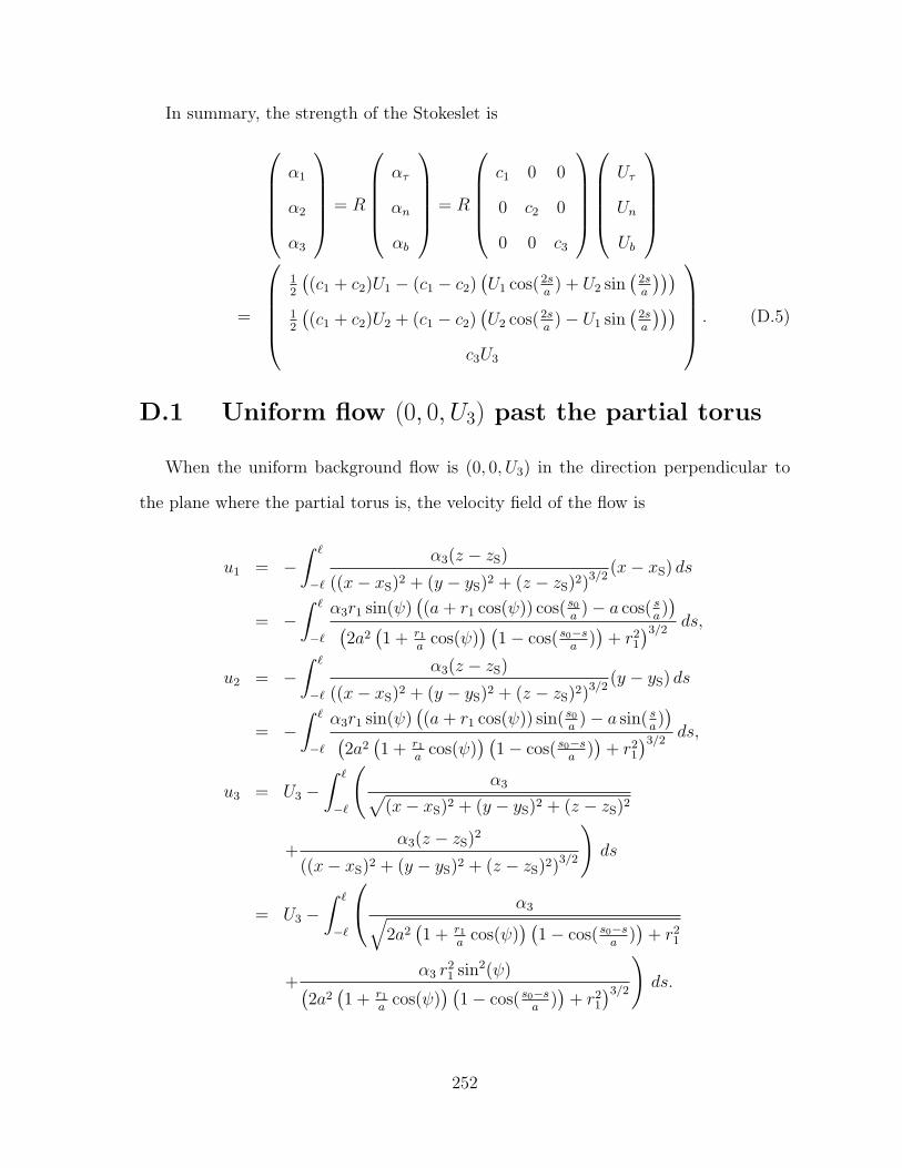
In summary, the strength of the Stokeslet is

α1

α2

α3

= R

ατ

αn

αb

= R

c1 0 0

0 c2 0

0 0 c3

Uτ

Un

Ub

=

12

((c1 + c2)U1 − (c1 − c2)

(U1 cos(2s

a) + U2 sin

(2sa

)))12

((c1 + c2)U2 + (c1 − c2)

(U2 cos(2s

a)− U1 sin

(2sa

)))c3U3

. (D.5)

D.1 Uniform flow (0, 0, U3) past the partial torus

When the uniform background flow is (0, 0, U3) in the direction perpendicular to

the plane where the partial torus is, the velocity field of the flow is

u1 = −∫ `

−`

α3(z − zS)

((x− xS)2 + (y − yS)2 + (z − zS)2)3/2(x− xS) ds

= −∫ `

−`

α3r1 sin(ψ)((a+ r1 cos(ψ)) cos( s0

a)− a cos( s

a))(

2a2(1 + r1

acos(ψ)

) (1− cos( s0−s

a))

+ r21

)3/2ds,

u2 = −∫ `

−`

α3(z − zS)

((x− xS)2 + (y − yS)2 + (z − zS)2)3/2(y − yS) ds

= −∫ `

−`

α3r1 sin(ψ)((a+ r1 cos(ψ)) sin( s0

a)− a sin( s

a))(

2a2(1 + r1

acos(ψ)

) (1− cos( s0−s

a))

+ r21

)3/2ds,

u3 = U3 −∫ `

−`

(α3√

(x− xS)2 + (y − yS)2 + (z − zS)2

+α3(z − zS)2

((x− xS)2 + (y − yS)2 + (z − zS)2)3/2

)ds

= U3 −∫ `

−`

α3√2a2(1 + r1

acos(ψ)

) (1− cos( s0−s

a))

+ r21

+α3 r

21 sin2(ψ)(

2a2(1 + r1

acos(ψ)

) (1− cos( s0−s

a))

+ r21

)3/2

)ds.

252

On the surface of the torus r1 = b, the no-slip boundary condition leads

u1 = −∫ `

−`

α3b sin(ψ)((a+ b cos(ψ)) cos

(s0a

)− a cos( s

a))(

2a2(1 + b

acos(ψ)

) (1− cos( s0

a− s

a))

+ b2)3/2

ds = 0,

u2 = −∫ `

−`

α3b sin(ψ)((a+ b cos(ψ)) sin

(s0a

)− a sin( s

a))(

2a2(1 + b

acos(ψ)

) (1− cos( s0

a− s

a))

+ b2)3/2

ds = 0,

u3 = U3 −∫ `

−`

α3√2a2(1 + b

acos(ψ)

) (1− cos( s0

a− s

a))

+ b2

+α3 b

2 sin2(ψ)(2a2(1 + b

acos(ψ)

) (1− cos( s0

a− s

a))

+ b2)3/2

)ds = 0.

Change of variable in the integral to make use of the stretched variable

s− s0

a=b

at, ds = bdt.

253

Then,

∫ `

−`

α3√2a2(1 + b

acos(ψ)

) (1− cos( s0

a− s

a))

+ b2

ds

=

∫ `−s0b

−`−s0b

α3b√2a2(1 + b

acos(ψ)

) (1− cos( b

at))

+ b2

dt

∼∫ `−s0

b

−`−s0b

α3b√a2(1 + b

acos(ψ)

) (bat)2

+ b2

dt

=

∫ `−s0b

−`−s0b

α3√(1 + b

acos(ψ)

)t2 + 1

dt

=α3√(

1 + ba

cos(ψ)) ∫ `−s0

b

−`−s0b

1√t2 + 1

(1+ ba

cos(ψ))

dt

=α3√(

1 + ba

cos(ψ)) log

`−s0b

+

√1

(1+ ba

cos(ψ))+(`−s0b

)2

−`−s0b

+

√1

(1+ ba

cos(ψ))+(−`−s0

b

)2

∼ α3√(1 + b

acos(ψ)

) log

`−s0b

+

√1

(1+ ba

cos(ψ))+(`−s0b

)2

−`−s0b

+

√1

(1+ ba

cos(ψ))+(−`−s0

b

)2

∼ α3 log

2 `−s0b

1

(1+ ba cos(ψ))

2`+s0b

∼ α3 log

(4`2 − s2

0

b2

(1 +

b

acos(ψ)

))

∼ 2α3 log

(2`

b

).

Away from the tips of the partial torus, the above asymptotic results is held.

254

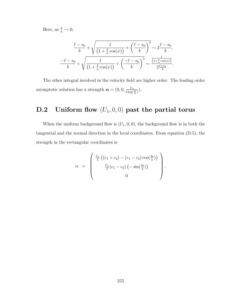
Here, as ba→ 0,

`− s0

b+

√1(

1 + ba

cos(ψ)) +

(`− s0

b

)2

∼ 2`− s0

b,

−`− s0

b+

√1(

1 + ba

cos(ψ)) +

(−`− s0

b

)2

∼1

(1+ ba

cos(ψ))

2 `+s0b

.

The other integral involved in the velocity field are higher order. The leading order

asymptotic solution has a strength α = (0, 0, U3

2 log( 2`b

)).

D.2 Uniform flow (U1, 0, 0) past the partial torus

When the uniform background flow is (U1, 0, 0), the background flow is in both the

tangential and the normal direction in the local coordinates. From equation (D.5), the

strength in the rectangular coordinates is

α =

U1

2

((c1 + c2)− (c1 − c2) cos(2s

a))

U1

2(c1 − c2)

(− sin(2s

a))

0

.

255

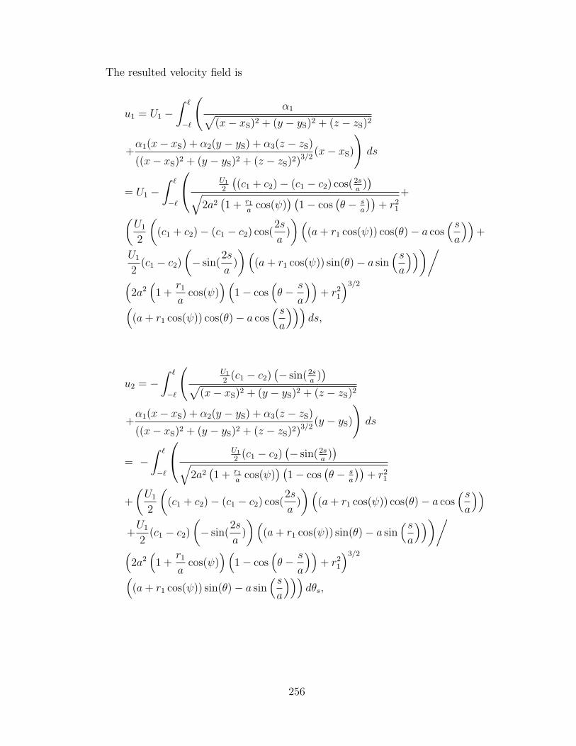
The resulted velocity field is

u1 = U1 −∫ `

−`

(α1√

(x− xS)2 + (y − yS)2 + (z − zS)2

+α1(x− xS) + α2(y − yS) + α3(z − zS)

((x− xS)2 + (y − yS)2 + (z − zS)2)3/2(x− xS)

)ds

= U1 −∫ `

−`

U1

2

((c1 + c2)− (c1 − c2) cos(2s

a))√

2a2(1 + r1

acos(ψ)

) (1− cos

(θ − s

a

))+ r2

1

+

(U1

2

((c1 + c2)− (c1 − c2) cos(

2s

a)

)((a+ r1 cos(ψ)) cos(θ)− a cos

(sa

))+

U1

2(c1 − c2)

(− sin(

2s

a)

)((a+ r1 cos(ψ)) sin(θ)− a sin

(sa

)))/(

2a2(

1 +r1

acos(ψ)

)(1− cos

(θ − s

a

))+ r2

1

)3/2

((a+ r1 cos(ψ)) cos(θ)− a cos

(sa

)))ds,

u2 = −∫ `

−`

(U1

2(c1 − c2)

(− sin(2s

a))√

(x− xS)2 + (y − yS)2 + (z − zS)2

+α1(x− xS) + α2(y − yS) + α3(z − zS)

((x− xS)2 + (y − yS)2 + (z − zS)2)3/2(y − yS)

)ds

= −∫ `

−`

U1

2(c1 − c2)

(− sin(2s

a))√

2a2(1 + r1

acos(ψ)

) (1− cos

(θ − s

a

))+ r2

1

+

(U1

2

((c1 + c2)− (c1 − c2) cos(

2s

a)

)((a+ r1 cos(ψ)) cos(θ)− a cos

(sa

))+U1

2(c1 − c2)

(− sin(

2s

a)

)((a+ r1 cos(ψ)) sin(θ)− a sin

(sa

)))/(

2a2(

1 +r1

acos(ψ)

)(1− cos

(θ − s

a

))+ r2

1

)3/2

((a+ r1 cos(ψ)) sin(θ)− a sin

(sa

)))dθs,

256

u3 = −∫ `

−`

(α1(x− xS) + α2(y − yS) + α3(z − zS)

((x− xS)2 + (y − yS)2 + (z − zS)2)3/2(z − zS)

)ds

= −∫ `

−`

[U1

2

((c1 + c2)− (c1 − c2) cos(

2s

a)

)((a+ r1 cos(ψ)) cos(θ)− a cos

(sa

))+U1

2(c1 − c2)

(− sin(

2s

a)

)((a+ r1 cos(ψ)) sin(θ)− a sin

(sa

))]/(

2a2(

1 +r1

acos(ψ)

)(1− cos

(θ − s

a

))+ r2

1

)3/2

r1 sin(ψ)

dθs.

On the surface of the partial torus r1 = b, the no-slip boundary condition is imposed.

Thus,

0 = U1 −∫ `

−`

U1

2

((c1 + c2)− (c1 − c2) cos(2s

a))√

2a2(1 + b

acos(ψ)

) (1− cos

(θ − s

a

))+ b2

+

[U1

2

((c1 + c2)− (c1 − c2) cos(

2s

a)

)((a+ b cos(ψ)) cos(θ)− a cos

(sa

))+

U1

2(c1 − c2)

(− sin(

2s

a)

)((a+ b cos(ψ)) sin(θ)− a sin

(sa

))]/(

2a2

(1 +

b

acos(ψ)

)(1− cos

(θ − s

a

))+ b2

)3/2

((a+ b cos(ψ)) cos(θ)− a cos

(sa

))ds,

0 = −∫ `

−`

U1

2(c1 − c2)

(− sin(2s

a))√

2a2(1 + b

acos(ψ)

) (1− cos

(θ − s

a

))+ b2

+

[U1

2

((c1 + c2)− (c1 − c2) cos(

2s

a)

)((a+ b cos(ψ)) cos(θ)− a cos

(sa

))+

U1

2(c1 − c2)

(− sin(

2s

a)

)((a+ b cos(ψ)) sin(θ)− a sin

(sa

))]/(

2a2

(1 +

b

acos(ψ)

)(1− cos

(θ − s

a

))+ b2

)3/2

((a+ b cos(ψ)) sin(θ)− a sin

(sa

))ds,

257

0 =

∫ `

−`

[U1

2

((c1 + c2)− (c1 − c2) cos(

2s

a)

)((a+ b cos(ψ)) cos(θ)− a cos

(sa

))+U1

2(c1 − c2)

(− sin(

2s

a)

)((a+ b cos(ψ)) sin[θ]− a sin

(sa

))]/(

2a2

(1 +

b

acos(ψ)

)(1− cos

(θ − s

a

))+ b2

)3/2

b sin(ψ)

ds.

In the following analysis, the observation position on the surface of the partial torus

is (r1, θ, ψ) = (b, s0a, ψ), where s0 is the arc-length and the no-slip boundary condition is

imposed. For the inner expansion, the integrals are determined by local contributions

when s is close to s0. Following Taylor expansions

b2 + 2a2(1− cos

(sa− s0

a

)) (1 + b

acos(ψ)

)∼ b2 + (s− s0)2 (1 + b

acos(ψ)

), (D.6)

a cos( s0a

)− a cos(sa

)∼ sin( s0

a) (s− s0) , (D.7)

a sin( s0a

)− a sin(sa

)∼ − cos( s0

a) (s− s0) (D.8)

will be applied to the analysis.

For u1

For the velocity in the x direction, the boundary condition implies

0 = U1 −∫ `

−`

U1

2

((c1 + c2)− (c1 − c2) cos(2s

a))√

2a2(1 + b

acos(ψ)

) (1− cos

(s0a− s

a

))+ b2

+

[U1

2

((c1 + c2)− (c1 − c2) cos(

2s

a)

)((a+ b cos(ψ)) cos(

s0

a)− a cos

(sa

))+

U1

2(c1 − c2)

(− sin(

2s

a)

)((a+ b cos(ψ)) sin(

s0

a)− a sin

(sa

))]((a+ b cos(ψ)) cos( s0

a)− a cos

(sa

))(2a2(1 + b

acos(ψ)

) (1− cos

(s0a− s

a

))+ b2

)3/2

ds.

258

Substitute (D.6) into denominators of the above equation,

0 = U1 −∫ `

−`

U1

2

((c1 + c2)− (c1 − c2) cos

(2sa

))√b2 + (s− s0)2

(1 + b cos(ψ)

a

)+

(−a cos

(sa

)+ cos( s0

a)(a+ b cos(ψ))

)(b2 +

(1 + b cos(ψ)

a

)(s− s0)2

)3/2

[−1

2(c1 − c2)U1 sin(

2s

a)(b cos(ψ) sin(

s0

a)− cos(

s0

a) (s− s0)

)+

1

2U1

(c1 + c2 − (c1 − c2) cos(

2s

a)

)(b cos(

s0

a) cos(ψ) + sin(

s0

a) (s− s0)

)]ds.

Approximate s with s0 and substitute (D.7) and (D.8) into the equation,

0 = U1 −∫ `

−`

U1

2

((c1 + c2)− (c1 − c2) cos

(2s0a

))√b2 + (s− s0)2

(1 + b cos(ψ)

a

)+

(sin( s0

a) (s− s0) + b cos( s0

a) cos(ψ)

)(b2 +

(1 + b cos(ψ)

a

)(s− s0)2

)3/2

[−U1

2(c1 − c2) sin(

2s0

a)(b cos(ψ) sin(

s0

a)− cos(

s0

a) (s− s0)

)+U1

2

(c1 + c2 − (c1 − c2) cos(

2s0

a)

) (b cos(

s0

a) cos(ψ) + sin(

s0

a) (s− s0)

)]ds.

259

Expand the equation and reorganize the terms,

0 = U1 − U1

2

((c1 + c2)− (c1 − c2) cos

(2s0a

)) ∫ `−`

1qb2+(s−s0)2(1+

b cos(ψ)a )

ds

−U1(c1−c2)4

sin2(2s0a

)

(1+b cos(ψ)

a )3/2

∫ `−`

1 b2

(1+b cos(ψ)

a )+(s−s0)2

!1/2 ds

+U1(c1−c2)4

(sin(2s0a

))2

(1+b cos(ψ)

a )3/2

∫ `−`

b2

(1+b cos(ψ)

a ) b2

(1+b cos(ψ)

a )+(s−s0)2

!3/2 ds

+U1(c1−c2)2

sin(2s0a

)∫ `−`

(b(sin2(s0a

)−cos2(s0a

))(s−s0) cos(ψ)+b2 cos(s0a

) cos2(ψ) sin(s0a

))

(b2+(1+b cos(ψ)

a )(s−s0)2)3/2 ds

− sin2(s0a

)

(1+b cos(ψ)

a )3/2

U1

2

(c1 + c2 − (c1 − c2) cos(2s0

a)) ∫ `−`

1 b2

(1+b cos(ψ)

a )+(s−s0)2

!1/2 ds

+sin2(

s0a

)

(1+b cos(ψ)

a )3/2

U1

2

(c1 + c2 − (c1 − c2) cos(2s0

a)) ∫ `−`

b2

(1+b cos(ψ)

a ) b2

(1+b cos(ψ)

a )+(s−s0)2

!3/2 ds

−U1

2

(c1 + c2 − (c1 − c2) cos(2s0

a)) (b cos( s0

a) cos(ψ)

)2 ∫ `−`

1

(b2+(1+b cos(ψ)

a )(s−s0)2)3/2ds

−U1

2

(c1 + c2 − (c1 − c2) cos(2s0

a))b sin(2 s0

a) cos(ψ)

∫ `−`

(s−s0)

(b2+(1+b cos(ψ)

a )(s−s0)2)3/2ds.

260

Drop the higher order terms,

0 ∼ U1 −U1

2(c1 + c2)

∫ `

−`

1√b2 + (s− s0)2

(1 + b cos(ψ)

a

) ds+U1

2(c1 − c2) cos(

2s0

a)

∫ `

−`

1√b2 + (s− s0)2

(1 + b cos(ψ)

a

) ds−U1

4(c1 − c2)

sin2(2s0a

)(1 + b cos(ψ)

a

)3/2

∫ `

−`

1√b2 + (s− s0)2

(1 + b cos(ψ)

a

) ds−

sin2( s0a

)U1

(c1 + c2 − (c1 − c2) cos(2s0

a))

2(

1 + b cos(ψ)a

)3/2

∫ `

−`

1√b2 + (s− s0)2

(1 + b cos(ψ)

a

) ds

= U1 +

−U1

2(c1 + c2) +

U1

2(c1 − c2) cos(

2s0

a)− 1

4(c1 − c2)

U1 sin2(2s0a

)(1 + b cos(ψ)

a

)3/2

−sin2( s0

a)(

1 + b cos(ψ)a

)3/2

U1

2

(c1 + c2 − (c1 − c2) cos(

2s0

a)

)∫ `

−`

1√b2 + (s− s0)2

(1 + b cos(ψ)

a

) ds

Thus, for the leading order,

1 +

−1

2(c1 + c2) +

1

2(c1 − c2) cos(

2s0

a)− (c1 − c2)

4

sin2(2s0a

)(1 + b cos(ψ)

a

)3/2−

(c1 + c2 − (c1 − c2) cos(2s0

a))

sin2( s0a

)

2(

1 + b cos(ψ)a

)3/2

∫ `

−`

1√b2 + (s− s0)2

(1 + b cos(ψ)

a

) ds = 0

261

1 +

(−1

2(c1 + c2) +

1

2(c1 − c2) cos(

2s0

a)− (c1 − c2)

4sin2(

2s0

a)−

1

2(c1 + c2) sin2(

s0

a) +

1

2(c1 − c2) cos(

2s0

a) sin2(

s0

a)

)2 log

(2`

b

)= 0

1 +1

2

(−2(2c1 + c2) + 4(c1 −

c2

2) cos(

2s0

a)

)log

(2`

b

)= 0

For u2

The no-slip boundary condition for the y-direction velocity,

u2 = −∫ `

−`

U1

2(c1 − c2)

(− sin(2s

a))√

2a2(1 + b

acos(ψ)

) (1− cos

(s0a− s

a

))+ b2

+

[U1

2

((c1 + c2)− (c1 − c2) cos(

2s

a)

)((a+ b cos(ψ)) cos(

s0

a)− a cos

(sa

))+

U1

2(c1 − c2)

(− sin(

2s

a)

)((a+ b cos(ψ)) sin(

s0

a)− a sin

(sa

))]((a+ b cos(ψ)) sin( s0

a)− a sin

(sa

))(2a2(1 + b

acos(ψ)

) (1− cos

(s0a− s

a

))+ b2

)3/2

ds = 0.

262

Applying the Taylor expansions (D.6)-(D.8) to the above condition,

0 = −∫ `

−`

U1

2(c1 − c2)

(− sin(2s0

a))√

b2 + (s− s0)2(

1 + b cos(ψ)a

)+U1

(b cos(ψ) sin( s0

a)− cos( s0

a) (s− s0)

)2(b2 + (a+b cos(ψ))(s−s0)2

a

)3/2

[(c1 + c2 − (c1 − c2) cos(

2s0

a)

)(b cos(

s0

a) cos(ψ) + sin(

s0

a) (s− s0)

)−(c1 − c2) sin(

2s0

a)(b cos(ψ) sin(

s0

a)− cos(

s0

a) (s− s0)

)]ds

= −∫ `

−`

U1

2(c1 − c2)

(− sin(2s0

a))√

b2 + (s− s0)2(

1 + b cos(ψ)a

) ds+U1

4

(c1 + c2 − (c1 − c2) cos(

2s0

a)

)sin(2

s0

a)

∫ `

−`

(s− s0)2(b2 + (a+b cos(ψ))(s−s0)2

a

)3/2ds

−U1

(c1 + c2 − (c1 − c2) cos(

2s0

a)

)∫ `

−`

(b2

2sin(2 s0

a) cos2(ψ) + b cos(ψ)

(sin2( s0

a)− cos2( s0

a))

(s− s0))

2(b2 + (a+b cos(ψ))(s−s0)2

a

)3/2ds

+U1(c1 − c2) sin(2s0

a)

∫ `

−`

(cos( s0

a) (s− s0)

)2

2(b2 + (a+b cos(ψ))(s−s0)2

a

)3/2ds

+U1

(c1 − c2) sin(2s0

a

)2

∫ `

−`

((b cos(ψ) sin( s0

a))2 − b cos(ψ) sin(2 s0

a) (s− s0)

)(b2 + (a+b cos(ψ))(s−s0)2

a

)3/2ds.

263

Drop the higher order term,

0 ∼ U1

2(c1 − c2) sin(

2s0

a)

∫ `

−`

1√b2 + (s− s0)2

(1 + b cos(ψ)

a

) ds+U1

4

(c1 + c2 − (c1 − c2) cos(

2s0

a)

)sin(2

s0

a)

∫ `

−`

1(b2 + (a+b cos(ψ))(s−s0)2

a

)1/2ds

+U1

2

(cos(

s0

a))2

(c1 − c2) sin(2s0

a)

∫ `

−`

1(b2 + (a+b cos(ψ))(s−s0)2

a

)1/2ds.

So,

1

2(c1 − c2) +

1

4

(c1 + c2 − (c1 − c2) cos(

2s0

a)

)+

1

2cos2(

s0

a)(c1 − c2) = 0

=⇒ c1 =c2

2.

Solve the linear system for the constant c1 and c2,

c1 =c2

2

1 +1

2

(−2(2c1 + c2) + 4(c1 −

c2

2) cos(

2s0

a)

)log

(2`

b

)= 0

c1 =1

4 log(

2`b

) , and c2 =1

2 log(

2`b

) .

264

For u3

0 = −b sin(ψ)

∫ `

−`

(−U1

2(c1 − c2) sin(

2s0

a)(b cos(ψ) sin(

s0

a)− cos(

s0

a) (s− s0)

)+U1

2

(c1 + c2 − (c1 − c2) cos(

2s0

a)

)(b cos(ψ) cos(

s0

a) + sin(

s0

a) (s− s0)

))1(

b2 + (1 + ba

cos(ψ)) (s− s0)2)3/2ds

The leading order for this condition is zero, which is automatically satisfied, i.e. not

contribute to the determination of the strength.

In summary, the strength of the Stokeslet in the rectangular coordinates is

α =U1

8

1

log(

2`b

)

3 + cos(2sa

)

sin(2sa

)

0

.

265

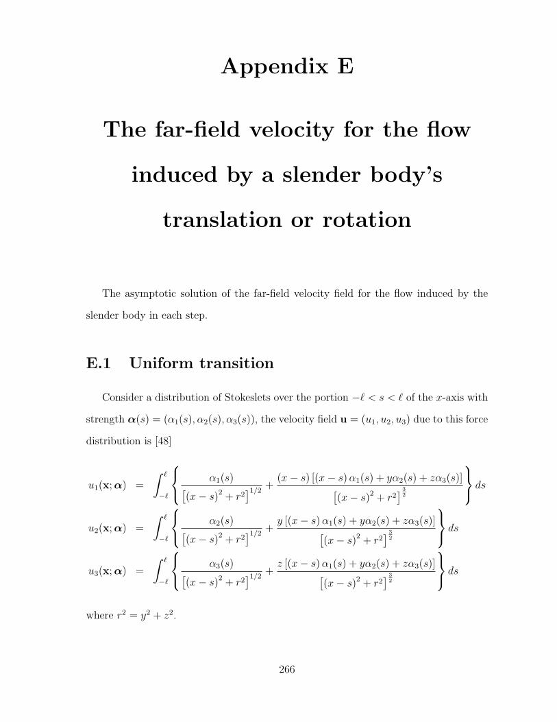
Appendix E

The far-field velocity for the flow

induced by a slender body’s

translation or rotation

The asymptotic solution of the far-field velocity field for the flow induced by the

slender body in each step.

E.1 Uniform transition

Consider a distribution of Stokeslets over the portion −` < s < ` of the x-axis with

strength α(s) = (α1(s), α2(s), α3(s)), the velocity field u = (u1, u2, u3) due to this force

distribution is [48]

u1(x;α) =

∫ `

−`

α1(s)[(x− s)2 + r2

]1/2 +(x− s) [(x− s)α1(s) + yα2(s) + zα3(s)][

(x− s)2 + r2] 3

2

ds

u2(x;α) =

∫ `

−`

α2(s)[(x− s)2 + r2

]1/2 +y [(x− s)α1(s) + yα2(s) + zα3(s)][

(x− s)2 + r2] 3

2

ds

u3(x;α) =

∫ `

−`

α3(s)[(x− s)2 + r2

]1/2 +z [(x− s)α1(s) + yα2(s) + zα3(s)][

(x− s)2 + r2] 3

2

ds

where r2 = y2 + z2.

266

As the observation point x is far from the body, we examine the far-field velocity.

Hence, a non-dimensional formulation is introduced. Let

x′ =x

R, s′ =

s

`, α′ =

α

U(E.1)

in which R is a characteristic length assumed to be large and U is a characteristic

velocity. Rewriting the velocity field as functions of the non-dimensional variables in

(E.1), we get

u′1(x′;α′) =

∫ 1

−1

`α′1(s′)[(Rx′ − `s′)2 +R2r2

]1/2ds′ +∫ 1

−1

` (Rx′ − `s′) [(Rx′ − `s′)α′1(s′) +Ry′α′2(s′) +Rz′α′3(s′)][(Rx′ − `s′)2 +R2r2

] 32

ds′

= ε0

∫ 1

−1

α′1(s′)[(x′ − ε0s′)2 + r2

]1/2ds′ +ε0

∫ 1

−1

(x′ − ε0s′) [(x′ − ε0s′)α′1(s′) + y′α′2(s′) + z′α′3(s′)][(x′ − ε0s′)2 + r2

] 32

ds′,

u′2(x′;α′) =

∫ 1

−1

`α′2(s′)[(Rx′ − `s′)2 +R2r2

]1/2ds′ +∫ 1

−1

`Ry′ [(Rx′ − `s′)α′1(s′) +Ry′α′2(s′) +Rz′α′3(s′)][(Rx′ − `s′)2 +R2r2

] 32

ds′

= ε0

∫ 1

−1

α′2(s′)[(x′ − ε0s′)2 + r2

]1/2ds′ +ε0

∫ 1

−1

y′ [(x′ − ε0s′)α′1(s′) + y′α′2(s′) + z′α′3(s′)][(x′ − ε0s′)2 + r2

] 32

ds′,

267

u′3(x′;α′) =

∫ 1

−1

`α′3(s′)[(Rx′ − `s′)2 +R2r2

]1/2ds′ +∫ 1

−1

`Rz′ [(Rx′ − `s′)α′1(s′) +Ry′α′2(s′) +Rz′α′3(s′)][(Rx′ − `s′)2 +R2r2

] 32

ds′

= ε0

∫ 1

−1

α′3(s′)[(x′ − ε0s′)2 + r2

]1/2ds′ +ε0

∫ 1

−1

z′ [(x′ − ε0s′)α′1(s′) + y′α′2(s′) + z′α′3(s′)][(x′ − ε0s′)2 + r2

] 32

ds′,

where r is the non-dimensional radius, r2 = (y′)2 + (z′)2, and

ε0 =`

R0

(E.2)

is the small parameter for the far field. Since the far-field limit of the velocity field is

of interest, we examine ε0 → 0 in the limit R0 → 0.

Drop all the primes,

u1(x;α) = ε0

∫ 1

−1

α1(s)[(x− ε0s)2 + r2

]1/2ds+

ε0

∫ 1

−1

(x− ε0s) [(x− ε0s)α1(s) + yα2(s) + zα3(s)][(x− ε0s)2 + r2

] 32

ds,

= ε0 [I (α1) + I2(α1) + yI1(α2) + zI1(α3)]

u2(x;α) = ε0

∫ 1

−1

α2(s)[(x− ε0s)2 + r2

]1/2ds+

ε0

∫ 1

−1

y [(x− ε0s)α1(s) + yα2(s) + zα3(s)][(x− ε0s)2 + r2

] 32

ds,

= ε0[I (α2) + yI1(α1) + y2I0(α2) + yzI0(α3)

]u3(x;α) = ε0

∫ 1

−1

α3(s)[(x− ε0s)2 + r2

]1/2ds+

ε0

∫ 1

−1

z [(x− ε0s)α1(s) + yα2(s) + zα3(s)][(x− ε0s)2 + r2

] 32

ds.

= ε0[I (α3) + zI1(α1) + yzI0(α2) + x2

3I0(α3)],

268

in terms of these integrals

I (α) =

∫ 1

−1

α(s)[(x− ε0s)2 + r2

]1/2ds (E.3)

I0(α) =

∫ 1

−1

α(s)[(x− ε0s)2 + r2

]3/2dsI1(α) =

∫ 1

−1

(x− ε0s)α(s)[(x− ε0s)2 + r2

]3/2dsI2(α) =

∫ 1

−1

(x− ε0s)2 α(s)[(x− ε0s)2 + r2

]3/2ds.Examine the integrand of I in (E.3). Taylor expansion about ε0 = 0 provides

1[(x− ε0s)2 + r2

]1/2 =1

|x|+

x

|x|3sε0 +

3x2 − |x|2

2|x|5s2ε20 +O(ε30).

Substituting this expansion into I gives that

I (α) =1

|x|

∫ 1

−1

α(s)ds+x

|x|3ε0

∫ 1

−1

sα(s)ds+3x2 − |x|2

2|x|5ε20

∫ 1

−1

s2α(s)ds+O(ε30).

Now examine the integrand of I0. Since

1[(x− ε0s)2 + r2

]3/2 =1

|x|3+

3x

|x|5sε0 +

15x2 − 3|x|2

2|x|7s2ε20 +O(ε30)

upon Taylor expanding about ε0 = 0,

I0(α) =1

|x|3

∫ 1

−1

α(s)ds+3xε0|x|5

∫ 1

−1

sα(s)ds+15x2 − 3|x|2

2|x|7ε20

∫ 1

−1

s2α(s)ds+O(ε30).

By applying Taylor expansion of the integrand of I1 for ε0 → 0,

(x− ε0s)[(x− ε0s)2 + r2

]3/2 =x

|x|3+

3x2 − |x|2

|x|5sε0 +

15x3 − 9x|x|2

2|x|7s2ε20 +O(ε30),

269

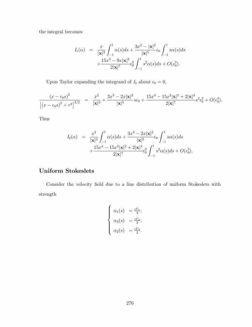
the integral becomes

I1(α) =x

|x|3

∫ 1

−1

α(s)ds+3x2 − |x|2

|x|5ε0

∫ 1

−1

sα(s)ds

+15x3 − 9x|x|2

2|x|7ε20

∫ 1

−1

s2α(s)ds+O(ε30).

Upon Taylor expanding the integrand of I2 about ε0 = 0,

(x− ε0s)2[(x− ε0s)2 + r2

]3/2 =x2

|x|3+

3x3 − 2x|x|2

|x|5sε0 +

15x4 − 15x2|x|2 + 2|x|4

2|x|7s2ε20 +O(ε30).

Thus

I2(α) =x2

|x|3

∫ 1

−1

α(s)ds+3x3 − 2x|x|2

|x|5ε0

∫ 1

−1

sα(s)ds

+15x4 − 15x2|x|2 + 2|x|4

2|x|7ε20

∫ 1

−1

s2α(s)ds+O(ε30).

Uniform Stokeslets

Consider the velocity field due to a line distribution of uniform Stokeslets with

strength

α1(s) = εU1

4;

α3(s) = εU2

2;

α2(s) = εU3

2.

270

Since

∫ 1

−1

α(s)ds = 2α,∫ 1

−1

sα(s)ds = 0,∫ 1

−1

s2α(s)ds =2

3α,

I (α) =2

|x|α +

3x2 − |x|2

3|x|5ε20α +O(ε30), (E.4)

I0(α) =2

|x|3α +

5x2 − |x|2

|x|7ε20α +O(ε30), (E.5)

I1(α) =2x

|x|3α +

5x3 − 3x|x|2

|x|7ε20α +O(ε30), (E.6)

I2(α) =2x2

|x|3α +

15x4 − 15x2|x|2 + 2|x|4

3|x|7ε20α +O(ε30). (E.7)

Substitute the above integrals into the dimensionless velocity field,

u1(x;α) = ε0 [I (α1) + I2(α1) + yI1(α2) + zI1(α3)]

= ε0

[2

|x|α1 +

3x2 − |x|2

3|x|5ε20α1

]+ ε0

[2x2

|x|3α1 +

15x4 − 15x2|x|2 + 2|x|4

3|x|7ε20α1

]+ε0y

[2x

|x|3α2 +

5x3 − 3x|x|2

|x|7ε20α2

]+ ε0z

[2x

|x|3α3 +

5x3 − 3x|x|2

|x|7ε20α3

]+O(ε40)

u2(x;α) = ε0[I (α2) + yI1(α1) + y2I0(α2) + yzI0(α3)

]= ε0

[2

|x|α2 +

3x2 − |x|2

3|x|5ε20α2

]+ ε0y

[2x

|x|3α1 +

5x3 − 3x|x|2

|x|7ε20α1

]+ε0y

2

[2

|x|3α2 +

15x2 − 3|x|2

3|x|7ε20α2

]+ ε0yz

[2

|x|3α3 +

15x2 − 3|x|2

3|x|7ε20α3

]+O(ε40)

u3(x;α) = ε0[I (α3) + zI1(α1) + yzI0(α2) + x2

3I0(α3)]

= ε0

[2

|x|α3 +

3x2 − |x|2

3|x|5ε20α3

]+ ε0z

[2x

|x|3α1 +

5x3 − 3x|x|2

|x|7ε20α1

]+ε0yz

[2

|x|3α2 +

5x2 − |x|2

|x|7ε20α2

]+ ε0x

23

[2

|x|3α3 +

5x2 − |x|2

|x|7ε20α3

]+O(ε40)

271

Rewrite it in the order of ε,

u1(x;α) = ε0

[2

|x|α1 +

2x2

|x|3α1 +

2xy

|x|3α2 +

2xz

|x|3α3

]+ε30

[3x2 − |x|2

3|x|5α1 +

15x4 − 15x2|x|2 + 2|x|4

3|x|7α1

+5x3 − 3x|x|2

|x|7(yα2 + zα3)

]+O(ε40) (E.8)

u2(x;α) = ε0

[2

|x|α2 +

2xy

|x|3α1 +

2y2

|x|3α2 +

2yz

|x|3α3

]+ε30

[3x2 − |x|2

3|x|5α2 + y

5x3 − 3x|x|2

|x|7α1 +

5x2 − |x|2

|x|7(y2α2 + yzα3

)]+O(ε40) (E.9)

u3(x;α) = ε0

[2

|x|α3 +

2xz

|x|3α1 +

2yz

|x|3α2 +

2x23

|x|3α3

]+ε30

[3x2 − |x|2

3|x|5α3 + z

5x3 − 3x|x|2

|x|7α1 +

5x2 − |x|2

|x|7(yzα2 + x2

3α3

)]+O(ε40) (E.10)

From the leading order of the far-field velocity

u1(x;α) = ε0

[2

|x|α1 +

2x2

|x|3α1 +

2xy

|x|3α2 +

2xz

|x|3α3

]+O(ε30) (E.11)

u2(x;α) = ε0

[2

|x|α2 +

2xy

|x|3α1 +

2y2

|x|3α2 +

2yz

|x|3α3

]+O(ε30) (E.12)

u3(x;α) = ε0

[2

|x|α3 +

2xz

|x|3α1 +

2yz

|x|3α2 +

2x23

|x|3α3

]+O(ε30) (E.13)

the fluid particle trajectory is

dx

dt= ε0

[2

|x|α1 +

2x2

|x|3α1 +

2xy

|x|3α2 +

2xz

|x|3α3

]+O(ε30),

dy

dt= ε0

[2

|x|α2 +

2xy

|x|3α1 +

2y2

|x|3α2 +

2yz

|x|3α3

]+O(ε30),

dz

dt= ε0

[2

|x|α3 +

2xz

|x|3α1 +

2yz

|x|3α2 +

2x23

|x|3α3

]+O(ε30).

272

E.2 Rotation

In this section, we derive the far-field for the flow induced by the rotation of the

body about its midpoint with constant angular velocity ω in the (x, y) plane. This is

a degenerate case of the slender body sweeping out a double cone.

If the rod is sweeping out a double cone, the velocity field in the body frame where

the rod is tilted is [48]

u1(x) = ωy +ωε sin(κ)

2

∫ `

−`

(x− s sin(κ))ys

[(x− s sin(κ))2 + y2 + (z − s cos(κ))2]3/2ds

u2(x) = −ωx+ωε sin(κ)

2

∫ `

−`

s

[(x− s sin(κ))2 + y2 + (z − s cos(κ))2]1/2

+y2s

[(x− s sin(κ))2 + y2 + (z − s cos k)2]32

ds

u3(x) =ωε sin(κ)

2

∫ `

−`

y(z − s cos(κ))s[(x− s sin(κ))2 + y2 + (z − s cos(κ))2

] 32

ds

where angle κ is the cone angle from the positive z-axis to the body.

Non-dimensionalization To examine the velocity field as the observation point x

gets far from the force distribution, a non-dimensional formulation is introduced. Let

x′ =x

R, s′ =

s

`, (E.14)

273

where R is a scalar parameter with the dimensions of length assumed to be large. The

velocity field written as function of the non-dimensional variables in (E.14) becomes

u′1(x′) = ωRy′ + ωε sin(κ)2

∫ 1

−1(Rx′−`s′ sin(κ))Ry′`s′

[(Rx′−`s′ sin(κ))2+(Ry′)2+(Rz′−`s′ cos(κ))2]3/2d(`s′)

u′2(x′) = −ωRx′ + ωε sin(κ)2

∫ 1

−1

`s′

[(Rx′−`s′ sin(κ))2+(Ry′)2+(Rz′−`s′ cos(κ))2]1/2

+ (Ry′)2`s′

[(Rx′−`s′ sin(κ))2+(Ry′)2+(Rz′−`s′ cos(κ))2]32

d(`s′)

u′3(x′) = ωε sin(κ)2

∫ 1

−1

Ry′(Rz′−`s′ cos(κ))`s′

[(Rx′−`s′ sin(κ))2+(Ry′)2+(Rz′−`s′ cos(κ))2]32

d(`s′).

Simplify above equations,

u′1(x′) = ωRy′ + ωε` sin(κ)2

∫ 1

−1(x′−ε0s′ sin(κ))y′ε0s′

[(x′−ε0s′ sin(κ))2+(y′)2+(z′−ε0s′ cos(κ))2]3/2ds′,

u′2(x′) = −ωRx′ + ωε` sin(κ)2

∫ 1

−1

ε0s′

[(x′−ε0s′ sin(κ))2+(y′)2+(z′−ε0s′ cos(κ))2]1/2

+ (y′)2ε0s′

[(x′−ε0s′ sin(κ))2+(y′)2+(z′−ε0s′ cos(κ))2]32

ds′,

u′3(x′) = ωε` sin(κ)2

∫ 1

−1y′(z′−ε0s′ cos(κ))ε0s′

[(x′−ε0s′ sin(κ))2+(y′)2+(z′−ε0s′ cos(κ))2]32ds′,

where ε0 = `R

. Drop all the primes,

u1(x) = ωRy +ωε` sin(κ)

2

∫ 1

−1

(x− ε0s sin(κ))yε0s

[(x− ε0s sin(κ))2 + y2 + (z − ε0s cos(κ))2]3/2ds,

u2(x) = −ωRx+ωε` sin(κ)

2

∫ 1

−1

ε0s

[(x− ε0s sin(κ))2 + y2 + (z − ε0s cos(κ))2]1/2

+y2ε0s

[(x− ε0s sin(κ))2 + y2 + (z − ε0s cos(κ))2]32

ds,

u3(x) =ωε` sin(κ)

2

∫ 1

−1

y(z − ε0s cos(κ))ε0s[(x− ε0s sin(κ))2 + y2 + (z − ε0s cos(κ))2

] 32

ds.

To examine the flow induced by a slender body rotating in the x-y plane as Phase

274

2 and Phase 4 in Chapter 8, we set the tilt angle κ = π2. Then,

u1(x) = ωRy +ωε`yε0

2

∫ 1

−1

(x− ε0s)s[(x− ε0s)2 + y2 + z2]3/2

ds,

u2(x) = −ωRx+ωε`ε0

2

∫ 1

−1

[s

[(x− ε0s)2 + y2 + z2]1/2+

y2s

[(x− ε0s)2 + y2 + z2]32

]ds,

u3(x) =ωε`yzε0

2

∫ 1

−1

s[(x− ε0s)2 + y2 + z2

] 32

ds.

Since The Taylor expanding about ε0 = 0 gives,

(x− ε0s)s[(x− ε0s)2 + y2 + z2]3/2

=sx

|x|3+

(3x2

|x|5− 1

|x|3

)s2ε0 +

(15x3

2 |x|7− 9x

2 |x|5

)s3ε20 +(

35x4

2 |x|9− 15x2

|x|7+

3

2 |x|5

)s4ε30 +O(ε0)4,

s

[(x− ε0s)2 + y2 + z2]1/2=

s

|x|+

x

|x|3s2ε0 +

(3x2

2 |x|5− 1

2 |x|3

)s3ε20 +(

5x3

2 |x|7− 3x

2 |x|5

)s4ε30 +O(ε0)4,

s

[(x− ε0s)2 + y2 + z2]32

=s

|x|3+

3x

|x|5s2ε0 +

(15x2

2 |x|7− 3

2 |x|5

)s3ε20 +(

35x3

2 |x|9− 15x

2 |x|7

)s4ε30 +O(ε0)4.

Upon the above Taylor expanding, the integrals are

∫ 1

−1

(x− ε0s)s[(x− ε0s)2 + y2 + z2]

32

ds

=x

|x|3∫ 1

−1

sds+

(3x2

|x|5− 1

|x|3

)ε0

∫ 1

−1

s2ds+

(15x3

2 |x|7− 9x

2 |x|5

)ε20

∫ 1

−1

s3ds

+

(35x4

2 |x|9− 15x2

|x|7+

3

2 |x|5

)ε30

∫ 1

−1

s4ds+O(ε40)

=

(3x2

|x|5− 1

|x|3

)2

3ε0 +

(35x4

2 |x|9− 15x2

|x|7+

3

2 |x|5

)2

5ε30 +O(ε40),

275

∫ 1

−1

s

[(x− ε0s)2 + y2 + z2]1/2ds

=1

|x|

∫ 1

−1

sds+x

|x|3ε0

∫ 1

−1

s2ds+

(3x2

2 |x|5− 1

2 |x|3

)ε20

∫ 1

−1

s3ds

+

(5x3

2 |x|7− 3x

2 |x|5

)ε30

∫ 1

−1

s4ds+O(ε40)

=x

|x|32ε03

+

(5x3

2 |x|7− 3x

2 |x|5

)2

5ε30 +O(ε40),

∫ 1

−1

s

[(x− ε0s)2 + y2 + z2]32

ds

=1

|x|3∫ 1

−1

ds+3x

|x|5ε0

∫ 1

−1

s2ds+

(15x2

2 |x|7− 3

2 |x|5

)ε20

∫ 1

−1

s3ds

+

(35x3

2 |x|9− 15x

2 |x|7

)ε30

∫ 1

−1

s4ds+O(ε40)

=3x

|x|52

3ε0 +

(35x3

2 |x|9− 15x

2 |x|7

)2ε305

+O(ε50).

In summary,

∫ 1

−1

(x− ε0s)s[(x− ε0s)2 + y2 + z2]3/2

ds =

(3x2

|x|5− 1

|x|3

)2

3ε0

+

(35x4

2 |x|9− 15x2

|x|7+

3

2 |x|5

)2

5ε30 +O(ε40),∫ 1

−1

s

[(x− ε0s)2 + y2 + z2]1/2ds =

x

|x|32

3ε0 +

(5x3

|x|7− 3x

|x|5

)1

5ε30 +O(ε40),∫ 1

−1

s

[(x− ε0s)2 + y2 + z2]32

ds =3x

|x|52

3ε0 +

(7x3

|x|9− 3x

|x|7

)ε30 +O(ε40).

276

So, the velocity field is

u1(x) = ωRy +ωε`yε0

2

∫ 1

−1

(x− ε0s)s[(x− ε0s)2 + y2 + z2]3/2

ds

= ωRy +ωε`yε0

2

(3x2

|x|5− 1

|x|3

)2ε03

+

(35x4

2 |x|9− 15x2

|x|7+

3

2 |x|5

)2ε305

+O(ε40)

,

u2(x) = −ωRx+ωε`ε0

2

∫ 1

−1

s

[(x− ε0s)2 + y2 + z2]1/2+

y2s

[(x− ε0s)2 + y2 + z2]32

ds

= −ωRx+ωε`ε0

2

x

|x|32ε03

+

(5x3

|x|7− 3x

|x|5

)1

5ε30 +O(ε40)

+ωε`ε0y

2

2

3x

|x|52

3ε0 +

(7x3

|x|9− 3x

|x|7

)ε30 +O(ε40)

,

u3(x) =ωε`yzε0

2

∫ 1

−1

s[(x− ε0s)2 + y2 + z2

] 32

ds

=ωε`yzε0

2

3x

|x|52

3ε0 +

(7x3

|x|9− 3x

|x|7

)ε30 +O(ε40)

,

which is

u1(x) = ωRy +ωε`yε0

2

(3x2

|x|5− 1

|x|3

)2

3ε0 +

(35x4

2 |x|9− 15x2

|x|7+

3

2 |x|5

)2

5ε30 +O(ε40)

,

u2(x) = −ωRx+ωε`ε0

2

x

|x|32ε03

+

(5x3

|x|7− 3x

|x|5

)1

5ε30 +O(ε40)

+ωε`ε0y

2

2

3x

|x|52

3ε0 +

(7x3

|x|9− 3x

|x|7

)ε30 +O(ε40)

,

u3(x) =ωε`yzε0

2

3x

|x|52

3ε0 +

(7x3

|x|9− 3x

|x|7

)ε30 +O(ε40)

.

277

Appendix F

Matlab scripts

The matlab scripts for a straight rod sweeping out a tilted cone and a bent rod

sweeping out an upright above a no-slip plane are included here. Various different

versions have been written for static cones and dynamic cones. The following matlab

scripts are for the basic static cone. The dynamics cone cases can be obtained by

changing parameters accordingly.

F.1 Matlab script for the straight rod case

% ————————–main.m—————————————–

% a straight rod sweeping out a tilted cone above a no-slip plane

% parameter() initializes the parameters

% the velocity field is constructed directly in the lab frame in fun tilt()

% integrals involved in the velocity fields are computed in

% fun int stokes() and fun int image()

% fun int stokes(): for the stokeslet along the center-line

% fun int image(): for the image system

% Written by: Longhua Zhao

% initial environment

clear all; clc; %clf;% close all;

278

global ell eps omega kappa lambda

[T0,T1,x0]=parameter();

options = odeset(’RelTol’,1e-8,’AbsTol’,1e-8);

tspan=[T0 T1];

[t1,x1]=ode45(’fun tilt’,tspan,x0,options);

tT=t1;

xX=x1;

[m1,n1]=size(x1);

% the centerline of the body along the x-axis

cx=-0:0.2:ell;

mg=length(cx);

cy=zeros(1,mg);

cz=cy;

% body tilted by an angle kappa

cy0=cy;

for j=1:mg

cx0(j)= cx(j)*sin(kappa)-cz(j)*cos(kappa);

cz0(j)= cx(j)*cos(kappa)+cz(j)*sin(kappa);

end

279

% body tilted sweeping a cone

tg=0:0.1:2*pi/omega;

czt=cz0;

for p=1:length(tg)

for j=1:mg

cxt(j,p)=cos(omega*tg(p))*cx0(j)-sin(omega*tg(p))*cy0(j);

cyt(j,p)=sin(omega*tg(p))*cx0(j)+cos(omega*tg(p))*cy0(j);

end

end

% save the data for trajectory

save(’x.data’,’xX’,’-ASCII’,’-append’)

% ————————–parameter function—————————–

function [t0,t1,x0]=parameter();

global ell eps omega kappa lambda

ell = 1.d0; % rod body length

%eps = 0.01d0;

delta = 0.01; %cross sectional radius

eps = 1.0/log(1.0/delta); %slenderness: e= 1/log(1/d)

omega = 2*pi; % angular velocity

kappa = pi/6; % cone angle

280

lambda = 5*pi/20; % tilt angle

t0 = 0.d0; % starting time

t1 = 100.0; % end time: number of revolutions

x0=zeros(1,3);

x0=[-0.1 0 1]; % initial position

%————————– velocity function——————————

function [dxdt]=fun tilt(t,xlab)

global ell eps omega kappa lambda

dxdt=zeros(size(xlab));

x= xlab(1);

y= xlab(2);

z= xlab(3);

A = sin(kappa)*cos(lambda)*cos(omega*t)+cos(kappa)*sin(lambda);

B = sin(kappa)*sin(omega*t);

C = cos(kappa)*cos(lambda)-sin(kappa)*cos(omega*t)*sin(lambda);

[u21L,I1L,I2L,I3L]=fun int stokes(A,B,C,x,y,z,ell);

[u210,I10,I20,I30]=fun int stokes(A,B,C,x,y,z,0);

[u23L,I4L,I5L,I6L,I7L,I8L,I9L]=fun int image(A,B,C,x,y,z,ell);

281

[u230,I40,I50,I60,I70,I80,I90]=fun int image(A,B,C,x,y,z,0);

u21= u21L-u210;

u23= u23L-u230;

I1=I1L-I10;

I2=I2L-I20;

I3=I3L-I30;

I4=I4L-I40;

I5=I5L-I50;

I6=I6L-I60;

I7=I7L-I70;

I8=I8L-I80;

I9=I9L-I90;

u11= x*y*I1 - (B*x+A*y)*I2 + A*B*I3;

u12= x*y*I4 - (B*x+A*y)*I5 + A*B*I6;

u13= 6*A*B*C*z*I9 - 6*C*z*(B*x+A*y)*I8 + 6*C*x*y*z*I7;

u22= B*B*I3-2*B*y*I2 + y*y*I1;

u24= B*B*I6 - 2*B*y*I5 + y*y*I4;

u25= 2*C*z*I5;

u26= 6*B*B*C*z*I9 - 12*B*C*y*z*I8 + 6*C*y*y*z*I7;

u31= -B*C*I6 + (C*y-B*z)*I5 + y*z*I4;

u32= B*C*I3 -(C*y+B*z)*I2 +y*z*I1;

282

u33= -2*B*C*I6 + 2*C*y*I5;

u34= -6*B*C*C*z*I9 + 6*C*z*(C*y-B*z)*I8 + 6*C*y*z*z*I7;

% alpha = omega* eps * sin(kappa)/2; %for an upright cone

% Alpha1= 0;

% Alpha3= 0;

Alpha1 = -cos(lambda)*sin(kappa)*sin(omega*t)*omega* eps /2;

Alpha2 = cos(omega*t)* sin(kappa)*omega* eps /2;

Alpha3 = sin(lambda)*sin(kappa)*sin(omega*t)*omega*eps/2;

%velocity field

u1a2 = Alpha2*(u11-u12+u13);

u2a2 = Alpha2*(u21+u22-u23-u24-u25+u26);

u3a2 = Alpha2*(-u31+u32+u33+u34);

u1a1= Alpha1*(u21 + A^2*I3 - 2*A*x*I2 + x^2*I1 - u23 - A^2*I6 ...

+ 2*(A*x-C*z)*I5 - x^2*I4 + 6*A^2*C*z*I9 - 12*A*C*x*z*I8 + 6*C*x^2*z*I7);

u2a1= Alpha1*(A*B*I3 - (B*x + A*y)*I2 + x*y*I1 - A*B*I6 + (B*x + A*y)*I5 ...

- x*y*I4 + 6*A*B*C*z*I9 - 6*C*z*( B*x + A*y)*I8 + 6*C*x*y*z*I7);

u3a1= Alpha1*(A*C*I3 - (C*x + A*z)*I2 + x*z*I1 - x*z*I4 + (C*x + A*z)*I5 ...

- A*C*I6 - 6*A*C^2*z*I9 + 6*C*z*(C*x - A*z)*I8 + 6*C*x*z^2*I7);

u1a3= Alpha3*(A*C*I3 - (C*x + A*z)*I2 + x*z*I1 - A*C*I6 + (C*x + A*z)*I5

...

- x*z*I4 + 6*A*C^2*z*I9 - 6*C*z*(C*x - A*z)*I8 - 6*C*x*z^2*I7);

283

u2a3= Alpha3*(B*C*I3 - (C*y + B*z)*I2 + y*z*I1 - B*C*I6 + (C*y + B*z)*I5 ...

- y*z*I4 + 6*B*C^2*z*I9 - 6*C*z*(C*y - B*z)*I8 - 6*C*y*z^2*I7);

u3a3= Alpha3*(u21 + C^2*I3 - 2*C*z*I2 + z^2*I1 - u23 - C^2*I6 ...

- z^2*I4 - 6*C^3*z*I9 - 12*C^2*z^2*I8 - 6*C*z^3*I7);

u1= u1a1 + u1a2 + u1a3;

u2= u2a1 + u2a2 + u2a3;

u3= u3a1 + u3a2 + u3a3;

dxdt(1)= u1;

dxdt(2)= u2;

dxdt(3)= u3;

%————-integral involved in the Stokeslet part of the velocity——

function [u21,I1,I2,I3]=fun int stokes(A,B,C,x,y,z,s)

x2= x*x; y2= y*y; z2= z*z;

A2= A*A; B2= B*B; C2= C*C;

r2= x2+y2+z2;

const= A2+B2+C2;

sqM = (x-A*s)*(x-A*s)+(y-B*s)*(y-B*s)+(z-C*s)*(z-C*s);

%sqP = (x-A*s)*(x-A*s)+(y-B*s)*(y-B*s)+(z+C*s)*(z+C*s);

284

tmpP = A*x+B*y+C*z;

%tmpM = A*x+B*y-C*z;

tmp1 = A2*x2 -B2*y2 +C2*z2;

comsqS = (A*z-C*x)^2+(B*z-C*y)^2+(A*y-B*x)^2;

if s-tmpP+sqrt(sqM)==0

warning(’divide by zero’)

end

logpart= log(2) + log( (const*s-tmpP)/sqrt(const) +sqrt(sqM));

%———————-

% integral u21

%———————-

u21= sqrt(sqM)/const+tmpP*logpart/sqrt(const^3);

%———————-

% integral I1

%———————-

num= -x*(x-A*s) - y*(y-B*s) - z*(z-C*s);

I1= num/sqrt(sqM)/comsqS;

%———————-

% integral I2

%———————-

num11= (A*x+B*y)^2- (A*x-C*z)^2 + (B*y+C*z)^2 - comsqS + tmp1;

285

den1= const*sqrt(sqM)*comsqS;

I2= (s*num11-tmpP*r2)/den1+logpart/sqrt(const^3);

%———————-

% integral I3

%———————-

p1num= (A*x+B*y)^2 - 2*comsqS + (A*x+C*z)^2 + (B*y+C*z)^2 - tmp1;

p2num= -5*comsqS +(A*x+C*z)^2 + (B*y+C*z)^2 + (A*x+B*y)^2 - tmp1;

den2= const*sqrt(sqM);

den1= const*den2*comsqS;

I3= -r2*p1num/den1 +s*tmpP*p2num/den1+s*s/den2+3*tmpP*logpart/sqrt(const^5);

%——————integrals involved in the image system——————

function [u23,I4,I5,I6,I7,I8,I9]=fun int image(A,B,C,x,y,z,s)

x2= x*x; y2= y*y; z2= z*z;

A2= A*A; B2= B*B; C2= C*C;

r2= x2+y2+z2;

const=A2+B2+C2;

286

%sqM = (x-A*s)*(x-A*s)+(y-B*s)*(y-B*s)+(z-C*s)*(z-C*s);

sqP = (x-A*s)*(x-A*s)+(y-B*s)*(y-B*s)+(z+C*s)*(z+C*s);

%tmpP = A*x+B*y+C*z;

tmpM = A*x+B*y-C*z;

tmp2 = A2*x2 +B2*y2 +C2*z2;

comsq = (A*y-B*x)^2 +(A*z+C*x)^2 +(C*y+B*z)^2;

logpart= log(2) + log( (const*s-tmpM)/sqrt(const) +sqrt(sqP));

%———————-

% integral u23

%———————-

u23= sqrt(sqP)/const+tmpM*logpart/sqrt(const^3);

%———————-

% integral I4

%———————-

num= -x*(x-A*s) - y*(y-B*s) - z*(z+C*s);

I4= num/sqrt(sqP)/comsq;

%———————-

% integral I5

%———————-

num11= (A*x+B*y)^2 -(A*x+C*z)^2 +(B*y-C*z)^2 -comsq + A2*x2 -B2*y2 +C2*z2;

287

den1= const*sqrt(sqP)*comsq;

I5= (s*num11-tmpM*r2)/den1+logpart/sqrt(const^3);

%———————-

% integral I6

%———————-

p1num= (A*x+B*y)^2 + (A*x-C*z)^2 + (B*y-C*z)^2 - 2*comsq - tmp2;

p2num= (A*x-C*z)^2 + (B*y-C*z)^2 + (A*x+B*y)^2 - 5*comsq - tmp2;

den2= const*sqrt(sqP);

den1= const*den2*comsq;

I6= -r2*p1num/den1 +s*tmpM*p2num/den1+s*s/den2

+3*tmpM*logpart/sqrt(const^5);

%———————-

% integral I7

%———————-

p1num= (A*x+B*y)^2 - 2*comsq + (A*x-C*z)^2 ...

+(B*y-C*z)^2 - tmp2;

p2num= -5*(A*z+C*x)^2 - 5*(B*z+C*y)^2 - 5*(A*y-B*x)^2 +(A*x-C*z)^2 ...

+ (B*y-C*z)^2 + (A*x+B*y)^2 - tmp2;

288

den= sqrt(sqP^3)*comsq^2;

part3= ( (A*y+B*x)^2 +(A*z-C*x)^2 +(C*y-B*z)^2+2*tmp2 ) *(const*s-3*tmpM);

I7= (2*s*tmpM^2*r2 -2/3*tmpM*r2^2 +s*s/3*part3)/den;

%———————-

% integral I8

%———————-

I8= (s*tmpM -r2)/3/sqrt(sqP^3)/comsq^2* ( 2*r2^2-4*s*tmpM*r2+3*s*s*comsq ...

+2*s*s*((A*x-C*z)^2 + (B*y-C*z)^2 + (A*x+B*y)^2- tmp2) ) ;

%———————-

% integral I9

%———————-

p0num= 5*comsq + 2*((A*x+B*y)^2 + (B*y-C*z)^2 + (A*x+C*z)^2) -2*tmp2;

p2num= 3*comsq + (A*x-C*z)^2 + (B*y-C*z)^2 + (A*x+B*y)^2 - tmp2;

p3num= 2*(-A*B*x*y-A*C*x*z+B*C*y*z)* ...

(A2*(x2-7*(y2+z2)) + B2*(y2-7*(x2+z2)) + C2*(z2-7*(x2+y2))) ...

+C2^2*( z2^2 - 2*(x2+y2)^2 + 3*(x2+y2)*z2 ) ...

+B2^2*( y2^2 - 2*(x2+z2)^2 + 3*(x2+z2)*y2 ) ...

+A2^2*( x2^2 - 2*(z2+y2)^2 + 3*(z2+y2)*x2 ) ...

+B2*C2*( 3*(y2^2-6*y2*z2+z2^2)-(z2+y2)*x2 -4*x2^2) ...

+A2*B2*( 3*(y2^2-6*y2*x2+x2^2)-(x2+y2)*z2 -4*z2^2) ...

289

+A2*C2*( 3*(x2^2-6*x2*z2+z2^2)-(z2+x2)*y2 -4*y2^2) ...

+32*A*B*C*x*y*z*tmpM;

p1num= p3num+const^2*r2^2;

den= 3*const^2*sqrt(sqP^3)*comsq^2;

I9= (-tmpM*r2^2*p0num +3*s*r2*p1num -6*s^2*tmpM^3*p2num

+2*s^3*const*p3num)/den ...

+logpart/sqrt(const^5);

F.2 Matlab script for the bent rod case

This is the matlab script for a bent rod sweeping out an upright cone above a no-slip

plane.

% ————————–main.m—————————————–

% a bend rod sweeping out an upright cone above a no-slip plane

% multPparameter() initializes the parameters

% the velocity field is constructed directly in the lab frame in fun tilt()

% integrals involved in the velocity fields are computed in

% fun int stokes() and fun int image()

% fun int stokes(): for the stokeslet along the center-line

% fun int image(): for the image system

% Written by: Longhua Zhao

% initial environment

290

clear all; clc; clf; % close all;

global Ell Eps Omega Kappa lambda delta Beta K

[T0,T1]=multPparameter();

save(’SimParameters.data’,...

’Ell’,’delta’,’Kappa’,’Omega’,’K’,’Beta’,’T0’,’T1’,’-ASCII’)

p0=[1 0 0.8];

Nx=1;

Nz=1;

gy=1;

for gz=1:Nz

for gx=1:Nx

clear xX tT

% color of the plots

R=0.2;%1-0.1*gz;

G=0;

B=0+0.1*gx;

[T0,T1]=multPparameter();

%x0=[gridx(gx) gridy(gy), gridz(gz)];

x0=p0(gz,:);

options = odeset(’RelTol’,1e-10,’AbsTol’,1e-10);

291

tspan=[T0 T1];

[tT,xX]=ode45(’Fvelocity’,tspan,x0,options);

[m1,n1]=size(xX);

% the centerline of the body along the x-axis

hs=0:0.2:Ell;

Lhs=length(hs); cy0=zeros(1,Lhs); cz0=cy0;

% the centre-line of bent rod tilted by an angel Kappa

cx0 = -2/K*cos(Beta)*cos(Kappa)*sin(0.5*(Ell-hs)*K).*sin(0.5*hs*K) ...

+2/K*cos(0.5*(Ell-hs)*K).*sin(0.5*hs*K)*sin(Kappa);

cy0 = -2/K*sin(0.5*(Ell-hs)*K).*sin(0.5*hs*K)*sin(Beta);

cz0 = 2/K*cos(0.5*(Ell-hs)*K).*cos(Kappa).*sin(0.5*hs*K) ...

+2/K*cos(Beta).*sin(0.5*(Ell-hs)*K).*sin(0.5*hs*K)*sin(Kappa);

% body tilted sweeping a cone

tend=min(2*pi/Omega,T1);

tg=0:0.125:tend;

czt=cz0;

for p=1:length(tg)

for j=1:Lhs

cxt(j,p)=cos(Omega*tg(p))*cx0(j)-sin(Omega*tg(p))*cy0(j);

cyt(j,p)=sin(Omega*tg(p))*cx0(j)+cos(Omega*tg(p))*cy0(j);

end

end

292

save([’SimP’,num2str(Nx*(gz-1)+gx+1),’ x.data’],’xX’,’-ASCII’)

save([’SimP’,num2str(Nx*(gz-1)+gx+1),’ t.data’],’tT’,’-ASCII’)

save([’SimP’,num2str(Nx*(gz-1)+gx+1),’ x Body.data’],’xbody’,’-ASCII’)

end

end

function [t0,t1]=parameter();

global Ell Eps Omega Kappa lambda delta K Beta

% Ell is the arclength of the body

% Eps is the small dimensionless parameter

% Omega is the angular velocity

% Kappa is the cone angle

% lambda is the tilted angle of the cone

% delta is the slenderness radius/Ell

% K is the constant curvature of the rod

% Beta is the scooping angle

Ell = 1.d0;

K = 0.395604;

%Eps = 0.01d0;

delta = 0.0367961*1; % straight rod radius

%Eps = 1.0/log(2.0/delta); %e= 1/log(2/d)

Eps = 1.0/log(1.0/delta); %e= 1/log(1/d)

293

Omega = 2*pi; % angular velocity

Kappa=23*pi/180;

Beta = pi-(60.0)*pi/180;

% Beta= 0 for belly in

% Beta= pi/2 for scooping

% Beta= -pi/2 for anti-scooping

% Beta= pi for belly out

lambda = 0.d0; % tilted angle

t0 = 0.71;

t1 = 20.d0;

%—————-velocity field——————————————–

function [dxdt]=Fvelocity(t,xlab);

global Ell Omega x y z

dxdt=zeros(size(xlab));

% change the position from lab frame to body frame,

% then compute the velocity in body frame.

x= xlab(1)* cos(Omega*t) + xlab(2)* sin(Omega*t);

y= xlab(2)* cos(Omega*t) - xlab(1)* sin(Omega*t);

z= xlab(3);

% compute the integral numerically with function in body frame

294

%dxdt=quadv(@(s)Fintegrand(s,3),0,Ell);

dxdt=quadv(@(s)multPFintegrandSandIMG(s,3),0,Ell);

u=dxdt(1);

v=dxdt(2);

w=dxdt(3);

% the constant velocity in the z-axis direction

% due to the buoyancy of the particle

Q=0.0093;

%Q=0; % neutrally buoyant particles

% % change the velocity from body frame to lab frame.

dxdt(1)= cos(Omega*t)*u - sin(Omega*t)*v;

dxdt(2)= sin(Omega*t)*u + cos(Omega*t)*v;

dxdt(3)= w+Q;

%————————————————————————–

% This is the function or compute the velocity field at X0=[x,y,z]

% The arclength of the bent rod is L, the rod has constant curvature K, and

% the rod sweeping an upright cone counter-clockwise with constant angular velocity

Omega.

% The scooping angle of the bent rod is Beta.

% The scooping angle is defined as:

% For belly-in, Beta=0, For Belly-out, Beta=Pi. The angle is defined

% counter-clockwise.

% The cone angle is Kappa.

%————————————————————————–

295

function vel = multPFintegrandSandIMG(s,n)

vel = zeros(3,1);

global Ell Eps Omega Kappa K x y z Beta

multPparameter();

L = Ell;

a=1/K; % K is the constant curvature of the bent rod

xb = - 2*a*cos(Beta)*cos(Kappa)*sin(0.5*(L-s)/a)*sin(0.5*s/a) ...

+ 2*a*cos(0.5*(L-s)/a)*sin(0.5*s/a)*sin(Kappa);

yb = - 2*a*sin(0.5*(L-s)/a)*sin(0.5*s/a)*sin(Beta);

zb = 2*a*cos(0.5*(L-s)/a)*cos(Kappa)*sin(0.5*s/a) ...

+ 2*a*cos(Beta)*sin(0.5*(L-s)/a)*sin(0.5*s/a)*sin(Kappa);

% strength in body frame

%R^T *Epsilong*R*V b

Alpha1=-(1/4)*a *Eps* Omega* sin(s/(2*a))*sin(Beta)*( ...

4*cos(Kappa)^2*sin((L-s)/(2*a))...

+2*cos(Beta)*cos(Kappa)*sin((L-2*s)/(2*a))*sin(s/(2*a))*sin(Kappa)...

+( sin((L-3*s)/(2*a))+3*sin((L-s)/(2*a)) )*sin(Kappa)^2 ...

);

Alpha2=-(1/4)*a *Eps* Omega* sin(s/(2*a))*( ...

-4*cos(Beta)*cos(Kappa)*sin((L-s)/(2*a)) ...

+4*cos((L-s)/(2*a))*cos(Beta)^2*sin(Kappa) ...

+( cos((L-3*s)/(2*a))+3*cos((L-s)/(2*a)) )*sin(Beta)^2*sin(Kappa)...

296

);

Alpha3=1/2*a *Eps* Omega* sin(s/(2*a))^2*sin(Beta)*sin(Kappa)*(...

cos((L-2*s)/(2*a))*cos(Kappa)+cos(Beta)*sin((L-2*s)/(2*a))*sin(Kappa));

Alpha1=-Alpha1;

Alpha2=-Alpha2;

Alpha3=-Alpha3;

Rx = x-xb;

Ry = y-yb;

Rz = z-zb;

% module of the (x-xb)

RM = sqrt(Rx^2+Ry^2+Rz^2);

imgRM = sqrt(Rx^2+Ry^2+(z+zb)^2);

imgax=Alpha1*Rx+Alpha2 *Ry-Alpha3*(z+zb);

F1=(Alpha1*Rx+Alpha2 *Ry+Alpha3*Rz)*Rx;

F2=(Alpha1*Rx+Alpha2 *Ry+Alpha3*Rz)*Ry;

F3=(Alpha1*Rx+Alpha2 *Ry+Alpha3*Rz)*Rz;

stokesu=Alpha1/RM+F1/(RM^3);

stokesv=Alpha2/RM+F2/(RM^3);

stokesw=Alpha3/RM+F3/(RM^3);

imageu= -Alpha1/imgRM- Rx*(Alpha1*Rx+Alpha2 *Ry+Alpha3*(z+zb))/(imgRM^3)

297

+...

2*zb*(-z*Alpha1/imgRM^3 + Rx*Alpha3/imgRM^3+3*z*Rx*imgax/imgRM^5);

imagev= -Alpha2/imgRM- Ry*(Alpha1*Rx+Alpha2 *Ry+Alpha3*(z+zb))/(imgRM^3)

+...

2*zb*(-z*Alpha2/imgRM^3 + Ry*Alpha3/imgRM^3+3*z*Ry*imgax/imgRM^5);

imagew= -Alpha3/imgRM- (z+zb)*(Alpha1*Rx+Alpha2 *Ry

+Alpha3*(z+zb))/(imgRM^3)+ ...

2*zb*(z*Alpha3/imgRM^3 +(Ry*Alpha2+Rx*Alpha1)/imgRM^3

+3*z*(z+zb)*imgax/imgRM^5);

vel(1)=stokesu+imageu;

vel(2)=stokesv+imagev;

vel(3)=stokesw+imagew;

298

Appendix G

Terminal velocity of falling spheres,

spheroids or slender bodies

In this appendix, we summarize the terminal velocity of one body falling in the

Stokes flow and compare the terminal velocity for different bodies and the results about

the terminal velocity of two spheres falling in a fluid in Stokes regime. The density of

the body ρm, the fluid density ρfluid, and the fluid viscosity µ are always the same to

simplify the comparison. The types of bodies consider here are sphere, prolate or oblate

spheroid, and cylindrical slender body.

G.1 Terminal velocity of a sphere in Stokes flow

By Stokes law, the hydrodynamics force on a rigid sphere with radius R falling in

a highly viscous fluid in free space is

F = 6πµRu∞,

where u∞ is the terminal velocity of the sphere and µ is the dynamic viscosity of the

fluid. By Newton’s law, when the sphere reaches its terminal velocity u∞, the forces

acting on the sphere are balanced, i.e.

6πµRu∞ =4

3πR3ρfluidg −

4

3πR3ρsg.

299

where g is the acceleration due to gravity, ρs is the density of the sphere, and ρfluid is

the density of the fluid. So,

u∞ =4

3

πR3 (ρfluid − ρs) g6πRµ

=2

9

R2 (ρfluid − ρs) gµ

. (G.1)

Consider the Faxen correction, the drag on a stationary rigid sphere in the Stokes

flow is

F = 6πµR(u+1

6R2∇2u),

where R is radius of the sphere and µ is the viscosity of the fluid. The second term

comes from Faxen correction. If the sphere reaches its terminal velocity, ∇2u∞ = 0, in

this case, the terminal velocity should be the same as (G.1).

G.2 Terminal velocity of a spheroid

To break the symmetry of the sphere, the simplest deformation is a spheroid. The

equation of a spheroid is

x2

a2+y2 + z2

b2= 1.

If a > b, it is a prolate spheroid with the eccentricity e =√

1− b2

a2 . Otherwise, it is an

oblate spheroid and its eccentricity is e =√

1− a2

b2

The terminal velocities of both a prolate spheroid and an oblate spheroid are con-

sidered. Some results summarized here available in [19], [31], and [67].

G.2.1 Terminal velocity of a prolate spheroid

The terminal velocity of a prolate spheroid is derived from Chwang and Wu’ s paper

[19], where they give the exact velocity field and the force acting on the spheroid in a

300

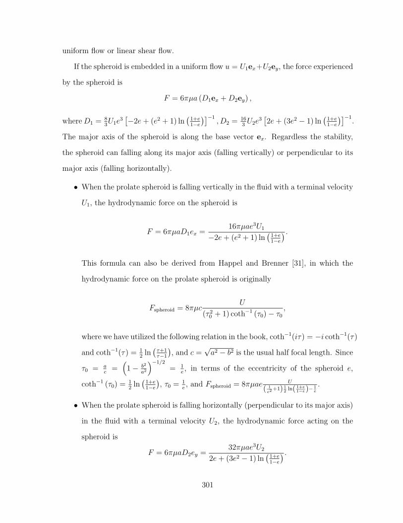
uniform flow or linear shear flow.

If the spheroid is embedded in a uniform flow u = U1ex+U2ey, the force experienced

by the spheroid is

F = 6πµa (D1ex +D2ey) ,

whereD1 = 83U1e

3[−2e+ (e2 + 1) ln

(1+e1−e

)]−1, D2 = 16

3U2e

3[2e+ (3e2 − 1) ln

(1+e1−e

)]−1.

The major axis of the spheroid is along the base vector ex. Regardless the stability,

the spheroid can falling along its major axis (falling vertically) or perpendicular to its

major axis (falling horizontally).

• When the prolate spheroid is falling vertically in the fluid with a terminal velocity

U1, the hydrodynamic force on the spheroid is

F = 6πµaD1ex =16πµae3U1

−2e+ (e2 + 1) ln(

1+e1−e

) .This formula can also be derived from Happel and Brenner [31], in which the

hydrodynamic force on the prolate spheroid is originally

Fspheroid = 8πµcU

(τ 20 + 1) coth−1 (τ0)− τ0

,

where we have utilized the following relation in the book, coth−1(iτ) = −i coth−1(τ)

and coth−1(τ) = 12

ln(τ+1τ−1

), and c =

√a2 − b2 is the usual half focal length. Since

τ0 = ac

=(

1− b2

a2

)−1/2

= 1e, in terms of the eccentricity of the spheroid e,

coth−1 (τ0) = 12

ln(

1+e1−e

), τ0 = 1

e, and Fspheroid = 8πµae U

( 1e2

+1) 12

ln( 1+e1−e)−

1e

.

• When the prolate spheroid is falling horizontally (perpendicular to its major axis)

in the fluid with a terminal velocity U2, the hydrodynamic force acting on the

spheroid is

F = 6πµaD2ey =32πµae3U2

2e+ (3e2 − 1) ln(

1+e1−e

) .301

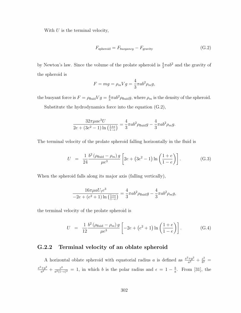
With U is the terminal velocity,

Fspheroid = Fbuoyancy − Fgravity (G.2)

by Newton’s law. Since the volume of the prolate spheroid is 43πab2 and the gravity of

the spheroid is

F = mg = ρmV g =4

3πab2ρmg,

the buoyant force is F = ρfluidV g = 43πab2ρfluidg, where ρm is the density of the spheroid.

Substitute the hydrodynamics force into the equation (G.2),

32πµae3U

2e+ (3e2 − 1) ln(

1+e1−e

) =4

3πab2ρfluidg −

4

3πab2ρmg.

The terminal velocity of the prolate spheroid falling horizontally in the fluid is

U =1

24

b2 (ρfluid − ρm) g

µe3

[2e+

(3e2 − 1

)ln

(1 + e

1− e

)]. (G.3)

When the spheroid falls along its major axis (falling vertically),

16πµaU1e3

−2e+ (e2 + 1) ln(

1+e1−e

) =4

3πab2ρfluidg −

4

3πab2ρmg,

the terminal velocity of the prolate spheroid is

U =1

12

b2 (ρfluid − ρm) g

µe3

[−2e+

(e2 + 1

)ln

(1 + e

1− e

)]. (G.4)

G.2.2 Terminal velocity of an oblate spheroid

A horizontal oblate spheroid with equatorial radius a is defined as x2+y2

a2 + z2

b2=

x2+y2

a2 + z2

a2(1−ε)2 = 1, in which b is the polar radius and ε = 1 − ba. From [31], the

302

hydrodynamic force exerted by the fluid on an oblate spheroid falling along its minor

axis (horizontal oblate spheroid) is

Fz = − 6πµaU34

√λ2 + 1 [λ− (λ2 − 1) cot−1(λ)]

= −6πµaUK,

where

K =1

34

√λ2 + 1 [λ− (λ2 − 1) cot−1(λ)]

and λ =b√

a2 − b2.

Using Newton’s law

6πµaUK =4

3πa2bρfluidg −

4

3πa2bρmg,

the terminal velocity U is

U =43πa2bρfluidg − 4

3πa2bρmg

6πµaK=

2

9

ab (ρfluid − ρm) g

µK=

2

9

(ρfluid − ρm) g

µf0(a, b), (G.5)

and f0(a, b) = 34

a2b√a2−b2

(b√

a2−b2 −(

b2

a2−b2 − 1)

arccot(

b√a2−b2

))The terminal velocity for a prolate and oblate spheroid falling in a fluid can also be

derived from the exact velocity field and the force on the object in [67].

G.3 Terminal velocity of a slender body

When a cylindrical slender rod with radius r and length 2` falls in a viscous flow, the

hydrodynamics force acting on the body is computed based on the slender body theory.

By the slender body theory, Stokeslets are uniformly distributed on the centerline, and

the strength is determined by the no-slip boundary condition to construct the velocity.

Once the strength is known, the hydrodynamic force can be computed based on the

strength. When the slender rod reaches its terminal velocity U , the body can fall

horizontally (perpendicular to its axis) or fall vertically (along it axis), which is an

303

unstable case.

If the density of rod is ρm, the volume of the cylindrical slender rod is Volrod = 2πr2`.

The weight of the body is

Fg = mg = ρmV g = 2ρmπr2`g,

and the buoyant force is

Fb = ρfluidV g = 2πr2Lρfluidg.

Falling horizontally If the slender rod is falling horizontally with the terminal ve-

locity U , then the strength of the Stokeslets along its centerline is α = (0, 0, α3) and

α3 =εU

2, where ε =

1

log(

2δ

) =1

log(

2`r

) .The hydrodynamics force at each point of the centerline of rod is

f = 8πµα3δ(x) = 4πµεUδ(x).

Since the Stokeslet is uniformly distributed on the rod, the total hydrodynamic force

on the rod is

Fh =

∫ `

−`4πµεWds = 8πµε`U.

By Newton’s’ law, the buoyant force acting on the body and the force due to gravity

are balanced with the hydrodynamic force Fb − Fg = Fh, i.e.,

2πr2`ρfluidg − 2ρmπr2`g = 8πµε`W.

304

The terminal velocity of a slender body falling horizontally is

W =(ρfluid − ρm) r2g

4µε=

(ρfluid − ρm) r2g

4log

(2`

r

).

Falling vertically If the slender rod is falling vertically with the terminal velocity

W , then the strength of the Stokeslet along its centerline is

α = (0, 0, α3) and α3 =εW

4, where ε =

1

log(

2δ

) =1

log(

2`r

) .The hydrodynamics force at each point of the centerline of rod is f = 8πµα3δ(x) =

2πµεWδ(x). Since the Stokeslet is uniformly distributed on the rod, the total hydro-

dynamic force on the rod is

Fh =

∫ `

−`2πµεWds = 4πµε`W.

By Newton’s’ law, the forces exerted on the body are balanced

2πr2`ρfluidg − 2ρmπr2`g = 4πµεW.

So,

W =(ρfluid − ρm) r2g

2µε=

(ρfluid − ρm) r2g

2log

(2`

r

).

In summary,

• If the slender rod is falling horizontally, the terminal velocity is

U =(ρfluid − ρm) r2g

4µlog

(2`

r

). (G.6)

305

• If the slender rod is falling vertically, the terminal velocity is

U =(ρfluid − ρm) r2g

2µlog

(2`

r

). (G.7)

Notice the ratio 2 for the different orientations.

G.4 A sphere vs a spheroid

G.4.1 A sphere with half mass vs a spheroid

To compare the terminal velocity of the a sphere with a spheroid, we first check the

terminal velocity of a sphere with half the mass of a spheroid. Then, the relation of

the body volumes is 43πa2b = 24

3πR3, or R = 3

√a2b2. From (G.1), the terminal velocity

of the sphere with radius R = 3

√a2b2

is

U∞ =2

9

R2 (ρfluid − ρm) g

µ=

2

9

(ρfluid − ρm) g

µ

(3

√a2b

2

)2

. (G.8)

The terminal velocity for a prolate spheroid is (G.3)-(G.4), and (G.5) for an oblate

spheroid.

Figure G.1 shows the terminal velocity of horizontal oblate spheroid and half mass

sphere R in terms of a and b, when a = 1 is fixed.

G.4.2 A sphere vs an oblate spheroid

Comparison of a sphere with a horizontal oblate spheroid

If the sphere has half mass of the horizontal oblate spheroid, then 43πa2b = 24

3πR3.

R = 3

√a2b2

, b = 2R3

a2 , or a =√

2R3

b. Under this condition, the terminal velocity of sphere

306

0.2 0.4 0.6 0.8 1.0b

0.2

0.4

0.6

0.8

1.0

1.2

Spheroid

Sphere

Figure G.1: Comparison of terminal velocity of a sphere in (G.8) with the terminal ve-

locity of a horizontal oblate spheroid (G.5) when the radius of the sphere R =

(3

√a2b2

)2

and the semimajor axis of the spheroid a = 1.

is

U∞ =2

9

(ρfluid − ρm) g

µR2,

and the terminal velocity of spheroid is

U =2

9

ab (ρfluid − ρm) g

µK=

2

9

(ρfluid − ρm) g

µ

√2R3b

K,

where K = 134

√λ2+1[λ−(λ2−1) cot−1(λ)]

and λ = b√a2−b2 . The ratio the terminal velocity of

the terminal velocity of the spheroid

the terminal velocity of a sphere=

2R

aK=

√2Rb

KR.

Ratio in terms of R and b Substitute a =√

2R3

b> b (b < 3

√2) into the terminal

velocity and define the ratio as a function fb(R, b),

fb(R, b) ≡√

2Rb

RK(G.9)

=3

4

√2b

R

√b2

2R3

b− b2

+ 1

b√2R3

b− b2

−

(b2

2R3

b− b2

− 1

)arccot

b√2R3

b− b2

,

307

0.002 0.004 0.006 0.008 0.010b

0.05

0.10

0.15

fb

Figure G.2: The ratio of terminal velocities fb(1, b) in (G.9) with a =√

2R3

band R = 1.

where

K =1(

34

√b2

2R3

b−b2

+ 1

(bq

2R3

b−b2−(

b2

2R3

b−b2− 1

)arccot

(bq

2R3

b−b2

))) .

Figure G.2 shows the coefficient fb(R, b) where R = 1 (0 < b < 3√

2). When fb(R, b) = 1,

the sphere and the horizontal oblate spheroid fall with the same terminal velocities.

Ratio in terms of R and a Define the ratio of the terminal velocities as fa(R, a), a

function of R and a. Since b = 2R3

a2 < a, the range of a is a > 3√

2,

K =1

34

√λ2 + 1 [λ− (λ2 − 1) cot−1(λ)]

, and λ =2R3

√a6 − 4R6

,

fa(R, a) =2R

aK(G.10)

=3R3

2a

√a6

a6 − 4R6

(2R3

√a6 − 4R6

−(

4R6

a6 − 4R6− 1

)arccot

(2R3

√a6 − 4R6

))

Figure G.3 shows the ratio fa(R, a) with R = 1 as a > 3√

2.

308

2 4 6 8 10 12 14a

1

2

3

4

5fa

Figure G.3: Ratio fa(1, a) in (G.10) with b = 2R3

a2 and R = 1.

Horizontal n-body oblate spheroid vs a sphere

If the polar radius of the oblate spheroid b (b < a) is fixed as the radius of the

sphere R, and the mass of the spheroid is n times the mass of the sphere, then 43πa2b =

43πa2R = n4

3πR3. So,

a2 = nR2, R =a√n

and a =√nR.

Substitute b = R and a =√nR into the terminal velocity formula. Since K =

134

√λ2+1[λ−(λ2−1) cot−1(λ)]

and λ = b√a2−b2 ,

K =4

3√

nn−1

(1√n−1

+(n−2)arccot

“1√n−1

”n−1

) and λ =1√n− 1

.

Thus,

U =2

9

ab (ρfluid − ρm) g

µK(G.11)

=2

9

√nR2 (ρfluid − ρm) g

µ

3

4

√n

n− 1

1√n− 1

+(n− 2)arccot

(1√n−1

)n− 1

The terminal velocity of the sphere is U∞ = 2

9(ρfluid−ρm)g

µR2.

309

To compare the terminal velocities, we check the ratio of U∞ of the sphere over the

terminal velocity in (G.11).

fns(n) =

29

√nR2(ρfluid−ρm)g

µ34

√nn−1

(1√n−1

+ n−2n−1

arccot(

1√n−1

))29

(ρfluid−ρm)gµ

R2

=3√n

4

√n

n− 1

(1√n− 1

+n− 2

n− 1arccot

(1√n− 1

)).

As n→∞,

fns(n) ∼ 3π

8

√n− 3

16π

1√n

+1

n− 27

64π

(1

n

)3/2

+8

5

(1

n

)2

+O

((1

n

)5/2).

G.4.3 A sphere vs a prolate spheroid

If the sphere has the same equatorial radius b of a prolate spheroid, the terminal

velocity of sphere is

U∞ =2

9

b2 (ρfluid − ρm) g

µ.

The terminal velocity for a horizontally falling prolate spheroid is

Uh =1

24

b2 (ρfluid − ρm) g

µ

[2e+ (3e2 − 1) ln

(1+e1−e

)]e3

. (G.12)

The terminal velocity for a vertically falling prolate spheroid is

Uv =1

12

b2 (ρfluid − ρm) g

µ

[−2e+ (e2 + 1) ln

(1+e1−e

)]e3

. (G.13)

N-body If the prolate spheroid x2

a2 + y2+z2

b2= 1 weights n times of the sphere and

b = R is the radius of the sphere,

4

3πab2 =

4

3πaR2 = n

4

3πR3, a = nR.

310

The eccentricity of the spheroid is

e =c

a=

√a2 − b2

a=

√a2 −R2

a=

√1− 1

n2.

We call such a spheroid a n-body spheroid.

For a horizontally falling n-body spheroid, the terminal velocity is

Uh =2

9

R2 (ρfluid − ρm) g

µ

3

8

√1− 1

n2 +(2− 3

n2

)log(n+√−1 + n2

)(1− 1

n2

)3/2.

For a vertically falling n-body spheroid, the terminal velocity is

Uv =2

9

R2 (ρfluid − ρm) g

µ

3

4

−√

1− 1n2 +

(2− 1

n2

)log(n+√n2 − 1

)(1− 1

n2

)3/2.

The ratio of terminal velocity of the n-body spheroid over the terminal velocity of the

sphere are

UhUs

=3

8

√1− 1

n2 +(2− 3

n2

)log(n+√−1 + n2

)(1− 1

n2

)3/2, (G.14)

UvUs

=3

4

−√

1− 1n2 +

(2− 1

n2

)log(n+√n2 − 1

)(1− 1

n2

)3/2. (G.15)

As n→∞,

UhUs

∼ 3

8(2 log(n) + 1 + 2 log(2)) +

3

16

(1

n

)2

+O

((1

n

)1/3),

UvUs∼ 3

4(2 log(n)− 1 + 2 log(2)) +

3

8(−3 + 4 log(2) + 4 log(n))

(1

n

)2

+O

((1

n

)1/3).

311

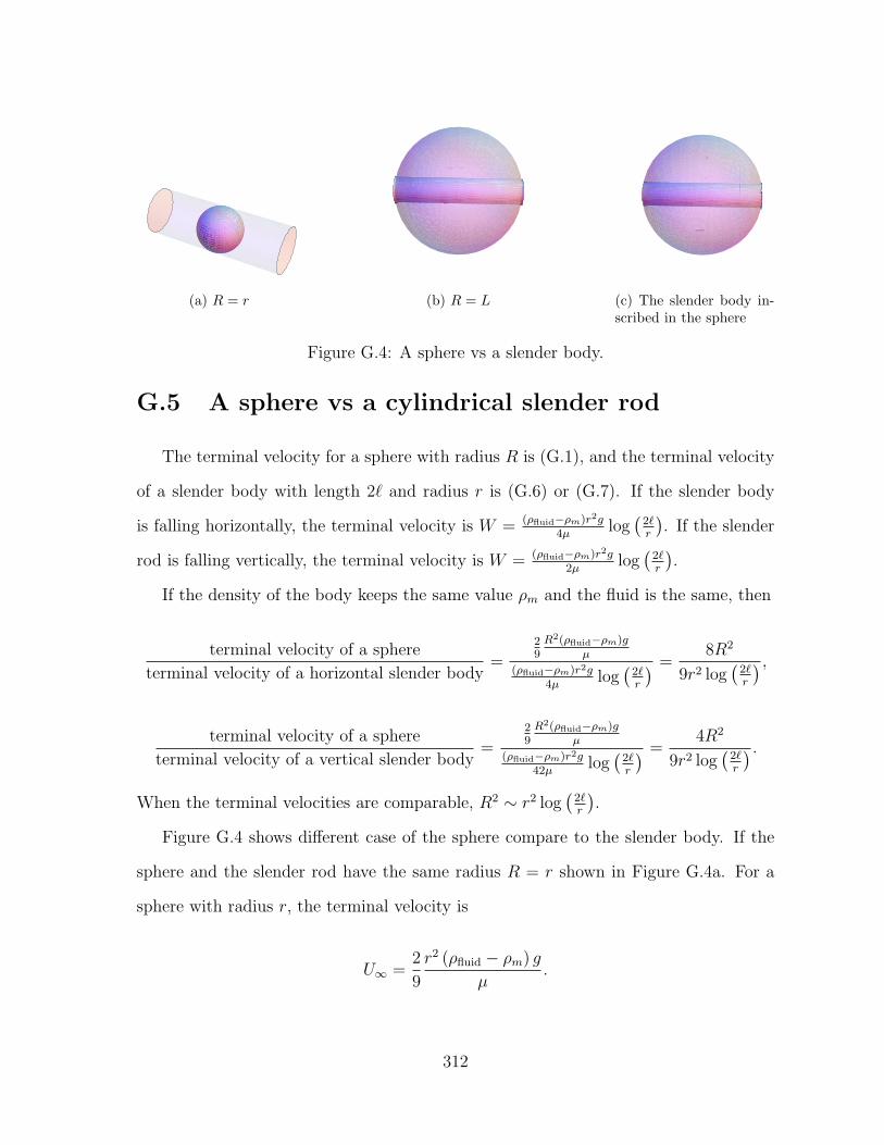
(a) R = r (b) R = L (c) The slender body in-scribed in the sphere

Figure G.4: A sphere vs a slender body.

G.5 A sphere vs a cylindrical slender rod

The terminal velocity for a sphere with radius R is (G.1), and the terminal velocity

of a slender body with length 2` and radius r is (G.6) or (G.7). If the slender body

is falling horizontally, the terminal velocity is W = (ρfluid−ρm)r2g4µ

log(

2`r

). If the slender

rod is falling vertically, the terminal velocity is W = (ρfluid−ρm)r2g2µ

log(

2`r

).

If the density of the body keeps the same value ρm and the fluid is the same, then

terminal velocity of a sphere

terminal velocity of a horizontal slender body=

29R2(ρfluid−ρm)g

µ

(ρfluid−ρm)r2g4µ

log(

2`r

) =8R2

9r2 log(

2`r

) ,terminal velocity of a sphere

terminal velocity of a vertical slender body=

29R2(ρfluid−ρm)g

µ

(ρfluid−ρm)r2g42µ

log(

2`r

) =4R2

9r2 log(

2`r

) .When the terminal velocities are comparable, R2 ∼ r2 log

(2`r

).

Figure G.4 shows different case of the sphere compare to the slender body. If the

sphere and the slender rod have the same radius R = r shown in Figure G.4a. For a

sphere with radius r, the terminal velocity is

U∞ =2

9

r2 (ρfluid − ρm) g

µ.

312

When the radius of the sphere equals to the half length of the slender body R = `

as shown in Figure G.4b, the terminal velocity of the sphere is

U∞ =2

9

`2 (ρfluid − ρm) g

µ.

When the slender body is inscribed in the sphere, R2 = `2 + r2 see Figure G.4c.

The terminal velocity of the sphere in terms of the dimensions of the slender body is

U∞ =2

9

(ρfluid − ρm) g

µ

(`2 + r2

).

G.6 Terminal velocity of two spheres

Stimson and Jeffery [71] first derived the stream function for axisymmetric flow past

two two solid spheres (equal or unequal) moving with equal small constant velocities

parallel to their line of centers, and calculated the forces acting on the spheres as an

infinite sum. Here we summarize the result using singularity method and method of

reflections from [41].

G.6.1 Two widely separated spheres

We take two non-rotating spheres’ centered at x1and x2, with radii a and b and

translational velocity U1 and U2, respectively [41]. The zeroth order solution is simply

the Stokes solution for the disturbance caused by an isolated, translating sphere in a

uniform stream. Thus, we have the velocity for both spheres

v1 = −F (0)1 ·

1 +

a2

6∆

G (x− x1)

8πµ,

v2 = −F (0)2 ·

1 +

b2

6∆

G (x− x2)

8πµ

313

with F(0)1 = 6πµa (U∞ − U1), T

(0)1 = 0, and S

(0)1 = 0. A similar set of results for sphere

2, F(0)2 = 6πµb (U∞ − U2), T

(0)2 = 0, S

(0)2 = 0.

By the method of reflections, the force exerted on sphere with radius a at x1 is

F1 = F(0)1 ·

[(1 +

9

4β( aR

)2

−(

3β

2+

81β2

16+

3β3

4

)( aR

)4)

dd

+

(1 +

9

4β( aR

)2

+

(3β

8− 81β2

256+

3β3

16

)( aR

)4)

(δ − dd)

]+F

(0)2 ·

[(−3

2

a

R+

1

2

(1− 27β

4+ β2

)( aR

)3)

dd

+

(3

4

a

R+

1

4

(1 +

27β

16+ β2

)( aR

)3)

(δ − dd)

],

where d denotes the unit vector (x2−x1)|x2−x1| and β = b

ais the ratio of sphere radii. The force

is accurate to O (R4).

The force on the other sphere with radius b at x2 is

F2 = F(0)2 ·

[(1 +

9

4β

(b

R

)2

−(

3β

2+

81β2

16+

3β3

4

)(b

R

)4)

dd

+

(1 +

9

4β

(b

R

)2

+

(3β

8− 81β2

256+

3β3

16

)(b

R

)4)

(δ − dd)

]

+F(0)1 ·

[(−3

2

b

R+

1

2

(1− 27β

4+ β2

)(b

R

)3)

dd

+

(3

4

b

R+

1

4

(1 +

27β

16+ β2

)(b

R

)3)

(δ − dd)

],

where d denotes the unit vector (x1−x2)|x1−x2| and β = a

bis the other ratio of sphere radii.

314

G.6.2 Two equal spheres

For two equal spheres, a = b and β = 1. If the flow at infinite is at rest

U∞ = 0, F(0)1 = 6πµa (−U1) ,

F(0)2 = 6πµa (−U2) .

The force on sphere is

F1 = −6πµaU2 ·[(−3

2

a

R− 19

8

( aR

)3)

dd −(

3

4

a

R+

59

64

( aR

)3)

(δ − dd)

](G.16)

−6πµaU1 ·[(

1 +9

4

( aR

)2

− 117

16

( aR

)4)

dd

+

(1 +

9

4

( aR

)2

+63

256

( aR

)4)

(δ − dd)

].

Parallel to each other If the two spheres are parallel to each other as they are falling

with the velocity U1 and U2, the unit vector d = (x2−x1)|x2−x1| = (1, 0, 0) and δ involved in Fi

is δij. From (G.16), the force on the sphere is

F1 = −6πµaU1 ·[(

1 +9

4

( aR

)2

+63

256

( aR

)4)δ

]+ 6πµaU2 ·

[(3

4

a

R+

59

64

( aR

)3)δ

].

Especially, the hydrodynamic force in the vertical direction to determine the termi-

nal velocity is interested, which is

F1 = −6πµa

(1 +

9

4

( aR

)2

+63

256

( aR

)4)U1 + 6πµa

(3

4

a

R+

59

64

( aR

)3)U2.

For the other sphere, the force is

F2 = −6πµa

(1 +

9

4

( aR

)2

+63

256

( aR

)4)U2 + 6πµa

(3

4

a

R+

59

64

( aR

)3)U1.

315

When the spheres reach their terminal velocity, U1 = U2. Otherwise, the distance

between them will change. Consequently, the force will is changed. When U1 = U2, the

hydrodynamic force is balanced with the buoyant force and the force due to gravity,

6πµa

(1 +

9

4

( aR

)2

+63

256

( aR

)4)U − 6πµa

(3

4

a

R+

59

64

( aR

)3)U

=4

3πa3ρfluidg −

4

3πa3ρmg.

So, the terminal velocity of the sphere is

U =2

9

a2g (ρfluid − ρm)

µ

256

(256− 192s+ 576s2 − 236s3 + 63s4)=

2

9

a2g (ρfluid − ρm)

µf1(s),

(G.17)

where s = aR

, a is the radius of the sphere, and R is distance between the centers of

two spheres.

Two spheres as a sequence If the two spheres are falling as a sequence, then the

unit vector d = (x2−x1)|x2−x1| = (0, 0, 1). The force exerted on sphere 1 is

F1 = −6πµa

(−3

2

a

R− 19

8

( aR

)3)U2 + 6πµaU2 ·

(3

4

a

R+

59

64

( aR

)3)

(δ − dd)

−6πµa

(1 +

9

4

( aR

)2

− 117

16

( aR

)4)U1

−6πµaU1 ·(

1 +9

4

( aR

)2

+63

256

( aR

)4)

(δ − dd).

The force in the vertical direction to determine the terminal velocity is

F1 = −6πµa

(1 +

9

4

( aR

)2

− 117

16

( aR

)4)U1 + 6πµa

(3

2

a

R+

19

8

( aR

)3)U2.

Similar results are hold for the other sphere.

316

0.0 0.1 0.2 0.3 0.4 0.5

1.0

1.5

2.0

2.5

3.0

f2HsL

f1HsL

Single Sphere

Figure G.5: Coefficients in the terminal velocities of one single sphere vs two spheres.

For the terminal velocity, U1 = U2. Balance the forces,

6πµa

(1 +

9

4

( aR

)2

− 117

16

( aR

)4)U + 6πµa

(−3

2

a

R− 19

8

( aR

)3)U

=4

3πa3ρfluidg −

4

3πa3ρmg.

The terminal velocity of the sphere is

U =2

9

a2g (ρfluid − ρm)

µ

16

(16− 24s+ 36s2 − 38s3 − 117s4)=

2

9

a2g (ρfluid − ρm)

µf2(s).

(G.18)

where s = aR

.

For a single rigid sphere falling in the Stokes flow, the terminal velocity is U =

29a2g(ρfluid−ρm)

µ, where a is the radius of the sphere and ρm is the density of the sphere.

Figure G.5 shows the coefficients in the terminal velocities for a single sphere and

two-sphere cases.

G.7 Two unequal spheres

When the two unequal spheres fall in the Stoke flow, we take two non-rotating

spheres’ centered at x1 and x2, with radii a and b and translational velocity U1 and

U2 respectively.

317

G.7.1 Two spheres as a sequence

If the two sphere are not equal and falling as a sequence one after the other, the

sphere with radius a at x1 =

(0 0 z1

)twith a uniform velocity

(0 0 −U1

)t,

the other sphere with radius b at x2 =

(0 0 z2

)twith the uniform velocity(

0 0 −U2

)tCompute the force on sphere a: d = (x2−x1)

|x2−x1| = (0, 0,−1) and β = ba.

dd =

0

0

−1

(0, 0,−1) =

0 0 0

0 0 0

0 0 1

, (δ − dd) =

1 0 0

0 1 0

0 0 0

F1 = 6πµa(−

U1

).

[(1 +

9

4

b

a

( aR

)2

−

(3 ba

2+

81(ba

)2

16+

3(ba

)3

4

)( aR

)4)

dd

+

(1 +

9

4

b

a

( aR

)2

+

(3 ba

8−

81(ba

)2

256+

3(ba

)3

16

)( aR

)4)

(δ − dd)

]

+6πµb(−

U2

).

[(−3

2

a

R+

1

2

(1−

27 ba

4+

(b

a

)2)( a

R

)3)

dd

+

(3

4

a

R+

1

4

(1 +

27 ba

16+

(b

a

)2)( a

R

)3)

(δ − dd)

]

= 6πµa

(1 +

9

4

b

a

( aR

)2

−(

3b

2a+

81b2

16a2+

3b3

4a3

)( aR

)4)

0

0

U1

+6πµb

(−3

2

a

R+

1

2

(1− 27b

4a+

(b

a

)2)( a

R

)3)

0

0

U2

.

318

Similarly, the force on sphere with radius b and velocity U2 is

F2 = 6πµb

(1 +

9

4

a

b

(b

R

)2

−(

3a

2b+

81a2

16b2+

3a3

4b3

)(b

R

)4)

0

0

U2

+6πµa

(−3

2

b

R+

1

2

(1− 27a

4b+(ab

)2)(

b

R

)3)

0

0

U1

.

The force in vertical direction is

F1 = 6πµa

(1 +

9

4

b

a

( aR

)2

−(

3b

2a+

81b2

16a2+

3b3

4a3

)( aR

)4)U1

+6πµb

(−3

2

a

R+

1

2

(1− 27b

4a+

(b

a

)2)( a

R

)3)U2

F2 = 6πµb

(1 +

9

4

a

b

(b

R

)2

−(

3a

2b+

81a2

16b2+

3a3

4b3

)(b

R

)4)U2

+6πµa

(−3

2

b

R+

1

2

(1− 27a

4b+(ab

)2)(

b

R

)3)U1

So, the velocities of the spheres satisfy the following equations,

6πµa

(1 +

9

4

b

a

( aR

)2

−(

3b

2a+

81b2

16a2+

3b3

4a3

)( aR

)4)U1 (G.19)

+6πµb

(−3

2

a

R+

1

2

(1− 27b

4a+

(b

a

)2)( a

R

)3)U2 =

4

3πa3ρfluidg −

4

3πa3ρmg

6πµb

(1 +

9

4

a

b

(b

R

)2

−(

3a

2b+

81a2

16b2+

3a3

4b3

)(b

R

)4)U2 (G.20)

+6πµa

(−3

2

b

R+

1

2

(1− 27a

4b+(ab

)2)(

b

R

)3)U1 =

4

3πb3ρfluidg −

4

3πb3ρmg

319

If both spheres reach the terminal velocity, then U1 = U2 = U ,

6πµ

[a

(1 +

9

4

b

a

( aR

)2

−(

3b

2a+

81b2

16a2+

3b3

4a3

)( aR

)4)

+

b

(−3

2

a

R+

1

2

(1− 27b

4a+

(b

a

)2)( a

R

)3)]

U

=4

3πa3ρfluidg −

4

3πa3ρmg,

6πµ

[b

(1 +

9

4

a

b

(b

R

)2

−(

3a

2b+

81a2

16b2+

3a3

4b3

)(b

R

)4)

+

a

(−3

2

b

R+

1

2

(1− 27a

4b+(ab

)2)(

b

R

)3)]

U

=4

3πb3ρfluidg −

4

3πb3ρmg

The terminal velocity

U =2

9

g (ρfluid − ρm)

µ

a3

a(

1 + 94ba

(aR

)2 −(

3b2a

+ 81b2

16a2 + 3b3

4a3

) (aR

)4)

+ b(−3

2aR

+ 12

(1− 27b

4a+(ba

)2) (

aR

)3)

U =2

9

g (ρfluid − ρm)

µ

b3

b(

1 + 94ab

(bR

)2 −(

3a2b

+ 81a2

16b2+ 3a3

4b3

) (bR

)4)

+ a(−3

2bR

+ 12

(1− 27a

4b+(ab

)2) (

bR

)3)

To reach the terminal velocity, the following condition need to be satisfied

a3

a(

1 + 94ba

(aR

)2 −(

3b2a

+ 81b2

16a2 + 3b3

4a3

) (aR

)4)

+ b(−3

2aR

+ 12

(1− 27b

4a+(ba

)2) (

aR

)3)(G.21)

=b3

b(

1 + 94ab

(bR

)2 −(

3a2b

+ 81a2

16b2+ 3a3

4b3

) (bR

)4)

+ a(−3

2bR

+ 12

(1− 27a

4b+(ab

)2) (

bR

)3) .

320

G.7.2 Numerical results for two spheres falling one after the

other

Both spheres are released from rest and have same density. For all numerical results,

the viscosity is chosen as 9.29 Pa·s. The density of fluid is 1 g/ml and the density of

sphere is 1.2 g/ml. The velocities of the spheres are computed from the coupled velocity

field equation (G.19)-(G.20).

For two equal spheres, take the radius r = a = b = 0.25. One sphere is located at

(0, 0, 0), the other at (0, 0,−1). The distance between the centers of spheres over time

t is a constant as the initial value.

For two unequal sphere, the small sphere with radius a = 0.2 is located at (0, 0, 0)

above the large one, whose radius is b = 0.5 and initially at (0, 0,−1). The distance

between centers of two spheres d is shown in figure G.6, which monotonically increases

over time. From (G.21), the equilibrium distance for two sphere with radius a = 0.5 and

b = 0.2 is d = 0.84133. If the initial distance between the two spheres is smaller than the

equilibrium distance, the smaller sphere will catch the larger one, which invalidates the

velocity equations (G.19)-(G.20) beyond a certain distance. More information about

the hydrodynamic force on the small sphere is documented at the end of this appendix.

If the small sphere with radius a = 0.2 is located at (0, 0,−1) below the other large

sphere with radius b = 0.5 at (0, 0, 0), the distance between centers of two spheres d

is shown in figure G.7. From this numerical result, we see the distance decreases and

converges to a finite value with a small gap between the spheres.

Figure G.8 shows the result for the same spheres but the initial distance is smaller

than the equilibrium distance, we see that the distance still converges.

321

1000 2000 3000 4000t

1.5

2.0

2.5

3.0

d

Figure G.6: The distance between cen-ters of two unequal spheres while the smallsphere above the large sphere.

500 1000 1500 2000 2500 3000t

0.85

0.90

0.95

1.00

d

Figure G.7: The distance between cen-ters of two unequal spheres while the smallsphere below the large sphere.

500 1000 1500 2000 2500 3000t

0.832

0.834

0.836

0.838

0.840

d

Figure G.8: Similar to Figure G.7 with a different initial distance.

322

G.7.3 Hydrodynamic force on a small sphere in flow induced

by a sphere moving uniformly

For a rigid sphere moving in Stokes flow, the induced velocity field is [4]

u = U

(1

r

df

dr

)+ x

x · Ur2

(2f

r2− 1

r

df

dr

),

where f = r2(

34ar− 1

4a3

r3

). In the moving frame [19], the velocity field is

u = Uex −3a

4

(U

r+ x

x · Ur3

)+a3

4x

x · Ur2∇(∇ · U

r

).

Rewrite the velocity vector in components format

u(x, y, z, a, U) = U +a3U (2x2 − y2 − z2)

4 (x2 + y2 + z2)5/2− 3

4a

(Ux2

(x2 + y2 + z2)3/2+

U√x2 + y2 + z2

),

v(x, y, z, a, U) =3a3Uxy

4 (x2 + y2 + z2)5/2− 3aUxy

4 (x2 + y2 + z2)3/2,

w(x, y, z, a, U) =3a3Uxz

4 (x2 + y2 + z2)5/2− 3aUxz

4 (x2 + y2 + z2)3/2.

Faxen correction of the drag on a small sphere with radius b on the center line (the

x-axis) is

F = 6πµb

(u+

1

6b2∆u

).

Fx = 6πµb

(U +

a3U

2 (x2)3/2− 3

2

aU√x2

+1

6b2 3aU

(x2)3/2

)

323

u(x, 0, 0, a, U) = U +a3U

2 (x2)3/2− 3

2

aU√x2

∆u(x, 0, 0, a, U) =3aU

(x2)3/2> 0, for any x.

Drag in the x-direction is

Fx = 6πµb

(u(x, 0, 0, a, U) +

1

6b2∆u(x, 0, 0, a, U)

)= 6πµb

(U +

a3U

2 (x2)3/2− 3

2

aU√x2

+b2

6

3aU

(x2)3/2

).

Without Faxen correction,

Fx = 6πµb u(x, 0, 0, a, U) =3bπU

(a3 + 2 (x2)

3/2 − 3ax2)µ

(x2)3/2.

The conclusion is the drag on a sphere falling behind another one never change sign

and it will try to catch the other one. This does not explain all the phenomena in the

numerical results for two spheres falling one after the other, but sheds light on part of

the mechanics.

324

————————————————————————

325

Bibliography

[1] A. Acrivos. Heat transfer at high Peclet number from a small sphere freely rotatingin a simple shear field. J. Fluid Mech., 46:233–240, 1971.

[2] K. Bajer and H. K. Moffatt. On a class of steady confined Stokes flows with chaoticstreamlines. J. Fluid Mech., 212:337–363, 1990.

[3] G. K. Batchelor. Slender-body theory for particles of arbitrary cross-section inStokes flow. J. Fluid Mech., 44:419–440, 1970.

[4] G. K. Batchelor. Introduction to Fluid Mechanics. Cambridge University Press,1999.

[5] J. R. Blake. A note on the image system for a stokelet in a no-slip boundary.Proceedings of the cambridge philosophical society, 70:303–310, 1971.

[6] J. R. Blake and A. T. Chwang. Fundamental singularities of viscous-flow. part1. image systems in vicinity of a stationary no-slip boundary. J. Eng. Math.,8:2329, 1974.

[7] S. Blaser. Forces on the surface of small ellipsoidal particles immersed in a linearflow field. Chemical Engineering Science, 57:515–526, 2002.

[8] J. Bouguet. Complete Camera Calibration Toolbox for Matlab.

[9] E. L. Bouzarth, A. Brooks, R. Camassa, H. Jing, T. J. Leiterman, R. M. Mclaugh-lin, R. Superfine, J. Toledo, and L. Vicci. Epicyclic orbits in a viscous fluid abouta precessing rod: Theory and experiments at the micro- and macro-scales. Phys-ical Review E, 76(1), 2007.

[10] F. P. Bretherton. The motion of rigid particles in a shear flow at low reynoldsnumber. J. Fluid Mech., 14(2):284–304, 1962.

[11] F. P. Bretherton. Slow viscous motion round a cylinder in a simple shear. J. FluidMech., 12:591–613, 1962.

[12] J. Buceta, M. Ibanes, D. Rasskin-Gutman, Y. Okada, N. Hirokawa, and J. C.Izpisua-Belmonte. Nodal cilia dynamics and the specification of the left/rightaxis in early vertebrate embryo development. Biophys J. 2005 Oct;89(4):2199-209. Epub 2005 Jul 22., 89:2199–209, 2005.

[13] J. M. Burgers. On the motion of small particles of elongated form, suspended in aviscous fluid. Nordemann Publishing, New York, 1938.

326

[14] R. Camassa, T. J. Leiterman, and R. M. McLaughlin. Trajectory and flow prop-erties for a rod spinning in a viscous fluid. Part 1. An exact solution. J. FluidMech., 612:153–200, 2008.

[15] R. Camassa, R. M. McLaughlin, L. Vicci, L. Zhao, and etc. Feeding by symmetrybreaking: The role of bend in spinning cilia. Inpreparing, 2009.

[16] J. H. E. Cartwright, O. Piro, and I. Tuval. Fluid-dynamical basis of the embryonicdevelopment of left-right asymmetry in vertebrates. Proc. Natl. Acad. Sci. USA,101(19):7234–7239, May 2004.

[17] A. T. Chan and A. T. Chwang. The unsteady stokeslet and oseenlet. Proceed-ings of the Institution of Mechanical Engineers. Part C, Journal of mechanicalengineering science, 214:175–179, 2000.

[18] A. T. Chwang and T. Y. Wu. A note on the helical movement of micro-organisms. Proceedings of the Royal Society of London. Series B, BiologicalSciences, 178(1052):327–346, Auguest 1971.

[19] A. T. Chwang and T. Y. Wu. Hydromechanics of low-Reynolds-number flow. Part2. Singularity method for Stokes flows. J. Fluid Mech., 67:787–815, 1975.

[20] B. Clipp, D. Gallup, H. Towles, R. Kumar, and P. Lincoln. The synchronizedmulti-camera digital recorder (ladybugrecord). Private communications.

[21] R. G. Cox. The motion of long slender bodies in a viscous fluid Part1: Generaltheory. J. Fluid Mech., 44:791–810, 1970.

[22] R. G. Cox. The motion of long slender bodies in a viscous fluid. Part 2. shear flow.J. Fluid Mech., 45(4):625–657, 1971.

[23] R. G. Cox, Y. Z. Zia, and S. G. Mason. Particle motion in sheared suspensions.XXV. Streamline around cylinders and spheres. Journal of Colloid and InterfaceScience, 27:7–18, 1968.

[24] M. Van Dyke. Perturbation methods in fluid mechanics. Parabolic Press, annotateded edition, 1975.

[25] B. A. Evans, A. R. Shields, R. Lloyd Carroll, S. Washburn, M. R. Falvo, andR. Superfine. Magnetically actuated nanorod arrays as biomimetic cilia. NanoLetters, 7(5):1428–1435, 2007.

[26] L. J. Fauci and R. Dillon. Biofluidmechanics of reproduction. Annual Review ofFluid Mechanics, 38:371–394, January 2006.

[27] D. L. Feke and W. R. Schowalter. The effect of brownian diffusion on shear-inducedcoagulation of colloidal dispersions. Journal of Fluid Mechanics, 133:17–35,1983.

327

[28] G. R. Fulford and J. R. Blake. Muco-ciliary transport in the lung. Journal ofTheoretical Biology, 121(4):381–402, August 1986.

[29] Hiroshi Hamada. Breakthroughs and future challenges in leftright patterning.Develop. Growth Differ., 50:S71S78, 2008.

[30] G. J. Hancock. The self-propulsion of microscopic organisms through liquids. Proc.R. Soc. Lond. A, 217(1128):96–121, March 1953.

[31] J. Happel and H. Brenner. Low Reynolds Number Hydrodynamics: with specialapplications to particulate media. The Hague; Boston: M. Nijhoff; Hingham,MA, USA, 1991.

[32] Masakazu Hashimoto, Kyosuke Shinohara, Jianbo Wang, Shingo Ikeuchi, SatokoYoshiba, Chikara Meno, Shigenori Nonaka, Shinji Takada, Kohei Hatta, An-thony Wynshaw-Boris, and Hiroshi Hamada. Planar polarization of node cellsdetermines the rotational axis of node cilia. Nature Cell Biology, 12:170 – 176,2010.

[33] N. Hirokawa, Y. Tanaka, and Y. Okada. Left-right determination: Involvement ofmolecular motor kif3, cilia, and nodal flow. Cold Spring Harbor Perspectives inBiology, 1:1:a000802, 2009.

[34] N. Hirokawa, Y. Tanaka, Y. Okada, and S. Takeda. Nodal flow and the generationof left-right asymmetry. Cell, 125(1):33–45, 7 April 2006.

[35] D. Holz. Body tracking program. Private communications, 2009.

[36] G. B. Jeffery. The motion of ellipsoidal particles immersed in a viscous fluid.Proceedings of the Royal Society of London. Series A, Containing Papers of aMathematical and Physical Character, 102(715):161–179, 1922.

[37] D. J. Jeffrey and J. D. Sherwood. Streamline patterns and eddies in low Reynoldsnumber flow. J. Fluid Mech., 96:315334, 1980.

[38] R. E. Johnson. An improved slender-body theory for Stokes flow. J. Fluid Mech,99:411–431, 1980.

[39] J. B. Keller and S. I. Rubinow. Slender-body theory for slow viscous flow. J. FluidMech., 75(4):705–714, 1976.

[40] S. Kim. Singularity solutions for ellipsoids in Low-Reynolds-Number flows: withapplications to the calculation of hydrodynamic interactions in suspensions ofellipsoids. International journal of multiphase flow, 12(3):469–491, 1986.

[41] S. Kim and S. J. Karrila. Microhydrodynamics: Principles and Selected Applica-tions. Dover Publications, 2005.

328

[42] C. A. Kossack and A. Acrivos. Steady simple shear flow past a circular cylinder atmoderate Reynolds numbers: A numerical solution. J. Fluid Mech., 66:353–376,1974.

[43] H. K. Kuiken. H.A. Lorentz: Sketches of his work on slow viscous flow and someother areas in fluid mechanics and the background against which it arose. Journalof Engineering Mathematics, 30:1–18, 1996.

[44] S. H. Lamb. Hydrodynamic. Dover publications, 1945.

[45] L. G. Leal. Particle motions in a viscous fluid. Ann. Rev. Fluid Mech., 12:435–476,1980.

[46] L. G. Leal. Laminar Flow and Convective Transport Processes: Scaling Principlesand Asymptotic Analysis. Butterworth-Heinemann, June 1992.

[47] L. G. Leal. Advanced Transport Phenomena: Fluid Mechanics and ConvectiveTransport Processes. Cambridge University Press, 2007.

[48] T. J. Leiterman. Mixing properties of exact and asymptotic low Reynolds, time-varying solutions for spinning nano-rods and biological applications to ciliaryfunction. PhD thesis, the University of North Carolina at Chapel Hill, 2007.

[49] M. J. Lighthill. Contributions o the theory of the Pitot-tube displacement effect.J. Fluid Mech., 2:493–512, 1957.

[50] N. Liron. The LGL (Lighthill-Gueron-Liron) Theorem–historical perspective andcritique. Mathematical methods in the applied science, 24:1533–1540, 2001.

[51] H. A. Lorentz. Eene algemeene stelling omtrent de beweging eener vloeistof metwrijving en eenige daaruit afgeleide gevolgen. Zittingsverslag van de KoninklijkeAkademie van Wetenschappen te Amsterdam, 5:168–175, 1896.

[52] T. Ma and S. Wang. A generalized Poincare-Hopf index formula and its applica-tions to 2-D incompressible flows. Nonlinear Analysis:Real World Applications,1:467–482, 2001.

[53] F. O. Marques, R. Taborda, S. Bose, and J. Antunes. Effects of confinementon matrix flow around a rigid inclusion in viscous simple shear: insights fromanalogue and numerical modelling. Journal of structural geology, 27:379–396,2005.

[54] A. Mashayek and C. Pozrikidis. Motion of a spherical particle inside a liquid film.Acta Mech, 210:27–46, 2010.

[55] H. Matsui, S. H. Randell, S. W. Peretti, C. W. Davis, and R. C. Boucher. Coor-dinated clearance of periciliary liquid and mucus from airway surfaces. J ClinInvest., 102(6):1125–1131, September 15 1998.

329

[56] W. J. McKiver and D. G. Dritschel. The motion of a fluid ellipsoid in a generallinear background flow. J. Fluid Mech., 474:147–173, 2003.

[57] D. R. Mikulencak and J. F. Morris. Stationary shear flow around fixed and freebodies at finite Reynolds number. J. Fluid Mech., 520:215–242, 2004.

[58] S. Nonaka, Y. Tanaka, Y. Okada, S. Takeda, A. Harada, Y. Kanai, M. Kido, andN. Hirokawa. Randomization of left-right asymmetry due to loss of nodal ciliagenerating leftward flow of extraembryonic fluid in mice lacking KIF3B motorprotein. Cell, 95(6):829–837, December 1998.

[59] S. Nonaka, Y. Tanaka, Y. Okada, S. Takeda, A. Harada, Y. Kanai, M. Kido,and N. Hirokawa. Erratum: Randomization of left-right asymmetry due to lossof nodal cilia generating leftward flow of extraembryonic fluid in mice lackingKIF3B motor protein. Cell, 99(1):116, October 1 1999.

[60] C. W. Oseen. Neure methoden und ergebnisse in der hydrodynamik. in akad.verlagsgesellschaft. Leipzig:Akad. Verlagsgesellschaft, page 337, 1927.

[61] R. L. Panton. Incompressible flow. John Wiley & Sons, 1984.

[62] G. G. Poe and A. Acrivos. Closed streamline flows past rotating single cylindersand spheres: Inertia effects. J. Fluid Mech., 72:605, 1975.

[63] C. Pozrikidis. Introduction to theoretical and computational fluid dynamics. NewYork : Oxford University Press, 1997.

[64] T. C. Price. Slow linear shear flow past a hemispherical bump in a plane wall. Q.J. Mech. Appl. Math., 38(1):93–104, 1985.

[65] C. R. Robertson and A. Acrivos. Low Reynolds number shear flow past a rotatingcircular cylinder. Part 1. momentum transfer. J. Fluid Mech., 40:685, 1970.

[66] P. G. Saffman. The lift on a small sphere in a slow shear flow. J. Fluid Mech.,22:385–400, 1965.

[67] L. F. Shatz. Singularity method for oblate and prolate spheroids in Stokes andlinearized oscillatory flow. Phys. Fluids, 16(3):664–677, 2004.

[68] K. Shintani, A. Umenura, and A. Takano. Low-reynolds-number flow past anelliptic cylinder. J . Fluid Mech., 136:277–289, 1983.

[69] D. J. Smith, J. R. Blake, and E. A. Gaffney. Fluid mechanics of nodal flow dueto embryonic primary cilia. Journal of The Royal Society Interface, 5:567–573,2008.

[70] L. A. Spielman. Particle capture from low-speed laminar flows. Annual Review ofFluid Mechanics, 9:297–319, January 1977.

330

[71] M. Stimson and G. B. Jeffery. The motion of two spheres in a viscous fluid.Proceedings of the Royal Society of London. Series A, 111(757):110–116, May 11926.

[72] G. Subramanian and D. L. Koch. Inertial effects on the transfer of heat or massfrom neutrally buoyant spheres in a steady linear velocity field. Phys. Fluids,18(7):73302, 2006.

[73] R. M. Taylor. http://cismm.cs.unc.edu/downloads/. 2005.

[74] J. P. K. Tillett. Axial and transverse Stokes flow past slender axisymmetric bodies.J. Fluid Mech., 44(3):401–417, 1970.

[75] E. O. Tuck. Some methods for flows past blunt slender bodies. J. Fluid Mech.,18(4):619–635, 1964.

[76] K. C. Wang, H. C. Zhou, C. H. Hu, and S. Harrington. Three-dimensional sepa-rated flow structure over prolate spheroids. Proceedings of the Royal Society ofLondon. Series A, Mathematical and Physical Sciences, 421:73–91, 1990.

[77] M. C. T. Wilson, P. H. Gaskell, and M. D. Savage. Nested separatrices in simpleshear flows: The effect of localized disturbances on stagnation lines. Physics ofFluids, 17:093601, 2005.

331