NASA/TM-2005-213667

Shock Location Dominated Transonic Flight

Loads on the Active Aeroelastic Wing

William A. Lokos and Andrew Lizotte

NASA Dryden Flight Research Center

Edwards, California

Ned J. Lindsley

AFRL/VASD

Wright Patterson, Ohio

Rick Stauf

Spiral Technology, Inc.

Edwards, California

December 2005

NASA/TM-2005-213667

Shock Location Dominated Transonic Flight Loads on the Active Aeroelastic Wing

William A. Lokos and Andrew Lizotte NASA Dryden Flight Research CenterEdwards, California

Ned J. Lindsley AFRL/VASDWright Patterson, Ohio

Rick Stauf Spiral Technology, Inc.Edwards, California

December 2005

National Aeronautics andSpace Administration

Dryden Flight Research CenterEdwards, California 93523-0273

ABSTRACT

During several Active Aeroelastic Wing research flights, the shadow of the over-wing shock could beobserved because of natural lighting conditions. As the plane accelerated, the shock location moved aft,and as the shadow passed the aileron and trailing-edge flap hinge lines, their associated hinge momentswere substantially affected. The observation of the dominant effect of shock location on aft controlsurface hinge moments led to this investigation. This report investigates the effect of over-wing shocklocation on wing loads through flight-measured data and analytical predictions. Wing-root and wing-foldbending moment and torque and leading- and trailing-edge hinge moments have been measured in flightusing calibrated strain gages. These same loads have been predicted using a computational fluiddynamics code called the Euler Navier-Stokes Three Dimensional Aeroelastic Code. The computationalfluid dynamics study was based on the elastically deformed shape estimated by a twist model, which inturn was derived from in-flight-measured wing deflections provided by a flight deflection measurementsystem. During level transonic flight, the shock location dominated the wing trailing-edge control surfacehinge moments. The computational fluid dynamics analysis based on the shape provided by the flightdeflection measurement system produced very similar results and substantially correlated with themeasured loads data.

NOMENCLATURE

AAW Active Aeroelastic WingAIL aileron

C

D

coefficient of drag

C

L

coefficient of lift

C

m

coefficient of momentCFD computational fluid dynamics______-

cfd

loads calculated using computational fluid dynamicsCS control surfacedeg degreeENS3DAE Euler Navier-Stokes Three Dimensional Aeroelastic Code

F

x

longitudinal force, lb

F

y

lateral force, lb

F

z

normal force, lbFDMS flight deflection measurement system______-

flt

loads measured during flight______-

ib

control surface inboard position measured during flight, degILEF inboard leading-edge flapLAIL left aileronLAIL CR1 left aileron criticality ratio (percent of load limit), prime

2

LILEF left inboard leading-edge flap

LITEF CR1 left inboard trailing-edge flap criticality ratio (percent of load limit), prime

LOLEF left outboard leading-edge flap

LSTAB left stabilator (horizontal, “rolling” tail)

LTEF left trailing-edge flap

LWFBND

left wing-fold bending moment, in.-lb

LWFTRQ

left wing-fold torque, in.-lb

LWING left wing

LWRBND

left wing-root bending moment, in.-lb

LWRTRQ

left wing-root torque, in.-lb

M

Mach number

M

free-stream Mach number

______-

ob

control surface outboard position measured during flight, deg

OLEF outboard leading-edge flap

RAIL CR1 right aileron criticality ratio, prime

RITEF CR1 right inboard trailing-edge flap criticality ratio (percent of load limit), prime

TEF trailing-edge flap

X

c

longitudinal centroid location, in.

Y

c

lateral centroid location, in.

Z

c

vertical centroid location, in.

angle of attack, deg

INTRODUCTION

For over a decade it has been proposed that wing torsional flexibility could be used to aeroelasticallyenhance the roll maneuverability of a high performance aircraft. Although aeroelastic control behaviorrelated to aileron reversal has, as a rule, always been avoided even at the expense of additional structuralweight, it offers significant benefits when incorporated as a preprogrammed control mode. It has beenproposed that if the aeroelastic control paradigm was designed into a new airframe, then lighter weight,increased maneuverability, and other advantages could be exploited (refs. 1–3).

The early version of the F/A-18 aircraft had the potential for aileron reversal within its performanceenvelope. Production F/A-18 aircraft were built with stiffer wings to preclude this tendency and increaseroll performance through conventional wing control surface use (refs. 4, 5). The NASA ActiveAeroelastic Wing (AAW) F/A-18 aircraft (fig. 1) has been structurally modified to support aeroelasticflight control research. The aft wing box skins were replaced with more flexible panels to essentiallyreplicate the stiffness of the original preproduction F/A-18 aircraft. The aircraft was extensively

!

"

3

instrumented for this research effort, including the installation of numerous strain gage bridges,accelerometers, and control surface position transducers on the wings. A wing deflection measurementsystem was installed on the left wing to track elastic structural displacements. An over-the-wing videocamera provided real-time imagery of the upper surface of the left wing. Flight loads measured by thestrain gages were monitored in real time for flight safety.

EC02-0264-19

Figure 1. Active Aeroelastic Wing aircraft in flight.

When transonic conditions were experienced during the first flight block of the AAW (ref. 6), naturallighting conditions occasionally were such that the over-wing shock on the left wing was visible on thereal-time flight video image. As the Mach number changed, this shock wave translated across the wing.These natural shadowgraphs have been noticed by flyers since the 1940s (ref. 7). Two successive timesduring an observable shock wave occurrence, as the shock wave translated past a certain point on thewing, the trailing-edge hinge moments abruptly offset from their previous levels.

This report investigates these shock location dominated transonic flight loads. The measurement ofAAW flight loads, prediction of flight loads and shock locations, and natural flow visualization of theover-wing shock wave are discussed. Predicted and measured shock-induced loads are comparedand contrasted.

MEASUREMENTS AND OBSERVATIONS

The AAW project was designed with substantial load measurement features so that the full strengthenvelope of the test aircraft could be exploited. As significant aeroelastic behavior was targeted, real-timewing deflection measurement was planned. Many other research measurements were included.

4

Flight load measurement was accomplished through the use of 200 four-active-arm strain gagebridges installed on the test wings. These strain gages were calibrated through an extensive ground loadscalibration test (ref. 8). Twenty component load measurements (fig. 2) were measured on the AAW fromthe installed strain gages and the application of the corresponding load equations. During the AAW flighttests, the loads measured by the strain gages were monitored in real time and recorded on the ground.Wing deflection measurement was provided through the installation of an electro-optical flight deflectionmeasurement system (FDMS) (refs. 9–12) on the left wing. Aircraft state parameters and various videosignals also were monitored and recorded for the purpose of research and general situational awareness.The upper surface of the left wing was imaged by one of the onboard video cameras. This video wasuseful for research augmentation to the FDMS (ref. 13) and for occasional viewing of over-wing shockwave indications.

Figure 2. Active Aeroelastic Wing measured loads.

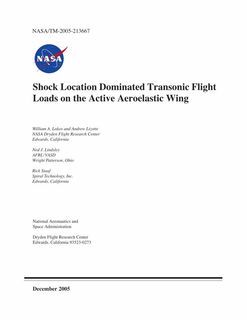
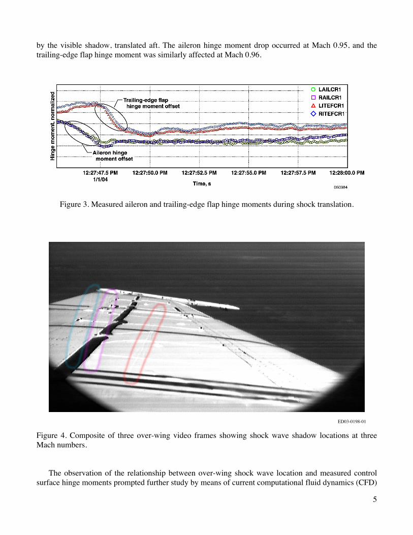
Figure 3 shows a time history of the left and right aileron and trailing-edge flap hinge moments forthe time interval during a transonic level acceleration. The left and right aileron data closely agree as dothe left and right trailing-edge flap data sets. Of interest is the significant change in aileron hinge momentstarting at 0.5 seconds into the time record closely followed by a similar change in the trailing-edge flaphinge moment. The cause of these hinge moment offsets, discovered through the use of real-time videodata, was the progressive translation of the over-wing shock wave first across the aileron hinge line andthen across the trailing-edge flap hinge line. Figure 4 presents a composite photo produced from threestill frames clipped from the wing video signal. This video based information corresponds to themeasured load data shown in figure 3. The three shock wave shadows were circled at Mach 0.94(orange), 0.95 (magenta), and 0.96 (blue) for clarity, because the shadows are more difficult to see in astill photo than in the moving video image. As Mach number increased, the shock location, as indicated

5

by the visible shadow, translated aft. The aileron hinge moment drop occurred at Mach 0.95, and thetrailing-edge flap hinge moment was similarly affected at Mach 0.96.

Figure 3. Measured aileron and trailing-edge flap hinge moments during shock translation.

ED03-0198-01

Figure 4. Composite of three over-wing video frames showing shock wave shadow locations at threeMach numbers.

The observation of the relationship between over-wing shock wave location and measured controlsurface hinge moments prompted further study by means of current computational fluid dynamics (CFD)

6

tools. Wing elastic shape information measured in flight enabled the study of the aircraft aerodynamicsresulting from the deformed condition.

COMPUTATIONAL METHODOLOGY

A CFD code called the Euler Navier-Stokes Three Dimensional Aeroelastic Code (ENS3DAE)(ref. 14) was employed to calculate wing upper and lower surface pressures. The aerodynamic analysisprocedure employed by ENS3DAE uses an implicit finite difference algorithm to integrate either theEuler or Navier-Stokes equations in general nonorthogonal curvilinear coordinates. The equations aresolved using a spatially varying time step for steady-state computations.

Time and budget had to be balanced with physical accuracy considerations. Therefore, the choice wasmade to run the CFD in an inviscid mode on the wing only with reflective boundary conditions, and withno free edges between the control surfaces. This approach was considered adequate for capturing theshocks associated with transonic flow behavior; however, viscous effects, “scissor” effects betweencontrol surfaces, and fuselage-wing leading-edge extension boundary condition effects at the wing rootwere not modeled.

As shown in figure 5, wing pressure distribution predictions were developed using a combination oftools. The CFD code was coupled with data measured during flight, which included control surfacedeflections and wing elastic deformations from the FDMS. The wing elastic deformations measured bythe FDMS were characterized and carried into the CFD grid through the use of a twist algorithm (ref. 15)as an intermediary process. The FDMS was considered a more accurate, time saving, and convenientmethod of representing the structure (than finite element modeling prediction) for coupled interactionwith the CFD aerodynamics.

Figure 5. Flowchart of modeling, analysis, and experimental results comparison.

Referring again to figure 5, note that the CFD initially was run on the wing in its rigid or “jig shape”geometry (zero control surface deflections and elastic wing-box deformations), producing a set of loadsfor each Mach number ranging from 0.92 to 0.99 in increments of 0.01. These solutions were used asrestart conditions for the elastic, in-flight configuration of the wing, which produced a set of elastic loadsfor comparison with those measured in flight. In-house code was written to project the control surface

7

and wing elastic deformations onto the CFD grid for the FDMS–CFD runs. The control surfacedeflections were input using the measured inboard and outboard deflection angles of each surface, withspanwise deflection varying linearly between the inboard and outboard edges. The angle of attack wasconstant with Mach number, reflecting the data measured in flight. The effect of stabilator (horizontaltail) position also was noted with regard to its influence on the upwash on the trailing-edge flap and thetotal aircraft lift.

Figure 6 shows the surface of the CFD grid used to model the AAW wing, with control surfaceboundaries demarcated. Figures 7 and 8 show the typical residual and force convergence histories,respectively, produced by the CFD analysis. The rigid CFD was run for 20,000 iterations, producingexcellent convergence as evidenced by the time histories from iterations 15,000 to 20,000. TheFDMS–CFD was run for 10,000 iterations, from 20,001 to 30,000. Figure 7 shows excellent residualconvergence occurring from iteration 27,000 onward, and figure 8 shows a global force convergence(wing total

C

L

,

C

D

,

C

m

, and so forth) occurring somewhat sooner. Residual convergence was used as thegoverning convergence decision, thereby ensuring local force convergence. Local force convergenceensures converged solutions for the individual control surface, wing-root, and wing-fold loads. Theresults for the Mach 0.97 case are shown. This particular Mach number will be used to compare the rigidCFD to the FDMS–CFD for the typical case.

Figure 6. Surface of the computational fluid dynamics grid used to model the Active Aeroelastic Wing.

8

Figure 7. Typical residual convergence of the computational fluid dynamics model of the ActiveAeroelastic Wing.

Figure 8. Typical force convergence of the computational fluid dynamics model of the Active AeroelasticWing.

9

RESULTS

This research allows several comparisons to be made. The rigid CFD can be compared to theFDMS-based elastic CFD. The CFD results can be compared to flight-measured data. Further, theinfluence of modeling features may be noted.

Comparison of Rigid CFD to FDMS–CFD

Figures 9 and 10 show the resulting upper and lower wing surface pressure distributions (units psi),respectively, for a typical rigid CFD run. Figures 11 and 12 show the upper and lower wing surfacepressures, respectively, for the FDMS–CFD. The contour scale is identical for all four figures, with aminimum (blue) to maximum (red) spectrum. A comparison between figures 9 and 11 shows that a muchlower downward pressure occurred on the FDMS–CFD upper surface, particularly for the trailing-edgesurfaces. Conversely, figures 10 and 12 show that a much higher upward pressure occurred on theFDMS–CFD lower surface, especially for the trailing-edge surfaces. These same trends, which accountfor the much higher lift (and loads) produced by the FDMS–CFD, also are evident to a somewhat lesserextent outboard of the wing fold. Figure 13, which shows the wing surface deflection contours measuredby the FDMS (in inches), provides an explanation for these differences in surface pressure distributions.Imposing small leading-edge flap deflections and larger trailing-edge downward deflections, coupledwith high bending and twist deflections outboard of the wing fold, naturally produce these changes insurface pressure because of the fluid-structure interaction typical of nonlinear aeroelastic systems.

Figure 9. Undeflected wing upper surface pressure contour, Mach 0.97.

10

Figure 10. Undeflected wing lower surface pressure contour, Mach 0.97.

Figure 11. Flight deflection measurement system: deflected wing upper surface pressure contour,Mach 0.97.

11

Figure 12. Flight deflection measurement system: deflected wing lower surface pressure contour,Mach 0.97.

Figure 13. Flight deflection measurement system: measured deflection contour for the left upper wingsurface, Mach 0.97.

12

0.92 M

Blue = Minimum pressureRed = Maximum pressure

0.93 M 0.94 M 0.95 M

Flow

0.96 M 0.97 M 0.98 M 0.99 M

Flow

Altitude = 18.5k ft, = 0.520 deg, M = 0.92–0.99

FlowFlow Flow

FlowFlowFlow

0.92 M

Blue = Minimum pressureRed = Maximum pressure

0.93 M 0.94 M 0.95 M

Flow

0.96 M 0.97 M 0.98 M 0.99 M

Flow

Altitude = 18.5k ft, = 0.520 deg, M = 0.92–0.99

FlowFlow Flow

FlowFlowFlow

0.92 M

Blue = Minimum pressureRed = Maximum pressure

0.93 M 0.94 M 0.95 M

Flow

0.96 M 0.97 M 0.98 M 0.99 M

Flow

Altitude = 18.5k ft, = 0.520 deg, M = 0.92–0.99

FlowFlow Flow

FlowFlowFlow

A comparison of the flight research video and rigid CFD predicted surface pressure distributionsshows general agreement and supports the interpretation that the shock translation directly caused thesignificant load change observed in the trailing-edge control surface hinge moments. This generalagreement is qualitative, because the CFD predicted shock magnitudes and locations for each Machnumber do not match those shown for the trailing-edge surfaces in figures 3 and 4. Figures 14 and 15show the resultant (lower minus upper) pressure distributions for the rigid CFD cases and FDMS–CFDcases, respectively. The contour scale is identical for both cases, with a symmetric, downward (blue) toupward (red) spectrum. These results show both the extreme pressure magnitudes and matching Machnumbers, Mach 0.95 (higher pressure) and 0.99 (lower pressure), for the left trailing-edge flap (LTEF),and Mach 0.96 for the left aileron (LAIL) for the transonic shock wave depicted in figures 3 and 4.Further analysis of the results and flight research data is expected to verify this observation.

Figure 14. Rigid computational fluid dynamics resultant pressure distributions.

0.92 M

050395

Blue = Minimum pressureRed = Maximum pressure

0.93 M 0.94 M 0.95 M

Flow

0.96 M 0.97 M 0.98 M 0.99 M

Flow

Altitude = 18.5k ft, = 0.520 deg, M = 0.92–0.99

FlowFlow Flow

FlowFlowFlow

13

Figure 15. Flight deflection measurement system computational fluid dynamics resultant pressuredistributions.

Comparison of CFD Analysis to Flight-Measured Data

For each Mach number, the surface pressure distributions shown in figures 9–12 were integrated overeach control surface, in addition to the inboard and outboard wing boxes, to produce a set of forces (

F

x

,

F

y

,

F

z

) and centroids (

X

c

,

Y

c

,

Z

c

). The cross product of these forces and their respective moment armsrendered a hinge moment for each of the four control surfaces, and values for shear, bending, and torqueat the wing fold and wing root. Eight of these ten loads (wing-root and wing-fold shears excluded), inaddition to the total lift generated by the wing, then were compared to those measured duringflight research.

Figure 16 shows the left wing trailing-edge flap deflections, which were measured at both the inboardand outboard edges of all wing control surfaces. Because the control surface transmissions are inboardmounted, their outboard deflections are more “free” to deflect under aerodynamic pressure loading. Thecorresponding extreme outboard deflections at Mach 0.95 and 0.99 for the LTEF-

ob

and Mach 0.96 forthe LAIL-

ob

reinforce the FDMS–CFD resultant pressure distributions shown in figure 15.

Flow

0.92 M

050396

Blue = Minimum pressureRed = Maximum pressure

0.93 M 0.94 M 0.95 M

Flow Flow Flow

0.96 M 0.97 M 0.98 M 0.99 M

Flow

Altitude = 18.5k ft, = 0.520 deg, M = 0.92–0.99

FlowFlowFlow

14

Figure 16. Left wing trailing-edge flap deflections.

Figure 17 shows the FDMS–CFD calculated centroids of the resultant aeroelastic forces on the wingand control surfaces. These results make physical sense, given that the centroid locations (1) move aftwith increasing Mach number, and (2) are located within the wing and control surface boundaries.

Figure 17. Left wing box and control surface load centroid locations.

15

Figure 18 compares the measured left inboard leading-edge flap (LILEF) and left outboardleading-edge flap (LOLEF) hinge moments with those calculated using the FDMS–CFD. Excellentagreement was achieved with the LOLEF hinge moment, whereas the measured LILEF hinge momentmagnitudes are less than those predicted but have the same general increasing trend. This discrepancymay be best explained by the fact that the CFD model does not include the (1) F/A-18 leading-edgeextension, (2) fuselage for flow field boundary conditions, and (3) flow fence representation. Thefunction of the flow fences on the F/A-18 aircraft is to move vortices away from the vertical tails toavoid buffet.

Figure 18. Left inboard and outboard leading-edge flap control surface hinge moments.

As shown in figure 19, even less agreement, both qualitative and quantitative, was achieved for theLTEF hinge moment. The three explanations for the LILEF discrepancy also apply to the LTEFdiscrepancy, and their effects are magnified when the position of the LTEF farther aft in the flow field isconsidered. Also highly important is the lack of a stabilator in the CFD modeling, because its interactionwith the LTEF is known to be highly coupled. The aerodynamic upwash from the stabilator on theinboard portion of the wing resulting from their physical proximity is still evident at these transonicconditions. The effect of the stabilator on the total lift force generated by the wing also was very high,and this interaction was accounted for by coupling the FDMS–CFD with an assumed coefficient of liftfor the stabilator.

16

Figure 19. Left trailing-edge flap control surface hinge moment.

Figure 20 compares the measured and predicted LAIL hinge moments. Similar to the LOLEF, theload history of this outboard surface was very well predicted (both qualitatively and quantitatively) byFDMS–CFD. Figures 21 and 22 compare the measured and predicted bending moment and torque at thewing root and wing fold, respectively. Generally good qualitative and quantitative agreement wasachieved for the wing-root bending moments; the wing-fold bending moments were smaller in magnitudethan the wing-root bending moments.

17

Figure 20. Left aileron control surface hinge moment.

Figure 21. Left wing-root bending moment and torque comparison.

18

Figure 22. Left wing-fold bending moment and torque comparison.

Importance of Stabilator Consideration When Modeling

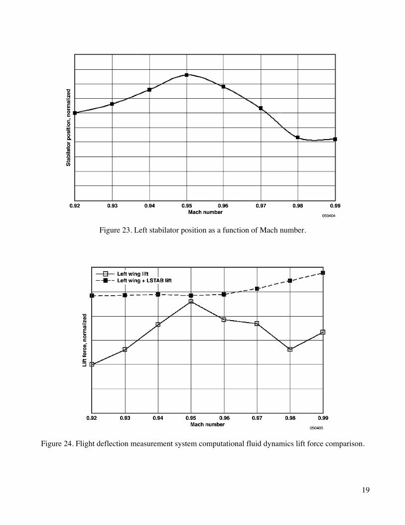
Because this flight event was trimmed and nominally level, the FDMS–CFD lift force generated bythe wing would be expected to remain constant with respect to Mach number. This relationship, however,is not obvious. Figure 23 shows the left stabilator position, on which the air vehicle trim condition isdependent, as a function of Mach number. The stabilator position varied throughout the maneuver.Therefore, for understandable reasons, the FDMS–CFD generated history of the lift produced by thewing also varied throughout the level acceleration. Figure 24 shows the total lift of the wing and the liftforce generated by the wing, in addition to that generated by the left stabilator when a constant stabilatorlift coefficient was assumed. The slight increase in overall lift force from Mach numbers 0.96 to 0.99 alsois reflected in an increase in altitude for those Mach numbers, as shown in figure 25. Therefore, althoughthis flight event was nominally level, the contribution to the total aircraft lift produced by the stabilatorwas consistent with the slight variation in altitude during the maneuver time interval. The stabilatorposition variation also has implications in understanding the trailing-edge flap predictions, aspreviously discussed.

19

Figure 23. Left stabilator position as a function of Mach number.

Figure 24. Flight deflection measurement system computational fluid dynamics lift force comparison.

20

Figure 25. Altitude as a function of Mach number.

CONCLUDING COMMENTS

In level transonic flight, the shock location dominated the wing trailing-edge control surface hingemoments. The predictive method of the computational fluid dynamics (CFD) based on the elastic shapeprovided by the flight deflection measurement system (FDMS) produced very similar results andsubstantially correlated with the measured loads data. Specifically, the FDMS–CFD method qualitativelyand quantitatively represented the flight loads for the outboard control surfaces, and to a slightly lesserextent for the wing-root moments. For inboard leading-edge surfaces and wing-fold moments on thisvehicle, however, the correlation was more qualitative. Moreover, the inboard trailing-edge controlsurface predictions were the least accurate of those studied, lacking both qualitative and quantitativeagreement. These shortcomings in predictive performance have understandable physical explanationsthat can be compensated for, however, if the computational expense of a full vehicle model is deemedacceptable. In-flight video, which first captured the attention of the flight research engineers and wasconfirmed through the measured data, sometimes has unexpected value.

Dryden Flight Research CenterNational Aeronautics and Space AdministrationEdwards, California, July 15, 2005

21

REFERENCES

1. Miller, Gerald D., “Active Flexible Wing (AFW) Technology,” Air Force Wright AeronauticalLaboratories, TR-87-3096, Feb. 1988.

2. Miller, Gerald D., “An Active Flexible Wing Multi-Disciplinary Design Optimization Method,”AIAA-94-4412-CP, 1994.

3. Yurkovich, Rudy, “Optimum Wing Shape for an Active Flexible Wing,” AIAA-95-1220-CP, 1995.

4. Pendleton, Ed, Kenneth E. Griffin, Michael W. Kehoe, and Boyd Perry, “A Flight Research Programfor Active Aeroelastic Wing Technology,” AIAA-96-1574-CP, 1996.

5. Pendleton, Edmund W., Denis Bessette, Peter B. Field, Gerald D. Miller, and Kenneth E. Griffin,“Active Aeroelastic Wing Flight Research Program: Technical Program and Model AnalyticalDevelopment,”

Journal of Aircraft

, Vol. 37, No. 4, July–Aug. 2000.

6. Voracek, David, Ed Pendleton, Eric Reichenbach, Dr. Kenneth Griffin, and Leslie Welch,

The ActiveAeroelastic Wing Phase I Flight Research Through January 2003

, NASA TM-2003-210741, 2003.

7. Fisher, David F., Edward A. Haering, Jr., Gregory K. Noffz, and Juan I. Aguilar,

Determination ofSun Angles for Observations of Shock Waves on a Transport Aircraft

, NASA TM-1998-206551,1998.

8. Lokos, William A., Candida D. Olney, Tony Chen, Natalie D. Crawford, Rick Stauf, and Eric Y.Reichenbach,

Strain Gage Loads Calibration Testing of the Active Aeroelastic Wing F/A-18Aircraft

, NASA TM-2002-210726, 2002.

9. DeAngelis, V. Michael, and Robert Fodale, “Electro-Optical Flight Deflection MeasurementSystem,”

SFTE 18th Annual Symposium Proceedings

, SFTE Technical Paper 22, Amsterdam,Netherlands, Sept. 1987.

10. Lokos, William A.,

Predicted and Measured In-Flight Wing Deformations of aForward-Swept-Wing Aircraft

, NASA TM-4245, 1990.

11. Lokos, William A., Catherine M. Bahm, and Robert A. Heinle,

Determination of Stores PointingError Due to Wing Flexibility Under Flight Load

, NASA TM-4646, 1995.

12. Lizotte, Andrew M., and William A. Lokos,

Deflection-Based Structural Loads Estimation From theActive Aeroelastic Wing F/A-18 Aircraft

, NASA TM-2005-212871, 2005.

13. Burner, Alpheus W., William A. Lokos, and Danny A. Barrows, “Aeroelastic Deformation:Adaptation of Wind Tunnel Measurement Concepts to Full-Scale Vehicle Flight Testing,” NATORTO-MP-AVT-124, Paper No. 9,

Research and Technology Organization Specialists' Meeting onRecent Developments in Non-Intrusive Measurement Technology for Military Application on Model-and Full-Scale Vehicles

, Budapest, Hungary, April 25–28, 2005.

22

14. Schuster, David M., Joseph Vadyak, and Essam Atta, “Static Aeroelastic Analysis of FighterAircraft Using a Three-Dimensional Navier-Stokes Algorithm,”

Journal of Aircraft

, Vol. 27, No. 9,Sept. 1990, pp. 820–825.

15. Lizotte, Andrew M., and Michael J. Allen,

Twist Model Development and Results From the ActiveAeroelastic Wing F/A-18 Aircraft

, NASA TM-2005-212861, 2005.