Chaos, Solitons & Fractals 44 (2011) 995–1003

Contents lists available at SciVerse ScienceDirect

Chaos, Solitons & FractalsNonlinear Science, and Nonequilibrium and Complex Phenomena

journal homepage: www.elsevier .com/locate /chaos

Elementary chaotic snap flows

Buncha Munmuangsaen, Banlue Srisuchinwong ⇑Sirindhorn International Institute of Technology (SIIT), Thammasat University, 131 M5, Tivanont Road, Bangkadi, Muang, Pathum-Thani 12000, Thailand

a r t i c l e i n f o

Article history:Received 15 October 2010Accepted 22 August 2011Available online 25 September 2011

0960-0779/$ - see front matter � 2011 Elsevier Ltddoi:10.1016/j.chaos.2011.08.008

⇑ Corresponding author. Tel.: +66 2 501 3505 till501 3505 till 20x1801.

E-mail address: banlue@siit.tu.ac.th (B. Srisuchin

a b s t r a c t

Hyperjerk systems with 4th-order derivative of the form x...:¼ f ðx

...; €x; _x; xÞ have been referred

to as snap systems. Five new elementary chaotic snap flows and a generalization of anexisting flow are presented through an extensive numerical search. Four of these flowsdemonstrate elegant simplicity of a single control parameter based on a single nonlinearityof a quadratic, a piecewise-linear or an exponential type. Two others demonstrate elegantsimplicity of all unity-in-magnitude parameters based on either a single cubic nonlinearityor three cubic nonlinearities. The chaotic snap flow with a single cubic nonlinearityrequires only two terms and can be transformed to its equivalent dynamical form of onlyfive terms which have a single nonlinearity. An advantage is that such a chaotic flow offersonly five terms even though the (four) dimension is high. Three of the chaotic snap flowsare characterized as conservative systems whilst three others are dissipative systems. Basicdynamical properties are described.

� 2011 Elsevier Ltd. All rights reserved.

1. Introduction

Chaotic flows can be characterized as either dissipativeor conservative [1]. A dissipative chaotic flow ~F1 has aproperty that (bounded) trajectories are attracted to a re-gion of space by a strange attractor and its divergencer �~F1 ¼ V�1 dV

dt

� �is negative, i.e. a volume (V) occupied

by a set of initial conditions collapses in state space. Bycontrast, a conservative (or equivalently Hamiltonian [2])chaotic flow ~F2 does not have phase space attractors andits divergence r �~F2 ¼ V�1 dV

dt

� �is zero, i.e. a volume (V)

in state space occupied by a set of initial conditions re-mains the same.

Early examples [3] of both dissipative and conservativechaotic flows were identified, through a computer search,to be algebraically simpler than the well-known Lorenz[4] and Rössler systems [5]. In response to this early work,Gottlieb [6] suggested a search for chaotic systems of theform x

...¼ jð€x; _x; xÞ where j is a jerk function and _x � dx

dt. Theterm ‘jerk’ comes from the fact that, successive time

. All rights reserved.

20x1806; fax: +66 2

wong).

derivatives of displacement are velocity, acceleration, andjerk [7]. Sprott [8] took up Gottlieb’s challenge and discov-ered the simplest dissipative chaotic flow using a singlequadratic nonlinearity in a jerk model of the form

x...¼ �a€xþ _x2 � x: ð1Þ

Chaos is found as ‘a’ is equal to or slightly greater than2.017. Another simple piecewise exponential nonlinearjerk model [9] in a dissipative system has been of the form

x...¼ �a€xþ j _xjb � x; ð2Þ

where ‘a’ and ‘b’ are bifurcation parameters which cannotbe unity. In addition, the simplest conservative jerk systemwith chaotic solutions [10] has been appeared as

x...¼ �8€xþ jxj � 1: ð3Þ

On the other hand, hyperjerk systems [11] involve timederivatives of a jerk function. Such derivatives are gener-ally higher than the 3rd-order. In particular, hyperjerk sys-tems with 4th-order derivative of the form x

...:¼ f ðx

...; €x; _x; xÞ

have been referred to as snap systems [10]. Early examplesof Chaotic Hyperjerks have been demonstrated via anextensive numerical search [11,12]. Two cases of chaoticsnap systems have been reported as the algebraically

Fig. 1. The largest Lyapunov exponent of Eq. (8) versus A.

996 B. Munmuangsaen, B. Srisuchinwong / Chaos, Solitons & Fractals 44 (2011) 995–1003

simplest Chaotic Hyperjerks. The first case has five terms ofthe form

x...:¼ � x

...�A€x� _xþ x2 � 1 ð4Þ

and the second case has four terms of the form

x...:¼ � x

...�A€x� _x2 � x: ð5Þ

Both cases have been characterized as the dissipative sys-tems. Very recently, simpler chaotic snap systems of bothdissipative and conservative flows have been summarized[10] including a chaotic snap hyperjerk of a conservativeflow with three terms and a single quadratic nonlinearityof the form

x...:¼ �8€xþ _x2 � x: ð6Þ

In this paper, five new examples of elementary chaoticsnap flows and a generalization of an existing chaotic snapflow are presented through an extensive numerical searchusing an equation of the form

x...:þa0 x

...þa1€xþ a2 _xþ a3x ¼ g x; _x; €xð Þ; ð7Þ

where gðx; _x; €xÞ is the nonlinearity and coefficients a0, . . . ,a3

are control parameters. Chaotic solutions for each of aspecified nonlinear function gðx; _x; €xÞ employ systematicprocedures of a numerical search developed in [1–3,10,12]. In such procedures, the control parameters andinitial conditions are scanned to find for a positive Lyapu-nov exponent, which is a signature of chaos. Although sev-eral chaotic snap flows have been found, only the systemswith elegant simplicity are selected and reported here.

In cases of a candidate for four-dimensional dissipativechaotic snap flows, the Lyapunov exponents are calculatedwith 107 iterations (to ensure that chaos is neither numer-ical artifacts nor chaotic transients) using the method de-scribed by Wolf et al. [13] with a fixed step sizeDt = 0.01. In cases of a candidate for four-dimensional con-servative chaotic snap flows, the largest Lyapunov expo-nent k1 is calculated using the method described in [10]with a 4th-order adaptive-step Runge–Kutta integrator[14], which avoids numerical trajectory divergences ob-served by the fixed-step integrator in association withoccasional large excursions from the chaotic attractors[15]. In conservative flows (the divergence r � F

!2 ¼ V�1 dV

dtis zero), Lyapunov exponents occur symmetrically in equalpairs with opposite signs and there must be two zero expo-nents (k2 = k3 = 0) (see Section 1.10 of [10]). Therefore theremaining exponent k4 is equal to the negative value ofthe largest Lyapunov exponent, i.e. k4 = �k1.

Four of these chaotic snap flows demonstrate elegantsimplicity of a single control parameter based on a singlenonlinearity of a quadratic, a piecewise-linear or an expo-nential type. Two other chaotic snap flows demonstrateelegant simplicity of all unity-in-magnitude parametersbased on either a single cubic nonlinearity or three cubicnonlinearities. The chaotic snap flow with a single cubicnonlinearity requires only two terms and can be trans-formed to its equivalent dynamical form of only five termswhich have a single nonlinearity. In comparison with anexisting three (lower) dimensional chaotic flow whereminimum terms have been identified to be five terms [8],

an advantage is that such a chaotic snap flow also offersfive (perhaps minimum) terms even though the (four)dimension is higher. Three of all examples are conservativesystems and three others are dissipative systems.

2. A generalization of an existing conservative systembased on a single quadratic nonlinearity

Through an extensive search, an elementary chaoticsnap flow of a conservative system based on a single qua-dratic nonlinearity has been found with elegant simplicityof a single control parameter ‘A’ as follows:

x...:¼ �A€x� _x2 � x; ð8Þ

where � _x2 is the single quadratic nonlinearity. AlthoughEq. (8) nearly resembles Eq. (6) except that ‘A’ is specifi-cally equal to 8 with � _x2 as a quadratic nonlinearity, thissection further examines in greater detail for new caseswhere ‘A’ is generally a single control parameter of variousvalues, with � _x2 as a single quadratic nonlinearity.

Fig. 1 shows the largest Lyapunov exponent k1 [2,10] ofEq. (8) versus the control parameter A using the initial con-ditions ðx; _x; €x; x

...Þ ¼ ð1:2;1:2;�0:1;0:5Þ. Chaos will be as-

sumed to exist if k1 exceeds 0.001. The value k1 will be setto zero if chaos does not exist or when the trajectory of thesolution escapes to a very large value (or infinity). Such anescape will be detected if the calculated value ofjxj þ j _xj þ j€xj þ j x

...j exceeds 1 � 106. At A = 4.3765, the value

of k1 = 0.03574 was found to be a maximum. As a result,the Lyapunov exponent spectrum of Eq. (8) was found tobe (k1,k2,k3,k4) = (0.03574,0,0,�0.03574). For the selectedinitial conditions (1.2,1.2,�0.1,0.5), chaos does not existafter A > 4.51 as evidenced in Fig. 1. At A = 8, k1 = 0.0005(<0.001) and therefore chaos does not exist. Nonetheless, ifthe set of the selected initial condition is (�1.94,1.43,�0.98,�1.48), then k1 = 0.0055 (>0.001) and therefore chaosdoes exist at A = 8 as reported in [10].

Equivalently, Eq. (8) can be rewritten as a dynamicalsystem in variables x, y, z, and w of the form

Fig. 2. A phase-space trajectory for A = 4.3765 of Eq. (8).

B. Munmuangsaen, B. Srisuchinwong / Chaos, Solitons & Fractals 44 (2011) 995–1003 997

_x ¼ y_y ¼ z_z ¼ w

_w ¼ �Az� y2 � x:

ð9Þ

Eq. (9) requires only six terms with elegant simplicity of asingle quadratic nonlinearity and a single control parame-ter ‘A’. Eq. (9) has a single equilibrium point at the origin.For the positive sign of the quadratic nonlinearity (+y2),for example, the corresponding Jacobian matrix is

J ¼

0 1 0 00 0 1 00 0 0 1�1 2y �A 0

26664

37775: ð10Þ

At the equilibrium point and for A = 4.3765, the Jacobianmatrix (10) has two complex conjugate pairs of eigen-values at ±2.0334i and ±0.4918i.

It has been known [1] that the total sum of all Lyapunovexponents represents an average rate of expansion (alongthe trajectory) of a small volume (V) in state space occu-pied by a set of initial conditions and can directly be calcu-lated either from the trace (sum of diagonal elements) ofthe Jacobian matrix J, or from the divergence of the flow

F!¼ ½ _x _y _z _w�T . For bounded trajectories, the total sum can-

not be positive [1]. If the total sum is negative, the systemis dissipative. If the total sum is zero, there is no contrac-tion (no dissipation) and the system is conservative. Exist-ing ‘Chaotic Hyperjerk’ and ‘Hyperchaotic Hyperjerk’ of4th-order in dissipative flows have the Lyapunov exponentspectrum of the form (+,0,�,�) and (+,+,0,�), respectively[11].

As mentioned earlier, the Lyapunov exponent spectrumof Eq. (8) is (k1,k2,k3,k4) = (0.03574,0,0,�0.03574) and is ofthe form (+,0,0,�) where k1 and k4 occur in an equal pairwith opposite sign, i.e. k1 = �k4. The total sum of all Lyapu-nov exponents of Eq. (8) apparently equals zero. As a result,the divergence of the flow is equally zero as follows:

r � F!¼ 1

VdVdt¼ @

_x@xþ @

_y@yþ @

_z@zþ @

_w@w

¼ k1 þ k2 þ k3 þ k4 ¼ htraceðJÞi ¼ 0: ð11Þ

As the trace(J) of Eq. (10) is independent of ‘A’, it follows thatEq. (8) is a conservative system with a single control param-eter ‘A’ of various values for a single quadratic nonlinearity� _x2, and is a ‘‘Chaotic Hyperjerk’’ system, or equivalently achaotic snap flow. As an example, the phase space trajectoryfor A = 4.3765 is shown in Fig. 2. A numerical simulation

Fig. 3. The largest Lyapunov exponent of Eq. (12) versus A.

998 B. Munmuangsaen, B. Srisuchinwong / Chaos, Solitons & Fractals 44 (2011) 995–1003

reveals that Eq. (8) also exhibits time-reversible Hamilto-nian chaos [2].

3. A single piecewise-linear nonlinearity

3.1. A conservative system

It is natural to wonder whether the quadratic nonlin-earity _x2 of Eq. (8) can be weakened and can be replacedwith an elementary piecewise-linear nonlinearity. Notethat a term p can be considered as a piecewise-linearapproximation to p2. It has been proven that such areplacement does not enable chaos in the three-dimen-sional jerk model of Eq. (1) [16]. In this section, anotherelementary chaotic snap flow of a conservative system ispresented with elegant simplicity of a single piecewise-lin-ear nonlinearity and a single control parameter ‘A’ asfollows:

x...:¼ �A€x� j _xj � x: ð12Þ

Chaos was indeed found. Fig. 3 shows the largest Lyapunovexponent (k1) of Eq. (12) versus the parameter A from 2 to5 using the initial conditions ðx; _x; €x; x

...Þ ¼ ð0:4;0:3;0:6;0:2Þ.

The calculation was in the same manner as described inSection 2. At A = 2.525, the value k1 = 0.05537 was found

Fig. 4. A phase space trajectory

to be a maximum. As a result, the Lyapunov exponentspectrum was found to be (k1,k2,k3,k4) = (0.05537,0,0,�0.05537).

Equivalently, Eq. (12) can be rewritten as a dynamicalsystem in variables x, y, z, and w in a similar manner toEq. (9) except that ±y2 in Eq. (9) is replaced by ±jyj. Forthe positive sign of the elementary piecewise-linear

for A = 2.525 of Eq. (12).

Fig. 5. (a) The largest Lyapunov exponent of Eq. (15) versus A. (b) Abifurcation diagram of Eq. (15) shows a period-doubling route to chaos asA is gradually decreased from 2 to 1.878.

B. Munmuangsaen, B. Srisuchinwong / Chaos, Solitons & Fractals 44 (2011) 995–1003 999

nonlinearity, +jyj, for example, the corresponding Jacobianmatrix is

J ¼

0 1 0 00 0 1 00 0 0 1�1 sgnðyÞ �A 0

26664

37775; ð13Þ

where the signum function sgn(y) is defined as:

sgnðyÞ ¼�1 for y < 00 for y ¼ 01 for y > 0

8><>:

ð14Þ

Eq. (12) has a single equilibrium point at the origin. At theequilibrium point and for A = 2.525, the Jacobian matrix(13) has two complex conjugate pairs of eigenvalues at±1.4259i and ±0.7013i.

In a similar manner to Eq. (11), the total sum of allLyapunov exponents of Eq. (12) equals zero and thetrace(J) of Eq. (13) is zero and independent of ‘A’. It followsthat Eq. (12) is a chaotic snap flow of a conservative systemwith a single control parameter ‘A’ of various values for asingle piecewise-linear nonlinearity j _xj. As an example, aphase space trajectory for A = 2.525 is shown in Fig. 4. Anumerical simulation reveals that Eq. (12) also exhibitstime-reversible Hamiltonian chaos [2].

Fig. 6. A chaotic attra

3.2. A dissipative system

An elementary chaotic snap flow of a dissipative system ispresented with elegant simplicity of a single piecewise-lin-ear nonlinearity and a single control parameter ‘A’ as follows:

x...:¼ � x

...�A€x� _x� ðjxj � 1Þ: ð15Þ

ctor of Eq. (15).

Fig. 7. A phase space trajectory of Eq. (16).

1000 B. Munmuangsaen, B. Srisuchinwong / Chaos, Solitons & Fractals 44 (2011) 995–1003

The four-dimensional snap model of Eq. (15) is anextension of an existing three-dimensional jerk modelwith a piecewise-linear nonlinearity described in [17].Such a nonlinearity can be implemented electronicallywith a full-wave rectifier with two diodes and an invertingunity gain amplifier and also with a single diode [18].Fig. 5(a) illustrates the largest Lyapunov exponent of Eq.(15) versus the control parameter A which is gradually de-creased from 2 to 1.6 using the initial conditionsx ¼ _x ¼ €x ¼ x

...¼ 0: A bifurcation diagram of Eq. (15) for x-

max is depicted in Fig. 5(b) as a function of the controlparameter A from 2 to 1.6. A period-doubling route tochaos is evident as A is gradually decreased from 2 to1.878. For positive and negative signs of jxj, the bifurcationand Lyapunov exponents of this system are the same. Theonly different is that both attractors are 180-degreerotated images to each other.

Comparison between Fig. 5(a) and (b) verifies that chaosdoes exist. At A = 1.686, chaos is maximized with theLyapunov exponent spectrum (k1,k2,k3,k4) = (0.11107,0,�0.43926,�0.67184) and the Kaplan–Yorke dimension[19] (or equivalently Lyapunov dimension) Dky = 2.25293.The total sum of the Lyapunov exponent is equivalent tothe average rate of fractional volume expansion along thetrajectory, and can be calculated in the same manner to thatof the conservative systems described by Eq. (11) [1,2]. Since

the total sum of the Lyapunov exponent spectrum or trace(J)of Eq. (15) is a negative value, i.e. trace(J) = �1, Eq. (15) is dis-sipative with constant state-space contraction of �1. Thefluctuations in the largest Lyapunov exponent of this systemlie in a small range of 10�4 for 106 iterations. Such a slightvariation in the Lyapunov spectrum, as iteration increases,helps to ensure that the Lyapunov exponent has converged(see Section 4 of [20] for more information). Eq. (15) hastwo equilibrium points at (±1,0,0,0). At the first equilibriumpoint (1,0,0,0), the Jacobian matrix has the eigenvalues at�0.6255 ± 0.7802i and 0.1255 ± 0.9921i. At the second equi-librium point (�1,0,0,0), the Jacobian matrix has the eigen-values at �0.1942 ± 1.3861i, �1.0830 and 0.4713. Fig. 6shows a chaotic attractor of Eq. (15) which resembles theRössler attractor [5] in a sense that it has a single folded-band structure.

4. Cubic nonlinearity

4.1. A conservative system

An elementary chaotic snap flow of a conservative sys-tem is presented with elegant simplicity of only two termsand a single cubic nonlinearity of the form

x...:¼ �€x3 � x: ð16Þ

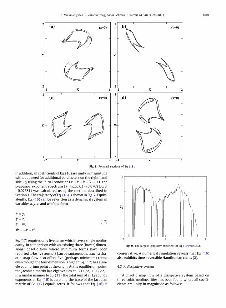
Fig. 8. Poincaré sections of Eq. (18).

B. Munmuangsaen, B. Srisuchinwong / Chaos, Solitons & Fractals 44 (2011) 995–1003 1001

In addition, all coefficients of Eq. (16) are unity in magnitudewithout a need for additional parameters on the right handside. By using the initial conditions x ¼ _x ¼ €x ¼ x

...¼ 0:1, the

Lyapunov exponent spectrum (k1,k2,k3,k4) = (0.07681,0,0,�0.07681) was calculated using the method described inSection 1. The trajectory of Eq. (16) is shown in Fig. 7. Equiv-alently, Eq. (16) can be rewritten as a dynamical system invariables x, y, z, and w of the form

_x ¼ y;_y ¼ z;_z ¼ w;

_w ¼ �x� z3:

ð17Þ

Fig. 9. The largest Lyapunov exponent of Eq. (19) versus A.

Eq. (17) requires only five terms which have a single nonlin-earity. In comparison with an existing three (lower) dimen-sional chaotic flow where minimum terms have beenreported to be five terms [8], an advantage is that such a cha-otic snap flow also offers five (perhaps minimum) termseven though the four dimension is higher. Eq. (17) has a sin-gle equilibrium point at the origin. At the equilibrium point,the Jacobian matrix has eigenvalues at �ð1=

ffiffiffi2pÞ � ð1=

ffiffiffi2pÞi.

In a similar manner to Eq. (11), the total sum of all Lyapunovexponents of Eq. (16) is zero and the trace of the Jacobianmatrix of Eq. (17) equals zeros. It follows that Eq. (16) is

conservative. A numerical simulation reveals that Eq. (16)also exhibits time-reversible Hamiltonian chaos [2].

4.2. A dissipative system

A chaotic snap flow of a dissipative system based onthree cubic nonlinearities has been found where all coeffi-cients are unity in magnitude as follows:

Fig. 10. Poincaré sections of Eq. (19).

1002 B. Munmuangsaen, B. Srisuchinwong / Chaos, Solitons & Fractals 44 (2011) 995–1003

x...:¼ � x

...�€x� €x3 � _x3 � x3: ð18Þ

By using the initial conditions ðx; _x; €x; x...Þ ¼

ð�8:5;�2:3;5:6;0:1Þ, the Lyapunov exponent spectrum is(k1,k2,k3,k4) = (0.05351,0,�0.20296,�0.85054), resultingin the Kaplan–Yorke dimension (or Lyapunov dimension)Dky = 2.26364. Since the total sum of the Lyapunov expo-nent spectrum and the trace(J) of Eq. (18) equal a negativevalue, i.e. trace(J) = �1, Eq. (18) is dissipative with constantstate-space contraction of �1. Eq. (18) has a single equilib-rium point at the origin. At the equilibrium point, theJacobian matrix has eigenvalues at 0, 0, �0.5 ± 0.866i.Fig. 8 displays the Poincaré sections of Eq. (18) with fractalstructures resulting from the fractal dimension Dky =2.26364.

5. A single exponential nonlinearity for a dissipativesystem

It is also interesting to identify an elementary chaoticsnap flow with elegant simplicity of a single exponentialnonlinearity and a single control parameter. One example is

x...:¼ � x

...�A _x� x� expð€xÞ: ð19Þ

Fig. 9 shows the largest Lyapunov exponent versus the con-trol parameter A using initial conditions x ¼ _x ¼ €x ¼ x

...¼ 0. It

is apparent that chaos is maximized at A � 6. The Lyapunovexponent spectrum at A = 6 is (k1,k2,k3,k4) = (0.16788,0,�0.15074,�1.01714) resulting in a Kaplan–Yorke dimen-sion (or Lyapunov dimension) Dky = 3.01685. Eq. (19) hasa single equilibrium point at (�1,0,0,0). The eigenvaluesat the equilibrium point for A = 6 are �1.9408,0.5558 ± 1.6453i and �0.1708. Since the total sum of theLyapunov exponent spectrum and the trace(J) of Eq. (19)equal a negative value, i.e. trace(J) = �1, Eq. (19) is dissipa-tive with constant state-space contraction of �1. The Poin-caré sections in several planes for A = 6 are shown inFig. 10. No conservative cases have been found for such anexponential nonlinearity.

6. Conclusions

Elementary chaotic snap flows have been presentedthrough an extensive numerical search. They consist of fivenew examples and a generalization of an existing flow.Four of them have demonstrated elegant simplicity of asingle control parameter based on a single nonlinearity ofa quadratic, a piecewise-linear or an exponential type.Two others have demonstrated elegant simplicity of allunity-in-magnitude parameters based on either a singlecubic nonlinearity or three cubic nonlinearities. The alge-braically simplest example found in this study has been

B. Munmuangsaen, B. Srisuchinwong / Chaos, Solitons & Fractals 44 (2011) 995–1003 1003

the chaotic snap flow with a single cubic nonlinearity andall unity-in-magnitude parameters. Although the 4th-or-der is higher, the equation requires only two terms in jerkrepresentation, and can be transformed to only five termsin its equivalent dynamical form. Such five terms offeralgebraically minimum terms comparable to those ofexisting lower-order chaotic flows. The dissipative chaoticsnap flow with a piecewise-linear nonlinearity suggests apossible implementation of electronic circuits using afull-wave rectifier with diodes and an inverting unity-gainamplifier. Basic dynamical properties have been demon-strated in three conservative and three dissipative chaoticflows.

Acknowledgements

The authors are grateful to Prof. J.C. Sprott for his usefulcomments. The first author appreciates CIC-Common Fundof SIIT for partially financial support. This work was sup-ported by Telecommunications Research and IndustrialDevelopment Institute (TRIDI), NBTC, Thailand, and the Na-tional Research University Project of Thailand, Office ofHigher Education Commission.

References

[1] Sprott JC. Some simple chaotic jerk functions. Am J Phys1997;65:537–43.

[2] Sprott JC. Chaos and time-series analysis. Oxford: Oxford UniversityPress; 2003.

[3] Sprott JC. Some simple chaotic flows. Phys Rev E 1994;50:R647–50.

[4] Lorenz EN. Deterministic nonperiodic flow. J Atmos Sci1963;20:130–41.

[5] Rössler OE. An equation for continuous chaos. Phys Lett A1976;57:397–8.

[6] Gottlieb WHP. What is the simplest Jerk function that gives chaos?Am J Phys 1996;64:525.

[7] Schot SH. Jerk: the time rate of change of acceleration. Am J Phys1978;65:1090–4.

[8] Sprott JC. Simplest dissipative chaotic flow. Phys Lett A1997;228:271–4.

[9] Sun KH, Sprott JC. A simple Jerk system with piecewise exponentialnonlinearity. Int J Nonlinear Sci Numer Simul 2009;10:1443–50.

[10] Sprott JC. Elegant chaos: algebraically simple chaoticflows. Singapore: World Scientific; 2010.

[11] Chlouverakis KE, Sprott JC. Chaotic hyperjerk systems. Chaos,Solitons Fract 2006;28:739–46.

[12] Munmuangsaen B, Srisuchinwong B, Sprott JC. Generalization of thesimplest autonomous chaotic system. Phys Lett A 2011;375:1445–50.

[13] Wolf A, Swift JB, Swinney HL, Vastano JA. Determining Lyapunovexponents from a time series. Physica D 1985;16:285–317.

[14] Press WH, Teukolsky SA, Vetterling WP, Flannery B. Numerical recipesin C: the art of scientific computing. 2nd ed. Cambridge: CambridgeUniversity Press; 1992.

[15] Marshall D, Sprott JC. Simple driven chaotic oscillators with complexvariables. Chaos 2009;19. pp. 013124-1–7.

[16] Sprott JC, Linz SJ. Algebraically simple chaotic flows? Int J ChaosTheory Appl 2000;5:3–22.

[17] Linz SJ, Sprott JC. Elementary chaotic flow. Phys Lett A 1999;259:240–5.

[18] Sprott JC. Simple chaotic system and circuits. Am J Phys2000;68:758–63.

[19] Kaplan J, Yorke J. Chaotic behavior of multidimensional differenceequations. In: Peitgen H-O, Walther H-O, editors. Functionaldifferential equations and approximations of fixed points. Lecturenotes in mathematics, vol. 730. Berlin: Springer; 1979. p. 228–37.

[20] Albers DJ, Sprott JC. Structural stability and hyperbolicity violation inhigh-dimensional dynamical systems. Nonlinearity 2006;19:1801–47.