COMPUTATIONAL FLUID DYNAMICS STUDY OF AEROSOL TRANSPORT

AND DEPOSITION MECHANISMS

A Dissertation

by

YINGJIE TANG

Submitted to the Office of Graduate Studies of Texas A&M University

in partial fulfillment of the requirements for the degree of

DOCTOR OF PHILOSOPHY

May 2012

Major Subject: Mechanical Engineering

Computational Fluid Dynamics Study of Aerosol Transport and Deposition Mechanisms

Copyright 2012 Yingjie Tang

COMPUTATIONAL FLUID DYNAMICS STUDY OF AEROSOL TRANSPORT

AND DEPOSITION MECHANISMS

A Dissertation

by

YINGJIE TANG

Submitted to the Office of Graduate Studies of Texas A&M University

in partial fulfillment of the requirements for the degree of

DOCTOR OF PHILOSOPHY

Approved by:

Co-Chairs of Committee, Bing Guo Devesh Ranjan Committee Members, Hamn-Ching Chen Qi Ying Head of Department, Jerald Caton

May 2012

Major Subject: Mechanical Engineering

iii

ABSTRACT

Computational Fluid Dynamics Study of Aerosol Transport and Deposition

Mechanisms.

(May 2012)

Yingjie Tang, B.S., Tsinghua University;

M.S., Tsinghua University

Co-Chairs of Advisory Committee: Dr. Bing Guo Dr. Devesh Ranjan

In this work, various aerosol particle transport and deposition mechanisms were

studied through the computational fluid dynamics (CFD) modeling, including inertial

impaction, gravitational effect, lift force, interception, and turbophoresis, within

different practical applications including aerosol sampling inlet, filtration system and

turbulent pipe flows. The objective of the research is to obtain a better understanding of

the mechanisms that affect aerosol particle transport and deposition, and to determine the

feasibility and accuracy of using commercial CFD tools in predicting performance of

aerosol sampling devices. Flow field simulation was carried out first, and then followed

by Lagrangian particle tracking to obtain the aerosol transport and deposition

information. The CFD-based results were validated with experimental data and empirical

correlations.

In the simulation of the aerosol inlet, CFD-based penetration was in excellent

agreement with experimental results, and the most significant regional particle

iv

deposition occurred due to inertial separation. At higher free wind speeds gravity had

less effect on particle deposition. An empirical equation for efficiency prediction was

developed considering inertial and gravitational effects, which will be useful for

directing design of similar aerosol inlets.

In the simulation of aerosol deposition on a screen, a “virtual surface” approach,

which eliminates the need for the often-ambiguous user defined functions, was

developed to account for particle deposition due to interception. The CFD-based results

had a good agreement compared with experimental results, and also with published

empirical correlations for interception.

In the simulation of turbulent deposition in pipe flows, the relation between

particle deposition velocity and wall-normal turbulent velocity fluctuation was

quantitative determined for the first time, which could be used to quantify turbulent

deposition, without having to carry out Lagrangian particle tracking. It suggested that

the Reynolds stress model and large eddy simulation would lead to the most accurate

simulated aerosol deposition velocity. The prerequisites were that the wall-adjacent y+

value was sufficiently low, and that sufficient number of prism layers was applied in the

near-wall region. The “velocity fluctuation convergence” would be useful criterion for

judging the adequacy of a CFD simulation for turbulent deposition.

v

DEDICATION

To my grandfather

vi

ACKNOWLEDGEMENTS

I would like to thank my advisory committee chair, Dr. Bing Guo, my committee

co-chair Dr. Ranjan, and my committee members, Dr. Chen and Dr. Ying, for their

guidance and support throughout the course of this research.

I would also like to thank Dr. Andrew McFarland for valuable guidance and

discussions on CFD simulation of aerosol sampling devices. I am grateful for the

instructions and helps from my colleagues and the faculty members of the department,

who made my study at Texas A&M University a great experience. I would like to extend

my gratitude to the Aerosol Technology Laboratory and Advanced Mixing Laboratory as

well, which provided a dynamic research environment, and to all the co-workers who

managed to help and participate in the study.

Finally, thanks to my mother and father for their encouragement and love.

vii

NOMENCLATURE

A the area

a the acceleration

Cc the Cunningham slip correction factor

Cp the particle concentration

CD the drag factor

D the molecular diffusivity

Di the inner diameter

Do the outer diameter

dc the characteristic dimension

df the fiber diameter

dp the aerodynamic particle diameter

erms the root-mean-square normalized error

FD the drag force

F the Fanning friction factor

fOA the fraction of open area

G the dimensionless gravitational settling parameter

GSD the geometric standard deviation

J the particle deposition flux

K the turbulence kinetic energy; wall-normal velocity fluctuation

Ku the Kuwabara hydrodynamic factor

viii

Kn the Knudsen number

L the length

mp the particle mass

n the particle number

P the penetration efficiency

Q the volumetric flow rate

R the interception parameter

Re the Reynolds number

Rint the interception ratio

rt the turbophoresis factor

rv the velocity ratio

Sc the particle source or sink term

Stk the Stokes number

TKE the turbulence kinetic energy

t the time

U the average velocity

U0 the uniform flow velocity

U* the sampling velocity

u the flow velocity

u the time-averaged velocity

u' the turbulence velocity fluctuation

up the particle velocity

ix

u* the turbulence friction velocity

Vdep the particle deposition velocity

V+ the dimensionless particle deposition velocity

Vc the particle convective velocity

α the particle responsiveness factor

p the eddy diffusivity

the molecular mean free path of the gas

the density

the effective particle diffusivity

τ the particle relaxation time

τ+ the dimensionless particle relaxation time

τL the Lagrangian time scale

µ the dynamic viscosity

ν the kinematic viscosity

νt the fluid turbulent viscosity

η the collection efficiency

ηSFE the single-fiber-efficiency

x

TABLE OF CONTENTS

Page

ABSTRACT .............................................................................................................. iii

DEDICATION .......................................................................................................... v

ACKNOWLEDGEMENTS ...................................................................................... vi

NOMENCLATURE .................................................................................................. vii

TABLE OF CONTENTS .......................................................................................... x

LIST OF FIGURES ................................................................................................... xiii

LIST OF TABLES .................................................................................................... xvii

1. INTRODUCTION ............................................................................................... 1

1.1 Background .......................................................................................... 1 1.2 Approach of CFD Modeling on Aerosol Transport and Deposition .... 11 1.2.1 Model Definition and Flow Field Simulation .......................... 11 1.2.2 Flow Turbulence Modeling ...................................................... 12 1.2.3 Wall Functions and Treatments ................................................ 14 1.2.4 Aerosol Transport and Deposition Simulation ......................... 15 1.2.5 Pre- and Post-Processing .......................................................... 18 1.3 Examples of Aerosol Transport and Deposition Simulation ................ 19 1.3.1 Probes and Inlets ...................................................................... 19 1.3.2 Channels and Ducts .................................................................. 23 1.3.3 Real and Virtual Impactors ...................................................... 25 1.3.4 Cyclones ................................................................................... 26 1.3.5 Filters ........................................................................................ 27 1.3.6 Turbulent Dispersion of Aerosols ............................................ 30 1.4 Research Scope and Objective ............................................................. 37 2. METHODOLOGY .............................................................................................. 39

2.1 Aerosol Deposition on Bell-Shaped Aerosol Inlet ............................... 39 2.1.1 Inlet Design and Wind Tunnel Testing .................................... 40 2.1.2 Computation Domain and Boundary Conditions ..................... 41 2.1.3 Turbulence Model .................................................................... 44

xi

2.1.4 Calculation of CFD-Based Penetration and Regional Deposition ................................................................................ 46 2.2 CFD Prediction of Interception in a Filter ........................................... 49 2.2.1 Fibrous Screen Model and the Virtual Surface ........................ 50 2.2.2 Flow Field Simulation and Lagrangian Particle Tracking ....... 54 2.2.3 Calculation of Deposition Efficiency Based on CFD Results .. 55 2.2.4 Calculation of Deposition Efficiency Using Empirical Correlations .............................................................................. 58 2.2.5 Quantitative Comparison of Efficiency Results ....................... 59 2.3 Turbulent Deposition - Turbophoresis ................................................. 60 2.3.1 Methods of CFD Simulation .................................................... 61 2.3.2 Methods of Post-Processing ..................................................... 67 3. RESULTS ............................................................................................................ 74 3.1 Aerosol Deposition and Efficiency of BSI-e ........................................ 74 3.1.1 Simulated Flow Field ............................................................... 74 3.1.2 CFD-Based Penetration and Regional Deposition ................... 77 3.1.3 Effect of Gravitational Settling on Penetration ........................ 82 3.1.4 Effect of Saffman Lift Force on Penetration ............................ 83 3.1.5 Relative Importance of Turbulent Dispersion .......................... 84 3.1.6 Dimensionless Numbers and Empirical Correlation of Penetration ................................................................................ 86 3.2 CFD Predicting of Filter Interception Results ...................................... 90 3.2.1 Flow Field and Particle Tracks ................................................. 90 3.2.2 Comparison between CFD Programs and Against Experimental Results ................................................................ 95 3.2.3 CFD-Based Results Compared against Empirical Correlations .............................................................................. 98 3.2.4 Deposition Efficiency by Interception and Interception Ratio ......................................................................................... 99 3.2.5 Gravitational Effect in Filter Model ......................................... 102 3.3 Turbophoresis Simulation Results ....................................................... 103 3.3.1 Effect of Turbulence Model ..................................................... 103 3.3.2 Mean Square Wall-Normal Fluid Velocity Fluctuation ........... 110 3.3.3 Effects of Mesh Resolution and Wall Treatment ..................... 111 3.3.4 The Particle Responsiveness Factor ......................................... 114 3.3.5 The Turbophoresis Factor ........................................................ 116 4. DISCUSSION ..................................................................................................... 117

4.1 Modeling on BSI-e Sampling Performance ......................................... 117 4.1.1 Selection of Boundary Conditions ........................................... 117 4.1.2 Particle Deposition on the Inner Plenum .................................. 118

xii

4.1.3 Particle Loss ............................................................................. 118 4.2 Modification Model – Shrouded BSI ................................................... 120 4.2.1 The Shrouded BSI-e model ...................................................... 121 4.2.2 Predicted Penetration Efficiency .............................................. 123 4.2.3 Visualization of Particle Deposition on Inner Plenum and Bottom Shrouded Eave ...................................................... 125 4.3 Modeling on Interception via the Virtual-Surface Approach ............... 129 4.4 Turbophoresis Modeling in the Vertical Straight Pipe ......................... 130 4.5 Major Challenges in Turbulence Modeling on Aerosol Deposition .... 132 4.5.1 Turbulence Modeling ............................................................... 132 4.5.2 Turbulent Dispersion Modeling ............................................... 134 4.5.3 Effect of Turbulent Dispersion ................................................. 136 5. SUMMARY AND CONCLUSIONS .................................................................. 138

REFERENCES .......................................................................................................... 143

APPENDIX A ........................................................................................................... 157

VITA ......................................................................................................................... 163

xiii

LIST OF FIGURES

Page Figure 1.1 A typical variation in measured deposition rate with particle relaxation time in fully developed vertical pipe flow. Regime 1, turbulent diffusion; regime 2, turbulent diffusion-eddy impaction; regime 3, particle inertia moderated. (Guha, 2008). ....................................................................... 34 Figure 2.1 (a) Cross-sectional view of the 100 L/min Bell-Shaped Inlet entrance section (BSI-e). In the figure: 1. Outer shell; 2. Inner shell; 3. Intake gap; 4. Between-shell passage; 5.Windows; 6. Exhaust tube; 7. Entrance of the exhaust tube; 8. Exit plane of exhaust tube; 9. Intake surface (facing the wind). (b) A 3-D view of the BSI-e. (c) Schematic of the computational domain used in numerical simulations. Boundary conditions: Inlet surface of the domain—“Velocity Inlet” (with velocity of wind speed); Lateral surfaces of the domain—“Symmetric”; Outlet surface of exhaust tube and domain—“Outflow” (with outlet flow rate of 100 L/min at exhaust tube); Surfaces of BSI-e—“Wall” (Tang et al. 2010). ................................................................................. 43 Figure 2.2 Three-dimensional electroformed screen model. Boundary conditions: Inlet surface -‘Velocity Inlet’ (with uniform face velocity); Lateral surfaces - ‘Symmetric’; Outlet surface – ‘Outflow’; Surfaces of fiber – ‘Wall’.. ................................................................................................... 52 Figure 2.3 A schematic showing a virtual-surface relative to the cross section of a cylindrical fiber and its functionality for recording particle interception.. ............................................................................. 53 Figure 2.4 A portion of the inlet surface mesh (perpendicular to direction of flow) showing polyhedral cells (left) and 15 layers of near-wall prism cells with minimum thickness 5 µm at the wall (far right). ............................ 62 Figure 3.1 CFD simulation of the flow field at a wind speed of 8 km/h (2.2 m/s). (a) Velocity vectors in the vertical plane through the BSI-e axis and parallel to the free stream (dashed lines "b" and "c" indicate locations of the two horizontal planes for (b) and (c). (b) Velocity vectors in a horizontal plane slightly above the rim of the outer shell. (c) Velocity vectors in a horizontal plane in the cylindrical section of the shells (shell radii do not change with height). Units of velocity scales are m/s. (Tang et al. 2010). ................................................................................. 76

xiv

Figure 3.2 Comparison of penetration from experiments and CFD simulations at wind speeds of: (a) 2 km/h, (b) 8 km/h, (c) 24 km/h. ....................... 78 Figure 3.3 Visualization of particle deposition locations on the surface of BSI inner shell (top view) for particle diameter of 10, 15 and 20 micrometers at free wind speed of 8 and 24 km/h. .................... 81 Figure 3.4 CFD simulation results with or without turbulent dispersion effect at the free wind speed of 24 km/h. .............................................. 85 Figure 3.5 Penetration predicted from correlation compared with experimental and CFD data at wind speeds of (a) 2 km/h, (b) 8 km/h, (c) 24 km/h. .. 89 Figure 3.6 Agreement of correlation equation predictions with experimental and CFD results. .................................................................................... 90 Figure 3.7 The k-ε model flow field simulation results with (a) FLUENT and (b) STAR-CCM+, and the particle tracks results with (c) FLUENT and (d) STAR-CCM+, at the face velocity of 1.06 m/s. ....... 91 Figure 3.8 Flow field vectors in the downstream region of the fiber, at the face velocity of 1.06 m/s (Re = 4.70), using (a) the k-ε model, and (b) the laminar model. .................................................................... 93 Figure 3.9 Flow field vectors in the downstream region of the fiber, at the face velocity of 0.6 m/s (Re = 2.44), using (a) the k-ε model, and (b) the laminar model. ...................................................................... 94 Figure 3.10 Particle trajectories (Impaction and Interception) for 5 micrometer particle. ............................................................................. 95 Figure 3.11 Comparison between FLUENT and STAR-CCM+ in simulations of total, impaction and deposition efficiency by interception at the face velocity of 1.06 m/s. ............................................................... 96 Figure 3.12 Comparison of experiment and CFD-based results of total, impaction and deposition efficiency by interception at all three face velocities. ............................................................................. 98 Figure 3.13 Comparison of deposition efficiency by interception between empirical correlations and CFD-based simulation. .............................. 99 Figure 3.14 Deposition efficiency by interception in various face velocities. ......... 100

xv

Figure 3.15 Interception ratio Rint in various face velocities. ................................... 102 Figure 3.16 Gravitational effect on total and deposition efficiency by interception at the face velocity of 0.213 m/s. ..................................... 103 Figure 3.17 Penetration through the vertical pipe against particle diameter for different turbulent models in the case when (a) Re = 10000, (b) Re = 50000. Experimental data from Liu & Agarwal (1974) and 2D CFD simulation from Parker (2008) using RSM. .................... 104 Figure 3.18 Dimensionless deposition velocity against dimensionless particle relaxation time for different turbulent models in both Re cases, with GSD values compared to experimental data from Liu & Agarwal (1974). 2D CFD simulation data from Parker (2008) using RSM is also included. ........................................................................... 107 Figure 3.19 Radial distribution of dimensionless mean square wall-normal fluid velocity fluctuation at half pipe length, each data set containing two Reynolds number cases. .............................................. 111 Figure 3.20 Dimensionless deposition velocity as a function of dimensionless particle relaxation time using the RSM turbulence model and various mesh conditions; both Reynolds number conditions included. (a) Re = 10000, (b) Re = 50000. ........................................... 112 Figure 3.21 Dimensionless deposition velocity as a function of dimensionless particle relaxation time using the RSM turbulence model and different wall treatments in both Re cases. Experimental data from Liu & Agarwal (1974) was included. ................................................... 113 Figure 3.22 The particle responsiveness parameter α against particle relaxation time τ for CFD simulation in both Re cases; multiple data points at a given τ value correspond to multiple turbulence models. ................. 115 Figure 3.23 The turbophoresis factor rt as a function of dimensionless particle relaxation time, both Re conditions included. ...................................... 116 Figure 4.1 The geometric models of (a) the origin BSI-e model and (b) the shrouded BSI-e model. .............................................................. 122 Figure 4.2 Comparison of penetration for shrouded and original BSI at the winds speed of (a) 2 km/h, (b) 8 km/h, and (c) 24 km/h. ...................... 124

xvi

Figure 4.3 Top view of particle deposition on the upper surface of the inner plenum and upper surface of bottom shrouded eaves in Shrouded BSI-e model at the wind speeds of (a) 8 km/h and (b) 24 km/h............ 127 Figure A.1 Maximum velocity on the top surface of domain as a function of height of domain based on CFD simulation at a wind speed of 24 km/h. ............................................................................................ 158 Figure A.2 Maximum velocity on the lateral surface of domain as a function of height of domain based on CFD simulation at a wind speed of 24 km/h. ................................................................................................. 158 Figure A.3 Penetration efficiency as a function of height of domain based on CFD simulation at a wind speed of 24 km/h and a particle diameter of 10 micrometer. .................................................................................. 159 Figure A.4 Penetration efficiency as a function of width of domain based on CFD simulation at a wind speed of 24 km/h and a particle diameter of 10 micrometer. .................................................................................. 159 Figure A.5 Sensitivity analyses on total particle number in simulation. .................. 160 Figure A.6 Sensitivity analyses on max number of steps in particle tracking. ........ 161

xvii

LIST OF TABLES

Page

Table 2.1 Parameters of the electroformed screen. ................................................... 51

Table 2.2 Single-fiber-efficiency empirical correlations used in this study to calculate deposition efficiency by interception. .................................... 59 Table 3.1 Estimated regional and overall penetration percentage of the BSI-e from CFD analyses (Tang et al. 2010). ........................................................ 79 Table 3.2 CFD-based overall penetration efficiency of the BSI-e with and without the gravitational effect. .......................................................... 83 Table 3.3 The difference of the prediction with or without the Saffman force. ........ 84 Table 3.4 Curve fitting results for the coefficients in Equation (3.1) with corresponding uncertainties (Tang et al. 2010). ........................................ 88 Table 3.5 Effects of mesh conditions and wall treatment on CFD-simulated dimensionless wall-normal velocity fluctuation gradient using the RSM model and all y+ wall treatment (unless otherwise noted), Re=10,000.. ............................................................................................... 114 Table 4.1 The comparison of the number of particle depositions on the inner plenum and number of particle depositions contribute to the wall loss (with total particle number of 400,000). ............................................ 120 Table 4.2 Important dimensions of the shrouded eaves. ........................................... 122 Table A.1 The comparison of the prediction for different orientation of the inner plenum. ................................................................................................................ 162

1

1. INTRODUCTION *

1.1 Background

An aerosol is a suspension of solid or liquid particulate matter in a gas (Hinds,

1999). Aerosols could be naturally existing in the earth atmosphere, in the forms of

originating residuals from volcanoes, dust storms, fires, living vegetation, and sea spray.

On the other hand, aerosols could as well be produced by human social activities, in both

incidental and intentional ways. Fossil fuel combustion could create aerosols, or

intentionally sources of human society could product the harmful substances or

pollutants as aerosols (Davies, 1966; Hinds, 1999; Reist, 1984; Vincent, 1995); an

aerosol is also a commonly applied form of medication delivery for therapeutic

treatments. As a consequence, the climate and the atmosphere visibility could be

affected by aerosols; and more importantly, unfavorably effects to the human health

would be caused by aerosols if inhaled. Thus, the detection and identification of critical

aerosol properties, such as the size distribution, the concentration and the material or

chemical composition, and the health effects of aerosol particles are extremely crucial

nowadays. Apparently, such research requires quantitative information of the particle

transport and deposition in an aerosol fluid of interest. For an accurate measurement of

____________ This dissertation follows the style of Journal of Aerosol Science. *Reprinted with permission from “Computational fluid dynamics simulation of aerosol transport and deposition” by Tang, Y.J., & Guo, B. 2011. Frontiers of Environ Sci & Eng in China, 5, 362-377, Copyright [2012] by GAODENG JIAOYU CHUBANSHE.

2

aerosol in the atmosphere, the particle deposition in aerosol sampling and collection

devices needs to be quantitated, which would be highly up to the prediction of particle

transport trajectories. (Tang & Guo, 2011)

Normally, an aerosol is treated as an active system, in which the particle

concentration, the size distribution, and the material/chemical composition would change

because of the coagulation, the evaporation/condensation, the dispersion, the deposition,

and the chemical reactions. It should be noted that the particle transport and deposition is

the emphasis of this dissertation research, without focusing on the particle growth due to

any process such as the coagulation, the chemical reaction, or physical changes like

condensation and evaporation. In other words, this study is only reasonable for processes

in which the particle dispersion/deposition time scales are so short, and that deviations of

the aerosol content because of other mechanisms could be negligible.

A general description of aerosol mechanical basics is before discussions on

particle transport and deposition. Typical mechanisms would include the particle inertial

separation, the gravitational settling, the electrostatic deposition, the interception effect,

the Brownian motion, the thermophoresis, and the turbulent dispersion/turboporesis

(Hinds, 1999):

In practical studies, it should be noted that the density of particles is normally

greater than that of the gas, and thus inertial separation (relative movements between

particles and the gas flow) usually happens when the air flow accelerates, decelerates, or

as the flow direction changes. The inertial separation of a particle happens when the

particle is unable to adjust quickly enough to the abruptly changing the streamlines. This

3

is a normal and perhaps dominating mechanism for particle deposition in cases such as

flows in cyclones, impactors, and pipe bends. The parameter which is used to govern this

mechanism is the Stokes number, Stk, which is defined as:

20

18p p c

c

d U CStk

d

(1.1)

where p is the particle density; pd is the aerodynamic diameter of particle; U0 is the

flow velocity; cC is Cunningham slip correction factor; is the dynamic viscosity of

fluid; and, dc is the characteristic dimension length. When the Stokes number is large,

higher inertia would make the particle more easily separated from the flow; when the

Stokes number is lower and approaching zero, the particle would be more likely

following the flow streamline, and less opportunities for separation.

The density difference between the particle and the air also could cause the

particle settling in the earth’s gravitational field. Since in most cases, the magnitude and

the direction of the gravity would be constant, the gravitational effect would be more

significant when the particle size is large (or the density is large) or the fluid velocity is

low (longer settling time through the flow channel).

Particles sometimes carry electrical charges, which could cause the particle

deposition due to electrostatic forces (Davies, 1966; Hinds, 1999; Vinchurkar et al.,

2009). It should be noted that it is always difficult to quantify the electrostatic deposition

unless the charge on the particles is known. And this effect would be significant only

when the charge on the particles would be in some quantifiable way (Hinds, 1999).

4

Another potentially important mechanism is the interception effect. Interception

occurs due to the finite size of a particle when it comes close to a surface (Hinds,1999).

When the particle follows a fluid streamline to get into one particle radius from any

surface, this particle would intercepted by this surface even the trajectory of this particle

mass point has not impacted on the surface. Interception could be an important factor if

the characteristic dimension of the device surface is small and in the similar magnitude

as the particles, and sometimes be overlooked.

Brownian motion causes the thermal diffusion process and is especially

important for the deposition of small particles (diameter smaller than 1 micrometer). It is

the unbalanced motion of an aerosol particle in air caused by random variations in the

relentless bombardment of gas molecules against the particle. For large particles, it

should be noted that this effect could be neglected compared to those mentioned earlier.

Thermophoresis is defined for the particle-motion phenomenon that particles

move due to temperature gradient in the gas, which causes particles to deposit when a

warm aerosol is in contact with a cold surface (Tsai et al., 2004).

Turbulence is another important factor to influence on the particle transport and

deposition, which is related to a phenomenon called the turbophoresis (Guha, 2008).

Change of velocity fluctuation (turbulent kinetic energy gradient) could also cause

inertial influence on particle transport and deposition. This is an effect similar to the

thermophoresis, and note that the driving force here is the turbulent kinetic energy

gradient, not the temperature gradient like thermophoresis. One classic research example

is that in a vertical straight pipe, the particles within the internal flow could also be

5

possible to deposit on the pipe wall, due to the turbophoresis effect, and other

mechanisms, like inertial separation or gravitational effect, would not be involved in this

case.

In some specific circumstances, the lift force would be considered (perpendicular

to the relative translational velocity between the particle and the gas) on a particle due to

relative rotation between the particle and the gas (Saffman, 1965). This would mostly

occur in a shear flow where the fluid velocity gradient becomes significant, like in a

boundary flow.

In a Lagrangian perspective, Newton’s second law was used for the motion of a

particle description:

p

d

dt m p D

u Fa , (1.2)

where up is the particle velocity; FD is the drag force; mp is particle mass; a is the

accelerations due to all forces other than drag force, which includes the gravity, the

electrostatic force, the thermophoretic force, and lift force (Hinds, 1999; Reist, 1984;

Saffman, 1965).

Note that in Equation (1.2), the turbulent influence on particles is employed

through the fluctuation of the gas velocity, which in turn leads to fluctuation of the drag

force FD. In most cases, the drag force may be expressed by applying the Stokes law

(Hinds, 1999):

p

c

3π d

C

D pF u u , (1.3)

6

where u is the gas velocity (local); µ is the fluid dynamic viscosity; dp is the

aerodynamic particle diameter; Cc is the Cunningham slip correction factor. The Stokes

law applies when the particle Reynolds number, based on the particle diameter and gas-

particle relative velocity (also known as the slip velocity), is much smaller than unity. If

the Reynolds number is high, then the appropriate drag force calculation should be used;

and for non-spherical particles, a shape factor should be used (Hinds, 1999).

The Cunningham slip correction factor is employed here in Equation (1.3) to

correct for the non-continuum effect when the particle size approaches the molecular

mean free path of the air, . It is defined as (Hinds, 1999):

pc

p

1 2.34 1.05exp 0.39d

Cd

, (1.4)

On the other hand, particle transport and deposition may also be defined and

processed with an Eulerian framework. The generally transport equation for the aerosol

concentration in an Eulerian approach is:

pp p c

CC C S

t

u , (1.5)

where Cp is the particle concentration; is the air density for dilute aerosols; is the

effective particle diffusivity; Sc the particle source or sink term. The effective particle

diffusivity is defined as a function of Brownian motion and eddy diffusivity (Hinds,

1999):

pD , (1.6)

7

where D represents the molecular diffusivity and p is the eddy diffusivity in Equation

(1.6).

Numerical modeling process to address the particle transport and deposition

profile could be carried out, based on different aerosol properties. Generally in most

applications, the particle concentration is considered to be low, and the particles are

several orders of magnitude smaller than the characteristic dimensions of the flow

channel. This is usually referred to as the “one-way coupling” problem (ANSYS, 2008).

The flow properties of the studied aerosol flow, like viscosity, are fundamentally the

same as those of the air. It could also be safe to assume that the particles do not

considerably influence the flow field profile, and the movement of any single particle is

not affected by other particles. Therefore, numerical modeling process could be carried

out on the gas flow field first without considering the particles, and then followed by the

Lagrangian particle tracking (Longest & Xi, 2007) or the Eulerian particle diffusion

simulation based on the simulated flow field (Mitsakou et al., 2005). On the contrary,

when particle concentration is high, or particle size is comparable to dimensions of the

flow channel, it is essential and necessary to consider aerodynamic particle-gas and

particle-particle interactions in modeling process (Tsuji, 2007; Zhou et al., 2011); if the

electrical effect remains, the effect of charged particles on the electric field must be

resolved, e.g. by solving the Poisson Equation (Hinds, 1999; Reist, 1984; Vinchurkar, et

al., 2009). Furthermore, when the particle concentration is sufficiently high, the flow

could become the granular flow, and the applicable flow equations are no longer the

same as for the normal dilute aerosols (Coroneo et al., 2011; S. H. Hosseini et al., 2010).

8

If the particle size is considerably large relative to the size of the flow channel, such as

aerosol flow through porous media, the effect of particles on the flow field must be

considered and addressed (Chen & Hsiau, 2008; Shapiro & Brenner, 1989). However in

this study, the study focus would be on low concentration aerosol flows with particles

size much smaller than the size of the flow channel, which is a practical situation in most

common aerosol cases in industry.

To study on particle transport and deposition, experimental and numerical

approaches are generally applied. Aerosol properties may be measured experimentally in

the laboratory or within an “uncontrolled” environment such as the earth atmosphere.

The typical test procedure involves locating the device or the model to an incoming

aerosol flow with a known particle size distribution and concentration profile. A usual

assumption is made that the concentration in the incoming aerosol flow is designed to be

spatially uniform. It could be measured that the aerosol concentration at the outlet of the

device or the model, which could be used to determine the fraction of deposition. The

particle concentration may be determined by gravimetric measurement, fluorescence

intensity, or other methods (Hinds, 1999). Experimental measurement is an

indispensable approach for quantifying particle transport and deposition. It has yielded

many useful empirical relations for relatively “standard” problems such as the particle

deposition in impactors, aspiration ratio of thin-wall probes, and turbulent deposition in

pipe flows (Gong et al., 1996; Hinds, 1999; S. Parker et al., 2008; Stein, 2008).

The motivation for using computational fluid dynamics (CFD) to simulate

aerosol transport and deposition is mainly to reduce cost of engineering design and to

9

obtain information that is difficult to obtain through experimental measurements (Tang

& Guo, 2011). For instance, the aerosol sampling system designs traditionally require

laborious experiments, especially for complex flow fields and cases without scaling

laws. CFD-based “numerical experiments” could comparatively be used to replace the

physical experiments because of its lower design cost. Also in other cases, experimental

measurements are difficult to obtain because of physical conditions (K. Miller et al.,

2000; Murphy et al., 1992; Rostami, 2009). For example in human respiratory tract,

information of the aerosol deposition could be very important for understanding the

biologic effects of inhaled aerosols, but special techniques, such as the tracing isotope-

tagged particles, are needed to measure regional particle deposition in the human

respiratory tract (Stahlhofen, 1980; Stahlhofen et al., 1983).

Since 1990s, CFD-based simulation of aerosol transport and deposition has a

crucial development. It has been employed to evaluate the aerosol deposition properties

in aerosol sampling devices including impactors (Stein, 2008; Vinchurkar, et al., 2009),

cyclones (Gimbun et al., 2005; Griffiths & Boysan, 1996; Gu et al., 2004; Hoekstra et

al., 1999; Hu & McFarland, 2007; Kim & Lee, 2001), filters (Deuschle et al., 2008;

Fortes & Laserna, 2010; T. Han, 2007; T. Han et al., 2009; S. A. Hosseini & Tafreshi,

2010; Tronville & Rivers, 2005; J. Wang & Pui, 2009), and inlets (Bird, 2005; Cain &

Ram, 1998; Chandra & McFarland, 1997; P. F. Gao et al., 2002; P. F. Gao et al., 1999;

S. R. Lee et al., 2008; Y. J. Tang et al., 2010). It has also been used for the medication

studies of the human respiratory tracts (Broday & Georgopoulos, 2001; Darquenne,

2001; Darquenne & Paiva, 1996; Jayaraju et al., 2007; Ma & Lutchen, 2009; Mitsakou,

10

et al., 2005; Nowak et al., 2003; Park & Wexler, 2007; Rostami, 2009; Stapleton et al.,

2000).

CFD contains numerically solving the Navier-Stokes equation that describes the

conservation of the momentum and the energy in a fluid flow. Most practical flow fields

include turbulence, in which case equations for modeling turbulence are resolved

simultaneously. In numerical solutions, the most common information provided by a

CFD simulation includes velocity, temperature and pressure profiles. As in the case of

turbulent flow field, a CFD simulation delivers the flow field profile (for instance, time-

averaged mean data) and turbulence properties such as turbulence kinetic energy and

dissipation rate of turbulence. As mentioned earlier, the particle concentration is

typically so low that the effect of particles on flow field itself is neglected. With the flow

field information obtained, two major approaches could be used to confirm the particle

transport and deposition: either the Lagrangian approach or the Eulerian approach.

With CFD packages applied today, CFD-based modeling is no longer a mere

supplement of physical experiments. “Numerical experiments” could be carried out by

properly validated CFD models, which is to provide sufficient information not yet

available from physical measurements. However, it should be noted that CFD simulation

of the aerosol transport and deposition should be “validated” with experimental results.

In the following sections, some of the general approaches and practical strategies

of CFD modeling of aerosol transport and deposition would be described, which

includes the basic theories in CFD-based modeling systems and applications.

11

1.2 Approach of CFD Modeling on Aerosol Transport and Deposition

Generally in numerical modeling process, the CFD-based simulation in the

subject of the aerosol transport and deposition may include several major steps: (1) the

flow field simulation, (2) the particle tracking, and (3) the post-processing to calculate

the particle deposition. The following section would provide an instructive description

on these strategies.

1.2.1 Model Definition and Flow Field Simulation

The geometry model could be built with any 2D or 3D design software. These

geometric surfaces may be created through computer aided design (CAD) programs, in

2D or 3D form, or they may be produced from scans of real surface (Longest et al.,

2009; Materialise, 2007; Rostami, 2009; Simpleware, 2007). The previous approach is

widely used for large scale aerosol device which used for sampling; while the latter one

is more likely applied in micro-scale or more complex flow passages such as human

respirational system.

After the geometry model of any aerosol device is introduced, confirm of the

computational domain (control volume in the flow case) is the first step of flow field

simulation. The computational domain is defined as the spatial region in which the flow

field and the particle transport/deposition are to be resolved (ANSYS, 2008), and

numerically speaking, it would be ‘bounded’ by various types of wall surfaces (with no-

slip flow boundary condition) or non-wall surfaces (e.g. in/out flow planes, symmetry or

periodic planes). The wall surfaces are representing the physical geometric surfaces of

12

the devices or structures, with strict no-slip flow condition defined. The non-wall

surfaces basically but entirely contain the inlets/outlets, symmetry planes, and surfaces

with periodic boundary conditions. In CFD-based simulation process, both internal

(control volume with real wall surfaces as boundaries) and external (control volume with

non-wall surfaces as outer boundaries) flows would be involved in this kind of study,

which might be referred to as a ‘domain’ or ‘region’ in CFD literatures.

The next critical step of flow field simulation is the mesh (or grid) generation.

The defined control volume, e.g. the computation domain, is divided into discrete cells

for simulation (ANSYS 2008). Normally, commercial CFD packages provide options for

users to adjust the mesh generation parameters, such as the mesh shapes (e.g. prismatic,

tetrahedral, or hexahedral), the growth ratio, etc. Generally speaking, higher resolution

and smaller mesh size is required at locations where high flow property gradients exist,

such as the near-wall region, boundary layers or near aerodynamic shocks. The mesh

density and quality is actually an crucial criteria for the simulation outcome (Matida et

al., 2004). The effect of mesh density is also intertwined with the choice of fluid

dynamics models (Parker, et al., 2008). Specifically, the “grid convergence” must be

achieved in flow field simulation, in other words, further refining of the mesh would not

produce any better accuracy (Longest & Xi, 2007).

1.2.2 Flow Turbulence Modeling

Turbulence is a common phenomenon in aerosol flows, which suggests that some

procedures of turbulence modeling is needed in aerosol simulations. It would cause

13

significant deviations in the aerosol transport and deposition simulation, if different

turbulence models and wall treatments were employed (Matida et al., 2003; Matida, et

al., 2004; Y. Zhang et al., 2004). Theoretically, turbulent flows can be designated with

the unsteady Navier-Stokes equation. By resolving the unsteady Navier-Stokes equation

within a given computational domain, the flow field information with its fluctuates could

be obtained. Consequently, this flow field solution is a function of location and time.

The above description is the governing conception of the direct numerical simulation

(DNS), which is proposed to resolve all turbulent length scales. DNS is an approach

without turbulence “modeling” but just “resolving”. Its computational cost would

increase with the Reynolds number as Re3 (Pope, 2000). In most turbulent flow fields,

simulation with DNS is excessively expensive, and therefore it is quite required for

turbulence models in academic and industry applications.

In nowadays commercial CFD tools, the most widely used turbulence models are

the Reynolds-Average Navier-Stokes (RANS) models. RANS models are established on

the Reynolds momentum equations which are derived from the Reynolds decomposition

and time averaging of the unsteady Navier-Stokes equation (Landau & Lifshits, 1987).

Within these equations, the turbulent velocity fluctuations terms (also named as the

Reynolds stress) are derived as additional unknown variables. These various kinds of

RANS models have been built to solve the turbulence closure problem, including the k-

ε, the k-ω, and the Reynolds stress transport models (RSM). The difference of these

models mainly lies in the treatment of the Reynolds stresses (Launder et al., 1975; B.

Launder & D. B. Spalding, 1974; B. E. Launder & D. B. Spalding, 1974; Wilcox, 2006).

14

In these models, mathematical relationships of these Reynolds stress terms must be

identified to solve the turbulence flow field.

Another most well-known turbulent model is the large eddy simulation (LES). It

is a strategy in which sub-grid scale models are used for the small scales of the turbulent

flow, while the large eddies are simulated in a time-dependent manner (Pope, 2000).

LES is proposed to resolve the largest and most important scales of turbulence, while

modeling the smallest scales. Therefore, LES generally could get more accurate

unsteady information compared to RANS model (requires more computational resources

than RANS methods), and greatly decreasing the computational cost comparing to DNS.

1.2.3 Wall Functions and Treatments

The effect of flow-wall interaction would cause a serious challenge to turbulence

modeling. In practical flow conditions, momentum parameters for the flow in one

boundary layer may change more than an order of magnitude as turbulent mixing gives

way to purely molecular transport at the wall. Thus a very fine mesh structure is needed

in order to numerically resolve the transition within this near-wall flow. Typically, the

criterion was raised to define this “sufficiently fine”, which required the cell Reynolds

number (or the cell Peclet number) to be on the order of unity (B. Launder & D. B.

Spalding, 1974). This would require extra computational resource and memory in a

CFD-based numerical simulation and most likely result in a slow convergence.

Furthermore, the turbulence models were designed to fit the flow with fully turbulent

conditions, apparently without dominant wall effects. The technique solution for this

15

issue is to create a “bridge”, or so called “wall treatment” between the fully turbulence in

the main flow region and the near-wall flow. Normally in commercial CFD packages, a

number of wall treatments could be employed which have different requirements on the

mesh resolution in the near-wall region (ANSYS, 2008). It should be noted that the

choice of wall treatments could as well influence on the flow simulation and the particle

tracking results, sometimes even in a significant way.

1.2.4 Aerosol Transport and Deposition Simulation

With the Lagrangian approach, Equation (1.2) was employed as the governing

equation and individual trajectories of particles are tracked as they move through the

control volume. In this case, a typical requirement is that the aerosol concentration is

low and the particle-particle interaction needs to be negligible.

With the Eulerian approach, the particle mass or number concentration is treated

as a scalar quantity, which is shown in the Eulerian transport equation (1.5). This scalar

equation may be resolved simultaneously at the same time as the flow field simulation. It

should be noted that the Eulerian approach is more appropriate used in aerosol cases for

ultrafine particles compared to the Lagrangian modeling. And in the Eulerian method,

the inertia is essentially negligible, but Brownian motion is significant.

Most aerosol flows are related to the turbulence, which significantly influences

on the particle transport and deposition (Benjamin Y.H Liu & Agarwal, 1974).

Normally, turbulent particle dispersion is simulated within the Lagrangian approach, by

16

using an instantaneous gas velocity in Equation (1.7) instead of the flow time-averaged

velocity. The instantaneous gas velocity includes a fluctuating component u':

u = u + u (1.7)

where u is the time-averaged local velocity of the turbulent flow field. The fluctuation

velocity u' is ensured to follow a Gaussian probability distribution with zero mean

(Casella & Berger, 2002; Schobeiri, 2010). For isotropic RANS models (e.g. the k-ε and

the k-ω models), the fluctuation velocity is:

2u k (1.8)

where k is the turbulence kinetic energy; is a normally distributed random vector with

a unity variance. The turbulence kinetic energy k would be obtained in the result of the

turbulent flow field. For an anisotropic turbulence model such as RSM or LES, the

fluctuation velocity will be anisotropic.

Within the Lagrangian tracking approach, some commercial CFD packages (such

as ANSYS FLUENT) predicted the turbulent dispersion of particles by integrating the

trajectory equations for individual particles, using the instantaneous fluid velocity as

shown in Equation (1.7), along the particle path during the integration. By computing the

trajectory in this manner for a sufficient number of representative particles, which could

be controlled by user interface, the random effects of turbulence on the particle

dispersion can be included.

The time interval over which the particle interacted with the randomly sampled

velocity field was calculated followed. They suggested that it was associated with a

turbulent eddy, in which case the interaction time was determined by one or the other of

17

the following two events: 1) the particle moved sufficiently slowly relative to the gas

phase to remain within the eddy during the whole of its lifetime, or 2) the relative or

"slip" velocity between the gas and particle was sufficient to allow it to traverse or cross

the eddy in a transit/crossing time. The interaction time scale will therefore be the

minimum of the above two. The commercial CFD package STAR-CCM+ (CD-adapco,

London, UK) employed the turbulent dispersion based on Gosman and Ioanniedes’s

model (CD-adapco, 2008)(CD-adapco, 2008), assuming particle passing through a

sequence of turbulent eddies as it traverses a turbulent flow field, with an eddy being a

local disturbance to the Reynolds-averaged velocity field. The particle remained in the

eddy until either the eddy time-scale was exceeded, or the separation between the

particle and the eddy exceeds the eddy's length scale, which would be as recast as a term

of eddy transit time (Longest & Xi, 2007).

In recent years, considering the potential errors when ignoring the particle

turbulent dispersion effect in predicting trajectories, the commercial CFD packages

developed models or approach to introduce the turbulent dispersion effect in particle

tracking process. For example, ANSYS FLUENT models either a stochastic discrete-

particle approach or a ‘cloud’ representation of a group of particles about a mean

trajectory (ANSYS, 2008). In the stochastic tracking technique, stochastic tracking

included the effect of turbulent velocity fluctuations on the particle trajectories using the

discrete random walk model. The fluctuating velocity components were treated as

discrete piecewise constant functions of time. Their random value would be kept

constant over an interval of time given by the characteristic lifetime of the eddies. Also,

18

the momentum and mass defined for the injection would be divided evenly among the

multiple particle/droplet tracks, and were thus spread out in terms of the interphase

momentum, heat, and mass transfer calculations.

1.2.5 Pre- and Post-Processing

In the Lagrangian approach, an injection surface built in the geometric model is

used to release particles to the domian. The shape, dimensions and location of this

injector need to be defined so that it would be applicable to the physical condition. In

most commercial CFD program, the conception of “parcel” is used as a sample particle

injection point that may represent a number of particles released in the same conditions.

The number of particle release points on the surface of the injector need to be

sufficiently large, and usually uniform. The number of “real” particles simulated in the

specific case, would depend upon the following parameters in CFD pre-setup: the

number of injection points, the spatial distribution of the particle injection, and the

particle mass flow rate respect to the injection surface. Once the Lagrangian particle

tracking was carried out, particle trajectories were drew in the computational domain,

based on which the particle deposition rate onto a specific surface (a solid wall or an

outflow surface) would be obtained in pro-processing. With such information, one can

readily calculate the fraction of deposition or penetration efficiency.

19

1.3 Examples of Aerosol Transport and Deposition Simulation

An important concern about hazardous aerosols, which might be potential threats

in the environment, drew more and more attention nowadays. In order to achieve early

detection and identification to prevent environmental threat, several effective aerosol

devices are used for aerosol sampling, collection and identification, such as probes,

inlets, channels/ducts, impactors, cyclones, and filters. In this section, literature review is

carried out to evaluate some practical studies on CFD-based particle transport and

deposition in such systems. Considering different shapes and dimensions of these

applied aerosol devices, a number of particle transport and deposition mechanisms were

actually involved in this part of study, including the inertial separation, the diffusion, the

electrostatic effect, the interception and the turbulent dispersion.

1.3.1 Probes and Inlets

Sampling probes or inlets are generally used in ambient monitoring of

environmental pollutants, perimeter monitoring of industrial and nuclear facilities, and

global monitoring of radionuclides (B. Y. H. Liu & Pui, 1981; Mcfarland et al., 1992;

McKinnon et al., 1998; Pleil et al., 1993; Witschger, 2000). Ambient aerosol sampling at

high volumetric flow rates is generally an essential part and the first step towards proper

agent detection. In order to achieve precise measurements, a demonstrative aerosol

sample, which covered the pre-selected particle size range of interest, must be drawn

through the probes or inlets into the particle identifying or collecting device in the next

20

level (Tang et al., 2010). Therefore, as the first component of the entire sampling system,

the performance of the inlet is critical.

There are two major types of inlets used for aerosol sampling: the uni-directional

and the omni-directional. Unidirectional inlets, such as shrouded probes (Chandra &

McFarland, 1997), are more applicable to higher speed sampling applications, e.g., wind

speeds greater than about 24 km/h (15 miles/h), as characterized by any source

identifying systems where the direction of the aerosol flow is known (Bisgaard, 1995).

Gong et al. (Gong, et al., 1996) carried out numerical simulations of a shrouded

probe, a device typically used for aerosol sampling in stacks. A finite element-based

code FIDAP was used in this study for a 2D problem. The k-ε turbulence model was

employed to simulate the flow field first, and the stochastic particle transport model was

appled to track particle trajectories. In this study, several factors were considered to

affect particle movements, including the drag effect, the gravity, the lift force, and

turbulent dispersion. The study suggested that the penetration efficiency through the

shrouded probe was well predicted with a difference of 5% compared to experiments.

And the free stream velocity was one of the important operating conditions that may

vary during the operation of a sampling probe. Based on this, Cain and Ram (Cain &

Ram, 1998) presented the results of axisymmetric numerical simulation studies of

turbulent airflow through a shrouded airborne aerosol sampling probe.

Omni-directional inlets on the other hand, are used extensively in the ambient air

sampling where the aerosol flow direction is greatly variable and such a properly

designed aerosol inlet should be able to sample independent of flow speed or coming

21

direction (P. F. Gao, et al., 1999). A typical omni-directional inlet used in the ambient

environment includes three main components: an entrance section, an insect screen and a

pre-separator. The entrance section generally has circumferential intakes that allow

particles to be aspirated regardless of the wind direction (B. Y. H. Liu & Pui, 1981). It

samples the horizontally directed aerosol flow, with any flow velocity and direction

changes. The sampling flow would change to vertical direction and be adjusted to a fixed

speed that corresponds to the sampling flow rate. The usage of the insect screen and pre-

separator is to prevent large unwanted debris and particles from the size distributed

sampling.

Ambient sampling introduces the challenge of sampling from an unknown

direction, which is why omnidirectional inlets are usually suitable. Wedding and

McFarland (Wedding et al., 1977; Wedding et al., 1980) developed the omni-directional

inlet in modified Anderson air sampler. The Bell Shaped Inlet entrance section used in

this study, which is referred to as BSI-e here in this study, is similar in design to an

ambient aerosol sampling inlet developed by McFarland et al. (Mcfarland et al., 1977).

A conically-shaped connector was used to ensure the sampling status remain the same

for various coming wind direction for all weather sampling. The inlet samples air via a

narrow circular slit into a chamber-shaped section that turns the sampled flow from a

horizontal to vertical direction, facilitating effective post-sampling analysis. Some

experimental study was done for this cylindrical symmetry inlet, Wedding et al. (1980)

used a variation of the BSI-e design in a PM-10 aerosol sampler, in which the inner shell

was curved and outer shell was straight with no extended rim. Loss by inertial impaction

22

on the inner shell was studied in this research (Wedding, et al., 1980). Nene (Nene,

2006) and Baehl (Baehl, 2007) tested the BSI-e in a wind tunnel and determined the

effects of wind speed and particle size on aerosol penetration. Nene (Nene, 2006) also

developed a semi-empirical correlation for the BSI-e inlet that was based on his

experimental data, however large deviations were existing in the lower wind speed case

(2 km/h).

For other types of omni-directional aerosol sampling inlets, CFD simulations

were carried out as a supplement to experiments. Gao et al. (P. F. Gao, et al., 1999)

predicted aerosol penetration efficiency through an omni-directional aerosol inlet (an

inverted funnel). A finite-element-based code, FIDAP 7.52 (Fluid Dynamics

International, Inc., Evanston, IL) was used in their study. The computational domain

comprised the flow fields inside and outside the inlet. The mesh structure consisted of

over 50000 nodal points. The mesh density around and within the manifold sampler was

set to be higher than that established in other regions of the flow field. Based on the flow

field profile, particle trajectories were tracked, with the turbulent dispersion involved,

which was considered by simulating along the velocity fluctuations obtained from a k-ε

turbulence model. The computed penetration efficiency agreed well with experimental

results for large particle sizes, but showed deviations of up to 10% for small particles.

In recent times, Lee et al.(Lee, Holsen et al. 2008) reported the development of a

novel, large particle inlet (LPI) designed using CFD techniques. CFD code FLUENT

was used at the design stage to achieve the optimal combination of geometrical and

operational parameters, and the inlet sampled aerosol flow from various directions by a

23

narrow circular slit and a funnel shape section. Over 4 million grids were involved in

simulations, and the RSM and the k-ε turbulence model was applied. While traditional

inlets are designed to sample particles below 10 µm (PM10), the LPI was designed to

accurately sample particles beyond 10 µm, over a wide range of wind velocities. Based

on the numerical results, an empirical equation aiming for the penetration was developed

in terms of a Stokes number.

1.3.2 Channels and Ducts

Particle deposition in channels and ducts would consider turbulence as an

important factor. The famous experimental results in the research by Liu and Agarwal

(Benjamin Y.H Liu & Agarwal, 1974) provided example and validation for CFD-based

simulation on the turbulent effect on particle deposition in the internal flow. Parker et al.

(Parker, et al., 2008) reproduced Liu and Agarwal’s experiment in CFD simulation,

based on the steady-state vertical pipe flow. ANSYS FLUENT software was applied in

this research and the simulation was processed within a new 2-D geometric model. The

turbulent flow field was simulated in RANS models (k-ε, k-ω and RSM), and based on

which the Lagrangian particle tracking was followed to obtain aerosol deposition results.

Besides different turbulent models, various near-wall mesh resolution (while keeping the

grid’s growth rate constant), and two kinds of wall treatments were applied in the

simulation. It suggested that the different turbulence models, the mesh resolutions, and

the wall treatments all had significant influences on the particle deposition rate. The

RSM model could lead to a good agreement with experimental results, but still required

24

sufficiently high mesh resolutions, e.g. the wall-adjacent grids’ y+ values in the order of

unity. Meanwhile, using isotropic turbulence models (k-ε and k-ω) apparently over-

predicted the near-wall turbulence kinetic energy gradient, thus caused a significant

over-prediction of aerosol depositions.

Wang and Squires (Q. Wang & Squires, 1996) simulated the aerosol dispersion

and deposition process in a fully-developed turbulent channel flow. LES was used for

turbulence modeling and a maximum Reynolds number of about 80,000 was applied in

this case with the incompressible Navier-Stokes. Both the drag and the lift effect

regarded as the governing parameters, and the particle-particle interaction was neglected

in this case. The DNS results obtained by McLaughlin (Mclaughlin, 1989) were refered

to compare to this LES simulation, with a reasonable agreement, however both were

below the experiment measured depositions (Benjamin Y.H Liu & Agarwal, 1974). The

authors claimed that it probably was due to the neglect of the particle–particle

interaction. Additionally, for very high Reynolds number, more complex wall treatments

seemed to be required, because LES could only be applicable to simulate the particle-

turbulence interactions in the outer flow.

Wang et al. (Q. Wang et al., 1997) accomplished simulations within turbulent

boundary layers and studies on the particle depositions with both DNS and LES

approaches. The Saffman lift force (Saffman, 1965) was involved in their model and the

effect on deposition was examined: it would apparently over-predict the dependence of

the deposition velocity on the particle relaxation time. Based on this result, an 'optimum'

lift force, in terms of the shear-induced lift components, was developed and represented

25

the lift force acting on a particle in a near-wall shear flow. It should be noted that this

term generated a dependent relationship between the deposition velocity and the particle

relaxation time. It suggested as well that LES results could provide a better agreement

after introducing this optimum force, compared with experimental measurements

(Benjamin Y.H Liu & Agarwal, 1974).

Kuerten and Vreman (Kuerten & Vreman, 2005) studied the particle-laden

turbulent flow in a channel. Both DNS and LES models were applied in this numerical

experiment. The simulation showed that turbophoresis could significantly cause an

accumulation of particles in the near-wall region. Through incorporating an inverse

filtration model, the LES results reduced the turbulent effect in particle motion. A good

agreement was observed between LES and DNS cases, and based on which the authors

indicates that the prediction of the Lagrangian particle tracking in LES modeling could

be accurate as well.

1.3.3 Real and Virtual Impactors

An impactor is one kind of widely-used collecting device, which captures

particles by inertial impaction. It could also be used to evaluate the size distribution of

aerosol particles or produce concentrated aerosols (Hinds, 1999).

Vinchurkar et al. (Vinchurkar, et al., 2009) developed the Mark II Andersen

cascade impactor (ACI) model using CFD tools and based on which the effect of

electrical charge on particle deposition was evaluated. The commercial CFD code

ANSYS FLUENT was used for modeling in this study. From 0.8 to 2.5 million grids

26

were generated for each impactor stage, in order to simulate the internal flow. The

incompressible laminar and transitional models (Low Reynolds number (LRN) k-ω

model) were used for the flow field simulation, and then particle trajectories were

simulated using that Lagrangian tracking approach. In this study, the effects of

impaction, sedimentation, diffusion, and electrostatic attraction were considered to track

the particles. The CFD-based predicted cut-off diameters for each ACI stage were found

to be within 10% difference from the published experimental data. This study showed

that CFD is capable to evaluate the effects acting on particle deposition, which might not

be readily available from experiments.

1.3.4 Cyclones

Cyclones are commonly used to collect aerosol particles through inertial

separation (Hinds, 1999). Generally, complex and turbulent flows would occur in the

cyclone, which indicates that the choice of turbulent models significantly affect the

accuracy of the flow field simulations.

Gimbun et al. (Gimbun, et al., 2005) evaluated the effects of cone tip diameter on

the collection efficiency of gas cyclones, using the commercial program FLUENT 6.1.

The RSM turbulent model was applied in this study to get flow fields prediction, and

then the Lagrangian approach was used to predict the particle trajectories and deposition

pattern. Development was applied to create a high density mesh near the cyclone cone,

in order to get a probably better prediction on the effect of cone tip diameter to the

collection efficiency. Compared to published experimental data, deviations up to 5.5%

27

was found with CFD simulations in predicting the cyclone collection efficiency for

different cone dimensions. The authors indicated that the RSM turbulence model would

be a feasible and effective method for modeling the collecting performance of gas

cyclones.

The bioaerosol collection in a wetted wall cyclone was evaluated by Hu and

McFarland (Hu & McFarland, 2007) using FLUENT, and the particle deposition pattern

was estimated. Approximately 1.1 million grids were generated in the computational

domain inside the cyclone. Sufficiently fine wall-adjacent cell prism layers were built for

intended accurate simulation of velocity boundary layer. Also, the RSM turbulent model

was employed for the flow field simulation and the Lagrangian particle tracking was

used to determine particle deposition rate and most importantly, the particle collection

efficiency of the cyclone. The simulations revealed that the stream-tubes experienced

significant narrowing and an inward displacement as the airflow traveled down the axis

of cyclone. The CFD-derived collection efficiency of the cyclone showed an excellent

agreement with the published experimental data. The CFD-based study provided

important information on the particle deposition locations, which would be difficult to

obtain in experiments, but useful as introducing modifications into future upgraded

versions of the wetted wall cyclone.

1.3.5 Filters

Filtration is an effective and widely applied method for removing particles from

air flows (Deuschle, et al., 2008). Fibrous filters are the most common type of filters. In

28

filtration there are several basic mechanisms by which an aerosol particle can be

deposited onto a fiber in a filter or in a screen including the inertial impaction, the

interception, the diffusion, the gravitational settling and the electrostatic effect. Among

these mechanisms, impaction is arguably the most important deposition mechanism for

micrometer-sized particles (Hinds, 1999). However, the other mechanisms cannot be

neglected, especially the interception effect when the particle diameter is large relative to

the characteristical length of the filtration device (usually the diameter of the fiber) (J.

Wang & Pui, 2009). CFD studies of filtration typically involved simulating particle

deposition on fibers (J. Wang & Pui, 2009).

Particle deposition by interception occurs when the center of a particle follows a

trajectory that would come within one particle radius of the surface or a fiber or wire. In

contrast, impaction occurs when the center of a particle follows a trajectory that would

directly hit the surface of the fiber or wire (Hinds, 1999). The theoretical analysis of

particle deposition by interception has been based on a boundary layer approach using

the Kuwabara-Happel flow field (Happel, 1959; Kuwabara, 1959). The Kuwabara-

Happel flow field is based on the solution of the Navier-Stokes equation for the case of

viscous flow around a cylinder by the use of the so-called cell model, which could

provide a reasonable representation of the flow around fibers and is widely used in

theoretical filtration analyses (Kirsch & Stechkina, 1978; K. W. Lee & Liu, 1982; Yeh &

Liu, 1974). Various empirical correlations for particle deposition by interception have

been developed (K. W. Lee & Gieseke, 1980; K. W. Lee & Liu, 1982; K. W. Lee &

Ramamurthi, 1993; B. Y. H. Liu & Rubow, 1990; Pich, 1966). These correlations

29

typically use a dimensionless parameter called the interception parameter, R, which is

defined as the ratio of particle diameter dp to fiber/wire diameter df: (Hinds, 1999)

p

f

dR

d (1.9)

A number of researchers have used Computational Fluid Dynamics (CFD) to

model aerosol flow fields in filtration systems. Liu (Z. Liu, 1993) simulated the gas flow

through arrays of circular fibers in CFD method, with filtration efficiency computed.

Tronville and Rivers (Tronville & Rivers, 2005) numerically modeled the flow

resistance of fibrous filter media with random fiber diameters. Deuschle et al. (Deuschle,

et al., 2008) presented an experimentally validated CFD model describing filtration,

regeneration and deposit rearrangement effects. However, in commercial CFD packages,

the standard Lagrangian particle tracking module does not account for the interception

effect. They treat particles as mass points; the particle size is only used for calculating

the aerodynamic drag force. This deficiency would not cause noticeable consequences if

interception were an insignificant mechanism for particle deposition. However, for a

filtration process such as a fibrous filter or screen, overlooking the interception events

could cause considerable errors for modeling and prediction (Fotovati et al., 2010;

Kasper et al., 2009).

Wang and Pui (J. Wang & Pui, 2009) created a 2D model for the nano-particle

deposition simulation on elliptical fibers. In this research, ANSYS FLUENT was used

and the near-fiber mesh grids were refined with the cell size gradually growing as the

distance away from the fiber surface. Considering the low Reynolds number flow

30

condition, only laminar viscous model was employed in this simulation. Afterwards, the

Lagrangian method was used to predict the particle transport and deposition, and the

effects of between-fiber distance on collection rate were examined. To count for the

intercepted particles, C++ subroutines in FLUENT modeling were written.

Similarly, a 3D electrospun nano-fibrous materials model was built by Hosseini

and Tafreshi (S. A. Hosseini & Tafreshi, 2010), which contained resembling of the

internal microstructure. FLUENT was used to simulate the pressure drop and the filter

collection efficiency using both the Lagrangian and the Eulerian methods. Tetrahedral

cells were used in volume mesh generation and higher mesh density was close to the

fiber surfaces. In a low Reynolds number case, the aerosol flow through this filtration

system was assumed to be laminar and at a steady state. Particle collection due to

interception and Brownian diffusion, as well as the slip effect at the surface of nano-

fibers, has been combined in FLUENT environment by developing customized user

defined function. The results showed that the particle collection efficiency and pressure

drop had good agreements compared with analytical/empirical results from the literature

(K. W. Lee & Gieseke, 1980; K. W. Lee & Liu, 1982; K. W. Lee & Ramamurthi, 1993;

B. Y. H. Liu & Rubow, 1990; Pich, 1966).

1.3.6 Turbulent Dispersion of Aerosols

Turbulence can cause aerosol particles to deposit on walls. In some scenarios,

turbulent transport may become the dominant mechanism of particle deposition.

Therefore particle deposition due to turbulence, or turbulent deposition, has long been a

31

topic of interest in aerosol research. In a turbulent flow, particles interact with eddies

(local fluctuations of the gas flow); as a result, the particles exhibit motion relative to the

time-averaged mean gas flow. This motion leads particle transport and deposition at the

wall. Experimental studies of turbulent deposition of aerosol particles have been carried

out by many researchers (Friedlander & Johnstone, 1957; Benjamin Y.H Liu & Agarwal,

1974; Papavergos & Hedley, 1984). Based on these experiments, empirical relations

have been developed for quantifying turbulent deposition in pipe flows.

A two-stage process theory was provided to describe the turbulent aerosol

deposition (Papavergos & Hedley, 1984). The first stage of turbulent effect on

deposition involved transport within the turbulent core region turbulent eddies, resulting

in an approximately uniform concentration profile in the turbulent core region of the

developed flow. In the second stage, particle reaches the near-wall viscous sub-layer,

where the turbulent fluctuating component reduced from the core region. Normally,

particles with sufficient inertia could move towards the wall and deposit, the rate of

which would depend on particle relaxation time. Apparently, turbulent deposition

mechanism would significantly influenced by the aerosol behavior within this second

stage, which depended on particle relaxation time and turbulent fluctuating gradient, in

another word, turbophoresis.

Empirical relations of turbulent deposition are typically presented in terms of the

dimensionless particle relaxation time and the dimensionless deposition velocity V+.

The dimensionless particle relaxation time is based on the particle relaxation time

(Hinds, 1999). For a spherical particle, the particle relaxation time is defined as:

32

2

18p p cd C

(1.10)

where ρp is the particle density, dp is the particle diameter, Cc is the Cunningham slip

correction factor (defined in Equation 1.4), and μ is the dynamic viscosity of the fluid.

The dimensionless particle relaxation time is then defined as:

2u

(1.11)

where u is the friction velocity (Landau & Lifshits, 1987), and ν is the kinematic

viscosity.

The deposition velocity, Vdep, is the effective velocity which particles travel to a

surface and is analogous to the settling velocity for deposition by settling (Hinds, 1999).

It is defined as:

0dep

p

JV

C (1.12)

Where J is the deposition flux (the number of particles deposited per unit surface area

and per unit time), and Cp0 is the undisturbed aerosol concentration (the number of

particles per unit volume). Apparently, this term of deposition velocity could represent

the particle deposition rate in respect to any surfaces.

The dimensionless deposition velocity V+ is the ratio of the deposition velocity

Vdep to the friction velocity (K. W. Lee & Gieseke, 1994; Benjamin Y.H Liu & Agarwal,

1974):

depVV

u

(1.13)

33

For turbulent pipe flows experimental studies have revealed some general

correlations, typically presented in terms of the dimensionless particle relaxation time

and the dimensionless particle deposition velocity V+ (K. W. Lee & Gieseke, 1994;

Benjamin Y.H Liu & Agarwal, 1974). These correlations may be summarized as follows

(Guha, 1997, 2008):

Regime I ( 0 3. ): Particles follow the flow almost perfectly; deposition is

dominated by Brownian motion; deposition velocity V+ decreases as increases; may

be described with a turbulent version of Fick’s law of diffusion.

Regime II ( 0 3 30. ): Particle “slip” relative to the flow is significant, and

particle motion is strongly affected by turbulent fluctuation; deposition velocity V+

increases as the second order of (or as the fourth order of the particle size).

Regime III ( 30 ): Particles have large inertia and the effect of turbulence on

particle motion is significantly reduced; deposition velocity V+ decreases with increasing

particle size.

With review on many previous studies giving experimental measurements of the

deposition velocity, Guha (Guha, 2008) also provided the data illustrated the basic

characteristics for the dimensionless deposition velocity, which is shown in Figure 1.1.

34

Figure 1.1 A typical variation in measured deposition rate with particle relaxation time in fully

developed vertical pipe flow. Regime 1, turbulent diffusion; regime 2, turbulent diffusion-eddy impaction;

regime 3, particle inertia moderated. (Guha, 2008).

Capability of simulating turbulent transport and deposition is available in most

major commercial CFD packages. The simulation is typically realized with the

Lagrangian approach, in which the motion of individual particles is simulated taking into

account the particle-eddy interaction (Tang & Guo, 2011). The characteristics of eddies

are derived from simulation results of the turbulent flow, which are strongly dependent

35

on the turbulence model selected. The turbulent transport models in commercially CFD

packages are validated with special cases, which may not be relevant to turbulent

deposition of aerosol particles. Therefore, to use CFD for solving turbulent deposition

problems, one needs CFD methods (including criterion for model selection and mesh

resolution) that are validated for the specific purpose.

To obtain validated CFD methods, a natural approach is to first simulate

turbulent deposition in pipe flow scenarios, for which experimental data are available to

validate the CFD methods; then the validated CFD methods may be extended to more

complex flows. Parker et al (Parker, et al., 2008) carried out CFD simulation of turbulent

deposition in turbulent pipe flows, with ANSYS FLUENT software, and compared

against the experimental study of Liu and Agarwal. They found the turbulence model

and the near-wall mesh resolution to be the two most important parameters. The

Reynolds stress turbulence model produced the best accuracy, while the mesh resolution

had to be sufficiently fine so that the y+ value of the wall-adjacent cells was on the order

of 1. Drobyshevsky et al. (Drobyshevsky et al., 2009) developed a so-called Diffusion-

Inertia Model for calculating aerosol particle deposition from turbulent flows, with the

open-source CFD code OpenFOAM. The model was targeting the simulation of aerosol

diffusion and turbophoresis deposition mechanisms. Deposition of particles in a

turbulent flow was considered for cases of a straight vertical pipe and for a 90◦ bend in

which the turbophoresis was coupled with centrifugal forces. Even based on a coarser

mesh scenario (y+>30), the calculation results from the new introduced model showed

good agreement with experimental data.

36

Guha (Guha, 1997, 2008) has proposed an Eulerian description of particle

transport in turbulent flow. This analytical description includes turbophoresis, i.e.

particle transport due to gradient in turbulent velocity fluctuation; it also includes other

mechanisms of particle transport such as thermophoresis, shear-induced lift force,

electrical forces, and gravitational effects. A Cartesian coordinate system is adopted in

Guha’s formulation, with the x axis in the direction of the flow and the y axis

perpendicular to the wall. The particle convective velocity perpendicular to the wall (i.e.

the deposition velocity), cpyV , is given in the following particle momentum equation:

2cpyc c

py py py yI

Vd dV V V F

dy dy

(1.14)

where τI is the particle inertial relaxation time, defined as:

24

ReI cs D

CC

(1.15)

where τ is the particle relaxation time, and Cc is the Cunningham correction factor; CD is

the drag factor, which is a function of slip Reynolds number Res, given by the following

empirical relation (Clift et al., 1978). For small particles and low “slip” velocity between

the particle and the gas flow, τ and τI are essentially equal.

0 687241 0 15 .. Re

ReD ss

C (1.16)

The term yF is the y-component of forces acting on the particles, such as shear-

induced lift force or electrical force. The term Vpy

2 is the mean square velocity

37

fluctuation of the particles in the y (wall-normal) direction, and the term 2py

dV

dy

represents the turbophoresis effect. In general, the particle mean square velocity

fluctuation Vpy

2 is not the same as the mean square velocity fluctuation of the gas flow

2fyV . This theoretical description of turbulent deposition was used in post-processing of

the simulation results in this study, as described in the following section.

1.4 Research Scope and Objective

In this dissertation work, different particle transport and deposition mechanisms

are studied through CFD modeling approach, including particle inertial impaction,

gravitational effect, lift force, interception, and most importantly, turbophoresis. These

mechanisms were examined within different practical applications, which included

aerosol sampling inlet (inertia impaction, gravitational settling, lift force, turbulent

dispersion), filtration system (interception) and vertical flow channels (turbophoresis).

Basically two widely-used commercial CFD packages, ANSYS FLUENT (ANSYS Inc.,

Canonsburg, PA) and STAR-CCM+ (CD-adapco, London, UK) are applied in the CFD

simulation of this study. According to the specific flow conditions, different flow

viscous models were used to predict the flow field, then the Lagrangian particle tracking

approach was applied to identify the particle trajectories and deposition rate.

The objective of this research is to get a better understanding and quantitative

estimation on the basic mechanisms that would influence on particle transport and

deposition, and evaluate the feasibility and accuracy of using commercial CFD tools in

38

predicting performance of aerosol sampling. Some of the published experimental data or

the empirical equations were used in validating the CFD predications.

39

2. METHODOLOGY *

For this doctoral dissertation study, performance of CFD tools in predicting

aerosol transport and deposition was evaluate through three major models, for different

focus on particle mechanisms. The CFD simulation was carried out for Bell-Shaped

aerosol Inlet (BSI) efficiency study, the electroform screen model in filtration system

and turbulent deposition model in a vertical straight pipe. Various aerosol deposition

mechanisms, such as particle inertial impaction, gravitational effect, lift force,

interception, and turbophoresis, were discussed through CFD approach based on these

simulations. And the method details were described as follows, including the ways to

build the geometric model (identify the computational domain), to generate the mesh

grids, choices of CFD simulation parameters (flow viscous models, boundary conditions,

wall functions, etc.), and finally the post-processing and analysis methods.

2.1 Aerosol Deposition on Bell-Shaped Aerosol Inlet

In this study, CFD approach was applied to carry out flow field simulations and

the Lagrangian particle tracking for the entrance section of a 100 L/min omni-directional

Bell-Shaped Inlet. Neither an insect screen nor a large-particle pre-separator was

____________ *Reprinted with permission from “A Computational Fluid Dynamics Study of Particle Penetration through an Omni-Directional Aerosol Inlet” by Tang, Y.J., Guo, B., & McFarland, A.R. 2010. Aerosol Science and Technology, 44, 1049-1057, Copyright [2012] by TAYLOR & FRANCIS INFORMA UK LTD – JOURNALS.

40

included with the inlet. For environmental wind speeds of 2, 8, and 24 km/h, the

penetration efficiency was examined through the inlet which was mainly associated with

flow that enters the intake region. Penetration efficiency and the regional particle

deposition were generally predicted in CFD method with this study.

2.1.1 Inlet Design and Wind Tunnel Testing

CFD approach was used to study the aerosol penetration efficiency through the

entrance section of a bell-shaped omni-directional inlet (BSI-e). The flow field

simulation were carried out for free wind speeds of 2, 8 and 24 km/h and a fixed exhaust

flow rate of 100 L/min; and the Lagrangian particle tracking was performed for 2 to 20

µm aerodynamic diameter particles to study the inlet penetration and the regional

deposition pattern.

The BSI-e, the inlet model shown in Figure 2.1 (a) and (b), is comprised of three

major components, i.e. the outer shell, the inner shell, and the exhaust tube. For the

device studied here in this study, which is designed to provide accommodations of a

fixed flow rate of 100 L/min, the heights of the inner and outer shells are approximately

172 mm and 150 mm, respectively. The radial distance between the cylindrically shaped

sections of the two shells is approximately 13 mm.

The wind tunnel experiments from two previous works, Nene (Nene, 2006) and

Baehl (Baehl, 2007), with the 100 L/min BSI-e were carried out at the free wind speeds

of 2, 8, and 24 km/h (0.56, 2.22, and 6.67 m/s) and with particle sizes differed from 5 to

20 μm aerodynamic diameter. The particle penetration efficiency, which used to evaluate

41

the aerosol inlet performance in industry, was defined as the ratio of the mean aerosol

concentration at the exit of the exhaust tube of the BSI-e, Cf,exhaustt, to the mean aerosol

concentration in the uniform free stream, Cf,free:

,

,

f exhaust

f free

CP

C (2.1)

Experimental practices for indentifying Cf,exhaustt and Cf,free are described in details

by Nene (Nene, 2006) and Baehl (Baehl, 2007).

2.1.2 Computation Domain and Boundary Conditions

In this CFD study, a box-shaped computational domain, as shown in Figure

2.1(c), with length, width, and height dimensions of 1.07m 0.53m 0.53m, was

developed using CFD modeling software GAMBIT 2.2.30 (ANSYS, Inc., Canonsburg,

PA). A numerical model of the BSI-e was built and placed in the center of the box with

the top of the outer shell a distance of 178 mm from the top of the computation domain,

and with the exit plane of the exhaust tube connected with the bottom of this

computation domain.

The dimensions of the computation domain were selected to be sufficiently large

to avoid excessive flow blockage in the simulated flow field. Relative sensitivity

analysis (S. R. Lee, et al., 2008) was carried out for different heights and widths to

ensure that the velocity near the lateral boundaries did not exceed 110% of the free

stream air velocity (see appendix A).

42

For the boundary conditions, the inlet flow surface of the computation domain

was set to have a uniform velocity boundary condition (velocity inlet boundary), with a

fixed pressure of 101 kPa. The boundary condition of the top, bottom and the lateral

surfaces of the box domain were set to be symmetry planes (no shear at surface); the

exhaust tube of the BSI-e model was set to be ‘outflow’ boundary, and it ensured a fixed

volumetric flow rate of 100 L/min through by adjusting the split ratio of the two outlet

surfaces (the BSI outlet and the domain outlet), with a given free wind speed; and the

domain outlet boundary was also set to be an ‘outflow’ surface, i.e. a boundary with a

specified volumetric flow rate.

Gambit 2.2.30 software was as well used in this case for mesh generation, after

building of this geometric model. First surface meshes were generated, with the

weighting ratio and the spacing factor which were set to allow for finer mesh stuctures in

regions with expected greater velocity gradients. Afterwards, 3D volume meshes were

built based on surface meshes and the tetrahedron and prism boundary layer meshes

were employed. High-resolution gridding in regions of possible large velocity gradients

(e.g., near the rims of the shells) was applied.

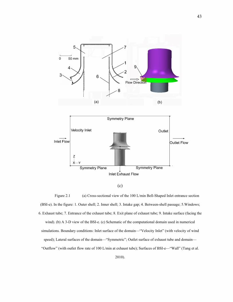
43

(c)

Figure 2.1 (a) Cross-sectional view of the 100 L/min Bell-Shaped Inlet entrance section

(BSI-e). In the figure: 1. Outer shell; 2. Inner shell; 3. Intake gap; 4. Between-shell passage; 5.Windows;

6. Exhaust tube; 7. Entrance of the exhaust tube; 8. Exit plane of exhaust tube; 9. Intake surface (facing the

wind). (b) A 3-D view of the BSI-e. (c) Schematic of the computational domain used in numerical

simulations. Boundary conditions: Inlet surface of the domain—“Velocity Inlet” (with velocity of wind

speed); Lateral surfaces of the domain—“Symmetric”; Outlet surface of exhaust tube and domain—

“Outflow” (with outlet flow rate of 100 L/min at exhaust tube); Surfaces of BSI-e—“Wall” (Tang et al.

2010).

44

Mesh size sensitivity was tested by evaluating the difference in the velocity

profile at high velocity-gradient locations when the mesh density was doubled. The final

mesh density was sufficiently high such that the flow field results were unaffected by

further mesh density increase (with less than 1% change in velocity when the mesh

density was doubled). Overall, approximately 4.5 million cells were generated in the

computational domain. The minimum cell volume was 10 31.88 10 m and the maximum

cell volume was 6 31.01 10 m , which were approximately the same as those volumes of

0.6 mm and 10 mm cubes.

2.1.3 Turbulence Model

In this case, the usage of a turbulence model in the CFD modeling was necessary

because the Reynolds number based on the gap width of the intake section could be as

high as 5,000 in the case of the free wind speed 24 km/h. Thus, the Reynolds Stress

Model (RSM) was applied for the BSI-e simulations.

A 5% of the turbulence intensity on the inlet boundary of the computational

domain was set before iterations, which was based on the previous wind tunnel

experiments (S. R. Lee, et al., 2008). The mass and momentum equations were solved

using a finite volume approach with double precision, and the numerical convergence

criterion for continuity calculations was set at ~10−6. The flow field simulations were run

until all the momentum residuals within the computational domain were almost

unchanged within the next 100 additional iterations.

45

After the flow field simulation in the computation domain was convergent, the

Lagrangian particle tracking method was carried out. The Discrete Phase model (DPM)

and Particle Tracks module of the FLUENT program was functioned to simulate for this

purpose, with assumed no particle-flow interaction. Considering the turbulence effect on

both flows and particles, the turbulent dispersion was carried out using the Stochastic

Tracking model in FLUENT. The turbulent dispersion of particles was calculated using

the instantaneous fluid velocity (shown in Equation 1.7) obtained from the flow field

simulation. In each particle injection point on the domain inlet surface, 100 parcels

(particle releasing attempts) were processed for the turbulence dispersion with

randomness. Time-dependent fluctuating velocity components were calculated based on

the characteristic lifetime of eddies.

The particle number concentration in the wind tunnel experiments of Nene and

Baehl (Baehl, 2007; Nene, 2006) was approximate to be about 109 particle per m3. For

such aerosol concentration levels, the Brownian motion and the kinematic coagulation

should be both negligible (Hinds, 1999). Therefore, particle-particle interactions were

neglected in CFD package here. Particles with a density of 1,000 kg/m3 and one

specified diameter were released from uniformly distributed locations on the inlet

surface of the computation domain. The attachment coefficient for particles on any walls

was set to be unity, i.e. no particle bounce allowed on the wall, and all the particles

would be stuck once impaction occurred which ended this particle trajectory.

Futhermore, the drag force, gravitational effect and the Saffman lift force were

considered in this numerical model through FLUENT momentum settings.

46

2.1.4 Calculation of CFD-Based Penetration and Regional Deposition

The most critical judge on the efficacy and feasibility of the CFD simulations

was to compare the CFD-derived particle penetration efficiency with the experimentally

measured results. In terms of the post-processing calculation, the physical definition of

particle penetration as given in Equation (2.1) can be expressed as:

/

/exhaust exhaust

simtotal total

n QP

n Q (2.2)

where nexhaust is the number of particles which exited the computation domain through

the exhaust tube outlet as determined by particle tracking process; ntotal is the total

number of particles released to this domain in tracking; Qexhaust is the volumetric airflow

rate through the exhaust tube (fixed aerosol sample flow rate, 100 L/min in this case);

and Qtotal is the total volumetric airflow rate through the inlet surface of the computation

domain, which could be calculated by the uniform environmental velocity, i.e. the free

wind speed. In the simulation the particles were released homogeneously and uniformly

over the entire inlet surface.

A root-mean-square normalized error, erms, for the relative deviation between the

CFD-derived and experimental penetration efficiency results can be evaluated from:

erms

1

n

Pexp,i

Pnum,i 2

Pexp,i2

i1

n

(2.3)

where n is the number of the experimental data pairs for penetration; P

exp,i is the the

experimentally measured penetration for the ith experimental condition (the specific case

47

of the particle size and the free wind speed); and, Pnum,i is the CFD-derived penetration

for the same ith condition. In this calculation, Pnum,i took the CFD value if a simulation

was run exactly at the ith condition; however, if CFD simulation for the ith condition was

not available, then Pnum,i was obtained from a spline curve generated from the CFD-

based penetration results, which were processed and obtained by OriginPro 7.5 software

(OriginLab Corporation, Northampton, MA).

The CFD results were as well used to determine the regional particle deposition

pattern within the BSI-e device, which was relevant to particle penetrations through the

inlet. It could be used to develop the correlations between the penetration and other

mechanisms causing deposition. After the tracking particle trajectories with the

Lagrangian method, FLUENT would provide the terminal coordinates of particle

trajectories for deposited particles. MatLab 2008a (The MathWorks, Inc., Natick, MA)

was then applied to plot 3D map of these deposited locations. The CFD results of

regional deposition could not be compared with experimental data, as the latter one was

not available.

Aspiration efficiency is a commonly used term to evaluate the performance of

unidirectional sampling probes (Belyaev & Levin, 1974). In this case of BSI-e, the

aspiration efficiency was defined as the ratio of two particle concentrations: one

concentration in the intake surface (Figure 2.1(b)); the other concentration in the uniform

free stream. The intake surface is where the aerosol flow enters the BSI-e between the

rims of the two shells, and is technically defined as a portion of the circumferential

entrance surface that is bound by the rims of the shells, forming a 60˚ azimuthal angle

48

about the axis of the BSI-e, and symmetric with respect to the free stream velocity on the

upwind side of the BSI-e (see the figure on page 81 in top view). Based on particle

tracking results, approximately only the aerosol flow that moved through the intake

surface was capable to reach in the exhaust tube, i.e. being sampled. Howerve in this

level, note that experiments could be difficult to measure this aspiration efficiency, P1.

Meanwhile, P1 could be simulated based on CFD simulation using the following

equation:

intake intake1

/

/total total

n QP

n Q

(2.4)

where nintake is the number of particles that pass through on the intake region; and, Qintake

is the volumetric airflow rate through the intake region.

Another two penetration were defined here as supplements. The penetration

through the between-shell passage, P2, was calculated from:

2intake intake

/

/dp exhaustn Q

Pn Q

(2.5)

where ndp is the number of particles that reach the entrance plane of the exhaust tube.

The flow rate through the exhaust tube was constant, so the penetration through

tube, P3, could be calculated using the following equation:

3exhaust

dp

nP

n

(2.6)

Note that the flow rate through the exhaust tube should be constant (100 L/min),

and the device penetration efficiency is actually the production of P1, P2 and P3. The

independent variables in Equations (2.4)~(2.6) were calculated from CFD simulation

49

results, with the particle index through defined surfaces or boundaries in the Lagrangian

particle tracking results.

2.2 CFD Prediction of Interception in a Filter

When the trajectory of a spherical particle’s center comes within one particle

radius of a solid surface, the particle will be captured on the surface because of its finite

size (Hinds, 1999). This mechanism of particle capture is referred as interception.

Typically for most cases, interception effect could be neglected in predicting particle

deposition, e.g. the BSI-e case mentioned earlier, because the particle would be too small

compared to the characteristic dimension of the flow channel. However in some other

cases, interception could be a very important mechanism of particle deposition,

especially when the particle size is large relative to the characteristic length of the target

device (e.g. fiber or wire diameter within a filter). However it should be noted that, in

most of commercial CFD packages, the standard Lagrangian particle tracking module

does not technically account for this interception effect. Instead, particles are treated as

mass points when they travel in the domain, and the only use of the particle size is to

derive the drag force acting on itself. This deficiency of neglecting interception normally

would not cause serious consequences as in those cases the interception is an

insignificant mechanism. Nevertheless, for a filtration flow, overlooking the interception

events could cause considerable errors in predicting the collection efficiency (Fotovati,

et al., 2010; Kasper, et al., 2009). To take into account the intercepted events in

commercial CFD simulations, researchers have to develop user-defined functions or

50

C++ subroutines (Fotovati, et al., 2010; S. A. Hosseini & Tafreshi, 2010; J. Wang & Pui,

2009). In these user-defined functions, the distance from each particle mass point to the

nearest wall surface would be monitored so as to capture interception events.

In this doctoral dissertation work, a novel “virtual surface” approach to simulate

particle deposition by interception in aerosol flows was developed and applied based on

ordinary CFD packages. Commercial CFD program was used to simulate the flow field

in a fibrous screen model as well as particle trajectories. By using standard functions of

each CFD program, a “virtual surfaces” which was a radius away from the fiber surface,

was generated by user to record interception events. The CFD-based results agreed well

with experimental results, and also with empirical correlations for interception. For

fibrous filter or screen applications, the approach developed in this study eliminates the

need for user defined functions to account for interception; the results obtained using this

approach can be readily validated by researchers in the field.

2.2.1 Fibrous Screen Model and the Virtual Surface

An electromesh screen model was chosen to demonstrate the “virtual surface”

approach. The screen was experimentally investigated by Han et al. (T. Han, 2007; T.

Han, et al., 2009) under various operating conditions. Experimental studies were carried

out to identify the aerosol deposition on commercial-used electroformed wire screens.

Particles with aerodynamic diameters between 3 and 20 μm were introduced in this

experiment. 3D numerical simulations were performed using the CFD tools in the

present study. This screen model consisted of a single layer of straight cylindrical wires,

51

crossing to form evenly-spaced square openings. The main parameters of the screen

model are given in Table 2.1.

ANSYS FLUENT 12.1 (ANSYS Inc., Canonsburg, PA) and STAR-CCM+ 5.02

(CD-adapco, London, UK) were used as the CFD tools in this study. A volume mesh

was generated using GAMBIT 2.2.30 (ANSYS, Inc., Canonsburg, PA), based on the 3-D

geometric model shown in Figure 2.2. The length, width, and height of the

computational domain were 1.269 mm 1.269 mm 2.538 mm, separately. Two

crossing cylinders of 65 µm in diameter were placed in the center of the volume mesh,

representing a unit section of the electroformed screen. The volume mesh included about

1.5 million tetrahedron cells, with the smallest cells near the fiber surface. The minimum

cell volume was about 1.410-18 m3, which was roughly the volume of a 1-µm cube. The

same volume mesh was used with both FLUENT 12.1 and STAR-CCM+ 5.02.

Table 2.1 Parameters of the electroformed screen.

Fraction of open area,

fOA

Mesh size (number of

openings/inch)

Screen fiber diameter

df

(micrometer)

Opening

width

(micrometer)

0.90 20 65 1204

The flow to be simulated was perpendicular to the cylindrical fibers, and the

same as the gravity direction. The upstream surface of the computational domain was set

to have a uniform velocity boundary condition, with a pressure of 1 atm. The lateral

52

surfaces were set to be symmetry planes, i.e. no shear across these surfaces. The

downstream surface was set to have the same mass flow rate as the upstream surface.

The fiber surfaces were set to be no-slip boundary. Also, the fiber surfaces were set to

“trap” any particles that deposit by impaction. The face velocity (velocity at the inlet

surface) was chosen to be 0.213, 0.6 and 1.06 m/s, for which experimental results were

available from the work by Han et al. (T. Han, 2007; T. Han, et al., 2009).

Figure 2.2 Three-dimensional electroformed screen model. Boundary conditions: Inlet

surface -‘Velocity Inlet’ (with uniform face velocity); Lateral surfaces - ‘Symmetric’; Outlet surface –

‘Outflow’; Surfaces of fiber – ’Wall’.

53

Standard functions of the CFD programs were used to construct “virtual

surfaces”, as shown in Figure 2.3, around the fibers. The virtual surfaces were concentric

with the cylindrical fibers. The distance between the virtual surface and the fiber surface

(real surface) is equal to the radius of the particles (dp/2) whose interception events were

to be recorded. In FLUENT, a “virtual surface” was created by building an Interior

Boundary with the Surface function; in STAR-CCM+, a virtual surface was created by

building a Cylinder Section with the Derived Parts function. The “virtual surfaces” were

not real, and did not alter the original geometric model or the mesh structure, hence did

not affect the flow field simulation or the Lagrangian particle tracking. For each particle

size, a separate set of virtual surfaces (two crossing cylinders) were created to record the

interception events. The construction of the virtual surfaces could be carried out either

before or after the flow field simulation was completed.

Figure 2.3 A schematic showing a virtual-surface relative to the cross section of a

cylindrical fiber and its functionality for recording particle interception.

54

2.2.2 Flow Field Simulation and Lagrangian Particle Tracking

The laminar model and the k-ε turbulence model were used for this simulation.

Both steady and unsteady cases were considered. Necessary precautions were taken to

ensure that near-wall resolution was sufficiently high (Y. J. Tang, et al., 2010). A

convergent flow field was obtained first within the computational domain, then particle

trajectories were tracked using the Lagrangian particle tracking function with each CFD

program. Each particle was tracked based on the following Newton’s second law

equation:

1

2p

p D a p a p a p

dvm C A v v v v

dt (2.7)

where vp and va are the velocity of the particle and the air flow, respectively, mp is the

mass of the single particle, ρa is the air density, Ap is the projected area of the particle on

the plane perpendicular to the flow direction, and CD is the drag coefficient, which can

be taken from functions (Morsi & Alexander, 1972) offered by CFD tools depending on

Reynolds number. In particle tracking, turbulent dispersion of particles was included

when using the k-ε model and the instantaneous fluctuating velocity components were

calculated based on the characteristic lifetime of eddies (Fluent_Inc., 2005). The

thermophoretic effect, Brownian motion and electrostatic forces were neglected in our

particle tracking.

Due to the low particle concentration of the simulated aerosol flow, one-way

coupling was assumed such that the air flow affected particle motion but not vice versa.

From the inlet surface, particles were released at a sufficiently high parcel density (Y. J.

55

Tang, et al., 2010), which is about 1011 particle injection points per square meter surface

area for both CFD tools. In FLUENT, the particle release density was dependent on the

surface mesh density, and in STAR-CCM+, a presentation grid (a Probe type Derived

Part) was built for the particle release.

Particle deposition by impaction was obtained directly through standard particle

tracking of the CFD programs. In FLUENT, the number of particles that deposited on

the ‘real’ fiber surface by impaction was obtained directly by Particle tracks in Display

function; while in STAR-CCM+, the incident mass flow rate of particles onto the fiber

surface (real surface) was obtained directly from Track: particle flow rate results in

Report function.

Meanwhile, information of particles passing through the virtual surfaces was

obtained. In FLUENT, the number of particles crossing the virtual surfaces was obtained

through Discrete Phase Sample in Report function; in STAR-CCM+, the mass flow rate

through the virtual surfaces was obtained from Track: particle flow rate results in Report

function.

2.2.3 Calculation of Deposition Efficiency Based on CFD Results

Particle deposition on the fiber surfaces was quantitatively described in terms of

collection or deposition efficiencies. Taking FLUENT simulation as an example, the

deposition efficiency due to impaction was calculated using the following equation:

impimp

total

n

n

(2.5)

56

where nimp is the number of particles that deposited on the fiber surface by inertial

impaction (output as simulation result through the standard function); ntotal is the total

particle number released to the domain (controlled as user input before simulation). With

STAR-CCM+, the deposition efficiency due to impaction was calculated using the

following equation:

impimp

total

m

m (2.6)

where mimp is the particle mass flow rate captured on the fiber surface (output as

simulation result through the standard function), mtotal is the total particle mass flow rate

released to the domain (controlled as user input before simulation).

Deposition by interception was calculated based on the particle crossing events

through the virtual surfaces. In FLUENT, the number of particle crossing events through

the virtual surfaces was obtained, which includes particle IDs for both impacted and

intercepted particles. The number of particles ‘impact’ on walls, nimp, which are captured

by the standard Lagrangian particle tracking, is obtained by particle tracks function. The

particle IDs for these ‘impact’ particles could be gained through discrete phase sample

result based on physical fiber walls. On the other hand, the number of particles that get

within virtual surfaces which would be trapped by walls due to interception but not

capture by standard functions, nint, could be obtained by comparing the particle IDs

between ‘discrete phase sample’ results based on fiber wall (nimp) and virtual surfaces

(actually nimp+ nint). So in this case, the deposition efficiency by interception would be:

intint

total

n

n

(2.7)

57

where nint should be the difference of the particle numbers between sample results on

virtual surface and fiber wall.

In STAR-CCM+, the particle mass flow rate through the virtual surfaces the

particle mass flow rate is counted, and the deposition efficiency by interception would

be defined as:

2VS imp

inttotal

m m

m

(2.8)

where mvs is the particle mass flow rate through the virtual surface, which includes

particles trapped by impaction, intercepted particles which goes in through the virtual

surface and intercepted particles which goes out through virtual surface since

interception particles would not be captured in the standard Lagrangian particle tracking.

So the actual mass flow rate of interception particles would be particle flow rate through

appropriated cylinder section minus impaction rate, then divided by 2, as shown in

Equation (2.8).

Thus in FLUENT, the total deposition efficiency due to inertial impaction and

interception is:

imp inttotal

total

n n

n

(2.9)

and in STAR-CCM+:

VStotal

total

m

m (2.10)

58

2.2.4 Calculation of Deposition Efficiency Using Empirical Correlations

For this filtration system, the deposition efficiency by interception and total

efficiency could be gained from previous method through CFD simulation. The results

could be validated using the experiment data (T. Han, 2007; T. Han, et al., 2009) and

calculations from empirical correlations (K. W. Lee & Gieseke, 1980; K. W. Lee & Liu,

1982; K. W. Lee & Ramamurthi, 1993; B. Y. H. Liu & Rubow, 1990; Pich, 1966).

These empirical correlations for the single fiber efficiency were used to calculate

the deposition efficiency by interception of the electroformed screen model. The

deposition efficiency by interception was related to the single fiber efficiency through

the following equation:

41 exp SFE

f

t

d

(2.11)

where α is the solidity, which equals to 1- fOA (fOA, the fraction of open area for a screen,

is given in Table 2.1); ηSFE is the single-fiber-efficiency due to interception based on

these correlations; t is the thickness of the screen, which equals to df here in our one-

layer screen model. The empirical correlations used to calculate ηSFE are shown in Table

2.2.

In the empirical correlations, Ku is the Kuwabara hydrodynamic factor, a

dimensionless factor that compensates for the effect of distortion of the flow field around

a cylinder because of its proximity to other cylinders. (Hinds, 1999)

2ln 3

2 4 4Ku

(2.12)

59

Kn is the Knudsen number. It is related to the gas mean free path λ through the

following equation:

2

f

Knd

(2.13)

Table 2.2 Single-fiber-efficiency empirical correlations used in this study to

calculate deposition efficiency by interception.

Investigator(s) Single-fiber-efficiency expressions for interception

Lee and Ramamurthi

(1993)

221 1

2ln 1 1 1 12 1 2 2SPE

RR R

Ku R

Lee and Gieseke

(1980)

21

(1 )SPE m

R

Ku R

,

2

3 1m

Pich (1966)

11 1 2 1 1.996 1 ln 1

2 0.75 0.5ln 1.996 0.5 lnSPE

R R Kn R R

Kn

Liu and Rubow (1990) 21

0.61SPE r

RC

Ku R

,

1.9961r

KnC

R

Lee and Liu (1982) 21

0.61SPE

R

Ku R

2.2.5 Quantitative Comparison of Efficiency Results

The CFD-derived deposition efficiency results were compared with experimental

results from a previous study (T. Han, 2007). The agreement between the CFD-based

60

collection efficiency and the experimental results was quantified using a root-mean-

square normalized error, erms, defined as follows:

2

1, 2,

21 1,

1 ni i

rmsi i

en

(2.14)

where n is the number of the data pairs for comparison; η1,i is the value of the efficiency

obtained by method 1 (experimental measurements or empirical calculations), for the ith

experimental condition (combination of particle size and face velocity); and, η2,i is the

efficiency obtained by method 2 (CFD simulation), for the same ith condition.

2.3 Turbulent Deposition - Turbophoresis

To quantitatively evaluate the turbophoresis effect and predict turbulent

deposition, simple straight pipe geometry with available experimental data is studied

here, and also, eliminates the interference of other deposition mechanism. The amount of

deposition predicted has been seen to depend on the choices of different turbulent

models and particle tracking procedure used (Y. Liu et al., 2007; Matida, et al., 2004).

Wall functions and mesh resolution also could greatly influenced the prediction of

turbulent conditions and aerosol deposition (Parker, et al., 2008). Therefore, a organized

study of the dependence of CFD-derived deposition with different turbulence models,

wall functions and mesh resolutions in vertical straight pipe flow was performed, in

order to provide a better understanding of the requirements for relevant quantitative

estimations.

61

Typically in practice, the selection of turbulence models and the control of near-

wall y+ may be both limited. Therefore, it is probably useful to investigate why certain

turbulence models and certain mesh conditions produce more accurate turbulent

deposition simulations. It is possible that such investigation may reveal more

fundamental criterion for CFD simulation of turbulent deposition, which may be applied

in practice. Herein I report such an investigation, in which the hypothesis is that the

accuracy of the turbulent deposition results is strongly dependent on the accuracy of the

simulated near-wall turbulence kinetic energy (TKE), or more specifically, the wall-

normal mean square fluctuation velocity. The objective of this study was to determine

the relation between particle deposition velocity and the wall-normal mean square

fluctuation velocity as predicted by CFD simulation.

In this study, I carried out flow field simulation using a quarter geometric model

of the pipe flow, and Lagrangian particle tracking with the one-way coupling

assumption. In post-processing of the simulation results, I used the Eulerian description

of turbulent deposition introduced above. Herein I describe the methods of CFD

simulation of turbulent deposition, and the post-processing methods.

2.3.1 Methods of CFD Simulation

In this study, CFD simulation of turbulent deposition was carried out using the

commercial code STAR-CCM+ 5.04 (CD-adapco, London, UK), with the effects of

several CFD parameters investigated. The simulation results were compared to

62

experimental results of Liu and Agarwal (Benjamin Y.H Liu & Agarwal, 1974) for

assessment of accuracy.

(1) Control Volume and Mesh Generation

The vertical straight pipe used in Liu & Agarwal’s experiment had a length of

1.02 m and an inner diameter of 12.7 mm. Taking advantage of the axisymmetric nature

of the flow, a quarter cylindrical control volume was used for the CFD simulation in this

study, representing one fourth of the pipe flow. A three-dimensional geometric model

was built using the STAR-CCM+ geometry function (3D-CAD models).

For mesh generation, polyhedral cells with a target size of 0.1 mm were used for

the bulk of the control volume. Fifteen layers of prism cells were applied in near-wall

regions and the cell thickness was increased away from the wall at a growth factor of 1.1

(more prism layers might be involved for mesh convergence study). A portion of the

inlet surface mesh (perpendicular to the direction of flow) is shown in Figure 2.4.

Figure 2.4 A portion of the inlet surface mesh (perpendicular to direction of flow) showing

polyhedral cells (left) and 15 layers of near-wall prism cells with minimum thickness 5 µm at the wall (far

right).

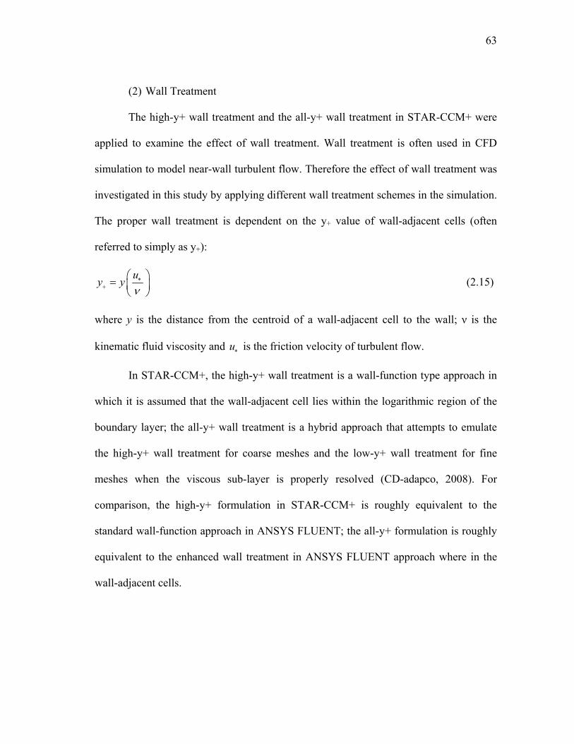
63

(2) Wall Treatment

The high-y+ wall treatment and the all-y+ wall treatment in STAR-CCM+ were

applied to examine the effect of wall treatment. Wall treatment is often used in CFD

simulation to model near-wall turbulent flow. Therefore the effect of wall treatment was

investigated in this study by applying different wall treatment schemes in the simulation.

The proper wall treatment is dependent on the y+ value of wall-adjacent cells (often

referred to simply as y+):

uy y

(2.15)

where y is the distance from the centroid of a wall-adjacent cell to the wall; ν is the

kinematic fluid viscosity and u is the friction velocity of turbulent flow.

In STAR-CCM+, the high-y+ wall treatment is a wall-function type approach in

which it is assumed that the wall-adjacent cell lies within the logarithmic region of the

boundary layer; the all-y+ wall treatment is a hybrid approach that attempts to emulate

the high-y+ wall treatment for coarse meshes and the low-y+ wall treatment for fine

meshes when the viscous sub-layer is properly resolved (CD-adapco, 2008). For

comparison, the high-y+ formulation in STAR-CCM+ is roughly equivalent to the

standard wall-function approach in ANSYS FLUENT; the all-y+ formulation is roughly

equivalent to the enhanced wall treatment in ANSYS FLUENT approach where in the

wall-adjacent cells.

64

The wall treatments have been specialized according to each turbulence model

used, since assumptions respect to each model need to be made for the wall boundary

conditions for the turbulence quantities.

For the all-y+ wall treatment, it is recommended to have y+ value on the order of

unity (CD-adapco, 2008). For the pipe flow in Liu and Agarwal’s study, a wall distance

of 5 µm would give a unity y+ value at Reynolds number of 50000, and a y+ of 0.25 at

Reynolds number 10000. Therefore, in this study the distance from the wall to the center

of the first layer of prism cells was varied from 5 µm to 50 µm (corresponding to y+ a

value of 1 to 10) to explore the effect of near-wall mesh resolution on turbulent

deposition prediction.

(3) Boundary Conditions

For the surface representing the wall of the pipe, the boundary condition was set

to be “wall” with no-slip condition. In accordance with the experimental installation

used by Liu and Agarwal (smooth glass pipe), the pipe wall boundary condition was set

to be smooth. The inlet surface of the control volume was assigned “velocity inlet”

boundary condition with a uniform velocity perpendicular to the inlet surface; the

magnitude of the velocity was calculated from the flow rate used by Liu and Agarwal.

The outlet surface of the control volume assigned ‘flow-split outlet’ boundary condition.

The two lateral boundaries were set to be connected “periodic plane” condition,

following the axisymmetric simplification mentioned earlier in building of the pipe

geometry model. For the particle phase, an “escape” boundary condition was assigned,

65

i.e. no reflection or bounce for particles was allowed at the surfaces of the control

volume.

(4) Turbulence Modeling

Four widely used turbulence models available with STAR-CCM+ were used in

this study, namely the k-ε model (RNG), the k-ω shear stress transport (SST) model, the

Reynolds Stress model (RSM), and the Large Eddy Simulation model (LES). For three

RANS models (k-ε, k-ω and RSM), maximum 5000 iterations were allowed for each

simulation (all momentum residuals became almost constant and less than 10-3). When

running the LES model, the flow field solution obtained with the RSM model was used

as the initial condition. The LES time step used was 1 μs, and total of 5000~10000 time

steps were used. The stopping criterion was either the simulation had reached 50

iterations, or the residuals had all become lower than 10-4.

(5) Particle Tracking

Particle trajectories were simulated following the turbulent flow field simulation,

and assumptions had been made that the aerosol was sufficiently dilute and thus no

influence acted on each other or the air flow (Y. J. Tang, et al., 2010). The Lagrangian

multiphase model (generally known as Lagrangian particle tracking) in STAR-CCM+

was applied to simulate the particle trajectories, in which the momentum equation of

individual particles was numerically solved. (Tang & Guo, 2011) Electrostatic forces,

shear-induced lift forces, Brownian motion and thermophoresis were not included in this

simulation. Particle diameter was varied from 1 to 20 μm in this study, corresponding to

dimensionless relaxation time from 0.1 to 43 at Reynolds number 10000, and

66

dimensionless relaxation time from 2 to 740 at Reynolds number 50000. The particle

density was set to be 920 kg/m3 (olive oil), as was the case in Liu and Agarwal’s

experiments (1974). Particles were released from an injection surface on the inlet

boundary of the pipe at an initial velocity equal to the mean flow velocity; there were

approximately 1,000 uniformly distributed injection points on the surface injector.

With the Reynolds-averaged Navier–Stokes (RANS) models (k-ε, k-ω and

RSM), the effect of turbulence on particle trajectory was simulated with the “turbulent

dispersion” model. From each particle injection point, 100 turbulence-affected particle

trajectories (called “parcels” in the CFD package) were simulated, using information of

the simulated turbulent flow field in conjunction with a random number generator. (Tang

& Guo, 2011) Thus, for each simulation a total of approximately 105 parcels were

tracked.

With LES, the turbulence effect on particle trajectory was not simulated with the

“turbulent dispersion” model, because evidently the turbulence parameters needed for

that model were no longer available. Instead, the effect of turbulence on particle

trajectory was simulated through the use of flow field solutions at multiple consecutive

time points. For each particle injection point, a particle trajectory was simulated using

the flow field solution at a particular instant (by using the “solver frozen” option in

STAR-CCM+); then from the same particle injection point, another particle trajectory

was simulated using flow field solution at the next instant in LES simulation. This was

repeated 100 times, so that for each injection time point, 100 particle trajectories were

simulated; the variation of the particle trajectory originated from the same injection point

67

would reflect a pseudo turbulence effect. The LES time step (1 µs) was chosen such that

it was much smaller than the Lagrangian time scale of the turbulent flow (approx. 100 µs

at Re=50,000) and the relaxation time of the smallest particle (approx. 5 µs), in order

for this scheme to be valid.

Calculations of the aerosol penetration and the particle deposition velocity are

described in the following section.

2.3.2 Methods of Post-Processing

(1) Calculation of Penetration and Dimensionless Deposition Velocity

Similar to the experimental approach used by Liu and Agarwal (Benjamin Y.H

Liu & Agarwal, 1974), particle deposition was quantified excluding locations near the

entrance and the exit of the pipe flow. For that purpose, two plane sections as “derived

parts” were created in the CFD control volume, to be used for particle counting and for

calculating the penetration for the pipe section in between. These two plane sections

were perpendicular to the direction of the flow, at a distance of 127.5 mm and 637.5 mm

from the inlet surface, respectively.

The aerosol penetration, defined as the ratio of aerosol concentration at the exit

of a pipe flow to that at the entrance, was calculated:

637 5

127 5

.

.

nP

n (2.16)

68

where 637 5.n and 127 5.n were the numbers of particles moving through the derived surface

sections which are perpendicular to the direction of the flow, and at a distance of 637.5

mm and 127.5 mm from the inlet surface, respectively.

With the penetration known, the deposition velocity can be calculated with the

following equation (Sehmel, 1970):

1ln /depi

QV P

D L

(2.17)

where Q is the volumetric flow rate through the pipe, Di is the inner diameter of pipe, L

is the length of the pipe and P is the aerosol penetration efficiency through the pipe

section. Then the dimensionless particle deposition velocity can be calculated using

Equation (1.13), where u is the friction velocity defined as:

0 5

2

.f

u U

(2.18)

where U is the average fluid velocity and f is the Fanning friction factor for the pipe

flow. For the smooth pipe used by Liu and Agarwal (Benjamin Y.H Liu & Agarwal,

1974), the friction factor is calculated from the Blasius formula given by Schlichting

(Schilichting, 1968), valid for Re < 100000:

0.25

0.316

4 Ref (2.19)

where Re is the pipe flow Reynolds number based on the pipe inner diameter.

The accuracy of the CFD simulations was quantified against the experimentally

derived results, both in terms of penetration and dimensionless deposition velocity. For

69

each flow condition, the discrepancy of dimensionless deposition velocity between the

CFD simulation and the experimental results, known as the Geometric Standard

Deviation (GSD), was quantified as:

0 52

1

.

ln lnexp

i simn V VGSD

N

exp (2.20)

where N represents the number of the comparison pairs. When a CFD-simulated

condition was not available from the experiments, interpolation was carried out to

generate an “experimental” data point V exp to be compared with the CFD result simV .

(2) Determination of the Particle Responsiveness Factor

According to Equation (4), 2py

dV

dy is a critical quantity for turbophoresis. The

mean square velocity fluctuation of the particles, Vpy

2 , is not directly known from the

CFD simulation, but the mean square velocity fluctuation of the fluid, 2fyV is readily

available from CFD simulation. Therefore, in this study 2py

dV

dy was quantified based

on 2fy

dV

dy from CFD simulation, using Guha’s formulation. In fact, the ratio of two

gradients of mean square velocity fluctuation was calculated and compared against an

empirical relationship, as a means of evaluating the validity of the CFD simulation of

turbulent deposition.

70

The particle responsiveness factor, α, is defined as the ratio of the wall-normal

gradient of the mean square particle velocity fluctuation to the wall-normal gradient of

the mean square fluid velocity fluctuation:

ddy

Vpy

2 w

ddy

Vfy

2 w

(2.21)

In order to obtain the value of α from the CFD simulation results, substituting

Equation (2.21) into Equation (1.12), and replacing the derivative with an expression

based on finite difference, it yields the following equation, expressed in terms of the

quantities at the wall and at the wall-adjacent cell centroid:

Vpy ,wc

Vpy ,1c V

py ,wc

y1

V

py ,wc

d

dyVfy

2 w

(2.22)

where ,cpy wV is the particle convective velocity in wall-normal direction at the

wall, i.e., the particle deposition velocity that may be experimentally measured; 1,cpyV is

the particle convective velocity in the wall-normal direction at the wall-adjacent cell

centroid in CFD simulation, which could be obtained from the particle convective flux

through a user-defined ‘virtual wall surface’ through the wall-adjacent cell centroids. y1

is the distance from the wall-adjacent cell centroid to the pipe wall.

The gradient term on the right hand side of Equation (2.22) was obtained from

the flow field simulation, to be described below; the two particle convective velocity

quantities on the left hand side were obtained from Lagrangian particle tracking results

71

and Equation (2.17). Note that in Equation (2.22), the particle relaxation time τ replaces

the particle inertial relaxation time τI. This approximation shall not introduce significant

error for the particle size range involved in this study, because the “slip” velocity

between the particle the gas flow should be small.

To provide references for the CFD-based results to be compared against,

empirical equations were also used to calculate the particle responsiveness factor. Using

the finite difference method, the ratio of 2py

w

dV

dy to 2

fyw

dV

dy would be approximately

equal to the ratio of Vpy

2 to 2fyV at the wall-adjacent cell centroid, with the assumption

that velocity fluctuation would be zero at y = 0. Thus, the particle responsiveness factor

at the wall-adjacent cell centroid may be calculated with following empirical equation

(Binder & Hanratty, 1991):

Vpy ,1

2

Vfy ,1

2 1

10.7 / L,1

(2.23)

where L,1

is the Lagrangian time scale of fluid turbulence at the wall-adjacent cell

centroid, which is calculated as (Johansen, 1991):

11 2

1

,,

,

tL

fyV

(2.24)

Where t ,1

is the fluid turbulent viscosity at the wall-adjacent cell centroid, which is

calculated as follows (Davies, 1966):

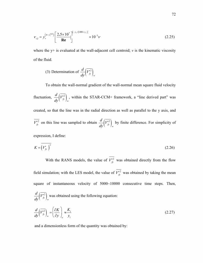
72

0 084007

4 31

2 5 1010

./

,

.

Re

y yy

t y

(2.25)

where the y+ is evaluated at the wall-adjacent cell centroid; ν is the kinematic viscosity

of the fluid.

(3) Determination of d

dyVfy

2 w

To obtain the wall-normal gradient of the wall-normal mean square fluid velocity

fluctuation, d

dyVfy

2 w

, within the STAR-CCM+ framework, a “line derived part” was

created, so that the line was in the radial direction as well as parallel to the y axis, and

Vfy

2 on this line was sampled to obtain d

dyVfy

2 w

by finite difference. For simplicity of

expression, I define:

2

fyK V (2.26)

With the RANS models, the value of Vfy

2 was obtained directly from the flow

field simulation; with the LES model, the value of Vfy

2 was obtained by taking the mean

square of instantaneous velocity of 5000~10000 consecutive time steps. Then,

d

dyVfy

2 w

was obtained using the following equation:

d

dyVfy

2 w K

y

w

K

1

y1

(2.27)

and a dimensionless form of the quantity was obtained by:

73

21

1

/

w

K uKuy

y

(2.28)

where K1 is the value of Vfy

2 at the wall-adjacent cell centroid, u is the friction velocity

of turbulent flow, and y1 is the distance from the wall-adjacent cell centroid to the pipe

wall.

(4) Determination of the Turbophoresis Factor

Equation (2.22) suggests that the particle deposition velocity is a function of the

gradient of wall-normal fluid velocity fluctuation. Quantification of this relationship

through experiments is typically not possible because the gradient of the velocity

fluctuation measurement is lacking. However, it is possible to obtain this relationship

from CFD simulation results. Herein I define a “turbophoresis factor”, as the ratio of the

dimensionless deposition velocity to the dimensionless gradient of the mean square wall-

normal fluid velocity fluctuation:

t

w

Vr

Ky

(2.29)

In this study, the turbophoresis factor was computed once the dimensionless

deposition velocity and the gradient of mean square wall-normal fluid velocity

fluctuation were obtained as described above. As will be discussed later, the

turbophoresis parameter may be of potential value for assessing the importance of

turbulent deposition in complex flows.

74

3. RESULTS *

Obtained results for this doctoral dissertation study were described in this

section. Different mechanisms of aerosol deposition were also discussed based on these

works, including BSI penetration prediction (inertial impaction, gravitational effect and

Saffman lift force), screen models in filtration system (particle interception), and

turbulent deposition in vertical straight pipe flow (turbophoresis).

3.1 Aerosol Deposition and Efficiency of BSI-e

3.1.1 Simulated Flow Field

The flow field simulation results were qualitatively similar for the three different

free stream velocities, so only the results for the wind speed of 8 km/h (2.22 m/s) are

presented (Figure 3.1). Figure 3.1(a) shows the air velocity in a vertical plane that cuts

through the BSI-e axis and is parallel to the free stream; Figures 3.1(b) and 3.1(c) show

the velocity in two horizontal planes, the vertical locations of which are indicated in

Figure 3.1(a). All velocity vectors shown are their projections in the respective planes.

With reference to Figure 3.1(a), the aerosol flow enters the upwind side of the intake gap

____________ *Reprinted with permission from “A Computational Fluid Dynamics Study of Particle Penetration through an Omni-Directional Aerosol Inlet” by Tang, Y.J., Guo, B., & McFarland, A.R. 2010. Aerosol Science and Technology, 44, 1049-1057, Copyright [2012] by TAYLOR & FRANCIS INFORMA UK LTD – JOURNALS.

75

and is accelerated in the curved converging flow channel between the two shells, where

it reaches a maximum speed of approximately 2.6 m/s, as compared with the free stream

speed of 2.22 m/s. The flow first decelerates before entering the inlet, then accelerates in

the curved converging gap between the shells. Recirculation zones can be observed near

the entrance of the exhaust tube. The three views of Figure 3.1 show there is a split in

the aerosol flow in the gap between the shells where the center portion on the upwind

side follows up the slope of the bell-shaped shells and, the off-center portions flow

around the waist of the bell-shaped shell and leave the gap between the shells on the

downwind side. Most of the flow goes around the inner shell and is discharged at the

downwind side, while part of the flow enters the openings (windows) between the roof

of the outer shell and the entrance of the exhaust tube. Part of the flow exits through the

downwind vertical openings and 100 L/min leaves through the exhaust tube.

76

Figure 3.1 CFD simulation of the flow field at a wind speed of 8 km/h (2.2 m/s). (a)

Velocity vectors in the vertical plane through the BSI-e axis and parallel to the free stream (dashed lines

"b" and "c" indicate locations of the two horizontal planes for (b) and (c). (b) Velocity vectors in a

horizontal plane slightly above the rim of the outer shell. (c) Velocity vectors in a horizontal plane in the

cylindrical section of the shells (shell radii do not change with height). Units of velocity scales are m/s.

(Tang et al. 2010).

77

3.1.2 CFD-Based Penetration and Regional Deposition

Aerosol penetration as a function of particle size and for wind speeds of 2, 8, and

24 km/h is shown in Figure 3.2. The CFD-based penetration results not only have the

proper trends, but they are also in excellent quantitative agreement with the experimental

results. The root-mean-square normalized error, erms calculated using Equation (2.3) with

all available experimental data, was 3.8%.

The CFD-based penetration decreases with increasing particle size, and for the

high inertia particles (e.g., 20 m AD), the penetration also decreases with increasing

wind speed. These results agree with the expectation of penetration based on aerosol

mechanics for situations where inertial impaction, as illustrated by deposition in the

accelerating curvilinear flow region near the entrance to the BSI-e, would control the

losses.

The three penetration terms, aspiration efficiency, P1, penetration through the

between-shell passage region, P2, and penetration through the exhaust tube, P3 (defined

in Equations 2.4 – 2.6), were calculated for 10 and 15 m AD particles and for wind

speeds of 2, 8, and 24 km/h; and, the results are shown in Table 3.1. The aspiration, P1,

is approximately equal to or slightly greater than 1, where values greater than unity are

apparently associated with subisokinetic sampling conditions (Hinds, 1999). From

Figures 3.1(a) and 3.1(b) it may be observed that the flow decelerates (indicated by a

shift in color of velocity vectors) just upstream of the BSI-e. Also, in Figure 3.1(b), it

may be noted that there is a divergence in flow away from the mean wind direction for

the vectors just outside of the BSI-e on the upwind side, i.e., curvilinear flow in the x-y

78

plane. This external flow deceleration effect tends to enrich the concentration of aerosol

in the approximate intake region subtended by the 60 angle and the height between the

shell rims.

(a)

(b)

Figure 3.2 Comparison of penetration from experiments and CFD simulations at wind speeds of:

(a) 2 km/h. (b) 8 km/h. (c) 24 km/h.

79

Figure 3.2 continued. (c)

Table 3.1 Estimated regional and overall penetration percentage of the BSI-e from CFD

analyses. (Tang et al. 2010)

Region

Free Stream Wind Speed

2 km/h 8 km/h 24 km/h

Aerodynamic Particle Diameter

10 m 15 m 10 m 15 m 10 m 15 m

P1 101% 102% 104% 105% 110% 112%

P2 88.0% 81.5% 94.1% 81.5% 85.7% 55.3%

P3 98.5% 96.4% 96.5% 94.7% 94.4% 90.1%

Ptotal 87.5% 80.1% 94.4% 81.0% 89.0% 55.8%

80

The penetration P3 is near unity, suggesting that the particle losses in the exhaust

tube are quite small. This is likely due to the low velocity in exhaust tube (less than 0.4

m/s in most cases) and there being no gravitational settling effect on particle deposition.

P2 had the lowest value among the three penetrations; it had approximately the same

value as the overall penetration of BSI-e.

No particle deposition was found on the internal surface of the outer shell.

However, significant particle deposition occurred on the curved surface of the inner

shell. Deposition locations of various particle sizes on the inner shell are shown in

Figure 3.3, for wind speeds of 24 km/h. The figure is the top view of the inner shell,

showing deposition locations of particles of 10, 15, 20 µm AD. Each dot in the views

represents a deposited particle. Each view shows approximately 200 to 1000 deposited

particles, from tracking a total of 400,000 particles that enter the upstream surface of the

computational domain. The visualization results clearly show that most particle

deposition was concentrated on an upwind area of the inner shell that lies within the

angle of about 60, and involves the sloped portion of the inner shell. Larger particle

sizes and higher wind speeds cause the particles to deposit closer to the rim of the shell.

The higher inertia could cause the particle turn less when the aerosol flow entering the

intake of inlet and make a turn, which means these particles with higher inertial (larger

diameter and higher speed) would be more likely to deposit on the relatively lower

region on the upwind area of the inner plenum just due to the inertial impaction

mechanism. Scattered particle deposition locations on the lateral side might be due to a

turbulent effect at those localities where turbulence intensity values of over 65% were

81

noted. Based on this deposition feature, some modification of the BSI design could be

considered, in order to reduce this part of the inertial impaction and particle depositions

in the front surface region.

Figure 3.3 Visualization of particle deposition locations on the surface of BSI inner shell (top view)

for particle diameter of 10, 15 and 20 micrometers at free wind speed of 8 and 24 km/h. (Tang et al. 2010).

82

3.1.3 Effect of Gravitational Settling on Penetration

CFD simulation was also used to determine the importance of gravitational

settling in particle deposition. The approach used was to first conduct the particle

tracking without including the gravitational force, and then repeat the calculations with

gravity included. As shown in Table 3.2, at the higher wind speeds (8 and 24 km/h), the

CFD-based penetration was essentially the same for all particle sizes whether gravity

was considered or not. However, at the wind speed of 2 km/h, the gravitational effect

was significant with the largest difference being about 8% in the case of 20 m AD

particles. At low wind speeds, the gravitational effect is more significant because of the

longer residence time of the particles in the sloped part of the between-shell passage, due

to the lower flow velocity in that region. This may also explain why the penetration of

intermediate particle sizes at the wind speed of 2 km/h can be lower than that at 8 km/h

(Figure 3.1), e.g. in Table 3.2, the penetration of 10 m AD particles is 87.5% at 2 km/h,

and 94.4% at 8 km/h.

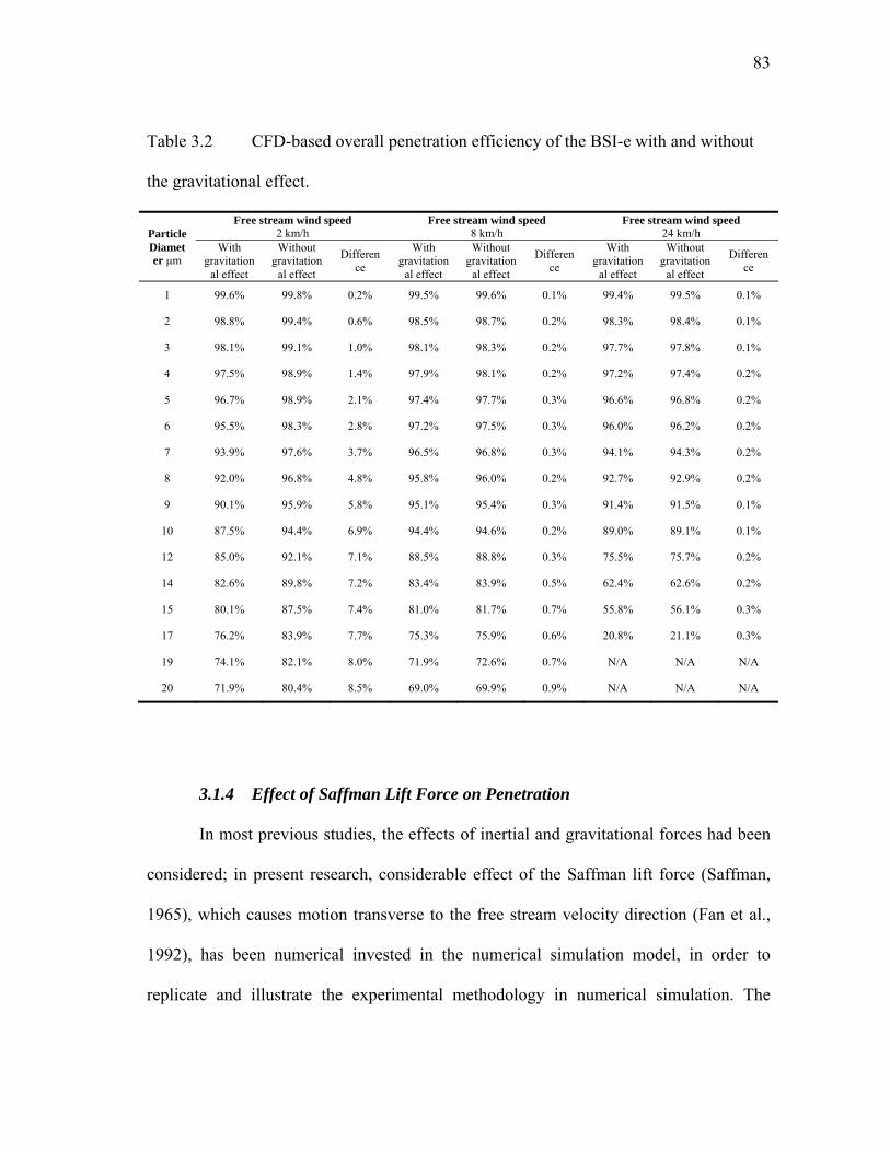
83

Table 3.2 CFD-based overall penetration efficiency of the BSI-e with and without

the gravitational effect.

Particle Diameter μm

Free stream wind speed 2 km/h

Free stream wind speed 8 km/h

Free stream wind speed 24 km/h

With gravitation

al effect

Without gravitation

al effect

Difference

With gravitation

al effect

Without gravitation

al effect

Difference

With gravitation

al effect

Without gravitation

al effect

Difference

1 99.6% 99.8% 0.2% 99.5% 99.6% 0.1% 99.4% 99.5% 0.1%

2 98.8% 99.4% 0.6% 98.5% 98.7% 0.2% 98.3% 98.4% 0.1%

3 98.1% 99.1% 1.0% 98.1% 98.3% 0.2% 97.7% 97.8% 0.1%

4 97.5% 98.9% 1.4% 97.9% 98.1% 0.2% 97.2% 97.4% 0.2%

5 96.7% 98.9% 2.1% 97.4% 97.7% 0.3% 96.6% 96.8% 0.2%

6 95.5% 98.3% 2.8% 97.2% 97.5% 0.3% 96.0% 96.2% 0.2%

7 93.9% 97.6% 3.7% 96.5% 96.8% 0.3% 94.1% 94.3% 0.2%

8 92.0% 96.8% 4.8% 95.8% 96.0% 0.2% 92.7% 92.9% 0.2%

9 90.1% 95.9% 5.8% 95.1% 95.4% 0.3% 91.4% 91.5% 0.1%

10 87.5% 94.4% 6.9% 94.4% 94.6% 0.2% 89.0% 89.1% 0.1%

12 85.0% 92.1% 7.1% 88.5% 88.8% 0.3% 75.5% 75.7% 0.2%

14 82.6% 89.8% 7.2% 83.4% 83.9% 0.5% 62.4% 62.6% 0.2%

15 80.1% 87.5% 7.4% 81.0% 81.7% 0.7% 55.8% 56.1% 0.3%

17 76.2% 83.9% 7.7% 75.3% 75.9% 0.6% 20.8% 21.1% 0.3%

19 74.1% 82.1% 8.0% 71.9% 72.6% 0.7% N/A N/A N/A

20 71.9% 80.4% 8.5% 69.0% 69.9% 0.9% N/A N/A N/A

3.1.4 Effect of Saffman Lift Force on Penetration

In most previous studies, the effects of inertial and gravitational forces had been

considered; in present research, considerable effect of the Saffman lift force (Saffman,

1965), which causes motion transverse to the free stream velocity direction (Fan et al.,

1992), has been numerical invested in the numerical simulation model, in order to

replicate and illustrate the experimental methodology in numerical simulation. The

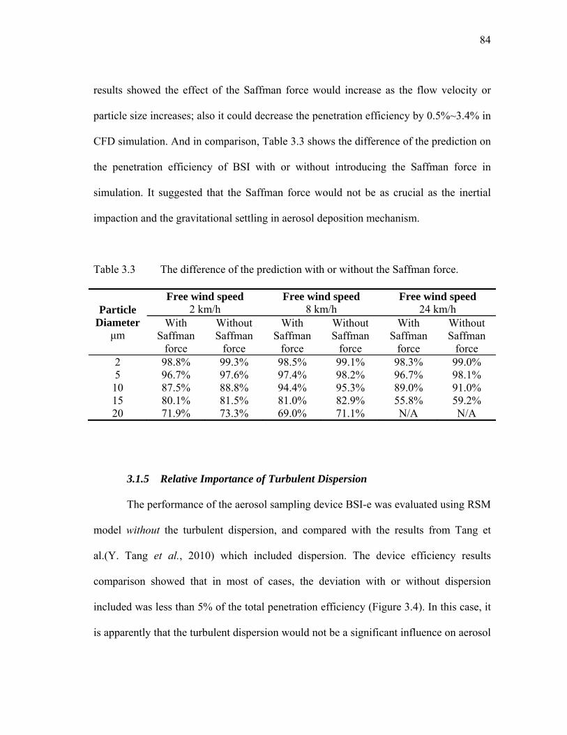
84

results showed the effect of the Saffman force would increase as the flow velocity or

particle size increases; also it could decrease the penetration efficiency by 0.5%~3.4% in

CFD simulation. And in comparison, Table 3.3 shows the difference of the prediction on

the penetration efficiency of BSI with or without introducing the Saffman force in

simulation. It suggested that the Saffman force would not be as crucial as the inertial

impaction and the gravitational settling in aerosol deposition mechanism.

Table 3.3 The difference of the prediction with or without the Saffman force.

Particle Diameter

μm

Free wind speed 2 km/h

Free wind speed 8 km/h

Free wind speed 24 km/h

With Saffman

force

Without Saffman

force

With Saffman

force

Without Saffman

force

With Saffman

force

Without Saffman

force 2 98.8% 99.3% 98.5% 99.1% 98.3% 99.0% 5 96.7% 97.6% 97.4% 98.2% 96.7% 98.1% 10 87.5% 88.8% 94.4% 95.3% 89.0% 91.0% 15 80.1% 81.5% 81.0% 82.9% 55.8% 59.2% 20 71.9% 73.3% 69.0% 71.1% N/A N/A

3.1.5 Relative Importance of Turbulent Dispersion

The performance of the aerosol sampling device BSI-e was evaluated using RSM

model without the turbulent dispersion, and compared with the results from Tang et

al.(Y. Tang et al., 2010) which included dispersion. The device efficiency results

comparison showed that in most of cases, the deviation with or without dispersion

included was less than 5% of the total penetration efficiency (Figure 3.4). In this case, it

is apparently that the turbulent dispersion would not be a significant influence on aerosol

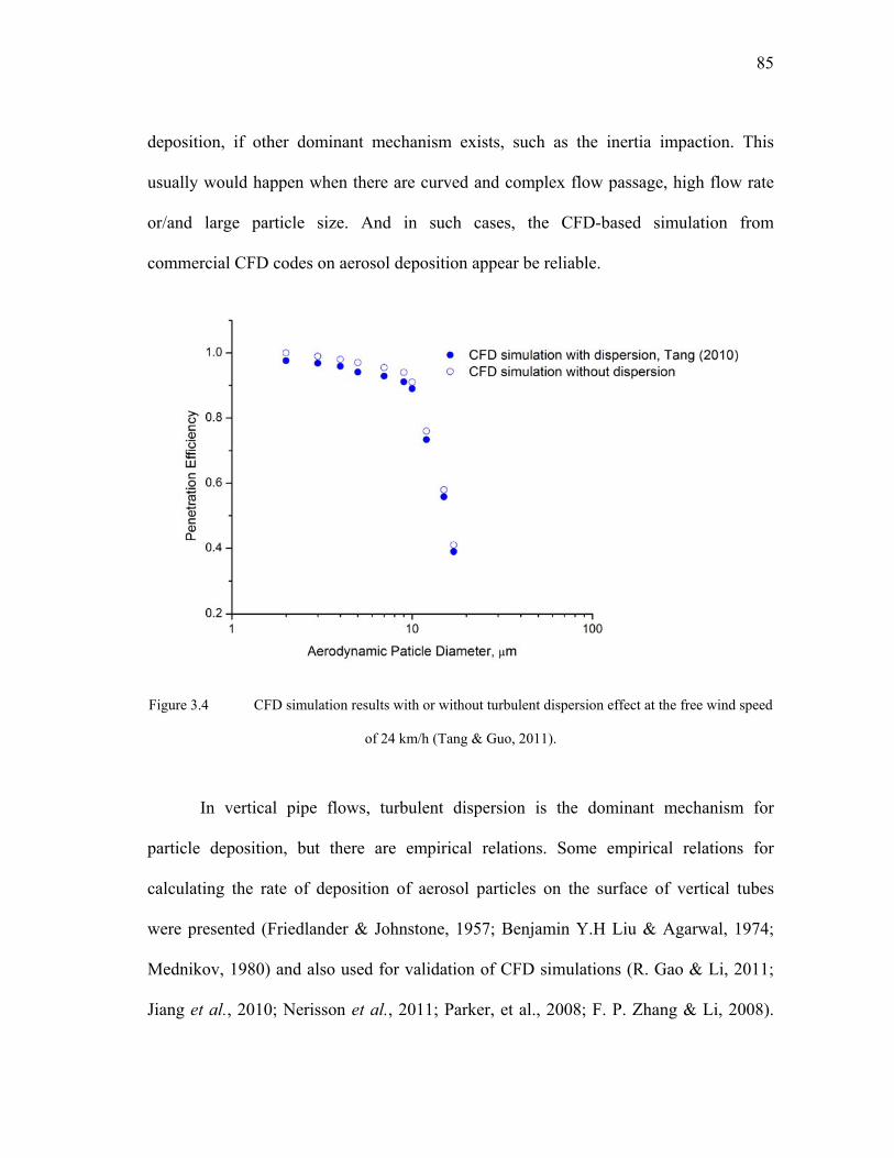
85

deposition, if other dominant mechanism exists, such as the inertia impaction. This

usually would happen when there are curved and complex flow passage, high flow rate

or/and large particle size. And in such cases, the CFD-based simulation from

commercial CFD codes on aerosol deposition appear be reliable.

Figure 3.4 CFD simulation results with or without turbulent dispersion effect at the free wind speed

of 24 km/h (Tang & Guo, 2011).

In vertical pipe flows, turbulent dispersion is the dominant mechanism for

particle deposition, but there are empirical relations. Some empirical relations for

calculating the rate of deposition of aerosol particles on the surface of vertical tubes

were presented (Friedlander & Johnstone, 1957; Benjamin Y.H Liu & Agarwal, 1974;

Mednikov, 1980) and also used for validation of CFD simulations (R. Gao & Li, 2011;

Jiang et al., 2010; Nerisson et al., 2011; Parker, et al., 2008; F. P. Zhang & Li, 2008).

86

The turbulent effect on particle deposition would be quantitatively discussed within

Section 3.3.

3.1.6 Dimensionless Numbers and Empirical Correlation of Penetration

Assuming that impaction and gravitational settling are the most important factors

affecting aerosol penetration through the BSI-e, a semi-empirical correlation equation

similar to that utilized in filtration theory (Hinds, 1999) can be constructed to relate

overall penetration to a Stokes number, Stk, a dimensionless gravitational settling

parameter, G, and a velocity ratio, rv, which represents the relationship of the external

and the internal flow fields, and provides a correction to the first two dimensionless

numbers. Assume the form of the correlation to be:

2 5

3 6

1 4

1 11 1

1 1C C

v vC C

PC r C r

Stk G

(3.1)

where C1 through C6 are parameters that are determined from curve fitting. Terms in the

first set of brackets on the rights size of Equation (3.1) represent the penetration if only

inertial impaction is considered, and those in the second pair of brackets represent the

penetration if only gravitational settling is in effect. The form of Equation (3.1) was

chosen so that it would be asymptotically correct in the sense that the penetration would

tend to zero when Stk or G approaches infinity and it would tend to unity for very small

particles for which Stk and G approach zero.

The Stokes number, Stk, is defined as:

87

20

18p p c

c

d U CStk

d

(3.2)

where p is the particle density; pd is the aerodynamic diameter of particle; U0 is the

free stream velocity (wind speed); cC is Cunningham slip correction factor; is the

viscosity of air; and, dc is the characteristic dimension, which is chosen as the width of

the intake gap at the flow entrance to the BSI-e (see Figure 2.1). The gravitational

settling parameter, G, is defined as (Hinds, 1999):

G

pd

p2C

cg

18U0

(3.3)

The velocity ratio, rv, is defined as:

*

0v

Ur

U (3.4)

where U* is the aerosol sampling flow rate divided by the annular area between the outer

and inner shells in the region where the two shells are cylindrical (Aannular):

* exhaust

annular

QU

A (3.5)

The impaction and gravitation settling effects are functions of the between-shell

air velocity, which depends on the free stream velocity, and the aerosol sample flow rate.

Since Stk and G use the free stream velocity, it is necessary to modify the results through

the use of the velocity ratio. Nene (Nene, 2006), in his experimental study of the BSI-e,

proposed an empirical correlation that included a Stokes number and a velocity ratio but

it did not include the gravitational settling factor. In the study of a cap-and-funnel type

omni-directional aerosol inlet, Lee et al. (S. R. Lee, et al., 2008) had proposed an

empirical equation that only included a Stokes number. The semi-empirical equation

88

generated in this study, which includes the three dimensionless numbers, takes into

account both inertial deposition and gravitational settling. Including the velocity ratio is

essentially equivalent to including a Reynolds number (based on the free stream

velocity) in the correlation.

Using the experimental and CFD-based data, curve fitting with the OriginPro 7.5

software provided the correlation coefficients for Equation (3.1), which are shown in

Table 3.4. With reference to Figure 3.5, the fitted curves for the three wind speeds are in

excellent agreement with the experimental and CFD penetration data, especially for the

lower Stokes number cases.

Table 3.4 Curve fitting results for the coefficients in Equation (3.1) with

corresponding uncertainties (Tang et al. 2010).

Coefficien C1 C2 C3 C4 C5 C6 Curve

fitting

values

0.0076 0.0003

0.105 0.004

2.91 0.08

0.072 0.003

0.507 0.009

0.955 0.022

89

Figure 3.5 Penetration predicted from correlation compared with experimental and CFD

data at wind speeds of (a) 2 km/h, (b) 8 km/h, (c) 24 km/h.

Figure 3.6 shows the agreement of the penetration predicted from Equation (3.1)

with the experimental and CFD penetration values. Note that there are two data points,

which are associated with the smallest abscissa values on the 24 km/h curve, that have

large errors. The slope of the penetration curves through these two data points, Figure

3.2(c), is steep so a small uncertainty in the abscissa value, e.g., experimentally

measured particle size or correlation fit to the numerical data, results in a large relative

deviation between the experimentally measured or numerically calculated penetration

and the prediction from the correlation. The root-mean-square relative error of the fitting

is 3.8% with the two outlying data points removed; however, it is 13.5% when all data

points are included. Omission of the two data points, which are associated with particle

sizes 15 m AD, is not a critical concern for most applications where a pre-separator

with a cutpoint ~ 10 m AD would be included in the overall inlet system; and, as the

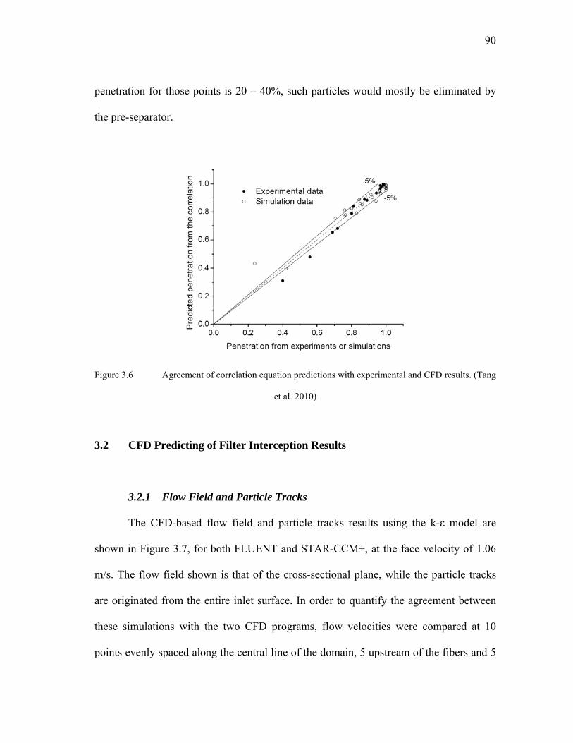
90

penetration for those points is 20 – 40%, such particles would mostly be eliminated by

the pre-separator.

Figure 3.6 Agreement of correlation equation predictions with experimental and CFD results. (Tang

et al. 2010)

3.2 CFD Predicting of Filter Interception Results

3.2.1 Flow Field and Particle Tracks

The CFD-based flow field and particle tracks results using the k-ε model are

shown in Figure 3.7, for both FLUENT and STAR-CCM+, at the face velocity of 1.06

m/s. The flow field shown is that of the cross-sectional plane, while the particle tracks

are originated from the entire inlet surface. In order to quantify the agreement between

these simulations with the two CFD programs, flow velocities were compared at 10

points evenly spaced along the central line of the domain, 5 upstream of the fibers and 5

91

downstream. The average deviation of the velocity magnitude at these 10 points was

about 4.8%; the maximum deviation in velocity magnitude was 7.1%.

Figure 3.7 The k-ε model flow field simulation results with (a) FLUENT and (b) STAR-CCM+,

and the particle tracks results with (c) FLUENT and (d) STAR-CCM+, at the face velocity of 1.06 m/s.

Figure 3.7 (c) and (d) show the particle tracking results with the two CFD

programs. The particle trajectories shown are from the entire inlet surface. Note that

particle tracks with high velocity at the vertical level of the fibers are actually located

close to the symmetric boundary of the domain, where the air velocity is high. The

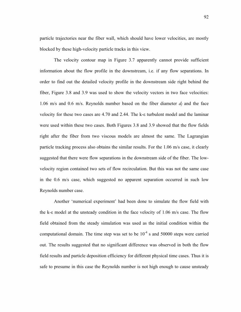
92

particle trajectories near the fiber wall, which should have lower velocities, are mostly

blocked by these high-velocity particle tracks in this view.

The velocity contour map in Figure 3.7 apparently cannot provide sufficient

information about the flow profile in the downstream, i.e. if any flow separations. In

order to find out the detailed velocity profile in the downstream side right behind the

fiber, Figure 3.8 and 3.9 was used to show the velocity vectors in two face velocities:

1.06 m/s and 0.6 m/s. Reynolds number based on the fiber diameter df and the face

velocity for these two cases are 4.70 and 2.44. The k-ε turbulent model and the laminar

were used within these two cases. Both Figures 3.8 and 3.9 showed that the flow fields

right after the fiber from two viscous models are almost the same. The Lagrangian

particle tracking process also obtains the similar results. For the 1.06 m/s case, it clearly

suggested that there were flow separations in the downstream side of the fiber. The low-

velocity region contained two sets of flow recirculation. But this was not the same case

in the 0.6 m/s case, which suggested no apparent separation occurred in such low

Reynolds number case.

Another ‘numerical experiment’ had been done to simulate the flow field with

the k-ε model at the unsteady condition in the face velocity of 1.06 m/s case. The flow

field obtained from the steady simulation was used as the initial condition within the

computational domain. The time step was set to be 10-4 s and 50000 steps were carried

out. The results suggested that no significant difference was observed in both the flow

field results and particle deposition efficiency for different physical time cases. Thus it is

safe to presume in this case the Reynolds number is not high enough to cause unsteady

93

vortex and the steady simulation would be feasible and reliable to predict the filter

efficiency.

(a)

(b)

Figure 3.8 Flow field vectors in the downstream region of the fiber, at the face velocity of 1.06 m/s

(Re = 4.70), using (a) the k-ε model, and (b) the laminar model.

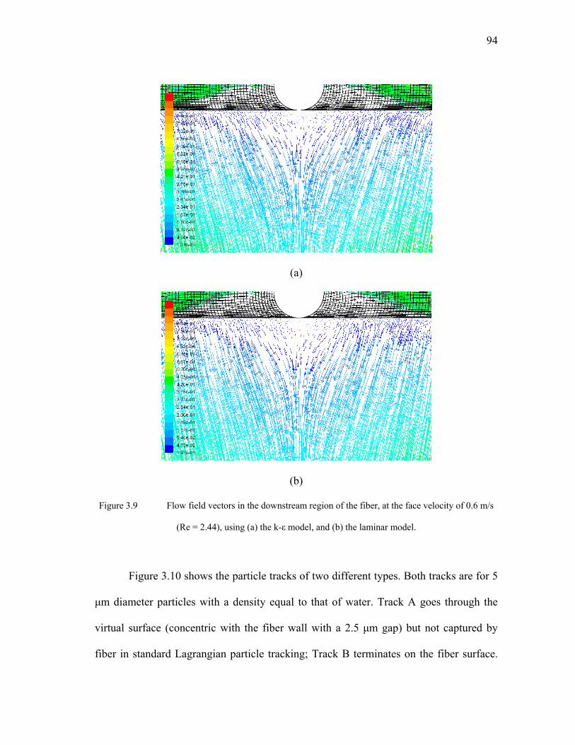
94

(a)

(b)

Figure 3.9 Flow field vectors in the downstream region of the fiber, at the face velocity of 0.6 m/s

(Re = 2.44), using (a) the k-ε model, and (b) the laminar model.

Figure 3.10 shows the particle tracks of two different types. Both tracks are for 5

μm diameter particles with a density equal to that of water. Track A goes through the

virtual surface (concentric with the fiber wall with a 2.5 μm gap) but not captured by

fiber in standard Lagrangian particle tracking; Track B terminates on the fiber surface.

95

Track A represents that of a particle that would deposit by interception, while Track B

represents that of a particle that deposits by impaction. As discussed before, programs do

not recognize that interception would occur for particle track A. However, standard

functions of these CFD programs are able to record the event that a particle track

(trajectory of the center of a particle) comes within on particle radius from the fiber, in

other words, go through the virtual surface.

Figure 3.10 Particle trajectories (Impaction and Interception) for 5 micrometer particle.

3.2.2 Comparison between CFD Programs and Against Experimental Results

Simulations were done based on the screen whose parameters are shown in Table

2.1, at face velocity of 0.213, 0.6 and 1.06 m/s, particle diameter of 4~20 micrometer.

Han (T. Han, 2007; T. Han, et al., 2009) used the same electroformed screen in

experimental test to find the collection efficiency. Our simulation results were compared

to Han’s experimental data in same conditions.

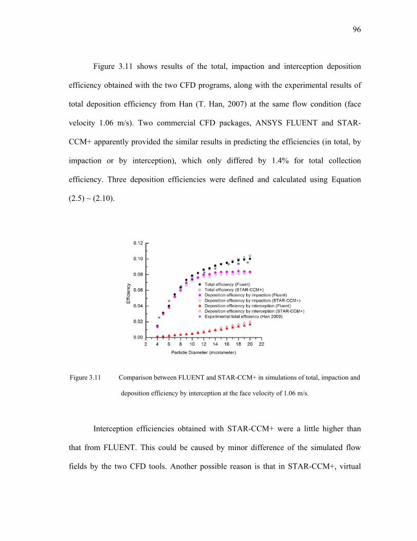
96

Figure 3.11 shows results of the total, impaction and interception deposition

efficiency obtained with the two CFD programs, along with the experimental results of

total deposition efficiency from Han (T. Han, 2007) at the same flow condition (face

velocity 1.06 m/s). Two commercial CFD packages, ANSYS FLUENT and STAR-

CCM+ apparently provided the similar results in predicting the efficiencies (in total, by

impaction or by interception), which only differed by 1.4% for total collection

efficiency. Three deposition efficiencies were defined and calculated using Equation

(2.5) ~ (2.10).

Figure 3.11 Comparison between FLUENT and STAR-CCM+ in simulations of total, impaction and

deposition efficiency by interception at the face velocity of 1.06 m/s.

Interception efficiencies obtained with STAR-CCM+ were a little higher than

that from FLUENT. This could be caused by minor difference of the simulated flow

fields by the two CFD tools. Another possible reason is that in STAR-CCM+, virtual

97

surfaces consisted of two crossing cylinders, and the intercepted particles might be

double counted in the crossing region of two cylindrical surfaces. In this case, it can

conclude that two CFD tools have a good agreement, and thus the study mainly used

FLUENT-based simulation efficiency results for discussion below.

Figure 3.12 provided the comparisons of the experiments and the CFD-based

results of total, impaction and deposition efficiency by interception at all three face

velocities, based on the Stokes number of particles. As shown in Figure 3.12, the CFD-

based (by FLUENT) screen efficiency results not only have the proper trends, but they

are also in good quantitative agreement with the experimental results. The root-mean-

square normalized error with all available experimental data, defined as Equation (2.14),

was 6.2% for CFD-based total efficiency. And it seems that after introducing

interception mechanism with virtual surface model, CFD tools could predict collection

efficiency for filtration electroformed screen. It was obvious that for larger particles,

interception accounts for a larger fraction of the total deposition. In these cases,

neglecting interception in CFD modeling would significantly under-estimate the total

deposition.

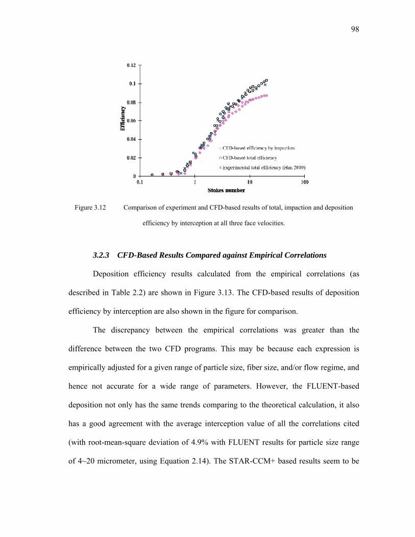
98

Figure 3.12 Comparison of experiment and CFD-based results of total, impaction and deposition

efficiency by interception at all three face velocities.

3.2.3 CFD-Based Results Compared against Empirical Correlations

Deposition efficiency results calculated from the empirical correlations (as

described in Table 2.2) are shown in Figure 3.13. The CFD-based results of deposition

efficiency by interception are also shown in the figure for comparison.

The discrepancy between the empirical correlations was greater than the

difference between the two CFD programs. This may be because each expression is

empirically adjusted for a given range of particle size, fiber size, and/or flow regime, and

hence not accurate for a wide range of parameters. However, the FLUENT-based

deposition not only has the same trends comparing to the theoretical calculation, it also

has a good agreement with the average interception value of all the correlations cited

(with root-mean-square deviation of 4.9% with FLUENT results for particle size range

of 4~20 micrometer, using Equation 2.14). The STAR-CCM+ based results seem to be

99

higher than the average interception correlation value due to possible reasons mentioned

earlier, but still with a similar trend.

Figure 3.13 Comparison of deposition efficiency by interception between empirical correlations and

CFD-based simulation.

3.2.4 Deposition Efficiency by Interception and Interception Ratio

In present research, the CFD results were utilized to determine the major

parameters or conditions that affect the interception mechanism. Figure 3.14 shows the

relation between interception parameter R (defined in Equation 1.9) and deposition

efficiency by interception. As observed in Figure 3.14, the deposition efficiency by

interception would increase significantly as R grows. And it could reach as over 1.6%

when the interception parameter exceeds 0.3. So this could be enlightening in filtration

study when estimate whether interception would be neglected or not. For a filtration

100

case, filter with fibers or fibrous screen, when the particle diameter is closed to or even

larger than the fiber diameter, i.e. the interception parameter R would be approaching or

even over unity, the interception effect could be significant enough and cannot be

neglected. And it seemed that the deposition efficiency would significantly increase as R

increased. Also apparently, the deposition efficiency by interception would have little

difference as face velocity increased, which suggests that interception is a mechanism

that does not depend on the normally flow velocity (Hinds, 1999).

Figure 3.14 Deposition efficiency by interception in various face velocities.

Another comparison was made to reveal the significance of interception in

collection efficiency. A new definition was made named the interception ratio, which

equals the deposition efficiency by interception divided by total collection efficiency

(impaction+interception):

101

intint

total

R

(3.6)

Obviously, this ratio is utilized to show the relative effect of interception

mechanism in the filtration study. Figure 3.15 gives the interception ratio value for

various interception parameters and three face velocities are used in our simulation. As

discussed before, as the interception parameter R increases (larger particles or smaller

filtration dimensions), the interception itself would become more and more important.

And note that, although absolute deposition efficiency by interception would be almost

constant if only face velocity changed, the interception ratio would decrease as face

velocity increases, because the impaction itself would obviously increase in this case.

For impaction itself, as air flows around the fibers, the impaction process is governed by

the Stokes number (Stk), the fraction open area, and the fiber Reynolds number, Ref,

which is calculated based on the velocity, U, in the screen, Parameters are given in the

Symbols and Abbreviations section. The average velocity through the mesh openings, U,

is related to the face velocity, U0. So in terms of dimensionless number, if the particle

size fixed, the interception ratio would decrease when the Stokes number or fiber

Reynolds number increased. As consequence, in the case of the highest interception

parameter (0.308) and lowest face velocity (0.213 m/s), intercepted particles may

account for up to 19% of the total aerosol depositions in CFD simulation.

102

Figure 3.15 Interception ratio Rint in various face velocities.

3.2.5 Gravitational Effect in Filter Model

CFD simulation was also used to determine the effect of gravity on particle

collection efficiency. The approach used here was to first conduct the particle tracking

without including the gravitational force, and then repeat the calculations with gravity

included. The gravitational force was set to be in the direction the same as the face

velocity. At the higher face velocity (0.6 and 1.06 m/s), the CFD-based total efficiency

was essentially the same for all particle sizes whether gravity was considered or not.

However, at the face velocity of 0.213 m/s, as shown in Figure 3.16, the gravitational

force would increase up to 6.9% of the total efficiency. At low face velocity, the

gravitational effect is more significant because of the longer residence time of the

particles in near-wall region could cause deposition velocity due to gravity more

relatively significant. However, for the deposition efficiency by interception, the

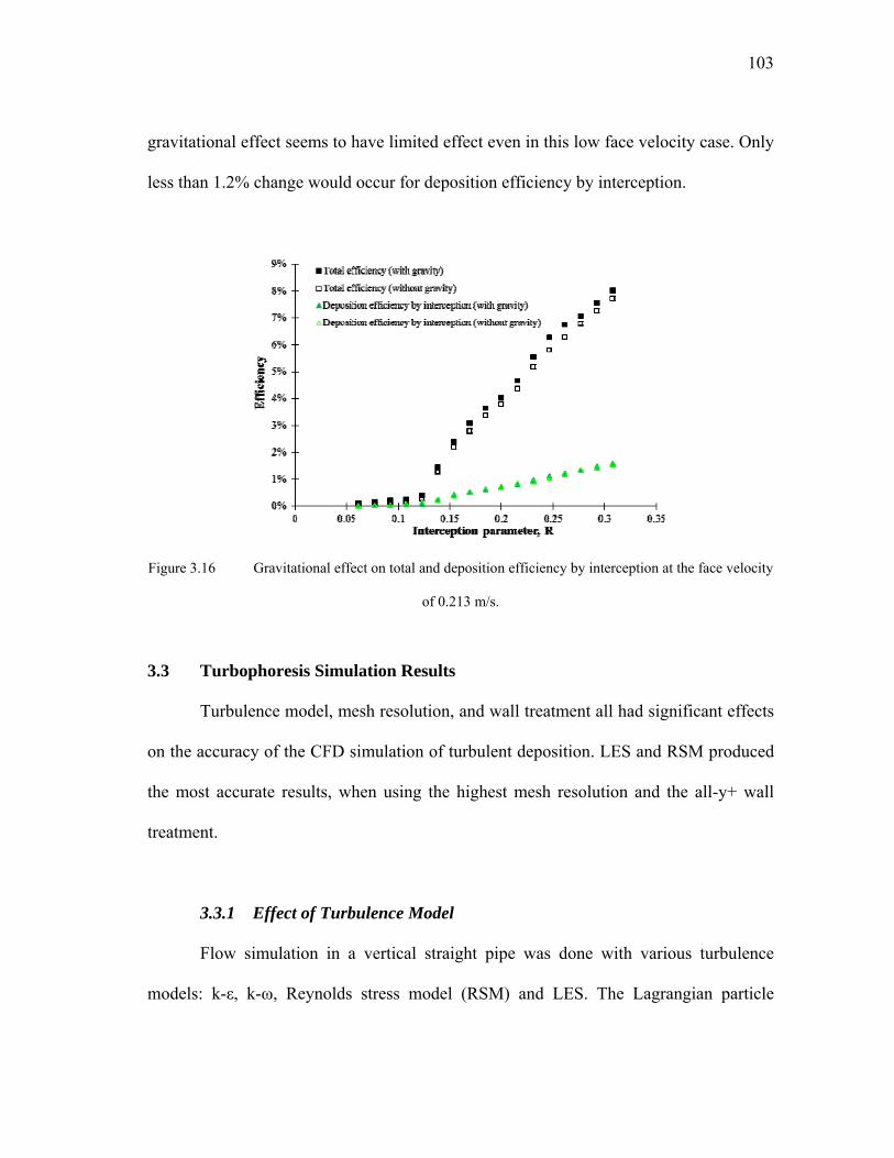
103

gravitational effect seems to have limited effect even in this low face velocity case. Only

less than 1.2% change would occur for deposition efficiency by interception.

Figure 3.16 Gravitational effect on total and deposition efficiency by interception at the face velocity

of 0.213 m/s.

3.3 Turbophoresis Simulation Results

Turbulence model, mesh resolution, and wall treatment all had significant effects

on the accuracy of the CFD simulation of turbulent deposition. LES and RSM produced

the most accurate results, when using the highest mesh resolution and the all-y+ wall

treatment.

3.3.1 Effect of Turbulence Model

Flow simulation in a vertical straight pipe was done with various turbulence

models: k-ε, k-ω, Reynolds stress model (RSM) and LES. The Lagrangian particle

104

tracking were carried out to evaluate the deposition based on turbulent flow filed

simulation. Penetration through the pipe was simulated with aerodynamic particle sizes

of 1 ~ 20 micrometer and the results were shown in Figure 3.17 for two separated

Reynolds number cases, together with experimental data from Liu and Agarwal

(Benjamin Y.H Liu & Agarwal, 1974) and 2D simulation data from Parker (Parker, et

al., 2008) with RSM model.

(a)

Figure 3.17 Penetration through the vertical pipe against particle diameter for different turbulent

models in the case when (a) Re = 10000, (b) Re = 50000. Experimental data from Liu and Agarwal

(Benjamin Y.H Liu & Agarwal, 1974) and 2D CFD simulation from Parker (Parker, et al., 2008) using

RSM.

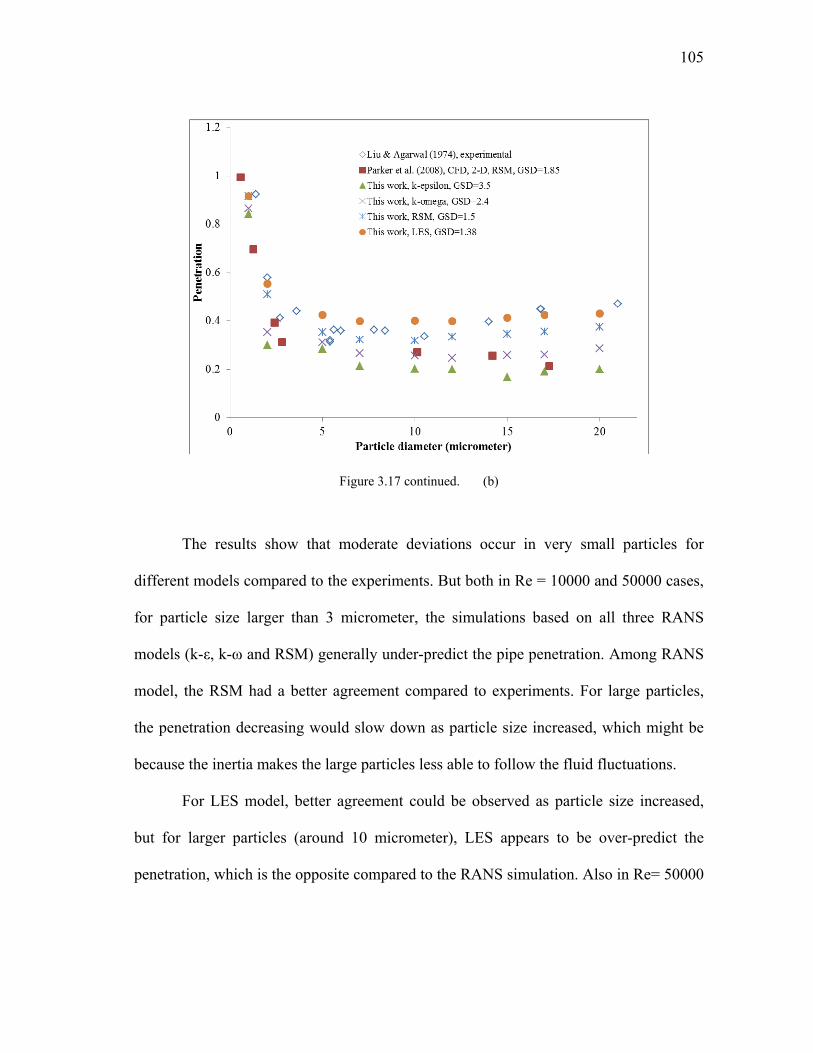
105

Figure 3.17 continued. (b)

The results show that moderate deviations occur in very small particles for

different models compared to the experiments. But both in Re = 10000 and 50000 cases,

for particle size larger than 3 micrometer, the simulations based on all three RANS

models (k-ε, k-ω and RSM) generally under-predict the pipe penetration. Among RANS

model, the RSM had a better agreement compared to experiments. For large particles,

the penetration decreasing would slow down as particle size increased, which might be

because the inertia makes the large particles less able to follow the fluid fluctuations.

For LES model, better agreement could be observed as particle size increased,

but for larger particles (around 10 micrometer), LES appears to be over-predict the

penetration, which is the opposite compared to the RANS simulation. Also in Re= 50000

106

case, LES seems to have a good agreement again when the particle size approaches to 20

micrometer.

The variation in predicted dimensionless deposition velocity with particle

dimensionless relaxation time is shown in Figure 3.18 for the four turbulence models.

The experimental data of Liu and Agarwal (Benjamin Y.H Liu & Agarwal, 1974) for

both Reynolds numbers and the 2D RSM simulation result from Parker (Parker, et al.,

2008) are also shown on this plot. Compared to the published experimental results, the

geometric standard deviations (GSD) are calculated for each turbulent model used in this

simulation. GSD for k-ε, k-ω, RSM and LES models were 3.4, 2.2, 1.37 and 1.29,

separately.

Apparently, for 10 < τ+ < 1000 (approximately 10 μm< dp <100 μm for

Re=10000, and 2 μm< dp <25 μm for Re=50000), all four turbulence models perform

reasonably well, predicting a dimensionless deposition velocity within approximately a

factor of less than 2 of the experimental data, although it seemed more significant

deviations in penetration predictions for k-ε and k-ω models in Figure 3.17. However,

for τ+ < 10 region, while penetrations predicted earlier shown moderate agreement with

experiments, the simulated deposition velocity varied very strongly compared to

experimental data with growth of the relaxation time, especially for two isotropic

turbulent models. These two isotropic turbulence models (k-ε and k-ω) seemed to fail to

capture the deposition behavior and both over-predict the deposition velocity at small

relaxation times by approximately 2~3 orders of magnitude. On the other hand, the

anisotropic RSM and LES performed much better, capturing the log-linear relaxation

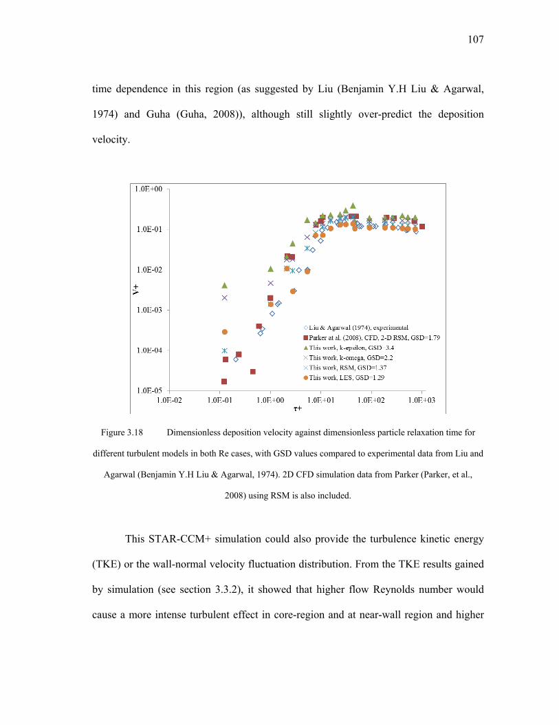
107

time dependence in this region (as suggested by Liu (Benjamin Y.H Liu & Agarwal,

1974) and Guha (Guha, 2008)), although still slightly over-predict the deposition

velocity.

Figure 3.18 Dimensionless deposition velocity against dimensionless particle relaxation time for

different turbulent models in both Re cases, with GSD values compared to experimental data from Liu and

Agarwal (Benjamin Y.H Liu & Agarwal, 1974). 2D CFD simulation data from Parker (Parker, et al.,

2008) using RSM is also included.

This STAR-CCM+ simulation could also provide the turbulence kinetic energy

(TKE) or the wall-normal velocity fluctuation distribution. From the TKE results gained

by simulation (see section 3.3.2), it showed that higher flow Reynolds number would

cause a more intense turbulent effect in core-region and at near-wall region and higher

108

TKE peak with greater decreasing gradient in near-wall viscous sub-layer. In the core

region within the pipe, the TKE slightly increased against the radial distance from

central axis, then a peak exist for each turbulent model in the near-wall region. After the

peak, the TKE would sharply decrease to 0 at wall surface due to no-slip boundary

condition.

For particle size greater than 1 μm, little diffusion effect would influence on

particle deposition in vertical pipe flow, and turbophoresis effect would dominate

turbulent deposition. So in this case, as the driven force of turbophoresis, the predicted

near-wall TKE gradient would have crucial influence on particle deposition rate gained

by CFD simulation: greater TKE or the wall-normal velocity fluctuation gradient would

cause a higher deposition velocity and overall deposition rate. The inability of the

isotropic models to capture the damping of the wall-normal fluctuations in the near-wall

region was believed to be the reason of their over-prediction of the wall-normal velocity

fluctuation distribution. Although more convergence time are needed for the RSM and

LES compared to an isotropic model, the particle tracking procedure, which can be a

considerable part of the overall solution time, should be independent to the chosen

turbulence models.

Based on these results, considering RANS models, greater decreasing gradient

would possibly cause a lower penetration prediction in Guha-defined Regime II

(Turbulent diffusion-eddy impaction area) (Guha, 2008), which refer to particles larger

than 5 micrometer in Re =10000 case and particle size range of 3 ~ 14 micrometer in Re

= 50000 case. In this particle size region, turbophoresis would have dominating

109

influence on particle deposition. So if CFD turbulent modeling has deviations or errors

in predicting the near-wall TKE gradient, deviations or errors would occur in predicted

deposition through Lagrangian particle tracking in CFD simulation, which is based on

turbulent flow modeling. For instance, over-predicting the wall-normal velocity

fluctuation using k-ε model, would over-predict the turbophoresis effect, which should

be dominant in Regime II on aerosol deposition, and directly leads to over-predict of

particle deposition rate in this regime. On the contrary, LES modeling seemed to slightly

under-predict the deposition (over-predict the penetration) in Regime II compared to

experiment. This leads to the possibility that LES modeling might provide a lower

kinetic energy gradient at near-wall region compared to the real physical case, but was

relatively closer to experiment compared to the RANS models did. Thus, penetration

result obtained by LES seemed to have a better agreement to experiments. If this

hypothesis above is true, the real physical wall-normal velocity fluctuation distribution

could lie between LES and RSM, which could be validated in future PIV test.

For the particle sizes used in this study, it is reasonable to neglect the deposition

effect due to diffusion. Thus, turbulent effect (turbophoresis) would be the dominant

effect on aerosol deposition under such flow and particle condition. Note that although

different turbulent models, wall functions or mesh resolutions were applied to derive the

flow field in this case, the same Lagrangian particle tracking method was used in CFD

code, which was based on the obtained turbulent flow field information. Therefore, any

deviations in particle deposition prediction among each case would generally due to

deviations coming from the flow field modeling (using different turbulent models, wall

110

functions and mesh resolutions). That is to say, deviations or errors in predicting near

wall gradient of wall-normal velocity fluctuation (driving force of turbophoresis) would

also cause difference in aerosol deposition results. However, these deviations due to

choices of different turbulent models, wall functions and mesh resolutions would not

influence on the analysis about the relation between the wall-normal velocity fluctuation

gradient and deposition velocity. In order to evaluate this relation, the first step is to

transformation of non-dimensional parameters.

3.3.2 Mean Square Wall-Normal Fluid Velocity Fluctuation

Figure 3.19 shows the radial distribution of K+ (the dimensionless term of 2fyV )

at half pipe length (0.51 m). As can be seen in the figure, simulations with the two

isotropic RANS models (k-ε and k-ω) produced steeper gradient of K+ than those with

the RSM and the LES models. However, with any of the turbulence models, the

dimensionless gradient appears to be independent of the Reynolds number. The fluid

velocity fluctuation results of this study are similar to those reported by Parker et al.

(Parker, et al., 2008).

111

Figure 3.19 Radial distribution of dimensionless mean square wall-normal fluid velocity fluctuation

( 2/K K u ) at half pipe length, each data set containing two Reynolds number cases.

3.3.3 Effects of Mesh Resolution and Wall Treatment

As shown in Figure 3.20, the accuracy of the turbulent deposition simulation was

dependent on the mesh resolution. All simulations shown in Figure 3.20 were with RSM

and the all-y+ wall treatment. Figure 3.20 shows that increasing the wall-adjacent cell

size (increasing y+ value) resulted in over-prediction of deposition; the number of the

mesh prism layers shows a “convergence” trend that more prism layers would be more

likely leading to accurate predicting, and no significance observed for simulations using

15, 20 and 25 prism layers; only when the wall-adjacent cell y+ values were sufficiently

low (around unity), the simulated deposition velocity was in good agreement with

experiments.

112

(a)

(b)

Figure 3.20 Dimensionless deposition velocity as a function of dimensionless particle relaxation

time using the RSM turbulence model and various mesh conditions; both Reynolds number conditions

included. (a) Re = 10000, (b) Re = 50000.

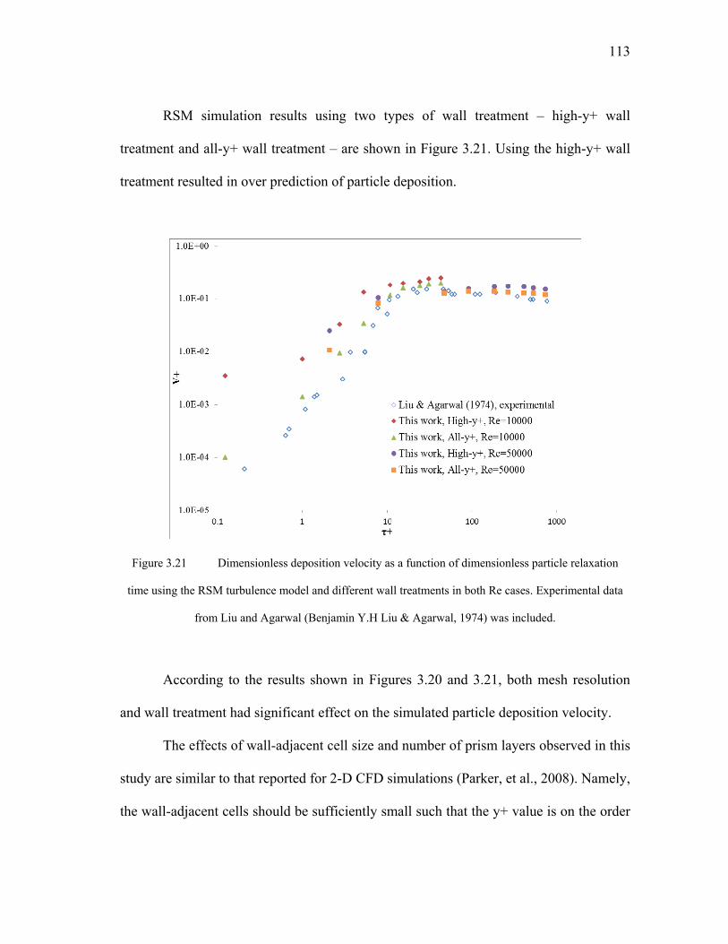
113

RSM simulation results using two types of wall treatment – high-y+ wall

treatment and all-y+ wall treatment – are shown in Figure 3.21. Using the high-y+ wall

treatment resulted in over prediction of particle deposition.

Figure 3.21 Dimensionless deposition velocity as a function of dimensionless particle relaxation

time using the RSM turbulence model and different wall treatments in both Re cases. Experimental data

from Liu and Agarwal (Benjamin Y.H Liu & Agarwal, 1974) was included.

According to the results shown in Figures 3.20 and 3.21, both mesh resolution

and wall treatment had significant effect on the simulated particle deposition velocity.

The effects of wall-adjacent cell size and number of prism layers observed in this

study are similar to that reported for 2-D CFD simulations (Parker, et al., 2008). Namely,

the wall-adjacent cells should be sufficiently small such that the y+ value is on the order

114

of unity, and the number of prism layers should be sufficiently large (15~20 in this case)

to cover the near-wall region, where steep gradient of turbulent velocity fluctuation

exists. Part of the results are shown in Table 3.5, along with the corresponding particle

deposition velocity and the simulated 2fyV , for the case Re=10000. It is clear that the

CFD configurations that predicted higher d

dyVfy

2 w

also over-predicted the particle

deposition velocity.

Table 3.5 Effects of mesh conditions and wall treatment on CFD-simulated

dimensionless wall-normal velocity fluctuation gradient using the RSM model and all y+

wall treatment (unless otherwise noted), Re=10,000.

Number of prism

layers First layer y+ K+/y+ V+ (τ+=1)

15

0.25 0.357 0.0014

0.25 (High-y+) 0.438 0.0064

1.25 0.405 0.0029

2.5 0.428 0.0059

10 0.25 0.416 0.0038

3.3.4 The Particle Responsiveness Factor

As shown in Figure 3.22, the particle responsiveness factor (defined as Equation

2.20), obtained from CFD simulations, increases as the particle size decreases, and

115

eventually approaches unity; the results agree well with results obtained from empirical

equations (Binder & Hanratty, 1991; Vames & Hanratty, 1988). For very small particles,

the particle follows the fluid streamline perfectly, consequently the particle

responsiveness factor approaches 1; for large particles, particle might not follow the flow

velocity fluctuation because of its great inertia, and the particle responsiveness factor

approaches 0. Note that, the relationship of α and τ appears to depend on the flow

Reynolds number; for the same τ value, α is smaller at higher Re. This suggests that in a

higher Reynolds number flow, there exists greater slip between the particle and the fluid.

This may be explained by the particles inability to follow the higher frequency fluid

velocity fluctuation in higher Reynolds number flows (P. L. Miller & Dimotakis, 1996;

Shang & Xia, 2001).

Figure 3.22 The particle responsiveness parameter α against particle relaxation time τ for CFD

simulation in both Re cases; multiple data points at a given τ value correspond to multiple turbulence

models.

116

3.3.5 The Turbophoresis Factor

The turbophoresis factor rt as a function of the dimensionless particle relaxation

time τ+ is shown in Figure 3.23. Multiple data points for the same dimensionless particle

relaxation time correspond to the various turbulence models used. Figure 3.23 suggests

that the relationship between rt and τ+ is similar to the relationship between V+ and τ+.

This is no surprise given that rt is the ratio of dimensionless deposition velocity to

dimensionless gradient of 2fyV , and the latter appears to be independent of the pipe flow

Reynolds number. Figure 3.23 suggests that, the effect of turbophoresis on particle

deposition increases with particle size in the range 0 1 10. ; for larger τ+ values, the

effect of turbophoresis on particle deposition decreases with increasing particle size.

Figure 3.23 The turbophoresis factor rt as a function of dimensionless particle relaxation time, both

Re conditions included.

117

4. DISCUSSION *

Based on all the CFD-based simulations in Result section, some discussions on

these mechanisms of particle transport and deposition would be necessary. Basically

notes in the CFD modeling of aerosol transport and deposition were raised as following,

and with relative difficulties and challenges.

4.1 Modeling on BSI-e Sampling Performance

4.1.1 Selection of Boundary Conditions

In this study, the boundary condition of the lateral boundary surfaces of the

tunnel was set to be ‘symmetric’, which means that it is defined that the flow rate

through these boundaries and the normal velocity both should be zero; and all the

variable gradients at the surface should be zero. So strictly, this ‘Symmetric’ surface

should be infinitely or sufficiently far away. Although space had been retained to avoid

excessive flow blockage between the inlet and the lateral surfaces of the wind tunnel, the

finite parameter could cause error to the flow field in numerical simulation and affect the

particle trajectories. The error caused by dimensions of the domain boundaries was

____________ *Reprinted with permission from “Computational fluid dynamics simulation of aerosol transport and deposition” by Tang, Y.J., & Guo, B. 2011. Frontiers of Environmental Science & Engineering in China, 5, 362-377, Copyright [2012] by GAODENG JIAOYU CHUBANSHE.

118

discussed in Appendix A. Various of dimensions of these ‘Symmetric’ boundaries were

tested for the local wind speed and penetration gained by simulation. The results

suggested that the potential error caused by the dimensions of the computational domain

could be acceptable under present simulation conditions.

4.1.2 Particle Deposition on the Inner Plenum

Figure 3.2 also shows that a small number of particles deposited outside the main

deposition region which refers to the upstream surface of the inner plenum (e.g. in the

case of 24 km/h and 20 μm particle). The possible reason for this is because there could

be some other aerosol flow with particles enter the intake, but also leave it without

getting into the windows on the top (either fairly immediately, with a grazing contact, or

all the way going “around” the inner and out at the downwind side). This would

probably cause some depositions on the lateral side of the inner plenum due to the

inertial impaction when the flow had a turn around the inner plenum. This part of flow

could also be observed in Figure 3.1 (b).

4.1.3 Particle Loss

Some calculation was made to shows the fraction of the particles deposited on

the inner plenum contributes to loss of the penetration. In present research, 400,000

particles were released from the inlet surface of the computational domain in simulation.

For different wind speed, a number of particles, 100%n could be calculated as the ideal

amount of particles going through the exhaust surface of BSI assuming there was no

119

wall loss, i.e. if all particles followed the flow streamline perfectly, 100%n of particles

would transport through the exit of BSI-e.

So,

100%exhaust

totaltotal

Qn n

Q (4.1)

Remember that the exhaustQ is the flow rate through the BSI, which is 100 L/min

in our case. The number of particle depositions contributes to loss of penetration could

be calculated as:

, 100% (1 )depo wl simn n P (4.2)

This parameter ,depo wln would represent how many sampling-loss particles, which

were supposed to transport through the BSI exit in an ideal case, would deposit on the

BSI-e surface.

Also, the particle number deposited on the inner plenum, ,depo ipn could be found

in the result of the Lagrangian particle tracking, which is also shown in Figure 3.2. Table

4.1 could show the comparison results of these two parameters, ,depo wln and ,depo ipn . It

suggested that the fraction of the particles deposited on the inner plenum surface

contributes to loss of penetration would decreased as wind speed increased. For various

particle diameters at same wind speed, this fraction could increase as particle size

increased at 24 km/h case, but minor difference was shown in 8 km/h case. It suggested

that the inertial effect more significantly influenced the particle loss of penetration. And

120

particles mentioned in Section 4.1.2 might not be as sensitive to the inertial effect as the

particle loss of penentration.

Table 4.1 The comparison of the number of particle depositions on the inner

plenum and number of particle depositions contribute to the wall loss (with total particle

number of 400,000).

Free wind speed 8 km/h Free wind speed 24 km/h

Particle Diameter

μm

Number of particle

deposited on inner plenum

,depo ipn

Number of particle

contribute to the wall loss

,depo wln

Particle Diameter

μm

Number of particle

deposited on inner plenum

,depo ipn

Number of particle

contribute to the wall loss

,depo wln

10 134 58 10 224 37 15 437 196 15 821 150 20 717 319 20 1327 340

4.2 Modification Model – Shrouded BSI

The purpose of the aerosol inlet research is to optimize the device and shape-

modification to ensure to obtain a highly quality aerosol sampling efficiency in different

flow conditions. It can be seen from the results and discussions above that there is still a

fair amount of research needed, in order to comprehensively prove that the currently

available CFD approach are indeed capable as a highly dependable design and

development tool for aerosol sampling inlets. The CFD simulation could provide the

predicted particle trajectories with fixed flow conditions, as a result of which, the

particle depositions on wall surfaces of interest. This result could be helpful to show and

prove the deposition mechanism for the aerosol particles in desired situations, and based

121

on which, some shape modification could be done to the geometric model to improve the

function of aerosol inlet. So our research goal here is to accomplish the shape

modification and try to reduce these particle depositions and increase the inlet efficiency,

and the result would be evaluate in CFD simulation.

4.2.1 The Shrouded BSI-e model

Based on the CFD simulation and analysis of the original BSI-e model, the

results suggested that the main particle loss and the particle depositions were most likely

due to the inertial impaction, which would cause the particles with higher inertia to

impact on the relatively lower positions on the upstream side of the inner plenum, since

the higher inertia made the particles turn less when they were entering the

circumferential intake of BSI.

For the BSI-e device, two shrouded eaves were added before the intake of the

original BSI (as Figure 4.1). The major purpose of the shrouded structure is to change

the streamline direction and reduce the turning angle near the intake which might reduce

the inertial effect of particle motion. So in this case, the shrouded eaves might have some

influence to improve the efficiency of original BSI-e, by reduce the particle deposition

due to the inertial impaction on the upstream side of inner plenum.

122

(a) (b) Figure 4.1 The geometric models of (a) the origin BSI-e model and (b) the shrouded BSI-e model.

In this case, the same CFD simulation settings (computational domain, mesh

generations, turbulence models, etc.) are applied for the shrouded BSI model. Based on

CFD simulations, particle penetration was calculated for particles from 2 to 20 µm in

aerodynamic diameter, at wind speed of 2, 8 and 24 km/h, and the fixed sampling flow

rate of 100 L/min.

Predictions for penetration efficiency were compared between the original and

the shrouded BSI model. Subsequent to the above determination, simulation was

performed to get the particles’ locations of deposition on the inlet walls, which would be

a significant factor to influence on the penetration efficiency, could help understanding

the turbulent flow pattern and particle trajectories, and modify the inlet shape toward this

basis. For the modification of the inlet, two circumferential shrouded (Figure 4.1) eaves

were added in front of the intake of BSI just to change the aerosol flow direction of the

streamlines to ensure that the aerosol flow entering absolutely towards the tangential

123

direction of the curvilinear surface of inner plenum instead of horizontally as the free

wind speed. The dimensions of these shrouded eaves were shown in Table 4.2.

Table 4.2 Important dimensions of the shrouded eaves.

Upper

Shrouded Eave

Top and Bottom Spacer

Dimension

Bottom Shrouded

Eave

Shrouded Eave Intake

Width

Eave Thickness

Do = 10″ Di = 7.5″

0.375″ Do = 9.5″

Di = 7.25″ 1.388″ 0.1″

4.2.2 Predicted Penetration Efficiency

For the modified Shrouded BSI-100 Model, the penetration results were shown

in Figure 4.2, at the same flow conditions and particle sizes as the simulations on the

original BSI model. Also comparison has been done for the penetration efficiency of

these two models. It suggested that the shrouded model indeed increased the penetration

and this difference would increase as the wind speed and particle diameter increased.

This is because the main function of the shrouded structure is to change the flow

direction and ensure that the aerosol flow entering absolutely towards the tangential

direction of the curvilinear surface of inner plenum instead of horizontally as the free

wind in the original BSI-e model. So, the advantage of the shrouded eaves is to reduce

the inertial impaction mechanism when aerosol flow entering the circumferential intake

of BSI, and decrease the opportunities of the particle depositions on the upstream side of

the inner plenum. Since the inertial impaction mechanism would become more

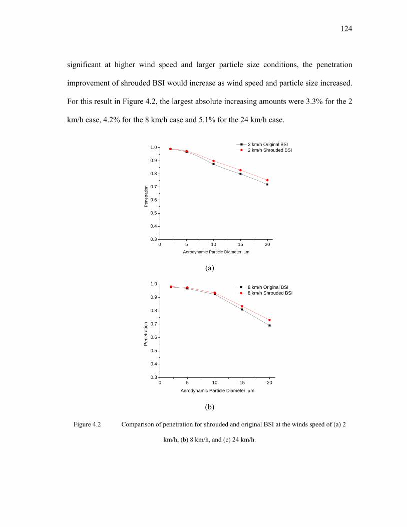
124

significant at higher wind speed and larger particle size conditions, the penetration

improvement of shrouded BSI would increase as wind speed and particle size increased.

For this result in Figure 4.2, the largest absolute increasing amounts were 3.3% for the 2

km/h case, 4.2% for the 8 km/h case and 5.1% for the 24 km/h case.

0 5 10 15 200.3

0.4

0.5

0.6

0.7

0.8

0.9

1.0 2 km/h Original BSI 2 km/h Shrouded BSI

Pen

etra

tion

Aerodynamic Particle Diameter, m

(a)

0 5 10 15 200.3

0.4

0.5

0.6

0.7

0.8

0.9

1.0

Pe

netr

atio

n

Aerodynamic Particle Diameter, m

8 km/h Original BSI 8 km/h Shrouded BSI

(b)

Figure 4.2 Comparison of penetration for shrouded and original BSI at the winds speed of (a) 2

km/h, (b) 8 km/h, and (c) 24 km/h.

125

0 5 10 15 200.3

0.4

0.5

0.6

0.7

0.8

0.9

1.0

Pe

netr

atio

n

Aerodynamic Particle Diameter, m

24 km/h Original BSI 24 km/h Shrouded BSI

Figure 4.2 continued. (c)

4.2.3 Visualization of Particle Deposition on Inner Plenum and Bottom

Shrouded Eave

Like the simulation on the original BSI-e model, the visualization of particle

deposition was accomplished for the upstream of inner plenum and the upper surface of

the bottom shrouded eave. The results were shown in Figure 4.3. Comparing to the

simulation on the original model, there were less particle depositions on the inner

plenum, which improves the penetration efficiency of the original BSI-e. Also, since the

effect of the shrouded eaves would change the streamline direction, it seems that the

differences of the deposited positions for particles with various of wind speeds and

particle sizes became less significant comparing to the original model. In other word,

from the deposition results at same wind speed, it showed that the particle deposition

positions seemed to be close to each case with different particle diameters.

126

On the other hand, in visualization of the depositions on the bottom shrouded

eave, it suggested that almost all particle depositions were located on the front surface

and the inertial impactions still made the particle with higher inertia more depositions

and the deposited region started at lower deposition locations. Also for the particles with

higher inertia (large particle size or high wind speed), the deposited region on the surface

of shrouded eave seemed to be wider than particles with lower inertia. It would be

similar to the analysis above as it was expected.

Also according to this deposition results, another new idea of shrouded structure

modification was provided. Since the research showed that a large number of the

particles could hit and be stuck on the front surface of inner plenum due to the inertial

impaction, the length dress-edge of the inner plenum could be reduced, and also extend

the length of the bottom shrouded eave. This change could possibly make these particles

which supposed to hit on the inner plenum by inertial impaction go through the gap

between the inner plenum and the bottom shrouded eave, which means probably much

fewer depositions on the front surface of inner plenum. So under this circumstance, some

different dimensions of the shrouded eaves, such as longer eaves as mentioned above or

curve planed eaves with less camber, could be considered in CFD simulation study in

future.

127

(a)

Figure 4.3 Top view of particle deposition on the upper surface of the inner plenum and upper

surface of bottom shrouded eaves in Shrouded BSI-e model at the wind speeds of (a) 8 km/h and (b) 24

km/h.

128

Figure 4.3 continued. (b)

129

4.3 Modeling on Interception via the Virtual-Surface Approach

A new approach using virtual-surface was utilized in order to account for particle

interception in two common used CFD tools: ANSYS FLUENT and STAR-CCM+. This

modeling strategy can be used to directly calculate the particle events captured by fiber

walls due to interception with any fiber diameters when challenged with aerosols of any

particles sizes, and then conclude with deposition efficiency by interception. More

important, this method could quantitatively predict the particle interception via the

standard function in commercial programs. The methods developed in this study, which

can be readily validated and adopted by researchers in the field, would help to study the

interception mechanism in filtration without the need for user defined functions or other

subroutines.

The approach to create virtual surfaces in order to count intercept particles is

shown in present work. The method successfully simulates the filtration process

including particle impaction and interception without the need for user defined functions

to account for interception. It can be readily validated and adopted by researchers in the

field, and the comparison to the experimental data and the theoretical correlations also

prove the feasibility of this approach. However, geometric limitations still remain for

this approach. The virtual surface could be very difficult to build in a more complex

geometric model, such as a randomly organized fibrous filter (S. A. Hosseini & Tafreshi,

2010), since extra considerations about the interaction between physical-virtual or

virtual-virtual surfaces are necessary, which significantly increase the difficulty of the

modeling process. Furthermore, for a large-dimension model such as an impactor or

130

inlet, the relative small distance between virtual and physical surfaces might also cause a

tolerance problem when building the geometric models during the modeling process.

After all, this “virtual surface” approach should be especially useful for filter or

screen models with cylindrical or elliptical fibers, in which case the “virtual surface” can

be readily created. When more complex geometries are involved, creation of the “virtual

surface” may become more challenging. Nevertheless, cylindrical or elliptical fibers are

widely used geometries in filtration systems. Therefore, the “virtual surface” approach

introduced in this study shall be useful in many modeling applications. Also, some

developments are expectable for the virtual-surface approach to work together with user

defined functions in order to extend its utilization.

4.4 Turbophoresis Modeling in the Vertical Straight Pipe

The effects of turbulence model, mesh resolution and wall treatment on the

accuracy of turbulent deposition simulation observed in this study are similar to those

observed in 2-D CFD simulations (Parker, et al., 2008). This suggests that similar

criteria (e.g., near-wall mesh resolution, wall treatment) may be applied to both 3-D and

2-D CFD simulations of turbulent deposition, in order to achieve accurate results.

Simulations with RSM and LES turbulence models yielded similar levels of

accuracy in terms of particle deposition velocity. The LES is associated with

significantly higher computation cost – several weeks for flow field simulation and

particle tracking, on a desktop computer with a 2.8 GHz processor, 8GB RAM running 8

parallel processes. Therefore, RSM – only a few days of computation time to produce

131

the flow field and particle tracking results – should probably be the choice of turbulence

model for most practical turbulent deposition simulations.

The results in this study suggest that the accuracy of turbulent deposition

simulation is critically dependent on the accuracy of the near-wall turbulence simulation.

All the effects of the CFD model parameters on the accuracy of turbulent deposition

appear to be through their effects on the accuracy of the near-wall turbulence simulation.

It should be noted that all CFD configurations resulted in similar results of particle

responsiveness factor, which agreed well with empirical results. In other words, the

Lagrangian scheme in the CFD package can produce sufficiently accurate simulation of

the particle random motion, as long as the turbulent flow field simulation is sufficiently

accurate. This further suggests that the accuracy of the near-wall turbulence simulation is

the most critical factor for turbulent deposition simulation.

The turbophoresis factor results should be useful for CFD simulation of turbulent

deposition. Even though the typical value of the turbophoresis factor may vary with

problem, what is presented in this study can at least serve as a reference point. For

example, if one has the CFD simulation of a complex turbulent flow field such as that in

a cyclone, and would like to know the relative contribution of turbulent deposition as

opposed to deposition due to centrifugal acceleration, then the values of turbophoresis

factor presented in this study will become useful.

The particle responsiveness factor computed from the CFD simulation and

Lagrangian particle tracking results is apparently useful for validating the numerical

model at a more fundamental level. The methodology used to obtain the particle

132

responsiveness factor suggests that the Eulerian description of turbulent deposition is

useful for the validation of numerical simulations based on a Lagrangian approach.

4.5 Major Challenges in Turbulence Modeling on Aerosol Deposition

In spite of the significant progress in CFD simulation of particle transport and

deposition in aerosol flows, many challenges remain in this field, especially in predicting

turbulence effect in stochastic turbulent dispersions. Even with RSM or LES modeling,

CFD tools could also be difficult to get accurate enough results here. The computational

expense could also draw sufficient attention in any industrial applications. In this

section, some challenges or opportunities were discussed.

4.5.1 Turbulence Modeling

The accuracy of the turbulent flow field simulated would be the first important

condition to obtain an accurate enough particle transport and deposition results. Even

though the more elaborate models such as LES may probably produce more accurate

results, RANS models are still the first choice in most cases due to the balance

consideration of computation economy. Unfortunately in current CFD studies, the

turbulence solution is usually dependent upon the RANS model choice and the wall

treatments, with no apparent universal rules for model and parameter selection. For

simple geometry or simple flows, the mean flow field solutions with various turbulence

models may be fairly similar, but the turbulence properties (e.g. turbulence kinetic

133

energy) can vary orders of magnitude from one model to another (Hoekstra, et al., 1999;

Parker, et al., 2008).

Parker et al.(Parker, et al., 2008) compared in their research the turbulent friction

velocities and wall-normal fluctuations obtained by several RANS model (RNG k-ε,

RMS and k-ω SST) and significant deviations were observed between the turbulence

models. All RANS models overpredicted the turbulent deposition velocity compared to

the experimental measurements. Among those results, it seemed that the RSM model

with a certain wall treatment could lead to relatively better agreement. The present study

also got similar results, and it suggested that in most of cases, RSM could be the first

choice in turbulence modeling on aerosol turbulent flow.

The high computational cost of LES still limits its utilization in CFD simulation.

However it should be noted that, there appears to be a development of increasing use of

LES in predicting particle transport and deposition. A cost-effectiveness assessment is

still needed to validate LES-based simulations in predicting aerosol depositions.

Currently, major efforts had been made using LES to evaluate the aerosol deposition in

human respiratory tracts (Jayaraju et al., 2008; Y. Liu, et al., 2007; Matida et al., 2006),

in channel or duct turbulent flow (Kuerten & Vreman, 2005; Lo Iacono et al., 2005; Q.

Wang & Squires, 1996), and in particle transport mechanism(Q. Wang, et al., 1997). It

seems promising in these studies to use LES to improve the prediction of aerosol

transport and deposition.

134

4.5.2 Turbulent Dispersion Modeling

When a RANS model was applied for turbulence modeling, the flow field

information is insufficient to allow an exact mathematical description of the particle

turbulence dispersion. The interaction between particles and turbulence can only be

modeled using the turbulence flow field information provided by the turbulence

modeling. Therefore, a turbulent dispersion model can be only as accurate as the

turbulence model itself. If a turbulence model cannot correctly describe the turbulent

profile, then the turbulent dispersion model would not be able to completely consider

particle-turbulence interactions. Especially, due to the inability of RANS models to

accurately simulate turbulence in the near-wall region, simulating turbulent depositions

on walls is above all challenging. For example, Longest(Longest et al., 2007) and

Matida (Matida, et al., 2004) both suggested it was typically inaccurate to use particle

dispersion models in combination with two-equation isotropic turbulence models. In

fact, the isotropic turbulence models could not account adequately for the dampening of

the wall-normal turbulent fluctuations, and consequently over-predict the particle

deposition (Parker, et al., 2008).

In a near-wall turbulent flow region, a large gradient (Reynolds number

dependent) of the wall-normal velocity fluctuation exits, because the velocity fluctuation

must decrease from a high value in the fully developed turbulence core zone to zero at

the wall due to the no-slip wall condition. This phenomenon turbophoresis causes

particles to concentrate near the wall, and contributes to particle deposition onto the wall

(Guha, 2008). Therefore, the accuracy of a RANS-based turbulent dispersion model

135

depends on the RANS model’s ability to compute not only the near-wall velocity

fluctuations, but also its gradient. However, even for a relatively simple pipe flow,

different RANS models could produce very different results of near-wall velocity

fluctuation distribution and particle deposition rate near the wall (Parker, et al., 2008).

However, it should be noted that in the near-wall region, some doubts would be

raised for any turbulent dispersion models based on RANS models as completely

feasible methods. First, turbulent dispersion models apparently work practically well in

any “homogeneous” turbulence flows where the wall effect is not significant. For

instance, the turbulent dispersion model in STAR-CCM+ was used to simulate the

dispersion of particles released from one single point source in decaying grid-generated

turbulence, and the simulation results agreed well with experiments (CD-adapco, 2008;

Gosman & Ioannides, 1983). Secondly, it is possible to well predict turbulent deposition

if an anisotropic RANS model, e.g. RSM, is used in conjunction with a proper wall

treatment and sufficiently fine mesh (Parker, et al., 2008). The open question is whether

an approach that works well for pipe flows will also work well for more complex flows,

such as that in and around an omni-directional inlet.

With sufficient computational power, LES could be a better choice to simulate

the turbulence and the particle dispersion/deposition. However, as discussed earlier, the

LES approach may need more computational sources, and become too computationally

expensive for simulations over significant time periods. It is not yet clear whether LES

would be able to provide sufficiently higher accuracy of particle deposition to justify the

added cost in general sampling cases.

136

4.5.3 Effect of Turbulent Dispersion

Noted among many cases, the turbulent dispersion is not the dominant particle

deposition mechanism. One example here is the study on the performance of the aerosol

sampling device (BSI), which was evaluated using RSM model without turbulent

dispersion, and compared with the results from Tang et al. (Y. Tang, et al., 2010) which

included dispersion. The device efficiency results comparison showed that in most of

cases, the deviation with or without dispersion included was less than 5% of the total

penetration efficiency (Figure 3.4). The results mentioned earlier suggested that the

inertial separation would be the dominant mechanism to cause deposition in such case.

Another example was for the cyclone simulation. Hu and McFarland (Hu &

McFarland, 2007) simulated the turbulent flow and the particle deposition in a cyclone

without including a turbulent dispersion model, but their CFD-derived particle

deposition rate were in an excellent agreement with obtained experimental data, which

would as well suggest that the turbulent dispersion should not be a dominant mechanism

to cause deposition. Furthermore, some currently researches (Y. Liu, et al., 2007;

Longest, et al., 2007) on RANS simulation of respiratory system also showed that, for

large particles, the regional aerosol deposition pattern could be likely independent to

dispersion. It is apparently that the turbulent dispersion would not be a significant factor

to cause particles deposit on the wall surface, if other dominant mechanism exists, such

as inertial separations. This most likely would occur when there are curved and complex

flow passages, and high flow rates or/and large particle sizes involved. While in such

137

cases, the simulation from most commercial CFD codes on aerosol deposition appear to

be reliable.

In vertical pipe flows, however, turbulent dispersion is the dominant mechanism

for particle deposition, and no other mechanisms would be so important (for large

particles, Brownian motion could be neglected). But there are published empirical

relations. Some empirical relations for calculating the rate of deposition of aerosol

particles on the surface of vertical tubes were presented (Friedlander & Johnstone, 1957;

Benjamin Y.H Liu & Agarwal, 1974; Mednikov, 1980) and also used for validation of

CFD simulations (R. Gao & Li, 2011; Jiang, et al., 2010; Nerisson, et al., 2011; Parker,

et al., 2008; F. P. Zhang & Li, 2008). On the other hand, the turbophoresis factor

provided by the present study results should be useful at least serve as a reference point

for the numerical research. Also, the methodology used to obtain the particle

responsiveness factor suggests that the Eulerian description of turbulent deposition is

useful for the validation of numerical simulations based on a Lagrangian approach.

In actual fact, CFD simulation of turbulent dispersion may be avoided if the

computational resources do not allow for accurate modeling. For instance, the mean flow

field obtained from a RANS model could be used to simulate particle deposition and still

led to satisfactory results, if the inertial separation is dominant and turbulent dispersion

only acts as a minor role. On the other hand, one may choose empirical relations or

mathematical relationship as the turbophoresis factor, instead of the Lagrangian particle

tracking in CFD tools to predict particle deposition, for a turbulent dispersion dominant

case (e.g. vertical pipe flow).

138

5. SUMMARY AND CONCLUSIONS

In this article I provided a brief review of CFD modeling of particle transport and

deposition in aerosol flows, followed by detailed CFD-based analysis on different

particle transport and deposition mechanisms, such as particle inertial impaction,

gravitational effect, lift force, interception, and most importantly, turbophoresis. These

mechanisms were evaluated within different practical applications, which included

aerosol sampling inlet, fibrous screen and vertical flow pipe. Two commonly used

commercial CFD packages, ANSYS FLUENT (ANSYS Inc., Canonsburg, PA) and

STAR-CCM+ (CD-adapco, London, UK) are applied in the CFD simulation of this

study. According to the specific flow conditions, different flow viscous models were

used to predict the flow field, then the Lagrangian particle tracking approach was

applied to identify the particle trajectories and deposition rate.

In the study on BSI-e performance, turbulent flow field simulations and

Lagrangian particle tracking were carried out for a 100 L/min omni-directional aerosol

inlet. For the free wind speeds of 2, 8, and 24 km/h, particle penetration efficiency

results based on the CFD simulations were in an excellent agreement with experimental

results in previous studies. The root mean square normalized standard error, from

comparing the simulation results with the experimental data group for all three wind

speeds, was 3.8%. CFD-derived regional deposition pattern revealed that particle

deposition took place essentially on the upstream surface of the inner shell, in a potion

139

where the flow was curvilinear and decelerating as it changed direction from horizontal

to vertical. Although the inertial separation was the dominant mechanism of particle

deposition, the gravitational effect was observed to contribute a significant effect at the

lowest wind speed test (2 km/h). Based on the knowledge of regional particle deposition

and the dominant deposition mechanisms, a six-parameter semi-empirical correlation

equation was constructed to predict the penetration through the inlet. The semi-empirical

correlation uses a Stokes number based on the free stream velocity and the width of the

intake gap at the flow entrance to the BSI-e, a dimensionless gravitational settling

parameter, and a velocity ratio for correction of the first two dimensionless numbers.

The findings of this study demonstrate that CFD simulation can provide

information that is difficult to acquire through experimental measurements, such as

regional distribution of particle deposition and the importance of specific deposition

mechanisms, e.g. the gravitational settling, the Saffman force and the turbulent

dispersion. Such information should be valuable for optimizing designs of aerosol inlets.

Also, the correlation should be used as a scaling law and allow designers to predict the

performance of an integrated inlet that may also include a screen and a pre-separator

with known penetration characteristics.

Shrouded structure was added in the BSI-e model in order to improve the

penetration efficiency of this sampling inlet. The predicted particle penetration

efficiency in numerical simulation suggested that the shrouded structure could enhance

the penetration and improve the efficiency of BSI-e. The visualization of particle

depositions on the inner plenum and the bottom shrouded eave suggested that the

140

shrouded structure could weaken the effect of inertial motion and reduce the inertial

impactions when entering the intake of BSI.

Secondly, for the fibrous screen simulation, a three-dimensional geometric model

was built in this study to simulate the flow field and particle tracks about two crossing

fibers. A new approach using “virtual-surfaces” was utilized in order to account for

particle interception with two commonly used CFD programs: Fluent and STAR-CCM+.

In particular, this CFD-based modeling strategy was demonstrated in comparing with

experimental study on the same physical screen model, and calculation results from the

existing empirical/semi-empirical correlations. The flow field and particle tracking

results for both CFD programs were compared in present study with no obvious

deviation observed. Also, comparing to the experimental data shows that the CFD

simulation could predict the total collection efficiency very well after introducing the

interception mechanism in particle tracking, and the root-mean-square normalized error

is about 6.2%; while the results from empirical/semi-empirical correlations also tell that

the deposition efficiency by interception predicted by CFD simulation – virtual-surface

approach, is apparently within the right range and agree with the average value of former

empirical estimations. The results after all prove that this modeling strategy is trustable

in predicting filtration efficiency. In practical utilization, this virtual-surface approach

can be used to calculate particle deposition due to interception with any fiber diameters

when challenged with aerosols of any particles sizes. This approach does not require

user defined functions or subroutines, and hence can be readily validated through peer

review, and widely adopted by the research community.

141

Turbulent dispersion is probably the greatest challenge for CFD simulation on

the aerosol transport and deposition. In this study, a 3-D CFD simulation of turbulent

aerosol particle deposition was carried out, the results of which compared with published

experimental results and previous 2-D simulations. The effects of the CFD modeling

parameters were examined; a particle responsiveness factor and a turbophoresis factor

were calculated based on the simulation results. Based on the results, the following may

be concluded. The criteria for accurate simulation of turbulent deposition are similar for

either 2-D or 3-D CFD models. Specifically, the Reynolds stress turbulent model should

be used, with sufficiently small wall-adjacent cells to ensure a cell centroid y+ on the

order of unity, sufficient number of prism layers to resolve the near-wall gradient of

turbulent velocity fluctuation, and an “advanced” wall treatment (the “all y+” wall

treatment in the case of STAR-CCM+). The more computationally expensive LES may

not be necessary for simulating turbulent deposition. The particle responsiveness factor

may be used for validating numerical simulations of turbulent deposition. The Eulerian

description of turbulent deposition is useful for analyzing and validating the numerical

simulations that are based on a Lagrangian approach. The “turbophoresis factor”

quantitatively relates the deposition velocity and the gradient of the wall-normal

turbulence fluctuation, and may be useful for assessing the importance of turbulent

deposition in complex flows.

From the applications that sampled in this study, it is clear that CFD is a very

useful tool, with significant limitations. Turbulent deposition is especially challenging

for CFD modeling, due to the difficulty in profiling turbulent flow and the interaction

142

between the particle and the eddy. Limitations of CFD tools remain, for instance, the

accuracy in simulating complex flow and the validation would be necessary.

Despite of this, CFD simulation, once validated with experiments, can be quite

useful to carry out “numerical experiments” and based on which correlations useful for

device design could be developed. It should be noted that CFD simulation or numerical

calculation is able to provide sufficient information which might be difficult to obtain

via physical experiments, or to reduce the cost and the number of experiments needed

for device design. It is possible to take a balanced approach towards quantitative

description of studied objects using CFD simulation in conjunction with empirical

relations. Challenges still remain in CFD research and I am willing and motivated to

make some contributions.

143

REFERENCES

ANSYS. (2008). ANSYS FLUENT 12.0/12.1 Documentation. ANSYS, Inc.,

Canonsburg, PA. http://www.ansys.com

Baehl, M.M. (2007). Ambient aerosol sampling inlet for flow rates of 100 and 400

L/min. M.S. Thesis, Department of Mechanical Engineering, Texas A&M

University, College Station, Texas.

Belyaev, S.P., & Levin, L.M. (1974). Techniques for collection of representative aerosol

samples. J Aerosol Sci, 5, 325–338.

Binder, J.L., & Hanratty, T.J. (1991). A diffusion-model for droplet deposition in gas-

liquid annular-flow. Int J Multiphas Flow, 17, 1-11.

Bird, A.J. (2005). Use of numerical calculations to simulate the sampling efficiency

performance of a personal aerosol sampler. Aerosol Sci Tech, 39, 596-610.

Bisgaard, H. (1995). A metal aerosol holding chamber devised for young children with

asthma. Eur Respir J, 8, 856-860.

Broday, D.M., & Georgopoulos, P.G. (2001). Growth and deposition of hygroscopic

particulate matter in the human lungs. Aerosol Sci Tech, 34, 144-159.

Cain, S.A., & Ram, M. (1998). Numerical simulation studies of the turbulent airflow

through a shrouded airborne aerosol sampling probe and estimation of the

minimum sampler transmission efficiency. J Aerosol Sci, 29, 1145-1156.

144

Casella, G., & Berger, R.L. (2002). Statistical inference (2nd ed.). Pacific Grove, CA:

Thomson Learning.

CD-adapco. (2008). STAR-CCM+ 5.04.006 Guide and Documentation, http://www.cd-

adapco.com/.

Chandra, S., & McFarland, A.R. (1997). Shrouded probe performance: Variable flow

operation and effect of free stream turbulence. Aerosol Sci Tech, 26, 111-126.

Chen, Y.S., & Hsiau, S.S. (2008). A new method for measuring cake thickness by a

powder pressure-displacement system. Adv Powder Technol, 19, 49-60.

Clift, R., Grace, J.R., & Weber, M.E. (1978). Bubbles, drops, and particles. New York:

Academic Press.

Coroneo, M., Mazzei, L., Lettieri, P., Paglianti, A., & Montante, G. (2011). CFD

prediction of segregating fluidized bidisperse mixtures of particles differing in

size and density in gas-solid fluidized beds. Chem Eng Sci, 66, 2317-2327.

Darquenne, C. (2001). A realistic two-dimensional model of aerosol transport and

deposition in the alveolar zone of the human lung. J Aerosol Sci, 32, 1161-1174.

Darquenne, C., & Paiva, N. (1996). Two- and three-dimensional simulations of aerosol

transport and deposition in alveolar zone of human lung. J Appl Physiol, 80,

1401-1414.

Davies, C.N. (1966). Aerosol science. New York: Academic Press.

Deuschle, T., Janoske, U., & Piesche, M. (2008). A CFD-model describing filtration,

regeneration and deposit rearrangement effects in gas filter systems. Chem Eng J,

135, 49-55.

145

Drobyshevsky, N.I., Zaichik, L.I., Mukin, R.V., & Filippov, A.S. (2009). Development

and application of a diffusion-inertia model for calculating aerosol particle

deposition from turbulent flows. J Eng Thermophys, 18, 271-278.

Fan, B., Mcfarland, A.R., & Anand, N.K. (1992). Aerosol-particle losses in isokinetic

sampling probe inlets. Environ Sci Technol, 26, 390-394.

Fluent Inc. (2005). FLUENT 6.2 User's Guide. Fluent Inc., Centerra Resource Park, 10

Cavendish Court, Lebanon, NH 03766.

Fortes, F.J., & Laserna, J.J. (2010). Characteristics of solid aerosols produced by optical

catapulting studied by laser-induced breakdown spectroscopy. Appl Surf Sci, 256,

5924-5928.

Fotovati, S., Tafreshi, H.V., Ashari, A., Hosseini, S.A., & Pourdeyhimi, B. (2010).

Analytical expressions for predicting capture efficiency of bimodal fibrous

filters. J Aerosol Sci, 41, 295-305.

Friedlander, S.K., & Johnstone, H.F. (1957). Deposition of suspended particles from

turbulent gas streams. Ind Eng Chem, 49, 1151-1156.

Gao, P.F., Chen, B.T., Baron, P.A., & Soderholm, S.C. (2002). A numerical study of the

performance of an aerosol sampler with a curved, blunt, multi-orificed inlet.

Aerosol Sci Tech, 36, 540-553.

Gao, P.F., Dillon, H.K., Baker, J., & Oestenstad, K. (1999). Numerical prediction of the

performance of a manifold sampler with a circular slit inlet in turbulent flow. J

Aerosol Sci, 30, 299-312.

146

Gao, R., & Li, A.G. (2011). Modeling deposition of particles in vertical square

ventilation duct flows. Build Environ, 46, 245-252.

Gimbun, J., Chuah, T.G., Choong, T.S.Y., & Fakhru'l-Razi, A. (2005). Prediction of the

effects of cone tip diameter on the cyclone performance. J Aerosol Sci, 36, 1056-

1065.

Gong, H.R., Chandra, S., McFarland, A.R., & Anand, N.K. (1996). A predictive model

for aerosol transmission through a shrouded probe. Environ Sci Technol, 30,

3192-3198.

Gosman, A.D., & Ioannides, E. (1983). Aspects of computer-simulation of liquid-fueled

combustors. Journal of Energy, 7, 482-490.

Griffiths, W.D., & Boysan, F. (1996). Computational fluid dynamics (CFD) and

empirical modelling of the performance of a number of cyclone samplers. J

Aerosol Sci, 27, 281-304.

Gu, F., Liu, C.J., Yuan, X.G., & Yu, G.C. (2004). CFD simulation of liquid film flow on

inclined plates. Chemical Engineering & Technology, 27, 1099-1104.

Guha, A. (1997). A unified eulerian theory of turbulent deposition to smooth and rough

surfaces. J Aerosol Sci, 28, 1517-1537.

Guha, A. (2008). Transport and deposition of particles in turbulent and laminar flow.

Annu Rev Fluid Mech, 40, 311-341.

Han, T. (2007). Experimental and numerical studies of aerosol penetration through

screens. PhD dissertation, Department of Mechanical Engineering, Texas A&M

147

University, College Station, Texas. Available online at:

http://repository.tamu.edu/handle/1969.1/ETD-TAMU-1344.

Han, T., Haglund, J.S., Hari, S., & McFarland, A. (2009). Aerosol deposition on

electroformed wire screens. Aerosol Sci Tech, 43, 112-119.

Happel, J. (1959). Viscous flow relative to arrays of cylinders. Aiche J, 5, 174-177.

Hinds, W.C. (1999). Aerosol Technology - Properties, Behavior, and Measurement of

Airborne Particles (2nd edition). New York: Wiley-Interscience.

Hoekstra, A.J., Derksen, J.J., & Van Den Akker, H.E.A. (1999). An experimental and

numerical study of turbulent swirling flow in gas cyclones. Chem Eng Sci, 54,

2055-2065.

Hosseini, S.A., & Tafreshi, H.V. (2010). 3-D simulation of particle filtration in

electrospun nanofibrous filters. Powder Technol, 201, 153-160.

Hosseini, S.H., Ahmadi, G., Razavi, B.S., & Zhong, W.Q. (2010). Computational fluid

dynamic simulation of hydrodynamic behavior in a two-dimensional conical

spouted bed. Energ Fuel, 24, 6086-6098.

Hu, S.S., & McFarland, A.R. (2007). Numerical performance simulation of a wetted

wall bioaerosol sampling cyclone. Aerosol Sci Tech, 41, 160-168.

Jayaraju, S.T., Brouns, M., Lacor, C., Belkassem, B., & Verbanck, S. (2008). Large eddy

and detached eddy simulations of fluid flow and particle deposition in a human

mouth-throat. J Aerosol Sci, 39, 862-875.

148

Jayaraju, S.T., Brouns, M., Verbanck, S., & Lacor, C. (2007). Fluid flow and particle

deposition analysis in a realistic extrathoracic airway model using unstructured

grids. J Aerosol Sci, 38, 494-508.

Jiang, H., Lu, L., & Sun, K. (2010). Simulation of particle deposition in ventilation duct

with a particle-wall impact model. Build Environ, 45, 1184-1191.

Johansen, S.T. (1991). The deposition of particles on vertical walls. Int J Multiphas

Flow, 17, 355-376.

Kasper, G., Schollmeier, S., Meyer, J., & Hoferer, J. (2009). The collection efficiency of

a particle-loaded single filter fiber. J Aerosol Sci, 40, 993-1009.

Kim, C.H., & Lee, J.W. (2001). A new collection efficiency model for small cyclones

considering the boundary-layer effect. J Aerosol Sci, 32, 251-269.

Kirsch, A.A., & Stechkina, I.B. (1978). The theory of aerosol filtration with fibrous

filters. In Fundamentals of Aerosol Science (D.T. Shaw Ed.), New York: Wiley.

Kuerten, J.G.M., & Vreman, A.W. (2005). Can turbophoresis be predicted by large-eddy

simulation? Phys Fluids, 17, 1.

Kuwabara, S. (1959). The forces experienced by randomly distributed parellel circular

cylinders or spheres in a viscous flow at small rynolds numbers. J Phys Soc Jpn,

14, 527-532.

Landau, L.D., & Lifshits, E.M. (1987). Fluid mechanics (2nd ed.). Oxford, England:

Pergamon Press.

Launder, B., Reece, G.J., & Rodi, W. (1975). Progress in the development of a

Reynolds-stress turbulence closure. J Fluid Mech, 68, 537-566.

149

Launder, B., & Spalding, D.B. (1974). The numerical computation of turbulent flows.

Computer Methods in Applied Mechanics and Engineering, 3, 269-289.

Lee, K.W., & Gieseke, J.A. (1980). Note on the approximation of interceptional

vollection rfficiencies. J Aerosol Sci, 11, 335-341.

Lee, K.W., & Gieseke, J.A. (1994). Deposition of particles in turbulent pipe flows. J

Aerosol Sci, 25, 699-709.

Lee, K.W., & Liu, B.Y.H. (1982). Theoretical-study of aerosol filtration by fibrous

filters. Aerosol Sci Tech, 1, 147-161.

Lee, K.W., & Ramamurthi, M. (1993). Filter Collection. In Aerosol Measurement:

Principles, Techniques, and Applications, New York: Van Nostrand Reinhold.

Lee, S.R., Holsen, T.M., & Dhaniyala, S. (2008). Design and development of novel large

particle inlet for PM larger than 10 mu m (PM > 10). Aerosol Sci Tech, 42, 140-

151.

Liu, B.Y.H., & Agarwal, J.K. (1974). Experimental observation of aerosol deposition in

turbulent flow. J Aerosol Sci, 5, 145-148, 149-155.

Liu, B.Y.H., & Pui, D.Y.H. (1981). Aerosol sampling inlets and inhalable particles.

Atmos Environ, 15, 589-600.

Liu, B.Y.H., & Rubow, K.L. (1990). Efficiency, Pressure drop and figure of merit of

high efficiency fibrous and membrane filter media. In Proceedings of the Fifth

World Filtration Congress, vol. 9.

150

Liu, Y., Matida, E.A., Gu, J., & Johnson, M.R. (2007). Numerical simulation of aerosol

deposition in a 3-D human nasal cavity using RANS, RANS/EIM, and LES. J

Aerosol Sci, 38, 683-700.

Liu, Z. (1993). Numerical Investigation of Particle Filtration Process in Fibrous Filters.

Ph.D. dissertation, University of Wisconsin, Madison.

Lo Iacono, G., Tucker, P.G., & Reynolds, A.M. (2005). Predictions for particle

deposition from LES of ribbed channel flow. Int J Heat Fluid Fl, 26, 558-568.

Longest, P.W., Hindle, M., & Das Choudhuri, S. (2009). Effects of heneration time on

spray aerosol transport and deposition in models of the mouth-yhroat geometry.

Journal of Aerosol Medicine and Pulmonary Drug Delivery, 22, 67-83.

Longest, P.W., Hindle, M., Das Choudhuri, S., & Byron, P.R. (2007). Numerical

simulations of capillary aerosol generation: CFD model development and

comparisons with experimental data. Aerosol Sci Tech, 41, 952-973.

Longest, P.W., & Xi, J.X. (2007). Effectiveness of direct Lagrangian tracking models for

simulating nanoparticle deposition in the upper airways. Aerosol Sci Tech, 41,

380-397.

Ma, B., & Lutchen, K. (2009). CFD Simulation of aerosol deposition in an anatomically

based human large-medium airway model. Ann Biomed Eng, 37, 271-285.

Matida, E.A., DeHaan, W.H., Finlay, W.H., & Lange, C.F. (2003). Simulation of

particle deposition in an idealized mouth with different small diameter inlets.

Aerosol Sci Tech, 37, 924-932.

151

Matida, E.A., Finlay, W.H., Breuer, M., & Lange, C.F. (2006). Improving prediction of

aerosol deposition in an idealized mouth using Large-Eddy Simulation. J Aerosol

Med, 19, 290-300.

Matida, E.A., Finlay, W.H., Lange, C.F., & Grgic, B. (2004). Improved numerical

simulation of aerosol deposition in an idealized mouth-throat. J Aerosol Sci, 35,

1-19.

Mcfarland, A.R., Rodgers, J.C., Ortiz, C.A., & Moore, M.E. (1992). A continuous

sampler with background suppression for monitoring alpha-emitting aerosol-

particles. Health Phys, 62, 400-406.

Mcfarland, A.R., Wedding, J.B., & Cermak, J.E. (1977). Large particle collection

characteristics of ambient aerosol samplers. Environ Sci Technol, 11, 387-390.

McKinnon, A.D., Bowyer, S.M., Hubbard, C.W., Miley, H.S., Perkins, R.W.,

Thompson, R.C., & Warner, R.A. (1998). Environmental measurements with a

comprehensive Nuclear Test Ban Treaty radionuclide particulate monitor. J

Radioanal Nucl Ch, 235, 115-119.

Mclaughlin, J.B. (1989). Aerosol-particle deposition in numerically simulated channel

flow. Phys Fluids a-Fluid, 1, 1211-1224.

McMurry, P.H. (1999). A review of atmospheric aerosol measurements. Atmos Environ,

34, 1959-1999.

Mednikov, E.P. (1980). Turbulent Transfer and Deposition of Aerosols. Moscow:

Nauka.

152

Miller, K., Chinzei, K., Orssengo, G., & Bednarz, P. (2000). Mechanical properties of

brain tissue in-vivo: experiment and computer simulation. J Biomech, 33, 1369-

1376.

Miller, P.L., & Dimotakis, P.E. (1996). Measurements of scalar power spectra in high

Schmidt number turbulent jets. J Fluid Mech, 308, 129-146.

Mitsakou, C., Helmis, C., & Housiadas, C. (2005). Eulerian modelling of lung

deposition with sectional representation of aerosol dynamics. J Aerosol Sci, 36,

75-94.

Morsi, S.A., & Alexander, A.J. (1972). An investigation of particle trajectories in two-

phase flow systems. J Fluid Mech, 55, 193-208.

Murphy, S.A., Tice, R.R., Smith, M.G., & Margolin, B.H. (1992). Contributions to the

Design and Statistical-Analysis of Invivo Sce Experiments. Mutat Res, 271, 39-

48.

Nene, R.R. (2006). Design of bio-aerosol sampling inlets. M.S. Thesis, Department of

Mechanical Engineering, Texas A&M University, College Station, Texas.

Available online at: http://txspace.tamu.edu/handle/1969.1/5736?show=full.

Nerisson, P., Simonin, O., Ricciardi, L., Douce, A., & Fazileabasse, J. (2011). Improved

CFD transport and boundary conditions models for low-inertia particles. Comput

Fluids, 40, 79-91.

Nowak, N., Kakade, P.P., & Annapragada, A.V. (2003). Computational fluid dynamics

simulation of airflow and aerosol deposition in human lungs. Ann Biomed Eng,

31, 374-390.

153

Papavergos, P.G., & Hedley, A.B. (1984). Particle deposition behavior from turbulent

flows. Chem Eng Res Des, 62, 275-295.

Park, S.S., & Wexler, A.S. (2007). Particle deposition in the pulmonary region of the

human lung: Multiple breath aerosol transport and deposition. J Aerosol Sci, 38,

509-519.

Parker, S., Foat, T., & Preston, S. (2008). Towards quantitative prediction of aerosol

deposition from turbulent flows. J Aerosol Sci, 39, 99-112.

Pich, J. (1966). The effectiveness of the barrier effect in fiber filters at small Knudsen

numbers. Staub Reinhalt. Luft., 26, 1-4.

Pleil, J.D., Mcclenny, W.A., Holdren, M.W., Pollack, A.J., & Oliver, K.D. (1993).

Spatially resolved monitoring for volatile organic-compounds using remote

sector sampling. Atmos Environ a-Gen, 27, 739-747.

Pope, S.B. (2000). Turbulent flows. Cambridge, England: Cambridge University Press.

Reist, P.C. (1984). Introduction to aerosol science. New York: Macmillan Pub. Co. &

Collier Macmillan.

Rostami, A.A. (2009). Computational modeling of aerosol deposition in respiratory

tract: A Review. Inhal Toxicol, 21, 262-290.

Saffman, P.G. (1965). Lift on a small sphere in a slow shear flow. J Fluid Mech, 22,

385-400.

Schilichting, H. (1968). Boundary layer theory. New York: McGraw-Hill.

Schobeiri, M. (2010). Fluid mechanics for engineers: a graduate textbook. Berlin

Heidelberg, Germany: Springer-Verlag.

154

Sehmel, G.A. (1970). Particle deposition from turbulent air flow. J Geophys Res, 75,

1766-1781.

Shang, X.D., & Xia, K.Q. (2001). Scaling of the velocity power spectra in turbulent

thermal convection. Phys Rev E, 64.

Shapiro, M., & Brenner, H. (1989). Dispersion and deposition of aerosol-particles in

porous filters. J Aerosol Sci, 20, 951-954.

Stahlhofen, W. (1980). Experimentally determined regional deposition of aerosol-

particles in the human respiratory-tract. Clin Res Proc, 16, P145-P147.

Stahlhofen, W., Gebhart, J., Heyder, J., & Scheuch, G. (1983). New regional deposition

data of the human respiratory-tract. J Aerosol Sci, 14, 186-188.

Stapleton, K.W., Guentsch, E., Hoskinson, M.K., & Finlay, W.H. (2000). On the

suitability of k-epsilon turbulence modeling for aerosol deposition in the mouth

and throat: A comparison with experiment. J Aerosol Sci, 31, 739-749.

Stein, S.W. (2008). Aiming for a moving target: Challenges with impactor

measurements of MDI aerosols. Int J Pharm, 355, 53-61.

Tang, Y.J., & Guo, B. (2011). Computational fluid dynamics simulation of aerosol

transport and deposition. Frontiers of Environ Sci & Eng in China, 5, 362-377.

Tang, Y.J., Guo, B., & McFarland, A.R. (2010). A computational fluid dynamics study

of particle penetration through an omni-directional aerosol inlet. Aerosol Sci

Tech, 44, 1049-1057.

155

Tronville, P., & Rivers, R. (2005). Numerical modeling of the flow resistance of fibrous

air filter media having random fiber diameter. In FILTECH conference (2005)

Wiesbaden, 2, 261-268.

Tsai, C.J., Lin, J.S., Aggarwal, S.G., & Chen, D.R. (2004). Thermophoretic deposition

of particles in laminar and turbulent tube flows. Aerosol Sci Tech, 38, 131-139.

Tsuji, Y. (2007). Multi-scale modeling of dense phase gas-particle flow. Chem Eng Sci,

62, 3410-3418.

Vames, J.S., & Hanratty, T.J. (1988). Turbulent dispersion of droplets for air-flow in a

pipe. Exp Fluids, 6, 94-104.

Vincent, J.H. (1995). Aerosol science for industrial hygienists. Tarrytown, N.Y:

Pergamon, Elsevier Science.

Vinchurkar, S., Longest, P.W., & Peart, J. (2009). CFD simulations of the Andersen

cascade impactor: Model development and effects of aerosol charge. J Aerosol

Sci, 40, 807-822.

Wang, J., & Pui, D.Y.H. (2009). Filtration of aerosol particles by elliptical fibers: a

numerical study. J Nanopart Res, 11, 185-196.

Wang, Q., & Squires, K.D. (1996). Large eddy simulation of particle deposition in a

vertical turbulent channel flow. Int J Multiphas Flow, 22, 667-683.

Wang, Q., Squires, K.D., Chen, M., & McLaughlin, J.B. (1997). On the role of the lift

force in turbulence simulations of particle deposition. Int J Multiphas Flow, 23,

749-763.

156

Wedding, J.B., Weigand, M., John, W., & Wall, S. (1980). Sampling effectiveness of the

inlet to the dichotomous sampler. Environ Sci Technol, 14, 1367-1370.

Wilcox, D.C. (2006). Turbulence modeling for CFD (3rd ed.). La Cãnada, Calif: DCW

Industries.

Witschger, O. (2000). Sampling of airborne dusts in workplace atmospheres.

Kerntechnik, 65, 28-33.

Yeh, H.C., & Liu, B.Y.H. (1974). Aerosol fIltration by fibrous filters. J Aerosol Sci, 5,

191-217.

Zhang, F.P., & Li, A.G. (2008). CFD simulation of particle deposition in a horizontal

turbulent duct flow. Chem Eng Res Des, 86, 95-106.

Zhang, Y., Finlay, W.H., & Matida, E.A. (2004). Particle deposition measurements and

numerical simulation in a highly idealized mouth-throat. J Aerosol Sci, 35, 789-

803.

Zhou, H., Mo, G.Y., Zhao, J.P., & Cen, K.F. (2011). DEM-CFD simulation of the

particle dispersion in a gas-solid two-phase flow for a fuel-rich/lean burner. Fuel,

90, 1584-1590.

157

APPENDIX A

In simulations on the performance of BSI-e device, some effects of individual

parameters on the simulation are discussed in this appendix. Sensitivity analysis are

carried out for the size of the computational domain, the number of particle released, the

tracking steps of particles and the effect of the orientation of the inner plenum.

A.1 Sensitivity Analysis on Effect of Size of the Computational Domain

The criterions of the height and the width of the domain ‘tunnel’ were considered

and simulated before the efficiency study. Various heights and widths were adjusted and

analyzed in multiple simulations, and the comparison results were shown in Figure A.1

and Figure A.2. The maximum velocity on the surface of domain could be more closed

to the free wind speed as the height and width of the domain increased. However, the

larger cross section of the domain ‘box-shaped tunnel’ was simulated, the more mesh

cells and simulation time would be needed. To consider about the balance between these

two, the criterion of height and width of the domain were set to be that the maximum

velocity on the ‘symmetric’ surfaces would remain less than 110% of the free wind

speed. So the cross-section of the domain was set to be 21 21 for this case. And in 24

km/h case, the maximum velocities of the top and lateral surfaces of the domain are

8.9% and 8.5% larger than the free wind speed, separately. Figure A.3 and A.4 showed

the penetration efficiency at various height and width of the computational domain. It

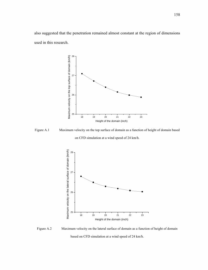
158

also suggested that the penetration remained almost constant at the region of dimensions

used in this research.

18 19 20 21 22 2325

26

27

28

Max

imu

m v

elo

city

on

the

top

sur

face

of d

omai

n (

km/h

)

Height of the domain (inch)

Figure A.1 Maximum velocity on the top surface of domain as a function of height of domain based

on CFD simulation at a wind speed of 24 km/h.

18 19 20 21 22 2325

26

27

28

Max

imum

vel

ocity

on

the

late

ral s

urf

ace

of d

omai

n (k

m/h

)

Height of the domain (inch)

Figure A.2 Maximum velocity on the lateral surface of domain as a function of height of domain

based on CFD simulation at a wind speed of 24 km/h.

159

18 19 20 21 22 230.0

0.2

0.4

0.6

0.8

1.0

Pe

ne

tra

tion

Height of the domain (inch)

Figure A.3 Penetration efficiency as a function of height of domain based on CFD simulation at a

wind speed of 24 km/h and a particle diameter of 10 micrometer.

18 19 20 21 22 230.0

0.2

0.4

0.6

0.8

1.0

Pe

ne

tra

tion

Width of the domain (inch)

Figure A.4 Penetration efficiency as a function of width of domain based on CFD simulation at a

wind speed of 24 km/h and a particle diameter of 10 micrometer.

160

A.2 Sensitivity Analysis on Effect of Number of the Particles Released/tracked

With the turbulent dispersion involved, the simulation would release 100

particles at each single particle injection points on the domain inlet boundary, and the

turbulence fluctuation would cause randomly different trajectories for these 100

particles. The total number of particles released/tracked was set to be 10000~100000 in

order to show sensitivity of the effect on the penetration efficiency in Figure A.5. The

predicted penetration efficiency remains constant after the maximum number of particles

used in simulation increases to 50,000. Considering the operation time for the numerical

simulation, the final results of simulation were taken under the condition that the

maximum particle number is 400,000 (4000 particle injection points were built on the

domain inlet boundary).

0 20000 40000 60000 80000 1000000.60

0.65

0.70

0.75

0.80

0.85

Pen

etr

atio

n

Total Particle Number

Figure A.5 Sensitivity analyses on total particle number in simulation.

161

A.3 Sensitivity Analysis on Effect of Max Number of Steps of Tracking Particles

The max number of steps in particles tracking was set to be 5000~40000 in order

to show sensitivity of the effect on the penetration efficiency in Figure A.6. The

predicted penetration efficiency reaches a constant value at approximately 15000

integration steps of tracking particles. Varying the number of tracking steps below 15000

results in a few percentage points difference in the predicted penetration efficiency. So

all the final results of simulation were taken under the parameter: Max number of steps

in particle tracking is 20000.

0 5000 10000 15000 20000 25000 30000 35000 40000 450000.0

0.2

0.4

0.6

0.8

1.0

Pen

etr

atio

n

Maximum number of steps in particle tracking

Figure A.6 Sensitivity analyses on max number of steps in particle tracking.

A.4 Effect of Orientation of the Inner Plenum

The bell-shaped inlet was designed for omni-directional aerosol sampling. The

circumferential intake ensured that the sampling process remained the same status when

162

the sample flow came from different direction. However, note that the windows (no. 5 in

Figure 2.1) at top of the inner plenum and the frames between the windows might cause

different effect on the flow field in chamber and the penetration efficiency of BSI-e. Six

windows (1.5 inch in height) are located near the top of the inner plenum, with 0.375

inch distance between. In this study, simulations had been done to show the difference

between two extreme conditions: the free wind flow direction is perpendicular to one of

the windows (CASE I) on the inner plenum or one of the frames between windows

(CASE II). The results (Table A.1) showed that the largest difference of the penetration

efficiency between these two conditions was about 2%.

Table A.1 The comparison of the prediction for different orientation of the inner plenum.

Particle Diameter

μm

Free stream wind speed 24 km/h

CASE I CASE II 2 98.3% 97.8% 5 96.7% 95.5%

10 89.0% 87.4% 15 55.8% 53.7% 20 N/A N/A

163

VITA

Name: Yingjie Tang

Address: Department of Mechanical Engineering, Texas A&M University,

College Station, TX 77843-3123

Email Address: tangyingjie823@gmail.com

Education: B.S., Thermal Engineering, Tsinghua University, China, 2006

M.S., Thermal Engineering, Tsinghua University, China, 2008

Ph.D., Mechanical Engineering, Texas A&M University, TX, 2012