A computational framework for fluid-solid-growth modeling in cardiovascular simulations

A Computational Framework for Fluid-Solid-Growth Modeling inCardiovascular Simulations

C. Alberto Figueroa1, Seungik Baek2, Charles A. Taylor1,3, and Jay D. Humphrey41 Department of Bioengineering, Stanford University2 Department of Mechanical Engineering, Michigan State University3 Department of Surgery, Stanford University4 Department of Biomedical Engineering, Texas A&M University

AbstractIt is now well known that altered hemodynamics can alter the genes that are expressed by diversevascular cells, which in turn plays a critical role in the ability of a blood vessel to adapt to newbiomechanical conditions and governs the natural history of the progression of many types of disease.Fortunately, when taken together, recent advances in molecular and cell biology, in vivo medicalimaging, biomechanics, computational mechanics, and computing power provide an unprecedentedopportunity to begin to understand such hemodynamic effects on vascular biology, physiology, andpathophysiology. Moreover, with increased understanding will come the promise of improveddesigns for medical devices and clinical interventions. The goal of this paper, therefore, is to presenta new computational framework that brings together recent advances in computational biosolid andbiofluid mechanics that can exploit new information on the biology of vascular growth andremodeling as well as in vivo patient-specific medical imaging so as to enable realistic simulationsof vascular adaptations, disease progression, and clinical intervention.

1 IntroductionSince the 1970s, we as a research community have come to appreciate the fundamentalimportance of biomechanical factors in regulating normal vascular biology and physiology andsimilarly in impacting the progression of many diseases as well as their responses to clinicalintervention. Although such factors clearly involve coupled effects between the flowing blood,vascular wall, and perivascular tissues, that is, fluid-solid-solute interactions, research invascular biomechanics has traditionally advanced along separate lines - biofluid mechanics,biosolid mechanics, and biotransport phenomena. There is, therefore, a pressing need to movetoward coupled problem formulations and solutions. Moreover, it is well known that mostphysiologic, pathophysiologic, and reparative processes in the vasculature manifest overperiods of days to weeks, months, or even years. Yet, most attention in vascular biomechanicshas focused on behaviors during a cardiac cycle or, at best, at select time points during theprogression of a disease or response to a treatment or injury. Clearly, there is also a pressingneed to understand better the underlying processes that are responsible for the conspicuouschanges in structure and function that occur over long periods, changes that likewise dependstrongly on the biomechanics.

This paper is motivated by these needs, indeed, the need for a new paradigm to address diversebiomechanical problems of the vasculature by accounting for coupled fluid-solid-transport

NIH Public AccessAuthor ManuscriptComput Methods Appl Mech Eng. Author manuscript; available in PMC 2010 September 15.

Published in final edited form as:Comput Methods Appl Mech Eng. 2009 September 15; 198(45-46): 3583–3602. doi:10.1016/j.cma.2008.09.013.

NIH

-PA Author Manuscript

NIH


NIH


over long periods of vascular adaptation and maladaptation [1]. Hence, in this paper we showhow computations of complex fluid-solid interactions during a cardiac cycle can be linked todetailed analyses of the solid mechanics of the vascular wall as well as descriptions of thekinetics of biological growth and remodeling which can depend strongly on solute transport.We refer to this new approach as Fluid-Solid-Growth (FSG) modeling. Toward this end, webuild primarily on four separate advances by our groups: biomechanics of growth andremodeling [2], a coupled momentum method for fluid-solid interactions during a cardiac cycle[3], a theory of small on large for coupling biosolid and biofluid mechanical models [4], andimproved approaches for modeling fluid boundary conditions in complex vascular systems[5]. Because these developments progressed independently, and tended to follow differentnotational conventions used by the biosolids and biofluids communities, we introducenotational changes herein to meld better these prior developments; where possible, we followMarsden and Hughes [6] for such notational conventions, including lightface italics for scalars,boldface italics for vectors and second-order tensors, and boldface block letters for higher-order tensors. Furthermore, where possible we use upper case characters to refer to materialquantities and lower case for spatial quantities.

Although the formalism presented herein is meant to be sufficiently general to accommodatemany different types of advances in modeling FSG problems, including 3-D patient-specificsimulations, we necessarily restrict our illustrative numerical results to a simple situation -influence of pressure-induced intramural stress and flow-induced wall shear stress on theevolution of shape and properties of a basilar artery following an initial concentric loss of aportion of the elastin within the wall. Notwithstanding the complexity of the associatedbiomechanical and biochemical processes, which will certainly require further research toidentify more complete constitutive relations for the growth and remodeling kinetics, wesubmit that the simple illustrative examples herein reveal both the need for and the greatpotential of Fluid-Solid-Growth modeling in basic research, industrial R&D, and clinicalapplications.

2 Methods2.1 General Framework for Fluid-Solid-Growth (FSG) Simulations

The FSG framework consists of two computational analyses defined over different time scales.On one hand, we consider long-term (weeks to months) simulations of the evolution of vascularwall geometry, structure, and properties governed by stress-mediated growth and remodeling(G&R). On the other hand, we study short-term (seconds) fluid-solid interaction (FSI)processes that characterize the hemodynamic forces acting on the wall throughout the cardiaccycle.

Each aspect of the framework uses different computational configurations. For the G&Rsimulation, we introduce a reference configuration κR and an intermediate configuration κs (seefigure 1). The reference configuration κR is a computationally convenient fixed configurationfrom which the position of each particle in other configurations can be mapped. In this work,the healthy arterial segment at G&R time 0 is chosen to be the reference configuration. Theintermediate configuration κs represents the mean geometry of the artery over the cardiac cycleat some later time s. Positions of a given particle in κR and κs are given by X and x(s),respectively. Evolution of a lesion is represented by a mapping between these two positionsand the deformation gradient F(s).

On the other hand, the FSI simulations utilize the intermediate configuration κs as a referenceconfiguration whereas the current configuration of the artery at any given time t during thecardiac cycle is given by κt. The deformation gradient corresponding to a mapping from κs toκt is denoted by Fκs(t), which is assumed to always be associated with a “small” deformation.

Figueroa et al.

Comput Methods Appl Mech Eng. Author manuscript; available in PMC 2010 September 15.

NIH


NIH


NIH


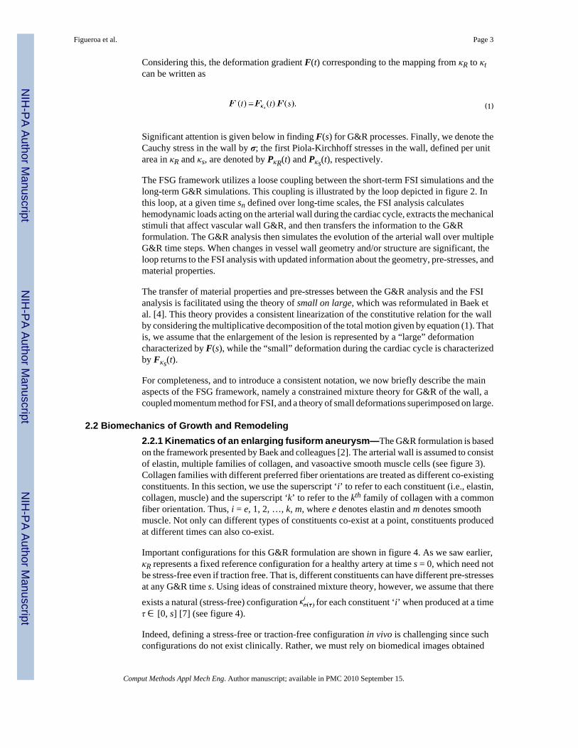
Considering this, the deformation gradient F(t) corresponding to the mapping from κR to κtcan be written as

(1)

Significant attention is given below in finding F(s) for G&R processes. Finally, we denote theCauchy stress in the wall by σ; the first Piola-Kirchhoff stresses in the wall, defined per unitarea in κR and κs, are denoted by PκR(t) and Pκs(t), respectively.

The FSG framework utilizes a loose coupling between the short-term FSI simulations and thelong-term G&R simulations. This coupling is illustrated by the loop depicted in figure 2. Inthis loop, at a given time sn defined over long-time scales, the FSI analysis calculateshemodynamic loads acting on the arterial wall during the cardiac cycle, extracts the mechanicalstimuli that affect vascular wall G&R, and then transfers the information to the G&Rformulation. The G&R analysis then simulates the evolution of the arterial wall over multipleG&R time steps. When changes in vessel wall geometry and/or structure are significant, theloop returns to the FSI analysis with updated information about the geometry, pre-stresses, andmaterial properties.

The transfer of material properties and pre-stresses between the G&R analysis and the FSIanalysis is facilitated using the theory of small on large, which was reformulated in Baek etal. [4]. This theory provides a consistent linearization of the constitutive relation for the wallby considering the multiplicative decomposition of the total motion given by equation (1). Thatis, we assume that the enlargement of the lesion is represented by a “large” deformationcharacterized by F(s), while the “small” deformation during the cardiac cycle is characterizedby Fκs(t).

For completeness, and to introduce a consistent notation, we now briefly describe the mainaspects of the FSG framework, namely a constrained mixture theory for G&R of the wall, acoupled momentum method for FSI, and a theory of small deformations superimposed on large.

2.2 Biomechanics of Growth and Remodeling2.2.1 Kinematics of an enlarging fusiform aneurysm—The G&R formulation is basedon the framework presented by Baek and colleagues [2]. The arterial wall is assumed to consistof elastin, multiple families of collagen, and vasoactive smooth muscle cells (see figure 3).Collagen families with different preferred fiber orientations are treated as different co-existingconstituents. In this section, we use the superscript ‘i’ to refer to each constituent (i.e., elastin,collagen, muscle) and the superscript ‘k’ to refer to the kth family of collagen with a commonfiber orientation. Thus, i = e, 1, 2, …, k, m, where e denotes elastin and m denotes smoothmuscle. Not only can different types of constituents co-exist at a point, constituents producedat different times can also co-exist.

Important configurations for this G&R formulation are shown in figure 4. As we saw earlier,κR represents a fixed reference configuration for a healthy artery at time s = 0, which need notbe stress-free even if traction free. That is, different constituents can have different pre-stressesat any G&R time s. Using ideas of constrained mixture theory, however, we assume that there

exists a natural (stress-free) configuration for each constituent ‘i’ when produced at a timeτ ∈ [0, s] [7] (see figure 4).

Indeed, defining a stress-free or traction-free configuration in vivo is challenging since suchconfigurations do not exist clinically. Rather, we must rely on biomedical images obtained

Figueroa et al.


NIH


NIH


NIH


under physiologic pressure; such images represent pre-stressed arterial configurations.Recently, two different approaches have been proposed to account for this pre-stress. The firstapproach enforces prescribed values of pre-stress (or pre-strain) [8] whereas the secondapproach uses an inverse elastostatic formulation to estimate the pre-stress [9,10]. Weemphasize, however, that in both cases the tissue is treated as a materially uniform continua.In this work, we employ an extension of the first approach: we assume that the pre-stress ineach constituent produced is the same as a postulated homeostatic value in κR. In other words,we assume that cells incorporate newly produced constituents within extant tissue at ahomeostatic (target) stress or strain. We describe how to enforce this homeostatic state in κRin section 3.2.

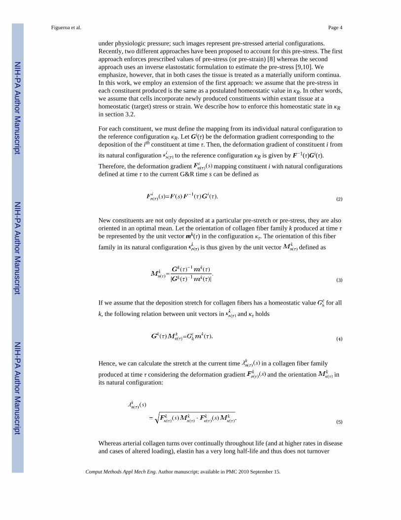
For each constituent, we must define the mapping from its individual natural configuration tothe reference configuration κR. Let Gi(τ) be the deformation gradient corresponding to thedeposition of the ith constituent at time τ. Then, the deformation gradient of constituent i from

its natural configuration to the reference configuration κR is given by F−1(τ)Gi(τ).Therefore, the deformation gradient mapping constituent i with natural configurationsdefined at time τ to the current G&R time s can be defined as

(2)

New constituents are not only deposited at a particular pre-stretch or pre-stress, they are alsooriented in an optimal mean. Let the orientation of collagen fiber family k produced at time τbe represented by the unit vector mk(τ) in the configuration κτ. The orientation of this fiber

family in its natural configuration is thus given by the unit vector defined as

(3)

If we assume that the deposition stretch for collagen fibers has a homeostatic value for all

k, the following relation between unit vectors in and κτ holds

(4)

Hence, we can calculate the stretch at the current time in a collagen fiber family

produced at time τ considering the deformation gradient and the orientation inits natural configuration:

(5)

Whereas arterial collagen turns over continually throughout life (and at higher rates in diseaseand cases of altered loading), elastin has a very long half-life and thus does not turnover

Figueroa et al.


NIH


NIH


NIH


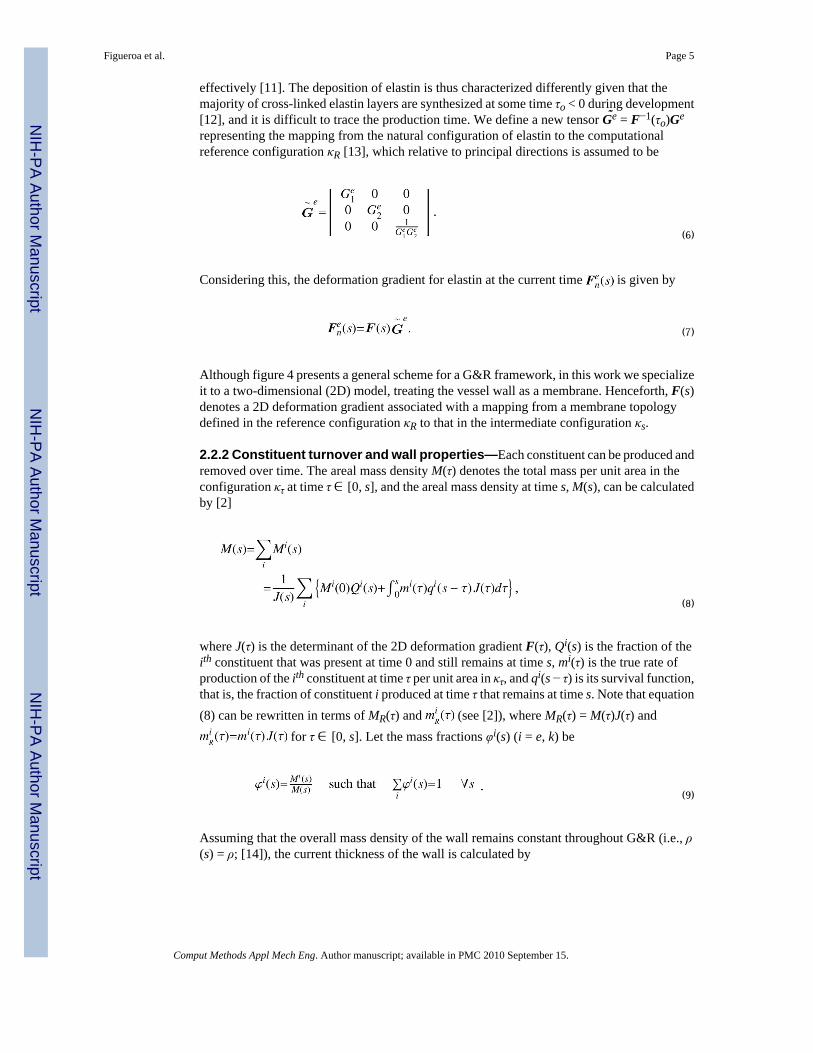
effectively [11]. The deposition of elastin is thus characterized differently given that themajority of cross-linked elastin layers are synthesized at some time τo < 0 during development[12], and it is difficult to trace the production time. We define a new tensor G ̃e = F−1(τo)Ge

representing the mapping from the natural configuration of elastin to the computationalreference configuration κR [13], which relative to principal directions is assumed to be

(6)

Considering this, the deformation gradient for elastin at the current time is given by

(7)

Although figure 4 presents a general scheme for a G&R framework, in this work we specializeit to a two-dimensional (2D) model, treating the vessel wall as a membrane. Henceforth, F(s)denotes a 2D deformation gradient associated with a mapping from a membrane topologydefined in the reference configuration κR to that in the intermediate configuration κs.

2.2.2 Constituent turnover and wall properties—Each constituent can be produced andremoved over time. The areal mass density M(τ) denotes the total mass per unit area in theconfiguration κτ at time τ ∈ [0, s], and the areal mass density at time s, M(s), can be calculatedby [2]

(8)

where J(τ) is the determinant of the 2D deformation gradient F(τ), Qi(s) is the fraction of theith constituent that was present at time 0 and still remains at time s, mi(τ) is the true rate ofproduction of the ith constituent at time τ per unit area in κτ, and qi(s − τ) is its survival function,that is, the fraction of constituent i produced at time τ that remains at time s. Note that equation(8) can be rewritten in terms of MR(τ) and (see [2]), where MR(τ) = M(τ)J(τ) and

for τ ∈ [0, s]. Let the mass fractions φi(s) (i = e, k) be

(9)

Assuming that the overall mass density of the wall remains constant throughout G&R (i.e., ρ(s) = ρ; [14]), the current thickness of the wall is calculated by

Figueroa et al.


NIH


NIH


NIH


(10)

In our previous work [2,15], we assumed that the production rate of collagen fibers dependedsolely on the intramural stress experienced by the cells interacting with the surrounding matrix.We know, however, that changes in wall shear stress affect the release of vasoactive substancesby the endothelium that also affect the turnover of collagen and smooth muscle. In this work,by coupling the G&R and FSI formulations, we can incorporate this additional mechanicalstimulus. Therefore, the rate of mass density production for a collagen family mk(s) ispostulated to depend on both the deviation of a scalar measure of the intramural stress from itspostulated homeostatic value (σk − σh) and the deviation of the wall shear stress from itshomeostatic value . Let σk be given by:

(11)

where Tc(s) and hc(s) are the collagen Cauchy membrane stress determined by satisfying wallequilibrium and collagen thickness at time s, respectively. The mean value of wall shear stressτw is obtained directly from the FSI simulations (see figure 2). As an illustrative example,consider the following linearized form for the rate of mass production:

(12)

where kσ and kτ are scalar parameters that control the stress-mediated G&R and is a basalrate of mass production for the kth fiber family. At the homeostatic state, therefore, theproduction rate follows the basal rate. We define the survival function for the kth collagenfamily as

(13)

We should note that the basal rate of mass production for each constituent must be selected ina way such that production and removal are perfectly balanced in the absence of altered stressesfrom homeostatic values. Using this condition, and Qk(s) can be obtained as [15]

(14)

The alignment of newly deposited collagen fibers within the arterial wall is not clearlyunderstood, but it has been suggested that it may depend on the deformation of existing collagen

Figueroa et al.


NIH


NIH


NIH


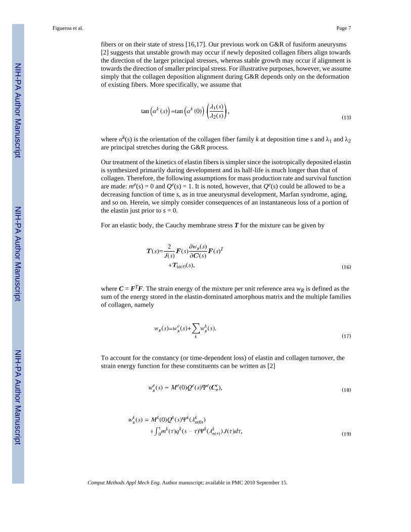
fibers or on their state of stress [16,17]. Our previous work on G&R of fusiform aneurysms[2] suggests that unstable growth may occur if newly deposited collagen fibers align towardsthe direction of the larger principal stresses, whereas stable growth may occur if alignment istowards the direction of smaller principal stress. For illustrative purposes, however, we assumesimply that the collagen deposition alignment during G&R depends only on the deformationof existing fibers. More specifically, we assume that

(15)

where αk(s) is the orientation of the collagen fiber family k at deposition time s and λ1 and λ2are principal stretches during the G&R process.

Our treatment of the kinetics of elastin fibers is simpler since the isotropically deposited elastinis synthesized primarily during development and its half-life is much longer than that ofcollagen. Therefore, the following assumptions for mass production rate and survival functionare made: me(s) = 0 and Qe(s) = 1. It is noted, however, that Qe(s) could be allowed to be adecreasing function of time s, as in true aneurysmal development, Marfan syndrome, aging,and so on. Herein, we simply consider consequences of an instantaneous loss of a portion ofthe elastin just prior to s = 0.

For an elastic body, the Cauchy membrane stress T for the mixture can be given by

(16)

where C = FTF. The strain energy of the mixture per unit reference area wR is defined as thesum of the energy stored in the elastin-dominated amorphous matrix and the multiple familiesof collagen, namely

(17)

To account for the constancy (or time-dependent loss) of elastin and collagen turnover, thestrain energy function for these constituents can be written as [2]

(18)

(19)

Figueroa et al.


NIH


NIH


NIH


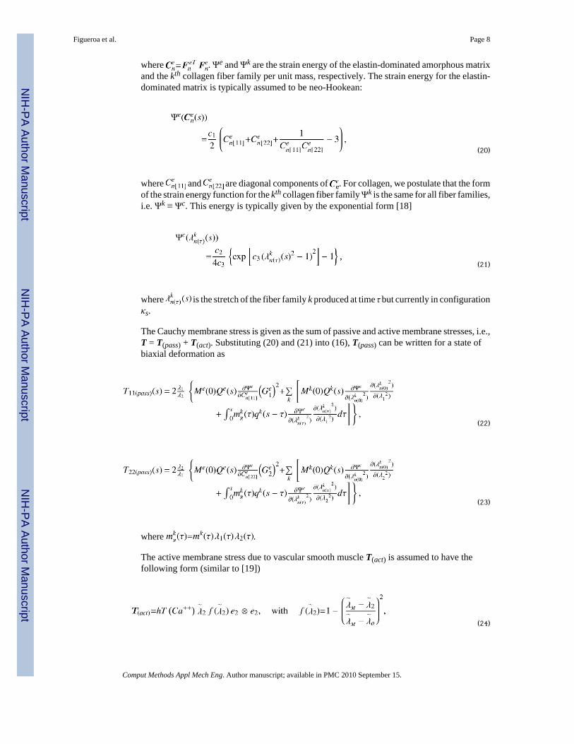
where . Ψe and Ψk are the strain energy of the elastin-dominated amorphous matrixand the kth collagen fiber family per unit mass, respectively. The strain energy for the elastin-dominated matrix is typically assumed to be neo-Hookean:

(20)

where and are diagonal components of . For collagen, we postulate that the formof the strain energy function for the kth collagen fiber family Ψk is the same for all fiber families,i.e. Ψk ≡ Ψc. This energy is typically given by the exponential form [18]

(21)

where is the stretch of the fiber family k produced at time τ but currently in configurationκs.

The Cauchy membrane stress is given as the sum of passive and active membrane stresses, i.e.,T = T(pass) + T(act). Substituting (20) and (21) into (16), T(pass) can be written for a state ofbiaxial deformation as

(22)

(23)

where .

The active membrane stress due to vascular smooth muscle T(act) is assumed to have thefollowing form (similar to [19])

(24)

Figueroa et al.


NIH


NIH


NIH


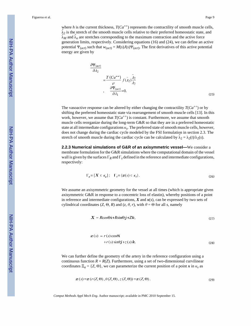
where h is the current thickness, T(Ca++) represents the contractility of smooth muscle cells,λ̃2 is the stretch of the smooth muscle cells relative to their preferred homeostatic state, andλ̃M and λ̃o are stretches corresponding to the maximum contraction and the active forcegeneration limits, respectively. Considering equations (16) and (24), we can define an activepotential Ψ(act) such that w(act) = M(s)J(s)Ψ(act). The first derivatives of this active potentialenergy are given by

(25)

The vasoactive response can be altered by either changing the contractility T(Ca++) or byshifting the preferred homeostatic state via rearrangement of smooth muscle cells [13]. In thiswork, however, we assume that T(Ca++) is constant. Furthermore, we assume that smoothmuscle cells reorganize during the long-term G&R so that they are in a preferred homeostaticstate at all intermediate configurations κs. The preferred state of smooth muscle cells, however,does not change during the cardiac cycle modeled by the FSI formulation in section 2.3. Thestretch of smooth muscle during the cardiac cycle can be calculated by λ̃2 = λ2(t)/λ2(s).

2.2.3 Numerical simulations of G&R of an axisymmetric vessel—We consider amembrane formulation for the G&R simulations where the computational domain of the vesselwall is given by the surfaces ΓR and Γs defined in the reference and intermediate configurations,respectively:

(26)

We assume an axisymmetric geometry for the vessel at all times (which is appropriate givenaxisymmetric G&R in response to a concentric loss of elastin), whereby positions of a pointin reference and intermediate configurations, X and x(s), can be expressed by two sets ofcylindrical coordinates (Z, Θ, R) and (z, θ, r), with θ = Θ for all s, namely

(27)

(28)

We can further define the geometry of the artery in the reference configuration using acontinuous function R = R(Z). Furthermore, using a set of two-dimensional curvilinearcoordinates Ξa = {Z, Θ}, we can parameterize the current position of a point x in κs as

(29)

Figueroa et al.


NIH


NIH


NIH


The associated bases for this curvilinear parametrization are

(30)

where A, a = 1, 2. Local orthonormal bases and outward normal vectors in the reference andintermediate configurations are thus given by

(31)

Consequently, the deformation experienced by the artery due to growth is defined by

(32)

and F(s) = FiJei ⊗ EJ where

(33)

where λ1 and λ2 are the two principal stretches and (·)′ = ∂(·)/∂Z.

G&R of the artery is simulated using a finite element method based on the principle of virtualwork to satisfy equilibrium at each G&R time s. It is noted, therefore, that inertial forces arenegligible in most arteries with respect to in vivo stress analyses [14]. The governing equationis given by

(34)

where P(x) is the transmural pressure and δx represents virtual changes in position, with a andA denoting surface areas in the current and reference configurations. A variation of equation(34) with respect to r and z yields two sets of nonlinear algebraic equations:

Figueroa et al.


NIH


NIH


NIH


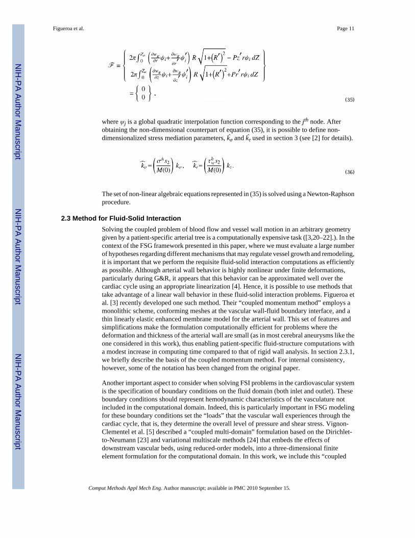
(35)

where ψj is a global quadratic interpolation function corresponding to the jth node. Afterobtaining the non-dimensional counterpart of equation (35), it is possible to define non-dimensionalized stress mediation parameters, k̂σ and k̂τ used in section 3 (see [2] for details).

(36)

The set of non-linear algebraic equations represented in (35) is solved using a Newton-Raphsonprocedure.

2.3 Method for Fluid-Solid InteractionSolving the coupled problem of blood flow and vessel wall motion in an arbitrary geometrygiven by a patient-specific arterial tree is a computationally expensive task ([3,20–22].). In thecontext of the FSG framework presented in this paper, where we must evaluate a large numberof hypotheses regarding different mechanisms that may regulate vessel growth and remodeling,it is important that we perform the requisite fluid-solid interaction computations as efficientlyas possible. Although arterial wall behavior is highly nonlinear under finite deformations,particularly during G&R, it appears that this behavior can be approximated well over thecardiac cycle using an appropriate linearization [4]. Hence, it is possible to use methods thattake advantage of a linear wall behavior in these fluid-solid interaction problems. Figueroa etal. [3] recently developed one such method. Their “coupled momentum method” employs amonolithic scheme, conforming meshes at the vascular wall-fluid boundary interface, and athin linearly elastic enhanced membrane model for the arterial wall. This set of features andsimplifications make the formulation computationally efficient for problems where thedeformation and thickness of the arterial wall are small (as in most cerebral aneurysms like theone considered in this work), thus enabling patient-specific fluid-structure computations witha modest increase in computing time compared to that of rigid wall analysis. In section 2.3.1,we briefly describe the basis of the coupled momentum method. For internal consistency,however, some of the notation has been changed from the original paper.

Another important aspect to consider when solving FSI problems in the cardiovascular systemis the specification of boundary conditions on the fluid domain (both inlet and outlet). Theseboundary conditions should represent hemodynamic characteristics of the vasculature notincluded in the computational domain. Indeed, this is particularly important in FSG modelingfor these boundary conditions set the “loads” that the vascular wall experiences through thecardiac cycle, that is, they determine the overall level of pressure and shear stress. Vignon-Clementel et al. [5] described a “coupled multi-domain” formulation based on the Dirichlet-to-Neumann [23] and variational multiscale methods [24] that embeds the effects ofdownstream vascular beds, using reduced-order models, into a three-dimensional finiteelement formulation for the computational domain. In this work, we include this “coupled

Figueroa et al.


NIH


NIH


NIH


multi-domain” approach for boundary condition specification and summarize this method insection 2.3.2.

2.3.1 A coupled momentum method for FSI—The coupled momentum method is basedon a stabilized finite element formulation [20,25] applied to the incompressible Navier-Stokesequations in a fixed computational grid. The method formulates the degrees-of-freedom (i.e.,displacements u) for the vascular wall as a function of the fluid velocities v at the fluid-solidinterface, using an enhanced linear membrane formulation. To characterize the method, wefirst introduce the configurations, domains, and boundaries considered for blood flow andvascular wall motion.

As described in section 2.1, the FSI problem defined on the small time scales employs anintermediate configuration κs representing the average geometry of the arterial structure overthe cardiac cycle. The position of any point x(s) on the fluid-solid interface at the intermediateconfiguration Γs ∈ κs will be mapped to a point x(t) on Γt ∈ κt via a “small” deformation andassociated deformation gradient Fκs(t) introduced in equation (1) (see figure 5).

Blood flow equations: The blood flow problem is defined within a domain Ωf that representsthe current configuration of the blood volume inside the artery at any time t during the cardiaccycle. The boundary of this blood flow domain Ωf is given by

(37)

where Γin represents the boundary where a velocity field v = vin is prescribed; this usuallycorresponds to the inflow face of the model. Γout represents the boundary where a traction fieldtout is prescribed; this usually corresponds to an outflow face of the model. This traction isprescribed weakly by considering a reduced-order model of the downstream vasculature viathe “coupled multi-domain” method (see section 2.3.2). Lastly, Γt represents the interfacebetween blood and vessel wall (i.e., the luminal surface). The traction tf acting on this boundaryis determined using information coming from the weak form solution for the dynamics of thevascular wall.

Because the motion of the vessel wall is considered to be small, we assume for the FSI problemthat the current configuration κt can be approximated by the intermediate configuration κs forall times: κt ≈ κs ∀t. Therefore, the Eulerian coordinates x(t) defining the boundaries of theflow domain will be given by the coordinates x(s) of the boundaries at the intermediateconfiguration. Considering this, the weak formulation of the blood flow problem in the fixedEulerian frame is:

(38)

Here, p and v are the blood pressure and velocity, respectively, and T is the period for a cardiaccycle (∼ 1 sec. in humans). The test functions for mass and momentum balance are q and w,respectively; ρf is the mass density of the blood, b is a body force per unit volume (e.g. gravity),and τ is the viscous part of the stress response for the blood, where

Figueroa et al.


NIH


NIH


NIH


(39)

and μ is the dynamic viscosity. The total response of the blood (considered Newtonian) is thus

(40)

where the Lagrange multiplier p that enforces incompressibility equals the blood pressure.

We refer the reader to the original paper [3] for the expression of the stabilization termsconsidered in equation (38).

Vessel wall equations: Assuming the wall to be a membrane, the problem is defined in a“volume” Ωs given by the interface between blood and the vascular wall in the intermediateconfiguration κs having some thickness h:

(41)

The boundaries of this domain are and (see figure 5), with aDirichlet condition on the velocity prescribed on the former and a Neumann boundary with atraction hs prescribed on the latter. Lastly, a traction ts acts on the fluid-solid interface Γs. TheGalerkin formulation for the vascular wall can then be given in Lagrangian form as

(42)

Here, v represents the velocity of the vascular wall, which is identical to the fluid velocity dueto the conforming meshes at the interface Γs, w is the wall test function, ρ is the mass densityof the vessel wall, (Pκs) is the linearization via small on large of the first Piola-Kirchhoffstress tensor defined in the G&R formulation, and bs is a body force per unit volume. In thiscontext, it is appropriate to characterize the vessel wall stress using a linearized first Piola-Kirchhoff tensor (Pκs), since we are relating forces in current time with a geometry given ina fixed configuration (i.e., intermediate configuration κs). This linearized first Piola-Kirchhofftensor is a function of the vessel wall displacement u(x(s), t), which is calculated via integrationof the vessel wall velocity using a Newmark scheme [26].

At the interface Γs, the deformation gradient Fκs is associated with a mapping from the positionx(s) on Γs to the position x(t) on Γt (see figure 5). The traction vectors can be written as tf =σfnf on Γt and ts = (Pκs)N

s on Γs, where nf and Ns are outward unit normals to the surfacesΓt and Γs, respectively. The mapping of the surface vector element is given by nf da =−JκsFκs

−TNsdA (e.g., [27]). Therefore, the term (∫Γt w · tf da) in equation (38) can be rewrittenas

(43)

Figueroa et al.


NIH


NIH


NIH


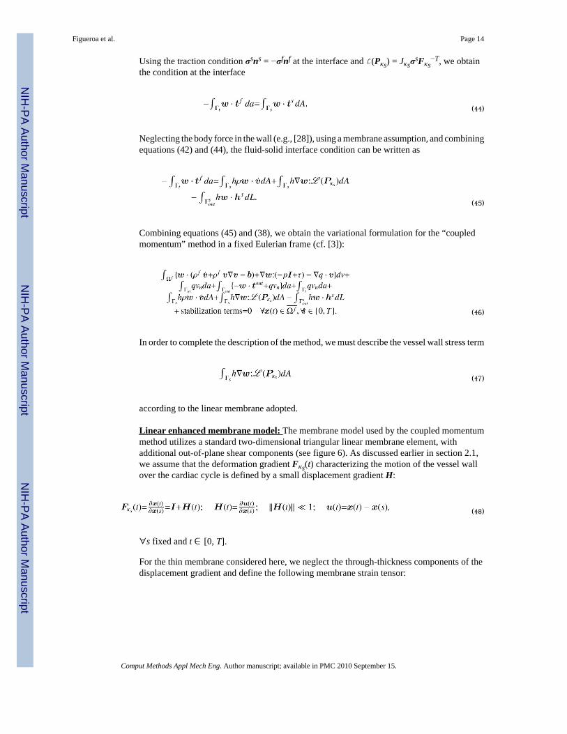
Using the traction condition σsns = −σfnf at the interface and (Pκs) = JκsσsFκs

−T, we obtainthe condition at the interface

(44)

Neglecting the body force in the wall (e.g., [28]), using a membrane assumption, and combiningequations (42) and (44), the fluid-solid interface condition can be written as

(45)

Combining equations (45) and (38), we obtain the variational formulation for the “coupledmomentum” method in a fixed Eulerian frame (cf. [3]):

(46)

In order to complete the description of the method, we must describe the vessel wall stress term

(47)

according to the linear membrane adopted.

Linear enhanced membrane model: The membrane model used by the coupled momentummethod utilizes a standard two-dimensional triangular linear membrane element, withadditional out-of-plane shear components (see figure 6). As discussed earlier in section 2.1,we assume that the deformation gradient Fκs(t) characterizing the motion of the vessel wallover the cardiac cycle is defined by a small displacement gradient H:

(48)

∀s fixed and t ∈ [0, T].

For the thin membrane considered here, we neglect the through-thickness components of thedisplacement gradient and define the following membrane strain tensor:

Figueroa et al.


NIH


NIH


NIH


(49)

The membrane model utilizes a linearization of the first Piola-Kirchhoff tensor defined in theG&R analysis (Pκs) around F(t) ≈ F(s). This linearization is accomplished via the theory ofsmall on large as summarized in section 2.4. The membrane stresses resulting from thislinearization are depicted in figure 6. Note that, as justified by the thin membrane formulation,we assume that the (Pκs)33 component of the linearized stress tensor is small compared to theother components.

Equation (46) is spatially discretized using linear tetrahedral elements. The resulting semi-discrete system of equations is integrated over time using a Generalized-alpha method [29].Details on the solution strategy are described in Figueroa et al. [3].

2.3.2 Boundary conditions for the FSI problem—The “coupled-multidomain”formulation for specifying outlet boundary conditions [5] for the fluid domain employs adisjoint decomposition of the blood flow spatial domain Ω̃f into an upstream “numerical”

domain Ωf and a downstream “analytical” domain Ω′f such that and Ωf ∩ Ω′f =Ø. These two domains are separated by the boundary Γout (see figure 7).

The method then applies a similar disjoint decomposition to the flow variables. If the solutionvector is written as Ṽ = {ṽ, p̃}T, then this vector can be separated into a component that isdefined within the numerical domain Ωf and a component defined within the analytical domainΩ′f, viz.

(50)

This decomposition further satisfies the condition V = V′ at the interface Γout, and is also appliedto the weighting functions. The coupled-multidomain method produces a variational form forthe numerical domain Ωf similar to the one given by equation (38), where the integral termdefined on Γout is written in terms of operators = { m, c}T|Γout and = { m,

c}T|Γout

(51)

where subscripts m and c denote the fluid momentum and mass balance components of theoperators, respectively. These operators are defined in the domain Ω′f based on the modelchosen to represent blood flow and pressure in that domain. For instance, if we consider a linearwave propagation model as the analytical solution in Ω′f defined as a one-dimensional network,then it is possible to derive an input vascular impedance function Z(ω) for the inlet of theanalytical domain (i.e., the boundary Γout) that is used as a terminal impedance of the numericaldomain [30]. This impedance function Z(ω) relates flow and pressure modes for all frequenciesω considered in the analysis, and is used to define the operators and . More specifically,for the examples considered in this paper, we have

Figueroa et al.


NIH


NIH


NIH


(52)

(53)

Equations (52) and (53) represent mass and momentum balance between the numerical andanalytical domains. In equation (52), we can see the convolution of the impedance function inthe time domain z(t) and flow Q(t) on Γout. This convolution integral sets the pressure p at theinterface as a function of the flow characteristics in the downstream domain Ω′f.

2.4 Theory of Small on Large for FSG SimulationsWe have previously suggested that the theory of small deformations superimposed on largecan serve as a useful tool to obtain a linearized response of the wall during the cardiac cyclewithout compromising important characteristics such as anisotropy and smooth muscle tone[4]. Furthermore, we have shown that this linearized response can provide a goodapproximation for the wall constitutive behavior during the cardiac cycle and can be used influid-solid interaction computations. Here, we briefly describe how to obtain a linearizedresponse from the constitutive relation used during arterial adaptation in section 2.2.2.

For an incompressible elastic material, the constitutive relation for Cauchy stress σ is given by

(54)

where p is a Lagrange multiplier and W is the strain energy per unit reference volume. Duringthe cardiac cycle we assume that the G&R time s and the configuration κs are fixed and weutilize the configuration κs as a reference configuration for FSI simulations. Hence, althoughnot specified explicitly, the kinematic quantities are functions of position x(s). The first Piola-Kirchhoff stress Pκs(t) with respect to an area of the intermediate configuration κs can be writtenas (see figure 1 and recall that F(t) = Fκs(t)F(s))

(55)

Note that, when Fκs(t) = I, Pκs(t) is the same as the Cauchy stress σ(t) and will be denoted asP(s). As introduced in section 2.3.1, Pκs can be linearized at Fκs(t) = I (or H(t) = 0) with respectto the small deformation gradient H(t) (see equation (48)), so that components of the linearizedstress (Pκs) can be written as (see [4])

Figueroa et al.


NIH


NIH


NIH


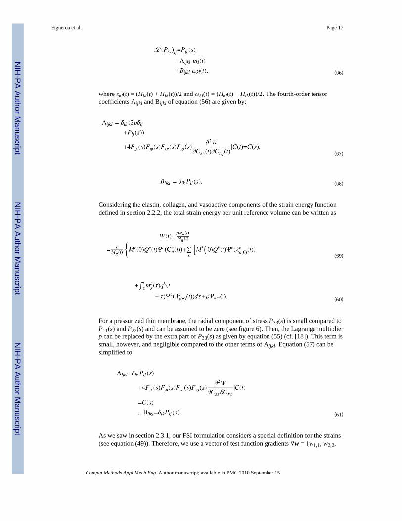
(56)

where εkl(t) = (Hkl(t) + Hlk(t))/2 and ωkl(t) = (Hkl(t) − Hlk(t))/2. The fourth-order tensorcoefficients Aijkl and Bijkl of equation (56) are given by:

(57)

(58)

Considering the elastin, collagen, and vasoactive components of the strain energy functiondefined in section 2.2.2, the total strain energy per unit reference volume can be written as

(59)

(60)

For a pressurized thin membrane, the radial component of stress P33(s) is small compared toP11(s) and P22(s) and can be assumed to be zero (see figure 6). Then, the Lagrange multiplierp can be replaced by the extra part of P33(s) as given by equation (55) (cf. [18]). This term issmall, however, and negligible compared to the other terms of Aijkl. Equation (57) can besimplified to

(61)

As we saw in section 2.3.1, our FSI formulation considers a special definition for the strains(see equation (49)). Therefore, we use a vector of test function gradients ∇w = {w1,1, w2,2,

Figueroa et al.


NIH


NIH


NIH


w1,2 + w2,1, w3,1, w3,2}T in equation (47). Considering this, components of this equation canbe written as:

(62)

Note that the dependency of wi,j, εkl, and ωkl with respect to time t is suppressed. The secondterm in the right hand side of equation (62) can be evaluated considering the following cases:

1) when i = j, k = l (no sum)

(63)

2) when i = j, k ≠ l (no sum)

(64)

3) when i ≠ j, k = l (no sum)

(65)

4) when i ≠ j, k ≠ l (no sum)

(66)

Considering equation (61), the following relations should be satisfied

(67)

Figueroa et al.


NIH


NIH


NIH


(68)

(69)

Furthermore, we assume that multiplications involving the following components {P12(s),P22(s) − P11(s), P33(s), ω12, w1,2 − w2,1, H13, H23, w1,3, w2,3} generate second-order terms thatare negligible based on the axisymmetric membrane assumption. Then, the term wi,j (Pκs)ij in(62) can be written in a matrix form

(70)

where P̃ = {P11(s), P22(s), P12(s), P31(s), P32(s)}T is a “pre-stress” tensor and K̃ is a “stiffnessmatrix” given by

(71)

The components of P̃ and K̃ are obtained from post-processing of the G&R simulation resultsat time s and given in the “membrane” polar coordinates defined in section 2.2.3. We mustthen transform these tensors to the “local” reference frame defined by the finite element meshof the FSI membrane formulation (see figure 8).

2.4.1 Mapping anisotropic material properties from the 2D G&R membraneframe to the 3D FSI local frame—The transformation of Aijkl and Pij(s) given in“membrane coordinates” to the FSI “local coordinates” is done by means of the rotation tensorQiα according to the following expressions:

(72)

Figueroa et al.


NIH


NIH


NIH


(73)

In order to characterize the components of the rotation tensor Qiα, we introduce the three setsof orthonormal bases represented in figure 8: (I = 1, 2, 3) are the bases of a “global” Cartesiancoordinate system; (α = 1, 2, 3) are the “membrane” orthonormal bases used by the G&Rformulation, where and are the bases in the circumferential and axial directions,respectively, and is the basis in the outward normal direction. (i = 1, 2, 3) is the “local”orthonormal bases for a triangular element of the FSI membrane formulation.

An orthogonal transformation Qm from the “global” frame to the “membrane” frame can becalculated by . Similarly, a transformation Ql from the “global” to the “local” frameis given by and the components of the tensor can be obtained from the three nodalpoints of the elements. Considering this, the orthogonal transformation Q from the “membrane”frame to the “local” frame becomes Q = Ql(Qm)−1 (or ).

In order to validate the linearization proposed here, we performed a hydrostatic pressurizationtest of a cylindrical vessel of radius R = 1.6 mm and length L = 25 mm. In this problem, weconstrained the longitudinal motion of both ends of the vessel. We compared deformations atthe central cross section of the vessel (Z = 12.5 mm) obtained from the nonlinear constitutivetheory used by the G&R formulation with the linearized theory used by the FSI formulationderived via small on large. The results of the pressurization test are shown in figure 9 anddemonstrate a good agreement between the two formulations over the physiologic range ofpressures (80 - 120 mmHg).

3 Illustrative Simulation3.1 Problem Definition

Consider a simple geometry given by an idealized cylindrical, axisymmetric representation ofa basilar artery. We first study the evolution of the artery from an initial state (time 0) wherethe geometry is perfectly cylindrical (i.e., no taper) and the spatial distribution of materialproperties is uniform, to a postulated homeostatic state (time sN, see figure 10). This stateexhibits a slight tapering in geometry and wall thickness and small longitudinal variations inmaterial properties. We study this state in section 3.2. Once this homeostatic state is obtained,we introduce a concentric insult in the central section of the artery. This insult results in theremoval of elastin, an associated change in intramural stress and geometry, and a consequentstress-mediated FSG process. Moreover, because intact elastin provides smooth muscle withmany important biological cues (e.g., to not proliferate, to not migrate, to not synthesize matrix,and to not enter the cell death cycle prematurely; Karnik et al., [31]), loss of elastin within theaneurysmal segment necessarily changes the smooth muscle phenotype. For simplicity here,we assume that loss of elastin results in an associated loss of smooth muscle, as seenhistologically in intracranial aneurysms [32], hence the primary growth and remodelingresponse is due to turnover of collagen (cf. Baek et al., [13]). Future models will need to includemore gradual loss of elastin and changes in smooth muscle, however.

We consider two different FSG cases (see figure 10): in Case 1, the growth and remodeling ismediated only via vessel wall tensile stress whereas in Case 2, this process is mediated by both

Figueroa et al.


NIH


NIH


NIH


tensile stress (via the effects of increased stretch on collagen production) and wall shear stress(via the effects of vasoactive molecules on collagen turnover).

We proceed to define the boundary conditions, vessel wall material parameters, and vasoactiveparameters used in the analysis for both the fluid-solid interaction problem defined over thesmall time scales and the growth and remodeling problem defined over the large time scales.

FSI problem over the small time scales—Consider a typical volumetric flow wavemapped to a Womersley velocity profile at the inlet face of the basilar artery (see figure 11).The mean flow is Q ̄ = 1.97 ml/s and the cardiac cycle has period T = 1.1 s. At the outlet faceof the model we prescribe an impedance function Z(ω) that produces a typical range ofpressures expected for this part of the vasculature: 85 mmHg diastolic pressure and 115 mmHgsystolic pressure. The zero-frequency component of this impedance function (i.e., the vascularresistance ℜ) is Z(ω = 0) = ℜ = 6.75 × 104 dyn · cm−5 · s. The vessel is held in place byclamping the inlet and outlet sections of the wall. This set of boundary conditions for the smalltemporal scales remain constant during the modest growth and remodeling process definedherein over the large time scales, because we assume that the changes experienced by the arteryare local and do not significantly affect the upstream and downstream hemodynamicconditions.

Vessel wall G&R problem over the large time scales—The boundary conditions forthe G&R problem are such that the ends (Z = 0, L) of the arterial wall are fixed in the longitudinaldirection but are free to move in the radial direction. The mass density of the vessel wall isassumed to remain constant at ρ = 1050 kg/m3. For the elastin fibers, the initial mass fractionis set to φe(0) = 0.1. The natural configuration mapping parameters (see equation (6)) are givenby and . Lastly, the coefficient for the amorphous neo-Hookean function(see equation (20)) is c1 = 526.94 N · m/kg. As for the collagen fibers, for each family k weconsider the following initial collagen mass fractions φk(0) and orientation angles αk(0):

The homeostatic deposition stretch for the collagen fiber families is and thecoefficients in the exponential function for the material behavior (see equation (21)) are set toc2 = 746.97 N · m/kg, c3 = 29.16. The parameters for vasoactive behavior are T(Ca++) = 39.86kPa, λ̃M = 1.2, and λ̃o = 0.7 (see equations (24-25)).

3.2 Identifying a Homeostatic StateAt time 0, the length L, reference radius R, and thickness H of the artery are set to 25, 1.6, and0.1047 mm, respectively. These are typical dimensions for a disease-free human basilar artery.In order to initialize the FSG computation, the fluid-solid interaction part of the analysis needsa distribution of material properties and geometry consistent with the known small pressuredrop along the length of the vessel. We obtain these properties by arbitrarily defining ahomeostatic state under a hydrostatic pressure of p(s = 0) = 13.332 kPa. This pressure is definedbased on the mean flow Q ̄ and resistance ℜ used in the subsequent pulsatile analysis. In thishomeostatic state, the rates of mass production and removal of collagen fibers are balanced,and the vasoactive response of the smooth muscle is “normal”. Since this homeostatic state isdefined by a hydrostatic loading, it has an associated uniform geometry and spatially uniformdistribution of material parameters and pre-stresses. We can then apply the theory of small on

large to compute the linearized material parameters and pre-stresses .

Figueroa et al.


NIH


NIH


NIH


We then proceed to run the fluid-solid interaction analysis to obtain the mechanical stimuliexperienced by the artery under pulsatile conditions. Identifying relevant stimuli is a challengeby itself, for many factors can regulate the biochemical processes defining growth andremodeling of the wall constituents. Here, we consider the simplest stimuli given by the time-average over the cardiac cycle of the blood pressure and the wall shear stress fields. We assumethat these mechanical stimuli, acting on the small time scales, remain unchanged during thegrowth and remodeling process, acting on the large time scales, that defines the homeostaticstate. These fields are presented in figure 12 (dashed lines). Observe the linear variation of thepressure along the vessel length and the spatially uniform wall shear stress field, as itcorresponds to a vessel with uniform radius R. Using these mechanical stimuli, the G&Rsimulation grows the artery iteratively, exchanging information with the FSI formulation (seefigure 2) until it reaches a new homeostatic equilibrium under such stimuli at some time tN.During this process, we consider the following non-dimensional stress mediation parametersk̂σ = 4.0 and k̂τ = 0.0, which induce a fast stable growth.

The result of this growth and remodeling is a new homeostatic configuration wherein the vesselis tapered. That is, the radius is slightly larger at the proximal end, where the average pressureis slightly larger. The wall thickness also decreases along the length of the artery, followingthe same linear trend of the radius and pressure (see figure 13). Figure 14 shows thecorresponding changes in circumferential stress and stiffness. The artery at time sN is under aslightly larger circumferential stress in the proximal segment, and the circumferential stiffnessis likewise higher proximally. These are manifestations of more collagen being turned overproximally due to the elevated tensile stress environment. These changes, although small, showa logical trend. In the homeostatic configuration we observe a linear variation in the time-averaged wall shear stress field, consistent with the observed variation in radius (see figure12). Changes in the pressure field between the homeostatic configuration at time sN and theinitial configuration at time 0 are negligible (i.e., less than a few dynes/cm2).

3.3 Role of Pressure and Shear Forces after an Initial Circumferential InsultOnce we have obtained numerically a homeostatic state 1, we introduce an insult in the centralsection of the artery at time sN, resulting in the concentric loss of elastin in that position of thearterial wall. The mathematical representation of this insult is given by the following expressionfor the elastin mass density for all s, Z ∈ [0, L]:

(74)

This insult results in an instantaneous thinning of the vessel wall in the affected region, a newstress environment, and a consequent departure from homeostatic conditions. Therefore, thepostulated rates of mass density production (see equation 12) for the different collagen familiesare altered from basal conditions. We study the stress-mediated growth and remodeling of theartery from this point on, considering two cases: Case 1 studies G&R mediated by tensile stressonly, with k̂σ = 0.1 for the non-dimensionalized tensile stress mediation parameter; Case 2considers G&R mediated by both tensile stress and wall shear stress, with tensile stress andwall shear stress mediation parameters k̂σ = 0.1 and k̂τ = 0.1, respectively.

1To properly define a homeostatic state resulting from developmental biology is of great interest, but exceedingly complex and not neededfor the present purposes.

Figueroa et al.


NIH


NIH


NIH


Figure 15 shows the evolution of the luminal radius for both cases. Case 2 yields a noticeablyfaster rate of enlargement in the center of the aneurysmal region, but a reduction in radius atthe distal end of the aneurysm (Z ≈ 17 mm). This is probably due to the increase in wall shearstress in that region (see figure 17) and the specific rule adopted for mass production as afunction of shear stress (see equation (12)). In figure 16, we observe a faster localized increasein pressure for Case 2 due to the corresponding faster increase in radius. The magnitude of thispressure increase is very modest in both cases, however, accounting for less than one mmHg.Figure 17 shows the evolution of time averaged wall shear stress. The shear stress decreasessignificantly over time within the aneurysmal region in both cases, but this reduction occursfaster in Case 2. This is consistent with the faster increase in radius seen in figure 15. In bothcases, we observe an increase in wall shear stress at the distal end of the aneurysm (Z ≈ 15mm). This increase is more pronounced in Case 2 due to the radius reduction seen in this regionin figure 15.

Figure 18 shows the evolution of the thickness h. Here, the differences between the two casesare remarkable: whereas in Case 1 we observe an eventual thickening due to the stress-mediatedG&R confined to the region that suffered the original insult, in Case 2 the wall gets thinner notonly in the aneurysmal region, but also at the proximal end of the aneurysm. On the other hand,the distal end thickens due to the higher wall shear stress concentration observed in figure 17.Figures 19 and 20 show the evolution of the circumferential and axial components of the wallstress Tθθ/h and Tzz/h, respectively. These trends also differ significantly. For Case 1, weobserve a symmetric concentration of circumferential stresses at the proximal (Z ≈ 11 mm) anddistal (Z ≈ 14 mm) ends of the aneurysm, whereas the axial stress reduces probably due to acombination of changes in fiber angle orientation (new collagen fibers are more aligned in thecircumferential direction due to the radial growth) and wall thickening. For Case 2, however,the circumferential stress is highest at the proximal end of the aneurysm (Z ≈ 11 mm),corresponding to the thinnest portion of the wall. The evolution of the axial stress can also beexplained by the changes in wall thickness and fiber orientation.

Lastly, figures 21 and 22 show the evolution of the main components of the linearizedcircumferential and longitudinal stiffness, Aθθθθ and Azzzz, respectively. In figure 21, we seethat for Case 1 the concentration of stresses at Z ≈ 11 mm and Z ≈ 14 mm observed in figure19 results in a faster turnover of collagen fibers and a consequent circumferential stiffening ofthe wall. This trend is the opposite in the central section of the vessel. For Case 2, thegeneralized increase in circumferential stress seen in figure 19 explains the stiffening of thewall. In figure 22 we observe a stiffness decrease in Case 1 consistent with the axial stressdecrease seen in figure 20. On the other hand, the increase in longitudinal stress seen in figure20 for Case 2 explains the increase in stiffness seen in this case.

4 DiscussionCell culture experiments have been very important in elucidating the types and extents ofresponses by individual vascular cells to changes in mechanical loading [34]. For example,smooth muscle cells of the vascular wall increase their production of collagen in response toincreased cyclic stretch (or stress). Such stress-mediated increases in collagen production areconsistent with, indeed explain in part, clinically observed increases in collagen content inpathologies ranging from hypertension to aneurysms. Production is typically balanced byremoval, however, thus it is not surprising that it has also been found that cyclic stretch (orstress) can also increase the production of matrix metalloproteinases (MMPs) by smoothmuscle cells. These MMPs enable selective enzymatic degradation of matrix constituents,including collagen, and are thus fundamental to refashioning the vascular wall in cases ofadaptation and disease [35]. Whereas these, and similar, changes in cell and matrix turnover

Figueroa et al.


NIH


NIH


NIH


clearly depend on changes in intramural wall stress, cell culture studies similarly reveal theimportance of endothelial-derived vasoactive molecules in cell and matrix turnover.

It is well known that local increases in wall shear stress increase the production of nitric oxide(NO) by the endothelium whereas decreases in wall shear stress increase the production ofendothelin-1 (ET-1). NO is a potent vasodilator whereas ET-1 is a potent vasoconstrictor, henceexplaining the clinically observed dilation of the wall in response to increases in flow andcontraction in response to decreases in flow, each of which tend to restore the wall shear stresstoward its local baseline value. What has become known more recently, however, is that NOis also an inhibitor of both smooth muscle cell proliferation and its synthesis of collagen [36]whereas ET-1 is a promoter of smooth muscle proliferation and the synthesis of collagen[37]. Note, too, that decreased wall shear stress upregulates adhesion molecules such asICAM-1 and VCAM-1, which promotes the recruitment of circulating blood cells to theendothelium that contribute to local degradation of underlying matrix [14]. In other words, notonly do changes in local wall shear stress from baseline play important roles in controllingsmooth muscle contractility, they also contribute to the rate and extent of cell and matrixturnover within the wall. Clearly, then, to understand hemodynamic-induced changes invascular geometry, structure, and function, we must quantify the complexities of the flow fieldand the distribution of stress on and within the arterial wall.

Motivated by these and similar observations, we have brought together for the first timecomputational frameworks for solving the full 3-D hemodynamics problem in complexdomains (e.g., patient-specific geometries) and the wall mechanics problem defined oncomplex domains and involving geometrically and materially nonlinear behaviors. Moreover,for the first time, this has been accomplished by incorporating within the mechanics aconceptual and mathematical framework that accounts for cell and matrix turnover in evolvingconfigurations as observed in vivo. We emphasize, however, that our goal here was to focuson developing a general framework, not to solve specific biological or clinical problems.Specifically, our goal was to develop a framework general enough to enable new data on stress-mediated growth and remodeling processes to be incorporated mathematically as they becomeavailable. For example, there is a pressing need for more data on which to build morecomprehensive constitutive models for mass production and removal as a function of theevolving state of stress (or strain). This may include the need to model turnover as a functionof changes in cyclic stress or stress rates associated with changes in pulse pressure, but thiswill be straightforward because the current FSI solver accounts for such complexities. Theremay also be a need to relate growth and remodeling directly to changes in smooth musclecontractility, but again that should be straightforward to accomplish given our formulation ofthe wall mechanics.

For illustrative purposes, we focused on a simple yet important situation: alteredhemodynamics within a nearly cylindrical section of an artery that experiences an axisymmetricloss of elastin within the central region. This situation is similar to that considered in Baek etal. [2] except that here we contrasted growth and remodeling responses that could occur inresponse to changes in both intramural stresses and wall shear stresses (cf. figure 10). One ofthe first observations is that because of the modest pressure drop along the vessel both beforeand after the loss of elastin (cf. figures 12a and 16a), subsequent growth and remodeling wasnearly symmetric about the center-point (Z = 12.5 mm) in response to pressure-inducedintramural stresses, as found by Baek et al. [2] (see their figure 3). Indeed, it is for this reasonthat the mechanical state that evolved reflected well the findings by Elger et al. [33] for a modellesion. One of the most notable changes that can occur with shear stress mediated growth andremodeling, therefore, is the breaking of this symmetry (i.e., differences in shear distally versusproximally). Indeed, clinical observation reveals time and again the myriad sizes and shapesof aneurysms, and the present simple simulation reveals the potential importance of complex

Figueroa et al.


NIH


NIH


NIH


shear stress fields in contributing to this biological diversity. Indeed, note that the growth andremodeling tended to be more localized to the region of the initial insult in the cases ofintramural stress mediated turnover whereas the region of active growth and remodelingextended more in the case of shear stress mediation. Figure 18, in particular, shows thepotentially dramatic influence of regional variations in wall shear stress (cf. figure 17) on wallthickness, a critical parameter in defining the enlargement and rupture-potential of an aneurysmfor it contributes directly to the structural stiffness of the vascular wall (figures 19 to 22). Thissituation will only increase in complexity once contributions such as shear stress mediatedmonocyte localization or platelet activation are included in the analyses.

For this illustrative problem we have assumed a smooth geometry for the blood vessel (evenafter introducing the damage) and have used mean values for the mechano-stimuli to rule thelong-term G&R. This results in a small local variation of the stimuli during the evolution (bothin time and space). Therefore increasing the time step size would not change the resultsqualitatively. However, when applying this method to patient-specific geometries or usingtemporal change of stress as mechano-stimuli, we should investigate the robustness of themethod by studying parameters such as frequency of ‘hand-shaking’ between codes, time stepsize, etc.

In summary, we emphasize that the simple case considered herein is intended to be forillustrative purposes only. Thus, although the results presented consider an axisymmetricgeometry, the code has been written generally to address three-dimensional flows and complexwall geometries. Idealized stress-mediated growth and remodeling kinetics were used simplyto show possible changes in the geometry, structure, and function of the wall in response toevolving changes in hemodynamic loading. Now that this framework has been completed andtested conceptually, there is pressing need to search for physiologically realistic models ofstress-mediated turnover and to design new classes of experiments that enable the validationof such FSG modeling. Once validated in well designed experiments, we suggest that FSGmodeling will become an essential tool in the understanding of diverse vascular pathologies,the design of improved clinical interventions (e.g., surgical planning), and the design ofimproved implantable medical devices.

AcknowledgmentsThis material is based upon work supported, in part, by grants from the National Science Foundation (ITR-0205741CAT) and the National Institutes of Health (HL-64372, HL-80415 JDH; U54-GM072970, P50 HL083800 CAT).

References1. Humphrey JD, Taylor CA. Intracranial and abdominal aortic aneurysms: Similarities, differences, and

need for a new class of computational models. Annual Review of Biomedical Engineering2008;10:221–246.

2. Baek S, Rajagopal KR, Humphrey JD. A theoretical model of enlarging intracranial fusiformaneurysms. ASME Journal of Biomedical Engineering 2006;128:142–149.

3. Figueroa CA, Vignon-Clementel IE, Jansen KE, Hughes TJR, Taylor CA. A coupled momentummethod for modeling blood flow in three-dimensional deformable arteries. Computer Methods inApplied Mechanics and Engineering 2006;195:5685–5706.

4. Baek S, Gleason RL, Rajagopal KR, Humphrey JD. Theory of small on large: Possible utility forcomputations of fluid-solid interactions in arteries. Computer Methods in Applied Mechanics andEngineering 2007;196:3070–3078.

5. Vignon-Clementel IE, Figueroa CA, Jansen KE, Taylor CA. Outflow boundary conditions for three-dimensional finite element modeling of blood flow and pressure in arteries. Computer Methods inApplied Mechanics and Engineering 2006;195:3776–3796.

6. Marsden, JE.; Hughes, TJR. Mathematical foundations of elasticity. Dover Publishers; Toronto: 1994.

Figueroa et al.


NIH


NIH


NIH


7. Humphrey JD, Rajagopal KR. A constrained mixture model for growth and remodeling of soft tissues.Mathematical Models and Methods in Applied Science 2002;12:407–430.

8. Alastrué V, Peña E, Martínez MA, Doblaré M. Assessing the use of the “opening angle method” toenforce residual stresses in patient-specific arteries. Annals of Biomedical Engineering 2007;35:1821–1837. [PubMed: 17638082]

9. Govindjee S, Mihalic PA. Computational methods for inverse finite elastostatics. Computer Methodsin Applied Mechanics and Engineering 1994;136:47–57.

10. Lu J, Zhou X, Raghavan ML. Inverse elastostatic stress analysis in pre-deformed biological structures:Demonstration using abdominal aortic aneurysms. Journal of Biomechanics 2007;40:693–696.[PubMed: 16542663]

11. Langille BL. Arterial remodeling: relation to hemodynamics. Can J Physiol Parmacol 1996;74:834–841.

12. Langille BL. Remodeling of developing and mature arteries: endothelium, smooth muscle, and matrix.Journal of Cardiology and Pharmacology 1993;21:S11–S17.

13. Baek S, Valentín A, Humphrey JD. Biochemomechanics of cerebral vasospasm and its resolution:II. constitutive relations and model simulations. Annals of Biomedical Engineering 2007;35:1498–1509. [PubMed: 17487585]

14. Humphrey, JD. Cardiovascular Solid Mechanics: Cells, Tissues, and Organs. Springer-Verlag; NewYork: 2002.

15. Baek S, Rajagopal KR, Humphrey JD. Competition between radial expansion and thickening in theenlargement of an intracranial saccular aneurysm. Journal of Elasticity 2005;80:13–31.

16. Driessen NJB, Wilson W, Bouten CVC, Baaijens FPT. A computational model for collagen fibreremodelling in the arterial wall. Journal of Theoretical Biology 2004;226:53–64. [PubMed:14637054]

17. Hariton I, deBotton G, Gasser TC, Holzapfel GA. Stress-modulated collagen fiber remodeling in ahuman carotid bifurcation. Journal of Theoretical Biology 2007;248:460–470. [PubMed: 17631909]

18. Holzapfel GA, Gasser TG, Ogden RW. A new constitutive framework for arterial wall mechanicsand a comparative study of material models. Journal of Elasticity 2000;61:1–48.

19. Rachev A, Hayashi K. Theoretical study of the effects of vascular smooth muscle contraction onstrain and stress distributions. Annals of Biomedical Engineering 1999;27:459–468. [PubMed:10468230]

20. Taylor CA, Hughes TJR, Zarins CK. Finite element modeling of blood flow in arteries. ComputerMethods in Applied Mechanics and Engineering 1998;158:155–196.

21. Heil M. An efficient solver for the fully coupled solution of large-displacement fluid-structureinteraction problems. Computer Methods in Applied Mechanics and Engineering 2004;193:11–23.

22. Torii R, Oshima M, Kobayashi T, Takagi K, Tezduyar TE. Computer modeling of cardiovascularfluid-structure interactions with the deforming-spatial-domain/stabilized space-time formulation.Computer Methods in Applied Mechanics and Engineering 2006;195:1885–1895.

23. Givoli D, Keller JB. A finite element method for large domains. Computer Methods in AppliedMechanics and Engineering 1989;76(1):41–66.

24. Hughes TJR. Multiscale phenomena: Green's functions, the dirichlet-to-neumann formulation,subgrid scale models, bubbles and the origins of stabilized methods. Computer Methods in AppliedMechanics and Engineering 1995;127:387–401.

25. Whiting CH, Jansen KE. A stabilized finite element method for the incompressible navier-stokesequations using a hierarchical basis. International Journal for Numerical Methods in Fluids2001;35:93–116.

26. Hughes, TJR. The finite element method: Linear static and dynamic finite element analysis. DoverPublishers; New York: 2000. page

27. Holzapfel, GA. Nonlinear Solid Mechanics: A Continuum Approach for Engineering. John Wiley &Sons; Chichester: 2000.

28. Humphrey JD, Na S. Elastodynamics and arterial wall stress. Annals of Biomedical Engineering2002;30:509–523. [PubMed: 12086002]

Figueroa et al.


NIH


NIH


NIH


29. Jansen KE, Whiting CH, Hulbert GM. Generalized-alpha method for integrating the filtered navier-stokes equations with a stabilized finite element method. Computer Methods in Applied Mechanicsand Engineering 2000;190(34):305–319.

30. Olufsen MS. Structured tree outflow condition for blood flow in larger systemic arteries. AmericanJournal of Physiology 1999;276:H257–H268. [PubMed: 9887040]

31. Karnik SK, Brooke BS, Bayes-Genis A, Sorensen L, Wythe JD, Schwartz RS, Keating MT, Li DY.A critical role for elastin signaling in vascular morphogenesis and disease. Development2003;130:411–423. [PubMed: 12466207]

32. Humphrey JD, Canham PB. Structure, mechanical properties, and mechanics of intracranial saccularaneurysms. Journal of Elasticity 2000;61:49–81.

33. Elger DF, Blackketter DM, Budwig RS, Johansen KH. The influence of shape on the stresses in modelabdominal aortic aneurysms. Journal of Biomechanical Engineering 1996;118(3):326–332.[PubMed: 8872254]

34. Humphrey JD. Vascular adaptation and mechanical homeostasis at tissue, cellular, and sub-cellularlevels. Cell Biochemistry and Biophysics 2008;50:53–78. [PubMed: 18209957]

35. Newby AC. Matrix metalloproteinases regulate migration, proliferation, and death of smooth musclecells by degrading matrix and non-matrix substrates. Cardiovascular Research 2006;69:614–624.[PubMed: 16266693]

36. Rizvi MAD, Myers PR. Nitric oxide modulates basal and endothelin-induced coronary artery vascularsmooth muscle cell proliferation and collagen levels. Journal of Molecular and Cellular Cardiology1997;29:1779–1789. [PubMed: 9236133]

37. Rizvi MAD, Katwa L, Spadone DP, Myers PR. The effects of endothelin-1 on collagen type i andtype iii synthesis in cultured porcine coronary artery vascular smooth muscle cells. Journal ofMolecular and Cellular Cardiology 1996;28:243–252. [PubMed: 8729057]

Figueroa et al.


NIH


NIH


NIH


Figure 1.In vivo configurations for FSG simulations. In the growth and remodeling (G&R) part of theanalysis we simulate the evolution of an artery over long time scales. This process is representedby a deformation gradient F(s) corresponding to the mapping from the reference configurationκR (a healthy configuration of the artery at time zero) to an intermediate configuration κs atG&R time s. This intermediate configuration represents the mean geometry of the artery overthe cardiac cycle. The fluid-solid interaction (FSI) part of the analysis computes thehemodynamic forces acting on the vessel wall over the cardiac cycle. This analysis considersa small-deformation gradient Fκs(t) from the intermediate configuration κs to a currentconfiguration κt, representing the position of the artery at any time t during the cycle. Hence,the variable s corresponds to long time scale G&R processes whereas the variable t is used forsmall time scale FSI processes.

Figueroa et al.


NIH


NIH


NIH


Figure 2.Iterative loop and information transferred in the coupling between the FSI and G&R parts ofthe FSG framework.

Figueroa et al.


NIH


NIH


NIH


Figure 3.Arterial wall as a constrained mixture of amorphous elastin matrix, collagen fibers and smoothmuscle.

Figueroa et al.


NIH


NIH


NIH


Figure 4.Configurations for arterial G&R. The reference configuration κR is an initial configuration ofa healthy artery under homeostatic and normal hemodynamic conditions. The growth andremodeling of the artery is tracked by F(τ) (τ = [0, s]) which maps κR to the intermediate

configurations κτ. The natural configuration is prescribed for a constituent i that wasproduced at time τ. The tensor Gi(τ) represents the prescribed “deposition stretch” of constituenti.

Figueroa et al.


NIH


NIH


NIH


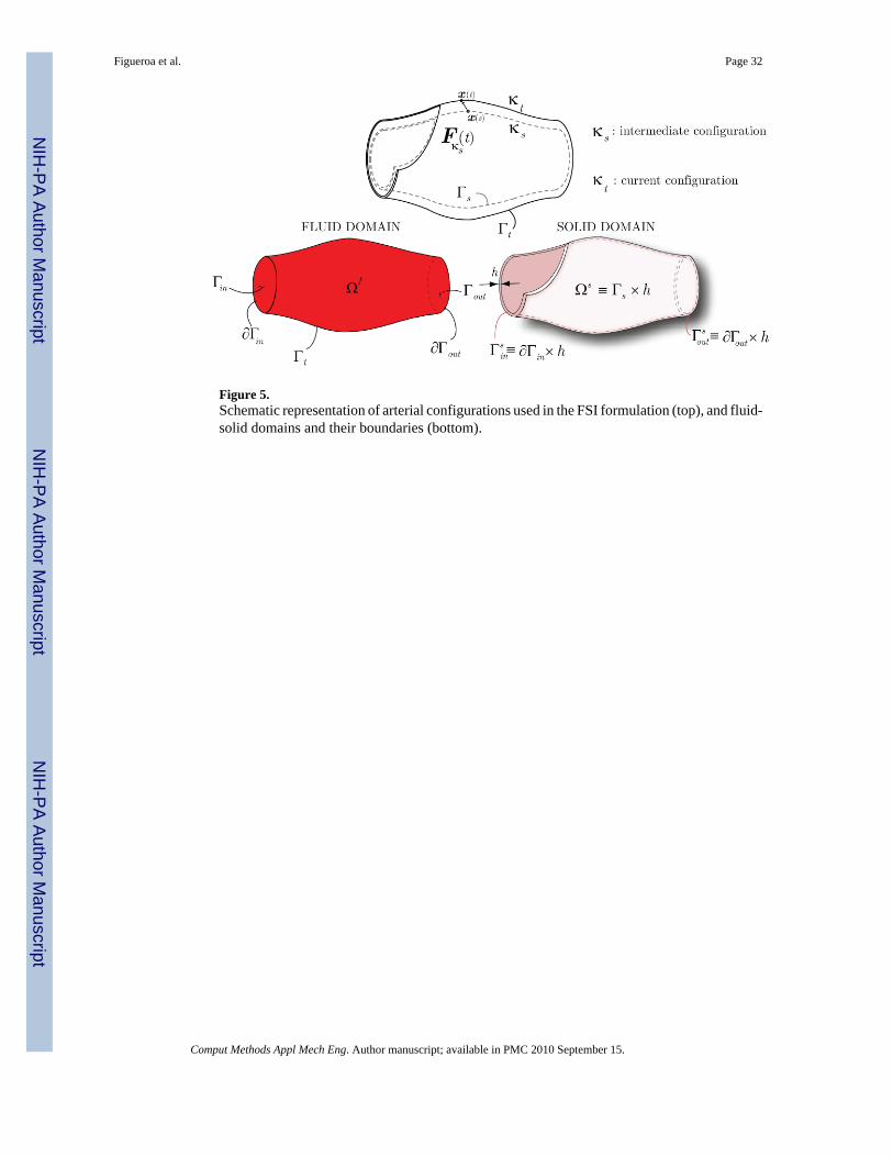
Figure 5.Schematic representation of arterial configurations used in the FSI formulation (top), and fluid-solid domains and their boundaries (bottom).

Figueroa et al.


NIH


NIH


NIH


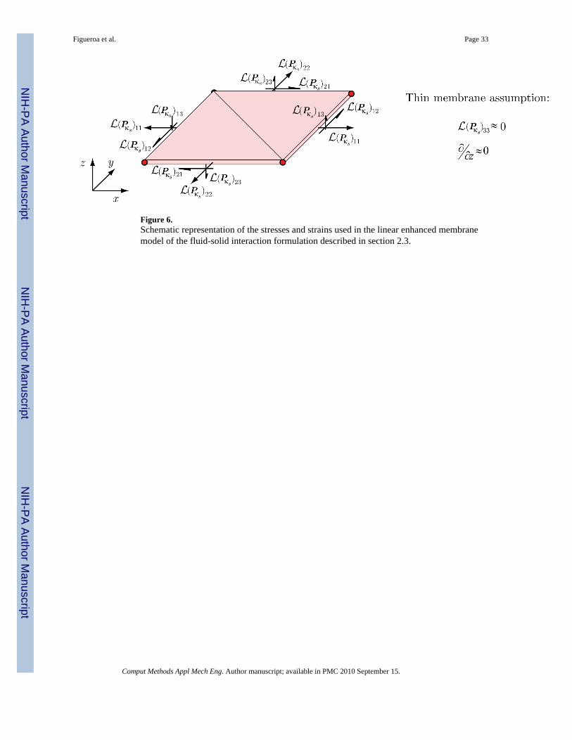
Figure 6.Schematic representation of the stresses and strains used in the linear enhanced membranemodel of the fluid-solid interaction formulation described in section 2.3.

Figueroa et al.


NIH


NIH


NIH


Figure 7.The spatial fluid domain Ω̃f is separated into an upstream “numerical” domain Ωf and adownstream “analytical” domain Ω′f, demarcated by the interface Γout. The effect of theanalytic domain on the numerical domain is incorporated in boundary operators thatcharacterize the relationship between pressure and flow in the downstream vasculature. Notethat distributed or lumped models can be used for the analytic domain. In this work, we haveused a distributed model to generate a terminal impedance function Z(ω).

Figueroa et al.


NIH


NIH


NIH


Figure 8.Definition of the transformation tensor Qiα between the reference systems used by theNonlinear G&R formulation and the FSI formulation. (I = 1, 2, 3) are the bases of a globalCartesian coordinate system. (α = 1, 2, 3) are the orthonormal bases of membrane at a point,where is the basis vector in the circumferential direction and is the basis in the outwardnormal direction. (i = 1, 2, 3) is the orthonormal bases for a local triangular element used bythe membrane formulation of the FSI code.

Figueroa et al.


NIH


NIH


NIH


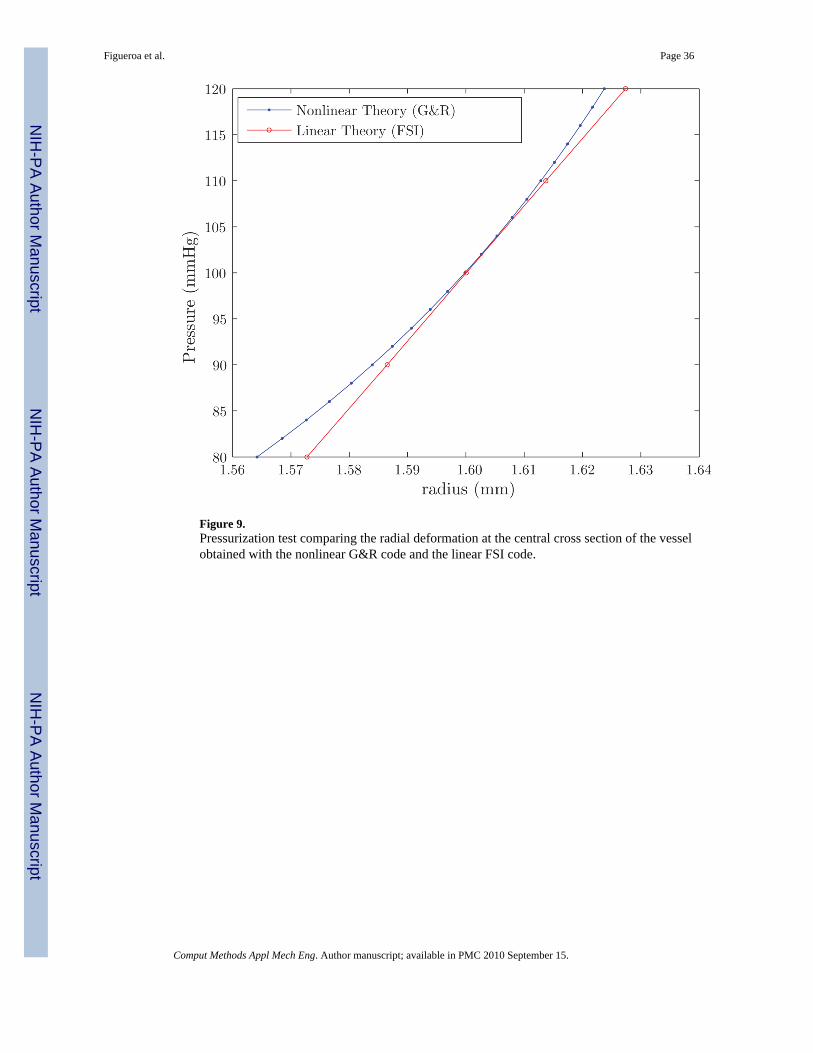
Figure 9.Pressurization test comparing the radial deformation at the central cross section of the vesselobtained with the nonlinear G&R code and the linear FSI code.

Figueroa et al.


NIH


NIH


NIH


Figure 10.Schematic representation of the FSG problem considered. In the first stage of the analysis, wegrow the artery until it reaches a homeostatic equilibrium at time sN. We then introduce aninsult in the vessel wall that results in a local concentric loss of the elastin matrix, and performtwo different FSG simulations: in Case 1, the arterial growth and remodeling is mediated bytensile stress only, whereas in Case 2, the growth is mediated by tensile and wall shear stress.For illustrative purposes, we show the evolution of the linearized circumferential componentof the stiffness Aθθθθ (left) and the vessel wall shear stress (right) for each time step of theanalysis.

Figueroa et al.


NIH


NIH


NIH


Figure 11.Geometry and boundary conditions considered in the FSI problem.

Figueroa et al.


NIH


NIH


NIH


Figure 12.Time-average pressure and wall shear stress at time 0 (dashed lines) and time sN (solid lines).This time sN defines the homeostatic state for the artery, wherein the growth and remodelingprocesses in the arterial wall are balanced with the hemodynamic environment.

Figueroa et al.


NIH


NIH


NIH


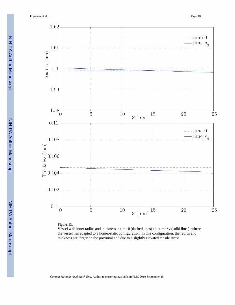
Figure 13.Vessel wall inner radius and thickness at time 0 (dashed lines) and time sN (solid lines), wherethe vessel has adapted to a homeostatic configuration. In this configuration, the radius andthickness are larger on the proximal end due to a slightly elevated tensile stress.

Figueroa et al.


NIH


NIH


NIH


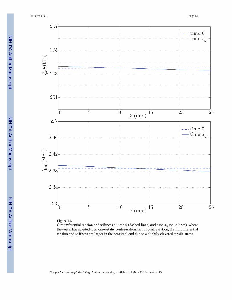
Figure 14.Circumferential tension and stiffness at time 0 (dashed lines) and time sN (solid lines), wherethe vessel has adapted to a homeostatic configuration. In this configuration, the circumferentialtension and stiffness are larger in the proximal end due to a slightly elevated tensile stress.

Figueroa et al.


NIH


NIH


NIH


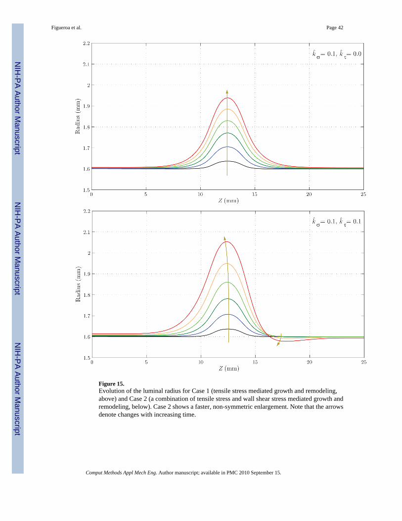
Figure 15.Evolution of the luminal radius for Case 1 (tensile stress mediated growth and remodeling,above) and Case 2 (a combination of tensile stress and wall shear stress mediated growth andremodeling, below). Case 2 shows a faster, non-symmetric enlargement. Note that the arrowsdenote changes with increasing time.

Figueroa et al.


NIH


NIH


NIH


Figure 16.Evolution of blood pressure for Case 1 (above) and Case 2 (below). Case 2 shows a fasterlocalized increase in pressure due to the faster increase in radius seen in figure 15. Themagnitude of pressure variation in the aneurysmal region is very small (only a fraction of amillimeter of mercury) in both cases, however. The arrows denote changes with increasingtime.

Figueroa et al.


NIH


NIH


NIH


Figure 17.Evolution of wall shear stress for Case 1 (above) and Case 2 (below). Note the faster reductionof shear stress in the aneurysmal region for Case 2, consistent with the faster enlargement seenin figure 15. In both cases, we observe an increase in wall shear stress at the distal end of theaneurysm (Z ≈ 15 mm). This increase is more pronounced in Case 2 due to the radius reductionseen in this region in figure 15.

Figueroa et al.


NIH


NIH


NIH


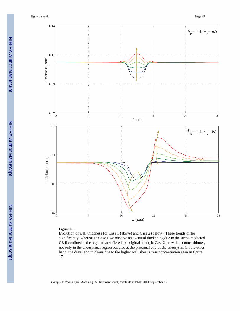
Figure 18.Evolution of wall thickness for Case 1 (above) and Case 2 (below). These trends differsignificantly: whereas in Case 1 we observe an eventual thickening due to the stress-mediatedG&R confined to the region that suffered the original insult, in Case 2 the wall becomes thinner,not only in the aneurysmal region but also at the proximal end of the aneurysm. On the otherhand, the distal end thickens due to the higher wall shear stress concentration seen in figure17.

Figueroa et al.


NIH


NIH


NIH


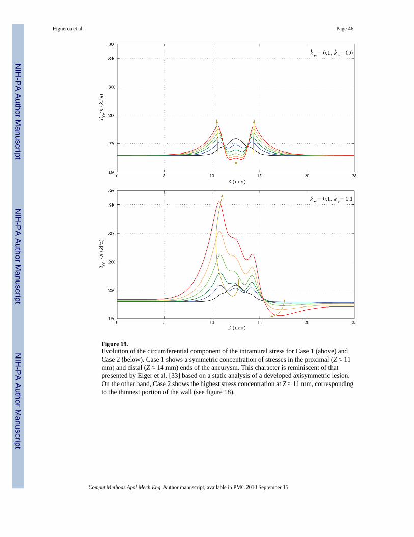
Figure 19.Evolution of the circumferential component of the intramural stress for Case 1 (above) andCase 2 (below). Case 1 shows a symmetric concentration of stresses in the proximal (Z ≈ 11mm) and distal (Z ≈ 14 mm) ends of the aneurysm. This character is reminiscent of thatpresented by Elger et al. [33] based on a static analysis of a developed axisymmetric lesion.On the other hand, Case 2 shows the highest stress concentration at Z ≈ 11 mm, correspondingto the thinnest portion of the wall (see figure 18).

Figueroa et al.


NIH


NIH


NIH


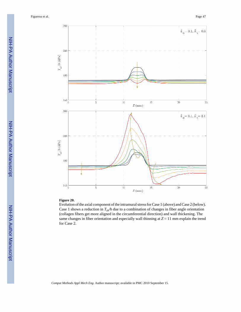
Figure 20.Evolution of the axial component of the intramural stress for Case 1 (above) and Case 2 (below).Case 1 shows a reduction in Tzz/h due to a combination of changes in fiber angle orientation(collagen fibers get more aligned in the circumferential direction) and wall thickening. Thesame changes in fiber orientation and especially wall thinning at Z ≈ 11 mm explain the trendfor Case 2.

Figueroa et al.


NIH


NIH


NIH


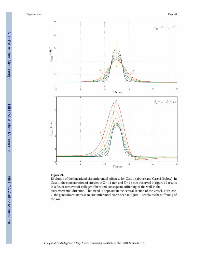
Figure 21.Evolution of the linearized circumferential stiffness for Case 1 (above) and Case 2 (below). InCase 1, the concentration of stresses at Z ≈ 11 mm and Z ≈ 14 mm observed in figure 19 resultsin a faster turnover of collagen fibers and consequent stiffening of the wall in thecircumferential direction. This trend is opposite in the central section of the vessel. For Case2, the generalized increase in circumferential stress seen in figure 19 explains the stiffening ofthe wall.

Figueroa et al.


NIH


NIH


NIH


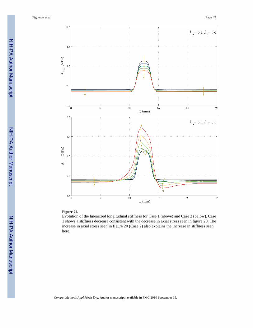
Figure 22.Evolution of the linearized longitudinal stiffness for Case 1 (above) and Case 2 (below). Case1 shows a stiffness decrease consistent with the decrease in axial stress seen in figure 20. Theincrease in axial stress seen in figure 20 (Case 2) also explains the increase in stiffness seenhere.

Figueroa et al.


NIH


NIH


NIH


A computational framework for fluid-solid-growth modeling in cardiovascular simulations

Documents

Transcript of A computational framework for fluid-solid-growth modeling in cardiovascular simulations