1

Data Envelopment Analysis of Different Climate Policy Scenarios

by

Valentina Bosetti* and Barbara Buchner**

* Fondazione Eni Enrico Mattei, C.so Magenta, 63 20123 Milano, Italy. Tel: +39 02 52036983; Fax: +39

02 52036946, E-mail: valentina.bosetti@feem.it

** Fondazione Eni Enrico Mattei, Campo S. M. Formosa, Castello 5252, 30122 Venezia, Italy. Present

address: International Energy Agency; 9, rue de la Fédération, 75739 Paris Cedex 15, France. Tel: +33

(0)1 4057 6687, Fax: +33 (0)1 4057 6739; E-mail: barbara.buchner@iea.org

Abstract

Recent developments in the political, scientific and economic debate on climate change suggest

that it is of critical importance to develop new approaches able to compare policy scenarios while also

taking their performance in terms of the sustainability paradigm into account . This paper discusses a

quantitative methodology to assess the relative performance of different climate policy scenarios when

accounting for their long-term economic, social and environmental impacts. The proposed procedure is

based on Data Envelopment Analysis, here employed in evaluating relative efficiency of ten global

climate scenarios. The methodology provides a promising comparison framework; it can be seen as a way

of setting some basic guidelines to frame further debates and negotiations and can be flexibly adopted and

modified by decision makers to obtain information relevant for policy design. In the present paper, we

find that the “do nothing” strategy is inevitably dominated either by moderate or by stringent policies,

depending on how much the policy -maker values environmental and social impacts in addition to policy

costs. More generally, scenarios that would not pass the economic efficiency test might reveal a good

performance in terms of sustainability notwithstanding their relatively high costs.

Keywords: Climate Policy, Valuation, Data Envelopment Analysis, Sustainability

JEL Classification: H41, Q51, Q54, C61

This paper is part of the research work being carried out by the Climate Change Modelling and Policy

Unit at Fondazione Eni Enrico Mattei. The authors are grateful to Christoph Böhringer, Carlo Carraro,

2

Marzio Galeotti and Henry Jacoby for helpful suggestions and remarks. Financial support from the EU

funded TranSust.Scan project is gratefully acknowledged. The usual disclaimer applies.

1. Introduction

During the last few decades, climate change has evolved as one of the major threats to the earth’s

sustainability. The political response in the form of the United Nations Framework Convention on

Climate Change (UNFCCC, 1997) and more specifically the Kyoto Protocol have started a process

towards a new policy architecture better able to cope with the complexities of climate change. However,

recent negotiations and developments suggest that it might be difficult to achieve a single global

agreement through the usual top -down way of designing policy architectures, and that regional or sub-

global agreements are more likely to emerge1. The usual way of planning climate policy has led to a

certain deadlock in negotiations, which has consequently induced the search for more successful policy

architectures to cope with the ever-increasing emissions. Indeed, even though the Kyoto Protocol came

into force in February 2005, its environmental effectiveness is very low due to the lack of participation of

several key countries, as in particular the world’s largest producer of GHG emissions, the US, and large

developing countries as China and India. As a consequence, general consensus has emerged that the

Kyoto Protocol represents only a first step towards the broader aim of minimising the danger of climate

change.2 This has stimulated detailed discussions on potential climate policy scenarios and a number of

different approaches have been applied in order to analyse the possible future of climate policy. In this

context, the recent experiences in the politics and economics of climate change control have given an

indication of how important it is to be accurate in measuring the efficiency of efforts towards climate

control in order to increase the feasibility of a possible policy scenario.

1 Indeed, due to free-riding incentives and strong economic and environmental asymmetries, it is unlikely that an international climate agreement will be signed by a large number of countries (Carraro and Siniscalco, 1993; Botteon and Carraro, 1997), unless its goals are not significantly different from those of a non-cooperative, business-as-usual, domestic policy (Barrett, 1994). Therefore, more recently the idea of a global bottom-up climate agreement has been proposed (Cf. Carraro, 1998, 1999; Buchner and Carraro, 2007; Egenhofer et al., 2001; Stewart and Wiener, 2003). The basic idea is to adopt a bottom-up, country-driven approach to defining national commitments, instead of a top-down, international negotiation of national emission targets. 2 Actually, in July 2005 six nations led by the US and Australia unveiled a complementary pact to the Kyoto Protocol, aimed to fight global warming. The Asia-Pacific Partnership on Clean Development and Climate constitutes a voluntary, technology-based initiative to reduce greenhouse gas emissions without legally binding emissions targets, whose main idea is to develop new technologies and deploy these in developing countries. Notwithstanding the characteristic of being voluntary, this agreement could be interpreted as a further step into the direction of a more comprehensive climate policy. For more information on this pact – signed by the US, Australia, Japan, China, India and South Korea – see http://www.ap6.gov.au/

Formatiert: Schriftart: 11 pt,Englisch (Großbritannien)

Formatiert: Schriftart: 11 pt,Englisch (Großbritannien)

Formatiert: Englisch(Großbritannien)

3

Yet, given the difficulty of measuring climate policies in a satisfactory way, no strategy that can

satisfy all the needs of all countries has yet been identified. This problem is becoming more pressing

because of the increasing urgency to improve the credibility of climate policy in general. In order to move

forward in climate negotiations, countries need to have a better way of evaluating efforts at their disposal.

The paper aims at contributing to this objective.

Two particular reasons stress the importance of such an evaluation tool. First, countries currently

outside the int ernational climate architecture need to have instruments to evaluate their next steps in

climate policy in order to justify their strategies both domestically and internationally. Second,

negotiations on a Post-2012 phase have started given that the Kyoto Protocol contains commitments only

through 2012. At the climate talks in Montreal in 2005, a new round of climate talks has been initiated

both under the UNFCCC and under the Kyoto Protocol, focusing on the future of the international climate

effort.3 The general stalemate in the Kyoto negotiations suggests that all countries would benefit from a

new approach to looking at climate change measures. Above all, focussing exclusively on emissions or

emission concentrations or temperature appears to be too narrow4. By moving beyond this perspective,

the efficiency of climate change control can be evaluated more comprehensively. In particular, given the

international commitment towards sustainable development as the overall guideline for all areas of policy

making5 , measurements of efficiency better able to account for the three dimensions of sustainability –

i.e., the economic, social and environmental aspects – are essential if climate-energy policy is to be more

effective and successful.

Attempts to compare and measure climate policies are not new. The climate policy scenarios

embedded in most of the existing policy proposals usually represent mitigation scenarios that are defined

through a description and a quantified projection of how GHG emissions can be reduced with respect to

3 The Conference of the Parties serving as the meeting of the Parties to the Kyoto Protocol on its first session (COP/MOP 1) took decisions on a process for considering new binding commitments after the end of the Protocol’s first commitment period, for post-2012, for the Kyoto countries. The Conference of the Parties on its eleventh session (COP 11) launched a process on the future of climate change control under the UNFCCC, opening a nonbinding “Dialogue on long-term cooperative action to address climate change by enhancing implementation of the Convention”. 4 Indeed, an increase in recent research efforts emphasises the need to go beyond traditional CO concentration stabilisation exercises (see e.g., Sarofim et al., 2004; Kemfert et al., 2006; Richels et al., 2004; Tol, 2006). 5 See, for example, the Johannesburg Declaration on Sustainable Development that was adopted at the World Summit on Sustainable Development held in Johannesburg, South Africa, from 2 to 4 September 2002. This statement reaffirms the world’s commitment to sustainable development.

4

some baseline scenario and/or how a specific GHG target can be achieved in order to stabilise

atmospheric concentrations (the so-called QUELRO approach6). They contain new emission profiles as

well as costs and benefits associated with emission reductions. In order to obtain the relevant information

that characterises the final outcome, policies are simulated using economic-climate models in order to

forecast the potential long-term effects on relevant variables, such as the implied increase in global

atmospheric temperature or the effect on GDP growth. By means of such simulations, a comparison of

different climate policy scenarios should be possible. Still, given the prevailing scientific uncertainties, an

accurate evaluation may need to account for a greater number of indicators and thus comparison of

climate policy proposals becomes more difficult.

Therefore, the objective of this paper is not solely to discuss and comment on different policies or

policy scenarios, but is primarily to extract useful information in the phase where proposed and simulated

climate policy scenarios are compared. This phase is usually crucial for the path the negotiations follow.

For this purpose, we apply the Data Envelopment Analysis (DEA), a methodology which is technically

closely related to Multi-Criteria Analysis, in that it allows us to deal with situations where multiple inputs

and outputs occur. In particular, we are interested in incorporating the economic, environmental and

social dimensions of the positive and negative impacts of each policy scenario, in order to bridge the gap

between the simulation phase, in which long-run effects of policies are mimicked, and the valuation

phase, in which usually a coherent cost benefit analysis framework is adopted. Indeed, these phases

should culminate by including the information obtained back into the policy -designing process.

DEA uses data observations to directly evaluate the relative performance of a set of policy

scenarios, in a multi input –multi output context. At first, DEA was developed to evaluate the relative

efficiency of firms by transforming multiple inputs into multiple outputs, making minimal prior

assumptions about the shape of the production possibility set, but inferring information from the data set.

While the conventional definition of efficiency can be traced back to Farrell (1957), the first publication

that made the DEA methodology popular and introduced it into the operation research world was Charnes

6 QUELRO stands for “Quantified Emission Limitation and Reduction Objective” and its terminology has been introduced by the Kyoto Protocol.

5

et al. (1978). Subsequently, DEA has been applied to evaluate the relative performance of medical

services, as in Nyman and Bricke (1989) , or of educational institutions, as in Charnes et al. (1981). It has

also been applied in the private sector, as in the valuation of banks, in Charnes et al. (1990)7. Applications

to environmental and resource management problems are less frequent. In general, environmental and

social impacts can be modelled as undesirable outputs or as conventional inputs. The absence of market

prices for these undesirable outputs, which is a generally recognised valuation problem, can be overcome

by employing DEA8 . However, to the authors’ knowledge, DEA has not yet been applied in the

comparative assessment of (climate) policies.

The present paper applies this technique in order to evaluate ten climate policy scenarios and

finds how scenarios that would not pass the economic efficiency test might represent a good performance

in terms of sustainability notwithstanding their relatively high costs.

The rest of the paper is organised as follows. Section 2 introduces the methodological framework

describing, on one hand, the model adopted to simulate long-run effects of the different policies, the

WITCH model, and on the other hand, the Data Envelopment Analysis (DEA) methodology, which is

then applied to compare the various policy scenarios. In particular, the choice of cost and benefit

indicators for each policy is introduced and discussed. Section 3 provides a detailed overview of the

policy scenarios that are the subject of this analysis. Both the features of the policy proposals and their

underlying motivations are tackled. Finally, Section 4 discusses the results and provides conclusions as

well as indications for further future research.

7 A thorough review of the theory and applications related to DEA can be found in Coelli et al. (1989), while an extensive bibliography is reported in the survey articles by Seiford (1996). 8 Some studies have applied DEA in measuring ecological efficiency (e.g. Dyckhoff and Allen, 2001); some others in measuring the environmental impact of different production technologies, as for example De Koeijer et al. (2002), where the impact of different production techniques in the farm industry are compared. Bosetti and Locatelli (2005) consider the economic and environmental dimensions of management performances of National Parks, while Hernandez-Sancho et al. (2000) consider the issue of efficiency in environmental regulation. An interesting overview of the role of DEA in environmental valuation can be found in Kortelainen and Kuosmanen (2007), while a survey of indicators of firms’ environmental behaviour can be found in Tyteca (1996).

6

2. Methodology

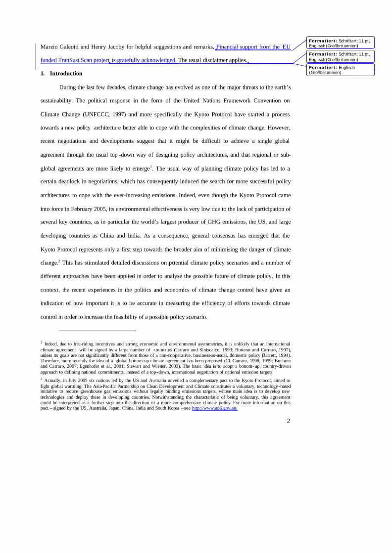
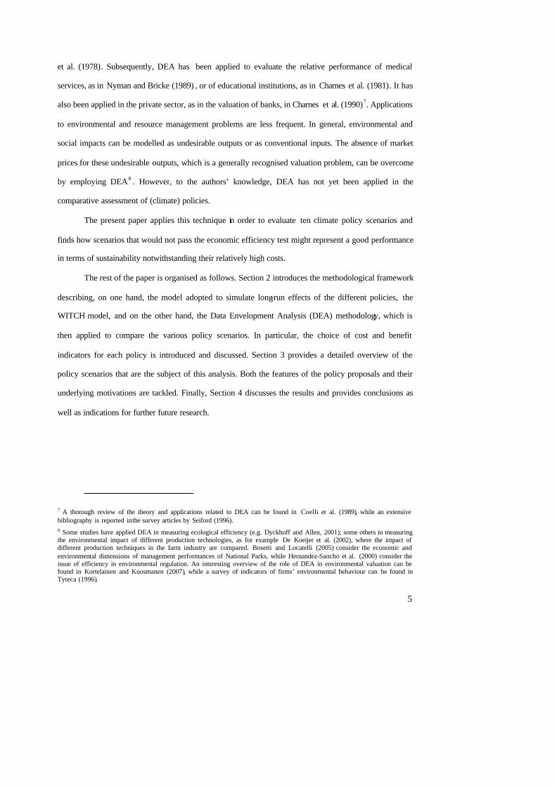
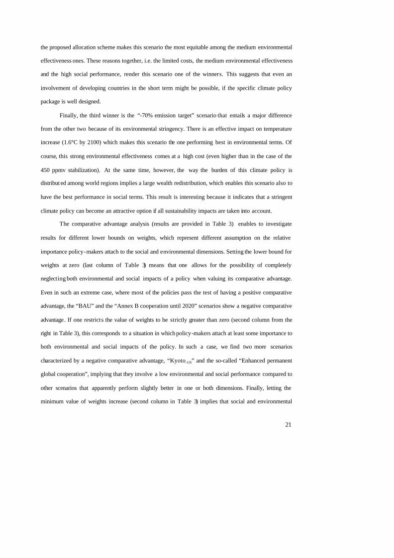
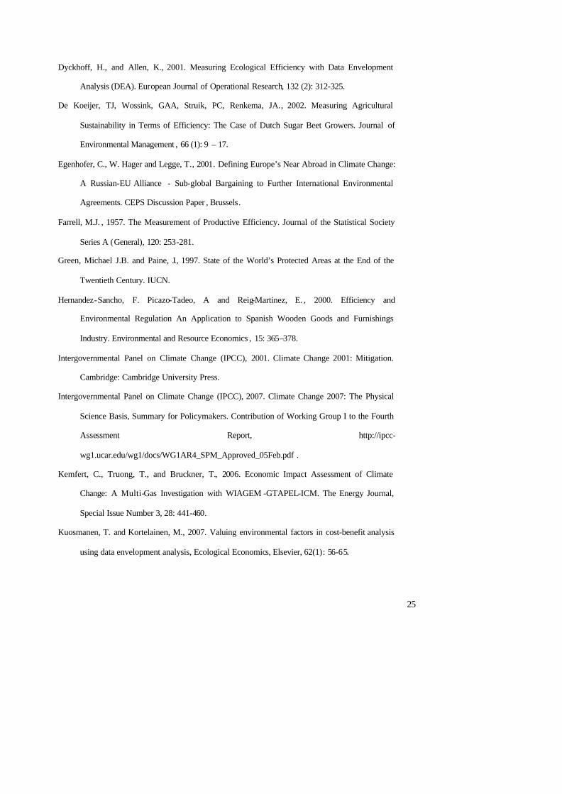
The proposed analysis is based on a composed methodology, as sketched in Figure 1, which

couples a traditional simulation analysis - performed in our case by means of a hybrid optimal growth

economic-climate model, the WITCH model - with a relative efficiency valuation technique, namely the

DEA.

This methodology allows comparing a set of policy scenarios; some of those stemming from

political feasibility considerations, some others from scientific concerns regarding global warming and

some others from a combination of the two. Motivations behind the design of each policy scenario both in

its short and long term features are discussed in greater detail in the subsequent section. We shall now

focus on the methodological issues.

Figure 1. A sketch of the hybrid methodology

Let us start by briefly discussing the simulation phase. Scenarios should be simulated using one,

or better, several simulation and/or optimization models (as in the case of the SRES scenarios 9 or several

other comparison exercises). For the sake of simplicity, in the present paper architectures are simulated

using one single model.

9 Based on an extensive assessment of the literature, a range of modeling approaches, and a close interaction with many groups and individuals, the IPCC has developed a set of long-term emission scenarios which are described in the IPCC Special Reports on Emission Scenarios (SRES). These scenarios cover a wide array of driving forces of future emissions, and encompass different future developments that might influence GHG sources and sinks. The most recent set of scenarios was published in 2000, more information is available at http://www.grida.no/climate/ipcc/emission/ .

Policy Scenarios Design

Simulation of Policy Scenarios

Multi -dimensional vector accounting for economic, social and environmental

performances of each Policy Scenario

Policy Scenarios comparison and relative evaluation, in all dimensions at stake

7

WITCH – World Induced Technical Change Hybrid model – is a regional integrated assessment

model structured to provide normative information on the optimal responses of world economies to

climate damages and to model the channels of transmission of climate policy to the economic system. It is

an hybrid model because it combines features of both top -down and bottom-up modelling: the top -down

component consists of an inter-temporal optimal growth model in which the energy input of the aggregate

production function has been expanded to give a bottom-up like description of the energy sector. World

countries are grouped in 12 regions that strategically interact following a game theoretic structure. A

climate module and a damage function provide the feedback on the economy of carbon dioxide emissions

into the atmosphere. WITCH top -down framework guarantees a coherent, fully intertemporal allocation

of investments that have an impact on the level of mitigation – R&D effort, investment in energy

technologies, fossil fuel expenditures. The regional specification of the model and the presence of

strategic interaction among regions – through CO2, exhaustible natural resources, and technological

spillovers – allow us to account for the incentives to free-ride. Applying an open-loop Nash game, the

investment strategies are optimized by taking into account both economic and environmental

externalities. In WITCH the energy sect or has been detailed and allows a reasonable characterization of

future energy and technological scenarios and an assessment of their compatibility with the goal of

stabilizing greenhouse gases concentrations. Also, by endogenously modelling fuel (oil, coal, natural gas,

uranium) prices, as well as the cost of storing the CO2 captured, the model can be used to evaluate the

implication of mitigation policies on the energy system in all its components. For a throughout

description of the model see Bosetti et al. (2006) and Bosetti et al. (2007).

The model simulates each climate policy scenario, thus providing the ingredients for the

subsequent comparison phase. A set of indicators accounting for performances in different dimensions is

stored for each simulated scenario; particularly relevant is information concerning its economic, social

and environmental performances. In principle, in the case when more than one model has been

simultaneously used to simulate each policy scenario, multiple values for each indicator should be stored.

The comparison phase is obviously extremely sensitive to the choice of indicators used to represent

8

different dimensions of sustainability. The choice may depend on what features one would like to

emphasise and/or on what features the model accounts for. Models with a regional detail can provide

information on the distribution of the burden across the world of positive and negative impacts.

Obviously, this cannot be accounted for in world aggregate models, even though the issue of un even

distribution is recognised as one of the most problematic features of the climate change issue. Besides,

models with a detailed description of different climate change impacts10 , can provide a wider set of

environmental indicators.

Given a set of indicators – the reader is referred later in the paper for a detailed discussion on

indicators used in the present analysis and reasons behind their choice – it is not always univocally

possible to assess which are the most promising policies, unless one weakl y dominates all the others (i.e.

a policy is superior in at least one dimension without being inferior in any of the remaining dimensions).

This depends on the fact that no straightforward way s of aggregating different impacts exist. Therefore,

even though a set of modelling groups is asked to report to an international organization, say the IPCC, on

long term implications of different policy scenarios, results might not be straightforward to be read. The

DEA approach overcomes the problem of incomparability in that it endogenously infers a set of weights

by enveloping the data. Note that DEA is extended from its traditional application, namely the evaluation

of production firms’ performances, to evaluating the performance of policies. Thus, terms such as inputs

and outputs, traditionally adopted in the DEA framework, have to be understood here in a broader sense

as indicators of costs (or whatever indicators for which lower values are preferred) and indicators of

benefits.

There exist two possible interpretations of performing Data Envelopment Analysis to compare the

sustainability of different policy scenarios. According to the first interpretation, for each scenario the net

economic impact, expressed in monetary value, is aggregated through weights to the social and

environmental impacts, expressed in their own unitary measures. DEA is applied in order to obtain the

weights by “letting the data speak”. The second interpretation, nearer to traditional DEA applications,

implies computing a relative efficiency measure for each policy, where efficiency is measured as the ratio

10 For example, information on the impact on sea-level rise could be included in the analysis. See Roson et al. (2004).

9

of the weighted sum of outputs (i.e., indicators whose value is better to maximize) to the weighted sum of

inputs (i.e., indicators measuring features that are optimal to minimize). In particular, a policy is 100

percent efficient if and only if:

- none of its output can be increased without either increasing one or more of its inputs, or

decreasing some of its other outputs;

- none of its inputs can be decreased without either decreasing some of its outputs or increasing

some of its other inputs.

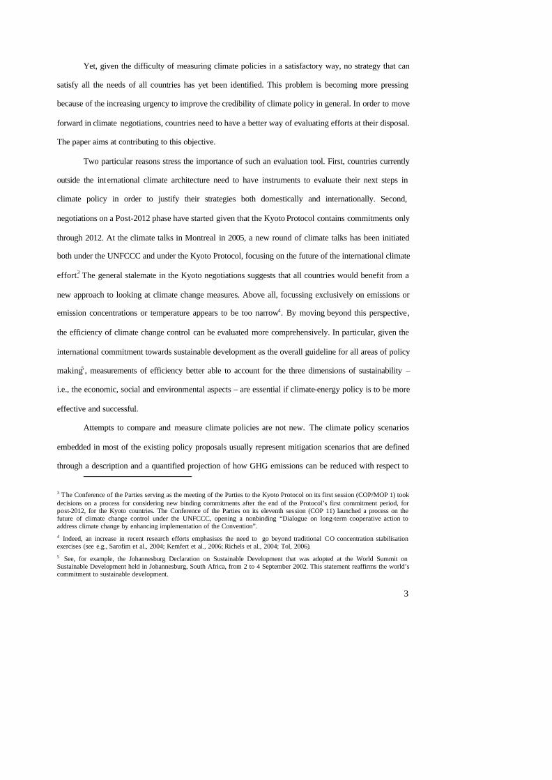
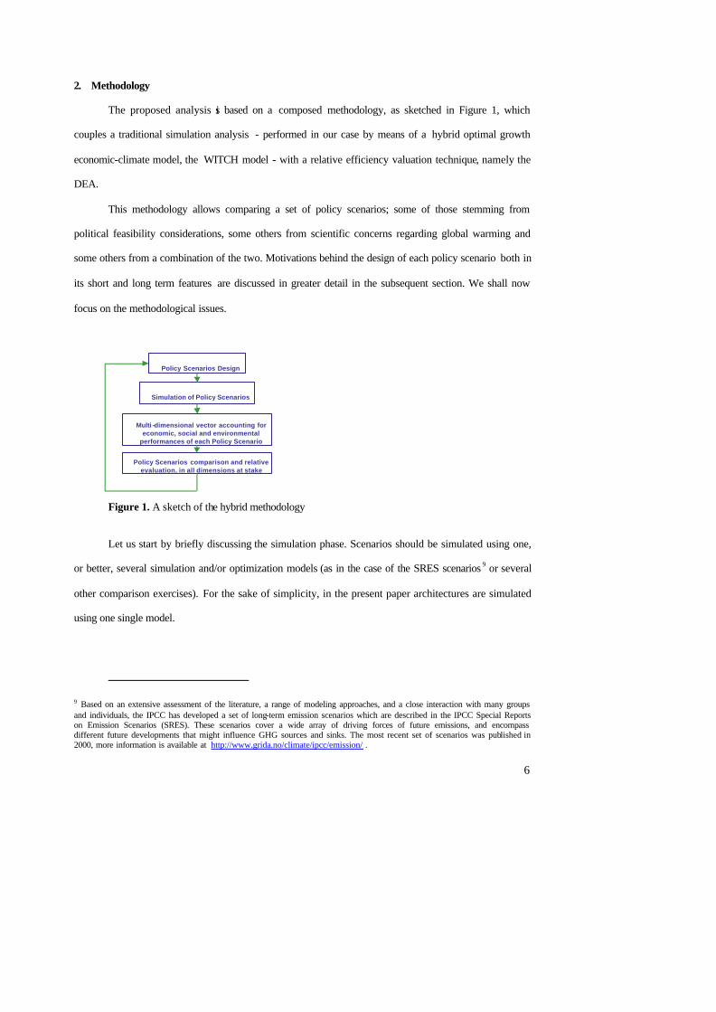
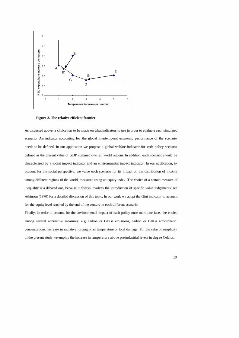
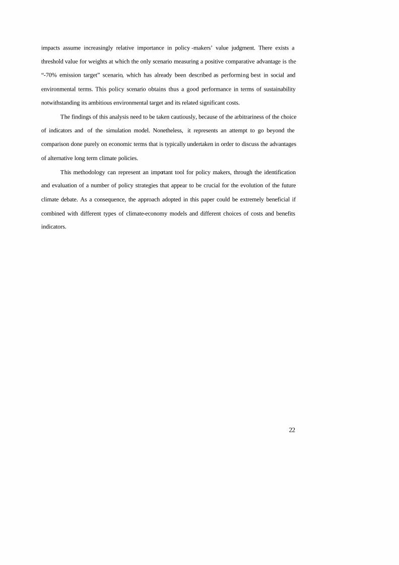
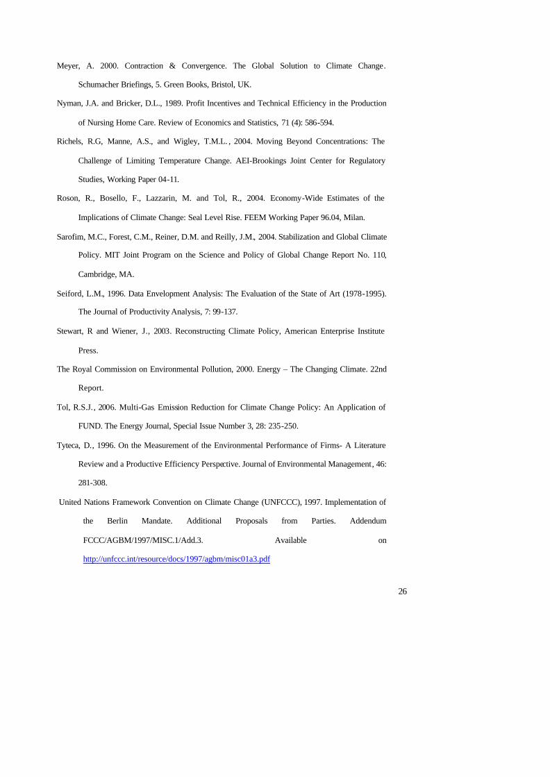
Let us now consider for the sake of clarity a simple numerical example of five policy scenarios,

denoted in Figure 2 as A, B, C, D and E, each using different combinations of two indicators to be

minimized (input), say some inequity indicator and the level of temperature increase, and one output to be

maximized, say some measure of global welfare. In order to facilitate comparisons, input levels are

expressed per unit of output. Data are plotted in Figure 2. A kinked frontier is drawn from A to C to D,

representing the set of relatively efficient scenarios, and the frontier envelopes all these data points and

approximates a smooth efficiency frontier. Scenarios on the efficient frontier are assumed to be efficient

relatively to scenarios B and D which are considered to be less efficient. It is always possible then to find

some projection on the efficient frontier of inefficient scenarios (see B’ in Figure 2), thus providing

information on potential levers that would improve the designing of inefficient policy scenarios.

10

Figure 2. The relative efficient frontier

As discussed above, a choice has to be made on what indicators to use in order to evaluate each simulated

scenario. An indicator accounting for the global intertemporal economic performance of the scenario

needs to be defined. In our application we propose a global welfare indicator for each policy scenario

defined as the present value of GDP summed over all world regions. In addition, each scenario should be

characterised by a social impact indicator and an environmental impact indicator. In our application, to

account for the social perspective, we value each scenario for its impact on the distribution of income

among different regions of the world, measured using an equity index. The choice of a certain measure of

inequality is a debated one, because it always involves the introduction of specific value judgements; see

Atkinson (1970) for a detailed discussion of this topic. In our work we adopt the Gini indicator to account

for the equity level reached by the end of the century in each different scenario.

Finally, in order to account for the environmental impact of each policy once more one faces the choice

among several alternative measures; e.g. carbon or GHGs emissions, carbon or GHGs atmospheric

concentrations, increase in radiative forcing or in temperature or total damage. For the sake of simplicity

in the present study we employ the increase in temperature above pre-industrial levels in degree Celcius.

0

1

2

3

4

5

6

0 1 2 3 4 5 6

Labour per tourist

Bed

spe

r to

uris

t

AB'

B

C D

E E'

0

1

2

3

4

5

6

0 1 2 3 4 5 6

Temperature increase per output

AB'

B

C D

E E'

R&

Dex

pen

dit

ure

incr

ease

per

ou

tpu

t

0

1

2

3

4

5

6

0 1 2 3 4 5 6

Labour per tourist

Bed

spe

r to

uris

t

AB'

B

C D

E E'

0

1

2

3

4

5

6

0 1 2 3 4 5 6

Temperature increase per output

AB'

B

C D

E E'

R&

Dex

pen

dit

ure

incr

ease

per

ou

tpu

t

11

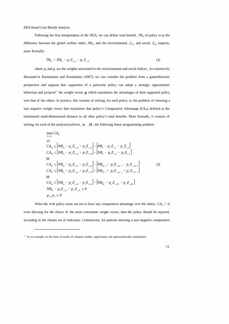
DEA-based Cost Benefit Analysis.

Following the first interpretation of the DEA, we can define total benefit, TBm of policy m as the

difference between the global welfare index, NBm, and the environmental , Ze,m and social, Zs,m impacts,

more formally:

mssmeemm ZpZpNBTB ,, −−= (1)

where pe and ps are the weights associated to the environmental and social indices. ,As extensively

discussed in Kuosmanen and Kortelainen (2007), we can consider the problem from a game-theoretic

perspective and suppose that supporters of a particular policy can adopt a strategic opportunistic

behaviour and propose11 the weight vector, p, which maximises the advantages of their supported policy

over that of the others. In practice, this consists of solving, for each policy m, the problem of choosing a

non negative weight vector that maximises that policy’s Comparative Advantage (CAm), defined as the

(minimum) multi-dimensional distance to all other policy’s total benefits. More formally, it consists of

solving, for each of the analysed policies, Mm∈ , the following linear programming problem:

[ ] [ ][ ] [ ]

[ ] [ ][ ] [ ]

[ ] [ ]

0,

0

..

max

,,

,,,,

1,1,1,,

1,1,1,,

2,2,2,,

1,1,1,,

,

≥

≥−−

−−−−−≤

−−−−−≤

−−−−−≤

−−−−−≤

−−−−−≤

+++

−−−

se

mssmeem

MssMeeMmssmeemm

mssmeemmssmeemm

mssmeemmssmeemm

sseemssmeemm

sseemssmeemm

mpp

pp

ZpZpNB

ZpZpNBZpZpNBCA

ZpZpNBZpZpNBCA

ZpZpNBZpZpNBCA

ZpZpNBZpZpNBCA

ZpZpNBZpZpNBCAts

CAse

Μ

Μ (2)

When the m-th policy turns out not to have any comparative advantage over the others, CAm < 0,

even allowing for the choice of the most convenient weight vector, then the policy should be rejected,

according to the chosen set of indicators. Contrariwise, for policies showing a non-negative comparative

11 As an example, on the basis of results of valuation studies, opportunely and opportunistically manipulated.

12

advantage over other policies 0≥mCA , a sensitivity analysis on weights should be performed in order to

obtain more information. Indeed, letting one or both weights be set to zero, in order to magnify the

deriving comparative advantage of the policy, implies that one or both dimensions, the environmental and

social one, have been dropped out from the valuation procedure. The process can be enhanced by

interfacing the discussion on the domain of weights to the political debate, thus enabling policy makers to

gain a better understanding of how to interpret analysis results.

DEA relative efficiency computation.

The second approach involves the computation of relative efficiency scores. A maximum score of unity

(or 100%) is considered as the benchmark. Indicators are now reinterpreted in terms of inputs (cost or in

general indicators which is preferable to minimize) and outputs (benefits or in general indicators which is

preferable to maximize). Both inputs and outputs may belong to the economic, environmental or social

dimension. In our application, we consider on the input side the social and environmental indicator. Both

the Gini indicator and the global atmospheric temperature should be minimized. Instead, on the output

side, we consider global discounted GDP, which should be maximized.

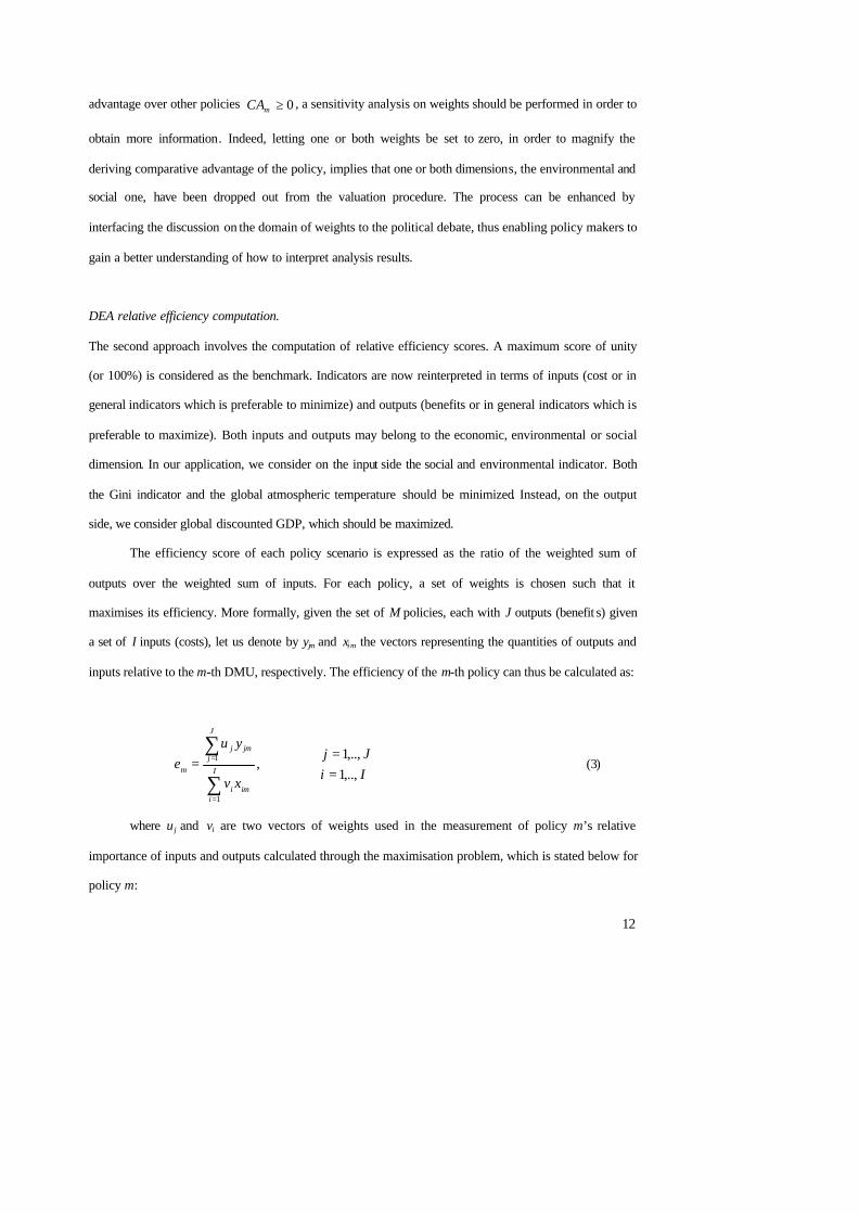
The efficiency score of each policy scenario is expressed as the ratio of the weighted sum of

outputs over the weighted sum of inputs. For each policy, a set of weights is chosen such that it

maximises its efficiency. More formally, given the set of M policies, each with J outputs (benefit s) given

a set of I inputs (costs), let us denote by yjm and xim the vectors representing the quantities of outputs and

inputs relative to the m-th DMU, respectively. The efficiency of the m-th policy can thus be calculated as:

==

=

∑

∑

=

=

IiJj

xv

yue

I

iimi

J

jjmj

m ,..,1,..,1

,

1

1 (3)

where u j and vi are two vectors of weights used in the measurement of policy m’s relative

importance of inputs and outputs calculated through the maximisation problem, which is stated below for

policy m:

13

10

10

,.,,.,11

..

max

1

1

,

≤≤

≤≤

=∀≤

∑

∑

=

=

i

j

I

iini

J

jjnj

mvu

v

u

Mmnxv

yu

ts

eij

(4)

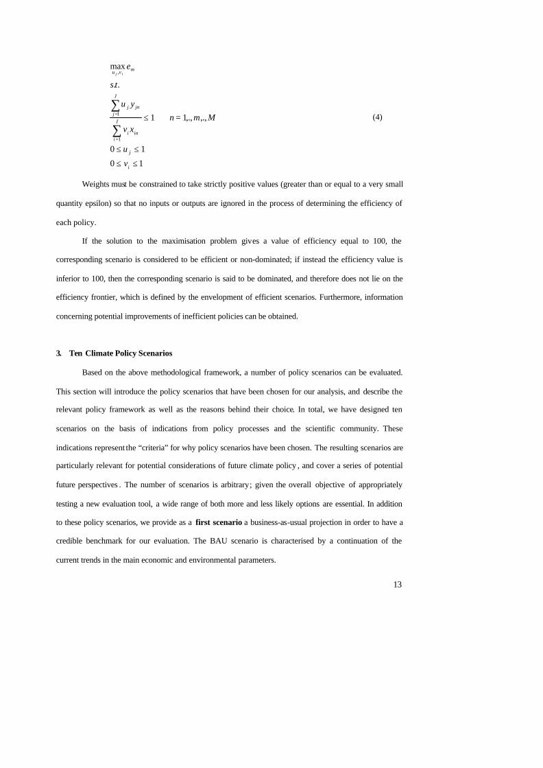
Weights must be constrained to take strictly positive values (greater than or equal to a very small

quantity epsilon) so that no inputs or outputs are ignored in the process of determining the efficiency of

each policy.

If the solution to the maximisation problem gives a value of efficiency equal to 100, the

corresponding scenario is considered to be efficient or non-dominated; if instead the efficiency value is

inferior to 100, then the corresponding scenario is said to be dominated, and therefore does not lie on the

efficiency frontier, which is defined by the envelopment of efficient scenarios. Furthermore, information

concerning potential improvements of inefficient policies can be obtained.

3. Ten Climate Policy Scenarios

Based on the above methodological framework, a number of policy scenarios can be evaluated.

This section will introduce the policy scenarios that have been chosen for our analysis, and describe the

relevant policy framework as well as the reasons behind their choice. In total, we have designed ten

scenarios on the basis of indications from policy processes and the scientific community. These

indications represent the “criteria” for why policy scenarios have been chosen. The resulting scenarios are

particularly relevant for potential considerations of future climate policy , and cover a series of potential

future perspectives . The number of scenarios is arbitrary; given the overall objective of appropriately

testing a new evaluation tool, a wide range of both more and less likely options are essential. In addition

to these policy scenarios, we provide as a first scenario a business-as-usual projection in order to have a

credible benchmark for our evaluation. The BAU scenario is characterised by a continuation of the

current trends in the main economic and environmental parameters.

14

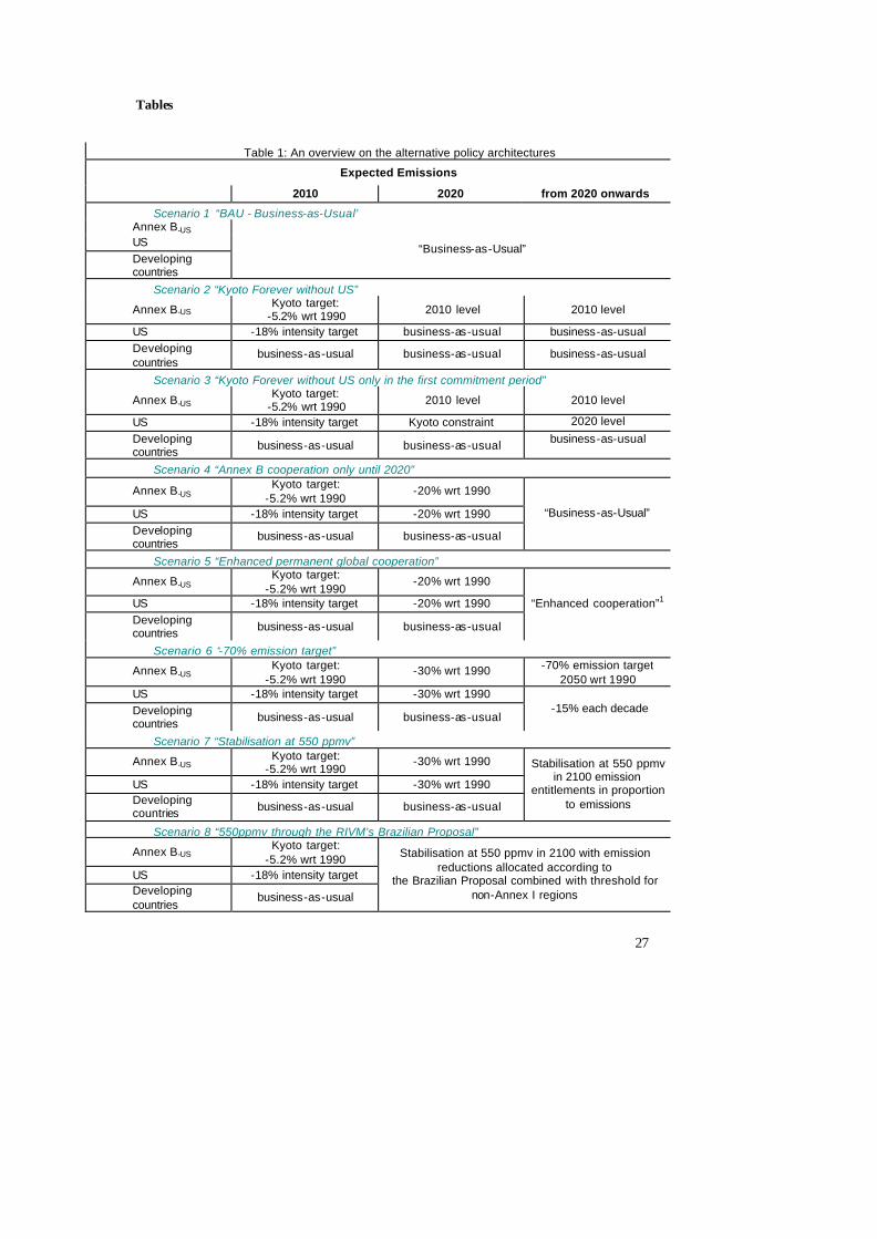
The remaining ten policy scenarios possess some common features. In particular, all scenarios

assume that the absolute emission reductions defined in the Kyoto Protocol will be achieved by the

Annex B–US countries 12 by 2010 (first commitment period). Indeed, it was Russia’s ratification of the

Kyoto Protocol on November 4, 2004 that opened the way for the Protocol’s coming into force on

February 16, 2005, making thus the emissions targets taken on for the 2008-2012 period by more than 30

developed countries (including the EU, Russia, Japan, Canada, New Zealand, Norway and Switzerland)

legally binding. 13 According to its domestic policy target, the US is assumed to achieve its –18%

emission intensity target in order to slow the growth of GHG emissions per unit of economic activity over

the next 10 years14. Developing countries have no target in the first commitment period.

Then, different assumptions characterise the different scenarios from 2020 onwards. 15.

The second scenario assumes a continuation of the current situation. After the US announced its

defection from the Kyoto Protocol in March 2001, the remaining Kyoto countries – in particular the EU

and Japan – put great effort into the continuation of the Kyoto process, in particular by convincing Russia

to participate in the Protocol. After meeting the Kyoto objectives at the end of the first commitment

period, this scenario assumes that the Annex B–US countries decide to maintain their initial Kyoto targets

and thus the corresponding emission level until the year 2100, whereas the US remains out of the Kyoto

Protocol and implements no effective climate policy. This scenario thus represents the situation in which

the Annex B– US countries behave according to the “Kyoto forever” hypothesis, whereas the US and the

developing countries have no binding emission constraints. All countries adopt cost-effective

environmental policies, and in particular, emissions trading takes place among the Annex B–US countries.

12 We denote by Annex B–US the countries listed in the Annex B of the Kyoto Protocol without the participation of the United States. 13 The Kyoto Protocol imposes absolute reduction targets, i.e. a reduction of absolute GHG emissions by a specified percentage. 14 In order to replicate the US strategy as precisely as possible, our model computes the –18% intensity reduction by 2010 compared to the year 2000. Climate policy in terms of emission intensity targets is typically expressed as percentage reductions from some base year level. In the US context, greenhouse gas intensity is given by the ratio of greenhouse gas emissions to economic output. 15 Note that scenarios 2 to 7, chosen to cover both optimistic and pessimistic predictions on future abatement targets, have already been discussed in greater detail in Buchner and Carraro (2007). In particular, using the integrated climate-economy model FEEM-RICE, the six different scenarios on future emission abatement commitments have been analysed to provide an assessment of their implications for the economy. However, given the different scope of this paper, we will briefly recall their main features in order to enable a comprehensive background to our analysis.

15

In the third scenario we assume that, given international and domestic political pressures, the US

decides to join the group of countries committed to the Kyoto Protocol in the second commitment period

and afterwards. Continuity with Kyoto could be attractive for the countries that are already engaged in the

Kyoto Protocol, i.e. the Annex B–US, since these countries have already made a substantial investment in

the Kyoto process (Bodansky, 2003). Developing countries, as in “Kyoto forever”, are assumed not to

adopt any emission target until 2050. Consequently, emissions in Annex B countries will be stabilised at

about –5% by 2100 w.r.t their 1990 value, whereas emissions in developing countries will keep growing.

Common assumptions characterise the second commitment period (2010-2020) of scenarios 4-7.

International and domestic pressures for climate change control are expected to induce countries to

further strengthen their efforts in international climate policy (Cf. IPCC WG1, 2007). In particular, both

the remaining Annex B countries and the US are assumed to agree by 2020 to reduce emissions by an

additional 20% compared to the level of emissions in 1990. The –20% objective for developed countries

appears a possible scenario given recent policy signals. On one hand, the European Commission

presented its Integrated Energy and Climate Package on 10 January 2007 with the objective of

establishing a new energy policy for Europe to combat climate change and boost at the same time the

EU’s energy security and competitiveness16. Amongst ot hers, the Commissions put forward plans on

ambitious targets on GHG emissions: a reduction target of –30% in GHG emissions from developed

countries by 2020 is proposed if an international agreement will be reached. In alternative, a unilateral EU

emissions reduction target of at least 20% by 2020 is proposed1 7. These targets have subsequently been

supported by the EU environmental ministries of the EU member states.18 On the other hand, a 10%-

target for developed countries was indicated as the most likely one for the second commitment period by

16 The communication from the Commission on “An energy policy for Europe” can be downloaded at http://eur-lex.europa.eu/LexUriServ/site/en/com/2007/com2007_0001en01.pdf 17 The Communication by the Commission on “Limiting Global Climate Change to 2 degrees Celsius - The way ahead for 2020 and beyond” can be downloaded at http://ec.europa.eu/environment/climat/pdf/future_action/com_2007_2_en.pdf 18 At the Council meeting in February 2007, the environment ministers agreed on the emission reduction targets proposed by the European Commission in January 2007, showing the willingness to commit to a reduction of 30% of GHG emissions by 2020 compared to 1990, “provided that other developed countries commit themselves to comparable emission reductions and economically more advanced developing countries adequately contribute according to their responsibilities and respective capabilities” and suggesting that the EU should reduce greenhouse gas emissions by 20 per cent below 1990 levels by 2020. This last conclusion will also be addressed at the Spring European Council (8-9 March 2007). Further details are provided under http://europa.eu/rapid/pressReleasesAction.do?reference=PRES/07/25&format=HTML&aged=0&language=EN&guiLanguage=en

16

a panel of 78 experts interviewed by Böhringer and Löschel (2003). Taking into account all these signals,

a 20%-target for industrialised countries appears a likely compromise. In order to account for the need for

developing countries to continue their economic and social development, they are still exempt from

complying with emission reduction targets. This assumption is also in line with recent research studies

which conclude that it is unlikely developing countries will be included in international climate change

control agreements before 20201 9 as well as with indications from the policy process (for instance arising

from the “Dialogue on long-term cooperative action to address climate change by enhancing

implementation of the Convention” that has been launched under the UNFCCC).

In the fourth scenario, therefore, the Annex B–US countries achieve the Kyoto target in the first

commitment period and the –20% target (w.r.t. 1990 emissions) in the second one. The US adopts its –

18% intensity target in the first commitment period and the –10% absolute target (w.r.t. 1990 emissions)

in the second one. Developing countries do not commit to any emission reductions. After 2020, we

assume that cooperation on climate change control collapses and emissions return to their business-as-

usual (BAU) paths.

The fifth scenario is based on the idea that Kyoto targets are largely sub-optimal – i.e. the

incentives to reduce carbon emissions should be great enough to reach more ambitious targets – and that

countries are only likely to adopt targets closer to the optimal ones in the medium term. The two initial

commitment periods stay the same as in scenario 4. Then, Annex B countries (including the US) and

developing countries adopt what we call “enhanced permanent cooperation emission targets”, computed

as follows. All countries cooperatively maximise their joint welfare with respect to their policy variables,

including GHG emissions. This yields the optimal path of GHG emissions in all world regions, as it

represents the cooperative outcome to all nations. Then, on the basis of the precautionary principle and

given the relatively low emissions reduction in their optimal strategy, all countries pledge to reduce their

emissions by an additional 10% below the optimal emission trajectories from 2020 onward.

19 For example, expert judgements presented in Böhringer and Löschel (2003) reveal that in the second commitment period up to 2020 “…in 75% of the policy-relevant scenarios, developing countries do not commit themselves to binding targets.” (p. 9)

17

The sixth scenario starts from the same premise as the previous one, namely that serious

emission reductions are essential. Therefore, developed countries are assumed to follow the suggestion by

the European Commission, e.g. to reduce their GHG emissions by 30% compared to their 1990 emissions

by 2020. Starting from 2020, the so-called Kyoto countries – Japan, European Union and Russia – are

supposed, by 2050, to have achieved a total reduction in GHG emissions of –70% with respect to their

1990 emissions. This target is based on the recommendations of several politicians regarding the dangers

of climate change. For example, the English Prime Minister Tony Blair has proposed to aim at a 60% cut

in carbon emissions by 2050, thus implementing an emission reduction target of –10% for each decade,

and he has advocated this target for all industrialised countries. 20 Also the French President Chirac

echoed Blair’s proposal and insisted on a strong commitment to reduce GHG emissions. 21 In a recent

announcement, the European Council re-affirmed this intention, although the ambitious goal has not yet

been supported by an agreed statement22. The other countries – the US and the developing regions –

reduce their emissions between 2020 and 2050 by –15% for each decade. These targets thus imply strong

emission reductions in both the US and the developing countries. From 2050 onwards, when countries

have achieved the ambitious emission levels, all nations are committed to maintaining these emission

levels.

Scenarios 7, 8 and 9 are based on the common view that a stabilisation level of 550 ppmv23 in

2100 represents a reasonable goal, also adopted in the emission mitigation scenarios examined by the

Third IPCC report (IPCC, 2001)24. In particular, the analysis of Working Group III in the TAR suggests

20 The reduction goal is based on the outcomes of a report by The Royal Commission on Environmental Pollution (2000) which found that a 60% reduction by 2050 was essential if the overall goal of stabilising GHG emissions at 550 ppmv was to be achieved already by 2050. 21Mr. Chirac emphasised the need for action to combat climate change again at a recent conference in January 2007. See for instance http://www.ft.com/cms/s/52e2cef2-b4bd-11db-b707-0000779e2340.html 22 The 25 ministers agreed on March 23 2005 that developed nations should pursue cuts of heat-trapping gases of 15-30 percent by 2020 and 60-80 percent by 2050 compared with levels set in the Kyoto Protocol, which uses 1990 as a bas e in most cases. But the longer-term 2050 goal has been omitted from an agreed statement. At the Council meeting in February 2007, the environment ministers agreed on the emission reduction targets proposed by the European Commission in January 2007, but made no progress on the 2050-target.

23 Parts per million by volume is a measure of concentration of gases in the atmosphere. 24 The target of not exceeding the 550 ppmv concentration level is also supported by the EU. The first significant EU proposal for a climate target for the post-2000 period, presented at the EU Council of Ministers in 1996, suggested stabilising the atmospheric concentrations of CO2 at a level around twice the pre-industrial level of about 280 ppmv, corresponding thus to the concentrat ion target of 550 ppmv.

18

that achieving the aggregate Kyoto commitments in the first commitment period can be consistent with

trajectories that achieve stabilisation at 550 ppmv by the end of the century (WGIII TAR, Section 2.5.2).

This concentration level also coincides with a doubling of CO2 atmospheric concentrations compared to

pre-industrial levels, implying a global warming of up to 3°C with a change in the mean surface

temperature in the range of 1.6°C - 2.9°C by 210025 . This long-term goal is imposed from the second

commitment period onwards, from 2020 to 2100, and is to be achieved through various means of burden-

sharing.

In the seventh scenario we assume that all countries agree to make substantial efforts to control

GHG emissions and to stabilise global GHG emissions at 550 ppmv in the year 2100. As indicated, this

concentration goal is often used as a baseline hypothesis for models examining climate sensitivity. We

assume linear convergence to 550 ppmv in 2100, starting in 2020. The two initial commitment periods are

designed as in Scenario 6. From 2020 onwards, targets are calculated to achieve the 550 ppmv

stabilisation goal. This global target is allocated among the different world regions according to the

“sovereignty” equity rule, as suggested by 78 experts Böhringer and Löschel (2003). This rule requires

that the emission entitlements are shared in proportion to emissions, current emissions constitute thus a

type of status quo at the moment. Therefore, the emission targets for 2030, 2040 and 2050 for all world

regions, including developing countries, are based on both the 550 ppmv stabilisation goal and the

sovereignty rule.

The eighth scenario is based on the so-called Brazilian Proposal, made for the first time by

Brazil during the negotiations on the Kyoto Protocol. The idea is to allocate the emissions reductions of

the industrialised, Annex I Parties in relation to the relative effect of a country’s historical emissions on

global temperature increase (UNFCCC, 1997). We use this approach as suggested by RIVM (Cf. del

Elzen et al., 2003), i.e. the Brazilian Proposal is applied on a global level from 2010, combined with a

threshold for participation for the non-Annex I regions. In particul ar, the stabilisation of atmospheric

concentrations at 550 ppm in 2100 is achieved through burden sharing based on the contribution to

25 In this range, although the strongest effects of climate change can be prevented, potentially serious damage attributable to climatic changes could still occur.

19

temperature increase, combined with an income threshold for participation of the non-Annex I regions.

This participation threshold is chosen as a percentage of the 1990 PPP Annex I per capita income.

The ninth scenario applies an allocation concept proposed by the Global Commons Institute, the

so-called Contraction & Convergence approach (Meyer, 2000), to stabilise atmospheric concentrations

at 550 ppm in 2100. This burden-sharing rule is also known as the Per Capita Convergence (PCC)

approach and defines emission permits on the basis of a convergence of per capita emissions under a

contracting global GHG emission profile. In such a convergence regime, all countries participate in the

climate regime with emission allowances converging to equal per capita levels over time.

The last two scenarios take into account the immense dangers embedded in a potential climate

change. They are thus derived from the scientific perspective of climatologists who claim that strong

emission reductions are required in order to halt the threat of global warming.

In particular, the tenth scenario is based on the aim to stabilise CO2 concentrations at 450 ppmv

by 2100. This emission reduction target is in general considered to be quite stringent, because it limits

global mean warming to less than 3°C (see e.g. the analysis by the Working Group III in IPCC, 2001),

making thus the achievement of the often-cited 2°C target possible. Indeed, such a stabilisation is

supposed to significantly reduce or even avoid many of the impacts listed for 3°C warming or more,

enabling thus much higher benefits than a stabilisation at lower levels.26 We assume linear convergence to

450 ppmv in 2100, starting in 2020, again according to the lines of Contraction & Convergence.

Table 1 provides a comprehensive summary of the main features of the 10 scenarios.

4. Discussion of results and conclusions

For the purpose of this paper, we have simulated a set of ten policy scenarios, computed the three

indicators for each of them (cumulated discounted GDP over the century, temperature increase by 2100,

and Gini equity indicator by 2100), and finally applied DEA in its two possible interpretations. As

mentioned above, the idea is to have each scenario evaluated as its supporters would do, thus selecting

weights to aggregate indicators in the most favourable way for that scenario. While the evaluation of a

26 Note, however, that there would still be risks for impacts associated with mean warming of less than 3°C.

20

policy is typically made on the basis of its short/long term economic or environmental performance

solely, this approach allows accounting for more dimensions contemporaneously. Results derived from

the two DEA interpretations are very similar, but we present both of them in order to emphasize the

potentials of each of the two approaches.

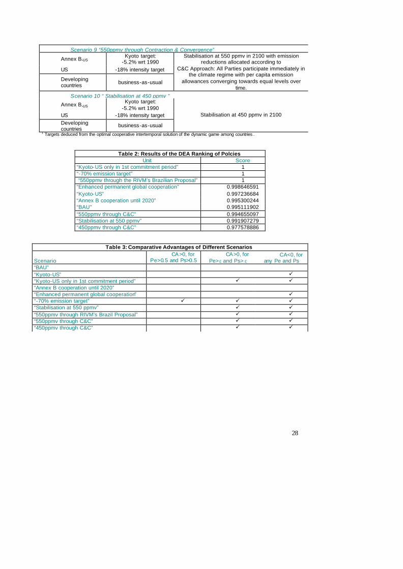
Let us first consider the ranking of scenarios shown in Table 2. There appear to be three winners,

namely three policies at least weakly dominating all the others: “Kyoto-US only in 1st commitment

period”, “550ppmv through the RIVM’s Brazilian Proposal”, “-70% emission target”. If we grouped the

scenarios in three categories, low (Scenarios 1 to 5), medium (Scenarios 7 to 9) and high environmental

effectiveness (Scenarios 6 and 10), these three policies represent the best performance within each of the

three categories, in terms of costs and of equity/wealth redistribution.

Let us analyze these three policies in detail. The attractiveness of the first one, “Kyoto-US only in

1st commitment period”, comes at no surprise. In addition to a modest environmental target, it also entails

very low costs (GDP remains therefore as high as in the business as usual throughout the century). This

depends on the fact that although the policy entails some costs, most of them are outweighed by the

benefits derived through the internalization of the climate change externality, in primis, and other

externalities as well, as for example the ones depending on the excessive use of natural resources and

those stemming from the underinvestment in R&D. Of course, in terms of avoided temperature increase

this policy is not extremely effective (by the end of the century temperature has increased of 2.5°C versus

the 2.75°C increase that would occur in the baseline). However, some redistribution of wealth takes place

because effort is undertaken by Annex 1 countries only while other countries will mainly benefit from the

policy. This entails a better performance in terms of equity with respect to all other scenarios within the

low environmental effectiveness ones .

The second scenario obtaining the highest score, the “550ppmv through the RIVM’s Brazilian

Proposal”, represent a slight improvement in terms of stringency of the climate target (even though a

stabilization of atmospheric CO2 at 550 ppmv implies with a high likelihood a temperature above the 2°C

target). Although costs are higher than for the low environmental effectiveness set of scenarios, they are

contained in the sense of not being excessive. On the other side, the redistribution potential entailed by

21

the proposed allocation scheme makes this scenario the most equitable among the medium environmental

effectiveness ones. These reasons together, i.e. the limited costs, the medium environmental effectiveness

and the high social performance, render this scenario one of the winners. This suggests that even an

involvement of developing countries in the short term might be possible, if the specific climate policy

package is well designed.

Finally, the third winner is the “-70% emission target” scenario that entails a major difference

from the other two because of its environmental stringency. There is an effective impact on temperature

increase (1.6°C by 2100) which makes this scenario the one performing best in environmental terms. Of

course, this strong environmental effectiveness comes at a high cost (even higher than in the case of the

450 ppmv stabilization). At the same time, however, the way the burden of this climate policy is

distribut ed among world regions implies a large wealth redistribution, which enables this scenario also to

have the best performance in social terms. This result is interesting because it indicates that a stringent

climate policy can become an attractive option if all sustainability impacts are taken into account.

The comparative advantage analysis (results are provided in Table 3) enables to investigate

results for different lower bounds on weights, which represent different assumption on the relative

importance policy-makers attach to the social and environmental dimensions. Setting the lower bound for

weights at zero (last column of Table 3) means that one allows for the possibility of completely

neglecting both environmental and social impacts of a policy when valuing its comparative advantage.

Even in such an extreme case, where most of the policies pass the test of having a positive comparative

advantage, the “BAU” and the “Annex B cooperation until 2020” scenarios show a negative comparative

advantage. If one restricts the value of weights to be strictly greater than zero (second column from the

right in Table 3), this corresponds to a situation in which policy-makers attach at least some importance to

both environmental and social impacts of the policy. In such a case, we find two more scenarios

characterized by a negative comparative advantage, “Kyoto–US” and the so-called “Enhanced permanent

global cooperation”, implying that they involve a low environmental and social performance compared to

other scenarios that apparently perform slightly better in one or both dimensions. Finally, letting the

minimum value of weights increase (second column in Table 3) implies that social and environmental

22

impacts assume increasingly relative importance in policy -makers’ value judgment. There exists a

threshold value for weights at which the only scenario measuring a positive comparative advantage is the

“-70% emission target” scenario, which has already been described as performing best in social and

environmental terms. This policy scenario obtains thus a good performance in terms of sustainability

notwithstanding its ambitious environmental target and its related significant costs.

The findings of this analysis need to be taken cautiously, because of the arbitrariness of the choice

of indicators and of the simulation model. Nonetheless, it represents an attempt to go beyond the

comparison done purely on economic terms that is typically undertaken in order to discuss the advantages

of alternative long term climate policies.

This methodology can represent an important tool for policy makers, through the identification

and evaluation of a number of policy strategies that appear to be crucial for the evolution of the future

climate debate. As a consequence, the approach adopted in this paper could be extremely beneficial if

combined with different types of climate-economy models and different choices of costs and benefits

indicators.

23

References

Atkinson, A.B., 1970. On the Measurement of Inequality . Journal of Economic Theory, 2: 244-263.

Barrett, S. , 1994. Self-Enforcing International Environmental Agreements. Oxford Economic

Papers, 46: 878-894.

Bodansky, D., 2003. Climate Commitments: Assessing the Options. Pew Center on Global Climate

Change. In: Aldy et al., Beyond Kyoto. Advancing the International Effort Against Climate

Change. Pew Center on Global Climate Change.

Böhringer, C. and Löschel, A., 2003. Climate Policy Beyond Kyoto: Quo Vadis? A Computable

General Equilibrium Analysis based on Expert Judgements. ZEW Discussion Paper No. 03-

09, Mannheim.

Bosetti, V. and Locatelli, G., 2006. A Data Envelopment Analysis Approach To The Assessment

Of Natural Parks’ Economic Efficiency And Sustainability. The Case Of Italian National

Parks. Sustainable Development (2006) DOI: 10.1002/sd.288.

Bosetti, V., Carraro, C., Galeotti, M., Massetti, E. and Tavoni, M., 2006. WITCH: A World

Induced Technical Change Hybrid Model. The Energy Journal, Special Issue on Hybrid

Modeling of Energy -Environment Policies: Reconciling Bottom-up and Top -down, 13—38.

Bosetti, V., Massetti, E. and Tavoni, M., 2007. FEEM’s WITCH Model: Structure, Baseline,

Solutions. FEEM Working Paper No 10/2007.

Botteon, M. and Carraro, C., 1997. Burden-Sharing and Coalition Stability in Environmental

Negotiations with Asymmetric Countries. In: C. Carraro (Editor), International

Environmental Agreements: Strategic Policy Issues, E. Elgar, Cheltenham.

Buonanno, P., Carraro, C., Castelnuovo, E. and Galeotti, M., 2000. Efficiency and Equity of

Emission Trading with Endogenous Environmental Technical Change. In: C. Carraro

(Editor), Efficiency and Equity of Climate Change Policy. Dordrecht: Kluwer Academic

Publishers.

Buchner, B. and Carraro, C., 2004. Emissions Trading Regimes and Incentives to Participation in

International Climate Agreements. European Environment , 14 (5): 276-289.

24

Buchner, B. and Carraro, C., 2005a. Economic and Environmental Effectiveness of a Technology -

based Climate Protocol. Climate Policy , 4: 229-248.

Buchner, B. and Carraro, C., 2005b. Modelling Climate Policy. Perspectives on Future

Negotiations. Journal of Policy Modeling, 27(6): 711-732.

Buchner, B. and Carraro, C., 2006. US, China and the Economics of Climate Negotiations.

International Environmental Agreements: Politics, Law and Economics, 6 (1): 63-89.

Buchner, B. and Carraro, C., 2007. Parallel Climate Blocs. Incentives to Cooperation in

International Climate Negotiations. In: R. Guesnerie and H. Tulkens (Editors), The Design

of Climate Policy. Forthcoming, MIT Press.

Carraro, C., 1998. Beyond Kyoto: A Game Theoretic Perspective. In the Proceedings of the OECD

Workshop on “Climate Change and Economic Modelling. Background Analysis for the

Kyoto Protocol”, Paris, 17-18.9, 1998.

Carraro, C., 1999. The Structure of International Agreements on Climate Change. In: C. Carraro

(Editor), International Environmental Agreements on Climate Change, Kluwer Academic

Pub.: Dordrecht.

Carraro, C. and Siniscalco, D., 1993. Strategies for the International Protection of the Environment.

Journal of Public Economics, 52: 309-328.

Charnes, A., Cooper, W.W., and Rhodes, E., 1978. Measuring Efficiency of Decision Making

Units. European Journal of Operational Research, 2 (6): 429–444.

Charnes, A., Cooper, W. W., and Rhodes, E., 1981. Evaluating Program and Managerial

Efficiency: An Application of Data Envelopment Analysis to Follow Through. Management

Science, 27 (6): 668–696.

Charnes, A., Cooper, W. W., Huang, Z. and Sun, D., 1990. Polyhedral Cone-Ratio DEA Models

with an Illustrative Application to Large Commercial Banks. Journal of Econometrics , 46

(1/2): 73-91.

Coelli, T., Prasada Rao, D.S. and Battese, G.E., 1998. An Introduction to Efficiency and

Productivity Analysis. Boston: Kluwer Academic Publishers.

25

Dyckhoff, H., and Allen, K., 2001. Measuring Ecological Efficiency with Data Envelopment

Analysis (DEA). European Journal of Operational Research, 132 (2): 312-325.

De Koeijer, TJ, Wossink, GAA, Struik, PC, Renkema, JA., 2002. Measuring Agricultural

Sustainability in Terms of Efficiency: The Case of Dutch Sugar Beet Growers. Journal of

Environmental Management , 66 (1): 9 – 17.

Egenhofer, C., W. Hager and Legge, T., 2001. Defining Europe’s Near Abroad in Climate Change:

A Russian-EU Alliance - Sub-global Bargaining to Further International Environmental

Agreements. CEPS Discussion Paper , Brussels.

Farrell, M.J. , 1957. The Measurement of Productive Efficiency. Journal of the Statistical Society

Series A (General), 120: 253-281.

Green, Michael J.B. and Paine, J., 1997. State of the World’s Protected Areas at the End of the

Twentieth Century. IUCN.

Hernandez-Sancho, F. Picazo-Tadeo, A and Reig-Martinez, E. , 2000. Efficiency and

Environmental Regulation An Application to Spanish Wooden Goods and Furnishings

Industry. Environmental and Resource Economics , 15: 365–378.

Intergovernmental Panel on Climate Change (IPCC), 2001. Climate Change 2001: Mitigation.

Cambridge: Cambridge University Press.

Intergovernmental Panel on Climate Change (IPCC), 2007. Climate Change 2007: The Physical

Science Basis, Summary for Policymakers. Contribution of Working Group I to the Fourth

Assessment Report, http://ipcc-

wg1.ucar.edu/wg1/docs/WG1AR4_SPM_Approved_05Feb.pdf .

Kemfert, C., Truong, T., and Bruckner, T., 2006. Economic Impact Assessment of Climate

Change: A Multi-Gas Investigation with WIAGEM -GTAPEL-ICM. The Energy Journal,

Special Issue Number 3, 28: 441-460.

Kuosmanen, T. and Kortelainen, M., 2007. Valuing environmental factors in cost-benefit analysis

using data envelopment analysis, Ecological Economics, Elsevier, 62(1): 56-65.

26

Meyer, A. 2000. Contraction & Convergence. The Global Solution to Climate Change.

Schumacher Briefings, 5. Green Books, Bristol, UK.

Nyman, J.A. and Bricker, D.L., 1989. Profit Incentives and Technical Efficiency in the Production

of Nursing Home Care. Review of Economics and Statistics, 71 (4): 586-594.

Richels, R.G, Manne, A.S., and Wigley, T.M.L. , 2004. Moving Beyond Concentrations: The

Challenge of Limiting Temperature Change. AEI-Brookings Joint Center for Regulatory

Studies, Working Paper 04-11.

Roson, R., Bosello, F., Lazzarin, M. and Tol, R., 2004. Economy-Wide Estimates of the

Implications of Climate Change: Seal Level Rise. FEEM Working Paper 96.04, Milan.

Sarofim, M.C., Forest, C.M., Reiner, D.M. and Reilly, J.M., 2004. Stabilization and Global Climate

Policy. MIT Joint Program on the Science and Policy of Global Change Report No. 110,

Cambridge, MA.

Seiford, L.M., 1996. Data Envelopment Analysis: The Evaluation of the State of Art (1978-1995).

The Journal of Productivity Analysis, 7: 99-137.

Stewart, R and Wiener, J., 2003. Reconstructing Climate Policy, American Enterprise Institute

Press.

The Royal Commission on Environmental Pollution, 2000. Energy – The Changing Climate. 22nd

Report.

Tol, R.S.J., 2006. Multi-Gas Emission Reduction for Climate Change Policy: An Application of

FUND. The Energy Journal, Special Issue Number 3, 28: 235-250.

Tyteca, D., 1996. On the Measurement of the Environmental Performance of Firms- A Literature

Review and a Productive Efficiency Perspective. Journal of Environmental Management, 46:

281-308.

United Nations Framework Convention on Climate Change (UNFCCC), 1997. Implementation of

the Berlin Mandate. Additional Proposals from Parties. Addendum

FCCC/AGBM/1997/MISC.1/Add.3. Available on

http://unfccc.int/resource/docs/1997/agbm/misc01a3.pdf

27

Tables

Table 1: An overview on the alternative policy architectures

Expected Emissions

2010 2020 from 2020 onwards

Scenario 1 “BAU - Business-as-Usual” Annex B-US

US Developing countries

“Business-as-Usual”

Scenario 2 “Kyoto Forever without US”

Annex B-US Kyoto target:

-5.2% wrt 1990 2010 level 2010 level

US -18% intensity target business-as-usual business-as-usual Developing countries

business-as-usual business-as-usual business-as-usual

Scenario 3 “Kyoto Forever without US only in the first commitment period”

Annex B-US Kyoto target:

-5.2% wrt 1990 2010 level 2010 level

US -18% intensity target Kyoto constraint 2020 level Developing countries business-as-usual business-as-usual business-as-usual

Scenario 4 “Annex B cooperation only until 2020”

Annex B-US Kyoto target: -5.2% wrt 1990

-20% wrt 1990

US -18% intensity target -20% wrt 1990 Developing countries

business-as-usual business-as-usual

“Business-as-Usual”

Scenario 5 “Enhanced permanent global cooperation”

Annex B-US Kyoto target: -5.2% wrt 1990

-20% wrt 1990

US -18% intensity target -20% wrt 1990 Developing countries business-as-usual business-as-usual

“Enhanced cooperation”1

Scenario 6 “-70% emission target”

Annex B-US Kyoto target: -5.2% wrt 1990

-30% wrt 1990 -70% emission target 2050 wrt 1990

US -18% intensity target -30% wrt 1990 Developing countries business-as-usual business-as-usual

-15% each decade

Scenario 7 “Stabilisation at 550 ppmv”

Annex B-US Kyoto target: -5.2% wrt 1990

-30% wrt 1990

US -18% intensity target -30% wrt 1990 Developing countries business-as-usual business-as-usual

Stabilisation at 550 ppmv in 2100 emission

entitlements in proportion to emissions

Scenario 8 “550ppmv through the RIVM’s Brazilian Proposal”

Annex B-US Kyoto target:

-5.2% wrt 1990 US -18% intensity target Developing countries

business-as-usual

Stabilisation at 550 ppmv in 2100 with emission reductions allocated according to

the Brazilian Proposal combined with threshold for non-Annex I regions

28

Scenario 9 “550ppmv through Contraction & Convergence”

Annex B-US Kyoto target:

-5.2% wrt 1990 US -18% intensity target

Developing countries business-as-usual

Stabilisation at 550 ppmv in 2100 with emission reductions allocated according to

C&C Approach: All Parties participate immediately in the climate regime with per capita emission

allowances converging towards equal levels over time.

Scenario 10 “ Stabilisation at 450 ppmv ”

Annex B-US Kyoto target: -5.2% wrt 1990

US -18% intensity target Developing countries

business-as-usual

Stabilisation at 450 ppmv in 2100

1 Targets deduced from the optimal cooperative intertemporal solution of the dynamic game among countries .

Table 2: Results of the DEA Ranking of Polcies Unit Score

“Kyoto- US only in 1st commitment period” 1 “-70% emission target” 1 “550ppmv through the RIVM’s Brazilian Proposal” 1 “Enhanced permanent global cooperation” 0.998646591 “Kyoto- US” 0.997236684 “Annex B cooperation until 2020” 0.995300244 “BAU" 0.995111902 “550ppmv through C&C” 0.994655097 “Stabilisation at 550 ppmv” 0.991907279 “450ppmv through C&C” 0.977578886

Table 3: Comparative Advantages of Different Scenarios

Scenario CA>0, for

Pe>0.5 and Ps>0.5 CA>0, for

Pe>ε and Ps> ε CA<0, for

any Pe and Ps “BAU" “Kyoto-US” ü “Kyoto-US only in 1st commitment period” ü ü “Annex B cooperation until 2020” “Enhanced permanent global cooperation” ü “-70% emission target” ü ü ü “Stabilisation at 550 ppmv” ü ü “550ppmv through RIVM’s Brazil Proposal” ü ü “550ppmv through C&C” ü ü “450ppmv through C&C” ü ü