no. 17/2004

Climate

Comparison of evaporation estimated by the HIRHAM and GWB models for present climate

and climate change scenarios

Kolbjørn Engeland, Torill Engen Skaugen, Jan Erik Haugen, Stein Beldring, Eirik Førland

Mist in Stormolinga, Røros

Postal address P.O.Box 43, Blindern NO-0313 OSLO Norway

Office Niels Henrik Abelsvei 40

Telephone +47 22 96 30 00

Telefax +47 22 96 30 50

e-mail: met@met.no Internet: met.no

Bank account 7694 05 00628

Swift code DNBANOKK

report

Title Comparison of evaporation estimated by the HIRHAM and GWB models for present climate and climate change scenarios

Date 25.11.2004

Section Climate

Report no. No. 17/04 Classification

Free Restricted ISSN 1503-8025

Author(s) Kolbjørn Engeland, Torill Engen Skaugen, Jan Erik Haugen, Stein Beldring, Eirik Førland

e-ISSN 1503-8025 Client(s) ’Regional climate development under global warming’ (NRC: RegClim), and ’Climate Change and Energy Production Potential’ (funded by EBL-Kompetanse AS).

Client’s reference NRC-NO 120656/720

Abstract The evaporation estimated by the regional climate model HIRHAM was compared to the evaporation given by the regional hydrological model GWB for selected points in Norway, Sweden and Finland. The report starts with a brief review of important evaporation processes and how they are represented in the two models. Then the evaporation estimated by the two models were compared to evaporation observations at three locations in Sweden and Finland for present climate, before the two models were compared at six points in Norway for the present climate and the future climate simulated by dynamical downscaling of HadAm3 with emission scenarios A2 and B2. Monthly and annual average values were compared. The results show that there is a potential for improving the evaporation calculations in both models. Both models over-estimate the average annual evaporation compared to observations at the three sites in Sweden and Finland. HIRHAM over-estimates winter evaporation whereas the GWB overestimates spring and autumn evaporation, and under-estimates winter-evaporation.The differences in estimated evaporation between the two models are more important than the differences between the scenarios A2 and B2. Both models indicate that the largest increase in evaporation will be in the spring and in the autumn.The summer evaporation might decrease at many locations. The GWB indicates a much higher increase in average annual evaporation than the HIRHAM model. Keywords HIRHAM, GWB, Evaporation, Climate change

Disiplinary signature

Eirik J. Førland

Responsible signature

Eirik J. Førland

Postal address P.O.Box 43, Blindern NO-0313 OSLO Norway

Office Niels Henrik Abelsvei 40

Telephone +47 22 96 30 00

Telefax +47 22 96 30 50

e-mail: met@met.no Internet: met.no

Bank account 7694 05 00628

Swift code DNBANOKK

5

Comparison of evaporation estimated by the HIRHAM and GWB models for present climate and climate change scenarios ............................................................................................................................... 1 1 Introduction................................................................................................................................................... 6 2 Evaporation processes................................................................................................................................... 6

2.1 Evaporation from snow free surfaces .................................................................................................... 7 2.2 Evaporation from snow covered surfaces. ............................................................................................. 7 2.3 Evaporation estimates for Norway ........................................................................................................ 8

3 Evaporation measurements ........................................................................................................................... 8 4 The GWB model ........................................................................................................................................... 9

4.1 Evaporation modelling in GWB ............................................................................................................ 9 4.1.1 The algorithms ................................................................................................................................ 9 4.1.2 Parameter values ........................................................................................................................... 10

5 The HIRHAM model .................................................................................................................................. 11 5.1 Evaporation modeling in HIRHAM .................................................................................................... 11

5.1.1 The algorithms .............................................................................................................................. 11 5.1.2 Parameter values ........................................................................................................................... 13

6 Climate scenarios........................................................................................................................................ 13 7 The comparison........................................................................................................................................... 13

7.1 Comparison of model estimates and observations............................................................................... 13 7.2 Comparison of HIRHAM and GWB ................................................................................................... 15 7.3 Forcing data ......................................................................................................................................... 15 7.4 Modeling scales ................................................................................................................................... 15

8 Results and discussion ................................................................................................................................ 15 8.1 Evaporation modeling for control period............................................................................................. 15

8.1.1 Comparison to eddy-correlation measurements ........................................................................... 15 8.1.2 Comparison between model estimates in Norway........................................................................ 17 8.1.3 Evaporation under climatic change scenarios............................................................................... 19

9 Conclusions................................................................................................................................................. 22 Refrences ....................................................................................................................................................... 23

6

1 Introduction Evaporation is an important part of the terrestrial water balance and the energy balance at the boundary between the land surface and the atmosphere. Evaporation processes are therefore important parts of both hydrological models that solve the water balance, and meteorological models that essentially solve the vertical energy balance. The difference in focus between meteorological and hydrological models makes it difficult to compare and integrate these two approaches (Graham and Bergström, 2000). The models operate on different spatial and temporal scales, and they account differently for the sub-grid variability.

In Norway the regional climate model HIRHAM (Christensen et al., 1996; Björge et al., 2000) and the regional hydrological model GWB (Beldring et al., 2002, 2003) have been used for assessing the changes in evaporation for climate change scenarios. The HIRHAM model has been used for dynamical downscaling of outputs from Atmosphere Ocean General Circulation Models (AOGCMs) to obtain 6 hourly time series of meteorological variables including evaporation, temperature, and precipitation. The precipitation and temperature provided by HIRHAM have then been used by the GWB model to estimate hydrological variables like evaporation, runoff and snow cover. The AOGCMs have provided results for a control period representing the present climate and for climate change scenarios. To assess the effects of climatic changes, the absolute or the relative differences between the variables of interest have been studied.

The aim of this report is to compare the evaporation estimated by the GWB and HIRHAM models for present climate and the estimated changes in evaporation for the climate change scenarios obtained with the AOGCM simulation HadAm3 (Gordon et al., 2000) and the emission scenario A2 and B2 (Cubash et al., 2001). To get an impression of how well the models describe the evaporation processes, we first compared the evaporation estimated by the GWB and HIRHAM models for the control period to evaporation observations. Then we compared the changes in evaporation predicted by the two models. Average monthly and annual values were compared.

We start to give an overview over important evaporation processes in the Norwegian climate and landscape and a summary of how the processes have been parameterized. We continue to present evaporation observations in Norway and in similar climates. We also give an overview over evaporation estimated by other models. We continue to show how the evaporation processes are represented in the GWB and HIRHAM models. It is followed by a section describing how the comparison was conducted before we present the results, discuss them and draw some conclusions.

2 Evaporation processes In this study the evaporation is considered to be all the vertical water fluxes between the land surface and the atmosphere, i.e. condensation, sublimation from snow, transpiration from vegetation, and evaporation from wet surfaces like intercepted rain or lakes. The local evaporation is a function of both local climate and regional air movement (Shuttleworth, 1993) as well as the shape and nature of the evaporation surface (Xu and Singh 1998). The total regional evaporation is a result of complex interactions between water and energy exchange processes at a wide range of temporal and spatial scales (Gryning et al., 2002). The two important factors driving the evaporation are air vapor deficit and the available energy. Important meteorological variables controlling evaporation include temperature, atmospheric pressure, solar radiation that are controlled by the geographical location, season, time of day, etc. The climate in Norway is characterized by relatively high precipitation and a seasonal variation in temperature, solar radiation and snow cover. The evaporation is also controlled by conductivity of the atmosphere and the land surface, i.e. the effectiveness of the vertical transport of water. The conductivity in the atmosphere is decided by wind speed and the surface roughness which is mainly controlled by vegetation length. For transpiration is the conductivity of the vegetation and the available water important, whereas for bare soils is the available water important. Evaporation from free water surfaces is mainly controlled by the atmospheric conductance. Important land use characteristics controlling evaporation includes vegetation, water bodies,

7

agricultural land, and urban areas. Norway is covered by coniferous forest (23%), deciduous forest (17%), open land (34%), mires (7%), lakes (5%), agricultural field (3%), urban areas (1%), glaciers (1%), and other types (9%) (Miljøstatus i Norge, 2004). Large parts of the open land is at high altitudes above the tree line. The Norwegian climate and landscape characteristics indicate that important evaporation processes include transpiration from vegetation, evaporation from intercepted precipitation, evaporation from bare soils, from lakes and from snow covered surfaces. The evaporation during winter season has to be given special attention since evaporation processes depend on the presence of snow cover.

2.1 Evaporation from snow free surfaces Many textbooks give an overview over evaporation from snow free surfaces (e.g. Dingman, 2002, Shuttleworth, W.J., 1993), and we only give a brief summary. Transpiration from vegetation depends on plant available water as well as the vegetation type. Evaporation from rain intercepted on vegetation depends on the interception capacity of vegetation and frequency, intensity and duration of storms. Evaporation from bare soils depends on the soil characteristics. Evaporation from lakes is controlled by the energy balance of the lake. Evaporation from agricultural fields is locally important, but since about 3% of the Norwegian land surface is used for agriculture it is of minor importance for the total water balance for Norway.

Grelle et al. (1999) give a summary of evaporation measurements in boreal forests. For the growing season (May – October) the measured evaporation is between 260 mm – 620 mm with most observations between 300 mm and 400mm. Due to smaller interception losses, the total evaporation from open land is smaller than the evaporation from forests, and Calder (1993) shows that, in a region in Wales, the total evaporation from grass-land is about 46% of the evaporation from forests. How the different evaporation processes contributes to the total evaporation depends on climate and vegetation characteristics. Interception loss is typically 20-40% in coniferous forest (Tallaksen et al., 1996). Field experiments in Norway indicate that the interception loss is an essential part of the water balance in forested areas. Ter Horst (2000) measured an interception loss of 29% of precipitation or 55.8 mm for three summer months in a high altitude birch forest stand close to Røros. Tallaksen et al. (1996) measured interception loss to be about 27% of the precipitation during summer seasons in a coniferous forest site close to Oslo. In the NOPEX area in southern Sweden, where average annual precipitation is 527 mm, Grelle et al. (1997) estimated 65% of the evaporation to be transpiration, 20% to come from interception and 15% to originate from the forest floor during the growing season. Calder (1993) indicates that transpiration is 36% and interception is 64% of the total evaporation at a forest site in Wales where annual precipitation is around 2400 mm.

Many methods for calculating evaporation is found in literature, and they can be grouped into five categories (Xu and Singh, 2002): 1 water budget (e.g. Guitjens, 1982), 2 mass-transfer (e.g. Harbeck, 1962), 3 radiation (Priestly and Taylor, 1972) 4 combination (e.g. Penman, 1948) and 5 temperature based (e.g. Hargreaves and Samani, 1985) parameterisations. The Penman Monteith model is currently the most advanced model for evaporation calculations used in hydrologic practice (Shuttleworth, 1993).

2.2 Evaporation from snow covered surfaces. The energy balance is strongly controlled by the snow cover. The snow has a high albedo and reflects about 90% of the incoming shortwave radiation. The snow cover in open areas gives a smoother surface that reduces the turbulent fluxes (Harding et al., 1995). The coniferous forest, on the other hand, has a large interception capacity (Parviainen and Pomery, 2000), a relatively small aerodynamic resistance, and a relatively high albedo and might act as light traps and become a significant source of energy for sublimation of intercepted snow (Gryning et al., 2001; Pomeroy and Dion, 1996). The difference between open snowfields and forests is probably the largest land surface contrast found in the terrestrial biosphere (Gryning et al., 2002). In open areas sublimation of airborne snow while still in motion may act as a source of moisture and a sink of sensible heat in high-latitude atmospheric boundary layers.(Dery et al., 1998).

The importance of evaporation from snow cover is discussed in the literature, see e.g. Lundberg and

8

Halldin (1994) for a brief overview. Dingman, (2002, page 181) argues that interception loss from snow-covered vegetation is of minor hydrologic importance since most of the intercepted snow will fall to the ground. Bengtsson (1980) indicates that the total amount of evaporation during the snow covered season amounts to maximum 10-20 mm, and that the evaporation rate hardly exceeds 1mm/day. Grelle et al.(1999), on the other hand, writes that winter evaporation is a substantial contribution to the annual evaporation. In the NOPEX area about 15% of the total annual evaporation occures in winter months November – April (Gustavsson et al. 2003). In Canada the observed sublimation from forests is between 13 and 40% of total snowfall (Pomeroy et al, 1999). Lundberg et al. (1998) indicate that the total interception loss from a snow covered forest can be up to 200mm a year. Modeling studies of sublimation of blowing snow in Pomeroy et al. (1997) indicates sublimation fluxes up to 30 mm/month, whereas Dery et al. (1998) indicates that the correct values are 2/3 less when edge-effects are accounted for since the sublimation process is self-limiting when the air becomes saturated.

Models ignore the winter-evaporation in two ways. Hydrological models tend to set the winter evaporation very small or equal to zero since this evaporation is assumed to be a minor part of the water balance (e.g. Bengtson, 1980). The winter evaporation is an essential part of the energy balance and cannot be ignored by meteorological models, and for many of them the evaporation from snow covered surfaces is equal to evaporation from the interception storage on snow free surfaces (e.g. Christensen et al., 1996). The winter evaporation is therefore over-estimated and the runoff under-estimated, both in forests (e.g. Gustavsson et al., 2003) and in open areas (e.g. Samuelsson et al., 2003; Beljaars and Viterbo, 1994; and Douville et al., 1995), if the winter evaporation processes are ignored. In open areas, the parameterization of the aerodynamic resistance is important to correctly simulate water and energy fluxes for winter conditions. The snow cover smoothens the surface and therefore increases the aerodynamic resistance in open areas. In many model parameterization (e.g. Samuelsson et al., 2003; Beljaars and Viterbo, 1994; and Douville et al., 1995) it is necessary to reduce the surface roughness by a factor around 10 in order to obtain good water balance simulations. If not the simulated snow evaporation is too large and spring runoff is too small. In forested areas it is possible to include a separate energy budget for the snow cover and an additional aerodynamic resistance for snow lying under high vegetation (Gustavsson et al., 2003; Gusev and Nasonova, 2003), or alternatively increase the aerodynamic resistance by a reasonable factor, e.g. Bringsfelt et al. (2001) and Samuelson et al. (2003) increase it by a factor 16. Due to feedback effects, the differences between original models and models with modified winter evaporation decrease when the land surface scheme is coupled with a GCM model (e.g. Samuelsson et al., 2003; Essery et al., 2003).

2.3 Evaporation estimates for Norway The evaporation has been estimated for Europe within the SWECLIM project (Räisänen et al., 2003). In Eastern Norway the results show annual rates between 350 and 400 mm, and at the west coast between 350 and 600 mm dependent on distance from coast. In the mountain regions the evaporation is 150-250 mm, in Trøndelag 300-500 mm, in Nordland 250-400 mm, and in Finnmark from 250mm up to 500 mm at the coast. Similar values and patterns are presented in Gjessing (1998) where average evaporation for 1901-30 are given. The seasonal variation is important. The results from SWECLIM indicates that the three winter months December, January, February have less than 8 mm/month except for costal regions where values up to 40 mm/month are indicated. The summer months June, July and August has 70-80 mm/month evaporation in Eastern Norway, 40-60 mm/month in Western Norway, 35-50 mm/month in the mountains, 60-80 mm/month in Trøndelag, 40-70 mm/month in Nordland, and 30-60 mm/month in Finnmark.

21 land surface schemes are compared for a catchment in northern Sweden in Nijssen et al.(2003). All models show a clear seasonal variation, and all models produce less than 1 mm/day during winter months, and less than 3 mm/day during summer. Annual values varies from 221 to 418 mm/year, with 300 mm/year as an average.

3 Evaporation measurements Few time series of observed actual evaporation exist. In the Nordic countries at least three time series are

9

available. Table 1 lists some characteristics of the three measurement sites that are located in Sweden and Finland. At all sites the actual evaporation is measured by eddy correlation instruments located at a tower above the forest canopy. For more information about the measurements and the sites see Valentini (2003).

Table 1 Characteristics of sites with evaporation measurements (from Valentini, 2003).

Norunda Flakaliden Hyytiala

Forest height (m) 25 8 11Measurement height (m) 70 15 23X-coord 60° 05' 10'' N 64° 06' 46'' N 61° 51' 51''NY-coord 17° 28' 13'' E 19° 27' 25''E 24° 17' 41''EElevation (m) 225 45 170

4 The GWB model The GWB-model (Beldring et al., 2002, 2003) is a distributed version of the Nordic HBV-model (Sæltun et al., 1996) operating on a regular grid cells and daily time steps. It was developed to simulate runoff from the entire land surface of Norway for the period 1961-1990 on a 1km2 grid. It has also been used for studying the effects of climatic changes on hydrology (Roald et al., 2002) and for creating snow maps (Skaugen et al., 2003). GWB requires precipitation and air temperatures as input. It has components for accumulation snow, interception storage, soil moisture storage, evapotranspiration, groundwater storage, runoff response, lake evaporation and glacier mass balance. The algorithms are found in Bergström(1995) and Sælthun (1996). The algorithms used for evaporation calculations are precented below.

4.1 Evaporation modelling in GWB

4.1.1 The algorithms The total evaporation E from land surfaces is calculated as:

( )[ ]{ } ( )SparPe WFEMNDETCE **11** −+= (1)

where Ce is an evaporation constant (mm °C-1 day-1 ), T is air temperature, Ep(MND) is a seasonal profile for potential evaporation, and Epar is a land-use dependent control factor for seasonal correction of potential evaporation. F(Ws)is a function that reduces the evaporation due to water deficit in the soil moisture zone:

( )

=

crmaxS

SS F*W

W,minWF 1 (2)

where Ws (mm) is amount of water in the soil moisture storage and WSmax (mm) is maximum soil moisture content (mm) and Fcr is a dimensionless parameter less than one deciding when evaporation should be reduced due to water stress. Only snow-free areas can evaporate, with exception of intercepted snow.

The evaporation is at the potential rate for the interception storage, until it is empty. The maximum interception storage is given by a parameter Imax. As long as water is present in the interception storage, the actual evaporation from the soil moisture zone is reduced by a factor Ered, a constant less than 1.0.

The sub-models for infiltration, surface- and subsurface runoff will also influence the estimated

10

evaporation, and more details are found in Sælthun et al., (1996).

We see that the GWB model has an empirical parameterisation of the evaporation processes where most of the original physical description of mass and energy fluxes are left out. The model adjusts a long-term seasonal dependent potential evaporation according to temperature. The same seasonal profile is used all over Norway. When the parameters are calibrated, this parameterisation might work satisfactory under present climate conditions, but the model should be used with care for conditions not included in the calibration. GWB takes into account the interception, but in order to simulate transpiration processes on a more physical basis, it is necessary to use time steps less than 3 hours. The GWB model ignores evaporation from snow covered areas. For applications in Sweden Graham and Bergström (2000) argue snow evaporation is included implicitly in the HBV model as a general snowfall correction factor.

4.1.2 Parameter values The parameters Ce Ep(MND) and Ered are identical for all the modeling area whereas Ered , Ws , WSmax and Imax. depend on the physical characteristics of each model element. The following landscape-classes were used: (i) areas above tree-line with extremely sparse vegetation, mostly lichens, mosses and grass; (ii) areas above the tree-line with grass, heather shrubs or dwarfed trees (iii) areas below the tree-line with sub-alpine forests; (iv) lowland areas with coniferous or deciduous forests; and (v) no-forested areas below the tree line. There are separate parameters for the lakes and the glaciers.

Digital maps from the Norwegian Mapping Authority were used to determine land use and elevation for each model grid. For each element the proportion of area covered by open land, forest, lakes and glaciers are obtained. The land use proportions of grid area covered by forest, lakes and glaciers were obtained from maps of scale 1:50000 or 1:250000. Data from a Norwegian vegetation atlas (Moen, 1998), while the tree level was obtained from Strand(1988).

The GWB model has been calibrated using monthly streamflow data from 141 catchments for the period 1 January 1968 – 31 December 1984, and daily discharge from the same stations and from 141 independent stations were used to evaluate the performance (Beldring et al., 2003)). Table 2 lists the applied parameter sets:

Table 2 Parameter values used in the GWB model. The landscape classes are (i) areas above three-line with extremely sparse vegetation, mostly lichens, mosses and grass; (ii) areas above the tree-line with grass, heather shrubs or dwarfed trees (iii) areas below the tree-line with sub-alpine forests; (iv)

lowland areas with coniferous or deciduous forests; and (v) no-forested areas below the tree line.

Parameter Values

Ce 0.25 Ep(MND) 0.7, 0.7, 0.7, 1.0, 1.3, 1.4, 1.3, 1.1, 1.0, 0.9, 0.7, 0.7 Ered 0.5

Landscape class: (i) (ii) (iii) (iv) (v)

Epar 0.1 0.5 0.8 1 1 Wcr 1 0.8 0.8 0.7 0.8 WSmax(mm) 20 76 120 150 150 Imax 0.4 0.4 1 2 0.4

11

5 The HIRHAM model The HIRHAM model (Christensen et al., 1996; Bjørge et al., 2000) is based on HIRLAM (High Resolution Limited Area Model) dynamics and ECHAM4 (the atmospheric global climate model at MPI-Hamburg based on an earlier version of the ECMWF model) physics. The HIRHAM model has resolution of appriximately 55x55 km2 and operates on a 6 hourly time resolution. The model has been used for dynamically downscaling of results from the AOGCM within the norwegian RegClim project (Bjørge et al., 2000).

5.1 Evaporation modeling in HIRHAM

5.1.1 The algorithms The algorithms for the evaporation are from Christensen et al. (1996), whereas the algorithms for the atmospheric heat conductance Ch are from Roeckner et al. (1996). Surface water has three reservoirs: Snow water equivalent Sn, interception (skin reservoir) Wl and soil water Ws. Time evolution of these fluxes is determined by rain P, snow Psn, evaporation E and runoff fluxes R. Dependent on the type of rain, a given fractional area Ca of a grid cell is wetted during a time step. For convective rain Ca = 50%, for large scale Ca = 100%. The maximum interception capacity is defined by Imax (mm).

Evaporation E is calculated as:

( )( )SSsatChh p,ThqqEvCE −= ρ (3) where ρ is density of water (kg/m3), Ch is the atmospheric heat conductance at lowest level, hv is the absolute wind speed at the lowest model level, q is the specific humidity at the lowest level and

( )SSsat p,Tq is the saturated specific humidity at the surface. In many evaporation parameterizations is the aerodynamic resistance applied in stead of the heat conductance, and the relationship between these quantities is:

ahh rv

C 1= (4)

Over snow and the interception reservoir E = h = 1, while over bare soil E = 1 and

( )

−=

SSsatmaxS

S

p,Tqq,min,

WW

cosmaxh 1121 π (5)

where Wsmax is maximum water holding capacity (mm). Over dry vegetation h = 1, while the conductance is modified by the evaporation efficiency:

( )( )

1

1−

+=

S

cohh WF

PARRvCE (6)

where Rco is the stomatal resistance of the canopy. An empirical expression is used for Rco

+

+−

++⋅

⋅⋅=

⋅−⋅

1ln

11ln

ded

ded

PARdbckR

tt LkLk

co (7)

12

where Lt is leaf area index, and d = (a + b·c)/(c·PAR). PAR is the photosynthetically active radiation and is set to 55% of net short-wave radiation. The water stress function is:

( ) ( )

−

−=

pwpcrmaxS

pwpmaxSSS FF*W

F*WW,min,maxWF 10 (8)

where WSmax is maximum soil moisture storage (mm), Fpwp is fraction of WSmax defining wilting point, Fcr factor deciding when evaporation is reduced due to water stress. WSmax depends on soil type.

The drag coefficient for heat (heat conductance) Ch is calculated as:

( )mmhNh zz,zz,RifCC 00⋅= , ( ) ( )hm

aN zzzz

kC

00

2

lnln ⋅= (9)

where ka is von Karman constant, z is the height of the model’s lowest layer (it depends on pressure and is on average 32 meters), z0m and z0h the roughness lengths for momentum and heat respectively.

Ri is the moist bulk Richardson number of the surface layer defined as (Christensen et al., 1996):

( )( ) ( )[ ]22 vu

zqBAgRi

v

tL

∆∆θ∆∆θθ∆

+

+⋅= (10)

where g is gravitational constant, θL is cloud water potential temperature, qt is total water content, specific as well as held in clouds, θ and θv are the usual potential and virtual potential temperatures defined without the liquid water term, u and v represent the horizontal components of the wind. ∆ of any quantity denotes the difference of the respective quantity between adjacent model levels. A and B are constants based on Deardorf (1980).

For unstable case (Ri < 0):

+⋅−+

⋅−=

131

1

0

2

mNR

Rh

zzRiCc

Riaf (11)

For stable conditions (Ri ≥ 0):

( ) ( )RicRiaf

RRh ⋅+⋅⋅+=

111 (12)

Runoff is calculated according to Dumenil and Todini (1992).

We see that HIRHAM has a physically based description of the evaporation processes, but the parameterization of the land surface is rather rough. HIRHAM does not consider the seasonal variation in green vegetation, and the particularity of evaporation processes from snow cover is ignored.

13

5.1.2 Parameter values Four parameters have a spatial distribution: Lt, WSmax, zveg and zoro. Description of the method used for deriving the vegetation parameters is found in Claussen et al., (1994), and Roeckner et al. (1996) refers to Patterson (1990) as a source for the soil parameters. The Lt has no seasonal variation. The roughness length is a function of orography and vegetation: 22

00 vegorohm zzzz +== .The roughness length zveg for the

different vegetation types are listed in Table 7 of Claussen et al. (1994). The parameter ρ is a physical constant. The remaining parameters are constant with k = 0.9, a = 5000Jm-3, b = 10Wm-2, c = 100 sm-1, Fcr = 0.75, Fpwp = 0.35, ka = 0.4, cR = 5 , aR = 3cR .

The elevation is averaged from the US Navy data base at 10 arc min resolution within each grid square. Fraction of land and fraction of sea within each grid cell (55x55km2) is also calculated.

6 Climate scenarios The climate change scenarios provided by the HadAm3 model developed at the Hadley centre in UK (Gordon et al., 2000) was used in this study. The spatial resolution of this AOGCM is approximately 300 * 300 km2. The results were dynamically downscaled with the regional climate model HIRHAM (Bjørge et al., 2000) for domain 2 (ref??).

HIRHAM was run with one control period and one scenario period. The control run is one realisation of today’s climate, representing the present climate. The estimated day-to-day variability is not comparable with observations. The mean monthly values and standard deviation based on daily values should, however, be comparable. The models were run with the emission scenarios A2 and B2 (Cubash et al., 2001). The control run represents the period 1961-1990 whereas the climate scenarios represent the period 2071-2100.

In order to compare only the evaporation algorithms, we chose to use the temperature and precipitation fields from the HIRHAM model directly as climatic forcing input in the GWB model. We did neither adjust nor interpolate them.

7 The comparison We chose to compare the modeling results at six HIRHAM points located all over Norway as shown in Fig. 1. The points were selected to cover most of the climatic variability in Norway. The model simulations were also compared to three point measurements located in Sweden and Finland. These model points are also shown in Fig. 1. The characteristics of the 9 points are listed in Table 3.

7.1 Comparison of model estimates and observations The observations and the simulations are not directly comparable. The simulated evaporation is based on meteorological variables calculated from the HIRHAM model and not on observed values. The day to day variation is therefore not identical, statistical measures should, however, be comparable. The observations are point measurements whereas the simulations represents larger areas. The simulations are also an average over 30 years whereas the observations are averaged over 2-5 years. The GWB model has been calibrated to streamflow measurements in Norway, but the same parameter sets can be applied in Sweden and Finland with some confidence since we find quite similar climate and land cover in Norway.

14

Figure 1. The points where the GWB and HIRHAM models were compared. The three sites with evaporation flux measurements are marked with triangles.

Table 3 Characteristics for the points used for comparison of evaporation estimates. Name Index in

domain 2 (i,j) Longitude (°) Latitude (°) HIRHAM

elevation (masl) Point elevation (masl)

East Norway 55,44 10.03873 60.10239 369 209 West Norway 51,42 5.86712 59.36072 304 160 Moutains 53,46 8.319516 61.23652 1181 1211 Trøndelag 54,50 9.998159 63.14359 456 280 Nordland 56,55 13.319020 65.41895 523 480 Finnmark 61,65 23.294052 69.41895 506 437 Norunda 62,45 17.070229 59.84721 42 45 Flakaliden 62,54 19.821774 64.15894 184 225 Hyytiala 68,50 24.480539 61.25232 123 170

15

7.2 Comparison of HIRHAM and GWB The two models use different parameterisations, spatial and temporal resolutions, and geographical data for estimating the spatial distribution of the parameters. It should also be noted that the calculated evaporation in HIRHAM is a part of the model dynamics whereas the GWB model is purely hydrologic and the calculated evaporation acts as a sink. In the HIRHAM model the model points are connected by the dynamics, whereas for the GWB model the calculations is performed independently for each grid cell. For both models the evaporation is an 'internal flux' that has not been explicitly validated. The aim of GWB model has been to obtain good simulation of runoff, whereas for the HIRHAM model the aim has been to obtain good simulations of climate in general. The evaporation estimates from the two models are therefore not directly comparable.

The GWB model runs on a 1x1km2 grid whereas HIRHAM uses 55x55km2. In previous applications of the GWB model the precipitation and temperature fields from the HIRHAM model has been adjusted and then interpolated to the 1x1 km2 GWB-grid (Roald et al., 2002). The differences between evaporation estimates in previous applications of these two models can partially be explained by the difference in the interpolation of climatic data.

The two models use different climatic variables for calculating the evaporation. In the GWB model the calculation of evaporation depends on temperature, whereas in the HIRHAM model the wind and the air vapor deficit are used. We also find a big difference in the modeling of evaporation from snow covered surfaces. The GWB model sets snow evaporation to zero whereas the HIRHAM model calculates an evaporation from the snow as it is interception storage.

The parameterisation of runoff has also a large effect on the seasonal cycle of surface evaporation (van der Hurk et al., 2002; Lohmann et al., 1998; Koster and Milly, 1997), and both the runoff processes and the parameter values differ between the two models.

7.3 Forcing data In order to compare only the evaporation algorithms, we chose to use the temperature and precipitation fields from the HIRHAM model directly as input in the GWB model. We neither adjusted nor interpolated the climate forcing data.

7.4 Modeling scales The HIRHAM model runs on a 55x55km2 grid whereas the hydrological model in its original form operates on a 1x1km2 grid. We used the GWB model at the 1x1km2 scale and run the model for those GWB-squares that contain the center points of the HIRHAM-squares. The lake and glacier percentages in the GWB model was set to be zero, and no elevation zones were used. Each grid cell in the GWB model can still be covered by different land-use classes depending on elevation and forest percentage.

8 Results and discussion

8.1 Evaporation modeling for control period

8.1.1 Comparison to eddy-correlation measurements The model altitudes are comparable to station altitudes (Table 3), so no height adjustments of model outputs are necessary. The simulated evaporation is available for 30 years whereas the observed values are provided for 2 -5 years only. Since the year to year variation in evaporation might be large, the mean values based on the observation are uncertain. We therefore chose to plot all the simulated and observed monthly data in Fig. 2 whereas Fig. 3 shows the average monthly evaporation. Based on the observations from 2-5 years only, we can identify significant differences between the models and the measurements. The HIRHAM model overestimates the winter evaporation (October – April) at all sites. The over-estimation of

16

winter-evaporation has been a problem for other meteorological models, and it is shown that specific surface parameters for snow-cover is necessary in order to obtain good results (see above). The winter-evaporation from the HIRHAM model would probably improve with a new parameterisation of evaporation from snow cover.

Jan

Feb

Mar Apr

May Jun

Jul

Aug

Sep Oct

Nov

Dec

0255075

100125

a) GWB-NorundaE(mm)

Jan

Feb

Mar

Apr

May Jun

Jul

Aug

Sep Oct

Nov

Dec

0255075

100125

c) GWB-FlakalidenE(mm)Ja

nFe

bM

ar Apr

May Jun

Jul

Aug

Sep Oct

Nov

Dec

0255075

100125

b) HIRHAM-NorundaE(mm)

Jan

Feb

Mar

Apr

May Jun

Jul

Aug

Sep Oct

Nov

Dec

0255075

100125

d) HIRHAM-FlakalidenE(mm)

Jan

Feb

Mar Apr

May Jun

Jul

Aug

Sep Oct

Nov

Dec

0255075

100125

e) GWB-HyytialaE(mm)

Jan

Feb

Mar Apr

May Jun

Jul

Aug

Sep Oct

Nov

Dec

0255075

100125

f) HIRHAM-HyytialaE(mm)

Figure 2 Observed monthly evaporation (thick, black lines) and simulated evaporation (thin, grey lines) for the three sites with eddy correlation measurements of evaporation fluxes.

Figure 3 Observed and simulated average monthly evaporation for a)Norunda b)Flakliden and c) Hyytiala. The GWB model underestimates the winter evaporation, especially in the months January – March. The reason is that the calculated evaporation from snow covered surfaces is zero. It is argued that the HBV model has an implicit modeling of snow evaporation through its snow correction factor, and that the total snow evaporation will therefore not show up (Graham and Bergström, 2002). This implicit snow evaporation is, however, not included in the application of the GWB model in Norway, since the snowfall correction factors were not calibrated. Instead standard correction factors depending on the exposure of the precipitation gauges were used. Anyway, the GWB model requires a more explicit parameterisation of winter evaporation in order to improve the results. In the spring, after the snow cover has melted, and in late autumn the GWB model overestimates the evaporation. Much of the water available after the snow

17

melt evaporates, and in the months July – September the GWB estimated evaporation is reduced since less water is available for evaporating. One factor that can explain these differences are that the simulated evaporation is not based on meteorological observations, but on the present climate simulated by the global climate model and the HIRHAM model. Table 4 compares observed and simulated average annual precipitation and temperatures. We see that both the annual temperature and the annual precipitation is larger than the observations at all sites. This might contribute to the over-estimation of evaporation by both models. Fig. 4 shows the average seasonal observed and HIRHAM-simulated temperatures. The seasonal variations in temperature is well described by the HIRHAM model at these points. However, Skaugen et al., (2003) have found that in areas with large altitude differences, it is necessary to adjust the temperatures given by HIRHAM before comparing them to observations.

One reason for that the evaporation given by the GWB model does not follow the observed seasonal profile might be that the seasonal profile on potential monthly evaporation (Table 2) does not follow the observed evaporation. The maximum monthly evaporation is in August whereas the seasonal profile indicates June is the moth with maximum evaporation. Another problem is that the evaporation formulation in GWB is empirical and requires some calibration in order to obtain good results. In this study the evaporation parameters have not been specifically fitted to this area.

Based on the available data, the GWB model overestimates the annual evaporation by 19%, 47% and 44%, whereas the HIRHAM model overestimates it by 31%, 87% and 71% at Norunda, Flakaliden and Hyytiala respectively.

Table 4 Observed and simulated precipitation and temperature.

Norunda Flakaliden Hyytiala Obs Sim Obs Sim Obs Sim Mean precipitation (mm/year) 527 726 587 825 640 804 Mean temperature(°C) 5.5 5.8 1.9 2.5 3.5 3.9

Figure 4 Observed and simulated average monthly temperatures for a)Norunda b)Flakliden and c) Hyytiala.

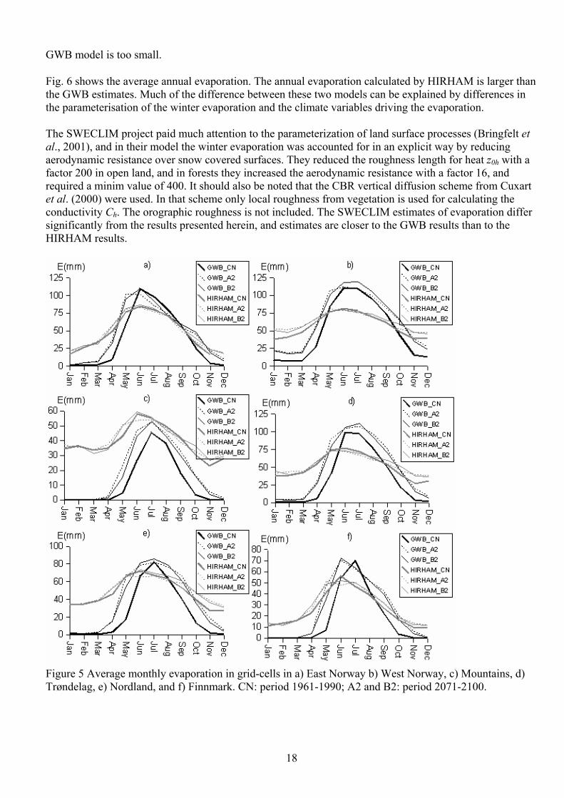
8.1.2 Comparison between model estimates in Norway Fig. 5 shows the seasonal variation in calculated evaporations for some selected HIRHAM points. The results presented in the figures are related to the altitude of the HIRHAM points and further adjustments are necessary to obtain representative values at locations with a different altitude.

The two models give different seasonal variation in evaporation, and we recognize the differences seen in Fig. 2. In the winter months the GWB model gives zero or a very small evaporation, whereas the HIRHAM evaporation is rather high. In the summer season the GWB model gives more evaporation than the HIRHAM model in 5 of the 6 selected squares. We find the largest difference between the models in the mountain cell where the GWB estimates are much smaller than the HIRHAM estimates (Figure 5c). Compared to observations and previous modeling studies (e.g. SWECLIM, Räisänen et al., 2003), the estimated evaporation in HIRHAM is much too high during the winter months. More than 30mm evaporation for January as indicated in Fig. 1c is not realistic. The estimated winter evaporation in the

18

GWB model is too small.

Fig. 6 shows the average annual evaporation. The annual evaporation calculated by HIRHAM is larger than the GWB estimates. Much of the difference between these two models can be explained by differences in the parameterisation of the winter evaporation and the climate variables driving the evaporation. The SWECLIM project paid much attention to the parameterization of land surface processes (Bringfelt et al., 2001), and in their model the winter evaporation was accounted for in an explicit way by reducing aerodynamic resistance over snow covered surfaces. They reduced the roughness length for heat z0h with a factor 200 in open land, and in forests they increased the aerodynamic resistance with a factor 16, and required a minim value of 400. It should also be noted that the CBR vertical diffusion scheme from Cuxart et al. (2000) were used. In that scheme only local roughness from vegetation is used for calculating the conductivity Ch. The orographic roughness is not included. The SWECLIM estimates of evaporation differ significantly from the results presented herein, and estimates are closer to the GWB results than to the HIRHAM results.

Figure 5 Average monthly evaporation in grid-cells in a) East Norway b) West Norway, c) Mountains, d) Trøndelag, e) Nordland, and f) Finnmark. CN: period 1961-1990; A2 and B2: period 2071-2100.

19

East Norway

West Norway

Mountains Trøndelag Nordland Finnmark0

100

200

300

400

500

600

700

800GWB_CNGWB_A2GWB_B2HIRHAM_CNHIRHAM_A2HIRHAM_B2

E(mm)

Figure 6 Average annual evaporation in grid-cells in Norway. CN: period 1961-1990; A2 and B2: period 2071-2100.

8.1.3 Evaporation under climatic change scenarios Fig. 5 shows the simulated seasonal and Fig. 6 the average annual evaporation for the scenarios A2 and B2 whereas Figs. 7 and 8 indicate the relative differences for the two scenarios compared to the control period for seasonal and average annual evaporation respectively. The differences between the two models are larger than the differences between the scenarios. We see some qualitative similarities between the two models. Both indicate the highest increase in evaporation in spring and autumn, and the lowest increase or in some cases decreased evaporation during summer. The average annual evaporation increases in both models. But quantitatively the differences are large. The GWB model indicates the highest rise in evaporation, both as percentage (Figs. 7 and 8) and as absolute values (Figs 5 and 6). At all locations the evaporation from the GWB model increases significantly in the months that become more snow-free in the scenario periods. This is because the GWB model sets transpiration from vegetation to zero for snow-covered areas. In most location the HIRHAM model indicates increased evaporation in the winter season and less evaporation in the summer season, probably due to water stress whereas the GWB model indicate reduced evaporation during summer season only in eastern Norway. Compared to results presented in the SWECLIM project the GWB model indicates too large increase in evaporation, whereas the HIRHAM model indicates too small increase. Also here the most important explanation is the differences in evaporation from snow covered surfaces. In application of the HBV model for climate change scenarios in Sweden, the HBV model gave larger increase in evaporation than that given by the climate model. The climate model was believed to give the best estimate of relative change in evaporation. In order to obtain consistent results in water balance estimates for climate change scnarios, they forced the HBV model to give the same relative increase in average annual evaporation as the climate model (Andréasson et al., 2004). The evaporation estimates from the HIRHAM model have to be improved before this procedure can be applied in Norway. In Fig. 9 the estimated changes in temperatures are shown whereas Fig. 10 shows the estimated changes in precipitation. Both the temperature and the precipitation increases. We see that in Southern Norway (Fig. 10 a-c) the winter evaporation increases and the summer evaporation decreases, whereas in northern Norway (Fig. 10 d-f) the summer precipitation increases and the winter precipitation decreases. It is therefore reasonable that the evaporation also will increase.

20

Figure 7 Changes in average monthly evaporation in grid-cells in a) East Norway b) West Norway, c) Mountains, d) Trøndelag, e) Nordland, and f) Finnmark from period 1961-1990 to period 2071-2100.

East Norway

West Norway

Mountains Trøndelag Nordland Finnmark0

10

20

30

40

50

60

70GWB_A2GWB_B2HIRHAM_A2HIRHAM_B2

Change in evaporation (%)

Figure 8 Changes in average annual evaporation in selected grid-cells in Norway from period 1961-1990 to period 2071-2100

21

Figure 9 Changes in average monthly temperatures in grid-cells in a) East Norway b) West Norway, c) Mountains, d) Trøndelag, e) Nordland, and f) Finnmark from period 1961-1990 to period 2071-2100.

22

Figure 10 Changes in average monthly precipitation in grid-cells in a) East Norway b) West Norway, c) Mountains, d) Trøndelag, e) Nordland, and f) Finnmark from period 1961-1990 to period 2071-2100.

9 Conclusions In this study we have compared the evaporation parameterisation and the estimates for the meteorological HIRHAM model and the hydrological GWB model. The results show that. • There is a potential for improving the evaporation calculations in both the HIRHAM and the GWB

model. • The different process parameterisation leads to significantly different evaporation estimates, both for

present climate and for climate change scenarios. • Both models over estimate the average annual evaporation compared to observations at the three sites in

Sweden and Finland. • HIRHAM over-estimates winter evaporation whereas the GWB overestimates spring and autumn

evaporation, and under estimates winter-evaporation. Furthermore, the HIRHAM model over estimates the evaporation especially in mountain regions with snow cover lasting for several months.

• The differences in estimated evaporation between the two models are more important than the differences between the scenarios A2 and B2.

• Both models indicate that the largest increase in evaporation will be in the spring and in the autumn. • The summer evaporation might decrease at many locations. • The GWB indicates a much higher increase in average annual evaporation than the HIRHAM model.

This difference is mainly explained by how the models parameterize evaporation from snow cover.

23

• Suggested improvements for the HIRHAM model are to reduce the heat conductance for snow covered surfaces and to use only the vegetation roughness for calculating the heat conductance.

• The HIRHAM and the GWB models could be tighter integrated in order to give consistent estimates of water balance components for climate change scenarios.

Acknowledgements I would like to thank Anders Lindroth at the University of Lund who provided the evaporation data at Norunda and Flakaliden, and Timo Vesala at the University of Helsinki who provided the data at Hyytiala through the Euroflux project. The study was done under the projects ‘Climate Change and Energy Production Potential’ (funded by EBL-kompetanse AS) and ‘Regional climate development under global warming’ (RegClim)

Refrences Andréasson, J., Bergström, S. Carlsson, B., Graham, l. P., and Lindström, G. (2004) Hydrological change – climate change impact simulations for Sweden, Ambio 33(4-5) 228 – 234.

Beldring, S., Engeland, K., Roald, L.A., Sælthun, N.R., and Voksø, A. (2003) Estimation of parameters in a distributed precipitation-runoff model for Norway, Hydrology and Earth System Sciences, 7, 304 – 316.

Beldring, S., Roald, L.A. Voksø, A. (2002) Avrenningskart for Norge NVE Dokument 2002, NVE, Oslo, Norge.

Beljas, A.C.M. and Viterbo, P. (1994) The sensitivity of winter evaporation to the formulation of aerodynamic resistance in the ECMWF model, Boundary-Layer Meteorology, 71, 135-149.

Bengtsson, L. (1980) Evaporation from a snow cover review and discussion of measurements, Nordic Hydrology, 11, 221-234.

Bergström S. (1995) The HBV model. In: Computer Models of Watershed Hydrology, V.P. Singh (Ed.). Water Resources Publications, Highland Ranch, 443-476.

Björge, D. Haugen, J.E., and Nordeng, T.E. (2000) Future climate in Norway, DNMI Research report No. 103.

Bringfelt, B., Räisänen, J., Gollvik, S., Lindström, G., Graham, L.P., and Ullerstig, A. (2001) The land surface treatment for the Rossby Centre Regional Atmospheric Climate Model – version 2 (RCA2), SMHI Reports Meteorology and Climatology No98, 2001, SMHI, Norrköping, Sweden.

Calder, I.R.. (1993) Hydrologic effects of land-use change, In: Handbook of hydrology ed. By D.R. MaidmentMcGraw-Hill, New York, USA.

Christensen, J.H., Cristensen, O.B., Lopez, P, Meijgaard, E., Botzet, M. (1996) The HIRHAM Regional Atmospheric Climate Model. DMI Scientific report 96-4, Cophenhagen, Denmark.

Claussen, M., Lohmann,U., Roeckner, E., and Schulzweida, U. (1994) A global data set of land-surface parameters. MPI Report 135, Max-Planck Institut fur Meteorologie, Hamburg, Germany.

Cubasch U, G.A. Meehl, GJ Boer, RJ Stouffer and 5 others (2001) `Projections of future climate change´. In: Houghton JT, Ding Y., Griggs DJ, Noguer M, van der Linden PJ, Dai X, Maskell K, Johnson CA (eds) Climate change 2001: the scientific basis. Contribution of Working Group I to the Third Assessment Report of International Panel on Climate Change. Cambridge University Press, Cambridge, p 583-638.

24

Cuxart J., Bougeault P., and Redelsperger J.L. (200) A turbulence scheme allowing for meso-scale and large-eddy simulations, Quarterly Journal of the Royal Meteorological Society, 126(562), 1-30

Deardorff, J.W. (1980) Stratocumulus-capped mixed layers derived from a three-dimensional model, Boundary Layer Meteorology, 18, 495-527.

Dery, S.J., Taylor, P.A., and Xiao, J. (1998) The thermodynamic effects of sublimating, blowing snow in the atmospheric boundary layer. Boundary-Layer Meteorology, 89, 251-283.

Deutches Klimarechenzentrum (1993) The ECHAM3 Atmospheric General Circulation Model, DKRZ Report No. 6, Hamburg, Germany.

Dingman, S. L. (2002) Physical Hydrology, Second Edition, Prentice Hall, Englewood Cliffs, New Jersey, USA.

Douville, H., Royer, J.-F., Mahfouf, J.-F. (1995) A new snow parameterization for the meteo-France climate model. Part I: validation in stand alone experiments, Climate Dynamics, 12, 21-35.

Dumenil, L. and Todini, E., (1992) A rainfall-runoff scheme for use in the Hamburg climate model. In: J.P. O'Kane, Editor, Advances in Theoretical Hydrology, A Tribute to James DoogeEur. Geophys. Soc. Ser. Hydrol. Sci. 1, Elsevier, Amsterdam, pp. 129–157.

Essery, R. Pomeroy, J., Parviainen, J., and Storck, P. (2003) Sublimation of Snow from Coniferous Forests in a Climate Model, Journal of Climate: 16(11), 1855–1865.

Gjessing, Just (1997) Norges geografi, Universitetsforlaget, Oslo, Norway.

Gordon, C., Cooper, C. Senior, C.A., Banks, H., Gregory, J.M., Johns, T.C., Mitchell, J.B.F., and Wood, R.A. (2000) The simulation of SST, sea ice extents and ocean heat transports in a version of the Hadley Centre coupled model without flux adjustments. Clim. Dyn., 16, 147-168.

Graham, L.P., and Bergström, S. (2000) Land surface modelling in hydrology and meteorology – lessons learned from the Baltic Basin, Hydrology and Earth System Sciences, 4(19), 13-22.

Grelle, A., Lindroth, A., and Mölder, M. (1999) Seasonal variation of boreal forest surface conductance and evaporation, Agricultural and Forest Meteorology, 98-99, 563-578.

Grelle, A., Lundberg, A., Lindroth, A., Morén, A.S., Cienciala, E. (1997) Evaporation components of a boreal forest: variations during growing season, Journal of Hydrology, 197, 70-87.

Gryning, S.E., Halldin, S., Lindroth, A. (2002) Area averaging of land surface-atmosphere fluxes in NOPEX: challenges, results and perspectives. Boreal Environment Research 7 (4): 379-387.

Gryning, S.E., Batchvarove, E. and de Bruin, H.A.R. (2001) Energy balance of a sparse coniferous high-latitude forest under winter conditions, Boundary-Layer Meteorology, 99, 465-488.

Guitjens, J. C. (1982) Models of Alfalfa Yield and Evapotranspiration, Journal of the Irrigation and Drainage Division, Proceedings of the American Society of Civil Engineers, 108(IR3), pp. 212–222.

Gusev, Y.M. and Nasonova, O.N. (2003) The simulation of heat and water exchange in the boreal spruce forest by the land-surface model SWAP, Journal of Hydrology, 280, 162-191.

Gustavsson, D., Lewan, E. Van den Hurk, B.J.J.M., Viterbo, P., Grelle, A., Lindroth, A., Cienciala, E.,

25

Mölder, M. Halldin, S. And Lundin, L.C. (2003) Boreal forest surface parameterization in the ECMWF model – 1D test with NOPEX long-term data, Journal of applied meteorology, 42, 95-112

Harbeck, G.E. (1962) A practical field technique for measuring reservoir evaporation utilizing mass-transfer theory. Washington, DC: U.S. Geological Survey Professional Paper 272-E.

Harding, R.J., Johnson, R.C. and Soegaard, H. (1995) The energy balance of snow and partially snow covered areas of Western Greenland, International Journal of Climatology, 15, 1043-1058.

Hargreaves, G.H. and Samani, Z.A. (1985) Reference crop evapotranspiration from temperature, Appl. Eng. Agric., 1(2), 96-99.

Van den Hurk, B.J.J.M, Graham, L.P., and Viterbo, P. (2002) Comparison of land surface hydrology in regional climate simulations of the Baltic Sea catchment, Journal of Hydrology, 255, 169-193.

Koster, R.D. and Milly, P.C.D. (1997) The interplay between transpiration and runoff formulations in land surface schemes used with atmospheric models, J. Climate 10, 1578–1591.

Lohmann, D., Lettenmaier, D.P., Liang, X., Wood, E.F., Boone, A., Chang, S., Chen, F., Dai, Y., Desborough, C., Dickinson, R.E., Duan, Q., Ek, M., Gusev, Y.M., Habets, F., Irannejad, P., Koster, R., Mitchell, K.E., Nasonova, O.N., Noilhan, J., Schaake, J., Schlosser, A., Shao, Y., Shmakin, A.B., Versghy, D., Warrach, K., Wetzel, P., Xue, Y., Yang, Z.-L. and Zeng, Q. (1998) The project for intercomparison of land-surface parameterization schemes (PILPS) phase 2(c) Red-Arkansas river basin experiment. 3. Spatial and temporal analysis of water fluxes, Glob. Planet. Change, 19, 161–179.

Lundberg, A., Calder,I., and Harding, R. (1998) Evaporation of intercepted snow: measurement and modelling, Journal of Hydrology, 206, 151-163.

Lundberg, A., and Halldin, S. (1994) Evaporation of intercepted snow: Analysis of governing factors, Water Resources research, 30(9), 2587-2598.

Miljøstatus i Norge http://www.mistin.dep.no/ -> Naturområder -> Arealbuk.

Nijssen, B., Bowling, L.C., Lettenmaier, D.P., Clark, D.P., El Maayar, M., Essery, R., Goers, S., Gusev, Y.M., Habets, F., van den Hurk, B., Jin, J., Kahan, D., Lohmann, D., Ma, X., Mahanama, S., Mocko, D., Nasonova, O., Niu, G.Y., Samuelsson, P., Shmakin, A.B., Takata, K., Verseghy, D., Viterbo, P., Xia, Y. Xue, Y., and Yang, Z.L. (2003) Simulation of high latitude hydrological processes in the Torne-Kalix basin: PILPS Phase 2(e) 2: Comparison of model results with observations, Global and Planetary Change 38, 31-53.

Parviainen, J. and Pomeroy, J.W. (2000) Multiple-scale modelling of forest snow sublimation: initial findings, Hydrological Processes, 14, 2669-2681.

Patterson, K.A., (1990) Global distributions of total and total-available soil water holding capacities. M.S. thesis, Dept. of Geography, University of Delware, 119 pp.

Penman, H. L., (1948) Natural evaporation from open water, bare soils and grass, Proc. R. Soc. London, vol. A193 pp 120-145.

Pomeroy, J.W. and Dion, K. (1996) Winter radiation extinction and reflection in a boreal pine canopy: measurements and modelling, Hydrological Processes, 10, 1591-1608.

Pomeroy, J.W., Marsh, P., and Gray, D.M. (1997) Application of a distributed blowing snow model to the

26

arctic, Hydrological Processes, 11, 1451-1464.

Pomeroy, J.W. Parviainen, J. Hedstrom, N. Gray, D.M. (1999) Coupled modelling of forest snow interception and sublimation, Hydrological Processes, 12(15), 2317 – 2337

Priestly, C.H.B., and Taylor, R.J.1972, On the assessment of surface heat flux and evaporation using large scale parameters, Month. Weather Rev., 100, 81-92.

Räisänen, J., Hansson, U., Ullerstig, A., Döscher, R., Graham, P., Jones, C., Meier, M., Samuelsson, P., Willén, U. (2003) GCM driven simulations of recent and future climate with the Rossby Centre coupled atmosphere – Baltic sea regional climate model RCAO. RMK NO. 101, SMHI, Norrköping, Sweden.

Roeckner, E., Arpe, K., Bengtsson, L., Christoph, M., Claussen, M., Dümenil, L., Esch, M., Glorgetta, M., Schlese, U., and Schulzweida, U. (1996), The atmospheric general circulation model ECHAM-4: model description and simulation of present-day climateReport No. 218, Mx-Planck-Institut für Meteorologie, Hamburg, Germany.

Roald, L.A., Beldring, S., Væringstad, T., Engeset, R., Engen Skaugen, T., and Førland, E.J. (2002) Scenarios of annual and seasonal runoff for Norway based on climate scenarios for 2030-49 (56 s.) NVE OppdragsrapportA Nr.10-2002, Oslo, Norway.

Samuelsson, P., Bringfelt, B. and Graham, L.P. (2003) The role of aerodynamic roughness for runoff and snow evaporation in land-surface schemes a comparison of uncoupled and coupled simulations, Global and Planetary Change, 38, 93-99.

Shuttleworth, J.W. (1993) Evaporation, In: Handbook of hydrology ed. By D.R. MaidmentMcGraw-Hill, New York, USA.

Skaugen, T., Beldring, S., Udnæs, H.K. (2003) Temporal properties of the spatial distribution of snow, NVE OppdragsrapportA Nr.3-2003, Oslo, Norway.

Sæthun, N.R. (1996) The Nordic HBV model. Norwegian Water Resources and Energy administration Publication 7, Oslo, 26pp.

Valentini, Riccardo (Ed.) (2003) Fluxes of carbon, water and energy of European forests. Ecological studies, Springer, Berlin, ISBN 3-540-43791-6

Walsh, J.E., Kattsov, V., Portis, D. and Meleshko, V. (1998) Arctic precipitation and evaporation: Model results and observational Estimates, Journal of Climate, II, 72-87.

Xu, C-Y and Singh, V.P. (2002) Cross-comparison of mass-transfer, radiation and temperature based evaporation models, Water Resources Management, 16, 197-219.

Xu, C-Y and Singh, V P, (1998) A review on monthly water balance models for water resources investigation and climatic impact assessment, Water Resources Management, 12, 31-50.