On Defining Climate and Climate Change

Charlotte Werndl, Associate Professor (c.s.werndl@lse.ac.uk)Department of Philosophy, Logic and Scientific Method

London School of Economics

Forthcoming in: The British Journal for the Philosophy of Science

Abstract

The aim of the paper is to provide a clear and thorough conceptual analysisof the main candidates for a definition of climate and climate change. Fivedesiderata on a definition of climate are presented: it should be empiricallyapplicable, it should correctly classify different climates, it should not dependon our knowledge, is should be applicable to the past, present and future andit should be mathematically well-defined. Then five definitions are discussed:climate as distribution over time for constant external conditions, climate asdistribution over time when the external conditions vary as in reality, climate asdistribution over time relative to regimes of varying external conditions, climateas the ensemble distribution for constant external conditions, and climate as theensemble distribution when the external conditions vary as in reality. The thirddefinition is novel and is introduced as a response to problems with existingdefinitions. The conclusion is that most definitions encounter serious problemsand that the third definition is most promising.

1

Contents

1 Introduction 3

2 Climate Variables and a Simple Climate Model 4

3 Desiderata on a Definition of Climate 5

4 Climate as Distribution Over Time 74.1 Definition 1. Distribution Over Time for Constant External Conditions 74.2 Definition 2. Distribution Over Time when the External Conditions

Vary as in Reality . . . . . . . . . . . . . . . . . . . . . . . . . . . . . 94.3 Definition 3. Distribution Over Time for Regimes of Varying External

Conditions . . . . . . . . . . . . . . . . . . . . . . . . . . . . . . . . . 114.4 Infinite Versions . . . . . . . . . . . . . . . . . . . . . . . . . . . . . . 13

5 Climate as Ensemble Distribution 155.1 Definition 4. Ensemble Distribution for Constant External Conditions 155.2 Definition 5. Ensemble Distribution when the External Conditions

Vary as in Reality . . . . . . . . . . . . . . . . . . . . . . . . . . . . . 185.3 Infinite Versions . . . . . . . . . . . . . . . . . . . . . . . . . . . . . . 19

6 Conclusion 21

2

1 Introduction

How to define climate and climate change is nontrivial and contentious, as also ex-pressed by Todorov (1986, 259):

The question of climatic change is perhaps the most complex and con-troversial in the entire science of meteorology. No strict criteria exist onhow many dry years should occur to justify the use of the words “climaticchange”. There is no unanimous opinion and agreement among clima-tologists on the definition of the term climate, let alone climatic change,climatic trend or fluctuation.

In both public and scientific discourse the notions of climate and climate changeare often loosely employed, and it remains unclear what exactly is understood bythem.1 This unclarity is problematic because it may lead to considerable confusionregarding the existence and extent of global warming, for example. How to defineclimate and climate change is conceptually interesting, but choosing good definitionsis also important for being able to make true statements about our climate system.As we will see, adopting definitions with serious problems may imply that the climatehas nothing to do with the actual properties of the climate system, that different cli-mates are not correctly classified or that there is no relation to observational recordssuch as past mean surface temperature values.

Of course, different definitions of climate and climate change are discussed inthe climate science literature. However, what is missing is a clear and thoroughconceptual analysis of the different definitions and their benefits and problems.2 Thispaper aims to contribute to filling this gap. After introducing climate variables and asimple climate model (Section 2), five main desiderata on a definition of climate willbe presented (Section 3). Then five main candidates for a definition of climate (andthe derivative definitions of climate change) will be discussed. By referring to thefive desiderata, their benefits and problems will be analysed (Sections 4-5). Problemswith existing definitions lead me to propose a novel definition of climate (Definition3) which has not been discussed in the literature before (the other four definitions areamong the most commonly endorsed definitions of climate). Finally, the conclusionwill summarise the discussion (Section 6).

1An example for this is Stott and Kettleborough (2002).2The most detailed discussion so far seems to be Lorenz (1995). Still, a more thorough analysis is

needed. For instance, Lorenz’s discussion does not take into account recent developments in definingclimate and in using time-dependent dynamical systems theory (where the external conditions areallowed to vary) to define climate.

3

2 Climate Variables and a Simple Climate Model

When talking about the climate of a certain region one is interested in the distribu-tion of certain variables (called the climate variables) of that region.3 These includethe dynamic meteorological variables, i.e., the variables that describe the state of theatmosphere, such as the surface air temperature or the surface pressure. In the liter-ature one often finds the statement that climate is the expected weather (e.g. Allen2003; Lorenz 1995), which suggests that the only variables of interest are the dynamicmeteorological variables. However, this is not clear. When scientists talk about cli-mate they often refer not only to dynamic meteorological variables but to a moreextended set of variables. These usually include the variables describing the stateof the ocean (such as the sub-surface ocean temperature) and sometimes also othervariables such as those describing glaciers and ice sheets. In general, when talkingabout climate, one is definitely interested in the dynamic meteorological variables,and there are some other variables one is definitely not interested in, such as thosewhich describe the flora and fauna on Earth in all its details. Apart from this, thereis a middle ground of other variables such as those describing glaciers and ice sheets,which one might only include in the list of climate variables in certain contexts. Itseems best to me to accept this middle ground. Depending on the purpose at hand,it is better to include more or fewer variables – as climate scientists do in practice.4

When illustrating the different definitions of climate, in order for the discussionto be as accessible as possible, it will be assumed that the following simple climatemodel is the true model of the evolution of the climate variables : The only climatevariable is the temperature with possible values in [0, 30]. It evolves according to thedeterministic evolution equation

xt+1 = f(xt) =

atxt for 0 ≤ xt ≤ 15at(30− xt) for 15 < xt ≤ 30,

(1)

where xt denotes the temperature at day t. For this assumed true simple climatemodel the external conditions (i.e. the phenomena not described by the climate vari-ables) consist just of at. at represents the solar energy reaching the Earth at day

3Here ‘region’ is broadly understood. For instance, the region could be London (site-specificclimate) or the Earth (spatially aggregated global climate). These spatial aspects of defining climatepresent further conceptual challenges, which are beyond the scope of this paper.

4The climate of a region is generated by the climate system, which is an interactive systemconsisting of the atmosphere, the hydrosphere, the cryosphere, the land surface and the biosphere,forced or influenced by various external forcing mechanisms such as solar radiation (Solomon etal. 2007). Note that many variables figuring in the climate system are not climate variables. Forinstance, the climate system includes a detailed description of the flora and fauna on Earth, butthese details are not of concern when talking about the climate.

4

Figure 1: The assumed true simple evolution of the temperature when at=1 (left) and at=2.(right)

t and is assumed to be periodically fluctuating between the values 1 and 2 (andat =1 on 1 July 1983). Figure 1 shows the evolution equation when at =1 (left) andat =2 (right). Realistic and state-of-the-art climate models are of course much morecomplex deterministic models (Parker 2006; see Appendix A for a general mathemat-ical definition of deterministic models).5 They usually arise from ordinary or partialdifferential equations, implying that the time parameter t varies continuously (andnot in discrete steps as for the simple model). For the purposes of this paper thesedifferences are irrelevant as all the points made for the simple model carry over tothe more complex continuous-time climate models.6

3 Desiderata on a Definition of Climate

For many policy decisions and scientific questions what matters are not the specificvalues of the climate variables at a certain point of time but the distribution overthe climate variables arising for a certain configuration of the climate system. Forinstance, when policy advisors ask whether events of extreme heat under our currentgreenhouse gas emissions will be roughly the same as under the greenhouse gas emis-sions projected towards the end of the 21th century, they have in mind a comparisonof two temperature distributions. They are not concerned with the temperature atcertain days (such as whether there will be extreme heat on 1 July 2099).

5For a discussion of how climate models are confirmed, see Steele and Werndl (2013).6It should be noted that, for several reasons (e.g., incomplete knowledge or the inability to

resolve processes numerically at sub-grid level), stochastic models are sometimes used to describethe evolution of climate variables (e.g. Hasselmann 1976; Checkroun et al. 2011). Deterministicmodels are the norm and thus what follows focuses on deterministic models. However, all thedefinitions of climate discussed in this paper have a stochastic counterpart.

5

Furthermore, climate scientists tend to think that distributions over climate vari-ables are easier to predict than the actual path taken by the climate variables. Thusboth in scientific and policy discourse the notion of the distribution over the climatevariables arising for a certain configuration of the climate system is needed, and at anintuitive level the climate simply amounts to this notion. The following five desideratapresent fairly weak requirements on a more rigorous definition of this notion (thesedesiderata will play a crucial role in the analysis of the five definitions of climate inSections 4 and 5).

Desideratum 1. A definition of climate should be empirically applicable. In par-ticular, (i) it should be possible to estimate the past and present climate from thetime series of observations (if good records are available), and (ii) the future climateshould be about the future values of the climate variables. A definition that neitherfulfills (i) nor (ii) is called empirically void.

Desideratum 2. A definition of climate should correctly classify different climatesfor time periods which are uncontroversially regarded as belonging to different cli-mates. For instance, the climate which prevailed in the middle of the last ice age inLondon is regarded as different from the climate in London in the past few years.Therefore, a definition of climate should classify that these time periods belong todifferent climates.

Desideratum 3. The climate should not depend on our knowledge. When, e.g., pol-icy advisors ask what the past climate was and whether there will be climate change,they do not refer to notions which would differ if we had better or worse knowledge.How well we can predict the climate and climate change, of course, depends on ourknowledge, but what the climate is and whether there is climate change is indepen-dent of our knowledge.

Desideratum 4. A definition of climate should be applicable to the past, presentand future. Scientists think that there were several climates in the past, that thereis a present climate and that there will be several climates in the future. Thus adefinition of climate should be applicable to all these cases. If, e.g., a definition wereonly about the future climate, it would be regarded as incomplete and a definitionthat can also be applied to the past and present would be demanded.

Desideratum 5. A definition of climate should be mathematically well-defined. Inparticular, it cannot refer to a limit which does not exist.

As we will see, it will turn out that only one definition discussed in this paper

6

Figure 2: The temperature distribution over time for the simple climate model with constantc = 1.5 and with initial value 18.85 from 1 July 1983 to 30 June 2013.

fulfills all the desiderata and hence is a promising definition of climate. Yet thisshould not be taken to imply that, in principle, there can only be one definition ofclimate. Different notions of the distribution over the climate variables arising for acertain configuration of the climate system (i.e. what climate intuitively amounts to)might be important for different purposes. Thus it is not excluded that there couldbe several definitions of climate.

Let us now turn to the five definitions of climate (and the derivative definitionsof climate change).

4 Climate as Distribution Over Time

4.1 Definition 1. Distribution Over Time for Constant Ex-ternal Conditions

In reality the external conditions (such as the amount of solar energy at for the as-sumed true simple evolution of the temperature) always fluctuate and thus are notconstant. Suppose that the external conditions take the form of small fluctuationsaround a mean value c over a certain time period. Then, according to the first def-inition, the climate over this time period is defined by the finite distribution overtime which arises for the true climate model under constant external conditions c.Different distributions over time correspond to different climates. There is climatechange when there are different distributions for two successive time periods. Thiscan be because of different external conditions (external climate change) or because ofdifferent initial values under constant external conditions (internal climate change).This definition is widely endorsed (e.g. Dymnikov and Gritsoun 2001; Lorenz 1995).

7

Figure 3: The actual temperature distribution over time for the assumed true simple climatemodel with initial value 18.85 from 1 July 1983 to 30 June 2013.

Let me illustrate this definition with the assumed true simple evolution of thetemperature (cf. Section 2). Here the amount of solar energy reaching the Earthfluctuated around the mean value c = 1.5 for the thirty years period from 1 July1983 to 30 June 2013. Suppose that the initial temperature on 1 July 1983 was18.85 C. Then the climate over this period is the distribution over time which ariseswhen the model (1) with at = c = 1.5 (for all t) and with initial value 18.85 is evolvedover thirty years. That is, the value assigned to a set A in [0, 30] is:7

The number of days under constant external conditions c with a temperature in A

The total number of modelled days (=10950 (30∗365)).

(2)The distribution arising in this way is shown in Figure 2. For instance, the valueassigned to [15, 20] (that the temperature was between 15 C and 20 C) is 0.517.

There is a fundamental distinction between climate as a distribution or average ofactual properties of the climate system versus climate as a model-immanent notion(a property of the true climate model). Because the external conditions are assumedto be constant but vary in reality, Definition 1 is a model-immanent notion andnot a distribution of the actual properties of the climate system. This would notrepresent a problem if this definition were empirically applicable in the followingsense: When the external conditions are small fluctuations around a mean value c,then the distributions over time of the actual climate system are approximately equal

7The question arises how long the time period should be over which the climate distribution isdefined (cf. Subsection 4.3). Suppose that the relevant time period is thirty years. Then even if theexternal conditions fluctuate around c for less than thirty years, say three years, then climate overthis time period is still defined as the distribution under constant external conditions over thirtyyears. This makes intuitive sense: if, e.g., there are high temperatures over three years because ofthe El Nino, then this is just a warm period under a certain climate.

8

to the distributions over time under constant external conditions c. However, thereare doubts about this. Let me illustrate this with the assumed true simple climatemodel. The actual distribution (where the solar energy at fluctuated between 1 and2 with at = 1 on 1 July 1983) is given by the actual evolution of the temperature overthe thirty years period from 1 July 1983 to 30 June 2013 (with initial temperature18.85). That is, the value assigned to a set A in [0, 30] is:

The number of days of the actual climate system with a temperature in A

The total number of days (=10950 (30∗365)). (3)

Figure 3 shows the distribution arising in this way. It is clear that the temperaturedistribution over time for constant external conditions c = 1.5 (Figure 2) and theactual temperature distribution over time (Figure 3) are completely different. Forinstance, the value assigned to [15, 20] (that the temperature is between 15 C and20 C) is 0.517 for the former distribution but 0.082 for the latter distribution.

Similar results can be found for several climate models. For instance, Daron(2012) numerically investigated the Lorenz equations where one parameter is subjectto fluctuations around a mean value. He found that the finite distributions over timecan differ significantly from the distributions arising when the parameters are heldfixed. A resonance effect, which can also arise for small fluctuations, is responsible forthese different distributions. Also, there is a body of work indicating that the seasonalcycle of the sun leads to different distributions over time. It was found in Goswamiet al. (2006) for a model of the monsoon, Jin et al. (1994) for a model of the El Nino,Lorenz (1990) for a simple general circulation model and Kurgansky et al. (1996) fora baroclinic low-order model of the atmosphere that the finite distributions over timeare different when the seasonal cycle of the sun is included. It could certainly be thatsimilar results hold for the true climate model. Thus the first definition of climatemay be empirically void (thereby violating Desideratum 1). Note also that there is theproblem that when the external conditions are not small fluctuations around a meanvalue c but vary considerably, then this definition is not applicable. All this showsa need to take the varying external conditions of the climate system into account.Thus the question arises whether a similar definition can be found where the externalconditions are allowed to vary.

4.2 Definition 2. Distribution Over Time when the ExternalConditions Vary as in Reality

Most directly this can be achieved by defining the climate over a certain time periodas the finite distribution over time for the actual evolution of the climate variables(i.e. when the external conditions vary as in reality). Again, different climates cor-respond to different distributions. There is climate change when there are different

9

Figure 4: The actual temperature distribution over time for the meteor scenario from 1July 1000 to 30 June 1030.

distributions for succeeding time periods (and there can be external climate changeas well as internal climate change due to different initial values for the same externalconditions). To come back to the assumed true simple evolution of the temperature(cf. Section 2): here the climate for the time period from 1 July 1983 to 30 June 2013is the temperature distribution (3) as shown in Figure 3.

This definition simply refers to a distribution of actual properties of the climatesystem (so, unlike Definition 1, it is not a model-immanent notion). Because of this,arguably, there could be no definition of climate that is easier to estimate from theobservations. For this reason, it is very popular and implicitly employed in manyclimate studies (cf. Lorenz 1995). The World Meteorological Organisation publishesstandard climate normals that are statistics taken over a period of thirty years (mostrecently from 1961 to 1990). Thus the climate is commonly identified with the actualdistribution of the atmosphere over a period of thirty years (cf. Hulme et al. 2009).

However, there is a serious problem with this definition, which can best be illus-trated with a simple hypothetical scenario. Suppose that the time period from 1 July1000 to 30 June 1030 was marked by two different regimes because on 1 July 1015the Earth was hit by a meteor and, as a consequence, became a colder place withless temperature variation. More specifically, suppose again that the only climatevariable is the temperature and that before the hit of the meteor the evolution of thetemperature was given by equation (1) where at fluctuates periodically between 1.8and 2 (with at = 1.8 and initial temperature 23.249 on 1 July 1000). After the hit ofthe meteor the evolution was given by equation (1) where at fluctuates periodicallybetween 1 and 1.2 (with at = 1 on 1 July 1015).

According to this second definition, climate is defined as the actual temperature

10

Figure 5: The actual temperature distribution over time before (from 1 July 1000 to 30June 1015, left) and after the hit of the meteor (from 1 July 1015 to 30 June 1030, right).

distribution over the thirty years period from 1 July 1000 to 30 June 1030 as shownin Figure 4. However, Figure 5 reveals that this distribution is composed of twodistributions: the actual temperature distribution over time before the hit of themeteor (from 1 July 1000 to 30 June 1015) and after the hit of the meteor (from1 July 1015 to 30 June 1030). These two distributions are very different, e.g., thevalue assigned to [25, 30] (that the temperature was between 25 C and 30 C) is0.142 for the former but zero for latter distribution. Because a change in externalconditions is responsible for these different distributions, one would like to say thatthe climate before and after the hit of the meteor differ. Yet, the second definitiondoes not imply this because the climate is simply the actual distribution over thethirty years period. To put it differently, the external conditions may well changedrastically over the time period for which the climate distribution is defined. Hencethe second definition suffers from the shortcoming that it does not correctly classifydifferent climates for time periods which are uncontroversially regarded as belongingto different climates (thereby violating Desideratum 2 ).

4.3 Definition 3. Distribution Over Time for Regimes ofVarying External Conditions

To avoid this problem, a promising possibility seems to be a slight modification ofthe second definition. Namely, suppose that the actual external conditions over atime period are subject to a certain regime of varying external conditions. Thenthe climate over this time period is defined as the finite distribution over time whicharises under the regime of varying external conditions. Some thoughts need to begiven on what counts as a regime of varying external conditions. For instance, areasonable requirement is that the mean of the external conditions should at least beapproximately constant. To my knowledge, this definition is novel and has not been

11

explicitly endorsed in the climate literature. Again, different climates correspondto different distributions. There is climate change when there are different climatesfor two successive time periods, and there can be external climate change as well asinternal climate change (due to different initial values).

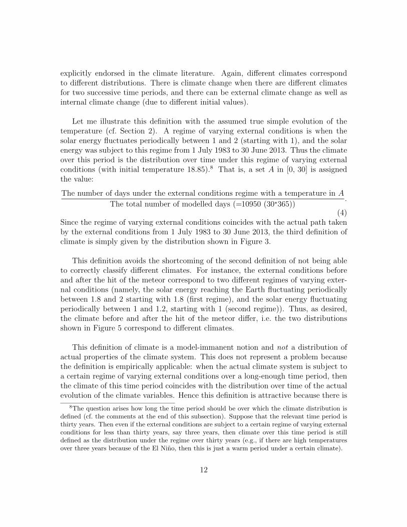
Let me illustrate this definition with the assumed true simple evolution of thetemperature (cf. Section 2). A regime of varying external conditions is when thesolar energy fluctuates periodically between 1 and 2 (starting with 1), and the solarenergy was subject to this regime from 1 July 1983 to 30 June 2013. Thus the climateover this period is the distribution over time under this regime of varying externalconditions (with initial temperature 18.85).8 That is, a set A in [0, 30] is assignedthe value:

The number of days under the external conditions regime with a temperature in A

The total number of modelled days (=10950 (30∗365)).

(4)Since the regime of varying external conditions coincides with the actual path takenby the external conditions from 1 July 1983 to 30 June 2013, the third definition ofclimate is simply given by the distribution shown in Figure 3.

This definition avoids the shortcoming of the second definition of not being ableto correctly classify different climates. For instance, the external conditions beforeand after the hit of the meteor correspond to two different regimes of varying exter-nal conditions (namely, the solar energy reaching the Earth fluctuating periodicallybetween 1.8 and 2 starting with 1.8 (first regime), and the solar energy fluctuatingperiodically between 1 and 1.2, starting with 1 (second regime)). Thus, as desired,the climate before and after the hit of the meteor differ, i.e. the two distributionsshown in Figure 5 correspond to different climates.

This definition of climate is a model-immanent notion and not a distribution ofactual properties of the climate system. This does not represent a problem becausethe definition is empirically applicable: when the actual climate system is subject toa certain regime of varying external conditions over a long-enough time period, thenthe climate of this time period coincides with the distribution over time of the actualevolution of the climate variables. Hence this definition is attractive because there is

8The question arises how long the time period should be over which the climate distribution isdefined (cf. the comments at the end of this subsection). Suppose that the relevant time period isthirty years. Then even if the external conditions are subject to a certain regime of varying externalconditions for less than thirty years, say three years, then climate over this time period is stilldefined as the distribution under the regime over thirty years (e.g., if there are high temperaturesover three years because of the El Nino, then this is just a warm period under a certain climate).

12

an immediate link to the observations.

Since this definition is promising, let me comment on a few issues (which alsoarise for Definition 1 and 2). First, there is the question over which finite time periodthe distributions should be taken. It seems promising to adopt a pragmatic approachas outlined by Lorenz (1995): The purpose of research will influence the choice ofthe time interval, e.g., if one is interested in inter-glacial climate the time period willbe relatively long. Also, the time period should be long enough so that no specificpredictions can be made (e.g., longer than the predictability horizon given by the ElNino) but short enough to ensure that changes which are conceived as climatic aresubsumed under different climates. What is important is to provide some motivationfor the chosen time period (often thirty years are chosen without any clear motiva-tion, which is problematic). Second, it should be mentioned that there will nearlyalways be climate change. Yet this does not constitute a problem: pragmaticallyone might say that of interest is only more major climate change with significantlydifferent distributions. Third, the climate depends on the initial value of the climatevariables, e.g., for the very simple model on the initial temperature. This does notspeak against this definition but implies that predicting the climate would be difficultif small changes in the initial values led to very different distributions.9

To sum up the discussion of climate as a finite distribution over time: Because ofthe assumption of constant external conditions, Definition 1 may be empirically void(thereby violating Desideratum 1). Definition 2 does not correctly classify differentclimates and thus fails to meet Desideratum 2. In contrast, Definition 3 is promisingbecause it meets all the desiderata.

4.4 Infinite Versions

There are also infinite versions of the three definitions of climate as distribution overtime discussed above. According to these infinite versions, the climate is defined bythe infinite distribution over time when the time period in equation (2) (for Definition1), equation (3) (for Definition 2) or equation (4) (for Definition 3) goes to infinity.According to the infinite version of Definition 2, the climate is the actual distributionof the climate system as time goes to infinity, which has the consequence that therecannot be climate change. Because of this, it is hardly ever adopted. The infiniteversions of Definition 1 and Definition 3, however, are widely endorsed (Dymnikovand Gritsoun 2001; Lorenz 1995; Palmer 1999).

9Note also that the climate of the true model may differ significantly from the climate of modelswhich are close to the true model (Frigg et al. 2013). While this does not speak against thisdefinition, this would make predicting the climate very difficult.

13

The main advantage of these infinite distributions is that they are mathematicallymore tractable, implying that the tools of dynamical systems theory can be used toanalyse them. For instance, recall that climate as distribution over time is definedrelative to the initial values of the climate variables. For the infinite version of Defi-nition 1 results of dynamical systems theory show that under certain conditions theclimate is the same for almost all initial values (no corresponding results are knownfor Definition 2 and Definition 3). Namely, this is the case when the dynamics isergodic or when there is a physical measure (see Appendix B for a mathematicalstatement of these results). These results are of limited relevance, however, becauseit is unclear whether the true climate model under constant external conditions isergodic or has a physical measure. What is more, as I will now argue, the infiniteversions of Definitions 1, 2 and 3 suffer from serious problems (in addition to theproblems already outlined in the Subsections 4.1-4.3). Therefore, for defining the cli-mate, finite distributions over time are preferable to infinite distributions over time(and this is the reason why the presentation above focused on finite distributions).

The first problem with these infinite versions is that the relevant infinite limitsmay not exist. More specifically, while infinite limits of equation (2) (Definition 1)usually exist (Petersen 1983), the infinite limits of equation (3) (Definition 2) andequation (4) (Definition 3) often do not exist (Mancho et al. 2013). To the best ofmy knowledge, it is an open question whether they exist for the true climate model.Hence there is the problem that the climate may not be mathematically well-defined(thereby violating Desideratum 5).10

Second, to make sure that the infinite distributions relate to the actual finite dis-tributions of the climate system, one has to assume that the distributions over finitetime periods of interest are approximated by the infinite distributions. However,there are doubts about this. For many climate models the convergence to the infinitedistributions is very slow. In particular, Lorenz (1968) introduced the notion of al-most intransitivity to describe systems where distributions taken over very long butfinite time intervals differ from one interval to each other and thus from the infinitedistribution. Lorenz (1968, 1970, 1976, 1995) gave examples of simple models that

10Furthermore, when the external conditions vary, i.e., for equation (3) (Definition 2) and equation(4) (Definition 3), there are two infinite distributions, which usually differ. More specifically, whenthe finite distributions range from time point t0 to time point t1, one infinite distribution arises fort0 → −∞ and the other for t1 → ∞ (Kloeden and Rasmussen 2011). Consequently, there is theproblem which of the infinite distributions should be identified with the climate. For the past onecan check which infinite distribution is approximated by the observed distributions. However, ifthe concern is the future, it is unclear how to choose between the two distributions. If the wrongdistribution is chosen, the climate will be empirically void (thereby violating Desideratum 1).

14

show almost intransitive behaviour. He concluded that the true climate model maywell be almost intransitive, particularly when the climate variables include the oceanvariables. Furthermore, there are several climate models that incorporate some real-ism about the evolution of the climate variables where the distributions taken overlong finite time intervals differ considerably from the infinite distributions. For in-stance, Bhattacharya et al. (1982) for an energy-balance model, Daron (2012) andDaron and Stainforth (2013) for a coupled ocean-atmosphere model and Sempf etal. (2007) for a model of the wintertime atmospheric circulation over the northernhemisphere found considerable differences between distributions taken over long fi-nite intervals and distributions in the infinite limit. It is an open question whethersimilar results hold for the true climate model, but there remains the worry that theinfinite distributions may not relate to the actual distributions of the climate systemand thus are empirically void (thereby violating Desideratum 1).

To sum up: climate as an infinite distribution over time is easier to analysemathematically. However, there are the additional problems that the relevant limitsmay not exist (thereby violating Desideratum 5) and that the definitions may beempirically void (thereby violating Desideratum 1).

5 Climate as Ensemble Distribution

5.1 Definition 4. Ensemble Distribution for Constant Exter-nal Conditions

The first three definitions of climate are distributions over time. In stark contrast tothis, the remaining two definitions are ensemble distributions of the possible values ofthe climate variables. Suppose that the concern is to make predictions at time t1 inthe future and that from the present t0 until t1 the external conditions take the formof small fluctuations around a mean value c. Then, according to the fourth definition,the climate at time t1 is the distribution of the possible values of the climate variablesat t1 under constant external conditions c conditional on our uncertainty in the initialvalues at t0. As before, different distributions correspond to different climates. Thisis a common definition (e.g., Lorenz 1995; Stone and Knutti 2010).

Let me illustrate this definition with the assumed true simple evolution of thetemperature (cf. Section 2). Suppose that the temperature is measured to be between29.77 C and 30.00 C degrees today, i.e. at t0 = 1 July 2013. Let pt0 be the uniformprobability density over [29.77, 30.00] representing this uncertainty in the initialtemperature. Further, suppose that the concern is to predict the temperature attime t1 = 1 July 2040. The amount of solar energy reaching the Earth will fluctuate

15

Figure 6: The temperature ensemble distribution on 1 July 2040 for the simple climatemodel under constant c = 1.5 given the uncertainty about the initial temperature on 1 July2013.

around the mean value c = 1.5 from 1 July 2013 to 1 July 2040. Hence the climateon 1 July 2040 is given by the distribution where the value of a set A in [0, 30] is

P ct0,t1

(A), (5)

where P ct0,t1

(A) is the value assigned to A by the density that arises when pt0 is evolvedforward to 30 June 2040 under equation (1) with at = c = 1.5 (for all t). Figure 6shows the distribution arising in this way. For instance, the value assigned to [20, 25](that the temperature will be between 20 C and 25 C) is 0.241.

Clearly, this definition is a model-immanent notion since it refers to an ensem-ble of initial conditions that is evolved forward in time but actual initial conditionsare unique. Proponents of this definition think that this model-immanent notion ispredictively useful in the following sense: What one is interested in is the actualensemble distribution at time t1, i.e. the distribution over the possible values of theclimate variables given the uncertainty in the initial values and the actual path ofthe external conditions taken by the climate system. So the assumption is madethat when the external conditions take the form of small fluctuations around a meanvalue c from t0 to t1, then the ensemble distribution at time t1 under constant externalconditions c is approximately the same as the actual ensemble distribution at time t1.

However, there are doubts about this assumption. Let me illustrate this with theassumed true simple climate model. The actual temperature ensemble distributionis shown in Figure 7. It is the distribution where the value of a set A in [0, 30] is

Pt0,t1(A), (6)

where Pt0,t1(A) is the value assigned to A by the density that arises when pt0 isevolved forward to 1 July 2040 under equation (1) given the periodic fluctuations of

16

Figure 7: The actual temperature ensemble distribution on 1 July 2040 for the simpleclimate model given the uncertainty about the initial temperature on 1 July 2013.

the solar energy at between 1 and 2 (with at = 1 on 1 July 2013). It is clear thatthe ensemble distribution for constant external conditions c = 1.5 (Figure 6) and theactual ensemble distribution (Figure 7) are very different. For instance, the valueassigned to [20, 25] (that the temperature will be between 20 C and 25 C) is 0.241for the former but 0 for the latter distribution.11

Similar results hold for several climate models. For instance, Daron (2012) nu-merically investigated the Lorenz equations where one parameter is subject to fluc-tuations around a mean value. He found that the ensemble distributions can differsignificantly from the ensemble distributions when the parameters are held fixed. Themechanism responsible for the different distributions is a resonance effect, which canalso arise for small fluctuations. Also, there is growing evidence that the inclusionof the seasonal cycle of the sun may lead to different ensemble distributions: it wasfound in Gowsami et al. (2006) for model of the monsoon, in Jin et al. (1994) for amodel of the El Nino and in Lorenz (1990) for a very simple general circulation modelthat the ensemble distributions differ when the seasonal cycle of the sun is included.It is certainly possible that similar results hold for the true climate model. Hencethere is the problem that this definition of climate may be empirically void (therebyviolating Desideratum 1). There is also the additional problem that when the exter-nal conditions are not small fluctuations around a mean value, then the definition isnot applicable. All this shows the need to take the varying external conditions intoaccount.

11Note that the actual ensemble distribution on 30 June 2040 is given by the uniform distributionover [0, 30]. Thus the ensemble distribution under constant external conditions c = 1.5 (Figure 6)is not the average of the ensemble distribution on 1 July 2040 (where at = 2) and the ensembledistribution on 30 June 2040 (where at = 1). That is, it is not the average of the ensembledistributions for the periodically fluctuating external conditions.

17

5.2 Definition 5. Ensemble Distribution when the ExternalConditions Vary as in Reality

Most directly this can be achieved by defining the climate as the actual ensembledistribution. More specifically, suppose again that the concern is to make predictionsat time t1 in the future. According to the fifth definition, the climate at time t1 isthe distribution of the possible values of the climate variables at t1 given the actualpath taken by the external conditions and conditional on our uncertainty in the initialvalues at t0. As before, different distributions correspond to different climates. Thisdefinition is widely endorsed (Daron 2012; Daron and Stainforth 2013; Smith 2002).To illustrate this definition with the assumed true simple evolution of the tempera-ture (cf. Section 2): The climate on 1 July 2040 conditional on our knowledge thatthe temperature was between 29.77 C and 30.00 C on 1 July 2013 is the ensembledistribution (6) as shown in Figure 7.

Definition 5 is again a model-immanent notion since it refers to an ensemble ofinitial conditions that is evolved forward in time but actual initial conditions areunique. This model-immanent notion is predictively very useful because it quantifiesthe likelihood of the future possible properties of the actual climate system given ourpresent uncertainty in the initial values.

However, there are several problems (which also arise for Definition 4). First ofall, climate is defined relative to our present uncertainty about the initial values. Thisimplies that the climate and the derivative notion of climate change are dependenton our knowledge and that Desideratum 3 is not met.

Second, this definition is always presented as defining the future climate. So thequestion arises what the past and present climate amount to (which are also neededto define climate change). While I have not found anything in print about this, itseems natural to say that the climate on 1 July 2013 is the distribution that scien-tists on, say, 1 July 1983 would have predicted as the climate of 1 July 2013 based ontheir uncertainty about the initial values on 1 July 1983 and the actual path takenby the external conditions.12 Climate change is then defined as the change betweenthe present and the future climate. Next to external climate change there is alsointernal climate change (because of different uncertainties in the initial values or dif-ferent prediction lead-times). In the example the climate of 1 July 2013 is definedby choosing the reference point thirty years in the past (i.e. a prediction lead-timeof thirty years), but this choice seems arbitrary. One could argue that pragmatic

12This has also been suggested by the climate scientist David Stainforth (personal communica-tion).

18

considerations as discussed in Subsection 4.3 will fix a suitable prediction lead-time,say 30 years. Yet, then the same prediction lead-time should be used when definingthe future climate. However, this is undesirable because for the future climate theprediction lead-time should only be determined by how many years scientists wantto predict in the future (and should not be constrained to, say, 30 years). So it isdifficult to see how the present and past climate could be defined. Hence Definition4 is not applicable to the past, present and future and Desideratum 4 is violated.

Third, there is the problem that climate, thus defined, does not have anythingto do with distributions over time of actual properties of the climate system (cf.Schneider and Dickinson 2000). This leaves us in the awkward situation that theobservational records of past temperatures etc. do not tell us anything about climateand climate change. Therefore, Desideratum 1 is not met.

To sum up the discussion of climate as future ensemble distribution: Because ofthe assumption of constant external conditions, Definition 4 may be empirically void(thereby violating Desideratum 1). While Definition 5 avoids this shortcoming, thereare several other problems (which also arise for Definition 4). Namely, the climatedepends on our knowledge about the initial values (thereby violating Desideratum3). Also, it is unclear how the past and present climate could be defined, and thusDesideratum 4 is not met. Finally, there is no relation to the past observations ofthe climate system, and thus Desideratum 1 is violated. Given all these problems, itseems better to say that Definition 5 is not about the climate but just refers to theexpected future distribution of the climate variables (a distribution which is usefulto consider for predictive purposes).13

5.3 Infinite Versions

There are also infinite versions of the two ensemble distributions of climate just dis-cussed. According to these infinite versions, the climate is defined as the infinitedistribution which arises when the prediction lead-time in equation (5) (for Defini-tion 4) or equation (6) (for Definition 5) goes to infinity. These infinite versions arepopular definitions (e.g. Checkroun et al. 2011; Stone et al. 2009).

The main advantage of these infinite versions is that they are mathematically moretractable, and, as a consequence, dynamical systems theory can be used to analyse

13One could also introduce an ensemble definition for regimes of varying external conditions (cor-responding to Definition 3). The need for Definition 3 arose because it avoids a serious problemencountered by Definition 2 (that different climates are not classified correctly). No problems areavoided by introducing an ensemble definition for regimes of varying external conditions (comparedto Definition 5). Hence there is no need for such a definition.

19

them. Let me give two examples for this. First, recall that climate as the future en-semble distribution is defined relative to the present uncertainty in the initial values.For the infinite versions conditions are known under which the infinite ensemble dis-tribution is the same for any arbitrary uncertainty in the initial values (then climatedoes not depend on our uncertainty and Desideratum 3 is not violated). Namely, thisis the case when the dynamics is mixing or when there is a strong physical measure(for the infinite version of Definition 4), or when there is a time-dependent strongphysical measure (for the infinite version of Definition 5) (see Appendix C for a math-ematical statement of these results). As nice as these results are, their relevance isunclear because it is unknown whether the true climate model under constant exter-nal conditions is mixing or has a strong physical measure, or whether the true climatedynamics has a time-dependent strong physical measure (cf. Daron 2012).

Second, recall that the climate as the future ensemble distribution does not seemto have anything to do with the time series of past observations. For the infiniteversion of Definition 4 it can be shown that when the dynamics is mixing or has astrong physical measure, then the infinite ensemble distribution and the infinite dis-tribution over time are the same for almost all initial conditions (note that there areno corresponding results for Definition 514). Hence if distributions over finite longtime periods approximate the distribution over an infinite time period, the infiniteensemble distribution can be estimated from the observations and Desideratum 1 isnot violated (see Appendix D for a mathematical statement of these results). How-ever, again, the relevance of these results is unclear because it is unknown whetherthe true climate model under constant external conditions is mixing or has a strongphysical measure (and whether distributions over finite long time periods approxi-mate the distributions over an infinite time period – cf. Subsection 4.4).

What speaks against the infinite versions of Definitions 4 and 5 is that they suf-fer from several shortcomings (in addition to the ones already outlined in Subsec-tions 5.1-5.2). Consequently, for defining the climate finite ensemble distributionsare preferable to infinite ensemble distributions, and for this reason the discussionabove concentrated on finite distributions. More specifically, there is the problemthat the infinite limits defining the infinite ensemble distributions may not exist, im-plying that Desideratum 5 may not be met (Lasota and Mackey 1985; Provatas andMackey 1991). To my knowledge, it is unknown whether these limits exist for thetrue climate model.15

14There cannot be any corresponding results for Definition 5: Because the external conditionsvary, the infinite ensemble distributions vary with time but the infinite distributions over time donot. Hence the infinite ensemble distributions cannot be equal to the infinite distributions over time.

15For Definition 5 where the external conditions vary (i.e. for equation (6)) there is the additionalproblem that there are two infinite limits: one for t0 → −∞ and one for t1 → ∞ (the latter limits

20

Furthermore, in order for the infinite ensemble distribution to be predictively use-ful, one has to assume that the ensemble distribution at time point t1 (what is ofconcern in practice) is approximated by the infinite ensemble distribution. However,there are doubts about this. For several models that incorporate some realism aboutthe evolution of the climate variables (including models with constant and varyingexternal conditions) the finite ensemble distributions only converge very slowly tothe infinite ensemble distributions (cf. Smith 2002). For instance, for the coupledocean-atmosphere model investigated by Daron (2012) and Daron and Stainforth(2013) there is convergence only after 100 model years. Further, if the true climatemodel turned out to be almost intransitive, the convergence could be very slow (Bhat-tacharya et al. 1982; Sempf et al. 2007). Whether for the true climate model the finiteensemble distributions for predictions lead-times of interest are approximated by theinfinite ensemble distributions is unknown, but there remains the worry that the in-finite ensemble distribution may be empirically void (thereby violating Desideratum 1).

To conclude: defining climate as an infinite ensemble distribution makes the math-ematical analysis of climate more tractable. However, there are the additional prob-lems that the relevant limits may not exist (implying that Desideratum 5 may not bemet) and that the definitions may be empirically void (implying that Desideratum 1may not be met).

6 Conclusion

The aim of the paper was to provide a clear and thorough analysis of the main candi-dates for a definition of climate and climate change. Five definitions were discussed:climate as the finite distribution of the climate variables over time for constant exter-nal conditions (Definition 1), climate as the finite distribution of the climate variablesover time when the external conditions vary as in reality (Definition 2), climate as thefinite distribution of the climate variables over time relative to a regime of varyingexternal conditions (Definition 3), climate as the ensemble distribution of the climatevariables for constant external conditions (Definition 4), and climate as the ensembledistribution of the climate variables when the external conditions vary as in reality(Definition 5). Definition 3 is a novel contribution of this paper and was proposedas a response to problems with existing definitions. The other four definitions areamong the most commonly endorsed definitions of climate.

exist only very rarely, cf. Kloeden and Rasmussen 2011). If both limits exist, they usually differ.Hence the question arises which of them should be identified with the climate, and it is unclear howto answer this question.

21

A definition of climate should be empirically applicable (Desideratum 1), it shouldcorrectly classify different climates (Desideratum 2), it should not depend on ourknowledge (Desideratum 3), it should be applicable to the past, present and future(Desideratum 4) and it should be mathematically well-defined (Desideratum 5). Thediscussion has shown that only Definition 3 (where climate is the finite distributionover time under a certain regime of varying external conditions) meets all the desider-ata and hence is the most promising definition.

This can also be seen as follows. The Definition 2 is unattractive because it doesnot classify different climates correctly (i.e., Desideratum 2 is not met). Definitionsof climate where the external conditions vary as in reality are preferable to definitionswhere the external conditions are held constant because the latter may be empiri-cally void (thereby violating Desideratum 1). Distributions over time are preferableto ensemble distributions because for the latter the climate depends on our knowledge(thereby violating Desideratum 3), it is unclear how to define the past and presentclimate (thereby violating Desideratum 4) and there is no relation to the observa-tional record (thereby violating Desideratum 1). Given this, Definition 3 comes outas the most promising definition.

Infinite versions of Definitions 1-5 were also discussed. They were quickly dis-missed since they suffer from the additional problems that they may be empiricallyvoid (thereby not meeting Desideratum 1) and that the relevant limits may not exist(thereby not meeting Desideratum 2).

Finally, we are now in the position to look at the characterisation of climate givenby the influential report of the IPCC (Solomon et al. 2007, 942):

Climate in a narrow sense is usually defined as the average weather, ormore rigorously, as the statistical description in terms of the mean andvariability of relevant quantities over a time period ranging from monthsto thousands or millions of years. The classical period for averaging thesevariables is 30 years, as defined by the World Meteorological Organiza-tion. The relevant quantities are most often surface variables such astemperature, precipitation and wind. Climate in a wider sense is thestate, including a statistical description, of the climate system.

This characterisation is vague and ambiguous. ‘Climate in a narrow sense’ may beintended to refer to the distributions of a more limited set of climate variables and‘climate in a wider sense’ to the distributions of a more extended set of climate vari-ables (cf. Section 2). Apart from this, ‘climate in a narrow sense’ seems to refer to adistribution over time, i.e. to Definition 1, 2 or 3. The most direct interpretation is

22

that it refers to the finite distribution over time for the actual path of the externalconditions (i.e. Definition 2, which, as argued, is unattractive). ‘Climate in a widersense’ is even more open to different interpretations and could in principle be inter-preted as referring to any of the definitions discussed in this paper.

In any case, the vagueness may well be intended to subsume under one charac-terisation the various different definitions of climate. Still, I hope that this paperhas raised awareness of the importance of choosing a good definition of climate. Inthis way conceptual confusion and wrong statements about our climate system canhopefully be avoided.

Appendix

A. Deterministic Models

Climate models are deterministic models (X,ΣX , T (x, t0, t)) of the evolution of theclimate variables. Here the set X represents all possible values of the climate vari-ables, the σ-algebra ΣX represents all subsets of X of interest, and T (x, t0, t) :X × Z × Z → X (the dynamics) is a measurable function such that T (x, t0, t0) = xand T (x, t0, t + s) = T (T (x, t0, t), t, s) for all t0, t, s and x.16 Intuitively speaking,T (x, t0, t) gives one the value of the climate variables at time t when x is the valueat time t0. The solution when x is the initial value of the climate variables at t0is the function Tx,t0(t) : Z → X, Tx,t0(t) = T (x, t0, t). These deterministic modelsare time-dependent, and the recently developed theory of time-dependent dynamicalsystems is needed to analyse them (cf. Kloeden and Rasmussen 2011).

If the governing equations do not depend on time, the models are time-independentand one is in the realm of classical dynamical systems theory. Then the referenceto t0 can be omitted because all that matters is the evolved time period t betweentwo values of the climate variables. That is, the solution through x is the functionTx(t) = T (x, t), where T (x, t) gives the value of the climate variables that started inx after t time steps. Suppose that the functions Tt : X → X, Tt(x) = T (x, t), arebijective for all t and that there is a probability measure µ on X which is invariant,i.e.

µ(T (A, t)) = µ(A) for all A ∈ ΣX and all t ∈ Z. (7)

Then (X,ΣX , T (x, t), µ) is a measure-preserving deterministic model (cf. Petersen1983).

16If T (x, t0, t) is defined only on X×Z×Z∩[t0,∞), then the dynamics is non-invertible (as opposedto the usual case in climate science when the dynamics is invertible, i.e. defined on X ×Z×Z). Allthat is stated in the Appendix can be easily adapted to carry over to a non-invertible dynamics.

23

B. Independence from the Initial Conditions for the InfiniteVersion of Definition 1

For the infinite version of Definition 1 there are two cases where the dependence on theinitial conditions is very weak (thus many argue that, pragmatically speaking, thereis no dependence – cf. Lorenz 1970, 1995). First, a measure-preserving deterministicmodel (X,ΣX , T (x, t), µ) is ergodic iff for all A ∈ ΣX

limk→∞

1

k

k−1∑t=0

χA(Tt(x)) = µ(A) (8)

for any x ∈ B with µ(B) = 1 (cf. Petersen 1983).17 Ergodicity immediately impliesthat the value assigned to any set A by the infinite version of Definition 1 is the samefor almost all x (i.e. those in B).

The second result is about attractors Ω which are invariant18 sets Ω ⊆ X ⊆ Rn

that attract all initial values in X, i.e., limt→∞ dist(Tt(x),Ω) = 0 for all x ∈ X. Ameasure µΩ on Ω is called a physical measure iff for Lebesgue-almost all19 x ∈ X

limk→∞

1

k

k−1∑t=0

χA(Tt(x)) = µΩ(A), (9)

whenever µΩ(δA) = 0 where δA denotes the boundary of A (cf. Eckmann and Ruelle1985; Ruelle 1976). Hence for a physical measure the value assigned to any A ∈ ΣX

with µΩ(δA) = 0 by the infinite version of Definition 1 is the same for Lebesgue-almostall initial values.

C. Independence from the Uncertainty in the Initial Valuesfor the Infinite Versions of Definitions 4 and 5

The independence result for the infinite version of Definition 4 holds under two con-ditions. First, a measure-preserving deterministic model (X,ΣX , T (x, t), µ) is mixingiff for all probability densities pt0 (relative to µ) and all sets A ∈ ΣX (Petersen 1983;Werndl 2009a; Werndl 2009b):20

limt1→∞

P ct0,t1

(A) = µ(A). (10)

17χ(A) is the characteristic function, i.e. χ(x) = 1 for x ∈ A and 0 otherwise.18That is, Tt(Ω) = Ω for all t ∈ Z.19That is, for all x ∈ Y , Y ⊆ X, with λ(X \ Y ) = 0, where λ is the Lebesgue measure.20Since all that matters is the evolved time period, the limit could equally be taken for t0 → −∞.

24

Mixing immediately implies that the measure assigned to a set by the infinite versionof Definition 4 is the same for all initial densities pt0 and hence there is no dependenceon the uncertainty.21

Second, a measure µΩ on the attractor Ω is called strongly physical iff for anydensity pt0 (relative to the Lebesgue measure λ) on X and for any set A ∈ ΣX :22

limt1→∞

P ct0,t1

(A) = µΩ(A), (11)

whenever µΩ(δA) = 0 where δA denotes the boundary of A (cf. Ruelle 1976; Tasakiet al. 1998). Here the dependence on the uncertainty in the initial values is negligiblein the sense that the measure assigned to any A with µΩ(δA) = 0 by the infiniteversion of Definition 4 is the same for all initial uncertainties.

The independence result for the infinite version of Definition 5 holds when t1 →∞23 and when there are time-dependent strong physical measures. To define them,the following definition is needed. A pullback attractor Ω ⊆ Z × Rn is an invariantset24 where for all initial values x ∈ X

limt0→−∞

dist(T (x, t0, t),Ω(t)) = 0. (12)

Time-dependent strong physical measures µΩt defined on Ω(t), t ∈ Z, where Ω is a

pullback attractor are defined by the condition that for any t and t0, any initialdensity pt0 (relative to the Lebesgue measure λ) on X and for any set A ∈ ΣX (cf.Buzzi 1999):

limt0→−∞

Pt0,t1(A) = µΩt (A), (13)

whenever µΩt (δA) = 0 (δA denotes the boundary of A). Hence for time-dependent

strong physical measures the dependence on the uncertainty is negligible because themeasure assigned to a set A with µΩ

t (δA) = 0 by the infinite version of Definition 5is the same for all initial uncertainties.

21One might ask when the stronger condition holds that any initial probability density pt0 con-verges to the measure µ in the sense that limt1→∞

∫X|1− pct0,t1 |dµ = 0, where pct0,t1 is the density

that arises when pt0 is evolved forward to t1. Most climate models are invertible (cf. footnote 16).In this case the stronger condition cannot hold because the measure is invariant. For non-invertiblemodels (X,ΣX , T (x, t), µ) this condition holds iff they are exact, i.e. when limt→∞ µ(T (A, t)) = 1for all A ∈ ΣX with µ(A) > 0 (Berger 2001; Lasota and Mackey 1985). Exactness is a strongercondition than mixing. It is unclear whether realistic non-invertible climate models are exact.

22Since all that matters is the evolved time period, the limit could equally be taken for t0 → −∞.23Recall that there are two possible infinite limits for the infinite version of Definition 5 (cf.

footnote 15).24That is, Ω(t) = T (Ω(t0), t0, t) for all t, t0 ∈ Z, where Ω(t) := x ∈ Rn | (t, x) ∈ Ω.

25

D. Relation to Infinite Distributions Over Time for the Infi-nite Version of Definition 4

For the infinite version of Definition 4 two conditions are known which relate infi-nite ensemble distributions to infinite distributions over time. First, if the measure-preserving deterministic system (X,ΣX , T (x, t), µ) is mixing, equations (10) and (8)imply that for any initial probability density pt0 and any set A ∈ ΣX

limt1→∞

P ct0,t1

(A) = µ(A) = limk→∞

1

k

k−1∑t=0

χA(Tt(x)) (14)

for all initial values x ∈ B with µ(B) = 1. Hence the measure assigned to a set A bythe infinite ensemble distribution and the infinite distribution over time is the samefor almost all initial values (i.e. those in B).

Second, for an attractor Ω with a strong physical measure µΩ equations (11) and(9) imply that for any initial density pt0 , any set A with µΩ(δA) = 0 and Lebesgue-almost all initial values x ∈ X:

limt1→∞

P ct0,t1

(A) = µΩ(A) = limk→∞

1

k

k−1∑t=0

χA(Tt(x)). (15)

Hence the measure assigned to a set A with µΩ(δA) = 0 by the infinite ensembledistribution and the infinite distribution over time is the same for Lebesgue-almostall initial values.

Acknowledgements

Many thanks to Mickael Checkroun, Stefaan Willem Conradie, Joseph Daron, Ro-man Frigg, Gary Froyland, Casey Helgeson, Wendy Parker, Leonard Smith, DavidStainforth, Erica Thompson and audiences at the CHESS Seminar at the Universityof Durham and the “Managing Severe Uncertainty”-Meetings at the London Schoolof Economics for valuable discussions and suggestions. Funding support for the re-search was provided by the Arts and Humanities Research Council and by the ESRCCentre for Climate Change Economics and Policy, funded by the Economic and So-cial Research Council.

26

References

Allen, M. (2003). Liability for climate change. Nature 421, 891-892.

Berger, A. (2001). Chaos and Chance. An Introduction to Stochastic Aspects ofDynamics. Berlin: Walter de Gruyter.

Bhattacharya, K., Ghil, M. and Vulis, I. L. (1982). Internal variability of an energy-balance model with delayed albedo effects. Journal of the Atmospheric Sciences39, 1747-1773.

Buzzi, J. (1999). Exponential decay of correlations for random Lasota-Yorke maps.Communications in Mathematical Physics 208, 25-54.

Checkroun, M. D., Simonnet, E. and Ghil, M. (2011). Stochastic climate dynamics:Random attractors and time-dependent invariant measures. Physica D, 240 (21),1685-1700.

Daron, J. D. (2012). Examining the Decision-Relevance of Climate Model Informa-tion for the Insurance Industry. Doctoral Thesis. London School of Economicsand Political Science. http://etheses.lse.ac.uk/380/

Daron, J. D. and Stainforth, D. (2013). On predicting climate under climate change.Environmental Research Letters 8, 1-8.

Dymnikov, V. and Gritsoun, A. (2001). Atmospheric model attractors: chaoticity,quasi-regularity and sensitivity. Nonlinear Processes in Geophysics 8, 201-208.

Eckmann, J.-P. and Ruelle, D. (1985). Ergodic theory of chaos and strange attractors.Reviews of Modern Physics 1985, 617-656.

Frigg, R., Bradley, S., Du, H. and Smith, L. A. (2013). Laplace’s demon and climatechange. Grantham Research Institute on Climate Change and the EnvironmentWorking Paper 103, London School of Economics.

Goswami, B. N. Wu, G. and Yasunari, T. (2006). The annual cycle, intraseasonaloscillations, and roadblock to seasonal predictability of the Asian summer mon-soon. Journal of Climate 19, 5078-5099.

Hasselmann, K. (1976). Stochastic climate models, Part 1. Tellus XXVIII (6), 473-484.

Hulme, M., Dessai, S., Lorenzoni, I. and Nelson, D. (2009). Unstable Climates:exploring the statistical and social constructions of climate. Geoforum 40, 197-206.

27

Jin, F.-F., Neelin, J. D., and Ghil, M. (1994). El Nino on the devil’s staircase: annualsubharmonic steps to chaos. Science 264, 70-72.

Kloeden, P. E. and Rasmussen, M. (2011). Nonautonomous Dynamical Systems.Mathematical Surveys and Monographs Volume 176. American MathematicalSociety.

Kurgansky, M. V., Dethloff, K., Pisnichenko, I. A., Gernandt, H., Chmielevski, F.-M. and Jansen, W. (1996). Long term climate variability in a simple, nonlinearatmospheric model. Journal of Geophysical Research 101 (D2), 4299-4314.

Lasota, A. and MacKey, M. C. (1985). Probabilistic Properties of DeterministicSystems. Cambridge: Cambridge University Press.

Lorenz, E. (1963). Deterministic nonperiodic flow. Journal of Atmospheric Sciences20, 130-141.

Lorenz, E. (1968). Climatic determinism. Meteorological Monographs 8, 1-3.

Lorenz, E. (1970). Climatic change as a mathematical problem. Journal of AppliedMeteorology 9 (3), 325-329.

Lorenz, E. (1976). Nondeterministic theories of climatic change. Quaternary Re-search 6 (4), 495-506.

Lorenz, E. (1995). Climate is what you expect. Prepared for publication by NCAR.Unpublished, 1-33.

Mancho, A. M., Wiggins, S., Curbelo, J. and Mendoza, C. (2014). Lagrangian de-scriptors: a method for revealing phase space structures of general time depen-dent dynamical systems. Forthcoming in: Communications in Nonlinear Scienceand Numerical Simulation.

Palmer, T. (1999). A nonlinear dynamical perspective on climate prediction. Journalof Climate 12, 575-591.

Parker, W. (2006). Understanding pluralism in climate modeling. Foundations ofScience 11, 349-368.

Provotas, N. and Mackey, M. C. (1991). Asymptotic periodicity and banded chaos.Physica D 53, 295-318.

Petersen, K. E. (1983). Ergodic Theory. Cambridge: Cambridge University Press.

Ruelle, D. (1976). A measure associated with Axiom A attractors. American Journalof Mathematics 98, 619-654.

28

Schneider, S. H. and Dickinson, R. E. (2000). Climate modelling. Climatic Change45, 203-221.

Sempf, M., Dethloff, K., Handorf, D., Kurgansky, M. V. (2007). Toward understand-ing the dynamical origin of atmospheric regime behavior in a baroclinic model.Journal of the Atmospheric Sciences 64, 887-904.

Smith, L. (2002). What might we learn from climate forecasts. Proceedings of theNational Academy of Sciences of the United State of America 99 (1), 2487-2492.

Solomon, S., Qin, D., Manning, M., Chen, Z., Marquis, M., Averyt, K. B., Tingor,M. and Miller, H. L. (2007). Climate Change 2007: The Physical Science Basis.Contribution of Working Group I to the Fourth Assessment Report of the In-tergovernmental Panel on Climate Change. Cambridge: Cambridge UniversityPress. (IPCC Report)

Steele, K. and Werndl, C. (2013). Climate Models, calibration and confirmation. TheBritish Journal for the Philosophy of Science 64 (3), 609-635.

Stone, D. A. and Knutti, R. (2010). Weather and climate. In: Fung, F., Lopez, A.and New, M. (eds), Modelling the Impact of Climate Change on Water Resources.Chichester: John Wiley & Sons.

Stone, D. A., Allen, M. R., Stott, P. A., Pall, P., Min, S.-K., Nozawa, T. and Yuki-moto, S. (2009). The detection and attribution of human influence on climate.The Annual Review of Environment and Resources 34, 1-16.

Stott, P. A. and Kettleborough, J. A. (2002). Origins and estimates of uncertaintyin predictions of twenty-first century temperature rise. Nature 416, 723-305.

Tasaki, S., Gilbert, T. and Dorfman, J. R. (1998). An analytical construction of theSRB measures for baker-type maps. Chaos 8, 424-444.

Todorov, A. V. (1986). Reply. Journal of Applied Climate and Meteorology 25,258-259.

Werndl, C. (2009a). What are the new implications of chaos for unpredictability?The British Journal for the Philosophy of Science 60, 195-220.

Werndl, C. (2009b). Justifying definitions in mathematics – going beyond Lakatos.Philosophia Mathematica 17, 313-340.

29