Empir EconDOI 10.1007/s00181-008-0231-0

ORIGINAL PAPER

Self-selection bias in estimated wage premiumsfor earnings risk

Bas Jacobs · Joop Hartog · Wim Vijverberg

Received: 15 January 2006 / Accepted: 15 May 2008© The Author(s) 2008. This article is published with open access at Springerlink.com

Abstract This note develops a simple occupational choice model to examine threetypes of selection biases that may occur in empirically estimating the premium foruncertain wages. Individuals may select themselves into risky (wage-uncertain) jobsbecause they have (1) lower risk aversion, or (2) lower income risks, or (3) higherindividual ability. We show that (1) gives no bias, (2) biases the OLS estimate of therisk-premium in a wage regression upward, and (3) yields a bias that analytically maybe positive or negative, but empirically is more likely to be negative if our occupationalchoice model is correct.

Keywords Wages · Earnings risk · Selectivity bias

JEL Classification J31 · C24

Comments from two anonymous referees are gratefully acknowledged. The sequence of the authors’names was determined by a dice rolled by Mrs. Hartog.

B. JacobsErasmus Universiteit Rotterdam, Rotterdam, The Netherlandse-mail: bjacobs@few.eur.nl

J. Hartog (B)Department of Economics, Universiteit van Amsterdam,Roeterstraat 11, 1018 WB Amsterdam, The Netherlandse-mail: j.hartog@uva.nl

W. VijverbergUniversity of Texas at Dallas, Dallas, USAe-mail: wvijverberg@gc.cuny.edu

123

B. Jacobs et al.

1 Introduction

A modest literature acknowledges the fact that individuals contemplating an investmentin an education–occupation career trajectory are unable to make a perfect predictionof the associated wage because they face a distribution of wages rather than a singlewage rate after they complete a given education. This literature seeks to test the hypo-thesis of compensation for the differences in variability of wages within occupationsand/or educations, as the premium that has to be paid to overcome individuals’ riskaversion, a hypothesis already discussed by Smith (1776/1976, p. 208). In thesemodels, individual wages are regressed on measures of income risk, typically theresidual variance of wages, within occupations or educations (King 1974;McGoldrick 1995; McGoldrick and Robst 1996; Feinberg 1981). A series of recentpapers confirms the basic finding that wages are higher in occupations/educationswhere the variance of wages is greater (Hartog et al. 2003; Hartog and Vijverberg2007; Diaz Serrano et al. 2003; Diaz Serrano and Hartog 2006; Christiansen andNielsen 2002).

To be more precise, the model is commonly estimated in two stages. The first stage isa standard Mincer earnings equation where wages are regressed on experience (linearand squared), demographic characteristics and regional variables as well as a fixedeffect that captures common factors across wage workers grouped by education and/oroccupation, i.e., groups that face the same wage risk. The residuals from this equationthen yield group-specific measures of earnings uncertainty, typically the variance.1 Inthe second stage, variance is added to the regression equation. Theory predicts thatvariance has a positive effect on wages, as potential students require compensation forrisk. Estimates for seven countries so far all confirm this prediction, at high levels ofsignificance. Roughly, the estimates indicate an increase in expected income by some1 to 4% for an increase in risk (variance) of 10%.

The results in the papers cited above are commonly criticised for ignoring selectivityproblems. Indeed, the simple two-stage model faces three problems that may bias theestimated regression coefficient as a measure of risk aversion. First, evidence suggeststhat risk attitudes differ among individuals (Hartog et al. 2002; Dohmen et al. 2006).Unlike related literature that estimates a single coefficient of risk aversion, we willreflect on the implication of heterogeneous risk attitudes.

Second, it is quite possible that the earnings risk of an education differs amongindividuals. Cunha et al. (2005) claim that 60% of variability in returns to education isforecastable at the individual level and, hence, is related to individual heterogeneity,leaving 40% for risk. The reason could be that some individuals may by their naturebe very targeted and organised, others may take life less as a controlled operation;and just as some individuals may be very accurate in manual activities, while othershave larger dispersion in their performances, in the same way dispersion in mentalactivities may vary between individuals (see also Hartog 2002). We therefore believethat it is quite relevant to analyze the implications of selection on individual-specificrisk on estimated risk premiums in wages.

1 The literature also considers skew, but that is beyond the scope of this paper.

123

Self-selection bias in estimated wage premiums for earnings risk

Third, individuals differ in ability: variation in a wide array of abilities amongindividuals is well documented.2 If individuals know their abilities, but the researcherdoes not, correction for selectivity bias is in order. However, it may be that individualsare no better informed and can only assess the relevant distribution of earnings fromobserving workers already active in an occupation, without adjustment for ability.3

Thus, one may argue over the extent to which individuals are informed about their ownabilities. We will therefore analyse both the case where individuals are fully ignoranton their ability and the case where they are fully informed.

Under the assumption that there are no selection problems, the OLS estimatorindeed correctly estimates the true economic price of risk. With selection of indivi-duals in risky jobs, we can no longer be sure that this is the case. This note shows,using a simple occupational choice model, that the OLS estimate is unbiased underselection on risk aversion. OLS estimates are biased upward if selection on incomerisks is important. If both income risk and risk aversion differ among individuals, wecannot recover structural parameters from a single wage equation, but we can give aprecise interpretation of the estimated coefficient. Under heterogeneity in unobservedability, the bias in OLS estimates is ambiguous, and we revert to simulation with rea-sonable parameter values. The next three sections derive these results. The last sectionconcludes.

2 Modeling the risk premium under selectivity

Individuals can choose between two types of jobs. There is a safe job without wageuncertainty where individual n earns ws

n . Alternatively, there is a risky job whereindividual n earns wr

n = wrn +εn , where wr

n is the expected wage and εn is the randomcomponent, with mean zero and variance σ 2

εn , independent from wrn . The expected

wage is what the individual expects to earn on the basis of known skills and abilities;he can infer it from the wages of individuals with the same observable skills andabilities as he has. The random component reflects risks inherent in fluctuations indemand and supply conditions, unknown specifics of future employment, inherentrandomness in individual performance and randomness due to aptitudes and abilitiesthat the individual does not know when choosing a job (or, in the broader context, aneducation; see also Levhari and Weiss 1974).

There is a continuum of individuals indexed n ∈ [n,∞), n > 0, who may differin three dimensions: risk aversion ρn , variance of earnings in the risky job σ 2

εn andexpected wages in risky work wr

n . These characteristics are assumed to be uncorrelated

2 Chen (2008) and Chen and Khan (2007) correct for selectivity bias when estimating the risk associatedwith an education.3 Dominitz and Manski (1996) show that students in the U.S. are highly uncertain about the benefits gainedfrom an education. Wolter (2000) reports the same result for Swiss students. Hartog and Webbink (2004)report that first-year students can predict mean salaries by education but they cannot predict their ownstarting salary after graduation, four years ahead: the correlation between an individual’s prediction and therealisation is 0.06. The degree to which individuals are not informed about their abilities represents risk allthe same.

123

B. Jacobs et al.

with the random component εn of the wage at the risky job, which indeed is consistentwith our characterization of εn .

Assuming that utility is a mean-variance function, selection by maximum expectedutility implies4 that we can write for the marginal individual (denoted by an asterisk)

wr∗ − 1

2ρ∗σ ∗2

ε = ws∗. (1)

If all individuals would be identical in ability, risk and risk attitude, we could dropthe asterisk. A competitive market would establish a wage differential between thesafe and the risky job equal to one half of the variance in risky wages weighted by thecoefficient of risk aversion, an application of the standard model for risk compensation(e.g., Gollier 2001, 19–20). This is essentially the model underlying the estimates ofrisk compensation referred to in the introduction. Under those conditions OLS yieldsan unbiased estimate of the coefficient of risk aversion (i.e., the price of risk). In thistwo-sector specification, it is estimated as twice the wage gap divided by the variancein the risky sector. The variance is an unbiased estimator of risk, as it is identical foreveryone and observations are not blurred by selectivity. Allocation of individuals tosectors is arbitrary, as they yield identical expected utility.

Extension to the case where individuals only differ in risk attitude is straightforward.If individuals are identical in all dimensions except risk aversion risk aversion of themarginal individual ρ∗ is defined by

ρ∗ = wr − ws

12σ 2

ε

. (2)

All individuals with ρn > ρ∗ will not choose the risky job and all individuals withρn < ρ∗ will. The expected market wage in the risky job should just compensate themarginal worker and will be equal to

wr = ws + 1

2ρ∗σ 2

ε , (3)

and the observed variance of wages in the risky job equals

V [wr |ρn < ρ∗] = E[(

wr − E[wr |ρn < ρ∗])2 |ρn < ρ∗] = σ 2ε , (4)

as all individuals have the same risk. Hence, the OLS estimate for the risk-premium12ρ∗ is consistent and unbiased.

We have specified the earnings function in terms of wages, whereas it is conventionalin empirical work to specify a function for log wages. However, the only widelyaccepted theoretical underpinning, Mincer’s human capital model, only applies forvariables reflecting investment (years of schooling, experience). For other variables it

4 This follows from a second-order Taylor approximation for a standard utility function, see Varian (1978)and Hartog and Vijverberg (2007).

123

Self-selection bias in estimated wage premiums for earnings risk

is not at all obvious that the relationship with wages should be logarithmic. In practice,labour supply may react to absolute wage differences at the low end of the scale andto relative differences at the high end. Blue-collar and low pay service worker, oftenpaid on an hourly basis, tend to measure, perceive and evaluate wage differences ineuro’s (or dollars). For workers at the high end, differences tend to be evaluated at arelative (percentage) scale. This suggests that somewhere along the line, the underlyingrelevant scale for labour supply behaviour switches from absolute to relative. Withrespect to risk attitude, there is a similar ambivalence. Absolute risk aversion leads torisk compensation in euro’s, relative risk aversion leads to relative compensation. Inthe formal development of our argument, we specify an earnings function in wages.In the qualitative sense (positive, negative or ambiguous bias) our analysis also holdsfor a logarithmic wage function. In the Appendix, we formally derive a logarithmicmodel that is fully equivalent to our model in the main text; according to that model, allour conclusions hold provided we interpret the coefficient of risk aversion as relativerather than absolute

Throughout this paper, we discuss issues in terms of risk averse individuals. Howe-ver, the model is perfectly general, and also covers risk loving. Career choices basedon a taste for risk are certainly conceivable. In the empirical work, positive estimatesfor ρ are the rule and we take risk aversion to be the normal case.

3 Selection on income risk

Now consider the case in which risk in the risky job, σ 2εn , differs between individuals.

Ex ante, this is a risk; ex ante, individuals know the dispersion of the distributionrelevant to them and base their occupational choice on it. Ex post, they will be paidaccording to performance that is random. Individuals are equal in all other respects,i.e., ws

n = ws, wrn = wr , and ρn = ρ. In this case, the degree of income risk for the

marginal individual equals

σ ∗2ε = wr − ws

12ρ

(5)

Individuals with σεn > σ ∗ε will not take the risky job and workers with σεn < σ ∗

ε do.Wage realisations in the risky job will vary because of different risk. The variance ofobserved wages will reflect the mean variance of individuals who have selected intothe risky job, which is lower than the risk for the marginal worker. The market willcompensate the marginal worker in the risky job, at a price 1

2ρ. Since the observedwage variance is an underestimate of the risk that the marginal worker faces, too muchof the wage gap between the safe and the risky job is allocated to risk aversion—as(5) indicates, dividing the estimated wage gap by the underestimated variance yieldsan overestimate of risk aversion. The magnitude of the overestimation will depend onthe underestimation of risk, that is, on the relation between marginal and average risk.This will depend on the distribution function of risk and the number of individualsselecting the risky job.

123

B. Jacobs et al.

For example, consider the case where risk follows a normal distribution truncatedat 0, i.e., where σε ∼ N+ (

µ, θ2). Under this assumption, the bias increases with the

level of threshold risk (i.e., marginal risk σ ∗ε ) and may increase or decrease with the

dispersion θ of risk across individuals. Defining v∗ = (σ ∗ε −µ)/θ and v0 = −µ/θ , and

denoting the standard normal probability density and cumulative distribution functionswith φ () and � () respectively, the mean observed risk equals,

E[σε|σε < σ ∗

ε

] = µ − θφ (v∗) − φ

(v0

)

�(v∗) − �(v0

) ≡ µ − θλ. (6)

Define the degree of underestimation (or bias) of risk as the difference between thethreshold risk5 and mean risk:

D = σ ∗ε − E

[σε|σε < σ ∗

ε

] = σ ∗ε − µ + θλ (7)

Note that λ > (<)0 as v∗ > (<)−v0, or σ ∗ε > (<) 2µ. Because of this, the spread of

risk among the population has an ambiguous impact on the bias. Furthermore, applyingL’Hôpital’s Rule shows that D goes to 0 when σ ∗

ε converges to 0, the smallest valueit could have. Moreover,

∂ D

∂σ ∗ε

= 1 − v∗λ − λ2 − (v∗ + λ) φ(v0

)

�(v∗) − �(v0

)

= V[σε|σε < σ ∗

ε

]

θ2 + E[σε|σε < σ ∗

ε

]

θ

φ(v0

)

�(v∗) − �(v0

) > 0 (8)

The slope as represented on the first line is difficult to evaluate but it may be written asthe scaled sum of the conditional variance of σε, which is positive, and the conditionalmean of σε, which is positive as well. Thus, D rises from 0 as σ ∗

ε grows: the higherthe upper bound, the larger the difference between the bound and the conditionalmean. In our application, this means that the underestimation of risk and hence, theoverestimation of risk aversion, increases with an increase in the dispersion of riskand with an increase in marginal risk.6

If individuals also differ in risk aversion, the situation is more complicated. Now,there is no longer a single marginal worker, but a set of marginal workers, definedby the condition that the product of risk and risk aversion be equal to twice the wagegap: 1

2

(ρσ 2

ε

)∗ = (wr − ws). A marginal worker may have a large risk aversion and alow income risk, or a low risk aversion and a large income risk. Structural parametersof interest are now the parameters of the joint distribution of risk and risk aversion,

5 We use threshold risk as the benchmark, as this is the relevant parameter in our case: the market woulddetermine the price of risk ρ as the wage gap per unit of risk for the marginal worker.6 A truncated normal distribution allows for a nonnegligible number of jobs with near-zero risk, whichmay be realistic since zero-risk jobs are present as well. Alternatively, one might assume that σε followsa lognormal distribution, without truncation and therefore in essence without job with near-zero risk. Thisleads to the same results, since σε < σ∗

ε implies ln σε < ln σ∗ε and thus the relationship between D and σ∗

εis a nonlinear but monotonic transformation of the case just examined here.

123

Self-selection bias in estimated wage premiums for earnings risk

and they can never be estimated from a single wage regression. The best we can hopefor is an estimate of the threshold contour, and a decomposition of this threshold incombinations of risk aversion and risk at the margin.

Formally, workers will take a risky job as long as E[wr

n

]> ws

n + 12ρnσ 2

εn . SinceE

[wr

n

] = wrn, w

rn = wr and ws

n = ws , we find that for the marginal worker wr =ws + 1

2

(ρσ 2

ε

)∗. Any worker for whom ρnσ 2

εn < 2 (wr − ws) = (ρσ 2

ε

)∗will select

into a risky job. For the mean of the observed wages, that is, the wages of those whoselect into risky jobs, we have:7

E[wr |ρσ 2

ε <(ρσ 2

ε

)∗] = wr + E[ε|ρσ 2

ε <(ρσ 2

ε

)∗]

= wr + Ecρ,σ 2

ε

[Eε

[ε|ρσ 2

ε <(ρσ 2

ε

)∗]] = wr (9)

since ε is independent of ρ and σ 2ε . This means that the estimated wage gap between

the risky and the safe job is an unbiased estimate of the threshold for entering therisky job. But we cannot divide by a single estimate of risk to get a single estimate ofmarginal risk aversion. All combinations of risk and risk aversion that multiply to thethreshold value are permissible. With heterogeneity in risk, the observed variance inthe risky job is the mean value of risk for all those individuals who have chosen therisky job:

V(wr |ρσ 2

ε <(ρσ 2

ε

)∗) = E

[(wr − E

[wr |ρσ 2

ε <(ρσ 2

ε

)∗])2 |ρσ 2ε <

(ρσ 2

ε

)∗]

= E[ε2|ρσ 2

ε <(ρσ 2

ε

)∗] = Ecρ,σ 2

ε

[σ 2

ε

](10)

again since ε is independent of ρ and σ 2ε , and where the last expectation is conditional

on being in the range ρσ 2ε <

(ρσ 2

ε

)∗.

Equations (9) and (10) provide an interpretation of the regression coefficient: it isthe highest degree of risk aversion among those in a risky job who face a level of riskequal to the average among all workers who hold risky jobs. One may debate whetherthis is interesting information, or whether one would rather uncover the mean riskaversion among the population or the mean risk aversion among risky job holders orthe maximum admitted value of risk aversion at the population mean risk. But the factof the matter is that the truly interesting parameters are those of the joint distributionof risk and risk aversion, and they can not be recovered from a single wage regression.To search for answers in this regard, a more elaborate model and a more extensivedataset are needed.

7 A subscript on the E operator denotes the random variable over which the expectation is taken. Thesuperscript c denotes a conditional expectation.

123

B. Jacobs et al.

4 Differences in ability

What is the impact of unobserved abilities on estimated risk premiums? As theintroduction indicated that full information is not necessarily the correct assumption,let us start by assuming that individuals do not know their exact ability in the risky jobbut rather only the distribution from which their performance will be drawn. We willassume identical risk attitudes and equal ability in the safe job: ρn = ρ,ws

n = ws .Moreover, risk is also identical: σ 2

εn = σ 2ε , where as always σ 2

εn refers to the varianceof the random income component εn .

Assume an individual’s expected wage in the risky job is given by the sum of acommon wage component ωr and individual ability an , where an is a draw from adistribution with mean 0 and variance σ 2

a :

wrn ≡ ωr + an . (11)

Thus, an individual’s ability an matters only for the risky job.8 As before, the observedwage is determined by wr

n = wrn + εn . As noted, we will assume that all individuals

face identical risk, reflected in the variance σ 2ε . Now, clearly, individuals will only

be observed in the risky job if they are compensated for the ability risk as well. Asindividuals are identical in every aspect except for unknown ability an , the expectedrisky wage equals E

[wr

n

] = ωr for all n, which contains no reference to an . As aresult, the equilibrium wage differential is determined by the equation

E[wr ] − ws = 1

2ρ

(σ 2

a + σ 2ε

), (12)

assuming ability an and risk εn are uncorrelated. The variance in the safe job is zero,the variance in the risky job is σ 2

a + σ 2ε , and this is exactly what individuals demand

compensation for: regressing wages on variances identifies ρ, the price of risk. Hence,the estimate for ρ is unbiased. In our reading, an represents the type of risk Smith wasconcerned about: “The probability that any particular person shall ever be qualifiedfor the employment to which he is educated is very different in different occupa-tions. … In a profession where twenty fail for one that succeeds, that one ought togain all that should have been gained by the unsuccessful twenty” (Smith 1776/1976,p. 208).

If individuals know their ability but the researcher does not, we must address theselectivity process. We might consider the situation where ability differences takeeffect as constant advantage: both ws

n and wrn vary across individuals but with constant

productivity advantage between risky and safe jobs: wrn −ws

n = c. Analytically, this isnot a very interesting case, since, with productivity gap, risk aversion and risk fixed andidentical for every individual, there is no mechanism to establish an equilibrium, sinceρσ 2

ε /2 may always be less than or greater than c. Moreover, constant (or absolute)

8 Technically, this unknown ability cannot possibly impact the productivity at a risk-free job. With unknownability, the job would not be risk-free anymore. On the other hand, if an impacts the safe job, making itrisky to the degree of σ 2

a makes no difference to the conclusion drawn from this case that ρ is estimatedwithout bias, as is evident from Eq. (12), appropriately modified.

123

Self-selection bias in estimated wage premiums for earnings risk

advantage is unlikely to hold in practice (Cunha et al. 2005; Willis and Rosen 1979).Hence, we will not elaborate this case.

More interesting and relevant is the case of varying advantage where wsn is identical

for all individuals, and wrn reflects an advantage in the risky job that depends on ability:

the productivity gap is individual-specific.9 Let us assume that individuals only differ intheir ability to earn incomes; everyone has equal risk aversion, ρn = ρ, and equal risk,σ 2

εn = σ 2ε . Individuals again choose their sector based on expected wages, allowing for

differences in risk. The marginal worker will be indifferent, and hence, the marginalworker in the risky job is defined by

w∗ = ws + 1

2ρσ 2

ε . (13)

Individuals with expected wage wrn < w∗ will take the safe job; individuals with

wrn > w∗ will take the risky job. There will not be a separate risk premium established

by supply reactions, as in the standard case of compensating wage differentials. Rather,the risk premium will be covered by the ability rent: only individuals with an expectedwage gain high enough to cover the required risk premium will opt for the riskyjob.

If we are able to control completely for all relevant ability, the parameters are allidentified. This, of course, gives panel data estimation an advantage over estimationfrom cross-section data.10 Residual variance identifies risk. Thus, after controlling forability and hence accounting for wr

n − ws , a regression of wages on residual varianceshould find no effect, since the difference has expected value zero and is unrelated toits variance. Applying a selectivity correction would make no difference in this case,as all wage differences between the two jobs are accounted for by observed abilitydifferences (i.e., the variables explaining the gap between wr

n and ws). However, theprice of risk ρ is identified from the selection equation (13).

In the case where we cannot control for ability and cannot control for the selectionprocess, the observations on wages and variances combine heterogeneity and riskeffects. For individuals in risky jobs, let wr

n once again be defined by (11) and wrn =

wrn + εn . A worker looks at the risky job as one that yields an expected wage of

E[wr

n|an] = ωr + an with a risk of V [εn] = σ 2

ε , which implies the assumptionof independence between ability and random income components.11 The marginalworker requires a compensation of 1

2ρσ 2ε to overcome his exposure to income risk; in

other words, ωr +a∗ = ws + 12ρσ 2

ε , where a∗ is this marginal worker’s ability. Workers

9 A third case where wrn , ws

n and wrn − ws

n all vary across n is analytically similar and does not need to bediscussed separately.10 It is not obvious that panel data are the perfect solution in all cases. Panel data may allow for eliminationof non-observed ability, but it is not so clear that panel data can also be exploited to eliminate individualspecific preferences or earnings risk profiles, which may also bias the results as we have shown in theprevious sections.11 This independence assumption is innocuous. If something in εn correlates with an , the value of E [εn |an ]is actually a payoff to ability and so belongs to an already.

123

B. Jacobs et al.

with a higher level of ability accept risky jobs. As a result, the average observed wageequals

E[wr |a > a∗] = ωr + E[a|a > a∗]. (14)

Note that the subscript n is dropped as this describes the mean across all who holdrisky jobs. Similarly, the observed variance of wages in risky jobs is given by

V(wr |a > a∗) = E

[(ε + a − E

[a|a > a∗])2 |a > a∗] (15)

which may be rewritten as

V [wr |a > a∗] = V [ε|a > a∗] + V [a|a > a∗] + 2cov[a, ε|a > a∗] (16)

The observed variance in wages is the sum of the variance of the random residualincome component ε, the variance of ability a across individuals and the covariancebetween ε and a, all conditional on a being larger than a∗. As we assume independencebetween ability and risk, (16) simplifies: V (ε|a > a∗)=σ 2

ε and cov[a, ε|a > a∗]=0.

Thus, let us pull the threads together. The value of ρ relates to the parameters ofthe model as

ρ = ωr + a∗ − ws

σ 2ε /2

(17)

but its estimate must rely on sample information represented by the equation

ρ = E[wr |a > a∗] − ws

V[wr |a > a∗]/2

= ωr + E[a|a > a∗] − ws

(σ 2

ε + V (a|a > a∗))/2

(18)

Both the numerator and the denominator in (18) are larger than those in (17). As aresult the bias in the estimate of ρ becomes indeterminate.

The direction of the bias depends of course on the magnitudes of E[a|a > a∗]−a∗

and V (a|a > a∗) relative to the other parameters of the model. It is possible that forplausible parameter values and plausible distributions of a and ε the bias still tends topoint in one particular direction. To get an indication which way the bias will go, letus simulate this model, based on a guess of reasonable parameter values.

As the model presented in this paper is additive in ability and risk, it is quite naturalto assume additive, normal distributions for ability and risk: a ∼ N

(0, σ 2

a

)and ε ∼

N(0, σ 2

ε

), and thus V

[w

] = σ 2a +σ 2

ε . Of course, the earnings function literature useslog earnings and lognormal distributions, hence employing a multiplicative structureof ability and risk, whereas our model has an additive structure. Even so, it is stilldesirable to simulate it with a skewed distribution such as the lognormal as well.Since in the lognormal distribution both mean and variance move with the parameterthat measures spread, we make an adjustment to maintain an expected value of zero.

123

Self-selection bias in estimated wage premiums for earnings risk

We start from w = ωr +a +ε. As to distributions we assume a# ∼ logN(0, σ 2

ln a

)and ε#∼ logN

(0, σ 2

ln ε

), and we transform a = a# − E

[a#

]and ε = ε# − E

[ε#

].12

The variance then equals

V[w

] = eσ 2ln a

(eσ 2

ln a − 1)

+ eσ 2ln ε

(eσ 2

ln ε − 1)

(19)

For parameter values, we start from V[w

] = 43.4059, which holds for a lognormaldistribution with E [w] = 15 and standard error of the regression equal to 0.42. Thisdispersion is taken from the wage regressions with data from the Current PopulationSurvey in Hartog and Vijverberg (2007); the mean just matches quite nicely with oursimulations. We let σln ε vary between 1.15 and 1.35, implying V [ε] ranges from 10.33to 32.10. Because V

[w

]is constrained at 43.4059, σln a and σln ε relate negatively,

allowing this simulation exercise to consider the effect of changes in the relative weightof heterogeneity and risk. The wage in the safe job ws is fixed at 10, but through ωr

the expected wage in the risky job varies, to allow for variation in the proportion ofindividuals choosing the risky job.

The simulation generates 10,000 workers who choose between the safe and the risky

job. ρ is estimated as in (18); thus, ρ = 2(

E[wr |a > a∗] − ws

)/V

[wr |a > a∗]

where a∗ = ws + 0.5ρσ 2ε − ωr . In other words, ρ equals the ratio of two times

the difference in the average wage on risky jobs and the wage on safe jobs over thevariance among risky jobs. The observed wage of the risky job contains a and ε. Infact, all of the distribution of ε is represented, but only the right tail of the distributionof a is allowed to contribute to the observed risky wage distribution.

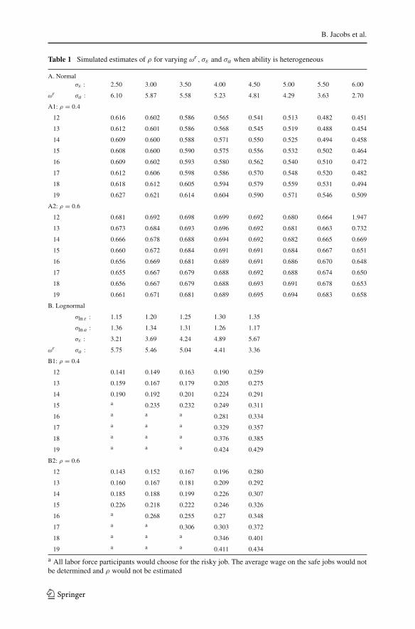
Results are given in Table 1. For the normal distribution, we always find workersin both jobs. For the lognormal distribution, the ability distribution has a short lowertail and a long upper tail, so with large ωr , everyone prefers the risky job and we willignore such cases. For the normal distribution case, ρ is always overestimated. Anincrease in ωr has a non-monotonic effect on ρ. Basically, there is a U-shaped pattern,although it is not always fully visible: it depends on the ability/risk ratio. If abilityvariation increases and risk decreases, the positive bias grows larger if ρ = 0.4, andmoves non-monotonically if ρ = 0.6.

For the lognormal distribution, ρ is always underestimated. If ωr increases, ρ

increases, and hence, the bias decreases. If ability variation increases and riskdecreases, ρ moves non-monotonically (U-shaped), although again, the parametercombination may allow only part of the U to show up.

The differently signed biases in the two cases can be understood from the underlyingdistributions. By design, σ 2

ε is similar between the normal and lognormal specifica-tions, but the right tail of the distribution of a that selects risky jobs is shaped diffe-rently, much thicker. For both normal and lognormal, when a∗ rises, the conditionalmean of a rises (obviously), but while the conditional variance of the normal a falls,the conditional variance of the lognormal a rises.13 Thus, the conditional variance of

12 Of course, E[a#

]= exp

(0.5σ 2

ln ε

).

13 This is all visible from our calculations, but will not be reproduced here.

123

B. Jacobs et al.

Table 1 Simulated estimates of ρ for varying ωr , σε and σa when ability is heterogeneous

A. Normalσε : 2.50 3.00 3.50 4.00 4.50 5.00 5.50 6.00

ωr σa : 6.10 5.87 5.58 5.23 4.81 4.29 3.63 2.70

A1: ρ = 0.4

12 0.616 0.602 0.586 0.565 0.541 0.513 0.482 0.451

13 0.612 0.601 0.586 0.568 0.545 0.519 0.488 0.454

14 0.609 0.600 0.588 0.571 0.550 0.525 0.494 0.458

15 0.608 0.600 0.590 0.575 0.556 0.532 0.502 0.464

16 0.609 0.602 0.593 0.580 0.562 0.540 0.510 0.472

17 0.612 0.606 0.598 0.586 0.570 0.548 0.520 0.482

18 0.618 0.612 0.605 0.594 0.579 0.559 0.531 0.494

19 0.627 0.621 0.614 0.604 0.590 0.571 0.546 0.509

A2: ρ = 0.6

12 0.681 0.692 0.698 0.699 0.692 0.680 0.664 1.947

13 0.673 0.684 0.693 0.696 0.692 0.681 0.663 0.732

14 0.666 0.678 0.688 0.694 0.692 0.682 0.665 0.669

15 0.660 0.672 0.684 0.691 0.691 0.684 0.667 0.651

16 0.656 0.669 0.681 0.689 0.691 0.686 0.670 0.648

17 0.655 0.667 0.679 0.688 0.692 0.688 0.674 0.650

18 0.656 0.667 0.679 0.688 0.693 0.691 0.678 0.653

19 0.661 0.671 0.681 0.689 0.695 0.694 0.683 0.658

B. Lognormal

σln ε : 1.15 1.20 1.25 1.30 1.35

σln a : 1.36 1.34 1.31 1.26 1.17

σε : 3.21 3.69 4.24 4.89 5.67

ωr σa : 5.75 5.46 5.04 4.41 3.36

B1: ρ = 0.4

12 0.141 0.149 0.163 0.190 0.259

13 0.159 0.167 0.179 0.205 0.275

14 0.190 0.192 0.201 0.224 0.291

15 a 0.235 0.232 0.249 0.311

16 a a a 0.281 0.334

17 a a a 0.329 0.357

18 a a a 0.376 0.385

19 a a a 0.424 0.429

B2: ρ = 0.6

12 0.143 0.152 0.167 0.196 0.280

13 0.160 0.167 0.181 0.209 0.292

14 0.185 0.188 0.199 0.226 0.307

15 0.226 0.218 0.222 0.246 0.326

16 a 0.268 0.255 0.27 0.348

17 a a 0.306 0.303 0.372

18 a a a 0.346 0.401

19 a a a 0.411 0.434

a All labor force participants would choose for the risky job. The average wage on the safe jobs would notbe determined and ρ would not be estimated

123

Self-selection bias in estimated wage premiums for earnings risk

wr falls with a rise in a∗ in the normal case, whereas the conditional variance of wr

rises with a∗ in the lognormal case. Moreover, for a very negative a∗, there is hardlyany selection in the lognormal case, since all want the risky job. Thus, the conditionalmean of a is close to 0. In the normal case, there is always selection, and always aconditional mean of a that is greater than 0.

We can only conclude that the predicted bias is very sensitive to variation in the spe-cification of the model. Apparently, the overestimation of both the numerator and thedenominator precludes the emergence of simple patterns. One distributional assump-tion leads to positive bias, another to negative bias and the basic pattern of sensitivityto parameter values appears to be reflected in a U-shaped profile. Thus, ambiguityremains within the set of parameter values we used for our simulations.14 However,as empirical wage distributions resemble lognormality rather than normality, we mayconclude that underestimation of risk aversion is most likely.

Empirical evidence on the relevance of ability bias is not completely conclusiveeither but tends to point in the direction of underestimation. In a Danish panel, DiazSerrano et al. (2003), distinguishing residual variance between individuals (permanentshocks) and within individual incomes over time (transitory shocks), find significantwage compensation for both components, thus indicating that the results from cross-section OLS estimates cannot be wholly due to upward bias. The elasticity of wagecompensation, while still very low, increases by a third in the panel estimates rela-tive to annual cross-sections on the same data. Bajdechi (2005), using NLSY data,finds significant compensation for transitory shocks and insignificant compensationfor permanent shocks. With risk measured by IQ decile, the compensation for tran-sitory shocks is unaffected, while compensation for permanent shocks increases andbecomes significant. Berkhout et al. (2005) use secondary school grades to condi-tion on ability, and find that for higher vocational graduates the risk compensationcoefficient slightly increases, while for university graduates it falls substantially.

We conclude that if ability is unknown to individuals the estimated risk attitude isunbiased, as unknown ability is simply a component of risk. If individuals do knowtheir ability and we have a case of unobserved heterogeneity, analytically the bias cango either way, but empirically we consider underestimation more likely.

5 Conclusion

Risk compensation in wages has been estimated from OLS regression of wages onresidual variance in education/occupation. Selection biases may result in biased esti-mates for the true price of risk because the true price is determined by the marginalindividual deciding to switch to more risky jobs. If individuals only differ in risk atti-tude, we have a textbook case where the simple two-stage OLS estimation obtains anunbiased estimate of marginal risk aversion. If only risk differs between individuals,risk aversion is overestimated. If only ability differs between individuals, assumptions

14 We have considered allowing for correlation between ability and risk. But apart from the fact there isno obvious reason to expect this, we conjecture that this will not resolve the basic ambiguity. Nor will wedwell on the possibility that risk aversion simultaneously varies among individuals, as Sect. 4 has indicatedthat this will lead into very complicated and untractable situations.

123

B. Jacobs et al.

on information are vital. With individuals ignorant on their abilities, as in the fifth ofSmith’s famous principal circumstances for wage differentials, abilities are a sourceof risk and risk aversion is estimated without bias. If individuals themselves knowtheir abilities, we have a textbook case of selectivity bias from unobserved heteroge-neity. The equation for the bias shows an ambiguity in sign that is not resolved bysimulation. This also implies that attempts to correct for this bias must be aware ofthe consequences of alternative distributional specifications. On empirical grounds,we think that underestimation is more likely than overestimation, but as always, thisconjecture rests on the realism of the simple selection model we analyzed.

Appendix: A lognormal specification

We can derive analytically that utility is a mean-variance utility function—as in themain text—if wage income is log-normally distributed and utility displays constantrelative risk aversion, see also Weiss (1972). Assume that all income is consumed, andthere is no other asset or non-labor income as in the text. Utility is then given by:

u(w) = w1−ρ

1 − ρ= wβ

β,

where ρ ≡ 1 − β is the coefficient of relative risk aversion. w is log-normally distri-buted with mean µ and standard deviation σ : ln w ∼ N (µ, σ 2). Taking logarithmsand expectations E[·] of the utility function yields:

E [ln[u(w)]] = βE[ln(w)] − ln(β) = βµ − ln(β).

Using the properties of the normal distribution, we can express the variance V [·] ofutility as

V [u(w)] = β2σ 2.

Therefore, we can derive that ln[u(w)] is log-normally distributed with meanβµ − ln(β) and variance β2σ 2 : ln [u(w)] ∼ N (βµ − ln(β), βσ). Since E[ln z] =exp[µz + 1

2σ 2z ] for any log-normally distributed variable z, expected utility can be

expressed as:

E[u(w)] = 1

βexp

[βµ + 1

2β2σ 2

].

After rewriting we obtain:

E[u(w)] = 1

βexp

[β

(µ + 1

2σ 2

)]exp

[1

2β(β − 1)σ 2

]

= 1

βwβ exp

[1

2β(β − 1)σ 2

],

123

Self-selection bias in estimated wage premiums for earnings risk

where w is the mean wage. Taking logarithms gives a utility function having only themean and variance as its arguments:

ln E[u(x)] = ln(1/β) + β ln w − 1

2β(1 − β)σ 2.

After taking an affine transformation, we can therefore express utility as a mean-variance function v(µ, σ 2):

v(µ, σ 2) = ln w − 1

2ρσ 2,

where v(µ, σ 2) ≡ ln[Eu(w)]/(1 − ρ) − c and c ≡ ln(1/(1 − ρ))/ρ.From the last equation we see that expected utility is only a function of log income

and the variance of log income. Therefore, our model in the main text carries over tothe case for log-normally distributed wages, provided that non-labor income is zeroand utility features constant relative risk aversion. Note that after estimation of thewage equation on log wages, ρ should now correctly be interpreted as the coefficientof relative risk aversion and not as the coefficient of absolute risk aversion.

Open Access This article is distributed under the terms of the Creative Commons Attribution Noncom-mercial License which permits any noncommercial use, distribution, and reproduction in any medium,provided the original author(s) and source are credited.

References

Bajdechi SM (2005) The risk of investment in human capital. Ph.D. thesis, Universiteit van Amsterdam.Tinbergen Institute Research Series 365

Berkhout P, Hartog J, Webbink D (2005) Compensation for earnings risk under worker heterogeneity. Paperpresented at the EEA Meetings, Amsterdam

Chen SH (2008) Estimating the variance of wages in the presence of selection and unobserved heterogeneity.Rev Econ Stat (forthcoming)

Chen S, Khan S (2007) Estimating the causal effect of education on wage inequality using IV methods andsample selection models. Working Paper, University of Rochester and SUNY Albany

Christiansen C, Nielsen HS (2002) The educational asset market: a finance perspective on human capitalinvestments. Aarhus School of Business Working Paper 02–10

Cunha F, Heckman J, Navarro S (2005) Separating uncertainty from heterogeneity in life cycle earnings.Oxford Econ Papers 57(2):191–261

Diaz Serrano L, Hartog J (2006) Is there a risk-return trade-off across educations? Evidence from Spain.Investigaciones Economicas XXX(2):353–380

Diaz Serrano L, Hartog J, Nielsen H (2003) Compensating wage differentials for schooling risk in Denmark.Bonn: IZA Discussion Paper 963; revision 2007

Dohmen T, Falk A, Huffman D, Sunde U (2006) Individual risk attitudes: new evidence from a largerepresentative experimentally validated survey. IZA Discussion Paper 1730

Dominitz J, Manski C (1996) Eliciting student expectations of the return to schooling. J Hum Resour31(1):1–26

Feinberg RM (1981) Earnings-risk as a compensating differential. Southern Econ J 48:156–163Gollier C (2001) The economics of risk and time. MIT Press, Cambridge, MAHartog J (2002) On human capital and individual capabilities. Rev Income Wealth 47(4):515–540Hartog J, Ferrer-i-Carbonell A, Jonker N (2002) Linking measured risk aversion to individual characteris-

tics. Kyklos 55(1):3–26

123

B. Jacobs et al.

Hartog J, Plug E, Diaz Serrano L, Vieira J (2003) Risk compensation in wages, a replication. Empir Econ28:639–647

Hartog J, Vijverberg W (2007) On compensation for risk aversion and skewness affection in wages. LabourEcon 14(6):938–956

Hartog J, Webbink D (2004) Can students predict their starting salaries? Yes! Econ Edu Rev 23(2):103–113King AG (1974) Occupational choice, risk aversion and wealth. Ind Labor Relat Rev, pp 586–596Levhari D, Weiss Y (1974) The effect of risk on the investment in human capital. Am Econ Rev 64(6):

950–963McGoldrick K (1995) Do women receive compensating wages for earnings risk. Southern Econ J 62:

210–222McGoldrick K, Robst J (1996) The effect of worker mobility on compensating wages for earnings risk.

Appl Econ 28:221–232Smith A (1776/1976) The wealth of nations. Penguin, HarmondsworthVarian HR (1978) Microeconomic analysis. W.W. Norton and Company, LondonWillis R, Rosen S (1979) Education and self-selection. J Polit Econ 87(5):S7–S36Wolter S (2000) Wage expectations: a comparison of Swiss and US students. Kyklos 53(1):51–69Weiss Y (1972) The risk element in occupational and educational choices. J Polit Econ 80(6):1203–1213

123