Day-ahead forward premiums in the Texas electricity market

1

Day-ahead forward premiums in the Texas electricity market

Jay Zarnikau*,a,b

, Chi-Keung Wooc, Carlos Gillett

a,b, Tony Ho

c, Shuangshuang Zhu

a, Eric

Leungc

a Frontier Associates LLC, 1515 S. Capital of Texas Highway, Suite 110

Austin, TX 78746, USA

b University of Texas at Austin, Department of Statistics, Austin, TX 78713, USA

c Department of Economics, Hong Kong Baptist University, Hong Kong, China

August 17, 2014

Keywords: Electricity markets; deregulation; electricity trading; Texas electricity market;

ERCOT

JEL Codes: D44, D47, G13, G14, Q41

* Corresponding author. Tel.: +1-512-372-8778; Fax: +1-512-372-8932; Email address:

[email protected] (J. Zarnikau)

2

Abstract

We investigate market-price convergence in the competitive Texas electricity market in

the presence of large-scale wind generation using a large data sample of over 30,000 hourly

observations for the period of December 1, 2010 to May 31, 2014. Hourly premiums vary by

time-of-day and month. Simple univariate analysis suggests patterns related to the day-of-the-

week, although multivariate regression analysis reveals that this pattern is weak. The levels of

the premiums are small and the forward premiums for a given hour exhibit serial correlation across

days. An increase in wind generation tends to increase the premiums. This effect is significant for six

of the 24 hours for non-West zones and half of the hours for the wind-rich West zone. The size of the

effect of rising wind generation on the West zone’s premium is larger than the effects on premiums in

other zones. However, an increase in wind generation tends to reduce the forward premium’s

volatility in nearly all hours.

Taken together, these findings suggest that ERCOT’s day-ahead market (DAM) and real-

time market (RTM) exhibit modest trading inefficiency. But making a sizable arbitrage profit on

a consistent basis is difficult because of the unpredictable nature of wind generation. To be sure,

accurate wind generation may arguably improve arbitrage profitability, especially for the West

zone that houses most of Texas’ wind farms. However, if the wind forecast accuracy also

improves price convergence, the arbitrage profit diminishes as well.

3

1. Introduction

Electricity market reform and deregulation in the U.S. have led to day-ahead and real-

time wholesale market trading in the transmission grids of Pennsylvania–New Jersey–Maryland

(PJM), New York, New England, California, and Texas (Sioshansi, 2013). A day-ahead hourly

forward premium is the day-ahead market (DAM) price for a given hour minus the real-time

market (RTM) price for the same hour.1 A growing literature examines the relationship between

spot market prices and forward or futures prices in these restructured electricity markets, in light

of electricity’s important role in modern economies and the unique attributes of this commodity.

The high costs and technical challenges inherent in storing electricity make real-time electricity

market prices exceptionally volatile and sensitive to various random factors that affect real time

load-resource balances, including unanticipated power plant outages, unpredictable weather

events, unanticipated fluctuations in demand, and intermittent wind and solar generation.

Forward or futures markets enable market participants to manage market price risks,

while introducing opportunities for trading and risk allocation to electricity resellers (for

example, local distribution companies and retail service providers), power generators, and

financial market participants. The degree of convergence between forward and spot markets has

been used to measure the trading efficiency of a restructured market (Borenstein et al. 2008;

Eydeland and Wolyniec, 2003). And the introduction of forward or futures markets may impact

the overall success of efforts to restructure electricity markets by reducing volatility in a spot

market (Kalantzis and Milonas, 2013).

1 While market structures vary, we shall use the term “real-time market” to refer to markets that set prices minutes

ahead of pricing or settlement intervals. In the U.S., prices in the forward or futures markets are generally set on a

day-ahead basis.

4

While Keynes (1930) speculated that a futures contract’s forward premium (= futures

price – spot price) should generally be negative, many studies report positive forward premiums.

Such studies include analyses of electricity futures traded on the New York Mercantile Exchange

for delivery at the California-Oregon Border by Shawky et al. (2003), day-ahead forward

premiums in the New York market by Hadsell and Shawky (2007), day-ahead forward premiums

in the California market by Borenstein et al. (2008), day-ahead forward premiums in the PJM

market by Hadsell (2011), and month-ahead premiums in the Iberian power market by Herráiz

and Monroy (2009). Persistent, positive (negative), and sufficiently-large forward premiums

imply that arbitrage profit can be made by selling (buying) electricity in the day-ahead market

and buying (selling) the same power in the real-time market.

While premiums in electricity markets tend to be positive, numerous studies report that

they have significant seasonal or hourly patterns. While positive premiums are reported by

Botterud et al. (2010) for the Nordic market, Lucia and Torró (2011) found that premiums vary

seasonally and are negligible in the summer. Furió and Meneu (2010) find periods of positive

and negative premiums in Spain’s month-ahead futures market and attribute the periodic pattern

to unexpected variations in demand and hydroelectric power generation. Bunn and Chen (2013)

report large positive premiums in the U.K. futures market in the winter peak period, smaller

positive premiums in the winter off-peak period, and small negative premiums in the summer

peak and off-peak periods. Longstaff and Wang (2004) observe positive premiums during peak

evening hours but negative premiums during early afternoon hours in the PJM market. Haugom

and Ullrich (2012) find that PJM’s premiums have been greatly reduced or eliminated in more-

recent years. Viehmann (2011) reports positive premiums in the German market during evening

peak hours in winter months and negative premiums during non-peak hours of low demand.

5

Woo et al. (under review) found that the positive day-ahead forward premiums in California’s

electricity markets depend on wind generation and vary by hour and month-of-year.

Virtual bidding (VB) that allows a trader to buy (sell) in the day-ahead market with the

liquidation obligation to sell (buy) in the real-time market may improve convergence between

the DAM and RTM market prices. Improvement is said to occur when the introduction of VB

shrinks the forward premium’s size and volatility. Examining the New York market, Hadsell

and Shawky (2007) conclude that VB has decreased premiums during off-peak hours, but has

increased premiums during peak hours. Hadsell (2007) finds VB has reduced the price volatility

in New York’s real-time and day-ahead markets, and Jha and Wolak (2013) and Woo et al.

(under review) report a similar finding for the California electricity market.

This paper analyzes day-ahead hourly premiums in the Electric Reliability Council of

Texas (ERCOT) market. Our interest in the ERCOT markets is motivated by three reasons.

First, the ERCOT Interconnection is large, accounting for about 8% of the total electricity

generation in the U.S.2 Second, we are unaware of any prior published analyses of ERCOT

markets’ forward premiums,3 even though, this is regarded as a very successful restructured

market and the performance of futures markets, may provide an overall indication of the

efficiency of a market. Third, Texas has the largest installed capacity of wind generation in the

U.S. and rising wind generation has been found to dampen the ERCOT market prices (Woo, et

al., 2011), although very little is known about how forward premiums move with the highly-

2 Generation in ERCOT was 324,859.7 GWH in 2012, as reported to NERC:

http://www.nerc.com/pa/RAPA/ESD/Pages/default.aspx. Total U.S. generation was 4,047,765 GWH in that year,

according to the U.S. Department of Energy’s Energy Information Administration:

http://www.eia.gov/electricity/monthly/epm_table_grapher.cfm?t=epmt_1_1.

3 We note, however, that the excellent annual reports published by Potomac Economics, the market monitor for

ERCOT, contribute simple graphical analyses of the performance of ERCOT’s day-ahead and real-time markets.

http://www.nerc.com/pa/RAPA/ESD/Pages/default.aspx

6

unpredictable wind generation. As renewable energy generation in the world’s electricity

markets increases, its impact on the formation of electricity prices in competitive wholesale

markets becomes increasingly important.

Our empirical examination has two parts. The first part is a descriptive analysis of hourly

price data for the 36-month period from December 1, 2010 to May 31, 2014. The second

component is an estimation of five location-specific sets of 24 hourly regressions based on prior

studies of the fundamental drivers of wholesale electricity market prices (Woo, et al., 2011,

2013).

The key findings are as follows:

As in many other electricity markets, electricity premiums are generally positive and vary by

hour and month of the year.

ERCOT’s hourly DAM and RTM prices for various zones are noisy and weakly

correlated. These prices can be negative and at times hit the price caps. This suggests

modest trading inefficiency that deserves further investigation.

Based on the descriptive statistics, ERCOT’s zonal hourly day-ahead forward premiums are

positive, on average, and highly correlated. The size of the average premiums is small –

between $1.5 and $2.5 per MWh.

Based on our regression results, the forward premiums for a given hour exhibit serial

correlation across days. Rising wind generation tends to reduce the volatility of the forward

premium.

Based on our regression results, an increase in wind generation raises the forward premiums.

This effect is significant for 25% of the 24 hours for non-West zones and half of the hours for

the West zone. The sizes of the effects in the West zone are larger than in other zones.

7

Based on our regression results, there are month-of-year effects.

The day-of-week effects suggested by simple univariate graphical analysis tend to be

insignificant in our multivariable regression models.

Taken together, these findings suggest that the ERCOT’s DAM and RTM markets show

modest trading inefficiency. But making sizable arbitrage profit consistently is difficult because

of the unpredictable nature of wind generation. To be sure, accurate wind generation may

arguably improve arbitrage profitability, especially for the West zone that houses most of Texas’

wind farms. However, if the wind forecast accuracy also improves price convergence, the

arbitrage profit diminishes as well.

The following section reviews ERCOT’s electricity market features, offering a contextual

background of our forward premium analysis. Section 3 describes our hourly data sample,

explores temporal patterns in the forward premiums, and identifies a relationship between wind

generation and the size of the premiums. In Section 4 we conduct a simple test for market

efficiency. Section 5 provides regression results, conducted to better isolate the factors

contributing to the observed patterns in the premiums. Section 6 concludes.

2. ERCOT market description

The ERCOT market is often cited as North America’s most successful attempt to

introduce competition in both generation and retail segments of the power industry (Distributed

Energy Financial Group, 2011; Alliance for Retail Choice, 2007; and Center for Advancement of

Energy Markets, 2003). This market covers about 75% of the area of America’s leading state in

electricity generation and consumption, and serves about 85% of Texas’ total electricity load.

Although there is no synchronous interconnection to North America’s Eastern or Western grids,

8

the Texas grid can exchange about 860 MW with other reliability councils in the U.S. and

Mexico through direct current links.

In the wholesale sector, there is competition among a large number of generators,

although one generation company, Luminant, holds a market share of roughly 20%. There

presently is no “capacity market” to maintain a target reserve margin. Consequently, market

forces are heavily relied upon to preserve reliability and resource adequacy and offer caps have

been raised to relatively-high levels in hopes of providing sufficient compensation to the

generation sector.

The competitive wholesale market has evolved over time, with an important structural

change occurring on December 1, 2010, upon the introduction of a nodal market structure.

Under the new structure, ERCOT assumed a central role in dispatching all resources using a

security-constrained economic dispatch (SCED) model. Nodal prices are used to determine the

compensation provided to generators, while a demand-weighted average of the nodal prices

within various zones is calculated to bill load-serving entities (LSEs) for wholesale energy

purchases (Zarnikau, et al., 2014).

The creation of a formal day-ahead market (DAM) with VB accompanied the nodal

market’s introduction. The DAM is a voluntary, financially-binding forward energy market,

which matches willing buyers and sellers, subject to various constraints. In the DAM, offers to

sell energy can take the form of either a three-part supply offer4 or an energy-only offer. Offers

and bids are location-specific. Hourly market-clearing DAM prices used to settle DAM’s

transactions result from the least-cost dispatch that co-optimizes with ancillary services and

4 An offer may include the following three components: Startup Offer, a Minimum-Energy Offer, and an Energy

Offer Curve.

9

certain congestion revenue rights. Deviations from a scheduled DAM transaction are settled at

the 5-minute RTM prices. By providing market participants with a means to make financially-

binding forward purchases and sales of power for delivery in real-time, the DAM enables market

participants to hedge energy and congestion costs on a day-ahead basis, mitigate the risk of price

volatility in real-time, and coordinate generation commitments.

In ERCOT, settlement point prices are calculated at three levels: resource nodes, load

zones, and hubs (ERCOT, undated). A load zone is a set of adjacent electrical buses with similar

prices, reflecting the expectation of minor intra-zonal transmission constraints. Given the role of

load zones within ERCOT’s settlement system, average locational marginal prices (LMPz) have

significant importance to the market.

The zones used in the calculation of LMPz values generally correspond with those

defined under the zonal market structure in place prior to December 1, 2010, although the former

South zone was split up to permit Austin Energy, the Lower Colorado River Authority (LCRA),

and CPS Energy (San Antonio) to have their own zones. The present zones are indicated in

Figure 1.

The offer caps on wholesale market prices were raised to $3,000 per MWh at the start of

the nodal market and DAM, and were further increased to $4,500 per MWh effective August

2012 to encourage the construction of new generating capacity. In August 2012, the Public

Utility Commission of Texas (PUCT) approved a plan to gradually raise the offer caps to $9,000

per MWh, with an initial increase to $5,000 per MWh on June 1, 2013 and a further increased to

$7,000 per MWh on June 1, 2014, just beyond the time frame examined here.

10

In the months following the introduction of the nodal market and the DAM, prices often

spiked. A cold front in early February 2011 led to unusual winter price spikes. The summer of

2011 was one of the hottest on record in Texas, leading to higher-than-expected demand and

numerous price spikes. In contrast, prices in 2013 reached the offer cap only once. This

market’s increasing reliance upon generation from wind farms has placed downward pressure on

energy prices in recent years (Woo, et al., 2011).

3. Descriptive statistics

While the current ERCOT market is divided into eight zones, our analysis will focus on

five zones: North, Houston, West, LCRA, and South. The North and Houston zones account for

about 37% and 27%, respectively, of the energy sales in this market, while the South and West

zones contribute 12% and 9%. The North, Houston, South, and West zones provide the stage for

nearly all of the state’s retail competition, and most of the competitive generation resides within

those zones. The Lower Colorado River Authority (LCRA) zone is included in this analysis

because it includes numerous rural electric cooperatives and municipal utilities. Our analysis

does not include the CPS (San Antonio), AEN (Austin), and RAYBN (Rayburn) zones, chiefly

because each of them is dominated by a single vertically-integrated utility system.

Our analysis for these five zones focuses on the time period beginning with the initiation

of the nodal market and the DAM on December 1, 2010 through May 31, 2014. The zonal DAM

price is the hourly price set in the DAM for each zone. The zonal RTM price is a load-weighted

average of the RTM market prices in each zone.5

5 While real-time prices are set at least every 5 minutes, 15-minute prices are used in ERCOT’s market settlement

processes. Thus, the 5-minute prices are first converted into 15-minute prices using a load-weighted average.

11

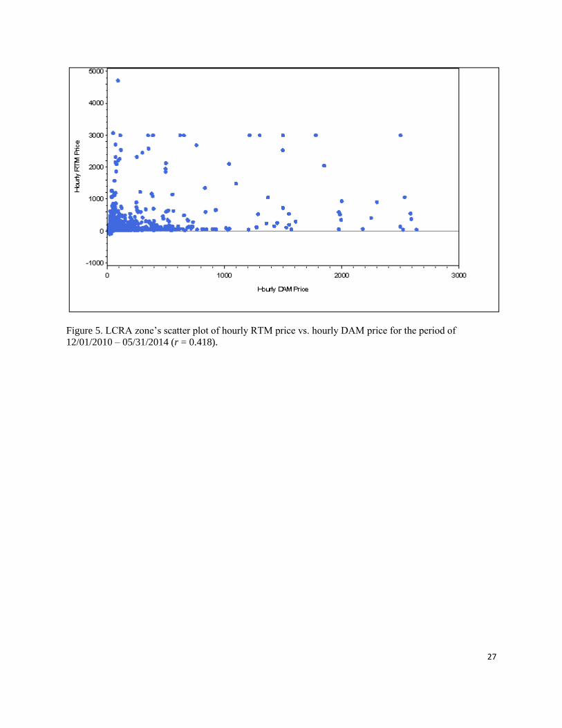
3.1 RTM price vs. DAM price

Figures 2 through 6 provide scatterplots of the hourly RTM price versus the hourly DAM

price for each of the five zones selected for analysis. These figures suggest that the DAM and

RTM prices are highly volatile and weakly correlated. At times they reach or exceed the price

caps of $3000 per MWh, $4500 per MWh, and $5,000 per MWh in effect during our period of

analysis. Prices in excess of the caps may occur when certain inter-zonal transmission

constraints are binding during periods that coincide with the acceptance of high-price energy

offers.6

3.2 Hourly day-ahead forward premiums

The hourly day-ahead forward premium is the hourly DAM price minus the hourly RTM

price. Table 1 presents the premiums’ summary statistics by zone. As in most other electricity

markets, the forward premium is positive. The premium is considerably higher in the West zone

and its adjacent LCRA zone. The West zone hosted the majority of the state’s wind generation

during this period. Moreover, premiums have the greatest volatility in the West zone, as

evidenced by the higher standard deviation shown in Table 1. Since prices converge in the

absence of transmission constraints, the premiums are mostly highly correlated with r > 0.9 (p-

value < 0.0001).

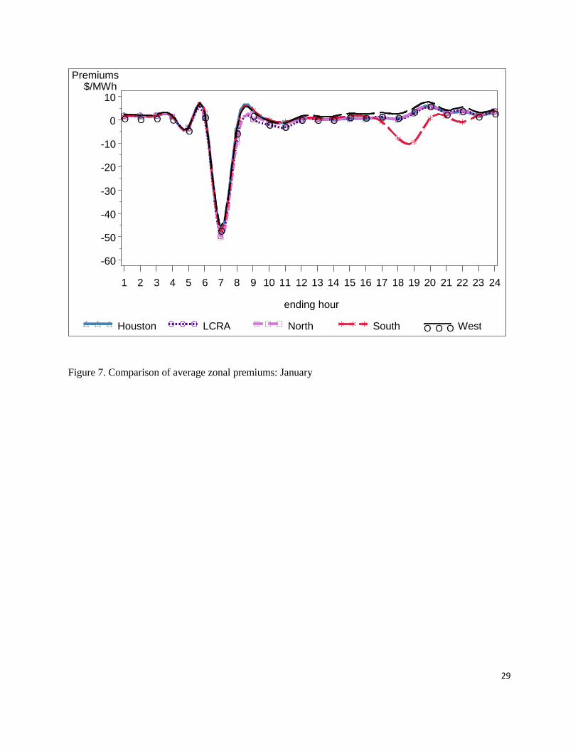
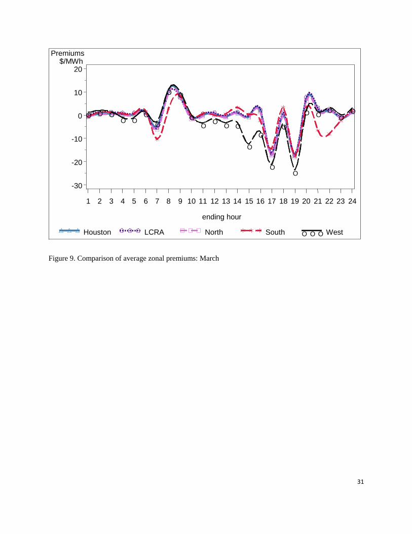
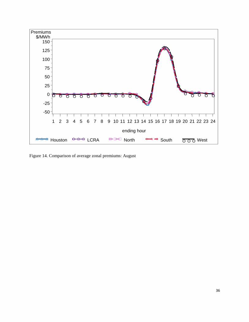
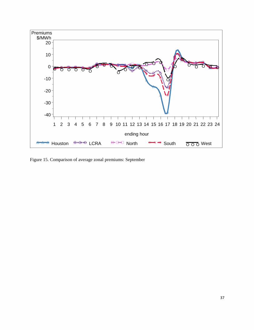
3.3 Hour-of-day patterns in price premiums

Figures 7 through 18 show that the hourly premiums generally tend to have the same

patterns among zones, as the high correlation among zones would suggest. However, in some

6 For a more technical explanation, see Dan Jones, Potomac Economics, MCPE and Offer Cap/Floor Consistency,

etc., presentation to ERCOT TAC/WMS, June 13, 2008, available at:

www.ercot.com/content/meetings/wms/keydocs/2008/0613/Jones_TAC_(20080613).ppt.

12

fall and spring months, the West zone, in particular, displays a pattern in forward premiums that

differ from the other zones. In these months, the ERCOT market has its greatest dependence

upon wind generation. To wit, Figure 16 reports the divergence in patterns among zones for

October.

Figures 19-21 portray the overall average of the hourly zonal premiums for three zones:

North, Houston and West because the LRCA and South zones have the very similar premium

patterns. Each figure demonstrates the premiums vary by hour with differing means and

volatilities implied by the 5- and 95-percentiles. The range of premiums tends to be the greatest

in the late afternoon in each zone, with the West zone exhibiting the greatest range, by far. The

premiums significantly differ from zero in each zone at the hours ending at 8 a.m., 9 a.m., or

both. In all three zones, the premiums are significantly different from zero during the last hour

of each day. In contrast to the West zone, the North and Houston zones exhibit small ranges of

premiums, yet significant values, during the hours ending 18 (6 p.m.) and 19 (7 p.m.).

3.4 Day-of-week patterns in price premiums.

Figures 22 - 24 suggest a day-of-week pattern in the premiums in North, Houston and

West, with statistically significant means during Thursday, Friday, Saturday, and Sunday.

However, the regression analysis presented later suggests that the day-of-week effects on

premiums are generally insignificant after controlling for the influence of month-of-year and

wind generation.

3.5 Month-of-year patterns in price premiums

13

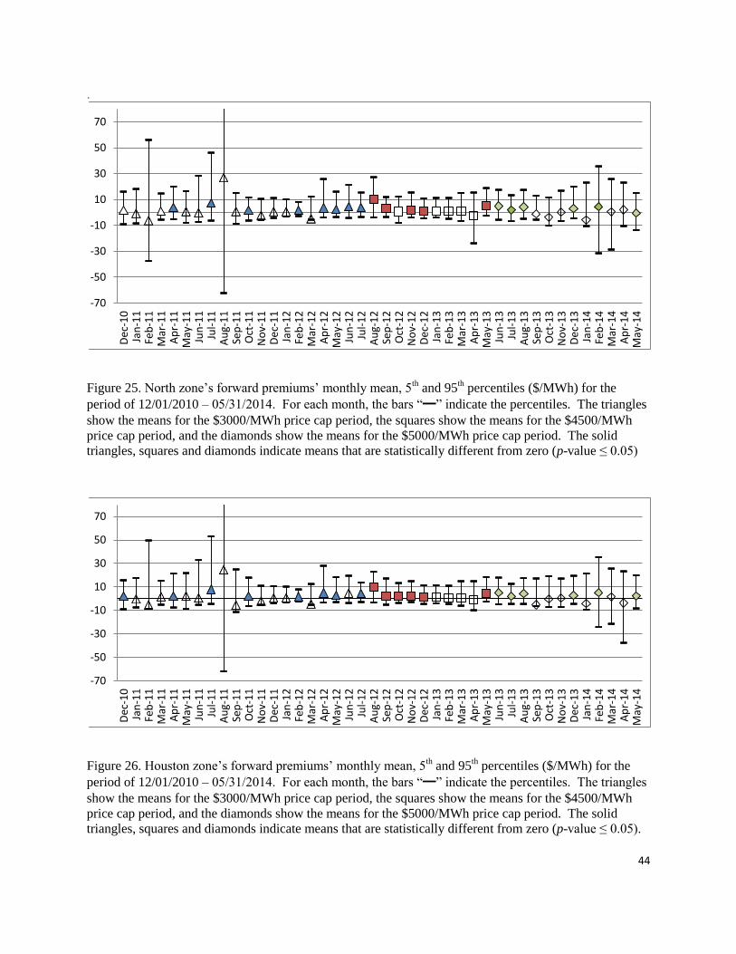
Figures 25-27 show how ERCOT forward premiums in North, Houston and West, varied

by month over the period of this study. These figures show the forward premiums’ means and

volatilities vary by month. The effects of the offer caps on the monthly means, however, are not

discernible. As noted earlier, unusually hot weather during the summer of 2011 and a severe

freeze during February 2011 resulted in numerous price spikes during those months. These

figures suggest that these weather events affected the price premiums, as well. There have been

far fewer price spikes in subsequent years, during which the price caps have been higher.

3.6. Wind generation and forward premiums

Large-scale wind generation provides power on an“as-available” basis, is intermittent,

and is largely outside the control of the ERCOT Independent System Operator.7 We explore

wind generation as a potential determinant of forward premiums because rising wind energy

output tends to reduce the RTM price (Woo et al., 2011, 2014), to the point that the RTM price

can become negative,8 thus greatly magnifying the forward premium. Wind generation data

were obtained from the ERCOT website.9 Wind generation data for the entire ERCOT market

were used, since zone-specific data are not readily available.

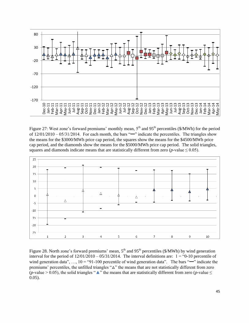
Figures 28 through 30 suggest ERCOT forward premiums in the North, Houston and

West zones depend on wind generation. Specifically, rising wind generation tends to increase

the premiums’ mean and reduce the premiums’ volatility. The range of premiums in the West

zone is far greater than in the North or Houston zones.

7 While an independent system operator can curtail wind generation, it cannot increase wind generation like

dispatchable generation (e.g., natural-gas turbines). 8 An example is the minimum-load condition when the system load cannot fully absorb the non-dispatchable

generation output from wind farms. As a result, negative prices are used to induce dispatchable- generation (e.g.,

natural-gas turbines) owners to curtail their output so as to maintain the real-time load-resource balance. 9 www.ercot.com.

14

4. Testing the market efficiency hypothesis

The efficient market hypothesis (EMH) suggests that, absent transaction cost, the RTM

price moves in tandem with the DAM price with no arbitrage opportunity between the two prices

(Siegel and Siegel, 1990). To test this hypothesis, we apply the simple bivariate regression

model:

Yht = α + β Xht + εht (1)

where Yht = RTM price, Xht = DAM price, and εht = AR(n) error. The price data used to estimate

equation (1) are stationary based on the Phillips-Perron (Phillips and Perron, 1988) unit root test

results that firmly reject the hypothesis of non-stationarity for all zones (p-values < 0.01), thus

assuaging any concerns about spurious price regression (Granger and Newbold, 1974). The

testable hypothesis is H0: α = 0 and β =1, whose rejection implies that the price data do not

support the EMH under the assumption of zero transaction costs. Table 2 reports the regression

results using the maximum likelihood method in the SAS/ETS PROC AUTOREG command. It

yields the following observations:

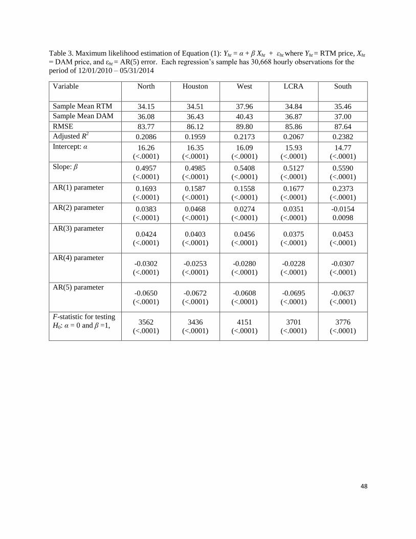
The R2 values are around 0.2, indicating a modest data fit by the regressions.

All regressions have statistically significant intercepts (p-value < 0.01). The slope estimates

are also statistically significant, lying between 0.49 and 0.56.

The AR parameter estimates suggest AR(5) errors.

The F-statistics reject H0: α = 0 and β =1 (p-value < 0.01) for all locations.

These observations suggest trading inefficiency and arbitrage opportunities.

15

5. Regression Analysis

5.1 Model

Figures 22 through 30 suggest that day-of-week, month-of-year, and wind generation may

drive ERCOT’s forward premiums. However, they do not delineate each driver’s individual

effect. Hence, we estimate 24 hourly regressions, each with the following specification:10

Zht = h + d hd Ddt + m hm Mmt + h Wht + ht (2)

In equation (2), the dependent variable is Zht = forward premium for hour h and day t for a

particular market price series, representing the North, Houston, West, LCRA, and South zones.11

The systematic portion is represented by the first four terms on the right hand side of equation

(2).

The first independent variable on the right-hand-side of equation (1) is the hour-specific

intercept h. Based on the variables introduced below, h measures the average premium for hour

h in December on a Sunday, after controlling for the effects of month-of-year, day-of-week, and

wind generation.

We use indicator Dmt = 1 to indicate if day t is d = 1 (Sunday), …, 6 (Friday); 0 otherwise.

The day-of-week effect for hour h is measured by the coefficient hd.

We use binary indicator Mmt = 1 to indicate if day t is in month m = 1 (January), …, 11

(November); 0 otherwise. The month-of-year effect for hour h is measured by the coefficient

hm.

10

We tested a single equation approach that uses hourly dummies to capture the hour-of-day effects. The

approach’s assumption of constant month-of-year and wind generation effects are rejected by the data. 11

We applied the Phillips-Perron unit-root test (Phillips and Perron, 1988) to decisively reject (p-value < 0.01) the

hypothesis that the forward premium data series are non-stationary. The other metric variable in equation (2) is

wind generation Wht, which is also found to be stationary.

16

The last independent variable is Wht, which is ERCOT’s hourly wind generation (MW) in

hour h on day t. Its hour-specific effect on the forward premium is given by the coefficient h.

The hour-specific random error in equation (2) is ht for hour h on day t. We consider

three stochastic specifications: (a) ht is AR(1), with an heteroskedastic variance that is an

exponential function of wind generation (SAS, 2008, p.351); (b) ht is an AR(1) error; and (c) ht

follows a GARCH (1, 1) process (Bollerslev, 1986). Obtained via PROC AUTOREG in

SAS/ETS (2008), we adopt (a) because (b) is rejected by the data and (c) leads to a non-

stationary GARCH (1, 1) process with undefined variance.

5.2 Results

Tables 3 through 12 report the regression results. Estimates presented in bold font are

statistically significant at the 1% level. Using the 5% significance level results in an almost

identical presentation of significant estimates.

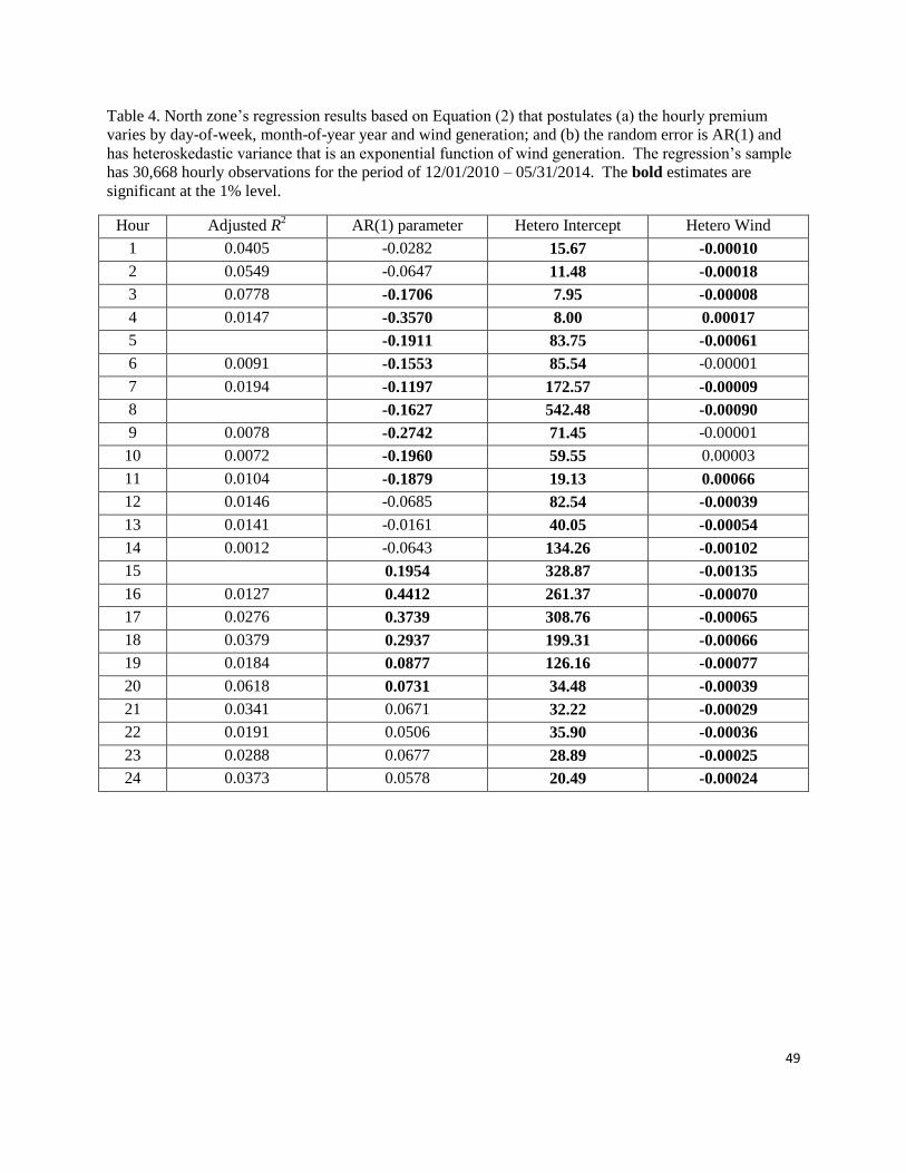
Based on Tables 3 through 7, residuals are serially correlated for the same hour across

days and statistically significant heteroskedasticity is evident in all zones. The hetero wind

coefficient is consistently negative in all hours and in all zones, suggesting an increase in wind

generation tends to reduce the volatility of the forward premium. This finding contrasts with the

results from a similar modeling effort in California (Woo et al., under review), where the picture

was not so clear.

The estimates of h in Table 8 suggests that the hourly average premiums are mostly

insignificant on a Saturday in December, after controlling for the effects of wind generation,

month-of-year, and day-of-week. Yet, exceptions hold in some zones in hours ending 1 a.m., 2

a.m., 3 a.m., and 3 p.m.

17

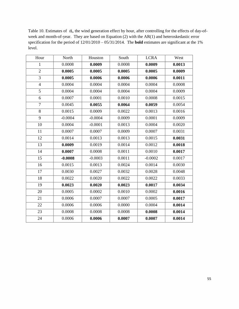
The estimates of h in Table 1 show the wind generation effect by hour, after controlling

for the effects of day-of-week and month-of-year. An increase in wind generation tends to

increase the forward premium. The effect is statistically significant in the hours ending 2 a.m., 3

a.m., and 7 p.m. (hour 19) in all zones. It is significant in the last hour of the day in four of the

five zones. The size of the effect tends to be the highest in the wind-rich West zone, with

significant estimates in half of the hours.

In contrast to the univariate analysis presented in Figures 22 through 24, Table 10

suggests that day-of-week effects are weak, after controlling for the effects of wind generation,

monthly patterns, and autocorrelation.

Month-of-year effects are more-pronounced, as suggested in Tables 11 and 12. These

effects are particularly significant in the hours ending 2 a.m., 3 a.m., and late afternoon hours.

6. Conclusion

In the competitive ERCOT electricity market, day-ahead hourly premiums vary by time-

of-day and month. The levels of the premiums are small (between $1.5 and $2.5 per MWh), and

the forward premiums for a given hour exhibit serial correlation across days. Day-ahead prices

are poor predictors of real-time prices, thus suggesting a modest level of trading inefficiency and

opportunities for arbitrage. An increase in wind generation tends to increase the premiums. This

effect is significant for six of the 24 hours for non-West zones and half of the hours for the wind-

rich West zone.

Making a sizable arbitrage profit on a consistent basis is difficult because of the

unpredictable nature of wind generation. Wind generation tends to increase the premiums,

18

although an increase in wind generation also tends to reduce the forward premium’s volatility in

nearly all hours. As Texas increases its reliance upon this renewable resource in the coming

years and as other regions of the world increase their reliance upon renewable resources, an

understanding of the relationship between intermittent resources and market prices will increase

in importance.

Accurate forecasts of wind generation may arguably improve arbitrage profitability,

especially for the West zone that houses most of Texas’ wind farms. However, if the wind

forecast accuracy also improves price convergence, the arbitrage profit diminishes as well. In

recent years, improving the accuracy of wind generation forecasts has indeed been a priority for

ERCOT. On February 26, 2008, a mismatch between load and generation led to a sudden drop

in system frequency and outages resulted. ERCOT’s day-ahead forecast anticipated 1,000 MW

of wind that ultimately was not available. Following this event, ERCOT began deliberately

under-forecasting wind power output.12

Nearly two years later, on January 28, 2010, a strong

cold front moved southward from the Texas Panhandle into the Sweetwater, Texas region. The

approaching front stalled and then moved backward. ERCOT’s wind forecast model was

incapable of predicting wind generation levels under this unusual weather event and two

different and conflicting 600 MW dispatch instructions to fossil fuel generators were issued --

one to ramp generation up and the other to ramp generation down. Following these events, the

critical importance of accurate wind generation forecasts became apparent and ERCOT

implemented a more-advanced wind forecasting system.

12

NPRR210 Wind Forecasting Change to P50. Comments of Morgan Stanley. Presentation to Technical Advisory

Committee of ERCOT. April 8, 2010.

19

These findings suggest that the ERCOT’s day-ahead market (DAM) and real-time market

(RTM) show modest trading inefficiency. Yet, such inefficiencies might be expected in the first

three and a half years of a new market structure, particularly when a new nodal wholesale real-

time pricing system is accompanied by a new formal day-ahead market. As noted earlier,

forward premiums appear to have declined and efficiencies have been improved in other

electricity markets in the U.S. as markets have matured. It will be interesting to see whether the

ERCOT market demonstrates similar improvement in the coming years.

References

Bollerslev, T. (1986). Generalized autoregressive conditional heteroskedasticity. Journal of

Econometrics, 31, 307–321.

Borenstein, S., Bushnell, J., Knittel, C.R. & Wolfram, C. (2008). Inefficiencies and market

power in financial arbitrage: A study of California's electricity markets. Journal of

Industrial Economics, 56, 347-378.

Botterud, A., Kristiansen, T., & Ilic, M.D. (2010). The relationship between spot and futures

prices in the Nord Pool electricity market. Energy Economics, 32, 967–978.

Bunn, D.W., & Chen, D. (2013). The forward premium in electricity futures. Journal of

Empirical Finance, 23, 173–186.

Center for Advancement of Energy Markets (2003). Retail Energy Deregulation Index 2003, 4th

Edition.

Distributed Energy Financial Group (2011). The Annual Baseline Assessment of Choice in

Canada and the United States (ABACCUS).

20

ERCOT (undated). Transmission 101. ERCOT Market Education.

Eydeland, A. & Wolyniec, K. (2003). Energy and power risk management: New development in

modeling, pricing and hedging. New York: John Wiley.

Furió, D., & Meneu, V. (2010). Expectations and forward risk premium in the Spanish

deregulated power market. Energy Policy, 38, 784–793.

Granger, C.W.J., & Newbold, P. (1974). Spurious regressions in econometrics. Journal of

Econometrics, 2, 111–120.

Hadsell, L. (2007). The impact of virtual bidding on price volatility in New York's wholesale

electricity market. Economics Letters, 95, 66-72.

Hadsell, L. (2011). Inefficiency in deregulated wholesale electricity markets: the case of the New

England ISO. Applied Economics, 43, 515–525.

Hadsell, L. & Shawky, H.A. (2007). One-day forward premiums and the impact of virtual

bidding on the New York wholesale electricity using hourly data. Journal of Futures

Market, 27, 1107–1125.

Haugom, E. & Ullrich, C.J. (2012). Market efficiency and risk premia in short-term forward

prices. Energy Economics, 34, 1931-1941.

Herráiz, A.C., & Monroy, C.R. (2009). Analysis of the efficiency of the Iberian power futures

market. Energy Economics, 37, 3566–3579.

Jha, A., & Wolak, F.A. (2013). Testing for Market Efficiency with Transactions Costs: An

Application to Convergence Bidding in Wholesale Electricity Markets. Available at:

http://www.stanford.edu/group/fwolak/cgi-

bin/sites/default/files/files/CAISO_VB_draft_V8.pdf

http://www.stanford.edu/group/fwolak/cgi-bin/sites/default/files/files/CAISO_VB_draft_V8.pdf

http://www.stanford.edu/group/fwolak/cgi-bin/sites/default/files/files/CAISO_VB_draft_V8.pdf

21

Jones, D. (2008) Presentation of Potomac Economics, MCPE and Offer Cap/Floor Consistency,

etc., presentation to ERCOT TAC/WMS, June 13, 2008, available at:

www.ercot.com/content/meetings/wms/keydocs/2008/0613/Jones_TAC_(20080613).ppt.

Kalantzis, F., & Milonas, N. (2013). Analyzing the impact of futures trading on spot price

volatility: Evidence from the spot electricity market in France and Germany. Energy

Economics, 36, 454–463.

Keynes, J. M. (1930). A treatise on Money, MacMillan, London.

Longstaff, F.A. & Wang, A.W. (2004). Electricity forward prices: a high-frequency empirical

analysis. Journal of Finance, 59, 1877-1900.

Lucia, J.J., & Torró, H. (2011). On the risk premium in Nordic electricity futures prices.

International Review of Economics and Finance, 20, 750–763.

Morgan Stanley (2010). NPRR210 Wind Forecasting Change to P50: Comments of Morgan

Stanley. Presentation to Technical Advisory Committee of ERCOT. April 8.

Parsons, J.E. & de Roo, G. (2008) Risk premiums in electricity forward prices - data from the

ISO New England market. 5th International Conference on European Electricity Market,

2008 (DOI: 10.1109/EEM.2008.4579089)

Phillips, P.C.B., & Perron, P. (1988). Testing for a unit root in time series regression. Biometrika,

75, 335–346.

SAS, 2008. SAS/ETS 9.2 User’s Guide. Available at:

http://support.sas.com/documentation/cdl/en/etsug/60372/HTML/default/viewer.htm#title

page.htm

Shawky, H.A., Marathe, A., & Barrett, C.L. (2003). A first look at the empirical relation between

spot and futures electricity prices in the United States. The Journal of Futures Markets,

http://dx.doi.org/10.1109/EEM.2008.4579089

http://support.sas.com/documentation/cdl/en/etsug/60372/HTML/default/viewer.htm#titlepage.htm

http://support.sas.com/documentation/cdl/en/etsug/60372/HTML/default/viewer.htm#titlepage.htm

22

23(10), 931–955.Siegel, D.R., & Siegel, D.F. (1990). The Futures Market: Arbitrage,

Risk Management and Portfolio Strategies. Chicago: Probus Publishing Company.

Siegel, D.R., & Siegel, D.F. (1990). The Futures Market: Arbitrage, Risk Management and

Portfolio Strategies. Chicago: Probus Publishing Company.

Sioshansi, F.P., 2013. Evolution of global electricity markets. New York: Academic Press.

Viehmann, J. (2011). Risk premiums in the German day-ahead electricity market. Energy

Policy, 39, 386–394.

Woo, C.K., Ho, S.T., Leung, H.Y., Zarnikau, J., Cutter, E., (under review). Virtual bidding,

wind generation and California’s day-ahead electricity forward premium.

Woo, C.K., Ho, T., Zarnikau, J., Olson, A., Jones, R., Chait, M., Horowitz, I., & Wang, J. (2014).

Electricity-market price and nuclear power plant shutdown: Evidence from California,

Energy Policy, 73, 234-244.

Woo, C.K., Horowitz, I., Moore, J. & Pacheco, A. (2011). The impact of wind generation on the

electricity spot-market price level and variance: the Texas experience. Energy Policy, 39,

3939-3944.

Woo, C.K., Zarnikau, J., Kadish, J., Horowitz, I., Wang, J. & Olson, A. (2013). The impact of

wind generation on wholesale electricity prices in the hydro-rich Pacific Northwest.

IEEE Transactions on Power Systems, 28, 4245-4253.

Zarnikau, J., Woo, C. K. & Baldick, R. (2014). Did the introduction of a nodal market structure

impact wholesale electricity prices in the Texas (ERCOT) market? Journal of Regulatory

Economics, 45, 194-208.

23

Figure 1. ERCOT Map with Zones Delineated. Approximate locations of the Austin Energy (AEN),

LCRA, Rayburn, and CPS zones are indicated.

LCRA

CPS

AustinEnergy

Rayburn

24

Figure 2. North zone’s scatter plot of hourly RTM price vs. hourly DAM price for the period of

12/01/2010 – 05/31/2014 (r = 0.420).

25

Figure 3 Houston zone’s scatter plot of hourly RTM price vs. hourly DAM price for the period of

12/01/2010 – 05/31/2014 (r = 0.407).

26

Figure 4. West zone’s scatter plot of hourly RTM price vs. hourly DAM price for the period of

12/01/2010 – 05/31/2014 (r = 0.437).

27

Figure 5. LCRA zone’s scatter plot of hourly RTM price vs. hourly DAM price for the period of

12/01/2010 – 05/31/2014 (r = 0.418).

28

Figure 6. South zone’s scatter plot of hourly RTM price vs. hourly DAM price for the period of

12/01/2010 – 05/31/2014 (r = 0.418).

29

Figure 7. Comparison of average zonal premiums: January

Premiums $/MWh

-60

-50

-40

-30

-20

-10

0

10

ending hour

1 2 3 4 5 6 7 8 9 10 11 12 13 14 15 16 17 18 19 20 21 22 23 24

Houston LCRA North South West O O O

O O O O O

O

O

O

O O O

O O O O O O O O

O O O

O O

30

Figure 8. Comparison of average zonal premiums: February

Premiums $/MWh

-30

-20

-10

0

10

20

ending hour

1 2 3 4 5 6 7 8 9 10 11 12 13 14 15 16 17 18 19 20 21 22 23 24


O O O O O

O

O

O

O O

O

O

O O O O O O

O

O O O

O O

31

Figure 9. Comparison of average zonal premiums: March

Premiums $/MWh

-30

-20

-10

0

10

20

ending hour

1 2 3 4 5 6 7 8 9 10 11 12 13 14 15 16 17 18 19 20 21 22 23 24


O O O O O

O

O

O O

O O

O O O

O

O

O

O

O

O O O

O O

32

Figure 10. Comparison of average zonal premiums: April

Premiums $/MWh

-20

-15

-10

-5

0

5

10

15

20

25

ending hour

1 2 3 4 5 6 7 8 9 10 11 12 13 14 15 16 17 18 19 20 21 22 23 24


O O O O O O

O

O

O

O O O

O O

O O

O O

O O

O O

O O

33

Figure 11. Comparison of average zonal premiums: May

Premiums $/MWh

-20

-15

-10

-5

0

5

10

15

20

25

ending hour

1 2 3 4 5 6 7 8 9 10 11 12 13 14 15 16 17 18 19 20 21 22 23 24


O O O O O O

O O

O O

O O

O

O O

O

O O

O

O O

O O O

34

Figure 12. Comparison of average zonal premiums: June

Premiums $/MWh

-20

-10

0

10

20

30

40

50

ending hour

1 2 3 4 5 6 7 8 9 10 11 12 13 14 15 16 17 18 19 20 21 22 23 24


O O O O O O O O O O O O

O

O

O

O

O

O

O O

O O O O

35

Figure 13. Comparison of average zonal premiums: July

Premiums $/MWh

-5

0

5

10

15

20

25

30

35

ending hour

1 2 3 4 5 6 7 8 9 10 11 12 13 14 15 16 17 18 19 20 21 22 23 24


O O O O O O

O O O O O

O O

O O

O

O

O O O

O O O O

36

Figure 14. Comparison of average zonal premiums: August

Premiums $/MWh

-50

-25

0

25

50

75

100

125

150

ending hour

1 2 3 4 5 6 7 8 9 10 11 12 13 14 15 16 17 18 19 20 21 22 23 24


O O O O O O O O O O O O O O

O

O

O

O

O

O O O O O

37

Figure 15. Comparison of average zonal premiums: September

Premiums $/MWh

-40

-30

-20

-10

0

10

20

ending hour

1 2 3 4 5 6 7 8 9 10 11 12 13 14 15 16 17 18 19 20 21 22 23 24


O O O O O O O O O

O O

O O O O O

O

O

O O O O O O

38

Figure 16. Comparison of average zonal premiums: October

Premiums $/MWh

-25

-20

-15

-10

-5

0

5

10

15

ending hour

1 2 3 4 5 6 7 8 9 10 11 12 13 14 15 16 17 18 19 20 21 22 23 24


O O O O O O O

O O

O O

O O O

O

O O

O

O

O

O O

O O

39

Figure 17. Comparison of average zonal premiums: November

Premiums $/MWh

-35

-25

-15

-5

5

15

ending hour

1 2 3 4 5 6 7 8 9 10 11 12 13 14 15 16 17 18 19 20 21 22 23 24


O O O O O O

O

O

O

O

O O O

O O

O O

O

O O O

O

O O

40

Figure 18. Comparison of average zonal premiums: December

Premiums $/MWh

-15

-10

-5

0

5

10

15

ending hour

1 2 3 4 5 6 7 8 9 10 11 12 13 14 15 16 17 18 19 20 21 22 23 24


O O O O O

O

O

O

O

O O O O O O O O

O

O

O O

O O O

41

Figure 19. North zone’s forward premiums’ mean, 5th and 95

th percentiles ($/MWh) by hour for the period

of 12/01/2010 – 05/31/2014. For each hour, the bars “━” indicate the 5- and 95 percentiles, the unfilled

triangles “△” the means that are not statistically different from zero (p-value > 0.05), the solid triangles

“▲” the means that are statistically different from zero (p-value ≤ 0.05).

Figure 20. Houston zone’s forward premiums’ mean, 5th and 95

th percentiles ($/MWh) by hour for the

period of 12/01/2010 – 05/31/2014. For each hour, the bars “━” indicate the 5- and 95 percentiles, the

unfilled triangles “△” the means that are not statistically different from zero (p-value > 0.05), the solid

triangles “▲” the means that are statistically different from zero (p-value ≤ 0.05).

42

Figure 21. West zone’s forward premiums’ mean, 5th and 95

th percentiles ($/MWh) by hour for the period

of 12/01/2010 – 05/31/2014. For each hour, the bars “━” indicate the 5- and 95 percentiles, the unfilled

triangles “△” the means that are not statistically different from zero (p-value > 0.05), the solid triangles

“▲” the means that are statistically different from zero (p-value ≤ 0.05).


th percentiles ($/MWh) by day-of-week for

the period of 12/01/2010 – 05/31/2014. For each day of week, the bars “━” indicate the percentiles, the



43











44

.

Figure 25. North zone’s forward premiums’ monthly mean, 5th and 95

th percentiles ($/MWh) for the

period of 12/01/2010 – 05/31/2014. For each month, the bars “━” indicate the percentiles. The triangles

show the means for the $3000/MWh price cap period, the squares show the means for the $4500/MWh

price cap period, and the diamonds show the means for the $5000/MWh price cap period. The solid

triangles, squares and diamonds indicate means that are statistically different from zero (p-value ≤ 0.05)

Figure 26. Houston zone’s forward premiums’ monthly mean, 5th and 95

th percentiles ($/MWh) for the

period of 12/01/2010 – 05/31/2014. For each month, the bars “━” indicate the percentiles. The triangles

show the means for the $3000/MWh price cap period, the squares show the means for the $4500/MWh

price cap period, and the diamonds show the means for the $5000/MWh price cap period. The solid

triangles, squares and diamonds indicate means that are statistically different from zero (p-value ≤ 0.05).

-70

-50

-30

-10

10

30

50

70D

ec-1

0Ja

n-1

1Fe

b-1

1M

ar-1

1A

pr-

11

May

-11

Jun

-11

Jul-

11

Au

g-1

1Se

p-1

1O

ct-1

1N

ov-

11

Dec

-11

Jan

-12

Feb

-12

Mar

-12

Ap

r-1

2M

ay-1

2Ju

n-1

2Ju

l-1

2A

ug-

12

Sep

-12

Oct

-12

No

v-1

2D

ec-1

2Ja

n-1

3Fe

b-1

3M

ar-1

3A

pr-

13

May

-13

Jun

-13

Jul-

13

Au

g-1

3Se

p-1

3O

ct-1

3N

ov-

13

Dec

-13

Jan

-14

Feb

-14

Mar

-14

Ap

r-1

4M

ay-1

4

-70

-50

-30

-10

10

30

50

70

Dec

-10

Jan

-11

Feb

-11

Mar

-11

Ap

r-1

1M

ay-1

1Ju

n-1

1Ju

l-1

1A

ug-

11

Sep

-11

Oct

-11

No

v-1

1D

ec-1

1Ja

n-1

2Fe

b-1

2M

ar-1

2A

pr-

12

May

-12

Jun

-12

Jul-

12

Au

g-1

2Se

p-1

2O

ct-1

2N

ov-

12

Dec

-12

Jan

-13

Feb

-13

Mar

-13

Ap

r-1

3M

ay-1

3Ju

n-1

3Ju

l-1

3A

ug-

13

Sep

-13

Oct

-13

No

v-1

3D

ec-1

3Ja

n-1

4Fe

b-1

4M

ar-1

4A

pr-

14

May

-14

45

Figure 27: West zone’s forward premiums’ monthly mean, 5th and 95

th percentiles ($/MWh) for the period

of 12/01/2010 – 05/31/2014. For each month, the bars “━” indicate the percentiles. The triangles show

the means for the $3000/MWh price cap period, the squares show the means for the $4500/MWh price

cap period, and the diamonds show the means for the $5000/MWh price cap period. The solid triangles,

squares and diamonds indicate means that are statistically different from zero (p-value ≤ 0.05).


th percentiles ($/MWh) by wind generation

interval for the period of 12/01/2010 – 05/31/2014. The interval definitions are: 1 = “0-10 percentile of

wind generation data”, …, 10 = “91-100 percentile of wind generation data”. The bars “━” indicate the

premiums’ percentiles, the unfilled triangles “△” the means that are not statistically different from zero

(p-value > 0.05), the solid triangles “▲” the means that are statistically different from zero (p-value ≤

0.05).

-170

-120

-70

-20

30

80

Dec

-10

Jan

-11

Feb

-11

Mar

-11

Ap

r-1

1M

ay-1

1Ju

n-1

1Ju

l-1

1A

ug-

11

Sep

-11

Oct

-11

No

v-1

1D

ec-1

1Ja

n-1

2Fe

b-1

2M

ar-1

2A

pr-

12

May

-12

Jun

-12

Jul-

12

Au

g-1

2Se

p-1

2O

ct-1

2N

ov-

12

Dec

-12

Jan

-13

Feb

-13

Mar

-13

Ap

r-1

3M

ay-1

3Ju

n-1

3Ju

l-1

3A

ug-

13

Sep

-13

Oct

-13

No

v-1

3D

ec-1

3Ja

n-1

4Fe

b-1

4M

ar-1

4A

pr-

14

May

-14

46







0.05).







0.05).

47

Table 2. Summary statistics of forward price premiums in the period of 12/01/2010 – 05/31/2014.

Zone N Mean Std Dev Sum Minimum Maximum

North 30,668 1.93 92 59155 -4439 2584

Houston 30,668 1.92 94 58763 -4296 2585

West 30,668 2.47 97 75666 -4465 2572

LCRA 30,668 2.03 94 62196 -4628 2593

South 30,668 1.54 95 47293 -4310 2589

Correlation coefficients

Zone North Houston West LCRA South

North 1 0.96 0.95 0.98 0.92

Houston 0.96 1 0.92 0.97 0.92

West 0.95 0.92 1 0.93 0.87

LCRA 0.98 0.97 0.93 1 0.93

South 0.92 0.92 0.87 0.93 1

48

Table 3. Maximum likelihood estimation of Equation (1): Yht = α + β Xht + εht where Yht = RTM price, Xht

= DAM price, and εht = AR(5) error. Each regression’s sample has 30,668 hourly observations for the

period of 12/01/2010 – 05/31/2014

Variable North Houston West LCRA South

Sample Mean RTM 34.15 34.51 37.96 34.84 35.46

Sample Mean DAM 36.08 36.43 40.43 36.87 37.00

RMSE 83.77 86.12 89.80 85.86 87.64

Adjusted R2

0.2086 0.1959 0.2173 0.2067 0.2382

Intercept: α 16.26

(<.0001)

16.35

(<.0001)

16.09

(<.0001)

15.93

(<.0001)

14.77

(<.0001)

Slope: β 0.4957

(<.0001)

0.4985

(<.0001)

0.5408

(<.0001)

0.5127

(<.0001)

0.5590

(<.0001)

AR(1) parameter 0.1693

(<.0001)

0.1587

(<.0001)

0.1558

(<.0001)

0.1677

(<.0001)

0.2373

(<.0001)


(<.0001)

0.0468

(<.0001)

0.0274

(<.0001)

0.0351

(<.0001)

-0.0154

0.0098


(<.0001)

0.0403

(<.0001)

0.0456

(<.0001)

0.0375

(<.0001)

0.0453

(<.0001)

AR(4) parameter -0.0302

(<.0001)

-0.0253

(<.0001)

-0.0280

(<.0001)

-0.0228

(<.0001)

-0.0307

(<.0001)

AR(5) parameter -0.0650

(<.0001)

-0.0672

(<.0001)

-0.0608

(<.0001)

-0.0695

(<.0001)

-0.0637

(<.0001)

F-statistic for testing

H0: α = 0 and β =1, 3562

(<.0001)

3436

(<.0001)

4151

(<.0001)

3701

(<.0001)

3776

(<.0001)

49

Table 4. North zone’s regression results based on Equation (2) that postulates (a) the hourly premium

varies by day-of-week, month-of-year year and wind generation; and (b) the random error is AR(1) and

has heteroskedastic variance that is an exponential function of wind generation. The regression’s sample

has 30,668 hourly observations for the period of 12/01/2010 – 05/31/2014. The bold estimates are

significant at the 1% level.

Hour Adjusted R2 AR(1) parameter Hetero Intercept Hetero Wind

1 0.0405 -0.0282 15.67 -0.00010

2 0.0549 -0.0647 11.48 -0.00018

3 0.0778 -0.1706 7.95 -0.00008

4 0.0147 -0.3570 8.00 0.00017

5 -0.1911 83.75 -0.00061

6 0.0091 -0.1553 85.54 -0.00001

7 0.0194 -0.1197 172.57 -0.00009

8 -0.1627 542.48 -0.00090

9 0.0078 -0.2742 71.45 -0.00001

10 0.0072 -0.1960 59.55 0.00003

11 0.0104 -0.1879 19.13 0.00066

12 0.0146 -0.0685 82.54 -0.00039

13 0.0141 -0.0161 40.05 -0.00054

14 0.0012 -0.0643 134.26 -0.00102

15 0.1954 328.87 -0.00135

16 0.0127 0.4412 261.37 -0.00070

17 0.0276 0.3739 308.76 -0.00065

18 0.0379 0.2937 199.31 -0.00066

19 0.0184 0.0877 126.16 -0.00077

20 0.0618 0.0731 34.48 -0.00039

21 0.0341 0.0671 32.22 -0.00029

22 0.0191 0.0506 35.90 -0.00036

23 0.0288 0.0677 28.89 -0.00025

24 0.0373 0.0578 20.49 -0.00024

50

Table 5. Houston zone’s regression results based on Equation (2) that postulates (a) the hourly premium






1 0.0462 -0.0043 16.44 -0.00012

2 0.0589 0.0131 10.85 -0.00021

3 0.0840 -0.0308 7.07 -0.00007

4 0.0172 -0.3745 7.73 0.00014

5 0.0001 -0.1980 82.41 -0.00063

6 0.0082 -0.1741 87.47 -0.00002

7 0.0178 -0.1182 753.16 -0.00083

8 0.0085 -0.1721 356.67 -0.00069

9 0.0091 -0.2612 70.08 0.00000

10 0.0075 -0.2292 24.72 0.00040

11 0.0104 -0.1990 21.57 0.00060

12 0.0138 -0.1044 59.60 -0.00016

13 0.0020 -0.0208 17.50 0.00041

14 0.0158 -0.0444 97.55 -0.00032

15 0.1746 329.87 -0.00119

16 0.0147 0.4015 278.09 -0.00065

17 0.0273 0.3462 345.44 -0.00070

18 0.0381 0.2992 193.12 -0.00064

19 0.0189 0.0803 125.03 -0.00079

20 0.0872 0.0487 30.75 -0.00039

21 0.0398 0.0503 32.33 -0.00032

22 0.0221 0.0392 35.76 -0.00036

23 0.0302 0.0945 28.15 -0.00027

24 0.0479 0.0645 22.53 -0.00043

51

Table 6. West zone’s regression results based on Equation (2) that postulates (a) the hourly premium






1 0.0779 0.0921 21.85 -0.00032

2 0.0623 0.0795 15.53 -0.00021

3 0.0691 0.0611 14.70 -0.00018

4 0.0318 -0.1899 29.74 -0.00027

5 0.0103 -0.1399 70.82 -0.00054

6 0.0096 -0.1816 85.13 -0.00001

7 0.0180 -0.1012 174.52 -0.00010

8 0.0088 -0.1645 441.10 -0.00078

9 0.0122 -0.2376 140.60 -0.00029

10 0.0159 -0.1781 69.42 -0.00001

11 0.0185 -0.1737 86.22 0.00001

12 0.0300 -0.0479 103.80 -0.00041

13 0.0183 0.0189 80.46 -0.00052

14 0.0110 -0.0203 135.13 -0.00065

15 0.0101 0.1914 268.29 -0.00081

16 0.0200 0.4204 261.17 -0.00058

17 0.0333 0.3563 302.94 -0.00055

18 0.0447 0.2854 196.37 -0.00055

19 0.0350 0.0873 130.17 -0.00061

20 0.0639 0.0625 49.97 -0.00040

21 0.0308 0.0397 54.19 -0.00044

22 0.0305 0.0746 49.69 -0.00047

23 0.0522 0.1219 31.80 -0.00039

24 0.0781 0.1336 22.96 -0.00028

52

Table 7. LCRA zone’s regression results based on Equation (2) that postulates (a) the hourly premium






1 0.0462 -0.0080 15.79 -0.00012

2 0.0623 -0.0175 10.95 -0.00020

3 0.0926 -0.0954 6.55 -0.00004

4 0.0153 -0.3277 6.67 0.00024

5 0.0005 -0.2071 85.33 -0.00061

6 0.0095 -0.1659 87.46 -0.00001

7 0.0165 -0.0849 790.05 -0.00087

8 0.0065 -0.1010 379.59 -0.00077

9 0.0070 -0.2379 96.61 -0.00014

10 0.0072 -0.2043 61.33 0.00002

11 0.0115 -0.1988 20.35 0.00063

12 0.0159 -0.0916 89.71 -0.00040

13 0.0183 -0.0135 30.14 -0.00016

14 0.0117 -0.0505 103.54 -0.00058

15 0.1965 276.52 -0.00105

16 0.0142 0.4411 264.61 -0.00069

17 0.0281 0.3675 319.44 -0.00066

18 0.0413 0.2984 195.70 -0.00062

19 0.0175 0.0907 129.21 -0.00074

20 0.0505 0.0947 38.45 -0.00044

21 0.0336 0.0521 30.91 -0.00020

22 0.0252 0.0342 35.16 -0.00028

23 0.0328 0.0440 27.84 -0.00025

24 0.0529 0.0615 22.71 -0.00043

53

Table 8. South zone’s regression results based on Equation (2) that postulates (a) the hourly premium






1 0.0406 0.0027 15.17 -0.00007

2 0.0719 0.0739 9.50 -0.00017

3 0.0850 0.0928 7.93 -0.00012

4 0.0189 -0.3274 11.59 0.00002

5 0.0008 -0.1657 82.95 -0.00064

6 0.0108 -0.1774 85.65 -0.00001

7 0.0183 0.0214 529.85 -0.00077

8 0.0073 0.1971 200.49 -0.00074

9 0.0009 0.2113 209.86 -0.00099

10 0.0090 0.2763 93.78 -0.00044

11 0.0100 -0.1416 75.98 0.00003

12 0.0125 0.3684 68.68 -0.00046

13 0.0132 -0.0070 50.77 -0.00022

14 0.0168 -0.0537 122.07 -0.00059

15 0.0043 0.1739 300.91 -0.00090

16 0.0130 0.4194 269.99 -0.00063

17 0.0259 0.3541 338.92 -0.00071

18 0.0362 0.2889 202.08 -0.00060

19 0.0141 0.1951 121.74 -0.00072

20 0.0366 0.1803 52.52 -0.00047

21 0.0257 0.0890 45.93 -0.00015

22 0.0166 0.0277 37.74 0.00002

23 0.0350 0.0728 27.75 -0.00021

24 0.0567 0.1153 21.34 -0.00041

54

Table 9. Estimates of h, the hourly premium in December on a Sunday, after controlling for the effects of

month-of-year, day-of-week, and wind generation. They are based on Equation (2) with the AR(1) and

heteroskedastic error specification for the period of 12/01/2010 – 05/31/2014. The bold estimates are


Hour North Houston South LCRA West

1 -5.1429 -5.5172 -5.0613 -5.8598 -4.9089

2 -4.2804 -4.0905 -3.7935 -4.1404 -4.0085

3 -2.6724 -2.4963 -2.6078 -2.4464 -3.3347

4 -1.6894 -1.4938 -1.6057 -1.6623 -1.4102

5 -1.2157 -1.0259 -1.1335 -0.9552 -1.2937

6 -2.7637 -2.6948 -3.8170 -2.7112 -4.9401

7 -2.2571 -8.1247 -9.1708 -10.6660 -4.3978

8 3.9558 6.4032 1.7231 3.5288 5.3828

9 6.0062 6.8011 1.7411 4.6829 4.4759

10 2.7368 5.0130 1.4447 1.9331 1.2812

11 2.1958 2.4105 0.9333 2.0617 -3.4144

12 -1.2930 -0.9524 0.3224 -0.6975 -3.9851

13 -1.4032 -2.1469 -1.3915 -2.6291 -1.1488

14 -3.1871 1.4889 2.5709 1.1089 -0.4740

15 10.5360 9.3599 4.4573 7.7699 2.3561

16 -4.7216 -1.9284 -7.9028 -3.7289 -9.3777

17 -9.8486 -6.9090 -9.0750 -8.5523 -13.8210

18 -26.0860 -25.5990 -23.7020 -24.7560 -28.0360

19 -6.9855 -5.0873 -3.2989 -0.1785 -6.2107

20 2.9402 4.1649 2.1319 6.0575 1.3401

21 0.1678 -0.3350 1.7329 1.9396 -1.2210

22 -2.0054 -1.7458 2.2376 -0.5137 -2.6296

23 -6.8994 -6.2320 -5.2810 -6.2565 -4.2551

24 -0.4835 -0.3366 -0.6981 -0.5544 -2.1710

55

Table 10. Estimates of h, the wind generation effect by hour, after controlling for the effects of day-of-

week and month-of-year. They are based on Equation (2) with the AR(1) and heteroskedastic error

specification for the period of 12/01/2010 – 05/31/2014. The bold estimates are significant at the 1%

level.


1 0.0008 0.0009 0.0008 0.0009 0.0013

2 0.0005 0.0005 0.0005 0.0005 0.0009

3 0.0005 0.0006 0.0006 0.0006 0.0011

4 0.0004 0.0004 0.0004 0.0004 0.0008

5 0.0004 0.0004 0.0004 0.0004 0.0009

6 0.0007 0.0001 0.0010 0.0008 0.0015

7 0.0045 0.0055 0.0064 0.0059 0.0054

8 0.0015 0.0009 0.0022 0.0013 0.0016

9 -0.0004 -0.0004 0.0009 0.0001 0.0009

10 0.0004 -0.0001 0.0013 0.0004 0.0020

11 0.0007 0.0007 0.0009 0.0007 0.0031

12 0.0014 0.0013 0.0013 0.0015 0.0031

13 0.0009 0.0019 0.0014 0.0012 0.0018

14 0.0007 0.0008 0.0011 0.0010 0.0017

15 -0.0008 -0.0003 0.0011 -0.0002 0.0017

16 0.0015 0.0013 0.0024 0.0014 0.0030

17 0.0030 0.0027 0.0032 0.0028 0.0048

18 0.0022 0.0020 0.0022 0.0022 0.0033

19 0.0023 0.0020 0.0023 0.0017 0.0034

20 0.0005 0.0002 0.0010 0.0002 0.0016

21 0.0006 0.0007 0.0007 0.0005 0.0017

22 0.0006 0.0006 0.0000 0.0004 0.0014

23 0.0008 0.0008 0.0008 0.0008 0.0014

24 0.0006 0.0006 0.0007 0.0007 0.0014

56

Table 11. p-values for testing H0: No day-of-week effects, after controlling for the effects of month-of-

year and wind generation. They are based on Equation (2) with the AR(1) and heteroskedastic error


level.


1 0.6946 0.7306 0.7478 0.6619 0.0485

2 0.1025 0.0309 0.0377 0.0469 0.0517

3 0.0600 0.1244 0.1164 0.1287 0.1149

4 0.9745 0.9796 0.9676 0.9841 0.6934

5 0.8473 0.9580 0.8734 0.9960 0.8646

6 0.9997 0.9995 0.9997 0.9997 0.9994

7 0.8774 <.0001 0.0635 <.0001 0.8557

8 0.8366 0.1728 0.0365 0.0325 0.0138

9 0.9993 0.9993 0.9782 0.9990 0.9840

10 0.9993 0.9734 0.9289 0.9978 0.9482

11 0.5758 0.7410 0.9997 0.6408 0.9764

12 0.9936 0.9997 0.9766 0.9971 0.1485

13 0.4655 0.5289 0.9999 0.9767 0.0832

14 <.0001 0.9877 0.1080 0.8134 0.1465

15 <.0001 0.2585 0.0435 0.3952 0.0004

16 0.3367 0.0272 0.0304 0.0590 0.0496

17 0.1458 0.0134 0.0823 0.0128 0.0160

18 0.1108 0.1937 0.4972 0.1505 0.0130

19 0.1644 0.8585 0.7986 0.4404 0.0004

20 0.8182 0.9292 0.2733 0.9580 0.1428

21 0.5666 0.9154 0.7641 0.9786 0.2032

22 0.9679 0.9463 0.9992 0.9749 0.0322

23 0.3368 0.4220 0.4545 0.4002 0.0076

24 0.8892 0.1969 0.0608 0.1319 0.0589

57

Table 12. p-values for testing H0: No month-of-year effects, after controlling for the effects of day-of-

week and wind generation. They are based on Equation (2) with the AR(1) and heteroskedastic error


level.


1 0.8519 0.5829 0.5820 0.8075 0.1556

2 <.0001 0.0007 0.0002 0.0009 0.3299

3 <.0001 <.0001 <.0001 <.0001 0.1138

4 1.0000 0.9999 0.9992 1.0000 0.9214

5 0.9259 0.6656 0.3636 0.8271 0.8928

6 1.0000 1.0000 0.9998 1.0000 0.9999

7 0.4830 <.0001 0.0627 <.0001 0.7313

8 0.4536 0.9927 0.9937 0.7732 0.8134

9 1.0000 0.9999 0.4405 1.0000 0.9938

10 1.0000 0.9999 0.9994 1.0000 0.9980

11 0.3065 0.6264 1.0000 0.2087 0.9999

12 0.9794 0.9999 0.7651 0.9001 0.6581

13 0.2428 0.8351 0.9997 0.9992 0.1260

14 <.0001 0.9954 0.8113 0.8584 0.3198

15 <.0001 <.0001 0.9390 0.0062 0.4328

16 <.0001 <.0001 <.0001 <.0001 <.0001

17 <.0001 <.0001 <.0001 <.0001 <.0001

18 <.0001 <.0001 <.0001 <.0001 <.0001

19 0.0008 0.0043 0.4273 0.0008 0.0283

20 0.2131 0.1235 0.0602 0.0711 0.0005

21 0.7682 0.9667 0.7299 0.9933 0.0007

22 0.9997 0.9994 0.9983 0.9999 0.0905

23 0.9256 0.9026 0.7668 0.9574 0.0005

24 0.1406 0.0003 0.0003 0.0007 0.0148

58

Table 13. p-values for testing H0: No day-of-week and month-of-year effects, after controlling for the

effect of wind generation. They are based on Equation (2) with the AR(1) and heteroskedastic error


level.


1 0.6341 0.3285 0.3432 0.4863 0.0355

2 <.0001 <.0001 <.0001 <.0001 0.0391

3 <.0001 <.0001 <.0001 <.0001 0.0383

4 1.0000 0.9999 0.9971 1.0000 0.7559

5 0.8979 0.6566 0.3337 0.9560 0.9037

6 1.0000 1.0000 1.0000 1.0000 1.0000

7 0.6508 <.0001 0.0003 <.0001 0.8555

8 0.1356 0.3438 0.0065 0.2804 0.1846

9 1.0000 1.0000 0.3888 1.0000 0.9902

10 1.0000 1.0000 0.9926 1.0000 0.9619

11 0.0685 0.4034 1.0000 0.0326 0.9999

12 0.9986 1.0000 0.9033 0.9824 0.3479

13 0.1602 0.6194 0.9999 0.9957 0.0018

14 <.0001 0.9998 0.3370 0.7623 0.0241

15 <.0001 <.0001 0.0301 0.0006 <.0001

16 <.0001 <.0001 <.0001 <.0001 <.0001

17 <.0001 <.0001 <.0001 <.0001 <.0001

18 <.0001 <.0001 <.0001 <.0001 <.0001

19 <.0001 0.0004 0.3451 <.0001 <.0001

20 0.1569 0.3074 0.0211 0.1224 <.0001

21 0.0109 0.8560 0.3013 0.9857 0.0002

22 0.9959 0.9964 0.7683 0.9724 0.0047

23 0.6446 0.7603 0.5422 0.7945 <.0001

24 0.0976 <.0001 <.0001 0.0002 0.0139

Day-ahead forward premiums in the Texas electricity market

Documents

Transcript of Day-ahead forward premiums in the Texas electricity market