Tail Variance Premiums for Log-EllipticalDistributions

Zinoviy Landsman�

Department of Statistics,University of Haifa

Nika PatDepartment of Statistics, University of Haifa

Jan DhaeneActuarial Research Group, K.U.Leuven

May 8, 2011

Abstract

In this paper we derive expressions for the Tail Variance and theTail Variance Premium of risks in a multivariate log-elliptical setting.The theoretical results are illustrated by considering lognormal andlog-Laplace distributions. We also derive approximate expressions fora Tail Variance - based allocation rule in a multivariate lognormal set-ting. A numerical example ilustrates the accureteness of the proposedapproximations.

1 Introduction

Consider the random variable (r.v.) X representing the claims related to aninsurance policy or portfolio over a given insurance period. The cumulativedistribution function and the probability density function of X are denotedby FX(x) and fX(x), respectively. A premium principle transforms the r.v. X

�Corresponding author: landsman@stat.haifa.ac.il

1

into a real number. It expresses the amount to be paid by the policyholder(or insurer) as compensation for the transfer of his risk to the insurer (orreinsurer).Suppose that the insurer is concerned about the claims related to X

exceeding a certain threshold, e.g. the quantile F�1X (p), which is de�ned by

F�1X (p) = inf fx 2 R j FX(x) � pg ; p 2 (0; 1):It is well-known that the Tail Conditional Expectation (TCE), which is de-�ned by

TCEp [X] = E�X j X > F�1X (p)

�; p 2 (0; 1);

is useful in measure the right-tail risk in this case.The TCE has been studied thoroughly by various authors, see e.g. Dhaene

et al. (2006) and the references therein. Furman & Landsman (2006) observethat in many cases the TCE does not provide adequate information about therisks on the right tail. They illustrate their opinion by numerical examples.In particular, TCE is a conditional expectation and hence, does not includesinformation about deviation of the risk from its expectation in the upper tail.In order to overcome this problem, Furman & Landsman (2006) introducetwo new risk measures, the (Conditional) Tail Variance and the (Conditional)Tail Variance Premium. The �rst is de�ned by

TVp [X] = Var�XjX > F�1X (p)

�; p 2 (0; 1):

The latter combines the CTE and TV risk measures and is de�ned by

TVPp [X] = CTEp [X] + � TVp [X] ; � � 0, p 2 (0; 1):Furman & Landsman (2006) derive expressions for these new risk mea-

sures for the class of elliptical distributions. In this paper, we will considerresults related to the TV and the TVP risk measures within the class oflogelliptical distributions.The remainder of this paper is structured as follows. In Section 2, we

recapitulate some results on (log-)elliptical distributions. Expressions for theTV of univariate log-elliptical distributions are derived in Section 3. Thegeneral results of Section 3 are illustrated in Section 4 where the TV forlognormal and log-Laplace distribution functions are considered. A TV-basedallocation rule for comonotonic risks is considered in Section 5. Based on thetheoretical results of Section 5, we derive approximate expressions for theTV-based allocation rule for general sums of lognormal r.v.�s. in Section 6.A numerical illustration of our results is presented in Section 7.

2

2 Elliptical distributions

The random vector X = (X1; X2; :::; Xn)T is said to have an elliptical dis-

tribution, written as X v En(�;�; ), if its characteristic function can beexpressed as

'X (t) = exp(itT�)

�12tT�t

�(1)

for some n-dimensional colum-vector �; some n�n positive-de�nite matrix� and scalar function (t), which is called the characteristic generator. Anellipticial distributed random vector X v En(�;�; ) does not necessarilyhave a probability density. However, if X has a density fX (x), then it hasthe following form:

fX (x) =cnpj�j

gn

�1

2(x� �)T ��1 (x� �)

�; (2)

for some function gn (�), which is called the density generator. The conditionZ 1

0

xn=2�1gn(x)dx <1 (3)

guarantees that gn(x) is a density generator (Fang, et al. 1987, Ch 2.2).The normalizing constant cn in (2) is given by

cn =� (n=2)

(2�)n=2

�Z 1

0

xn=2�1gn(x)dx

��1; (4)

which is assumed to be �nite. From (1) it follows that if X � En (�;�; gn) ;A is am�n matrix of rankm � n and b is anm-dimensional column-vector,then

AX+ b � Em�A�+ b;A�AT ; gm

�: (5)

In other words, any linear combination of elliptical distributions is again anelliptical distribution with the same characteristic generator , or with samesequence of density generators g1; :::gn, corresponding to :Notice that condition (3) does not require the existence of the mean and

the covariance of vector X. It can be shown by a simple transformation inthe integral for the mean that the conditionZ 1

0

g1(x)dx <1; (6)

3

guarantees the existence of the mean. In this case, the mean vector of X �En (�;�; gn) is given by E (X) = �: On the other hand, the condition

j 0(0)j <1; (7)

guarantees that the covariance matrix exists and is given by

Cov (X) = � 0 (0)�: (8)

Chosing the characteristic generator such that

0 (0) = �1; (9)

implies that the covariance matrix is given by

Cov (X) = �:

More details on the elliptical family of distributions can be found in Kelker(1970), Fang et al. (1987), Embrechts et al. (1999) and Landsman & Valdez(2003), amongst others.Recall that random vector X has a multivariate log elliptical distribu-

tion, written as X vLEn(�;�; ), if log(X)v En(�;�; ) with expectations�, generalized covariance matrix � and characteristic generator .As special cases, consider the lognormal distribution LNn(�;�) and logLaplace distribution LNn(�;�). Their characteristic generators are givenby

(u) = exp(�u) (10)

and (u) =

1

1 + u; (11)

respectively.

3 The Tail Variance of univariate log-ellipticaldistributions.

Throughout this paper we will only consider elliptical distributions whichhave a probability density, and hence have a continuous cumulative distrib-ution function.We will use the notations FX and FX to denote the cumulative and the

decumulative distribution function of the random vector X.

4

Theorem 1 Let X � LE1(�; �; ), with � > 0. Suppose that the relatedspherical distributed r.v. Z � E1(0; 1; ) is such that (�2�2) is �nite. TheTail Variance TVp [X] of X is then given by

TVp [X] =e2�

1� p ��2�2

��FZ0�F�1Z (p)

���1

1� p

���

2

2

��FZ��F�1Z (p)

��2;(12)

p 2 (0; 1);

where Z� and Z 0 are r.v.�s with respective probability densities given by

fZ�(z) =e�z

���2

2

�fZ(z) and fZ0(z) =e2�z

(�2�2)fZ(z): (13)

Proof. From Zd= lnX��

�it follows that

fX(x) =1

�xfZ

�lnx� �

�

�: (14)

Substituting x by z = lnx���

in the following integral expression, we �nd that

TCEp [X] =1

1� p

Z 1

F�1X (p)

xfX(x)dx =1

1� p

Z 1

F�1Z (p)

e�+�zfZ(z)dz

=e�

���2

2

�1� p

FZ�(F�1Z (p)); (15)

This expression for TCEp [X] can be found in Valdez et al. (2009).Again substituting x by z = lnx��

�, we �nd that E

�X2jX > F�1X (p)

�can

be expressed as

E�X2jX > F�1X (p)

�=

1

1� p

Z 1

F�1X (p)

x2fX(x)dx =1

1� p

Z 1

F�1Z (p)

e2(�+�z)fZ(z)dz

=e2�

1� p ��2�2

��FZ0(F

�1Z (p)) (16)

The expression (12) for the Tail Variance of X follows then from substituting(14) and (12) in

TVp [X] = E�X2jX > F�1X (p)

�� [TCEp(x)]2 : (17)

5

4 Examples

In this section, we will illustrate Theorem 1 by applying it to the case oflognormal and log-Laplace distributions.

Example 1 (TV for lognormal distributions) Suppose thatX � LE1(�; �; ) withcharacteristic generator

(u) = e�u:

Then X is said to be lognormal distributed with parameters � and �, notationX � LN(�; �).In this case, Z � N(0; 1) has probability density

fZ(z) =1p2�e�

12z2 :

Furthermore,

��t

2

2

�= e

t2

2:

From the de�nition of Z� in Theorem 1, we obtain that

fZ�(z) =e�z

e�2

2

fZ(z) =1p2�exp(�1

2(z � �)2);

which means thatZ� � N(�; 1);

and also�FZ�(F

�1Z (p)) = �(� � ��1 (p));

where �(x) is the standard normal cdf. Substituting these expressions in (15),we �nd

TCEp [X] =e�+

�2

2

1� p��� � ��1 (p)

�: (18)

This expression for TCEp [X] of X � LN(�; �) can be found in Dhaene etal. (2008).Similarly, we �nd that

fZ0(z) =e2�z

e2�2fZ(z) =

1p2�exp

��12(z � 2�)2

�;

6

which means that Z 0 � N(2�; 1). Furthermore,

�FZ0(F�1Z (p)) = �

�2� � ��1 (p)

�Substituting these expressions in (12), we �nd

TVp [X] =e2(�+�

2)

1� p��2� � ��1 (p)

��"e�+

�2

2

1� p�(� � ��1 (p))

#2(19)

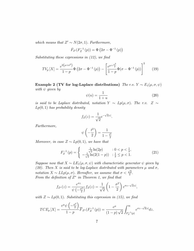
Example 2 (TV for log-Laplace distributions) The r.v. Y � E1(�; �; )with given by

(u) =1

1 + u(20)

is said to be Laplace distributed, notation Y � Lp(�; �). The r.v. Z �Lp(0; 1) has probability density

fZ(z) =1p2e�

p2jzj:

Furthermore,

��t

2

2

�=

1

1� t2

2

Moreover, in case Z � Lp(0; 1); we have that

F�1Z (p) =

(1p2ln(2p) : 0 < p < 1

2;

� 1p2ln(2(1� p)) : 1

2� p < 1:

(21)

Suppose now that X � LE1(�; �; ) with characteristic generator given by(20). Then X is said to be log-Laplace distributed with parameters � and �,notation X � LLp(�; �). Hereafter, we assume that � <

p22.

From the de�nition of Z� in Theorem 1, we �nd that

fZ�(z) =e�z

���2

2

�fZ(z) = 1p2

�1� �2

2

�e�z�

p2jzj;

with Z � Lp(0; 1). Substituting this expression in (15), we �nd

TCEp [X] =e�

���2

2

�1� p

FZ�(F�1Z (p)) =

e�

(1� p)p2

Z 1

F�1Z (p)

e�z�p2jzjdz:

7

Taking into account (21), we �nd

TCEp [X] =

8><>:e��2p2�(

p2��)(2p)(�=

p2+1)

�p2(1�p)(2��2) : 0 < p < 1

2;

p2 e�

(2(1�p))�p2 (p2��)

: 12� p < 1:

(22)

This expression of TCEp [X] for X � LL1(�; �) can be found in Dhaene etal. (2008).Similarly, we �nd that

fZ0(z) =e2�z

(�2�2)fZ(z) =1� 2�2p

2e2�z�

p2jzj;

Taking into account (16), the expressions derived above lead to

E�X2jX > F�1X (p)

�=

e2�

1� p ��2�2

��FZ0(F

�1Z (p))

=

8><>:e2�p2(1�p)

�1�(2p)(

p2�+1)

(2�+p2)

+ 1p2�2�

�: 0 < p < 1

2;

p2e2�

(2(1�p))p2�(p2�2�)

: 12� p < 1:

(23)

Combining (17), (22) and (23) leads to the following expression for TV:

TVp [X] =

8>>>>>><>>>>>>:

e2�p2(1�p)

�1�(2p)(

p2�+1)

(2�+p2)

+ 1p2�2�

���e��2p2�(

p2��)(2p)(�=

p2+1)

�p2(1�p)(2��2)

�2;

0 < p < 12

p2e2�

(2(1�p))p2�(p2�2�)

�� p

2 e�

(2(1�p))�p2 (p2��)

�212� p < 1

(24)

5 A TV-based allocation rule for comonotonicr.v.�s

The capital allocation problem consists of allocating a given aggregate capitalK associated with an aggregate loss

S = X1 +X2 + : : :+Xn

8

to its di¤erent constituents Xi, see e.g. Dhaene et al. (2011) for a generalintroduction to capital allocation. Tasche (2004) introduced the TCE basedallocation rule, where the aggregate capital K is determined as

K = TCEp [S] ; p 2 (0; 1);

whereas the capital Ki that is located to Xi is determined by

Ki = E�Xi j S > F�1S (p)

�; i = 1; 2; : : : ; n and p 2 (0; 1):

It is clear that Ki can be interpreted as the contribution of Xi to TCEp [S].Landsman & Valdez (2003) derived a closed-form expression for the TCEbased allocation rule in case X v En(�;�; ).Furman & Landsman (2006) introduced the tail covariance allocation rule

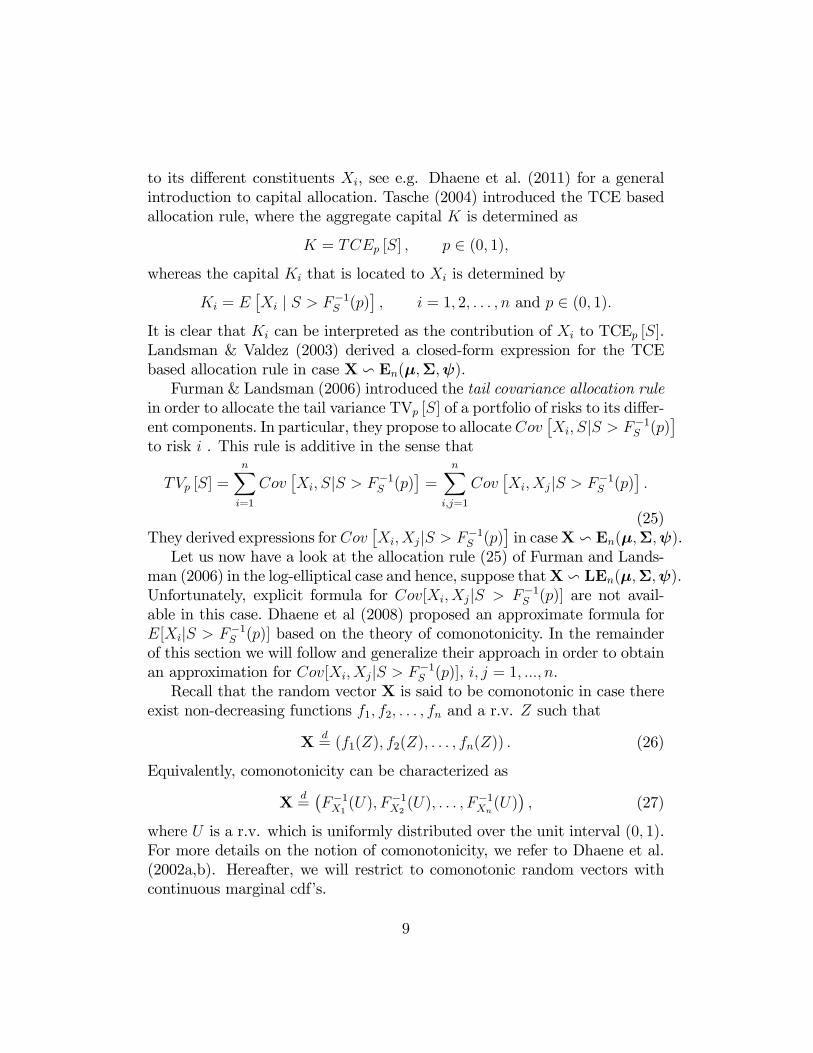
in order to allocate the tail variance TVp [S] of a portfolio of risks to its di¤er-ent components. In particular, they propose to allocateCov

�Xi; SjS > F�1S (p)

�to risk i . This rule is additive in the sense that

TVp [S] =nXi=1

Cov�Xi; SjS > F�1S (p)

�=

nXi;j=1

Cov�Xi; XjjS > F�1S (p)

�:

(25)They derived expressions forCov

�Xi; XjjS > F�1S (p)

�in caseX v En(�;�; ).

Let us now have a look at the allocation rule (25) of Furman and Lands-man (2006) in the log-elliptical case and hence, suppose thatX v LEn(�;�; ).Unfortunately, explicit formula for Cov[Xi; XjjS > F�1S (p)] are not avail-able in this case. Dhaene et al (2008) proposed an approximate formula forE[XijS > F�1S (p)] based on the theory of comonotonicity. In the remainderof this section we will follow and generalize their approach in order to obtainan approximation for Cov[Xi; XjjS > F�1S (p)], i; j = 1; :::; n.Recall that the random vector X is said to be comonotonic in case there

exist non-decreasing functions f1; f2; : : : ; fn and a r.v. Z such that

Xd= (f1(Z); f2(Z); : : : ; fn(Z)) : (26)

Equivalently, comonotonicity can be characterized as

Xd=�F�1X1 (U); F

�1X2(U); : : : ; F�1Xn (U)

�; (27)

where U is a r.v. which is uniformly distributed over the unit interval (0; 1).For more details on the notion of comonotonicity, we refer to Dhaene et al.(2002a,b). Hereafter, we will restrict to comonotonic random vectors withcontinuous marginal cdf�s.

9

Theorem 2 Let X be a comonotonic random vector with continuous mar-ginal cdf�s FXi (x). Let S be de�ned by S = X1 + : : :+Xn. Furthermore, letg(x1; :::; xm); m = 1; : : : ; n be a measurable function such that E [g(Xi1 ; :::; Xim)] <1 for any fi1; : : : ; img � f1; : : : ;mg. Then one has that

E�g(Xi1 ; : : : ; Xim)jS > F�1S (p)

�(28)

= Ehg(Xi1 ; : : : ; Xim)jXi1 > F�1Xi1

(p); : : : ; Xim > F�1Xim (p)i; p 2 (0; 1):

Proof. As X is comonotonic we have that F�1S (p) =nXi=1

F�1Xi (p). Further-

more, the continuity of the marginal cdf�s implies that each F�1Xi (p) is astrictly increasing function in p, 0 < p < 1. Combining these results we �ndthat the the following equivalence relations hold for each i:

nXj=1

F�1Xj (U) >nXj=1

F�1Xj (p), U > p() F�1Xi (U) > F�1Xi (p); i = 1; : : : ; n.

Taking into account that X is comonotonic, we have that

(g(Xi1 ; : : : ; Xim); S)d=

g�F�1Xi1

(U); : : : ; F�1Xim (U)�;nXj=1

F�1Xj (U)

!:

Hence,

E�g(Xi1 ; :::; Xim)jS > F�1S (p)

�= E

"g�F�1Xi1

(U); : : : ; F�1Xim (U)�j

nXj=1

F�1Xj (U) >nXj=1

F�1Xj (p)

#= E

hg�F�1Xi1

(U); : : : ; F�1Xim (U)�j F�1Xi1 (U) > F�1Xi1

(p); : : : ; F�1Xim(U) > F�1Xim(p)i

= Ehg(Xi1 ; : : : ; Xim) j Xi1 > F�1Xi1

(p); : : : ; Xim > F�1Xim (p)i:

Theorem 2 is a generalisation of Theorem 3.1 in Dhaene et al. (2008),who proved this result for the special case g(x) = x.As a corollary of the previous theorem, we immediately �nd the following

result, by choosing m = 2 and g(x1; x2) = (x1�TCEp [Xi])(x2�TCEp [Xj]).

10

Corollary 1 Let X be a comonotonic random vector with continuous mar-ginal cdf�s FXi (x). For any p 2 (0; 1), the contribution Cov

�Xi; XjjS > F�1S (p)

�of risks i and j to the Tail Variance TVp [S] of S is given by

Cov�Xi; XjjS > F�1S (p)

�= Cov

�Xi; XjjXi > F�1Xi (p); Xj > F�1Xj (p)

�;

i; j = 1; :::; n;

In the sequel we will call Cov�Xi; XjjS > F�1S (p)

�the tail-covariance of

Xi and Xj, and denote it by TCovp [Xi; Xj].

6 A TV based allocation rule for sums of log-normal r.v.�s.

Let the random vector X = (X1; : : : ; Xn) be de�ned by

X = (eY1 ; : : : ; eYn); (29)

where Y = (Y1; : : : ; Yn) � Nn (�;�) is an n - dimensional normal vector.Furthermore, S is de�ned by

S =nXk=1

eYk : (30)

In general, it is not possible to derive an analytical expression for E[Xk j S >F�1S (p)] in this case. Therefore, we follow the idea presented in Kaas et al.(2000) to approximate (the distribution of) the r.v. S by (the distributionof) the r.v. T which is de�ned by

T = E[S j �] =nXk=1

E[eYk j �] =nXk=1

Tk; (31)

where Tk = E[Xk j �] and the conditioning r.v. � is a linear combination ofthe Yi:

� =

nXk=1

�k Yk (32)

for appropriate constants �k; k = 1; : : : ; n.Let us denote the elements of the vector � by �k and the elements of the

11

positive de�nite assumed matrix � by �kl, k; l = 1; 2; :::; n. The correlationbetween Yk and � is denoted by rk:

rk = corr [Yk;�] =1

�k ��

nXl=1

�l �kl; k = 1; 2; :::; n; (33)

with �2� given by

�2� =nXk=1

nXl=1

�k �l �kl: (34)

One possible choice for the coe¢ cients �k is given by

�k = e�k+12�2k ; k = 1; :::; n: (35)

This choice of the coe¢ cients is proposed in Vandu¤el et al. (2005), as a slightnumerical improvement to the original choice proposed in Kaas et al. (2000)which is such that � is a linear transformation of a �rst-order approximationto the sum S. In the Theorem below we will need the assumption that thecorrelation coe¢ cients rk de�ned in (33) are positive. This assumption isful�lled when the �k are given by (35).Dhaene et al. (2008) approximated E[Xk j S > F�1S (p)] as follows:

E[Xk j S > F�1S (p)] � E�Tk j T > F�1T (p)

�= TCEp [Tk] ; k = 1; 2; : : : ; n: (36)

Based on this observation, we propose to approximate the tail-covariance ofXk and Xj in the following way:

TCovp [Xk; Xj] t E[E(eYk+Yj j�)jT > F�1T (p)]� TCEp (Tk)TCEp (Tj) :(37)

In the following theorem we derive an expression for this approximation.

Theorem 3 Let the random vector X be de�ned by (29). Furthermore, letT be de�ned by (31), where � is such that all correlations rk de�ned in (33)are positive. The approximation (37) for TCovp [Xk; Xj] can be expressed asfollows:

1

1� pexp

��k + �j +

�2k + �2j2

���exp(�kj)�

��krk + �jrj � ��1 (p)

�� 1

1� p���krk � ��1 (p)

����jrj � ��1 (p)

��(38)

12

Proof. Denote by Ykj = Yk + Yj: It is clear that

Ykj v N��k + �j; �

2kj

�with �2kj = �2k + 2�kj + �2j : (39)

We easily �nd that

Ykjj� = � v N

��k + �j +

Cov(Ykj;�)

�2�(�� ��) ; �

2kj �

Cov2 (Ykj;�)

�2�

�:

Furthermore, one has that

Cov (Ykj;�) = (rk�k + rj�j)��:

Hence,

Ykjj� = � v N

�(�k + �j + (rk�k + rj�j)

(�� ��)

��; �2kj � (rk�k + rj�j)

2

�:

Now we de�ne the r.v.�s Wkj as follows:

Wkj = E�eYkj j�

�= exp

��k + �j +

1

2

��2kj � (rk�k + rj�j)

2�+ (rk�k + rj�j)Z

�;

where

Z =�� ����

v N(0; 1):

Taking into account (37) we �nd that

TCovp [Xk; Xj] t TCEp(Wkj)� TCEp (Tk)TCEp (Tj) : (40)

To determine TCEp (Wkj) we notice that

Wkj v LN

��k + �j +

1

2(�2kj � (rk�k + rj�j)

2); (rk�k + rj�j)2

�:

Now using the formula (18) for the TCE of a lognormal distribution, weobtain

TCEp (Wkj) =1

1� pexp

��k + �j +

1

2�2kj

����krk + �jrj � ��1 (p)

�:

(41)

13

Combining (41) and (18) we �nally obtain the following expression from (40):

TCovp [Xk; Xj]

t1

1� pexp

��k + �j +

1

2�2kj

����krk + �jrj � ��1 (p)

�� 1

(1� p)2exp

��k + �j +

�2k + �2j2

����krk � ��1 (p)

����jrj � ��1 (p)

�:

Taking into account the expression for �2kj given in (39), we �nd the approx-imation (38) for the tail-covariance TCovp [Xk; Xj].From this Theorem we can immediately derive the following approximate

expression for V ar(XkjS > F�1S (p)) in the multivariate lognormal case:

1

1� pexp

�2�k + �2k

� �exp(�2k)�

�2�krk � ��1 (p)

�� 1

1� p

����krk � ��1 (p)

��2�From this Theorem, we also �nd the following approximation for the tail-variance TVp(S):

1

1� p

nXk;j=1

exp

��k + �j +

�2k + �2j2

���exp(�kj)�

��krk + �jrj � ��1 (p)

�� 1

1� p���krk � ��1 (p)

����jrj � ��1 (p)

��(42)

7 Numerical illustration

In this section we give a numerical illustration of our theoretical results.We use the example of a company with 4 business lines that was presentedin Dhaene et al. (2008). We illustrate the appropriateness of the proposedapproximation for the TV - based allocation rule in a multivariate lognormalsetting.Let us assume that the multivariate risk X = (X1; :::; X4) faced by the

company has a multivariate lognormal distribution, X � LN4 (�;�) ; withmarginal expectations and variances given by

(E [X1] ; E [X2] ; E [X3] ; E [X4]) = (20; 40; 10; 5)

14

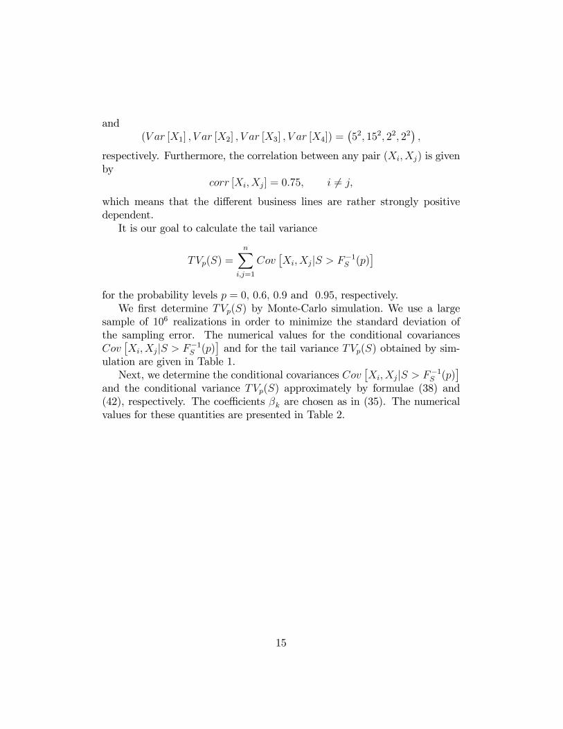
and(V ar [X1] ; V ar [X2] ; V ar [X3] ; V ar [X4]) =

�52; 152; 22; 22

�;

respectively. Furthermore, the correlation between any pair (Xi; Xj) is givenby

corr [Xi; Xj] = 0:75; i 6= j;

which means that the di¤erent business lines are rather strongly positivedependent.It is our goal to calculate the tail variance

TVp(S) =nX

i;j=1

Cov�Xi; XjjS > F�1S (p)

�for the probability levels p = 0; 0:6; 0:9 and 0:95, respectively.We �rst determine TVp(S) by Monte-Carlo simulation. We use a large

sample of 106 realizations in order to minimize the standard deviation ofthe sampling error. The numerical values for the conditional covariancesCov

�Xi; XjjS > F�1S (p)

�and for the tail variance TVp(S) obtained by sim-

ulation are given in Table 1.Next, we determine the conditional covariances Cov

�Xi; XjjS > F�1S (p)

�and the conditional variance TVp(S) approximately by formulae (38) and(42), respectively. The coe¢ cients �k are chosen as in (35). The numericalvalues for these quantities are presented in Table 2.

15

Table 1 Table 2Monte Carlo Estimation of Comonotonic Approximation ofCov

�Xk; XjjS > F�1S (p)

�Cov

�Xk; XjjS > F�1S (p)

�p = 0:95����������

22:621 10:409 3:356 4:41410:409 170:686 5:700 7:7363:356 5:700 3:262 1:8144:414 7:736 1:814 5:730

TVp (S) 269:158

����������

p = 0:95����������20:909 9:186 2:924 3:9579:186 172:575 5:413 7:7102:924 5:413 3:153 1:6693:957 7:710 1:669 5:577

TVp (S) 263:931

����������p = 0:9����������

20:626 13:563 3:323 4:22513:563 162:453 6:629 8:5933:323 6:629 3:098 1:7374:225 8:593 1:737 5:001

TVp (S) 267:317

����������

p = 0:9����������19:727 13:516 3:077 3:98613:516 165:018 6:660 8:9653:077 6:660 3:019 1:6593:986 8:965 1:659 4:895

TVp (S) 268:383

����������p = 0:6����������

18:769 25:501 3:903 4:52525:501 163:507 10:654 12:4983:903 10:654 2:924 1:8204:525 12:498 1:820 3:831

TVp (S) 306:835

����������

p = 0:6����������18:656 25:810 3:901 4:52325:810 164:318 10:702 12:6473:901 10:702 2:929 1:8264:523 12:647 1:826 3:837

TVp (S) 308:559

����������p = 0����������

25:000 55:423 7:450 7:37355:423 225:000 22:142 22:1007:450 22:142 4:000 2:9457:373 22:100 2:945 4:000

TVp (S) = V (S) 492:865

����������

p = 0����������25:000 55:423 7:450 7:37355:423 225:000 22:142 22:1007:450 22:142 4:000 2:9457:373 22:100 2:945 4:000

TVp (S) = V (S) 492:865

����������Table 3Level (p) The relative di¤erence0:95 1:942%0:9 �0:399%0:6 �0:562%0 0%

In Table 3 the relative di¤erence between the results of the Monte-Carlosimulation and the results obtained via the comonotonic approximations are

16

given. From Tables 1, 2 and 3 one can conclude that the proposed approxima-tions based on the theory of comonotonicity perform well. This is particularlytrue because the comonotonic approximations reduce the n -dimensional ran-domness of the problem to a univariate randomness via the introduction ofthe condition r.v. � de�ned in (32).

Acknowledgement 4 Jan Dhaene acknowledges the �nancial support of theOnderzoeksfonds K.U. Leuven (GOA/07: Risk Modeling and Valuation of Insur-ance and Financial Cash Flows, with Applications to Pricing, Provisioning andSolvency).

References

[1] Dhaene, J., Denuit, M., Goovaerts, M.J., Kaas, R. & Vyncke, D.,(2002a). �The concept of comonotonicity in actuarial science and �-nance: Theory�, Insurance: Mathematics & Economics, 31(1), 3-33.

[2] Dhaene, J., Denuit, M., Goovaerts, M.J., Kaas, R. & Vyncke, D.,(2002b). �The concept of comonotonicity in actuarial science and �-nance: Applications�, Insurance: Mathematics & Economics, 31(2),133-161.

[3] Dhaene, J., Henrard, L., Lansdman, Z., Vandendorpe, A., Vandu¤el,S. (2008). "Some results on the CTE based capital allocation rule",Insurance: Mathematics and Economics, 42, 855�863.

[4] Dhaene, J., Tsanakas, A., Valdez, E.A., Vandu¤el, S. (2011). "Optimalcapital allocation principles", Journal of Risk and Insurance, 78.

[5] Dhaene, J., Vandu¤el, S., Tang, Q., Goovaerts, M.J., Kaas, R. andVyncke, D. (2006). �Risk measures and comonotonicity: a review�, Sto-chastic Models, 22, 573-606.

[6] Embrechts, P., McNeil, A. & Straumann, D. (2001) (1999). "Correla-tion and dependence in risk management: properties and pitfalls", RiskManagement: Value at Risk and Beyond, Dempster, M. & Mo¤att, H.K.(eds.), Cambridge University Press.

17

[7] Fang, K.T.; Kotz, S. & Ng, K.W. (1990). Symmetric multivariate andrelated distributions. London: Chapman & Hall.

[8] Furman, E. & Landsman, Z. (2006). "Tail Variance Premium with Ap-plications for Elliptical Portfolio of Risks", Astin Bulletin, 36(2) 433-462.

[9] Kaas, R., Dhaene, J. & Goovaerts, M. (2000). "Upper and lower boundsfor sums of random variables", Insurance: Mathematics & Economics,27(2), 151-168.

[10] Kelker, D. (1970). "Distribution theory of spherical distributions and alocation-scale parameter generalization.�Sankhya: The Indian Journalof Statistics, Series A, 32 (4), 419-438.

[11] Landsman, Z. & Valdez, E. (2003) "Tail Conditional Expectations forElliptical Distributions", Astin Bulletin 35(1), 189-209.

[12] Tasche, D. (2004). �Allocating portfolio economic capital to sub-portfolios,� Economic Capital: A practitioner�s Guide , Risk Books,75-302.

[13] Valdez, E., Dhaene, J., Maj, M., Vandu¤el, S. (2009). "Bounds andapproximations for sums of dependent log-elliptical random variables",Insurance: Mathematics & Economics, 44, 385-397.

[14] Vandu¤el, S., Hoedemakers, T. & Dhaene, J. (2005). "Comparing ap-proximations for risk measures of sums of non-independent lognormalrandom variables", North American Actuarial Journal, 9(4), 71-82.

18