Downward Nominal Wage Rigidity in Europe∗

Steinar HoldenUniversity of Oslo, Norges Bank and CESifo

Department of Economics, University of OsloBox 1095 Blindern, 0317 Oslo, Norway

steinar.holden@econ.uio.nohttp://folk.uio.no/sholden/

Fredrik WulfsbergNorges Bank

Box 1179 Sentrum, 0107 Oslo, Norwayfredrik.wulfsberg@norges-bank.no

http://www.norges-bank.no/research/wulfsberg.html

First draft: 14th February 2003This version: October 2004

Abstract

This paper explores the existence of downward nominal wage rigidity (DNWR) in theindustry sectors of 16 European countries, over the period 1973–1999, using data for hourlynominal wages at industry level. Based on a novel nonparametric statistical method, which al-lows for country and year specific variation in both the median and the dispersion of industrywage changes, we reject the hypothesis of no DNWR. The fraction of wage cuts preventeddue to DNWR has fallen over time, from 70 percent in the 1970s to 20 percent in the 1990s,but the number of industries affected by DNWR has increased. Wage cuts are less likely incountries and years with high inflation, low unemployment, high union density and strictemployment protection legislation.

JEL: J5, C14, C15, E31Keywords: Downward nominal wage rigidity, European countries, employment protectionlegislation

Preliminary version – UNDER REVISION

∗We wish to thank Lars Holden and Tore Schweder for invaluable help in the formulation of the statistical methodsthat we use. We are also grateful to Bill Dickens, Mike Elsby, Christoph Knoppik, Alan Manning, Halvor Mehlumand seminar participants at ESEM2003, Norges Bank and University of Oslo for useful comments to earlier drafts.Views and conclusions expressed in this paper are those of the authors alone and cannot be attributed to Norges Bank.

1 Introduction

In recent years, a number of countries have adopted explicit inflation targets for monetary policy,

reflecting a general agreement that monetary policy must ensure low inflation. The deliberate

policy of low inflation has led to renewed interest among academics as well as policy makers

for the contention of Tobin (1972) that if policy aims at too low inflation, downward rigidity

of nominal wages (DNWR) may lead to higher wage pressure, involving higher equilibrium un-

employment (see e.g. Akerlof et al., 1996, 2000, Holden, 1994, and Wyplosz, 2001). Other

economists have been less concerned, questioning the existence of (DNWR), in particular in low

inflation economies (see e.g. Gordon, 1996 and Mankiw, 1996). The issue has also received

considerable attention among policy makers, cf. e.g. (ECB, 2003, OECD, 2002 and IMF, 2002).

To shed light of this issue, a fast growing body of empirical research has explored the existence

of DNWR in many OECD countries (see references in section 2 below). Almost all of these studies

use various kinds of micro data, mostly of the wage of individual workers, but occasionally also

the wage in specific jobs in individual firms. While these studies generally seem to document the

existence of DNWR, a number of key questions are still left unresolved. As the different studies

vary considerably concerning both type of data and the methods that are used, it is difficult to

compare the degree of DNWR across countries and the extent to which DNWR has varied over

time. Furthermore, while individual data is necessary to explore whether wages are rigid at

employee level, it will often be unable to answer the question of whether firms can circumvent

wage rigidity at the individual level, for example by changing the composition of the workforce

by turnover. Correspondingly, even if wage rigidity binds in one firm, jobs might be shifted over

to other firms where wages are lower, so that the industry effects are small. Then DNWR may be

less important for macroeconomic performance. It therefore seems valuable also to investigate

DNWR using industry level data.

This paper explores the existence of DNWR in the industry sectors of 16 European countries,

2

over the period 1973–1999, using data for hourly nominal earnings at industry level. The study

is to be seen as complementary to the large number of micro studies, as it allows for comparisons

across different groups of countries, and comparisons over time. More importantly, by using data

for the hourly earnings at industry level, our study captures effects of changes in the composition

of the workforce, as well as the effect of changes in the wage rates. Furthermore, our study covers

a number of countries in Continental Europe, for which there so far is little available evidence

of the existence of DNWR, in spite of the considerable policy importance of this issue in relation

to the ambitious inflation target of the ECB.

To investigate the extent of DNWR, we construct a statistical method not previously used

on this issue (at least to the best of our knowledge). The advantage of the method is that it

uses much weaker assumptions than most previous analyses, implying that the results should

be more robust. First, the method is based on a nonparametric analysis, using data for hourly

earnings only, so that no assumptions concerning explanatory variables or specific functional

forms are involved. Second, we allow for country and year specific variation in the median and

the dispersion of wage changes, while most other tests are based on more restrictive assumptions.

To further explore the determinants of nominal wage ridigidy, we regress the incidence of

nominal wage cuts in each country-year sample on economic and institutional variables, like

inflation, unemployment, employment protection legislation, union density, etc.

The paper is organised as follows. In Section 2, we briefly present the main theoretical

explanations for DNWR, and we refer to related empirical literature. The empirical approach

is laid out in Section 3, while the empirical results on DNWR are documented in Section 4. In

Section 5, we explore the determinants of nominal wage rigidity. Section 6 concludes. The data

we use are described in the Appendix.

3

2 Theoretical framework and related literature

In the literature, two alternative explanations of the existence of DNWR have been proposed.1

The most common explanation, advocated by e.g. Blinder & Choi (1990) and Akerlof et al.

(1996), is that employers avoid nominal wage cuts because both they and (in particular) the em-

ployees think that a wage cut is unfair. The other explanation, proposed by MacLeod & Malcom-

son (1993) in a individual bargaining framework, and Holden (1994) in a collective agreement

framework, is that nominal wages are given in contracts that can only be changed by mutual con-

sent. Both these theories predict that nominal wage cuts will be prevented in some, but not all

circumstances. For our purposes, there is no need to distinguish between these two explanations

of DNWR, and, as argued by Holden (1994), they are likely to be complementary.

Empirical work on DNWR have grown rapidly in recent years, with various types of evid-

ence. Blinder & Choi (1990), Akerlof et al. (1996), Bewley (1999) and Agell & Lundborg (2003)

report results from interviews and surveys of employees and employers. A few papers docu-

ment the existence of DNWR on aggregate data, see Holden (1998) and Fortin & Dumont (2000).

However, the great majority of studies explore large micro-data sets, following either two types of

approaches. The first type, initiated by the skewness-location approach of McLaughlin (1994), fo-

cuses on the effect of inflation on the distribution of wage changes; Christofides & Leung (2003),

Lebow et al. (2003) and Nickell & Quintini (2003) are recent applications. The second type,

referred to as the "earnings function approach" by Knoppik & Beissinger (2003), add other ex-

planatory variables that are usually included in wage equations, see e.g. Fehr & Gotte (2003) and

Altonji & Devereux (2000). Our study is of the first type, thus a brief discussion of this method

is warranted. As is well known (see e.g. discussion in Knoppik & Beissinger (2003) or Nickell &

Quintini (2003)), the validity of variants within this type of approach rests of various restrictive

additional assumptions concerning the underlying or notional distribution of wage changes (fol-

1Efficiency wage theories and insider-outsider theories are also sometimes mentioned as explanations of DNWR,but these theories explain real wage rigidity and need additional assumptions to generate DNWR.

4

lowing the terminology of Akerlof et al. (1996)), i.e. the wage changes that would prevail in the

absence of DNWR. The LSW statistic, suggested by Lebow et al. (1995), requires that the notional

nominal wage change distribution is symmetric. The Kahn test (Kahn, 1997) allows for asym-

metry of the notional wage change distribution, as long as the shape of the notional distribution

is invariant to inflation, i.e. the only effect of inflation on the distribution of wage changes comes

in the form of DNWR. As illustrated in figure 2 below, the wage change distribution is asymmet-

ric in our data, and dispersion changes over time (as does inflation), so both these methods are

problematic in our case. The Nickell & Quintini (2003) method is based on the assumption (or

approximation) that the probability of a nominal wage cut is a quadratic function of the median

wage change.

In general these studies document that nominal wages are rigid downwards. However, with

the exception of Dessy (2002), different methods and data in the above-mentioned studies make

it in general difficult to compare the degree of downward nominal wage rigidity across countries.2

3 Empirical approach

We use an unbalanced panel of industry level data for the annual growth rate of gross hourly

earnings for manual workers from the manufacturing, mining and quarrying, electricity, gas and

water supply, and construction sectors of 16 European countries in the period 1973–1999. The

countries included in the sample are Austria, Belgium, Germany, Denmark, Spain, Finland,

France, Greece, Ireland, Italy, Luxembourg, Netherlands, Norway, Portugal, Sweden and the

UK. The main data source for wages are harmonized hourly earnings from Eurostat.3 The

observational unit is thus denoted ∆wjit where j is index for industry, i is index for country and

t is index for year. There are all together 7650 observations distributed across N = 379 country-

2The International Wage Flexibility Project, organised by William Dickens and Erica Groshen, may change that,as it comprises studies on comparable micro data for many OECD countries.

3Data for Austria, Finland and Sweden are from the ILO, while data for Norway is from Statistics Norway.

5

year samples, on average 20 industries per country-year. More details on data are provided in

the appendix.

Before proceeding, let us first note that an observation of a nominal wage cut in our data

differs in several respect from an observation of a nominal wage cut in most studies based on

micro data. In micro studies, a nominal wage cut is usually understood as a reduction in hourly

nominal pay for a job stayer. In our data, covering average hourly earnings for manual workers

in an industry, a wage cut might be caused by a reduction in average hourly pay for job stayers,

but it might also be caused by changes in the composition of the workers, within firms or between

firms. Thus, our data involves considerable ‘noise’ relative to observations at the individual level,

so we are unlikely to uncover all the rigidity that may exist at the individual level. Yet precisely

because our data also captures other ‘avenues’ for flexibility, it may yield a better measure of

rigidity at industry level. Furthermore, estimates based on individual data for job stayers may

also be biased due to self selection, if employees whose wage is cut may quit, and thus no longer

be job stayers. On the other hand, micro data studies have an advantage in a much larger number

of observations, with the possibility of controlling for other explanatory variables. Overall, it

seems worthwhile to explore DNWR with both types of data.

There are no nominal wage cuts in 295 (78%) of the country-year samples. In our data

we observe, however, no less than 217 events of nominal wage reductions, i.e., 2.84% of all

observations. There were fewer wage cuts in the 1970s, early 1980s and early 1990s, while most

wage cuts occured after 1992, cf. figure 1. Table A1 in the Data Appendix reports the distribution

of wage cuts and observations across countries and years.

As an illustration figure 2 displays box plots of annual wage growth in Portugal, as well as

a histogram of the wage changes in 28 industries in Portugal in 1998. We see that the average

and the dispersion of wage growth vary over time. The histogram for 1998 seems consistent

with the idea that DNWR has prevented some nominal wage cuts, compressing the empirical

6

010

2030

Num

ber

of w

age

cuts

1975 1980 1985 1990 1995 2000

Figure 1: The number of wage cuts over time.

0.1

.2.3

.4

1981

1982

1983

1984

1985

1986

1987

1988

1989

1990

1991

1992

1993

1994

1995

1996

1997

1998

05

1015

20

Den

sity

−.1 0 .1 .2

Wage growth, Portugal 1998

Figure 2: Box plots of annual wage growth in Portugal (left) and histogram of annual wage growth in 1998 (right). Thebox plot illustrates the distribution of wage changes within a country-year. The box extends from the 25th to the 75thpercentile with the median inside the box. The whiskers emerging from the box indicate the tails of the distributions andthe crosses represent outliers.

wage distribution relative to the notional by pushing the left tail to positive values. However, to

evaluate this properly, we need to use a formal statistical method.

To detect whether the empirical distribution is compressed relative to the notional, we must

obtain an estimate for the notional distribution, as well as compare the notional distributions

with the empirical outcomes. We estimate the shape of the notional distribution on the basis of

all observations for the period 1973–1992, assuming the same shape in all country-years, except

that we allow for the median and dispersion to differ across country-year samples. The estimated

shape may also be affected by DNWR, but this effect should be small given that we only use

7

observations from the high-inflation years where DNWR is less likely to be binding. Alternatively,

we could have assumed that the notional distribution was normal, however, as illustrated in

Figure 3 below, this would not be a good approximation.

To compare the notional distributions with the empirical outcomes, we simulate all country-

year samples based on the notional distributions, and count the number of wage cuts in the

simulations. If the empirical outcomes were affected by DNWR, the simulations based on the

notional distributions will involve a higher number of wage cuts than what actually took place. If

the difference between the simulated number of wage cuts, based on the notional distributions,

and the actual number of wage cuts, is sufficiently large (which will be made more precise below),

we conclude that DNWR has been binding in some country-year samples. In the next section,

our test is presented more formally.

3.1 The formal test

As mentioned above, our test is based on the assumption that the median and dispersion of the

wage change distribution may vary among country-year samples, but otherwise the shape of the

distribution is the same (in the absence of possible DNWR). To ensure robustness to outliers, we

measure dispersion by the inter quartile range (i.e. the difference between the 75th percentile

and the 25th percentile) rather than the standard deviation (for the same reason, we use the

median rather than the mean). Under these assumptions, we obtain an underlying distribution

of wage changes based on the sample of 5726 empirical wage change observations for the period

1973–92,4 where the empirical wage changes are adjusted for the country-year specific median

(µit) and inter quartile range IQRit, i.e.

∆wns ≡(

∆wjit − µitIQRit

)

, s = 1, . . . , 5726 (1)

4We also tried country-specific normalised distributions, but this had little impact on the qualititative results.

8

For simplicity we use subscript s which runs over all j, i and t = 1973, . . . , 1992.

The country-year specific samples of notional wage changes are constructed on the basis of the

underlying wage change distribution 1, by adjusting the underlying normalised wage changes,

∆wns , with the country-year specific median and inter quartile range. However, as the country-

year specific 25th percentiles may be affected by DNWR, leading to a downward bias in the inter

quartile ranges, we estimate the inter quartile range by two times the difference between the 75th

percentile and the median. In effect, we assume that the notional wage change distribution is

symmetric with respect to the 25th and 75th percentiles.5 However, in the appendix, we also

report results without this assumption, where we use the observed inter quartile range to calculate

the country-specific notional distribution, cf. the third bullet point below. In the appendix,

we also report results based on country-specific underlying distribution, i.e. where we estimate

separate ∆wns for each country. Under both these alternatives, the qualitative results are similar

to those reported in the main text, although the evidence of DNWR is somewhat weaker, as would

be expected as these alternatives are more sensitive to a downward bias due to DNWR.

Figure 3 compares the underlying distribution of wage changes with the standard normal

distribution; we notice that the underlying distribution is skewed with the mean at 2.2 percent.

The right panel of figure 3 compares the country-specific notional distribution for Portugal 1998,

i.e the underlying distribution after adjustment for the mean and inter quartile range in Portugal

1998, with the empirical distribution. We observe that country-specific notional distribution in-

dicates a considerable probability of negative wage changes, in contrast to the empirical outcome.

One complication is that the empirical samples, as well as the moments based on them, are

stochastic and thus burdened with unknown uncertainty. To allow for that, we use a bootstrap

5This is a much weaker assumption than assuming complete symmetry of the notional distribution, as used byLSW 1995 and Card & Hyslop (1997). While Card & Hyslop (1997) point out that most conventional models of wagedetermination imply symmetry, Elsby (2004) shows that DNWR is likely to affect also the upper tail of the distribution,as wage setters may set lower wage increases in years where DNWR does not bind, to reduce the risk that DNWR willbind in the future.

9

0.2

.4.6

.8

Den

sity

−5 0 5

010

2030

−.1 0 .1 .2

Figure 3: Left: Histogram and normal density (solid line) of the normalised underlying distribution of wage growth. 20extreme observations are omitted. Right: Histogram of observed wage growth and notional wage distribution in Portugal1998.

method. More specifically, for each of the 379 country-year samples, we bootstrap the empirical

country-year sample (for example, in a country-year with 24 observations, we make 24 random

draws from the empirical sample of 24 industry wage changes, with replacement). Then we

• count the number of bootstrapped wage cuts in the country-year, yBit ,

• calculate country-specific bootstrapped median, µBit , and 75th percentile, P75Bit ,

• construct the country-year specific distribution of notional wage changes by adjusting the

underlying wage change distribution for the country-specific bootstrapped median and

75th percentile

∆ ˜wits ≡ ∆wn

s

(

2(P75Bit − µBit ))

+ µBit , s = 1, . . . , 5726 (2)

• calculate the corresponding country-year specific probabilities of a notional wage cut in

country-year it as the proportion of notional wage cuts out of the total sample of observa-

tions S = 5726

qit ≡#∆ ˜wit

s < 0S

, s = 1, . . . , 5726 (3)

• simulate the number of wage cuts in each country-year specific notional sample, yit, by

10

drawing from a binomial distribution using the country-specific notional probabilities qit,

and

• compare the total number of bootstrapped wage cuts Y B =∑

it yBit for all 379 country-year

samples with the total number of simulated notional wage cuts, Y =∑

it yit .

If the empirical samples are affected by DNWR, there will be a tendency that there are more

simulated wage cuts than bootstrapped wage cuts, i.e. Y > Y B. We therefor repeat this procedure

5000 times, undertaking a new bootstrap for each country-year sample each time, and count the

number of times where Y > Y B. The null hypothesis is rejected with a level of significance at 5%

if 1− #(Y > Y B)/5000 ≤ 0.05.

Note that if the notional distributions are correctly estimated, 5000 simulations will ensure a

close approximation to the distribution of the total number of wage cuts if there were no DNWR.

6 Thus, the significance level of our test should be reliable. However, if DNWR is at work

in some country-year samples, the empirical wage distribution will be compressed, and so will

our estimates of the underlying and notional wage changes, as these are based on the empirical

distributions for all country-year samples. Thus, the notional probabilities will also be biased

downwards, reducing the number of simulated wage cuts, which will reduce the power of our

test.

4 Results

There are more simulated than bootstrapped wage cuts in all 5000 simulations. Thus we reject

the null hypothesis comfortably with a p-value of 0, and we may conclude that DNWR has been

at work in our sample. To illustrate the power of the test we plot the histogram of the number

of simulated and bootstrapped wage cuts in Figure 4. On average, we simulate 304 notional6Given the notional country-years specific distributions it would in principle be straightforward to calculate the

probability distribution function for the total number of wage cuts by use of a formulae for draws from multinomialdistributions. However, with 7650 observations, this is computationally very demanding. Simulation is computation-ally simpler, allows for bootstrapping, and still accurate.

11

0.0

1.0

2.0

3

150 200 250 300 350 400

Bootstrapped cuts

Simulated cuts

Figure 4: The frequency distributions of the number of 5000 bootstrapped (empirical) and simulated (notional) wagecuts.

wage cuts and bootstrap 217 wage cuts (due to the large number of simulations, the bootstrapped

average of 217 clearly equals the number of observed wage cuts). The average fraction of notional

wage cuts that do not result in an observed wage cut due to DNWR, may be expressed by (1−Y/Y )

where Y is the number of observed wage cuts and Y is the average number of simulated cuts.

For the whole sample this fraction is (1 − 217/304) = 0.29. Thus, a bit more than one out of

five notional wage cuts does not result in an observed wage cut due to DNWR. Another measure

which illustrates the economic significance of DNWR is the average fraction of industry-years

affected by DNWR. This fraction may be calculated by (Y − Y )/S where S is the number of

industry-years. For the whole sample this fraction is (304− 217)/7650 = 0.011.

A number of interesting questions arise. Is there evidence for DNWR for different time peri-

ods, regions and countries? To what extent is DNWR related to labour market institutions as

proposed by theory? We first investigate whether DNWR has changed over time by splitting the

sample into four subperiods 1973–1979, 1980–1989, 1990–1994 and 1995–1999, see Table 1.

There is evidence of DNWR in all periods. In the high-inflation 1970s, on average almost 70

percent of the notional wage cuts did not result in observed wage cuts. In the 1980s and early

1990s, about 30 percent of the notional wage cuts did not result in observed wage cuts, while in

the late 1990s, the probability that DNWR prevented a notional wage cut leading to an observed

12

Table 1: Results from 5000 simulations on subperiods using bias adjusted probabilities.

Sample properties: 1973–1979 1980–1989 1990–1994 1995–1999

No. of observations 1754 3016 1546 1334No. of country-years 89 153 75 62Average wage growth 14.27% 8.92% 6.22% 4.31%Average inflation rate 10.33% 8.21% 4.75% 2.27%Average unemployment rate 3.49% 7.30% 8.38% 8.37%Observed wage cuts (Y ) 5 57 51 104Proportion of wage cuts (%) 0.29 1.89 3.30 7.80

Simulation results:Average simulated wage cuts 16 89 72 127#(Y > Y B) 4911 4950 4856 4672Probability of significance 0.018 0.010 0.029 0.066Fraction of wage cuts prevented 0.687 0.360 0.295 0.181Fraction of industry-years affected 0.006 0.011 0.014 0.017

wage cut was 18 percent. While the results indicate that the fraction of wage cuts prevented by

DNWR decreased over time, the average fraction of industry-years affected by DNWR increased

from 0.6 percent in the 1970s to 1.1 percent in the 1980s, 1.4 percent in the early 1990s and finally

1.7 percent in the late 1990s.

Nominal rigidities may be related to labour market institutions. Based on a theoretical frame-

work allowing for bargaining over collective agreements as well as individual bargaining, Holden

(2004) argues that workers who have their wage set via unions or collective agreements have

stronger protection against a nominal wage cut, thus the extent of DNWR is likely to depend on

the coverage of collective agreements and union density. For non-union workers, the strictness of

the employment protection legislation (EPL) is key to their possibility of avoiding a nominal wage

cut. As documented by among others OECD (1999), such institutions differ considerably among

European countries, and it would therefore be interesting to investigate existence of DNWR for

regions as well as individual countries.

We first split the sample into regions which have comparable labour market institutions. We

operate with four regions; the British Isles, Core (Austria, Belgium, France, Germany, Luxem-

13

Table 2: Results from 5000 simulations on regions using bias adjusted probabilities.

Sample properties: All regions British Isles Core Nordic South

No. of observations 7650 1078 3110 1984 1478No. of country-years 379 49 158 97 75Observed wage cuts (Y ) 217 45 125 18 29Proportion of wage cuts (%) 2.84 4.17 4.02 0.91 1.96

Simulation results:Average simulated wage cuts 304 58 161 35 50#(Y > Y B) 5000 4374 4917 4913 4894Probability of significance 0 0.125 0.017 0.017 0.021Fraction of wage cuts prevented 0.287 0.224 0.226 0.483 0.421Fraction of industry-years affected 0.011 0.012 0.012 0.008 0.014

bourg and the Netherlands), the Nordic Region (Denmark, Finland, Norway and Sweden) and

South (Italy, Greece, Portugal and Spain). The results from simulations using these regions are

presented in columns 2–5 in Table 2.

We reject the hypothesis of no DNWR for all regions, but the British Isles. In the South, a

region where bargaining coverage is fairly high (see e.g. Calmfors et al., 2001, table 4.4) and EPL

is very strict OECD (1999), 42 percent of the notional wage cuts did not result in an observed cut,

while 1.4 percent of the industries were affected by DNWR. In the Core, where there is generally

high bargaining coverage and fairly strong EPL, 23 of the notional wage cuts did not result in

observed cuts, which is considerably lower than in the South. In the British Isles, 22 percent

of the notitional wage cuts were prevented by DNWR. In this region, EPL is less strict than in

most of the rest of Europe; however, union density and bargaining coverage are fairly high in

Ireland, but not in the UK. 1.2 percent of the industries were affected by DNWR in the Core, and

the British Isles. In the Nordic region 48 percent of the notitional wage cuts were prevented by

DNWR.

Splitting the sample by combining the regions and the sub-periods reduces the significance

levels, see Table 3. These results should be treated more cautiously, as they are based on a smaller

number of observations. At the ten percent level, we find significant DNWR in the Core (1970s

14

Table 3: Results from 5000 simulations on regions and sub-periods using bias adjusted probabilities.Region 1973–1979 1980–1989 1990–1994 1995–1999

No. of observations 228 432 227 191No. of country-years 11 20 10 8

British Observed wage cuts (Y ) 0 8 17 20Isles Proportion of wage cuts (%) 0 1.85 7.49 10.47

Average simulated wage cuts 2 14 22 20#(Y > Y B) 3709 4303 3891 2200Probability of significance 0.258 0.139 0.222 0.560Fraction of wage cuts prevented 1 0.440 0.237 0Fraction of industry-years affected 0.007 0.015 0.023 0No. of observations 794 1183 587 546No. of country-years 41 60 30 27Observed wage cuts (Y ) 4 40 18 63

Core Proportion of wage cuts (%) 0.50 3.38 3.07 11.54Average simulated wage cuts 10 57 24 70#(Y > Y B) 4513 4616 4102 3754Probability of significance 0.097 0.077 0.180 0.249Fraction of wage cuts prevented 0.604 0.293 0.267 0.104Fraction of industry-years affected 0.008 0.014 0.011 0.013No. of observations 474 888 362 260No. of country-years 23 40 20 14Observed wage cuts (Y ) 1 3 12 2

Nordic Proportion of wage cuts (%) 0.21 0.34 3.31 0.77Average simulated wage cuts 2 8 16 8#(Y > Y B) 2950 4503 3716 4704Probability of significance 0.410 0.099 0.257 0.059Fraction of wage cuts prevented 0.531 0.647 0.252 0.757Fraction of industry-years affected 0.002 0.006 0.011 0.024No. of observations 258 513 370 337No. of country-years 14 33 15 13Observed wage cuts (Y ) 0 6 4 19

South Proportion of wage cuts (%) 0 1.17 1.08 5.64Average simulated wage cuts 2 10 9 29#(Y > Y B) 4074 3788 4344 4329Probability of significance 0.185 0.242 0.131 0.134Fraction of wage cuts prevented 1 0.384 0.580 0.340Fraction of industry-years affected 0.008 0.007 0.015 0.029

15

Table 4: Results from 5000 simulations on countries using bias adjusted probabilities.

Country No.of

obser

vatio

ns

No.of

years

Observ

edwag

e cuts

(Y)

Prop.

ofwag

e cuts

(%)

Averag

e simula

tedwag

e cuts

#(Y>YB )

Proba

bility

ofsig

nifica

nce

Frac

tion of

wage cu

tspr

even

ted

Frac

tion of

indus

try-ye

arsaff

ected

Austria 408 26 2 0.49 7 4621 0.076 0.721 0.013Belgium 575 26 31 5.39 42 4683 0.063 0.268 0.020Denmark 464 25 8 1.65 14 4191 0.162 0.426 0.013Finland 368 23 2 0.54 6 4216 0.157 0.656 0.010France 556 26 21 3.78 19 1740 0.652 0 0Germany 665 26 16 2.41 18 2878 0.424 0.114 0.003Greece 469 26 7 1.49 7 2194 0.561 0.016 0.000Ireland 463 23 27 5.83 36 4210 0.158 0.260 0.020Italy 312 13 0 0 3 4430 0.114 1 0.010Luxembourg 423 27 32 7.57 39 3877 0.225 0.182 0.017Netherlands 483 27 23 4.76 35 4717 0.057 0.351 0.026Norway 674 27 2 0.30 4 3243 0.351 0.469 0.003Portugal 411 18 3 0.73 22 4999 0.000 0.863 0.046Spain 286 18 19 6.64 18 1958 0.608 0 0Sweden 478 22 6 1.26 11 4471 0.106 0.472 0.011UK 615 26 18 2.93 22 3427 0.315 0.162 0.006

and 1980s) and the Nordic region (1980s and late 1990s). For all regions with the exeption of

the Nordic region, the fraction of notional wage cuts that did not lead to observed cuts has fallen

over time, consistent with the aggregate picture as seen in Table 1. The fraction of industry-years

affected by DNWR has increased the Nordic region, the South and the British Isles.

In Table 4, we report the results concerning individual countries. Bearing in mind that that

the results are based on fewer observations, we observe that for all countries except France and

Spain, the simulations indicate that some of the notional wage cuts do not result in observed

wage cuts due to DNWR. For four countries (Austria, Belgium, the Netherlands, and Portugal),

DNWR is significant at the ten percent level. For the other countries, DNWR is not statistically

significant, even if the average fraction of notional wage cuts that do not result in observed cuts

for some countries is more than 40 percent in the Nordic countries and as high as 11 percent for

16

Germany and 16 percent for the UK. This illustrates the considerable uncertainty involved in this

measure. The fraction of industry-years affected by DNWR varies from 4.6 (Portugal) percent at

the top, to 0 (France and Spain) percent at the bottom.

To further explore the reliability of our measures of DNWR, we undertake Poisson regressions

with the number of observed wage cuts in each country-year sample it, Yit, as the dependent

variable, and normalise on the number of simulated wage cuts, Yit. A Poisson regression seems

appropriate as the endogenous variable is based on count data, see Cameron & Trivedi (1998).

Adding dummys for region, period, combined region and period, as well as for countries, we

are then able to derive confidence intervals for the fraction of wage cuts prevented for all the re-

spective subsamples, see Figure 5. Note that the point estimates of the fractions in Figure 5 differ

slightly from the fractions in the tables, as the former are based on the Poisson regressions, and

thus are non-linear, while the latter are linear averages based on the simulations. The confidence

intervals are fairly large, and with few exceptions, we are not able to conclude that the fractions

are significantly different from one another.

However, we also undertake a Poisson regression of Yit, as the dependent variable, normal-

ising on Yit, and adding a time trend. The estimated trend coefficient is 0.035 and is significantly

positive at the one percent level, implying that we can conclude that DNWR as measured by the

fraction of wage cuts prevented, has fallen over time. Furthermore, we also regress the country-

year observations of the fraction of industry-years affected, (Yit − Yit)/Sit on a time trend (now

using OLS, as a Poisson regression is not feasible when some observations are negative). We find

a trend coefficient of 0.010 with a p-value of 5.2 percent, indicating that the number of industries

affected by DNWR has increased over time.

17

All regions

BI

Core

Nordic

South

0 .1 .2 .3 .4 .5 .6 .7 .8 .9 1

Fraction of wage cuts prevented

BI 1973−79

BI 1980−89

BI 1990−94

BI 1995−99

Core 1973−79

Core 1980−89

Core 1990−94

Core 1995−99

Nordic 1973−79

Nordic 1980−89

Nordic 1990−94

Nordic 1995−99

South 1973−79

South 1980−89

South 1990−94

South 1995−99

−2.5 −2 −1.5 −1 −.5 0 .5 1

Fraction of wage cuts prevented

1973−79

1980−89

1990−94

1995−99

0 .1 .2 .3 .4 .5 .6 .7 .8 .9 1

Fraction of wage cuts prevented

Austria

Belgium

Denmark

Finland

France

Germany

Greece

Ireland

Italy

Luxembourg

Netherlands

Norway

Portugal

Spain

Sweden

UK

−1 −.8 −.6 −.4 −.2 0 .2 .4 .6 .8 1 1.2

Fraction of wage cuts prevented

Figure 5: Estimated fractions of wage cuts prevented with 95% confidence intervals.

5 Explaining the number of wage cuts

While the previous analysis documents the existence of DNWR, it does not shed light on to what

extent the incidence of nominal wage cuts depends on economic and institutional variables.

Treating the number of wage cuts in each country-year sample as one observation, we have 379

observations. As mentioned above, Holden (2004) shows that the incidence of wage cuts is likely

to depend on inflation in a non-linear way, as well as on institutional variables like EPL and union

density/bargaining coverage. Furthermore, high unemployment may also weaken workers’ res-

istance to nominal wage cuts. Thus, we apply a Poisson regression model of the number of wage

cuts in each country-year sample, with a number of explanatory variables including inflation and

inflation squared, an index of EPL, union density, the unemployment rate, as well as an interac-

18

tion between EPL and inflation.7 We do the analysis in two different ways. First, we normalise

on the number of industries in the country-year sample, Sit, i.e. we explain the incidence of

wage cuts. Second, we normalise on the number of simulated wage cuts, Yit, i.e. we explain the

fraction of wage cuts prevented. Adding institutional variables as regressors, we can then test

directly whether these variables lead to fewer observed that notional wage cuts, i.e. to DNWR.

The conditional density in a Poisson model is

f (Yit = yit | xit) =e−λitλ

yitit

yit!(4)

where E(Yit | xit) = λit, and

lnλit = x′itβ (5)

where xit represents the explanatory variables and β is the parameter vector. In the Poisson

model the variance is equal to the mean. However, data are often characterised by ‘overdisper-

sion’ and hence at odds with the Poisson assumption. Undertaking the Poisson regression of

Yit/Sit, a goodness-of fit test formally rejects the hypothesis that the data are generated according

to the Poisson regression model (χ2(254) = 389.6). We therefore use a negative binomial regres-

sion model, which allows for overdispersion and can be seen as a generalisation of the Poisson

model. Specifically, we use two alternative specifications for the Poisson parameter:

lnλit = x′itβ + εit, εit ∼ Γ(1, δ) (5’)

lnλit = x′itβ + εit, εit ∼ Γ(1, φie−αi) (5”)

Including a Gamma distributed error term, εit, in (5’) and (5”) allows the variance to mean ratios

of Yit to be larger than unity. (4) and (5’) yield the pooled negative binomial regression model.

7Regrettably, the data for union density and bargaining coverage apply to the whole economy, and not to theindustry sector. As variation in density or coverage in other parts of the economy would affect the density/coveragevariable, but presumably not affect wage setting in the industry sector, the estimates of these variables might be biaseddownwards. See further details in the Data Appendix.

19

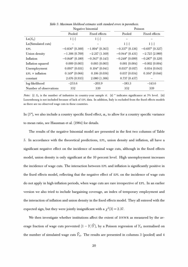
Table 5: Maximum likelihood estimates with standard errors in parenthesis.Negative binomial Poisson

Pooled Fixed effects Pooled Fixed effects

Ln(Sit) 1 (–) 1 (–) – –

Ln(Simulated cuts) – – 1 (–) 1 (–)

EPL −0.836∗ (0.300) −1.004∗ (0.365) −0.337∗ (0.136) −0.697∗ (0.327)

Union density −1.306 (0.709) −2.217 (1.169) −0.944∗ (0.431) −2.725 (2.989)

Inflation −0.848∗ (0.189) −0.565∗ (0.145) −0.248∗ (0.099) −0.287∗ (0.129)

Inflation squared 0.009 (0.005) 0.005 (0.005) 0.001 (0.004) −0.002 (0.004)

Unemployment 0.095∗ (0.031) 0.104∗ (0.041) 0.035∗ (0.017) 0.034 (0.043)

EPL × inflation 0.149∗ (0.066) 0.106 (0.056) 0.057 (0.034) 0.104∗ (0.046)

constant 2.676 (0.935) 2.080 (1.306) 0.737 (0.457) —

log-likelihood –253.6 –203.9 –183.3 –143.6

Number of observations 352 339 352 339

Notes: (i) Sit is the number of industries in country-year sample it. (ii) ∗ indicates significance at 5% level. (iii)Luxembourg is not included because of lack of EPL data. In addition, Italy is excluded from the fixed effects modelsas there are no observed wage cuts in these countries.

In (5”), we also include a country specific fixed effect, αi, to allow for a country specific variance

to mean ratio, see Hausman et al. (1984) for details.

The results of the negative binomial model are presented in the first two columns of Table

5. In accordance with the theoretical predictions, EPL, union density and inflation, all have a

significant negative effect on the incidence of nominal wage cuts, although in the fixed effects

model, union density is only significant at the 10 percent level. High unemployment increases

the incidence of wage cuts. The interaction between EPL and inflation is significantly positive in

the fixed effects model, reflecting that the negative effect of EPL on the incidence of wage cuts

do not apply in high-inflation periods, when wage cuts are rare irrespective of EPL. In an earlier

version we also tried to include bargaining coverage, an index of temporary employment and

the interaction of inflation and union density in the fixed effects model. They all entered with the

expected sign, but they were jointly insignificant with a χ2(3) = 2.37.

We then investigate whether institutions affect the extent of DNWR as measured by the av-

erage fraction of wage cuts prevented (1 − Y/Y ), by a Poisson regression of Yit normalised on

the number of simulated wage cuts Yit. The results are presented in columns 3 (pooled) and 4

20

(fixed effects) of Table 5. Note that in this case the restriction imposed by the Poisson regression

relative to the negative binomial regression is accepted easily; indeed the results are the same in

the negative binomial model for both specifications.8 Again, we find a significant negative effect

on the number of wage cuts, implying a positive effect of EPL and union density on the fraction

of wage cuts prevented. Also, there is a positive effect of inflation, which implies that there are

fewer wage cuts prevented when inflation is lower. In the fixed effects model, union density is

insignificant. In an earlier version we also tried to include bargaining coverage, an index of tem-

porary employment and the interaction of inflation and union density in the fixed effects model.

They all entered with the expected sign, but they were jointly insignificant with a χ2(3) = 1.37.

6 Conclusions

This paper explores the existence of downward nominal wage rigidity (DNWR) in the manufac-

turing, mining and quarrying, electricity, gas and water supply, and construction sectors of 16

European countries, over the period 1973–1999, using data for hourly nominal wages at industry

level. Based on a novel nonparametric statistical method, which allows for country and year

specific variation in both the median and the dispersion of industry wage changes, we reject the

hypothesis of no DNWR for the total sample. Splitting into subsamples, we document the exist-

ence of DNWR for the high inflation period 1973–1989, as well as for the low inflation periods

1990–1994 and 1995–1999. Furthermore, we also find evidence for DNWR for groups of coun-

tries: the South (Italy, Greece, Portugal, Spain), the Core (Austria, Belgium, France, Germany,

Luxembourg, Netherlands), and the Nordic region (Denmark, Finland, Norway and Sweden),

but not the British Isles. Dividing further into individual countries, the results indicate that, for

all countries except France and Spain, some of the notional wage cuts do not lead to observered

wage cuts due to DNWR. However, DNWR is statistically significant only for some of the coun-

8The goodness-of-fit test yields χ2(254) = 133.0.

21

tries: for Austria, Belgium, the Netherlands, and Portugal at ten percent level.

Interestingly, our results show that the fraction of notional wage cuts that do not result in

observed wage cuts has fallen over time, for all the groups of countries we consider. The simula-

tions indicate that for all countries together, the fraction of wage cuts prevented has fallen from

70 percent in the 1970s to 20 percent in the late 1990s. On the other hand, as the inflation has

fallen over time, the fraction of industry-years affected by DNWR has increased from less than

0.6 percent in the 1970s, to 1.7 percent in the late 1990s.

We then proceed to explore whether the incidence of nominal wage cuts can be explained

by economic and institutional variables. Treating the incidence of nominal wage cuts in each

country-year sample as one observation, we find significant negative effect of inflation, the strict-

ness of employment protection legislation and of union density. We also find that inflation, the

strictness of employment protection legislation and union density have significant positive im-

pact on our measure of DNWR: in country-year samples with high inflation, strict employment

protection legislation and high union density, the number of observed wage cuts is significantly

reduced relative to the number of simulated, notional wage cuts.

Our study should be seen as complementary to the increasing number of empirical studies on

the existence of DNWR based in individual data. Compared to these studies, our approach has

the advantage that it focusses on industry level effects, and thus is not subject to the critique that

significant DNWR at individual or firm level might be circumvented by employment being shifted

over from high-wage to low-wage jobs. In comparison, Card & Hyslop (1997) find evidence of

DNWR on US microdata, but inconclusive evidence for state level data. On the other hand, as we

(obviously) have much fewer observations than most micro-studies, and use weak assumptions

– no functional form assumption, and allowing for time and country variation in the median

and dispersion of wage changes – our test presumably has lower power. Indeed, Knoppik &

Beissinger (2003) find significant DNWR for Germany, while we do not.

22

We are reluctant to draw strong policy conclusions from our study. Overall in our sample,

DNWR is significant but of moderate size. Labour markets appear to adapt to lower inflation,

as the fraction of wage cuts prevented by DNWR has fallen over time. Yet the fraction of total

industries that have been affected by DNWR has increased over time, suggesting that the overall

effect on DNWR of a more determined effort towards low inflation, as the monetary policy of the

ECB arguably implies, are uncertain.

References

Agell, J. & Lundborg, P. (2003). Survey evidence on wage rigidity and unemployment. Scand-inavian Journal of Economics, 105, 15–30.

Akerlof, G., Dickens, W., & Perry, W. (1996). The macroeconomics of low inflation. BrookingsPapers on Economic Activity, 1 : 1996, 1–76.

Akerlof, G., Dickens, W., & Perry, W. (2000). Near rational wage and price setting and the longrun phillips curve. Brookings Papers on Economic Activity, 1 : 2000, 1–60.

Altonji, J. & Devereux, P. (2000). The extent and concequences of downward nominal wagerigidity. In S. Polachek (Ed.), Worker Well-Being, number 7236. Elsevier.

Bewley, T. (1999). Why Wages Do Not Fall During a Recession. Boston: Harvard University Press.

Blanchard, O. & Wolfers, J. (2000). The role of shocks and institutions in the rise of europeanunemployment: The aggregate evidence. The Economic Journal, 110 (462), C1–C33.

Blinder, A. & Choi, D. (1990). A shred of evidence of theories of wage stickiness. Quarterly Journalof Economics, 105, 1003–1016.

Calmfors, L., Booth, A., Burda, M., Checchi, D., Naylor, R., & Visser, J. (2001). The future ofcollective bargaining in europe. In T. Boeri, A. Brugiavinin, & L. Calmfors (Eds.), The Role ofUnions in the Twenty-First Century. Oxford University Press.

Cameron, A. & Trivedi, P. (1998). Regression Analyses of Count Data. Cambridge University Press.

Card, D. & Hyslop, D. (1997). Does inflation grease the wheels of the labor market? In C. Romer& D. Romer (Eds.), Reducing Inflation: Motivation and Strategy (pp. 71–121). University of ChicagoPress.

Christofides, L. & Leung, M. (2003). Nominal wage rigidity in contract data: A parametricapproach. Economica, 70, 619–638.

Dessy, O. (2002). Nominal wage rigidity and institutions: Micro-evidence form the europanel.Technical report, University of Milan.

Elsby, M. (2004). Evaluating the economic significance of downward nominal wage rigidity.Unpublished manuscript, London School of Economics.

23

Fehr, E. & Gotte, L. (2003). Robustness and real concequences of nominal wage rigidity. Journalof Monetary Economics, Forthcoming.

Fortin, P. & Dumont, K. (2000). The shape of the long-run phillips curve: Evidence from Cana-dian macrodata, 1956− 97. Technical report, Canadian Institute for Advanced Research.

Gordon, R. J. (1996). Comment on Akerlof, Dickens and Perry: The macroeconomics of lowinflation. Brookings Papers on Economic Activity, 1 : 1996, 60–66.

Hausman, J., Hall, B., & Z., G. (1984). Econometric models for count data with an application tothe patents-R&D relationship. Econometrica, 52(4), 909–938.

Holden, S. (1994). Wage bargaining and nominal rigidities. European Economic Review, 38, 1021–1039.

Holden, S. (1998). Wage drift and the relevance of centralised wage setting. Scandinavian Journalof Economics, 100, 711–731.

Holden, S. (2004). The costs of price stability—downward nominal wage rigidity in Europe.Economica, 71, 183–208.

Kahn, S. (1997). Evidence of nominal wage stickiness from micro-data. American Economic Review,87 (5), 993–1008.

Knoppik, C. & Beissinger, T. (2003). How rigid are nominal wages? Evidence and implicationsfor Germany. Scandinavian Journal of Economics, 105 (4), 619–641.

Lazear, E. (1990). Job security provisions and employment. Quarterly Journal of Economics, 105 (3),699–725.

Lebow, D., Saks, R., & Wilson, B. (2003). Downward nominal wage rigidity. Evidence fromthe employment cost index. Advances in Macroeconomics, 3(1), Article 2. http://www.bepress.com/bejm/advances/vol3/iss1/art2.

Lebow, D., Stockton, D., & Wascher, W. (1995). Inflation, nominal wage rigidity and the efficien-cly of labor markets. Finance and Economics DP 94-45, Board of Governors of the FederalReserve System.

MacLeod, W. & Malcomson, J. (1993). Investment, holdup, and the form of market contracts.American Economic Review, 37, 343–354.

Mankiw, N. (1996). Comment on Akerlof, Dickens and Perry: The macroeconmics of lowinflation. Brookings Papers on Economic Activity, 1:1996, 66–70.

McLaughlin, K. (1994). Rigid wages? Journal of Monetary Economics, 34(3), 383–414.

Nickell, S., Nunziata, L., W., O., & Quintini, G. (2002). The beveridge curve, unemployment andwages in the OECD from the 1960s to the 1990s. Discussion Paper 502, Center for EconomicPerformance.

Nickell, S. & Quintini, G. (2003). Nominal wage rigidity and the rate of inflation. Economic Journal,113, 762–781.

24

ECB (2003). Background Studies for the ECB’s Evaluation of its Monetary Policy Strategy. Frankfurt amMain: European Central Bank.

EIRO (2003). Industrial relations in the EU, japan and the USA, 2001. Technical report,The European Industrial Relations Observatory, http://www.eiro.eurofound.ie/2002/

12/feature/tn0212101f.html.

ILO (1997). World labour report 1997–98 industrial relations, democracy and social stabil-ity. Technical report, International Labour Organization, http://www.ilo.org/public/

english/dialogue/ifpdial/publ/wlr97/summary.htm.

IMF (2002). Monetary and exchange rate policies of the european area—selected issues. CountryReport 02/236, IMF.

OECD (1999). Employment Outlook. Paris: OECD.

OECD (2002). Economic Outlook. Paris: OECD.

Tobin, J. (1972). Inflation and unemployment. American Economic Review, 62, 1–18.

Wyplosz, C. (2001). Do we know how low inflation should be? In A. Herrero, V. Gaspar,L. Hoogduin, J. Morgan, & B. Winkler (Eds.), Why price stability (pp. 15–33). ECB, Frankfurt.

Young, D. (2003). Employment protection legislation: Its economic impact and the casefor reform. Technical Report 186, European Commission, http://europa.eu.int/comm/economy_finance/publications/economic_papers/economicpapers186_en.htm.

A Data appendix

We have obtained our wage data from Eurostat. The precise source is Table HMWHOUR in theHarmonized earnings domain of under the Population and Social Conditions theme in the NEWCRO-NOS database. Our wage variable (HMWHOUR) is labelled Gross hourly earnings of manual workersin industry. Gross earnings cover remuneration in cash paid directly and regularly by the em-ployer at the time of each wage payment, before tax deductions and social security contributionspayable by wage earners and retained by the employer. Payments for leave, public holidays, andother paid individual absences, are included in principle, in so far as the corresponding days orhours are also taken into account to calculate earnings per unit of time. The weekly hours ofwork are those in a normal week’s work (i.e. not including public holidays) during the referenceperiod. These hours are calculated on the basis of the number of hours paid, including over-time hours paid. Furthermore, we use data in national currency and males and females are bothincluded in the data. The data for Germany does not include GDR before 1990 or new Lander.

The data are recorded by classification of economic activities (NACE Rev. 1). The sectionsrepresented are Mining and quarrying (C), Manufacturing (D), Electricity, gas and water supply(E) and Construction (F). We use data on various levels of aggregation from the section levels(e.g. D Manufacturing) to group levels (e.g. DA 159 Manufacturing of beverages), however,using the most disaggregate level available in order to maximize the number of observations. Iffor example, wage data are available for D, DA 158 and DA 159, we use the latter two only toavoid counting the same observations twice.

25

The average number of observations per country-year sample is 20.5, with a standard errorof 4.7. The distribution of the number of wage cuts relative to the number of observations onyears and countries are reported in Table A1.

Data for inflation and unemployment are from the OECD Economic Outlook database.The primary sources for the employment protection legislation index, which is displayed in

Table A2, are Lazear (1990) for the period 1973–79 and OECD (1999) for the remaining years.We follow the same procedure as Blanchard & Wolfers (2000) to construct time-varying serieswhich is to use the OECD summary measure in the ‘Late 1980s’ for 1980–89 and the ‘Late 1990s’for 1995–99. For 1990-94 we interpolate the series, and use the percentage change in Lazear’sindex to back-cast the OECD measure. However, we are not able to reconstruct the Blanchardand Wolfers data exactly.

Data for union density until 1995 is from Nickell et al. (2002, Table 5). For the remainingyears we interpolate using observations for 2001 from EIRO (2003, Table 9). Data for Greece(1985 and 1995), Ireland (1985 and 1993) and Luxembourg (1987 and 1995) are from ILO (1997,Table 1.2). Data for intervening years are produced by interpolation, while we extrapolate before1985(87) and after 1993(95).

Data for bargaining coverage until 1994 are from Nickell et al. (2002, Table 4), which providedata with five year intervals. Yearly data are calculated by interpolation. EIRO (2003, Table1) presents data for 2000 (1999 for Portugal and 2001 for the Netherlands) which allows us tointerpolate for the late 1990s. Data for Greece and Ireland are only available for 1994 from ILO

(1997, Table 1.2).Data for the incidence of temporary employment is from Young (2003, Table 4.1), which

provides observations with five year intervals from 1985–2000. We interpolate to obtain yearlydata and extrapolate before 1985.

26

Tabl

eA1:

Thed

istri

butio

nof

nom

inal

wag

ecut

srela

tivet

oth

enum

bero

fobs

erva

tions

byco

untr

iesa

ndye

ars

Year

Austria

Belgium

German

y

Denmark

Spain

Finlan

d

Fran

ce

Greece

Irelan

d

Italy

Luxem

bourg

Netherl

ands

Norway

Portu

gal

Swede

n

UK

Total

1973

0/20

0/23

0/19

–0/

160/

200/

12–

0/24

0/14

0/19

0/24

––

0/21

0/21

219

740/

160/

201/

230/

19–

0/16

0/21

0/13

–0/

240/

140/

190/

25–

–0/

211/

231

1975

0/16

0/20

0/24

1/19

–0/

160/

220/

13–

0/24

0/15

0/19

0/25

––

0/21

1/23

419

760/

160/

210/

240/

19–

0/16

0/22

0/13

0/18

0/24

0/15

0/19

0/25

––

0/23

0/25

519

770/

160/

210/

240/

19–

0/16

0/22

0/13

0/18

0/24

0/15

0/19

0/25

––

0/23

0/25

519

780/

160/

210/

240/

19–

0/16

0/22

0/13

0/18

0/24

2/15

0/20

0/25

–0/

260/

233/

282

1979

0/16

0/21

0/24

0/20

–0/

160/

220/

130/

200/

240/

150/

190/

25–

0/28

0/22

0/28

519

800/

160/

210/

241/

20–

0/16

0/22

0/13

0/19

0/24

0/15

0/19

0/25

–0/

280/

221/

284

1981

0/16

0/21

0/24

0/20

–0/

160/

220/

130/

190/

242/

150/

190/

250/

220/

280/

222/

306

1982

0/16

0/21

0/24

0/20

0/2

0/16

0/21

0/13

0/20

0/24

0/16

0/18

0/25

0/22

0/28

0/22

0/30

819

830/

160/

211/

240/

201/

20/

160/

210/

110/

180/

240/

160/

180/

250/

220/

270/

243/

305

1984

0/16

0/21

1/27

0/20

0/2

0/16

0/22

0/17

0/18

0/24

1/16

0/16

0/25

0/22

0/27

0/24

5/31

319

850/

160/

210/

270/

200/

20/

160/

230/

181/

200/

241/

160/

170/

250/

220/

280/

242/

319

1986

0/16

6/21

0/27

2/20

0/2

0/16

2/23

2/18

1/21

–0/

140/

180/

250/

220/

280/

2415

/295

1987

0/16

0/21

0/27

0/20

0/2

0/16

1/23

0/18

3/20

–3/

140/

180/

250/

220/

280/

247/

294

1988

1/16

3/21

0/27

0/20

0/2

0/16

5/23

0/18

1/20

–3/

140/

180/

250/

210/

280/

2515

/295

1989

0/16

0/22

0/27

0/20

0/2

0/16

1/23

0/17

2/20

–0/

170/

170/

253/

240/

280/

267/

297

1990

0/16

0/24

0/27

0/20

0/26

0/16

1/23

0/24

1/21

–1/

160/

171/

250/

230/

280/

254/

332

1991

0/16

0/24

0/27

0/20

0/26

0/16

1/23

0/25

0/21

–0/

160/

170/

250/

230/

60/

251/

310

1992

0/16

0/23

0/24

1/20

0/26

0/16

0/23

1/25

0/21

–0/

170/

170/

250/

231/

130/

253/

314

1993

1/16

0/22

2/24

2/20

1/26

1/16

2/24

0/25

1/21

–0/

170/

140/

250/

235/

142/

2517

/312

1994

0/16

0/22

1/26

0/2

2/26

1/16

8/15

0/25

2/21

–1/

170/

80/

250/

230/

1411

/22

26/2

7819

950/

1619

/22

0/26

–0/

260/

160/

100/

256/

20–

0/17

0/10

1/25

0/23

0/14

1/21

27/2

7119

960/

140/

277/

25–

4/26

–0/

120/

252/

23–

6/19

0/20

0/25

0/23

0/14

0/26

20/2

7919

970/

142/

282/

310/

166/

29–

0/27

1/25

4/23

–7/

141/

230/

250/

230/

153/

2726

/320

1998

0/14

0/28

1/31

0/16

3/29

–0/

253/

243/

23–

4/17

0/23

0/25

0/29

0/14

1/28

15/3

2619

990/

14–

–1/

162/

30–

––

––

1/17

12/2

20/

25–

0/14

–16

/138

Tota

l2/

408

31/5

7516

/665

8/46

420

/286

2/36

821

/556

7/46

927

/463

0/31

232

/423

23/4

832/

674

3/41

16/

478

18/6

1521

7/76

50

27

Table A2: Indices for employment protection legislationYear BE DE DK ES FI FR GR IE IT NL PT SW UK1973 3.10 3.20 2.10 3.89 2.30 2.44 3.60 0.76 4.10 2.70 3.16 2.57 0.461974 3.10 3.20 2.10 3.89 2.30 2.57 3.60 0.83 4.10 2.70 3.42 3.03 0.481975 3.10 3.20 2.10 3.89 2.30 2.70 3.60 0.90 4.10 2.70 3.67 3.50 0.501976 3.10 3.20 2.10 3.86 2.30 2.70 3.60 0.90 4.10 2.70 3.75 3.50 0.501977 3.10 3.20 2.10 3.82 2.30 2.70 3.60 0.90 4.10 2.70 3.83 3.50 0.501978 3.10 3.20 2.10 3.78 2.30 2.70 3.60 0.90 4.10 2.70 3.92 3.50 0.501979 3.10 3.20 2.10 3.74 2.30 2.70 3.60 0.90 4.10 2.70 4.00 3.50 0.501980 3.10 3.20 2.10 3.70 2.30 2.70 3.60 0.90 4.10 2.70 4.10 3.50 0.501981 3.10 3.20 2.10 3.70 2.30 2.70 3.60 0.90 4.10 2.70 4.10 3.50 0.501982 3.10 3.20 2.10 3.70 2.30 2.70 3.60 0.90 4.10 2.70 4.10 3.50 0.501983 3.10 3.20 2.10 3.70 2.30 2.70 3.60 0.90 4.10 2.70 4.10 3.50 0.501984 3.10 3.20 2.10 3.70 2.30 2.70 3.60 0.90 4.10 2.70 4.10 3.50 0.501985 3.10 3.20 2.10 3.70 2.30 2.70 3.60 0.90 4.10 2.70 4.10 3.50 0.501986 3.10 3.20 2.10 3.70 2.30 2.70 3.60 0.90 4.10 2.70 4.10 3.50 0.501987 3.10 3.20 2.10 3.70 2.30 2.70 3.60 0.90 4.10 2.70 4.10 3.50 0.501988 3.10 3.20 2.10 3.70 2.30 2.70 3.60 0.90 4.10 2.70 4.10 3.50 0.501989 3.10 3.20 2.10 3.70 2.30 2.70 3.60 0.90 4.10 2.70 4.10 3.50 0.501990 2.93 3.08 1.95 3.60 2.25 2.75 3.60 0.90 3.97 2.60 4.03 3.28 0.501991 2.77 2.97 1.80 3.50 2.20 2.80 3.60 0.90 3.83 2.50 3.97 3.07 0.501992 2.60 2.85 1.65 3.40 2.15 2.85 3.60 0.90 3.70 2.40 3.90 2.85 0.501993 2.43 2.73 1.50 3.30 2.10 2.90 3.60 0.90 3.57 2.30 3.83 2.63 0.501994 2.27 2.62 1.35 3.20 2.05 2.95 3.60 0.90 3.43 2.20 3.77 2.42 0.501995 2.10 2.50 1.20 3.10 2.00 3.00 3.60 0.90 3.30 2.10 3.70 2.20 0.501996 2.10 2.50 1.20 3.10 2.00 3.00 3.60 0.90 3.30 2.10 3.70 2.20 0.501997 2.10 2.50 1.20 3.10 2.00 3.00 3.60 0.90 3.30 2.10 3.70 2.20 0.501998 2.10 2.50 1.20 3.10 2.00 3.00 3.60 0.90 3.30 2.10 3.70 2.20 0.501999 2.10 2.50 1.20 3.10 2.00 3.00 3.60 0.90 3.30 2.10 3.70 2.20 0.50

Table A3: Indices for union denistyYear BE DE DK ES FI FR GR IE IT LU NL PT SW UK1973 0.48 0.32 0.62 0.09 0.61 0.22 0.37 0.53 0.43 0.53 0.36 0.61 0.72 0.501974 0.49 0.34 0.65 0.09 0.63 0.22 0.37 0.54 0.46 0.53 0.36 0.61 0.73 0.521975 0.52 0.35 0.69 0.09 0.65 0.22 0.37 0.56 0.48 0.53 0.38 0.61 0.74 0.541976 0.53 0.35 0.73 0.09 0.68 0.21 0.37 0.57 0.50 0.53 0.37 0.61 0.75 0.551977 0.54 0.35 0.74 0.09 0.66 0.21 0.37 0.57 0.50 0.53 0.37 0.61 0.78 0.571978 0.53 0.35 0.78 0.09 0.67 0.21 0.37 0.58 0.50 0.53 0.37 0.61 0.79 0.571979 0.54 0.35 0.77 0.09 0.68 0.19 0.37 0.58 0.50 0.53 0.37 0.61 0.80 0.571980 0.53 0.35 0.79 0.09 0.69 0.19 0.37 0.57 0.50 0.53 0.35 0.61 0.80 0.561981 0.53 0.35 0.80 0.09 0.68 0.18 0.37 0.57 0.48 0.53 0.33 0.61 0.81 0.551982 0.52 0.35 0.80 0.10 0.68 0.17 0.37 0.56 0.47 0.53 0.32 0.61 0.82 0.541983 0.52 0.35 0.81 0.10 0.69 0.16 0.37 0.57 0.46 0.53 0.31 0.61 0.83 0.531984 0.52 0.34 0.79 0.12 0.69 0.15 0.37 0.57 0.45 0.53 0.29 0.61 0.84 0.531985 0.51 0.34 0.78 0.12 0.69 0.14 0.37 0.56 0.43 0.53 0.28 0.56 0.84 0.511986 0.49 0.34 0.77 0.12 0.70 0.13 0.35 0.53 0.41 0.53 0.27 0.51 0.84 0.501987 0.49 0.33 0.75 0.12 0.71 0.12 0.34 0.51 0.41 0.53 0.24 0.46 0.84 0.491988 0.48 0.33 0.74 0.13 0.72 0.12 0.33 0.52 0.41 0.52 0.24 0.41 0.82 0.471989 0.49 0.33 0.76 0.13 0.73 0.11 0.32 0.53 0.40 0.51 0.24 0.37 0.82 0.451990 0.50 0.32 0.75 0.14 0.73 0.10 0.31 0.52 0.40 0.49 0.24 0.32 0.80 0.441991 0.52 0.33 0.76 0.16 0.75 0.10 0.29 0.53 0.40 0.48 0.25 0.32 0.80 0.431992 0.53 0.32 0.76 0.18 0.77 0.10 0.28 0.51 0.40 0.47 0.25 0.32 0.83 0.411993 0.54 0.30 0.77 0.20 0.79 0.10 0.27 0.50 0.40 0.46 0.24 0.32 0.86 0.401994 0.54 0.29 0.77 0.20 0.79 0.10 0.26 0.48 0.39 0.45 0.25 0.32 0.91 0.381995 0.54 0.27 0.77 0.18 0.80 0.10 0.24 0.46 0.39 0.43 0.24 0.32 0.90 0.371996 0.56 0.28 0.79 0.18 0.80 0.10 0.26 0.46 0.38 0.44 0.25 0.32 0.88 0.351997 0.59 0.28 0.81 0.17 0.79 0.10 0.27 0.46 0.38 0.46 0.25 0.31 0.86 0.341998 0.61 0.29 0.82 0.17 0.79 0.09 0.28 0.45 0.37 0.47 0.26 0.31 0.84 0.331999 0.64 0.29 0.84 0.16 0.79 0.09 0.30 0.45 0.37 0.48 0.26 0.31 0.83 0.32

28

Table A4: Indices for bargaining coverageYear BE DE DK ES FI FR GR IE IT NL PT SW UK1973 0.83 0.90 0.69 0.65 0.95 0.80 0.90 0.90 0.86 0.70 0.64 0.73 0.701974 0.84 0.90 0.70 0.66 0.95 0.81 0.90 0.90 0.86 0.71 0.65 0.74 0.711975 0.85 0.90 0.70 0.66 0.95 0.82 0.90 0.90 0.85 0.72 0.65 0.75 0.721976 0.86 0.90 0.70 0.66 0.95 0.82 0.90 0.90 0.85 0.73 0.66 0.76 0.721977 0.87 0.90 0.71 0.67 0.95 0.83 0.90 0.90 0.85 0.74 0.67 0.76 0.711978 0.88 0.91 0.71 0.67 0.95 0.84 0.90 0.90 0.85 0.74 0.68 0.77 0.711979 0.89 0.91 0.72 0.68 0.95 0.84 0.90 0.90 0.85 0.75 0.69 0.78 0.701980 0.90 0.91 0.72 0.68 0.95 0.85 0.90 0.90 0.85 0.76 0.70 0.79 0.701981 0.90 0.91 0.72 0.68 0.95 0.86 0.90 0.90 0.85 0.77 0.71 0.79 0.691982 0.90 0.91 0.73 0.69 0.95 0.86 0.90 0.90 0.85 0.78 0.72 0.80 0.681983 0.90 0.90 0.73 0.69 0.95 0.87 0.90 0.90 0.85 0.78 0.73 0.81 0.661984 0.90 0.90 0.74 0.70 0.95 0.88 0.90 0.90 0.85 0.79 0.74 0.82 0.651985 0.90 0.90 0.74 0.70 0.95 0.89 0.90 0.90 0.85 0.80 0.75 0.82 0.641986 0.90 0.90 0.73 0.71 0.95 0.89 0.90 0.90 0.85 0.81 0.75 0.83 0.621987 0.90 0.90 0.72 0.72 0.95 0.90 0.90 0.90 0.84 0.81 0.76 0.84 0.601988 0.90 0.90 0.71 0.74 0.95 0.91 0.90 0.90 0.84 0.82 0.77 0.85 0.581989 0.90 0.90 0.70 0.75 0.95 0.91 0.90 0.90 0.83 0.82 0.78 0.85 0.561990 0.90 0.90 0.69 0.76 0.95 0.92 0.90 0.90 0.83 0.83 0.79 0.86 0.541991 0.90 0.90 0.69 0.76 0.95 0.93 0.90 0.90 0.83 0.83 0.77 0.87 0.511992 0.90 0.91 0.69 0.77 0.95 0.94 0.90 0.90 0.82 0.84 0.75 0.88 0.471993 0.90 0.92 0.69 0.77 0.95 0.94 0.90 0.90 0.82 0.84 0.73 0.88 0.441994 0.90 0.92 0.69 0.78 0.95 0.95 0.90 0.90 0.82 0.85 0.71 0.89 0.401995 0.90 0.93 0.69 0.78 0.95 0.96 0.90 0.90 0.82 0.86 0.69 0.90 0.371996 0.90 0.93 0.69 0.79 0.95 0.96 0.90 0.90 0.81 0.86 0.67 0.90 0.331997 0.90 0.94 0.69 0.79 0.95 0.97 0.90 0.90 0.81 0.87 0.65 0.91 0.291998 0.90 0.94 0.69 0.80 0.95 0.98 0.90 0.90 0.81 0.87 0.63 0.92 0.261999 0.90 0.95 0.69 0.80 0.95 0.99 0.90 0.90 0.81 0.88 0.61 0.93 0.22

Table A5: Indices for incidence of temporary employmentYear BE DE DK ES FI FR GR IE IT LU NL PT SW UK1973 6.90 10.00 12.30 15.60 16.50 4.70 21.10 7.30 4.70 4.70 7.50 14.40 13.00 6.901974 6.90 10.00 12.30 15.60 16.50 4.70 21.10 7.30 4.70 4.70 7.50 14.40 13.00 6.901975 6.90 10.00 12.30 15.60 16.50 4.70 21.10 7.30 4.70 4.70 7.50 14.40 13.00 6.901976 6.90 10.00 12.30 15.60 16.50 4.70 21.10 7.30 4.70 4.70 7.50 14.40 13.00 6.901977 6.90 10.00 12.30 15.60 16.50 4.70 21.10 7.30 4.70 4.70 7.50 14.40 13.00 6.901978 6.90 10.00 12.30 15.60 16.50 4.70 21.10 7.30 4.70 4.70 7.50 14.40 13.00 6.901979 6.90 10.00 12.30 15.60 16.50 4.70 21.10 7.30 4.70 4.70 7.50 14.40 13.00 6.901980 6.90 10.00 12.30 15.60 16.50 4.70 21.10 7.30 4.70 4.70 7.50 14.40 13.00 6.901981 6.90 10.00 12.30 15.60 16.50 4.70 21.10 7.30 4.70 4.70 7.50 14.40 13.00 6.901982 6.90 10.00 12.30 15.60 16.50 4.70 21.10 7.30 4.70 4.70 7.50 14.40 13.00 6.901983 6.90 10.00 12.30 15.60 16.50 4.70 21.10 7.30 4.70 4.70 7.50 14.40 13.00 6.901984 6.90 10.00 12.30 15.60 16.50 4.70 21.10 7.30 4.70 4.70 7.50 14.40 13.00 6.901985 6.90 10.00 12.30 15.60 16.50 4.70 21.10 7.30 4.70 4.70 7.50 14.40 13.00 6.901986 6.58 10.10 12.00 15.60 16.50 5.88 20.18 7.54 4.80 4.44 7.52 14.40 13.00 6.541987 6.26 10.20 11.70 15.60 16.50 7.06 19.26 7.78 4.90 4.18 7.54 15.40 13.00 6.181988 5.94 10.30 11.40 20.37 16.50 8.24 18.34 8.02 5.00 3.92 7.56 16.40 13.00 5.821989 5.62 10.40 11.10 25.13 16.50 9.42 17.42 8.26 5.10 3.66 7.58 17.40 13.00 5.461990 5.30 10.50 10.80 29.90 16.50 10.60 16.50 8.50 5.20 3.40 7.60 18.40 13.00 5.101991 5.30 10.48 11.06 30.92 16.50 10.92 15.24 8.84 5.60 3.28 8.24 16.74 13.00 5.461992 5.30 10.46 11.32 31.94 16.50 11.24 13.98 9.18 6.00 3.15 8.88 15.08 13.00 5.821993 5.30 10.44 11.58 32.96 16.50 11.56 12.72 9.52 6.40 3.03 9.52 13.42 13.00 6.181994 5.30 10.42 11.84 33.98 16.50 11.88 11.46 9.86 6.80 2.90 10.16 11.76 13.00 6.541995 5.30 10.40 12.10 35.00 16.50 12.20 10.20 10.20 7.20 2.98 10.80 10.10 13.00 6.901996 6.04 10.88 11.72 34.44 16.74 12.84 10.78 9.34 7.78 3.07 11.40 12.16 13.26 6.841997 6.78 11.36 11.34 33.88 16.98 13.48 11.36 8.48 8.36 3.15 12.00 14.22 13.52 6.781998 7.52 11.84 10.96 33.32 17.22 14.12 11.94 7.62 8.94 3.23 12.60 16.28 13.78 6.721999 8.26 12.32 10.58 32.76 17.46 14.76 12.52 6.76 9.52 3.32 13.20 18.34 14.04 6.66

29

B Results without bias adjustment

category Observ

edwag

e cuts

(Y)

Averag

e simula

tedwag

e cuts

#(Y>YB )

Proba

bility

ofsig

nifica

nce

Frac

tion of

wage cu

tspr

even

ted

Frac

tion of

indus

try-ye

arsaff

ected

All 217 275 4995 0.001 0.210 0.008

1970–79 5 12 4751 0.050 0.587 0.004

1980–89 57 75 4787 0.043 0.241 0.006

1990–94 51 65 4664 0.067 0.219 0.009

1995–99 104 122 4658 0.068 0.148 0.014

British Isles 45 54 4107 0.179 0.160 0.008

Core 125 148 4760 0.048 0.154 0.007

Nordic 18 28 4731 0.054 0.365 0.005

South 29 45 4861 0.028 0.354 0.011

Austria 2 6 4373 0.125 0.641 0.009

Belgium 31 38 4394 0.121 0.190 0.013

Germany 16 15 2007 0.599 0 0

Denmark 8 11 3598 0.280 0.281 0.007

Spain 19 18 1950 0.610 0 0

Finland 2 5 3944 0.211 0.568 0.007

France 21 18 1108 0.778 0 0

Greece 7 6 1555 0.689 0 0

Ireland 27 34 4069 0.186 0.198 0.014

Italy 0 3 4517 0.097 1.000 0.008

Luxembourg 32 38 3833 0.233 0.151 0.013

Netherlands 23 33 4740 0.052 0.307 0.021

Norway 2 3 2644 0.471 0.274 0.001

Portugal 3 18 5000 0.000 0.836 0.037

Sweden 6 10 4225 0.155 0.391 0.008

UK 18 20 3015 0.397 0.097 0.003

30

C Results with country specific underlying distributions

category Observ

edwag

e cuts

(Y)

Averag

e simula

tedwag

e cuts

#(Y>YB )

Proba

bility

ofsig

nifica

nce

Frac

tion of

wage cu

tspr

even

ted

Frac

tion of

indus

try-ye

arsaff

ected

All 217 266 4977 0.005 0.185 0.006

1970–79 5 12 4801 0.040 0.601 0.004

1980–89 57 72 4585 0.083 0.205 0.005

1990–94 51 64 4542 0.092 0.201 0.008

1995–99 104 118 4405 0.119 0.121 0.011

British Isles 45 47 2859 0.428 0.043 0.002

Core 125 147 4764 0.047 0.152 0.007

Nordic 18 26 4500 0.100 0.318 0.004

South 29 45 4874 0.025 0.363 0.011

Austria 2 4 3478 0.304 0.489 0.005

Belgium 31 36 3769 0.246 0.127 0.008

Germany 16 16 2280 0.544 0.004 0.000

Denmark 8 10 3325 0.335 0.228 0.005

Spain 19 15 1054 0.789 0 0

Finland 2 2 2282 0.544 0.194 0.001

France 21 21 2130 0.574 0 0

Greece 7 12 4206 0.159 0.408 0.010

Ireland 27 28 2689 0.462 0.045 0.003

Italy 0 3 4678 0.064 1.000 0.010

Luxembourg 32 39 4172 0.166 0.183 0.017

Netherlands 23 32 4598 0.080 0.281 0.019

Norway 2 3 3090 0.382 0.402 0.002

Portugal 3 15 4992 0.002 0.801 0.029

Sweden 6 10 4334 0.133 0.412 0.009

UK 18 19 2573 0.485 0.039 0.001

31