PROTEIN RIGIDITY AND FLEXIBILITY: APPLICATIONS TO

FOLDING AND THERMOSTABILITY

By

Andrew John Rader

A DISSERTATION

Submitted toMichigan State University

in partial fulfillment of the requirementsfor the degree of

DOCTOR OF PHILOSOPHY

Department of Physics and Astronomy and

Department of Biochemistry and Molecular Biology

2002

ABSTRACT

PROTEIN RIGIDITY AND FLEXIBILITY: APPLICATIONS TO FOLDING

AND THERMOSTABILITY

By

Andrew John Rader

The mechanism of protein folding is an unsolved, difficult problem. Performing the

inverse problem of unfolding a known protein structure has the advantage of known initial

conditions. This study relates protein unfolding to a loss of structural stability and rigidity.

Drawing on the wealth of knowledge about structural rigidity and flexibility from physics

and mathematics, connections are made with proteins. Proteins are identified as a special

case of amorphous (glassy) materials and are analyzed as such. The development of the

FIRST software as a method to identify flexible and rigid regions in proteins along with a

justification for its use to enumerate and partition the number of degrees of freedom (floppy

modes) by constraint counting in networks (proteins) is presented. By removing hydrogen

bonds in order from the weakest to strongest, protein unfolding by thermal dilution is sim-

ulated. This process also describes protein folding under the reasonable assumption (for

two-state folders) that the problem is reversible. Along the simulated unfolding pathway

two unique points are identified: the transition state and the folding core. The transition

state occurs at the inflection point in the change in the fraction of floppy modes with re-

spect to decreasing mean atomic coordination. The fraction of floppy modes as a function

of mean coordination is similar to the fraction-folded curve for a protein as a function of

denaturant concentration or temperature. Its second derivative, a specific heat-like quan-

tity, shows a peak around a mean coordination of 〈r〉= 2.41 for the 26 diverse proteins we

have studied. As the protein denatures, it loses rigidity at the transition state, proceeds to

a state where only the initial folding core remains stable, then becomes entirely denatured

or flexible. This universal behavior is found for proteins of diverse architecture, including

monomers and oligomers, and is analogous to the rigid to floppy phase transition in net-

work glasses. This approach provides a unifying principle for proteins and glasses, and

identifies the mean coordination as the relevant structural variable, or reaction coordinate,

for the unfolding pathway. The identification of the folding core is compared to a set of

10 structures that have hydrogen-deuterium exchange data. This computational procedure

is shown to identify and predict biologically significant flexibility by comparison with ex-

perimental measures of flexibility for several proteins. In general, flexibility is observed to

decrease upon ligand binding. Completing the study on structural flexibility and stability

in proteins is an investigation into the role rigidity plays in thermostability. An increase

in rigidity is shown to correlate with increased thermostability for eight families of ho-

mologous proteins. Comparisons are made between rigidity analysis from FIRST and ex-

perimental measures of thermostability, supporting rigidity as a general thermostabilizing

mechanism.

For Jennie

iv

ACKNOWLEDGMENTS

Foremost, I would like to thank my advisors, Dr. Michael F. Thorpe and Dr. Leslie A.

Kuhn. Beginning my graduate studies as an eager physicist-to-be, I could not have antic-

ipated the adventure that would ensue from working on network glasses with Dr. Thorpe.

With his complete support, I began learning terms and concepts from biochemistry that

were quite a departure from a traditional physics graduate education. Additionally he fos-

tered a love for simple, yet clever models to study difficult problems. Dr. Kuhn constantly

challenged me to show evidence that these models could be believed, always concerned

with even the finest details. I owe much of my understanding about protein structure and

folding to Dr. Kuhn who enthusiastically taught biochemistry to all who would listen.

These two advisors encouraged me to enter a novel dual degree program between the De-

partment of Physics and Astronomy and the Department of Biochemistry and Molecular

Biology. Over the years I have had a chance to work closely with Dr. Thorpe and Dr.

Kuhn, experiencing first-hand the sometimes difficult, but always rewarding, results of in-

terdisciplinary scientific collaboration. I am very fortunate to have been mentored by two

outstanding scientists who are knocking down the traditional barriers between scientific

disciplines. I hope that I may apply the skills they imparted to me to well-balanced, inter-

disciplinary research in the future.

With interdisciplinary work such as this, there is a community of people including fac-

v

ulty, post docs and graduate students that deserve thanks. Thanks to the other members of

my thesis committee: Dr. Phil Duxbury, Dr. Simon Billinge, and Dr. Shelagh Ferguson-

Miller. Their support of my interdisciplinary study was crucial to it becoming a reality.

They also provided necessary encouragement, criticism, and guidance in shaping the final

version of this dissertation. The development of the FIRST software would not have hap-

pened without Dr. Donald Jacobs, a research associate of Dr. Thorpe when I began my

research. He wrote the code for the Pebble Game and the initial version of FIRST. During

my initial years of research, his direction and code guided me in writing better programs,

an invaluable skill. A giant thanks also goes to the newly minted Dr. Brandon Hespen-

heide, a former graduate student of Dr. Kuhn, who also completed a dual degree with Dr.

Thorpe and Dr. Kuhn. Over the years we jointly poured many hours into writing, testing

and correcting the FIRST software and model. I am very grateful for his part in my re-

search, my part in his research, and the friendship that grew from working together. The

final chapter of this dissertation would not have been possible without the persistent effort

of Dr. Claire Vieille, a research associate, and Harini Krishnimurty, a graduate student,

both in the biochemistry lab of Dr. J.G. Zeikus. Their understanding of thermostability

and experimental biochemical techniques were critical in applying FIRST to the study of

thermostability. Additionally, they provided encouragement for the development of FIRST

and were enthusiastically receptive to the applications of protein rigidity. I also thank the

other graduate students from the research groups of Dr. Thorpe and Dr. Kuhn: Ming

Lei, Valentin Levashov, Mykyta Chubynsky, and Maria Zavodszky for providing feedback

concerning my dissertation research and a great work environment.

vi

Finally, I would like to thank my wonderful family and great friends that saw me

through this work. Thank-you to my beloved wife, Jennie, I owe more love and thanks

than I will ever be able to repay — she never doubted and always reminded me why I

did this: “Great are the works of the LORD, studied by all who delight in them.” Thanks

to mom and dad, Marc and Allison, Steve and Becky, Patty and Harold, Grandma and

Grandpa Rader, Grandma and Grandpa Weiss and my extended family for shaping me and

always supporting whatever I did, even when they didn’t quite get it. Thanks to the friends

that made life during graduate school so enjoyable, and those that predate MSU. Their en-

couragement and diversions made the whole process a wonderful experience and left an

indelible impression on me. Thanks to all the dear friends that came alongside me with so

many words and prayers of encouragement in small groups over the years.

vii

TABLE OF CONTENTS

LIST OF TABLES xii

LIST OF FIGURES xiii

LIST OF ABBREVIATIONS xv

1 Introduction 1

1.1 Motivation . . . . . . . . . . . . . . . . . . . . . . . . . . . . . . . . . . . . . 1

1.2 Glasses and Rigidity . . . . . . . . . . . . . . . . . . . . . . . . . . . . . . . 3

1.2.1 Glasses . . . . . . . . . . . . . . . . . . . . . . . . . . . . . . . . . . . . . 3

1.2.2 Constraints and Maxwell Counting . . . . . . . . . . . . . . . . . . . . . . . 5

1.2.3 Calculating Rigidity . . . . . . . . . . . . . . . . . . . . . . . . . . . . . . 7

1.3 Protein Structure, Flexibility, and Folding . . . . . . . . . . . . . . . . . . . . 10

1.3.1 Protein Flexibility and Stability . . . . . . . . . . . . . . . . . . . . . . . . 10

1.3.2 The Protein Folding Problem . . . . . . . . . . . . . . . . . . . . . . . . . . 12

1.4 Methods to Understand Folding and Flexibility . . . . . . . . . . . . . . . . . 14

1.4.1 Experimental Methods . . . . . . . . . . . . . . . . . . . . . . . . . . . . . 14

1.4.2 Computational Methods . . . . . . . . . . . . . . . . . . . . . . . . . . . . 19

1.4.3 Summary: Theory of Protein Folding . . . . . . . . . . . . . . . . . . . . . 24

1.5 Thermophiles . . . . . . . . . . . . . . . . . . . . . . . . . . . . . . . . . . . 26

1.5.1 Mechanisms of Thermostability . . . . . . . . . . . . . . . . . . . . . . . . 27

1.5.2 Rigidity and Thermostability . . . . . . . . . . . . . . . . . . . . . . . . . . 29

1.6 Direction . . . . . . . . . . . . . . . . . . . . . . . . . . . . . . . . . . . . . 30

viii

2 Rigidity in Glasses 33

2.1 Introduction . . . . . . . . . . . . . . . . . . . . . . . . . . . . . . . . . . . . 33

2.2 Network Glasses and Rigidity . . . . . . . . . . . . . . . . . . . . . . . . . . 34

2.2.1 Computational View of Glasses . . . . . . . . . . . . . . . . . . . . . . . . 34

2.2.2 Generic Rigidity . . . . . . . . . . . . . . . . . . . . . . . . . . . . . . . . 35

2.2.3 Maxwell Counting and Laman’s Theorem . . . . . . . . . . . . . . . . . . . 38

2.2.4 Bond-bending Networks . . . . . . . . . . . . . . . . . . . . . . . . . . . . 40

2.3 The Pebble Game . . . . . . . . . . . . . . . . . . . . . . . . . . . . . . . . . 44

2.3.1 Extensions to 3D Networks . . . . . . . . . . . . . . . . . . . . . . . . . . . 46

2.4 Rigidity in Network Glasses . . . . . . . . . . . . . . . . . . . . . . . . . . . 51

2.4.1 The Effect of Rings . . . . . . . . . . . . . . . . . . . . . . . . . . . . . . . 51

2.4.2 Universality . . . . . . . . . . . . . . . . . . . . . . . . . . . . . . . . . . . 55

3 Flexibility and Rigidity in Proteins: The FIRST Software 57

3.1 Introduction . . . . . . . . . . . . . . . . . . . . . . . . . . . . . . . . . . . . 57

3.2 Protein Structures and FIRST . . . . . . . . . . . . . . . . . . . . . . . . . . 58

3.2.1 Constraint Model of Proteins . . . . . . . . . . . . . . . . . . . . . . . . . . 59

3.2.2 Hydrogen Bonds . . . . . . . . . . . . . . . . . . . . . . . . . . . . . . . . 62

3.2.3 Hydrophobic Contacts . . . . . . . . . . . . . . . . . . . . . . . . . . . . . 67

3.3 From PDB Structure to FIRST Results . . . . . . . . . . . . . . . . . . . . . 68

3.3.1 Metal Ions, Buried Waters, and Ligands . . . . . . . . . . . . . . . . . . . . 70

3.3.2 Hydrogen Bonding . . . . . . . . . . . . . . . . . . . . . . . . . . . . . . . 71

3.4 Flexibility Index . . . . . . . . . . . . . . . . . . . . . . . . . . . . . . . . . . 77

3.5 Ligand Induced Conformational Changes . . . . . . . . . . . . . . . . . . . . 79

3.5.1 HIV Protease . . . . . . . . . . . . . . . . . . . . . . . . . . . . . . . . . . 80

3.5.2 DHFR . . . . . . . . . . . . . . . . . . . . . . . . . . . . . . . . . . . . . . 87

3.5.3 Adenylate Kinase . . . . . . . . . . . . . . . . . . . . . . . . . . . . . . . . 91

ix

4 Applications: Protein Folding and Unfolding 95

4.1 Introduction . . . . . . . . . . . . . . . . . . . . . . . . . . . . . . . . . . . . 95

4.1.1 Protein Unfolding . . . . . . . . . . . . . . . . . . . . . . . . . . . . . . . . 95

4.1.2 HD exchange and the Folding Core . . . . . . . . . . . . . . . . . . . . . . 97

4.2 Selection of Proteins for Analysis . . . . . . . . . . . . . . . . . . . . . . . . 100

4.3 Visualizing Results . . . . . . . . . . . . . . . . . . . . . . . . . . . . . . . . 102

4.4 Simulated Thermal Denaturation . . . . . . . . . . . . . . . . . . . . . . . . . 106

4.4.1 Identifying the Folding Core . . . . . . . . . . . . . . . . . . . . . . . . . . 107

4.4.2 Unfolding Pathways and Folding Cores from Thermal Denaturation . . . . . 108

4.5 Evaluating Other Denaturation Models . . . . . . . . . . . . . . . . . . . . . . 113

4.5.1 Random Removal of Hydrogen Bonds over a Small Energy Window . . . . . 113

4.5.2 Completely Random Removal of Hydrogen Bonds . . . . . . . . . . . . . . 116

4.6 Proteins as Glasses . . . . . . . . . . . . . . . . . . . . . . . . . . . . . . . . 119

4.6.1 Rigid Cluster Analysis . . . . . . . . . . . . . . . . . . . . . . . . . . . . . 121

4.6.2 Bond Dilution and Pruning . . . . . . . . . . . . . . . . . . . . . . . . . . . 121

4.6.3 Numerical Differentiation . . . . . . . . . . . . . . . . . . . . . . . . . . . 124

4.7 Phase Transitions in Proteins . . . . . . . . . . . . . . . . . . . . . . . . . . . 125

4.8 Self-organization and Proteins . . . . . . . . . . . . . . . . . . . . . . . . . . 129

4.9 Comparisons to Native State Predictions . . . . . . . . . . . . . . . . . . . . . 131

5 Applications: Thermostability 134

5.1 Introduction . . . . . . . . . . . . . . . . . . . . . . . . . . . . . . . . . . . . 134

5.2 Methods . . . . . . . . . . . . . . . . . . . . . . . . . . . . . . . . . . . . . . 135

5.2.1 Selection of Families . . . . . . . . . . . . . . . . . . . . . . . . . . . . . . 135

5.2.2 Global Rigidity Measure . . . . . . . . . . . . . . . . . . . . . . . . . . . . 137

5.2.3 Construction of Mutants . . . . . . . . . . . . . . . . . . . . . . . . . . . . 138

x

5.3 Rubredoxin: A Case Study . . . . . . . . . . . . . . . . . . . . . . . . . . . . 139

5.3.1 Unfolding and Folding Steps . . . . . . . . . . . . . . . . . . . . . . . . . . 140

5.3.2 Folding and Stability of apo-Rubredoxin . . . . . . . . . . . . . . . . . . . . 145

5.3.3 Chimeric Forms, Mutational Analysis, and Hydrophobic Stabilization . . . . 147

5.3.4 Flexibility Comparison of Mesophilic and Hyperthermophilic Rubredoxins . 149

5.3.5 Collective Motions and Flexibility . . . . . . . . . . . . . . . . . . . . . . . 152

5.4 Rigidity in Families of Homologous Proteins . . . . . . . . . . . . . . . . . . 155

5.5 Stabilization by Substrates and Oligomerization . . . . . . . . . . . . . . . . . 163

6 Conclusions and Future Directions 166

6.1 Conclusions . . . . . . . . . . . . . . . . . . . . . . . . . . . . . . . . . . . . 166

6.1.1 Rigidity Studies of Glasses and Proteins . . . . . . . . . . . . . . . . . . . . 166

6.1.2 Unfolding and Folding Predictions . . . . . . . . . . . . . . . . . . . . . . . 168

6.1.3 Thermostability and Rigidity . . . . . . . . . . . . . . . . . . . . . . . . . . 169

6.2 Future Directions . . . . . . . . . . . . . . . . . . . . . . . . . . . . . . . . . 171

6.2.1 The Protein Model of FIRST . . . . . . . . . . . . . . . . . . . . . . . . . 171

6.2.2 The Folding Core and Transition State Predictions . . . . . . . . . . . . . . 173

6.2.3 Thermostability and Rigidity . . . . . . . . . . . . . . . . . . . . . . . . . . 173

BIBLIOGRAPHY 176

xi

LIST OF TABLES

1.1 Structural thermostabilizing mechanisms. . . . . . . . . . . . . . . . . . . . . 29

2.1 〈r〉c for various 3D network glasses. . . . . . . . . . . . . . . . . . . . . . . . 56

3.1 Hydrogen bond donors and acceptors in proteins. . . . . . . . . . . . . . . . . 63

3.2 The effect of hydrogen atom placement on hydrogen bond assignment. . . . . . 72

4.1 Dataset of 10 proteins used to identify folding cores. . . . . . . . . . . . . . . 99

4.2 Dataset of 26 structurally diverse protein analyzed using FIRST . . . . . . . . 101

5.1 Families of homologous proteins. . . . . . . . . . . . . . . . . . . . . . . . . . 136

xii

LIST OF FIGURES

Images in this thesis are presented in color.

1.1 Atomic level view of crystalline and amorphous material. . . . . . . . . . . . . 4

1.2 2D Maxwell constraint counting. . . . . . . . . . . . . . . . . . . . . . . . . . 7

1.3 The protein folding funnel. . . . . . . . . . . . . . . . . . . . . . . . . . . . . 13

1.4 Free energy versus temperature: three models for thermostabilization. . . . . . 28

2.1 A small random bond model network. . . . . . . . . . . . . . . . . . . . . . . 35

2.2 2D rigidity example. . . . . . . . . . . . . . . . . . . . . . . . . . . . . . . . 37

2.3 Graph rigidity differences between 2D and 3D. . . . . . . . . . . . . . . . . . 40

2.4 Fraction of floppy modes versus 〈r〉in network glass. . . . . . . . . . . . . . . 43

2.5 First derivative of the fraction of floppy modes in a Bethe lattice and randombond model network. . . . . . . . . . . . . . . . . . . . . . . . . . . . . . 52

2.6 First derivative of the fraction of floppy modes in network glasses. . . . . . . . 53

3.1 The ranking of microscopic forces in proteins with an adjustable energy pointer. 61

3.2 The constraint model of the hydrogen bond. . . . . . . . . . . . . . . . . . . . 62

3.3 The hydrogen bond geometry. . . . . . . . . . . . . . . . . . . . . . . . . . . 64

3.4 Model of hydrophobic contacts in proteins. . . . . . . . . . . . . . . . . . . . 69

3.5 Hydrogen bond energy histogram. . . . . . . . . . . . . . . . . . . . . . . . . 75

3.6 Rigid cluster decomposition and flexibility index plot of HIVP. . . . . . . . . . 81

3.7 Calculated and experimental measures of flexibility for HIVP. . . . . . . . . . 83

3.8 Flexibility index map of DHFR in three enzymatic conformations. . . . . . . . 88

xiii

3.9 Flexibility index plotted versus residue number for DHFR. . . . . . . . . . . . 89

3.10 Flexibility index map for ADK in two conformations. . . . . . . . . . . . . . . 92

4.1 Rigid cluster decomposition plots for chymotrypsin inhibitor 2. . . . . . . . . . 103

4.2 Standard hydrogen bond dilution for barnase. . . . . . . . . . . . . . . . . . . 105

4.3 Results of simulated thermal denaturation for bovine pancreatic trypsin inhibitor.110

4.4 Comparison of protein folding cores predicted by FIRST to those observed inHD exchange experiments. . . . . . . . . . . . . . . . . . . . . . . . . . . 112

4.5 Comparison of two models for hydrogen bond dilution in cytochrome c. . . . . 114

4.6 Four completely random hydrogen bond dilutions of cytochrome c. . . . . . . . 117

4.7 Rigid cluster decompositions of barnase. . . . . . . . . . . . . . . . . . . . . . 120

4.8 The fraction of floppy modes as a function of 〈r〉in proteins. . . . . . . . . . . 122

4.9 The first derivative of the fraction of floppy modes in proteins. . . . . . . . . . 126

4.10 The second derivative of the fraction of floppy modes for proteins. . . . . . . . 128

4.11 Flexibility index compared to experimental Φ-values for barnase. . . . . . . . . 133

5.1 Hydrogen bond dilution plots for rubredoxin. . . . . . . . . . . . . . . . . . . 142

5.2 Comparative rubredoxin flexibility measures. . . . . . . . . . . . . . . . . . . 151

5.3 Collective motions in two rubredoxin structures. . . . . . . . . . . . . . . . . . 154

5.4 Fraction of rigid residues as a function of energy cutoff for families of homol-ogous proteins. . . . . . . . . . . . . . . . . . . . . . . . . . . . . . . . . 156

5.5 Temperature (Ecut) versus 〈r〉for eight families of homologous proteins. . . . . 159

5.6 Fraction of rigid residues as a measure of the effect of oligomerization on ther-mostability in DHFR. . . . . . . . . . . . . . . . . . . . . . . . . . . . . . 164

xiv

LIST OF ABBREVIATIONS

1D one-dimensional

2D two-dimensional

3D three-dimensional

ADK adenylate kinase

AFM atomic force microscopy

AFU autonomous folding unit

BPTI bovine pancreatic trypsin inhibitor

CATH Class, Architecture, Topology and Homology superfamily

CD circular dichroism

CI2 chymotrypsin inhibitor 2

DC diffusion–collision

DHFR dihydrofolate reductase

DSSP Dictionary of Secondary Structures of Protein

FC folding core

FIRST Floppy Inclusions in Rigid Substructure Topography

xv

FT-IR Fourier transform infrared spectroscopy

GAPDH glyceraldehyde-3-phosphate dehydrogenase

GNM Gaussian network model

HB hydrogen bond

HD exchange hydrogen-deuterium exchange NMR

HIV human immunodeficiency virus

IPMDH isopropyl-malate dehydrogenase

MD molecular dynamics

MDH malate dehydrogenase

NC nucleation–condensation

NMA normal mode analysis

NMR nuclear magetic resonance

PDB Protein Data Bank

〈r〉 mean coordination

RBM random bond model

Rd rubredoxin

RMSD root mean squared deviation

RMSF root mean squared fluctuation

SOD superoxide dismutase

SVD singular value decomposition

xvi

Chapter 1

Introduction

1.1 Motivation

The term, physics, is derived from the Greek word, physike, meaning the science of nature.

This leaves little outside the realm of possible study for a physicist. The field of biophysics

represents a set of topics that share the methodology of studying biological processes with

perspective from underlying physical properties. Although the idea of applying techniques

and theories from physics to problems of biological significance is not new, biophysics

as a field is still in the development stage with many significant, unresolved questions.

Mixing physics into the biological sciences began in the eighteenth and nineteenth cen-

turies as physicians and physicists such as Julius Robert Mayer and Hermann Ludwig von

Helmholtz sought to explain biological phenomena such as photosynthesis, muscle contrac-

tion, and nerve impulse conduction from a physics formalism. The application of electric

stimuli to frogs by Galvani in the eighteenth century demonstrates the sometimes ill-fated

(for the frogs) application of physics to biological systems. As technologies developed

1

from a greater understanding of physics in the twentieth century, many became standard

procedures for studying biological processes. It is now commonplace to use X-ray diffrac-

tion or nuclear magnetic resonance (NMR) spectroscopy to analyze biological structures.

Many of the optical techniques used to observe structures and mechanisms in biological

molecules such as fluorescence, circular dichroism, and spectroscopy on both infrared and

ultraviolet wavelengths (Sybesma, 1989) have flourished because the underlying physi-

cal phenomena are well understood. Other techniques such as atomic force microscopy

(AFM) and electron paramagnetic resonance are still being applied to measure and test

theories on individual molecules or bonds. Single molecule AFM and optical tweezers

experiments that pull on opposite ends of muscle proteins in conjunction with molecular

dynamics (MD) simulations have shown the importance and strength of specific hydrogen

bonds (Lu and Schulten, 1999; Li et al., 2000). AFM experiments are also providing a

means to investigate the folding properties of membrane-bound proteins (Oesterhelt et al.,

2000; Forbes and Lorimer, 2000).

Contributions of physics to biology extend beyond experimental techniques to theo-

retical predictions and simulations of biological systems. Often the challenge in applying

theories from physics to biological systems is how to deal with the increased complexity

and range of relevant interactions for the biological system. For example, quantum me-

chanics defines how the molecule is structured on an atomic level while thermodynamics

governs many of the intracellular processes. Biomolecules such as DNA and proteins are

well-poised for theoretical studies because of their small size (relative to bulk materials)

and polymeric structures. Bryngelson and Wolynes (1987) applied concepts regarding spin

2

glasses (a favorite model of condensed matter theorists) to describe the folding transition

in proteins in terms of energy landscapes and folding funnels. Frauenfelder et al. (1991)

suggested that analogies from glasses and spin glasses provide insight into the complex

dynamics of proteins on a variety of time scales. Following in this tradition of physicists

making a contribution in the understanding of proteins, this dissertation strives to enrich the

understanding of protein flexibility and folding with concepts from theoretical physics and

lies at the interface between soft condensed matter physics and computational biochem-

istry. Since proteins are polymers of amino acids, it is reasonable to apply some of the

same techniques used on other polymers to proteins. Glasses, which can be thought of as

cross-linked polymers, provide the template to study the more complex protein polymers.

Drawing on concepts from graph theory, it will be shown that rigidity percolation can lead

to a greater understanding of glasses and then be extended to a special case of glasses,

namely proteins.

1.2 Glasses and Rigidity

1.2.1 Glasses

Glasses are non-crystalline materials. Although glass has been used by humans for millen-

nia, the detailed atomic structure has only been known for the past 70 years. Zachariasen

(1932) first suggested a continuous random network (CRN) model for amorphous materials

and built physical models of vitreous oxides to determine how the atomic arrangement in

glasses differed from that in crystals. A perfect crystal is a structure in which the substituent

3

Figure 1.1: Illustrating the atomic level difference between two states of condensed matter.The bottom shows a crystal with regular bond lengths and angles while the top shows aglass (amorphous) with distorted bond lengths and angles (Wooten, 1995).

atoms, or groups of atoms, are arranged in a pattern that repeats itself periodically to form

a solid. Protein scientists refer to crystals, such as those used in determining the three-

dimensional (3D) structure of proteins from X-ray crystallography, because of the periodic

or near-periodic arrangement of individual or multiple protein chains (i.e. groups of atoms)

with respect to one another composing these crystals. Proteins that do not crystallize are

those lacking a stable solid with regular pattern. The difference then between amorphous

and crystalline materials lies in the atomic arrangement within the repeating unit. For in-

stance, crystalline diamond forms a lattice which is produced by the periodic repetition of

the 8 atom diamond cubic cell in all three spatial directions. Amorphous materials do not

have such periodicity, also referred to as long range order. Figure 1.1 illustrates the differ-

ences in atomic arrangement between a crystal (bottom) and glass (top). Computers can

4

generate CRN models of glasses that have slight distortions in the geometries of bonds and

angles but preserve the number of nearest neighbors, and thus the chemistry (Wooten et al.,

1985; Djordjevic et al., 1995). To obtain an amorphous structure from a crystalline one, it

is necessary not only to introduce randomness in the atomic positions, but also to change

the topology of the original perfect lattice.

1.2.2 Constraints and Maxwell Counting

The study of networked structures has fascinated scientists in many areas — ranging from

engineering and mechanics to the material and biological sciences. The idea of a constraint

in a mechanical system can be traced back to Lagrange (1788) who used the concept of

holonomic constraints to reduce the effective dimensionality of the system space. The dif-

ficult part is to determine which constraints are linearly independent; however, in most

large systems this identification is not possible except using a numerical procedure for a

particular realization. Over a century ago, Maxwell (1864) was intrigued with the condi-

tions under which mechanical structures made of struts joined together at their ends, would

be stable (or unstable). Maxwell used the method of constraint counting to determine the

stability without performing any detailed calculations. This counting is a mean-field ap-

proximation that proves to be accurate for structures where the density (of struts or joints)

is roughly uniform.

The problem under consideration is a static one — given a mechanical system, how

many independent deformations are possible without any cost in energy? These are the

zero frequency modes, which have been termed floppy modes (Thorpe, 1983), because

5

in any real system there will usually be some weak restoring force associated with the

deformations. Maxwell’s method finds the number of floppy modes by subtracting the

number of constraints from the number of degrees of freedom. The simplest network one

can define is the bar-joint framework where edges (bars) connect the nodes (joints) of a

graph. These bars are free to pivot at the joints but have their lengths fixed. Thus the bars

serve as constraints in a bar-joint network and the number of floppy modes, F , is given by

Equation 1.1 for N atoms connected by B bars (bonds) for various dimensions.

F =

2N − B − 3 in two dimensions

3N − B − 6 in three dimensions

dN − B − d(d + 1)/2 in d dimensions

(1.1)

The last term of each case in Equation 1.1 refers to the trivial, macroscopic degrees of

freedom.

Thorpe first applied Maxwell counting to glass networks (1983) following the work

of Phillips (1979) on ideal coordinations for glass formation. However, Maxwell counting

shown for simple bar-joint networks in Figure 1.2 ultimately fails since the number of inde-

pendent constraints is not simply the total number of bonds as some bonds are dependent.

In the third case of Figure 1.2, the added bond is redundant because it attempts to remove a

floppy mode from an already rigid network. A redundant bond can only cause or reinforce

internal stress in an existing rigid body. Maxwell counting only considers a global count

of constraints, whereas the actual distribution of these constraints will in general produce

rigid and stressed regions alongside floppy regions. Specific types of networks that agree

6

4 atoms, 4 bonds

F= 4*2 - 4 - 3 = 1

Floppy

4 atoms, 5 bonds

F= 4*2 - 5 - 3 = 0

Isostatically Rigid

4 atoms, 6 bonds

F= 4*2 - 6 - 3 = -1

Rigid

Figure 1.2: Maxwell constraint counting on a simple 2D network. Taking only bonds asconstraints, Maxwell counting gives the number of floppy modes by Equation 1.1: F =2N − B − 3. The three cases demonstrate that as the number of constraints increase, thenumber of floppy modes, F , decreases linearly. Isostatically rigid in the second exampleimplies that upon removal of any one of the constraints the network would become floppyas in the first example.

and depart from Maxwell’s constraint counting method will be discussed in Chapter 2.

1.2.3 Calculating Rigidity

Often it is convenient to look at the system as a dynamical one by assigning potentials or

spring constants to deformations involving the various bars (bonds) and angles. It does not

matter whether these potentials are harmonic or not, as the displacements are virtual but it

is convenient to use harmonic potentials so that the system is linear. A random network of

such Hooke springs can be characterized by the simple potential of Equation 1.2 where the

7

sum is over all bonds 〈ij〉 connecting sites i and j in the network.

V =1

2

∑〈ij〉

kijηij

(lij − l0ij

)2(1.2)

A bond connecting sites i and j is present if ηij = 1 and absent if ηij = 0. The spring

constants, kij, and the equilibrium bond lengths, l0ij , are positive real numbers, defined

by the specific network being studied. With this potential, it is then possible to set up a

Lagrangian for the system of coupled harmonic oscillators in terms of generalized normal

coordinates, �Qi, and hence define a dynamical matrix,↔D= M†FM†, which is a real sym-

metric 3N×3N matrix where M is a 3N×3N matrix containing the atomic masses and

F is the force matrix calculated from a given pair potential such as Equation 1.2 with real

eigenvalue solutions to Equation 1.3.

↔D �Qi = Λ �Qi (1.3)

The normal frequencies, ωi, are obtained by solving the 3N equations of motions in Equa-

tion 1.3 where ω2i = Λii are either positive or zero. The number of finite (non-zero) eigen-

values defines the rank of the matrix and corresponds to the independent springs. Thus

the counting problem of finding independent constraints is rigorously reduced to finding

the rank of the dynamical matrix,↔D. The rank of a matrix is also the number of linearly

independent rows or columns in the matrix. Neither of these definitions is of much prac-

tical help, since the numerical determination of the rank of a large matrix is difficult and

requires a particular realization of the network to be constructed within the computer. Nev-

8

ertheless, the rank is a useful notion as it defines the mathematical framework within which

the problem is well posed.

For rigidity, the fundamental step on which all such calculations are based is the ability

to test whether a constraint (bond between atoms) is redundant or independent; a constraint

is considered redundant if breaking it causes no effect on the flexibility of the network, and

independent if breaking it does effect the flexibility. To use the eigenvalue solutions of

Equation 1.3 for determining rigidity, one must first remove a given constraint and count

the number of zero eigenvalues (which corresponds to the number of floppy modes). Next

add the constraint back into the network as another spring and re-solve Equation 1.3, count-

ing the number of zero eigenvalues again. If the number is the same as before, the added

constraint is redundant; otherwise it is independent. This brute-force methodology requires

repetition for each constraint in the network that is to be tested for redundancy or indepen-

dence.

Until recently, it has not been possible to improve on the approximate Maxwell con-

straint counting method, except on small systems (N ≈ 104 sites) using these brute-force

numerical methods. However, using techniques from graph theory, a powerful combinato-

rial algorithm called the Pebble Game (Jacobs and Thorpe, 1995; Jacobs and Hendrickson,

1997) has been developed allowing very large systems to be analyzed in two-dimensional

(2D) central-force networks and 3D bond-bending networks. The Pebble Game and the

theorems supporting it will be described in Chapter 2.

9

1.3 Protein Structure, Flexibility, and Folding

Proteins form the basis for most functions in living organisms including structure, storage,

transportation, regulation, and catalysis. The amino acid sequence for each protein is de-

termined by the DNA sequences within the genome of a given organism. Knowledge of

these sequences (protein primary structure) does not determine the function of a given pro-

tein. The native 3D, folded conformation of a protein has been proposed to be the Gibbs

free energy minimum conformation, and to be uniquely determined by the sum of inter-

actions between amino acids in the proteins (Anfinsen et al., 1961; Anfinsen, 1973). The

biological function of a protein depends upon this folded, 3D conformation. Thus, knowl-

edge of the 3D structure of a protein complements the knowledge of sequence gained by

mapping genomes. The protein folding problem is predicting how a protein goes from a

one-dimensional (1D) sequence to a 3D structure, and remains one of the greatest unsolved

questions in structural molecular biology. The Protein Data Bank (PDB) serves as the

repository for protein structures that have been determined experimentally (Berman et al.,

2000). The nearly 20,000 structures stored in the PDB to date represent only a fraction of

all proteins, but provide an excellent source to extract data about many structural properties

of proteins.

1.3.1 Protein Flexibility and Stability

Proteins in their native states are not static objects but can be described as a collection

of stable fragments (Bennett and Huber, 1984), ranging in size from a small number of

10

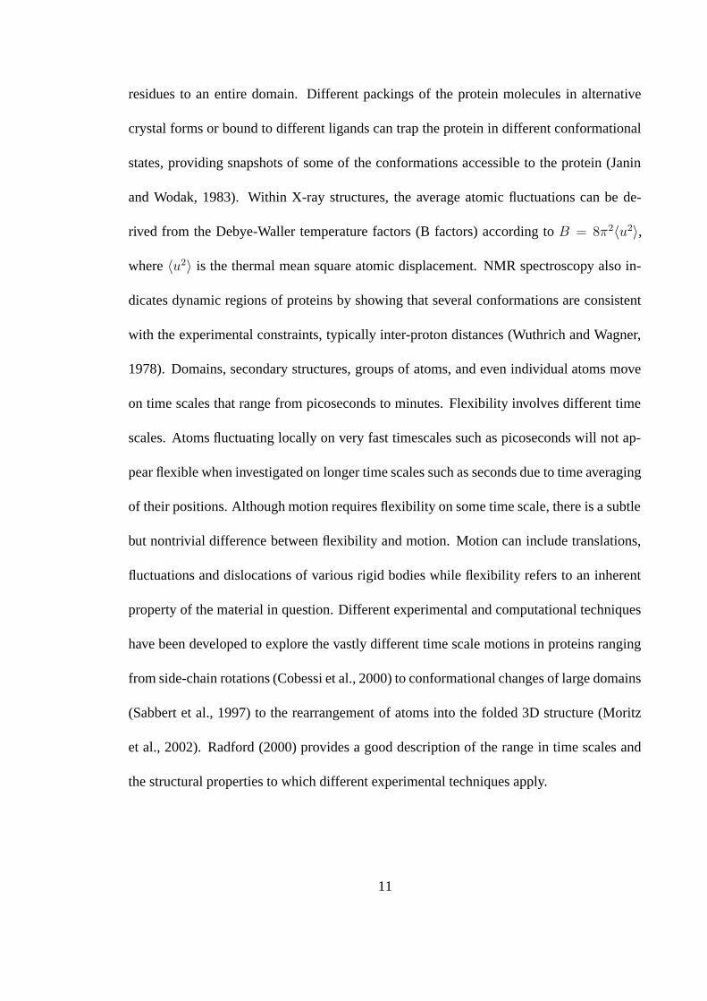
residues to an entire domain. Different packings of the protein molecules in alternative

crystal forms or bound to different ligands can trap the protein in different conformational

states, providing snapshots of some of the conformations accessible to the protein (Janin

and Wodak, 1983). Within X-ray structures, the average atomic fluctuations can be de-

rived from the Debye-Waller temperature factors (B factors) according to B = 8π2〈u2〉,

where 〈u2〉 is the thermal mean square atomic displacement. NMR spectroscopy also in-

dicates dynamic regions of proteins by showing that several conformations are consistent

with the experimental constraints, typically inter-proton distances (Wuthrich and Wagner,

1978). Domains, secondary structures, groups of atoms, and even individual atoms move

on time scales that range from picoseconds to minutes. Flexibility involves different time

scales. Atoms fluctuating locally on very fast timescales such as picoseconds will not ap-

pear flexible when investigated on longer time scales such as seconds due to time averaging

of their positions. Although motion requires flexibility on some time scale, there is a subtle

but nontrivial difference between flexibility and motion. Motion can include translations,

fluctuations and dislocations of various rigid bodies while flexibility refers to an inherent

property of the material in question. Different experimental and computational techniques

have been developed to explore the vastly different time scale motions in proteins ranging

from side-chain rotations (Cobessi et al., 2000) to conformational changes of large domains

(Sabbert et al., 1997) to the rearrangement of atoms into the folded 3D structure (Moritz

et al., 2002). Radford (2000) provides a good description of the range in time scales and

the structural properties to which different experimental techniques apply.

11

1.3.2 The Protein Folding Problem

For more than thirty years there has been great interest in understanding how proteins

rapidly and faithfully adopt a biologically functional 3D structure from a 1D sequence of

amino acids. Protein folding occurs within the long time scale limit of protein flexibility,

involving the rearrangement of atoms and domains within proteins into a unique 3D struc-

ture. Levinthal (1968) pointed out that randomly searching the conformational space by a

polymer chain would require vastly more time than what it actually takes for proteins to

adopt their native, folded form. To resolve this paradox, Levinthal suggested that protein

folding must proceed through some directed process. From available data, it was originally

postulated that the directed process of protein folding involved specific intermediate steps

and a well defined pathway much like chemical reactions (Kim and Baldwin, 1982). Lattice

models, described below, and experiments on very fast, two-state folding proteins did not

fit this classical view of protein folding, leading to the development of a “new” view of pro-

tein folding landscapes (Bryngelson and Wolynes, 1987). This concept of a funnel-shaped

free energy landscape to describe the folding reaction (Bryngelson and Wolynes, 1987;

Onuchic et al., 1997; Chan and Dill, 1998; Brooks, III et al., 2001), as shown in Figure

1.3, has changed the way experiments are done and how protein folding is explored. The

classical view of protein folding following very specific steps, has been reconciled to the

“new” view of protein folding landscapes which has many competing pathways to reach the

folded state (Bryngelson et al., 1995). Simplified lattice models that are computationally

tractable (Chan and Dill, 1998; Klimov and Thirumalai, 1999; Mirny and Shakhnovich,

2001) and more detailed, but computationally intensive, off-lattice models and molecular

12

En

erg

y

Re

actio

n C

oo

rdin

ate

, Q

1.0Native

State

Denatured States

Entropy

Figure 1.3: The “new” view of protein folding as an energy funnel or landscape. As a pro-tein folds, the entropy decreases and the reaction coordinate, Q, increases to reach a unique,folded native state. The funnel shape represents the energetic bias towards the native stateat the bottom of the funnel. The width of the funnel corresponds to the conformationalentropy present in a protein as it folds. The top of the funnel, representing the denaturedstate, is wide indicating a large amount of conformational entropy. As the protein folds, itloses entropy and the width of the funnel shrinks. The many local small groves in the fun-nel represent local energy minima where the protein can get trapped for various amountsof time depending on the depth of the minima.

dynamics simulations (Daggett et al., 1996; Duan et al., 1998; Shea and Brooks, III, 2001)

have added much to the understanding of protein folding. These approaches have increased

our understanding considerably, but the actual steps along the folding pathway continue to

remain elusive. Since protein folding can take place on time scales from microseconds to

seconds (Myers and Oas, 2002), a series of challenging experiments is required to probe

this wide range of time scales (Jackson, 1998; Gruebele, 1999; Radford, 2000; Eaton et al.,

2000). Fast-folding proteins that fold in 1 millisecond or faster, and the formation of stable

13

substructures such as α-helical segments and β hairpins that occur within microseconds,

have led to the development of new experimental techniques to measure protein folding on

the sub-millisecond time scale.

1.4 Methods to Understand Folding and Flexibility

Describing the vast range of techniques available for measuring folding and unfolding reac-

tion is beyond the scope of this work. A few techniques are presented in this section to give

a flavor of the field and provide a point of reference for the results to follow. Chemical and

thermal denaturation of proteins are the standard techniques to unfold (and refold) proteins

in biochemistry. The experimental procedures described below can be used in conjunction

with denaturation to observe the unfolding equilibria and kinetics (Radford, 2000; Jackson,

1998; Eaton et al., 2000). Experimental techniques such as circular dichroism (CD), mon-

itoring the fluorescence of tryptophan residues, hydrogen-deuterium exchange, and NMR

have also been used to probe the flexibility of native proteins.

1.4.1 Experimental Methods

HD Exchange

An experimental technique that gives detailed structural information about unfolding is

hydrogen-deuterium exchange NMR (HD exchange). Under native conditions, rotation

about main-chain Φ and Ψ dihedral angles leads to fluctuations in which a protein can

14

explore its local conformational space. HD exchange occurs when the amide (N-H) and

carbonyl (C-O) groups involved in a hydrogen bond separate enough for deuterated water to

intervene, allowing the shared proton to be replaced by a deuteron, or when a buried proton

becomes solvent-accessible (Englander et al., 1997). Because deuterium does not produce a

signal in proton NMR experiments, it is possible to identify which amide protons undergo

hydrogen exchange by comparing the NMR spectra before and after the exchange. By

allowing the experiment to run for different time steps, individual exchange rate constants

can be assigned to each of the main-chain amide protons identified in the spectra.

Linderstrøm-Lang (1958) initially proposed that the mechanism of hydrogen-deuterium

(HD) exchange in proteins occurs according to the unfolding reaction (local or global) of

Equation 1.4.

CH

kop−→←−kcl

OH kint−→ OD

kcl−→←−kop

CD

(1.4)

In this equation, C represents a closed form of the amide group in which exchange cannot

occur. O represents an open state of the amide proton able to participate in HD exchange.

Equilibrium between these two forms is defined by the rate constants for opening, kop,

and closing, kcl. Once in the O state, the amide can exchange its hydrogen with solvent.

Because the apparent rate of exchange depends on both the rate of opening, kop, and the

intrinsic rate of exchange, kint, it is nearly impossible to determine these rates individually

in the context of whole protein studies. Therefore, kint is typically determined from the

rate of exchange observed, for each amino acid type, within the structure of small model

peptides (Bai et al., 1993; Molday et al., 1972), for which no “opening” reaction is required.

15

When kcl � kop, conditions favor folding and one can express the observed rate of

exchange, kex, by Equation 1.5.

kex =kopkint

kcl + kint(1.5)

Two limiting scenarios of exchange arise from Equation 1.5. The first case, termed EX1,

occurs when kint � kcl, reducing the observed rate of exchange in Equation 1.5 to kex =

kop. The EX1 limit for exchange is rarely observed in proteins under native conditions. The

fact that exchange occurs more quickly than reprotection of the amide suggests a significant

structural instability for the protein in the EX1 case. Experiments have shown that most

amides favor the EX1 mechanism at increasing concentrations of denaturant.

The second case, referred to as the EX2 limit, occurs when kcl � kint. In this case,

Equation 1.5 reduces to equation 1.6, where the term Kop = kop/kcl represents the equi-

librium constant between opening and closing the amide. Kop also represents the limiting

rate of unfolding required for exchange. An apparent free energy of exchange, ∆Gappex ,

can be computed for the observed exchange rate, kex, and the intrinsic exchange rate, kint,

according to Equation 1.7. EX2 exchange has been shown to be the dominant mechanism

of exchange under native conditions, allowing the apparent free energies of exchange to be

computed from Equation 1.7, where R is the universal gas constant and T is the tempera-

ture.

kex =kop

kcl· kint = Kop · kint (1.6)

∆Gappex = −RT ln Kop (1.7)

The usefulness of HD exchange as a means to study protein folding is based on the

16

thermodynamic premise that a protein can sample all of its higher energy conformations

along the folding pathway according to a Boltzmann distribution. This means that even

under native conditions, at any given time a small population of protein molecules will

be in an unfolded state. Although the protein will rapidly refold, highly sensitive NMR

techniques can observe the HD exchange which can occur while the protein is unfolded

(Clarke and Itzhaki, 1998).

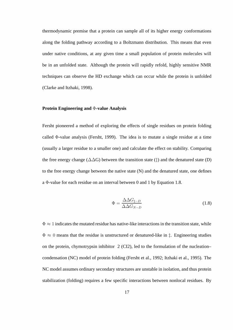
Protein Engineering and Φ-value Analysis

Fersht pioneered a method of exploring the effects of single residues on protein folding

called Φ-value analysis (Fersht, 1999). The idea is to mutate a single residue at a time

(usually a larger residue to a smaller one) and calculate the effect on stability. Comparing

the free energy change (∆∆G) between the transition state (‡) and the denatured state (D)

to the free energy change between the native state (N) and the denatured state, one defines

a Φ-value for each residue on an interval between 0 and 1 by Equation 1.8.

Φ =∆∆G‡−D

∆∆GN−D(1.8)

Φ ≈ 1 indicates the mutated residue has native-like interactions in the transition state, while

Φ ≈ 0 means that the residue is unstructured or denatured-like in ‡. Engineering studies

on the protein, chymotrypsin inhibitor 2 (CI2), led to the formulation of the nucleation–

condensation (NC) model of protein folding (Fersht et al., 1992; Itzhaki et al., 1995). The

NC model assumes ordinary secondary structures are unstable in isolation, and thus protein

stabilization (folding) requires a few specific interactions between nonlocal residues. By

17

conducting many single and double cycle mutants, researchers identify the folding nucleus

as the specific residues with the highest Φ-values. Mutations that disrupt interactions from

these residues will cause a significant change in the rate of folding, while mutations in other

regions will have no effect on the folding rate. Thus, residues in this folding nucleus are

critical for protein folding.

Although these limiting cases are well understood, a comparison of Φ-values for a num-

ber of proteins shows many values of Φ to be fractional (Nolting and Andert, 2000). How

to interpret fractional values of Φ is still a matter of debate (Myers and Oas, 2002), but

involves some combination of the following three cases: (i) a partial weakening of the tran-

sition state in all interactions involving the mutated residue, (ii) a full or partial weakening

of some interactions but no weakening in others, and (iii) the presence of parallel folding

pathways indicated by interactions that are required for one pathway but not others. Con-

flicts with other measures of folding such as NMR and the folding rate reaction coordinate,

βT , suggest that Φ-values cannot be used blindly to predict the level of the folding structure.

NMR studies on BPTI, for example, indicate a greater native-like structure in intermediates

than would be predicted from Φ-values (Bulaj and Goldenberg, 2001). Lattice simulations

have shown that non-classical values of Φ, i.e. < 0 or > 1, are the result of multiple, parallel

folding pathways (Chan and Dill, 1998; Ozkan et al., 2001).

18

1.4.2 Computational Methods

Lattices

Lattice models of protein folding provided some of the earliest theories about protein fold-

ing. Ueda et al. (1975) used a 2D lattice to describe the native state of a protein. Embellish-

ments were soon added to model proteins more realistically. The Go model (Go, 1983) uses

native state topology to identify preferred contacts between lattice sites. The HP model uses

two types of lattice monomers: H for hydrophobic and P for polar (Lau and Dill, 1989).

With these more physical potentials, it was possible to investigate which sequences could

or could not fold (Chan and Dill, 1991). Bryngelson and Wolynes (1987) applied concepts

about spin glasses to explain how proteins fold, which led to the concept of folding funnels

and landscapes. Due to the simplicity of such models, complete sampling of configura-

tion space (Ozkan et al., 2001) can be performed, allowing characterization of how folding

proceeds. These very simple models of interactions between amino acids within proteins

have contributed immensely to the concept of how proteins fold and to our understanding

of the nature of transitions between unfolded and folded proteins. Go-like models are often

employed to calculate Φ-values and make connection with experiment (Vendruscolo et al.,

2001; Paci et al., 2002). Lattice models have also been used to predict folding kinetics

(Klimov and Thirumalai, 1998) and folding nuclei (Abkevich et al., 1994). Thinking of

proteins as independently interacting hard spheres or as a self-interacting random poly-

mer chain such as in lattice models, led to the diffusion–collision (DC) model (Karplus

and Weaver, 1979, 1994) of protein folding. The DC model assumes folding proceeds

from diffusive interactions between partially structured secondary elements in isolated mi-

19

crodomains. The rate limiting step of folding is governed by the rates of diffusion and

collision of (quasi)stable subunits. The DC model seems to accurately describe the folding

pathways and folding times for small, all-helical proteins like the engrailed homeodomain

protein (Islam et al., 2002).

Molecular Dynamics

A more computationally expensive technique to explore protein folding and flexibility is

molecular dynamics. The basic approach is to apply Newton’s equations of motion to a

macromolecule and observe how the system changes over time. Since F = ma = mx

and F = −∇V , it becomes a matter of assigning an accurate potential, V , obtaining the

initial coordinates, and numerically integrating over very short time intervals to observe

the dynamics of the system. One commonly used energy potential (Weiner et al., 1986) for

MD calculations is given by Equation 1.9, where tabulated values for various parameters

are used as input depending on the particular atom types involved.

Vtotal =∑

bonds

Kb(r − r0)2 +

∑angles

Kθ(θ − θ0)2

+∑

dihedrals

Vn

2[1 + cos(nφ− γ)]

+∑i<j

[Aij

R12ij

− Bij

R6ij

+qiqj

εRij

]+

∑Hbonds

[Cij

R12ij

− Dij

R10ij

] (1.9)

MD simulations use timesteps on the order of femtoseconds, requiring a very large

number of steps to run before observing motion on the time scale of protein folding. Em-

ploying the techniques of spatial decomposition, massive parallelization and an 8A non-

bonded interaction distance cutoff, a Herculean MD study ran for long enough (1µs) to ob-

20

serve folding (Duan et al., 1998) of the villin headpiece protein fragment. Research groups

have employed these and other methods to effectively “speed” up the MD simulation. Typ-

ical techniques used within MD simulations to observe folding/unfolding include: using

implicit rather than explicit solvent, applying force (Lu and Schulten, 1999) or pressure

(Hillson et al., 1999) to the protein, running at elevated temperatures to simulate unfold-

ing (Daggett et al., 1996), and conducting studies on a multitude of parallel and connected

systems via the replica symmetry method (Sanbonmatsu and Garcıa, 2002) or distributed

computing techniques (Snow et al., 2002).

To obtain results that can be compared to experimentally observable long time scale

motions such as folding or flexibility, other simplifications can be made in the MD simula-

tion that allow for greater sampling of space. Normal mode analysis (NMA) has been used

for 20 years (Brooks and Karplus, 1983; Ma and Karplus, 1997) to identify the function-

ally relevant motion. Varieties of NMA run significantly faster than MD by assuming the

k lowest frequency eigensolutions to the dynamical matrix of Equation 1.3 account for the

largest structural fluctuations and thus correspond to the long time scale functional motion.

Tirion (1996) showed that one was able to produce similar NMA results using either the

complex potential of Equation 1.9 or a much simpler pairwise potential similar to Equa-

tion 1.2, significantly reducing the complexity of solving the dynamical matrix. However

NMA and similar essential dynamics methods tend to suffer from the same limitations as

MD: dependence upon an empirical force field and long computation time (Tama et al.,

2000; Berendsen and Hayward, 2000). Another single-parameter model of proteins is the

Gaussian Network Model (GNM) which reduces the protein to a network of Hooke springs

21

between contacted residues (Bahar et al., 1997, 1998). The coarse-grained features of rele-

vant protein motions are detectable from an extension of GNM (Atilgan et al., 2001) which

faces the same computational intensity as NMA.

Conformational Comparisons

Computationally superimposing different conformations of the same protein structure often

has been used to identify the flexible regions in proteins (Gerstein et al., 1994). Such stud-

ies examine differences between relevant geometrical parameters (Korn and Rose, 1994;

Nichols et al., 1995) to identify the flexible hinges. These methods are limited by the di-

versity of the conformational states that are available from experiments for comparison. A

recent variation of this technique has employed multiple structural alignments to overcome

some of the biases present from superimposing only two conformations (Shatsky et al.,

2002).

Autonomous Folding Units

This class of modeling protein folding relies upon identifying foldable substructures from

the native conformation of proteins. Such work is related to efforts that identify domains

in proteins (Janin and Wodak, 1983) but these foldable substructures, termed autonomous

folding units (AFUs), may or may not coincide with domains. The identification of AFUs

often relies on defining rigid section or flexible hinge joints within the single protein con-

formation (Maiorov and Abagyan, 1997). Other measures such as compactness (Zehfus

and Rose, 1986), contact ratios (Siddiqui and Barton, 1995), and low-frequency NMA

22

(Holm and Sander, 1994) have met with varying degrees of success, but no single tech-

nique works well in all cases. Peng and Wu (2000) provides a comparison and review of

many efforts at identifying AFUs. These methods are usually computationally very fast

and have a well defined starting point of the native state. An unfolding energy function is

used by Wallqvist et al. (1997) to rank the stability of combinations of small folded units.

This search then predicts the folding core based upon an unfolding energy function. Corre-

lation between HD exchange data and the calculated unfolding scores suggests this method

has promise. Another method in this class identifies hydrophobic folding building blocks

(Tsai and Nussinov, 1997; Tsai et al., 2000). After partitioning a protein into such building

blocks, predicted protein folding pathways can be made by assembling the blocks in differ-

ent ways. Although this method has dissected every protein in the PDB into such building

blocks, correlation with actual folding cores from HD exchange or Φ-values is thin. Chap-

ter 4 will present a recently developed method (Hespenheide et al., 2002) of identifying

folding cores using rigidity theory.

No matter how fast or elegant the computational method is, it must accurately describe

the physical system to have any relevance. Since the method for identifying rigid and

flexible regions of proteins explained in Chapter 3 involves analysis of the native state, it

can be understood in terms of both AFU and NMA type methods. Results from our method

will also be compared to a variety of experimental measures, including HD exchange data,

in Chapters 4 and 5.

23

1.4.3 Summary: Theory of Protein Folding

Socci et al. (1998) demonstrated on lattice models that one could convert from a strictly

hierarchical folding pathway to a DC dominated pathway by changes the balance of nonlo-

cal to local interaction strengths. Continuing in this line of thinking, it has been suggested

that secondary structural formation and chain collapse can occur concomitantly (Thiru-

malai and Klimov, 1999). Although no single mechanism seems to describe folding for all

proteins, the NC and DC models are basically extremes of the same process united by an

understanding of an extended transition state (Fersht, 1997, 2000). The common element

of these folding models is the cooperative nature of folding, that is, many interactions work

concertedly to drive a protein from a random coil to a unique folded state. Additionally,

the inverse process of protein denaturation is a first-order (“all-or-none”) phase transition

in small, single-domain proteins (Privalov, 1979; Shakhnovich and Finkelstein, 1989).

Hydrophobic Collapse

The combination of interactions within proteins leads to the compact, fully folded native

state. One of the reasons this problem remains unsolved is that proteins in the native state

are only marginally stable. That is to say the total free energy of folding, ∆G, is on the

order of 5 - 15 kcal/mol, while the entropy (∆S) and enthalpy (∆H) are both comparatively

large (on the order of 100 kcal/mol). The dominant forces in protein folding must explain

why the folded state is lower in free energy than the unfolded state. The non-covalent

interactions provide for the increase in ∆H, while the ordering of atoms into secondary

and tertiary structures and the exclusion of water from the protein core contributes to the

24

change in entropy. Since proteins fold in an aqueous environment, hydrogen bonds that

would be made in the final folded form would also be satisfied by hydrogen bonds with

the ambient water. Thus, although hydrogen bonds provide very specific and essential

information about the folded conformation, they cannot be the driving force in protein

folding (Kauzmann, 1959).

The general view of protein folding is that it begins with hydrophobic collapse, in which

the random coil changes to a compact state, with the hydrophobic groups in the interior re-

gion and polar groups at the surface interacting with the surrounding water (Dill, 1990).

The packing is not yet optimal, with hydrophobic groups somewhat free to slide about in

the interior of the globule, until residues are locked in place by the formation of specific

hydrogen bonds. These hydrogen bonds can be regarded as a sort of velcro that locks the

various structural elements in the folded protein together, while the hydrophobic interac-

tions form a slippery glue. Once these interactions are optimized, the native state is pre-

dominantly rigid with flexible hinges or loops at the surface — the number and distribution

of these depending on the particular protein.

Whether folding is initiated by nucleation of tertiary interactions or diffusion-controlled

coalescence of already folded secondary structures is being debated, and a single model

may not hold for all proteins. However, a unifying theme is that the initial steps in the

folding process involve the interaction of nonlocal regions in the protein sequence forming

a substructure that is substantially preserved in the fully folded protein. Several theoretical

techniques have been designed to identify early folding substructures (Hilser et al., 1998;

Galzitskaya and Finkelstein, 1999; Torshin and Harrison, 2001). These techniques rely

25

solely on analysis of the native-state conformation, instead of following the folding reaction

from a denatured state to the native state. The advantage of analyzing the native state is that

this conformation is largely ordered, whereas the denatured state is typically an ensemble

of dissimilar, unfolded conformations. Identifying the transition state ensemble, that is the

set of conformations through which all pathways must go to reach the folded state, is also

difficult due to being an ensemble of partially ordered states.

1.5 Thermophiles

Over the past twenty years, there has been a growing interest in proteins from organisms

that live in extreme environments. Some of the interest has been due to industrial applica-

tions that require enzymatic activity at elevated temperatures. Additionally, proteins from

thermophilic organisms (thermophiles) tend to crystallize more readily making them an ac-

tive field of research. Throughout this dissertation, the term thermozyme will be applied to

refer to any protein from a thermophilic organism and the term mesozyme will refer to any

protein from an organism that lives at room temperature. Since thermolysin, the first struc-

ture from a thermostable organism, was crystallized in 1974 (Matthews et al., 1974), many

other thermophilic structures have been determined. As more protein structures from ther-

mophilic organisms are found, it is natural to question what makes these structures stable

and active even at elevated temperatures. The issue of stability as it relates to temperature

is an intriguing one simply from a basic science point of view.

26

1.5.1 Mechanisms of Thermostability

A large variety of experimental and theoretical approaches have been applied to identify-

ing the molecular and energetic factors contributing to protein thermostability, including

genome-wide sequence comparisons (Das and Gerstein, 2000), overall amino acid distri-

butions (Ponnuswamy et al., 1982), site-directed mutagenesis (Querol et al., 1996; Vieille

and Zeikus, 1996), 3D structure comparisons (Vogt et al., 1997; Szilagyi and Zavodsky,

2000; Kumar et al., 2000), directed evolution (Eidsness et al., 1997; Strop and Mayo,

2000), molecular dynamics simulations of protein unfolding (Caflisch and Karlpus, 1995;

Lazaridis et al., 1997), and analysis of protein flexibility by amide HD exchange (Hol-

lien and Marqusee, 1999b; Hernandez and LeMaster, 2001). Most studies agree that no

single molecular mechanism is responsible for protein thermostabilization and that stabi-

lization mechanisms vary from one protein to another. Hence, despite intense research

efforts, protein thermostability remains widely unexplained. The increase of stability

can be explained in terms of plots of free energy of stabilization, ∆G, versus temperature.

Observable trends or mechanisms of greater thermostablility result from a combination of

three fundamental methods for increasing thermostability, ∆G(T). These three methods of

stabilization are sketched with respect to a typical free energy curve for a mesophilic pro-

tein (curve a) in Figure 1.4. The other curves demonstrate these three sources of increased

stability: (i) a greater maximum stability (curve b), (ii) a shift to higher optimal temperature

(curve c), and (iii) a flattening of ∆G — indicating a weaker dependence upon temperature

(curve d).

As with the free energy changes in protein folding, the difference in ∆G values between

27

-25

-20

-15

-10

-5

0

-40 -20 0 80 100 120604020

Temperature oC

∆G

(kcal/m

ol)

a

b

c

d

Figure 1.4: Free energy of stabilization, ∆G, as a function of temperature and the sourceof thermostability. Curve a (solid) shows the free energy dependence on temperature for atypical mesophilic protein. Curves b through d indicate the potential sources of thermosta-bility for thermophilic proteins. Curve b (dashed) indicates an overall increase in ∆G forall temperatures leading to an increased stability at higher temperatures. Curve c (long-dashed) shows a shift to higher temperatures and curve d (dotted) shows a broadening ofthe free energy curve, indicating a weaker temperature dependence.

thermozymes and mesozymes is typically small (in the range 5–15 kcal/mol) (Vieille and

Zeikus, 1996). This means that a few additional interactions (hydrogen bonds, hydrophobic

interactions, or salt-bridges) out of a vast number can account for this difference. Since

thermozymes and mesozymes are generally similar in sequence, structure, and catalytic

function; several research groups have conducted pairwise (Kumar et al., 2000; Szilagyi

and Zavodsky, 2000) and multiple (Vogt et al., 1997; Gianese et al., 2002) comparisons

of protein structures to identify these few interactions. These studies involved looking

at numerous structural properties within families of homologous proteins and observing

trends that correlate with the temperature of optimal growth (Tg) or melting (Tm). Table

1.1 presents some of the proposed thermostabilizing structural properties investigated by

28

Table 1.1: Proposed structural thermostabilizing mechanisms compiled from Kumar et al.(2000) and Vieille and Zeikus (2001).

Mechanism1. Increased hydrophobicity and aromatic interactions2. Better packing and decreased solvent accessible hydrophobic surface area3. Deletion of or shortened loops4. Smaller and less numerous cavities5. Increased oligomeric state and intersubunit interactions6. Amino acid substitution within and outside secondary structure7. Increased occurence of proline residues8. Decrease of thermolabile residues (Cys,Ser)9. Increased helical content

10. Increased polar surface area11. Increased number of hydrogen bonds12. Increased number of salt bridges (ion pairs)13. Conformational strain release

these studies. Although most of these properties did not show consistent trends across

the families studied, properties such as an increased number of salt bridges and side-chain

hydrogen bonds were more universal (Kumar et al., 2000).

1.5.2 Rigidity and Thermostability

A working hypothesis explaining the remarkable stability of hyperthermophilic enzymes

is that these enzymes have enhanced conformational rigidity at low temperatures (Vihinen,

1987; Vieille and Zeikus, 2001). According to this hypothesis, psychrophilic (stable at

cold temperatures), mesophilic, thermophilic, and hyperthermophilic homologous enzymes

have comparable catalytic efficiencies (indicated by kcat/KM ) at their respective optimal

temperatures, because optimal activity requires a certain degree of conformational flexibil-

29

ity in the active site. Due to their increased rigidity at low temperatures, thermophilic and

hyperthermophilic enzymes are only marginally active at these temperatures, and they gain

the flexibility required for optimal activity only at higher temperatures (Jaenicke, 1991).

Recent experimental data from amide HD exchange (Hollien and Marqusee, 1999a) and

Fourier transform infrared spectroscopy (FT-IR) (Bonisch et al., 1996) along with molec-

ular dynamics simulations (Colombo and Merz, Jr., 1999) show that results vary from one

protein to another. Some thermophilic enzymes are less flexible than their mesophilic coun-

terparts (Wrba et al., 1990; D’Auria et al., 2000; Manco et al., 2000), whereas others are

as flexible (if not more flexible) than their mesophilic counterparts (Lazaridis et al., 1997;

Hernandez and LeMaster, 2001). Some of these discrepancies may stem from the difficulty

in decoupling the complex interactions responsible for activity from those responsible for

thermostability. On a global level, a thermozyme at low temperatures has a high level of

flexibility because that flexibility gives the folded thermozyme high entropy, and thus a low

entropic cost of folding (Caflisch and Karlpus, 1995; Lazaridis et al., 1997). Chapter 5 will

present comparisons between flexibility and thermostability on both local (active-site) and

global (folding) flexibility levels.

1.6 Direction

This dissertation investigates the flexibility, stability and folding of proteins from the per-

spective of rigidity theory. Chapter 2 presents the mathematics of rigidity and rigidity

percolation on which the analysis of proteins is built. The rigidity phase transition is dis-

cussed for different network glasses in terms of the mean coordination. This parameter will

30

later be connected to an unfolding reaction coordinate.

Proteins are introduced as a special case of amorphous materials in Chapter 3. The

application of rigidity analysis to proteins has resulted in the development of the FIRST

(Floppy Inclusions and Rigid Substructure Topography) software. How this computer pro-

gram models protein structures and identifies all rigid and flexible regions in the structure is

presented. Results for the flexibility of several specific proteins is also presented in Chap-

ter 3. Predicted flexibility is compared to experimental B-values, and the effect of ligand

binding on flexibility is presented.

Chapter 4 presents the applications of this FIRST software to proteins in the context

of protein unfolding. Beginning with the native state conformation, unfolding is computa-

tionally simulated. Various methods for unfolding are discussed with results compared to

experimental folding data. Assuming the reversibility of protein folding (a valid assump-

tion for proteins lacking folding intermediates), this analysis traces out potential unfolding

pathways. Using this procedure, a method for identifying the protein folding core is pre-

sented and compared to experimentally determined folding cores. Validation of the FIRST

software is shown by observing the same, universal rigidity phase transition in proteins that

is observed in network glasses. This phase transition is shown to coincide with the protein

unfolding transition, providing a powerful tool to predict the transition state from the native

state of proteins.

Since the structural properties in Table 1.1 are built into the protein model described

in Chapter 3, quantitative measures of rigidity and flexibility will be compared to ther-

mostability in general in Chapter 5. Additionally, specific flexibility results from FIRST

31

will be compared with experimental studies on several families of homologous proteins. A

summary of the dissertaion is presented in Chapter 6, and potential future applications of

protein rigidity theory are discussed.

32

Chapter 2

Rigidity in Glasses

Parts of the research presented in this chapter have been previously published in

M.F. Thorpe, D.J. Jacobs, N.V. Chubynsky, and A.J.Rader. Generic Rigidity of NetworkGlasses. In Rigidity Theory and Applications, M.F. Thorpe and P.M. Duxbury, eds., pp.239–277, Kluwer Academic, New York, 1999.

2.1 Introduction

This chapter develops the concepts of rigidity percolation and its applications to particular

materials. These concepts are presented in the context of network glasses and extended

to proteins in later chapters. Applying concepts from physics to the understanding of bi-

ological problems is the underlying motivation. Understanding results for the simpler 2D

case aids in interpreting the results for 3D networks, such as proteins, that will come later.

Special attention is given to the nature of the phase transition from floppy to rigid in var-

ious network glasses. A relationship between the number of floppy modes and the mean

33

coordination is presented.

2.2 Network Glasses and Rigidity

2.2.1 Computational View of Glasses

Network glasses are 3D cross-linked, covalently bonded amorphous materials. Using the

procedure of Wooten and Weire (1985) it is possible to build a computational model of

amorphous silicon, a-Si, with a unit cell containing up to 4096 atoms (Djordjevic et al.,

1995). Unlike a-Si where each atom has four nearest neighbors, glasses are often formed

of mixtures of elements such as GexAsySe1−x−y where the subscripts identify the atomic

fractions of four-fold coordinated germanium, three-fold coordinated arsenic, and two-fold

coordinated selenium atoms respectively. Because the calculations that follow will not in-

volve actually solving the dynamical matrix of Equation 1.3, the connectivity or topology

of the network is more important than the specific geometry of the original network tem-

plate. Focusing on the connectivity simplifies some of the computations as one can begin

with the a-Si model or various distorted lattices and generate diluted networks of atoms

with the desired concentrations of two-, three-, and four-fold coordinated atoms. The mean

coordination, 〈r〉, serves as an important parameter to describe such a network glass. If one

takes N as the total number of atoms and Nr as the number of r-coordinated atoms, then

N =∑

r

Nr (2.1)

34

Figure 2.1: Example of a small random bond model network with 64 atoms and 〈r〉= 3.0.The squares are four-fold coordinated sites, the triangles are three-coordinated sites and thecircles are two-fold coordinated sites.

where 〈r〉is defined by

〈r〉 =∑

r rNr

N. (2.2)

In the case of the above covalent glass GexAsySe1−x−y this gives 〈r〉= 2+2x+2y. If the

network lacks singly-coordinated atoms then the lower bound on 〈r〉is 2 corresponding to a

polymer chain. Since connectivity is the relevant object, random bond models (RBM)s rep-

resent an alternative method of constructing a continuous random network (glass). RBMs

such as the one shown in Figure 2.1 are constructed by randomly connecting N atoms in

d-dimensions to with the desired values of two-, three- and four-fold coordinated atoms.

2.2.2 Generic Rigidity

The rigidity of a network glass is related to how amenable that glass is to continuous de-

formations that require very little (zero) cost in energy. Thus a collection of atoms forms a

35

rigid cluster whenever no relative motion or deformation within that cluster can be achieved

without a finite energy cost. Conversely, floppy modes correspond to finite motions within

the system which do not cost energy. Deviations from the mean-field approximation of

Maxwell counting in network glasses have been described by small rigid regions within

a floppy network when 〈r〉 is low and the opposite case of a few floppy pockets within

a rigid structure when 〈r〉 is high. Thus by increasing 〈r〉, rigidity percolates through

the network (Thorpe, 1983). Connectivity percolation is a limiting case of the broader

problem of rigidity percolation. Unlike connectivity percolation that has been applied to

a large number of physical phenomena (Stauffer and Aharony, 1998), rigidity percolation

has not been as widely studied. In rigidity percolation the propagation of a vector, rather

than a scalar quantity is monitored. There is also an inherent nonlocal or long-range aspect

to rigidity percolation. These differences make the rigidity problem become successively

more difficult as the dimensionality of the network increases.

Figure 2.2 displays an example of these nonlocal effects in rigidity percolation along

with the notion of generic rigidity. Whether or not the underlying framework is generic is

another major consideration for the application of rigidity to physical systems. A generic

structure is one that has no special symmetries, such as parallel bonds or bond angles of

180◦, that could create geometrical singularities (Guyon et al., 1990). This means that

generic structures are not on a lattice, but amorphous. Figure 2.2A shows four distinct

rigid clusters consisting of two rigid bodies in gray attached by two rigid bars at pivot

joints (open circles). The placement of one additional rigid bar in Figure 2.2B, locks the

previous four clusters into a single rigid cluster and the joints (shown by filled circles)

36

A B

C

Figure 2.2: The gray shaded regions represent 2D rigid bodies. The open (closed) circlesdenote joints that free to pivot (rigidly fixed). A. A floppy network with four distinct rigidclusters: two bodies and two bars. B. Three generic cross-links between two rigid bod-ies make the whole structure rigid. If the cross-linking bonds were parallel, the structurewould no longer be generic and thus susceptible to zero-energy shear deformations (Guyonet al., 1990). C. Three non-collinear, joined bars contain one internal floppy mode as theygenerically reconnect the rigid body. If they were collinear (along the dotted line) instead,two infinitesimal (zero-energy) floppy motions would exist allowing buckling under a hor-izontal compression.

are no longer free to pivot. This nonlocal character of rigidity allows a single bar (bond)

in one region of the network to affect the rigidity in the entire network. The position of

bonds in Figure 2.2C, is generic and contains one internal floppy mode. If the bonds were

instead placed collinearly along the dashed line, they would be non-generic and experience

buckling under a compressive force. Such buckling is absent from the generic case. Due

to the amorphous nature of glasses, we can restrict our study to include only generic cases.

Thus the calculated floppy modes will accurately describe the total number of internal

degrees of freedom in the network. The random bond model described above is an example

of a generic network where the connectivity or topology is uniquely defined but the bond

lengths and bond angles are arbitrary.

37

2.2.3 Maxwell Counting and Laman’s Theorem

In simple cases like the one shown in Figure 1.2, Maxwell constraint counting described

in Section 1.2.2 accurately provides the number of floppy modes, F , and a good account

of where the network undergoes a phase transition from rigid to floppy. The number of

floppy modes in the network, or normalized per degree of freedom, f = F/dN , will

prove to be a key quantity. Thus for the simple 2D bar-joint networks of Figure 1.2, f =

1 − 14〈r〉 by substituting 〈r〉 from Equation 2.2 into Equation 1.1. Then for large N the

network undergoes a rigidity phase transition at 〈r〉= 4. The applications of such concepts

have traditionally been to solve problems in engineering, such as the structural stability of

different truss configurations in bridges. Solving these problems, one speaks of networks of

struts, bars, or constraints. The nature of structural rigidity has two main conceptual bases:

one of statics and one of mechanics. A network is rigid according to the statics definition iff

it resolves all equilibrium loads while a network is rigid according to a mechanics viewpoint

iff all infinitesimal motions are rigid motions (Guyon et al., 1990; Whiteley, 1999).

In a 3D bond-bending network (one where bond lengths and angles are fixed by con-

straints), Maxwell counting gives the following result:

F = 3N −rmax∑r=2

Nr

[r

2+ (2r − 3)

], (2.3)

or in terms of f ,

f = 2− 5

6〈r〉. (2.4)

Thus at 〈r〉= 2.4 the number of floppy modes is zero, signifying the phase transition from

38

rigid to floppy. Since Maxwell counting is a mean field approximation, it ultimately fails

to give the exact transition point. Instead of studying the network globally with Maxwell

counting, the following theorem of Laman (1970) suggests how to consider the detailed

distribution of constraints and improve upon Maxwell counting.

Theorem 1 (Laman) A generic network in two dimensions with N sites and B bonds

(defining a graph) does not have a redundant bond iff no subset of the network containing

n sites and b bonds (defining a subgraph) violates b ≤ 2n− 3.

Whenever Laman’s theorem is violated, there must be at least one redundant constraint.

This necessary part generalizes to all dimensions such that if b > dn − d(d + 1)/2 then

there is a redundant bond for n ≥ d vertices and for n < d vertices it follows that if

b > n(n − 1)/2 then there is a redundant bond. (Note that n = 1 is an excluded case

because two sites are required for a bond to be present.) The essence of Laman’s theorem

says by finding all subgraphs where b > 2n−3 one uniquely identifies all redundant bonds

in two dimensions. Thus the rigidity on any two-dimensional generic framework (network)

can be completely characterized by applying constraint counting to all the subgraphs within

the framework requiring constraint counting on all levels (subgraphs) rather than just the

global level of Maxwell counting.

Unfortunately this sufficient part of the theorem does not generalize to higher dimen-

sions (Hendrickson, 1992; Tay and Whiteley, 1985). Application of Laman’s theorem ac-

curately defines the rigidity of such 2D networks where the angles between fixed edges

of the graph are free to pivot. However, such constraint counting over the subgraphs on

39

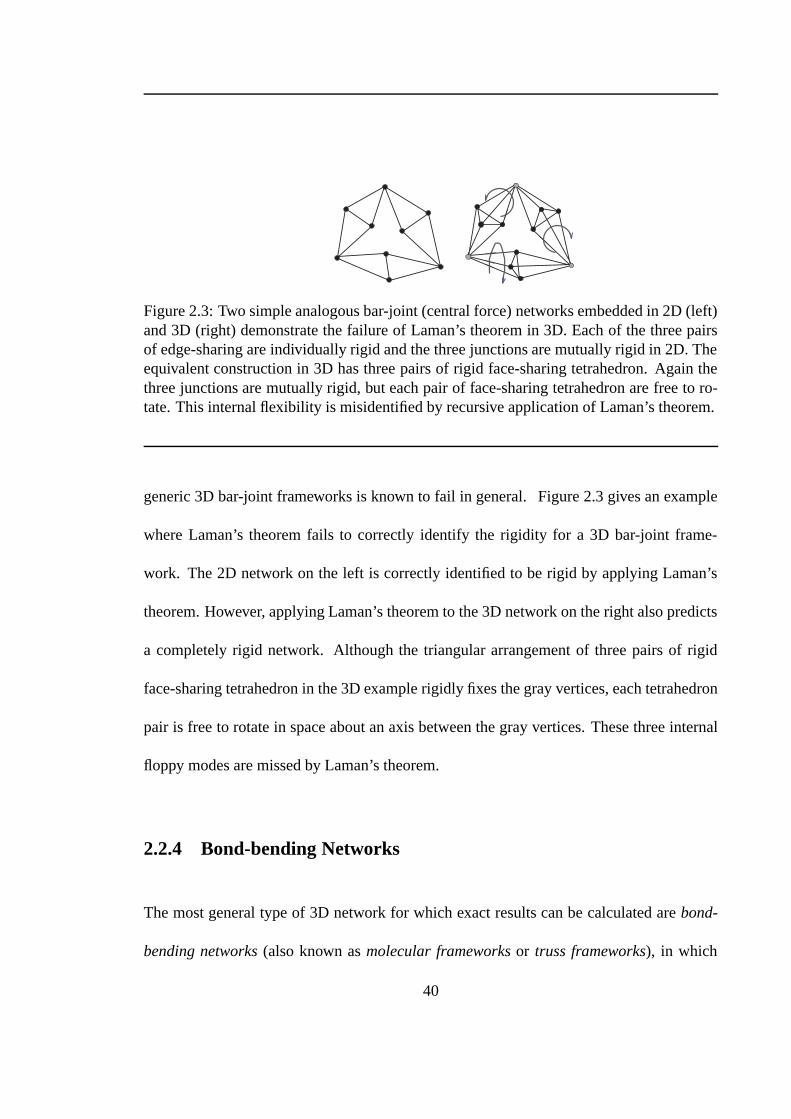
Figure 2.3: Two simple analogous bar-joint (central force) networks embedded in 2D (left)and 3D (right) demonstrate the failure of Laman’s theorem in 3D. Each of the three pairsof edge-sharing are individually rigid and the three junctions are mutually rigid in 2D. Theequivalent construction in 3D has three pairs of rigid face-sharing tetrahedron. Again thethree junctions are mutually rigid, but each pair of face-sharing tetrahedron are free to ro-tate. This internal flexibility is misidentified by recursive application of Laman’s theorem.

generic 3D bar-joint frameworks is known to fail in general. Figure 2.3 gives an example

where Laman’s theorem fails to correctly identify the rigidity for a 3D bar-joint frame-

work. The 2D network on the left is correctly identified to be rigid by applying Laman’s

theorem. However, applying Laman’s theorem to the 3D network on the right also predicts

a completely rigid network. Although the triangular arrangement of three pairs of rigid

face-sharing tetrahedron in the 3D example rigidly fixes the gray vertices, each tetrahedron

pair is free to rotate in space about an axis between the gray vertices. These three internal

floppy modes are missed by Laman’s theorem.

2.2.4 Bond-bending Networks

The most general type of 3D network for which exact results can be calculated are bond-

bending networks (also known as molecular frameworks or truss frameworks), in which

40

vertices of the graph are connected by edges and every angle between these edges is also

fixed. The Molecular Framework Conjecture (Tay and Whiteley, 1985; Whiteley, 1999;

Chubynsky and Thorpe, 2002b) indicates that Laman’s theorem of constraint counting ex-

tends to non-generic molecular models in which all bonds (hinges) of an atom pass through

a single central point of the atom. This generalization of Laman’s theorem to 3D bond-

bending networks has been shown (Jacobs, 1998) to eliminate so-called double banana

problems of the type in Figure 2.3 because bond-bending (chemical) angles are fixed by

constraints between next-nearest neighbors. Although the Molecular Framework Conjec-

ture requires a rigorous proof, there are no known exceptions after more than fifteen years

of exact testing. Fortunately, many network glasses of interest are ones where the atoms

are connected by covalent bonds which impose restrictions on the bond-bending angles

between next-nearest neighbors. This makes bond-bending networks an appropriate model

for glasses (Chubynsky and Thorpe, 2002b).

Rigidity on networks with different geometries of Hooke springs as described in Section

1.2.3 has been studied by brute-force methods (Feng and Sen, 1984; Feng et al., 1985; Day

et al., 1986; Hansen and Roux, 1989; Arbabi and Sahimi, 1993; Moukarzel et al., 1997b).

The behavior of the elastic constants and the number of floppy modes for central force

networks compares remarkably well with the mean-field theory (Feng and Sen, 1984; Feng

et al., 1985; Day et al., 1986) except for very close to the phase transition from rigid to

floppy. Figure 2.4 shows the striking agreement with Maxwell counting for two different

types of network glasses. Each point along the curves is calculated by the Pebble Game (see

below) as bonds are randomly removed from the network. The black curve corresponds to

41

a continuous random model of a-Si and the gray line corresponds to an RBM glass like the

one shown in Figure 2.1.

Such central force networks described by the potential of Equation 1.2 omit the bond-

bending nature of covalent glasses. Continuing to think of the glass in terms of pairwise

harmonic potentials, a bond-bending model is created by the Keating-type potential of

Equation 2.5 where x refers to a displacement from the equilibrium bond length as in the

usual central force model and θ refers to the change from the equilibrium bond angle.

V =α

2x2 +

βx

2θ2 (2.5)

The Keating-type potential in Equation 2.5 not only describes glass well (Keating, 1966),

but also corresponds to a modified Hooke spring network for the molecular framework

model. Thus both central-force (bond-stretching) and bond-bending constraints required

for the molecular framework conjecture of Laman’s theorem can be modeled as springs ac-

cording to Equation 2.5. In real networks a small energy cost will always arise from weak

forces, which are present in addition to the hard covalent forces described in Equation 2.5

that involve bond-lengths and bond-angles. These small energies can be ignored because

the degree to which the network deforms is well quantified by the number of floppy modes

(Guyon et al., 1990) within the system and can be thought of as weak with respect to the

strong energies of Equation 2.5. Neglecting these weaker forces has the effect of collaps-

ing the floppy modes onto zero rather than spread at small but finite frequencies. Finite

frequency modes are also, shifted, but only slightly and in a noninteresting way.

42

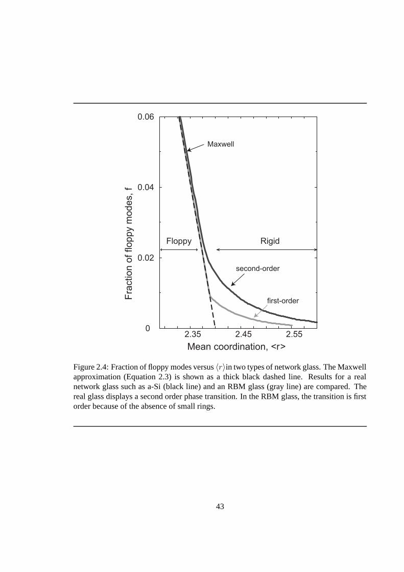
Mean coordination, <r>

Fra

ctio

n o

f flo

pp

y m

odes, f

Floppy Rigid

2.35 2.45 2.550

0.02

0.04

0.06

second-order

first-order

Maxwell

Figure 2.4: Fraction of floppy modes versus 〈r〉in two types of network glass. The Maxwellapproximation (Equation 2.3) is shown as a thick black dashed line. Results for a realnetwork glass such as a-Si (black line) and an RBM glass (gray line) are compared. Thereal glass displays a second order phase transition. In the RBM glass, the transition is firstorder because of the absence of small rings.

43

2.3 The Pebble Game

Due to the nonlocal characteristic of rigidity percolation demonstrated in Figure 2.2,

burning-type algorithms (Stauffer and Aharony, 1998) commonly used in connectivity per-

colation are useless. This implies that the entire structure needs to be stored in memory

since the rigidity of a given region may depend on distant bonds. Such brute-force meth-

ods, as described in Section 1.2.3, have been used (Feng and Sen, 1984; Day et al., 1986;

Hansen and Roux, 1989; Arbabi and Sahimi, 1993) but face size limitations due to matrix

inversion and costly relaxation methods making it difficult to study networks with more

than 104 sites. By contrast, a very efficient integer algorithm (the Pebble Game) (Jacobs

and Hendrickson, 1997) has been implemented on networks with more than 106 sites to

(i) calculate the exact number of floppy modes, (ii) locate all overconstrained regions and

(iii) identify all rigid clusters for 2D generic bar-joint networks (Jacobs and Thorpe, 1995,

1996). The basic structure of the algorithm is to apply Laman’s theorem recursively by

building the network up one bond at a time specifying only the topology. Because of the

recursion, only the subgraphs that contain the newly added bond need to be checked. If

each of these subgraphs satisfy the Laman condition, b ≤ 2n− 3, then the last bond placed

is independent, otherwise it is redundant. By counting the number of redundant bonds, the

exact number of floppy modes is determined. The computational complexity of the Pebble

Game scales in the worst case as O(N 2) for pathological networks, where N is the number

of vertices or atoms in the network, and scales linearly in practice. The algorithm also

scales linearly with N in computer memory.

A pebble game is employed to search over the subgraphs by counting and searching for

44

free pebbles. Each atom in the network has pebbles associated with it that correspond to

free and/or locked degrees of freedom. As bonds are placed between atoms to construct

the desired network, any free pebble associated with the connected atoms is moved onto

the bond, covering it. This process continues, with the requirements that each atom retains

its initial number of pebbles and every covered bond remains covered. Since free pebbles

can be switched with covering pebbles, a directed graph is built and tested one bond at a

time by shuffling pebbles until the desired network has been constructed. Each atom in a

2D network has two associated pebbles so that it is always possible through rearrangement

to free up three pebbles across a bond. Bonds for which the fourth pebble can be found

are independent and thus floppy. The Pebble Game reduces to finding the fourth pebble.

Examples of the Pebble Game execution and more details can be found in Jacobs and

Thorpe (1996) or Thorpe et al. (1999). Thus whenever a fourth free pebble cannot be

found, that bond is redundant and not covered. The set of bonds that were involved in

this failed pebble search are identified as Laman subgraphs because the Laman condition,

b ≤ 2n − 3, is violated. Any bond added to a Laman subgraph will be redundant and

thus form the set of stressed bonds in an overconstrained region. Although the location of

redundant bonds is degenerate and depends upon the order of bond placement, the number

of redundant bonds is unique and each redundant bond belongs to a unique overconstrained

region (Laman subgraph).

Once the network is completely built, all the rigid clusters can be identified by placing

a test-bond between some test-atom and either atom of a reference bond. When test-bonds

are found to be redundant with respect to the reference bond, then the test-atom is rigid

45

with respect to the reference bond. Since bonds can only belong to one rigid cluster (unlike

atoms), all the bonds within a rigid cluster are ascribed to a particular reference bond and

a systematic search is made to map out all rigid clusters. In 2D networks, rigid clusters

consist of bonds (bars) or sets of bonds (bodies). The exact number of floppy modes is

determined by the number of free pebbles remaining when the network is completely built.

These free pebbles will in general be localized by pebble searches, defining locally floppy

or rigid regions unlike the global approximation of Maxwell counting. The resulting lo-

calization of free pebbles gives rise to complex collective floppy motion. Rigid clusters

typically have sub-regions that are overconstrained, such that if a (redundant) bond is re-

moved from the overconstrained region, the rigidity of the network remains the same.

2.3.1 Extensions to 3D Networks

Extending the Pebble Game to 3D networks involves generalizing Laman’s Theorem as

described in Section 2.2.3. Avoiding double banana-type constructions like the ones in

Figure 2.3 is crucial. Three pebbles are associated with each vertex representing the three

degrees of freedom per atom in 3D bond-bending networks. As before, each bond is rep-

resented by a distance constraint, or edge; and a pebble from one of the two connected

vertices must cover each independent edge. The network is built up by adding one dis-

tance constraint at a time, until the final network is complete. To maintain a bond-bending

network, each central-force distance constraint having incident vertices v1 and v2 has asso-

ciated with it angular (i.e. second-nearest-neighbor) constraints about both vertices. These

angular constraints correspond to the bond-coordination angles about an atom as defined

46

by its chemistry.

Unlike the 2D Pebble Game, the distance constraints cannot be placed in random order.

The first distance constraint that is introduced must correspond to a central-force constraint

(one signifying a direct bond between two atoms). After each central-force distance con-

straint is placed, all of its associated angular or bond-bending constraints (next-nearest-

neighbor distance constraints) must be placed before another central-force constraint can

be introduced. Within this restriction, the order of placing either central force or the as-

sociated bond-bending constraints is completely arbitrary, and the resulting rigid cluster

decomposition is unique. This restriction on recursively placing constraints is sufficient

(Jacobs, 1998) for constraint counting to remain valid in characterizing the rigidity of 3D

bond-bending networks within proteins or other structures.

After all distance constraints have been placed, the number of free pebbles remaining on

the vertices gives the total number of degrees of freedom required to describe the motion of

the framework. This includes the six trivial rigid body translational and rotational degrees

of freedom of the whole network. The free pebbles can be rearranged, but are restricted

to certain regions because of the pebble-covering rule. For example, no more than six free

pebbles can be found within a rigid cluster. Based on the location and number of free

pebbles throughout the framework, one can identify overconstrained regions, rigid clusters

and underconstrained regions, as described below.

47

Overconstrained (Stressed) Regions

A redundant constraint is identified when a failed pebble search occurs. A failed pebble

search consists of a set of vertices that have no extra free pebbles to give up. This physi-

cally corresponds to placing an additional distance constraint between a pair of atoms that

have a predefined fixed distance. Placing a distance constraint between this pair of atoms

generally causes a length mismatch and leads this region to become internally strained.

Thus, a failed pebble search identifies overconstrained regions. Overconstrained regions

always consist of closed loops. As distance constraints are added to the framework, more

overconstrained regions will be found, and generally these regions will overlap. Overlap-

ping, overconstrained regions merge together into a single overconstrained region. As these

frameworks are generic, stress will propagate and redistribute throughout the merged over-

constrained regions. Redundant bonds reside within overconstrained regions. Therefore,

the more redundant bonds that are present within a given rigid region, the more stable that

region will be against removal of constraints.

Rigid Cluster Decomposition

The method used to identify the rigid clusters, including overconstrained regions, is very

simple once all edges in the graph are in place and the Pebble Game is finished. All rigid

clusters can at most have six free pebbles distributed over the vertices within the cluster.

Therefore, to identify these clusters, select a vertex and two of its bonded nearest-neighbor

vertices. Collect three pebbles on the selected vertex and two pebbles and one pebble,

respectively, on its two neighboring vertices. Because we are considering bond-bending

48

networks, it is always possible to collect these six pebbles and never any more. Mark these

three vertices. Then, iteratively in a breadth-first search, check all bonded, unmarked near-

est neighbors to the current set of marked vertices, to see if a free pebble can be obtained.

If a free pebble cannot be obtained, then mark the new vertex, and note that it is part of the

same rigid cluster. This method works because all rigid clusters in bond-bending networks

are contiguous through bonded nearest neighbors (Jacobs, 1998); this point is essential and

implicit in the generalization of Laman’s theorem to 3D bond-bending networks.

The rigid cluster decomposition using the 3D Pebble Game has been compared to the

numerical brute-force method described in Section 1.2.3. For a variety of generic bond-

bending networks containing as many as 450 atoms, exact agreement has always been

found (Xiao et al., 1997). It is worth mentioning that in contrast to the numerical method,

the 3D pebble game can be used on networks with over 10 million atoms with the security of

knowing the results are exact, because the Pebble Game is an integer counting algorithm,

eliminating the possibility of any numerical round-off errors. Therefore even the largest

proteins and protein complexes can be analyzed precisely and rapidly.

Underconstrained (Flexible) Regions

Once the rigid cluster decomposition on a network has been made, it is a simple proce-

dure to go through and identify the hinge joints. In 2D these hinges will correspond to

sites while in 3D rotatable bonds between atoms, known as dihedral angles, are the hinges.

Only central-force bonds and not constraints between next nearest-neighbors representing

the bond-angles will form the set of hinge joints (Jacobs, 1998). If the two incident ver-

49

tices of a bond-stretching constraint belong to different rigid clusters, then a dihedral angle

rotation is possible, and the bond is recorded as a hinge joint; otherwise the dihedral angle

motion is locked, as it is part of a rigid cluster. The number of rotatable dihedral angles

will generally be considerably more than the number of residual internal degrees of free-

dom in the network. Not all the rotatable dihedral angles associated with hinge joints are

independent, due to their being part of a ring of bonds.

Collective motions consist of coupled dihedral angles within the network and take place

in underconstrained regions. Distinct underconstrained regions are partitioned such that

collective motions can occur within one underconstrained region without directly affecting

internal coordinates within all the other underconstrained regions. The underconstrained

regions are identified by attempting to specify a value for each dihedral angle and deter-

mining whether it can be satisfied. Specifying a dihedral angle is equivalent to placing an

external torsional constraint to lock in this choice of angle. Independent, externally im-

posed torsional constraints represent independent degrees of freedom available to the sys-

tem, while redundant, externally imposed constraints indicate the angle is predetermined

as part of a collective motion. Therefore, the algorithm for finding these distinct undercon-

strained regions is the same as that for finding the overconstrained regions, except that now

the only constraints placed in the network are the external torsional constraints.

50

2.4 Rigidity in Network Glasses

Comparisons between rigidity on central force and bond-bending networks have produced

a wide range of results and interpretations (Feng and Sen, 1984; He and Thorpe, 1985;

Sahimi and Arbabi, 1993). Early attempts to study the critical behavior in central-force net-

works were not very satisfactory (Feng and Sen, 1984; Feng et al., 1985; Day et al., 1986;

He and Thorpe, 1985; Arbabi and Sahimi, 1993; Hansen and Roux, 1989; Guyon et al.,

1990); but with the application of more accurate techniques (Moukarzel and Duxbury,

1995; Jacobs and Thorpe, 1995, 1996), a consistent picture of rigidity percolation in phys-

ical materials has emerged. Figure 2.4 indicates that some of this confusion may have

resulted because there are differences between types of network glasses along with devia-

tions from the mean field approximation of Maxwell counting.

2.4.1 The Effect of Rings

A main feature of the RBM shown in Figure 2.1 is that there are no loops or rings of

bonds in the thermodynamic limit (Jacobs and Thorpe, 1998a). This places RBMs in an

equivalence class with the Bethe lattice or Cayley tree. Rigidity on a Bethe lattice has been

solved analytically (Moukarzel et al., 1997a; Duxbury et al., 1999) by adding a busbar to the

lattice. Although both display a first order transition, rigidity is nucleated a little differently

in these two networks without loops. In the Bethe lattice rigidity nucleates from the busbar

but there is no busbar in the RBM of Figure 2.1, so rigidity must nucleate using the (few)

large rings that are present in any finite RBM. Thus as the size of the network increases,

51

2.2 2.25 2.3 2.35 2.4 2.45 2.5 2.55 2.6 2.65 2.7

Mean coordination, <r>

-1.0

-0.8

-0.6

-0.4

-0.2

0.0

First

derivative,

df/

d<

r>

2.387 2.389 2.391 2.393<r>

-1.0

-0.8

-0.6

-0.4

-0.2

0.0

df/

d<

r>

Figure 2.5: Plots of the derivative of the fraction of floppy modes, df/d〈r〉, versus againstthe mean coordination, 〈r〉, obtained by random bond dilution. This is a comparison ofthe analytical Bethe lattice solution on a 2-3 bond-bending network (Thorpe et al., 1999)with an equivalent 2-3 RBM. The solid line indicates the analytical solution, solid trianglesrepresent an RBM with 32,768 sites, and open circles an RBM with 8,000 sites. The insetshows the tendency to become more first order with increasing network size as the opendiamonds represent an RBM with 103,823 sites and the solid circles represent an RBMwith 262,144 sites.

the transition becomes more convincingly first order in RBMs. Figure 2.5 plots the first

derivative of the fraction of floppy modes for a 2-3 RBM and Bethe lattice with random

bond dilution. Random bond dilution removes bonds randomly from an initial network

glass with the restriction that no atom is permitted to be less than two-fold coordinated.

Analytical results for rigidity on a 2-3 Bethe are shown to agree precisely with those for

the RBM. A small area around the first order transition is magnified in the insert of Figure

52

2.3 2.35 2.4 2.45 2.5

Mean coordination, <r>

-0.9

-0.8

-0.7

-0.6

-0.5

-0.4

-0.3

-0.2

-0.1

0

First

de

riva

tive

, d

f/d

<r>

RBM (z=4)

Normal DIA

n6,8

=0, DIA

Figure 2.6: First derivative of the fraction of floppy modes, df/d〈r〉, as a function of themean coordination, 〈r〉, for three different network glasses. The open circles are the RBM,the open diamonds are from a bond-diluted diamond lattice (Normal DIA), and the solidtriangles are from the bond-diluted diamond lattice that contains no six and eight fold rings(n6,8 = 0, DIA).

2.5, where it can be seen that the transition sharpens up as the number of sites in the RBM

increases (i.e. approaches the thermodynamic limit).

Figure 2.6 plots the first derivative of the number of floppy modes obtained by random

bond dilution for three different networks. The smooth transition from floppy to rigid

shown by the open diamond symbols in the bond-diluted diamond lattice network glass

signifies a second order phase transition. The open circles, however, show a large jump

indicative of a first order phase transition in the RBM. The main difference between these

glasses is the absence of loops or rings of bonds in the thermodynamic limit (N → ∞) of

53

RBMs.

It is interesting to speculate how to evolve the first order transition on networks without

rings into the second order transition on real lattices with rings. In an attempt to induce

a first order transition in a 3D network, we have removed bonds from an initially four-

fold coordinated bond-bending diamond lattice until we have a network that is everywhere

three-fold coordinated, obeying the condition that all six and eight membered rings are

eliminated. In the absence of these six and eight membered rings, Figure 2.6 shows a first

order transition that is similar to that obtained in a RBM. The RBM was formed from a

network like that shown in Figure 2.1, but starting with all four fold coordinated sites and

then randomly diluting so that only 3 and 2 fold coordinated sites remain. Studies have

also been conducted in 2D networks to drive a first order transition to a second order one

by introducing small rings into RBMs. Results on such networks have indicated that small,

independently rigid rings can act as nucleation sites for rigidity (Babalievsky, 1998; Thorpe

et al., 1999).

In fact, the concentration of these small nucleating rings determines whether the transi-

tion is first or second order (Thorpe et al., 1999). Combinations of rings larger than size 6

and 8 can also become rigidity nucleation sites, suggesting that this concept of nucleating

rings may be a bit too simplistic. Nevertheless, the evidence is fairly strong that the pres-

ence of small nucleating rings determines whether the transition is first or second order.

As the mean coordination is increased, these nucleating rings concentrate rigidity in small

locales, preventing a catastrophic rigidity percolation that is found in ringless networks.

There is some recent evidence for a first order transition found in very accurate Raman

54

scattering measurements of chalcogenide glasses (Boolchand et al., 2001). Although edge

sharing tetrahedra in these chalcogenide glasses do have rings, these rings are irrelevant

rather than nucleating (with respect to rigidity) and favor a first order rigidity transition.

Irrelevant rings do not nucleate rigidity because although they are rigid, they lack the min-

imum number of interactions with the rest of the network for rigidity to percolate through

them. Experiments to validate the order of the phase transition are very difficult and time

consuming since a new sample must be made for each desired mean coordination, and it is

necessary to have very many samples to go through the transition in small steps.

2.4.2 Universality

The question of the order and universality class of the rigidity transition has only recently

been resolved (Duxbury et al., 1999; Thorpe et al., 2000). This question is fundamental

to understanding the nature of the rigidity transition, and may have important implications

as to how the character of the glass transition is affected by the mean coordination, as

has been discussed via fragile and strong glass formers (Bohmer and Angell, 1992). In

general, connectivity percolation is a second order phase transition, but rigidity percolation

can be first or second order (as demonstrated in Figure 2.6). Drawing from connectivity

percolation, the negative of the number of floppy modes was shown to be a free energy

analogue (Duxbury et al., 1999). Theories that generalized connectivity percolation to

rigidity pointed to a first order transition due to the long-range order of rigidity (Obukhov,

1995; Moukarzel et al., 1997a). Numerical simulations on different networks, pointed

to second order transition and first order transitions as described above (see Figure 2.4

55

Table 2.1: 〈r〉c for various 3D network glasses.

Glass order 〈r〉c

a-Si 2nd 2.385bond-diluted diamond lattice 2nd 2.375n6,8 = 0 bond-diluted diamond lattice 1st 2.385RBMBethe lattice

1st 2.3893

for example). However, for all kinds of network glasses, there appears to be a universal

rigidity transition point, 〈r〉c. Table 2.1 shows very little deviation in 〈r〉c from the Maxwell

approximation of 〈r〉c = 2.4 for various 3D network glasses described above.

The phase transition from rigid to floppy in RBMs is continuous, or second order, at

〈r〉c = 2.385. Recent work shows two transitions for RBMs (Thorpe et al., 2000): one first

order and one second order with an intermediate phase (Thorpe and Chubynsky, 2001).

The lower, first-order transition is obtained by testing each bond as the network is built and

allowing only those that would not introduce stress into the network. At a certain point,

no more bonds can be placed without introducing stress. Then bonds are again placed

randomly, and a continuous (second order) transition from isostatically rigid to stressed and

rigid is seen. This suppression of small rings of bonds and/or of locally stressed regions is

a mechanism of self-organization and can cause the transition to become discontinuous or

first order (Thorpe et al., 2000; Chubynsky and Thorpe, 2002c).

56

Chapter 3

Flexibility and Rigidity in Proteins: The FIRST

Software

Parts of the research presented in this chapter have been previously published in

D.J. Jacobs, A.J. Rader, L.A. Kuhn, and M.F. Thorpe. Protein flexibility predictions usinggraph theory. Proteins: Struct., Func., and Gen., 44:150–165, 2001.

M.F. Thorpe M. Lei, A.J. Rader, D.J. Jacobs, and L.A. Kuhn. Protein flexibility and dy-namics using constraint theory. J. Mol. Graph. Model., 19:60–69, 2001.

A.J. Rader, B.M. Hespenheide, L.A. Kuhn, and M.F. Thorpe. Protein unfolding: Rigiditylost. Proc. Natl. Acad. Sci., 99:3540–3545, 2002.

3.1 Introduction

This chapter applies the concepts of rigidity percolation from the previous chapter in the

context of proteins. The extension of the 3D Pebble Game to proteins in the form of the

FIRST software is presented. The empirical and theoretical considerations used during

57

the software development to ensure its validity are discussed. Results are presented for

identifying the flexibility associated with conformational changes in several proteins. The

predicted flexible regions in these proteins are shown to be biologically significant through

comparisons to experimental measures of flexibility.

3.2 Protein Structures and FIRST

Like glasses, proteins are complex, cross-linked polymers held together by covalent and

weaker non-covalent interactions. The bonds within a protein can be represented as a con-

straint network, with appropriate distance constraints to model the covalent bonds, hydro-

gen bonds, and other interactions between atoms. The mechanical stability (rigidity) of

the corresponding constraint network of a protein can then be analyzed using the graph

theoretical techniques described above. We have developed the FIRST software (Floppy

Inclusions and Rigid Substructure Topography) (Jacobs and Thorpe, 1998b; Jacobs et al.,

1999, 2001) as an implementation of the 3D Pebble Game to analyze the intrinsic rigid

and flexible regions of proteins. FIRST gives the exact mechanical properties of a protein

structure under a given set of constraints. This approach defines not only the rigid regions

in a protein, but also those regions that move collectively (whose motions are coupled), as

well as those that move independently of other regions in the structure. Furthermore, the

relative flexibility or rigidity of each region is quantified, based on the density of bonds

remaining rotatable in each flexible region. For 3D bond-bending networks, the flexibility

in the system derives from dihedral or torsional rotations of the bonds that are not locked

in by the network since these are the (potential) hinge-joints in the network.

58

3.2.1 Constraint Model of Proteins

Both bonding and non-bonding forces play an important role in determining the structure

of a protein and the dynamics about the native fold. The covalent bonding within the pro-

tein resulting from bond-stretching (central), bond-bending, and torsional forces defines a

natural set of interactions that are modeled by distance constraints as was done for network

glasses. It is common practice to represent the degrees of freedom accessible to a protein

by fixing the covalent bond lengths and associated bond angles, while allowing the dihe-

dral angles to rotate (Korn and Rose, 1994). Using the rotatable dihedral angles as a set

of internal coordinates, the number of degrees of freedom to describe the flexibility of a

protein is typically reduced by a factor of about seven relative to a Cartesian representa-

tion (Abagyan et al., 1994). The torsional forces associated with peptide bonds and the

other partial-double or double bonds in proteins effectively prevent dihedral rotation about

the bond. To account for this reduction in a degree of freedom, an additional constraint

must be added in proteins to lock the dihedral angle associated with all such peptide bonds.

A third-nearest-neighbor distance constraint is used to lock the peptide bond. Therefore,

along the backbone of a protein the Φ and Ψ dihedral angles are a priori allowed to ro-

tate, but the peptide bonds and other double-bonded groups are kept planar. Both long-

and short-ranged non-bonding forces act to stabilize proteins. Hydrophobic interactions,

van der Waals forces, short-range hydrogen bonding, and long-range electrostatic forces

all play an important role in stabilizing a protein structure in the native, folded state (Dill,

1990). Hydrogen bonds, like covalent bonds, have a high directional dependence but act

over short distances. In contrast, hydrophobic forces are less specific regarding direction

59

and may be regarded as slippery, meaning that the energy associated with the hydrophobic

forces does not change significantly for gentle conformational shifts away from the native

state. Directionally dependent hydrogen bonds would break should the specific donor–

acceptor pair exceed a certain distance during similar conformational shifts.

Continuing as with network glasses, it is useful to make a distinction between strong

and weak forces. Figure 3.1 illustrates the relative strength of various interactions within

proteins. The covalent bonds and bond-bending forces described by Equation 2.5 and the

first two terms of Equation 1.9 are the same, but one must accurately describe the relative

strengths of all microscopic interactions. Only when there is a clear separation between

these forces, can the weak forces be ignored in the calculation. A physically sensible

choice of where to draw the cutoff must be made. After covalent bonds, salt bridges and

then hydrogen bonds form the next strongest interactions within proteins, as shown in Fig-

ure 3.1. Hydrogen bonds vary in strength from nearly as strong as the covalent bonds to

as weak as the van der Waals interactions (Fersht, 1987; Jeffrey, 1997). Hydrogen bonds

form directional cross-links in the bond-bending network that lead to large-scale rigid re-

gions. In proteins, the regular hydrogen-bonding patterns between main-chain amide and

carbonyl groups form the regular secondary structures — α-helices, β-sheets, and reverse

turns. Hydrogen bonds also stabilize the tertiary structure of proteins through side-chain

interactions that interlock parts of the protein chain distant in sequence. As can be seen

by the pointer, the range of energies for hydrogen bonds becomes the great discriminator

between rigid and flexible structures.

60

D

Strong

+ U

Weak

Covalent bond stretching

U = U mol CF

Covalent bond bending

+ UBB + U H

Hydrogen bond range

Dihedral/torsionalrotations

weak electrostatic,van der Waals,

other+ USB+ U

Salt bridges

and non-bondedforces

Microscopic Interactions

Figure 3.1: The ranking of microscopic forces in proteins with an adjustable energy pointer.The microscopic forces in proteins are schematically ordered from strongest to weakest.The energy pointer at the top is adjustable to include or exclude a certain set of forces.Distance constraints are used in FIRST to model strong bonding forces to the left of asliding pointer. This approach defines a network of covalent and hydrogen bonds and saltbridges in the protein.

61

N

OH

C

Figure 3.2: The constraint model of the hydrogen bond. For each Hydrogen bond three con-straints, one central-force (between the ‘H’ and ‘O’ atoms) and two bond-bending (shownby dashed lines) are added in FIRST.

3.2.2 Hydrogen Bonds

The hydrogen bond shown in Figure 3.2 is modeled in a way similar to a covalent bond.

Each hydrogen bond introduces three distance constraints, corresponding to one central

force between the hydrogen and acceptor atoms and two bond-bending forces associated

with the hydrogen and acceptor atoms. Since hydrogen bonds are almost never precisely

linear, it is reasonable to use this model for hydrogen bonds and describe the protein struc-

ture as a typical (generic) bond-bending network. The three remaining dihedral angle de-

grees of freedom associated with this representation of the hydrogen bond allow it to have

some flexibility. Modeling the hydrogen bond to be more or less constrained than this has

been tested, but the model in Figure 3.2 proves a good balance between neither over- nor

under-representing the flexibility of a hydrogen bond. This model results in ideal α-helices

being rigid, β-sheets ranging from rigid to somewhat flexible depending on size and the

regularity of their hydrogen-bonding patterns. Moreover, protein structures typically show

a substantial proportion of rigid regions, while having regions that remain flexible. Deter-

62

Table 3.1: Hydrogen bond donors and acceptors in proteins. Donor and acceptor types,along with their orbital hybridization are assigned in FIRST according to this table(adapted from Stickle et al. (1992)). The atoms and their orbitals are listed in the firstcolumn. The subsequent columns list all cases found in proteins for that atom and orbitaltype.

donorsN sp2 >NH -NH2 -NH+

2 >NH+

peptide, Trp, His Asn, Gln Arg ArgN sp3 -NH+

3

LysO sp3 -OH

Ser, ThrO sp2 -OH

Tyracceptors

N sp2 �NHHis

O sp3 -OHSer, Thr

O sp2 =O -COO− -OHpeptide, Asn, Gln Asp, Glu Tyr

S sp3 -S- -SHMet Cys

mination of constrained and rotatable dihedrals by FIRST has been tested against exact

counting and shown to agree for all the elementary structures: α-helices, parallel and an-

tiparallel β-sheets, and reverse turns.

FIRST defines the electron orbital hybridization and donor or acceptor status for each

nitrogen, oxygen and sulfur atom in the protein structure as shown in Table 3.1 (Stickle

et al., 1992). Additionally, main-chain nitrogens of the N-terminal residue of each chain

and protonated side-chain nitrogens of arginine, lysine and histidine residues are considered

charged donors. Likewise, main-chain oxygens of the C-terminal residue of each chain and

63

d

r

N

θ

O

C

φ

H

Figure 3.3: The geometry used in the hydrogen bond energy potential. Here, θ is the donor– hydrogen – acceptor angle, φ is the hydrogen – acceptor – base angle, where the baseis the atom (C, in this case) covalently bonded to the acceptor, d is the donor – acceptordistance, r is the hydrogen – acceptor distance, and γ (not shown) is the angle between thenormals of the planes defined by the donor and base atoms’ covalent bonds (e.g., the planesdefined by the two sp2 centers, N and C, in this case).

side-chain carboxyl oxygens of aspartate and glutamate residues are considered charged

donors. This permits us to define a salt bridge as a special case of hydrogen bonds whenever

two such oppositely charged atoms satisfy the salt bridge geometric criteria.

To analyze a protein, it must first be decided which hydrogen bonds to include and

model as distance constraints. A superset of possible hydrogen bonds is identified based

on the geometric parameters shown in Figure 3.3: r (hydrogen – acceptor distance), d

(donor – acceptor distance), and θ (donor – hydrogen – acceptor angle). Salt-bridge (ion-

pair) interactions are considered a special case of hydrogen bonds with a more significant

Coulombic component, which is less geometrically sensitive. For the two distances listed

(d and r), different screening options apply based upon whether or not the hydrogen bond

involves any sulfur atoms or charged atoms (salt bridges). The maximum values for the

64

three cases: standard hydrogen bonds, sulfur hydrogen bonds and salt bridges are listed

below.

standard case: d ≤ 3.6A r ≤ 2.6A

sulfur case: d ≤ 4.0A r ≤ 3.0A

salt bridge case: d ≤ 4.6A r ≤ 3.6A

For all types of potential hydrogen bonds, θ must be greater than or equal to 80◦. These

prescreening values are slightly larger than values observed in protein datasets (Stickle

et al., 1992; McDonald and Thornton, 1994) so that all possible hydrogen bonds might be

identified. Our identification of salt bridges follows previous studies (Barlow and Thornton,

1983; Gandini et al., 1996; Xu et al., 1997) by extending the maximum donor–acceptor

distance (d) to 4.6 A.

Once all possible pairs of hydrogen bonding atoms have been identified with the above

geometrical criteria, we use the modified Mayo energy function (Mayo et al., 1990; Rader

et al., 2002) in Equation 3.1 and a non-angular dependent salt bridge energy function in

Equation 3.2 to rank these interactions.

EHB = V0

{5

(R0

d

)12

− 6

(R0

d

)10}

F (θ, φ, γ) (3.1)

and

ESB = Vs

{5

(Rs

d + a

)12

− 6

(Rs

d + a

)10}

(3.2)

65

where

sp3 donor – sp3 acceptor F = g(θ) cos2 (φ− 109.5◦)

sp3 donor – sp2 acceptor F = g(θ) cos2 φ

sp2 donor – sp3 acceptor F = [g(θ)]2

sp2 donor – sp2 acceptor F = g(θ) cos2 (max [φ, γ])

V0 = 8 kcal/mol R0 = 2.80A

Vs = 10 kcal/mol Rs = 3.2A and a = 0.375A.

The hydrogen bond energy (EHB) is a function of the equilibrium hydrogen bond distance,

d0, and well depth, V0. The angular dependence of the function, F (θ, φ, γ) in Equation 3.1,

is dependent upon the hybridization of the donor and acceptor atoms listed in Table 3.1.

As shown in Figure 3.3, θ is the donor – hydrogen – acceptor angle while φ is the angle

between the hydrogen atom, the acceptor, and the atom bonded to the acceptor (labeled as

base). If more than one atom is bonded to the acceptor, that atom which results in a larger

binding energy is selected. The γ angle (not shown) is between the normals of the two

planes defined by the sp2 centers. If the γ angle is less than 90◦, the supplement is used.

After examining in detail the hydrogen bonds being identified and energies that were

assigned to them by the original Mayo potential (where g(θ) = cos2 θ) (1990), it became

clear that this energy function was not adequate for the needs of FIRST. The most trouble-

some results were seen in α-helices where i + 3 → i main chain to main chain hydrogen

bonds were being identified with small but non-neglegible energies throughout the helix.

Also i → i and i → i ± 1 main chain to main chain hydrogen bonds had to be screened

out prior to the energy criteria. For consistency, a single tunable parameter to screen out

66

all unfavorable and non-physical hydrogen bonding interactions was desirable. All of the

identified non-physical hydrogen bonds had θ values less than 120◦ and many were near

90◦. To eliminate these non-physical hydrogen bonds, a new function with a more re-

strictive angular dependence was introduced. This function replaced g(θ) = cos2 θ by

g(θ) = cos2 θe−(π−θ)6 . The exponential multiplier in this angular term smoothly interpo-

lates between a maximum at θ = 180◦ and minimum near θ = 110◦ so that non-physical

hydrogen bonds are eliminated while physical ones remain.

Salt bridges can be viewed as strong hydrogen bonds (Jeffrey, 1997) with average ener-

gies of -6 (±4) kcal/mol (Kumar and Nussinov, 1999). Salt bridges have broader distance

and angular distributions than are found for non-ionic hydrogen bonds, and these observed

distributions are not well reflected by the angular dependent hydrogen-bond energy func-

tions in Equation 3.1. Salt bridges within the above specified geometric ranges generally

have stronger interactions than hydrogen bonds at neutral pH. Therefore the angular depen-

dence was removed and a deeper, broader well was introduced in Equation 3.2 to model

the range of salt bridge energies. Salt bridges are included as a special case of hydrogen

bonds in FIRST.

3.2.3 Hydrophobic Contacts

Owing to the fact that native state proteins result from a balance of entropic and enthalpic

gains, the question of how one folds or unfolds seems to depend largely on hydrophobic

collapse (Dill, 1990). As described in Chapter 1, hydrophobic collapse drives proteins in

the unfolded state to bury hydrophobic residues and reach a more compact state. This col-

67

lapse is followed quickly by hydrogen bond formation. As such these hydrophobic interac-

tions are important in stabilizing (rigidifying) the protein. A single hydrophobic interaction

however would be classified as weak according to Figure 3.1. An accurate model of such

interactions must take into account both the non-specific and weak features of hydrophobic

contacts. We model this tendency for hydrophobic atoms, principally carbon and sulfur

atoms within proteins, to remain relatively near one another, rather than unfolding to in-

teract with the solvent. These hydrophobic tethers restrict the local motion, which can be

thought of as slippery. Hydrogen bonding groups, on the other hand, have angular as well

as distance preferences, and thus are more specific and constraining.

Hydrophobic contacts are identified and modeled by introducing three pseudoatoms

with both bond-length and bond-angle constraints in FIRST as shown in Figure 3.4. This

model restricts the maximum distance between the two hydrophobic groups, while allowing

them to slide with respect to one another. Such a tether is also less specific than a hydrogen

bond, which removes three degrees of bond-rotational freedom from the system, whereas

each hydrophobic contact removes only two.

3.3 From PDB Structure to FIRST Results

Beginning with the native structure of a protein from the Protein Data Bank (PDB) (Berman

et al., 2000), a constraint model of all its covalent bonds (with appropriate bond orders,

lengths, and coordination angles) and its defined non-covalent hydrophobic, salt-bridge,

and hydrogen-bond interactions is created. How FIRST accommodates additional atom

68

Hydrophobic

Contacts

Hydrophobic Tether

with 3 pseudoatoms

A.

C.

B.

rb

ra

R

d

Figure 3.4: Model of hydrophobic contacts in proteins. A. Pairs of carbon and/or sul-fur atoms are considered to make hydrophobic contacts if their van der Waals surfaces,represented by sphere radii ra and rb (without correction for attached hydrogen atoms)are within R=0.25A. B. This allows atoms to either be in contact or lightly separated butwithout enough space between for water to intervene (requiring a separation of ∼1.4A). C.Because FIRST represents the protein as interatomic constraints, multi-jointed tethers withpseudoatoms at the joints are used to flexibly join atoms to form hydrophobic interactions.The flexible tethers allow two atoms forming a hydrophobic interaction to slip relative toone another, while remaining in the same vicinity.

69

types and considerations are described below.

3.3.1 Metal Ions, Buried Waters, and Ligands

Metal ions should form bonds to protein atoms that differ from the standard covalent bonds

used to generate the constraint model of FIRST. Ionic bonds have a tendency to adopt

a variety of coordinations and resulting geometries. This means that the bond angles be-

tween next-nearest neighbors are not strictly fixed. However, for the 3D Pebble Game to

work, these next-nearest neighbor constraints must be present in a bond-bending network.

Recently a method involving pseudoatoms to remove the angular constraints about metal

centers has been proposed (Whiteley, 2002) but not yet tested. Metals often adopt pre-

ferred coordination geometries in proteins depending on their ionization states (da Silva

and Williams, 1991; Creighton, 1993) indicating that modeling these bonds within the

bond-bending framework should be a fair approximation. From database studies of dis-

tances between heavy atoms and metal ions in proteins (Karlin et al., 1997; Karlin and

Zhu, 1997) we set the maximum distance criteria for identifying such metal-protein bonds.

The default distances are less than 2.90 A for nitrogen and oxygen and less than 3.00 A for

sulfur. These values properly select the majority of metal-protein bonds. FIRST allows

the user to add or remove any bond in case such defaults are too lax or too restrictive.

Water molecules are included if they are entirely buried according to the program

PRO ACT (Williams et al., 1994), and then can contribute to the protein hydrogen-bonding

network. Although there is a wide variation in the number of buried waters per residue for

individual proteins, there is on average 1 buried water molecule per 27 residues (Williams

70

et al., 1994). For a set of 18 monomers the number of buried waters ranged from 0 and

14 (Rader et al., 2002). Ligand atoms are also included as if they were part of the protein.

Distances between atom types have a range of acceptable values so that covalent bonds can

be assigned generally for unknown ligand types. Polar and hydrophobic atoms within lig-

ands are subject to the same rules as protein atoms for determining non-covalent (hydrogen

bonding and hydrophobic) interactions. Once the bonds between the protein and ligands,

including metals and other ions, have been identified, they are treated as any other covalent

bonds with associated bond-bending and central force constraints added in FIRST.

3.3.2 Hydrogen Bonding

For protein structures in which the hydrogen atom positions are not experimentally defined

(the case for most structures determined by X-ray diffraction), the WhatIf software pack-

age is used to assign polar hydrogen atoms positioned such that their hydrogen-bonding

opportunities are optimized (Hooft et al., 1996). Because FIRST results will depend on

how accurately these polar hydrogen atoms are placed, we have compared WhatIf-defined

hydrogen positions to the experimentally determined positions in five neutron diffraction

structures from the PDB (Berman et al., 2000). The set of five neutron structures from

the PDB are lysozyme (PDB code 1lzn), trypsin (1ntp), insulin (3ins), myoglobin (2mb5),

and ribonuclease A (5rsa). For each structure, we processed the file through FIRST using

two different hydrogen-bond energy threshold or cutoff values, as discussed below. We

then created a modified version of the neutron structure by stripping the hydrogen atoms

from it and adding new hydrogens with WhatIf. This new structure was then processed

71

Table 3.2: The effect of hydrogen atom placement on the number of hydrogen bonds iden-tified. The experimentally defined hydrogen positions and resulting hydrogen bonds of fiveneutron structures are compared with the hydrogen bonds resulting from assignment of hy-drogen positions by WhatIf in the same five structures. The rows labeled unique to neutroninclude the number of hydrogen bonds from experimentally determined hydrogen posi-tions, and the rows labeled unique to modified include the number of hydrogen bonds fromWhatIf calculated hydrogen atom positions in neutron diffraction structures from which theexperimentally determined hydrogen atom positions had been removed.

H-bond Energy PDB code: 1lzn 1ntp 2mb5 3ins 5rsa Total

# of residues 129 223 153 102 124 —# of protein atoms 1762 1790 1836 1305 1556 —resolution (A) 1.70 1.80 1.80 1.50 2.00 —

# H-bonds with # common to both 184 216 249 108 140 897E ≤ −0.1 # unique to neutron 3 9 13 3 4

# unique to modified 11 17 6 6 476

kcal/molpercent in common 96.3 94.3 96.3 96.0 97.2 95.9

# H-bonds with common to both 130 168 182 80 116 676E ≤ −0.6 unique to original 7 16 22 3 3

unique to modified 6 9 8 6 484

kcal/molpercent in common 95.2 93.1 92.4 94.7 97.1 94.2

through FIRST for comparison with the results obtained using neutron diffraction-defined

hydrogen atom positions.

Table 3.2 contains results for these five neutron structures at two different energy cutoff

values: −0.1 kcal/mol and −0.6 kcal/mol (the latter corresponding to thermal fluctuations

at room temperature). The comparative results show only slight differences due to a few

hydrogens placed differently in the two structures. The percentages shown are calculated

by dividing twice the number of hydrogen bonds in common by the total number of hydro-

gen bonds for both versions of the protein structure. While the energy threshold of −0.6

kcal/mol is more restrictive and includes only the strongest hydrogen bonds, there was

72

slightly less overall agreement (94%) between the hydrogen bonds at this energy threshold

in the WhatIf and neutron versions of the structure than was found at the chosen threshold

of −0.1 kcal/mol (96%). Thus, on average, only 4% of the hydrogen bonds were assigned

differently in the two types of structures. Not surprisingly, many of the hydrogen-bond

differences resulted from different placement of hydrogens on histidine residues. Histidine

has two side chain nitrogen atoms that can bond to 0, 1 or 2 hydrogens, depending on

the local environment. Overall, we conclude that the WhatIf software package positions

hydrogen atoms sufficiently accurately to permit analysis of the resulting hydrogen-bond

network.

For hydrogen bonds, we can tune the energy threshold (the sliding pointer in Figure 3.1)

used to define which hydrogen bonds are included in the network. Setting the threshold

at less negative (less favorable) energy values includes weaker hydrogen bonds, which

tend to be common in proteins and have a significant influence on structural stabilization.

The ability to select hydrogen bonds based on strength allows investigation of how the

stability in each region of the protein varies as the hydrogen-bond network is strengthened

or weakened. By changing the criteria for modeling a hydrogen bond as a constraint, a

protein can be substructured from containing a few, large rigid clusters down to being

completely floppy, with many small rigid clusters involving single atoms with their covalent

bonds acting as rotatable dihedral angle hinges. Individual hydrogen bonds or small sets

of hydrogen bonds that form critical cross-links can therefore be identified by shifting the

energy threshold and observing which hydrogen bonds, when included or omitted, have a

large effect on the rigidity of the network.

73

Ideally we would like to be able to set this energy cutoff value, perform a single FIRST

analysis, and know that the output describes the physically relevant flexibility of a protein.

One way of setting the energy threshold objectively is to choose it such that maximum

agreement in the hydrogen-bond network is obtained for pairs of independently-determined

structures for a protein (e.g., by different researchers or in different crystallographic pack-

ings) in which the main-chain conformations are the same. This ensures that the results of

FIRST analysis are not sensitive to the sorts of fluctuations known to occur within protein

structures. Since the energy cutoff is the tunable parameter in using FIRST, we tested

which setting gave the most similar results between pairs of such structures. Such a cutoff

value should naturally be below when all hydrogen bonds are present (Ecut ≤ 0.0 kcal/mol)

and above when the protein substructures into many tiny rigid clusters (Esplinter). A very

natural place to look at the behavior of these proteins is near room temperature which cor-

responds to Ert = −0.6 kcal/mol. However, because the energy function is approximate

(does not take into account the effect of more distant neighboring atoms on hydrogen-bond

strength), it is important to not take these energies too literally, and to consider them as

relative rather than absolute.

To determine a reasonable default energy threshold for hydrogen bonds, we evaluated

which threshold best conserves the hydrogen bonds within a family of protein structures.

Multiple structures within four different protein families were studied to find such a thresh-

old. The PDB codes used for each family are as follows: trypsin (1tpo, 2ptn, 3ptn), trypsin

inhibitor (4pti, 5pti, 6pti, 9pti), adenylate kinase (1zin, 1zio, 1zip), and HIV protease (1dif,

1hhp, 1htg). Figure 3.5 shows the hydrogen-bond energy distribution for one of these fam-

74

-10 -8 -6 -4 -2 0

Energy (kcal/mol)

0

20

40

60

80

100

120

140

160

180

200

Num

ber

of H

ydro

gen

Bon

ds

-0.2 -0.1 0.0 0.10

25

50

75

100

Figure 3.5: Histogram of energies for hydrogen bonds. Distribution of hydrogen bondenergy for three structures of HIVP (PDB codes 1dif, 1hhp, 1htg). Hydrogen positionswere established by WhatIf. The insert expands the low-energy (weak hydrogen bond)region between −0.2 and 0 kcal/mol. An energy threshold of −0.1 kcal/mol is used toeliminate the large number of very weak hydrogen bonds in the spike near 0 kcal/mol.

ilies, namely the three HIV protease (HIVP) structures. A large spike in the distribution of

possible bonds located between −0.1 kcal/mol and 0.0 kcal/mol for the number of hydro-

gen bonds in the three structures appears in Figure 3.5. This spike is largely due to the fact

that quite generous definitions of hydrogen bonds are allowed initially (donor–hydrogen–

acceptor angle, θ ≥ 80◦ and donor–acceptor distance, d ≤ 3.6 A, as shown in Figure

3.3). The inset of Figure 3.5 expands the region near 0.0 kcal/mol, demonstrating how a

large number of very weak hydrogen bonds, often with θ angles near 90◦, can be removed

by setting Ecut ≤ −0.1 kcal/mol. Thus, the generous hydrogen bond distance and angle

screening criteria can be effectively filtered by setting Ecut. When these geometric criteria

and an energy threshold of −0.1 kcal/mol are applied to analyze the hydrogen bonds and

75

salt bridges in five neutron diffraction structures, a Gaussian distribution is observed for

the number of hydrogen bonds as a function of donor–acceptor distance, with virtually all

hydrogen bonds and salt bridges having distances between 2.6 and 3.6 A. The distribution

in donor–hydrogen–acceptor angles is bimodal, with a strong, Gaussian peak between 130◦

and 180◦ and a weaker peak between 90◦ and 130◦.

The above analysis was completed in the absence of the hydrophobic tethers described

in Section 3.2.3. Such hydrophobic tethers are necessary to correctly model protein folding

interactions that will be described in Chapter 4. With the inclusion of hydrophobic tethers,

it became necessary to adjust the value of Ecut to find the native state of the protein. The

native-like flexibility of most proteins now occurs for values of Ecut between -1.0 and -2.5

kcal/mol.

In the choice of protein structures to analyze, the stereochemical quality of the structure

can have a significant influence on the definition of its network of hydrogen bonds, due

to their angular dependence. The result is that FIRST analysis on a structure with poor

stereochemistry is likely to indicate the protein as being more flexible than it actually is,

due to the missing hydrogen bonds. It is advisable to assess the main-chain stereochemistry

through a Φ/Ψ plot, as well as focus on high-resolution, well-refined structures for FIRST

analysis, to avoid this possibility of missing hydrogen bonds due to the misorientation of

main-chain hydrogen-bonding groups.

76

3.4 Flexibility Index

A flexible region consisting of many interconnected rigid clusters within a protein may

define a collective motion having only a few independent degrees of freedom. Although

underconstrained, this region could be nearly rigid and thus mechanically stable. An iso-

statically rigid region, which contains no redundant constraints and is just rigid, is not

expected to be as stable as an overconstrained region. Overconstrained regions have more

constraints than necessary to be rigid, and therefore are considered more stable. Due to this

continuum between rigidity and flexibility, a continuous index is useful.

The total number of floppy modes in a protein, denoted by F , corresponds to the num-

ber of independent, internal degrees of freedom. To obtain F , the six trivial rigid body de-

grees of freedom are subtracted from the total number of independent degrees of freedom.

The global count of the number of floppy modes gives a good sense of overall intrinsic

flexibility. However, a more useful measure is to track how the degrees of freedom are

spatially distributed throughout the protein. In particular, we are interested in locating the

underconstrained or flexible regions.

The quantity, fi, is defined as a flexibility index that characterizes the degree of flexi-

bility of the i-th central-force bond in the protein. Let Hk and Fk respectively denote the

number of hinge joints (rotatable bonds) and the number of floppy modes within the k-th

underconstrained region. Let Cj and Rj respectively denote the number of central-force

bonds and the number of redundant constraints within the j-th overconstrained region. The

flexibility index provides a quantitative range from most to least constrained and is given

77

by:

fi ≡

Fk

Hk

in an underconstrained region

0 in an isostatically rigid region

−Rj

Cjin an overconstrained region.

(3.3)

When the i-th central-force bond is a hinge joint, the flexibility index is defined to be

given by number of floppy modes divided by the total number of hinges within the under-

constrained region. When the i-th central-force bond is not a hinge joint, it is part of a rigid

cluster. If the central-force bond is within an overconstrained region, the flexibility index

is assigned a negative value with magnitude given by the number of redundant constraints

divided by the total number of central-force bonds within the region. This number becomes

more negative as the region becomes more overconstrained. Since the number of indepen-

dent dihedral rotations must be less than or equal to the number of hinge joints in a flexible

region and the number of redundant constraints must be less than or equal to the number of

bonds in a rigid region, |fi| ≤ 1.

As a simple example, consider a single n-fold ring of atoms that are connected by

covalent bonds. From constraint counting, the number of degrees of freedom minus the

number of constraints is given by F = n− 6. The number of hinge joints is simply given

by n. Therefore, the flexibility index for a n-fold ring is given by:

fi =n− 6

nfor each central-force bond in a n-fold ring. (3.4)

78

Notice that as the ring becomes large, the flexibility index goes to the limit of +1; in this

case, each dihedral angle is nearly independent, and the ring is almost as flexible as a

linear chain. For a six-fold ring, the flexibility index is zero, indicating an isostatically

rigid structure. The flexibility index of a protein can be plotted as a function of residue

number, and regions within the plot (corresponding to segments within the sequence) can

be colored according to whether they are coupled in motion (see Figure 3.7). Alternatively

the flexibility index can be mapped onto the 3D structure according to a spectrum as in

Figure 3.6B&D. A nice property of the flexibility index is that it varies gradually when

hydrogen bond constraints are added or removed.

3.5 Ligand Induced Conformational Changes

An important feature of FIRST is that it can predict the intrinsic flexibility of a protein

given a single 3D structure. Most proteins are not rigid in nature, and enzymes especially

adopt various conformations during their catalytic cycle (Bennett and Huber, 1984; Miller

and Benkovic, 1998b). A database of macromolecular motions housing morph movies that

interpolate between different crystallized conformations of the same protein resides at Yale

(Gerstein and Krebs, 1998). Many of these motions are the result of ligand binding. Since

the hydrogen-bond pattern will typically change upon ligand binding, the predicted confor-

mational flexibility from FIRST will depend on whether the structure being analyzed is an

open (ligand-free) form, or a closed (ligand-bound) form. Crystal contacts can also influ-

ence the flexibility of a protein, and their influence can be assessed in two ways by FIRST:

by analyzing the flexibility of the protein independent of its crystal lattice neighbors (in

79

which case the effects of intermolecular hydrogen bonds are removed from analysis), and

by comparing the flexible regions found for the same protein crystallized in different lattice

packings. The general features of flexible and rigid regions found by FIRST are remark-

ably consistent among different 3D structures (in the same ligand-binding state) for a pro-

tein, as will be shown for human immunodeficiency virus protease (HIVP), dihydrofolate

reductase (DHFR), and adenylate kinase (ADK).

3.5.1 HIV Protease

An initial application is to HIVP, a major inhibitory drug target for current anti-AIDS ther-

apy. Two ligand-free X-ray crystal structures available for HIV protease, PDB entries 1hhp

and 3phv, are superficially very similar in structure and have similar resolution and crys-

tallographic residual error (2.7 A resolution for both, and an R-factor of 0.190 for 1hhp

and 0.191 for 3phv). However, PROCHECK (Laskowski et al., 1993) indicated that 3phv

had significantly fewer residues with stereochemically favored Φ, Ψ values, which results

in distorted main-chain hydrogen-bond geometries; therefore we chose 1hhp to represent

the open HIVP conformation. The open form of the protein (PDB code 1hhp) is dominated

by a single rigid cluster shown as blue in Figure 3.6A, including the base and walls of

the substrate and inhibitor binding site (cavity at center) and three flexible regions shown

as alternating-colored bonds (each color indicating a rigid microcluster within the flexi-

ble region). The ends of the flaps (β labeled region in Figure 3.6A, residues 45–56) are

known from crystallographic and NMR structures to be important for closing over and

binding inhibitors (Nicholson et al., 1995), and appear as the most flexible (red) regions

80

Figure 3.6: Rigid cluster decomposition and flexibility index plot of HIVP. A. Rigid clus-ter decomposition of the open conformation of HIVP (PDB code 1hhp). Singly coloredregions signify rigid cluster such as the large blue regions while multicolored regions cor-respond to flexible regions in these rigid cluster decomposition plots. B. Flexibility index,color-mapped onto the same HIVP structure. In this representation, red regions indicatehigher relative flexibility while blue regions indicate the most rigid regions as determinedby Equation 3.3. Four regions of interest, α, β, γ, and δ, are identified for one of the dimersand discussed in the text. C. Rigid cluster decomposition of the closed conformation ofHIVP (PDB code 1htg) D. Flexibility index, color-mapped onto the same HIVP structure.Contrast the change in rigidity between the four labeled regions between the ligand-bound(closed) and ligand-free (open) case.

81

α

δ

γ

β

α

δ

γ

β

α

δ

γ

β

α

δ

γ

β

flaps flexible

flaps rigid

Flexible

Rigid

A. B.

C. D.

Figure 3.6

82

0 20 40 60 80 100

Residue Number

0

20

40

60

80

100

∆Φ,∆Ψ

(De

g.)

0 20 40 60 80 1000

0.5

1

1.5

2

Mo

bili

ty

0 20 40 60 80 100-0.4

-0.2

0

0.2

0.4

Fle

xib

ility

αγδA.

B.

C.

β

Figure 3.7: Four regions of interest, α, β, γ, and δ, are identified for one of the dimers.A. Flexibility index plotted versus residue number for open HIVP (PDB code 1hhp). Ofthe four regions, α, β and γ are most flexible (colored red in Figure 3.6B) while δ is rigid(colored in blue) in this open conformation of HIVP. Parts of the sequence that are cou-pled in motion are plotted in the same color, then the same regions in panels B and C arecolored accordingly. B. Mobility plotted versus residue for this conformation. Mobility isdetermined as the average crystallographic temperature factor (B-value, or Debye-Wallerfactor) divided by the average atomic occupancy, averaged over the main-chain atoms ineach residue. C. Dihedral angle changes between the main chains of the above open confor-mation and the closed conformation (Figure 3.6C&D, PDB code 1htg). The three flexibleregions identified by FIRST are also those with the greatest experimentally defined mobil-ity values and dihedral angle changes.

83

when the structure is characterized by the flexibility index in Figure 3.6B & 3.7A. Other

flexible regions include the base of each flap (region α, residues 39–42), which may act as

a cantilever, and the γ region.

The flexibility index for HIVP is compared with experimental measures of protein flex-

ibility in Figure 3.7. The major peaks in main-chain thermal mobility (B-value), measured

crystallographically and shown in Figure 3.7B, correlate directly with the α, β, and γ flexi-

ble regions predicted by FIRST. The region labeled δ is the dimer interface, formed by the

N- and C-termini of the two, identical protein chains. It should be noted that for proteins

with mobile domains or other moving rigid bodies, such as α-helices, the crystallographic

mobility and FIRST results will not necessarily compare well with B-values. Crystallo-

graphically, they appear as mobile regions, whereas in FIRST they appear as rigid regions

flanked by flexible loops (allowing the motion). This confusion can be avoided when NMR

relaxation rates are available for comparison, since they also indicate moving rigid bodies

as rigid regions flanked by flexible loops. The Indiana Dynamical Database (IDD) (Good-

man et al., 2000) contains such data for a number of proteins, including HIVP. This data is

provided for PDB entry 1bvg, a ligand-bound form; as in the FIRST results for a different

ligand-bound structure described below, the base of the flaps are the most flexible region.

HIVP has also been crystallized with various inhibitors bound, resulting in a closed

conformation with the flaps lowered. The main-chain dihedral angle (Φ, Ψ) changes (sim-

ilar to the analysis of Korn and Rose 1994) observed for crystal structures of the open

(entry 1hhp) and closed (entry 1htp) conformations are shown in Figure 3.7C. The FIRST-

predicted flexible regions also directly correspond with the regions of greatest dihedral

84

angle change. In the three flexible regions (α, β, and γ), the flexibility is associated with

a flip in at least one dihedral angle (defined as a change of more than 60 degrees) within

a rigid β-turn in the center of each flexible region (Figure 3.6A & 3.7C). The results here

are consistent with the motion observed by interpolation between different HIVP crystal

structures (Gerstein and Krebs, 1998) and an earlier dihedral analysis for a different pair

of HIVP structures (Korn and Rose, 1994) indicating that large changes at residues 40, 50,

and 51 in the α and β regions result in a large, concerted movement of the flaps. Flexibility

of the γ region has not been emphasized in other studies of HIVP; however, it is known that

drug-resistant mutants of the protease include two residues that pack against the γ region:

63 and 71, with residue 63 proposed to induce a conformational perturbation (Chen et al.,

1995; Patrick et al., 1995). Thus, conformational coupling between the γ region and the

flaps, through the γ–α loop interactions, may explain why mutations in the γ region, which

are distal from the active site, cause resistance to drug binding.

Ligand binding restricts the motion of the flaps through new hydrogen bonds linking

the two flaps to each other and to the ligand. Some of these hydrogen bonds between

the flaps and ligand are mediated by a conserved water molecule found in retroviral but

not mammalian homologs of HIVP (Wlodawer and Erickson, 1993), providing a useful

basis for designing more HIV-specific drugs. To compare the influence of ligands on HIVP

flexibility, there were a number of ligand-bound structures of good stereochemistry from

which to choose. I present the results from PDB entry 1htg, with GR137615 bound to

represent the closed form of HIV protease. (We have also analyzed two other ligand-

bound structures, 1hiv and 1dif, and found these ligands’ influence on protein flexibility

85

to be substantially similar.) Unlike the open form, the closed structures were resolved

crystallographically as dimers, and thus independent structural information is available for

the two subunits of the dimer. This means it is possible to assess the influence of different

side-chain conformations in the two halves (due to thermal fluctuations and environmental

differences) in terms of their effects on the hydrogen-bonding network and flexibility. The

top and bottom sides of each HIVP in Figure 3.6 indicate that the only substantial difference

in their flexibility is caused by the asymmetry of the ligand bound (at center).

Comparison of this ligand-bound structure with the open HIVP also demonstrates how

a ligand can rigidify part of the protein through new hydrogen bonds even though the ligand

itself is not rigid (note black bonds indicating hydrogen bonds between the protease flaps in

Figure 3.6C, and that the flaps are now rigidified), while making other parts of the protein

more flexible. Particularly note the dimer interface, where inter-subunit rotation occurs

upon ligand binding, breaking some of the interfacial stabilizing hydrogen bonds, and the

loop to the right of the binding cavity, shown as a flexible (orange) region of the main-

chain ribbon in Figure 3.6D. This loop flexibility is not reflected in the other HIVP subunit,

due to ligand asymmetry. Flexibility of the dimer interface in a ligand-bound structure is

also a prominent feature found by NMR (Ishima et al., 1999) and MD analyses (Scott and

Schiffer, 2000); MD also identifies flap flexibility in the ligand-free conformation.

The influence of water is easily seen in a comparison of the ligand-bound cases. A

specific water molecule (WAT301) positioned between the β flaps and the ligand is con-

served in the majority of HIVP ligand-bound structures (Wlodawer and Erickson, 1993).

In this rigid region analysis, we found the inclusion of this water essential to rigidify the

86

β flaps. This particular water molecule serves as a hydrogen acceptor from residue 50 of

each protein chain and a hydrogen donor to the ligands. Adding this single water molecule

introduces four hydrogen bonds to the structure, with energies ranging from -1.5 to -7.5

kcal/mol. For both 1htg and 1dif, the β flaps become flexible without the intermolecu-

lar hydrogen bonds created by this water molecule. We have only included buried water

molecules making intermolecular hydrogen bonds in HIVP, as these tend to be reliably as-

signed between structures, whereas surface water molecules are unevenly assigned in many

of the crystal structures of HIVP, as well as being variable in crystallographic temperature

factor.

3.5.2 DHFR

By trapping different ligand-bound states crystallographically, Sawaya and Kraut (1997)

noted six conformational states for E. coli dihydrofolate reductase (DHFR) during its cat-

alytic cycle. FIRST analysis for three of these crystallographic structures (PDB codes

1ra1, 1rx1, and 1rx6) is presented here. These three structures, corresponding to the open,

closed, and occluded conformations of DHFR, are as shown in Figure 3.8. The Cα traces

are colored according to each residue’s flexibility index, fi, with the most flexible regions

colored red and the most rigid colored blue.

According to the previous study (Sawaya and Kraut, 1997), the regions of most interest

are the rotations of two major subdomains: the adenoside binding subdomain (residues

38–106) and the loop subdomain (residues 1–37,107–159). The M20 and βF–βG loops

of the loop subdomain are denoted in Figure 3.8 and Figure 3.9. Studies by Miller and

87

M20 loop

M20 loop

M20 loop

βF-βG loop

βF-βG loop

βF-βG loop

C.

A.

B.

Flexible

Rigid

Figure 3.8: Flexibility index map of dihydrofolate reductase for A. the open conformation(PDB code 1ra1), B. the closed conformation (PDB code 1rx1), and C. the occluded con-formation (PDB code 1rx6). The ligands bound in these reaction pathway intermediates areshown in green. Two loops experimentally determined to be flexible, M20 and βF–βG arealso noted. The motion of the M20 loop is essential to accommodate a variety of ligandsduring catalysis. The flexible βF–βG loop participates in ligand-induced conformationalchanges. At the top of the graph is the scale for the flexibility index used to map color ontothe Cα trace. The scale runs from red (flexible) through gray (isostatic) to blue (rigid).

88

0 20 40 60 80 100 120 140 160 -0.6

-0.3

0

0.3

0.6

open

0 20 40 60 80 100 120 140 160 -0.6

-0.3

0

0.3

0.6

clo

se

d

0 20 40 60 80 100 120 140 160 -0.6

-0.3

0

0.3

0.6

occlu

de

d

subdomain I subdomain Isubdomain II

M20 loopM20 loop βF-F-βG loopG loop

residue

Figure 3.9: Flexibility index plot for the three conformations of DHFR shown in Figure3.8. Each panel of this figure shows the value of the flexibility index as defined in (Equation3.3), plotted versus residue number (similar to the plot shown for HIVP in Figure 3.7A).The two experimentally determined loops, M20 and βF–βG are shown at the top of theplot, and correspond to highly flexible regions. Each collective motion within the structurehas a unique color plotted.

89

Benkovic (Miller and Benkovic, 1998b,a) concluded that the flexibility of these loops is

interrelated such that the flexibility of the outer βF–βG loop guides the conformation of

the M20 loop. It is this correlated flexibility that gives DHFR ligand specificity. We would

expect the regions that move the most and are important for binding to appear flexible

in the FIRST analysis, at least in the open conformation. Figure 3.8A shows that the

M20 loop is detected by FIRST to be fully flexible, but in the closed form (panel B),

this loop has moved and become partially locked into place. Comparing the flexibility

indices for all three conformations in Figure 3.9, the residues within these two mobile

loops tend to be most flexible, and this flexibility is fairly independent of conformation

being analyzed. This points to a functional requirement for these loops to remain flexible

during the catalytic cycle. The flexible region around residue 88 in all three conformations

of Figure 3.9 corresponds to a hinge between the two subdomains. Similarly, the flexible

region found by FIRST around residue 70 (orange in the flexibility index plot, Figure 3.9)

is within the adenoside binding subdomain and has also been identified as flexible by NMR

techniques (Epstein et al., 1995; Osborne et al., 2001). Plots of crystallographic mobility

and regions of greatest main-chain dihedral angle change (data not shown) for the three

DHFR structures in Figure 3.8 are remarkably consistent between the structures and also

agree with FIRST results that the most flexible regions are in the M20 loop and the βF–βG

loop. We have analyzed several other DHFR structures by FIRST (PDB codes 1rx2, 3, 4,

and 5) and found substantial agreement with the above conclusions. In general, changes in

ligands as seen between these structures can influence the flexibility of their neighborhood

in the protein, but the major features of flexibility remain consistent.

90

3.5.3 Adenylate Kinase

Another protein whose motion has been studied experimentally is adenylate kinase (Ger-

stein et al., 1993; Schlauderer et al., 1996; Zhang et al., 1997). Previous work indicates that

adenylate kinase uses hinges rather than shear motions for conformational change. This in-

trinsic, large scale hinge motion upon ligand binding is easily identifiable in both the open

and closed conformations analyzed by FIRST, as indicated in Figure 3.10 by gold arrows.

Several helices at the extreme right of Figure 3.10 move in like fingers via hinges that are

the defined as the most flexible (red) portions of the protein by FIRST.

Adenylate kinase binds two ligands, ATP and AMP, in a two-step mechanism. Unfor-

tunately, structures of adenylate kinase from the same species are not available for all three

steps (ligand-free, followed by two binding/conformational change events). By compar-

ing enzymes from different species, four hinges were previously defined to contribute to

the conformational change between open and ligand-bound forms (Gerstein et al., 1993).

These hinges move in a concerted way to account for the large conformational change clos-

ing the lid domain (residues 131–165) over the ligand. In Figure 3.10, panels A and B show

structures with ligands bound to this domain and not this initial ligand-binding step (Ger-

stein et al., 1993). However, the peak in main-chain dihedral change shown around residue

167 in Figure 3.10C corresponds to a conformational switch the red flexible loop (part of

the lid) in Figure 3.10A makes between structures. Crystallographic mobility analysis for

the open structure (Figure 3.10A) and the closed structure (Figure 3.10B) are generally in

good agreement with FIRST results, the only difference being that regions between residue

135 and 160 appear crystallographically mobile in the closed structure.

91

Figure 3.10: Flexibility plot of adenylate kinase in A. the open conformation (PDB code1dvr) and B. the closed conformation (PDB code 1aky). C. Difference in main-chain di-hedral angles between these two conformations, indicating the locations of large, localizedconformational changes. The ligands bound to these structures are shown in green tubes.The open state, A, has only adenosine triphosphate (ATP) bound. In the closed state, B, theligand, P1,P5-bis(adenosine-5′-)pentaphosphate (AP5A) mimics the roles of AMP and ATPbinding concurrently. Dark blue corresponds to highly overconstrained and rigid, with aflexibility index and bright red corresponds to highly flexible. All three panels have labeledregions that are discussed in the text.

92

B.

large hinge motion

A.

Flexible

Rigid

residue number0 20 40 60 80 100 120 140 160 180 200 220

0

50

100

150

∆Φ,∆

Ψ

C.

lid

lid

a

a

b

c

d

e

f

b

c

d

e

f

b c d e fa lid

Figure 3.10

93

Closing of the lid domain is associated with the binding of ATP (green tubes at center

in panel A). Binding of the ligand AP5A (green tubes, Figure 3.10B) produces the fully

closed conformation of adenylate kinase and locks many of the domain linking hinges (a–

f), as seen by the transition between flexible (red) and rigid (blue) regions in Figure 3.10

panels A and B. The NMPbind site is where the part of AP5A that is non-overlapping with

ATP binds, and this site is formed by the interface between the two domains as they clamp

down on the inhibitor (Zhang et al., 1997).

Comparing these structures, FIRST shows that the flexibility of the NMPbind domain

(especially hinges a, e, and f) decreases upon AP5A binding to this domain. The flexible

linkage (b) between helices α3 and α4 around residue 62 (identified in the Figure 3.10C plot

of change in Φ/Ψ angles between the open and closed structures in panels A and B) seems

to account for a large part of the motion transforming the open to the closed conformation.

This region (b in Figure 3.10A and B) is found to decrease in size but remains flexible in

the closed conformation. The persistent flexibility in the closed conformation hints at the

reversibility of the motion required for catalytic turnover. Even in the ATP-bound closed

lid conformation exhibited by both of these structures, certain key hinges (Gerstein et al.,

1993; Schlauderer et al., 1996) remain flexible. For example, hinges c and d between

helices α4 and α5, remain flexible in both states. Thus, FIRST results correlate well

with the crystallographically observed conformational changes upon ligand binding for the

complex motions within adenylate kinase.

94

Chapter 4

Applications: Protein Folding and Unfolding

Parts of the research presented in this chapter have been previously published in

A.J. Rader, B.M. Hespenheide, L.A. Kuhn, and M.F. Thorpe. Protein unfolding: Rigiditylost. Proc. Natl. Acad. Sci., 99:3540–3545, 2002.

B.M. Hespenheide, A.J. Rader, M.F. Thorpe and L.A. Kuhn. Identifying protein foldingcores from the evolution of flexible regions during unfolding. J. Mol. Graph. Model.,21:195–207, 2002.

4.1 Introduction

4.1.1 Protein Unfolding

This chapter builds on the previous by exploring the applications of the FIRST software

to the problem of protein folding. As discussed in Chapter 1, how proteins go from a

1D amino acid sequence to a 3D structure remains one of the largest unsolved problems

in structural biology. The folding funnel of Figure 1.3 helps to conceptualize how this

95

might take place; however, what the crucial reaction coordinate, Q, to describe folding

may be has not yet been determined. A general view of protein folding is that it begins

with hydrophobic collapse, where the random coil changes into a compact state with the

hydrophobic groups on the interior and polar groups on the surface interacting with the

surrounding water. The packing is not yet optimal, with hydrophobic groups somewhat

free to slide about in the interior of the globule, until residues are locked in place by the

formation of specific hydrogen bonds. These hydrogen bonds can be regarded as a sort

of velcro that locks the various structural elements in the folded protein together, while

the hydrophobic interactions form a slippery glue. Once these interactions are optimized,

the native state is predominantly rigid with flexible hinges or loops at the surface — the

number and distribution of these depends on the particular protein.

We have concentrated on a simpler problem — that of analyzing the unfolding tran-

sition by diluting contacts from the native structure. For proteins in which the unfolding

process is reversible, this approach also decodes the folding pathway. We postulate that in-

formation about the folding pathway is contained within the density, strength, and specific

location of the hydrogen bonds that act as velcro in the native state. To simulate denatura-

tion, the hydrogen bonds and salt bridges within the structure are ranked according to their

relative energies and broken one by one, from weakest to strongest, similar to the way these

bonds would break in response to slowly increasing temperature. An increase in structural

flexibility in the protein is observed as the hydrogen-bond and salt-bridge network is dis-

rupted. These results are found to be robust against the introduction of some noise, or

stochastic character, into the order in which the hydrogen bonds are broken. Since the ef-

96

fective hydrophobic interactions actually strengthen somewhat with moderate increases in

temperature (Tanford, 1980), they are maintained rather than broken in this simulation.

The unfolding of a protein can be described as a transition from a predominantly rigid,

folded structure to an ensemble of denatured states. We test the hypothesis that information

about the folding pathway is encoded in the energetic hierarchy of non-covalent interactions

in the native-state structure. Thermal denaturation of protein structures is simulated by di-

luting the network of salt bridges and hydrogen bonds, breaking them one by one, from

weakest to strongest. The structurally stable and flexible regions are identified at each step,

providing information about the evolution of flexible regions during denaturation. Using

the FIRST software to measure protein flexibility and rigidity, we present two significant

points along the unfolding pathway: the folding core and the transition state. The folding

core, or center of structure formation during folding, is predicted in terms of mutually rigid

secondary structures and compared to results from hydrogen-deuterium exchange exper-

iments. The transition state is defined in the context of the rigidity reaction coordinate,

mean coordination (〈r〉), and shown to be universally 2.4 for a wide range of proteins.

4.1.2 HD exchange and the Folding Core

Woodward has proposed that amide protons that exchange only after long periods of expo-

sure to deuterated water define the slow-exchange core of a protein (Woodward, 1993). Li

and Woodward compiled the results from a number of studies on native-state HD exchange

for different proteins, identifying the residues forming the slow-exchange core in each pro-

tein (1999). They have proposed that the secondary structures to which these residues

97

belong define the folding core for the protein. Additionally, they have shown for barnase

and chymotrypsin inhibitor 2 (CI2) that the folding core identified by HD exchange consists

of residues with high Φ-values (Oliveberg and Fersht, 1996), indicating that slow-exchange

core residues have significant structure in the folding transition state.

For HD exchange to occur in main-chain amides involved in hydrogen bonds, flexibility

in the protein structure is required to allow access to deuterated water. Given that residues in

the folding core have small exchange rates, it is reasonable to assume that the folding core

protons either are not accessible to solvent or are in regions that are sufficiently rigid that

the hydrogen bond donor and acceptor cannot move apart enough to allow HD exchange.

This can be probed by observing how the flexibility of a protein structure changes as it is

gradually denatured.

Our hypothesis is that the folding core is stabilized by a network of particularly dense or

strong non-covalent interactions, which tend to resist unfolding or denaturation. Following

this hypothesis, we present a novel computational method for predicting the folding core

of a protein. This approach employs the FIRST software, which accurately predicts flex-

ible regions in proteins by analyzing the constraints on flexibility formed by the covalent

and non-covalent bond network as described in Chapter 3. Covalent bonds, salt bridges,

hydrogen bonds, and hydrophobic interactions are included in the protein representation.

Because thermal denaturation or unfolding involves the breaking of hydrogen bonds and

salt bridges, we compare several methods for simulating thermal denaturation, and observe

how the removal of these bonds affects the stability and flexibility of the protein. As hydro-

gen bonds are removed, the protein structure becomes increasingly flexible, and the stable

98

Table 4.1: Dataset of 10 proteins used to identify folding cores. The PDB code and num-ber of residues (Nres) are listed for each protein. The fourth column provides the CATH(Orengo et al., 1997) structure classification. The point in the hydrogen bond dilution whenthe folding core is found, 〈r〉FC , is listed in the fifth column.

Protein PDB Size Stuct. Number of ResolutionName Code (Nres) Class

〈r〉FC S-S Bonds (A)BPTI 1bpi 58 few 2.38 3 1.10Ubiquitin 1ubi 76 αβ 2.40 0 1.80CI2 2ci2 83 αβ 2.41 0 2.00Ribonuclease T1 1bu4 104 αβ 2.39 2 1.90Cytochrome c 1hrc 104 α 2.39 0 1.90Barnase 1a2p 110 αβ 2.39 0 1.50α-Lactalbumin 1hml 123 α 2.38 0 1.70Apo-myoglobin 1a6m 151 α 2.37 0 1.00Interleukin-1β 1i1b 153 β 2.39 0 2.00T4 Lysozyme 3lzm 164 α 2.38 0 1.70

regions decrease in size. The folding core can then be predicted as the most stable region

involving at least two secondary structures. The thermal denaturation model in which hy-

drogen bonds and salt bridges are removed from weakest to strongest predicts folding cores

that correlate best with the experimentally observed folding cores. The ability to predict an

early state in folding indicates that information about the folding pathway is encoded in the

covalent and non-covalent bond network of the native state.

99

4.2 Selection of Proteins for Analysis

Folding Core Dataset

Crystallographic structures for the 10 monomeric proteins listed in Table 4.1 were selected

from the PDB (Berman et al., 2000) for analysis. These proteins were chosen based on

their diversity of structure and the availability of native state HD exchange data for compar-

ison (Li and Woodward, 1999). Since a 3D structure was not available for apo-myoglobin

(which lacks heme), we analyzed holo-myoglobin (with heme) after removing the heme

group. Experimental data has shown that the fold of both forms are qualitatively very

similar except for dynamic fluctuations of the F helix (Fontana et al., 1997). For this ap-

proximated apo-myoglobin structure, FIRST analysis also found the F helix to be one of

the two most flexible helices in the protein (data not shown). The experimental results of

HD exchange used for comparison in this study are for apo-myoglobin. The proteins were

preprocessed as described in Chapter 3

Augmented Protein Dataset

We augmented the set of 10 proteins used to calculate protein folding cores shown in Table

4.1 to create a set with a representative range of CATH architectures (α, β, mixed α and

β, few) (Orengo et al., 1997), oligomeric states (monomers, dimers, and tetramers), folding

mechanisms (two-state and multi-state folders), and sizes (58 to 1332 residues). Table

4.2 lists the 26 proteins used in this study. The PDB code and name of each protein are

given, grouped by the oligomeric state for the biologically active form in which they are

100

Table 4.2: Set of 26 structurally diverse protein analyzed using FIRST. The PDB code,protein name, and CATH (Orengo et al., 1997) structural class are listed in the first threecolumns. Nres is the number of residues in the protein; NH2O is the number of buried watermolecules in the protein. 〈r〉T is the mean coordination of the protein in the transition stateof the protein, identified as the inflection point in the plot of f ′ versus 〈r〉. 〈r〉FC is themean coordination of the protein when the folding core has been identified.

PDB ProteinCode Name

Class Nres NH2O 〈r〉T 〈r〉FC

monomers1a2p barnase αβ 108 5 2.41 2.391a3k galectin β 137 5 2.40 –1a6m myoglobin α 151 7 2.40 2.371ake adenylate kinase αβ 214 14 2.40 –1bpi BPTI few 58 4 2.39 2.381bu4 ribonuclease T1 αβ 104 0 2.40 2.391hml α-Lactalbumin α 123 4 2.40 2.381hrc cytochrome c α 105 4 2.42 2.381nkr killer cell β 201 5 2.39 –

inhibitor receptor1ruv ribonuclease A αβ 124 3 2.41 2.401rx1 DHFR αβ 159 0 2.41 –1ten tenascin β 90 0 2.40 –1ubi ubiquitin αβ 76 1 2.39 2.402chf CheY αβ 128 7 2.39 –2ci2 chymotrypsin inhibitor 2 αβ 83 0 2.40 2.412liv LIV-binding protein αβ 344 7 2.40 –3lzm T4 lysozyme α 164 7 2.41 2.384i1b interleukin 1-β β 153 9 2.40 2.39

dimers1bif PFKinase/FBPase αβ 864 242 2.40 –1cku electron transfer protein few 170 4 2.40 –1hhp HIV-1 protease β 198 0 2.39 –1vls aspartate receptor β 292 32 2.39 –

tetramers1ice interleukin 1-β αβ 514 19 2.41 –

converting enzyme1ids Fe-SOD αβ 792 43 2.40 –1szj GAPDH αβ 1332 105 2.40 –2cts citrate synthase α 874 60 2.40 –

101

analyzed in this paper (monomeric, dimeric or tetrameric). For each protein, the structure

classification as defined by CATH (Orengo et al., 1997) is listed along with the total number

of residues for that structure (Nres). The fifth column, NH2O, lists the number of buried

water molecules, as determined by PRO ACT (Williams et al., 1994), that are included as

part of the protein in the FIRST calculations. The last two columns, 〈r〉T and 〈r〉FC , are the

values of mean coordination obtained for the transition state and folding core, respectively.

4.3 Visualizing Results

As described in Chapter 3, we take all the covalent bonds, the set of hydrophobic tethers,

and the set of hydrogen bonds and salt bridges to define the constraint network for the

protein from the given initial protein structure. With these constraints, FIRST identifies

all the rigid and flexible regions within a protein. The results of FIRST indicate for each

bond in the protein whether it is flexible (free to rotate) or rigid (not rotatable) due to the

covalent and non-covalent constraints within the structure. Groups of atoms coupled to

each other via rigid bonds form a rigid cluster. One or more independent rigid clusters with

intervening flexible regions may occur in a protein structure.

A slightly reduced view of the rigid cluster decompositions as presented for HIVP in

Figure 3.6A&C, is presented at the top of Figure 4.1 (for clarity, the side chains are not

shown). This 3D rigid cluster decomposition emphasizes the rigid bonds by thick, col-

ored tubes while depicting the flexible bonds by thin black lines. Each independently rigid

cluster is distinguished by a different color. With the goal of changing the underlying

102

N

N C

C

Figure 4.1: Rigid cluster decomposition plots for CI2 (PDB code 2ci2) when 67% of theweakest hydrogen bonds have been removed. This slightly simplified image, compared tothose in Figure 3.6, emphasizes the rigid clusters. There are four independent rigid clus-ters computed by FIRST. The rigid clusters are depicted by thick colored tubes (blue, red,orange and yellow, from largest to smallest). Each thin black tube represents a rotatableor flexible bond. The thin, dark gray lines show the location of hydrogen bonds and hy-drophobic tethers. Since the main chain for a protein monomer is an unbranched linearpolymer, the rigid cluster results for the main chain can be mapped onto a 1D line. Fromthe N-terminus to the C-terminus, each backbone bond is represented as a thin black line ifit is flexible or a thick colored block if it is rigid. Independently rigid clusters are assigneddifferent colors.

constraint network by removing hydrogen bonds (to simulate thermal denaturation), this

representation is too complicated. It would be nearly impossible to gather useful infor-

mation by looking at many different 3D rigid cluster decomposition plots corresponding

to slightly different sets of hydrogen bonds. Figure 4.7 presents plots from three well-

separated points along the unfolding pathway, but it would be very difficult to select these

three out of a series containing one plot for each removed hydrogen bond. Instead, we re-

103

duce the 3D rigid cluster decomposition into a 1D line representation. Thus the main-chain

rigidity is mapped onto the 1D sequence stretching from the N-terminal to the C-terminal

shown at the bottom of Figure 4.1. We compare these reduced, 1D representations (corre-

sponding to a given 3D rigid cluster decomposition) by placing lines next to one another.

As in the 3D figure (Figure 4.1), each main-chain bond is represented as a thin black line if

it is flexible (rotatable), or as a colored tube if it is rigid. This is the case even when these

regions are discontinuous in sequence because the rigidity depends upon the underlying 3D

structure.

The complete denaturation can now be viewed as a series of horizontal lines in Figure

4.2, ordered from native state (top) to a substantially flexible, or denatured state (bottom).

Each line shows the current regions of structural stability and flexibility for the backbone

atoms after a step in the denaturation process. Frequently, several successive lines would

be identical because the flexibility of the backbone has not been affected by changes in the

non-covalent bond network. These redundant lines are omitted, and only those steps that

result in a change in backbone flexibility are displayed. Figure 4.2 provides an example of

a complete hydrogen bond dilution (i.e., simulated thermal denaturation) for barnase. The

three columns on the left-hand side describe: the number of remaining hydrogen bonds in

the protein at each step; the energy according to the modified Mayo potential of Equation

3.1 of the just-broken bond (in kcal/mol); and the mean coordination, 〈r〉, of the atoms in

the network at that step, counted as the number of covalent bonds, hydrogen bonds, salt

bridges, and hydrophobic interactions per atom, averaged over all atoms in the protein as

in Equation 2.2. The mean coordination decreases along the unfolding pathway and is a

104

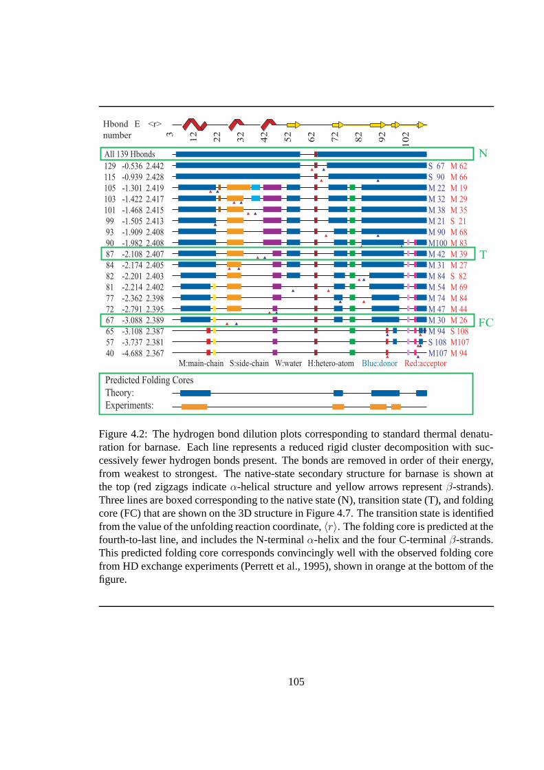
3

12

22

32

42

52

62

72

82

92

102

All 139 Hbonds

129 -0.536 2.442

115 -0.939 2.428

105 -1.301 2.419

103 -1.422 2.417

101 -1.468 2.415

99 -1.505 2.413

93 -1.909 2.408

90 -1.982 2.408

87 -2.108 2.407

84 -2.174 2.405

82 -2.201 2.403

81 -2.214 2.402

77 -2.362 2.398

72 -2.791 2.395

67 -3.088 2.389

65 -3.108 2.387

57 -3.737 2.381

40 -4.688 2.367

S 67 M 62

S 90 M 66

M 22 M 19

M 32 M 29

M 38 M 35

M 21 S 21

M 90 M 68

M100 M 83

M 42 M 39

M 31 M 27

M 84 S 82

M 54 M 69

M 74 M 84

M 47 M 44

M 30 M 26

M 94 S 108

S 108 M107

M107 M 94 Blue:donor Red:acceptorM:main-chain S:side-chain W:water H:hetero-atom

Hbond

number

E <r>

N

T

FC

Predicted Folding Cores

Theory:

Experiments:

Figure 4.2: The hydrogen bond dilution plots corresponding to standard thermal denatu-ration for barnase. Each line represents a reduced rigid cluster decomposition with suc-cessively fewer hydrogen bonds present. The bonds are removed in order of their energy,from weakest to strongest. The native-state secondary structure for barnase is shown atthe top (red zigzags indicate α-helical structure and yellow arrows represent β-strands).Three lines are boxed corresponding to the native state (N), transition state (T), and foldingcore (FC) that are shown on the 3D structure in Figure 4.7. The transition state is identifiedfrom the value of the unfolding reaction coordinate, 〈r〉. The folding core is predicted at thefourth-to-last line, and includes the N-terminal α-helix and the four C-terminal β-strands.This predicted folding core corresponds convincingly well with the observed folding corefrom HD exchange experiments (Perrett et al., 1995), shown in orange at the bottom of thefigure.

105

structure-based variable, that will be regarded as a folding/unfolding reaction coordinate.

Regular secondary structure content is shown at the top, as determined by DSSP (Kab-

sch and Sander, 1983). The right-hand columns, together with the solid triangles beneath

each line, show the residue locations of the donor (blue) and acceptor (red) atoms of the

hydrogen bond or salt bridge broken to generate this step. For instance, “S 67” indicates

the side chain of residue 67 and “M 62” indicates the main chain of residue 62. Likewise,

“W 120” would indicate water molecule 120 in the PDB structure and “H” would indicate

other heteroatoms, belonging to non-protein functional groups such as bound heme.

4.4 Simulated Thermal Denaturation

As a protein is gradually denatured, the covalent bonds remain intact, while hydrogen bonds

begin to break. It is reasonable to expect that most buried hydrogen bonds will be substan-

tially maintained as the protein undergoes conformational changes near its native structure.

It has been suggested that the breaking of a hydrogen bond occurs as a well defined event

(Lu and Schulten, 1999), involving going over an energy barrier, as opposed to a contin-

uous stretching until a feeble final breaking occurs. Thus hydrogen bonds typically break

one by one as the protein unfolds, although in some cases a consortium of hydrogen bonds

break simultaneously, giving a much higher effective barrier. The flexibility in the protein

will increase as the number of hydrogen bonds in the protein decreases. Our hypothesis

is that the folding core is the region that will remain structurally stable the longest under

denaturing conditions. This hypothesis was tested by incrementally removing hydrogen

bonds from a protein structure to simulate thermal denaturation, then using FIRST to ob-

106

serve the evolution of flexible regions in the structure. The results depend upon the order

in which hydrogen bonds are removed. Because hydrophobic interactions actually become

somewhat stronger with moderate temperature increases (Tanford, 1980), these interactions

are maintained throughout the simulation. Three methods for diluting the hydrogen bond

network of a protein are presented, each designed to test the importance of the strength

and/or density of the hydrogen bonds when selecting which bond to remove next.

4.4.1 Identifying the Folding Core

Generally, in the native state, most of the residues belonging to an α-helix or β-strand are

rigid, and the secondary structures are mutually rigid, or approximately rigid. As the hy-

drogen bonds are removed from the protein, parts of the secondary structures may become

flexible, particularly the ends of helices and strands. Also, the secondary structures tend to

become independently rigid at intermediate steps in denaturation, due to loss of inter- and

intra secondary structure bonds.

The protein folding core is defined in this study as the set of secondary structures that

remain mutually rigid the longest in the simulated denaturation. The secondary structures

for the native states of each of the ten proteins were identified using the Dictionary of

Secondary Structures of Protein (DSSP) (Kabsch and Sander, 1983) and tracked during

the unfolding simulation. Not all residues in the secondary structure are required to be

rigid when identifying the folding core. An α-helix is considered to be rigid if at least five

consecutive residues, corresponding to one complete turn of an α-helix, belong to the rigid

cluster. If a helix is defined by DSSP to contain less than five residues, as can occur with 310

107

helices, all its residues must be mutually rigid to be considered a rigid secondary structure.

The β-strands are required to have at least three consecutive residues rigid to be considered

as part of the folding core. This criterion of three consecutive rigid residues allows for at

least two hydrogen bonds to an adjacent strand. If a strand is defined by DSSP as consisting

of less than three residues, the entire strand is required to be rigid to be counted as part of

the folding core.

4.4.2 Unfolding Pathways and Folding Cores from Thermal Denatu-

ration

As the temperature of a protein is gradually increased, the hydrogen bonds are expected

to break in an energy-dependent manner. We mimic this process by using the following

procedure. Initially, the flexibility of the native protein structure is analyzed with all its co-

valent and non-covalent interactions (hydrogen bonds and hydrophobic interactions). The

weakest hydrogen bond in the structure is then broken by removing any constraints created

by that bond. The effect of removing this bond is then observed by applying FIRST to

identify the flexible regions in the protein. We continue this process of breaking the weak-

est hydrogen bond remaining in the structure and updating the identification of flexible

regions until all the hydrogen bonds have been removed.

The detailed unfolding pathway and folding core predictions upon thermal denaturation

are shown for barnase in Figure 4.2. There was a significant change in the flexibility of the

protein observed after 35 hydrogen bonds had been removed (line 4), resulting in several

small rigid regions that could move independently of one another (as indicated by their

108

different colors in the plot), and one large rigid region (shown in blue). An intermediate

structural state (T) in barnase is formed by the packing of an α-helix against the β-sheet

as can be seen by the boxed line “T” in Figure 4.2 and the middle panel of Figure 4.7.

The β-sheet in this super-secondary structure partially denatures to form the folding core

itself, consisting of the α-helix packed against part of the β-sheet (fourth line from bottom

in Figure 4.2 indicated by “FC” and lower panel in Figure 4.7). The HD exchange folding

core, shown at bottom (orange), matches the predicted folding core (blue) well, with the

exception of the short, C-terminal β-sheet.

The hydrogen bond dilution results for BPTI are shown in Figure 4.3. BPTI is a member

of the DSSP secondary structure class few due to its small size and few secondary struc-

tures. Its disulfide bonds were included as part of the covalent bond network. The steps in

the unfolding pathway represented in Figure 4.3 show a gradual breakup of the structure

into small rigid regions linked by flexible hinges. The N-terminal helix becomes flexi-

ble when hydrogen bond 29 is broken, followed by the C-terminal helix when hydrogen

bond 15 is broken. The remaining two secondary structures (β-strands between residues

15 and 35) remain mutually rigid, along with residues 45 and 51, to form the predicted

folding core of BPTI. Again, the predicted and experimentally determined folding cores

correspond closely.

For cytochrome c, the native state is composed of a single, structurally stable region

represented by the top line in Figure 4.5A. When hydrogen bonds 113 through 65 (the

weakest 49) were removed, the large rigid cluster (colored red) significantly decreased in

size (at the fifth line in panel A), resulting in new flexibility in those residues between the

109

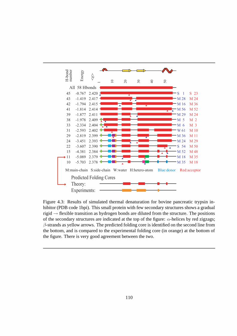
1 10

20

30

40

50

All 58 Hbonds

45 -0.767 2.420 S 1 S 23

43 -1.419 2.417 M 28 M 24

42 -1.794 2.415 M 16 M 36

41 -1.814 2.414 M 56 M 52

39 -1.877 2.411 M 29 M 24

38 -1.978 2.409 M 5 M 2

33 -2.334 2.404 M 6 M 3

31 -2.593 2.402 W 61 M 10

29 -2.819 2.399 M 36 M 11

24 -3.451 2.393 M 24 M 29

22 -3.607 2.390 S 54 M 50

15 -4.381 2.384 M 52 M 48

11 -5.089 2.379 M 18 M 35

10 -5.703 2.378 M 35 M 18

Blue:donor Red:acceptorM:main-chain S:side-chain W:water H:hetero-atom

H-b

on

dn

um

ber

En

erg

y

<r>

Predicted Folding Cores

Theory:

Experiments:

Figure 4.3: Results of simulated thermal denaturation for bovine pancreatic trypsin in-hibitor (PDB code 1bpi). This small protein with few secondary structures shows a gradualrigid→ flexible transition as hydrogen bonds are diluted from the structure. The positionsof the secondary structures are indicated at the top of the figure: α-helices by red zigzags;β-strands as yellow arrows. The predicted folding core is identified on the second line fromthe bottom, and is compared to the experimental folding core (in orange) at the bottom ofthe figure. There is very good agreement between the two.

110

N- and C-terminal helices. These helices formed the only significantly rigid region in the

protein. The folding core was predicted as the last point in the denaturation when at least

two secondary structures formed a single rigid region. This point in cytochrome c occurred

in the fifth-to-last line, where the N- and C-terminal helices remained mutually rigid. On

the next line, no single rigid cluster contained more than one secondary structure. The

predicted folding core is summarized by a 1D representation just below the denaturation

results, along with the folding core determined by HD exchange (Li and Woodward, 1999;

Jeng et al., 1990) in Figure 4.5A. The predicted and observed folding cores correspond

well, both indicating that the N- and C-terminal helices together form a stable folding core.

The study of folding transition states to follow indicates that the rigid core of proteins

disintegrates into several independent rigid regions when the mean atomic coordination,

〈r〉, decreases below ≈2.41. This is seen to be the case for both barnase and cytochrome c

in Figure 4.2 and Figure 4.5A.

Thermal denaturation simulations were performed to predict the folding core for each

of the 10 proteins in Table 4.1. Figure 4.4 summarizes the folding core predictions from

these simulations, comparing the predicted folding core (green lines labeled P) to that ob-

served experimentally (orange lines labeled E). For a majority of the proteins (8 out of

10), the folding core predictions agree well with folding cores predicted by regions of slow

HD exchange, and often involve tertiary interactions between sequence-distant secondary

structures. For α-lactalbumin, half of the folding core region is in agreement, and for T4

lysozyme, the folding core identified by experiment is much larger than that identified by

flexibility analysis. Given that different experimental conditions can also produce different

111

BarnaseP.

E.

Cytochrome cP.

E.

Bovine Pancreatic Trypsin InhibitorP.

E.

Ribonuclease T1P.

E.

Chymotrypsin Inhibitor 2P.

E.

Interleukin-1βP.

E.

T4 lysozymeP.

E.

UbiquitinP.

E.

α-LactalbuminP.

E.

Apo-myoglobinP.

E.

Figure 4.4: Comparison of the folding core predicted by FIRST flexibility analysis (P) tothe observed folding core of HD exchange experiments (E) for barnase (Perrett et al., 1995),cytochrome c (Jeng et al., 1990), ubiquitin (Pan and Briggs, 1992), BPTI (Woodward andHilton, 1980), ribonuclease T1 (Mullins et al., 1997), CI2 (Neira et al., 1997), interleukin-1β (Driscoll et al., 1990), T4 lysozyme (Anderson et al., 1993), α-lactalbumin (Schulmanet al., 1995) and apo-myoglobin (Hughson et al., 1990)

112

results, we are consulting a broader range of experimental probes of T4 lysozyme folding,

as well as doing further structural analysis.

Given the diverse structures and folding mechanisms for these ten proteins, the good

agreement between theory and experiment indicates that flexibility analysis is a useful tool

for probing the stability of substructures, in particular the folding core, along the unfolding

pathway. This approach provides explicit 3D structural maps of the stable regions predicted

in the protein at each step during denaturation, as well as providing a model for the interac-

tions important in stabilizing folding cores: a dense network of hydrogen-bond interactions

that augment the ubiquitous, but less specific, hydrophobic interactions.

4.5 Evaluating Other Denaturation Models

4.5.1 Random Removal of Hydrogen Bonds over a Small Energy Win-

dow

The thermal denaturation scheme above removes hydrogen bonds strictly in order of en-

ergy. To introduce some noise into the method, reflecting the stochastic nature of thermal

denaturation and testing the effect of inaccuracies in the hydrogen-bond energy function,

the next hydrogen bond to be removed is randomly selected from the 10 weakest bonds

remaining in the protein. This method was developed to test whether the small fluctuations

expected to occur during thermal denaturation will influence the flexibility or folding core

predictions.

113

Figure 4.5: Comparison of two models for hydrogen bond dilution in cytochrome c. A. Re-sults of thermal denaturation, in order of hydrogen-bond energy. This figure shows how thestructure fragments into smaller rigid regions, with intervening flexible linkers, as the hy-drogen bond network denatures with increased thermal energy. α-helices within the nativestructure are indicated by red zigzags at the top. The predicted folding core at the bottomof panel A corresponds closely to the most stable supersecondary region and the foldingcore as defined by protection from HD exchange (Jeng et al., 1990). B. Results of randomhydrogen bond dilution over a window of 10 hydrogen bonds for cytochrome c. Denatura-tion is simulated by removing hydrogen bonds as in panel A, except that a hydrogen bondis randomly selected from the 10 weakest bonds for removal instead of always removingthe weakest one. Beneath the figure the predicted folding core (red) is again compared tothe observed folding core (orange). The similarity in folding core predictions between thisresult and that of thermal denaturation simulation in panel A indicate that the results ofsimulated thermal denaturation are robust.

114

1 20

30

40

50

60

70

80

90

100

All 114 Hbonds

111 -0.110 2.455

83 -1.221 2.430

78 -0.867 2.425

67 -1.020 2.416

66 -2.142 2.415

65 -2.289 2.414

60 -1.799 2.410

46 -2.266 2.401

40 -2.226 2.396

36 -4.234 2.392

35 -3.656 2.391

22 -4.574 2.381

18 -4.336 2.377

M 2 S 93

M 7 M 3

M 8 M 4

M 69 M 66

M 9 M 5

M 21 S 21

M 79 S 105

M 78 M 75

M 91 M 87

M 10 M 6

M102 M 98

M 95 M 91

M 97 M 93

Blue:donor Red:acceptorM:main-chain S:side-chain W:water H:hetero-atom

H-b

on

dnum

ber

Ener

gy

<r>

10

B

Predicted Folding Cores

Theory:

Experiments:

A

1 10

20

30

40

50

60

70

80

90

100H-b

ond

num

ber

Ener

gy

<r>

All 113 Hbonds

111 -0.110 2.448

75 -1.221 2.416

70 -1.408 2.413

65 -1.694 2.408

61 -2.142 2.405

59 -2.226 2.404

58 -2.266 2.403

52 -2.432 2.400

35 -3.656 2.387

27 -4.234 2.379

25 -4.311 2.377

24 -4.336 2.377

19 -4.928 2.372

M 2 S 93

M 7 M 3

M 56 S 40

M 73 M 70

M 9 M 5

M 91 M 87

M 78 M 75

M 43 S 48

M102 M 98

M 10 M 6

M 93 M 89

M 97 M 93

M 14 M 10

Blue:donor Red:acceptorM:main-chain S:side-chain W:water H:hetero-atom

Predicted Folding Cores

Theory:

Experiments:

Figure 4.5

115

Figure 4.5B shows the result of simulating cytochrome c denaturation by removing a

hydrogen bond randomly from the ten lowest-energy bonds in the protein at each step. It

can be seen in the second column on the left that the energies of the bonds being removed

are generally becoming more negative (stronger), however they are not removed strictly

from weakest to strongest energy as in the thermal denaturation in Figure 4.5A.This ap-

proach tests the robustness of the thermal denaturation scheme to thermal fluctuations or

some inaccuracy in the calculation of hydrogen-bond energies. Comparing the panels of

Figure 4.5 shows that introducing some randomness into the thermal denaturation has little

effect on accurate prediction of the folding core for cytochrome c, and mainly predicts a

more rigid unfolding intermediate state between -1 and -2.3 kcal/mol. Twenty separate runs

were performed with different random selection of the hydrogen bonds to be removed from

the 10 lowest-energy hydrogen bonds (data not shown), and all runs predicted the same

folding core.

4.5.2 Completely Random Removal of Hydrogen Bonds

To check whether the relative energies of hydrogen bonds, and not just their density in

the structure, are indeed important in thermal denaturation, we have also performed com-

pletely random dilutions of the hydrogen bonds in the network, without respect to their

energies. In this case, each hydrogen bond was weighted equally, and the next bond to

be removed was chosen randomly from all hydrogen bonds remaining in the protein. If the

folding core of a protein could be identified solely by having the highest density of covalent

bonds, hydrogen bonds and hydrophobic interactions, regardless of their energies, then the

116

Figure 4.6: Four completely random hydrogen bond dilutions of cytochrome c. Each panelrepresents a single unfolding simulation in which the hydrogen bonds were removed inrandom order. The secondary structures are shown at the top of each panel (the red zigzagsrepresent α-helices). The predicted folding core from each panel is compared to the ob-served folding core (in orange) at the bottom of each panel. The panel at the lower leftshows that an accurate folding core prediction can by chance be obtained from a com-pletely random hydrogen bond removal scheme. However, the results in the other threepanels are in poor agreement with the observed folding core, indicating that the hydrogenbond density is not the sole determinant in forming a folding core.

117

1

20

30

40

50

60

70

80

90

100

All

114

Hbo

nds

78

-3.

772

2.4

25

M 8

5 M

68

68

-4.

220

2.4

17

M 6

7 M

63

62

-0.

200

2.4

13

M 5

5 M

51

61

-6.

020

2.4

12

M 4

9 S

105

58

-3.

867

2.4

09

M 9

6 M

92

54

-4.

163

2.4

08

M 2

7 M

29

53

-1.

588

2.4

07

M 3

1 S

26

49

-0.

121

2.4

03

M 6

6 M

63

46

-6.

948

2.4

01

M10

1 M

97

40

-0.

110

2.3

96

M 2

S

93

39

-0.

489

2.3

95

M 7

3 S

70

37

-0.

372

2.3

93

M 7

0 M

67

35

-4.

556

2.3

91

M 9

2 M

88

33

-4.

928

2.3

90

M 1

4 M

10

32

-1.

694

2.3

89

M 7

3 M

70

30

-2.

226

2.3

86

M 9

1 M

87

28

-0.

931

2.3

85

M 4

6 M

43

19

-0.

297

2.3

78

M 5

2 M

49

11

-2.

792

2.3

74

M 1

7 M

14

1

20

30

40

50

60

70

80

90

100

All

114

Hbo

nds

74

-0.

714

2.4

24

S 3

3 M

20

71

-1.

054

2.4

21

S 9

1 S

69

69

-2.

295

2.4

19

M 1

S

93

68

-3.

058

2.4

18

M 6

M

2

62

-3.

763

2.4

13

M 1

2 M

8

61

-1.

277

2.4

12

M 7

0 M

66

60

-2.

819

2.4

11

M 5

3 M

49

53

-0.

331

2.4

06

M 6

3 M

60

51

-4.

163

2.4

04

M 2

7 M

29

50

-2.

266

2.4

03

M 7

8 M

75

49

-0.

931

2.4

02

M 4

6 M

43

44

-3.

656

2.3

99

M10

2 M

98

36

-2.

327

2.3

92

M 5

2 S

49

35

-0.

103

2.3

91

M 5

S

2

34

-2.

432

2.3

90

M 4

3 S

48

32

-2.

859

2.3

89

M 1

3 M

9

25

-1.

445

2.3

84

M 2

9 M

17

21

-0.

109

2.3

81

M10

0 M

97

10

-0.

333

2.3

73

M 1

8 M

14

9

-1.

694

2.3

72

M 7

3 M

70

1

20

30

40

50

60

70

80

90

100

All

114

Hbo

nds

83

-0.

372

2.4

32

M 7

0 M

67

82

-0.

489

2.4

31

M 7

3 S

70

80

-1.

694

2.4

29

M 7

3 M

70

70

-0.

110

2.4

20

M 2

S

93

66

-4.

958

2.4

18

M 3

4 M

102

65

-2.

819

2.4

17

M 5

3 M

49

60

-1.

020

2.4

13

M 6

9 M

66

56

-0.

931

2.4

10

M 4

6 M

43

54

-0.

121

2.4

08

M10

3 M

99

46

-4.

241

2.4

02

M 6

4 M

60

43

-1.

445

2.3

99

M 2

9 M

17

42

-2.

226

2.3

98

M 9

1 M

87

41

-2.

266

2.3

97

M 7

8 M

75

37

-0.

109

2.3

93

M10

0 M

97

36

-3.

867

2.3

93

M 9

6 M

92

21

-2.

432

2.3

81

M 4

3 S

48

19

-2.

360

2.3

79

M 4

S

2

H-bondnumber

Energy

<r>

H-bondnumber

Energy

<r>

H-bondnumber

Energy

<r>

H-bondnumber

Energy

<r>

10

10 10

10

AB

CD

1

20

30

40

50

60

70

80

90

100

All

114

Hbo

nds

86

-0.

200

2.4

34

M 5

5 M

51

79

-4.

556

2.4

28

M 9

2 M

88

74

-2.

357

2.4

24

M 3

8 M

35

64

-5.

004

2.4

16

M 7

5 M

71

63

-1.

433

2.4

15

M 3

5 M

32

61

-0.

109

2.4

13

M10

0 M

97

60

-4.

241

2.4

12

M 6

4 M

60

58

-3.

275

2.4

10

M 2

4 M

21

54

-3.

436

2.4

07

M 7

4 M

70

52

-1.

219

2.4

05

M 2

7 W

107

50

-0.

931

2.4

03

M 4

6 M

43

48

-1.

277

2.4

01

M 7

0 M

66

43

-1.

445

2.3

96

M 2

9 M

17

34

-5.

613

2.3

91

M 1

1 M

7

20

-0.

333

2.3

79

M 1

8 M

14

13

-0.

110

2.3

76

M 2

S

93

7

-2.

432

2.3

72

M 4

3 S

48

4

-1.

694

2.3

70

M 7

3 M

70

Figure 4.6

118

results of this approach would be accurate. Four separate, random denaturation simulations

for cytochrome c are shown in Figure 4.6. Below each panel, a comparison between the

folding core predicted from this simulation and the experimentally observed folding core is

shown. Panel C in Figure 4.6 shows that a completely random simulation can, by chance,

produce a correct folding core prediction and have similar intermediate features to thermal

denaturation according to hydrogen-bond energy (compare with Figure 4.5A). However,

the other panels in Figure 4.6 indicate that a random hydrogen bond removal scheme most

commonly mispredicts the folding core. Thus, the energy of hydrogen bonds is a signifi-

cant factor in simulating the denaturation and unfolding of proteins, as validated by folding

core prediction.

4.6 Proteins as Glasses

Since proteins have some similar properties as glasses, we investigated the properties of the

rigidity phase transition. Setting F = 0 in the Maxwell approximation of Equation 2.3, one

can estimate the transition point at which the number of floppy modes, and hence flexibility,

vanishes. This occurs at a mean coordination, 〈r〉= 2.4, separating the rigid and flexible

phases (Phillips, 1979; Thorpe, 1983). As described for network glasses in Chapter 2, the

Pebble Game algorithm used in the FIRST software goes beyond this estimate, by using

the actual structure and an exact enumeration. Both the density and placement of cross-

linking hydrogen bonds and hydrophobic interactions result in the differential distribution

of rigid (structurally stable) and flexible links, in the native as well as unfolded states of

proteins.

119

Folding Core (FC)

<r> = 2.39

Transition state (T)<r> = 2.41

Native state (N)

<r> = 2.45

Figure 4.7: Rigid cluster decompositions of barnase (PDB code 1a2p). Each image corre-sponds to a different value of 〈r〉 along the unfolding pathway shown in Figure 4.9 andFigure 4.10. Calculations were carried out for the entire protein structure, but only thebackbone is shown for clarity, with main chain to main chain hydrogen bonds drawn asthinner black lines. Each bond is colored according to the rigid cluster to which it belongs.Bonds split into two colors indicate that the bond remains rotatable, and small regions ofalternating color indicate a sequence of flexible bonds. Note how the largest rigid cluster,shown in dark blue, shrinks as the protein goes from the Native state at 〈r〉= 2.45, throughthe Transition state at 〈r〉= 2.41, to the Folding Core at 〈r〉= 2.39, which just precedes theonset of complete flexibility.

120

4.6.1 Rigid Cluster Analysis

Figure 4.7 shows these rigid regions mapped onto the protein structure of barnase (PDB

code 1a2p). Singly colored regions represent a rigid cluster, while bonds divided into two

colors remain rotatable and contribute to flexibility. The three panels in Figure 4.7 corre-

spond to different subsets of hydrogen bonds used in the calculation at different steps in the

dilution of bonds along the unfolding pathway. For each set of constraints used, FIRST

calculates the mean coordination, 〈r〉, from Equation 2.2. The top panel in Figure 4.7

roughly corresponds to the native state, N, with 〈r〉= 2.45. The center panel corresponds

to the transition state, T, with 〈r〉= 2.41 and the bottom panel corresponds to the folding

core, FC, with 〈r〉= 2.39.

4.6.2 Bond Dilution and Pruning

As was done for network glasses in Chapter 2, the dependence of the number of floppy

modes F upon mean coordination 〈r〉 can be determined by removing bonds and recalcu-

lating the parameters F and 〈r〉. The analog to decreasing the mean coordination in glasses

by bond dilution is to remove the non-covalent interactions in proteins (hydrogen bonds),

simulating thermal denaturation.

Starting with the native structure, we decrease 〈r〉 by removing hydrogen bonds and

salt bridges one by one, according to their assigned energies. Singly coordinated atoms

are stripped until there are none left, and side groups that do not connect to the rest of the

protein via hydrophobic tethers or hydrogen bonds are also removed. This is because such

121

2.35 2.45 2.550

0.02

0.04

0.06

Unfolded Folded

Mean coordination, <r>

Fra

ctio

n o

f flo

pp

y m

od

es, f

Floppy Rigid

Figure 4.8: Plots of the fractional number of floppy modes, f = F/3N , for a representativeset of 26 proteins listed in Table 4.2 where the blue lines represent monomers, red lines –dimers, and green lines – tetramers. The Maxwell approximation (Equation 2.3) is shownas a thick black dashed line. Results for glass networks from Figure 2.4 are superimposed toshown how proteins exhibit similar behavior. The trajectories of f in proteins fall betweenthat of a second order transition (upper, purple line) and first order transition (lower, orangeline). The gray shaded region indicates that the range where folding/unfolding takes placecoincides with the phase transition from rigid to floppy.

122

atoms do not contribute to the rigidity of the protein (Boolchand and Thorpe, 1994). This

procedure, allows the results on proteins to be compared directly with those for network

glasses, as shown in Figure 4.8 and Figure 4.9. The same bond dilution and flexibility

analysis could be applied to molten globule or other intermediate states if structures were

available. Having only native structures available we simulate denaturation by breaking

hydrogen bonds, making the results somewhat less reliable the further away from the native

state we are.

Peptide Bond Correction.

The differences between proteins and covalent network glass have been modeled into the

contraint model used by FIRST as described in Chapter 3. The peptide bond, in partic-

ular, poses an additional complication for comparisons with Maxwell constraint counting.

Rotations about the peptide bond and other double or partial double bonds in proteins are

restricted in FIRST by a length constraint involving third-nearest-neighbor Cα atoms on ei-

ther side of the peptide bond. We use an equivalent counting scheme for calculating 〈r〉 by

forming a six-membered ring which is the simplest isostatic unit (just rigid, i.e. when no

bond deformation is allowed, as would be required for a boat-to-chair interconversion, as

in cyclohexane). This representation locks the peptide and other non-rotatable bonds (e.g.,

in the guanidinium group in Arg). As with the elimination of all singly coordinated atoms,

this correction is made to afford a more straightforward comparison of proteins to other 3D

bond-bending networks.

The results of rigid cluster analysis can also be tracked quantitatively along the unfold-

123

ing pathway in terms of the change in number of bond-rotational degrees of freedom (F ) as

the mean coordination decreases. The fraction of floppy modes f = F/3N , shown in Fig-

ure 4.8 for a range of proteins and two limiting cases of network glasses. The approximate

Maxwell result of Equation 2.3 is shown as the black dashed straight line in both panels.

The overall similarity in the flexibility transition behavior of f for the diverse proteins and

glasses is striking.

4.6.3 Numerical Differentiation

As each hydrogen bond is removed, the fraction of floppy modes and mean coordination

of the pruned network is calculated. Thus all dangling ends are removed as described

above and the peptide bonds are replaced by isostatic six-fold rings, resulting in a network

that only only central force and bond-bending constraints with a minimal coordination

of 2.0. Removing hydrogen bonds traces out a trajectory in the f -〈r〉plane. To find the

phase transition location, we desire the first and second derivatives of this data. Typical

methods to obtain these curves include smoothing and least-squares curve fitting. Due to

the volatility of adjacent data points, these methods failed to give satisfactory results. Since

the fraction of floppy modes in proteins is typically less than 0.1 in even the most hydrogen

bond diluted state, attempts at calculating the numerical derivative by difference methods

resulted in a small numerator which also produced numerical instabilities. Because we

wanted to extract the second derivative with some degree of confindence, we fit a cubic

function of the form

y(x) = ax3 + bx2 + cx + d (4.1)

124

through successive sets of four data points along the trajectory, matching the derivatives

at each point. This generalized linear least squares fit depends on solving a 4 × 4 design

matrix. The shape of the f(〈r〉) curve is roughly hyperbolic, making the leading order

term likely quadratic. This means the typical solutions to the design matrix are singular or

nearly singular with the given f(〈r〉) data. Inspired by “Numerical Recipies” (Press et al.,

1988), a singular value decomposition (SVD) method, which avoids many of the roundoff

errors and differences between near infinite numbers commonplace in other methods, was

employed. Using SVD, the function, first derivative, and second derivative at the center of

a moving window along the trajectory were calculated.

4.7 Phase Transitions in Proteins

In examining the effects of simulated thermal denaturation on proteins, particular attention

is given to the nature of the transition from folded to denatured. Experimentally, small

proteins demonstrate a cooperative, “all-or-nothing” transition from native to denatured

state (Privalov, 1979). Thus two-state protein folders as observed by Φ-value (Nolting

and Andert, 2000) and contact order (Baker, 2000) analysis are examples of first-order

phase transitions (Shakhnovich and Finkelstein, 1989). Building on the analysis of phase

transitions in network glasses from Chapter 2 and the viewpoint of proteins as amorphous

materials, the rigidity phase transition is investigated for a number of proteins. Details

concerning the characteristics of the phase transition between rigid and flexible states of the

protein, and how the transitions compare between different proteins and between proteins

and network glasses are presented. The phase transition in proteins from rigid to flexible

125

Mean coordination, <r>

First derivative, df/d<

r>

ND

2.35 2.45 2.55

-0.8

-0.6

-0.4

-0.2

0

Fra

ctio

n f

old

ed

Temperature

1.0

0.0

T

Figure 4.9: Change in the fraction of floppy modes as a function of mean coordination forthe set of 26 representative proteins shown in Figure 4.8. Gray shading shows the transitionregion where folding takes place. The curves for the two kinds of glass networks from theleft panel of Figure 4.8 (thick purple and thick orange lines) are shown superimposed onthe protein curves. The notations at top indicate Denatured, Transition, and Native statesof the proteins. For a qualitative comparison with results for a typical thermal denaturationexperiment, the inset sketches the decrease in fraction of folded protein as temperatureincreases (adapted from Fig. 7.11 in Creighton (1993)).

126

is coincident with the unfolding transition. The method described here indicates that the

mean coordination, 〈r〉, serves as a universal reaction coordinate for protein unfolding and

a fast means to identify the transition state.

Using the numerical procedure described above, we obtained the first and second

derivatives, shown in Figure 4.9 and Figure 4.10, to examine the phase transition region

(shaded gray in Figure 4.8) in more detail. The fraction of floppy modes, f , plays the role

of a free energy as the transition is traversed (Duxbury et al., 1999), and as such the sec-

ond derivative couples to the fluctuations and reaches a maximum at the transition point as

shown in Figure 4.10. In Figure 4.9, we see the sharp rise of the first derivative through

the transition region, again marked in gray. One of the glass models, shown by an or-

ange line, shows a first order transition as indicated by the discontinuity at 〈r〉= 2.389.

We note that the approximate Maxwell result would give a discontinuity at 〈r〉= 2.4 from

−5/6 = −0.833 to zero. The insert in Figure 4.9 is adapted from several folding experi-

ments (Creighton, 1993), showing that as the temperature increases, the fraction of folded

protein decreases.

The second derivative, shown in Figure 4.10, is noisier, due to the numerical differenti-

ations, but nevertheless shows very similar behavior for the 26 proteins, with the peak that

defines the transition state occurring at 〈r〉= 2.405 ± 0.015. There is no obvious pattern

in size, architecture, oligomeric state, or ligand content for the few proteins with irregu-

lar curves. Cytochrome c (PDB code 1hrc) is the one protein with a bimodal curve that

decreases near the transition region, and this behavior occurs both when the heme group

is included or excluded from the calculation. Proteins with somewhat broad peaks and a

127

T

0

5

10

15

20

25

Mean coordination, <r>

Se

co

nd

de

riva

tive

, d

2f/d

2<

r>

Specific

heat

D

N

T

FC

‡

2.35 2.45 2.55

Temperature

Figure 4.10: The second derivative of the fraction of floppy modes as a function of meancoordination for the set of 26 proteins from Figure 4.8 and Figure 4.9. The insert shows asketch of the specific heat for a protein with the Denatured state, Folding Core, Transitionstate and Native state indicated. The x-axis of the insert has the temperature increasing tothe left.

128

shoulder at lower 〈r〉values are α-lactalbumin (1hml), barnase (1a2p), and GAPDH (1szj).

The behavior of all proteins becomes predictably noisier at low mean coordination values,

as more and more hydrogen bonds are removed from the native structure. The insert in Fig-

ure 4.10 compares these results with the specific heat curve for a typical protein (Privalov,

1996; Angell, 1999). The shape of the second derivative in Figure 4.10 is suggestive of a

relationship with the specific heat, sketched in the insert. Both quantities are similar in that

they are related to fluctuations — for example the specific heat is a measure of fluctuations

in the energy. It is unclear whether the width of the measured specific heat is associated

with a single protein, or broadened due to the ensemble of proteins. It is possible that

the specific heat of a single protein as it unfolds could be considerably narrower than the

measured specific heat, and this will not be known until experiments can be done on single

proteins. We note that within the folding regime (gray region) common to the proteins, we

do see substructure in the second derivative curve, which has become more pronounced

upon differentiation. Whether this is significant and can be used to define different types

of unfolding pathways, or whether this is due to noise, remains to be studied.

4.8 Self-organization and Proteins

Remarkably both glasses and proteins display a very similar dependence of the number of

independent bond-rotational degrees of freedom, or floppy modes, upon mean coordina-

tion, as seen by comparing the results from glass networks to the results from proteins in

Figure 4.8 and Figure 4.9. This result implies that proteins are similar to network glasses,

in that the folded to unfolded transition in proteins can be viewed as a rigid to flexible

129

transition of the kind observed in network glasses.

From studies of network models for glasses, it is known that the phase transition from

rigid to floppy is continuous or second order if the network is random. However, if struc-

tural restrictions are placed upon the topology of the network, such as the absence of small

rings of bonds or the avoidance of stressed regions as far as possible, then the transition

can become discontinuous or first order (Thorpe et al., 2000). A protein can be consid-

ered as a particular example of a self-organized network (Baker, 2000), where the linear

polypeptide chain folds and cross-links to create the 3D native structure. The hydrogen

bond dilutions such as in Figure 4.2 and Figure 4.3 show that the largest rigid cluster frag-

ments into typically four or five independently rigid regions of the protein at the transition

point; hence, the transition appears to have more of a catastrophic or first order character,

albeit rounded due to the finite size of a protein. We use the terms first and second order

to refer to the thermodynamic behavior of the phase transition, and not to refer to the ki-

netics of the transition; that is, whether the protein is a two-state folder or goes through

intermediates. Future studies looking at the detailed structural pathways during unfolding

as shown in Figure 4.7, should allow such questions to be addressed within this approach.

The differences between proteins and glasses are in the nature of their self-organization

and the fact that proteins have a finite number of atoms and are not at the thermodynamic

limit, in which the number of atoms tends to infinity as is strictly required for a phase

transition to occur. Nevertheless, the number of atoms in a protein, which is typically

thousands, is enough to give strong resemblance of phase transition behavior. The self-

organization noted here undoubtedly helps drive folding rapidly towards a unique structure,

130

overcoming Levinthal’s paradox (1968).

4.9 Comparisons to Native State Predictions

As mentioned in Chapter 1, several theoretical techniques have been developed to probe

protein folding pathways through an analysis of the native state. Often Φ-values are com-

puted to measure the similarity between transition-state structure and native-state structure

for a given residue (Daggett et al., 1996; Galzitskaya and Finkelstein, 1999).

Vendruscolo et al. (2001) and Dokholyan et al. (2002) probed the transition-state en-

sembles of small proteins for residues important in forming the transition state, and rep-

resented the results in terms of networks of interactions between residues. In particular,

Dokholyan, et. al. identify three residues, A16, L49, and I57 that have experimentally

been shown to be important for forming the folding nucleus in CI2 (Itzhaki et al., 1995).

This agrees with our results on CI2, as residues A16, L49 and I57 are predicted to be

part of the folding core. A difference between these methods is that the FIRST approach

directly predicts from the native state which residues contribute to the folding core, and

does not require an ensemble of near-transition-state conformers for the analysis. FIRST

also predicts which residues are mutually rigid or flexible from the complete network of

interactions, rather than focusing on the number of interactions with neighboring residues.

Given that the experimentally identified folding core represents a region of structure

that resists unfolding, we have used FIRST to identify the region of structure that resists

becoming flexible as we simulate unfolding. The good correlation between the predicted

131

and experimental folding cores shown in Figure 4.4 supports the hypothesis that the native

state structure of a protein, specifically the distribution and strength of the non-covalent

forces, encodes information about the folding pathway. Figure 4.11 summarizes experi-

mental data about folding cores and Φ-values for barnase in the context of FIRST flexibil-

ity analysis. The predicted and experimental folding cores for barnase are presented along

with the secondary structure assessment at the top of the figure. The lower two panels show

the flexibility index plotted versus residue for the transition (T) and native (N) states much

like Figure 3.9. Rigid clusters and collective motions are denoted by separate colors. The

top panel plots experimental Φ-values from barnase (Serrano et al., 1992; Nolting and An-

dert, 2000) along with predicted values from FIRST. The predicted Φ-value for a residue

is taken as the fraction of atoms for that residue in the largest rigid cluster at the transition

state (i.e. at 〈r〉= 2.4). These quickly attained predicted values qualitatively agree with the

experimental results.

The power of FIRST flexibility analysis lies in its simplicity and computational speed;

all steps in thermal denaturation of a large protein can be calculated in a minute on a

personal computer. FIRST, combined with thermal denaturation of the non-covalent bond

network, also provides an explicit structural description of which regions of the protein are

flexible or structurally stable at each step along the unfolding pathway. Using this approach,

the phase transition from the folded state to unfolded can be tracked structurally as rigidity

in the protein is lost, and, as shown here, the folding cores can be identified and prove to

be in good agreement with experimental results.

132

-0.5

0

0.5

1

-0.5

0

0.5

1

-0.5

0

0.5

1

1.5Φ

predicted folding cores

80 100 60 40 20 0

80 100 60 40 20 0

80 100 60 40 20 0

residue number

NT

Figure 4.11: Flexibility index compared to experimental Φ-values for barnase (PDBcode1a2p). The predicted folding cores (blue for theory and orange for experimental (Li andWoodward, 1999)) for barnase are shown at the top of the figure. Below this is the sec-ondary structure assignment from DSSP (Kabsch and Sander, 1983). The top panel plotsexperimental Φ-values for barnase (Serrano et al., 1992; Nolting and Andert, 2000) asgreen triangles. Low Φ-values indicate residues that are not involved in the folding transi-tion while high Φ-values identify residues that are crucial for folding and form the foldingnucleus. The blue dashed line connects predicted Φ-values for each residue. These valuesare calculated as the fraction of rigid atoms for a given residue in the transition state. Themiddle and bottom panels plot the flexibility index versus residue number in the transition(T) and native (N) states, respectively. Residues are rigid for all values ≤ 0.0 and flexiblefor values > 0.0. One can see qualitative agreement between the experimental and pre-dicted Φ-values. Also an agreement between high Φ and rigid residues in the T state isobservable.

133

Chapter 5

Applications: Thermostability

5.1 Introduction

Through experimental and computational studies, many different mechanisms of ther-

mostability have been proposed (see Table 1.1). This chapter addresses the link between

thermostability and rigidity. Many of these thermostabilizing mechanisms can be described

in terms of structural rigidity. Using rubredoxin as a case study, experimental and molecular

dynamics flexibility results are compared to our computational flexibility analysis. Quali-

tative agreement is shown between FIRST flexibility analysis of this pair of enzymes and

hydrogen-deuterium exchange experiments. The flexibility of structures of homologous

mesophilic and (hyper)thermophilic proteins are also compared. In all families of homolo-

gous proteins studied, an increase in rigidity (equivalent to a decrease in flexibility) is seen

for the more thermostable enzyme. The effects of oligomerization on thermostability are

also interpreted in terms of decreasing flexibility in the case of dihydrofolate reductase.

134

5.2 Methods

5.2.1 Selection of Families

Previous structural comparison studies (Vogt et al., 1997; Kumar et al., 2000; Szilagyi

and Zavodsky, 2000; Gianese et al., 2002) of homologous psychrophilic, mesophilic,

thermophilic, and hyperthermophilic proteins have involved from 7 to 25 protein fami-

lies. These studies were restricted to protein families in which high-resolution structures

were available. We also chose protein families based on the availability of high quality

(≤ 2.5A resolution) structures in the PDB. Due to the nature of our computational algo-

rithm, FIRST, it is essential to have high quality input structures. Of particular interest

were protein families for which experimental data comparing the flexibility of mesophilic,

thermophilic, and hyperthermophilic homologues homologues were available. Protein fam-

ilies chosen for the study are listed in Table 5.1. For cases where more than one structure

was available, the structures with the greatest structural homology and best resolution are

used. In all families, proteins from psychrophilic organisms (those that live at very cold

temperatures) were excluded on the basis that (i) the mechanisms underlying protein func-

tion at low temperatures are not necessarily related to those responsible for thermostability

(Russell, 2000) and (ii) many so-called psychrophilic enzymes are from organisms living

in mildly cold environments (e.g., lobsters) rather than in extremely cold environments.

For oligomeric proteins, calculations were performed on the biologically active, qua-

ternary structure. When necessary, the biologically active oligomer of a given protein

was constructed from the crystallographic coordinates and symmetry operations using the

135

Table 5.1: Families of homologous mesophilic, thermophilic, and hyperthermophilic pro-teins used in this comparison. Tg, the second column, is the growth temperature of thesource organism. “Res.” refers to the structural resolution and “Olig.” signifies theoligomeric state of the structure (M for monomer, D for dimer and T for tetramer). Theninth family, DHFR, was used to study the connection between oligomerization, rigidity,and thermostability. Structures noted by ∗ were obtained from Garry L. Taylor’s Lab, Uni-versity of Bath, Bath, U.K.

# Protein Tg (◦C) PDB Res. (A) Olig.

37 1iro 1.10 M1. Rubredoxin100 1caa 1.80 M37 1gad 1.80 T2. GAPDH55 1gd1 1.80 T82 1hdg 2.50 T37 1cm7 2.06 D3. IPMDH

72.5 1ipd 2.20 D65 1evq 2.20 M4. Esterase83 1jji 2.60 M37 2cts 2.00 D55 ∗ ∗ D5. Citrate synthase87 ∗ ∗ D

100 1aj8 1.90 D37 1b7b 2.80 D6. Carbamate kinase

100 1e19 1.50 D37 1ak3 1.90 M7. ADK55 1zin 1.60 M37 5mdh 2.40 D8. MDH

72.5 1bmd 1.90 Dapo 37 5dhfr 2.30 M

holo 37 1rb3 2.30 M9. DHFRapo 82 1cz3 2.10 D

holo 82 1d1g 2.10 D

136

asymmetric unit deposited in the PDB. The oligomeric state of the protein was chosen ac-

cording to the structural properties described in the relevant literature. All structures were

then analyzed with FIRST as described in Chapter 3.

5.2.2 Global Rigidity Measure

Since most experimental data comparing thermostability to flexibility lacks detail on the

level of each residue, a global measure of flexibility will be used for many of the compar-

isons. Simulated thermal dilution by removing the hydrogen bonds and salt bridges based

upon energy, following the method described in Chapter 4, is used to investigate the global

unfolding and local effects of certain interactions on protein thermostability. In such an

analysis, the parameter Ecut is analogous to temperature. XR is introduced as the fraction

of rigid residues in a protein. This measure gives a global measure of the rigidity and is

defined as the number of rigid residues divided by the number of residues. Because side

chain atoms tend to be more flexible, a rigid residue is defined based on the backbone di-

hedral Φ and Ψ angles: a residue is counted as rigid if the N–C and Cα–C bonds (Φ and Ψ

dihedral angles) are part of the same rigid cluster. The fraction of atoms in the largest rigid

cluster, P1, could have been used as an alternate measure of global rigidity. Plots of P1

versus 〈r〉 (data not shown) are similar to those of f ′ versus 〈r〉 (shown in Figure 4.9), and

emphasize the sharpness of the rigidity transition at 〈r〉≈ 2.405 where all proteins unfold.

A more continuous parameter is desired to understand how the overall flexibility/rigidity

depends on the temperature. The structural parameters, XR and 〈r〉, are shown with re-

spect to the temperature analogue, Ecut, in Figure 5.4 and Figure 5.5. These parameters are

137

continous measures of structural rigidity and connectivity, respectively.

5.2.3 Construction of Mutants

Since the FIRST analysis depends upon atomic coordinates for accurate analysis, by re-

moving interactions from the initial pdb structure, one can predict the rigidity effects of

single or multiple interactions. Obviously, if all interactions were removed the rigid clus-

ters within the protein would vanish, being replaced by an entirely flexible backbone (see

for example line 14 of Figure 5.1). Having defined the protein network by its set of covalent

bonds, hydrophobic tethers, salt bridges, and hydrogen bonds, we can then select a subset

of interactions and examine their impact on local and global rigidities by removing this

subset from the initial structure and proceeding with HB dilution. With such a technique,

we can begin to identify interactions whose absence would alter protein stability. Because

we use a computational approach with atomic level detail, we can generate mutations that

represent changes in single or multiple bonds. This allows us to decouple the effects that

electrostatic interactions and packing have on rigidity.

Computationally, it is possible to create interactions that are not present in the native

state. Adding and breaking bonds should be simulated in the context of what can be done

experimentally. For example, substituting a glutamate residue with an alanine would elim-

inate every interaction that the glutamate atoms CG, CD, OE1, and OE2 make to the rest of

the protein. We simulate this mutation by breaking all the interactions involving these glu-

tamate side chain atoms. In vivo, such a mutation could have additional effects on the local

protein structure because of the cavity created by deleting these four atoms. Our simulated

138

mutation is a first-order approximation of the actual mutation, focusing on the change in

rigidity with and without a given set of bonds, much like the HB dilution scheme presented

in Chapter 4. A less severe example would be to break an individual interaction between

two atoms. Here, we can break a single interaction and compare the protein rigidity in the

presence and absence of this bond. Using this approach, we can determine whether any

of the interactions involving side chain atoms play a significant role in protein stability.

The opposite example of substituting an alanine with a glutamate is not done, because the

initial static structure does not have space to insert these additional four heavy atoms. The

iron atom in rubredoxin is part of a FeS4 cluster bound to the SG atoms of four cysteine

residues. Later, we present results of the HB dilution when these four iron-sulfur bonds are

initially absent. One can think of this as mutating the four cysteines to alanines.

5.3 Rubredoxin: A Case Study

Among the various families of homologous proteins studied, special focus has been given to

rubredoxin as it has been the best studied protein in comparative thermostability and flex-

ibility research. Rubredoxins (Rds) are small (50 to 53 residues), non-heme, iron-sulfur

proteins that are thought to participate in electron transfer reactions in some anaerobic bac-

teria and archaea. With a melting temperature of 113◦C for its oxidized form (Klump et al.,

1994), the Rd from Pyrococcus furiosus (PfRd) (a hyperthermophilic archaeon that grows

optimally at 100◦C) is one of the most thermostable proteins characterized so far. PfRd’s

exceptional stability has been the subject of multiple studies, often in comparison with

Clostridium pasteurianum Rd (CpRd) as PfRd’s mesophilic counterpart (Bradley et al.,

139

1993; Richie et al., 1996; Eidsness et al., 1997; Cavagnero et al., 1998a,b; Hernandez and

LeMaster, 2001; Zartler et al., 2001). These two proteins show 59% sequence identity,

and their structures (PDB codes 1iro and 1caa) are highly similar. The two proteins’ iron-

sulfur clusters have the same geometry and coordination. Their hydrophobic cores differ

in three of eight positions. The hydrophobic core is defined in PfRd by the following set

of residues: Trp3, Tyr10, Tyr12, Ile23, Phe29, Leu32, Trp36, and Phe48. Taking into ac-

count an offset of one in numbering, the hydrophobic core in CpRd is comprised of the

same eight residues, except for the following three substitutions: Tyr4, Val24, and Ile33.

Rubredoxin is well suited for MD simulations since there are many high quality structures

of this small, 53 residue protein available. In particular, comparative MD simulations have

been performed on mesophilic and hyperthermophilic Rds to understand the mechanisms

of thermostability on unfolding (Bradley et al., 1993; Lazaridis et al., 1997; Tavernelli and

Di Iorio, 2001; Grottesi et al., 2002).

5.3.1 Unfolding and Folding Steps

Fluorescence spectroscopy measurements of PfRd’s thermal unfolding indicate a complex

unfolding mechanism involving several intermediates. This mechanism contrasts CpRd’s

two-state unfolding. At least three unfolding intermediates have been inferred from follow-

ing the unfolding process of PfRd with absorption, tryptophan flourescence emission and

far-UV CD techniques (Cavagnero et al., 1998b). The experimentally defined unfolding

steps were (i) loss of some secondary structure, (ii) Fe3+ release, (iii) loss of more sec-

ondary structure, and (iv) opening of the hydrophobic core, which leads to the exposure of

140

the tryptophan residues to solvent (Cavagnero et al., 1998a,b). Figure 5.1A & B show the

HB dilution plots for CpRd and PfRd. As described in Chapter 4, each line is a condensed

representation of the backbone rigid region decomposition for a defined set of hydrogen

bonds. The energy cutoff and mean coordination number, 〈r〉, is listed for each line. Taken

as a whole, the HB dilution simulates thermal unfolding.

Although unfolding steps are known only for PfRd, it may be instructive to compare

the simulated unfolding pathways for both rubredoxin structures. Following the loss of

rigidity in CpRd as hydrogen bonds are diluted, one begins at line 1 of Figure 5.1A and

notices the initial flexibility increase in line 2 to be localized between residues 17 and 27. In

this representation it is important to remember that any block colored differently from the

largest rigid cluster (shown in red) and attached to a single (flexible) thin line is thus flexible

and free to move with respect the large rigid cluster. Over the next few lines, flexibility

rapidly increases (residues 40 – 47) so that by line 5 the β-sheet remains mutually rigid,

but much of the rest of the structure is independently rigid or flexible. Simulated unfolding

for PfRd is shown in Figure 5.1B. The initial rigidity loss in this structure is seen on line

3 by an increase in flexibility between residues 20 – 27 and 30 – 35. Lines 3 to 7 display

a persistent rigidity between residues 36 and 50 not observed in CpRd. Residues 36 – 39

remain rigid and part of the main rigid cluster down to line 12, unlike the corresponding

residues in CpRd. This persistent rigidity probably contributes to the thermostability of

PfRd. Applying the folding core analysis presented in Chapter 4 (Hespenheide et al., 2002),

the folding core of CpRd is given by line 9 of Figure 5.1A, while the folding core of PfRd

is given by line 10 of Figure 5.1B. In both proteins, the folding core is composed of the

141

Figure 5.1: Hydrogen bond (HB) dilution plots for mesophilic Clostridium pasteurianum(left) and hyperthermophilic Pyrococcus furiosus (right) rubredoxins. A and B: StandardHB dilution plots for the wild-type proteins; C and D: HB dilution plots for the apo-proteins; E: HB dilution plot of the CpRd P1+ mutant; and F: HB dilution plot of the PfRdP1− mutant. As in Chapter 4, each line of the HB dilution plot depicts which residues arerigid and flexible with a specific set of hydrogen bonds present. Residues are colored ac-cording to the rigid cluster to which they belong. Thin black lines represent residues with aflexible backbone. As one moves down the HB dilution plot, hydrogen bonds are removedone at a time based upon energy. Lines are only shown when the removed hydrogen bondproduces a change in the backbone rigid clusters. The columns at the left of the HB dilutionplot show the line number, energy of hydrogen bond cutoff (Ecut) in kcal/mol, and meancoordination (〈r〉). Blue and red triangles under each line show the donor and acceptorresidues from the last hydrogen bond removed between lines. The secondary structure, asdetermined by DSSP, is shown at the top of each column.

142

B.

Pf (1caa)Cp (1iro)

E.

A.

D.C.

F.

1 20

30

40

50

10

-1.819 2.413

-1.823 2.411

-1.844 2.409

-2.325 2.406

-2.628 2.402

-2.673 2.400

-2.893 2.398

-3.022 2.396

-4.443 2.390

-4.781 2.385

-5.329 2.383

-5.443 2.381

-6.079 2.376

-0.100 2.443 1

2

3

4

5

6

7

8

9

10

11

12

13

14

E <r>line

1 20

30

40

50

10

1

2

3

4

5

6

7

8

9

10

11

12

13

-0.338 2.442

-1.668 2.412

-1.716 2.412

-2.245 2.411

-2.580 2.406

-2.665 2.402

-3.037 2.401

-3.047 2.399

-6.075 2.382

-6.138 2.381

-6.555 2.379

-7.016 2.375

-0.100 2.444

E <r>line

1 20

30

40

50

10

-0.338 2.435

-1.632 2.406

-1.668 2.405

-1.716 2.404

-2.245 2.403

-2.435 2.400

-2.580 2.398

-2.665 2.395

-3.047 2.391

-3.147 2.389

-6.075 2.374

-0.100 2.437 1

2

3

4

5

6

7

8

9

10

11

12

E <r>line

1 20

30

40

50

10

-1.528 2.404

-1.819 2.399

-2.325 2.392

-2.628 2.388

-2.673 2.386

-2.893 2.383

-2.961 2.382

-4.443 2.375

-4.546 2.373

-5.329 2.367

-6.079 2.360

-0.100 2.431 1

2

3

4

5

6

7

8

9

10

11

12

E <r>line

1 20

30

40

50

10

-0.338 2.438

-1.668 2.408

-1.716 2.407

-2.245 2.406

-2.435 2.403

-2.580 2.401

-2.665 2.398

-3.047 2.394

-5.436 2.379

-0.100 2.440 1

2

3

4

5

6

7

8

9

10

E <r>line

1 20

30

40

50

10

2.406

-1.819 2.408

-1.823

-1.844 2.404

-2.325 2.401

-2.628 2.397

-2.673 2.395

-2.893 2.393

-3.022 2.391

-3.172 2.389

-4.443 2.384

-4.546 2.382

-5.329 2.377

-6.079 2.370

-0.100 2.439 1

2

3

4

5

6

7

8

9

10

11

12

13

14

E <r>line

Figure 5.1

143

three-stranded β-sheet. PfRd’s folding core contains an additional mutually rigid region

comprised of residues 36 – 39 not maintained in the CpRd. The source of increased rigidity

in this region will be discussed later in relationship to the extreme thermostability of PfRd.

Simulated unfolding presented in Figure 5.1B follows the experimental unfolding steps

as described above. Lines 5 to 7 demonstrate a decrease in rigidity in the first two β-

strands, particularly residues 1, 13 – 14. This corresponds to the loss of some secondary

structure (step i). Next, flexibility increases between residues 40 – 46 on line 8, partially

releasing the bound Fe atom (step ii). The third β-strand, residues 47 – 51, becomes flexible

between lines 10 and 11. This loss of secondary structure is followed in line 12 by increased

flexibility in part of the first β-strand (step iii). The final unfolding step is seen in lines 12

and 13 with residues Trp3 and Trp36 becoming flexible (step iv).

Short MD simulations (between 260 ps and 1 ns) compared PfRd to its mesophilic ho-

mologue from Desulfovibrio vulgaris (DvRd) at four different temperatures to explore their

respective unfolding pathways (Lazaridis et al., 1997). The unfolding presented by the HB

dilution plots in Figure 5.1 is calculated by breaking interactions present in the native state.

In contrast, MD simulations of unfolding allow interactions to form as well as break during

the simulation. Due to this difference in methodology, detailed comparisons between the

unfolding from MD simulations and from HB dilution plots are difficult to make. How-

ever, general conclusion from both methods should agree. Lazaridis et al. (1997) found

that the β-sheet is kinetically stable and thus also likely to be thermodynamically stable.

Figure 5.1A&B show the β-sheet to be part of the folding core, on lines 9 (CpRd) and

10 (PfRd), and thus thermodynamically stable. A different MD study comparing CpRd to

144

PfRd concluded that non-bonded interactions (hydrophobic tethers and hydrogen bonds)

are less frustrated, i.e. better optimized, in PfRd than in CpRd which leads to an increased

flexibility in the mesophilic structure (Tavernelli and Di Iorio, 2001).

5.3.2 Folding and Stability of apo-Rubredoxin

Rubredoxin has a conserved FeS4 cluster formed by four cysteine residues bonding to an

iron atom. Previous studies indicate that the cysteine-Fe3+ core is kinetically very stable.

Iron release in PfRd occurs only after the secondary structure around it has been relaxed.

However, these studies also show that release of Fe is not the rate limiting step in PfRd and

hence may not be the sole contributor to its high thermostability (Lazaridis et al., 1997;

Hiller et al., 1997; Cavagnero et al., 1998a; Zartler et al., 2001). Additional experiments

have found that except for the region immediately adjacent to the metal-binding site, apo-

PfRd (defined as lacking the metal) folds properly at 25◦C and starts to unfold around 70◦C

(Zartler et al., 2001). In contrast, apo-CpRd folds at 25◦C into a structure that shows sig-

nificant structural differences compared to the native state structure of metal-bound CpRd

(Zartler et al., 2001). Yet another experimental study showed that a PfRd quadruple mutant

containing none of the four iron-binding cysteine residues (Strop and Mayo, 2000) folds

properly at room temperature, and unfolds reversibly at 82◦C. Although iron binding might

be important for Rd thermostability, it does not appear to be the sole contributor.

To simulate the apo-proteins for computational study by FIRST, the four Fe-S bonds

were removed in both the mesophilic and hyperthermophilic structures. These bonds in-

volved cysteine residues 5, 8, 38, and 41 (PfRd) and 6, 9, 39, and 42 (CpRd). Removing

145

all the bonds connecting Fe to the protein isolates it from the network and can indicate

what effect the Fe has on the protein rigidity. Unfolding of these apo-Rd structures was

simulated by HB dilution as before and shown in Figure 5.1C&D. In contrast to line 1

of Figure 5.1A&B, where the entire CpRd and PfRd backbones belong to a single rigid

cluster, line 1 of Figure 5.1C indicates that residues 39 – 45 are flexible in apo-CpRd. This

result suggests that apo-CpRd does not form a fully folded structure. By contrast, the initial

backbone rigidity of apo-PfRd is no different from that of the Fe-bound form since line 1

is the same in Figure 5.1B&D, suggesting that apo-PfRd folds properly. The HB dilution

plots of the holo- (i.e., metal-bound) and apo-forms of PfRd (Figure 5.1B&D) differ in two

major places. First, residues 39 – 43, which normally bind to one side of Fe in holo-PfRd,

become flexible much more quickly in apo-PfRd (compare line 3 of Figure 5.1D to line 8

of Figure 5.1B). Second, near the end of unfolding, line 11 of Figure 5.1D shows residues

6 – 10 (which bind to the other side of Fe in holo-PfRd) becoming flexible and independent

from the first two rigid β-strands. Otherwise, the general HB dilution pattern is similar for

holo- and apo-PfRd. As the HB dilutions progress, the main changes in rigidity occur at

identical energy levels in the apo- and holo-PfRd. For example, the same event depicted

in lines 3 of Figure 5.1B and 4 of Figure 5.1D occurs in both cases at an energy cutoff of

−1.668 kcal/mol. The folding cores of holo- and apo-PfRd are depicted in lines 10 of Fig-

ure 5.1B & D. They are both lost in lines 11 of Figure 5.1B & D. The 3 kcal/mol difference

in the energy cutoffs of lines 11 of Figure 5.1B & D illustrates a significant destabilization

experimentally observed for apo-PfRd (namely, a 31◦C difference in Tm between apo-and

holo-PfRd). The simulated unfolding of apo-CpRd conversely demonstrates a rapid de-

crease in the size of the mutually rigid cluster, confirming that CpRd does not fold entirely

146

properly without the stabilizing effect of the Fe-S4 cluster.

5.3.3 Chimeric Forms, Mutational Analysis, and Hydrophobic Stabi-

lization

No single mechanism has yet been identified to explain the stabilization of PfRd with re-

spect to its mesophilic homologue. It has been speculated that one major stabilization

mechanism is likely to be hydrophobic in origin, a view supported by the fact that the hy-

drophobic energy associated with protein folding may be greater in the case of PfRd com-

pared to CpRd (Swartz and Ichiye, 1996). The FIRST analysis shows an overall increase

in the number of hydrophobic contacts (51 in PfRd compared to 37 in CpPf), supporting

this proposal that increased local stability in PfRd stems from increased hydrophobicity.

Experiments with chimeric Rds found that the key stabilizing elements were interactions

between residues 1 – 15 and the hydrophobic core (Eidsness et al., 1997).

Point mutations were introduced to investigate whether two salt bridges unique to PfRd

and connecting the β-strands are responsible for increased thermostability (Eidsness et al.,

1997; Strop and Mayo, 2000). The effect on rigidity for each of these salt bridges (Ala1.N–

Glu14.OE1 and Lys6.NZ–Glu49.OE1) was tested with FIRST by computationally remov-

ing these salt bridges and recalculating the HB dilution plots. Both HB dilution plots

looked like the wild type dilution in Figure 5.1B (data not shown) indicating that one such

interaction was not sufficient to increased PfRd stability.

Comparing the HB dilution plots of PfRd and CpRd (Figure 5.1A&B) reveals in-

147

creased rigidity in PfRd between residues 36 – 48 and particularly between 36 and 39.

Figure 5.1D confirms that residues Trp36 – Pro39 maintain apo-PfRd rigidity even in the

absence of metal. This four-residue sequence is highly hydrophobic and thus could be

involved in stabilizing hydrophobic interactions in PfRd. Although the PfRd sequence

Trp36-Val37-Cys38-Pro39 is conserved in CpRd, suggesting that these residues make

the same hydrophobic interactions in the two proteins; these residues form four addi-

tional hydrophobic interactions in PfRd (Tyr10.CE2–Pro39.CD, Trp36.CH2–Phe48.CZ,

Cys38.CB–Phe48.CZ, and Cys38.SG–Pro39.CD) than in CpRd. In CpRd, the correspond-

ing hydrophobic interactions fall outside the distance criteria described in Section 3.2.3.

The effect of these hydrophobic interactions on Rd unfolding was calculated using

FIRST. The four hydrophobic interactions were introduced in CpRd, creating CpRd mu-

tant P1+. Figure 5.1E shows the HB dilution plot of this mutant. Overall, rigidity increases

in mutant P1+ mutant compared to the wild-type CpRd. Specifically, the region surround-

ing the Fe-S4 cluster (residues 30 – 40) now becomes flexible on line 7 instead of line 2.

Residues 2 – 11 also become flexible much later in CpRd P1+ (line 14 in Figure 5.1E versus

line 10 in Figure 5.1A). This result could be due to the fact that the other two iron-binding

cysteine residues (Cys6 and Cys9) are in this region. The metal site could be stabilized

by the extra hydrophobic interactions of the P1+ mutant. Comparing the unfolding of the

P1+ mutant to that of PfRd (Figure 5.1B), one is inclined to say that adding these interac-

tions has made Cp more Pf-like. Particularly, residues 37 – 40 become part of the folding

core as in PfRd. To confirm these results, a P1− mutant of PfRd was created, where the

four additional hydrophobic interactions were deleted from the PfRd structure. Figure 5.1F

148

shows the HB dilution of the P1− mutant. Unfolding proceeds similar to the unfolding of

wild-type PfRd shown in Figure 5.1B, with the exception that residues 36 – 39 now become

flexible much sooner (line 6 in Figure 5.1F versus line 13 in Figure 5.1B). Mutant P1− is

destabilized compared to PfRd since its folding core is lost at a lower energy level than

for PfRd (−6.138 kcal/mol and −5.436 kcal/mol on lines 11 in Figure 5.1B and line 10 in

Figure 5.1F, respectively). These results suggest that the hydrophobic interactions in this

region stabilize the metal binding site and may delay its unfolding. However, they are not

the sole contributors to the higher thermostability of PfRd.

5.3.4 Flexibility Comparison of Mesophilic and Hyperthermophilic

Rubredoxins

As described in Chapter 1, amide HD exchange experiments provide information about

both global stability and local conformational changes on the millisecond time scale. Work-

ing in the EX2 limit of Equation 1.6, Hernadez, et al. (2000,2001) compared the exchange

rates for each amide of PfRd and CpRd. Overall, the flexibility (as indicated by the ex-

change rates) of PfRd is similar to that of CpRd at 23◦C. The difference in exchange rates

between CpRd and PfRd; however, shows a non-uniform distribution along the sequence.

In PfRd, exchange is at least ten times slower in the region surrounding the FeS4 cluster

and in the proximal end of the β-sheet (Hernandez and LeMaster, 2001), suggesting that

these regions are much more rigid in PfRd than in CpRd. Figure 5.2A plots the differential

amide exchange rates onto the 3D structure of CpRd. The regions exhibiting faster HD

exchange rates in PfRd are colored blue in Figure 5.2A (i.e., residues 2, 3, 14, 18, 19, 21,

149

24, 27, 29, 35, 36, 47, and 53 using CpRd numbering). Red residues indicate the opposite

case of greater flexibility in CpRd while gray residues indicate a lack of experimental data.

Since the experimental data presented in Figure 5.2A is provided for main chain amides,

it is useful to calculate a main-chain flexibility index, ηi, for each residue, i. Explicitly,

ηi =

bi∑j=1

fj

bi

(5.1)

where bi = the number of main chain bonds in residue i and fj is the flexibility index

(Equation 3.3) of main chain bond j. A higher value of ηi indicates a more flexible residue.

The values of ∆ηi = ηCpi − ηPf

i are plotted onto the three dimensional structure of CpRd

such that red corresponds to positive values, gray to zero, and blue to negative values in

Figure 5.2B&C. Figure 5.2B corresponds to the native state with Ecut = −1.0 kcal/mol

and 〈r〉≈2.43 (shown as line 1 in Figure 5.1A and line 2 in Figure 5.1B). Figure 5.2C

shows the flexibility difference between the transition states with Ecut = −2.5 kcal/mol

and 〈r〉≈2.405 (shown by line 5 in Figure 5.1A&B). These FIRST-generated differential

flexibility plots match the differential flexibility plot (Figure 5.2B) generated from HD

exchange data at 23◦C (Hernandez and LeMaster, 2001) remarkably well. Both FIRST-

generated results demonstrate a greater local flexibility in the metal binding region and

β-sheet of CpRd, as was seen in the HD exchange study (Figure 5.2B). In contrast to the

HD exchange results, FIRST predicts that residues 2 and 3 (red in Figure 5.2B&C) to

be more rigid in PfRd than in CpRd. This result supports the assertion that the Ala1.N–

Glu14.OE1 salt bridge in PfRd keeps its β-sheet from “unzipping” (Blake et al., 1992).

150

A.

B. C.

Figure 5.2: Differences in the CpRd and PfRd flexibilities mapped onto the structure ofCpRd. A. The differential exchange rates between CpRd and PfRd are plotted using thedata of Hernandez and LeMaster (2001). Residues that have a larger HD exchange ratein CpRd than in PfRd are shown in red. Residues that have a smaller HD exchange ratein CpRd than in PfRd are shown in blue. Residues for which no data are available areshown in gray. CpRd appears to be more flexible around the metal binding region. B.The difference between CpRd and PfRd flexibility indices, ∆ηi, calculated by FIRST inthe native-like state represented by line 1 in Figure 5.1A and line 2 in Figure 5.1B. Thedifferential flexibility index is calculated for each residue according to Equation 5.1. Herered corresponds to a more flexible residue in CpRd, blue — a more rigid residue in CpRd,and gray — equivalent flexibilities. C. Another plot of flexibility index differences, ∆ηi,corresponding to the transition state (line 5 in Figure 5.1A and line 5 in Figure 5.1B).

151

The HD exchange study, however, was performed with recombinant PfRd, purified from

E. coli (Hernandez and LeMaster, 2001). Recombinant PfRd is mainly produced with an

additional N-terminal methionine or formylmethionine residue. In the presence of this

extra N-terminal residue, Ala2.N (now uncharged) would not be able to form a salt bridge

with Glu14.OE1. The higher HD exchange rates observed for residues 2 and 3 of PfRd

might be due to the presence of this additional N-terminal residue, and might not reflect the

exchange rates in the wild-type PfRd (LeMaster and Hernandez, 2002).

5.3.5 Collective Motions and Flexibility

MD simulations can provide some added information about what types of motions proteins

undergo and what sort of conformational space is sampled. One MD simulation study of

CpRd and PfRd suggests that the observed sampling of a more complex conformational

space by CpRd is related to its greater frustration and hence larger folding rate (Taver-

nelli and Di Iorio, 2001). A long (6.0 to 7.2 ns) MD simulation comparing the folding

of CpRd and PfRd (Grottesi et al., 2002) begins to approach the length of time scale that

is observable in HD exchange experiments and FIRST. Greater flexibility is correlated

with larger root-mean-squared deviations (RMSDs) and root-mean-squared fluctuations

(RMSFs). The largest RMSDs were found to be localized in residues 22 – 28, 30 – 37 for

PfRd and residues 21 – 24, 41 – 45 for CpRd. The flexibility index obtained from FIRST

(data not shown) also indicates that these residues have the greatest flexibility, apart from

the termini. Both proteins demonstrated comparable overall flexibility at Tg, their optimum

growth temperature.

152

Along with these measures of global flexibility, the concerted motions of flexible re-

gions provide local measures of flexibility and can be extracted from principle component

analysis of the MD simulations. These motions, expressed in terms of the first (largest) 10

eigenvectors, in loops 1 and 2 differ between CpRd and PfRd. The largest principle com-

ponent eigenvector corresponds to the largest, i.e. longest time scale, motion of the protein.

This long time scale, flexible motion is the same flexibility that FIRST analysis identifies.

The MD simulations indicate that in CpRd loop 1 (residues 16 – 20) and loop 2 (residues

30 – 39) move away from each other in an uncorrelated way, leading to a partial exposure

of the protein core. In PfRd, however, the motion of loop 1 (residues 15 – 19) is coupled to

the motion of loop 2 (residues 29 – 38) (Grottesi et al., 2002).

As described in Chapter 3, FIRST identifies the rigid and flexible regions in proteins.

Using the Pebble Game described in Chapter 2, the flexible regions are partitioned into

collective motions, each containing a certain number of floppy modes. The collective mo-

tions as identified by FIRST are mapped onto the 3D structure by the thick colored tubes

in Figure 5.3 where each independent correlated motion has a distinct color. FIRST anal-

ysis can predict which regions are able to move cooperatively but cannot predict where

these regions move. The results for CpRd and PfRd in Figure 5.3 are shown for the same

transition-like state, Ecut = −2.5 kcal/mol, as Figure 5.2C. For each image, independent

rigid clusters along the backbone are shown as thin dark tubes of varying colors. The blue

rigid cluster at the tip of loop 1 (around residue 20) is contained within the green collective

motion indicating that as the green flexible bonds rotate, this cluster will move as a rigid

body within it. Thus they belong to the same collective motion. Figure 5.3A also has a

153

A. B.C-terminus

C-terminus

Loop 1

Loop 1

Loop 2Loop 2

Figure 5.3: Collective motions in RdCp (A) and RdPf (B) mapped onto the backbone of therespective 3D structures. Main chains are shown with an energy cutoff of −2.5 kcal/molcorresponding to line 5 in Figure 5.1A&B. The thin, dark colored lines (i.e., black, blue, andpurple) represent rigid clusters. The thick, bright colored lines (i.e., orange, red, and green)represent flexible regions that show concerted motions. Each color represents independentcollective motions, as identified by FIRST.

violet rigid cluster contained by the orange collective motion which behaves in a similar

way. In CpRd loops 1 and 2 belong to different collective motions, indicated by the dif-

ferent colors of green and orange. However, Figure 5.3B shows that for PfRd, these loops

belong to the same (green) collective motion. The MD simulation, explained above, identi-

fied the same correlated motions. A collective conformational transition for CpRd residues

14 to 32 (roughly loop 1) at room temperature is also suggested by similar exchange rates

and similar differential enthalpies of conformational opening (Hernandez and LeMaster,

2001). This evidence of collective motions supports the idea that homologous proteins

may partition flexibility differently to accommodate differences in thermostability.

154

5.4 Rigidity in Families of Homologous Proteins

Mentioned in Chapter 1, a number of studies have shown the activity of homologous en-

zymes from hyperthermophiles, thermophiles, and mesophiles to be similar at the optimal

growth temperature, Tg, of their organism. In addition, thermophilic and hyperthermophilic

enzymes are often poorly active or even inactive at mesophilic temperatures. A common

explanation for these observations links protein flexibility to stability and activity. Evidence

for this lower flexibility or greater rigidity of thermophilic and hyperthermophilic enzymes

has been obtained experimentally from HD exchange (Wrba et al., 1990; Zavodszky et al.,

1998), proteolysis (Daniel et al., 1982; Fontana et al., 1997, 1986), tryptophan phospho-

rescence (Gershenson et al., 2000), frequency domain flourometry and anisotropic decay

(Manco et al., 2000) studies. Here we use FIRST to test the following hypothesis: if

thermostability is described by rigidity, ordering homologous proteins according to their

rigidity should also order them according to their thermostability. To test this hypothesis,

we monitor the fraction of rigid residues, XR, as a function of temperature.

FIRST was run on eight families of homologous mesophilic and thermophilic proteins

at various energy cutoffs throughout the unfolding transition. To observe the effect of tem-

perature on the rigidity of these enzymes, the fraction of rigid residues (XR) was plotted

against the energy cutoff, Ecut, in Figure 5.4. The structures used for these calculations

are listed in Table 5.1. From left to right, as the absolute value of Ecut increases (i.e.,

the temperature increases), the number of hydrogen bonds decreases and the proteins be-

come more flexible simulating thermal denaturation (Rader et al., 2002; Hespenheide et al.,

2002). In each panel, the diamonds indicate results for hyperthermozymes, the squares for

155

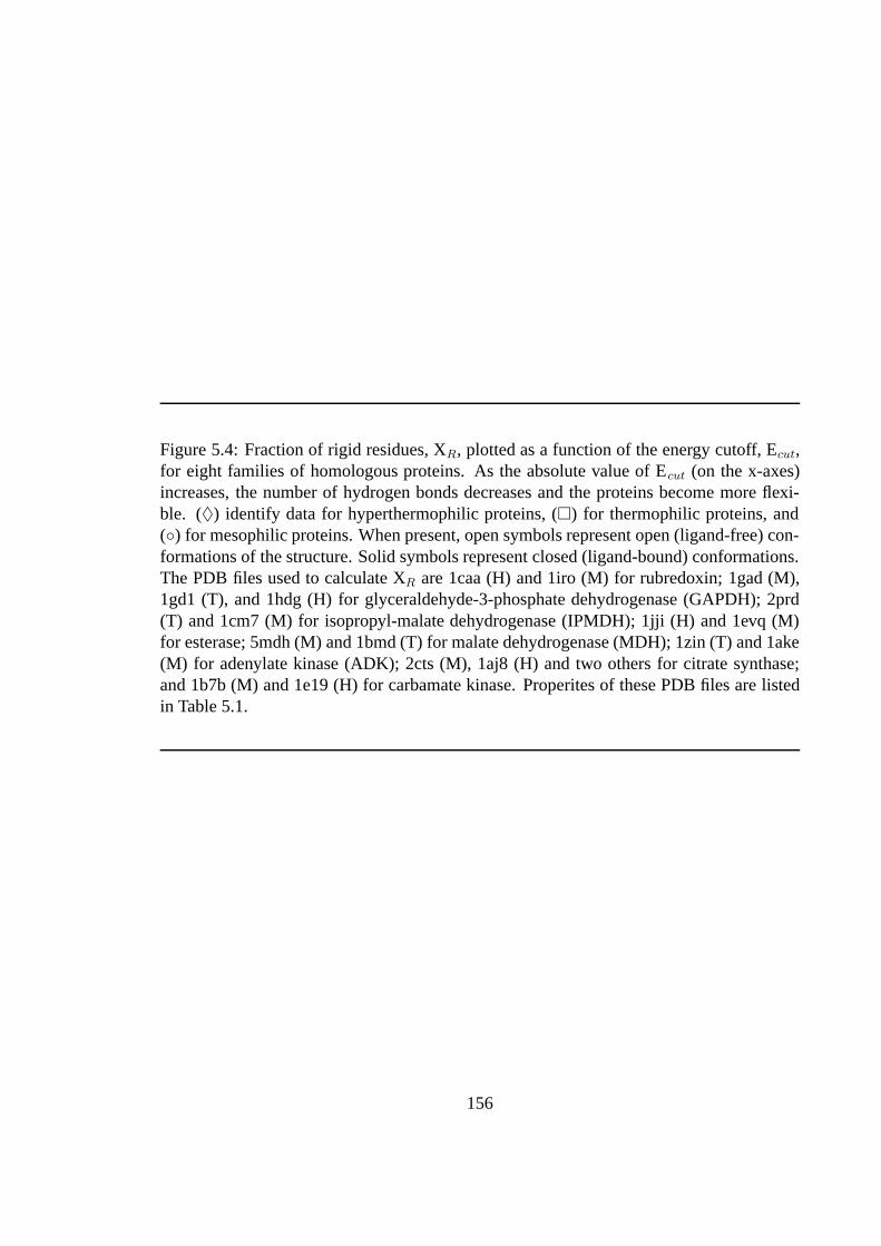
Figure 5.4: Fraction of rigid residues, XR, plotted as a function of the energy cutoff, Ecut,for eight families of homologous proteins. As the absolute value of Ecut (on the x-axes)increases, the number of hydrogen bonds decreases and the proteins become more flexi-ble. (♦) identify data for hyperthermophilic proteins, (�) for thermophilic proteins, and(◦) for mesophilic proteins. When present, open symbols represent open (ligand-free) con-formations of the structure. Solid symbols represent closed (ligand-bound) conformations.The PDB files used to calculate XR are 1caa (H) and 1iro (M) for rubredoxin; 1gad (M),1gd1 (T), and 1hdg (H) for glyceraldehyde-3-phosphate dehydrogenase (GAPDH); 2prd(T) and 1cm7 (M) for isopropyl-malate dehydrogenase (IPMDH); 1jji (H) and 1evq (M)for esterase; 5mdh (M) and 1bmd (T) for malate dehydrogenase (MDH); 1zin (T) and 1ake(M) for adenylate kinase (ADK); 2cts (M), 1aj8 (H) and two others for citrate synthase;and 1b7b (M) and 1e19 (H) for carbamate kinase. Properites of these PDB files are listedin Table 5.1.

156

Rubredoxin

MDH ADK

-3.5-2.5-1.5-0.50

0.5

1

-3.5-2.5-1.5-0.50

0.5

1

-3.5-2.5-1.5-0.50

0.5

1

-3.5-2.5-1.5-0.50

0.5

1

-3.5-2.5-1.5-0.50

0.5

1

-3.5-2.5-1.5-0.50

0.5

1

-3.5-2.5-1.5-0.50

0.5

1

-3.5-2.5-1.5-0.50

0.5

1

IPMDH

GAPDH

Esterase

Citrate synthase Carbamate kinase

Figure 5.4

157

thermozymes, and the circles for mesozymes. Figure 5.4 shows a clear and consistent trend

of increased rigidity of the hyperthermophilic and thermophilic enzymes compared to their

mesophilic homologues at each energy level in each protein family.

A parallel comparison is presented in Figure 5.5. These plots emphasize the connection

between thermostability and rigidity through the values of Ecut and 〈r〉. In Chapter 4, I

showed that all proteins went through an universal phase transition from rigid and folded

to flexible and unfolded near 〈r〉=2.4. Since 〈r〉 is a reaction coordinate characterizing

where the protein is along the folding trajectory, this value relates to the structural rigid-

ity/stability of the protein. The panels in Figure 5.5 again plot the same eight families of

homologous proteins, showing that different structures require a higher temperature (more

negative value of Ecut to reach the same value of 〈r〉. Green arrows are drawn at 〈r〉=2.41

(roughly the native state) and point toward higher thermostability. In the individual panels,

hyperthermozymes are colored in pink (and red for the case of citrate synthase where there

are two hyperthermophilic proteins); thermozymes in orange; and mesozymes in black.

Comparing the two proteins as in the first panel for rubredoxin (Rd), the hyperthermophilic

one has a consistently larger 〈r〉 making it inherently more stable. Looking at the set of

eight families, three (GAPDH, esterase, and ADK) are inconclusive while the other five

demonstrate a trend that the curves of the most thermostable proteins tend to represent the

most rigid structures. As hypothesized, increasing the rigidity reaction coordinate, 〈r〉,

corresponds to increasing the thermostability.

According to the HD exchange data for PfRd and CpRd (Hernandez and LeMaster,

2001), the two proteins show similar flexiblity at 23◦C, but CpRd exhibits a more rapid

158

Figure 5.5: Temperature (Ecut) versus 〈r〉for eight families of homologous proteins. AsEcut (on the y-axes) increases more hydrogen bonds are included in the analysis and thusthe protein has a higher mean coordination, 〈r〉. From Chapter 4, values greater than 2.4indicate the protein is in the native state. Thus as 〈r〉increases, so does rigidity. Verticalarrows are drawn at 〈r〉= 2.41 to to indicate the direction of increasing stability of thenative state. The colors indicate different growth temperatures of the protein organisms:pink and red for hyperthermozymes, orange for thermozymes and black for mesozymes.Although three families (GAPDH, Esterase and ADK) appear inconclusive, a trend that themore thermostable proteins (pink or orange versus black) are also more rigid emerges forthe remaining five families. The proteins used for this study are the same as those in Figure5.4 and listed in Table 5.1.

159

Rubredoxin

MDH ADK

IPMDH Esterase

Citrate Synthase Carbamate Kinase

2.38 2.4 2.42-3.5

-2.5

-1.5

-0.5

2.38 2.4 2.42-3.5

-2.5

-1.5

-0.5

2.38 2.4 2.42-3.5

-2.5

-1.5

-0.5

2.38 2.4 2.42-3.5

-2.5

-1.5

-0.5

2.38 2.4 2.42-3.5

-2.5

-1.5

-0.5

2.38 2.4 2.42-3.5

-2.5

-1.5

-0.5

2.38 2.4 2.42-3.5

-2.5

-1.5

-0.5

2.38 2.4 2.42-3.5

-2.5

-1.5

-0.5

GAPDH

Figure 5.5

160

flexibility increase with temperature than PfRd. The FIRST results shown in Figure 5.4

for CpRd and PfRd are in good agreement with the conclusions from the HD exchange

experiments. The two proteins contain nearly the same fraction of rigid residues up to an

energy cutoff of −2.4 kcal/mol. Beyond this point, PfRd retains more rigidity than does

CpRd. The time course of HD exchange in the isopropylmalate dehydrogenases (IPMDHs)

of the thermophile Thermus thermophilus and of the mesophile E. coli was followed by

FT-IR spectroscopy (Zavodszky et al., 1998). At 25◦C, HD exchange was far slower in the

thermophilic IPMDH than in its mesophilic counterpart. The HD exchange rates became

similar at the optimum temperatures of the two enzymes. Figure 5.4 confirms the HD ex-

change results as it indicates greater rigidity for T. thermophilus IPMDH than for the E.

coli enzyme, at all chosen energy cutoffs. Frequency domain fluorimetry and anisotropic

decay measurements of thermophilic and mesophilic esterases indicate that the mesophilic

esterase has a more dynamic and solvent exposed structure than the thermophilic homo-

logue (Gershenson et al., 2000; Manco et al., 2000). Since the structure of the mesophilic

esterase is not known, we compared the structure of the thermophilic esterase with that of a

hyperthermophilic homologue. Figure 5.4 shows a slight rigidity increase in the hyperther-

mophilic esterase compared to its thermophilic homologue, although not at Ecut = −2.5

kcal/mol. A greater rigidity difference between hyperthermophilic and mesophilic esterases

is expected from the observed trend.

The remaining panels of Figure 5.4 and Figure 5.5 represent families of proteins for

which no comparative experimental flexibility data are available, namely glyceraldehyde-

3-phosphate dehydrogenase (GAPDH), adenylate kinase (ADK), malate dehydrogenase

161

(MDH), citrate synthase, and carbamate kinase. In these families, the proteins from the

most thermophilic organism are also always the most rigid. Although no comparative flex-

ibility data are available for the GAPDHs represented in Figure 5.4, the GAPDH from

the hyperthermophile Thermotoga maritima was shown by HD exchange at 25◦C to be

significantly more rigid than its mesophilic counterpart from yeast (Wrba et al., 1990).

These experimental results plus the FIRST analysis in Figure 5.4 suggest that T. maritima

GAPDH is also more rigid than Bacillus stearothermophilus and E. coli GAPDHs.

Figure 5.4 shows FIRST results for four different citrate synthases, three of which orig-

inate from organisms living at temperatures above 50◦C. Binding of citrate and coenzyme

A in the enzyme catalytic site induce a significant conformational change in the protein.

For this reason, the structures of citrate synthases solved in the presence (i.e., P. furiosus

and pig enzymes) and in the absence (i.e., Sulfolobus solfataricus and Thermoplasma aci-

dophilum enzymes) of citrate and coenzyme A are shown with closed and open symbols,

respectively. In both enzyme pairs, the more thermostable enzyme appears to be the more

rigid one. In this enzyme family, the presence of ligands in some of the structures (which

can stabilize the enzyme as was seen in the case of ADK in Chapter 3) does not affect the

rigidity ranking, which follows the thermostability ranking P. furiosus > S. solfataricus

> T. acidophilum > pig citrate synthase. The FIRST results obtained for the P. furiosus

and the Enterococcus faecalis carbamate kinases (PfCK and EfCK, respectively) show that

the hyperthermophilic PfCK consistently shows a higher fraction of rigid residues than its

mesophilic counterpart. PfCK contains more ion-pairs and ion-pair networks than EfCK

(103 ion pairs in PfCK versus 39 in EfCK). An extensive ion-pair network linking two

162

subunits of PfCK is thought to be the main thermostabilizing mechanism in this enzyme

(Ramon-Maiques et al., 2000). The FIRST results presented here should be taken with

caution, though since the only known structure of EfCK was solved in the absence of lig-

and whereas that of PfCK was solved in the presence of ADP. As demonstrated in Chapter

3, binding of the ADP ligand could have provided additional rigidity to PfCK.

5.5 Stabilization by Substrates and Oligomerization

For many of the hyperthermophilic and themophilic proteins studied, oligomerization and

intersubunit interactions emerge as major stabilizing mechanisms (Vieille and Zeikus,

2001). Site-directed mutagenesis has shown that increased hydrophobic contacts between

the two subunits of T. thermophilus IPMDH have made it more resistant to dimer disso-

ciation as compared to its mesophilic E. coli counterpart (Moriyama et al., 1995; Kirino

et al., 1994). Also, hyperthermophilic proteins often have a higher oligomerization state

than their mesophilic homologs (Vieille and Zeikus, 2001). T. maritima dihydrofolate re-

ductase (TmDHFR) is an extremely stable homodimer unlike the E. coli dihydrofolate re-

ducase (EcDHFR), which is monomeric. The subunit interactions in TmDHFR span a

relatively large surface area involving numerous residues (Dams and Jaenicke, 1999). Sub-

strate molecules have also been known to stabilize enzyme active sites (Vieille and Zeikus,

2001). TmDHFR has been shown to become kinetically more stable upon binding sub-

strates, in particular NADPH resulting in a six-fold increase in t1/2 at 80◦C (Wilquet et al.,

1998). In Chapter 3, ligand binding in several monomeric protein structures (including

EcDHFR) was shown to accompany an increase in rigidity by FIRST.

163

-3.5-2.5-1.5-0.5Ecut

0

0.2

0.4

0.6

0.8

1

XR

Figure 5.6: Fraction of rigid residues (XR) as a function of the energy cutoff (Ecut) in dihy-drofolate reductase (DHFR) from Thermotoga maritima and Escherichia coli. An increasein the absolute value of Ecut can be likened to increase in temperature. As temperatureincreases, the protein becomes more flexible and eventually unfolds. Open symbols indi-cate apo forms (no ligand), closed symbols indicate ligand bound forms. Gray symbolscorrespond to the various hyperthermophilic DHFR forms from T. maritima whereas blacksymbols refer to the mesophilic DHFR forms from E. coli. The triangles correspond tomonomeric TmDHFR which are not biologically relevant whereas the circles in all casescorrespond to the biologically active forms (monomer in the case of EcDHFR and homod-imer in the case of TmDHFR).

The effects of substrate binding and oligomerization on the rigidity of DHFRs were

tested using FIRST. Differences in the fraction of rigid residues, XR, provide a measure of

these ligand binding effects. Figure 5.6 shows XR plotted against Ecut for the monomeric

versus dimeric, and the ligand-bound versus ligand-free forms of TmDHFR and EcDHFR.

The active (dimeric), ligand-free (apo) form of TmDHFR consistently demonstrates a

higher fraction of rigid residues that apo-EcDHFR, especially at Ecut ≤ −1.5 kcal/mol. The

ligand-bound (holo) TmDHFR also consitently shows a higher fraction of rigid residues

164

than holo-EcDHFR. These results are in keeping with the trends seen in other families of

homologous proteins in Figure 5.4.

The fraction of rigid residues was also calculated by FIRST for one of the monomers

of TmDHFR. Although TmDHFR is not biologically active as a monomer, the goal was

to specifically determine the increase in rigidity (and hence thermostability) conferred

by dimerization. The apo and holo forms of the TmDHFR monomer are both less rigid

than their dimeric TmDHFR counterparts. The apo-TmDHFR monomer (open gray tri-

angles) becomes only marginally more rigid than apo-EcDHFR (open black circles). The

monomeric holo-TmDHFR (solid gray triangles) is now even less rigid than holo-EcDHFR

at all values of Ecut tested. These observations are a clear confirmation that dimerization is

a major thermostabilizing mechanism in TmDHFR (Dams and Jaenicke, 1999).

165

Chapter 6

Conclusions and Future Directions

6.1 Conclusions

6.1.1 Rigidity Studies of Glasses and Proteins

Results from computational studies on network glasses presented in Chapter 2 provided

the basis for the development of the FIRST software. The novel computational method of

the Pebble Game algorithm allows exact enumeration and localization of flexible and rigid

regions for specific types of networks. The concepts of Maxwell constraint counting were

shown to give a good estimate of the location of the phase transition from rigid to floppy

for a variety of 3D glasses. The Bethe lattice solution was shown to exactly match that

of the random bond model. This discovery revealed that the discrepancies between first

and second order rigidity transitions were caused by the absence or presence of nucleating

rings. Continued investigation of network glasses has shown that these rings induce stress

in the network. When bonds are diluted in a nonrandom way (namely without stress), the

166

character of the phase transition changes from first to second order and the glasses are said

to be self-organizing (Thorpe et al., 2000).

Chapter 3 introduced a novel distance constraint approach for characterizing the in-

trinsic flexibility of a protein. The underlying physical and mathematical assumptions

were outlined, and implemented computationally in the FIRST software. FIRST deter-

mines the Floppy Inclusion and Rigid Substructure Topography of a given protein struc-

ture, based on a set of distance constraints determined by the network of covalent and

non-covalent (hydrogen bonds, salt bridges, and hydrophobic contacts) interactions within

a single conformation of the protein. Developed as a collaboration between D.J. Jacobs,

M.F. Thorpe and L.A. Kuhn, a version of the FIRST software is now available online

at http://firstweb.pa.msu.edu. Several means of visualizing and comparing

flexibility in proteins have been presented here, and are included in the online software,

including the rigid cluster decomposition and the flexibility index.

Analysis of a single protein structure by FIRST indicates the regions likely to un-

dergo conformational change as part of the protein’s function. For a given set of distance

constraints, the rigid regions and the flexible joints between them are determined exactly.

FIRST has the ability to identify sets of atoms that are mutually rigid or mutually flexible

leading to collective motion analysis. Each collective motion indicates a region of influ-

ence within the protein where changing one dihedral angle could influence other dihedral

angles. Analysis of the relative flexibility within HIV protease, dihydrofolate reductase,

and adenylate kinase, even when performed on a single structure, captures much of the

functionally important conformational flexibility observed experimentally between differ-

167

ent ligand-bound states. Ligand binding was seen to alter the rigid and flexible regions in

Chapter 3. In Chapter 5, ligand binding in TmDHFR and EcDHFR is seen to accompany

an increase in rigidity and thermostability. Holo-EcDHFR remains more rigid than apo-

EcDHFR as the temperature increases (shown by changing Ecut). A similar trend is seen

in the ligand-bound form of TmDHFR compared to apo-TmDHFR. These results are in

agreement with the experimental evidence that substrate binding increases the rigidity and

hence the thermostability of TmDHFR (Wilquet et al., 1998).

6.1.2 Unfolding and Folding Predictions

Chapter 4 presented applications of FIRST to understand the mechanisms of unfolding

and folding in proteins. Two parameters: the fraction of floppy modes, f , and the mean

coordination, 〈r〉, were shown to specify the unfolding transition for a set of proteins. For

reversible, two-state folding proteins, this unfolding transition also corresponds to the fold-

ing transition. Beginning from the native state, the transition state and folding core were

identified as the protein was unfolded by simulated thermal denaturation. These two spe-

cial states along the unfolding pathway were identified by applying rigidity analysis to the

proteins: the transition state from the peak in the specific heat-like curve of f ′′(〈r〉), and the

folding core from the final point of mutually rigid secondary structures. The good agree-

ment between experimental and predicted folding core data supports that our hypothesis

that removing hydrogen bonds in order of relative energy simulates thermal denaturation.

A larger dataset is required for more conclusive evidence. However, the native-state topol-

ogy, defined by the network of non-covalent interactions, appears to encode information

168

about how proteins fold. Coupled with the correlation between the flexibility index and

Φ-values for barnase, this suggests that one might be able to predict folding nuclei with

FIRST analysis of the native state.

It was also shown that the protein folding transition can be viewed as a flexible to

rigid phase transition, similar to that observed for network glasses. The cross-linking, non-

covalent interactions are summarized in the mean coordination, 〈r〉, for all protein atoms.

Thus, 〈r〉 can be regarded as a reaction coordinate for protein folding, and provides a unify-

ing measurement of several dynamic and structural processes, including protein flexibility

and folding. In the folded state, proteins have inherent substructure, namely α-helices and

β-sheets. The bonds removed during denaturation have the special role of cross-linking

the polypeptide chain into a 3D, folded protein structure. These traits, along with the co-

operative nature of protein folding, suggest that proteins, like glasses, are self-organized

networks. Additionally, the protein folding transition appears approximately first-order —

rounded due to finite size effects in the network (protein). This transition is shared among

diverse proteins ranging from all-α to all-β folds, and from monomers to tetramers, and

occurs once the protein denatures to a mean coordination of 〈r〉= 2.405±0.015. This value

is very similar to the rigidity transition in network glasses.

6.1.3 Thermostability and Rigidity

Chapter 5 presented correlations between quantitative measures of rigidity from FIRST

and several types of thermostability data. The case study of rubredoxin provided an inter-

esting paradox: HD exchange data suggests similar overall flexibility for hyperthermophilic

169

PfRd and mesophilic CpRd, yet the hyperthermophilic version demonstrates increased ther-

mostability. Even detailed knowledge of a structure does not necessarily provide the key to

unlocking the thermostabilizing mechanisms. Experimental HD exchange data and FIRST

analysis indicate that these homologous proteins may partition flexibility and rigidity dif-

ferently. Such partitioning likely results because proteins are not rigid solids, but require

a certain degre of flexibility to function. FIRST provides a tool to identify the flexible

regions and a launching point for studies that could draw comparisons between this mea-

sure of flexibility and structural similarities. Simulated mutations coupled with FIRST

analysis indicated that both local and nonlocal effects contribute to this greater stability in

PfRd. For the rubredoxin pair, altering a few specific hydrophobic interactions between

conserved residues produced drastic changes rigidity and stability, suggesting that several

conserved residues might be more optimally aligned in PfRd to create interactions not

present in CpRd. This confirms the suggestion that “the extraordinary thermostability of

PfRd may involve a precise, optimal alignment of a large number of residues, whose net-

work of interactions are very sensitive to small structural changes dictated by the context

of the sequence” (Eidsness et al., 1997).

Comparisons within families of homologous proteins indicated that, in general, the

global rigidity increased as temperature increased (Ecut decreased). The trends in global

rigidity as measured by the structural quantities of mean coordination, 〈r〉, and fraction

of rigid residues, XR, are in agreement with experimental evidences indicating either de-

creased conformational dynamics or increased intermolecular interactions for the hyper-

thermozyme and thermozyme compared to their mesophilic homologues. Although the

170

source of thermostability is likely different in each protein family, a quantitative measure

of rigidity can describe the intrinsic structural changes that produce thermostability. Com-

paring the temperature (through changing the energy threshold value) to the fraction of

rigid residues showed an emerging correlation between increased rigidity and increased

thermostability for the nine families studied. This dissertation has introduced the computa-

tional method of FIRST as a tool to better understand the delicate balance between rigidity

and flexibility in thermostability.

6.2 Future Directions

6.2.1 The Protein Model of FIRST

Within the FIRST program there are some technical adjustments that could be imple-

mented to improve the modeling of proteins. One example is the identification of hy-

drophobic contacts. The current model may overestimate the number of contacts by count-

ing all hydrophobic pairs within a given distance and constrains them too tightly with the

three-pseudoatom model. An alternative selection criterion in which hydrophobic atoms

only bound to other hydrophobic atoms are considered as potential contacts needs to be

tested and implemented. Additionally, these contacts should be connected by a single ef-

fective constraint rather than two. The current model of hydrophobic tethers was chosen

because of its correspondence to folding cores from experimental HD exchange data. Any

change in the strength or number of these interactions will have repercussions on the energy

threshold of hydrogen bonds to include in the native state and require additional validation

171

against experimental results. As was explained in Chapter 4, although 〈r〉≈ 2.4 uniquely

specifies the transition state as the point where the fraction of floppy modes has the greatest

curvature, the degree of flexibility in the native state is less well-defined. Assigning the

native state on the basis of 〈r〉 has not been investigated yet. Another case for improve-

ment involves how to accommodate strong ionic bonds such as those involving metals into

the required bond-bending network. Comparisons are currently being conducted to mea-

sure the errors created by simply removing angular constraints versus a recently suggested

exact model (Whiteley, 2002; Chubynsky and Thorpe, 2002a).

A more interesting avenue of inquiry is the application of FIRST to larger

biomolecules. To date, the largest protein that has been analyzed with FIRST is the GroEL

complex (PDBcode 1aon) which has 8337 residues and 58,884 heavy atoms. The size of

this complex approaches the current limits of experimental atomic resolution. However,

because FIRST runs almost linearly in time with respect to the number of atoms, molec-

ular size is not a limitation in practice for FIRST. Protein-DNA complexes, ribosomes

and viruses are potential large biomolecular structures that FIRST can be applied to with

minimal additional programming. Applications of constraint counting and rigidity to larger

complexes by FIRST is limited by the accuracy of structural detail available for these com-

plexes. It may become advantageous to develop additional, low-resolution models so that

FIRST can be applied to these larger systems and aid in the experimental refinement and

understanding of these structures.

172

6.2.2 The Folding Core and Transition State Predictions

Although the set of 26 proteins in Table 4.1 shows striking universality upon unfolding by

simulated thermal denaturation, there is some degree of noise in the plots of f ′′ versus 〈r〉.

Whether these differences correlate to multiple step protein folders and how that may occur

is an interesting question. The ability to predict the transition state of proteins from a simple

structural parameter, 〈r〉, has a great deal of potential for understanding the problem of

protein folding. The predicted Φ-values for barnase show promise but require refinements

of the hydrophobic model and/or hydrogen bond dilution scheme as a next step.

Each of the hydrogen bond dilution plots in Chapter 4 represent one of many possi-

ble unfolding pathways. Since much experimental work in protein folding focuses on the

identification of pathways and possible intermediates, it would be useful to apply FIRST

to this question and probe the entire landscape of protein unfolding in terms of relevant

parameters: 〈r〉, f , etc. Already FIRST has been used as a starting point for sampling

accessible conformations of folded proteins (Thorpe et al., 2001). Combining these con-

formational sampling procedures with precise knowledge of the reaction coordinate could

lead to complete characterization of protein folding pathways and landscapes.

6.2.3 Thermostability and Rigidity

Mutatagenesis studies have shown that certain residues are critical for folding and/or activ-

ity. Predicted flexibility and stability upon mutation of a residue is a very good potential

application of the FIRST software. This parallels the initial correlations between flexibility

173

indices and Φ-values to describe the folding parameters presented in Chapter 4. Contin-

ued research and calibration of the predictive ability of such simulated mutations could

produce a reliable guide for experimental studies. Currently there is a disjoint between

what can be measured experimentally and what can be calculated theoretically regarding

thermostability. Because thermostabilizing mechanisms often differ from one pair of ho-

mologous proteins to another, it is difficult to make generalizations about this area of study.

The structural comparisons of homologous proteins presented in Chapter 5 may provide

a starting point to reduce the complexity of what causes thermostability and guide exper-

imental investigations. A few parameters measuring rigidity were presented to compare

homologous structures quantitatively on a global level and eliminate some of the local dif-

ferences due to residue level differences. Although conducted on a small set of proteins,

this study suggested possible trends linking increased thermostability to increased rigidity,

which can be verified with experimental thermostability data as more structures become

known.

Comparisons between FIRST-defined collective motions and results from molecular

dynamic simulations like those presented for rubredoxin in Chapter 5 are still being de-

veloped. This is an area with much interest because knowing a priori which regions are

flexible and rigid could dramatically speed up MD simulations. Integrating FIRST into

MD simulations may yield informative results about large scale motions and afford greater

agreement with experimental folding results, where non-native interactions are sampled

during kinetic folding simulations.

Knowledge from several fields was required to undertake the studies of rigidity in pro-

174

teins presented in this dissertation. However, the fruits of bridging the disciplines of physics

and biochemistry has produced a novel and powerful computational tool to identify flexi-

bility in protein structures. This dissertation presents a picture of protein rigidity theory by

viewing proteins as a very special case of glassy material. The applications of FIRST to

characterize the flexibility, stability, and folding of proteins presented here are only a few

of many yet to be discovered.

175

BIBLIOGRAPHY

R. Abagyan, M. Totrov, and D. Kuznetsov. ICM — a new method for protein modelingand design: Applications to docking and structure prediction from the distorted nativeconformation. J. Comput. Chem., 15(5):488–506, 1994.

V. Abkevich, A. Gutin, and E. Shakhnovich. Specific nucleus as the transition state forprotein folding: evidence from the lattice model. Biochemistry, 33:10026–10036, 1994.

D. E. Anderson, J. Lu, L. McIntosh, and F. W. Dahlquist. NMR of Proteins, pages 258–304.CRC Press, 1993.

C. Anfinsen. Principles that govern the folding of protein chains. Science, 181:223–230,1973.

C. Anfinsen, E. Haber, M. Sela, and F. White, Jr. The kinetics of formation of nativeribonuclease during oxidation of the reduced polypeptide chain. Proc. Natl. Acad. Sci.,47:1309–1314, 1961.

C. A. Angell. Hydration Processes in Biology, pages 127–139. IOS Press, Amsterdam,1999.

S. Arbabi and M. Sahimi. Mechanics of disorderd solids. I. percolation on elastic networkswith central forces. Phys. Rev. B, 47:695–702, 1993.

A. Atilgan, S. Durell, R. Jernigan, M. Demirel, O. Keskin, and I. Bahar. Anisotropy offluctuation dynamics of proteins with an elastic network model. Biophys. J., 80:505–515, 2001.

F. Babalievsky. Unpublished results, 1998.

I. Bahar, A. Atilgan, M. Demirel, and B. Erman. Vibrational dynamics of folded proteins:Significance of slow and fast motions in relation to function and stability. Phys. Rev.Lett., 80:2733–2736, 1998.

I. Bahar, A. Atilgan, and B. Erman. Direct evaluation of thermal fluctuations in proteinsusing a single-parameter harmonic potential. Fold. Des., 2:173–181, 1997.

Y. Bai, J. S. Milne, L. Mayne, and S. W. Englander. Primary structure effects on peptidegroup hydrogen exchange. Proteins:Struct. Func. Gen., 17:75–86, 1993.

176

D. Baker. A surprising simplicity to protein folding. Nature, 405:39–42, 2000.

D. J. Barlow and J. Thornton. Ion-pairs in proteins. J. Mol. Biol., 168:867–885, 1983.

W. Bennett and R. Huber. Structural and functional aspects of domain motions in proteins.Crit. Rev. Biochem., 15:291–384, 1984.

H. Berendsen and S. Hayward. Collective protein dynamics in relation to function. Curr.Opin. Str. Biol., 10:160–169, 2000.

H. Berman, J. Westbrook, Z. Feng, G. Gilliland, T. Bhat, H. Wessig, I. Shindyalov, andP. Bourne. The protein data bank. Nucleic Acids Research, 28:235–242, 2000.

P. R. Blake, J.-B. Park, Z. H. Zhou, D. R. Hare, M. W. W. Adams, and M. F. Summers.Solution-state strucure by NMR of zinc-substitued rubredoxin from the marine hyper-thermophilic archaebacterium pyrococcus furiosus. Prot. Sci., 1:1508–1521, 1992.

R. Bohmer and C. A. Angell. Correlations of the nonexponentiality and state dependence ofmechanical relaxations with bond connectivity in Ge-As-Se supercooled liquids. Phys.Rev. B, 45:10091–10094, 1992.

H. Bonisch, J. Backmann, T. Kath, D. Naumann, and G. Schafer. Adenylate kinase fromsulfolobus acidocaldarius: expression in escherichia coli and characterization by Fouriertransform infrared spectroscopy. Archives of Biochemistry and Biophysics, 333:75–84,1996.

P. Boolchand, D. Selvanathan, Y. Wang, D. Georgiev, and W. Bresser. Onset of rigidity insteps in chalcogenide glasses. In M. Thorpe and L. Tichy, editors, Properties and Appli-cations of Amorphous Materials, pages 97–132. Kluwer Academic, Dordrecht, 2001.

P. Boolchand and M. Thorpe. Glass-forming tendency, percolation of rigidity, and onefold-coordinated atoms in covalent networks. Phys. Rev. B, 50:10366–10368, 1994.

E. Bradley, D. Stewart, M. Adams, and J. Wampler. Investigations of the thermostability ofrubredoxin models using molecular dynamics simulations. Prot. Sci., 2:650–665, 1993.

B. Brooks and M. Karplus. Harmonic dynamics of proteins: Normal modes and fluctua-tions in bovine pancreatic trypsin inhibitor. Proc. Natl. Acad. Sci., 80:6571–6575, 1983.

C. Brooks, III, J. Onuchic, and D. Wales. Taking a walk on a landscape. Science, 293:612–613, 2001.

J. Bryngelson, J. Onuchic, N. Socci, and P. Wolynes. Funnels, pathways, and the energylandscape of protein folding: A synthesis. Proteins: Struct., Func., and Gen., 21:167–195, 1995.

J. D. Bryngelson and P. G. Wolynes. Spin glasses and the statistical mechanics of proteinfolding. Proc. Natl. Acad. Sci., 84:7524–7528, 1987.

177

G. Bulaj and D. P. Goldenberg. φ-values for BPTI folding intermediates and implicationsfor transition state analysis. Nature Structural Biology, 8:326–330, 2001.

A. Caflisch and M. Karlpus. Acid and thermal denaturation of barnase investigated bymolecular dynamics simulations. J. Mol. Biol., 252:672–708, 1995.

S. Cavagnero, D. Debe, Z. Zhou, M. Adams, and S. Chan. Kinetic role of electrostatic inter-actions in the unfolding of hyperthermophilic and mesophilic rubredoxins. Biochemistry,37:3369–3376, 1998a.

S. Cavagnero, Z. Zhou, M. Adams, and S. Chan. Unfolding mechansim of rubredoxin frompyrococcus furiosus. Biochemistry, 37:3377–3385, 1998b.

H. Chan and K. Dill. Protein folding in the landscape perspective: chevron plots and non-arrhenius kinetics. Proteins: Struct., Func., and Gen., 30:2–33, 1998.

H. S. Chan and K. A. Dill. ‘Sequence space soup’ of proteins and copolymers. J. Chem.Phys., 95:3775–3787, 1991.

Z. Chen, Y. Li, H. B. Schock, D. Hall, E. Chen, and L. C. Kuo. Three dimensional struc-ture of a mutant HIV-1 protease displaying cross-resistance to all protease inhibitors inclinical trials. J. Biol. Chem., 270:21433–21436, 1995.

M. V. Chubynsky and M. F. Thorpe. Personal communication, 2002a.

M. V. Chubynsky and M. F. Thorpe. Rigidity percolation and the chemical threshold innetwork glasses. J. Optoelectron. Adv. Mater., 2002b. in press.

M. V. Chubynsky and M. F. Thorpe. Self-organization and rigidity in network glasses.Curr. Opin. in Solid State Mater. Sci., 5:525–556, 2002c.

J. Clarke and L. Itzhaki. Hydrogen exchange and protein folding. Curr. Opin. Str. Biol., 8:112–118, 1998.

D. Cobessi, F. Tete-Favier, S. Marchal, G. Branlant, and A. Aubry. Structural and bio-chemical investigations of the catalytic mechanism of an NADP-dependent aldehydedehydrogenase from streptococcus mutants. J. Mol. Biol., 300:141–152, 2000.

G. Colombo and K. M. Merz, Jr. Stability and activity of mesophilic subtilisin E and itsthermophilic homolog: Insights from molecular dynamic simulations. J. Am. Chem.Soc., 121:6895–6903, 1999.

T. E. Creighton. Proteins: Structures and Molecular Properties, pages 287–291. W. H.Freedman, New York, second edition, 1993.

J. F. da Silva and R. Williams. The biological chemistry of the elements : the inorganicchemistry of life. Oxford University Press, New York, 1991.

178

V. Daggett, A. Li, L. S. Itzhaki, D. E. Otzen, and A. R. Fersht. Structure of the transitionstate for folding of a protein derived from experiment and simulation. J. Mol. Biol., 257:430–440, 1996.

T. Dams and R. Jaenicke. Stability and folding of dihydrofolate reductase from the hyper-thermophilic bacterium thermotoga maritima. Biochemistry, 38:9169–6178, 1999.

R. M. Daniel, D. A. Cowan, H. W. Morgan, and M. P. Curran. A correlation betweenprotein thermostability and resistance to proteolysis. Biochem. J., 207:641–644, 1982.

R. Das and M. Gerstein. The stability of thermophilic proteins: a study based on compre-hensive genome comparison. Funct. Integr. Genomics, 1:76–88, 2000.

S. D’Auria, P. Herman, J. R. Lakowicz, F. Tanfani, E. Bertoli, G. Manco, and M. Rossi. Theesterase from the thermophilic eubacterium bacillus acidocaldrius: Structural-functionalrelationship and comparison with the esterase from the hyperthermophilic archaeon ar-chaeoglobus fulgidus. Proteins: Struct., Func., and Gen., 40:473–481, 2000.

A. Day, R. Tremblay, and A.-M. S. Tremblay. Rigid backbone: A new geometry for perco-lation. Phys. Rev. Lett., 56:2501–2504, 1986.

K. Dill. Dominant forces in protein folding. Biochemistry, 29:7133–7155, 1990.

B. Djordjevic, M. Thorpe, and F. Wooten. Computer model of tetrahedral amorphousdiamond. Phys. Rev. B, 52:5685–5689, 1995.

N. Dokholyan, L. Li, F. Ding, and E. Shakhnovich. Topological determinants of proteinfolding. Proc. Natl. Acad. Sci., 99:8637–8641, 2002.

P. C. Driscoll, A. M. Wingfield, and G. M. Clore. Determination of the secondary struc-ture and molecular topology of interleukin-1β by use of two- and three-dimensionalheteronuclear 15N-1H NMR spectroscopy. Biochemistry, 29:4668–4682, 1990.

Y. Duan, L. Wang, and P. Kollman. The early stage of folding of villin headpiece subdomainobserved in a 200-nanosecond fully solvated molecular dynamics simulation. Proc. Natl.Acad. Sci., 95:9897–9902, 1998.

P. M. Duxbury, D. J. Jacobs, M. F. Thorpe, and C. Moukarzel. Floppy modes and thefree energy: Rigidity and connectivity percolation on bethe lattices. Phys. Rev. E, 59:2084–2092, 1999.

W. Eaton, V. Munoz, S. Hagen, G. Jas, L. Lapidus, E. Henry, and J. Hofrichter. Fast kineticsand mechanisms in protein folding. Annu. Rev. Biophys. Biomol. Struct., 29:327–359,2000.

M. K. Eidsness, K. A. Richie, A. E. Burden, D. M. Kurtz, Jr., and R. A. Scott. Dis-secting contributions to the thermostability of pyrococcus furiosus rubredoxin: β-sheetchimeras. Biochemistry, 36:10406–10413, 1997.

179

S. W. Englander, L. Mayne, Y. Bai, and T. R. Sosnick. Hydrogen exchange: The modernlegacy of Linderstrøm-Lang. Prot. Sci., 6:1101–1109, 1997.

D. Epstein, S. Benkovic, and P. Wright. Dynamics of the dihyrdofolate reductase – folatecomplex: Catalytic sites and regions known to undergo conformational change exhibitdiverse dynamical features. Biochemistry, 34:11037–11048, 1995.

S. Feng and P. Sen. Percolation on elastic networks: New exponent and threshold. Phys.Rev. Lett., 52:216–219, 1984.

S. Feng, M. F. Thorpe, and E. Garboczi. Effective-medium theory of percolation on central-force elastic networks. Phys. Rev. B, 31:276–280, 1985.

A. Fersht. Nucleation mechanisms in protein folding. Curr. Opin. Str. Biol., 7:3–9, 1997.

A. Fersht. Structure and Mechanism in Protein Science. W.H. Freeman and Company, NewYork, 1999.

A. R. Fersht. The hydrogen bond in molecular recognition. Trends in Biochemical Science,12:301–304, 1987.

A. R. Fersht. Transition-state structure as a unifying basis in protein-folding mechanisms:Contact order, chain topology, stability, and the extended nucleus mechanism. Proc.Natl. Acad. Sci., 97:1525–1529, 2000.

A. R. Fersht, A. Matouschek, and L. Serrano. The folding of an enzyme. I. Theory ofprotein engineering analysis of stability and pathway of protein folding. J. Mol. Biol.,224:771–782, 1992.

A. Fontana, G. Fassina, C. Vita, D. Dalzoppo, M. Zamai, and M. Zambonin. Correlationbetween sites of limited proteolysis and segmental mobility in thermolysin. Biochem-istry, 25:1847–1851, 1986.

A. Fontana, M. Zambonin, P. P. de Laureto, V. de Filippis, A. Clementi, and E. Scaramella.Probing the conformational state of apomyoglobin by limited proteolysis. J. Mol. Biol.,266:223–230, 1997.

J. Forbes and G. Lorimer. Unravelling a membrane protein. Science, 288:63–64, 2000.

H. Frauenfelder, S. Sligar, and P. Wolynes. The energy landscapes and motions of proteins.Science, 254:1598–1603, 1991.

O. V. Galzitskaya and A. V. Finkelstein. A theoretical search for folding/unfolding nucleiin three-dimensional protein structures. Proc. Natl. Acad. Sci., 96:11299–11304, 1999.

D. Gandini, L. Gogioso, M. Bolognesi, and D. Bordo. Patterns in ionizable side chaininteractions in protein structures. Proteins: Struct., Func., and Gen., 24:439–449, 1996.

180

A. Gershenson, J. A. Schauerte, L. Giver, and F. H. Arnold. Trypophan phosphorescencestudy of enzyme flexibility and unfolding in laboratory-evolved thermostable esterases.Biochemistry, 39:4658–4665, 2000.

M. Gerstein and W. Krebs. A database of macromolecular motions. Nucleic Acids Re-search, 26:4280–4290, 1998.

M. Gerstein, A. Lesk, and C. Chothia. Structural mechanisms for domain movements inproteins. Biochemistry, 33(22):6739–6749, 1994.

M. Gerstein, G. Schulz, and C. Chothia. Domain closure in adenylate kinase: Joints oneither side of two helices close like neighboring fingers. J. Mol. Biol., 229:494–501,1993.

G. Gianese, F. Bossa, and S. Pascarella. Comparative structural analysis of psychrophilicand meso- and thermophilic enzymes. Proteins: Struct., Func., and Gen., 47:236–249,2002.

N. Go. Theoretical studies of protein folding. Annu. Rev. Biophys. Bioeng., 12:183–210,1983.

J. Goodman, M. Pagel, and M. Stone. Relationships between protein structure and dy-namics from a database of NMR-derived backbone order parameters. J. Mol. Biol., 295:963–978, 2000.

A. Grottesi, M.-A. Ceruso, A. Colosimo, and A. Di Nola. Molecular dynamics study of ahyperthermophilic and a mesophilic rubredoxin. Proteins: Struct., Func., and Gen., 46:287–294, 2002.

M. Gruebele. The fast protein folding problem. Annu. Rev. Phys. Chem., 50:485–516,1999.

E. Guyon, S. Roux, A. Hansen, D. Bibeau, J. P. Troadec, and H. Crapo. Non-local and non-linear problems in the mechanics of disordered systems: Application to granular mediaand rigidity problems. Rep. Prog. Phys., 53:373–419, 1990.

A. Hansen and S. Roux. Universality class of central-force percolation. Phys. Rev. B, 40:749–752, 1989.

H. He and M. Thorpe. Elastic properties of glasses. Phys. Rev. Lett., 54:2107–2110, 1985.

B. Hendrickson. Conditions for unique graph realizations. SIAM J. Comput., 21:65–84,1992.

G. Hernandez, F. Jenney, Jr., M. Adams, and D. LeMaster. Millisecond time scale confor-mational flexibility in a hyperthermophile protein at ambient temperature. Proc. Natl.Acad. Sci., 97:3166–3170, 2000.

181

G. Hernandez and D. LeMaster. Reduced temperature dependence of collective confor-mational opening in a hyperthermophile rubredoxin. Biochemistry, 40:14384–14391,2001.

B. M. Hespenheide, A. J. Rader, M. F. Thorpe, and L. A. Kuhn. Identifying protein foldingcores from the evolution of flexible regions during unfolding. J. Mol. Graph. & Model.,21:195–207, 2002.

R. Hiller, Z. H. Zhou, M. W. Adams, and S. W. Englander. Stability and dynamics in ahyperthermophilic protein with melting temperature close to 200◦C. Proc. Natl. Acad.Sci., 94:11329–11332, 1997.

N. Hillson, J. N. Onuchic, and A. E. Garcia. Pressure-induced protein-folding/unfoldingkinetics. Proc. Natl. Acad. Sci., 96:14848–14853, 1999.

V. J. Hilser, D. Dowdy, T. G. Oas, and E. Freire. The structural distribution of cooperativeinteractions in proteins: Analysis of the native state ensemble. Proc. Natl. Acad. Sci., 95(17):9903–9908, 1998.

J. Hollien and S. Marqusee. Structural distribution of stability in a thermophilic enzyme.Proc. Natl. Acad. Sci., 96:13674–13678, 1999a.

J. Hollien and S. Marqusee. A thermodynamic comparison of mesophilic and thermophilicribonucleases H. Biochemistry, 38:3831–3836, 1999b.

L. Holm and C. Sander. Parser for protein folding units. Proteins: Struct., Func., and Gen.,19:256–268, 1994.

R. Hooft, C. Sander, and G. Vriend. Positioning hydrogen atoms by optimizing hydrogen-bond networks in protein structures. Proteins: Struct., Func., and Gen., 26:363–376,1996.

F. M. Hughson, P. E. Wright, and R. L. Baldwin. Structural characterization of a partiallyfolded apomyoglobin intermediate. Science, 249:1544–1548, 1990.

R. Ishima, D. Freedberg, Y.-X. Wang, J. Louis, and D. Torchia. Flap opening and dimer-interface flexibility in the free and inhibitor-bound HIV protease and their implicationsfor function. Struct. Fold. Des., 7:1047–1055, 1999.

S. A. Islam, M. Karplus, and D. L. Weaver. Application of the diffusion–collision modelto the folding of three-helix bundle proteins. J. Mol. Biol., 318:199–215, 2002.

L. S. Itzhaki, D. E. Otzen, and A. R. Fersht. The structure of the transition state for foldingof chymotrypsin inhibitor 2 analysed by protein engineering methods: Evidence for anucleation–condensation mechanism for protein folding. J. Mol. Biol., 254:260–288,1995.

S. E. Jackson. How do small single-domain proteins fold? Fold. Des., 3:R81–R91, 1998.

182

D. Jacobs and M. Thorpe. Comment on “infinite cluster geometry in central force net-works”. Phys. Rev. Lett., 80:5451, 1998a.

D. J. Jacobs. Generic rigidity in three-dimensional bond-bending networks. J. Phys. A:Math. Gen., 31:6653–6668, 1998.

D. J. Jacobs and B. Hendrickson. An algorithm for two-dimensional rigidity percolation:The pebble game. J. Comput. Phys., 137:346–365, 1997.

D. J. Jacobs, L. A. Kuhn, and M. F. Thorpe. Flexible and rigid regions in proteins. In M. F.Thorpe and P. M. Duxbury, editors, Rigidity Theory and Applications, pages 357–384.Kluwer Academic, New York, 1999.

D. J. Jacobs, A. J. Rader, M. F. Thorpe, and L. A. Kuhn. Protein flexibility predictionsusing graph theory. Proteins: Struct., Func., and Gen., 44:150–165, 2001.

D. J. Jacobs and M. F. Thorpe. Generic rigidity percolation: The pebble game. Phys. Rev.Lett., 75:4051–4054, 1995.

D. J. Jacobs and M. F. Thorpe. Generic rigidity percolation in two dimensions. Phys. Rev.E, 53:3683–3693, 1996.

D. J. Jacobs and M. F. Thorpe. Computer-implemented system for analyzing rigidity ofsubstructures within a macromolecule. US Patent number 6,014,449, 1998b.

R. Jaenicke. Protein stability and molecular adaptation to extreme conditions. EuropeanJournal of Biochemistry, 202:715–728, 1991.

J. Janin and S. Wodak. Structural domains in proteins and their role in the dynamics ofprotein function. Prog. Biophys. Molec. Biol., 42:21–78, 1983.

G. A. Jeffrey. An Introduction to Hydrogen Bonding. Oxford University Press, New York,1997.

M.-F. Jeng, S. W. Englander, G. A. Elove, A. J. Wand, and H. Roder. Structural descriptionof acid-denatured cytochrome c by hydrogen exchange. Biochemistry, 29(46):10433–10437, 1990.

W. Kabsch and C. Sander. Dictionary of protein secondary structure: Pattern recognitionof hydrogen-bonded and geometrical features. Biopolymers, 22:2577–2637, 1983.

S. Karlin and Z.-Y. Zhu. Classification of mononuclear zinc metal sites in protein structures.Proc. Natl. Acad. Sci., 94:14231–14236, 1997.

S. Karlin, Z.-Y. Zhu, and K. Karlin. The extended environment of mononuclear metalcenters in protein structures. Proc. Natl. Acad. Sci., 94:14225–14230, 1997.

M. Karplus and D. L. Weaver. Diffusion–collision model for protein folding. Biopolymers,18:1421–1437, 1979.

183

M. Karplus and D. L. Weaver. Protein folding dynamics: The diffusion-collision modeland experimental data. Prot. Sci., 3:650–668, 1994.

W. Kauzmann. Some factors in the interpretation of protein denaturation. Adv. ProteinChem., 14:1–63, 1959.

P. Keating. Effect of invariance requirements on the elastic strain energy of crystals withapplication to the diamond structure. Phys. Rev., 145:637–645, 1966.

P. Kim and R. Baldwin. Specific intermediates in the folding reactions of small proteinsand the mechanism of protein folding. Annu. Rev. Biochem., 51:459–489, 1982.

H. Kirino, M. Aoki, M. Aoshima, Y. Hayashi, M. Ohba, A. Yamagishi, T. Wakagi, andT. Oshima. Hydrophobic interaction at the subunit interface contributes to the ther-mostability 3-isopropylmalate dehydrogenase from an extreme thermophile, thermusthermophilus. European Journal of Biochemistry, 220:275–281, 1994.

D. Klimov and D. Thirumalai. Lattice models for proteins reveal multiple folding nucleifor nucleation-collapse mechanism. J. Mol. Biol., 282:471–492, 1998.

D. Klimov and D. Thirumalai. Stretching single-domain proteins: Phase diagram andkinetics of force-induced unfolding. Proc. Natl. Acad. Sci., 96:6166–6170, 1999.

H. H. Klump, M. W. sW. Adams, and F. Robb. Life in the pressure cooker — the thermalunfolding of proteins from hyperthermophiles. Pure Appl. Chem., 66:485–489, 1994.

A. P. Korn and D. R. Rose. Torsion angle differences as a means of pinpointing localpolypeptide chain trajectory changes for identical proteins in different conformationalstates. Protein Engineering, 7:961–967, 1994.

S. Kumar and R. Nussinov. Salt bridge stability in monomeric proteins. J. Mol. Biol., 293:1241–1255, 1999.

S. Kumar, C.-J. Tsai, and R. Nussinov. Factors enhancing protein thermostability. ProteinEngineering, 13:179–191, 2000.

J. Lagrange. Mecanique Analytique. Paris, 1788.

G. Laman. On graphs and rigidity of plane skeletal structures. J. Eng. Math., 4:331–340,1970.

R. A. Laskowski, M. W. MacArthur, D. S. Moss, and J. M. Thornton. PROCHECK: aprogram to check the stereochemical quality of protein structures. J. Appl. Cryst., 26:283–291, 1993. ftp.biochem.ucl.ac.uk/pub/procheck/tar3 4/procheck.tar.Z.

K. Lau and K. Dill. A lattice statistical mechanics model of the conformational and se-quence spaces of proteins. Macromolecules, 23:3986–3997, 1989.

T. Lazaridis, I. Lee, and M. Karplus. Dynamics and unfolding pathways of a hyperther-mophilic and a mesophilic rubredoxin. Prot. Sci., 6:2589–2605, 1997.

184

D. LeMaster and G. Hernandez. Personal communication, 2002.

C. Levinthal. Are there pathways for protein folding? J. Chim. Phys., 65:44–45, 1968.

H. Li, M. Carrion-Vazquez, A. Oberhauser, P. Marszalek, and J. Fernadez. Point mutationsalter the mechanical stability of immunoglobin modules. Nature Structural Biology, 7:1117–1120, 2000.

R. Li and C. Woodward. The hydrogen exchange core and protein folding. Prot. Sci., 8:1571–1591, 1999.

K. Linderstrøm-Lang. Deuterium exchange and protein structure. In A. Neurberger, editor,Symposium on protein structure, London, 1958. Metheun.

H. Lu and K. Schulten. Steered molecular dynamics simulation of conformational changesin immunoglobulin domain 127 interpret atomic force microscopy observations. Chem-ical Physics, 247:141–153, 1999.

J. Ma and M. Karplus. Ligand-induced conformational changes in ras p21: A normal modeand energy minimization analysis. J. Mol. Biol., 274:114–131, 1997.

V. Maiorov and R. Abagyan. A new method for modeling large-scale rearrangements ofprotein domains. Proteins: Struct., Func., and Gen., 27:410–424, 1997.

G. Manco, E. Giosue, S. D’Auria, P. Herman, G. Carrea, and M. Rossi. Cloning, overex-pression, and properties of a new thermophilic and thermostable esterase with sequencesimilarity to hormone-sensitive lipase subfamily from the archaeon archaeoglobusfulgidus. Archives of Biochemistry and Biophysics, 373:182–192, 2000.

B. Matthews, L. Weaver, and W. Kester. The conformation of thermolysin. J. Biol. Chem.,7:8030–8044, 1974.

J. Maxwell. On the calculation of the equilibrium and stiffness of frames. Phil. Mag., 27:294–299, 1864.

S. L. Mayo, B. D. Olafson, and W. A. Goddard, III. DREIDING: A generic force field formolecular simulations. J. Phys. Chem., 1990.

I. McDonald and J. Thornton. Satisfying hydrogen bonding potential in proteins. J. Mol.Biol., 238:777–793, 1994.

G. Miller and S. Benkovic. Deletion of a highly motional residue affects formation ofthe michaelis complex for escherichia coli dihydrofolate reductase. Biochemistry, 37:6327–6335, 1998a.

G. Miller and S. Benkovic. Stretching exercises — flexiblity in dihydrofolate reductasecatalysis. Chemistry & Biology, 5:R105–R113, 1998b.

L. Mirny and E. Shakhnovich. Protein folding theory: From lattice to all-atom models.Annu. Rev. Biophys. Biomol. Struct., 30:361–396, 2001.

185

R. S. Molday, S. W. Englander, and R. G. Kallen. Primary structure effects on peptidegroup hydrogen exchange. Biochemistry, 11:150–158, 1972.

R. Moritz, D. Reinstadler, H. Fabian, and D. Naumann. Time-resolved FT-IR differencespectroscopy as tool for investigating refolding reactions of ribonuclease T1 synchro-nized with trans→cis prolyl isomerization. Biopolymers, 67:145–155, 2002.

H. Moriyama, K. Onodera, M. Sakurai, N. Tanaka, H. Kirino-Kagawa, T. Oshima, andY. Katsube. The crystal structures of mutated 3-isopropylmalate dehydrogenase fromthermus thermophilus HB8 and their relationship to the thermostability of the enzyme.J. Biochem., 117:408–413, 1995.

C. Moukarzel and P. Duxbury. Stressed backbone and elasticity of random central-forcesystems. Phys. Rev. Lett., 75:4055–4058, 1995.

C. Moukarzel, P. Duxbury, and P. Leath. First-order rigidity on cayley trees. Phys. Rev. E,55:5800–5811, 1997a.

C. Moukarzel, P. Duxbury, and P. Leath. Infinite-cluster geometry in central-force net-works. Phys. Rev. Lett., 78:1480–1483, 1997b.

L. S. Mullins, C. N. Pace, and F. M. Raushel. Conformational stability of ribonuclease T1determined by hydrogen-deuterium exchange. Prot. Sci., 6:1387–1395, 1997.

J. K. Myers and T. G. Oas. Mechanisms of fast protein folding. Annu. Rev. Biochem., 71:783–815, 2002.

J. L. Neira, L. S. Itzhaki, D. E. Otzen, B. Davis, and A. R. Fersht. Hydrogen exchange inchymotrypsin inhibitor 2 probed by mutagenesis. J. Mol. Biol., 270:99–110, 1997.

W. Nichols, G. Rose, L. Ten Eyck, and B. Zimm. Rigid domains in proteins: An algorithmicapproach to their identification. Proteins: Struct., Func., and Gen., 23:38–48, 1995.

L. K. Nicholson, T. Yamazaki, D. A. Torchia, S. Grzesiek, A. Bax, S. J. Stahl, J. D. Kauf-man, P. T. Wingfield, P. Y. S. Yam, P. K. Jadhav, C. N. Hodge, P. J. Domaille, and C.-H.Chang. Flexibility and function in HIV-1 protease. Nature Structural Biology, 2(4):274–280, 1995.

B. Nolting and K. Andert. Mechanism of protein folding. Proteins: Struct., Func., andGen., 41:288–298, 2000.

S. Obukhov. First order rigidity transition in random rod networks. Phys. Rev. Lett., 74:4472–4475, 1995.

F. Oesterhelt, D. Oesterhelt, M. Pfeiffer, A. Engel, H. Gaub, and D. Muller. Unfoldingpathways of individual bacteriorhodopsins. Science, 288:143–146, 2000.

M. Oliveberg and A. R. Fersht. Thermodynamics of transient conformations in the foldingpathway of barnase: Reorganization of the folding intermediate at low pH. Biochemistry,35:2738–2749, 1996.

186

J. Onuchic, Z. Luthey-Schulten, and P. Wolynes. Theory of protein folding: The energylandscape perspective. Annu. Rev. Phys. Chem, 48:545–600, 1997.

C. A. Orengo, A. D. Michie, S. Jones, D. T. Jones, M. B. Swindells, and J. M. Thornton.CATH-A hierarchic classification of protein domain structures. Structure, 5(8):1093–1108, 1997.

M. Osborne, J. Schnell, S. Benkovic, H. Dyson, and P. Wright. Backbone dynamics indihydrofolate reductase complexes: Role of loop flexibility in the catalytic mechanism.Biochemistry, 40:9846–9859, 2001.

S. Ozkan, I. Bahar, and K. Dill. Transition states and the meaning of φ-values in proteinfolding kinetics. Nature Structural Biology, 8:765–769, 2001.

E. Paci, M. Vendruscolo, and M. Karplus. Native and non-native interactions along proteinfolding and unfolding pathways. Proteins: Struct., Func., and Gen., 47:379–392, 2002.

Y. Pan and M. S. Briggs. Hydrogen exchange in native and alcohol forms of ubiquitin.Biochemistry, 31:11405–11412, 1992.

A. Patrick, R. Rose, J. Greytok, C. Bechtold, M. Hermsmeier, P. Chen, J. Barrish, R. Zahler,R. Colonno, and P. Lin. Characterization of a human immunodeficiency virus type 1variant with reduced sensitivity to an aminodiol protease inhibitor. J. Virol., 69:2148–2152, 1995.

Z.-Y. Peng and L. Wu. Autonomous protein folding units. Adv. Protein Chem., 53:1–47,2000.

S. Perrett, J. Clarke, A. M. Hounslow, and A. R. Fersht. Relationship between equilibriumamide proton exchange behavior and the folding pathway of barnase. Biochemistry, 34:9288–9298, 1995.

J. Phillips. Topology of covalent non-crystalline solids. I. short-range order in chalcogenidealloys. J. Non-Cryst. Sol., 34:153–181, 1979.

P. Ponnuswamy, R. Muthusamy, and P. Manavalan. Amino acid composition and thermalstability of proteins. Int. J. Biol. Macromol., 4:186–190, 1982.

W. Press, B. Flannery, S. Teukolsky, and W. Vetterling. Numerical Recipes in C, chapter 2.Cambridge University Press, 1988.

P. Privalov. Stability of proteins: small globular proteins. Adv. Protein Chem., 33:167–241,1979.

P. L. Privalov. Intermediate states in protein folding. J. Mol. Biol., 258:707–725, 1996.

E. Querol, J. Perez-Pons, and A. Mozo-Villarias. Analysis of protein conformational char-acteristics related to thermostability. Protein Engineering, 9:265–271, 1996.

187

A. J. Rader, B. M. Hespenheide, L. A. Kuhn, and M. F. Thorpe. Protein unfolding: Rigiditylost. Proc. Natl. Acad. Sci., 99:3540–3545, 2002.

S. E. Radford. Protein folding: progress made and promises ahead. Trends in BiochemicalScience, 25:611–618, 2000.

S. Ramon-Maiques, A. Marina, M. Uriarte, I. Fita, and V. Rubio. The 1.5 a resolution crys-tal structure of the carbamate kinase-like carbamoyl phosphate synthetase from the hy-perthermophilic archaeon pyrococcus furiosus, bound to ADP, confirms that theis ther-mostable enzyme is a carbamate kinase, and provides insight into substrate binding andstability in carbamate kinases. J. Mol. Biol., 299:463–476, 2000.

K. A. Richie, Q. Teng, C. J. Elkin, and D. M. Kurtz, Jr. 2D 1H and 3D 1H-15N NMR ofzinc-rubredoxins: contributions of the β-sheet to thermostability. Prot. Sci., 5:883–894,1996.

N. J. Russell. Toward a molecular understanding of cold activity of enzymes from psy-chrophiles. Extremophiles, 4:83–90, 2000.

D. Sabbert, S. Engelbrecht, and W. Junge. Functional and idling rotatory motion withinF1-ATPase. Proc. Natl. Acad. Sci., 94:4401–4405, 1997.

M. Sahimi and S. Arbabi. Mechanics of disorderd solids. II. percolation on elastic networkswith bond-bending forces. Phys. Rev. B, 47:703–711, 1993.

K. Y. Sanbonmatsu and A. E. Garcıa. Structure of Met-enkephalin in explicit aqueoussolution using replica exchange molecular dynamics. Proteins: Struct., Func., and Gen.,46:225–234, 2002.

M. Sawaya and J. Kraut. Loop and subdomain movements in the mechanism of escherichiacoli dihydrofolate reductase: Crystallographic evidence. Biochemistry, 36:586–603,1997.

G. J. Schlauderer, K. Proba, and G. E. Schulz. Structure of a mutant adenylate kinaseligated with an ATP-analogue showing domain closure over ATP. J. Mol. Biol., 256:223–227, 1996.

B. A. Schulman, C. Redfield, Z. Peng, C. M. Dobson, and P. S. Kim. Different subdomainsare most protected from hydrogen exchange in the molten globule and native state ofhuman α-lactalbumin. J. Mol. Biol., 253:651–657, 1995.

W. Scott and C. Schiffer. Curling of flap tips in HIV-1 protease as a mechanism for substrateentry and tolerance of drug resistance. Struct. Fold. Des., 8:1259–1265, 2000.

L. Serrano, A. Matouschek, and A. R. Fersht. The folding of an enzyme. III. structure ofthe transition state for unfolding of barnase analysed by a protein engineering procedure.J. Mol. Biol., 224:805–818, 1992.

188

E. I. Shakhnovich and A. V. Finkelstein. Theory of cooperative transitions in proteinmolecules. I. why denaturation of globular protein is a first-order phase transition.Biopolymers, 26:1667–1680, 1989.

M. Shatsky, R. Nussinov, and H. Wolfson. Flexible protein alignment and hinge detection.Proteins: Struct., Func., and Gen., 48:242–256, 2002.

J.-E. Shea and C. Brooks, III. From folding theories to folding proteins: A review andassessment of simulation studies of protein folding and unfolding. Annu. Rev. of Phys.Chem., 52:499–535, 2001.

A. S. Siddiqui and G. J. Barton. Continuous and discontinuous domains: an algorithm forthe automatic generation of reliable protein domain definition. Prot. Sci., 4:872–884,1995.

C. D. Snow, H. Nguyen, V. S. Pande, and M. Gruebele. Absolute comparison of simulatedand experimental protein-folding dynamics. Nature, 420:102–106, 2002.

N. Socci, J. Onuchic, and P. Wolynes. Protein folding mechanisms and the multidimen-sional folding funnel. Proteins: Struct., Func., and Gen., 32:136–158, 1998.

D. Stauffer and A. Aharony. Introduction to Percolation Theory. Taylor & Francis, Inc.,Philadelphia, PA, 1998.

D. Stickle, L. Presta, K. Dill, and G. Rose. Hydrogen bonding in globular proteins. J. Mol.Biol., 1992.

P. Strop and S. Mayo. Contribution of surface salt bridges to protein statbility. Biochem-istry, 39:1251–1255, 2000.

P. Swartz and T. Ichiye. Temperature dependence of the redox potential of rubredoxinfrom pyrococcus furiosus: a molecular dynamics study. Biochemistry, 35:13772–13779,1996.

C. Sybesma. Biophysics: An Introduction. Kluwer Academic, Dordrecht, 1989.

A. Szilagyi and P. Zavodsky. Structural differences between mesophilic, moderately ther-mophilic and extremely thermophilic protein subunits: results of a comprehensive sur-vey. Structure, 8:493–504, 2000.

F. Tama, F. Gadea, O. Marques, and Y.-H. Sanejouand. Building-block approach for deter-mining low-frequency normal modes of macromolecules. Proteins: Struct., Func., andGen., 41:1–7, 2000.

C. Tanford. The Hydrophobic Effect: Formation of Micelles & Biological Membranes.Wiley-Interscience, New York, second edition, 1980.

I. Tavernelli and E. E. Di Iorio. The interplay between protein dynamics and frustrationof non-bonded interactions as revealed by molecular dynamics simulations. ChemicalPhysics Letters, 345:287–294, 2001.

189

T.-S. Tay and W. Whiteley. Recent advances in generic rigidity of structures. StructuralTopology, 9:31–38, 1985.

D. Thirumalai and D. Klimov. Stretching single-domain proteins: Phase diagram and ki-netics of force-induced unfolding. Curr. Opin. Str. Biol., 9:197–207, 1999.

M. Thorpe and M. Chubynsky. Rigidity and self-organization of network glasses and theintermediate phase. In M. Thorpe and L. Tichy, editors, Properties and Applications ofAmorphous Materials, pages 61–96. Kluwer Academic, Dordrecht, 2001.

M. Thorpe, D. Jacobs, M. Chubynsky, and J. Phillips. Self-organization in network glasses.J. Non-Crystalline Solids, 226–269:859–866, 2000.

M. F. Thorpe. Continuous deformations in random networks. J. Non-Cryst. Solids, 57:355–370, 1983.

M. F. Thorpe, D. J. Jacobs, N. V. Chubynsky, and A. J. Rader. Generic rigidity of networkglasses. In M. F. Thorpe and P. M. Duxbury, editors, Rigidity Theory and Applications,pages 239–277. Kluwer Academic, New York, 1999.

M. F. Thorpe, M. Lei, A. J. Rader, D. J. Jacobs, and L. Kuhn. Protein flexibility anddynamics using constraint theory. J. Mol. Graph. & Model., 19:60–69, 2001.

M. M. Tirion. Large amplitude elastic motions in proteins from a single-parameter, atomicanalysis. Phys. Rev. Lett., 77:1905–1908, 1996.

I. Y. Torshin and R. W. Harrison. Charge centers and formation of the protein folding core.Proteins:Struct. Func. Gen., 43:353–364, 2001.

C.-J. Tsai, J. Maizel, Jr., and R. Nussinov. Anatomy of protein structures: Visualizing howa one-dimensional protein chain folds into a three-dimensional shape. Proc. Natl. Acad.Sci., 97:12038–12043, 2000.

C.-J. Tsai and R. Nussinov. Hydrophobic folding units at protein-protein interfaces: Im-plications to protein folding and to protein-protein association. Prot. Sci., 6:1426–1437,1997.

T. Ueda, H. Taketomi, and N. Go. Studies on protein folding, unfolding and fluctuationsby computer simulation. Int. J. Pep. Res., 7:445–459, 1975.

M. Vendruscolo, E. Paci, C. Dobson, and M. Karplus. Three key residues form a criticalcontact network in a protein folding transition state. Nature, 409:641–645, 2001.

C. Vieille and J. Zeikus. Thermozymes: Identifying molecular determinants of proteinstructural and functional stability. Trends in Biotechnology, 14:183–189, 1996.

C. Vieille and J. Zeikus. Hyperthemophilic enzymes: Sources, uses and molecular mecha-nisms for thermal stabilization. Microbiol. & Mol. Bio. Reviews, 65:1–43, 2001.

190

M. Vihinen. Relationship of protein flexibility to thermostability. Protein Engineering, 1:477–480, 1987.

G. Vogt, S. Woell, and P. Argos. Protein thermal stability, hydrogen bonds, and ion pairs.J. Mol. Biol., 269:631–643, 1997.

A. Wallqvist, G. Smythers, and D. Covell. Identification of cooperative folding units in aset of native proteins. Prot. Sci., 6:1627–1642, 1997.

S. J. Weiner, P. A. Kollman, D. T. Nguyen, and D. A. Case. An all atom force-field forsimulations of proteins and nucleic-acids. J. Comput. Chem., 7:230–252, 1986.

W. Whiteley. Rigidity of molecular structures: Generic and geometric analysis. InM. Thorpe and P. Duxbury, editors, Rigidity Theory and Applications, pages 21–46.Kluwer Academic/Plenum Publishers, 1999.

W. Whiteley. Personal communication. 2002.

M. A. Williams, J. M. Goodfellow, and J. M. Thornton. Buried water and internal cavitiesin monomeric proteins. Prot. Sci., 3:1224–1235, 1994.

V. Wilquet, J. A. Gaspar, M. van de Lande, M. Van de Casteele, C. Legrain, E. M. Meier-ing, and N. Glansdorff. Purification and characterization of recombinant thermotogamaritima dihydrofolate reductase. European Journal of Biochemistry, 255:628–637,1998.

A. Wlodawer and J. Erickson. Structure-based inhibitors of HIV-1 protease. Annu. Rev.Biochem, 62:543–585, 1993.

C. Woodward. Is the slow exchange core the protein folding core? TIBS, 18:359–360,1993.

C. K. Woodward and B. D. Hilton. Hydrogen isotope exchange kinetics of single protonsin bovine pancreatic trypsin inhibitor. Biophys. J., 32:561–575, 1980.

F. Wooten. Unpublished, 1995.

F. Wooten, K. Winer, and D. Weaire. Computer-generation of structural models of amor-phous si and ge. Phys. Rev. Lett., 54:1392–1395, 1985.

A. Wrba, A. Schweiger, V. Schultes, and R. Jaenicke. Extremely thermostable d-glyceraldehyde-3-phosphate dehydrogenase from the eubacterium thermotoga maritima.Biochemistry, 29:7584–7592, 1990.

K. Wuthrich and G. Wagner. Internal motion in globular proteins. Trends in BiochemicalScience, 3:227–230, 1978.

Y. Xiao, D. Jacobs, and M. Thorpe. Unpublished results, 1997.

191

D. Xu, C.-J. Tsai, and R. Nussinov. Hydrogen bonds and salt bridges across protein–proteininterfaces. Protein Engineering, 10(9):999–1012, 1997.

W. H. Zachariasen. The atomic arrangement in glass. J. Am. Chem. Soc., 54:3841–3851,1932.

E. R. Zartler, F. E. Jenney, Jr., M. Terrell, M. K. Eidsness, M. W. W. Adams, and J. H.Prestegard. Structural basis for thermostability in aporubredoxins from pyrococcus fu-riosus and clostridium pasteurianum. Biochemistry, 40:7279–7290, 2001.

P. Zavodszky, J. Kardos, A. Svingor, and G. Petsko. Adjustment of conformational flex-ibility is a key event in the thermal adaptation of proteins. Proc. Natl. Acad. Sci., 95:7406–7411, 1998.

M. Zehfus and G. Rose. Compact units in proteins. Biochemistry, 25:5759–5765, 1986.

H.-J. Zhang, X.-R. Sheng, X.-M. Pan, and J.-M. Zhou. Activation of adenylate kinase bydenaturants is due to the increasing conformational flexibility at its active sites. Bio-chemical and Biophysical Research Communications, 238:382–386, 1997.

192