Modelling Manufacturing Systems Flexibility

Nicola Bateman B.Eng., C.Eng., M.I.E.E.

A Thesis Submitted in partial fulfillment of the requirements of De Montfort University for the Degree of Doctor of Philosophy

June 1998

De Montfort University

ABSTRACT

The flexl.bility to change product and processes quickly and economically represents a significant competitive advantage to manufacturing organisations. The rapid rise in global sourcing, has resulted in manufacturers having to offer greater levels of customisation, thus a wider product range is essential to an organisation's competitiveness. The rate at which new products are introduced to the market has also increased, with greatly reduced development times being essential to a new product's market success. Hence there is a strong need to have a flexible manufacturing system such that new products may be introduced rapidly. These drivers have made the need for flexibility within manufacturing systems of great importance. However, there are many types of flexibility and to ensure that organisations correctly target these types of flexibility there is a need to measure fleXlbility, because, measuring fleXlDility allows manufacturers to identify systems which will improve their performance.

This research, therefore, has focused on the development measures for two types of flexibility ie. mix fleXlDility and product flexibility. These represent the ability to change between the manufacture of current products i. e. mix flexibility and the ability to introduce new products i.e. product fleXlDility. In order to develop effective measures for these types of fleXlbility a conceptual model has been developed, which represents the current and potential future product range of manufacturing systems.

The methodology developed for measuring mix and product flexibility has been successfully applied in two companies. These companies represent diverse manufacturing environments. One operates in high volume chemical manufacture and the other in low to medium volume furniture manufacture. Through applying this methodology in these two companies it has been demonstrated that the methodology is generic and can be used in a wide range of companIes.

Contents

1. IN'DODUcrION •...•......•..................•.................•..••...................•............................ 1

1.1 The Importance ofFlexl.bility ................................................................................ 1 1.2 Benefits of Flexibility ........................................................................................... 2 1. 3 Initial Attempts at Improving Flexibility ............................................................... 4 1. 4 Difficulties in Measuring Flexibility ...................................................................... 5 1.5 Aims and Objectives ............................................................................................. 6 1.6 Summary of Thesis ............................................................................................... 8

2. FLEXIBn..ITY AN'D MANUF AcruRIN"G SYSTEMS ........................................ 11

2.1 Manufacturing Layouts ...................................................................................... 11 2.1.1 Fixed Position Layouts .............................................................................. 11 2.1.2 Process or Functional Layouts ................................................................... 12 2.1.3 Product Layout ......................................................................................... 12 2.1.4 Cellular Manufacture ................................................................................. 13

2.2 Manufacturing Systems and ControL ................................................................. 14 2.3 Methods of Achieving or Coping with the Need for Flexl.bility ............................ 17

3. MANUFACTURING STRATEGY AND TYPES OF FLEXIBILITY •.•••••••••••••••• 21

3.1 Manufacturing Strategy And Performance Measures ......................................... 21 3.1.1 Flexibility as a Performance Measure ......................................................... 23 3.1.2 Focused Flexibility .................................................................. : .................. 28

3.2 Qualitative Research .......................................................................................... 29 3.2.1 Typologies ................................................................................................ 29 3.2.2 Internal And External Flexibility ................................................................ 33 3.2.3 Time Scales ............................................................................................... 34

3.3 Summary ............................................................................................................ 36

4. MODELLING AND QUANTITATIVE RESEARCH ........................................... 37

4.1 Numerical Evaluation of Flexibility ..................................................................... 37 4.2 Indirect Measures of Flexibility .......................................................................... 38 4.3 Financial Evaluation and Justification of Flexibility ............................................. 46 4.4 Modeling Flexibility ........................................................................................... 48

4.4.1 Petri Nets .................................................................................................. 49 4.4.2 Conceptual Models .................................................................................... 53

4.5 Summary ............................................................................................................ 55

5. DEVELOPMENT OF A CONCEYfUAL MODEL. •••••••••••••••••••••••••••••••••••••••••••• 57

5.1 Introduction ....................................................................................................... 57 5.2 Model Development ........................................................................................... 57 5.3 Development of the Simple Model of Product and Mix Flexibility ...................... 60 5.4 Development of the Detailed Model.. ................................................................. 63 5.5 Measuring Product FleXloility ............................................................................. 64

5.5.1 Measuring Mix FleXloility .......................................................................... 64

6. MEASURIN"G PRODUcr FLEXIBarrv ••••••••••••••••••••••••••••••••••••.•••.•••••••••.•.••.•••. 69

6.1 Requirements for a Product Flexibility Measure .................................................. 69 6.2 Theory of Calculating Product Flexibility ............................................................ 70 6.3 Calculating the Total Response Cost .................................................................. 73 6.4 Development of Total Response Cost ................................................................. 75

6.4.1 Comparing Systems with Different Numbers of Sub-systems ..................... 75 6.4.2 Parallel Processes ...................................................................................... 76 6.4.3 Sub-systems that Cannot Achieve a Criterion of a Characteristic ................ 76 6.4.4 Weighting of Characteristics ...................................................................... 77

6.5 Calculating TRC ................................................................................................ 78 6.6 Verification and Validation ................................................................................. 79 6.7 Summary of Measuring Product Flexibility ......................................................... 80

7. MEASURIN"G MIX FLEXIBD...ITY' ••••••••••••••••••••••••••••••••••••••••••••••••••••••••••••••••••••••. 81

7.1 Manufacturing Systems A, B, and C ................................................................... 8 ] 7.1.1 System A ................................................................................................... 82 7.l.2 System B ................................................................................................... 82 7.1.3 System C ................................................................................................... 84

7.2 Method for Measuring Mix Response Flexibility ................................................. 84 7.2.1 Multiple Machine Systems ......................................................................... 87

7.3 Validation Method ............................................................................................. 88 7.4 Results ............................................................................................................... 90

7.4.1 Results for System A ................................................................................. 90 7.4.2 Results for System B ................................................................................. 90 7.4.3 Results for System C ................................................................................. 9]

7.5 Validation of Results .......................................................................................... 93 7.5.1 Face Validity ............................................................................................. 93 7.5.2 Comparison of Mix Response Flexibility with Simulation Results ............... 94

8. J:N'DUSTR.IAL APPLICATION ...•..••...••..............•............•..................................... 98

8.1 Bostik Ltd .......................................................................................................... 98 8.1.1 Manufacturing Processes ........................................................................... 99 8.1.2 Conceptual Model Applied to Bostik Ltd ................................................. 101 8.1.3 Calculation of Mix Response Flexibility ................................................... 102 8.1.4 Calculation of Product Range Flexibility .................................................. 106

8.2 Richard Kimbell Ltd ......................................................................................... 108 8.2.1 Manufacturing Processes ......................................................................... 108 8.2.2 Conceptual Model Applied To Richard Kimbell Ltd ................................. III 8.2.3 Calculation of Mix Response Flexibility ................................................... 112 8.2.4 Calculation of Product Range Flexibility .................................................. 116

9. DISCUSSION ........................................................................................................ 118

9.1 Methodology ................................................................................................... 118 9.2 The Conceptual ModeL .................................................................................... 121 9.3 Product Flexibility ............................................................................................ 122 9.4 Mix Response Flexibility .................................................................................. 125

10. CONCLUSIONS .................................................................................................. 132

11. RECOMMENDATIONS FOR FURTHER WORK •••••••••••••••••••••••••••••••••••••••••• 134

LIST OF TABLES

Table 2-1 Typical Characteristics of Robotic assembly Systems in the UK and Japan (Tidd, 1988) 19

Table 3-1 Five Step Manufacturing Strategy Framework (Chambers 1992) 23 Table 3-2 Comparison Between Manufacturing Strategy Frameworks

(Wainwright 1993) 24 Table 3-2 continued Comparison Between Manufacturing Strategy

Frameworks (Wainwright 1993) 25 Table 3-3 Browne et al's (1984) Flexibility Types 30 Table 3-4 Slack's (1991) Flexibility Types 32 Table 4-1 Incidence Matrix of Petri Net in Figure 4.1 51 Table 5-1 Response Types for the Simple Model 60 Table 6-1 Example of Categorisation for a Characteristic 72 Table 6-2 Calculations of Product Flexibility for Three Alternative Systems 74 Table 6-3 Summary of Data for Systems X, Y and Z 78 Table 7-1 System A Data 82 Table 7-2 System B Data 83 Table 7-3 System C Data 84 Table 7-4 Resuhs for System A 90 Table 7-5 Summary of Calculations for System B 91 Table 7-6 Results for System B 91 Table 7-7 Summary of Calculations for System C 92 Table 7-8 Resuhs for System C 92 Table 7-9 "z" Test Results 96 Table 7-10 ''F'' Test Resuhs 96 Table 8-1 Set-up Durations on Extruders 102 Table 8-2 Results for Mix Response Flexibility for Bostik Ltd 105 Table 8-3 Bostik Product Range Matrix 107 Table 8-4 Calculation of Product Flexibility at Bostik Ltd 108 Table 8-5 Summary of Processes at Richard Kimbell Ltd 109 Table 8-6 Set-up Procedures at Richard Kimbell Ltd 113 Table 8-7 Extract from the Master List of Products Manufactured 114 Table 8-8 MSTC and SD for each of Richard Kimbell Machines 115 Table 8-9 Matrix of Product Range for Richard Kimbell Ltd 117 Table 8-10 Calculations for Product Flexibility at Richard Kimbell Ltd 117 Table 9-1 Comparison ofMSTC and Mean Set-up Time per Product 127

LIST OF FIGURES

Figure 2.1 Volume vs Variety for Manufacturing Systems 13 Figure 3.1 Predominant Model of Manufacturing Strategy Leong et al (1990) 22 Figure 3.2 Relationships between Flexibility Types Browne et al. ( 1984) 31 Figure 4.1 Petri Net of Machine Barad and Sipper (1990) 50 Figure 4.2 Expanding an Application Domain (Dooner 1991) 53 Figure 4.3 A Nodal Model of a Universal Profiling Machine (Dooner 1991) 54 Figure 4.4 Relationship Between Measures of Flexibility 56 Figure 5.1 Simple Model of Product and Mix Flexibility 69 Figure 5.2 Model with Fuzzy Area a 61 Figure 5.3 Model Showing Step Changes in Area a 62 Figure 5.4 Occurrence of Set-ups 67 Figure 6.1 Three Dimensional Matrix of Product Flexibility 73 Figure 7.1 Process Routes for System B 83 Figure 8.1 Summary ofBostik Processes 100 Figure 8.2 Conceptual Model ofBostik Ltd 102 Figure 8.3 Manufacturing Processes at Richard Kimbell's 109 Figure 8.4 Conceptual Model Of Richard Kimbell Ltd 112 Figure 9.1 Flow Diagram of Measurement Method within a Company 119

GLOSSARY

U .,.

Uc

13 AGV eM Duri

FMM FMS IRR TIT MSTC MSTC J

MSTC T

MSTC y

nla nip Pi QA QC ROI SD SDJ

S~

SDy

U WCM

Indicates that set u is fuzzy Set of manufacturing system states for potential products that can be manufactured by changes in data in the manufacturing system. Set of manufacturing system states for potential products that can be manufactured by low cost changes to the manufacturing system Set of manufacturing system states for potential products that can be manufactured by moderate to high cost changes to the manufacturing system Set of manufacturing system states for actual products Automated Guided Vehicle Cellular Manufacture Set-up duration of product i Flexible Manufacturing Module Flexible Manufacturing System Internal Rate ofRetum Just In Time Mean Sensitivity To Change Mean Sensitivity To Change of an individual machine within a system Mean Sensitivity To Change of a system of parallel machines Mean Sensitivity To Change of a system of series machines Not applicable Not possible Probability of product i occurring Quality Assurance Quality Control Return on Investment Standard deviation of Sensitivity To Change Standard deviation of Sensitivity To Change of an individual machine within a system Standard deviation of Sensitivity To Change of a system of parallel machines Standard deviation of Sensitivity To Change of a system of series machines Universe of all products World Class Manufacturing

Acknowledgments

Thanks to my supervisors Dr David Stockton and to Dr Peter Lawrence for their help and

to the Department of Engineering and Manufacture for allowing time during my

employment to conduct my research. Thanks to Bostik Ltd and Richard Kimbell Ltd for

their valuable assistance. Thanks to my friends and family, particularly Oakham Women's

Rugby club for their robust support. Finally many thanks to George Bateman for his proof

reading and generosity.

1. INTRODUCTION

AeXloility has two meanings, the ability to bend and the ability to adapt. It is the latter

meaning that is applicable to manufacturing systems. In this respect a manufacturing

system must have the ability to adapt to changing internal and external influences such

as customer demands.

1.1 The Importance of Flexibility

The ability to adapt has caused manufacturing fleXloility to be an area of interest for

industrialists for many years, (Mandelbaum and Buzzacott 1986). It has been

highlighted as of particular importance in the 1980's (Zelenovich and Dragutin 1982)

and 90's (Slack and Correa 1992; Garwood 1990). This is further reflected in the

survey by De Meyer, Nakane, Miller and Ferdows ( 1989) of manufacturing futures,

who identified flexibility as 'the next competitive battle '.

Flexibility has become important in recent years because of the change in the

competitive environment faced by manufacturing organisations. For example product

life cycles have become shorter, customers expect a wider choice of products, and the

globalization of manufacturing means there are many more manufacturers entering the

market (Kidd, 1994). Shorter product life cycles require flexibility in manufacturing

systems so that the system can easily adapt to new products (Chen, Catalone and

Chun, 1992). Offering a wider range of products to the customer, (without

increasing stock levels), requires a more flexible manufacturing system to allow

production changes between existing products. Increased globalization resuhs in

companies' having to increase their competitiveness; fleXibility in manufacturing

systems can aid this by allowing the manufacturing system to deal robustly with

unexpected occurrences such as machine breakdown. whilst minimising additional

costs.

The need for flexibility is not limited to the manufacturing function. It is important in

all areas of the manufacturing company from design, (Pandiarajan and Putan, 1994)

through to logistics (Daugherty and Pittman. 1995) and at all levels, including

personnel (Goyal and Gunasekaran. 1995) and infrastructural flexibility (Slack and

Correa, 1992). In addition, flexibility has been cited as a desirable characteristic for

products, seIVices (Anon, 1986; Harvey, Lefebvre and Lefebvre, 1997) and people

(Atkinson, 1985). The need for flexibility has also affected a wide range of industries

including semi-conductor manufacture (Pandiarajian and Putan, 1994; Chen et aI.,

1992) process industries (Upton, 1995; Thilander, 1992 and Hendry, 1985), and the

manufacture of consumer durables (Tighe, 1993).

1.2 Benefits of Flexibility

Many of the benefits of flexibility can be related to specific types offlexibility. These

are discussed at greater length in Section 2.5.1, however, this section takes a more

general approach.

Slack ( 1990) has identified a number of reasons how organisations may benefit from

greater flexibility:

2

a. to cope effectively with a wide range of existing parts, components or

products,

b. to adapt products to the specific requirements of customer,

c. to adjust output levels to be able to cope with demand variations such as

seasonal fluctuations.

d. to expedite priority orders though the plant.

e. to cope with plant breakdowns,

£: to provide adjustments in capacity when demand is very different from

forecast,

g. to cope with failure of suppliers (internal and external).

h. so that future generations of product can be manufactured on the same plant,

i. because there is no clear idea about how much capacity will be needed in the

future, and

j. because there isn't any accepted forecast or plan for the future, so options

need to be kept open.

Slack has provided a comprehensive list of benefits, however, it can be anticipated

that individual companies in different business areas may have other industry specific

reasons for wanting flexibility. For example in the food industry, raw materials such

as flour can vary in specification. There is a need to have a manufacturing process

that is flexible enough to cope with these variations in specification and still produce a

consistent product.

3

1.3 Initial Attempts at Improving Flexibility

In response to the increased interest in flexibility, fleXIble manufacturing systems

(FMS' s) were developed, with many manufacturers considering FMS as the principal

method of achieving flexibility (N agarkar and Bennet, 1988).

This, however, proved to be a limited view and a number of practitioners

demonstrated this by achieving flexibility using alternative methods such as strategic

use ofCNC machines (Kellock, 1985), cellular manufacture (Hutchinson 1984) and

computerised shop floor control systems (Holmgren 1988). The initial faith placed in

the ability of FMS's to provide flexibility also lessened as companies installed FMS's

and discovered their shortcomings. This disappointment arose partly because the

performance ofFMS's was rarely quantified in terms of flexibility before or after

installation and thus no improvement in flexibility could be demonstrated. This is

illustrated by Diesch and Matsrom ( 1985) who assess the performance of an FMS in

terms of down-time. but neglect flexibility.

The limited achievement towards increased flexibility is identified by Gerwin (1989)

who states "The most successful FMS's are matched sets of machines and parts

flexible only within a strictly limited repertoire". Jaikumar (1986) also highlights the

lack of flexibility in many FMS's. This is supported by practitioners such as Stokes

(1982) who states with regard to FMS's flexibility "It is not the answer to a

maiden's prayer and it should not be assumed that any part you like can be made at

the drop of a hat!". However, this focus on flexibility often led companies who had

installed FMS' s that failed to fulfil flexibility requirements, to deal with the need for

4

flexibility in ahernative ways. For example Tombak and DeMeyer (1988) concluded

that a better approach is to reduce the need for flexibility and reduce the number of

product lines.

1.4 Difficulties in Measuring Flexibility

The desire to achieve flexibility through FMS' s or alternative methods drove the need

for more precise fleXIbility definitions and measurements. The lack of definition and

the misunderstanding of the nature of flexibility is outlined by Hill and Chambers

( 1991) who identify a lack of uniformity in interpretations of the meaning of flexibility

in manufacturing industry.

Other researchers identify the need to measure flexibility, for example Kaplan (1990)

identifies flexibility along with quality, delivery times and suitable operational

measures to allow managers to control their managerial functions. Naik and

Chakravarty (1992) quote flexibility amongst other long term strategic benefits, as

difficult to quantify. Kaplan (1990) cites a number of case studies illustrating good

practice using these operational measures, but none of the case studies actually

measure flexibility. Instead they focus on the easier to measure quality and delivery

times.

Industrialists therefore need to have a clear concept of what needs achieving before

they can take logical steps to achieve it.

5

In order to improve understanding researchers defined different types or typologies of

flexibility. Also to justify and manage projects where flexibility is quoted as a major

benefit, there exists a need to quantify flexibility (Lenz, 1992 and Blackburn and

Millen, 1986). It is acknowledged, however, by Parkinson and Avlonitis (1982) that

some of the benefits that accrue from flexibility are intangible and difficult to

evaluate.

1.5 Aims and Objectives

In Section 1.4 the need to measure flexibility is highlighted. Quantifying flexibility in

terms of its value to the company, allows investment to improve flexibility. This

section will outline the requirements of such a measuring system, which will form the

aims and objectives for the thesis.

The aim of the thesis is to develop measures for flexibility which can easily be used in

a manufacturing environment. Shown below are specific objectives that allow this

aim to be achieved:

1. The data for input values must be easy to obtain.

For example numbers of machines rather than an abstract notion such as the concept

of machine interaction (Roll, Karni and Arzi, 1990).

2. Outputs must be meaningful.

The outputs must relate to the existing theory and preferably relate to existing types

of flexibility previously defined in the literature.

3. Methodology must be easy to use.

6

Uses a technique which is famiJiar to most manufacturing engineers

4. Must be cheap.

Minimises use of expensive specialist hardware or software such as a manufacturing

simulator

5. Be able to assess flexibility across a range of industries.

Is relevant to different types of production such as batch, continuous.

The major requirements of any measuring system for industrial use are that it should

be easy to use and have a relevant output. For the output of a flexibility measuring

system to be relevant, it should be theoretically sound and it has to be focused on a

particular type of flexibility. The type of flexibility can be defined by the designer of

the measuring system or preferably, relate to one of the existing flexibility types. To

meet this requirement, this thesis examines Product and Mix Flexibility as defined

by Slack (1990). Product and Mix Flexibility were specifically chosen because

they relate to the product range offered by the company and are therefore are

among the principle types of flexibility through which the customer perceives

flexibility in the manufacturer. It is also important that the measurement method be

useable across a range of industries as flexibility, as highlighted in section 1. 1, is

relevant to many different sectors.

The ease of use is dependent on the inputs required by the measurement system, the

cost of the system and the tools it requires. The inputs to the system should be easily

quantified by the user. The methodology of the measuring system should be easy to

7

use, and employ a technique familiar to most industrialists. Also the methodology

should also not require tools that are not usually available to most companies.

1.6 Summary of Thesis

Chapter 2 is the first of three literature swvey chapters. It considers different types of

manufacturing systems in terms offleX11>ility. Methods of controlling manufacturing

systems are examined in terms of their impact on the flexibility of the manufacturing

system The chapter further considers some of the methods that have been developed

to achieve flexibility or minimise the need for fleX1"ility.

Chapter 3 examines how manufacturing strategy relates to flexibility. It identifies

flexibility as an important performance metric within manufacturing strategy and

identifies that flexibility should be used in a focused manner rather than

indiscriminately. Typologies, the frameworks which define different types of

flexibility, are discussed and the two dimensional nature of flexibility is considered.

Internal flexibility and external flexibility are identified and time scales for change are

outlined.

Chapter 4, the final literature swvey chapter, considers the quantitative aspects of

flexibility research. A number of numerical approaches to measuring flexibility are

identified and their disadvantages highlighted. Flexibility is also considered in the

context of financial evaluation and finally a number of flexibility modelling techniques

are explored.

8

Chapter 5 outlines a methodology for measuring flexibility and develops a conceptual

model that represents the basis of this methodology. It simplifies an initially proposed

model to allow practical use. The model is then interpreted and methods for

numerical evaluation are identified. These methods allow measurement of product

and mix flexibility.

Chapter 6 considers measurement of product flexibility. A three dimensional database

is outlined and a method for numerical interpretation is identified. Examples are

provided to illustrate aspects of the measurement method.

Chapter 7 develops a method for measuring mix flexibility. The method is based on

the theoretical model proposed by Chyssolouris and Lee (1992) but applies the model

to measure mix response flexibility. The method developed is tested using three

different theoretical manufacturing systems and validated against simulation data.

Chapter 8 applies the methodology developed in Chapters 5,6 and 7 in two

contrasting companies. One company Bostik Ltd processes chemicals, the other

Richard Kimbell Ltd. manufactures wooden furniture.

Chapter 9 discusses the research methodology and explores issues related to the

application of the flexibility measurement method developed. The results from the

case studies are discussed and interpreted, providing an illustration of how the

measurement method can be generically applied.

9

Chapter 10 compares the aims identified in Section 1.5 with the work achieved and

concludes that the methodology is usable in a manufacturing environment and

applicable across a range of industries.

to

2. FLEXIBll..ITY AND MANUFACTURING SYSTEMS

This chapter considers flexibility in relation to types of manufacturing systems. This

includes different types of layout and methods of controlling manufacturing systems

including scheduling and stock control. The final section looks at methods that

have been developed to achieve flexibility or to minimise the need for flexibility.

2.1 Manufacturing Layouts

2.1.1 Fixed Position Layouts

The fixed position layout is the most traditional of all types of layout. The product

stays in a fixed position and machines and operators move to the product. Today

this type oflayout is used for construction and other large scale projects. It is

generally used for 'one off' type production and is comparatively expensive.

In terms of flexibility, this type oflayout is generally considered to be the most

flexible (Black, 1983). On closer examination, however, it can be seen that fixed

layouts do have limitations to their flexibility. They can potentially make a wide

range of products but their response in changing from product to product is slow.

11

2.1.2 Process or Functional Layouts

Process layouts focus their design around the different processes required to

manufacture a range of products. Machines that fuIfi1 the same function or perform

the same process are grouped together. Products move from functional group to

functional group according to their process requirements.

This type of layout is generally used where flexibility is needed in the range of

products and a moderate quantity of product is required. It is generally considered

to be the most common type of layout for flexibility of product range, within a mass

manufacture environment (Gupta and Goyal 1989). Process layouts also have

additional flexibility in terms of being able to manufacture a number of different

products at the same time, providing there is no conflict between processing

requirements of products.

2.1.3 Product Layout

Product layouts are generally used in high volume manufacture. The factory is

designed around the manufacture of a single or range of similar products. The

machinery in this type of layout is often specifically designed for the manufacture of

the product, and uses a high degree of automation.

Flexibility in terms of the range of products manufactured is very limited (Gupta and

Goyal 1989). If a manufacturer wishes to produce another product, it will often be

12

necessary to build a new line. However, if a line is capable of manufacturing more

than one product the change over between products can be fast.

2.1.4 Cellular Manufacture

Cellular manufacturing (C.M.) started to be more widely adopted in the early

1980' s (Stevenson 1993). The drive for C.M. was caused by the need to

manufacture a wider variety of products cheaply. Cellular manufacture tends to fit

between process and product layouts in terms of volume and variety of product as

shown in Figure 2.1. It works by grouping products or components by process

requirements, such that a simple manufacturing cell that meets all the manufacturing

requirements of those products or components can be designed. A factory would

consist of a number of different cells which service different product groups.

Variety Fixed position I layout

Process layout

Cellular I layout

l Product layout I

Volume

Figure 2.1: Volume vs Variety for Manufacturing Systems

Cellular manufacture tends to improve the overall flexibility of the manufacturing

system (Bateman and Stockton, 1993). This is because each cell can focus on the

13

type of flexibility that is important to its group of products; there is no need to

dilute effort to cater for process variety that is outside the needs of the group of

products assigned to the cell. This means that the manufacturing system as a whole

aggregates the flexibilities of the separate cells to provide a portfolio of different

types of flexibility, focused as required by product groups.

2.2 Manufacturing Systems and Control

Value adding activities in manufacturing take place on the shopfloor, and require to

function effectively, control systems to manage these activities. To respond to

changing product and volume demands there is a need for the systems that control

the shopfloor to have flexibility (Bauer 1995). Bauer (1995) recognised these

needs and stated that flexibility can be achieved through reconfiguring control

systems software. He suggested an economic way of achieving this through the use

of software modules that can be re-used.

Slack and Correa (1992) took a more general approach and discusses what they

termed infra-structural flexibility, which is defined as 'the systems, procedures and

practices which bind the manufacturing operation together '. This can be

considered to include shopfloor management and control systems.

Slack and Correa (1992) examined two manufacturing plants: Plant A which was

run using a nT system and Plant B which was run using an MRP system. Broadly,

14

Plant A had the capability to respond quickly to changes but only within prescribed

limits. The limitations on flexibility in Plant A tended to derive from ill's

philosophy of stability. Plant B could not respond as quickly as Plant A but could

respond to a greater degree. The reasons for this were two fold, firstly company B

was experienced in changing the product range as designs were often modified and

secondly an MRP system is not subject to the philosophical stability of TIT. The

limits to flexibility of Plant B tended to stem from the technological limitations of

MRP such as the need for high data integrity.

Muramatsu, Ishii and Takahashi ( 1985) analyse the flexibility of push and pull

systems more numerically. They analysed the two types of system with regard to

how they each coped with variations in order quantity. They measured the degree

of amplification of variations in order quantity, where amplification is defined as an

over response to an increase in orders of a product, for example if the number

ordered of product A is increased by 10 units the order processing system may

order 12 of each of the components. In turn the raw materials to make these

components is increased to make an additional 14 of each of the components. Thus

amplification is an undesirable feature of manufacturing control systems. The

findings illustrate that, as might be expected, pull systems exhibit a lower level of

amplification compared to push systems, such as MRP It is the hierarchical nature

ofMRP that uses bills of materials and master production schedules to determine

demand, combined with specific lot sizes that would tend to amplify variations in

demand.

15

Nakha (1995) discusses the need for scheduling flexibility particularly in the food

industry where cross contamination of flavours and the strict hygiene rules impose

rigorous requirements on the schedule of products. He proposed that conventional

methods of scheduling are not appropriate to this environment and outlined a new

method that allows operators scheduling flexibility despite the limitations imposed

by cross contamination. He suggested that for a yoghurt production process three

types of manufacturing system are used. The first type is a continuous flow with a

dedicated line for each product. The second, uses a fixed sequence of products,

which avoids cross-contamination and mjnjmises wash-outs. Here flexibility is

achieved by varying the volumes manufactured of each product and omitting

products in the sequence ifnecessary. The third type deals with low volume

products and requires intelligent application of cross contamination rules and

generally results in more wash-outs than the second type.

2.3 Methods of Achieving or Coping with the Need for Flexibility

An alternative to possessing flexibility in a manufacturing system is to reduce the

need for flexibility. This approach has been identified by Fisher, Hamman,

Obermeyer and Hammond (1994) and Mather ( 1995). Mather discusses the

variability of demand in business and identifies the cost and disruptive effects of this

on the manufacturing system. He proposes that a number of practices in companies

actually cause additional variability in demand. Examples ofthese practices include:

16

1. Sales promotions during periods of existing demand - this creates demand during

periods which already run the factory at peak volume.

2. Price increases which are flagged to the customer before they occur - customers

understandably want to place their orders before the price increase.

3. Periodic sales targets - sales staff are encouraged to increase the number of

orders placed as deadlines approach.

4. Calendar fixed payment dates - customers will use this to exploit credit terms, for

example ifpayment dates are on the 15th and 29th of each month they will place

orders on the 16th and 30th.

5. Inventory replenishment systems - this forces customers to order in fixed batch

sizes. This will tend to over stock their stores in one period, and thus in successive

periods they will order less.

Mather proposes a number of solutions to eliminate these erroneous peaks in

demand.

A more sophisticated approach is taken by Fisheret a1. (1994) who investigate the

variations in demand of seasonal products such as ski clothing. Inaccurate forecasts

17

in the fashion business are particularly expensive because products rapidly become

obsolete. This costs the company both in terms of having to discount unwanted

items and loss of income through not being able to meet demand. To reduce these

costs the authors try to reduce variation in demand, but acknowledge that there will

always be variation in seasonal products such as ski wear. This will inevitably put

pressure on the manufacturing system To reduce this pressure they adopted a two

stage approach:

The first stage is to even out demand by making to stock and using common

components such as same colour zippers. The second stage is to identifY those

products that are likely to have a predictable demand and assign those products to

be made to stock. Other products that have more prediction risk associated with

them, will be made in response to demand as it occurs. This approach is

compatible with the concept of focused flexibility outlined in Section 3.1.3. A

company could focus the flexibility of their manufacturing system on those products

that are identified as requiring flexibility; other products that are more predictable

can be aggregated to a more stable overall demand.

The use of computerised technology and particularly FMS have been associated

with the provision of flexibility (Harvey and Page 1986) as identified in Section 1.3.

Computerised technology yields benefits over hard wired automation in a number of

different ways. The most obvious is the ability to rapidly download programs from a

storage medium such as hard or floppy disk. This enables the instructions to

18

manufacture a different product to be readily available, thus reducing change-over

times (Kellock 1985).

Tidd (1991) reviews the impact of technology on issues associated with flexibility.

In his chapter on manufacturing strategy and technological divergence he compares

the experience of Japan and the UK. Japan has a higher population of robots than

the UK as shown in Table 2-1.

UK Japan

Number of robots 3 15

Most common type of Articulated SCARA

robot

System configuration Cell Line

Annual production 250,000 1,000,000

volume

Number of product 6 15

variants

Product life cycle 7 4

(years)

Table 2-1: Typical Characteristics of Robotic Assembly Systems in the UK

and Japan (Tidd. 1988)

Despite the higher sophistication of the UK robots it can be seen that the Japanese

robots exhibit higher flexibility, in that they can cope with more product variants

and product introductions.

19

Tidd explains this apparent contradiction by stating that " Clearly technology has

not been the most significant factor" in achieving flexibility but "organisational

context has strongly injluenced development and adoption of the technology which

has in tum affected manufacturingjlexibility"

An ahernative to achieving flexibility through computerised technology, has been

suggested by Owen, McIntosh, Mileham, Culley, and Gest (1995), who proposed

the use of excess capacity to increase the ability to change between products. They

proposed using parallel machines where long set-up times inhibit product changes.

Having parallel machines allows all set-ups to be "external" (Shingo 1985) i.e. all

set-ups occur offline on the excess machine, whilst the other machine is in use for

production. Using this method there is no penalty in lost production time due to

changing product. Owen at al. acknowledge this could be an excessively expensive

approach, and advise the judicial use of this technique, only where excess machines

are available.

20

3. MANUFACTURING STRATEGY AND TYPES OF FLEXIBILITY

Researchers into manufacturing flexibility have taken a number of different

approaches, which can be divided into three areas: strategic, qualitative and

quantitative. The strategic work outlines the role flexibility should take within a

manufacturing strategy and highlights the need for flexibility as part of an overall

strategy. The qualitative work attempts to further reveal the nature of flexibility. It

consists of defining flexibility into types and examining the need for flexibility over

different time scales. This chapter considers the qualitative and strategic aspects of

this research.

3.1 Manufacturing Strategy And Performance Measures

Porter (1985) defines competitive business (or corporate) strategy as:

"The search for a favourable competitive position in an industry, the fundamental arena in which competition occurs. Competitive strategy aims to establish a profitable and sustainable position against the forces that determine industry competition"

Manufacturing strategy is related to business strategy in that manufacturing strategy's

purpose is to focus the manufacturing function to facilitate the business strategy and

thereby improve competitiveness. This is demonstrated by Leong, Sydner and Ward

(1990) who illustrate the relationships between business strategy, manufacturing

strategy and competitive priorities in Figure 3.1. Decision areas relate to the long

term performance of the manufacturing system. Competitive priorities are the

elements of the business goals that have been translated into manufacturing decisions.

21

Business Strategy

I Manufacturing

Strategy

I

Competitive Decision Priorities Areas

Figure 3.1 Predominant Model of Manufacturing Strategy Leong et al.

(1990)

Specific competitive priorities are identified by Chambers (1992) in his formulation

of manufacturing strategy. Outlined in Table 3-1 is a five stage framework for the

formulation of manufacturing strategy. Step 3 identifies a number of competitive

priorities including several that are related to flexibility. such as colour and product

range. This shows how flexibility can support the corporate objectives identified in

step 1.

22

Table 3-1: Five Step Manufacturing Strategy Framework (Chambers 1992)

Manufacturing Strategy

Corporate Marketing Strategy How do products Process Choice Infrastructure objectives Step 1 win orders in the Step 4 StepS Step 1 market place?

Step 3

• Growth, • Product markets • Price • Choice of • Function Survival, and segments • Quality processes support

• Profit, • Range • Delivery • Trade-offs • Planning

• ROI, • Mix speed/ in process control

• Others • Volumes reliability choice systems

• Standardisation! • Demand • Process • QAlQC

customisation increases positioning • Procedures

• Level of innovation • Colour range • Capacity • Payment

• Leader/follower • Product range size system

• Design timing, • Work

leadership location structuring

• Technical • Role of • Organisatio support inventory nal structure

3.1.1 Flexibility as a Performance Measure

Flexibility is identified by Leong et a1. (1990) as a competitive priority along with

quality, cost and delivery performance. As a competitive priority, flexibility can be

generally considered to be one of the measures ofperformance of a manufacturing

strategy. This is specifically mentioned by Voss ( 1995) who identifies flexibility as

one of the "statements of the competitive dimensions of manufacturing". This is also

reflected by Wainwright (1993) who summarises ten manufacturing strategy

frameworks in Table 3-2. It can be seen that eight of the frameworks identifY

flexibility as a performance criterion.

23

Table 3-2: Comparison between Manufacturing Strategy Frameworks (Wainright 1993)

SKINNER WHEELWRIGHT HAYES AND FINEANDHAX BUFFA WHEELWRIGHT

• Capacity • Capacity • Capacity • Capacity location

• Plant and • Facilities • Facilities • Facilities • Facilities equipment

D Structural • Technology • Technology • Technology • Technology

E C • Vertical • Vertical • Vertical • Vertical

I Integration Integration Integration Integration

S • Production • Production • Production • Operational

I planning and planning and planning and decisions

0 control control control

N • Labour and • Workforce • Workforce • Human • Workforce staffing resources

A • Quality control • Quality • Quality

R Infra management

E Structural • Organisation ! A and

S management

• Product design / • New products engineering

I

• Efficiency • Efficiency • Cost • Cost • Cost Performance • Quality • Dependability • Dependability • QUality • Dependability Criteria • Delivery • Delivery • Delivery • Deliverv • Qwdity

• Flexibility • Flexibility • Flexibility • Flexibility • Flexibility

24

Table 3-2 continued :Comparison between Manufacturing Strategy Frameworks (Wainright 1993) --- - --

COHEN AND LEE GUNDASON AND RIIS HILL HAAS BECKMAN et 01

• Capacity • Capacity

• Facilities • Facilities

D Structural • Technology • Technology ,. Technology • Technology

E • Plant layout • Plant layout I

C ,. Supplier roles • Vertical I

I 1 Integration

S • Control i • Production • Controls and : I organisation 1 planning and procedures

0 I cootrol N • Human • Workforce

resources A • Product • Quality

R Infra quality

E Structural • Organisation • Organisation • Organisation

A and

S management

, • Information

systems • Cost • Delivery • Price • Price • Cost

Performance • Service • Features • Delivery • Service • Quality Criteria • Quality • Flexibility • Reliability • Quality • Flexibility

• Flexibility • Quality • Features -

25

It has been argued by Primrose and Verter (1996) that there is no need to define or

measure flexibility. They state that all aspects offlexibility can be measured by other

means such as improvements in delivery performance. Primrose and Verter do not,

however, discount the value of flexibility as they go on to conclude that

"Manufacturingfacilities must have suffiCient capability to cope with change and

uncertainty".

To avoid the need to measure flexibility directly, Primrose and Verter suggest that

manufacturers should assess whether their manufacturing system is capable of

dealing with the uncertainty that is forecast. This should certainly assist in the

selection of systems but does not provide an indication of the degree of ability to cope

with change. The development of a measure of flexibility will provide this degree of

ability to cope, and so enhance decision making.

Maskell ( 1989) in his paper on performance measurement for World Class

Manufacturing (WCM), specifically identified flexibility as an important performance

measure along with, quality and work force management measures. He further

identified seven common characteristics for performance measures in WCM

companies i.e.

1. Directly related to manufacturing strategy

2. Non-financial

3. Vary between locations

4. Change over time

5. Simple and easy to use

26

6. Fast feed back

7. Intended to teach rather than to monitor

Flexibility as a performance measure exhibits the first two of these characteristics: the

link between flexibility and manufacturing strategy is clearly shown in Table 3-2 and

flexibility is generally a non-financial measure. The remainder of the characteristics

could apply to a measure of flexibility but largely depend on how the measure is

designed, and thus should be considered at the design stage of a flexibility

measurement system

Flexibility is also important as a day to day measure~ it has been shown that managers

adapt their actions to the measures that are made of their departments performance

(Neely, Mills, Platts, Gregory and Richards, 1994). A typical example is cost

accounting, which is a strong driver for managerial behaviour. It has become evident

that traditional cost accounting methods are suppressing activities that are now

deemed desirable. Kaplan (1990) in his chapter on the limitations of cost accounting,

outlines a number of case studies in which traditional cost accounting measures such

as machine efficiency and labour variances inhibit attempts to improve quality and

flexibility. He suggests that cost accounting still has a role to play in measuring

performance but should be modified to reflect modem manufacturing practices and be

part of a suite of other operational measures, which should include flexibility.

27

3.1.2 Focused Flexibility

It could be considered that flexibility undermines the need for a manufacturing

strategy i.e. if the manufacturing function is totally flexJ.ble it would negate the need

for the focus that manufacturing strategy brings. However, Hill (1985) and Slack

(1990) identify that having a totally flexible manufacturing system is not practical. As

Slack states "Any operation which is flexible enough to fit in with strategic direction

no matter what it is, at best will be using its capabilities in a hopelessly ineffective

manner". In order to avoid this, it is suggested by Slack (1990) and Hill (1985) that

flexibility be used in a focused manner to support the manufacturing strategy. This

avoids wasting flexibility effort to support inadequacies in the manufacturing function

or trying to fulfil flexibilities that are not important to the market. This approach

accords with Skinner's (1974) general statement on performance measures "a

factory cannot perform well on every yardstick" if it is considered that different types

of flexibility represent different yardsticks.

Examples of how flexibility can help specific areas of competitiveness are outlined by

Kim ( 1991) and Hayes and Wheelwright ( 1984). Kim ( 1991) identifies a number of

ways in which types of flexibility can help support competitive priorities, such as

dependable deliveries and fast delivery. Hayes and Wheelwright (1984) state that

flexibility can be used explicitly as a competitive tool, for example through broad

product lines and rapid design changes. Thus as Hill (1985) states "flexibility as

panacea" should be replaced by the concept of "what level and type of flexibility do

we require?" in order to fully exploit the potential of flexibility as a competitive tool.

28

Adler (1988) also supports this view offocused flexibility, and goes further to suggest

that in order to fully utilise aspects of fleXIbility, a backdrop of stability is required.

He argues that managing fleXibility takes a great deal of management effort and so is

expensive. Thus, in order not to waste management effort, it is important to find

those aspects of the business that should be flexible and those that should be stable.

3.2 Qualitative Research

The general theme of the qualitative research is to explore the nature of flexibility.

This consists of authors outlining a flexibility typology. fleXibility typologies have

been further elaborated by the consensus among researchers that each type of

flexibility has two dimensions; range and response. Qualitative research also has

looked at internal and external flexibility, terms that shall be examined later in this

section.

3.2.1 Typologies

The purpose of a flexibility typology is to divide flexibility into types that can be

considered separately. This enables the designer of a manufacturing system to

incorporate those flexibilities that are considered important to the manufacturer and

ignore those which are not. Typologies also allow the people concerned with

flexibility, a framework within which they can communicate, i.e. to specify what type

of flexibility they mean rather than just "flexibility". Thus it is possible, as

recommended in Section 3.1.2, to specify more clearly on which type of flexibility

effort should be focused.

29

Examples of two typologies are Browne, Dubois, Rathmill, Sethi and Stecke (1984)

and Slack's (1990) which are shown below in Table 3-3 and Table 3- 4 respectively.

Table 3-3: Browne et ai's (1984) Flexibility Types

Flexibility type Definition

Machine The ease of changing between a given set of parts: for example the set up time required to change manufacture from one part to another.

Process The range of parts that the manufacturing system can produce.

Product The ability to change the given set of parts: i. e. the ability to incorporate new designs of product in the manufacturing system

Routing The ability to handle breakdowns and continue manufacture.

Volume The ability to operate profitably at different volumes.

Expansion The capability to expand as needed.

Operation The ability to change the ordering of several operations required to manufacture a part.

Production The universe of products that can be produced

The typology outlined in Table 3-3 was originally conceived for FMS's, however, it

can be applied to other common manufacturing systems such as job shops, flow lines

and to some extent the process industries.

Browne further stated that these types offlexibility are to some extent dependent on

each other. That is, one type offlexibility may contribute to the flexibility of another

30

type. The hierarchy of the different types of Browne's flexibilities is shown in Figure

3.2.

Machine Product flexibility ---~.~Process flexibility ~

flexibility Operation flexibility

Routing ____ .~Volume flexibility ~ flexibility Expansion flexibility

Production flexibility

Figure 3.2: Relationships between Flexibility Types, Browne et ale (1984)

Slack's (1990) typology (Table 3-4) consists offour main areas; volume, delivery.

product and mix. Each of these is expressed in terms of

a. range - i.e. how much flexibility; and

b. response - i.e., how easily the flexibility can be achieved

Response can be considered in two ways, either as a response time, or the effort

required to respond to a change. Response time can be simply measured in terms of

its duration, but effort may be measured in terms of other resources such as finance

or labour.

31

Table 3-4: Slack's (1990) Flexibility Types

Flexibility type Range Response

Mix The range of products a company How quickly the company can can currently manufacture change between manufacturing

different current products

Product The range of products the How quickly new products could company could produce be introduced

Volume The output range over which the How quickly the output call be company can economically changed manufacture

Delivery The range over which delivery How quickly delivery times can be times can be altered altered

Comparing Slack's and Browne's typologies it is evident that Slack's is a simpler

typology because it has fewer types. This simplicity has two effects: firstly Slack's is

a more robust definition and so may be applied to business functions other than

manufacturing, and secondly it only considers the operational system from the

outside, i.e. events that occur inside the operational system such as breakdowns are

not considered. Browne's typology, however, does consider internal change by using

routing flexibility, which expresses the changes that take place within the

manufacturing system This can be related to internal and external change, which is

further discussed below.

The other main difference between Browne's and Slack's typologies is the two

dimensional nature of Slack's typology, i.e. each flexibility type can be expressed in

terms of range and response. If Browne's flexibility types are examined, it can be

seen that they do incorporate concepts of range and response, but in a less

32

comprehensive way than Slack's. For example, machine flexibility is largely a response

flexibility and Browne proposes that it be measured in terms of time and process

flexibility is a range flexibility and should be measured in terms of the number of

parts to be manufactured. Slack's explicit use of range and response is a more lucid

approach that is supported by other researchers in the field, for example Crowe

(1992) stated "At a minimum. appropriate measures offlexibility must evaluate

diversity and time".

Although range and response are generally considered to be independent variables, a

relationship can exist: if response is considered over a sufficient length of time then

any range can be achieved given enough resources. However, this would involve

changing the manufacturing system beyond its current commercial purpose. Thus

strictly a system's range flexibility is dependent on response flexibility. However,

they can be considered independent if a realistic time frame is considered.

The typologies outlined above are two examples of many (Sethi and Sethi 1990).

Other typologies express similar concepts and so it is considered that these two

examples give a good overview of the research available.

3.2.2 Internal And External Flexibility

Buzacott (1982) stated that there are internal changes and external changes to

manufacturing systems. Internal changes are changes within the manufacturing

system such as machine breakdowns, and external changes are changes to the output

of the manufacturing system such as producing a different product range. Buzacott

33

(1982) further cited Mandelbaum's definition of action flexibility and state flexibility

that related them to internal and external flexibility. Action flexibility is the ability to

change the outputs of the manufacturing system and can be considered to be external

flexibility. State flexibility is the ability to deal with internal changes and changes to

the inputs of the manufacturing system, and still continue to output the same product.

State flexibility can also be thought of as system robustness which Correa ( 1992)

outlines and proposes as an addition to Slack's (1990) typology ofmix, product.

volume and delivery flexibilities

The concept of external flexibility is further considered by Swamidas and Newell

( 1987) who state that manufacturing flexibility helps companies deal successfully with

changing environmental uncertainty. They demonstrate this by showing that

companies with higher flexibilities performed better in areas such as sales growth and

growth in total assets.

3.2.3 Time Scales

Carter ( 1986), Gustavsson (1984) and Gupta and Buzacott (1989) have used time

scales as a method of classifYing flexibility. Gustavsson identifies various problems

that are associated with specific time scales. These problems are incentives for having

flexibility. He identifies these as:

a. Short term operational problems e.g. replanning due to breakdowns.

b. Medium term tactical problems e.g. changes in design.

c. Long term strategic problems e.g. investments in expansion.

34

These problems are then related to three main areas where a company would require

flexibility ie. changes in the product, changes in the production system and changes

in demand. Gustavsson concludes that to achieve flexibility effectively there is need

for some standardisation. This mix of flexibility in a context of standardisation is

similar to that of Adler's (1988) mix of flexibility and stability.

Carter considers that different types of flexibility impact on the manufacturing system

over different time frames. Carter identifies four time frames over which flexibility

should be considered ie.

a. Very Short Term: One to three days, e.g. delivery schedules.

b. Short Term: One to two months, e.g. engineering changes lead times.

c. Medium term: Six months to two years, e.g. new product design.

d. Long Term: Five or more years, e.g. time to develop new markets.

Carter states that driving the need for each of these flexibilities, are one or more of

the three incentives shown below:

Insurance

Economics

Strategy

: Protection against uncontrollable variables

: The most economic method of production

: Manifestation of business strategy

F or instance, expansion flexibility (as defined by Browne et a1. 1984), is identified as

a medium to long term time frame and driven by strategic incentives.

Gupta and Buzacott (1989) considered Carter's (1986) and Gustavsson's (1984)

work and concluded that it is better to consider changes over the three time scales

35

(short, medium and long) rather than flexibility over different time scales (as in

Carters work).

3.3 Summary

Flexibility has been identified as an important performance criterion, particularly as

part of manufacturing strategy. In order to effectively utilise flexibility it should be

focused in areas that are of importance to the market. This avoids wasting effort in

obtaining flexibility where it is not required.

Examining the nature of flexibility it has been acknowledged that it has different

types, and each type has two dimensions, range and response. Flexibility types can

also be described as interna~ which aids system robustness, or external that allows

change in outputs. In terms of analysing flexibility it is also useful to consider

flexibility over a range of time scales.

36

4. MODELLING AND QUANTITATIVE RESEARCH

This chapter considers the different approaches that researchers have taken to

evaluating flexibility. These approaches stem from diverse areas of research such as

information theory, probability, set theory and entropy. A number of different

methods for evaluating flexibility are considered: numerical values for flexibility;

indirect measures of flexibility; financial evaluation and justification of flexibility; and

modelling flexibility.

4.1 Numerical Evaluation of Flexibility

Many approaches to the numerical evaluation of flexibility have been documented.

Outlined below are a representative sample of the methods that have been proposed.

The rig our with which these measures have been developed, the degree to which they

accord with the typologies identified in chapter 2, and their practical implementation

are examined.

RolL Kami and Arzi (1990) concentrate on routing flexibility as defined by Browne

et.al. (1984). This measure they define as Fl., which is calculated as shown in

Equation 4.1

Equation 4-]

37

Where:

M = number of machines in a cell

Mo = number of machines in the bottleneck area,

No = number of operations performed in the bottleneck area,

S} = no of machines out ofMthat can do operation},

a = The marginal effect of adding extra machines, and

p = Interactivity between two elements Al and BI ,.

The measure for FI is developed from the product of two elements, Al and BI raised

to the power p. Thus:

Equation 4-2

Where Al represents a measure of flexibility, which relates the number of machines M

to~, the number of machines that can perform operation} and Pis a parameter that

takes into account the interaction between A and B. Thus at maximum flexibility

Sj=M, i.e. all machines can perform any operation. Hence, flexibility can be

expressed as the proportion of machines that can perform each operation.

Mathematically this can be expressed as:

AI = _1 ,,[Sj]a = _1_" sa N L.J M NMa L.J J

J j

Equation 4-3

Where:

a <1.

N = number of operations in cell

38

The putpose of a is to reflect non-linear, marginal effect of adding additional

machines. Thus there is a necessity to raise SjM to the power of a.

Flexibility will not be the same throughout the manufacturing system Hence, it is

important to find the limiting factor on flexibility. lIDs will be a "bottleneck" area, so

to highlight the limiting factor on flexibility the additional parameter B 1 is introduced.

B =_N_/M_ I No/Mo

Where:

NO = the number of operations associated with a bottleneck,

M 0= the number of machines associated with a bottleneck.

Equation 4-4

In order to use the formula for flexibility derived, it is necessary to evaluate (l and J3.

This could represent a problem, as neither of the values of these parameters is evident

immediately from a manufacturing system lIDs measure does however have the

advantage of being defined in terms of an established typology.

Kumar ( 1987) takes an information theory approach. He adapts the concept of

entropy from its most common interpretation of disorder in a system, to represent a

measure of uncertainty. He then relates uncertainty i.e. a possible number of

outcomes, as the flexibility in a system He goes on to identifY a number of essential

axioms and desirable axioms for such a measure of flexibility. These are principally

39

related to ease of analysis rather than what would clearly represent flexibility in

manufacturing systems. Kumar then assesses a number of known measures of

entropy against the desirable and essential axioms.

These concepts are developed by Gupta and Gupta (1991). who expand the most

sophisticated measure proposed by Kumar and apply it to a number of simple

examples. These examples look at the probability that a cell will be available for

processing a component. They use a measure S of entropy and equate it to

flexibility. This is developed into a function for S expressed in terms of the

probability of machine cells being available. The case outlined below is for two cells

and one component.

1 1 [f qf(ay+P-l] +[(1- a)/(a)y+P-1 J

S = 1-P I In [qf(a)y +[(I-a)/(a)Y Equation 4-6

Where:

a = the probability of a cell being available. It is assumed that a, the probability of a

cell being available is the same as the probability ofthe component visiting that cell.

f( a) = the density function of a and

P and r are parameters whose values are dependent on the type of manufacturing

system being modelled.

Gupta and Gupta ( 1991) explore a method for maximising S for different distributions

f( a) subject to the constraint shown in Equation 4-7

40

1

jf(a)da=l Equation 4-7 o

Using Lagrangian multipliers, a function for/raj can be calculated in terms of a,p'y

and A (where A is the Lagrangian multiplier) as shown in Equation 4.8

_ [aY+P-1 + (1- a y+P-I ]"(l-P) /(a)-e ..t

Y (1 )Y a + -a Equation 4-8

It is shown that as p and A vary, the maximum value for/raj remains at a =0.5.

Thus proving for maximum flexibility for a two cell, one component model, there

should be an equal probability, of using each cell. The paper develops similar sets of

equations for different numbers of cell and components. There are a number of

problems associated with this method i.e.

1. The values of~ and A are not known- Gupta and Gupta state that they depend on

the type of manufacturing system and the maintenance policies employed.

2. Each different system modelled requires new and complex equations to be

developed from first principles.

3. There is an assumption that a the probability of a cell being available is the same

as the probability of the component visiting that cell, this has not been

demonstrated in the paper.

4. The type of flexibility being measured is not defined.

Chryssolouris and Lee ( 1992) have acknowledged some of these above problems.

They develop equations for two specific types of flexibility, operational flexibility and

product flexibility, as defined by Browne et al. (1984). Their models are based on the

41

concept that a measure of flexibility should take into account the difficulty of

changing, or as described in the paper, the penalty and the probability of that change

occurring. The paper defines flexibility as being inversely proportional to sensitivity

to change (STC) ie

Flexibility = 1 Equation.4-9

STC

STC is defined as:

STC = Penalty x Probability of occurrence Equation 4-10

For the variety of potential changes that are posSIble within a manufacturing system..

this can be formalised to:

n

STC = LPn(X; )Pr(X;) Equation 4-1 1 ;=1

Where:

n = the number of potential changes,

j = the state or change transition index,

X; = the ith potential change and

Pn(XJ = the penalty of the ith potential change.

Pr(XJ = the probability of the ith potential change

Chryssolouris and Lee developed these equations to calculate the product flexibility

and operational flexibility of a number of manufacturing systems and used them to

compare different types of manufacturing system The models successfully identified

42

the system that has least cost for a number of potential product introductions and the

least cost for a range oflevels of volume expansion.

This method has the advantage of being fairly simple, the values of the variables are

quantifiable and the measure is related to specific types of flexibility.

The methods outlined in this section have a common application of providing a

numerical assessment of flexibility. These methods, however, are not without

problems. For the methods outlined by Roll et a1. (1990) and Gupta and Gupta

( 1991) it is difficult to evaluate all the parameters required by the equations and it is

not obvious where to apply them Some of the mathematics required to develop the

equations for specific cases in Gupta and Gupta (1991) are complex and difficult to

use. These factors are likely to inhibit their general application in manufacturing.

Both Roll et a1. (1990) and Chryssolouris and Lee (1992) relate their flexibility

measure to specific types of flexibility. This is important because a single measure of

flexibility would not be able to assess different types of flexibility.

4.2 Indirect Measures of Flexibility

An alternative approach to developing a direct numerical measure of flexibility as

outlined in Section 4.1, is to measure the benefits accrued from flexibility. This

approach has been used and supported by Primrose and Verter( 1996) and Byrne

(1992).

43

Primrose and Leonard (1984) examine the performance of different types ofFMS.

The paper considers three levels of automation, CNC machines, FMM (flexible

manufacturing modules), and FMS's. Primrose defines FMS's as a development of

FMM's, and FMM's as a development of CNC machines. Primrose identifies the

advantages afforded by the development ofCNC machines into FMM's, and from

FMM's into FMS' s, but does not identify fleXloility specifically as an advantage.

Instead he identifies the reduction in set-ups as a key advantage ofFMM's over

individual CNC machines.

Primrose further identified decreased lead times as an advantage ofFMS over

FMM's. Achieving shorter lead times, as Primrose stated, is highly dependent on the

interchangeability of the roles of individual machines in the FMS. Interchangeability

of machines could be expressed as a function of the range flexibility of individual

machines.

N agarajah and Thompson (1994) measured flow time and number of parts produced

in a cell. These measures, they equated with operational flexibility. Initially they

identified a need to reach an optimal cell size to maximise product range and minimise

throughput times. To further investigate this, Nagarajah and Thompson simulated

two manufacturing systems: a large cell that can process five part types; and five small

cells which can each process one part type.

Cart speed, machine reliability and machine flexibility were varied and the

performance in terms offlow time and output of products were measured. It should

44

be noted that increased machine flexibility meant a machine being able to perform two

processes rather than one. The paper concludes that increasing transporter speed and

machine flexibility improves the performance of large manufacturing cells in relation

to small manufacturing cells.

A similar method of indirect measurement is taken by Byrne and Chutima (1995) who

measure mean flow time and mean tardiness from a series of simulations of FMS' s.

These measures are used to indicate improved routing flexibility. It is concluded that

routing policies, the number of alternative machines and penalty for using alternative

machines have significant impact on the performance of the systems. An interesting

finding was the reduction in performance where significant penalties were incurred for

using alternative machines. Intuitively one would expect alternative machines to

increase performance.

From the research outlined it can be seen that indirect measures of flexibility can be

useful in exploring the influence of flexibility. The controlled experiments conducted

have enabled researchers to see how specific types of flexibility can improve

performance. Most of the research outlined above has been conducted on simulators,

where all of the factors influencing the manufacturing system can be controlled. In

actual manufacturing systems it is not possible to control such factors without

unreasonably limiting production activities. It is inevitable that factors such as

machine loading or product mix will influence performance measures, for example

through-put time or mean tardiness. This indicates that indirect measures can only be

45

used to measure fleXIbility in highly controlled environments such as simulators.

Hence there are, limitations to indirect measures' usefulness.

4.3 Financial Evaluation and Justification of Flexibility

One of the major reasons for determining a value for flexibility is to allow the

proposal and approval of capital projects that improve flexibility (Blackburn and

Millen, 1986). Many companies take different approaches to project proposals.

depending on their financia~ legal and cultural structure. The justification of projects

that improve so called unquantifiable criteria such as flexibility or quality has long

been an area of interest to managers, engineers and accountants. It is important that

such criteria are taken into account when approving projects, in order that a company

can take advantage of opportunities; conversely it is also important that companies do

not undertake projects simply as an act of faith, thereby risking capital on projects

that may not benefit the company.

Slagmulder and Bruggeman (1992) review a number of case studies concerning

investment in flexible technologies. From these case studies they derive a number of

conclusions:

1. The explicit definition of the manufacturing strategy justification contributes to the

effectiveness of the financial justification.

2. The use of traditional financial justification tools such as IRR (internal rate of

return) have become of secondary importance to other factors.

3. The existence of a project champion is not a sufficient factor for success.

46

However, despite these valid conclusions they do not propose an alternative

methodology for financial justification of flexibility but simply acknowledge that .. no

consensus exists about which of the different decision-making aspects are most likely

to affect success or failure n.

Naik. and Chakravarty (1992) acknowledge the problems associated with justifying

projects concerned with new technology. They identifY the need to quantify long

term strategic benefits such as quality, flexibility and delivery dependability. Their

comprehensive review of techniques that are available for project justification

identifies a number of different approaches including: Economic, such as payback and

internal rate of return; Analytic such as portfolio analysis and risk analysis; and

Strategic and Integrated approaches.

Naik. and Chakravarty (1992) reviewed the available economic, analytic and strategic

and integrated approaches, and identified them as only addressing a limited aspect of

a complex problem They suggest that the integrated approaches provide the best

method but the strategic and the financial aspects should be "decoupled". To achieve

this a three phase framework is suggested of strategic, operational and financial

evaluation.

Naik and Chakravarty acknowledge the existence of methods for financial and

operational evaluation, but identify the need for a strategic evaluation method. A

method is also outlined for evaluating technology in terms of strategic importance.

47

This is achieved by initially relating competitive strategy such as innovation to a

number of market requirements such as wide product ranges. The market

requirements are then related to a number of manufacturing system attributes, such

as ability to cope with a large number of product designs. These relationships are

expressed in terms of an importance rating, i.e. very high, high, medium, low and not

relevant. From these relationships it is possible to establish how important a system

attribute is to a competitive strategy. Once this is achieved it is then possible to

identifY manufacturing systems that have the required system attributes to meet the

competitive strategic needs of the company. This method to some degree

encompasses the measurement of flexibility in that it can be used to assess the benefits

of flexibility e.g. the ability to cope with a large number of product designs.

However, it does not deal with the subject of assessing direct measures of flexibility.

It can be seen from the research outlined above that applying conventional methods to

justify flexible technologies has severe limitations. Both Naik and Chakravarty

( 1992) and Slagmulder and Bruggeman (1992) identify the need to include strategic

as well as financial justification in this process. Slagmulder and Bruggeman ( 1992)

suggest a complex and subtle combination of these two approaches. They have also

used a rating scheme that classifies the importance of manufacturing system

attributes.

4.4 Modelling Flexibility

Researchers, having noted the problems associated with numerical assessment of

flexibility, have applied modelling techniques to overcome the problem with two main

48

techniques being applied, Petri nets (Barad and Sipper 1988 and Ito 1987) and

conceptual modelling (Dooner 1991).

4.4.1 Petri Nets

Petri Nets are a system of modelling that can be used for "discrete-event-dynamic

systems" (Decistere, Harhalakis, Proth, Silva and Vemadat, 1993). Petri Nets can

show discrete processes and events and indicate time scales. They were originally

developed for information systems applications, but have been used in a range of

applications associated with logic and engineering.

Barad and Sipper (1988), in their first paper outlined a method for using Petri Nets to

model manufacturing systems and from this model they measured operational

flexibility. Operational flexibility is defined by Barad and Sipper as the ability to

change the order in which operations are performed on a product. It is proposed that

Petri Nets are used as a simple simulation tool. The ability to cope with disturbances

such as breakdowns is measured, for systems with varying levels of operational

flexibility.

Barad and Sipper ( 1990) developed their initial ideas to incorporate flexibility defined

as dependent on operations' variety and machines' set-ups. A Petri Net is developed

for a machine that can process two products. Figure 4.1 shows the Petri Net for the

machine; Table 4-1 shows the incidence matrix for this Petri net.

49

T7 !---(Pl)

'--..-/

TI = part arrival

T2 = start part processing

T3 = end part processing

T4 = failure arrival

T5 = start tool change

T6 = end tool change

T~ = chang~over arrival

T21

HP20 \ ~

T4

I (~/~T5

)1--: -~.(~)

Ts = start of set-up

T9 = end of set-up

T2I = arrival of part 2

T2: = start processing part 2

T:3 = end processing part

Figure 4.1: Petri Net of a Machine Barad and Sipper (1990)

In Figure 4.1, transitions are shown as bars and are identified TI • T: .... Tn. and places

are shown by circles and identified Pl. P: .... Pm. Places and transitions are then

connected by arcs that indicate a relationship between a particular place and

50

T6

transition. The incidence matrix expresses the network of arcs mathematically with

, l' representing an arc from a transition to a place and '-1' representing an arc from a

place to a transition.

Table 4-1: Incidence matrix of Petri Net in Figure 4.1

~ 1 2 3 4 5 6 7 8 9 21 22 23

1 1 -1

2 -1 1 1 -1 1 -1 1

3 1 -1 -1

4 1 -1

5 1 -1

7 1 -1

8 1 -1

21 1 -1

23 1 -1

Barad and Sipper ( 1990) have developed an expression shown in Equation 4-12 for

the Flow Recovery ratio (FR) of the machine. FR is defined as "the ratio of the

maximum total flow of the machine when machining two parts to the maximum total

.flow when machining only one part" i. e. it is an expression ofloss of throughput due

to the necessity to machine two different products instead of one. This relates to

flexibility, in that a machine that has a FR of 1 is able to manufacture two products

just as easily as one and therefore has high flexibility. A machine which has an FR of

less than one has lower flexibility. Barad and Sipper state ''.flexibility may be

quantified as the flow recovery", FR is numerically expressed as:

51

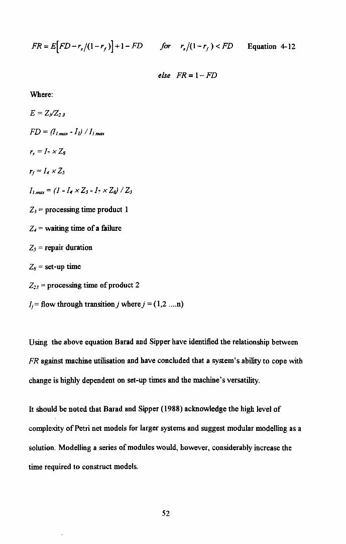
FR = E[FD-r,,/(I-rj )]+1- FD

Where:

E = Z3I"Z2.3

FD = (hmQ)t - 1/) / hmQ)t

rs = 17 X Zs

rf = 14 x Z5

hm(J)t = (J - 14 X Z5 - I: x ZtJJ / Z.3

Z3 = processing time product 1

Z4 = waiting time of a failure

Z5 = repair duration

Z8 = set-up time

Z23 = processing time of product 2

else FR = I-FD

Ij = flow through transition) where) = (1,2 .... n)

Equation 4-12

Using the above equation Barad and Sipper have identified the relationship between

FR against machine utilisation and have concluded that a system's ability to cope with

change is highly dependent on set-up times and the machine's versatility.

It should be noted that Barad and Sipper (1988) acknowledge the high level of

complexity of Petri net models for larger systems and suggest modular modelling as a

solution. Modelling a series of modules would, however, considerably increase the

time required to construct models.

52

4.4.2 Conceptual Models

A conceptual model is a representation of a system that requires interpretation to

yield any results. Dooner (1991) developed a conceptual model, the first stage of

which is illustrated in Figure 4.2, it shows a systems application domain and a

representation of expanding this domain. The system application doma.in represents

the scope of ability of the manufacturing system.

Original application

Extended application domain

domain ~

Figure 4.2 Expanding an Application Domain (Dooner 1991)

Dooner also states that at anyone time a system or machine can only be in one state.

This implies that the application domain consists of a number of discrete states that

Dooner calls state domains. Dooner also outlines the structure of his conceptual

model, which consists of many interconnecting "concept nodes" . Where, concept

nodes represent parts of the manufacturing system, this is shown in Figure 4.3 in

which concept nodes are used to model a universal profiling machine.

S3

Dooner proposed three concepts that need to be modelled to outline the flexibility of

a system in terms of its application domain where an application domain represents

what a system can do.

1. The range of the domain.

2. The time-effort to move around the domain.

3. The time-effort to expand the range of the domain

MACHINING SYSTEM NOOE

TABLE INTERFACE PITOOl

CAROUSEL

Figure 4.3 A Nodal Model of a Universal Proming Machine (Dooner 1991)

Associated with each node are three items of data, the concept name (e. g. part

program store), the flexibility descriptor(e.g. program switching time) and a value

for flexibility descriptor (e.g. five seconds switching time). It can be seen from Figure

4.3 that the nodal model is complex for a single piece ofmachillery. For an entire

system this would be extremely complex.

54

4.5 Summary

Sections 4.1 to 4.4 have examined a range of approaches to measuring flexibility.

The diversity and complexity of these approaches illustrate the difficulty in measuring

flexibility. The use of modelling techniques has the advantage of providing a richer

picture than a simple numerical measure, and thus better reflects flexibility's and

manufacturing's complex nature (Vernadat, 1996). The disadvantage of this

approach is that it is less easy to compare models for the purposes of decision

making.

The relationship between the types of flexibility measure explored in Sections 4.1 to

4.3 is summarised in Figure 4.4. This shows that numerical measures of flexibility are

direct measures of flexibility. These measures attempt to measure flexibility itself

Indirect measures of flexibility, which measure manufacturing systems performance

flexibility have two influences:

1. Types of flexibility.

2. Other Manufacturing system variables.

Financial measures of flexibility interpret the benefits of flexibility into a monetary

value and also have two direct influences:

1. The manufacturing system performance.

2. The commercial position of the company.

55

Other Manufacturing I---Mi

System Variables

Manufacturing System

Penormance

Con:onercial Position

Figure 4.4: Relationship between Measures of Flexibility

Fmancial Measures

of FleXlbility

Thus it can be concluded, that numerical measures of flexibility provide the most

direct measure of flexibility and are least influenced by distorting factors such as

manufacturing system variables other than flexibility and by the commercial position

ofthe company.

56

5. DEVELOPMENT OF A CONCEPTUAL MODEL

5.1 Introduction

This chapter descnoes the development of a conceptual model that is used to

represent the flexibility of a manufacturing system This model is then used to

provide a basis for the two numerical measurement methods that are developed in

Chapters 6 and 7. The conceptual model provides a context for the results of the

numerical methods, by relating the output from these two methods to the

manufacturing system being examined. The model, used in this way derives the

benefits associated with modelling techniques, identified in Chapter 4, in that it

provides not only a rich picture of the system flexibility but, also by using numerical

indicators, it avoids the disadvantages associated with using qualitative models, i. e. it

is able to directly compare alternative systems.

5.2 Model Development

The conceptual model developed for this research was derived from the model

proposed by Dooner (1991) ( Figure 4.2). in which an application domain is

described, which is an abstract concept to represent the ability of a manufacturing

system Here, the larger the application domain, the greater the ability of the system.,

and hence the greater its flexibility. In the model shown in Figure 4.2., Dooner

represents the concept of an application domain as a shaded area. For the model

derived in this research, Dooner's concept ofan application domain has been applied

57

specifically to the manufacture of products. This approach was chosen because

producing products is the primary function of manufacturing systems and it is

through products that customers principally perceives the manufacturer. Thus area J3

shown in Figure 5.1 represents the application domain of the manufacturing system in

terms of products it can make.

Figure 4.2 also shows the transition of a manufacturing system from an original

application domain to an extended application domain. This illustrates a different

type of flexibility which relates to changes in the ability of a manufacturing system.

In the current research this is shown as area a in Figure 5.1 which represents an

extended application domain of the products the manufacturing system could be

modified to manufacture.

In addition to the model shown in Figure 4.2, Dooner outlines the concept of

machine or system states. He asserts that a machine or system can have many states,

but can only be in one state at one time. Relating this to the conceptual model for this

research, area f3 in Figure 5.1, represents a set of states that the manufacturing

system must adopt to produce a current product. Each discrete state represents one

product. Summarising and expressing this more simply:

1. Area P represents the system states for products that the company currently

makes. This area is finite and is composed of discrete states, with each state

representing a specific product.

58

2. Area a represent the system states for products the company could make. This

area has a finite boundary, but consists potentially of an infinite number of different

products.

3. The area U lies outside area a and is the universe of all potential products. It is

infinite and unbounded.

U

Key:

a -Set of manufacturing system states for potential products

- Set of manufacturing system states for actual products

U - Universe of alJ products

Figure S.l Simple Model of Product and Mix Flexibility

Examining this model in terms of Slack's (1990) definitions of flexibility, range and

response, range can be identified in Figure 5.1 as the size of areas a and f3 .

Response can be defined into three types, identified in Table 5-1 .

59

Table 5-1: Response Types for the Simple Model

Response Description

types

Response 1 The time it takes to change between states in area f3 ie. the amount of time it

takes to change from manufacturing one product to another.

Response 2 The effort it takes to enlarge area 13 i e. the time and cost of introducing a new

product to manufacturing.

Response 3 The effort it takes to enlarge area a. ie. increasing the manufacturing

capabilities of the system

5.3 Development of the Simple Model of Product and Mix Flexibility

If the boundaries of areas a and f3 and the universe of states "U" are considered, it is

possible to identify the system states in area f3 (ie. those states which are required to

make the current product range), and thus it is possible to define the boundaries of

area f3. However, defining the boundaries of area a is less straightfolWard .

Area a is defined as the set of states required to make a potential product. Defining

these potential products presents a difficulty, because given sufficient effort, the

manufacturing system may be changed so radically as to be able to manufacture any

product, thus, it can be considered that the boundary between area a and ''U'' is

blurred.

60

In order to resolve this problem, the model shown in Figure 5.1 has been modified as

shown in Figure 5.2 such that the boundary between U and area ex is ambiguous.

System states which require little modification to the manufacturing system, are

differentiated from states which require large modifications to the manufacturing

system, by their distance from the edge of area J3. For example, the state which

relates to a new product that merely requires the programming of a CNC machine,

Figure 5.2 Model with Fuzzy Are~,-a

is placed near to the edge of area J3 i.e. in the darker area. The state for products that

require small increases in investment levels such as a jig are placed further away from

the edge of area J3. The states for products that require higher levels of investment

such as expensive production machinery, are placed still further away from area J3 i.e.

almost into the U area.

61

The modifications shown in Figure 5.2 results in set a possessing a fuzzy boundary

as opposed to a classical or crisp set boundary. The number of states in set p, known

as the cardinality, is equal to the number of products. The cardinality of set a is

infinite, because there are an infinite number of products possible within area a. This

coheres with theory for all fuzzy sets which states that cardinality is one of the

significant differences between classical sets and fuzzy sets (Ross 1995).

The existence offuzzy boundaries results in the model shown in Figure 5.2 being

difficult to convert into a working model, since these fuzzy boundaries are difficult to

express simply in terms of set membership. In order to overcome this problem area a

has been modified to a series of step changes as shown in Figure 5.3 .

These step changes are shown as a number of concentric bands for area a , with each

band representing varying levels of financial investment i.e. :

Figure 5.3: Model Showing Step Changes in Area a

62

aA represents the range of products that can be manufactured simply through

changes in the information system, such as process plans or computer

programs.

aB represents the range of products that can be manufactured through minor

hardware changes such as jigs and fixtures.

ac represents the range of products that would need a major cost investment

in the manufacturing system in order to produce them

The definitions of the costs of minor and major changes vary between industries. For

example a minor change may be defined as costing up to £500 and a major change

between £501 and £6,000.

5.4 Development of the Detailed Model

In order to use the conceptual model shown in Figure 5.3 to assess the flexibility of a

manufacturing system, the user would need to know the size of each area and cost of

responses I to 3 identified in Table 5-1 . Relating these responses and areas to

Slack's (1990) typology, mix range flexibility is equivalent to the size of area P and

mix response flexibility relates to response 1 in Table 5-1. Ahhough the area

occupied by the a sets relate to Slack's product flexibility, there is no direct

equivalence for the a sets, as Slack has not considered product flexibility in such a

63

way. Product range flexibility relates to the size of the a sets, as mix range flexibility

relates to the J3 set. Product response flexibility has been simplified from Slack's

(1990) original concept Le. from a continuous to a discrete measure as defined by the

individual a sets. The response between the a sets is inherent in their definition, i. e.

the response from aA to aB is identified by the response cost at which area aB is

specified.

5.5 Measuring Product Flexibility

To measure the a sets in Figure 5.3 it is necessary to consider the potentia] of a

manufacturing system in terms of what could be manufactured by the system To

achieve this there is a need to map the ability of the manufacturing system in terms of

the characteristics of the products each part of the manufacturing system can

produce. A method of achieving this is outlined in Chapter 7.

5.5.1 Measuring Mix Flexibility

To measure mix flexibility there is a need to measure both range and response. Mix

range flexibility, can be measured by identifying the number of products the company

produces (Muramastu, Ishii and Takahashi, 1985) and is represented by the size of

the poofofproducts from which products can be selected i.e. the cardinality of~.

This provides an adequate measure of mix range flexibility.

64

Mix response flexibility is represented by the ability to change the product being

manufactured (from the pool of products) e.g. the time it takes to change from

manufacturing one current product to another. The method outlined below to

measure mix response fleX11>ility builds on the work of Chryssolouris and Lee ( 1992)

who state that the flexibility for a machine is inversely proportional to the sensitivity

to change (STC) as shown in Equation 5.1. Where:

n

STC = LPn(XI )Pr(XI ) Equation 5-1 1-1

Where:

n= the number of potential changes,

i= the change index,

Xi= the ith potential change,

Pn(Xi)= the penalty of the ith potential change and

Pr(Xi)= the probability of the ith potential change.

Chryssolouris and Lee use this measure for long term changes in manufacturing

systems, and have examined the ability of alternative manufacture systems to produce

new products. This approach can, however, also be used for short term changes

which occur when changing from manufacturing one product to another. STC can be

evaluated in terms of mix response flexibility by regarding the change identified in

Equation 5.1 as a change from one product to another. The penalty incurred is the

65

set-up time and the probability of the change occurring is the probability of a set-up

being required. Substituting in to Equation 5.1:

If-I

STC= L~.durs Equation 5-2 If-I

Where:

Ps = the probability of a set-up s occurring

durs = the duration of set-up s

t = the number of different set-ups

Thus STC is expressed in time- l, and flexibility in units of time. In order to calculate

the STC and hence mix response flexibility, there is a need to evaluate each of the

components Ps, durs and t. The number of different set-ups, t, can be found from

production data. The duration of a set-up, durs, can be timed in the case of an

existing system or estimated in the case of a proposed system. The probability of a

set-up occurring P i has to be taken from historical data or calculated from the

probability of a product occurring. However, it should be noted that a product

occurring does not always mean a set-up is required.

In order_to quantify Ps i.e. the probability of set-up "s" occurring, an assumption as

to when a set-up occurs needs to be made. For the purposes of this model it is

assumed that when a product follows an identical product, no set-up occurs. Shown

66

below in Figure 5.4 is an example of the occurrence of set-ups for four products, j, k,

landm

jkklmkjjmkj

1 1 1t 1 1 t 11 time

1 = set-up

Figure 5.4 Occurrence of Set-ups

It can be seen that if these products are re-ordered then a varying number of set-ups

may occur. Thus for any set of products the order of products will affect the total

time spent in set-up. To minimise set-up for a group ofproducts, all the same type of

product should be grouped together. Thus for the group of products shown in

Figure 5.4 the total number of set-ups can be reduced to four, one for each type of

product, thus the order will be iilikkkklmm A scheduler would naturally try to group

the same products together, reducing the overall time spent in set-up. However,

market forces often force the sequence of products into a less optimal order.

Thus for a group of products the total time spent in set-up is not fixed, and it is

dependent on the order of the products. Therefore, for a group of products, a set-up

time per product may either be calculated for a specific sequence of products, or a

mean and standard deviation may be calculated for all the different possible sequences

67

of the products. By generating the set-up time all possible sequences it can be shown

that the distnbution generated approximates to a normal distnbution. Adopting the

distribution approach a method for measuring the mean STC and the standard

deviation associated with it is developed in Chapter 7.

68

6. MEASURING PRODUcr FLEXIBILITY

For practical use, the conceptual model outlined in Chapter 5 needs to be interpreted

in a quantitative manner. This chapter outlines the first stage of this interpretation by

identifying a method for measuring product flexibility, represented in the conceptual

model by the a. areas.

6.1 Requirements for a Product Flexibility Measure

In order to comply with objective 5 stated in Section 1.5, (i.e. that a measure of

flexibility should be able to assess flexibility in different types of industry), it is

important that the product flexibility measure should be able to cope with different

types of manufacturing system. Hence, the measure should be able to :

1. Compare systems with different numbers of machines.

2. Cope with parallel and alternative processes.

3. Reflect lack of flexibility for sub-systems that have no ability to manufacture a

particular type of product.

4. Reflect the relative importance a manufacturer may place on having the potential

to develop particular types of product.

69

6.2 Theory of Calculating Product Flexibility

A measure of the product flexibility of a manufacturing system, needs to assess the

ability of the system to make different types of products. In order to achieve this, the

manufacturing system is divided into simpler sub-systems, such as individual machine

tools. Each sub-system is then considered in terms of its ability to manufacture

different types of product.

In this respect, when assessing the ability of a sub-system to make potential products

it is necessary to identifY criteria by which the individual sub-systems will be

measured. This aids consistency of measurement between sub-systems and providing

the correct criteria is chosen, ensures that value is placed only on the potential to

manufacture products which contribute to manufacturers' competitiveness.

The criteria for assessment of the sub-systems is based on a number of product

characteristics such as size, or material type. These characteristics normally relate to

the physical attributes of the product and often identify the processing requirements.

These characteristics are then expressed as specific criteria, such as numerical ranges

and it is against these criteria, defined within a product characteristic that sub-systems

are assessed.

70

Identifying product characteristics can be achieved using a suitable group technology

classification scheme such as VUOSO or YUSTE (Gallagher and Knight, 1973).

Using these schemes an example of a characteristic would be size of maximum

product diameter, with the specific criteria being 0 to 50mm, 50mm to IOOmm and

greater than IOOmm. A characteristic's criteria may also be defined qualitatively, for

example for the characteristic shape the criteria could be rotational, flat, extruded or

prismatic.

From Figure 5.3 it can be seen that the evaluation of sub-systems against the specified

criteria needs to be performed in terms of the graduations of the <X rings. This is

performed by denoting an A, B or C for each sub-system against a particular criteria.

Where:

I. An "A" represents a sub-system that can achieve the criteria with no changes to the

manufacturing system

2. A ''B'' represents a sub-system that can achieve the criteria with small to medium

cost changes

3. A ''C'' represents a sub-system that can achieve the criteria with medium to high

cost changes.

Table 6-1 illustrates for a small FMS an example of assessing the characteristic

"component diameter". The diameter of the product the manufacturing system

71

currently makes is 30mm, hence all the sub-systems are categorised as "A"s for the 0-

4Omm. criteria. However, it can be seen from Table 6-1 that as the diameter increases

it becomes more expensive to enable each of the sub-systems to deal with these larger

diameters. It can also be seen that the robots have a particular problem in this

respect. In practice this arises because the robots have the same type of gripper that

can only handle up to 40mm component diameters.

Table 6-1 Example of Categorisation for a Characteristic

Characteristic: Dimensions (in mm) component diameter

Sub-system 0-40 40-80 80-200 200-400

CNClathe A A C C

CNCmi1ler A A C C

Gauge A A A C

Visual inspection A A A C

AGV A A A A

RobotRI A B C C

RobotR2 A B B C

RobotR3 A B C C

RobotR4 A B B C

Carrousels A B B B

Software A A A A

Output station A B B B

Input station A B B B

72

To fully assess the product flexibility of a manufacturing system it is necesSllI)' to

categorise the sub-systems in terms of several characteristics. The table for each

individual characteristic is termed a "characteristic layer". These layers build up into

a three dimensional matrix as shown in Figure 6.1

Sub­systems

Criteria .. ~ Characteristic

"-"", layers

'""

Figure 6.1: Three Dimensional Matrix of Product Flexibility

6.3 Calculating the Total Response Cost

From the three dimensional matrix shown in Figure 6.1 a single comparative measure

can be developed. This measure can be developed by assuming that the manufacturer

would eventually want to manufacture all possible products. It is then possible to

calculate the cost of incorporating all the characteristic criteria in the manufacturing

system A cost is allocated to each of the classifications A, B and C and the total

73

summed for the system. The costs allocated to each of the categories is determined

by the user, and should reflect the average cost of implementing each of the category

of changes. This measure is termed ''the total response cost" or TRC.

Table 6-2 shows the calculations for three FMS' s in which the cost allocated to A's

is zero, to D's is £500 and to C's is £3000. The product of the number of each A, B,

or C and its cost allocation is summed to give a total cost.

Table 6-2: Calculations of Product Flexibility for Three Alternative Systems

FMS 1 FMS2 FMS3

No of A's 109 109 XO=O 100 100XO=O 113 113XO=O

No ofB's 19 19X 500 = 9500 13 13X 500 = 11500 8 8X500=4000

No ofe's 35 35X 3000 = 105000 40 40X3000 = 41 41X 3000=116000

120000

Total (TRC) 114500 131500 130000

It can be seen from Table 6-1 that FMS 1 has the lowest total cost and is therefore

the most flexible system with FMS 2 having the highest total cost and therefore is the

least flexible system in terms of product flexibility. It should be noted that the totals

calculated in Table 6-2 are an inverse measure of flexibility as the system with the

highest TRC has the least flexibility.

74

6.4 Development of Total Response Cost

Outlined in Section 6.3 is a basic method for assessing product flexibility and the total

response cost. This section examines this measure with respect to the requirements

identified in Section 6.1 and develops the measure where necessary to meet these

requirements.

6.4.1 Comparing Systems with Different Numbers of Sub-systems

Normally designers of manufacturing systems, need to compare alternative systems,

which have differing numbers of machines, or sub-systems. It is therefore necessary

to investigate whether systems that have different numbers of machines or subsystems

can be compared using the TRC measure.

The TRC is dependent on the number of machines in the system, each additional

machine can contribute a cost to the TRC. This however, does not present a

problem, because, it is important that the TRC reflects the relative costs that may be

incurred through either a system having fewer complex machines that require high

cost changes, or a system having many simple machines that all require simple

modifications to allow a product introduction.

75

6.4.2 ParaDel Processes

It is likely that some manufacturing systems will contain processes that operate in

parallel. Here some individual characteristic criteria may not be appropriate for all

parallel processes. For example if two sub-systems operate in parallel, with one

processing liquids and the other solids, it would not be senSlole to expect the sub­

systems that processes liquids to be able to deal with different hardness materials,

equally it would not be senSlole to expect the sub-systems that processes solids to be

able to pump. Thus it is necessary to identify these inappropriate criteria, in the

matrix as nla which has a cost weighting of zero.

6.4.3 Sub-systems that Cannot Achieve a Criterion of a Characteristic

It can be anticipated that despite a characteristic being appropriate, a machine or sub­

system may not have the capability to achieve a criteria without replacing the machine

or sub-system entirely. This has two implications, firstly there should be an upper

limit to the cost range of a C change to a machine. Ifthere is not, then any change

could be incorporated into the system, by replacing the machine or sub-system with

another which is capable, in which case any criteria could be achieved and the outer

a c boundary shown in Figure 5.3 becomes fuzzy to incorporate the universe of all

possible products. The second effect is that machines that breach the upper limit for

C costs, should have a detrimental effect on the measurement of product flexibility

i.e. by increasing the total response cost. Hence an additional, high cost weighting

76

should be allocated if a sub-system cannot achieve a criteria. For example, the cost

weighting for A, B and Cs may be £0, £500 and £3000 and if the user wishes to

discriminate heavily against sub-systems that cannot achieve a particular criterion, the

weighting applied could for example, be in the region of £200,000. If the user wishes

to consider more favourably systems which cannot achieve a criterion, then the

weighting may be much less e.g. £6000. When a sub-system cannot achieve a criteria

it is indicated in the matrix as nip.

6.4.4 Weighting of Characteristics

To reflect the relative importance placed on possessing the potential to develop

particular types of product, a manufacturer will regard some criteria as more

important than others. For instance, ifa company regarded the ability to make

components with larger diameters as likely to have more potential value than other

characteristics, the company would want to be able to identify systems that have the

ability to make this type of product.

This requirement can be provided by introducing a weighting factor V. Such that all

A. B and C' s from the characteristic "component diameter" use a cost factor that has

been multiplied by V. If V> I this will tend to increase the relative cost of the

characteristic, and so favour systems which have less costs associated with

developing products with this characteristic.

77

6.5 Calculating TRC

Consider three systems X, Y and Z, which have differing numbers of machines and

hence different numbers of cells. Let the A, B, C and nip categories be costed at £0,

£1,000, £4,000 and £10,000. Table 6.6 shows the number of A, B, C, nla and nip

cells for each system One characteristic, colour, is deemed to be of more importance

that the other characteristics, and so has an additional weighting of 1.2.

Table 6-3: Summary of Data for Systems X, Y and Z

System X System Y System Z

T otaI number of cells 150 170 200 No. of A's 81 86 90 No.ofB's 22 10 20 No.ofC's 35 35 40 No. of nip cells 12 35 40 No ofnla cells 0 4 10 No. A's in Colour characteristic 14 16 15 No. B's in Colour characteristic 5 10 5 No. C's in Colour characteristic 3 5 5 No. of nip cells in Colour characteristic 2 5 5 No. ofnla cells in Colour characteristic 0 1 0

TRe (in £) 289400 516000 595000

Using the data sho\W in Table 6-3 the TRC for each system has been calculated using

the procedures sho\W in Appendix 1. It can be seen from Table 6-3 that

78

system X has the lowest TRC (£289,400) and therefore the highest product

flexibility, system Z has the highest TRC (£595,000) and therefore the lowest product

flexibility.

6.6 Verification and Validation

A useful method offace validation for this application is to substitute relatively simple

values into the model (Robinson 1994). These values allow the user to predict what

the output of the model should be. It is often useful to use extremes of possible

values as inputs, as the result from using this data can often be predicted. In this case

two situations can be modelled:

1. The system that has the ability to make all possible changes. It can be predicted

that this system has a very high level of flexibility. For example if there are 200

cells all would be A's and there would be no nla or nip cells. This would give a

TRC of zero which indicates a high level of flexibility.

2. The converse system, in which no changes are possible. This system will have a

very low level of flexibility. There would be the minimum number of A's, e.g. 60,

which is the capability that is required to make the current product range. The

remaining 140 cells would be rated as nip. Using the same weighting used for

systems X, Y and Z the TRC is £1,400,000 which indicates a low flexibility.

79

6.7 Summary of Measuring Product Flexibility

Product flexibility may be initially assessed by developing a three dimensional matrix

as shown in Figure 6.1. A single measure can then be derived from this matrix which

allows comparison of product fleXJ.bility between systems. This measure is termed

the total response cost (TRC) and is an inverse measure of flexibility i.e. a low TRC

indicates high flexibility. Individual TRC measures need to be developed using a

manufacturers own product characteristics, criteria and cost categories.

80

7. MEASURING MIX FLEXIBILITY

This chapter outlines a method for measuring mix flexibility which is defined as the

ability to change between the products that a company currently makes. This is

represented by the J3 area in Figure 5.3. The measurement method developed in this

chapter is tested on three hypothetical manufacturing systems A, B and C. The

results obtained are validated against data from a simulation.

7.1 Manufacturing Systems A, B, and C

The three systems used to test the method developed are as follows:

1. System A is a single machine system The simplicity of this system is used to

highlight basic flaws in the method.

2. System B is a simple multiple machine manufacturing system where products

occur with equal probabilities. This system is used to ensure the method is valid

for systems with several machines.

3. System C is a more complex multiple machine system with products that occur

with unequal probabilities. This ensures that the method can cope with the

complexity inherent in real manufacturing systems

81

7.1.1 System A

System A consists of a single machine on which four parts j, k, I, and mare

processed The parts have an equal probability of being the next part to be

processed. The durations of the set-up for each part val)' and are shown in Table

7-1.

Table 7-1: System A Data

Product Duration of set-up in Probability of occurrence minutes

j 7 0.25

k 5 0.2S

I 10 0.2S

m 6 0.2S

7.1.2 System B

System B consists of five machines and four products j, k, I, and m It is designed

to represent a simple manufacturing cell. All products are processed within the cell,

however, not all the machines are used for each product. The process routes for

each part are shown in Figure 7.1, with part j for example being processed on

machines 1 and 3.

82

l ................... ~~~k···~~B····· . ;J ... chine lE~"-' machine2 .~~~>'" ~j 'J~~~31

1

8 _····_-1····8··· ....... .,,> ....... .. . ." ,m ." ... -. m machine 5 -- . - . m - . machine 4 ~ ... k ./.,,'"

... --·k·---- - ---------- ... -

Figure 7.1: Process Routes for System B

The products have an equal probability of being the next part to enter the cell, and

the set-up durations are shown in Table 7-2.

Table 7-2: System B Data

Set-up duration in minutes

Product Probability of Machine 1 Machine 2 Machine 3 Machine 4 Machine 5 occurrence

j 0.25 5 10 7 6 -k 0.25 4 - 5 6 -1 0.25 - 8 10 - 3

m 0.25 7 8 6 5 6

83

7.1.3 System C

This system has the same process routes as system B, however, the probabilities of

a product entering the cell are not equal as for system B, but vary as shown in Table

7-3.

Table 7-3 System C Data

Product Probability of occurrence

J 0.2

k 0.4

I 0.1

m 0.3

7.2 Method for Measuring Mix Response Flexibility

Chapter 5 identified the work of Chtyssolouris and Lee (1992) as a basis for

measuring flexibility. They stated that the flexibility of a machine is inversely

proportional to its sensitivity to change (STC). Chtyssolouris and Lee applied their

model to measure for long term flexibility. Section 5.3.2 identifies how this model

can be modified to provide a short term measure for mix flexibility. Equation 5.2

is derived from this modification and is shown here as Equation 7.1 for ease of

reference.

9=1

STC= L~.durs Equation 7-1 9~1

Where:

84

Ps = the probability ofa set-up s occurring,

dur s = the duration of set-up s, and

t = the number of different set-ups.

As identified in Section 5.2.3 in order to calculate STC and hence mix response

flexibility, there is a need to evaluate each of the individual components Ps, durs

and t. The number of different set-ups, t, can be found from production data. The

duration of a set-up durs can be physically measured in the case of an existing

system or estimated in the case of a proposed system The probability of a set-up

occurring Pi has to be taken from historical data or calculated from the probability

of a product occurring.

Section 5.3.2 also identifies that for a group of products, the order in which the

products are processed will affect the total set-up time. This means that there is a

need to develop:

1. A mean STC per product for the distribution of all sequences of product based

on the probability of a product occurring.

2. A standard deviation of the STC distribution.

The probability of a set-up occurring Ps, can be calculated from the probability of a

product Pi occurring. When performing this calculation, account must be taken of

the probability of the same product occurring consecutively, i.e. when no set-up is

85

required, as shown in Figure 5.4. Thus the probability ofa set-up occurring is

equivalent to the probability of a product occurring Pi followed by a dissimilar

product probability (J -P;). The probability of a set up occurring is therefore:

Equation 7.2

Hence Equation 7.1 becomes:

1-

MSTC= L~(I-~)durl Equation 7.3 1-1

Where:

MSTC = the mean sensitivity to change (for all sequences of product)

n = the number of different products.

It should also be noted that the duration of a set-up durs is the same as dur; the

set-up duration for product i.

The standard deviation may be calculated using the generic formula for the variance

ofa probability distribution (Freund and Simon, 1992) I.e.:

(52 = ~:<x - Jll./(x) Equation 7.4

Where:

(5= standard deviation,

f.J = calculated mean,

86

x = the variable, and

f(x) = the function from which the mean is calculated.

Substituting the probability of a set-up occwring, Pi(J -Pi )for f(x) with, MSTC for

p and dur s for x provides equation 7.5:

/.11

(J" = L (du'i - MSTC) 2 ~ (1- ~) Equation 7.5 /-1

U sing Equations 7.4 and 7.5 the mean and the standard deviation for the sensitivity

to change may be calculated for a single machine.

7.2.1 Multiple Machine Systems

In order to model systems B and C it is necessary to combine data from individual

machines. In this respect, for a system in which all machines are in series and all

products are processed on all machines, i.e. effectively a flow line, the MSTC and

SD are calculated as follows:

j=m

MSTCy = L MSTCj Equation 7.6 j=1

jam

SDy = LSD~ Equation 7.7 I

Where:

m = the number of machines,

MSTC y = the mean sensitivity to change for the system in series,

87

MSTCj = the mean sensitivity to change for a machine),

SDy = the standard deviation for STC for the system in series, and

SDj = the standard deviation for STC for a machine)

For systems where products have different processing requirements, the probability

of using a particular machine, needs to be taken into account. Thus Equations 7.6

and 7.7 are modified to Equations 7.8 and 7.9 which now include the probability

that a generic part will visit machine).

j=m

MSTCT = L PjMSTCj Equation 7.8 j=1

}-IJI 2

SDT = ~ljSDJ Equation 7.9

Where:

MSTCT = the mean sensitivity for the parallel system.

SDT = the standard deviation for STC for the parallel system. and

Pj = the probability of a machine) being used for a part.

7.3 Validation Method

In order to validate the results from the method outlined in section 7.2 it is possible

to compare them against similar measures (Robinson 1994). In order to develop

suitable similar measures, MSTC must be considered as the mean set-up time for a

set of products Q for all orders of Q. i. e.:

88

• x MSTC=L-1 v

Equation 7.10

Where:

set 91 ={ x 1 x is mean set-up for an order of the products in 0 },

v = 1911, and

o -a set of products.

The size of set 91, i.e. the value of V, becomes very large even for modest sizes of

set O. For example, for 101= 50 with 5 different products, and 10 of each type of

product, 91 has 2.5 x 1061 members. This is derived from the formula for number of

permutations in a set n, where there are k distinct objects and rk is the number of

each distinct objects i.e.:

n! number of permutations = ----

r 1 ·r2 • •••• ·rl. Equation 7. 11

If a subset of91 can be generated by another method, the mean of the subset

members can be compared with the MSTC. This subset of data can be generated

using a computer based manufacturing simulator, in this case using Promodel

(1993). By inputting a product stream i.e. a specific order of set 0 into the

simulation, x the mean set-up time per product can be calculated, and hence one

member of set 91 is generated. Using this procedure for a number of product

streams i.e. the same mix of products in a different order, a subset of91 is

89

generated. The mean and standard deviation of the subset elements can be

calculated and then compared with the MSTC and the SD derived from Equations

7.3 to 7.9.

7.4 Results

7.4.1 Results for System A

Equations 7.3 and 7.5 were applied to system A using the data from Table 7-1. and

a simulation model of system A was also developed. To generate a set of data from

the simulation model, thirty simulations were conducted, each using the same mix of

parts but in a different sequence. The results from both methods are shown in

Table 7-4. Detailed calculations are shown in appendix 2.

Table 7-4 Results for System A

Mix Response Simulation Measure

Measure

MSTCin mins 5.250 5.267

SD in mins 3.437 3.443

7.4.2 Results for System B

The mix response method for measuring flexibility was applied to eacb oftbe

machines in system B and the Equations 7.8 and 7.9 outlined in Section 7.2. 1 were

used to obtain an overall measure. The results for each machine are shown in Table

7-5.

90

Table 7-5 Summary of Calculations for System B

Colunm 1 Colunm2 Colunm3 Column 4 Column 5

Mach- Probability of MSTCfor Variance (02

) of Column 1 x Column 1 x using machine machine MSTC for each Column 2 Column 3 me

machine

1 0.75 3.56 7.28 2.67 5.46

2 0.75 5.78 17.11 4.33 12.83

3 1 5.25 11.81 5.25 11.81

4 0.75 3.78 7.28 2.84 5.46

5 0.5 2.25 6.19 1.125 3.09

Sum of column 5 38.67

System SD (Sum of column 5)112 6.22

System MSTC (Sum of column 4) 16.2

A simulation model of system B was developed and thirty different sequences of

parts were input into it. Table 7-6 shows a comparison of the results obtained from

the simulation and the calculations shown in Table 7-6.

Table 7-6 Results for System B

Mix response Simulation measure measure

MSTC in mins 16.21 16.10

SD in mins 6.22 7.38

91

7.4.3 Results for System C

The method for measuring mix response flexibility was applied to system C and a

simulation model was developed. 30 different sequences of product were used with

the simulation. The results for the individual machines are shown in Table 7-7, and a

comparison between the mix response measure and the simulation measure is shown

in Table 7-8.

Table 7-7: Summary of Calculations for System C

Column 1 Column 2 Column 3 Column 4 Column 5

Probability of MSTCfor Variance (02) of Column Ix Column 1 x

using machine machine MSTC for each Column 2 Column 3 machine

A 0.75 3.41 7.55 2.56 5.66

B 0.75 5.33 18.67 4 14

C 1 4.48 10.33 4.48 10.33

D 0.75 3.63 7.49 2.72 5.62

E 0.5 1.69 5.59 0.84 2.80

Sum of column 5 38.406

System SO (Sum of column 2)1/2 6.20

System MSTC (Sum of column 4) 14.60

Table 7-8 :Results for System C

Mix response Simulation measure measure

MSTC in mins 14.60 14.66

SD in mins 6.20 7.27

92

7.~ Validation of Results

Two methods of validation are used for the results obtained from the mix response

measure. The first method is face validity (Robinson 1994) which is to examine the

output of the mix response measure in terms of what should be estimated or

expected. The second method is comparison with the results generated from

simulation models as identified in Section 7.3.

7.~.1 Face Validity

Examining the outputs in terms of what would be logically expected is an acceptable

method offace validation. In this respect, examining the resuhs from Table 7-4, a

MSTC of 5.25 minutes is slightly lower than might be expected as the mean of the

set-up times for the product types k to m is 7 minutes. However, when it is

considered that there will be occasions when no set-ups occur, such as when two

products are manufactured sequentially, then it could be anticipated that the mean

set-up time per product (MSTC) would be lower than 7 minutes. This validation

technique can be extended to include using input data which would provide an

obvious output. For example if the set-up time is zero for all products then the

system has infinite mix response flexibility. Using this method, substituting into

Equation 7.3 the expected result of zero for MSTC is obtained, which represents

infinite mix response flexibility.

93

7.5.2 Comparison of Mix Response Flexibility with Simulation Results

The purpose of generating data from the manufacturing simulation is to allow

validation of the mix response flexibility measure. To validate the measure it is

necessary to prove that differences between output data from the simulation and

the mix response flexibility measure, are insignificant. This can be achieved using an

hypothesis test, a z-test is used for comparison of means and an F-test for

comparison ofSD's. The z test is a follows:

equation 7.12

Where:

XI = the mean of population 1,

01= the standard deviation of population 1,

nl = the size of population 1,

X2 = the mean of population 2,

02= the standard deviation of population 2,

n2 = the size of population 2, and

0= the intended difference between the mean of population 1 and population 2,

in this case o.

94

In order to accept the null hypothesis that there is no significant difference between

Xl and X2, at a confidence level of 0.05, Z must satisfy the following conditions:

-1.96~ Z ~ 1.96

For the hypothesis test on the standard deviation of the resuhs, the F test is as

follows:

CJ2 u 2

F = -lor F = _2 such that F<I 2 2 u 2 U 1

In order to accept the null hypothesis that there is no significant difference between

the standard deviations at a confidence level of 0.01, F must satisfy the following

condition:

F < Critical value for F

The critical value for F is specified by standard statistical tables and depends on the

degrees of freedom for each sample.

Table 7-9 shows the results for z test for systems A, B and C. The null hypothesis

can be accepted for all the systems, hence the differences between the means can be

considered insignificant.

95

Table 7-9: "z" Test Results

Population values Xl - X2- 'u 2 u 2 z- Can null _I +_2 hypothesis be

~ n l n2 accepted?

System A Mix response 0.017 0.629 0.027 Yes flexibility, n = 00

Simulation, n = 30

SystemB Mix response 0.115 1.348 0.085 Yes flexibility, n = 00

Simulation, n = 30

System C Mix response 0.066 1.7618 0.038 Yes flexibility, n = 00

Simulation, n = 30

The calculations for the F test are shown below in Table 7-10. From this data it can

be seen that the differences between the standard deviations of the groups of data

can be considered insignificant.

Table 7-10: "F" Test Results

Critical value of F u 2 u 2 Can null hypothesis be F=-I or F=_2 accepted? 2 2 u 2 u l

System A 1.7 1.005 Yes

SystemB 1.7 1.412 Yes

System C 1.7 1.376 Yes

96

Section 7.5.2 therefore demonstrates that there are no significant differences

between the measure for mix response flexibility and the simulation results. This

further validates the mix response flexibility measure.

97

8. INDUSTRIAL APPLICATION

The purpose of this chapter is to examine the industrial application of the conceptual

model outlined in Chapter 5, and to demonstrate that measures for product flexibility

and mix response flexibility can be applied in industry. Successful industrial

application of the methodology will demonstrate whether the aims 1,3 and 5

identified in section 1.5, can be achieved i. e. that

1. The data for the input values must be easy to obtain

2. Methodology must be easy to use

3. The measure must be able to assess flexibility across a range of industries

In order to demonstrate the ability to measure across a range of industries it is

important to apply the model and measurement methods in different types of

company. Thus Bostik Ltd and Richard Kimbell Ltd were selected for their

contrasting manufacturing environments.

Bostik Ltd. manufactures sealants and adhesives and is part of a large chemical and

petrochemical group, Total Ltd. Bostik's product range is relatively stable and is

manufactured on a high volume flow line that consists of up to seven stages of

manufacture.

Richard Kimbell Ltd is an owner managed private company, which produces a wide

range of pine furniture mainly for export or for sale in its own retail outlets. The

product range is constantly changing and is manufactured in small batches.

98

8.1 Bostik Ltd.

Bostik is a manufacturer of adhesives and sealants for both the industrial and

consumer markets. It has an annual turnover of £22m and employs 180 people.

Consumer products include Blu-tack, the AIl-Putpose adhesive range and glue-sticks.

Industrial sectors served include footwear, automotive and the construction

industries. Major manufacturing activities include the chemical reaction of polymers

and polyesters, mixing and extrusion of sealants and packaging of consumer

products.

8.1.1 Manufacturing Processes

The manufacturing process shown in Figure 8.1 can be divided into three main stages,

react, crystallise and form. The first stage reaction, is carried out within three

alternative reactors 2tonA, 2tonB and Mowlem At this stage the materials that make

up the product are combined by chemical reaction in the controlled environment of an

enclosed reactor. Reacted products are then either decanted into drums if they are

sold as liquids, or crystallised if they are sold as solids. Varying crystallisation rates

are available due to a range of temperature controlled environments. The final stage

is forming into reels, granules or chips. In addition, a proportion of granulated

material may be further processed, by extrusion and then reeled or chipped.

99

Process st~ge +-React~~4 Crystallise~ 4 Form •

: : "I Dry I

I 2 ton A ~r-:

J Freeze r ; ~ Extruder 1 4 Reel 1 12 ton B ~ ~ Cool I t -;{Granulator f-. Extruder 2 . 1

~J 1 Warm I ~ Extruder 3 L.I Chip

IMowiem ~ JDrumsl

Figure 8.1 Summary of Bostik Processes

100

Set-ups occur when there is a need to clean out process machinery between different

products, in order to reduce cross contamination between products. The equipment

that requires cleaning are the reactors and the extruder. Traditionally products were

processed in long product runs due to the long set-up times associated with cleaning

out between products.

8.1.2 Conceptual Model Applied to Bostik Ltd

The conceptual model applied to Bostik Ltd is influenced by the cost and life of plant

equipment in the chemical processing industries. Plant equipment of this type tends

to have a high initial cost, but a long operational life (Wahers 1997). This results in

the difference between the cost of ''B'' cells and ''C'' cells which is greater than the

difference in other industries. This is reflected by the relative sizes of area ab and a c

shown in Figure 8.1. Within Bostik Ltd "B" cells represent small to medium cost

changes to the plant processing equipment such as changing a valve type. The "e"

cells represent medium to high cost changes such as changing the type of reactor

vessel, or replacing the type of heating process.

101

Figure 8.2: Conceptual Model of Bostik Ltd

8.1.3 Calculation of Mix Response Flexibility

Results were calculated for each stage of the production process in which a set-up

occurs i.e. the reaction stage and the extrusion stage. To calculate the MSTC and

the SD for each process Equations 8.3 and 8.5, shown below, have been used.

I=n

MSTC = IP;(I- ~)durl Equation 8.3 1=1

i=n

a = I(dulj - MSTC)2 ~(1- PJ Equation 8.5 ;=1

Where:

Pj = the probability of a product i occurring,

dur,= the duration of the set-up for product i ,and

102

n = the number of different products.

In order to evaluate the components of these equations it is necessary to obtain the

duration of each set-up and the probability of each product occurring. At Bostik the

probability of occurrence of products was obtained from manufacturing data collected

over a period of two months, this period represented a typical production cycle. Set-

up duration data for the reactors was obtained from existing process information.

The data for set-up durations for the extruders was more complex. This is because

the duration of the set-up procedure for a product is influenced by the chemistry of

the previous product. At Bostik Ltd there are two types of product manufactured,

polyesters and polyamides. A table showing the set-up times from one type of

product to another is shown in Table 8-1.

Table 8-1: Set-up Durations on Extruders

~ Polyester Polyamide From

Polyester 0.75 hrs 2 hrs

Polyamide 1 hrs 0.75 hrs

Thus a single value of dur;cannot be specified for product i, therefore it was

necessary to take into account two possible values of dur; when calculating the

MSTC and SD. This was achieved by calculating both the probability that a specific

product will be preceded by a polyamide and calculating the probability that the same

product will be preceded by a polyester. This method is equivalent to treating a

103

single product as two separate products. The calculations for this method are shown

in Appendix 3.

It can be seen from Figure 8.1 that the reactors 2tonA, 2tonB and Mowlem process

are in parallel, and thus the data from these items of equipment needs to be combined

to obtain a MSTC and SD for this stage in the process. Similarly after the

crystallisation, parallel processes occur. To combine data from parallel processes

Equations 8.8 and 8.9 are used.

}=m

MSTCT = ~ P.MSTC. L.J J J Equation 8.8 }=1

SDT = IljSD2

,-1 J

Equation 8.9

Where:

m = number of parallel machines,

MSTC;= the mean sensitivity for machine).

SDj = the standard deviation for STC for machine).

MSTCT = the mean sensitivity for the parallel system,

SDT = the standard deviation for STC for the parallel system, and

Pj = the probability of a machine j being used for a part.

104

Thus applying equation 8.8, at the reaction stage, the number of parallel machines Ill.

three. The data for MSTCj and SDj is shown in Table 8-2. The probability Pj can be

calculated using the number of batches that pass through each individual machines.

Thus the probability that the 2tonB reactor will be used is 0.26 i.e. number of batches

that go through the machine divided by the total number of batches. With this data the

MSTCT can be calculated for the reaction stage. A similar approach needs to be

taken with the extruder except that as no set-up occurs in the ahemative route all that

is required it to multiply the machine MSTC and the variance by 0.27 (Pj the

probability that a product will go through each extruder).

Table 8-2 provides a summary of the calculations for the system MSTC and SD with

Appendix 3 providing details of these calculations. From the table it can be seen that

the MSTC for the manufacturing system at Bostik is 2.952 hours and the SD is 3.581

hours. This is a relatively low value when compared to the overall product

processing times which are of several days duration.

Table 8-2 Results for Mix Response Flexibility for Bostik Ltd

Colunm 1 Column 2 Column 3 Column 4 Column 5

Machine MSTCj in SD-in J p.

J MSTC xp· J J (SD-)2Xp· .I J

hours hours

Mowlem 3.880 4.511 0.61 2.366 12.410 2tonB 1.243 1.087 0.26 0.318 0.303 2tonA 0 0 0.13 0 0 Extruder 1 0.998 0.646 0.27 0.268 0.112 Extruder 2 0.998 0.646 0.27 0.268 0.112

Extruder 3 0.998 0.646 0.27 0.268 0.112

Sj'stem SD {Sum of column 5)112 in hours 3.581 System MSTC ( sum of column 4) in hours 2.952

105

8.1.4 Calculation of Product Range Flexibility

The product flexibility matrix is shown in Table 8-3. The product is descn"bed in terms

of the batch volume to be manufactured, the viscosity and the form. Using the

method outlined in Chapter 7, Table 8-4 has been generated which shows the Total

Response Cost for the system is £128,000. To calculate this value A's are costed at

zero, B's are costed at £500 and C's at £10,000. The value ofnla cells was zero.

The values for A changes, B changes and C changes were derived from the estimated

average cost of implementing changes within each of the categories.

106

Table 8-3: Bostik Product Range Matrix

--_ .. _- --

Equipment Volume output in tonnes Viscosity in poise Form

0-0.5 0.5-1 1-2 2-3 3-4 20- 200- 1000- liquid block reeled granulated pellets 200 1000 50,000

Mowlem C B B A C A A A A A A A A 2TA B A A B C A A C A A A A A 2TB B A A C C A A C A A A A A Granulator I A A A A A nla A C nla nla A B A Granulator 2 A A A A A nla A C nla nla A B A i

Granulator 3 A A A A A nla A C nla nla A A A I

Extruder 7 A A A A A nla A B nla nla A nla A ,

Extruder 8 A A A A A nla A B nla nla A nla A Extruder 9 B B B A A nla A B nla nla A nla A Reeler 7/8 A A A A A nla A A nla nla A nla nla Reeler 9 A A A A A nla A A nla nla A nla nla Chipper big A A A A A nla A B nla nla nla nla A Chipper sm A A A A A nla A B nla nla nla nla A Dryer A A A A A nla A A nla nla nla nla A !Hot Room A A B C C nla A A nla A A A A Cold Room A A A A A nla A A nla A A A A Trays A A A A A nla A A nla A A A A

107

Table 8-4: Calculations for Product Flexibility at Bostik Ltd.

Category of cell No. of each Cost per cell Cost for each

category of cell (£'s) category of cell (£' s)

A's 145 0 0

B's 16 500 8,000

C's 12 10,000 120,000

nip cells 0 not specified 0

nla cells 52 0 0

Total Response Cost £ 128,000

8.2 Richard Kimbell Ltd

Richard Kimbell Ltd. manufactures a wide range of wooden furniture and has a sales

turnover of £6m and a workforce of 150 people. Much of the product is for export,

principally to the USA and Japan, and distributed via prestigious department stores

and interior design companies. Domestic sales are largely through the company's

own retail outlets, with a small amount being sold through department stores. For the

company to maintain its competitive edge it is essential to be able to introduce new

product designs quickly and economically.

8.2.1 Manufacturing Processes

A flow diagram of the manufacturing processes at Richard Kimbell's is shown in,

Figure 8.3.

108

Table 8-5 provides details of the functions of each machine. The processes shown in

Figure 8.3 essentially convert rough sawn pine planks into a variety of components

that are subsequently assembled into a range of finished products.

Figure 8.3: Manufacturing Processes at Richard Kimbell's

109

D.E.~

ASSEMBLY PRCXESSES

Table 8-5: Summary of Processes at Richard Kimbell Ltd

Machine Function Comments

Resaw Cuts wood to four inch Manual saw with vary little process variety widths

Dimter Cuts wood to Optimises use of material by minimising approximate length and waste due to unusable lengths or defects in the reject unusable sections wood. Detecting flaws and fits in pre-

programmed lengths around these limitations. This has the effect of cutting many different components for different products at once.

Planer/ Planes to thickness and Uses up to five rotating drum shaped cutters moulder width of wood, cuts to remove waste material. To achieve

linear features different shapes and sizes the cutters have to be changed and set at the appropriate position.

Press Glues together sections The process involves applying adhesive to the of wood to make panels wood, assembling the pieces, and the

assembled component going through the press, which also cures the adhesive.

Sander Provides good surface The sander has two sets of sanding belts. The finish, sands to exact first is very coarse, the second belt is changed thickness between medium and fine sanding for every

component. Dimension Cuts components to A simple disk cutter, with an adjustable guide Saw exact length to allow accurate lengths to be cut CNC Cuts complex shapes Has a number of heads and a tool turret where

and adds any features different cutting tools are stored. The wood is such as grooves and however held on specially made beds, that holes need to be changed for each different

component. D.E. Tenoner Produces a tenon joint

at one or both ends Spindle Adds any linear features

that cannot be done on the planer moulder

With respect to Figure 8.3 it can be seen that all components pass through the first

three processes i.e. resaw, Dimter and planer/moulder. Once the components are

cut, using the Dimter, they are grouped together such that all components for a

product batch are then moved together through the remaining processes as a single

110

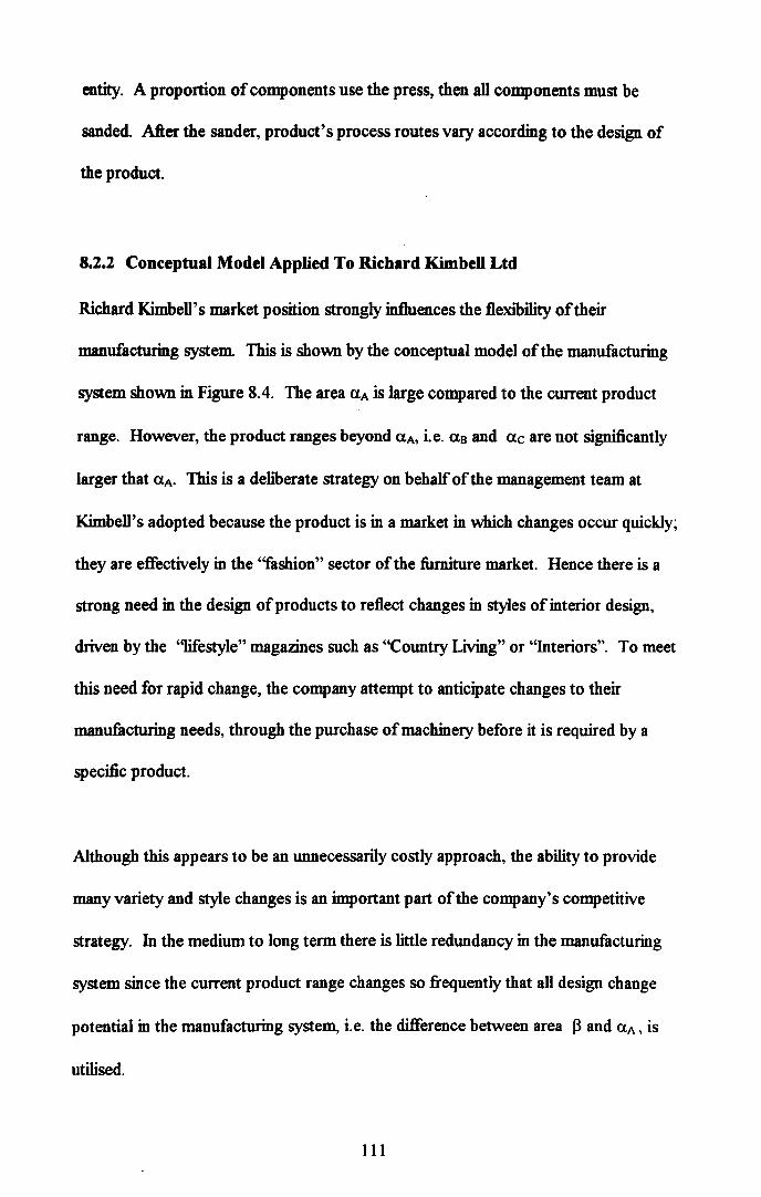
entity. A proportion of components use the press, then all components must be

sanded. After the sander, product's process routes vary according to the design of

the product.

8.2.2 Conceptual Model Applied To Richard Kimbell Ltd

Richard Kimbell's market position strongly influences the flexibility of their

manufacturing system. This is shown by the conceptual model of the manufacturing

system shown in Figure 8.4. The area UA is large compared to the current product

range. However, the product ranges beyond UA, i.e. as and Uc are not significantly

larger that UA. This is a deliberate strategy on behalf of the management team at

Kimbell's adopted because the product is in a market in which changes occur quickly;

they are effectively in the ''fashion'' sector of the furniture market. Hence there is a

strong need in the design of products to reflect changes in styles of interior design,

driven by the ''lifestyle'' magazines such as ''Country Living" or ''Interiors''. To meet

this need for rapid change, the company attempt to anticipate changes to their

manufacturing needs, through the purchase of machinery before it is required by a

specific product.

Although this appears to be an unnecessarily costly approach, the ability to provide

many variety and style changes is an important part of the company's competitive

strategy. In the medium to long term there is little redundancy in the manufacturing

system since the current product range changes so frequently that all design change

potential in the manufacturing system, i. e. the difference between area J3 and aA, is

utilised.

111

B

C

Figure 8.4: Conceptual model of Richard KimbeU Ltd

8.2.3 Calculation of Mix Response Flexibility

To calculate the mix response flexibility there is a need to determine the probability of

a product or component being manufactured and the duration of set-ups at each of

the items of process equipment. Since all the manufactured components are made

from the same raw material, there is little component differentiation in the early stages

of the manufacturing process. Hence on the resaw and Dimter, individual

components are not processed separately, i.e. components are processed in groups, so

set-up times of these groups need to be identified. As the components become more

diverse, set-up times for individual products at each of the processes needs to be

identified.

112

Shown in Table 8-6 are the set-up procedures for each machine, and component

groups for each machine where appropriate are identified. Several of the machines

require an identical set-up procedure, irrespective of the component or product for

which the set-up is being performed, for example the set-up procedure on the sander

is to change the sanding beh for each new product, and therefore durj is constant for

this machine.

Table 8-6: Set-up Procedures at Richard Kimbell's

Machine Function Set-up procedure Groups classified by:

Resaw Cuts to correct width, Sets-up for different wood Thickness from 8" to 4". widths and thickness.

Dimter Saws wood into Download program and set Thickness approximate length for thickness.

Planer/ Cuts to exact width and Set cutters to correct Width, thickness moulder approximate thickness position. Change cutters as and linear shape

Puts in linear mouldings required.

Press Presses wood planks Need to set width and Width and together to make large thickness thickness panels

Sander }\bradesto desired Change over sanding behs. No groups, each surface finish product considered

separately

CNC Drills holes and cuts Set beds and download No groups, each complex shapes program product considered

separately

Dimension Cuts wood to accurate Set cutter guide Length saw length

Double End Cuts rails to length and Set length and cutter No group, each Tenoner shapes ends product considered

separately

Spindle- Mtemative to Set cutter No group, each planer/moulder product considered can also cut angled work separately

To calculate the probability of occurrence of individual components or component

groups, a historical list of products produced over a 120 day period was used

113

(Appendix 3). From this list, an extract of which is shown in Table 8-7, the

probability of occurrence of each of the products was calculated.

The individual components that make up each product, can be identified from a

cutting list for the product. A cutting list identifies the components, specifies their

size and details manufacturing notes. Thus a cutting list performs the role of a parts

list and process plan. An example of a cutting list is provided in appendix 3.

Table 8-7 Extract from tbe Master List of Products Manufactured

No Code Description No. manufactured % probability of occurrence

1 C-PAFF03 small b' case front frame 17 1.164 2 C-PAFF04 wide b' case front frame 29 1.986 3 C-QI070T Quebec f7h top 5'x35" 18 1.233 4 C-Q1080T Quebec f7h top 6'x35" 16 1.096 5 ENIGMA 02 lamp table 20"x20" 4 0.274 6 K-AFHB farm house base arhous 30 2.055 7 KR-43 0007 Console 30 2.055 8 KR-43 00 14 cricket table wax 40 2.740 9 KR-43 0095 wash stand 20 1.370 10 KR-430151 leather top writing table 1 0.001 11 KR-430185 cabriole leg end table II 0.753 12 KR-430214 triangle 12 0.822

Using the probabilities of the products from the master list of products manufactured,

the component groups identified in Table 8-6 and the cutting lists, it is possible to

identifY the probability of occurrence of each component group or product. This was

performed for each of the machines in the manufacturing process.

Once the set-up times for each machine have been identified, and the probability of a

product or product group has been established, the MSTC for each machine can be

calculated. Table 8-8 shows a summary of the calculations for each machine.

114

Table 8-8: MSTC and SD for each of the Richard Kimbell Machines

Machine Machine Machine Data for Cales System System MSTCin SDin whole MSTC SDin minutes minutes product mmms mins

set? Resaw 2.1 1.7 No for multiply 2.5 1.9

thickness mean and var groups by 1.190

Dimter 2.8 2.3 No for multiply 3.3 2.5 thickness mean and var groups by 1.190

Planer/ 25.2 17.7 Yes None 25.2 17.7 moulder required Press 4.0 2.7 No for No. going 3.8 2.7

subset through 1431

Sander 12.0 0.7 Yes None 12.0 0.7 required

CNC 34.4 14.7 No for No. going 27.2 13.0 subset through

1174 Dimensi 21.0 18.1 Yes None 21.0 18.1 on saw required Double 45 13 No for No. going 4.2 4.0 End subset through 137 Tenoner Spindle 9.6 8.0 No for No. going 2.3 3.9

subset through 353 TOTAL 101.5 29.3

To calculate the total set-up time per product for the system it is necessary to convert

the data from individual machines to data for the whole manufacturing system. It is

necessary to categories machines into three different groups and take different

approaches accordingly.

115

Group 1: Machines through which all products have at least one component

processed ie. planer/moulder, sander and dimension saw. As all products

have at least one component which goes through these machines the machine

data can be used directly for the system data.

Group 2: Machines where products are not identified separately, but specified in

groups i.e. resawand Dimter. The data from these two machines represents

the MSTC and SD per thickness group, this has to be converted into MSTC

and SD per product. This can be achieved by knowing the mean number of

thickness groups per product which is 1.19.

Group 3: The remainder of the machines, i.e. press, CNC machine, D.E. Tenoner and

spindle all process a subset of products. Therefore Equations 8.8 and 8.9

for parallel machines can be used.

Table 8-8 shows a summary of the calculations for each machine, the details of these

calculations are provided in Appendix 3. The total system results are

MSTC=101.520 and SD=29.285 minutes.

8.2.4 Calculation of Product Range Flexibility

Shown below in Table 8-9 is the matrix for the product range flexibility of the

manufacturing system at Richard Kimbell Ltd. In addition to the machines analysed in

8.2.3 an extra machine, the lathe, is included. This is because the lathe is not

currently used but is, however, available for future use.

116

Table 8-9: Matrix of Product Range for Richard Kimbell Ltd

Max.len~ Form Machine O-Im I-2m 2-3m Plank Rotational Flat Irregular

Resaw A A A A A A Dimter A A A A A A Planer/moulder A A A A A A Press A A B A A A Sander A A B A nla A CNC A A B A nla A Lathe A A nip nla A nla Dimension saw A A B A B nla Double End Tenoner A A nlj> A B B Spindle A A A A A B

Table 8-10 shows that the total response cost is £22,400, where B's are costed at

£300, Cs are not costed and nip are costed at £10,000.

Table 8-10: Calculations for Product Flexibility at Richard KimbeU Ltd

Category of ceU No. of each Cost per cell Cost for each

category of cell category of cell

A's 35 0 0

8's 8 300 2400

C's 0 nla 0

nip cells 2 10,000 20,000

nla cells 4 0 ° Total Response Cost £22,400

117

9. DISCUSSION

9.1 Methodology

From the literature review four main requirements for the research emerged in order

that a practical measurement of flexibility could be developed:

1. The measure should build on the existing research which defines types of

flexibility and relates fleXibility to manufacturing strategy. This is necessary so

that the measure developed has meaning in terms of competitive advantage.

2. To ensure relevance to a wide range of industries the measure should be robust

enough to be applicable to different types of manufacturing systems.

3. The measure should be simple to use or busy industrialists will not to attempt to

use it, and

4. The measure should reflect the subtle nature of flexibility in manufacturing,

otherwise it would not give a reliable measure .

These last two requirements are difficult to reconcile, as simplicity will tend to

obliterate subtly, as identified in Chapter 4. In order to overcome these problems a

two-stage approach was adopted. The first stage was a development of a

conceptual model (chapter 5), the second stage was the development of two

numerical methods to interpret the model. As identified in Section 5. I, using a

conceptual model in conjunction with numerical assessment achieves the

requirements 3 and 4 listed above. The conceptual model provides a rich picture

118

that enables the user to express an overall view of the flexibility of the system

simply. The numerical assessment then provides greater detail and that enables the

user to compare the fleXIbility of ahemative manufacturing systems.

Figure 9.1 shows how the different stages in the methodology can be applied in a

company.

Gain basic Wlderstanding of company strategy and identify manufacturing system

Outcomes for modeling JJ.

Sketch conceptual , ::> Conceptual model of system's model flexibility n.

Identify all subsystems and machines in system

.u. Construct three dimensional matrix of pro duct flexibility

il ::>1 I /

Calculate TRC /' Measure of Product Flexibility

I1 Identify all products that are

manufactured in system

,U. For all products identify

I. Probalility of OCCWTence 2. Process routes

3. Set-up times for machines or su1;systems

lJ.

I Calculate machine MSTC and SO /

.LJ. Measure of Mix Response I Calculate System MSTC and SD > - Flexibility

Figure 9.1 Flow diagram of measurement method within a company

119

In order to ensure that the flexibility methods were applicable to a wider range of

manufacturing organisations, careful selection of the case study companies was

necessary. In this respect the companies Bostik Ltd and Richard Kimbell Ltd were

selected in order to demonstrate that the measurement methods could be applied in

a range of manufacturing environments. Thus it was important that the companies

adopted were different from each other, and were representative of major sectors of

manufacturing industry. In this respect there were three main areas in which the

companies differed:

1. Industrial sector. The case study companies were taken from two different

industrial sectors. Bostik is in the sector defined by the Department of Trade and

Industry as "extraction and processing of chemicals and ores" which represents

approximately 20 % of UK manufacturing industry (HMSO 1992). Richard

Kimbell is in the sector defined as "other manufacturing", which includes the

manufacture of domestic items including textiles and furniture. This sector

represents approximately 42% of UK manufacturing industry (HMSO 1992).

2. Organisational structure. Bostik is part of a large processing group Total Ltd,

whereas Richard Kimbell Ltd is a small, owner managed company.

3. Type of Manufacturing System Bostik's manufacturing system is largely a flow

line based on a product layout, whereas Richard Kimbell's is a process layout, and

manufacturing in small to medium sized batches.

120

9.2 The Conceptual Model

The conceptual model focuses on the products a company makes i.e. mix flexibility,

and the potentW products a company could make ie. product flexibility. This was

done because using specific types of flexibility, in this case mix flexibility and

product fleXibility as defined by Slack ( 1990), focuses the research effort to a

limited range offleXioility types and thus concurs with requirement 1 specified

earlier in this section, and to aim 2 specified in Section 1.5, that a measurement

method should relate to specific types of flexibility.

The conceptual model can be sketched for a company's product range and

manufacturing system, in order to provide a general picture of their product and mix

flexibility. Different types of industry are typified by characteristic conceptual

models. This is reflected by the models developed for Bostik Ltd and Richard

Kimbell Ltd. The conceptual model ofBostik Ltd, shown in Figure 8.2, is typical of

chemical alid other processing industries. The model reflects the long operational

life and high cost of plant equipment in these types of industry. The conceptual

model developed for Richard Kimbell Ltd, is characteristic for their specific

strategic stance of being able to introduce new designs easily. It shows how a

company in a fashionable market can focus their flexibility for competitive

advantage.

121

The conceptual model proved a useful tool for introducing the case study

companies to the concept of the different types of flexibility, since mix flexibility and

product flexibility are clearly shown in the model The model was also used for

explaining the meaning of the Mean Sensitivity To Change and the Total Response

Cost measures.

9.3 Product Flexibility

The TRC measure provides the system designer with the ability to differentiate in

terms of product flexibility between alternative manufacturing systems. However,

the process of calculating TRC, using the ratings A, B, and C is subjective. The use

of ratings is, however, established in both flexibility measurement (Naik and

Chakravarty, 1992 and Slagmulder and Bruggeman, 1992) and operations

management in general (Stevenson 1993).

It was found when applying the product flexibility measure to Richard Kimbell Ltd

and Bostik Ltd the process of categorisation of A. B and Cs to cells was best

achieved by differentiating between the changes in terms of small to medium sized

changes and medium to large changes, rather than setting specific financial limits.

Once the TRC matrix has been completed, it is possible to estimate the cost of each

of these categories. This overcame the problem of setting definite cost limits before

categorising each cell, which forced the user into allocating cells into categories

which although numerically correct, were conceptually incorrect i. e. it was difficult

122

to set the correct numerical limits to reflect the A, B and C categories before the

process of developing the matrix.

Greater understanding of the fleXloility of the system from the calculation of TRC

highlights flexibility bottlenecks. Two examples of this is shown in the Bostik Ltd

matrix (Table 8-3 page 107). The first example relates to the hot room, which

could only process batches of up to 1 tonne, whereas the remains of the

manufacturing system, if parallel processes are considered, was able to process 2

tonne batches. In response to this analysis, the company increased the size of the

hot room. Thus enabling Bostik to avoid splitting batches, this had the advantage

of reducing through put time and improving process consistency through the batch.

The second example is high viscosity products. These are products that are

identified as a potentially growing market. It can be seen from the matrix. in Table

8-3 that high viscosity products are generally difficult to process at all stages except

crystallisation. Hence considerable investment is required if the company wishes to

exploit this market. Thus the analysis required to derive a TRC value has provided

Bostik Ltd with direction for future development.

The product range flexibility matrix of Richard Kimbell Ltd (Table 8-9, page 117) is

simple, reflecting the clear strategic direction of being able to introduce new designs

123

easily, identified in Section 8.2.2. It can be seen that the majority of the cells are

A's, which is also represented in the conceptual model in Figure 8.4, page 112.

Table 8-9 indicates that there are few characteristics that vary, i.e. only size and

form. This is because many aspects which could change are established as standard

policy by the company e.g. the use of exclusively pine material.

It can be seen that for the case study companies the calculation of TRC was not

used in a comparison against an alternative system, but that the process of

calculating TRC gives direction for short and long term development of the

manufacturing system. If an alternative system were to be considered and there was

sufficient information known about its machines and subsystems, then the TRC

could be used for the purposes of comparison between systems.

The TRC does not directly measure product flexibility, but measures product

inflexibility. This arises because the TRC measures the cost of implementing all

possible changes, hence, the higher the TRC, the lower the system flexibility. A

direct measure of product flexibility can be derived using the inverse ofTRC, i.e.

1 product flexibility = --. However, by this inverse measure TRC, is directly

TRC

related to a monetary value and is therefore easier to interpret in a commercial

environment.

124

It should be noted that the TRC, measure is limited by the confidence with which

predictions in the A, B and C bands can be made. In the case of both Bostik Ltd

and Richard Kimbell Ltd an accuracy of between 10 to 15% can be estimated for

the TRC measure. This based on the estimations of employees supplying the data

for the calculations.

The TRC measure with weighting factors for important characteristics described in

Section 6.4.4, no longer has significance in terms of the cost of implementing all

possible changes, because the weighting factor V augments the cost categories

allocated to the important characteristics beyond their true value. Also no

comparison can be made between systems' product flexibilities using different

weightings in their calculation. It could be considered that given the limitations in

using weightings, and the difficulties manufacturers have in making future

predictions about which characteristics are likely to be important (Fisher

Hammond, Obermeyer, and Raman, 1994) that the use of weighting factors should

be limited.

9.4 Mix Response Flexibility

The mean sensitivity to change (MSTC) is a measure of mix response flexibility.

The measure for MSTC and its associated SD, developed in Chapter 7, is derived

from the probability that a product will be manufactured on a machine and the time

associated with setting-up for that product. Section 7.5.2 has shown that the

125

MSTC, ifproducts are manufactured in a random order, is analogous to the mean

set-up time per product, with the SD reflecting the distnDution of mean set-up times

for different orders. Hence the MSTC measure reflects the mix flexibility of the

machines that make up a manufacturing system It does not take into account the

order in which the products are manufactured. In order to use this information the

simplest interpretation would be to compare the MSTC and SD's of two alternative

manufacturing systems, in which case the MSTC could be compared between

systems and used to judge the best system to adopt in the context of other criteria

such as cost and output levels.

In the absence of alternative systems, data derived from a production run can be

used for a comparison between the MSTC and the mean set-up time per product.

This type of comparison reveals information concerning the effectiveness of the

schedule in reducing the time spent in set-up. It could be assumed that the

relationship between batch size and the time spent in set-up is roughly inversely

linear, hence as the Production Scheduler doubles the batch size the time spent in

set-up halves. However, this linear relationship breaks down as the product range

reduces, since there will be an increase in the probability of a product type occurring

after the same product type. The relationship between mean set-up time and batch

size will also be influenced by the level of variability of both the probabilities of

occurrence and set-up times of different products. For example the reduction of

the mean set-up time will be more substantial if a Production Scheduler batches

126

together a product type with long set-up durations, as opposed to product types

with equivalent batch sizes and short set-up durations. Similarly, if a Production

Scheduler batches together products with a low probability of occurrence rather

than a product type that occurs more frequently, this will incur a greater number of

undesirable features such as variance between desired and actual delivery dates or

higher stock levels.

Table 9-1 shows a comparison between the relative values ofMSTC and mean set­

up time per product as derived from a production schedule. This comparison allows

the user to differentiate between the influence of the schedule and the influence of

the set-up times of the machines.

Table 9-1: Comparison of MSTC and Mean Set-Up Times per Product

The relative value of Comparisons

MSTC vs mean set-up

time per product

MSTC > mean set-up 1. The scheduling system can batch products together to

time per product improve production time.

2. Batching products together may adversely affect lead

times or stock levels

3. lfbatch sizes need to be reduced, problems with

throughput levels may be incurred i.e. more production

time will be dedicated to set-up durations.

MSTC~ mean set-up I. The scheduling system does not batch products together

time per product significantly.

MSTC< mean set-up 1. Split batches are incurred hence the mean set-up time

time per product per product is higher than would be expected.

127

A similar analysis can be performed by comparing the MSTC and the total

production time. A system that has a high MSTC when compared to the production

time, possesses a low mix response flexibility, when these values are reversed i.e. a

system that possesses a relatively low MSTC has a high mix response flexibility. It

can be anticipated that different industries could benchmark appropriate ratios of

MSTC to total throughput time, to indicate high and low mix response flexibility

levels of their manufacturing systems.

By examining the separate MSTC for each machine it is possible to identifY those

machines that contribute the most to the system MSTC, and hence most inhibit the

flexibility of the system Effort can then be focused on reducing the set-up times of

these machines and thus reduce the system MSTC.

It should be noted that MSTC is similar to TRC in a measure of inflexibility, in that

the higher the value ofMSTC the lower the flexibility of the system

For Bostik the calculations in section 8.1.3 show a MSTC of3 hours and a SD of

3.6 hours. This is relatively low compared to the processing time ofBostik

products which can be periods of up to several days, this is primarily due to slow

reaction and crystallisation rates. The MSTC is also low compared to the variation

in processing times, which can vary by up to two days. In this case the MSTC

128

analysis was used to focus effort in improving the manufacturing system by reducing

the variation in processing times, as opposed to reducing set-up times which were

shown to have a negligible effect.

The results for Richard Kimbell Ltd from Section 8.2.3.1 reveal a MSTC of 101.5

minutes with an SD of29.3 minutes. The MSTC is high in comparison to the

measured average setup time per product which is approximately 13.7 minutes.

This occurs because Richard Kimbell Ltd tend to manufacture in batch sizes that

range from 1 to 50 products, with an average batch size of approximately 8.

Manufacturing in larger batches will reduce the average setup time per product,

whereas, the MSTC assumes that products are manufactured individually. Within

Richard Kimbell the batch size is largely determined by customer orders, i. e. large

batches are generated by orders from overseas department stores who will typically

order in batches sizes of20. Thus it can be seen from Table 9-1 that ifbatch sizes

need to be reduced, problems with throughput levels may be incurred i.e. more

production time will be dedicated to set-up durations.

Examining the machines individually, Table 8-7 (page 114) shows that the

planer/moulder, CNC machine, dimension saw and the double ended tenoner have

the highest MSTC. Although the double ended tenoner has the highest machine

MSTC, its impact on the system MSTC is limited. However, the CNC machine,

planer/moulder and the dimension saw have much greater contributions to the

129

system MSTC. The differences between the impact of these machines on the

MSTC is because of the differences in the machine's processing volume. Out of the

1480 products the CNC machine processed 1174, whereas the double ended

tenoner processed 137. This type of analysis provides clear indications how

improvement of the flexibility of the manufacturing system can be accomplished and

since gathering this data the company has taken steps to reduce the impact of the

set-up times of the CNC machine and the planer/moulder. This has been achieved by

purchasing an additional CNC machine and recommissioning a disused

planer/moulder. Reduction exercises were also being examined for set-up times on

the planer/moulder.

The process of calculating the MSTC at Richard Kimbell Ltd highlighted two main

limitations with the measurement method.

1. A high number of calculations is needed for companies with large product ranges.

2. Where it is not possible to identify separate products the required calculations

have additional complexity.

The first limitation is demonstrated by the MSTC calculations for Richard Kimbell

Ltd. shown in appendix 3. It can be seen that each machine requires several pages of

a spreadsheet to calculate the MSTC. In compensation it should be noted that the

calculations are relatively simple and the basic structure can be copied from one

machine's spreadsheet to another.

130

The second limitation is encountered in the MSTC calculations required for the

resaw and the Dimter, where products are identified in groups rather than as

individuals. The data from these two machines represents the MSTC and SD for

each group of products that are the same thickness. This data has to be converted

into MSTC and SD for individual products. This was achieved by identifying the

mean number of thickness groups per product i.e. 1.9, calculated by:

mean number of

thickness groups

the total number of thickness group occurrences, 125

the total number of products, 106

131

10. CONCLUSIONS

The objectives identified in Section 1.5 have been achieved:

1. Data for input values should be easy to obtain

The data for Bostik was readily available. The data at Richard Kimbell Ltd was

less available because it is a smaller company where there is less opportunity for

employees to gather data. However, the type of data required was possible to

obtain, given the opportunity to gather it.

(Sections 8.1 and 8.2)

2. Outputs must be meaningful

The outputs of the measurement methodology relate to the types of flexibility

specified by Slack (1990).

(Section 5.4)

3. Methodology should be easy to use.

The basis of the methodology consists of simple mathematics and the

methodology was applicable to both companies although interpreting what

represented a product was complex for Richard Kimbell Ltd in the case of the

resaw and the Dimter. It was also complex identifying the duration of a set-up for

the extruders for Bostik Ltd, because of the influence on set-up times between

product types. (Sections 9.3 and 9.4)

132

4. Must be cheap

The use of equations and the three dimensional matrix means that no investment

in software is required, although a spreadsheet program is useful for the MSTC

calculations.

(Sections 6.7, 7.1, 7.2 and 9.4)

5. Be able to assess Oexibility across a range of industries

The results obtained indicate that the methodology can be used in a range of

industries. The difference in emphasis in the results demonstrates that it can adapt

to different areas of focus in different industries.

(Section 9.4)

Therefore, it can be concluded that the aim of the thesis, to develop measures for

flexibility that can be easily used in a manufacturing environment has been

achieved.

133

11. RECOMMENDATIONS FOR FURTHER WORK

1. Characteristic conceptual models for different types of industry should be

developed. This will allow companies to compare their own conceptual model to

an industry standard.

2. Bench marks for different industries' ratios for:

1. MSTC and mean set-up time per product.

2. MSTC and total manufacturing time.

This will allow companies to assess their comparative mix response flexibility.

134

Bibliography

ALLISON, B. (1993). A Guide to Dissertation preperation (4th edit.). Leicester: Ariad Associates.

BRYMAN, A(1989). Research Methods And Organizational Studies. London: Routledge. ISBN 00442128

FREUND, J. and SIMON, G. (1992): Modern Elementary Statistics (8th edit.). New Jersey: Prentice Hall. ISBN 0135934753

PEDRYZ, W. (1991). Fuzzy Modelling. Fundamemtals,Construction And Evaluation. Fuz..-y Sets And Systems 41, 6th May, 1-15

SCHIDLT, H. (1991): C++ The Complete Reference. Berkeley: McGrawHill. ISBN 0078816548

WU, B.(1992). Manufacturing Systems Design and AnalySiS. London: Chapman Hall ISBN 0412408406

References

ADLER, PAUL S. (1988). Managing Flexible Automation. California Management Review. Spring issue 34-56

ANON (1986). Us Air Offers Maintenance Software To Improve Scheduling Flexibility. Aviation Week And Space Technology Nov, 131-137.

ATKINSON, J. (1985). Flexibility: Planning For An Uncertain Future. Manpower Policy And Practice 1, 26-29.

BARAD, M. and SIPPER, D (1988).Flexibility in Manufacturing Systems: Definitions and Petri Net Modelling. International Journal of Production Research. 26, 2,237-248

BARAD, M. and SIPPER, D. (1990). Flexibility And Types Of Change In Fms's: A Timed Petri-Nets Assessment Of Machine Flexibility. Int J Adv ManufTechnol5, 296-306

BATEMAN, N. and STOCKTON, D. (1993).Flexibility in Manufacturing Systems Advances inManufacturing Technology VII 87-90

BAUER, A. (1995). Flexible Control. Manf Eng. 76, 6, 287-289

BLACK, 1. (1983). Cellular Manufacturing Systems Reduce Set-Up Time Make Small Lot Production Economical. Industrial Engineering. Nov, 36-48.

BLACKBURN, J. and MILLEN, R( 1986). Perspectives on Flexibility in Manufacturing: Hardware versus Software in Kusiak A (Ed.), Modelling and Design of Flexible Manufacturing Systems Elevier Science Publishers 157-170. ISBN 0444425969

BROWNE, J., DUBOIS, D., RATHMILL, K, SETIfl, S., AND STECKE, K (1984). Classification ofHexible Manufacturing Systems The FMS Magazine. April, 114-117

BUZACOTI, J. (1982). The Fundamental Principles of Flexibility in Mnaufacturing Systems. Proceedings of the 1st International conference ofFMS Brighton UK ISBN 0903608308

BYRNE, M.C. (1992). A Simulation-Based Method To Aid The Improvement Of Manufacturing Flexibility. International Journal Of Production Economics 26, 153-159.

BYRNE,M. and CHUTIMA,P. (1995) Real-Time Routing Decisions In FMS's With Full Routing Flexibility And Failure Prone Machines., 346-351. Advances in Manufacturing Technology IX 11th National Conference on Manufaturing Research Leicester D. Stockton and C. Wainwright (Ed). London: Taylor and Francis. ISBN 0748404007

CARTER, M. (1986). Designing Flexibility into Automated Manufacturing Systems Proceedings of 2nd ORSAITMS conference on Flexible Manufacturing Systems 107-118 University of Michigan Ed. KStecke, Oxford: Elsevier. ISBN 0444426795

CHAMBERS,S. (1992) Flexibility in the context of manufacturing strategy. in Voss, C. (Ed.) Manufacturing Strategy Process And Content. London. Chapman Hall. ISBN 0412436604

CHEN, I., CALATONE, R, CHUNG, C-H,. (1992). The Marketing-Manufacturing Interface And Manufacturing Flexibility. Int J Of Man Sci 20 4, 431-443.

CHRYSSOLOURIS, G., LEE, M. (1992). An Assessment of Flexibility in Manufacturing Systems. Manufacturing Review 5, 105-116.

CORREA, H. (1992). The Links Between Uncertainty, Variability Of Outputs And Flexibility In Manufacturing Systems. PhD University of Warwick

CROWE, T.(l992).Integration is not Synonymous with flexibility International Journal of Operations and Production Management. 12, 10, 26-33

DAUGHERTY, P. and PITTMAN, P. (1995). Utilization Of Time-Based Strategies Creating Disrtibution Flexibility/ Responsiveness. International Journal Of OperatiollS And Production Management. 15,2,54-60.

DECISTERE, F., HARHALAKIS, G., PROm, J., Sn..vA, M., and VERNADAT, F.( 1993). Practice of Petri Nets In Manufacturing London:Chapman Hall ISBN 0412412306

DEISCH, K and MALSTROM, E. (1985).Physical Simulator Analyses Performance of FMS. Industrial Engineering. June, 66-75

DE MEYER, A, NAKANE, 1., MILLER, IG. and FERDOWS, K (1989). Flexibility: The Next Competitive Battle The Manufacturing Futures Survey. Strategic Managema1l1 Journal 10, 135-144.

DOONER, M. (1991). Conceptual modelling of Manufacturing Flexibility Computer IntegratedManufacturing. 4,3, 135-144

FISHER.. M., HAMMOND, 1., OBERMAYER, W. and RAMAN, A (1994). Making Supply Meet Demand In An Uncertain World. Harvard Business Review May-June, 83-93.

FREUND, J., SIMON, G. (1992). Modem Elementary Statistics. Englewood Cliffs: Prentice Hall. ISBN 0-1359-3475-3

GARWOOD, D. (1990). Flexibility Is Job 2. Conference Proceedings Of The American Production And Inventory Control SOCiety, 568-569.

GALLAGHER, C.C and KNIGHT, W.A(1973). Group Technology London: Butter worth. ISBN 0408705337

GERWIN, D. (1989). Manufacturing Flexibility In The CAM Era. Business Horizons. Jan-Feb 78-84.

GOYAL, S., GUNASEKARAN, A( 1995). Labour Stability And Fexibility - Conditions To Reach Just-In-Time International Journal Of Operations And Productions Management, 15, 9,26-44

GUPTA, D. and BUZACOTT, J(1989) .. A framework for Understanding Flexibility of Manufacturing Systems Journal of Manufacturing Systems. 8, 2, 89-97.

GUPTA, Y GOYAL,S (1989). Flexibility Of Manufacturing Systems: Concepts And Measurements. European Journal Of Operational Research Vol 43 Pt 2, 119-135.

GUPTA, Y.and GUPTA, M. (1991). Flexibility And Availability Of Flexible Manufacturing Systems: an Infonnation Theory Approach. Computers In Industry 17, 391-406

GUSTAVSSON,S. (1984). Flexibility and Productivity in Complex production Processes International Journal of Production Research. 22, 5, 801-808

HARVEY, R, and PAGE, M.(1986). Fitting An Fms Into The Small Plant. Iron Age, 18th July 23-32.

HARVEY, J., LEFEBVRE, L. and LEFEBVRE, E. (1997). Flexibility and Technology in Services: a Conceptual Model International Journal Of Operations And Production Management. 17, 1,29-45.

HAYES, R. and WHEELWRIGHT, S, (1984). Restoring our Competitive Edge. New York: Wiley. ISBN 0471051594

HENDRY, AL. (1985). Flexibility Is Key For Small Paint Companies. Modern Paint And Coatings. Jan,40-43

HILL, T. (1985). Manufacturing Strategy. Basingstoke: Macmillan. ISBN 0333394771

HILL, T., CHAMBERS, S. (1991). Flexibility - A Manufacturing Conundrum. International Journal Of Operations And Production Management 11, 5-13. ISBN 0-3333-9477-1

HMSO (1992). Annual Census of production HMSO

HOLMGREN, K M. (1988). Workstation Producer's New Plant Provides Manufacturing Flexibility To Introduce Or Switch Products. Industrial Engineering. March, 32-35 and 74.

HUTCIDNSON, G. K (1984). Flexibility Is Key To Economic Feasibility Of Automating Small Batch Manufacturing. Industrial Engineering. June 77-84.

ITO, Y. (1987) Evaluation ofFMS: Sate of the Art regarding how to Evaluate System Flexibility. Robotics and Computer Integrated Manufacturing. 3, 3, 327-334

JAIKUMAR, R. (1986). Postindustrial Manufacturing. Harvard Business Review Nov­Dec, 69-76.

KAPLAN, R, (1990) Limitations of Cost Accounting in Advanced Manufacturing Environments in Kaplan R (Ed) Measuresfor Manufacturing Excellence. Harvard: Harvard Business School Press ISBN 0875842291

KELLOCK, B (1985). Sheet Metal's Flexible Friends. Machinery And Production Engineering, 6th Feb 29-34

KIOD, P. (1994). Agile Manufacturing Forging New Frontiers Wokingham: Addison­Wesley. ISBN 0210631636

KIM, C (1991). Issues on Manufacturing Flexibility. Integrated Manufacturing Systems. 2, 4-13

KUMAR,V. (1987). Entropic Measures Of Manufacturing Flexibility. Int J. Prod Res. 25,957-966

LENZ, J. E. (1992). How Well Can Flexibility Be Measured. Industrial Engineering. June, 14-15.

LEONG, G.K, SYDNE~ D.L. and WARD P.T.(1990). Research in the Process and Content of Manufacturing Strategy. OMEGA International Journal of Management Science. 18,2, 109-122

MANDELBAUM, M. and BUZACOTT, J. (1986). Flexibility And Its Use: A Formal Decision Process And Manufacturing View. 2nd Orsal TMS Conference On FMS . University of Michigan Ed. KStecke, Oxford: Elsevier. ISBN 0444426795

MURAMATSU, R., ISHII, K., and TAKAHASHI, K., (1985). Some Ways To Increase Flexibility In Manufacturing Systems. Intemation Journal Of Production Research. 23,4, 691-703

MASKELL,B (1989). Performance Measurement for World class Manufacturing. Man Ace. May, 32-33.

MATHER, H. (1995). Don't Flex The Factory, Stabilise The Demand. Industrial Engineereing Solutions Nov 41-43.

NAGARAJAH,C., THOMPSON, W. (1994) A Methodology For Investigating Effects Of Cell Size On Operational Flexibility In Flexible Manufacturing Systems. Int J Adv Mallu! Technol. 9, 5, 333-342

NAG~ S.and BENNETT, D. (1988). fleXIble Manufacturing System Lets Small Manufacturer Of Mainframes Compete With Giants. Industrial Engineering, Nov 42-46.

NAIK, B. and CHAKRAVARTY, A. (1992) Strategic Aquisition Of New Manufacturing Technology: A Review And Research Framework. Int J. Prod Res. 30, 7, 1575-1601.

NAKHA, M (1995). Production Control In The Food Processing Industry. The Need For Flexibilityy In Operations Scheduling. Int J of Op and Prod 15, 8, 73-88.

NEELY,A., MILLS,J., PLATTS,K, GREGORY,M., and RICHARDS,H. (1994). Realizing Strategy Through Measurement. Int J of Op and Prod 14,3, 140-152

OWEN, G., MCINTOSH, R,. MILEHAM, A., CULLEY,S., and GEST,G (1995). Manufacturing Flexibility - A Case for Excess Capacity .. Advances in Manufacturing Technology IX 1 lth National Conference on Manufaturing Research Leicester. D. Stockton and C. Wainwright (Ed).:London: Taylor & Francis. ISBN 0748404007

PANDIARAJAN V.,and PUTAN, R, (1994). Agile Manufacturing Initiatives At Concurrent Technologies Corp Industrial Engineering Feb, 46-49

PARKlNSON, S.and A VLONITIS,G. (1982). Management Attitudes To FMS.Proceedings of 1st International Conference on Flexible Manufacturing systems

PINE, B.J.,VICTOR B., and BOYNTON a.,(1993). Making Mass Customization Work. Harvard Business Review Sept/Oct, 108-119.

PORTER, M .. E. (1985). Competitive advantage: Creating and sustaining Superior Performance, London: The free press ISBN 0029250900

PRIMROSE, P. and LEONARD R,( 1984). Conditions under which flexible manufacturing is financially viable Proceedings of 3rd International conference on FMS.Boebliogen W. Gerrmany. Bedford: IFS

PRIMROSE, L. and VERTER V, (1996). Do Companies Need To Measure Their Production Flexibility? International Journal Of Production Management. 16, 6, 4-11

PROMODEL (1993). Versionl.03 Promodel Corporation, 1875 South State Suite 3400 Orero, Utah 84058 USA

ROBINSON S.(1994) Successful Simulation London: Me Graw-Hill. ISBN 0077076222

ROLL, Y., KARNI, R, and ARZI, Y., (1990). Measurement ofProeessing Flexibility in Flexible Manufacturing Cells Journal of Manufacturing Systems. 11, 4, 258-268

ROSS TIMOTHY J (1995). Fuzzy logic with engineering applications. London: McGraw-Hill. ISBN 007539170

SETIn, A. and SETIfl. S.( 1990) Flexibility in Manufacturing: A Survey The International Journal of Flexible Manufacturing Systems. 2 , 289-328

SIflNGO, S-(1985) The Revolution In Manufacturing: SMED System Productivity Press: Cambridge. ISBN 0915299038

SKINNER, W (1974). The Focused factory Harvard Business Review. May/June, 113-121

SLACK N. (1990).The manufacturing Advantage Mercury: London. ISBN 1852510382

SLACK, N. and CORREA, H. (1992). The Flexibilities Of Push And Pull International Journal Of Operations And Production Management 12, 82-92 .

SLAG MULDER, R. and BRUGGEMAN, W. (1992). Investment Justification Of Flexible Manufacturing Technologies: Inferences From Field Research. International Journal Of Operations And Production Management 12, 168-186.

SOHAL, A., RAMSAY, L, and SAMSON, D. (1993) JIT Manufacturing: Industry Analysis and a methodology for Implementation International Journal of Operations and Production Management 13, 7, 22-56

STEVENSON, W. (1993). Production/Operations Management Irwin: Boston USA ISBN 0256208514

STOKES, J. (1982) How To Justify Installing Fms. Production Engineer April, 30-32

SWAMIDAS, P. and NEWELL, W. (1987). Manufacturing strategy, Environemental Uncertainty and performance of a Path Analytic Model Management Science. 33, 4 April 177-182

THILANDER, M. (1992).FleXlble Production in the Chemical Industry - a Question of Competance International Journal of Operations and Production Management 12, 147-167

TIDD, J. (1988). Divergent Trends In Robotic Assembly In The UK And Japan Assembly Automation. 8, 4,211-212

TIDD, J. (1991). Flexible Manufacturing Technologies and International Competitiveness London: Pinter Publishers. ISBN 0861871030

TIGHE, C. (1993). A Line That Suits Tumble Dryers Financial Times Sept 14th, 11

UPTON, D. (l995).What Makes Factories Flexible? Harvard Business Review luI/Aug

TOMBAK, M.and DE MEYER, A. (1988). FleXlbility and FMS: An Empirical Analysis. IEEE Transactions On Engineering Management. 35,2, May, 101-107.

VERNADAT, F.,B.( 1996) Enterprise Modelling and Integration Chapman and Hall: London:. ISBN 042605503

VOSS C. (1995). Alternative Paradigms For Manufacturing Strategy International Journal of operations and Production Management. 15, 4, pp5-16

WALTERS A-M. (1997). Demanding Data - The Pull for Life-Time Information Management Conference on Demand Driven Agile Manufacturing 16,17th September P. Kidd (Ed. )London.

WAINWRIGHT C (1993). Considerations Relating to Formulations of Manufacturing Strategies PhD Thesis UMIST

ZELENOVIC,D DRAGUTIN M. (1982). Flexibility - A Condition For Effective Production Systems. Int J. Prod Res 20,319-337.

Published Papen

BATEMAN, N. and STOCKTON, D. (1993) Flexibility in Manufacturing. Advances in Manufacturing Technology vn. Proceedings of the Ninth National Conference on Manufacturing Research. University of Bath, Bramley, A. and Mileham A.,(Ed).Bath University: Bath ISBN 185790007

BATEMAN, N. and STOCKTON, D. (1994). Assessing and Improving Manufacturing Flexibility. Advances in Manufacturing Technology VllI. Proceedings of the Tenth National Conference on Manufacturing Research. University of Lough borough. Taylor & Francis: London ISBN 0748402543

BATEMAN, N. and STOCKTON, D. (1995) Measuring the Production Range of a FMS Journal of Integrated Manufacturing Systems 6,2 27-34

BATEMAN, N. and STOCKTON, D. (1995) Measuring Mix response Flexibility: The Ability to Change between Existing Products Advances in manufacturing technology IX 11th National Conference on Manufacturing Research. De Montfort University, STOCKTON D. and Wainwright, C. (Ed.) Taylor & Francis: London ISBN 0748404007

BATEMAN, N., STOCKTON, D. and LAWRENCE, P. (1998) Measuring the Mix response Flexibility of Manufacturing Systems International Journal of Production Research. To be published in September

BATEMAN, N. AND WAINWRIGHT, C (1995) A Strategic audit Tool to Asses Manufacturing Flexibility Intelligent Manufacturing systems Colloquium lEE: London

STOCKTON D., LINDLEY R, and BATEMANN.(1994), A Sequence of Cells Manufacturing Engineer 73, 1 Feb

STOCKTON D., LINDLEY R, and BATEMANN.(l994), Developing the Sequence Manufacturing Engineer 73,2 April

Appendix 1

Calculations for total response cost.

System X System Y SystemZ Total number of cells 150 170 200 No. of A's 81 90 100 No.ofB's 22 10 20 No.ofC's 35 35 40 No. of cells that cannot be achieved 12 35 40 No. A's in Colour characteristic 14 17 15 No. B's in Colour characteristic 5 15 5 No. C's in Colour characteristic 3 5 5 No. of cells that cannot be achieved in Colour 2 0 5 characteristic

System X System Y System Z Total number of cells 150 170 200 No of A's minus colour A's 81-14=67 90-17=73 100-15=85 No. ofB's minus colour B's 22-5=17 10-0=10 20-5=15 No. ofC's minus colour C's 35-3=32 35-10=25 40-5=35 No. of cells that cannot be achieved minus No. 12-2=10 35-0=35 40-5=35 of colour cells that cannot be achieved

Cost in £ A 0 B 1000 C 4000 criteria that cannot be achieved 10000 Ain colour OX 1.2=0 B in colour l000X 1.2=1200 C in colour 4000X 1.2=5000 Criteria that cannot be achieved in colour l0000X 1.2=12000

System X SystemY SystemZ Cost of A's minus 67XO=O 73XO=O 85XO=O colour A's Cost ofB's minus 17Xl000= lOX 1000= 15Xl000= colour B's 17000 10000 15000 Cost of C' s minus 32X4OOO= 25X4OOO= 35X4000= colour C's 128000 100000 140000 Cost of cells that lOX 10000= 35Xl0000= 35Xl0000= cannot be achieved 100000 350000 350000 minus No. of colour cells that cannot be achieved Cost of A's in Colour 14XO=O 17XO=O 15XO=O characteristic Cost ofB's in Colour 5X1200= 15X1200= 5X1200= characteristic 6000 18000 18000 Cost C's in Colour 3X5OOO= 5X 5000=2500 5X5000= characteristic 15000 0 25000 Cost of cells that 2X12000= OX 12()()()q) 5X12000= cannot be achieved in 24000 60000 Colour characteristic Total cost 290000 503000 608000

APPENDIX 2

Calculations for mix resposne flexibility System A

MSTC in minutes per product

part dura pn Pn(l-Pn) dur s. Pn(l-Pn)

J 7 0.25 0.1875 1.3125

k 5 0.25 0.1875 0.9375

1 10 0.25 0.1875 1.875

m 6 0.25 0.1875 1.125

total MSTC 5.25

Calculation of SD of STC in minutes per product

J 7 3.0625 0.1875 0.5742

k 5 0.625 0.1875 0.1172

1 10 22.5625 0.1875 4.2305

m 6 0.5625 0.1875 0.1055

all zero setups 0 27.5625 0.25 6.8906

ri 11.918

(J' 3.452

Note: "All zero setups" are included in the calculation of the standard deviation STC to represent all occasions when a product type follows the same product type.

Calculations for mix resposne flexibility System B

Machine 1

MSTC

part durs po Po(1-po) dur s. Po(1-po)

J 5 0.33 0.22 1.1111

k 4 0.33 0.22 0.8889

m 7 0.33 0.22 1.5556

total MSTC 3.5556

Calculation of SD of STC in minutes per product

part durs (durs- MSTCi Po(1-po) (durs- MSTC/ Po(I-po) ................................................................................................................................................................................................................

J 5 2.0736 0.22 0.456192

k 4 0.1936 0.22 0.042592

m 7 11.8336 0.22 2.603392

all zero setups 0 12.6736 0.33 4.182288

02 7.284464

0 2.699

Machine 2

MSTC

part dura pn Pn(1-Pn) dur s. Pn(1-Pn)

j 10 0.33 0.22 2.222222

1 8 0.33 0.22 1.77776

m 8 0.33 0.22 1.77776

total MSTC 5.777742

Calculation of SD of STC in minutes per product

part durs (durs- MSTCi Pn(l-Pn) (durs- MSTCf Pn(l-Pn) .............................................................................................................. u ............................................................................................... .

J 10 17.8084 0.22 3.917848

k 1.084248 8 4.9284 0.22

m 8 4.9284

all zero setups 0 33.4084

0.22

0.33

CJ2

CJ

1.084248

11.02477

17.11112

4.137

Machine 3

MSTC

part durs pn pn(I-Pn) dur s. Pn( I-Pn)

j 7 0.25 0.1875 1.3125

k 5 0.25 0.1875 0.9375

1 10 0.25 0.1875 1.875

m 6 0.25 0.1875 1.125

total MSTC 5.25

Calculation of SD of STC in minutes per product

part durs (durs- MSTC)2 pn(I-Pn) (durs- MSTCl Pn(l-pn) ................... __ .......................................................................................................................................................................................... .

j 7 3.0625 0.1875 0.574219

k 5 0.0625 0.1875 0.011719

10 22.5625 0.1875 4.230469

m 6 0.5625 0.1875 0.105469

all zero setups 0 27.5625 0.25 6.890625

02 11.8125

0 3.44

Machine 4

MSTC

part durs pn Pn(1-Pn) dur s. Pn( I-pn)

J 6 0.33 0.22 1.333333

k 6 0.33 0.22 1.333332

m 5 0.33 0.22 1.11111

total MSTC 3.78

Calculation of SD of STC in minutes per product

part durs (durs- MSTC)2 Pn(l-Pn) (durs- MSTC)2. Pn(l-Pn) ' ............................................................................................................................................................................................................. .

J 6 4.938283 0.22 1.097395

k 6 4.938283 0.22 1.097395

m 5 1.493833 0.22 0.331963

all zero setups 0 14.27159 0.33 4.75719

02 7.283943

0 2.699

Machine 5

MSTC

part durs pn Pn(1-Pn) dur s· Pn(1-Pn) .......................................................... -.............................................................................. .

1 3 0.5 0.25 0.75

m 6 0.5 0.25 1.5

total MSTC 2.25

Calculation of SD of STC in minutes per product

part durs (durs- MSTCi Pn(l-Pn) (durs- MSTC)2. Pn( I-Pn)

m

all zero setups

3 0.5625 0.25 0.140625

6

o 14.0625

12.6736

0.25

0.5

o

3.515625

2.53125

6.1875

2.487

Data for simulation of System 2

Replication Duration of % of time spent in set-up at: set-up per simulation in product in minutes minutes

A B C D E

1 2816 10.26 16.62 20.03 10.55 4.79 17.53

2 2776 10.37 16.14 18.84 9.29 4.21 16.34

3 2950 8.31 16.41 18.75 8.88 4.58 16.79

4 2828 8.83 15.8 17.54 8.19 4.16 IS.32

5 2880 11.6 17.71 20.14 12.5 3.12 18.28

6 2783 12 16.39 18.07 11.25 2.59 16.78

7 2777 9.61 16.2 17.97 8.93 3.89 15.72

8 2878 9.76 15.01 17.55 9.24 3.75 IS.92

9 2930 8.02 14.81 18.05 9.39 2.76 IS.54

10 2839 8.91 13.46 16.66 8.59 3.17 14.42

11 2837 9.62 15.44 19 9.13 4.12 16.26

12 2818 8.8 17.74 18.81 8.84 4.47 16.53

13 2814 9.45 14 17.87 9.74 3.2 lS.27

14 2781 8.99 16.97 19.81 9.64 3.88 16.49

15 2905 7.71 19.14 19.79 7.95 4.03 17.03

16 2900 9.28 12.76 16.76 9.62 3.72 IS.12

17 2793 9.63 16.25 19.69 9.34 4.83 16.68

18 2900 10.62 16 18.07 10.79 3.1 16.99

19 2868 7.53 13.53 17.12 8.3 3.45 14.32

20 2790 9.25 14.34 16.95 9.82 16.95 IS.J3

21 2882 11.21 16.24 18.53 11 3.75 17.S0

22 2813 9.14 14.43 18.34 9.74 4.16 IS.70

23 2856 9.31 12.32 15.23 9.59 2.21 13.90

24 2835 10.69 16.23 17.95 11.01 4.13 17.01

25 2779 12.4 13.03 19.81 9.51 3.56 14.86

26 2791 9.49 14.4 17.38 9.82 3.55 15.25

27 2842 8.48 13.09 17.1 8.97 3.17 14.44

28 2865 9.91 15.57 18.64 9.28 4.08 16.46

29 2857 10.26 15.82 17.92 10.19 4.1 16.63

30 2906 10.77 17.27 20.65 10.77 4.65 18.63

MSTC 16.095

SOl 7.383275

1 this standard deviation is not calculated from the data in the "setup time per product" column because this would indicate the SO of the mean setup time per product per simulation. The SD has to be calculated using the equation 7.3 and the frequency of occurrence of the product.

Calculations for mix resposne flexibility System C

Summary of data

machine I I 2 2 3 4 4 4 5 5 product dur p dur lI! dur p dur p dur p

j 0.2 5 0.2222 10 0.3333 7 0.2 6 0.2222 0 k 0.4 4 0.4444 0 5 0.4 6 0.4444 0 1 0.1 0 8 0.1667 10 0.1 0 3 0.25 m 0.3 7 0.3333 8 0.5 6 0.3 5 0.3333 6 0.75

Machine 1

MSTC

part durs po Po(1-po) dur s. Po( I-po)

J 5 0.222 0.173 1.1111

k 4 0.444 0.247 0.8889

m 7 0.333 0.222 1.5556

total MSTC 3.407

Calculation of SD of STC in minutes per product

part durs (duTs- MSTCi Po(l-po) (durs- MSTC)2. Po(1-po) ................................................................................................................................................................................................................

J 5 2.536351 0.173 0.438

k 4 0.351166 0.247 0.087

m 7 12.90672 0.222 2.868

all zero setups 0 11.61043 0.358 4.157 (]'2 7.55

cr 2.748

Machine 2

MSTC

part dura po Po(I-po) dur s. Po( I-po)

J 10 0.333 0.222 2.222

I 8 0.167 0.139 1.111

m 8 0.5 0.25 2

total MSTC 5.333

Calculation of SD of STC in minutes per product

part durs (durs- MSTC)2 pn(1-po) (dur.- MSTC)2. Pn(1-pn) ...............................................................................................................................................................................................................

j 10 21.77778 0.222 4.84

k 8 7.111111 0.139 0.988

m

all zero setups

8

o 7.111111

28.44444

0.25

0.389

cr

18.666

4.320

1.778

11.06

Machine 3

MSTC

part durl Pn Pn(1-Pn) dur s. Pn( I-Pn)

j 7 0.2 0.16 1.12

k 5 0.4 0.24 1.2

10 0.1 0.09 0.9

m 6 0.3 0.21 1.26

total MSTC 4.48

Calculation of SD of STC in minutes per product

part durs (durs- MSTC)2 Pn( I-Pn) (durs- MSTC)2. Pn( I-Pn) ............................................................................................................. -................................................................................................ .

J 7 6.3504 0.16 1.016

k 0.065 5 0.2704 0.24

1 10 30.4704

m 6 2.3104

all zero setups 0 20.0704

0.09

0.21

0.3 (j2

cr

10.329

3.214

2.742

0.485

6.021

Machine 4

MSTC

part durs pn Pn(l-Pn) dur s. Pn(l-Pn)

J 6 0.222 0.173 1.037

k 6 0.444 0.247 1.481

m 5 0.333 0.222 1.111

total MSTC 3.63

Calculation of SD of STC in minutes per product

part durs (durs- MSTC)2 Pn(l-Pn) (dur.- MSTCl Pn(l-Pn) .................................................................................................................................................................................................................

j 6 5.618656 0.173 0.971

k 6 5.618656 0.247 1.387

m

all zero setups

Machine 5

MSTC

part durs

I

m

3

6

pn

5

o

0.25

0.75

1.877915

13.17421

0.188

0.188

0.222

0.358

0.563

1.125

total MSTC 1.688

Calculation of SD of STC in minutes per product

part durs (durs- MSTCi Pn( I-Pn)

3 1.722656 0.188

m 6 18.59766 0.188

all zero setups o 2.847656 0.625

7.492

2.737

0.417

4.717

(durs- MSTC)2. Pn( I-Pn)

0.323

3.487

1.78

5.59

2.364

Data for Simulation method system C

Replication Duration of % of time spent in se-tup at: set-up per simulation product in in minutes minutes

A B C D E

1 2825 12.07 11.02 15.05 11.65 2.12 14.66458

2 2873 10.48 10.09 14.62 11.52 1.88 13.95991

3 2802 10.74 12.71 15.54 11.6 1.93 14.7161

4 2828 11.32 13.37 15.7 11.21 2.23 15.22312

5 2927 9.05 9.5 15 10.04 2.15 13.3881

6 2889 11.01 10.87 14.92 11.35 1.87 14.45078

7 2848 11.45 11.1 15.34 11.55 2.21 14.70992

8 3020 10.33 11.59 16.62 11.89 2.68 16.03922

9 2930 9.38 10.44 14.33 10.41 2.76 13.86476

10 2900 13.41 12.14 16.45 13.41 1.86 16.6083

11 2933 10.48 10.6 14.83 10.74 2.45 14.40103

12 2833 10.48 9.78 9.16 13.35 1.46 12.53036

13 2889 12.18 12.81 17.2 12.18 2.8 16.51641

14 2884 10.02 10.06 15.19 10.92 1.87 13.8605

15 2691 10.48 8.55 15.61 10.03 3.01 12.83069

16 2881 10.97 10.76 14.14 11.18 1.56 14.00454

17 2819 10.32 11.14 15.25 9.97 2.23 13.78773

18 2878 10.74 10.91 15.15 10.7 2.81 14.47922

19 2846 10.75 13.07 18.1 11.98 3.16 16.23928

20 2908 9.15 12.38 18.19 11.11 2.17 15.4124

21 2828 11.41 13.6 15.76 10.38 2.55 15.18636

22 2942 10.84 10.13 15.84 11.05 1.84 14.62174

23 2779 10.33 11.44 15.19 9.75 3.24 13.88111

24 2893 11.23 8.5 14 12.24 1.45 13.71861

25 2943 12.4 10.6 13.93 12.3 1.12 14.81801

26 2863 10.09 11.25 15.51 10.69 2.83 14.42093

27 2790 11 10.32 15.38 11.22 1.94 13.91094

28 2871 12.47 11.77 15.05 11.74 1.25 15.00959

29 2825 9.35 10.69 14.83 10.87 2.55 13.64193

30 2890 13.01 9.97 15.36 12.32 1.87 15.18117

MSTC 14.53591

SO 7.270046

APPENDIX 3

. r'

No. of Description Pieces t--

L- ..... --..... --... Timber

Master List of Products Manufactured at Richard Kimbell Ltd No Code Desc. No. % No. Code Desc. No. %

prob. Iprob. 1 C·PAFF 03 small b'case front frame 17 l.164 54KR.NOVAQ nova bed 5' 10 0.685 2 C·PAFF04 wide b' case front frame 29 1.986 55 KR-NOVAS 3' nova bed 6 0.411 3 C·QI07OT [Quebec fib top 5'x35" 18 l.233 56 KR·PA02 I panel 2 drawer bedside 14 0.959 4 C'Q1080T IQuebec fib top 6'x35" 16 l.096 57KR·PA05 Ipanel 2 drawer sidetable 6 0.411 5 ENIGMA 02 lamp table 20"x20" 4 0.274 58 KR·PAI2 213 chest of drawers 9 0.616 6 K·AFHB fimn house base arhous 30 2.055 59 KR·PA21 I door ward.robe 10 0.685 7 KR·430007 Console 30 2.055 60 KR-PA22 2 door wardrobe 13 0.890 8 KR·430014 cricket table wax 40 2.740 61 KR·PA23 3 door wardrobe 30 2.055 9 KR-430095 wash stand 20 1.370 62 KR·PA24 4 door wardrobe 44 3.014

10 KR·43015I leather top writing table I 0.001 63 KR-PA30 I panel comer cupboard 6 0.41 I 11 KR·430185 cabriole leg end table 11 0.753 64 KR·PA35 I gents wardrobe 12 0.822 12 KR·430214 triangle 12 0.822 65 KR·PA40 Ipanel wellington chest 10 0.685 13 KR·430286 astragal bookcase 21 l.438 66 KR·PA50 Ipanel open top bsidelvideo 14 0.959 14 KR·ALI9 19 drawer chest 20 l.370 67 KR·PABC01 panel b' case 1962x305 23 U75 15 KR·BALLOI 19othic dresser + locks I 0.068 68 KR·PABC02 panel b 'case 40x48x16.5 17 I. 164 16 KR·OBOX02 blanket box 24" 13 0.890 69 KR·PABC03 panel b 'case narrow 32 2. 192 17 KR·OBOX03 ottoman 36" 11 0.753 70 KR·PABC04 panel b'case 82x49x17.5 34 2.329 18 KR·OBOX04 ottoman 54" 10 0.685 71 KR·PBS pot board server 9 0.616 19 KR·CDOI computer cupboard 17 1.164 72 KR·PTBS butterlly table 5x 37.5 3 0.205 20 KR·COBCOI corbel cupboard 13 0.890 73 KR·PTBT butterfly table 6' 3 0.205 21 KR·CTBA3 barley coffee 36"x24" 27 l.849 74 KR·Q1l90T 48" rOlmd table top 6 0.41 I 22 KR·CTB3 barley coffee 42"x30" 29 l.986 75 KR·Q1406 small bookcase 16 1.096 23 KR·CTBF barley coffee 4'x3' II 0.753 76 KR·QHfOP60 fib top thick 5'x35" 61 4. 178 24 KR·ClUSA3 Iqebec coffee table 36x24 17 1.164 77 KR·QHfOP72 f7h top 6'x35" 25 1.712 25 KR·ClUSAC3 Iqebec coffee table 42x30 36 2.466 78 KR·QDGB4 ; quebec gothic 4 dr base 4 0.274 26 KR·ClUSF3 Iqebec coffee table 48x36 19 1.301 79 KR·QGRJ open gothic rack 9 0.616 27 KR·BEDI daybed 4'6" 4 0.274 80 KR·QGTI glazed rack 3 door 5 0.342 28 KR·BEDBI daybed 4'6" with back 12 0.822 81 KR·RBED54 ribbon and bow bed 4'6" 7 0.479 29 KR·FHIOI 4'x30" fib table 20 1.370 82 KR·RBED60 ribbon and bow bed 5' 8 0 . ~48

30 KR-FHI06 4'6"x35" f7h table 20 1.370 83 KR·RBHB60 ribbon & bowh'bd 60" 2 0. 137

3 1 KR·FHI07 5'x35" f7h table 21 1.438 84 KR·RTI17 round 35" ped. table 15 1.027

32 KR·FHI08 6'x35" f7h table 13 0.890 85 KR·RTlI8 rOWld 42" ped table 15 1.027

33 KR-FILE2PA 2 drawer filing cabinet 24 1.644 86 KR·RTlI9 round 48" ped table 15 1.027 34 KR·G2DDR Igothic 2 door dresser 5 0.342 87 KR-RU I glazed comer unit rut ' 10 0 . 68~

35 KR-G3DDR Igothic 3 door dresser 5 0.342 88 KR·Tl02 fib 4'6"x 3" 1 0.068

36 KR-GCC Iglazed comer cupboard 2 0.137 89 KR·Tl03 fIh 4'6"x 2'6" 26 1.781 37 KR-GDB2 2 dr gothic dresser base 2 0. 137 90 KR·T04 card table 29 1.986

38 KR-GGBC Igothic glazed book case 14 0.959 91 KR·TlOI blue fib 6'x 35" I 0.068

39 KR-GGDR3 :gothic glazed dresser 9 0.6H 92 KR-TTIOI tongue table4'x30" 3 0 . 20 .~

40 KR-GGDR4 gothic 4 dresser glazed 4 0.274 93 KR-TTI02 tongue table4. 5'x30" th 3 0.205

41 KR-GRBC gothic open bookcase 10 0.685 94 KR·TTllO tongue table5'x3 7" I 0.068

42 KR-JENKINS gothic glazed see spec I 0.068 95 KR-TTlll tongue table6'x3 7" 1.5 6 0.411

43 KR-LPOIL L.P. pot cupboard 15 1.027 96 KR-TT139 tongue table6'x37" ex2" 1 0.068 44 KR-LPOIR L.P. pot cupboard 15 \.02 97 KR-TT165 8'x41" refectory table I 0.068

45 KR-LPIO louis phillipe double cod 13 0.890 98 LANE 04 I gothic dresser 10 0.685 46 KR·LPI5 3+ I drawer chest 7 0.479 99 LANE27 cricket table waxed 12 0.822 47 KR·LP22 L. P. 2 door wardrobe 4 0.274 100 LANE39 astral glazed bookcase 22 1.507 48 KR-LP40 L.P. langerie clboard 5 0.342 101 LANE46 console table I 0.068 49 KR-MUY02 iquebec f7h 5" thick leg 20 l.3IQ 102 MACYIO coffee table 59 4.041

50 KR·MUY03 quebec f7h 6" thick leg 20 1.370 103 MACYII end table 6 0.411 51 KR·MUY04 coffee table 22 1.507 104 SOFA03 cross board table 6x44 I 0.068 52 KR-NOVAD nova bed 4'6" 9 0.616 105 SOFA04 cross board table 7x44 2 0. 137

53 KR-NOVADH 4'6" nova headboard I 0.068 106 SOFA05 salemes bed 3 0.205

MOWLEM AND 2TONB CALCULATIONS i : i I I

MCMiem

PROD No. Pn Pn (1-Pn) Setup dur C5*05 mean-dur"2 var

HM732 11 0.22 0.1716 2 0.3432 3.5344 0.606503 ZE47 6 0.12 0.1056 2 0.2112 3.5344 0.373233 HM5584 5' 0.1 0.09 2 0.18 3.5344 0.318096 38SA869 3 0.06 0.0564 2 0.1128 3.5344 0.19934 HRESIN 3 0.06 0.0564 21 0.1128 3.5344 0.19934 38SA881 1 0.02 0.0196 2 0.0392 3.5344 0.069274 HM746 1 0.02 0.0196 2 0.0392 3.5344 0.069274 38SA871 2 0.04 0.0384 2 0.0768 3.5344 0.135721 CAPA650 18 0.36 0.23041 121 2.76481 1 65.9344 15.19129 total 50 zeros 0.2121 01 15.0544 3.191533

IMSTC 1 3.881 ISigma sqr I 20.3536 1 ; I 1 sigma 4.511496

composed 13.3.96 1 I I i , I

I I I

2tonB I 1 PROD No. Pn Pn (1-Pn) . Setup dur C5*05 mean-dur"2Ivar

249 5 0.238 0.1811 21 0.362812 0.77408076 0.140423 FRESIN 1 1 0.048 0.045 21 0.090703 1.32693682 0.060179

72421 2 0.095 0.0861 2i 0.172336 1.14553093 0.098708 79151 1 0.0481 O.045i 01 0 1.54413027 0.070029

DT 171 I 2 0.0951 0.086 01 01 1 1.54413027 0.133054 1 H RESIN i 6 0.2861 0.204i 0 01 ! 1.54413027 0.315129

9437 4 0.190 0.154 4: 0.61678 10.391688651 0.060396 TOTAL 1 21 !zeros 1 0.1971 01 01 t 1.54413027 0.304624

I , Imstc 1 1.242631 I , ,

i ! I ! I ·sigma sqr I 1.182542 1 1 1 I I I !sigma I 1.087447 I I

Page 1

Sheet1

EXTRUDER CALCULATIONS --------cL~---------- -----------------------,---- ------- -~-- ._-- ._- ----- --- ---------Product list POL YAIMIDES ----- ------f=-:-:-- ------- ~--- ------Product No. of batches E/A p!QbabilLty p(1-p) __ dur dur.p(1-p) (m-x)"2 sd calcs ---- ------- ----------- --~ ------ -----r--------- --0.030992 HM5591 4 A 0.181818 HM5591 A to A 0.041322 0.75 0.061471 0.00254

-- --------_.- -------- ------- r----------- - -- ~----

HM5563 3 A 0.136364 A to E 0.107438 1 0.107438 4.27E-06 4. 59E-07 -------:--~--------- ------- ~---- ---- ----::-~---- ---- -------HM5558 2 A 0.090909 HM5563 A to A 0.03719 0.75 0_027893 0.061471 0.002286

-.----~ ------- --------- f------- ------r:---:---- ----- ----- -----~E-07 249 3 E 0.136364 A to E 0.080579 1 0.080579 4.27E-06 -------- ----- ------ -- -----~to-A-Q028926 HM746 1 E 0.045455 HM5558 0.75 0.021694 0.061471 0.001778 ------r---------- --- -------- f----- -~ ------ ---------- ---- ------

9437 1 E 0.045455 A to E 0.053719 1 0.053719 4. 27E-06 2. 29E-07 -.------ -------- --- ------ -----. - ---------- -HM5539 3 E 0.136364 ----- ----- -------ZE47 5E 0.227273 POLYESTERS TOT~

-- '------r- ----22

----249 E toA 0.055785 2 0.11157 1.004137 0.056016

-----0.001983

---- ---------Setup duration Nos E to E 0.75 0.046488 0.061471 0.00381

r- --- E toA-- ---- --------- ---HM746 0.018595 2 0.03719 1.004137 0.018672 ------

EtoA 2 Es 0.590909 E to E 0.024793 0.75 0.018595 0.061471 0.001524 ---- -----~ +-------~-- -------- --_._--- --. ---- --- ------ --,:c---- --- ------- ---'--- ------ --------AtoE 1 As 0.409091 9437 E toA 0.018595 2 0.03719 1.004137 0.018672

-------- ... _--- ------ ---------- f--------AtoA 0.75 E to E 0.024793 0.75 0.018595 0.061471 0.001524 ------------ ---- ------. --------- ------- -------- ----- -O.-111s7 ----f-------EtoE 0.75 HM5539 E toA 0.055785 2 1.004137 0.056016 --- .- --- ---------- -------- -----_ .. _- - ---- ----- - ---_.- ------- -------- ---_._-- -------f----------

E to E 0.061983 0.75 0.046488 0.061471 0.00381 ------- ---~-- --------- -----.-- -"--_ .. ---- ---_._.- ------- --'- ------ ----~ ------ --------- ---_.-

ZE47 E toA 0.092975 2 0.18595 1.004137 0.09336 ------ ------_. - ----_ .. _- -------- ---- ----_._- - ---- ._- --- ------~-. ----- - ._-----_.- ------ ---------- --------

E to E 0.082645 0.75 0.061983 0.061471 0.00508 ----~.-.------. -- -----_.- - -------- ._------ ---- _._._----- -- -------- - ._----- -. _ .. - ._--- -_. -.--- . ------ ---- -- ._----- _. __ . --_._----- ---------- ---------

~Clf!l~pr_~~ t~ ~ClfT!~ __ 0.152893 0 0.995872 0.152261 ------------- -------- .. ------- - -------- ----_.- ~------- -"- ---- . -- --- ------- --- - ------------ ._.- - ------- - - ---------- -- - --------

mean 0.997934 var 0.417351 ------- ----- _ .. _---_. -- ._-------- ---- ------.---~- ---_ .. _------ ---------- - _.- -- --------- . ---- ------ ------- ---- --------- -----_.- -----------sd 0_646027 _.-------- - ------- ._--- ------_.- --------_._.- ------- - -----_. -----_. - _. -- ---- --- - ._---------_.----- .. _--- --- - - . --------- ---_._------- -~---- ----

Method ------------1 ------ ---_ .. - -_._---- f----~ -------- ------- ------.--- -- -------.-- --------c- ------ -- ---- -----_._--- -----~---

AtoA p(~!~~!~ide~pL_ ------- _._----- --------- -- ------ ------_.---- -- ----'- ----_. --------- ----------- _. __ ._- ----------_. __ ... _-- --- -

A to E p(all esters)

Page 1

Sheet1

FINAL CALCULATIONS FOR BOSTIK

MSTC SO All mean var MOVv1em 3.88 4.511496 No 150 shifts 'Mlrth 2.365854 12.41073 T'Mltonne 1.24263 1.087447INo 21 shifts 'Mlrth 0.3182351 0.302846 T'Mltonne 0 o No 11 shifts 'Mlrth 0 0 I Barmag 0.997934 0.646027 No 22 shifts 'Mlrth 0.267738 0.111972

mean 2.951827 12.82555 sci 3.581277

Page 1

Sh~,,"

1-l~DctC IND. 1~lsteul!-OJ 1 1 I I-f-I ---I ---~--- - -1 C~AFF03 ...... bock:a .... ath 17 1.1&4 C~AFF03 1.082113 _ ~AF~~ 1.845953 1- C'()1070~ J..:..! 45767 C'()I 0e0T 1.01846 _ ENIGMA02 0.254615

2 C~AFf04 "jde -.. t-at h 29 1.9116 length thickness lieiigiil thickness 'ieilgih thickness r- length thickness lengttl thickness I 3 C-<)1070T o.bec"""""lop 18 1.233 10?0 1 2150 1 1600 1.5 1900 1.5 e-- 5110 1 r-

4 C-<)I080T o.beclwntna.top 16 1.096 940 1 1180 1 --5 COI.NVE 3P1ne_clslcrloriv.. 0 0.000 -------goo 1 1135 1 ---

f-----:: -- ---- - ---_~ DIXON 01 Cd""'ve. tldrQmedl O~:ooo ____ 1050 1 __

7 ENIGMAO ~_.2O"X2O" 4 0 .27~ -- f-----. -- ---- ---- r-

I

8 HOlDEtIB thcp"lJl 0 0.000 K·AfHj 1.909612 KR-430007 ._ 0 KR-430014 _2.546149 KR-430095 1.273074 KR-4JOI 51 0 .063654 KR-4J0185 0.700191 9 K·Affe linn ha.ae _.,...,., 30 2.055 :~ thickness lieilgih thickness length thickness length thickness length thickness length thickness

10 KR-430007 Ccnod. 30 ~ ____________ '~ ___ , ___ ,520 __ 1 _ ~ --.-.l} _ _ 635 1 680 ___ ' 1-11 KR-430014 atdIoi _. wax 40 2.740 700 1 570 1 575 1 490 1

12 KR-430095 _"' • .-.1 20 f--1.3iO 1------180 1 ----- - ---- --- - ----- ----- - --- 1- - - -. --- ----

13 KR-4301S1 _tcpYdingtalll. 0 0.000 14 KR-430teS cob1deleg_t.lj. 11 --

15IKR-430214 ~-v. 12 16 KR-4302a6 ;*-911 bookca.. 21

KR-OBOX I 0 .753 KR-OBOXI 0.685 Ilet-igih Ithickness length Ithlckness

17IKR-Al.1S Ita_ell .. l 1 20 910 1 13701

t---- I--j--- I---I-- I I----f--

KR-NOVA 0.068

P_ge ,

Sheel1

53 KR-MUYOl IJJObeC I.h .. heir III Ie 20 1.370 1030 1 1280 ____ 1 - 54 KR·MUY04 ooIf,.t.t:je 22 ~siI7 ---- --1600 ~25 - - ----- --- f-- ---- -_. --- -- ---

55 KR-NOVAD I"Dllllbed4'6"" 9 0.6ui 1-

56 KR-NOVAI: 4'8'",..,.."'-.:1 1 0.06! "- .-57 ~_5· 10 0.685 "i<R-Nc5VA ~13.p~~ 0.685 KR_~ KR-NOVA KR-NOVA 0.685 0.411 KR-PA02 0.959 KR-PA05 0.411 0.616 KR-PA21 b 0890

lenath lellgth IhIckness '--I~ IhIckness

t- thickness 1- 1engtt1 58 KR~IOVAS 3"~_ 6 ~Jl length IhIckness IhIckness length thickness 1iei1iiih IhIckness

59 KR~A02 ponI2 __ de

14 0.959 1560 1.5 960 __ 1_.5 f--

535 1 S80 1 930 1 780 1 1290 1 - 6 - - --1100 ----u5 60 KR~A05 ponI2_._. 0.411 570 1 1020 1 1100 1.25 -

61 KR~AI2 213 chell cI_. 9 0.616 460 1 780 1 1290 1 ---s2 KR~A21 ~cI<u_aobc 10 --0:685 780 1 1290 1 -

63 KR~A22 2 cI<u __ aobc 13 0.890 64 KR~A23 3c1<u_aobe 30 2.055 KR-PA23 2.055 KR-PA24 3.014 KR-PAJO 0.411 KR-PA35 0.822 KR-PA40 0.685 KR-PA50 0.959 KR-PABC 1.575

f-65 KR~A24 4c1<u_aobc 44 3.014 length thickness length thickness length thickness I~ thickness length thickness le~ thickness ienQih thickness 66 KR~A30 ponI caner C4lI>owd 6 0.4i1 1840 1

f-23SO 1 f-- 18SO 1.25 f __ WO 1 660 1 670 1 1070 1

67 12 0.822 1100 1.25 ~~oo ~ - --~ ---1 - 6SO 1 1180 ---1 -KR~A35 gor1._aobc 10SO 1

68 KR~A40 10 0.685 1690 1 1690 "- 10SO 580 1 ~~~ ---1 f-

ponI ~cnchell 1 1 f--69 KR~A.50 ponI cpen lop b.dsldel 14 0.959 645 1 1155 1 1290 ---1

70 KR~A8CO ponI bcckca •• 1962lc3 23 1.575 71 KR~A8CO ponI_.40X4S' 17 1.164 KR-PABC 1.164 KR-PABC 2.192 KR-PABC 2.329 KR-PBS 0.616 KR-PTBS 0.205 KR-PTBT 0.205 KR-01190 0.411 n KR~A8CO ponI bcckca •• .-.row 32 2.192 ~ thickness lenath IhIckness f--~ thickness IlenaIh thickness ~ thickness length thickness length IhIckness

73 KR~A8CO ponI bcckca •• a2X49X 34 2.329 1070 1 1070 1 2150 1 1600 1 1550 1.25 le60 1.25 74 KR-PBS pal_d ........ 9 0.616 1180 1 940 1 1180 1 width 200 wt'-'200 1290 1.25 -75 3 0.205 1180 1 900 --I-ii5 KR~1BS b.JI<rty ~e 5. 31 5 1 1

1_

76 KR~1BT b.JI..ty!abl. 6" J 0 .205 1290 1 10SO 1 _ _ _.

77 KR-Ql1IlOT 4S- ro.nItaIle top 6 0.411 ]a 16 1.096 KR-01406 1.096

.-KR-OHTO 4.178

-KR:OHTO 1.712 'KR:aooii --0.274 - KR-OGR3 0.616 KR-OGT3 KR-RBED ----o:ill -

KR-Q1406 smII bcxlkcase f--

0.342 79 KR-<»iTOP Ill.cp ttielr 5'X35" 61 ~?~ i~_ thickness ' - ~-- thickness le~=--::: ~c~~ f- length thickness - ~~ - thickness length thickness I~ IhIckness eo 25 ---1 --- 2 - "1:5 - --,:5

KR-<»iTOP III top 6'X35" 1.712 1070 1600 1900 2 2290 1300 1.25 1300 1 1360 -81 KR-CDGB4 Q.Jtboc gatic 4 cI<u t. 4 _~.2H 940 1 920 1 1630 1 1630 f---. l 1360 1.5 82 9 900

----2130 - 1700 - -re3o KR-OGR3 cpengcltic rode 0.616 1 1 1 1 1.36 1.25

f--8J KR-OGTl lIazedrode 3 cI<u 5 0.342 1020 1 - ---..!.!!!!. 1 - 84 7 0.479

- ---KR·R8ED5 ribbcn on! ""'" bed 4'6- - --- 85 KR·R8ED6 ~!><,",bed~ 8 --M~ KR-flBED ~.o.54~ KR-RBHB ---0:137 KR-RTH7 - 1 027 KR-RT118 --1.027 KR-RTI19 1.027

-KR -RU 0.685 KR-T102 0.068

86 - 2 length - length .- itiickness

-I~= iiilckness !~Igth .- ---- _.

KR.flBHl6 ribbcn on! ""'" h<acIJo __ O)~ thickness - thickness I,,-~- thickness ~- thickness !!...~- thickness - 87 --- ---- 15 --- -'="'~151o --"""1.5 - 1510 ---, - --1:5 -- -- 1:5 ---1.-5 f- - - 1.25 f- ----1

KR·RTlt1 rarrl 35- peel taIle _ ! ,027 965 1140 1290 1850 1440 ee KR-RTl1S ~4:rperl~_ -~~ ~;027 _l~Q ----, ! :~

- ----- f-

eS -_.- ------ - ----KR·RT118 ~:40-ped~ 15 1.027 ~~Q 1.25 ---- 90 10 - 0.68S --- -KR·RU \Ialed ccrnr "" nJIa-Il -- - - ---9i KR.T!~ III 4'6-. ,- -~ _Q:~

- 92 -- - --- i<R:f1ii3 ----uBi KR-TO'-- - 1.986 KR-T101 .,":.,": Q,065 - --- ----KR·T103 III 4"" 2'6" 26 1.7111 -9J 29 --I~e6 length thlckness- i~~= !1.1ckness i~~ --

------KR·T04 ard~. thickness

- 94 ~~

---1 - - --"2 ----KR·T101 _'lllI'X3!- 1 1290 - 730 1 - 1900

- 95 KR·TF~ III tall, 5'l135- 0 0.000 ---- --

-_.- --- ---- - --96 KR·TFHK4 Ill~. 8'X35- 0 0.000

97 - 0 --0.000 --- .- --- ------ --_.- -_. -- - - ---- --- -KR·TFH.4 Ill.oIj,6">40""

- S5 .- a - 0.000 ._--- -------- - - ---- --- -

KR·lF~4 III toljo 1')(40"" ---KR-TIiOT -- 99 KR·TI101 t<rQJI,oIje4'X30"" 3 ----o:2Os ~ KR-TI102 0.205 KR-TI110 0.068 KR-TI111 --0.411 -= !<_~:m39 0.066 KR-TII65 0068 LANE 04 .~ 100 KR·TI102 3 0.205 ~- thickness le~ ~~ thickness =. Imgth= Ihlckness

-I~~ IiiiClffiess-~'~'4.5'>13O""1Hn - - _ !!.~th thickness _ I~ thickness _ 'ength...,,= thickness

101 KR·TI1!~ ~'oIj.S'x3r __ 1 ~~~ 1290 _ 1 1440 1 _ ___ 1600 -----,:5 1900 --1:5 1900 :2 2600 ----2 -~~

---1-5

102 6 950 - - 1100 ---1 -.-----KR·TI111 '<rQJI ~e6"x3r 1 5 0.411 1 920 1

c-103 KR·TII39 tav-- !able6"x3r 1 5. 1 0.06! 580 ---1 --S10 ----1 1630 1 104 KR·TI165 8'X41-,eleclay_' 1 - 0.068 - ----- ---- -.-.. -- - ,- -- -

105 l»IE 04 gaHc ac-ss. 10 -0.685 - --- ----- --- - ---- ---- - ---- --- --- - -- - ------ _.

106 l»IE21 alelrcl tolj. waxed __ I-'!~ 0.822 LANE27 3.562 1--

LANE39 --1.507 - lANE46 - 0.068 - MACY10 - ~~1~_ f-~~ --"Q.i37

4.041 0.411 -~~ 0.066 107 WIE39 .... (lazed bookcase 22 -·1.S07 ieiiaih - iiifckness ieniiih ' - iiiicia:.ess- - ,eilQiii'- tt-.ickness - lenath . thickness thickness- thickness

1-lenoth thickness' Ie length

Poge 2

Sheet 1

~§~ ~~ ==. ~; ._~::~ == ~.J~ ____ ': ~ _ ~l'JI _~1 ~_ _ 15~QI__ 1!~. _ ~~Q !.IACYII enltaIi. 6 _ _ Q:~~~ I--__ ___ __ _ _ _ _____ . _ ~!! SOFA03 cros.bcord_.6x.. 1 0.068 _ __ + __ _ ___ _ ______ . ~~~~_ ~bcordtali'1'44 2 _.Q: ~~? I--_________ . __ .

'" =~ g-~ , • . ,,' """'" - ."" . ] I' I------ ~ - . ---.---. _____ ~d~ • ... _______ '!~ __ 1hJ~~~ _ _ __ _

_ + __ -j ___ _ __ +-_~---I_--·t---~575 --1~ _ _ -I 1_ . ___ • __ _ 1575 1.5

I----j--------j·- t---- I----~-......;I =::esii - --1:5 - --I---·I- -------j--t---- ---- - --

_ ...E.QOI __ ~ 1900 2 1.25 _ ...!...J4..!! I __ ! ·~ 730

1 ----.--------.---- -

---I-~-.---.- -

- .- - -1---1-1 1 ---1--1---1--- .

- ---II I- l-l--~ I ~ 1=- -1- =~.C ---1--- 1 1---1- - - 1 I 1- \-·--+--·-.- . ---

1 I !!!i~~~ss ~_ -= ~~kness ~ __ _ lhJckne~ ~~~_ .- ~i~~ss ~::::: ._ ~Ickness _ ~ __ thicknes!, ~_ _ ~.i~~nes~_ ~E= -1 15.123 1 15.605 r=. 1 5.068 1 5.765 1 5.246 1 5.753 1 7.1104 - - - - - - -. --.-- -. ---1---':"- - - -.- - - - --- - -.---- - - -- - --- -- ,-- - - - - - - -- - - - - - .- -- -.- - --_ 1---.!.1~ 2.1177 1.25 ~ ___ 1.25~~?1 1.25 5205

1_ 1.25 2.055 1.25 2.26Q _ 1.25 _ ~ . 260

1.5 ~ ___ 1_.5 _ 0.753 ____ 1_.5 ~ _ _ 1~ 8.633 1.5 ~:795 ____ 1 . ~ _ ~Q~~ _ . _ _ 1~ __ ~ 123 2 ° 2 4.178 2 2.123 r- 2 1.370 2 0.066 2 0.137 2 0.753

- -- - - 1--'--- ---I- ---- lx200 0.205 - lx200 0-0.205 --- - -- --____ _ _ _ ___ ____ ___ _ ___ ___ _ i _ _ ____ _ • -- -- -.--- -

noof~~ 16 noofp'od r--~~ _ noof.e_~ r____1~ _ n~~~ _ __ 1~ _ noofp'ods 14 _ ~of~I-'!~ _ noof~ __ -.J ~ _ ~grou _ __ 2_0 _ ~od grou 111 ~ r----1~ I-- ~od ~ou 18 . ~groups 17 ~od gou f---' ..! ~ _ ~~u __ .!~ _

1-1 I I 1-==t-j=I--t---'- I ~ ~-=. ~ ---E3-_ lotal p'ods ~Q? _

__ 1 __ -1 _ 1---._1 ___ I · I~~ -.125L

- - - \---4 ----t----if-

1---1 -1- - - 1- 1- --1 \-.---.. --- .----. - - . - I---j

--.----. --1-. ' 1 1----1=- 1-= -~=~ I===I=I -I--t:t~==J==-' -= ---1--1:"'1==1==-. 1 ~ 1~'y!..;:;,n;t;,;rOt~i!i~ i~ _ . __ ._ .. _ . _.~__ _._L

-._--,- -. '-I -- ---.. ---- -- - - - --- ---

_~ -._ E-=!~I 1-t---t-------t-+---I- --I---I ·--I- I--I 1 1

~-I~-··· - . - --.------ -- - ---=1===I _ __ t=1 ==1==1 ---'-==1:=-1- ==- -= ~=----• - - - _ . ____ I .- I . 1 __ _

---1--- ---I 1- 1----1--.- -- 1·-- -

Page 3

I 111 1 I III I II 111I II I I I I I I I ,

I III I I I I II i I I

I II III II i II II I I I I

1111I ! III 111 1 ! 1111I : III ! I I ,II II I I: I I I

1'1 i i ; III : i ,I I I, II I i II ! I i 111111 I II11 I II III i II ! I III j ! Iii I1I1IIII ! i i

I! I! I I ' I

! I I i III i , I, i I I , ' , II ; I I I I I I I , : i I I I ' I, i I I

I1I111 i 111111111 ! ! III II I I I II i /11

Ii: i : ; ! i I I III III i I' ! I II11 II: 11 11 '

I

I I I ! I I : i I , I I I I I ' , II "I I ii, I I ,,! I

I ! ! i I! I! I i 1111 1111 111111111111 I

II111 I II ! I : , I

11111111111111111111111 I 11I1 I I I I II ! I I! , I I I

TT i! Iii I1I11111 i 1I111111111 II I 1

: I i I I I

I ' I I,

II 111 1111 I I I III I

III11 II" III II I1111 I I I I II I I I i I

i IIII11 II I II I I I I I I I I I I I I

1II111111 ! III ! i II II : 1III I

I i i i I i 1 ,

1/ iii I11I1 II i I! ii' II!! I j IIII IIIIIII III I [ I i III

I ! j ! ! I j I ! ! ! ! ! I I' ! ! !! ! I ! I ! II I I I !! IIII I I I III !! iii ! ; , :! "I I ' Iii I ; , I Ii i I I I II ! i I I I I Iii I , 1 I i

I 1 I' I, ii' 'i I I t

I I ! ! I I I' I i III i II II III i II i I : i II I II j I I, I I i I I I 1111 II I II II iii i II :

Sheet!

----- ---------- ._- --- --- ---~- I --- ----- --- I

------ ---- --- I

--- ---- -- ---- ----- I

1---'- --- ---f------ - .-- _._- - --- ._---- ------ ---

Data for Oimter

TOTALS PROS ." prob ~ IUsebJp IU(~ (lU-ffistC) il!evXp(l -n inrrbl

1 60.365 0.603651 0.239256 4 0.957026 3.357013 0.803187 1.25 21 .507 0.215068 0. 16~14 4 0.675256 4.468932 0.754415

1.5 29.094 0.290939 0.206294 ---4

0.825175 3.857556 0.795789 2 8.630 0.01l6301 0.078853 4 ~~~5414 6.1 19821 0.482569

1x2oo 0.411 0.00411 0.004093 4 0.016371 7.688809 0.031468 ---

0.30269 0 0 7. 7791165 2.35481l6 sum mean 2.789241 5.222317

sd 2.285239 cU{B!:pl lcU-mstc) ~'i)

Data for Resaw

0603651 0.239256 3 0.717769 U8832 ~;1793 ---$ per Pro "'1.190476 0:215068 0.168814 3 _Q~06~~ 2.513774 0.42436

0.290939 0.206294 3 0.618881 2.169875 ro.wsn - ----

0.01l6301 ~~ 3 ---0:23656 3:442399 '0.271445 0.00411 0.004093 ---3 0.012278 024955 -0.017701

0.30269 0 ---'0 - 4.376174 1.324623 mean 2.091931 2 .937553

sd--- 1:m929 --

Page 6

Shftt1

ICALCULATIONS FOR PI.ANER T I

I Code lOne No. 100000p) staup dur I , I I ,.meu I,um prOD lP(l-p) cU.P(l.g) x-X)A2 ad c.lc

l ic-PAFF 03 1 __ t\"cJ't n 17 0.012 40 o.on 0.0707113 2.83132375 220.26311 15.59095 2Ic-PAFF~ I ... de bocIccas. t\"cJ't "" 29 0.020 C-PAFF 03 a 0 0 a 31C-<l1070T

Q.JeIIec _ teo 111 0 .012 2 0.012 0.012169 0.02.337OS 536.326 6.526304 I

4 1c.Q1OSOT ()Aoec ......... teo 16 0.011 2 0.011 0.0101131 0.021_ 536.326 5.11091951 , 71ENIGMAO

10m> _. 2O"X2O" 4 0.003 6 0.003 0.00273 0.011138213 367.0563 1.002194 I"

9 1K-"FH! '"'"' ""'- _ omcuo 30 0.021 I 16 0.021 0.020112 0.32179585 113.!I!I205 1.6117056 : 10 1KR~1 ca-.c;. 30 0.021 16 0.021 0.020112 0.32179585 113.1111205 1.6117056 11IKR ... 3001.

cncket __ 40 0.027 111 0.036 0.034325 0.e17~78 51.24719 1.759073

121KR-I30095 _1IIrd 20 0.014 12 0.014 0.013502 0.1820223 173.15111 2.3371171 , 13 IKR ... 30151 l_tcD,..,ung_. 1 0.001 30 0.001 0.0006114 0.02051883 23.431105 0.016031 I 14 IKR ... 30185 l'*>no".g .... -. 11 0.0011 4 1 I 0 .0011 0.0074n 0.028U881 «7.6912 3.345329 !

15IKR"'3021, IInA'1gle I 121 0.008 6 1 0.008 0.0011146 0.~887es. 367.0563 2.990074 I 16 KR ... 302I11lI.-gol_ .. I 21 1 0.014 62 1 0.014 0.014167 0.818381 1357.211 19.221174 I I 17 KR~19 119_cnes I 20 1 0.014 46 1 0.014 0.013502 0.821OSS.8 434.3592 5.1164656 1 II KR-8AU.Ol l gaI'IC '"" .... ",,11\ laclcsl 11 0.001 Ikr-3ddr 0 0 0 0 1 I 19 KR.Q80XO ItHriCe( bOX 2.- I 13 1 0.009 26 1 0.009 0.00111119 0.22928985 0.7on62 I 0.006242 1 20 KR.Q80XO cttcnwl:lll" I 11 1 0.0011 1 26 ' 0.014 0.014167 0.38~.9' 0.70n62 I 0.010027 , 21 KR.Q80XO cttcnwl s.- I 10 1 0.007 1 KR-OBox03 1 a 0 a a , 22 IKR-COOl carc:u .. ~ 17 0.012 1 411 0 .012 0.0115 0.55202288 521 .n43 6.000076 231 KR-COBCO ocrt>"~d 13 0.009 44 0.009 0.00111119 0.3U028SS 354.994 3.130636 , 24 1 KR-C'TBA3 _ey cotI •• 38"><2." 27 0.018 Diu quebec 0 0 0 0 i 25 1KR-CTB3 tw1ey c:oft.e "2"x3cr 29 0.020 1 a 8S quebec 0 0 a 0 T 26 IKR-ClBF t.1ey ccf1ee .')(3' 11 1 0.0011 a las quebec l a 0 a a 27 1 KR-CTUSA ClJOboc cotI .. 1IIIi. 36" 171 0.012 1 24 I 0.030 1 0.029209 0.70102H3 1 1.342619 1 0.039217 1 211 IKR-CTUSA IlJ,JIbec cotI.e llllie.2" I 36 1 0.025 24 I 0.049 0.0461153 1.12,.a3SS 1.3426191 0.062905 1 29 IKR-CTUSF IQAboc cctf •• _ •• S" I 19 0.013 1 24 I 0 .021 0.020112 0 .• 4269378 1.342619 0.027003 30 IKR-8EDl IcIoybed.'6" 4 0.003 1 KR-BEDSl a 0 a a , 31 IKR-6EDBl _.0''6''",,'''-'< I 12 0.0011 14 I 0.011 0.0101131 0.1516'058 124.5169 1.348701 I 32 KR-FH10l 1.')00" ,.n_. 20 1 0.014 6 I 0.129 0.112121 O.enn.23 I 367.0563 41 .15461 , 33 IKR-FH106 1''6''')05-''''''''''. 20 0.014 IKR-FH10l 0 0 0 0 34 1KR-FH107 1'')05" ''''IIIIi. 21 0.014 IKR-FH10l 0 0 a 0 35 1KR-FH1OS 18'lO'-'..,IIIIi. 13 0.009 1 IKR-FH10l 0 0 0 0

36 1 KR-F1lE2P 2 _ling C81J ..... 24 0.016 44 1 I 0 .016 0.016157 0.71091822 354.994 5.735n9 37 I KR-G200R IgaI'Ic 2 aarlS' ..... 5 0.003 30 1 I 0.003 0.003411 0. 10231~ 23.431105 0.079938

381 KR-G3DOR octhc 3 doer tran. 5 0.003 34 1 I 0.004 0.00409 0.13805688 711.161133 0.319701

39 IKR-GCC gI_dcaTW~ 2 1 0.001 34 1 0.001 0.001367 0.~187' 711.161133 0.10686 , 40 IKR-GDB2 2-d:xr gatlc cr-n,. bal 2 1 0.001 30 1 I 0.001 I 0.001367 0.~1011S. 23.431105 0.032041

41 IKR-GGBC gaI'Ic glazed boc* _e l 14 1 0.010 22 1 I 0.010 ' 0.009491 0.20S1e.39 9.9n476 I 0.094693 42 IKR-GGORJI..anc glazed IS'n.... I 9 1 0.006 30 i 0 .006 0.006122 01836685 23.43805 1 0.143493 1 43 IKR-GGOR' gaI'Ic. IS'H ... glazed I 4 0.003 411 i 0.003 0.00273 0. 131057~ 521 .n43 1.424493 44 IKR-GRBC ..anc op..., "",*"",0 10 1 0.007 1 40 0.007 0.0067911 0.27191112 220.26311 1.497304 45 IKR..JENKINlgaI'Ic glaz.d.oo IDee I 1 1 0.001 ! 34 1 0.001 0.000684 0.0232558 I 78.16833 0.053467 , 46 IKR -U'01L liou."".P. oct QAlDCII'I lS I 0.010 1 38 1 0.021 1 0.020112 0.76.2651' 164.8986 , 3.316481 I 47 1 KR -U'01 R ita ... pri.pe oct QAlDCII" 15 , 0.010 1 0 lkr4pl01 , , 0 1 01 0 1 0 1 I 48 1KR-U'10 liou. "".pe dO.,Ij. COd 13 0.009 , 44 1 0.009 0.008819 o 38802S9S I 354.994 1 3.130636 1

49 1KR-U'15 13.1 "..."".a\e. 7 ' 0.005 1 64 1 , 0.005 0.0047611 0.30'17011 1 15011.645 7.1936411 I 50 I KR-U'Z! liou. ""Ipe 2 aco-_ 41 0.003 1 20 1 I 0.003 0.00273 0.05.a071 26.61233 0.On661 I 51 IKR-U"0 liou.pril ... _.cAI 5 0.003 1 66 1 I 0 .003 0.003411 0.22509968 1668.011 5.61111919 T 52 I KR-MUV02 I ~bOC tk1'"II1ci1 ,..". 20 1 0.014 6 1 0.01" 0.013502 0.0810111' 367.0563 ".955943 53 1 KR-MUV03 ~uoc'''' 6"lI1ck ,.n I. 20 1 0.014 6 1 I 0.014 1 0.013502 0.OS101115 367.0563 4.955943

54 IKR-Muva. lcoIf •• """e ,

22 1 0.015 1 6 1 I 0.015 1 0.0141131 o OSS9SS'S 367.0563 5.443971 , 5S IKR-l'IOVAOI,..,.". bed ''6'' , 9 1 0.006 1 18 1 I 0.006 1 0.006122 1 o 110199S 51 .24719 1 0.313746

56 1 KR-l'IOVAOI''6'' rova hMdbOIrd I 1 1 0.001 I 16 ' I 0.012 1 0.0115 o 1a.OO7561 113.811205 1 0.9646113 1

57 1KR-l'IOVA jr'Ol/8 bed 5' I 10 : 0.007 1 IKR-l'IOVAO 0 1 0 0 0 I 511 IKR-l'IOVASI3' r'OI/8 bed 6 1 0.004 1 IKR-l'IOVAO I I 0 01 0 0 1 I 59 IKR-PA02 Ipenet2 chwer bOd_de I 14 0.010 1 42 1 , 0.010 1 0.009491 0.3911607.al 263.6289 2.6911124 I 60 1KR-PA05 Ipenet2chwer __ 01 6 0.004 1 42 1 I 0.004 0.00409 0.1711782.1 2113.62119 1.160017 I 61 1KR-PA12 1213 chell at ~ I 9 0.006 1 52 1 I 0.006 0.006122 0.318355271 720.45"6 4.410779 I 62 IKR-PA21 11 doa_iS'OO. I 10 0.007 1 40 1 I 0.007 0.006798 1 0.271911121 220.2638 1.497304 I 63 IKR-PA22 12 aar_IS'OI>' i 13 0.009 1 52 1 I 0.009 0.00111119 1 0.585797 1 n0.4546 6.353574 I 64IKR-PA23 13aar_iS'OO. 30 , 0.021 I 56 1

, 0.051 0.04110115 1 2.6927.a. 1 951 .11149 1 45.73753 :

65 IKR-PA2. I. aar _IS'OI>. I 44 : 0.030 1 IKR-PA23 : oj oj 0 0 I 66 IKR-PAlO IpenetcaTW~d I 6 1 0.004 1 411 1 0.004 0.00409 1 0.18831571 1 521 .7243 1 2.1331106 1 --, 67 1KR-PAl5 ; gent Wlrl2"ODe I 12 1 0.0011 1 44 1 , 0.008 1 0.008146 0.35SC2196 I 354.994 2.11911113 I 611IKR-PA'0 Ipenet-r'9C1'la>elJ[ I 10 1 0.007 1 52 1 , 0.007 1 0.006798 0.35~S • .a1 nO.4546 1 ".1197491 I 69 IKR-PA50 I penet open'op b_ dil l 14 0.010 1 22 1 , 0.010 1 0.009491 0.2087e.39 I 9.9n476 0.094693 T 70 IKR-PABCO 1 __ - •• 1962x3 I 23 0.016 1 40 1 I 0 .016 0.015495 0.619192,51 220.26311 1 3.412945 I 71 IKR-PABCO 1_ bcckc ... ,0x'SXI 17 1 0.012 1 40 1 I 0 .012 1 0.0115 o . .aDOlss l 220.26311 1 2.533137 I 72 IKR-PABCO lpenet bDcicca •• rwTOW i 32 1 0.022 1 IC-PAFF 03 0 1 01 0 1 0 1 I 73IKR-PABCO 1_ bDcicca •• S2X'9XI 34 1 0.023 1 IC-PAFF 03 , 0 1 01 0 1 0 I 74 IKR-PBS joctbcWd .. rvl<

, 9 : 0.006 1 48 1 0.006 1 0.006122 1 0.29~ 1 521 .7243 : 3.194109 ' I 75 IKR-PTBS IbUI«1Iytacl. 5. 37 5 3 1' 0 .002 1 20 , 0.004 1 0.00409 1 0.OS179821 I 26.61233 1 0.108842 i 76 IKR-PTBT IbUI«1IytatJe 6' 3 1 0.002 1 IKR-PTBS I , 0 01 0 1 0 1 I n IKR-all90TI.S" rc>nllalje.op I 6 1 0.004 1 24 1 I 0.004 1 0.00409 0.09815785 1 1.3426191 0.005491 ; , 711 IKR-aU06 1 __ •• , 16 1 0.011 I 66 , I 0.011 1 0.010831 011.81701 1 16611.011 1 18.06701 I 79 IKR.QHTOP lt""opll1ci15'><35" I 61 I 0.042 1 IKR-FH10l I I a 01 0 1 0 1 I 110 IKR.QHTOPI'.n.op 8')05" I 25 1 0.0171 IKR-Fl-Il0l I 0 1 01 0 1 0 81 I KR-ao~ l~bec gaI'Ic' doalla ' 4 1 0.003 1 34 1

, 0.003 1 0.00273 0092832011 711.16833 1 0.213427 I 82 1 KR.QGR3 leo<n gaI'IC racI< I 9 1 0.006 1 26 1 , 0.006 1 0.006122 1 015917763 1 0.70n62 I 0.004333 1

83 IKR-aGTJ Iglaz.d,..,. 3 aar I 5 1 0.003 1 26 1 , 0.003 1 0.003411 0.081161563 1 0.70n6210.002414 1 I 84 1 KR·RBE05 Inbba'l"" boN be(! ''6'" 7 0.005 1 10 1 0.010 1 0.010162 1 010181531 229.7866 2.3349114 1 I

Page 1

Shee"

IIS IKR-RBE06 lnbll<nlr<ltlOW_S' 1 II O.OOS I IKR-RBEDS4 1 I 0 1 01 0 1 0 1 56 KR.- Inbll<n.-l tIOW'- ; 2 0.001 6 1 I 0.001 1 0.001367 0D0a2023, 1 367.0563 1 0.S017I1S , !

117 KR-RT,'7 1ra.nl3S· pod. I11III. I 1S 0.010 20 I 0.010 1 0.010162 ! 0.2032306, I 26.61233 1 0.270422 !

III! KR-RT"a ra.nl 42" pod _. I 1S 0.010 20 I 0.010 / 0.010162 1 0.203230611 26.61233 1 0.270422 1 89 KR-RT,,8 ra.nl •• • .. dllllll. I 15 0.010 20 I 0.010 1 0.010162 0.20323011, I 26.61233 1 0.270422 ' 1 9O IKR-RU 5JaleO CCI'TW" U'1't n.DIr"d! 101 0.007 3<4 0.007 ' 0.006798 1 023"2«51 711.161133 1 0.531371 , 91 KR.T1D2 '011.'6">< 3' I 11 0.001 1 KR-FH'O' ! 0 01 oi 0 I 92 KR·T103 'oil 4'!!"x2'6" I 26 1 0.0111 1 KR-FH'O, I i 0 01 0 1 0 1 I , 93 KR·TQ4 ..,,_.

I 29 0.020 1 I I 0 1 01 632.96091 0 1 I I 94 KR·T10' _'1>8'><3S' 1 0.001 1 KR.fH,O, 0 0 0 1 ci f I 99 IKR.TT'0, ~CIIIiI •• 'X3O" I 3 0.002 6 0.002 1 0.002049 1 0.0,229503 1 367.0563 1 0.752161 1 I I

l00 !KR.TT102 It<ro.oe 1IIIII,..S'1<3O" 111" I 3 0.002 1 6 0.002 1 0.002049 1 0.0,2295031 367.0563 1 0.752161 1 i I 101 IKR·TT1'0 ita9-eClllil.s'X3r I 11 0.001 1 6 0.001 1 0. 0006~ 1 0.004'0397 , 367.0563 1 0.251064 1 , I 102 IKR·TT1" 11c:r1!/A CIIIiIe8'X3r ' .5 ~ 6 1 0.004 6 1 0.004 1 0.00409 1 0.024538-48T 367.0563 1 1.501228 1 I 103 IKR·TT139 ~av..eClllil06'1C3r 1.5. 11 0.001 1 6 0.001 1 0.000634 0.00410387 1 367.0563 1 0.251064

104 KR·TT'8S 8 .... 1· refectay table I 1 0.001 1 8 ' 0.001 , 0. 0006~ 0.0054719S I 294.-4215 1 0.20131131 I 105 ~E04 gcG1c Chi .. I 10 0.007 1 36 1 I 0.007 1 0.0067911 1 02«7200' 117.5335 1 0.798966 1 , 106 1~E27 cndult table ~ed I 12 ' 0.0011 I KR~300" I I 0 1 01 0 1 0 1 ,

1 107 1~E39 .... lJaZod bOCiICCne 1 22 0.015 1 28 1 I 0.015 1 0.01-4831 0.4'52aooel 8.072904 1 0.119733 1 I 108 1~EoI8 cx::rwa.~. I 1 0.001 1-4 1 0.001 1 0.000611-4 1 0.009515112 1 12-4.5169 1 0.01151691 1 I 1091MACY'0 IcoII •• -- I 59 1 0.0-40 1 1-4 1 I 0.040 1 0.0311752 1 0.54~ 1 12-4.5169 1 -4.11253<4 1 1 I 110 IMACY"

11r<I __ I 6 1 0.004 14 1 I 0.00<4 1 0.00-409 0.0572587S I 124.5169 0.509263 1 i

111 1s0FA03 laoo. Ix.l! _. ex.. I 1 0.001 1 26 1 I 0.001 1 0.00068-4 o.om'3Isl 0.70n62 I 0 .0004~1 I 112 1s0FA04 laos. tICIWd table 7x" I 2 ' 0.001 26 0.001 1 0.001367 0.035543341 0.70n621 0.000968 1 I 113 1soFAOS ItIIIIII..".. bed I 3 1 0.002 1 211 1 I 0.002 ' 0.0020-49 0.05737111' I 11.072904 1 0.0165-43 1 1 , IlctaI n.rnI>er d ~.1 1461 1 I 0 Izeros T 0.0528119 632.9609 1 33.-47676 , I

: 1 , Ime.n 25.151171 1sd 17.671-46 • 132 to go I , I , , I 'I

Page 2

Sheetl

ICALCULATIONS FOR SiUWER , , , , I ,

i I I COd< 10Hc INa. ,OCCU"(p) IsteuP dur I I I

, I I I

, I Isame as ,sum prob lP(l-p) Idur.p(l.p) l (x-x)"2 lid CIIle I l lc-PAFF 03 1_lIDOicI:Ue -. .... 1 17 0.012 1 12 1 0.012 0.0115 1 0 '34cm67 0.0014411 1 1 .67E~5 1

2 IC-PAFF04 I"'de lIDOicI:Ue trat h i 291 0.020 1 121 0.020 0.019455 1 0.23~503 1 0.001448 2.82E~5 1 3 C.Q'070T 1Q..e\)eC lImtnae tcc> I 1111 0 .012 1 12 0.0121 0.012169 1 0.,.s022.s1 0.0014411 1 . 76E~5 r 4 C.Q, oaoT 1Q..e\)eC -""0 tee> I 161 0 .011 1 121 0.011 1 0.010831 1 o.'29una. 1 0.0014411 1 .57E~5 7 ENIGMA 0 -.., '*>I. 2O"lc2O" I 4 1 0.003 1 12 I 0.003 1 0.00273 1 0.0327S.28 0.0014411 3.95E-061 9K..+.FH! I,."., hcut. ba.e or1aJI l 30 0.021 12 I 0.021 1 0.020112 1 0.2.'J.4889 0.001448 2.91E~5 1

1 0 I KR~30007 ICcnode I 301 0.021 12 I 0.021 1 0.020112 0.2.'J.4889 1 0.0014411 2.91E~51 11 IKR-43OO'. lalcl<c_e-. 401 0 .027 12 I 0.036 0.034325 0.'''803'9 0.001448 4 .97E~5 ' 12 I KR-43009~ 1_-., I 201 0 .014 12 0.014 0 .013502 0.'= 0.0014411 1.96E~5 r 13IKR-430'51 , __ • Icc> """no-. I 11 0.001 1 12 0.001 0.000654 0.ooa:2!I793 0.0014411 9. 91E~7 14 IKR~30' 8~ ICIIIlndeleg reI_ ·1 111 0.0011 1 12 ' 0.0011 0.007472 0.0486&83 1 0.0014411 1 . 0IlE~5 1 15 I KR~3021.Itnrge I 12. 0 .008 1 12; 0.008 1 0.008146 0.OIIn5304 0.001448 1 . 18E~5 1

16 1 KR~3021!6 'unool bCICICCII .. , 21 1 0 .014 121

, 0.014 0.014167 0 . 17000~3~ 0.001448 2. 05E~5

17 1 KR-AI.' 9 1'8 ClYNe< dlHI I 201 0.014 1 12 1 I 0.014 0.013502 0.1= 0.0014411 1.96E'()5 1 18 IKR.aAll.0' I\1tII1c ......... ""'til Ioebl 11 0.001 1 12 1 I 0.001 0.000684 0.00820783 0.001448 9.91E.()iT 19 1KR.oBOxoltNn<c ba>C 2'" I 131 0.009 1 12 ' , 0.009 1 0.0081119 O . 'O~a:zeoa 0.001448 1 1.2I1E'()5 1

20 IKR.oBOXO louaNr'l36" ,

11 1 0 .0011 1 12 1 I 0.008 1 0.007472 0.08886883 0.001448 1 1.08E'()5 1 21IKR-OBOXOltUaNr'l54" 101 0.007 1 121 I 0.007 0.006798 0.oa1~7334 0.001'1411 1 9.114E-061 22 jKR-COO1 I",,",,"or CU)DDW1l I 171 0.012 1 12 1 I 0.012 1 0.0115 0.'3800$7 1 0.0014411 1.67E'()5 1 23 IKR-coeco lcxrt>1i C1I>IXWd I 131 0.009 1 12 ,

0.009 1 0.00111119 o . ,o~a:zeos l 0.001448 1 .28E~5 1 24 1KR-cTBA3 I_or ccIf •• 38"lc2'" I 271 0.0111 1 12 1 0.018 0.0111139 1 0.2'766757 0.001448 2.63E~5 1 25 1KR-CTB3 _or cott •• '2"x3O" I 291 0.020 1 121 0.020 1 0.019455 0.233~503 0.0014411 2.112E~5T 26 IKR-CTBF j~.y cotfee .'X3' 1 11 1 0.008 1 12: 0.0011 0.007472 0.0886&43 1 0.0014411 1 .0IlE~5 '

27 IKR-CTUSA 100000ec cott .. _e 36" I 171 0.012 1 12 1 , 0.012 1 0.0115 0.'3800567 0.0014411 1 1.67E'()5 1 28 IKR-CTUSA l(J.Jebee cott.e _. 02" • 36' O.02S ' 12 : 0.025 1 0 .024033 1 0.24400'90 0.0014411 3 . 4I1E~5 ,

29 IKR-CTUSF ' (J.JebeC cott •• _e Oil" , 19 0 .013 12 0.013 1 0.0121136 ' o '~'028 0.001448 1 1.66E'()5 ,

30IKR-8ED' I_dO'S" , 4 , 0.003 1 121 0.003 1 0.00273 1 0.0327a.28 0.001'148 1 3.95E-06 ' 31 1KR-8EDB1 IdoyDed O'6" ... tIl '** 121 0 .0011 1 12 1 , 0.008 1 0.0011146 0.08775308 0.001448 1 1 . 18E~5 1

32 IKR-FH'0' 10'X30" ''''_e I 201 0.014 1 12 1 I 0.014 1 0.013502 1 0.1620223 0.0014411 1 1.96E.Q5 ' 33 IKR-FH'06 10'6"X3S"''''_. ! 201 0.014 1 12 1 I 0.014 0.013502 1 0.,620223 0.001448 1 1.96E.Q51

34 IKR-FH'07 1 ~'X35"'''' faIlI. I 21 0.014 12 1 I 0.014 0.014167 0.170005351 0.001441112.05E.Q5 1

35 IKR-FH'08 i8'X35"''''_e i 131 0 .009 1 12 1 I 0.009 0 .008819 1 O. '0582808 0.001448 1 1.2I1E.Q5 !

36 1 KR-FILE2P 12 ClYNe< ft~f'!I caD"'" I 24 1 0.016 1 12 1 0.016 0.016157 0.183887061 0.001<4<48 2 .34E.Q5

37 IKR-=ORI\1tII1c 2 """'"<rH .... I 5 ' 0.003 1 12 1 I 0.003 1 0.003<411 0.04092722 1 0.001<448 4.94E-06 i

38 IKR~300R l gcCI1c 3 """'" crH' .. I 5 1 0 .003 1 12 : 0.003 1 0.003411 1 0.040927221 0.001<4<48 4.94E.()6 1

39IKR~CC lIaZ.d caner C1I>IXWd ' 2 ' 0.001 1 12 1 I 0.001 1 0.001367 0.0'600482 0.001448 1.98E.()61

40 IKR~ 12-<1cXr gcCI1C cr ...... bal 2 1 0 .001 1 12 1 0.001 1 0.001367 0.0'800482 0.001<448 1.98E.()6 1

41 IKR~C IgcCI1e !:I.zed bCXIIt ca,e l 141 0.010 1 121 I 0.010 1 0.009491 0.11388785 0.001448 1.37E'()5 1

42 I KR-GGOR31gcCI1e llaZed!S"H_ 9 1 0.006 1 12 1 , 0.006 1 0.006122 00734666 0.0014<48 8.87E.()61 43 IKR~GORo l gcCl1e • cr ..... !:IAUd I <4 1 0.003 1 12 1 I 0.003 0.00273 0.03278028 0.0014411 1 3.95E-06 1

« IKR~RBC IgcCI1c ooenbCXlltca,. , 101 0.007 1 12 1 , 0.007 0.006798 O.oam334 I 0.0014<48 1 9.114E.()6 i ,

45 IKR-.lENKINlgcCI1c "azed 'ee.pee I 11 0.001 , 12 1 0.001 0.000654 1 0.008207831 0.001448 9.91E.Q7 1

46 IKR-iPO'L 1Ia..I'''''.Deoa~ IS , 0.010 1 12 1 0.010 1 0.010162T 0.12193838 0.001448 1 1.47E~5 1

47 1KR -LPO'R 1IC1J, ori.Deoa~, 15 0.010 1 12 , 0.010 , 0.010162 1 0.'2'93838 1 0.001<448 1.47E'()5 1

48 1KR-LP10 1IC1J, orilDe CIc:UJIe cod I 13 1 0 .009 1 12 1 0.009 0.008819 1 o. 'O~8280ar 0.001448 1 1.2I1E.Q5 1

49 1KR-LP15 13+1 IhW<r al •• 7 ' 0.005 1 12 I 0.005 1 0.004768 1 0.05n'939 0.001448 1 6 .91 E.()6

50 1KR.u>22 1IC1J, "".00 2 """'"_ 'I I 0.003 1 12 1 I 0.003 0.00273 1 0.03276428 1 0.001<448 1 3. 95E.()6 1

51 IKR-LPoO 11a..I. on'POIlnO"'O c.t> I 5 ' 0 .003 1 12 , 0.003 1 0.003411 1 0.04092722 1 0.001<448 4.94E.()6 ,

52 IKR-MUY02 IOJ1t1ec '''' 5"!I1c1< '''' Ie I 20 1 0.014 1 12 ! 0.014 1 0 .013502 1 01620223 1 0.001448 1 1.96E.Q5 ,

53 1KR-MUY03 ,co.ecec '''' 6" thel< '''' 'e I 20 1 0.014 1 12 1 0.014 1 0.013502 1 0.16202231 0.0014<48 1 1.96E'()5 ,

54 IKR.MUY04 'cotte._. , 22 1 0.015 1 12 0.015 , 0.014831 1 0,7797717 1 0.001448 1 2 .15E.Q5 1

55 IKR-NOVAD',..,... bed 0'6" 9 0.006 12 0.018 1 0.017479 1 0.20975194T 0.001448 1 2 .53E'()5 1

56 1 KR-NOVADlo'6" ""'" neaCllXlWd 1 ' 0 .001 , 12 ' 0.001 1 0.000664 1 000820793 1 0.001446 9.91E.Q7 ' 57 IKR-NOVA I""'" Ded ~' i 10 ' 0 .007 12 . 0.007 : 0.006798 1 0.08'57334 1 0.001446 9. 64 E.()6 I

511 I KR-NOVASI 3' rova bed 6 , 0.004 1 12 1 0.004 1 0.00409 1 0.04907893 1 0.001<448 5.92E.Q6 1

59 KR-PA02 Ipa"lIII 2 aawer DeChtae 14 ' 0.010 1 12 1 0.010 1 0.009491 1 011388785 1 0.001<448 1.37E.Q5 ,

60 1KR-PA05 Ip8'>eI 2 ClYNe< __ . ,

6 1 0.004 1 12 1 , 0.004 1 0.00409 1 0.04907893 1 0.001<448 1 5.92E.Q6 1

61 1KR-PA12 12J3 dlHI at <hwerI I 9 1 0.006 1 12 1 0.006 1 0.006122 ' 0.073_1 0.001446 1 6.87E.()6 1

62 IKR-PA21 11 """'"....-a"OIl. I 10 1 0.007 1 12 1 , 0.007 1 0.006798 1 0.08,57334 1 0.0014<48T 9.84E.Q6 1

63 IKR-PA22 12 """'" wortraDe I 13 1 0 .009 1 12 1 I 0.009 1 0.006819 1 0'054280& 1 0.001448 1 1.28E.Q5 1

64 IKR-PA23 13doa_acoe I 30 1 0.021 1 12 1 I 0.021 1 0.020112 1 0.20'J.48891 0.001<4<48 2 .91 E'()5 I

65 IKR-PA20 '4 Cb::r WS"crobe I 44 1 0.030 1 12 1 , 0.030 1 0.029209 1 0.3505'238 1 0.001448 4.23E.Qs l

66 IKR-PAJO I ........ caner CU)DDW1l I 6 1 0.004 , 12 ' 0.004 1 0.00409 1 0.04907893 1 0.001<446 5.92E.()6 i

67 IKR-PA3s ; oen:,~e I 121 0.008 1 12 0.008 1 0.006146 1 0.08775308 1 0.0014<48 1.18E'()5 ,

68 IKR-PAOO ipanel weIiI~cn en •• I 10 1 0.007 1 12 ' , 0.007 1 0.006798 1 0.04,57330 1 0.0014<48 1 9.84E.Q6 1

69 IKR-PASO I p8'>eI CC>..., tcc> bedS del l 14 1 0.010 1 12 1 , 0.010 1 0 .009<491 I 0.11388785 1 0.001448 1 1.37E'()5 1

70 I KR-PABCO Ip8'>eIbc:acca.e 1962x3 1 23 1 0.016 1 12 ! , 0.016 1 0.015495 1 0'8593773 1 0.001448 1 2.24E.Q5 1

71 IKR-PABCO Ip8'>eI bCICICCII.e oox"ax i 17 1 0 .012 1 12 1 , 0.0121 0.0115 1 0.'3800567 1 0.001<448 1 1 ,67E.Q5 I

72 IKR-PABCO 1_ bOOIa:ase rwmw I 32 1 0.022 1 12 1 , 0.022 1 0.021423 1 02~707884 1 0.001448 1 3.1E.QS I 73 IKR-PABCO Ip8'>eI booIa:a,e 82X4SXI 34 1 0.023 1 12 ' 0.023 1 0.02273 1 0.2n76,9 1 0.001<448 1 3.29E'()5 1

74 IKR-PBS lpet !><WD ,"" ... , 9 1 0 .006 , 12 ' 0.006 1 0.006122 1 0.0734666 1 0.001'148 1 6. 87E.Q6 I

75 IKR-PTBS It:Uter1lV tatte Sx 37 5 I 3. 0.002 1 12 0.002 1 0.002049 1 0.0205SOO6 I 0 .0014<48 1 2 .97E.Q6 1

76 IKR-PTBT IWI.-ftyfallle6' , 3 1 0.002 1 12 1 0.004 1 0.00409 1 0.00907893 1 0 .001448 1 5.92E.Q6 1

77 IKR-O' 1S0TloS" ra.rd faille too I 6 1 0.004 1 12 1 0.004 1 0.00409 1 004807893 1 0.001448 1 5.92E.Q6

78 1 KR-O' 006 "moI booIa:a,e 16 1 0.011 1 12 ' 0.011 1 0.010831 1 0 '28977a. 1 0.001448 1 1.57E'()5 1

79 1 KR-OKTOP"'" tcc> thek 5'><35" I 61 1 0.042 1 12 1 0.042 1 0.040009 1 0 '80'0772 1 0 .001448 1 5.79E.QS ' 80 IKR-OHTOPII"'tCX> 6'><3S" 25 0 .017 1 12 , 0.017 1 0.016819 1 020'825' 01 0 .001448 1 2 .44E,()S I

81 IKR-OOGB4I(J.Jebec gane 0 """'" ba , 4 1 0 .003 ' 12 0.003 , 0.00273 1 003276028 1 0.001448 1 3.95E.Q6 ,

82 IKR.QGR3 'CIO«l gcCI1e rack 9 0.006 12 0.006 1 0.006122 1 00734666 1 0.001448 1 8. 87E.Q6 I

83 IKR-OGT3 '!:lazed rack 3 """'" 5 , 0.003 1 12 0.003 1 0.003411 1 0000927:::2 1 0 .001448 1 4.94E.Q6 1

84 1 KR·RBEOS Inbbcrl rei boN Oed ' 'S" 7 ' 0.005 12 ' 0.005 : 0.004768 1 00sn'93s l 0 .0014<48 1 6 .91 E.Q6 I

Plge 1

Sheet1

115 KR-RSED8lnDbalrd _ bed 5' II I 0.005 12 1 I 0.005 1 0.0054.6 1 0.011534862 0.001 •• 11 1 7.119E-06 , 116 KR-RlIHB8 I~Dbalrd_'- 2 0.001 12 1 ~ 0.001 1 0.0013671 0.01a.0462 I 0.0014411 1 1.9I1E-06 1 117 KR-RTI17 lra.rd 3:\' pod. lllble 15 0.010 12 1 1 0.010 1 0.010162 1 0.12183&361 0.001"11 1 1 .• 7E.Q5 1 l1li KR·RTI18 ra.rd 42" pod_. 15 0 .010 1 121 , 0.010T 0.010162 0.12183&361 0.001.411 1 1.47E.Q51 119 KR-RT118 1ra.rd48·pedlllbl. 15 0.010 121 0 .010 1 0.010162 0.12183&361 0.0014411 1 1.47E.Q5 1 90 IKR-RU . LgI .. •• .,.,.... U'1f IUIonI 10 0.007 12 1 1 0 .007 1 0.0067911 0.08151334 1 0.001.411 1 9.114E-06 j 91 IKR·T102 It" 4'8"X 3" 1 0.001 12 1 1 0.001 ! 0.0006114 0.ooa20783 I 0.0014411 1 9.91E.Q7 92 IKR·T103 I'" 4'8"X 2'B" 26 1 0 .0111 121 I 0.0111 1 0.017.79 O.2Oll751S8 0.0014411 2.53E.Q5 1 93IKR.T04 Icrdlllbl. 29 0.020 121 I 0.020 0.019455 0.233-46503 0.0014411 1 2.I12E.Q5T 9. KR·T101 1_'''8'1<35' 1 0 .001 1 121 j 0.001 0.0006114 1 0.ooa20783 0.0014.11 9.91 E.Q7 I 99 KR·TT10l IIa'q..e _"''><30'' 3 0 .002 1 121 I 0.002 0.002049 0.02459008 0.0014411 1 2 .97E-06

1001KR.TT102 Itcrq..aIllbl.45'><30"Ihn l 3 1 0.002 1 121 I 0.002 0.0020.9 0.0245Il006 0.0014411 1 2.97E-06 1 101 1KR.TT110 Itcrq..a _.5'><3r 1 1 0.001 1 12 1 0.001 1 0.000684 1 0.0011207831 0.0014411 1 9.91E.Q7 1 102 1KR·TTlll '1O"OJO_t6'X3r 1.5 , 6 1 0.004 ' 12 ' 0.004 1 0.00409 0.04807893 1 0.001 •• 8 1 5.92E-06 1 103 1KR.TT139 l'a-q"a_e6'><3r B. , 1 1 0 .001 1 12 1 0.001 1 0.0006114 1 0.00820783 0.001"11 1 9.91E.Q7 1 104 1KR.TT165 le .. 41·rtfeaay_. I 1 1 0.001 1 12 , 0.001 1 0.0006114 0.ooa20783 I 0.001448 1 9.91E.Q7 1 105 LNlEo. ladhC~"" 10 0.007 121 , 0.007 0.0067911 0.08157334 0.0014.11 1 9.I14E-06 106 ILN1E27 ImClctt _._td 12 0.008 12 1uIRV 1 0 0 0 1

107 11.HlE39 1_ IIazed bacIa:a •• 22 0.015 12 1 I 0.015 0.0141131 0.1778nI7 0.0014411 2. 15E.Q51

108 11.HlE.a IccnocIe_. 1 0.001 12 1 i 0.001 0.0006114 0.001120793 0.001"8 9.91E-<l7 1 1091MACY10 Ic:cfIH_. 591 0 .0.0 121 0.040 0.038752 o .a502888 1 0.0014411 5.61 E-<l5 ,

110 lMACY11 Ird~e I 6 i 0 .004 12 . 0.004 1 0.00409 0.049078931 0.0014411 1 5.92E-06T

111 1s0FA03 leros. tICWd _. 6l!44 I 1 0.001 1 12 1 0.001 1 0.000684 1 0.ooa20783 I 0.001.48 9.91 E-<l7 1 112 1s0FA04 leros.tICWd_.7.44 I 2 0.001 1 12 1 I 0.001 0.001367 0.01a.0462 I 0.0014411 1 1.98E-06 113 1s0FA05 I".,.,..bed I 3 0.002 ' 12 1 , 0.002 0.002049 0.0245800II 0.001"8 1 2.97E-061

I ,,,,,,,...,..,erot,,,,,,u., 11461 I 0 1 I zeros 0.003171 143.0881 0.4537621

I 1 I I I 11 .96195 0.6746119 1 I I 1 I cui in zeros

Page 2

Sheen

ICALCULATIONS FOR PRESS I I , I I I I

c- lOne. No. IOCCU-(P) ISteup dur I I 1 Isame as Isum prob lP<l-p) dur.P<l-p) x-xl"2 sd calc

l lc-PAFF03 __ lI'<Irth l 171 0 .012 2 1 0.012 0.011739 O.0234n35 3.997289 1 0.tlE923 2 C-PAFF04 I""do _ fItlrt tnI 29 0.020 2 1 0.020 0.0191l55 I 0.03970871 3.997289 0.079366 3 C.Ql070T lo...occ hm'lu.n,o 18 0.013 1 2 1 0.013 0.01242 0.02.&4079 3.99721l9 0.049641l 4=1~ ~-tq> 16 0.011 2 1 0.011 0.011056 0.022111116 3. 9972119 0.044194 7 ENIGMA 0 I...., _. 2O"lC2O" 4 0.003 2 0.003 1 0.00271l7 0.00557487 3. 9972119 0.011142 9KoMl-II

Iorm __ ........

0 0.000 0 0.000 0 0 01 0 10 KR~30007 Ccrwcl. 30 0.021 2 I 0.021 0.020525 0.0<10<971 3.99721l9 0.01l2044 I 11 KR~30014 Q'1Cket tItIIe 'tIMX I 401 0.028 1 4 I 0.0211 0.027171 0.10_~ 4.59E-07 1.25E-01l 12 IKR~30095 -...., I 20 0.014 1 4 1 I 0.014 0.0137111 0.0551= 4.59E-07 6 .33E-09 13 1KR~301S1 h-..-tq>'""""!J-' I 11 0.001 1 2 1 I 0.001 1 0.000698 0.00131166S 3.997289 0.002791 14 IKR~30115 ',*,"d".g .,., ..... I 11 1 0.008 1 2 1 I 0.001l 1 0.007621l 001525569 1 3.99721l9 0.030491 1 15 I KR~3021411"a"I\I' I 121 0.008 1 2 ' 0.0011 1 0.0011315 0.011l63085 3.9972119 1 0.033239 16 IKR~3021!61""" tIOoICC8 .. I 21 1 0.015 2 1 I 0.015 1 0.01446 0.02191939 3.997289 0.05711 1 17 1KR..t.L19

119 ___ 201 0.014 4 1 0.014 0.013781 0.OM1= 4.59E-07 1 6 .33E..()9I

18 1KR-8AI..I.Ol1gclhe ~., .... _1Odcs1 1 1 0.001 10 1 0.001 0.000698 1 0.0069832. 36.00813 1 0.025145 1 19 KR.QBOXO 1-.._ bole 24- 131 0.009 6 ' i 0 .009 1 0.009002 0.05401216 1 4.002712 0.036033 1 20 IKRoOBoxo lcaonw> 38" I " , 0.008 1 6 1 , 0.015 0.01446 0.0I!675817 4.002712 1 0.0571l71l 1 21 IKR.QBOXO lcaonw> 54- I 10 ' 0.007 la. aDC:Ne 0 0 0 1 0 1 22 IKR-COOl lecnv.Ltr Cl.l>bCII1I , 17 0 .012 1 121 i 0.012 0.011739 o 1401!6409 64.01085 1 0.751402 , 231 KR-COBCO la:n>tI CUlIJCWd 131 0.009 6 1 I 0.009 0.009002 0.05401216 4.002712 / 0.036033 1 24 !KR-ClBA3 I_ey ctltfee 36"X24- I 27 1 0.019 2 1 I 0.019 1 0.011l512 0.03702385 3.99721l9 0.073991l 1 25 1KR.clB3 _ey ctltf •• 42"x30" I 29 0.020 2 1 : 0.020 1 0.019855 0.03970971 3.9972119 1 0.079366 26 IKR-CT1lF I_ey ctltfee 4')(3' 1 11 1 0.001l 2 1 0.008 0.007628 0.01525569 3.997289 1 0.030491

27IKR.cTUSA IcaJOt>ec ctltf"""o 36" 171 0.012 2 1 I 0.012 0.011739 0.0234n35 / 3.997289 0.046923 1 28 IKR-CTUSA I .... t>ecctltf •• ..".42" ' 36 : 0.025 2 1 0.025 0.024524 0.0<904869 1 3.997289 0.0911031 ' 29 IKR-cruSF 1CLet>ec ctltf .. ..". 48- I 191 0.013 1 2 1 0.013 0.013101 0.02620228 1 3.99721l9 1 0.052369 1

30 IKR-8EDl 1 .. _d4'6" I 4 1 0 .003 1 2 : 1 0.003 1 0.0027117 0.00557.17 1 3.9972119 1 0.011H2 1

31 IKR-8EDBI _d.'6""""'DCK 121 0.00ll 1 4 1 0.001l 0.0011315 0.03326169 / 4.59E-07 1 3.112E-091 32 1KR-FH101 1''x3O''IotI_. I 20 1 0.014 1 2 1 I 0.014 0.013781 0.02756111 3.9972119 1 0.055086 33 IKR-FH106 1.'6"l<3S-IotI .... o I 201 0.014 2 1 I 0.031l 1 0.036312 0.07262371 I 3.9972119 1 0.145149 1 34 1KR-FH107 jS'x35- IotI_. I 21 1 0.015 1 •• - I 0 0 0 1 0 1 35 1 KR-FHl OS I6'x3S- IotI_. 1 131 0 .009 1 I .. ....,.,. 0 0 0 1 0 1 36 IKR-F1LE2P 12 _ ling cellnol I 24 1 0.017 II I 1 0.017 0.01649 0.13192165 16.00542 1 0.263933 1 37 IKR-G2DDRlgclhe 2 CICI:r ~..... I 5 1 0.003 10 1 I 0.003 0.003482 0.03481152 36.00813 1 0.125375 1 38 1KR-G300R lgclhc 3 CICI:r~_ I 5 1 0 .003 1 10 i 0.0031 0.003482 0.03481152 36.001113 1 0.125375 1

39 IKR-GCC Il1azed ccnw eu>bCII1I I 2 1 0.001 1 2 ! , 0.001 0.001396 0.00279134 3.9972119 1 0.005579 1

40 1KR-G0B2 12-da:r gclhc ~HI .. bel 2 ! 0 .001 6 1 0.001 1 0.001396 0.00137402 1 4.002712 0.005586 1 41 IKR-GGBC Igclhc!/AHd bocK .... I 141 0 .010 1 4 1 , 0.010 1 0.0096811 1 0.03175062 4.59E'()7 4. 45E'()9 42 IKR-GGOR3Igclhe!/AHd ..-..- I 9 1 0.006 1 10 1 I 0.006 , 0.00625 1 0.092'9753 1 36.001113 0.225042 1 43 IKR-GGOR'lgclhc' ~.n. _d , 4 1 0 .003 1 10 1 I 0.003 0.0027117 1 0.02787'3SI 36.00813 0.10037 44 IKR-GRBC gclhe ooent>oOi<cas. I 101 0.00 71 6 ! 0.007 1 0.006939 1 0.0<163572T 4.002712 ' 0.02m6 1 45 IKR.,JENKINlgclhc!/AHd ••• soe< I 1 , 0.001 1 10 ' O.OOl i 0.000698 1 0.0069832. 1 36.001113 1 0.025145 1 46 1 KR -lP01L 110..11 ",...,pe ocr C\AltlOW, 15 , 0.010 1 8 ' 0.021 ' 0.020525 1 018"91IS I 16.00542 1 0.328509 1 47 1KR -{'p01R 110..0. III1_P. ocr "'-""<W 15 1 0.010 1 Olas above 0 1 0 0 1 0 1 48 1KR-{.Pl0 110..0.1111_0' 1ICUlf. COd I 13 1 0 .009 1 4 , 0.014 1 0.013781 1 005512362 1 4.59E'()7 1 6.33E-09 1

49 1KR-{.P15 13.' ___ , 7 1 0.005 1 In above , , 0 1 0 0 1 0 1

50 I KR-U'22 11o..o.,..lpe 2 CIOO' _ I 4 , 0.003 1 6 ' , 0.003 1 0.002787 1 0.016n<el I 4.002712 1 0.011157 1

51 IKR-{'p'O liou. 11111111.,",-' CIb I 5 1 0 .003 1 4 1 I 0.003 0.0034112 0. 013B27~1 4.59E-07 1 1.6E"()9 1

52 IKR-MUY02 I<aJ01>ec'..,S"thd<'otIl. 1 20 1 0 .014 1 2 1 I 0.028 0.027171 005434228 1 3.99721l9 1 0.108611 53 IKR-MUY03 IcaJOt>ec loti s- .... d< loti I. 20 1 0.014 1 las above 0 1 0 0 1 0 1 54 IKR-MUYo, Ictltf •• .."o I 22 1 0.015 1 2 ' 0.015 1 0.015138 1 0.03027S02 I 3.9972119 1 0.060509 1

55 I KR~OVAD''''''' b.d ~'6" I 9 ' 0.006 1 2 : 0.0111 1 0.0171l39 I 0.035677991 3.997289 1 0.071308 1

56 I KR~OVADI4'6"I'CMI_d i 11 0.001 , , IS above 0 1 01 0 1 0 : 57 I KR~ovA ,,..,.. bod 5' I 10 1 0 .007 1 I.'~ I of 0 0 1 0 1 511 I KR~OVAS I 3' ''''' bed 6 1 0.004 1 ,., Mx:Jw I 0 1 01 0 1 0 1

59 1 KR-PA02 I""" 2 craw. bedSIde I 14 1 0.010 1 6 ' 0.010 1 0.009688 1 0.OS812592 4.002712 ' 0.038m l

60 IKR-PAOS 1".,.,2 ___

0

1 6 1 0 .004 1 2 1 , 0.004 1 0.004175 1 0.00135OS8 3.9972119 1 0.01669 1

61 1KR-PA12 1 2r.l<nestat~ I 9 1 0.006 1 4 1 : 0.006 1 0.00625 i 0.02499901 4.59E'()7 1 2.87E"()9 1

62 IKR-PA21 II CICI:r-.rob. I 10 1 0.007 1 6 1 , 0.016 1 0 .015814 1 0.09481!607 4 .002712 1 0.0633 1

63 IKR-PA22 12doa_ I 13 / 0.009 1 las above , 0 1 01 Oi 0 1

64 IKR-PA23 13 CIOO'_IS"OI>' i 30 1 0 .021 1 10 1 I 0.052 1 0 .049038 1 0,'9037949 1 36.00813 1 1.765765 1

65 I KR-PA2' I.CICI:r........,. I 44 1 0.031 1 I.' .oo.,.e I 0 1 01 0 1 0 1 66 IKR-PAJO I".... ccmor a.c>IXWd I 6 1 0.004 1 2 ' , 0.004 1 0.004175 1 000835058 1 3.99721l9 1 0.01669 1

67 1KR-PAJ5 I gen. -""""" I 12 ! 0 .001l 1 4 0.008 1 0.008315 1 0.033261S9 1 4.59E'()7 1 3.112E'()9 1

68 IKR-PA.0 I",""", -n:JCn""''' , 10 1 0.007 1 4 , 0.007 1 0.006939 [ 0.02775715 4.59E-07 1 3.19E-09 ;

69 IKR-PASQ i.,...,. open'cc> bed."le/ l 14 1 0 .010 1 6 1 0.010 1 0.009688 1 o 05112S92 I 4.002712 1 0.0311777 1

70 IKR-PABCO lcanol tIOoICC8 •• 1962x3 1 23 1 0 .016 1 6 1 I 0.016 1 0.015814 1 0.09411!607 4.002712 1 0.0633 1

71 IKR-PABCO lcanol tIOoICC8.e .ox.axi 17 1 0 .012 1 6 1 0.012 1 0.011739 1 0070<3205 1 4.002712 1 0.0469117 1

72 IKR-PABCO I canol bcxlIcca .. rwmw I 32 1 0 .022 1 8 , : o.otil 0.021862 1 017'19541 I 16.00542 1 0 .349909 1 73 IKR-PABCO ,_ "",,*,,-se 82X.sxl 34 1 0.024 1 6 1 0.024 1 0 .023195 1 0.1391705' 4.002712 1 0.0921l43 I

74 1KR-PB5 I ocr tlCd'd .ervtr 9 1 0.006 1 6 · 0.006 0.00625 1 0037'9152 4.002712 1 0.025016 1

75 1KR-PTB5 IllUIor1Iv _. 5. 37 S 3 1' 0.002 1 2 , 0.004 1 0.004175 1 0.00135051 1 3.997289 1 0.01669 1 76 IKR-PTBT IllUIor1Iv 'IOIlIo 6' I 3 1 0.002 1 I .. ..,.,.. 0 1 0 0 1 0 1 n II(RoOl 190TI'I- ranI_e 'OIl I 6 1 0.004 1 4 1 , 0.004 1 0.004175 1 0.01870117 1 4.59E'()7 1 1.92E'()9 1

78IKR-<l14oe 1_ tIOoICC8.e I 16 1 0.011 1 6 1 0.011 1 0.011056 1 0.06633S87 I 4.002712 1 0.044254 1 79 I KR-OHTOPIIkltq> 1hdc 5')(35- I 61 1 0.043 1 2 1 , 0.060 1 0.056486 1 O.1129n17 3.9972119 1 0.225791 I 80 I KR-OHTOPlIotI Icc> 6'x3S- I 25 1 0.017 1 I., .oote , I 0 1 01 0 1 0 1 III I KR-ODG84 l<aJOI>ec gclhC 4 CIOO'DII I 4 1 0.003 1 6 1 0.003 1 0.002787 1 0.01sn<el l 4.002712 1 0 .011157 '

82 1 KR-<lGR3 I""",, gclhC rw:I< 1 9 1 0.006 1 4 1 0.006 1 0.00625 1 002.99901 I 4.59E'()7 1 2 .87E'()9 1

83 IKR-OGT'J Iglazeo node 3 CICI:r 5 0 .003 1 4 1 0.003 1 0.003482 1 0013927., I 4 .59E-07 1 1.6E'()9 1 114 IKR-R8EDS 'nbt>a1rcl boW bed.'6'" 7 0 .005 2 0.012 ' 0.011739 1 002347735 1 3 .997289 1 0.046923 1

Page 1

Sheet1

a5 I KR-RlIED6 I~IIIXn"" _ bOd S' lS I 0.006 1 , .. - I a 01 0 1 0 , I16 IKR_ I~IIIXn"" _.- 2 ' 0.001 1 las above 0 1 0 OT 0 1 57 1KR-RTI17 Irard3S·I>Od.IIIi. 15 1 0.010 1 2 1 0.010 0.0103n 0.0207'481 3.99n591 0 . 0~1~61 i 55 IKR-RTI1S Iro.rd'2" ... d_ 15 0.010 1 2 1 I 0.010 0.0103n l 0.0207'481 3.99n59 I 0.~1461 1 59 1KR-RT118 !ro.rd.S· ... dllli. I 15 1 0.010 1 2 1 0.010 0.0103nr 0.02074481 3.99n59 I 0. ~1461 1

9O IKR-RU I_cd cxnw 1111 ..--cII 101 0.007 1 2 ' I 0.007 1 0.006939 1 0.013678S7 3.99n59T 0.027735 1 91 IKR·T102 If".n:s- I 1 1 0.001 1 2 1 I 0.001 1 0.000695 1 0.OO131166S 3.99n1l9 1 0.002791 ' 92 KR·T103 11".n :zoe- 261 0.015 2 1 0.015 0.0171139 0.03!16n88 3.99n59 0.0713011 1

93 IKR·T04 CWl!lIIIIe 29 0.020 2 1 0.020 0.0191155 O.0387oe71 3.99n1l9 0.079366 ;

9~ I KR·T10' _'''trx3S' 1 0.001 1 2 1 0.001 0.000695 0.00'3I11III5 3.99n1l9 0.002791 95 1KR.TT10l tx:rva II1II •• '><30" 3 0.002 2 1 0.002 0.002092 0.00418408 3.99n1l9 0.0011362 1 96 I KR·TT1 02 I~ II1II' • . 5'><30" 11m 3 0.002 2 0.003 0.0027117 0.00S57'S7 3.99n1l9 1 0.011142 / 97 IKR.TTIIO Itx:rva 1IIII.5l<3r 1 0.001 las above 0 0 0 1 0 , 95 1KR·TTm Itcro-elllll0trx3r 1.5 I 6 O.~ I 2 1 0.005 0.~1I611 0.0091=' 3.99n1l9 0. 019~5I1 ,

99 IKR.TTI38 ItcroJollli0trx3r 1.5, 11 0.001 1 las above I a 0 a Oi l00 IKR·TT\65 8'lc"'rotectaylllic

, 11 0.001 2 ' 0.001 0.000695 1 0.00138885 3.99n1l9 0.002791 1 101 LANE 04 laatwc ~" •• 101 0.007 6 ' , 0.015 0.0151311 0090a250S 4.002712 0.060591 1

1021LANE27 Ia'1Cktt table .....xed 121 0.0011 1 4 1 .. _ a 0 0 0 1

103 1LANE38 --1Ialed-' 221 0.015 4 0.015 0.0151311 0.0605S003 4.59E~7 6 .9!5E~9 1

104 1LANE48 c::cred.~. 1 1 0.001 1 6 1 0.001 0.000695 O.0041a~ 4.002712 0.002795 ,

105 1MACYIO cottHtliie 591 0.041 4 1 0 .~1 1 0.03953 0.15S12OO1 4 .59E~7T 1 .I12E~8T 106 IMACVl1 ...,II1II. 6 1 O .~ 4 1 0.004 0.~175 0.01670117 4 .59E~7 1 1 .92E~9 1 1071s0FA03 aOIl bcWd II1II. 1Ix" 11 0.001 6 1 0.001 0.0006911 0.00418884 4.002712 0.002795

101l 1S0FA04 crot, bC.W"d table rx .... 2 1 0.001 4 1 0.001 0.001396 O.OO55a8 4 .59E~7 6.41E·l0 1 109 1S0FA05

' ' ''''''' bed 3 1 0.002 1 ~ I I 0.002 0.002092 0.oo83lle,a 4.59EoC7 9.61E·l01

110 1 Ita. ~ of p-04J:lt 1431 1 0 1 Izeros 0.0214411 15.994511 0.343057 1 111 1 I I I I I 3.999322 I 2.653902 1 112 132to aD I I , I PUt In zeros 113 , : I : , I I I

Page 2

Sheet1

Page 1

Sheet1

55 IKR-RSE08inlll>ITund bcM bod 5' I 8 1 0.005 1 9 1 0.005 1 0.00s..cs 0.048011018 1 U5.01~9T 0.75971 1 86 IKR.-e8 rllll>a1rdbcM"""" I 21 0.001 1 6 0.001 0.001367 0.00820231 226.2682 1 0.30932 1 57 1KR-R1'117 ro.rd 35" lled._ 15 0.000 1 0.000 0 0 0 1 0 1 sa KR-R1'118

ro.rd4T __ • 15 1 0.000 1 I I 0.000 0 0 0 0 1

59 KR-R1'IIS ro.rdW __ 151 0.000 1 0.000 1 0 0 of 0 1 9O IKR-RU

1 __ 1111 rus.... 101 0.007 1 301 0.007 0.006798 1 O.203S:w. ao .2~1~ 0.S.s.67 1

91 KR.T102 f.tl 4'8"lr 3" 1 1 0.001 6 1 I 0.001 O.~ I 0.00410387 226.2682 1 0.1S.766 1 92 KR·T103 f.tl4'8"lr2'l!" 26 0.018 6 0.018 0.017.79 0.10487588 226.2682 1 3.955016 1 93 KR·T04 ardlJllllo 29 0.020 6 0.020 0.01~55 0.11673251 226.2682 .... 021.21" ~ KR·T101 ... '.tIIS'l<35" 1 0.001 6 0.001 0.0CI06804 0.00410387 226.2682 0.15-4766 ; 99 KR·TT10l ""-1JIIlI04'><3O" 3 0.002 9 0.002 0.0020049 0.010«255 ,.5.01.9 0.29716 1

100 KR·TT102 It'""'" 1JIIlI.4.5'><3O" Inn 31 0.002 9 0.002 0.0020049 0.01e«255 U5.01~9 0.29716 101 1KR.TTll0 ~1JIIlI.5'><3r I 11 0.001 9 1 I 0.001 0.0CI06804 0.00815585 ,.5.0,"91 0.099189 1 l02 IKR.TTlll \tav.a lJIIlIe6'>Glr 1.5 i 6 1 0.0004 9 1 I 0.0004 0.000409 0.0_ 145 .01~9 1 0.593098 103 IKR·TTI38 Itcro.a _o6'lOr 1.5 • I 1 1 0.001 1 9 1 I 0.001 0.0006804 0.00815595 145.01.9 1 0.0991119 1 l004 IKR.TTI85 8'X41"reloctay_. I 1 0.001 121 0.001 1 0.0CI06804 0.0Da20783 111 .76162 0.055924 105 II . .ANE 04 Ipc<hc ........ 10 0.007 S. I I 0.007 1 0.0067911 0.3670e00l 10116.216 1 7.31131153 1 106 11..ANE27 CIIck.~.\IIIAX.CI I 12 0.0011 In IT"" 1 I 0 01 0 1 0 ,

107 1L.ANE39 ...,.paua_ 1 22 0.015 1 36 1 I 0.015 1 0.01~1I31 0.5338315 223.735-4 1 3.315316 1 101l11..ANE46 c:a.j.IJIIlI. 1 0.001 9 1 I 0.001 1 O.~ 0.00815595 145.01.9 1 0.0991119 1 1091MACY10 IcoII •• -'

59 1 0.0040 6 1 I 0.0040 1 0.0311752 0.23251'83 226.2682 1 5.76II<C55 I 110 lMACYll Ird_. 6 1 0.004 6 1 I 0.004 0.000409 0.02453946 226.26112 1 0.9254171 111 1s0FA03 aos. bCW'd tatIIe 8x"" I 1 1 0.001 1 21 1 0.001 0.0006804 0.0143638/1 0.001782 1 1 .22E~

112 1S0FA04 0"011 bc.-d table 7x" : 2 ' 0.001 1 21 I 0.001 1 0.001367 o 02870a0a 0.0017112 1 2.0404E~ 1

113 1S0FAIl5 .. emesbed I 3 1 0.002 1 27 1 i 0.002 1 0.002049 0055:12784 35.49522 1 0.072736 1 I .......... 01 oroct.<:ts I 1461 I I I zelOS 0.113.804 .42.77"7 1 50.247~ 1

1 I I I I 21 .04221 I 111.05547 . I I I I I cut In zeroa

Page 2

Sheet1

ICALCULATIONS FOR CNC I I

Code Due IND. loccur(p) Isteup du' ' lumen sum llI'ob 11)(1-0) dur.1)(1-o) .-.)"2 ad calc

1C~AFF03 _ baaIcI:n. tn:>t ... 17 O.OH 60 0.014 0.014271 0.8~438 654.5692 9.3411n 2 C~AFF04 wde bc:Ickcne frat ... 29 0.025 30 0.025 0.024092 O .7227~74 19.49621 0.469697 3 ~107OT ~-ICP 111 0.015 30 0.015 0.015097 0 .• 528,384 19.49621 0.294337 4 C.Q,oaOT ~-tcp 16 0 .014 30 0.014 0.013443 0..0328642 19.49621 0.2620115 7 ~IGMAO

__ .'2!r">t2O" 4 0 .003 30 0.003 0.003396 0.,0'l1li638 19.49621 0.0662

9K..AFHi firm hc:Lae bat • .mea.. 0 0 .000 0.000 0 0 0 0 10 KR-4301lO7 ecr.2. 30 0.026 30 0.026 0.024901 0.747='8 19.49621 0.485469 11 KR-4300'. at~~.ViICIC 40 0 .034 60 1- 0.0.44 0.042331 2.5_ 654.5692 27.701166 12 I KR-430085 _--.cI 20 0 .017 90 0.017 0.016746 U507,OO,7 30119.642 51 .73nll 13 KR-430'5' I_top_ng_e 0 0 .000 0.000 0 0 0 0 14 KR-430'85 cMln"" I.g rei lJII:je 11 0.009 90 0.009 0.0092112 0.83536969 30119.642 211.6777 15 KR-4302,4 lIri..-oe 12 0.010 60 0.010 0.010117 0.8070'82 654.5692 6 .622267 16 KR-430286 -.pel baaIcI:n. 0 0.000 0.000 0 0 0 0 17 KR~'8 '8_c:nnt 20 0.017 30 0.017 0.016746 0.5D2:l6612 19.49621 0.326475 181KR-8ALLO' IlIC#1c crener Wth IOcIcJ 1 0.001 30 kr-3da- 0 0 0 0 19 KR-OBOXO !JIrj(. bcoC 2'- 13 0.011 30 0.011 0.010951 0.3285'8" 19.49621 0.213496 20 KR.QBOXO cacrrwo36" 11 0.009 30 0.009 0.0092112 027843838 19.49621 1 0.1110962 21 IKR.QBOXO cacrrwo54· 10 0.009 30 0.009 0.0011445 0.25335888 19.49621 0.164652

22 IKR-COO' c:aro.rS" Q4lI>crd 17 0 .014 30 O.OH 0.014271 0 .• 28,2,8 19.49621 0.2711225 23 1 KR-COBCO ccr1>tII Q4lI>crd 13 0.011 30 0.011 0.010951 0.3285'811 ,9.49621 0.213496 24 IKR-CTBA3 _ev coif •• 36"124· 27 0.023 30 as quebec 0 01 0 0 25 1KR-ClB3 -ev coif •• ,2"lQO" 29 0 .025 30 as quebec 0 0 0 0 26 KR-C1BF _evcolf •• 4'l13· 11 0 .009 30 as quebec 0 01 0 0 27 KR.cTUSA lJ.JOI)ec coif •• _.36" 17 0.014 30 0.037 0.036074 1 ' .011222'38 19.49621 0.703307 211 IKR.cTUSA ~oc coif •• _e '2" I 361 0.031 30 1 I 0.055 0.052301 ' .38802538 19.49621 1 1.019666 29 I KR.cTUSF .... bec coif •• _. 48" I 19 0 .016 30 1 i 0.026 0.024901 0.747='9 19.49621 0.4115469 30IKR-Seo, _.0''6" 4 0 .003 30 1 0.003 0.003396 0.,0,86638 19.49621 0.0662 31 KR-SEDB' __ "4'6"wtIl-" 12 0.010 60 0.010 1 0.010117 0.8070'82 654.5692 1 6.622267 32 KR~'O' .'X3O", .... _. 20 0.017 30 0.017 0.016746 0.50236612 19.49621 0.326475 33 KR.fH'oe .'S'"X35·' .... _. 20 0.017 30 0.017 0.016746 0.5D2:l6672 19.49621 0.326475 34 KR.fH'07 5'l<:l5·' .... _. 21 0 .0111 30 0.0111 0.0175611 0.52702787 19.49621 0.342502 35 KR~'oe 18'X35·,,,,1JII:j. I 13 0.011 301 0.011 0.010951 0.3285'811 19.49621 0.213496

36 KR-4'ILE2P 2_Mngcab .... 24 0.020 30 1 0.020 0.020025 0.8007505 19.49621 0.390412

371KR-G200R gclHc2doa.,. ..... 5 0.004 301 0.004 0.004241 0.,27224,6 19.49621 0.0112611 311 KR-G3COR IIC#1c 3 doa .,._ I 5 0.004 1 30 1 0.005 0.0050115 0.,5253838 19.49621 0.099131

39 KR~C 1JaZ'" ..",.. Q4lI>crd 0 0.000 1 0.000 0 0 0 0 401KR-G0B2 2-<1oa gce-oc chO ... be 2 1 0.002 1 30 0.002 0.001701 0.05'02026 19.49621 0.033157 41 iKR-GGBC gclhc _0 0001< cue 0 1 0.000 1 I 0.000 0 0 0 0 421KR-GGCR3 IIC#1c llI .. e" ........ 0 1 0.000 1 I 0.000 0 1 0 0 0 43 1 KR-GGCR'I gclhc • "'H ... lJaZed 4 0.003 1 30 1 I 0.003 1 0.003396 1 0.'0'86638 19.49621 1 0.0662 44 1 KR-GRBC JgcII'iC 008" baaIcI:n. 0 0.000 1 I I 0.000 0 0 0 0 45 1 KR..JENKlNlgclhc 1JAl0" ... IOOC I 1 0.001 30 . 0.001 0.0001151 0.02553'9 1 19.49621 1 0.016593 46 1KR -lPO'L lieu. prillpe IlCI ~I 15 1 0 .013 1 30 1"'- I 0.026 1 0.024901 0.7.7='91 19.49621 0 .4115469 47 1KR ~O'R lieu. en ••• IlCI ~ 15 0.013 1 I kr-lpl 01 0 0 0 0

48 I KR~'O leu. onl.o da.ilIo c:cd I 0 1 0 .000 1 I 0.000 1 0 0 0 1 0

49 KR~'5 3·1~cne'C 0 1 0 .000 I I 0.000 1 0 0 0 0 50KR~ leu. It'll .. 2 doa __ 0 1 0.000 I 0.000 0 0 0 1 0 51 KR~.O kl,Js ""I". i.rIQen. cA:I +

0 1 0.000 I 0.000 0 0 0 1 0 52 IKR-MUY02 QAbec t.h 5- thdc t.h I. 20 0.017 1 30 1 I 0.017 0.016746 0.50236612 19.49621 1 0.326475

53 I KR-MUY03 1 ~ec'''' 8" Ihcic ' .... 1. I 20 1 0 .017 1 30 1 I 0.017 0 .016746 0.50238612 19.496211 0.326475 54 KR·MUYO<t 1I:::of'fee taDle 22 0.019 1 30 1 I 0.019 1 0.01113811 0.55'84388 19.49621 : 0.35115 55 IKR-NOVAOlnow b." ''S" I 9 1 0 .0011 1 60 1 0.0011 1 0.007607 0.4ss.3876 654 .5692T 4.979523 56 IKR-NOVAOI.'6" now_ 1 1 0.001 1 30 1 0.00, I 0.000851 0.02553'9 19.49621 1 0.016593 57 IKR-NOVA I,..,.. b." 5' I 101 0 .009 1 60 0.009 1 0.0011445 0.5087'989 654 .5692 1 5.5211055

58 I KR-NOVASI3' ""'" bod I 6 1 0.005 1 60 0.005 0.005085 0.30507&78 654.5692 3.3211231

59 IKR-PA02 I pa'1IIi2~"""de I 14 0.012 1 30 1 I 0.012 0.0117113 0.:15348508 19.49621 0.229721

60 1KR~A05 "'2~._. 6 1 0.005 1 30 I 0.005 0.0050115 0.,5253839 19.49621 1 0.099131

61 KR-PA,2 1213 dleot d IftwW'O 9 1 0.0011 1 30 1 i 0.0011 0.007607 0.2282,989 1 19.49621 0.148314

62 KR~A2' , doa WW'II'tlbe 0 0.000 I I 0.000 0 01 0

63 KR-PA22 2 doa --.reb. I 0 1 0 .000 I 0.000 1 0 01 0 64 KR-PA23 300a~. 0 1 0 .000 I 0.000 1 0 0 I 0 65 KR~A2. I. 0XIa -.roo. I 0 0.000 I I I 0 01 0 0 66 I KR~A3o pa'1IIi carw a.ot>tW'" I 6 0.005 1 30 1 0.005 1 0.0050115 0.,5253838 19,49621 0.099131 67 I KR~A35 perl' ¥4'O'1:ItIe 0 1 0.000 1 0.000 1 0 0 0 68 IKR~MO "'~a\_ 10 1 0.009 30 0.009 1 0.0011445 0.253:15989 19.49621 0.164652 69 IKR-PASO ... 008"101> b'''''001 0 1 0.000 I 0.000 1 0 0 I 0 70 KR~ABCO pone! booIa:as. , 962x3 23 1 0.020 30 I 0.020 1 0.019207 0.5762'886 19.49621 1 0.37447 71 1 KR-PABCO pone! booIa:as •• OX.8X 17 1 0 .014 301 I 0.014 1 0.014271 0.428'2'6 19.49621 1 0.2711225 72 1 KR-PABCO prill bc:Jokcas. r'WT'OroIli I 321 0.027 30 I 0.027 1 0.026514 0.795428'9 19.49621 1 0.516928

73 IKR-PABCO 1"'_" 82X.9XI 34 0.029 1 30 1 I 0.029 1 0.028122 084366286 1 19.49621 1 0.548274 74 IKR-PBS IllCIboIInI ........... I 0 1. 0 .000 1 I 0.000 1 0 0 I 0 75 IKR-PTBS IllLJIer1IylJll:je 5x 375 I 3 0 .003 1 30 1 0.003 0.002549 0.07846509 19.49621 1 0.049693 76 IKR-PTBT llLJIer1IylJll:j.6' 3 0.003 30 1 0.003 1 0.002549 0.07646509 19.49621 1 0.049693 n IKR.Q1190T 48" rtU"<l 1JII:j. 101> 6 0.005 301 0.005 0.005085 1 O. ,5253838 19.49621 1 0.099131 76 1 KR.QUoe ",., booIa:as. 16 0.014 1 30 1 0.014 0.013443 1 0.03286.2 1 19.49621 1 0.2620115

79 1KR-O-ITOP ''''Ioolhclc 5'l13S· I 61 1 0.052 1 30 1 1 0.052 1 0.049259 1 , 4meoS4 1 19.49621 1 0.960371

80 I KR-O-ITOP " .... 100 6'lC5· 1 25 1 0.021 1 301 0.021 1 0.0201141 1 0.62523762 1 19.49621 1 0.406325 81 IKR..QOGB .. J (l.Jebec gahc 4 aoc:r ba I 4 1 0.003 1 30 1 0.003 1 0 .003396 1 0'0'86639 1 19.49621 1 0.0662 82 1 KR.QGR3 1008" gclhC rxt< I 0 1 0 .000 1 I I 0.000 1 0 1 01 I 0 83 IKR.QGT3 10az." rwdc 3 0X1a 0 1 0.000 1 I I 0.000 1 0 1 01 0 84 1 KR-RBEOS 1"!lIla> .... bow oed ''6" ' 7 1 0006 1 60 1 1 0.006 1 0.005927 1 03556'8'8 1 654.5692 1 3.879611

Page 1

Sheet1

115 IKR-RBE08 IrtDOcn rei __ DOd S' II I 0.007 60 1 I 0.007 1 0.0067611 1 040607251 1 654.5692 1 4.4300<42 86 IKR.-e8 IrtDOcnrel ___ 2 0.002 30 1 I 0.002 1 0.001701 0.05102Q26 I 19 .• 9621 1 0.033157 117IKR-RTI17 11Qftj3S· __ • 15 0.013 30 1 I 0.013 1 0.012614 0.37840752 19 .• 9621 0.2.5917 IIII IKR-RT111 ra.J"ld4ToeOtMJe 15 1 0.013 30 1 0.013 i 0.012614 1 0.378407521 19 .• 9621 1 0.2045917 119 1KR-RT118 IQftj 48· oed~. 15 1 0.013 30 1 I 0.013 i 0.012614 0.378407521 19.49621 0.2045917 9O IKR-RU l~ •• COTW U1t ruwdI 10 1 0.009 30 1 I 0.009 1 0.0011«5 0.253351891 19 .• 9621 0.1s.c652 91 I KR.T1 02 I.tI4'8"l<:!" 1 1 0.001 30 1 I 0.001 1 0.0001151 0.0255318 19.049621 0.016593 92 IKR·T103 I.tI4'8"l<2'8" 26 0.022 30 1 I 0.022 1 0.0Z1656 0.048118121 19.49621 0 .• 22211 93IKR.T04 c:a-atab. 29 0.025 1 30 1 I 0.025 1 0.024092 0. 7227~07' 19.49621 0.469697 904 IKR.T10' Itul.tl!'lc3S· 1 0.001 30 1 I o.ool i 0.0001151 o ~318 1 19.49621 0.016593 99 1KR·TT10l "",-_.4'><30" I 3 0.003 1 30 1 I 0 .003 1 0.002549 0 .07648~ 19.049621 1 0.0<49693

l00 IKR.TT102 ~_".5'X3O"t,," 1 3 0.003 1 30 1 I 0.003 1 0.()025.49 1 0.07_~ 1 19.49621 1 0.0<49693 1011KR·TTll0 ItO'OJO _~'><3r 1 0.001 30 ' 0.001 , 0.000851 0.O2~~318 1 19.49621 1 0.016593 102 1KR·TTlll ~"'9'" _08'X3r I 5 I 6 0.005 1 30 1 I o.OO5T 0.0050II5 0.1525583' 19.049621 1 0.099131 1031KR.TT139 tcro.a t.rJIe6"x3r 1.5 • I 1 0.001 30 1 0.001 1 0.000II51 0.025531' 1 19.049621 1 0.016593 10<4 IKR·TTISS 8'114 , ... ,ecrcry_. 1 1 0.001 1 30 1 0.001 1 0.000II51 0.=5319 1 19.49621 0.016593 105h . .ANE 04 IpoU'Ic ..... - 10 1 0.009 1 30 1 I 0.009 1 0.0011445 0.2S335999 1 19.49621 0.1s.c652 106 llN1E27 O"ICIc«tIIb ....... d I 121 0.010 I KR~30014 1 0 0 0 0

107 1lN1E39 _~ld_ 1 0 1 0.000 1 I I 0.000 1 0 01 0

101l llNlE46 ICCIWlIIIIIIlI. 1 1 0.001 90 1 I 0.001 1 0.0001151 0.0~9569 1 3089.6.c2 I 2.6294111

109 MACYl0 IDCII .. _. 59 0.050 30 1 , 0.050 0.0<4773 I 43'88753 19.49621 i 0.930552

110 MACY11 reI_. 6 0.005 30 1 I 0.005 1 0.0050115 015255839 19 .• 9621 0.099131

111 SOFA03 Icrotl bc:rd lallte ex ... 1 0.001 90 1 I 0.001 1 0.000851 0.078~8569 30119.6.c2 I 2.6294111

112 SOFAQ.4 crow, ~ tatie 7x". 2 0.002 120 1 I 0.002 1 0.001701 0.20408104 7324.715 1 12.045696 113 SOFA05 .. .,.., bed 0 I I 0.000 1 0 0 0

tcDIruro.or..-.... 1 ... 0 1 lzeros I 0.0240047 1 11804.0423 1 28.04112304 I I I 1 I 34 .415045 I 14.67479

Page 2

Sheet1

ICALCULATIONS FOR D.E. TENONER ; I I I I

~ One I No. IOCCU'(D ISleup au- I I I I lome 8' Isum prob iD<Hi) Idur.Dl1-D) (x-x·2 lad calc

1 c.pMF 03 ..... bcxlIccM.ttn ... 01 0.000 I I 0.000 1 a 01 lIT a 2 C.pAFF04 \Mde bQQICca1e trtrt h 01 0.000 Ic.pAFF 03 I I 0 1 01 01 0 31c.Q1070T o...oec ........... tcc> 01 0.000 I 0.000 1 a 0 0 a 4!C.Q'O&OT Q..eDeC ."..,.... tell> I 0 1 0.000 I 0.000 1 a 0 a a 71ENIGMAO .... taIlIe 2O"lc2O" a 0.000 1 0.000 1 a 0 0 a 9IK .... FHB flrmna..a ............ 1 01 0.000 1 0.000 a 0 0 a

10 I KR-430007 C<nocI. 1 0 1 0.000 0.000 a 0 01 a 11 KR-43001. a1cket t.tie-...ex 1 01 0.000 1 - 0.000 a 0 a a 12IKR-430085 _srd 20 0.1461 0 0 0 a 13 IKR-43015'II_Ioo_ ..... ·1 01 0.000 1 0.000 a 01 01 a 14 IKR-4JO'85 Icellnd'''O ..... -. I 01 0.000 1 I I 0.000 1 0 1 0 01 a 15 IKR-4J02,0Itn-'!J. 1 01 0.000 1 0.000 1 0 1 01 01 0 16 IKR-430286 I.!ft!IIIItxxlICCa •• 01 0.000 1 , 0.000 1 0 1 01 01 a 17 IKR-A!.'8 1'9 tnWr ""'. I 201 0.146 1 60 1 I 0.146 0.124674 7 .804,98' 225.83991 28.15629 161KR.8ALunlgane ", ... ", ... tnloclcs 01 0.000 1 Ikr-3ddr a 0 01 a 19 IKR.oeoxoItiIr*ll box 2'" 01 0.000 0.000 a 0 01 a 20 1 KR.oeOXO CIIICnW'l36" 01 0.000 1 - 0.000 a 0 01 a 211KR.oeOXO CIIICnW'l54 - 0 0.000 1 IKR.oeox03 a 0 01 a 22 IKR-COO' """""' .. ~ 01 0.000 0.000 0 1 0 a a 23 1 KR-COBCO cort>eI t:U>bC:Wd 01 0.000 1 0.000 1 a 0 a 0 24 1KR-CTBAJ IlWtey edt .. 36"X2'" 01 0.000 as quebec 0 0 01 a 25 1KR-CTB3 IlWtey edt •• '2"X30" 01 0.000 as quebec a 0 a a 26IKR-CTBF lWtey coif •• ''>0' 01 0.000 1 la, quebec I I 0 1 0 01 a 27 IKR-CTUSA i ..... bec edt •• _.36" I 0 1 0.000 I I 0.000 a 0 01 a 28 IKR-CTUSA I ..... DIC coif •• tabI •• 2" I 01 0.000 1 I I 0.000 0 1 0 01 a 291 KR-CTUSF ..... DOC edt •• table 48" I 01 0.000 1 I 0.000 1 of 0 01 a 301KR-8E01 dI'!t>ed 0'6" I 0 1 0.000 1 IKR-BEDB1 I 0 1 01 01 a 31 IKR-8eoe, IcIeyb.o.'6" """" '*'" I 01 0.000 1 1- 0.000 1 0 1 0 01 a 32IKR-FH10' .'>00" ,..,bIti. I 01 0.000 1 - 0.000 1 0 1 01 01 0 33 IKR-FH106 14'B"X35" ,..,bIti. I 01 0.000 1 IKR·FH'01 I I 0 1 01 01 a 34 1KR-FH107 15'>OS- ,"'_. 0 1 0.000 1 IKR-FH101 I 0 1 01 01 0 35IKR-FH108 16'X35"'..,UIIlI. 1 01 0.000 1 KR.fH101 0 1 01 01 a 36 IKR.FILE2P 1211"WWf1ftino COOl"'" 01 0.000 1 I 0.000 1 a 01 01 a 37 IKR-G2OQRlgane 2 <lOa' "'H ... I 01 0.000 1 I 0.000 1 a 01 01 a 36IKR-G300R gane 3 <lOa' "' .... I 01 0.000 1

_. I 0.000 1 a 01 01 0

39 IKR-GCC 0 .. 00 caner ~ 1 01 0.000 1 I I 0.000 1 a 01 01 a 401KR-G0B2 12-dccr gane "' .... bel 01 0.000 1 I I 0.000 1 0 ' 01 01 a 41 I KR.-GGBC OCIhc Oazed bcx:* ca,e i 01 0.000 1 I I 0.000 1 0 1 01 01 a 42 IKR-GGORJ gane o ... d "' ..... ! 01 0.000 1 0.000 1 01 0 01 a 43 I KR~GOR4 I ganC" O'"en. ~~d I 0 1 0.000 0.000 1 0 1 01 01 a 44 IKR-GRBC gane ooen _ •• ! 0 1 0.000 1 I I 0.000 1 A, 01 01 a 45 IKR-.lENKINlgane oaz.d ••• IDee I 01 0.000 1 ! 0.000 1 01 01 01 0 46 1KR -lP01L ho. .. m ••• oa ~I 15! 0.1091 60 1····· I 0.219 1 0.171027 1 10.2l!180181 225.63991 36.62466 47 1KR -!.PO 1 R 11o.J. "" •• 0 pea ~I 151 0.109 1 I kr-lp1 01 I I 0 1 01 01 a 46 1 KR-lP' 0 11o.J. 1lI11 •• oa.bIe cod I 131 0.095 1 60 1 0.095 i 0.085886 1 5.153178,, 1 225.8399 1 19.39656 49 IKR-lP'5 13.,...- ...... I 71 0.051 1 60 1 I 0.051 1 0.048484 i 2.909052,8 1 225.8399 1 10.94967 50 I KR-1.P22 haJl m ••• 2 <IOa'''''' I 0 1 0.000 1 I I 0.000 1 0 1 01 01 a 51 I KR-lP'O 11o.J. m1po.long<r1. cAl i 51 0.036 1 60 1 I 0.036 1 0.035164 1 2.10986201 1 225.8399 1 7.941518 52 IKR·MUY02 I ..... 0oc'''' 5"lttck''''10 I 01 0.000 1 I I 0.000 1 0 1 01 01 a 53 IKR-MUY03 1 ...... ee '''' S"lttck''''lo I 0 1 0.000 1 I , 0.000 1 0 1 01 01 a 504 I I<R-MUYO" lcof'f •• tatIIe , 01 0.000 1 I I 0.000 ' 0 1 0 01 a 55IKR-NOVADI,..,.,. bod 0'6" I 01 0.000 1 , : 0.000 1 0 1 01 01 a 56IKR-NOVADIO'6",..,... _dIxwlI I 01 0.000 1 t···· I 0.000 1 0 01 01 0 57 IKR-NOVA IroI8 bed S' i 0 1 0.000 1 IKR-NOVAD i I 01 01 01 a 58 IKR-NOVASI3' """'000 I 0 , 0.000 1 IKR-NOVAD , I 0 1 01 01 a 59 IKR,pA02 DIIW 2 rzw.Nf!T beade 1 14 1 0.1021 60 1 i 0.1021 0.091747 1 S.S04821781 225.83991 20.72014 60 1KR-PA05 Iponi2 .... ·M ... _.1 6 1 0.044 1 60 ' I 0.044 1 0.041878 1 2.S'265384 I 225.8399 1 9.457626 61 1KR,pA12 1213 ChetI cA '*'-" I 9 1 0.066 1 60 1 I 0.066 1 0.061378 1 3.68266823 1 225.8399 1 13.86156 62 IKR,pA2' 11 <lOa' wrO'tlIIe I 01 0.000 1 I I 0.000 1 0 1 oT 01 a 63 IKR,pA22 12<1Oa'_ I 01 0.000 1 I I 0.000 1 0 1 01 01 a 64 IKR.pA2J 13 <lOa' _<roDe I a 0.000 1 I····· I 0.000 1 01 01 01 a 65 IKR,pA20 I. docr ....... CI"OtIe

, 0 : 0.000 1 I KR.p~3 I

, 01 01 01 a ,

66 IKR,pAJO lponi ccmor "",baWd I 0 1 0.000 1 I 0.000 1 01 01 01 a 67 IKR,pAJS [9 .... _crcoo , 01 0.000 1 I , 0.000 1 0 1 01 01 a 68 IKR-PA.0 lponi _ngIcn"",. I 10 1 0.073 1 60 1 0.073 1 0.067665 1 .059885981 225.8399 1 15.28141 69 IKR,pASO lponi 00""100 O.dSlde/ l 01 0.000 1 0.000 : 01 01 01 a 70IKR,pABCO lponi _.0 1962x3 1 0 1 0.000 1 , 0.000 1 oj 01 01 a 71 IKR-PABCO lponi _.0 .oX.8XI 01 0.000 1 I I 0.000 1 01 01 01 0 72 1 KR,pABCO I poni DCr:IIccaso rwrow I 01 0.000 1 IC,pAFF OJ i I 0 1 oi 01 a 73 1 KR-PABCO lponi _so 82X.SXI 01 0.000 1 Ic.pAFF 03 I I 0 1 01 01 a 74 IKR,pBS loa Door'd.orw< I 0 1 0.000 1 I I 0.000 1 0 1 01 01 a 75 IKR-PTBS ItlUIor1IyUllll. 5. 37.5 01 0.000 ' ,- 0.000 OJ 01 01 a 76 IKR-PTBT ItlUIor1Iytalllo 6' I 01 0.000 1 IKR,plBS I

, 0 1 01 01 a n I KR~1 '90TI.8" ta.reI tablotell> I 0 1 0.000 1 I I 0.000 1 01 01 01 a 78 I KR~"06 1 __ •• 01 0.000 1 I , 0.000 1 0 1 01 01 a 79 I KR.QH1'OPII.t\ tell> Itte. 5'X35" I 01 0.000 1 IKR-FH10' I I 0 1 01 01 a 80 I KR.QHTOP I rll 100 6'X3S" I 01 0.000 1 IKR-FH101 I I 0 1 01 01 a 81 I KR~DG80 1 ,"-,"DOC gcCI1e • <lOa' be , 01 0.000 1 I 0.000 1 0 1 01 01 a 82 1 KR~GR3 100"" gane rock I 01 0.000 1 I 0.000 1 0 1 01 01 a 83 I KR~GT3 loaz.orock J<IOa' I 0 1 0.000 1 I I 0.000 1 0 1 01 01 a 84 IKR-RBEOS Inllbcn end DON beO 0'6" I 01 0.000 1 I •••• , 0.000 01 01 A' a

Page 1

Sheel1

85 IKR-RBE06 lnbbCnrel bow bed S' 0 1 0.000 1 IKR-RBE05< 0 1 01 0 1 0 as KR-ReH!B nbbCnrelbow'- 0 1 0.000 1 0.000 1 0 1 01 0 0 87 KRoRT117 II'C1I>d 35' ped. _. I 0 1 0.000 1 I 0.000 1 0 1 01 0 0 88 KR·RT11a ra.rd .T Mel lat'e : 0 1 0 .000 1 0.000 1 0 1 01 0 0 89 KRoRT1U 1'C1I>d48"ped_. 0 0.000 1 0 .000 0 1 01 0 0 90 KR-RU ~d ccmor \111 n.IlrdI 0 1 0.000 1 0.000 0 01 0 1 0 91 KR.T1(12 ,.., 4'11"lrT 0 1 0.000 1 I KR~101 0 1 01 0 0 92 KR·T103 '..,4'11"lr2'B" 0 1 0 .000 1 KR~101 0 01 0 0 93 KR·T04 conI_' 0 1 0 .000 1 0 1 01 0 0 94 KR·T101 1IU''''8'lc35" 0 1 0 .000 1 KRofCH10l 0 1 01 0 0 95 KR· TFH.I4 'oh_.5'l<3S· 0 1 0.000 1 KR~101 0 1 01 0 0 96 KR·TFHK4 ,..,_.8'lc35' 0 1 0.000 1 KR~101 0 1 01 0 0 97 KR-TFML4 t..,~.8"x"O- I 0 1 0 .000 1 KR-FHIOI 0 1 01 0 0 98 KR-TFHN4 ,..,_. rx4o- 0 1 0.000 1 I KR~101 0 1 01 0 0 99 KR-TT10l ltav.-UIbI.4'l13O" 0 1 0.000 1 0.000 0 1 01 0 0

100 KR·TT102 11aOJI_.4.5'X3O"1tm1 0 1 0.000 1 I 0.000 1 0 1 01 0 0 101 KR-TTll0 Itav.-_.5'X31' 0 0.000 1 1 0.000 1 0 1 01 0 1 0 102 KR·TTlll Itcroa _06'X37" 1.5 1 0 1 0.000 1 0.000 0 1 01 0 0 103 KR-TTI3i 1aOJI_06'X37" 1.5. i 0 1 0.000 1 I 1 0.000 0 1 01 0 0 104 IKR-TT165 8'lc41",ofoacry_. 0 1 0.000 1 0.000 1 0 1 01 0 0

105 L»IE 04 gclhc ern •• 0 1 0 .000 1 0 .000 1 0 1 01 0 0 106 L»IE27 a'lCWC table waxed 1 0 1 0.000 1 KR~300" I 0 1 01 0 0 107 L»IE39 .... """d_ I 0 1 0.000 1 0.000 1 0 1 01 0 0 108 L»IEoI8 c::owc:Iet8t1te 0 1 0.000 1 0.000 0 01 0 0 109 MACY10 cof'f •• tIIt'e I 0 1 0 .000 1 1 0.000 1 0 1 01 0 0 110 1lAACYll IreI_. I 0 1 0.000 1 I 0.000 0 1 0 0 0 111 SOFA03 IC>'I».~_.8X'4 1 1 0.007 1 60 1 I 0.007 1 0.00n46 I 0.43475944 1 225.11399 1.636434 112 SOFA04 10'01' bOWd tatJle rx..... I 2 1 0.015 60 1 0.015 0.014385 1 0.863125371 225.8399 1 3.248803

113 1S0FA05 __ bOd

0 0.000 1 I 0.000 1 0 1 01 0 1 0 1"""'~ot..-.a. 1 137 ! I 0 , lzerol I 0.250466 1 I 2022.483 506.5637

I 1 I I I I 44 .97203 1 12.8851

Page 2

Sheet1

I , ICode One IND. laccur{p) steup dIz I I

same as sum l70b 11)(1;p) dur.1)(1-p x-x)"2 ad calc 1 C~AFF 03 ...... bocM:aS. tIO't .... I 17 0.0"8 20 -- I 0.431 0.2"5183 ' .9036586. 109.0003 1 26.72502

2 C~AFF04 'eMde bCICIta::'.aH Pra't n 29 0 .082 1 20 C~AFF 03 0 01 0 0

3 C.Ql070T ~bec"""""""_ 0 0.000 I 0 .000 0 0 0 0

4 C.Ql0e0T O-wOoc,.,.,.,..,...,top 0 0.000 I 0.000 0 0 0 0 7 ENIGMA 0 1t ..... _.2O"lc2O" 0 0.000 0.000 0 0 0 0 9K .... FHB 1aTn ...... _....,.. 0 0 .000 0.000 0 0 0 0

10 KR~30007 ea-I. 0 0.000 0.000 0 0 0 0 11 KR~30014 CI1dc.tIIbI.~ 0 0.000 - 0.000 0 0 0 0 12 KR~30095 _..-.:I 0 0.000 0 0 0 0 13 1KR~30151

I __ ....mno_. 0 0.000 0 .000 0 0 0 0

1 .. KR~301a5 ""0.'00 reI_. 0 0.000 0 .000 0 0 0 0 15 KR-43021. 11riongI· 0 0.000 0.000 0 0 0 0

16 KR~3o:zee -.goI-', 0 0.000 0.000 0 0 0 0

17 KR-AL19 19_c:helIt I 0 0.000 I 0.000 0 0 0 0

18 KR.QAUDl IgtU'lc er ...... ";1Il lades 1 0.003 kr-3dcr 0 0 0 0

19 KR-OIIOXO -"._2.- a 0.000 20 0.000 0 0 0 0 20 KR-OIIoxo lClltmW136" 0 0.000

_. 0.000 0 0 0 0

21 KR-OIIOXO CIItmW154' 0 0.000 KR-OIIOX03 0 0 a 0

22 KR.cDOl !"""""' .. ~ 0 1 0 .000 0.000 0 01 0 0

23 KR-coBco lcat>d ~ 0 0 .000 0.000 0 0 0 0 2 .. KR.cTBA3 Iblrlev coIfee 36"K2.' I 0 0.000 as quebec 0 0 0 0

25 KR~3 Iblrlev coIfee 42"><30" I 0 0.000 as quebec 0 0 0 0

26 KR~F Iblrlev coif ... ')(3' I 0 0.000 as quebec 0 0 0 0

27 KR-CruSA _ coif •• _. 36" I 0 0.000 0.000 1 0 01 0 0 28 1 KR-CruSA ~oo coIfe. _. 42" I 0 1 0.000 1 0.000 0 0 0 0 29 KR-cruSF I ~boccolfoe_e 4a- , 0 0.000 0.000 0 01 0 1 0 30 KR-8ED, IlIOybod .'8" I .. I 0.011 ll 1KR,BEDB1 0 01 0 0 31 I KR-8EDB 1 IIIOyb.d.'8" W1I1I>OC1C I 12 1 0.034 11 '-- , 0.0 .. 5 0.043271 0.'75864ea l 2 .07"526 0.089768 32 1KR-FH10l 1.')(30"1.tl_. 0 1 0.000 1 1"- : 0.2 .... 0 .1 84272 01 0 0 33 IKR-FH106 1''8''X35''.tlIalj. 0 0.000 IKR-FH10l 0 0 0 0

3" 1 KR-FHl 07 5')(35'I.tl_. 0 1 0.000 IKR-FH101 0 0 0 0 351 KR-FH10a 8')(35".tl_. I 0 1 0.000 KR-FH10l 0 0 0 0 36 IKR-FIL.E2P 2 _ ftl ng.,..,,... I 0 1 0.000 0.000 0 0 0 a 37 1 KR-G200R gtU'lc 2 doer ere ..... 5 1 0.014 11 0.01" 0.013964 0.15360048 2 .074526 0.028968

38 1 KR-G300R gtU'lc 3 doer erH." 5 1 0.01" 11 0.042 0.040687 0.4475591l7 2 .074526 0.084407

39IKR-GCC I QIaZlIdccmor~ I 0 1 0.000 0 .000 0 0 0 0 .. OIKR-G0B2 2«xr gtU'lc er ...... bal 0 1 0.000 0.000 0 1 0 0 0 .. , IKR-GGBC I gclhc gtazed booi< cue I 0 1 0 .000 1 0.000 0 1 01 0 0 .. 2 I KR-GGOR31gtU'lc \laud er..... I 0 1 0.000 I 0.000 0 01 0 0 .. 3 IKR-GGOR. gclhc .. ern, .. ,,&Zed I 0 1 0.000 I 0.000 1 0 01 a a .... IKR-GRBC gtU'lcopon_ •• I 10 0 .028 20 1 0.0211 0.027526 0.55052203 109.0003 3.00035 .. 45 IKR..JENKIN gtU'lc pazed I .. II>OC 0 1 0.000 1 I I 0.000 0 1 01 0 0

.. 6 IKR -lP01L Ia.Jlpt'ilp.pet~ 0 1 0.000 1 I I 0.000 0 1 0 0 0

.. 7 IKR -lP01R Iai. pt'iIpe pet <U>boW1 a 0.000 kr-ip101 I 0 1 01 0 a

.. II IKR-lPl0 11a.J.li'ilpe dCUlI. cod ' 0 1 0.000 I 0.000 01 01 0 0

49 1KR-lP15 13"_eno" I 0 1 0.000 I 0.000 1 0 1 0 0 0 50 1KR.u>Z! 1a.J. phtpo 2 dOer __ I 0 1 0.000 I 0.000 0 1 01 0 0

51 IKR-lP'0 IIa.JI phl ... _.c:.b , 0 1 0.000 1 I 0.000 0 1 01 0 0 52 ! KR-MUY02 ..-00 l.tl 5' h ell l.tl I. I 0 1 0.000 1 I 0.000 0 1 01 0 a 53 1KR-MUY03 ~bool.tl6'helll.tl I. 1 0 1 0 .000 1 0.000 0 1 01 0 0 54 IKR-MUY04 IcoIf •• _. I 0 1 0.000 1 , 0.000 1 0 1 01 0 a 55 1 KR-NOVADI""" b.d 4'6" 0 1 0.000 1 , 0.000 1 0 1 01 a a 56 IKR-NOVADI.'S,,..,,,. -~ ! 0 1 0.000 1 , 0.000 1 0 1 01 0 0

57 IKR-NOVA I,..,.. b.d 5' 0 1 0.000 1 IKR-NOVAD I 0 1 01 a 0

511 IKR-NOVASI3' """" b.d 0 , 0.000 KR-NOVAD I 0 1 01 0 0

59 IKR-PA02 1_ 2 cr-. DeMidt I 0 1 0.000 I I 0.000 1 0 1 0 0 0

60 1KR.pA05 ,_ 2 ___ . ,

0 1 0.000 , 0.000 0 01 0 0

61 1KR.pA12 2IJ "'"' 01 cr--. I 0 1 0.000 I 0.000 0 01 0 0 62 IKR.pA21 1 dOer wwtt'Ob. I 0 1 0.000 I 0.000 0 1 01 0 0 63 IKR.pA22 12 dOer_ I 0 1 0.000 0.000 0 1 01 0 0 64 IKR.pA23 13 doer-.ree. I 0 0.000 I 0.000 1 0 1 01 0 0 65 IKR.pA2. • dOer wr<rtX><I I 0 0.000 IKR.pA23 0 1 01 0 0 66 IKR.pAJO

_ ccmor a..cI>ClWd I 6 0.017 11 1 0.017 0.016708 0.18379091 2 .074526 0 .034662

67 1KR.pAJ5 Igert·WWO'Cbe 1 12 0 .034 22 I 0.034 0.0321139 0.722'51a31 154.7616 5.082173 SII IKR.pA.o __ rq:C7lcn." I

0 1 0.000 1 I 0.000 0 0 a 0 69 IKR.pA50 _ opon tOP b.dltdol l , .. 0.040 20 I 0.0"0 0.0380117 0.78174273 109.0003 4.15151 70 IKR.pABCO 1 __ • 1116:2Jc3 I 23 0.065 20 C~AFF 03 I 0.000 0 0 0 0 71 IKR.pABCO 1 __ •• ox.axi 17 0.048 20 IC.pAFF 03 I 0.000 0 0 0 a 72 1 KR.pABCO _-.,...".,. 1 32 0 .091 C.pAFF 03 1 1 0 1 01 0 0

73 1 KR.pABCO __ .. 82X.9XI 34 0 .096 1 I C~AFF 03 I 0 1 01 0 0

74 IKR.pBS pet bCW'd S8'Ve" I 0 1 • 0.000 I I 0.000 0 1 01 0 1 0

75 IKR-PTBS tur .... V _e 5x 37 5 I 0 1 0.000 1 I I 0.000 0 1 01 0 1 0

76 IKR-PTBT tur .... V_·6' I 0 1 0.000 1 IKR-PTBS I 0 1 01 0 1 a n IKR.Q1190T I.a' rt1TId _. top I 0 1 0.000 1 i 0.000 0 1 01 0 a 711 IKR.Q1406 ,_ bCIcIcI2J. I 16 1 0.045 1 11 I 0.0"5 1 0.0"3271 I 0.7598.88 1 2.07<4526 1 0.01197611

79 IKR.QHTOP".tltoohell5'X35' I 61 1 0.173 1 KR.fl-Il01 I 1 0 1 01 or 0

80 I KR.QHTQP".tl 100 8')(35' I 25 1 0.071 1 KR-FH10l I I 0 1 01 0 1 0 81 IKR.QQGB. ,.....- gclhc. dOer ... , 0 1 0.000 1 I 0.000 1 0 1 01 0 1 a 62 IKR.QGRJ lcoon gtU'lC .... 9 1 0.025 1 IKR-GJOOR 0 .025 1 0.0248"6 1 01 0 1 0

83 IKR.QGT:I \lAZed'- 3 dOer 0 1 0.000 1 I 0.000 1 0 1 01 0 1 0

84 IKR.RBE05 nObCrl rei bow bed <'6" 0 1 0.000 1 0.000 0 1 01 0 1 a 115 1 KR·RBE06 'nbtX71 rei bow b.d 5' 0 1 0.000 1 IKR-RBED54 , 0 1 01 0 1 a

Page 1

Sheet1

86 KR·RSHB6 lnbbcn""bOw~ 1 0 1 0.000 1 1 0.000 0 1 01 0 1 0 87 KR-RT1I7 ra.nd 35- ped_ ... 0 1 0.000 0.000 1 0 1 0 0 0

as KR-RT118 1'C>1"C14Toeo_. 0 1 0.000 1 I 0 .000 1 0 1 0 0 1 0

89 KR-RT118 l'C>1"C148"oe<I_. 0 ' 0.000 1 0.000 ' 0 0 0 0

90 KR-RU 1" ... oa:mor.n1\Jla'>dj 101 0.028 20 0.028 0.027526 0.55052203 109.0003 3.000354

91 IKR·T102 II.tI4'8"X 3" 0 1 0.000 1 I KR~101 0 0 0 0 92 IKR.T103 1r.tl4'8"X2'S" 0 1 0.000 rKR.fH10' 1 0 0 0 0

93 IKR·T04 ic.dtalll. 0 1 0.000 I 0 0 0 0 94 IKR.T101 1_,.tI6'><35' 0 1 0.000 I KR.fH1 01 0 0 0 0 99 1KR.TT101 tcrvA_e4-.:lO" 0 0.000 0.000 1 0 0 0 0

l00 IKR.TT'02 tav-oo _e4.5'lOO""'" 1 0 1 0.000 0.000 0 0 0 0 101 KR·TT110 Ita'OJt _e5\Glr 1 0 1 0.000 1 I 0 .000 1 0 1 0 0 0 102 KR.TT1I1 tcro.a_06'X3r 1.5 I 0 0.000 1 0.000 0 0 0 0 103 IKR.TT139 1Icro.a_e6'x3r1.5e 0 1 0.000 1 , I 0.000 1 0 1 01 0 0 104 1KR.TT185 8-X.'· retectay tIIbIe 0 1 0.000 0.000 1 0 1 01 0 0

1051L.ANE 04 IgcII1c ........ 1 101 0.028 1 11 1 I 0.028 1 0.027526 0.30278712 2.074526 0.057104

106 1L.ANE27 latClc __ e_

I 0 o.ooor l KR .. :IOO14 I 0 0 0 0

107 1L.ANE39 .-..... d_ 0 0.000 1 1 0.000 0 0 0 0

108 1L.ANE46 1"",*,o _. 1 0.003 11 1 0.003 0.002825 0.03'0732 2.074526 0.00586

109 1 MACY1 0 1""" .. _. 0 0.000 0.000 0 0 0 0

110 lMACYl1 ,''''_. 0 1 0.000 I 0.000 1 0 1 0 0 1 0

111 SOFA03 Ic:roH bcrd _. SlIce 1 0 1 0.000 I I 0.000 1 0 01 0 1 0

1121s0FA04 c:ron rx::.d tabI e 7JC44 0 1 0.000 I 0.000 0 01 0 1 0

113 1soFA05 1 ........... 0 I 0 1 0.000 1 1 0.000 0 0 0 1 0

I Itc:ui runoor at oroclJ:U ' 353 1 0 1 ,zeros 1 0.231468 1 91.38746 1 21 .15327

I 1 I I , I 9.559679 1 I 7.96889

Poge 2

FINAL CALCULATIONS FOR RK ----- -------- .-----~---

mean var sd Resaw 2.091931 1.713929 No for thickness multiply mean and var by 1.: 190 2.489398 3.495688 1.869676 .------

2.789241 2.285239 6.214558 T492901 Dimter 3.319197 Plarief/mo

--~- ----17.67146

------~---

25.15871 Yes None required 25.15871 312.2805 17.67146 ---------1-3.919013

------No for subSet -- No:-OOIrlg throug~--1-~31 2.6587B1 Press 2.686506 3.83854 7.069115

---------~ -~----- ---0.676093 Yes - 11.96195 D.4571 02 Sander 11.96195 None required 0.676093

-~- -~----- ---~-~--

- -14.67479 ----.-~ No. gOing-through 1154 13.042171 eNC 34.41545 No for subset 27.18373 170.0981

----0- ~---- --~--

~ 18.08547 -------------- -- -- -------1461

2-r04221 ~27.0842 Dimension 21.04221 Yes 18.08547 --~-----

No for subset No.'going throogh'137 4.21709 15.56847 ~4569 Double En 44.97203 12.8851 -'----Oc--

9.559679 7.96889 No for subset No. going throl!Q~-3?3 2.309765 15.34335 ~:917059 SP!!l~!~_ --~-~ r-----'

-----~' -~-,~- ----- -.--~ - ~ ---------------'----~--

Grand tot mean -----

101.5206 857.6111 29.285 ---_ .. _---

Page 1

APPENDIX NOT COPIED

ON INSTRUCTION FROM

THE UNIVERSITY