From weather observations to atmospheric and ... - DORA 4RI
457
Saskia Willemse, Markus Furger (eds.) From weather observations to atmospheric and climate sciences in Switzerland Celebrating 100 years of the Swiss Society for Meteorology
-
Upload
khangminh22 -
Category
Documents
-
view
0 -
download
0
Transcript of From weather observations to atmospheric and ... - DORA 4RI

1961 1962 1963 1964 1965 1966 1967
1969 1970 1971 1972 1973 1974 1975
1977 1978 1979 1980 1981 1982 1983
1985 1986 1987 1988 1989 1990 1991
© MeteoSwiss
−2.5
−2
−1.6
−1.3
−1
−0.8
−0.6
−0.4
−0.2 0.2
0.4
0.6
0.8
1
1.3
1.6
2
2.5
Saskia Willemse, Markus Furger (eds.)
From weather observations to atmospheric and climate sciences in SwitzerlandCelebrating 100 years of the Swiss Society for Meteorology


Saskia Willemse, Markus Furger (eds.)
From weather observations to atmospheric and climate sciences in SwitzerlandCelebrating 100 years of the Swiss Society for Meteorology
A book of the Swiss Society for Meteorology Sponsored by Federal Office of Meteorology and Climatology MeteoSwiss Swiss Academy of Sciences
vdf Hochschulverlag AG an der ETH Zürich
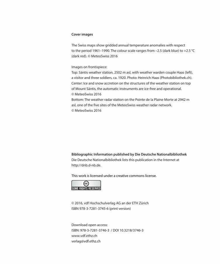
Cover images
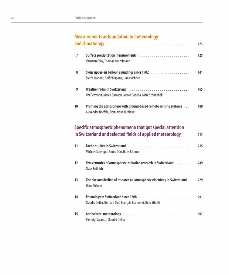
The Swiss maps show gridded annual temperature anomalies with respect to the period 1961–1990. The colour scale ranges from –2.5 (dark blue) to +2.5 °C (dark red). © MeteoSwiss 2016
Images on frontispiece:Top: Säntis weather station, 2502 m asl, with weather warden couple Haas (left), a visitor and three soldiers, ca. 1920. Photo: Heinrich Haas (Photobibliothek.ch).
Center: Ice and snow accretion on the structures of the weather station on top of Mount Säntis, the automatic instruments are ice-free and operational. © MeteoSwiss 2016Bottom: The weather radar station on the Pointe de la Plaine Morte at 2942 m asl, one of the five sites of the MeteoSwiss weather radar network. © MeteoSwiss 2016
Bibliographic Information published by Die Deutsche Nationalbibliothek Die Deutsche Nationalbibliothek lists this publication in the Internet at http://dnb.d-nb.de.
© 2016, vdf Hochschulverlag AG an der ETH ZürichISBN 978-3-7281-3745-6 (print version)
Download open access:ISBN: 978-3-7281-3746-3 / DOI 10.3218/[email protected]
This work is licensed under a creative commons license.

5
Table of contents
Foreword 9Acknowledgements 11
1 Introduction 13
2 The Swiss Society for Meteorology – the first 100 years 19Markus Furger
From the early pioneers to the basics of meteorology and climatology 31
3 Early pioneers of Swiss meteorology and climatology 33Heinz Wanner
4 Producing climate information for Switzerland – Historical and recent developments 43Simon C. Scherrer, Mischa Croci-Maspoli, Christof Appenzeller
5 History of forecasting services in Switzerland 63Saskia Willemse, Marcel Haefliger, Tobias Grimbacher
6 Dynamical Meteorology: The Swiss contribution 103Huw C. Davies, Heini Wernli
6 Table of contents
Measurements as foundation to meteorology and climatology 123
7 Surface precipitation measurements 125Christian Félix, Thomas Konzelmann
8 Swiss upper-air balloon soundings since 1902 141Pierre Jeannet, Rolf Philipona, Hans Richner
9 Weather radar in Switzerland 165Urs Germann, Marco Boscacci, Marco Gabella, Marc Schneebeli
10 Profiling the atmosphere with ground-based remote sensing systems 189Alexander Haefele, Dominique Ruffieux
Specific atmospheric phenomena that got special attention in Switzerland and selected fields of applied meteorology 213
11 Foehn studies in Switzerland 215Michael Sprenger, Bruno Dürr, Hans Richner
12 Two centuries of atmospheric-radiation research in Switzerland 249Claus Fröhlich
13 The rise and decline of research on atmospheric electricity in Switzerland 279Hans Richner
14 Phenology in Switzerland since 1808 291Claudio Defila, Bernard Clot, François Jeanneret, Reto Stöckli
15 Agricultural meteorology 307Pierluigi Calanca, Claudio Defila

7Table of contents
Evolution of atmospheric chemistry into an integrated part of atmospheric sciences 323
16 The value of Swiss long-term ozone observations for international atmospheric research 325Johannes Staehelin, Stefan Brönnimann, Thomas Peter, Rene Stübi, Pierre Viatte, Fiona Tummon
17 The High Altitude Research Station Jungfraujoch – the early years 351Hans Balsiger, Erwin Flückiger
18 Reactive gases, ozone depleting substances and greenhouse gases 361Brigitte Buchmann, Christoph Hueglin, Stefan Reimann, Martin K. Vollmer, Martin Steinbacher, Lukas Emmenegger
19 History of atmospheric aerosol science in Switzerland 375Urs Baltensperger
Broadening the view from climatology to climate sciences 393
20 Paleoclimatology and polar ice cores 395Bernhard Stauffer
21 IPCC Working Group I: The Swiss contribution 1988–2014 413Thomas F. Stocker
22 Appendix A 439
23 Appendix B 449


9
Foreword
In 2016 the Swiss Society for Meteorology (Schweizerische Gesellschaft für Mete-orologie, SGM) celebrates its 100th anniversary. Compared to other meteorological societies it is not among the oldest ones, but nevertheless in its century of exis-tence meteorology has gone through such a remarkable evolution that it is worth-while to take a look back and recapitulate the developments of both the science and the society – and to reveal their interaction. The idea of this book is to give an overview of what happened in the field of atmospheric sciences in Switzerland between the time of the first systematic long-term meteorological observations and today. As meteorology grew from the beginning on in a very international context, nearly all described developments have a more or less strong connection to the international scene. Although aware of these close ties, we nevertheless decided to concentrate on contributions to atmospheric sciences that originated in Switzerland. Depending on the discipline, the retrospection covers a timespan exceeding the century, for example, in the case of ground measurements and of theoretical dynamic meteorology – or covers just a few decades, for example, in the case of the newest remote sensing techniques.
The idea to collect and document the achievements of the last century in atmo-spheric sciences in Switzerland ripened within the executive committee of the SGM sometime in 2013, when it set up a draft of the content and searched for a first group of voluntary authors within the community of atmospheric scientists to refine the plan. It soon became clear that the workload for coordinating the publication was better distributed on the shoulders of more than one person, so an editorial team was established with the acting and the past presidents as its members. Our team provided knowledge about the SGM issues and the experi-ence in networking, atmospheric sciences (physics and chemistry), research and weather services as well as publishing, but less so in history of sciences. In the meantime, the publication, originally meant as a simple report, had become a real book. Yet, it was a primer for both the editorial team members and for some of the authors.
10 Foreword
Although this retrospect into the past events of the atmospheric sciences in Swit-zerland is quite comprehensive, it was not possible to cover all the topics we were aware of, and indeed we cannot be sure not to have missed something important. Therefore, we ask the reader to be appreciative of the fact that this book does not comprehensively cover all of the growing field of atmospheric sciences. On the other hand, some facts are mentioned in more than one chapter, being relevant as they are for each of them. Where possible, cross-references to other chapters have been made. Furthermore, it was deliberately decided not to describe the international developments in detail as this would have gone beyond the scope of this book.
In a multilingual country like Switzerland the choice of the language is often a difficult issue: A fair treatment of every language area would have meant publishing the book in German as well as in French and in Italian. On the other hand, the main language in natural sciences today is English, and we wanted to facilitate the book’s international dissemination. Consequently, we decided to publish it in English. We also wanted to make it available for free as an eBook. Of course, some of the cited literature, especially the older references, was published in one of the national lan-guages, as can be abundantly seen in the various chapters’ reference lists.
Concerning the scientific level of the individual chapters, our intention was to set it at the level of a masters degree in natural sciences without specialisation in atmospheric sciences. Somewhere along the way, however, we realized that it wouldn’t be possible to attain a homogeneous level between all the chapters – on the one hand, because of the different writing styles of the authors and, on the other hand, because of the different scientific and technical level of the topics. The content of the individual chapters should give a broad overview of the topic, whereas the references can be used to delve further into detail. Besides the refer-ences listed in the chapters, some authors also put together a list of further pub-lications not mentioned in their texts which could be useful for the interested reader. The complete compilation of these lists is available for download on the website of the publisher (www.vdf.ethz.ch).
Saskia Willemse (SGM President 2012–2015, i. e., at the time of the realisation of the book) Markus Furger (SGM President 2008–2011)

11
Acknowledgements
In the course of this project, many members of the Swiss atmospheric sciences community were involved in the compilation of this book; 46 of them wrote the chapters and even more acted as reviewers or provided useful information. We are very grateful to everyone who contributed to this book, also in light of the fact that the authors will not increase their impact factor. The whole work was done solely on a voluntary basis. Though some of the contributors might have been allowed to use some labour time, nobody got payed for the writing or the review of a chapter. The authors are mentioned together with the title of their respective chapter, and the contributors of useful information are acknowledged at the end of each chapter. Every chapter was reviewed at least by one author of another chapter as well as by a specialist of the topic not involved in the writing of the book. The following external experts were involved in the review of the chapters (in alphabetical order):
Christof Ammann Stefan Brönnimann Pierre Dèzes Josef Egger Heinz W. Gäggeler Regula Gehrig Robert Gehrig Thomas Gutermann Christian Häberli Niklaus Kämpfer Reto Knutti Cornelia Lüdecke Fritz Neuwirth
Stephan Nyeki Rolf Philipona Michel Rossi This Rutishauser Eva Schüpbach Christoph Spirig Hans Volkert Hansruedi Völkle Laurent Vuilleumier Rudolf O. Weber Rolf Weingartner Martin Wild

12 Acknowledgements
The size of the community of atmospheric scientists in Switzerland is manageable, but we were unfortunately unable to involve everybody in the process. We apol-ogise if we left out someone who would have been able to deliver an important additional contribution.
Furthermore, we thank the sponsors who, with their contribution to the funding of the publishing costs, made it possible to produce this book:
Swiss Academy of Sciences SCNAT Federal Office of Meteorology and Climatology MeteoSwiss
Last but not least, we also thank the publishing company vdf Hochschulverlag and in particular Angelika Rodlauer, who coordinated the whole publishing process and supported us with good advice whenever we needed it, as well as the lan-guage editor Joseph Smith, who made sure that the English of our texts is correct without influencing too much the style of the individual authors, as well as Claudia Wild, who put everything in an attractive layout.
13
1 Introduction
1.1 Atmospheric sciences in a global context
The weather doesn’t care about political borders! Weather forecasting would be impossible without a strong international collaboration for the exchange of mea-surements and observations. But also research in the field of meteorology, clima-tology and the atmospheric sciences in general needs international exchange, particularly in a small country like Switzerland. The atmosphere is a huge labora-tory that prevents experiments from being shaped by the scientists and or repeated systematically. To study a specific phenomenon, it may therefore be nec-essary to measure it in different settings in different parts of the world in order to define and sharpen the scientific rules and characteristics that describe it. In some cases such measurements require costly and elaborate field campaigns, which often are carried out by a consortium of different countries, especially in areas with many small countries like Europe.
Swiss atmospheric scientists were participating in the international community already in the early days of meteorology, particularly in the decades before World War I. Research collaborations like the International Polar Years (IPY) and the Inter-national Geophysical Year (IGY) strengthened international relations, and after 1980 large international field experiments under the auspices of World Meteoro-logical Organisation WMO (such as ALPEX or MAP) cemented the integration of the Swiss community in the international research networks. These international connections, which were probably also favoured by the presence of WMO in Geneva, can be found in fairly every chapter of this book. The interested reader will also find many hints and further information about these developments in the referenced literature.

14 From weather observations to atmospheric and climate sciences in Switzerland1
1.2 Content in a nutshell
The main goal of this book is to document the historical development of the atmo-spheric sciences, so clearly time becomes the main criterion defining the thread of its contents. But aligning all contributions only according to when the story of the respective topic started would give the impression of a rather casual sequence of contributions. Following a chapter on the history of the Swiss Society for Mete-orology (Chapter 2) we therefore grouped the contributions in five blocks, begin-ning with the early pioneers:
a. From the early pioneers to the basics of meteorology and climatology
The first witnesses of routine observations and measurements of the weather in Switzerland date back to the end of the Middle Ages, i. e., long before the founda-tion of organisations like the Swiss Society for Natural Sciences, the Swiss Central Meteorological Institute or the Swiss Society for Geophysics, Meteorology and Astronomy (from which the Swiss Society for Meteorology originated). The main goal of these routine observations was to study the climate as well as its connec-tion with glaciers (Chapter 3). The start of a centrally organised Swiss Meteorolog-ical Network in 1863 set the basis for a long-term, systematic climatological work still going on today. The availability of long time series of observations and mea-surements of homogeneous quality triggered the development of methods to classify and analyse the data and the advent of powerful computers has boosted this development in the last few decades (Chapter 4). Although the meteorolog-ical network was originally set up for climatological purposes, from the second half of the 19th century it also was used to satisfy the growing need to (better) predict the weather. In the following decades, the pace in the evolution of weather fore-casting was set by technological developments, first in the field of communication technologies, then in the field of computer and remote-sensing technologies as well as of mathematical and numerical methods (Chapter 5). Another basic com-ponent of meteorology was the formulation of the basic laws governing atmo-spheric flow. The discipline of dynamical meteorology took its very first steps in the 19th century and developed only slowly until the 1960s. In the last half of the past century, thanks to the improvement and extension of all kinds of measuring networks and the development of high performance computing, dynamical mete-orology experienced an enormous development, which in turn led to an impres-sive improvement in the capability of predicting the weather (and later on also the climate) with numerical models (Chapter 6).

15Introduction 1
b. Measurements as foundation to meteorology and climatology
Measurements are fundamental to the analysis and forecasting of weather and climate. At the very beginning of systematic measurements – and for many years to follow – weather and climate analyses were based completely on ground mea-surements at single spots (including mountain observatories). Among the main meteorological parameters measured on a routine basis, precipitation – which at first glance might look as the simplest parameter to measure as it requires only a reservoir to be set up under the open sky – is the parameter that causes meteo-rologists and climatologists the most troubles because of its very high spatial and temporal variability (Chapter 7). Although it has always been clear that the weather doesn’t take place only in the first few meters above the ground, until the beginning of the 18th century it was not possible to investigate the structure of the atmosphere at higher levels, and reasonable temporal and spatial coverage was not achieved before the early 20th century. With the development of the balloon sounding technology, it became possible to carry out first studies on the stratifi-cation of the (lower) atmosphere. Yet it took a few more decades before the first and to date only operational balloon sounding station in Payerne commenced measuring on a daily basis (Chapter 8). It took another half century after the first balloon sounding before the next step in the exploration of the free atmosphere could be made: Radar technology was the first remote-sensing technology to allow for the measurement of a whole volume of air. In Switzerland, the first mete-orological radar was deployed in the 1950s, and the science of radar meteorology has played an important role in the meteorological community ever since (Chap-
ter 9). In the past 40 years further technologies for the remote sensing of the atmosphere were developed, and some of them are in use for specific applications also in Switzerland. Among them are the radar wind profiler, the microwave radi-ometer and the LIDAR (Chapter 10).
c. Specific atmospheric phenomena that got special attention in Switzerland and selected fields of applied meteorology
A special meteorological phenomenon that can be observed in the Alps when a large-scale flow crosses them more or less perpendicularly is the foehn. This spe-cial, locally strongly variable wind has been the subject of several studies in the past centuries and still gets special attention today (Chapter 11). The measure-ment and research of atmospheric radiation has a long tradition in Switzerland and started in two locations in the Swiss Alps, which at the beginning of the 20th
16 From weather observations to atmospheric and climate sciences in Switzerland1
century were known mainly as health resorts, namely Davos and Arosa. In the meantime, the PMOD in Davos has attained the status of a World Radiation Centre (WRC) of the World Meteorological Organization, and its instruments are flown on satellites in space to accurately measure the solar irradiance which is the basic energy input into the climate system (Chapter 12). A special field of atmospheric sciences in the late 19th and early to mid-20th century in Switzerland (but which later lost the attention of the researchers) is atmospheric electricity. The main goals of these research activities were to better understand the atmospheric elec-tric field and to find connections with other atmospheric phenomena like light-ning as well as possible influences on human health. (Chapter 13). One of the oldest fields of applied meteorology is phenology: Plants react to climate and can therefore be used as indicators for varying seasons. The spatial climatic informa-tion derived from phenological observations is useful not only to agronomists, but also to other professionals (Chapter 14). Before the advent of aviation and other weather dependent economies, the main field of professional application of mete-orology was agriculture. Although nowadays many vegetables and fruits are grown in the controlled atmosphere of greenhouses, many crops still grow under the open sky and are therefore exposed to the extremes of weather and climate. With the intensification of land exploitation in a changing climate, agricultural meteorology is still an important field of applied meteorology (Chapter 15).
d. Evolution of atmospheric chemistry into an integrated part of atmospheric sciences
Since the discovery of ozone in 1839 and the start of atmospheric ozone measure-ments in the 1920s, Swiss observatories and scientists have played a key role in developing our understanding of this important atmospheric trace gas. The world’s longest measurement series of column ozone and the first reliable obser-vations of the ozone profile were made in Arosa (Chapter 16). In times when the basic meteorological parameters could not yet be measured in the free atmo-sphere, mountain research stations played an important role in the investigation of the third dimension of the atmosphere. Jungfraujoch was not among the first mountain stations to be installed in the Alps, but it was the first one accessible all year long by train – and it was, and today still is, also a very important research station in the field of atmospheric chemistry (Chapter 17). In the course of the 20th century other natural and anthropogenic chemical components of the atmo-sphere were investigated more thoroughly, and in the 1970s Switzerland started its contribution to international programmes for the monitoring of pollutants.

17Introduction 1
Nowadays, more than 70 gaseous compounds are monitored at Jungfraujoch, and some long-term series spanning decades contribute to the monitoring of the implementation of international treaties like the Kyoto Protocol (Chapter 18). Beside some gaseous pollutants in the atmosphere also the aerosols affect the Earth’s climate and the health of all living beings. In Switzerland modern aerosol science started in the 1970s, and the research station of Jungfraujoch played a major role in this field as well. Long-term series of aerosol parameters show a decrease in particulate matter concentration in Switzerland over the past decades (Chapter 19).
e. Broadening the view from climatology to climate sciences
For many decades the climate sciences concentrated on the analysis and interpre-tation of long time series of weather measurements. As these time series cover only about 150 years at the most, indirect methods were developed to derive information on the climate variations the Earth experienced before modern mete-orological measurements. Ice cores extracted from glaciers are an excellent archive of atmospheric composition in the past, and the analyses of stable isotopes con-tained in these ice cores deliver a good estimate of the temperature at the Earth’s surface at the time where the ice was formed. This is one of the disciplines of paleoclimatology which help to reconstruct the Earth’s climate of many thousands of years ago and some important contributions to this discipline were delivered by Swiss scientists (Chapter 20). With the increasing awareness that the climate changes at a rate perceptible within the measured time series, and that mankind has an influence on climate change, the interest in projections of future climate change grew and spread well beyond the scientific community. Because climate change has an influence on all life forms and on many economic sectors as well, it has increasingly caught the attention of politicians and governments. The Inter-governmental Panel on Climate Change (IPCC) was founded in 1988, and nowa-days it is a well-established organisation providing the whole world with the sci-entific evidence of all aspects of climate change. Swiss scientists have been involved in IPCC from the initial years of its existence and have made the most numerous and substantial contributions in Working Group I, which deals with the natural science aspects (Chapter 21).
The historical developments described in this book show how an increasing num-ber of scientific and technical disciplines have become part of atmospheric sci-ences since the beginning of the 19th century. In the future some additional disci-

18 From weather observations to atmospheric and climate sciences in Switzerland1
plines may join the field, but the development that will likely be even more important will be the increasing multidisciplinarity. Atmospheric processes, at first investigated as isolated phenomena, are now increasingly being integrated into complex models that simulate physical as well as chemical processes of the atmo-sphere and connect them to other processes of the Earth system. Computer power will continue to grow, and, together with that development, also the resolution and the complexity of the models will increase, demanding in turn a more precise assessment of the state of the atmosphere and therefore for more and better mea-surements. The amount of data produced with these activities will reach gigantic dimensions and will require new data-processing methods. But at the very end of the chain, as recipient of the information produced, will still be human beings, whose brain will not develop at the same pace as computer power. Hence, new methods and technologies will become necessary to simplify and condense the huge amount of information into digestible and usable portions.
19
2 The Swiss Society for Meteorology – the first 100 yearsMarkus Furger
In the middle of World War I a small group of scientists established a scholarly society to foster the
exchange of knowledge and ideas within the disciplines of geophysics, meteorology and astronomy in
Switzerland. Today, 100 years later, the former multidisciplinarity has evolved into a holistic approach
typical for the atmospheric sciences: The full breadth of topics, from atmospheric physics and dynamics
to chemistry, from climate sciences to the impacts on society, are now subsumed under this name.
2.1 Formation of the Society
The Swiss Society for Geophysics, Meteorology and Astronomy (GMA) was founded in Schuls (Scuol), Grisons, on 8 August 1916 at the Annual Assembly of the Swiss Academy for Natural Sciences (formerly the Schweizerische Natur-forschende Gesellschaft, SNG). The meeting (Anonymous 1916) was initiated by a small group of interested individuals led by Alfred de Quervain, professor at ETH Zurich (Chapters 3, 17). The other members of the group were Robert Billwiller II (Zurich), Paul-Louis Mercanton (Lausanne), and Albert Riggenbach (Basel). The idea behind the formation of a new academic society was to create a forum for scientists more specifically interested in the three main disciplines (astronomy, geophysics, meteorology) than was the case with associations of mathematicians, physicists or geologists, where these topics had become marginalised during their respective annual meetings. It was hoped that a smaller, but more engaged group would better serve the exchange of ideas and knowledge. The call for membership brought more than 40 participants to the constitutional meeting, whose names are listed in the 25-year anniversary publication (Schweizerische Gesellschaft für Geophysik 1941). On the day prior to the constitutional meeting of the GMA, the SNG plenary had already accepted the GMA as one of its member societies. The event was celebrated with 10 scientific presentations given by a selection of the new members.
Paul Scherrer Institute, Laboratory
of Atmospheric Chemistry, Villigen PSI
20 From weather observations to atmospheric and climate sciences in Switzerland2
2.2 The Society’s names and members
The name of the new society reflected the wide scope of interests and the multi-disciplinarity of its original members. Paul-Louis Mercanton (Figure 2.1 and Appendix B), the first President (1916–1920), was Professor of Physics in Lausanne, where he later also held the chair in geophysics and meteorology. He was head of the Service Météorologique Vaudois and became later director of the Meteorolo-gische Zentralanstalt (MZA) in Zurich (1934–1941). Alfred de Quervain, the first Vice-President, was at that time a geophysicist involved in earthquake research, though he is better remembered for his Greenland expedition in 1912, where he traversed the Greenland ice sheet from West to East. He habilitated in meteorology and was especially interested in the upper atmosphere. The President of the day during GMA’s foundation session, Albert Riggenbach (Basel), was the head of the Astronomical-Meteorological Agency in Basel. He worked in the areas of meteo-
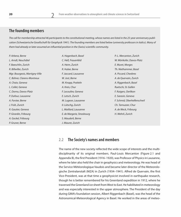
The founding members
The call for membership attracted 46 participants to the constitutional meeting, whose names are listed in the 25-year anniversary publi-
cation ( Schweizerische Gesellschaft für Geophysik 1941). The founding members are listed below ( university professors in italics). Many of
them had already or later assumed an influential position in the (Swiss) scientific community.
P. Arbenz, Berne
L. Arndt, Neuchâtel
F. Baeschlin, Zurich
R. Billwiller, Zurich
Mgr. Bourgeois, Martigny-Ville
C. Bührer, Clarens-Montreux
A. Chaix, Geneva
L. Collet, Geneva
C. Dorno, Davos-Platz
P. Dufour, Lausanne
A. Forster, Berne
J. Früh, Zurich
R. Gautier, Geneva
P. Girardin, Fribourg
A. Gockel, Fribourg
P. Gruner, Berne
A. Hagenbach, Basel
C. Heß, Frauenfeld
A. Heim, Zurich
R. Huber, Berne
F. Jaccard, Lausanne
W. Jost, Berne
M. Knapp, Pratteln
A. Kreis, Chur
F. Lecoultre, Geneva
E. Letsch, Zurich
M. Lugeon, Lausanne
0. Lütschg, Zurich
L. Maillard, Lausanne
E. de Margerie, Strasbourg
S. Mauderli, Berne
J. Maurer, Zurich
P.-L. Mercanton, Zurich
W. Mörikofer, Davos-Platz
E. Muret, Morges
Th. Niethammer, Basel
A. Piccard, Chexbres
A. de Quervain, Zurich
A. Riggenbach, Basel
Ruetschi, St. Gallen
F. Rutgers, Oerlikon
E. Sarasin, Geneva
F. Schmid, Oberhelfenschwil
Ch. Tarnuzzer, Chur
A. de Weck, Fribourg
H. Wehrli, Zurich

21The Swiss Society for Meteorology – the first 100 years 2
rology, physics, geophysics, astronomy and geodesy. Such strong interdisciplinar-ity of both people and institutions was not unique, neither for the time nor for Switzerland, as numerous institutes abroad still demonstrate, e. g., the ZAMG (Zen-tralanstalt für Meteorologie und Geodynamik – Central Institute for Meteorology and Geodynamics) in Vienna, Austria. This interdisciplinarity is also reflected in the topics of the presentations given at the annual assemblies of the society, as shown in the insert A wealth of research topics.
The society changed its name from GMA to SGG (Schweizerische Gesellschaft für Geophysik – Swiss Society for Geophysics) in 1970, after the Swiss astrono-mers had founded their own Society for Astronomy and Astrophysics in 1969. In 1994 the geophysicists then separated from the SGG to join the Swiss Geological Society, and the remaining meteorologists once more changed the name of the society into SGM (Schweizerische Gesellschaft für Meteorologie – Swiss Society for Meteorology). This name has prevailed to the present day (Appendix B). These many name changes reflect to some degree the separation between disciplines, and hence the loss of multidisciplinarity, as a consequence of the growth of the various research fields both in research topics and in the number of people involved. At the same time the atmospheric sciences themselves developed into a truly interdisciplinary science, requiring and fostering a holistic approach to the subject.
The professional activity of the Society’s members spanned a broad range, from university professors to weather-service practitioners and students. In the early decades, high-school teachers were also actively involved in research. Their con-tributions, however, has decreased over the last few decades, possibly because of the inherent professionalisation that occurred in accessing and operating the data acquisition and processing facilities required for modern studies of atmo-spheric phenomena. Examples are Alfred Kreis, a high-school teacher in Chur and Secretary of the GMA from 1917–1940, and Hans-Ulrich Dütsch, a teacher in Zürich before he received a position at ETHZ. He was also President of GMA from 1966–1968.
Honorary membership was awarded to three individuals: Walter Mörikofer in 1972, Max Bouët in 1977, and Hans Richner in 2010, the latter for his outstanding engagement for the society over the past 20 years. Hans Richner was also instru-mental in significantly increasing the number of members in 2001. He was active in establishing the European Meteorological Society (EMS) and was an avid editor of the Meteorologische Zeitschrift in the 1990s.
Figure 2.1: Paul-Louis Mercanton, the first President of the Swiss Society for Geophysics, Mete-orology and Astronomy (GMA), 1916–1920. Photograph taken in 1919. © Fonds de Jongh, Musée de l’Elysée, Lausanne.
Alfred de Quervain was not only the ini-
tiator of the GMA, he was also a driving
force for the establishment of the
high-Alpine research station Jungfrau-
joch and became the first President of
the Jungfraujoch Commission in 1922.
In the annual report of the society of
1965 the A of GMA stands for ‘astrology’ –
a rather amusing typo.
The Swiss Association for Natural
Sciences (SNG) was originally founded in
1815 for academics and amateurs alike,
comprising the minimum denominator
for all pre-existing scholarly societies of
the time (Kupper and Schär 2015).

22 From weather observations to atmospheric and climate sciences in Switzerland2
2.3 The Annual Meetings – the society’s main activity and communication channel
From the very beginning, the annual meetings were the main activity of the soci-ety. These meetings were expressly used as a platform for the exchange of ideas, scientific discussions, cultivating friendships, creating new contacts and much more. Most of these annual meetings took place in the framework of the SNG’s (later Schweizerische Akademie der Naturwissenschaften – SANW) own annual meetings. From 2002 to 2006 the society’s annual meetings were organised inde-pendently by the SGM. In 2007, the SGM – then a new member of the newly estab-lished Platform Geosciences of the Swiss Academy of Sciences SCNAT (SANW had meanwhile changed its acronym into SCNAT) – joined the 5th Swiss Geoscience Meeting with a session on meteorology and climatology. This ‘marriage’ lasted until 2013. Although participants could in principle have profited from attending sessions on a large variety of geoscience topics, this option was regrettably not extensively used. Therefore, in 2014 the SGM took its own path with an annual meeting in Zurich apart from the Swiss Geoscience Meeting. Except for the years 1918 and 1939, the annual meetings always took place in a Swiss location, typi-cally (though not exclusively) in the capital city of a canton (Appendix B). In 1918 the meeting did not take place because of the influenza epidemic, and in 1939 the general mobilisation of troops at the beginning of World War II absorbed the attention of most of the potential participants.
It is interesting to browse through the list of presentations of these meetings. The listings were prepared for the 25th and 50th anniversaries of the society in 1941 (Schweizerische Gesellschaft für Geophysik 1941) and 1966 (Schweizerische Gesellschaft für Geophysik 1966), respectively. They mirror the development of the disciplines as well as its members and their activities. In the first 25 years of its existence, 333 presentations were given at the meetings, in the second 25 years there were 402 (Dütsch 1967). They covered all disciplines in a well-balanced man-ner, even more so because some of the presenters were active across the disci-plines. In the traditional Swiss way the presentations were given in German, French or Italian until the merger with the Swiss Geoscience Meeting, at which point English became the language of choice. Most talks given during the annual meet-ings were published in the volumes of the Verhandlungen der Schweizerischen Naturforschenden Gesellschaft, which appeared annually. They have been ret-ro-digitised by the ETH library and are freely available on the internet (SEALS – Swiss Electronic Academic Library Services 2014).

23The Swiss Society for Meteorology – the first 100 years 2
A wealth of research topics
The annual meetings of the SNG were the central events of the society to foster contacts and exchange of ideas among its members. They nicely mir-ror the development of the disciplines over the past century, as most of the presentations were given by members or persons active in contemporary research. Many presentations dealt with the development of instrumenta-tion and measurement and forecasting methods, e. g., deployment of aircraft for glaciological studies (Mercanton 1922), the radiosounding system in the 1930s (Berger 1937), the automated weather station network in the 1970s, and remote sensing instruments in the 1990s. In hindsight, it is fascinating to see that topics of such strong relevance in the 21st century were already on the screen of careful observers 100 years earlier. A few selected examples shall illustrate this, without pretence to completeness, and with an emphasis on the first half of the 20th century. The references are taken from Schweize-rische Gesellschaft für Geophysik (1966, 1941).
Long-range transport of Saharan dust to Switzerland was described by Jost (1930), referring to a particular event of 24 April 1926, and by Glawion (1937). At about the same time research on the chemical composition of snow was reported (Gassmann 1927) as were dust bands in glacier ice (Nussbaum 1929). The health effects of airborne particulate matter were discussed by Verzár (1954). From a modern perspective of global warming we have to take notice of presentations on the growth of the Upper Grindelwald Glacier in the 1920s (Lütschg 1932), and on climate and glacier variations in the Alps (Zingg 1953). In 1938 and thereafter, Milankovitch’s theory of insolation was discussed intensely (Schneider 1938, 1940). Many presentations also dealt with sky brightness, sky colours, twilight, light transmission through the atmosphere and light extinction (a topic of special interest to astronomers) as well as other phenomena of atmospheric optics. Cosmic rays were dis-cussed as early as 1929 (Hess and Mathias 1929; Lindholm 1929), roughly 15 years after their discovery. Their influence on cloud formation remains a topic of research to the present day. Atmospheric electricity was a topic from the beginning of the society’s existence (Gockel 1922, 1924). Research on UV radiation started out in the 1920s with applications to biometeorology, but in the 1930s it became more relevant to atmospheric chemistry and ozone (Dobson and Götz 1932). Historical records of key meteorological parame-ters dating back to the 18th and early 19th century were presented by Ambühl
24 From weather observations to atmospheric and climate sciences in Switzerland2
2.4 Journals and other communication channels
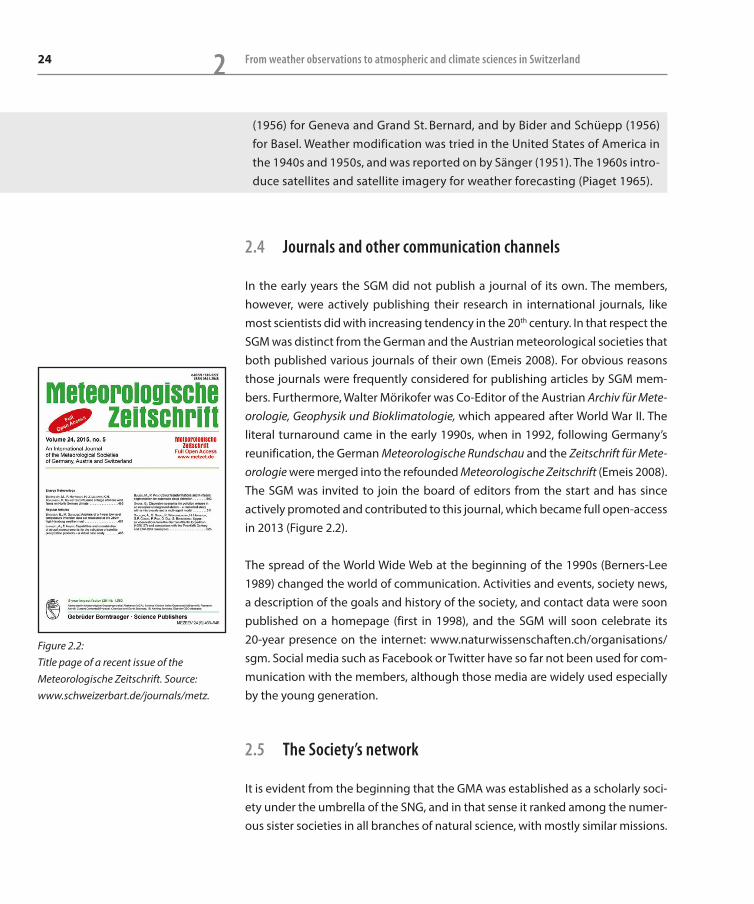
In the early years the SGM did not publish a journal of its own. The members, however, were actively publishing their research in international journals, like most scientists did with increasing tendency in the 20th century. In that respect the SGM was distinct from the German and the Austrian meteorological societies that both published various journals of their own (Emeis 2008). For obvious reasons those journals were frequently considered for publishing articles by SGM mem-bers. Furthermore, Walter Mörikofer was Co-Editor of the Austrian Archiv für Mete-orologie, Geophysik und Bioklimatologie, which appeared after World War II. The literal turnaround came in the early 1990s, when in 1992, following Germany’s reunification, the German Meteorologische Rundschau and the Zeitschrift für Mete-orologie were merged into the refounded Meteorologische Zeitschrift (Emeis 2008). The SGM was invited to join the board of editors from the start and has since actively promoted and contributed to this journal, which became full open-access in 2013 (Figure 2.2).
The spread of the World Wide Web at the beginning of the 1990s (Berners-Lee 1989) changed the world of communication. Activities and events, society news, a description of the goals and history of the society, and contact data were soon published on a homepage (first in 1998), and the SGM will soon celebrate its 20-year presence on the internet: www.naturwissenschaften.ch/organisations/sgm. Social media such as Facebook or Twitter have so far not been used for com-munication with the members, although those media are widely used especially by the young generation.
2.5 The Society’s network
It is evident from the beginning that the GMA was established as a scholarly soci-ety under the umbrella of the SNG, and in that sense it ranked among the numer-ous sister societies in all branches of natural science, with mostly similar missions.
(1956) for Geneva and Grand St. Bernard, and by Bider and Schüepp (1956) for Basel. Weather modification was tried in the United States of America in the 1940s and 1950s, and was reported on by Sänger (1951). The 1960s intro-duce satellites and satellite imagery for weather forecasting (Piaget 1965).
Figure 2.2: Title page of a recent issue of the Meteo rolo gische Zeitschrift. Source: www.schweizerbart.de/journals/metz.

25The Swiss Society for Meteorology – the first 100 years 2
The evolution over the past 100 years has not substantially changed its mission, but over the course of time a remarkable extension of activities characterise its development within the national and international context. This evolution ran parallel to the development of the SNG, which changed its name from Schweize-rische Naturforschende Gesellschaft to Schweizerische Akademie der Naturwis-senschaften and its acronym from SANW (ASSN in French and Italian) to SCNAT (in all four national languages), and was reorganised in disciplinary platforms. The SGM today belongs to the Platform Geosciences, established in 2007 during the reformation process of SCNAT. The society maintains informal contacts to the working groups ACP (Commission for Atmospheric Chemistry and Physics) and SKF (Commission for Remote Sensing) of the Platform Geosciences, and to the Forum for Climate and Global Change (ProClim-) of the Platform Science and Pol-icy. On the international level, one SGM member is delegated to act as the Swiss National Correspondent to the International Association for Meteorology and Atmospheric Sciences IAMAS (via the Swiss National Committee of the IUGG) and to liaise between the Swiss atmospheric science community and this global research network. A true highlight in this context was the Davos Atmosphere and Cryosphere Assembly 2013, with some 989 participants from 52 countries on 5 continents, originally initiated by the IAMAS and the International Association of Cryospheric Sciences IACS, and organised by a national organizing committee of several Swiss institutes.
Of perhaps even higher importance and better visibility to Swiss atmospheric sci-entists is the European Meteorological Society (EMS), of which SGM is a full mem-ber since its foundation in Norrköping, Sweden, in 1999. The EMS was formed on the initiative of four individuals representing their respective national meteoro-logical societies (United Kingdom, France, Germany and The Netherlands), and in the meantime it counts 36 member societies from all over Europe. The EMS is a ‘society of societies’, not of individual members. The annual meetings of the EMS have become an attractive opportunity for scientists and practitioners in atmo-spheric sciences to exchange new ideas and research results.
2.6 Conferences
The foundation of the GMA during the years of World War I might be considered to have been a remedy against the travel restrictions of that time and as a general strengthening of national contacts. A closer look at the presentations given in the annual meetings reveals, however, that the members were well connected within

26 From weather observations to atmospheric and climate sciences in Switzerland2
Europe, and indeed worldwide, both before and after WWI. Nevertheless, the organisation of international scientific meetings and conferences by the GMA was not mentioned in their protocols until the second half of the 20th century. A list of conferences sponsored or co-organised by the Society is given in Table 2.1. The 3rd International Conference on Alpine Meteorology (ICAM/ITAM) was held in Davos in 1954, but is not mentioned in the annual report of the SNG. The 9th ICAM 1966 in Brig coincided with the 50-year anniversary of the SGM, which is mentioned in the proceedings volume for hosting the conference. The IUGG General Assembly in 1967 in Zurich, Berne, Lucerne and St. Gall was supported by the SGM as a co- organizer. Two more ICAMs were organised with SGM support in Grindelwald in 1978 and in Engelberg in 1990. Two specialised conferences, one on biometeorol-ogy (Interlaken 1976) and the other on radar meteorology (Zurich 1984), were jointly organised with the American Meteorological Society. In 2001 the first DACH Meteorologentagung took place in Vienna and became a 3-yearly event in the German speaking countries of Europe (DACH stands for Germany – D, Austria – A, and Switzerland – CH), always with support of the SGM and its members.
Table 2.1: Conferences co-organised by the GMA/SGG/SGM.
Year Conferences Location Date
1954 3rd ICAM – International Conference on Alpine Meteorology Davos 12–14 Apr
1966 9th ICAM – International Conference on Alpine Meteorology Brig and Zermatt 14–17 Sep
1967 IUGG 1967 – International Union of Geodesy and Geophysics Zurich, Berne, Luzern, St. Gallen
25 Sep – 9 Oct
1976 Joint AMS/SGG Meeting on Meteorology and Biometeorology in mountain areas Interlaken 9–14 Jun
1978 15th ICAM – International Conference on Alpine Meteorology Grindelwald 19–23 Sep
1980 Internationales Alfred Wegener Symposium Berlin, Germany 25–29 Feb
1984 22nd International Conference On Radar Meteorology Zurich 10–13 Sep
1990 21st ICAM – International Conference on Alpine Meteorology Engelberg 17–21 Sep
2001 DACH 2001 Vienna, Austria 18–21 Sep
2003 ICAM-MAP’03 – International Conference on Alpine Meteorology/MAP Meeting Brig 19–23 May
2004 DACH 2004 Karlsruhe, Germany 7–10 Sep
2007 DACH 2007 Hamburg, Germany 10–14 Sep
2010 EMS–ECAC 2010 Zurich 13–17 Sep
DACH 2010 Bonn, Germany 20–24 Sep
2013 DACA-13 – Davos Atmosphere and Cryosphere Assembly Davos 8–12 Jul
DACH 2013 Innsbruck, 2–6 Sep 2013 Innsbruck, Austria 2–6 Sep
27The Swiss Society for Meteorology – the first 100 years 2
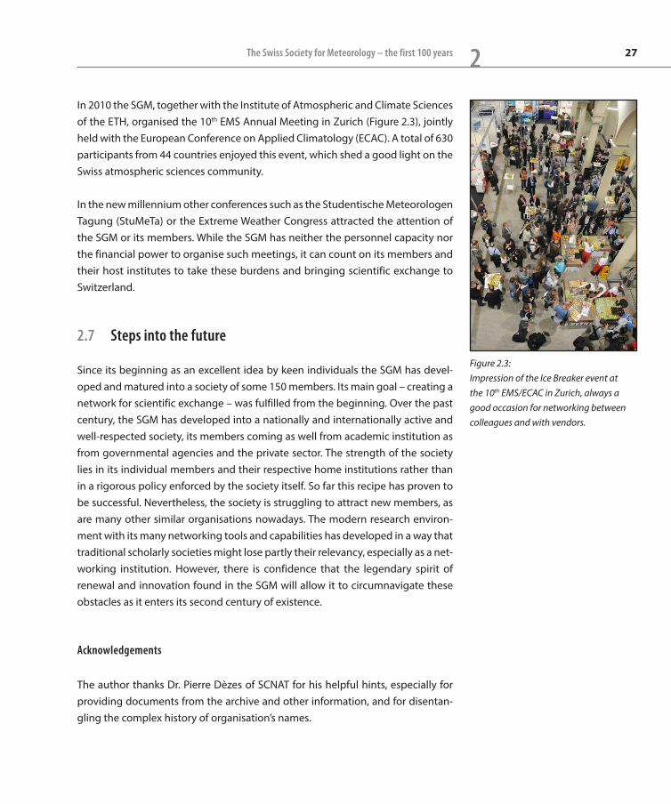
In 2010 the SGM, together with the Institute of Atmospheric and Climate Sciences of the ETH, organised the 10th EMS Annual Meeting in Zurich (Figure 2.3), jointly held with the European Conference on Applied Climatology (ECAC). A total of 630 participants from 44 countries enjoyed this event, which shed a good light on the Swiss atmospheric sciences community.
In the new millennium other conferences such as the Studentische Meteorologen Tagung (StuMeTa) or the Extreme Weather Congress attracted the attention of the SGM or its members. While the SGM has neither the personnel capacity nor the financial power to organise such meetings, it can count on its members and their host institutes to take these burdens and bringing scientific exchange to Switzerland.
2.7 Steps into the future
Since its beginning as an excellent idea by keen individuals the SGM has devel-oped and matured into a society of some 150 members. Its main goal – creating a network for scientific exchange – was fulfilled from the beginning. Over the past century, the SGM has developed into a nationally and internationally active and well-respected society, its members coming as well from academic institution as from governmental agencies and the private sector. The strength of the society lies in its individual members and their respective home institutions rather than in a rigorous policy enforced by the society itself. So far this recipe has proven to be successful. Nevertheless, the society is struggling to attract new members, as are many other similar organisations nowadays. The modern research environ-ment with its many networking tools and capabilities has developed in a way that traditional scholarly societies might lose partly their relevancy, especially as a net-working institution. However, there is confidence that the legendary spirit of renewal and innovation found in the SGM will allow it to circumnavigate these obstacles as it enters its second century of existence.
Acknowledgements
The author thanks Dr. Pierre Dèzes of SCNAT for his helpful hints, especially for providing documents from the archive and other information, and for disentan-gling the complex history of organisation’s names.
Figure 2.3: Impression of the Ice Breaker event at the 10th EMS/ECAC in Zurich, always a good occasion for networking between colleagues and with vendors.

28 From weather observations to atmospheric and climate sciences in Switzerland2
References
All references to Verh. Schweiz. Naturforsch. Ges. (Verhandlun-
gen der Schweizerischen Naturforschenden Gesellschaft = Actes
de la Société Helvétique des Sciences Naturelles = Atti della
Società Elvetica di Scienze Naturali) are accessible at SEALS
(e. g. http://retro.seals.ch/digbib/vollist?UID=sng-005).
Ambühl, E., 1956: Temperaturreihen von Genf und Grossem St. Bernhard ab 1798 bzw. 1817. Verh. Schweiz. Naturforsch. Ges., 136, 100.
Anonymous, 1916: Bericht der Sektion für Geophysik und Mete-orologie. Verh. Schweiz. Naturforsch. Ges., 98, 127–138.
Berger, P., 1937: Étude préliminaire des sondages de vent à Cointrin. Verh. Schweiz. Naturforsch. Ges., 118, 112.
Berners-Lee, T., 1989: info.cern.ch – Tim Berners-Lee’s proposal. CERN. http://info.cern.ch/Proposal.html
Bider, M., and M. Schüepp, 1956: Die Reduktion der 200jährigen Bodentemperaturreihe. Verh. Schweiz. Naturforsch. Ges., 136, 87–88.
Dobson, G. M. B., and F. W. P. Götz, 1932: Ozon der Atmosphäre. Verh. Schweiz. Naturforsch. Ges., 113, 326–327.
Dütsch, H.-U., 1967: Administrativer Bericht 1966 der Schweize-rischen Gesellschaft für Geophysik, Meteorologie und Astrono-mie. Verh.Schweiz. Naturforsch. Ges., 147, 86.
Emeis, S., 2008: History of the Meteorologische Zeitschrift. Mete-orol. Z., 17, 685–693, doi:10.1127/0941-2948/2008/0330.
Gassmann, T., 1927: Über das Vorkommen von Phosphor und Selenoxyd im Natureis. Verh. Schweiz. Naturforsch. Ges., 108, 103.
Glawion, H., 1937: Staub und Staubfälle in Arosa. Verh. Schweiz. Naturforsch. Ges., 118, 108–109.
Gockel, A., 1922: Über die Sohnckesche Theorie der Ge -witterelektrizität. Verh. Schweiz. Naturforsch. Ges., 103, 193–194.
Gockel, A., 1924: Über einige luftelektrische Probleme, welche durch Beobachtungen auf dem Jungfraujoch gelöst werden können. Verh. Schweiz. Naturforsch. Ges., 105, 111–112.
Hess, V. F., and O. Mathias, 1929: Neue Registrierungen der kos-mischen Ultrastrahlung auf dem Sonnblick (3100 m). Verh. Schweiz. Naturforsch. Ges., 110, 126–127.
Jost, W., 1930: Der gelbe Schnee vom 24. April 1926. Verh. Schweiz. Naturforsch. Ges., 111, 283.
Kupper, P., and B. C. Schär, 2015: Die Naturforschenden. hier + jetzt, 305pp.
Lindholm, F., 1929: Registrierbeobachtungen der kosmischen Höhenstrahlung auf Muottas-Muraigl. Verh. Schweiz. Natur-forsch. Ges., 110, 125–126.
Lütschg, O., 1932: Beobachtungen über das Verhalten des vor-stossenden Oberen Grindelwaldgletschers im Berner Oberland. Verh. Schweiz. Naturforsch. Ges., 113, 320–322.
Mercanton, P.-L., 1922: L’avion au service de la glaciologie. Verh. Schweiz. Naturforsch. Ges., 103, 199.
Nussbaum, F., 1929: Über die Schmutzbänderung der Gletscher. Verh. Schweiz. Naturforsch. Ges., 110, 129–130.
Piaget, A., 1965: L’utilité des satellites en météorologie. Verh. Schweiz. Naturforsch. Ges., 145, 69–71.
Sänger, R., 1951: Bemerkungen über die Wetterbeeinflussungs-versuche in den USA und Demonstration eines Films über “Pro-ject Cirrus”. Verh. Schweiz. Naturforsch. Ges., 131, 122–123.
Schneider, J. M., 1938: Zur quartären Temperaturkurve nach Spi-taler gegen Milankowitsch. Verh. Schweiz. Naturforsch. Ges., 119, 131–132.
Schneider, J. M., 1940: Die Sonnenstrahlungskurve nach Milan-kowitsch und die Postglacialzeit. Verh. Schweiz. Naturforsch. Ges., 120, 131–133.
Schweizerische Gesellschaft für Geophysik, Meteorologie und Astronomie – Société suisse de Géophysique, météorologie et astronomie, 1966: Verzeichnis der in den “Verhandlungen der Schweizerischen Naturforschenden Gesellschaft” publizierten Referate. Zeitraum 1941–1965. Verzeichnis der Präsidenten und Mitglieder. – Liste des communications scientifiques publiées dans les “Actes de la Société helvétique des sciences naturelles”. Période

29The Swiss Society for Meteorology – the first 100 years 21941–1965. Liste des Présidents et des membres. Fotorotar AG, Zürich, 32 pp.
Schweizerische Gesellschaft für Geophysik, Meteorologie und Astronomie, 1941: Liste der Vorträge gehalten an den Jahresver-sammlungen 1916–1940. Zum 25-jährigen Bestehen der Schwei-zerischen Gesellschaft für Geophysik, Meteorologie und Astrono-mie. City-Druck AG, Zürich, 32 pp.
SEALS – Swiss Electronic Academic Library Services, cited 2014: Retro-digitized journals. [Available online at retro.seals.ch.]
Verzár, F., 1954: Die Retention atmosphärischer Kondensations-kerne in den Atemwegen. Verh. Schweiz. Naturforsch. Ges., 134, 117–118.
Zingg, T., 1953: Klima und Gletscherschwankungen. Verh. Schweiz. Naturforsch. Ges., 133, 70–71.


31
From the early pioneers to the basics of meteorology and climatology


33
3 Early pioneers of Swiss meteorology and climatologyHeinz Wanner
3.1 The predecessors of Swiss meteorology and climatology
There is no doubt that already the Celtic, Roman, Alemannic and Burgundian population living in what is today Switzerland observed the weather and climate and drew conclusions for their life. The first individuals to study the weather and climate in a more scientific sense were passionate observers of such natural phe-nomena. In Zurich the provost of the Grossmünster cathedral, Wolfgang Haller (1525–1601), chronicled his daily weather observations between 1545 and 1576, thereby documenting an important period of what is known as the “Little Ice Age.” Pfister (1984) considered Haller’s diary the most important source for climate his-tory during the third quarter of 16th century. He also mentioned it was not trivial to decode Haller’s diary because Haller partly used a special vocabulary to describe specific weather phenomena. The second eminent weather observer was the pharmacist and town clerk Renward Cysat (1545–1614), who recorded
University of Bern, Oeschger Centre
for Climate Change Research and
Institute of Geography, Bern
Figure 3.1: Portraits of Renward Cysat (left; Photo: Stadtarchiv Luzern), Johann Jakob Scheuchzer (middle; painted by Hans Ulrich Heidegger in 1734) and Horace-Bénédict de Saussure (right; portrayed by Christian von Melchel after Jens Juel).
34 From weather observations to atmospheric and climate sciences in Switzerland3
the weather in Lucerne between 1570 and 1613 (see Figure 3.1, left panel). Pfister (2013) said Cysat was an “interdisciplinary” pioneer of climate research in the Alps and a contemporary witness for the climax of the Little Ice Age. Cysat regularly contacted farmers around Rigi and Pilatus and made profit of their knowledge. Interestingly, he also worked out the first simplified statistics. From his observa-tions he concluded that a change in climate had occurred at the end of the six-teenth century.
Another famous scholar was Johann Jakob Scheuchzer (1672–1733; see Figure 3.1, middle portrait). Scheuchzer was junior town physician and later professor of mathematics in Zurich – and the first classical polymath of Switzerland (Fueter, 1941). He described fossils and attributed them to the deluge. Between 1702 and 1711 Scheuchzer undertook several scientific excursions to the Alps and, aside from making precise meteorological observations, he also carried out the first barometric measurements with a glass tube and mercury on the Gotthard Pass. Scheuchzer also kept a weather station near his house in Zurich. He was the first to attempt precipitation measurements in Switzerland. Even the original version of his diary is undiscoverable, most of the information was published in Latin lan-guage (Pfister, 1984).
3.2 The first mountain meteorologist
Barry (1978) noted that the physicist and philosopher Horace-Bénédict de Sauss-ure (1740–1799), professor at the Geneva Academy, was likely the first mountain meteorologist in the world (see Figure 3.1, right panel). De Saussure not only left very broad scientific work behind, he also constructed several new meteorolog-ical instruments such as the first hair-tension hygrograph (using human hair), a sling psychrometer, a “heliothermometer” and a cyanometer. De Saussure’s hygrograph became an internationally used standard instrument until the estab-lishment of first automatic networks. The heliothermometer, also called “hot box,” consisted of a thermometer exposed to a wooden box lined with blackened cork and covered with three sheets of glass. With this instrument de Saussure demon-strated that solar radiation increased with altitude. The cyanometer was used to measure the blue of the sky and was also utilized by Alexander von Humboldt on his scientific journeys.
Barry (1978) reported that H.-B. de Saussure was not only the second person to climb Mont Blanc in August 1787. During July 1788 he organized a famous moun-

35Early pioneers of Swiss meteorology and climatology 3
tain meteorological experiment and camped 2 weeks on the Col du Géant (3360 m) in the Mont Blanc area with his son. Figure 3.2 shows his drawing of the mountain camp. The two men recorded the pressure, temperature and relative humidity (with a boiling-point thermometer) every 2 hours between 4 a.m. and midnight and compared their measurements with synchronous ones taken at Chamonix (1050 m) and Geneva (375 m). Using these measurements, they showed that temperature decreases with altitude with a lapse rate of 0.64 °C / 100 m at noon and 0.48 °C / 100 m at midnight. They also demonstrated that the absolute humidity was clearly less on Col du Géant than at Chamonix or Geneva. During his career de Saussure also made observations on clouds, atmospheric electricity (Chapter 13), hail and air contained in snow, and he did extensive glacier studies. Complementary to the measurements of H.-B. de Saussure, meteorological mea-surements were carried out from 1781 to 1789 by monks of the Franciscan Order at the Gotthard Pass, initiated by the so-called international European network Societas Meteorologica Palatina (Pfister, 1984).
3.3 The ice age theory and first attempts to organize meteorological networks
Switzerland was one of the birthplaces of the modern Ice Age theory and, inter-estingly, the early Swiss glaciologists also promoted meteorological science and supported the establishment of the first meteorological networks. The Swiss Acad-
Figure 3.2: View of the Entreves glacier and the Aiguille du Géant together with the two tents of father and son de Saussure as well as the stake with the two thermo-meters to the left of the tents (from de Saussure, 1779–1796).

36 From weather observations to atmospheric and climate sciences in Switzerland3
emy of Sciences (today called SCNAT) was founded in Geneva in 1815 (Kupper and Schär, 2015). At its second annual meeting in Geneva in 1816, the director of the salines in Bex, Jean de Charpentier (1786–1855), presented a report written by his friend, the engineer Ignaz Venetz (1788–1859). It was a description about the transport of large rocks within the ice body of glaciers (Krüger, 2013). In light of the cold summers and the increasingly advancing Alpine glaciers the interest in glacier dynamics was growing strongly. Venetz made additional use of his moun-tain tours with the farmer and chamois hunter Jean-Pierre Perraudin (1767–1858), who lived in the Val de Bagnes in the Valais. Venetz also discussed his ideas with Charpentier, who in the first phase was not convinced by Perraudin’s theory about growing ice masses reaching down to the large plains (Krüger, 2013). However, in 1841 Charpentier published a famous map representing the Rhone glacier extend-ing its ice masses to the Swiss Plateau east of Solothurn (see Figure 3.3). In order to discuss fossil fish skeletons, Charpentier invited the professor from Neuchâtel, Louis Agassiz (1807–1873), to his villa near Bex. Not the least thanks to his contacts with Charpentier and Venetz, Agassiz started his world career as one of the found-ers of the Ice Age theory. He was an active and successful researcher, but was also accused of plagiarism by several colleagues.
In light of the glacier advances in the Alps around 1820–1826, several scientists started studying glaciers and organising private meteorological networks. The successor to H.-B. de Saussure in Geneva, Marc-Auguste Pictet (1752–1825), sup-ported by the Swiss Academy of Sciences, organised a meteorological network
Figure 3.3: Maximum extent of the Rhone glacier during the last ice age, reconstructed by Jean de Charpentier (Charpentier 1841; photo by Tobias Krüger).

37Early pioneers of Swiss meteorology and climatology 3
with a total of 12 stations between 1823 and 1837. It also included the mountain station Grand Saint Bernard with its famous temperature and precipitation obser-vations starting in 1817. Earlier the Economic Society of Berne had started the first small and short-lived network of meteorological stations in the canton of Berne from 1760 to 1770, which was equipped with standardized barometers, thermom-eters and rain-gauges (Pfister, 1975). Other networks occasionally existed in the cantons of Grisons, Thurgau and Ticino, but they ceased to exist a few years later because it was difficult to find inspired observers. Notably the network in Grisons, which was operated by Christian Gregor Brügger (1833–1899), a teacher at the Chur gymnasium, encompassed temporarily a total of 90 stations.
The upper atmosphere: What was known in the year 1900?
Markus Furger, Paul Scherrer Institute, Laboratory of Atmospheric Chemistry, Villigen PSI
The vertical structure of the lower atmosphere, i. e., the troposphere, was accessible to in-situ measurements of the basic meteorological values by ground-based instruments deployed on elevated sites and mountain-top stations (e. g., Grand St. Bernard, Säntis, or de Saussure’s Mont Blanc expedi-tion), or by episodic airborne measurements with manned or unmanned balloons. However, before 1900 all of these measurements were restricted to the lowest few kilometres. Careful observations of clouds yielded indirect estimations of temperature and wind up to the then still unknown tropo-pause.
The upper atmosphere (i. e., above the troposphere) required a different approach for quantitative measurements (apart from wind measurements at the level of noctilucent clouds). One of the techniques developed in chem-istry and physics laboratories during the 19th century was atomic spectros-copy. Around 1860 Robert Wilhelm Bunsen and Gustav Robert Kirchhoff recognized that the elements emitted characteristic colours when burnt in a flame. These spectral lines could be precisely measured with spectrome-ters in the lab, and the spectra of emitting atoms and molecules could then be compared to those of distant objects such as the Sun or the upper atmo-sphere, where phenomena such as the aurora borealis and meteors excited atoms to emit light. Spectroscopic measurements provided information about the vertical extent and composition of the upper atmosphere (Chap-
38 From weather observations to atmospheric and climate sciences in Switzerland3
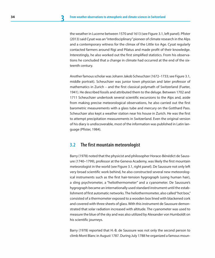
ter 12). Together with theoretical considerations on the behaviour of gases and gas mixtures, a realistic, albeit not yet fully correct, picture of the upper atmosphere emerged (Figure 3.4). Refinements and corrections of this pic-ture were obtained during the 20th century by in-situ measurements with manned and unmanned balloons to the stratosphere in the 1930s (Chap-
Figure 3.4: Scheme of the Earth’s atmosphere ”after Hann, Wegener etc.” (Heim 1912). The dia-gram shows the vertical extent of the atmosphere, the unmixing of the atmo-spheric gases (Sauerstoff – oxygen, Stick-stoff – nitrogen, helium, Wasserstoffgas – hydrogen) with altitude, and Wegener’s hypothetical geocoronium layer, which was similar in composition to the Sun’s corona (visible during total solar eclipses) and based on observations of the zodia-cal light. The vertical dimension of Kraka-toa’s eruption and the maximum height achieved by balloon sondes (30 km) is marked. The height ranges of meteors (Aufleuchten der Meteorite und Stern-schnuppen) and aurora (Polarlichter) are also indicated. The stratospheric tempera-ture minimum of –55 °C is correctly located. The existence of an ozone layer was unknown at the time, as was the exis-tence of the turbopause at 120 km, up to which level the gases are rather homoge-neously mixed (apart from the trace gases H2O, CO2 and O3).
39Early pioneers of Swiss meteorology and climatology 3
3.4 From the Swiss Meteorological Network to the Swiss Meteorological Society
Thanks to the persuasive power of a few famous scientists, and thanks to the support of the Swiss Academy of Sciences, a Meteorological Commission with the professors Heinrich Wild (Berne, 1833–1902), Charles Guillaume Kopp ( Neuchâtel, 1822–1891) and Albert Mousson (Zurich, 1805–1890) was formed around 1860. At this time Wild (see Figure 3.5, middle portrait) had already constructed new meteorological instruments (barometer, anemometer, evapo-ration balance) as well as his original Wild screen. He had also started measure-ments with the world’s first automatic weather station in Berne, operated with large batteries.
ter 8) and after World War II, when rocket technology was developed to carry scientific instruments into space.
Although the aurora borealis is a rare phenomenon to observe in Switzer-land, the mechanical engineer Hermann Fritz (1830–1893) at ETH Zurich is now considered the father of modern auroral research and one of the found-ers of modern geophysics (Schröder 1981, 2008). Inspired by his friend Rudolf Wolf, Director of the Eidgenössische Sternwarte in Zurich at the time, he collected the worldwide available aurorae observations and published a comprehensive catalogue in 1873 and a book in 1881 (Fritz 1873, 1881). He demonstrated the strong connection between number of sunspots and auroral events, and he investigated all kinds of relationships between solar activity and weather parameters, with varying success (Fritz 1893).
Another example of progress in atmospheric physics at the turn of the 19th to the 20th century was the study of atmospheric electricity (Chapter 13) by the physicist Albert Gockel (1860–1927) in Fribourg, with seminal contribu-tions to the distribution and characteristic behaviour of electric charges in the lower atmosphere (Gockel 1908; Lacki 2014). Gockel, a founding member of GMA, used the term ”cosmic rays” as early as 1915 in a publication in the Physikalische Zeitschrift, although with a question mark, i. e., before Robert Millikan who is generally acknowledged to have coined this term (Völkle 2014). The Austrian researcher Viktor Franz Hess had discovered the cosmic radiation in 1912, which earned him the Nobel Prize in 1936.
40 From weather observations to atmospheric and climate sciences in Switzerland3
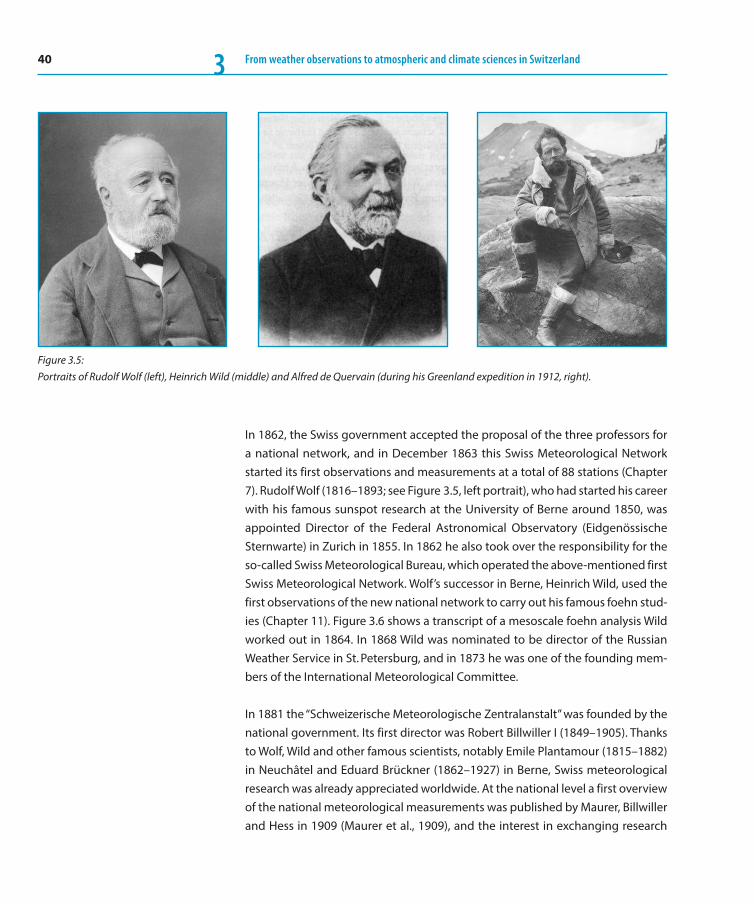
In 1862, the Swiss government accepted the proposal of the three professors for a national network, and in December 1863 this Swiss Meteorological Network started its first observations and measurements at a total of 88 stations (Chapter 7). Rudolf Wolf (1816–1893; see Figure 3.5, left portrait), who had started his career with his famous sunspot research at the University of Berne around 1850, was appointed Director of the Federal Astronomical Observatory (Eidgenössische Sternwarte) in Zurich in 1855. In 1862 he also took over the responsibility for the so-called Swiss Meteorological Bureau, which operated the above-mentioned first Swiss Meteorological Network. Wolf’s successor in Berne, Heinrich Wild, used the first observations of the new national network to carry out his famous foehn stud-ies (Chapter 11). Figure 3.6 shows a transcript of a mesoscale foehn analysis Wild worked out in 1864. In 1868 Wild was nominated to be director of the Russian Weather Service in St. Petersburg, and in 1873 he was one of the founding mem-bers of the International Meteorological Committee.
In 1881 the “Schweizerische Meteorologische Zentralanstalt” was founded by the national government. Its first director was Robert Billwiller I (1849–1905). Thanks to Wolf, Wild and other famous scientists, notably Emile Plantamour (1815–1882) in Neuchâtel and Eduard Brückner (1862–1927) in Berne, Swiss meteorological research was already appreciated worldwide. At the national level a first overview of the national meteorological measurements was published by Maurer, Billwiller and Hess in 1909 (Maurer et al., 1909), and the interest in exchanging research
Figure 3.5: Portraits of Rudolf Wolf (left), Heinrich Wild (middle) and Alfred de Quervain (during his Greenland expedition in 1912, right).

41Early pioneers of Swiss meteorology and climatology 3
results was growing. In 1912, the team of the geophysicist Alfred de Quervain (1879–1927; see Figure 3.5, right portrait), supported by the glaciologist Paul-Louis Mercanton (1876–1963), undertook the first West-East crossing of Green-land. During their adventurous trip they also carried out famous meteorological measurements and proved that a stationary band of westerlies exists in the upper troposphere. Based on the enthusiasm this event provoked in Switzerland as well as on the growing interest in scientific meteorology, Alfred de Quervain, together with his colleagues Robert Billwiller, Albert Riggenbach and Paul-Louis Mercanton, founded the Swiss Society of Geophysics, Meteorology and Astronomy, from which later the Swiss Society of Meteorology emerged (Chapter 2). The initial meeting took place on 8 August, 1916 in Scuol in the Engadin.
Acknowledgements
I am indebted to Christian Pfister for valuable hints and comments.
Figure 3.6: Transcript of a handwritten mesoscale foehn analysis Heinrich Wild carried out in the year 1864.
42 From weather observations to atmospheric and climate sciences in Switzerland3
References
Barry, R. G., 1978. H.-B. de Saussure: The first mountain meteo-rologist. Bull. Amer. Meteor. Soc., 59, 702–705.
Charpentier, J. de, 1841: Essai sur les glaciers et sur le terrain erra-tique du bassin du Rhône. M. Ducloux, Lausanne, 362 pp.
Fritz, H., 1873: Verzeichnis beobachteter Polarlichter. C. Gerold‘s Sohn, 260 pp.
Fritz, H., 1881: Das Polarlicht. F. A. Brockhaus, 376 pp.
Fritz, H., 1893: Die Perioden solarer und terrestrischer Erschei-nungen. Vierteljahresschr. Naturforsch. Ges. Zürich, 38, 77–107.
Fueter, E. (Ed.), 1941: Grosse Schweizer Forscher. Atlantis Verlag, Zurich, 340 pp.
Gockel, A., 1908: Die Luftelektrizität. Methoden und Resultate der neueren Forschung. S. Hirzel Verlag, 222 pp.
Heim, A., 1912: Luft-Farben. Hofer, 93 pp.
Krüger, T., 2013: Discovering the Ice Ages: Reception and Conse-quences for a Historical Understanding of Climate. Brill, Leiden, 534 pp.
Kupper, P., B. C. Schär, 2015: “Eine einfache und anspruchslose Organisation” – Zur Geschichte der Akademie der Naturwissen-schaften Schweiz. Die Naturforschenden, P. Kupper, and B. C. Schär, Eds., Verlag hier + jetzt, 281–295.
Lacki, J., 2014: Albert Gockel, a pioneer in atmospheric electric-ity and cosmic radiation. Astropart. Phys., 53, 27–32, doi: 10.1016/j.astropartphys.2013.05.006
Maurer, J., Billwiller, R. II, Hess, C., 1909: Das Klima der Schweiz auf Grundlage der 37-jährigen Beobachtungsperiode 1864–1900. Ver-lag Huber & Co. Frauenfeld, 2 volumes, 302 and 216 pp.
Pfister, C., 1975: Agrarkonjunktur und Witterungsverlauf im westlichen Schweizer Mittelland zur Zeit der Ökonomischen Patrioten 1755–1797. Ein Beitrag zur Umwelt- und Wirtschafts-geschichte des 18. Jahrhunderts. Geographica Bernensia, G2, Berne, 231 S.
Pfister, C., 1984: Das Klima der Schweiz von 1525–1860 und seine Bedeutung in der Geschichte von Bevölkerung und Landwirtschaft. Verlag P. Haupt, Berne und Stuttgart, Volume 1, 184 pp.
Pfister, C., 2013: Renward Cysat – ein “interdisziplinärer” Pionier der Klimaforschung im Alpenraum. Der Geschichtsfreund, Alt-dorf, 166, 188208.
Saussure, H.-B. de, 17791796 : Voyages dans les Alpes. Précédes d’un Essai sur l‘Histoire Naturelle des Environs de Genève. Vols. 14. S. Fauche, Père et Fils, Neuchâtel, 521 pp.
Schröder, W., 1981: Hermann Fritz, Wegbereiter der Polarlicht-forschung. Vierteljahresschr. Naturforsch. Ges. Zürich, 126, 199204.
Schröder, W., 2008: Hermann Fritz und sein Wirken für die Polar-lichtforschung. Zur Geschichte der Geophysik. www.dgg-online.de/geschichte/birett/BAND1P.HTM
Völkle, H., 2014: Was ist kosmische Strahlung? Strahlenschutz-Praxis, 20, 2/2014, 3134.
43
4 Producing climate information for Switzerland – Historical and recent developmentsSimon C. Scherrer, Mischa Croci-Maspoli, Christof Appenzeller Federal Office of Meteorology
and Climatology MeteoSwiss,
Zurich-Airport
Both the development of new analysis methods and datasets as well as the emergence of climate
changes have influenced the way climate information was and is being produced. We review the
developments in Switzerland over the last 150 years and show that the focus changed from (1)
describing what climate means to physically understanding the changing climate, (2) from analysing
local observations to producing climate change scenarios based on climate models, and (3) from pure
science to a service-oriented discipline.
4.1 Introduction and outline
The global and Swiss climates have changed substantially over the last century. This statement is based on the continuous measurements from the meteorologi-cal observational networks worldwide. In Switzerland, the country-wide ground-based measurement network was established in 1863. According to the classical definition of climate by Julius von Hann, the main aim of climatology – the disci-pline of “the study of the climate” – is to determine the means and other basic statistical properties of all relevant atmospheric variables (Hann, 1932). However, the main focus of the discipline, its tools, methods and the way in which climate information was produced and communicated have changed considerably over the last 150 years. Climate information developed from giving basic descriptive information on the mean climate toward more physically based information as well as understanding and predicting the climate system. Another main change was from gathering information at relatively few points in space toward high- resolution climate monitoring in time and space.
Beside new observational techniques to acquire climate data (e. g., remote sensing and modern automated measurement systems such as the SwissMetNet, cf. Chap-ters 6–9) and highly sophisticated statistical methods, the main new tools devel-oped were numerical weather and climate models on both the global and regional scale. These models allow the simulation of the past and potential future develop-ments of the climate system. They are also used to produce climate information
44 From weather observations to atmospheric and climate sciences in Switzerland4
on the expected future climate, whether for the next season, decade or multiple decades. Ongoing climate change led to greater visibility and practical use of past, current and future climate information, especially over the last 20–30 years. Slowly, a transition of the discipline toward a service and more operationally orientated discipline took place.
Considering these rapid developments in the last 50 years, it is no surprise that in the Festschrift Hundert Jahre Meterologie in der Schweiz 1864–1963 (MZA, 1964) the measurement network and climate monitoring (Schüepp, 1964) was already prominent, though the value of the data as “climate information” could not be assessed in detail at that time.
In this chapter we present some historical aspects of the evolution and presenta-tion of climate information in Switzerland. We focus on the developments con-cerning some major tools, datasets, products, communication forms and climate services in the field of “classical climatology.” This chapter cannot cover all de -velopments of Swiss climate research in the last 25 years or so – that would demand a book by itself. A nice overview of physical, institutional and political aspects of climate change in Switzerland was recently published by Brönnimann et al. (2014). Here, we only briefly outline some of the developments that led to explicit climate information. The focus is on the generation of climate change sce-narios for Switzerland.
We first look at some aspects and developments of classical climate information. Then we discuss the transition from the description of the means toward more application-oriented information and the physical understanding of the climate system and anthropogenic climate change. The impact and availability of new datasets (e. g., reanalysis products, new types of predictions) in climate informa-tion is briefly touched upon. A short discussion of the main Swiss research initia-tives and new Swiss climate centres is given to show that over time Swiss climate science became a highly interdisciplinary field, and that parts thereof are slowly transforming into a service-oriented discipline for delivering important informa-tion to decision makers, e. g., for planning purposes in conjunction with the adap-tation to climate change.

45Producing climate information for Switzerland – Historical and recent developments 4
4.2 Early climate information: Climate means and basic statistical measures
Climate bulletins
In the first half of the 20th century, climatology was mainly a descriptive discipline. The goal was to obtain a basic knowledge of the mean state of the climate and deviations thereof at a certain place using in-situ measurements. Possibly the first climate information product was the Witterungsbericht. Its publication in Switzer-land started in 1882 with a monthly edition, right after the establishment of the Schweizerische Meteorologische Centralanstalt in 1881. The early Witterungs-berichte were very descriptive, and because of the lack in knowledge about the means and variability, comparisons with longer period means were cumbersome
The climate bulletin 1882 and 2015
Excerpt from the January 1882 report“Der verflossene Januar wird als ein ausserordentlich trockener, ruhiger und dabei gar nicht sehr kalter Wintermonat noch lange in unserer Erinnerung blei-ben. Das Wetter war zu dieser Zeit milde, […] und wir zählten bis zum 9. Januar Regentage. An keinem derselben war indessen die Regenmenge bedeutend. […]. Mit dem 11. Januar begann dann die lang andauernde, ruhige Trockenperiode, die bis zu Ende des Monats anhielt. […] der Boden trocknete daher sehr stark aus und das Grundwasser erreichte einen sehr niedrigen Stand. Die Atmosphäre dagegen war meist von mehr oder weniger dichtem, meist tiefliegendem Nebel erfüllt. In den höheren Regionen war […] das Wetter meist hell und ausseror-
dentlich mild, während unten Kälte herrschte und bei Niederungen von Nebel und Duft erfüllt waren […] Nicht ohne erheblichen Einfluss auf die Lufttempera-tur war der völlige Mangel einer Schneedecke.”
Excerpt from the February 2015 report“Der Februar gab sich winterlich mit verbreitet unterdurchschnittlichen Tem-peraturen und Schneefällen bis in tiefe Lagen beidseits der Alpen. Die Nieder-schlagsmengen stiegen im Süden zum Teil erheblich über die Norm. Im Norden und in den Alpen fielen hingegen regional weniger als die Hälfte der normalen
Mengen.”
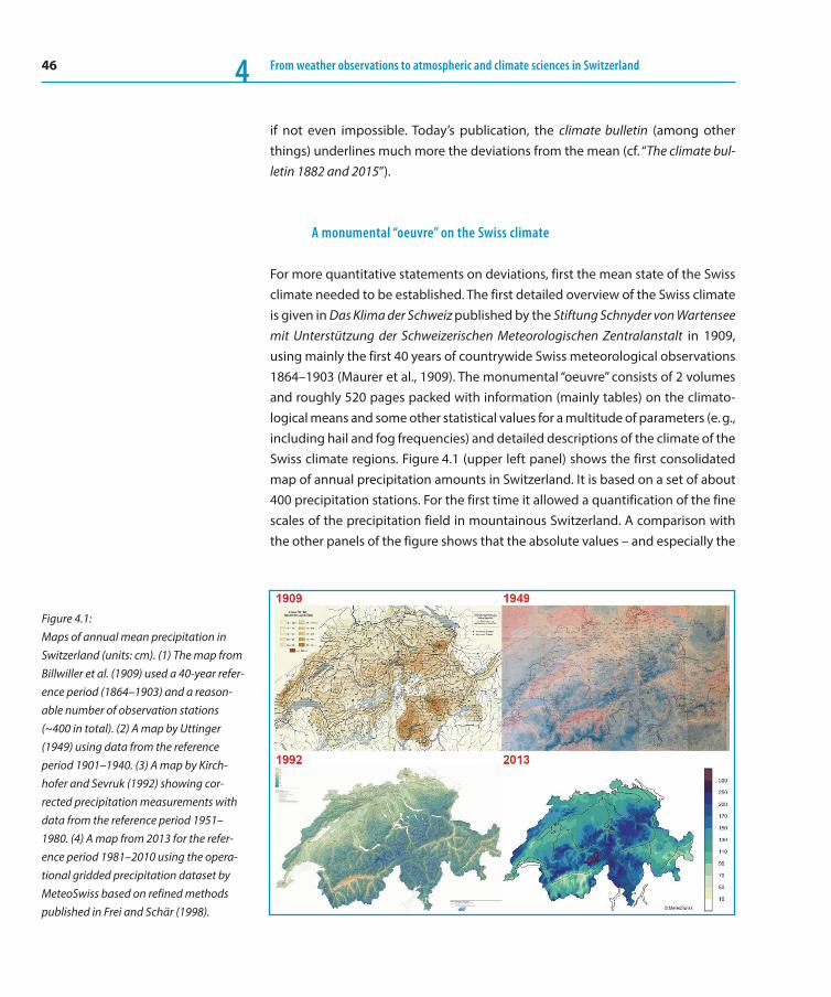
46 From weather observations to atmospheric and climate sciences in Switzerland4
if not even impossible. Today’s publication, the climate bulletin (among other things) underlines much more the deviations from the mean (cf. “The climate bul-letin 1882 and 2015”).
A monumental “oeuvre” on the Swiss climate
For more quantitative statements on deviations, first the mean state of the Swiss climate needed to be established. The first detailed overview of the Swiss climate is given in Das Klima der Schweiz published by the Stiftung Schnyder von Wartensee mit Unterstützung der Schweizerischen Meteorologischen Zentralanstalt in 1909, using mainly the first 40 years of countrywide Swiss meteorological observations 1864–1903 (Maurer et al., 1909). The monumental “oeuvre” consists of 2 volumes and roughly 520 pages packed with information (mainly tables) on the climato-logical means and some other statistical values for a multitude of parameters (e. g., including hail and fog frequencies) and detailed descriptions of the climate of the Swiss climate regions. Figure 4.1 (upper left panel) shows the first consolidated map of annual precipitation amounts in Switzerland. It is based on a set of about 400 precipitation stations. For the first time it allowed a quantification of the fine scales of the precipitation field in mountainous Switzerland. A comparison with the other panels of the figure shows that the absolute values – and especially the
Figure 4.1: Maps of annual mean precipitation in Switzerland (units: cm). (1) The map from Billwiller et al. (1909) used a 40-year refer-ence period (1864–1903) and a reason-able number of observation stations (~400 in total). (2) A map by Uttinger (1949) using data from the reference period 1901–1940. (3) A map by Kirch-hofer and Sevruk (1992) showing cor-rected precipitation measurements with data from the reference period 1951–1980. (4) A map from 2013 for the refer-ence period 1981–2010 using the opera-tional gridded precipitation dataset by MeteoSwiss based on refined methods published in Frei and Schär (1998).

47Producing climate information for Switzerland – Historical and recent developments 4
local details – differ quite a bit from modern gridded precipitation datasets. Nev-ertheless, some regional details can be identified. For example, the precipitation maxima in the Jura mountains, along the Prealps and along the Western boundary of the canton Ticino, as well as the minima in the inner Alpine valleys (Valais and Engadina) were generally captured. Measurements from the high mountain regions, however, were missing completely. This changed with the establishment of the precipitation totalizer network in 1913, which were placed predominately in high mountain regions (Wolfensberger, 1994). The measurements of these addi-tional stations (e. g., 139 stations in 2008/2009) are incorporated in the maps from 1949, 1992 and 2013 (cf. Figure 4.1).
Classical analyses and climate information
Das Klima der Schweiz remained the standard reference in most regards until at least the 1940s and for some parameters even until the 1950s. The observational network was expanded substantially and the quality was enhanced around the year 1900. The improvements were mainly the result of more strict measurement rules for the observers and their enforcement by inspectors. Therefore, most of the following early climatological analyses and information focussed on data starting in 1901. Uttinger’s famous precipitation map from 1949 (Figure 4.1, upper right panel) used 1901–1940 data as the data basis (Uttinger,1949). Some parts of Schüepp’s contributions to the Klimatologie der Schweiz even used data from 1901–1960 to compute the statistics. A nice descriptive overview of the Swiss cli-mate mainly based on 1901–1940 data can be found in the chapter “Vom Klima der Schweiz” by Uttinger in the book Wolken / Wind und Wetter (Schüepp, 1950). That book was a bestseller in the 1950s and 1960s. Note however, that the term climate and the aim of climate information had already been recognised as being more than just descriptions of the mean state of the atmosphere. Terms like vari-ability, extremes, scatter, averaged deviations, quartiles and quantiles became more important because information on these quantities were needed more and more in engineering and technical applications.
The next larger collection of works on the Swiss climate was the series Klimatologie der Schweiz. It was a “loose” collection of 34 supplementary volumes of the annu-ally published Annalen between 1959 and 1996 (SMA, 1959–1996). In the early and most active period of the collection, from 1959 to 1978, most of the contributions were authored by Max Schüepp and Heinrich Uttinger. The content of the volumes was divided into three parts: (1) climatological mean tables for the different
Annalen und Klimareport der MeteoSchweiz
From 1864 to 2010 (147 years) the
annually published Annalen were a
good source of climate information.
The content changed considerably over
time, with climate information in the
form of tables, figures and chapters on
different aspects of the Swiss climate
becoming more and more important
(e. g., MeteoSchweiz, 2005). Since 2011,
the annual Klimareport has been pub-
lished containing a wealth of climate
information (e. g., MeteoSchweiz,
2015).
48 From weather observations to atmospheric and climate sciences in Switzerland4
weather elements (2) regional climate descriptions and (3) climatological means for different weather situations.
Data from the Klimatologie der Schweiz formed an important basis for some of the first important applications of Swiss climate data. One example may be found in the detailed maps of the Klimaeignung für die Landwirtschaft in der Schweiz by Jeanneret and Vautier (1977). Another important example are the Blaue Bände (Zeller et al., 1976–1992), presenting information on extreme precipitation in Swit-zerland. They were heavily used for all kinds of dimensioning questions in environ-mental engineering and planning purposes. At present, the outdated information on extreme precipitation are being updated and extended in the “Extremnieder-schläge” project running at MeteoSwiss from 2012 to 2015.
Weather classification, e. g., the Alpine weather statistics AWS classification after Schüepp (1968, 1979), was a very active research topic in Swiss climatology (cf., e. g., Wanner et al. 1998). In later years many different subjects related to the works at SMA were discussed in the Klimatologie der Schweiz series. Two examples are phenological analyses (Defila, 1992; cf. also Chapter 14) and results from data homogenization projects such as KLIMA90 (Aschwanden et al., 1996).
Another major milestone in Swiss climate information was the Klimaatlas der Schweiz, published between 1982 and 1995 by the SMA under the direction of Walter Kirchhofer (MeteoSchweiz, 2000). It definitively replaced the outdated Das Klima der Schweiz as well as some older climate analyses from the 1940s to the 1970s using higher quality data and applying more sophisticated statistical meth-ods. Beside information on the observing system, weather types and information on phenology, it contains a wealth of maps of climatological means and frequen-cies of all kinds of weather parameters.
An additional aspect of climate information lie in expert opinions requested mainly for insurance claims. At SMA, the “golden age” for these expert opinions was in the 1980s, where several thousand written reports were produced per year (over 2000 reports per year by one person alone!). Later, climate consulting more and more shifted from written reports to telephone consulting. Nowadays, short expert opinions have become rare and are mainly requested for court cases.
Because of the mainly descriptive character of studies on the Swiss climate, pub-lications in peer-reviewed scientific literature containing climate information were relatively scarce until the 1980s. The discussion in the scientific literature predom-

49Producing climate information for Switzerland – Historical and recent developments 4
inantly focussed on interesting local weather phenomena and their climatological features (e. g., Föhn (Hann, 1866; Frey, 1944), fog (Wanner and Kunz, 1983), Bise (Wanner and Furger, 1990)). Most of the knowledge gained on the climatological timescale was collected in the above-mentioned collected works or scientific reports of MeteoSwiss or the corresponding series of some other institutions and universities. A good overview of many different aspects of the current Alpine cli-mate (including Switzerland) and the literature is given in Schär et al. (1998).
4.3 Physical understanding, first climate change scenarios and trend analysis
In the 1960s and 1970s it became clear that global carbon dioxide concentrations in the atmosphere were increasing strongly, and by the 1980s global temperatures had started to react to the increasing greenhouse gas concentrations. In 1988, the Intergovernmental Panel on Climate Change (IPCC) was established by the World Meteorological Organization (WMO) and the United Nations Environment Pro-gramme (UNEP). Their first report was published in 1990, stressing that “human activities may be inadvertently changing the climate of the globe” (IPCC, 1990). For details on the Swiss contribution to IPCC we refer to Chapter 21, which is ded-icated to this topic.
Climate modelling
The notion of a changing climate implied that detailed maps and statistical descrip-tions of the climate, although very useful climate information for many applications, were not sufficient for a good understanding of the climate system and possible future climate change. As a consequence, the analysis of trends and variability and their changes and impacts in the past, present and future became an important aspect of climate information. To obtain this information, a physical understanding of the system is indispensable, and this knowledge can be achieved only by running appropriate physical numerical models. Only they are able to give a more complete picture of the highly nonlinear processes that determine the climate system and allow us to identify the drivers of past and future climate changes (e. g., greenhouse gases). Hence, the development and analysis of climate models to simulate the past and future climate became a major task of the emerging discipline of model-based climate science. For a more detailed discussion of the history of climate modelling we refer to the comprehensive review by Edwards (2010). Although the Swiss cli-

50 From weather observations to atmospheric and climate sciences in Switzerland4
mate science research groups were small in the 1970s and 1980s, there were some contributions to the development of climate models. Pioneering work on the atmo-spheric carbon dioxide levels and their prediction and climate-carbon cycle mod-elling was performed at the University of Bern (cf. Siegenthaler and Oeschger, 1978). In the late 1980s and early 1990s, important early contributions to global and regional climate modelling also were done at ETH Zurich.
First climate change scenarios for Switzerland
In the 1980s, climate change was primarily a topic that focussed on the global scale. On the regional scale, e. g., Switzerland, change signals were still too weak to be detected as clear signals. However, climatology with a focus on climate change research then got a major boost. Interestingly, the first peer-reviewed pub-
Figure 4.2: Early climate change signals for Switzer-land published by Rotach et al. (1997): Shown are differences in the 2 m tempera-ture (in °C) between the 2xCO2 scenario and the control run (1xCO2). Results from the global model (a) winter (DJF) and (b) summer (JJA). Panels (c) and (d): for the nested regional simulation.

51Producing climate information for Switzerland – Historical and recent developments 4
lications on observed climate change in Switzerland (Beniston et al., 1994) and first publications on climate modelling in Switzerland (Beniston et al., 1993) as well as basic regionalised scenarios on future climate change (e. g., Gyalistras et al., 1994; Schär et al., 1996; Rotach et al., 1997) were all published in the mid-1990s. The Rotach et al. (1997) scenarios for example, were based on 2xCO2 runs using global and regional simulations (cf. Figure 4.2). Although they differ in detail from today’s scenarios quite a bit, some of the features still valid today were already found there. Note that, in contrast to today’s state of the art scenarios (CH2011, 2011), some of the future scenarios showed increases in summer precipitation (cf. Table 4.7 in Gyalistras et al., 1998).
Climate change trend analyses and homogeneous datasets
Similarly, the analysis of time series of climate parameters and climate monitoring gained increased attention when it became clear that the global temperatures were starting to react to man-made greenhouse gas emissions. Before that time, time series were rarely shown, also since the mechanisms behind changes and the statistical tools to analyse the series were very limited. Figure 4.3a shows an early temperature series of Basel from ~1830 to the late 1940s as published by Schüepp (1950). The reasons for the observed changes were unknown at that time. Inter-estingly, Schüepp already pointed to the changing atmospheric composition as a possible culprit, but he then states that the composition “has not changed signifi-cantly as far as detectable”.
Good data quality is essential for reliably detecting local climate change. The cli-mate time-series need to be homogenised (i. e., all nonclimate-related changes removed, see also Chapter 7) before a reliable study of the real development of the climate is possible. Important work in this respect was often performed by the weather services, which also have access to the station history and other metadata such as instrumentation details. The application of sophisticated statistical tools and data treatment of the climate series allowed new data homogenisation tech-niques. The SMA projects KLIMA90 (Aschwanden et al., 1996) and NORM90 (Begert et al., 2003; 2005) provided such homogenised series and thus reliable information on observed changes for Switzerland (see Figure 4.3 b). In 2007, the Swiss National Basic Climatological Network (NBCN) was introduced (cf. Begert et al., 2007). It is a part of the more general SwissMetNet (cf. Chapter 7) and the backbone of cli-mate monitoring of near surface weather and climate.

52 From weather observations to atmospheric and climate sciences in Switzerland4
Further important contributions to climate research leading to climate informa-tion before the start of the national climate research programs in the 1990s and 2000s were on the understanding of the small-scale climate (for details, see sec-tion below). Particular foci were, for example, precipitation climatology, the radi-ation balance over different surfaces (e. g., snow and ice), urban climatology, wind climatology and boundary layer meteorology in general and on paleoclimatology.
4.4 Toward more user-oriented climate information
The time period roughly from the 1990s to 2010 was a very active phase of climate science in which a wealth of new climate information and datasets about the past and possible future climate change became available. Parallel to the stronger sig-nals of climate change and the IPCC process, climate information became more visible to the public. This awareness of climate research culminated with the Nobel Peace prize being awarded to the IPCC in 2007 (cf. Chapter 21). The developments were in many ways rapid and occurred in many subfields. With the climate change amplitude becoming larger and changes more obvious, also on regional scales (cf. Figure 4.3), it became possible to detect and attribute changes to anthropogenic factors. This was first possible on global and continental scales (IPCC, 2007) and
Climate normals – a concept with problems
Climate change also lead to problems
with the concept and interpretation of
certain climate terms, such as the
“ climate normal” (i. e., 30-year aver-
ages of climatological variables). They
have often been used by weather ser-
vices to communicate the anomalous-
ness of the current climate. However,
because of overall increasing tempera-
tures, for example, the probability of
observing a positive temperature
anomaly with respect to the 1961–
1990 normal increased from 50 % to
near 80 % for certain months of the
year in the 1975–2004 period (cf.
Scherrer et al., 2006) – and since then
possibly to even higher numbers.
Figure 4.3: Temperature evolution in Switzerland. (a) Early estimates of smoothed summer, winter and annual temperatures in Basel from the 1830s to the late 1940s as pre-sented in Schüepp (1950). (b) “Modern” Swiss temperature anomaly (°C) (1864–2014, red) and global temperature (1850–2014, black and greyscale). Shown are the Swiss temperature anomalies based on 12 long-term series and three global tem-perature curves: Met Office HadCRUT 4 (black), NOAA MLOST (dark grey) and NASA GISTEMP (light grey). Anomalies are computed with respect to the 1961–1990 period. For the Swiss series also a 20–year Gaussian smoothed curve is added (thick red line). The 1880–2014 temperature trend in Switzerland (+ 1.96 °C) is a factor 2.2 of the global trend.
53Producing climate information for Switzerland – Historical and recent developments 4
today increasingly also on the regional scale. In addition, much was learned about climate variability, e. g., the influence of the large scale flow on Swiss climate vari-ability (e. g., Brönnimann et al. 2008; Ceppi et al. (2012); Schär et al., 2004; Scherrer, 2006; Scherrer and Appenzeller, 2006; Wanner et al., 2001).
New datasets and sources
Considerable progress was also made in the availability of climate datasets for climate data analysis. As one example we want to mention the high-resolution Alpine precipitation grid dataset (Isotta et al., 2014), which provided daily precip-itation on a 5 km by 5 km grid over the entire Alpine region in the 1971–2008 period. Swiss researchers were also leading in establishing climate monitoring networks such as the Baseline Surface Radiation Network (BSRN/WCRP) in the 1990s (Ohmura et al., 1998). The BSRN data allowed (among other things) estab-lishing know-how of how pollutants modified the atmospheres visibility and how a phase of global dimming was followed by a global brightening phase (Wild et al., 2005). More and more climate information based on satellite data has become available. Especially useful are satellite observations to monitor radiation, clouds, snow pack and precipitation parameters. Many of these parameters are potentially very useful for certain applications such as solar power production and winegrow-ing (to name just two). The establishment of the European Organisation for the Exploitation of Meteorological Satellites (EUMETSAT) Satellite Application Facility on Climate Monitoring (CM SAF, www.cmsaf.eu) was an important step toward establishing satellite-based climate monitoring in Europe.
Beside data collection efforts concerning observational, both in-situ and remote-sensed data, the production of reanalyses, i. e., reprocessing observational data spanning an extended historical period using a consistent modern analysis system (e. g., a sophisticated weather model with a data assimilation system) was estab-lished as an important new source of climate information. The largest additional benefit of reanalysis is the continuous information obtained about the three- dimensional atmospheric conditions also in regions with sparse or no observa-tional data. Clearly reanalysis data have their limitations, and the limits to accuracy need to be communicated to potential users and customers. Several global reanal-yses are in use whose potential is being evaluated by many users. Visit http:// reanalyses.org for a good overview of available data sets. Also regional reanalyses have become available, e. g., for Europe in the EURO4M (www.euro4m.eu) and UERRA (www.uerra.eu) projects.

54 From weather observations to atmospheric and climate sciences in Switzerland4
Earth system models and seasonal to decadal predictions
Climate model development was very lively in the period from the 1990s to 2010. Beside strongly increasing grid resolution and general enhancements, climate modelling has moved in the direction of increasingly comprehensive models cou-pling climate-related systems such as the land surface, cryosphere, hydrology and vegetation to the atmosphere-ocean system, so-called Earth system models (ESM) (e. g., Edwards, 2010). This development had the effect of climate science becom-ing an interdisciplinary discipline, so that major advances could often be reached only by community efforts involving dozens or even hundreds of scientists. In the large climate centres, climate models are used not only to make projections about the climate several decades in the future, but increasingly also to produce opera-tional predictions of the coming seasons and years (i. e., interannual to decadal predictions, Palmer et al., 2004). The skill of these predictions is promising in the tropics but unfortunately still very limited in the extra tropics, especially over Swit-zerland (e. g., Müller et al., 2005; Schmuki and Weigel, 2006).
National climate research programs
In Switzerland, a major boost for climate science and in the end climate informa-tion came from major climate projects funded by the Swiss National Science Foun-dation and other founding agencies. The first coordinated effort was the NRP31 “Climatic Changes and Natural Hazards” which ran from 1992 to 1997 (Bader and Kunz, 1998). It was followed by the Swiss Environmental Priority Programme, spe-cifically the subproject ”Climate and Environment in the Alpine Region” (CLEAR) from 1997 to 2000. Finally, the National Competence Centre for Research (NCCR) in Climate was established which ran from 2001 to 2013 and was by far the largest and longest climate project in Swiss history. The NCCR Climate research network consisted of over 130 scientists from eight institutions which formed an interna-tionally competitive community in Switzerland with the University of Bern as lead-ing house. A major outcome of the NCCR Climate was the establishment of two new Swiss centres for climate research. The Center for Climate Systems Modeling (C2SM) and the Oeschger Centre for Climate Change Research (OCCR). The OCCR was founded in 2007 by the University of Bern where about 200 scientists work under its umbrella. Its main focus is on interdisciplinary climate research, such as natural sciences, humanities, social sciences, economics and law. The C2SM was founded in 2008 by ETH Zurich, MeteoSwiss, EMPA, WSL and Agroscope. The cen-tre encompasses the technical and scientific expertise of more than 300 persons.
Gridded data for users
There is a user-driven development
toward providing climate information
more and more in the form of gridded
datasets instead of graphs and
reports. In particular gridded datasets,
both from observations or reanalysis,
can directly be used by various appli-
cation software, such a Geographical
Information Systems (GIS), and hence
provide an easy interface to generate
spatial climate information. One such
example is the operational gridded
precipitation data set of MeteoSwiss,
which has been used for various
reports including an Alpine-wide
extension for mean annual precipita-
tion published in the Hydrological
Atlas of Switzerland
(www.hades.unibe.ch).

55Producing climate information for Switzerland – Historical and recent developments 4
Its main objective is to improve the understanding of the Earth’s climate system, and our capability to predict weather and climate. For regional scale modelling, one important tool is the Consortium for Small-Scale Modelling (COSMO) Climate Limited-Area Model (CLM) which uses the “same” model as MeteoSwiss uses for its operational forecasts and several groups of C2SM and the Institute for Atmo-spheric and Climate Science (IAC) of ETH Zürich are using.
Climate change scenarios for Switzerland
Beside funded research initiatives, there were several coordinated initiatives of the scientific community reporting on many aspects of climate change and its possi-ble impacts. The first report with climate-change scenarios solely focussing on Switzerland was “Climate Change and Switzerland 2050 – Impacts on Environ-
Climate-change scenarios for Switzerland – coordinated initiatives
� CH2007 (originally known
as CH2050) published in 2007
(OcCC, 2007)
� CH2011 published in 2011
(CH2011, 2011)
� CH2018 to be published in 2018
Figure 4.4: Past and future changes in seasonal temperature (°C) and precipitation (%) in northeastern Switzerland as presented by CH2011. The changes are relative to the reference period 1980–2009. The thin coloured bars display the year-to-year differences with respect to the aver-age of observations over the reference period, the heavy black lines are the corresponding smoothed 30-year averages. The grey shading indicates the range of year-to-year differences as projected by climate models for the A1B scenario. The thick coloured bars show best estimates of the future projections, and the associated uncertainty ranges, for selected 30-year time-periods and for three greenhouse gas emission scenarios.

56 From weather observations to atmospheric and climate sciences in Switzerland4
ment, Society and Economy” (OcCC, 2007). It included the first national climate change scenarios based on regional PRUDENCE models (cf. Frei, 2004; Frei et al., 2006) and qualitative results on possible impacts.
The second report was a result of the coordinated CH2011 initiative, a multi-insti-tutional collaboration between the C2SM, MeteoSwiss, ETH Zurich, the NCCR Cli-mate, and the Organe consultatif sur les changements climatiques (OcCC). The Swiss Climate Change Scenarios (CH2011, 2011) were produced on the basis of the regional climate simulations of the European ENSEMBLES project (van der Linden and Mitchell, 2009) and applying state-of-the-art statistical methods (Buser et al., 2009; Fischer et al., 2011). CH2011 provided projections of changes in temperature and precipitation relative to the reference period 1980–2009 for three greenhouse gas scenarios (RCP3PD, A1B, and A2) and for three 30-year projection periods cen-tred around 2035, 2060 and 2085 (cf. Figure 4.4).
The CH2011 data were used for a large number of different applications and ini-tiatives. Figure 4.5 gives an overview of a few reports using CH2011 climate infor-mation. Among them is the CH2014-Impacts report (CH2014-Impacts, 2014) which gives the latest comprehensive overview of possible impacts of climate
Figure 4.5: Selection of recent application oriented reports using climate information from the CH2011 climate change scenarios (adapted from a slide by A. M. Fischer, MeteoSwiss).
57Producing climate information for Switzerland – Historical and recent developments 4
change on many socioeconomic sectors in Switzerland using the common set of CH2011 climate scenarios. Presently, the next coordinated effort to produce cli-mate change scenarios called CH2018 is about to start (see below), where user orientation will become even more important and a thorough market survey part of the effort.
4.5 The post-2010 era: Climate information as a services for Switzerland
Climate change impacts many sectors of society, economy and public life in Swit-zerland (BAFU 2012; 2014). Winter tourism, hydro-power production, agriculture and the health sector are examples often cited. Scientifically based climate infor-mation and the risks and chances potentially connected with climate change form an important basis for many decisions taken in politics, economy and administra-tion. The incorporation of reliable and up–to-date climate information of today and tomorrow allow optimisation of costs, actions to minimize risks and enable to recognize and take action on developing opportunities. The requirements for the decision-making processes – and therefore the need for high-quality information and data – are increasing due to climate change.
Global Framework for Climate Services
The above reasoning was also recognized at a broad international level, so that the World Climate Conference-3 in Geneva 2009 unanimously decided to establish a Global Framework for Climate Services (GFCS), a United Nations-led initiative spearheaded by the WMO to guide the development and application of sci-ence-based climate information and services in support of decision-making in climate sensitive sectors. The GFCS Vision is “to enable better management of the risks of climate variability and change and adaptation to climate change, through the development and incorporation of science-based climate information and prediction into planning, policy and practice on the global, regional and national scale” (http://gfcs.wmo.int/vision).
What are climate services and what are they used for?
Climate services include information
about the past, present and future cli-
mate variability as well as the medium-
and long-term expected changes in the
climate. The information is based on
high-quality observations and moni-
toring products and their statistical
analyses as well as on the results from
global and regional climate models.
With climate services, the decision
makers in politics, economy and
administration get basic information
to take climate-compatible decisions
and create strategic planning for adap-
tation and mitigation actions. A key to
“successful” climate services is that they
must respond to user needs and hence
provide a strong interaction between
producers and users. This allows adap-
tation of the services, but it also
enables and ensures the communica-
tion of the limitations of the products.
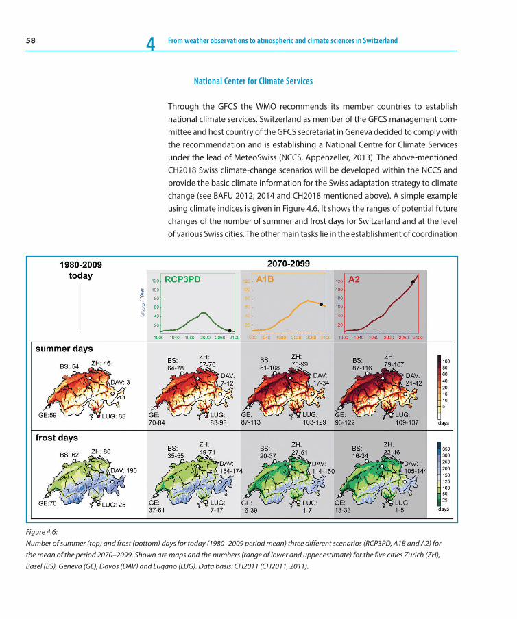
58 From weather observations to atmospheric and climate sciences in Switzerland4
National Center for Climate Services
Through the GFCS the WMO recommends its member countries to establish national climate services. Switzerland as member of the GFCS management com-mittee and host country of the GFCS secretariat in Geneva decided to comply with the recommendation and is establishing a National Centre for Climate Services under the lead of MeteoSwiss (NCCS, Appenzeller, 2013). The above-mentioned CH2018 Swiss climate-change scenarios will be developed within the NCCS and provide the basic climate information for the Swiss adaptation strategy to climate change (see BAFU 2012; 2014 and CH2018 mentioned above). A simple example using climate indices is given in Figure 4.6. It shows the ranges of potential future changes of the number of summer and frost days for Switzerland and at the level of various Swiss cities. The other main tasks lie in the establishment of coordination
Figure 4.6: Number of summer (top) and frost (bottom) days for today (1980–2009 period mean) three different scenarios (RCP3PD, A1B and A2) for the mean of the period 2070–2099. Shown are maps and the numbers (range of lower and upper estimate) for the five cities Zurich (ZH), Basel (BS), Geneva (GE), Davos (DAV) and Lugano (LUG). Data basis: CH2011 (CH2011, 2011).

59Producing climate information for Switzerland – Historical and recent developments 4
and steering structures of a NCCS and the strengthening of the flow of information between producers and users of climate services. Last but not least, the NCCS shall be embedded and well positioned in the GFCS and European initiatives like the Copernicus Climate Change Service (www.copernicus.eu/main/climate-change).
4.6 Synthesis
The available climate information for Switzerland has strongly evolved over the last 150 years, similar to how this climate information was developed and pro-duced by scientists. It changed from being mainly descriptive, analysing meteo-rological observations of the atmosphere in the first half of the 20th century, to a very computer-intensive, physical and model-based science discipline in the last few decades, with the aim of enabling detailed answers on the past, present and future climate in Switzerland. With the rising awareness of climate change as a major issue of the 21st century, climate analysis has recently also become a ser-vice-oriented discipline with products that are of value for a very broad range of users and decision makers in society, economy and public life.
Acknowledgements
We thank Jacqueline Flückiger Knutti, Andreas M. Fischer and Stephan Bader (all MeteoSwiss) for their input/help in connection with this book chapter.
References
Appenzeller, C., 2013: National Framework for Climate Services, Editoral, ProClim-Flash, 57, available at http://proclimweb.scnat.ch/portal/ressources/2875.pdf.
Aschwanden, A., M. Beck, C. Häberli, G. Haller, M. Kiene, A. Roesch, R. Sie, and M. Stutz, 1996: Bereinigte Zeitreihen. Die Ergebnisse des Projekts KLIMA90. Klimatologie 1961–1990, Heft 2, Band 1 von 4. Schweizerischen Meteorologische Anstalt, Zürich, 161 pp.
Bader S., and P. Kunz, 1998: Klimarisiken: Herausforderung für die Schweiz, vdf Hochschulverlag AG, Zürich, 276 pp., ISBN 3-7281-2605-5 (in German, ISBN of english version: 3-7281-2709-4).
BAFU (Bundesamt für Umwelt), 2014: Anpassung an den Klima-wandel in der Schweiz. Aktionsplan 2014–2019. Zweiter Teil der Strategie des Bundesrates vom 9. April 2014. 100 pp. www.bafu.admin.ch/publikationen/publikation/01762.
BAFU (Bundesamt für Umwelt), 2012: Anpassung an den Klima-wandel in der Schweiz. Ziele, Herausforderungen und Hand-lungsfelder. Erster Teil der Strategie des Bundesrates vom 2. März 2012. 64 pp. www.bafu.admin.ch/publikationen/publi kation/01673.
Begert M., G. Seiz, T. Schlegel, M. Musa, G. Baudraz, and M. Moesch, 2003. Homogenisierung vom Klimareihen der Schweiz und Bestimmung der Normwerte 1961–1990. Schlussbericht des

60 From weather observations to atmospheric and climate sciences in Switzerland4
Projekts NORM90. Veröffentlichung der MeteoSchweiz, 67, 170 pp.
Begert M., T. Schlegel, and W. Kirchhofer, 2005: Homogeneous temperature and precipitation series of Switzerland from 1864 to 2000. Int. J. Clim., 25, 65–80, doi:10.1002/joc.1118.
Begert, M., G. Seiz, N. Foppa, T. Schlegel, C. Appenzeller, and G. Müller, 2007. Die Überführung der klimatologischen Referenz-stationen der Schweiz in das Swiss National Basic Climatological Network (Swiss NBCN), Arbeitsberichte der MeteoSchweiz, 215, 43 pp.
Beniston, M., A. Ohmura, M. Wild, P. Tschuck, M. Marinucci, L. Bengtsson, U. Schlese, M. Esch, F. Giorgi, and A. Bernasconi, 1993: Coupled simulations of global and regional climate in Switzerland. Supercomputing Switzerland, 80–86.
Beniston, M., M. Rebetez, F. Giorgi, and M. R. Marinucci, 1994: An analysis of regional climate change in Switzerland. Theor. and Appl. Clim., 49, 135–159.
Brönnimann, S., J. Luterbacher, T. Ewen, H. F. Diaz, R. Stolarski, and U. Neu (Eds.), 2008: Climate variability and extremes during the past 100 years. Advan. Global Change Res., 33, 361 pp.
Brönnimann, S., and Coauthors, 2014: Climate change in Swit-zerland: a review of physical, institutional, and political aspects. WIREs Clim Change, 5, 461–481, doi:10.1002/wcc.280.
Buser C. M., H. R. Künsch, D. Lüthi, M. Wild, and C. Schär, 2009: Bayesian multi-model projection of climate: bias assumptions and interannual variability. Climate Dynamics, 33, 849–868, doi:10.1007/s00382-009-0588-6.
Ceppi, P., S. C. Scherrer, A. M. Fischer, and C. Appenzeller, 2012: Revisiting Swiss temperature trends 1959–2008. Int. J. Clim., 32, 203–213, doi:10.1002/joc.2260.
CH2011, 2011: Swiss Climate Change Scenarios CH2011, pub-lished by C2SM, MeteoSwiss, ETH, NCCR Climate, and OcCC, Zurich, Switzerland, 88 pp.
CH2014-Impacts, 2014: Toward Quantitative Scenarios of Climate Change Impacts in Switzerland, published by OCCR, FOEN, MeteoSwiss, C2SM, Agroscope, and ProClim, Bern, Switzerland, 136 pp.
Defila, C., 1992: Pflanzenphänologische Kalender ausgewählter Stationen in der Schweiz. Klimatologie der Schweiz Heft 30/L, Bei-
heft Annalen der Schweizerischen Meteorologischen Anstalt (Jg. 1989), Zürich, 234 pp.
Edwards, D. N., 2010: History of climate modeling. WIREs Clim Change, 2, 128–139, doi:10.1002/wcc.95.
Fischer, A. M., A. P. Weigel, C. M. Buser, R. Knutti, H. R. Künsch, M. A. Liniger, C. Schär, and C. Appenzeller, 2011: Climate Change Projections for Switzerland based on a Bayesian multi-model approach. Int. J. Clim., 32, 2348–2371, doi:10.1002/joc.3396.
Frei, C., and C. Schär, 1998: A precipitation climatology of the Alps from high-resolution rain-gauge observations. Int. J. Clim., 18, 873–900.
Frei, C., 2004: Die Klimazukunft der Schweiz – Eine probabi-listische Projektion. www.occc.ch/Products/CH2050/CH2050- Scenarien.pdf.
Frei, C., R. Schöll, S. Fukutome, J. Schmidli, and P. L. Vidale, 2006: Future change of precipitation extremes in Europe: Intercom-parison of scenarios from regional climate models. J. Geophys. Res., 111, 1–22, doi:10.1029/2005JD005965.
Frey, K., 1944: Zur Entwicklung des Föhns. Verh. Schweiz. Natur-forsch. Ges. Sils, 90 pp.
Gyalistras, D., H. von Storch, A. Fischlin, and M. Beniston, 1994: Linking GCM-simulated climatic changes to ecosystem models: case studies of statistical downscaling in the Alps. Clim. Res., 4, 167–189.
Gyalistras, D., C. Schär, H. C. Davies, and H. Wanner, 1998: Chap-ter 4: Future Alpine Climate. A View from the Alps: Regional perspectives on climate change, Cebon P., U. Dahinden, H. C. Davies, D. Imboden, and C. Jäger, Eds., MIT Press, Boston, pp. 171–223.
Hann, J., 1866: Zur Frage über den Ursprung des Föhns. Zeit-schrift der österr. Gesell. für Meteorol., 1, 257–263.
Hann, J., 1932: Handbuch der Klimatologie. 4. Auflage. K. von Knoch, Ed., 1. Band: Allgemeine Klimalehre, Stuttgart, 444 pp.
IPCC, 1990: Summary for Policymakers. Climate Change: The IPCC Scientific Assessment. Report prepared for Intergovern-mental Panel on Climate Change by Working Group I, J. T. Houghton, G. J. Jenkins and J. J. Ephraums (Eds.), Cambridge University Press, Cambridge, Great Britain, New York, NY, USA and Melbourne, Australia.

61Producing climate information for Switzerland – Historical and recent developments 4 IPCC, 2007: Summary for Policymakers. Climate Change 2007: The Physical Science Basis. Contribution of Working Group I to the Fourth Assessment Report of the Intergovernmental Panel on Climate Change, S. Solomon, S., D. Qin, M. Manning, Z. Chen, M. Marquis, K. B. Averyt, M. Tignor and H. L. Miller (Eds.), Cambridge University Press, Cambridge, UK and New York, NY, USA.
Isotta, F. A., and Coauthors, 2014: The climate of daily precipita-tion in the Alps: development and analysis of a high-resolution grid dataset from pan-Alpine rain-gauge data. Int. J. Clim., 34, 1657–1675, doi:10.1002/joc.3794.
Jeanneret, F., and P. Vautier, 1977: Kartierung der Klimaeignung für die Landwirtschaft in der Schweiz. Geogr. Bernensia G6, 108 pp.
Kirchhofer, W., and B. Sevruk, 1992: Mean Annual Corrected Pre-cipitation Depths 1951–1980. FOWG: Hydrological Atlas of Swit-zerland, Plate 2.2, Bern.
Maurer, J., R. Billwiller, and C. Hess,1909: Das Klima der Schweiz, Stiftung Schnyder von Wartensee mit Unterstützung der schweizerischen meteorologischen Zentralanstalt Schweiz. 2 Bände. Frauenfeld.
MeteoSchweiz, 2000: Klimaatlas der Schweiz. Bundesamt für Meteorologie und Klimatologie MeteoSchweiz, Ed., Gesamt-leitung: W. Kirchhofer, ISBN 3-302-09606-2.
MeteoSchweiz, 2005: Annalen 2004, 141. Jahrgang, Bundesamt für Meteorologie und Klimatologie MeteoSchweiz, Zürich, 160 pp, SZ ISSN 0080-7338.
MeteoSchweiz, 2015: Klimareport 2014, Bundesamt für Meteo-rologie und Klimatologie MeteoSchweiz, Zürich, 80 pp, ISSN 2296-1488.
Müller, W. A., C. Appenzeller, F. J. Doblas-Reyes, and M. A. Liniger, 2005: A debiased ranked probability skill score to evaluate probabilistic ensemble forecasts with small ensemble sizes. J. Climate, 18, 1513–1523, doi:10.1175/JCLI3361.1.
MZA (Schweizerische Meteorologische Zentralanstalt), 1964: Festschrift “Hundert Jahre Meteorologie in der Schweiz 1864–1963”, Zürich, Sonderbeiheft der Annalen, 111 pp.
OcCC/ProClim, Ed., 2007: Klimaänderung und die Schweiz 2050. Erwartete Auswirkungen auf Umwelt, Gesellschaft und Wirtschaft, Bern, 168 pp, ISBN: 978-3-907630-26-6.
Ohmura, A., and Coauthors, 1998: Baseline Surface Radiation Network (BSRN/WCRP): New precision radiometry for climate change research, Bull. Amer. Meteor. Soc.,79, 2115–2136.
Palmer, T. N., and Coauthors, 2004: Development of a European multimodel ensemble system for seasonal-to-interannual pre-diction (DEMETER). Bull. Amer. Meteor. Soc., 85, 853–872, doi:10.1175/BAMS-85-6-853.
Rotach, M. W., M. R. Marinucci, M. Wild, P. Tschuck, A. Ohmura, and M. Beniston, 1997: Nested regional simulations of climate change over the Alps for the scenario of a doubled greenhouse forcing. Theor. and Appl. Clim., 57, 209–227.
Schär, C., C. Frei, D. Lüthi, and H. C. Davies, 1996: Surrogate cli-matic-change scenarios for regional climate models. Geophys. Res. Let., 23, 669–672.
Schär, C., T. Davies, C. Frei, H. Wanner, M. Widmann, M. Wild, and H. C. Davies, 1998: Chapter 2: Current Alpine Climate. A View from the Alps: Regional perspectives on climate change, Cebon P., U. Dahinden, H. C. Davies, D. Imboden, and C. Jäger, Eds,. MIT Press, Boston, 21–72.
Schär, C., P. L. Vidale, D. Lüthi, C. Frei, C. Häberli, M. A. Liniger, and C. Appenzeller, 2004: The role of increasing temperature vari-ability in European summer heatwaves. Nature, 427, 332–336, doi:10.1038/nature02300.
Scherrer, S. C., 2006: Interannual climate variability in the Euro-pean and Alpine region. Dissertation, Eidgenössische Tech-nische Hochschule ETH Zürich, No. 16338, 120 pp, doi:10.3929/ethz-a-005133273.
Scherrer, S. C., and C. Appenzeller, 2006: Swiss Alpine snow pack variability: major patterns and links to local climate and large-scale flow, Clim. Res., 32, 187–199, doi:10.3354/cr032187.
Scherrer, S. C., C. Appenzeller, and M. A. Liniger, 2006: Tempera-ture trends in Switzerland and Europe: Implications for climate normals. Int. J. Climatol., 26, 565–580, doi:10.1002/joc.1270.
Schmuki, D., and A. P. Weigel, 2006: Saisonale Vorhersage in Tradi-tion und Moderne: Vergleich der “Sommerprognose“ des Zürcher Bööggs mit einem dynamischen Klimamodell, Arbeitsberichte der MeteoSchweiz, 213, 41 pp.
Schüepp, M., 1950: Wolken, Wind und Wetter. Mit einer Skizze “Vom Klima der Schweiz“ von Heinrich Uttinger. Büchergilde Gutenberg, Zürich, 263 pp.
62 From weather observations to atmospheric and climate sciences in Switzerland4
Schüepp, M., 1964: 100 Jahre schweizerisches Beobachtungs-netz 1864–1964. Festschrift “Hundert Jahre Meteorologie in der Schweiz 1864–1963“, Schweizerische Meteorologische Zentral-anstalt, Zürich, 111 pp.
Schüepp, M., 1968: Kalender der Wetter- und Witterungslagen im zentralen Alpengebiet. Veröffentlichungen der Schweizerischen Meteorologischen Anstalt, 11, 44 pp.
Schüepp, M., 1979: Witterungsklimatologie. Beiheft Annalen der Schweizerischen Meteorologischen Anstalt (Jg. 1978). Schwei-zerische Meteorologische Anstalt, Zürich, 93 pp.
Siegenthaler, U., and H. Oeschger, 1978: Predicting future atmo-spheric carbon dioxide levels, Science, 199, 388–395, doi:10.1126/science.199.4327.388.
SMA (Schweizerische Meteorlogische Anstalt), 1959–96: Bei-hefte zu den Annalen der Schweizerischen Meteorologischen Anstalt (Jahrgang 1959–1996).
Uttinger, H., 1949: Die Niederschlagsmengen in der Schweiz 1901–1940. Mit einer Niederschlagskarte der Schweiz. Schwei-zerische Meteorologische Zentralanstalt, Zürich. 27 pp.
van der Linden P., and J. F. B. Mitchell (Eds.), 2009: ENSEMBLES: Climate Change and its Impacts: Summary of research and results from the ENSEMBLES project. Met Office Hadley Centre, FitzRoy Road, Exeter EX1 3PB, UK. 160 pp.
Wanner, H., S. Brönnimann, C. Casty, D. Gyalistras, J. Luterbacher, C. Schmutz, D. B. Stephenson, and E. Xoplaki, 2001: North Atlan-tic oscillation – Concepts and studies. Surv. Geophys., 22, 321–382.
Wanner, H., E. Salvisberg, R. Rickli, and M. Schüepp, 1998: 50 years of Alpine weather statistics. Met. Z., 7, 99–111.
Wanner, H., and S. Kunz, 1983: Climatology of fog and cold air layers in the Swiss prealpine basins using weather satellite data. Archives Met., Geophys. and Bioclim., Ser. B, 33, 31–56.
Wanner, H., and M. Furger, 1990: The Bise – climatology of a regional wind north of the Alps. Meteorol. Atmos. Phys., 43, 105–115.
Wild, M., H. Gilgen, A. Roesch, A. Ohmura, C. N. Long, E. G. Dut-ton, B. Forgan, A. Kallis, V. Russak, and A. Tsvetkov, 2005: From dimming to brightening: decadal changes in solar radiation at earth’s surface, Science, 308, 847–850, doi:10.1126/science. 1103215.
Wolfensberger, H., 1994: Chronik der Totalisatoren. Veröffent-lichungen der Schweizerischen Meteorologischen Zentral-anstalt, 55, 390 pp.
Zeller, J., H. Geiger, and G. Röthlisberger, 1976–1992: Stark-niederschläge des schweizerischen Alpen- und Alpenrandgebietes (blaue Bände). Eidgenössische Anstalt für das forstliche Ver-suchswesen, Birmensdorf.

63
5 History of forecasting services in SwitzerlandSaskia Willemse1, Marcel Haefliger1, Tobias Grimbacher2
Mankind has long sought to predict the weather, but the first science-based efforts could not be
attempted before the second half of the 19th century. Prior to that time the important ingredient for
success – a network of systematic and coordinated observations – was not yet available, and the
processes governing the dynamics of the atmosphere were not sufficiently well established (see also
Chapter 6 on dynamic meteorology).
The earliest national weather forecasting services were established around 1850. The Austrian National
Weather Service ZAMG was founded in 1851 and is the oldest still existing national weather service in
the world. The United States, The Netherlands, the United Kingdom and France were also among the
pioneers in initiating weather services at a national level (more information in Kutzbach, 1979). In
Switzerland, the national meteorological service was founded in 1881, which followed the initiatives of
the Swiss Society for Natural Sciences in 1862. Moreover, a few Swiss scientists were already active in
the emerging international meteorological community in its early years.
Many activities in atmospheric sciences have been and remain motivated by the goal of improving
weather and climate forecasts, and several of the chapters in this book describe the scientific and
technological progress that proved fundamental to the advancement of weather forecasting. In this
chapter we refer to these advances but concentrate more on the developments triggered directly within
the forecasting services to improve routine weather forecasting activities.
5.1 The first challenge: installing and running a network of mea -suring stations for coordinated routine weather observations
Instrumental weather observation in Switzerland dates at least as far back as 1697, when the natural scientist Johann Jakob Scheuchzer made systematic measure-ments and used his observations to draft weather reports. Indeed, he suggested carrying out systematic standardized measurements of the weather at as many locations as possible, but his appeal was not successful. Nevertheless, systematic measurements were started at some locations in the following century, and these have generated very long time series, e. g., Basel (since 1755) and Geneva (since 1798) and first measurements at a mountain station (Grand St. Bernard) starting in 1817. The next attempt to systematically measure weather parameters was made
1 Federal Office of Meteorology
and Climatology MeteoSwiss,
Zurich-Airport2 Meteo News AG, Zürich

64 From weather observations to atmospheric and climate sciences in Switzerland5
in 1823 by the Swiss Society for Natural Sciences, which organized and coordi-nated a network with 12 measuring stations. However, these measurements were ceased some 14 years later. In 1861, the Meteorological Commission of the same Society drafted a proposal to set up a national weather observing network, which was approved in 1862 by the Federal Convention. This observing network would become part of the “Meteorologisches Büro” of the Swiss Society for Natural Sci-ences and thereby heralded the first step towards founding a national weather service. Funded by the federal government, every member of the Meteorological Commission was responsible for the installation of a certain number of stations, and a network of 88 ground stations became operational in 1863. At first these observations mainly served climatological analysis, but over the years the requests for information about the current and expected weather increased. In western Switzerland it emerged that the French weather office had begun issuing daily weather bulletins for France, so that the call for a Swiss weather forecasting service in support of agriculture became louder. The Meteorological Commission was reluctant to start issuing daily weather reports for the Swiss territory since the scientific basis was too weak, and they were afraid of compromising their reputa-tion. Yet Swiss governmental pressure increased, and in 1879 the Meteorological Office of the Swiss Society for Natural Sciences started issuing daily weather reports. The weather chart was still rudimentary, as the available number of obser-vations from other countries transmitted by telegraph was very limited. In 1880, the daily report was redesigned and obtained the structure that was retained until early 2000 (“grünes Bulletin”): a weather chart on the left side, the observations of the current day of the Swiss weather stations as well as the outlook for the next day on the right side. The weather chart was drawn on the basis of the observa-tions of 36 European weather stations transmitted telegraphically by the collect-ing centres in Hamburg, Vienna and Rome. These reports were transmitted as a coded dispatch, according to an internationally agreed code, and the French transmitted the information about the isobars (instead of the single observations).
5.2 The foundation of the national weather service
On November 23, 1880, the Federal Convention approved the foundation of the “Meteorologische Centralanstalt” (Central Meteorological Institute), and this insti-tution officially started operating on May 1, 1881. Its yearly budget was initially fixed at 25’000 Swiss francs, a fifth of which was reserved for the salary of the director. The tasks of this institution comprised observing and analysing the weather, including compilating weather reports (see Figure 5.1), but did not
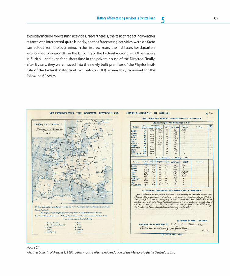
65History of forecasting services in Switzerland 5
explicitly include forecasting activities. Nevertheless, the task of redacting weather reports was interpreted quite broadly, so that forecasting activities were de facto carried out from the beginning. In the first few years, the Institute’s headquarters was located provisionally in the building of the Federal Astronomic Observatory in Zurich – and even for a short time in the private house of the Director. Finally, after 8 years, they were moved into the newly built premises of the Physics Insti-tute of the Federal Institute of Technology (ETH), where they remained for the following 60 years.
Figure 5.1: Weather bulletin of August 1, 1881, a few months after the foundation of the Meteorologische Centralanstalt.
66 From weather observations to atmospheric and climate sciences in Switzerland5
Over the course of time the national weather service changed its name a few times:
– After a few years it changed from the Meteorologische Centralanstalt to Meteo-rologische Zentralanstalt, MZA, in French Institut suisse de météorologie, in Ital-ian Istituto Svizzero di Meteorologia and in English Swiss Central Meteorological Institute.
– In 1979, it became the Schweizerische Meteorologische Anstalt (SMA), in French and in Italian it remained unchanged, and in English it became Swiss Meteorological Institute.
– In 1999 it became, depending on the pertinent language, MeteoSchweiz, MétéoSuisse, MeteoSvizzera and MeteoSwiss, respectively, but for administra-tive purposes Bundesamt für Meteorologie und Klimatologie in German, in French Office Fédéral de Météorologie et de Climatologie, in Italian Ufficio Fede-rale di Meteorologia e Climatologia and in English Federal Office of Meteorology and Climatology.
For this reason the reader will find different names describing the same institution, depending on the time period under consideration.
5.3 The first half century: advancement at a leisurely pace
In the first half century after the foundation of the Meteorologische Centralan-stalt (up until about the end of World War II), the development of the forecast-ing services advanced at a rather leisurely pace. The basic laws governing atmo-spheric flow were still being formulated, the technical means (computers) to set this knowledge into practice (integrating the governing laws into the future to get a weather forecast) were not yet available, and the technologies for data transmission and communication were as yet unable to transmit large amounts of data within a reasonable timespan. Beside producing daily weather bulletins, the activities of the meteorological institute were concentrated on improving the observation and measurement quality, on increasing the number of weather stations, on gaining empirical and theoretical knowledge of the pro-cesses governing weather and climate as well as on rapidly transmitting the weather bulletins.
These activities were severely disrupted during both World War I and II; forecasting activities had to be reduced and during some periods were assumed by the army (see also Section 6).
67History of forecasting services in Switzerland 5
From the initial five collaborators in 1881 the personnel of the MZA grew to about 35 staff members at the end of World War II. An important factor in this increase was the recruitment of aviation meteorologists at the end of the 1920s. In fact, with the advent of commercial aviation, the MZA was faced with requests for new kinds of forecasting services: The information for pilots delivered by the general weather forecast was inadequate because they needed more precise and quantitative information, also in the third (vertical) dimension, about weather parameters such as cloud base, visibility, wind and temperature. Thus, whereas the main customers of the national weather services during its first 40 years of operation were the general public and the farmers, aviation needs became most important after the 1920s, triggering new developments (also described in Section 6).
Observations and measurements
On the observational and measurement side, a major step was the installation in 1882 of the mountain observing station on the Säntis, the highest peak of the Alpstein, a pre-Alpine massif in eastern Switzerland (2502 m asl). The need for regular measurements of the atmospheric conditions at higher levels in the atmo-sphere had already been recognised by the international meteorological commu-nity, which had long encouraged such a development. To this end, the Federal Council approved a contribution of 5’000 Swiss francs for establishing such an Observatory, but this sum merely covered the annual operating costs. Säntis, located away from the main Alpine ridge and with a guesthouse near the summit, had both observational and logistic advantages. An observer was accommodated in the guesthouse and took up his activities in September 1882. In subsequent years funding was acquired for building an observatory on the summit with dona-tions of 6’000 Swiss francs from the eastern cantons, the Swiss Alpine Club and the regional societies for natural sciences. This was supplemented in 1885 when Frie-derich Brunner, a salesman from Winterthur, in his will left most of his fortune (125’000 Swiss francs) to the Meteorologische Centralanstalt. Two years later, the observatory was built, the telegraph line connecting it with the valley was installed, and in October 1887 the observer moved into his new working place and accommodation. At that time there were only a few meteorological mountain stations at that height in Europe and North America, and the Säntis Observatory became a reference point for forecasters and researchers abroad as well. The story of the Säntis observatory, which even includes an episode of crime (one of the observers was murdered together with his wife), and which was operated until a
68 From weather observations to atmospheric and climate sciences in Switzerland5
cable car right to the top of the mountain was built in 1969, is documented in a book by B. Meier (1996).
Further information on the development of the network of ground stations can be found in Chapter 7.
The polar front theory and the development of telegraphy enable first improvements of the weather forecasts
The main advancement in the context of forecasting methods in the first half cen-tury was probably the development of the polar front theory by the Norwegian Vilhelm Bjerknes and his colleagues (see also Chapter 6). Although this approach was not developed in Switzerland, it quickly got the attention of the Swiss mete-orologists, and a lively exchange with the Norwegian colleagues ensued. In Spring 1922 the so-called “first assistant” and later Director of the MZA, Dr. R. Billwiller jun., spent a few weeks with the developers of the polar front theory in Bergen, Norway, to become acquainted with the new forecasting method and to prepare to dis-seminate it within the forecasting team of the MZA. In the Autumn of the same year Vilhelm Bjerknes’s son came to Zurich and stayed for more than half a year to investigate the applicability of the Norwegian method in the Alpine area.
Communication technologies played an important role in the evolution of weather forecasts. The drawing of daily weather maps became possible only after the advent of telegraphy, which for the first time enabled the transmission of the meteorological observations needed for an assessment of the weather situation within a few hours. But the telegraphic transmission of weather dispatches at the MZA reached its limits when the number of transmitted observations increased from 36 in 1881 to around 80 in 1910. A first improvement was attained with the introduction of wireless telegraphy (also called radiotelegraphy), which enabled increasing the reception of observations to about 130 in 1922 and to around 300 by 1930. Of course, not only technology determines the transmission efficiency of an increasing amount of data; also international agreements and clearly defined codes are important. In this context, the International Meteorological Organisa-tion (IMO), founded in 1873 and turned into the World Meteorological Organisa-tion in 1951, played an important role.
In all these years, the lead time of the forecast stayed unchanged, covering the current (T+ 0) and the following (T+ 1) day. Nevertheless, the level of detail of the

69History of forecasting services in Switzerland 5
forecasts increased. While the first bulletins covered just the north-eastern area of Switzerland, over the course of time coverage was gradually extended to the West and in 1893 the whole Swiss territory north of the Alps was divided in two forecast areas: eastern, northern and central Switzerland in one forecast area and western Switzerland in another forecast area. The Swiss territory south of the Alpine crest was not covered by any weather forecast until after World War I.
The introduction of the forecasting methods based on the polar front theory increased the capabilities of the forecasters to differentiate the weather develop-ment in the different areas of the country, and in 1924 the area south of the Alps was added as a third area to the daily forecast, which now covered the whole country. However, in the following years the quality of the forecast for this third area was generally lower than that for the area north of the Alps, which was attributed to a lack of knowledge about the connection between the large scale and the local conditions. Therefore, in 1935 the MZA started operating a regional forecasting centre south of the Alps (Osservatorio Ticinese di Locarno Monti), founded on the basis of a bioclimatological and geophysical observatory originat-ing from a regional initiative in 1926, which in those years was experiencing a crisis due to the death of its founder.
The newspapers were the main channel for the distribution of the weather bulle-tin to the general public until the early 1930s. A limited number of customers received the forecast in the form of a telegram (120 subscribers in 1909). Then, the introduction of radio broadcasting accelerated and extended the distribution of the weather forecasts. Swiss Radio began operating in 1931 in the German-speak-ing (Beromünster) and in the French-speaking (Sottens) areas, whereas the Ital-ian-speaking southern regions had to wait for their own channel until 1933.
5.4 From the end of World War II until the 1980s: technological development and international cooperation accelerate the evolution of weather forecasts
After World War II the civil weather services for the general public were reactivated in the forecasting centres of Zurich and Locarno Monti (Geneva was not yet a general forecasting centre), and the distribution of the weather forecasts was reor-ganised. The Swiss telegraphic agency was now the central channel distributing the weather information to the radio, the print media and the telephone informa-tion service. After the war the MZA staff began growing at a higher rate, and soon
During the first months of operation of
the regional centre of Locarno Monti,
no telegraph line was available, so that
the data needed for the production of
the forecast were sent by night train
from Zurich to Locarno (Gaia, 2007).

70 From weather observations to atmospheric and climate sciences in Switzerland5
the premises of the headquarters in the physics building of ETH Zurich reached capacity. Hence, in 1949, the headquarters were moved to a newly built building located slightly higher on the same hillslope, at Krähbühlstrasse (Figure 5.2). The weather forecasting centre, which had been moved from the old airport of Düben-dorf to the new airport in Kloten just a year before, remained in Kloten. In the 1970s, with the installation of the first central computing system METEOR (described further below), all the forecasting activities, for aviation as well as for the general public, were moved to the headquarters.
In 1974 the aviation weather service of Geneva was extended to a regional fore-casting centre for the western part of the country. The main task of this French-speaking forecasting centre was the production of short-term weather forecasts for the general public. Also, depending on the season, the centre issued gale warnings for the lakes, frost warnings for agriculture and road weather fore-casts. Some of the employees started investigating some local phenomena that had not been examined so far by their colleagues in the forecasting centre of Zurich and participated in the development of forecasting methods. The regional centre also took over the climatological information service for the French speak-ing area.
Figure 5.2: Headquarters of the MZA on the Zürichberg (1949–2014).

71History of forecasting services in Switzerland 5
The advent of computer technologies: completely new kinds of measurements and a boost in forecast lead time
A factor that contributed to the increase of the amount of meteorological data available to the forecaster after World War II was the development of new data transmission technologies, which became available in the 1950s. The introduction of facsimile instruments (“fax”) in 1956 made it possible to receive weather maps from foreign weather services, which otherwise would take much manpower to be drawn from the coded dispatches of the individual weather stations. At the same time, they allowed exchanging own products among the Swiss forecasting centres and disseminating them to other weather centres abroad.
Also, thanks to the new data-transmission technologies, in 1962 the first numerical weather prediction (NWP) model runs produced by the American weather service were received per telex in the Swiss forecasting rooms, in the form of gridded data sets. They had a lead time of 4 days, were derived with a barotropic model cover-ing much of the northern hemisphere, and yielded an estimate of the 500 hPa geopotential field. In July 1966, for the first time after about 90 years of existence of the weather services, this step allowed an extension of the lead time of the weather forecast by 24 hours from T+ 1 to T+ 2.
Another factor that contributed to the increase in meteorological information was the advent of remote-sensing systems based on computer technologies.
The Swiss radio-sounding station of Payerne started operations in 1942 (see also Chapter 8), and in 1966 the first images of the American circumpolar satellite sys-tems TIROS and NIMBUS found their way into the Swiss forecasting rooms. Eleven years later, in 1977, the first images of another remote-sensing device, the radar, became available on a routine basis to the forecasters (the first device started operations on Mount La Dôle, see also Chapter 9). With these systems it became possible to assess on a daily basis the state of the higher atmosphere over Europe and to draw weather maps at different levels above the ground. Furthermore, for the first time the real shape and dimension of a synoptic weather system could be seen in its full extent at once.
In November 1974, to satisfy the increasing demand for data processing, the MZA acquired and began operating its first central computing system, METEOR, a cus-tom-made system developed by Siemens-Albis. Beside its main employment for data acquisition, storage and dissemination at the regional and international level,
72 From weather observations to atmospheric and climate sciences in Switzerland5
the system was also used to plot weather observations directly on a map, elimi-nating the tedious work of drawing every single station with its data by hand. One could also plot the output of numerical weather prediction models in the form of isolines (geopotential and temperature), delivered as gridded data by foreign weather centres.
A few years later, in 1977, the MZA started the deployment of its first network of automatic ground stations, called ANETZ. This allowed for a quantum leap from ten stations with a 3-hour resolution and 30 stations with three observations per 24 hours to 64 automatic stations (in 1984) measuring 20 to 30 meteorological parameters at a time resolution of up to 10 min for the fastest changing param-eters.
In 1979 the European Centre for Medium range Forecast (ECMWF: www.ecmwf .int) began producing operational medium-range weather forecasts, which were made available at the SMA in the form of the 500 and 1000 hPa geopotential and the 500 and 850 hPa temperature fields. In the following years the ECMWF model developed into the most important medium-range weather forecast used in the forecasting rooms of the SMA. This model set the pace for the increase in lead time of the general forecast issued for the public also in the following years.
Increasing amount of meteorological information and the development of new forecasting methods
In a topographically complex country like Switzerland, downscaling a mesoscale forecast to a local weather prediction was and still remains a challenge. When observations and measurements had a temporal resolution of 3 hours at best, the empirical rules used for deriving the local weather evolution were based on rather sparse data and simple statistics, sometimes even just on observations and expe-rience. The introduction of the central computing facility and the network of auto-matic measurements at MZA between 1974 and 1984 heralded a new era in data processing and opened up a wealth of new possibilities for statistical studies and development of methods.
However, some important milestones in the development of forecasting methods for predictions at the local scale had been set already before this time, starting in the 1960s.
73History of forecasting services in Switzerland 5
In the following we present a choice of the applied research and development results obtained by researchers and forecasters at MZA. The in-house publication of these results was integrated into the MZA annals up until 1963, whereas in the following years they were published in separate scientific publications, which are nowadays available on the website of the institution. Kuhn’s publication (1982) summarizes the topics treated in the annals until 1963 and is very useful when searching for a specific topic. Unfortunately, most of the work carried out by the forecasters is poorly documented and unpublished, as these collaborators had to set the priorities on their shift work and not on the writing of publications.
The main meteorological phenomena challenging the forecasters when predict-ing the weather at the local scale were (and still are) the distribution of precipita-tion, the foehn and local winds in general as well as fog and low stratus, also called “high fog” (Hochnebel).
PrecipitationPrecipitation is one of the most relevant meteorological parameters – and at the same time the most difficult to predict in detail, even more in the Swiss complex topography. When the only technical means available were ground measure-ments and observations, accurate quantitative precipitation forecasts were beyond reach. With the introduction of remote sensing and the automation of ground stations it became possible to assess the distribution of moisture in the atmosphere and to localise existing precipitation systems – and consequently, to improve the nowcasting capabilities, i. e., the prediction for the very short term (up to 6–8 hours, depending on the season and the weather situation). For a longer term quantitative prediction, the forecaster had to – and still does – rely on numer-ical weather prediction models. But during the first two decades after their intro-duction in the forecasting services, these models didn’t predict precipitation. Con-sequently, different methods for systematically deducing precipitation forecasts from model fields of other parameters were developed based on physical laws and/or statistical algorithms, e. g., Müller (1967), Courvoisier (1970), Kuhn et al. (1976), Courvoisier (1981), Altherr et al. (1982) and Ambühl (1984). However, the improvements in quantitative precipitation forecasts given by these methods, particularly in the first decade, were often rather disappointing. Furthermore, the fact that no powerful computing facility to efficiently process these methods was available until the mid-1970s was also a limiting factor. Not all developed methods were implemented for operational forecasting. Later on the methods proposed by Altherr et al. and by Ambühl were implemented on the METEOR computing sys-

74 From weather observations to atmospheric and climate sciences in Switzerland5
tem, and their results were made available to the forecasters (both methods were also extended to predict further parameters, like sunshine duration). The informa-tion about the improvement of quantitative precipitation forecast brought by these methods is rather sparse. Only Altherr mentions a verification of his objec-tive method with respect to climatology, which shows a mean improvement between 19 % (for a lead time of 24 hours) and 10 % (for a lead time of 72 hours), as well as a comparison with the coded forecasts of the forecasters of the regional centre of Geneva (which is of limited significance, as their forecast didn’t go beyond 48 hours and they were using the output of the method to be verified).
FoehnBecause the foehn is a special mountain-related phenomenon that caught the attention of many researchers in the Alpine area, a special chapter is dedicated to it (see Chapter 11). The main concern of the forecaster is to define the foehn onset and end, how strong it will be, how far it will propagate into the Swiss Plateau and how much temperature increase it will produce in the valleys where it blows. To answer these questions a number of objective empirical methods was developed, among which the probably most well-known was that developed by Widmer (1966, also described in Chapter 11) and simplified for the routine application in the forecasting room by Courvoisier and Gutermann (1971).
Besides the Widmer index, other unpublished methods and checklists requiring the continuous monitoring of certain parameters were produced to support the foehn forecasts. However, the tremendous amount of information available to the forecaster nowadays makes it very difficult to repeatedly and systematically work through such checklists. Some of the aspects, rules and values have been implemented as computer routines and integrated into the warning and fore-casting system.
Although foehn research continued to produce results on dynamical and phe-nomenological aspects, the foehn forecasting methods used in the forecasting room didn’t experience significant changes. A relevant work by Dürr (2008), based on the automatic detection of foehn, could be developed further to obtain a new automatic foehn forecasting algorithm, but this work is still in the pipeline.
The most marked and best-known South foehn cases in Switzerland are those observed in the valleys of the central and eastern Alpine area, though foehn epi-sodes connected with a South-North pressure gradient over the Alps are also
Unpublished method found in the
documentation in the forecasting
room:
Empirical formula to predict the foehn
temperature in the foehn valleys start-
ing from the wet bulb potential tem-
perature at 700 hPa in the upstream
area south of the Alps (usually some-
where over the Po valley).
TF = 1.3 * Thetaf + 4
where Thetaf is the wet-bulb potential
temperature
and TF the maximum expected tem-
perature (as an average for all foehn
valleys), with a correction of –1 °C
in November, December and January
and of + 1 °C between May and August.

75History of forecasting services in Switzerland 5
observed in some valleys of the western area and particularly of the Valais. How-ever, no specific index was developed to predict it, as the impact of these episodes is less relevant than in the central and eastern areas.
Foehn (North foehn) is a relevant phenomenon on the southern side of the Alpine ridge, but its characteristics are somewhat different than the South foehn, as the air masses leading to North foehn events are different. A specific forecasting method was developed only recently by a forecaster of the MeteoSwiss regional centre of Locarno Monti but has not yet been thoroughly implemented and doc-umented.
FogOne of the bigger challenges in weather forecasting at the local scale was and still remains the prediction of fog, as even the very high resolution models available nowadays cannot predict fog with a satisfying reliability, particularly of fog at ground level. On the Swiss Plateau, fog and low-hanging stratus are quite frequent in Autumn and Winter. Ground fog can cause disruptions particularly in air traffic, whereas low stratus affects larger areas and is less disruptive for traffic but more disturbing for tourism.
Main issues connected with fog prediction are the time of development and dis-solution, the height of its top and its base as well as visibility. In the case of ground fog, the need for a good local prediction is more important in the areas where airports are located and the specific documentation is rather sparse and limited to a number of climatological analyses and a few rules. For “high fog” (low stratus) the available documentation is somewhat more comprehensive, although in this case too most of it is unpublished, like in the case of foehn methods.
Investigating the connection between the pressure gradient Payerne-Strasbourg and the percentage of possible sunshine hours, on the one hand, and the upper limit of the fog in wintery high-pressure situations with a temperature inversion in the lower layers, on the other hand, Courvoisier (1976) found a correlation between the two parameters. Since then these results have been used to empiri-cally predict the top of the stratus layer and its dissolution (see examples in Figures 5.3 and 5.4).

76 From weather observations to atmospheric and climate sciences in Switzerland5
Figure 5.3: Relationship between mean sunshine duration and pressure gradient Payerne-Strasbourg for Zurich (from Courvoisier, 1976).
Figure 5.4: Top of high fog in function of the pressure difference Payerne- Strasbourg (unpublished diagram, by P. Hächler and R. Baumberger).
Unpublished methods found in the documentation of the
forecasting room in Zurich:
A. A method for defining the chance of fog dissolution
before the end of the morning was developed by G.
Truog in 1981. This method puts the ratio of the sum of
the global irradiance measured at a station in or below
the fog and of the same sum measured at the nearest
mountain top station above the fog layer (Säntis, Pila-
tus, la Dôle) in connection with the chance of dissolu-
tion. I f this ratio reaches or exceeds a value between
0.16 and 0.21 (depending on the considered lowland
station), fog dissolution is likely (no further probabilis-
tic information is available).
B. Someone else (author and year unknown) defined a
formula for determining the temperature Ta that has to
be reached at ground level in order to start fog dissolu-
tion: Ta = To + (0.7 * fog thickness in m)/100,
where To is the lowest temperature still within the fog,
at the top of it. This means that, when the ground tem-
perature reaches a value that corresponds to the top
temperature descended moist adiabatically to the
ground level, fog will begin dissolving.
C. R. Schneider (year unknown, work unpublished) devel-
oped a formula to determine the top of the fog layer in
function of its base: Top (in m above sea level)
= 1.3 * Base (in m above sea level) + 40.

77History of forecasting services in Switzerland 5
The lead time of the general forecast makes a leap and a more systematic forecast verification becomes an issue
With the increasing number of available NWP models the interest in knowing more about their quality also rose. Züllig (1976), Gensler (1983), as well as Schacher and Schubiger (1988) documented a few comparisons between the American, the German and the ECMWF models. The work by Gensler led to the conclusion that the time had come to increase the lead time of the general weather forecast from T+ 2 to T+ 5, which was implemented in 1983 (17 years after the last increase from T+ 1 to T+ 2).
During its first century, the Swiss national forecasting service issued forecasts that were regularly verified against measurements, but up to the 1960s the methods were very general, stating only whether the forecast was good, useable or useless, and the results of the verification were subjective, depending on the person who carried it out. In 1966, a more detailed procedure that took separately the most important meteorological parameters into account was introduced, but the veri-fication was still quite subjective. At the beginning of the 1980s every regional forecasting centre made a survey in its own language area among the general public, and the results were used to optimise the wording used in the general forecast. About the same time Ganter (1981) carried out a study to find out whether the forecasters of the regional centre of Geneva tended to be particularly pessimistic or optimistic in their prediction of specific parameters and how repro-ducible the forecasts are. He found that the forecasters tended to be more opti-mistic regarding sunshine duration (too many sunshine hours) and pessimistic regarding precipitation (too much rain). However, he also found that there were visible differences between the individual forecasters; no similar studies are doc-umented for the other regional centres. An important step in the verification of the man-made forecasts was made in 1984 with the introduction of a routine for systematic verification of the general short-term forecast (Schönbächler, 1996). With this new method, which verified the forecast against the measurements of the automatic measuring network ANETZ, subjectivity was clearly reduced, albeit not completely eliminated. The subjective component lay in the words used to describe the forecast (e. g., “partly cloudy”, “light rain”, etc.) being coded and con-nected with predefined values of the related parameters. For this verification the Swiss territory was divided into 14 regions, and the forecast was verified against persistence to quantify the performance of the forecaster. A separate verification based on a comparison with climatology was used for the medium-range forecast. Interestingly enough, the quality of the “man-made” forecast in all these years was
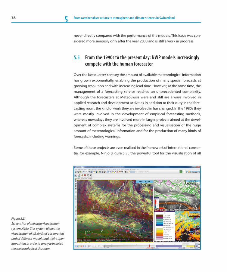
78 From weather observations to atmospheric and climate sciences in Switzerland5
never directly compared with the performance of the models. This issue was con-sidered more seriously only after the year 2000 and is still a work in progress.
5.5 From the 1990s to the present day: NWP models increasingly compete with the human forecaster
Over the last quarter century the amount of available meteorological information has grown exponentially, enabling the production of many special forecasts at growing resolution and with increasing lead time. However, at the same time, the management of a forecasting service reached an unprecedented complexity. Although the forecasters at MeteoSwiss were and still are always involved in applied research and development activities in addition to their duty in the fore-casting room, the kind of work they are involved in has changed. In the 1980s they were mostly involved in the development of empirical forecasting methods, whereas nowadays they are involved more in larger projects aimed at the devel-opment of complex systems for the processing and visualisation of the huge amount of meteorological information and for the production of many kinds of forecasts, including warnings.
Some of these projects are even realised in the framework of international consor-tia, for example, Ninjo (Figure 5.5), the powerful tool for the visualisation of all
Figure 5.5: Screenshot of the data visualisation system Ninjo. This system allows the visualisation of all kinds of observation and of different models and their super-imposition in order to analyse in detail the meteorological situation.
79History of forecasting services in Switzerland 5
kinds of meteorological data used in the forecasting rooms of MeteoSwiss. Here the forecasters are not so much involved in the development of the system itself anymore.
Nevertheless, some forecasting methods were developed also during the last 25 years. Besides the development of nowcasting methods, an increasing number of these developments are based on postprocessing of NWP model output, like the application of a Kalman filter to correct the minimum and maximum temperatures produced by the ECMWF model (Cattani, 1994) and the application of expert sys-tems for specific types of forecasts (Ambühl, 1991). Unfortunately, not all develop-ments of this kind have been described in publicly accessible documents.
A major step in the development of the SMA was made at the beginning of the 1990s when it started working on a regional model (see the insert on “The begin-nings of operational numerical weather prediction in Switzerland” in this chapter).
At the international level, the first ensemble prediction systems (EPS), which allow for probabilistic forecasts, were routinely being made available and appeared also in the forecasting rooms of the SMA. The interpretation of EPS output is not straightforward and led to the development of several methods to postprocess and interpret the large amount of information produced by such a system. One such method is based on a neural network and was developed by a few collabo-rators at the regional centre of Geneva (Ambühl et al., 2010).
The consequence of the major worldwide achievements in numerical weather prediction is that it is becoming increasingly difficult for the forecasters to top the performance of NWP models. The forecaster’s role is changing, the work is increas-ingly shifting from routine activities to the handling of exceptional situations. MeteoSwiss made first steps towards a more general semi-automated production system in the first years of the new millennium by developing a production system based on a so-called forecast matrix: A first guess of the weather forecast for a given set of locations is generated starting from a NWP model and can be modi-fied by the forecaster; the result is then used to generate a number of products for different end users. The experience with this system showed that it is impossible to generate all specific forecasts from one basic forecast produced for a limited number of stations. In 2014 a new system based on a gridded dataset instead of on selected locations began operation but has not yet completely substituted the older production systems.
80 From weather observations to atmospheric and climate sciences in Switzerland5
The public mandate that regulates the activities of MeteoSwiss also contains a statement on the quality of the issued general forecasts, which implies a systematic verification of the prediction with a method that doesn’t change every few years. At the beginning of the new millennium, however, the method introduced in the 1980s, which still had a subjective component, was approaching its limits. It is cur-rently being substituted by another method, called COMFORT (for CONtinuous MeteoSwiss FORecast qualiTy), which better suits the needs of the institute con-nected with the reporting to the central government. COMFORT, a so-called Global Continuous Accuracy Score (GCAS), is a linear combination of partial scores defined for each verified quantity. Each partial score encompasses tuneable thresholds defining what a correct, useful or useless forecast for the given quantity is, as well as a continuous distance-based measure of accuracy (Cattani et al., 2015).
The beginnings of operational numerical weather prediction in Switzerland
Francis Schubiger
The first numerical weather prediction model in Switzerland that became operational was the Swiss Model (SM) of MeteoSwiss, which ran on a CRAY Y-MP 4/464 at ETH Zurich with a grid mesh of 14 km and was run every 12 hours to issue a forecast with a lead time of 36 hours (Figure 5.6.a). In 1993 it began running in a preoperational mode (and already caught the flash flood in Brigue on 24 September 1993) and became fully operational on 1 September 1994. Results were made available to all forecasters with graphics and tables with values for the locations of the automatic measuring network of MeteoSwiss. This represented great progress in short-range weather fore-casting and opened up novel applications.
But the beginning of numerical modelling actually occurred much earlier. In 1973 Walter Kuhn (head of a section in the Forecast Department at MeteoSwiss and Lecturer for Synoptic and Dynamic Meteorology at ETHZ from 1955 to 1980) and Jean Quiby (head of the Modelling Section from 1980 to 2004) started the development of a dynamical-statistical method based on the so-called omega equation (Kuhn et al., 1976). The model based on large-scale grid-point data computed the fields of vertical velocities at 850, 700 and 500 hPa on a finer grid. In 1981 this baroclinic model was
81History of forecasting services in Switzerland 5
adapted to run operationally on the computers of MeteoSwiss with the ECMWF analysis and forecast fields: The results of the vertical velocities were obtained over the Alpine area with a grid mesh of 28 km. With statistical methods (principal component analysis followed by a forward selective mul-tiple linear regression), precipitation forecasts were calculated based on these vertical velocities and further predictor fields of ECMWF (Schubiger, 1986). In 1982 the arrival of Huw Davies at ETH as Professor for Dynamical Meteo-rology at the Laboratory for Atmospheric Physics (today Institute for Atmo-spheric and Climate Science) provided the opportunity to start a study with a one-layer model based on the shallow water equations (Schubiger et al., 1987). In 1986 the SMA started the project MESOMOD with the aim of improving the short-range weather forecasts (with a lead time of 36 h) with a better regionalisation and timing of the forecasts (Quiby et al., 1988). It was decided to develop a meso-scale model together with a foreign meteorolog-ical service. After a thorough evaluation, the SMA started a collaboration with the Deutscher Wetterdienst (DWD) in early 1988 for the development of a high-resolution model (HRM) covering the Alpine area. The basis was the Europa-Model (EM) of DWD, which ran since 1991 on a CRAY Y-MP twice daily covering all Europe with a grid mesh of 55 km. In the years 1988–1992, MeteoSwiss and DWD jointly developed a 14 km-model with initial and lat-eral boundary conditions from EM, which became operational in 1994 under the name Swiss Model (SM). Among other contributions, MeteoSwiss stud-ied the impact of enhanced horizontal resolution and cumulus parameter-ization on the simulation of precipitation (Binder, 1992).
The collaboration with Germany was extended at the end of the 1990s first to Italy and then to Greece, leading to the official creation of the Consortium for Small-scale Modelling (COSMO, see www.cosmo-model.org) in October 2001. Today, seven national weather services work together within COSMO to develop, improve and maintain a nonhydrostatic, limited-area atmo-spheric model which is used both for research and operations by the mem-bers of the consortium. In 2001, the SM was replaced by the nonhydrostatic Alpine Model (aLMo) covering western and central Europe with a grid mesh of 7 km and 45 vertical layers. The lead time of the forecasts was extended from 48 to 72 hours in 2004. In 2008 aLMo was renamed COSMO-7, the grid mesh reduced to 6.6 km and the vertical layers extended to 60 (Figure 5.6.b). Since 2003 COSMO-7 has used the lateral boundaries from the European

82 From weather observations to atmospheric and climate sciences in Switzerland5
Centre for Medium-Range Weather Forecasts (ECMWF). In 2008 a convec-tion-permitting model, COSMO-2, with a grid mesh of 2.2 km, became oper-ational (Figure 5.6.c). It is nested inside COSMO-7 and is run 8 times a day for a lead time of 33 hours (45 hours for the run of 03 UTC).
Figure 5.6: 12 h-forecast of the 10 m-wind field for 14 April 2001 12 UTC. It shows a NE wind (“bise”) over the south western part of Switzerland and the canalisation of the wind into the Rhone valley upstream of the lake of Geneva for the forecasts of all 4 operational models since 1994: the Swiss Model, SM (Figure 5.6.a, 14 km grid mesh), aLMo, called COSMO-7 after 2008 (Figure 5.6.b, 6.6 km grid mesh), COSMO-2 ( Figure 5.6.c, 2.2 km grid mesh) and the newest COSMO-1 running in test mode in Summer 2015 (Figure 5.6.d, 1.1 km mesh grid). Wind speed and direction are illustrated by the wind barbs, whereas the height of the topography in each grid box is indicated in colour. The increase in resolution is clearly visible from SM to COSMO-7, COSMO-2 and finally COSMO-1.
83History of forecasting services in Switzerland 5
With regard to extreme situations, an important task of the national weather service is to warn the population, the authorities and weather-sensitive busi-nesses about dangerous weather developments. In the years before the auto-mation of observing systems and the introduction of remote-sensing systems, it was difficult to detect rapidly developing small-scale dangerous weather phe-nomena like wind gusts (especially if caused by short-lived thunderstorms), hail, flash floods or even freezing rain. Although the MZA began issuing storm warn-ings for the airfields and the larger lakes in 1938 and later on added frost warn-ings for agriculture and roads, it wasn’t until the 2000s that the warning system experienced remarkable developments. After a series of larger storms, like Lothar in 1999, and extreme convective systems with extended flash floods, like
The initial state of the atmosphere is computed for both models with an own assimilation system incorporating all measurements over the full domain (surface observations, balloon soundings, composite of all the Swiss radars (Leuenberger, 2005), data from commercial airplanes, etc.). This assimilation system, available in hourly steps over Europe since 2001 (and since 2008 over the Alpine area with 2.2 km grid mesh) gives the best estimation of the three-dimensional state of the atmosphere.
The project COSMO-NExT at MeteoSwiss aims at developing two new con-vection-permitting models COSMO-1 (operational since April 2016) with a grid mesh of 1.1 km will provide eight daily deterministic forecasts for the short range (Figure 5.6.d), and COSMO-E (operational in June 2016), using the ensemble technique enabling a prediction of the forecast uncertainty, will provide twice-daily probabilistic forecasts up to 5 days in advance. Both models will cover the Alpine area and get their initial condition from a new ensemble based assimilation method LETKF (Local Ensemble Transform Kal-man Filter; Schraff et al., 2015).
The computations occur on supercomputers of the Swiss National Super-computing Centre (CSCS) passing from a NEC-SX-5 in 2001 to a Cray XE6 in 2015. A substantial effort has been made with partners especially from ETHZ and CSCS to port COSMO to new supercomputer technologies. The new models COSMO-1 and COSMO-E will run on a Cray CS-Storm with a high density of graphic processing units (GPUs). With this, MeteoSwiss is the first national weather service worldwide that can run a full numerical weather forecast model on supercomputers making extensive use of GPUs.
84 From weather observations to atmospheric and climate sciences in Switzerland5
those on the northern Alpine slope in 2005 and 2007, it became clear that the warning activities had to be extended from the single lakes and airports to the whole territory, and that the way of communicating the warnings had to be improved. At the same time, the private weather companies began competing with the national weather service by issuing warnings of their own. Nowadays, several kinds of extreme event warnings are issued by MeteoSwiss as well as by private weather companies, and the discussion about whether it really is in the sense of public safety to issue several uncoordinated warnings for the same event is not yet resolved. In any case, the expectations on the accuracy and reliability of the warnings grows with their growing degree of detail. A major challenge lies in the development of automatic systems for the early detection of dangerous, rapidly generating extreme events to support the forecasters in their warning tasks.
As already mentioned above, another aspect that changed the world of weather forecasting in Switzerland and abroad was the appearance of private weather services. This important development, which plays a large role as well in the future of forecasting services, is treated in a separate section of this chapter (Section 7).
Current and future challenges
The following scientific challenges will keep the Swiss weather services busy also in the years to come; they are among the most important ones and are similar for the weather services of all other mid-latitude countries:
– The amount of meteorological information and the variety of sources of such information will continue to increase. Therefore, larger investments will have to be made in the development of new methods to process large amounts of data with varying and sometimes unknown quality (keywords big data and crowdsourcing) and to consolidate it into “digestible” pieces of information.
– The lead time of routinely issued forecasts will increase further, demanding methods to obtain a smooth transition between the different forecasting sys-tems like nowcasting tools, very high-resolution regional models and global models for medium-range, monthly and seasonal forecasts (keyword seamless) and from a deterministic to a probabilistic information.
– Although ensemble prediction systems (EPS), which provide information about the probability of occurrence of a forecast, were already developed in
85History of forecasting services in Switzerland 5
the 1990s, there is still considerable potential for the delivery of probabilistic information to the users of the forecasts. With the already mentioned increase of lead time of the forecast the need for generally understandable informa-tion about the uncertainty connected with this forecast will grow.
One challenge more specific to Switzerland is the liberalisation of meteorologi-cal data, something MeteoSwiss plans to implement in the future. This step might look like a merely administrative matter, but it has the potential of chang-ing the way MeteoSwiss works and interacts with the private weather services. In some other countries of the world such a liberalisation was already realised a few years ago, but the implementation and the impact have been different in every country and therefore cannot be extrapolated to the Swiss conditions.
5.6 The role of aviation in the development of the Swiss Meteorological Service
The pioneer years
Since the first successful motorized flight on 17 December 1903 by Orville Wright at Kitty Hawk, North Carolina, USA, flying and meteorology have been closely linked. Although that flight lasted only some 12 seconds and went only about 37 meters, it would not have been possible at all without knowledge of the prevailing wind situation.
The following decade saw many further developments of the originally very fragile flying machines. Motor planes came to fly over long stretches and reach even greater heights. In 1914 the Swiss Air Force was founded. This period, in which also the first flights over the Alps took place, marks the foundation of the Swiss Aviation Weather Service. During World War I the MZA in Dübendorf offered its first courses in meteorology for military pilots. An early Swiss pioneer of that day was Oskar Bider (1891–1919), who first succeeded in crossing the Alps by plane in both directions on 13 July 1913. When World War I broke out in the summer of 1914, Oskar Bider and the small band of trained Swiss pilots were called to duty together with their airplanes near Bern and became the new Swiss Air Force. Because of his experiences, Bider became head pilot and trainer of the military pilots and himself flew 4249 flights. He was killed in an accident on 7 July 1919.

86 From weather observations to atmospheric and climate sciences in Switzerland5
The boom following World War I
Following World War I many companies around the world established airlines. In Switzerland, the air postal route Zurich–Bern–Lausanne–Geneva was set up in 1919 and serviced by military airplanes. The pilots were provided with weather observations for the airstrips lying along the route of post offices. At that time, the weather service, like the weather reports for the airstrips, was being run by the military since the MZA was still very sceptical about the idea of flying.
However, based on a resolution passed by the Federal Council on 27 January 1920 concerning the regulation of air traffic in Switzerland, the Swiss Confederate Air Traffic Authority was created, and in 1922 Switzerland joined the “Convention Aéri-enne Internationale (CAI)”. The MZA assumed the duties of weather consultation and the transmission of weather data. However, because this agency did not have the personnel and effectively no legally binding laws had been passed, the Swiss Confederate Air Traffic Authority set up a rudimentary weather service using fed-eral employees from the Telegraph Office in Zurich. It was their duty to exchange data internationally and to prepare weather charts. With this service in place, in 1922 pilot reports were used to initiate the first international route Geneva–Zurich–Fürth (in Germany).
The year 1920 was a very important one for the development of air traffic in Europe. The “International Air Traffic Conference” voted to establish a series of very important regulations and guidelines that were also relevant for flight weather services. Among other things, it set up the radio operations regulations for flight safety services and a regional weather report plan for hourly weather reports. This plan put an end to the previous chaos in the ether. The weather observation sta-tions in Geneva, Lausanne and Basel hourly transmitted coded weather reports that were intercepted in Dübendorf, collected as Swiss observations and then redirected through its own transmitter as “Meteo Suisse.”
In 1923, a second international air route was established, going from Zurich–Basel–London (UK), so that weather observations regularly became available during the summer at the three airports of Dübendorf, Birsfelden and Cointrin. Weather reports from France, England and Germany were also received in Morse code and passed on to the pilots.
87History of forecasting services in Switzerland 5
The flight weather service in Dübendorf
From 1924 on the MZA was assigning meteorologists to Dübendorf, and from 1926 on warnings about expected wind gusts were being sent to the airports. Over time more and more airlines were flying to and from Switzerland, and the number of weather reports being received was also increasing steadily. Thus, in 1927 the MZA founded a new section for flight weather services and took over the weather observation network that had previously been organized by the Swiss Confederate Air Traffic Office. Beginning in the winter of 1928/1929 the three main airports in Zurich-Dübendorf, Geneva-Cointrin and Basel-Birsfelden regularly received weather reports according to the new international synoptic coding sys-tem (Copenhagen Code) at set time-points. So-called hazard alerts were issued in cases of poor visibility, low clouds, strong winds, thunderstorms, etc.
Then, on 1 May 1929, the first official meteorologist started working in Dübendorf. Up to that point the MZA had been concerned primarily with climatological tasks as well as offering a limited service for weather forecasts, but now in 1929 it assumed the full responsibility for the flight weather service. Previously, pilots had been receiving weather reports before taking off, whereas now the flight meteo-rologist could provide a weather forecast and advice for the entire flight route.
The main tasks of the flight weather observatory in Zurich-Dübendorf were to issue hourly weather observations, drawing up weather charts as well as preparing notes for flight routes and advising about a dozen pilots daily.
The weather observatory in Geneva-Cointrin was established in 1931, that in Sternenfeld near Basel-Birsfelden about a year later. In the years that followed, aviation experienced a rapid development. The improved instruments built into the airplanes allowed blind flights. Whereas the vast majority of the airplanes still needed ground sight along their flight route, a number of machines were now flying through clouds and at night. Besides the usual weather observations deliv-ered from stations along the route, pilots flying by instruments were now expect-ing to receive also reports on winds at different levels above ground, on the zero degree level, as well as icing and turbulence risks.
When in 1935 the German Lufthansa began flying over Switzerland at night on their way to Rio de Janeiro, the flight weather service had to initiate night shifts. Furthermore, as already mentioned in Section 5, in these years the MZA began issuing storm warnings for the airfields. It didn’t take very long before flights were
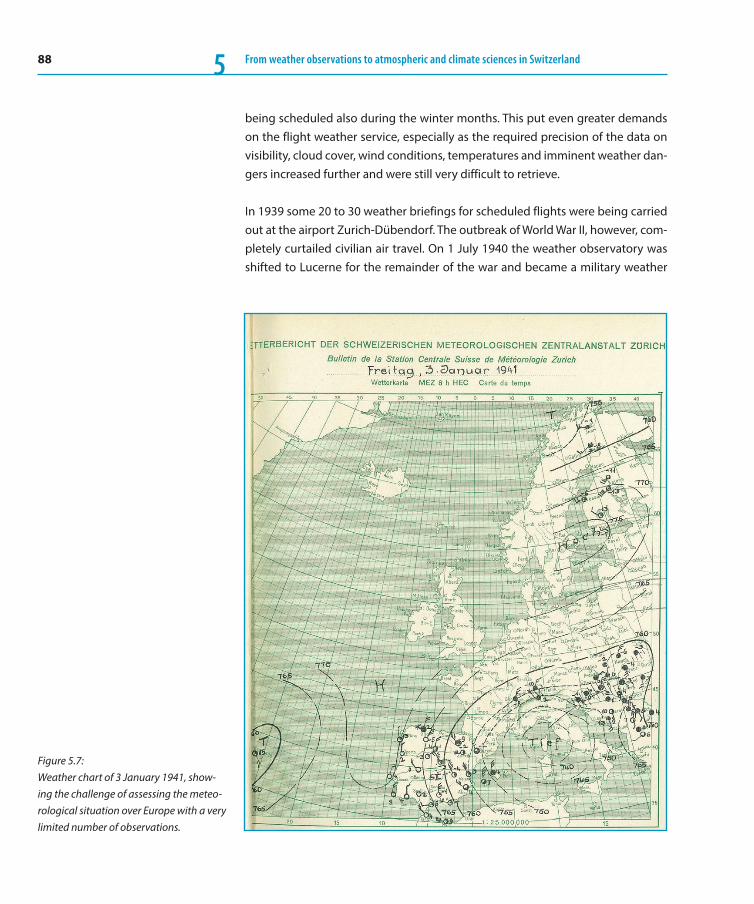
88 From weather observations to atmospheric and climate sciences in Switzerland5
being scheduled also during the winter months. This put even greater demands on the flight weather service, especially as the required precision of the data on visibility, cloud cover, wind conditions, temperatures and imminent weather dan-gers increased further and were still very difficult to retrieve.
In 1939 some 20 to 30 weather briefings for scheduled flights were being carried out at the airport Zurich-Dübendorf. The outbreak of World War II, however, com-pletely curtailed civilian air travel. On 1 July 1940 the weather observatory was shifted to Lucerne for the remainder of the war and became a military weather
Figure 5.7: Weather chart of 3 January 1941, show-ing the challenge of assessing the meteo-rological situation over Europe with a very limited number of observations.
89History of forecasting services in Switzerland 5
observatory. For many years the weather service had to be content with its own observations and those coming from Spain and a few other locations, as can be seen in Figure 5.7; other weather information was simply not available at the time.
The postwar era and the move to Kloten
Following World War II, air transportation experienced a turbulent boom. Not only was there a dramatic increase in the number of scheduled, tourist and sport flights, but also the airspace was increasingly being extended further into the ver-tical. The flight weather service of the MZA initially could not keep up with the development as the needed resources were not being allotted the necessary credit line, but finally the number of personnel attached to the flight weather service could be gradually increased over the next few years.
1948 marked the opening of the intercontinental airport in Zurich-Kloten. The flight weather station Kloten was officially opened on 17 November 1948, once barracks with sufficient space had become available. The weather observations were done on a meadow right next to the barracks. Visibility was estimated stand-ing on a ladder that rose above the height of the barracks.
Then Swissair introduced two flights each month to New York, also adding Cairo and Manchester to its roster, and in the following years further flights to Africa and Asia were added. The demands made of the weather service increased further: It was now expected to deliver weather advice and to procure the necessary data from many new regions around the globe.
Up to the end of the 1940s weather briefings were based on weather charts at ground level and reports on the upper winds, since most commercial aircraft did not fly much higher than 300 m above ground. Beginning in 1949, however, the airplanes were outfitted with pressurized cabins and could fly longer routes, so that new charts of the 500 hPa level had to be provided additionally to those of the 700 hPa level. Swissair was now already flying twice weekly to New York, with a stopover in Shannon, so that weather information only had to be available for the part ending in Ireland.
In the autumn of 1949 a new weather observation post, complete with a tele-phone, heating and light, started operating at the northern end of the instru-ment-landing runway (runway 16/34). Under foggy conditions, this post was
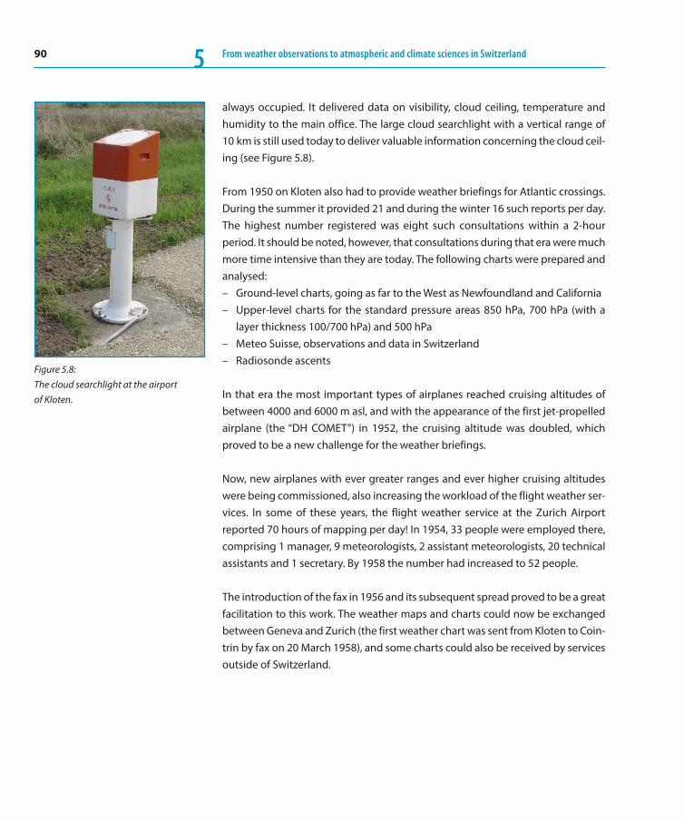
90 From weather observations to atmospheric and climate sciences in Switzerland5
always occupied. It delivered data on visibility, cloud ceiling, temperature and humidity to the main office. The large cloud searchlight with a vertical range of 10 km is still used today to deliver valuable information concerning the cloud ceil-ing (see Figure 5.8).
From 1950 on Kloten also had to provide weather briefings for Atlantic crossings. During the summer it provided 21 and during the winter 16 such reports per day. The highest number registered was eight such consultations within a 2-hour period. It should be noted, however, that consultations during that era were much more time intensive than they are today. The following charts were prepared and analysed:
– Ground-level charts, going as far to the West as Newfoundland and California – Upper-level charts for the standard pressure areas 850 hPa, 700 hPa (with a
layer thickness 100/700 hPa) and 500 hPa – Meteo Suisse, observations and data in Switzerland – Radiosonde ascents
In that era the most important types of airplanes reached cruising altitudes of between 4000 and 6000 m asl, and with the appearance of the first jet-propelled airplane (the “DH COMET”) in 1952, the cruising altitude was doubled, which proved to be a new challenge for the weather briefings.
Now, new airplanes with ever greater ranges and ever higher cruising altitudes were being commissioned, also increasing the workload of the flight weather ser-vices. In some of these years, the flight weather service at the Zurich Airport reported 70 hours of mapping per day! In 1954, 33 people were employed there, comprising 1 manager, 9 meteorologists, 2 assistant meteorologists, 20 technical assistants and 1 secretary. By 1958 the number had increased to 52 people.
The introduction of the fax in 1956 and its subsequent spread proved to be a great facilitation to this work. The weather maps and charts could now be exchanged between Geneva and Zurich (the first weather chart was sent from Kloten to Coin-trin by fax on 20 March 1958), and some charts could also be received by services outside of Switzerland.
Figure 5.8: The cloud searchlight at the airport of Kloten.
91History of forecasting services in Switzerland 5
The “jet age”
On 30 May 1960 the first DC-8 flight of the Swissair took off for New York. This type of airplane had a cruising altitude of between 8000 and 12000 meters. The intro-duction of the “jet airplane briefing” was a major act. Besides the charts for the standard pressures of 700, 500, 400, 300 and 200 hPa, now tropopause and maxi-mal wind charts became necessary. In the same year the weather fax network MOTNE (Meteorological Operational Telecommunication Network for Europe) was started, meaning that the weather reports and forecasts of more than 100 Euro-pean airports were available within half an hour.
In 1966, the first weather charts of the regional forecast centres (Frankfurt, Paris, London) organised by the WMO (World Meteorological Organization) were being received by fax. Swissair, however, was not happy with the quality of the new system. The same year a new station to receive weather satellite data began oper-ation at Colovrex near Geneva. The satellite pictures (TIROS, NIMBUS) became a very important new source of information for the flight weather services since only little other information was available for certain long-haul flights (Africa, South America). 1 January 1969 saw the first version of the coded flight weather report METAR (METeorological Aerodrome Report).
A few months later the transmissometer system with five units for measuring runway visibility became operational following an extensive test period. This ended a long and rather bizarre phase in which observers would travel to the different observation posts to fire up the runway lights to measure the runway visibility (RVR).
In 1988, a new inversion measurement system AMETIS1 was commissioned which provided very precise information and warnings of marked inversion and the respective wind shears.
The technical development during the past few decades has allowed flights to be carried out under ever more difficult weather conditions. The result was that, besides providing information on the status of ever higher atmospheric layers, it also became necessary to very precisely determine the weather conditions around the airports without increasing the overall staff necessary to do so.
At the same time, technical progress allows the systems in use to be automated. An in-house development of MeteoSwiss, called SM/\RT, is in place at the airports

92 From weather observations to atmospheric and climate sciences in Switzerland5
and supports the observer in reporting METAR. At the regional aerodromes, the system is capable of producing fully automated METAR (AUTO METAR), thus reduc-ing costs without reducing the quality. Further progress will allow automating the observations at the international airports Geneva and Zurich. The days of meteo-rological observers at airports will probably be history within the next decade!
5.7 The advent of private forecasting services
The assessment and forecasting of weather phenomena were originally purely private endeavours. Human beings were inherently dependent on nature and agricultural successes for their livelihood and thus became experts concerning the local weather. This led to the rise of the so-called “farmers’ rules” or “country lore”, which attempted to “nowcast” the weather or to predict it for the upcoming sea-son – and had a relatively good hit rate. The final remnants from that day and age may still be found in the Muothataler weather prophets, who have survived to the present day and are well known throughout Switzerland.
How weather became part of the private sector
Up to now we have learned that, from the very beginning, the scientifically based task of forecasting the weather was a government affair (in part at public univer-sities). During the 1990s, however, both the technical and social contexts under-went a change: The necessity of maintaining many state and public functions was questioned by more liberal economic forces, and some became privatized or were complemented by private alternatives. For example, as early as the 1980s many private radio and television stations were presenting stiff competition to the state-run institutions.
Parallel to this development it became technically possible to more quickly pro-vide greater amounts of weather data – whether from ground station and satellite measurements or from a numerical weather prediction model – from a central spot (such as a government-run weather service) to any number of individual places, whether by Videotex/BTX, fax, modem or some other medium (especially via the ever more important and powerful internet). On the other hand, the added value created with these data was also able to reach the media as end clients in rapid succession (whether via the internet, Tele News Combi (TNC), special ISDN protocols (as Leonardo) or – as with some private television weather programs –
93History of forecasting services in Switzerland 5
via courier on a tape). Furthermore, the internet proved to have ways to offer ads and earn money on the weather portals.
The first private weather services initially hit the market as meteorological advi-sors and experts. The oldest such service was founded in 1962 in Pennsylvania (USA): AccuWeather. In Switzerland Meteotest is the oldest such service, having been founded in 1981. It developed from a company in Bern offering expert opinions and data processing to one that also provides weather forecasts in newspapers and on the radio. “The Weather Channel” has been on the air in the United States since 1982. In Europe the Dutch company MeteoConsult began offering media and B2B in 1986 and subsequently went international as the MeteoGroup. It eventually bought up the Swiss company meteomedia, which was founded in 1990 and, like the smaller meteoCOM from Western Switzerland (founded 1989 and recently dissolved), was one of the pioneers in the private market for weather forecasts. From 1995 on, the number of new start-ups increased considerably (in Switzerland there was MeteoNews in 1997, meteodat in 1998 and meteoradar in 1999). This privately run market for weather data relies (sometimes not deliberately) on an economic liberalism which presumes that competitive companies can equally and unimpededly enter the market and will produce the best product at the best price (and in some cases also poorer products at lower prices). However, this situation was not present on either the Swiss market or most of the European market as well. MeteoSwiss as the public national weather service was, from the very beginning, supported by tax reve-nue, though in part the government expected that it should become active in the marketplace to cover some of the expenses, albeit without resorting to advertising. The ensuing conflicts between the government demand to deliver information such as aviation weather and warning services and the existing eco-nomic pressures, which often made MeteoSwiss a target of criticism by its pri-vate competitors, went through several phases and is still an issue even today. A second public participant, SF meteo, was founded in 1992 when the German Swiss television station decided to set up its own weather service. On the one hand, it is understandable that a television station that is unhappy with its pre-vious supplier, or prefers not to have to deal with a number of suppliers, should decide to install its own weather department to meet its own special needs. On the other hand, one could bring the same arguments as those levelled at the tax-supported MeteoSwiss against SF meteo, which is paid for by fees levied on all citizens, since besides the fees other income is produced by providing third-party customers with its services. The relationship between the tax- and fee- financed weather services and those in private hand have always been tense
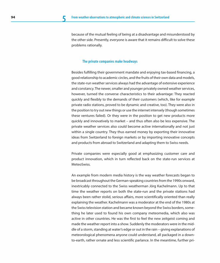
94 From weather observations to atmospheric and climate sciences in Switzerland5
because of the mutual feeling of being at a disadvantage and misunderstood by the other side. Presently, everyone is aware that it remains difficult to solve these problems rationally.
The private companies make headways
Besides fulfilling their government mandate and enjoying tax-based financing, a good relationship to academic circles, and the fruits of their own data and models, the state-run weather services always had the advantage of extensive experience and constancy. The newer, smaller and younger privately owned weather services, however, turned the converse characteristics to their advantage: They reacted quickly and flexibly to the demands of their customers (which, like for example private radio stations, proved to be dynamic and creative, too). They were also in the position to try out new things or use the internet intensely (though sometimes these ventures failed). Or they were in the position to get new products more quickly and innovatively to market – and thus often also be less expensive. The private weather services also could become active internationally and not just within a single country. They thus earned money by exporting their innovative ideas from Switzerland to foreign markets or by importing innovative concepts and products from abroad to Switzerland and adapting them to Swiss needs.
Private companies were especially good at emphasizing customer care and product innovation, which in turn reflected back on the state-run services at MeteoSwiss.
An example from modern media history is the way weather forecasts began to be broadcast throughout the German-speaking countries from the 1990s onward, inextricably connected to the Swiss weatherman Jörg Kachelmann. Up to that time the weather reports on both the state-run and the private stations had always been rather stolid, serious affairs, more scientifically oriented than really explaining the weather. Kachelmann was a moderator at the end of the 1980s at the Swiss television station and became known beyond the Swiss borders, some-thing he later used to found his own company meteomedia, which also was active in other countries. He was the first to feel the new zeitgeist coming and made the weather report into a show. Suddenly the moderators were in the mid-dle of a storm, standing at water’s edge or out in the rain – giving explanations of meteorological phenomena anyone could understand, all packaged in a down-to-earth, rather ornate and less scientific parlance. In the meantime, further pri-
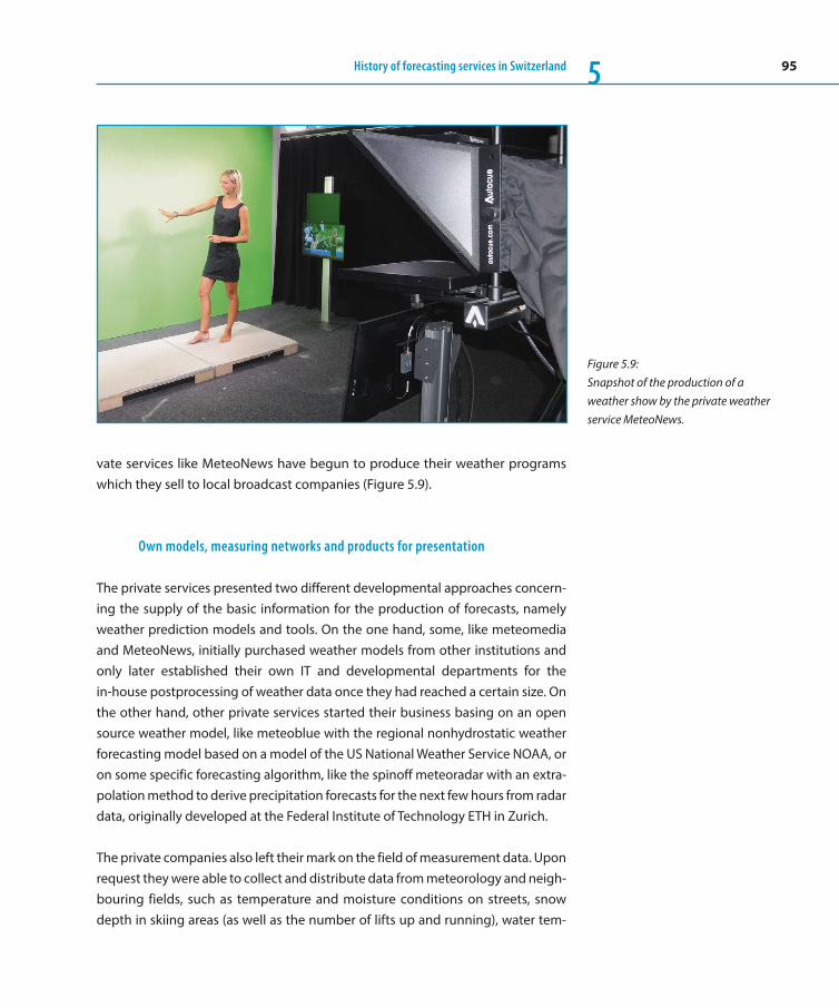
95History of forecasting services in Switzerland 5
vate services like MeteoNews have begun to produce their weather programs which they sell to local broadcast companies (Figure 5.9).
Own models, measuring networks and products for presentation
The private services presented two different developmental approaches concern-ing the supply of the basic information for the production of forecasts, namely weather prediction models and tools. On the one hand, some, like meteomedia and MeteoNews, initially purchased weather models from other institutions and only later established their own IT and developmental departments for the in-house postprocessing of weather data once they had reached a certain size. On the other hand, other private services started their business basing on an open source weather model, like meteoblue with the regional nonhydrostatic weather forecasting model based on a model of the US National Weather Service NOAA, or on some specific forecasting algorithm, like the spinoff meteoradar with an extra-polation method to derive precipitation forecasts for the next few hours from radar data, originally developed at the Federal Institute of Technology ETH in Zurich.
The private companies also left their mark on the field of measurement data. Upon request they were able to collect and distribute data from meteorology and neigh-bouring fields, such as temperature and moisture conditions on streets, snow depth in skiing areas (as well as the number of lifts up and running), water tem-
Figure 5.9: Snapshot of the production of a weather show by the private weather service MeteoNews.
96 From weather observations to atmospheric and climate sciences in Switzerland5
peratures in outdoor public pools (and whether they were being heated or not) as well as the water level of rivers and lakes. The network of official weather compa-nies soon proved to have its own limitations for the needs of the private compa-nies. MeteoSwiss with its measuring network SwissMetNet (SMN) had to meet contemporaneously very different demands, on the one hand for warning and forecasting services, on the other hand for climatological purposes. The first – and largest – private network for gathering measurement data in Switzerland was set up by meteomedia from 2003 onward and was expressly established to meet the demands of the media. In fact, at least some of these measuring stations are located in places with a high chance of measuring extreme values like very low or high temperatures or very strong winds, which make good headlines in the media – reinforcing one’s name and holding one’s flag up. Additionally, the choice of the location of these stations had to satisfy also another purpose, namely to deliver a good basis for the postprocessing of the NWP data with model output statistics (MOS) in all populated areas in Switzerland, including all the main valleys. From a climatological point of view the measurements of such networks are in some cases of a questionable value.
The desire to continually be present in the media and to be able to report any unusual weather data and dramatize any spectacular weather phenomena led to a wealth of meteorological reports of little value and content. The relevant infor-mation was in danger of being smothered. On the other hand, all of this activity in the media did increase the public interest in weather-related stories, which are easy to research and be outfitted with attractive images to which the readers or viewers could personally relate. Behind a small, contained heat wave, a stretch of bad weather or the first flakes of snow is a “story” that keeps the media machine humming for many days.
The advantages of presenting graphically understandable data were recognized early on by the private companies. They soon showed the nicely prepared films of air currents with their flying arrows (Figure 5.10). Any television or internet viewer could quickly grasp what was happening weather-wise. Thus, also films depicting rainfall and the popular “weather flights” appeared. Pictures stemming from web-cams, used e. g. by MeteoNews long before they had their first weather station or were gathering data from individuals, are valuable in two respects: In regional television programs they show the local weather and attune viewers to their own weather conditions. On the other hand, compared to measuring stations “just” delivering parameters like temperature and precipitation, they allow for a more comprehensive analysis of the overall weather situation: Now the fog situation,

97History of forecasting services in Switzerland 5
cloud cover (or absence thereof ), frost, new snow, etc., can all be viewed directly in front of the lens of the webcam.
Future challenges
An important challenge facing the private services in the future lies in being able to continue to present interesting (and that means entertaining as well as infor-mative) content in appealing ways. A general challenge which concerns the pri-vate as well as the national weather services is the issue of coping with ever larger amounts of data. Other, more specific challenges concern the ongoing crisis in the field of print media, which in some cases are already doing away with weather reports altogether, and with the general tendency toward internationalization, with a few private weather services growing into large international corporations beside a number of small weather providers acting on a very local scale. Some private companies expand their existing business models or launch completely new ventures and develop new services for other branches such as the energy sector or the transportation business, insurance companies and agriculture. Their advantage compared to the national weather services is that they can react more quickly and flexibly to customer needs – and they can offer their customers added values without having to sustain a state-of-the-art scientific level.
Last but not least, the plan of MeteoSwiss to liberalize the distribution of their meteorological data over the next few years – and that means providing them free of charge – raises many questions. No one knows right now how the landscape of
Figure 5.10: Example of visualization of wind and temperature as presented by meteoblue (the original version is an animated loop).

98 From weather observations to atmospheric and climate sciences in Switzerland5
private providers of weather services will react to this step and whether such a liberalisation will, in the end, have more advantages or disadvantages for them.
The Advent of Private Forecasting Services
The entire privately owned meteorological branch presently employs more than 400 persons in all of Switzerland. The following list provides an overview of the largest companies and their specialties (with no claims to completeness).
Meteotest was the first private Swiss weather company. It was founded in 1981 by some former employees of the University of Bern and has the legal form of a cooperative. Besides providing weather forecasts at the regional level, Meteotest is active throughout Switzerland and in part also abroad with expert opinions and for the energy industry.
Meteomedia was founded in 1990 in Gais/Appenzell, but then concentrated largely on serving the German market. In 2003 it began establishing the larg-est network of private weather stations in Switzerland, using its own MOS to improve the quality of the forecasts. In 2006, the storm platform meteocen-trale began as the first private Swiss weather service a 24/7 service. In 2013 meteomedia was bought out by the MeteoGroup and changed its name to MeteoGroup Schweiz AG. MeteoGroup is now the largest private weather service in all of Europe and thus the first international meteorological com-pany to have a subsidiary in Switzerland. It offers its own products to the media industry and increasingly also as B2B services.
SF Meteo started up in 1992 and is presently organized as the editorial office for weather information of German-Swiss Television. In 2002 it initiated the first live weather report from the “roof.” Different from the other private weather services, SF Meteo is partially financed through fees collected from the viewers.
MeteoNews AG first appeared in 1997 as an offshoot of meteomedia. Besides its office in Zurich, MeteoNews also has an office in Western Switzerland and provides the print media in all three parts of Switzerland as well as radio stations and regional television stations in the German-speaking and west-ern parts of Switzerland with weather information. Its internet presence (meteonews.ch) was the first weather portal to be available in all four official
99History of forecasting services in Switzerland 5
languages of Switzerland, and since 2012 also in Romansh (Rumantsch Gri-schun). MeteoNews is the only private service to run its own television studio and the internet weather television channel meteonews.tv. Besides Switzer-land, it also provides services to Liechtenstein, France and Belgium.
Meteodat GmbH was founded in 1998 as a spinoff of the ETH Zurich (Swiss Federal Institute of Technology) and has still today a close link to research. Its main business is the implementation of projects mandated by customers with weather-dependent activities, like the energy sector – hydrology, but also the national weather service. Additionally, meteodat produces opera-tional weather forecasts for very specific purposes, like for energy produc-tion and distribution.
Meteoradar GmbH was founded in 1999, also as a spinoff of the ETH Zurich. Its main business lies in providing weather analysis and forecasts with the respective radar data. Besides its own internet website, it provides data to its main customers from the areas of traffic conditions and insurance. Also, Meteoradar founded the so-called Storm Forum in 2001, the most important meteorological community platform in Switzerland to connect the employ-ees of various private and public services with the many interested hobby meteorologists.
Meteoblue AG, too, was founded in 2006 as a spinoff of the University of Basel. This company was the first one in Switzerland to run its own private weather model for the various regions as a special parametric model. It offers both nationwide and worldwide model data both as forecast and retrospec-tive reports on the internet. It also prepares expert opinions for large cus-tomers in over 20 countries. It was the first to develop air-current films (see Figure 5.10) or meteograms with depictions of the cloud situation as well as sight prognoses for (amateur) astronomers.
The Association of Swiss Meteorological Services (SMA) is an interest group of most of the private weather services and was founded in 2011. Its main concerns are connecting its members at the highest level as well as developing and (if possible) lobbying for common positions and interests toward MeteoSwiss. It serves to influence national (political) decisions regarding the weather marketplace. All of the above-mentioned services except for SF Meteo belong to the SMA.
100 From weather observations to atmospheric and climate sciences in Switzerland5
Acknowledgements
We would like to thank Eugen Müller, Daniel Gerstgrasser, Marco Gaia and Urs Keller (MeteoSwiss) for their valuable input to Sections 1–5 as well as Guy de Morsier (also MeteoSwiss) for the special preparation of Figure 5.6.
References
Altherr, J.-D., M. Dupanloup, Y. Ganter, and E. Junet, 1982: Prévi-sion objective des hauteurs de Précipitations et de l’ensoleille-ment relative au moyen de l’analyse discriminante. Publications de l’Institut Suisse de Météorologie, No. 44, 45 pp.
Ambühl, J., 1984: Interprétation statistique des prévisions numériques. Rapports de travail de l’Institut Suisse de Météoro-logie, No. 123, 52 pp.
Ambühl, J., 1991: Systèmes experts d’aide à la prévision. Rap-ports de travail de l’Institut Suisse de Météorologie, No. 161, 38 pp.
Ambühl, J., D. Cattani, and P. Eckert, 2010: Neural interpretation of ECMWF ensemble predictions. Veröffentlichungen der MeteoSchweiz, No. 85, 47 pp.
Binder , P., 1992: Aspects of precipitation simulation in numeri-cal weather prediction – Towards an operational mesoscale NWP model. Veröffentlichungen der Schweizerischen Meteoro-logischen Anstalt, No. 51, 148 pp.
Cattani, D., 1994: Application d’un filtre de Kalman pour adapter les températures à 2 mètres fournies par le modèle ECMWF aux stations météorologiques de la Suisse. Rapports de travail de l’ISM, No. 175, 30 pp.
Cattani, D., A. Faes, M. Giroud Gaillard, and M. Matter, 2015: Global forecast quality score for administrative purposes. MAUSAM, 66, No. 3, 645–656
Courvoisier, H. W., 1970: Die quantitative Niederschlagsprog-nose winterlicher zyklonaler Witterungslagen auf der Alpen-nordseite der Schweiz. Veröffentlichungen der Schweizerischen Meteorologischen Zentralanstalt, No. 15, 18 pp.
Courvoisier, H. W., and T. Gutermann, 1971: Zur praktischen Anwendung des Föhntests von Widmer. Arbeitsberichte der
Schweizerischen Meteorologischen Zentralanstalt, No. 21, 11 pp.
Courvoisier, H. W., 1976: Die Abhängigkeit der Sonnenschein-dauer vom kleinräumigen Druckgradienten in den Niederungen bei winterlichen Inversionslagen. Arbeitsberichte der Schweize-rischen Meteorologischen Zentralanstalt, No. 62, 29 pp.
Courvoisier, H. W., 1981: Starkniederschläge in der Schweiz in Abhängigkeit vom Druck-, Temperatur- und Feuchtefeld. Veröf-fentlichungen der Schweizerischen Meteorologischen Anstalt, No. 42, 61 pp.
Dürr, B., 2008: Automatisiertes Verfahren zur Bestimmung von Föhn in Alpentälern. Arbeitsbericht MeteoSchweiz, No. 223, 27 pp.
Gaia, M., 2007: Dal tempo alla meteo. Edizioni San Giorgio, 132 pp. ISBN 978-88-85922-01-3.
Ganter, Y., 1981: Prévisions optimistes et pessimistes. Rapports de travail de l’Institut Suisse de Météorologie, No. 107, 13 pp.
Gensler, G. A., 1983: Erfahrungen mit neuen numerischen Pro-dukten anlässlich der Erprobung und Einführung einer Wo -chenprognose für die Schweiz. Arbeitsberichte der Schweizeri-schen Meteorologischen Zentralanstalt, No. 114, 56 pp.
Kuhn, W., J. Quiby, and P. Fink, 1976: Modelle zur Berechnung der vertikalen Windkomponente über dem Alpengebiet als Hilfe für die Niederschlagsprognose. Arbeitsberichte der Schweizeri-schen Meteorologischen Zentralanstalt, No. 56, 22 pp.
Kuhn, W., 1982: Bibliographie der wissenschaftlichen Beiträge in den “Schweizerischen Meteorologischen Beobachtungen” (1864–1880) und “Annalen der Schweizerischen Meteorologi-schen Zentralanstalt” (1881–1963). Arbeitsbericht der Schwei-zerischen Meteorologischen Anstalt, No. 109, 25 pp.

101History of forecasting services in Switzerland 5Kutzbach, G., 1979: The thermal history of cyclones – A history of meteorological thought in the nineteenth century. American Meteorological Society, 255 pp.
Leuenberger, D., 2005: High-resolution radar rainfall assimila-tion: exploratory studies with latent heat nudging. Veröffent-lichungen MeteoSchweiz, No. 71, 105 pp.
Meier, B., 1996: Säntiswetter – Freuden und Leiden der Wetter-warte 1880–1970. Appenzeller Verlag, 206 pp. ISBN 3-85882-099-7.
Quiby, J., F. Schubiger, and P. Binder, 1988: Le programme MESO-MOD de l’ISM. Rapports de travail de l’Institut Suisse de Météo-rologie, No. 150, 40 pp.
Schacher, F., and F. Schubiger, 1988: Objektive Kontrolle von numerischen Prognosenkarten anhand verschiedener Wetter-lagen. Arbeitsberichte der Schweizerischen Meteorologischen Anstalt, No. 152, 53 pp.
Schönbächler, M., 1996: Objektive Kontrolle der Textprognosen SMA OPKO. Arbeitsberichte der Schweizerischen Meteorologi-schen Anstalt, No. 191, 31 pp.
Schraff, C., H. Reich, A. Rhodin, A. Schomburg, K. Stephan, A. Perianez, and R. Potthast, 2015: Kilometre-Scale Ensemble Data Assimilation for the COSMO Model (KENDA). Q. J. R. Meteorol. Soc., submitted.
Schubiger, F., 1986: Principal component analysis of ECMWF analysis fields taken as predictors for a regression model of pre-cipitation forecasts. Working Reports of the Swiss Meteorologi-cal Institute, No. 139, 31 pp.
Schubiger, F., G. de Morsier, G., and H. C. Davies, 1987: Numerical studies of mesoscale motion in a mixed layer over the Northern Alpine foreland. Boundary-Layer Meteorology, 41, 109–121.
Schweizerische Meteorologische Anstalt, 1981: 100 Jahre Schweizerische Meteorologische Anstalt.
Widmer, R., 1966: Statistische Untersuchungen über den Föhn im Reusstal und Versuch einer objektiven Föhnprognose für die Station Altdorf. Vierteljahrsch. der Naturforsch. Ges. in Zürich, 111, 331–375.
Züllig, W., 1976: Kontrolle der numerischen Vorhersagekarten. Arbeitsberichte der Schweizerischen Meteorologischen Zent-ralanstalt, No. 61, 38 pp.


103
6 Dynamical Meteorology: The Swiss contributionHuw C. Davies, Heini Wernli
6.1 Introduction
The discipline of Dynamical Meteorology has evolved with time to encompass the analysis, diagnosis, modeling, prediction and understanding of atmospheric flow phenomena, and one particular enduring focus has been the study of weather- related flow systems. It emerged as a distinct discipline in the early 20th century around the time of the founding of the SGM. Thereafter the nature of research in the field has changed radically and developed remarkably, and its progress con-stituted one of the major scientific achievements of the second half of the 20th century. In this study the Swiss-related contribution to the development will be set against the backcloth of three consecutive phases in the discipline’s history.
During a first foundational phase, extending to the time of the SGM’s establish-ment in 1916, the basic laws governing atmospheric flow were formulated. Prog-ress was inevitably sporadic but many nations did develop sparse networks of surface observations during this phase.
The second phase from 1916 to 1966, corresponding to the first 50 years of the SGM, saw a slow evolution of the nascent discipline. At first it was hampered by a lack of adequate observations, limited by a seemingly intractable set of governing equations, and characterized by an emphasis upon an empirical approach to syn-optic-scale forecasting. However by 1966 the discipline was ripe for expansion being equipped with an increasing amount of observational data, significant com-puting power, a tractable theoretical framework in the form of the quasi-geo-strophic equations, and the development of viable routine numerical weather predictions.
The third phase, covering the last half-century, witnessed a veritable scientific rev-olution engendered in part by rapid and major observational and technological developments including a spectacular increase in the availability of surface, air-craft and satellite-based observations, a massive increase in the available comput-
ETH Zurich, Institute for Atmospheric
and Climate Science, Zurich

104 From weather observations to atmospheric and climate sciences in Switzerland6
ing power, and the conduct of many international field campaigns. These devel-opments underpinned and helped propel major advances in the dynamics and prediction of synoptic-scale phenomena, and also a flowering of meso-scale and stratospheric dynamical research.
In the succeeding sections we highlight successively some of the Swiss-related contributions to the evolution of the discipline during each of the three phases. The rapid growth of the discipline and in the number of Swiss participants is reflected in the nature and number of the contributions in each period. The focus here is on the theoretical understanding of synoptic and sub-synoptic flow, and the reader is referred to other chapters in this compendium for consideration of contributions to meso-scale Alpine flow systems, advances in measurement tech-niques and instrumentation design, and operational forecasting aspects.
6.2 The foundational phase to 1916
The discipline’s primary physical foundations (– the classical laws of physics applied to atmospheric flow) emerged in embryonic form during the few decades preceding the establishment of the SGM in 1916. The equations governing inviscid fluid flow on a rotating sphere were derived by Ferrel in 1856, the concept of vor-ticity, vortex filaments and vorticity conservation set out by Helmholtz in 1858, the first law of thermodynamics established by Thomson (Lord Kelvin) and others around 1862, and equations for atmospheric moisture and water content by Rich-ardson around 1916.
Swiss-related scientists played an important role in the development of the gov-erning equations. The Basle polymaths, contemporaries and friends, Daniel Ber-noulli (1700–1782) and Leonhard Euler (1707–1783), played key roles in the formulation of the governing equations for fluid flow. In 1738 Bernoulli explored the relationship between pressure, density and fluid flow, and his ‘conservation formula’ for inviscid flow linking a fluid parcel’s kinetic energy with pressure (– the Bernoulli principle) is integral to the formulation of the flow equations. In 1757 Euler went further and in a remarkable and elegant study provided the full mathematical formulation of the equations for inviscid flow (– the Euler Equa-tions), and in so doing laid the cornerstone for hydrodynamics in general and atmospheric dynamics in particular. Bearing in mind the subsequent history of the discipline it is pertinent to record that Euler commenting on his equations stated,
105Dynamical Meteorology: The Swiss contribution 6
“Since a general solution must be deemed impossible due to the shortcomings of analysis, we must content ourselves with the consideration of certain par-ticular cases, especially as the study of several cases seems to be the only means of perfecting our knowledge.”
By ‘analysis’ Euler here refers to the mathematical treatment of the derived partial differential equations. In the study he also set out the ‘Trajectory Perspective’ for studying fluid motion, an approach nowadays attributed incorrectly to Lagrange (1736–1813), and noted that
“The determination of these trajectories is of the utmost importance and should be used to apply the Theory to each case considered.”
He concluded the paper with the following perceptive remark
This makes it quite clear how far removed we are from a complete under-standing of the motion of fluids and that my exposition is no more than a mere beginning.Nevertheless, everything that the Theory of Fluids contains is embodied in the two equations …, so that it is not the laws of Mechanics that we lack in order to pursue this research but only the Analysis, which has not yet been suffi-ciently developed for this purpose. It is therefore clearly apparent what discov-eries we still need to make in this branch of Science before we can arrive at a more perfect Theory of the motion of fluids.
In the present context it is also worth noting that both Bernoulli and Euler fol-lowed Newton in studying the theory of tides, and thus prepared the way for Laplace’s classical work.
Likewise key contributions to classical thermodynamics and its application to the atmosphere are also linked to two individuals – Rudolf Clausius (1822–1888) and Theodor Reye (1838–1919). Both were German–born but conducted some of their seminal work whilst based in Switzerland. Clausius held a professorship at the ETH in Zurich from 1855–1867, and Reye spent part of his studies at the ETH (– coming under the influence of Clausius), and he was made a Lecturer at the ETH in 1863 and held a professorship there between 1867–1870.
Prior to his arrival in Zurich, Clausius had asserted in 1850 that heat was but a form of energy and proceeded to formulate the second law of thermodynamics, and
106 From weather observations to atmospheric and climate sciences in Switzerland6
thereby drew together the disparate studies of heat transfer into the science of thermodynamics. Later whilst at the ETH, Clausius made significant contributions to the kinetic theory of gases in 1857 and he introduced the concept of entropy in 1865. Entropy, along with its close meteorological relative – potential tempera-ture, was to become a central feature in Dynamical Meteorology. Again the Clau-sius-Clapeyron Equation, linked by Clausius to both the first and second laws of thermodynamics, has entered Meteorology’s hall of fame and indeed has become a lynchpin equation in considering thermodynamic aspects of climate change.
Reye in studies published in 1864 and 1865 was arguably the first to apply the first law of thermodynamics to meteorology. He considered the expansion of air and the buoyancy changes that accompany ascent and cloud formation using what has now come to be termed ‘the parcel method’, and in so doing examined stabil-ity criteria for dry and moist ascent. Reye, who was also rapidly establishing him-self as a leader in the field of Projective Geometry, consolidated his meteorological studies in a magisterial overview and critique of observations and extant theories of cyclonic wind systems (Reye 1870). He tended to view all such systems, from tornadoes through to hurricanes and cyclones, as belonging to the same species, and he favoured the thermal as opposed to mechanical origin of cyclones in the then prevailing debate. See Kutzbach (1979) for a historical account of the thermal theories of cyclones.
A cameo Swiss contribution to theoretical fluid dynamics was that of Walter Gröbli (1852–1903) from Oberutzwil. In 1875 he submitted a Diplomarbeit to the ETH on the motion of three rectilinear vortices, and he then studied the topic further in Berlin under the tutelage of, amongst others, Helmholtz and Kirchhoff. In his doctoral dissertation published in 1877, Gröbli demonstrated that the three-vor-tex problem was integrable, solved several specific examples (examples given later in Figures 6.2, 6.3), and considered some special four-vortex and n-vortex configurations. His study with its focus upon vorticity is pertinent to large-scale quasi-geostrophic atmospheric flow, and his consideration of vortex-vortex inter-action is a delightful forerunner of a present day paradigm for studying atmo-spheric dynamics.
Another feature of meteorology in the run-up to 1916 was the establishment of national weather services and the development of networks of surface observa-tions, but upper-air data remained the province of a few limited field campaigns. However there was an aversion to issuing routine storm or weather forecasts pred-icated upon the sparsity of observations and the limited theoretical underpinning
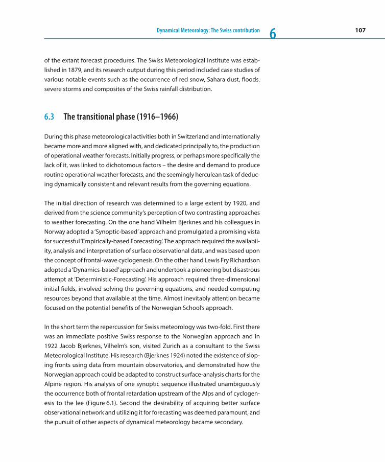
107Dynamical Meteorology: The Swiss contribution 6
of the extant forecast procedures. The Swiss Meteorological Institute was estab-lished in 1879, and its research output during this period included case studies of various notable events such as the occurrence of red snow, Sahara dust, floods, severe storms and composites of the Swiss rainfall distribution.
6.3 The transitional phase (1916–1966)
During this phase meteorological activities both in Switzerland and internationally became more and more aligned with, and dedicated principally to, the production of operational weather forecasts. Initially progress, or perhaps more specifically the lack of it, was linked to dichotomous factors – the desire and demand to produce routine operational weather forecasts, and the seemingly herculean task of deduc-ing dynamically consistent and relevant results from the governing equations.
The initial direction of research was determined to a large extent by 1920, and derived from the science community’s perception of two contrasting approaches to weather forecasting. On the one hand Vilhelm Bjerknes and his colleagues in Norway adopted a ‘Synoptic-based’ approach and promulgated a promising vista for successful ‘Empirically-based Forecasting’. The approach required the availabil-ity, analysis and interpretation of surface observational data, and was based upon the concept of frontal-wave cyclogenesis. On the other hand Lewis Fry Richardson adopted a ‘Dynamics-based’ approach and undertook a pioneering but disastrous attempt at ‘Deterministic-Forecasting’. His approach required three-dimensional initial fields, involved solving the governing equations, and needed computing resources beyond that available at the time. Almost inevitably attention became focused on the potential benefits of the Norwegian School’s approach.
In the short term the repercussion for Swiss meteorology was two-fold. First there was an immediate positive Swiss response to the Norwegian approach and in 1922 Jacob Bjerknes, Vilhelm’s son, visited Zurich as a consultant to the Swiss Meteorological Institute. His research (Bjerknes 1924) noted the existence of slop-ing fronts using data from mountain observatories, and demonstrated how the Norwegian approach could be adapted to construct surface-analysis charts for the Alpine region. His analysis of one synoptic sequence illustrated unambiguously the occurrence both of frontal retardation upstream of the Alps and of cyclogen-esis to the lee (Figure 6.1). Second the desirability of acquiring better surface observational network and utilizing it for forecasting was deemed paramount, and the pursuit of other aspects of dynamical meteorology became secondary.

108 From weather observations to atmospheric and climate sciences in Switzerland6
In the realm of meteorology Swiss researchers continued to undertake synop-tic-orientated case studies of individual weather events using the country’s high quality surface pressure data. One example is the study of divergence-lines ahead of surface fronts over the Swiss Middleland by M. Bouet in 1938. Also the data was used by S. Eggenberger to compute the solar tidal variations of surface pressure and his results, recorded in a 19pp doctoral dissertation to the University of Zurich in 1944, have stood the test of time.
In the final decades of this second phase there was a marked transition in the character and status of Dynamic Meteorology. Internationally advances were
Figure 6.1: Panels (a) and (b) are surface charts 24 hours apart (31 Jan. and 1 Feb. 1913) depicting a cold front approaching and then traversing the Alps. The charts capture indications of frontal retar-dation, an incipient lee-cyclone, and the build up of an arch of high pressure as cold air is retarded upstream of the Alps but progresses almost unimpeded to the east and west. The analysis was undertaken using the (then) new Norwegian School’s approach and constructed by J. Bjerknes (1924), and constitute the first such analysis for the Alpine region.Panels (c) and (d) are the analogue of the two earlier panels and show similar synoptic fea-tures albeit with more pronounced lee-cyclogenesis (– the dashed oval outlines the location of the orography). In this case the figures were derived by C. Schär from a simulation undertaken with an idealized quasi-geostrophic numerical model, and thereby illustrate the significant role of quasi-geostrophic effects to the dynamics of lee-cyclones.

109Dynamical Meteorology: The Swiss contribution 6
made in the understanding and prediction of weather systems. This included the formulation and consolidation of quasi-geostrophic theory, and the propounding of more dynamically-based theories for synoptic development and cyclogenesis. There was also a gradual replacement of empirical forecasting procedures by numerical weather prediction using better data. This entailed the use of the first generation of computers and was based sequentially upon barotropic, two-level quasi-geostrophic, and finally full primitive equation models. In contrast free-at-mosphere observations were confined principally to a limited network of radio-sondes and the acquisition of the first images from weather satellites. Detailed study of sub-synoptic and stratospheric flow phenomena remained essentially beyond reach.
6.4 The post-1966 phase
The last 50 years has seen a veritable revolution in the computing power and the range of observational data available to study atmospheric flows. This phase has been matched by an increase in the range and scope of dynamical studies, the conduct of numerous international and national observational field programmes directed to examining specific flow phenomena, and the increasing sophistication of the numerical models developed for performing research and producing oper-ational forecasts.
Advances in the understanding and prediction of synoptic and sub-synoptic-scale flow during this phase has been based firmly upon: (a) establishing and exploiting dynamically consistent and insightful frameworks and perspectives that utilize effectively the increasing and vast range of available observational and mod-el-produced data; (b) utilizing these perspectives to elucidate the dynamics of specific flow features such as cyclones and fronts, jet streams and blocks, tropo-pause folds and across-tropopause transport, and the role and impact of the Alps; and (c) responding to the dynamically-based challenges posed by numerical weather prediction that include consideration of fundamental and technical issues such as model initialization, the assimilation of space-time data, numerical integration techniques, grid resolution and structure, and forecast verification. In the succeeding sub-sections we trace the Swiss-related contribution to these three fore-mentioned overarching themes. A selected Bibliography cover-ing this period has been compiled and is available at http://vdf.ch/from-weather- observations-to-atmospheric-and-climate-sciences-in-switzerland.html.

110 From weather observations to atmospheric and climate sciences in Switzerland6
(a) Frameworks & perspectives
The quasi-geostrophic, semi-geostrophic and primitive sets of equations consti-tute a hierarchy of mathematical frameworks based upon various degrees of phys-ically justified approximations, and were derived to represent atmospheric flows in the extra-tropics. Research in Switzerland exploited these frameworks to study the range of phenomena referred to in the next sub-section.
From the mid-1980s onwards the so-called potential vorticity (PV) framework became a focus for dynamical meteorological studies. This framework exploited the conservation of PV on isentropic surfaces in three-dimensional adiabatic flow and thereby was a subtle extension of Gröbli’s approach that was based upon the conservation of vorticity in two- dimensional flow (see Figure 6.2). Thus the frame-work provides a means of studying and quantifying the far-field effect and the interaction of prominent flow anomalies (e. g., upper-level troughs, surface fronts). It has been exploited extensively internationally and by Swiss researchers in case studies to examine the key dynamical processes leading to important weather events (e. g., storms and heavy precipitation events).
Figure 6.2: Left panels show the PV distribution at upper-tropospheric levels for two time instances 12 hours apart (adapted from Massacand et al. 2001). The indicated negative (blue) and positive (red) PV cen-tres are seen to move in tandem equator-ward under their mutual influence.The right panel (adapted from Gröbli 1877) shows the trajectories of three vortices initially co-aligned at (A, B, C) and of respective strengths (–2, –1, + 1) units. During their time evolution the vor-tices initially at B & C eventually move together away from the vortex initially at A and toward their respective locations (a, b, c). This development bears compari-son with the displayed atmospheric evo-lution.
111Dynamical Meteorology: The Swiss contribution 6
Another important and insightful framework was the reinvigoration of the so-called Lagrangian trajectory approach that was referred to in Section 6.2. It involves the calculation of fluid parcel trajectories given the time-evolving wind fields. In the 1990s Swiss researchers pioneered a more intensive and extensive use of the Lagrangian approach. The newly available and high-quality global data sets (e. g., ECMWF reanalyses) and the growth in computer power enabled a sys-tematic computation to be undertaken for the first time of vast numbers of trajec-tories. This in turn allowed the identification and visualization of the space-time evolution of individual weather systems from a Lagrangian perspective, and the computation of the material change of key variables, such as temperature, PV and humidity, along the parcel trajectories. This approach has become a staple and widely used diagnostic tool.
Furthermore Swiss researchers have been at the forefront of melding the PV per-spective and Lagrangian approach to pinpoint the role and relevance of diabatic processes (e. g., condensational heating in clouds) in the evolution of mid-latitude weather systems and upper-level Rossby waves, and to analyze the individual cloud microphysical heating and cooling rates along moist airflows and thereby assess the linkage between cloud processes and the PV dynamics of the host weather system.
A further closing of a theoretical circle was a series of Swiss studies that general-ized the Bernoulli theorem to specifically atmospheric flow and moreover linked it to potential vorticity.
(b) Dynamics of specific flow phenomena
I CYCLONES AND CYCLOGENESISThe genesis processes, structure, track and intensification of extratropical cyclones exhibit fascinating case-to-case variability. Research in Switzerland contributed to the characterization and improved ‘process-understanding’ of several categories of cyclones (frontal-wave cyclones, upstream development, diabatic Rossby wave cyclones, Kona Lows).
A strong focus of the Swiss contribution to this research area was on the analysis of upper-level Rossby wave-breaking which accompanies the mature stage of cyclones, and can trigger new frontal-wave cyclones at the surface. Studies of baroclinic wave development using a hierarchy of idealized models together with

112 From weather observations to atmospheric and climate sciences in Switzerland6
observational analyses using sophisticated algorithms to detect wave-breaking and filamentary structures (sic. PV streamers), served to demonstrate the occur-rence and pinpointed the dynamics of two archetypical classes of wave-develop-ment referred to as either anticyclonic & cyclonic (or LC1 & LC2). Further case stud-ies conducted by Swiss researchers have provided clear illustrations of such development, and for example the former category was shown to be instrumental in the genesis of so-called Kona Lows near Hawaii.
A contrasting category of extra-tropical cyclones is that of diabatic Rossby waves, for which no prominent upper-level forcing is present during the rapid propaga-tion phase of the small surface cyclone (cf. the early phase of the storm ‘Lothar’ in December 1999). These diabatically sustained but shallow cyclones can intensify explosively if they subsequently interact with an upper-level trough.
A common characteristic of these diverse Swiss studies on cyclones is the system-atic application of the PV perspective as a means to gaining a better understand-ing of the interaction of diabatically-driven flow structures with dry dynamics. This also includes the identification of coherent airstreams in extra-tropical cyclones (dry intrusions and precipitation-producing warm conveyor belts) using objective Lagrangian flow criteria.
II FRONTS AND FRONTOGENESISFronts, viewed as demarking the transition zone between air masses of different origin, had been regarded as the seat for cyclone development by Fitzroy in the 1860s, Margules in 1900s, and they were central to the Norwegian School’s con-cept of forecasting based upon the concept of frontal-wave cyclogenesis in the late 1910s.
Theoretical considerations were hampered by the intrinsic sub-synoptic structure and the decidedly non-geostrophic dynamics of fronts, but progress became pos-sible with (a) the development of meso-scale surface observational networks, and (b) the formulation of higher-order balanced flow systems valid beyond quasi- geostrophy.
With regard to surface networks the Swiss ANETZ configuration of the 1980s was arguably one of the earliest such networks, and made possible the detailed meso-scale tracking of fronts as they approached and sought to traverse the Alps. More

113Dynamical Meteorology: The Swiss contribution 6
recently an objective front detection algorithm has been developed and used to quantify the role of surface fronts for (intense) precipitation.
With regard to theoretical advances Swiss contributions included the demonstra-tion that the surface warm band ahead of a cold front was itself unstable and could spawn frontal wave-like disturbances on realistic space and time-scales, and the derivation of analytic solutions for both deformation-induced and baroclinic wave-related frontogenesis to shed light on the time-scale of frontal development and the structure of the accompanying fronts.
III JET STREAMS AND ROSSBY WAVESThe extra-tropical jet stream constitutes a meandering stream of high velocity air almost circumnavigating the globe at tropopause-levels and is one of the atmo-sphere’s most striking phenomena.
Swiss research on this phenomenon has resulted in an event-based climatology of its occurrence, and also helped elucidate in more detail from a PV and Lagrangian perspective its structure and the nature of the attendant dynamics. In particular it has emphasized (a) its distinctive ribbon-like structure of highly enhanced lateral gradient of the PV on isentropic surfaces that transect the jet at the tropo-pause-break, (b) its role as a slowly evolving wave-guide capable of transmitting coherent and fast-propagating Rossby wave-perturbations far downstream, and (c) the dynamical processes that occur on the jet’s flank capable of either strengthen-ing the jet or inducing and amplifying wave perturbations along the jet. It has been shown that for instance a strongly amplified wave perturbation on the midlatitude wave-guide can instigate a new wave development along the subtropical jet.
IV BLOCKSAn atmospheric block serves to severely disrupt the background circumpolar flow over a substantial depth of the troposphere; it is quasi-stationary and persists for typically five or more days. Thus it represents a major flow phenomenon, and its repeated occurrence within one season strongly influences the resulting pattern of large-scale inter-annual variability.
A series of Swiss studies in the 21st century have examined blocks from a PV per-spective. These studies established that a block’s structure corresponds to an iso-lated anomaly of low PV in the upper troposphere (and the necessity of accompa-

114 From weather observations to atmospheric and climate sciences in Switzerland6
nying anomalies of high PV on its equatorward side, see Figure 6.3); computed a comprehensive climatology of the genesis, lysis, duration and trends of block occur-rence; and explored the linkage between blocks and patterns of climate variability as well as between blocks and co-located temperature extremes. Again combining the PV and Lagrangian perspectives, it could be shown that diabatic airstreams are of first order importance in providing the source of the block’s low PV.
V TROPOPAUSE FOLDS AND ACROSS-TROPOPAUSE EXCHANGEAn early contribution to Swiss research on cross-tropopause transport was that of Piaget in 1971 (Figure 6.4a). Inspired by earlier studies in the USA, he computed isentropic trajectories in the vicinity of upper-level fronts and used vertical sound-
Figure 6.3: The upper panel (adapted from Gröbli 1877) shows the trajectories of three vorti-ces initially co-aligned at (A, B, C) and of respective strengths (+ 1, + 1, –1) units. The trajectories show that the vortices ini-tially at A & B remain in close proximity, retain their separation distance from the vortex initially at C, and emphasize the comparative stability of this three vortex configuration.The lower panel (derived by Mischa Croci-Maspoli) depicts the instantaneous PV anomaly pattern in a layer across the tropopause on 15 Dec. 1975. It too shows a three-vortex configuration characteris-tic of many atmospheric blocks and com-prising one negative PV centre (enclosed by the red contour) and two positive centres located to its SE and SW. These three centres retained their configuration (cf. the upper panel) for several days as they drifted slowly eastward, and the open white ribbon shows the trajectory of the negative centre during this period.

115Dynamical Meteorology: The Swiss contribution 6
ings of ozone to identify episodes when high ozone air originally located within the stratosphere entered the troposphere.
More than two decades later, thanks to the availability of high-quality gridded ECMWF data sets, it became possible to automatically calculate very large number of trajectories in the tropopause region, and to systematically investigate the cross-tropopause transport in both directions (Figure 6.4b). Swiss scientists con-tributed to the EU project STACCATO and to the airborne observational project SPURT in Germany and compiled the first global Lagrangian-based climatology of stratosphere-troposphere exchange. A particular focus of these Swiss studies was on the so-called deep stratosphere-to-troposphere transport, whereby the dynamics of stratospheric intrusions leads to ozone injections into the planetary boundary layer where it can affect human health and the environment.
Again the PV perspective was central for these studies, as the material change of PV along air parcel trajectories was used to objectively identify cross-tropopause exchange events. Further Swiss studies investigated the key tropopause flow fea-tures associated with these exchange events, and devoted particular attention to
Figure 6.4: Examples of trajectory calculations. Pan-els (a), from Piaget (1971), and (b), from Wernli and Davies (1997) show the path-way of descending isentropic flows in the upper troposphere associated with strato-sphere-to-troposphere transport. In (b) the trajectories descend from the lower stratosphere to the boundary layer over the Arabian Sea. Panels (c), from Kljun et al. (2001), and (d), from Miltenberger et al. (2013) show how the Alps can disturb the impinging flow from the northwest, lead-ing to an orographic flow blocking. The trajectories in (d) have been calculated online during the integration of a cloud-resolving COSMO simulation.

116 From weather observations to atmospheric and climate sciences in Switzerland6
tropopause folds and filamentary PV streamers that often fragment into meso-scale cut-off vortices.
VI ATMOSPHERIC TIDESGlobal atmospheric tides are driven by solar and lunar effects and thus bear some analogy with oceanic tides. They play a significant role in the dynamics of the mesosphere and lower ionosphere because of their large amplitude at these ele-vations. In contrast their amplitude in the troposphere is weak, and they are deemed less important. Nevertheless the tidal signature can influence regional circulation patterns and if not properly accounted for also adversely affect the initial state for numerical weather prediction models.
Euler and Bernoulli’s original consideration of oceanic tides has been comple-mented by more recent Swiss studies of atmospheric tidal signals extracted from extended time series of surface pressure. Eppenberger’s earlier computations of the surface solar signal at Zurich and on Säntis were repeated and extended to consider the lunar tidal signal by Haurwitz and Cowley in 1975. Also Bouet, in a contribution published in 1976, documented the diurnal signal over the Suisse Romande.
A cameo Swiss study in 1990s detected a striking asymmetry in diurnal surface pressure signal across the Alpine ridge with a semi-diurnal oscillation most prom-inent on the northern side and a pronounced diurnal oscillation on the south side. Physical and theoretical considerations suggested that this pattern resulted from an Alpine modification of the global diurnal solar signal in the form of a laterally confined Kelvin-wave disturbance propagating clockwise around the Alpine massif.
VII SUB-SYNOPTIC ALPINE FLOW PHENOMENAThe length and lateral scale of the Alps combined with the significant height of the main Alpine ridge suggests that its configuration can exert a major perturba-tion of the impinging synoptic-scale flow and concomitantly generate striking sub-synoptic features and flow systems.
This circumstance helped prompt the selection of the Alpine region as the loca-tion for two major international field experiments. The first was the Alpine Exper-iment (ALPEX) of 1982, which was the concluding experiment of the Global Atmo-spheric Research Programme (GARP), and GARP itself dominated dynamical meteorology in the 1970s and early 1980s. The second was the Mesoscale Alpine
117Dynamical Meteorology: The Swiss contribution 6
Programme (MAP) of 1999. The overall aims and the specific objectives of the two programmes along with a description and details of the field campaigns and the gathered observational data can be found respectively at:
https://www.eol.ucar.edu/field_projects/alpex http://www.map.meteoswiss.ch/
ALPEX was the inspiration of the atmospheric dynamicist Jule Charney, and it was developed by the WMO. The operational centre for the field programme was located at Geneva and managed and staffed predominantly by Swiss scientists. For MAP one of the chief instigators was Thomas Gutermann, the then Director of MeteoSwiss, and Switzerland hosted the Programme Office and the Data Centre.
Major themes of these two programmes that relate to synoptic and sub-synoptic (i. e., meso-α scale) flow include the study of upstream blocking (Staulage), oro-graphic frontal retardation, lee cyclogenesis, and the occurrence of severe precip-itation events on the Alpine south-side. Here we resume aspects of the Swiss con-tribution to the foregoing themes.
For upstream flow blocking a generalization of Bernoulli’s relationship to stratified flow indicates that an airstream incident normally upon the Alpine ridge will find it difficult to traverse the ridge if the Froude number F = (NH/U) > 1. Here U is the flow strength, H the height of the ridge, and N a measure of static stability. For the Alpine setting F ∼ 1, so that the low-level air may frequently be forced to flow around rather than over the ridge.
A series of Swiss studies in the 1980s and 1990s sought to link the overall synoptic setting to weather in Switzerland, and to delineate more precisely the nature and dynamics of the flow as it encountered the orography. For example trajectory cal-culations demonstrated the upstream flow splitting and the diverse pathways of air impinging upon the Alps (Figure 6.4c, d). Likewise both special flight missions and idealized numerical modeling studies illustrated both the splitting and the refined features in the flow in the wake of the terrain. More recently similar model and observational analysis have been employed to study the airflow over and around southern Greenland.
For studying Alpine frontal retardation, Swiss research both capitalized on the ANETZ network to track and illustrate the retardation of the surface frontal signa-ture as the front moved toward and over the Alps, and also utilized a hierarchy of model systems to study the accompanying dynamics.
118 From weather observations to atmospheric and climate sciences in Switzerland6
Climatologically the Alpine southside constitutes one of the globe’s most cyclo-genetic regions. Typically an incident front is deformed over the northern slopes and western extremity of the Alps, and then cyclogenesis occurs to the lee as cold air preferentially debouches into the Mediterranean between the Alps and the Pyrenees. Esoteric theories for lee cyclogenesis abounded both prior to and after the ALPEX campaign, but a Swiss contribution demonstrated that the essence of the lee cyclone formation, via the deformation of an incident deep baroclinic zone, was captured by the quasi-geostrophic dynamics (see Figure 6.1).
The Alpine southside, and in particular the region around Lago Maggiore, is also a preferred location for heavy precipitation events. Detailed examination of such orographically induced or enhanced events was one of the central goals of the MAP campaign. From the standpoint of the accompanying dynamics a Swiss study demonstrated the role of the Alpine arch in helping to localize the precipitation to the Lago Maggiore region. A further series of Swiss studies demonstrated that a major precursor signature of such events was a north-south elongated PV streamer approaching the Alps, showed the sensitivity of the amplitude and location of the precipitation to the structure of the streamers, and traced the origin of the stream-ers themselves to Rossby wave-dynamics on the jet back extending back over six or more days to the western Pacific. Very recent studies focused on the transport of water vapour that eventually leads to Alpine heavy precipitation events. Trajec-tories and a Eulerian tagging technique revealed an enormous variability of mois-ture sources for these events with sources potentially extending from tropical Africa, the North Atlantic, Mediterranean and the European continent.
Alongside these studies that examined the dynamical aspects linking the large and synoptic-scale circulation to Alpine weather and precipitation, there have also been a range of empirically-based studies that sought to specify regional weather categories and their link to precipitation in Switzerland.
(c) Challenges posed by Numerical Weather Prediction
The development of sophisticated numerical models in their entirety for either research or operational purposes is a major task that is often undertaken in a col-laborative effort involving several research groups and weather services. However the refinement and operation of these models often pose intricate challenges related to fundamental issues of Dynamical Meteorology, and these challenges are often amenable to tackling by small research groups and individuals.

119Dynamical Meteorology: The Swiss contribution 6
Swiss researchers have addressed a range of such issues. In the realm of numeri-cal analysis they have devised refined schemes for accurate positive definite advection; vertical coordinate schemes that accommodate effectively terrain undulations; and lateral boundary formulations for limited area models. In the realm of representing physical processes, studies include the examination of: the development and occurrence of low-level inversions and stratus formation; con-vection over complex terrain; the deployment of radar data in constructing the model initial state, the representation of land surface processes including snow cover; and the contribution of various processes in influencing meso-scale pre-dictability. In the realm of forecast evaluation and assessment they have devel-oped approaches for: identifying and categorizing precipitation events; diagnos-ing the dynamics of forecast error growth; calibrating the physical factors influencing the effectiveness of regional forecast models; examining atmospheric predictability in the context of high resolution cloud-resolving models; and developing a module for computing accurate air parcel trajectories for high-res-olution weather forecasts.
6.5 Internationality
Dynamical Meteorology encompasses both the understanding of the entire pan-oply of weather phenomena and their worldwide prediction. This perforce has leant the Discipline a notable and distinctive character because it transcends national boundaries. Indeed throughout the Discipline’s history nationally acquired meteorological data has been freely shared internationally, and major meteorological field programmes have invariably involved multi-national partici-pation and collaboration.
The governmental component of this international activity has been underpinned by the World Meteorological Organization (WMO) and in particular its World Weather Research Programme (WWRP). The non-governmental component is pro-moted by the International Association of Meteorology and Atmospheric Sciences (IAMAS). In addition there have been a myriad of European and independent multi-national groupings.
In the realm of Dynamical Meteorology Switzerland has played a significant role in these international organizations. This includes erstwhile membership of the WWRP Executive Committee, Presidency of IAMAS and Chair of the International Commission for Dynamical Meteorology (Huw Davies) and involvement in the

120 From weather observations to atmospheric and climate sciences in Switzerland6
THORPEX initiative of the WWRP (Huw Davies, Heini Wernli) and one of its fol-low-up projects on High-Impact Weather.
In addition Swiss atmospheric dynamicists have played lead roles in the develop-ment and execution of major field programmes conducted during the fore-dis-cussed ‘Post-1966 Phase’. This includes first of all contributions for ALPEX (Thomas Gutermann, Hans Richner, Heinz Wanner, and others) and MAP (Thomas Guter-mann, Peter Binder, Andrea Rossa, Hans Richner, Christoph Schär, Huw Davies, Mathias Rotach, Heinz Wanner, and others). Recently the partnership with the German research initiative PANDOWAE (Heini Wernli, Olivia Romppainen-Martius) and the general involvement in THORPEX activities related to Dynamical Meteo-rology further strengthened the profile of Swiss research in this area on an inter-national level.
6.6 Concluding remark
The account given in the preceding sections demonstrates that the Swiss con-tributions to Dynamical Meteorology have been fundamental, long-standing, diverse and numerous. They helped establish the foundation of the Discipline, led to an improved understanding of atmospheric flow phenomena that form the centerpiece of the Discipline, and to advances in a wide range of NWP- related issues that form the practical wing of the Discipline. It can be asserted with justification that Swiss contributions contributed significantly to tackling the challenges that Euler foresaw in 1755 of seeking “a complete understanding of the motion of fluids” and the “discoveries we still need to make in this branch of Science”.

121Dynamical Meteorology: The Swiss contribution 6
Selected bibliography
Contributions related to phase I & phase II.
Bernoulli, D., 1738: Hydrodynamica. Publ. J. H. Decker, Basiliensis, 304 pp.
Bjerknes, J., 1924: Diagnostic and prognostic application of mountain observations. Geof. Publ. Vol. III, No. 6.
Bouet, M., 1938: Les phénomènes préfrontaux dans les Alpes. Bull. Soc. Vaud. Sc. nat. 60, 83–94.
Clausius, R., 1850: Über die bewegende Kraft der Wärme, Part I, Part II Annalen der Physik 79, 368–397 & 500–524. English Translation: On the moving force of heat, and the laws regarding the nature of heat itself which are deducible therefrom. Phil. Mag., 1851: Series 4, 2, 1–21, 102–119.
Clausius, R., 1865: Über die Wärmeleitung gasförmiger Körper. Annalen der Physik, 125, 353–400.
Eggenberger, S., 1944: Beitrag zu den Untersuchungen des Lufdrucks in der Schweiz. Doctoral Thesis, University of Zurich. 19 pp.
Euler, L., 1775: General principles of the motion of fluids. Acadé-mie Royale des Sciences et des Belles-Lettres de Berlin, Mémoires 11: 217–273.
Gröbli, W., 1877: Spezielle Probleme über die Bewegung gerad-liniger paralleler Wirbelfäden. Vierteljahresschrift der Naturfor-schenden Gesellschaft Zurich, 22, 37–81; 129–65. For further details and an assessment of Gröbli’s salient study see, Aref, H., Rott, N. and H. Thomann, 1992: Grobli’s solution of the three vortex problem. Annu. Rev. Fluid Mech., 24, 1–20.
Kutzbach, G., 1979: The thermal theory of cyclones. American Meteorological Society; 255 pp.
Reye, Th., 1864: Über vertikale Luftströme in der Atmosphäre. Zeit. für Mathematik und Physik, 9, 250–276.
Reye, Th., 1865: Die Ausdehnung der atmosphärischen Luft bei der Wolkenbildung. Annalen der Physik, 201(8), 618–626.
Reye, Th., 1872: Die Wirbelstürme, Tornados und Wettersäulen. (Hannover, C. Rümpler) 248 pp.
Phase III Contributions
For a list of Swiss-related contributions during this phase, sub-divided according to the major themes considered in Section 4, see http://vdf.ch/from-weather-observations-to-at-mospheric-and-climate-sciences-in-switzerland.html.

123
Measurements as foundation to meteorology and climatology


125
7 Surface precipitation measurementsChristian Félix1, Thomas Konzelmann2
A description of 150 years of precipitation measurements on the surface in Switzerland, starting from
empirical information to temporal and spatial high-resolution precipitation information.
7.1 Introduction
Precipitation is one of the key elements in the climate system. Information on precipitation are used in various applications such as warnings, numerical models, hydrological models, climatological purposes (gridded datasets, extreme value statistics), agricultural and economic issues. Weather forecasting requires a highly available, dense and extensive network with real-time data transmission, whereas for climate analysis continuity in location, instruments and data-processing meth-ods is more important than real-time availability. In both cases reliable and long-lasting instruments as well as appropriate quality control and data process-ing are of great importance. In this chapter we describe 150 years of surface pre-cipitation measurements in Switzerland, starting from empirical point information to high temporal and spatial resolution rainfall coverage. The focus lies on precip-itation, the development of the observational networks, data-handling and the measurement technology. For snow and hydrological aspects we refer to Spreaf-ico and Weingartner (2005).
7.2 Historical background and current observational networks
Evolution of networks
Before 1863 individual observations of precipitation were performed solely by observatories, monasteries and private persons. The systematic registration of precipitation in Switzerland started in 1863, initiated by the Swiss Academy of Natural Sciences (Chapters 4 and 5). In 1864, a network of 88 sites became opera-tional (Table 7.1). The general purpose was to observe and measure meteorolog-
1 Federal Office of Meteorology and
Climatology MeteoSwiss, Payerne2 Federal Office of Meteorology
and Climatology MeteoSwiss,
Zurich-Airport

126 From weather observations to atmospheric and climate sciences in Switzerland7
ical conditions like air temperature, humidity, pressure, precipitation, wind speed and wind direction, cloudiness, fog and lightning. Because of the high spatial vari-ability of precipitation, the climatology network originally installed was not dense enough. So, other official bodies started to construct additional sites to record only precipitation. With the founding of the ”Meteorologischen Centralanstalt” in 1881 (the Swiss Meteorological Institute (SMI), now called MeteoSwiss), all of the nearly 140 sites (climatology network: 88, precipitation network: 50) were taken over by one institution. During the period from 1880 to 1960 the climatology net-work increased to 125 sites, while the precipitation network increased significantly to about 330 stations. This great number of sites led to a mean density of one station about every 90 km2, albeit with large regional differences. Following the establishment of the first fully automated meteorological network (called ANETZ, A=Automatic, NETZ=Net) in the late 1970s, the manually operated climatology network sites were gradually reduced. In 1980 there were less than 100 climato-logical sites in operation, together with 40 automatic stations and 355 manually operated precipitation sites. The size of the current automatic network SwissMet-Net increased to 155 stations from 1980 to 2015 due to requirements like automa-tion of climate stations and wind-warning sites. From 2010 on, about 120 sites were transformed to automatic stations where only precipitation is measured, reducing the manually operated precipitation stations to about 190.
Beside these networks, a totaliser network records precipitation with collectors operating year round. This network was established from 1914 on due to missing
Table 7.1: Development of the number of precipitation measurement sites in the various meteorological networks in Switzerland since 1864 (operated by MeteoSwiss). The climatology and automatic networks contain precipitation measurements besides other meteorological parameters. The precipitation network contains either daily manual measurements or automatic measurements every 10 minutes.
Year Climatology network (manual observation)
Automatic network
Precipitation network (manual/automatic)
Totaliser network
Total number of stations
Data availability >1 per day every 10 min 1 per day/every 10 min 1 per year per day/per year
1864 88 – – 88/88
1880 88 – 50 – 138/138
1920 120 – 290 25 410/435
1960 125 – 330 85 455/540
1980 95 40 355 130 490/620
2005 25 115 340 140 480/620
2015 – 155 190/120 55 465/520

127Surface precipitation measurements 7
information of the precipitation conditions in the high-Alpine environment and was originally started by water-power companies. Based on a systematic network analysis (Scherrer, 2010) and for economic reasons the network was reduced from 140 sites in 2010 to 55 official sites in 2015.
In addition, a new automatic precipitation network of about 35 sites was estab-lished from 2010 on in the canton of Valais as part of the natural hazard preven-tion. The different types of precipitation-measuring networks are presented in Figure 7.1. The evolution of the networks and their spatial distribution are pre-sented in Figure 7.2. Additional precipitation-measuring networks in Switzerland are operated by the hydrological agencies of various cantons as well as by private companies (Chapter 5).
Figure 7.1: Different types of precipitation measuring networks: a) manual precipitation site, b) manual totaliser site, c) manual climatology site, d) automatic site, e) Lambrecht 1518H3 Joss-Tognini gauge and f) OTT Pluvio2 weighting gauge (Photos: MeteoSwiss).
a) b) c)
d) e) f )
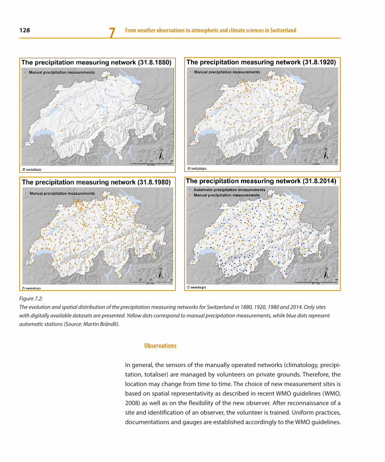
128 From weather observations to atmospheric and climate sciences in Switzerland7
Observations
In general, the sensors of the manually operated networks (climatology, precipi-tation, totaliser) are managed by volunteers on private grounds. Therefore, the location may change from time to time. The choice of new measurement sites is based on spatial representativity as described in recent WMO guidelines (WMO, 2008) as well as on the flexibility of the new observer. After reconnaissance of a site and identification of an observer, the volunteer is trained. Uniform practices, documentations and gauges are established accordingly to the WMO guidelines.
Figure 7.2: The evolution and spatial distribution of the precipitation measuring networks for Switzerland in 1880, 1920, 1980 and 2014. Only sites with digitally available datasets are presented. Yellow dots correspond to manual precipitation measurements, while blue dots represent automatic stations (Source: Martin Brändli).
129Surface precipitation measurements 7
In the climatology network precipitation was measured once a day (06.30 UTC) until 1971 and twice a day thereafter (06.30/18.30 UTC), with internet-based data transmission. In the precipitation network the reading is done daily at 06.30 UTC and immediately transmitted via GSM/SMS. In the totaliser measuring network a yearly reading is done around the end of September due to the hydrological year (which starts on October 1 and ends on the following September 30). At automatic stations the measurements are recorded and transmitted every 10 minutes.
Network concepts
The development of the meteorological networks was based on several network concepts that were in use for specific periods of time. The currently used concept at MeteoSwiss was established in 2004 (Frei et al., 2002) and has been continuously developed. In general, the goals are (1) to preserve climatological relevant stations, (2) to conduct parallel measurement in cases of measurement-site changes, (3) to perform increased temporal resolution of measurements, (4) to preserve measure-ments of the Alpine environment, (5) to ensure representative site distribution on vertical and horizontal axes, (6) to consider economic and urban-settlement aspects, (7) to occasionally automate manually operated sites, (8) to reduce ”unnec-essary” sites, and (9) to integrate weather stations of other institutions for data exchange (e. g., between cantons, private companies, national weather services).
Nowadays the development of the network is based also on an analysis of the requirements of all users who follow the WMO Integrated Global Observing Sys-tem (WIGOS) concepts introduced by the WMO. New requirements are collected using a Rolling Review of Requirements (RRR) process as defined in the Manual on the Global Observing System (WMO-No. 544, Part II, Requirements for observa-tional data). An analysis of these requirements compared with the capabilities of present and planned observing systems results in a revised network concept.
7.3 Types of instruments
The development of technology, both in logging electronics and in communica-tion, brought many new opportunities, particularly by increasing considerably the time resolution of the recordings as well as offering the possibility of real-time data. This was a strong motivation for public-safety decision-makers to start mak-ing decisions based on observations compared to historical records of precipita-
130 From weather observations to atmospheric and climate sciences in Switzerland7
tion. For such safety-relevant application, timely data availability are required even during severe weather conditions. At the same time, the design of the rain gauges changed with new technology and requirements. The principal instruments used at MeteoSwiss over the years are described below.
Manual rain gauges
The manual rain gauges in the volunteer network are of Hellmann type (Fig-ure 7.1a) and fundamentally consist of a receiving vessel with a predetermined receiving surface (200 cm2), of a collecting receptacle and of a measuring cylinder. The collecting surface lies 1.5 to 2 m above ground. The precipitation collected – which may first have to be melted – is measured by an observer at uniformly agreed upon observation periods.
Mougin annual storing collectors with a windshield and a collecting surface 3 to 4 m above ground (Figure 7.1b) are used in the totalizer network of MeteoSwiss. The containers are prefilled with a solution of water, salt and oil to prevent them from freezing and to prevent the evaporation of the collected water.
Automated measurements: Joss-Tognini tipping bucket gauges
In a first step towards automated measurements, pluviographs (mainly Hell-man-type pluviographs produced by Lambrecht, Göttingen) were introduced by the SMI in Switzerland, initially before 1864, but mainly between 1935 and 1960, at a limited number of observatories. In these systems the accumulation of water in a reservoir was measured by the elevation of a floater attached to a pen. The level of the reservoir was continuously recorded on a paper strip attached to a mechanical clock. An automatic purging system allowed recording the precipita-tion for up to 31 days without the intervention of a human operator. While the time resolution was increased considerably, the time delay for the user was still long since the paper strips had to be collected by an operator and sent to the office for analysis. These systems are not used anymore at MeteoSwiss.
In order to achieve the desired time resolution, measurement accuracy and avail-ability, it became necessary to find a new design for the rain gauges. Joss and Tognini (1967) at the SMI designed a new rain gauge based on the known tipping bucket principle. This device contained a swiveling part below its funnel, both com-
131Surface precipitation measurements 7
partments of which could receive water alternately (tipping bucket). Upon tipping, the bucket activated a REED relay with a small magnet. The relay impulsion was counted by the acquisition electronics, and the device was adjusted such that each impulsion corresponded to 0.1 mm water accumulation. The top edge ring of the gauge as well as the funnel were both heated, and the temperature was controlled to allow the measurements of solid precipitation and therefore all-season opera-tion in Switzerland. This robust and efficient gauge was produced by Gertsch in Zürich and was introduced in 1975 on the first ANETZ stations. Production was later transferred to Lambrecht GmbH in Göttingen. It is still in operation 40 years later at MeteoSwiss (Figure 7.1e) as well as at many automatic stations around the world. The collecting surface of the precipitation gauge is usually 1.5 m above ground.
The operation of automatic weather stations with high requirements in terms of precision and availability requires both a robust design of the instrument and regular maintenance by trained technicians. An operational team insuring the remote daily surveillance and preventive and corrective maintenance was there-fore established with the introduction of the ANETZ automatic measuring net-work. The increased availability of the data turned out to be very important both for safety relevant applications and for climatological time series.
While having many advantages the tipping bucket rain gauge also has some incon-veniencies. Tipping buckets tend to underestimate the amount of rainfall, particu-larly during summer precipitation (the first drops of water evaporate cooling down the funnel heated by the sunshine), in snowfall (sublimation of the snow on the heated pluviometer funnel) and heavy rainfall events (overfilling and spilling of the bucket, though correction algorithms can be applied for this). Also, the rainfall may stop before the lever has actually tipped, resulting in a small underestimation of the precipitation event. Conversely, when the next period of rain begins, it may take no more than one or two drops to tip the lever, indicating that the preset amount has fallen when in fact only a fraction of that amount has actually fallen. Because of their design, they are sensitive to dirt accumulation in the funnel (dust, insects, leaves, needles, etc.) and need regular (weekly) maintenance to run reliably.
Introduction of weighting gauges
Starting in 2010 an important change to the automatic precipitation measure-ment network commenced as the result of the OWARNA project (optimisation of alerts and alarm transmission) launched by the Swiss Federal Council. This more

132 From weather observations to atmospheric and climate sciences in Switzerland7
than doubled the number of automatic gauges in service (Figure 7.2). To allow this move at reasonable costs, MeteoSwiss introduced a new type of gauge in its oper-ational network (Figure 7.1f ) based on the weighting principle (Pluvio2 produced by OTT Hydromet GmbH, in Kempten, Germany). The weighting gauges allowed measurement of the precipitation in remote locations with only one or two main-tenance runs a year while keeping a high accuracy as well as increasing catching in case of low precipitation and solid precipitations, because of its open neck design (no funnel).
Because of its design, this type of gauge is sensitive to vibrations (for example, induced by wind) and to rapid temperature variations that can induce false pre-cipitation peaks. To minimize these effects, it needs very solid foundations, a spe-cific orientation as well as a filtering algorithm of the raw data.
The measuring technology is constantly evolving, and it is likely that in the future new types of gauges, for example, fully optical gauges, will find their way into the measuring networks.
7.4 Data handling
Data acquisition
In the past the data that were measured and observed were written on dedicated forms or in volumes (”Schwarze Bände”) and were regularly sent to the main office. The installation of computers, the development of digital acquisition electronics as well as the advent of the first digital communication solutions brought a mas-sive improvement to the delay of data availability (three orders of magnitude improvement). The high temporal resolution (10-minute acquisition, two orders of magnitude improvement) allowed the concept of real-time meteorological data to be introduced on a wide scale.
Today, data are transferred to and stored on the central Data Warehouse System (DWH) of MeteoSwiss (Insert ‘Data Warehouse System’). The whole data-chain of automatic measuring data is shown in Figure 7.3 (van Geijtenbeek et al., 2009). Level 1 and Level 2 correspond to raw data at the station level itself, while levels 3 to 5 correspond to clean, enhanced and homogenised datasets, respectively, on the data-warehouse level.

133Surface precipitation measurements 7
Quality control
Data quality control (QC) is mainly performed at level 3 and level 4 at the high temporal resolution of 10-minute values. The goal of the QC is to clean and enhance the climatological time-series by flagging suspicious data, interpolating missing values, and removing or correcting faulty data. According to the recom-mendations of the WMO, the tests for climatological survey are classified into four main categories: (1) limit tests, where the variables are compared to physical and climatological limits, (2) variability tests, where the maximally allowed variability during a specified time interval is tested as well as the minimal required variability during a certain period (”dead band” range), (3) interparameter consistency tests, where values measured at the same time and at the same place may not be incon-sistent to each other, and (4) spatial consistency tests, where values of the same parameter measured at the same time at nearby stations may not differ much. The QC is performed using a specific plausibility and mutation module. This process starts automatically once a day and is split into one part automatic treatment and a second part that allows interactive checking and manual mutation of data for stations with meteorological and climatological importance.
The QC of the manual precipitation sites is performed in part automatically and mostly manually on a monthly basis. Recently, a semi-automated spatio-climato-logical approach (Scherrer et al., 2011) was implemented. The spatial integrity tests use spatio(-temporal) information to find suspicious data and to provide objective interpolation values. This approach is an important step towards objec-tification of precipitation QC.
Figure 7.3: The data quality control chain for auto-matic surface observation data at Meteo-Swiss. SwissMetNet (left side, light green) corresponds to the station level, while Data Warehouse (right side, light blue) corresponds to the database and the data treatment level (van Geijtenbeek et al., 2009). Examples for data applications in operational and scientific activities are given at the bottom line representing the dependency on temporal resolution (GIN: Gemeinsame Informationsplattform Naturgefahren, www.gin-info.admin.ch).
134 From weather observations to atmospheric and climate sciences in Switzerland7
Beside the data values themselves, metadata provide essential information for data analysis such as the homogenisation (Figure 7.3, level 5) of data series (e. g., Begert et al., 2005; Insert ‘Homogenisation of long-term climate measurements’). All changes at the measurement site and instrumentation over time impact data series and could lead to inhomogeinity. For this reason, information on the dis-location of sites, changes of instruments and observers, introduction of new measurement methods and alteration of the environment are also collected and stored in the data warehouse.
Data Warehouse System
Estelle Grüter
In its role as national weather service, MeteoSwiss has the mandatory task of collecting, storing and managing a vast amount of various meteorological and climatological data.
In order to guarantee the long-term and efficient execution of this task, it also operates a data warehouse system, which comprises applications and a central databank optimised for analytical and information purposes – the so-called Data Warehouse (DWH). It is a fully configurable, high-performance and expandable infrastructure that provides the tools for the preparation and processing of meteorological and climatological data (aggregation, quality control, correction) including the related metadata.
The DWH system offers in-house and external users customised data access. Both current data and historical measurement series can be obtained. In addition, the data from the DWH form the basis for creating the majority of meteorological and climatological products.
To date, several billion datasets have been archived in the DWH, and every day measurements are added from a multitude of sources (including partner networks) and in many different formats.

135Surface precipitation measurements 7
Measurement uncertainty
The uncertainty of precipitation measurements has various components, such as measurement representativeness due to siting and wind exposure, instrument design (form, precision, reliability) as well as operation, maintenance and calibra-tion procedures. The Commission for Instruments and Methods of Observations, CIMO (WMO, 2010) provides a classification system for the representativeness of a site and recommendations for the design and operation of rain gauges.
Based on different studies (see WMO, 2010, and references therein), the magni-tude of typical errors is estimated as follows: (a) error due to systematic wind-field deformation above the gauge orifice: typically 2 to 10 % for rain and 10 to 50 % for snow; (b) error due to the wetting loss on the internal walls of the collector; (c) error due to the wetting loss in the container when it is emptied: typically 2 to 15 % in summer and 1 to 8 % in winter, for (b) and (c) together; (d) error due to evapo-ration from the container (most important in hot climates): 0 to 4 %; (e) error due
Homogenisation of long-term climate measurements
Michael Begert
The measuring conditions under which meteorological data are collected have changed over time in almost all available long-term climate data series. The most common reasons for such changes include the relocation of mea-suring stations, the use of new instrument types or changes in the surround-ings. The problem is illustrated in more detail in connection with the reloca-tion of temperature measurements associated with a difference in altitude. As the temperature on average decreases with increasing altitude, such a shift results in an abrupt change in the series of measurements, which does not in any way correspond to the actual and natural development.
The homogenisation process removes these artificial changes in the data series. Historical measurements are adapted to current measuring condi-tions and non-climatic influences are hence removed. Homogenised data series reveal an unaltered picture of the past climatic development. Such climatic series are the only option available to make accurate statements about the climatic development, because the discrepancies between inho-mogeneous original and homogeneous climatic series can be considerable.
136 From weather observations to atmospheric and climate sciences in Switzerland7
to blowing and drifting snow; (f ) error due to the in- and out-splashing of water: 1 to 2 %; (g) random observational and instrumental errors (dependent on instru-ment type with a recommended achievable laboratory precision of 0.1 mm for ≤ 5 mm and 2 % for > 5 mm and maintenance procedures in field), including incor-rect gauge reading times; (h) representativeness uncertainty, dependent on siting (0 % for WMO class 1 to 100 % for WMO class 5 sites (WMO, 2010)). Sevruk (1985) estimated the overall precipitation measurement error on 64 stations in Switzer-land to be 4 to 35 % depending on location and season.
7.5 Products of high spatial resolution datasets
Rain gauges have the advantage of being more or less precise and robust, although they are point measurements and monitor only a limited amount of Switzerland’s total territory. Even 1000 rain gauges of 200 cm2 would cover only 20 m2 out of about 41’000 km2 (~0.5 ppb). In order to significantly improve the spatial resolution of the precipitation observation, a new technological move is required. Two currently used methods are described below.
Combination of radar and surface measurements
Radar precipitation measurements provide a spatial resolution of about 1 km2, which is up to two orders of magnitude higher than all the rain gauges situated in Switzerland. The precision of the measurements is lower because of the compli-cated signal processing necessary to convert the radar reflectivity in water equiv-alent as well as because of the necessity for the radar to infer the precipitation on the ground from reflectivity measurements done at higher altitudes, in particular with the topography of Switzerland.
A method developed at MeteoSwiss, which combines the surface point measure-ments with radar measurements called Combi-Precip, allows us to take advantage of the strength of both observations technologies (Sideris et al., 2014). With this technology, we now have real-time and high spatial resolution of good quality precipitation information on the whole territory (Chapter 9).

137Surface precipitation measurements 7
Grid-data products
Grid data provide estimates of the spatial distribution of weather and climate at the Earth’s surface (e. g., Isotta et al., 2014; Frei, 2014). While instrumental measure-ments are taken at irregularly distributed stations, grid data represent meteoro-logical parameters on a predefined lattice (grid) with regular spacing. ”Gridding” integrates measurements, knowledge of their representativeness and physical understanding into statistical procedures that estimate the weather/climate at locations without measurements.
Grid data are of great benefit in disciplines that apply distributed quantitative models, such as hydrological and ecological ones. The forecasting of river flow, the understanding of glacier retreat and the assessment of crop suitability all require spatially comprehensive meteorological input. Grid data also serve a number of native meteorological applications, such as in-climate monitoring and the verifi-cation of weather forecasts. A detailed description for the daily precipitation grid-data product of MeteoSwiss is given under http://www.meteoschweiz.admin.ch/content/dam/meteoswiss/de/service-und-publikationen/produkt/raeumliche- daten-niederschlag/doc/ProdDoc_RhiresD.pdf
7.6 Data application in operational and scientific activities
Data and enhanced datasets are available for all kind of users and for meteorolog-ical and climatological applications and analysis (Figure 7.3; Chapter 4).
The operational activities have a strong temporal focus, whereby data are needed immediately for aviation purposes (e. g., at airports towers), as real-time alarms for warnings of meteorological hazards (e. g., Gemeinsame Informationsplattform Naturgefahren (GIN), www.gin-info.admin.ch), in near real-time for weather-fore-cast issues (various weather services), as input for regular bulletins and reports (e. g., daily and monthly charts) and for climatological purposes.
On the scientific level, the high-quality datasets of the dense network contribute, among other things, to international projects like the Mesoscale Alpine Pro-gramme MAP (Bougeault et al., 2001; Volkert et al., 2007), to an extensive dataset of rain-gauge observations of all Alpine countries (Frei and Schär, 1998), to the Hydrological Atlas of Switzerland (HADES, Weingartner (1986)), to the assessment of changes in the precipitation regime under present and future climatic condi-
138 From weather observations to atmospheric and climate sciences in Switzerland7
tions (e. g., Bates et al., 2008) and to the assessment of extreme precipitation events (Fukutome et al., 2014; Fukutome and Schindler, 2015). Data are also dis-tributed to international datacenters (e. g., Swiss GCOS Office, 2011).
7.7 Outlook
Today, surface precipitation measurements are used in combination with weather radar, models and gridded datasets as well as for verification purposes (e. g., mod-els). Parallel to the increase in data available in real time, the quality of these com-bined products has constantly increased. These products can also be used to improve quality control at the ground level.
But there is still room to refine the estimation of precipitation, particularly in mountainous areas where the influence of the topography is crucial for local pre-cipitation variations. To this end, different development directions should proba-bly be pursued:
– the better evaluation of the real-time uncertainty balance (including all sources of uncertainties), of the different measurement technologies,
– the even more improved real-time quality control of the measurements, – the better understanding of the local topographic effects on the precipitation.
Therefore, the number of automated precipitation sites should increase some-what in upcoming years. In particular, some test-beds with several automatic sta-tions at different altitudes in the same slope should be constructed in order to better understand local topographic effects. However, because of the quality of the information already available with the combination of different observation sources, it is likely that further systematic densification of the automatic rain gauge network will take place in the future through the integration of 3rd body precipitation measurements.
These constantly improving, high spatial and temporal resolution of precipitation datasets (1) provide better information for warnings of natural hazards and con-tribute to the enhanced safety of the Swiss population, (2) provide the opportu-nity to enhance the extreme value statistic on short range and (3) provide much more input for run-off models.

139Surface precipitation measurements 7
Acknowledgements
We are grateful to Estelle Grüter, Michael Begert and Christoph Frei for providing detailed information on the Data Warehouse (DWH), the homogenisation proce-dure and the grid-data products, respectively.
References
Bates, B. C., Z. W. Kundzewicz, S. Wu, and J. P. Palutikof (Eds.), 2008: Climate change and water. Technical Paper of the Inter-governmental Panel on Climate Change, IPCC Secretariat, Geneva, 210 pp.
Begert, M., T. Schlegel, and W. Kirchhofer, 2005: Homogeneous temperature and precipitation series of Switzerland from 1864 to 2000. Int. J. Climatology, 25, 65–80.
Bougeault, P., P. Binder, A. Buzzi, R. Dirks, R. J. Houze, J. Kuettner, R. B. Smith, R. Steinacker, and H. Volkert, 2001: The MAP special observing period. Bull. Amer. Meteorol. Soc., 82, 433–462.
Frei C., and C. Schär, 1998: A precipitation climatology of the Alps from high-resolution rain-gauge observations. Int. J. Clima-tology, 18, 873–900.
Frei, C., 2014: Interpolation of temperature in a mountainous region using nonlinear profiles and non-Euclidean distances. Int. J. Climatol., 34, 1585–1605, doi: 10.1002/joc.3786
Frei, T., R. Dössegger, G. Galli, and D. Ruffieux, 2002: Konzept Messsysteme 2010 von MeteoSchweiz. Arbeitsbericht, 199, 62 pp.
Fukutome, S., M. A. Liniger, and M. Süveges, 2014: Automatic threshold and run parameter selection: a climatology for extreme hourly precipitation in Switzerland. Theoretical and Applied Climatology 120, 3–4, 403–416.
Fukutome S., and A. Schindler, 2015: MeteoSwiss extreme value analyses: User manual and documentation. Technical Report MeteoSwiss, 255, 50 pp.
Isotta, F. A., and Coauthors, 2014: The climate of daily precipita-tion in the Alps: Development and analysis of a high-resolution grid dataset from pan-Alpine rain-gauge data. Int. J. Clim., 34, 1657–1675, doi: 10.1002/joc.3794
Joss, J., and E. Tognini, 1967: Ein automatisch arbeitender Ombrograph mit grossem Auflösungsvermögen und mit Fern-übertragung der Messwerte. Pure and Applied Geophysics, 68, 229–239.
Scherrer, S. C., 2010: Die Niederschlagstotalisatoren der Schweiz – Eine basisklimatologische Netzanalyse und Be -stimmung besonders wertvoller Stationen. Arbeitsberichte der MeteoSchweiz, 231, 35 pp.
Scherrer, S. C., C. Frei, M. Croci-Maspoli, D. van Geijtenbeek, C. Hotz, and C. Appenzeller, 2011: Operational quality control of daily precipitation using spatio-climatological plausibility test-ing. Meteorologische Zeitschrift, 20, 397–407.
Sevruk, B., 1985: Der Niederschlag in der Schweiz. Beiträge zur Hydrologie in der Schweiz, 31, B. Sevruk, Ed., 65–75.
Sideris, I. V., M. Gabella, R. Erdin, and U. Germann, 2014: Real-time radar–rain-gauge merging using spatio-temporal co-krig-ing with external drift in the alpine terrain of Switzerland. Q. J. R. Meteorol. Soc., 140, 1097–1111.
Spreafico, M., and R. Weingartner, 2005: The Hydrology of Switzerland. Reports of the FOWG Num. 7, Water Series, Bern, 139 pp.
Swiss GCOS Office, 2011. Schweizer GCOS Daten in Interna-tionalen Datenzentren (GCOS Schweiz). Online Publication MeteoSchweiz, 54 pp.
van Geijtenbeek D, C. Naguel, S. C. Scherrer, and B. Landl, 2009: The data quality control chain for automatic surface observa-tion data at MeteoSwiss. 7th ECSN Data Management Workshop 2009, DMI Copenhagen.
Volkert, H., C. Schär, and R. B. Smith, 2007: Editorial: “MAP Find-ings.” Q. J.R. Meteorol. Soc., 133: 809–810. doi: 10.1002/qj.102

140 From weather observations to atmospheric and climate sciences in Switzerland7
Weingartner, R., 1986: Konzept eines “Hydrologischen Atlas der Schweiz“. Publikation Gewässerkunde, Nr. 67, Berne.
WMO, 2008: Guide to meteorological instruments and methods of observation. WMO-No. 8, Annex 1.B, 2008 edition, update 2010.
WMO, 2010: Guide to meteorological instruments and methods of observation. WMO-No. 8.
141
1 retired, last affiliation: Federal
Office of Meteorology and Climatology
MeteoSwiss, Payerne2 Federal Office of Meteorology and
Climatology MeteoSwiss, Payerne3 ETH Zurich, Institute for Atmospheric
and Climate Science, Zurich
8 Swiss upper-air balloon soundings since 1902Pierre Jeannet1, Rolf Philipona2, Hans Richner3
8.1 Introduction
The first meteorological balloon was launched in Switzerland at the end of 1902, the year of the publication of the discovery of the stratosphere. Up to World War I, the Swiss Meteorological Office performed several ascents each year in Zurich. In the 1920s and 1930s, pilot balloons were visually tracked in order to help secure the air traffic near the newly opened Swiss airports. On 27 May 1931, the Swiss physicist Auguste Piccard and his assistant Paul Kipfer took off from Augsburg, Germany, in a pressurised aluminium capsule attached to a large hydrogen bal-loon; they reached a record height of 15781 m in the stratosphere. Piccard’s sec-ond flight started in Dübendorf on 18 August 1932 and reached 16201 m altitude. In 1937, Switzerland decided to join the European aerological network. The only Swiss aerological station was established at Payerne in 1942, starting the history of Swiss radiosounding.
This chapter is devoted to the key developments of Swiss upper-air balloon mea-surements and to the subsequent tropospheric and stratospheric temperature trends as well as to tropospheric water vapour and its development. We begin with the discovery of the stratosphere, which is as old as the theory of relativity published by Einstein in 1905.
8.2 The discovery of the stratosphere
For centuries, meteorological measurements were bound to the Earth’s surface, since there were no capabilities of ascending into the free atmosphere. Since the 18th century (first ascent of the Mont Blanc 1786 und later on of other sum-mits in the Alps), scientists had climbed on mountains in order to study the gaseous characteristics of air in light of the newly discovered gas theory. In the 19th century, large hot-air or hydrogen-filled balloons (the first hot-air balloon 1783) brought scientists and their instrumentation a few kilometres up into in
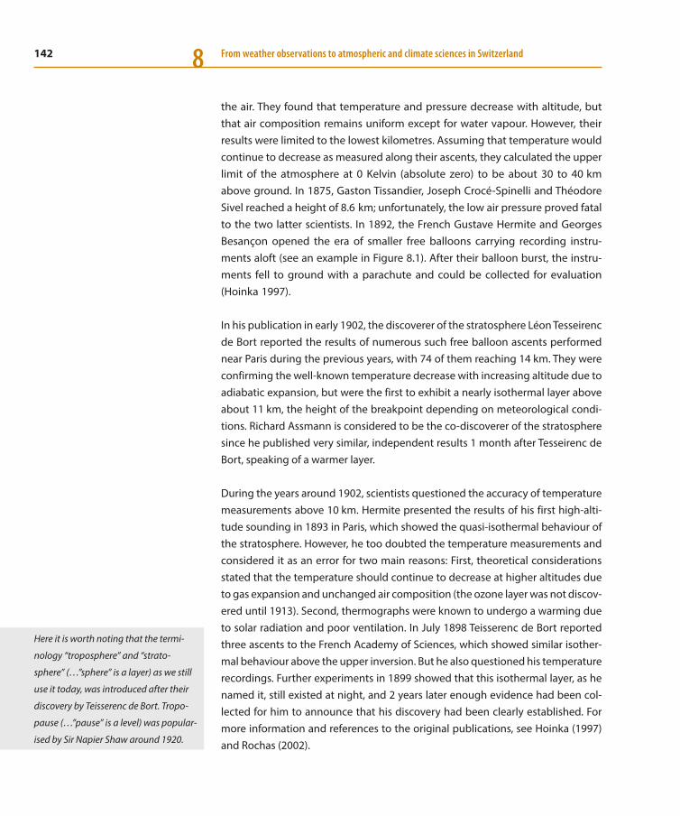
142 From weather observations to atmospheric and climate sciences in Switzerland8
the air. They found that temperature and pressure decrease with altitude, but that air composition remains uniform except for water vapour. However, their results were limited to the lowest kilometres. Assuming that temperature would continue to decrease as measured along their ascents, they calculated the upper limit of the atmosphere at 0 Kelvin (absolute zero) to be about 30 to 40 km above ground. In 1875, Gaston Tissandier, Joseph Crocé-Spinelli and Théodore Sivel reached a height of 8.6 km; unfortunately, the low air pressure proved fatal to the two latter scientists. In 1892, the French Gustave Hermite and Georges Besançon opened the era of smaller free balloons carrying recording instru-ments aloft (see an example in Figure 8.1). After their balloon burst, the instru-ments fell to ground with a parachute and could be collected for evaluation (Hoinka 1997).
In his publication in early 1902, the discoverer of the stratosphere Léon Tesseirenc de Bort reported the results of numerous such free balloon ascents performed near Paris during the previous years, with 74 of them reaching 14 km. They were confirming the well-known temperature decrease with increasing altitude due to adiabatic expansion, but were the first to exhibit a nearly isothermal layer above about 11 km, the height of the breakpoint depending on meteorological condi-tions. Richard Assmann is considered to be the co-discoverer of the stratosphere since he published very similar, independent results 1 month after Tesseirenc de Bort, speaking of a warmer layer.
During the years around 1902, scientists questioned the accuracy of temperature measurements above 10 km. Hermite presented the results of his first high-alti-tude sounding in 1893 in Paris, which showed the quasi-isothermal behaviour of the stratosphere. However, he too doubted the temperature measurements and considered it as an error for two main reasons: First, theoretical considerations stated that the temperature should continue to decrease at higher altitudes due to gas expansion and unchanged air composition (the ozone layer was not discov-ered until 1913). Second, thermographs were known to undergo a warming due to solar radiation and poor ventilation. In July 1898 Teisserenc de Bort reported three ascents to the French Academy of Sciences, which showed similar isother-mal behaviour above the upper inversion. But he also questioned his temperature recordings. Further experiments in 1899 showed that this isothermal layer, as he named it, still existed at night, and 2 years later enough evidence had been col-lected for him to announce that his discovery had been clearly established. For more information and references to the original publications, see Hoinka (1997) and Rochas (2002).
Here it is worth noting that the termi-
nology “troposphere” and “strato-
sphere” (…”sphere” is a layer) as we still
use it today, was introduced after their
discovery by Teisserenc de Bort. Tropo-
pause (…”pause” is a level) was popular-
ised by Sir Napier Shaw around 1920.

143Swiss upper-air balloon soundings since 1902 8
Before returning to Swiss activities, we would like to point out the important role of the international collaboration and exchanges related to the discovery of the stratosphere. First, the above-mentioned meteorologist group leaders had regular contact through correspondence, conferences and scientific journals, although they were clearly competitive. Second, they had collaborators from other coun-tries, or sent them on missions to other countries or continents. A good example is the Swiss Alfred de Quervain, who for a few years was a collaborator of Tes-seirenc de Bort in Trappes, then Secretary of the International Aeronautical Com-mission in Strasbourg, before returning in 1906 to the Schweizerische Meteorolo-gische Zentralanstalt.
8.3 Swiss upper-air activities before World War I
On 6 November 1902, the German president of the International Aeronautical Commission, Hugo Hergesell, came to Berne at the invitation of the Swiss Meteo-rological Commission and demonstrated an ascent of a free balloon with an attached meteorograph. The balloon type was from Assmann and the sonde type from Bosch-Hergesell (see Figure 8.1). Thereafter, Switzerland joined the simulta-neous meteorological balloon ascents coordinated by the Aeronautical Commis-sion (1903 to 1914). On one specific day per month, or on selected meteorological situations lasting for a few days, a dozen European stations made upper-air mea-surements with meteorographs attached to free or tethered balloons. The Swiss ascents were very successful and were documented every year in the Annalen der Meteorologischen Zentralanstalt (MZA). Julius Maurer, MZA director, was responsi-ble for this task in the first 2 years and published articles on the measurement errors of sonde thermographs (Maurer 1904). De Quervain took the lead of the Swiss balloon activities in 1905. In 1906, he published a very interesting article presenting new evidence on the existence of the tropopause, at that time called “large inversion” (de Quervain 1906). He showed a figure comparing the flight of 8 January 1899 at Trappes with flights from Zurich and Strasbourg between 1903 and 1905, which all clearly depicted the onset of the stratosphere. In response to concerns about radiation errors, he concluded that the excellent symmetry of the temperature and pressure registrations in the ascent phase before balloon burst – and in the much faster descent phase – speak strongly against any error in the conclusions of Tesseirenc de Bort and Assmann (see Figure 8.2, which reproduces a fragment of this original figure). He perfectly knew the measurements per-formed at Trappes, Strasbourg and Zurich, because he participated in the different experiments. Actually, his name appears on the first sheet of the Trappes sounding
Figure 8.1: Recording meteorograph (temperature, pressure and humidity), German model Bosch-Hergesell (1902) used in Switzer-land.

144 From weather observations to atmospheric and climate sciences in Switzerland8
of 8 January 1899 together with a special handwritten remark related to the tem-perature correction method (Dady 2003). Hence, de Quervain was very actively involved in the discovery of the stratosphere.
Like the other scientists before him, he measured an important change in wind regime near the tropopause level. He optimised the theodolite tracking of recording and pilot balloons and performed many flights with coupled tempera-ture, pressure (or altitude), and wind measurements, or with wind only (de Quer-vain 1906b). Upper-air winds were another research topic (e. g., weather predic-tion, foehn studies as illustrated by Figure 11.8 of Chapter 11), and de Quervain was convinced that the stratosphere could also be detected by pilot balloons. It is worth noting that the upper-air research work of Teisserenc de Bort was strongly linked to the origin and characteristics of the general atmospheric cir-culation, both between equator and pole, and between troposphere and low stratosphere.
The flight of 3 September 1903 launched at Zurich was one of the few European flights to reach a height of over 16 km that year. Because some instruments carried by free balloons got lost in the Alps, also tethered balloons on very thin piano strings of several km lengths were operated. The free balloon of 5 May 1909 reached approx. 32 km, but the mechanical clock stopped at 9 km. The free bal-loon ascent of 3 February 1914 successfully reached 26 km. World War I, however, put an end to Swiss balloon ascents with recording instruments.
Figure 8.2: Fragment of a figure in de Quervain (1906), with six balloon flights: the first one on 8 January 1899 at Trappes, the other ones 1903–1906 at Zurich. The horizontal axis is time (see scale on top). The temperature curve is labelled with “Th”, the corresponding pressure curve with “B”. Their scales are not given, but temperature values at launch and at tropopause are printed as well as altitude at tropopause and at top. Except for the first flight, the measurements continue down to ground.
“Tropopause” is historically defined on
the base of temperature profile, as can
be measured by a single aerological
flight. Today, numerical models define
a dynamical tropopause at a thresh-
old value in the vertical potential vor-
ticity (PV) profile. Isentropic surfaces
making the transition from the tropo-
sphere to the stratosphere usually fea-
ture a sharp gradient of PV between
the two air masses. The tropopause
can also be determined with wind pro-
filers (Chapter 10) by looking at the
turbulence. In this case, the transition
height from the turbulent troposphere
to the isothermal, stable (thus, nontur-
bulent) lower stratosphere is defined
as tropopause height.

145Swiss upper-air balloon soundings since 1902 8
8.4 Swiss radiosonde history
The upper-air network with recording instrumentation had strong drawbacks. Measurements could not be transmitted in real-time to the ground stations, and the network was too coarse, prohibiting the drawing of upper-air meteorological maps. In 1927, Pierre Idrac and Robert Bureau in France were able to couple mete-orological sensors to a radio transmitter. This new radiosonde technology led to the development of the worldwide radiosonde network.
In 1937, Switzerland decided to join the European aerological network (Billwiller 1942). Jean Lugeon was appointed for this task. He had led the building of aero-logical stations in Poland several years before and had gained experience with nearly all existing radiosonde systems. He also was an expert in radio-meteorol-ogy with radiogoniographs, which allowed long-range lighting detection (Chap-ter 13). Guido Nobile (a radio-physicist) and Pierre de Haller (a physicist) strongly contributed to the development of the first Swiss radiosonde system. The first trials were performed at Zurich and Dübendorf in 1939. They demonstrated the feasibility of VHF radiosonde transmission 18 km into the stratosphere around the Alps. Simultaneously, an appropriate site for the Swiss aerological station was found south of Payerne.
The aerological station Payerne and its radiosonde systems
This station was put into operation in 1942, starting the history of Swiss radio-soundings (Lugeon et al. 1942). The 20 ascents performed in 1942 steadily increased in the following years. Workday ascents started in 1948 and twice-daily ascents in mid-1953 (near 00 and 12 UTC). The mechanical chronometric radio-sonde was continuously improved. Several improvements of the bi-metallic ther-mometer and of the aneroid barometer allowed measurements in the lower stratosphere since 1956, reaching over 20 km in 1958 and over 30 km in 1968. Computer automation of sensor calibration and real-time raw data processing was achieved in 1974.
The move to an electronic radiosonde on 1 April 1990 was a major step in the Swiss radiosonde history (Richner et al. 1999). This analogue SRS-400 radiosonde is still in operation on its basic physical principles, but was upgraded to digital transmis-sion with GPS positioning in 2011.
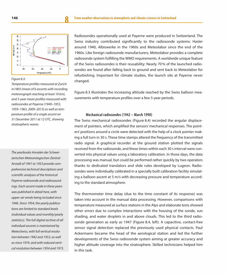
146 From weather observations to atmospheric and climate sciences in Switzerland8
Radiosondes operationally used at Payerne were produced in Switzerland. The Swiss industry contributed significantly to the radiosonde systems: Hasler around 1940, Albiswerke in the 1960s and Meteolabor since the end of the 1960s. Like foreign radiosonde manufacturers, Meteolabor provides a complete radiosonde system fulfilling the WMO requirements. A worldwide unique feature of the Swiss radiosondes is their reusability: Nearly 70 % of the launched radio-sondes are found after falling back to ground and sent back to Meteolabor for refurbishing. Important for climate studies, the launch site at Payerne never changed.
Figure 8.3 illustrates the increasing altitude reached by the Swiss balloon mea-surements with temperature profiles over a few 5-year periods.
Mechanical radiosondes (1942 – March 1990)The Swiss mechanical radiosondes (Figure 8.4) recorded the angular displace-ment of pointers, which amplified the sensors’ mechanical responses. The point-ers’ positions around a circle were detected with the help of a clock pointer mak-ing a full turn in 30 s. These time stamps altered the frequency of the transmitted radio signal. A graphical recorder at the ground station plotted the signals received from the radiosonde, and these times within each 30 s interval were con-verted into physical values using a laboratory calibration. In those days, the data processing was manual, but could be performed rather quickly by two operators thanks to dedicated translators and slide rules developed by Lugeon. Radio-sondes were individually calibrated in a specially built calibration facility simulat-ing a balloon ascent at 5 m/s with decreasing pressure and temperature accord-ing to the standard atmosphere.
The thermometer time delay (due to the time constant of its response) was taken into account in the manual data processing. However, comparisons with temperature measured at surface stations in the Alps and elaborate tests showed other errors due to complex interactions with the housing of the sonde, sun shading, and water droplets in and above clouds. This led to the third radio-sonde generation as early as 1947 (Figure 8.4, left). A capacitive, contact-free sensor signal detection replaced the previously used physical contacts. Paul Ackermann became the head of the aerological station and led the further developments of the Swiss radiosonde system aiming at greater accuracy and higher altitude coverage into the stratosphere. Skilled technicians helped him in this task.
Figure 8.3: Temperature profiles measured at Zurich in1903 (mean of 6 ascents with recording meteorograph reaching at least 10 km), and 5-year mean profiles measured with radiosondes at Payerne (1949–1953, 1959–1963, 2009–2013) as well as tem-perature profile of a single ascent on 31 December 2011 at 12 UTC, showing stratospheric waves.
The yearbooks Annalen der Schwei-
zerischen Meteorologischen Zentral-
Anstalt of 1941 to 1953 provide com-
prehensive technical descriptions and
scientific analyses of the historical
Payerne radiosonde and radiosound-
ings. Each ascent made in these years
was published in detail here, with
upper-air winds being included since
1946. Since 1954, the yearly publica-
tions are limited to standard levels
(individual values and monthly/yearly
statistics). The full digital archive of all
individual ascents is maintained by
MeteoSwiss, with full vertical resolu-
tion between 1942 and 1953, as well
as since 1974, and with reduced verti-
cal resolution between 1954 and 1973.
147Swiss upper-air balloon soundings since 1902 8
In 1962, model IV (shown in the middle of Figure 8.4) was put into operation. The new thermometer was a spiral bimetal strip protected by a rotating radiation and droplets shield; its calibration could be stably performed in a silicon oil bath and no longer in air. This technique brought improvements for soundings up to 15 km, but proved to be inadequate for higher altitudes. Therefore, radiosonde model V with a bare – but electro-silveredplated and polished – spiral bimetal strip replaced model IV in October 1970 (Ackermann 1968). On the same occa-sion, a temperature correction for daylight ascents was introduced so that, on average, daylight profiles were the same as those obtained during the night. The correction was set to zero below the 200 hPa level and to –4.5 K at 10 hPa (about 31 km). Later on, this value appeared to be too low (nearly –7 K at 10 hPa). The model V radiosonde is shown on the right side in Figure 8.4. One can see the pair of aneroids (Graw company, Germany), which allowed measuring pressure in two ranges: from 1000 to 100 hPa (about 16 km), and from 100 hPa to less than 10 hPa (about 31 km). With this arrangement, a greater pressure accuracy could be obtained than with a single capsule. Temperature compensation for the aneroids was then introduced, accounting for the aneroid temperature difference between calibration cycle and flight.
Figure 8.4: Three mechanical radiosonde models in their housings used at Payerne between July 1947 and March 1990 (from left to right: models III, IV and V). Common main features are best seen on the bare radio-sonde (on a black stand) in the rightmost frame: the clock (below the mounting plate), the rigid plate with transducer arms (pointers), two pairs of aneroid capsules as barometer (right), the gold-beater’s skin hygrometer (left), and the bimetallic thermometer on top of vertical axis. Radio transmitters can be seen on all three radiosondes. For more details, see www.radiosonde.eu/RS03/RS03A01.html.
148 From weather observations to atmospheric and climate sciences in Switzerland8
In 1969, Meteolabor replaced the secondary radar of Albiswerk first put in opera-tion in 1964. In 1974, Meteolabor used transistors in the 400 MHz oscillators of radiowind sondes for the first time. As previously mentioned, Meteolabor also took over the responsibility of producing the Swiss radiosondes and its ground installation. The mechanical sonde assembly was subcontracted to the Maurer mechanical workshop near Payerne.
Electronic calculators appeared on the market in the 1960s. In 1966, a LOCI-2 replaced the 25-year-old slide rulers that were used for calculating geopotential altitude and wind. Thereafter, MeteoSwiss took several years to set up a full and coherent data-acquisition system. In a first stage, the calibration of batches of four sondes was fully automated with a dedicated Hewlett-Packard computer, producing a plot with the calibration curves for each sonde as well as a punched tape with the polynomial coefficients. Then, the Payerne specialists programmed the real-time computation of the physical parameters on the basis of time stamps sent by the radiosonde to the ground receiver. This allowed a single operator to perform radiosoundings since mid-1975. Most important, it brought a more accurate, stable data handling and opened the door for more sophisti-cated corrections.
In the following years, several improvements were introduced in this program-ming. With only minor changes to the radiosonde itself, a last major upgrade of the ground system software took place in May 1980. Parallel to laboratory experi-ments and special soundings, every conversion algorithm between raw and final physical measurements had been analysed with scrutiny and adapted to latest findings (Rieker and Joss 1985). After this, the whole Payerne system remained almost unchanged until the transition to the purely electronic radiosonde in April 1990. But the quality control of the products (TEMP and PILOT messages) transmit-ted to the worldwide meteorological community – and in particular to the ECMWF – received high priority and was supported by specific computer programs.
Electronic radiosondes (April 1990 – present)A very fruitful collaboration between MeteoSwiss (Buno Hoegger, Gilbert Levrat, Jean Rieker, Pierre Viatte, Jürg Joss, Thomas Gutermann), Meteolabor (Paul Rup-pert), Laboratory for Atmospheric Physics at ETHZ (Hans Richner) and the Swiss Army (Rudolf Schneeberger, Markus Reber), involving many other contributors, led to the ambitious technological development of the Swiss electronic SRS-400 radio-sonde in the late 1980s (Figure 8.5). For the first time, a very thin copper-constantan

149Swiss upper-air balloon soundings since 1902 8
thermocouple was chosen as thermometer on an operational radiosonde. As an additional innovation, pressure data were obtained from a hypsometer, i. e., from the boiling temperature of water in a small vessel, the boiling temperature also being measured by a thermocouple. The electronic circuits had to be designed to accurately measure the voltages in the microvolt-range next to a radio transmitter with 0.5 W peak power. The fact that the SRS-400 thermocouples must resolve tem-perature to 0.01 K for its water hypsometer also had a positive impact on the qual-ity of the air-temperature measurement. A small aluminium block inside the radio-sonde contains the reference junction of the thermocouple, a pure copper coil inside this block measuring the reference temperature. The resistance-to-tempera-ture relationship of the copper was accurately determined in collaboration with the Swiss Federal Institute of Metrology (METAS). The almost perfect linearity of resis-tivity-to-temperature of copper in the range of –100 to + 100 °C makes calibration of individual radiosondes very simple: They only need to be compared and adjusted to a reference thermometer at room temperature. During prelaunch procedure, the radiosonde is crosschecked to a reference thermometer in a climate chamber. Con-sequently, the temperatures measured by the radiosonde rely on reference stan-dards, and their traceability is warranted throughout the whole flight. Furthermore, because all copper and constantan wires have come from the same batches since 1990, the thermocouple transfer function and the resistance-to-temperature rela-tion remain the same for all radiosondes.
The tiny junction of the thermocouple (0.1 mm) is placed in the upper right-hand corner of the radiosonde box without any sun shading. Although the thermocou-ple junction is very small, air temperature measurements suffer from errors due to convection, diffusion as well as visible and infrared radiation. Careful analysis showed that nighttime soundings need no correction (infrared error < 0.1 K). However, during daytime, a warming of the sensor of about 0.8 K at 100 hPa and 1.8 K at 10 hPa were found to result from solar shortwave radiation (Ruffieux and Joss 2003). These values are much lower than those of bimetallic thermometers. A recent study based on radiation measurements performed on the radiosonde as well as on the results of the international radiosonde intercomparison of 2010 in China led to even smaller daytime correction of the Swiss radiosonde (Phili-pona et al. 2013).
The SRS hypsometer consists basically of a glass tube containing 1 cm3 of distilled water (see Figure 8.5). An electric resistor heats the water to its boiling point, and the water vapour temperature is measured by a thermocouple. The evaporated water condenses on the wall of the upper part of the tube and flows back (Richner
Figure 8.5: Electronic radiosonde operated at Pay-erne since April 1990 (first version with analogue transmission and carbon resis-tive hygristor). The second symmetric Styrofoam cover is removed. A white sheet is placed behind the thermocouple in order to see it (for the flight, it is placed as explained below). Blue arrows show the air stream in the hygristor’s air duct.
150 From weather observations to atmospheric and climate sciences in Switzerland8
et al. 1996). Because the saturation vapour pressure at the boiling temperature is identical with the ambient pressure, the latter can be calculated with an approx-imation of the Clausius-Clapeyron equation. The hypsometer is a full range barometer between 1000 hPa and the water triple-point near 6 hPa. Hypsometers using Freon had already been in use in previous decades at Payerne on the Amer-ican VIZ radiosonde coupled to the ozone sonde, but using water instead of an ozone-depleting substance has indeed been an environmentally substantial improvement.
On the operational SRS-400 radiosonde, humidity was measured with a car-bon-resistive hygristor from the VIZ/Sippican supplier between April 1990 and April 2009. In the 2000s, this hygristor no longer fulfilled the quality requirements. Hence, Meteolabor and MeteoSwiss decided to introduce a new high-perfor-mance capacitive sensor from the Swiss manufacturer Rotronic. The new sensor (HC2) was tested during the international radiosonde campaign LUAMI at Linden-berg (D) and in a large number of test flights at Payerne. It was put into operation in May 2009. Generally, it shows striking superiority over the old hygristor and compares very well in the lower and middle troposphere with sensors used on international radiosondes. The new sensors show also much better agreement with integrated water vapour obtained from path delay measurements by GPS receivers. However, at very low temperatures in the upper troposphere, the sen-sitivity of the HC2 sensors is low.
The GPS technology opened a new age for high-accuracy radiosonde position-ing, with an altitude error of a few meters over the whole altitude range (see in the further section “Special note on wind finding and radiosonde location”). Accordingly, Meteolabor introduced a GPS receiver in its new digital radiosonde SRS-C34. At the same time, Meteolabor extended its radiosonde product line with a PC-based ground system fulfilling the WMO guidelines for operational stations. After intensive tests at Payerne, the SRS-C34 and its new ground system replaced the analogue radiosonde SRS-400 and the Hewlett-Packard computer in January 2011. Following the GCOS guidelines, MeteoSwiss made nearly weekly soundings with both previous and new systems during 2011 and continued its intercomparisons with the newest Vaisala systems. In 2014–15, Meteolabor took a new step in order to meet the increasing accuracy requirements of the climate community and developed its third generation of electronic radiosonde (new electronic, improved GPS and humidity sensors, reduced size and weight, etc.). This SRS-C50 radiosonde will replace the SRS-C34 at Payerne.

151Swiss upper-air balloon soundings since 1902 8
Intercomparisons of radiosonde systems and GCOSHydrometeors in the troposphere, low temperatures in the upper troposphere as well as low pressure and high solar radiation in the stratosphere were highly chal-lenging all components of radiosonde systems in the first years of upper-air mea-surements. Because almost all countries were developing their own radiosonde systems, the world-wide aerological network lacked common standards and homogeneity, which prevented the production of accurate upper-air weather maps. Therefore, the radiosonde working group of the WMO Instrument Commis-sion, headed by J. Lugeon, in 1949 decided to organise an international radiosonde comparison. Seven countries took part in this first experiment hosted at Payerne in May 1950. It revealed large discrepancies in the measurements of the different radiosondes, which were behaving differently during the day and at night, and there were no upper-air measurement references available. Consequently, the working group urged the participants to check and improve their radiosondes. A second international radiosonde comparison again took place at Payerne in 1956, with 13 countries and 14 radiosonde types. In addition to very valuable results, it strengthened the procedural techniques of radiosonde intercomparisons.
International radiosonde intercomparisons proved to be very important. They warrant an objective assessment of the homogeneity of the WMO upper-air net-work and promote the continuous improvement of the different radiosondes operated worldwide. Meteolabor (as radiosonde manufacturer) and MeteoSwiss (as radiosonde operator strongly involved in the radiosonde development) regu-larly took part in international intercomparisons. Prior to the Alpine Experiment (ALPEX) focusing on airflow over and around the Alps, different intercomparisons of the involved radiosonde systems were organised. Payerne hosted ASOND-78 in 1978 (a comparison of Vaisala, VIZ and Swiss radiosondes) and SONDEX in 1981 (Alpine radiosonde experiment: Richner and Philips 1982). Shortly after the oper-ational start of the SRS 400, the Crawley campaign (GB, near London) allowed a checking and improvement of its initial performances. Swiss participations in the WMO intercomparisons in Brazil (2001), on Mauritius Island (2005, see Nash et al. 2006) and in China (2010, see Nash et al. 2011) devoted to high-quality radiosonde systems, proved the willingness of performing among the best. Despite the avail-ability of remote-sensing instruments with remarkable capabilities, particularly on board meteorological satellites, accurate radiosonde measurements are needed not the least to calibrate these remote-sensing instruments. They still form the backbone of WMO’s composite observing system and a major data provider for climate research, provided their operational data quality and data coverage fulfils the requirements of the Global Climate Observing System (GCOS).

152 From weather observations to atmospheric and climate sciences in Switzerland8
In addition to the intercomparisons organised in Switzerland, a group informally called “aerology coordination Switzerland” was set up, which met about twice a year for decades. This very unique group (already mentioned in relation with the electronic radiosonde) gathered experts from MeteoSwiss, Meteolabor, the mili-tary weather service, the artillery weather service, the Army Procurement Agency, ETH, military educators, physicists, software engineers, etc., in various combina-tions. The major achievements of the group were – as its name suggests – the coordination of all activities related to upper-air observations, be it hardware problems or evaluation procedures. The group was initiated prior to ALPEX: In first intercomparisons, it was realised that there were significant differences in the way in which raw sonde data were processed. Up until then, these differences were tolerable since they were within the data accuracy. However, as data quality improved, the evaluation procedures had to be harmonised. This was achieved in a very constructive, albeit tedious way.
The group also discussed recuperations on the data quality caused by technical alterations (mechanical, electrical or software) of receiving systems and/or sondes. Thanks to the broad knowledge gathered, the problems could almost always be solved or at least their effects mitigated. Last but not least, as reported in previous sections, it supported the continuous improvement of the Swiss radiosondes and the development of new systems. The group also successfully negotiated solutions for frequency-allocation problems, safety issues with hydro-gen usage, and coordination issues with air traffic controllers and civil aviation authorities.
In 2002, the Swiss aerological station Payerne became part of the GCOS Upper-Air Network (GUAN), which is part of WMO and has about 170 stations worldwide. The aim of GUAN is to provide consistent high-quality upper-air measurements from well-distributed locations worldwide. Thereafter, Payerne became part of the newly set up GCOS Reference Upper Air Network (GRUAN) in 2008. GRUAN is a reference network for upper-air measurements with presently 16 stations world-wide and the aim of having about 30 stations in the near future. GRUAN aims at providing long-term records of upper-air essential variables for climate investiga-tions, with a strong focus on upper-troposphere and lower-stratosphere humidity and temperature. GRUAN requests high-quality measurements that are traceable to SI reference units and that provide uncertainty values for each record. In the spirit of GRUAN, Payerne also became a WMO-CIMO testbed for upper-air mea-surements; as such it was used in recent years to mainly compare the Swiss radio-sonde to other GRUAN radiosonde systems.

153Swiss upper-air balloon soundings since 1902 8
Special note on wind finding and radiosonde locationAlthough we have focussed primarily on temperature and humidity in this chap-ter, we should not forget the large efforts devoted to the development of wind measurements and radiosonde positioning, such as in the 1940s with the novel “echo sonde” technique for Payerne.
Wind finding is an issue that in the past required (and today still requires) much debate. For the computation of the wind, the sonde must be tracked continuously. This can be done in several ways, each having its own advantages and disadvan-tages:
Active: Independent tracking radar (was never used in Switzerland) Secondary radar (yields slant range and azimuth, sonde must be tran-sponding)
Passive: Radiotheodolite (phase measurement on different antennas) Directional antennas (azimuth and elevation plus geopotential height from sonde‘s data) Navigation transmitters (signals received by sonde, processed mainly on ground; Omega, Loran, GPS, Glonass, Galileo)
I f good wind accuracy is required, one has to use either a transponder system or a navigation system. The transponder solution is costly, and its ground installation can easily be located in the event of an armed conflict. Navigation systems provide high accuracy and are relatively cheap, but since Switzerland has no national nav-igation system, winds would depend on infrastructure under foreign control. Thus, the selection of the wind-finding method was long not only a technical matter, but also a political one. As mentioned further below for the Swiss military system, a solution was reached that allows switching from active to passive tracking, the latter at the price of a reduction in wind-data accuracy.
When the first ideas for using GPS for wind and altitude measurements by radio-sondes were brought forward at an AMS Symposium for Instrumentation and Meteorological Observation, the audience was quite amused. Who would need the very high accuracy of the GPS in a system whose data were to be representa-tive for thousands of square kilometres? Who would be able to afford such an expensive system? How could the required high data rate be handled?
Since then, all doubts have vanished, and the initial problems have been solved thanks to progress made in technology! In fact, there was a great surprise: Quite
154 From weather observations to atmospheric and climate sciences in Switzerland8
unexpectedly it was found that the height accuracy of GPS was so much better than pressure-derived heights that a barometer is really no longer needed in a radiosonde! Pressure can easily be derived from GPS height using the hydrostatic equation backwards.
Military systems
During the first half of the 20th century, there was considerable activity in upper-air research for purely scientific reasons, which, of course, was closely linked to the hope that the results could be used to improve weather forecasts. However, the military too realised that meteorological data of the third dimension are very useful, particularly for aircraft activities and for long-range firing. Later on, the willingness of having a single Swiss radiosonde used both in the civil and the military weather service led to a fruitful collaboration between the civil and mil-itary applications.
ArtilleryOne man name is closely linked with today’s artillery weather service: Raymond Sänger, the later founder of the Laboratory for Atmospheric Physics at ETH (LAPETH). He was a Captain, commanding a Forward Observer Artillery Unit. Being a physicist and being familiar with ballistics, he knew how wind and air density would influence the accuracy of the fire. Consequently, he was charged with build-ing up the Swiss Artillery Weather Service in the early 1940s.
After World War II, tests were conducted with surplus systems used by the U. S. forces in Europe. Based on these experiences, a radiosonde system specifically for ballistic purposes was then developed. It was optimised for obtaining wind and air density up to about 5000 m, and stratospheric data were not of importance. The Swiss company Hasler AG, Berne, developed a ground station for receiving data from a radiosonde built by Thommen, Waldenburg. Although this occurred more or less independently from civilian activities, some resemblance between the military system and the civilian METOX was obvious.
The ground station consisted of a manually steerable antenna and a receiver. The sonde was very similar to the J-R3 (see www.radiosonde.eu/RS03/RS03V/RS03V30.html). The transmitter used a vacuum tube operating at around 480 MHz, i. e., for reasons unknown outside the frequency bands officially allocated for meteorolog-
The move from pressure to altitude as
primary radiosonde measurement has
implications on the ground system. In
the former case, geopotential altitude is
integrated through the hydrostatic
equation on the basis of pressure, tem-
perature and humidity. The starting
level is the station geopotential altitude
and corresponding pressure provided by
the station barometer before balloon
launch. In the latter case, measured GPS
altitudes are first transformed to geo-
potential altitudes and then pressure is
integrated through the inverse hydro-
static equation, starting from surface
pressure. Please note that numerical
weather prediction models use pressure
as primary vertical coordinate.

155Swiss upper-air balloon soundings since 1902 8
ical aids. The ground operator had to point the directional antenna in order to receive the signal of the sonde with maximum intensity. The geometric height of the sonde was determined by integrating the hydrostatic equation. Combined with the angle measurements from the antenna, the position of the sonde – nec-essary for computing winds – could thus be determined. Air density could be com-puted directly from pressure and temperature, the two parameters transmitted by the sonde. Although humidity has almost no effect on air density, it was still mea-sured and used in the computations. Obviously, whoever designed the system was convinced that even very minute corrections must be applied, despite the fact that the corrections were significantly smaller than the accuracy of the basic sen-sors; this attitude could be found in several other observing systems as well.
As time went on, the operation of the system proved to be increasingly trouble-some because of interference. Also, the tedious manual data evaluation was prone to errors, and the technology of the sondes was outdated. Starting in 1991, the Artillery Weather Service was equipped with 30 units of the P-763, a completely newly designed system by Meteolabor consisting of a self-propelled calibration and evaluation unit, and a trailer with the antenna. This system operates in the 1680 MHz range, which allows accurate tracking of the sonde using a relatively small antenna. Contrary to the previous system, the P-763 uses a transponder sonde that is triggered by pulses from the ground segment. The slant range to the sonde can be computed from the time delay. The tracking of the sonde is auto-matic, using conical scan (i. e., the antenna beam of maximum sensitivity rotates a few degrees off the boresight-axis of the antenna). Slant range and antenna angles provide complete polar coordinates of the position of the sonde, and wind is computed from its change. Temperature is measured by a thermocouple and transmitted to the ground station. Prior to launch, an overall calibration is per-formed; control and evaluation during the ascent of the sonde is computer-con-trolled. The original system provided profiles of temperature and wind plus derived quantities (such as density) up to about 10 km. As artillery weapons became more powerful, the P-763 was upgraded for longer slant range and greater height.
General military weather serviceTo secure reliable upper-air data over Switzerland even during an international conflict, the Swiss Army, in particular the Swiss Air Force, decided to acquire four mobile upper-air stations. In contrast to those used by the artillery, these must be fully WMO compatible, i. e., they have to provide data up to 10 hPa (about 32 km).
Since 1940, the Swiss Army has operated
a military weather service, which was
gradually expanded over the years. Since
the early 1970s this weather service –
originally part of the Territorial Service –
was put under the command of the Air
Force. Basically, the military weather ser-
vice relies on the stations and the data of
the civilian services that, in a crisis, can
be militarised; this is also true for the
upper-air station Payerne.
156 From weather observations to atmospheric and climate sciences in Switzerland8
In the early 1970s, Siemens developed and built a system, the P-760, which used the same mechanical sonde as the civil weather service. Unfortunately, the orig-inal hardware did not meet the reliability and accuracy required. Therefore, it was completely redesigned by a group consisting of Meteolabor, MeteoSwiss, ETH and the Army Procurement Agency (today Armasuisse). The result is a modified P-760, computer-controlled radiosonde system operating in the 403 MHz range. Wind finding is based on a composite method using both the polar coordinates obtained from the tracking antenna, and the hydrostatic height computed from the data of the sonde. The active tracking (the sending of pulses from the antenna for interrogating the sonde) can be switched off, so that the sonde can be tracked passively. In this mode, wind data is less accurate as it is based only on angular data from the tracking antenna and the hydrostatic height. In this operation mode the station can no longer be located on the bases of its radiofrequency emissions.
Research systems
Up to now, we have discussed only true Swiss systems serving operational civil and military applications. In addition, numerous systems with free or tethered balloons have been engaged within field campaigns. These campaigns brought together very different measurement techniques devoted to a better understand-ing of various atmospheric processes (e. g., foehn, flow above and around moun-tains, pollutant dispersion, winter and summer smog, influence of nuclear power plant cooling towers). Hence, several research groups have operated and still operate commercially available foreign systems.
When ozone research started at the Laboratory for Atmospheric Physics (LAPETH) in the mid-1960s, an experimental upper-air station was assembled at Thalwil. It used U. S. VIZ 1392 sondes modified to carry a chemical ozone sensor. The sondes operated in the 1680 MHz range, they were launched about twice a week for about 2 years. After that, operations were transferred to Payerne, where a perma-nent station for ozone upper-air measurements was established (Chapter 16).
In 1970, LAPETH equipped a mobile laboratory with a permanent radiosonde- receiving station that was gradually improved for automatic wind finding. The system was used in various research projects of the institute as well as in large field experiments like ALPEX, POLLUMET, etc. Later, the VIZ 1392 was improved (i. e., transistorised) to become the VIZ 1393.
157Swiss upper-air balloon soundings since 1902 8
The VIZ 139x sondes were passively tracked for wind finding. A unique feature of the sonde was its measuring system: An aneroid cell actuated a switch that connected the temperature sensor (an NTC resistor), a humidity sensor (a car-bon element) and two reference values in such a sequence to the modulator of the transmitter that the position of the switch (which had about 150 steps) could be determined unambiguously. A calibration list on punched tape – pre-viously read into the computer – related then the switch position to the pres-sure value.
In the late 1980s, the institute acquired a new radiosonde system operating in the 403 MHz range. Wind finding was based on Loran-C navigation transmitters; hence, the prominent dish antenna previously used for tracking the sondes could be eliminated. (Loran is a navigation system using hyperbolic location techniques; it is intended primarily for maritime coastal navigation.) Nowadays, ETH operates a Meteolabor system ARGUS 37 for research and education purposes; wind finding is based on GPS.
The Institute for Geography (run jointly by the University of Zurich and ETH) oper-ated a low-altitude radiosonde system using the Vaisala RS-18 sonde. Wind finding was accomplished by using a radiotheodolite: Three receiving antennas spaced by several tens of meters in L-shape received the signals from the sonde. By measur-ing the phase differences of the signals received at the different antennas, the direction to the sonde can be computed. This system was extensively used for measuring energy budgets in Switzerland and Greenland and was also opera-tional for ALPEX. The sonde was a so-called windmill sonde, meaning that a pro-peller set in motion by the ascent of the sonde, switched alternately the different sensors to the transmitter.
Several other Swiss institutions have or have had other radiosonde systems, mainly procured off-the-shelf, for example, Vaisala (Armasuisse, MeteoSwiss Pay-erne, Paul Scherrer Institute), tethered balloon systems (Meteolabor type at MeteoSwiss, A. I.R. system at the University of Berne), etc. Most of them are mobile systems that have been intensively engaged in projects, e. g., CLIMOD (Dütsch 1985), POLLUMET (Neininger and Dommen 1996), NFP 14 (Hämmerli et al. 1992), MAP (Volkert and Gutermann 2007), TRANSALP (Ambrosetti et al. 1998). Constant level balloons have allowed low-level local (e. g., tracked with a Fledermouse radar) or trans-Alpine trajectory analyses within national and international proj-ects, e. g., CLIMOD, MAP, ETEX (Addis et al. 1998).

158 From weather observations to atmospheric and climate sciences in Switzerland8
8.5 Scientific results from the Payerne sounding data base
The monitoring and analysis of long-term changes constitute a key goal for the climate-change scientific community, not only at the surface of the Earth but also in the troposphere and stratosphere. As part of GCOS-GRUAN (see above), Payerne reevaluated its historical radiosonde series. This reevaluation differs from a homo-genisation as it is the result of a careful reassessment of the original data. It took into account all existing historical documentation on instruments and methods used in the past and applied corrections in the light of the latest technical knowl-edge of the Payerne radiosondes (Brocard et al. 2013). It is important to note that this project benefited from a previous project that compiled a thorough station history until 1990 and developed a sophisticated statistical adjustment method (Häberli 2005, Aschwanden et al. 1996).
Long-term temperature evolution
Because the radiosonde temperatures are independent from the surface network data (apart from the surface level), and because the radiosonde reevaluation is inde-pendent from the homogenisation of the surface network data, the long-term com-parison of these two data types allows qualification of their trends. Figure 8.6 super-poses the annual temperatures of Payerne (491 m), Chaumont (1073 m), Säntis (2502 m) and Jungfraujoch (3580 m), and the Payerne radiosonde temperatures at nearby standard pressure levels over the last 61 years (1954–2014). Over these timespan, upper-air and surface data show a similar behaviour between low alti-tude and Jungfraujoch (3580 m). Periods with high temperatures around 1960, cool-ing between 1960 and 1980, strong warming between 1981 and 2000, and rather constant high values in recent years are consistently reproduced in all time-series. The slight shifts between radiosonde and surface station temperatures remain nearly constant, and all linear trends over the 60 years are parallel and close together. The temperature over Switzerland has effectively increased by about 1.5 K in the last 60 years, not only at the surface, but also in the low troposphere. This comparison underlines the quality and representativeness of the historical radiosonde mea-surements in the low troposphere since the beginning of the twice-daily ascents.
Figure 4.3 from Chapter 4 helps to putting the results of our Figure 8.6 in a national and global framework. As expected, our results fit well with the “Swiss mean” (red curve) of Figure 4.3. In addition, this Figure 4.3 compares national and global trends. Temperature trend is smaller on a global scale than in the Alpine region.
1960 1980 2000
1510
50
510
(thick) (thin)Payerne surfaceChaumont 900 hPaSaentis 750 hPaJungfraujoch 650 hPa
Figure 8.6: Comparison of annual mean tempera-tures of mountain surface stations (heavy lines) and radiosonde at nearby pressure levels (thin lines) in the 61-year period 1954–2014 (homogenised resp. reevalu-ated series). Radiosonde surface values are derived from surface observations at radiosonde launch times.

159Swiss upper-air balloon soundings since 1902 8
Based on Payerne radiosonde measurements, and coherent with international results, one can state that surface positive temperature trends remain nearly the same in the low free troposphere.
1960 1970 1980 1990 2000 2010
SurfaceTrend = 0.35 C / Decade
p value = < 0.05Mean = 9.2 C
850hPaTrend = 0.32 C / Decade
p value = < 0.05Mean = 4.9 C
500hPaTrend = 0.25 C / Decade
p value = < 0.05Mean = 19.8 C
300hPaTrend = 0.12 C / Decade
p value = < 0.05Mean = 46.3 C
200hPaTrend = 0.11 C / Decade
p value = < 0.05Mean = 56.9 C
100hPaTrend = 0.16 C / Decade
p value = < 0.05Mean = 58.1 C
50hPaTrend = 0.33 C / Decade
p value = < 0.05Mean = 58.1 C
20hPaTrend = 0.44 C / Decade
p value = < 0.05Mean = 53.9 C
Figure 8.7: Reevaluated radiosonde annual mean temperatures in the 61-year period 1954–2014 at the surface and at seven standard pressure levels between 850 hPa (1.5 km asl) and 20 hPa (26 km asl). Temperatures are represented by their deviation around the long-term mean (dotted horizontal line), and the vertical scale at the right corresponds to 1 °C. Linear trends over the full period are given up to 200 hPa, and higher up only since 1971.
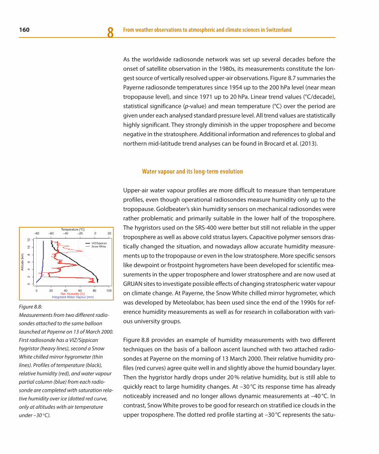
160 From weather observations to atmospheric and climate sciences in Switzerland8
As the worldwide radiosonde network was set up several decades before the onset of satellite observation in the 1980s, its measurements constitute the lon-gest source of vertically resolved upper-air observations. Figure 8.7 summaries the Payerne radiosonde temperatures since 1954 up to the 200 hPa level (near mean tropopause level), and since 1971 up to 20 hPa. Linear trend values (°C/decade), statistical significance (p-value) and mean temperature (°C) over the period are given under each analysed standard pressure level. All trend values are statistically highly significant. They strongly diminish in the upper troposphere and become negative in the stratosphere. Additional information and references to global and northern mid-latitude trend analyses can be found in Brocard et al. (2013).
Water vapour and its long-term evolution
Upper-air water vapour profiles are more difficult to measure than temperature profiles, even though operational radiosondes measure humidity only up to the tropopause. Goldbeater’s skin humidity sensors on mechanical radiosondes were rather problematic and primarily suitable in the lower half of the troposphere. The hygristors used on the SRS-400 were better but still not reliable in the upper troposphere as well as above cold stratus layers. Capacitive polymer sensors dras-tically changed the situation, and nowadays allow accurate humidity measure-ments up to the tropopause or even in the low stratosphere. More specific sensors like dewpoint or frostpoint hygrometers have been developed for scientific mea-surements in the upper troposphere and lower stratosphere and are now used at GRUAN sites to investigate possible effects of changing stratospheric water vapour on climate change. At Payerne, the Snow White chilled mirror hygrometer, which was developed by Meteolabor, has been used since the end of the 1990s for ref-erence humidity measurements as well as for research in collaboration with vari-ous university groups.
Figure 8.8 provides an example of humidity measurements with two different techniques on the basis of a balloon ascent launched with two attached radio-sondes at Payerne on the morning of 13 March 2000. Their relative humidity pro-files (red curves) agree quite well in and slightly above the humid boundary layer. Then the hygristor hardly drops under 20 % relative humidity, but is still able to quickly react to large humidity changes. At –30 °C its response time has already noticeably increased and no longer allows dynamic measurements at –40 °C. In contrast, Snow White proves to be good for research on stratified ice clouds in the upper troposphere. The dotted red profile starting at –30 °C represents the satu-
0 20 40 60 80 100
02
46
810
12
Alti
tude
[km
]
Rel. Humidity [%]Integrated Water Vapour [mm]
80 60 40 20 0 20
VIZ/SippicanSnow White
Figure 8.8: Measurements from two different radio-sondes attached to the same balloon launched at Payerne on 13 of March 2000. First radiosonde has a VIZ/Sippican hygristor (heavy lines), second a Snow White chilled mirror hygrometer (thin lines). Profiles of temperature (black), relative humidity (red), and water vapour partial column (blue) from each radio-sonde are completed with saturation rela-tive humidity over ice (dotted red curve, only at altitudes with air temperature under –30 oC).

161Swiss upper-air balloon soundings since 1902 8
ration relative humidity over ice. Snow White catches well the thin cirrus cloud and the strong humidity drop near the tropopause. This explains why this Swiss humidity sensor is used in several research projects, e. g., in the tropics (Fujiwara et al. 2003) and in Switzerland (Cirisan et al. 2014).
In the same Figure 8.8, relative humidity (red) has been converted into absolute humidity (blue), here specifically as integrated column of water vapour content between surface and each further measurement level. The usual acronym is IWV and units are mm water column. In this case, the total atmospheric water vapour content is close to 11 mm, and – as always the case – most of the water vapour is confined in the lower troposphere. Relative humidity measurement errors in the lower troposphere strongly impact IWV measurements, but similar errors in the middle and upper troposphere have only a marginal influence on IWV. The main reason stems from the huge dependency of saturation water vapour pressure from temperature. Hence, relative humidity is not an appropriate parameter for many atmospheric studies. Within the climate framework, absolute humidity must be strongly recommended, e. g., as mass mixing ratio (absolute water vapour mass per kilo of dry air: g/kg) at a specific level, or integrated water vapour column within the whole atmosphere (mm water). Mixing ratios span four orders of mag-nitude between warm surface air and cold stratospheric air. But IWVs only span one order of magnitude (approx. 3–35 mm in middle latitudes).
Figure 8.9 shows the water vapour mixing ratio trend inferred from Swiss moun-tain surface stations and Payerne operational radiosonde measurements at nearby standard levels since 1974. Compared to radiosonde values in the free atmo-sphere, the larger values at surface stations derive from direct fluxes at soil surface. However, a similar interannual variability appears in both datasets. Moreover, both measurements sets depict an astonishingly good agreement in their time evolu-tion. Similar slight positive long-term trends can be observed from the Plateau surface up to the Jungfraujoch altitude. Linked to the long-term temperature increase, the absolute water vapour also increased in the low troposphere above Switzerland. This result is in agreement with the newest IPCC assessment, which states that global tropospheric water vapour is increasing (Hartmann et al. 2013). One should note that the Payerne radiosonde mixing ratios do not compare very well with those of the surface stations before the 1970s.
For more than a decade, integrated
water vapour has also been continu-
ously measured at Payerne and several
other sites of the Swiss global naviga-
tion satellite system network (AGNES)
of swisstopo, this meteorological prod-
uct being derived from the wet total
zenith delay.
1980 1990 2000 2010
01
23
45
67
Mix
ing
ratio
[g/k
g]
(thick) (thin)Payerne surfaceChaumont 900 hPaSaentis 750 hPaJungfraujoch 650 hPa
Figure 8.9: Comparison of annual mean water vapour mixing ratio (g/kg) of surface stations (heavy lines) and Payerne radio-sonde at nearby levels (thin lines) in the 41-year period 1974–2014 (homogenised resp. reevaluated series). Radiosonde surface values are derived from surface observations at radiosonde launch times.
162 From weather observations to atmospheric and climate sciences in Switzerland8
8.6 Outlook
Several aspects were left out of this history of Swiss balloon-borne measurements. The main focus was put on the results of the Payerne radiosoundings, whose num-ber outreaches the number of ascents performed within field campaigns by one to two orders of magnitude. The Payerne radiosonde time-series spans several decades, is very well documented, has been undergoing a thorough reevaluation, and its digital archive holds for most years high vertical resolution data. Hence, it is invaluable for weather and climate research, as has been shown here with two examples. Furthermore, it is coupled to the long-term Payerne radiosonde ozone series (Jeannet et al. 2007). Last but not least, it has been and still remains essential to the validation of several remote sensing methods.
Because of their continuous functioning without operator assistance, remote sensing methods play an increasingly important role in upper-air meteorological measurements. To illustrate this, we mention the recent discontinuation of radio-wind ascents at 06 and 18 UTC at Payerne, because of the good operational data from tropospheric wind profilers with hourly time resolution. However, despite advanced satellite and sophisticated remote sensing methods, in-situ radiosonde measurements will likely remain the backbone of upper-air measurements for weather prediction, for climate change monitoring and for scientific investiga-tions. The GRUAN reference upper-air network will likely play an important role for global climate change monitoring and research. Radiosonde based radiation mea-surements through the atmosphere (Philipona et al. 2012) recently showed large potential for investigations of cloud effects, radiative forcing, greenhouse warm-ing and other climate-change issues.
References
Ackermann, P., 1968: Die neue Radiosondenstation Payerne der Schweizerischen Meteorologischen Zentralanstalt. Publications de l’Institut Suisse de Météorologie, 12, 34 pp, www.meteo suisse.admin.ch/content/dam/meteoswiss/de/Ungebundene- Seiten/Publikationen/Scientific-Reports/doc/veroeff12.pdf
Addis, R., and Coauthors, 1998: ETEX: A European tracer expe-riment; observations, dispersion modelling and emergency response. Atmos. Environ., 32, 4089–4094, doi:10.1016/S1352-2310(98)00248-9.
Ambrosetti, P., and Coauthors, 1998: Mesoscale transport of atmospheric trace constituents across the central Alps: TRANSALP tracer experiments. Atmos. Environ., 32, 1257–1272, doi:10.1016/S1352-2310(97)00185-4.
Aschwanden, A., M. Beck, Ch. Häberli, G. Haller, M. Kiene, A. Roesch, R. Sie, and M. Stutz,1996: Bereinigte Zeitreihen. Die Ergebnisse des Projekts KLIMA90. Klimatologie 1961–1990. Klimatologie der Schweiz, Schweiz. Meteorolog. Anstalt, 4 volumes.

163Swiss upper-air balloon soundings since 1902 8Billwiller, R., 1942: Die bisherige und zukünftige Mitarbeit der Schweiz an der aerologischen Forschung. Annalen der Schweizerischen meteorologischen Zentralanstalt. 1941. An -hang No. 7, 1–3.
Brocard, E., P. Jeannet, M. Begert, G. Levrat, R. Philipona, G. Romanens, and S. C. Scherrer, 2013: Upper air temperature trends above Switzerland 1959–2011, J. Geophys. Res. Atmos., 118, 4303–4317, doi:10.1002/jgrd.50438.
Cirisan, A., and Coauthors, 2014: Balloon-borne match mea-surements of midlatitude cirrus clouds. Atmos. Chem. Phys., 14, 7341–7365, doi:10.5194/acp-14-7341-2014.
Dady, G., 2003: Commentaire sur “Il y a un siècle: le contexte scientifique de la surprenante découverte de la stratosphère” de M. Rochas (La Météorologie 8e série, no 37, mai 2002, 57–69). La Météorologie, 41, 43–44, doi:10.4267/2042/36283.
de Quervain, A., 1906: Neue Beweise für die Realität der oberen Inversion in 8 bis 13 km Höhe. Meterol. Zeitschrift, 23, 529–540.
de Quervain, A., 1906b: Über die Bestimmung atmosphärischer Strömungen durch Registrier- und Pilotballons. Meterol. Zeit-schrift, 23, 149–152.
Dütsch, H., 1985: Large-scale domination of a regional circula-tion during winter-time anticyclonic conditions: results of the field program of the CLIMOD project. Meteorologische Rund-schau, 38(3), 65–75.
Fujiwara, M., M. Shiotani, F. Hasebe, H. Vömel, S. J. Oltmans, P. W. Ruppert, T. Horinouchi and T. Tsuda, 2003: Performance of the Meteolabor “Snow White” chilled-mirror hygrometer in the tropical troposphere: Comparisons with the Vaisala RS80 A/H-Humicap sensors. J. Atmos. Oceanic Technol., 20, 1534–1542, doi:10.1175/1520-0426(2003)020<1534:potmsw>2.0.co;2.
Hartmann, D. L., and Coauthors, 2013: Observations: Atmo-sphere and Surface. In: Climate Change 2013: The Physical Sci-ence Basis. Contribution of Working Group I to the Fifth Assess-ment Report of the Intergovernmental Panel on Climate Change [Stocker, T. F., D. Qin, G.-K. Plattner, M. Tignor, S. K. Allen, J. Boschung, A. Nauels, Y. Xia, V. Bex and P. M. Midgley (Eds.)]. Cam-bridge University Press, Cambridge, United Kingdom and New York, NY, USA.
Häberli, Ch., 2006: The comprehensive Alpine Radiosonde Dataset (CALRAS). Wiener Meteorologische Schriften, Volume 4, 297 pp.
Hämmerli, F., N. Krauchi, and M. Stark, 1992: The Swiss National Research Program “Forest Damage and Air-Pollution” (NFP 14+). Studies in Environmental Science, 50, 449–459, doi:10.1016/S0166-1116(08)70138-9.
Hoinka, K. P., 1997: The tropopause: discovery, definition and demarcation. Meterol. Zeitschrift, 6, 281–303.
Jeannet, P., R. Stübi, G. Levrat, P. Viatte, and J. Staehelin (2007): Ozone balloon soundings at Payerne (Switzerland): Reevalua-tion of the time series 1967–2002 and trend analysis, J. Geophys. Res., 112, D11302, doi:10.1029/2005JD006862.
Lugeon, J., G. Nobile and P. de Haller, 1942: Le Poste Aérologique de la Station centrale de Météorologie à Payerne et les nouvel-les méthodes suisses de radiosondage. Annalen der Schweize-rischen meteorologischen Zentralanstalt. 1941. Anhang No. 7, 3–46.
Maurer, J., 1904: Experimentelle Untersuchungen über das Ver-halten des Trägheitskoeffizienten der ventilierten Thermometer unter variablem Druck des aspirierenden Mediums, Anhang: Einiges über die Tätigkeit der Schweizer Registrierballonstation. Meteorol. Zeitschrift., 21, 489–502.
Nash, J., R. Smout, T. Oakley, B. Pathack, S. Kurnosenko, 2006: The WMO Intercomparison of Radiosonde Systems – Final Report, Vacoas, Mauritius, 2 – 25 February 2005. WMO/TD No. 1303, OM Report No. 83, WMO, Geneva, pp. 21–27.
Nash, J., T. Oakley, H. Vömel, and LI Wei, 2011: WMO Intercom-parison of high quality radiosonde systems. Yangjiang, China, 12 July – 3 August 2010. WMO Instruments and Observing Methods Report 107, 238 pp.
Neininger, B., and J. Dommen, 1996: POLLUMET Schlussbericht, Umweltmaterialien No. 63 Luft. Bundesamt für Umwelt, Wald und Landschaft, BUWAL, Berne, Switzerland.
Philipona, R., A. Kräuchi, and E. Brocard, 2012: Solar and ther-mal radiation profiles and radiative forcing measured through the atmosphere. Geophys. Res. Lett., 39, L13806 doi:10.1029/ 2012GL052087
Philipona, R., A. Kräuchi, G. Romanens, G. Levrat, P. Ruppert, E. Broccard, P. Jeannet, D. Ruffieux, and B. Calpini, 2013: Solar and

164 From weather observations to atmospheric and climate sciences in Switzerland8
thermal radiation errors on upper-air radiosonde temperature measurements. J. Atmos. Oceanic Technol., 30, 2382–2393, doi:10.1175/jtech-d-13-00047.1.
Richner, H., and P. D. Phillips, 1982: The Radiosonde Intercom-parison SONDEX Spring 1981, Payerne. PAGEOPH, 120, 852–907.
Richner, H., S. von Hünerbein et al. (Eds.), 1999: Grundlagen aero-logischer Messungen speziell mittels der Schweizer Sonde SRS 400. Veröffentlichungen der SMA-MeteoSchweiz, 61, 140 pp.
Richner, H., J. Joss, and P. Ruppert, 1996: A water hypsometer utilizing high-precision thermocouples. J. Atmos. Oceanic Technol., 13(1), 176–182, doi:10.1175/1520-0426(1996)013 %3 C0175:AWHUHP%3E2.0.CO;2.
Rieker, J., and J. Joss, 1985: Correction des données aérolo-giques brutes du radiosondage de Payerne. Arbeitsberichte der
Schweizerischen Meteorologischen Zentralanstalt, 135, www.meteosuisse.admin.ch/content/dam/meteoswiss/fr/Ungebun dene-Seiten/Publikationen/Fachberichte/doc/arbeitsbericht 135.pdf.
Rochas, M., 2002: Il y a un siècle. Le contexte scientifique de la surprenante découverte de la stratosphère. La Météorologie, 37, 57–69, doi:10.4267/2042/36222.
Ruffieux, D., and J. Joss, 2003: Influence of radiation on the tem-perature sensor mounted on the Swiss radiosonde. J. Atmos. Oceanic Technol., 20, 1576–1582, doi:10.1175/1520-0426(2003) 020<1576:iorott>2.0.co;2.
Volkert, H., and T. Gutermann, 2007: Inter-domain cooperation for mesoscale atmospheric laboratories: The mesoscale Alpine programme as a rich study case. Quarterly Journal of the Royal Meteorological Society, 133(625), 949–967, doi:10.1002/qj.95.

165
9 Weather radar in SwitzerlandUrs Germann, Marco Boscacci, Marco Gabella, Marc Schneebeli
9.1 Five decades of weather radar operations in Switzerland
The first weather radar was deployed in Switzerland back in 1959 (Figure 9.1). It was a one-parameter/one-customer solution with analogue technology and a monochromatic radar screen showing the location of precipitation and thunder-storms to the air-traffic controller. Five decades later, in May 2011, the first system of the fourth generation MeteoSwiss radar network was commissioned (Figure 9.2 and Figure 9.3) combining dual-polarisation Doppler receiver-over-elevation tech-nology – and 50 years of experience on how to optimise hardware configuration and data processing for operational usage in a mountainous country. In a response to the demanding requirements of quantitative end-to-end applications, within less than 60 seconds after the completion of a volume scan, the network, consist-ing of five radar stations (Figure 9.4), delivers various meteorological products such as fields of precipitation rates, hail maps and thunderstorm alerts to a large number of customers.
Federal Office of Meteorology
and Climatology MeteoSwiss,
Locarno-Monti
Figure 9.1: The 1959 first-generation Swiss weather radar on La Dôle, 1682 m asl (Photo: courtesy of L. Martin).
Figure 9.2: The Monte Lema radar, 1626 m asl, after the commissioning of the fourth-generation radar system in 2011. (Photo: S. Müller).

166 From weather observations to atmospheric and climate sciences in Switzerland9
9.2 Switzerland, a pioneer in radar meteorology and hydrology in complex orography
Upon installing its first radar in the 1950s Switzerland became one of the pioneers in the use of radar technology for meteorology. Over the years it developed, in close collaboration with industrial and academic partners around the world, many solutions adapted to the operational quantitative usage of weather radars in a mountainous region.
In the 1960s, shortly after the installation of the first-generation radar network, Jürg Joss and Albert Waldvogel developed the very first disdrometer, a device designed to sample the number and size of falling rain drops (Joss and Waldvogel,
Figure 9.3: Very first radar image of the fourth-generation Swiss radar network obtained on 5 May 2011 at 17:01 UTC after the newly installed radar on Monte Lema was turned on. The image shows reflectivity at verti-cal polarisation at -0.2° elevation, the range rings are at 50 and 100 kilometres. Radar reflectivity is usually shown on a logarithmic scale in units of dBZ. The echoes range from minus 15 dBZ (dark blue) to over 80 dBZ (orange). Most of the echoes in the image including the yellow dots above 50 dBZ are ground clutter signals. The blue line to the Southeast of the radar (white arrow) has an intensity in the order of 5 dBZ and is possibly a so-called “dry-line,” that is, a line of echoes from insects that sometimes form in a region of low-level convergence. Such dry-lines can indicate the location of later development of a convective storm.
Figure 9.4: The fourth-generation Swiss weather radar network with the five sites on La Dôle (since 1959), Albis (since 1959), Lema (since 1993), Plaine Morte (since 2014) and Weissfluhgipfel (2015).

167Weather radar in Switzerland 9
1967). The invention was received by the radar community with enthusiasm, because knowledge of the drop-size distribution is mandatory for making the link between radar measurements and rainfall rates by means of the so-called Z-R rela-tion. The Joss-Waldvogel disdrometer was the starting point for quantitative rain-fall estimation from radar and triggered numerous research projects and publica-tions over the following decades. It soon became clear that there are several other important topics to be dealt with when aiming at quantitative interpretation of radar data (Austin, 1987; Zawadzki, 1982). But studies of the hydrometeor size distribution have retained their important role up to this day (Jaffrain and Berne, 2012), and the disdrometer is still in use for microphysical studies and as a refer-ence for more recent particle-sampling devices based on optical principles.
In an Alpine region like Switzerland there is no perfect solution for the design of a weather radar. Siting is a trade-off between having good visibility over a large area from a high location versus observing weather close to the ground from a lower site. One has to select a site as high as necessary to cover the desired area, but as low as possible to get accurate measurements of precipitation on the ground. A radar operator has to cope with complex shielding by mountains, strong echoes from the ground (so-called ground clutter, over large parts of the radar domain), the need to extrapolate radar measurements from aloft down to the unseen floor of the valleys, and harsh climatic conditions for installing and operating a radar on remote locations at high altitudes. In Switzerland the operational weather radars are installed on mountain tops. However, good visibility from a high site implies a large number of ground clutter pixels (Figure 9.5).
Figure 9.5: Left: image before cancellation of ground clutter. Right: same image after clutter processing using the algorithm of the fourth-generation network including dual-polarisation measurements. The colour scale ranges from lilac-violet corresponding to weak rainfall intensities to red indicating heavy rainfall or hail.
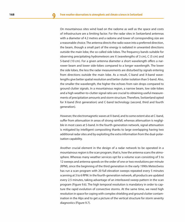
168 From weather observations to atmospheric and climate sciences in Switzerland9
On mountainous sites wind load on the radome as well as the space and costs of infrastructure are a limiting factor. For the radar sites in Switzerland antennas with a diameter of 4.2 metres and a radome and tower of corresponding size are a reasonable choice. The antenna directs the radio wave into a preferred direction, the beam, though a small part of the energy is radiated in unwanted directions outside the main lobe, the so-called side lobes. The frequency bands suitable for observing precipitating hydrometeors are X (wavelengths of 3 cm), C (5 cm) and S-band (10 cm). For a given antenna diameter a short wavelength offers a nar-rower beam and lower side-lobes compared to a longer wavelength. The lower the side lobes, the less the radar measurements are disturbed by signals entering from directions outside the main lobe. As a result, C-band and X-band wave-lengths give better spatial resolution and better clutter isolation than S-band. Also, the smaller the wavelength, the higher the echoes from rain drops compared to ground clutter signals. In a mountainous region, a narrow beam, low side-lobes and a high weather-to-clutter signal ratio are crucial to obtaining useful measure-ments of precipitation amounts and storm structure. Therefore, Switzerland opted for X-band (first generation) and C-band technology (second, third and fourth generation).
However, the electromagnetic waves at X-band, and to some extent also at C-band, suffer from attenuation in areas of strong rainfall, whereas attenuation is negligi-ble in most cases at S-band. In the fourth-generation network, signal attenuation is mitigated by intelligent compositing thanks to large overlapping having two additional radar sites and by exploiting the extra information from the dual-polar-isation capability.
Another crucial element in the design of a radar network to be operated in a mountainous region is the scan program, that is, how the antenna scans the atmo-sphere. Whereas many weather services opt for a volume scan consisting of 5 to 12 sweeps and antenna speeds on the order of one or two revolutions per minute (RPM), since the beginning of the third generation in the early 1990s MeteoSwiss has run a scan program with 20 full elevation sweeps repeated every 5 minutes scanning at 3 to 6 RPM. In the fourth-generation network, all products are updated every 2.5 minutes, taking advantage of an interleaved sweep pattern in the scan program (Figure 9.6). The high temporal resolution is mandatory in order to cap-ture the rapid evolution of convective storms. At the same time, we need high resolution in space for coping with complex shielding and ground clutter contam-ination in the Alps and to get a picture of the vertical structure for storm severity diagnostics (Figure 9.7).
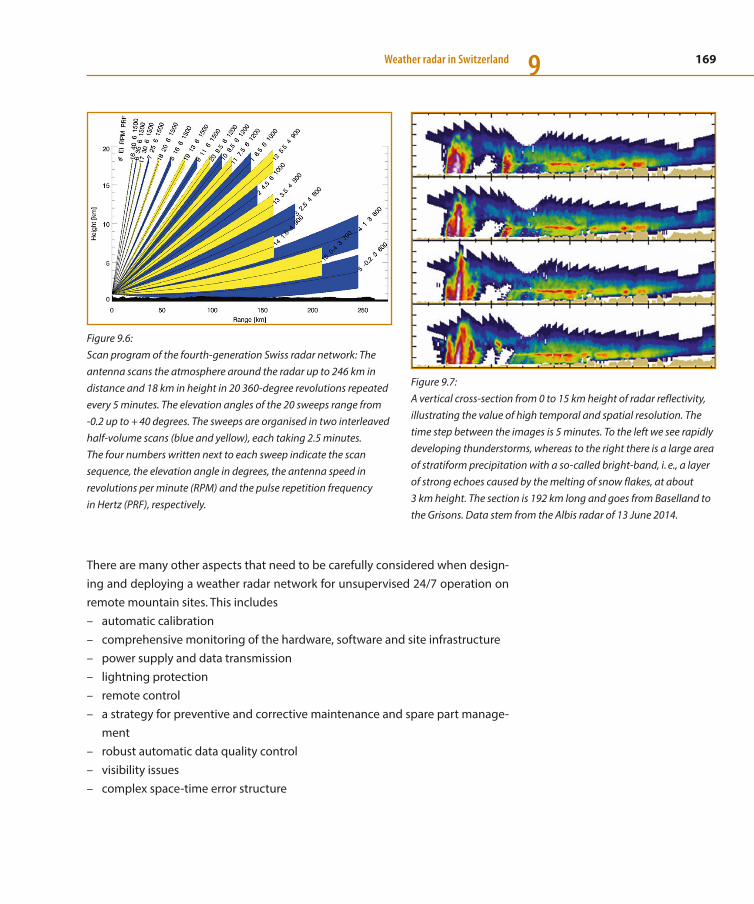
169Weather radar in Switzerland 9
There are many other aspects that need to be carefully considered when design-ing and deploying a weather radar network for unsupervised 24/7 operation on remote mountain sites. This includes
– automatic calibration – comprehensive monitoring of the hardware, software and site infrastructure – power supply and data transmission – lightning protection – remote control – a strategy for preventive and corrective maintenance and spare part manage-
ment – robust automatic data quality control – visibility issues – complex space-time error structure
Figure 9.6: Scan program of the fourth-generation Swiss radar network: The antenna scans the atmosphere around the radar up to 246 km in distance and 18 km in height in 20 360-degree revolutions repeated every 5 minutes. The elevation angles of the 20 sweeps range from -0.2 up to + 40 degrees. The sweeps are organised in two interleaved half-volume scans (blue and yellow), each taking 2.5 minutes. The four numbers written next to each sweep indicate the scan sequence, the elevation angle in degrees, the antenna speed in revolutions per minute (RPM) and the pulse repetition frequency in Hertz (PRF), respectively.
Figure 9.7: A vertical cross-section from 0 to 15 km height of radar reflectivity, illustrating the value of high temporal and spatial resolution. The time step between the images is 5 minutes. To the left we see rapidly developing thunderstorms, whereas to the right there is a large area of stratiform precipitation with a so-called bright-band, i. e., a layer of strong echoes caused by the melting of snow flakes, at about 3 km height. The section is 192 km long and goes from Baselland to the Grisons. Data stem from the Albis radar of 13 June 2014.

170 From weather observations to atmospheric and climate sciences in Switzerland9
9.3 From analogue-standalone to Doppler dual polarisation
The first weather radar generation deployed in 1959 was a fully analogue system manufactured by Plessey with two radar sites, one on La Dôle near Geneva, the other on Albis near Zurich. At that time only few weather services around the world were operating a radar. The system was using a wavelength of 3 centimetres and an antenna with a cosecant squared radiation pattern initially developed for air surveillance. Having a broad beam in elevation the cosecant squared antenna integrated echoes from the ground to the top of precipitating clouds. In the azi-muth the beam was narrow. The result was a two-dimensional picture of the three-dimensional atmosphere in one single antenna rotation, a good solution given the technology available at that time. The signals were made available to the air-traffic controllers of Geneva and Zurich airport as a plan position indicator (PPI) showing the signals as a function of range and azimuth on a monochromatic screen located in a dark room. Each radar was a stand-alone system, and the sig-nals were not archived.
During the same period, for research purposes the Swiss Central Meteorological Institute operated a 6 GHz radar in Locarno-Monti, a system previously used by the US Air Force as a height finder to determine the altitude of an aircraft (Figure 9.9). The research was coordinated by Jürg Joss, who had been responsible for radar meteorology at MeteoSwiss since the very beginning and got training on radar technology during his research stays in the United States. The initial goal was to observe hail over the tobacco plants in the plain of Magadino. It was triggered by “Grossversuch I-III,” a major initiative of the Federal Department of Economy looking for ways to suppress hail by cloud seeding. But the odds of seeing hail during the experiments were small, and the focus of the research using the height finder moved to the vertical profile of radar reflectivity and cloud physics, building up knowledge that turned out to be essential when defining the scan strategy for precipitation monitoring in the design phase of the second radar generation. The height finder had a wavelength of 46 mm and was equipped with two separate antennas. One was used for transmission, another for reception, a design that is particularly suitable for vertical scanning, because on reception there is no lower limitation in distance and one can start to analyse data right above the antenna. In Locarno-Monti people continued studying cloud physical processes (e. g., Roesli et al, 1974; Joss and Gori, 1978), but the lead of the hail suppression initiative was assumed by Prof. Bruno Federer of ETH Zurich, and the “Grossversuch IV” ended up being held in the region of Napf, a hail-prone region near Lucerne in the late 1970s (Federer et al., 1986). This was the last field experiment on hail in Switzerland
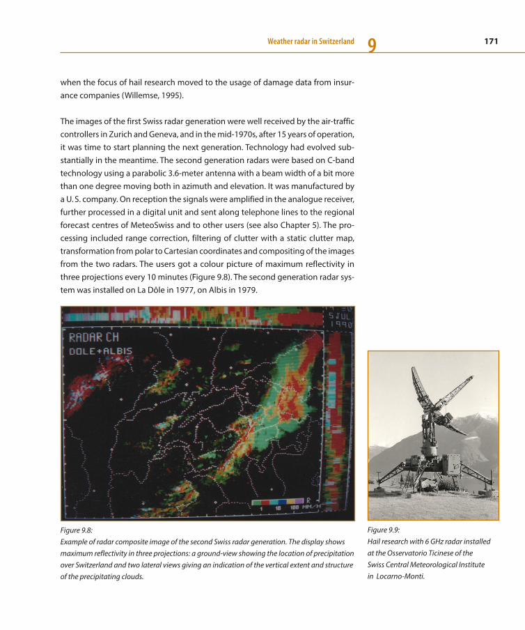
171Weather radar in Switzerland 9
when the focus of hail research moved to the usage of damage data from insur-ance companies (Willemse, 1995).
The images of the first Swiss radar generation were well received by the air-traffic controllers in Zurich and Geneva, and in the mid-1970s, after 15 years of operation, it was time to start planning the next generation. Technology had evolved sub-stantially in the meantime. The second generation radars were based on C-band technology using a parabolic 3.6-meter antenna with a beam width of a bit more than one degree moving both in azimuth and elevation. It was manufactured by a U. S. company. On reception the signals were amplified in the analogue receiver, further processed in a digital unit and sent along telephone lines to the regional forecast centres of MeteoSwiss and to other users (see also Chapter 5). The pro-cessing included range correction, filtering of clutter with a static clutter map, transformation from polar to Cartesian coordinates and compositing of the images from the two radars. The users got a colour picture of maximum reflectivity in three projections every 10 minutes (Figure 9.8). The second generation radar sys-tem was installed on La Dôle in 1977, on Albis in 1979.
Figure 9.8: Example of radar composite image of the second Swiss radar generation. The display shows maximum reflectivity in three projections: a ground-view showing the location of precipitation over Switzerland and two lateral views giving an indication of the vertical extent and structure of the precipitating clouds.
Figure 9.9: Hail research with 6 GHz radar installed at the Osservatorio Ticinese of the Swiss Central Meteorological Institute in Locarno-Monti.

172 From weather observations to atmospheric and climate sciences in Switzerland9
In the early 1980s the Laboratory for Atmospheric Physics of ETH Zurich (LAPETH) installed a C-band radar similar to the second generation radars of MeteoSwiss on the roof of the physics building at the campus on Hönggerberg. The antenna had a diameter of 2.5 metres, resulting in a beam width of 1.65 degrees. The radar was the workhorse of many research projects under the lead of Prof. Albert Waldvogel, head of LAPETH. After 20 years of radar research, ETH decided to abandon the field and the radar was operated by the spinoff meteoradar schmid until 2008, when the system was shut down completely and dismantled.
When designing the third Swiss radar generation Jürg Joss had the pioneering vision that the new radars should provide quantitative measurements of precipi-tation over the whole country. He was encouraged by the promising results of the previous two generations (Joss and Waldvogel, 1990; Joss and Pittini, 1991) and the demands from the hydrological community for precise measurements of areal precipitation over Alpine catchments. The specifications of the third generation were largely driven by this vision (Joss and Lee, 1995; Joss et al., 1998), including Doppler capability for the improved suppression of clutter and the extension of the network by a third site to the South of the Alps on Monte Lema. It utilised latest technology and advanced data processing. Antennas of a diameter of 4.2 metres were used resulting in a beam width of 1.0 degree. The quality of the radar images was high, though the first quantitative comparisons of radar rainfall amounts with measurements from rain-gauges and river-gauges were disappoint-ing, showing large discrepancies. It took many years of research to develop algo-rithms appropriate to quantitative radar rainfall estimation in a mountainous region (Germann et al., 2006a). In 2003, 10 years after the start of the third gener-ation, for the first time the sophisticated algorithms provided better rainfall esti-mates than a simple approach that takes the maximum of reflectivity in the verti-cal column to estimate precipitation at the ground pixel. For more details see Germann (1999), Gabella et al. (2000), Gabella et al. (2001), Germann and Joss (2002) and Germann and Joss (2004).
An important event in the Swiss radar history was the special observing period (SOP) of the Mesoscale Alpine Programme (MAP) field experiment in 1999 (Bougeault et al, 2003). One major focus of MAP was to study the role of the orog-raphy in the formation of heavy precipitation and flooding with an impressive number of ground-based and airborne radars and other observing facilities oper-ated in the Lago Maggiore region next to the Swiss radar on Monte Lema. In preparation for the SOP, MeteoSwiss organised in Locarno-Monti the pre-SOP, an instrument intercomparison campaign for mobile radars and disdrometers, before

173Weather radar in Switzerland 9
the instruments were actually deployed in their final locations. The intercompari-son campaign was organised in collaboration with several partners from Europe and the United States and included S-band, C-band, X-band and K-band radars and mechanical, optical and acoustic disdrometers. The MAP initiative was com-pleted with a concerted forecast demonstration phase (MAP D-PHASE) linking in real-time a number of observing systems and hydro-meteorological forecast mod-els involving many meteorologists, hydrologists and end users. The data collected during MAP provided new insight into the mechanisms of orographic rainfall and flooding (Rotunno and Houze, 2007; Rotach et al, 2009), and MAP was a valuable experience for the future of radar operations in Switzerland.
By the time MeteoSwiss started designing the fourth-generation radar network in 2009, many improvements had been achieved in the field of quantitative radar data processing in a mountainous region (Joss et al., 1998; Gabella et al., 2005; Germann et al., 2006a), and the promising results triggered the set-up of several quantitative applications in Switzerland, including meteo-hydrological end-to-end forecasting chains (Germann et al., 2009). Accuracy in quantitative terms remained a key element in the design of the fourth generation, but the vision of Rad4Alp, the project for the renewal of the radar network, went much further. The fourth generation is designed to improve sensitivity, coverage, accuracy and stability, to exploit the potential of dual-polarisation in a mountainous region, to extend the product portfolio adding hydrometeors, hail and snowfall, to foster the integration with satellite observations and other external data sources, and to serve as a springboard for 15 years of innovation for monitoring and warnings of heavy rainfall, thunderstorms, hail, flash floods, debris flows, and snow serving the public and private.
9.4 Rad4Alp – The fourth-generation MeteoSwiss weather radar network
As part of the project Rad4Alp, MeteoSwiss completely renewed and extended the Swiss operational radar network (Figure 9.10). The renewal was done in close col-laboration with many partners from industry and government, including SELEX for the radar hardware, ELDES for the radar software and the BBL (Bundesamt für Bauten und Logistik) for managing the civil construction works. The specifications of the fourth generation were largely driven by user requirements, who needed high availability, stability and accurate observations of precipitation and thunder-storms over the whole territory including the populated Alps with high mountain

174 From weather observations to atmospheric and climate sciences in Switzerland9
crests, deep valleys and sensitive infrastructure. The design and configuration of the fourth generation (Table 9.1) was a combination of proven solutions from the previous generations, new technologies from the industry, results from many research projects MeteoSwiss was involved in and valuable input from colleagues from other national weather services and academia from around the world.
In order to improve radar coverage in the inner-Alpine regions, it was decided to install two additional radars, one in southwestern Switzerland (canton of Valais, Figure 9.11), one in eastern Switzerland (canton of Grisons). The selected sites on Pointe de la Plaine Morte, 2937 m asl, and Weissfluhgipfel, 2840 m asl, offer good visibility and accessibility by cable car. In addition to better coverage in the Alps, the new radars have large overlapping areas with the existing three radars and hence can serve as backup in the case of malfunction of one of the other radars.
The fourth-generation network has a number of significant innovations. First, the systems are equipped with fully digital receivers, a mature technology resulting in higher sensitivity and data quality. Second, the radars have polarimetric capability to determine dual-polarisation meteorological quantities from simultaneous hor-izontal (H) and vertical (V) transmissions. On transmission, the power is split and half is transmitted at horizontal, the other half at vertical polarisation; on recep-
Figure 9.10: Fourth-generation radar with new tower on Albis, 938 m asl. The old tower from the 1960s was replaced and the technical room with the transmitter and radar control and signal processor was moved to the top of the tower directly below the antenna, which simplifies maintenance work and resulted in an increase of sensitivity of several decibel.

175Weather radar in Switzerland 9
Figure 9.11: Picture of the radar on Pointe de la Plaine Morte, 2937 m asl, one of the two additional radar sites installed as part of Rad4Alp.
Table 9.1: Technical characteristics of third and fourth Swiss radar generation.
Parameter 3rd generation 4th generation
Industrial partners Gematronik, LASSEN SELEX, ELDES
Radio frequency 5.4 GHz 5.4 GHz
Mode Doppler, Single Polarization (horizontal)
Doppler, Simultaneous Dual Polarization (horizontal + vertical)
Peak power 250 kW 470 kW (235 kW per channel)
Antenna Parabolic, elevation-over-azimuth pedestal, 4.2 m diameter
Parabolic, elevation-over-azimuth pedestal, 4.2 m diameter
Antenna gain (beamwidth) 45 dB (1° beamwidth at 3 dB) 45 dB (1° beamwidth at 3 dB)
Side lobes below –27 dB below –29 dB
Pulse length 0.5 microseconds 0.5 microseconds
Pulse repetition frequency 600 –1200 Hz 600–1500 Hz
Maximum range, height 230 km, 12 km 246 km, 18 km
Losses @ Albis (transmission and reception path including radome)
12.7 dB 2.9 dB
Product update rate 5 min 2.5 min
Receiver technology Analog, one intermediate frequency, A/D conversion at bipolar video
ROEL, digital, two intermediate frequencies for down-conversion, A/D conversion at IF
Receiver dynamic range 90 dB 105 dB linear (@ 0.5 microseconds pulse)
Data processing chains 1 real-time processing chain 4 parallel real-time processing chains (1 operational, 3 for research)

176 From weather observations to atmospheric and climate sciences in Switzerland9
tion, there are separate channels for the two polarisations, and by combining the two information on the shape and orientation of the scatterers is obtained. The advantage of simultaneously transmitting and receiving H and V polarisations is that polarimetric observables are determined directly from the same transmitted pulse and are thus not contaminated by Doppler effects that occur when H and V polarisations are transmitted in alternating mode. The approach has the additional advantage that a high-power polarisation switch is not needed. The technology itself is not new, but long-term performance and robustness for automatic appli-cations in an operational context have yet to be proven, in particular in a moun-tainous region (Friedrich et al. 2007; Friedrich et al., 2009). Provided that the hori-zontal and vertical channel on transmit and receive are calibrated and monitored properly, dual-polarisation measurements allow us
– to better distinguish between weather and nonweather signals (clutter cancel-lation),
– to know more about the type and size distribution of hydrometeors in the pulse volume (Figure 9.12),
– to diagnose hardware anomalies, – to correct reflectivity measurements for signal attenuation, – to improve estimates of precipitation rates and amounts.
A striking example of the added value of dual-polarisation measurements is clut-ter cancellation (Figure 9.5). Introducing dual-polarisation in the operational data processing chain resulted in a substantial reduction of the level of residual clutter and, at the same time, less erroneously cancelled weather signals.
Figure 9.12: Plotting the cross-correlation between reflectivity at horizontal and vertical polarisation, one of the dual-polarisation moments, the melting layer appears as a distinct ring of low values.
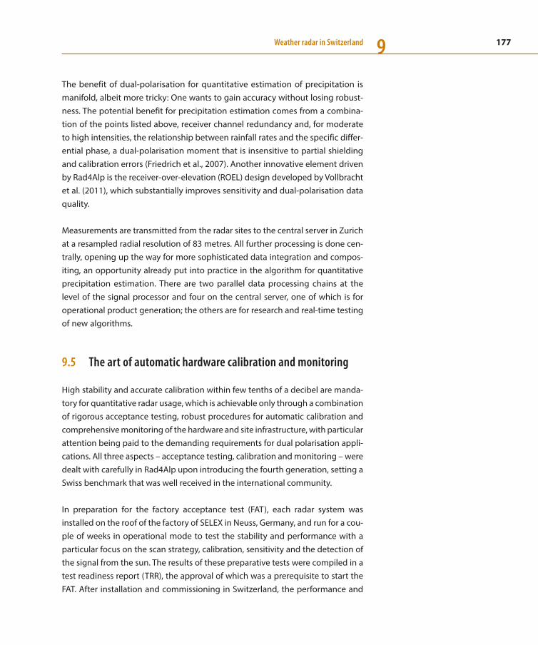
177Weather radar in Switzerland 9
The benefit of dual-polarisation for quantitative estimation of precipitation is manifold, albeit more tricky: One wants to gain accuracy without losing robust-ness. The potential benefit for precipitation estimation comes from a combina-tion of the points listed above, receiver channel redundancy and, for moderate to high intensities, the relationship between rainfall rates and the specific differ-ential phase, a dual-polarisation moment that is insensitive to partial shielding and calibration errors (Friedrich et al., 2007). Another innovative element driven by Rad4Alp is the receiver-over-elevation (ROEL) design developed by Vollbracht et al. (2011), which substantially improves sensitivity and dual-polarisation data quality.
Measurements are transmitted from the radar sites to the central server in Zurich at a resampled radial resolution of 83 metres. All further processing is done cen-trally, opening up the way for more sophisticated data integration and compos-iting, an opportunity already put into practice in the algorithm for quantitative precipitation estimation. There are two parallel data processing chains at the level of the signal processor and four on the central server, one of which is for operational product generation; the others are for research and real-time testing of new algorithms.
9.5 The art of automatic hardware calibration and monitoring
High stability and accurate calibration within few tenths of a decibel are manda-tory for quantitative radar usage, which is achievable only through a combination of rigorous acceptance testing, robust procedures for automatic calibration and comprehensive monitoring of the hardware and site infrastructure, with particular attention being paid to the demanding requirements for dual polarisation appli-cations. All three aspects – acceptance testing, calibration and monitoring – were dealt with carefully in Rad4Alp upon introducing the fourth generation, setting a Swiss benchmark that was well received in the international community.
In preparation for the factory acceptance test (FAT), each radar system was installed on the roof of the factory of SELEX in Neuss, Germany, and run for a cou-ple of weeks in operational mode to test the stability and performance with a particular focus on the scan strategy, calibration, sensitivity and the detection of the signal from the sun. The results of these preparative tests were compiled in a test readiness report (TRR), the approval of which was a prerequisite to start the FAT. After installation and commissioning in Switzerland, the performance and
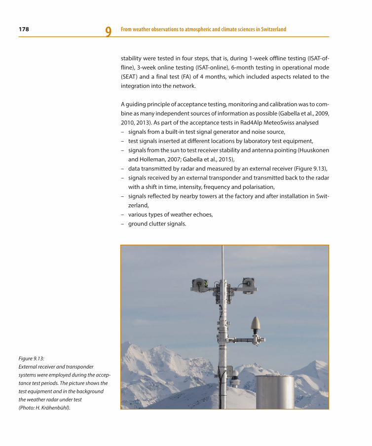
178 From weather observations to atmospheric and climate sciences in Switzerland9
stability were tested in four steps, that is, during 1-week offline testing (ISAT-of-fline), 3-week online testing (ISAT-online), 6-month testing in operational mode (SEAT) and a final test (FA) of 4 months, which included aspects related to the integration into the network.
A guiding principle of acceptance testing, monitoring and calibration was to com-bine as many independent sources of information as possible (Gabella et al., 2009, 2010, 2013). As part of the acceptance tests in Rad4Alp MeteoSwiss analysed
– signals from a built-in test signal generator and noise source, – test signals inserted at different locations by laboratory test equipment, – signals from the sun to test receiver stability and antenna pointing (Huuskonen
and Holleman, 2007; Gabella et al., 2015), – data transmitted by radar and measured by an external receiver (Figure 9.13), – signals received by an external transponder and transmitted back to the radar
with a shift in time, intensity, frequency and polarisation, – signals reflected by nearby towers at the factory and after installation in Swit-
zerland, – various types of weather echoes, – ground clutter signals.
Figure 9.13: External receiver and transponder systems were employed during the accep-tance test periods. The picture shows the test equipment and in the background the weather radar under test (Photo: H. Krähenbühl).

179Weather radar in Switzerland 9
Calibration of the hardware is done (1) automatically during operation using a noise source and an integrated test signal generator, and, (2) offline during the acceptance tests and in a periodic manner during preventive maintenance. The noise source signal is inserted in both polarisation channels of the receive path, every 2.5 minutes, when the antenna is scanning at the highest elevation angle of each half-volume scan. The usage of a noise source and the procedure for auto-matic calibration in operational mode represent another innovative element of the Swiss radar network (Joss et al., 1998; Vollbracht et al., 2014).
Another crucial element for quantitative radar usage is automatic monitoring of the radar hardware and site infrastructure. In the fourth generation more than 350 parameters are monitored and submitted from each radar site to the central server after completion of every single sweep, that is, 20 times every 5 minutes. The parameters are automatically checked for anomalies and archived for diagnostic analyses in case of malfunctions and statistical studies of system performance.
9.6 X-band research radars
In the 1990s, X-band weather radars became increasingly popular among scien-tists regarding various applications related to the measurement of precipitation at small to medium scales (1 to 50 km) as well as for probing the atmosphere in vertical direction in order to investigate microphysical processes of precipitation formation. Since X-band weather radars are cheaper than C- and S-band systems and also less bulky (allowing easier transportation and deployment), they are suit-able for network operation, research campaigns (e. g. Berne et al., 2005) and for supplementary coverage in mountainous regions. In contrast to S- and C-band systems, signal power attenuation along the propagation path through precipita-tion as well as radome attenuation plays a more significant role because of the shorter wavelength (3 cm). With the introduction of polarimetric methods, prog-ress was made in overcoming the problem of attenuation in rain. Such correction techniques allowed employment of X-band radars in quantitative precipitation estimation applications.
Since the beginning of the 1980s, with the skilful support of Donat Högl research-ers at LAPETH had employed a mobile vertically pointing nonpolarimetric X-band Doppler radar in order to study aerosol and hydrometeor concentrations in winter precipitation, together with scavenging processes that influence the chemical composition of precipitation (Schumann et al., 1988; Waldvogel et al., 1989). Later
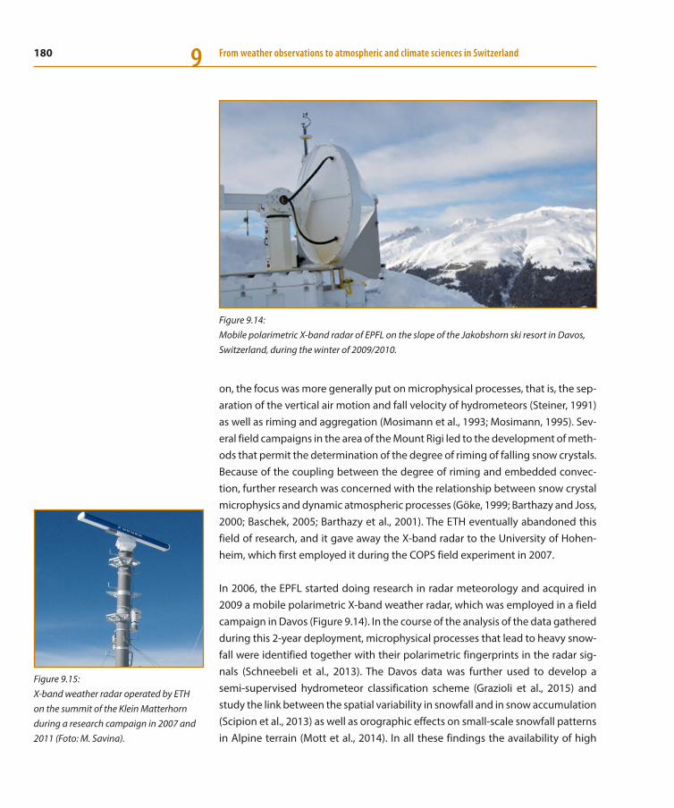
180 From weather observations to atmospheric and climate sciences in Switzerland9
on, the focus was more generally put on microphysical processes, that is, the sep-aration of the vertical air motion and fall velocity of hydrometeors (Steiner, 1991) as well as riming and aggregation (Mosimann et al., 1993; Mosimann, 1995). Sev-eral field campaigns in the area of the Mount Rigi led to the development of meth-ods that permit the determination of the degree of riming of falling snow crystals. Because of the coupling between the degree of riming and embedded convec-tion, further research was concerned with the relationship between snow crystal microphysics and dynamic atmospheric processes (Göke, 1999; Barthazy and Joss, 2000; Baschek, 2005; Barthazy et al., 2001). The ETH eventually abandoned this field of research, and it gave away the X-band radar to the University of Hohen-heim, which first employed it during the COPS field experiment in 2007.
In 2006, the EPFL started doing research in radar meteorology and acquired in 2009 a mobile polarimetric X-band weather radar, which was employed in a field campaign in Davos (Figure 9.14). In the course of the analysis of the data gathered during this 2-year deployment, microphysical processes that lead to heavy snow-fall were identified together with their polarimetric fingerprints in the radar sig-nals (Schneebeli et al., 2013). The Davos data was further used to develop a semi-supervised hydrometeor classification scheme (Grazioli et al., 2015) and study the link between the spatial variability in snowfall and in snow accumulation (Scipion et al., 2013) as well as orographic effects on small-scale snowfall patterns in Alpine terrain (Mott et al., 2014). In all these findings the availability of high
Figure 9.14: Mobile polarimetric X-band radar of EPFL on the slope of the Jakobshorn ski resort in Davos, Switzerland, during the winter of 2009/2010.
Figure 9.15: X-band weather radar operated by ETH on the summit of the Klein Matterhorn during a research campaign in 2007 and 2011 (Foto: M. Savina).

181Weather radar in Switzerland 9
resolution radar observations was decisive. The EPFL radar has a beam width of 1.45 degrees and a resolution in range of 75 metres.
Our understanding of Alpine hydrology in general, and the interaction of orogra-phy with mountainous precipitation in particular, was also driven forward by the Klein Matterhorn X-band radar project, a collaboration between the canton of Valais and the group of Prof. P. Burlando at the ETH Zurich. During 2007 and 2011, a cost-effective single polarisation X-band weather radar was deployed on the summit of the Klein Matterhorn at an altitude of 3883 m above sea level (Figure 9.15; Savina, 2011). The results of the experiment showed that the complex space-time structure of Alpine precipitation can indeed be assessed (Savina et al., 2011).
In order to study wind shear and precipitation at airports, in 2012 armasuisse acquired a state-of-the art mobile polarimetric X-band weather radar operated by MeteoSwiss (Figure 9.16). This radar as well as the EPFL radar can acquire polari-metric data in spectral mode, that is, polarimetric observables are obtained not only as a function of range, but also as a function of the Doppler velocity. This will pave the way for sophisticated microphysical analyses, advanced clutter elimina-tion and signal-processing techniques (Figure 9.17).
Figure 9.16: Mobile polarimetric X-band radar of MeteoSwiss/armasuisse. As part of an experiment in Magadino in 2012, the radar was exposed to artificial rain with support from the local fire bri-gade to quantify attenuation of the radar signal by water on the radome, the white protection sphere around the antenna (Photo: B. Lerch).
Figure 9.17: Radar reflectivity as a function of height and of the Doppler velocity; from a scan taken with the MeteoSwiss/armasuisse X-band radar pointing in the vertical direction. The sharp drop in Doppler velocities marks the location of the melt-ing layer: The snowflakes above fall at speeds of around 2 m/s, whereas the drops below fall at higher speeds of up to 10 m/s.

182 From weather observations to atmospheric and climate sciences in Switzerland9
9.7 Recent achievements and forthcoming research opportunities
The progress in stability and accuracy achieved recently in the operational radar network triggered several research projects and innovative pilot applications in the field of nowcasting of heavy rainfall and severe convective storms.
In order to express the uncertainty in quantitative radar precipitation estimates, MeteoSwiss developed a technique for generating an ensemble of precipitation fields. It combines our knowledge of the space-time structure of radar errors with stochastic simulation techniques and was implemented in a real-time test chain in 2007 as part of the European concerted research action COST-731 (Rossa et al., 2011) and the Mesoscale Alpine Programme forecast demonstration project MAP D-PHASE (Rotach et al., 2009). The radar ensemble was coupled with a runoff model and configured for several rivers in Ticino (Figure 9.18) in collaboration with the Swiss Federal Institute for Forest, Snow and Landscape Research WSL (Zappa et al., 2011; Liechti et al., 2013). The experiment was a novel contribution to the emerging field of uncertainty propagation in hydro-meteorological forecast sys-tems and was one of the first of its kind worldwide (Germann et al., 2009). Hydrol-ogists applauded the initiative, but at the same time they were concerned with the fact that the uncertainties in radar precipitation estimates remained large. This triggered the development of a geostatistical technique for real-time merging of radar and rain-gauge data in the Alpine region as part of a project in the frame-work of NCCR-Climate (Figure 9.19; also mentioned in Chapter 7). See Sideris et al. (2014) and Erdin et al. (2012) for more details.
Figure 9.18: Performance of the radar ensemble generator coupled with a runoff model during a flash flood in the Pincascia catchment, southern Switzerland. See Germann et al. (2009) for more details.

183Weather radar in Switzerland 9
In order to generate short-term forecasts, one must extrapolate the radar precip-itation fields using echo motion observed in the immediate past (Germann et al., 2006; Mandapaka et al., 2012). This approach is presently being further developed by adding orographic forcing (Panziera and Germann, 2010; Foresti and Pozd-noukhov, 2011) and knowledge from past events retrieved from the rapidly grow-ing radar archives (Panziera et al, 2011).
Another major research focus relates to the nowcasting of thunderstorms and hail (Figure 9.20), combining volumetric radar data with lightning and satellite observations and the output of the numerical weather prediction model COSMO. In 2003, a first version of the Thunderstorms Radar Tracking nowcasting system was launched (Hering et al, 2004). It has since been improved and extended con-tinuously over the years to become the standard for official warnings of severe convective storms in Switzerland. In 2012 TRT was complemented by COALITION (Nisi et al., 2014), a system that makes substantial usage of satellite observations. This is a field of ongoing research, and further innovations will surely follow which exploit among other things the additional information on the type and size dis-tribution of hydrometeors derived from the dual-polarisation variables of the fourth generation.
Radar networks play an increasingly important role in numerical weather predic-tion (NWP). Because of the high spatial and temporal resolution, radars have been
Figure 9.19: Hourly rainfall amounts on 31 May 2013, 22 UTC, of radar (left) and radar-rain-gauge merging (right). The colour inside the circles show the hourly amounts reported by the rain-gauges for comparison. The significant underestimation of the radar (left) disappears when combined with rain-gauge observations (right). See Sideris et al. (2014) for more details.

184 From weather observations to atmospheric and climate sciences in Switzerland9
recognised as a valuable data source for the validation and verification of, as well as the assimilation into, high-resolution weather models; see, for example, Action 717 on the “Use of Radar Observations in Hydrological and NWP Models” (Rossa et al., 2005) of the European Cooperation in Science and Technology Programme COST. MeteoSwiss uses radar precipitation fields in the COSMO model validation (Weusthoff et al., 2010) and assimilation (Leuenberger and Rossa, 2007). Future challenges in the radar-model interplay include the assimilation of radar volume reflectivity and Doppler velocity as well as polarimetric information in order to improve the meso- and microscale dynamical and microphysical model processes.
The capabilities of the fourth-generation network, integration with other data sources and data mining technologies combined with the rapidly growing archives of remote sensing data as well as advances in environmental modelling will trigger many innovations in the near future.
Figure 9.20: Trajectories of July hail cells of 2002–2013 identified by the hail algorithm and tracked by the Thunderstorms Radar Tracking nowcasting system TRT. The colour indicates the density of trajectories. Peaks are found in the region of Napf and southern Ticino with more than one trajectory per year and km2.
185Weather radar in Switzerland 9
Acknowledgments
This chapter reflects the intense collaborations and exchange with many partners in Switzerland. Special thanks go to J. Joss, G. Galli and R. Cavalli who provided excellent training in radar meteorology to the first three authors during the 3rd Swiss radar generation! An important recent radar project of national dimension was Rad4Alp. The authors would like to thank P. Ambrosetti, P. Binder, B. Calpini, L. Clementi, M. Dippon, F. Keller, A. Hering, M. Sartori, I. Sideris and N. Tschichold for the excellent team spirit in Rad4Alp, and J. Figueras, R. Hüppi, R. König, A. Leuen-berger and O. Progin for very valuable support. Thanks go also to all the scientists who contributed to the chapter with material and research projects, in particular A. Berne, D. Leuenberger, L. Nisi, L. Panziera, O. Romppainen and B. Puigdomènech Treserras.
References
Austin, P. M., 1987: Relation between measured radar reflectivity and surface rainfall. Mon. Wea. Rev., 115, 1053–1070.
Barthazy, E., and J. Joss, 2000: Air motion, estimated by vertically pointing radars. Phys. Chem. Earth, 25, 1209–1214.
Barthazy, E., S. Göke, J. Vivekanandan, and S. M. Ellis, 2001: Detection of snow and ice crystals using polarization radar measurements: Comparison between ground-based in situ and S-Pol observations. Atmos. Res., 73, 137–162.
Baschek, B., 2005: Influence of updrafts and embedded convec-tion on the microphysics of riming. Ph.D. thesis, ETH Zurich, Switzerland.
Berne, A., Delrieu, G., and H. Andrieu, 2005: Estimating the verti-cal structure of intense Mediterranean precipitation using two x-band weather radar systems. J. Atmos. Oceanic Technol., 22, 1656–1675.
Bougeault P., R. A. Houze, R. Rotunno and H. Volkert (Guest edi-tors), 2003: Special issue on the Mesoscale Alpine Programme MAP Field Experiment. Quart. J. Roy. Meteor. Soc., 129, 341–895.
Erdin R., C. Frei, and H. R. Künsch, 2012: Data transformation and uncertainty in geo-statistical combination of radar and rain gauges. J. Hydrometeor., 13, 1332–1346.
Federer B. et al., 1986: Main results of Grossversuch IV. J. Appl. Meteor. Climatol., 25, 917–957.
Foresti, L, and A. Pozdnoukhov, 2011: Exploration of Alpine oro-graphic precipitation patterns with radar image processing and clustering techniques. Meteor. Appl., 19, 407–419.
Friedrich, K., U. Germann, J. J. Gourley, and P. Tabary, 2007: Effects of radar beam shielding on rainfall estimation for polari-metric C-band radars. J. Atmos. Oceanic Technol., 24, 1839–1859.
Friedrich, K., U. Germann, and P. Tabary, 2009: Influence of ground clutter contamination on polarimetric radar parame-ters. J. Atmos. Oceanic Technol., 26, 251–269.
Gabella, M., J. Joss, and G. Perona, 2000: Optimizing quantitative precipitation estimates using a non-coherent and a coherent radar operating on the same area. J. Geophys. Res., 105, 2237–224.
Gabella, M., J. Joss, G. Perona, and G. Galli, 2001: Accuracy of rainfall estimates by two radars in the same Alpine environment using gauge adjustment. J. Geophys. Res., 106, 5139– 5150.
Gabella, M., M. Bolliger, U. Germann, and G. Perona, 2005: Large sample evaluation of cumulative rainfall amounts in the Alps using a network of three radars. Atmos. Res., 77, 256–268.
186 From weather observations to atmospheric and climate sciences in Switzerland9
Gabella, M., M. Boscacci, M. Sartori, O. Progin, and U. Germann, 2009: Planning acceptance tests of the next generation Swiss weather radar network, Preprints, 34th Int. Conf. on Radar meteo-rology, Williamsburg, Virginia.
Gabella M., M. Sartori, O. Progin, M. Boscacci, and U. Germann, 2010: An innovative instrumentation for checking electromag-netic performances of operational meteorological radar, 6th European Conference on Radar meteorology – ERAD2010, Sibiu, Romania, 91–96.
Gabella M., M. Sartori, O. Progin, and U. Germann, 2013: Accep-tance tests and monitoring of the next generation polarimetric weather radar network in Switzerland, Proc. IEEE Int. Conf. Elec-tromagn. Adv. Appl., Torino, Italy.
Gabella M., M. Sartori, M. Boscacci, and U. Germann, 2015: Verti-cal and horizontal polarization observations of slowly varying solar emissions from operational Swiss weather radars, Atmo-sphere, 6, 50–59.
Germann, U., 1999: Radome attenuation — a serious limiting fac-tor for quantitative radar measurements? Meteorol. Z., 8, 85–90.
Germann, U., and J. Joss, 2002: Mesobeta profiles to extrapolate radar precipitation measurements above the Alps to the ground level. J. Appl. Meteorol., 41, 542–557.
Germann, U., J. Joss, 2004: Operational measurement of precip-itation in mountainous terrain (Chapter 2). Weather radar: Princi-ples and advanced applications, P. Meischner, Ed.,. Physics of Earth and space environment, vol. XVII. Springer Verlag, Heidel-berg, Germany, pp. 52–77.
Germann, U., I. Zawadzki, and B. Turner, 2006: Predictability of precipitation from continental radar images. Part IV: Limits to prediction. Journal of Atmos. Sci., 63, 2092–2108.
Germann, U., G. Galli, M. Boscacci, and M. Bolliger, 2006a. Radar precipitation measurement in a mountainous region. Quart. J. Roy. Meteor. Soc., 132, 1669–1692.
Germann U., Berenguer M., Sempere-Torres D., and Zappa M., 2009: REAL – Ensemble radar precipitation estimation for hydrology in a mountainous region. Quart. J. Roy. Meteor. Soc., 135, 445–456.
Göke, S., 1999: Microphysics of the melting layer: Comparison of model results and in situ measurements. Ph.D. thesis no. 13352, ETH Zurich, 156 pp.
Grazioli, J., D. Tuia, and A. Berne, 2015: Hydrometeor classifi-cation from polarimetric radar measurements: a clustering approach. Atmos. Meas. Tech., 8, 149–170.
Hering, A., C. Morel, G. Galli, S. Senesi, P. Ambrosetti, and M. Bos-cacci, 2004: Nowcasting thunderstorms in the Alpine region using a radar based adaptive thresholding scheme. Third Euro-pean Conf. on Radar in Meteorology and Hydrology (ERAD2004), Visby, Sweden, Swedish Meteorological and Hydrological Institute, 206–211.
Huuskonen, A., and I. Holleman, 2007: Determining weather radar antenna pointing using signals detected from the Sun at low antenna elevations. J. Atmos. Oceanic Technol., 24, 476–483.
Jaffrain, J., and A. Berne, 2012: Quantification of the small-scale spatial structure of the raindrop size distribution from a Net-work of Disdrometers. J. Appl. Meteor. Climatol., 51, 941–953.
Joss, J., and E. G. Gori, 1978: Shapes of raindrop size distribu-tions. J. Appl. Meteor. Climatol., 17, 1054–1061.
Joss, J., and A. Waldvogel, 1967: A raindrop spectrograph with automatic analysis. Pure Applied Geophysic, 68, 240–246.
Joss, J., A. Waldvogel 1990: Precipitation measurements and hydrology. A review. (Chapter 29). Radar Meteorology, D. Atlas, Ed., Boston, MA: Amer. Meteorol. Soc, 1990, pp. 577–606.
Joss, J., and A. Pittini, 1991: Real time estimation of the vertical profile of radar reflectivity to improve the measurement of pre-cipitation in an Alpine region. J. Meteor. Atmos. Phys., 47, 61–72.
Joss, J., and R. Lee, 1995: The application of radar-gauge com-parisons to operational precipitation profile corrections, J. Appl. Meteor., 34, 2612–2630, 1995.
Joss, J et al., 1998: Operational Use of Radar for Precipitation Measurements in Switzerland. vdf, 108 pp.
Leuenberger, D., and A. Rossa, 2007: Revisiting the latent heat nudging scheme for the rainfall assimilation of a simulated con-vective storm. Meteor. Atmos Phys., 98, 195–215.
Liechti K., M. Zappa, F. Fundel, and U. Germann, 2013: Probabilis-tic evaluation of ensemble discharge nowcasts in two nested Alpine basins prone to flash floods. Hydrological Processes, 27, 5–17.
Mandapaka, P. V., U. Germann, L. Panziera, and A. Hering, 2012: Can Lagrangian extrapolation of radar fields be used for pre-
187Weather radar in Switzerland 9cipitation nowcasting over complex Alpine orography? Wea. Forecasting, 27, 28–49.
Mosimann, L., M. Steiner, J. L. Collet, W. Heinrich, W. Schmid, and A. Waldvogel, 1993: Ice crystal observations and the degree of riming in winter precipitation. Water, Air, Soil Poll., 68, 29–42.
Mosimann, L., 1995: An improved method for determining the degree of snow crystal riming by vertical Doppler radar. Atmos. Res., 37, 305–323.
Mott, R., D. Scipion, M. Schneebeli, N. Dawes, A. Berne, and M. Lehning, 2014: Orographic effects on snow deposition patterns in mountainous terrain. J. Geophys. Res., 119, 1419–1439.
Nisi, L., P. Ambrosetti, and L. Clementi, 2014: Nowcasting severe convection in the Alpine region: the COALITION approach. Quart. J. Roy. Meteor. Soc., 140, 1684–1699.
Panziera, L., and U. Germann, 2010: The relation between air-flow and orographic precipitation on the southern side of the Alps as revealed by weather radar. Quart. J. Roy. Meteor. Soc., 136, 222–238.
Panziera, L., U. Germann, M. Gabella, and P. Mandapaka, 2011: NORA — Nowcasting of orographic rainfall by means of ana-logues. Quart. J. Roy. Meteor. Soc., 137, 2106–2123.
Roesli, H. P., J. Joss, and M. Schüepp, 1974: Possible influence of evaporation below cloud base on rain enhancement. J. Appl. Meteor. Climatol., 13, 783–787.
Rotach, M. W. et al., 2009 : MAP D-PHASE: Real-time demonstra-tion of weather forecast quality in the Alpine region. Bull. Amer. Meteor. Soc., 90, 1321–1336.
Rotunno, R., and R. A. Houze, 2007: Lessons on orographic pre-cipitation from the Mesoscale Alpine Programme. Quart. J. Roy. Meteor. Soc., 133, 811–830.
Rossa, A, M. Bruen, D. Frühwald, B. Macpherson, I. Holleman, D. Michelson, and S. Michaelides (Eds), 2005: COST 717 Final Report, Use of Radar Observations in Hydrological and NWP Models, COST Publication Series, EUR 21954. COST Office: Brussels, Belgium; 286 pages.
Rossa A., K. Liechti, M. Zappa, M. Bruen, U. Germann, G. Haase, C. Keil, and P. Krahe, 2011: The COST 731 Action: A review on uncertainty propagation in advanced hydro-meteorological forecast systems. Atmos. Res., Elsevier, 100, 150–167.
Savina, M., 2011: The use of a cost‐effective X‐band weather radar in Alpine region. Ph.D. thesis, ETH Zurich, Switzerland.
Savina, M., P. Molnar, and P. Burlando, 2011: Seasonal long – term persistence in radar precipitation in complex terrain. Water Res. Res., 47, W10506, 9 pages.
Schneebeli, M., N. Dawes, M. Lehning, and A. Berne, 2013: High-resolution vertical profiles of polarimetric X-band weather radar observables during snowfall in the Swiss Alps. J. Appl. Meteor. Clim., 52, 378–394.
Schumann, T., B. Zinder, and A.Waldvogel, 1988: Aerosol and hydrometeor concentration and their chemical composition during winter precipitation along a mountain slope. part I: Temporal evolution of the aerosol, microphysical and meteo-rological conditions. Atmos. Environ., 22, 1443–1459.
Scipion, D., R. Mott, M. Lehning, M. Schneebeli, and A. Berne, 2013: Seasonal small-scale spatial variability in Alpine snowfall and snow accumulation. Water Res. Res., 49, 1446–1457.
Sideris, I., M. Gabella, R. Erdin, and U. Germann, 2014: Real-time radar-raingauge merging using spatio-temporal co-kriging with external drift in the alpine terrain of Switzerland. Quart. J. Roy. Meteor. Soc., 140, 1097–1111.
Steiner, M., 1991: Die Kombination von Doppler- und Polarisa-tionsradarmessungen im Niederschlag: Neue Perspektiven für die Radarmeteorologie. Ph.D. thesis no. 9558, ETH Zurich, avail-able from e-collection.library.ethz.ch.
Vollbracht, D., D. Ridene, and F. Gekat, 2011: Receiver over Eleva-tion (ROEL) Weather Radar System Design and its Advantages, 12th URSI Commission F Triennial Open Symposium on Wave Prop-agation and Remote Sensing, Garmisch-Partenkirchen, Germany.
Vollbracht, D., M. Sartori, and M. Gabella, 2014: Absolute dual-polarization radar calibration: temperature dependence and stability with focus on antenna-mounted receivers and Noise Source-generated reference signal, 8th European Confer-ence on Radar in Meteorology and Hydrology – ERAD2014, Gar-misch-Partenkirchen, Germany, 111–122.
Waldvogel, A., et al., 1989: A multidisciplinary field experiment to study scavenging processes. J. Aerosol Sci., 20, 1163–1166.
Weusthoff, T., F. Ament, M. Arpagaus, and M. W. Rotach, 2010: Assessing the benefits of convection permitting models by
188 From weather observations to atmospheric and climate sciences in Switzerland9
neighborhood verification – examples from MAP D-PHASE.. Mon. Wea. Rev., 138, 3418–3433.
Willemse, S., 1995: A statistical analysis and climatological inter-pretation of hailstorms in Switzerland, Ph.D. thesis no. 11137, ETH Zurich, available from e-collection.library.ethz.ch.
Zawadzki, I., 1982: The quantitative interpretation of weather radar measurements. Atmos. Ocean., 20, 158–180.
Zappa, M., S. Jaun, U. Germann, A. Walser, and F. Fundel, 2011: Superposition of three sources of uncertainties in operational flood forecasting chains. Atmos. Res., 100, 246–262.
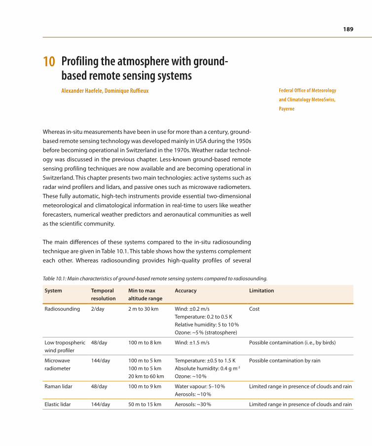
189
10 Profiling the atmosphere with ground-based remote sensing systemsAlexander Haefele, Dominique Ruffieux
Whereas in-situ measurements have been in use for more than a century, ground-based remote sensing technology was developed mainly in USA during the 1950s before becoming operational in Switzerland in the 1970s. Weather radar technol-ogy was discussed in the previous chapter. Less-known ground-based remote sensing profiling techniques are now available and are becoming operational in Switzerland. This chapter presents two main technologies: active systems such as radar wind profilers and lidars, and passive ones such as microwave radiometers. These fully automatic, high-tech instruments provide essential two-dimensional meteorological and climatological information in real-time to users like weather forecasters, numerical weather predictors and aeronautical communities as well as the scientific community.
The main differences of these systems compared to the in-situ radiosounding technique are given in Table 10.1. This table shows how the systems complement each other. Whereas radiosounding provides high-quality profiles of several
Federal Office of Meteorology
and Climatology MeteoSwiss,
Payerne
Table 10.1: Main characteristics of ground-based remote sensing systems compared to radiosounding.
System Temporal resolution
Min to max altitude range
Accuracy Limitation
Radiosounding 2/day 2 m to 30 km Wind: ±0.2 m/s Temperature: 0.2 to 0.5 K Relative humidity: 5 to 10 % Ozone: ~5 % (stratosphere)
Cost
Low tropospheric wind profiler
48/day 100 m to 8 km Wind: ±1.5 m/s Possible contamination (i. e., by birds)
Microwave radiometer
144/day 100 m to 5 km 100 m to 5 km 20 km to 60 km
Temperature: ±0.5 to 1.5 K Absolute humidity: 0.4 g m-3 Ozone: ~10 %
Possible contamination by rain
Raman lidar 48/day 100 m to 9 km Water vapour: 5–10 % Aerosols: ~10 %
Limited range in presence of clouds and rain
Elastic lidar 144/day 50 m to 15 km Aerosols: ~30 % Limited range in presence of clouds and rain

190 From weather observations to atmospheric and climate sciences in Switzerland10
parameters with a high vertical resolution and a good vertical coverage, ground-based remote sensing systems are often limited to measuring one or two param-eters, though they are fully automatic and able to measure at a high temporal resolution. Examples of time-series from these ground-based remote sensing sys-tems operated in Switzerland can be found in Figure 10.1.
Time (UTC)
Alti
tude
(m
asl
)
−20
−18−16
−16
−14−14
−14
−14−12
−12
−12 −12
−10
−10
−10−10
−10
−8
−8
−8
−8
−8
−6
−6
−6
−6−6
−4
−4
−4−4 −4
−2
−2
−2
−2
−2 −2
−2
0
0 0
0
0
0 0
0
2
2
22
4 4
4
6
6
6
8
03 09 15 21 03 09 15 210
1000
2000
3000
4000
5000
Tem
pera
ture
(° C)
−30
−20
−10
0
10
20
Figure 10.1: Typical profile time-series obtained with ground-based remote sensing systems. Upper left panel: radar wind profiler time-series of wind speed and direction, Julier Pass, 6 November, 1999. One can observe northerly winds (cold front) close to the ground topped by southerly winds (foehn). Upper right panel: microwave radiometer temperature profile time-series, Payerne, 9–10 March, 2012. The diurnal cycle of temperature as well as a temperature increase with time above can be well observed during this 18-hour clear-day period. Lower left panel: elastic lidar (ceilometer) aerosol profile time-series, Payerne, 24 June 2015. High aerosol concentration in the boundary layer below approxi-mately 2000 m as well as aerosols in the free troposphere above are visible. Lower right panel: Raman lidar humidity profile time-series, Payerne, 8–9 April, 2011. Intrusion of water vapour into the planetary boundary layer is visible during the second night of the period.
Time (UTC)
Alti
tude
(m
asl
)
00 06 12 18 00 06 120
1000
2000
3000
4000
5000
6000
7000
8000
9000
Mix
ing
Rat
io (
g/kg
)0
1
2
3
4
5
6
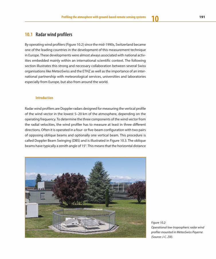
191Profiling the atmosphere with ground-based remote sensing systems 10
10.1 Radar wind profilers
By operating wind profilers (Figure 10.2) since the mid-1990s, Switzerland became one of the leading countries in the development of this measurement technique in Europe. These developments were almost always associated with national activ-ities embedded mainly within an international scientific context. The following section illustrates this strong and necessary collaboration between several Swiss organisations like MeteoSwiss and the ETHZ as well as the importance of an inter-national partnership with meteorological services, universities and laboratories especially from Europe, but also from around the world.
Introduction
Radar wind profilers are Doppler radars designed for measuring the vertical profile of the wind vector in the lowest 5–20 km of the atmosphere, depending on the operating frequency. To determine the three components of the wind vector from the radial velocities, the wind profiler has to measure at least in three different directions. Often it is operated in a four- or five-beam configuration with two pairs of opposing oblique beams and optionally one vertical beam. This procedure is called Doppler Beam Swinging (DBS) and is illustrated in Figure 10.3. The oblique beams have typically a zenith angle of 15°. This means that the horizontal distance
Figure 10.2: Operational low-tropospheric radar wind profiler mounted in MeteoSwiss Payerne (Source: J-C. Zill).

192 From weather observations to atmospheric and climate sciences in Switzerland10
between the oblique beam and the vertical beam is 1500 m at a height of 6 km (3000 m between the oblique beams), which is in the order of the mesh size of a regional weather prediction model. The height information is derived from the travel time of the pulse. Typical profile time-series from a radar wind profiler are shown in Figures 10.1 and 10.4.
The unique characteristic of radar wind profilers is their use of longer wavelengths, compared to classical weather radars. The typical wavelength range is from about 20 cm (L-Band) to about 6 m (VHF). Electromagnetic waves in this range are scat-tered by fluctuations of the refractive index of particle-free “clear air,” which are almost omnipresent due to the turbulent state of the atmosphere. This effect is called clear-air scattering. In case of precipitation, the three-dimensional motions of the droplets reflect a much stronger signal than clear air does. While vertical motions can be easily filtered, horizontal velocities might be biased in case of heavy precipitation events. More details on radar wind profiler fundamentals, operational use, error characteristics, practical aspects, as well as wind profiler challenges can be found in http://cfa.aquila.infn.it/wiki.eg-climet.org/index.php5/Final_Report. Comprehensive reviews of the technical and scientific aspects of radar wind profilers have been provided, among others, by Fukao (2007).
Radar wind profilers are also able to provide additional information about the atmospheric state (e. g., melting level, cloud top and planetary boundary layer) through the profiles of backscattered signal intensity and frequency spread (spec-tral width) of the echo signal. In contrast to the automated wind measurement, however, such data need still to be carefully analyzed because of the complexity of the measurement process (Bianco et al., 2008; Collaud Coen et al., 2014).
Frequency issues
The high sensitivity of the radar wind profilers makes them vulnerable to any external radio-frequency interference of sufficient strength that is in-band. Fre-quency management is therefore an essential issue for operational networks. As more and more technical applications come to use electromagnetic waves, the frequency spectrum has become an important resource. Radar wind profiler fre-quency allocations are assigned for the bands 50 MHz, 400 MHz and 1000 MHz, depending on the International Telecommunication Union (ITU) Region. Switzer-land took an active role in the debate on radar wind profiler frequency allocation in Europe (Richner and Griesser, 1996a and 1996b; Dibbern et al., 2003).
Figure 10.3: Illustration of the typical scan strategy of a radar wind profiler called Doppler Beam Swinging (DBS).
193Profiling the atmosphere with ground-based remote sensing systems 10
Frequency allocations have been constantly under pressure from other intended usage of radar wind profiler bands. For example, the European Radio Navigation Satellite Service GALILEO uses an L-band frequency range assigned to bound-ary-layer radar wind profilers. Compatibility studies (e. g., ECC, 2006) are therefore necessary to ensure the best possible protection.
Radar wind profiler historical development
After the first successful demonstration of clear-air wind measurements by Wood-man and Guillen (1974), the potential capabilities of the radar wind profiler tech-nique for meteorological applications became suddenly apparent (Larsen and Röttger, 1982), so that meteorological profiler systems were eventually suggested (Hogg et.al., 1983). A historical overview of wind-profiling radars can be found in van Zandt (2000). The first truly operational network, the Wind Profiler Demonstra-tion Network (WPDN), was built in the United States and completed in 1992. It became later known as the NOAA National Profiler Network (Federal Coordinator for Meteorological Services and Supporting Research, 1998).
In Europe, a demonstration of radar wind profiler networking was organised during the COST Action 76 (European Research Programme) in early 1997 (Dib-bern et al., 2003) as the “COST WIND Initiative for a Network Demonstration in Europe Project” (Nash and Oakley, 2001). Since 2015, the operational European radar wind profiler network consists of 30 systems including three in Switzerland (http://www.eumetnet.eu/e-profile). This network is dedicated mainly to provid-ing real-time data for assimilation into numerical weather prediction model and as a complementary tool for weather forecasters.
In Switzerland, first radar wind profiler tests were undertaken in the early 1990s at the MeteoSwiss regional centre of Payerne in close collaboration with ETH Zurich. The main goal of these tests was to study the feasibility of running a wind profiler in operational mode in Switzerland (Steiner, 1994). The first L-band radar wind profiler became operational in 1995 and was operated in Payerne as well as in several locations inside and outside Switzerland, e. g., during the Mesoscale Alpine Programme (MAP) in 1999 on the Julier Pass (Ruffieux and Stübi, 2001), during the PIPAPO experiment in Northern Italy (Ruffieux, 1999), and in downtown Basel during the urban heat island BUBBLE Experiment in 2002 (Rotach et al., 2005). Several studies used also data from this L-band radar wind profiler to improve signal processing (Griesser, 1998) as well as to develop new filtering techniques
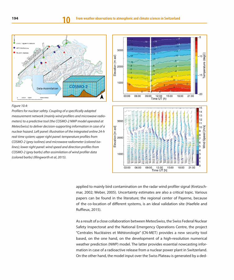
194 From weather observations to atmospheric and climate sciences in Switzerland10
applied to mainly bird contamination on the radar wind profiler signal (Kretzsch-mar, 2002; Weber, 2005). Uncertainty estimates are also a critical topic. Various papers can be found in the literature; the regional center of Payerne, because of the co-location of different systems, is an ideal validation site (Haefele and Ruffieux, 2015).
As a result of a close collaboration between MeteoSwiss, the Swiss Federal Nuclear Safety Inspectorat and the National Emergency Operations Centre, the project “Centrales Nucléaires et Météorologie” (CN-MET) provides a new security tool based, on the one hand, on the development of a high-resolution numerical weather prediction (NWP) model. The latter provides essential nowcasting infor-mation in case of a radioactive release from a nuclear power plant in Switzerland. On the other hand, the model input over the Swiss Plateau is generated by a ded-
Figure 10.4: Profilers for nuclear safety. Coupling of a specifically adapted measurement network (mainly wind profilers and microwave radio-meters) to a predictive tool (the COSMO-2 NWP model operated at MeteoSwiss) to deliver decision-supporting information in case of a nuclear hazard. Left panel: illustration of the integrated online 24-h real-time system; upper right panel: temperature profiles from COSMO-2 (grey isolines) and microwave radiometer (colored iso-lines); lower right panel: wind speed and direction profiles from COSMO-2 (grey barbs) after assimilation of wind profiler data ( colored barbs) (Illingworth et al, 2015).

195Profiling the atmosphere with ground-based remote sensing systems 10
icated network of surface and upper air observations including remote sensing instruments (radar wind profilers and temperature/humidity passive microwave radiometers). This network consists of three main sites ideally located for measur-ing the inflow/outflow and central conditions of the main wind field in the plane-tary boundary layer over the Swiss Plateau as well as a number of surface auto-matic weather stations (AWS). The network data are assimilated in real-time into a fine grid NWP model using a rapid update cycle of eight runs per day (one forecast every 3 hours). This high resolution NWP model has replaced the former security tool based on in-situ observations (in particular one meteorological mast at each of the power plants) and a local dispersion model. It is used to forecast the dynamics of the atmosphere in the planetary boundary layer (typically the first 4 km above ground layer) and over a time period of 24 h. This tool provides at any time (e. g., starting at the initial time of a nuclear power plant release) the best picture of the 24-h evolution of the air mass over the Swiss Plateau and further-more generates the input data (in the form of simulated values substituting for in-situ observations) required for the local dispersion model used at each of the nuclear power plants locations (Calpini et al, 2011). This system (Figure 10.4) has been fully operational since 2010.
10.2 Ground-Based Microwave Radiometry
Introduction
Microwave radiometry is widely used from space and from the ground to measure the thermodynamic state and the chemical composition of the atmosphere. A microwave radiometer (Figure 10.5) is a passive instrument that measures electro-magnetic radiation in the microwave region, i. e., at frequencies between approx-imately 3 and 300 GHz (1–100 mm wavelength).
The measured radiation depends on the composition and the temperature of the atmosphere as described by the radiative transfer equation
Tbðf,zÞ ¼ T0 e�τðf,zÞ þZz∞
z
Tðz0Þ�ðf,z0Þe�τðf,z0Þdz0
Where Tb(f,z) is the brightness temperature at frequency f and surface altitude z, T0 is the cosmic background, τ(f,z) is the opacity between top of the atmosphere z∞ and the altitude z, T(z’) is the physical temperature at altitude z’, and α(f,z’) is the
Figure 10.5: Operational microwave radiometer profiler mounted in MeteoSwiss Payerne in 2009 (Calpini et al., 2011) (Source: B. Ruffieux).

196 From weather observations to atmospheric and climate sciences in Switzerland10
absorption coefficient at altitude z’. Note that α depends on the number density of the molecules as well as on temperature and pressure. Figure 10.6 shows the simulated microwave spectrum as it would be measured at different altitudes by a radiometer looking upward. The precise shape of the spectrum depends on the spectroscopy and the number density of the molecules present in the atmosphere as well as on the temperature and pressure profiles. Therefore, profiles of atmo-spheric species, such as water vapour or ozone, and temperature can be retrieved from measured microwave spectra as explained below. For a more thorough dis-cussion of microwave radiometry, the interested reader is referred to Janssen (1993).
To calculate the parameter of interest (i. e., water vapour, ozone or temperature) from a measured spectrum, the radiative transfer equation needs to be inverted. This problem is generally mathematically ill-posed and is solved using special inverse methods like optimal estimation. The inversion provides an averaging ker-nel for each profile which shows the response of the retrieval to a perturbation in the real atmosphere at a given altitude. It hence characterizes the vertical resolu-tion and the sensitivity of the retrieval. Figure 10.7 shows an example of an aver-aging kernel of a tropospheric temperature measurement and a stratospheric ozone retrieval from microwave measurements at 60 and 142 GHz, respectively.
Figure 10.6: Simulated emission spectra as observed in zenith direction at three different altitudes (from Kämpfer et al., 2013).

197Profiling the atmosphere with ground-based remote sensing systems 10
The averaging kernel reveals the relatively coarse vertical resolution characteristic of ground-based microwave radiometry, which does not allow for resolving sharp features. On the other hand, it is possible to do continuous observations with a high temporal resolution allowing for the detection of variations with short peri-odicities in the order of minutes to hours.
Ground-based observations of ozone with microwave radiometers over Switzer-land started in the 1980s at the Institute of Applied Physics (IAP) of the University of Berne (Lobsiger and Künzi, 1986; Lobsiger, 1987; Zommerfelds et al., 1989). Con-tinuous observations of the ozone layer started in the early 1990s at the IAP with the GROMOS instrument (Peter, 1997). In the framework of the Global Atmosphere Watch (GAW) program, MeteoSwiss complemented its operational ozone mea-surements at Payerne and Arosa (see Chapters 7 and 16) with a microwave radi-ometer in the year 2000 and since performs routine measurements (Calisesi, 2003).
Figure 10.7: Left panel: Averaging kernel of an ozone retrieval. The measurement was made with a spectral resolution of 60 kHz, a bandwidth of 1 GHz and a time integration of 30 min. Right panel: Averaging kernel of a retrieval of tropospheric temperature (from Löhnert and Maier, 2012). The measurement was made with seven broadband channels at six different elevation angles. The integration time is a few seconds for each elevation angle and frequency. The colored lines correspond to different perturbation heights.

198 From weather observations to atmospheric and climate sciences in Switzerland10
This was also the start of a close collaboration between the IAP and MeteoSwiss. Middle atmospheric water vapour became a research focus at the IAP (Kämpfer et al., 2003) and space-borne (Croskey et al., 1992), airborne (Peter, 1998) and ground-based (Deuber et al., 2005) experiments have been developed to measure water vapour from the ground up to the mesopause.
Microwave measurements of tropospheric humidity and temperature became more and more interesting for meteorological applications because of their capa-bility to continuously measure the thermodynamic state of the lower troposphere (Solheim et al., 1998; Crewell et al., 2001; Ware et al., 2003; Martin et al., 2006). The Temperature and hUmidity Campaign (TUC), organised by MeteoSwiss at the regional center of Payerne, was an extensive intercomparison campaign to char-acterise novel instruments like microwave radiometers and cloud radars (Ruffieux et al., 2006). Tropospheric humidity and temperature microwave profilers have been in operational use at MeteoSwiss since 2006 (Calpini et al., 2011; Löhnert und Maier, 2012).
The arrival of digital fast Fourier transform spectrometers in the microwave com-munity (Müller et al., 2009) allowed for the observation of other parameters like middle atmospheric wind and temperature (Rüfenacht et al., 2014; Stähli et al., 2013). With these latest developments four of the Global Climate Observing Sys-tem (GCOS) essential climate variables can be continuously measured by ground-based microwave radiometry.
Monitoring Climate Change
Microwave radiometers are robust and stable instruments and therefore very well suited for long-term observations. The Network for the Detection of Atmospheric Composition Change (NDACC) coordinates the operation of about 10 microwave radiometers and a suite of other remote-sensing instruments, collecting their data in a central database. This network provided additional evidence for the decline of stratospheric ozone in the 1980s and 1990s (Steinbrecht et al., 2009). Figure 10.8 shows the 14-year record of stratospheric and mesospheric ozone above Payerne.
Ozone shows a pronounced diurnal cycle in the upper stratosphere and meso-sphere, which has been extensively studied with microwave radiometers (Lob-siger and Künzi, 1986; Zommerfelds et al., 1989; Connor et al., 1994). Technical improvements recently allowed us also to address diurnal variations in strato-

199Profiling the atmosphere with ground-based remote sensing systems 10
spheric ozone and water vapour (Haefele et al., 2008, Scheiben et al., 2013, Studer et al., 2014). These variations are important for the understanding of middle atmo-spheric dynamics and photochemistry and for the interpretation of satellite data, which are taken at specific hours during the day. Hence, drifts in the orbit param-eters can shift the satellite measurements to different solar times, which produces an artificial trend in the time-series at altitudes where a diurnal cycle is present.
Water vapour is the most important greenhouse gas and plays a key role in the radiative budget of the atmosphere. Under the assumption of constant relative humidity, water vapour increases with increasing temperature and presents a pos-itive feedback to temperature increases due to greenhouse gas emissions (Dessler et al., 2008). Long-term observations of integrated water vapour made at Berne by the IAP with a dual-channel microwave radiometer revealed a positive trend of 3.9 %/decade, which is consistent with trends derived from radiosondes and sun photometer measurements performed by MeteoSwiss at the regional center of Payerne (Morland et al., 2009; Hocke et al., 2011). Other long-term observations of water vapour with microwave radiometers and other instruments are carried out in the framework of the Atmospheric Radiation Measurement (ARM) program (Revercomb et al., 2003).
Applications in Meteorology
The tropospheric temperature and humidity microwave profilers are of particular interest for meteorology and numerical weather prediction. These instruments provide profiles of the temperature and humidity with a vertical resolution of a
Figure 10.8: Time series of stratospheric and meso-spheric ozone volume mixing ratio as observed by the microwave radiometer SOMORA above Payerne from 2000 to 2014. The maximum of the ozone layer at 35 km can be easily seen as well as the seasonal cycle with higher ozone concen-trations in the Summer.
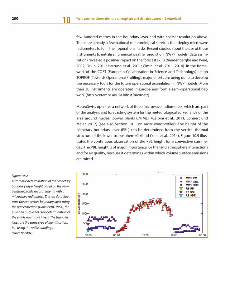
200 From weather observations to atmospheric and climate sciences in Switzerland10
few hundred metres in the boundary layer and with coarser resolution above. There are already a few national meteorological services that deploy microwave radiometers to fulfil their operational tasks. Recent studies about the use of these instruments to initialise numerical weather prediction (NWP) models (data assim-ilation) revealed a positive impact on the forecast skills (Vandenberghe and Ware, 2002; Otkin, 2011; Hartung et al., 2011; Cimini et al., 2011, 2014). In the frame-work of the COST (European Collaboration in Science and Technology) action TOPROF (Towards Operational Profiling), major efforts are being done to develop the necessary tools for the future operational assimilation in NWP models. More than 30 instruments are operated in Europe and form a semi-operational net-work (http://cetemps.aquila.infn.it/mwrnet/).
MeteoSwiss operates a network of three microwave radiometers, which are part of the analysis and forecasting system for the meteorological surveillance of the area around nuclear power plants CN-MET (Calpini et al., 2011; Löhnert und Maier, 2012) (see also Section 10.1. on radar windprofiler). The height of the planetary boundary layer (PBL) can be determined from the vertical thermal structure of the lower troposphere (Collaud Coen et al., 2014). Figure 10.9 illus-trates the continuous observation of the PBL height for a convective summer day. The PBL height is of major importance for the land atmosphere interactions and for air quality, because it determines within which volume surface emissions are mixed.
Figure 10.9: Automatic determination of the planetary boundary layer height based on the tem-perature profile measurements with a microwave radiometer. The red dots illus-trate the convective boundary layer using the parcel method (Holzworth, 1964), the blue and purple dots the determination of the stable nocturnal layers. The triangles illustrate the same type of identification, but using the radiosoundings (twice per day).
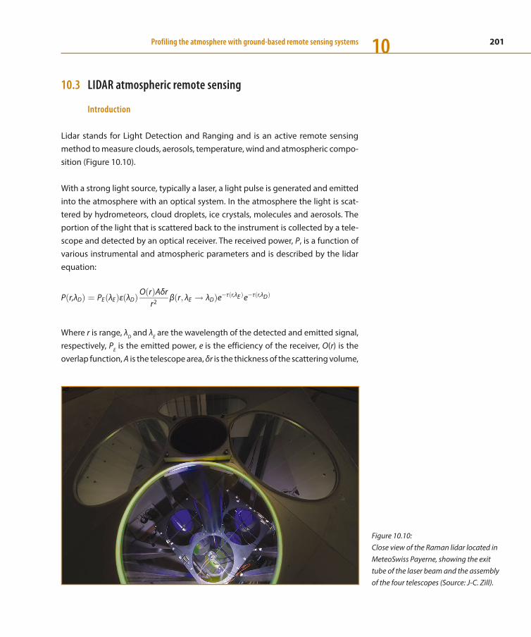
201Profiling the atmosphere with ground-based remote sensing systems 10
10.3 LIDAR atmospheric remote sensing
Introduction
Lidar stands for Light Detection and Ranging and is an active remote sensing method to measure clouds, aerosols, temperature, wind and atmospheric compo-sition (Figure 10.10).
With a strong light source, typically a laser, a light pulse is generated and emitted into the atmosphere with an optical system. In the atmosphere the light is scat-tered by hydrometeors, cloud droplets, ice crystals, molecules and aerosols. The portion of the light that is scattered back to the instrument is collected by a tele-scope and detected by an optical receiver. The received power, P, is a function of various instrumental and atmospheric parameters and is described by the lidar equation:
Pðr,λDÞ ¼ PEðλEÞεðλDÞOðrÞAδr
r2βðr; λE ! λDÞe�τðr,λEÞe�τðr,λDÞ
Where r is range, λD and λE are the wavelength of the detected and emitted signal, respectively, PE is the emitted power, e is the efficiency of the receiver, O(r) is the overlap function, A is the telescope area, δr is the thickness of the scattering volume,
Figure 10.10: Close view of the Raman lidar located in MeteoSwiss Payerne, showing the exit tube of the laser beam and the assembly of the four telescopes (Source: J-C. Zill).

202 From weather observations to atmospheric and climate sciences in Switzerland10
β is the backscatter coefficient for the wavelength shift λE→λD, e–τ(r,λE) and e–τ(r,λD) are the transmittances of the atmosphere between the instrument and range r at the detected and emitted wavelengths, respectively. Note that the backscatter coefficient and the opacity depend on the number densities of the intervening scattering and absorbing atmospheric components (aerosols and atmospheric gases). With numerical methods the lidar equation can be solved for those number densities or for the backscatter and extinction coefficients. For more detailed infor-mation the reader is referred to Weitkamp 2005 and references therein.
A variety of lidars exist that utilise different properties of scattering and extinction in the atmosphere. The following list is not exhaustive, but should give a very brief overview of the currently used techniques.
– Elastic lidarThe elastic lidar is used to measure the cloud base and aerosols (backscatter and extinction coefficient) as well as temperature in aerosol-free regions like the upper stratosphere and mesosphere. It works with a single wavelength for emission and detection (λE=λD) and is thus sensitive to elastic scattering. Typi-cal elastic scattering mechanisms are Rayleigh and Mie scattering, which occur on molecules, aerosols, cloud droplets and hydrometeors for wavelengths in the ultraviolet, visible and near-infrared region.
– Raman lidarThe Raman lidar is mostly used to measure profiles of temperature and water vapour as well as the extinction coefficient. It emits at one wavelength and detects at several specific wavelengths. Because of inelastic scattering, the backscattered light has a different wavelength compared to the emitted light (λE≠λD). The typical scattering mechanism is Raman scattering, which gives this type of lidar its name. In the case of vibrational Raman scattering, the change in wavelength is characteristic for the scattering molecule which allows mea-suring specific gazes in the atmosphere. In the case of pure rotational Raman scattering, the scattering cross-section is strongly temperature dependent and a temperature profile can be derived from the lidar return.
– Differential absorption lidar (DIAL)The differential absorption lidar (DIAL) is used mostly to perform range-re-solved measurements of trace gases like ozone or water vapour. A DIAL is able to emit and receive simultaneously at two specific wavelengths at which the light is strongly and weakly absorbed by the gas under consideration, respec-tively. The gas concentration can be derived from calculating the difference in the power of the received signals while knowing the absorption cross-section at the two wavelengths.
203Profiling the atmosphere with ground-based remote sensing systems 10
– Doppler lidarThe Doppler lidars measures atmospheric wind and turbulence. Through its design it is able to measure the small wavelength shift due to the speed of the scattering object (typically aerosols) relative to the lidar. The Doppler law then allows derivation of the radial speed of the scattering object from the wave-length shift, in the same way as for radar wind profilers (see Section 10.1).
Air quality
Lidar activities started at the Ecole Politechnique Fédérale de Lausanne (EPFL) in the context of testing air quality in the late 1980s. A scanning mobile differential absorption lidar (DIAL) was developed to measure the key pollutants NO2, SO2 and O3 in 3 dimensions with high spatial and temporal resolution (Wolf and Wöste, 1987; Kölsch et al., 1989). Several measurement campaigns in the vicinity of indus-trial sources were made and the measurements were used to validate the mod-elled 3-D field of the pollutants (Beniston et al., 1990). Later, differential absorption lidars (DIAL) for ozone were developed and used in field campaigns to study urban pollution (Calpini et al., 1997). The DIAL technique was improved through the development of Raman-shifting cells to generate high-power light emission at two different wavelengths (Schoulepnikoff et al., 1997). The DIAL technique was coupled with an innovative correlative method to determine the radial wind, which in turn allowed us to determine ozone fluxes (Fiorani et al., 1998). Ozone flux measurements were further improved by the combination of ground-based and airborne lidars with wind profilers, which allowed determination also of the horizontal flux components (Quaglia et al., 1999). The ozone measurements were complemented with water vapour measurements using the Raman lidar method (Lazzarotto et al., 2001). Water vapour was used as a tracer of the vertical mixing and allowed to determine the height of the boundary layer, which is a very impor-tant parameter in air quality because it defines the volume in which the pollutants are dispersed (Froidevaux et al., 2013).
Climate change
When the focus of the atmospheric sciences and society shifted from air quality to climate change at the beginning of this century, the Air Pollution Laboratory of EPFL committed to contributing to the open questions surrounding the role of aerosols and water vapour in climate change (IPCC 2001). For this purpose a

204 From weather observations to atmospheric and climate sciences in Switzerland10
Raman lidar was developed for the measurement of water vapour and aerosols at the Jungfraujoch (Larchevêque et al., 2002). The system had a small built-in tele-scope for tropospheric measurements and used the existing 76-cm Casseg-rain-type astronomical telescope for observations in the stratosphere and meso-sphere. Figure 10.11 shows a night-time picture of the lidar in operation. This pioneering work will be honoured on the new 200 Swiss Franks bill (www.snb.ch).
Operational meteorology
In order to study relative humidity and boundary layer processes, lidars were designed to simultaneously measure water vapour, aerosols and temperature (Balin et al., 2004). This new capability to measure relative humidity was also of major interest for applications in meteorology. In 2004 MeteoSwiss, together with EPFL, launched a project co-financed by the National Science Foundation (NSF) to develop a fully automatic Raman lidar for meteorological applications. This lidar measures water vapour, aerosol and temperature simultaneously during night and day (Dinoev et al., 2013; Brocard et al., 2013). After the devel-opment, construction and testing at EPFL, it was taken over by MeteoSwiss in 2007 and has since been operated at the regional center of Payerne. The instru-ment is unique in its capability to operate unattendedly and demonstrates how this technology meets standards of operational meteorology. Further, the water vapour measurements reach the lower stratosphere covering the weather rele-vant part of the atmosphere as well as the altitude region of the UTLS (upper troposphere and lower stratosphere), which is a key region for climate change.
Figure 10.11: Night-time picture of the “Ecole Poly-technique Federal Lausanne” (EPFL) lidar system at Jungfraujoch, Switzerland. Photo from Larchevêque et al., 2002.
Figure 10.12: Monthly mean water vapour volume mixing ratio above Payerne, Switzerland, at approximately 11 km, as measured by the operational Raman lidar.

205Profiling the atmosphere with ground-based remote sensing systems 10
Figure 10.12 shows the annual cycle of upper tropospheric humidity above Pay-erne from 2007 to 2014.
Aerosol stratification and boundary layer
Lidar activities started at the Observatoire de Neuchâtel at around the same time as at EPFL. However, this research group focussed on studying the aerosol stratifi-cation in the boundary layer and the free troposphere with elastic backscatter lidars (Frioud et al., 2004; Martucci et al., 2005; Mitev et al., 2005; Martucci et al., 2007). A major effort was effected to develop compact and portable depolariza-tion lidar systems suited for measurement campaigns (Mitev et al., 2011). The depolarization measurement allows differentiation of spherical and nonspherical particles, such as liquid cloud droplets and ice crystals. Such compact lidar systems were also deployed from the high altitude research aircraft Geophysica in order to detect polar stratospheric clouds in the polar region at an altitude of 20–25 km (Mitev et al., 2014).
MeteoSwiss operates a Raman lidar and two compact elastic lidars for the detec-tion of aerosols in the boundary layer and the free troposphere. Well-known aero-sol events are the long-range transport of Saharan dust (Papayannis et al., 2008) and, albeit very much rarer, volcanic ash (Pappalardo et al., 2013). Figure 10.13 shows the measurement of volcanic ash over Payerne after the eruption of the Eyjafjallajökull volcano in April 2010 as observed with the MeteoSwiss Raman lidar. With a special calibration method the ash mass density could be estimated,
Figure 10.13: Measurement of volcanic ash above Payerne, Switzerland, from 16 to 18 April 2010 after the eruption of the Eyjafjalla-jökull in Iceland. The measurement was performed with the operational Raman lidar of MeteoSwiss. Figure from Dinoev et al., 2010.

206 From weather observations to atmospheric and climate sciences in Switzerland10
which was the determining factor for the assessment of air safety and hence for the decision whether or not to close the airspace (Dinoev et al., 2010).
Wind Energy and Aviation
Doppler lidars measure wind in the lower troposphere at a very high temporal and spatial resolution. These instruments are nowadays technically mature, and are compact and suitable for unattended operation. This has opened up new applica-tion areas in the field of wind energy and aviation. The Wind Engineering and Renewable Energy Laboratory (WIRE) at EPFL uses Doppler lidars systematically to study the wakes of wind turbines and the effect of wind turbines on the boundary layer (Iungo et al., 2013; Iungo et al., 2014).
In the framework of pilot projects first Doppler lidar systems have been installed at airports for the detection of dangerous wind-shear situations and wake turbu-lences (Shun and Chan, 2008). Here, the application of Doppler lidars has a big potential, and this instrument is likely to be established as a standard method in the wind energy and aviation sector.
10.4 Summary
Ground-based remote sensing systems are assuming an ever greater role among the palette of available measurement techniques. Switzerland is an active partner in developing these systems and making them fully operational. Final users like the numerical weather prediction modelers are using ever finer grid meshes, and the aeronautical community is under great pressure to optimise their activities. Weather forecasters are more exactly tuning their forecasts, and more recently the renewable energy community as well as the scientific community in general have become keen on getting high-quality, high temporal resolution information on the state of the atmosphere. Ground-based remote sensing techniques are important actors in this game.
Switzerland is a small country and cannot develop these apparatus/procedures on its own without collaborating with the international community. At the interna-tional level, it can assist in the networking of all these systems in order to optimise data collection, quality control and real-time delivery of the products to the users (Illingworth et al, 2015).

207Profiling the atmosphere with ground-based remote sensing systems 10
References
Balin, I., I. Serikov, S. Bobrovnikov, V. Simeonov, B. Calpini, Y. Arshinov, and H. van den Bergh, 2004: Simultaneous measure-ment of atmospheric temperature, humidity, and aerosol extinction and backscatter coefficients by a combined vibra-tional–pure-rotational Raman lidar. Applied Physics B, 79(6), 775–782.
Beniston, M., J.-P. Wolf, M. Beniston-Rebetez, H. J. Kölsch, P. Pairoux, and L. Wöste, 1990: Use of Lidar Measurements and Numerical Models in Air Pollution Research. J. of Geophys. Res., 95, D7, 9879–9894.
Bianco L., J. M. Wilczak, and A. B. White, 2008: Convective boundary layer depth estimation from wind profilers: statistical comparison between an automated algorithm and expert estimations. J. Atmos. Ocean. Technol., 25, 1397–1413, doi: 10.1175/2008JTECHA981.1.
Brocard, E., R. Philipona, A. Haefele, G. Romanens, A. Mueller, D. Ruffieux, V. Simeonov, and B. Calpini, 2013: Raman Lidar for Meteorological Observations, RALMO – Part 2: Validation of water vapor measurements. Atmos. Meas. Tech., 6, 1347–1358.
Calisesi, Y., 2003: The stratospheric ozone monitoring radiome-ter SOMORA: NDSC application document. Tech. Rep. 2003-11, Inst. Of Appl. Phys., Univ. of Berne, Berne, 58 pp.
Calpini, B., V. Simeonov, F. Jeanneret, J. Kuebler, V. Sathya, H., and Van den Bergh, 1997: Ozone LIDAR as an Analytical Tool in Effec-tive Air Pollution Management: The Geneva 96 Campaign. Chimia, 51, 700–704.
Calpini B., D. Ruffieux, J.-M. Bettems, C. Hug, P. Huguenin, H.-P. Isaak, P. Kaufmann, O. Maier, and P. Steiner, 2011: Ground-based remote sensing profiling and numerical weather prediction model to manage nuclear power plants meteorological surveil-lance in Switzerland. Atmos. Meas. Tech., 4, 1617–1625, doi: 10.5194/amt-4-1617-2011.
Cimini, D., E. Campos, R. Ware, S. Albers, G. Giuliani, J. Oreamuno, P. Joe, S. E. Koch, S. Cober, and E. Westwater, 2011: Thermody-namic atmospheric profiling during the 2010 Winter Olympics using ground-based microwave radiometry. IEEE Trans. Geosci. Remote Sens., 49, 4959–4969.
Cimini D., O. Caumont, U. Löhnert, L. Alados-Arboledas, R. Bleisch, T. Huet, M. E. Ferrario, F. Madonna, A. Haefele, F. Nasir, G. Pace, and R. Posada, 2014: A data assimilation experiment of temperature and humidity profiles from an international net-work of ground-based microwave radiometers. Proc. Microrad 2014, Pasadena, USA, 24–27 March, ISBN: 978-1-4799-4645-7, 978-1-4799-4644-0/14/$31.00, doi: 10.1109/MicroRad.2014. 6878913.
Collaud Coen M., C. Praz, A. Haefele, D. Ruffieux, P. Kaufmann, and B. Calpini, 2014: Determination and climatology of the planetary boundary layer height above the Swiss plateau by in situ and remote sensing measurements as well as by the COSMO-2 model. Atmos. Chem. Phys., 14, 13205–13221, doi: 10.5194/acp-14 13205-2014.
Connor, B. J., D. E. Siskind, J. J. Tsou, A. Parrish, and E. E. Rems-berg, 1994: Ground-based microwave observations of ozone in the upper stratosphere and mesosphere. J. Geophys. Res., 99, 16757–16770.
Crewell, S., H. Czekala, U. Löhnert, and C. Simmer, 2001: Micro-wave Radiometer for Cloud Carthography: A 22–channel ground–based microwave radiometer for atmospheric research. Radio Science, 36, 621–638.
Croskey, C. L., and Coauthors, 1992: The Millimeter Wave Atmo-spheric Sounder (MAS), 1992: A shuttle-based remote sens-ing experiment. IEEE Transactions on Microwave Theory and Techniques, 40, 1090–1100, doi: 10.1109/22.141340.
Dessler, A. E., Z. Zhang, and P. Yang, 2008: Water-vapor climate feedback inferred from climate fluctuations, 2003–2008. Geo-physical Research Letters, 35, L20704, doi: 10.1029/2008GL035333.
Deuber, B., A. Haefele , D. G., Feist, L. Martin, N. Kämpfer, G. E. Nedoluha, V. Yushkov, S. Khaykin, R. Kivi, and H. Vömel, 2005: Middle Atmospheric Water Vapour Radiometer – MIAWARA: Val-idation and first results of the LAUTLOS / WAVVAP campaign. J. of Geophys. Res., 110, D13306, doi: 10.1029/2004JD005543.
Dibbern J., W. Monna, J. Nash, and G. Peters (Eds.), 2003: Devel-opment of VHF/UHF wind profilers and vertical sounders for use in European observing systems. EUR 20614 – COST Action 76, 433 pp.
208 From weather observations to atmospheric and climate sciences in Switzerland10
Dinoev, T. S., V. Simeonov, B. Calpini, and M. B. Parlange, 2010: Monitoring of Eyjafjallajökull Ash Layer Evolution over Payerne Switzerland with a Raman Lidar. Proceedings of the TECO 2010, Helsinki, Finland, 7pp.
Dinoev, T., V. Simeonov, Y. Arshinov, S. Bobrovnikov, P. Ristori, B. Calpini, M. Parlange, and H. van den Bergh, 2013: Raman Lidar for Meteorological Observations, RALMO – Part 1: Instrument description. Atmos. Meas. Tech., 6, 1329–1346.
Electronic Communications Committee (ECC), 2006: Compati-bility of Wind Profilers radars in the radiolocation service (RLS) with the radionavigation satellite service (RNSS) in the band 1270–1295 MHz. ECC Report90, 98 pp.
Federal Coordinator for Meteorological Services and Support-ing Research, 1998: U. S. Wind Profilers: A review. FCM-R14-1998, 37pp.
Fiorani, L., B. Calpini, L. Jaquet, H. Van den Bergh, and E. Durieux, 1998: A combined determination of wind velocities and ozone concentrations for a first measurement of ozone fluxes with a DIAL instrument during the MEDCAPHOT-TRACE campaign. Atm. Env., 32(12), 2151–2159.
Frioud, M., V. Mitev, R. Matthey, H. Richner, M. Furger, and S. Gub-ser, 2004: Variation of the aerosol stratification over the Rhine Valley 13 during Foehn development: A backscatter lidar study. Met. Zeitschrift., 13, 175–181.
Froidevaux, M. , C. W. Higgins b, V. Simeonov, P. Ristori, E. Pardy-jak, I. Serikov, R. Calhoun, H. van den Bergh, and M. B. Parlange, 2013: A Raman lidar to measure water vapor in the atmospheric boundary layer. Advances in Water Resources, 51, 345–356.
Fukao S., 2007: Recent advances in atmospheric radar study, 2007. Journal of the Meteorological Society of Japan, 85B, 215–239.
Griesser T., 1998: Multipeakanalyse von Dopplerspektren aus Windprofiler-Radar-Messungen. Diss. Naturwiss. ETH Zurich, Nr. 12470, Switzerland, 114 pp.
Haefele, A., K. Hocke, N. Kämpfer, P. Keckhut, M. Marchand, S. Bekki, B. Morel, Egorova, T., and E. Rozanov, 2008: Diurnal changes in middle atmospheric H2O and O3: Observations in the Alpine region and climate models. J. Geophys. Res., 113, D17303, doi: 10.1029/2008JD009892.
Haefele, A., and D. Ruffieux, 2015: Validation of the 1290MHz wind profiler at Payerne, Switzerland, using radiosonde GPS wind measurements. Meteorol. Appl. (2015), doi: 10.1002/met.1507.
Hartung, D. C., J. A. Otkin, R. A. Petersen, D. D. Turner, and W. F. Feltz, 2011: Assimilation of surface-based boundary layer pro-filer observations during a cool-season weather event using an observing system simulation experiment, Part II: Forecast assessment. Mon. Wea. Rev., 139, 2327–2346.
Hocke, K., N. Kämpfer, C. Gerber, and C. Mätzler, 2011: A com-plete long-term series of integrated water vapour from ground-based microwave radiometers. Int. J. of Remote Sensing, 32, 751–765.
Hogg, D. C., and Coauthors, 1983: An automatic profiler of the temperature, wind and humidity in the troposphere. J. Climate Appl. Meteor., 22, 807–831.
Holzworth, G. C., 1964: Estimates of mean maximum mixing depths in the contiguous United States. Mon. Wea. Rev., 92, 235–242.
Illingworth, A., D. Cimini, C. Gaffard, M. Haeffelin, V. Lehmann, U. Loehnert, E. O’Connor, and D. Ruffieux, 2015: Exploiting existing ground-based remote sensing networks to improve high reso-lution weather forecast. Bull. Amer. Meteor. Soc. doi: 10.1175/BAMS-D-13-00283.1, in press.
IPCC, 2001: Climate Change 2001: The Scientific Basis. Contribu-tion of Working Group I to the Third Assessment Report of the Intergovernmental Panel on Climate Change [Houghton, J. T.,Y. Ding, D. J. Griggs, M. Noguer, P. J. van der Linden, X. Dai, K. Mas-kell, and C. A. Johnson (Eds.)]. Cambridge University Press, Cam-bridge, United Kingdom and New York, NY, USA, 881 pp.
Iungo, G. V., Y.-T. Wu, and F. Porté-Agel, 2013: Field measure-ments of wind turbine wakes with lidars. J. of Atmos. and Oceanic Technol., 30, 2, 274–287.
Iungo, G. V., and F. Porte-Agel, 2014: Volumetric lidar scanning of wind turbine wakes under convective and neutral atmospheric stability regimes. J. of Atmos. and Oceanic Technol., 31, 10, 2035–2048.
Janssen, M. A. (Ed), 1993: Atmospheric remote sensing by micro-wave radiometry. Wiley Series in Remote Sensing, John Wiley & Sons, Inc, 572 pp.

209Profiling the atmosphere with ground-based remote sensing systems 10Kämpfer, N., B. Deuber, D. Feist, D. Gerber, C. Mätzler, L. Martin, J. Morland, and V. Vasic, 2003: Microwave remote sensing of water vapor in the atmosphere. Geographica Helvetica, 58, 81–89.
Kämpfer, N. (Ed), 2013: Monitoring atmospheric water vapor – ground based remote sensing and in situ measurements. Springer Verlag, 325 pp.
Kölsch, H. J., P. Rairoux, J. P. Wolf, and L. Wöste, 1989: Simulta-neous NO and NO2 DIAL Measurements using BBO crystals, Applied Optics, 28, 11, 2052–2056.
Kretzschmar R., 2002: A survey of neural network classifiers for local wind prediction. Diss. Naturwiss. ETH Zurich, No. 14538, Switzerland, 226 pp.
Larchevêque G., Balin I., Nessler R., Quaglia P., Simeonov V., Van den Bergh H., and Calpini B., 2002: Development of a multi-wavelength aerosol and water vapor lidar at the Jungfraujoch Alpine Station (3580 m ASL) in Switzerland, Applied Optics-LP, 41, 15, 2781–2790.
Larsen M. F., and J. Röttger, 1982: VHF and UHF Doppler radars as tools for synoptic research. Bull. Amer. Meteor. Soc., 63, 996–1008.
Lazzarotto, B., M. Frioud, G. Larchevêque, B. Mitev, P. Quaglia, V. Simeonov, A. Thompson, H. van den Bergh, and B. Calpini, 2001: Ozone and water-vapor measurements by Raman lidar in the planetary boundary layer: error sources and field measure-ments, Applied Optics, 40, 18, 2985–2997.
Lobsiger, E., and K. F. Künzi, 1986: Night-time increase of meso-spheric ozone measured with ground-based microwave radi-ometry, J. Atmos. Solar Terr. Phys., 48, 1153–1158.
Lobsiger, E., 1987: Ground-based microwave radiometry to determine stratospheric and mesospheric ozone profiles, J. of Atmos. Terrestrial Phys., 49, 5, 493–501.
Löhnert, U., and O. Maier, 2012: Operational profiling of tem-perature using ground-based microwave radiometry at Pay-erne: prospects and challenges. Atmos. Meas. Tech., 5, 1121–1134, doi: 10.5194/amt-5-1121-2012.
Martin, L., M. Schneebeli, and C. Mätzler, 2006: Tropospheric water and temperature retrieval for ASMUWARA. Met. Zeitschrift, 15, 37–44, doi: 10.1127/0941-2948/2006/0093.
Martucci, G., R. Matthey, V. Mitev, and H. Richner, 2005: Lidar determination of mixing layer height with high resolution. Proc. SPIE 5979, Remote Sensing of Clouds and the Atmosphere X, doi: 10.1117/12.627628, 597924-1 – 597924-10.
Martucci, G., R. Matthey, and V. Mitev, 2007: Comparison between backscatter Lidar and radiosonde measurements of the diurnal and nocturnal stratification in the lower tropo-sphere. J. Atmos. and Oceanic Technol., 24, 7, 1231–1244.
Mitev, V., R. Matthey, M. Frioud, M. K. Srivastava, S. Eckhardt, and A. Stohl, 2005: Backscatter lidar observation of the aerosol strat-ification in the lower troposphere during winter Bise: a case study. Met. Zeitschrift, 14, 663–669.
Mitev, V., R. Matthey, and V. Makarov, 2011: Compact micro-pulse backscatter lidar and examples of measurements in the planetary boundary layer. Rom. Journ. Phys., 56, 3–4, 437–447.
Mitev, V., R. Matthey, and V. Makarov, 2014: Backscatter-depolar-isation lidars on high-altitude research aircraft. Proc. SPIE 9292, 20th International Symposium on Atmospheric and Ocean Optics: Atmospheric Physics, doi: 10.1117/12.2075634, 929227-1- 929227-8.
Morland, J., M. Collaud Coen, K. Hocke, P. Jeannet, and C. Mät-zler, 2009: Tropospheric water vapor above Switzerland over the last 12 years. Atmos. Chem. Phys., 9, 5975–5988, doi: 10.5194/acp-9-5975-2009
Müller, S. C., A. Murk, C. Monstein, and N. Kämpfer, 2009: Inter-comparison of Digital Fast Fourier Transform and Acousto Opti-cal spectrometers for microwave radiometry of the atmosphere. IEEE Transactions on Geoscience and Remote Sensing, 47, 2233–2239.
Nash J., and T. J. Oakley, 2001: Development of COST 76 wind profiler network in Europe. Physics and Chemistry of the Earth, Part B: Hydrology, Oceans and Atmosphere, 26, 3, 193–199.
Otkin, J. A., D. C. Hartung, D. D. Turner, R. A. Petersen, W. F. Feltz, and E. Janzon, 2011: Assimilation of surface-based boundary layer profiler observations during a cool-season weather event using an observing system simulation experiment. Part I: Analy-sis impact. Mon. Wea. Rev., 139, 2309–2326.
Papayannis, A., and Coauthors, 2008: Systematic lidar obser-vations of Saharan dust over Europe in the frame of EARLINET

210 From weather observations to atmospheric and climate sciences in Switzerland10
(2000–2002). J. of Geophys. Res., 113, D10204, doi: 10.1029/2007 JD009028.
Pappalardo, G., and Coauthors, 2013: Four-dimensional distri-bution of the 2010 Eyjafjallajökull volcanic cloud over Europe observed by EARLINET. Atmos. Chem. Phys., 13, 4429–4450, doi: 10.5194/acp-13-4429-2013.
Peter, R., 1997: The ground-based millimeter-wave ozone spec-trometer-GROMOS, IAP Research Report. University of Berne, Berne, Switzerland, 23 pp.
Peter, R., 1998: Stratospheric and mesospheric latitudinal water vapor distributions obtained by an airborne millimeter-wave spectrometer. Journal of Geophysical Research, 103, 16275–16290.
Quaglia, P., G. Larchevêque, V. Simeonov, B. Lazzarotto, G. Ancel-let, H. Van den Bergh, and B. Calpini, 1999: Planetary boundary layer ozone fluxes from combined airborne, ground based LIDARs and Wind profilers measurements. Eur. J. of An. Chem. (Analusis), 27, 4, 305–310.
Revercomb, H. E., and Coauthors, 2003: The ARM program’s water vapor intensive observation periods. Bull. Amer. Meteor. Soc., 84, 2, 217–236.
Richner H., and T. Griesser, 1996a: Parameters for characterizing electromagnetic properties of wind profiler radars. ITU Radio Radiocommunication Study Groups, Document 8-2/10-E, 5 pp.
Richner H., and T. Griesser, 1996b: A comparative analysis of electromagnetic field intensities from Air Route Surveillance Radar (ARSR) and wind profilers radar (WPR) acting on aircraft. ITU Radiocommunication Study Groups, Document 8-2/7-E, 7 pp.
Rotach M. W., and Coauthors, 2005: BUBBLE – an urban bound-ary layer meteorology project. Theoretical and Applied Climatol-ogy, 81, 3–4, 231–261.
Rüfenacht, R., A. Murk, N. Kämpfer, P. Eriksson, and S. A. Buehler, 2014: Middle-atmospheric zonal and meridional wind profiles from polar, tropical and mid-latitudes with the ground-based microwave Doppler wind radiometer WIRA. Atmos. Meas. Tech., 7, 4491–4505.
Ruffieux D., 1999: Use of a wind profiler in a planetary boundary layer experiment. ANALYSIS, 1999, 27,4, 310–313.
Ruffieux D., and R. Stübi, 2001: Wind profiler as a tool to check the ability of two NWP models to forecast winds above highly complex topography. Met. Zeitschrift, 10, 6, 489–495, doi: 10.1127/0941-2948/2001/0010-0489.
Ruffieux D., J. Nash , P. Jeannet, and J. L. Agnew, 2006: The COST 720 temperature, humidity, and cloud profiling campaign: TUC. Met. Zeitschrift, 15, 5–10.
Scheiben, D., A. Schanz, B. Tschanz, and N. Kämpfer, 2013: Diur-nal variations in middle-atmospheric water vapor by ground-based microwave radiometry. Atmos. Chem. Phys., 13, 6877–6886.
Schoulepnikoff, L., V. Mitev, V. Simeonov, B. Calpini, and H. van den Bergh, 1997: Experimental investigation of high-power single-pass Raman shifters in the ultraviolet with Nd:YAG and KrF lasers. Applied Optics, 36, 21, 5026–5043.
Shun, C. M., and P. W. Chan, 2008: Applications of an infrared Doppler lidar in detection of wind shear. J. Atmos. Oceanic Tech-nol., 25, 637–655.
Solheim, F., J. R. Godwin, E. R. Westwater, Y. Han, S. J. Keihm, K. Marsh, and R. Ware, 1998: Radiometric profiling of temperature, water vapor and cloud liquid water using various inversion methods. Radio Science, 33, 393–404.
Stähli, O., A. Murk, N. Kämpfer, C. Mätzler, and P. Eriksson, 2013: Microwave radiometer to retrieve temperature profiles from the surface to the stratopause. Atmos. Meas. Tech., 6, 2477–2494.
Steinbrecht, W., and Coauthors, 2009: Ozone and temperature trends in the upper stratosphere at five stations of the Network for the Detection of Atmospheric Composition Change. Int. J. of Remote Sensing, 30, 3875–3886.
Steiner A., 1994: Doppler-Radar Windprofiler: Auswertemetho-den und Perspektiven für den Einsatz im operationellen Betrieb und in der Forschung. Diss. Naturwiss. ETH Zurich, No. 10520, Switzerland, 124 pp.
Studer, S., K. Hocke, A. Schanz, H. Schmidt, and N. Kämpfer, 2014: A climatology of the diurnal variations in stratospheric and mesospheric ozone over Bern, Switzerland. Atmos. Chem. Phys., 14, 5905–5919.
Vandenberghe F., and R. Ware, 2002: 4-dimensional variational assimilation of ground-based microwave observations during a
211Profiling the atmosphere with ground-based remote sensing systems 10winter fog event. International Symposium on Atmospheric Sensing with GPS, Tsukuba, Japan, 5 pp.
Van Zandt, T. E., 2000: A brief history of the development of wind-profiling or MST radars. Ann. Geophys., 18, 740–749, doi:10.1007/s00585-000-0740-4.
Ware, R., R. Carpenter, J. Güldner, J. Liljegren, T. Nehkorn, F. Sol-heim, and F. Vandenberghe, 2003: A multichannel radiometric profiler of temperature, humidity, and cloud liquid. Radio Science, 38, 8079, doi: 10.1029/2002RS002856, 4.
Weber H. C., 2005: Classification of contaminated data from wind profiler measurements by neural networks. Diss. Natur-wiss. ETH Zurich, No. 15909, Switzerland, 114 pp.
Weitkamp, Lidar, 2005: Range-resolved optical remote sensing of the atmosphere, Series: Springer Series in Optical Sciences, Vol. 102, 455 pp.
Wolf, J.-P., and L. Wöste, 1987 : Détection sélective et à distance de la pollution par LIDAR. Helvetica Physica Acta, 60, 161–170.
Woodman, R. F., and A. Guillen, 1974: Radar observations of winds and turbulence in the stratosphere and mesosphere. J. Atmos. Sci., 31, 493–505.
Zommerfelds, W. C., K. F. Künzi, M. E. Summers, R. M. Bevilacqua, D. F. Strobel, M. Allen, and W. J. Sawchuck, 1989: Diurnal varia-tions of mesospheric ozone obtained by ground-based micro-wave radiometry. J. Geophys. Res., 94, 12819–12832.

213
Specific atmospheric phenomena that got special attention in Switzerland and selected fields of applied meteorology


215
11 Foehn studies in SwitzerlandMichael Sprenger1, Bruno Dürr2, Hans Richner1
11.1 Introduction
Foehn is a characteristic feature of Alpine and Swiss meteorology, exhibiting strong gusty winds, low relative humidity and significant temperature increases in the affected foehn valleys. Furthermore, it is accompanied by very distinct cloud patterns in the sky (Figure 11.1).
There are several aspects of foehn that deserve a detailed analysis: (1) What mech-anism explains the strong wind? (2) What causes the considerable warming in the downstream foehn valleys? (3) Why does the relatively warm foehn air descend into the valleys and displaces the cold pools there? In addition to these more process-oriented questions, other aspects must be considered: (4) What is the sea-sonal, climatological and interannual variability of foehn occurrence? (5) How can foehn be forecast and how reliable are these forecasts? Finally, it is crucial to keep
1 ETH Zurich, Institute for Atmospheric
and Climate Science, Zurich2 Alpine Research Group Foehn Rhine
Valley/Lake Constance (AGF)
Figure 11.1: Left panel: Foehn on 22 October 2013 (11 am), view from Gräfimattnollen (central Switzerland) to the East. Altocumuli lenticularis duplicatus can be seen above Brisen (2404 m). They remain stationary over several hours [picture provided by Daniel Gerstgrasser, MeteoSwiss]. Right panel: Drawing of a the sky during a foehn event on 27 October 1928 , seen from Zurich. The labels on the left indicate: (a) foehn wall; (b) clearing sun with foehn clouds; and (c) clouds associated with a cyclone front [taken from Streiff-Becker (1930)].
216 From weather observations to atmospheric and climate sciences in Switzerland11
the multifaceted nature of the foehn in mind. Hence the final question: (6) Which different forms of foehn occur, either because of different synoptic- and mesoscale weather conditions or because of valley-specific topography?
The overall importance of foehn for the people living in the northern Alpine val-leys is reflected, for instance, by the ‘Föhngesetzgebung im Kanton Glarus’ (law regarding foehn storms in canton Glarus). There are most likely not many wind systems on Earth which led to a specific ‘law,’ like this one presented by Hans Jenny-Marti (1951) at a meeting of Swiss insurance companies! In fact, the high temperatures and dryness of foehn air can significantly enhance the risk of fire outbreaks, as was devastatingly the case in May 1861 in Glarus.
In 1812 a law was introduced which demands special behaviour on the part of the population during intense foehn periods. For example, the law states: “Bei Föhnen oder anderm starkem anhaltendem Wind ist den Pfistern das Feuern gänzlich ver-boten; sie sollen daher pflichtig sein, ehe sie anfeuern, vor das Haus zu gehen und wenn das Wetter föhnig ist, sich nicht unterstehen anzufeuern (During foehn or other strong enduring winds, it is not allowed to make fire; hence, people are required to go outside before making fire, and if there is a tendency for foehn not to ignite it)“. Several adaptions to the foehn law were established. Finally, in 1931, the strict foehn law was relaxed due to the installation of electric light in the houses.
Understanding and forecasting foehn has always attracted the interest of many researchers and/or meteorologists in Switzerland. This contribution presents the history and the state of the art of foehn studies in Switzerland. First, it considers the many different aspects of foehn flows and then provides a historic overview of the many contributions by Swiss researchers to the understanding of foehn mechanisms, followed by a concise summary about foehn climatology and fore-casting techniques. Special consideration is given to field campaigns and mea-surement systems applied in foehn research. The bridge to current research proj-ects in Switzerland is finally provided in an exemplary way, mentioning some current or very recent studies. The last section lists some open questions.
11.2 The multifaceted nature of foehn flows
Foehn is not foehn! There is a rich variety of foehn features that clearly show that foehn flow can be very complex and cannot be conceptually reduced to one sim-ple theory – although that was partly the aim of the foehn theories discussed
A detailed discussion of many terms
related to the Alpine foehn can be found
in Gubser (2006) and in Richner and
Hächler (2013). Foehn winds around the
world are discussed, for example, in
Brinkmann (1971). Bundy (1899) dis-
cussed the etymology of the name
‘foehn.’ He wrote: “Foehn is derived
probably from the Italian favonio, which
in turn is from the Latin favonius, the
name of a gentle west wind. Hence the
Italian west wind becomes a Swiss south
wind.“ In this short contribution he also
remarked on Friedrich Schiller’s ‘William
Tell,’ where it is written: “The Foehn has
broken loose; you see how wild the lake
is. I cannot steer against storm and
waves.“ Hence, in addition to its meteo-
rological impact, the foehn found also
its way into world literature.
More than 600 houses were destroyed
in Glarus during the devastating event
in1861. Even today, foehn can be a fire
threat as was clearly demonstrated by
a foehn event in Liechtenstein in 2001,
when the village of Balzers experienced
a foehn storm that helped to maintain
a fire, eventually destroying 15 houses
(a detailed description of this event
from the perspective of the fire
department is available at
http://www.feuerwehr-balzers.li).
217Foehn studies in Switzerland 11
below. Here are some illuminating and fascinating case studies to illustrate this variety. The list is neither complete nor very systematic.
First, it is worthwhile to consider a general classification of foehn in its larger-scale setting (see Figure 11.2 for some typical synoptic- and meso-scale signatures of a foehn event). A typical characterisation of foehn may be found in the introduction to Burri et al. (1999). A prefrontal foehn is characterised by an essentially westerly flow with embedded low-pressure systems. On the downstream side of these low-pressure systems a southwesterly flow is established in the warm sector ahead of the cold front. This in turn leads to a south foehn in the northern Alpine valleys, which however typically does not reach very far to the North because of the (rapid) cold frontal progression towards the East. The foehn episode is characterised by a sudden breakdown as soon as the cold front has passed over Switzerland. On the other hand, a foehn flow can also be established on the downstream side of a quasistationary trough – the passage of the trough over Switzerland can indeed take several days, inducing long-lasting foehn episodes (see Burri et al. 1999 for a list of long-lasting events). Often these foehn cases follow a typical development as already outlined by Ficker (1910) and is often used in case studies of Swiss foehn episodes (e. g., by Streiff-Becker as discussed in Kuhn, 1984). During the prephase (‘Vorstadium’) a cold air pool resides in the northern valleys with generally anticy-clonic large-scale conditions (‘Grosswetterlage’), associated large-scale subsid-ence, and no clouds and precipitation on the Alpine south side. In the next anticy-clonic phase (‘Antizyklonalstadium’) the cold air moves out of the valleys and is replaced by the warm, subsiding foehn air (during the anticyclonic phase, the midtropospheric flow is essentially determined by a high-pressure system, i. e., an anticyclone, to the East of Switzerland). As soon as the top of the cold air pool falls below the station height, foehn sets in – this is associated with the typical jump in temperature and relative humidity. Finally, in the main foehn phase (‘Stationäres Stadium’ or ‘Zyklonalföhn’), the foehn is well established, precipitation sets in on the Alpine south side and a clear foehn wall is built up. The foehn episode typically ends when the trough continues moving eastward, or if the upper-level trough cuts off at its southern part leading to a slow transition in the prevailing wind direc-tion and, simultaneously, to a weakening of the foehn in the valleys.
Let’s start with a ‘typical’ foehn case, although the term ‘typical’ is misleading in the sense that there is no pure idea, in a platonic meaning, of foehn. Nevertheless, we shall consider the foehn in the Rhine Valley during 20–30 April 1993, which is discussed in great detail by Burri et al. (1999). This is one of the longest continuous foehn periods ever measured in Vaduz, starting on 23 April (11 am) and ending on

218 From weather observations to atmospheric and climate sciences in Switzerland11
27 April (1 am). With respect to its synoptic- and mesoscale characteristics, it exhibits many typical features, and it is explicitly stated that the long foehn epi-sode resulted from the continued sequence of rather typical foehn episodes; fur-thermore, the foehn event does not stand out with respect to the damage it entailed. Burri et al. (1999) pointed out that a comprehensive overview of a foehn case means considering many different spatial scales. I f we consider the synoptic scale during the main phase of the foehn event on 24 April 1993, a low-pressure system was residing over the Iberian peninsula, i. e., to the West of Switzerland and drove a southwesterly flow over Switzerland at 500 hPa. The associated frontal system (at the mesoscale) extended from the Norwegian coast, over the North Sea to Marseille and Morocco. I f the frontal system had moved toward the East, one would have the typical situation of a prefrontal foehn, which would eventually lead to foehn breakdown or transient interruption. However, in this case the fron-tal system remained rather stationary and finally dissolved. As a rather typical sig-nal, a pronounced deformation of the isobars on a surface weather map was dis-cernible: the so-called ‘foehn knee,’ i. e., the isobars align themselves essentially parallel to the Alpine crest. This deformation, of course, goes along with a large pressure differences between the Alpine south and north side.
Figure 11.2: Surface weather chart for 8 November 1982 01 UTC, shortly before the foehn reached its maximum intensity. This exceptional foehn event (‘Der Jahrhundert-föhn’) is in detail discussed by Frey (1984). The chart shows several typical features of a foehn: a low-pressure system over the gulf of Biscaya which remains rather sta-tionary. Furthermore, the isobars over the Alps show the characteristic bending (‘Föhnknie’) of the isobars, which are asso-ciated with a large pressure difference across the Alps (with higher pressure on the Alpine south side). At mid-tropo-spheric levels a southwesterly flow prevails (not shown). The wind speeds in Altdorf reach 138 km /h, going along with a huge pressure difference between Kloten and Locarno-Monti (23.6 hPa, corresponding to 18 hPa/100 km) [taken From Frey (1984), reproduced in Kuhn (1989)].
219Foehn studies in Switzerland 11
There is another interesting study of an extraordinary foehn storm. Güller (1977) described the special synoptic- and mesoscale weather situation that lead to foehn in the Rhine and Reuss Valleys, although the synoptic northwesterly flow above the Alpine crest clearly contradicts the typical signature of foehn (i. e., a southwesterly flow). The foehn flow in the Rhine Valley on 13 February 1976 was restricted to the lowest 3000 m and therefore represented a shallow foehn event in contrast to the deep foehn events that exhibit a southwesterly flow above the Alpine crest. Indeed, the weather forecast for 13 February 1976 was “cloudy, with beginning snow fall down to low levels.” However, in the night from 12 to 13 Feb-ruary the surface pressure began to decrease north of the Alps due to an approach-ing warm front. The increasing pressure difference across the Alps finally resulted in strong foehn winds in the Reuss and Rhine Valleys. At the northern exit of the foehn valleys (e. g., southern part of Lake Constance for the Rhine Valley), the east-ward-moving front dominated the southerly foehn winds and substantial snowfall set in. This case clearly shows how complex the ‘struggle’ between different air masses can be, and how it can easily mislead even the most experienced forecast-ers. Another intriguing foehn situation, not unrelated to the previous one, was described by Frey (1986a, 1986b). Normally, the synoptic situation is either favour-able for a south foehn or for a north foehn, but not simultaneously for both. On 13 December 1981, however, a westerly flow led to simultaneous occurrence of north foehn in Locarno-Monti and south foehn in Altdorf during a 4-hour period. The north foehn was initiated by a significant cold-air intrusion leading to a substantial north-south pressure difference across the Alps. After the peak of the north foehn phase, anticyclonic subsidence warming set in, which was more pronounced on the Alpine north side than on the south side. This finally led to south foehn in Altdorf overlapping during 4 hours with the north foehn on the Alpine south side. Frey clearly recognised that this very rare situation of simultaneous north and south foehn can occur only if an essentially zonal midtropospheric flow prevails.
There are other variants of foehn discussed in several case studies, among them the dimmer foehn. Streiff-Becker already mentioned this variant in his first publi-cation “Über den Föhn” (1925) and stated that the first mentioning can be found already in 1846 by the Swiss naturalist Oswald Heer (see Figure 11.3, showing Streiff-Becker’s foehn variants). Also, Billwiller identified in 1926 the Glarus dimmer foehn as a particular case (see Section 3). In a short article Streiff-Becker (1947) explicitly returned to this special situation, which he characterised for the foehn in the Glarus Valley as follows: “Da verbleibt die hintere Talhälfte im natürlichen Windschutz. Die stark vergrösserte Föhnmauer überdeckt auch die vorderen Berge bis gegen Schwanden hinaus und unter ihr herrscht Luftruhe und Sprüh-

220 From weather observations to atmospheric and climate sciences in Switzerland11
regen (The back part of the valley remains in the natural wind shelter. The consid-erably enlarged foehn wall covers the mountain down to Schwanden and beneath, the air is calm and light rain occurs)”. The gusty foehn winds hence arrived only at the valley floor rather far down-valley and then reached full strength far north in the pre-Alpine region. Furthermore, the air was rather dizzy, somehow like during twilight, from which this kind of foehn gets its name: ‘dimmrig’ is a Swiss-German word meaning ‘hazy, obscure’ (Richner and Dürr, 2015). Streiff-Becker wondered about the difference between this kind of foehn and the more typical deep foehn (‘Höhenföhn’ in his words), which he associated with southerly winds over Alpine crest height, or the valley foehn (‘Talföhn’), which remains restricted to the valley. He found a distinct synoptic-scale signature of dimmer foehn: The Biscay depres-sion is rather close to the Alps, and a tongue of this depression or a separate low can be found near Corsica. This special synoptic situation leads to substantial cross-Alpine pressure gradients that drive the very strong winds as dimmer foehn.
A completely different aspect of foehn was studied by Richner (1974), starting with his doctoral thesis in 1969 at ETH Zurich. He looked at the biometeorological
Figure 11.3: Main types of foehn in the Glarus Valley according to Streiff-Becker, schematically represented by streamlines in a profile along the valley axis. The three types are (b) the anticyclonic foehn; (c) the ‘normal’ foehn (cyclonic foehn); and (d) the special dimmer foehn, for which the southerly foehn winds do not reach the valley floor deep within the valley, but possibly only in the Alpine foreland. The inset (a) illus-trates Streiff-Becker’s injector theory which explains the descent of the foehn air down into the valley [taken from Kuhn (1984)].
221Foehn studies in Switzerland 11
aspects of foehn, thus extending the pioneering studies by Heinrich von Ficker and Bernhard de Rudder on the same subject (Ficker and de Rudder, 1943). The foehn illness was already described in 1820 in a letter from a Dr. Lusser in Altdorf to a professor in Berne. He wrote: “Apathie bemächtigt sich fast aller Menschen, sehr viele empfinden Kopfweh, …; grosse Mattigkeit, Schläfrigkeit, und dennoch Schlaflosigkeit sind ebenfalls gewöhnlich (Apathy takes possession of nearly everyone, many experience a headache, …; an intense weariness, doziness, but also sleeplessness are also rather typical; cited in Bernhard de Rudder, 1948, repro-duced in Kuhn, 1989). Several potential reasons for these symptoms were then discussed by de Rudder, without conclusively determining the reason for the ill-ness. One mechanism, already presented in 1911 by von Ficker, was particularly considered by Richner (1974): the impact of rapid pressure oscillations and/or perturbations, possibly induced at the interface between the cold air pool over the pre-Alpine region and the foehn winds above. It was suggested that Kel-vin-Helmholtz waves from the strong wind shear are induced there and go along with pressure signals, which then might even penetrate buildings (Richner and Graber, 1978). In his study, Richner concluded that a statistically significant rela-tionship links pressure perturbations and subjective well-being, while at the same time he pointed out that the cause-and-effect link between the two is still missing.
Finally, there is the influence of foehn on air quality and air pollution transport. As an example, let us look again at the foehn case of 20-30 April 1993 discussed above (Burri et al., 1999). In addition to the meteorological characterisation of the foehn case, the influence of the foehn on visibility, aerosol load and ozone con-centration was considered. Indeed, the visibility reveals a rather complex be -haviour: During 25–26 April 1993, the visibility in the Rhine Valley stations Feld-kirch and Bregenz reached a maximum of 60 and 40 km, respectively. However, in the next few days it dropped to values of about 10 km, i. e., in the course of the main foehn phase a rather abrupt and significant change took place. This change is consistent with a study by Hächler and Schüepp (1994), who found that the visibility on 27 February even fell below 10 km at several observation sites in northeastern Switzerland. Of course, this temporal evolution of visibility begs for an explanation, which readily comes with the dust load of the air masses. The dust concentrations, partly attributed to Saharan sources, turned out to be 2–3 times higher than in the climatological mean. Finally, ozone concentrations are also significantly affected during foehn episodes. In fact, the ozone concentration is negatively correlated with relative humidity: I f relative humidity is low, as is the case during the main foehn phase, the ozone concentration becomes high. Sev-eral additional studies investigated this aspect, e. g., Baumann et al. (2001) made

222 From weather observations to atmospheric and climate sciences in Switzerland11
use of the extensive data from MAP (see Section 4) and addressed the questions: Do south foehn episodes in the Rhine Valley affect ozone concentration? And if so, does it depend on the season? And maybe more fundamentally: What is the origin of this ozone-rich air in the Rhine Valley? As a main conclusion the authors stated that “the increased ozone values in the foehn flow on 20–24 October 1999 originated only from the lower troposphere above the Po Valley.” Another study by Campana et al. (2005) looked at the ozone-mixing ratios at the high-Alpine station Arosa during south foehn. Arosa, with its very long tradition of ozone research (see Chapter 16), experiences enhanced ozone mixing ratios during south foehn in summer and spring. Based on backward trajectories and trace-gas correlations, NOy vs O3, it was concluded that the ozone must be recently photo-chemically produced, either on its advection to the North or via mixing with air masses in the Po Valley boundary layer. Interestingly, the situation changes during winter: The ozone concentration is reduced for air parcels passing over the Po Valley. In summary, these examples clearly show that foehn is not only a problem of dynamic meteorology, but also of atmospheric chemistry and tracer transport: Ozone levels can easily be tripled during foehn periods, though they seldom reach alarm levels.
11.3 Foehn theories
The first scientific ideas about Alpine foehn regarded it as warm air masses advected northward. In 1852, the Swiss naturalists Oswald Heer and Conrad Escher von der Linth stated that the foehn air originates over the Sahara and is therefore so warm and dry. This Sahara theory of foehn origin was very popular among Swiss scholars at this time, partly because it was used to explain the occur-rence of ice ages. Indeed, it was assumed that the Sahara was covered with water during the quaternary geological period and hence no foehn winds occurred in the Alpine region. The lack of warm and dry foehn, which in spring can very effi-ciently melt away the remaining snow cover, allowed the glaciers to continuously spread, resulting in the ice age (Lehmann, 1937). However, the Berlin meteorolo-gist Heinrich Wilhelm Dove contradicted this concept in 1864 and pointed to the moist air masses south of the Alpine massif. This revived a lively debate on the origin of the foehn air (Dove 1867, 1868). The basic issue was not the warmth of the foehn air, but rather its dryness. According to Dove, the origin of the foehn air can only be the warm Caribbean Sea, more specifically the descending trade winds, because only this mechanism would be in accordance with the often heavy precipitation on the Alpine south side during foehn – quite in contrast to the

223Foehn studies in Switzerland 11
already dry Saharan air mass. On the other hand, the Swiss naturalists were relying on humidity observations of new stations installed in Switzerland. But the eminent meteorological authority of Dove and his challenge of the accuracy of the mea-surements resulted in a partly fierce dispute.
A landmark article related to this dispute was published in 1866 by the Austrian physicist Julius von Hann, thus establishing the physical foehn theories and end-ing the Sahara theory (Hann, 1866). In his ‘local theory,’ thermodynamic pro-cesses play a key role and are used to explain the foehn warming. Indeed, von Hann referred to a local wind with foehn characteristics in western Greenland, i. e., in a region where the dryness of the airflow cannot be attributed to the dryness of a desert. In the same discussion, von Hann formulated the hypothesis that the warmth and relative dryness of the foehn air can result from a compres-sion of the air masses as they descend into the foehn valleys. In summary, the main conclusion from these new findings was that the typical characteristics of the foehn, i. e., its warmth and relative dryness, are not ‘imported’ from the Sahara, but are in fact only acquired as the air masses descend into northern foehn valleys.
A new physical question arose in 1867 with Heinrich Wild, who at his inaugural lecture at the University of Berne asked why the warm and light foehn air is able to descend into the northern Alpine valleys and there to displace the colder air. In the written version of this lecture (Wild, 1868), he wondered why the foehn winds are most fierce in the inner-Alpine valleys, or in his words: “Während wir nämlich erwarten, dass die Stürme draussen in der Ebene am heftigsten toben und dage-gen die Thalgründe zunächst am Gebirge durch das letztere vor dem Winde ge -schützt sein werden, finden wir in Wirklichkeit fast das Gegenteil, der Föhnsturm tobt weitaus am heftigsten in den inneren Alpenthälern, sogar unmittelbar am nördlichen Fusse von über 2000 m hohen Felswänden (While we expect the storms to be most fierce in the open plains and in contrast the lower parts of val-leys to be protected from the winds, in reality nearly the opposite is true: The foehn storms are most fierce in the inner-Alpine valleys, even at the foot of moun-tain walls exceeding 2000 m height)”. Wild then exemplified his thought in a con-crete case, the storm of 22–23 September 1866. At the pass heights, observations exhibited a strong wind from south or southwest. He then explained that in the Alpine valleys a ‘thinning of air’ must take place, which in turn explains the descent of the foehn winds down to the lower parts of the valleys. He defended this aspi-ration theory with the observation that the air within a vessel open at its top (anal-ogous to an inner-Alpine valley) becomes thinned every time a strong wind gust
The thermodynamic foehn theory has a
long and lively history. It aims to explain
the warming of the foehn air by the
moist-adiabtic ascent of air masses on
the Alpine south side, parallel to precipi-
tation on the southern Alpine slope, and
the dry-adiabtic descent on the Alpine
north side. Often, this warming mecha-
nism is the sole one described in text-
books (see Seibert, 2005, for a critical dis-
cussion) and hence it attracted a lot of
criticism. Particularly, researchers from
Innsbruck, Austria, contributed to this
debate (e. g., H. v. Ficker), whereas Swiss
researchers seem not to be directly
involved. Therefore, this well-known ‘the-
ory’ of foehn warming is not extensively
discussed in this overview article about
Swiss contributions to foehn research.
224 From weather observations to atmospheric and climate sciences in Switzerland11
passes over the vessel’s side wall. Heuristically, he assumed that as the wind passes over the mountain crest, lee vortices build, detach and subsequently ‘somehow’ descend down into the valley. However, at the time of its presentation Wild’s expla-nation of the descending foehn air did not receive much attention, and the vortex mechanisms remained rather elusive.
Robert Billwiller, a later director of the Schweizerische Meteorologische Zen-tralanstalt, attributed the descending foehn air to aspiration due to low pressure to the North or Northeast. In 1895 and 1899 he thus ‘solved’ the problem by basi-cally stating that there is no problem at all! The foehn air simply displaces the cold air masses retreating from the foehn valleys and, then, by mass continuity, the foehn air has to descend from the passes down into the valleys because the valley walls prohibit the retreating cold air pool from being replaced from the side. Per-haps the main progress that Billwiller brought into the discussion was a widening of the perspective by looking at the larger-scale flow situation. In his words: “Die geheimnisvolle Kraft, welche diese herabsteigende Bewegung der Luft veran-lasst, ist nichts anderes als die Aspiration eines in grösserer oder geringerer Ent-fernung vorüberziehenden barometrischen Minimums (The miraculous force that enforces the descending motion of the air masses is nothing else but the ‘aspiration’ due to a barometric minimum passing at nearer or larger distance)“. In contrast to Wild’s aspiration theory, there was no need for ‘aspiration’ vortices at the mountain passes. In fact, initially, he even declared these vortices to be problematic, although at later stages he accepted them, but denied their rele-vance for the descending air masses. In reply to Billwiller’s theory, Wild indicated that the foehn starts very abruptly in the valleys, a fact contradicting the ‘smooth’ aspiration as described by Billwiller. Further problems were soon discussed (as presented in Lehmann, 1937), e. g., that the foehn breakthrough occurs at the inner-Alpine part of the valley, and that the descending foehn air actually has to struggle against an up-valley flow. Billwiller subsequently modified his theory, while still keeping its core aspiration aspect. An interesting idea was clearly for-mulated by Billwiller in the course of these discussions, namely, that the cold air pool resting over the northern Alpine valleys hinders the descending foehn flow, and that foehn air actually flows over these cold air pools. At this place it is impor-tant to divert a little from the Swiss-centered perspective because important contributions to foehn theory were also developed in Innsbruck, Austria. In fact, the scientific debate between Billwiller and Wild partly motivated and encour-aged the very fruitful foehn studies in Innsbruck. There, Heinrich von Ficker took a ‘mediating’ role in the debate, essentially denying Wild’s aspiration theory, while at the same time accepting his observation that foehn initially occurs in the upper

225Foehn studies in Switzerland 11
parts of the valleys – a fact that cannot easily be explained by Billwiller’s theory (for a discussion see Walter, 1938).
New ideas about the descending foehn air came from the Glarner Rudolf Streiff-Becker (1925), who became one of the best experts on foehn. In 1920, he became a permanent member of the commission on Glaciers of the Physical Society Zurich. During a hike with A. de Quervain, a strong foehn storm started – leading to heated debates about the origin of these gusty winds and finally motivating him to start his own foehn studies (as mentioned in the preface to Altes und Neues über den Glarner-Föhn, 1930). He established the injection theory of foehn and attributed a very active role to the foehn flow itself in descending into the valleys. In particular he found clear arguments that ruled out Billwiller’s aspiration theory as the determining factor for the Glarus foehn. He characterised the form of the cold air pool as a northward, thickening wedge, and even a wave-like structure was diagnosed at the inclined surface of the cold air pool. Furthermore, he found the ‘Talfoehn’ (see Section 2) to often be rather fierce, i. e., abruptly touching the valley floor and detaching again – mimicking the progression and retreat of the foehn air in the valley. Additionally, he attributed an important role to narrowing gaps in the along-valley profile. There, he assumed, the down-valley foehn prefer-entially detaches from the valley floor. In short, Streiff-Becker drew a picture of the foehn descent which is much more ‘dynamic’ and transient in nature than a smooth aspiration would allow. Or in his words: “In Wirklichkeit bricht der Föhn nur in gewissen Tälern los, gerade am häufigsten und stärksten in solchen Tälern, wo das Abfliessen der Kaltluft nicht stattfindet, oder sehr erschwert wird (In reality, the foehn only breaks through in particular valleys; actually, most frequently and strongly in these valleys where the flowing out of the cold air does not take place, or is very much hindered).” (Streiff-Becker, 1933). The basic mechanism can be explained, he stated, as an analogue to a steam injector (see also inset in Figure 11.3): As air originating from the Alpine ridge moves down the narrow mountain passes (which progressively widen), it pulls up air from the valley floor, hence act-ing like a suction pump. This in turn leads to ‘air thinning’ in the inner-Alpine valley, which forces air originating from the Alpine crest to strongly descend into this ‘vacuum interface-layer’ – this being the terminology Streiff-Becker initially used and attracted a lot of criticism from educated circles. Note that the injection the-ory has some similarity to Wild’s theory and brings the very active role of the foehn flow itself back into discussion.
A third theory was established by Karl Frey in 1945 in his dissertation at the Uni-versity of Basel. His theory is based on the baroclinic solenoid field on the lee side

226 From weather observations to atmospheric and climate sciences in Switzerland11
of the Alpine crest. Prohaska (1947) nicely summarised the key elements in Frey’s foehn theory (Figure 11.4): During a foehn case there is a temperature difference between Pilatus and Gotthard of about 7 oC, or in extreme cases even of 10 oC. Hence, at the same pressure level the air density is significantly higher near the Alpine crest than over the Alpine foreland. In other words, the isobaric and isosteric surfaces intersect and lead to a baroclinic field immediately to the lee of the Alpine crest. This so-called solenoid field, hence the name of Frey’s theory, induces a sec-ondary circulation, which in this case drives the air masses downward to the lee of the Alpine crest. The kinetic energy associated with this downward flow is, accord-ing to Frey, sufficiently large to displace the cold air pool residing initially in the foehn valley. In fact, Frey pointed out that the huge kinetic energy of a foehn flow cannot entirely be explained by pressure differences along the valley, but are actu-ally a result of the well-established solenoid field north of the Alps. Furthermore, according to Frey, the particularities of the foehn in different valleys can be
Figure 11.4: Schematic depiction of the foehn evolution according to Frey (1945). Basically, the temperature near the Alpine crest is colder than further north, leading to a horizontal density gradient along the pressure surfaces. This baroclinic field, i. e., the intersection of the isoteric and iso-baric surfaces, drives a downward motion along the northern slopes by a ‘solenoid’ effect: the foehn’s downward progression into the valley and the displacement of the cold air pool [taken from Frey (1945), reproduced in Gubser (2006)].
227Foehn studies in Switzerland 11
attributed to different characteristics of the solenoid field north of the Alpine crest, which in turn is determined by valley geometry and surface structure. One nice aspect of Frey’s foehn theory is that it brings quantitative concepts of atmospheric fluid dynamics into the discussion, i. e., the effect of the solenoid field could, in principle, be quantitatively assessed – which is much more difficult for Streiff-Beck-er’s injection theory. Indeed, in his thesis Widmer (1966) found strong evidence that the solenoid field is relevant. He did this by comparing observed fields during foehn and nonfoehn cases. Finally, it is worthwhile noting that Frey’s presentation of the solenoid theory in 1945 entailed some critical comments, e. g., by Kuhn (1947). He pointed out that some corrections to Frey’s original explanatory figures are necessary, and that the initial establishment of the solenoid field had not been sufficiently discussed. Furthermore, Kuhn also mentioned that a first indication of the relevance of the baroclinic field for foehn was already given by Wenger (1916). In short, this new theory too could not convince everyone!
Other theories were also proposed: For instance, Fritz Rossmann (1950) and Walter Schüepp (1952) attributed the descending foehn flow to the foehn wall, i. e., the cloud that forms above the mountain crest (see Figure 11.7 below) – leading finally to what became known as the waterfall theory of foehn. In a few sentences this theory can be summarised as follows: The foehn wall builds up as the moist air ascends along the southern slopes of the Alps, the emerging clouds reach the Alpine crest, then the air starts descending on the northern side. There, evapora-tion of water droplets sets in, which, according to this theory, leads to the cooling of the surrounding air masses and an associated increase in density. It is this den-sity increase, compared to the less dense air outside the foehn wall, that finally drives the air bora-like into the northern Alpine valleys – driven by its own surplus weight as it were. Of course, as soon as the water droplets are fully evaporated, the extra gain in density stops. But then the downward moving air parcels have acquired enough momentum to continue their descent and even to displace the cold air pool residing in the Alpine valleys. In a similar vein is the theory proposed by Berg (1952), who assumed that it is the nocturnal cooling of the air masses at the slopes north of the Alpine crests that initially triggers a down-valley wind. The foehn air then replaces the air mass ‘lost’ due to this down-valley wind.
Up to this day, the relevance and/or applicability of the preceding foehn theories remain unclear, and they still lie in the focus of foehn research (see Section 6)! In fact, the diversity of foehn theories is not restricted to the ones presented above. We mention some of them only briefly because they are not directly linked to Swiss meteorologists. For instance, Schweitzer (1952, 1953) proposed that foehn is simi-

228 From weather observations to atmospheric and climate sciences in Switzerland11
lar to a hydraulic flow, corresponding to the shallow water flow over an obstacle. Or, Scorer and Klieforth (1959) studied the mathematical and physical impacts of gravity waves and rotors in the lee of a mountain, which led them to the assump-tion that lee waves of strong amplitude are responsible for certain foehn winds.
In summary, it is fascinating to see how such a basic weather element like foehn, viz. its descending into the northern valleys, is not fully understood until this day. A nice and recent critical discussion of the different foehn theories (or maybe they should be labelled hypotheses) is given in Gubser (2006). He concluded that a final theory of foehn is elusive, simply because no unifying theory will ever be able to explain all foehn cases. It is only the combination of all foehn theories that can explain the case-to-case variability of descending air masses (see Section 6).
11.4 Climatology, forecasting and objective identification of foehn
In addition to the more process-oriented research, important studies have been done in Switzerland with respect to the seasonality, climatology and interannual variability of foehn. Early studies investigated the rich variety of local foehn cli-mates, such as Billwiller jun. (1904) concerning the north foehn in the Bergell, Streiff-Becker (1942) for the Linth/Glarus Valley, Frey (1957), Widmer (1966) and others for the Reuss Valley, Bouët (1961, 1964) for the Rhone Valley, where the foehn manifests itself as an easterly or even northeasterly flow following the valley orientation, and Gutermann (1970) in the Rhine Valley between Chur and Lake Constance. Gutermann was the first to develop an objective foehn index (‘Föhn-mass’) to separate foehn from nonfoehn periods at the sites Bad-Ragaz in the Rhine and Altdorf in the Reuss Valley. He also revealed the large uncertainty of the subjective foehn diagnosis, letting 14 different forecasters decide about the foehn occurrence in Bad-Ragaz for a 1-year period. The outcomes and open issues of Gutermann’s thesis triggered the founding of the Alpine Research Group Foehn Rhine Valley/Lake Constance (AGF) in 1971 (see also Section 5). Within the frame-work of the AGF, Waibel (1984) published a detailed statistical analysis of 10 years of additional field measurements of foehn hours around Lake Constance with a special emphasis on linking foehn frequencies with Max Schüepp’s Alpine weather classification (‘Alpenwetterstatistik’). Astonishingly, each of Schüepp’s 40 different weather classes produced at least one foehn day! Of course, most of the foehn cases are found during the expected weather classes, which in Schüepp’s nomen-clature are the advective westerly and southerly classes. Waibel’s publication also
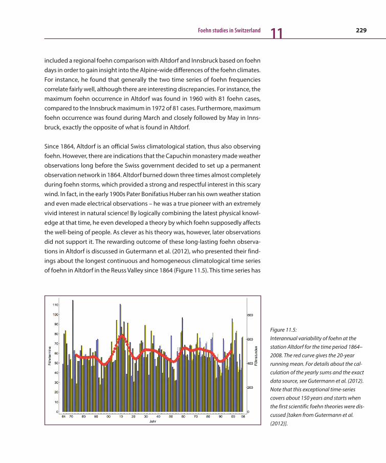
229Foehn studies in Switzerland 11
included a regional foehn comparison with Altdorf and Innsbruck based on foehn days in order to gain insight into the Alpine-wide differences of the foehn climates. For instance, he found that generally the two time series of foehn frequencies correlate fairly well, although there are interesting discrepancies. For instance, the maximum foehn occurrence in Altdorf was found in 1960 with 81 foehn cases, compared to the Innsbruck maximum in 1972 of 81 cases. Furthermore, maximum foehn occurrence was found during March and closely followed by May in Inns-bruck, exactly the opposite of what is found in Altdorf.
Since 1864, Altdorf is an official Swiss climatological station, thus also observing foehn. However, there are indications that the Capuchin monastery made weather observations long before the Swiss government decided to set up a permanent observation network in 1864. Altdorf burned down three times almost completely during foehn storms, which provided a strong and respectful interest in this scary wind. In fact, in the early 1900s Pater Bonifatius Huber ran his own weather station and even made electrical observations – he was a true pioneer with an extremely vivid interest in natural science! By logically combining the latest physical knowl-edge at that time, he even developed a theory by which foehn supposedly affects the well-being of people. As clever as his theory was, however, later observations did not support it. The rewarding outcome of these long-lasting foehn observa-tions in Altdorf is discussed in Gutermann et al. (2012), who presented their find-ings about the longest continuous and homogeneous climatological time series of foehn in Altdorf in the Reuss Valley since 1864 (Figure 11.5). This time series has
Figure 11.5: Interannual variability of foehn at the station Altdorf for the time period 1864–2008. The red curve gives the 20-year running mean. For details about the cal-culation of the yearly sums and the exact data source, see Gutermann et al. (2012). Note that this exceptional time-series covers about 150 years and starts when the first scientific foehn theories were dis-cussed [taken from Gutermann et al. (2012)].

230 From weather observations to atmospheric and climate sciences in Switzerland11
been continued and is now even longer than 150 years. Some of the main results extracted from this exceptional data base are: (1) There is no long-term trend dis-cernible in the foehn frequency over 150 years. (2) However, the variability from year to year is considerable – with an average of 60 foehn observations per year (observations are taken three times a day in the morning, at noon and in the eve-ning), a maximum of 114 climate observations in 1872 and a minimum of 27 observations in 1955. (3) Whereas the foehn frequency shows a pronounced sea-sonal cycle, the same is not true for wind gusts (i. e., foehn intensity): strong foehn winds can occur anytime throughout the year (since 1967, the highest wind speed was recorded on 13 December 1981 with 157 km h–1).
The methods for the identification of foehn varied over time due to the step-wise improvement of weather measurements both in space and time. The most prominent example again is the long-term foehn series of Altdorf: For the first 97 years information was available only from the routine climate observations three times a day. The main criteria for foehn were increased temperature, low relative humidity and strong turbulent winds from southeasterly direction. Beginning in 1961, a southerly wind direction at the Alpine-crest site Gütsch became an additional requirement for foehn identification, this to highlight the Alpine-crossing nature of the foehn flow. Gensler, Wolfensberger and many oth-ers maintained the so-called foehn calendar (‘Föhnkalender’) for Altdorf con-taining the foehn onsets and foehn endings for the years 1955–2008 with 10-min time resolution.
An objective foehn identification algorithm suitable for automatic stations and routinely applied at MeteoSwiss was developed between 1999 and 2008 by Dürr
(2008). The foehn index is based on the 10-min data gathered by the MeteoSwiss automatic network. For the stations considered, wind direction, wind speed and relative humidity at the station (e. g., Altdorf ) are used. In addition, the wind direc-tion at a reference station at Alpine crest (Gütsch) as well as the difference in potential temperature between Gütsch and the foehn station in the valley enter as criteria. Whereas the wind speed, direction and relative humidity at the station are obviously important parameters in the objective identification, the potential temperature difference was taken into account to handle its quasi-conservation as the air descends dry-adiabatically into the foehn valley. A comparison between manually and objectively determined foehn instances gives excellent agreement, hence opening the door for further studies. In particular, the objective classifica-tion allowed foehn climatologies to be compiled at more than 17 foehn stations in northern Alpine valleys since 1981 (since 1955 at 28 stations).
Fisher’s discriminant analysis is a statis-
tical method used to separate distinct
classes based on a set of predictors.
In the case of Widmer’s foehn index
(Widmer, 1966) the separating formula
for foehn breakdown in Altdorf takes,
e. g., the following form: Y = α1 x1 + α2
x2 + α3 x3, where xi refer to three mete-
orological predictors (tendencies of sur-
face pressure and relative topography)
and αi are empirically determined
parameters. I f the value Y falls below a
certain threshold, the foehn is expected
to break down in Altdorf.

231Foehn studies in Switzerland 11
Forecasting foehn events is of major public interest, e. g., for the sake of safety (air safety, cable cars, lakes, traffic), agriculture and power economy. Widmer (1966) tested the short-time prognostic skill of a variety of routinely measured horizontal and vertical gradients such as air pressure (see Figure 11.6 for the distinct pressure differences observed during a foehn event), potential temperature and winds based on the Fisher discriminant analysis.
This empirical exercise provided deeper insight into the underlying physical pro-cesses and strengthened the solenoid theory of Frey (1945). Widmer expanded his
Figure 11.6: Detailed pressure analysis for the Foehn case between 13–19 January 1975. (a) prephase (‘Vorphase’), pressure reduced to 450 m; (b) main phase (‘Föhnhöhepunkt’), pressure reduced to 450 m; (c) as in (b), but pressure reduced to sea level; (d) afterphase (‘Nachphase’). The case study, with special focus on the foehn in the Rhine Valley, is discussed in great detail in Gutermann (1979). In addition to establishing a large pressure difference between the Alpine north and south side, many local features are discernible, e. g., the pressure gradient along the Rhine Valley is split in two separate regions, one between the Alpine crest and the upper Rhine Valley, the other between Chur and Lake Constance [taken from Gutermann (1979)].

232 From weather observations to atmospheric and climate sciences in Switzerland11
method to meso-scale fields over Central Europe to gain some skill for forecasting the foehn onset in Altdorf within 12–36 hours. This well-known ‘Widmer Föhn Index,’ slightly simplified by Courvoisier and Gutermann (1971), still forms the basis of the routine foehn forecasting at MeteoSwiss. Later, Truog (1986) devel-oped several nowcasting procedures for storm warnings on lakes, e. g., a proce-dure called URFEX (‘Urnersee Föhnexperiment’) for the lake Uri based on real-time measurements of the automatic MeteoSwiss network site in Altdorf. A nice sum-mary presenting the current state of foehn forecasting is given in Richner and Hächler (2013).
11.5 Field campaigns
Field campaigns contributed a lot to our understanding of foehn mechanisms. This section describes some campaigns and their foehn-related objectives in greater detail. The section also makes clear how the methods and tools of foehn research have evolved over the course of time. In fact, in the beginning only sur-face-based measurements at (potentially) sparse locations were available. As a further refinement, vertical soundings were then added to the set of instrumen-tation (see, e. g., Figure 11.8 for a very early attempt to characterize the vertical structure of the atmosphere during a foehn event). For a long time, these obser-
Figure 11.7: Left panel: foehn wall in the upper Linth Valley on 5 October 1929 during a dimmer foehn [taken from Streiff-Becker (1933)]; right panel: The foehn flow is detached from the valley floor near Ziegelbrücke and then moves over the cold air pool located there. The interface between the foehn air and the cold air pool takes a wedge-like structure. It is assumed that, at the interface between the two air masses, characterised by strong vertical wind shear, Kelvin-Helmholtz instabilities can evolve and lead to short-term pressure fluctuations (see Gubser (2006) and Richner (1974)) [taken from Streiff-Becker (1942)].

233Foehn studies in Switzerland 11
vational methods, combined with careful theoretical considerations, formed the basis for foehn research. Only in the last decades did additional instruments become available and the density of the measurements substantially increased. Furthermore, with numerical weather prediction (NWP) models, a new and pow-erful tool entered the field. Particularly the combined application of many obser-vational methods (at high spatial density) and high-resolution NWP models allowed the vertical structure of foehn flows to be studied in great detail. The fol-lowing discusses some key field campaign since the 1970s.
As mentioned before, the Gotthard cross section with the Reuss Valley on the Alpine north and the Ticino Valley on the south side exhibits a close-to-ideal topography for establishing foehn flows. There is only one barrier in the main valley, the Rossberg. In the early 1970s, an array of seven meteorological stations recording temperature and humidity was operated for 3 years on the southern slope of the Rossberg. The lowest station was located on the shore of the Lake
Figure 11.8: Balloon sounding on 7:55 MEZ on 22 March 1911 in Erstfeld during a foehn event. The weather was charac-terised as slightly cloudy (ACu, CuSSW), where the ACu build the foehn wall in the South. Although foehn is observed in Erstfeld, the temperature profile is essentially isothermal up to 620 m, only from 1000 m a nearly adiabatic tem-perature decrease is seen. An unex-pected decrease in vertical velocity is observed around 2300 m. At this time the balloon is in between Erstfeld and Altdorf and has reached about the height of the surrounding mountains. The minimum vertical velocity coin-cides with the change of temperature gradient at ca. 2500 m (inversion) [taken from Billwiller and de Quervain (1912)].

234 From weather observations to atmospheric and climate sciences in Switzerland11
Lauerz, the top station on Wildspitz; these two stations also recorded pressure. The objective was to investigate the dynamics of the interaction between the foehn air with the cold pool, and to observe the thickness of the internal boundary layer as well as its characteristics. From the observations, several characteristics of foehn cases could be derived, such as the inclination of the internal boundary, the speed at which the cold pool was eroded, and – most importantly – the wave-like motion of the separation layer, which was described as a “fierce battle between two huge air masses” (see Figure 11.6 of an early depiction by Streiff-Becker of the wedge-like structure of the cold pool).
Near Merenschwand, in the lower Reuss Valley, a field station was built and equipped for observations. The most impressive tool was a tethered balloon of 40 m3, which could be raised up to about 1200 m above ground. The instrument package included wind, temperature, humidity and pressure sensors, and the data was sent to the ground by radio. In some other projects ozone was also measured or sound recordings were made. On the ground, a classical meteoro-logical station with a 12-m tower recorded data digitally on tape. A mobile lab-oratory was equipped with a receiving station for high-altitude radiosondes. In the late 1970s the electronics for an acoustic echo sounder (i. e., an acoustic radar) were added to the mobile lab. The activation of these instruments proved to be very tricky: Optimal observations were possible only when the depth of the cold pool was somewhere between 300 and 600 m. After missing several potentially interesting foehn cases, ground stations were set up on mount Rigi, Zugerberg, and Horben (Lindenberg). These stations recorded wind speed and direction as well as temperature locally. In addition, they were equipped with a radio link so they could be interrogated in real-time from anywhere in northeast-ern Switzerland. After setting up an alarm scheme based on the data from these three stations, all activities at the field station Merenschwand were successfully timed (Richner and Phillips, 1978). The objectives of the activities in the lower Reuss Valley were primarily related to the structure of the internal boundary layer and its dynamics, i. e., on the gravity waves occurring on the cold pool (not to be confused with the elevated, quasistationary lee waves that also occur with foehn!). While the instrumentation allowed precise in-situ measurements, the waves themselves could be inferred only from pressure measurements on the ground using microbarographs (a network of 20 microbarographs had earlier been deployed in the area between Schaffhausen, Lake Constance, Altdorf and Berne). To get a better picture of the actual wave activity on top of the cold pool, an acoustic echo sounder (also called sodar or sound radar) was built (Nater et al., 1979).
Billwiller and de Quervain (1912) per-
formed a balloon sounding in Zurich
during foehn 6 December 1910 (Figure
11.8). They recorded unexpected varia-
tions in the vertical velocity, which they
attributed to the strong foehn storm in
the northern Alpine valleys, although
the foehn did not reach the surface in
Zurich itself. Motivated by these results
and after surmounting many technical
problems, they announced the “unseres
Wissens erste Sondierung der freien
Atmosphäre während Föhn in einem
Föhntale (according to our knowledge
the first sounding of the free atmo-
sphere during a foehn epsiode in a
foehn valley)“. Again a diminished verti-
cal velocity was found in certain layers.
In 1880 Lord Kelvin postulated the exis-
tence of what he called cat’s eye vorti-
ces. Almost 100 years later, in the early
1970s, cat’s eye vortices were actually
observed for the first time in the United
States with a radar. On 9 January 1976
the acoustic echo sounder showed clear
cat’s eye waves 500 m above Meren-
schwand! While the observation was
scientifically not really relevant, it was
an extremely pleasing and rewarding
experience for one of the authors
(Hans Richner)!

235Foehn studies in Switzerland 11
In summary, the lower Reuss Valley provided a great test bed for numerous inves-tigations related to the dynamics of foehn. In particular, it literally provided insight into the wave motion on top of the cold pool by the optical recordings of the acoustic echo sounder. The Jura Mountains contributed significantly to successful observations because they prevent a rapid flushing out of the cold pool. Thus, the situation with a significant foehn a few hundred meters above the ground can persist for many hours if not days.
As part of the Global Atmospheric Research Program (GARP), the ALPine EXperi-ment (ALPEX) took place from 1 September 1981 to 30 September 1982. Partici-pants from 17 nations contributed to this field campaign, which culminated in a 2-month intensive observation period in March and April 1982. Although the time window chosen would climatologically be very favourable for Alpine crossing flows, the number of foehn cases remained rather small: Only short foehn epi-sodes occurred. An objective that was already investigated in the Reuss Valley before ALPEX was to determine the vertical momentum flux during a foehn event (Neininger, 1987). This could be derived directly from the vertical motion of con-stant level balloons, which were already being used in the years before ALPEX to derive the horizontal extension of the waves at the cold pool’s interface with the foehn flow above. The balloons follow the streamlines and with it the wave-like motion. At first, the balloons were tracked by optical means with a stereoscopic range finder. For ALPEX, the constant-level balloons were equipped with reflec-tors, and two military radars set up on the eastern slope of the Lindenberg tracked the balloons. Using these observations, the physical relationship between wind and temperature profile, the pressure signals on the ground, and the wave param-eters (phase and group velocities, amplitude) were established (Nater, 1979).
Furthermore, during ALPEX, the collection of high-precision pressure data in the Reuss Valley was significantly extended: The northernmost station was in Hechin-gen (near Stuttgart), the southernmost near Genoa. Based on this data, the drag between the atmosphere and the Alpine massive could be determined (Davies and Phillips, 1985; early global models produced too high wind speeds in the Alpine area because drag was underestimated).
Much more fruitful for foehn research than ALPEX was the Mesoscale Alpine Pro-gramme (MAP), a large international field campaign with an intensive observation period in autumn of 1999. Within MAP, the subproject FORM (FOehn in the Rhine Valley during MAP) specifically addressed the foehn flow in the Rhine Valley, whereas a ‘partner’ project looked at the foehn flow in the Innsbruck region as a
Only loosely related to foehn was an
experiment in the Reuss Valley: Meteoro-
logical data from all available ground
stations were used to compute the
potential temperature field and its
change over time. Assuming that poten-
tial temperature was a conservative tag
for the air mass, the wind field was
inferred (Richner and Griesser, 1993).

236 From weather observations to atmospheric and climate sciences in Switzerland11
gap-flow problem. The main objectives of FORM are concisely summarised in Rich-ner et al. (2005): (1) to study the dynamics of shallow foehn, i. e., foehn situations that remain restricted to levels below Alpine crest height; (2) to better understand the complexity and diversity of interactions governing the foehn flow within the (main) Rhine Valley, e. g., the interaction with foehn flows emanating from side valleys, or the interaction of the foehn flow with the boundary layer and in partic-ular the removal of the cold air pool before foehn breakthrough; (3) to understand the temporal and spatial evolution of the foehn flow, e. g., to assess why the foehn sometimes only follows one branch when a valley branches, and why sometimes it splits. Of course, an ultimate application aim of FORM was to better predict the whole lifecycle of a foehn event. In fact, one reason why the Rhine Valley was cho-sen as a target region during MAP was the practical significance of improving storm wind forecasts for Lake Constance – a problem that is still a focus of current research and many years before MAP led to the foundation of a foehn-related research group (see Section 5). The other research topics are, of course, also well adapted to the Rhine Valley, e. g., a foehn splitting can often be observed near Sargans, where the Seez Valley branches off from the main Rhine Valley. Apart from that, the fre-quency of foehn events in autumn is higher in the Rhine Valley than at any other station in Switzerland. Given these favourable conditions, the implementation of FORM required a substantial effort. In fact, the number of measurement devices in operation during FORM along the Rhine Valley is rather impressive: radiosondes, wind profiling radars, scintillation anemometers, sodars, lidars, microbarographs, time lapse cameras, surface flux instrumentation, tethered balloon, instrument package on cable cars, instrumented cars, constant volume balloons, surface sta-tions, and several aircrafts. A nice overview of key results of FORM during MAP is presented by Drobinski et al. (2007), who also compared the foehn flow in the Rhine Valley to the one in the Austrian Wipp/Inn Valley. It was shown, for instance, that 3D gravity wave activity is important to fully understanding the low-level wind field, both in the Rhine Valley and in the Wipp Valley. However, it was further shown that shallow foehn flows are more frequent in the Wipp Valley than in the Rhine Valley, and that this flow can conceptually be ‘reduced’ to the simpler shallow-water model. Furthermore, it was also shown that cold-air pools are more prevalent in influencing foehn onset in the lower Rhine Valley than in the Wipp Valley.
Several doctoral theses related to foehn were completed in the framework of MAP. Sprenger (1999) and Sprenger and Schär (2001) investigated the dynamics of the shallow foehn in a highly idealised numerical study. The main Alpine ridge is reduced to a smooth two-dimensional mountain, extending from West to East, into which an equally idealised south-north transect is introduced. It was then

237Foehn studies in Switzerland 11
investigated whether under a purely westerly flow along the Alpine ridge a sym-metry-breaking southerly (or northerly) flow across the idealised pass can be established. Indeed, it was shown that such a flow can persist, driven by the South-North pressure gradient associated with the main along-ridge geostrophic flow. As a remarkable fact it was also shown that a symmetry-breaking flow can even be induced in the limit of vanishing Coriolis parameter. Another doctoral thesis, by Gubser (2006), took advantage of the many observations during the MAP to consider in particular the mechanism by which the cold air pools are eroded. Three mechanisms can be of relevance: turbulent erosion, sun-induced shallow convec-tion, and static and dynamic displacement of the cold air by foehn air. Micro-baro-graphs mounted in Vaduz, in Altenrhein at the northern ‘exit’ of the Rhine Valley, and in Quinten in the Seez side-valley were used to particularly investigate the first mechanism. It was shown that pressure fluctuations before foehn breakthrough are induced at the interface between cold air pool and foehn flow, not showing any wave signature but essentially expected to emanate from turbulence. Further-more, motor glider measurements were used to assess during two case studies if and at what rate heat fluxes allow for the removing of the cold pool. Substantial warming rates were found, with the caveat that these rates are slowed down by nighttime cooling and northerly cold air advection. Finally, this study also looked at the splitting of the foehn flow near Sargans. Based on the onset of the foehn in the Rhine Valley and the Seez Valley and underlined by comparing the potential temperature in the two valleys it was concluded that the foehn in the two valleys is not directly connected: They are rather distinct foehn branches.
11.6 Recent research activities
Foehn research is still actively being undertaken in Switzerland. Some specific examples are: (1) At the Institute of Atmospheric and Climate Science of ETH Zurich (IACETH) Lagrangian methods are being used to establish the paths taken by air parcels arriving in foehn valleys. (2) Numerical modelling of foehn flows remains a big challenge, even with the step to 1-km horizontal model resolution currently being undertaken by MeteoSwiss. (3) The Alpine Research Group Foehn Rhine Valley/Lake Constance (AGF), established in 1971, meets twice yearly to dis-cuss case studies and other foehn research. In the following, some selected studies are presented in greater detail.
Würsch and Sprenger (2015) revisited the Austrian and the Swiss foehn types in their study. Whereas the former more closely exhibits the characteristics of the
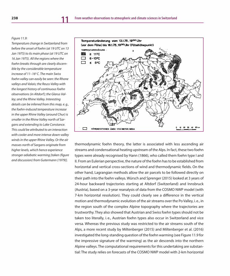
238 From weather observations to atmospheric and climate sciences in Switzerland11
thermodynamic foehn theory, the latter is associated with less ascending air streams and condensational heating upstream of the Alps. In fact, these two foehn types were already recognised by Hann (1866), who called them foehn type I and II. From an Eulerian perspective, the nature of the foehn has to be established from horizontal and vertical cross-sections of wind and thermodynamic fields. On the other hand, Lagrangian methods allow the air parcels to be followed directly on their path into the foehn valleys. Würsch and Sprenger (2015) looked at 3 years of 24-hour backward trajectories starting at Altdorf (Switzerland) and Innsbruck (Austria), based on a 3-year reanalysis of data from the COSMO NWP model (with 7-km horizontal resolution). They could clearly see a difference in the vertical motion and thermodynamic evolution of the air streams over the Po Valley, i. e., in the region south of the complex Alpine topography where the trajectories are trustworthy. They also showed that Austrian and Swiss foehn types should not be taken too literally, i. e., Austrian foehn types also occur in Switzerland and vice versa. Whereas the previous study was restricted to the air streams south of the Alps, a more recent study by Miltenberger (2015) and Miltenberger et al. (2016) investigated the long-standing question of the foehn warming (see Figure 11.9 for the impressive signature of the warming) as the air descends into the northern Alpine valleys. The computational requirements for this undertaking are substan-tial: The study relies on forecasts of the COSMO NWP model with 2-km horizontal
Figure 11.9: Temperature change in Switzerland from before the onset of foehn (at 19 UTC on 13 Jan 1975) to its main phase (at 19 UTC on 16 Jan 1975). All the regions where the foehn breaks through are clearly discern-ible by the considerable temperature increase of 11–16o C. The main Swiss foehn valley can easily be seen: the Rhone valleys and Valais; the Reuss Valley with the longest history of continuous foehn observations (in Altdorf); the Glarus Val-ley; and the Rhine Valley. Interesting details can be inferred from this map, e. g., the foehn-induced temperature increase in the upper Rhine Valley (around Chur) is smaller in the Rhine Valley north of Sar-gans and extending to Lake Constance. This could be attributed to an interaction with cooler and more intense down-valley winds in the upper Rhine Valley. Or the air masses north of Sargans originate from higher levels, which hence experience stronger adiabatic warming [taken (figure and discussion) from Gutermann (1979)].
239Foehn studies in Switzerland 11
resolution and on millions of forward trajectories calculated online with the NWP simulation (Miltenberger et al. 2013). The option of online trajectories, in contrast to the offline trajectories used by Würsch and Sprenger (2015), takes advantage of the full temporal resolution of wind and thermodynamic fields within a NWP simu-lation. Indeed, the 20-s time step of the COSMO model allows one to reasonably capture the complex flow in and over complex topography, and hence to select a subsample of forward trajectories that descend into the foehn valleys. In their study, Miltenberger et al. (2016) considered all trajectories descending into the Rhine Val-ley for a dry and a wet foehn case, where the wetness/dryness is defined by the precipitation on the Alpine south side. Fascinating new results emerge from these case studies: Adiabatic descent is responsible for the foehn air warming in the absence of precipitation. In case of upstream precipitation, air parcels close to the surface experience latent cooling, and only trajectories at higher levels are heated by condensational processes. Although these statements rely on only two case studies of south foehn, the prospect of the online trajectories with tracing micro-physical and thermodynamic fields along the trajectories looks very promising.
One of the major limitations of foehn studies based on NWP simulations is the reliable representation of foehn in the model (Figure 11.10). Indeed, the foehn valleys are typically 2–5 km wide, with many side valleys connected to the main foehn valleys (e. g., Reuss Valley and Rhine Valley). On the other hand, to date the highest-resolution NWP model run in Switzerland (COSMO-2) has a horizontal grid spacing of 2 km, i. e., the complex structure of the valleys and surrounding topog-raphy can only partly be resolved. Furthermore, gravity wave activity, small-scale turbulence and complex surface-atmosphere interactions make foehn simula-tions very challenging. Wilhelm (2012) systematically looked at the performance of the COSMO-2 model in simulating foehn during the period 2008–2011. He found that “overall model errors in wind speed and air temperature during south foehn are approximately 2.5 times larger in magnitude than the climatological errors over Switzerland.” The presence of a linear relationship between the relative humidity bias and altitude rather than with distance from the main Alpine ridge suggests that topographical smoothing influences relative humidity to a greater extent than inaccuracies in the PBL parameterisation scheme. Hence, in a nutshell, a forecaster still has to rely on own experiences to diagnose foehn. Even with the step to operational 1-km horizontal resolution at MeteoSwiss with the COS-MO-NExT project, it still has to be seen whether and how the representation of foehn has improved. The new system is planned to be in operation by 2016. In their overview article about foehn forecasting, Richner and Hächler (2013) under-line the still-existing deficiencies of NWP models in representing foehn. In fact,
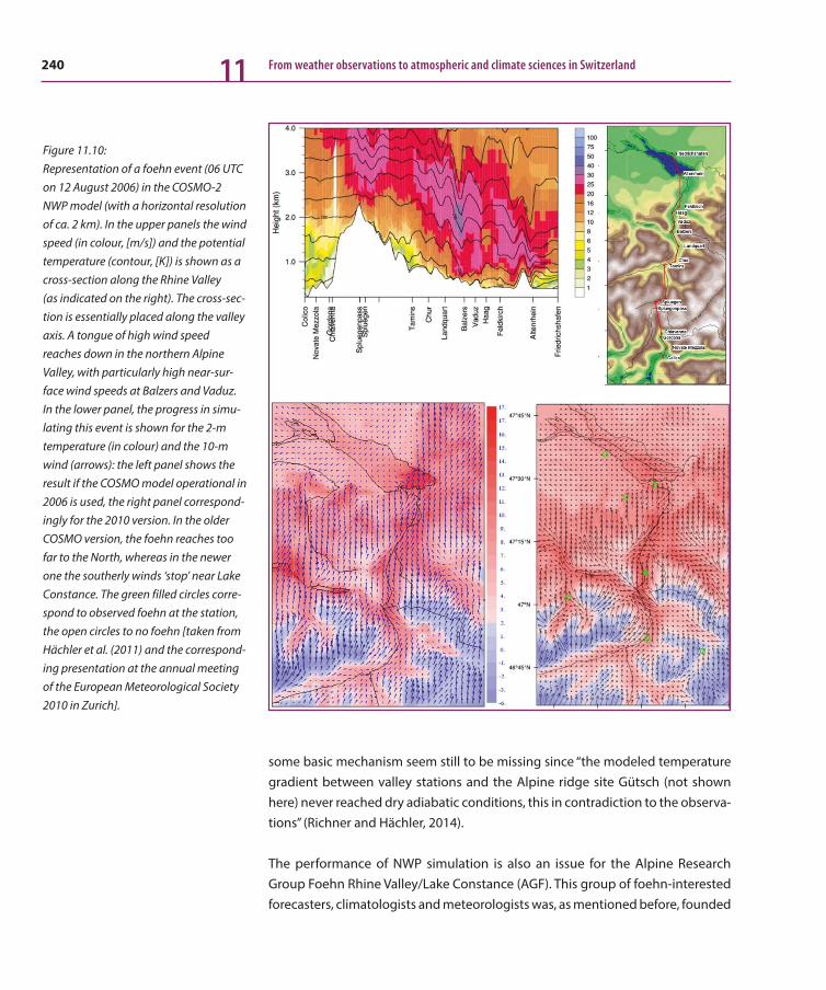
240 From weather observations to atmospheric and climate sciences in Switzerland11
some basic mechanism seem still to be missing since “the modeled temperature gradient between valley stations and the Alpine ridge site Gütsch (not shown here) never reached dry adiabatic conditions, this in contradiction to the observa-tions” (Richner and Hächler, 2014).
The performance of NWP simulation is also an issue for the Alpine Research Group Foehn Rhine Valley/Lake Constance (AGF). This group of foehn-interested forecasters, climatologists and meteorologists was, as mentioned before, founded
Figure 11.10: Representation of a foehn event (06 UTC on 12 August 2006) in the COSMO-2 NWP model (with a horizontal resolution of ca. 2 km). In the upper panels the wind speed (in colour, [m/s]) and the potential temperature (contour, [K]) is shown as a cross-section along the Rhine Valley (as indicated on the right). The cross-sec-tion is essentially placed along the valley axis. A tongue of high wind speed reaches down in the northern Alpine Valley, with particularly high near-sur-face wind speeds at Balzers and Vaduz. In the lower panel, the progress in simu-lating this event is shown for the 2-m temperature (in colour) and the 10-m wind (arrows): the left panel shows the result if the COSMO model operational in 2006 is used, the right panel correspond-ingly for the 2010 version. In the older COSMO version, the foehn reaches too far to the North, whereas in the newer one the southerly winds ‘stop’ near Lake Constance. The green filled circles corre-spond to observed foehn at the station, the open circles to no foehn [taken from Hächler et al. (2011) and the correspond-ing presentation at the annual meeting of the European Meteorological Society 2010 in Zurich].
241Foehn studies in Switzerland 11
in 1971, motivated by the then unsatisfactory foehn storm warnings for the east-ern part of Lake Constance. In the 10-year period from 1973 to 1982, over 100 foehn events in the eastern region of Lake Constance were documented. In addi-tion, various individual case studies with special measuring expeditions in adja-cent foehn areas were performed. The study of interesting foehn cases continued even after this period and recently resulted in two reports that compare actual observations of foehn with NWP simulations (Burri et al., 1999; Hächler et al., 2011). It was found that, in current NWP models, the coupling between soil and atmosphere is too strong during foehn, leading to too low forecasted tempera-tures especially during wintertime. Also, wind speeds in the model might be underestimated, although the pressure differences along the Rhine Valley are realistically captured. These issues, in addition to a detailed tracking and classifi-cation of all foehn occurrences, are regularly discussed in the AGF meetings, which are held twice per year in one of the countries where the AGF members are coming from (Austria, Germany and Switzerland). Finally, the group keeps track of relevant research articles related to foehn, all of which are listed on the AGF web page (www.AGFoehn.org).
The above three examples of ongoing foehn research in Switzerland should not conceal the fact that there are several other interesting studies that cannot be mentioned in detail here (they are listed in the literature list). Among these are new approaches for predicting foehn with sophisticated machine-learning methods and comparing the outcome with the traditional Widmer index. Other studies consider the prediction and characterisation of foehn on the Alpine north side with its cousin on the Alpine south side. Indeed this wind system is much less discussed in the scientific literature than the south foehn, although it is an important environmental factor for the whole Po Valley. Ambrosetti et al. (2005) found that there is a gradual reduction of foehn frequency with increasing distance from the Alpine watershed, though a relevant presence of this wind is also found in the low plain. Hence, it is very encouraging that the objective foehn identification developed by Dürr (2008) was recently adapted to the north foehn and that a comprehensive climatology (> 20 stations) has been compiled (Cetti et al., 2015). Still other studies considered the occurrence and forecasting of foehn in the Bas-Valais. Finally, it is fascinating to see that today we are even able to study long-gone foehn events: Stucki et al. (2015) reconstructed a foehn storm in the Swiss Alps that occurred on 15 February 1925 and was already described by Streiff-Becker. In short, numerous additional studies remain unmentioned, although they substantially contribute to foehn research in Switzerland.
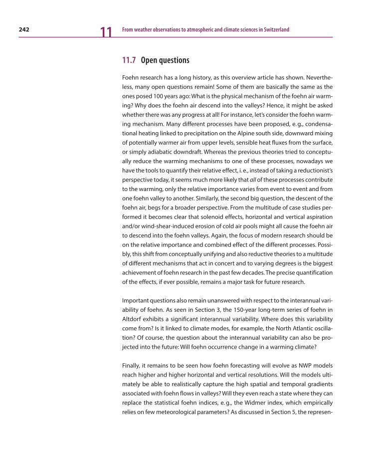
242 From weather observations to atmospheric and climate sciences in Switzerland11
11.7 Open questions
Foehn research has a long history, as this overview article has shown. Neverthe-less, many open questions remain! Some of them are basically the same as the ones posed 100 years ago: What is the physical mechanism of the foehn air warm-ing? Why does the foehn air descend into the valleys? Hence, it might be asked whether there was any progress at all! For instance, let’s consider the foehn warm-ing mechanism. Many different processes have been proposed, e. g., condensa-tional heating linked to precipitation on the Alpine south side, downward mixing of potentially warmer air from upper levels, sensible heat fluxes from the surface, or simply adiabatic downdraft. Whereas the previous theories tried to conceptu-ally reduce the warming mechanisms to one of these processes, nowadays we have the tools to quantify their relative effect, i. e., instead of taking a reductionist’s perspective today, it seems much more likely that all of these processes contribute to the warming, only the relative importance varies from event to event and from one foehn valley to another. Similarly, the second big question, the descent of the foehn air, begs for a broader perspective. From the multitude of case studies per-formed it becomes clear that solenoid effects, horizontal and vertical aspiration and/or wind-shear-induced erosion of cold air pools might all cause the foehn air to descend into the foehn valleys. Again, the focus of modern research should be on the relative importance and combined effect of the different processes. Possi-bly, this shift from conceptually unifying and also reductive theories to a multitude of different mechanisms that act in concert and to varying degrees is the biggest achievement of foehn research in the past few decades. The precise quantification of the effects, if ever possible, remains a major task for future research.
Important questions also remain unanswered with respect to the interannual vari-ability of foehn. As seen in Section 3, the 150-year long-term series of foehn in Altdorf exhibits a significant interannual variability. Where does this variability come from? Is it linked to climate modes, for example, the North Atlantic oscilla-tion? Of course, the question about the interannual variability can also be pro-jected into the future: Will foehn occurrence change in a warming climate?
Finally, it remains to be seen how foehn forecasting will evolve as NWP models reach higher and higher horizontal and vertical resolutions. Will the models ulti-mately be able to realistically capture the high spatial and temporal gradients associated with foehn flows in valleys? Will they even reach a state where they can replace the statistical foehn indices, e. g., the Widmer index, which empirically relies on few meteorological parameters? As discussed in Section 5, the represen-

243Foehn studies in Switzerland 11
tation of foehn flows in NWP models still can and must improve. It will be a signif-icant task to reach this goal!
In summary, foehn research has not reached its end. In fact, we might now be entering a very fruitful era of foehn research where powerful new NWP and mea-surement tools allow long-standing questions of foehn research to be addressed in new ways.
References
A comprehensive literature review was undertaken by Dürr in the framework of a semester thesis at the Department of Earth Sciences of ETH (‘Literaturkatalog zu MAP-FORM,’ available at URL www.AGFoehn.org). More than 150 literature entries are given, and more than 50 scientific articles are listed together with their abstract. Furthermore, an extensive list of foehn stu-dies can be found on the AGF webpage (www.AGFoehn.org, see Section 5). The literature in the following is split into ‘historical’ ones (before 1990!) and recent ones. The watershed year cho-sen is subjective and does not imply any shift in quality and/or relevance! Non-Swiss articles on foehn are listed only if they are discussed in the text. Swiss contributions are more comprehen-sively listed to reflect also important studies not discussed in the text.
Historical articles and monographs
Berg, H., 1952: Der Föhn im nördlichen Alpen- und Voralpenge-biet vom 11. bis 14. März 1951. Bericht deutscher Wetterdienst, US-Zone, 35.
Billwiller, R., 1878: Besprechung von M. F. F. Hébert’s “Etude sur les grands mouvements de l’atmosphère et sur le Foehn et le Scirocco pendant l’hiver 1876/77.” Z. österr. Ges. Meteor, 13, 317–320.
Billwiller, R., 1899: Über verschiedene Entstehungsarten und Erscheinungsformen des Föhns. Meteorol. Z., 16, 204–215.
Billwiller, R., 1904: Der Bergeller Nordföhn. Ann. Schweiz. Meteor. Centralanst., Jahrg. 1902, 56 pp.
Billwiller, R., A. de Quervain, 1912: Registrierballonaufstiege in einem Föhntale. Meteor. Z., 29, 249–251.
Bouet, M., 1954: Coup de foehn sur le Lac Léman. Bull. Murith. Soc. Valais, Sc. Nat., 71, 52–55.
Bouet, M., 1958: Note sur le foehn. Verh. Schweiz. Naturf. Ges., 138, 102–103.
Bouet, M., 1961: Sur le foehn dans la vallée du Rhône en Suisse. Météorologie, 4, 309–313.
Bouet, M., 1964: Le foehn a Sierre. Bull. Murith. Soc. Valais Sc. Nat., 81, 1–13.
Bouet, M., 1972: Le foehn du Valais. Zürich, Veröff. Schweiz. Meteor. Zentralanst, 12 pp.
Brinkmann, W. A. R., 1971: What is Foehn? Weather, 26, 230–239.
Bundy, C. W., 1899: Science, New Series, Vol. 10, No. 242 (Aug. 18, 1899), 218–219.
Courvoisier, H. W., T. Gutermann, 1971: Zur praktischen Anwen-dung des Föhntests von Widmer. Arbeitsber. Schweiz. Meteor. Zentralanst., 21, 7 pp.
Davies, H. C. and P. D. Phillips, 1985: Mountain Drag along the Gotthard Section during ALPEX. J. Atmos. Sci., 42, 2093–2109.
Dove, H. W., 1867: Über Eiszeit, Föhn und Scirocco. Reimer Berlin, 116 pp.
Dove, H. W., 1868: Der Schweizer Föhn, Nachtrag zu Eiszeit, Föhn und Scirocco. Reimer Berlin, 34 pp.
Espy, J. P., 1841: The Philosophy of Storms. Little and Brown, Boston, 552 pp.
244 From weather observations to atmospheric and climate sciences in Switzerland11
Ficker, H., B. de Rudder, 1943: Föhn und Föhnwirkungen. Leipzig, 112 pp.
Ficker, H., 1910: Über die Entstehung der Föhnwinde auf der Nordseite der Alpen. Meteor. Z., 27, 439–451. (English transla-tion by Volken/Brönnimann in Meteor. Z., 21, 597–605, doi: 10.1127/0941-2948/2012/0532).
Ficker, H., 1912: Die Erforschung der Föhnerscheinungen in den Alpen. Eine meteorologische Studie. Z. Deutsch. Österr. Alpen-Vereins, 43, 53–77.
Ficker, H., 1931: Warum steigt der Föhn in die Täler herab? Meteor. Z., 66, 227–229.
Frey, K., 1945: Beiträge zur Entwicklung des Föhns und Unter-suchungen über Hochnebel. Trimbach Olten, 119 pp.
Frey, K., 1950: Der Dimmerföhn vom 18. Dezember 1945. Geof. Pura Applic., 17, 167–182.
Frey, K., 1953: Die Entwicklung des Süd- und des Nordföhns. Arch. Met. Geoph. Biokl., 5, 432–477.
Frey, K., 1957: Zur Diagnose des Föhns. Meteor. Rundsch., 10, 181–185.
Frey, K., 1984: Der “Jahrhundertföhn” vom 8. November 1982. Meteor. Rundsch., 37, 209–220.
Frey, K., 1986a: Gleichzeitigkeit von Nord- und Südföhn bei einer Westlage. Arch. Met. Geoph. Biokl., 34, 349–366.
Frey, K., 1986b: The simultaneous occurrence of North and South Foehn during a westerly flow over Central Europe. Meteor. Atmos. Phys., 34, 349–366.
Gensler, G., 1972: Föhn- oder Wetterfühligkeit und Bioklima. Beih. Ann. Schweiz. Meteor. Zentralanst., 13, 121–134.
Güller, A., 1977: Der aussergewöhnliche Föhnsturm vom 13. Februar 1976 in der Ostschweiz, Arbeitsbericht der Schweiz. Met. Zentralanstalt, 69, 18 pp.
Gutermann, T., 1970: Vergleichende Untersuchungen zur Föhn-häufigkeit im Rheintal zwischen Chur und Bodensee. Diss. Univ. Zürich, 69 pp.
Gutermann, T., 1979: Der Föhn vom 14. bis 18. Januar 1975 im Bodenseeraum. Arbeitsber. Schweiz. Meteor. Anst., 90, 42 pp.
Gutermann, T., H. Wanner, 1982: ALPEX SOP März/April 1982. Die spezielle Beobachtungsperiode von ALPEX.: Struktur und Aktivitäten des Operationszentrums (AOC) in Genf. Arbeitsber. MeteoSchweiz, 111, 87 pp.
Gutersohn, H., 1938: Lokale Winde im Gebiet der Baye de Mon-treux. Vierteljahresschr. Naturf. Ges. Zürich, 83, 211–264.
Hann, J., 1866: Zur Frage des Ursprung des Föhn. Z. Oester. Ges. Meteorol., 1, 257–263.
Hann, J., 1867: Buchbesprechung von “Dove 1867: Ueber Eiszeit, Föhn und Scirocco”, Z. Oester. Meteorol. Ges., 2, 477–480.
Hann, J., 1867: Der Föhn in den österreichischen Alpen. Z. Oester. Ges. Meteorol., 2, 434–445.
Hann, J., 1885: Einige Bemerkungen zur Entwickelungs- Geschichte der Ansichten über den Ursprung des Föhn. Meteor. Z., 2, 393–399 (English translation by Volken/Brönnimann in Meteor. Z., 21 (2012), 591–596.
Hann, J., 1906: Lehrbuch der Meteorologie. Tauchnitz Verlag, Leipzig, 642 pp.
Helmholtz, H., 1865: Über Eis und Gletscher. Vorlesung, Frankfurt am Main.
Jenny-Marti, H., 1951: Die Föhngesetzgebung im Kanton Glarus. Mitt. Vereinig. kantonal-schweiz. Feuerversicherungsanst., 4, 147–157.
Kanitscheider, R., 1932: Beiträge zur Mechanik des Föhns. Beitr. Phys. Atmos., 53, 486–508.
Koschmieder, H., 1951: Föhn und Rohrströmung (pp. 353–354). In: Physik der Atmosphäre, Band 2: Dynamische Meteorologie. 3. Aufl., Akad. Verlagsges. Leipzig, 404 pp.
Kuhn, M., 1989: Föhnstudien. Wissenschaftl. Buchgesellsch., Darmstadt, 504 pp.
Kuhn, W., 1947: Bemerkungen zu K. Freys Föhntheorie. Experien-tia, 3, 423–424.
Kuhn, W., 1984: Rudolf Streiff – Becker als Föhnforscher. Mitt. Naturforsch. Ges. Kant. Glarus, XIV: “Dr. h.c. Rudolf Streiff-Becker”, Herausgg. zum Anlass des 25. Todestages, 25–47.
Lammert, L., 1920: Der mittlere Zustand der Atmosphäre bei Südföhn. Veröff. Geoph. Inst. Leipzig, 2, 261–323.

245Foehn studies in Switzerland 11Lehmann, O., 1937: Zur Geschichte der Föhntheorie. Viertel-jahresschr. Naturforsch. Ges. Zürich, 82, 45–76.
Mörikofer, W., 1950: Zur Meteorologie und Meteorobiologie des Alpenföhns. Verhandl. Schweiz. Naturforsch. Ges., 130, 11–32.
Mühry, A., 1867: Über den Föhnwind. Z. Oester. Ges. Meteorol., 2, 385–397.
Nater, W., 1979: Grenzschichtwellen als Ursache von kurzperio-dischen Druckschwankungen. ETH Diss. Nr. 6469, 128 pp.
Nater, W., H. Richner, P. D. Phillips, 1979: Shear instabilities and their characteristics during foehn. Geophys. Astrophys. Fluid Dyn., 13, 215–223.
Neininger, B., 1987: Quasi-Lagrange’sche Turbulenzmessung mit Schwebeballonen in der planetaren Grenzschicht: Optimie-rung der Methode für die robuste Bestimmung von Impulsfluss und Dispersion über komplexem Gelände. Diss. ETH Zurich, Nr. 8463, 299 pp.
Prohaska, F., 1947: Neuere Anschauungen über die Meteorolo-gie und Klimatologie des Föhns. Experientia, 3, 232–237.
Quiby, J. C., 1970: Some considerations on Foehn winds. Diss., London, 58 pp.
Richner, H., P. D. Phillips, 1978: Automatic station for monitoring wind and temperature via a radio link. Meteor. Rundsch., 31, 33–36.
Richner, H., W. Graber, 1978: The ability of non-classical meteo-rological parameters to penetrate into buildings. Int. J. Bio-meteo., 22, 242–248.
Richner, H., 1974: Zusammenhänge zwischen raschen atmo-sphärischen Druckschwankungen, Wetterlage und subjek tivem Befinden. LAPETH-8, 97 pp.
Richner, H., 1987: The design and operation of a microbaro-graph array to measure pressure drag on the mesoscale. J. Atmos. Oceanic Technol., 4, 105–115.
Rossmann, F., 1950: Über das Absteigen des Föhns in die Täler. Ber. deutsch. Wetterd. US-Zone, 12, 94–98.
Schüepp, M., 1950: Wolken/Wind und Wetter. Büchergilde Gutenberg, Zürich, 263 S.
Schüepp, W., 1952: Die qualitative und quantitative Bedeutung der Föhnmauer. Meteor. Rundsch. 5, 136–138.
Schüepp, W., 1983: Auswirkungen der verschiedenen Wetter-lagen auf die Strömungsverhältnisse beidseits der Alpen: Föhn und Nordföhn. Innsbr. geogr. Studien, 8 (‘Fliri-Festschrift’), Inns-bruck.
Schweitzer, H., 1952: Wie entsteht der Föhn? Umschau, 52., p 586.
Schweitzer, H., 1953: Versuch einer Erklärung des Föhns als Luft-strömung mit über-kritischer Geschwindigkeit. Arch. Meteor. Geophys. Bioklim., 5, 350–371.
Scorer, R. S., H. Klieforth, 1959: Theory of mountain waves of large amplitude. Quart. J. Roy. Meteor. Soc., 85, 131–143.
Scorer, R. S., 1951: Forecasting the occurrence of lee waves. Weather, 6, 99–103.
Scorer, R. S., 1978: Föhn fallacies. Subsection 11.6(2) (pp. 419–422). In: Environmental Aerodynamics. Ellis Horwood Publisher, Chichester, 488 pp.
Streiff-Becker, R., 1925: Über den Glarner Föhn. Vierteljahresschr. Naturforsch. Ges. Zürich, 70, 85–103.
Streiff-Becker, R., 1931a: Warum steigt der Föhn in die Täler herab? Meteor. Z., 48, 393– 394.
Streiff-Becker, R., 1931b: Zur Dynamik des Föhns. Meteor. Z., 48, 49–152.
Streiff-Becker, R., 1933a: Die Föhnwinde. Meteor. Z.,, 48, 149–152.
Streiff-Becker, R., 1933b: Nochmals über den Föhn. Meteor. Z., 50, 388–389.
Streiff-Becker, R., 1935: 71 Jahre Glarnerföhn. Meteor. Z., 52, 147–150.
Streiff-Becker, R., 1942: Neue Untersuchungen über den Föhn in den Schweizer Alpen. Denkschr. Schweiz. Naturforsch. Ges., 74, 241–278.
Streiff-Becker, R., 1947: Der Dimmerföhn. Vierteljahresschr. Naturforsch. Ges. Zürich, 92, 195–198.
Streiff, D., 1984: Dr. h.c. Rudolf Streiff-Becker 1873 – 1959 (Bio-graphie). Mitt. Naturforsch. Ges. Kant. Glarus, XIV: “Dr. h.c. Rudolf Streiff-Becker,” Herausgg. zum Anlass des 25. Todestages, 3–24.

246 From weather observations to atmospheric and climate sciences in Switzerland11
Streiff, D., W. Kuhn, P. Kasser, H. Gutersohn, 1984: Dr. h.c. Rudolf Streiff-Becker. Mitt. Naturforsch. Ges. Kantons Glarus, 14, 111 pp.
Truog, G., 1986: URFEX (Urnersee Föhnexperiment). Arbeitsber. Schweiz. Meteor. Anst., 138, 73pp.
Waibel, K., T. Gutermann, 1976: Föhnhäufigkeiten und Föhn-warnmöglichkeiten im Bodenseegebiet. Arbeitsber. Schweiz. Meteor. Anst., 68, 34 pp.
Waibel, K., 1984: Statistik des Föhns im Bodenseeraum im Ver-gleich mit dem Reusstal (Altdorf ). Arbeitsbericht der Schweiz. Met. Anstalt, 118, 60 pp.
Walter, E., 1938: Der Schweizerföhn. Neujahrsbl. Naturforsch. Ges. Zürich, 140, 40 pp.
Ward, R., 1922: Obituary Julius von Hann. Geogr. Rev., 12, 312.
Wenger, R., 1916: Über den gegenwärtigen Stand der Föhn-theorie. Meteorol. Z., 1.
Widmer, R., 1966: Statistische Untersuchungen über den Föhn im Reusstal und Versuch einer objektiven Föhnprognose für die Station Altdorf. Vierteljahresschr. Naturforsch. Ges. Zürich, 111, 331–375.
Wild, H., 1901: Über den Föhn und Vorschlag zur Beschränkung seines Begriffs. Denkschr. Schweiz. Naturf. Ges., 38, 99 p. plus appendix.
Zenone, E., 1951: Der Föhn im Tessin. Schweiz. Aero-Revue, 26, 140–143.
Recent foehn studies
Ambrosetti, P., L. Mariani, P. Scioli, 2005: Climatology of north föhn in canton Ticino and western Lombardy. Riv. Ital. Agro-meteorol., 2, 24–30.
Baeriswyl, P. A., 1997: L’influence de différents régimes de vent sur la qualité de l’air en milieu alpin. Météorologie, 8, 34–48.
Baumann, K., H. Maurer, G. Rau, M. Piringer, U. Pechinger, A. Pré-vôt, M. Furger, B. Neininger, U. Pellegrini, 2001: The influence of south Foehn on the ozone distribution in the Alpine Rhine Val-ley – results from the MAP field phase. Atmos. Environ., 35, 6379–6390.
Beffrey, G., G. Jaubert, A. Dabas, 2004: Föhn flow and stable air mass in the Rhine Valley: The beginning of a MAP event. Quart. J. Roy. Meteor. Soc., 130, 541–560.
Bougeault, P., P. Binder, J. Kuettner (Eds.), 1998: MAP Mesoscale Alpine Programme, Science Plan. MAP Office, c/o MeteoSwiss, CH-8044 Zürich, 64 S.
Burri, K., P. Hächler, M. Schüepp, R. Werner, 1999: Der Föhnfall vom April 1993. Arbeitsber. MeteoSchweiz, 196, 89 pp.
Campana, M., Y. Li, J. Staehelin, A. S. Prevot, P. Bonasoni, H. Loet-scher, T. Peter, 2005: The influence of south foehn on the ozone mixing ratios at the high alpine site Arosa. Atmos. Environ., 39, 2945–2955.
Cetti, C., M. Buzzi, M. Sprenger, 2015: Climatology of Alpine north foehn. Scientific Report MeteoSwiss, 100, 76 pp.
Drobinski, P., C. Haeberli, E. Richard, M. Lothon, A. M. Dabas, P. H. Flamant, M. Furger, R. Steinacker, 2003: Scale interaction pro-cesses during the MAP IOP 12 south föhn event in the Rhine Valley. Quart. J. Roy. Meteor. Soc., 129, 729–753.
Drobinski, P., R. Steinacker, H. Richner, K. Baumann-Stanzer, G. Beffrey, B. Benech, H. Berger, B. Chimani, A. Dabas, M. Dorninger, B. Dürr, C. Flamant, M. Frioud, M. Furger, I. Groehn, S. Gubser, T. Gutermann, C. Häberli, E. Häller-Scharnhorst, G. Jaubert, M. Lothon, V. Mitev, U. Pechinger, M. Piringer, M. Ratheiser, D. Ruf-fieux, G. Seiz, M. Spatzierer, S. Tschannett, S. Vogt, R. Werner, G. Zängl, 2007: Föhn in the Rhine Valley during MAP: Reviewing its unstationary aspects in a complex valley geometry. Quart. J. Roy. Meteor. Soc., 133, 897–916.
Dürr, B., 2008: Automatisiertes Verfahren zur Bestimmung von Föhn in Alpentälern. Arbeitsber. MeteoSchweiz, 223, 22 pp.
Frey, K., 1992: Entwicklung und Eigenschaften des Südföhns. Geogr. Helvetica, 2, 57–63.
Frey, K., 1996: Der Föhn. Seine Eigenschaften und Erscheinungs-formen. Mitt. Natur-forsch. Ges. Solothurn, 37, 185–199.
Frioud, M., V. Mitev, R. Matthey, H. Richner, M. Furger, S. Gubser, 2004: Variation of the aerosol stratification over the Rhine Valley during Foehn development: a backscatter lidar study. Meteor. Z., 13, 175–181.
Furger, M., P. Drobinski, A. H. Prévôt, R. O. Weber, W. K. Graber, B. Neininger, 2001: Comparison of horizontal and vertical scintil-
247Foehn studies in Switzerland 11lometer crosswinds during strong foehn with lidar and aircraft measurements. J. Atmos. Oceanic Technol., 18, 1975–1988.
Gubser, S., 2006: Wechselwirkung zwischen Föhn und planeta-rer Grenzschicht, ETH Diss. Nr. 16286, 133 pp.
Gutermann, T., B. Dürr, H. Richner, S. Bader, 2012: Föhnklimato-logie Altdorf: die lange Reihe (1864–2008) und ihre Weiterfüh-rung, Vergleich mit anderen Stationen. e-collection ETH Zürich, 53 pp., doi: 10.3929/ethz-a-007583529.
Hächler, P., M. Schüepp, 1994: Der Föhn im St. Galler Rheintal und in den Nachbarregionen. Ber. St. Gall. Naturwissensch. Ges., 87, 29–78.
Hächler, P., K. Burri, B. Duerr, T. Gutermann, A. Neururer, H. Rich-ner, R. Werner, 2011: Der Föhnfall vom 8. Dezember 2006 – Eine Fallstudie. Arbeitsber. MeteoSchweiz, 234, 52 pp.
Miltenberger, A., 2014: Lagrangian Perspective on Dynamic and Microphysical Processes in Orographically Forced Flows. Diss. No. 22227, ETH Zürich.
Miltenberger, A., S. Reynolds, M. Sprenger, 2016: Revisiting foehn air warming – Lagrangian analysis of two foehn events over the Swiss Alps. Quart. J. Roy. Meteor. Soc. (in press).
Miltenberger, A. , S. Pfahl, H. Wernli, 2013: An online trajectory module (version 1.0) for the nonhydrostatic numerical weather prediction model COSMO. Geosci. Model Dev., 6, 1989–2004.
Piringer, M., K. Baumann, U. Pechinger, S. Vogt, 2001: Meteoro-logical and ozone sounding experience during a strong foehn event – a MAP case study. Meteor. Z., 10, 445–455.
Richner, H., B. Dürr, 2015: Facts and fallacies related to dimmer-foehn. e-collection ETH Zurich, doi: 10.3929/ethz-a-010439615.
Richner, H. and Th. Griesser, 1993: Air motion from potential temperature analysis on a meso-b-scale over complex terrain during POLLUMET 1990 and 1991. Meteor. Z., 2, 145–152.
Richner, H., P. Hächler, 2013: Understanding and Forecasting Alpine Foehn. In: F. K. Chow, S. F. J. De Wekker, B. J. Snyder (Eds.):
Mountain weather research and forecasting, Springer Atmo-spheric Sciences 4, 219–260.
Richner, H., B. Dürr, T. Gutermann, S. Bader, 2014: The use of automatic station data for continuing the long time series (1864 to 2008) of foehn in Altdorf. Meteor. Z., 23, 159–166.
Richner, H., K. Baumann-Stanzer, B. Benech, H. Berger, B. Chi-mani, M. Dorninger, P. Drobinski, M. Furger, S. Gubser, T. Guter-mann, C. Häberli, E. Häller, M. Lothon, V. Mitev, D. Ruffieux, G. Seiz, R. Steinacker, S. Tschannett, S. Vogt, R. Werner, 2005: Unsta-tionary aspects of foehn in a large valley part I: operational setup, scientific objectives and analysis of the cases during the special observing period of the MAP subprogramme FORM. Meteor. Atmosph. Phys., 92, 255–284.
Seibert, P., 2005: Hann’s thermodynamic foehn theory and its presentation in meteorological textbooks in the course of time. From Beaufort to Bjerknes and Beyond, Algorismus, 52, 169–180.
Sprenger, M., C. Schär, 2001: Rotational aspects of stratified gap flows and shallow foehn. Quart. J. Roy. Meteor. Soc., 127, 161–187.
Sprenger, M., 1999: Rotational aspects of atmospheric flow past alpine-scale orography. Diss. No. 13250 ETH Zurich, 122 pp.
Stucki, P., S. Brönnimann, O. Martius, C. Welker, R. Rickli, S. Dierer, D. Bresch, G. Compo, P. Sardeshmukh, 2015: Dynamical down-scaling and loss modeling for the reconstruction of historical weather extremes and their impacts – A severe foehn storm in 1925. Bull. Amer. Meteor. Soc. doi: 10.1175/BAMS-D-14-00041.1 (in press).
Wilhelm, M., 2012: COSMO-2 Model Performance in Forecasting Foehn: a systematic process-oriented verification. Forschungs-ber. MeteoSwiss, 89.
Würsch, M., M. Sprenger, 2015: Swiss and Austrian Foehn revis-ited: a Lagrangian-based analysis. Meteorol. Z., 24, 225–242.
Zängl, G., B. Chimani, C. Häberli, 2004: Numerical Simulations of the Foehn in the Rhine Valley on 24 October 1999 (MAP IOP 10). Mon. Wea. Rev., 132, 368–389.


249
12 Two centuries of atmospheric-radiation research in SwitzerlandClaus Fröhlich
12.1 Introduction
Research on atmospheric radiation started with simple observations of the sky during the day and questions such as “Why is the sky blue and why is the sun red at sunrise and sunset” needed an answer. Moreover, special colours at different places on the sky were observed during dusk and dawn raising questions about what produces these colours of the twilight and why they change from time to time. Related to these effects is also the “alpenglow” observed in Alpine regions, especially Switzerland, which besides being sung by poets, was an interesting phenomenon related to the twilight colours and asked for a physical explanation. With a direct-view polariscope observations of the polarisation of the sky became popular already in the early 19th century. They yielded interesting results such as neutral points observed close to and opposite the sun at the solar vertical, during low solar elevations.
Accurate measurements of solar radiation started with electrically-calibrated pyrheliometers during the last decade of the 19th century with the development of the Ångström pyrhliometer (e. g., Ångström, 1899). Somewhat later, Abbot and Aldrich (1913) developed the water-flow and water-stir radiometers, which were then used to define the Smithsonian scale of the Silverdisk pyrheliometers (Abbot and Aldrich, 1913) used as secondary standards. The major question of how these results refer to the absolute scale of Wm–2 was of great concern to the international community for the next 70 years until modern, electrically-calibrated cavity radi-ometers became available and the World Radiometric Reference (WRR) could be defined (Fröhlich, 1978). The relationship between the different scales in use, mainly the Ångström and Smithsonian scales relative to the “absolute” is discussed in detail by Fröhlich (1991) who also details the conversion factors of all the scales in use in the past to WRR.
Although an important objective of radiation research was to define a local cli-mate and its influence on life, the contributions became very important for the
Davos-Dorf

250 From weather observations to atmospheric and climate sciences in Switzerland12
understanding of the radiation in the atmosphere in general. The following sec-tions describe the main institutes involved and selected results of observations of twilight and rings, polarisation, direct solar radiation and the surface radiation budget, turbidity, ultraviolet (UV) radiation, and finally the Swiss determinations of the “solar constant”.
12.2 The main institutes involved in radiation research
Three institutes lead the research and were heavily involved in the foundation and study of atmospheric radiation: the Physikalisch-Meteorologisches Observatorium Davos (PMOD) and the Lichtklimatisches Observatorium Arosa (LKO), both of which were specifically founded for radiation research, and the Swiss Meteorolog-ical Institute, now MeteoSuisse, which contributed directly to or supported radia-tion research. Besides these institutes are many universities who also contributed important results to this field.
Carl Dorno (1865–1942) moved with his family to Davos in 1905 because his daughter suffered tuberculose. In 1907 he founded the Physikalisch-Meteorolo-gisches Observatorium Davos (PMOD) in order to search for reasons why Davos should be good for curing tuberculosis. His programme can be summarised by his statement, “that radiation there presented one of the most important climatic factors” and determined his and PMOD’s work in all its facets namely the needs for improvement of instrumentation and understanding the processes. Combin-ing new approaches with common laboratory instruments, he started a new and very fruitful era of radiation research. He financed the observatory from his means until 1926, when he retired and legated PMOD to Institut für Tuberkulosefor-schung which became then the Schweizerisches Forschungsinstitut für Hochge-birgsklima und Tuberkulose with the two departments, the PMOD and the med-ical institute. Besides more than 100 journal articles Dorno published monographs and books (Dorno, 1911, 1917a, 1919a,b, 1927a). He compared the Davos data also with those from other stations in Europe and was impressed by how much more radiation is received at Davos. His work stimulated radiation research in Switzerland so that the PMOD became a centre and reference point (see e. g., Lindholm and Mörikofer, 1929).
251Two centuries of atmospheric-radiation research in Switzerland 12
After the retirement of Dorno PMOD was first directed by Ferdinand Lindholm from 1926 to 19291, and then by Walter Mörikofer from 1929 to 1966, Emil Flach from 1966 to 1974, Claus Fröhlich from 1975 to 1999 and since 1999 by Werner Schmutz. On recommendation of the Commission of Instruments and Methods of Observation (CIMO), the World Meteorological organisation (WMO) designated PMOD in 1971 as a World Radiation centre (WRC), responsible for the world-wide standardisation of solar radiation measurements. WRC’s excellent performance in this task demonstrated the institute’s metrology competence, so that other cali-bration tasks were delegated to PMOD/WRC in recent years: the World Optical Depth Research and Calibration centre (WORCC) in 1996, the World Radiation Cen-tre for Infrared Radiation Sensors (WRC-IRS) in 2004 and the World Calibration Centre – Ultraviolet (WCC-UV) in 2013.
The Lichtklimatisches Observatorium in Arosa (LKO) was founded 1921 by the “Kurort Arosa” with F. W. Paul Götz (1891–1954) as its first director. Like the PMOD the basic idea for LKO was – in the sense of Dorno’s charisma – to support the “Kurort” with scientific arguments and vigour. The main research was on solar radi-ation and UV and the first instrumentation was from PMOD. Dorno introduced the astrophysicist Götz in solar radiation measurements during a stay of several weeks at the PMOD when he learned to operate the instruments for this new kind of work. The first period of LKO was presented by Götz (1926) describing the results of his first observations of solar radiation in general and more specifically of the UV radiation with Cadmium cells, which allowed him a first determination of the ozone content in the stratosphere and its annual course. Götz started also the longest series of ozone measurements for which the LKO became famous (see Chapter 16). In 1965 the LKO became part of the Laboratory for Atmospheric Phys-ics of the ETH (LAPETH) and its supervision was transferred to the MeteoSwiss Aerological Station in Payerne. Recent plans are to transfer the instrumentation of LKO to PMOD/WRC, where the operation would be continued and the LKO closed.
The Meteorologische Zentralanstalt in Zürich was founded in 1863 as part of the Schweizerischen Naturforschenden Gesellschaft and as such was directed by a commission with Rudolf Wolf as president, then professor of Astronomy and direc-tor of the Sternwarte of the Polytechnikum in Zürich (now Eidgenössische Tech-nische Hochschule, ETH). In 1880 the institute became public and was then called
1 ad interim, on leave from the Swedish Meteorological and Hydrological Institute, Stockholm
252 From weather observations to atmospheric and climate sciences in Switzerland12
Eidgenössische Meteorologische Zentralanstalt (later simply MZA, see also Chap-ter 3). Josef Maurer (1857–1938) after his studies at ETH started as an assistant of the Sternwarte where he was after 1880 also involved in the analysis of meteoro-logical observations. In 1881 he was then employed by the MZA as Adjunkt and from 1905–1934 he was its director. Maurer (1887) presented his first contribution to radiation research with measurements of the nocturnal IR radiation with an instrument similar to a silverdisk, developed by H. F. Weber, professor of physics at ETH. From 1910–1929 he served also as president of International Radiation Com-mission (IRC) of the International Meteorological Organisation (IMO) – during an important period of the discussions about the basics of pyrheliometry and its scale. The Osservatorio Ticinese in Locarno-Monti started its operation as part of the MZA in 1935 to improve the weather forecast for the southern part of the Swiss Alps and Johann-Christian Thams (1907–1973) with his experience gained before at the PMOD promoted radiation research since 1944, when he became director of the Osservatorio. Furthermore, Raymond Schneider (1922–2010), director from 1964 to 1975, supported the creation of the WRC at PMOD and found an ingenious way to get financial support from the government by designating it as the contri-bution of Switzerland to the World Weather Watch (WWW), a programme of WMO.In the framework of the Global Atmospheric Watch of WMO a consortium of MeteoSwiss, PMOD/WRC, the Geographic Institute of the ETH (GIETHZ) and the Institute of Applied Physics of the University of Berne in the mid 1990s launched a radiation programme, called CHARM. Among the four stations operated by CHARM MeteoSwiss was responsible for the Jungfraujoch station (e. g. Heimo et al., 1998; Ingold et al., 2001a), which is also one of the main European GAW sta-tions.
12.3 Results and interpretation of atmospheric-Radiation observations in Switzerland
In the following sections I present Swiss observations and theoretical studies regarding their interpretation. Each section describes a selection of the observa-tions and their interpretation at the time and as well as the situation in light of the present knowledge. This served to show interesting aspects of the evolution of the theory of radiation transfer in the atmosphere. Gruner (1921) prepared a compre-hensive list of observations made in Switzerland of twilight and related effects from the 18th century until 1920 with comments and explanations. This is a very interesting compilation with more than 200 references and copies of extracts of original publications – it made me aware of all the important contributions Swiss

253Two centuries of atmospheric-radiation research in Switzerland 12
scientists made to radiation research before the founding of PMOD. Paul Gruner entered the scene around the turn of the century when he was teaching physics at a gymnasium in Bern. He inherited the interest in atmospheric phenomena from his father August Gruner, as documented by a watercolour painting of the sky after sunset (Gruner, 1921). In 1904 he was named professor at the University of Bern and in 1913 he was elected professor of theoretical physics, the first such in a university department in Switzerland.
Observations of twilight, rings around the sun and the influence of volcanoes
Charles Dufour, professor of astronomy at the University of Lausanne since 1874, reports on observations before the specular twilight effects of the Krakatoa erup-tion in 1883, (e. g. Dufour, 1885, p. 100ff ) namely the “dry fog” (brouillard sec) and the purple light after a volcanic eruption south-west of Sicily in July 1831. This eruption created the Isola Ferdinandea which disappeared 6 month later. More-over, an old citizen of Vevey told Dufour that he had as a youngster in the 1780s observed such dry fog, so dense that the mountains across the lake could no lon-ger be distinguished. This event was from the eruptions of Laki, a fissure with 130 craters in Iceland which started in June 1783 (VEI 6)2 and has since then became known as the “Laki haze” in Europe (e. g. Thordarson and Self, 2003). This dry fog is also mentioned in the meteorological records of Geneva, Neuchâtel and St. Gott-hard. Finally, Dufour (1885, p. 102) provides a possible explanation why only dry fog was observed and no rings as was the case after Krakatoa. These two eruptions were rather close (2700 km in the NE and 1400 km in the S) and so the large par-ticles were still in the dust layer, whereas only the smallest particles from Krakatoa reached Europe.
The eruptions of the Perbuwatan volcano on the Krakatoa Island started on 20 May 1883 and ended on 27 August with an explosion (VEI 6). When the ashes reached Europe spectacular sunsets and rings around the sun were observed. Charles Dufour (1885) observed unusual twilights; François-Alphonse Forel (1884, 1885) in Morges and Albert Riggenbach (1886) in Basel observed the new ring phenomenon, which Forel (1885) called “Bishop ring” in memory of S. E. Bishop (1884), a missionary residing in Honolulu, Hawaii, who observed this optical phe-
2 Volcanic Explosivity Index: describing on a scale 0–8 the explosivity of the eruption. It is a logarithmic scale with about 1 km3 for VEI = 5 and 100 km3 for VEI = 7.

254 From weather observations to atmospheric and climate sciences in Switzerland12
nomenon first on 23. September 1884 and then every day. Riggenbach (1886) describes the purple light and the Bishop ring as being both produced by diffrac-tion by particles in a layer high up in the atmosphere, an explanation which was originally proposed by Babinet (1837) and refined by Kiessling (from Schröder and Wiederkehr, 2000, and references therein, see also Pernter, J. M. and Exner, F. M., 1922, p. 508–511). The Bishop ring is difficult to see with a high sun at low altitude because the natural turbidity bleaches the sky. It has a silver-white central area and a brownish-red ring surrounding it. Depending on the solar elevation, the central area has a radius of 10º–16º, the external ring brightest region is at 14º–18º and it extends up to 22º–24º (Riggenbach, 1886, Table on p. 13). Interestingly enough, the radius of the brightest part of the brownishred ring corresponds almost exactly to the height of the brightest region of the first purple light – a strong indication that both are being produced by the same scattering effects, as stated by Riggenbach (1886).
Dufour (1898) presented some interesting thoughts about total lunar eclipses, observed recently and compared to earlier ones. The recent eclipse was quite nor-mal with a reddish moon, but there were at least two observations in the 19th century of the moon completely disappearing, namely on 4 October 1884 (Dufour, 1885) and on 9 June 1816 (e. g. observed at Bushey Heath, England). One theory was that these rare events were due to clouds in the atmosphere that prevent the solar rays from reaching the moon by refractions through the Earth’s atmosphere. Dufour (1898) rejected this explanation and provided a much more convincing one: the high turbidity due to the volcanic eruptions of Krakatoa and Tambora which erupted in April 1815 on the island Sumbawa in Indonesia with VEI 7. This is the only mention of Tambora in the radiation related literature of Switzerland, although there was no summer in 1816, a lot of rain, bad harvest and famine (e. g. Luterbacher and Pfister, 2015).
The next atmospheric disturbance was the eruption of Mount Pele in Martinique in April/May 1902 which again produced special twilight effects first observed by Forel (1903) and reported by Gruner (1903) including now his own observations. These first observations marked the begin of his continuous interest in the twilight phenomena and their observation (e. g. Gruner, 1915, 1934) and the optics of tur-bid media and the explanation of the purple light (e. g. Gruner, 1919b). The erup-tion of Mount Pele with a VEI≈ 4 was a rather small, but a catastrophic local event with more than 25000 deaths. On 7 May Soufrière Saint Vincent, south of Marti-nique in the Caribbean exploded with a VEI< 4 and most probably the effects observed in Europe were due to both eruptions (Forel, 1905, p. 232). On 25 Octo-
255Two centuries of atmospheric-radiation research in Switzerland 12
ber 1902 Santa Maria erupted in Guatemala which with its VEI= 6 was about 5–10 times stronger than the two other eruptions together – but this eruption was not known at the time. In summary Forel (1905) states for the rings that their intensity of the colours was less but the size was about the same as in 1883/1884 with an average of all observations 10º–12º compared to 10.5º for the radius of the inner silver-white part and of 20º–25º compared to 22.7º for the outer edge of the brownish-red ring. The period during which Bishop rings were seen was shorter this time with about 2 years compared with 4 years for Krakatoa.
During this period observations of the extinction of solar radiation were also reported. In 1896 Christian Bührer, pharmacist and founder of the pharmacy at Clarens, part of Montreux on the Lake of Geneva, and Henri Dufour started mea-surements of the solar irradiance at these places (Bührer and Dufour, 1899) which continued until 1910 (Bührer, 1911). Dufour (1903) reported on a decrease of the radiation after the eruption of Santa Maria by about 17 % to 24 % from December 1902 to March 1903. They used a radiometer of Crova and after 1905 an Å-pyrhe-liometer on which the values were referred afterwards. At the same time Gockel (1903) observed also a strong decrease in the UV measured with an improved Zinc-sphere photometer of Elster and Geitel (1904). These two measurement sets would be an interesting extension of Dorno’s series of solar and UV radiation.
Dorno (1917a) started twilight and ring observations in November 1911 with his usual commitment to observations. This publication covers the period 1911–1917 and describes first the periods of minor disturbances and then the massive effects of 1912/1915 – probably to underline the beauty and the diversity of the “normal” twilight in contrast to the brute effects of a volcanic eruption.
The large eruption of Katmai in Alaska on 6 June 1912 produced an important increase of turbidity in Europe first seen in Switzerland on 23 June (Maurer, 1912). Because the Katmai region is very remote, no direct or even close-by observations of the eruption are available and only later was it found that it was not Katmai that erupted, but a region about 10 km to the West, named Novarupta (Hildres, W. and Fierstein, J., 2014) with VEI= 6, but with an amount of the ejecta 1.5 times greater than Krakatoa. Dorno was not in Davos to see the first effects arriving and started observations only in September 1912 (Dorno, 1917a, pp. 17–23). He observed very intense and extended purple lights that lasted until May 1914 and impressive Bishop rings after mid September 1912 until about April 1915 with an interruption from July to December 1914. The observations of the Bishop ring (Dorno, 1917a, p. 90) were quite different from those observed in 1883 and 1902. The average
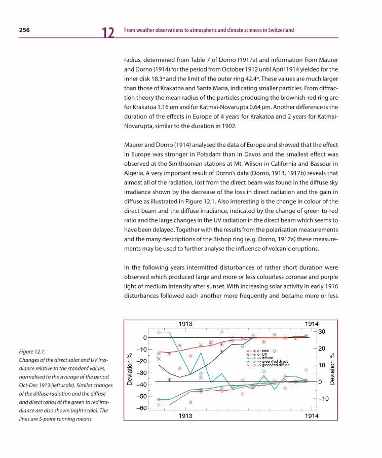
256 From weather observations to atmospheric and climate sciences in Switzerland12
radius, determined from Table 7 of Dorno (1917a) and information from Maurer and Dorno (1914) for the period from October 1912 until April 1914 yielded for the inner disk 18.3º and the limit of the outer ring 42.4º. These values are much larger than those of Krakatoa and Santa Maria, indicating smaller particles. From diffrac-tion theory the mean radius of the particles producing the brownish-red ring are for Krakatoa 1.16 µm and for Katmai-Novarupta 0.64 µm. Another difference is the duration of the effects in Europe of 4 years for Krakatoa and 2 years for Katmai- Novarupta, similar to the duration in 1902.
Maurer and Dorno (1914) analysed the data of Europe and showed that the effect in Europe was stronger in Potsdam than in Davos and the smallest effect was observed at the Smithsonian stations at Mt. Wilson in California and Bassour in Algeria. A very important result of Dorno’s data (Dorno, 1913, 1917b) reveals that almost all of the radiation, lost from the direct beam was found in the diffuse sky irradiance shown by the decrease of the loss in direct radiation and the gain in diffuse as illustrated in Figure 12.1. Also interesting is the change in colour of the direct beam and the diffuse irradiance, indicated by the change of green-to-red ratio and the large changes in the UV radiation in the direct beam which seems to have been delayed. Together with the results from the polarisation measurements and the many descriptions of the Bishop ring (e. g. Dorno, 1917a) these measure-ments may be used to further analyse the influence of volcanic eruptions.
In the following years intermitted disturbances of rather short duration were observed which produced large and more or less colourless coronae and purple light of medium intensity after sunset. With increasing solar activity in early 1916 disturbances followed each another more frequently and became more or less
Figure 12.1: Changes of the direct solar and UV irra-diance relative to the standard values, normalised to the average of the period Oct-Dec 1913 (left scale). Similar changes of the diffuse radiation and the diffuse and direct ratios of the green to red irra-diance are also shown (right scale). The lines are 5-point running means.
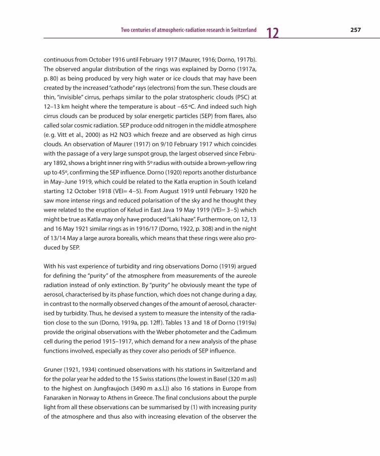
257Two centuries of atmospheric-radiation research in Switzerland 12
continuous from October 1916 until February 1917 (Maurer, 1916; Dorno, 1917b). The observed angular distribution of the rings was explained by Dorno (1917a, p. 80) as being produced by very high water or ice clouds that may have been created by the increased “cathode” rays (electrons) from the sun. These clouds are thin, “invisible” cirrus, perhaps similar to the polar stratospheric clouds (PSC) at 12–13 km height where the temperature is about −65 ºC. And indeed such high cirrus clouds can be produced by solar energetic particles (SEP) from flares, also called solar cosmic radiation. SEP produce odd nitrogen in the middle atmosphere (e. g. Vitt et al., 2000) as H2 NO3 which freeze and are observed as high cirrus clouds. An observation of Maurer (1917) on 9/10 February 1917 which coincides with the passage of a very large sunspot group, the largest observed since Febru-ary 1892, shows a bright inner ring with 5º radius with outside a brown-yellow ring up to 45º, confirming the SEP influence. Dorno (1920) reports another disturbance in May–June 1919, which could be related to the Katla eruption in South Iceland starting 12 October 1918 (VEI= 4−5). From August 1919 until February 1920 he saw more intense rings and reduced polarisation of the sky and he thought they were related to the eruption of Kelud in East Java 19 May 1919 (VEI= 3−5) which might be true as Katla may only have produced “Laki haze”. Furthermore, on 12, 13 and 16 May 1921 similar rings as in 1916/17 (Dorno, 1922, p. 308) and in the night of 13/14 May a large aurora borealis, which means that these rings were also pro-duced by SEP.
With his vast experience of turbidity and ring observations Dorno (1919) argued for defining the “purity” of the atmosphere from measurements of the aureole radiation instead of only extinction. By “purity” he obviously meant the type of aerosol, characterised by its phase function, which does not change during a day, in contrast to the normally observed changes of the amount of aerosol, character-ised by turbidity. Thus, he devised a system to measure the intensity of the radia-tion close to the sun (Dorno, 1919a, pp. 12ff ). Tables 13 and 18 of Dorno (1919a) provide the original observations with the Weber photometer and the Cadimum cell during the period 1915–1917, which demand for a new analysis of the phase functions involved, especially as they cover also periods of SEP influence.
Gruner (1921, 1934) continued observations with his stations in Switzerland and for the polar year he added to the 15 Swiss stations (the lowest in Basel (320 m asl) to the highest on Jungfraujoch (3490 m a.s.l.)) also 16 stations in Europe from Fanaraken in Norway to Athens in Greece. The final conclusions about the purple light from all these observations can be summarised by (1) with increasing purity of the atmosphere and thus also with increasing elevation of the observer the

258 From weather observations to atmospheric and climate sciences in Switzerland12
purple light is brighter, with longer duration and larger size. (2) after a volcanic eruption the purple light is also intensified in parallel with the intensified rings.
In order to explain purple light and ring phenomena Gruner (1919a, 1932a,b,c) developed a method to calculate scattered radiation, which in 1919 started using results from the PhD thesis of H. Kleinert, as well as the angular distribution of the scattered radiation calculated by H. Blumer (Blumer, 1925, 1926a,c,b), also a PhD student of Gruner. Kleinert’s calculations were based on King (1913) and general-ized for non-Rayleigh scattering functions. Blumer’s calculations used the theory of Mie (1908) and the output of tedious and exhausting calculations were the first available and very useful, although the range of the Mie parameter x = 2πr/λ with r the particle radius and λ the wavelength was rather limited from 0.01 to 12 in 24 steps.
Gruner refined these theoretical calculations in order to provide a consistent theory of twilight and ring appearance and Gruner and Kleinert (1927) provides a review of the relevant effects and a nice qualitative explanation in an informative illustra-tion. The purple light and the rings are produced by the same phenomenon with the main difference that the source for the rings is the white light of the direct sun and for the twilight the red rays of the sun below the horizon illuminating the sky above the observer. In the case of a distinct aerosol layer in the atmosphere as for example after a volcanic eruption with a narrow size distribution the scattering is according to Blumer (1926a) stronger in the red than in the green, yielding the brownish outer ring of the Bishop ring, the diameter of which depends on the mean particle size of the aerosol. For the purple light the source is red and hence the colour ratio unimportant and the height depends as for the rings on the mean size. I f there is no distinct aerosol layer there are no rings, only an aureole and the purple light is caused by scattering in the lower atmosphere. Hence, for clear-sky conditions the smaller extinction makes the purple light brighter, but less coloured.
The eruption of Pinatubo in the Philippines on 15 June 1991 produced Bishop rings as well and a detailed investigation of the volcanic aerosol layer with lidar and radiosondes by Sassen et al. (1994) provides a consistent explanation. The strato-spheric aerosol from eruptions consists of aqueous sulfuric acid which can freeze as sulphuric acid tetrahydrate (H2 SO4 + 4H2 O = H1 0O8 S) at temperatures from –65 to –75 ºC. Such temperatures exist in the mid-latitude lower stratosphere and a stable region for the formation of these aerosols exists. Once formed these particles remain non-volatile unless they leave the stable region and melt. This is similar to the production of stratospheric cirrus by SEP which produce H2 NO3, instead.

259Two centuries of atmospheric-radiation research in Switzerland 12
What can be learned from polarisation measurements?
Polarisation observations are rather simple and were started in the early 19th cen-tury by Arago who discovered the first neutral point in the solar vertical in the region opposite to the sun, which was then called after him. In 1840 Babinet found another neutral point close to and above the sun and Brewster followed from symmetry that there must a corresponding neutral point below the sun. From the theory of Rayleigh (1881) it was clear that the sky must be polarized and the max-imum should be reached at 90º from the sun. The neutral points, however, were not explained and furthermore, these points wandered up and down on the solar vertical depending on solar elevation and aerosol loading. Polarisation is defined relative to the scattering plane between the direction from the observer to the source and the direction of the observation. It is given by the intensities of the oscillation parallel and perpendicular to this plane Iℓ and Ir (Dorno and others at the time used i1 and i, respectively). The degree of polarisation was defined as P = (Iℓ − Ir)/(Iℓ + Ir). George G. Stokes in 1852 defined a mathematically convenient alternative to the more common description of polarized radiation with a vector (I , Q, U, V), the components of which are for linearly polarized radiation I = Iℓ + Ir, Q = Iℓ − Ir , U = ±Q tan 2ϕ0 and V = 0 (no circular component) with Iℓ and Ir at ϕ = 0º and ϕ = 90º and ϕ0 the direction of the scattering plane. An important property is that all parameters are individually additive and the radiation may contain some part that is neutral so that I >
ffiffiffiffiffiffiffiffiffiffiffiffiffiffiffiffiffiffiffiffiffiffiffiffiffiffiffiQ2 þ U2 þ V2
p.
Jacques-Louis Soret, a Swiss chemist and professor at University Geneva, who dis-covered Holmium, observed polarisation of the sky during sunsets. He found that the light coming from air in the shadow is also polarized and introduced second order scattering to explain this observation. With the sun at the horizon he calcu-lated the secondary scattered radiation from the whole sky in a small band all around the horizon (Soret, 1888) and found that the polarisation is horizontal at the anti-solar point. Thus, by adding this secondary scattered radiation to lr , P becomes negative and the existence of the Arago neutral point was explained. His theory implicitly also produces neutral lines outside of the solar vertical as observed by Dorno. The results of Dorno (Figure 12.3, right) lead to the contro-versy with Exner (Exner, 1921) who stated that the results of Dorno (1919a) are misleading. Dorno measured the intensity of each polarisation separately and always referred them to the scattering plane (Q= 0) and Exner (1921) stated cate-gorically that Iℓ must always be greater than Ir outside the solar vertical. Hence, Dorno should replace his parameter q = Iℓ /Ir outside the solar vertical by its recip-rocal values if it goes below 1. Fortunately he did not listen as the results of Sekera
Figure 12.2: Picture of the Weber polarisation- photometer used by Dorno for the mea-surements of polarisation and intensity at any point of the sky. The vertical tube on the side of the instrument allows direct comparison with the zenith intensity and polarisation, which can then be determined by a Weber photometer in absolute terms.

260 From weather observations to atmospheric and climate sciences in Switzerland12
(1957) demonstrate (Figure 12.3, left). For a point on the sky with the zenith angle θ and the azimuth ϕ the neutral lines (U (θ, ϕ) = 0) separate regions of positive and negative polarisation. The lemniscate-shape curve shows the Brewster and Arago points on the solar vertical at low sun. With the sun rising in the sky the Arago point vanishes, the Brewster point rises and from about 20º solar elevation the Babinet point becomes visible.
An interesting feature is at the zenith which is from observations not a neutral point. The crossing of the two U (0, ϕ) = 0 under 90º, however, means that at the zenith the polarisation plane is perpendicular to the solar vertical. And if one mea-sures polarisation of the zenith, the plane is assumed to be the solar vertical and no neutral point is found.
Furthermore, polarisation depends on wavelength and Dorno (1919a) measured either in the UV (photoelectric measurements, for example with Cadmium cells)
Figure 12.3: The left plot shows the result of the calculations of Sekera (1957) and the right the redrawn figure of Dorno (1919a, Tafel XVIa). Besides some deviations on the western side, which is probably due to missing data close and below the horizon at Davos, it is perfect!

261Two centuries of atmospheric-radiation research in Switzerland 12
or in the green and red part with corresponding filters (photometric measure-ments with the Weber photometer). Gockel (1920) studied also polarisation and its colours mainly to get information about how it changes with different atmo-spheric conditions. He comes to the following conclusions: (1) in a pure atmo-sphere the polarisation does not depend on wavelength within the uncertainty of the measurement. (2) With increasing turbidity the polarisation in the blue increases relative to red and (3) Radiation from the white aureole around the sun is more polarized in the red than in the blue. The influence of aerosols was later explicitly explained by the results of Blumer (1926b) for the red and green colours.
Transparency of direct solar radiation and the surface radiation budget
The era of “real” measurements with radiometers started towards the end of the 19th century and complemented the direct observations, but also supported their findings in a more rigorous manner (e. g. Bührer and Dufour, 1899; Bührer, 1911). Dorno started with more or less continuous observations of direct solar radiation in 1909 measuring with the Michelson actinometer 5100, traceable to the Å-scale. In October 1921 the pyrheliograph (Figure 12.4), an automatically recording radi-ometer took over the task of recording the solar irradiance. It was designed by Dorno (1922), constructed by Thilenius in Darmstadt with a thermopile as receiver and mounted on a clock-driven tracker (Figure 12.4). From 1969–1990 the obser-vations of the pyrheliograph were replaced by data from the comparison during very clear days and afterwards by the measurements with the automatic absolute radiometer, connected to the data system of MeteoSwiss.
The first evaluation of the Davos data from 1909–1926 in terms of aerosol trans-mission was done by Lindholm (1927) for which he corrected the observations for water-vapour extinction based on surface humidity and Rayleigh scattering. The period from 1909–1979 was first evaluated by Hoyt and Fröhlich (1983) during a stay of Douglas V. Hoyt at PMOD/WRC. A re-evaluation of the now 100-year-long record was then performed by (Lachat and Wehrli, 2012, 2013). Figure 12.5 shows the annual mean values from Lachat and Wehrli (2013) with interesting variations from year to year. The noise seems to have increased, especially during 1969–1990 probably because during this period only results from comparisons/calibrations during clear days were available. The record shows a more or less constant trans-parency after recovery from the Katmai-Novarupta disturbance until the 1940s when the dimming and subsequent recovery started. Lindholm’s values can be
Figure 12.4: Picture of the Pyrheliograph from Dorno (1922).

262 From weather observations to atmospheric and climate sciences in Switzerland12
directly compared to the aerosol transmission determined by Lachat and Wehrli (2013) and with their ratio of the total to the aerosol transmission his values can be accordingly reduced and added to Figure 12.5 b. The high level of agreement confirms that the very different methods to calculate atmospheric transmission are valid and it is astounding that neither Hoyt and Fröhlich (1983) nor Lachat and Wehrli (2013) were aware of this early evaluation.
Figure 12.5: a) Sunspot number as an indicator of solar activity that may influence atmospheric transparency. b) Annual transparency from Lachat and Wehrli (2013) with a polynomial fit to the period 1915–2012 (red line) and to the period of the global radiation 1935–2004 (green line). Moreover the mean fit from Ohmura (2006) scaled to the max-min difference of the 1935–2004 fit is also shown (blue line). The results of the analysis of Lindholm (1927) are also plotted. c) Annual mean global radiation of Davos and Locarno and a polynomial fit to the aver-age ((digitized from Figure 1 of Ohmura, 2006)). Note the different deviation of the Davos and Locarno record from the fit which probably indicates differences of cloud cover. Also plotted is the polynomial fit to the average of all European station from Figure 1 of Ohmura (2006) (here the relative deviation from the mean is plotted and not the observed value as in Ohmura’s figure).
263Two centuries of atmospheric-radiation research in Switzerland 12
From 13 long-term records of global radiation in Europe Ohmura and Lang (1989) detected what was later called ‘global dimming’, a substantial decrease of global radiation after about 1960. Later the reported decrease at these 13 stations was better quantified and a change of −8 Wm-2 between 1959 and 1988 was discov-ered. Wild (2009) presents an excellent review of the dimming which turned to a brightening period after 1990, which includes not only a discussion of the reliabil-ity of data sets but also presents the results from model calculations of this inter-esting phenomenon – a fascinating story initiated by Atsumu Ohmura in the 1970s. The resemblance of the solar transmittance with the global radiation at Davos and Locarno [from the GEBA archive of Gilgen and Ohmura (1999)] is impressive and shows that trends in global radiation may be related to the solar transmittance of the atmosphere. The relative changes of the global radiation are with almost 10 % much larger than the transmittance changes of a few percent. This means that the direct influence of aerosols is rather small and that clouds and indirect effects of aerosols seem to be more important. Moreover, there is an important difference for the time before 1940 when all the European stations show an increase with time which is hardly seen in the transmittance of Davos. The obvious question is: What happened to the global radiation at Davos and Locarno and also to the other European stations? Why is it increasing at the beginning of the measurements in the mid 1930, whereas the direct solar radiation record does not? Dorno (1922) presents not only the introduction of the pyrheliograph, but also an year of global radiation with an Ångström pyranometer, calibrated at Davos by the shading technique, yielding an annual mean value for 1921 of 197 Wm–2 which is much higher than the corresponding GEBA record. This needs to be clarified though, unfortunately there are no global radiation data for the earlier period 1909–1910.
For the surface radiation budget also measurements are needed of the long-wave part (λ > 2.5 µm). Dorno (1922) describes measurements of the atmospheric long-wave radiation during nights from November 1920 to October 1921 and compares them to global radiation during the same period. Further observations of the short and long-wave radiation were performed at Muottas Muraigl (Dorno, 1927a, pp. 77–80). These results could be used to get further points in time to determine secular trends of the surface radiation budget.
The development of instrumentation at PMOD during 1940 and 1950 – supported by theoretical considerations (e. g. Courvoisier and Wierzejewski, 1948, 1949; Courvoisier, 1954) – is summarised in Mörikofer (1964). It improved the situation for the accurate determination of the surface radiation budget substantially. How-

264 From weather observations to atmospheric and climate sciences in Switzerland12
ever, the introduction of the pyrgeometer (PIR by Eppley) in 1970 solved almost all problems of the long-wave radiation measurement with pyrradiometers, because the polyethylene dome (transparent to solar and IR radiation) was replaced by a dome that is blind to the shortwave radiation (Silicon with a special coating transparent in the range of 3.5–50 µ). With new techniques to calibrate these instruments (Philipona et al., 1995) the surface radiation budget became more accurate. This lead to a request by the World Climate Research program-meme (WCRP) to establish a network of base-line stations to provide Earths sur-face irradiances, the baseline surface radiation network (BSRN) (Ohmura et al., 1998), primarily for validating satellite-based estimates of the surface radiation budget and also for scientific research. More than half of the authors of Ohmura et al. (1998) are members of Swiss institutes, providing expertise in instrument calibration and use (PMOD/WRC with the calibration facilities, WRC-IRS), in data management (GI-ETHZ with storage and quality control at the World Radiation Monitoring centre, WRMC) and support in climate modelling. The WRMC was ini-tiated by Ohmura in 1992 and operated at ETH until 2007. Since 2008 it is at the Alfred Wegener Institute for Polar and Marine Research (AWI), Germany (König-Lan-glo et al., 2013). Improvements in the calibration were demonstrated by Philipona et al. (1998) and the adoption of a standard group of pyrgeometers lead finally to the adoption of WRC-IRS calibration centre. A recent study of Gröbner et al. (2014) confirms the direct traceability of the pyrgeometers to the SI unity system.
In addition to the BSRN station in Payerne an Alpine Surface Radiation Budget (ASRB) network was established by PMOD/WRC to study the elevation depen-dence of the SRB. It started in 1994 and has since 1997 11 station at altitudes between 380 and 3580 m. Marty et al. (2002) provided first results which show the great potential of such measurements for better understanding the influence of green-house gases in the Alpine region and its monitoring provides important information about the effect of climate change (e. g. Ruckstuhl et al., 2007).
Turbidity and the determination of aerosol loading from radiation measurements
Most of the observation of the extinction within the atmosphere, generally called turbidity, were performed with pyrheliometers measuring total (integrated over all wavelengths) and also with broad-band filters, as e. g. OG1 (0.630–2.8 µm) and RG2 (0.695–2.8 µm). The radiation community wanted one or two numbers to characterise turbidity and the definition of the Ångström coefficients α and β were

265Two centuries of atmospheric-radiation research in Switzerland 12
an acceptable proposal (Ångström, 1929). It describes the dependence of the aerosol extinction on the air mass m and wavelength λ by exp(−mβλ−α). Ångström called α a measure of the size of the scattering particles which was very misleading and led Götz (1932) to call the deviation from the linear behaviour, the maximum of the extinction at λ = 350 nm he found in his measurements at Arosa anomalous extinction. These measurements along a horizontal path over 1.5 km with two carefully calibrated spectrometers, however, show substantial scatter and the results can be fitted to a straight line with α = 0.86 ± 0.30 which is fully compatible with the rural aerosol used in MODTRAN (Berk et al., 2008). Götz (1934) showed that a single size of 0.25 µm would show the observed maximum at λ = 350 nm, but he missed the point that aerosols in the atmosphere have not a single size, but a distribution with a wide range of particle diameters. The many small particles add to the extinction at shorter wavelength and are thus smearing out the max-ima of the individual sizes. Only when Junge (1955) presented his power-law par-ticle-size distribution was it easy to calculate the wavelength dependence of the extinction. So, α is a measure of the exponent of a power-law-size distribution and not of the mean size of a narrow distribution. The analysis of the broad-band mea-surement with a constant wavelength dependence was saved and α became an important parameter characterising atmospheric turbidity.
The introduction of sunphotometers (SPM) by Volz (1959) opened a new area of aerosol research as the aerosol optical depth (AOD) at a given wavelengths could now be determined directly. These SPM were at time hand-held wooden boxes and the early version allowed the determination of the aerosol optical depth (AOD) at 500 nm. In the 1970s the PMOD/WRC started research for aerosol diag-nostics and developed a spectro-radiometer to determine the wavelength best suited for the determination of aerosol, water-vapour and ozone. First results with such an instrument mounted on the mobile station of MeteoSwiss were presented by Heimo and Valko (1977). With this experience the performance specifications of a new sunphotometer for the world-wide monitoring of AOD were established by the Working Group on Radiation Measurement Systems of CIMO/WMO at its meeting in Geneva, 21–25 June 1977 with Fröhlich as chairman. Around the same time Glen Shaw of the University of Alaska at Fairbanks built a new 9-channel SPM that was compatible with the CIMO specification. During his sabbatical stay at PMOD/WRC in the summer of 1977 his SPM was a kind of prototype of the new development and was used to test calibration by the Langley method (extrapolat-ing daily measurements to zero air mass) and by absolute calibrations in the lab-oratory together with a reliable value for the extraterrestrial spectral value. Both methods have been tested for Shaw’s SPM with standard lamps and the newly
266 From weather observations to atmospheric and climate sciences in Switzerland12
developed laser facility at PMOD/WRC according to Geist et al. (1975). After his stay he determined the zero-air mass value at Mauno Loa and with it a first comparison of the extrapolated and the laboratory calibrated extraterrestrial spectrum of Labs and Neckel (1967, 1972) could be performed. The results demonstrated that all values were within ±2 % (Fröhlich and Brusa, 1981) – a nice confirmation of the accuracy of the scales from different metrology institutes.
During the development of the space experiments SOVA, IPHIR, VIRGO and SOVIM the design of the SPM were improved, leading also to the SPM2000, manufactured by the Centre Suisse d’Electronique et de Microtechnique (CSEM) in Neuchâtel (see Schmid and Wehrli, 1995). These SPM were widely used in CHARM (Heimo et al., 1998). In the 1990s further tests of the calibration of these SPM by extrapola-tion were performed at Jungfraujoch ( Schmid and Wehrli, 1995) and compared to laboratory calibrations ( Schmid et al., 1998). They showed, that Jungfraujoch is a good station to perform zero-air mass determinations with a precision of 0.25 % and an accuracy of about 1 %.
With this wide experience in sunphotometry PMOD/WRC was designated by WMO as World Optical Depth Research and Calibration Centre (WORCC) which started its operation in 1996. The first task was to develop a 4-channel precision filter radiometer (PFR) for a global trial network at 12 GAW stations with the objective to “demonstrate that the new generation of instruments together with new cali-bration techniques and quality assurance procedures is indeed able to determine AOD with a precision adequate for the fulfillment of the objectives of GAW” (cited from WMO, 2001, p. 45). After successful tests of a prototype PFR at Jungfraujoch in 1998, the first units were shipped to GAW global observatories at Hohenpeis-senberg (Gernany), Mauna Loa (Hawaii, U. S. A.) and Mace Head (Ireland) (see also Wehrli, 2008). The data of presently 29 stations are transferred on a monthly basis to the WORCC which acts as a central processing hub for data evaluation. The hourly data are stored at the GAW World Data centre for Aerosol, EBAS, at the Norwegian Institute for Air Research (NILU, http://ebas.nilu.no/).
Ultraviolet radiation
Dorno (1911) started UV measurements with a Zinc-sphere photometer of Elster and Geitel (1904). On 97 days from May 1909 until October 1910 he did observa-tions. The spectral response of this instrument is not really known and Dorno esti-mated from tests with filters that the main part is coming from the UV. The most

267Two centuries of atmospheric-radiation research in Switzerland 12
important measurements are those with an instrument for recording the solar spectrum over a day on a photographic film, suggested by Dorno and constructed by Carl Zeiss (Figure 12.6). From November 1907 until September 1910 hundreds of daily films were exposed and after some improvements of the instrument the data from December 1908 until November 1909 were chosen as final, and the missing from July 1909 were replaced by July 1908. Tables 20 and 21 of Dorno (1911) present the result from the best, clearest day of each month. The lower cut-off as a function of solar elevation can now be analysed with our knowledge of the ozone absorption, its distribution in the atmosphere and the solar spectrum, as shown in Figure 12.7. Although this analysis is for the annual means it is surprising how well it can be explained. This contradicts the assumption that stray light may have influenced the data by masking the real cutoff. However, stray light was not the problem, but rather the sensitivity of the film. With a correction of the sensi-tivity of the orthochromatic film the observations can be explained quite well (Figure 12.7). So, we may determine the ozone content for each day from these observations and extend the long-term record of Arosa. A similar analysis was performed by Edgar Meyer (Meyer, 1925), then professor at the University of Zürich who was since his PhD thesis (Meyer, 1903) involved in the determination of absorption of the ozone in the UV. Meyer (1925) stated that the stray-light prob-lem could be avoided by using the level of an intensity close to solar line at a higher wavelength (as Dorno (1911) explains) and he could also reasonably well explain the cutoff due to ozone. An other interesting result of Meyer’s ozone research was that the solar UV below 210 nm can again be observed due to less absorption by ozone which was demonstrated with very sensitive measurements at Zürich (Meyer et al., 1934).
In 1934 Götz established a small network with UV-dosimeters (Götz, 1937) at Chur, Arosa and Jungfraujoch which provided measurements until 1939, some of which are available in Götz (1937). However, most of data seem to be lost as stated by Nicolet (1992). Götz (1942) presents also new data for the end of the UV spectrum observed at Arosa where he can see lines down to 287.44 nm whereas the last one of Fabry and Buisson (1921) was at 289.84 nm and Dorno’s last was at 295.0 nm.
Table 68 of Dorno (1919a) lists the UV measurements with the cadmium cell for the period March 1915 until October 1918 and Table 6 of Dorno (1922) the data for the period November 1919 until June 1922. The period 1921–1928 is sum-marised in Lindholm (1929). All these data are referenced to the cadmium cell Cd II which is described in detail in Dorno (1924) with a contribution by Hausser and Vahle (1921) providing sensitivity curves of both the Cd I and Cd II. Götz (1926,
Figure 12.6: Picture of the UV spectrum recorder from (photo and drawing from Dorno, 1911, opposite page 15). The axis of the instru-ment is oriented parallel to the earth axis and rotates to follow the sun with the clockwork below. This is also the axis of the spectrometer with an entrance tele-scope which receives the solar light over a mirror with a central hole (needs to be adjusted for the solar declination). The solar image from the telescope illumi-nates the entrance slit of a spectrometer with four quartz prisms which finally proj-ects the spectrum on the film in the com-partment open on the picture. As the spectrometer turns with the sun during the day it leaves a daily trace of the spec-trum on the film, and hence allows deter-mination of the end of the UV spectrum as a function of the air mass. Below the instrument picture is a copy of a sample film with the daily course of the cut-off and the hourly markers.
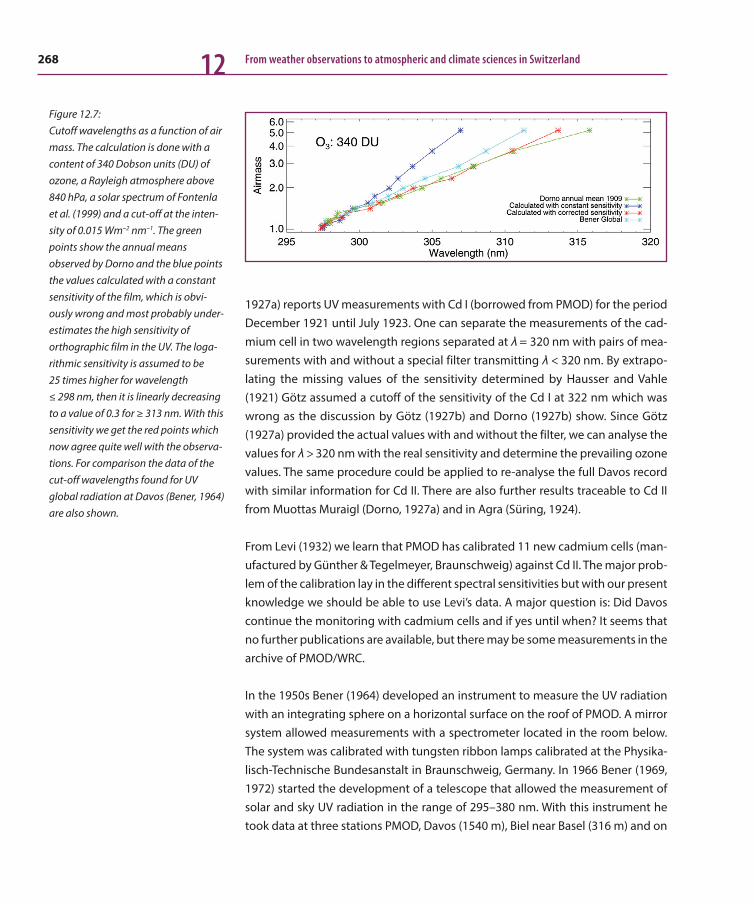
268 From weather observations to atmospheric and climate sciences in Switzerland12
1927a) reports UV measurements with Cd I (borrowed from PMOD) for the period December 1921 until July 1923. One can separate the measurements of the cad-mium cell in two wavelength regions separated at λ = 320 nm with pairs of mea-surements with and without a special filter transmitting λ < 320 nm. By extrapo-lating the missing values of the sensitivity determined by Hausser and Vahle (1921) Götz assumed a cutoff of the sensitivity of the Cd I at 322 nm which was wrong as the discussion by Götz (1927b) and Dorno (1927b) show. Since Götz (1927a) provided the actual values with and without the filter, we can analyse the values for λ > 320 nm with the real sensitivity and determine the prevailing ozone values. The same procedure could be applied to re-analyse the full Davos record with similar information for Cd II. There are also further results traceable to Cd II from Muottas Muraigl (Dorno, 1927a) and in Agra (Süring, 1924).
From Levi (1932) we learn that PMOD has calibrated 11 new cadmium cells (man-ufactured by Günther & Tegelmeyer, Braunschweig) against Cd II. The major prob-lem of the calibration lay in the different spectral sensitivities but with our present knowledge we should be able to use Levi’s data. A major question is: Did Davos continue the monitoring with cadmium cells and if yes until when? It seems that no further publications are available, but there may be some measurements in the archive of PMOD/WRC.
In the 1950s Bener (1964) developed an instrument to measure the UV radiation with an integrating sphere on a horizontal surface on the roof of PMOD. A mirror system allowed measurements with a spectrometer located in the room below. The system was calibrated with tungsten ribbon lamps calibrated at the Physika-lisch-Technische Bundesanstalt in Braunschweig, Germany. In 1966 Bener (1969, 1972) started the development of a telescope that allowed the measurement of solar and sky UV radiation in the range of 295–380 nm. With this instrument he took data at three stations PMOD, Davos (1540 m), Biel near Basel (316 m) and on
Figure 12.7: Cutoff wavelengths as a function of air mass. The calculation is done with a content of 340 Dobson units (DU) of ozone, a Rayleigh atmosphere above 840 hPa, a solar spectrum of Fontenla et al. (1999) and a cut-off at the inten-sity of 0.015 Wm–2 nm–1. The green points show the annual means observed by Dorno and the blue points the values calculated with a constant sensitivity of the film, which is obvi-ously wrong and most probably under-estimates the high sensitivity of orthographic film in the UV. The loga-rithmic sensitivity is assumed to be 25 times higher for wavelength ≤ 298 nm, then it is linearly decreasing to a value of 0.3 for ≥ 313 nm. With this sensitivity we get the red points which now agree quite well with the observa-tions. For comparison the data of the cut-off wavelengths found for UV global radiation at Davos (Bener, 1964) are also shown.

269Two centuries of atmospheric-radiation research in Switzerland 12
the peak of Weissfluh (2667 m). All these data are described in Fröhlich and Bener (1981) and available from ftp://ftp.pmodwrc.ch/pub/data/irradiance/bener_uv/.
In the early 1990s, a UV monitoring network in Switzerland was discussed as a contribution to GAW and in the framework of CHARM. The first two stations at Davos and Payerne started with UV-biometers (similar to the Robertson-Berger instruments) in May 1995 (e. g. Philipona et al., 1997). The data were used among other applications to validate the UV-index distributed by MeteoSwiss, based on the Davos data and a forecast of the ozone content (Renaud, 1998; Renaud et al., 1998). Another study at the Weissfluhjoch dealing with the albedo effect in the UV region followed Schmucki et al. (2001). Around the same time a 4-channel UV-PFR in the range of 305–332 nm was developed (Ingold et al., 2001b) which can also be used to determine ozone. Moreover, they are used for monitoring the solar UV radiation at PMOD/WRC on a operational basis (available at http://intranet.pmodwrc.ch/wcc_uv/uv_pmodwrc.php). Calibration of the UV-biometers is main-tained by a standard group of three reference biometers which are compared yearly to spectroradiometers. UV-PFRs are periodically calibrated against trap- detectors in the laboratory which allow very high accuracy of the order of 0.5 % and are therefore well suited for monitoring UV trends. The increased use of spectroradiometer of the type Brewer and others necessitated a reference. This reference – called QASUME – for the routine quality assurance and calibration of spectroradiometers measuring spectral solar UV irradiance has been operated at PMOD/WRC since 2004. In 2008 PMOD/WRC became a GAW regional UV calibration centre for the European region (WMO RA VI (Europe)). In 2013 the World Calibration centre–Ultraviolet (WCC-UV) at PMOD/WRC was officially recognized by the GAW programme.
Determination of the ‘solar constant’
Already Abbot et al. (1913) reported an increase of the total solar irradiance (TSI), called ‘solar constant’, with increasing solar activity, represented by the sunspot number of Wolf (SSN). They found a change of 3.6 % for a change of SSN by 100. Like Abbot et al. (1913), Dorno (1919a, p. 282) also found from his data that the change in the UV and blue is larger than the one of the total radiation. Compared to TSI observations from space since 1978 the variability of these extrapolated values is much higher, several percent compared to a few tenth of a percent, which may be explained by the transparency variation during the observations and e. g. the dependence on the solar cycle by a kind of amplification by changing solar

270 From weather observations to atmospheric and climate sciences in Switzerland12
energetic particles from flares. The standard value form the Smithsonian observa-tions of 1354 Wm–2 used by e. g. Schüepp (1949) is only about 0.5 % lower than the presently accepted value, which is most likely due to missing power from unob-served wavelength ranges in the UV and IR – an overall impressive result.
When the newly developed PMO-type radiometers became available in the 1970s (Brusa and Fröhlich, 1986) in 1979 PMOD/WRC started with solar constant deter-minations from stratospheric balloons. These experiments were performed in cooperation with the Geneva Observatory which provided the gondola and the experience needed for such experiments. The balloons were launched and oper-ated by the Centre National d’Etudes Spatiales (CNES) at Air sur l’Adours and Gap in France. They reached altitudes of 34–40 km and allowed measurements of 20–340 minutes duration. Furthermore, PMOD participated also in rocket experi-ments of NASA, launched from White Sands, New Mexico USA, in cooperation with Richard C. Willson of the Jet Propulsion Laboratory. Also the space experiments were performed in international cooperations: SOVA (SOlar VAriability) had three parts: SOVA1 and SOVA2 with the instruments from IRMB and PMOD/WRC respec-tively and SOVA3 with the data processing unit from the Space Science Depart-ment (SSD) of ESA (Crommelynck et al., 1991) and was flown on EURECA (EUro-pean REtrievable CArrier), launched 31 July 1992 and retrieved on 1 July 1993. VIRGO (Variability of IRradiance and Gravity Oscillations) (Fröhlich et al., 1997) was developed under the leadership of PMOD/WRC and has radiometers and spectral instruments from PMOD/WRC, IRMB and SSD and is part of SOHO (SOlar and Helio-pheric Observatory) a cooperative ESA/NASA mission. SOHO was launched 5 December 1995 and operational measurements started between mid January and April 1996. SOHO is still operational and VIRGO still producing data, covering since January 2016 measurements over 20 years. The third experiment was SOVIM (SO]lar Variability and Irradiance Monitoring) with radiometers from PMOD/WRC and IRMB, developed under the leadership of PMOD/WRC. SOVIM was originally planned as a re-flight of SOVA, but due to the constraints of the International Space Station and the integration with two other experiments on SOLAR, it became mostly a new design. It was launched in February 2008 and installed on the ESA Columbus module (Schmidtke et al., 2006), measurements started in April 2008 and for SOVIM ended unfortunately already in September due to a failure of the power supply (re-flown hardware of SOVA). Nonetheless, observations could be made during 46 days, enough for comparison with VIRGO. The fourth experi-ment of PMOD/WRC was PREMOS on the CNES mission PICARD with PMO6 radi-ometers and sunphotometers (Schmutz et al., 2009; Schmutz et al., 2013). PICARD was launched in 2010 and PREMOS operational until February 2014.

271Two centuries of atmospheric-radiation research in Switzerland 12
In summary PMOD/WRC performed since 1979 extraterrestrial TSI measurements with seven balloon flights, three rocket flights and four space experiments. Besides radiometers also SPMs were flown which provided extraterrestrial spec-tral irradiance values for turbidity determinations and as well detailed informa-tion on the atmospheric extinction at the balloon height, needed for the correc-tions of TSI. The measurements of the SPM with a signal-to-noise ratio of more than 107 were mainly used for helioseismology, the analysis of solar oscillations for information about the solar interior. For the evaluation in terms of absolute solar spectral irradiance there are still degradation problems to be solved – espe-cially for the now 20-year-long record of VIRGO (some results are shown in Figure 2.2 of http://www.pmodwrc.ch/pmod.php?topic=tsi/virgo/proj_space_ virgo). All PMOD/WRC measurements of TSI are shown in Figure 12.8 together with a composite TSI record. This composite is constructed from the various measure-ments in space since 1978 and since 1996 from VIRGO. With the large experience gained during the evaluation the VIRGO TSI record – especially for the long-term changes of radiometers in space, called degradation – the records of ACRIM I on
Figure 12.8: The plot shows the PMOD composite of total solar irradiance, scaled to the new VIRGO scale, the old on the right hand side and the new on the left hand side. The rocket and the baloon experiment have been shifted to agree with the scale for the first observations. The SOVA, SOVIM and PREMOS data are also shifted to lie on the composite record by −545, + 630 and 0 ppm. The deviations of the balloon/rocket measure-ments from the daily composite values have a mean of −555 ± 329 ppm with the extremes of −18 ppm in 1988 and −1258 ppm in 1992 or a range of + 537 and −703 ppm about the mean.
272 From weather observations to atmospheric and climate sciences in Switzerland12
the Solar Maximum Mission and HF on MIMBUS 7 could be corrected for effects unknown at the time of the original evaluation, which improved their com-parability with the other records substantially (Fröhlich, 2006). The present VIRGO version (since 6.4) is based on new corrections (for details see http://www.pmodwrc.ch/pmod.php?topic=tsi/virgo/proj_space_virgo) which has also changed the absolute value, shown on the right hand scale of Figure 12.8. All the balloon, rocket and space results are well within the stated 2σ uncertainty of the PMO6 radiometers of ±1.4 Wm-2 or ±1000 ppm (Brusa and Fröhlich, 1986) com-pared to the composite which is impressive, as these measurements span about three decades and are based on different radiometers.
12.4 Summary
In the 19th century, radiation research started with observation of nature and reports at the sessions of the regional sections of the Schweizerische Natur-forschende Gesellschaft or Société Helvétique des Sciences Naturelles and more extensively at the society’s annual meetings. It was not only the scientific interest but also the beauty which fascinated the naturalists. Many of the scientists in the 19th century were from the francophone part of Switzerland and Geneva was an important centre hosting also the Archives des Sciences Physiques et Naturelles, which contains short personal reports presented at weekly meetings as well as full papers. The cooperation with French scientists was also very close. It seems that most of the scientists at that time – famous for other important contributions to physical and natural sciences – did their radiation studies as a kind of hobby. Excel-lent examples are Soret, Foret, Ch. Dufour, Wolf, Gruner, Gockel and Maurer; Dorno was probably the first who dedicated his scientific work to radiation research. Maurer and Dorno introduced many German scientists, discussed their important results stimulating interesting scientific publications. When Dorno started the instrumental period he used essentially all possible means from the physics labo-ratory to improve radiation measurements; this finally gave PMOD the lead in many instrument developments for radiation research. Although the measure-ments became more reliable, the understanding of the physics behind them was often lacking – a very interesting aspect of the evolution of atmospheric radiation research. This also means that many of the records should be analysed again in view of the present understanding of radiative transfer in the atmosphere, not only to extend existing time series, but also to better understand the prejudices of the scientists. Moreover, such reviews may also help to improve our under-standing of climate change during the 20th century. An important point is also the
273Two centuries of atmospheric-radiation research in Switzerland 12
observer’s belief in the correctness of his results even if their understanding is unclear: Dorno resisted changing his polarisation data although some scientists argued strongly that he should (see Figure 12.3).
Nowadays we have much more data from automatic systems and need intelligent algorithm to judge the quality of the data. In the old days the observers looked at the sky at sunrise, during the day and at sunset, so they knew what they could expect from the data, even after the 1920s when they were taken automatically. By the lack of eye observations we may miss some important connections not obvious from the data alone.
Acknowledgements
In the 6 months of the preparation of this paper I had many discussions with Chris-toph Wehrli, Alain Heimo, Rolf Philipona, Julian Gröbner and others which is grate-fully acknowledged. It was also a great help to have access to the archive of PMOD and finally, I thank for the patience of the organizer/editor accepting my delays in delivering the manuscript.
References
Ångström A., 1929: On the atmospheric transmission of sun radiation and on dust in the air. Geogr. Ann. A, 11, 156–166.
Ångström, K., 1899: Ueber absolute Bestimmungen der Wärme-strahlung mit dem elektrischen Compensationspyrheliometer, nebst einigen Beispielen der Anwendung dieses Instrumentes. Ann. Phys., 303, 633–648, doi:10.1002/andp.18993030310.
Abbot, C. G., and L. B. Aldrich, 1913: Smithsonian Pyrheliometry Revised. Smithsonian Misc. Coll., 60 (18), 1–7.
Abbot, C. G., F. E. Fowle, and L. B. Aldrich, 1913: The Variation of the Sun. Astrophys. J., 38, 181, doi: 10.1086/142020.
Babinet, J., 1837: Mémoires d’optique météorologique. II. Sur les couronnes. CR Hept. Acad. Sci., 4, 642–645.
Bener, P., 1964: Tages- und Jahresgang der spektralen Intensität der ultravioletten Global- und Himmelsstrahlung bei wolken-freiem Himmel in Davos (1590 m/M). Strahlenther., 123, 306–316.
Bener, P., 1969: Spectral intensity of natural ultraviolet radiation and its dependence on various parameters. The Biologic Effects of Ultraviolet Radiation, F. Urbach, Ed., Pergamon Press, New York, USA, 351–358.
Bener, P., 1972: Approximate values of intensity of natural ultra-violet radiation for different amounts of atmospheric ozone. Tech. rep., Physikalisch-Meteorologisches Observatorium Davos.
Berk, A., G. Anderson, P. Acharya, and E. Shettle, 2008: MODTRAN 5.2.0.0 User’s Manual. Spectral Sciences, Inc. Burlington, and Air Force Research Laboratory, Hanscom AFB, Ma. U. S. A.
Bishop, S. E., 1884: The Remarkable Sunsets. Nature, 29, 259–260, doi:10.1038/029259b0.
Blumer, H., 1925: Strahlungsdiagramme kleiner dielektrischer Kugeln. Z. Phys., 32, 119–134, doi:10.1007/BF01331653.
Blumer, H., 1926a: Die Farbenzerstreuung an kleinen Kugeln. Z. Phys., 39, 195–214, doi:10.1007/BF01321987.
274 From weather observations to atmospheric and climate sciences in Switzerland12
Blumer, H., 1926b: Die Zerstreuung des Lichtes an kleinen Kugeln. Z. Phys., 38, 920–947, doi:10.1007/BF01397192.
Blumer, H., 1926c: Strahlungsdiagramme kleiner dielektrischer Kugeln. II. Z. Phys., 38, 304–328, doi:10.1007/BF01397500.
Brusa, R. W., and C. Fröhlich, 1986: Absolute radiometers (PMO6) and their experimental characterization. Appl. Opt., 25, 4173–4180, doi:{10.1364/AO.25.004173}.
Bührer, C., 1911: Observations actinometriques faites à Clarens en 1910. Arch. Sci. Phys. Nat., 31, 573–574.
Bührer, C., and H. Dufour, 1899: Observations actinometriques. Arch. Sci. Phys. Nat., 8, 174–176.
Courvoisier, P., 1954: Zur Definition der Sonnenstrahlung. Arch. Meteor. Geophy. B, 5, 125–145, doi:10.1007/ BF02244619.
Courvoisier, P., and H. Wierzejewski, 1948: Beiträge zur Strah-lungsmeßmethodik I: Die physikalischen Grundlagen der kalori-schen Strahlungsmeßmethoden. Arch. Meteor. Geophy. B, 1, 45–53, doi:10.1007/BF02246595.
Courvoisier, P., and H. Wierzejewski, 1949: Beiträge zur Strah-lungsmeßmethodik II. Arch. Meteor. Geophy. B, 1, 156–199, doi:10.1007/BF02248571.
Crommelynck, D., V. Domingo, and C. Fröhlich, 1991: The Solar Variations (SOVA) experiment in the EURECA space platform. Adv. Space Phys., 11, 83–87, doi:10.1016/0273-1177(91)90442-M.
Dorno, C., 1911: Studie über Licht und Luft des Hochgebirges. Druck und Verlag von Friedr. Vieweg & Sohn, Braunschweig.
Dorno, C., 1913: Über den Einfluss der gegenwärtigen atmo-sphärisch-optischen Störung auf die Strahlungsintensitäten der Sonne und des Himmels sowie auf die luftelektrischen Ele-ments. Meteor. Z., 30, 465–474.
Dorno, C., 1917a: Beobachtungen der Dämmerung und von Ringerscheinungen um die Sonne 1911 bis 1917. Veröffent-lichungen des Preussischen Meteorologischen Instituts: Abhand-lungen Bd. VI, Veröffentlichungen des Preussischen Meteoro-logischen Institutes: Abhandlungen Bd. V, Nr. 5, Berend Co., Berlin, Germany, 1–94.
Dorno, C., 1917b: Ringerscheinungen um die Sonne während der Jahre 1912 bis 1917 und ihre Beziehung zur Sonnentätig-keit. Meteor. Z., 34, 246–260.
Dorno, C., 1919: Eine auf den momentanen Zustand der Erd-atmosphäre abstellende Methode zur Bestimmung des Extink-tionskoeffizienten. Astron. Nachr., 209, 101–108.
Dorno, C., 1919a: Himmelshelligkeit, Himmelspolarisation und Sonnenintensität in Davos 1911 bis 1918. Veröffentlichungen des Preussischen Meteorologischen Institutes: Abhandlungen Bd. VI, Berend & Co., Berlin.
Dorno, C., 1919b: Physik der Sonnen- und Himmelstrahlung. Die Wissenschaft: Einzeldarstellungen aus der Naurwissenschaft und der Technik. Band 63, Friedr. Vieweg & Sohn in Braunschweig.
Dorno, C., 1920: Der optische Reinheitsgrad der Erdatmosphäre im Jahre 1919 und im Januar/Februar 1920. Meteor. Z., 37, 79–82.
Dorno, C., 1922: Fortschritte in Strahlungsmessungen. Meteor. Z., 39, 303–323.
Dorno, C., 1924: Zur Technik der Sonnenstrahlungsmessungen in einzelnen Spektralbezirken (Filterdurchässigkeit, Zellenemp-findlichkeit, Michelson-Aktinometer). Meteor. Z., 41, 234–248, mit Beiträgen von K. W. Meissner und W. Vahle.
Dorno, C., 1927a: Grundzüge des Klimas von Muottas-Muraigl (Oberengadin). Schweiz. Inst. für Hochgebirgs-Physiologie und Tuberkolose-Forschung in Davos, Heft 3, Friedr. Vieweg und Sohn AG, Braunschweig, Germany.
Dorno, C., 1927b: Ozonmessungen auf spektroskopischem Weg. Meteor. Z., 44, 462–464.
Dufour, C., 1885: Lueurs crépusculaires de l’hivers 1883–1884. Arch. Sci. Phys. Nat., 13, 89–109.
Dufour, C., 1898: Phénomènes intéressants constatés pendant l’éclipse de Lune du 3 juillet 1898. Arch. Sci. Phys. Nat., 6, 438–445.
Dufour, H., 1903: Absorption anormale de la radiation solaire. Arch. Sci. Phys. Nat., 15, 687–689.
Elster, J., and H. Geitel, 1904: Über eine verbesserte Form des Zinkkugelphotometers zur Bestimmung der Ultravioletten Son-nenstrahlung. Phys. Z., 5, 238–241.
Exner, F., 1921: Zur Darstellung des Polarisationsgrades des Himmelslichts. Meteor. Z., 38, 220–221.
Fabry, C., and H. Buisson, 1921: A Study of the Ultra-Violet End of the Solar Spectrum. Astrophys. J., 54, 297–322, doi:10.1086/ 142647.
275Two centuries of atmospheric-radiation research in Switzerland 12Fontenla, J., O. R. White, P. A. Fox, E. H. Avrett, and R. L. Kurucz, 1999: Calculation of Solar Irradiances. I. Synthesis of the Solar Spectrum. Astrophys. J., 518, 480–499.
Forel, F., 1884: Couronne solaire d’été de 1884. Arch. Sci. Phys. Nat., 12, 173–184.
Forel, F., 1885: Le Cercle de Bishop. Arch. Sci. Phys. Nat., 13, 465–476, available at http://gallica.bnf.fr/ark:/12148/bpt6k299071t.image.
Forel, F., 1903: Grande apparitions de feux crépusulaires anor-meaux. Arch. Sci. Phys. Nat., 15, 216–217. Forel, F., 1905: Le cercle de Bishop de la montagne Pelée 1902–1904. Arch. Sci. Phys. Nat., 19, 229–258. Fröhlich, C., 1991: History of Solar Radiometry and the World Radiometric Reference. Metrologia, 28, 111–115, doi:10.1088/0026-1394/28/3/001.
Fröhlich, C., 2006: Solar irradiance variability since 1978: Revi-sion of the PMOD composite during solar cycle 21. Space Sci. Rev., 125, 53–65, doi:10.1007/s11214-006-9046-5.
Fröhlich, C., and P. Bener, 1981: Ultraviolet radiation data bank. Tech. Rep. PMOD Publ. 654, Physikalisch-Meteorologisches Observatorium Davos.
Fröhlich, C., and R. W. Brusa, 1981: Solar radiation and its varia-tion in time. Sol. Phys., 74, 209–213, doi:{10.1007/BF00151291}.
Fröhlich, C., and Coauthors, 1997: First results from VIRGO, the experiment for helioseismology and solar irradiance monitor-ing on SOHO. Sol. Phys., 170, 1–25.
Fröhlich, C., 1978: World Radiometric Reference, Annex to Rec-ommendation 3 (CIMO-VII). Abridged Final Report of the Seventh Session of the Commission for Instruments and Methods of Obser-vation, Hamburg, 1–12 August 1977, World Meteorological Orga-nization, WMO-No. 490, 7bis Avenue de la Paix, Geneva, Swit-zerland, 97–100.
Geist, J., B. Steiner, R. Schaefer, E. Zalewski, and A. Corrons, 1975: Electrically based spectral power measurements through use of a tunable cw laser. Appl. Phys. Lett., 26, 309–311, doi:10.1063/ 1.88168.
Gilgen, H., and A. Ohmura, 1999: The Global Energy Balance Archive. Bull. Amer. Meteor. Soc., 80, 831–850, doi:10.1175/1520- 0477(1999)080⟨0831:TGEBA⟩2.0.CO;2.
Gockel, A., 1903: Atmospharische Trübung im Winter und Früh-ling 1902–1903. Meteor. Z., 20, 328.
Gockel, A., 1920: Beiträge zur Kenntnis von Farbe und Polarisa-tion des Himmelslichtes. Ann. Phys., 367, 283–292, doi:10.1002/andp.19203671105, This is the last article in a series with Arch.Sci.Phys.Nat. 44, 349, 1917 and Ann.Phys. 361, 617–638, 1918.
Götz, F. W. P., 1927a: Das Strahlungsklima von Arosa. Meteor. Z., 44, 138–142.
Götz, F. W. P., 1927b: Erwiederung zu C.Dorno, Über Ozonmes-sungen auf spektroskopischem Weg. Meteor. Z., 44, 389–390.
Götz, F. W. P., 1932: Trübung und anomale extiktion. Helv. Phys. Acta., 5, 336–340.
Götz, F. W. P., 1934: Wellenlängenabhängigkeit der Dunstextink-tion. Meteor. Z., 51, 472–474.
Götz, F. W. P., 1937: Bericht über das UV-Dosimeter. Protokolle der Sitzungen in Oxford, 12.–15. September 1936, Imprimörie Eduard Ijdo, Leiden, Hollande, Sécretariat de l’Organisation Météorolo-gique Internationale, 80–82.
Götz, F. W. P., 1937: Das Ultra-Violett Klima von Chur. Helv. Phys. Acta., 10, 352–354.
Götz, F. W. P., 1942: Photographie des ultravioletten Strahlendes. Z. angew. Photogr., 4, 65–67.
Götz, F. W. P., 1926: Das Strahlungsklima von Arosa. Springer- Verlag GmbH Berlin Heidelberg.
Gröbner, J., I. Reda, S. Wacker, S. Nyeki, K. Behrens, and J. Gor-man, 2014: A new absolute reference for atmospheric longwave irradiance measurements with traceability to SI units. J. Geo-phys. Res., 119, 7083–7090, doi:10.1002/2014JD021630.
Gruner, P., 1903: Über die neueren Dämmerungserscheinungen. Mitt. Naturforsch. Ges. Bern, 1–5.
Gruner, P., 1915: Schematische Darstellung des Verlaufs der Dämmerfarben. Mitt. Naturforsch. Ges. Bern, 264–312.
Gruner, P., 1919a: Dämmerungsstörungen. Astron. Nachr., 210, 13.
Gruner, P., 1919b: Über die Gesetze der Beleuchtung der irdi-schen Atmosphäre durch das Sonnenlicht. Beitr. Phys. Atmos., 8, 120–156.
Gruner, P., 1921: Beiträge zur Kenntnis der Dämmerungs- Erscheinungen und des Alpenglühens: I. Historisch-chronologi-sche Übersicht der schweizerischen Beobachtungen und Veröf-

276 From weather observations to atmospheric and climate sciences in Switzerland12
fentlichungen über Dämmerungsfärbungen und Alpenglühen. Denkschriften der Schweizerischen Naturforschenden Gesell-schaft, Kommission für Veröffentlichungen der Schweizerischen Naturforschenden Gesellschaft, Kommisionsverlag von Georg & Co., Basel, Genf und Lion.
Gruner, P., 1932a: Anwendung der Optik trüber Medien auf die Beleuchtung der Atmosphäre I. Die Beleuchtung der idealen Atmosphäre im Sonnenvertikal bei Sonnenuntergang und während der bürgerlichen Dämmerung. Helv. Phys. Acta., 5, 31–58.
Gruner, P., 1932b: Anwendung der Optik trüber Medien auf die Beleuchtung der Atmosphäre II. Vereinfachte Ausdrücke zur Berechnung der Helligkeit der Atmosphäre. Helv. Phys. Acta., 5, 145–160.
Gruner, P., 1932c: Anwendung der Optik trüber Medien auf die Beleuchtung der Atmosphäre III. Beleuchtung inhomogener, gekrümmter Schichten: Theorie des Purpurlichtes. Helv. Phys. Acta., 5, 351–361.
Gruner, P., 1934: Internationale Dämmerungsbeobachtungen wähend des Polarjahres 1932/33. Mitt. Natur- forsch. Ges. Bern, 185–213.
Gruner, P., and H. Kleinert, 1927: Die Dämmerungserscheinun-gen. Probleme der Kosmischen Physik, herausgegeben von Prof. C. Jensen and Prof. A. Schwassmann, Verlag von Henri Grand, Hamburg.
Hausser, K., and W. Vahle, 1921: Die Abhängigkeit des Lich-terythems und der Pigmentbildung von der Schwingunszahl (Wellenlänge) der erregenden Strahlung. Strahlenther., 13, 41–71.
Heimo, A., R. Philipona, C. Fröhlich, C. Marty, and A. Ohmura, 1998: The Swiss atmospheric radiation monitoring network CHARM. TECO-98, Casablanca, Marocco, 13th–15th May, WMO/TD 877: Instruments and Observing Methods No. 70, WMO, Geneva, Switzerland, 291–294.
Heimo, A. and Valko, P., 1977: First results obtained from the Swiss mobile system for solar radiation measurements. WMO Solar Energy Meeting, World Meteorological Organization, Geneva, Switzerland.
Hildres, W. and Fierstein, J., 2014: The Novapupta-Katmai Erup-tion of 1912 – Largest Eruption of the Twentieth Centura: Cen-
tennial Perspectives. Professional Paper 1791 of the U. S. Geo-logical Survey, Reston, Virginia, U. S. A.
Hoyt, D. V., and C. Fröhlich, 1983: Atmospheric transmission at Davos, Switzerland 1909–1979. Climate Change, 5, 61–71.
Ingold, T., C. Mätzler, N. Kämpfer, and A. Heimo, 2001a: Aerosol optical depth measurements by means of a Sun photometer network in Switzerland. J. Geophys. Res., 106, 27 537, doi:10.1029/ 2000JD000088.
Ingold, T., C. Mätzler, C. Wehrli, A. Heimo, N. Kämpfer, and R. Phi-lipona, 2001b: Ozone Column Density Determination From Direct Irradiance Measurements in the Ultraviolet Performed by a Four-Channel Precision Filter Radiometer. Appl. Opt., 40, 1989–2003, doi:10.1364/AO.40.001989.
Junge, C., 1955: The size distribtion and aging of natural aero-sols as determined from electrical and optical data on the atmo-sphere. J. Meteor., 12, 13–25.
King, L., 1913: On the Scattering and Absorption of Light in gas-eous Media, with Applications to the Intensity of Sky Radiation. Philos. Trans. Roy. Soc. A, 212, 375–433.
König-Langlo, G., R. Sieger, H. Schmithüsen, A. Bücker, F. Richter, and E. Dutton, 2013: The Baseline Surface Radiation Network and its World Radiation Monitoring Centre at the Alfred Wege-ner Institute. World Climate Reseach Programme Report, GCOS-174, World Meteorological Organization, Geneva, Switzerland.
Labs, D., and H. Neckel, 1967: Die absolute Strahlungsinten-sität der Mitte der Sonnenscheibe im Spektralbereich 3288 ≤ λ ≤ 12480 ˚A. Z. Astrophys., 65, 133–185.
Labs, D., and H. Neckel, 1972: Remarks on the Convergency of Photospheric Model Conceptions and the Solar Quasi Contin-uum. Sol. Phys., 22, 64–69, doi:10.1007/BF00145462.
Lachat, D., and C. Wehrli, 2012: A century of apparent atmo-spheric transmission over Davos, Switzerland. Theor. Appl. Cli-matol., 110, 539–547, doi:10.1007/s00704-012-0685-z.
Lachat, D., and C. Wehrli, 2013: Dimming and brightening trends in direct solar irradiance from 1909 to 2010 over Davos, Switzer-land: Proportions of aerosol and gaseous transmission. J. Geo-phys. Res., 118, 3285–3291, doi:10.1002/jgrd.50344.
Levi, F., 1932: Erfahrungen bei der Eichung von Cadmiumzellen. Meteor. Z., 49, 139–151.
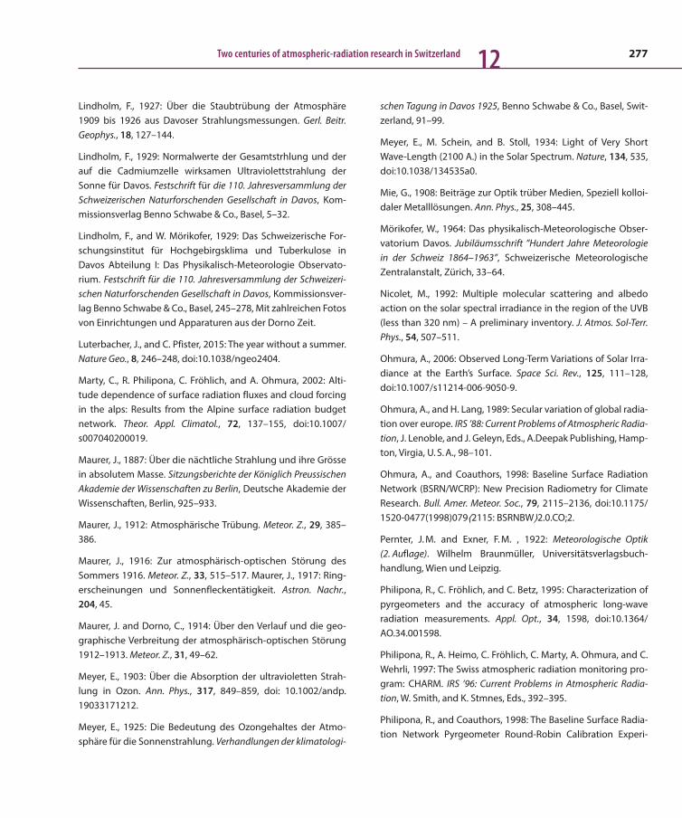
277Two centuries of atmospheric-radiation research in Switzerland 12Lindholm, F., 1927: Über die Staubtrübung der Atmosphäre 1909 bis 1926 aus Davoser Strahlungsmessungen. Gerl. Beitr. Geophys., 18, 127–144.
Lindholm, F., 1929: Normalwerte der Gesamtstrhlung und der auf die Cadmiumzelle wirksamen Ultraviolettstrahlung der Sonne für Davos. Festschrift für die 110. Jahresversammlung der Schweizerischen Naturforschenden Gesellschaft in Davos, Kom-missionsverlag Benno Schwabe & Co., Basel, 5–32.
Lindholm, F., and W. Mörikofer, 1929: Das Schweizerische For-schungsinstitut für Hochgebirgsklima und Tuberkulose in Davos Abteilung I: Das Physikalisch-Meteorologie Observato-rium. Festschrift für die 110. Jahresversammlung der Schweizeri-schen Naturforschenden Gesellschaft in Davos, Kommissionsver-lag Benno Schwabe & Co., Basel, 245–278, Mit zahlreichen Fotos von Einrichtungen und Apparaturen aus der Dorno Zeit.
Luterbacher, J., and C. Pfister, 2015: The year without a summer. Nature Geo., 8, 246–248, doi:10.1038/ngeo2404.
Marty, C., R. Philipona, C. Fröhlich, and A. Ohmura, 2002: Alti-tude dependence of surface radiation fluxes and cloud forcing in the alps: Results from the Alpine surface radiation budget network. Theor. Appl. Climatol., 72, 137–155, doi:10.1007/s007040200019.
Maurer, J., 1887: Über die nächtliche Strahlung und ihre Grösse in absolutem Masse. Sitzungsberichte der Königlich Preussischen Akademie der Wissenschaften zu Berlin, Deutsche Akademie der Wissenschaften, Berlin, 925–933.
Maurer, J., 1912: Atmosphärische Trübung. Meteor. Z., 29, 385–386.
Maurer, J., 1916: Zur atmosphärisch-optischen Störung des Sommers 1916. Meteor. Z., 33, 515–517. Maurer, J., 1917: Ring-erscheinungen und Sonnenfleckentätigkeit. Astron. Nachr., 204, 45.
Maurer, J. and Dorno, C., 1914: Über den Verlauf und die geo-graphische Verbreitung der atmosphärisch-optischen Störung 1912–1913. Meteor. Z., 31, 49–62.
Meyer, E., 1903: Über die Absorption der ultravioletten Strah-lung in Ozon. Ann. Phys., 317, 849–859, doi: 10.1002/andp. 19033171212.
Meyer, E., 1925: Die Bedeutung des Ozongehaltes der Atmo-sphäre für die Sonnenstrahlung. Verhandlungen der klimatologi-
schen Tagung in Davos 1925, Benno Schwabe & Co., Basel, Swit-zerland, 91–99.
Meyer, E., M. Schein, and B. Stoll, 1934: Light of Very Short Wave-Length (2100 A.) in the Solar Spectrum. Nature, 134, 535, doi:10.1038/134535a0.
Mie, G., 1908: Beiträge zur Optik trüber Medien, Speziell kolloi-daler Metalllösungen. Ann. Phys., 25, 308–445.
Mörikofer, W., 1964: Das physikalisch-Meteorologische Obser-vatorium Davos. Jubiläumsschrift ”Hundert Jahre Meteorologie in der Schweiz 1864–1963”, Schweizerische Meteorologische Zentralanstalt, Zürich, 33–64.
Nicolet, M., 1992: Multiple molecular scattering and albedo action on the solar spectral irradiance in the region of the UVB (less than 320 nm) – A preliminary inventory. J. Atmos. Sol-Terr. Phys., 54, 507–511.
Ohmura, A., 2006: Observed Long-Term Variations of Solar Irra-diance at the Earth’s Surface. Space Sci. Rev., 125, 111–128, doi:10.1007/s11214-006-9050-9.
Ohmura, A., and H. Lang, 1989: Secular variation of global radia-tion over europe. IRS ’88: Current Problems of Atmospheric Radia-tion, J. Lenoble, and J. Geleyn, Eds., A.Deepak Publishing, Hamp-ton, Virgia, U. S. A., 98–101.
Ohmura, A., and Coauthors, 1998: Baseline Surface Radiation Network (BSRN/WCRP): New Precision Radiometry for Climate Research. Bull. Amer. Meteor. Soc., 79, 2115–2136, doi:10.1175/ 1520-0477(1998)079⟨2115: BSRNBW⟩2.0.CO;2.
Pernter, J. M. and Exner, F. M. , 1922: Meteorologische Optik (2. Auflage). Wilhelm Braunmüller, Universitätsverlagsbuch-handlung, Wien und Leipzig.
Philipona, R., C. Fröhlich, and C. Betz, 1995: Characterization of pyrgeometers and the accuracy of atmospheric long-wave radiation measurements. Appl. Opt., 34, 1598, doi:10.1364/AO.34.001598.
Philipona, R., A. Heimo, C. Fröhlich, C. Marty, A. Ohmura, and C. Wehrli, 1997: The Swiss atmospheric radiation monitoring pro-gram: CHARM. IRS ’96: Current Problems in Atmospheric Radia-tion, W. Smith, and K. Stmnes, Eds., 392–395.
Philipona, R., and Coauthors, 1998: The Baseline Surface Radia-tion Network Pyrgeometer Round-Robin Calibration Experi-
278 From weather observations to atmospheric and climate sciences in Switzerland12
ment. J. Atmos. Oceanic Technol., 15, 687–696, doi:10.1175/1520-0426(1998)015⟨0687: TBSRNP⟩2.0.CO;2.
Rayleigh, L., 1881: On the electromagnetic theory of light. Phil. Mag. S5, 12, 81–101, doi:10.1080/14786448108627074.
Renaud, A., 1998: Solar Erythemal Ultraviolet Radiation: Analysis of Swiss Mesurements and Modelling. Ph.D. thesis, Swiss Fed-eral Institue of Technology (ETH), Zürich.
Renaud, A., J. Staehelin, M. Blumthaler, and R. Philipona, 1998: Influence of total ozone variation on UV (erythema) radiation. An analysis of direct Robertson-Berger measurements at Davos, Switzerland. Atmospheric Ozone Proceedings XVIII Quadriennial Ozone Symposium L’Aquila (1996), R. D. Bojkov, and G. Visconti, Eds., 861 – 864.
Riggenbach, A., 1886: Beobachtungen über die Dämmerung, insbesondere über das Purpurlicht und seine Beziehungen zum Bishop’schen Ring. Verh. Naturforsch. Ges. Basel, 8, 1–102.
Ruckstuhl, C., R. Philipona, J. Morland, and A. Ohmura, 2007: Observed relationship between surface specific humidity, integrated water vapor, and longwave downward radiation at different altitudes. J. Geophys. Res., 112, D03302, doi:10.1029/ 2006JD007850.
Sassen, K., T. Peter, B. P. Luo, and P. J. Crutzen, 1994: Volcanic Bishop’s ring: evidence for a sulfuric acid tetrahydrate particle aureole. Appl. Opt., 33, 4602–4606, doi:10.1364/AO.33.004602.
Schmid, B., P. R. Spyak, S. F. Biggar, C. Wehrli, J. Sekler, T. Inglod, C. Mätzler, and N. Kämpfer, 1998: Evaluation of the applicability of solar and lamp radiometric calibrations of a precision sun photometer operating between 300 and 1025nm. Appl. Opt., 3923–3941.
Schmid, B., and C. Wehrli, 1995: Comparison of sun photometer calibration by use of the langley technique and the standard lamp. Appl. Opt., 34, 4500–4512.
Schmidtke, G., C. Fröhlich, and G. Thuillier, 2006: ISS-SOLAR: Total (TSI) and spectral (SSI) irradiance measurements. Adv. Space Phys., 37, 255–264, doi:10.1016/j.asr.2005.01.009.
Schmucki, D., S. Voigt, R. Philipona, C. Fröhlich, J. Lenoble, A. Ohmura, and C. Wehrli, 2001: Effective albedo derived from UV measurements in the Swiss Alps. J. Geophys. Res., 106, 5369–5383, doi:10.1029/2000JD900712.
Schmutz, W., A. Fehlmann, W. Finsterle, G. Kopp, and G. Thuillier, 2013: Total solar irradiance measurements with PREMOS/PICARD. IRS2012: Proceedings of the International Radiation Sym-posium (IRC/IAMAS), R. F. Cahalan, and J. Fischer, Eds., AIP Conf. Proc. 1531, American Institute of Physics, 624–627.
Schmutz, W., and Coauthors, 2009: The PREMOS/PICARD instru-ment calibration. Metrologia, 46, S202, doi:10.1088/0026-1394/46/4/S13.
Schröder, W., and K.-H. Wiederkehr, 2000: Johann Kiessling, the Krakatoa Event and the Development of Atmospheric Optics after 1883. Notes Rec. Roy. Soc., 54, 249–258.
Schuepp, W., 1949: Die Bestimmung der Komponenten der atmosphärischen Trübung aus Aktinometermessungen. Arch. Meteor. Geophy. B, 1, 257–346, doi:10.1007/BF02242830.
Sekera, Z., 1957: Polarization of Skylight, Vol. XLVIII: Geophysics II, 288–328. Springer Verlag, Berlin, Gttingen, Heidelberg.
Soret, J., 1888: Sur la polarisation atmospherique. Ann. Chim. Phys, Serie 6.
Süring, R., 1924: Strahlungsklimatische Untersuchungen in Agra (Tessin). Meteor. Z., 41, 325–346. Thordarson, T., and S. Self, 2003: Atmospheric and environmental effects of the 1783–1784 Laki eruption: A review and reassessment. J. Geophys. Res., 108, 4011, doi:10.1029/2001JD002042.
Vitt, F. M., T. E. Cravens, and C. H. Jackman, 2000: A two-dimen-sional model of thermospheric nitric oxide sources and their contributions to the middle atmospheric chemical balance. J. Atmos. Sol-Terr. Phys., 62, 653–667, doi:10.1016/S1364-6826 (00)00049-3.
Volz, F., 1959: Photometer mit Selen-Photoelement zur spekt-ralen Messung der Sonnenstrahlung und zur Bestimmung der Wellenlängenabhängigkeit der Dunsttrübung. Arch. Meteor. Geophy. B, 10, 100–131, doi:10.1007/BF02243122.
Wehrli, C., 2008: Remote sensing of aerosol optical depth in gloabal surface network. Ph.D. thesis, Eidgenössisch-Technische Hochschule Zürich, DissETH 17591.
Wild, M., 2009: Global dimming and brightening: A review. J. Geophys. Res.), 114, D00D16, doi:10.1029/2008JD011470.
WMO, 2001: Global Atmosphere Watch Measurement Guide. WMO GAW Report 143, TD No. 1073, World Meteorological Orga-nization, Geneva, Switzerland.

279
13 The rise and decline of research on atmospheric electricity in SwitzerlandHans Richner
Atmospheric electricity is no longer a research topic in Switzerland. However, Swiss researchers once
were the worldwide leading experts. Everybody knows Benjamin Franklin’s experiments, but only few
people are aware that it was Horace-Bénédict de Saussure, a Swiss botanist and glaciologist, who made
the first quantitative investigations of the atmospheric electric field at the end of the 18th century
(though he eventually became more famous for his humidity measurements). Around 1900, Albert
Gockel, University of Fribourg, investigated atmospheric electricity in connection with meteorological
elements. In the first half of the 20th century, activities peaked again when Jean Lugeon, later director
of the Swiss Meteorological Institute, built his radiogoniograph and atmoradiograph. The expectations
were high that weather forecasting would greatly benefit from these instruments, which, in fact, were
the very first remote sensing devices to be used in meteorology. The participation in the “Geophysical
Years” in the 1950s stimulated the development of novel and highly reliable instruments for observing
electrical properties of the atmosphere; they were designed and built by Leonhard Saxer and Werner
Sigrist, physics teachers at the Kantonsschule Aarau. These instruments were used in many countries,
and a complete set thereof continued to operate at the “Luftelektrische Station Aarau.” In the 1970s, at
the Institute for Snow and Avalanche Research, Armin Aufdermaur und Othmar Buser carried out
experiments, searching for mechanisms that generate the atmospheric electric field. Except for this last
peak endeavor, however, activities declined continuously until 2002, when the operational station in
Aarau had to be shut down for lack of funds.
13.1 The early days of research into atmospheric electricity
As early as 1785, the Swiss physicist Horace-Bénédict de Saussure made the very first quantitative measurements of atmospheric electric quantities.
De Saussure measured the electric charge in the air using two small insulating balls suspended from fine threads. This arrangement was placed inside a glass container and called “electrometer.” In order to increase the sensitivity of this instrument, de Saussure added a wire (Figure 13.1). With this new electrometer, de Saussure was able to show that there is a diurnal and seasonal variation of the electric parameter (the term “electric field” was not known at that time). He also
ETH Zurich, Institute for Atmospheric
and Climate Science, Zurich
Dalibart’s and Benjamin Franklin’s
experiments in 1752 were not proper
measurements; the same is true for
Coulomb’s observations in 1785.
280 From weather observations to atmospheric and climate sciences in Switzerland13
invented a new method for using the electrometer, namely, by moving the wire in the air. He interpreted the reaction of the electrometer as the influence (in a physical sense) of electric charges contained in the atmosphere. With this inter-pretation he came close to what would later be known as electric field. (de Saus-sure, 1786)
Hermann Fritz (1875) published an article in which he brought atmospheric elec-tricity together with a whole range of geophysical phenomena. Quite carefully he remarked that the postulated occurrence of cirrus clouds together with electric phenomena in the air had not yet been fully proven. He also doubted that atmo-spheric electricity parameters (unfortunately he does not specify the ones he is referring to) have a 10- or 11-year cycle like sunspots do.
Figure 13.1: Electrometer used by Saussure (1786) for the first quantitative measurements of the atmospheric field.

281The rise and decline of research on atmospheric electricity in Switzerland 13
13.2 Observations of non-propagating atmospheric electricity parameters before 1940
In Switzerland, instrument-based observations began around 1900. In an attempt to explain aurorae and “radioactive” radiation, Albert Gockel – a researcher at the University of Fribourg – focused his attention on measuring atmospheric conduc-tivity and eventually became a widely reputed expert on thunderstorms. (At that time, it was postulated that a radioactive layer exists in the upper atmosphere.) He organized and participated in numerous field campaigns, many of which involved manned gas balloon flights. Radiation-induced ionization alters atmospheric con-ductivity, an issue that became Gockel’s life-long interest. While the primary aims of the balloon flights were to investigate (cosmic) radiation, he always included careful observations of meteorological phenomena, the most important being thunderstorms (Figure 13.2 shows a string electrometer as used by Gockel). Already in 1895 he had published the first edition of “Das Gewitter” [The thunder-storm] that readily became a reference publication. The last edition, enlarged and continuously updated, dates from 1925 (Gockel, 1925). There as well as in his somewhat more scientific work “Die Luftelektrizität” [The atmospheric electricity] (Gockel, 1908) one finds a lengthy discussion of a still pertinent and unsatisfacto-rily solved problem: What mechanism leads to charge separation in a cloud, and how is the electric field in the atmosphere generated?
Gockel investigated atmospheric electricity in connection with meteorological elements. In collaboration with Gockel, but expanding the measured parameters to ions, Father B. Huber in Altdorf made atmospheric electricity measurements in foehn situations. Similar observations were also made in Glarus. The measure-ments concentrated on counting ions of different sizes. It was hoped that with these observations an explanation for the adverse biometeorological effects of foehn could be found. Similarly, in the 1930s, atmospheric electricity parameters (together with numerous meteorological factors) were recorded at Davos, in the hope that general weather sensitivity could be explained (Mörikofer, 1950).
In 1939 the first atmospheric electricity station was established south of the Alps, in Locarno-Monti at the Osservatorio Ticinese of the Meteorologische Zentralan-stalt (Ambrosetti, 1943). The parameters measured included ions of three different size ranges, and conductivity. With a careful statistical analysis, the daily and sea-sonal variations of mean ion counts and of air conductivity could be computed, the data being stratified with humidity, wind, cloud cover, and visibility. Again, foehn events (meaning northfoehn, in this case) received special attention.
Surprisingly modern is a remark in the
summary of a talk delivered by “an engi-
neer Wirth” (NGZH, 1921): After demon-
strating the advantages of heat pumps
over burning coal for energy production,
he briefly mentions that the tides and
atmospheric electricity should seriously
be considered as power sources. Alter-
nate energy disputes already in the
1920s …
Figure 13.2: String electrometer as used by Gockel (1908) for measuring the atmospheric field.

282 From weather observations to atmospheric and climate sciences in Switzerland13
13.3 History of general electric and radio observations in the atmosphere
On the one hand, propagation of extreme low frequency radiowaves (ELF, i. e., 0.1 to 10 kHz) was studied with the aim of finding out more about the ionosphere. On the other hand, the sources of the ELF, i. e., electric discharges in clouds and thun-derstorms, were of major interest. Finally, the electric in-situ properties of the atmosphere were investigated. This effort was purely research oriented in the attempt to relate electric characteristics of the atmosphere to ozone concentra-tion, radioactivity, air pollution, etc.
During the International Polar Year (IPY) 1932/33, the Meteorologische Zentralan-stalt (Swiss Meteorological Institute) installed and operated a meteorological observatory at Snaefellsjökull (Lugeon, 1941). This station was used to monitor several radio transmitters. Jean Lugeon – at that time director of the Polish Mete-orological Institute – installed an additional receiver at the Polish observing sta-tion on Bear Island.
With the observations of the propagation of radio signals from long-wave and short-wave transmitters, the build-up and decay of the different layers of the iono-sphere as a function of daytime, weather, and magnetic activity was studied. It was also planned to continuously monitor aurora activity and to determine its location and radiation spectrum. Because of the high workload and the harsh environment, however, this task could be accomplished only partially.
Based on the experience, a radiogoniograph built in the 1930s by Guido Nobile was installed on the roof of the old ETH physics building where the Meteorolo-gische Zentralanstalt was located at that time. The instrument recorded continu-ously; it used a rotating loop antenna, which allowed to determine the direction from which radio signals were being received (Figure 13.3). The goal was to use atmospheric signals from lightning (sferics) and/or the propagation conditions inferred from the reception of distant radio stations for forecasting purposes. The radiogoniograph was most probably the first meteorological remote sensing instrument used in Switzerland. A second instrument was later installed at the aerological station Payerne (Rieker, 1960). The hopes that this instrument would eventually become an important tool for weather forecasting were quite high – and this not only in Switzerland (Lugeon, 1950). Also, the International Meteoro-logical Organization (IMO, which later became the WMO) discussed a permanent network of sferics receivers.

283The rise and decline of research on atmospheric electricity in Switzerland 13
In addition, an atmoradiograph was operated, which – basically a nondirectional ELF pulse counter – was used to study the propagation characteristics as function of daytime. This knowledge allowed a better interpretation of data from the radiogoniograph, which, in turn, could make it more useful for forecasting.
Figure 13.3: The radiogoniograph on the roof of the physics building of ETH around 1937; on the ladder stands Jean Lugeon, who became director of the Meteorologische Zentralanstalt in 1945. Note the (rotating) crossed loop antennae in the wooden hut. (Lugeon, 1939)
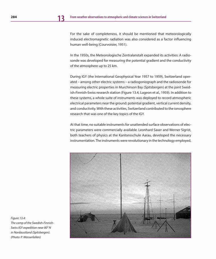
284 From weather observations to atmospheric and climate sciences in Switzerland13
For the sake of completeness, it should be mentioned that meteorologically induced electromagnetic radiation was also considered as a factor influencing human well-being (Courvoisier, 1951).
In the 1950s, the Meteorologische Zentralanstalt expanded its activities: A radio-sonde was developed for measuring the potential gradient and the conductivity of the atmosphere up to 25 km.
During IGY (the International Geophysical Year 1957 to 1959), Switzerland oper-ated – among other electric systems – a radiogoniograph and the radiosonde for measuring electric properties in Murchinson Bay (Spitsbergen) at the joint Swed-ish-Finnish-Swiss research station (Figure 13.4, Lugeon et al., 1959). In addition to these systems, a whole suite of instruments was deployed to record atmospheric electrical parameters near the ground: potential gradient, vertical current density, and conductivity. With these activities, Switzerland contributed to the ionosphere research that was one of the key topics of the IGY.
At that time, no suitable instruments for unattended surface observations of elec-tric parameters were commercially available. Leonhard Saxer and Werner Sigrist, both teachers of physics at the Kantonsschule Aarau, developed the necessary instrumentation. The instruments were revolutionary in the technology employed,
Figure 13.4: The camp of the Swedish-Finnish- Swiss IGY expedition near 80° N in Nordaustland (Spitsbergen). (Photo: P. Wasserfallen)
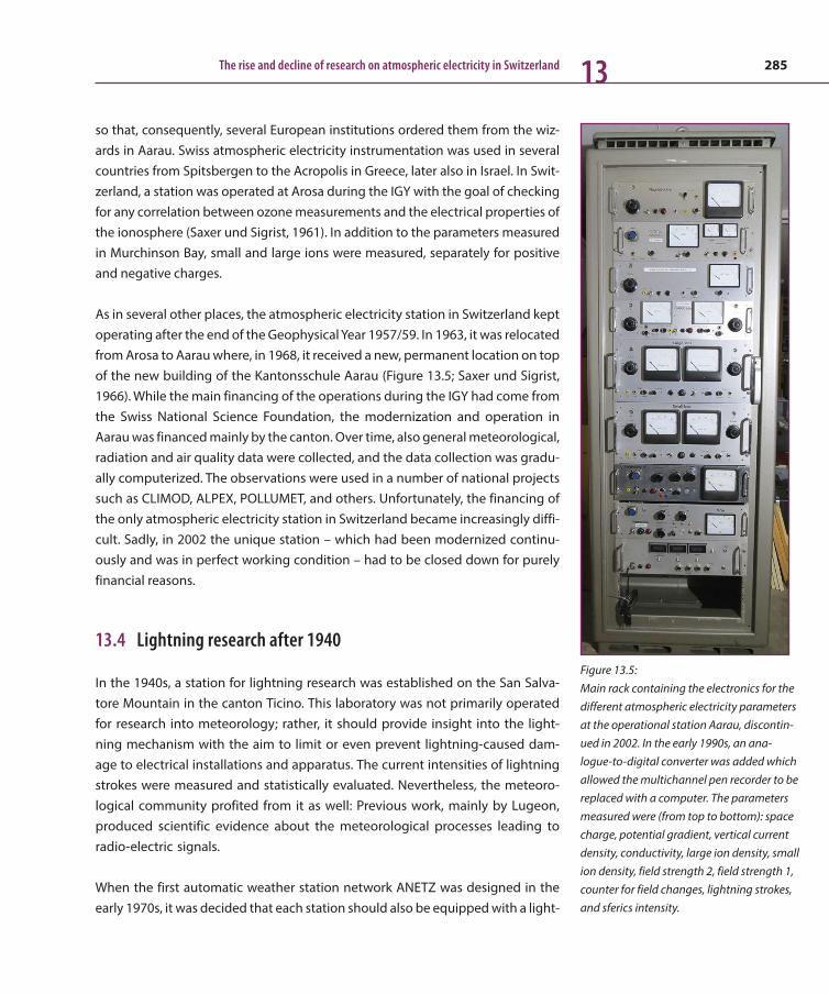
285The rise and decline of research on atmospheric electricity in Switzerland 13
so that, consequently, several European institutions ordered them from the wiz-ards in Aarau. Swiss atmospheric electricity instrumentation was used in several countries from Spitsbergen to the Acropolis in Greece, later also in Israel. In Swit-zerland, a station was operated at Arosa during the IGY with the goal of checking for any correlation between ozone measurements and the electrical properties of the ionosphere (Saxer und Sigrist, 1961). In addition to the parameters measured in Murchinson Bay, small and large ions were measured, separately for positive and negative charges.
As in several other places, the atmospheric electricity station in Switzerland kept operating after the end of the Geophysical Year 1957/59. In 1963, it was relocated from Arosa to Aarau where, in 1968, it received a new, permanent location on top of the new building of the Kantonsschule Aarau (Figure 13.5; Saxer und Sigrist, 1966). While the main financing of the operations during the IGY had come from the Swiss National Science Foundation, the modernization and operation in Aarau was financed mainly by the canton. Over time, also general meteorological, radiation and air quality data were collected, and the data collection was gradu-ally computerized. The observations were used in a number of national projects such as CLIMOD, ALPEX, POLLUMET, and others. Unfortunately, the financing of the only atmospheric electricity station in Switzerland became increasingly diffi-cult. Sadly, in 2002 the unique station – which had been modernized continu-ously and was in perfect working condition – had to be closed down for purely financial reasons.
13.4 Lightning research after 1940
In the 1940s, a station for lightning research was established on the San Salva-tore Mountain in the canton Ticino. This laboratory was not primarily operated for research into meteorology; rather, it should provide insight into the light-ning mechanism with the aim to limit or even prevent lightning-caused dam-age to electrical installations and apparatus. The current intensities of lightning strokes were measured and statistically evaluated. Nevertheless, the meteoro-logical community profited from it as well: Previous work, mainly by Lugeon, produced scientific evidence about the meteorological processes leading to radio-electric signals.
When the first automatic weather station network ANETZ was designed in the early 1970s, it was decided that each station should also be equipped with a light-
Figure 13.5: Main rack containing the electronics for the different atmospheric electricity parameters at the operational station Aarau, discontin-ued in 2002. In the early 1990s, an ana-logue-to-digital converter was added which allowed the multichannel pen recorder to be replaced with a computer. The parameters measured were (from top to bottom): space charge, potential gradient, vertical current density, conductivity, large ion density, small ion density, field strength 2, field strength 1, counter for field changes, lightning strokes, and sferics intensity.

286 From weather observations to atmospheric and climate sciences in Switzerland13
ning sensor. Lightning strokes in the vicinity of the stations were identified using a band-pass receiver for ELF signals. It counted and recorded the trains of low-fre-quency electromagnetic radiation emitted by the stroke and received by a whip antenna (Cavalli, 1977; Joss und Cavalli, 1985). The signal intensity was discrimi-nated into two levels, allowing a rough estimate of the distance to the lightning stroke. For the time being, the station density of the ANETZ was rather high. So despite the fact that no angular information was available from the lightning detectors, the location of thunderstorms could be obtained by mapping the sig-nals from different stations.
Since 2005, MeteoSwiss relies on lightning data provided by private companies. Their stations are much more sophisticated than the simple band-pass receivers of ANETZ; they allow a true and accurate triangulation of the stroke location, and provide information on the lightning current. Also, their networks cover a large part of Europe. Nevertheless, with the ANETZ, Switzerland was a pioneer: the first country to have an operational lightning detection and location system for mete-orological purposes.
13.5 An activity in a new area just before the shutdown
Once the Commission for Atmospheric Electricity (see insert) had been dissolved, the only remaining activity was at the “Luftelektrische Station Aarau,” although this was primarily a monitoring site. In the 1970s, the development of lightning sen-sors for the ANETZ marked a certain revival. Then, research received a last signifi-cant boost: At the Institute for Snow and Avalanche Research (WSL), laboratory experiments were being conducted to obtain insight into the microphysics of charge separation in clouds (Aufdermaur and Johnson, 1972). In the institute’s hail tunnel, frozen water droplets collided with a metal cylinder, so that the transferred charge could then be measured as electric current (Buser and Jaccard, 1976; Buser and Aufdermaur, 1977). While the results of these experiments certainly provided some clues as to how an electric field is generated in a cloud, they are still not conclusive and are debated controversially. It seems that these activities were the only experimental investigations related to atmospheric electricity carried out in Switzerland, whereas all other research was confined to observations of naturally occurring phenomena.
The amusing human side of science
During the IGY, atmospheric electrical
parameters were recorded in Arosa at
the Lichtklimatologisches Observato-
rium. Instead of going to the school ski-
ing week, Saxer and Dütsch (who were
both teachers) spent their time analyz-
ing data in Arosa. An unexpected result
fascinated them: When the temperature
was low and the humidity was high,
strong anomalies occurred regularly at
certain times of the day. Quite puzzled,
they discussed possible mechanisms,
but no plausible explanation turned up.
At least not until Friday night of that
week when Saxer studied the train
schedule for his trip back to Aarau. Sud-
denly everything became obvious: High
humidity and freezing temperatures
had caused hoarfrost on the electric
overhead contact line of the train. When
a train approached Arosa on cold and
humid days, heavy sparking occurred
between the engine’s pantograph and
the overhead line, which, of course, dis-
turbed the natural electric field. A disap-
pointingly simple explanation for a
potentially fascinating new discovery …
287The rise and decline of research on atmospheric electricity in Switzerland 13
13.6 The provisional (?) end
In Switzerland, atmospheric electricity was a topic for only few research groups. After World War I, Gockel shifted his research topics more and more to cosmic radiation. Consequently, it was the Swiss meteorological service, later Saxer and Sigrist, and a few other individuals who were active in atmospheric electricity research. At the universities there was no research going on except at the Physics Institute of Fribourg, where Gockel was active.
In 2002, the final shutdown of the Aarau atmospheric electricity station marked the sad end of atmospheric electricity research in Switzerland, an activity that had started in 1785 and had its numerous highs and lows. There might be reasons for discontinuing a monitoring of electric phenomena without using the data for
The Commission for Atmospheric Electricity
In 1912, the Swiss Academy of Science established the “Luftelektrische Kom-mission” (Commission for Atmospheric Electricity) as its 14th commission. It was primarily Gockel who rallied for its instigation, so he naturally became the first president. In 1942 the terms of reference were updated for the com-mission to fit the on-going activities.
The commission dealt with all aspects of atmospheric electricity. Of course, the main activities changed over time because of the type of the on-going research described above. After all, it was the scientific work that dictated the commission’s activity and not vice versa. There were periods when activi-ties were low, and the commission did not even produce any report to the Swiss Society for Natural Sciences.
After the 1950s, the importance of research in sferics and electromagnetic propagation for forecasting purposes diminished, and the research work by the meteorological institute slipped into a crisis. As Jean Rieker presented it in retrospect at a colloquium at ETHZ in 1980, there were only two options: “Conclude all activities, cease collaborations on the international level, and forget about the investments; or improve the existing system by making it automatic, which necessarily implies a new financial effort.” Obviously, the first option was chosen. Closely connected with this choice, the commission was no longer needed and was dissolved in 1964.

288 From weather observations to atmospheric and climate sciences in Switzerland13
active research or operational purposes, and it might be more economical to acquire lightning data from special networks for nowcasting and forecasting than to run one’s own observation network. In fact, lightning detection (now based on acquired data) seems to be the only remaining use of electric phenomena for operational meteorology. But there are still many open problems, e. g., the micro-physics of charge separation is still not really understood. Also the effects of vol-canic eruptions on the electric field (Mather and Harrison, 2006) need further investigations. Maybe in the future, one of these topics will inspire a new Swiss research project …
Acknowledgments
Erich Fischer, former head of the Luftelektrische Station Aarau, and Jürg Joss, for-merly with MeteoSwiss, contributed to this chapter with many suggestions and additional information. Their support is gratefully acknowledged! The text was critically read by Pierre Jeannet and by Hansruedi Völkle. Their corrections and recommendations were highly appreciated as they led to a significant improve-ment of the article.
References
Ambrosetti, F., 1943: Luftelektrische Messungen in Locarno- Monti. Ann. M. Z.A., 80, Anh. No. 6, 7–17.
Aufdermaur, A. N. and D. A. Johnson, 1972: Charge separation due to riming in an electric field. Quart. J. Roy. Meteor. Soc., 98(416), 369–382.
Buser, O. and A. N. Aufdermaur, 1977: Electrification by collisions of ice particles on ice or metal targets. Electrical processes in atmospheres, H. Dolezalek and R. Reiter, Eds., Steinkopff Darm-stadt, 294–300.
Buser, O. and C. Jaccard, 1976: Charge separation by collision of ice particles on metals: electronic surface states. J. Glaciology, 21(85), 547–557.
Cavalli, R., 1977: Möglichkeit und Probleme der Blitzzählung im automatischen Messnetz der MZA (ANETZ). Beih. Jahrb. SNG, 1977–1981, 15–16.
Courvoisier, P., 1951: Die Schwankungen des elektrischen Feldes in der Atmosphäre und ihre Bedeutung für die Meteoropatho-logie. Experientia, 7, 242–254.
de Saussure, 1786: Voyages dans les Alpes, tome second, chap. XXVIII, “Nouvelles recherches sur l’électricité atmosphérique.” Genf 1786, 202–267.
Fritz, H. 1875: Aus der kosmischen Physik. Neujahrsbl. Natur-forsch. Ges. Zürich, 77, 28 pp.
Gockel, A., 1908: Die Luftelektrizität. Hirzel, Leipzig, 206 pp.
Gockel, A., 1925: Das Gewitter. Dümmler, Berlin und Bonn, 316 pp.
Joss, J. and R. Cavalli, 1985: Blitzschutz im Schweizerischen Netz von Automatischen Wetterstationen (ANETZ). Proc. 18th Int. Conf. Lightning Protect., Munich, Sept. 16 to 20.

289The rise and decline of research on atmospheric electricity in Switzerland 13Lugeon, J., 1939: Le radiogoniographe de la Station centrale suisse de météorologie et son utilisation pour la prévision du temps. Ann. Station central suisse de météorol., chap. 10, 24 pp.
Lugeon, J., 1941: Etude de l’ionosphère d’après la propagation des ondes courtes pendant l’Année Polaire Internationale. Année Polaire Internationale 1932–1933, M. Z.A. Zurich, chap. 4, 1–24.
Lugeon, J., 1950 : L’essor de la Radiométéorologie mondiale et la Prévision du Temps. Arch. Met. Geoph. Biokl. A, 3(1–2), 120–138.
Lugeon, J., A. Junod, and P. Wasserfallen, 1959: Mesures de l’électricité atmosphérique et de la radioactivité de l’air à Mur-chison Bay, Spitzberg (80° N), pendant l’Année géophysique internationale 1957–58. Actes Soc. Helv. Sci. Naturelles. Lausanne, 12–126.
Mather, T. A. and R. G. Harrison, 2006: Electrification of volcanic plumes. Surv. Geophys., 27, 387–432, doi: 10.1007/s10712-006-9007-2.
Mörikofer, W., 1950: Zur Meteorologie und Meteorobiologie des Alpenföhns. Verh. Schweiz. Naturforsch. Ges., 130, 11–32.
NGZH, 1921: Sitzungsberichte von 1921. Vierteljahrsschr. Naturf. Ges. Zürich, 66, p. 10.
Rieker, J., 1960: Le lever du soleil dans l’ionosphère et ses réper-cussions sur la propagation des ondes longues. Geofisica Pura Appl., 46, 241–328.
Saxer, L. and W. Sigrist, 1961: Tages- und Jahresgänge der luftelektrischen Elemente in Arosa. Arch. Met. Geoph. Biokl. A, 12, 366–375.
Saxer, L. and W. Sigrist, 1966: Die luftelektrische Station der Kan-tonsschule Aarau. Mitt. Aarg. Naturforsch. Ges., 27, 187–224, doi: 10.5169/seals-172527.

291
14 Phenology in Switzerland since 1808Claudio Defila1, Bernard Clot2, François Jeanneret3, Reto Stöckli4
14.1 Introduction
Phenology studies the timing of annual life-cycle events including the driving factors and involved biotic and abiotic processes (Defila, 1991). The occurrence times of these events – called phenological phases or phenophases – are observed and recorded. Leaf unfolding, beginning of flowering, full flowering, leaf colouring and leaf fall are typical plant phenophases; bird migration and bee activity are examples of observed animal phenophases. Biophysical phenological quantities such as Leaf Area Index or vegetation greenness can be automatically observed on a large scale by satellite sensors and ground-based remote sensing.
Many disciplines make use of phenological data. Geographers, climatologists, agronomists, regional planners and many others appreciate the spatially highly variable phenological signals. Vegetation is present on most land surfaces and exercises a very local-scale variability of phenophases in response to site-specific biogeographical boundary conditions and large-scale climatological forcing. Spa-tially dense phenological data contains information on biophysical land surface processes which is not present in classical climatological observations. Phenolog-ical data are well suited for upscaling meso- or topoclimatic surveys and helps defining seasons (Figure 14.1) (Jeanneret et al., 2011). Site-based phenological information can be combined with satellite-based phenology, classical climato-logical data and landscape phenological modeling to yield a spatio-temporal mapping of environmental state and function.
Detailed phenological data provide an integrated view of the impact of weather and climate conditions on living systems. Next to the dominant factor of cli-mate, additional factors influence the observed phenological patterns. For plants these are, for example, photoperiod, soil, exposition, genetic differences, human influence or interspecies competition. Land surface vegetation is an interactive part of the climate system. Leaf photosynthesis and transpiration influences cloudiness, temperature, moisture and the carbon dioxide content
1 retired, last affiliation:
Federal Office of Meteorology
and Climatology MeteoSwiss,
Zurich-Airport2 Federal Office of Meteorology
and Climatology MeteoSwiss, Payerne3 retired, last affiliation:
University of Bern, Institute
of Geography, Berne4 Federal Office of Meteorology
and Climatology MeteoSwiss,
Zurich-Airport

292 From weather observations to atmospheric and climate sciences in Switzerland14
of the atmosphere on the synoptic to climatological timescales. Leaf phenology, on the other hand, modulates leaf photosynthesis and transpiration through leaf appearance, presence and senescence. It can be linked to the large-scale seasonal to inter-annual climatic variability. The influence of phenological and biophysical states on the terrestrial energy, water and carbon cycle in a variable and changing climate are the most important applications of phenology in the broad field of ecosystem and climate science. A better understanding of this functionality is one of the key challenges for modern phenology. This under-standing is needed to maximise the usefulness of phenological observations and to guarantee their continuity into the future. Many applications, such as the modeling of the global water and carbon cycle, prediction of pollen distri-bution or the spatial analysis of plant and animal diseases nowadays rely on precise and long-term phenological data. The currently observed and statisti-cally significant shifts of seasons in many living systems are very likely an impact of climate change (Rutishauser and Studer, 2007). Seasonality and the analysis of its driving forces is the core business of phenology (Rutishauser et al., 2007; Jeanneret and Rutishauser, 2009b).
Phenology has always been an interdisciplinary research topic serving broad needs, from fundamental terrestrial ecological research to operational climate monitoring. This statement holds true even more in the 21st century.
Figure 14.1: Temporal and spatial scale of biological methods. Phenological data are useful at the topo-scale, embracing local, meso- and macro-scales. On the timescale, the phenology fits from day to year character-istics and is especially valuable for sea-sonality questions, along with chrono-biology dealing with periodic phenomena in living organisms and growth measure-ments of phenometry.

293Phenology in Switzerland since 1808 14
14.2 The first records
People have always been fascinated by seasonality. For centuries now, individuals have noted the greening or the flowering of plants in Spring, or the first snow or frost at the beginning of Winter: They were the first phenologists (Wegmann, 2005). The world longest phenological time series goes back to year 705 (Sekigu-chi 1969). Since then, the date of the full flowering of cherry tree has been recorded every year in Kyoto, Japan by the emperor’s administration. It marks the beginning of Spring and gives rise to important celebrations.
In Switzerland, the oldest phenological time series known were recorded by Jakob Sprüngli (1717–1803), who collected weather data and numerous phenological phases. Private initiatives still deliver important datasets, when they are made available. This was the case in Zug since 1993 (Röthlisberger, 2010) and in the Alpine garden at Schynige Platte from 1932 to 1939 and again from 1997 on, where the flowering of alpine plants is recorded at an altitude of 2000 m asl (Hegg et al. 2012).
Two long-term series are available in Switzerland: the bud burst of the horse chest-nut in Geneva, officially recorded since 1808 by the head of the General secretariat of the legislative body of the city (Figure 14.2), and the cherry tree flowering in
Figure 14.2: Date of the leaf bud burst of the official horse-chestnut in Geneva, 1808–2015. The red line shows the 20-year weighted average (Gaussian low-pass filter).
Figure 14.3: Date of the full flowering of cherry trees in Liestal, 1894–2015. The red line shows the 20-year weighted average (Gaussian low-pass filter).
294 From weather observations to atmospheric and climate sciences in Switzerland14
Liestal since 1894 (Figure 14.3) (Defila and Clot, 2001). Observations will be carried out in the future at both sites.
14.3 Coordinated initiatives
Phenological observations were also made and published on a regular basis in the “Schweizerische Meteorologische Beobachtungen” during the first years of the meteorological networks from 1864 to 1873. The national phenological observa-tions network was founded in 1951 by Bernard Primault, the head of the group of agrometeorology of the Swiss Central Meteorological Institute (MZA, nowadays Swiss Federal Office for Meteorology and Climatology MeteoSwiss). Similar national networks were founded across Europe, inspired by the work of Friedrich Schnelle and colleagues. In the first years, it included some 70 observations sites, 24 wild plants, 12 crops, 3 bird species and the first frost – in total 66 phenological phases (Primault, 1955). Nowadays, the network includes 160 sites in all areas of Switzerland, at altitudes ranging from 200 to 1800 m asl, and includes 26 plant species for a total of 69 phases. The observation program was slightly adapted in 1953 and 1959, and more important changes were introduced in 1996, as a result of a study underlying the possible improvements (Defila, 1991) and the works of an expert group. It was then decided to discard the observations of bird migration, because bird specialists were already performing exhaustive observations in the country (Bruderer, 1996). The observation of crop plants were also limited to grape harvest, haymaking and the flowering of cherry, apple and pear trees, because others were more influenced by the crop varieties selection and agricultural practices than by climatic factors.
The importance of long-term observations has been underlined. To support the work of the observers of the national network, an instructions manual was pub-lished in 1957, followed by a second (1962) and a third edition (Primault, 1971). The changes in the program that occurred in 1996 precipitated a new manual including instructions, drawings and pictures as well as much information con-cerning phenology (Brügger and Vassella, 2003).
The first and only International Phenological Garden (IPG) in Switzerland was cre-ated in 1963 in Birmensdorf by the Swiss Federal Institute for Forest, Snow and Landscape Research. The IPG network had been founded in 1959 with the aim of observing clones (owning the same genome) of a list of tree and shrub species planted in gardens in different climatic areas in Europe (Schnelle and Volkert, 1957).
295Phenology in Switzerland since 1808 14
The Bernese topoclimatic network BernClim started in 1970 at the Geographical Institute of the University of Berne (Wanner, 1972; Jeanneret, 1996). It was designed for spatial information that could be applied for landscape planning purposes (Jeanneret and Rutishauser, 2009b, 2012). With three observed sites per 100 km2 its spatial density allowed modelling of the influence of different topo-graphic factors, such as altitude. Even if that special network lost some of its den-sity over time, it is possible to interpolate phenological details in space. For each point of a grid-based scheme the regression equation for different variables (e. g., altitude, exposition, slope angle) is applied to compute the phenological date and therefore show the topographic specificities in different seasons (Figure 14.4) or in a seasonal synthesis (Rutishauser and Studer, 2007). Beyond the well-known phenological calendars, combined season diagrams can offer a well-illustrated and comprehensible graph. In order to cover seasonal patterns in time outside the vegetation periods, data on fog and snow are recorded in Winter. Snow is an obvi-ous climatic feature of Winter; fog is representative of lower regions with less snow than mountain areas.
An additional special network for frost warnings was founded in 1975 by the MZA for the observation of fruit trees and grapevine at 20 stations in the main produc-tion areas of Switzerland in order to prevent damages due to frost. As the sensitiv-ity of these plants to frost varies according to their development stage, real-time information about this stage is important for accurate frost-damage prevention (Defila, 1986). Today, this information is used for pest-prevention purposes as real-ised by Agroscope in Wädenswil und Changins (Agroscope is the Swiss centre for agricultural research affiliated with the Federal Office for Agriculture).
Forest phenology started in 1993 (Brügger, 1998), and data are collected and stored by the Swiss Federal Institute for Forest, Snow and Landscape Research WSL. Compared to the national network, additional species and at least 10 differ-ent individuals of each species at each site are observed, offering another view on spatial aspects and more easily reflecting changing environmental conditions and differentiations of mountain areas. It can also be surveyed with cameras (Brügger, 1998; Brügger et al., 2003; Ahrends et al., 2008, 2009). Important shifts of pheno-logical phases were also described for the past 500 years (Rutishauser, 2009).
In 1994, the Swiss National Park in Engadin set up a phenological network (Defila, 1999). In addition to a few plants and phases observed in the national network, this observation programme includes typical Alpine plants such as the Clusius’ gentian (Gentiana clusii), the hawks beard, the Winter heath (Erica carnea) and the

296 From weather observations to atmospheric and climate sciences in Switzerland14
lingonberry (Vaccinium vitis-idaea). In three areas (Val Mingèr, Ofenpass und Val Trupchun), the guards of the park observe a total of 11 plant species. Val Mingèr, which has not been visited by the guards since 2009, was then replaced by Val Cluozza.
Actual regional Specifities 2000–2011
Jura Mountains Lake of Thoune
Hazel General bloom
Apple Tree General bloom
Figure 14.4: Detailed maps of phenological conditions for the general bloom of hazel (upper maps) and the general bloom of apple trees (lower maps) in a middle mountain conditions (central Jura mountains, left maps) and North Alpine conditions (Thun Lake, right maps), generated with topographic interpolation modelling (Jeanneret and Rutishauser, 2012).
297Phenology in Switzerland since 1808 14
14.4 Different applications during the 20th century
In the mid-20th century, phenology networks were created in many European coun-tries, e. g., Germany, Austria and Switzerland. The data were primarily used for agri-cultural purposes, such as the optimal timing of agricultural activities and frost-damage prevention (Primault, 1970). Phenologists were less active during the 1970s and 1980s. Four phenological maps were included in the Swiss Climate Atlas (Primault, 1984). Until the mid-1980s, the original observation sheets were simply archived. Later, all data were retrospectively digitised, which allowed for a detailed analysis. In order to determine whether a particular season occurs early or late, for every station and phenophase, the observations of the data series were separated into five classes according to their date of occurrence. The earliest dates (10 %) were considered to be “very early,” and the latest 10 % to be “very late.” Data from quan-tiles 11 to 25 were considered to be “early,” and those 75 to 89 as “late.” The 50 % around the average were considered to be “normal” occurrences. Such phenologi-cal calendars were produced for each station (Defila, 1992). From the mid-1980s, a number of papers were published in scientific journals, so that the awareness about phenology increased among the nature lovers and the public. Annual retro-spectives were published in forest and agriculture journals since 1987 and 1989, respectively (e. g., Defila, 2010a, 2010b) and in the MeteoSwiss annals. With the development of Internet, weekly phenological bulletins were made available to a wide audience. More recently, a Spring index showing the mean development of the vegetation in Spring was developed and is regularly updated on the Internet (http://www.meteoschweiz.admin.ch/) (Figure 14.5). Today, phenological bulle-tins are published regularly in the meteorological bulletins of MeteoSwiss (http://www.meteoschweiz.admin.ch/content/dam/meteoswiss/de/Klima/Gegenwart/Klima-Berichte/doc/klimabulletin).
In order to intensify the exchanges among different groups of persons interested in phenology – such as scientists, observers and users – in 2004 the Swiss Phenol-ogy Circle was created, thanks to collaboration between the Geography Institute of the University of Berne and MeteoSwiss. Two excursions were organised and two newsletters were published per year. In turn, this group was at the origin of the foundation of the Commission for Phenology and Seasonality of the Swiss Academy of Sciences (SCNAT) in 2011 (http://www.naturwissenschaften.ch/kps), which continues these excursions and organises yearly phenology symposia in the framework of the Swiss Geoscience Meetings.
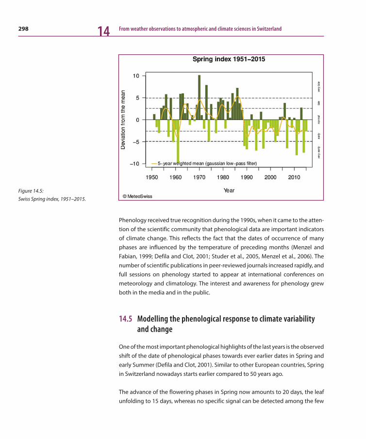
298 From weather observations to atmospheric and climate sciences in Switzerland14
Phenology received true recognition during the 1990s, when it came to the atten-tion of the scientific community that phenological data are important indicators of climate change. This reflects the fact that the dates of occurrence of many phases are influenced by the temperature of preceding months (Menzel and Fabian, 1999; Defila and Clot, 2001; Studer et al., 2005, Menzel et al., 2006). The number of scientific publications in peer-reviewed journals increased rapidly, and full sessions on phenology started to appear at international conferences on meteorology and climatology. The interest and awareness for phenology grew both in the media and in the public.
14.5 Modelling the phenological response to climate variability and change
One of the most important phenological highlights of the last years is the observed shift of the date of phenological phases towards ever earlier dates in Spring and early Summer (Defila and Clot, 2001). Similar to other European countries, Spring in Switzerland nowadays starts earlier compared to 50 years ago.
The advance of the flowering phases in Spring now amounts to 20 days, the leaf unfolding to 15 days, whereas no specific signal can be detected among the few
Figure 14.5: Swiss Spring index, 1951–2015.

299Phenology in Switzerland since 1808 14
observed phases in Autumn. Compared to 50 years ago the colouring of the leaves seems to occur a little earlier, and the leaf fall a little later (Defila, 2004). Such infor-mation is of particular interest to plant sciences, agronomy and forestry.
A comparison of phenological time series in the Alps (> 1000 m asl) and at low altitude (< 600 m asl) in Switzerland during the period 1951–2002 showed that the proportion of significant trends is higher in the Alps (42 %) than at low altitude (33 %). The Spring phases at low altitude occur 20 days earlier and over 1000 m asl only 15 days earlier than 50 years before (Defila and Clot, 2005). However, with regard to the duration of the vegetation period at both altitudes, the change is much more pronounced in the Alps, so that productivity there could benefit more from an earlier seasonal start.
A comparison of the fourth IPCC report (Rosenzweig et al., 2007) showed that the calculated prolongation of the vegetation period in Switzerland of 2.7 days/decade for the period 1951 to 2000 (Defila and Clot, 2001) corresponds well to the 2.3 days/decade obtained in Germany for the same period (Menzel et al., 2001), and to the 3.5 days/decade of the IPG for the period from 1959 to 1998. When not affected by long dry periods, a prolonged vegetation period would allow an increase in biomass production, although herbivore insects and plant pests could also benefit from a longer period favourable to their development.
In temperate climate zones like Switzerland the date of Spring phenophases is driven mainly by the temperature in the preceding months; this observation can be linked to recent climate warming. The ultimate proof is gained through pheno-logical models. For instance, a statistical study of the Spring phenophases (Studer et al., 2005) demonstrated that the advance is not linear over time. Rather, a shift occurred at the end of the 1980s, and it was also found that not all plant species or phenophases react with an equal intensity. Studies have documented the co-limitation of both temperature and photoperiod for light-sensitive temperate tree species (Körner and Basler, 2010; Vitasse and Basler, 2013).
Unfortunately, temperature is still the main climatic driver in most ecosystem models, leaf physiology and leaf phenology being treated separately. Many phe-nological models are accurate only for today’s climate and for specific locations and species since statistically they relate the timing of observed phenological events to observed climatic variability. They have been trained specifically with long-term phenological observations restricted to the temperate climate zone, such as the long phenological record of MeteoSwiss. On the other hand, pheno-
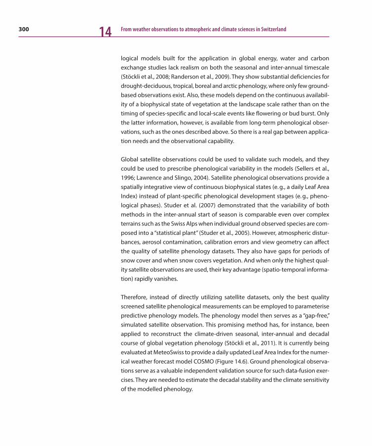
300 From weather observations to atmospheric and climate sciences in Switzerland14
logical models built for the application in global energy, water and carbon exchange studies lack realism on both the seasonal and inter-annual timescale (Stöckli et al., 2008; Randerson et al., 2009). They show substantial deficiencies for drought-deciduous, tropical, boreal and arctic phenology, where only few ground-based observations exist. Also, these models depend on the continuous availabil-ity of a biophysical state of vegetation at the landscape scale rather than on the timing of species-specific and local-scale events like flowering or bud burst. Only the latter information, however, is available from long-term phenological obser-vations, such as the ones described above. So there is a real gap between applica-tion needs and the observational capability.
Global satellite observations could be used to validate such models, and they could be used to prescribe phenological variability in the models (Sellers et al., 1996; Lawrence and Slingo, 2004). Satellite phenological observations provide a spatially integrative view of continuous biophysical states (e. g., a daily Leaf Area Index) instead of plant-specific phenological development stages (e. g., pheno-logical phases). Studer et al. (2007) demonstrated that the variability of both methods in the inter-annual start of season is comparable even over complex terrains such as the Swiss Alps when individual ground observed species are com-posed into a “statistical plant” (Studer et al., 2005). However, atmospheric distur-bances, aerosol contamination, calibration errors and view geometry can affect the quality of satellite phenology datasets. They also have gaps for periods of snow cover and when snow covers vegetation. And when only the highest qual-ity satellite observations are used, their key advantage (spatio-temporal informa-tion) rapidly vanishes.
Therefore, instead of directly utilizing satellite datasets, only the best quality screened satellite phenological measurements can be employed to parameterise predictive phenology models. The phenology model then serves as a “gap-free,” simulated satellite observation. This promising method has, for instance, been applied to reconstruct the climate-driven seasonal, inter-annual and decadal course of global vegetation phenology (Stöckli et al., 2011). It is currently being evaluated at MeteoSwiss to provide a daily updated Leaf Area Index for the numer-ical weather forecast model COSMO (Figure 14.6). Ground phenological observa-tions serve as a valuable independent validation source for such data-fusion exer-cises. They are needed to estimate the decadal stability and the climate sensitivity of the modelled phenology.
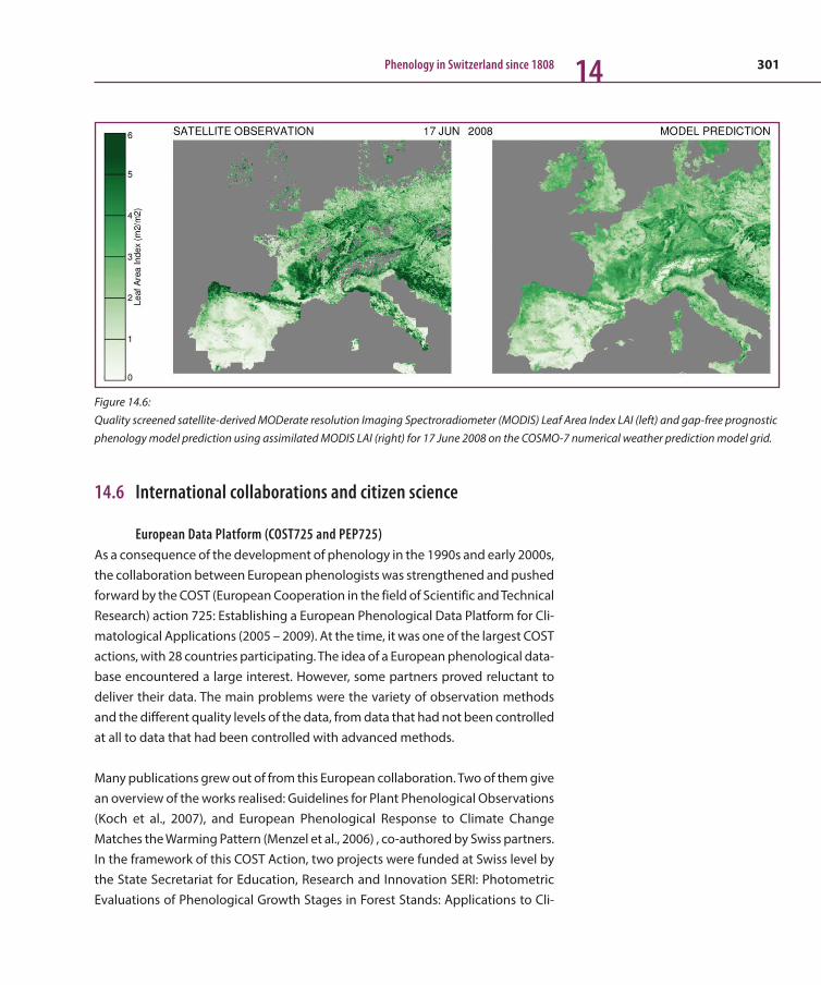
301Phenology in Switzerland since 1808 14
14.6 International collaborations and citizen science
European Data Platform (COST725 and PEP725)As a consequence of the development of phenology in the 1990s and early 2000s, the collaboration between European phenologists was strengthened and pushed forward by the COST (European Cooperation in the field of Scientific and Technical Research) action 725: Establishing a European Phenological Data Platform for Cli-matological Applications (2005 – 2009). At the time, it was one of the largest COST actions, with 28 countries participating. The idea of a European phenological data-base encountered a large interest. However, some partners proved reluctant to deliver their data. The main problems were the variety of observation methods and the different quality levels of the data, from data that had not been controlled at all to data that had been controlled with advanced methods.
Many publications grew out of from this European collaboration. Two of them give an overview of the works realised: Guidelines for Plant Phenological Observations (Koch et al., 2007), and European Phenological Response to Climate Change Matches the Warming Pattern (Menzel et al., 2006) , co-authored by Swiss partners. In the framework of this COST Action, two projects were funded at Swiss level by the State Secretariat for Education, Research and Innovation SERI: Photometric Evaluations of Phenological Growth Stages in Forest Stands: Applications to Cli-
Figure 14.6: Quality screened satellite-derived MODerate resolution Imaging Spectroradiometer (MODIS) Leaf Area Index LAI (left) and gap-free prognostic phenology model prediction using assimilated MODIS LAI (right) for 17 June 2008 on the COSMO-7 numerical weather prediction model grid.
302 From weather observations to atmospheric and climate sciences in Switzerland14
mate Monitoring Using Digital Image Analyses PHENOPHOT (Ahrends et al., 2008) and Inter-Annual Variations in European Phenology Patterns and Their Relation to Climate Change (Studer at al., 2005). As a follow-up of the COST action, the PEP725 (Pan European Phenological database) was created with the goal to maintain and develop the European phenological database (www.pep725.eu).
Global Climate Observing System, GCOSGCOS was founded in 1992 by the World Meteorological Organisation (WMO) and several other international organisations with the goal to perform systematic cli-mate observations, not only for common parameters such as temperature, precip-itations, air pressure, etc., but also for essential parameters in the atmosphere, oceans and overland. Phenological data were defined as relevant climatic vari-ables. From the Swiss observation network, 12 observation stations with long record series in different regions and altitudes as well as the two long data series of the horse-chestnut bud-burst in Geneva since 1808 and cherry tree flowering in Liestal since 1894 were recognised by GCOS Switzerland as important observa-tions to be maintained at long-term (Seiz and Foppa, 2007).
Global Learning and Observations to Benefit the Environment, GLOBEGLOBE is a worldwide school-based science and education program. It started in 1995 in the USA, with Switzerland joining in 1998. The students are encour-aged to get to know, understand and take care of the environment; they are made aware of environmental questions, of the “system Earth” and of scientific methods. Topics such as climate/weather, hydrology and bio indication, soil, land use/biology, remote sensing (satellite data) and phenology are developed. Today, teachers realise phenological observations with their students in several Swiss schools. Some of these results are then used for scientific studies (e. g. Gazal et al., 2008).
PhaenoNetThe Internet platform PhaenoNet was created in 2013 thanks to a collaboration between Globe, the ETH-Zurich and MeteoSwiss. In addition to the national net-work’s observers, this platform allows schools and indeed every person in Switzer-land to contribute to phenological observations by registering observation data online, and thus to spatially densify the observations.
303Phenology in Switzerland since 1808 14
OpenNature.chThe citizen science platform OpenNature (http://opennature.ch) was launched in Spring 2015. It is directed toward the scientifically interested public who is willing to share their local observations with peer observers and professional scientists across Switzerland. The initiative is part of a growing movement of “citizen sci-ence” which aims to involve the public in the scientific collection and analysis of data. Data gathered by OpenNature should also contribute to a better under-standing of seasons, plants, animals, weather and climate. A large potential of the website is undoubtedly the strengthening of the community of phenological observers, making phenology a valuable climate change indicator and directing the attention of the public and media to the ever-changing phenology of plants and seasons.
14.7 The future of Swiss phenology
One of the major challenges for phenology science will be to better integrate the historically driven focus on point-scale phenological observations with modern satellite-based spatial information on vegetation state and phenological predic-tion models to form a consistent and continuous climate service of geospatial climate information on vegetation and ecosystem state for user-driven applica-tions like for instance drought monitoring, insect pest prediction, climate variabil-ity and change impact assessment or the combination flowering/airborne pollen. The currently, often temperature-based prediction of phenophases needs to move away from statistical to more process-based modeling of the combined veg-etation phenology and physiology driven by a multiple set of limiting climate and biophysical factors including the human influence on ecosystem functioning. This is needed in order to better assess the impact of climate variability and change on phenological timing, but also to quantify the resulting feedback of an earlier Spring on the terrestrial carbon uptake or on for instance Summer drought. Such understanding can be gained only from multi-decadal, ground-based phenolog-ical datasets and models that are not only exercised in temperate climate zones like Switzerland, but are also realistic for Mediterranean, tropical, boreal and Arctic climate zones. Embedding national phenology observation networks as part of the global climate science driven by requirements from international climate monitoring initiatives (e. g., GCOS) will better foster the scientific and socioeco-nomic potential of both biology and climate backed by a really valuable long-term and often voluntary “citizen driven” climate data record of both natural and man-made climate variability and change.
304 From weather observations to atmospheric and climate sciences in Switzerland14
References
Ahrends H. E., R. Brügger, R. Stöckli, J. Schenk, P. Michna, F. Jean-neret, H. Wanner, and W. Eugster, 2008: Quantitative phenolog-ical observations of a mixed beech forest in northern Switzer-land with digital photography. J. Geophys. Res., 113, G04004, 261–274.
Ahrends, H. E., Etzold, S., W. L. Kutsch, R. Stöckli, R. Brügger, F. Jeanneret, H. Wanner, N. Buchmann, and W. Eugster, 2009: Tree phenology and carbon dioxide fluxes: use of digital photogra-phy for process-based interpretation at the ecosystem scale. Climate, Research, 39, 1–11.
Bruderer, B., 1996: Vogelzugforschung im Bereich der Alpen 1980–1995. Onnitzol. Beob., 93, 119–130.
Brügger, R., 1998: Die phänologische Entwicklung von Buche und Fichte. Geographica Bernensia, 186 pp.
Brügger, R., 1998: Phänologie von Buche und Fichte: Beobach-tung, Variabilität, Darstellung und deren Nachvollzug in einem Modell. Geographica Bernensia, 186 pp.
Brügger, R., and A. Vassella, 2003: Pflanzen im Wandel der Jah-reszeiten. Geographica Bernensia, 287 pp.
Brügger, R., M. Dobbertin, and N. Kräuchi, 2003: Phenological variation of forest trees. In M. D. Schwartz (Ed.), Phenology: An Integrative Environmental Science. Tasks for Vegetation Science, 39, Kluwer Academic Publishers, Dordrecht, 255–267.
Defila, C., 1986: Frostwarnungen im Frühling. Die Grüne, 114, 17, 9–14.
Defila, C., 1991: Pflanzenphänologie der Schweiz. Inaugural- Dissertation, Uni Zürich, 235 S.
Defila, C., 1992: Pflanzenphänologische Kalender ausgewählter Stationen in der Schweiz, 1951–1990. Klimatologie der Schweiz, 30/L, Beihefte zu den Annalen der Schweiz. Meteorologischen Anstalt (1989), 233 pp.
Defila, C., 1999: Pflanzenphänologische Beobachtungen im SNP (Schweiz. Nationalpark). Cratschla, 2, 19.
Defila, C., 2004: Regionale Trends bei Pflanzenphänologischen Zeitreihen in der Schweiz. Meteorologen-Tagung DACH 2004, Karlsruhe. Langfassungen der Beiträge auf CD, 6 pp.
Defila, C., 2010a: Meteorologischer und phänologischer Jahres-rückblick 2009. Schweiz Z Forstwes, 161, 5, 181–185.
Defila, C., 2010b: Phänologischer Rückblick ins Jahr 2009. Agrar-forschung Schweiz, 1, 7/8, 266–271.
Defila, C., and B. Clot, 2001: Phytophenological trends in Swit-zerland. Int. J. Biometeorol., 45, 203–207.
Defila, C., and B. Clot, 2005: Phytophenological trends in the Swiss Alps, 1951–2002. Meteorologische Zeitschrift, 14, 2, 191–196.
Gazal, R., M. A. White, R. Gillies, E. Rodemaker, E. Sparrow, and L. Gordon, 2008: GLOBE students, teachers, and scientists demonstrate variable differences between urban and rural leaf phenology, Global Change Biology, 14, 1568–1580, doi: 10.1111/j.1365-2486.2008.01602.x
Hegg, O., and Coauthors, 2012: 80 Jahre experimentelle Öko-systemforschung auf der Schynigen Platte im Berner Oberland. Bristol-Schriftenreihe, 31, Haupt Bern, 108 pp.
Jeanneret, F., 1996: Phänologie in einem Querschnitt durch Jura, Mittelland und Alpen, Jb. Gg. Ges. BE, 59, 159–203.
Jeanneret, F., and T. Rutishauser, 2009a: Phenology for topocli-matological surveys and large-scale mapping. In Hudson I. L., and Keatly M. R. (Eds): Phenologic Research: Methods for environ-mental and climate change analysis. Springer Berlin, Heidelberg, New York, 159–175.
Jeanneret, F., and T. Rutishauser, 2009b: Seasonality as a core business of phenology. In Hudson I. L. and Keatly M. R. (Eds.): Phenologic Research: Methods for environmental and climate change analysis. Springer Berlin, Heidelberg, New York, 63–74.
Jeanneret, F., T. Rutishauser, and R. Brügger, 2011: Phänologie und Saisonalität: Geschichte, Monitoring, Raumansprache. Geo-graphica Bernensia, 178 pp.
Jeanneret, F., and T. Rutishauser, 2012: BernClim. Saisonali-täts-Monitoring – Jura, Mittelland, Alpen / Surviellance de la saisonalité – Jura, Moyen-Pays, Alpes. Geographica Bernensia, 112 pp.
Koch, E., E. Bruns, C. Defila, W. Lipa, and A. Menzel, 2007: Guide-lines for plant phenological observations, http://www.omm.urv.cat/documentation.html, 10 pp.

305Phenology in Switzerland since 1808 14Körner C., and D. Basler, 2010: Phenology under global warm-ing. Science, 327, 1461–1462.
Lawrence, D. M., and J. M. Slingo, 2004: An annual cycle of vege-tation in a GCM. Part I: Implementation and impact on evapora-tion. Clim. Dyn., 22, 87– 105.
Menzel, A., and P. Fabian, 1999: Growing season extended in Europe. Nature, 397, 659.
Menzel, A., N. Estrella, and P. Fabian, 2001: Spatial and temporal variability of the phenological seasons in Germany from 1951 to 1996. Glob. Change Biol., 7, 657–666.
Menzel, A., and Coauthors, 2006: European phenological response to climate change matches the warming pattern. Glob. Change Biol., 12, 1969–1976.
Pfister, C., 1999: Wetternachhersage. 500 Jahre Klimavaria-tionen und Naturkatastrophen. Haupt Bern.
Primault, B., 1955: Cinq ans d’observations phénologiques sys-tématiques en Suisse. Ann Schweiz Meteorol Anst, 92, 7/4–7/5.
Primault, B. 1970 : Essais de prévision de la date de maturité des abricots en Valais. Recherche agronomique en Suisse, 9, 3/4, 288–306.
Primault, B., 1971: Phänologischer Atlas. 3. Auflage, Zürich 1971, 76 pp.
Primault, B., 1984: Phänologie ; Blatt 13.1,13.2. in Kirchofer, W. : Klimaatlas der Schweiz, 2. Lieferung, Verlag des Bundesamtes der Landestopographie Bern, 2 Kartenblätter.
Randerson, J. T., and Coauthors, 2009: Systematic assessment of terrestrial biogeochemistry in coupled climate‐carbon models. Global Change Biol., 15, 10, 2462–2484, doi:10.1111/j.1365-2486. 2009.01912.x
Rosenzweig, C., G. Casassa, D. J. Karoly, A. Imeson, C. Liu, A. Men-zel, S. Rawlins, T. L. Root, B. Seguin, and P. Tryjanowski, 2007: Assessment of observed changes and responses in natural and managed systems. Climate Change 2007: Impacts, Adaptation and Vulnerability. Contribution of Working Group II to the Fourth Assessment Report of the Intergovernmental Panel on Climate Change. M. L. Parry, O. F. Canziani, J. P. Palutikof, P. J. van der Lin-den and C. E. Hanson, Eds., Cambridge University Press, Cam-bridge, UK, 79–131.
Röthlisberger, J., 2010: Früher Frühling – früher Herbst? Beob-achtungen und Reflexionen zur Herbstphänologie. Bauhinia, 22, 93–110.
Rutishauser, T., 2009: Historical Phenology in Central Europe. Seasonality and climate during the past 500 years. Geographica Bernensia, 136 pp.
Rutishauser, T., J. Luterbacher, F. Jeanneret, Ch. Pfister, and H. Wanner, 2007: A phenology-based reconstruction of inter- annual changes in past Spring seasons. Journal of Geophysical Research – Biogeosciences, 112, G04016.
Rutishauser, T., and S. Studer, 2007: Klimawandel und der Ein-fluss auf die Frühlingsphänologie. Schweizerische Zeitschrift für Forstwesen, 158, 105–111.
Rutishauser, T., and F. Jeanneret, 2009: Phänologie im Gebirge. Über den Rhythmus der Jahreszeiten im Schweizer Alpenraum. in: Pfister, C. and Imboden, G. (Eds.): Klimageschichte in den Alpen. Methoden – Probleme – Ergebnisse, Blätter aus der Walliser Geschichte, XLI. Band, herausgegeben vom Geschichtsforschen-den Verein Oberwallis, Brig, 171–187.
Schnelle, F., and E. Volkert, 1957: Vorschläge zur Einrichtung “Internationaler Phänologischer Gärten” als Stationen eines Grundnetzes für internationale phänologische Beobachtungen. Meteorologische Rundschau, 10, 4, 130–133.
Seiz, G., and N. Foppa, 2007: National Climate Observing System (GCOS Switzerland). Publication of MeteoSwiss and ProClim, 92 pp.
Sekiguchi, T., 1969: The historical dates of Japanese cherry festi-val since the 8th century and her climatic changes. Tokyo Geog-raphy Papers, 13, 175–190.
Sellers, P. J., S. O. Los, C. J. Tucker, C. O. Justice, D. A. Dazlich, G. J. Collatz, and D. A. Randall, 1996: A revised land surface parame-terization (SiB2) for atmospheric GCMs. 2. The generation of global fields of terrestrial biophysical parameters from satellite data. J. Clim., 9, 706–737.
Stöckli, R., T. Rutishauser, D. Dragoni, J. O’Keefe, P. E. Thornton, M. Jolly, L. Lu, A. S. Denning, 2008: Remote sensing data assimila-tion for a prognostic phenology model. J. Geophy. Res. –Biogeo-sciences, 113, G4, doi:10.1029/2008JG000781
306 From weather observations to atmospheric and climate sciences in Switzerland14
Stöckli, R., T. Rutishauser, I. Baker, M. Liniger, A. S. Denning, 2011: A global reanalysis of vegetation phenology. J. Geophys. Res. – Biogeosciences, 116, G03020, doi: 10.1029/2010JG001545
Studer, S., C. Appenzeller, and C. Defila, 2005: Inter-annual vari-ability and decadal trends in Alpine spring phenology: A multi-variate analysis approach. Climatic Change, 73, 395–414.
Studer, S., R. Stöckli, C. Appenzeller, and P. L. Vidale, 2007: A com-parative study of satellite and ground-based phenology. Int. J. Biometeorol., 51, 5, 405–414.
Vitasse J. and D. Basler 2013: What role for photoperiod in the bud burst phenology of European beech. European Journal of Forest Research, 132, 1, 1–8.
Wanner, H., 1972: 1970–1972: Die ersten zwei phänologischen Beobachtungsjahren des Berner Netzes – Probleme und vorläu-fige Resultate. Inform. U. Beitr. zur Klimaforschung, 8, Geogr. Inst. Univ. Bern, 5–14.
Wegmann, M., 2005: Naturwahrnehmung im Mittelalter im Spiegel der lateinischen Historiographie des 12. und 13. Jahr-hunderts. Peter Lang Bern.
Wolf, R., 1864–1873: Schweizerische Meteorologische Beobach-tungen. Zürcher und Furrer Zürich.
307
15 Agricultural meteorologyPierluigi Calanca1, Claudio Defila2
15.1 Introduction
It is not easy to provide an unambiguous definition of agricultural meteorology. The American Meteorological Society’s Glossary of Meteorology (Glickman, 2000) defines agricultural meteorology as “… meteorology and micrometeorology as applied to specific agricultural systems and of agriculture as applied to specific atmospheric conditions,” referring to agricultural climatology as “… climatology as applied to the effect of climate on crops,” and to biometeorology as “the branch of meteorology that deals with the effects of weather on plants and animals as well as on the health and activity of human beings … and on the short term feedbacks of the biosphere on the atmosphere.” Thus, while in theory there appears to be a distinction between the various disciplines, in practice the objectives often over-lap, and agricultural meteorology has largely remained confined to the study of the interactions between weather and crops.
This contribution provides insights into the background of agricultural meteorol-ogy in Switzerland since about 1950. It starts with a few historical notes and con-tinues by discussing five topics that exemplify the range of questions addressed in the past in 60 years this field of research. The next section deals with operational aspects of agricultural meteorology, and the chapter concludes with a few words on two institutions rooted in Switzerland which have supported agricultural mete-orology at the international level: the Commission for Agricultural Meteorology (CAgM) of the World Meteorological Organization (WMO) and the International Society of Biometeorology (ISB).
This chapter is neither comprehensive nor is it intended to be an introduction to agricultural meteorology. For readers interested in deepening their knowledge with regard to this discipline, the handbooks by Griffiths (1994) and WMO (2012) can be recommended as a starting point.
1 Agroscope, Institute for
Sustainability Sciences, Zurich2 retired, last affiliation: Federal Office
of Meteorology and Climatology
MeteoSwiss, Zurich-Airport
308 From weather observations to atmospheric and climate sciences in Switzerland15
15.2 Historical notes
The agrometeorological services
The motivation to establish agrometeorological services at the “Schweizerische Meteorologische Zentralanstalt” (MZA; today Federal Office of Meteorology and Climatology, MeteoSwiss) can be traced back to 1945, when unusual frosts caused considerable damage to fruit- and winegrowers. In the wake of this event, the MZA was asked to prepare and disseminate frost warnings. The process was implemented following recommendations formulated by the International Commission on Agricultural Meteorology and the International Agricultural Institute in Rome.
In order to prepare frost warnings, the MZA had to put an empirical forecasting procedure into place. The idea was to forecast minimum temperatures in the early morning (an indicator of the likelihood of frost) based on meteorological obser-vations taken during the preceding 24 hours. This required dedicated meteorolog-ical data, which the MZA started to collect in different fruit- and wine-production regions of Switzerland. These efforts resulted in the launch of special phenological observations on fruit trees and grapevines, since knowledge of the developmental stage was necessary to estimate critical temperatures. During this initial phase, special phenological observations were scheduled to take place once a week (Defila, 1986).
The dissemination of frost warnings, however, was not the only task of the new branch of MZA. The goal was to offer general information to support farmers in planning field operations and to provide forecasts for pest management. To this end, weather stations at selected sites were equipped with sensors for recording soil temperature and evaporation pans (so-called evaporimeters). In 1979, a weighing lysimeter was installed at the headquarters of MZA at the Krähbühl-strasse in Zurich and used to monitor actual evapotranspiration. The design of the lysimeter was later adopted for the construction of similar facilities at other sites (Section 15.3).
The data collected were used to prepare weekly agrometeorological bulletins spanning a period of 5 to 30 days. Around 1990 these bulletins were supple-mented with special forecasts for agriculture issued as 5-day forecasts and deliv-ered by fax to farmers, advisory services and the agricultural research stations. The forecasts were later distributed via the internet.

309Agricultural meteorology 15
In addition to the special observations on crops, a broader phenological observa-tion programme was formally put in place in 1951 (Defila, 2007; Chapter 14 in this book). The network originally consisted of 70 sites and was later continuously enlarged to include 160 sites. Key developmental stages were observed on wild plants, arable crops, fruit trees and grapevines. Phenological observations on annual crops were stopped in 1996 due to lack of interest, and in the early 2000s the data archives were handed over to Agroscope Changins-Wädenswil. Pheno-logical observations on wild plants, however, are still part of the observational programme of MeteoSwiss.
Since the establishment of agrometeorological services in the early 1950s, the MZA has undergone various changes, first becoming the Schweizerische Meteo-rologische Anstalt (SMA) in 1979 and MeteoSwiss in 1996. This reorganization had many implications for the activities in the field of agricultural meteorology. The agrometeorological services were first integrated into the division of Biological and Environmental Meteorology (a step entailing new tasks such as the monitor-ing, analysis and forecasting of pollen concentrations) and later given up as an independent unit.
Agricultural meteorology as a scientific discipline nevertheless continues to be pursued at various institutions, including Agroscope, the Department for Environ-mental Systems Science of the Swiss Federal Institute of Technology in Zurich (ETHZ) (formerly Abteilung für Landwirtschaft and Department of Agronomy), or the School of Agricultural, Forest and Food Sciences at Berne University of Applied Sciences. Moreover, relevant information for the agricultural sector continues to be provided through specialized forecasts (Section 15.4) and new dissemination platforms. An example of the latter is www.drought.ch (WSL/ETH/UniZH, 2015), an internet site established in the context of the National Research Programme 61, “Sustainable Water Management” (Stähli et al., 2013). The sequence of extreme events with impact on agriculture during the recent decades, such as the heat-wave in the summer of 2003, the drought in the spring of 2011 or the more recent drought in the summer of 2015 (Figure 15.1), has revived the attention for this type of information.

310 From weather observations to atmospheric and climate sciences in Switzerland15
The Working Group on Agricultural and Forest Meteorology
The agrometeorological research community has always kept sight of the scien-tific developments in forest meteorology. Toward the end of the 1980s, the need for coordination and exchange of information between the two research commu-nities became compelling. Hence, it became quite natural to propose the launch of a Working Group on Agricultural and Forest Meteorology (WG AFM) that would meet regularly and provide a floor for joint initiatives. Potential participants were addressed in 1989 by the then director of SMA, André Junod.
The first meeting of the WG AFM was held in June 1989 at the SMA headquarters. The meeting was attended by 15 people from SMA, the Federal Institute of Tech-nology (ETHZ), the Federal Research Institutions for Agriculture (Agroscope), the Federal Office of Agriculture and the Swiss Federal Institute for Forest, Snow and Landscape Research (WSL). Claudio Defila was nominated chair of the WG (a posi-tion he kept until his retirement in autumn 2008, when the task was handed over to Christof Ammann from Agroscope).
During the first years the group grew rapidly, with new members representing also institutions such as the agricultural advisory services and the cantonal colleges of agriculture and forestry (the so-called Fachhochschulen). The WG is still very active, holding meetings twice a year, with experts being invited to talk on various
Figure 15.1: Effects of the drought in the summer of 2015 on maize (left) and sugar beet (right) production in two fields located north of Zurich. In such extreme situations dedicated agrometeorological forecasts and analyses are critically needed to support farmers in making decisions. © Garbiela Brändle, Agroscope.

311Agricultural meteorology 15
subjects of general relevance. Research areas addressed in these seminars testify to the broad spectrum of interests of the WG, including over the years climate change, CO2 enrichment experiments, dendroclimatology, radiation, natural disas-ters, pests and diseases, and much more.
15.3 Selected research topics
A formula for computing crop evapotranspiration
Evapotranspiration is a key variable in agricultural meteorology, forming the basis for the assessment of crop-water requirements (Steduto et al., 2012) and for the classification of climates (Thornthwaite, 1948). It is also a key ingredient in our understanding of the temporal variability of water stress in agricultural systems (Calanca, 2004).
Evapotranspiration can be measured in various ways, viz. by weighing lysimeters, the profile or Bowen-ratio approach, or the so-called eddy covariance technique. While all of these techniques are suitable for field experiments and short-term or local evaluations, establishing an operational monitoring network on a national scale is extremely demanding and has been beyond the possibilities of most weather services until recently. From a historical perspective, it can therefore be said that empirical formulas for deducing evapotranspiration estimates from conventional weather observations have long been the sole option available to agricultural meteorologists at the operational level.
Major steps toward a quantitative formulation of evapotranspiration are reviewed in Brutsaert (1982). Landmark papers were published during the first decades of the Swiss Society for Meteorology, including those by Bowen (1926) (of Bowen- ratio fame), by Penman (1948), who laid down the physical rationale for develop-ing the so-called combination equation, and by Thornthwaite (1948), who intro-duced the concept of potential evapotranspiration.
The 1960s and 1970s saw various advances. Particularly important were the con-tributions by Slatyer and McIlroy (1961), who proposed the concept of equilib-rium evaporation; by Monteith (1965), who extended Penman’s formula to what is now known as the Penman-Monteith equation by examining the role of vege-tation in the transfer of heat and moisture between the earth’s surface and the atmosphere; by Priestley and Taylor (1972), who revisited the idea of equilibrium
312 From weather observations to atmospheric and climate sciences in Switzerland15
evaporation for conditions characterized by minimal advection; and by Thom and Oliver (1977), who examined the possibilities to apply Penman’s equation at the regional scale.
For practical applications, important advances toward a standardization of the approach for computing crop evapotranspiration took place in the 1980s and 1990s, mainly thanks to the Food and Agriculture Organization (FAO) of the United Nations and the American Society of Civil Engineers (ASCE). The method-ology was eventually presented in three cornerstone reports known as FAO 24 (Doorenbos and Pruitt 1984), FAO 56 (Allen et al. 1998) and ASCE Manual 70 (Jen-sen et al. 1990).
In Switzerland, operational estimates of actual evapotranspiration have long been based on the so-called Primault’s formula. The origin of the latter goes back to the 1960s (Primault, 1962), and its derivation was motivated by the fact that Bernard Primault, at that time head of the agrometeorological services of MZA, was unsat-isfied with the performance of the formulas of Penman (1948) and Thornthwaite (1948). His effort was underpinned by a field experiment in Kloten that remains, even from a today’s perspective, a quite unique undertaking.
The reasons why the formulas of Penman and Thornthwaite failed to provide sat-isfactory results when applied under the climatic conditions of Switzerland are various and cannot be reviewed here. Nevertheless, it is interesting to note that Penman himself was unsatisfied by the parameterisation he had proposed in 1948. For some time he had tried to improve his formula (Brutsaert, 1982).
The chief and practical advantage of Primault’s formula is that it relates evapo-transpiration to two variables (relative humidity and sunshine duration), which were observed on a regular schedule even in the early days. Later, the equation was extended to include the effects of altitude, making it in principle suitable for use in different climatic regimes (Primault 1981). It has been shown, however, that the formula tends to deliver biased estimates even in relatively simple settings (e. g., Calanca et al., 2011). For this reason, the operational evaluation of the actual evapotranspiration from routine weather observations, at MeteoSwiss, is now based on the FAO 56 approach.
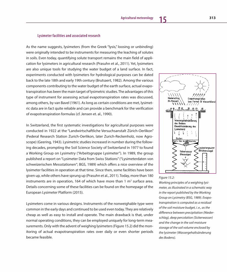
313Agricultural meteorology 15
Lysimeter facilities and associated research
As the name suggests, lysimeters (from the Greek “lysis,” loosing or unbinding) were originally intended to be instruments for measuring the leaching of solutes in soils. Even today, quantifying solute transport remains the main field of appli-cation for lysimeters in agricultural research (Prasuhn et al., 2011). Yet, lysimeters are also unique tools for studying the water budget of a land surface. In fact, experiments conducted with lysimeters for hydrological purposes can be dated back to the late 18th and early 19th century (Brutsaert, 1982). Among the various components contributing to the water budget of the earth surface, actual evapo-transpiration has been the main target of lysimetric studies. The advantages of this type of instrument for assessing actual evapotranspiration rates was discussed, among others, by van Bavel (1961). As long as certain conditions are met, lysimet-ric data are in fact quite reliable and can provide a benchmark for the verification of evapotranspiration formulas (cf. Jensen et. al., 1990).
In Switzerland, the first systematic investigations for agricultural purposes were conducted in 1922 at the “Landwirtschaftliche Versuchsanstalt Zürich-Oerlikon” (Federal Research Station Zurich-Oerlikon, later Zurich-Reckenholz, now Agro-scope) (Geering, 1943). Lysimetric studies increased in number during the follow-ing decades, prompting the Soil Science Society of Switzerland in 1977 to found a Working Group on Lysimetry (“Arbeitsgruppe Lysimeter”). In 1989, the group published a report on “Lysimeter Data from Swiss Stations” (“Lysimeterdaten von schweizerischen Messstationen“; BGS, 1989) which offers a nice overview of the lysimeter facilities in operation at that time. Since then, some facilities have been given up, while others have sprung up (Prasuhn et al., 2011). Today, more than 180 instruments are in operation, 164 of which have more than 1 m2 surface area. Details concerning some of these facilities can be found on the homepage of the European Lysimeter Platform (2015).
Lysimeters come in various designs. Instruments of the nonweighable type were common in the early days and continued to be used even today. They are relatively cheap as well as easy to install and operate. The main drawback is that, under normal operating conditions, they can be employed uniquely for long-term mea-surements. Only with the advent of weighing lysimeters (Figure 15.2) did the mon-itoring of actual evapotranspiration rates over daily or even shorter periods became feasible.
Figure 15.2: Working principles of a weighing lysi-meter, as illustrated in a schematic way in the report published by the Working Group on Lysimetry (BSG, 1989). Evapo-transpiration is computed as a residual of the soil moisture budget, i. e., as the difference between precipitation (Nieder-schlag), deep percolation (Sickerwasser) and the change in the soil moisture storage of the soil volume enclosed by the lysimeter (Wassergehaltsänderung des Bodens).
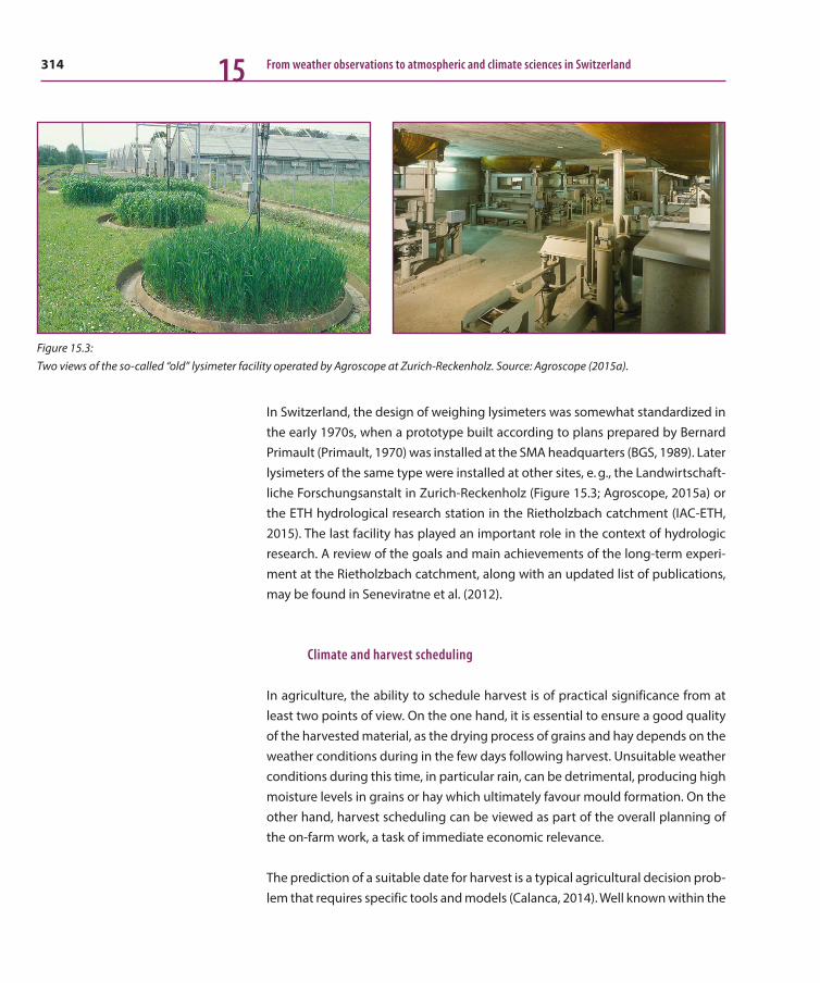
314 From weather observations to atmospheric and climate sciences in Switzerland15
In Switzerland, the design of weighing lysimeters was somewhat standardized in the early 1970s, when a prototype built according to plans prepared by Bernard Primault (Primault, 1970) was installed at the SMA headquarters (BGS, 1989). Later lysimeters of the same type were installed at other sites, e. g., the Landwirtschaft-liche Forschungsanstalt in Zurich-Reckenholz (Figure 15.3; Agroscope, 2015a) or the ETH hydrological research station in the Rietholzbach catchment (IAC-ETH, 2015). The last facility has played an important role in the context of hydrologic research. A review of the goals and main achievements of the long-term experi-ment at the Rietholzbach catchment, along with an updated list of publications, may be found in Seneviratne et al. (2012).
Climate and harvest scheduling
In agriculture, the ability to schedule harvest is of practical significance from at least two points of view. On the one hand, it is essential to ensure a good quality of the harvested material, as the drying process of grains and hay depends on the weather conditions during in the few days following harvest. Unsuitable weather conditions during this time, in particular rain, can be detrimental, producing high moisture levels in grains or hay which ultimately favour mould formation. On the other hand, harvest scheduling can be viewed as part of the overall planning of the on-farm work, a task of immediate economic relevance.
The prediction of a suitable date for harvest is a typical agricultural decision prob-lem that requires specific tools and models (Calanca, 2014). Well known within the
Figure 15.3: Two views of the so-called “old” lysimeter facility operated by Agroscope at Zurich-Reckenholz. Source: Agroscope (2015a).
315Agricultural meteorology 15
agronomic community (albeit less well known to agrometeorologists) are empir-ical or mechanistic models for predicting the drying time of grass or cereals (Dyer and Brown, 1977; Gupta et al. 1989; Atzema, 1992). The models can be used in conjunction with weather forecasts to provide targeted information in support of farmers (Dyer and Baier, 1981).
In Switzerland, the question of developing tools for scheduling hay making was taken up by Luder (1982) in his PhD thesis. There, Luder developed a model to estimate the time needed to dry hay in the field and used it in combination with an analysis of the probability of consecutive dry days to estimate what he called “the potential number of working days.” He then applied the model to estimate the potential number of working days for different regions of Switzerland. This work was later resumed by Luder (1996) and extended by Luder and Moriz (2005), who investigated the potential number of working days in the context of climate change. The latter study is interesting because it is one of the few investigations providing a “positive” perspective of climate change impacts on agriculture.
Climate suitability
Knowledge of the climate suitability, i. e., of the match between local climatic con-ditions and crop requirements, is of paramount importance to agricultural policy, and it is in this context that information available from the so-called “climate suit-ability map for the agriculture” (BLW, 2015) is mostly employed today.
From a historical perspective, the development of a climate suitability map at the national scale was motivated by an increasing concern during the 1960s about the loss of agricultural land and the need to establish regional landscape planning. Indeed, it was at the Institute for Local, Regional and National Planning of the ETH Zurich that the first climate suitability map for the agricultural sector was devel-oped and published in the late 1960s.
This work was considerably extended by François Jeanneret (University of Berne) in collaboration with Philippe Vautier (“Station fédérale de recherches agrono-miques de Changins,” RAC; today Agroscope Changins) during the 1970s. The final result was a map at the scale of 1:200’000 providing an overall appreciation of the climatic potential for crop and forage production at the national scale (Jeanneret and Vautier, 1977).
316 From weather observations to atmospheric and climate sciences in Switzerland15
In carrying out their analysis, Jeanneret and Vautier (1977) exploited what at the time was probably the most comprehensive climatic baseline. The available data included monthly precipitation sums for 297 stations spanning the period 1901 to 1962 or 1970, the number of rainy days per month for 1901 to 1960 at 273 locations and monthly mean temperatures for 1901 to 1960 at 91 sites. The anal-ysis of the climatic requirements relied on comparing actual weather data with crop specific thresholds.
In light of the considerable interest by stakeholders, authorities and other deci-sion-making bodies, the map was digitized in 1999 at the request of the Swiss Federal Office for the Environment. This version is still the one that can be officially accessed through the portal of the Swiss Federal Administration (Schweizerische Eidgenossenschaft, 2015).
Limitations to the methods and ways to improve the climate suitability map were pointed out by Jeanneret himself (Jeanneret, 1978). Apart from the advances in the appreciation of climate-crop relations, the necessity to update the climate suitability map has become pressing, also in light of the fact that the data used for preparing the original map no longer represent the current state of the climate in Switzerland. Alone the increase in temperature that has taken place since the 1980s (Ceppi et al. 2012) has potentially caused shifts in suitability patterns for crops not accounted for by the analysis of Jeanneret and Vautier (1977).
It is precisely from this point of view that efforts to update the existing climate suitability map are being undertaken (Holzkämper et al., 2013 and 2014). The ongoing work takes advantage of the availability of high-resolution gridded data recently released by the Federal Office of Meteorology and Climatology (Frei, 2014; MeteoSwiss, 2015).
Climate change and agriculture
Agriculture is one of the economic sectors most directly exposed to shifts in climatic conditions, and concern about possible negative impacts of global warm-ing has been growing over the last few decades. The topic has also been at the focus of the various Assessment Reports by the Working Group II on Adaptation of the Intergovernmental Panel on Climate Change (IPCC) (Easterling et al., 2007; Porter et al., 2014).
317Agricultural meteorology 15
In Switzerland, as elsewhere, studies dealing with climate change impacts on agri-culture have mostly been conducted within the overall framework of climate change research (Brönnimann et al., 2014). In this context, investigations con-nected to agricultural meteorology have been fostered through various research programs and initiatives, such as the NRP 31, “Climatic Changes and Natural Haz-ards” (see, e. g., Fuhrer, 1997; Rieder and Flückiger, 1997) or the NRP 61, “Sustain-able Water Management” (Fuhrer et al., 2013).
An outstanding role has been played by the National Centre for Competence in Research (NCCR) Climate (“Climate Variability, Predictability and Climate Risks”). NCCR was operative between 2001 and 2013, providing a platform for high-profile climate and climate change impact studies. Research areas addressed within NCCR Climate were (1) past climate – variability, trends and extreme events, (2) future climate – processes and forecasting, (3) impacts of climate variability and change and (4) risk assessment, risk hedging and socioeconomic response. Agricultural meteorology has found its way into NCCR Climate through the third area of research, with projects on climate change impacts on fodder and food production (project GRASS), the application of short-term climate predictions to agriculture (project CROPFOR) and the assessment of the implications of climate change for agricultural production risks (project AGRISK). With the end of the NCCR Climate Programme, activities initiated during its 12 years of existence have been handed over to a newly founded organisation, namely, the Oeschger Centre for Climate Change Research (OCCR) at the University of Berne.
Results of these research activities have been published in scientific journals and made available to authorities, advisory bodies, stakeholders and the public in gen-eral. The dissemination process was supported by OcCC, the Advisory Body on Climate Change, and ProClim, the Forum for Climate and Global Change of the Swiss Academy of Sciences. Worth mentioning among the various reports pub-lished by these two organizations is “Climate Change and Switzerland 2050 – Impacts on Environment, Society, and Economy (CH2050)” (OcCC/ProClim, 2007). The chapter dedicated to agriculture covers a broad range of relevant topics, including plant production, the impacts of extreme weather events, yield stability (as affected by climate variability), access to water resources, pests and diseases, animal husbandry, farm management and agricultural politics (Fuhrer et al., 2007).
More recently, three of these topics were examined in a more quantitative way within the initiative “Toward Quantitative Scenarios of Climate Change Impacts in Switzerland – CH2014-Impacts” (CH2014-Impacts, 2014; Calanca et al., 2014).

318 From weather observations to atmospheric and climate sciences in Switzerland15
15.4 Operational aspects
As mentioned earlier, agrometeorological bulletins and dedicated 5-day weather forecasts for agriculture were and still are routinely issued by the Federal Office of Meteorology and Climatology. In addition to these products, targeted information in support of wine and fruit producers as well as farmers in general can be accessed since 2001 through the internet site www.agrometeo.ch (Agroscope, 2015b).
The origins of this decision-support platform can be dated back to the 1990s, when a group of wine producers in western Switzerland started to operate a mete-orological monitoring network. The initiative was motivated by the fact that local weather data in wine and fruit production regions were not being collected by the Federal Office of Meteorology and Climatology (MeteoSwiss). It took advantage of the availability of small and affordable weather stations.
In the year 2000 the growing number of stations and data as well as the obvious necessity to coordinate the efforts prompted the then so-called “Station fédérale de recherches agronomiques de Changins” (RAC; today Agroscope Changins) to contact the Ministry of Agriculture with the request to take over the network and further develop the initiative by establishing a dedicated internet platform to pro-vide access to various types of information. Along with a positive reaction from the authorities, support was also obtained from the German “Staatliches Weinbau-institut Freiburg” (WBI Freiburg).
Various types of information are available on the internet site maintained by Agro-meteo: Meteorological data for more than 150 stations (in addition to those of the SwissMetNet operated by MeteoSwiss) are distributed in all major agricultural areas of Switzerland and can be accessed free of charge; local weather forecasts for the same sites; phenological observations; forecasts concerning the appear-ance of major diseases and pests; pest-management information regarding the application of chemicals and other forms of treatment; information relevant for irrigation scheduling; and, various technical documents and links concerning, among other things, the legal aspects of plant protection.
Since going online in 2001, www.agrometeo.ch has been updated many times and extended in terms of end-user applications (see, e. g., Viret et al., 2005, 2007; Naef et al., 2011). Improvements have also been made with regard to the density and hence spatial representativeness of the meteorological network and the quality of the observations (basically through the replacement of the old LUFFT weather sta-

319Agricultural meteorology 15
tions with Campbell stations). These efforts have been much appreciated by the user community, as suggested by the results of a recent survey (Dubuis et al., 2011).
15.5 The international dimension
At the international level, research and operational activities in agricultural mete-orology have been endorsed by various institutions, two of which are, either for historical or geographical reasons, linked to Switzerland. The first is the Interna-tional Society of Biometeorology (ISB). Bernard Primault, whom we have already encountered in this chapter, was one of its founding members (Weihe, 1997) and for almost two decades (1975 to 1993) acted as its General Secretary, a position for which he eventually was awarded the honorary lifetime membership in 1999 (Hoeppe, 2000). As an active member of the society he also contributed to several of the ISB Study groups, including Plant Biometeorology.
The second institution is the Commission for Agricultural Meteorology (CAgM) of the World Meteorological Organization (WMO), which was established at the beginning of the 20th century and has its headquarters in Geneva. According to WMO (2016), “the IMO [International Meteorological Organization] Commission for Agricultural Meteorology (CAgM) was appointed in 1913, but the First World War delayed its first meeting. Re-constituted in 1919, that first meeting finally took place in Utrecht, The Netherlands, in 1923. Its seventh, and last meeting, was held in Toronto, Canada, in 1947. The policies and programmes of this last meeting became the foundation of the new WMO Commission for Agricultural Meteorol-ogy.” The latter step took place in 1951 when the IMO became the WMO and hence a specialized agency of the United Nations. The objectives of the CAgM, which currently meets every 4 years, are set down by the General Regulations for Technical Commissions, and activities are aligned with the terms of reference.
Acknowledgments
The authors would like to express their gratitude to Pierre-Henri Dubuis for pro-viding the background information and material used in writing Section 15.4.

320 From weather observations to atmospheric and climate sciences in Switzerland15
References
Agroscope, 2015a: Gewässerschutz und Stoffflüsse, Auswa-schung/Lysimeter. Accessed 9 November 2015. [Available online at: http://www.agroscope.admin.ch/gewaesserschutz- stoffhaushalt/00755/07887/07889/index.html?lang=de].
Agroscope, 2015b: Agrometeo, Prévision et gestion des risques pour l’agriculture. Accessed 9 November 2015. [Available online at: http://www.agrometeo.ch].
Allen, R. G., L. S. Pereira, D. Raes and M. Smith, 1998: Crop Evapo-transpiration. Guidelines for Computing Crop Water Require-ments. FAO Irrigation and Drainage Paper 56. Food and Agricul-ture Organization of the United Nations, 300 pp.
Atzema, A. J., 1992: A model for the drying of grass with real-time weather data. J. Agric. Eng. Res., 53, 231–247.
BGS (Bodenkundliche Gesellschaft der Schweiz), 1989: Lysime-terdaten von Schweizerischen Messstationen. Bodenwassergehalt, Sickerwasser, Niederschlag und Evaporation. BGS Dokument 4. Bodenkundliche Gesellschaft der Schweiz, 123 pp.
BLW (Bundesamt für Landwirtschaft), 2015: Klimaeignungs-karte für die Landwirtschaft in der Schweiz. Accessed 9 No -vember 2015. [Available online at: http://www.blw.admin.ch/ dienstleistungen/00334/00336/index.html?lang=de].
Bowen, I. S., 1926: The ratio of heat losses by conduction and by evaporation from any water surface. Phys. Rev., 27, 779–787.
Brönnimann, S. and Coauthors, 2014: Climate change in Swit-zerland: a review of physical, institutional, and political aspects. WIREs Climate Change, 5, 461–481.
Brutasert, W., 1982: Evaporation into the Atmosphere. D. Reidel Publishing, 299 pp.
Calanca, P., 2004: Interannual variability of summer mean soil moisture conditions in Switzerland during the 20th century: A look using a stochastic soil moisture model. Water Resour. Res., 40, W12502, doi:10.1029/2004WR003254.
Calanca, P., 2014: Weather Forecasting Applications in Agricul-ture. Encyclopedia of Agriculture and Food Systems, Vol. 5. N. Van Alfen, Ed., Elsevier, 437–449.
Calanca P., P. Smith, A. Holzkämper and C. Ammann, 2011: Die Referenzverdunstung und ihre Anwendung in der Agrarmeteo-
rologie/L’évapotranspiration de référence et son application en agrométéorologie. Agrarforschung Schweiz/Recherche Agrono-mique Suisse, 2(4), 176–183.
Calanca P., C. Spirig, S. Stoeckli, J. Samietz, A. Holzkämper and M. Hirschi, 2014: Implications of changes in seasonal mean tem-perature for agricultural production systems: three case studies. Towards Quantitative Scenarios of Climate Change Impacts in Switzerland, CH2014-Impacts, OCCR, FOEN, MeteoSwiss, C2SM, Agroscope, and ProClim, 91–97.
Ceppi, P., S. C. Scherrer, A. M. Fischer and C. Appenzeller, 2012: Revisiting Swiss temperature trends 1959–2008. Int. J. Climatol., 32, 203–213.
CH2014-Impacts, 2014: Toward Quantitative Scenarios of Climate Change Impacts in Switzerland. OCCR, FOEN, MeteoSwiss, C2SM, Agroscope, and ProClim, 136 pp.
Defila, C., 1986: Frostwarnungen in Frühling. Die Grüne, 114(17), 9–14.
Defila, C., 2007: Zur Geschichte der Phänologie in der Schweiz. Berichte des Meteorologischen Institutes der Universität Freiburg, 16 (Proceedings zur 6. Fachtagung BIOMET), 218–233.
Doorenbos, J. and W. O. Pruitt, 1984: Guidelines for Predicting Crop Water Requirements. FAO Irrigation and Drainage Paper 24. Food and Agriculture Organization of the United Nations, 144 pp.
Dubuis, P.-H., A.-L. Fabre, B. Bloesch and O. Viret, 2011: Agrome-teo: une plate-forme très appréciée. Revue suisse Viticulture, Arboriculture, Horticulture, 43(5), 324–326.
Dyer, J. A. and D. M. Brown, 1977: A climatic simulator for field–hay drying. Agric. Meteorol., 18, 37–48.
Dyer, J. A. and W. Baier, 1981: The use of weather forecasts to improve hay–making reliability. Agric. Meteorol., 25, 27–34.
Easterling, W. E. and Coauthors, 2007: Food, fibre and forest products. Climate Change 2007: Impacts, Adaptation and Vulner-ability. Contribution of Working Group II to the Fourth Assessment Report of the Intergovernmental Panel on Climate Change, M. L. Parry, O. F. Canziani, J. P. Palutikof, P. J. van der Linden and C. E. Hanson, Eds., Cambridge University Press, 273–313.
321Agricultural meteorology 15European Lysimeter Platform, 2015: internet platform for Euro-pean lysimeter stations. Accessed 9 November 2015. [Available online at: http://www.lysimeter.at/HP_EuLP/index.html].
Frei, C., 2014: Interpolation of temperature in a mountainous region using nonlinear profiles and non-Euclidean distances. Int. J. Climatol., 34, 1585–1605.
Fuhrer, J., 1997: Klimaänderungen von Grünland. Verlag der Fach-vereine (vdf ), ISBN 3-7281-2399-4.
Fuhrer, J. and Coauthors, 2007: Landwirtschaft. Klimaänderung und die Schweiz 2050, OcCC/ProClim (Organe consultative sur les changements climatiques/Proclim – Forum for Climate and Global Change), 41–53.
Fuhrer, J., D. Tendall, T. Klein, N. Lehmann and A. Holzkaemper, 2013: Water Demand in Swiss Agriculture – Sustainable Adap-tive Options for Land and Water Management to Mitigate Impacts of Climate Change. ART-Schriftenreihe 19, Agroscope Reckenholz-Tänikon, 61 pp.
Geering, J., 1943: Lysimeter-Versuche der Eidg. Landw. Ver-suchsanstalt Zürich-Oerlikon. Landw. Jahrbuch der Schweiz, 57, 107–182.
Glickman, T. S., Ed., 2000: Glossary of Meteorology, Second Edi-tion. American Meteorological Society. Accessed 9 November 2015. [Available at http://glossary.ametsoc.org/].
Griffiths, J. F., Ed., 1994: Handbook of Agricultural Meteorology. Oxford University Press, 320 pp.
Gupta, M. L., R. H. MacMillan, T. A. McMahon and D. W. Bennett, 1989: A simulation model to predict the drying time for pasture hay. Grass Forage Sci., 44, 1–10.
Hoeppe, P., 2000: ISB honorary lifetime membership awarded to Dr. Bernard Primault. Int. J. Biometeor., 44, 104.
Holzkämper, A., P. Calanca and J. Fuhrer, 2013: Identifying cli-matic limitations to grain maize yield potentials using a suitabil-ity evaluation approach. Agric. For. Meteor., 168, 149–159.
Holzkämper, A., D. Fossati, J. Hiltbrunner and J. Fuhrer, 2014: Spatial and temporal trends in agro-climatic limitations to pro-duction potentials for grain maize and winter wheat in Switzer-land. Reg. Environ. Change, 15, 109–122.
IAC-ETHZ (Institute for Atmospheric and Climate Science, Swiss Federal Institute of Technology), 2015: Rietholzbach Research
Catchment. Accessed 9 November 2015. [Available online at http://www.iac.ethz.ch/group/land-climate-dynamics/research/rietholzbach.html].
Jeanneret, F., 1978: Die Klimaeignung für die Landwirtschaft: Methode und Probleme einer gesamtschweizerischen Grund-lagenkartierung. Geographica Helvetica, 33, 49–54.
Jeanneret, F. and P. Vautier, 1977: Kartierung der Klimaeignung für die Landwirtschaft in der Schweiz – Levé cartographique des aptitudes climatique pour l’agriculture en Suisse (Climate suit-ability mapping for agriculture in Switzerland), Jahrbuch der Geographischen Gesellschaft von Bern, Beiheft, 4, 108 pp.
Jensen, M. E., R. D. Burman and R. G. Allen, Eds., 1990: Evapo-transpiration and Irrigation Water Requirements. ASCE Manuals and Reports on Engineering Practice No. 70. American Society of Civil Engineers, 332 pp.
Luder, W., 1982: Ermittlung der Erntegelegenheiten und des Verlustrisikos aufgrund von Klimadaten. Dissertation 6981, Eid-genössische Technische Hochschule (ETH), 177 pp.
Luder, W., 1996: Wetterrisiko und verfügbare Feldarbeitstage in der Schweiz. FAT-Berichte, 490, 7 pp.
Luder, W. and C. Moriz, 2005: Raufutterernte: Klimaerwärmung besser nutzen. FAT-Berichte, 634, 8 pp.
MeteoSwiss (Federal Office of Meteorology and Climatology), 2015: Gridded Datasets. Accessed 9 November 2015. [Available online at: http://www.meteoswiss.admin.ch/home/services-and- publications/produkte.html].
Monteith, J. L., 1965: Evaporation and environment. Symposium of the Society for Experimental Biology, the State and Movement of Water in Living Organisms, Vol. 19, Fogg, G. E., Ed., Academic Press, 205–234.
Naef, A., M. Hubert, P.-H. Dubuis and G. Bleyer, 2011: Verbesser-ter Warndienst für den falschen Rebenmehltau. Schweiz. Zeit-schrift f. Obst- und Weinbau, 11/10, 6–9.
OcCC/ProClim (Organe consultative sur les changements clima-tiques/Proclim – Forum for Climate and Global Change), 2007: Klimaänderung und die Schweiz 2050. OcCC / ProClim, 168 pp.
Penman, H. L., 1948: Natural evaporation from open water, bare soil, and grass. Proc. Roy. Soc. London, Ser. A, 193, 120–145.

322 From weather observations to atmospheric and climate sciences in Switzerland15
Porter, J. R., L. Xie, A. J. Challinor, K. Cochrane, S. M. Howden, M. M. Iqbal, D. B. Lobell, and M. I. Travasso, 2014: Food security and food production systems. Climate Change 2014: Impacts, Adaptation, and Vulnerability. Part A: Global and Sectoral Aspects. Contribution of Working Group II to the Fifth Assessment Report of the Intergovernmental Panel on Climate Change, Field, C. B. and Coauthors, Eds., Cambridge University Press, 485–533.
Prasuhn, V., E. Spiess, C. Humphrys and C. Vögeli Albisser, 2011: Lysimeterforschung an ART – dem Nitrat auf der Spur. Bulletin der Bodenkundlichen Gesellschaft der Schweit (BGS), 32, 85–90.
Priestley, C. H. B. and R. J. Taylor, 1972: On the assessment of sur-face heat flux and evaporation using large-scale parameters. Mon. Wea. Rev., 100, 81–92.
Primault, B., 1962: Du calcul de l’évapotranspiration. Archiv Meteor., Geophys. Bioklimatol., Ser. B, 12(1), 124–150.
Primault, B., 1970: A large-scale electronic weighing lysimeter for agricultural meteorology. Philips Serv. Sci. + Ind. Eindhoven, 16, 10–11.
Primault, B., 1981: Extension de la validité de la formule Suisse de calcul de l’évapotranspiration. Arbeitsberichte der Schweizeri-schen Meteorologischen Zentralanstalt (Working Reports of the Swiss Meteorological Institute), 103, 8 pp.
Rieder P. and S. Flückiger, 1997: Ökonomische Implikationen innerhalb der Landwirtschaft und ihres Umfeldes aus globaler, nationaler und regionaler Sicht. Verlag der Fachvereine (vdf ), ISBN 3-7281-2443-5.
Schweizerische Eidgenossenschaft, 2015: Geokatalog. Accessed 9 november 2015. [Available online at: https://map.geo.admin.ch, Geokatalog, Natur & Umwelt, Atmo-sphäre, Luft, Klima].
Seneviratne, S. I and Coauthors, 2012: Swiss prealpine Riet-holzbach research catchment and lysimeter: 32 year time series and 2003 drought event. Water Resour. Res., 48, W06526, doi:10.1029/2011WR011749.
Slatyer, R. O. and I. C. McIlroy, 1961: Practical Microclimatology, with Special Reference to the Water Factor in Soil-Plant-Atmo-sphere Relationships. United Nations Educational, Scientific and Cultural Organization (UNESCO), 338 pp.
Stähli M., S. Kruse, F. Fundel, M. Zappa, K. Stahl, L. Bernhard and I. Seidl, 2013: drought.ch – auf dem Weg zu einer Trocken-
heits-Informationsplattform für die Schweiz. Wasser Energie Luft, 105 (2), 117–121.
Steduto, P., T. C. Hsiao, E. Fereres and D. Raes, 2012: Crop Yield Response to Water. FAO Irrigation and Drainage Paper 66. Food and Agriculture Organization of the United Nations, 500 pp.
Thom, A. S. and H. R. Oliver, 1977: On Penman’s equation for esti-mating regional evapotranspiration. Quart. J. Roy. Meteor. Soc., 103, 345–357.
Thornthwaite, C. W. 1948: An approach toward a rationale classi-fication of climate. Geogr. Rev., 38, 55–94.
Van Bavel, C. H. M., 1961: Lysimetric measurements of evapo-transpiration rates in the eastern United States. Proc. Soil Sci. Soc. Am., 25, 138–141.
Viret, O., B. Bloesch, A.-L. Fabre, W. Siegfried, G. Bleyer, B. Huber and H.-H. Kassemeyer, 2005: Vitimeteo: un nouveau modèle de prévision pour le mildiou de la vigne. Revue Suisse Vitic. Arboric. Hortic., 37(1), 65–68.
Viret, O., B. Bloesch, A.-L. Fabre and W. Siegfried, 2007: Prévision du mildiou sur www.agrometeo.ch et gestion de la lutte. Revue Suisse Vitic. Arboric. Hortic., 39(1), 57–59.
Weihe, W. H., 1997: Review of the history of the International Society of Biometeorology. Int. J. Biometeor., 40, 9–15.
WMO (World Meteorological Organization), 2012: Guide to Agricultural Meteorological Practices. WMO-No. 134. World Meteorological Organization.
WMO (World Meteorological Organization), 2016: Commission for Agricultural Meteorology (CAgM), History. Accessed 21 April 2016. [Available online http://public.wmo.int/en/about-us/gov-ernance/commission-agricultural-meteorology-cagm].
WSL/ETH/UniZH (Eidg. Forschungsanstalt für Wald, Schnee und Landschaft, Eidg. Technische Hochschule, Universität Zürich), 2015: Drought-CH. Accessed 21 April 2016. [Available online at: http://www.drought.ch].

323
Evolution of atmospheric chemistry into an integrated part of atmospheric sciences


325
16 The value of Swiss long-term ozone observations for international atmospheric researchJohannes Staehelin1, Stefan Brönnimann2, Thomas Peter1, Rene Stübi3, Pierre Viatte3, Fiona Tummon1
Since the discovery of ozone by C. F. Schönbein in 1839 and the very start of atmospheric ozone
measurements in the 1920s, Swiss observatories and scientists have played a key role in developing
our understanding of this important atmospheric trace gas. The world’s longest measurement series
of column ozone is from Arosa and dates all the way back to 1926. A few years later, Umkehr
measurements, also performed in Arosa (1932/1933), provided the first reliable observations of
the ozone profile. Umkehr measurements have been performed in Arosa on a regular basis since 1956
and balloon-borne ozone measurements started in 1966 in Thalwil but were moved in 1968 to
Payerne (western Switzerland) for continuous measurements with 2–3 launches per week. Data
from Arosa and Payerne served as the “gold standard” in international ozone assessments and
continue to be of undiminished importance, providing an extended high-quality record of use for
long-term ozone change studies. In addition extended surface ozone measurements are available
from Arosa from the 1950s.
16.1 Basic questions in ozone research and ozone history prior to the start of Swiss long-term measurements
Today we know that the Earth’s atmosphere consists of several layers usually defined by the temperature profile. Ozone concentrations, in partial pressure, peak in the lower stratosphere in the mid-latitudes at around 22 km above sea level (asl), see Figure 16.1. Ozone in the stratosphere is formed from molecular oxygen at wavelengths λ < 242 nm. Ozone is essential for preventing harmful ultraviolet (UV) radiation at wavelengths below 300 nm from penetrating through the Earth’s atmosphere to the surface. Ozone in the troposphere, on the other hand, is formed by a sequence of reactions of nitrogen oxides (NOx) with volatile organic compounds (VOCs) or carbon monoxide (CO). Tropospheric ozone pro-duction also requires UV radiation, but at much longer wavelengths (λ < 310 nm). Ozone in the troposphere is an air pollutant and harmful to the biosphere. It is also the precursor of hydroxyl (OH) radicals, the most important cleansing agent of tropospheric air. Furthermore, ozone is an important greenhouse gas of relevance for climate change. Changes and trends in column or total ozone essentially reflect
1 ETH Zurich, Institute for Atmospheric
and Climate Science, ETHZ, Zurich2 University of Bern, Oeschger Centre
for Climate Change Research and
Institute of Geography, Bern3 Federal Office of Meteorology and
Climatology MeteoSwiss, Payerne
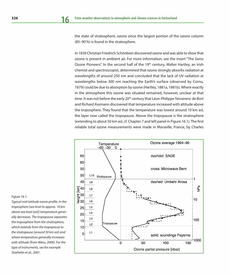
326 From weather observations to atmospheric and climate sciences in Switzerland16
the state of stratospheric ozone since the largest portion of the ozone column (85–90 %) is found in the stratosphere.
In 1839 Christian Friedrich Schönbein discovered ozone and was able to show that ozone is present in ambient air. For more information, see the insert “The Swiss Ozone Pioneers”. In the second half of the 19th century, Walter Hartley, an Irish chemist and spectroscopist, determined that ozone strongly absorbs radiation at wavelengths of around 250 nm and concluded that the lack of UV radiation at wavelengths below 300 nm reaching the Earth’s surface (observed by Cornu, 1879) could be due to absorption by ozone (Hartley, 1881a, 1881b). Where exactly in the atmosphere this ozone was situated remained, however, unclear at that time. It was not before the early 20th century that Léon-Philippe Teisserenc de Bort and Richard Assmann discovered that temperature increased with altitude above the troposphere. They found that the temperature was lowest around 10 km asl, the layer now called the tropopause. Above the tropopause is the stratosphere (extending to about 50 km asl, cf. Chapter 7 and left panel in Figure 16.1). The first reliable total ozone measurements were made in Marseille, France, by Charles
Figure 16.1: Typical mid-latitude ozone profile. In the troposphere (sea level to approx. 10 km above sea level (asl)) temperature gener-ally decreases. The tropopause separates the troposphere from the stratosphere, which extends from the tropopause to the stratopause (around 50 km asl) and where temperature generally increases with altitude (from Weiss, 2000). For the type of instruments, see for example Staehelin et al., 2001.

327The value of Swiss long-term ozone observations for international atmospheric research 16
Fabry and Hénri Buisson (1921). Using early measurements they concluded that an ‘ozone layer’ should be situated at an altitude of around 40 km. However, knowledge of atmospheric ozone in the early 1920s remained very limited.
16.2 Early ozone measurements in Arosa: Total ozone, profile information by the Umkehr method, and surface ozone
Important advances in ozone science in the years 1900–1970 were intrinsically connected with research performed in Switzerland. The geographic position of the country with its high mountains made and continue to make it ideal for ozone-related observations. The interest in high-altitude radiation and in the apparently clean and healthy air enhanced this particular situation.
The years before 1940
Early Swiss contributions relevant to atmospheric ozone research started with Carl Dorno, who founded the Physikalisch-Meteorologisches Observatorium Davos (PMOD) in 1907. His studies of the climatology of high-altitude radiation stemmed from his interest in its medical application, and he introduced an instrument to measure the biologically active shortwave UV-radiation, which was operated in Davos (Dorno, 1917). This instrument contained a photoelectric cell, which was used as a detector with a cadmium cathode and a filter with a cut-off at 320 nm. This allowed one to separate out the biologically active shortwave radiation. Early Swiss contributions further include the work of Edgar Meyer, who graduated with a PhD thesis about “Die Absorption von ultraviolettem Licht in Ozon” (Meyer, 1903) and later became Professor of Physics at the University of Zurich (1916–1949), and of Alfred Läuchli, one of Meyer’s PhD students, who published laboratory measurements of the absorption cross-sections of ozone (Läuchli, 1928). At the time spectroscopic knowledge – particularly in the wavelength range from 290–340 nm – was still very poor. Meyer (1925) analysed Dorno’s measurements and found that the measurements could be explained when assuming a column ozone amount of 300 DU. Such an instrument was also operated at the Light Climatic Observatory (LKO) in Arosa by Friedrich Wilhelm Paul Götz (see insert “Swiss Ozone Pioneers”). He analysed the measurements from October 1921 to 1924 (Götz, 1925; 1926a, p. 45; 1926b) and found (using a relative scale) an indication of the seasonal cycle of total ozone with a maximum in spring and a minimum in autumn typical for Northern mid-latitudes. Götz published this before measurements from
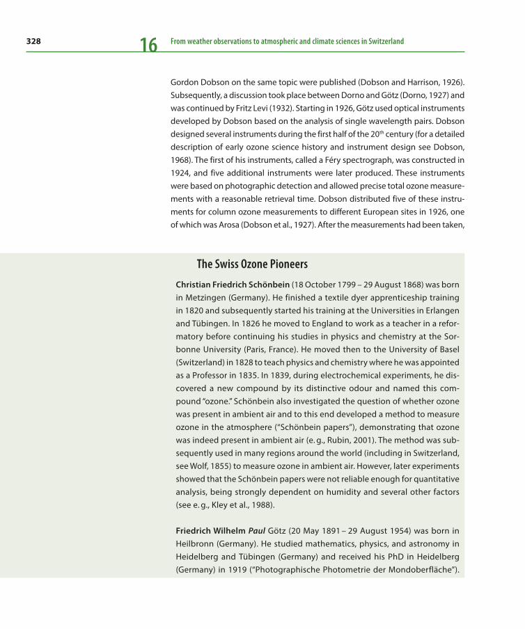
328 From weather observations to atmospheric and climate sciences in Switzerland16
Gordon Dobson on the same topic were published (Dobson and Harrison, 1926). Subsequently, a discussion took place between Dorno and Götz (Dorno, 1927) and was continued by Fritz Levi (1932). Starting in 1926, Götz used optical instruments developed by Dobson based on the analysis of single wavelength pairs. Dobson designed several instruments during the first half of the 20th century (for a detailed description of early ozone science history and instrument design see Dobson, 1968). The first of his instruments, called a Féry spectrograph, was constructed in 1924, and five additional instruments were later produced. These instruments were based on photographic detection and allowed precise total ozone measure-ments with a reasonable retrieval time. Dobson distributed five of these instru-ments for column ozone measurements to different European sites in 1926, one of which was Arosa (Dobson et al., 1927). After the measurements had been taken,
The Swiss Ozone Pioneers
Christian Friedrich Schönbein (18 October 1799 – 29 August 1868) was born in Metzingen (Germany). He finished a textile dyer apprenticeship training in 1820 and subsequently started his training at the Universities in Erlangen and Tübingen. In 1826 he moved to England to work as a teacher in a refor-matory before continuing his studies in physics and chemistry at the Sor-bonne University (Paris, France). He moved then to the University of Basel (Switzerland) in 1828 to teach physics and chemistry where he was appointed as a Professor in 1835. In 1839, during electrochemical experiments, he dis-covered a new compound by its distinctive odour and named this com-pound “ozone.” Schönbein also investigated the question of whether ozone was present in ambient air and to this end developed a method to measure ozone in the atmosphere (“Schönbein papers”), demonstrating that ozone was indeed present in ambient air (e. g., Rubin, 2001). The method was sub-sequently used in many regions around the world (including in Switzerland, see Wolf, 1855) to measure ozone in ambient air. However, later experiments showed that the Schönbein papers were not reliable enough for quantitative analysis, being strongly dependent on humidity and several other factors (see e. g., Kley et al., 1988).
Friedrich Wilhelm Paul Götz (20 May 1891 – 29 August 1954) was born in Heilbronn (Germany). He studied mathematics, physics, and astronomy in Heidelberg and Tübingen (Germany) and received his PhD in Heidelberg (Germany) in 1919 (“Photographische Photometrie der Mondoberfläche”).

329The value of Swiss long-term ozone observations for international atmospheric research 16
Because of health problems he moved to Davos (Switzerland) in 1916 where he worked as a teacher at a private school (Fridericianum) during several years. In 1921 he accepted the invitation from the Chamber of Commerce of Arosa (Kurverein) to found the so-called “Light-Climatic Observatory” (LKO) in Arosa. During the first phase he collaborated closely with Carl Dorno, founder of the Physical Meteorological Observatory Davos (PMOD) also using instruments used in Davos. Götz was personally motivated to carry out a careful evaluation of different environmental factors contributing to a bet-ter probability of recovery from tuberculosis (at that time modern antibiotics were not available). His comprehensive studies (Götz, 1926a, 1954) included studies of climatology and stratospheric ozone (see Dütsch, 1992a, for more details). While his scientific main merits are related to stratospheric ozone research, he also carefully measured ozone in ambient air and postulated that such measurements were required for a proper rating of resort areas (see Section 2). He wrote that healthy air contains much more ozone than urban air, in which ozone concentrations were low, and which he called “dead air” like the air in a mine when ventilation is sluggish. Based on the analysis of measurements of his expedition to Spitsbergen (summer 1929) he wrote his habilitation thesis (1931) allowing him to give lectures at the University of Zurich. In 1940 he obtained the title of a Professor of the Uni-versity of Zurich, where he became responsible for teaching meteorology.
Hans-Ulrich Dütsch (26 October 1917 – 27 December 2003) was born in Winterthur (Switzerland). He studied physics at the University of Zurich (1940: Diploma degree in theoretical physics with a minor in meteorology). From 1943 to 1946 he was a graduate student of Götz (“Photochemische Theorie des atmosphärischen Ozons unter Berücksichtigung von Nicht-gleichgewichstzuständen und Luftbewegungen“). Subsequently, he worked as a high school (Gymnasium) teacher in physics, mainly in Zurich, but still continued with his ozone research. In 1950 he visited MIT (Massachusetts Institute of Technology, Cambridge, MA, USA) and then became a researcher at the High Altitude Observatory in Boulder (CO, USA). He was Head of the Ozone Research Program at the newly founded NCAR (National Center of Atmospheric Research in Boulder, CO, USA) from 1962–1964. Later he was appointed as professor at the ETH Zurich from 1965–1985. Dütsch was one of the leading scientists in ozone research and strongly engaged in the con-tinuation of the measurements of LKO in Arosa twice, following the death of Götz and after his own retirement as ETH Zurich Professor.

330 From weather observations to atmospheric and climate sciences in Switzerland16
most of the instruments were shipped back to Oxford except the one operated at Arosa, since Dobson was pleased by the observations made by Götz. Indeed, the instrument stayed in Arosa until 1950 and was used to achieve a homogeneous series with the next generation instrument developed by Dobson, which used photoelectric detection (Dobson, 1931). In 1928 Dobson redistributed the other instruments around the globe in order to learn more about the variability and seasonal cycle of total ozone in different regions of the world. These measure-ments were used to produce a (quasi-)global total ozone climatology and also to show that short-term variability of mid-latitude total ozone was characterized by a strong anti-correlation with surface pressure (Dobson, 1930). Comparisons between instruments from different stations were also performed in Arosa from 1929 onwards (Dütsch, 1992a), see Figure 16.2. Such comparisons continue to this day (Bojkov, 2010).
Götz went to Spitsbergen (Norway) in the summer of 1929, where he performed extended measurements with the Féry spectrograph. Although the most precise total ozone measurements are made by analysing direct solar radiation, in Spits-bergen he also made ozone measurements using zenith sky observations. He derived stratospheric ozone levels using wavelength pair observations. From these observations Götz found that the ratio of intensities of a wavelength strongly absorbed by ozone over a wavelength weakly absorbed steadily decreased with
Figure 16.2: Comparison of two Dobson instruments at Arosa on the roof of the Kurhaus Florentinum (1954). On the left: C. D. Walshaw, serving as travelling scientist to check and calibrate the Dobson spectrophotometers. F. W.P. Götz can be seen standing in the centre behind the instruments.
331The value of Swiss long-term ozone observations for international atmospheric research 16
decreasing solar elevation (as expected) until low solar elevation (around 2–5°) was reached, but thereafter reversed (‘Umkehren’) and increased again, i. e. in the evening close to sunset. Götz was convinced that the observed time evolution of the signal contained ozone profile information. Afterwards, Dobson repeated Götz’s measurements in Oxford and later travelled to Arosa in 1932 with two newly designed Dobson instruments (using photoelectric detection) to perform such Umkehr observations. One of these instruments he left in Arosa and was sub-sequently used by Götz. Götz continued to make Umkehr observations (which require cloudless conditions for one half day) and Götz et al. (1934) determined the first ozone profile measurements based on the “Götz” or Umkehr effect. Soon thereafter ozone profile results determined by the Umkehr method were con-firmed by in situ ozone measurements taken with balloon-borne instruments (Regener, 1934). Although his research interests were not restricted to ozone, Götz was one of the leading early ozone scientists, and during his long career he wrote several review articles on the subject (see Dütsch, 1992a).
16.3 The years 1940–1970
By the mid-1940s more was known about ozone and its variability, particularly in the northern mid-latitudes, where the seasonal variability of total ozone and the ozone profile were relatively well documented. Furthermore, the theory of Sidney Chapman (1930) could explain the occurrence of stratospheric ozone with just four chemical equations, including the formation of ozone from molecular oxygen and its chemical depletion by reaction with atomic oxygen. Hans-Ulrich Dütsch (see insert “the Swiss Ozone Pioneers”), a PhD student of Götz, investigated this theory further, exploring whether the observed features of stratospheric ozone, particularly the seasonal cycle with a spring peak, could be explained using Chap-man’s theory. Using extended calculations, he concluded, independently of two others, that the chemistry described using Chapman’s theory could not explain the observed stratospheric ozone climatology alone (Dütsch, 1946). This problem was later solved when Brewer (1949) published his study on stratospheric circula-tion (later termed the Brewer-Dobson circulation; for recent review see Butchart, 2014), which is required to fully understand the seasonal cycle of total ozone in the mid-latitudes.
The first international scientific Conference on “Ozone and Atmospheric Absorp-tion” took place in Paris, in 1929, and was organized by C. Fabry (see Bojkov, 2010). In 1948 the International Ozone Commission (IO3C) was established. The
332 From weather observations to atmospheric and climate sciences in Switzerland16
aim of the IO3C (which at present is part of the International Association of Meteorology and Atmospheric Sciences (IAMAS)), was to facilitate scientific col-laboration through the organization of international ozone symposia, to improve ozone measurements and the collection of these measurements (initially a task of the commission’s secretary), and to provide the possibility of lending Dobson instruments to suitable sites. Through the commission, Götz was able to maintain a Dobson instrument continuously in Arosa, which the LKO would otherwise never have been able to afford. For more information on the history of the IO3C see Bojkov (2010).
Dütsch strongly contributed to the IO3C (see insert “The International Ozone Com-mission (IO3C), International flavour of Ozone Research”), serving as its Secretary from 1960–1975 and then later as its President (1975–1980). During this time he was the main organiser of two atmospheric ozone symposia, which took place in
The International Ozone Commission (IO3C): International flavour of ozone research
Originally, the IO3C was strongly involved in the development of instrumen-tation and procedures for the precise measurement of atmospheric ozone. During the International Geophysical Year (IGY), held from 1957–1958, the basic method of ozone observation using Dobson instruments was finalized (using two wavelength pair observations). Today, this method continues to be used in essentially the same way. Contact between ozone scientists (as represented by the IO3C) and those from the World Meteorological Organi-sation (WMO) started in the 1950s, with the aim of supporting an observa-tional network of high-quality, ground-based Dobson measurements. Sub-sequently, the WMO approved ozone measurements as part of their network and took the responsibility for introducing standard operational procedures enabling national meteorological services to contribute to regular ozone observations. The WMO also agreed to support the collection and publica-tion of ozone measurements from the IGY, after which the Canadian Meteo-rological Service continued this task for several years until the World Ozone and Ultraviolet Data Center (WOUDC) was established in 1962. These ele-ments also provided the pillars of the WMO’s Global Ozone Monitoring Sys-tem (GO3OS). The IO3C was, and still is, responsible for the organisation of ozone-related conferences such as the Quadrennial Ozone Symposia (see Bojkov et al., 2010).

333The value of Swiss long-term ozone observations for international atmospheric research 16
Arosa in 1961 and 1972. Dütsch was also heavily involved in the improvement of methods used to determine ozone profiles from Umkehr measurements; he and Carlton Mateer were the first to use modern computers for Umkehr retrievals (e. g., Mateer and Dütsch, 1964). Dütsch also initiated regular Umkehr measurements at Arosa, starting in 1956, and regular ozone profile measurements using ozone-sondes in Switzerland, first in Thalwil (close to Zurich) and subsequently at the aerological station in Payerne as part of the MeteoSwiss measurement programme (Jeannet et al., 2007).
Besides stratospheric ozone, Götz was also interested in tropospheric ozone. He aimed to obtain representative measurements, as he was convinced that ozone in ambient air was an important factor to grade air quality of resort areas; ozone concentrations are low in the polluted urban air but high in the “healthy Alpine air” (Götz, 1954, pp. 56). Götz first used long-path UV absorption techniques to measure ozone in the Arosa area (Götz and Ladenburg, 1931 (see Figure 16.3); Götz and Maier-Leibnitz, 1933; Götz and Penndorf, 1941). However, measure-ments using long-path observations were only feasible during clear nights and the analysis of the data was rather time consuming. Representative data of sur-face ozone were later obtained using chemical measurements; two extensive data sets of which are available from the 1950s. The large number of measure-ments made in Arosa allowed a proper determination of surface ozone variabil-ity, in particular the seasonal cycle, since surface ozone measurements made at
Figure 16.3: Götz (April 30, 1930) and the apparatus used for surface ozone measurements from Tschuggen (Arosa) (see Götz and Ladenburg, 1931).

334 From weather observations to atmospheric and climate sciences in Switzerland16
other sites during this period were performed only during campaigns and thus did not cover a long enough time period to be representative (see Staehelin et al., 1994). The seasonal cycle of surface ozone peaking in May was viewed as experimental evidence for the textbook knowledge that ozone originates from the stratosphere since total (stratospheric) ozone peaks in spring at Northern mid-latitudes (see e. g., Junge, 1962). Götz and Volz (1951) also compared sur-face ozone with synoptic weather conditions, and Perl (1961) confirmed the seasonal cycle of surface ozone showing the largest concentrations to be in May. The attribution of the May maximum purely to import of ozone-rich air from the stratosphere was somewhat oversimplified as became clearer only later, when the meteorological and radiative dependences of tropospheric in situ ozone production were better understood in the context of the Los Angeles summer smog.
16.4 Paradigm shift in ozone research (around 1970)
The potential impact of human activities on stratospheric and tropospheric ozone moved to the centre of scientific and public interest with the discovery of the Antarctic ozone hole and with the realisation that massive events of summer pho-tosmog in North American cities were intrinsically tied to the development of tropospheric ozone.
Stratospheric ozone
The possibility of anthropogenic depletion of the ozone layer was first discussed in the early 1970s. Paul Crutzen (1970) was the first to identify the role of nitrogen oxides in the catalytic destruction of stratospheric ozone. This was also inde-pendently discovered by Harald Johnston (1971) who described the possible impact of nitrogen emissions from a large fleet of civil aircraft planned to operate at supersonic speed in the stratosphere. High-speed supersonic transport systems regained some attention with new plans of the aircraft industry in the 1990s, but this fleet was never built, and the problem eventually lost its political importance. However, in 1974 Mario Molina and Sherwood Rowland (1974) as well as Richard Stolarski and Ralph Cicerone (1974) independently described stratospheric ozone loss by a radical chain reaction of chlorine oxides (ClOx), and Molina and Rowland (1974) identified chlorofluorocarbons (CFCs) as a potential source gas of strato-spheric ClOx. Chlorofluorocarbons are part of a group of compounds containing
335The value of Swiss long-term ozone observations for international atmospheric research 16
halogens (Cl, Br, I) that destroy stratospheric ozone, which are collectively called ozone-depleting substances (ODSs).
In 1985, the Antarctic ozone hole was discovered by Farman et al. (1985), which was completely unexpected. The scientific explanation for the ozone hole was found within a few years of intensive research, namely, the effect of heteroge-neous chemical reactions taking place on the surface of polar stratospheric clouds (PSCs) that occur only in the very cold temperatures of the (winter) polar vortex air, combined with the ability of large PSC particles to remove stratospheric nitro-gen species via gravitational settling (cf. Peter (1997) and Solomon (1999)). In 1987 the Montreal Protocol was signed, which was subsequently strengthened by sev-eral amendments (WMO/UNEP, 2014).
Tropospheric Ozone
High ozone concentrations close to the surface were documented around the end of World War II in the Los Angeles area. Subsequent research showed that these high concentrations were attributable to ozone formation from anthropogenic emissions, namely nitrogen oxides reacting with volatile hydrocarbons or carbon monoxide (Haagen-Smit, 1952). However, this phenomenon was viewed as local without any discernible effect on the global scale (e. g. Brönnimann, 2002) and it was believed that stratospheric ozone was the dominating source of tropospheric ozone (Junge, 1962). Crutzen (1973, 1974) and Chameides and Walker (1973) were among the first to show, using numerical simulations, that ozone formed in the troposphere resulting from the oxidation of ozone precursors could strongly affect tropospheric ozone on a large scale. During the 1970s an extended debate took place around this new view (Fabian, 1974; 1976; Fabian and Pruchniewicz, 1977; Chameides and Walker, 1976; Chatfield and Harrison, 1976). Later, during the 1980s the important role of in situ chemical ozone production in the troposphere even on the global scale became more and more evident.
16.5 Swiss stratospheric ozone measurements in modern atmospheric research
From the early 1970s onwards, stratospheric ozone monitoring became a politi-cally relevant topic, particularly since the chemical industry questioned Molina and Rowland’s theory. DuPont, the largest producer of CFCs at the time, made a

336 From weather observations to atmospheric and climate sciences in Switzerland16
statement that they would stop producing CFCs if damage to the ozone layer by ODSs could be documented. Stratospheric ozone measurements had previously only been used for research purposes, for example, for studying the relationship between stratospheric ozone and weather (this relationship was explored because it was thought that the use of stratospheric ozone measurements could possibly improve weather forecasts). Data quality requirements for these studies were gen-erally not very high, since total ozone in the mid-latitudes can change from day to day by up to ± 20 %. However, ozone depletion caused by CFC emissions and other ODSs, while persistent, was expected to be much smaller in magnitude than natural variability. Demands on the Global Ozone Observing System (GO3OS) operated under the auspices of the World Meteorological Organisation (WMO) therefore became much more exigent, namely to improve the quality of ozone observations obtained from the network to enable reliable long-term trend anal-yses of ozone changes by a few percent per decade (e. g., Dlugokencky et al., 2010). (These efforts were subsequently extended to other compounds leading to the present Global Atmosphere Watch (GAW) programme of WMO.) Important aspects of data quality control include regular intercomparisons between stations and standard instruments as well as the storage of data in the World Ozone and Ultraviolet Radiation Data Centre (WOUDC) in Toronto, Canada. Column ozone and Umkehr measurements (the longest available records are from Arosa) and measurements from ozonesondes (of which Payerne has one of the most compre-hensive records, particularly regarding the number of ascents) are also stored in the WOUDC. High-quality ground-based records are also crucial for the validation of satellite ozone observations and to assess the stability of their long-term cali-bration. Satellite and ground-based observations are complementary, since the space-borne satellite observations allow global coverage but need to be validated against ground-based measurements, which have much lower spatial coverage but higher accuracy (e. g., Staehelin et al., 2001). At present, more automated mod-ern instruments such as Brewer and SAOZ (Système d’Analyse par Observation Zénithale) spectrometers are also being used for total ozone monitoring, while lidars and microwave radiometers can be used to measure the ozone profile. Many of these instruments are part of another measurement network, the Network for the Detection of Atmospheric Composition Changes (NDACC), which was estab-lished in the early 1990s.
Dütsch was one of the leading ozone scientists actively involved in ozone research both in the decades before and after anthropogenic ozone depletion was discov-ered. He made a number of important contributions (e. g., Dütsch, 1974; 1978a; 1979; Dütsch and Braun, 1980; Dütsch et al., 1991), and he wrote important review

337The value of Swiss long-term ozone observations for international atmospheric research 16
papers (Dütsch, 1968; 1969; 1971; 1978b; 1981; 1992b). Even after he retired, he was heavily involved in the move of LKO to MeteoSwiss in 1988, to ensure the continuation of the measurements. After this changeover, the station at Arosa was renewed and modernised, for example, by adding Brewer instruments to comple-ment the measurements already being made with Dobson spectrometers (see Hoegger et al., 1992).
Because of its unique length, the continuous multi-decadal record from Arosa is particularly important for studying long–term changes of stratospheric ozone. The Arosa measurements are based on high-quality direct sun total ozone observa-tions, which, owing to Arosa’s fair weather conditions, are possible on around two thirds of all days of the year (see textbox). The data quality of the Arosa record has been ensured since the mid-1950s through the statistical Langley Plot procedure, which requires a large number of measurements (Dütsch, 1984). The same calibra-tion procedure was adapted to the Dobson data series from Halley Bay, from which the Antarctic ozone hole was discovered (Farman et al., 1985). Dütsch inspected every ozone measurement (he went to Arosa for several days every year) and applied small corrections as derived from the Langley Plot procedure. Data from the beginning of the Arosa record until 1949 were carefully analysed in the PhD thesis of Walter Birrer (1975). Nevertheless, the total ozone record of Arosa needed further adjustments to provide a fully homogenized data set for use in reliable long-term trend analysis. To this end, Staehelin et al. (1998a) homogenized some of the measurements from Arosa, that had been calibrated by the statistical Langley plot method, with others that had been compared with the primary world Dobson instrument. Furthermore, they corrected for an optical misalignment problem of one instrument, and compared the Arosa Dobson with Arosa Brewer instruments by developing a transfer function between Dobson and Brewer spec-trophotometric measurements, which was then further developed by Scarnato et al. (2010). Finally, they compared them with the daily overpass data of the Total Ozone Mapping Spectrometer (TOMS), which operated on board the Nimbus 7 satellite (1978–1993), suggesting fluctuations among the Arosa instruments and drifts over the lifetime of the TOMS instrument to be less than about 1 %. Such adjustments were similarly applied to records from all other observation sites that provided measurements prior to the 1970s.
As mentioned above, the Arosa total ozone record has been used for long-term trend analysis (see Figure 16.4, lower panel, and Staehelin et al., 1998b). The data from the decades before anthropogenic ozone depletion begun contain import-ant information about long-term interdecadal variability, which can be compared
Before 1932 some years only have a few
observations and are thus less represen-
tative. This is in part because Götz used
the instrument in the campaign on Spits-
bergen, see Staehelin et al., 1998a)

338 From weather observations to atmospheric and climate sciences in Switzerland16
with anthropogenic ozone depletion. The time series shows a significant decrease starting in the early 1970s and continuing more strongly in the 1980s until a min-imum was reached in the early 1990s. Thereafter, the trend changes and total ozone shows a small increasing tendency, which is, however, not yet statistically significant (as the comparison with the interannual variability also suggests). This long-term evolution of total ozone at Arosa is connected to the emissions of ODSs. The chemical ozone destruction induced by ODSs can be described by the Equiv-alent Effective Stratospheric Chlorine, EESC (see upper panel in Figure 16.4), which suggests peak stratospheric chemical ozone depletion in the mid-latitudes in the second part of the 1990s. The absolute minimum values in the Arosa record that occur prior to the peak EESC values are attributable to the Pinatubo volcanic erup-tion, which injected large amounts of sulphur into the stratosphere leading to additional ozone depletion as well as to changes in stratospheric transport affect-ing ozone. The volcanic effects play no big role in the 11-year running mean (red line), which is very well anti-correlated with EESC.
Because of its unique length, the Arosa total ozone series allows us not only to study the long-term effects of anthropogenic emissions of ODSs, but also to draw important conclusions regarding dynamical processes. For example, the North Atlantic Oscillation (NAO) has a large effect on ozone variability in the northern
Figure 16.4: Total ozone time series from Arosa (annual mean values in Dobson Units [DU], lower panel) and effect of chemical ozone depletion as described by the Equivalent Effective Stratospheric Chlo-rine (EESC) for mid-latitudes (top panel).
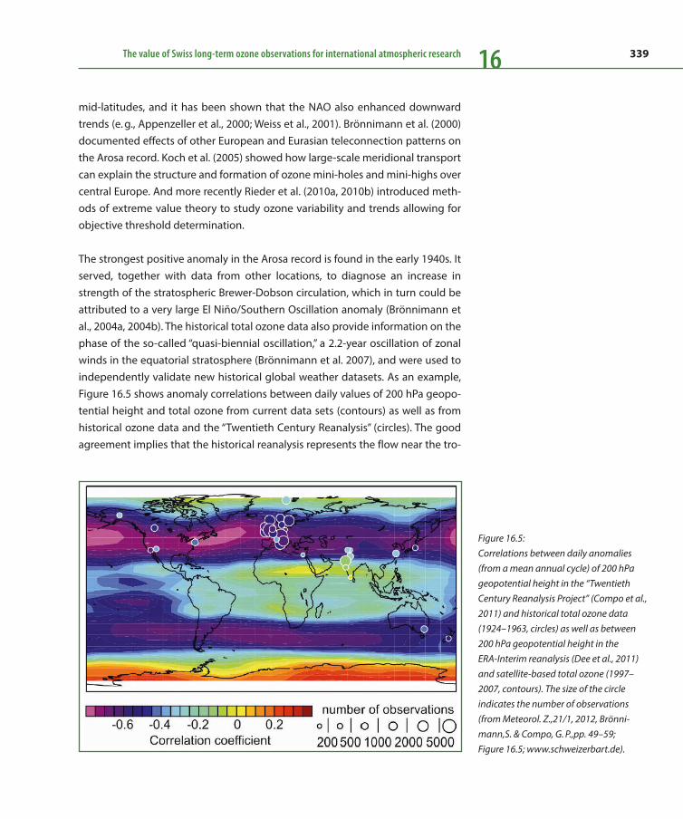
339The value of Swiss long-term ozone observations for international atmospheric research 16
mid-latitudes, and it has been shown that the NAO also enhanced downward trends (e. g., Appenzeller et al., 2000; Weiss et al., 2001). Brönnimann et al. (2000) documented effects of other European and Eurasian teleconnection patterns on the Arosa record. Koch et al. (2005) showed how large-scale meridional transport can explain the structure and formation of ozone mini-holes and mini-highs over central Europe. And more recently Rieder et al. (2010a, 2010b) introduced meth-ods of extreme value theory to study ozone variability and trends allowing for objective threshold determination.
The strongest positive anomaly in the Arosa record is found in the early 1940s. It served, together with data from other locations, to diagnose an increase in strength of the stratospheric Brewer-Dobson circulation, which in turn could be attributed to a very large El Niño/Southern Oscillation anomaly (Brönnimann et al., 2004a, 2004b). The historical total ozone data also provide information on the phase of the so-called “quasi-biennial oscillation,” a 2.2-year oscillation of zonal winds in the equatorial stratosphere (Brönnimann et al. 2007), and were used to independently validate new historical global weather datasets. As an example, Figure 16.5 shows anomaly correlations between daily values of 200 hPa geopo-tential height and total ozone from current data sets (contours) as well as from historical ozone data and the “Twentieth Century Reanalysis” (circles). The good agreement implies that the historical reanalysis represents the flow near the tro-
Figure 16.5: Correlations between daily anomalies (from a mean annual cycle) of 200 hPa geopotential height in the “Twentieth Century Reanalysis Project” (Compo et al., 2011) and historical total ozone data (1924–1963, circles) as well as between 200 hPa geopotential height in the ERA-Interim reanalysis (Dee et al., 2011) and satellite-based total ozone (1997–2007, contours). The size of the circle indicates the number of observations (from Meteorol. Z.,21/1, 2012, Brönni-mann,S. & Compo, G. P.,pp. 49–59; Figure 16.5; www.schweizerbart.de).

340 From weather observations to atmospheric and climate sciences in Switzerland16
popause at mid-latitudes in both hemispheres remarkably well (Brönnimann and Compo, 2012).
As outlined above, one motivation behind Dobson’s work in the 1920s was to obtain a simple observation of atmospheric variability at the tropopause level, from which weather forecasts could be improved. Today, 80 years later, ozone information from satellites has successfully been assimilated into weather forecast models and leads to increased forecast skill. In future, the historical ozone data might also be assimilated into historical reanalysis products and might lead to improved six-hourly weather data for the last century.
16.6 The importance of early Swiss ozone measurements for tropospheric ozone research
Surface ozone trends and background values
Surface ozone measurements made in Arosa from 1989–1990 were used for com-parison with measurements from the 1950s. These comparisons show a large increase of more than a factor two in surface ozone between the two decades. The Arosa surface ozone measurements provide the
Figure 16.6: Surface ozone at Jungfraujoch, Switzerland (Cui et al., 2011, adapted) (see Chapter 18).
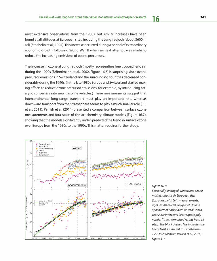
341The value of Swiss long-term ozone observations for international atmospheric research 16
most extensive observations from the 1950s, but similar increases have been found at all altitudes at European sites, including the Jungfraujoch (about 3600 m asl) (Staehelin et al., 1994). This increase occurred during a period of extraordinary economic growth following World War II when no real attempt was made to reduce the increasing emissions of ozone precursors.
The increase in ozone at Jungfraujoch (mostly representing free tropospheric air) during the 1990s (Brönnimann et al., 2002, Figure 16.6) is surprising since ozone precursor emissions in Switzerland and the surrounding countries decreased con-siderably during the 1990s. (In the late 1980s Europe and Switzerland started mak-ing efforts to reduce ozone precursor emissions, for example, by introducing cat-alytic converters into new gasoline vehicles.) These measurements suggest that intercontinental long-range transport must play an important role, whereas downward transport from the stratosphere seems to play a much smaller role (Ciu et al., 2011). Parrish et al. (2014) presented a comparison between surface ozone measurements and four state-of-the-art chemistry-climate models (Figure 16.7), showing that the models significantly under-predicted the trend in surface ozone over Europe from the 1950s to the 1990s. This matter requires further study.
Figure 16.7: Seasonally averaged, wintertime ozone mixing ratios at six European sites (top panel, left). Left: measurements; right: NCAR model. Top panel: data in ppb; bottom panel: data normalised to year 2000 intercepts (least square poly-nomial fits to normalized results from all sites). The black dashed line indicates the linear least squares fit to all data from 1950 to 2000 (from Parrish et al., 2014, Figure S1).
342 From weather observations to atmospheric and climate sciences in Switzerland16
Photo-oxidant studies in Switzerland
In Switzerland, air pollution from ozone received little attention before the 1980s, and legislation regulating air pollution in Switzerland was only introduced by the “Luftreinhalteverordnung” adopted in 1988. In the 1980s the political debate around “Waldsterben” and air pollution started photo-oxidant research in Swit-zerland, which led to the National Research Program (NFP) no. 14 “Luftschad-stoffe, Luftverschmutzung und Waldschäden in der Schweiz, 1991“ (supported by the Swiss National Science Foundation). The program covered a wide range of investigations, from the effect of ozone on vegetation to the development of analytical methods, both including emission and ambient air measurements, such as PAN (Peroxyacetlynitrate, Wunderli and Gehrig, 1991), further automated techniques, which were also very useful for the Swiss air pollution monitoring network (NABEL). The synthesis report of the program also contains a summary of atmospheric research important for the domain of air pollution (Schüpbach and Wanner, 1991). It is outside the scope of this article to review the recent prog-ress of air pollution research in Switzerland, so what follows is only a summary of the larger campaigns devoted to tropospheric ozone research.
After NFP14, POLLUMET (Pollution and Meteorology) was established, an interdis-ciplinary research program for studying pollutant emission, atmospheric chemis-try, air motion, and pollutant dispersion and deposition (see insert “POLUMET, Foci and Important Results”).
Research related to the vertical transport of ozone and air pollutants over the complex Alpine terrain were further studied during the second half of the 1990s by the international program VOTALP (Vertical Ozone Transports in the Alps) sup-ported by the European Commission (Wotawa and Kromp-Kolb, 1999; Furger et al., 2000). In VOTALP chemical and meteorological measurements techniques developed in POLLUMET were applied in addition to transport and chemistry modeling. Field measurements also took place, for example, in Val Mesolcina, a valley south of the Alps.
In spring 1996, the FREETEX (FREE Tropospheric Experiment) field campaign took place at the Jungfrauoch to study the role of in-situ gas phase chemistry. For conditions being typical for free tropospheric air, models showed good agree-ment of net ozone production with values derived from measurements (Zanis et al., 2000).
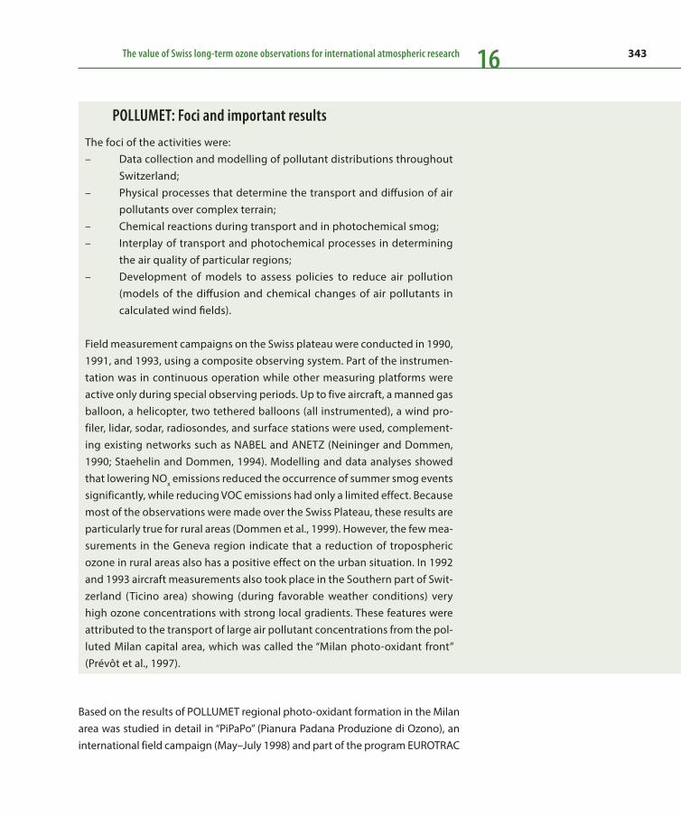
343The value of Swiss long-term ozone observations for international atmospheric research 16
Based on the results of POLLUMET regional photo-oxidant formation in the Milan area was studied in detail in “PiPaPo” (Pianura Padana Produzione di Ozono), an international field campaign (May–July 1998) and part of the program EUROTRAC
POLLUMET: Foci and important results
The foci of the activities were: – Data collection and modelling of pollutant distributions throughout
Switzerland; – Physical processes that determine the transport and diffusion of air
pollutants over complex terrain; – Chemical reactions during transport and in photochemical smog; – Interplay of transport and photochemical processes in determining
the air quality of particular regions; – Development of models to assess policies to reduce air pollution
(models of the diffusion and chemical changes of air pollutants in calculated wind fields).
Field measurement campaigns on the Swiss plateau were conducted in 1990, 1991, and 1993, using a composite observing system. Part of the instrumen-tation was in continuous operation while other measuring platforms were active only during special observing periods. Up to five aircraft, a manned gas balloon, a helicopter, two tethered balloons (all instrumented), a wind pro-filer, lidar, sodar, radiosondes, and surface stations were used, complement-ing existing networks such as NABEL and ANETZ (Neininger and Dommen, 1990; Staehelin and Dommen, 1994). Modelling and data analyses showed that lowering NOx emissions reduced the occurrence of summer smog events significantly, while reducing VOC emissions had only a limited effect. Because most of the observations were made over the Swiss Plateau, these results are particularly true for rural areas (Dommen et al., 1999). However, the few mea-surements in the Geneva region indicate that a reduction of tropospheric ozone in rural areas also has a positive effect on the urban situation. In 1992 and 1993 aircraft measurements also took place in the Southern part of Swit-zerland (Ticino area) showing (during favorable weather conditions) very high ozone concentrations with strong local gradients. These features were attributed to the transport of large air pollutant concentrations from the pol-luted Milan capital area, which was called the “Milan photo-oxidant front” (Prévôt et al., 1997).
344 From weather observations to atmospheric and climate sciences in Switzerland16
with strong Swiss contributions (Spirig et al., 2002). Results from these campaigns confirmed exceptionally large ozone concentrations (up to 200 ppb, see Thiel-mann et al., 2002) in the air loaded by (primary) air pollutants over Milan and transported from there towards the Swiss Alps. Detailed analyses showed that ozone production was VOC-limited within the Milan air pollution plume but NOx-limited outside of the plume.
16.7 Conclusions and Outlook
High-quality measurements of total ozone started in Switzerland in 1926. These observations provided and continue to provide the basis for pioneering research that contributes to the advancement of ozone science. The total ozone record from Arosa is the longest in the world. Similarly, the Umkehr observations from this site, which started in the 1950s (Zanis et al., 2006), also provide one of the very few records of ozone profiles available back to the pre-satellite era. Finally, also the Payerne ozonesonde time series provides one of the longest and most complete records in the world (Jeannet et al., 2007). Because of the high quality, homoge-neity, and representativeness of the measurements covering such a long period, they are suitable benchmark records for the study of the effect of anthropogenic emissions on the ozone layer. Through the successful implementation of the Mon-treal Protocol (1987) the ozone layer is predicted to recover in most parts of the atmosphere by about the middle of the 21st century, while the Antarctic ozone hole is predicted to close about a decade later (WMO/UNEP, 2014). However, in the second half of the 21st century changes in stratospheric circulation patterns result-ing from climate change are projected to dominate over anthropogenic changes of the ozone layer by ODSs because of the enhancement of the Brewer Dobson circulation (e. g., Butchart, 2014). The Brewer Dobson circulation transports ozone from the tropical source region to mid-latitudes, and therefore its acceleration is expected to lead to more stratospheric ozone in (Northern) mid-latitudes, the so-called “super-recovery” but simultaneously leading to an ozone deficit in the tropics (e. g., Shepherd, 2008). The Arosa total ozone series needs to be continued in order to document these effects, since it provides a world-class record of long-term stratospheric ozone variability during periods when ozone was still unaf-fected by ODSs, through periods when stratospheric ozone depletion reached its maximum, at present while the turnaround is still insignificant, in future as ozone makes a slow recovery, and finally to verify or falsify the “super-recovery” towards the end of this century.
345The value of Swiss long-term ozone observations for international atmospheric research 16
The surface ozone measurements from Arosa are also unique in terms of their rep-resentativeness, as they cover the 1950s, allowing the possibility of making con-crete statements about how much surface ozone increased in the decades follow-ing World War II and how ozone concentrations later responded to the air pollution legislation introduced in Switzerland and European countries in the late 1980s. The measurements have also proven very useful for the validation of state-of-the-art chemistry-climate models, which have been shown to strongly under-predict the surface ozone increases between World War II and the turn of the century (Parrish et al., 2014). These findings require further investigation. Since upper-tropospheric ozone is a strong greenhouse gas and chemistry-climate models have been used by the Intergovernmental Panel on Climate Change (IPCC) to make climate change projections for the next century, care is to be exercised to ensure the reliability and homogeneity of the Swiss ozone time series also in the future.
Acknowledgements
We thank Hans Richner and Markus Furger for suggestions to include POLLUMET and VOTALP in this article.
References
Appenzeller, C., A. K. Weiss, and J. Staehelin, 2000: North Atlantic Oscillation modulates total ozone winter trends. Geophys. Res. Lett., 27, 1131–1134.
Birrer, W., 1975: Homogenisierung und Diskussion der Totalo-zon-Messreihe von Arosa 1926–1971. LAPETH-11, Laboratorium für Atmosphärenphysik ETH Zürich, Schweiz.
Bojkov, R. D., 2010: The International Ozone Commission (IO3C), its history and activities related to atmospheric ozone. Academy of Athens, Research Centre for Atmospheric Physics and Climatol-ogy, Publication 18, Athens, May 2010 (https://ioc.atmos.illinois.edu/about/History%20of%20International%20Ozone%20Commission%203.pdf).
Brewer, A. W., 1949: Evidence for a world circulation provided by the measurements of helium and water vapour distribution in the stratosphere. Q. J. R. Meteorol. Soc., 75, 351–363.
Brönnimann, S., 2002: Ozon in der Atmosphäre. Paul Haupt, 184 pp.
Brönnimann, S., and G. P. Compo, 2012: Ozone highs and associ-ated flow features in the first half of the twentieth century in different data sets. Meteorol. Z., 21, 49–59.
Brönnimann, S., J. Luterbacher, C. Schmutz, H. Wanner, and J. Staehelin, 2000: Variability of total ozone at Arosa, Switzerland, since 1931 related to atmospheric circulation indices. Geophys. Res. Lett., 27, 2213–2216.
Brönnimann, S., B. Buchmann, and H. Wanner, 2002: Trends in near-surface ozone concentrations in Switzerland: the 1990s. Atmos. Environ., 36, 2841–2852.
Brönnimann, S., J. Luterbacher, J. Staehelin, and T. Svendby, 2004a: An extreme anomaly in stratospheric ozone over Europe in 1940–1942. Geophys. Res. Lett., 31, L08101, doi: 10.1029/ 2004GL019611.
Brönnimann, S., J. Luterbacher, J. Staehelin, T. M. Svendby, G. Hansen, and T. Svenoe, 2004b: Extreme climate of the global
346 From weather observations to atmospheric and climate sciences in Switzerland16
tropopsphere and stratosphere 1940–1942 related to El Nino. Nature, 431, 971–974.
Brönnimann, S., J. L. Annis, C. Vogler, and P. D. Jones, 2007: Reconstructing the Quasi-Biennial Oscillation back to the early 1900s. Geophys. Res. Lett., 34, L22805, doi: 10.1029/2007GL031354.
Butchart, N., 2014: The Brewer-Dobson circulation. Rev. Geo-phys., 52, 157–184, doi: 10.1002/2013RG000448.
Chameides, W. L., and J. C. Walker, 1973: a photochemical theory of tropospheric ozone. J. Geophys. Res., 81, 413–420.
Chameides, W. L., and J. C. Walker, 1976: A time dependent pho-tochemical model for ozone near the ground. J. Geophys. Res., 78, 8751–8760.
Chapman, S., 1930: A theory of upper atmospheric ozone. Mem. R. Meteorol. Soc., 3, 103–125, 1930.
Chatfield, R., and H. Harrison, 1976: Ozone in the remote tropo-sphere: mixing versus photochemistry. J. Geophys. Res., 81, 421–423.
Compo, G. P., and Coauthors, 2011: The Twentieth Century Reanalysis Project. Quart. J. Roy. Meteorol. Soc., 137, 1–28. doi: 10.1002/qj.776.
Cornu, A., 1879: Sur la limite ultraviolette du spectre solaire. Compt. Rendus Acad. Sci. Paris, 88, 1101.
Crutzen, P. J., 1970: The influence of nitrogen oxides in the atmo-spheric ozone content. Q. J. R. Meteorol. Soc., 96, 320–325.
Crutzen, P. J., 1973: A discussion of the chemistry of some minor constituents in the stratosphere and the troposphere. Pure appl. Geophys., 106–108, 1385–1399.
Crutzen, P. J., 1974: Photochemical reactions initiated by and influencing ozone in unpolluted tropospheric air. Tellus, 26, 47–57.
Cui, J., S. Pandey Deolal, M. Sprenger, S. Henne, J. Staehelin, M. Steinbacher, and P. Nedelec, 2011: free tropospheric ozone changes over Europe as observed at Jungfraujoch (1990–2008): an analysis based on backward trajectories. J. Geophys. Res., 116, D10304, doi: 10.1029/2010JD015154
Dee, D. P., and Coauthors, 2011: The ERA-Interim reanalysis: con-figuration and performance of the data assimilation system. Q. J. R. Meteorol. Soc., 137, 553–597.
Dlugokencky, E., J. Miller, and J. Staehelin, 2010: The Global Atmosphere Watch: a history of contributing to climate moni-toring. WMO Bulletin, 59, 35–39.
Dobson, G. M.B., 1930: Measurements of the amount of ozone in the Earth’s atmosphere and its relation to other geophysical condition – part IV. Proc. R. Soc., London, A129, 411–433.
Dobson, G. M.B., 1931: A photoelectric spectrometer for mea-suring the amount of atmospheric ozone. Proc. Phys. Soc., 43, 324–339.
Dobson, G. M.B., 1968: Forty years’ research on atmospheric ozone at Oxford: a history. Applied Optics, 7, 387–405.
Dobson, G. M.B., and D. N. Harrison, 1926: Measurements of the amount of ozone in the Earth’s atmosphere and its rela-tion to other geophysical condition. Proc. R. Soc., London, A110, 660–693.
Dobson, G. M.B., D. N. Harrison, and J. Lawrence, 1927: Measure-ments of the amount of ozone in the Earth’s atmosphere and its relation to other geophysical condition – part II. Proc. R. Soc., London, A114, 521–541.
Dommen, J., A. S.H. Prévôt, A. M. Hering, T. Staffelbach, G. L. Kok, and R. D. Schillawski, 1999: Photochemical production and aging of an urban air mass. J. Geophys. Res., 104, 5493–5506.
Dorno, C., 1917: Erfahrungen mit photoelektrischen Zellen. Phys. Z., 18, 381–388.
Dorno, C., 1927: Über Ozonmessungen auf spektroskopischem Wege. Meteorol. Z., 44, 385–390 (including Reply of Götz).
Dütsch, H. U., 1946: Photochemische Theorie des atmosphäri-schen Ozons unter Berücksichtigung von Nichtgleichgewichts-zuständen und Luftbewegungen. Inaugural Dissertation, Philo-sophische Fakultät II der Universität Zürich.
Dütsch, H. U., 1968: The photochemistry of stratospheric ozone. Quart. J. Roy. Meteorol. Soc., 94, 483–497.
Dütsch, H. U., 1969: Atmospheric ozone and ultraviolett radia-tion, climate of the free atmosphere. D. F. Rex, (Editor). Chap. 8.: World survey of climatology, 4, H. E. Landsberg (Editor-in-Chief ), Elsevier Publ. Company, Amsterdam-London-New York.
Dütsch, H. U., 1971: Photochemistry of atmospheric ozone. Adv. Geophys., 15, 219–321.

347The value of Swiss long-term ozone observations for international atmospheric research 16Dütsch, H. U., 1974: The ozone distribution in the atmosphere. Can. J. Chem., 52, 1491–1504, 1974.
Dütsch, H. U., 1978a: Vertical ozone distribution on a global scale. Pure Appl. Geophys., 16, 511–529.
Dütsch, H. U., 1978b: Ozonschicht und atmosphärisches Spu-rengassystem: Gefährdet der Mensch die Ozonschicht? Chimia, 32, 149–163.
Dütsch, H. U., 1979: The search for solar cycle-ozone relation-ships. J. Atmos. Terr. Phys., 41, 771–785, 1979.
Dütsch, H. U., 1981: Ozone research – past – present – future. Bull. Amer. Meteorol. Soc., 62, 213–217.
Dütsch, H. U., 1984: An update of the Arosa ozone series to the present using a statistical instrument calibration. Q. J. R. Meteo-rol. Soc., 110, 1079–1096.
Dütsch, H. U., 1986: Die Geschichte der atmosphärischen Ozon-forschung. ProMet., Heft 4, 3–6.
Dütsch, H. U., 1992a: F. W. Paul Götz: The man and his work. J. Atmos. Terr. Phys., 54, 485–496.
Dütsch, H. U., 1992b: Seventy years of ozone research. Current Science, 63, 701–711.
Dütsch, H. U., W. Braun, 1980: Daily ozone soundings during two winter months including a sudden stratospheric warming. Geophys. Res. Lett., 7, 785–788.
Dütsch, H. U., J. Bader, J. Staehelin, 1991: Separation of solar effects on ozone from anthropogenically produced trends. J. Geomagn. Geoelectr., 43, suppl.,657–665.
Fabian, P., 1974: Comments on ‘A photochemical theory of tro-pospheric ozone’ by Chameides W. and Walker J. C. J. Geophys Res. 79, 4124–4125.
Fabian, P., 1976: Tropospheric ozone: injection from the strato-sphere versus photochemistry. in Quadr. Ozone Symp. Dresden, Vol. III, 183–185.
Fabian, P., and P. G. Pruchniewiecz, 1977: Meridional distribution of ozone in the troposphere and its seasonal variation. J. Geo-phys. Res., 82, 2063–2073.
Fabry, C., and H. Buisson, 1921: Etude de l’extrémité ultra- violette du spectre solaire. J. Phys. Paris, Serie 6 (2), 197–226.
Farman, J. C., B. G. Gardiner, and J. D. Shanklin, 1985: Large losses of total ozone in Antarctic reveal seasonal ClOx/NOx interactios. Nature, 315, 207–210.
Furger, M., and Coauthors, 2000: The VOTALP Mesolcina Valley Campaign 1996 – Concept, background and some highlights. Atmos. Environ., 34, 1395–1412.
Götz, F. W.P., 1925: Das ultraviolette Ende des Spektrums von Sonne und Sternen. Sterne, 5, 189–195.
Götz, F. W.P, 1926a: Das Strahlungsklima von Arosa. Verlag von Justus Springer, Berlin
Götz, F. W.P, 1926b: Der Jahresgang des Ozongehaltes der hohen Atmosphäre. Beitr. Phys. fr. Atmosph., 13, 15–22.
Götz, F. W.P., 1954: Klima und Wetter in Arosa. Huber, Frauenfeld, 148 pp.
Götz, F. W.P., and R. Ladenburg, 1931: Ozongehalt der unteren Atmosphäreschichten. Naturwiss., 18, 373–374.
Götz, F. W.P., and H. Maier-Leibnitz, 1933: Zur Ultraviolettabsorp-tion bodennaher Luftschichten. Z. Geophys., 9, 253–260.
Götz, F. W.P., and R. Penndorf, 1941: Weitere Frühjahrsmessun-gen des bodennahen Ozons in Arosa. Meteorol. Z., 58, 409–415.
Götz, F. W.P., and F. Volz, 1951: Aroser Messungen des Ozon-gehaltes der unteren Troposphäre und sein Jahresgang. Z. Naturforsch, 6a, 634–639.
Götz, F. W.P., A. R. Meetham, and G. M.B. Dobson, 1934: The ver-tical distribution of ozone in the atmosphere. Proc. R. Soc., London, A145, 416–446.
Haagen-Smit, A. J., 1952: Chemistry and physiology of Los Angeles smog. Ind. Engng Chem., 44, 1342–1346.
Hartley, W. N., 1881a: On the absorption spectrum of ozone. J. Chem. Soc., 39, 57.
Hartley, W. N., 1881b: On the absorption of solar rays by atmo-spheric ozone. J. Chem. Soc., 39, 111.
Hoegger, B., G. Levrat, H. Schill, J. Staehelin, and P. Ribordy, 1992: Recent developments of the Light Climatic Observatory – Ozone measuring station of the Swiss Meteorological Institute (LKO) at Arosa. J. Atmos. Terr. Phys, 54, 497–505.
348 From weather observations to atmospheric and climate sciences in Switzerland16
Jeannet, P., R. Stübi, G. Levrat, P. Viatte, and J. Staehelin, 2007: Ozone balloon soundings at Payerne (Switzerland): Re-evalua-tion of the time series 1967–2002 and trend analysis. J. Geophys. Res., 112, D11302, doi: 10.1029/2005JDD006862.
Johnston, H., 1971: Reduction of stratospheric ozone by nitro-gen oxide catalysts from supersonic transport exhaust. Science, 173, 517–522.
Junge, C. E., 1962: Global ozone budget and exchange between stratosphere and troposphere. Tellus, 14, 364–377.
Kley, D., A. Volz, and F. Mülheims, 1988: Ozone measurements in historic perspective. Tropospheric Ozone, I. S.A. Isaksen, Ed., D. Reidel, Dodrecht, 63–73.
Koch, G., H. Wernli, C. Schwierz, J. Staehelin, and T. Peter, 2005: A composite study of ozone miniholes and minihighs over Central Europe and their formation mechanisms. Geophys. Res. Lett., 32, L12810, doi: 10.1029/2004GL022062.
Läuchli, A., 1928: Über die Absorption des ultravioletten Lichts in Ozon. Helv. Phys. Acta, 1, 208–236.
Levy, F., 1932: Erfahrungen mit der Eichung der Cadmiumzelle. Meteorol. Z., 49, 139–151.
Luftschadstoffe, Luftverschmutzung und Waldschäden in der Schweiz, 1991: Ergebnisse aus dem Nationalen Forschungspro-gramm 14. vdf, Verlag der Fachvereine Zürich.
Mateer, C. L., and H. U. Dütsch, 1964: Uniform evaluation of Umkehr observations from the World ozone network, Part I: pro-posed standard Umkehr evaluation technique. Report National Centre for Atmospheric Research (NCAR), Boulder, Colorado.
Meyer, E., 1903: Über die Absorption der ultravioletten Strah-lung in Ozon. Ann. d. Phys., 12, 849–859.
Meyer, E., 1925: Die Bedeutung des Ozongehaltes der Atmo-sphäre für die Sonnenstrahlung. Verhandlungen der klimatologi-schen Tagung in Davos 1925. 91–99.
Molina, M. J., and F. S. Rowland, 1974: Stratospheric sink for chlorofluoromethanes: chlorine atom catalyzed destruction of ozone. Nature, 249, 810–812.
Neininger, B., and J.Dommen, 1990: POLLUMET – Luftver-schmutzung und Meteorologie in der Schweiz. 23 p.
Parrish, D. D., and Coauthors, 2014: Long-term changes in lower tropospheric baseline ozone concentrations: Comparing
chemistry-climate models and observations at northern mid-latitudes. J. Geophys. Res., 119, 5719–5736, doi: 10.1002/ 2013JD021435.
Perl, G., 1961: Das bodennahe Ozon in Arosa, seine regelmässi-gen und unregelmässigen Schwankungen. Arch. Met. Geophys. Bioklimat., 14, 449.
Peter, T., 1997: Microphysics and heterogeneous chemistry of polar stratospheric clouds. Ann. Rev. Phys. Chem., 48, 785–822.
Prévôt, A. S.H., J. Staehelin, G. L. Kok, R. D. Schillawski, B. Neininger, T. Staffelbach, and A. Neftel, 1997: The Milan phoo-toxidant plume. J. Geophys. Res., 102, 23375–23388.
Regener, E. (1934): Erfahrungen und Ergebnisse mit Registrier-ballonen und Registrierapparten in der Stratosphäre. Beitr. Phys. fr. Atmosph., 22, 249–260.
Rieder, H. E., and Coauthors, 2010a: Extreme events in total ozone over Arosa – Part 1: Application of extreme value theory. Atmos. Chem. Phys., 10, 10021–10031.
Rieder, H. E., J. Staehelin, J. A. Maeder, T. Peter, M. Ribatet, A. C. Davison, R. Stübi, P. Weihs, and F. Holawe, 2010b: Extreme events in total ozone over Arosa – Part 2, 2010: Fingerprints of atmospheric dynamics and chemistry and effects on mean val-ues and long-term changes. Atmos. Chem. Phys., 10, 10033–10045.
Rubin, M. B., 2001: The history of ozone. The Schönbein period, 1839–1868. Bull. Hist. Chem., 26, 40–56.
Scarnato, B., J. Staehelin, R. Stübi, and H. Schill, 2010: Long term total ozone observations at Arosa (Switzerland) with Dobson and Brewer instruments (1988–2007). J. Geophys. Res., 115, D13306, doi: 10.1029/2009JD011908
Schüpbach, E., and H. Wanner, 1991 (Eds.): Luftverschmutzung und Lufthaushalt in der Schweiz, Luftschadstoffe, Luftverschmut-zung und Waldschäden in der Schweiz, Band 2, Ergebnisse aus dem Nationalen Forschungsprogramm 14. vdf, Verlag der Fach-vereine Zürich.
Shepherd, T. G., 2008: Dynamics, stratospheric ozone, and cli-mate change. Atmos. Ocean, 46, 117–138, doi: 10.3137/ao. 460106.
Solomon, S., 1999: Stratospheric ozone depletion: A review of concepts and history. Rev. Geophys., 37, 275–316.

349The value of Swiss long-term ozone observations for international atmospheric research 16Spirig, C., A. Neftel, L. A. Kleinamn, and J. Hjorth: NOx versus VOC limitation of O3 production in the Po valley, 2002: Local and inte-grated view based on observations. J. Geophys. Res., 107(D22), 8191, doi: 10.1029/2001JD00561.
Staehelin, J., and J. Dommen, 1994: Sommersmog aus der Sicht der Atmosphärenchemie. GAlA, 3(3), 157–169.
Staehelin, J., J. Thudium, and R. Bühler, A. Volz-Thomas, W. Gra-ber, 1994: Surface ozone trends at Arosa (Switzerland). Atmos. Environ., 28, 75–87.
Staehelin J., A. Renaud, J. Bader, R. McPeters, P. Viatte, B. Högger, V. Bugnion, M. Giroud, and H. Schill, 1998a: Total ozone series of Arosa (Switzerland). Homogenization and data comparison. J. Geophys. Res., 103, 5827–5841.
Staehelin, J., R. Kegel, and N. R.P. Harris, 1998b: Trend analysis of the homogenized total ozone series of Arosa (Switzerland), 1926–1996. J. Geophys. Res., 103, 8389–8399.
Staehelin, J., N. R.P. Harris, C. Appenzeller, and J. Eberhard, 2001: Ozone trends: A review. Rev. Geophys., 39, 231–290.
Stolarski, R. S., and R. J. Cicerone, 1974: Stratospheric chlorine: A possible sink for ozone. Can. J. Chem., 52, 1610–1615.
Thielmann, A., S. H. Prévôt, and J. Staehelin, 2002: Sensitivity of Ozone Production derived from field measurements in the Italian Po Basin. J. Geophys. Res., 107(D22), 8194, doi: 10.1029/ 2000JD00119.
Weiss, A. K., 2000: Anthropogenic and dynamic contributions to ozone trends of the Swiss total ozone, Umkehr and balloon sounding series. PhD thesis ETH 13635.
Weiss, A. K., J. Staehelin, C. Appenzeller, and N. R.P. Harris, 2001: Chemical and dynamical contributions to ozone profile trends of the Payerne (Switzerland) balloon soundings. J. Geophys. Res., 106, 22,685-22,694.
WMO/UNEP, 2014: Scientific Assessment of Ozone Depletion 2014. Global Ozone Research and Monitoring Project. Rep. No. 55, World Meteorological Organization, Geneva, Switzerland, 2014. Avail-able at https://www.wmo.int/pages/prog/arep/gaw/ozone_ 2014/ozone_asst_report.html.
Wolf, H. R., 1855: Über den Ozongehalt in der Luft und seinen Zusammenhang mit der Mortalität. Vorträge gehalten in der bernischen naturforschenden Gesellschaft, Bern, Verlag Huber und Co.
Wotawa, and G., H. Kromp-Kolb, 1999: The research project VOTALP – general objectives and main results. Atmos. Environ., 34, 1319–1322.
Wunderli, S., and R., Gehrig, R., 1991: Influence of temperature of formation and stability of surface PAN and ozone. A two-year field study in Switzerland. Atmos. Environ., 25, 1599–1608, doi: 10.1016/0960 1686(91)90018-3.
Zanis, P., P. S. Monks, E. Schüpbach, and S. A Penkett, 2000: The role of in situ photochemistry in the control during spring at the Jungfraujoch (3580 m asl) – comparison of model results with measurements. J. Atmos. Chem., 37, 1–27.
Zanis, P., E. Maillard, J. Staehelin, C. Zerefos, E. Kosmidis, K. Tour-pali, and I. Wohltmann, 2006: On the turnaround of strato-spheric ozone trends deduced from the re-evaluated Umkehr record of Arosa, Switzerland. J. Geophys. Res., 111, D22307, doi: 10.1029/2005JD006886.


351
17 The High Altitude Research Station Jungfraujoch – the early yearsHans Balsiger, Erwin Flückiger
Doing research in a high-Alpine environment has always been and will remain a challenging experience.
It took courage and a big portion of foresight in 1931 to establish a well-equipped research station at
3500 meters. The scientists then profited from the same daring spirit that enabled the construction of
the Jungfrau Railway. The collaboration and partnership between the railway and the scientists has
always been very close and to the mutual profit of both partners.
Continuous meteorological recordings at Jungfraujoch started in 1925, and to this very day it remains
the highest permanently manned weather station in Europe. But the early years included also
pioneering research in astronomy, physiology, cosmic radiation, glaciology as well as solar and
atmospheric chemistry and physics.
17.1 Overview
The High Altitude Research Station Jungfraujoch is the highest in Europe, and it is the highest research station in the world accessible year round by public transpor-tation. This fact enables the easy transportation of sophisticated equipment, which in turn allows very complex experiments to be performed. It also facilitates the exchange of hardware components or whole experimental set-ups. This has made Jungfraujoch a very dynamic place where scientific projects are free to oper-ate on short, medium and long timescales. Some monitoring programs depend on continuous measurements over many years, while other campaigns can achieve their goals within weeks or months.
The intention of the founders to provide scientists with an infrastructure that allows world-class research at a high-altitude, Alpine environment has been ful-filled. What kind of research is done is the decision of the scientists. Because of this “bottom-up” policy, the character of the scientific projects has changed appreciably over the years. The Research Station started out hosting mainly phys-iologists and astronomers, whereas today it has become one of Europe’s leading labs for environmental science, being situated above the pollution layer.
High Altitude Research Stations
Jungfraujoch and Gornergrat,
International Foundation, Bern

352 From weather observations to atmospheric and climate sciences in Switzerland17
Until the late 19th century, the world of high mountainous areas was considered unconquerable. Only a few bold and venturous souls dared to enter the inhospi-table and hostile areas of the Alps. Before the Meyer brothers made the first ascent to the summit of the Jungfrau on 3 August 1811, no one had envisioned that the Jungfrau area would become a centre of international tourism and scientific research. But only 30 years later scientists began working at Jungfraujoch. During every summer between 1838 and 1845, the famous Swiss natural scientist Louis Agassiz undertook expeditions to the Aletschgletscher and Jungfraujoch. In 1841 he even climbed the Jungfrau. The goal of these daring expeditions was to mea-sure the glacier and to study the migration and form of the ice. The observations Agassiz and his colleagues made were decisive in supporting the theory that the glaciers once covered large regions of the foothills of the Alps. Even today these observations serve as valuable information for the changes in the glaciers over the last 150 years.
Initially, the scientists found shelter only in ice caves. Later, on the middle moraine of the Unteraargletscher, they built a simple refuge out of stone, which served simultaneously as sleeping quarters, kitchen and laboratory, and which would become world famous as the “Hôtel des Neuchâtelois”. When the boulder that had served as the roof of the “Hôtel” burst, a more solid block house was finally built on the site. It was obvious to scientists at this early point in time that research in high mountainous areas needed secure and stable housing.
Toward the end of the 19th century, scientists began to focus increasingly on the problems involved in working at high altitudes. Research stations were opened in 1886 in Austria on Sonnblick (3105 m), in 1893 in France in the Vallot Alpine hut (4365 m), in 1901 in Italy in the Capanna Regina Margherita (4560 m) and in 1907 on Col d’Olen (2900 m). These research institutes were accessible only to scientists who were also alpinists, which is not often the case. The Swiss came to the game somewhat later – they gave their plans more time to mature, and in the end their projects were of a larger dimension. The idea of building a Swiss research station in the high mountainous area originated with the famous meteorologist Alfred de Quervain, who in 1912 was the leader of a Swiss expedition that traversed central Greenland and made a name for himself at home and abroad. Upon his return to Switzerland, de Quervain realized that there was a unique place for a high-altitude research station at Jungfraujoch, where accessibility by train and hotel accommo-dation had been available since 1912. He put all his efforts into convincing the scientific community and the general public of the need for a research station at Jungfraujoch. He succeeded in gaining the support of the Schweizerische Natur-

353The High Altitude Research Station Jungfraujoch – the early years 17
forschende Gesellschaft (now the Swiss Academy of Sciences), and in 1922, under his presidency, the Jungfraujoch Commission was established. This attracted sci-entists from Switzerland and abroad to the Jungfraujoch area. The Geneva astron-omer Emile Schär set up his telescope on the terrace of the hotel “Berghaus” and on the glacier firn, carrying out the first astronomical observations at Jungfraujoch between 1922 and 1927 (Figure 17.1). During the same years Daniel Chalonge, a French astronomer and astrophysicist, started a long-term relationship with Jung-fraujoch and later contributed significantly to the expansion of this unique obser-vational site.
In 1925 de Quervain himself set up a floating wood hut on the ice of the Jochfirn (Figure 17.2), where he installed various meteorological instruments that were thus well-protected from the rigours of the weather and tourists. Around the same time, in 1923 and 1925/26, Werner Kolhörster and Gubert von Salis carried out cosmic ray measurements between Eigergletscher and the summit of the Mönch. These measurements found worldwide acclaim. Hence, by the end of the 1920s scientific research at Jungfraujoch was established. The next step was to imple-ment de Quervain’s idea of a permanent station, i. e., to establish a building. It was quite helpful that, in the concession to Guyer-Zeller for building the railway, there was a clause that the railway company would have to support such an endeavour.
Figure 17.1: First astronomical observations from Jungfraujoch by the Geneva Observatory (Source: Jungfrau Railway/HFSJG).
Figure 17.2: First meteorological pavilion at the Jungfraujoch built in 1925 (Source: Jungfrau Railway/HFSJG).
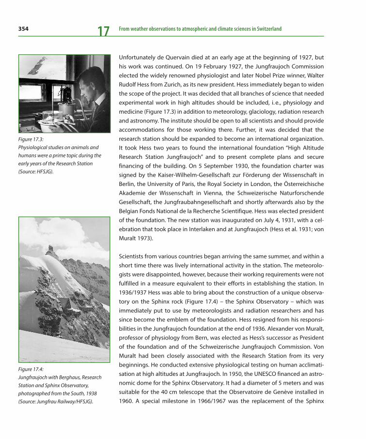
354 From weather observations to atmospheric and climate sciences in Switzerland17
Unfortunately de Quervain died at an early age at the beginning of 1927, but his work was continued. On 19 February 1927, the Jungfraujoch Commission elected the widely renowned physiologist and later Nobel Prize winner, Walter Rudolf Hess from Zurich, as its new president. Hess immediately began to widen the scope of the project. It was decided that all branches of science that needed experimental work in high altitudes should be included, i. e., physiology and medicine (Figure 17.3) in addition to meteorology, glaciology, radiation research and astronomy. The institute should be open to all scientists and should provide accommodations for those working there. Further, it was decided that the research station should be expanded to become an international organization. It took Hess two years to found the international foundation “High Altitude Research Station Jungfraujoch” and to present complete plans and secure financing of the building. On 5 September 1930, the foundation charter was signed by the Kaiser-Wilhelm-Gesellschaft zur Förderung der Wissenschaft in Berlin, the University of Paris, the Royal Society in London, the Österreichische Akademie der Wissenschaft in Vienna, the Schweizerische Naturforschende Gesellschaft, the Jungfraubahngesellschaft and shortly afterwards also by the Belgian Fonds National de la Recherche Scientifique. Hess was elected president of the foundation. The new station was inaugurated on July 4, 1931, with a cel-ebration that took place in Interlaken and at Jungfraujoch (Hess et al. 1931; von Muralt 1973).
Scientists from various countries began arriving the same summer, and within a short time there was lively international activity in the station. The meteorolo-gists were disappointed, however, because their working requirements were not fulfilled in a measure equivalent to their efforts in establishing the station. In 1936/1937 Hess was able to bring about the construction of a unique observa-tory on the Sphinx rock (Figure 17.4) – the Sphinx Observatory – which was immediately put to use by meteorologists and radiation researchers and has since become the emblem of the foundation. Hess resigned from his responsi-bilities in the Jungfraujoch foundation at the end of 1936. Alexander von Muralt, professor of physiology from Bern, was elected as Hess’s successor as President of the foundation and of the Schweizerische Jungfraujoch Commission. Von Muralt had been closely associated with the Research Station from its very beginnings. He conducted extensive physiological testing on human acclimati-sation at high altitudes at Jungfraujoch. In 1950, the UNESCO financed an astro-nomic dome for the Sphinx Observatory. It had a diameter of 5 meters and was suitable for the 40 cm telescope that the Observatoire de Genève installed in 1960. A special milestone in 1966/1967 was the replacement of the Sphinx
Figure 17.3: Physiological studies on animals and humans were a prime topic during the early years of the Research Station (Source: HFSJG).
Figure 17.4: Jungfraujoch with Berghaus, Research Station and Sphinx Observatory, photographed from the South, 1938 (Source: Jungfrau Railway/HFSJG).
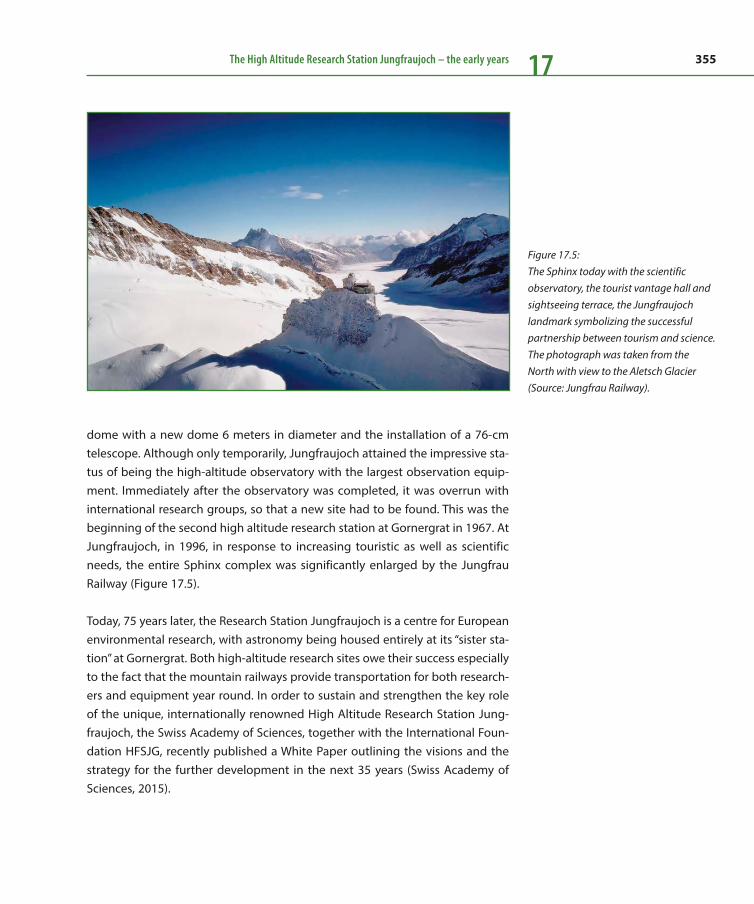
355The High Altitude Research Station Jungfraujoch – the early years 17
dome with a new dome 6 meters in diameter and the installation of a 76-cm telescope. Although only temporarily, Jungfraujoch attained the impressive sta-tus of being the high-altitude observatory with the largest observation equip-ment. Immediately after the observatory was completed, it was overrun with international research groups, so that a new site had to be found. This was the beginning of the second high altitude research station at Gornergrat in 1967. At Jungfraujoch, in 1996, in response to increasing touristic as well as scientific needs, the entire Sphinx complex was significantly enlarged by the Jungfrau Railway (Figure 17.5).
Today, 75 years later, the Research Station Jungfraujoch is a centre for European environmental research, with astronomy being housed entirely at its “sister sta-tion” at Gornergrat. Both high-altitude research sites owe their success especially to the fact that the mountain railways provide transportation for both research-ers and equipment year round. In order to sustain and strengthen the key role of the unique, internationally renowned High Altitude Research Station Jung-fraujoch, the Swiss Academy of Sciences, together with the International Foun-dation HFSJG, recently published a White Paper outlining the visions and the strategy for the further development in the next 35 years (Swiss Academy of Sciences, 2015).
Figure 17.5: The Sphinx today with the scientific observatory, the tourist vantage hall and sightseeing terrace, the Jungfraujoch landmark symbolizing the successful partnership between tourism and science. The photograph was taken from the North with view to the Aletsch Glacier (Source: Jungfrau Railway).

356 From weather observations to atmospheric and climate sciences in Switzerland17
The International Foundation High Altitude Research Stations Jungfraujoch and Gornergrat HFSJG
The International Foundation High Altitude Research Stations Jungfraujoch and Gornergrat (HFSJG, as per the German abbreviation of the name) is a foundation according to articles 80 ff. of the Swiss Code of Civil Law; it is under the auspices of the Swiss Federal Government. It is dedicated to pro-viding the infrastructure and support for scientific research of international significance which must be carried out at an altitude of 3000–3500 meters above sea level and/or for which a high-Alpine climate and environment are necessary. The Foundation presently has nine members, four of them from abroad (Fonds National de la Recherche Scientifique, Belgium; Max-Planck Gesellschaft, Germany; Österreichische Akademie der Wissenschaf-ten, Austria; Royal Society, United Kingdom) and five from Switzerland it -self (Swiss Academy of Sciences SCNAT; Jungfraubahn; Gornergrat Bahn; Burgergemeinde Zermatt; University of Bern). The Swiss Academy of Sci-ences is charged with looking after the interests of the Swiss research com-munity within the Foundation and has delegated this task to its Commission for the High Altitude Research Station Jungfraujoch.
The Foundation is funded by annual fees and contributions in kind from member countries and institutions, income from researchers and voluntary contributions. The Swiss National Science Foundation (SNF) has financed the substantial Swiss contribution for the operation and maintenance of the Research Stations since 1965.
The Foundation’s offices and its administration are at the University of Bern.
Contact:High Altitude Research Stations Jungfraujoch and GornergratInternational FoundationSidlerstrasse 5CH-3012 BernSwitzerlandwww.hfsjg.ch
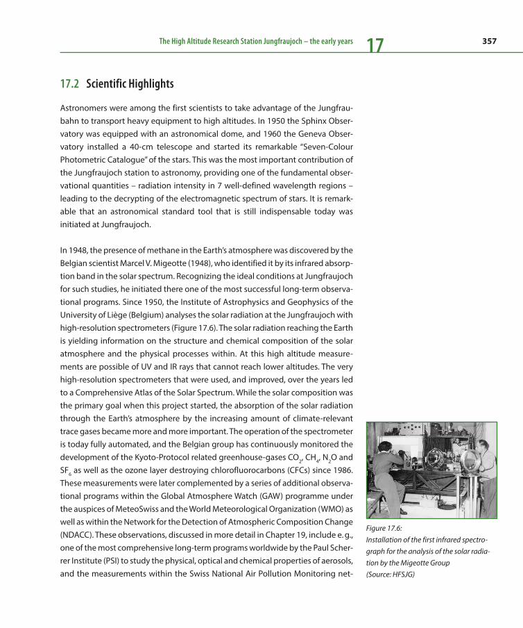
357The High Altitude Research Station Jungfraujoch – the early years 17
17.2 Scientific Highlights
Astronomers were among the first scientists to take advantage of the Jungfrau-bahn to transport heavy equipment to high altitudes. In 1950 the Sphinx Obser-vatory was equipped with an astronomical dome, and 1960 the Geneva Obser-vatory installed a 40-cm telescope and started its remarkable “Seven-Colour Photometric Catalogue” of the stars. This was the most important contribution of the Jungfraujoch station to astronomy, providing one of the fundamental obser-vational quantities – radiation intensity in 7 well-defined wavelength regions – leading to the decrypting of the electromagnetic spectrum of stars. It is remark-able that an astronomical standard tool that is still indispensable today was initiated at Jungfraujoch.
In 1948, the presence of methane in the Earth’s atmosphere was discovered by the Belgian scientist Marcel V. Migeotte (1948), who identified it by its infrared absorp-tion band in the solar spectrum. Recognizing the ideal conditions at Jungfraujoch for such studies, he initiated there one of the most successful long-term observa-tional programs. Since 1950, the Institute of Astrophysics and Geophysics of the University of Liège (Belgium) analyses the solar radiation at the Jungfraujoch with high-resolution spectrometers (Figure 17.6). The solar radiation reaching the Earth is yielding information on the structure and chemical composition of the solar atmosphere and the physical processes within. At this high altitude measure-ments are possible of UV and IR rays that cannot reach lower altitudes. The very high-resolution spectrometers that were used, and improved, over the years led to a Comprehensive Atlas of the Solar Spectrum. While the solar composition was the primary goal when this project started, the absorption of the solar radiation through the Earth’s atmosphere by the increasing amount of climate-relevant trace gases became more and more important. The operation of the spectrometer is today fully automated, and the Belgian group has continuously monitored the development of the Kyoto-Protocol related greenhouse-gases CO2, CH4, N2O and SF6 as well as the ozone layer destroying chlorofluorocarbons (CFCs) since 1986. These measurements were later complemented by a series of additional observa-tional programs within the Global Atmosphere Watch (GAW) programme under the auspices of MeteoSwiss and the World Meteorological Organization (WMO) as well as within the Network for the Detection of Atmospheric Composition Change (NDACC). These observations, discussed in more detail in Chapter 19, include e. g., one of the most comprehensive long-term programs worldwide by the Paul Scher-rer Institute (PSI) to study the physical, optical and chemical properties of aerosols, and the measurements within the Swiss National Air Pollution Monitoring net-
Figure 17.6: Installation of the first infrared spectro-graph for the analysis of the solar radia-tion by the Migeotte Group (Source: HFSJG)

358 From weather observations to atmospheric and climate sciences in Switzerland17
work of the Swiss Federal Office for the Environment (FOEN) and the Laboratory for Air Pollution and Environmental Technology of the Swiss Federal Laboratories for Materials Science and Technology (Empa), discussed in Chapter 18.
The evolution of snow and ice covers are natural indicators of the ongoing cli-mate change. Monitoring of long-term glacier variations of the Grosser Aletsch-gletscher was initiated at Jungfraujoch as early as 1918, and systematic glaciolog-ical research by the ETHZ began in 1940. Important observations included length changes at the glacier tongue, firn accumulation and mass balance on Jungfrau-firn (since 1918) and the hydrological water balance of the whole catchment based on runoff measurements (since 1922). More short-term phenomena at the Mönch’s hanging glacier were aimed at predicting life-threatening ice avalanches.
Because the intensity of the cosmic radiation increases with altitude, the Jungfrau-joch with its easy access became a coveted location for its investigation. After the pioneering experimental work by Werner Kolhörster and Gubert von Salis, and shortly after the opening of the scientific station, physicists from various countries began to investigate the interaction between cosmic ray particles and atomic nuclei in the atmosphere. These investigations are known today in connection with the most famous names in research history, e. g., Arthur H. Compton, Pierre Auger and Cecil F. Powell (Figure 17.7). The exposure of photographic emulsions to cosmic radiation at Jungfraujoch by the University of Bristol group played a key role in the discovery of the pion in 1947. From 1950 to 1957 the University of Manchester, under the supervision of Patrick M. S. Blackett, operated a huge cloud chamber with a 14-ton electromagnet (Figure 17.8). The results obtained led to the discovery of the V-particles (Figure 17.9) and contributed significantly to a better knowledge of new elementary particles. The pioneering work of the two British groups at European high-Alpine research sites became the major basis for two Nobel Prizes (Blackett in 1948, Powell in 1950). The large Wilson chamber was later transferred to the European Organization for Nuclear Research (CERN) in Geneva, where it ushered in the era of modern high-energy particle experiments. During the International Geophysical Year 1957/1958 the University of Bern installed a neutron monitor for the continuous measurement of cosmic ray inten-sity. This apparatus is still in operation today, together with a second instrument installed in 1986. The long-term cosmic ray measurements at Jungfraujoch cover more than five solar sunspot cycles. They reflect the intensity of galactic and solar protons with energies above 3.5 GeV and solar neutrons with energies as low as 250 MeV. Hence, they play a significant role in the analysis of sporadic solar parti-cle events. The most famous result was the first identification of solar neutrons by
Figure 17.7: Note by cosmic ray physicist Pierre Auger in the guestbook of the Research Station (Source: HFSJG).
Figure 17.8: Scientist operating the huge cloud chamber of the University of Manchester (1951). (Source: Ciné Journal Suisse/HFSJG)

359The High Altitude Research Station Jungfraujoch – the early years 17
ground-based detectors on June 3, 1982. From the analysis of the worldwide neu-tron monitor data and of further measurements from space, scientists can learn more about the physics in high-energy processes at the sun and about the trans-port of cosmic rays in the interplanetary and near-Earth space. More recent work based on near-real time data addresses technological and radiation environment aspects, as well as the investigation of established and postulated effects in atmo-spheric chemistry and physics, meteorology and climate (“space weather”).
A review of other major achievements in the past and details of more recent research can be found, among others, in von Muralt (1937, 1942, 1946, 1951, 1957 and 1973), Debrunner (1981), Balsiger and Flückiger (2006), Flückiger and Bütikofer (2008), in the HFSJG White Paper (Swiss Academy of Sciences, 2015) as well as in the HFSJG Annual Reports (www.hfsjg.ch).
Acknowledgements
The authors gratefully acknowledge the outstanding scientific work conducted over the years by the many national and international research teams, and the long-standing support of the Foundation’s member institutions and of the Swiss National Science Foundation.
Figure 17.9: The first cloud chamber photograph of a neutral V-particle (Rochester and Butler, 1953).
References
Balsiger, H., and E. Flückiger, 2006: Top Science at the Top of Europe, published at the occasion of the 75th anniversary of the High Altitude Research Station Jungfraujoch. International Foundation High Altitude Research Stations Jungfraujoch and Gornergrat, CH-3012 Bern, Switzerland, 50 pp.
Debrunner, H., 1981: 50 Jahre Forschungsstation Jungfraujoch. Kantonalbank von Bern, Bulletin Nr. 23, 100pp.
Flückiger, E. O., and R. Bütikofer, 2008: Untersuchungen der kos-mischen Strahlung auf Jungfraujoch – 50 Jahre Neutronen-monitore. Mitteilungen der Naturforschenden Gesellschaft in Bern, 65, 123–141. [Available online at http://www.ngbe.ch/wordpress/wp-content/uploads/2014/08/123-141_Flueckiger.pdf.]
Hess, W. R., and Coauthors, 1931: Hochalpine Forschungsstation Jungfraujoch. Art. Institut Orell Füssli, Zürich; International
Foundation High Altitude Research Stations Jungfraujoch and Gornergrat HFSJG, 100 pp.
Migeotte, M. V., 1948: Methane in earth’s atmosphere. Journal of Astrophysics, 107, 400–403.
Rochester, G. D., and C. C. Butler, 1953: The new unstable cosmic ray particles. Physical Society Progress Reports, 16, 364–407.
Swiss Academy of Sciences, 2015: White Paper Research at Jungfraujoch – Vision and Mission Statement 2015–2050, 43 pp. [ Available online at http://www.sciencesnaturelles.ch/service/publications/43929-research-at-jungfraujoch-vision-and- mission-statement-2015-2050.]
von Muralt, A., and Coauthors, 1937: Fünf Jahre Hochalpine Forschungsstation Jungfraujoch. International Foundation High Altitude Research Stations Jungfraujoch and Gornergrat HFSJG, 72 pp.

360 From weather observations to atmospheric and climate sciences in Switzerland17
von Muralt, A., 1942: Zehn Jahre Hochalpine Forschungsstation Jungfraujoch. International Foundation High Altitude Research Stations Jungfraujoch and Gornergrat HFSJG, 45 pp.
von Muralt, A., 1946: Fünfzehn Jahre Hochalpine Forschungs-station Jungfraujoch. International Foundation High Altitude Research Stations Jungfraujoch and Gornergrat HFSJG, 45 pp.
von Muralt, A., and Coauthors, 1951: Zwanzig Jahre Hochalpine Forschungsstation Jungfraujoch. International Foundation High Altitude Research Stations Jungfraujoch and Gornergrat HFSJG, 106 pp.
von Muralt, A., and Coauthors, 1957: 25 Jahre Hochalpine Forschungsstation Jungfraujoch. Experientia Supplementum VI, Birkhäuser Verlag, Basel; International Foundation High Altitude Research Stations Jungfraujoch and Gornergrat HFSJG, 86 pp.
von Muralt, A., 1973: 42 Years of Jungfraujoch. International Foundation High Altitude Research Stations Jungfraujoch and Gornergrat HFSJG, 23 pp.
361
18 Reactive gases, ozone depleting substances and greenhouse gasesLong-term time series supporting international treatiesTrend analysis & early warning
Brigitte Buchmann, Christoph Hueglin, Stefan Reimann, Martin K. Vollmer, Martin Steinbacher, Lukas Emmenegger
The Swiss contribution to international atmospheric measurement programmes has a long tradition.
Continuous measurements of air pollutants supporting the “OECD Cooperative Technical Programme to
measure the long-range transport of air pollutants” started in 1972. Thereafter, these activities
continued in the frame of the Ottar Programme, which was one of the first devoted to the acid rain issue.
Today, long-term time series of more than 70 gaseous atmospheric compounds are measured at the
high-Alpine site Jungfraujoch, contributing to the European Monitoring and Evaluation Programme
(EMEP) of the United Nations Economic Commission for Europe (UNECE) and the Global Atmosphere
Watch (GAW) programme of the World Meteorological Organization (WMO). Long-term time series
provide the basic information for estimating trends and emissions in support of international treaties,
such as the Kyoto and the Montreal Protocols as well as for the EMEP. The latter is a scientifically based
and policy-driven programme under the Convention on Long-range Transboundary Air Pollution
(CLRTAP) for international cooperation.
The following provides examples of analyses of long-term measurements for trend and emission
estimates and illustrates their benefit and impact for international protocols and treaties.
18.1 Historical Background
In the 1950s, attention of governments from all over Europe turned to the traces of harmful substances present in the Earth’s atmosphere. The first measurements were started mainly targeting local sources and industrial emissions. For the pur-pose of investigating the long-range transport of pollutants, Switzerland installed the first two continuous measurement sites at Payerne and Jungfraujoch in 1968. Sulfur dioxide (Figure 18.1), particulate sulfate and total suspended particulates (TSP) were the first three parameters to be scrutinized for air pollution and to support international treaties (Filliger et al. 1994).
In addition, triggered by scientific interests such as the investigation of the radia-tion budgets and ozone depletion, regular measurements started in Arosa 1926
Empa, Swiss Federal Laboratories
for Materials Science and Technology,
Dübendorf

362 From weather observations to atmospheric and climate sciences in Switzerland18
for in-situ ozone and in 1956 for total column ozone (Staehelin et al. 2009), in Pay-erne 1968 for ozone profiles (Chapter 16), and at Jungfraujoch in the 1970s for total vertical column abundances of chlorofluorocarbons (Zander et al. 2008).
It rapidly became clear that continuous time-series are essential for providing answers to the emerging air pollution issues. Therefore, in 1978, the National Air Pollution Monitoring Network (NABEL) was initiated as a joint activity of Empa and the Swiss Federal Office for the Environment (FOEN). The NABEL network was ini-tially established with eight sites emerging from activities that had started already in 1968 as the above contributions to international observation networks (WMO and OECD). In 1990/1991, the NABEL network was extended to 16 monitoring stations that are distributed throughout Switzerland. The locations of these mon-
NABEL
The National Air Pollution Monitoring Network (NABEL) measures air pollut-ants at 16 locations in Switzerland. The stations are distributed throughout the country and monitor pollution at typical locations (e. g., urban traffic locations, residential areas, rural locations).
The monitoring network commenced operations in stages since 1979 and is jointly operated by the Federal Office for the Environment (FOEN) and Empa. Article 39 of the Ordinance on Air Pollution Control (OAPC) requires FOEN to collect data on air pollution throughout Switzerland. The fulfilment of this legal mandate is among the principal purposes of the NABEL network. NABEL measures indicator pollutants of national significance (e. g., nitrogen dioxide, ozone, particulate matter). It is an important instrument for enforc-
Figure 18.1: Time series of long-term sulfur dioxide (SO2) measurements at the high-Alpine site Jungfraujoch. Data are aggregated to monthly averages.
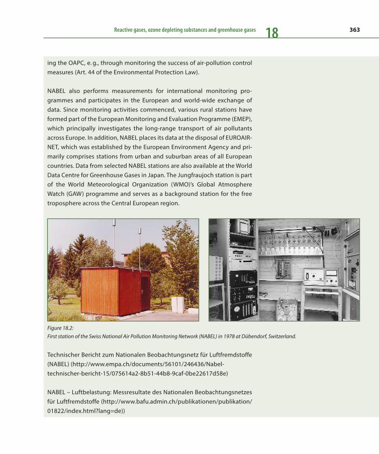
363Reactive gases, ozone depleting substances and greenhouse gases 18
ing the OAPC, e. g., through monitoring the success of air-pollution control measures (Art. 44 of the Environmental Protection Law).
NABEL also performs measurements for international monitoring pro-grammes and participates in the European and world-wide exchange of data. Since monitoring activities commenced, various rural stations have formed part of the European Monitoring and Evaluation Programme (EMEP), which principally investigates the long-range transport of air pollutants across Europe. In addition, NABEL places its data at the disposal of EUROAIR-NET, which was established by the European Environment Agency and pri-marily comprises stations from urban and suburban areas of all European countries. Data from selected NABEL stations are also available at the World Data Centre for Greenhouse Gases in Japan. The Jungfraujoch station is part of the World Meteorological Organization (WMO)’s Global Atmosphere Watch (GAW) programme and serves as a background station for the free troposphere across the Central European region.
Technischer Bericht zum Nationalen Beobachtungsnetz für Luftfremdstoffe (NABEL) (http://www.empa.ch/documents/56101/246436/Nabel- technischer-bericht-15/075614a2-8b51-44b8-9caf-0be22617d58e)
NABEL – Luftbelastung: Messresultate des Nationalen Beobachtungsnetzes für Luftfremdstoffe (http://www.bafu.admin.ch/publikationen/publikation/ 01822/index.html?lang=de))
Figure 18.2: First station of the Swiss National Air Pollution Monitoring Network (NABEL) in 1978 at Dübendorf, Switzerland.

364 From weather observations to atmospheric and climate sciences in Switzerland18
itoring stations are representative for the most significant air pollution levels in Switzerland, ranging from urban kerbside in city centres to the relatively unpol-luted tropospheric background station Jungfraujoch. Parallel to these long-term continuous measurements, several research programmes were initiated in Swit-zerland as well as in Europe. In Switzerland, one of the most comprehensive pro-grammes was POLLUMET, with several field campaigns between 1990 and 1993 (Chapter 16).
18.2 Measurements at Jungfraujoch
In 1973, Empa started continuous measurements of reactive gases as part of an early engagement of Switzerland in a programme organised by the Organisation for Economic Co-operation and Development (OECD). This programme, designed to investigate changes in the atmospheric composition, aimed at the collection of data needed to ensure a sustainable development in the member states – and consequently in the entire world. Today, more than 70 gaseous species including reactive gases, greenhouse gases and some of their isotopes (e. g., 12CO2 and 13CO2), are currently being measured at Jungfraujoch, 3580 m above sea level.
Measurements at this unique site in the heart of the Swiss Alps are representative for clean tropospheric air masses and hence are well suited for the analysis of long-
Figure 18.3: High-Alpine ambient air measurement site at the Sphinx – Observatory at Jungfraujoch (left), air inlet system under harsh conditions in winter time (right).
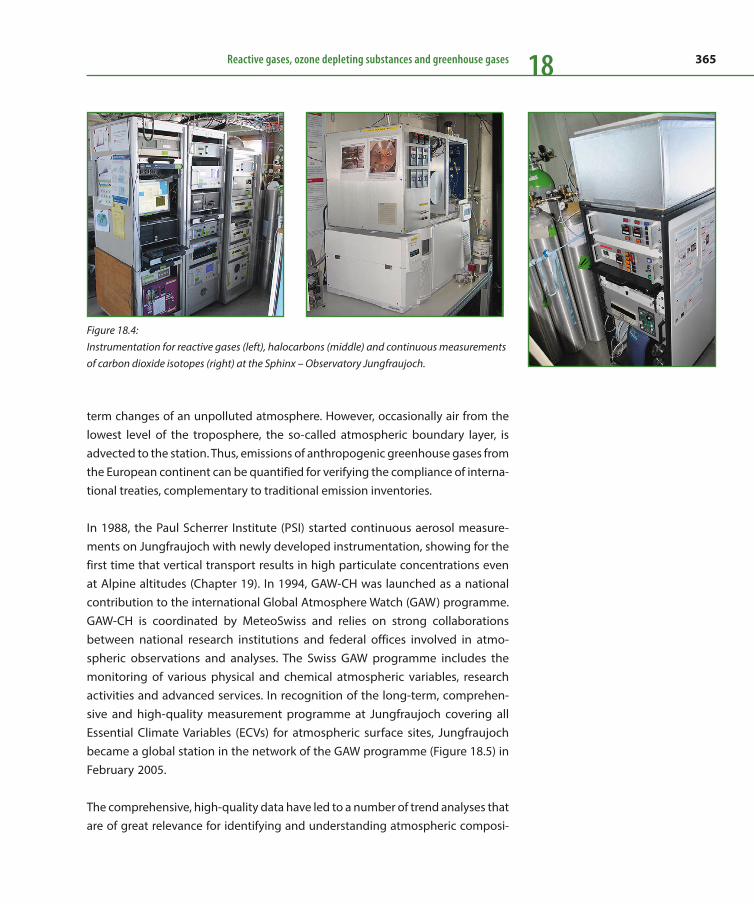
365Reactive gases, ozone depleting substances and greenhouse gases 18
term changes of an unpolluted atmosphere. However, occasionally air from the lowest level of the troposphere, the so-called atmospheric boundary layer, is advected to the station. Thus, emissions of anthropogenic greenhouse gases from the European continent can be quantified for verifying the compliance of interna-tional treaties, complementary to traditional emission inventories.
In 1988, the Paul Scherrer Institute (PSI) started continuous aerosol measure-ments on Jungfraujoch with newly developed instrumentation, showing for the first time that vertical transport results in high particulate concentrations even at Alpine altitudes (Chapter 19). In 1994, GAW-CH was launched as a national contribution to the international Global Atmosphere Watch (GAW) programme. GAW-CH is coordinated by MeteoSwiss and relies on strong collaborations between national research institutions and federal offices involved in atmo-spheric observations and analyses. The Swiss GAW programme includes the monitoring of various physical and chemical atmospheric variables, research activities and advanced services. In recognition of the long-term, comprehen-sive and high-quality measurement programme at Jungfraujoch covering all Essential Climate Variables (ECVs) for atmospheric surface sites, Jungfraujoch became a global station in the network of the GAW programme (Figure 18.5) in February 2005.
The comprehensive, high-quality data have led to a number of trend analyses that are of great relevance for identifying and understanding atmospheric composi-
Figure 18.4: Instrumentation for reactive gases (left), halocarbons (middle) and continuous measurements of carbon dioxide isotopes (right) at the Sphinx – Observatory Jungfraujoch.

366 From weather observations to atmospheric and climate sciences in Switzerland18
tion change (Zellweger et al. 2009; Gilge et al. 2010; Cui et al. 2011; Logan et al. 2012; Pandey Deloal et al. 2012; Parrish et al. 2012, 2014).
From 2000 onwards, Empa successfully used long-term datasets to quantify and localize European emissions of halogenated ozone-depleting substances and greenhouse gases for the verification of the Montreal and Kyoto Protocols (Zander et al. 2008; Reimann et al. 2004, 2005, 2008; Stemmler et al. 2007; Vollmer et al. 2011, 2015; Keller et al. 2011; Brunner et al. 2012).
The current measurement programme of reactive and greenhouse gases at Jung-fraujoch includes continuous in-situ analyses of ozone (O3), carbon monoxide (CO), nitrogen monoxide (NO), nitrogen dioxide (NO2), the sum of nitrogen oxides (NOy), sulfur dioxide (SO2), methane (CH4), carbon dioxide (CO2) and nitrous oxide (N2O). These data are stored as 10-min averages. Furthermore, the concentrations of CH4, N2O and H2 are monitored at half-hourly intervals. An extended set of halo-carbons, sulfur hexafluoride (SF6) and a selection of volatile organic compounds (VOCs) are measured with a time resolution of two hours. The concentration of
Figure 18.5: The global measurement sites of the GAW Programme.
367Reactive gases, ozone depleting substances and greenhouse gases 18
particulate matter < 10 µm (PM10) is determined both continuously and in 24-hour integrated samples. Daily samples are taken to quantify particulate sulfur. More recently, continuous measurements of the stable CO2 isotopes were started, con-tributing to its source attribution.
With this comprehensive suite of measurements, Empa’s activities at Jungfrau-joch go beyond the operational setup at other NABEL stations. On the one hand, this is driven by the wide range of scientific aims at such a remote site. On the other hand, it is also a response to the various international projects and programmes (EMEP, GAW, CLRTAP, UNECE) in which the observations at Jungfraujoch are embedded. The observations of the halogenated greenhouse gases are furthermore part of the Advanced Global Atmospheric Gases Experi-ment (AGAGE) with nine stations worldwide striving for a comprehensive pic-ture of the composition of ozone-depleting substances and their replacement products. On the European scale, Jungfraujoch is one of the monitoring sta-tions of the atmospheric network of the Integrated Carbon Observation System (ICOS) research infrastructure. ICOS aims at establishing harmonized high- precision greenhouse gas observations across Europe in order to understand the greenhouse gas budgets and perturbations. With an envisaged time frame of 20 years, ICOS provides the long-term observations necessary to under-stand the present state and to predicting future behaviour of the global carbon cycle and greenhouse gas emissions. Figure 18.6 shows 5-year time series of CO2, CH4, and CO, which are integral parts of the ICOS research infrastructure programme.
On shorter time scales, Jungfraujoch is also a prime-site in the European Com-mission’s Seventh Framework Programmes InGOS (Integrated non-CO2 Green-house gas Observing System) and ACTRIS (Aerosol, Clouds, and Trace Gases Research Infrastructure Network), both of which run for 4 years. A close liaison with many programmes is beneficial on various aspects: Round-robin compari-sons as part of the GAW programme and the InGOS project (both for greenhouse gases) and the ACTRIS project (for nitrogen oxides and VOCs) allow additional quality control activities, which are crucial for time series that support interna-tional treaties and protocols.
Human-induced changes of the atmosphere’s composition and its feedback on the global climate system are major challenges in the future. In order to face them, modern research increasingly relies on three pillars: targeted laboratory and field experiments to assess processes, long-term research monitoring from
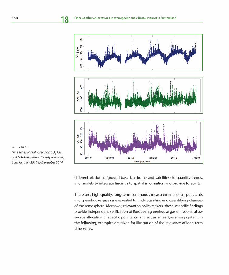
368 From weather observations to atmospheric and climate sciences in Switzerland18
different platforms (ground based, airborne and satellites) to quantify trends, and models to integrate findings to spatial information and provide forecasts.
Therefore, high-quality, long-term continuous measurements of air pollutants and greenhouse gases are essential to understanding and quantifying changes of the atmosphere. Moreover, relevant to policymakers, these scientific findings provide independent verification of European greenhouse gas emissions, allow source allocation of specific pollutants, and act as an early-warning system. In the following, examples are given for illustration of the relevance of long-term time series.
Figure 18.6: Time series of high-precision CO2, CH4 and CO observations (hourly averages) from January 2010 to December 2014.

369Reactive gases, ozone depleting substances and greenhouse gases 18
18.3 Atmospheric composition change
Chlorofluorocarbons (CFCs), halons and long-lived chlorinated solvents (e. g., 1,1,1,-trichloroethane), which are globally banned from usage by the Montreal Protocol, have shown a steady decline of the background concentrations and pollution events (Figure 18.7). Mixing ratios of their first-generation substitutes, the hydrochlorofluorocarbons (HCFCs), are still slowly increasing because of ongoing emissions in developing countries. However, second-generation substi-tutes, i. e., hydrofluorocarbons (HFCs, e. g., such as HFC-134a, a cooling agent in mobile air conditioners), regulated only in the Kyoto Protocol, still show large increases (Figure 18.7).
18.4 Identification of European sources of greenhouse gases
European emissions of halogenated greenhouse gases can be derived from con-tinuous atmospheric trace gas measurements combined with sophisticated meteorological models (Reimann et al. 2004, 2005; Keller et al. 2011; Brunner et al. 2012). Our approach has revealed large emissions from Italy of a fluorinated greenhouse gas (HFC-152a: 1,1-difluoroethane), used in insulation foams (Figure 18.7). Surprisingly, the official Italian emission inventory performed under the Kyoto Protocol does not declare these emissions. Thus, our findings pro-vide independent support for the evaluation of the compliance to interna-tional treaties.
Figure 18.7: Time series (2000–2015) of the cooling agent HFC-134a and 1,1,1-trichloroethane at Jungfraujoch (2-hourly averages) and their modelled European emission regions of HFC-152a (2011–2015)

370 From weather observations to atmospheric and climate sciences in Switzerland18
18.5 Independent emission estimation
Current emission inventories of fluorinated greenhouse gases are derived mainly from sales statistics. They are thus limited to those countries and compounds for which adequate data are available. In contrast, emission estimates based on atmo-spheric measurements can provide a more complete picture of European sources (e. g., Brunner et al. 2012). These emission estimates are becoming ever more important, given that they offer independent verification of the production/con-sumption-based emission data and include also countries without complete inventories.
Western European emission inventories of the potent greenhouse gas trifluoro-methane (HFC-23) have been validated by combining atmospheric in situ mea-surements at Jungfraujoch (Switzerland) and Mace Head (Ireland) with transport models (Keller et al. 2011). In 2009, we observed emissions that were 60–140 % higher than the official data in the national inventory report. Altogether, our work demonstrates the importance of independent validation of reported emissions data – and it corroborates the potential of top-down methods (derived from mea-surements) to assess greenhouse gas emissions with high spatial and temporal resolution and a sufficient accuracy of 30–50 %. Together with other nations – such as Australia and the UK – Switzerland is one of the first countries to include this type of independent verification in their national inventory reporting. In the future, this approach may well become binding for international treaties (Nisbet and Weiss 2010).
18.6 Early warning system
Cutting-edge instrumentation allows data to be gathered with very high precision even at extremely low concentrations. This enables us to capture the first appear-ance of newly produced greenhouse gases such as hydrofluorocarbons [HFCs: e. g., HFC-365mfc, HFC-245fa, HFC-227ea and HFC-236fa (Stemmler et al. 2007, Vollmer et al. 2011)] with very high global warming potential. These anthropo-genic substances, predominantly used as refrigerants, foam blowing agents, fire retardants and propellants, replace the stratospheric ozone-depleting CFCs and hydrochlorofluorocarbons (HCFCs). Our results show that the mole fractions of the above-mentioned four HFCs have grown rapidly over the past years, although their abundance is still low compared to other greenhouse gases. Given the upcoming phasing-out of HCFCs in developing countries, the use of these four

371Reactive gases, ozone depleting substances and greenhouse gases 18
new substances is expected to increase significantly in the near future (Velders et al. 2012). This may be attenuated by a currently pending proposal to include HFCs under the Montreal Protocol.
18.7 Conclusions and Outlook
Scientific data collection requires continuity. Trends and new developments can-not be detected with an isolated snapshot (Reimann et al. 2005). Examples for trend analyses, source identification and emission estimation illustrate the benefit and importance of long-term, continuous measurements of air pollutants and greenhouse gases such as those at Jungfraujoch and other European background sites. These measurements will be invaluable in future legally binding international treaties for limiting greenhouse gases. This makes emission commitments of indi-vidual countries verifiable by independent emission estimations based on real-world observations. It may become even more important in the future when more demanding goals, rigorous enforcement mechanisms and penalties for non-com-pliance possibly become an integral part of international agreements.
The Global Climate Observing System GCOS was established in 1992. It sup-ports the implementation of systematic climate observation in accordance with the requirements of the UN Framework Convention on Climate Change and the Kyoto Protocol. The necessary climate-relevant information is made available to all potential users from science, politics and business – an enor-mous challenge.
GCOS is coordinated at the global level by four organisations: the World Meteorological Organization (WMO), the UN Environment Programme (UNEP), the Intergovernmental Oceanographic Commission (IOC) of UNE-SCO, and the International Council for Science (ICSU). The GCOS Secretariat is based at WMO headquarters in Geneva. GCOS comprises measurements of some 40 so-called Essential Climate Variables in the atmosphere, the oceans and on land. The global network is supported by more detailed net-works at regional and national level according to user requirements in order to effectively plan and implement the overall response to climate change.
Brochure about GCOS Switzerland: Local observations for global understanding, 2008 (Seiz and Foppa 2007).
372 From weather observations to atmospheric and climate sciences in Switzerland18
We conclude that long-term time-series, combined with models, are essential for environmental research. This is particularly important because atmospheric com-position change and independent emission estimations, supporting international treaties and protocols, rely on quality-controlled and homogeneous time series over several decades. Therefore, establishing long-term monitoring activities, as planned in the European Strategy Forum on Research Infrastructures (ESFRI), is crucial for future environmental and climate research.
References
Brunner, D., S. Henne, C. A. Keller, S. Reimann, M. K. Vollmer, S. O’Doherty, and M. Maione, 2012: An extended Kalman-filter for regional scale inverse emission estimation. Atmos. Chem. Phys., 12, 3455–3478.
Cui, J., S. Pandey Deolal, M. Sprenger, S. Henne, J. Staehelin, M. Steinbacher, and P. Nedelec, 2011: Free tropospheric ozone changes over Europe as observed at Jungfraujoch (1990–2008): An analysis based on backward trajectories. J. Geophys. Res., 116, D10304, doi: 10.1029/2010JD05154.
Filliger, P., B. Buchmann, and B. Schwarzenbach, 1994: The Pro-ceedings of EUROTRAC Symposium, 94, SPB Academic Publish-ing bv, The Hague, The Netherlands, 229–262.
Gilge, S., C. Plass-Duelmer, W. Fricke, A. Kaiser, L. Ries, B. Buch-mann, and M. Steinbacher, 2010: Ozone, carbon monoxide and nitrogen oxides time series at four Alpine GAW mountain sta-tions in Central Europe. Atmos. Chem. Phys., 10, 12295–12316.
Keller, C. A., D. Brunner, S. Henne, M. K. Vollmer, S. O’Doherty, and S. Reimann, 2011: Evidence for under‐reported western European emissions of the potent greenhouse gas HFC‐23. Geo-phys. Res. Lett., 38, L15808, doi: 10.1029/2011GL047976.
Logan, J. A., and Coauthors, 2012: Changes in ozone over Europe: analysis of ozone measurements from sondes, regular aircraft (MOZAIC) and alpine surface sites. J. Geophys. Res., 117, D09301, doi: 10.1029/2011JD016952.
Nisbet, E., and R. Weiss, 2010: Top-down versus bottom-up, Science, 328, 1241–1243.
Pandey Deloal, S., D. Brunner, M. Steinbacher, U. Weers, and J. Staehelin, 2012: Long-term in-situ measurements of NOx and
NOy at Jungfraujoch 1998–2009: time series analysis and evalu-ation. Atmos. Chem. Phys., 12, 2551–2566.
Parrish, D. D., and Coauthors, 2012: Long-term changes in lower tropospheric baseline ozone concentrations at northern mid- latitudes. Atmos. Chem. Phys., 12, 11485–11504.
Parrish, D. D., and Coauthors, 2014: Long-term changes in lower tropospheric baseline ozone concentrations: Comparing chemistry-climate models and observations at northern mid-latitudes. J. Geophys. Res., 119, 5719–5736, doi: 10.1002/ 2013JD021435.
Reimann, S., D. Schaub, K. Stemmler, D. Folini, P. Hofer, B. Buch-mann, P. G. Simmonds, B. R. Greally, and S. O’Doherty, 2004: Halogenated greenhouse gases at the Swiss high Alpine site of Jungfraujoch (3850 m asl): Continuous measurements and their use for regional European source allocation. J. Geophys. Res., 109, D5, D05307 10.1029/2003JD003923.
Reimann, S., and Coauthors, 2005: Low European methyl chloro-form emissions inferred from long-term atmospheric measure-ments. Nature, 433, 506–508.
Reimann, S., M. K. Vollmer, D. Folini., M. Steinbacher., M. Hill, B. Buchmann, R. Zander., and E. Mahieu, 2008: Observations of long-lived anthropogenic halocarbons at the high-Alpine site of Jungfraujoch (Switzerland) for assessment of trends and Euro-pean sources. Sci. Total Environ., 391, 224–231.
Seiz, G., and N. Foppa., 2007: National Climate Observing Sys-tem (GCOS Switzerland), Publication of MeteoSwiss and Pro-Clim, 92 pp.
Staehelin, J., C. Vogler, and S. Brönnimann, 2009: The long his-tory of ozone measurements: Climatological information
373Reactive gases, ozone depleting substances and greenhouse gases 18derived from long ozone records. Twenty Years of Ozone Decline – Proceedings of the Symposium for the 20th Anniver-sary of the Montreal Protocol, Springer, 119–131.
Stemmler, K., D. Folini, S. Ubl, M. K. Vollmer, S. Reimann, S. O’Doherty, B. R. Greally, P. G. Simmonds, and A. Manning, 2007: European emissions of HFC-365mfc, a chlorine-free substitute for the foam blowing agents HCFC-141b and CFC-11. Environ. Sci. Technol., 41, 1145–1151.
Velders, G. J.M., A. R. Ravishankara, M. K. Miller, M. J. Molina, J. Alcamo, J. S. Daniel, D. W. Fahey, S. A. Montzka, and S. Reimann, 2012: Reducing HFC influence: Preserving Montreal Protocol climate benefits. Science, 335, 922–923.
Vollmer, M. K.,and Coauthors,. 2011: Atmospheric histories and global emissions of the anthropogenic hydrofluorocarbons HFC-365mfc, HFC-245fa, HFC-227ea, and HFC-236fa. J. Geophys. Res., 116, D08304, doi: 10.1029/2010JD015309.
Vollmer, M. K., S. Reimann, M. Hill, and D. Brunner, 2015: First Observations of Fourth Generation Synthetic Halocarbons HFC-1234yf, HFC-1234ze(E), and HCFC-1233zd(E) in the Atmosphere. Environ. Sci. Technol., 49, 2703–2708.
Zander, R., E. Mahieu, P. Demoulin, P. Duchatelet, G. Roland, C. Servais, M. D. Mazière, S. Reimann, and C. P. Rinsland, 2008: Our changing atmosphere: Evidence based on long-term infrared solar observations at the Jungfraujoch since 1950. Sci. Total Environ., 391, 184–195.
Zellweger, C., C. Hueglin, J. Klausen, M. Steinbacher, M. K. Voll-mer, and B. Buchmann, 2009: Inter-comparison of four different carbon monoxide measurements techniques and evaluation of the long-term carbon monoxide time series of Jungfraujoch. Atmos. Chem. Phys., 9, 3491–3503.

375
19 History of atmospheric aerosol science in SwitzerlandUrs Baltensperger
Aerosol science (the research on solid or liquid particles suspended in a gas) is a relatively young science,
both in Switzerland and worldwide. In the last 40 years, however, the field has evolved enormously. This
paper gives an overview on these developments in Switzerland and then presents the evolution of
aerosol research at the high-altitude research station Jungfraujoch, which currently has one of the most
comprehensive aerosol programs worldwide.
19.1 Introduction
The atmospheric aerosol denotes the system of liquid or solid particles suspended in our atmosphere. These particles have a variety of sources, both natural and anthropogenic, and can be emitted directly as particles into the atmosphere (pri-mary aerosol) or be formed after chemical transformation of gaseous precursors (secondary aerosol). In the early years, aerosol constituents came into focus as a result of ecosystem acidification. Today, aerosols are mostly investigated because of their effects on air pollution and climate. The atmospheric aerosol contains a large number of toxic components, and the relationship between the aerosol mass concentration and increased mortality is well established (WHO 2013). The effect of aerosols on climate is related to an aerosol-radiation interaction as well as an aerosol-cloud interaction (IPCC 2013). The former was previously known as the direct effect and relates to the fact that aerosol particles can scatter and absorb radiation and in this way influence the Earth’s radiation balance. The latter was previously known as the indirect effect and relates to the fact that an increase of particles of a sufficiently large size such that they can form cloud droplets at a given supersaturation (cloud condensation nuclei, CCN) through anthropogenic activities modifies the properties of the clouds formed, which also has an effect on the radiation balance.
The basic principles of aerosol science were only established just over 100 years ago (e. g., by Tyndall, Kelvin, Einstein, or Mie), which highlights how relatively young this science is on a worldwide basis. The same is true for aerosol science in Switzer-
Paul Scherrer Institute, Laboratory
of Atmospheric Chemistry, Villigen PSI
376 From weather observations to atmospheric and climate sciences in Switzerland19
land, where this branch was virtually inexistent 40 years ago, with the exception of aerosol use related to human health such as aerosol inhalators (sprays). Since then, with the advancement of instrumentation for a comprehensive characterisation of aerosols, we have seen an enormous growth of scientific activities in this field and related areas. This paper gives a short overview of the history of aerosol science in Switzerland and then focuses on specific examples of the evolution of aerosol research at the high-altitude research station Jungfraujoch.
19.2 Aerosol science in Switzerland
While atmospheric optical effects were observed and correctly attributed to parti-cle layers in the upper atmosphere already in late 19th-century Switzerland (Chapter 12), fundamental aerosol research was performed only from the 1970s onward by Hans-Christoph Siegmann. Together with his co-workers (notably Andreas Schmidt-Ott and Heinz Burtscher), Siegmann developed innovative automatic sen-sors such as the instrument that was later known as the photoelectric aerosol sen-sor ( Schmidt-Ott and Siegmann 1978; Burtscher et al. 1982). While Siegmann retired in 2000 and Schmidt-Ott moved to the University of Duisburg, Germany, in 1989, Heinz Burtscher moved to ABB in 1994 and to the University of Applied Sciences Northwestern Switzerland in 1996, where the development of instrumentation for aerosol characterisation has continued to be one of his prime research topics.
At Empa (Swiss Federal Laboratories for Materials Science and Technology), Robert Gehrig pioneered ambient aerosol measurements (at that time called Schwebe-staub in Switzerland), which were embedded in the Swiss National Network for Air Pollution (Nationales Beobachtungsnetz für Luftfremdstoffe, NABEL) and com-menced in 1979 (Gehrig 1986). While at the beginning the aerosol measurements focussed on total mass and sulfate (see below), the programme was continuously expanded, and the present measuring programme encompasses a comprehen-sive suite of aerosol and trace gas measurements (http://www.bafu.admin.ch/luft/00612/00625/index.html?lang=en). Today, the NABEL activity at Empa is led by Christoph Hüglin.
A detailed study on aerosol characterisation and source identification was per-formed by Urs Baltensperger in his PhD thesis (Baltensperger 1985). He then moved to the Swiss Federal Institute for Reactor Research (Eidgenössisches Insti-tut für Reaktorforschung, EIR), which became part of the Paul Scherrer Institute (PSI) in 1988. Together with Heinz Gäggeler, he began ambient aerosol measure-

377History of atmospheric aerosol science in Switzerland 19
ments, mostly at high-Alpine sites (see below). In 2000, the Laboratory of Atmo-spheric Chemistry was founded, which allowed the portfolio of aerosol investiga-tions to be enlarged. To date, research has focussed on secondary organic aerosol formation from a variety of sources, source apportionment of the atmospheric aerosol, and aerosol-cloud-climate interactions, with the group leaders André Prévôt, Ernest Weingartner (who moved to the University of Applied Sciences Northwestern Switzerland at the end of 2013), Martin Gysel, as his successor, Josef Dommen, and Rolf Siegwolf (focussing on stable isotopes and ecosystems research). Markus Ammann has lead another group dealing with aerosol research at PSI (since 1997), with a focus on surface reactions.
At EPFL (Ecole Polytechnique Fédérale de Lausanne), Ludger Wöste, together with Jean-Pierre Wolf, built a mobile lidar (light detection and ranging) for the remote sensing of trace gases (Wolf and Wöste 1987). This technique was later also extended to the remote sensing of aerosol particles (Flesia et al. 1989). Under the lead of Bertrand Calpini, a lidar for the remote sensing of aerosol and water vapour at the Jungfraujoch was built (Larcheveque et al. 2002). Also at EPFL Michel Rossi investigated the uptake of NO2 and other gases to model aerosol substances such as soot (Tabor et al. 1993), sea salt and ices in laboratory studies. These activities were discontinued at the end of 2008, and only recently (in 2012) has Satoshi Takahama resumed aerosol research at EPFL.
At PMOD (Physikalisch-Meteorologisches Observatorium) Davos, Claus Fröhlich intensified radiation measurements in the early 1970s (Chapter 12). As aerosols play an important role in radiation measurements, he and his co-workers (mostly Schmid and Wehrli) developed highly accurate instruments (PFR, precision filter radiometers) for the measurement of the aerosol optical depth (AOD) (Fröhlich 1983; Schmid and Wehrli 1995), which have been used within the Global Atmo-sphere Watch (GAW) programme of the World Meteorological Organization since 1999 (Wehrli 1999).
At ETHZ (Eidgenössische Technische Hochschule Zürich), Albert Waldvogel (since 1985) performed research in the field of radar meteorology and cloud physics. From 1985–1992 he was actively involved in the large interdisciplinary ETH project WaBoLu (Schadstoffe in der Luft und ihr Einfluss auf Wasser- und Boden-Ökosys-teme), designed to analyse the influence of atmospheric pollutants on aquatic and terrestrial ecosystems. Its subproject on the interaction between air pollutants and precipitation involved a year-long field activity at Mount Rigi, with a close link to aerosol research.
378 From weather observations to atmospheric and climate sciences in Switzerland19
Thomas Peter joined ETHZ in 1999 as Professor for Atmospheric Chemistry at the Institute for Atmospheric and Climate Science. He has since performed fundamen-tal research on chemical reactions and physical processes of aerosol particles including their interactions with the gas phase chemistry of the atmosphere. His group performs laboratory experiments on the thermodynamics and kinetics of trapped aerosol particles (e. g., Colberg et al. 2004) and uses physico-chemical models to investigate microscale aerosol processes and their effects on atmo-spheric chemistry (e. g., Marcolli et al. 2004).
Ulrike Lohmann joined ETHZ in 2004 as Professor for Experimental Atmospheric Physics in the Institute for Atmospheric and Climate Science. Her research focuses on the role of aerosol particles and clouds in the climate system (Lohmann and Feichter 2005). Of specific interest are the formation of cloud droplets and ice crystals and the influence of aerosol particles on the radiation balance and on the hydrological cycle in the present, past and future climate. Her research includes ice nuclei counter measurements at the Jungfraujoch (see below).
Moreover, there are a number of groups at ETHZ which are involved with aerosols in various ways: Sotiris Pratsinis (since 1998) has focussed on the fundamentals of aerosols and reactor design for synthesis of materials for catalysis, gas sensors and life science applications. Wendelin Stark (since 2004) has combined materials with specific functions for medical or industrial use, and has developed methods to improve treatment concepts, laboratory processes and materials for environmen-tal applications. Ruth Signorell (since 2012) has investigated the interaction of light with aerosol particles and nanoparticles, aiming at a better understanding of the light-particle interaction on a molecular level with the goal of exploiting this knowledge for particle characterisation. Jing Wang (since 2010, joint appointment with Empa) has performed research on air pollution control, nanoparticle trans-port and emission reduction, instrumentation for airborne nanoparticle measure-ment, air and water filtration, and the mechanics of multiphase flow.
Sönke Szidat has developed methods for the determination of radiocarbon in atmospheric aerosols at the University of Berne since 2000. These results are highly important for the distinction between fossil and nonfossil carbon in the atmo-spheric aerosol, thus facilitating its source apportionment (Szidat et al. 2006).
A number of other groups have investigated the link between aerosols and human health. These include Peter Gehr (University of Berne, retired), Marianne Geiser (University of Berne) and Barbara Rothen (University of Fribourg). Moreover, Nino
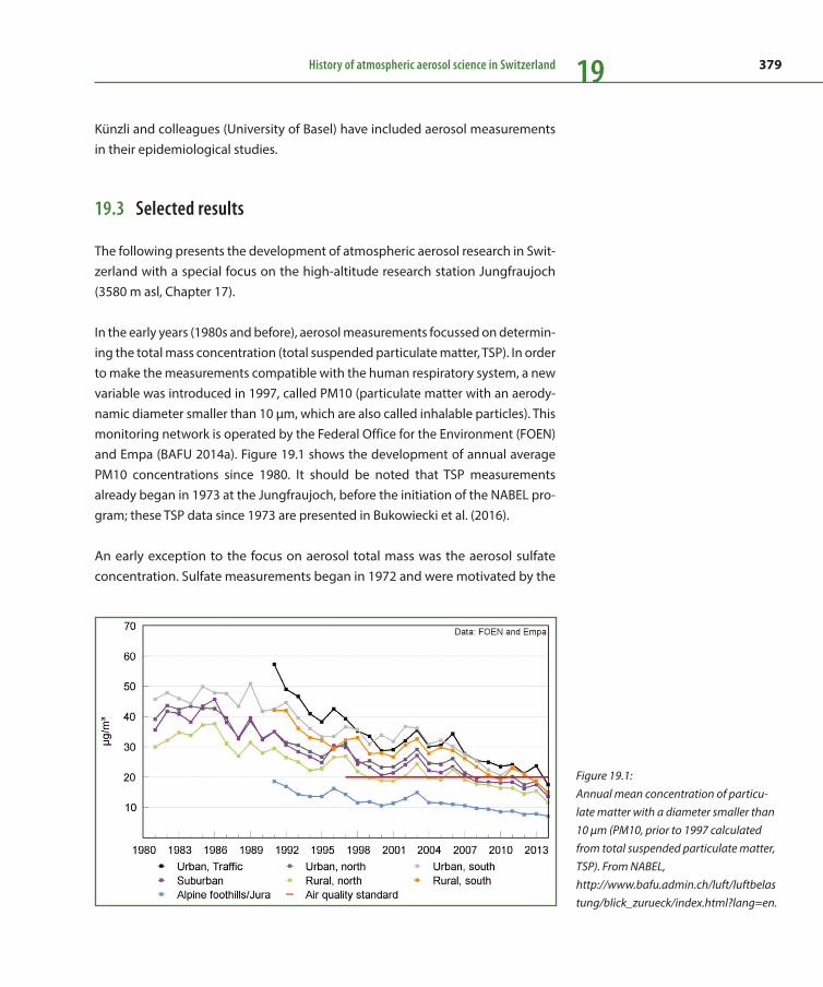
379History of atmospheric aerosol science in Switzerland 19
Künzli and colleagues (University of Basel) have included aerosol measurements in their epidemiological studies.
19.3 Selected results
The following presents the development of atmospheric aerosol research in Swit-zerland with a special focus on the high-altitude research station Jungfraujoch (3580 m asl, Chapter 17).
In the early years (1980s and before), aerosol measurements focussed on determin-ing the total mass concentration (total suspended particulate matter, TSP). In order to make the measurements compatible with the human respiratory system, a new variable was introduced in 1997, called PM10 (particulate matter with an aerody-namic diameter smaller than 10 μm, which are also called inhalable particles). This monitoring network is operated by the Federal Office for the Environment (FOEN) and Empa (BAFU 2014a). Figure 19.1 shows the development of annual average PM10 concentrations since 1980. It should be noted that TSP measurements already began in 1973 at the Jungfraujoch, before the initiation of the NABEL pro-gram; these TSP data since 1973 are presented in Bukowiecki et al. (2016).
An early exception to the focus on aerosol total mass was the aerosol sulfate concentration. Sulfate measurements began in 1972 and were motivated by the
Figure 19.1: Annual mean concentration of particu-late matter with a diameter smaller than 10 μm (PM10, prior to 1997 calculated from total suspended particulate matter, TSP). From NABEL, http://www.bafu.admin.ch/luft/luftbelas tung/blick_zurueck/index.html?lang=en.

380 From weather observations to atmospheric and climate sciences in Switzerland19
observed increase in the acidity of precipitation and the potential adverse effects on ecosystems (Torseth et al. 2012, and references therein). These mea-surements were first performed in the years 1972–1977 to study long-range transportation of air pollutants within an OECD (Organisation for Economic Cooperation and Development) project and was continued in 1979 under the umbrella of the Convention on Long-range Transboundary Air Pollution (CLR-TAP) and later under the European Monitoring and Evaluation Program (EMEP) (Torseth et al. 2012). In Switzerland, sulfate measurements were initiated in 1973 in Payerne and at the Jungfraujoch by Empa within the EMEP Programme (BAFU 2014a), later to be complemented by measurements at Rigi and in Lugano (BAFU 2014b).
The Ordinance on Air Pollution Control (Luftreinhalteverordnung) went into effect on 1 March 1986 and has undergone a number of amendments since then (Chap-ter 18). However, the standards related to atmospheric aerosols have not changed since then and only concerned PM10, lead and cadmium. (For sulfate, which was a concern for ecosystems as mentioned above but not for human toxicity, no stan-dard was established, although in 1979 Switzerland had signed and ratified the UN-ECE protocols on long-range transboundary air pollution, accepting their crit-ical load and critical level values for sulfur and nitrogen compounds). A compari-son of the PM10 standard (annual average concentration of 20 μm/m3) with Figure 19.1 shows that this standard was exceeded at many sites in the early years but exeedence is nowadays mostly restricted to urban sites influenced by traffic or rural sites in Southern Switzerland. Lead and cadmium, an issue in the early years, are well below the standards at all sites.
First sporadic research activities took place in the late 1970s at the Jungfraujoch to investigate the aerosol chemical composition (Dams and De Jonge 1976; Adams et al. 1980). More systematic aerosol measurements at the Jungfraujoch were initiated by Heinz Gäggeler from EIR/PSI in 1986. These activities were moti-vated by the possibility of using glaciers as archives of past climates, but required a better knowledge on the transfer function from the atmosphere to the snow. These new measurements were facilitated by the development of the epiphani-ometer (Gäggeler et al. 1989), which allowed the continuous measurement of the aerosol surface area concentration with a time resolution of about 30 minutes. Because of the very low power consumption of the epiphaniometer, continuous measurements were performed not only at the Jungfraujoch (since 1988), but also at Colle Gnifetti (4450 m asl Monte Rosa region, Figure 19.2) for several years (Baltensperger et al. 1991).

381History of atmospheric aerosol science in Switzerland 19
A strong seasonal variation of the aerosol mass concentration (summer values higher by one order of magnitude than in winter) was found in these measure-ments both at the Jungfraujoch and at the Colle Gnifetti (Baltensperger et al. 1991). Similar observations had already been reported by Dams and De Jonge (1976), and were confirmed by continuous TSP measurements initiated at the Jungfraujoch in 1973 (Gehrig 1986; BUWAL 1983; annual reports can be found on the FOEN web-site, e. g., BAFU 2014a, 2014b). However, while the diurnal upslope-downslope flow pattern had been recognized for Mauna Loa, Hawaii (3400 m asl) many years ago (Mendonca 1969), the Jungfraujoch was considered to be in the free troposphere and thus unaffected by the injections of polluted air from the planetary boundary
Figure 19.2: Left: Urs Baltensperger, Heinz Gäggeler, and Martin Emmenegger (from left to right) in front of the solar panel for the epiphaniometer on Colle Gnifetti, 4450 m asl. Right: The epiphaniometer box and battery installed in a snow pit on Colle Gnifetti.

382 From weather observations to atmospheric and climate sciences in Switzerland19
layer (PBL). The latter was mainly based on ozone measurements, where good agreement between ozone data from high-elevation mountain stations and ozone soundings was found for some altitude (Kley et al. 1994). Together with the absence of diurnal variations in the ozone concentration at these high-elevation stations in summer, it was concluded that high-elevation mountain stations were in the free troposphere most of the time. The 30-minute time resolution of the epiphaniome-ter now made it possible to link the increased aerosol concentrations to vertical transport processes. A 10-year dataset allowed a climatology of the aerosol con-centration at the Jungfraujoch (Baltensperger et al. 1997) to be determined for the first time, as well as allowing evaluation of the dependence of the vertical transport on meteorological conditions (Lugauer et al. 1998; Lugauer et al. 2000), which con-firmed enhanced vertical transport during the warmer months. A nice visualisation of the vertical transport was accomplished by airborne lidar measurements (Nyeki et al. 2000; 2002), where the Jungfraujoch was in the undisturbed free troposphere in the morning, but injection of PBL air masses reached altitudes as high as 4000 m later in the afternoon (Figure 19.3).
In 1995, MeteoSwiss initiated a Swiss contribution to the Global Atmosphere Watch (GAW) programme of the World Meteorological Organization (WMO). This programme included an aerosol component, with a wide variety of additional variables being measured (light scattering and absorption coefficients, particle
Alti
tude
in k
m (a
sl)
0
1
2
3
4
5
0
1
2
3
4
5
B
Back
scat
ter R
atio
B
1.001.081.171.271.371.481.601.731.872.002.202.402.602.803.00>
Figure 19.3: Airborne lidar transects, illustrating the boundary layer evolution in the Jungfrau-joch region. Abbreviations: I = Interlaken town (563 m), L = Lauberhorn (2472 m), JFJ= Jungfraujoch station (3580 m), and E = Eggishorn (2927m). Adaped from Nyeki et al. (2000).

383History of atmospheric aerosol science in Switzerland 19
number concentration and major inorganic components (all since 1995), as well as size distribution and cloud condensation nuclei concentration (since 2008)). In addition, Empa measured TSP from 1973 to 2005, while PM10 has been measured from 2006 to the present. Today, the Jungfraujoch is one of the global stations within GAW and currently has one of the most comprehensive aerosol programs worldwide. The same is true of gas phase measurements at the Jungfraujoch (Chapter 18).
The enhanced continuous aerosol measurements at the Jungfraujoch have allowed further assessment of the annual cycle (Nyeki et al. 1998) as well as a more detailed analysis of the dependence on meteorology (Collaud Coen et al. 2011). As an example, Figure 19.4 shows the temporal evolution of the aerosol scattering coefficient measured continuously since 1995. The data have been complemented by the active surface area measurements from an epiphaniometer. Because the aerosol size distribution at the Jungfraujoch aerosol remains fairly constant over the year (Weingartner et al. 1999; Herrmann et al. 2015), there is a high correlation between the active surface area concentration and the aerosol light scattering coefficient, such that the data can easily be combined. The data on the scattering and absorption coefficients as well as the number concentration have been used for various trend analyses (Collaud Coen et al. 2007; 2013; Asmi et al. 2013). Differ-ent trends were found for different times of the year, and the analyses clearly showed that long data series (typically >10 years) are required before reliable statements about trends become possible.
Continuous measurements are highly useful for the detection of individual me -teo rological events. This is exemplified by the detection of Saharan dust events (Schwikowski et al. 1995; Collaud Coen et al. 2004). In the latter publication, the detection of Saharan dust events was based on the fact that Saharan dust pres-ents different optical properties (different wavelength dependences of both the light scattering and the light absorption coefficient). Collaud Coen et al. (2004) also reported a climatology of Saharan dust events at the Jungfraujoch, where it was found that Saharan dust events contributed a surprisingly high percentage (24 %) of the aerosol mass concentration on an annual average. An updated Saha-ran dust climatology covering the years 2001 to 2014 is presented by Bukowiecki et al. (2016).
Another important event where these continuous aerosol measurements were highly useful was the eruption of the Eyjafjallajökull volcanic eruption on Iceland in Spring 2010 (Bukowiecki et al. 2011). The Jungfraujoch was among the sites

384 From weather observations to atmospheric and climate sciences in Switzerland19
with the most comprehensive in situ data sets (Figure 19.5), providing a detailed characterisation of the volcanic ash plume. The extensive physical, chemical and optical datasets helped in the interpretation of remote sensing data.
An important feature of aerosol particles is that they can take up water and grow in size. The growth factor is defined as the ratio of the particle diameter at a given high relative humidity (RH) (typically 85 % to 90 % RH) to a low RH (typically < 40 %). The growth factor is influenced by the chemical composition of the particle, which
Figure 19.4: Panel a: View of the station at the Jung-fraujoch (JFJ). Panels b–e: Temporal evo-lution of the continuously measured aero-sol parameters at the Jungfraujoch. Monthly average values are shown for TSP and PM10, for the rest of the variables the 30-day running average of the daily average values. The dashed vertical lines (Panels c–e) indicate that, in January 1998, the entire aerosol laboratory was moved from the old JFJ research station (3454 m asl) to the JFJ Sphinx research station (3580 m asl) and a new inlet was employed (Weingartner et al. 1999; Collaud Coen et al. 2007). Gravimetric TSP and PM10 is sampled separately. From Bukowiecki et al. (2016).

385History of atmospheric aerosol science in Switzerland 19
in turn determines at which supersaturation, for a given size, particles can act as cloud condensation nuclei (CCN). Since there are no major aerosol sources close to the Jungfraujoch, the aerosol chemistry remains rather constant over the course of the year (e. g., Cozic et al. 2008; Fröhlich et al. 2013). Therefore, the growth factor stays rather constant, too, with an average hygroscopicity factor of 0.24 (Sjögren et al. 2008; Kammermann et al. 2010).Thus, the CCN number concentrations can be estimated with high accuracy based on the measured size distribution and the measured average hygroscopicity factor, which strongly simplifies the calculation of the CCN number concentrations in global models (Jurányi et al. 2010; 2011). The particle increase in size due to water uptake also leads to an enhanced scattering coefficient. This scattering enhancement factor is an important measured param-eter: In the GAW programme it is recommended that all aerosol variables be mea-sured for ”dry” conditions, i. e., at RH < 40 % (to avoid the situation that data cannot be compared due to different RH at different stations). However, in order to com-pare these dry in situ scattering coefficients with results from remote sensing instruments such as lidars (which measure under ambient conditions), the scatter-ing enhancement as a function of the ambient RH needs to be known. This has been determined at the Jungfraujoch (Fierz-Schmidhauser et al. 2010) as well as at other sites (Zieger et al. 2013) with a humidified nephelometer.
As mentioned above, the attempt was made to use a lidar to determine the vertical aerosol profile above the Jungfraujoch. However, because the lidar is
Figure 19.5: Online measurements of physical and optical properties of the aerosol from the Eyjafjallajökull volcanic eruption arriving at the Jungfraujoch allow the refractive index to be estimated with relatively narrow boundaries. Adapted from Bukowecki et al. (2011).
386 From weather observations to atmospheric and climate sciences in Switzerland19
”blind” in the first few hundred metres above the station, and the aerosol layer above the Jungfraujoch during injection of air from the PBL is typically only several hundred metres in depth (see Figure 19.2), these attempts were unsuc-cessful, with the exception of occasional Saharan dust events (Larchevêque et al. 2002). The installation of a lidar at the Kleine Scheidegg (2061 m asl), below the Jungfraujoch proved to be more successful and allowed a closure study between in situ and lidar measurements to be made (Zieger et al. 2012). Since 2014, a ceilometer has been continuously running at Kleine Scheidegg (oper-ated by MeteoSwiss, funded by Empa via the pan-European Research Infrastruc-ture ICOS, https://www.icos-ri.eu/).
The Jungfraujoch site itself is within clouds about one third of the time (Baltens-perger et al. 1998). This presents an excellent opportunity to study in situ aero-sol-cloud interactions in the real atmosphere. An even more interesting, almost unique feature is that while clouds mostly exist in the liquid phase in summer, mixed-phase and glaciated clouds are frequently present in winter. This allows the study of both the cloud droplet formation from cloud condensation nuclei and the glaciation of a cloud through ice nuclei. To investigate these pro-cesses, a series of CLACE (Cloud and Aerosol Characterization Experiment) cam-paigns have been performed since the year 2000, often with international col-laboration.
Henning et al. (2002) showed that in a liquid cloud aerosol particles roughly larger than 100 nm were activated to form cloud droplets, where the actual activation diameter depended on a large number of parameters such as the liquid water content or the particle number concentration with a diameter larger than 100 nm. Hammer et al. (2014) then found that the effective peak supersaturation is one of the major driving parameters of the actual value of the activation diameter, and that this peak supersaturation was different for air mass flows from the Northwest compared to the Southeast, due to different topographical features at the Jung-fraujoch (Figure 19.3a).
In a mixed-phase or glaciated cloud, additional processes such as the Wege-ner-Bergeron-Findeisen process (Bergeron 1937; Pruppacher and Klett 1997) come into play: Liquid droplets evaporate in the presence of ice crystals, because of the lower vapour pressure over ice (Figure 19.6). This in turn leads to a decrease in the activated fraction, since the number of ice crystals is much less than the number of liquid droplets before their evaporation. Verheggen et al. (2007) were able to experimentally verify this in the natural clouds at the Jungfraujoch and

387History of atmospheric aerosol science in Switzerland 19
showed that the activated fraction of particles larger than 100 nm did indeed decrease strongly with decreasing temperature, due to the increased ice nucle-ation activity. During several CLACE campaigns, these experiments were accom-panied by measurements of the ice nuclei activity by Ulrike Lohmann’s group (e. g., Chou et al. 2011).
Several other aerosol research areas besides the ones described above are covered at the Jungfraujoch. For example, the investigation of new particle formation is the subject of extensive research. The motivation lies in comparing the new par-ticle formation mechanisms with those determined within the CLOUD project at CERN, where it was shown, for example, that sulfuric acid cannot alone initiate new particle formation (Kirkby et al. 2011), and that oxidized organic compounds from biogenic emissions greatly enhance the formation rates (Riccobono et al. 2014). However, the analysis is still ongoing here, and the reader is referred to papers appearing in the near future. Clearly, the Jungfraujoch, by its combination of remoteness and easy accessibility as well as the frequent presence of clouds, is a hotspot for research into aerosols and their links to climate.
Figure 19.6: Aerosols into cloud droplets. (Left) The red curve presents a typical number size distri-bution of dry aerosol particles at the Jung-fraujoch (Weingartner et al. 1999). The red-shaded area represents particles that are activated to cloud droplets at a very low supersaturation (0.1 %); orange and yellow areas represent activated particles for increasing supersaturation up to 1 %. Critical diameters for Jungfraujoch aero-sols can vary slightly with water solubility, surface tension or mixing state; however, size is the most important parameter. The blue distribution represents an example of the size distribution of cloud droplets measured at the Jungfraujoch (Henning et al. 2002). (Right) When ice crystals are formed, water vapour is transported from the cloud droplets to the ice crystals because of the lower saturation vapour pressure over ice than over liquid water (Wegener- Bergeron-Findeisen process). This eventually results in evaporation of the cloud droplets, and the radiative prop-erties of the cloud are no longer influenced by the number of CCN but only by the properties of the ice nuclei (IN) and ice crystals (Baltensperger 2010). Reproduced from Science.
References
Adams F. C., M. J. Van Craen, and P. J. Van Espen, 1980: Enrich-ment of trace elements in remote aerosols. Environ. Sci. Technol., 14, 1002–1005.
Asmi, A., M. Collaud Coen, J. A. Ogren, E. Andrews, P. Sheridan, A. Jefferson, E. Weingartner, U. Baltensperger, N. Bukowiecki, H. Lihavainen, N. Kivekäs, E. Asmi, P. P. Aalto, M. Kulmala, A. Wieden-sohler, W. Birmili, A. Hamed, C. O’Dowd, S. G Jennings, R. Weller, H. Flentje, A. M. Fjaeraa, M. Fiebig, C. L. Myhre, A. G. Hallar, E. Swi-
etlicki, A. Kristensson, and P. Laj, 2013: Aerosol decadal trends – Part 2: In-situ aerosol particle number concentrations at GAW and ACTRIS stations. Atmos. Chem. Phys., 13, 895–916.
BAFU, 2014a: NABEL, Luftbelastung 2013, Messresultate des Nationalen Beobachtungsnetzes für Luftfremdstoffe (NABEL). Bern, 128 pp, http://www.bafu.admin.ch/publikationen/publi kation/01777/index.html?lang=de
388 From weather observations to atmospheric and climate sciences in Switzerland19
BAFU, 2014b: NABEL measurement programme. downloaded from http://www.bafu.admin.ch/luft/00612/00625/index.html? lang=en, last accessed 2 May 2015.
Baltensperger U.,1985: Chemische und morphologische Cha-rakterisierung von partikelförmigen Luftfremdstoffen. PhD Thesis, University of Zürich.
Baltensperger, U., H. W. Gäggeler, D. T. Jost, M. Emmenegger, and W. Nägeli, 1991: Continuous background aerosol monitoring with the epiphaniometer. Atmos. Environ., 25, 629–634.
Baltensperger, U., 2010: Aerosols in clearer focus. Science, 329, 1474–1475.
Baltensperger, U., M. Schwikowski, D. T. Jost, S. Nyeki, H. W. Gäggeler, O. Poulida, 1998: Scavenging of atmospheric constit-uents in mixed phase clouds at the high-Alpine site Jungfrau-joch part I: Basic concept and aerosol scavenging by clouds. Atmos. Environ., 32, 3975–3983.
Bergeron, T., 1935: On the physics of cloud and precipitation. 5th Assembly, Union Geodes. et Geophys. Int., Lisbon.
Bukowiecki, N., P. Zieger, E. Weingartner, Z. Jurányi, M. Gysel, B. Neininger, B. Schneider, C. Hueglin, A. Ulrich, A. Wichser, S. Henne, D. Brunner, R. Kaegi, M. Schwikowski, L. Tobler, F. G. Wienhold, I. Engel, B. Buchmann, T. Peter, and U. Baltensperger, 2011: Ground-based and airborne in-situ measurements of the Eyjafjallajökull volcanic aerosol plume in Switzerland in spring 2010. Atmos. Chem. Phys., 11, 10011–10030.
Bukowiecki, N., E. Weingartner, M. Gysel, M. Collaud Coen, P. Zieger, E. Herrmann, M. Steinbacher, H. W. Gäggeler, and U. Baltensperger, 2016: Insights from more than 20 years of aero-sol observation at the high altitude research station Jungfrau-joch, Switzerland (3580 m asl). Aerosol and Air Quality Research, 16, 764–788, doi: 10.4209/aaqr.2015.05.0305
Burtscher, H., L. Scherrer, H. C. Siegmann, A. Schmidt‐Ott, and B. Federer, 1982: Probing aerosols by photoelectric charging. J. Appl. Phys., 53, 3787-3791, http://dx.doi.org/10.1063/1.331120
BUWAL, 1983: Bundesamt für Umweltschutz, Luftbelastung 1982. Schriftenreihe Umweltschutz No. 16, Bern, Juni 1983.
Chou, C., O. Stetzer, E. Weingartner, Z. Jurányi, Z. A. Kanji, and U. Lohmann, 2011: Ice nuclei properties within a Saharan dust event at the Jungfraujoch in the Swiss Alps. Atmos. Chem. Phys., 11, 4725–4738, 2011.
Colberg, C. A., U. K. Krieger, and T. Peter, 2004: Morphological investigations of single levitated H2SO4/NH3/H2O aerosol parti-cles during deliquescence/efflorescence experiments. J. Phys. Chem. A, 108, 2700–2709.
Collaud Coen, M., E. Weingartner, D. Schaub, C. Hueglin, C. Corri-gan, S. Henning, M. Schwikowski, and U. Baltensperger, 2004: Saharan dust events at the Jungfraujoch: detection by wave-length dependence of the single scattering albedo and first cli-matology analysis. Atmos. Chem. Phys., 4, 2465–2480.
Collaud Coen, M., E. Weingartner, S. Nyeki, J. Cozic, S. Henning, B. Verheggen, R. Gehrig, and U. Baltensperger, 2007: Long-term trend analysis of aerosol parameters at the high-Alpine site Jungfraujoch. J. Geophys. Res., 112, D13213, doi: 10.1029/ 2006JD007995
Collaud Coen, M., E. Weingartner, M. Furger, S. Nyeki, A. S.H. Prévôt, M. Steinbacher, and U. Baltensperger, 2011: Planetary boundary influence at the Jungfraujoch analyzed by aerosol cycles and synoptic weather types. Atmos. Chem. Phys., 11, 5931–5944.
Collaud Coen, M., E. Andrews, A. Asmi, U. Baltensperger, N. Bukowiecki, D. Day, M. Fiebig, A. M. Fjaeraa, H. Flentje, A. Hyvärinen, A. Jefferson, S. G. Jennings, G. Kouvarakis, H. Liha-vainen, C. Lund Myhre, W. C. Malm, N. Mihapopoulos, J. V. Mole-nar, C. O’Dowd, J. A. Ogren, B. A. Schichtel, P. Sheridan, A. Virk-kula, E. Weingartner, R. Weller, and P. Laj, 2013: Aerosol decadal trends Part 1: In-situ optical measurements at GAW and IMPROVE stations. Atmos. Chem. Phys., 13, 869–894.
Cozic, J., B. Verheggen, E. Weingartner, J. Crosier, K. Bower, M. Flynn, H. Coe, S. Henning, M. Steinbacher, St. Henne, M. Col-laud Coen, A. Petzold, and U. Baltensperger, 2008: Chemical composition of free tropospheric aerosol for PM1 and coarse mode at the high Alpine site Jungfraujoch. Atmos. Chem. Phys., 8, 407–423.
Dams R., and J. De Jonge, 1976: Chemical composition of Swiss aerosols from the Jungfraujoch. Atmos. Environ., 10, 1079–1084.
Fierz-Schmidhauser, R., P. Zieger, M. Gysel, L. Kammermann, P. F. DeCarlo, U. Baltensperger, and E. Weingartner, 2010: Measured and predicted aerosol light scattering enhancement factors at the high Alpine site Jungfraujoch. Atmos. Chem. Phys., 10, 2319–2333.
389History of atmospheric aerosol science in Switzerland 19Flesia, C., H. J. Koelsch, P. Rairoux, J. P. Wolf, and L. Wöste, 1989: Remote measurement of the aerosols size distribution by lidar. J. Aerosol Sci., 20, 1213–1216.
Fröhlich, C., 1983: Determination of aerosol optical depth from ground measurements. Adv. Space Res., 5, 139–145.
Fröhlich, R., M. J. Cubison, J. G. Slowik, N. Bukowiecki, A. S.H. Prévôt, U. Baltensperger, J. Schneider, J. R. Kimmel, M. Gonin, U. Rohner, D. R. Worsnop, and J. T. Jayne, 2013: The ToF-ACSM: a portable aerosol chemical speciation monitor with TOFMS detection. Atmos. Meas. Tech., 6, 3225–3241.
Gehrig, R., 1986: Nationales Beobachtungsnetz für Luftfremd-stoffe (NABEL), Bisherige Messungen- geplante Erweiterungen. Sozial- und Präventivmedizin, 31,46–48.
Hammer, E., N. Bukowiecki, M. Gysel, Z. Jurányi, C. R. Hoyle, R. Vogt, U. Baltensperger, and E. Weingartner, 2014: Investigation of the effective peak supersaturation for liquid-phase clouds at the high-Alpine site Jungfraujoch, Switzerland (3580 m asl). Atmos. Chem. Phys., 14, 1123–1139.
Henning, S., E. Weingartner, S. Schmidt, M. Wendisch, H. W. Gäg-geler, and U. Baltensperger, 2002: Size dependent aerosol acti-vation at the high Alpine site Jungfraujoch (3580 m asl). Tellus Series B Chemical and Physical Meteorology, 54B, 82–95.
Herrmann, E., E. Weingartner, S. Henne, L. Vuilleumier, N. Buko-wiecki, M. Steinbacher, F. Conen, M. Collaud Coen, E. Hammer, Z. Jurányi, U. Baltensperger, and M. Gysel, 2015: Analysis of long-term aerosol size distribution data from Jungfraujoch with emphasis on free tropospheric conditions, cloud influence, and air mass transport. J. Geophys. Res. Atmos., 120, 9459–9480, doi: 10.1002/2015JD023660
IPCC 2013: Climate Change 2013: The Physical Science Basis. Con-tribution of Working Group I to the Fifth Assessment Report of the Intergovernmental Panel on Climate Change. Cambridge University Press, 1552 pp. https://www.ipcc.ch/report/ar5/wg1/
Jurányi, Z., M. Gysel, E. Weingartner, P. F. DeCarlo, L. Kammer-mann, and U. Baltensperger, 2010: Measured and modelled cloud condensation nuclei concentration at the high Alpine site Jungfraujoch. Atmos. Chem. Phys., 10, 7891–7906.
Jurányi, Z., M. Gysel, E. Weingartner, N. Bukowiecki, L. Kammer-mann, and U. Baltensperger, 2011: A 17 month climatology of the cloud condensation nuclei number concentration at the
high Alpine site Jungfraujoch. J. Geophys. Res., 116, D10204, doi: 10.1029/2010JD015199
Kammermann, L., M. Gysel, E. Weingartner, and U. Baltensperger, 2010: 13-month climatology of the aerosol hygroscopicity at the free tropospheric site Jungfraujoch (3580 m asl). Atmos. Chem. Phys., 10, 10717–10732.
Kirkby, J., J. Curtius, J. Almeida, E. Dunne, J. Duplissy, S. Ehrhart, A. Franchin, S. Gagné, L. Ickes, A. Kürten, A. Kupc, A. Metzger, F. Riccobono, L. Rondo, S. Schobesberger, G. Tsagkogeorgas, D. Wimmer, A. Amorim, F. Bianchi, M. Breitenlechner, A. David, J. Dommen, A. Downard, M. Ehn, R. C. Flagan, S. Haider, A. Han-sel, D. Hauser, W. Jud, H. Junninen, F. Kreissl, A. Kvashin, A. Laak-sonen, K. Lehtipalo, J. Lima, E. R. Lovejoy, V. Makhmutov, S. Mathot, J. Mikkilä, P. Minginette, S. Mogo, T. Nieminen, A. Onnela, P. Pereira, T. Petäjä, R. Schnitzhofer, J. H. Seinfeld, M. Sipilä, Y. Stozhkov, F. Stratmann, A. Tome, J. Vanhanen, Y. Viisanen, A. Vrtala, P. E. Wagner, H. Walther, E. Weingartner, H. Wex, P. M. Winkler, K. S. Carslaw, D. R. Worsnop, U. Baltens-perger, and M. Kulmala, 2011: Role of sulphuric acid, ammonia and galactic cosmic rays in atmospheric aerosol nucleation. Nature, 476, 429–433.
Kley, D., H. Geiss, and V. A. Mohnen, 1994: Tropospheric ozone at elevated sites and precursor emissions in the United States and Europe. Atmos. Environ., 28, 149–158.
Larchevêque, G., I. Balin, R. Nessler, P. Quaglia, V. Simeonov, H. van den Bergh, and B. Calpini, 2002: Development of a multi-wavelength aerosol and water-vapor lidar at the Jungfraujoch Alpine Station (3580 m above sea level) in Switzerland. Appl. Opt., 41, 2781–2790.
Lohmann, U., and J. Feichter, 2005: Global indirect aerosol effects: a review. Atmos. Chem. Phys., 5, 715–737.
Lugauer, M., U. Baltensperger, M. Furger, H. W. Gäggeler, D. T. Jost, M. Schwikowski, and H. Wanner, 1998: Aerosol transport to the high Alpine sites Jungfraujoch (3454 m asl) and Colle Gnifetti (4452 m asl). Tellus Series B Chemical and Physical Meteorology, 50B, 76–92.
Lugauer, M., U. Baltensperger, M. Furger, H. W. Gäggeler, D. T. Jost, S. Nyeki, and M. Schwikowski, 2000: Influences of vertical transport and scavenging on aerosol particle surface area and Radon decay product concentrations at the Jungfraujoch (3454 m asl). J. Geophys. Res., 105, 19869–19879.
390 From weather observations to atmospheric and climate sciences in Switzerland19
Marcolli, C, B. P. Luo, and T. Peter, 2004: Mixing of the organic aerosol fractions: Liquids as the thermodynamically stable phases. J. Phys. Chem. A, 108, 2216–2224.
Mendonca, B. G., 1969: Local wind circulation on the slopes of Mauna Loa. J. Appl. Meteor., 8, 533–541.
Nyeki, S., U. Baltensperger, I. Colbeck, D. T. Jost, E. Weingartner, and H. W. Gäggeler, 1998: The Jungfraujoch high-Alpine research station (3454 m) as a background continental site for the measurement of aerosol parameters. J. Geophys. Res., 103, 6097–6107.
Nyeki, S., M. Kalberer, I. Colbeck, S. de Wekker, M. Furger, H. W. Gäggeler, M. Kossmann, M. Lugauer, D. Steyn, E. Weingartner, M. Wirth, and U. Baltensperger, 2000: Convective boundary layer evolution to 4 km asl over high-Alpine terrain: Airborne lidar observation in the Alps. Geophys. Res. Lett., 27, 689–692.
Nyeki, S., K. Eleftheriadis, U. Baltensperger, I. Colbeck, M. Fiebig, A. Fix, C. Kiemle, M. Lazaridis, and A. Petzold, 2002: Airborne lidar and in-situ aerosol observations of an elevated layer, lee-ward of the European Alps and Apennines. Geophys. Res. Lett., 29, 1852, doi: 10.1029/2002GL014897
Pruppacher, H. R., and J. D. Klett, 1997: Microphysics of Clouds and Precipitation. 2nd ed., Kluwer, 447 pp.
Riccobono, F., S. Schobesberger, C. E. Scott, J. Dommen, I. K. Ortega, L. Rondo, J. Almeida, A. Amorim, F. Bianchi, M. Breiten-lechner, A. David, A. Downard, E. M. Dunne, J. Duplissy, S. Ehrhart, R. C. Flagan, A. Franchin, A. Hansel, H. Junninen, M. Kajos, H. Kes-kinen, A. Kupc, A. Kürten, A. N. Kvashin, A. Laaksonen, K. Lehti-palo, V. Makhmutov, S. Mathot, T. Nieminen, A. Onnela, T. Petäjä, A. P. Praplan, F. D. Santos, S. Schallhart, J. H. Seinfeld, M. Sipilä, D. V. Spracklen, Y. Stozhkov, F. Stratmann, A. Tomé, G. Tsagko georgas, P. Vaattovaara, Y. Viisanen, A. Vrtala, P. E. Wagner, E. Weingartner, H. Wex, D. Wimmer, K. S. Carslaw, J. Curtius, N. M. Donahue, J. Kirkby, M. Kulmala, D. R. Worsnop, and U. Baltensperger, 2014: Oxidation products of biogenic emissions contribute to nucle-ation of atmospheric particles. Science, 344, 717–721.
Schmid B. and C. Wehrli, 1995: Comparison of sun photometer calibration by use of the Langley technique and the standard lamp. Appl. Opt., 34, 4500–4512, doi: 10.1364/AO.34.004500
Schmidt−Ott, A. and H. C. Siegmann, 1978: Photoelectron emis-sion from small particles suspended in air. Appl. Phys. Lett., 32, 710–713, doi: 10.1063/1.89915
Schwikowski, M., P. Seibert, U. Baltensperger, and H. W. Gägge-ler, 1995: A study of an outstanding Saharan dust event at the high-Alpine sit Jungfraujoch, Switzerland. Atmos. Environ., 29, 1829–1842.
Sjögren, S., M. Gysel, E. Weingartner, M. R. Alfarra, J. Duplissy, J. Cozic, J. Crosier, H. Coe, and U. Baltensperger, 2008: Hygroscop-icity of the submicrometer aerosol at the high-Alpine site Jung-fraujoch, 3580 m asl, Switzerland. Atmos. Chem. Phys., 8, 5715–5729.
Szidat, S., T. M. Jenk, H.-A. Synal, M. Kalberer, L. Wacker, I. Hajdas, A. Kasper-Giebl, and U. Baltensperger, 2006: Contributions of fossil fuel, biomass-burning, and biogenic emissions to carbo-naceous aerosols in Zurich as traced by 14C. J. Geophys. Res., 111, D07206, doi: 10-1029/2005JD006590
Tabor, K., L. Gutzwiller and M. J. Rossi, 1993: The heterogeneous interaction of NO2 with amorphous carbon. Geophys. Res. Lett., 20, 1431–1434.
Tørseth, K., W. Aas, K. Breivik, A. M. Fjæraa, M. Fiebig, A. G. Hjell-brekke, C. Lund Myhre, S. Solberg, and K. E. Yttri, 2012: Introduc-tion to the European Monitoring and Evaluation Programme (EMEP) and observed atmospheric composition change during 1972–2009. Atmos. Chem. Phys., 12, 5447–5481.
Verheggen, B., J. Cozic, E. Weingartner, K. Bower, S. Mertes, P. Connolly, M. Gallagher, M. Flynn, T. Choularton, and U. Baltens-perger, 2007: Aerosol activation in mixed phase clouds at the high Alpine site Jungfraujoch. J. Geophys. Res., 112, D23202, doi: 10.1029/2007/JD008714
Wehrli, C., 1999: World Optical Depth Research and Calibration Center, Global Atmosphere Watch International Activities and Swiss Contribution: Ozone, Radiation and Aerosols in the Atmosphere, Swiss Agency for the Environment, Forests and Landscape UM-110-E, 19-22, ftp://ftp.pmodwrc.ch/pub/worcc/gaweth98.pdf
Weingartner, E., S. Nyeki, and U. Baltensperger, 1999: Seasonal and diurnal variation of aerosol size distributions (10 < D < 750 nm ) at a high-Alpine site (Jungfraujoch 3580 m asl). J. Geophys. Res., 104, 26809–26820.
WHO, 2013: Review of Evidence on Health Aspects of Air Pollu-tion – REVIHAAP Project. Final technical report. World Health Organization, Geneva, 309 pp.

391History of atmospheric aerosol science in Switzerland 19Wolf, J. P., and L. Wöste, 1987: Détection sélective et à distance de la pollution atmosphérique par LIDAR. Helv. Phys. Acta, 60, 161–170.
Zieger, P., E. Kienast-Sjögren, M. Starace, J. von Bismarck, N. Bukowiecki, U. Baltensperger, F. G. Wienhold, T. Peter, T. Ruhtz, M. Collaud Coen, L. Vuilleumier, O. Maier, E. Emili, C. Popp, and E. Weingartner, 2012: Spatial variation of aerosol optical proper-
ties around the high-Alpine site Jungfraujoch (3580 m asl). Atmos. Chem. Phys., 12, 7231–7249.
Zieger, P., R. Fierz-Schmidhauser, E. Weingartner, and U. Baltens-perger, 2013: Effects of relative humidity on aerosol light scat-tering: results from different European sites. Atmos. Chem. Phys., 13, 10609–10631.


393
Broadening the view from climatology to climate sciences


395
20 Paleoclimatology and polar ice coresBernhard Stauffer
20.1 Introduction
Mankind has been confronted with climate changes since time immemorial. In ancient times it was presumed that the gods were responsible for such changes. In the Alpine regions our ancestors experienced retreating and advancing glaciers as evidence for such changes, whether through own observations or in oral lore. Also legends reported drastic events, such as the legend of the Blüemlisalp. About 200 years ago, Ignaz Venetz, Jean de Charpentier and Louis Agassiz (Agassiz 1840) proposed that erratic blocks spread around our country and other places in Europe had been transported by glaciers, and that, as a consequence, large parts of Europe had been covered by a kind of ice sheet during an “ice age” several thou-sand years previously. The investigation of landscapes and especially of moraines subsequently confirmed this presumption. At the beginning of the 20th century it became clear that several ice ages had afflicted Europe in the past, and that the last one had ended about 10,000 years ago, merging to the so-called Holocene. Many regional climatic variations can be reconstructed from this epoch. For the past few hundred years historical documents describe the climate at least quali-tatively (Pfister 1984). The width and density of tree rings, for example, provide information about climatic conditions for the entire Holocene (Schweingruber 1983) and the last part of the last glacial epoch. The composition of pollen in well-stratified peat bogs and lake sediments provide information about the local flora (Welten 1982). The age of the different layers can be determined by the 14C method. A combination of the different methods allows very detailed descriptions of past climatic changes (De Jong, 2013).
In the mid-20th century Cesare Emiliani and Samuel Epstein developed a new analytical method to determine ocean temperature and the global ice volume by measuring the concentration ratio of the stable isotopes 18O and 16O in car-bonates from ocean sediments (Emiliani 1957). The first results showed that ice ages were a global phenomenon, that there were many more than four ice ages in the Pleistocene, as hitherto assumed, and that the cold climates were inter-
University of Bern,
Physics Institute, Climate and
Environmental Physics, Bern

396 From weather observations to atmospheric and climate sciences in Switzerland20
rupted about every 100,000 years by warm phases called interglacials. The oceans now cover more than two thirds of the Earth’s surface, and the new method initiated the start of many national and international ocean-drilling pro-grams. Together with the findings on the continents, mainly from pollen analy-ses, it was now possible to reconstruct the climate globally for a certain epoch. The international program CLIMAP reconstructed a kind of temperature map for the maximum of the last glacial epoch about 18,000 years ago (CLIMAP Project Members 1976).
At about the same time Willi Dansgaard observed that the 18O/16O ratio in pre-cipitation was correlated with temperature (Dansgaard 1954). Measurements along ice cores from Greenland showed that stable isotope ratios in ice are quite well correlated with the annual temperature at the time the ice was deposited as snow (Dansgaard 1961). Suitable ice cores are mainly available in polar regions, but it became evident that they are an archive for much more climatic and environmental information than only local temperature (Oeschger and Langway 1989). Analysing the air enclosed in bubbles of the ice allows us to reconstruct the atmospheric composition in the past, e. g., to investigate the interplay between temperature and greenhouse gases over the past 800,000 years. Polar ice cores have, therefore, become one of the most important archives for paleoclimatology.
20.2 The recovery of polar ice cores
To find support for the ice age theory, in 1840 Louis Agassiz investigated the movement of glaciers on Unteraargletscher in Switzerland (Agassiz 1840). The flow of ice was later also investigated in Greenland. The main motivation for his work to explain the form of the ice sheet and the age of the ice at its edges. The Swiss-born U. S. citizen Henry Bader (Bader et al. 1962) was head of the US Snow, Ice and Permafrost Research Establishment (SIPRE). He started several core drilling proj-ects in Greenland and the Antarctica. The first ice cores were obtained in Green-land by hand augers. Soon, however, it became clear that the analyses of these cores provided valuable information not only about snow and ice properties, but also about climate and environmental conditions. In 1957 an ice core was recov-ered at Site 2 in North Greenland to a depth of 411 m. Nine years later the first ice core drilling down to the bedrock at a depth of 1387 m was performed at Camp Century. A cable-suspended electromechanical coring device was used, providing ice cores of 100 mm diameter. The very heavy drill rig was then transported to Byrd
397Paleoclimatology and polar ice cores 20
Station in Antarctica where in 1968 a core drilling reached bedrock at a depth of 2164 m. These two deep cores were the only ones available for the next 10 years, and some of this core material is still used for analyses and comparisons.
A much lighter drill rig called ISTUK was developed in Denmark. It was used in a Danish, U. S. and Swiss research project at Dye 3 in South Greenland and reached bedrock in 1981 at a depth of 2037 m. Many analyses along the core were performed for the first time in the field. The results were very interesting and partly also very surprising. Scientists wanted, therefore, another core to confirm the results.
Hans Oeschger (University Bern) and Willy Dansgaard (University Copenhagen) initiated the GReenland Ice Core Project (GRIP) with 8 European nations partici-pating. I had the privilege to chair the Steering Committee. In 1992 the core drill-ing at Summit, the centre of the ice sheet, reached bedrock at a depth of 3029 m. The age of the ice at the bottom is about 115,000 years. The analyses of the core confirmed the findings from Dye 3 and provided in addition a wealth of new infor-mation. A year later the U. S. colleagues reached a depth of 3057 m in their camp 32 km west of GRIP.
In Antarctica, with its core drilling in 1998 Russia reached a depth of 3658 m, where the age of the ice is about 420,000 years. Core drilling was continued until 2007, when it stopped at 3658 m to prevent any risk of a contamination of the subjacent lake Vostok.
Ten European nations again unified their efforts for two core drilling projects in Antarctica called “European Project for Ice Coring in Antarctica” (EPICA). The deep drilling at Dome Concordia reached the bottom of the ice sheet in 2005 at 3270 m depth. It provides the hitherto oldest ice core record covering the past 800,000 years.
Japan also drilled an ice core to 3035 m in 2007 at Dome Fuji in Antarctica.
While the EPICA core from Dome Concordia covers the last 800,000 years, the GRIP ice core from Summit covers only100,000 years, so that the last interglacial, the Eem (about 135–115 years BP), cannot be investigated. This was the main reason why international consortia under the leadership of Denmark performed two new core drillings north of Summit at North-GRIP (North Greenland ice Core Project members 2004) and at NEEM (NEEM Community Members 2013).

398 From weather observations to atmospheric and climate sciences in Switzerland20
20.3 Analytical methods to analyse ice cores
Stable isotope ratio
Like other elements, the constituents of water – oxygen and hydrogen – occur in different isotopes. The different isotopes of one element have different atomic masses because of the different number of neutrons in the nucleus. Stable oxygen atoms (which have always 8 protons) have 8, 9 or 10 neutrons, resulting in three isotopes with the atomic mass numbers 16, 17 and 18 (16O, 17O and 18O):Oxygen: 16O 17O 18OMixing ratio: 997,600 ppm 400 ppm 2,000 ppm
Isotopes of one element have the same chemical characteristics. Small fraction-ations in their composition occur in processes depending on the atomic mass like evaporation, condensation and diffusion (Figure 20.1). Isotopic ratios R can be measured very precisely in special IR mass spectrometers and recently also by laser spectroscopy.
Different δ18O values for summer and winter snow allow us to count annual layers like tree rings. Because of the compression of the ice, however, the annual layers
Stable isotope ratio basics: The δ value
I f water masses in the atmosphere (i. e., clouds) loose water by precipitation, heavier isotopes are preferred and become depleted in the remaining water in the atmosphere. The remaining water content depends on the tempera-ture. Therefore, the isotopic composition in the remaining water mass depends on the condensation temperature. This is the main principle on which isotopic “paleothermometry” is based.
Because variations of isotopic ratios are small, they are expressed as so called δ-values, defined as:
δ ¼ 1,000 Rsample � RstandardRstandard
‰½ ¼ 1,000 Rsample
Rstandard� 1
� �‰½
The standard for 18O is provided by the IAEA in Vienna and corresponds with the concentration of mean ocean water. It was precisely determined in the 1970s at the Swiss Federal Institute for Reactor Research (EIR; Bärtschi 1976).
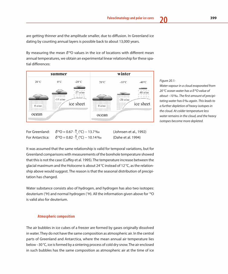
399Paleoclimatology and polar ice cores 20
are getting thinner and the amplitude smaller, due to diffusion. In Greenland ice dating by counting annual layers is possible back to about 13,000 years.
By measuring the mean δ18O values in the ice of locations with different mean annual temperatures, we obtain an experimental linear relationship for these spa-tial differences:
For Greenland: δ18O = 0.67 ∙ Ts (°C) − 13.7 ‰ (Johnsen et al., 1992)For Antarctica: δ18O = 0.82 ∙ Ts (°C) − 10.14 ‰ (Dahe et al. 1994)
It was assumed that the same relationship is valid for temporal variations, but for Greenland comparisons with measurements of the borehole temperature showed that this is not the case (Cuffey et al. 1995). The temperature increase between the glacial maximum and the Holocene is about 24 °C instead of 12 °C, as the relation-ship above would suggest. The reason is that the seasonal distribution of precipi-tation has changed.
Water substance consists also of hydrogen, and hydrogen has also two isotopes: deuterium (2H) and normal hydrogen (1H). All the information given above for 18O is valid also for deuterium.
Atmospheric composition
The air bubbles in ice cubes of a freezer are formed by gases originally dissolved in water. They do not have the same composition as atmospheric air. In the central parts of Greenland and Antarctica, where the mean annual air temperature lies below –30 °C, ice is formed by a sintering process of cold dry snow. The air enclosed in such bubbles has the same composition as atmospheric air at the time of ice
Figure 20.1: Water vapour in a cloud evaporated from 20 °C ocean water has a δ18O value of about –10 ‰. The first amount of precipi-tating water has 0 ‰ again. This leads to a further depletion of heavy isotopes in the cloud. At colder temperature less water remains in the cloud, and the heavy isotopes become more depleted.
400 From weather observations to atmospheric and climate sciences in Switzerland20
formation. To reconstruct past atmospheric composition, air first has to be extracted from well-suited ice and then the air is analysed in a gas chromatograph or by laser spectroscopy.
The extraction of air from bubbles in the ice has to be done mechanically to avoid any interaction with melt water, which could produce air components by chemical reactions (for CO2 especially with carbonates) or deplete components by dissolution in water. Air bubbles are opened by grating, cracking or milling ice samples. All these mechanical methods have the disadvantage that the extraction efficiency is less than 100 %. Below a depth of about 1,000 m in an ice sheet, air in bubbles forms clathrates due to the high hydrostatic pressure. The extraction efficiency is different for bubbles and clathrates, which causes frac-tionation of air components, especially at depth intervals where bubbles coexist with clathrates. An extraction of the air by sublimation of ice provides an effi-ciency of 100 % (Schmitt et al. 2011), but it is very time consuming and difficult. It can only be used for selected samples especially to test mechanical extraction methods. The group of Hans Oeschger at the Physics Institute of the University of Berne from the beginning took a leading position in extracting and analysing air from ice cores.
For measurements of CO2 concentration, the reproducibility of measurements is about 1.5 ppm (measurements on ice samples from the same depth). Comparisons of the CO2 records measured in atmospheric air with overlapping records from ice cores show good agreement. However, this is no guarantee for the reliability in old ice: CO2 could be produced or depleted by chemical reaction with impurities in the ice. Such effects are certainly small because the results from ice cores from different drilling sites and with different chemical impurity concentrations yield consistent results. Based on such investigations, the accuracy of CO2 records is estimated to be about 5 ppm (2015 CO2 concentration is about 400 ppm).
Chemical impurities and dust concentration
Ice in the central parts of the Greenland and the Antarctic ice sheets is very clean. Its level of purity is better than that of normal distilled water. The con-centrations of dust and chemical tracers provide important information about past environmental conditions. At the Physics Institute of Berne a “continuous flow analysis” (CFA) system was developed (Kaufmann et al. 2008). A section of an ice core is continuously melted on a melter head. The sample water obtained

401Paleoclimatology and polar ice cores 20
is then analysed online in the field. The concentration of dust, of Na+, Ca++, NH4+,
NO3–, SO4
– – , H2O2 and HCHO can be measured continuously with a depth reso-lution of about 10 mm. A newly improved system can also measure the total organic carbon and the air content. It is now even possible to measure the methane concentration, and tests are being done to measure the isotopic ratio of oxygen on the sample water as well. Details on chemical impurities are dis-cussed in the insert ‘Study of Aerosol Deposition on Alpine Glaciers.’ Volcanic eruptions can be relevant for the global climate, mainly caused by an enhanced concentration of sulphate aerosols in the atmosphere. Based on sulphate results along the Greenland and Antarctic ice core records, the history of volcanic activ-ities has been reconstructed (Castellano et al. 2004). Finally, it has to be men-tioned that records of the 10Be concentration in ice allow investigating solar activity in the past (Beer et al. 1990).
20.4 Results and interpretation
The last millennium
According to Antarctic ice cores the atmospheric CO2 concentration during the first 8 centuries of the last millennium was rather constant at about 280 ppm (Fig-ure 20.2). Over the last two centuries it increased to about 350 ppm (2014 annual mean value approximately 400 ppm).
Figure 20.2: CO2 and CH4 concentrations from various ice cores over the last millennium and from direct atmospheric measurements. CO2: (Anklin et al. 1995), (Siegenthaler et al. 2005b)CH4: (Blunier et al. 1993), (Etheridge et al. 1998).

402 From weather observations to atmospheric and climate sciences in Switzerland20
The values measured in the Greenland ice cores are significantly higher. The reason could be higher ice temperature or higher concentrations of some chem-ical tracers. Measuring CO2 concentration with a very high depth resolution shows a larger scatter for Greenland samples than for samples from the Antarc-tica, even in ice representing the last glacial epoch, where the temperature in central Greenland was below –50 °C. The higher values and the larger scatter cannot be caused by variations of the atmospheric concentrations. It has to be an artefact, though its cause is still an open question. In the discussions of other time periods in the following chapters only CO2 results from Antarctic ice cores will be considered.
The atmospheric methane (CH4) concentration was rather constant at about 700 ppb during the first 7 centuries. During the last 250 years of the last millennium it increased to more than the double the value. Also the values from Greenland for methane are slightly higher. In this case it is not an artefact but caused because natural sources for methane are mainly wetlands, which are more fre-quent in the northern hemisphere. The anthropogenic methane increase started a little earlier than the CO2 increase. Anthropogenic CO2 is emitted by the burn-ing of fossil fuel (carbon and oil). Anthropogenic methane sources are mainly farming ruminants and rice agriculture. The CO2 increase follows, therefore, industrialisation, whereas the methane increase follows the increase in the global population.
The Holocene
The δ18O record, a proxy for the local surface temperature, shows no clear trend (Figure 20.3). It shows a distinct cooling event 8,200 years BP (BP: before present) lasting about 200 years. There is no indication of a “Holocene thermal maximum” as observed around 8,000 to 6,000 years BP with global temperatures being about 0.7 °C higher than for preindustrial conditions (Wanner et al. 2008).
The atmospheric CO2 concentration was about 265 ppm at the beginning of the Holocene (it was about 200 ppm during the glacial epoch) and dropped to values below 260 ppm. The main reasons lie most probably in the uptake of carbon by the biosphere developing in the regions where the ice cover disappeared and the wetter climate at the low latitudes. The increase of CO2 after about 7,000 years BP caused by a drier climate in the low latitudes and an almost linear increase of the ocean temperature (Indermühle et al. 1999).

403Paleoclimatology and polar ice cores 20
The atmospheric CH4 concentration was about 700 ppb at the beginning of the Holocene. It then decreased by more than 100 ppb to about 560 ppb around 5300 years BP. The tropics and neighbouring low-latitude regions were very wet at the beginning of the Holocene, but these regions got steadily drier until about 5,000 years BP. Wetlands in northern latitude had been modest CH4 sources until about 6,000 years BP, but afterwards they became more and more important. Support for this interpretation comes from the increasing difference between the methane concentration of the northern hemisphere (GRIP (Greenland) record) und that of the southern hemisphere (Dome C (Antarctica) record). The distinct cooling event at 8,300 years BP runs parallel to lower CH4 concentrations in both records. While the δ18O record represents a local cooling event, the drop in both methane records indicates that it was a global event. The drop in the Dome C record is less pro-nounced, caused by the lower annual snow accumulation rate at Dome C than at Summit (GRIP) (Spahni et al. 2003). The drop of the CH4 concentration indicates a period of dry climate of large regions at low latitudes.
Figure 20.3: The black crosses of the δ18O record represent single measurements along the GRIP ice core (Johnsen et al. 1992), the solid black line a spline with 200 years cut-off frequency (1 ‰ difference corresponds to about 1.5 °C). The red diamonds show CO2 concentrations from Dome C (Monnin et al., 2004), the red crosses from Taylor Dome ( Indermühle et al. 1999) (both Antarctica). The blue circles show CH4 concentrations from Dome C (Spahni et al. 2003), the blue crosses CH4 concentrations from GRIP (Greenland) (Blunier et al. 1993).
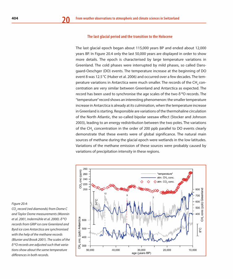
404 From weather observations to atmospheric and climate sciences in Switzerland20
The last glacial period and the transition to the Holocene
The last glacial epoch began about 115,000 years BP and ended about 12,000 years BP. In Figure 20.4 only the last 50,000 years are displayed in order to show more details. The epoch is characterised by large temperature variations in Greenland. The cold phases were interrupted by mild phases, so called Dans-gaard-Oeschger (DO) events. The temperature increase at the beginning of DO event 8 was 12.5 °C (Huber et al. 2006) and occurred over a few decades. The tem-perature variations in Antarctica were much smaller. The records of the CH4 con-centration are very similar between Greenland and Antarctica as expected. The record has been used to synchronise the age scales of the two δ18O records. The “temperature” record shows an interesting phenomenon: the smaller temperature increase in Antarctica is already at its culmination, when the temperature increase in Greenland is starting. Responsible are variations of the thermohaline circulation of the North Atlantic, the so-called bipolar seesaw effect (Stocker and Johnson 2003), leading to an energy redistribution between the two poles. The variations of the CH4 concentration in the order of 200 ppb parallel to DO events clearly demonstrate that these events were of global significance. The natural main sources of methane during the glacial epoch were wetlands in the low latitudes. Variations of the methane emission of these sources were probably caused by variations of precipitation intensity in these regions.
Figure 20.4: CO2 record (red diamonds) from Dome C and Taylor Dome measurements (Monnin et al. 2001, Indermühle et al. 2000). δ18O records from GRIP ice core Greenland and Byrd ice core Antarctica are synchronised with the help of the methane records (Blunier and Brook 2001). The scales of the δ18O records are adjusted such that varia-tions show about the same temperature differences in both records.
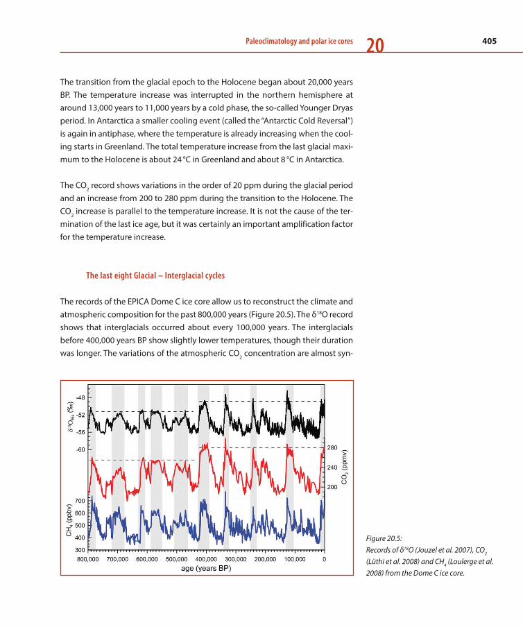
405Paleoclimatology and polar ice cores 20
The transition from the glacial epoch to the Holocene began about 20,000 years BP. The temperature increase was interrupted in the northern hemisphere at around 13,000 years to 11,000 years by a cold phase, the so-called Younger Dryas period. In Antarctica a smaller cooling event (called the “Antarctic Cold Reversal”) is again in antiphase, where the temperature is already increasing when the cool-ing starts in Greenland. The total temperature increase from the last glacial maxi-mum to the Holocene is about 24 °C in Greenland and about 8 °C in Antarctica.
The CO2 record shows variations in the order of 20 ppm during the glacial period and an increase from 200 to 280 ppm during the transition to the Holocene. The CO2 increase is parallel to the temperature increase. It is not the cause of the ter-mination of the last ice age, but it was certainly an important amplification factor for the temperature increase.
The last eight Glacial – Interglacial cycles
The records of the EPICA Dome C ice core allow us to reconstruct the climate and atmospheric composition for the past 800,000 years (Figure 20.5). The δ18O record shows that interglacials occurred about every 100,000 years. The interglacials before 400,000 years BP show slightly lower temperatures, though their duration was longer. The variations of the atmospheric CO2 concentration are almost syn-
Figure 20.5: Records of δ18O (Jouzel et al. 2007), CO2 (Lüthi et al. 2008) and CH4 (Loulerge et al. 2008) from the Dome C ice core.
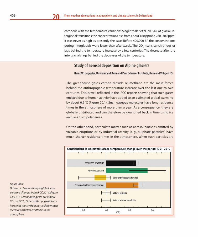
406 From weather observations to atmospheric and climate sciences in Switzerland20
chronous with the temperature variations Siegenthaler et al. 2005a). At glacial-in-terglacial transitions the concentrations rise from about 180 ppm to 260–300 ppm; it was never as high as presently the case. Before 400,000 BP the concentrations during interglacials were lower than afterwards. The CO2 rise is synchronous or lags behind the temperature increase by a few centuries. The decrease after the interglacials lags behind the decreases of the temperature.
Study of aerosol deposition on Alpine glaciers
Heinz W. Gäggeler, University of Bern and Paul Scherrer Institute, Bern and Villigen PSI
The greenhouse gases carbon dioxide or methane are the main forces behind the anthropogenic temperature increase over the last one to two centuries. This is well reflected in the IPCC reports showing that such gases emitted due to human activity have added to an estimated global warming by about 0.9 °C (Figure 20.1). Such gaseous molecules have long residence times in the atmosphere of more than a year. As a consequence, they are globally distributed and can therefore be quantified back in time using ice archives from polar areas.
On the other hand, particulate matter such as aerosol particles emitted by volcanic eruptions or by industrial activity (e. g., sulphate particles) have much shorter residence times in the atmosphere. When such particles are
Figure 20.6: Drivers of climate change (global tem-perature changes from IPCC 2014, Figure 1.09-01). Greenhouse gases are mainly CO2 and CH4. Other anthropogenic forc-ing stems mostly from particulate matter (aerosol particles) emitted into the atmosphere.

407Paleoclimatology and polar ice cores 20
emitted into the troposphere, their lifetime is about 2 weeks only – hence, far too short to quantitatively reach the polar regions because the transport time from mid- and low latitude emission sources (for example, to Antarc-tica) amounts to more than a year. Information on the chronology of emis-sions can therefore be gained only exploiting archives that exist in the vicin-ity of emission sources. Such archives are Alpine glaciers. The only exceptions refer to the emission of particulate matter from explosive scenarios that reach the stratosphere, examples being volcanic eruptions or debris from nuclear weapons testing. Then the residence times are a few years, which again ensures global distribution. The total influence of particulate matter emission on climate change is estimate to be about –0.6 °C and + 0.1 °C, respectively (Figure 20.6).
Studies of particle-bound pollution chronologies over the last few millennia have been performed at many glaciers worldwide. The first deep drill cam-paigns at Colle Gnifetti (4450 m asl; Figure 20.7) in the Swiss Alps were per-formed in 1976 and 1977 and reached a depth of 65 m (H. Oeschger et al. 1978). Meanwhile, ice core projects have been conducted at glaciers in South America (Andes), Patagonia, the European Alps, Northern Europe (e. g., Svalbard), Siberia (e. g., Russian Altai), Mongolia (e. g., Tsast Ul) as well as in glaciers from the Tibetan plateau, Tien Shan, Pamir, and at Kilimanjaro in Africa or New Zealand (Mt. Cook area). To reach such drill sites, expeditions
Figure 20.7: Colle Gnifett (4450 m asl) with Zumstein-spitze and Dufourspitze. This place is the highest site in the Alps used for ice core drill projects. The thickness of the glacier is about 100 m. The oldest ice close to bedrock reaches back to the last glacial period (Würm ice age) (source: PSI archive).
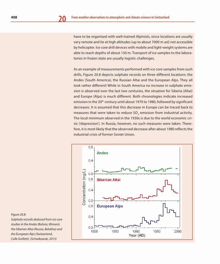
408 From weather observations to atmospheric and climate sciences in Switzerland20
have to be organised with well-trained Alpinists, since locations are usually very remote and lie at high altitudes (up to about 7000 m asl) not accessible by helicopter. Ice core drill devices with mobile and light-weight systems are able to reach depths of about 150 m. Transport of ice samples to the labora-tories in frozen state are usually logistic challenges.
As an example of measurements performed with ice core samples from such drills, Figure 20.8 depicts sulphate records on three different locations: the Andes (South America), the Russian Altai and the European Alps. They all look rather different! While in South America no increase in sulphate emis-sion is observed over the last two centuries, the situation for Siberia (Altai) and Europe (Alps) is much different. Both chronologies indicate increased emission in the 20th century until about 1970 to 1980, followed by significant decreases. It is assumed that this decrease in Europe can be traced back to measures that were taken to reduce SO2 emission from industrial activity. The local minimum observed in the 1930s is due to the world economic cri-sis (‘depression’). In Russia, however, no such measures were taken. There-fore, it is most likely that the observed decrease after about 1980 reflects the industrial crisis of former Soviet Union.
Figure 20.8: Sulphate records deduced from ice core studies in the Andes (Bolivia, Illimani), the Siberian Altai (Russia, Belukha) and the European Alps (Switzerland, Colle Gnifetti). (Schwikowski, 2015)

409Paleoclimatology and polar ice cores 20
References
Agassiz, L., 1840 : Etude sur les glaciers. Gent et Gassmann, Neu-chatel, 346 pp.
Anklin, M., J. M. Barnola, J. Schwander, B. Stauffer, and D. Ray-naud, 1995: Processes affecting the CO2 concentrations mea-sured in Greenland ice. Tellus B, 47, 461–470.
Bader, H., 1962: Scope, problems, and potential value of deep core drilling in ice sheets. Special Report 58, US Army Cold Re -gions Research and Engineering Laboratory, Hanover, NH, 15 pp.
Bärtschi, P., 1976: Absolute 18O content of standard mean ocean water. Earth and Planetary Science Letters, 31, 341–344.
Beer, J., A. Blinov, G. Bonani, R. C. Finkel, H. J. Hofmann, B. Leh-mann, H. Oeschger, A. Sigg, J. Schwander, T. Staffelbach, B. Stauffer, M. Suter, and W. Wölfli, 1990: Use of 10Be in polar ice to trace the 11-year cycle of solar activity. Nature, 347, 164–166.
Blunier, T., J. Chappellaz, J. Schwander, J. Barnola, T. Desperts, B. Stauffer, and D. Raynaud, 1993: Atmospheric methane, record from greenland ice core over the last 1000 years. Geophysical Research Letters, 20, 2219–2222.
Blunier, T., J. Chappellaz, J. Schwander, B. Stauffer, and D. Ray-naud, 1995: Variations in atmospheric methane concentration during the Holocene epoch. Nature, 374, 46–49.
Blunier, T., and E. J. Brook., 2001: Timing of millennial-scale cli-mate change in Antarctica and Greenland during the last glacial period. Science, 291, 109–112.
Castellano, E., S. Becagli, J. Jouzel, A. Migliori, M. Severi, J. P. Stef-fensen, R. Traversi, and R. Udisti, 2004: Volcanic eruption fre-quency over the last 45 ky as recorded in Epica-Dome C ice core (East Antarctica) and its relationship with climatic changes. Global and Planetary Change, 42, 195–205.
CLIMAP Project Members, 1976: The surface of the ice-age Earth. Science, 191, 1131–1136.
Cuffey, K. M., G. D. Clow, R. B. Alley, M. Stuiver, E. D. Waddington, and R. W. Saltus, 1995: Large Arctic temperature change at the Wisconsin-Holocene glacial transition. Science, 270, 455–458.
Dahe, Q., J. R. Petit, J. Jouzel, and M. Stievenard, 1994: Distribu-tion of stable isotopes in surface snow along the route of the
The CH4 variations fluctuated in a range of about 350 ppb during the glacial and about 750 ppb during the interglacials. There is no clear trend for lower concen-trations during the interglacials before 400,000 years BP. It has to be kept in mind that variations of the CH4 concentration are mainly caused by variations of the emission by wetlands in low and mid latitudes.
The observed 100,000 years cycles support the explanation that the large natural climatic changes are mainly caused by cycles of the insolation and its latitudinal distribution on Earth. Such changes are caused by the precession of Earth’s axis (21,000 years cycle), its obliquity (41,000 years cycle) and the eccentricity of Earth’s orbit (100,000 years cycle) (Hays et al. 1976). It is not well understood that the orbital cycle is the dominant one, and it is presumed that the 41,000-year cycle could be dominant before 900,000 years BP. An ice core covering the last 1.5 million years could provide us with an answer. This is the main motivation for the “Interna-tional Partnerships in Ice Core Sciences” (IPICS), an international consortium of 17 laboratories, to perform a new core drilling in Antarctica (Fischer et al. 2013).
410 From weather observations to atmospheric and climate sciences in Switzerland20
1990 International Trans-Antarctica Expedition. Journal of Gla-ciology, 40, 107–118.
Dansgaard, W., 1954: The 18O abundance in fresh water. Geo-chimica et Cosmochimica Acta, 6, 241–260.
Dansgaard, W., 1961: The isotopic composition of natural waters. Meddelelser om Groenland, 165, 120 pp.
De Jong, R., L. von Gunten, and M. Grosjean, 2013: Cold-season temperatures in the European Alps during the past millennium: variability, seasonality and recent trends. Quaternary Science Reviews, 82, 1–12.
Emiliani C, 1957: Temperature and age analysis of deep sea cores. Science, 125, 383–385.
Etheridge, D. M., L. P. Steele, R. J. Francey, and R. J. Lagenfelds, 1998: Atmospheric methane between 1000 A. D. and present, Evidence of anthropogenic emissions and climatic variability. Journal of Geophysical Research, 103, 15979–15993.
Fischer, H., J. Severinghaus, E. Brook, E. Wolff, M. Albert, O. Ale-many, R. Arthern, C. Bentley, D. Blankenship, J. Chappellaz, T. Creyts, D. Dahl-Jensen, M. Dinn, M. Frezzotti, S. Fujita, H. Gallee, R. Hindmarsh, D. Hudspeth, G. Jugie, K. Kawamura, V. Lipenkov, H. Miller, R. Mulvaney, F. Pattyn, C. Ritz, J. Schwander, D. Stein-hage, T. van Ommen, and F. Wilhelms, 2013: Where to find 1.5 million year old ice for the IPICS “Oldest-Ice” ice core. Climate of the Past, 9, 2489–2505.
Hays, J. D., J. Imbrie, and N. J. Shackleton,. 1976: Variations in the Earth’s orbit: Pacemaker of the ice ages. Science, 194 1121–1132.
Huber, C., M. Leuenberger, R. Spahni, J. Flückiger, J. Schwander, T. F. Stocker, S. Johnsen, A. Landais, and J. Jouzel, 2006: Isotope calibrated Greenland temperature record over Marine Isotope Stage 3 and its relation to CH4. Earth and Planetary Science Let-ters, 243, 504–519.
Indermühle, A., T. F. Stocker, F. Joos, H. Fischer, H. J. Smith, M. Wahlen, B. Deck, D. Mastroianni, J. Tschumi, T. Blunier, R. Meyer, and B. Stauffer, 1999: Holocene carbon-cycle dynamics based on CO2 trapped in ice at Taylor Dome, Antarctica. Nature, 398, 121–126.
Indermühle, A., E. Monnin, B. Stauffer, T. F. Stocker, and M. Wahlen, 2000: Atmospheric CO2 concentration from 60 to 20 kyr BP from the Taylor Dome ice core, Antarctica. Geophysical Research Letters, 27, 735–738.
IPCC, 2014: Climate Change 2014: Synthesis Report. Contribu-tion of Working Groups I, II and III to the Fifth Assessment Report of the Intergovernmental Panel on Climate Change [Core Writ-ing Team, R. K. Pachauri and L. A. Meyer (eds.)]. IPCC, Geneva, Switzerland, 151 pp.
Johnsen, S., W. Clausen, W. Dansgaard, K. Fuhrer, N. Gundestrup, C. Hammer, P. Iversen, J. Jouzel, B. Stauffer, and J. Steffensen, 1992: Irregular glacial interstadials recorded in a new greenland ice core. Nature, 359, 311–313.
Jouzel, J., V. Masson-Delmotte, O. Cattani, G. Dreyfus, S. Falourd, G. Hoffmann, B. Minster, J. Nouet, J. M. Barnola, J. Chappellaz, H. Fischer, J. C. Gallet, S. Johnsen, M. Leuenberger, L. Loulergue, D. Luethi, H. Oerter, F. Parrenin, G. Raisbeck, D. Raynaud, A. Schilt, J. Schwander, E. Selmo, R. Souchez, R. Spahni, B. Stauffer, J. P. Stef-fensen, B. Stenni, T. F. Stocker, J.-L. Tison, M. Werner, and E. W. Wolff, 2007: Orbital and millennial Antarctic climate variability over the past 800,000 years. Science, 317, 793–796.
Kaufmann, P. R., U. Federer, M. A. Hutterli, M. Bigler, S. Schüp-bach, U. Ruth, J. Schmitt, and T. F. Stocker, 2008. An improved continuous flow analysis system for high-resolution field mea-surements on ice cores. Environmental Science & Technology, 42, 8044–8050.
Loulergue, L., A. Schilt, R. Spahni, V. Masson-Delmotte, T. Blunier, B. Lemieux, J.-M. Barnola, D. Raynaud, T. F. Stocker, and J. Chap-pellaz, 2008: Orbital and millennial-scale features of atmo-spheric CH4 over the past 800,000 years. Nature, 453, 383–386.
Lüthi, D., M. Le Floch, B. Bereiter, T. Blunier, J.-M. Barnola, U. Sie-genthaler, D. Raynaud, J. Jouzel, H. Fischer, K. Kawamura, and T. F. Stocker, 2008: High-resolution carbon dioxide concentra-tion record 650,000–800,000 years before present. Nature, 453, 379–382.
Monnin, E., A. Indermühle, A. Dällenbach, J. Flückiger, B. Stauffer, T. F. Stocker, D. Raynaud, and J.-M. Barnola, 2001: Atmospheric CO2 concentrations over the last glacial termination. Science, 291, 112–114.
Monnin, E., E. J. Steig, U. Siegenthaler, K. Kawamura, J. Schwan-der, B. Stauffer, T. F. Stocker, D. L. Morse, J.-M. Barnola, B. Bellier, D. Raynaud, and H. Fischer, 2004: Evidence for substantial accumu-lation rate variability in Antarctica during the Holocene, through synchronization of CO2 in the Taylor Dome, Dome C and DML ice cores. Earth and Planetary Science Letters, 224, 45–54.

411Paleoclimatology and polar ice cores 20NEEM Community Members, 2013: Eemian interglacial recon-structed from a Greenland folded ice core. Nature, 493, 489–494.
North Greenland Ice Core Project members, 2004: High-resolu-tion record of Northern Hemisphere climate extending into the last interglacial period. Nature, 431, 147–151.
Oeschger, H., and C. C. Langway, 1989: The environmental record in glaciers and ice sheets. Dahlem Workshop Report, Wiley, 400 pp.
Oeschger, H., U. Schotterer, B. Stauffer, W. Haeberli, and H. Röthlisberger, 1978: First results from Alpine core drilling proj-ects. Z. Gletscherkd. Glazialgeol., 13, 193–208.
Pfister, C., 1984: Das Klima der Schweiz von 1525–1860 und seine Bedeutung in der Geschichte von Bevölkerung und Landwirtschaft. P. Haupt, Bern, 2 volumes, 245 pp. and 174 pp.
Schmitt, J., R. Schneider, and H. Fischer, 2011: A sublimation technique for high-precision measurements of δ13CO2 and mix-ing ratios of CO2 and N2O from air trapped in ice cores. Atmo-spheric Measurement Techniques, 4, 1445–1461.
Schweingruber, F., 1983: Der Jahrring: Standort, Methodik, Zeit und Klima in der Dendrochronologie. P. Haupt, Bern, 234 pp.
Schwikowski, M. 2015: Personal communication. Paul Scherrer Institut, Villigen, Switzerland.
Siegenthaler, U., T. F. Stocker, E. Monnin, D. Lüthi, J. Schwander, B. Stauffer, D. Raynaud, J.-M. Barnola, H. Fischer, V. Masson-Del-motte, and J. Jouzel, 2005a: Stable carbon cycle-climate rela-tionship during the late Pleistocene. Science, 310, 1313–1317.
Siegenthaler, U., E. Monnin, K. Kawamura, R. Spahni, J. Schwan-der, B. Stauffer, T. F. Stocker, J.-M. Barnola, and H. Fischer, 2005b: Supporting evidence from the EPICA Dronning Maud Land ice core for atmospheric CO2 changes during the past millennium. Tellus B, 57, 51–57.
Spahni, R., J. Chappellaz, T. F. Stocker, L. Loulergue, G. Hausam-mann, K. Kawamura, J. Flückiger, J. Schwander, D. Raynaud, V. Masson-Delmotte, and J. Jouzel, 2005: Atmospheric methane and nitrous oxide of the late Pleistocene from Antarctic ice cores. Science, 310, 1317–1321.
Spahni, R., J. Schwander, J. Flückiger, B. Stauffer, J. Chappellaz, and D. Raynaud, 2003: The attenuation of fast atmospheric CH4 variations recorded in polar ice cores. Geophysical Research Letters, 30, 1571.
Stocker, T. F., and S. J. Johnson, 2003: A minimum thermody-namic model for the bipolar seesaw. Paleoceanography, 18, 1087.
Wanner, H., J. Beer, T. J. Crowley, U. Cubasch, J. Flückiger, H. Goosse, M. Grosjean, F. Joos, J. O. Kaplan, M. Küttel, O. Solomina, T. F. Stocker, P. Tarasov, M. Wagner, and M. Widmann, 2008: Mid- to Late Holocene climate change: an overview. Quaternary Science Reviews, 27, 1791–1828.
Welten, M., 1982: Pollenanalytische Untersuchungen im jüngeren Quartär des nördlichen Alpenvorlandes der Schweiz. Stämpfli, Bern, 174 pp.

413
21 IPCC Working Group I: The Swiss contribution 1988–2014Thomas F. Stocker
21.1 Introduction
The foundation of the Intergovernmental Panel on Climate Change (IPCC) by both the World Meteorological Organization (WMO) and the United Nations Environment Programme in 1988 was prompted by the determination to pro-vide scientific information to the planned United Nations Conference on Envi-ronment and Development in Rio de Janeiro in June 1992 [Bolin, 2008]. Three international conventions were opened for signature at this conference: the Convention on Biological Diversity, the United Nations Convention to Combat Desertification and the United Nations Framework Convention on Climate Change (UNFCCC). The UNFCCC is the most comprehensive, but probably also the most difficult document that resulted from this first Earth Summit. It entered into force on 21 March 1994, within less than 2 years from the first Earth Sum-mit – an astoundingly short period of time considering the challenges associ-ated with the implementation of the goals laid down in this document. The scientific evidence provided by the First Assessment Report of the IPCC (FAR), published in 1990, made a convincing case that climate change will alter in a significant way the physical conditions on Earth, and that this will have an impact on the ecosystems around the world.
This chapter reflects on the role of the Swiss scientific community in IPCC and highlights its various important contributions over the years. I focus on Working Group I (WGI), the group that deals with the natural science aspects, the science area to which Switzerland has so far made the most numerous and substantial contributions. Swiss climate research has long focused on the physical aspects of the problem: the first research institution at a Swiss university to include the term “climate” in its name was the division of Climate and Environmental Physics at the University of Berne founded by Hans Oeschger [Stocker, 1999]. Hans Oeschger and his colleague Uli Siegenthaler were Lead Authors of a chapter in the WGI contri-bution to the FAR [Watson et al., 1990].
University of Bern, Physics Institute,
Climate and Environmental Physics,
Bern

414 From weather observations to atmospheric and climate sciences in Switzerland21
Understanding climate change requires an approach that encompasses many dis-ciplines of science: the natural sciences, biology, ecology, risk analysis and many others. I f response strategies to anthropogenic climate change are also included, as foreseen in the mandate of the IPCC, economics, social science and even phi-losophy are making important contributions to a comprehensive understanding of the problem. The three IPCC working groups (WGI – the Physical Science Basis, WGII – Impacts, Adaptation, and Vulnerability and WGIII – Mitigation) cover these areas of science in their three comprehensive reports [IPCC, 2013; 2014a, 2014b, 2014c], and provide the basis for a collective and integrated assessment in the Synthesis Report [IPCC, 2014d]. Because of this complexity, a well-structured pro-cess of scientific assessment that brings the wide ranging science to the user in digestible form is indispensable.
Various approaches could be envisaged to convey the science to the decision-mak-ers and governments with different degrees of effectiveness and robustness. There are the voices of eminent scientists, such as James Hansen, who in 1988 testified that “the global warming is now sufficiently large that we can ascribe with a high degree of confidence a cause and effect relationship to the greenhouse effect …” [Hansen, 1988]. Or notably 10 years earlier, by the two scientists from the Physics Institute of the University of Berne in a landmark paper in Science: “… a maximum atmospheric CO2 level might be found which should not be exceeded if the atmo-spheric radiation balance is not to be disturbed in a dangerous way” [Siegenthaler and Oeschger, 1978]. Alternatively, one could establish a “think-tank” with a few eminent scholars which would select the information and communicate it to the policymakers. Or the collection and digestion of scientific information could be tasked to a union of scientific academies. A “modern” approach would be the out-sourcing to a private company. Yet another way would be to simply leave this cru-cial problem to the well-oiled machinery of classic lobbying by which filtered “infor-mation” is delivered to the policymakers on a “free market” basis.
During the preparations towards the Rio Summit, and in light of the experience of the Brundtland Report “Our Common Future,” published in 1987, Bert Bolin, the founding Chair of the IPCC, and others realized that none of the above approaches would be an effective way to bring the scientific knowledge authentically and authoritatively to politicians. Statements by individual researchers could be taken out of context and result in a “chaotic debate between scientists and the public,” as noted by Bolin [2008]. Elitist “think-tanks” might produce very valuable informa-tion, but they would not have the broad support of the scientific community and the governments. Finally, academy reports or “free market” information would not

415IPCC Working Group I: The Swiss contribution 1988–2014 21
have the important buy-in by governments worldwide, and their production pro-cess might risk a lack of transparency. Instead, thorough scientific information was sought from findings in the peer-reviewed literature – and therefore transparently available to all – assessed by the leaders in the respective scientific fields, reviewed and commented on critically by experts and governments, and finally distilled into understandable information.
Fortunately, for man-made climate change, “one of the greatest challenges of our time,” as stated in UNFCCC [2010], the IPCC was able to establish itself as the authoritative source of comprehensive scientific information on this problem. The consistent efforts by the IPCC to increase awareness about man-made climate change and its impacts on resources and potential conflicts in the near future caused by it were prominently recognized by the Noble Peace Prize in 2007. Cer-tainly, the early years of IPCC were important and formative, and the very small number of colleagues who served as authors in various reports were pioneers and laid the solid ground for this success.
It must have been evident that the scientific information provided by the IPCC would be a threat to some interests outside science. Before long, therefore, there were massive attacks from various quarters, often by illegal means, launched towards IPCC and directly towards scientists. Despite a continuing string of biased, spin-doctored and even plain wrong media coverage on the IPCC’s work and find-ings [Oreskes and Conway, 2010] – even despite numerous ad hominem attacks on scientists – the scientific community has continued to deliver robust informa-tion through IPCC to governments since the release of the FAR in 1990.
The firm position of the IPCC is the consequence of three characteristics. First, the panel is constituted by the participating governments and is the supreme body of the IPCC. This implies that it elects the leadership of the IPCC, and defines the work program and the products. The panel also approves, line-by-line, the “Summary for Policymakers” of the assessment and adopts the underlying reports. Second, the reports, including the “Summary for Policymakers,” are written by the scientists who are selected by the panel on the basis of their expertise and given the man-date to carry out the scientific assessment. The clear separation between the panel requesting the report and the scientists writing it guarantees that the science is upheld, and that particular policy interests do not influence or bias these assess-ments. And third, because of the complexity of the task, the IPCC has clear proce-dures (the Principles Governing IPCC Work), which are established and agreed upon by the panel. In addition to defining the structure and work flow, two ele-
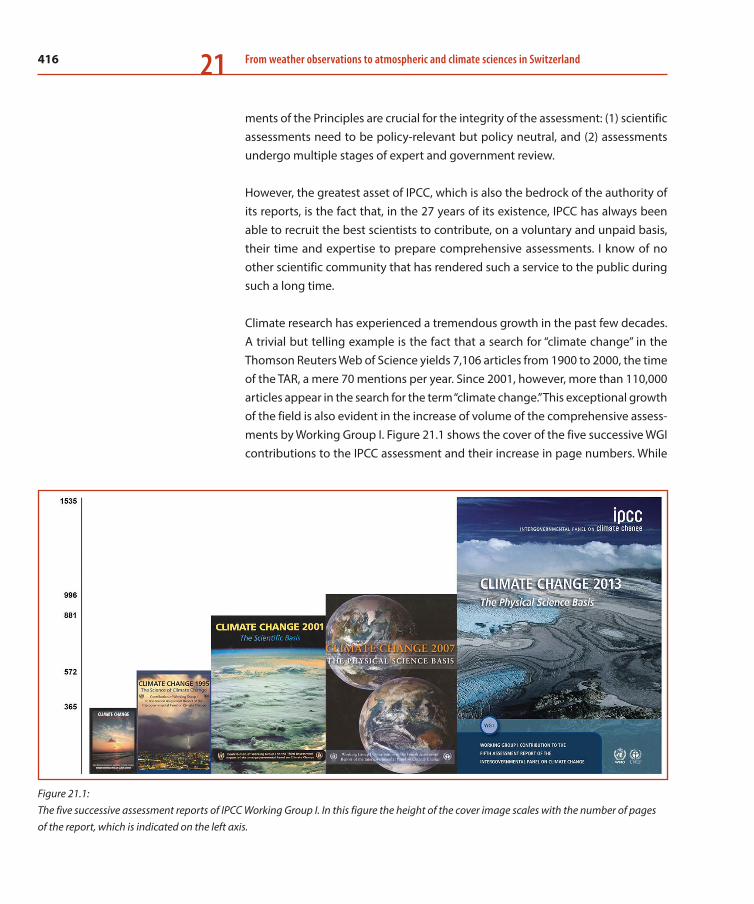
416 From weather observations to atmospheric and climate sciences in Switzerland21
ments of the Principles are crucial for the integrity of the assessment: (1) scientific assessments need to be policy-relevant but policy neutral, and (2) assessments undergo multiple stages of expert and government review.
However, the greatest asset of IPCC, which is also the bedrock of the authority of its reports, is the fact that, in the 27 years of its existence, IPCC has always been able to recruit the best scientists to contribute, on a voluntary and unpaid basis, their time and expertise to prepare comprehensive assessments. I know of no other scientific community that has rendered such a service to the public during such a long time.
Climate research has experienced a tremendous growth in the past few decades. A trivial but telling example is the fact that a search for “climate change” in the Thomson Reuters Web of Science yields 7,106 articles from 1900 to 2000, the time of the TAR, a mere 70 mentions per year. Since 2001, however, more than 110,000 articles appear in the search for the term “climate change.” This exceptional growth of the field is also evident in the increase of volume of the comprehensive assess-ments by Working Group I. Figure 21.1 shows the cover of the five successive WGI contributions to the IPCC assessment and their increase in page numbers. While
Figure 21.1: The five successive assessment reports of IPCC Working Group I. In this figure the height of the cover image scales with the number of pages of the report, which is indicated on the left axis.

417IPCC Working Group I: The Swiss contribution 1988–2014 21
some of this growth can be attributed to a certain laxness of the Co-Chairs leading the process − distinguished colleagues excluded − it is obvious that the ever-in-creasing number of published papers in this field demands some increase of vol-ume of an assessment that has the ambition to be comprehensive.
21.2 Production Process: Complex but Transparent
The production process of a scientific assessment is very complex, and the work cannot be completed successfully without a Technical Support Unit (TSU) under the direct leadership of a Co-Chair, who bears co-responsibility with a colleague Co-Chair for all products of the working group. The TSU coordinates and handles the entire workflow, which entails creating a working space for the lead authors and providing the end-to-end service necessary to bring a number of chapters written by more than 200 scientists around the world into one coherent and inter-nally consistent assessment report. Figure 21.2 illustrates the flow of work of WGI during the fifth assessment cycle. This work flow is shared in principle by the three working groups, albeit with different timeframes for the drafts of their reports. The cycle starts with the election of the leadership of a working group, which consists of two Co-Chairs, from a developing and a developed country, and six Bureau Members from different UN regions. During the entire cycle, three groups closely
Science Community Governments
Scoping of Outline of the Fi�h Assessment Report
Approval of Outline
Nomina�on and Selec�on of Experts
0-Order Dra� (ZOD) Informal Review
1-Order Dra� (FOD) Expert Review
Government Review 2-Order Dra� (SOD) Expert Review
Final Dra� Government Review
Approval of Summary for Policymakers and Acceptance of Report
Working Group Authors
2011
2010
2012
2013
Elec�on of WG Bureau
2009
2008
Sept 2013
IPCC Working Group I: Process of Fi�h Assessment Report Cycle
1
2
3
4 TS
TS SPM
SPM
Figure 21.2: The complex, interactive process between the scientific community, the selected authors and the governments during the fifth assessment report cycle. The timeline is for Working Group I, but all three work-ing groups followed this process from the election to the approval and acceptance of their report. The timing of the four Lead Author Meetings of WGI is indicated by numbered diamonds.

418 From weather observations to atmospheric and climate sciences in Switzerland21
interact: the governments represented in the panel, the authors of the assess-ment, and the worldwide community of scientists and experts.
The first action of invited representatives of the three groups is to work out an outline of the assessment, which consists of the list of the proposed chapters of the report plus a few bullet points to inform the prospective author team about the desired content of the chapters. This scoping document is discussed by the Panel. After approval, it becomes the primary guidance for the authors of a work-ing group. The outline also determines the expertise needed on the author team. For the fifth assessment cycle, in 2010 WGI received 1,014 nominations from gov-ernments and international organisations. It is worth remembering that this was a period during which IPCC was under heavy attack in the media in the wake of stolen emails in November 2009. These were the stormy months of the so-called “Climategate.” Critics were many, and the most extreme proponents even called for the complete dissolution of the IPCC. It was therefore very reassuring to see so many nominations of experts for all three working groups. With this the science community demonstrated that they stood firmly behind the IPCC process and the broader purpose of its work.
Once the author team has been selected, considering the required expertise and taking into account regional and gender balance, a sequence of drafts is prepared by the authors, which are then submitted to the TSU, usually several weeks after the face-to-face meetings of the entire author team and the working group lead-ership. These lead author meetings, usually 4 days long, are absolutely crucial to the consensus finding process on which the assessment relies. It turns out that, as the report matures, these meetings are the one opportunity to deal with import-ant cross-cutting issues that emerge during the assessment. Important examples for WGI AR5 include the implication of changes in the perturbation of the Earth’s radiative balance (Chapter 8) on the energy content of the ocean (Chapter 3), on attribution of climate change (Chapter 10), on climate sensitivity and other metrics (Chapter 12) and on sea level rise (Chapter 13).
The parallel production of the summary documents, the Technical Summary and the Summary for Policymakers (SPM) is also indicated in Figure 21.2. It starts once the first order draft of the report is ready. These additional key documents make the management of the process increasingly challenging because of the risk that inconsistencies might develop in the course of the many text revisions. A further challenge is the Summary for Policymakers, which needs to be written in an understandable and yet scientifically accurate language. The relevant scientific
419IPCC Working Group I: The Swiss contribution 1988–2014 21
information, including numbers and uncertainties, must be available in the SPM, while at the same time messages should be clear. The text must be traceable back to the chapters of the assessment, and it should include only material that is robust and relies on multiple lines of independent evidence. It must have the sup-port of the author team and have undergone a thorough review. Finally, it is debated and approved, line-by-line, by the panel. This is a lengthy and sometimes cumbersome process, but eventually it transfers special power to this document. Provided excellent authorship and good leadership throughout the process, this approach is able to generate a strong document that is the true voice of the sci-ence and at the same time accepted by governments. It forms the scientific basis for informed decisions without actually prescribing them.
The most important element ensuring transparency in the production of the IPCC assessment is the multi-stage review process. The first- and second-order drafts undergo a wide expert review. In AR5 this was an internet-based review by which an expert could sign up and obtain access to the draft documents and then submit a review. The bar of what constitutes expertise was kept deliberately low: A self-declaration of expertise was sufficient to be invited to participate. In addition to the two expert reviews, there are also two government reviews (Figure 21.2). In total, WGI has received 54,677 comments, all of which have been responded to in writing by the author team. The responses are public, so again transparency is ensured in the process.
An additional element of transparency was achieved by the implementation of a Conflict of Interest policy for all authors and functionaries of IPCC, first designed and implemented by WGI already in October 2010 and then adopted by the panel in November 2011.
Today, many agencies and organizations carry out “assessments.” However, because of the rigorous procedures that guide the IPCC process, the breadth of the author teams, the multi-stage review of the successive drafts and the govern-ment approval process, the IPCC assessment remains one of a kind. The price paid for this thoroughness and comprehensiveness is the overall duration of the assess-ment: Generally 4 years or more pass from the scoping to the final approval. Rapid responses or updates, as often called for, are fundamentally at odds with the cur-rent approach and quality standards of an IPCC assessment.

420 From weather observations to atmospheric and climate sciences in Switzerland21
21.3 Switzerland and IPCC: Contributions by the Swiss Scientists to IPCC WGI
Since the FAR of the IPCC, Swiss scientists have held leading roles in WGI, then simply called “The Scientific Assessment” [IPCC, 1990]. Hans Oeschger and Uli Sie-genthaler of the University of Berne served as two of the only four lead authors of the first chapter on greenhouse gases and aerosols. Siegenthaler continued this role in the first special report on radiative forcing [IPCC, 1995], which laid an important foundation for projections. For this report he used the “Berne model,” a simplified climate-carbon cycle model [Siegenthaler and Joos, 1992]. This Swiss contribution was among the first systematic projections using a carbon cycle com-ponent in the model, and it became the representative model to project CO2 con-centrations resulting from fossil fuel emissions.
Fortunat Joos from the University of Berne was elected Lead Author of chapter 2 on radiative forcing in IPCC [1996] and carried out the calculations of future CO2 concentrations using the Bern model as one of three models employed in the second assessment report. The model provided updated values of the Global Warming Potential which were used in the Kyoto Protocol to calculate the CO2 equivalence of anthropogenic emissions of various greenhouse gases.
For the third assessment cycle, Fortunat Joos was nominated by Switzerland and was elected WGI Vice-Chair, a member of the leading body of WGI. This third com-prehensive assessment reflected significant advances in climate sciences by pre-senting a chapter on aerosols and their direct and indirect effects on the radiative forcing, a chapter on the carbon cycle, and a much extended assessment on the detection and attribution of climate change [IPCC, 2001]. The Berne model was one of the leading models in the assessment of the carbon cycle and related pro-cesses on a global scale [Joos et al., 2001]. I was tasked to coordinate the chapter on Physical Climate Processes and Feedbacks and take a very broad view of the climate system ranging from water vapour and cloud feedbacks, to processes involving modes of natural variability and nonlinear changes and thresholds, such as those associated with the Atlantic meridional overturning circulation [Stocker et al., 2001]. The major challenge of this assignment, however, was the diverse composition of the authors of this chapter, as it included personalities with firm convictions regarding the causes of observed climate change, ranging from unequivocal human-caused climate change to essentially primarily natural varia-tions and irreducible uncertainties in the climate system. It was personally a very demanding task, but ultimately highly educational for me to lead this interesting

421IPCC Working Group I: The Swiss contribution 1988–2014 21
group of colleagues, find consensus on hotly debated issues, and finally arrive at acceptable and robust formulations.
Following the third assessment report (TAR) the number of Swiss scientists increased significantly, not the least because of a higher activity and visibility of climate research in Switzerland. The National Centre for Competence in Research, NCCR Climate, which was created in 2001 with the University of Berne as the lead-ing house, indirectly contributed to this enhanced role. In the fourth assessment report (AR4), three scientists served as lead authors (Fortunat Joos, University of Berne, and Ulrike Lohmann and Reto Knutti, later at ETH Zurich), who contributed their expertise in paleoclimate, aerosols and cloud physics, and climate modelling, respectively. I was charged with co-leading the chapter on climate change projec-tions [Meehl et al., 2007], which combined projections across an entire hierarchy of climate models.
The fifth assessment report cycle (AR5) then saw a further strengthening of the Swiss contribution to IPCC by the willingness of the government of Switzerland to nominate me for the position of Co-Chair of WGI. A secret ballot was necessary as for the first time four nominations were submitted for the developed-coun-try co-chair position. On September 3, after two rounds of ballot, I was elected Co-Chair of WGI and took joint leadership with Qin Dahe from China.
The first task was to establish a Technical Support Unit (TSU) at the University of Berne, which was funded by a special grant of the Swiss Federal Office for the Environment. The premises, IT and administrative embedding were provided by the University of Berne. The TSU formally started operations with the appointment of Melinda Tignor (USA) and Gian-Kasper Plattner. Melinda Tignor brought in unique experience as the Administrative Officer of the WGI TSU of AR4 and ensured a smooth transition with continuing institutional memory. With Gian-Kasper Plat-tner I was able to recruit an excellent scientist and colleague as Director of Science, a former PhD student and postdoc at the University of Berne who has had ample knowledge on the carbon cycle and who had carried out and coordinated the projections based on simulations using Earth System Models of Intermediate Complexity (EMICs) for AR4. What was important for this new position in a TSU was the combination of deep scientific understanding with a keen interest in the polit-ical process and the societal implications of our assessment work. Pauline Midgley joined as the Head of TSU with previous experience as the leader of the German IPCC Coordination Office and member of the German delegation to IPCC plena-ries, providing the important perspective of the policymakers. Judith Boschung

422 From weather observations to atmospheric and climate sciences in Switzerland21
joined as an all-round Administrative Assistant, and Vincent Bex served as IT Offi-cer. The starting phase of the work was extremely demanding since the panel had already requested information about the current state of knowledge on green-house gas metrics, an issue of highest policy relevance, and the scoping of a spe-cial report on extreme events and disaster reduction [IPCC, 2012a], jointly with Working Group II in the lead. The latter required the appointment of a Science Officer, Simon Allen, a young postdoc from New Zealand. Later in the process, Yu Xia and Alexander Nauels joined the TSU as Science Officer and Science Assistant, respectively. With this international team of excellent and dedicated colleagues forming the WGI TSU, we were ready for the challenging task to once more pro-duce a comprehensive assessment on the physical science basis of climate change. Working with this fine TSU, on which I and the entire author team could rely any-time, anywhere and under any circumstance, was one of the most rewarding expe-riences of my co-leading WGI.
After the scoping of the special report and the later scoping of the WGI report, scientists were nominated by the governments for the various functions of Coor-dinating Lead Authors, Lead Authors, and Review Editors. The WGI contribution to the special report consisted of one chapter for which Sonia Seneviratne (ETH Zurich) served as Coordinating Lead Author. For the comprehensive report of Working Group I, the involvement of scientists from institutions in Switzerland was substantial (Table 21.1).
The selection of the author team is a crucial task at the start of the assessment process; it determines the success of the venture. It takes several weeks serious consideration and requires the full attention of the TSU, the working group Bureau and the Co-Chairs. The TSU prepared for each of the 1,014 nominated scientists a documentation that included the curriculum vitae, a list of publications, informa-tion about the areas of scientific expertise and an overview of their most recent research. Based on the requirement to have expertise on all topics mentioned in the panel-approved WGI scoping document, ideally covered by more than one scientist, and taking into consideration regional and gender balance, a team of 259 scientists was selected by the panel. It is remarkable that Switzerland could contribute expertise to all but one chapter of the WGI contribution (Table 21.1).
Finally, it should be emphasized that Swiss scientists engaged in all reports pro-duced in the IPCC’s fifth assessment cycle, i. e., not only in the comprehensive assessment reports of the three working groups, but also in the two Special Reports of that cycle (Table 21.2).
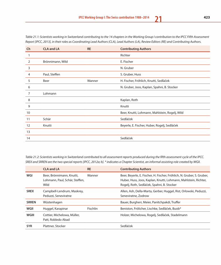
423IPCC Working Group I: The Swiss contribution 1988–2014 21
Table 21.1: Scientists working in Switzerland contributing to the 14 chapters in the Working Group I contribution to the IPCC Fifth Assessment Report [IPCC, 2013], in their roles as Coordinating Lead Authors (CLA), Lead Authors (LA), Review Editors (RE) and Contributing Authors.
Ch CLA and LA RE Contributing Authors
1 Richter
2 Brönnimann, Wild E. Fischer
3 N. Gruber
4 Paul, Steffen S. Gruber, Huss
5 Beer Wanner H. Fischer, Fröhlich, Knutti, Sedlàček
6 N. Gruber, Joos, Kaplan, Spahni, B. Stocker
7 Lohmann
8 Kaplan, Roth
9 Knutti
10 Beer, Knutti, Lohmann, Mahlstein, Rogelj, Wild
11 Schär Sedlàček
12 Knutti Beyerle, E. Fischer, Huber, Rogelj, Sedlàček
13
14 Sedlàček
Table 21.2: Scientists working in Switzerland contributed to all assessment reports produced during the fifth assessment cycle of the IPCC. SREX and SRREN are the two special reports [IPCC, 2012a; b]. * indicates a Chapter Scientist, an informal assisting role created by WGII.
CLA and LA RE Contributing Authors
WGI Beer, Brönnimann, Knutti, Lohmann, Paul, Schär, Steffen, Wild
Wanner Beer, Beyerle, E. Fischer, H. Fischer, Fröhlich, N. Gruber, S. Gruber, Huber, Huss, Joos, Kaplan, Knutti, Lohmann, Mahlstein, Richter, Rogelj, Roth, Sedlàček, Spahni, B. Stocker
SREX Campbell-Lendrum, Maskrey, Peduzzi, Seneviratne
Allen, Ash, Della-Marta, Gerber, Huggel, Rist, Orlowski, Peduzzi, Seneviratne, Zodrow
SRREN Wüstenhagen Bauer, Burgherr, Meier, Panitchpakdi, Truffer
WGII Huggel, Karapinar Fischlin Beniston, Frölicher, Lischke, Sedlàček, Buob*
WGIII Cottier, Michelowa, Müller, Patt, Robledo Abad
Holzer, Michelowa, Rogelj, Sedlàček, Stadelmann
SYR Plattner, Stocker Sedlàček
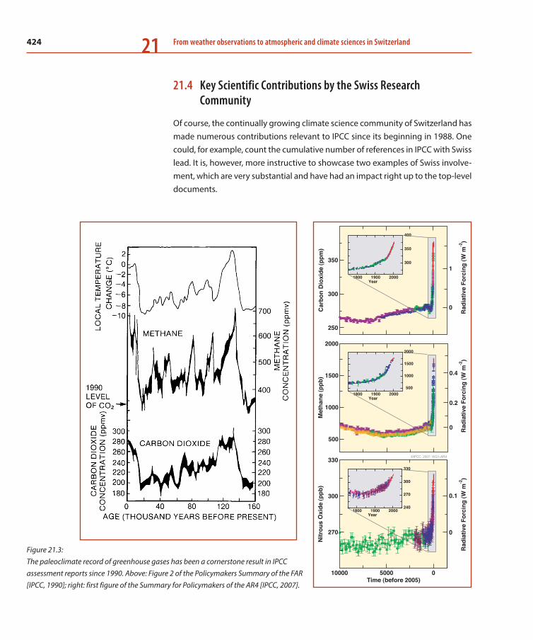
424 From weather observations to atmospheric and climate sciences in Switzerland21
21.4 Key Scientific Contributions by the Swiss Research Community
Of course, the continually growing climate science community of Switzerland has made numerous contributions relevant to IPCC since its beginning in 1988. One could, for example, count the cumulative number of references in IPCC with Swiss lead. It is, however, more instructive to showcase two examples of Swiss involve-ment, which are very substantial and have had an impact right up to the top-level documents.
Figure 21.3: The paleoclimate record of greenhouse gases has been a cornerstone result in IPCC assessment reports since 1990. Above: Figure 2 of the Policymakers Summary of the FAR [IPCC, 1990]; right: first figure of the Summary for Policymakers of the AR4 [IPCC, 2007].
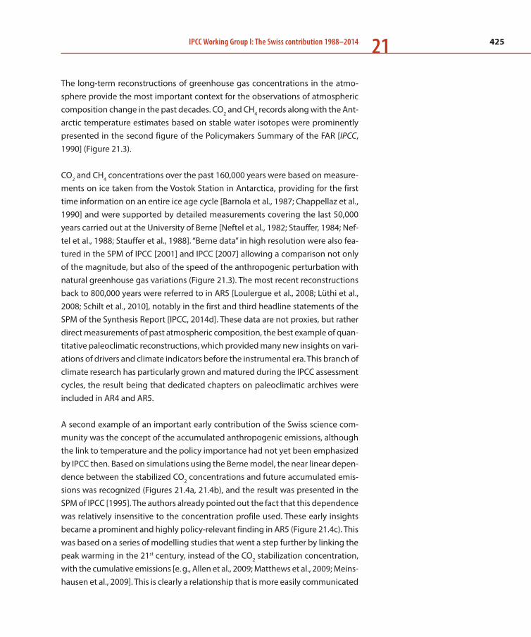
425IPCC Working Group I: The Swiss contribution 1988–2014 21
The long-term reconstructions of greenhouse gas concentrations in the atmo-sphere provide the most important context for the observations of atmospheric composition change in the past decades. CO2 and CH4 records along with the Ant-arctic temperature estimates based on stable water isotopes were prominently presented in the second figure of the Policymakers Summary of the FAR [IPCC, 1990] (Figure 21.3).
CO2 and CH4 concentrations over the past 160,000 years were based on measure-ments on ice taken from the Vostok Station in Antarctica, providing for the first time information on an entire ice age cycle [Barnola et al., 1987; Chappellaz et al., 1990] and were supported by detailed measurements covering the last 50,000 years carried out at the University of Berne [Neftel et al., 1982; Stauffer, 1984; Nef-tel et al., 1988; Stauffer et al., 1988]. “Berne data” in high resolution were also fea-tured in the SPM of IPCC [2001] and IPCC [2007] allowing a comparison not only of the magnitude, but also of the speed of the anthropogenic perturbation with natural greenhouse gas variations (Figure 21.3). The most recent reconstructions back to 800,000 years were referred to in AR5 [Loulergue et al., 2008; Lüthi et al., 2008; Schilt et al., 2010], notably in the first and third headline statements of the SPM of the Synthesis Report [IPCC, 2014d]. These data are not proxies, but rather direct measurements of past atmospheric composition, the best example of quan-titative paleoclimatic reconstructions, which provided many new insights on vari-ations of drivers and climate indicators before the instrumental era. This branch of climate research has particularly grown and matured during the IPCC assessment cycles, the result being that dedicated chapters on paleoclimatic archives were included in AR4 and AR5.
A second example of an important early contribution of the Swiss science com-munity was the concept of the accumulated anthropogenic emissions, although the link to temperature and the policy importance had not yet been emphasized by IPCC then. Based on simulations using the Berne model, the near linear depen-dence between the stabilized CO2 concentrations and future accumulated emis-sions was recognized (Figures 21.4a, 21.4b), and the result was presented in the SPM of IPCC [1995]. The authors already pointed out the fact that this dependence was relatively insensitive to the concentration profile used. These early insights became a prominent and highly policy-relevant finding in AR5 (Figure 21.4c). This was based on a series of modelling studies that went a step further by linking the peak warming in the 21st century, instead of the CO2 stabilization concentration, with the cumulative emissions [e. g., Allen et al., 2009; Matthews et al., 2009; Meins-hausen et al., 2009]. This is clearly a relationship that is more easily communicated
426 From weather observations to atmospheric and climate sciences in Switzerland21
as it directly connects the global climate impact, i. e., the warming, with the total-ity of anthropogenic carbon emissions.
The final figure (Figure 21.4c) as accepted in the SPM of IPCC [2013] was the result of many months of iterations among the lead authors, the TSU and the Co-Chairs. The first-order draft of the SPM did not include such a figure; but given the need for a policy relevant statement derived from the wealth of information from cli-mate model projections carried out under CMIP5 and models of reduced complex-ity, the author team finally converged on the basic layout shown in Figure 21.4c. It was a challenge to include information from the entire model hierarchy and combine it with a careful assessment of uncertainty, in order to have a figure based on multiple lines of independent evidence, a requirement for all figures in the WGI SPM. Here, the research group of Reto Knutti at ETH Zurich generated from their numerical database literally hundreds of different figure versions until a solid con-sensus on this figure was reached in the author team. This produced sufficient confidence to present it to the policymakers in the final draft of the SPM and to defend it during the approval plenary.
21.5 The IPCC Work as a Unique Stimulus of Scientific Research
Participating as a Lead Author or Coordinating Lead Author in an IPCC represents a significant commitment for a period of over 4 years. The contribution is voluntary, unpaid and mostly unassisted. Yet, for the past 27 years the IPCC has succeeded in recruiting many of the best and most active scientists to join the author teams. A
Figure 21.4: Concept of cumulative CO2 emissions: (a) as shown already in the SPM of IPCC [1995]; (b) anthropogenic emissions of (a), plotted in a diagram with swapped axes, for comparison with panel (c); (c) Figure 10 in the SPM of IPCC [2013].
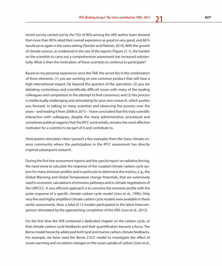
427IPCC Working Group I: The Swiss contribution 1988–2014 21
recent survey carried out by the TSU of WGI among the AR5 author team showed that more than 90 % rated their overall experience as good or very good, and 68 % would serve again in the same setting [Stocker and Plattner, 2014]. With the growth of climate science, as evidenced in the size of the reports (Figure 21.1), the burden on the scientists to carry out a comprehensive assessment has increased substan-tially. What is then the motivation of these scientists to continue to participate?
Based on my personal experience since the TAR, the secret lies in the combination of three elements: (1) you are working on one common product that will have a high international impact, far beyond the quarters of the specialists; (2) you are debating contentious and scientifically difficult issues with many of the leading colleagues and competitors in the attempt to find consensus; and (3) the process is intellectually challenging and stimulating for your own research, which pushes you forward. In talking to many scientists and observing the process over the years – and leading it from 2008 to 2015 – I have concluded that this truly scientific interaction with colleagues, despite the many administrative, procedural and sometimes political vagaries that the IPCC work entails, remains the most effective motivator for a scientist to be part of it and contribute to.
Participation stimulates: Here I present a few examples from the Swiss climate sci-ence community where the participation in the IPCC assessment has directly inspired subsequent research.
During the first two assessment reports and the special report on radiative forcing, the need arose to calculate the response of the coupled climate-carbon cycle sys-tem for many emission profiles and in particular to determine the metrics, e. g., the Global Warming and Global Temperature change Potentials, that are extensively used in economic calculations of emission pathways and in climate negotiations of the UNFCCC. A very efficient approach is to convolve the emission profile with the pulse response of a specific climate-carbon cycle model [Joos et al., 1996]. Only very few and highly simplified climate-carbon cycle models were available in these earlier assessments. Now, a total of 15 models participated in the latest intercom-parison stimulated by the approaching completion of the AR5 [Joos et al., 2013].
For the first time the TAR contained a dedicated chapter on the carbon cycle, so that climate-carbon cycle feedbacks and their quantification became a focus. The Berne model hierarchy addressed both land and marine carbon-climate feedbacks. For example, we have used the Berne 2.5CC model to investigate the effect of ocean warming and circulation changes on the ocean uptake of carbon [Joos et al.,

428 From weather observations to atmospheric and climate sciences in Switzerland21
1999]. The warming increases the atmospheric CO2 concentration by only 4 % com-pared to a model simulation in which the ocean feedback is ignored. While this is a moderate positive feedback, a collapse of the thermohaline circulation would reduce the uptake profoundly, as these model simulations demonstrated.
The very large uncertainty about the aerosol indirect effect in the Earth’s radiative balance was another important finding of the TAR. This prompted us to use the Berne 2.5D model of reduced complexity to perform extensive Monte Carlo sim-ulations, which were constrained by observations of surface warming and ocean heat uptake. The simulations yielded probabilistic estimates of the equilibrium climate sensitivity and the indirect aerosol effect [Knutti et al., 2002].
By the time of AR4, Earth System Models of Intermediate Complexity (EMICs) have closed the gap between the comprehensive climate models, then available from CMIP3, and the simple climate models that have been used since the IPCC FAR. EMICs were included in the climate model projections for the first time in a sys-tematic way in AR4 [Meehl et al., 2007]. This motivated a study comparing various EMICs and presenting projections based on them [Plattner et al., 2008]. Because these models are computationally efficient, they were well suited to estimate the long-term climate change commitments.
The visualization of uncertainty is an important issue in multimodel ensemble simulations. The first attempt at this was made in AR4 when presenting precipita-tion projections in the SPM [IPCC, 2007]. The goal was to provide a multimod-el-based guidance for the uncertainty language, e. g., in which regions a likely (> 66 % probability) increase or decrease of precipitation was projected. A small number of authors of the chapters dealing with projections in AR4 held intensive discussions at the last lead author meeting and in the few weeks thereafter, and after many iterations we settled on a convention to stipple areas where more than 90 % of the models agreed in the sign of the change and to leave areas uncolored where models did not agree in the sign of the projected change (Figure 21.5a). This was critically revisited in the subsequent assessment. The new author team of AR5 favoured showing all information as multimodel means but using two patterns instead, i. e., indicating areas where the signal-to-noise ratio is too small for a robust statement and where model agreement is strong, respectively. This issue continued to be debated during three lead author meetings involving several chapters until finally a consensus was found (Figure 21.5b). These lead author dis-cussions motivated three groups involved in AR5 to publish their considerations in the peer-reviewed literature [Tebaldi et al., 2011; Power et al., 2012; Knutti and
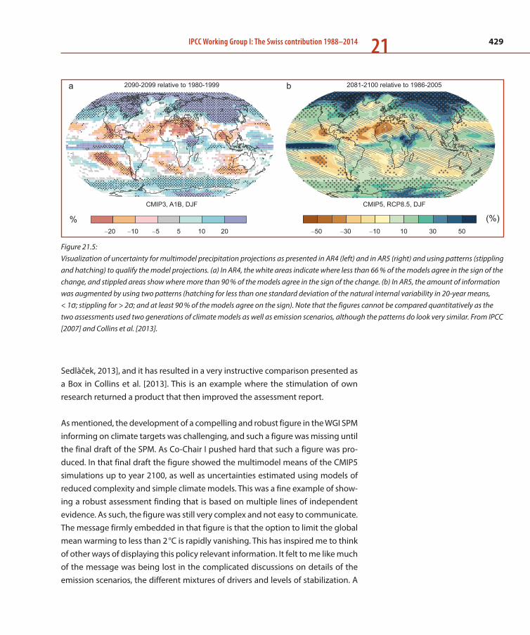
429IPCC Working Group I: The Swiss contribution 1988–2014 21
Sedlàček, 2013], and it has resulted in a very instructive comparison presented as a Box in Collins et al. [2013]. This is an example where the stimulation of own research returned a product that then improved the assessment report.
As mentioned, the development of a compelling and robust figure in the WGI SPM informing on climate targets was challenging, and such a figure was missing until the final draft of the SPM. As Co-Chair I pushed hard that such a figure was pro-duced. In that final draft the figure showed the multimodel means of the CMIP5 simulations up to year 2100, as well as uncertainties estimated using models of reduced complexity and simple climate models. This was a fine example of show-ing a robust assessment finding that is based on multiple lines of independent evidence. As such, the figure was still very complex and not easy to communicate. The message firmly embedded in that figure is that the option to limit the global mean warming to less than 2 °C is rapidly vanishing. This has inspired me to think of other ways of displaying this policy relevant information. It felt to me like much of the message was being lost in the complicated discussions on details of the emission scenarios, the different mixtures of drivers and levels of stabilization. A
2090-2099 relative to 1980-1999 2081-2100 relative to 1986-2005
CMIP5, RCP8.5, DJFCMIP3, A1B, DJF
−20 −10 −5 −50 −30 −105 10 20
%10 30 50
(%)
a b
Figure 21.5: Visualization of uncertainty for multimodel precipitation projections as presented in AR4 (left) and in AR5 (right) and using patterns (stippling and hatching) to qualify the model projections. (a) In AR4, the white areas indicate where less than 66 % of the models agree in the sign of the change, and stippled areas show where more than 90 % of the models agree in the sign of the change. (b) In AR5, the amount of information was augmented by using two patterns (hatching for less than one standard deviation of the natural internal variability in 20-year means, < 1σ; stippling for > 2σ; and at least 90 % of the models agree on the sign). Note that the figures cannot be compared quantitatively as the two assessments used two generations of climate models as well as emission scenarios, although the patterns do look very similar. From IPCC [2007] and Collins et al. [2013].
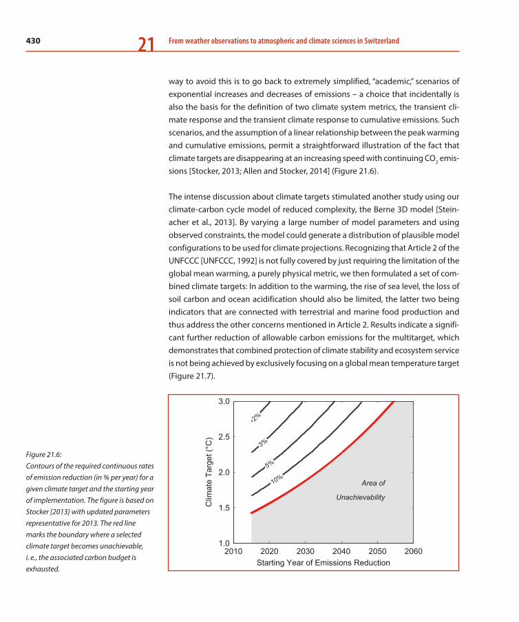
430 From weather observations to atmospheric and climate sciences in Switzerland21
way to avoid this is to go back to extremely simplified, “academic,” scenarios of exponential increases and decreases of emissions – a choice that incidentally is also the basis for the definition of two climate system metrics, the transient cli-mate response and the transient climate response to cumulative emissions. Such scenarios, and the assumption of a linear relationship between the peak warming and cumulative emissions, permit a straightforward illustration of the fact that climate targets are disappearing at an increasing speed with continuing CO2 emis-sions [Stocker, 2013; Allen and Stocker, 2014] (Figure 21.6).
The intense discussion about climate targets stimulated another study using our climate-carbon cycle model of reduced complexity, the Berne 3D model [Stein-acher et al., 2013]. By varying a large number of model parameters and using observed constraints, the model could generate a distribution of plausible model configurations to be used for climate projections. Recognizing that Article 2 of the UNFCCC [UNFCCC, 1992] is not fully covered by just requiring the limitation of the global mean warming, a purely physical metric, we then formulated a set of com-bined climate targets: In addition to the warming, the rise of sea level, the loss of soil carbon and ocean acidification should also be limited, the latter two being indicators that are connected with terrestrial and marine food production and thus address the other concerns mentioned in Article 2. Results indicate a signifi-cant further reduction of allowable carbon emissions for the multitarget, which demonstrates that combined protection of climate stability and ecosystem service is not being achieved by exclusively focusing on a global mean temperature target (Figure 21.7).
2%
3%
5%
10%
Starting Year of Emissions Reduction
Clim
ate
Targ
et (°
C)
Area of
Unachievability
2010 2020 2030 2040 2050 20601.0
1.5
2.0
2.5
3.0
Figure 21.6: Contours of the required continuous rates of emission reduction (in % per year) for a given climate target and the starting year of implementation. The figure is based on Stocker [2013] with updated parameters representative for 2013. The red line marks the boundary where a selected climate target becomes unachievable, i. e., the associated carbon budget is exhausted.

431IPCC Working Group I: The Swiss contribution 1988–2014 21
21.6 Evolution of Communication in IPCC
It is instructive to revisit the evolution of how the findings in the top-level docu-ments of the IPCC reports have been communicated and how this has changed with the advent of electronic tools since the FAR in 1990. The Policymakers Sum-mary of the FAR had a well-designed structure, organized along specific ques-tions, such as “What are the greenhouse gases and why are they increasing?”, or “How much confidence do we have in our predictions?” The document was pre-ceded by a succinct 2-page Executive Summary, which again was structured along assertions: “We are certain of the following …”, “We calculate with confi-dence …”, or “Based on current model results, we predict …” The Policymakers Summary was rather long, with 33 text pages and 13 figures, all in black and white. Nevertheless, the access for the reader was certainly facilitated by such structuring along simple questions.
This strategy was changed fundamentally in the second assessment report. Here, the SPM was very short, only 7 pages with no figures. The scientific substance with detailed numbers and figures was deferred to a Technical Summary, an innovation in that assessment.
The TAR presented a 20-page SPM with coloured figures and two types of headline statements. Although the scientific details were back again in the SPM, the Tech-nical Summary was also retained, now larger in size and complexity, like the entire report compared to its predecessors. The headline statements in this assessment were short and succinct, for example, “An increasing body of observations gives a collective picture of a warming world and other changes in the climate system” or
Cumulative fossil-fuel CO2 emission (Gt carbon)0 500250 750 1000
1750
1950
1980
2000
2010
2020
2°C-Target
all targets
Figure 21.7: Allowable carbon emissions compatible with staying below the global mean tem-perature target of 2 °C, and the associated Earth System multitargets consisting of limiting simultaneously global mean temperature, sea level rise, acidification in the Southern Ocean and globally, pro-ductive cropland area loss, and carbon loss on croplands. Results are based on Steinacher et al. [2013]; the figure was designed by M. Steinacher.
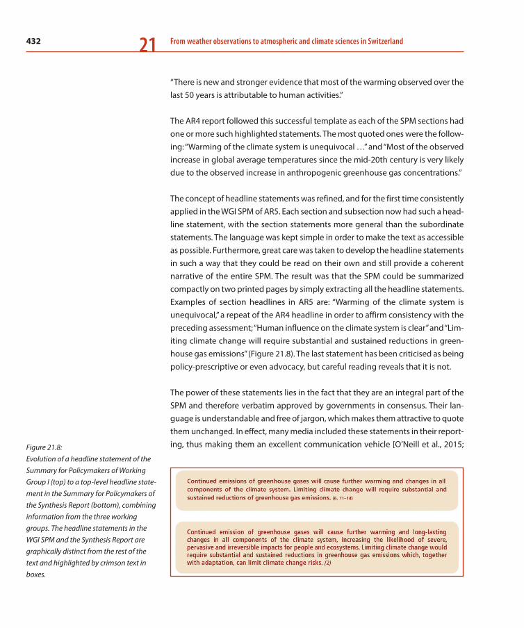
432 From weather observations to atmospheric and climate sciences in Switzerland21
“There is new and stronger evidence that most of the warming observed over the last 50 years is attributable to human activities.”
The AR4 report followed this successful template as each of the SPM sections had one or more such highlighted statements. The most quoted ones were the follow-ing: “Warming of the climate system is unequivocal …” and “Most of the observed increase in global average temperatures since the mid-20th century is very likely due to the observed increase in anthropogenic greenhouse gas concentrations.”
The concept of headline statements was refined, and for the first time consistently applied in the WGI SPM of AR5. Each section and subsection now had such a head-line statement, with the section statements more general than the subordinate statements. The language was kept simple in order to make the text as accessible as possible. Furthermore, great care was taken to develop the headline statements in such a way that they could be read on their own and still provide a coherent narrative of the entire SPM. The result was that the SPM could be summarized compactly on two printed pages by simply extracting all the headline statements. Examples of section headlines in AR5 are: “Warming of the climate system is unequivocal,” a repeat of the AR4 headline in order to affirm consistency with the preceding assessment; “Human influence on the climate system is clear” and “Lim-iting climate change will require substantial and sustained reductions in green-house gas emissions” (Figure 21.8). The last statement has been criticised as being policy-prescriptive or even advocacy, but careful reading reveals that it is not.
The power of these statements lies in the fact that they are an integral part of the SPM and therefore verbatim approved by governments in consensus. Their lan-guage is understandable and free of jargon, which makes them attractive to quote them unchanged. In effect, many media included these statements in their report-ing, thus making them an excellent communication vehicle [O’Neill et al., 2015; Figure 21.8:
Evolution of a headline statement of the Summary for Policymakers of Working Group I (top) to a top-level headline state-ment in the Summary for Policymakers of the Synthesis Report (bottom), combining information from the three working groups. The headline statements in the WGI SPM and the Synthesis Report are graphically distinct from the rest of the text and highlighted by crimson text in boxes.
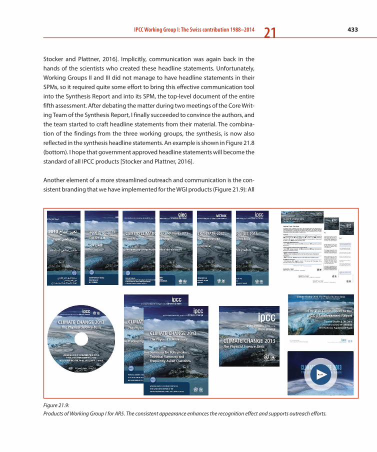
433IPCC Working Group I: The Swiss contribution 1988–2014 21
Stocker and Plattner, 2016]. Implicitly, communication was again back in the hands of the scientists who created these headline statements. Unfortunately, Working Groups II and III did not manage to have headline statements in their SPMs, so it required quite some effort to bring this effective communication tool into the Synthesis Report and into its SPM, the top-level document of the entire fifth assessment. After debating the matter during two meetings of the Core Writ-ing Team of the Synthesis Report, I finally succeeded to convince the authors, and the team started to craft headline statements from their material. The combina-tion of the findings from the three working groups, the synthesis, is now also reflected in the synthesis headline statements. An example is shown in Figure 21.8 (bottom). I hope that government approved headline statements will become the standard of all IPCC products [Stocker and Plattner, 2016].
Another element of a more streamlined outreach and communication is the con-sistent branding that we have implemented for the WGI products (Figure 21.9): All
Figure 21.9: Products of Working Group I for AR5. The consistent appearance enhances the recognition effect and supports outreach efforts.
434 From weather observations to atmospheric and climate sciences in Switzerland21
feature the WGI title photograph of the Folgefonna glacier in Norway, a rapidly melting body of ice. This consistent appearance supports the recognition effect and enhances outreach. Various additional products were also developed: a Sum-mary Volume, a brochure with the FAQs (Frequently Asked Questions), the sheets of the extracted headline statements in all UN languages, a USB containing all WGI material, a professionally produced video and presentation slides (Figure 21.9). For scientists, WGI also made available all of the more than 9,000 references in elec-tronic bibliographic formats and the more than 1,200 figures of the report, almost all of which are embedded in vector format and therefore in unlimited resolution, in the published pdf files.
21.7 Outlook
The fifth assessment has impressively demonstrated the limits that the scientists are confronted with when carrying out a comprehensive task on a voluntary, unpaid and largely unassisted basis. Given the continuing growth of scientific information about the Earth System, and the call of governments and stakehold-ers to receive ever more and more detailed information on regional changes and impacts, begs the question whether the scientists will be able to deliver another assessment in the next 5 to 7 years at the same level of quality and rigor. The will-ingness of the scientific community is certainly intact: Most colleagues are con-vinced that contributing to an assessment is indeed a duty and represents one way to “give back” to society by making the best information available for smart decisions regarding the future of us all. However, the amount of work during AR5 was staggering. More than 9,000 publications from the peer-reviewed literature were considered in this assessment, more than 2 million GB of numerical data were produced by climate models, and more than 50,000 comments were responded to, by WGI. None of these numbers are expected to become smaller in the next assessment if no changes are implemented in the assessment process, nor will it be possible to deliver an equally comprehensive and robust report with-out having more hands on deck.
In a recent article in Nature, Gian-Kasper Plattner and I have considered how to ensure the success of the next assessment [Stocker and Plattner, 2014]. We pro-pose that those who commission these assessments – the governments – should consider some form of institutionalized support for scientists in leading or partic-ularly demanding positions such as those coordinating a chapter, working on cross-cuts or serving in more than one working group. The extension of the assess-
435IPCC Working Group I: The Swiss contribution 1988–2014 21
ment cycle would not only reduce the time pressure, it would open up the possi-bility for enhanced cross-working group collaboration. For example, climate model simulations so far could not be used to the full potential for impact studies because the time-lag between the schedules of the different working groups was too short. Assessing specific common topics jointly between working groups would reduce the workload and ease the synthesis towards the end of the cycle. On the other hand, smaller, more focused reports such as a series of Special Reports, would likely not generate the broad and worldwide impact that a series of well-coordinated working group assessment reports enjoys.
As this book is being published, the sixth assessment cycle of the IPCC has started. At its 41st Plenary Session in February 2015, the IPCC decided to keep the current structure of Working Groups I, II and III as well as a Task Force on National Green-house Gas Inventories, and requested each working group to produce a compre-hensive assessment report within the next 5 to 7 years. More regional participation of scientists, particularly from developing countries, was a recurrent request by the member countries of the IPCC. Several suggestions for Special Reports during the next cycle were also made. In summary, the Panel chose the conservative approach of “business-as-usual” and did not really come to grips with the ever-growing bur-den put on the shoulders of the scientific community by this process. This is an issue the future leadership must address in a proactive way, for example, by enhancing the scoping of the reports, modifying the way chapters cutting across working groups are produced or considering how the Synthesis Report will be writ-ten, the goal being to make the process overall more efficient for the scientific community – without jeopardizing the high level of respect and international rec-ognition that the IPCC has built up in the past 27 years of its existence.
Any adjustment to the IPCC process, however, needs to be mindful of the fact that a rigorous and comprehensive assessment can be delivered to the policymakers and stakeholders only if it is based on the wide support of the scientific commu-nity, foremost the leading scientists of their field.
Acknowledgements
I gratefully acknowledge the collective work the Swiss climate science community, the many friends and colleagues who have donated their expertise and a substan-tial amount of their time to the production of the past five assessment reports of the IPCC WGI. I thank Fortunat Joos and Gian-Kasper Plattner for comments and
436 From weather observations to atmospheric and climate sciences in Switzerland21
René Bleisch for preparing Figure 21.4b. I wish to express my deep appreciation to all colleagues of the Technical Support Unit of WGI, whose dedication, commit-ment and intellectual input was truly exceptional and on whom I could count since its establishment for AR5 in January 2009. My sincere thanks go to the Swiss Federal Office of the Environment and the University of Berne for the financial and logistical support of the TSU and my co-chairship during AR5 from 2008 to 2015. The dedication of Jose Romero for the IPCC process, and the dedication of the Swiss scientists who contributed to it, is respectfully acknowledged. Finally, thanks go to all WGI colleagues for their enthusiasm and their fine spirit during AR5.
References
Allen, M. R., D. J. Frame, C. Huntingford, C. D. Jones, J. A. Lowe, M. Meinshausen, N. Meinshausen, Warming caused by cumulative carbon emissions towards the trillionth tonne, Nature, 458, 1163–1166, 2009.
Allen, M. R., T. F. Stocker, Impact of delay in reducing carbon dioxide emissions, Nature Clim. Change, 4, 23–26, 2014.
Barnola, J. M., D. Raynaud, Y. S. Korotkevich, C. Lorius, Vostok ice core provides 160,000-year record of atmospheric CO2, Nature, 329, 408–414, 1987.
Bolin, B., A History of the Science and Politics of Climate Change: The Role of the Intergovernmental Panel on Climate Change 292 pp., Cambridge, 2008.
Chappellaz, J., J.-M. Barnola, D. Raynaud, Y. S. Korotkevich, C. Lorius, Ice core record of atmospheric methane over the past 160,000-years, Nature, 345, 127–131, 1990.
Collins, M., R. Knutti, J. Arblaster, J.-L. Dufresne, T. Fichefet, P. Friedlingstein, X. Gao, W. J. Gutowski, T. Johns, G. Krinner, M. Shongwe, C. Tebaldi, A. J. Weaver, M. Wehner, Long-term Climate Change: Projections, Commitments and Irreversibility, in Cli-mate Change 2013: The Physical Science Basis. Contribution of Working Group I to the Fifth Assessment Report of the Intergovern-mental Panel on Climate Change, [T. F. Stocker et al. (Eds.)], pp. 1029–1136, 2013.
Hansen, J., The greenhouse effect: impacts on current global temperaturey and regional heat waves., Testimony befroe the Committee on Energy and Natural Resources, US Senate, Wash-ington DC, June 23, 1988.
IPCC, Climate Change, The IPCC Scientific Assessment, [J. T. Hough-ton et al. (Eds.)], 365 pp., Intergovernmental Panel on Climate Change, Cambridge University Press, Cambridge, 1990.
IPCC, IPCC Climate Change 1994: Radiative Forcing of Climate Change and An Evaluation of the IPCC IS92 Emission Scenarios, [J. T. Houghton et al. (Eds.)], 339 pp., Cambridge University Press, 1995.
IPCC, Climate Change 1995: The Science of Climate Change. Con-tribution of Working Group I to the Second Assessment Report of the Intergovernmental Panel on Climate Change, [J. T. Houghton et al. (Eds.)], 572 pp., Cambridge University Press, 1996.
IPCC, Climate Change 2001: The Scientific Basis. Contribution of Working Group I to the Third Assessment Report of the Intergovern-mental Panel on Climate Change, [J. T. Houghton et al. (Eds.)], 881 pp., Cambridge University Press, Cambridge, 2001.
IPCC, Climate Change 2007: The Physical Science Basis. Contri-bution of Working Group I to the Fourth Assessment Report of the Intergovernmental Panel on Climate Change, [S. Solomon et al. (Eds.)], 996 pp., Cambridge University Press, Cambridge, 2007.
IPCC, Managing the Risks of Extreme Events and Disasters to Advance Climate Change Adaptation. A Special Report of Working Groups I and II of the Intergovernmental Panel on Climate Change, [C. B. Field et al. (Eds.)], 582 pp., Cambridge University Press, Cambridge, 2012a.

437IPCC Working Group I: The Swiss contribution 1988–2014 21IPCC, Renewable Energy Resources and Climate Change Mitiga-tion, [O. Edenhofer et al. (Eds.)], 1076 pp., Cambridge University Press, Cambridge, UK, New York, NY, USA, 2012b.
IPCC, Climate Change 2013: The Physical Science Basis. Contribu-tion of Working Group I to the Fifth Assessment Report of the Inter-governmental Panel on Climate Change, [T. F. Stocker et al. (Eds.)], 1535 pp., Cambridge University Press, Cambridge, 2013.
IPCC, Climate Change 2014: Impacts, Adaptation, and Vulnerabil-ity. Part A: Global and Sectoral Aspects. Contribution of Working Group II to the Fifth Assessment Report of the Intergovernmental Panel on Climate Change, [C. B. Field et al. (Eds.)], 1132 pp., Cam-bridge University Press, Cambridge, 2014a.
IPCC, Climate Change 2014: Impacts, Adaptation, and Vulnerabil-ity. Part B: Regional Aspects. Contribution of Working Group II to the Fifth Assessment Report of the Intergovernmental Panel on Climate Change, [C. B. Field et al. (Eds.)], 668 pp., Cambridge Uni-versity Press, Cambridge, 2014b.
IPCC, Climate Change 2014: Mitigation of Climate Change. Contri-bution of Working Group III to the Fifth Assessment Report of the Intergovernmental Panel on Climate Change, [O. Edenhofer et al. (Eds.)], 1435 pp., Cambridge University Press, Cambridge, 2014c.
IPCC, Climate Change 2014: Synthesis Report, [R. K. Pachauri et al. (Eds.)], 148 pp., Cambridge University Press, 2014d.
Joos, F., M. Bruno, R. Fink, T. F. Stocker, U. Siegenthaler, C. Le Quéré, J. L. Sarmiento, An efficient and accurate representation of complex oceanic and biospheric models of anthropogenic carbon uptake, Tellus, 48B, 397–417, 1996.
Joos, F., G.-K. Plattner, T. F. Stocker, O. Marchal, A. Schmittner, Global warming and marine carbon cycle feedbacks on future atmospheric CO2, Science, 284, 464–467, 1999.
Joos, F., I. C. Prentice, S. Sitch, R. Meyer, G. Hooss, G.-K. Plattner, S. Gerber, K. Hasselmann, Global warming feedbacks on terrestrial carbon uptake under the Intergovernmental Panel on Climate Change (IPCC) emission scenarios, Glob. Biogeochem. Cyc., 15, 891–908, 2001.
Joos, F., R. Roth, J. S. Fuglestvedt, G. P. Peters, I. G. Enting, W. von Bloh, V. Brovkin, E. J. Burke, M. Eby, N. R. Edwards, T. Friedrich, T. L. Frölicher, P. R. Halloran, P. B. Holden, C. Jones, T. Kleinen, F. T. Mackenzie, K. Matsumoto, M. Meinshausen, G.-K. Plattner, A. Reisinger, J. Segschneider, G. Shaffer, M. Steinacher, K. Strass-
mann, K. Tanaka, A. Timmermann, A. J. Weaver, Carbon dioxide and climate impulse response functions for the computation of greenhouse gas metrics: a multi-model analysis, Atm. Chem. Phys., 13, 2793–2825, 2013.
Knutti, R., J. Sedlàček, Robustness and uncertainties in the new CMIP5 climate model projections, Nature Clim. Change, 3, 369–373, 2013.
Knutti, R., T. F. Stocker, F. Joos, G.-K. Plattner, Constraints on radi-ative forcing and future climate change from observations and climate model ensembles, Nature, 416, 719–723, 2002.
Loulergue, L., A. Schilt, R. Spahni, V. Masson-Delmotte, T. Blunier, B. Lemieux, J.-M. Barnola, D. Raynaud, T. F. Stocker, J. Chappellaz, Orbital and millennial-scale features of atmospheric CH4 over the past 800,000 years, Nature, 453, 383–386, 2008.
Lüthi, D., M. Le Floch, B. Bereiter, T. Blunier, J.-M. Barnola, U. Sie-genthaler, D. Raynaud, J. Jouzel, H. Fischer, K. Kawamura, T. F. Stocker, High-resolution carbon dioxide concentration record 650,000–800,000 years before present, Nature, 453, 379–382, 2008.
Matthews, H. D., N. P. Gillett, P. A. Stott, K. Zickfeld, The propor-tionality of global warming to cumulative carbon emissions, Nature, 459, 829–833, 2009.
Meehl, G. A., T. F. Stocker, W. D. Collins, P. Friedlingstein, A. T. Gaye, J. M. Gregory, A. Kitoh, R. Knutti, J. M. Murphy, A. Noda, S. C.B. Raper, I. G. Watterson, W. A. J., Z.-C. Zhao, Global Climate Projec-tions, in Climate Change 2007: The Physical Science Basis. Contri-bution of Working Group I to Fourth Assessment Report of the Intergovernmental Panel on Climate Change, [S. Solomon et al. (Eds.)], pp. 747–845, 2007.
Meinshausen, M., N. Meinshausen, W. Hare, S. C.B. Raper, K. Frieler, R. Knutti, D. J. Frame, M. R. Allen, Greenhouse-gas emission targets for limiting global warming to 2 degrees C, Nature, 458, 1158–1163, 2009.
Neftel, A., H. Oeschger, J. Schwander, B. Stauffer, R. Zumbrunn, Ice core sample measurements give atmospheric CO2 content during the Past 40,000 Yr, Nature, 295, 220–223, 1982.
Neftel, A., H. Oeschger, T. Staffelbach, B. Stauffer, CO2 record in the Byrd ice core 50,000–5,000 years BP, Nature, 331, 609–611, 1988.
438 From weather observations to atmospheric and climate sciences in Switzerland21
O’Neill, S., H. W.T. Williams, T. Kurz, B. Wiersma, M. Boykoff, Dom-inant frames in legacy and social media coverage of the IPCC Fifth Assessment Report, Nature Clim. Change, 5, 380–385, 2015.
Oreskes, N., E. Conway, Merchants of Doubt, 355 pp., Bloomsbury Press, 2010.
Plattner, G.-K., R. Knutti, F. Joos, T. F. Stocker, W. von Bloh, V. Brovkin, D. Cameron, E. Driesschaert, S. Dutkiewicz, M. Eby, N. R. Edwards, T. Fichefet, J. C. Hargreaves, C. D. Jones, M. F. Loutre, H. D. Matthews, A. Mouchet, S. A. Mueller, S. Nawrath, A. Price, A. Sokolov, K. M. Strassmann, A. J. Weaver, Long-term climate com-mitments projected with climate – carbon cycle models, J. Clim., 21, 2721–2751, 2008.
Power, S. B., F. Delage, R. Colman, A. Moise, Consensus on twen-ty-first-century rainfall projections in climate models more widespread than previously thought, J. Clim., 25, 3792–3809, 2012.
Schilt, A., M. Baumgartner, T. Blunier, J. Schwander, R. Spahni, H. Fischer, T. F. Stocker, Glacial-interglacial and millennial-scale variations in the atmospheric nitrous oxide concentration during the last 800,000 years, Quat. Sci. Rev., 29, 182–192, 2010.
Siegenthaler, U., F. Joos, Use of a simple model for studying oceanic tracer distributions and the global carbon cycle, Tellus, 44B, 186–207, 1992.
Siegenthaler, U., H. Oeschger, Predicting future atmospheric carbon dioxide levels, Science, 199, 388–395, 1978.
Stauffer, B., H. Hofer, H. Oeschger, J. Schwander, U. Siegenthaler, Atmospheric CO2 concentration during the last glaciation, Ann. Glaciol., 5, 160–164, 1984.
Stauffer, B., E. Lochbronner, H. Oeschger, J. Schwander, Methane concentration in the glacial atmosphere was only half that of the preindustrial Holocene, Nature, 332, 812–814, 1988.
Steinacher, M., F. Joos, T. F. Stocker, Allowable carbon emissions lowered by multiple climate targets, Nature, 499, 197–201, 2013.
Stocker, T., Obituary – Hans Oeschger (1927–98) – Pioneer in environmental physics, Nature, 397, 396, 1999.
Stocker, T. F., The closing door of climate targets, Science, 339, 280–282, 2013.
Stocker, T. F., G. K.C. Clarke, H. Le Treut, R. S. Lindzen, V. P. Meles-hko, R. K. Mugara, T. N. Palmer, R. T. Pierrehumbert, P. J. Sellers, K. E. Trenberth, J. Willebrand, Physical Climate Processes and Feedbacks, in Climate Change 2001: The Scientific Basis. Contri-bution of Working Group I to the Third Assessment Report of the Intergovernmental Panel on Climate Change, [J. T. Houghton et al. (Eds.)], pp. 417–470, 2001.
Stocker, T. F., G.-K. Plattner, Rethink IPCC reports, Nature, 513, 163–165, 2014.
Stocker, T. F., G.-K. Plattner, Correspondence: Making use of the IPCC’s powerful communication tool. Nature Clim. Change, 6, advance online, doi: 10.1038/nclimate3010, 2016.
Tebaldi, C., J. M. Arblaster, R. Knutti, Mapping model agreement on future climate projections, Geophys. Res. Lett., 38, L23701, 2011.
UNFCCC, United Nations Framework Convention on Climate Change (FCCC/INFORMAL/84 GE.05-62220 (E) 200705), New York, 1992.
UNFCCC, The Cancun Agreements, United Nations Framework Convention on Climate Change, The Cancun Agreements, FCCC/CP/2010/7/Add.1, 2010.
Watson, R. T., H. Rodhe, H. Oeschger, U. Siegenthaler, Green-house Gases and Aerosols, in Climate Change. The IPCC Scientific Assessment, [J. T. Houghton et al. (Eds.)], pp. 1–40, 1990.
439
22 Appendix A
Acronyms and abbreviations
The following list is a compilation of acronyms and abbreviations used in the dif-ferent chapters of this book, sorted in alphabetical order. Most of the acronyms are in English, as is typically the case for recent names of organizations, experi-ments, etc. Some abbreviations are given in their original language (German, French).
A1. Organisations and institutions
Abbreviation English name Original name (German, French, Italian) Period*
armasuisse Swiss Army Procurement Agency armasuisse (ehem. Gruppe für Rüstung 1994–2003 / Gruppe für Rüstungsdienste 1968–1994)
2003–present
AWI Alfred Wegener Institute for Polar and Marine Research
1980–present
C2SM Center for Climate Systems Modeling 2008–present
CAI Convention Aérienne Internationale
CERN European Organization for Nuclear Research
Centre Européen de la Recherche Nucléaire 1954–present
CIMO WMO Commission for Instruments and Methods of Observations
1951–present
CLRTAP Convention on Long Range Trans-boundary Air Pollution
1983–present
CNES National Centre for Space Studies, Toulouse F
Centre National d’Études Spatiales, Toulouse, F 1961–present
CN-MET Centrale Nucléaire et METéorologie 2009–present
COSMO Consortium for Small-scale Modelling 1998–present

440 From weather observations to atmospheric and climate sciences in Switzerland22
A1. Organisations and institutions
Abbreviation English name Original name (German, French, Italian) Period*
COST European Collaboration in Science and Technology
1971–present
CSCS Swiss National Supercomputing Centre 1991–present
CSEM Swiss Center for Electronics and Micro-technology
Centre Suisse d’Electronique et de Microtech-nique
1984–present
EAN European Aerological Network ca. 1939–present
ECMWF European Centre for Medium-Range Weather Forecasts, Reading UK
Europäisches Zentrum für mittelfristige Wettervorhersage (EZMW)
1975–present
EIR Swiss Federal Institute for Reactor Research
Eidgenössisches Institut für Reaktorforschung 1960–1988
Empa Swiss Federal Laboratories for Materials Science and Technology
Eidgenössische Materialprüfungs- und Forschungsanstalt
1880–present
EPFL Swiss Federal Institut of Technology Lausanne
Ecole Polytechnique Féderal Lausanne (1853) 1890–present
ETH, ETHZ Swiss Federal Institut of Technology Zurich
Eidgenössische Technische Hochschule Zürich 1855–present
FHNW University of Applied Sciences and Arts Northwestern Switzerland
Fachhochschule Nordwestschweiz 2006–present
FOEN Federal Office for the Environment Bundesamt für Umwelt, Wald und Landschaft (BUWAL)
until 2005
FOEN Federal Office for the Environment Bundesamt für Umwelt (BAFU) 2006–present
GIETH Institute of Geography ETH Geografisches Institut ETH
GMA Swiss Society for Geophysics, Meteorology and Astronomy
Gesellschaft für Geophysik, Meteorologie und Astronomie
1916–1969
HFSJG High Altitude Research Stations Jungfraujoch and Gornergrat
Hochalpine Forschungsstation Jungfraujoch und Gornergrat
1930–present
IACETH Institute for Atmospheric and Climate Science ETH (Merger of LAPETH and IKF)
2001–present
IAMAS International Association of Meteorol-ogy and Atmospheric Sciences
1993–present
IAP Institute of Applied Physics, University of Bern
Institut für Angewandte Physik, Universität Bern
ICDM International Commission for Dynamic Meteorology
1967–present

441Appendix A 22
A1. Organisations and institutions
Abbreviation English name Original name (German, French, Italian) Period*
ICSU International Council for Science 1931–present
IKF Institut for Climate Research Institut für Klimaforschung 2000–2001
IMC International Meteorological Commit-tee
1879–1951
IMO International Meteorological Organisa-tion
1879–1951
IOC International Ozone Commission 1948–present
IPCC Intergovernmental Panel on Climate Change
1988–present
IUGG International Union of Geodesy and Geophysics
1919–present
LAPETH Laboratory for Atmospheric Physics ETH Laboratorium für Atmosphärenphysik ETH 1962–2001
LKO Light-climatic Observatory Arosa Lichtklimatisches Observatorium Arosa 1926–present
METAS Federal Institute of Metrology Eidgenössisches Institut für Metrologie (METAS = METrologie und Akkreditierung Schweiz)
(1862) 2001–present
MeteoSchweiz, MétéoSuisse, MeteoSvizzera, MeteoSwiss
Swiss Federal Office for Meteorology and Climatology
Bundesamt für Meteorologie und Klima tologie (ehemals MZA, dann SMA)
2000–present
MZA – ISM Swiss Central Meteorological Institute Schweizerische Meteorologische Zentral-anstalt = Institut suisse de météorologie
1880–1979
NDACC Network for the Detection of Atmo-spheric Composition Change
1991–present
NOAA National Oceanic and Atmospheric Administration
1807–present
OcCC Organe consultatif sur les changements climatiques / Beratendes Organ für Fragen der Klimaänderung
1996–present
OCCR Oeschger Centre for Climate Change Research
2007–present
OECD Organisation for Economic Co- operation and Development
1961–present
OeG Economic Society of Bern Oekonomische Gesellschaft Bern 1759–1890

442 From weather observations to atmospheric and climate sciences in Switzerland22
A1. Organisations and institutions
Abbreviation English name Original name (German, French, Italian) Period*
OSCE Organisation for Security and Co- operation in Europe
Organisation für Sicherheit und Zusammen-arbeit in Europa (OSZE)
1975–present
OTL Osservatorio Ticinese Locarno 1935–present
PMC Permanent Meteorological Committee 1873–1879
PMOD-WRC World Radiation Centre Davos Physikalisch-Meteorologisches Observatorium Davos
1907–present
PSI Paul Scherrer Institute Paul Scherrer Institut 1988–present
SAC Swiss Alpine Club Schweizer Alpenclub 1863–present
SAP Station Aérologique Payerne 1941–present
SAS, SANW-ASSN Swiss Academy of Sciences Schweizerische Akademie der Naturwissen-schaften = Académie suisse des sciences naturelles = Accademia svizzera di scienze naturali
1988–2003
SCNAT Swiss Academy of Sciences Akademie der Naturwissenschaften Schweiz = Académie suisse des sciences naturelles = Accademia svizzera di scienze naturali
2004–present
SGG Swiss Society for Geophysics Schweizerische Gesellschaft für Geophysik 1970–1994
SGGN Allgemeine Schweizerische Gesellschaft für die Gesammten Naturwissenschaften = Société Helvétique des Sciences Naturelles
1815–1837
SGM – SSM Swiss Society for Meteorology Schweizerische Gesellschaft für Meteorolo-gie – Société Suisse de Météorologie – Società Svizzera della Meteorologia
1994–present
SIPRE Snow, Ice and Permafrost Research Establishment (fore-runner of Cold Regions Research and Engineering Laboratory, CRREL)
1949–1961
SMA – ISM – SMI Swiss Meteorological Institute Schweizerische Meteorologische Anstalt = Institut suisse de météorologie
1979–1999
SNG – SHSN Swiss Society for Natural Sciences Schweizerische Naturforschende Gesellschaft = Société Helvétique des Sciences Naturelles = Società Elvetica di Scienze Naturali
1838–1987
SNSF Swiss National Science Foundation Schweizerischer Nationalfonds zur Förderung der Forschung (SNF)
1952–present
Swisscom Swiss Telecommunication Service Swisscom (1852) 1997–present
443Appendix A 22
A1. Organisations and institutions
Abbreviation English name Original name (German, French, Italian) Period*
swisstopo Federal Office of Topography Bundesamt für Landestopografie 1838–present
UNECE United Nations Economic Commission for Europe
1947–present
WCC-UV World Calibration Centre-Ultraviolet 2013–present
WHO World Health Organization Weltgesundheitsorganisation der UNO 1948–present
WMO World Meteorological Organzation 1951–present
WORCC World Optical Depth Research and Calibration Centre
1996–present
WRC-IRS World Radiation Centre for Infrared Radiation Sensors
2004–present
WRMC World Radiation Monitoring Centre 1992–2007
ZAMG Central Institution for Meteorology and Geodynamics, Vienna
Zentralanstalt für Meteorologie und Geodynamik, Wien
1851–present
Commission for Aeronautics (part of IMC)
Aeronautische Kommission 1896–1902
Swiss Meteorological Commission Meteorologische Kommission 1862–1881
Eidgenössische meteorologische Fachkommission
1882–2007
Federal Astronomical Observatory Eidgenössische Sternwarte 1862–1980
Federal Convention Bundesversammlung
Federal Council Bundesrat
Swiss Institute for High-Alpine Physiol-ogy and Tuberculosis Research in Davos
Schweizerisches Institut für Hochgebirgs-physiologie und Tuberkuloseforschung in Davos
1923–1926
Swiss Research Institute for High-Alpine Climate and Tuberculosis
Schweizerisches Forschungsinstitut für Hochgebirgsklima und Tuberkulose
1926–ca. 1950
Swiss Research Institute for High-Alpine Climate and Medicine
Schweizerisches Forschungsinstitut für Hochgebirgsklima und Medizin
ca 1950–present
* Numbers in brackets indicate when a forerunner institution was established

444 From weather observations to atmospheric and climate sciences in Switzerland22
A2. Experiments, infrastructure and projects
Abbreviation English name Original name (German, French, Italian)
ACTRIS Aerosol, Clouds, and Trace Gases Research Infrastructure Network
AGAGE Advanced Global Atmospheric Gases Experiment
AGNES Swiss global navigation satellite system network
ALPEX The Alpine Experiment
AMETIS Aeronautical Meteorological Information System
ANETZ National Automatic Meteorological Monitoring Network Automatisches Beobachtungsnetz für Meteorologie
ASOND-78 Intercomparison of Väisälä, VIZ and Swiss Radiosondes
ASRB Alpine Surface Radiation Budget network
BSRN Baseline Surface Radiation Network
CLACE Cloud and Aerosol Characterization Experiment
CLIMAP Climate: Long range Investigation, Mapping, and Prediction
CLIMOD Climate Modification Klimamodifikation
CM SAF Satellite Application Facility on Climate Monitoring
DWH Data Warehouse System
EMEP European Monitoring and Evaluation Programme
EPICA European Project for Ice Coring in Antarctica
ETEX European Tracer Experiment
EURO4M European Reanalysis and Observations for Monitoring
EuroAirnet European Air Quality monitoring network
EUROTRAC European Experiment on Transport and Transformation of Trace Gases in the Troposphere
FREETEX FREE Tropospheric Experiment
GARP Global Atmospheric Research Programme
GAW Global Atmosphere Watch
GAW-CH Global Atmosphere Watch – Switzerland
GCOS Global Climate Observing System
GFCS Global Framework for Climate Services
GIN Common Information Platform for Natural Hazards Gemeinsame Informationsplattform Naturgefahren
445Appendix A 22
A2. Experiments, infrastructure and projects
Abbreviation English name Original name (German, French, Italian)
GO3OS Global Ozone Monitoring System
GRIP GReenland Ice core Project
GRUAN GCOS Reference Upper Air Network
GUAN GCOS Upper Air Network
HADES Hydrological Atlas of Switzerland Hydrologischer Atlas der Schweiz
ICOS Integrated Carbon Observation System
IGY International Geophysical Year Internationales Geophysikalisches Jahr
InGOS Integrated non-CO2 Greenhouse gas Observing System
IPHIR InterPlanetary Helioseismology with IRradiance observations
IPY International Polar Year Internationales Polarjahr
ISTUK IS = ice in Danish, TUK = drill in Greenlander
LETKF Local Ensemble Transform Kalman Filter
MAP Mesoscale Alpine Programme
MAP D-PHASE MAP Demonstration Phase
METAR METeorological Aerodrome Report
NABEL National Air Pollution Monitoring Network Nationales Beobachtungsnetz für Luftfremd-stoffe
NBCN Swiss National Basic Climatological Network
NCCS National Centre for Climate Services
NDACC Network for the Detection of Atmospheric Composition Changes
NEEM North Greenland Eemian Ice Drilling
NRP-14 National Research Programme 14 – Circulation and Pollution of Air and Forest Damage in Switzerland
Nationales Forschungsprogramm 14 – Lufthaushalt, Luftverschmutzung und Wald-schäden in der Schweiz
NRP-31 National Research Programme 31 – Climatic Changes and Natural Hazards
Nationales Forschungsprogramm 31 – Klimaänderungen und Naturkatastrophen
OWARNA Optimierung von Warnung und Alarmierung vor Naturgefahren
PANDOWAE Predictability ANd Dynamics Of Weather Systems in the Atlantic-European Sector
PIPAPO PIanura PAdana Produzione d’Ozono

446 From weather observations to atmospheric and climate sciences in Switzerland22
A2. Experiments, infrastructure and projects
Abbreviation English name Original name (German, French, Italian)
POLLUMET Pollution and Meteorology in Switzerland
SMN SwissMetNet Nachfolge-Netzwerk des ANETZ
SONDEX The ALPEX Radiosonde Inter comparison
SOVA Solar Variability
SOVIM Solar Variability and Irradiance Monitor
SPURT Trace gas transport in the tropopause region
STACCATO Influence of Stratosphere-Troposphere Exchange in a Chang-ing Climate on Atmospheric Transport and Oxidation Capacity
THORPEX The Observing System Research and Predictability Experiment
TOPROF Towards Operational Profiling
TRANSALP Mesoscale transport of atmospheric pollutants across the Alps Mesoskaliger Transport von Luftschadstoffen über die Alpen
UERRA Uncertainties in Ensembles of Regional ReAnalyses
VIRGO Variability of Solar Irradiance and Gravity Oscillations
VOTALP Vertical Ozone Transport in the Alps
WaBoLu Project Water, Soil, and Air Projekt Wasser-Boden-Luft (WaBoLu)
WIGOS WMO Integrated Global Observing System
WOUDC World Ozone and Ultraviolet Data Center
WWRP World Weather Research Programme

447Appendix A 22
A3. Other abbreviations and terminology
Abbreviation English name Original name (German, French, Italian)
AOD aerosol optical depth
asl above sea level
CCN cloud condensation nuclei
CFC chlorofluorocarbon
COMFORT COntinuous MeteoSwiss FORecast qualiTy
DIAL differential absorption lidar
ECV essential climate variable
ELF extreme low frequency radiowave
EPS ensemble prediction system
GCAS global continuous accuracy score
HCFC hydrochlorofluorocarbon
HFC hydrofluorocarbon
HTM holocene thermal maximum
IN ice nuclei
IR infrared
ISDN integrated services digital network
IWV integrated water vapour
LIDAR light detection and ranging
NAO north atlantic oscillation
NOx nitrogen oxide
NWP numerical weather prediction
OAPC ordinance on air pollution control Luftreinhalteverordnung (LRV)
ODS ozone depleting substance
PAN peroxyacetyl nitrate
PBL planetary boundary layer
PFR precision filter radiometer
QC quality control
RH relative humidity
RRR rolling review of requirements
SAOZ Système d’Analyse par Observation Zénithale
448 From weather observations to atmospheric and climate sciences in Switzerland22
A3. Other abbreviations and terminology
Abbreviation English name Original name (German, French, Italian)
SM Swiss model
SPM sun photometer
SRB surface radiation budget
TNC tele news combi
TSI total solar irradiance
TSP total suspended matter
UTC universal time coordinated
UTLS upper troposphere and lower stratosphere
UV ultraviolet
VOC volatile organic compound
forest decline Waldsterben

449
23 Appendix B
Compilation of the general assemblies and committee members: 1916–2015
The data is based on the yearbooks of the SNG (available as full text at http://retro.seals.ch/) and on the compilations in the 25th and 50th anniversary documents of 1941 and 1966 (Schweizerische Gesellschaft für Geophysik 1966, 1941). After 1972, the yearbook reports have changed in their contents and were signed by the pres-ident or the secretary. Hence, the information on the vice-president is not always confirmed (denoted by italics). Since 1991, the records are complete and are based on the minutes of committee meetings and the annual meetings.
Schweizerische Gesellschaft für Geophysik, Meteorologie und Astronomie – Société suisse de géophysique, météorologie et astronomie, 1966: Verzeichnis der in den “Verhandlungen der Schweizerischen Naturforschenden Gesellschaft” publizierten Referate. Zeitraum 1941–1965. Verzeichnis der Präsidenten und Mitglieder. – Liste des communications scientifiques publiées dans les “Actes de la Société helvétique des sciences naturelles”. Période
1941–1965. Liste des Présidents et des membres. Fotorotar AG, Zürich, 32 pp.
Schweizerische Gesellschaft für Geophysik, Meteorologie und Astronomie, 1941: Liste der Vorträge gehalten an den Jahresver-sammlungen 1916–1940. Zum 25-jährigen Bestehen der Schwei-zerischen Gesellschaft für Geophysik, Meteorologie und Astrono-mie. City-Druck AG, 32 pp.
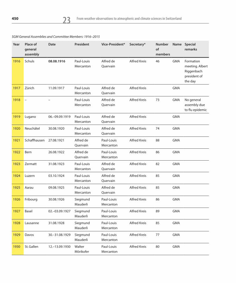
450 From weather observations to atmospheric and climate sciences in Switzerland23
SGM General Assemblies and Committee Members: 1916–2015
Year Place of general assembly
Date President Vice-President* Secretary* Number of members
Name Special remarks
1916 Schuls 08.08.1916 Paul-Louis Mercanton
Alfred de Quervain
Alfred Kreis 46 GMA Formation meeting. Albert Riggenbach president of the day
1917 Zürich 11.09.1917 Paul-Louis Mercanton
Alfred de Quervain
Alfred Kreis GMA
1918 – – Paul-Louis Mercanton
Alfred de Quervain
Alfred Kreis 73 GMA No general assembly due to flu epidemic
1919 Lugano 06.–09.09.1919 Paul-Louis Mercanton
Alfred de Quervain
Alfred Kreis GMA
1920 Neuchâtel 30.08.1920 Paul-Louis Mercanton
Alfred de Quervain
Alfred Kreis 74 GMA
1921 Schaffhausen 27.08.1921 Alfred de Quervain
Paul-Louis Mercanton
Alfred Kreis 88 GMA
1922 Bern 26.08.1922 Alfred de Quervain
Paul-Louis Mercanton
Alfred Kreis 86 GMA
1923 Zermatt 31.08.1923 Paul-Louis Mercanton
Alfred de Quervain
Alfred Kreis 82 GMA
1924 Luzern 03.10.1924 Paul-Louis Mercanton
Alfred de Quervain
Alfred Kreis 85 GMA
1925 Aarau 09.08.1925 Paul-Louis Mercanton
Alfred de Quervain
Alfred Kreis 85 GMA
1926 Fribourg 30.08.1926 Siegmund Mauderli
Paul-Louis Mercanton
Alfred Kreis 86 GMA
1927 Basel 02.–03.09.1927 Siegmund Mauderli
Paul-Louis Mercanton
Alfred Kreis 89 GMA
1928 Lausanne 31.08.1928 Siegmund Mauderli
Paul-Louis Mercanton
Alfred Kreis 85 GMA
1929 Davos 30.–31.08.1929 Siegmund Mauderli
Paul-Louis Mercanton
Alfred Kreis 77 GMA
1930 St. Gallen 12.–13.09.1930 Walter Mörikofer
Paul-Louis Mercanton
Alfred Kreis 80 GMA
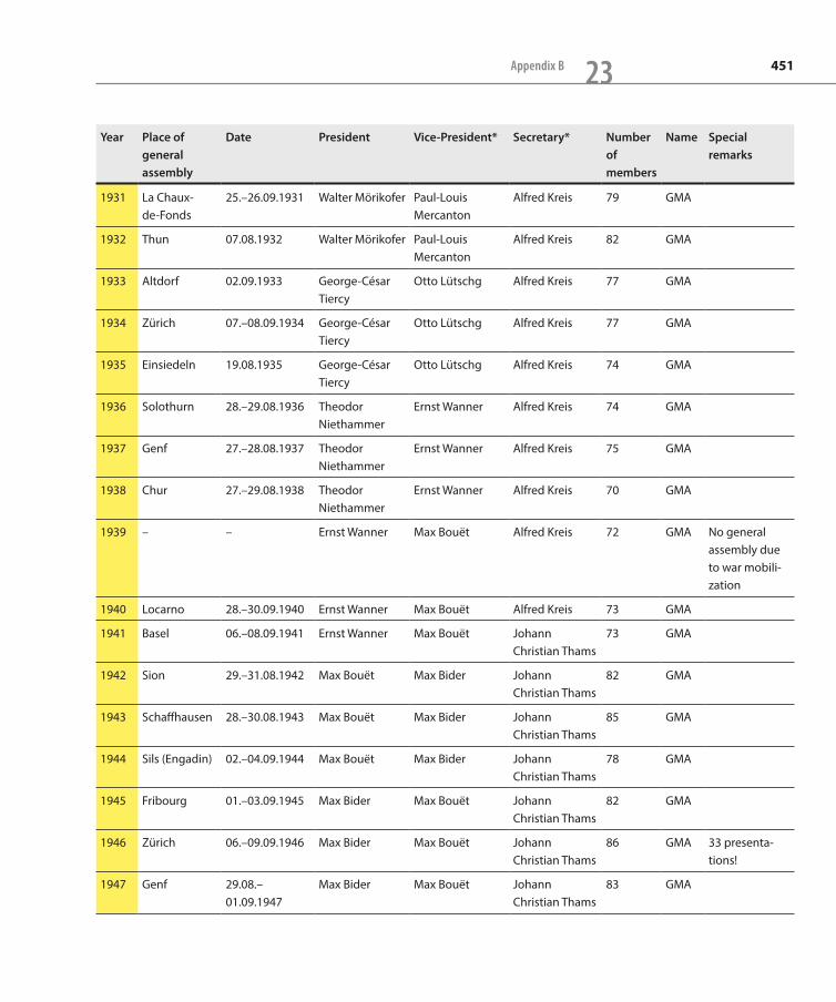
451Appendix B 23
Year Place of general assembly
Date President Vice-President* Secretary* Number of members
Name Special remarks
1931 La Chaux- de-Fonds
25.–26.09.1931 Walter Mörikofer Paul-Louis Mercanton
Alfred Kreis 79 GMA
1932 Thun 07.08.1932 Walter Mörikofer Paul-Louis Mercanton
Alfred Kreis 82 GMA
1933 Altdorf 02.09.1933 George-César Tiercy
Otto Lütschg Alfred Kreis 77 GMA
1934 Zürich 07.–08.09.1934 George-César Tiercy
Otto Lütschg Alfred Kreis 77 GMA
1935 Einsiedeln 19.08.1935 George-César Tiercy
Otto Lütschg Alfred Kreis 74 GMA
1936 Solothurn 28.–29.08.1936 Theodor Niethammer
Ernst Wanner Alfred Kreis 74 GMA
1937 Genf 27.–28.08.1937 Theodor Niethammer
Ernst Wanner Alfred Kreis 75 GMA
1938 Chur 27.–29.08.1938 Theodor Niethammer
Ernst Wanner Alfred Kreis 70 GMA
1939 – – Ernst Wanner Max Bouët Alfred Kreis 72 GMA No general assembly due to war mobili-zation
1940 Locarno 28.–30.09.1940 Ernst Wanner Max Bouët Alfred Kreis 73 GMA
1941 Basel 06.–08.09.1941 Ernst Wanner Max Bouët Johann Christian Thams
73 GMA
1942 Sion 29.–31.08.1942 Max Bouët Max Bider Johann Christian Thams
82 GMA
1943 Schaffhausen 28.–30.08.1943 Max Bouët Max Bider Johann Christian Thams
85 GMA
1944 Sils (Engadin) 02.–04.09.1944 Max Bouët Max Bider Johann Christian Thams
78 GMA
1945 Fribourg 01.–03.09.1945 Max Bider Max Bouët Johann Christian Thams
82 GMA
1946 Zürich 06.–09.09.1946 Max Bider Max Bouët Johann Christian Thams
86 GMA 33 presenta-tions!
1947 Genf 29.08.–01.09.1947
Max Bider Max Bouët Johann Christian Thams
83 GMA

452 From weather observations to atmospheric and climate sciences in Switzerland23
Year Place of general assembly
Date President Vice-President* Secretary* Number of members
Name Special remarks
1948 St. Gallen 04.–06.09.1948 William Brunner-Hagger
Max Bouët Johann Christian Thams
86 GMA
1949 Lausanne 03.–05.09.1949 William Brunner-Hagger
Max Bouët Johann Christian Thams
85 GMA
1950 Davos 26.–28.08.1950 William Brunner-Hagger
Max Bouët Johann Christian Thams
88 GMA
1951 Luzern 29.09.–01.10.1951
Max Schürer Max Bouët Johann Christian Thams
89 GMA
1952 Bern 23.–25.08.1952 Jean Lugeon Max Schürer Johann Christian Thams
87 GMA
1953 Lugano 05.–07.09.1953 Jean Lugeon Max Schürer Johann Christian Thams
91 GMA
1954 Altdorf 25.–27.09.1954 Fritz Gassmann Edmond Guyot Johann Christian Thams
88 GMA
1955 Pruntrut 24.–26.09.1955 Fritz Gassmann Edmond Guyot Johann Christian Thams
82 GMA
1956 Basel 22.–24.09.1956 Fritz Gassmann Edmond Guyot Walter Kuhn 82 GMA
1957 Neuchâtel 21.–23.09.1957 Edmond Guyot Theodor Zingg Walter Kuhn 87 GMA
1958 Glarus 13.–15.09.1958 Edmond Guyot Theodor Zingg Walter Kuhn 88 GMA
1959 Lausanne 11.–13.09.1959 Edmond Guyot Theodor Zingg Walter Kuhn 86 GMA
1960 Aarau 23.–25.09.1960 Theodor Zingg Marcel Golay Walter Kuhn 85 GMA
1961 Biel 22.–24.09.1961 Theodor Zingg Marcel Golay Walter Kuhn 85 GMA
1962 Scuol- Tarasp-Vulpera
07.–09.09.1962 Theodor Zingg Marcel Golay Walter Kuhn 86 GMA
1963 Sion 30.08.–01.09.1963
Flavio Ambrosetti
Reto Florin Walter Kuhn 93 GMA
1964 Zürich 09.–11.10.1964 Flavio Ambrosetti
Reto Florin Walter Kuhn-Klipstein
94 GMA
1965 Genf 24.–26.09.1965 Flavio Ambrosetti
Reto Florin Walter Kuhn-Klipstein
93 GMA
1966 Solothurn 30.09–02.10.1966
Hans-Ulrich Dütsch
Max Bouët Walter Kuhn-Klipstein
93 GMA
1967 Schaffhausen 30.09.1967 Hans-Ulrich Dütsch
Max Bouët Walter Kuhn-Klipstein
96 GMA
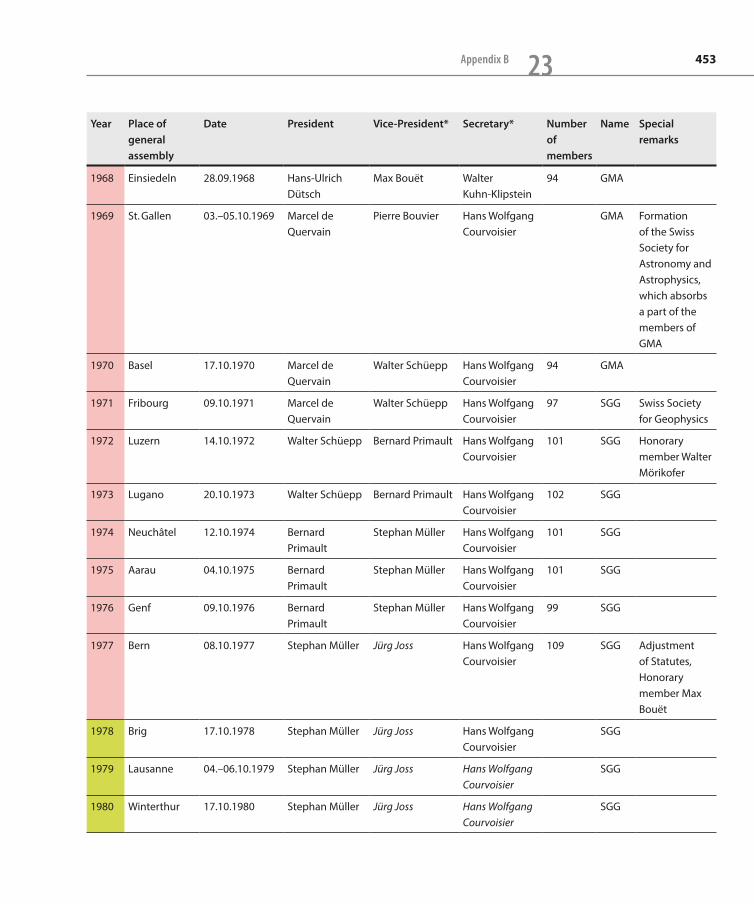
453Appendix B 23
Year Place of general assembly
Date President Vice-President* Secretary* Number of members
Name Special remarks
1968 Einsiedeln 28.09.1968 Hans-Ulrich Dütsch
Max Bouët Walter Kuhn-Klipstein
94 GMA
1969 St. Gallen 03.–05.10.1969 Marcel de Quervain
Pierre Bouvier Hans Wolfgang Courvoisier
GMA Formation of the Swiss Society for Astronomy and Astrophysics, which absorbs a part of the members of GMA
1970 Basel 17.10.1970 Marcel de Quervain
Walter Schüepp Hans Wolfgang Courvoisier
94 GMA
1971 Fribourg 09.10.1971 Marcel de Quervain
Walter Schüepp Hans Wolfgang Courvoisier
97 SGG Swiss Society for Geophysics
1972 Luzern 14.10.1972 Walter Schüepp Bernard Primault Hans Wolfgang Courvoisier
101 SGG Honorary member Walter Mörikofer
1973 Lugano 20.10.1973 Walter Schüepp Bernard Primault Hans Wolfgang Courvoisier
102 SGG
1974 Neuchâtel 12.10.1974 Bernard Primault
Stephan Müller Hans Wolfgang Courvoisier
101 SGG
1975 Aarau 04.10.1975 Bernard Primault
Stephan Müller Hans Wolfgang Courvoisier
101 SGG
1976 Genf 09.10.1976 Bernard Primault
Stephan Müller Hans Wolfgang Courvoisier
99 SGG
1977 Bern 08.10.1977 Stephan Müller Jürg Joss Hans Wolfgang Courvoisier
109 SGG Adjustment of Statutes, Honorary member Max Bouët
1978 Brig 17.10.1978 Stephan Müller Jürg Joss Hans Wolfgang Courvoisier
SGG
1979 Lausanne 04.–06.10.1979 Stephan Müller Jürg Joss Hans Wolfgang Courvoisier
SGG
1980 Winterthur 17.10.1980 Stephan Müller Jürg Joss Hans Wolfgang Courvoisier
SGG

454 From weather observations to atmospheric and climate sciences in Switzerland23
Year Place of general assembly
Date President Vice-President* Secretary* Number of members
Name Special remarks
1981 Davos 24.09.1981 Jürg Joss William Lowrie Albert Wald-vogel
SGG
1982 Basel 07.–08.10.1982 Jürg Joss William Lowrie Albert Wald-vogel
SGG
1983 Delémont 13.–14.10.1983 Jürg Joss William Lowrie Albert Wald-vogel
SGG
1984 Zürich 04.–05.10.1984 William Lowrie Claus Fröhlich Albert Wald-vogel
122 SGG
1985 Biel 04.10.1985 William Lowrie Claus Fröhlich Albert Wald-vogel
SGG
1986 Bern 09.–12.10.1986 William Lowrie Claus Fröhlich Albert Wald-vogel
SGG
1987 Luzern 09.10.1987 Claus Fröhlich Nazario Pavoni Karin Schram 127 SGG
1988 Lausanne 07.10.1988 Claus Fröhlich Nazario Pavoni Karin Schram SGG
1989 Fribourg 12.10.1989 Nazario Pavoni Albert Waldvogel Karin Schram 126 SGG
1990 Genève 04.10.1990 Nazario Pavoni Albert Waldvogel Karin Schram 125 SGG
1991 Chur 11.10.1991 Nazario Pavoni Albert Waldvogel Karin Schram 123 SGG
1992 Basel 02.10.1992 Albert Waldvogel
Dieter Mayer-Rosa
Karin Schram 125 SGG
1993 Verbier 23.09.1993 Albert Waldvogel
Dieter Mayer-Rosa
Karin Schram 121 SGG
1994 Aarau 07.10.1994 Albert Waldvogel
Dieter Mayer-Rosa
Karin Schram 118 SGM
1995 St. Gallen 08.09.1995 Albert Waldvogel
Dieter Mayer-Rosa
Karin Schram 114 SGM Adjustment of statutes, Swiss Society for Meteo-rology
1996 Zürich 08.10.1996 Pierre Jeannet Hans Richner Karin Schram 113 SGM
1997 La Chaux-de-Fonds
09.10.1997 Pierre Jeannet Hans Richner Hans-Heinrich Schiesser
125 SGM
1998 Airolo 23.–25.09.1998 Pierre Jeannet Hans Richner Hans-Heinrich Schiesser
127 SGM EMS in forma-tion, first SGM website

455Appendix B 23
Year Place of general assembly
Date President Vice-President* Secretary* Number of members
Name Special remarks
1999 Luzern 14.10.1999 Hans Richner Peter Binder Hans-Heinrich Schiesser
128 SGM SGM member of EMS, extended committee (due to MetZet)
2000 Winterthur 13.10.2000 Hans Richner Peter Binder Hans-Heinrich Schiesser
128 SGM
2001 Yverdon 18.–19.10.2001 Hans Richner Peter Binder Eszter Barthazy 129 SGM
2002 Davos 18.–20.09.2002 Hans Richner Peter Binder Eszter Barthazy 159 SGM
2003 Fribourg 08.10.2003 Hans Richner Peter Binder Eszter Barthazy 159 SGM
2004 Sarnen 06.10.2004 Peter Binder Markus Furger Eszter Barthazy 161 SGM
2005 Villigen 23.09.2005 Peter Binder Markus Furger Eszter Barthazy 156 SGM
2006 Zürich 04.10.2006 Peter Binder Markus Furger Eszter Barthazy 154 SGM
2007 Genf 16.–17.11.2007 – Markus Furger Eszter Barthazy 156 SGM
2008 Lugano 22.11.2008 Markus Furger Gabriela Seiz Eszter Barthazy 157 SGM
2009 Neuchâtel 21.11.2009 Markus Furger Gabriela Seiz Eszter Barthazy 159 SGM Adjustment of statutes
2010 Fribourg 20.11.2010 Markus Furger Saskia Willemse Daniel Walker 151 SGM Honorary member Hans Richner
2011 Zürich 12.11.2011 Markus Furger Saskia Willemse Daniel Walker 152 SGM
2012 Bern 17.11.2012 Saskia Willemse Michael Sprenger
Daniel Walker 152 SGM
2013 Lausanne 16.11.2013 Saskia Willemse Michael Sprenger
Daniel Walker 150 SGM
2014 Zürich 08.11.2014 Saskia Willemse Michael Sprenger
Daniel Walker 152 SGM
2015 Zürich 07.11.2015 Saskia Willemse Michael Sprenger
Daniel Walker 157 SGM

456 From weather observations to atmospheric and climate sciences in Switzerland23
Year Place of general assembly
Date President Vice-President* Secretary* Number of members
Name Special remarks
Sources:
Verhandlungen der Schweizerischen Naturforschenden Gesellschaft. Wissenschaftlicher und administrativer Teil = Actes de la Société Helvétique des Sciences Naturelles. Partie scientifique et administrative = Atti della Società Elvetica di Scienze Naturali
Jahrbuch der Schweizerischen Naturforschenden Gesellschaft. Wissenschaftlicher und administrativer Teil = Annuaire de la Société Helvétique des Sciences Naturelles. Partie scientifique et administrative
Verhandlungen der Schweizerischen Naturforschenden Gesellschaft = Actes de la Société Helvétique des Sciences Naturelles = Atti della Società Elvetica di Scienze Naturali
Swiss Geoscience Meeting, http://www.geoscience-meeting.ch/
Unpublished minutes of committee meetings of the SGM
* unverified names in italics
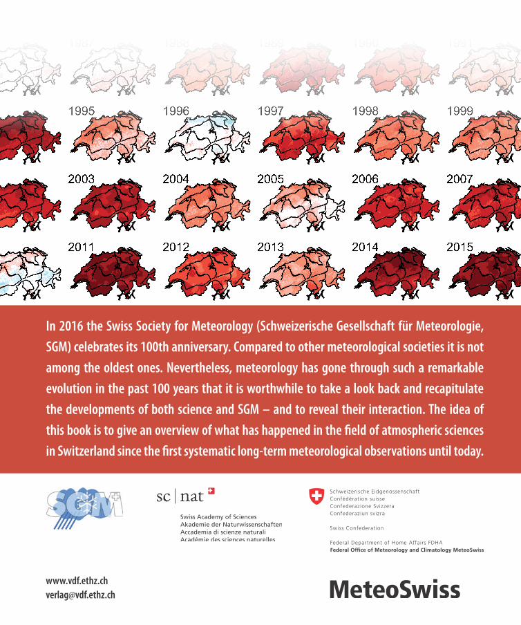
© MeteoSwiss
−2.5
−2
−1.6
−1.3
−1
−0.8
−0.6
−0.4
−0.2 0.2
0.4
0.6
0.8
1
1.3
1.6
2
2.5
1961 1962 1963 1964 1965 1966 1967 1968
1969 1970 1971 1972 1973 1974 1975 1976
1977 1978 1979 1980 1981 1982 1983 1984
1985 1986 1987 1988 1989 1990 1991 1992
1993 1994 1995 1996 1997 1998 1999 2000
2001 2002 2003 2004 2005 2006 2007 2008
2009 2010 2011 2012 2013 2014 2015
In 2016 the Swiss Society for Meteorology (Schweizerische Gesellschaft für Meteorologie,
SGM) celebrates its 100th anniversary. Compared to other meteorological societies it is not
among the oldest ones. Nevertheless, meteorology has gone through such a remarkable
evolution in the past 100 years that it is worthwhile to take a look back and recapitulate
the developments of both science and SGM – and to reveal their interaction. The idea of
this book is to give an overview of what has happened in the field of atmospheric sciences
in Switzerland since the first systematic long-term meteorological observations until today.