VALUING THE FLEXIBILITY

OF FLEXIBLE MANUFACTURING SYSTEMS

by

Nalin Kulatilaka

Working Paper No.March 1988 MIT-EL 88-006WP

THE VIEWS EXPRESSED HEREIN ARE THE AUTHOR'S RESPONSIBILITY

AND DO NOT NECESSARILY REFLECT THOSE OF THE MLT ENERGY

LABORATORY OR THE MASSACHUSETTS INSTITUTE OF TECHNOLOGY.

Valuing the Flexibility of Flexible Manufacturing Systems*

Nalin Kulatilaka

School of ManagementBoston University

and

Center for Energy Policy ResearchEnergy Laboratory

Massachusetts Institute of Technology

March 1988

Mailing Address:

School of ManagementBoston University704 Commonwealth AvenueBoston, MA 02215

(617) 353-4601

* Some of the ideas contained in this paper were presented at the 1986 IAEE Conference on SystemsMan and Cybernetics, Atlantic, Georgia. I thank Roger Bohn and participants at the BostonUniversity Colloquium on Manufacturing Systems for helpful discussions. I am also grateful totwo anonymous referees and the associate editor, James Evans, for comments on an earlier draft.I am solely responsible for any remaining errors.

Abstract

This paper studies a topical issue: Flexible Manufacturing System (FMS)justification. We contend that current evaluation methods fall short ofcapturing a key advantage of an FMS: the value of flexibility. We identifyvarious benefits of FMS that arise from the ability to switch between modes ofproduction, and in particular, we model the value derived from the ability tobetter cope with uncertainty. A model to capture this value must solve forthe value of flexibility together with the dynamic operating schedule of theproduction process. We present a stochastic dynamic programming model thatcaptures the essential elements of this problem. A numerical example furtherdemonstrates the optimal mode switching decision rules.

This research has several important managerial implications. Itemphasizes the importance of ex ante economic justification of flexiblemanufacturing systems and proposes a way to modify existing capital budgetingtechniques to incorporate the special features of flexibility. As the valueof flexibility depends inherently on the design of the manufacturing system,the design and justification stages must be conducted simultaneously. We alsoshow how to include other operating decisions in the valuation model. Thesecan include the investment timing or the decision to temporarily shut down orto abandon the project entirely.

Introduction

Many managers and production engineers believe that conventional

evaluation methods, such as net present value techniques, are not suited for

analyzing investment in modern flexible manufacturing systems (FMS). Instead

such investment decisions often are based on non-economic criteria. Recent

surveys, for example, show that improvements in throughput, product quality,

information flows, reliability, and other strategic advantages have been the

primary motivations behind the decision to invest in FMS.1

At the same time, there is much evidence that despite large investments

in modern manufacturing hardware, the productivity gap between the U.S. and

Japan has been widening.2 In particular, researchers have found that while

flexibility is purported to be a prime advantage of modern manufacturing

technologies, systems installed in the U.S. either are not very flexible or do

not use the available flexibilities to best advantage3 These observations

have given rise to growing realization of the need to revamp the design,

procurement, and management techniques used in modern manufacturing.

There is no question that engineering design and good operations

management are very important to the success of FMS, but it is our contention

that the main failure of FMS in the U.S. stems from the use of inappropriate

ex ante criteria used in the justification of investments. Consequently, in

1 See Graham and Rosenthal [1986].

2 For example see Adler [1985] and Jaikumar [1986].

3 See exhibit 1 in Jaikumar [1986], a comparison of functioning FMSs in Japanand the U.S. The author finds that in the U.S. relatively fewer parts aremanufactured per machine and drastically fewer new parts are introduced.

- 1 -

some installations, tasks that are not suited for FMS have been assigned to

the system. In others, inappropriately designed FMS are used in tasks that

would have been profitably mechanized with a correctly designed FMS.

For FMS to succeed, it is essential to (a) include all effects arising

from the introduction of the FMS in the capital budgeting decision, and (b)

conduct the ex ante analysis under all feasible configurations in order to

choose the optimum design configuration.

This paper takes a closer look at why conventional capital budgeting

rules fail to capture the complexities of FMS projects. Once problems are

identified we suggest ways to incorporate, in the justification stage, the

special features of FMS. In particular, we develop a dynamic model that

captures the option value of flexibility arising from the ability to better

cope with uncertainty, and we implement this stochastic dynamic programming

model using a stylized example.

The paper is organized as follows: In section 1, we describe issues that

complicate the justification of flexible projects. Section 2 highlights the

need for a stochastic dynamic model. Section 3 elucidates the model using an

illustration. Section 4 presents results from a numerical simulation and

interprets them. Section 5 discusses the feasibility of practical

implementation of the approach, with some caveats.

1. Complexities of FMS Justification

A flexible manufacturing process adds value to the firm that can be

attributed to changes in direct and indirect cash flows, operating

flexibilities that enhance the firm's ability to cope with uncertainty, and

non-pecuniary effects such as learning value. An evaluation of such an

investment must weigh these effects against the incremental initial investment

costs of installing an FMS. Although the problems associated with measuring

- 2-

costs and benefits are not trivial, we do not address them in this paper.4

The primary aim of this paper is to introduce a framework that

incorporates the option value of flexibility. Flexible production processes

give the firm an ability to modify, or in some cases reverse, decisions made

in earlier periods. The option value stemming from such operating

flexibilities has been noted by several researchers.5

Most previous efforts to model production flexibility fail to capture the

essentially dynamic facets of operating flexibility. They have not

acknowledged that the decision to operate a flexible system during the current

period in a particular mode influences not only the payoffs in future periods

but also the future operating decisions.

It is only recently that the operations research and management science

community has focused on the value of flexibility. Fine and Freund [1986]

have developed a static model that captures the value of product flexibility

when firms face uncertain product demand.6 In their model firms make a

capacity investment decision before the resolution of future demand

uncertainties. Flexible capacity that gives the firm the ability to respond

to a variety of future demand outcomes is traded off against the increased

investment cost. They model a firm that produces two products and chooses a

portfolio of fixed and flexible capacity before receiving final demand

information. Under strong assumptions about the form of the technology

4 Kulatilaka [1985] gives a review of the pertinent literature and develops acash flow forecasting model that includes both direct and indirect effects.

5 Jones and Ostroy [1984] first formalized this notion.

6 Discussions of definitions and classification of flexibility types can befound in Jaikumar [1985] and Graham and Rosenthal [19861. Son and Park [1987]also discuss some static measures of flexibility.

- 3 -

(linear production functions), they solve a two-stage convex quadratic program

and characterize the optimal profit function and the optimal investment

policies.

Although the Fine and Freund model provides useful insights and takes a

first crack at modeling the value of flexibility, it fails to capture the

extremely important dynamic features. An example is switching between modes

of production. When switching is costly, future switching decisions will be

affected not only by revelations of demand change but also by the current

production mode (and hence, past switching decisions).

In this paper we study the value of flexibility within a stochastic

dynamic model. Monahan and Smunt [1984] took a similar approach in their

study of the FMS investment decision. They develop a discrete time stochastic

dynamic programming model where interest rates and "levels of technology" are

assumed to be exogenous and evolving stochastically over time. The proportion

of production using FMS is then chosen so that discounted costs are

minimized.7

The approach we take here departs from that of Monahan and Smunt in two

important aspects. First, we endogenize the utilization of the flexible

technology, in that we model the choice of the optimal operating mode of the

flexible system simultaneously with the valuation of the technology. Second,

we explicitly derive the value of flexibility. In addition, we think that the

7 A review of FMS justification studies can be found in Suresh, N. C. and J.R. Meredith [1985].

- 4 -

exogenous variable with the most striking impact on value is the level of

either input or output prices. Hence, we treat these as exogenous.8

The main insight leading to our formulation is that operating

flexibilities can be viewed as a series of nested compound options similar to

those encountered in complex financial securities. Financial options allow

the exchange of one asset, whose value evolves stochastically over time, for

another. A call option on a stock, for example, gives the holder the right to

purchase the stock at a future date at a pre-specified exercise price. At any

future date until expiration of the option, the holder of the option has the

right to exchange the exercise price for the stock (i.e., purchase the stock

at the exercise price).

Pursuing this analogy, consider a flexible technology with two modes of

operation A and B (or the ability to produce two products). The firm is

operating currently in mode A, and it can costlessly and instantaneously

switch modes. At the next decision point, if mode B is more profitable than

mode A the firm will switch modes. Otherwise it will continue to produce

under mode A. If switching between modes is costly, though, the decision rule

must take into account the effects of a current switch on all future

production scenarios. The process describes a set of sequential options that

are nested. We can value such options using results from compound option

valuation.9

8 The interest rate dynamics and dynamics of technology levels, which aretreated as exogenous in the Monahan and Smunt model, are very difficult toestimate in practice. Furthermore, the conventional wisdom in the financeliterature is that interest rate uncertainty is not a critical element incapital budgeting.

9 See Kulatilaka and Marcus [1986].

-5-

Unfortunately, the imperfect (not necessarily efficient) nature of

production input and output markets makes it difficult to relate models of

financial option valuation to the manufacturing setting. In particular, the

arbitrage arguments used in financial option valuation do not apply when

assets are not traded in efficient markets. Furthermore, the stochastic

processes used to model stock prices are inappropriate in modeling sources of

uncertainties that are typical in production systems.

The framework we propose resolves these problems and permits the

inclusion of many realistic features of manufacturing by making explicit a

simultaneous system of stochastic dynamic programs, which must be solved to

obtain the optimal scheduling of the FMS and the ex ante value of flexibility.

As a result of this generalization it is no longer possible to obtain closed

form solutions. Nevertheless, numerical techniques used in solving such

systems of dynamic programs are well known and easily implemented.

2. Valuing Operating Flexibilities: The Theoretical Framework

Here we outline a stochastic dynamic programming model that explicitly

derives the value of flexibility stemming from the ability of an FMS to

respond to changing conditions.1 0 A flexible technology is stylized as one

that embodies M alternative "modes" of operation. A mode of operation may

refer to a routing within a production system, or to a particular set of

inputs used in manufacturing the product. Such a definition describes process

flexibility. A mode also may refer to the choice of output, in which case it

will describe product flexibility. Finally, a mode can be used to

characterize waiting to invest, shutting down, and abandoning of projects.

10 This model is described in detail in Kulatilaka [1986].

- 6 -

Associated with each mode is a cash flow pattern (profit stream) that is

determined by the realization of some uncertain variable(s), (e.g., demand,

price, exchange rate). The ith mode's profit (or cost) function (over a unit

of time), given that state of the world k occurs, is denoted by Tt(Ok). The

FMS can switch between modes i and j incurring a cost 6 ij. Switching costs

may come from a variety of sources such as retooling, retraining, lost time,

inventory changes, and compensatory wages.

The evolution of is characterized by a stochastic process.11 Suppose

that k can realize N different states. Define the transition probability

that e(t+l) is state i given that (t) was state j as Pij: i.e.,

Pij=prob(Ot+=i/et=j). In general Pij can depend on time, values of , or any

other variables. In the numerical example we assume to be stationary, and

hence parameters are constant over time. The NxN transition probability

matrix with elements Pij is denoted by P.

Suppose the flexible system has a life of T periods and that it reaches

the last period employing mode m (mE(1,M)}. The chronology is defined such

that the first period begins at time 0 so that the last (Tth) period begins at

time T-1. At T-1 the firm will observe the realization of e(T-1), say state

j, and realize a profit of m(eTl). 1 2 One way to think of the time periods

11 For example, we can represent 8 with a diffusion process:

dO = a(8,t) dt + o(e,t) dZ

where dZ is a standard Wiener process. We can then discretize the process tofit this model.

12 The profit functions are the begining-of-period present values of the flowprofits over a single period.

- 7 -

is as discrete approximations to the continuous decision process.1 3

Alternatively, we can think of the time periods as given exogenously by

contracting arrangements or other organizational constraints, for example.

With just one period remaining in its life (i.e., at time T-1), the value

of the system is known with certainty and is given by the maximum of the

profits under the different modes:

i(1) F(T-1,m) = max [ (0 ) d

where the indicator variable di = 0 if i=m (remain in mode m)

di = 6mi if im (switch to mode i)

At periods prior to T-1, however, the future realizations of are

unknown to the firm. For example, consider the mode choice decision at time

T-2. Suppose T-2 is reached with mode m in use. The value of the flexible

system at T-2 is then the value over the next period using the mode that

maximizes that period's net profits (net of switching costs) plus the expected

value (at time T-2) of the value at T-1.

(2) F(T-2,m) = Max { i( 0T2) - di+ E [F(T,i)] i=l,...,Mi

where is the one-period present value factor, which is computed as 1/(l+r),

and r is the risk-adjusted discount rate.

Several caveats regarding the discount rate bear noting. If the

underlying asset follows an equilibrium growth rate, then we can take "risk

13 By choosing arbitrarily small time periods we can approximate thecontinuous time case.

- 8-

neutral expectations" as in Cox and Ross [1976] and use the risk-free rate in

discounting cash flows. The problem is that production inputs and outputs are

not necessarily traded in efficient markets, unlike financial markets. Hence,

their growth rates need not equal the fair rate of return. In such cases we

can use an insight due to McDonald and Siegel [1984]: replace the drift term

of the diffusion process by the equilibrium rate and then follow risk-neutral

discounting. Such an adjustment, however, requires the additional imposition

of an asset pricing model.1 4

Expectations are taken over all possible realizations of and can, in

general, be computed as follows:

N

(3) Et[F(t)] = Z {F(t+,1 1 k) Pmk(t)k=l

Thus, the dynamic programming equations at time t can be written as

(4) F(t,m) = Max { -i_ di+ Et[F(t+l)] }i

i,m=l,...,M and t=O,...,T-2.

14 See Kulatilaka and Marcus [1986] for details.

-9-

These M-simultaneous dynamic programs can be solved numerically to obtain the

value functions F(t,i) for all t and i. Furthermore, argument maximum will

yield the optimal mode choice (i.e., Mt/Mt_-lm is obtained by replacing Max

with Argmax in equation 4).

3. A Stylized Example

A firm facing some exogenous uncertainty, say price (e), is considering

an investment in a flexible manufacturing system. The price dynamics are

modeled by a mean reverting stochastic process:

de = i(8e-e) dt + e dZe

= .05(.5-e) dt + .4 dZ8

The instantaneous drift term (e°-) acts as an elastic force that produces

mean reversion. In the numerical solutions we discretize within the range

[0,1] with a grid size of .02 (i.e., 8 is allowed to take 51 discrete values

from 0 through 1.0). The base case probability transition matrix appears in

Table 1.

We characterize the firm before it makes the investment as "waiting to

invest," which we define as mode 1. Once it makes the investment, the firm

can produce in one of two modes (mode 2 or mode 3) and incur the investment

cost, I. While operating in either production mode, the system has the

ability to switch to the other production mode or to temporarily shut down

(mode 4). Shutting down the plant will incur some shutdown costs, and while

the firm remains in this mode it will continue to incur fixed costs. From the

shutdown mode, the firm can start up in one of the two production modes or

abandon the plant (mode 5) and receive the salvage value. We summarize the

options in our notation as follows;

- 10 -

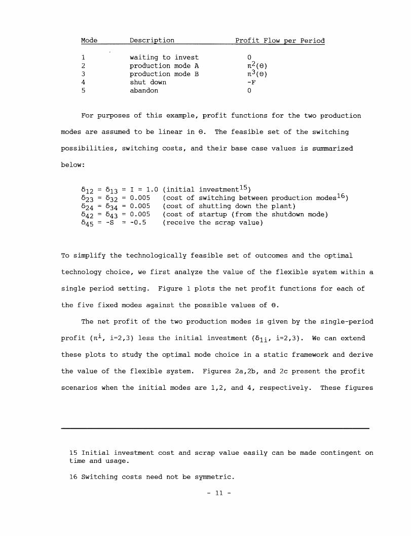
Mode Description Profit Flow per Period

1 waiting to invest 02 production mode A L2 (E)3 production mode B 3 (E)

4 shut down -F5 abandon 0

For purposes of this example, profit functions for the two production

modes are assumed to be linear in . The feasible set of the switching

possibilities, switching costs, and their base case values is summarized

below:

612 = 13 = I = 1.0 (initial investment 1 5)

623 = 632 = 0.005 (cost of switching between production modes1 6)624 = 634 = 0.005 (cost of shutting down the plant)642 = 43 = 0.005 (cost of startup (from the shutdown mode)545 = -S = -0.5 (receive the scrap value)

To simplify the technologically feasible set of outcomes and the optimal

technology choice, we first analyze the value of the flexible system within a

single period setting. Figure 1 plots the net profit functions for each of

the five fixed modes against the possible values of 8.

The net profit of the two production modes is given by the single-period

profit (i, i=2,3) less the initial investment (61i, i=2,3). We can extend

these plots to study the optimal mode choice in a static framework and derive

the value of the flexible system. Figures 2a,2b, and 2c present the profit

scenarios when the initial modes are 1,2, and 4, respectively. These figures

15 Initial investment cost and scrap value easily can be made contingent ontime and usage.

16 Switching costs need not be symmetric.

- 11 -

also can be interpreted as the value functions as of the beginning of the last

period: i.e., F(T-1,i), i=1,2,4.

Consider Figure 2a. The solid line plots F(T-1,1), the value of the

flexible system if the firm reaches time T-1 without having made the initial

investment, against . The switching decision rule requires only a simple

comparison of net profits.

Condition

OT- 1 < 12

< T- 1 < e13

< T-1

Decision

do not invest

invest and operate in mode 2

invest and operate in mode 3

Figure 2b graphs F(T-1,2) and the decision rule is now:1 7

Condition

eT-1 24

< T-1 < 824

< T-1

Decision

shut down the plant

continue to operate with mode 2

switch to operating with mode 3

We must highlight the determination of the switch points 824 and 023.

024, the price at which it becomes optimal to shut down given that the plant

is operating in mode 2, is the intersection of 2 and the horizontal line, -F-

624; 823, which has a similar interpretation as above is the intersection of

n2 and r3-623. We compute these values for comparison with the corresponding

switch points for the dynamic case.

17 A very similar decision rule can be derived by studying F(T-1,3).

- 12 -

E*012

0e13

e3*034

E34

Figure 2c shows the case when starting with the shutdown mode. The

resulting decision rule is

Condition Decision

ST-1 < 042 = 045 abandon project

042 < T-1 < 43 start up with mode 2

043 < OT-1 start up with mode 3

Notice that in this essentially static approach, the firm will never

remain shut down: it will either abandon the project or start up. As there is

no future switching opportunity, when prices are low enough it is best to

abandon and receive the scrap value, or, when prices are high enough it is

best to start up.

Our model builds richness by expanding this static framework to a dynamic

one. We have included so much discussion in order to clarify why and how the

decision rules and the optimal switching points are modified when the firm has

future switching opportunities. For example, consider the situation depicted

in figure 2c at some time prior to T-1 and when the price is below 45. As

it is possible that future values of can be very high, thereby allowing the

realization of high profits, it may be optimal to remain shut down and not

abandon the project altogether.

4. Numerical Simulations

The numerical simulations use the following profit functions to represent

cash flows from the two production modes (mode 2 and mode 3);

n2 (0) = a2 + b2 0 = -.6 + 20

T3(E) = a3 + b3 0 = -.1 +

- 13 -

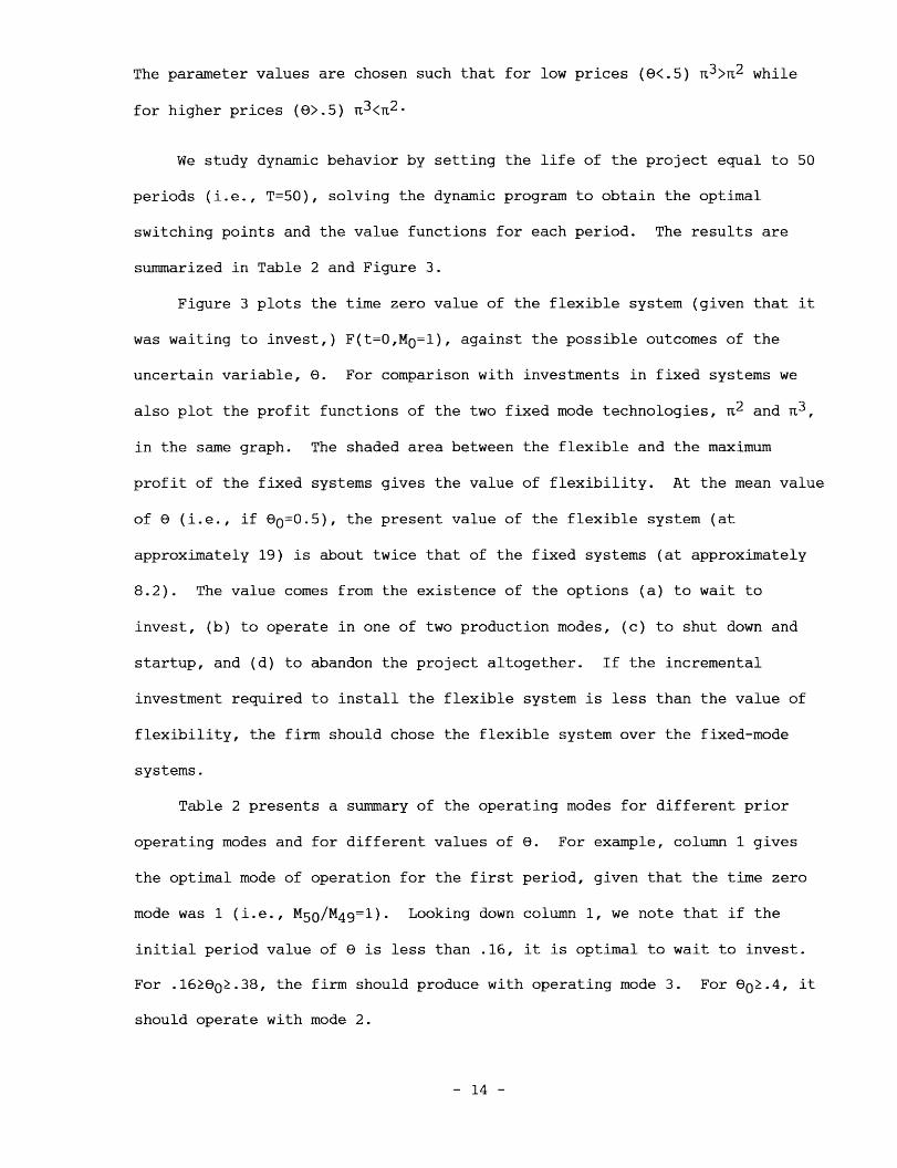
The parameter values are chosen such that for low prices (8<.5) 3>R2 while

for higher prices (>.5) 3 <r2.

We study dynamic behavior by setting the life of the project equal to 50

periods (i.e., T=50), solving the dynamic program to obtain the optimal

switching points and the value functions for each period. The results are

summarized in Table 2 and Figure 3.

Figure 3 plots the time zero value of the flexible system (given that it

was waiting to invest,) F(t=O,MO=1), against the possible outcomes of the

uncertain variable, . For comparison with investments in fixed systems we

also plot the profit functions of the two fixed mode technologies, 2 and 3,

in the same graph. The shaded area between the flexible and the maximum

profit of the fixed systems gives the value of flexibility. At the mean value

of (i.e., if 0=0.5), the present value of the flexible system (at

approximately 19) is about twice that of the fixed systems (at approximately

8.2). The value comes from the existence of the options (a) to wait to

invest, (b) to operate in one of two production modes, (c) to shut down and

startup, and (d) to abandon the project altogether. If the incremental

investment required to install the flexible system is less than the value of

flexibility, the firm should chose the flexible system over the fixed-mode

systems.

Table 2 presents a summary of the operating modes for different prior

operating modes and for different values of 8. For example, column 1 gives

the optimal mode of operation for the first period, given that the time zero

mode was 1 (i.e., M5 0/M49 =1). Looking down column 1, we note that if the

initial period value of 8 is less than .16, it is optimal to wait to invest.

For .16Ž0.38, the firm should produce with operating mode 3. For 80.4, it

should operate with mode 2.

- 14 -

The second column of Table 2 gives optimal modes for time 1 when starting

in mode 2 (i.e. M1/MO=2). Now it is optimal to shut down the plant if 80<.10;

switch modes and operate with mode 3 if 0.10 0<O0.38; continue operating with

mode 2 if O2.40. Similarly, column 3 gives the operating mode when M0=3. The

only change between this and the previous case is that the firm should choose

to operate in mode 3 until O0<.40 (compared with .38) because of the cost of

switching between modes 2 and 3. Finally, column 4 reports the recommended

modes when the plant is shut down during at the start. Because there are no

shutdown or startup costs, these values are identical to those in column 2.

It should be noted that for the base case parameter values, with 50

periods of life remaining, the plant will not be abandoned for any realization

of e0. With shorter times to maturity (remaining life), however, sometimes it

is optimal to abandon the project. These are depicted in Table 3, which

reports the optimal mode choices for the last period.

5. Managerial Implications, Caveats, and Limitations of the Model

Our point has been that current evaluation methods fall short of

capturing an essential feature of an FMS: the value of flexibility. An

important benefit of flexibility is enhancement of the firm's ability to

better cope with uncertainty. The model developed here aims to specify how

much flexibility is worth.

This research has several important managerial implications. Recognizing

the importance of ex ante economic justification of FMS, it proposes a way to

modify existing capital budgeting techniques to incorporate the special

features of flexibility. As the value of flexibility is inherently dependent

on the design of the manufacturing system, the design and justification must

be conducted simultaneously. We also show that other operating decisions,

- 15 -

such as investment timing and decisions to temporarily shut down or abandon a

project, can be included in the valuation model.

Appealing as the concept may be, admittedly its practical implementation

requires overcoming many measurement and modeling hurdles. Although common to

all capital budgeting exercises, a foremost problem is the measurement of flow

profit functions over the life of the project. Typically engineering cost

studies or economic factor demand studies are used to estimate such profit

functions.1 8 This model, however, requires ex ante measures of future cash

flows and deal with new technologies for which there may not be historical

cost data. Hence, profit function estimation must be derived by combining

information from design engineers and manufacturing managers. The profit

function coefficients will depend not only on the engineering specifications

but also on the way the plant is configured and operated.19

Another major hurdle is the estimation of the stochastic dynamics of .

If is the price of a traded input, then the stochastic process can be

statistically estimated using historical time series data on its spot price.2 0

An especially relevant example is seen in the case of modern manufacturing

plants that purchase electricity in spot markets. A firm may switch away from

purchased electricity (either to another source of energy or to an

inoperative mode by shutting down the plant) depending on relative fuel

prices. The spot price is determined by random supply and demand conditions

18 See Berndt and Wood [1979] for details on the estimation and interpretationof cost and profit functions.

19 For example, scheduling algorithms and pricing strategies can bothinfluence the cash flows.

20 See Marsh and Rosenfeld [1983].

- 16 -

facing the power grid, so the spot price of electricity (and hence relative

fuel prices) will evolve stochastically over time.

In some cases, the implied parameter values of the stochastic process may

be inferred from market rationality. For example, if the source of exogenous

uncertainty is oil prices, and the market for a particular oil-using machine

is competitive, then the implied variance can be solved for by setting the

market price equal to the value of the machine.

In many other instances, however, the process may be much harder to

estimate. In extreme cases the possible outcomes and the associated

probabilities may require subjective judgment.

- 17 -

References

Adler, P. [1985], "Managing Flexibility: A Selective Review of the Challengesof Managing the New Production Technologies' Potential for Flexibility,"mimeo, Department of Industrial Engineering and Engineering Management,Stanford University.

Berndt, Ernst and David Wood [1979], "Engineering and Economic Interpretationsof Capital-Energy Complementarity," American Economic Review, June, vol.69, no. 3, 342-354.

Bohn, Roger and Ramachandran Jaikumar [1987], "The Dynamic Approach: AnAlternative Paradigm for Operations Management," Working paper, HarvardBusiness School.

Cox, John and Stephen Ross [1976], "The Valuation of Options for AlternativeStochastic Processes," Journal of Financial Economics, 3, 145-166.

Fine, Charles and Robert Freund [1986], "Optimal Investment in Product-Flexible Manufacturing Capacity, Part I: Economic Analysis," MIT, SloanSchool, Working paper, #1803-86.

Graham, Margaret and Stephen Rosenthal [1986], "Institutional Aspects ofProcess Procurement for Flexible Manufacturing Systems," Working Paper,Manufacturing Roundtable, Boston University.

Jaikumar, Ramachandran [1986], "Postindustrial Manufacturing," HarvardBusiness Review (November-December), 69-76.

Jones, R. A., and J. M. Ostroy [1984], "Flexibility and Uncertainty", Reviewof Economic Studies, LI, 13-32.

Kulatilaka, Nalin [1985], "Capital Budgeting and Optimal Timing of Investmentsin Flexible Manufacturing Systems," Annals of Operations Research, 3, 35-57.

Kulatilaka, Nalin [1986], "The Value of Flexibility," MIT Energy Laboratoryworking paper.

Kulatilaka, Nalin and Alan Marcus [1986], "A General Formulation of CorporateOperating Options," forthcoming in Research in Finance, ed. Andrew Chen.

Marsh Terry and Eric Rosenfeld [1983], "Stochastic Processes for InterestRates and Equilibrium Bond Prices," Working Paper No. 83-45, HarvardBusiness School.

Monahan, G. E. and T. L. Smunt [1984], "The FMS Investment Decision,"ORSA/TIMS Conference Proceedings, November 1984.

Son, Young Hyn and Chan S. Park, [1987], "Economic Measure of Productivity,Quality and Flexibility in Advanced Manufacturing Systems," Journal ofManufacturing Systems, Vol. 6, No. 3, 193-207.

Suresh, N. C. and J. R. Meredith [1985], "Justifying Multimachine Systems: AnIntegrated Strategic Approach", Journal of Manufacturing Systems, Vol. 4,No. 2.

- 18 -

Table 1

Transition Probability Matrix

d = .05(.5-e) dt + .4 dZ

0.0 .01 .02

0.525

0.098

0.090

0.079

0.064

0.049

0.036

0.024

0.015

0.009

0.010

0.431

0.099

0.098

0.090

0.078

0.064

0.049

0.035

0.024

0.015

0.019

0.340

0.095

0.099

0.097

0.089

0.077

0.063

0.048

0.034

0.023

0.033

.03

0.258

0.087

0.096

0.099

0.097

0.089

0.077

0.062

0.047

0.034

0.055

.04

0.187

0.074

0.087

0.096

0.099

0.097

0.088

0.076

0.061

0.046

0.087

.05 .06

0.130

0.060

0.075

0.088

0.096

0.099

0.096

0.088

0.075

0.060

0.130

0.087

0.046

0.061

0.076

0.088

0.097

0.099

0.096

0.087

0.074

0.187

.07

0.055

0.034

0.047

0.062

0.077

0.089

0.097

0.099

0.096

0.087

0.258

.08 .09 1.0

0.033

0.023

0.034

0.048

0.063

0.077

0.089

0.097

0.099

0.095

0.340

0.019

0.015

0.024

0.035

0.049

0.064

0.078

0.090

0.098

0.099

0.431

0.010

0.009

0.015

0.024

0.036

0.049

0.064

0.079

0.090

0.098

0.525

- 19 -

0.0

0.1

0.2

0.3

0.4

0.5

0.6

0.7

0.8

0.9

1.0

-

Table 2

The Optimal Mode to Operate: t=l

e M1/MO=l M1/Mo=2 M1/MO=3 M1/MO=4

0.00 1 4 4 4

0.02 1 4 4 4

0.04 1 4 4 4

0.06 1 4 4 4

0.08 1 4 4 4

0.10 1 4 4 4

0.12 1 3 3 3

0.14 1 3 3 3

0.16 3 3 3 3

0.18 3 3 3 3

0.20 3 3 3 3

0.22 3 3 3 3

0.24 3 3 3 3

0.26 3 3 3 3

0.28 3 3 3 3

0.30 3 3 3 3

0.32 3 3 3 3

0.34 3 3 3 3

0.36 3 3 3 3

0.38 3 3 3 3

0.40 2 2 3 2

0.42 2 2 2 2

0.44 2 2 2 2

0.46 2 2 2 2

0.48 2 2 2 2

0.50 2 2 2 2

0.52 2 2 2 2

0.54 2 2 2 2

0.56 2 2 2 2

0.58 2 2 2 2

0.60 2 2 2 2

0.62 2 2 2 2

0.64 2 2 2 2

0.66 2 2 2 2

0.68 2 2 2 2

0.70 2 2 2 2

0.72 2 2 2 2

0.74 2 2 2 2

0.76 2 2 2 2

0.78 2 2 2 2

0.80 2 2 2 2

0.82 2 2 2 2

0.84 2 2 2 2

Definition: M1/M0 =i is the optimal mode at time 1 (M1) given that the mode inthe previous period (M0) was mode i.

- 20 -

Table 3

The Optimal Mode to Operate: t=50

0 M5 0/M4 9=1 M5 0/M4 9=2 M5 0/M4 9=3 M5 0/M4 9=4________________________________________________________

0.000.020.040.060.080.100.120.140.160.180.200.220.240.260.280.300.320.340.360.380.400.42

0.440.460.480.500.52

0.54

0.560.580.600.620.640.660.680.700.720.740.760.780.800.820.84

1

1

1

1

1

4

4

4

4

4

Definition: M5 0/M4 9=i is the optimal mode at time 50 (M50) given that the modein the previous period (M4 9) was mode i.

- 21

Fiure

Profit Functions for the Fixed Modes against

i' 3 ( prfi ,e

t -l l) - : Static Case

S

'oIf

8'

F

Lnst *E

*

Ciw% . nl) ;;

Fioaure 2b

Value Function when startinr from Mode 2 piotted aainst F(T-1,2) : Static Case

-1ir

a.

I/

/

Figure 2c

Value Function when startinr; from Mode 4 lotted aai;-ist F(T-1,4) : Static Case

'3

42I tr

iS

-

.Figure 3

Value of Flexible System at tO'

also 1 Ulc ;

22

20

18

10

14

12

10

aa4

2

[!

r

InU.2U 0al