“Effective methods for valuing a bank: an empirical analysis”

1

Department of Business and Management

Chair of Advanced Corporate Finance

“Effective methods for valuing a bank: an empirical analysis”

Supervisor Candidate

RAFFAELE ORIANI DANIEL GORINI

(692351)

Co-supervisor

ROSELLA SANTELLA

Academic Year 2018/2019

2

Table of Contents

LIST OF ABBREVIATIONS................................................................................................................ 3

ABSTRACT .......................................................................................................................................... 4

CHAPTER 1. INTRODUCTION TO BANKS VALUATION ............................................................... 5

1.1 THE IMPORTANCE OF VALUATION............................................................................................................. 5 1.2 REASONS FOR VALUATION ........................................................................................................................ 6 1.3 SPECIFICS OF BANKS: DEFINITION AND CORE ACTIVITIES ......................................................................... 7 1.3.1 FINANCIAL STATEMENTS ANALYSIS ...................................................................................................... 9 1.4 SPECIFICS OF BANKS VALUATION: OVERVIEW ON POSSIBLE ISSUES. ...................................................... 10 1.4.1 DEBT, “RAW MATERIAL” OR SOURCE OF CAPITAL? ............................................................................. 10 1.4.2 THE REGULATORY FRAMEWORK .......................................................................................................... 11 1.4.3 REINVESTMENTS .................................................................................................................................. 13 1.5 INTRINSIC VALUATION VS RELATIVE VALUATION .................................................................................. 14 1.5.1 EQUITY VERSUS FIRM ........................................................................................................................... 15 1.5.2 DIVIDEND DISCOUNT MODEL .............................................................................................................. 16 1.5.3 FREE CASH FLOW TO EQUITY MODEL.................................................................................................. 19 1.5.4 RESIDUAL INCOME MODEL (OR “EXCESS RETURN”) .......................................................................... 21 1.5.5 MARKET ORIENTED APPROACH: RELATIVE VALUATION.................................................................... 22

CHAPTER 2. LITERATURE REVIEW ............................................................................................. 26

2.1 OVERVIEW OF BANKS VALUATION LITERATURE ........................................................................................ 26 2.2 VALUATION METHODS: RELIABILITY AND APPLICABILITY TO BANKS ....................................................... 29

CHAPTER 3. EMPIRICAL ANALYSIS ............................................................................................ 32

3.1 SAMPLING CRITERIA AND DATA COLLECTION ............................................................................................ 32 3.2 METHODOLOGIES APPLICATION AND RESULTS .......................................................................................... 33 3.2.1 DIVIDEND DISCOUNT MODEL RESULTS................................................................................................... 33 3.2.2 RESIDUAL INCOME MODEL RESULTS ....................................................................................................... 40 3.2.3 RELATIVE VALUATION RESULTS ............................................................................................................. 45 3.2.4 FREE CASHFLOW TO EQUITY MODEL RESULTS ....................................................................................... 49 3.3 EVOLUTION OF THE STOCK PRICES IN 2019 ................................................................................................ 52 3.4 CONCLUSIONS ............................................................................................................................................. 54

APPENDIXES .................................................................................................................................... 56

REFERENCES ................................................................................................................................... 58

3

List of abbreviations

ACA Credit Agricole

BIS Bank of International Settlements

BNP BNP Paribas

BV Book Value

CAPM Capital Asset Pricing Model

CET1 Common Equity Tier 1

CNY Chinese Yuan

COE or Ke Cost of Equity

DCF Discounted Cash Flow

DDM Dividend Discount Model

DPS Dividend Per Share

ER Excess Return

EPS Earnings per Share

EBIT Earnings Before Interest and Taxes

EBITDA Earnings Before Interest Taxes Depreciation & Amortization

ERP Equity Risk Premium

FCFE Free Cashflow to Equity

FY Fiscal Year

G Growth Rate

IMI Intesa SanPaolo IMI

MSDW Morgan Stanley Dean Witter

NOSH Number of Shares

PV Present Value

RI Residual Income

Rf Risk Free Rate

ROE Return on Equity

RWA Risk-Weighted Assets

SocGen Societe Generale

UCG Unicredit Bank S.p.A.

UBS Union Bank of Switzerland

4

Abstract

This paper presents the framework for valuing bank stocks using different valuation

models and investigates the explanatory power of each valuation model in the most

important world’s stock markets.

In the first chapter we give an introduction to business valuation, its importance and its

reasons for being performed. Moreover, we explain which are the specifics of banks,

from financial statements to core activities.

We begin by explaining what makes banks unique by showing ways of dealing with the

differences between them and industrial companies in a valuation perspective.

Then, we will see how best we can adapt discounted cash flow models for valuing banks

by considering three alternatives — the classic dividend discount model, a creative

version of a cash flow to equity model and an excess return model (or “Residual

Income” model).

In the meantime, we explain how relative valuation can be used as a valuation model as

well as a method for checking previous results from Discounted Cash Flows methods.

In the second chapter we make a literature review, in order for the reader to better

understand how this topic has been covered from other authors and professionals and

what they think about every single methodology in terms of reliability and applicability

to financial services firms.

This study compares the performances of different valuation models in determining

banks’ stock price: the third chapter is an empirical analysis on a sample of 40 listed

universal banks from Europe, Asia and USA&Canada holding a minimum of 2 Billion

euros of total assets.

We will show strengths and weaknesses of every model, their reliability with respect to

an application to banks, their advantages and disadvantages.

We compared the stock prices resulting from the application of the methodologies with

the share price listed on the stock exchange as of 31.12.2018.

The results show that there is not a clear superiority of a method with respect to others,

their errors in absolute value range from a 19% of the FCFE to the 42% of the DDM

model.

5

While the Dividend discount model is still too linked to possible calculation error in the

growth rate, from the Residual Income model emerges a good result due to an in-depth

market analysis of the companies (26,4% absolute value error).

The Flow to Equity model is the most comprehensive one because it also considers the

regulatory capital requirements that a bank must be aware of, together with a strong

connection between growth of Net Income and dividend policy.

In fact, it gives the best result in terms of deviation of implied share price from the real

listed price.

Generally speaking, the more we add peculiarities and information to a model, the more

it gives back precise results in terms of deviation from the listed price.

Chapter 1. Introduction to banks valuation

As many private business owners are aware, the value of their business is more than a

number. We all have the predisposition to measuring value of everything we spend our

money on.

Starting up a business involves high risk, so it becomes important to check its

economic worth from time to time.

“A business valuation provides the business owner with multiple facts and figures

regarding the actual worth or value of the company in terms of market competition,

asset values, and income values.”1 (Kulkarni, 2016)

Even though there are a growing number of articles surrounding the concept of

Valuation and shareholder value maximization, the evidence surrounding this in

connection to banks is limited.2 (Gounder et. al, 2017)

1.1 The importance of valuation

The term “Valuation” refers to the process of determining the present value of a

company or an asset through a number of techniques. The goal of analysts when doing

valuation is to know if an asset or a company is undervalued or overvalued by the

market.

1 Kulkarni C. (2016), “5 Benefits of getting a business valuation” Inc.com

2 Gounder C., Venkateshwarlu M. (2017), “Bank Valuation Models – A comparative Analysis”, Sciedupress, Vol. 6,

No. 3; 2017

6

Knowing and understanding what the value of a business is, and what impacts its value

makes all the difference from not only a tax perspective, but also when it comes time

to merge, sell or divest. In fact, valuation of companies is important for many

professions.

“Private and Institutional investors try to estimate the value of a company, seeking for

a high yield and limited risks.

Auditors and consultants need to estimate companies’ worth for mergers and

acquisitions as well as for other special events.

The CFO needs to know the principles of valuation in order to understand what drives

the value of the company.”3 (Koller et al., 2010)

1.2 Reasons for valuation

Why would a business owner want a valuation? Valuations are actually performed for

a myriad of reasons. Let’s analyse some of them.

1. Exit strategy planning

In circumstances where there is a plan to sell a business, it is important to come up

with a base value for the company and then think about a strategy to enhance the

company’s profitability so as to increase its value as an exit strategy. Your

business exit strategy needs to start early enough before the exit, addressing both

involuntary and voluntary transfers.

A valuation with annual updates will keep the business ready for unexpected and

expected sale. It will also ensure that you have correct information on the company

fair market value and prevent capital loss due to lack of clarity or inaccuracies.

2. Litigation

Someone may need to provide proof of his company’s worth during a court case such

as an injury case, divorce, or where there is an issue with the value of the business so

that in case of any damages, they are based on the actual worth of the business and not

on inflated numbers estimated by someone else.

3 Koller, T., Goedhart, M., & Wessels, D. (2010), “Valuation: Measuring and Managing the

Value of Companies (5th ed.)”. John Wiley & Sons, Inc.

7

3. Selling a business

If someone wants to sell a business or company to a third party, she needs to be sure

that she’ll get what it is worth. The price should be attractive to prospective purchasers,

but she does not have to lose her money.

4. Funding

An objective valuation is usually needed when you have to negotiate with banks or

any other potential investors for funding. Professional documentation of your

company’s worth is usually required since it enhances your credibility to the lenders.

5. Selling a share in a business

A proper business valuation enables an investor to know the worth of his shares and

be ready when he wants to sell them. Just like during the sale of an entire business, an

investor must be sure that no money is left on the table and that he gets good value

from his shares.

6. Strategic planning

The true value of assets may not be shown with a depreciation schedule, and if there

has been no adjustment of the balance sheet for various possible changes, it may be

risky.

Having a current valuation of the business will give you good information that will

help you make better business decisions.

7. Buying a business

Even though sellers and buyers always have different opinions about the worth of the

business, the real business value is what the buyers are willing to pay.

A good business valuation will look at potential income, market conditions and other

similar topics to ensure that the investment you are making is good and viable.4

(Corporate Finance Institute, 2017)

1.3 Specifics of banks: definition and core activities

4 Corporate Finance Institute, “Valuation - Definition and Reasons for Business Valuation” (2017)

8

Before all, we must clarify the basic elements. What is a bank?

“A bank is a financial institution licensed to receive deposits and make loans. Banks

may also provide financial services, such as wealth management, currency exchange,

and safe deposit boxes. There are two types of banks: commercial/retail banks and

investment banks. In most countries, banks are regulated by the national government

or central bank.”5

The essential function of a bank is to provide services related to the storing of value and

the extending of credit.

A bank is a financial institution that provides banking and other financial services, and

the term bank is generally understood to refer to an institution that holds a banking

license.

The banking licenses granted by financial supervision authorities allow banks to provide

basic banking services such as accepting deposits and making loans. Typically, a bank

generates profits from the interest spread on the resources it holds in trust for its clients

while paying them interest on the assets, and from transaction fees on financial services.

“Banking services include the deposit, transport, exchange and provision of liquid

funds. Production and selling are thereby intertwined and cannot be isolated.

Furthermore, the use of various banking products is interwoven for cross-selling

purposes. For example, it is almost impossible for customers to use a bank’s credit

services or most of its capital investment services without making use of its payment

transaction services.”6 (Gross S., 2006)

The main difference between the banking industry and the industrial companies is that

banking services are not concrete physical goods. Indeed, customers often do not

perceive the intangible products offered as discrete, fee-worthy services.

Furthermore, banking services are not storable. Due to the missing shelf life of banking

services, banks must hold out sufficient capacity.

“Due to the phenomena of universal banking and consolidation within the financial

services industry, a large and increasing number of banks have become diversified

financial institutions, operating in more than one area of business, including insurance,

investment banking and asset management. Conversely, institutions offering the latter

5 Investopedia

6 Gross S. (2006), “Banks and Shareholder Value: An Overview of Bank Valuation and Empirical Evidence on

Shareholder Value for Banks.” Gabler Ed.

9

types of financial services have also diversified and now too offer traditional banking

services.”7 (Gross S., 2006)

1.3.1 Financial statements analysis

Analyzing the structure of the balance sheets and income statements of banks and

industrial companies allows us to derive several banking specifics relevant to valuation.

The major positions on the asset side of the balance sheet of industrial companies are

property, plant and equipment, inventories and receivables. The asset side of a bank

balance sheet, however, is dominated by receivables from customers and from credit

institutions, accounting for three quarters of total assets.

Tangible assets are of minor importance for banks whose major input factors are

personnel expenses and investment in knowledge. Inventories and changes therein do

not exist, as banks provide services that are not storable. Consequently, bank earnings

are usually collected in the period in which they accrue.

The net income of banks before any risk adjustments therefore has the character of a

cash equivalent.

If we look at the liabilities’ side of the balance sheet, we see that industrial companies

are financed to the tune of approximately 50 percent by debt and to the tune of

approximately 50 percent by equity and provisions, whereas bank financing is

dominated by debt capital.

However, a significant part of this debt relates to the deposit business and it has no

financing function, but instead it is part of the operating business of the bank. Banks

create value on both the assets and the liabilities side of the balance sheet, and the

function of debt is hard to determine.

Equity capital and provisions only account for a minor part of the liabilities side, and

equity in banks functions as a liability and compensation for losses incurred rather than

as a source of funding for the landing business.

For what concerns the Income Statement, we can say that supplies expenses and staff

expenses dominate the operating expenses of industrial companies.



10

“For banks, interest expenses and staff expenses account for the majority of operating

expenses. Depreciation accounts for about 3 per cent of the expenses of industrial

companies, whereas for banks depreciation is very low.”8 (Mercer C., 1992)

“Banking revenues are dominated by interest income (83 per cent of total on average)

and only a small portion of income comes from provisions, whereas for industrial

companies are mainly the sales proceeds resulting from exchange of goods. In contrast

to banks, interest income and expenses are not part of the operating activities of

industrial companies but belong to financing activities.”9 (Gross S., 2006)

1.4 Specifics of banks valuation: overview on possible issues.

Financial service firms have much in common with industrial firms but,

in this section, we need to understand which are the features that make them different

from the other firms and which are the implications in a valuation perspective.

1.4.1 Debt, “raw material” or source of capital?

“When we talk about capital for non-financial service firms, we tend to talk about

both debt and equity. A firm raises funds from both equity investor and bondholders (and

banks) and uses these funds to make its investments. When we value the firm, we value the

value of the assets owned by the firm, rather than just the value of its equity.”10 (Damodaran

A., 2009)

With a financial service firm, debt seems to take on a different connotation. Rather

than view debt as a source of capital, most financial service firms seem to view it as a raw

material.

In other words, debt is to a bank what steel is to General Motors, something to be

sold at a higher price in order to yield a profit. Consequently, capital at financial service firms

seems to be more narrowly defined as including only equity capital.

This definition of capital is reinforced by the regulatory authorities who evaluate the equity

capital ratios of banks and insurance firms.

8 Mercer C., (1992), “Valuing Financial Institutions”, Irwin Ed.



10 Damodaran, A. (2009). Valuing Financial Service Firms Financial Service firms – The Big

Picture, (April), 1–34.

11

Moreover, the definition of what comprises debt is also murkier with a financial services firm

than it is with other types of firms. “For instance, should deposits made by customers into

their checking accounts at a bank be treated as debt by that bank? Especially on interest-

bearing checking accounts, there is little distinction between a deposit and debt issued by the

bank. If we do categorize this as debt, the operating income for a bank should be measured

prior to interest paid to depositors, which would be problematic since interest expenses are

usually the biggest single expense item for a bank.”11 (Damodaran, 2009)

1.4.2 The regulatory framework

Due to the risks taken on by banks, their specific role in the economic system, and their

dependency on economic cycles, banks are subject to various bank-specific rules and

regulations, and the effect of regulatory requirements on value have to be considered.

Due to banks’ specific dependency on macroeconomic factors, legislators give them specific

rights to build up reserves.

“In their role as financial intermediaries, banks absorb imbalances in the savings and

investment behaviour of their customers, leading to high volatility in the profit contributions

of different bank products before and after risks”12 (Gross S., 2006).

“Apart from specific rules concerning the accounting of various balance sheet items, banks

are subject to specific capital adequacy rules given their role as macroeconomic institutions,

including the capital standards put forward by the Basle Committee on Banking Regulations

and Supervisory Practices”13 (Rezaee Z., 2001).

“In addition, rules on the maintenance of minimum reserves and systems for the protection of

deposits regulate capital management within banks. This capital rules restrict the pay-out of

distributable profits to investors and therefore determine largely the equity value of a bank”14

(Gross S., 2006).

The extent of the regulation varies from country to country and, in general, these regulations

take three forms.





13 Rezaee, Z., (2001). Financial Institutions, Valuations, Mergers, and Acquisitions. The Fair Value Approach, 2nd

edition, New Yorketal



12

First, banks are required to maintain capital ratios to ensure that they do not expand beyond

their means and put their claimholders or depositors at risk.

Second, financial service firms are often constrained in terms of how they can invest their

funds. For instance, the Glass-Steagall act in the United States restricted commercial banks

from investment banking activities and from taking active equity positions in manufacturing

firms.

Third, entry of new firms into the business is often restricted by the regulatory authorities, as

are mergers between existing firms.

From a valuation perspective, assumptions about growth are linked to assumptions about

reinvestment.

With financial service firms, these assumptions have to be scrutinized to ensure that they pass

regulatory constraints.

There might also be implications for how we measure risk at financial service firms. If

regulatory restrictions are changing or are expected to change, it adds a layer of uncertainty

to the future, which can have an effect on value.

Regulation, moreover, can affect the perceived risk of investing in these firms as well as

the expected cash flows. Consequently, it affects the value of these firms.

When valuing financial service firms using discounted cash flow models, the regulatory

effects can be incorporated explicitly into both the discount rate as well as the expected future

cash flows.

For what concerns the discount rate, we need to decide if the regulatory risk is diversifiable

or not, and in the most cases it is. So, it should not affect the discount rate.

For what concerns the expected cash flows, the expected growth rate (which is derived from

the retention ratio and the return on equity) will be affected by regulatory restrictions on where

financial service firms can invest.

If the restrictions on investments are severe, for instance, financial service firms may be

destined to earn low returns on equity for the foreseeable future, which will negatively affect

their values.

Provisions for losses are also an issue for valuation. These provisions reduce net income in

the current period but are used to meet expected losses in future periods.

In general, while the actual bad debts that occur in any year will not match the provision set

aside for that year exactly, the cumulative provisions over time should be equal to the

cumulated bad debts over the same period.

“There can be a problem, however, when firms consistently set aside more (or less) in

13

provisions than they expect to lose. If they set aside too much, the net income will be

understated which will also lower the return on equity and the retention ratio. If expected

growth is the product of these two, the value of equity in the firm will be reduced. If too little

is set aside, the net income will be overstated (at least for the moment) and you could

overestimate the value of equity. The quickest fix for this problem is too look at the provisions

set aside over time and the actual losses over time. If the numbers do not match, the provision

should be re-estimated, based upon the actual loss ratio, and the net income should be

restated”15 (Damodaran A., 2009).

1.4.3 Reinvestments

In the last section, we noted that financial service firms are often constrained by

regulation in both where they invest their funds and how much they invest.

If we define reinvestment as necessary for future growth, there are other problems associated

with measuring reinvestment with financial service firms.

Usually we consider two items in reinvestment – net capital expenditures and working

capital. Unfortunately, measuring either of these items for a financial service firm can be

problematic.

Consider net capital expenditures first. Unlike manufacturing firms that invest in

plant, equipment and other fixed assets, financial service firms invest in intangible assets

such as brand name and human capital. Consequently, their investments for future growth

often are categorized as operating expenses in accounting statements. Not surprisingly, the

statement of cash flows to a bank show little or no capital expenditures and correspondingly

low depreciation.

With working capital, we run into a different problem. If we define working capital as the

difference between current assets and current liabilities, a large portion of a bank’s balance

sheet would fall into one or the other of these categories.

Changes in this number can be both large and volatile and may have no relationship to

reinvestment for future growth.

“As a result of this difficulty in measuring reinvestment, we run into two practical

problems in valuing these firms. The first is that we cannot estimate cash flows without

estimating reinvestment. In other words, if we cannot identify net capital expenditures and

changes in working capital, we cannot estimate cash flows either. The second is that



14

estimating expected future growth becomes more difficult, if the reinvestment rate cannot be

measured”16 (Damodaran A., 2009).

1.5 Intrinsic valuation vs relative valuation

We start this section by talking about the intrinsic value. Intrinsic value is the perceived

or calculated value of an asset, an investment, or a company. The term finds use in

fundamental analysis to estimate the value of a company through its future cash flows.

In a certain sense, "intrinsic value" is a philosophical concept, wherein the worth of an

object or endeavor is derived in and of itself—or, in layman's terms, independent of

other extraneous factors. A company's stock also is capable of holding intrinsic value,

outside of what its perceived market price is, and is often touted as an important aspect

to consider by value investors when picking a company to invest in.17

Some buyers may simply have a "gut feeling" about the price of a stock, taking into

deep consideration its corporate fundamentals. Others may base their purchase on the

hype behind the stock ("everyone is talking positively about it; it must be good!").

However, we will look at another way of figuring out the intrinsic value of a stock,

which reduces the subjective perception of a stock's value by analyzing its fundamentals

and determining the worth of a stock in and of itself (in other words, how it generates

cash).

For instance, as we will see later, in discounted cash flow valuation, we begin with a

simple proposition: the value of an asset is not what someone perceives it to be worth

but it is a function of the expected cash flows on that asset.

While the focus in classrooms and academic discussions remains on discounted cash

flow valuation, the reality is that most assets are valued on a relative basis.

In relative valuation, we value an asset by looking at how the market prices similar

assets. Thus, when determining what to pay for a house, we look at what similar houses

in the neighborhood sold for rather than doing an intrinsic valuation. Extending this

analogy to stocks, investors often decide whether a stock is cheap or expensive by

comparing its pricing to that of similar stocks.



17 Investopedia

15

“Relative valuation approach is probably the simplest way and can be used on regular

basis to value a bank”18 (Deev O., 2011). To find a comparable bank with the same

proportions in the banking business model from the outside is relatively hard.

“The use of this model for the measurement and management of bank valuation is

limited but multiples in relative valuation have an important auxiliary function and

support the fundamental valuation methods as an early indicator, control methodology

and negotiation tool”19 (Rezaee Z., 2001).

“Relative valuation does not focus on the future cash flow generated by banks, it only

concentrates on earnings of banks it also is based on the assumption that stock market

values correctly the shares of bank which is true only under the efficient market

condition”20 (Dermine J., 2009).

In this context, firm value multiples such as Value to EBITDA or Value to EBIT cannot

be easily adapted to value financial service firms, because neither value nor operating

income can be easily estimated for banks.

“In keeping with our emphasis on equity valuation for financial service firms, the

multiples that we will work with to analyse financial service firms are equity multiples.

The three most widely used equity multiples are price earnings ratios, price to book

value ratios and price to sales ratios. Since sales or revenues are not really measurable

for financial service firms, price to sales ratios cannot be estimated or used for these

firms”21 (Damodaran, 2009).

We will look, in this section, at the use of price earnings and price to book value ratios

for valuing financial service firms.

1.5.1 Equity versus firm

We value firms by discounting expected cash flows prior to debt payments at the weighted

average cost of capital. We value equity by discounting cash flows to equity investors at the

cost of equity.

Estimating cash flows prior to debt payments or a weighted average cost of capital is

18 Deev O. (2011), “Methods of bank valuation: a critical overview”, Masaryk University, Dept. of Finance.

19 Rezaee, Zabihollah. (2001). Financial Institutions, Valuations, Mergers, and Acquisitions. The Fair Value Approach,

2nd edition, New Yorketal

20 Dermine, J. (2011), “Bank Valuation with an Application to the Implicit Duration of non-

Maturing Deposits”. International Journal of Banking, Accounting and Finance



16

problematic when debt and debt payments cannot be easily identified, which, as we argued

earlier, is the case with financial service firms. Equity can be valued directly, however, by

discounting cashflows to equity at the cost of equity. Consequently, we would argue for the

latter approach for financial service firms.

We would extend this argument to multiples as well. Equity multiples such as price to earnings

or price to book ratios are a much better fit for financial service firms than value multiples

such as value to EBITDA. For this reason, we are going to take in consideration only equity

multiples in this work.

Even with equity valuation, we have a secondary problem. To value the equity in a firm,

we normally estimate the free cashflow to equity but, if we cannot estimate net capital

expenditures or non-cash working capital, we clearly cannot estimate the free cashflow

to equity.

Since this is the case with financial services firms, we have three choices.

The first is to use dividends as cashflows to equity and assume that firms, over time,

pay out their free cashflows to equity as dividends. Since dividends are observable, we

therefore do not have to confront the question of how much firms reinvest.

The second is to adapt the free cashflow to equity measure to allow for the types of

reinvestment that financial services firms make.

The third is to keep the focus on excess returns, rather than on earnings, dividends, and

growth rates, and to value these excess returns.

1.5.2 Dividend Discount Model

In the basic dividend discount model that we are going to use, the value of a stock is the

present value of the expected dividends on that stock. While many analysts view the

model as old-fashioned, it retains a strong following among analysts who value financial

services companies, because of the difficulties we face in estimating cashflows.

In the special case where the expected growth rate in dividends is constant forever, the

classic DDM model collapses into the “Gordon growth model”.

Value per share of equity in stable growth.

DPS1

Ke−g

17

In this equation, g is the expected growth rate in perpetuity and DPS1 is the expected

dividends per share next year.

The Gordon growth model can be used to value a firm that is in 'steady state' with

dividends growing at a rate that can be sustained forever.

In the more general case, where dividends are growing at a rate that is too high to be

sustainable in the long term (called the extraordinary growth period), we can still assume

that the growth rate will become sustainable (and constant) at some point in the future.

This allows us to then estimate the value of a stock, in the dividend discount model, as

the sum of the present values of the dividends over the extraordinary growth period and

the present value of the terminal price, which itself is estimated using the Gordon growth

model.

Value per share of equity in extraordinary growth =

∑𝐷𝑃𝑆𝑡

(1 + Keℎ𝑔)𝑡

𝑡=𝑛

𝑡=1

+DPS𝑛+1

(Ke𝑠𝑡 − g𝑛)(1 + Keℎ𝑔)𝑛

The extraordinary growth is expected to last n years, gn is the expected growth rate after

n years and Ke is the cost of equity (hg: high growth period and st: stable growth period).

While the dividend discount model is intuitive and has deep roots in equity valuation,

there are dangers in using the model blindly.

For the model to yield a value that is reasonable the assumptions have to be internally

consistent, with the expected growth rate numbers gelling with the dividend forecasts

and risk measures.

Looking at the inputs into the dividend discount model, there are three sets of inputs

that we are going to consider for the determination of the value of equity. The first is

the cost of equity that we use to discount cashflows. The second is the proportion of the

earnings that we assume will be paid out in dividends: this is the dividend pay-out ratio

and higher pay-out ratios will translate into more dividends for any given level of

earnings. The third is the expected growth rate in dividends over time, which will be a

function of the earnings growth rate and the accompanying pay-out ratio; in general, the

more you pay out in dividends, the lower your expected growth rate will tend to be.

In addition to estimating each set of inputs well, we also need to ensure that the inputs

are consistent with each other.

18

There is an inherent trade-off between dividends and growth.

When a company pays a larger segment of its earnings as dividends, it is reinvesting

less and should thus grow more slowly. With financial services firms, this link is

reinforced by the fact that the activities of these firms are subject to regulatory capital

constraints: banks have to maintain equity (in book value terms) at specified percentages

of their activities. When a company is paying out more in dividends, it is retaining less

in earnings; the book value of equity increases by the retained earnings.

To ensure that assumptions about dividends, earnings, and growth are internally

consistent, we have to bring in a measure of how well the retained equity is reinvested:

the return on equity is the variable that ties together pay-out ratios and expected growth:

Expected growth in earnings = return on equity × (1 — pay-out).

However, firms can deliver growth rates that deviate from this expectation, if the

return on equity is changing.

Expected growth EPS =

(1 − 𝑝𝑎𝑦𝑜𝑢𝑡)(ROE𝑡+1) +ROE𝑡+1 − ROE𝑡

ROE𝑡

Return on equity in the long term, in conjunction with pay-out ratios, will help in

determining growth.

In the Gordon growth model, the dividend payout of the firm has to be consistent with

the assumption of stability, since stable firms generally pay substantial dividends.

In particular, this model will underestimate the value of the stock in firms that

consistently pay out less than they can afford and accumulate cash in the process.

The conventional wisdom is that the dividend discount model cannot be used to value a

stock that pays low or no dividends. It is wrong.

If the dividend payout ratio is adjusted to reflect changes in the expected growth rate, a

reasonable value can be obtained even for non-dividend paying firms. Thus, a high-

growth firm, paying no dividends currently, can still be valued based upon dividends

that it is expected to pay out when the growth rate declines. If the payout ratio is not

adjusted to reflect changes in the growth rate, however, the dividend discount model

will underestimate the value of non-dividend paying or low dividend paying stocks.

19

The version of the Dividend Discount Model we are going to use discounts the dividends

of the next year (calculated through a normalized growth rate) at the present Cost of

Equity (COE) minus the same growth rate. The COE is calculated with CAPM formula.

The normalized growth rate is calculated as the product of average Return on Equity

(ROE) of the previous four years and the average Retention Ratio of the previous four

years.

This model is best suited for firms growing at a rate comparable to or lower than the

nominal growth in the economy and which have well established dividend pay-out

policies that they intend to continue into the future.

Dividends paid must be substantial and they have to be paid on a regular basis.

When they are not, we estimate the equity value by forecasting dividends 10 years in

the future and discounting them at the cost of equity.

1.5.3 Free Cash Flow to Equity model

Another method we are going to use is a revisited FCFE by taking in consideration the

amount reinvested annually in regulatory capital.

Banks are required to maintain minimum capital to sustain their operations, and there

are two measures of capital: Tier 1 capital is the narrower measure and is composed

primarily of common equity but also includes noncumulative preferred stock, while Tier

2 capital is a broader measure of capital that includes subordinated debt and cumulative

preferred stock.

To implement this FCFE model, we need two ingredients.

The first is the expected net income over time. The second is the investment in

regulatory capital, which will be a function of both the degree to which the financial

services firm is under or over-capitalized to begin the process and the expected growth

rate in its risk-adjusted assets.

“It should be noted that net income is not equal to cash flow, because with the growth

of financial institutions should also increase its capital.

The growth of FCFE lowers the capital, because it means that the bank is inserted into

the banking business of profits that would otherwise be paid to owners as dividends.

20

If the bankʹs growth has not been accompanied by an adequate increase in the capital, it

could happen the failure of the financial institution due to lack of solvency”22

(Horvatova E., 2010).

As we said, the regulation of banks includes the compliance with solvency constraints:

based on the Basel 3 rules, the Core Tier 1 (CT1) ratio of each bank has to reach

progressively 7% from 2013 to 2019.

However, most banks have announced that their CT1 ratio would reach 9% or 10% from

2013 onwards.

“The CT1 ratio is equal to CT1 / RWA, where RWA are the risk weighted assets of the

banks which are mainly composed of loans granted to clients. They also include off

balance sheets elements (guarantees) and other assets.

The CT1 or common equity is based on the shareholders equity. In other terms, it does

not include any hybrid or debt instrument.

The CT1 and RWA are published by the listed banks”23 (BIS, 2013).

The book value of equity corresponds to the amount the shareholders would receive

should the firm be liquidated, assuming the selling prices of its assets correspond to their

book values.

As the goodwill and intangible assets can’t be sold, their book values are deducted from

the shareholders equity in the CT1 calculation as a Tangible Book Value calculation.

Moreover, the shareholdings in financial institutions which represent at least 10% of

their capital have to be deducted from the CT1: if the shareholding is in a 10-19% range,

the owned financial institution is not consolidated, and its net book value of the

corresponding investment is deducted from the CT1. If the shareholding is in a 20-50%

range, the owned financial institution is consolidated by the equity method and its

amount in the bank’s consolidated balance sheet is deducted from the CT1.

In this approach, the equity value is the sum of the discounted future theoretical

dividends i.e. the dividends which could be paid so that the CT1 ratio reaches its target

level. For example, if the CT1 and RWA are respectively worth 120 and 1000, the CT1

ratio reaches 12%. If the target CT1 ratio is 9%, the bank has an excess equity for a

consideration of 120 – 9%x1000 = 30.

In that case, the theoretical dividend amounts to 30.

22 Horvatova E. (2010), “Method of Banks Valuation”, EA (2010, Vol. 43, No, 1-2, 50-60)

23 Bank for International Settlement, (2013) “A brief history of the Basel Committee”

21

This dividend payment is not included in the business plan of the bank. Then, the after-

tax cost of its financing has to be included in the net income which has therefore to be

restated.

“If the excess equity is negative, the bank suffers a CT1 insufficiency and has to be

recapitalised. In that case, the amount of the required capital increase is equal to the

negative dividend. The product of the capital increase can be invested in short term

securities. Then it enables to increase the net banking income of the bank and therefore

its net income”24 (Levyne O., 2018)

As dividends are discounted, the discount rate is the cost of equity of the bank.

1.5.4 Residual Income Model (or “Excess Return”)

The Residual Income Model (or Excess Return Model) is, next to the DDM and FCFE,

the third DCF approach. In this model the equity value of a bank is the sum of the PV

of expected excess return and the capital currently invested in the bank.

In other words, assuming market efficiency, market value added incorporates the market

expectations of future value creation, i.e. the present value of all future residual incomes

of a bank expected by the market.

The difference between a DDM and a RIM is that, in a Dividend Discount Model, we

use the present value of Dividends and the present value of the Terminal Value of

Dividends to value a bank, but in a Residual Income Model you use the difference

between ROE and Cost of Equity plus the current Book Value to value the bank.

Hence, the excess equity return needs to be calculated.

𝐸𝑥𝑐𝑒𝑠𝑠 𝐸𝑞𝑢𝑖𝑡𝑦 = (𝑅𝑂𝐸 – 𝐶𝑂𝐸) ∗ 𝐵𝑜𝑜𝑘 𝑉𝑎𝑙𝑢𝑒 𝑜𝑓 𝐸𝑞𝑢𝑖𝑡𝑦

When it comes to bank stocks, the book value pertains to the net asset value of the

company. That net asset value is determined by subtracting total liabilities from total

assets on the balance sheet.

The beginning book value (BV) of equity for the following year is simply the BV of

equity of the following year plus the expected retained earnings of the year.

𝐵𝑉 𝑜𝑓 𝐸𝑞𝑢𝑖𝑡𝑦n= 𝐵𝑉 𝑜𝑓 𝐸𝑞𝑢𝑖𝑡𝑦n-1 + (𝑁𝑒𝑡 𝐼𝑛𝑐𝑜𝑚𝑒n-1*𝑅𝑒𝑡𝑒𝑛𝑡𝑖𝑜𝑛 𝑅𝑎𝑡𝑖𝑜)

Projecting a bank’s future return on equity can be challenging.

24 Levyne O., (2018), “Corporate Valuation”, p.30-32

22

“A logical starting point is to look at a long history of the bank’s actual returns on equity, and

then making adjustments for the future. This is the stage where the analysts take into account

the bank’s strengths and weaknesses relative to its competitors, as well as expected changes

to the macroeconomic environment” 25(Damodaran, 2009)

The excess equity is then discounted by the cumulated COE and added to the initial BV of

equity.

Afterwards, the terminal value is added to result in current value of equity, before dividing by

the diluted number of shares in order to obtain the result of the model: the implied price per

share. In conclusion, it can be compared to the listed share price in order to understand if the

company is undervalued or overvalued by the market.

1.5.5 Market Oriented Approach: Relative Valuation

Picking a set of comparable companies or precedent transactions for a bank is very

similar to what you’d do for any other company – here are the differences:

1. The set has to be more specific due to differing regulatory requirements for different

countries and types of banks. For example, if you’re looking at large-cap commercial

banks in the US, you should not include regional banks or insurance companies even if

they’re also large-cap – nor should you include Credit Suisse or Deutsche Bank, because

they’re not US-based.

2. Rather than cutting the set by revenue or EBITDA, you use metrics like total assets

or total deposits to determine the “size” of banks.

3. Instead of traditional metrics like revenue and EBITDA, you list the metrics and

multiples that are relevant to a bank: EPS, Return on Equity (ROE), Book Value (BV),

P/E, P/BV, and so on. Many of these metrics such as ROE and BV can be calculated in

different ways – so you need to be internally consistent.

1.5.5.1 P/E Multiple

One of the more intuitive ways to think of the value of any asset is as a multiple

of the earnings it generates. When buying a stock, it is common to look at the price paid

as a multiple of the earnings per share generated by the company. This price/earnings


Picture, (April), 1–34

23

ratio can be estimated using earnings per share over the last four quarters, which is

called a trailing P/E, or an expected earnings per share in the next financial year, called

a forward P/E.

The price earnings ratio for a bank is measured much the same as it is for any other firm.

The price earnings ratio is a function of three variables – the expected growth rate in

earnings, the pay-out ratio and the cost of equity.

As with other firms, the price earnings ratio should be higher for financial service firms

with higher expected growth rates in earnings, higher pay-out ratios and lower costs of

equity.

“An issue that is specific to financial service firms is the use of provisions for expected

expenses. For instance, banks routinely set aside provisions for bad loans. These

provisions reduce the reported income and affect the reported price earnings ratio.

Consequently, banks that are more conservative about categorizing bad loans will report

lower earnings and have higher price earnings ratios, whereas banks that are less

conservative will report higher earnings and lower price earnings ratios.” 26

(Damodaran, 2009)

“A second issue is that, in the case of non-profitable companies (i.e. loss firms), the

multiple loses significance because of the negative denominator: the sample of

comparable companies must be accordingly restricted. Outliers may also develop in the

case of low net income and cause inflated multiples.

The P/E metric is biased if banks report large provisions for credit losses and imply low

earnings because it provokes greater volatility in the multiple”27 (Dermine J., 2010).

As we said before, “because earnings represent the bottom line of the income statement,

they can also be affected by different accounting policies”28 (Forte G., 2018).

1.5.5.2 P/BV multiple

This multiple represents the ratio between the market capitalization of the firm and the

book value of equity.



27 Dermine, J. (2011), “Bank Valuation with an Application to the Implicit Duration of non-

Maturing Deposits”. In International Journal of Banking, Accounting and Finance. Forthcoming, p. 40

28 Forte G., (2018), “Does Relative Valuation Works For Banks?”, Global Finance Journal

24

“It is widely used for capital-intensive businesses although it is subordinate for sectors

where the main driver of price performance is future growth, such as technology or

media. The measure is suitable for financial institutions because of the regulatory stress

on solvency, capital requirements, and equity maintenance”29 (Nissim, 2013).

Although markets provide one estimate of the value of a business, accountants

often provide a very different estimate. The accounting estimate of book value is

determined by accounting rules and is heavily influenced by the original price paid for

the asset and any accounting adjustments (such as depreciation) made since that time.

The price to book value ratio for a financial service firm is the ratio of the price per

share to the book value of equity per share.

Investors often look at the relationship between the market’s assessment of the value of

equity and the book value of equity (or net worth) as a measure of how over- or

undervalued a stock is; the price/book value ratio that emerges can vary widely across

industries, depending again on the growth potential and the quality of the investments

in each. When valuing businesses, we estimate this ratio using the value of the firm and

the book value of all capital (rather than just the equity).

Other things remaining equal, higher growth rates in earnings, higher pay-out ratios,

lower costs of equity and higher returns on equity should all result in higher price to

book ratios. Of these four variables, the return on equity has the biggest impact on the

price to book ratio, leading us to identify it as the companion variable for the ratio.

If anything, the strength of the relationship between price to book ratios and returns

on equity should be stronger for financial service firms than for other firms, because the

book value of equity is much more likely to track the market value of equity invested in

existing assets. Similarly, the return on equity is less likely to be affected by accounting

decisions.

“One issue is that book value of equity is not capable of reflecting unrecognized

relationship assets and fee-generating activities, which are typical in banking”30 (Forte

G., 2018).

As a reminder, if we use relative valuation models and are comparing financial service

firms that operate under different regulatory regimes, either because they are from

different countries (European banks versus U.S. banks) or are in different businesses

29 Nissim, D. (2013) Relative valuation of U.S. insurance companies. Review of Accounting Studies, 18(2), 324-359

30 Forte G., (2018), “Does Relative Valuation Works For Banks?”, Global Finance Journal

25

(investment banks versus commercial banks), the multiples may vary across firms

because of the regulatory differences.

1.5 General assumptions about the market

“When doing a valuation for investment purposes, one needs to assume that the market

is not strong efficient according to the efficient market hypothesis, otherwise the share

price of a stock multiplied by the number of shares outstanding would always be the

same as the intrinsic value of a company. Therefore, valuation practitioners assume that

the market is at the most, semi-strong efficient but will correct mispricing over time.

When performing a relative valuation, one assumes that the market prices assets

correctly on average, but is wrong on individual assets” (Damodaran, 2012).31

31 Damodaran, A. (2012). Valuation - Tools and Techniques for Determining the Value of Any

Asset (3rd ed., p. 155). New Jersey: John Wiley & Sons, Inc.

26

Chapter 2. Literature review

The literature published in the area of shareholder value is manifold in nature.

As the shareholder value approach was originally developed for industrial companies,

the majority of contributions focuses on the valuation of industrial companies and do

not account for bank-specific issues.

In this chapter we will look at the specifics of banks valuation literature by selecting the

most important authors in order to analyze their works and get some information and

ideas to performing our empirical analysis in the next section.

2.1 Overview of banks valuation literature

Copeland et al. (2000), authors of the standard work on valuation, devote just a single

chapter to bank valuation. “Copeland et al. also paid attention to the fact that bank

liabilities consist of customer deposits and borrowings on funds market, which

apparently perform the same function, but with a different margin. As a result, the spread

between the interest received on loans and the cost of capital is so low that small errors

in estimating the cost of capital can result in huge swings in the value of the bank”32

(Deev O., 2011).

Overall, coverage of bank-related valuation issues is sporadic.

“Studies about valuation in general and bank valuation in particular can be classified

into four approaches. Surveys that ask market participants about what valuation models

they apply and what values they use as their input factors. Secondly, studies that focuses

on just one or more input factors. Thirdly, studies about bank valuation approaches, that

summarize what models to use and what input factors to apply, in the end proposing a

guideline or framework to bank valuation. And fourthly, other studies like event studies

that focus on events and their impact on firm value” (Leister F., 2015).33

Bancel and Mittoo conducted a survey beyond 356 European valuation experts in

2012 to gain insight on how practitioners make use of valuation methods. They asked

what valuation methods they use and respectively, what values they use in these models.

This survey is the most recent and focuses on European valuation experts.


33 Leister F., (2015), “Valuation Methods for Banks: An Empirical Comparison of Intrinsic Valuation Methods for

Banks”, IUBH School of Business, 2015

27

Even if the number of articles and doctoral thesis in the area of bank valuation and bank

management has increased recently, only a few contributions give a detailed and

comprehensive overview of the adjustments to valuation necessary in a banking context

and go on to deliver practical, hands-on advice for valuing banks.

There are German contributions from the eighties, such as Zessin (1982), Schell (1988)

and Adolf et al. (1989), focus on the subject from a purely accounting viewpoint

promoted by German auditors, and do not share the cash orientation of Copeland et al.

(2000) and standard valuation literature.

North American contributions in the 1990s such as Mercer (1992), Johnson (1996) and

Rezaee (2001), give a comprehensive overview of the banking industry, introduce the

general principles of valuation, and cover some of the bank-specific issues.

Few recent authors cover existing bank valuation literature comprehensively. Most

articles are typically limited to a general discussion of valuation principles and their

application to banks instead of further developing existing insights on bank-specific

valuation issues.

Seidel (2000) limits his work to a description of the valuation standards set by Copeland

et al. (2000) and does not cover the fundamental specifics when valuing a bank.

Kirsten (2000) and Geltinger (2003) also follow the work of Copeland et al. (2000) but

illustrate the relevant specifics of banks in detail. Their work, however, remains very

theoretical, and hands-on advice for practitioners is rare (Gross S., 2006).34

Generally speaking, some of these works talk about a comparison between DCF models

and Residual Income models, with many bank specifics supporting the use of a residual

income approach for bank valuation.

Unfortunately, the existing studies do not provide empirical evidence for this superiority

for the banking industry. Except from Fiordelisi (2002), none of the listed contributions

differentiates by industry and most of the studies explicitly exclude banks and other

financial services providers. Fiordelisi (2002) focuses on the banking industry and

provides evidence supporting the superiority of residual income compared to traditional

performance measures (Gounder et al., 2017).35

As in the case of non-banks, however, the DCF approach is the standard valuation model

that is generally focused on in bank valuation literature, with only a few contributions



35 Gounder C., Venkateshwarlu M. (2017), “Bank Valuation Models – A comparative Analysis”, Sciedupress, Vol. 6,

No. 3; 2017

28

such as Bodmer (2001) and MSDW (2001) including the residual income approach in

their discussions.

Table I – Literature overview

Horter (2000) and Koch (2002) illustrate their insights using many practical examples,

while Damodaran (1994) gives hands-on advice for the practical external valuation of

banks.

Other contributions, however, like Bodmer (2001), remain very much on a technical

level and don’t provide assistance with the practical issues involved in bank valuation.

Further contributions highlight recent trends or specifics of banking industry.

Koch (2002) focuses on the valuation of banks’ mergers and acquisitions, while Merkle

(2001) illustrates the problems involved in valuing the individual business units of the

universal banks.

“Few academic studies focus on assessing relative valuation’s performance and

accuracy in the banking industry despite multiples’ practice is widespread among

29

practitioners and they represent the most common equity valuation technique. A study

of the performance of multiples in the banking sector, and their accuracy, is therefore

required”36(Forte G., 2018).

Nissim (2013) analysed the accuracy of relative valuation for US insurance companies.

The author used a sample of 372 firms with monthly data from March 1990 to January

2011. The author emphasized two points that are quite relevant also in banking

valuation. First, he focused on the differences between diluted and basic shares when

valuing using P/Es. Diluted shares have higher predictive properties. Secondly, the

author showed that using income before special items instead of reported income

improves valuation accuracy.

Beyond Nissim contribute on insurance industry, we noticed that the majority of the

existing literature focus mainly on non-financial firms, that in some cases may be

relevant also for banks. Cooper and Cordeiro’s (2008) work, for example, discussed the

optimal number of comparable firms to be used when computing out-of-sample

multiples. The authors provided evidence that using five comparables can be enough

when the comparable firms are selected from the same industry. Expected growth rates

must proximate the target firm, and the average growth rate must be within 1% of the

target firm’s growth rate. Applying additional comparables to the valuation has the

benefit of adding more information, but the disadvantage of adding more noise.

2.2 Valuation methods: reliability and applicability to banks

In the book “Banks and Shareholder Value: An Overview of Bank Valuation and

Empirical Evidence on Shareholder Value for Banks” (2006), Stephanie Gross comes

to the problem of the applicability of the relative valuation methods to financial services

firms by talking about the specific reliability and applicability of the method to banking

given the value-relevant specifics of banks discussed in our first chapter.

As we said, equity value multiples are much better suited for valuing banks than value

multiples. Firm value multiples such as EV/EBIT or EV/EBITDA are not applicable to

bank valuation, as the operating and financing activities of banks cannot be clearly

separated. The actual P/E multiple typically uses historical earnings as an approximate

value for earnings, and therefore lacks a forward-looking perspective. The use of

36 Forte G., (2018), “Does Relative Valuation Works for Banks?”, Global Finance Journal

30

predicted P/E ratios and an estimate of future earnings can solve this problem, but

valuation using P/E ratios is still limited to a return view and does not consider risk,

which plays an important role when assessing future performances.37

“High earnings growth in the short term may lead to the destruction of shareholders

value for banks in the longer term if earnings growth is realized by a decrease in the

quality of the credit portfolio” (Gross S., 2006).38

As we said in the first chapter, it is clear the fact that banks can significantly manipulate

the basis of this multiple thanks to provisions for possible losses. Consequently, in the

case of banks, the application of P/E ratios is highly questionable.

The application of this multiple has been questioned also from a practical viewpoint,

because several empirical studies demonstrated a very low correlation between P/E and

EPS growth.

Concerning the P/B ratio, it compares the market value of equity to the book value. It is

forward-looking and relates the market’s expectations concerning future performance

to invested capital. Due to the balance of risk ability and profitability, P/B ratios have a

higher explanatory power with respect to P/E multiples when it comes to banking.39

The relationship between P/B and ROE is very strong for banks and it is validated by

empirical evidences with a high correlation, Damodaran and Kirsten found a R squared

of 0.70 respectively for US and European banks.40

In summary, multiples represent a good solution for valuing banks in general, this

approach is fast and simple, and the required information are easily accessible.

However, the availability of comparable assets is limited, and firm-specific factors that

might affect a company’s multiple can only be accounted for to a certain degree.

Consequently, some of the shortcomings of multiples are even increased in a banking

context. “Multiples lack transparency when it comes to the underlying value drivers and

are therefore not suitable for a stand-alone use. They have an important auxiliary

function by helping other methodologies as early indicators or control systems,

particularly if the business environment is changing quickly” (Gross S., 2006).41

37 See Damodaran A., 2009, p.34



39 See Kirsten (2000), p.192

40 See Damodaran (2009) p.37 and Kirsten (2000) p.192.



31

Concerning the cash-flow oriented approaches based on the principle of future benefits,

with respect to banks there is a general agreement in literature that the equity approach

is the more reliable and appropriate model to use for several reasons explained in the

first chapter.

According to Charumathi B. (2014), Tobias Olweny (2011) conducted a study in

Nairobi stock exchange to establish the reliability of the dividend discount model (which

is based on the discounted cash flow techniques) on the valuation of common stocks.

Data was collected in form of share prices, market indices and dividend per share from

the Nairobi Stock Exchange secretariat and were used to predict share prices for each

of the eighteen companies studied.

“Predicted share prices were compared with the actual prices by computing the

differences between them. The differences were then subjected to t-test.

The study concluded that the dividend discount model was not reliable in the valuation

of common stocks at the Nairobi Stock Exchange” (Olweny T., 2000).42

The result can be justified thanks to Thomas H. Payne (1999). “His paper demonstrates

that the valuation measure derived from using the DDM is very sensitive to the

relationship between the required return on investment (Ke) and the assumed growth

rate (g) in earnings and dividends” (Charumathi B., 2014).43

In his work, Charumathi explains why it makes far more sense to focus on equity

(instead of the entire capital invested) when using an excess return model for valuing a

financial services firm. Once more, it is due to the difficulty associated with defining

total capital in a bank. Concerning the Excess Return Model, the value of equity in a

firm can be written as the sum of the equity invested in a firm’s current investments and

the expected excess returns to equity investors from these and future investments.

From a practical point of view, in a study conducted for Stern University by Damodaran

on February 2009, he analysed the share value of Goldman Sachs through the excess

return model. He proved that ERM (Excess Returns Model) can be considered as a

reliable model for valuing bank stocks, at least in the US stock market, but there are

persistent issues when it comes to the estimation of important input factors. The choice

of these estimates is crucially important.

42 Olweny T., (2000), “The Reliability of Dividend Discount Model in Valuation of Common Stock at the Nairobi

Stock Exchange”, International Journal of Business and Social Science, Vol. 2 No. 6; April 2011

43 Charumathi B. & Suraj E. (2014), “Comparing Stock Valuation Models for Indian Bank Stocks”, International

Journal of Accounting and Taxation June 2014, Vol. 2, No. 2, pp. 111-127

32

Chapter 3. Empirical analysis

The aim of this work is to better understand which is the best method for valuing a

financial services firm, by comparing the listed share prices with the results obtained by

the application of the methodologies described in the first section.

In the following paragraphs we will look at how the sample for the empirical analysis

has been built, which are its most important features and how data have been collected.

3.1 Sampling criteria and data collection

The sample is made up of 40 financial services firms.

We applied four different criteria:

1. Geographic: in order to set a comparison half of them are European banks, while

the other half is composed for 50% by USA and Canada banks, and 50% by Asian

banks.

2. Market criterium: in order to have a market’s benchmark for our results, we

decided to select a list of banks listed on the major stock exchanges of their home

countries.

3. Core activities criterium: for coherence reasons our sample is composed only by

Universal banks, performing all the corporate and investment banking activities as

well as retail and consumer banking activities.

4. Size criterium: we decided to take a sample made of banks with Market cap and

total Assets both higher than 2 billion euros.

All the required data have been collected on Saturday 30th of November 2019.

The following fundamental variables were collected on Bloomberg and on companies’

FY18 financial statements for performing the valuation models:

- Earnings (E)

- Number of Shares (NOSH)

- Share Price

- DPS

- Pay-out ratio and Retention ratio

- Number of shares

- Net income

- Book value of equity (BV)

33

- Risk Free

- Country Risk Premium

Moreover, cost of equity has been calculated through CAPM formula, while the growth

rate (g) has been calculated as ROE*Retantion ratio.

The chosen Beta are historical 5-years Beta of our sample’s banks with respect to their

respective most important country’s Indexes.

Data about dividends paid by single banks are taken from “Investors relations” section

of their websites.

3.2 Methodologies application and results

This work is aimed at understanding how a valuation method precise can be for the

banking industry by comparing the results with the listed share price at 31.12.2018, in

order to figure out which is the estimated error of each applied method and in order to

understand where there is an overpricing or an underpricing for each methodologies.

This should lead us to the understanding of the most reliable method for the valuation

of banks.

3.2.1 Dividend Discount Model results

In order to perform the models, every caption and item on financial statements has been

collected by the dataset of “Bankscope” by Bureau van Dijk.

The starting point of the Dividend Discount Model has been the collection of DPS data

from the “investors relations” section of the banks’ websites.

It has been useful to look at historical DPS and EPS of last 4 years in order to calculate

the average historical retention ratio.

From the Bloomberg database we collected the last-4-years average ROE and we used

these data for the calculation of the growth rate (“g = avg. ROE*avg. Retention Rate).

Furthermore, in order to perform the model, we were in need of the cost of equity.

It has been calculated by collecting a 5-years country’s index Beta for each bank and

the risk-free rates from the 10-years countries’ treasury bonds, both from the Bloomberg

database. The total equity risk premium was found in the specific section on

Damodaran’s database.

34

When performing the model, we focused our attention on the “g” factor, because every

little change in it can bring huge changes in the final result.

The model has been performed as the literature teaches with the Gordon Model in the

case of stable dividends and EPS (“perpetuity” growth), by multiplying the last DPS by

“1+g” (in order to get the DPS in t+1) and by discounting the result by “Ke – g”.

In the other cases where dividends and earnings were not stable during the last years,

we used a classic DDM with a 10-years forecast and a flat growth rate.

The Terminal Value has been calculated in Year 11 by changing the “g” rate with a

Long-Term growth rate that has been chosen by looking at a Bloomberg’s “analyst

consensus” section.

For any result we calculated the Error with respect of the actual share price: when the

Error comes out with the positive sign, the stock is underpriced by the market; on the

contrary, when it comes out with the sign “minus”, the stock is overpriced by the market.

In the case of Credit Agricole, the DDM gives back an intrinsic share value of 11,89,

slightly higher than the listed share price at 31.12.2018 of 9,43.

For Credit Agricole, it comes out to be underpriced with an Error of 26%.

Now let’s look at the other two French banks on the sample.

Regarding BNP Paribas, it seems to be strongly underpriced by the market. The model’s

resulted intrinsic value is 59,24 Euro per share, with respect to 39,47 Euro per share on

the market and an Error of 50%.

The reason is hidden behind the fact that BNP Paribas showed a good aptitude in paying

huge dividends in a regular manner. The pay-out ratio is stable over time around 50%,

with dividends constantly increasing (from 2,4 Euro per share in FY15 to 3,4 Euro per

share in FY18).

Société Générale is especially well-valued by this type of Dividend Discount Model, it

resulted to be underpriced by the market with an Error of about 9%. The difference is

between the calculated intrinsic value per share of 30,3 Euro and the real price per share

on 31.12.2018 of 27,8 Euro. In this case, the pay-out is not as stable as the paid dividends

per share (ranging from 2,2 to 2,5 Euro per share in fiscal years 2015-2018).

The Gordon model has been used for these three observations, because dividends paid

were stable and significant.

The Betas of our French financial services firms are very close one to the other: 1.14,

1.14 and 1.24 respectively for a 5-years Beta on the CAC40 French index.

35

Now let’s look at Barclays and HSBC banks from the UK.

Concerning the first one, the model reflects the actual share price almost perfectly, with

a 1% positive Error. This particular observation must be analysed better.

The ROE of the last 8 years was ranging between -3% and 4%, so we decided to apply

a future “average analysts’ consensus” ROE of 5% in order to calculate the g rate.

The result of the 10-years forecast plus the Terminal Value is 1,52 GBP per share,

meanwhile it was listed at 1,50 GBP per share on 31st December 2018.

The intrinsic value of 5,68 GBP per share (Gordon model) seems to be particularly

accurate for the HSBC’s stock, which was listed on the London Stock Exchange at the

price of 6,46 GBP per share (as of 31st of December 2018).

Together with ING Bank, Barclays is the only one result perfectly reflecting the actual

real value per share of the stock. It is possible to guess why by looking at the historical

DPS and EPS of the two banks.

If we also look at the pay-out ratio, it seems to be very regular throughout the years. As

a result, the model is more accurate, and the intrinsic value is less dependent on possible

change in “g”.

ING Bank sets itself on the market with a “g” of 4%, and it was traded at 9,4€ per share

on 31st December 2018, meanwhile the model gives back almost exactly the same price

(9,35 € per share).

From the website of Intesa San Paolo, we read: “Strong, constant and increasing cash

dividend distribution over the course of the 2014-2017”. This makes the model working

in the right way, with a positive error of about 20%.

Unicredit Bank S.p.A. is a particular case. With a negative error of about 55%, it seems

to be very overpriced by the market. The intrinsic value per share of 4,47€ crashes

against an actual listed share price of 9,9€ (as of 31st of December 2018).

In this calculation we excluded the fiscal year 2016, in which Unicredit suffered of a

huge loss due to a “major balance sheet clean-up”44 (Legorano G., 2017). Because of a

-9,17 € EPS loss, we considered it as an outlier.

On the other hand, it is impossible to exclude the importance of a negative ROE. In this

case, the model doesn't work in the right way. The growth estimate is not correct.

Moreover, dividends are not substantial neither constantly paid.

44 Legorano G., 2017, “UniCredit Sees €11.8 Billion 2016 Loss on Balance-Sheet Cleanup”, The Wall Street Journal

36

If we look at the percentage of growth, is it quite high with respect to competitors

(6,52%). This is because of a very low average pay-out ratio which leads to a high level

of retained earnings.

It makes sense, but Unicredit has to deal with a required cost of equity of 13,17%

because of two factors: the high Italian Equity Risk Premium and the Beta of 1.6, that

is much higher than its peers on the market.

These features make the model not working in this particular case, and estimates are not

correctly performed.

Credit Suisse was traded at 10,8 € per share (as of 31/12/2018). We can read on

Bloomberg: "Credit Suisse has strong start to 2018 after third straight loss". In fact, it

suffedered from three consecutive losses in fiscal years 15, 16 and 17 due to market

volatility, and 2018 is set to be a year in which Credit Suisse should be able to deliver

turnaround benefits from a large-scale restructuring plan to refocus activities on its core

business (wealth management).

Moreover, they decided to cut dividends in 2016 from 0,7 to 0,25 on a per share basis,

then the intrinsic value is affected from this decision when we perform this model.

The estimate of the growth is also confusing because averages of ROE and Retention

ratio are strongly altered. We needed an 8-years horizon in the past instead of a 4-years

to make the assumptions more reliable because of the recent huge losses.

The calculated cost of equity (with a Beta of 1.24) is in line with the sector average for

Switzerland, and the growth resulted in 3,78%.

Even if the intrinsic value of the model is not far from the real one (11,9 € per share

instead of a listed price of 10,8€), these features make the model not reliable.

If we move from the EU to USA and Canada, the model seems to work in the right way,

even if there is a general tendency for the banks to be underpriced by the market, with

positive errors ranging from 3% to 185%.

The applications on Citigroup, Bank of America and Bank of Montreal have been

successful for the model, with low errors (3,2%, 3,6% and 7,6% respectively) and good

results.

The model doesn’t fit with US Bancorp, where an average ROE higher than the other

peers in the market (15%) pushed the growth rate at a higher level with respect to the

cost of equity. Consequently, the model gives a negative result.

Concerning the Asian market, the average error in absolute value is about 56% with an

overall tendency for underpricing the stocks. Generally speaking, the model has been

37

performed with the Gordon method because of stability in pay-out ratios and substantial

dividends regularly paid.

In conclusion, this kind of Dividend Discount Model resulted in an overall Error of

about 42% in absolute terms.

Here below it is possible to look at a summary table describing the findings of the model.

Table II – Dividend Discount Model results overview

This high error’s value is due to several reasons: the lack of flexibility in the input

factors, the extent in which the result is linked to errors in the estimate of g and the lack

of regularity and consistency of historical input factors are the most important reasons.

38

“A standard critique of the dividend discount model is that it provides too conservative

estimates of value. This criticism is predicated on the notion that the value is determined

by more than the present value of expected dividends. For instance, it is argued that the

dividend discount model does not reflect the value of 'unutilized assets'. Moreover, it

does not incorporate other ways of returning cash to stockholders (such as stock

buybacks).”45 (Damodaran, 2009)

Due to these difficulties in the application of the method, it was impossible to apply the

model to some of the observation (we got errors up to 185%).

If we put the observations with an Error higher than 100% aside from the overall result

(we consider them as outliers), the obtained result is an average error of 28% in absolute

terms, with the model performing with low errors on 35 observations out of 40.

It seems to work better in the European market (27,7% average error in absolute value)

with respect to Asian and USA/Canada markets (56% and 54% average errors in

absolute value, respectively).

3.2.1.1 Non-paying Dividends Stock’s Valuation

It is wrong to think that the dividend discount model can’t be used to value a stock that

pays no dividends. The retention ratio must be adjusted to reflect changes in the

expected growth rate, so that we can obtain a reasonable valuation of a non-dividend

paying stock.

“Thus, a high-growth firm, paying no dividends currently, can still be valued based upon

dividends that it is expected to pay out when the growth rate declines. If the pay-out

ratio is not adjusted to reflect changes in the growth rate, however, the dividend discount

model will underestimate the value of non-dividend paying or low dividend-paying

stocks.”46

Essentially, the principles of discounting the dividend back can be applied to non-

dividend paying stocks by assuming that the company is not paying dividends today but

may start paying a dividend a few years down the line.

In general, we use a multistage model where we assume that, in the first stage, the pay-

out ratio would be zero.

45 Damodaran, A. (2009). “Valuing Financial Service Firms Financial Service firms – The Big Picture, (April)”, 1–34.

46 NYU Stern, “30 Issues in using the dividend discount model”

39

We can make two examples by looking at the Italian banking sector: Banca Monte dei

Paschi di Siena and Banco Popolare di Milano.

From Bloomberg we read: “Italian lender MPS laid out a five-year restructuring plan

that includes cutting thousands of jobs and selling assets as part of an agreement with

the European Union and lets the bank receive about 6 Billion euros in state aid”. The

bank planned to cut 5,500 jobs and 600 branches and dispose of 28,6 Billion euros of

bad loans by 2021. Moreover, the expected ROE for 2022 is around 10%.

The General Manager of MPS said in a statement that “dividends are absolutely

forbidden until the end of restructuring plan in 2021” (Lecci, 2017)47.

In this scenario, we can assume a restart of dividends payments in the first possible fiscal

year in which state aids are not received from the bank: 2022.

In our analysis, with a 10-years forecast, the dividends paid out in fiscal years 2019,

2020 and 2021 are zero, and the ROE is around 1%.

From 2022 we expect the dividends pay-out ratio to be stable around 50%, with the

growth rate increasing to 5% (due to the expected 10% ROE) and be flat until year 10

and over.

The intrinsic value calculated with the model is 0,72 Euro per share, strongly lower than

the listed share price at 31.12.2018 of 1,49 Euro per share.

Apparently, the stock is overpriced by the market.

The second case is the BPM case, slightly different from the last one.

The General Manager of the bank said in an official statement that “there are high

possibilities for the bank of paying the first-ever dividend of its history at the end of

FY19” (Neri, 2017)48. This is due to a strong action of de-risking through the selling of

a portion of bad loans during the years 2017 and 2018 and a positive guidance about the

expected net income of FY19.

In our analysis, for prudential reasons, we have zero dividends in FY18 and FY19,

meanwhile by the end of FY20 we estimate that the bank will start paying dividends

with a pay-out ratio of 40%. An expected ROE of 8% leads to a growth rate of 4,8%

and an intrinsic value per share of 1,1 Euros. The listed price at 31.12.2018 is 1,96 Euros

per share. Again, the stock seems to be actually overpriced by the market.

47 Lecci E., 2017, “Dividendi MPS assolutamente vietati fino al termine degli aiuti di Stato”

48 Neri S., 2017, “Banco Bpm triplica l’utile e progetta il primo dividendo. Hsbc alza raccomandazione a buy”,

FinanzaReport

40

In both the above circumstances we collected data from official statements and

declarations from the managers, but it happens often that the analysis must be done

without any kind of information about the future, so looking at the work of financial

data companies’ analysts is clearly helpful in this case.

3.2.2 Residual Income model results

In order to perform the model, every caption and item of financial statements has been


Let’s look at the sources: the starting point of the Residual Income model is the

calculation of the Book Value of equity for the companies of our sample: Total Assets

minus Total Liabilities (data from published financial statements FY18).

Then, as we need to find an ROE for a 5-years horizon projection and then a Long Term

ROE for Terminal Value, the Expected ROE of the next fiscal year has been collected

on Bloomberg and then adjusted on the basis of a SWOT analysis performed by us in

order to get a possible Long Term ROE (we analysed whether the company is healthy

or not, which is its position on the market with respect to its competitors, possible

opportunities and weaknesses by looking at several market reports).

For the calculation of dividend pay-out ratio, we used the last DPS published by the

firm’s official website (FY2018) together with normalized EPS (average of last 4 years).

The aim of this model is to value the company share by calculating the value of future

expected residual incomes.

We begin with an overview of the model application on Credit Agricole and then we

move to the results of the application on the entire sample.

This model has been used in 2009 by Damodaran for the valuation of Goldman Sachs

and JP Morgan Chase in the paper “Valuing Financial Service Firms Financial Service

firms – The Big Picture”.

We construct the Residual Income model as a two-phase model, with Phase 1

representing a simple forecast period of 5 years similar to the one in a traditional DCF

approach, and Phase 2 describing the remaining life of the bank as a Terminal Value.

You can see from the tables how the model has been applied to the Credit Agricole

stock.

41

First of all, we calculated the Equity cost by multiplying the COE by the BV of equity.

The latter has been calculated for each year by subtracting the Equity cost to the Net

Income (Net Income=ROE*BV Equity) and then by multiplying the result for the

dividend pay-out ratio.

Table III – Residual Income model performed on “ACA" stock (pt.1)

The retained Earnings have been added to the BV of Equity in year 1 to find the BV of

Equity in year 2.

Then, we calculate the Excess Equity Return by subtracting the Equity cost to Net

Income and then discounting the results by the cumulated COE.

The last step of the model is the calculation of the terminal value at year 6.

In this step the choice of input factors is crucial and requires strong assumptions.

Some experts argue that the ROE should decrease in the long run due to limited

investment opportunities and that the beta factor should decrease due to lower risk for

mature companies49 (Leister, 2015).

In the case of ACA, after an accurate analysis, we decided to apply a long-term ROE of

about 9%, slightly higher than the previous one due to three important factors: a

recognized highly skilled and experienced workforce, the historical high return on new

investments and the high level of customers’ satisfaction.

At the same time, there is a lack of choice due to a gap in products range with respect

to competitors. Moreover, the increase in salaries and prices in China (where ACA has

a strong presence) could have an impact on profitability.


Banks”, IUBH School of Business, 2015.

42

We calculate the Terminal Value as the difference between Net Income at year 6 and

Equity Cost, all discounted by “Ke – g”.

The final result of the model is the new Book Value of Equity, calculated as the sum of

the Book Value of Equity at the beginning, the present value of excess return and the

terminal value at year 6. This value is then divided by the Diluted Number of Share in

order to get the Implied Price per Share.

Table IV – Residual Income model performed on “ACA" stock (pt.2)

The model results in a final intrinsic value of 10,5€ per share, which is satisfying if we

consider that the price at 31.12.2018 was 9,43 € per share.

In our analysis for BNP, we decided to adjust the Long-Term ROE upward of 2,5% with

respect to historical data. BNP is facing a very high competition in the domestic market,

but it is going on with strong cash flows by providing services and products which are

adaptable to changing times. It is investing a lot on digitalization and innovation, and it

benefits from a wide geographic presence all over the world which gives it the

possibility to maintain a strong market position.

The model gives back an intrinsic value of 55,87 € per share, meanwhile the stock was

traded at 39,47 € per share as of 31st December 2018, so it seems to be strongly

underpriced by the market. The result of this model agrees with the one of the Dividend

Discount Model.

The same situation we can find for ING stock, with DDM and ER models in accord with

the fact that it is underpriced by the market.

ING has a strong market position in domestic country, stable cash flows and ROE, but

its presence is limited to EU countries. In our analysis we decided to apply a long-term

ROE of 8,5% and the model resulted in an implied per-share price of 10,69€ while it

was traded at 9,41 € as of 31st December 2018.

43

UCG is facing problems with regulatory capital ratios and liquidity, as well as a decline

in revenues. Moreover, Italian economy is growing at a very low speed, and the presence

of UCG in foreign markets is very low too.

So, even if the bank has a strong reputation, market position and recognizable brand

name in the domestic country, we calculated an adjusted long-term ROE of 7,50% which

is slightly less than the actual 8,5%.

The model resulted in an intrinsic price of 10,43 € per share, while it was traded on

Borsa Italiana at 9,89 € per share as of 31st December 2018.

We now move abroad in USA, where Wells Fargo Inc. is an American multinational

financial services company headquartered in San Francisco, California, with central

offices throughout all the United States. It is the world's fourth-largest bank by market

capitalization and the fourth largest bank in the US by total assets. The company is stable

and mature, so we decided for a ROE of about 10% stable throughout the years.

The model resulted in an implied share price of 61,44$, while it was listed at 53,25$ per

share as of 31st December 2018. It seems to be underpriced by the market with an error

of 15%.

In the Asian Market, the financial services firms are facing high growth rates and stable

ROEs. The model has been well performed with stable parameters for almost all the

observations.

For example, the Industrial and Commercial Bank of China has a stable pay-out ratio

around 30%, ROE of about 11% and a growth rate in line with the sector average.

The result of the model is the implied share price of 4,87 CNY, meanwhile it was listed

on the Shanghai Stock Exchange at 5,29 CNY per share as of 31st December 2018.

It seems to be overpriced by the market with an error of 8% in absolute value.

There is no tendency in over or under pricing the stocks within the Residual Income

model, which seems to be more reliable than a DDM with an average Error in absolute

value of 26,4%.

For healthy companies, equity value far exceeds book value as the market value of the

company’s shares appreciates over the years.

This is not true in the case of banks.

44

As a consequence of the crisis of 2008, due to the depreciation of shares almost all the

P/B ratios in the banking sector are lower than 1, and the Book Values of Equity are

largely higher than respective Market Capitalizations.

This would make the Residual Income method not completely reliable if performed as

a one-stage model, so it is important and crucial to perform a perfect SWOT analysis,

to look at the economic situation of banks’ countries and to calculate a reliable Long-

Term ROE in order to give stability to the model.

Moreover, an especially weak point of this model is the assumption about the future

pay-out ratio of banks, which is often very volatile over time.

If we look at the geographical differences, the model performed better for EU and Asian

banks with Errors in absolute value of 23% and 25% respectively.

For USA companies the error in absolute value resulted in a 35%, and in 9 cases out of

10 the error is positive, so the observations result underpriced by the market.

The estimated ROEs of USA banks are largely higher than the required Cost of Equity,

consequently they are experiencing a special growth higher than the global sector

average.

45

Table V – Residual Income model results overview

3.2.3 Relative Valuation results

First of all, we explain how we performed the valuation method, and which are the

sources.

In order to perform the model, every caption and item of financial statements has been


For each bank we selected a list of comparable companies from the Bloomberg terminal.

In the same terminal we directly collected the ratios for the FY18 in order to get the

model results. We go on with the multiplication of the average P/E of comparable firms

(or, in alternative, the median if we recognize outliers) by the Earnings (in the case of

46

P/E) or the Book Value of Equity (in the case of P/B) of our sample’s banks. Then, the

market capitalization divided by the diluted number of shares gave the implied price per

share as a result.

Even if it is a simple and fast methodology, there are several limitations in using

multiples.

“A weakness of P/E is the level of freedom surrounding the accounting practices on Net

Income for banks. Provisions for possible losses (non-performing loans) are usually

manipulated and Net Income shown could be higher or lower than the real value.

In general, one would expect a more conservative bank to set aside more money and a

less conservative bank to set aside less money which would increase the earnings

multiple”50 (Damodaran, 2009).

Secondly, in order for P/E ratios to have an explanatory power, earnings must be

positive, so it makes impossible to analyse companies that are suffering losses in this

fiscal year.

Moreover, the multiple that an investor is willing to pay for one Euro in earnings from

trading is clearly different from the multiple that the same investor is willing to pay for

one Euro of earnings from commercial lending, so it is hard to value Universal banks

for this reason.

A possible solution would be collecting information about P/E of every single

department of the bank, in order to make better comparisons. But, again, it is quite

impossible to get such data for all the bank in the sample.


47

Table VI – Price/Earnings multiple model results overview

Generally speaking, it is hard to find comparable firms when the firm of your sample is

in multiple businesses with different risks and growth estimates.

What emerges by the application of the model is an absolute value Error of 27,4% and

a special performance for USA banks (11,7%). The model is in line with the stocks’

price at 31.12.2018 for HSBC (abs. value Error -0,14%), IMI (0,7%), UOB Singapore

(1%) and BB&T Bank (1%).

Regarding the P/B ratio, as we said in the previous paragraph it is not a reliable indicator

in our analysis because of the huge differences between Market values and Book values

of equity. It is not by chance that it brings a result of 38% abs. value error, which is

much higher than the P/E model.

48

We can “break up” the multiple, in order to understand better how the ROE impacts on

the results. From the function of the price we know: P0 =Div

Ke−g.

So, we can say that:

P0 =EPS × 𝑝𝑎𝑦𝑜𝑢𝑡

Ke−g

P0 =B × ROE ×𝑝𝑎𝑦𝑜𝑢𝑡

Ke−g

P0

B=

ROE×𝑝𝑎𝑦𝑜𝑢𝑡

Ke−g

When there are huge differences between the returns of the companies, multiples cannot

be reliable as we want it to be. In particular, ROE has a strong impact on the Price to

Book ratio.

The P/B ratio is an increasing function of the return on equity, the pay-out ratio and the

growth rate and a decreasing function of the riskiness of the firm.

For example, the last ROE of SunTrust bank is about 14%, which is higher than sector

average and higher than its Cost of Equity. It produces an increase in the P/B multiple

and a positive valuation error of 28%.

On the contrary, a drop in the ROE has a double impact. First, it reduces the growth rate

in earnings and the expected pay-out ratio, so it has an indirect effect on the P/BV ratio.

Second, it lowers the P/B multiple directly.

The influence of the return on equity and the cost of equity can be consolidated in one

measure by taking the difference between the two a measure of excess equity return (see

Residual Income model). The larger the return on equity relative to the cost of equity,

the greater is the price-book value ratio.

In conclusion, it should be noted that this kind of multiples has the limitation to be stuck

in time, without considering important variables like possibility of growth, capability of

management and other internal processes.

49

Table VII – Price/Book Value multiple model results overview

3.2.4 Free Cashflow to Equity Model results

To overcome the problem with volatile pay-out ratios, we need to consider what

influences the dividend pay-out policy.

The most important driver for this is the regulatory requirement that a bank has to fulfil

in terms of capital ratios.

50

So far, all the models ignored the reinvestment needs. For a more realistic valuation one

needs to know the RWA of a bank as well as the required CET 1 ratio51 (Leister F.,

2015).

Let’s look at the sources for performing this model: as the RWA amount is not shown

in the financial statements, the calculation of a target CET1 ratio is only possible by

looking at financial reports and banks’ Pillar III fulfilments, which can be very time-

consuming.

We decided to explain the model by showing the application on ING Bank stock.

Table VIII – Flow to Equity method application on “ING” stock (pt.1)

The model has been performed as explained in chapter 1 and it is based on the

assumptions of the business plan of ING and the Pillar III requirements fulfilment report

published at the end of FY18. The model consists in a 10-years forecast comprehensive

of 3 years of business plan assumptions and 6 years of “soft landing” period.



51

We started from the Net Income of 4,7 B € for FY18 and a Book Value of Equity (net

of intangible assets) of about 51 B € (data from Financial Statements). The risk weighted

assets as of 31st December 2018 are 313 Billion € and the prevision of the business plan

remarks a 6% growth for the following 3 years until 2021 (decreasing in the long term).

As we said in chapter 1, the equity value in this approach is the sum of the discounted

future theoretical dividends (i.e. the dividends which could be paid so that the CT1 ratio

reaches its target level) and a terminal value placed at the end of the “soft landing”

period, as we can see from the table below.

Table IX – Flow to Equity method application on “ING” stock (pt.2)

The model results in an equity value of about 40 Billion €.

The stock was listed at 9,41€ as of 31.12.2018 and the model results in an implied price

per share of 10,04€ and with a positive error of 6,7% the market is underpricing the

stock.

This model is the only one which takes in consideration the regulatory framework a

bank must deal with, so it should also be the most reliable.

52

Although this model seems to be the theoretically most appropriate for bank valuation,

a practical adoption is difficult and based on a variety of assumptions that make the

model fragile.

Moreover, it is hard to find all the necessary information and data.

Generally speaking, as we can see from the table below, the model generates an average

error of 19,21%, which is slightly lower than the others.

There is no general tendency for overvaluing or undervaluing stocks, and results are

geographically homogeneous.

Table X – Flow to Equity model results overview

3.3 Evolution of the stock prices in 2019

In this section we want to analyse the predictive power of each model, by looking at the

coherence of the movement of the stock prices during the year following the valuations.

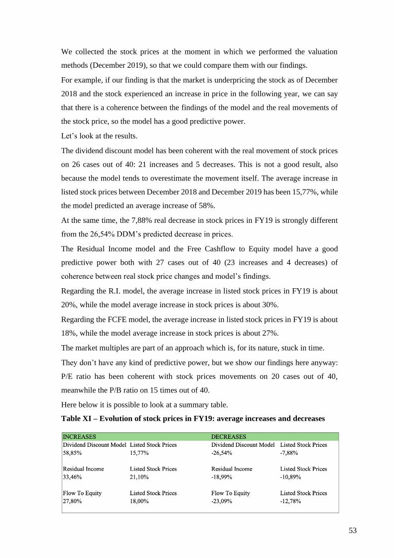
53

We collected the stock prices at the moment in which we performed the valuation

methods (December 2019), so that we could compare them with our findings.

For example, if our finding is that the market is underpricing the stock as of December

2018 and the stock experienced an increase in price in the following year, we can say

that there is a coherence between the findings of the model and the real movements of

the stock price, so the model has a good predictive power.

Let’s look at the results.

The dividend discount model has been coherent with the real movement of stock prices

on 26 cases out of 40: 21 increases and 5 decreases. This is not a good result, also

because the model tends to overestimate the movement itself. The average increase in

listed stock prices between December 2018 and December 2019 has been 15,77%, while

the model predicted an average increase of 58%.

At the same time, the 7,88% real decrease in stock prices in FY19 is strongly different

from the 26,54% DDM’s predicted decrease in prices.

The Residual Income model and the Free Cashflow to Equity model have a good

predictive power both with 27 cases out of 40 (23 increases and 4 decreases) of

coherence between real stock price changes and model’s findings.

Regarding the R.I. model, the average increase in listed stock prices in FY19 is about

20%, while the model average increase in stock prices is about 30%.

Regarding the FCFE model, the average increase in listed stock prices in FY19 is about

18%, while the model average increase in stock prices is about 27%.

The market multiples are part of an approach which is, for its nature, stuck in time.

They don’t have any kind of predictive power, but we show our findings here anyway:

P/E ratio has been coherent with stock prices movements on 20 cases out of 40,

meanwhile the P/B ratio on 15 times out of 40.

Here below it is possible to look at a summary table.

Table XI – Evolution of stock prices in FY19: average increases and decreases

54

3.4 Conclusions

There are several aspects that affect how financial services firms can be valued.

This paper provides empirical evidences on the drivers of shareholders value of

universal banks. We looked at a sample of 40 financial services firms in the FY18.

The widely spread method is the DDM, but there is a lack of precision even if it is used

in alternative ways like the Extraordinary growth (descripted in the first chapter) or a

three-stage model, because it remains linked to possible errors in the calculation of

growth as well as in the prediction of a possible pay-out policy.

Moreover, the DDM is wrongly used without considering the effect of regulatory capital

on the available cashflow to shareholders at the end of fiscal years.

The DDM is simple and logical but the explanatory power is not sufficient, in our

analysis it results in a 42% absolute value error with no tendency for underpricing or

overpricing stocks.

For some banks, some valuation method seems to have a higher explanatory power than

for other banks.

The Dividend discount model gives the impression to operate better with European

banks (for example Barclays, BNP Paribas, Credit Agricole, ING Bank) which have a

regular and constant historical pay-out ratio and substantial and regularly paid dividends

(27% error); this is not true for banks that are experiencing an extraordinary revenues’

growth and high pay-out ratios like USA banks. The trend of the model is to overvalue

these institutions.

In the Residual Income approach, we add some elements like the two-step analysis and

the SWOT analysis. Moreover, even if the dividend policy is stable (and this is not a

realistic assumption), dividends are strictly related to the Net Income’s growth.

This make the model reliable with the result of 26% absolute value error with no

tendency for under or over pricing the stocks.

USA banks are also overvalued by the R.I. model because of higher revenues’ growth

with respect to their cost of equity, meanwhile we get good results with the same model

for EU and Asian banks with errors ranging between 20% and 25%.

USA banks, in the contest of our entire analysis, tend to be underpriced by the market

(in 9 cases out of 10), meanwhile there is no general tendency for EU and Asian banks.

55

Let’s look at the market approach. The P/B ratio is an increasing function of the return

on equity, the pay-out ratio and the growth rate and a decreasing function of the riskiness

of the firm.

In particular, ROE has a strong impact on the ratio: a drop in the ROE has a double

impact. First, it reduces the growth rate in earnings and the expected pay-out ratio, so it

has an indirect effect on the P/BV ratio. Second, it lowers the P/B multiple directly.

On the other hand, we can observe that companies with strong and regular free cash

flows are overvalued by the model.

It happens, for instance, with some NYSE companies like SunTrust, Citigroup and Bank

of America. The last ROE of SunTrust bank is about 14%, which is higher than sector



In the FCFE model, we add another important factor for valuation, which is the

regulatory capital need of a bank. This means that the dividend policy is strictly related

both to the growth in Net Income and the needs of a Tier 1 capital buffer. This method

is the most complete and reliable simply because it takes in consideration the overall

issues of the banking industry. It results, in our analysis, in a 19% absolute value error.

As of now, we didn’t find a method reliable as much as the industrial Discounted Free

Cash Flow, because it is hard in the banking industry to deal with the problem of the

Debt and the issue of Reinvestments as described in chapter 1.

While the former can be faced by valuing only the Equity part through the Cost of

Equity, the latter can be solved by considering regulatory capital requirements in the

valuation of stocks (it is possible to consider regulatory capital needs in every method)

like the Free Cashflow to Equity model, but the result remains very volatile and linked

to factors which are hard to be estimated.

56

Appendixes

1. Sample (pt.1)

2. Sample (pt.2)

57

3. Sample (pt.3)

4. Sample (pt.4)

58

References

Bank for International Settlement, (2013) “A brief history of the Basel Committee”.

Charumathi B. & Suraj E. (2014), “Comparing Stock Valuation Models for Indian Bank

Stocks”, International Journal of Accounting and Taxation June 2014, Vol. 2, No. 2, pp.

111-127.

Damodaran, A. (2009). “Valuing Financial Service Firms Financial Service firms – The

Big Picture, (April)”, 1–34.

Damodaran, A. (2012). “Valuation - Tools and Techniques for Determining the Value

of Any Asset” (3rd ed., p. 155). New Jersey: John Wiley & Sons, Inc.

Deev O. (2011), “Methods of bank valuation: a critical overview”, Masaryk University,

Dept. of Finance.

Dermine, J. (2011), “Bank Valuation with an Application to the Implicit Duration of

non-Maturing Deposits”. In International Journal of Banking, Accounting and Finance.

Forthcoming, p. 40.

Deustche Bank AG (2014), Financial Report 2013.

Forte G., (2018), “Does Relative Valuation Works For Banks?”, Global Finance Journal.

Gounder C., Venkateshwarlu M. (2017), “Bank Valuation Models – A comparative

Analysis”, Sciedupress, Vol. 6, No. 3; 2017.

Gross S. (2006), “Banks and Shareholder Value: An Overview of Bank Valuation and

Empirical Evidence on Shareholder Value for Banks.” Gabler Ed.

Horvatova E. (2010), “Method of Banks Valuation”, EA (2010, Vol. 43, No, 1-2, 50-

60).

59

Hughes B., 13 Feb. 2018 “Credit Suisse has strong start to 2018 after third straight

loss”, Thomson Reuters Zurich.

Kaplan S. N., Ruback R. S., (1995), “The Valuation of Cash Flow Forecasts: An

Empirical Analysis”, Journal of Finance, 50(4): 1059-1093.

Koller, T., Goedhart, M., & Wessels, D. (2010), “Valuation: Measuring and Managing

the Value of Companies (5th ed.)”. John Wiley & Sons, Inc.

Koller, T., Copeland T. & Murrin, J. (2000), “Valuation: Measuring and Managing the

Value of Companies (3rd ed.)”. John Wiley & Sons, Inc.

Kulkarni C. (2016), “5 Benefits of getting a business valuation” Inc.com.

Legorano G., 2017, “UniCredit Sees €11.8 Billion 2016 Loss on Balance-Sheet

Cleanup”, The Wall Street Journal.

Leister F., (2015), “Valuation Methods for Banks: An Empirical Comparison of Intrinsic

Valuation Methods for Banks”, IUBH School of Business, 2015.

Levyne O., (2018), “Corporate Valuation”, HEC Paris, p.30-32.

Massari M., Gianfrate G., Zanetti L. (2014), “The valuation of financial companies:

tools and techniques to value banks and other financial institutions”. John Wiley &

Sons, Inc.

Mercer C., (1992), “Valuing financial services firms”, Irwin Ed.

Nissim, D. (2013) “Relative valuation of U.S. insurance companies”. Review of

Accounting Studies, 18(2), 324-359.

60

Olweny T., (2000), “The Reliability of Dividend Discount Model in Valuation of

Common Stock at the Nairobi Stock Exchange”, International Journal of Business and

Social Science, Vol. 2 No. 6; April 2011.

Rezaee, Zabihollah. (2001). “Financial Institutions, Valuations, Mergers, and

Acquisitions. The Fair Value Approach”, 2nd edition, New Yorketal.

Breaking Into Wall Street, (2018) “Bank Valuation, Quick Reference”

NYU Stern, “30 Issues in using the dividend discount model”

Lecci E., 2017, “Dividendi MPS assolutamente vietati fino al termine degli aiuti di Stato”

Neri S., 2017, “Banco Bpm triplica l’utile e progetta il primo dividendo. Hsbc alza

raccomandazione a buy”, FinanzaReport

61

Department of Business and Management

Chair of Advanced Corporate Finance

“Effective methods for valuing a bank: an empirical analysis” Summary

Supervisor Candidate

RAFFAELE ORIANI DANIEL GORINI

(692351)

Co-supervisor

ROSELLA SANTELLA

Academic Year 2018/2019

62

Table of Contents

ABSTRACT ........................................................................................................................................ 63

CHAPTER 1. INTRODUCTION TO BANKS VALUATION ............................................................. 63

1.1 THE IMPORTANCE OF VALUATION .............................................................................................................. 63 1.2 SPECIFICS OF BANKS: CORE ACTIVITIES AND FINANCIAL STATEMENTS ANALYSIS .................................... 64 1.3 SPECIFICS OF BANKS’ VALUATION: OVERVIEW ON POSSIBLE ISSUES ......................................................... 65 1.4 METHODOLOGIES ....................................................................................................................................... 66 1.4.1 DIVIDEND DISCOUNT MODEL ................................................................................................................... 66 1.4.2 FREE CASH FLOW TO EQUITY.................................................................................................................. 67 1.4.3 RESIDUAL INCOME MODEL ...................................................................................................................... 68 1.4.4 RELATIVE VALUATION ............................................................................................................................ 68

CHAPTER 2. LITERATURE REVIEW ............................................................................................. 69

2.1 OVERVIEW OF BANKS VALUATION LITERATURE ........................................................................................ 69 2.2 VALUATION METHODS: RELIABILITY AND APPLICABILITY TO BANKS ....................................................... 70

CHAPTER 3. EMPIRICAL ANALYSIS ............................................................................................ 71

3.1 SAMPLING CRITERIA AND DATA COLLECTION ............................................................................................ 72 3.2 DIVIDEND DISCOUNT MODEL RESULTS ....................................................................................................... 72 3.3 RESIDUAL INCOME MODEL RESULTS .......................................................................................................... 73 3.4 FREE CASHFLOW TO EQUITY MODEL ......................................................................................................... 75 3.5 P/E AND P/B APPLICATION RESULTS .......................................................................................................... 76 3.6 CONCLUSIONS ............................................................................................................................................. 78

APPENDIXES .................................................................................................................................... 80

63

Abstract

This paper presents the framework for valuing bank stocks using different valuation

models and investigates the explanatory power of each valuation model in the most

important world’s stock markets.

In the first chapter we give an introduction to business valuation, its importance and its

reasons for being performed.

In the second chapter we make a literature review, in order for the reader to better

understand how this topic has been covered from other authors and professionals.

This study compares the performances of different valuation models in determining

banks’ stock price: the third chapter is an empirical analysis on a sample of 40 listed

universal banks from Europe, Asia and USA&Canada holding a minimum of 2 Billion

euros of total assets.

We will show strengths and weaknesses of every model, their reliability with respect to

an application to banks, their advantages and disadvantages.

We compared the stock prices resulting from the application of the methodologies with

the share price listed on the stock exchange as of 31.12.2018.

The results show that there is not a clear superiority of a method with respect to others,

their errors in absolute value range from a 19% of the FTE to the 42% of the DDM

model.

Chapter 1. Introduction to banks valuation

1.1 The importance of valuation

“A business valuation provides the business owner with multiple facts and figures

regarding the actual worth or value of the company in terms of market competition, asset

values, and income values.”52 (Kulkarni, 2016)

The term “Valuation” refers to the process of determining the present value of a

company or an asset through a number of techniques. The goal of analysts when doing

valuation is to know if an asset or a company is undervalued or overvalued by the

market.

52 Kulkarni C. (2016), “5 Benefits of getting a business valuation” Inc.com

64

Knowing and understanding what the value of a business is, and what impacts its value

makes all the difference from not only a tax perspective, but also when it comes time

to merge, sell or divest.

In fact, valuation of companies is important for many professions.

1.2 Specifics of banks: core activities and financial statements analysis

A bank is a financial institution that provides banking and other financial services, and

the term bank is generally understood to refer to an institution that holds a banking

license.

The banking licenses granted by financial supervision authorities allow banks to provide

basic banking services such as accepting deposits and making loans. Typically, a bank

generates profits from the interest spread on the resources it holds in trust for its clients

while paying them interest on the assets, and from transaction fees on financial services.

Analyzing the structure of the balance sheets and income statements of banks and

industrial companies allows us to derive several banking specifics relevant to valuation.

The major positions on the asset side of the balance sheet of industrial companies are

property, plant and equipment, inventories and receivables. The asset side of a bank

balance sheet, however, is dominated by receivables from customers and from credit

institutions, accounting for three quarters of total assets.

Tangible assets are of minor importance for banks whose major input factors are

personnel expenses and investment in knowledge. Inventories and changes therein do

not exist, as banks provide services that are not storable. Consequently, bank earnings

are usually collected in the period in which they accrue.

The net income of banks before any risk adjustments therefore has the character of a

cash equivalent.

If we look at the liabilities’ side of the balance sheet, we see that industrial companies

are financed to the tune of approximately 50 percent by debt and to the tune of

approximately 50 percent by equity and provisions, whereas bank financing is

dominated by debt capital.

However, a significant part of this debt relates to the deposit business and it has no

financing function, but instead it is part of the operating business of the bank. Banks

create value on both the assets and the liabilities side of the balance sheet, and the

function of debt is hard to determine.

65

1.3 Specifics of banks’ valuation: overview on possible issues

With a financial service firm, debt seems to take on a different connotation. Rather than

view debt as a source of capital, most financial service firms seem to view it as a raw

material.

In other words, debt is to a bank what steel is to General Motors, something to be

moulded into other financial products which can then be sold at a higher price and yield a

profit. Consequently, capital at financial service firms seems to be more narrowly defined as

including only equity capital.

Due to the risks taken on by banks, their specific role in the economic system, and their

dependency on economic cycles, banks are subject to various bank-specific rules and

regulations, and the effect of regulatory requirements on value have to be considered.

Due to banks’ specific dependency on macroeconomic factors, legislators give them

specific rights to build up reserves.

First, banks are required to maintain capital ratios to ensure that they do not expand

beyond their means and put their claimholders or depositors at risk.

Second, financial service firms are often constrained in terms of how they can invest

their funds. For instance, the Glass-Steagall act in the United States restricted

commercial banks from investment banking activities and from taking active equity

positions in manufacturing firms.

Third, entry of new firms into the business is often restricted by the regulatory

authorities, as are mergers between existing firms.

From a valuation perspective, assumptions about growth are linked to assumptions

about reinvestment.

With financial service firms, these assumptions have to be scrutinized to ensure that

they pass regulatory constraints.

Provisions for losses are also an issue for valuation. These provisions reduce net income

in the current period but are used to meet expected losses in future periods.

In general, while the actual bad debts that occur in any year will not match the provision

set aside for that year exactly, the cumulative provisions over time should be equal to

the cumulated bad debts over the same period.

If we define reinvestment as necessary for future growth, there are other problems associated

with measuring reinvestment with financial service firms.

Usually we consider two items in reinvestment – net capital expenditures and working

66

capital. Unfortunately, measuring either of these items for a financial service firm can be

problematic.

Consider net capital expenditures first. Unlike manufacturing firms that invest in

plant, equipment and other fixed assets, financial service firms invest in intangible assets such

as brand name and human capital.

With working capital, we run into a different problem. If we define working capital as the

difference between current assets and current liabilities, a large portion of a bank’s balance

sheet would fall into one or the other of these categories.

Changes in this number can be both large and volatile and may have no relationship to

reinvestment for future growth.

1.4 Methodologies We value firms by discounting expected cash flows prior to debt payments at the weighted

average cost of capital. We value equity by discounting cash flows to equity investors at the

cost of equity.

Estimating cash flows prior to debt payments or a weighted average cost of capital is

problematic when debt and debt payments cannot be easily identified, which, as we argued

earlier, is the case with financial service firms. Equity can be valued directly, however, by

discounting cashflows to equity at the cost of equity. Consequently, we would argue for the

latter approach for financial service firms.

1.4.1 Dividend discount model

In the basic dividend discount model that we are going to use, the value of a stock is the

present value of the expected dividends on that stock. While many analysts view the

model as old-fashioned, it retains a strong following among analysts who value financial

services companies, because of the difficulties we face in estimating cashflows.

In the special case where the expected growth rate in dividends is constant forever, the

classic DDM model collapses into the “Gordon growth model”.

In the Gordon growth model, the dividend payout of the firm has to be consistent with

the assumption of stability, since stable firms generally pay substantial dividends.

In particular, this model will underestimate the value of the stock in firms that

consistently pay out less than they can afford and accumulate cash in the process.

67

The version of the Dividend Discount Model we are going to use discounts the dividends

of the next year (calculated through a normalized growth rate) at the present Cost of

Equity (COE) minus the same growth rate. The COE is calculated with CAPM formula.

The normalized growth rate is calculated as the product of average Return on Equity

(ROE) of the previous four years and the average Retention Ratio of the previous four

years.

This model is best suited for firms growing at a rate comparable to or lower than the

nominal growth in the economy and which have well established dividend pay-out

policies that they intend to continue into the future.

Dividends paid must be substantial and they have to be paid on a regular basis.

When they are not, we estimate the equity value by forecasting dividends 10 years in

the future and discounting them at the cost of equity.

1.4.2 Free Cash Flow to Equity

Banks are required to maintain minimum capital to sustain their operations, and there

are two measures of capital: Tier 1 capital is the narrower measure and is composed

primarily of common equity but also includes noncumulative preferred stock, while Tier

2 capital is a broader measure of capital that includes subordinated debt and cumulative

preferred stock.

To implement this FCFE model, we need two ingredients.

The first is the expected net income over time. The second is the investment in

regulatory capital, which will be a function of both the degree to which the financial

services firm is under or over-capitalized to begin the process and the expected growth

rate in its risk-adjusted assets.

The CT1 or common equity is based on the shareholders equity. In other terms, it does

not include any hybrid or debt instrument.

In this approach, the equity value is the sum of the discounted future theoretical

dividends i.e. the dividends which could be paid so that the CT1 ratio reaches its target

level. For example, if the CT1 and RWA are respectively worth 120 and 1000, the CT1

ratio reaches 12%. If the target CT1 ratio is 9%, the bank has an excess equity for a

consideration of 120 – 9%x1000 = 30. In that case, the theoretical dividend amounts to

30.

68

1.4.3 Residual Income model

In this model the equity value of a bank is the sum of the PV of expected excess return

and the capital currently invested in the bank.

The difference between a DDM and a RIM is that, in a Dividend Discount Model, we

use the present value of Dividends and the present value of the Terminal Value of

Dividends to value a bank, but in a Residual Income Model you use the difference

between ROE and Cost of Equity plus the current Book Value to value the bank.

Hence, the excess equity return needs to be calculated.

𝐸𝑥𝑐𝑒𝑠𝑠 𝐸𝑞𝑢𝑖𝑡𝑦 = (𝑅𝑂𝐸 – 𝐶𝑂𝐸) ∗ 𝐵𝑜𝑜𝑘 𝑉𝑎𝑙𝑢𝑒 𝑜𝑓 𝐸𝑞𝑢𝑖𝑡𝑦

The beginning book value (BV) of equity for the following year is simply the BV of

equity of the following year plus the expected retained earnings of the year.

𝐵𝑉 𝑜𝑓 𝐸𝑞𝑢𝑖𝑡𝑦n= 𝐵𝑉 𝑜𝑓 𝐸𝑞𝑢𝑖𝑡𝑦n-1 + (𝑁𝑒𝑡 𝐼𝑛𝑐𝑜𝑚𝑒n-1*𝑅𝑒𝑡𝑒𝑛𝑡𝑖𝑜𝑛 𝑅𝑎𝑡𝑖𝑜)

Projecting a bank’s future return on equity can be challenging.

“A logical starting point is to look at a long history of the bank’s actual returns on equity, and

then making adjustments for the future. This is the stage where the analysts take into account

the bank’s strengths and weaknesses relative to its competitors, as well as expected changes

to the macroeconomic environment” 53(Damodaran, 2009)

The excess equity is then discounted by the cumulated COE and added to the initial BV of

equity.

Afterwards, the terminal value is added to result in current value of equity, before dividing by

the diluted number of shares in order to obtain the result of the model: the implied price per

share. In conclusion, it can be compared to the listed share price in order to understand if the

company is undervalued or overvalued by the market.

1.4.4 Relative Valuation

One of the more intuitive ways to think of the value of any asset is as a multiple

of the earnings it generates. When buying a stock, it is common to look at the price paid as a

multiple of the earnings per share generated by the company.

The price earnings ratio for a bank is measured much the same as it is for any other firm.

As with other firms, the price earnings ratio should be higher for financial service firms

with higher expected growth rates in earnings, higher pay-out ratios and lower costs of

equity.



69

The most important issue about the multiple is that “earnings represent the bottom line of the

income statement, they can also be affected by different accounting policies” (Forte G., 2018).

The second multiple we are using is the P/B value. It represents the ratio between the market

capitalization of the firm and the book value of equity.

“It is widely used for capital-intensive businesses although it is subordinate for sectors where

the main driver of price performance is future growth, such as technology or media. The

measure is suitable for financial institutions because of the regulatory stress on solvency,

capital requirements, and equity maintenance”.

Other things remaining equal, higher growth rates in earnings, higher pay-out ratios,

lower costs of equity and higher returns on equity should all result in higher price to

book ratios. Of these four variables, the return on equity has the biggest impact on the

price to book ratio, leading us to identify it as the companion variable for the ratio.

Chapter 2. Literature review

The literature published in the area of shareholder value is manifold in nature.

As the shareholder value approach was originally developed for industrial companies,

the majority of contributions focuses on the valuation of industrial companies and do

not account for bank-specific issues.

2.1 Overview of banks valuation literature

Even if the number of articles and doctoral thesis in the area of bank valuation and bank

management has increased recently, only a few contributions give a detailed and

comprehensive overview of the adjustments to valuation necessary in a banking context

and go on to deliver practical, hands-on advice for valuing banks.

Copeland et al. (2000), authors of the standard work on valuation, devote just a single

chapter to bank valuation. “Copeland et al. also paid attention to the fact that bank

liabilities consist of customer deposits and borrowings on funds market, which

apparently perform the same function, but with a different margin. As a result, the spread

between the interest received on loans and the cost of capital is so low that small errors

in estimating the cost of capital can result in huge swings in the value of the bank”54

(Deev O., 2011).


70

There are German contributions from the eighties, such as Zessin (1982), Schell (1988)

and Adolf et al. (1989), focus on the subject from a purely accounting viewpoint

promoted by German auditors, and do not share the cash orientation of Copeland et al.

(2000) and standard valuation literature.

North American contributions in the 1990s such as Mercer (1992), Johnson (1996) and

Rezaee (2001), give a comprehensive overview of the banking industry, introduce the

general principles of valuation, and cover some of the bank-specific issues.

Few recent authors cover existing bank valuation literature comprehensively. Most

articles are typically limited to a general discussion of valuation principles and their

application to banks instead of further developing existing insights on bank-specific

valuation issues.

Generally speaking, some of these works talk about a comparison between DCF models

and Residual Income models, with many bank specifics supporting the use of a residual

income approach for bank valuation.

2.2 Valuation methods: reliability and applicability to banks

Equity value multiples are much better suited for valuing banks than value

multiples. Firm value multiples such as EV/EBIT or EV/EBITDA are not applicable to

bank valuation, as the operating and financing activities of banks cannot be clearly

separated. The actual P/E multiple typically uses historical earnings as an approximate

value for earnings, and therefore lacks a forward-looking perspective. The use of

predicted P/E ratios and an estimate of future earnings can solve this problem, but

valuation using P/E ratios is still limited to a return view and does not consider risk,

which plays an important role when assessing future performances.55

“High earnings growth in the short term may lead to the destruction of shareholders

value for banks in the longer term if earnings growth is realized by a decrease in the

quality of the credit portfolio” (Gross S., 2006).56

Concerning the P/B ratio, it compares the market value of equity to the book value. It is

forward-looking and relates the market’s expectations concerning future performance

to invested capital. Due to the balance of risk ability and profitability, P/B ratios have a

higher explanatory power with respect to P/E multiples when it comes to banking.57

55 See Damodaran A., 2009, p.34



57 See Kirsten (2000), p.192

71

The relationship between P/B and ROE is very strong for banks and it is validated by

empirical evidences with a high correlation, Damodaran and Kirsten found a R squared

of 0.70 respectively for US and European banks.58

According to Charumathi B. (2014), Tobias Olweny (2011) conducted a study in

Nairobi stock exchange to establish the reliability of the dividend discount model (which

is based on the discounted cash flow techniques) on the valuation of common stocks.

“Predicted share prices were compared with the actual prices by computing the

differences between them. The differences were then subjected to t-test.

The study concluded that the dividend discount model was not reliable in the valuation

of common stocks at the Nairobi Stock Exchange” (Olweny T., 2000).59

The result can be justified thanks to Thomas H. Payne (1999): “his paper demonstrates

that the valuation measure derived from using the DDM is very sensitive to the

relationship between the required return on investment (Ke) and the assumed growth

rate (g) in earnings and dividends” (Charumathi B., 2014).60

In his work, Charumathi explains why it makes far more sense to focus on equity

(instead of the entire capital invested) when using an excess return model for valuing a

financial services firm. Once more, it is due to the difficulty associated with defining

total capital in a bank.

From a practical point of view, in a study conducted for Stern University by Damodaran

on February 2009, he analysed the share value of Goldman Sachs through the excess

return model. He proved that ERM can be considered as a reliable model for valuing

bank stocks, at least in the US stock market, but there are persistent issues when it comes

to the estimation of important input factors. The choice of these estimates is crucially

important.

Chapter 3. Empirical analysis

The aim of this work is to better understand which is the best method for valuing a

financial services firm, by comparing the listed share prices with the results obtained by

the application of the methodologies described in the first section.

58 See Damodaran (2009) p.37 and Kirsten (2000) p.192.

59 Olweny T., (2000), “The Reliability of Dividend Discount Model in Valuation of Common Stock at the Nairobi

Stock Exchange”, International Journal of Business and Social Science, Vol. 2 No. 6; April 2011

60 Charumathi B. & Suraj E. (2014), “Comparing Stock Valuation Models for Indian Bank Stocks”, International

Journal of Accounting and Taxation June 2014, Vol. 2, No. 2, pp. 111-127

72

3.1 Sampling criteria and data collection

The sample is made up of 40 financial services firms.

We applied four different criteria:

5. Geographic: in order to set a comparison half of them are European banks, while the

other half is composed for 50% by USA and Canada banks, and 50% by Asian

banks.

6. Market criterium: in order to have a market’s benchmark for our results, we decided

to select a list of banks listed on the major stock exchanges of their home countries.

7. Core activities criterium: for coherence reasons our sample is composed only by

Universal banks, performing all the corporate and investment banking activities as

well as retail and consumer banking activities.

8. Size criterium: we decided to take a sample made of banks with Market cap and total

Assets both higher than 2 billion euros.

All the required data have been collected on Saturday 30th of November 2019.

The cost of equity has been calculated through CAPM formula, while the growth rate

(g) has been calculated as ROE*Retention ratio.

The chosen Beta are historical 5-years Beta of our sample’s banks with respect to their

respective most important country’s Indexes.

Data about dividends paid by single banks are taken from “Investors relations” section

of their websites.

This work is aimed at understanding how a valuation method precise can be for

the banking industry by comparing the results with the listed share price at 31.12.2018,

in order to figure out which is the estimated error of each applied method and in order

to understand where there is an overpricing or an underpricing for each methodologies.

3.2 Dividend discount model results

In order to perform our models, every caption and item on financial statements has been


The starting point of our Dividend Discount Model has been the collection of DPS data

from the “investors relations” section of the banks’ websites.

It has been useful to look at historical DPS and EPS of last 4 years in order to calculate

the average historical retention ratio.

From the Bloomberg database we collected the last-4-years average ROE and we used

these data for the calculation of the growth rate (“g = avg. ROE*avg. Retention Rate).

73

Furthermore, in order to perform the model, we were in need of the cost of equity.

It has been calculated by collecting a 5-years country’s index Beta for each bank and

the risk-free rates from the 10-years countries’ treasury bonds, both from the Bloomberg

database. The total equity risk premium was found in the specific section on

Damodaran’s database.

For any result we calculated the Error with respect of the actual share price: when the

Error comes out with the positive sign, the stock is underpriced by the market; on the

contrary, when it comes out with the sign “minus”, the stock is overpriced by the market.

This kind of Dividend Discount Model resulted in an overall Error of about 42% in

absolute terms. It is possible to look at a summary table in appendix 1.

This high error’s value is due to several reasons: the lack of flexibility in the input

factors, the extent in which the result is linked to errors in the estimate of g and the lack

of regularity and consistency of historical input factors are the most important reasons.

“A standard critique of the dividend discount model is that it provides too conservative

estimates of value. This criticism is predicated on the notion that the value is determined

by more than the present value of expected dividends. For instance, it is argued that the

dividend discount model does not reflect the value of 'unutilized assets'. Moreover, it

does not incorporate other ways of returning cash to stockholders (such as stock

buybacks).”61 (Damodaran, 2009)

Due to these difficulties in the application of the method, it was impossible to apply the

model to some of the observation (we got errors up to 185%).

It seems to work better in the European market (27,7% average error in absolute value)

with respect to Asian and USA/Canada markets (56% and 54% average errors in

absolute value, respectively).

3.3 Residual Income model results

In order to perform our models, every caption and item of financial statements has been


Let’s look at the sources: the starting point of the Residual Income model is the

calculation of the Book Value of equity for the companies of our sample: Total Assets

minus Total Liabilities (data from published financial statements FY18).


74

Then, as we need to find an ROE for a 5-years horizon projection and then a Long Term

ROE for Terminal Value, the Expected ROE of the next fiscal year has been collected

on Bloomberg and then adjusted on the basis of a SWOT analysis performed by us in

order to get a possible Long Term ROE (we analysed whether the company is healthy

or not, which is its position on the market with respect to its competitors, possible

opportunities and weaknesses by looking at several market reports).

For the calculation of dividend pay-out ratio, we used the last DPS published by the

firm’s official website (FY2018) together with normalized EPS (average of last 4 years).

The aim of this model is to value the company share by calculating the value of future

expected residual incomes.

We construct our residual income model as a two-phase model, with Phase 1

representing a simple forecast period of 5 years similar to the one in a traditional DCF

approach, and Phase 2 describing the remaining life of the bank as a Terminal Value.

There is no tendency in over or under pricing the stocks within the Residual Income

model, which seems to be more reliable than a DDM with an average Error in absolute

value of 26,4%.

For healthy companies, equity value far exceeds book value as the market value of the

company’s shares appreciates over the years.

This is not true in the case of banks.

As a consequence of the crisis of 2008, due to the depreciation of shares almost all the

P/B ratios in the banking sector are lower than 1, and the Book Values of Equity are

largely higher than respective Market Capitalizations.

This would make the Residual Income method not completely reliable if performed as

a one-stage model, so it is important and crucial to perform a perfect SWOT analysis,

to look at the economic situation of banks’ countries and to calculate a reliable Long-

Term ROE in order to give stability to the model.

Moreover, an especially weak point of this model is the assumption about the future

pay-out ratio of banks, which is often very volatile over time.

If we look at the geographical differences, the model performed better for EU and Asian

banks with Errors in absolute value of 23% and 25% respectively.

For USA companies the error in absolute value resulted in a 35%, and in 9 cases out of

10 the error is positive, so the observations result underpriced by the market.

75

The estimated ROEs of USA banks are largely higher than the required Cost of Equity,

consequently they are experiencing a special growth higher than the global sector

average. It is possible to look at model’s results in appendix 2.

3.4 Free Cashflow to Equity Model

To overcome the problem with volatile pay-out ratios, we need to consider what

influences the dividend pay-out policy.

The most important driver for this is the regulatory requirement that a bank has to fulfil

in terms of capital ratios.

So far, all the models ignored the reinvestment needs. For a more realistic valuation one

needs to know the RWA of a bank as well as the required CET 1 ratio62 (Leister F.,

2015).

Let’s look at our sources for performing this model: as the RWA amount is not shown

in the financial statements, the calculation of a target CET1 ratio is only possible by

looking at financial reports and banks’ Pillar III fulfilments, which can be very time-

consuming.

The model has been performed as explained in chapter 1 and it is based on the

assumptions of the business plan of the banks in the sample and the Pillar III

requirements fulfilment report published at the end of FY18.

The model consists in a 10-years forecast comprehensive of 3 years of business plan

assumptions and 6 years of “soft landing” period.

The equity value in this approach is the sum of the discounted future theoretical

dividends (i.e. the dividends which could be paid so that the CT1 ratio reaches its target

level) and a terminal value placed at the end of the “soft landing” period.

This model is the only one which takes in consideration the regulatory framework a

bank must deal with, so it should also be the most reliable.

Although this model seems to be the theoretically most appropriate for bank valuation,

a practical adoption is difficult and based on a variety of assumptions that make the

model fragile.

Moreover, it is hard to find all the necessary information and data.



76

Generally speaking, as we can see from appendix 3, the model generates an average

error of 19,21%, which is slightly lower than the others.

There is no general tendency for overvaluing or undervaluing stocks, and results are

geographically homogeneous. It is possible to look at a summary table in appendix 3.

3.5 P/E and P/B application results

First of all, we explain how we performed the valuation method, and which are the

sources.

In order to perform our models, every caption and item of financial statements has been


For each bank we selected a list of comparable companies from the Bloomberg terminal.

In the same terminal we directly collected the ratios for the FY18 in order to get the

model results. We go on with the multiplication of the average P/E of comparable firms

(or, in alternative, the median if we recognize outliers) by the Earnings (in the case of

P/E) or the Book Value of Equity (in the case of P/B) of our sample’s banks. Then, the

market capitalization divided by the diluted number of shares gave the implied price per

share as a result.

Even if it is a simple and fast methodology, there are several limitations in using

multiples.

“A weakness of P/E is the level of freedom surrounding the accounting practices on Net

Income for banks. Provisions for possible losses (non-performing loans) are usually

manipulated and Net Income shown could be higher or lower than the real value.

In general, one would expect a more conservative bank to set aside more money and a

less conservative bank to set aside less money which would increase the earnings

multiple” (Damodaran, 2009).

Secondly, in order for P/E ratios to have an explanatory power, earnings must be

positive, so it makes impossible to analyse companies that are suffering losses in this

fiscal year.

Moreover, the multiple that an investor is willing to pay for one Euro in earnings from

trading is clearly different from the multiple that the same investor is willing to pay for

one Euro of earnings from commercial lending, so it is hard to value Universal banks

for this reason.

What emerges by the application of the model is an absolute value Error of 27,4% and

a special performance for USA banks (11,7%). The model is in line with the stocks’

77

price at 31.12.2018 for HSBC (abs. value Error -0,14%), IMI (0,7%), UOB Singapore

(1%) and BB&T Bank (1%).

Regarding the P/B ratio, as we said in the previous paragraph it is not a reliable indicator

in our analysis because of the huge differences between Market values and Book values

of equity. It is not by chance that it brings a result of 38% abs. value error, which is

much higher than the P/E model.

We can “break up” the multiple, in order to understand better how the ROE impacts on

the results. From the function of the price we know: P0 =Div

Ke−g.

So, we can say that:

P0 =EPS × 𝑝𝑎𝑦𝑜𝑢𝑡

Ke−g

P0 =B × ROE ×𝑝𝑎𝑦𝑜𝑢𝑡

Ke−g

P0

B=

ROE×𝑝𝑎𝑦𝑜𝑢𝑡

Ke−g

When there are huge differences between the returns of the companies, multiples cannot

be reliable as we want it to be. In particular, ROE has a strong impact on the Price to

Book ratio.

The P/B ratio is an increasing function of the return on equity, the pay-out ratio and the

growth rate and a decreasing function of the riskiness of the firm.

For example, the last ROE of SunTrust bank is about 14%, which is higher than sector



On the contrary, a drop in the ROE has a double impact. First, it reduces the growth rate

in earnings and the expected pay-out ratio, so it has an indirect effect on the P/BV ratio.

Second, it lowers the P/B multiple directly.

The influence of the return on equity and the cost of equity can be consolidated in one

measure by taking the difference between the two a measure of excess equity return (see

Residual Income model). The larger the return on equity relative to the cost of equity,

the greater is the price-book value ratio.

It is possible to look at a summary table in appendixes 4 and 5.

78

3.6 Conclusions

There are several aspects that affect how financial services firms can be valued.

This paper provides empirical evidences on the drivers of shareholders value of

universal banks. We looked at a sample of 40 financial services firms in the FY18.

The widely spread method is the DDM, but there is a lack of precision even if it is used

in alternative ways like the Extraordinary growth (descripted in the first chapter) or a

three-stage model, because it remains linked to possible errors in the calculation of

growth as well as in the prediction of a possible pay-out policy.

Moreover, the DDM is wrongly used without considering the effect of regulatory capital

on the available cashflow to shareholders at the end of fiscal years.

The DDM is simple and logical but the explanatory power is not sufficient, in our

analysis it results in a 42% absolute value error with no tendency for underpricing or

overpricing stocks.

For some banks, some valuation method seems to have a higher explanatory power than

for other banks.

The Dividend discount model gives the impression to operate better with European

banks (for example Barclays, BNP Paribas, Credit Agricole, ING Bank) which have a

regular and constant historical pay-out ratio and substantial and regularly paid dividends

(27% error); this is not true for banks that are experiencing an extraordinary revenues’

growth and high pay-out ratios like USA banks. The trend of the model is to overvalue

these institutions.

In the Residual Income approach, we add some elements like the two-step analysis and

the SWOT analysis. Moreover, even if the dividend policy is stable (and this is not a

realistic assumption), dividends are strictly related to the Net Income’s growth.

This make the model reliable with the result of 26% absolute value error with no

tendency for under or over pricing the stocks.

USA banks are also overvalued by the R.I. model because of higher revenues’ growth

with respect to their cost of equity, meanwhile we get good results with the same model

for EU and Asian banks with errors ranging between 20% and 25%.

USA banks, in the contest of our entire analysis, tend to be underpriced by the market

(in 9 cases out of 10), meanwhile there is no general tendency for EU and Asian banks.

79

Let’s look at the market approach. The P/B ratio is an increasing function of the return

on equity, the pay-out ratio and the growth rate and a decreasing function of the riskiness

of the firm.

In particular, ROE has a strong impact on the ratio: a drop in the ROE has a double

impact. First, it reduces the growth rate in earnings and the expected pay-out ratio, so it

has an indirect effect on the P/BV ratio. Second, it lowers the P/B multiple directly.

On the other hand, we can observe that companies with strong and regular free cash

flows are overvalued by the model.

It happens, for instance, with some NYSE companies like SunTrust, Citigroup and Bank

of America. The last ROE of SunTrust bank is about 14%, which is higher than sector



In the FCFE model, we add another important factor for valuation, which is the

regulatory capital need of a bank. This means that the dividend policy is strictly related

both to the growth in Net Income and the needs of a Tier 1 capital buffer. This method

is the most complete and reliable simply because it takes in consideration the overall

issues of the banking industry. It results, in our analysis, in a 19% absolute value error.

As of now, we didn’t find a method reliable as much as the industrial Discounted Free

Cash Flow, because it is hard in the banking industry to deal with the problem of the

Debt and the issue of Reinvestments as described in chapter 1.

While the former can be faced by valuing only the Equity part through the Cost of

Equity, the latter can be solved by considering regulatory capital requirements in the

valuation of stocks (it is possible to consider regulatory capital needs in every method)

like the Free Cashflow to Equity model, but the result remains very volatile and linked

to factors which are hard to be estimated.

80

Appendixes

Appendix 1.

Dividend Discount Model results overview

81

Appendix 2.

Residual Income model results overview

82

Appendix 3.

Free Cashflow to Equity model results overview

83

Appendix 4.

Price/Earnings multiple model results overview

84

Appendix 5.

Price/Book Value multiple model results overview

“Effective methods for valuing a bank: an empirical analysis”

Documents

Transcript of “Effective methods for valuing a bank: an empirical analysis”