Valuing Flexibility in Ship DesignA Real Options Approach

Tara Jahangiry

Marine Technology

Supervisor: Bjørn Egil Asbjørnslett, IMT

Department of Marine Technology

Submission date: June 2015

Norwegian University of Science and Technology

1

"In the middle of difficulty lies opportunity." - Albert Einstein

iii

PREFACE During the spring semester of 2015 this master thesis has been produced at the

Department of Marine Technology, NTNU for the sub-department of marine systems –

ship design and logistics. The main supervisor has been Bjørn Egil Asbjørnslett.

This master thesis has the overall objective to evaluate the option value of owning a

Multipurpose Offshore Construction Vessel that is able to operate in the markets of

offshore subsea construction, well intervention and pipe laying. This has been achieved

by performing a Real Options Analysis using the Black-Scholes Option Pricing Model

often used when valuing European call options. Most of the time was spent studying the

method, assessing the necessary deck equipment for the different vessel types and

finding information about prices related to these. This created a foundation for the Real

Options Analysis that is performed.

The work presented here is a continuation of my project thesis from the fall semester of

2014, where I used Real Options in marine systems design. Some of the information in

this study is thus gathered from the project work. The rest of the relevant information

has been provided by professors at NTNU and PUC-Rio, internet sources or helpful

employees at NOV, Wartsila and Ulstein.

Finally, I would like to express my great appreciation to Bjørn Egil Asbjørnslett, Marco

Antonio Guimarães Dias, David Hoy, Erlend Sandvik, Per Olaf Brett, Jose Jorge Garcia

Agis, Mikkel Haslum, the office girls and everyone else who participated in making this

thesis possible.

Trondheim 10.06.2015

Tara Jahangiry

v

SUMMARY This thesis is a Real Options (RO) approach to valuing flexibility in ship design. The

overall object is to find the value of owning a Multipurpose Offshore Construction Vessel

(MOCV) by applying the Black-Scholes Option Pricing Model. The MOCV holds the option

of switching into an Offshore Subsea Construction Vessel (OSCV), a Well Intervention

Vessel or a Pipe Laying Vessel. The thesis aims to discuss the owner’s economic benefit

of owning an MOCV instead of three separate single purpose vessels. Dimensions,

equipment types and capacities on the MOCV are based on the reference vessel, The

Island Performer.

To solve this task, the problem has been limited by the following boundaries: at the time

T=0, the vessel will be completed as an OSCV with options for further evolvement. At the

end of each contract the owner has the option to switch to a different market by

switching vessel type. Each of the three markets have different contract lengths and the

analysis only considers the first four contracts of the vessel’s service time.

In the RO Analysis, the time to maturity of the option is considered equal to the

remaining time of the current contract. The stock prices and the stock price volatility are

estimated based on the vessel’s daily hire rates under long-term contracts in the North

Sea. The strike price is equal to the cost of switching vessel types and each switching

option has a different strike price. Lastly, ten-year government bonds underlie the risk-

free rate.

The main results from this analysis confirm that a vessel that can work as a working

platform for different vessel types is a good investment in an uncertain market. From

the results it can be seen that the value of owning a MOCV is strictly positive in all three

cases. The values even exceed the initial investment. It has also been demonstrated that

the maximum amount one can save by storing the deck equipment for future periods is

25 mUSD. Due to different assumptions made the for vessel types, it is difficult to

comment on whether one of the vessel types is more preferred than the other two.

vii

SAMMENDRAG Denne oppgaven er en evaluering av et fleksibelt skipsdesign, som er gjort ved å ta i

bruk en realopsjons-tilnærming. Oppgavens hovedformål er å vurderer verdien av å

benytte seg av at flerfunksjonelt offshore konstruksjonsfartøy (MOCV) ved å anvende

Black-Scholes opsjonsprisingsmodell. MOCVen eier opsjonene om å operere som et

offshore undervanns konstruksjonsfartøy (OSCV), et brønnintervensjonsfartøy eller et

rørleggingsfartøy. Oppgaven sikter mot å diskutere hva en reders økonomiske fordeler

kan være ved å eie en MOCV istedenfor tre konvensjonelle fartøy. Referanseskipet,

Island Performer, brukes til valg av dimensjoner, dekksutstyr og kapasitet.

For å løse oppgaven har problemet blitt begrenset av følgende antakelser: Ved tiden T=0

ferdigstilles båten som en OSCV med forsterkninger i skrog og rundt moonpool området.

Ved hver kontraktsslutt har rederen mulighet til å bytte modus på fartøyet ved å utøve

en av de tilgjengelige opsjonene, eller å forbli uforandret i enda en periode. De tre

kontraktstypene har ulik lengde grunnet ulikt arbeid som utføres. Kun de fire første

kontaktene blir analysert i denne modellen.

I realopsjonsanalysen er opsjonens tid til utløp ansett som den gjenværende tiden i den

nåværende kontrakten. Aktivaverdien og prisenes flyktighet er estimert ut i fra

fartøyenes daglige rater under langtidskontrakter i Norsjømarkedet. Prisen for å utøve

opsjonen estimeres ut fra kostnadene tilknyttet bytte av fartøysmodus og er antatt ulik

avhengig av modusene det byttes mellom. Til slutt er den risikofrie renten hentet ut ifra

tiårige statsobligasjoner.

Hovedresultatene fra denne analysen bekrefter at et fartøy som kan fungere som en

arbeidsplattform for ulike skipsmoduser er en god investering i et usikkert marked. Fra

resultatene sees det at verdien av å eie en MOCV er positiv i alle de tre opsjonstilfellene.

Verdiene overskrider til og med den initiale investeringen. Det har også blitt vist at ved å

lagre dekksutstyret til senere perioder kan man spare opptil 25 mUSD. Grunnet ulikt

grunnlag for beregning av aktivaverdiene, er det vanskelig å kommentere hvorvidt en av

fartøystypene er mer fordelaktig enn de to andre.

ix

TABLE OF CONTENTS

1 INTRODUCTION........................................................................................................................................ 2

1.1 OBJECT ...................................................................................................................................................................... 3 1.2 LITERATURE STUDY ........................................................................................................................................... 4 1.3 THE STRUCTURE OF THE THESIS ................................................................................................................. 6

2 PROBLEM DESCRIPTIONS .................................................................................................................... 8 2.1 OFFSHORE SUPPORT VESSELS....................................................................................................................... 8

2.1.1 Offshore Subsea Construction Vessels ................................................................................................ 8 2.1.2 Well Intervention Vessels ...................................................................................................................... 10 2.1.3 Pipe Laying Vessels ................................................................................................................................... 12 2.1.4 Multifunctional Offshore Construction Vessel .............................................................................. 14

2.2 MARKET DESCRIPTION ................................................................................................................................... 15 2.3 CASE DESCRIPTION ........................................................................................................................................... 19

3 REAL OPTIONS ....................................................................................................................................... 24 3.1 INTRODUCTION TO REAL OPTIONS .......................................................................................................... 24

3.1.1 Terminology ................................................................................................................................................ 25 3.1.2 Types of Options ........................................................................................................................................ 27 3.1.3 Real Options in Our Everyday Life ..................................................................................................... 28

3.2 VALUATION OF REAL OPTIONS ................................................................................................................... 29 3.2.1 Net Present Value ...................................................................................................................................... 29 3.2.2 Discounted Cash Flow ............................................................................................................................. 30 3.2.3 The Binomial Option Pricing Method ................................................................................................ 30 3.2.4 Monte Carlo Simulation .......................................................................................................................... 30 3.2.5 The Black-Scholes Method ..................................................................................................................... 31

3.3 CHALLENGES WITH REAL OPTIONS.......................................................................................................... 35

4 USING THE BLACK-SCHOLES METHOD TO VALUE THE MOCV ......................................... 38 4.1 TIME TO MATURITY ......................................................................................................................................... 38 4.2 THE STOCK PRICE .............................................................................................................................................. 40 4.3 THE STRIKE PRICE ............................................................................................................................................ 41 4.4 THE VOLATILITY ................................................................................................................................................ 43 4.5 THE RISK-FREE RATE OF RETURN ............................................................................................................ 44

5 RESULTS ................................................................................................................................................... 46

6 DISCUSSION ............................................................................................................................................ 50 6.1 DISCUSSION OF THE INPUT DATA ............................................................................................................. 50

6.1.1 Discussion of the Time to Maturity .................................................................................................... 50 6.1.2 Discussion of the Stock Price ................................................................................................................ 51 6.1.3 Discussion of the Strike Price ............................................................................................................... 53 6.1.4 Discussion of the Volatility .................................................................................................................... 54 6.1.5 Discussion of the Risk-Free Rate of Return .................................................................................... 57

6.2 DISCUSSION OF THE RESULTS ................................................................................................................ 57

x

7 CONCLUSION .......................................................................................................................................... 62 FURTHER WORK ........................................................................................................................................................ 63

REFERENCES .................................................................................................................................................. 64

APPENDIX ........................................................................................................................................................ 68 APPENDIX A – PROBLEM DESCRIPTION ......................................................................................................... 68 APPENDIX B – CALCULATION OF VOLATILITY OF STOCK PRICE ........................................................ 70 APPENDIX C – CALCULATION OF STOCK PRICE .......................................................................................... 71 APPENDIX D – OSCV, WIV, PLV AND MOCV FLEET OVERVIEW ............................................................ 72 APPENDIX E – CALCULATION OF VOLATILITY OF OIL PRICE ............................................................... 75 APPENDIX F – CALCULATION OF STRIKE PRICE ......................................................................................... 75 APPENDIX G – CUMULATIVE STATISTICAL VALUES ................................................................................. 77 APPENDIX H – CUMULATIVE NORMAL PROBABILITIES ......................................................................... 78 APPENDIX I – CALL OPTION VALUE FROM EXCEL ..................................................................................... 79 APPENDIX J – CALL OPTION VALUE WHEN T=3 .......................................................................................... 80

xi

LIST OF FIGURES Figure 2.1: OSCV with Elevated Crane Winch. (Roll’s Royce) ..................................................... 10 Figure 2.2: OSCV with Crane Winch Installed under Deck. (Roll's Royce) ............................. 10 Figure 2.3: Global Well Intervention Demand by Water Depth.(Infield Systems Ltd.) ..... 12 Figure 2.4: Illustration of Pipe Laying Methods. (Inspired by Luslier. Modified by Author) ............................................................................................................................................................................. 13 Figure 2.5: Shares of Primary Energy. (BP, 2014) ........................................................................... 17 Figure 2.6: First Four Periods of Vessel Lifetime. (Compiled by Author) .............................. 21 Figure 2.7: OSCV Performance Expectations. (Inspired by ABD Lecture, Ulstein. Modified by Author) ....................................................................................................................................................... 22 Figure 2.8: WIV Performance Expectations. (Inspired by ABD Lecture, Ulstein. Modified by Author) ....................................................................................................................................................... 22 Figure 2.9: PLV Performance Expectations. (Inspired by ABD Lecture, Ulstein. Modified by Author) ....................................................................................................................................................... 22 Figure 2.10: Deck Arrangement of OSCV. (Inspired by ABD Lecture, Ulstein. Modified by Author) ............................................................................................................................................................. 23 Figure 2.11: Deck Arrangement of WIV. (Inspired by ABD Lecture, Ulstein. Modified by Author) ............................................................................................................................................................. 23 Figure 2.12: Deck Arrangement of WIV. (Inspired by ABD Lecture, Ulstein. Modified by Author) ............................................................................................................................................................. 23 Figure 2.13: Deck Arrangement of PLV. (Inspired by ABD Lecture, Ulstein. Modified by Author ............................................................................................................................................................... 23 Figure 3.1: The Basic Structure of Real Options. (Adner & Levinthal, 2012) ........................ 25 Figure 3.2: The Relationship between Option Value and Stock Price. (Black & Scoles, 1973) ................................................................................................................................................................. 35 Figure 5.1: Results if the Option is not Exercised at the first Decision Node ........................ 48 Figure 5.2: Results if the Option of Switching to a WIV is Exercised at the first Decision Node ................................................................................................................................................................... 48 Figure 5.3: Results if the Option of Switching to a PLV is Exercised at the first Decision Node ................................................................................................................................................................... 49 Figure 6.1: Change in Daily Hire Rate from 2012 - 2015. (Compiled by Author) ................ 56 Figure 6.2: Brent Average Price and Range. (Victor, 2015) ......................................................... 57 Figure 6.3: Sale Prices for WIV and PLV Equipment. (Compiled by Author) ........................ 61

xiii

LIST OF TABLES Table 2.1: Necessary Adjustments between Vessel Types. (Compiled by Author)............. 15 Table 2.2: Exploration and Production in Oil and Gas. (Pareto Research, Modified by Author) ............................................................................................................................................................. 18 Table 2.3: Deck Equipment on Vessel Types. (Island Performer) ............................................. 20 Table 4.1: Contract Lengths for each Vessel Type ........................................................................... 39 Table 4.2: Daily Hire Rate and Stock Price. (JJG Agis, 2015, pers. comm,. 28 April) ........... 41 Table 4.3: Equipment Costs and Strike Price. (D Hoy, 2015, pers. comm., 28 April) ......... 41 Table 4.4: Strike Price when Switching. Cost of New Equipment Included ........................... 43 Table 4.5: Strike Price when Switching. Cost of New Equipment Excluded .......................... 43 Table 4.6: Daily Hire Rate [USD]. (JJG Agis 2015, pers. comm., 28 April) ............................... 44 Table 4.7: Calculated Annual Historical Volatility for each Vessel Type ................................. 44 Table 5.1: Value of Switching between Vessel Types. Equipment Cost Included ................ 49 Table 5.2: Value of Switching between Vessel Types. Equipment Cost Excluded ............... 49 Table 6.1: Determinants of the Call Option Value (Gitman et al., 2010) ................................. 50 Table 6.2: Building Costs. (E. Sandvik 2015, pers. comm., 24 April) ........................................ 58 Table 6.3: OPEX and Hire Rate. (JJG. Agis 2015, pers. comm., 21 May) ................................... 59

xv

LIST OF ACRONYMS

AHC

AHTS

BOPM

BS OPM

DCF

DP

E&P

GBM

KBC

MHT

MOCV

NFF

NPV

OSCV

OSV

PLV

PSV

RO

ROA

ROV

RLWI

R&D

VLT

WIV

Active Heave Compensation

Anchor Handling Tug Supply

Binomial Option Pricing Model

Black-Scholes Option Pricing Model

Discounted Cash Flow

Dynamic Positioning

Exploration and Production

Geometric Brownian Motion

Knuckle Boom Crane

Module Handling Tower

Multipurpose Offshore Construction Vessel

Norwegian Society of Financial Analysts

Net Present Value

Offshore Subsea Construction Vessel

Offshore Support Vessel

Pipe Laying Vessel

Platform Supply Vessel

Real Options

Real Options Analysis

Remotely Operated Vehicle

Riserless Light Well Intervention

Research and Development

Vertical Lay Tower

Well Intervention Vessel

2

1 INTRODUCTION For over half a century, the offshore industry has been moving forward with new

inventions and developments. New technologies outperform old solutions frequently,

and to avoid Kodak moments, companies have to be ahead of the market. However, the

fundamental way of thinking when designing ships has been to optimize the vessel for

only one set of tasks and requirements, which restricts the vessel to operate in one

specific market. This can be unfortunate since the markets are uncertain and contain

risk. Factors that are affecting the industry to a great extent is the demand for oil and the

oil price. Environmental, governmental, economic and technical concerns influence the

market as well. Since these are fluctuating values, the market can be seen as quite

volatile.

A vessel is a big investment. Offshore Support Vessels (OSV) can cost more than a

hundred million dollars. By not adapting quickly to new business actualities companies

can lose large amounts of money due to their inability to scale. Tomorrow’s market

winners will be the companies that know how to combine investments with flexibility. A

Real Options Analysis (ROA) is one of the tools that can be used by investors to find the

value of investing in a flexible design.

In ship design, flexibility can be achieved by preparing the vessel to handle several types

or different sizes of equipment. When facing exogenous changes in prices, a vessel can

protect itself against some of the price fluctuations by switching into an alternative

mode of operation that is less affected by such changes. The preparatory work should be

done in the design and construction process because it will ensure the lowest cost rather

than adding flexibility later in the vessel’s lifetime. In cases where flexibility is added

after the completion of the vessel, the ship owner must be prepared to pay extra for the

changes made. An example of this is the rebuilding of the Aker Wayfarer, which is being

retrofitted from an Offshore Subsea Construction Vessel (OSCV) to a Well Intervention

Vessel (WIV). The dry docking period is set at three and a half to four months where the

yard will be doing comprehensive preparatory work and reinforcement of parts before

3

the tower can be put up above the moonpool. Hydraulic equipment is also to be

mobilized and integrated with the ship’s other systems, in addition to adding skidding

rails on the deck (Stensvold, 2014).

Offshore Support Vessels are used as a toolbox in offshore and subsea operations, and

each vessel type within the OSV category has its own particular purpose. Specialized

single purpose vessels are usually built at a lower cost than the more advanced

multifunctional vessels, which has led to a variety of specialized offshore vessels.

However, over the last few years new trends have emerged: clean design, stronger and

longer winches for deep-water operations, ROV capacity, helideck and most importantly

multifunctionality.

The subsea market has blossomed in the past due to a high oil price and a large demand.

The demand for OSCV in the development of new oil and gas fields has been large, and

an increased number of subsea wells have made the demand for well intervention and

maintenance increase. The cost level on the Norwegian shelf has increased.

Simultaneously the development of new subsea fields has contracted pipe-laying vessels

for hundreds of kilometres. But recently, with the drop in the oil price a new

competition has started among the actors, where cost efficiency is in focus. Still the

increasing demand for energy and the declining resources, forces the petroleum

production into deeper and harsher waters. This creates demands for improved

technology and equipment on the vessels performing these operations, and an increased

focus on multifunctionality has developed.

1.1 OBJECT

The object of this thesis is to find the value of owning a Multipurpose Offshore

Construction Vessel (MOCV) by applying the Black-Scholes Option Pricing Model (BS

OPM). The problem considers a MOCV holding the option to transform into an OSCV,

WIV or Pipe Laying Vessel (PLV). The thesis aims to discuss what the economic benefit

of owning one MOCV is instead of three separate vessels. The thesis also seeks to

identify and price the underlying assets necessary for the design of each vessel type.

4

1.2 LITERATURE STUDY

Real Options (RO) were apparently used in ancient Greece as the story of Thales,

narrated by Aristotle, tells us. Thales speculated that the coming olive harvest would be

record-breaking, therefore he made a prepayment to the field owner for the right (but

not obligation) to rent the olive pressing factory for a predetermined price for the rest of

the season. As it turned out Thales’ prediction were correct and the olive harvest rose.

He then sublet the facility for a much higher price. (Copeland & Antikarov, 2001)

In 1973, Fischer Black and Myron Scholes presented a new financial analytical tool, the

Black-Scholes Option Pricing Model (BS OPM), in their article on pricing of options and

corporate liabilities. By assuming ideal conditions and no arbitrage, their formula was

revolutionary since it was solvable by using only observable variables. Knowledge about

the expected return of the stock was not required. In an extension of the formula,

Merton (1973) showed how the BS OPM still applied even when the risk-free interest is

stochastic, the stock pays dividends and the option is exercisable prior to expiration. In

an article on exchanging assets, Margrabe (1978) developed a formula for the value of

the option to exchange one risky asset for another. His formula grew from the Black-

Scholes formula and Merton’s extension of it. Geske (1979) used the Black-Scholes

formula to derive a method for valuing compound options with non-constant returns on

the stock price, where the volatility is a function of the stock price. Geske argued that for

compound options, the volatility cannot be assumed constant because they depend on

the stock price or on the value of the firm.

The concept of option pricing has its origin from finance theory, but it has been adapted

to engineering systems since the 1990s by numerous economists and researchers. The

term Real Options was coined by Stewart Myers (1977). It was used to value non-

financial or “real” investments with learning and flexibility. In conjunction with the

project thesis done prior to this thesis, a literature study was conducted, where I looked

into the use of Real Options in projects. The examples found are included in this sub-

section:

The bridge over the Tagus River in Lisbon is an example of the use of Real Options. The

bridge was originally built stronger than necessary, so that an extra level could be added

5

in the future. During the 1990s the option of the second level was exercised (Gesner &

Jardim, 1998).

Kulatilaka (1993) used Real Options to value flexible steam boilers that can switch

between using residual fuel oil and natural gas. In the analysis the author found that the

flexible boiler has a value exceeding the initial investment of purchasing it, meaning that

the initial investment of buying the dual boiler should be made.

While solving a problem quite similar to the one assessed in this study, Gregor (2003)

used a Real Options approach to value flexibility in the ship design for the United States

Navy vessels. In his thesis he evaluated three different hull options and compared them

to a single hull approach. Based on Gregor’s results from the Monte Carlo simulation, it

can be concluded that the value of any design combination would be preferred over

preparing for only one hull.

A Real Options approach was used in an architectural project by Greden and Glicksman

(2004). They developed a Real Options model to determine the value of the option to

convert an apartment into an office space. The time at which the investment can be

made is American and the option of renovation is a call option. A Binomial Option

Pricing Model (BOPM) was used to determine how much it would be worth to invest in

such a space.

Cruz and Zavoni (2005) used Real Options to evaluate maintenance for offshore jacket

platforms in a paper presented at the 24th International Conference on Offshore

Mechanics and Arctic Engineering. In this study, a platform was subjected to fatigue and

damage, and different maintenance options were evaluated. Similar to our case, the

option is a European call option, since the exercise date is when the structure fails.

Hence, the project is valued by using the Black-Scholes method. The results of their

empirical work show that the project using Real Options on maintenance has a greater

value than when using the traditional Net Present Value (NPV) approach. Their

discovery could make a great difference in future decision making about maintenance

strategies for other structures.

6

Scoltes and Wang (2006) evaluated the size of a garage space by using the spread-sheet

method. This process looks into the Net Present Values by comparing future revenues

and expenses of the garage space. The case is studying a space where structural

reinforcements make future addition of parking levels possible as the population grows.

They seek to find the value of the American call option that is to expand the garage at

any time before the expiration of the project.

Greden, Glicksman and Betanzos (2006) used a Real Options Analysis (ROA) to evaluate

risk and opportunity of natural ventilation. This was done by looking into a building

designed for natural ventilation with the American call option to install mechanical

cooling in the future. They are interested in valuing the cost savings by using the option-

based ventilation system, rather than installing a completely new system in an already

built house. By describing future stock prices as Geometric Brownian Motion, and using

binomial lattices the option is priced when the volatility is known in a market without

arbitrage.

1.3 THE STRUCTURE OF THE THESIS

The first chapter has presented an introduction to the theme of Real Options and flexible

ship design, including a literature study of Real Options used in engineering practice.

Chapter 2 is an introduction to the problem that will be solved in this thesis. The first

section of the chapter provides a study of the vessel types included in the MOCV. It

covers the vessel type’s main tasks, operations, deck equipment and market situation.

The design areas that could benefit from applying Real Options are identified. The

second part of Chapter 2 is a description of the current offshore market and an

explanation of the limitations of the case study.

In Chapter 3 the Real Options methodology is explained, and its general properties,

principles, pros, and cons are described. Different methods for valuing Real Options are

presented and compared to the Black-Scholes method, which is used in this analysis. A

thorough explanation of the Black-Scholes method is included in this section. Chapter 4

is a validation of the assumptions and decisions made regarding the implementation of

the data into the Black-Scholes analysis. In Chapter 5 the results of the analysis are

presented and explained. Finally the results and sources of errors are discussed in

7

Chapter 6. Chapter 7 contains concluding remarks and recommendations for further

work, followed by references and appendixes.

8

2 PROBLEM DESCRIPTIONS

2.1 OFFSHORE SUPPORT VESSELS

Offshore Support Vessels (OSV) transport large modules or piping systems to install

them at the seabed and then connect them between the processing unit and the ocean

surface. The vessels can also be used for inspection, maintenance, repair and

decommissioning of subsea installations. For the analysis in this thesis, it has been

chosen to look deeper into the three OSV types: Offshore Subsea Construction Vessels

(OSCV), Well Intervention Vessels (WIV) and Pipe Laying Vessels (PLV). The following

sub-chapters will elaborate on the common deck equipment and ship systems on these

vessel types. A lot of this information was found by studying the specifications of other

similar vessels, and in Appendix D, a list of the relevant vessels and their specifications

can be seen.

2.1.1 Offshore Subsea Construction Vessels

The Offshore Subsea Construction Vessel is designed to perform various tasks, such as

inspection, maintenance and repair to more heavy operations like lifting and

installation. The vessel has customers from both the oil and gas industry and the green

energy market. The vessel’s stakeholders are mainly the owner and the operator of the

ship, but also the charterer, supplier, classification society, design company and the

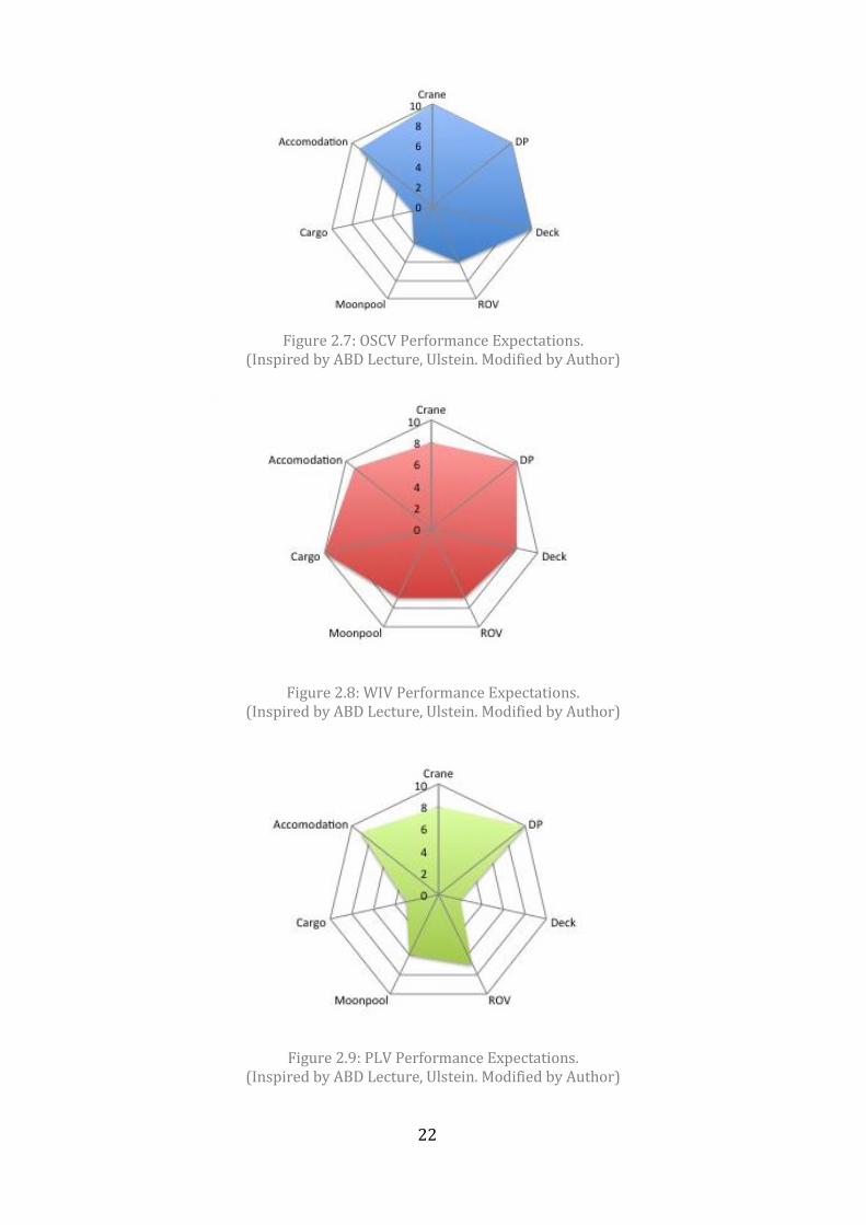
government. These interested parties have various performance expectations for the

vessel, and the spider web in Figure 2.7 illustrates the most important ones. The

diagram shows that the deck area on the vessel is of importance; the deck is mainly used

for transportation of large modules that are going to be installed. Further the Dynamic

Positioning (DP) system is crucial to maintain a high level of position accuracy and good

station keeping during the operations. Another important design feature is the offshore

crane, where the main considerations are the crane type, capacity and its location on

deck. The vessel’s tasks and operations are also dependent on ROV support and a large

crew. OSCVs are often categorized based on the vessel’s crane size and loading area,

making the definition of high-end and low-end less obvious.

9

Nearly all offshore cranes are currently installed with Active Heave Compensating (AHC)

systems that can withstand wave motions so that the module’s vertical position relative

to land does not change even in high waves. For an OSCV the crane type is typically a

Knuckle Boom Crane (KBC) with AHC. These cranes have the same moving pattern as an

excavator: they transform power through a momentum that makes them extremely

heavy, and can weigh up to 150 tons. The crane rests on a pedestal that transfers forces

and momentum into the hull through the decks. When the crane is in operation and the

boom, with the attached load, is rotated out to the ship’s side, the stability of the vessel

is maintained by a ballasting system. Ballast tanks are filled with water on the opposite

ship’s side of the crane, this way the rolling motion is kept to a minimum.

The OSCV’s ability to operate in deeper waters require a longer crane wire, and

therefore also a bigger and heavier winch. There are several possibilities to where the

crane winch can be located. For bigger cranes, the winch is usually installed on or under

the deck, whereas smaller cranes have an elevated winch attached on the top of the

crane pedestal. This is illustrated in Figure 2.1 and Figure 2.2. Although the reference

vessel, Island Performer, has its crane winch installed under the deck, in this case we

have assumed that the winch is elevated.

Almost all the new OSCVs have capacity to launch and operate Remotely Operated

Vehicles (ROV). This comes from an increased focus on deep-water subsea installations

with different support requirements than conventional oilrigs. The ROVs enable safer

access into deeper waters, and facilitate the assignments in areas where divers cannot

reach. The ROV is equipped with visibility or recording abilities, and is launched from a

heave compensated handling system through the moonpool or from auxiliary side

systems. The illustration in Figure 2.10 shows an example of a deck arrangement for this

vessel type.

10

Figure 2.1: OSCV with Elevated Crane Winch. (Roll’s Royce)

Figure 2.2: OSCV with Crane Winch Installed under Deck. (Roll's Royce)

2.1.2 Well Intervention Vessels Well Intervention Vessels are mainly used to extend the lifetime of the well, by

performing inspection, maintenance, repair and construction work on the wells. From

the spider web in Figure 2.8 we can see that cargo capacity is of high importance. This is

because mud and brine are directly involved in the maintenance work on the wells and

need to be transported on-board the WIV in tanks. The DP system is also crucial in well

intervention because of the danger of oil spills if the well is penetrated without

precision.

Well Intervention Vessels are equipped with a Module Handling Tower (MHT) located

above a centred moonpool. The tower supports wire lines, which are used to lift and

lower the modules into the water, and a cursor frame to guide the hook and prevent

horizontal displacement of the modules inside the tower. The WIV we will be looking

11

into is a monohull vessel, which commonly uses Riserless Light Well Intervention

(RLWI). RLWI is done by installing downhole tools into the well, under full pressure,

using a Subsea Intervention Lubricator (SIL). A SIL is a single trip system that accesses

the subsea wells. This method reduces the operational costs by 40-60% from

conventional drill rigs (FMC, 2014). On deck there is a skidding system transporting the

modules to and from the crane, the moonpool and the ROV hangar. The moonpool can be

closed using a door structure enabling the skidding rails to continue over the closed

doors. Other deck equipment include offshore crane(s) and ROVs, often used for visual

support. Figure 2.11 and Figure 2.12 show the deck arrangement on a Well Intervention

Vessel seen from above and from the starboard side. From the study presented in

Appendix D it is observed that most WIVs today are performing Riserless Light Well

Intervention consisting of bore-hole surveys, fluid displacement, sand washing, zonal

isolation etc.

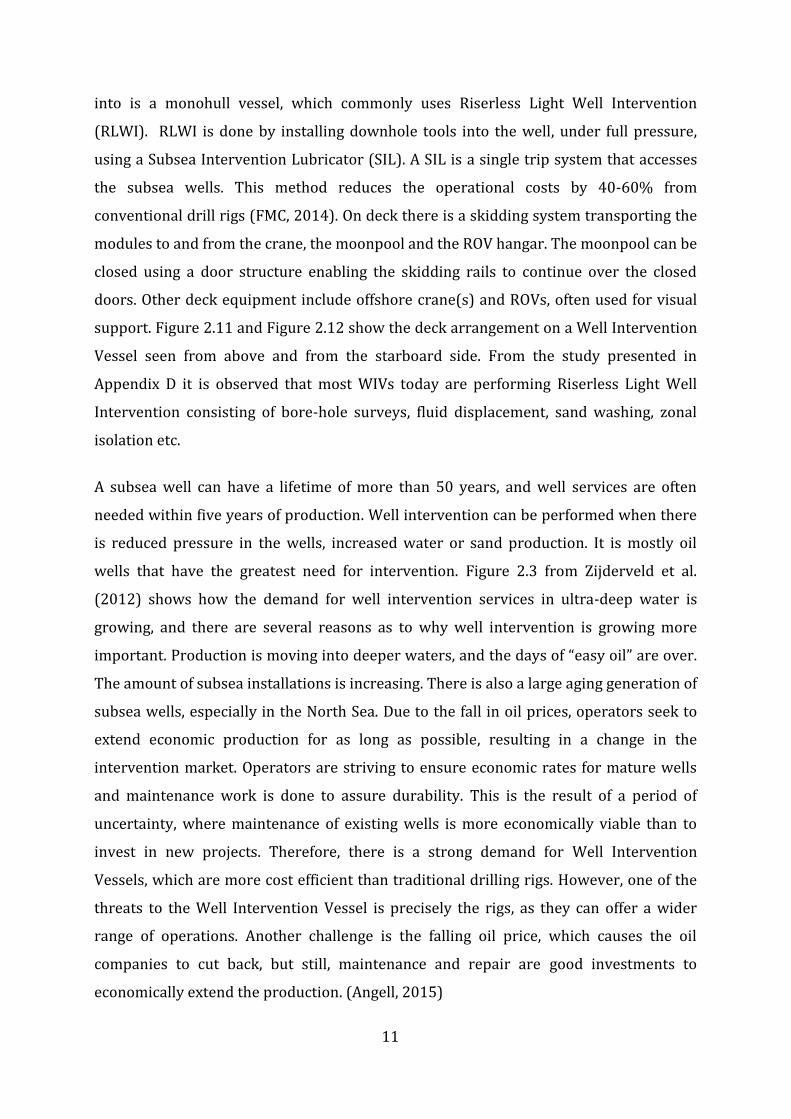
A subsea well can have a lifetime of more than 50 years, and well services are often

needed within five years of production. Well intervention can be performed when there

is reduced pressure in the wells, increased water or sand production. It is mostly oil

wells that have the greatest need for intervention. Figure 2.3 from Zijderveld et al.

(2012) shows how the demand for well intervention services in ultra-deep water is

growing, and there are several reasons as to why well intervention is growing more

important. Production is moving into deeper waters, and the days of “easy oil” are over.

The amount of subsea installations is increasing. There is also a large aging generation of

subsea wells, especially in the North Sea. Due to the fall in oil prices, operators seek to

extend economic production for as long as possible, resulting in a change in the

intervention market. Operators are striving to ensure economic rates for mature wells

and maintenance work is done to assure durability. This is the result of a period of

uncertainty, where maintenance of existing wells is more economically viable than to

invest in new projects. Therefore, there is a strong demand for Well Intervention

Vessels, which are more cost efficient than traditional drilling rigs. However, one of the

threats to the Well Intervention Vessel is precisely the rigs, as they can offer a wider

range of operations. Another challenge is the falling oil price, which causes the oil

companies to cut back, but still, maintenance and repair are good investments to

economically extend the production. (Angell, 2015)

12

Figure 2.3: Global Well Intervention Demand by Water Depth.(Infield Systems Ltd.)

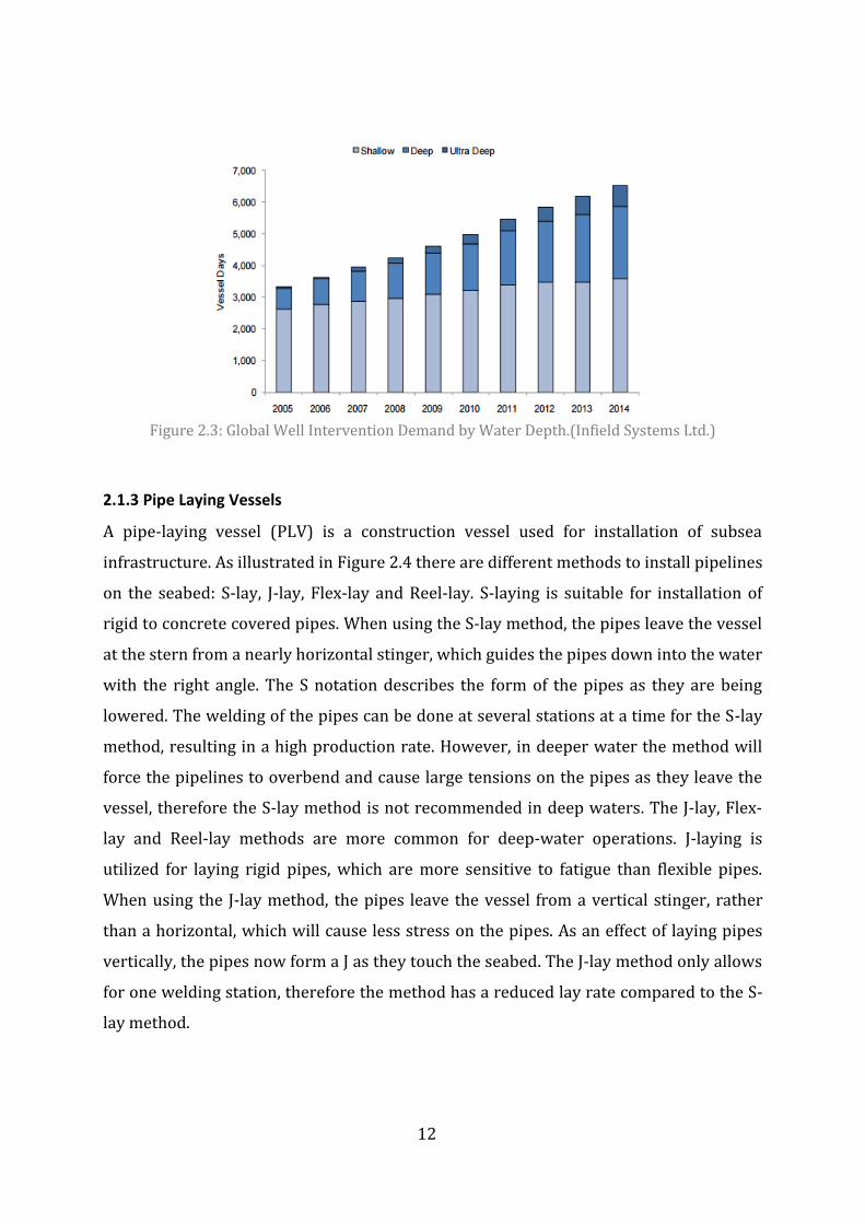
2.1.3 Pipe Laying Vessels

A pipe-laying vessel (PLV) is a construction vessel used for installation of subsea

infrastructure. As illustrated in Figure 2.4 there are different methods to install pipelines

on the seabed: S-lay, J-lay, Flex-lay and Reel-lay. S-laying is suitable for installation of

rigid to concrete covered pipes. When using the S-lay method, the pipes leave the vessel

at the stern from a nearly horizontal stinger, which guides the pipes down into the water

with the right angle. The S notation describes the form of the pipes as they are being

lowered. The welding of the pipes can be done at several stations at a time for the S-lay

method, resulting in a high production rate. However, in deeper water the method will

force the pipelines to overbend and cause large tensions on the pipes as they leave the

vessel, therefore the S-lay method is not recommended in deep waters. The J-lay, Flex-

lay and Reel-lay methods are more common for deep-water operations. J-laying is

utilized for laying rigid pipes, which are more sensitive to fatigue than flexible pipes.

When using the J-lay method, the pipes leave the vessel from a vertical stinger, rather

than a horizontal, which will cause less stress on the pipes. As an effect of laying pipes

vertically, the pipes now form a J as they touch the seabed. The J-lay method only allows

for one welding station, therefore the method has a reduced lay rate compared to the S-

lay method.

13

Figure 2.4: Illustration of Pipe Laying Methods. (Inspired by Luslier. Modified by Author)

A Vertical Lay Tower (VLT) is suitable for J-laying, flex-laying and reel-laying. When

using reel-laying, all the welding and coating is done onshore and the pipes are

transported offshore on large reels ready for submerging. Since all the welding is done

onshore during the non-critical vessel time, reel-laying gives a high production rate. A

separate barge can also transport the reels offshore where a heavy lifting crane will lift

the reels onto the PLV. This requires a large crane capacity (2500t) on the PLV. In

Appendix D we can see that some of the PLVs have such cranes with capacity to lift the

reels on-board the vessel. In flex-laying and reel-laying, the pipes are spooled from the

carousel or the reel, and then guided over a chute or a wheel at the top of the VLT and

lead by the tensioners into the water. Since the pipes are bent around the reel and the

chute, fatigue sensitive pipes are not suitable for this type of transportation and

installation, thus flexible flow lines and risers are installed using this method.

In order to facilitate the transformation between pipe laying equipment and well

intervention equipment, it is decided that a flex-lay system with a moonpool located

behind the accommodation area will be more compatible. This is also in accordance to

the design of the reference vessel, Island Performer. A traditional flex-lay system

consists of a storage system often located below deck and a loading system from the

storage to the pipe laying system. Most of the new PLVs are combinable between flex-

lay, reel-lay and J-lay. Figure 2.13 shows the deck arrangement for a conventional flex-

laying PLV. Since the main task of the PLV is to lay pipes along a planned route while

moving slowly, the accuracy of the DP system is operationally crucial. Other important

14

factors for the PLV are accommodation for the large crew on-board, crane capacity and

ROV support. Figure 2.9 shows the most important performance expectations for a PLV.

2.1.4 Multifunctional Offshore Construction Vessel

The Multipurpose Offshore Construction Vessel (MOCV) is designed with flexibility as a

main attribute. It will have the opportunity to clear the deck from equipment, and install

new deck equipment when the market demand indicates it to be necessary. The MOCV is

a commitment to the deep-water construction market, and it can potentially be further

customized to meet the client’s individual requirements.

With a unique understanding of the operational market and the client’s needs, the

advantage of the MOCV is its probability to win contracts for offshore operations. As a

shipowner it is important to establish an overview of the market segments with the

highest utilisation rates and revenue yields. It is then important to obtain a fleet of

vessels and gain information about when to expand or exit markets to maximise profits.

The MOCV’s main task will be subsea construction, installation, inspection, repair and

maintenance work. Further the vessel will be built with the option of performing well

intervention or pipe lying as secondary tasks, and can therefore be expected to benefit

from the economy of scale. This means that when a new contract is available on the

market, the probability that the MOCV is qualified for the task is three times higher than

for an OSCV, WIV or PLV alone. This is due to the vessel’s flexible operability, and its

suitability to enter multiple market segments in the subsea industry. The most

important goal for a vessel owner is of course to have his vessels under a contract at all

times and to avoid situations where one or several of the vessels are laid-up. The MOCV

is a way to invest in a vessel with a higher likelihood of not being laid-up. Bram

Lambregts (2013), Marketing and Sales Manager at Ulstein Sea of Solutions, says “what

is unique with the MOCV is that it is developed for coping with future requirements in

mind”. The vessel is adaptable to the swings in the market.

When studying the MOCV it is important to understand the relations between the

different operational modes. What needs to be done when switching from one vessel

type to another, and back? The adjustments from vessel type A to type B may not be the

same as from type B to type A. This will be shown in the matrix in Table 2.1 below. The

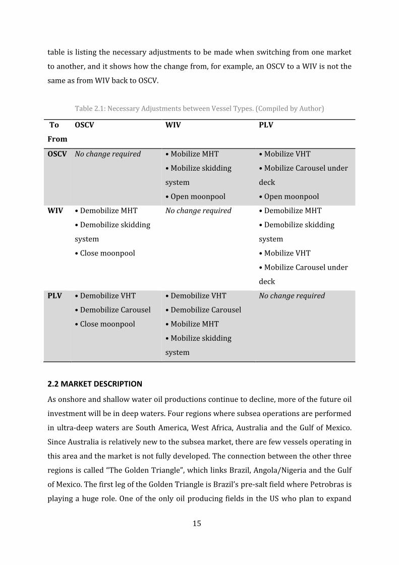
15

table is listing the necessary adjustments to be made when switching from one market

to another, and it shows how the change from, for example, an OSCV to a WIV is not the

same as from WIV back to OSCV.

Table 2.1: Necessary Adjustments between Vessel Types. (Compiled by Author)

To

From

OSCV WIV PLV

OSCV No change required • Mobilize MHT

• Mobilize skidding

system

• Open moonpool

• Mobilize VHT

• Mobilize Carousel under

deck

• Open moonpool

WIV • Demobilize MHT

• Demobilize skidding

system

• Close moonpool

No change required • Demobilize MHT

• Demobilize skidding

system

• Mobilize VHT

• Mobilize Carousel under

deck

PLV • Demobilize VHT

• Demobilize Carousel

• Close moonpool

• Demobilize VHT

• Demobilize Carousel

• Mobilize MHT

• Mobilize skidding

system

No change required

2.2 MARKET DESCRIPTION

As onshore and shallow water oil productions continue to decline, more of the future oil

investment will be in deep waters. Four regions where subsea operations are performed

in ultra-deep waters are South America, West Africa, Australia and the Gulf of Mexico.

Since Australia is relatively new to the subsea market, there are few vessels operating in

this area and the market is not fully developed. The connection between the other three

regions is called “The Golden Triangle”, which links Brazil, Angola/Nigeria and the Gulf

of Mexico. The first leg of the Golden Triangle is Brazil’s pre-salt field where Petrobras is

playing a huge role. One of the only oil producing fields in the US who plan to expand

16

production is the Gulf of Mexico. And in Africa a growing economy and numerous new

findings cause for great potential. Africa has prepared to spend around $60billion on

deep-water spendings, while Brazil and Mexico are following with nearly $30 billion

each (Gue, 2009).

The investments in Exploration and Production (E&P) of petroleum are mostly of long

term. Managerial and/or operational decisions are normal, and the projects have a high

irreversibility. The market is under conditions of economic and technical uncertainty,

such as: oil prices, the hire rates, costs and equipment reliability. Historically the

offshore industry has experienced many booms, and in good periods it is common for

shipowners to reinvest their profits into new vessels to expand their fleet. The problems

only occur when the market switches and there is a sudden oversupply, which was

exactly the case when the market dropped in the second half of 2014. To make a long

story short, the oil price fell because of an oversupply in the oil market when the USA

started producing shale oil and was no longer importing as much oil as before.

Simultaneously the good period from 2002-2009 resulted in an increase in the

development of new fields, and Saudi-Arabia is maintaining a high production rate even

with low oil prices. This can have coherence with wanting to reduce the growth in the

American shale oil industry and put economic pressure on competitive countries.

Although some companies want to expand their business by benefitting from historically

low asset and building prices, most banks are unwilling to take more risk and lend

money to new high-margin projects. Downscaling and down payment of loans, rather

than making new investments will therefore probably dominate the following years. In

the market report from RS Platou published in July 2014, predictions of high and stable

oil prices for the following years were made (Platou, 2014). This is proof that market

developments are difficult to foresee. Still, with shifting markets and a declining oil

price, the need for flexible investments is important. Given the recent drop in oil prices,

one might assume that all the involved producers and companies will fall along with the

oil price, but companies with knowledge on weathering volatile markets are more

trusted and supported by banks and investors who are interested in the energy market

(Lorusso, 2014).

17

Despite the low oil price over the past year, a report from British Petroleum shows that

the demand for energy will grow by 41% between 2012 and 2035. With the

industrializing and electrification of the non-OECD countries, “the decade between 2002-

2012 recorded the greatest ever increase of energy consumption over any ten year period,

which most likely will not be surpassed in the future” (BP, 2014). It is reported that 95%

of the growth is represented by the non-OECD. Especially China and India, who

represent the main growth contributors. The total world energy production will also

increase with a rate of 1.5% from 2012-2035, and the growth includes all regions except

Europe. (BP, 2014)

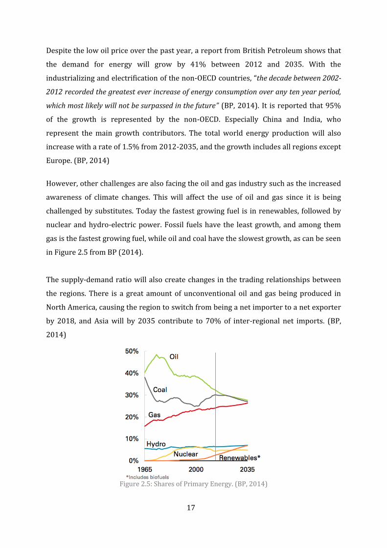
However, other challenges are also facing the oil and gas industry such as the increased

awareness of climate changes. This will affect the use of oil and gas since it is being

challenged by substitutes. Today the fastest growing fuel is in renewables, followed by

nuclear and hydro-electric power. Fossil fuels have the least growth, and among them

gas is the fastest growing fuel, while oil and coal have the slowest growth, as can be seen

in Figure 2.5 from BP (2014).

The supply-demand ratio will also create changes in the trading relationships between

the regions. There is a great amount of unconventional oil and gas being produced in

North America, causing the region to switch from being a net importer to a net exporter

by 2018, and Asia will by 2035 contribute to 70% of inter-regional net imports. (BP,

2014)

Figure 2.5: Shares of Primary Energy. (BP, 2014)

18

OSVs are important tools in Exploration and Production (E&P) of offshore oil and gas

fields, rigs, platforms and FPSOs. Therefore the oil price and the production of oil and

gas play a vigorous part in the Offshore Support Vessel industry. The E&P process in the

oil and gas industry is the first period of a long value chain of producing petroleum for

our everyday use. Within the E&P process are four phases: Exploration, Development,

Production and Decommissioning, and different vessel types are required in the four

stages. This is shown in Table 2.2 below. During the first stage, the exploration stage, the

common task is searching for hydrocarbons. Important vessels in the exploration phase

are seismic vessels, Anchor Handling Tug Supply (AHTS), Platform Supply Vessels (PSV)

and barges. When a prominently large field of hydrocarbons is found the development

phase can commence, involving installation of subsea wells and infrastructure. These

tasks require dive support vessels, OSCVs, PLVs and pipelay barges. The production

phase can start when oil and gas is ready to be extracted from the wells. Further the oil

and gas is processed, stored and transported from the field. Important vessels are AHTS,

PSV, crew boats, utility vessels and subsea support vessels such as WIVs. The final stage,

the decommissioning phase is initiated when the field no longer can provide economic

benefits. Decommissioning consist of plugging the wells and removing the production

installations. The required vessels for this stage are naturally the same as for the

development phase (Yeo, 2010).

Based on the information in Table 2.2 we are able to say something about the duration

of the tasks performed by the different vessels in each phase. The period lengths from

this table will be used as an underlying argument for the choice of contract lengths in

Chapter 4.1. The table also shows how affected the vessels are by the oil price. This can

be helpful in later chapters when the volatility of the income opportunities is discussed.

Table 2.2: Exploration and Production in Oil and Gas. (Pareto Research, Modified by Author)

Exploration Development Production Decommissioning Period 1-3 years 2-4 years 5-50+ years Upon oilfield

depletion Sensitivity to oil price

High Medium High oil price extends lifespan of oilfield

High oil price defers decommissioning

OSVs deployed

OSCV PLV

OSCV WIV

OSCV

19

2.3 CASE DESCRIPTION

As mentioned in the objective, this thesis is a Real Options Analysis to find the value of a

Multipurpose Offshore Construction Vessel compared to owning several single purpose

vessels. Consider an OSCV with an initial building cost of 107 mUSD (E Sandvik, 2015,

pers. comm., 24 April) and a service life of 20 years. Initial building cost includes hull

structure, machinery, accommodation, reinforced moonpool area, deck equipment such

as offshore cranes, ROV capacity and installation of the equipment. The vessel has the

option of transforming into a PLV or WIV subject to contract requirements. The vessel is

initially constructed as an OSCV, because the deck equipment on an OSCV, such as cranes

and ROV capacity, is a common denominator between the three vessel types. A 250t

Knuckle Boom Crane with AHC is chosen and there will be an ROV hangar in the deck

house on the starboard side. Further it is necessary in both well intervention and pipe

lying with a closable moonpool with the typical dimensions 8x8 meters. The deck

structure around the moonpool needs reinforcement to be able to support the heavy

equipment used, such as the Module Handling Tower (300tons) and the Vertical Lay

System (250tons). It is also essential to have enough space under deck for a carousel

(2500tons). The deck equipment on OSVs commonly only need to be provided with

electricity from the ship. The machinery itself is located inside the equipment. The

chosen dimensions and capacities are selected from a reference vessel, the Island

Performer, designed and built by Ulstein. Table 2.3 summarizes the deck equipment

chosen for the case analysis.

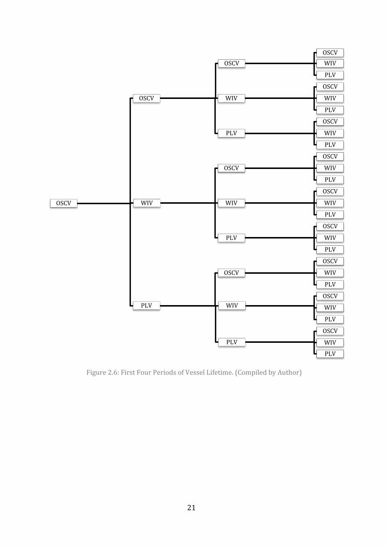
Figure 2.6 shows an example of the periods of the vessels lifetime and the options it

holds. The initial deck arrangement will be optimized for tasks related to the OSCV. At

expiration of the first contract, the owner has the option to switch the vessel into a PLV

or WIV. The option holder can also decide to keep the vessel as an OSCV. The figure

shows how the vessel will be built and operated as an OSCV the first period. This is

illustrated with a single node. From the end of the node a line is drawn which leads to

three new nodes. This line represents the length of which the vessel will operate as an

OSCV. The end of the line represents the end of the contract where the vessel owner has

to make a final decision about what contract type to take in the next phase and thus

what vessel type to retrofit the vessel into. The rest of the figure follows the same

principle. In the analysis, the contract lengths will vary based on the vessel type and

20

what a typical duration of the performed tasks can be, but the lines in the figure have the

same length for graphical simplicity. The intention of this study is to evaluate each node

and find the value of holding the options to switch, by using the Black-Scholes formula.

The case is limited from the following boundaries:

x At the time t=0, the vessel will be completed as an OSCV, and the following first period it operates as an OSCV

x At the time t=T, the owner has the option to switch to a different vessel type x The vessel can enter into the OSCV, WIV or PLV markets x Each of the three markets have different contract lengths x Each contract represents a period in the analysis x The analysis only addresses the first four periods of the vessel’s lifetime

Table 2.3: Deck Equipment on Vessel Types. (Island Performer)

Vessel Type OSCV WIV PLV

Deck Equipment 250t KBC 300t MHT

100t Skidding System

250t VLS

2500t Carousel

21

Figure 2.6: First Four Periods of Vessel Lifetime. (Compiled by Author)

OSCV

OSCV

OSCVOSCVWIV

PLV

WIV

OSCV

WIV

PLV

PLV

OSCV

WIV

PLV

WIV

OSCV

OSCV

WIV

PLV

WIV

OSCV

WIV

PLV

PLV

OSCV

WIV

PLV

PLV

OSCV

OSCV

WIV

PLV

WIVOSCV

WIV

PLV

PLV

OSCV

WIV

PLV

22

Figure 2.7: OSCV Performance Expectations. (Inspired by ABD Lecture, Ulstein. Modified by Author)

Figure 2.8: WIV Performance Expectations.

(Inspired by ABD Lecture, Ulstein. Modified by Author)

Figure 2.9: PLV Performance Expectations.

(Inspired by ABD Lecture, Ulstein. Modified by Author)

23

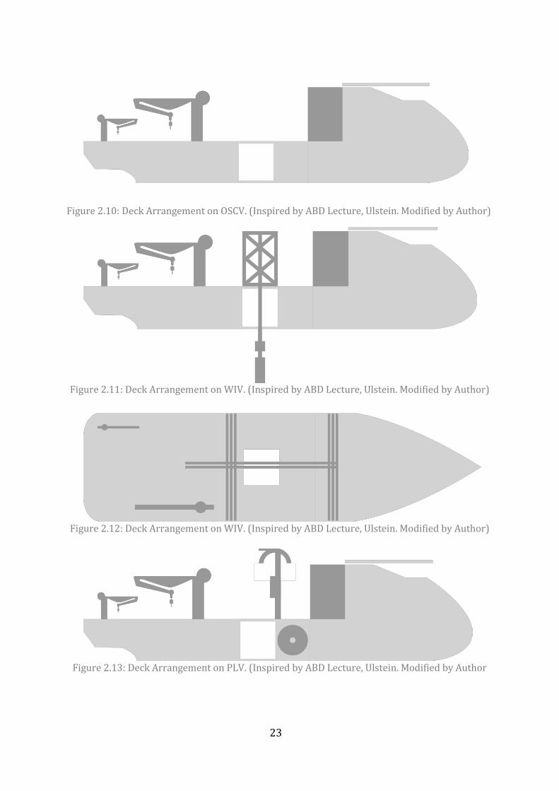
Figure 2.10: Deck Arrangement on OSCV. (Inspired by ABD Lecture, Ulstein. Modified by Author)

Figure 2.11: Deck Arrangement on WIV. (Inspired by ABD Lecture, Ulstein. Modified by Author)

Figure 2.12: Deck Arrangement on WIV. (Inspired by ABD Lecture, Ulstein. Modified by Author)

Figure 2.13: Deck Arrangement on PLV. (Inspired by ABD Lecture, Ulstein. Modified by Author

24

3 REAL OPTIONS It is said that: “50% of the value of Real Options is simply thinking about it. Another 25%

comes from generating the models and getting the right numbers, and the remaining 25%

of the value of Real Options is explaining the results to the person beside you, or to

yourself” (Leggio, 2006).

Each project holds countless numbers of possibilities of expansion, waiting, switching or

abandoning. The systems we value are so complex that during their engineering and

creation, more options are possible than the human mind can fathom. In Real Options

thinking we ask ourselves what would happen if we begin to think down a new path.

What options will be available for us and what can we gain by holding these options?

The very first and toughest step to take when entering into this thinking path is to

identify the existing Real Options in the investment already in the Research and

Development (R&D) stage. After this the actual valuation analysis can begin.

3.1 INTRODUCTION TO REAL OPTIONS

To analyse and determine an option value, we must first define the concept of Real

Options (RO). A Real Option is the right, but not obligation, to undertake some business

decision such as buying or selling an asset. Real Options refer to physical assets, like

equipment, in contrast to options defined as financial instruments (Investopedia, 2015).

All projects can be expanded, delayed, sped up or abandoned. A Real Options Analysis

(ROA) is not just an equation or a formula, but it is a method used to value these choices

by using different pricing techniques (Wijst, 2010).

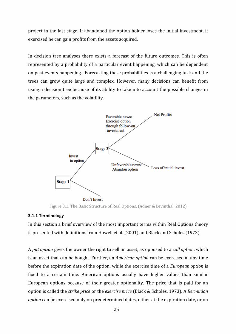
In Figure 3.1 the basic structure of Real Options is illustrated in a decision tree by Adner

and Levinthal (2002). The decision tree is organized as follows: In the first stage an

option is purchased by investing an initial amount of money. This gives the option

holder the opportunities, such as choosing between assets, or whether or not to expand

a project. In the second stage the option value has changed due to external influence,

which affect the decision since it is based on the expected outcomes. Finally, based on

the acquired information the option holder choses to either invest or to abandon the

25

project in the last stage. If abandoned the option holder loses the initial investment, if

exercised he can gain profits from the assets acquired.

In decision tree analyses there exists a forecast of the future outcomes. This is often

represented by a probability of a particular event happening, which can be dependent

on past events happening. Forecasting these probabilities is a challenging task and the

trees can grow quite large and complex. However, many decisions can benefit from

using a decision tree because of its ability to take into account the possible changes in

the parameters, such as the volatility.

Figure 3.1: The Basic Structure of Real Options. (Adner & Levinthal, 2012)

3.1.1 Terminology

In this section a brief overview of the most important terms within Real Options theory

is presented with definitions from Howell et al. (2001) and Black and Scholes (1973).

A put option gives the owner the right to sell an asset, as opposed to a call option, which

is an asset that can be bought. Further, an American option can be exercised at any time

before the expiration date of the option, while the exercise time of a European option is

fixed to a certain time. American options usually have higher values than similar

European options because of their greater optionality. The price that is paid for an

option is called the strike price or the exercise price (Black & Scholes, 1973). A Bermudan

option can be exercised only on predetermined dates, either at the expiration date, or on

26

specific dates before the expiration date. A Bermudan option is commonly valued using

the swaption method. In this thesis we are valuing European call options. The

background for this will be further explained in Chapter 4.

The option holder is in the position of holding the rights to buying or selling the option,

while the option writer has the obligation to sell or buy the option to/from the option

holder. The date when an option expires is called the expiration date or the time to

maturity. For European options the time at which the option can be exercised is at this

particular date (Howel et al. 2001). In Real Options the time to maturity can be as long

as decades depending on contract times, equipment lifetime etc., while financial options

are traded much faster, within months. In this case the option holder is the owner of the

Multipurpose Offshore Construction Vessel, the option writer is the supplier of the

prospective deck equipment, and the expiration date of the option is when a contract

expires and the vessel is in need of a new assignment.

The underlying asset can be sold and bought as a remedy to enter into different markets

(Howel et al. 2001). In this study the deck equipment is considered the underlying asset.

This will also be further explained in Chapter 4. The value of the underlying asset is

financially called the stock price, but what it really represents is the highest amount

someone is willing to pay for the stock, or the lowest amount that it can be bought for.

The Net Present Value (NPV) of the potential investment represents the stock price.

The volatility is a critical parameter for option pricing models, as it is a measure for the

fluctuation of the return of an asset over time. The volatility is usually expressed as a

percentage where a high volatility implies a risky security (Investopedia, 2015b). The

volatility is the logarithmic return of the stock price. And one can use the historic

volatility of the stock to determine the future volatility.

The initial investment or the option premium is essential when owning call or put

options, and serves as a platform for a company to extend further into market

opportunities. The initial investment is what gives us the opportunity to install new

equipment after the vessel has been built, and is therefore the most important

investment made in order to realize the Multipurpose Offshore Construction Vessel.

From Chapter 2.1 we learned that for the MOCV the pre-investment is in the

27

strengthening of the deck to support large deck equipment, arrange space under the

deck for cargo and pipes, the installation of the moonpool and the costs related to this. In

the Black-Scholes formula this cost is not included, but the knowledge of its existence is

still important.

To invest long in a company is to buy a stock, with the expectation that the asset value

will increase. The opposite is a short investment, which is defined as the sale of a

borrowed security with the expectation that the asset value will decrease. For example if

you want to invest in a company with better numbers than their competitor, you go long

on the company, and short on their competitor. If the industry you invested in goes up,

you profit from the long and lose on the short. If the industry goes down, you lose money

on the long and make money on the short. This is called hedging, an investment made to

limit the risk of another investment. A common example of a hedge is insurance.

3.1.2 Types of Options

There exists different types of options and they turn up at different stages of an

investment. From Brealey et al. (2006), Amram and Kulatilaka (1999) and Trigeorgis

(1996) some of the most relevant option types are selected:

The option of waiting to invest is useful when a project might turn more profitable in the

future. Under some conditions it can prove to be more valuable when deferring to invest

when immediate cash flow is low, rather than to commit to invest. Waiting to invest also

enables the holder to learn more about the market trends and developments (Brealey et

al., 2006). To halt further investment is to abandon or exit a project. Abandoning can

often leave other options valueless. In our example abandoning the project would be to

sell the vessel.

We have timing and switching options that should be exercised when the demand for a

certain product rises. As an example, the owner of a Pipe Laying Vessel notices a drop in

the market while the Offshore Wind Turbine market is constantly growing, the timing

for doing a switch between these markets would then be perfect if he already owns the

option. Further, a growth option is when a business is expanded. An Offshore Subsea

Construction vessel with a 150 ton crane could get more contracts with a bigger crane,

28

and holding the option of installing such a crane is a growth option. The option to add

flexibility to an investment can be done by for example using shipbuilding yards in

different continents so that productions can be regulated by the demand, exchange rates

and production costs in the different continents. This is called a flexibility option. In

many examples of RO, these option types exist simultaneously and it is therefore

important to identity all the options a project holds (Amram & Kulatilaka, 1999).

Wang & de Neufville (2005) stated that there is a difference between Real Options “on”

projects and “in” projects. The main difference is that when using Real Options “on”

projects the physical system is treated as a “black box”. To contrast, Real Options “in”

systems are where the design features are considered in the project. Real Options “in”

systems require that the analyst has a good knowledge about the technology that is

being worked with. This is because there is little available data for these types of options

compared to the RO “on” projects. Another reason is because the equipment can be

complex and have numerous options or limitations that need to be regarded in the

project. This thesis is an example of RO being used “in” projects, and many other

examples are presented in the literature study such as the parking garage case or the

office space case.

3.1.3 Real Options in Our Everyday Life

The Real Options way of thinking is quite similar to the way we make decisions in our

everyday life: we wait until the uncertainty is resolved to be able to make a safer choice.

A relevant example of the modern use of Real Options is when an oil company buys the

drilling rights for a piece of land, they are buying an option with the right to extract oil

that can be exercised when they can gain profit from it. Although oil prices vary all the

time and at the moment being quite low, the possibility of making a profit from the oil

prices going up again is worth having.

A common example of Real Options is the leasing of cars or equipment with the option

to buy at the end of the leasing period. Typically these agreements have a predefined

lease time and exercise price in the contract. The decision to buy the car or not is often

made at the expiration time of the leasing, like a European call option. Another example

of options in our life is insurance. We pay a small annual premium to protect us from

29

potential economic losses. The amount of money we get in return is equal to the size of

the damage minus the deductible. The payoff from buying insurance resembles an

American put option.

3.2 VALUATION OF REAL OPTIONS

The process of valuing Real Options is one of the most difficult in strategic management

and R&D. The RO approach solves problems that the traditional Discounted Cash Flow

(DCF) method and Net Present Value (NPV) method fail to do. Some of the pioneers in

financial Options thinking were Fisher Black and Myron C. Scholes who invented the

Black-Scholes Option Pricing Model (BS OPM) in the seventies, which is an important

method for valuing European call options. Some years later John Cox, Steve Ross, and

Mark Rubenstein developed the Binomial Option-Pricing Model (BOPM) for the

valuation of American options. In this chapter, the traditional NPV and DCF methods will

be presented with a discussion of their weaknesses, together with a brief summary of

the BOPM and Monte Carlo Simulation and a more detailed explanation of the Black-

Scholes method.

3.2.1 Net Present Value

A traditional method to value investments is with the Net Present Value (NPV). The NPV

is a formula representing the difference between the present values of cash inflows and

outflows, and is used in capital budgeting to determine whether an investment or a

project will turn out profitable. The method uses the future cash inflow with regards to

inflation and returns over the years of the project. If the NPV is negative the project

should be abandoned, but considered if the opposite occurs. The challenge with the NPV

analysis is that it undervalues the option, as the risk-adjusted discount rate is not

properly identified, and the fact that the project’s risk is different at each decision point

is not considered. Therefore the NPV is not suited to value flexibility in a project,

because it assumes that the investment has to be done fully now or never, even if the

project can still hold options for development (de Neufville & Scholtes, 2011; Trigeorgis,

1996). In Real Options Analyses we sometimes invest in projects with a negative NPV,

when this investment generates new options. These can be options to expand

productions, and/or generate valuable new information and options. ROA can also

recommend to postpone projects with positive NPV (option to wait and see) (Dias,

2004).

30

3.2.2 Discounted Cash Flow

Similarly, the Discounted Cash Flow (DCF) method also tends to undervalue the R&D

projects. The method was developed by Irvin Fisher to evaluate financial investments

and decisions to invest in real assets. There is an increased risk from abandoning and an

increased potential from expanding and delaying. The DCF method fails to capture the

implications of this, and is thus best used for valuing short-term projects with low

uncertainty. The method undertakes no flexibility to make decisions during the project

lifetime, and future decisions are fixed at the outset (Damodaran, 2007; de Neufville &

Scholtes, 2011).

3.2.3 The Binomial Option Pricing Method

The most important tool for valuing American options is the Binomial Option Pricing

Method. BOPM creates a periodic view of the stock price and the option value, and is

performed by creating a simple spread sheet. Binomial option pricing is based on a no-

arbitrage assumption, which means that the market is efficient, and investors will earn

the risk-free rate of return. The process of solving the binomial method is quite similar

to using decision trees with “discrete-time” (lattice based) steps, where the stock price is

considered logarithmic. The value of the asset can go in two directions, up or down with

the probability of p and 1-p. In the BOPM, the up and down factors, and the probabilities

can be found by using the asset’s volatility and the risk-free rate. The option value is

found eventually by solving the tree backwards by multiplying each state with the risk-

neutral probability and discounted with the risk-free interest rate.

3.2.4 Monte Carlo Simulation

For complex problems of Real Options, where analytical or tree building methods are

too time consuming to perform, the Monte Carlo method is often used instead. The

Monte Carlo method simulates the possible value of an asset over a time period by

drawing random numbers from the probability distributions to recreate the asset

behaviour. By using a computer to repeat numerous simulations, a distribution of the

option payoffs is obtained. The average of these payoffs is then discounted back to

determine the present value of the Real Option (de Neufville & Scholtes, 2011).

31

3.2.5 The Black-Scholes Method

Introduction to the Black-Scholes Method

The probability distribution of the option price and the risk-free rate are two factors

which are not directly observable, but they are both necessary in order to discount the

future probable payoffs of the option. Fischer Black and Myron Scholes created the

Black-Scholes formula to resolve this major problem in valuating options.

In the development of their formula, Black and Scholes defined these assumptions

regarding the stock and option:

1. “The short-term interest rate is known and is constant through time

2. The stock price follows a random walk in continuous time with a variance rate

proportional to the square of the stock price. Thus the distribution of possible stock

prices at the end of any finite interval is lognormal. The variance rate of the return on

the stock is constant.

3. The stock pays no dividends or other distributions.

4. The option is "European," that is, it can only be exercised at maturity.

5. There are no transaction costs in buying or selling the stock or the option.

6. It is possible to borrow any fraction of the price of a security to buy it or to hold it, at

the short-term interest rate.

7. There are no penalties to short selling. A seller who does not own a security will simply

accept the price of the security from a buyer, and will agree to settle with the buyer on

some future date by paying him an amount equal to the price of the security on that

date.” (Black & Scholes, 1973)

The assumptions listed above tell us that the option value depends on the stock price

and other known constants. It is therefore possible to create a hedge where we invest

long in the stock, and short in the option. The hedge value will thus only depend on the

time period where we are hedging, and not on the stock price. This is useful because it

guarantees a return on the hedge. (Black & Scoles, 1973)

The explanation to this is because the stock price follows a continuous random walk also

called a Geometric Brownian Motion (GBM). A GBM is a continuous-time stochastic

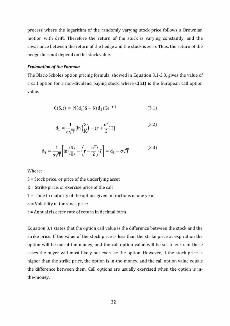
32

process where the logarithm of the randomly varying stock price follows a Brownian

motion with drift. Therefore the return of the stock is varying constantly, and the

covariance between the return of the hedge and the stock is zero. Thus, the return of the

hedge does not depend on the stock value.

Explanation of the Formula

The Black-Scholes option pricing formula, showed in Equation 3.1-3.3, gives the value of

a call option for a non-dividend paying stock, where C(S,t) is the European call option

value.

C(S, t) = N(d1)S − N(d2)Ke−r∙T

(3.1)

d1 =1

σ√T[ln (

SK) − (r +

σ2

2 )T]

(3.2)

d2 =1

σ√T[ln (

SK) − (r −

σ2

2 ) 𝑇] = d1 − σ√T (3.3)

Where:

S = Stock price, or price of the underlying asset

K = Strike price, or exercise price of the call

T = Time to maturity of the option, given in fractions of one year

𝜎 = Volatility of the stock price

r = Annual risk-free rate of return in decimal form

Equation 3.1 states that the option call value is the difference between the stock and the

strike price. If the value of the stock price is less than the strike price at expiration the

option will be out-of-the money, and the call option value will be set to zero. In these

cases the buyer will most likely not exercise the option. However, if the stock price is

higher than the strike price, the option is in-the-money, and the call option value equals

the difference between them. Call options are usually exercised when the option is in-

the-money.

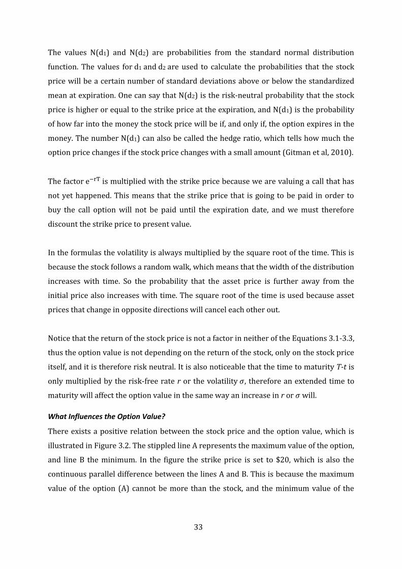
33

The values N(d1) and N(d2) are probabilities from the standard normal distribution

function. The values for d1 and d2 are used to calculate the probabilities that the stock

price will be a certain number of standard deviations above or below the standardized

mean at expiration. One can say that N(d2) is the risk-neutral probability that the stock

price is higher or equal to the strike price at the expiration, and N(d1) is the probability

of how far into the money the stock price will be if, and only if, the option expires in the

money. The number N(d1) can also be called the hedge ratio, which tells how much the

option price changes if the stock price changes with a small amount (Gitman et al, 2010).

The factor e−rT is multiplied with the strike price because we are valuing a call that has

not yet happened. This means that the strike price that is going to be paid in order to

buy the call option will not be paid until the expiration date, and we must therefore

discount the strike price to present value.

In the formulas the volatility is always multiplied by the square root of the time. This is

because the stock follows a random walk, which means that the width of the distribution

increases with time. So the probability that the asset price is further away from the

initial price also increases with time. The square root of the time is used because asset

prices that change in opposite directions will cancel each other out.

Notice that the return of the stock price is not a factor in neither of the Equations 3.1-3.3,

thus the option value is not depending on the return of the stock, only on the stock price

itself, and it is therefore risk neutral. It is also noticeable that the time to maturity T-t is

only multiplied by the risk-free rate r or the volatility 𝜎, therefore an extended time to

maturity will affect the option value in the same way an increase in r or 𝜎 will.

What Influences the Option Value?

There exists a positive relation between the stock price and the option value, which is

illustrated in Figure 3.2. The stippled line A represents the maximum value of the option,

and line B the minimum. In the figure the strike price is set to $20, which is also the

continuous parallel difference between the lines A and B. This is because the maximum

value of the option (A) cannot be more than the stock, and the minimum value of the

34

option (B) cannot be less than the stock price minus the exercise price ($20). (Black &

Scoles, 1973)

The dotted lines T1, T2 and T3 represent the values of the options for successively

shorter maturity times. If the date of expiration for an option is in a long time, the value

of the option is close to the price of the stock. However, if the expiration date is close, the

option value is the stock price minus the exercise price, or zero if negative. If the stock

price does not change, the option value normally reduces when the expiration date is

close. (Black & Scoles, 1973)

The option value as a function of the stock price is characteristically represented by a

convex curve, and since it is below 45°, the option is more volatile than the stock. This

means that a small change in the stock price gives a larger change in the option value. Or

that the rate of variation in the option is higher than the stock rate of variation. This can

be proven from the Equation 3.1 showing how the option value is dependent on the

stock price.

As a result of the market demand and supply, the stock price of an investment vary each

day. If there are many vessels of the same type available on the market and the demand

for these vessels are lower than the supply, the price will go down. Conversely, if the

demand for a vessel type is higher than the amount of unchartered vessels the stock

price goes up. Therefore Real Options can sometimes be referred to as a set of strategic

options where the decision is triggered by market-priced risk.

The oil price is an example of market-priced risk because it is valued by future contracts.

By securing their position in trading, assets with market-priced risk can reshape their

risk. The ability of Real Options is to give this uncertainty a positive value. (Amram &

Kulatilaka, 2000)

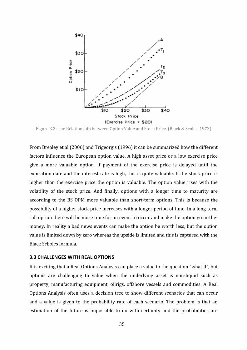
35

Figure 3.2: The Relationship between Option Value and Stock Price. (Black & Scoles, 1973)

From Brealey et al (2006) and Trigeorgis (1996) it can be summarized how the different

factors influence the European option value. A high asset price or a low exercise price

give a more valuable option. If payment of the exercise price is delayed until the

expiration date and the interest rate is high, this is quite valuable. If the stock price is

higher than the exercise price the option is valuable. The option value rises with the

volatility of the stock price. And finally, options with a longer time to maturity are

according to the BS OPM more valuable than short-term options. This is because the

possibility of a higher stock price increases with a longer period of time. In a long-term

call option there will be more time for an event to occur and make the option go in-the-

money. In reality a bad news events can make the option be worth less, but the option

value is limited down by zero whereas the upside is limited and this is captured with the

Black Scholes formula.

3.3 CHALLENGES WITH REAL OPTIONS

It is exciting that a Real Options Analysis can place a value to the question “what if”, but

options are challenging to value when the underlying asset is non-liquid such as

property, manufacturing equipment, oilrigs, offshore vessels and commodities. A Real

Options Analysis often uses a decision tree to show different scenarios that can occur

and a value is given to the probability rate of each scenario. The problem is that an

estimation of the future is impossible to do with certainty and the probabilities are

36

pulled out of thin air. However, other valuation methods (DCF, NPV) have the same

problem when estimating the risk-free rate and the expected cash flow of a project.

Real Options shall not be used when there are no options at all, although this is almost

never the case. When the level of uncertainty is low or the consequences of the

uncertainty can be ignored, Real Options theory is not useful. Apart from this almost all

projects are subject to option valuation.

Some of the statistical data such as the volatility, are difficult to implement to

engineering. Even if the ROA is performed thoroughly and assumptions are carefully

made, the results are based on assumptions that are difficult to explain, since the

technique is optimized for financial assets. Because Real Option models use more

complex tools like stochastic processes and optimization under uncertainty, the results

can be difficult to present to a boss or manager who is responsible for the project.

38

4 USING THE BLACK-SCHOLES METHOD TO VALUE THE MOCV Primarily it is important to justify the choice of method namely the Black-Scholes

method. Black-Scholes is a method used for valuing European call options. It must

therefore be explained as to why the option in this problem is European and why it is a

call option. As described in Chapter 2.3, the ship owner has the option of entering into a

new market by changing the equipment on the vessel. Since this can only be done at the

expiration date of the current contract and not before, the option cannot be American.

The option can in reality be exercised after the expiration date. However, there is a cost

to keep the vessel idle, without contract. So, in this thesis I consider that at the first

contract expiration the owner has an immediate decision to make: ether to invest in

upgrading the vessel or not. If not, the owner will get a new contract with the same type

of vessel (continue unchanged). Hence, the nature of this application points to a

European option style. To argue that the option is a call, it should be mentioned that in

order for the ship owner to perform the switch, he must buy the new equipment or pay

an amount for installation, so there is a payment that needs to be made in order to

exercise the option. Or you can say that the asset has to be bought. If this was a put

option, the owner would earn money from selling an asset. Thus, the aforementioned

explains why the option is a European call option and the choice of method is verified.

In the following sub-chapters, the Real Options theory from Chapter 3.2.5 will be applied

to find a value to the pre-investment of creating a MOCV. In order to perform the ROA

we need to obtain some market data that will be used in the Black-Scholes formula.

Some of the data, such as the volatility and the strike price are difficult to find and must

be drawn from a comparison of many references. This chapter gives an explanation of all

the assumptions and input data used in the analysis.

4.1 TIME TO MATURITY

In the Black-Scholes formula the time to maturity of the option is required. This value

represents the time period the option owner has to decide whether to exercise it or not.

In our analysis, this is the time window the investors have to decide what equipment

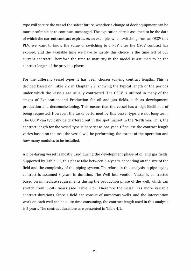
39

type will secure the vessel the safest future, whether a change of deck equipment can be

more profitable or to continue unchanged. The expiration date is assumed to be the date

of which the current contract expires. As an example, when switching from an OSCV to a

PLV, we want to know the value of switching to a PLV after the OSCV contract has

expired, and the available time we have to justify this choice is the time left of our

current contract. Therefore the time to maturity in the model is assumed to be the

contract length of the previous phase.

For the different vessel types it has been chosen varying contract lengths. This is

decided based on Table 2.2 in Chapter 2.2, showing the typical length of the periods

under which the vessels are usually contracted. The OSCV is utilized in many of the

stages of Exploration and Production for oil and gas fields, such as development,

production and decommissioning. This means that the vessel has a high likelihood of

being requested. However, the tasks performed by this vessel type are not long-term.

The OSCV can typically be chartered out in the spot market in the North Sea. Thus, the

contract length for the vessel type is here set as one year. Of course the contract length

varies based on the task the vessel will be performing, the extent of the operation and

how many modules to be installed.

A pipe-laying vessel is mostly used during the development phase of oil and gas fields.

Supported by Table 2.2, this phase take between 2-4 years, depending on the size of the

field and the complexity of the piping system. Therefore, in this analysis, a pipe-laying

contract is assumed 3 years in duration. The Well Intervention Vessel is contracted

based on immediate requirements during the production phase of the well, which can

stretch from 5-50+ years (see Table 2.2). Therefore the vessel has more variable

contract durations. Since a field can consist of numerous wells, and the intervention

work on each well can be quite time consuming, the contract length used in this analysis

is 5 years. The contract durations are presented in Table 4.1.

40

Table 4.1: Contract Lengths for each Vessel Type

Vessel Type Contract Length [years]

OSCV 1

WIV 5

PLV 3

During one year the total amount of operational days is 365 minus days in off-hire. The

off-hire period depends on the vessel’s need for repairs, dry-docking and surveys, and is

highly undesirable as it often occurs unscheduled. During this time the charterer is not

required to pay for the vessel. It is assumed that without severe problems or drastic

need for maintenance we can set an average amount of off-hire days for Offshore

Support Vessels to 2 days (SIEM, 2014). Resulting in 363 operational days per year,

which will become useful for the calculation of the stock price in the next section.

4.2 THE STOCK PRICE

In this analysis it is assumed that the stock price is represented by the daily hire rate of

the vessel multiplied by the amount of days in the contract, and several explanations for

this exist. In finance, the stock price is the value of which you can sell a stock. Another

way to see it is that the stock price is the potential income one can earn from selling the

stock. When chartering out a ship, the potential income comes from the vessel’s daily

hire rate. This rate is a result of the operational region, the time (month and year), what

type of contract it is etc., and they can be represented as an average yearly value.

Because the Black-Scholes formula requires the current value of the stock, the charter

rates used for this analysis are taken from 2015. Table 4.2 shows the daily hire rates for

the three vessel types and their associated stock prices. In Appendix C, the full

calculations of the stock prices are included. The hire rates are gathered from personal

communication with Ulstein, and they are for vessels operating in the North Sea based

on long to medium term contracts.

41

Table 4.2: Daily Hire Rate and Stock Price. (JJG Agis, 2015, pers. comm,. 28 April)

Vessel Type Daily Hire Rate, 2015 [$] Stock Price [$]

OSCV 75 000 27 225 000

WIV 243 000 441 045 000

PLV 203 000 221 067 000

4.3 THE STRIKE PRICE

The strike price is defined as the price paid to exercise the option, or the cost of

purchasing the underlying asset. In this thesis we are valuing the option of switching

markets by switching the deck equipment on our vessel, and the deck equipment can be

referred to as the underlying asset. The strike price represents the cost related to

transforming the vessel from one phase to another. This cost is dependent on various

factors, but the most dominant expense is the cost of acquiring the deck equipment.

Further, an additional cost for mobilization and demobilization of the equipment is

included. The installation cost consists of the man-hours and the use of equipment

required to perform the installation, such as cranes. Since the vessel is prepared for the

additional deck equipment, further modifications to support the equipment and engage

it with the rest of the vessel are not included. Supported by these assumptions, the

installation cost is set as 10% of the equipment cost (JJG Agis, 2015, pers. comm., 28

April). When removing the equipment the same procedure is followed, thus the cost of

demobilizing is also assumed to be 10% of the equipment cost. The chosen type and

dimensions of the deck equipment for each vessel type is explained in Chapter 2 and the

costs of buying the deck equipment are listed in Table 4.3. The equipment costs are

gathered from personal communication with NOV.

Table 4.3: Equipment Costs and Strike Price. (D Hoy, 2015, pers. comm., 28 April)

Vessel Type Equipment Equipment Cost Total Equipment Cost

OSCV 250t KBC 9.6 mUSD 9.6 mUSD

WIV 300t MHT

100t Skidding System

25 mUSD

1 mUSD

25 mUSD

PLV 250t VLS

2500t Carousel

16 mUSD

5.5 mUSD

21.5 mUSD

42

The strike price is also affected by the decision of whether to sell the used equipment or

store it, or buy the new equipment or to rent it. This is solved in the analysis by

assuming that the first time the vessel will undergo a change into a new vessel type, the

shipowner will have to acquire all the necessary equipment, but once it is bought the

equipment can be stored for future periods. The next time the vessel will operate with

this particular equipment it will only be necessary to transport the equipment from the

storage and do the installation at the dock. This is implemented in the calculations by

calculating different stock prices based on what operational modes the vessel has been

in before.

When switching from an OSCV mode the only change is to add new equipment, and no

equipment will need to be removed. If the vessel takes on a new OSCV contract without

changing, the strike price is 0 and the option has not been exercised. However, if the

option is exercised the strike price is calculated as the cost of the new equipment plus an

additional 10% covering the installation, plus the 10% additional cost of removing the

previous equipment, if there is any. Formula 4.1 shows the calculation of the strike price

the first time new equipment is mobilized. The second time this particular equipment

will be utilized, the strike price only includes removal of the previous equipment, if

there is any, and installation of the new equipment. This is shown in Formula 4.2. The

cost of storage is neglected.

If the equipment is being demobilized for the last time, because it is not going to be used

anymore, or the end of the vessel’s lifetime is approaching, the equipment can be sold in

the second hand market. The second hand sale price for this type of equipment can be

estimated equally as the sale of a used car; with a 10% discount for each year since it

was built (D Hoy, 2014, pers. comm., 10 December). This is shown in formula 4.3. In the

analysis, the income from selling the equipment is not included because then the strike

price would be negative which the Black-Scholes formula cannot handle. Therefore the

potential earnings are included in the discussion of the value of the call option in

Chapter 6.

𝐾1 = 𝑃𝑟𝑒𝑣. 𝐸𝑞𝑢𝑖𝑝𝑚𝑒𝑛𝑡 𝐶𝑜𝑠𝑡 ∙ 0,1 + 𝑁𝑒𝑤 𝐸𝑞𝑢𝑖𝑝𝑚𝑒𝑛𝑡 𝐶𝑜𝑠𝑡 ∙ 1,1 (4.1)

𝐾2 = 𝑃𝑟𝑒𝑣. 𝐸𝑞𝑢𝑖𝑝𝑚𝑒𝑛𝑡 𝐶𝑜𝑠𝑡 ∙ 0,1 + 𝑁𝑒𝑤 𝐸𝑞𝑢𝑖𝑝𝑚𝑒𝑛𝑡 𝐶𝑜𝑠𝑡 ∙ 0,1 (4.2)

𝐾3 = 𝐸𝑞𝑢𝑖𝑝𝑚𝑒𝑛𝑡 𝐶𝑜𝑠𝑡 ∙ 0,9𝑦𝑒𝑎𝑟𝑠 𝑖𝑛 𝑢𝑠𝑒 (4.3)

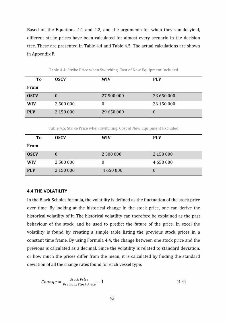
43

Based on the Equations 4.1 and 4.2, and the arguments for when they should yield,

different strike prices have been calculated for almost every scenario in the decision

tree. These are presented in Table 4.4 and Table 4.5. The actual calculations are shown

in Appendix F.

Table 4.4: Strike Price when Switching. Cost of New Equipment Included

To

From

OSCV WIV PLV

OSCV 0 27 500 000 23 650 000

WIV 2 500 000 0 26 150 000

PLV 2 150 000 29 650 000 0

Table 4.5: Strike Price when Switching. Cost of New Equipment Excluded

To

From

OSCV WIV PLV

OSCV 0 2 500 000 2 150 000

WIV 2 500 000 0 4 650 000

PLV 2 150 000 4 650 000 0

4.4 THE VOLATILITY

In the Black-Scholes formula, the volatility is defined as the fluctuation of the stock price

over time. By looking at the historical change in the stock price, one can derive the

historical volatility of it. The historical volatility can therefore be explained as the past

behaviour of the stock, and be used to predict the future of the price. In excel the

volatility is found by creating a simple table listing the previous stock prices in a

constant time frame. By using Formula 4.4, the change between one stock price and the

previous is calculated as a decimal. Since the volatility is related to standard deviation,

or how much the prices differ from the mean, it is calculated by finding the standard

deviation of all the change rates found for each vessel type.

𝐶ℎ𝑎𝑛𝑔𝑒 = 𝑆𝑡𝑜𝑐𝑘 𝑃𝑟𝑖𝑐𝑒𝑃𝑟𝑒𝑣𝑖𝑜𝑢𝑠 𝑆𝑡𝑜𝑐𝑘 𝑃𝑟𝑖𝑐𝑒

− 1 (4.4)

44

The historical volatility of the stock price is represented by the volatility of the daily hire

rates for the vessel types from 2012-2015. This can be justified because the stock price

is proportional to the daily hire rate. So the volatility of the stock price would be the

same as the volatility of the daily hire rate. The historical daily hire rates are presented

in Table 4.6 and the calculated volatilities for each vessel type in Table 4.7. A complete

calculation of the volatilities is added to Appendix B.

The Black-Scholes formula requires the annual volatility of the stock price. When the

volatility was calculated, the input had a time frame of one year; therefore the output is

the annualized volatility. However, if the input had been, for example monthly, the

results would need further calculations to be converted into annualized historical

volatility.

Table 4.6: Daily Hire Rate [USD]. (JJG Agis 2015, pers. comm., 28 April)

Vessel Type 2012 2013 2014 2015

OSCV 105.000 106.667 100.000 75.000

WIV 277.000 246.667 309.000 243.000

PLV 150.000 203.333 242.125 203.000

Table 4.7: Calculated Annual Historical Volatility for each Vessel Type

Vessel Type Volatility

OSCV 0,14

WIV 0,24

PLV 0,26

4.5 THE RISK-FREE RATE OF RETURN

The risk-free rate of return or risk-free interest rate is the theoretical rate of return from

an investment without risk. The rate is the expected interest from a risk-free investment

over a specific time period. It is common to base the interest rate on government bonds,

because they are the safest investments one can make (Johansen et al., 2013). The risk-

free rate can be expressed as a ten-year rate or sometimes a five-year rate. From a

market survey answered by the members of the Norwegian Society of Financial Analysts

45

(NFF) most respondents utilize the ten-year bond as the risk-free rate. It has therefore

been chosen to utilize the ten-year risk-free rate of a government bond from 2014 found

from a report by PWC on the Norwegian risk premium (PWC, 2014). The interest rate

was given as 48% for a ten-year bond, but the Black-Scholes formula requires the rate to

be annual, so to convert the ten-year rate from 48% the tenth root of the number was

used. The yearly interest rate became 1.47%, and was implemented in the formula as

the decimal 0.0147.

46

5 RESULTS Based on the assumptions and decisions made in Chapter 4, the Black-Scholes analysis

was implemented in Excel for all switching options. The main results from the case

analysis will be presented in this chapter; this includes the call option value for each

node in the decision tree. When applying the Black-Scholes formula obtain the value C,

representing the value of the European call option. For visual simplicity the results will

be presented in three separate tables, representing the first three options and their

following three options. The total structure of the decision tree is equal to Figure 2.6 in

Chapter 2.3.

Figure 5.1 represents the option values of the vessel’s opportunities if the next contract

after the initial OSCV contract is another OSCV contract. In other words, if the option is

not exercised. Towards the end of the second period operating as an OSCV the figure

shows the option values for the next three alternatives, and from the next nodes there

are three new opportunities with each their own value. Figure 5.2 shows the option

values if the first contract the vessel takes on is within well intervention. Similar to

Figure 5.1 the following nodes give the values of the three possible choices, and the next

three choices after that. Figure 5.3 shows the values if the option of switching to PLV is

exercised at the first expiration date.

In Table 5.1 and Table 5.2 the same results are presented, but in matrix form. The tables

illustrate the values of switching between different operational modes. Table 5.1 shows

the option values in the scenario where the new equipment has to be acquired before

switching, while Table 5.2 represent option values when the equipment is already

bought and stored for use. It is noticeable that the option values of all scenarios where

switching to an OSCV are the same in both of the tables. This is because no new deck

equipment has to be acquired when switching from one of the other vessel types to an

OSCV. Another observation is that the values of not exercising the option - going from

one vessel type to the same vessel type in the table – cannot calculated by the BS OPM.

This is because when no change is made the strike price is zero. The BS OPM does not

47

comply with a strike price equal to zero because it would force the model to divide by

zero. In these scenarios the option is delayed for the next period. The rest of the values

will always be higher in Table 5.2. As explained in Chapter 4.3, this is because the strike

prices were calculated differently based on whether or not the new equipment had to be

bought or not. When the equipment has already been stored from previous periods the

strike price is lower and thus the total option value becomes higher.

The main discovery from the results is that to invest in a multifunctional vessel is

valuable. This can be seen because all the call option values C, in the figures 5.1-5.3 and

the tables 5.1-5.2 are strictly positive. From Equation 3.1 in Chapter 3.2.5 we know that

in order for C to be positive, the stock price has to be higher than the strike price, which

means that the potential income from exercising the option is more than the cost of

exercising the option. Another variable that can justify this observation is the value

N(d2), which is defined in Chapter 3.2.5 as the probability that the stock price is higher

than the strike price at expiration. When using the BS OPM, an option will usually be

exercised at expiration if the stock price is higher than the strike price. Thus, N(d2)

actually represents the probability of the option being exercised at expiration. From

Appendix H it can be seen that for almost all scenarios, N(d2) has the value 1, which

means that the probability of exercising is 100%. The value N(d1), representing how far

into the money the stock price will be if, and only if, the option expires in the money, is

also always equal to 1. Meaning that the stock is 100% into the money at expiration. The

only occurrences where these values are not 1, with a three decimal approximation, is

when the vessel retrofits into a PLV for the first time after it has been operating as a

WIV. The reason for the option value being lower in these scenarios might be because

the stock price for the PLV is a lot lower than for a WIV, while the strike prices are quite

close. Also the deck equipment for the PLV will have to be bought and installed, at the

same time as the expensive WIV equipment has to be demobilized. The strike price

between this particular switch is among the highest in the analysis. Therefore the value

of exercising the option of switching between a WIV and a PLV when the strike price is

at its highest is lower than for the other switching options.

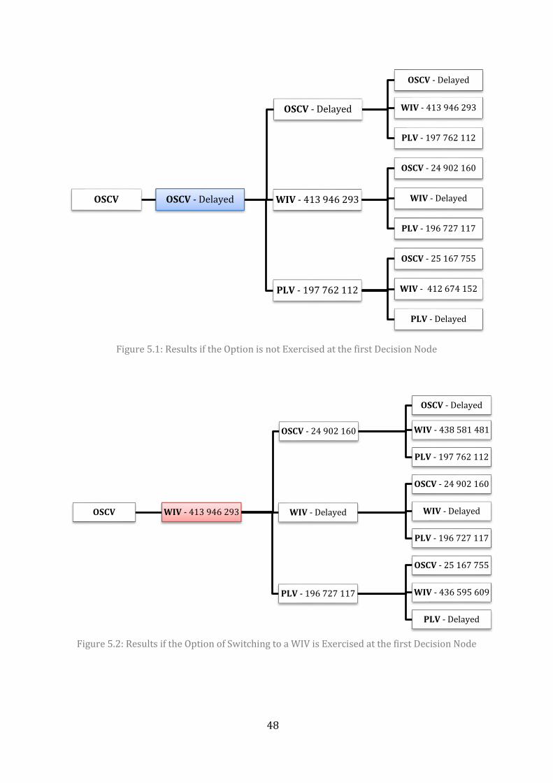
48

Figure 5.1: Results if the Option is not Exercised at the first Decision Node

Figure 5.2: Results if the Option of Switching to a WIV is Exercised at the first Decision Node

OSCV OSCV - Delayed

OSCV - Delayed

OSCV - Delayed

WIV - 413 946 293

PLV - 197 762 112

WIV - 413 946 293

OSCV - 24 902 160

WIV - Delayed

PLV - 196 727 117

PLV - 197 762 112

OSCV - 25 167 755

WIV - 412 674 152

PLV - Delayed

OSCV WIV - 413 946 293

OSCV - 24 902 160

OSCV - Delayed

WIV - 438 581 481

PLV - 197 762 112

WIV - Delayed

OSCV - 24 902 160

WIV - Delayed

PLV - 196 727 117

PLV - 196 727 117

OSCV - 25 167 755

WIV - 436 595 609

PLV - Delayed

49

Figure 5.3: Results if the Option of Switching to a PLV is Exercised at the first Decision Node

Table 5.1: Value of Switching between Vessel Types. Equipment Cost Included

To

From

OSCV WIV PLV

OSCV - 413 946 293 197 762 112

WIV 24 902 160 - 196 727 117

PLV 25 167 755 412 674 152 -

Table 5.2: Value of Switching between Vessel Types. Equipment Cost Excluded

To

From

OSCV WIV PLV

OSCV - 438 581 481 218 948 374

WIV 24 902 160 - 216 746 517

PLV 25 167 755 436 595 609 -

OSCV PLV - 197 762 112

OSCV - 25 167 755

OSCV - Delayed

WIV - 413 946 293

PLV - 218 948 374

WIV - 412 674 152

OSCV - 24 902 160

WIV - Delayed

PLV - 216 746 517

PLV - Delayed

OSCV - 25 167 755

WIV - 412 674 152

PLV - Delayed

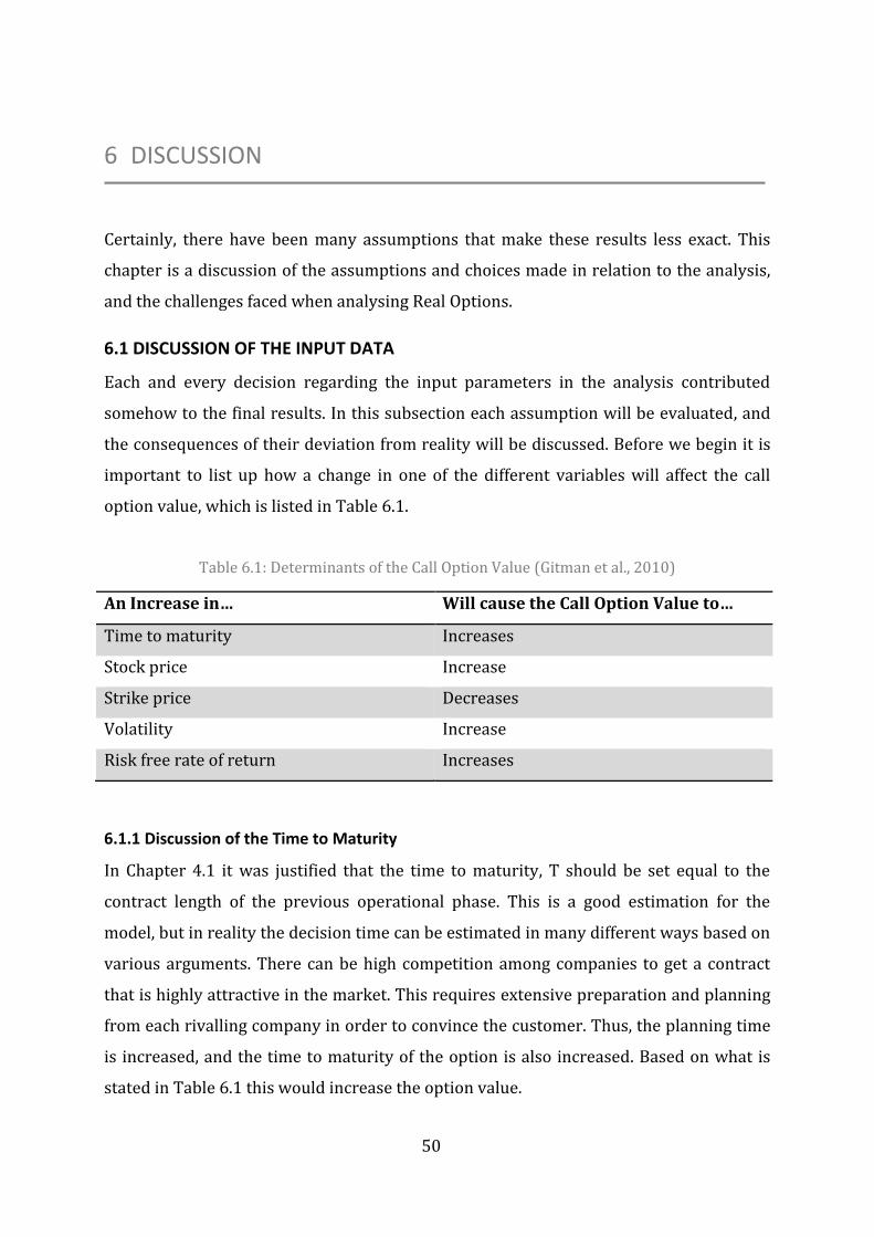
50

6 DISCUSSION Certainly, there have been many assumptions that make these results less exact. This

chapter is a discussion of the assumptions and choices made in relation to the analysis,

and the challenges faced when analysing Real Options.

6.1 DISCUSSION OF THE INPUT DATA

Each and every decision regarding the input parameters in the analysis contributed

somehow to the final results. In this subsection each assumption will be evaluated, and

the consequences of their deviation from reality will be discussed. Before we begin it is

important to list up how a change in one of the different variables will affect the call

option value, which is listed in Table 6.1.

Table 6.1: Determinants of the Call Option Value (Gitman et al., 2010)

An Increase in… Will cause the Call Option Value to…

Time to maturity Increases

Stock price Increase

Strike price Decreases

Volatility Increase

Risk free rate of return Increases

6.1.1 Discussion of the Time to Maturity

In Chapter 4.1 it was justified that the time to maturity, T should be set equal to the

contract length of the previous operational phase. This is a good estimation for the

model, but in reality the decision time can be estimated in many different ways based on

various arguments. There can be high competition among companies to get a contract

that is highly attractive in the market. This requires extensive preparation and planning

from each rivalling company in order to convince the customer. Thus, the planning time

is increased, and the time to maturity of the option is also increased. Based on what is

stated in Table 6.1 this would increase the option value.

51

It is also a common fact that the complexity and the length of the operation described in

the contract will demand a longer preparation time from the shipping company. Thus, a

contract over five years requires a longer planning time than one of three years. This

means that an assignment for a well intervention task following an OSCV contract can be

in planning even before the OSCV contract has begun. Following this argument, the time

to maturity used in the model is too short, which results in an option value that is lower

than it should be. If the analysis was performed with these considerations in mind, and

the times to maturity of each option were set equal or proportional to the contract

duration of the new vessel type, this would have affected the results.

6.1.2 Discussion of the Stock Price

The seven assumptions underlying the stock price in the Black-Scholes model were first

presented in Chapter 3.2.5. In this subsection, the assumptions will be investigated to

determine if they can be justified. In the Black-Scholes formula, the stock price is

assumed to follow a random-walk behaviour. This is based on the presumption that

buyers invest rationally, which means that they act self-interested and with economic

profit in mind. The asset value is estimated based on future expectations, which can be

forecasted from existing information, and it changes when new information is available.

When the forecast of the future stock price is favourable investors rush to buy the asset

before the value jumps down. The Black-Scholes model also assumes that the market is

efficient, meaning that the price will be adjusted quickly with new information, and

investors cannot “beat the market”. This is because all investors do thorough research

on each stock before making decisions. The big question is therefore: can the offshore

vessel charter market be described as efficient? If so, the assumptions in the Black-

Scholes model will be entirely accurate. But this is not a simple question, and it is an

issue to which economists have devoted a lot of time and effort.

If the freight market is inefficient the profit can be maximized by wisely switching from

one market to another, like entering the spot market or locking in the time charter rates.

According to Karakitsos and Varnavides (2014) consultants must “instantly learn all new

information, absorb its implications for profit opportunity or loss and react instantly to

take advantage of it” for a market to be efficient. But this is not possible in a realistic

market, as many investors do not act upon the new information, because they do not

52

appreciate its implication or they are not prepared to take the risk. There are many

factors affecting this subject. Like how the risk can be measured and adjusted. Can

anyone have control over all available information that can change the market, and how

does someone know what information is relevant? In some cases investors are not in the

market long enough to be aware of the changes. Or secret data can be discovered by

snooping or looking hard enough for it. Therefore Karakitsos and Varnavides describe

the market as inefficient in the short run, but not necessarily in the long run. However,

in reality if the market can be beaten, there is no obvious way to do so, and market

movements are difficult to foresee. During the Greek financial crisis in 2010 the demand

fell short of the supply, and many ship owners did not act on the information by locking

in the time charter rates. If the market had been efficient this decision would not have

had an economic impact, but since the market can be observed as inefficient during

short time periods, the owners that did lock in the charter rates benefited from it.

The initial assumption of a random walk behaviour of the stock price can also be

discussed. An article by MacKinlay and Lo (1988) states that there exists a low

correlation between the prices on a short basis and a slightly stronger correlation over

the long term. Our stock price was implemented into the calculations with yearly

intervals. In finance, one year is considered to be a long time period and there will thus

exist a correlation between the values. The final results are most likely affected by the

error related to this assumption.

Another assumption regarding the stock price in the Black-Scholes method is that the

stock price does not pay dividends, which is not compatible to the real world. A way of

adjusting this in the formula is to subtract the discounted value of the future dividend

from the stock price, but this is neglected in this analysis. If the dividends had been

included in the calculations, it would have resulted in a lower stock price and thus a

lower call value, which is supported by Table 6.1.

The stock is also assumed to follow a lognormal distribution. The difference between

lognormal and normal distribution is that the tail of the lognormal function is longer,

which allows for stock prices between zero and infinity. The lognormal distribution also

assumes that the stock can only drop by a 100%, but it can rise by more than 100%

53

(Hodley, 2015). In reality, dramatic movements in the market affect the stock price by

making their tails shorter than the lognormal. Measuring the degree to which the real

asset price differs from the lognormal distribution can prevent the errors from the

lognormal assumption.

6.1.3 Discussion of the Strike Price

The strike price, representing the price at which the option can be exercised, is

implemented in this analysis as an approximation of the total cost of switching from one

vessel type to another. The strike price affects the results so that a lower strike price

increases the option value. In Chapter 4.3 the content of this cost was verified as the cost

of purchasing the new equipment, plus the cost of installing the equipment and

demobilizing the old equipment. The installation and demobilizing cost was assumed

10% of the equipment cost. However, it is problematic to give a mutual estimate for all

equipment types. Some equipment can be considered cheap to purchase, but it can be

quite complicated to install, while other equipment may be expensive, but the

mobilization procedure can be quite simple and fast. Despite that, with errors and

omissions accepted a 10% assumption is valid.

When performing the actual retrofitting from one vessel type to another, the vessel will

be in off-hire during the time this process will take place. The potentially lost income

from days in off-hire is neglected from the strike price. This is because it is assumed that

when the vessel is dry-docked and the deck equipment is demobilized/mobilized, the

vessel will already be unchartered, and it will not be under a specific contract. In the

absence of the off-hire contribution, the strike price is lower in the analysis than what it

should be in real life. Based on Table 6.1 this makes the calculated option value

somewhat higher than the realistic value.

It is assumed that after the period where an equipment type is used for the last time, the

equipment can be sold with a 10% discount for each year since it has been fabricated.

Although the income from selling the used equipment is part of the transformation

phase between the vessel types, the earning contribution cannot be included in the

strike price of this call option because it will in some cases result in a negative strike

price. This is not compatible with the Black-Scholes formula. Mathematically, because it

54

we will be trying to find the natural logarithm of a negative value, which is not possible.

It also coincides with the original definition of holding a call option. The option holder

has the right, but not obligation to exercise the option at the expiration date, but if

exercising the option gives an income, then no matter the stock price, the owner would

exercise the option with a negative strike price. Therefore the sales income is presented

additionally in the results as an extra potential income and not used in the calculations.

In the demobilization of the equipment needed for well intervention it can be beneficial

to keep some lengths of the skidding system, especially in the areas around the ROV

hangar. The ROVs are helpful in the other operational modes as well, and the skidding

rails in the hangar area would not obstruct other operations. In the analysis it is

assumed that after operating as a Well Intervention Vessel, all the purchased equipment

such as MHT and all lengths of the skidding system is removed upon the switch. By not

removing parts of the skidding system the strike price could have been lower resulting

in a higher call option value. There is also some other small, but necessary equipment

that were not included in the strike price, like the cargo tanks for mud and brine on the

WIV. By including these, the actual strike price would have been higher, making the call

value lower.

6.1.4 Discussion of the Volatility

The most significant assumption regarding the volatility in the Black-Scholes formula is

that it is constant over time. This might be true over a short time, but never for a longer

period. Figure 6.1 shows how the daily hire rate for the three different vessels has

changed over the past three years, which is a relatively short time period compared to

the vessel’s total lifetime of 20 years. Still, during this short period of time it is

observable that the rates change drastically. The constant volatility that was

implemented in the BS OPM would therefore differ from the non-constant volatility that

could have been used instead. In some advanced option-valuation methods, like the one

presented by Geske (1979) a non-constant volatility is generated by a stochastic

process, which could have been done in this analysis to simulate more realistic non-

constant volatilities over time. The results would become somewhat different and more

realistic if this method was used.

55

Another interesting observation to discuss regarding the volatilities is shown by

comparing Figure 6.1 and Figure 6.2. Figure 6.2 shows that from 2013 to 2014 the oil

price dropped almost 60%. The figure also shows the oil price over the last decade.

Since we calculated the volatility of the stock price by looking at its change over the last

three years, we will use the same time period for calculating the volatility of the oil price.

By using the same method as in Chapter 4.4 to calculate the volatility of the oil price we

discover that the volatility is 0.25 for the last three years. The Excel calculations are

shown in detail in Appendix E. As a reminder, the volatilities of the stock prices for the

OSCV, WIV and PLV were calculated in Chapter 4.4 as 0.14, 0.24 and 0.26. This means

that in the case of the WIV and PLV the stocks change proportionally to the oil price

from 2012 to 2015. However, the volatility of the OSCV is much lower than for the oil

price.

An initial thought was that the volatility of the oil price could be used in the analysis as a

good approximation to the volatility of the stock price. If this had been done in the

analysis, the option values for the WIV and PLV would not have differed much, but the

option value of the OSCV would have ended up too high. It was therefore wise to use

different volatilities for the different vessel types as was done eventually in this analysis.

This enables the method to evaluate each vessel type separately and discover their

differences.

It can be also interesting to look into the physical factors causing the OSCV’s volatility to

not be equal to the other vessel types’, and why it is not equal to the volatility of the oil

price. It can have something to do with the fact that the OSCV is not as dependent on the

oil and gas industry as the other two vessel types. For example the vessel can be utilized

in construction and maintenance of wind turbine fields and other offshore tasks. Table

2.2 shows how the OSCV is needed in three of four phases in Research and Development

of oil and gas. The table also shows how the different phases are affected by the oil price.

Another reason for the dissimilarity between the volatilities could have been the way

the volatility was calculated that caused an error. Still it can be seen from

Figure 6.1 that the span in the change of the hire rates is bigger for WIV and PLV than

OSCV. Based on this it should be correct that OSCV has a lower volatility.

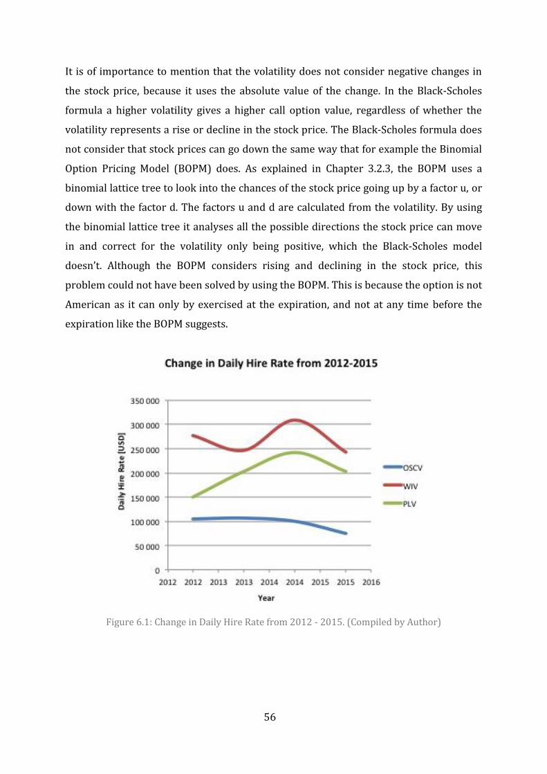
56

It is of importance to mention that the volatility does not consider negative changes in

the stock price, because it uses the absolute value of the change. In the Black-Scholes

formula a higher volatility gives a higher call option value, regardless of whether the

volatility represents a rise or decline in the stock price. The Black-Scholes formula does

not consider that stock prices can go down the same way that for example the Binomial

Option Pricing Model (BOPM) does. As explained in Chapter 3.2.3, the BOPM uses a

binomial lattice tree to look into the chances of the stock price going up by a factor u, or

down with the factor d. The factors u and d are calculated from the volatility. By using

the binomial lattice tree it analyses all the possible directions the stock price can move

in and correct for the volatility only being positive, which the Black-Scholes model

doesn’t. Although the BOPM considers rising and declining in the stock price, this

problem could not have been solved by using the BOPM. This is because the option is not

American as it can only by exercised at the expiration, and not at any time before the

expiration like the BOPM suggests.

Figure 6.1: Change in Daily Hire Rate from 2012 - 2015. (Compiled by Author)

57

Figure 6.2: Brent Average Price and Range. (Victor, 2015)

6.1.5 Discussion of the Risk-Free Rate of Return

The value of the risk-free rate of return is dependent on the development in the market

and is not constant in time, or directly observable in the market, therefore different

market surveys can give varying rates. The last years the market has been irregularly

volatile and characterized as highly uncertain. This has resulted in a risk-free rate at

historically low values. The numbers used in this analysis are from 2014, but the

numbers from 2015 might be even lower because of recent changes in the economy. By

using the rate from 2015 the results would thus have been lower. In this analysis, the

ten-year bond was used, but the five-year bond gives a higher risk-free rate than the ten-

year. If the five-year bond had been used instead the results would have been higher.

Since there are many different ways of choosing the risk-free rate, there follows a level

of error in the results.

6.2 DISCUSSION OF THE RESULTS

Based on the results presented in Chapter 5 it has been established that the option value

is positive for all nodes. A factor that has not been considered in the calculations is the

initial investment of building the MOCV. It is understandable that the OSCV with a

reinforced moonpool area is more expensive to build than a conventional OSCV. In Table

6.2 the building costs of each vessel type is listed, estimated based on the vessel

specifications and equipment capacities presented in Chapter 2.3. The numbers were

obtained from personal communication with Wartsila, and the values were converted

from NOK to USD by using the currency rate 0.134 (April 24th 2015). From the table it

can be seen that the difference in building costs between the multipurpose OSCV and the

conventional OSCV is 13 mUSD. Thus, the necessary extra investment that has to be

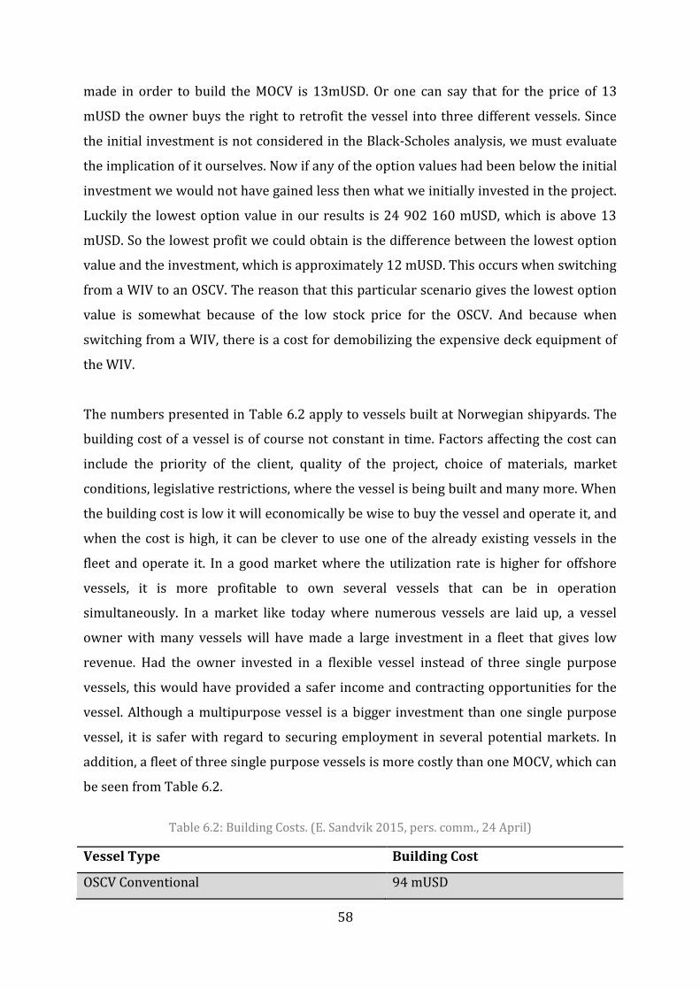
58

made in order to build the MOCV is 13mUSD. Or one can say that for the price of 13

mUSD the owner buys the right to retrofit the vessel into three different vessels. Since

the initial investment is not considered in the Black-Scholes analysis, we must evaluate

the implication of it ourselves. Now if any of the option values had been below the initial

investment we would not have gained less then what we initially invested in the project.

Luckily the lowest option value in our results is 24 902 160 mUSD, which is above 13

mUSD. So the lowest profit we could obtain is the difference between the lowest option

value and the investment, which is approximately 12 mUSD. This occurs when switching

from a WIV to an OSCV. The reason that this particular scenario gives the lowest option

value is somewhat because of the low stock price for the OSCV. And because when

switching from a WIV, there is a cost for demobilizing the expensive deck equipment of

the WIV.

The numbers presented in Table 6.2 apply to vessels built at Norwegian shipyards. The

building cost of a vessel is of course not constant in time. Factors affecting the cost can

include the priority of the client, quality of the project, choice of materials, market

conditions, legislative restrictions, where the vessel is being built and many more. When

the building cost is low it will economically be wise to buy the vessel and operate it, and

when the cost is high, it can be clever to use one of the already existing vessels in the

fleet and operate it. In a good market where the utilization rate is higher for offshore

vessels, it is more profitable to own several vessels that can be in operation

simultaneously. In a market like today where numerous vessels are laid up, a vessel

owner with many vessels will have made a large investment in a fleet that gives low

revenue. Had the owner invested in a flexible vessel instead of three single purpose

vessels, this would have provided a safer income and contracting opportunities for the

vessel. Although a multipurpose vessel is a bigger investment than one single purpose

vessel, it is safer with regard to securing employment in several potential markets. In

addition, a fleet of three single purpose vessels is more costly than one MOCV, which can

be seen from Table 6.2.

Table 6.2: Building Costs. (E. Sandvik 2015, pers. comm., 24 April)

Vessel Type Building Cost

OSCV Conventional 94 mUSD

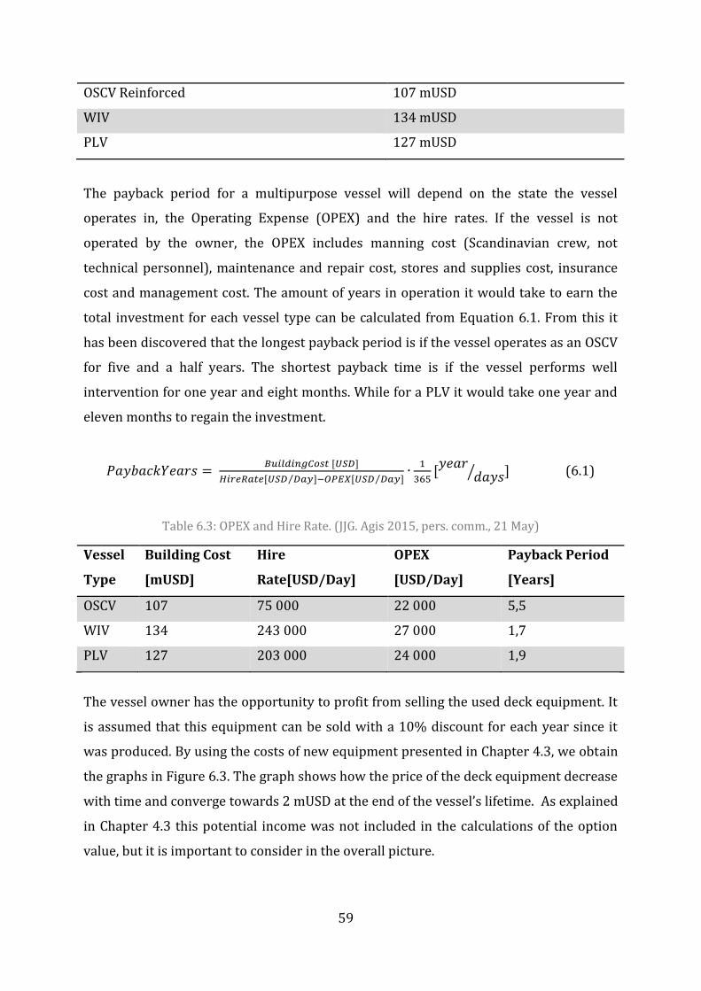
59

OSCV Reinforced 107 mUSD

WIV 134 mUSD

PLV 127 mUSD

The payback period for a multipurpose vessel will depend on the state the vessel

operates in, the Operating Expense (OPEX) and the hire rates. If the vessel is not

operated by the owner, the OPEX includes manning cost (Scandinavian crew, not

technical personnel), maintenance and repair cost, stores and supplies cost, insurance

cost and management cost. The amount of years in operation it would take to earn the

total investment for each vessel type can be calculated from Equation 6.1. From this it

has been discovered that the longest payback period is if the vessel operates as an OSCV

for five and a half years. The shortest payback time is if the vessel performs well

intervention for one year and eight months. While for a PLV it would take one year and

eleven months to regain the investment.

𝑃𝑎𝑦𝑏𝑎𝑐𝑘𝑌𝑒𝑎𝑟𝑠 = 𝐵𝑢𝑖𝑙𝑑𝑖𝑛𝑔𝐶𝑜𝑠𝑡 [𝑈𝑆𝐷]𝐻𝑖𝑟𝑒𝑅𝑎𝑡𝑒[𝑈𝑆𝐷 𝐷𝑎𝑦⁄ ]−𝑂𝑃𝐸𝑋[𝑈𝑆𝐷 𝐷𝑎𝑦⁄ ]

∙ 1365

[𝑦𝑒𝑎𝑟𝑑𝑎𝑦𝑠⁄ ] (6.1)

Table 6.3: OPEX and Hire Rate. (JJG. Agis 2015, pers. comm., 21 May)

Vessel

Type

Building Cost

[mUSD]

Hire

Rate[USD/Day]

OPEX

[USD/Day]

Payback Period

[Years]

OSCV 107 75 000 22 000 5,5

WIV 134 243 000 27 000 1,7

PLV 127 203 000 24 000 1,9 The vessel owner has the opportunity to profit from selling the used deck equipment. It

is assumed that this equipment can be sold with a 10% discount for each year since it

was produced. By using the costs of new equipment presented in Chapter 4.3, we obtain

the graphs in Figure 6.3. The graph shows how the price of the deck equipment decrease

with time and converge towards 2 mUSD at the end of the vessel’s lifetime. As explained

in Chapter 4.3 this potential income was not included in the calculations of the option

value, but it is important to consider in the overall picture.

60

From the discussion of the input parameters in this chapter, we know that the results

have errors and deviations. Since Real Options is relatively new in engineering practice,

many errors occur when financially-based approaches are used in practice. Many

deviations have been discovered and discussed earlier in this chapter. Probably, many

more sources of errors exist that have been missed here. Since there is no available data

available from previous analyses of this particular multipurpose vessel, the results

cannot be compared to previous or similar work.

It has been chosen to use the BS OPM in four stages of the service time to clearly see the

economic benefit of storing the equipment for future periods. And this is shown in Table

5.1 and Table 5.2. It can be seen that the biggest amount of money one can save by doing

this is about 25 mUSD, which is in the case of switching from OSCV to WIV. This is a

5.6% increase in option value. Although the actual price of storing the equipment has

been neglected the results demonstrate the increase in value.

Although it looks like WIV is the most profitable operational mode, it is difficult to give a

recommendation of what operational mode is most preferred and when it should be

used. The results clearly show that the WIV mode always gives the highest option value,

followed by the PLV and lastly the OSCV. This is because WIV hire rates usually exceed

hire rates for OSCV and PLV to compensate for the complexity of the vessel and the

higher building cost. Since the stock price is calculated based on the hire rates, the stock

price of the WIV will always be greater than for OSCV and PLV. Also, in Chapter 4.2 it

was explained that the stock prices were calculated by multiplying the daily hire rates

for each type with the amount of days in the contracts of each vessel type. Since it was

assumed that the operational modes would have different contract lengths with the WIV

having the longest of 5 years, the stock prices of the vessel types are multiplied with a

different number of years. This makes a huge difference in the results as the stock price

of the WIV is, for example, 5 times higher than for the OSCV. Therefore it becomes

unrealistic to compare the vessel types to each other based on the results. The results

also underscore the already known fact that a longer contract is more valuable.

However, had the time to maturity of the options been given a mutual value, for example

3 years, for each of the cases, the option values would have been closer to each other in

value, but from Appendix J it can be seen that the WIV still gives the highest value.

61

Figure 6.3: Sale Prices for WIV and PLV Equipment. (Compiled by Author)

62

7 CONCLUSION In this thesis we have evaluated the value of a Multipurpose Offshore Construction

Vessel. A Real Options approach has been used to solve the problem because of its

insight into handling uncertainty and flexibility. Using Real Options and adding

flexibility to a design allows it to be reshaped with time, when the market is more

predictable. By using the Black-Scholes Option Pricing Model we have estimated the

values of switching between different operational modes.

In a bad market, such as the one we are experiencing today, many ship owners are left

with vessels in lay-up. A Multipurpose Offshore Construction Vessel can serve as a work

platform where switching deck equipment can enable the vessel to enter different

markets. In the discussion it was said that the vessel charter market can be observed as

inefficient in the short-run. This means that by acting rationally ship owners can gain

profits by switching vessel types. From the results obtained in this study, one can see

that the value of owning a MOCV is positive. Although it has been difficult to justify many

of the assumptions that have contributed to the final results, the study has shown that

by using a Real Options approach one can determine the value of flexible ship design.

Though Real Options is more commonly used to value financial instruments, the results

show that the shipping sector can win over the uncertainties of the future by investing in

flexibility in projects.

Albert Einstein said that "In the middle of difficulty lies opportunity". Difficult markets

often work as a wakeup call to invoke experimentation in engineering. They make

options available, and new knowledge forces adjustments over time. Real Options

thinking is an efficient tool when valuing risk and uncertainty since it actually becomes

more valuable when uncertainty is high. The method is betting on market volatility, and

that one will eventually require a plan B. Although the Real Options method has its

weaknesses, it has revolutionized investors’ way of handling companies as it forces the

option holder to consider hidden assets as business opportunity. It is risky to bet too

much on uncertainty, but it is also a mistake to forget all about it.

63

FURTHER WORK Future applications of Real Options in ship design could be to value the option of

creating a flexible vessel able to operate in both the fishing and the offshore

construction industry. It would be interesting to identify vessels with similar

performance expectations and create a mutual design platform combining these. An

example of a concept to consider is a combination between a fishing trawler and an

Anchor Handling Tug Supply.

Extensions of this problem can be made by performing the analysis with more sets of

data to compare the results. The volatility could have been calculated over a longer time

period, or it could have been implemented as a non-constant in the model, like Geske

(1979) suggested in his work. It could also be interesting to compare the Net Present

Values of the flexible project to a traditional inflexible design.

The problem has been solved by applying the Black-Scholes Option Pricing Model into

Excel. Matlab could have been used to check the validity of the method or to create a

more interactive model that could be used by others later.

64

REFERENCES Adner, R. & D. Levinthal (2002). The Emergence of Emerging Technologies. California

Management Review

Angell, T. (2015). Infield Systems Review North Sea Well Intervention Market. Infield

Systems’ Bent Mathisen speaks with Tommy Angell of Offshore Network

Amram, M. & N. Kulatilaka (1999). Managing Strategic Investment in an Uncertain

World: Disciplined Decisions - Aligning Strategy with the Financial Markets.

Harvard Business Review

Amram, M. & N. Kulatilaka (2000). Managing Strategic Investment in an Uncertain

World: Strategy and Shareholder Value - The Real Options Frontier. Journal of

Applied Corporate Finance, Summer

Black, F. & M. Scholes (1973). The Pricing of Options and Corporate Liabilities.

Chicago Journals

BP (2012). British Petroleum Energy Outlook 2035. January

Brealey, R.A., S.C. Myers & F. Allen (2006). Principles of Corporate Finance

Copeland, T. & V. Antikarov (2001). Real Options: A Practitioner's guide. New York

TEXERE LLC

Cruz, S.S. & E.H. Zavoni (2005). Real Options Models for Maintenance Decision Making

for Offshore Jacket Platforms

Damodaran, A. (2007). Strategic Risk Taking: A Framework for Risk Management.

Chapter 8: Real Options

de Neufville, R. & S. Scholtes (2011). Flexibility in Engineering Systems. MIT Press.

Dias, M.A.G. (2004). Valuation of Exploration and Production Assets: an Overview of Real

Options Models. Journal of Petroleum Science and Engineering. 44(1-2), 93-114

FMC (2014). Riserless Light Well Intervention (RLWI)

Gesner, G.A. & J. Jardim (1998). Bridge within a bridge, Civil Engineering. 68 (10), 44–47.

Geske, R. (1979). The Valuation of Compound Options. Journal of Financial Economics

Gitman, L.J., M.D. Joehnk & S.B Smart (2010). Fundamentals of Investing. 11th Edition

Greden, L.V. & L.R. Glicksman (2004). Options Valuation of Architectural Flexibility: A

65

Case Study of the Option to Convert to Office Space. Journal of Corporate Real

Estate Volume 7 Number 1

Greden, L.V., L.R. Glicksman & G.L. Betanzos (2006). A Real Options Methodology

for Evaluating Risk and Opportunity of Natural Ventilation. Journal of Solar

Energy Engineering

Gregor, J.A. (2003). Real Options for Naval Ship Design and Acquisition: A Method for

Valuing Flexibility under Uncertainty. MSc MIT.

Gue, E.H. (2009). The Golden Triangle. Investing Daily

Howell, S., A. Stark, D.P. Newton, D.A. Paxson, M. Cavus, J.A. Pereira, J.K. Patel (2001).

Real Options - Evaluating Corporate Investment Opportunities in a Dynamic

World. Financial Times: Prentice Hall

Karakitsos, E. & L. Varnavides (2014). Maritime Economics - A Macroeconomical

Approach. p.95-96.

Kulatilaka, N. (1993). The Value of Flexibility: The Case of a Dual-Fuel Industrial Steam

Boiler. Financial Management

Leggio, K.B. (2006). Managing Enterprise Risk: What the Electric Industry Experience

Implies for Contemporary Business. Elsevier

MacKinlay, A.C & A.W. Lo (1988). Stock Market Prices Do Not Follow Random Walks:

Evidence From Simple Specification Test. The Review of Financial Studies

Margrabe, W. (1978). The Value of an Option to Exchange one Asset for Another. The

Journal of Finance

Merton, R.C. (1973). Theory of Rational Option Pricing. Belt Journal of Economics and

Management Science

Myers, S.C. ( 1977). Determinants of Corporate Borrowing. MIT Cambridge. Journal of

Financial Economics

Platou, RS (2014). Market Report July 2014

PWC (2014). Risikopremien i det norske markedet. December. Page 5

Scoltes, S. & T. Wang (2006). Real Options by Spreadsheed: Parking Garage Case

Example

SIEM (2014). Fourth Quarter Report 2014 - Siem Offshore

Trigeorgis, L. (1996). Real Options - Managerial Flexibility and Strategy in Recourse

Allocation. MIT Press

66

Victor, S (2015). New Oil Shock - What Does the Future Hold? Singapore Offshore

Finance Forum, IHS Energy

Wang, T & R. de Neufville (2005). Real Options “in” Projects. Prepared for the 9th Real

Options Annual International Conference in Paris, France

Wijst, D.V.D (2010). Finance for Science and Technology Students. Tapir Akademiske

Forlag, Kompendieforlaget

Zijderveld G.H.T., H.J. Tiebout, S.M. Hendriks & L. Poldervaart (2012). Subsea Well

Intervention Vessel and Systems - OTC

ONLINE REFERENCES Gue, E.H. (2009). The Golden Triangle. Investing Daily. October 15th

Hodley Trading and Investment Tools (2015). Option Pricing Models and the "Greeks".

Lognormal distribution - but how realistic?. May 19th

Investopedia (2015a). Definition of 'Options'. March 16th

Investopedia (2015b). Definition of 'volatility'. March 16th

Johansen, T.H., A. Laake & M.F. Aulie (2013). Risikopremien i det norske markedet:

Verdsettelse i volatile tider – hva skjer med avkastningskravet? MAGMA: Econas

Tidsskrift for Økonomi og Ledelse. May 25th

Lorusso, M. (2014). Drop in Oil Prices Increase Value of Flexible Financing. Oil and Gas

Monitor. June 1st

Stensvold, Tore (2014). Kleven skal bygge om Aker Wayfarer til brønnintervensjon.

Teknisk Ukeblad. October 28th

Yeo, A. & M.M. Øy (2010). Introduction to Offshore Support Vessels. Marine Money

Offshore, Pareto Securities Asia. February 20th

68

APPENDIX

APPENDIX A – PROBLEM DESCRIPTION Master Thesis in Marine Systems Design For Stud. Techn. Tara Jahangiry “Valuing Flexibility in Ship Design: A Real Options Approach” Spring 2015 Background Today's construction vessels are usually built with a specific deck equipment type, and operate throughout their entire lifetime with this particular equipment. In a competitive industry the equipment composition and performance area of a vessel can be crucial to signing a contract with an operator, due to changing marked demands. For the future generation of construction vessels, a new trend is being more and more popular that enables the vessel to change deck equipment during the vessel's lifetime. This change is dependent on available contracts and market demand. This requires a ship design where the deck structure is prepared to support different equipment types, and implies a large deck area with high deck strength and sufficient space under deck. It also includes a lay up for installation of different deck equipment used on offshore vessels, such as of offshore- and deck cranes, winches, pipelay spread, flex lay tower, carousels, ROV hangars, moon pool, diving bell etc. A Real Options approach can be used to find a value of a multipurpose vessel that owns the options of switching between vessel types. Objective The object of this thesis is to evaluate the value of the Multipurpose Offshore Construction Vessel (MOCV), using the Black-Scholes Option Pricing Model (BS OPM). The problem considers a MOCV holding the option to transform into an OSCV, WIV or Pipe Laying Vessel (PLV). The thesis aims to discuss what the economic benefit of owning one MOCV is instead of three separate vessels. The thesis also seeks to identify and price the underlying assets necessary for the design of each vessel type.

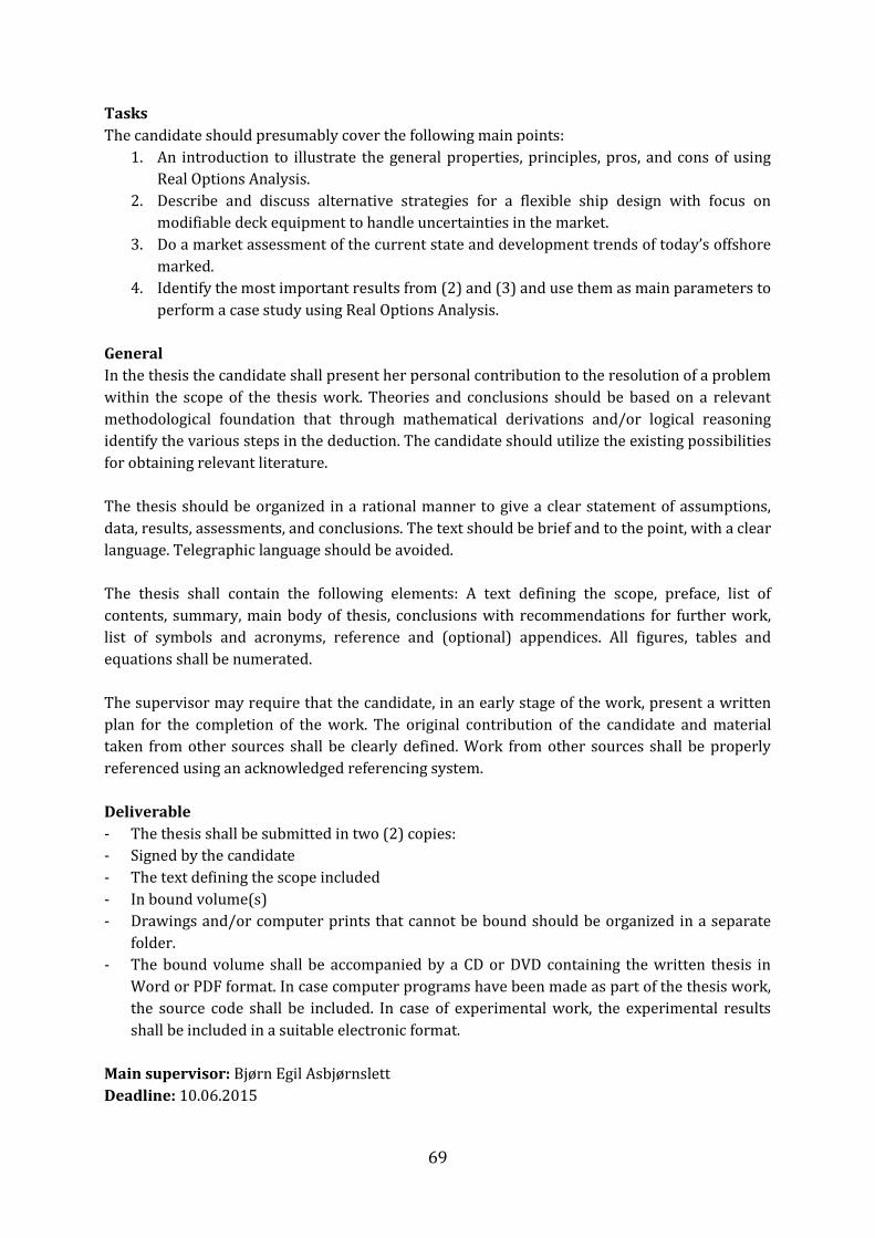
69

Tasks The candidate should presumably cover the following main points:

1. An introduction to illustrate the general properties, principles, pros, and cons of using Real Options Analysis.

2. Describe and discuss alternative strategies for a flexible ship design with focus on modifiable deck equipment to handle uncertainties in the market.

3. Do a market assessment of the current state and development trends of today’s offshore marked.

4. Identify the most important results from (2) and (3) and use them as main parameters to perform a case study using Real Options Analysis.

General In the thesis the candidate shall present her personal contribution to the resolution of a problem within the scope of the thesis work. Theories and conclusions should be based on a relevant methodological foundation that through mathematical derivations and/or logical reasoning identify the various steps in the deduction. The candidate should utilize the existing possibilities for obtaining relevant literature. The thesis should be organized in a rational manner to give a clear statement of assumptions, data, results, assessments, and conclusions. The text should be brief and to the point, with a clear language. Telegraphic language should be avoided. The thesis shall contain the following elements: A text defining the scope, preface, list of contents, summary, main body of thesis, conclusions with recommendations for further work, list of symbols and acronyms, reference and (optional) appendices. All figures, tables and equations shall be numerated. The supervisor may require that the candidate, in an early stage of the work, present a written plan for the completion of the work. The original contribution of the candidate and material taken from other sources shall be clearly defined. Work from other sources shall be properly referenced using an acknowledged referencing system. Deliverable - The thesis shall be submitted in two (2) copies: - Signed by the candidate - The text defining the scope included - In bound volume(s) - Drawings and/or computer prints that cannot be bound should be organized in a separate

folder. - The bound volume shall be accompanied by a CD or DVD containing the written thesis in

Word or PDF format. In case computer programs have been made as part of the thesis work, the source code shall be included. In case of experimental work, the experimental results shall be included in a suitable electronic format.

Main supervisor: Bjørn Egil Asbjørnslett Deadline: 10.06.2015

70

APPENDIX B – CALCULATION OF VOLATILITY OF STOCK PRICE Volatility of Stock Price of OSCV Year Daily Hire Rate [USD] Change Volatility 2012 OSCV2012 2013 OSCV2013 =OSCV2013/OSCV2012-1 2014 OSCV2014 =OSCV2014/OSCV2013-1 2015 OSCV2015 =OSCV2015/OSCV2014-1 =STDAV(Change1:Change3) Volatility of Stock Price of WIV Year Daily Hire Rate [USD] Change Volatility 2012 WIV2012 2013 WIV2013 =WIV2013/WIV2012-1 2014 WIV2014 =WIV2014/WIV2013-1 2015 WIV2015 =WIV2015/WIV2014-1 =STDAV(Change1:Change3) Volatility of Stock Price of PLV Year Daily Hire Rate [USD] Change Volatility 2012 PLV2012 2013 PLV2013 =PLV2013/PLV2012-1 2014 PLV2014 =PLV2014/PLV2013-1 2015 PLV2015 =PLV2015/PLV2014-1 =STDAV(Change1:Change3)

71

APPENDIX C – CALCULATION OF STOCK PRICE Calculation of stock price, S for OSCV under a contract with a length of 1 year:

S(OSCV) = 75 000USDDay ∙ 363[Days] ∙ 1[Year] = 27 375 000 USD

Calculation of stock price, S for WIV under a contract with a length of 5 year:

S(WIV) = 243 000USDDay ∙ 363[Days] ∙ 5[Year] = 443 475 000 USD

Calculation of stock price, S for PLV under a contract with a length of 3 year:

S(PLV) = 203 000USDDay ∙ 363[Days] ∙ 3[Year] = 222 285 000 USD

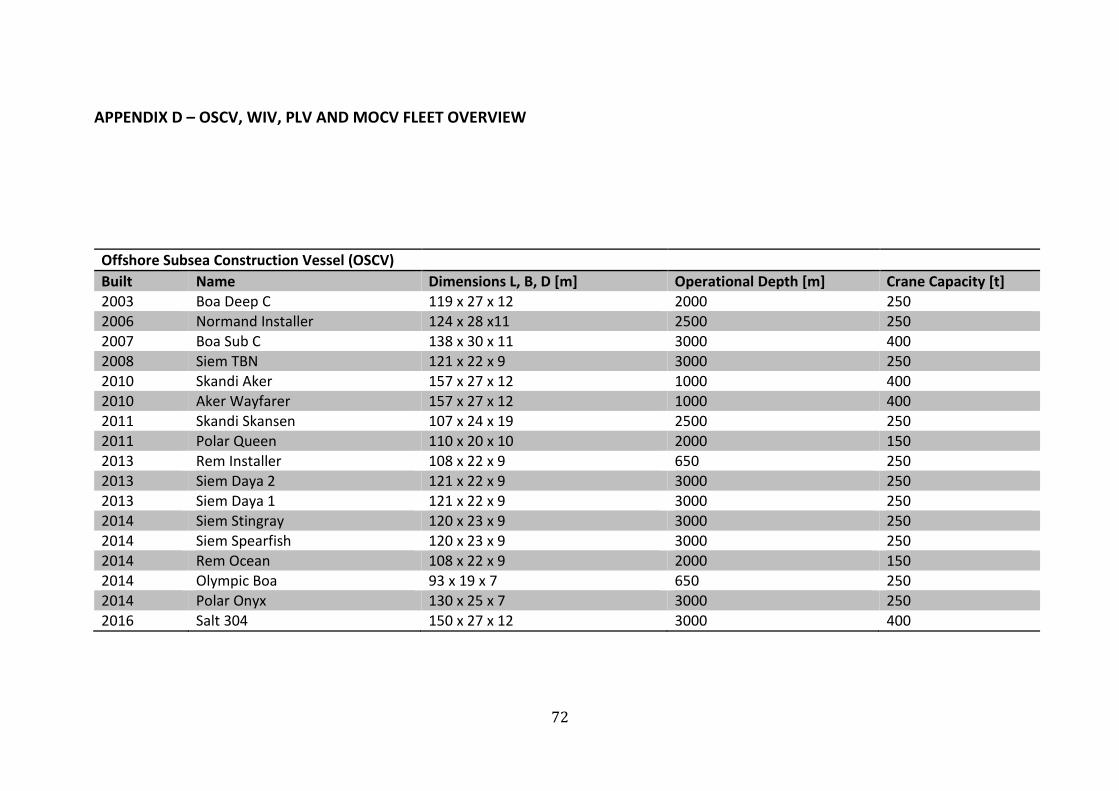
72

APPENDIX D – OSCV, WIV, PLV AND MOCV FLEET OVERVIEW

Offshore Subsea Construction Vessel (OSCV) Built Name Dimensions L, B, D [m] Operational Depth [m] Crane Capacity [t] 2003 Boa Deep C 119 x 27 x 12 2000 250 2006 Normand Installer 124 x 28 x11 2500 250 2007 Boa Sub C 138 x 30 x 11 3000 400 2008 Siem TBN 121 x 22 x 9 3000 250 2010 Skandi Aker 157 x 27 x 12 1000 400 2010 Aker Wayfarer 157 x 27 x 12 1000 400 2011 Skandi Skansen 107 x 24 x 19 2500 250 2011 Polar Queen 110 x 20 x 10 2000 150 2013 Rem Installer 108 x 22 x 9 650 250 2013 Siem Daya 2 121 x 22 x 9 3000 250 2013 Siem Daya 1 121 x 22 x 9 3000 250 2014 Siem Stingray 120 x 23 x 9 3000 250 2014 Siem Spearfish 120 x 23 x 9 3000 250 2014 Rem Ocean 108 x 22 x 9 2000 150 2014 Olympic Boa 93 x 19 x 7 650 250 2014 Polar Onyx 130 x 25 x 7 3000 250 2016 Salt 304 150 x 27 x 12 3000 400

73

Well Intervention Vessels (WIV) Built Name Dimensions [m] Moonpool [m] Offshore Crane MHT [t] Skidding [t] 2004 Island Frontier 106 x 21 7.2 x 7.2 130t 70 2008 Island Constructor, RLWI 120 x 25 x 10 8.1 x 8.1 150t, 2500m 300 100, 60 2008 Skandi Constructor, RLWI 120 x 25 x 10 8.0 x 8.0 150t, 2500m 150 2008 Island Wellserver, LWI 116 x 25 7.8 x 7.8 150t 100 2009 Skandi Santos 121 x 23 x 9 7.2 x 7.2 250t, 1000m 125 125 2010 Aker Wayfarer 157 x 27 x 12 7.2 x 7.2 400t, 3000m 125 125, 60 2010 Skandi Aker, RLWI 157 x 27 x 12 7.2 x 7.2 400t, 1000m 450 100, 60 2011 Island Intervention, RLWI 120 x 25 x 10 8.0 x 8.0 150t, 2500m 150 100, 60 2014 Island Performer, LWI 130 x 25 x 10 8.0 x 8.0 25t 300 100, 60 Pipe Laying Vessel (PLV) Built Name Dimensions [m] Moonpool [m] Offshore Crane Pipelay Method VLS [t] Carousel [t] 1980 Deep Constructor 126 x 25 x 11 8.0 x 8.0 300t, 1570m Reel-lay 270 2000 1997 Seven Eagle 139 x 29 x 7 250t Flex-lay 90 1200 2001 Seven Mar 145 x 27 x 13 300t, 2000m Tiltable Flex-lay 340 2 x 1600 2008 Seven Seas 153 x 28 x 8 7.5 x 8.5 400t J and Flex-lay 400 (J) 430 (f) 1390 (aft) + 1510 (fwd) 2008 Skandi Seven 121 x 23 x 9 7.2 x 7.7 250t, 2500m Flex-lay 110 300 2008 Skandi Acergy 157 x 27 x 12 7.2 x 7.2 400t, 3000m Flex-lay 125 3000 2010 Seven Pacific 134 x 24 x 10 7.5 x 7.0 250t Flex-lay 260 2 x 1250 2012 Seven Borealis 182 x 46 x 16 5000t 6000m J and S-lay 937 (J) 600 (S) 2800 2014 Polar Onyx 130 x 25 x 7 8.0 x 8.0 250t, 3000m Flex-lay 275 2000 2016 Salt 304 150 x 27 x 12 7.2 x 7.2 400t, 3000m Flex-lay 150 3000 2016 Seven Arctic 162 x 32 x 14 7.2 x 7.7 900t, 3000m Flex-ley 325 7000

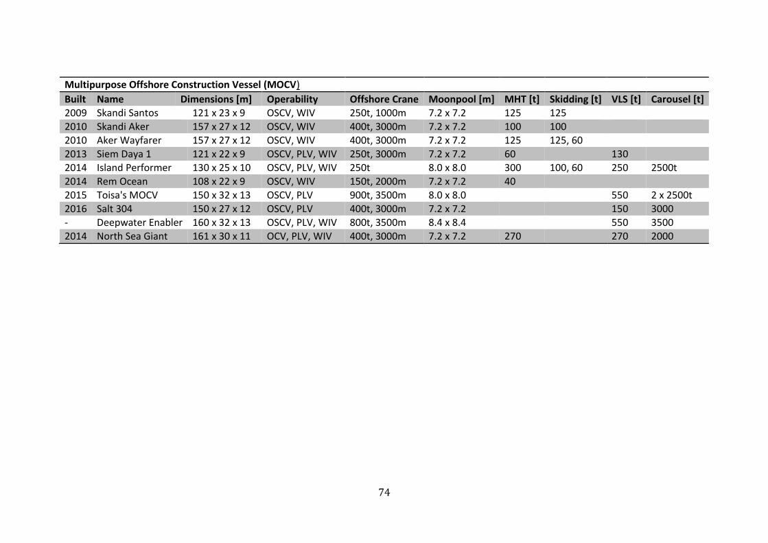
74

Multipurpose Offshore Construction Vessel (MOCV) Built Name Dimensions [m] Operability Offshore Crane Moonpool [m] MHT [t] Skidding [t] VLS [t] Carousel [t] 2009 Skandi Santos 121 x 23 x 9 OSCV, WIV 250t, 1000m 7.2 x 7.2 125 125 2010 Skandi Aker 157 x 27 x 12 OSCV, WIV 400t, 3000m 7.2 x 7.2 100 100 2010 Aker Wayfarer 157 x 27 x 12 OSCV, WIV 400t, 3000m 7.2 x 7.2 125 125, 60 2013 Siem Daya 1 121 x 22 x 9 OSCV, PLV, WIV 250t, 3000m 7.2 x 7.2 60 130 2014 Island Performer 130 x 25 x 10 OSCV, PLV, WIV 250t 8.0 x 8.0 300 100, 60 250 2500t 2014 Rem Ocean 108 x 22 x 9 OSCV, WIV 150t, 2000m 7.2 x 7.2 40 2015 Toisa's MOCV 150 x 32 x 13 OSCV, PLV 900t, 3500m 8.0 x 8.0 550 2 x 2500t 2016 Salt 304 150 x 27 x 12 OSCV, PLV 400t, 3000m 7.2 x 7.2 150 3000 - Deepwater Enabler 160 x 32 x 13 OSCV, PLV, WIV 800t, 3500m 8.4 x 8.4 550 3500 2014 North Sea Giant 161 x 30 x 11 OCV, PLV, WIV 400t, 3000m 7.2 x 7.2 270 270 2000

75

APPENDIX E – CALCULATION OF VOLATILITY OF OIL PRICE 2012 2013 2014 2015 Brent Price Brent2012 Brent2013 Brent2014 Brent2015 Change =Brent2013/Brent2012-1 =Brent2014/Brent2013-1 =Brent2015/Brent2014-1 Volatility =STDAV(Change1:Change3)

APPENDIX F – CALCULATION OF STRIKE PRICE Vessel Type Equipment Price OSCV 0,001 WIV 25000000 PLV 21500000

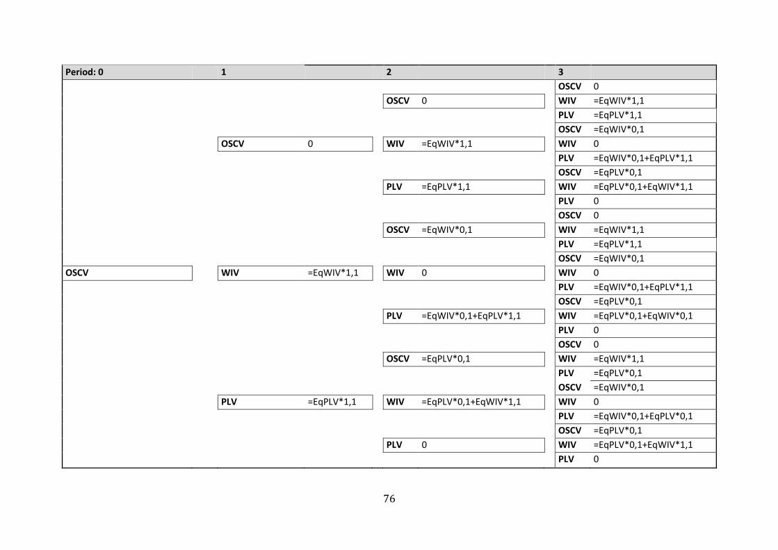
76

Period: 0 1 2 3 OSCV 0 OSCV 0 WIV =EqWIV*1,1 PLV =EqPLV*1,1 OSCV =EqWIV*0,1 OSCV 0 WIV =EqWIV*1,1 WIV 0 PLV =EqWIV*0,1+EqPLV*1,1 OSCV =EqPLV*0,1 PLV =EqPLV*1,1 WIV =EqPLV*0,1+EqWIV*1,1 PLV 0 OSCV 0 OSCV =EqWIV*0,1 WIV =EqWIV*1,1 PLV =EqPLV*1,1 OSCV =EqWIV*0,1 OSCV WIV =EqWIV*1,1 WIV 0 WIV 0 PLV =EqWIV*0,1+EqPLV*1,1 OSCV =EqPLV*0,1 PLV =EqWIV*0,1+EqPLV*1,1 WIV =EqPLV*0,1+EqWIV*0,1 PLV 0 OSCV 0 OSCV =EqPLV*0,1 WIV =EqWIV*1,1 PLV =EqPLV*0,1 OSCV =EqWIV*0,1 PLV =EqPLV*1,1 WIV =EqPLV*0,1+EqWIV*1,1 WIV 0 PLV =EqWIV*0,1+EqPLV*0,1 OSCV =EqPLV*0,1 PLV 0 WIV =EqPLV*0,1+EqWIV*1,1 PLV 0

77

APPENDIX G – CUMULATIVE STATISTICAL VALUES Period: 0 Period: 1 Period: 3 OSCV Delayed OSCV Delayed WIV d1 = 11,155 d2 = 10,910 PLV d1 = 8,273 d2 = 8,009 OSCV d1 = 7,423 d2 = 7,118 OSCV Delayed WIV d1 = 11,155 d2 = 10,910 WIV Delayed PLV d1 = 3,194 d2 = 2,603 OSCV d1 = 10,424 d2 = 10,187 PLV d1 = 8,273 d2 = 8,009 WIV d1 = 6,052 d2 = 5,628 PLV Delayed OSCV Delayed OSCV d1 = 7,423 d2 = 7,118 WIV d1 = 20,952 d2 = 20,707 PLV d1 = 8,273 d2 = 8,009 OSCV d1 = 7,423 d2 = 7,118 WIV WIV Delayed WIV Delayed d1 = 11,155 PLV d1 = 3,194 d2 = 2,603 d2 = 10,910 OSCV d1 = 10,424 d2 = 10,187 PLV d1 = 3,194 d2 = 2,603 WIV d1 = 10,422 d2 = 9,998 PLV Delayed OSCV Delayed OSCV d1 = 10,424 d2 = 10,187 WIV d1 = 11,155 d2 = 10,910 PLV d1 = 17,349 d2 = 17,085 OSCV d1 = 7,423 d2 = 6,876 PLV WIV d1 = 6,052 d2 = 5,628 WIV Delayed d1 = 8,273 PLV d1 = 6,117 d2 = 5,526 d2 = 8,009 OSCV d1 = 10,424 d2 = 10,187 PLV Delayed WIV d1 = 6,052 d2 = 5,628 PLV Delayed

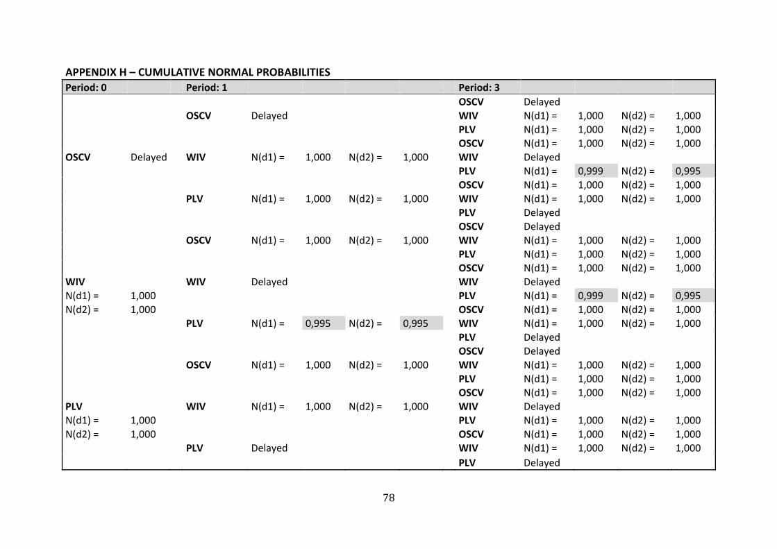
78

APPENDIX H – CUMULATIVE NORMAL PROBABILITIES Period: 0 Period: 1 Period: 3 OSCV Delayed

OSCV Delayed

WIV N(d1) = 1,000 N(d2) = 1,000

PLV N(d1) = 1,000 N(d2) = 1,000

OSCV N(d1) = 1,000 N(d2) = 1,000 OSCV Delayed

WIV N(d1) = 1,000 N(d2) = 1,000

WIV Delayed

PLV N(d1) = 0,999 N(d2) = 0,995

OSCV N(d1) = 1,000 N(d2) = 1,000

PLV N(d1) = 1,000 N(d2) = 1,000

WIV N(d1) = 1,000 N(d2) = 1,000

PLV Delayed

OSCV Delayed

OSCV N(d1) = 1,000 N(d2) = 1,000

WIV N(d1) = 1,000 N(d2) = 1,000

PLV N(d1) = 1,000 N(d2) = 1,000

OSCV N(d1) = 1,000 N(d2) = 1,000

WIV

WIV Delayed

WIV Delayed N(d1) = 1,000

PLV N(d1) = 0,999 N(d2) = 0,995

N(d2) = 1,000

OSCV N(d1) = 1,000 N(d2) = 1,000

PLV N(d1) = 0,995 N(d2) = 0,995

WIV N(d1) = 1,000 N(d2) = 1,000

PLV Delayed

OSCV Delayed

OSCV N(d1) = 1,000 N(d2) = 1,000

WIV N(d1) = 1,000 N(d2) = 1,000

PLV N(d1) = 1,000 N(d2) = 1,000

OSCV N(d1) = 1,000 N(d2) = 1,000 PLV

WIV N(d1) = 1,000 N(d2) = 1,000

WIV Delayed

N(d1) = 1,000

PLV N(d1) = 1,000 N(d2) = 1,000 N(d2) = 1,000

OSCV N(d1) = 1,000 N(d2) = 1,000

PLV Delayed

WIV N(d1) = 1,000 N(d2) = 1,000 PLV Delayed

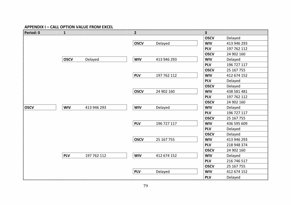
79

APPENDIX I – CALL OPTION VALUE FROM EXCEL Period: 0 1 2 3

OSCV Delayed

OSCV Delayed

WIV 413 946 293

PLV 197 762 112

OSCV 24 902 160

OSCV Delayed

WIV 413 946 293

WIV Delayed

PLV 196 727 117

OSCV 25 167 755

PLV 197 762 112

WIV 412 674 152

PLV Delayed

OSCV Delayed

OSCV 24 902 160

WIV 438 581 481

PLV 197 762 112

OSCV 24 902 160

OSCV

WIV 413 946 293

WIV Delayed

WIV Delayed

PLV 196 727 117

OSCV 25 167 755

PLV 196 727 117

WIV 436 595 609

PLV Delayed

OSCV Delayed

OSCV 25 167 755

WIV 413 946 293

PLV 218 948 374

OSCV 24 902 160

PLV 197 762 112

WIV 412 674 152

WIV Delayed

PLV 216 746 517

OSCV 25 167 755

PLV Delayed

WIV 412 674 152 PLV Delayed

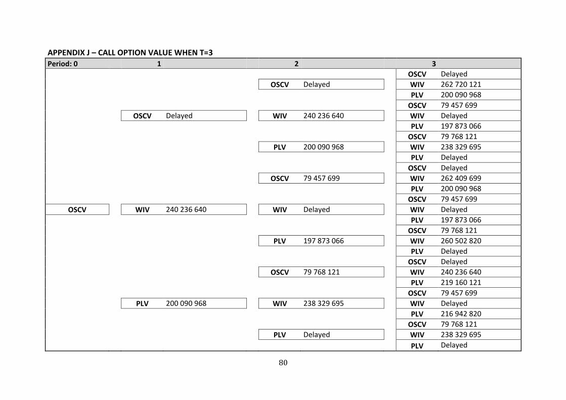
80

APPENDIX J – CALL OPTION VALUE WHEN T=3 Period: 0 1 2 3

OSCV Delayed

OSCV Delayed

WIV 262 720 121

PLV 200 090 968

OSCV 79 457 699

OSCV Delayed

WIV 240 236 640

WIV Delayed

PLV 197 873 066

OSCV 79 768 121

PLV 200 090 968

WIV 238 329 695

PLV Delayed

OSCV Delayed

OSCV 79 457 699

WIV 262 409 699

PLV 200 090 968

OSCV 79 457 699

OSCV

WIV 240 236 640

WIV Delayed

WIV Delayed

PLV 197 873 066

OSCV 79 768 121

PLV 197 873 066

WIV 260 502 820

PLV Delayed

OSCV Delayed

OSCV 79 768 121

WIV 240 236 640

PLV 219 160 121

OSCV 79 457 699

PLV 200 090 968

WIV 238 329 695

WIV Delayed

PLV 216 942 820

OSCV 79 768 121

PLV Delayed

WIV 238 329 695 PLV Delayed