MASTER THESIS - NTNU Open
96
NTNU Norwegian University of Science and Technology Department of Marine Technology MASTER THESIS Address: NTNU Department of Marine Technology N-7491 Trondheim Location Marinteknisk Senter O. Nielsens vei 10 Tel. +47 73 595501 Fax +47 73 595697 Title: Launch and recovery of ROV: Investigation of operational limit from DNV Recommended Practices and time domain simulations in SIMO Student: Magnus Valen Delivered: 14.06.2010 Number of pages: 96 Availability: Open ROV Splash zone SIMO Tor Einar Berg Advisor: Keyword: Abstract: Offshore contractors seek to operate their remotely operated vehicles for the widest range of sea conditions where particularly launch and recovery through splash zone are critical phases in the offshore operation. The analytical methods for calculation of operational limit proposed by guidelines from DNV Recommended Practices may lead to an over-estimation of the hydrodynamic forces and consequently to an unduly restrictive operational limit. Accurate predictions of the hydrodynamic forces are important, and there is an opening in the regulations which allow the use of other analysis tools to determine the forces on the ROV system during launch and recovery. The main objective of the master thesis was to carry out splash zone analyses for DOF Subsea’s ROV system by use of DNV Recommended Practices and compare the results found by modeling the marine operation in the time domain simulation program SIMO. This involved a broad study of SIMO and a complete modeling of the offshore operation including calculation of the hydrodynamic data for the vessel Skandi Bergen and modeling of the ROV system. In SIMO, particularly the sea state of 4.5 [m] significant wave height was investigated since this is the current operational limit for DOF Subsea’s ROV system. The investigation of operational limits by use of the analytical method and SIMO have shown that DNV Recommended Practices over-estimates the hydrodynamic forces acting in the wave zone leading to an restrictive operational limit in comparison to the time domain calculations in SIMO. The calculations by the analytical method have shown that the operational limit for launch and recovery of ROV should be limited to 2.5 [m] significant wave height, while analyses in SIMO have shown that the current operational limit of 4.5 [m] could be justified. However, it is seen that the possibility for slack umbilical is present in the sea state of 4.5 [m] and peak periods in the range of T p = 6 – 9 [s]. It is also to be noted that the slack umbilical occurrences show a thoroughly dependency of the vessel heading. Furthermore, the snap loads induced by the slack umbilical occurrences are not found to be critical in the irregular wave analyses. This can justify the operational limit of 4.5 [m] significant wave height as long as the weather is assessed by experienced personnel during deployment through wave zone and Skandi Bergen is positioned head sea.
-
Upload
khangminh22 -
Category
Documents
-
view
4 -
download
0
Transcript of MASTER THESIS - NTNU Open

NTNU Norwegian University of Science and Technology Department of Marine Technology MASTER THESIS
Address: NTNU Department of Marine Technology N-7491 Trondheim
Location Marinteknisk Senter O. Nielsens vei 10
Tel. +47 73 595501 Fax +47 73 595697
Title:
Launch and recovery of ROV: Investigation of operational limit from DNV Recommended Practices and time domain simulations in SIMO
Student:
Magnus Valen
Delivered:
14.06.2010
Number of pages:
96
Availability:
Open
ROV Splash zone
SIMO
Tor Einar Berg
Advisor: Keyword:
Abstract:
Offshore contractors seek to operate their remotely operated vehicles for the widest range of sea conditions where particularly launch and recovery through splash zone are critical phases in the offshore operation. The analytical methods for calculation of operational limit proposed by guidelines from DNV Recommended Practices may lead to an over-estimation of the hydrodynamic forces and consequently to an unduly restrictive operational limit. Accurate predictions of the hydrodynamic forces are important, and there is an opening in the regulations which allow the use of other analysis tools to determine the forces on the ROV system during launch and recovery. The main objective of the master thesis was to carry out splash zone analyses for DOF Subsea’s ROV system by use of DNV Recommended Practices and compare the results found by modeling the marine operation in the time domain simulation program SIMO. This involved a broad study of SIMO and a complete modeling of the offshore operation including calculation of the hydrodynamic data for the vessel Skandi Bergen and modeling of the ROV system. In SIMO, particularly the sea state of 4.5 [m] significant wave height was investigated since this is the current operational limit for DOF Subsea’s ROV system. The investigation of operational limits by use of the analytical method and SIMO have shown that DNV Recommended Practices over-estimates the hydrodynamic forces acting in the wave zone leading to an restrictive operational limit in comparison to the time domain calculations in SIMO. The calculations by the analytical method have shown that the operational limit for launch and recovery of ROV should be limited to 2.5 [m] significant wave height, while analyses in SIMO have shown that the current operational limit of 4.5 [m] could be justified. However, it is seen that the possibility for slack umbilical is present in the sea state of 4.5 [m] and peak periods in the range of Tp = 6 – 9 [s]. It is also to be noted that the slack umbilical occurrences show a thoroughly dependency of the vessel heading. Furthermore, the snap loads induced by the slack umbilical occurrences are not found to be critical in the irregular wave analyses. This can justify the operational limit of 4.5 [m] significant wave height as long as the weather is assessed by experienced personnel during deployment through wave zone and Skandi Bergen is positioned head sea.

MSc. thesis, spring 2010
by
Magnus Valen
Launch and recovery of ROV: Investigation of operational limit from DNV Recommended Practices and time domain simulations in SIMO
Work description
DOF Subsea’s current ROV launch and recovery system has an operational design limit of 4.5 [m] significant wave height which is based upon the DNV Rules and Regulations for Planning and Execution of Marine Operations 1996. This set of rules has now been replaced by DNV-RP-H103, which may be on the more conservative side. DOF Subsea and other offshore contractors, seek to operate their remotely operated vehicles for the widest range of sea conditions, where particularly launch and recovery through splash zone are critical phases in the offshore operation. The analytical methods proposed by guidelines from DNV Recommended Practices may lead to an over-estimation of the hydrodynamic forces and consequently to an unduly restrictive operational limit. Accurate predictions of the hydrodynamic forces are important for the operational limit, and there is an opening in the regulations which allow the use of other analysis tools to determine the forces on the ROV system during launch and recovery. As a consequence, it would be interesting to determine the operational limit by use of the Simplified Method in DNV-RP-H103 and the time domain simulation program SIMO (simulation of marine operations) and compare the forces and consequently the operational limits.
The master thesis has its origin to the project thesis written fall 2009, where launch and recovery analyses by use of DNV-RP-H103 were performed. The main objective of the master thesis is to carry out a more refined splash zone analyses by use of the analytical method and compare the results found by modeling the marine operation in the time domain simulation program SIMO.
Scope of work
1. Study the time domain simulation program SIMO. 2. Compute the motion transfer functions and the hydrodynamic properties of the multipurpose
construction vessel Skandi Bergen by use of VeRes and model the ship in SIMO. 3. Define the hydrodynamic and structure properties of the ROV system and model the system in
SIMO. 4. Perform a more refined launch and recovery analyses than in the project thesis by use of DNV-
RP-H103 with the hydrodynamic properties as found in (3). 5. Investigate the current operational limit of DOF Subsea’s ROV system by use of SIMO. 6. Visualize the launch and recovery in SimVis 7. Compare the operational limit obtained from SIMO and DNV-RP-H103 and discuss the results
from both analyses.
The report shall be written in English and include description of theory, analysis of the results, discussion and a conclusion including a proposal for further work. Source code should be provided on a CD with code listing enclosed in appendix. It is supposed that Department of Marine Technology, NTNU, can use the results freely in its research work, unless otherwise agreed upon, by referring to the student’s work.
The report should be well organized and give a clear presentation of the work and all conclusions. It is important that the text is well written and that tables and figures are used to support the verbal presentation. The report should be complete, but still as short as possible.
The thesis should be submitted within 14th of June 2010.
Supervisor: Tor Einar Berg
Trondheim 10 June 2010
Tor Einar Berg

V
Abstract Offshore contractors seek to operate their remotely operated vehicles for the widest range of sea conditions where particularly launch and recovery through splash zone are critical phases in the offshore operation. The analytical methods for calculation of operational limit proposed by guidelines from DNV Recommended Practices may lead to an over-estimation of the hydrodynamic forces and consequently to an unduly restrictive operational limit. Accurate predictions of the hydrodynamic forces are important, and there is an opening in the regulations which allow the use of other analysis tools to determine the forces on the ROV system during launch and recovery.
The main objective of the master thesis was to carry out splash zone analyses for DOF Subsea’s ROV system by use of DNV Recommended Practices and compare the results found by modeling the marine operation in the time domain simulation program SIMO. This involved a broad study of SIMO and a complete modeling of the offshore operation including calculation of the hydrodynamic data for the vessel Skandi Bergen and modeling of the ROV system. In SIMO, particularly the sea state of 4.5 [m] significant wave height was investigated since this is the current operational limit for DOF Subsea’s ROV system.
The investigation of operational limits by use of the analytical method and SIMO have shown that DNV Recommended Practices over-estimates the hydrodynamic forces acting in the wave zone leading to an restrictive operational limit in comparison to the time domain calculations in SIMO. The calculations by the analytical method have shown that the operational limit for launch and recovery of ROV should be limited to 2.5 [m] significant wave height, while analyses in SIMO have shown that the current operational limit of 4.5 [m] could be justified. However, it is seen that the possibility for slack umbilical is present in the sea state of 4.5 [m] and peak periods in the range of Tp = 6 – 9 [s]. It is also to be noted that the slack umbilical occurrences show a thoroughly dependency of the vessel heading. Furthermore, the snap loads induced by the slack umbilical occurrences are not found to be critical in the irregular wave analyses. This can justify the operational limit of 4.5 [m] significant wave height as long as the weather is assessed by experienced personnel during deployment through wave zone and Skandi Bergen is positioned head sea.

VI

VII
Acknowledgements This report is the result of my master thesis work carried out spring 2010 at Norwegian University of Science and Technology in accordance with 5 years of education.
I would like to acknowledge Knut Mo and Peter Christian Sandvik for help and guidance with the time domain simulation program SIMO. Gratitude is given to the PhD fellow Fredrik Dukan for introducing and giving me valuable input about SIMO.
I would also like to thank Vidar Horneland at DOF Subsea for proposing the master thesis and providing documentation and answering questions related to the launch and recovery of the ROV system.
The help and motivation from fellow student are also highly appreciated.
Finally, I would like to thank my supervisor, Tor Einar Berg, for guidance throughout the master thesis.
Magnus Valen
Trondheim 14th June 2010

VIII
IX
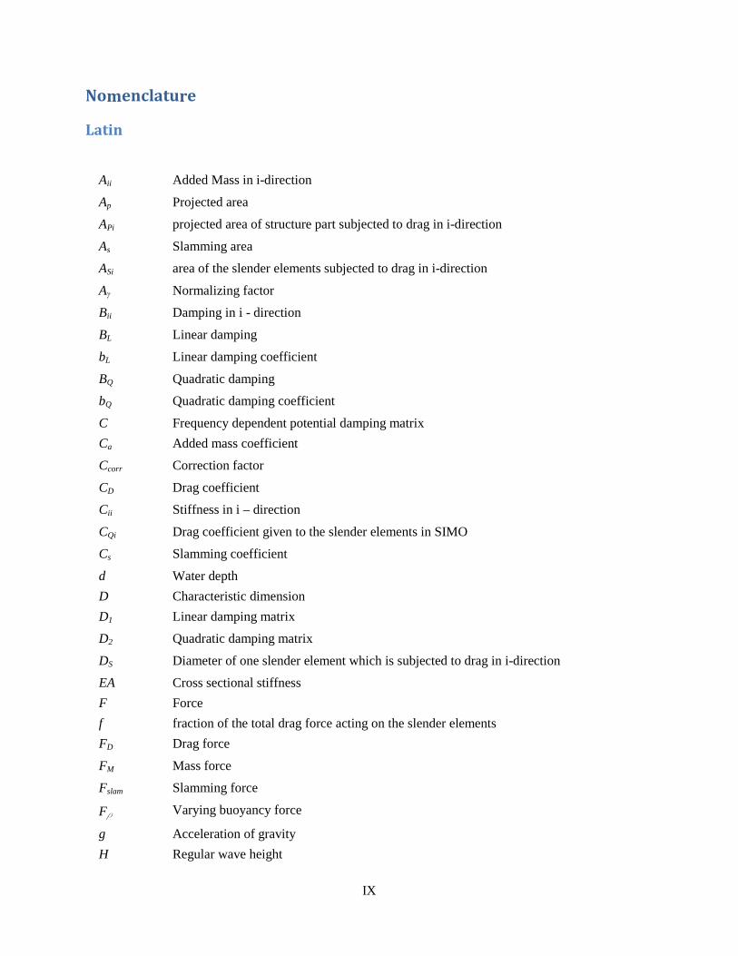
Nomenclature
Latin
Aii Added Mass in i-direction
Ap Projected area
APi projected area of structure part subjected to drag in i-direction
As Slamming area
ASi area of the slender elements subjected to drag in i-direction
Aγ Normalizing factor
Bii Damping in i - direction
BL Linear damping
bL Linear damping coefficient
BQ Quadratic damping
bQ Quadratic damping coefficient
C Frequency dependent potential damping matrix
Ca Added mass coefficient
Ccorr Correction factor
CD Drag coefficient
Cii Stiffness in i – direction
CQi Drag coefficient given to the slender elements in SIMO
Cs Slamming coefficient
d Water depth
D Characteristic dimension
D1 Linear damping matrix
D2 Quadratic damping matrix
DS Diameter of one slender element which is subjected to drag in i-direction
EA Cross sectional stiffness
F Force
f fraction of the total drag force acting on the slender elements
FD Drag force
FM Mass force
Fslam Slamming force
Fρ Varying buoyancy force
g Acceleration of gravity
H Regular wave height

X
H(ω) Complex transfer function
Hs Significant wave height
K Umbilical stiffness
k Wave number
KC Keulegan-Carpenter number
Km Position dependent hydrostatic stiffness matrix
M Structure mass
m0 First spectral moment
mh Hydrodynamic mass (added mass)
Mobject Mass of object lowered through wave zone
Ms Frequency dependent mass matrix
qex Exciting forces
r44 Roll radius of gyration
r55 Pitch radius gyration
r66 Yaw radius of gyration
Rηη(w) Autocorrelation function
SJ JONSWAP Spectrum
SPM Pierson – Moskowitz spectrum
Sηη(w) Vertical response spectra
Tni Natural period in i-direction
Tp Peak period
Tz Wave zero crossing period
V Volume
vc Crane velocity
vff Free fall velocity
vr Relative velocity
x0 Longitudinal distance from center of gravity to crane tip
y0 Transverse distance from center of gravity to crane tip

XI
Greek
ζa Wave amplitude β Heading angle ω Angular wave frequency ρ Density of sea water γ Peak shape parameter δV Varying buoyancy
ctη Crane tip displacement
ctηɺ Crane tip velocity
ctηɺɺ Crane tip acceleration
3η Heave motion
4η Roll motion
5η Pitch motion
ησ Standard deviation of crane tip displacement spectra
ησɺ Standard deviation of crane tip velocity spectra
ησɺɺ Standard deviation of crane tip spectra
σ Spectral width parameter �0 Wave potential b Direction of wave propagation ∅ζ Wave component phase angle
ζɺɺ Wave particle velocity
xɺɺ Acceleration
Abbreviations
IWRC Independent Wire Rope Core
BL Baseline
CL Center line
DNV Det Norske Veritas
JONSWAP Joint North Sea Wave Project
LARS Lifting And Recovery System
LCG Longituinal center of gravity
RAO Response Amplitude Operator
WROV Working class Remotely Operated Vehicle
ROV Remotely Operated Vehicle
RP Recommended Practices
TMS Tether Management System
VCG Vertical center of gravity
SIMO Simulation of Marine Operations

XII

XIII
Contents Abstract .........................................................................................................................................................V
Acknowledgements .................................................................................................................................... VII
Nomenclature .............................................................................................................................................. IX
Latin ........................................................................................................................................................ IX
Greek ....................................................................................................................................................... XI
Abbreviations .......................................................................................................................................... XI
1 Introduction ........................................................................................................................................... 1
1.1 Background and motivation .......................................................................................................... 1
1.2 Contributions ................................................................................................................................. 1
1.3 Outline of thesis ............................................................................................................................. 1
2 Operational description ......................................................................................................................... 3
2.1 Skandi Bergen ............................................................................................................................... 3
2.2 ROV System .................................................................................................................................. 4
2.2.1 ROV and TMS ....................................................................................................................... 4
2.2.2 Umbilical data ....................................................................................................................... 4
2.3 Lifting through splash zone ........................................................................................................... 4
3 Software description .............................................................................................................................. 7
3.1 VeRes ............................................................................................................................................ 7
3.2 SIMO & SimVis ............................................................................................................................ 7
3.2.1 Program layout ...................................................................................................................... 7
3.2.2 SimVis ................................................................................................................................... 9
4 Theory ................................................................................................................................................. 11
4.1 Simplified Method ....................................................................................................................... 11
4.1.1 Lifting through splash zone ................................................................................................. 11
4.1.2 Environmental conditions .................................................................................................... 11
4.1.3 Hydrodynamic forces .......................................................................................................... 12
4.1.4 Hydrodynamic coefficients ................................................................................................. 13
4.1.5 Snap force ............................................................................................................................ 15
4.1.6 Accept criteria ..................................................................................................................... 16
4.1.7 Crane tip motions ................................................................................................................ 16
4.2 SIMO theory ................................................................................................................................ 20
4.2.1 Coordinate systems .............................................................................................................. 20

XIV
4.2.2 Environment ........................................................................................................................ 21
4.2.3 Distributed element force .................................................................................................... 21
4.2.4 Coupling forces ................................................................................................................... 22
4.2.5 Solution of the equation of motion ...................................................................................... 23
4.3 Estimation of hydrodynamic coefficients .................................................................................... 23
4.3.1 Discussion of hydrodynamic coefficients for ROV system ................................................ 24
5 Procedure – DNV Recommended Practices ........................................................................................ 27
5.1 Launch and Recovery of ROV .................................................................................................... 27
5.1.1 Load cases during deployment through wave zone ............................................................. 27
5.1.2 Environmental data .............................................................................................................. 28
5.1.3 Crane tip motions ................................................................................................................ 28
5.1.4 Hydrodynamic forces .......................................................................................................... 29
5.1.5 Snap loads ............................................................................................................................ 29
6 Procedure –SIMO ................................................................................................................................ 31
6.1 System description SIMO............................................................................................................ 31
6.1.1 Environment specification ................................................................................................... 31
6.1.2 Body data specification - Skandi Bergen ............................................................................ 32
6.1.3 Body data specification – ROV system ............................................................................... 36
6.1.4 Coupling data ...................................................................................................................... 38
6.2 Modeling the ROV system .......................................................................................................... 38
6.3 Visualization in SimVis ............................................................................................................... 40
6.3.1 SimVis project file ............................................................................................................... 40
6.4 Running time domain analysis in SIMO ..................................................................................... 41
6.4.1 STAMOD ............................................................................................................................ 41
6.4.2 DYNMOD ........................................................................................................................... 41
6.4.3 S2XMOD ............................................................................................................................. 42
6.5 Limitations................................................................................................................................... 42
7 Results from Simplified Method ......................................................................................................... 43
7.1 Vessel Response .......................................................................................................................... 43
7.1.1 RAO at crane tip .................................................................................................................. 43
7.1.2 Most probable largest single amplitude responses .............................................................. 43
7.2 Launch and recovery analyses ..................................................................................................... 43
7.2.1 Case study of the ROV system lowered through wave zone ............................................... 44
XV
7.2.2 Case study using significant responses ................................................................................ 45
7.2.3 Snap loads ............................................................................................................................ 46
7.3 Discussion of results from Simplified Method ............................................................................ 47
7.3.1 Vessel response ................................................................................................................... 47
7.3.2 Launch and recovery analyses ............................................................................................. 47
7.3.3 Considerations regarding operational limit from results in Simplified Method .................. 47
8 Results from SIMO ............................................................................................................................. 49
8.1 Investigation of current operational limit .................................................................................... 49
8.1.1 Stationary analyses in irregular sea ..................................................................................... 49
8.1.2 Repeated lowering through splash zone .............................................................................. 51
8.1.3 Repeated recovery through splash zone .............................................................................. 52
8.1.4 Investigation of heading angles ........................................................................................... 53
8.2 Analyses in regular sea ................................................................................................................ 54
8.3 Parametrical study of the hydrodynamic coefficients ................................................................. 55
8.4 Discussion of results from SIMO ................................................................................................ 56
8.4.1 Comments on statistics ........................................................................................................ 56
8.4.2 Discussion of current operational limit ............................................................................... 56
8.4.3 Discussion of analyses in regular sea .................................................................................. 57
8.4.4 Discussion of parametrical study of the drag coefficient .................................................... 58
8.4.5 Considerations regarding operational limit from results in SIMO ...................................... 58
8.5 Comparison of results from Simplified Method and SIMO ........................................................ 59
9 Conclusions ......................................................................................................................................... 61
9.1 Conclusion ................................................................................................................................... 61
9.2 Proposal for further work ............................................................................................................ 61
10 References ....................................................................................................................................... 63
Appendix A Results from simplified method ............................................................................................ ii
A.1 Significant wave height of 2.0 [m] .................................................................................................... ii
A.2 Significant wave height of 3.0 [m] .................................................................................................... ii
A.3 Significant wave height of 3.5 [m] ................................................................................................... iii
A.4 Significant wave height of 4.0 [m] ................................................................................................... iv
Appendix B Results from SIMO................................................................................................................ v
B.1 Repeated lowering through splash zone ............................................................................................ v
B.2 Parametrical study of drag coefficient ............................................................................................... x

XVI
B.3 Lowering in regular waves ............................................................................................................... xi
Appendix C Contents on CD .................................................................................................................. xiii
C.1 Veres folder .................................................................................................................................... xiii
C.2 MATLAB folder ............................................................................................................................. xiii
C.3 Documents folder ........................................................................................................................... xiii
C.4 Visualization folder ........................................................................................................................ xiii
C.5 SIMO folder ................................................................................................................................... xiii
C.6 SimVis folder ................................................................................................................................. xiv

XVII
List of figures Figure 1 Skandi Bergen ................................................................................................................................. 3
Figure 2 ROV system .................................................................................................................................... 4
Figure 3 Layout of the SIMO program system and file communication [4, p. 9] ......................................... 8 Figure 4 SIMO coordinate systems, [11, p. 6] ............................................................................................ 21
Figure 5 Load cases during lowering through wave zone ........................................................................... 27 Figure 6 Body location data for Skandi Bergen .......................................................................................... 32
Figure 7 Body mass data for Skandi Bergen ............................................................................................... 32
Figure 8 Mass coefficients for Skandi Bergen ............................................................................................ 33
Figure 9 Added mass of Skandi Bergen for zero frequency ........................................................................ 33 Figure 10 Linear stiffness matrix of Skandi Bergen.................................................................................... 33
Figure 11 Linear damping matrix for Skandi Bergen.................................................................................. 35
Figure 12 Body location data for ROV system ........................................................................................... 36
Figure 13 Example of slender element ........................................................................................................ 37
Figure 14 ROV system modeled by slender elements ................................................................................. 39
Figure 15 Response amplitude operators at tip of the LARS for heading angles of 0º and ±15º ................ 43 Figure 16 Most probable largest single amplitude velocity and acceleration at the tip of the launch and recovery system ........................................................................................................................................... 43
Figure 17 Case study of hydrodynamic forces in a significant wave height of 2.5 [m] .............................. 44 Figure 18 Case study of hydrodynamic forces in a significant wave height of 4.5 [m] .............................. 45 Figure 19 Hydrodynamic forces when exposed for significant responses in a significant wave height of 3.0 [m] and 4.5 [m] ............................................................................................................................................ 46 Figure 20 Snap loads for load case 4 in sea states from Hs = 3.0 – 4.5 [m] ................................................ 46 Figure 21 Irregular wave realization in a sea state of Tp = 8 [s] and Hs = 4.5 [m] ...................................... 49
Figure 22 Time histories from a 0.5 hour stationary analysis in sea states of Hs = 4.5 [m] & Tp = 6 -11 [s] ..................................................................................................................................................................... 51 Figure 23 Time histories and graphs of the maximum/minimum umbilical tension in a sea state of Hs = 4.5 [m] & Tp = 8 [s] ........................................................................................................................................... 52
Figure 24 Time histories of umbilical tension during recovery in a sea state of Hs = 4.5 [m] & Tp = 8 [s] 53
Figure 25 Time histories of umbilical tension during lowering through splash zone in a sea state of β =
±15º, Hs = 4.5 [m] & Tp = 8 [s] .................................................................................................................... 54
Figure 26 Umbilical tension for regular waves with amplitude za = 2.25 [m] and Tz = 4.5 & 6.0 [s]........ 55
Figure 27 Umbilical tension for regular waves with amplitude za = 4.05 [m] and Tz = 6.0 & 9.0 [s]........ 55
Figure 28 Lowering through splash zone in regular waves with ζa = 2.25 [m] and Tz = 6 [s] and different
drag coefficients .......................................................................................................................................... 56 Figure 29 Typical horizontal translation of the ROV system during water entry ....................................... 58
XVIII
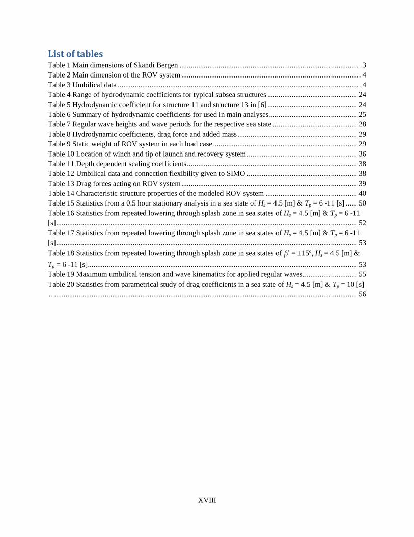
List of tables Table 1 Main dimensions of Skandi Bergen ................................................................................................. 3
Table 2 Main dimension of the ROV system ................................................................................................ 4
Table 3 Umbilical data .................................................................................................................................. 4
Table 4 Range of hydrodynamic coefficients for typical subsea structures ................................................ 24 Table 5 Hydrodynamic coefficient for structure 11 and structure 13 in [6] ................................................ 24 Table 6 Summary of hydrodynamic coefficients for used in main analyses ............................................... 25 Table 7 Regular wave heights and wave periods for the respective sea state ............................................. 28 Table 8 Hydrodynamic coefficients, drag force and added mass ................................................................ 29 Table 9 Static weight of ROV system in each load case ............................................................................. 29
Table 10 Location of winch and tip of launch and recovery system ........................................................... 36 Table 11 Depth dependent scaling coefficients ........................................................................................... 38
Table 12 Umbilical data and connection flexibility given to SIMO ........................................................... 38 Table 13 Drag forces acting on ROV system .............................................................................................. 39
Table 14 Characteristic structure properties of the modeled ROV system ................................................. 40 Table 15 Statistics from a 0.5 hour stationary analysis in a sea state of Hs = 4.5 [m] & Tp = 6 -11 [s] ...... 50 Table 16 Statistics from repeated lowering through splash zone in sea states of Hs = 4.5 [m] & Tp = 6 -11 [s] ................................................................................................................................................................. 52 Table 17 Statistics from repeated lowering through splash zone in sea states of Hs = 4.5 [m] & Tp = 6 -11 [s] ................................................................................................................................................................. 53
Table 18 Statistics from repeated lowering through splash zone in sea states of β = ±15º, Hs = 4.5 [m] &
Tp = 6 -11 [s] ................................................................................................................................................ 53 Table 19 Maximum umbilical tension and wave kinematics for applied regular waves ............................. 55 Table 20 Statistics from parametrical study of drag coefficients in a sea state of Hs = 4.5 [m] & Tp = 10 [s] ..................................................................................................................................................................... 56

1
1 Introduction
1.1 Background and motivation
DOF Subsea’s current ROV launch and recovery system has an operational design limit of 4.5 [m] significant wave height which is based upon the DNV Rules and Regulations for Planning and Execution of Marine Operations 1996. This set of rules has now been replaced by DNV-RP-H103, which may be on the more conservative side. DOF Subsea and other offshore contractors, seek to operate their Remotely Operated Vehicles for the widest range of sea conditions, where particularly launch and recovery through splash zone are critical phases in the offshore operation. The analytical methods proposed by guidelines from DNV Recommended Practices may lead to an over-estimation of the hydrodynamic forces and consequently to an unduly restrictive operational limit. Accurate predictions of the hydrodynamic forces are important for the operational limit, and there is an opening in the regulations which allow the use of other analysis tools to determine the forces on the ROV system during launch and recovery. As a consequence, it would be interesting to determine the operational limit by use of the Simplified Method in DNV-RP-H103 and the time domain simulation program SIMO (simulation of marine operations) and compare the forces and consequently the operational limits.
This thesis presents a step by step procedure of how to determine the operational limit for launch and recovery of ROV by use of DNV-RP-H103 and how to simulate the same operations in the time domain simulation program SIMO. The marine operation is performed by the multipurpose construction vessel Skandi Bergen where the current operational limit of 4.5 [m] significant wave height is mainly investigated.
1.2 Contributions
The MATLAB scripts RAOcalculation.m and SimplifiedMethod.m found at the enclosed CD, Appendix C.2, determine the response amplitude operator in heave at an arbitrary position of Skandi Bergen and the corresponding response spectra for the applied sea state. The latter MATLAB script also determines the operational limit for launch and recovery of ROV based upon DNV-RP-H103 which may be further developed to be applicable for other launch and recovery analyses. The theory behind determining the crane tip responses may be of use for other students since there is not found any literature which consistently covers the subject.
The step by step procedure going through the modeling and analyses in SIMO may also be used by future students since it easily explain each step for modeling an offshore crane operation. A complete description of the multipurpose construction vessel Skandi Bergen using motion transfer functions is included in the SIMO system description file which may be to future use for DOF Subsea.
The work carried out in this master thesis have been completely individual, but with help from fellow students through discussions and advices regarding SIMO from employees at MARINTEK.
1.3 Outline of thesis
Chapter 2 gives a brief introduction to the vessel Skandi Bergen and the ROV system while chapter 3 introduces the software tool VeRes, SIMO and SimVis for the reader.

2
Chapter 4 describes the theory which is applied in the launch and recovery analyses. This includes a complete description of the analytical method to determine loads on an object in splash zone, a brief description of the theory behind solving the equation of motion in SIMO and how the hydrodynamic properties of the ROV system are found.
Chapter 5 goes through the splash zone analyses by use of the analytical method from DNV Recommended Practices.
Chapter 6 describes each step in modeling the launch and recovery of ROV in SIMO with aim of executing time domain calculations which later can be visualized in SimVis.
In chapter 7 and chapter 8 are the results obtained from the analytical method and the time domain calculations in SIMO presented and discussed.
Chapter 9 presents conclusions based upon results found in chapter 7 and 8. A proposal for further work is also included.
In the Appendix A – B are some results from the analytical method and time domain simulations presented. MATLAB scripts, SIMO – files, videos of some of the time domain simulations and other documents are found in Appendix C.

3
2 Operational description
2.1 Skandi Bergen
Figure 1 Skandi Bergen
The main dimensions of the multipurpose construction vessel Skandi Bergen are presented in Table 1. The analyses are only performed for Skandi Bergen’s design waterline and without roll stabilizing tanks.
Main dimensions Mass [tonne] 7460.1 Mean draught [m] 5.7 LCG [m] 45.9 VCG [m] 8.8 Roll radius of gyration, r44 [m] 7.9 Pitch radius of gyration, r55 [m] 25.6 Yaw radius of gyration, r66 [m] 25.6 Table 1 Main dimensions of Skandi Bergen
The longitudinal center of gravity, LCG, is given from after perpendicular and the vertical center of gravity, VCG, is given from baseline.

4
2.2 ROV System
Figure 2 ROV system
2.2.1 ROV and TMS
Skandi Bergen is equipped with 2 Schilling UHD WROV with an active heave compensated launch and recovery system (LARS). Table 2 shows the main dimensions of the ROV system where the skid is included in the mass and volume of the ROV.
Main dimensions ROV TMS Total Mass [tonne] 5.3290 4.559 9.888 Volume [m3] 5.1056 1.630 6.7356 Length [m] 2.84 2.18 - Breadth [m] 1.87 2.18 - Height [m] 1.94 2.20 4.14 Table 2 Main dimension of the ROV system
2.2.2 Umbilical data
Umbilical data Diameter [mm] 31.2 Tensile strength [N/mm2] 2237 Umbilical cross section stiffness (EA) [kN] 3.7692·104 Table 3 Umbilical data
The umbilical data is given in Table 3 for the 1st layer armoring. The cross sectional stiffness of the umbilical is unknown and is approximated based upon values for IWRC steel wire rope and guidelines from section 4.7.6.3 in DNV-RP-H103 [1].
2.3 Lifting through splash zone
Lifting through splash zone is often recognized as the most crucial phase during a marine crane operation. To evaluate the regularity and feasibility of the crane operation it is necessary to predict the forces and

5
motions related to the object lifted through wave zone. The following must be true during an offshore crane operation:
• A marine operation shall be designed to last from a safe condition to another safe condition • The operation must remain in a stable and controlled situation even if a failure arises.
• It should be possible to stop the operation and bring the object back to safe condition.
It is important that the lifting operation is thoroughly analyzed to determine the loads acting on the object lowered through wave zone in order to find the operational limit for the lifting operation.

6

7
3 Software description
3.1 VeRes
VeRes is a plug-in of the ShipX Workbench which is a software developed by MARINTEK. VeRes offers the ability to calculate ship motions and loads, including the calculation of short term statistics, long term statistics and operability. The program calculates [2]:
• Relative motion transfer functions • Global induced loads • Short and long term statistics of transfer functions and global induced loads • Post processing of slamming pressures • Operability limiting boundaries
• Percentage operability
VeRes has been used to obtain the Response Amplitude Operators in the center of gravity of Skandi Bergen from a ShipX database file provided by DOF Subsea and to verify own short term statistics and response calculations at the tip of the launch and recovery system. Input to SIMO like hydrodynamic coefficients and mass coefficients are also found by VeRes.
3.2 SIMO & SimVis
Simulation of Marine Operations is a computer program developed by MARINTEK for time domain simulation of motion and station-keeping behavior of complex system of floating vessels and suspended loads. The results from the program are presented as time traces, statistics and spectral analysis of all forces and motions of all bodies in the analyzed system. Typical applications of SIMO include TLP installations, offshore crane operations, floating production systems and dynamic positioning systems [3]. The essential features are:
• Flexible modeling of multibody systems. • Non-linear time domain simulation of wave frequency as well as low frequency forces. • Environmental forces due to wind, waves and current. • Passive and active control of forces. • Interactive or batch simulation.
The time domain simulations from SIMO may be visualized by the stand alone program SimVis.
3.2.1 Program layout
SIMO consists of five modules communicating by a file system. In addition to this the stand alone visualization program SimVis can visualize the operation in 3D. The following information is extracted from the SIMO User’s Manual [4].

8
Figure 3 Layout of the SIMO program system and file communication [4, p. 9]
INPMOD The main purpose of INPMOD is to import data from external sources into the SIMO system description file and to present such data. INPMOD can also modify/manipulate the system description in terms of body and environmental data. STAMOD STAMOD defines the initial conditions for the dynamic simulation which are needed to perform the dynamic simulation. The initial conditions are written to an INIFIL that contains the complete description of the environment, body- and position data which is read by DYNMOD for time domain calculations. Before the INIFIL is written it is possible to select the environmental conditions and/or run a static equilibrium calculation with or without average environmental forces. STAMOD can also write a visualization file for SimVis which is a useful tool to check whether the system is modeled correct. DYNMOD The time domain simulations are executed in DYNMOD with the initial conditions as described in the INIFIL. Before starting the time integration of the equation of motion, the various simulation techniques must be initialized.
OUTMOD The purpose of OUTMODE is to prepare plots of static geometry and to analyze and present results from time domain simulation. Any part of the time series can be selected for post-processing and the average value, standard deviation and extreme values are written to the print file and PLOFIL.
9
S2XMOD The main purpose of S2XMOD is to export time series to other file formats than applied by SIMO. S2XMOD can give an overview of all series generated by SIMO, produce statistics of series, plot series and write selected time series to MATLAB “m”-file format or direct access file.
PLOMOD PLOMOD can plot results generated by OUTMOD.
3.2.2 SimVis
The stand alone program SimVis can be used to visualize the time domain simulations from SIMO. The essential features of SimVis are [5]:
- Modeling support: Detection of modeling errors, check static equilibrium calculations and distance measurements.
- Visualization of operation: Still pictures and video clips of the marine operations. - Documentation of analysis: Detail studies and help to understand the physics behind the results
obtained from SIMO.
3D models of vessel and other units can be imported to SimVis and forces in wires and contact elements may be displayed in time series plots.

10

11
4 Theory
4.1 Simplified Method
The following sub chapters will go through the Simplified Method for calculation of loads on objects lowered through splash zone as described in DNV-RP-H103 Modeling and Analysis of Marine Operations [1] and in the project thesis, Appendix C.3.
4.1.1 Lifting through splash zone
The objective of the simplified method is to give simple conservative estimates of the forces acting on an object lowered through wave zone. The simplified method is based upon the following main assumptions:
• The horizontal extent of the lifted object is small relative to the wavelength. • The load case is dominated by the vertical acting forces.
• The vertical motion of the object follows the crane tip motion.
4.1.2 Environmental conditions
The deployment analysis should cover the following zero crossing wave periods:
8.9 13s
z
HT
g⋅ ≤ ≤ (4.1)
where
Hs significant wave height Tz zero crossing period g acceleration of gravity
For marine crane operations assumed to be performed within 30 minutes including contingency time, the characteristic wave amplitude applied in the analysis can be taken as:
0.9a SHζ = ⋅ (4.2)
For operations longer than 30 minutes the wave amplitude is equal to the significant wave height. The characteristic wave particle velocity and acceleration can then be calculated by:
k dw av eζ ω − ⋅= ⋅ (4.3)
2 k dw aa eζ ω − ⋅= ⋅ (4.4)
where
w wave angular frequency k wave number d depth
The dispersion relationship at deep water is given as:

12
2 kgω = (4.5)
4.1.3 Hydrodynamic forces
Static force The static force of a submerged object lowered through wave zone is:
static objectF M g Vgρ= − (4.6)
where
Mobject mass of object in air V volume of object ρ density of sea water
Slamming force The characteristic slamming impact force on the structure lowered through wave zone may be taken as:
20 .5s la m S S sF C A vρ= (4.7)
Here is AS the relevant slamming area on the exposed structure part that will be subjected to slamming loads. CS is the slamming coefficient as described in chapter 4.1.4. The characteristic slamming impact velocity vS is expressed by:
2 2s c ct wv v vη= + +ɺ (4.8)
vc is the crane lowering velocity while ctηɺ is the characteristic single amplitude velocity at the crane tip.
Varying buoyancy force The varying buoyancy force is the change in buoyancy due to the wave surface elevation. It is expressed:
F Vgρ ρδ= (4.9)
δV is estimated based upon a relationship between mean water level, crane tip displacement and wave amplitude: 2 2
w a ctV Aδ ζ η= +ɶ (4.10)
ctη is the characteristic single amplitude displacement at the crane tip. The varying buoyancy force is
limited to not be larger than half of the submerged weight of the object.
Mass force The mass force term is denoted as the combination of the inertia force and the hydrodynamic force contributions from Froude-Krylov and diffraction forces. The characteristic mass force on the structure due to the combined acceleration of object and water particles is taken as:

13
[ ]2 2
, 33 33( ) ( )Mi object i i ct i i wF M A V A aη ρ = + ⋅ + + ⋅ ɺɺ (4.11)
The added mass can be estimated as described in Chapter 4.1.4. If the object is in air, the following relation can be used to determine the inertia force:
Mi object ctF M η= ɺɺ (4.12)
Since the structure can be divided into main items it is sufficient to calculate the mass force separately and then summarize them.
M Mii
F F=∑ (4.13)
Drag force The viscous drag force is given as:
20 .5D i D i p i RF C A vρ= (4.14)
Here is vR the characteristic vertical velocity between the object system and water particles expressed by:
2 2
r c ct wv v vη= + +ɺ (4.15)
The drag coefficient, CD, in oscillatory flow is described in chapter 4.1.4 and Ap is the projected area of the structure part which is subjected to drag forces. As for the mass forces, can the drag forces be divided into separate parts and then summarized:
D Di
i
F F=∑ (4.16)
Total hydrodynamic force The total hydrodynamic force can be calculated from the following combinations of the various load components:
( ) ( )22
hyd D slam MF F F F Fρ= + + − (4.17)
4.1.4 Hydrodynamic coefficients
Viscous drag coefficient The drag coefficient in oscillatory flow is dependent of the Keulegan-Carpenter number and can typically be two or three times larger than the steady flow drag coefficient. This is seen in O. Øritsland & E. Lehn [6] and in DNV [7]. Hence, using steady state drag coefficient may underestimate the damping force and overestimate resonant motions. As a consequence of this, it may be convenient to express the viscous drag force, equation (4.14), as a sum of linear and quadratic damping:

14
Di L r Q r rF B v B v v= + (4.18)
The linear damping, quadratic damping and the KC - number can be calculated from the formulas:
2
2 2
3P
L L
A gDB b
ρπ
= (4.19)
1
2Q p QB A bρ= (4.20)
HKC
D
π= (4.21)
where
BL linear damping BQ quadratic damping D characteristic dimension of the object normal to the direction of motion bL linear damping coefficient bQ quadratic damping coefficient KC Keulegan-Carpenter number H Regular wave height
The drag coefficient may then be written as:
'L
D Q
bC KC b KC
ω= + (4.22)
where the non-dimensional frequency of oscillation is given as:
' / 2D gω ω= (4.23)
When the body oscillates in the vicinity of free surface outgoing waves will be created. The energy the outgoing waves create comes from the work done to dampen the object lowered through wave zone and the resulting force is the wave (linear) damping force. However, the wave damping force vanishes for low frequencies and high frequencies and can be neglected if the following is fulfilled [7]:
2 /zT D gπ>> (4.24)
Another factor to take into account is that waves, current and vertical fluid flow due to lowering speed may partly wash away some of the wake. This may lead to a reduced drag coefficient compared to model test data without this influence. DNV [1] propose that the drag coefficients for typical subsea structures in oscillatory flow shall be taken as CD ≥2.5 [-] and for circular cylinders may the drag coefficients be taken as twice the steady state drag coefficient.

15
Slamming coefficient The slamming coefficient is defined by:
33 332 2
ss S s
dA dAC
A v dt A dhρ ρ
∞ ∞
= = (4.25)
where
33dA
dh
∞
rate of change of added mass
The slamming coefficient, Cs, may be determined by theoretical and/or experimental methods. For a circular cylinder it should not be taken less than 3.0 [-]. Otherwise it should not be taken less than Cs= 5.0 [-].
Added mass coefficient The added mass is expressed in terms of an added mass coefficient defined by:
h
aR
mC
Vρ= (4.26)
Here is mh the added mass of the object and VR a reference volume, usually the displaced volume of the structure. The added mass coefficient can be determined by model tests, CFD studies or published added mass coefficient. DNV Recommended Practices also proposes an analytical method which takes into account the perforation of the structure.
4.1.5 Snap force
The characteristic snap load which is based upon the stiffness of hoisting system, the mass of the object in air and the heave added mass of the object can be expressed:
33( )snap snapF v K M A= ⋅ + (4.27)
The snap velocity is based upon the free fall velocity, the characteristic relative velocity between object and water particles and a correction factor, Ccorr.
snap ff co r r rv v C v= + ⋅ (4.28)
The correction factor should be taken as:
1 0.2
cos[ ( 0.2)] 0.2 0.7
0 0.7
corr ff r
ffcorr r ff r
r
corr ff r
C for v v
vC for v v v
v
C for v v
π
= < ⋅
= − ⋅ < < ⋅
= > ⋅
(4.29)

16
And the free fall velocity is estimated as:
2 staticff
p D
Fv
A Cρ= (4.30)
If the snap force is caused by a slamming impact the snap velocity may be assumed equal to the slamming impact velocity.
4.1.6 Accept criteria
Snap forces should as far as possible be avoided during deployment through wave zone. To ensure a safe loading condition the following accept criteria in the hydrodynamic loading must be fulfilled:
0 .9h yd sta ticF F≤ ⋅ (4.31)
If the hydrodynamic loading exceeds the static weight of the object the tether may be slack and snap forces may occur.
4.1.7 Crane tip motions
The applied values for crane tip displacement, velocity and acceleration should represent the most probable largest characteristic single amplitude responses. The significant responses can be found by combining the crane tip Response Amplitude Operator, RAO, with a given wave spectrum in order to find the crane tip response spectrum. From the crane tip spectrums it is possible to obtain the most probable largest single amplitude crane tip displacement, velocity and acceleration. For lift operations that are performed independent of vessel heading the vessel response should be analyzed for wave direction ±15° off the vessel heading.
JONSWAP spectrum The JONSWAP spectrum is applied in the analyses since this is a wave spectrum that describes the wind sea conditions that often occur in the North Sea. The JONSWAP spectrum is formulated as a modification of the Pierson-Moskowitz spectrum for a developing sea state in a fetch limited situation. The PM spectrum is defined by: 4
2 4 55 5( ) exp
16 4PM S PP
S Hωω ω ωω
−−
= ⋅ ⋅ −
(4.32)
The JONSWAP spectrum extends the PM spectrum to include fetch limit:
2
exp 0.5
( ) ( )P
P
J PMS A S
ω ωσω
γω ω γ
− − =
(4.33)
Here are the normalizing factor, Aγ, and the spectral width parameter, σ, defined by the average values for JONSWAP experiments:
1 0.287 ln( )Aγ γ= − ⋅ (4.34)

17
0.07
0.09a P
b P
for
for
σ ω ωσ
σ ω ω= ≤
= = > (4.35)
Typical value of the peak shape parameter is γ = 3.3 [-] in the North Sea. The zero up crossing period is related to the peak period of the spectrum by the following equation:
2 30.6673 0.05037 0.006230 0.0003341Z
P
T
Tγ γ γ= + − + (4.36)
Crane tip transfer function The RAO in heave at the crane tip must be obtained in order to perform spectral analysis to determine the significant values for the vertical crane tip motions. The theoretical background for the following derivations is found in O.M. Faltinsen [8], Dag Myrhaug [9] and D.E. Newland [10]. The complex transfer functions in heave, roll and pitch can be expressed by:
3 3
1 3 1 3 3( ) ( ) ( )i iH H e RAO eθ θζ η ζ ηω ω ω= ⋅ = ⋅ (4.37)
4 4
1 4 1 4 4( ) ( ) ( )i iH H e RAO eθ θζ η ζ ηω ω ω= ⋅ = ⋅ (4.38)
5 5
1 5 1 5 5( ) ( ) ( )i iH H e RAO eθ θζ η ζ ηω ω ω= ⋅ = ⋅ (4.39)
Here is ζ1 the surface elevation in COG of the vessel, θi the phase angle and RAOi denotes the Response Amplitude Operator for the three motions in COG. If r3 denotes the heave displacement at an arbitrary point, P, on the vessel, the following relationship between the response and wave excitation can be established:
2 33 2( ) ( ) ( )rr t H tζ ω ζ= ⋅ (4.40)
Here are 2 3
( )rHζ ω the heave transfer function and ζ2 the wave excitation at P. The heave response at P
can also be expressed in terms of the motions at the centre of gravity [8]:
3 3 0 5 0 4( ) ( ) ( ) ( )r t t x t y tη η η= − + (4.41)
The heave response at the arbitrary point, P, can then be expressed in terms of the transfer functions:
1 3 1 5 1 4 2 33 1 0 1 0 1 2( ) ( ) ( ) ( ) ( ) ( ) ( ) ( ) ( )rr t H t x H t y H t H tζ η ζ η ζ η ζω ζ ω ζ ω ζ ω ζ= − + = ⋅ (4.42)
By ordering equation (4.42) the transfer function of the heave response at P can be expressed:
( )2 3 1 3 1 5 1 4
10 0
2
( )( ) ( ) ( ) ( )
( )r
tH H x H y H
tζ ζ η ζ η ζ ηζω ω ω ωζ
= − + (4.43)

18
Where the transfer function between the wave excitation in COG and at the arbitrary point P can be expressed:
0 0
2 1 0 0
( )( cos sin )1
( cos sin )2
( )( )
( )
i ti kx kya
i t kx kya
etH e
t e
ωβ β
ζ ζ ω β βζζ ω
ζ ζ⋅ + ⋅
− ⋅ − ⋅= = = (4.44)
Here is β the wave direction. Then the heave transfer function at an arbitrary point P can be obtained:
( )2 3 1 3 1 5 1 4 2 10 0( ) ( ) ( ) ( ) ( )rH H x H y H Hζ ζ η ζ η ζ η ζ ζω ω ω ω ω= − + ⋅ (4.45)
The corresponding Response Amplitude Operator is then found as the magnitude of the complex transfer function:
2 3 2 3
( ) ( ) ( )P r rRAO H Hζ ζω ω ω= ⋅ (4.46)
2 3( )rHζ ω
is the complex conjugate of the complex transfer function.
Crane tip response spectrum The vertical crane tip displacement spectrum can be found by combining the RAO at crane tip with the wave excitation response spectrum SJ(ω). This can be expressed:
2( ) ( ) ( )JS RAO Sηη ω ω ω= (4.47)
The response spectrum for heave velocity and acceleration can be obtained by considering the wave excitation as a Gaussian distributed stationary stochastic process. Then the spectral density of the heave response and the corresponding autocorrelation function can be expressed:
1( ) ( )
2iS R e dωτ
ηη ηηω τ τπ
∞−
−∞
= ∫ (4.48)
( ) ( ) iR S e dωτ
ηη ηητ ω ω∞
−∞
= ∫ (4.49)
By introducing the fact that:
2
2
( )( )
d RR
dηη
ηη
ττ
τ= −
ɺ ɺ (4.50)
The autocorrelation function for heave velocity can be expressed:

19
2
2( ) ( ) ( )i t i td
R S e d S e dd
ω ωηη ηη ηητ ω ω ω ω ω
τ
∞ ∞
−∞ −∞
= − =∫ ∫ɺ ɺ (4.51)
( ) ( ) i tR S e dω
ηη ηητ ω ω∞
−∞
= ∫ɺ ɺ ɺ ɺ (4.52)
And by comparison can the following relationship between the vertical heave displacement response spectrum and heave velocity response spectrum be established:
2( ) ( )S Sηη ηηω ω ω=ɺ ɺ
(4.53)
Similarly, the heave acceleration spectrum is obtained:
4( ) ( )S Sηη ηηω ω ω=ɺɺɺɺ
(4.54)
The spectrums obtained in this section are used further in the analysis in order to determine the most probable largest crane tip displacement, velocity and acceleration.
The most probable largest characteristic single amplitude responses DNV [1] proposes that the applied values for the crane tip velocity and acceleration should represent the most probable largest characteristic single amplitude responses. For lifting operations shorter than 30 minutes the most probable largest responses can be taken as 1.80 times the significant responses and for operations exceeding 30 minutes it can be taken as 2.0 times the significant responses. The significant response amplitude is given as:
0 0
14 2 2
2S sm mη σ= ⋅ ⋅ = = (4.55)
Here is m0 the first spectral moment of the response spectrum defined by equation (4.56):
0
0 0
( ) ( )nn R Rm S d m S dω ω ω ω ω
∞ ∞
= ⇒ =∫ ∫ (4.56)
SR(ω) denotes the respective response spectra for displacement, velocity and acceleration as expressed above. The spectral moment, m0, is also denoted as the variance where the standard deviation is the square root of the variance. This implies that the most probable largest characteristic single amplitude crane tip displacement, velocity and acceleration during a 0.5 hour sea state can be expressed:
1.8 2 3.6ct η ηη σ σ= ⋅ ⋅ = (4.57)
1.8 2 3.6ct η ηη σ σ= ⋅ ⋅ =ɺ ɺ
ɺ (4.58)
1.8 2 3.6ct η ηη σ σ= ⋅ ⋅ =ɺɺ ɺɺ
ɺɺ (4.59)

20
where
ησ standard deviation of crane tip displacement spectra
ησɺ standard deviation of crane tip velocity spectra
ησɺɺ standard deviation of crane tip acceleration spectra
4.2 SIMO theory
The main object of SIMO is to solve the equation of motion which in simplified form for a system of one or several bodies may be written [11]:
1 2 ( ) ( , , )s exMx Cx D x D f x K x q t x x+ + + + =ɺɺ ɺ ɺ ɺ ɺ (4.60)
where
M frequency dependent mass matrix C frequency dependent potential damping matrix D1 linear damping matrix D2 quadratic damping matrix Ks position dependent hydrostatic stiffness matrix qex exciting forces
The exciting force is contribution from wind, current, 1st and 2nd order wave forces and other specified forces from station-keeping and coupling elements. The following chapters will give a brief description of the theory behind solving the equation of motion with reference to SIMO – Theory Manual [11].
4.2.1 Coordinate systems
The program applies four different right-handed Cartesian coordinate systems with positive rotations counterclockwise. The global earth fixed coordinate system (XG) is where the position of all local systems is referred. The xy-plane coincides with the calm water with the z-axis pointing upwards. The local coordinate system (XB) is a coordinate system which follows the body motions and is used to describe coordinates of positioning elements and coupling elements. The body related coordinate system (XR) is following the body horizontal motion for floating vessels. Forces and motion transfer functions are referred to this coordinate system. The initial coordinate system (XI) coincides with the body related coordinate system when the time domain simulation start and remains fixed during the simulation.

21
Figure 4 SIMO coordinate systems, [11, p. 6]
4.2.2 Environment
SIMO offers the possibility to simulate environmental data from wind, waves and current. Several different wind and wave spectra may be applied in time domain analyses and along with a current profile any weather condition may be simulated. The splash zone analyses carried out in this paper are only considering environmental forces from waves. Wind spectra and current profiles are further described in MARINTEK [11].
Waves Linear potential wave theory is used where the incoming undisturbed wave field is determined by the
wave potential, �0. The wave potential �0 is according to Airy’s theory expressed by:
0
cosh ( )cos( cos sin )
coshag k z d
t kx kykd ζ
ζϕ ω β β φω
+= − − + (4.61)
where
ζa wave amplitude
ω wave frequency k wave number d water depth β direction of wave propagation
∅ζ wave component phase angle
Irregular waves are defined from a wave spectrum describing the sea state. SIMO can describe the sea state with many different types of spectra (Pierson-Moskowitz, JONSWAP, Torsethaugen or a numerically defined spectrum).
4.2.3 Distributed element force
The distributed element force model applies for two different modeling features:
• Long, slender elements
22
• Concentrated, fixed elements with zero extension
Both the force models give 6 degrees of freedom forces on the body which the elements are attached. Slender elements are used to model the ROV system.
Slender elements Slender elements have a broad range of application; Complex subsea structures may be modeled by a set of several slender elements with different orientation and hydrodynamic properties like hydrodynamic coefficients, mass and volume. The forces on each slender element are calculated by small-body theory with the forces transferred to the main body.
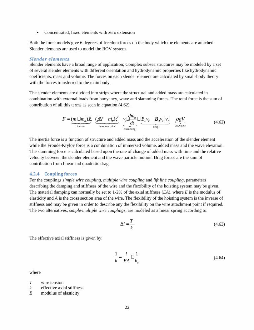
The slender elements are divided into strips where the structural and added mass are calculated in combination with external loads from buoyancy, wave and slamming forces. The total force is the sum of contribution of all this terms as seen in equation (4.62).
�
buoyancyFroude-Krylov dragslamming
( ) ( ) hh h r L r Q r r
inertia
dmF m m x V m v B v B v v gV
dtρ ζ ρ= + + + + + + +ɺɺɺɺ
����� ����� ����������
(4.62)
The inertia force is a function of structure and added mass and the acceleration of the slender element while the Froude-Krylov force is a combination of immersed volume, added mass and the wave elevation. The slamming force is calculated based upon the rate of change of added mass with time and the relative velocity between the slender element and the wave particle motion. Drag forces are the sum of contribution from linear and quadratic drag.
4.2.4 Coupling forces
For the couplings simple wire coupling, multiple wire coupling and lift line coupling, parameters describing the damping and stiffness of the wire and the flexibility of the hoisting system may be given. The material damping can normally be set to 1-2% of the axial stiffness (EA), where E is the modulus of elasticity and A is the cross section area of the wire. The flexibility of the hoisting system is the inverse of stiffness and may be given in order to describe any the flexibility on the wire attachment point if required. The two alternatives, simple/multiple wire couplings, are modeled as a linear spring according to:
Tl
k∆ = (4.63)
The effective axial stiffness is given by:
0
1 1l
k EA k= + (4.64)
where
T wire tension k effective axial stiffness E modulus of elasticity

23
A cross section area l unstretched wire length 1/k0 connection flexibility ∆l change in elongation of line
The material damping is included as:
wC l
Fl t
∆=∆
(4.65)
Simple wire coupling The simple wire coupling is modeled as a linear spring and may be convenient to use in lifting operations with a single attachment point on the lifted object. By knowing the position of each line end, the elongation and thereby the tension may be determined.
Multiple wire coupling The multiple wire system gives the possibility of several wire segments sharing a common branch point. In this way lifting systems using slings may be modeled. All the wire segments will have one end fastened in a body and the other in the common branch point and by using the same procedure as simple wire coupling the tension is determined. However, an iteration procedure is used by SIMO to determine the exact location of the branch point.
4.2.5 Solution of the equation of motion
Two different solution methods of the equation of motion are available in SIMO:
• Solution by convolution integral
• Separation of motions.
The solution by convolution integral is characterized by solving equation (4.60) in time domain by use of the retardation function while the other alternative separates the motions in high frequency part and low frequency part. For a more in-depth study of solving the equation of motion read chapter 4.1 in [11].
4.3 Estimation of hydrodynamic coefficients
The estimation of hydrodynamic forces acting on a load object during lifting through splash zone in order to reveal the resulting motion and the force responses is a complicated problem. Input of hydrodynamic coefficients is required and for many cases these coefficients are difficult to establish. Through the years it has been published a vast amount of papers considering the problem of fluid forces in viscous flow on a circular cylinder. This has contributed to a solution of the problem by hydrodynamic coefficients and use of semi-empirical methods, as Morison equation, to determine the forces during various conditions. In cases where the body geometry is far more complex than for a circular cylinder (e.g. ROV system) the most efficient way to determine the correct hydrodynamic coefficients is by model experiments. However, model experiments are expensive and time-consuming, and when carrying out analyses where the resulting motion and force responses are of interest, a reasonable good estimate on the hydrodynamic coefficients is often satisfactory.

24
4.3.1 Discussion of hydrodynamic coefficients for ROV system
The ROV system is a complicated structure and the estimation of the hydrodynamic coefficients is both difficult and uncertain. Because of this, O. Øritsland & E. Lehn [6] has been studied in order to find hydrodynamic data that may describe the system. This booklet provides hydrodynamic data for considerable numbers of complex bodies with certain characteristic parameters describing the structures. It is to be stressed that the coefficients presented in this booklet still are for idealized subsea structures and should be used with care to ensure a conservative approach to the problem.
KC Ca bL bQ CDS
Buoyant body <6 0.6-0.9 0.2-0.3 1.9-2.5 0.9-1.2 Working tool <6 0.8-0.9 0.3-0.6 3.8-4.7 1.6-1.9 Table 4 Range of hydrodynamic coefficients for typical subsea structures
Table 4 shows ranges of hydrodynamic coefficients for typical subsea module structures as found in chapter 5 in O. Øritsland & E. Lehn [6]. The drag coefficient in steady flow, CDS, is obtained from towing tests and the evaluation of added mass and damping are performed by decay tests. The buoyant type module is characterized by a fairly large central body and surrounding framework, being neutrally buoyant, while the working tool module is characterized by a heavy mass/buoyancy ratio where the added mass will be relatively less important [12]. From the definition of the different modules it may be concluded that the hydrodynamic properties of the ROV system can be described by the data from O. Øritsland & E. Lehn [6]. The ROV is a typical buoyant module while the top hat can be characterized as a working tool. After studying the properties of the various subsea modules tested, like mass/buoyancy ratio and fullness factor (V/LBH), the following structures may represent the hydrodynamic properties of the ROV and TMS: structure 13 [6, p. 5.13] and structure 11 [6, p. 5.11]. Table 5 summarizes the data for the two structures. The coefficients given in this table indicate which range a parametrical study considering the added mass and damping coefficients should be performed.
Structure 11 Structure 13 bL 0.20 0.45 bQ 2.03 3.92 Ca 0.86 0.91 CDS 1.00 1.60 Table 5 Hydrodynamic coefficient for structure 11 and structure 13 in [6]
Quadratic damping coefficient Since the ROV system should be regarded as one single structure a deeper investigation of the hydrodynamic properties has been performed. Figure 5.8 in O. Øritsland & E. Lehn [6] shows a comparison of bQ and CDS as function of fullness factor (V/LBH) for the various subsea modules tested. The trend is that the quadratic damping tends to decrease as the fullness of the structure increases. Since the whole system can be regarded as a buoyant structure with fullness factor of around 0.36 [-], indicates the figure that the quadratic damping coefficient may be in the region of bQ = 2.0 [-].DNV [1] proposes that the drag coefficient in oscillatory flow should be at least CD = 2.5 [-] unless specific model test or CFD studies are performed. This is fairly close to the quadratic damping coefficient found based upon the fullness of the structure; hence the guideline value from DNV [1] could be a reasonable good and conservative estimate of the quadratic damping coefficient for the whole system. As stated in chapter 4.1.4, may waves, current and vertical fluid flow wash out some of the wake leading to lower drag force.

25
This strengthen the belief that a quadratic damping coefficient of 2.5 [-] may be a reasonable and conservative value when applied on the ROV system. As mentioned in chapter 4.1.4 is the drag coefficient, CD, in oscillatory flow normally dependent of the Keulegan-Carpenter number. However, O. Øritsland & E. Lehn [12] concludes that the coefficient can be kept constant over a fairly wide range of KC-numbers (KC<10). The quadratic damping is assumed equal to the drag term in Morison’s equation while the linear term is neglected since the criteria in equation (4.24) is fulfilled and the quadratic drag contribution is comparatively dominating when velocities are high. This is assumed even though O. Øritsland & E. Lehn [13] indicates that a linear term may give a significant contribution to the damping for even fully submerged structures.
Added mass coefficient The added mass coefficient has been assumed to be 0.9 [-] and can also be a reasonable and conservative estimate. Model tests performed by P. Sayer [14] indicate that values for the inertia coefficient Cm=(1+Ca) for typical work class ROVs are in the range of 1.4-1.6, leading to smaller hydrodynamic forces than the limited amount of published hydrodynamic coefficients.
Slamming coefficient The slamming coefficient for the ROV system may be the most difficult coefficient to establish because of lack of literature on the subject. DNV [1] proposes the slamming coefficient for a non-cylindrical subsea structure should be Cs=5.0 [-]. This value is highly questionable since the lower part of the ROV is a complicated structure with holes and perforation. In combination with the slamming area and velocity is the slamming force the limiting case for launch and recovery of ROV, something that may be dubious. A slamming coefficient of 5.0 [-] is transferable to a flat plate without ventilation. If the flat plate is compared to the lower part of the ROV the reader will apprehend the difficulty in predicting the slamming coefficient for the ROV system.
An efficient slamming area has been established in order take the openings in the lower part of the ROV into consideration. This will reduce the slamming term and hopefully give more correct slamming loads. From 3D drawings of the ROV it is seen that the slamming area at the lower part of the ROV can be reduced at least 30-40 %. If this is included in the slamming coefficient instead of the slamming area a coefficient of Cs≈ 3.0 [-], as for a cylindrical shaped body can be established. This assumption is clearly arguable and is dependent of whether a third party will accept the assumptions. However, based upon results from SIMO where the slamming force is calculated based upon the variation of added mass, it is seen that the slamming term has much less influence on the total forces acting on the ROV system than compared to the DNV rules. Because of this, the slamming coefficient has been assumed to Cs = 3.0 [-].
Summary of hydrodynamic coefficients Table 6 shows the hydrodynamic coefficients for the ROV system applied in the main analyses.
Summary of hydrodynamic coefficients CD [-] 2.5 Ca [-] 0.9 Cs [-] 3.0 Table 6 Summary of hydrodynamic coefficients for used in main analyses

26

27
5 Procedure – DNV Recommended Practices
5.1 Launch and Recovery of ROV
This section will go through the deployment analyses with theoretical background from chapter 4.1. In the project thesis, Appendix C.3, launch and recovery analyses were performed for the ROV system with the Simplified Method. However, after a more in-depth study of the analyses performed fall 2009, a new and more refined approach to the problem is taken. The differences between the new calculations and the project thesis are for example a less conservative approach to the slamming loads and a more refined analysis based upon the drag force, added mass etc. The calculations by the Simplified Method are performed in MATLAB and the script can be found in Appendix C.2.
5.1.1 Load cases during deployment through wave zone
The lowering through wave zone is divided into four load cases:
• The 1st case when the ROV is in air. • The 2nd case when the ROV penetrates surface. • The 3rd case when ROV is partly submerged.
• The 4th case when ROV is fully submerged.
In the following sections the four different load cases are described during lowering through wave zone.
Case 1 Case 2 Case 3 Case 4
Figure 5 Load cases during lowering through wave zone
Case 1 – ROV in air In this case the ROV is in air and the only load component acting on the ROV system is inertia force due to the heave acceleration at crane tip. In this case there are no hydrodynamic forces acting on the ROV system.
Case 2 – ROV penetrates the surface The lower part of the ROV is hit by waves which cause slamming loads on the ROV system. The force components contributing to dynamic forces are the slamming impact force on the bottom of ROV and inertia force due to the heave acceleration of the vessel. Since the inertia force in air is small compared to the slamming load it may be neglected. The relative velocity between ROV system and water particles governs the slamming impact.
Case 3 – ROV system partly submerged For case 3 is the ROV considered as submerged and the TMS is in air. The load components are drag force, mass force and inertia force on the TMS. The mass force term includes the contribution from the

28
hydrodynamic mass and water particle acceleration at the submerged part of ROV system. The wave particle velocity and acceleration induced forces are related to the vertical center of gravity of the ROV, approximated as HROV/2 from the free surface. The varying buoyancy force is assumed to be half of the total volume of the ROV system.
Case 4 – ROV system fully submerged The load components for case 4 are drag forces and mass forces on the whole ROV system. Varying buoyancy force is neglected. The vertical water particle acceleration and velocity are related to the center of gravity of the TMS and ROV, approximated as (HTMS/2) and (HTMS+HROV/2) from the free surface respectively. The vertical drag force is based upon the projected area of the ROV and the drag coefficient CD. Since the vertical water particle velocity and acceleration are found in the centre of gravity of each object the total drag force has been divided between the TMS and ROV; 1/3 of the total drag force is acting on the TMS while the rest is acting on the ROV. This assumption will give almost the same forces as if the total drag force is estimated to be acting in COG of the whole ROV system.
5.1.2 Environmental data
The crane operation during launch and recovery is assumed to be performed within 30 minutes; hence the
regular wave amplitude applied in the analyses is ζa = 0.9·Hs and the crane tip motions can be taken as 1.8
times the significant responses. The applied zero up crossing periods are found according to the limits given in equation (4.1). Table 7 shows the regular wave amplitude and the corresponding zero up crossing period for each of the analyzed sea states.
Hs ζa = 0.9·Hs Tz
2.00 [m] 1.80 [m] 4.0 – 13 [s] 2.50 [m] 2.25 [m] 4.5 – 13 [s] 3.00 [m] 2.70 [m] 5.0 – 13 [s] 3.50 [m] 3.15 [m] 5.5 – 13 [s] 4.00 [m] 3.60 [m] 6.0 – 13 [s] 4.50 [m] 4.05 [m] 6.0 – 13 [s] Table 7 Regular wave heights and wave periods for the respective sea state
It is to be noted that for the lowest zero up crossing periods the waves will nearly break.
5.1.3 Crane tip motions
The crane tip motions were found according to theory described in chapter 4.1.7. The Response Amplitude Operators in the centre of gravity of Skandi Bergen for heading angles of 0º and ±15º were obtained in VeRes and imported to the MATLAB script RAOcalculation.m. This script calculates the RAO in heave at an arbitrary position on the vessel; in this case the tip of the launch and recovery system. Further, the calculated RAOs in heave have been imported to the MATLAB script SimplifiedMethod.m for post-processing and statistical description. SimplifiedMethod.m calculates the response spectrum in heave based upon the RAOs and the applied JONSWAP spectra for the given sea state. From the response spectra can the most probable crane tip displacement, velocity and acceleration be found, which are required in the calculation of forces acting on the object lowered through wave zone. All the results from the different MATLAB scripts have been verified by calculations in VeRes and the scripts can be found in Appendix C.2.

29
5.1.4 Hydrodynamic forces
The upward acting hydrodynamic forces are of particular interest when studying the ROV system being lowered through wave zone. This is because of the low submerged weight of the system in combination with the upward acting hydrodynamic forces may give slack umbilical which increases the possibility of severe snap loads. The hydrodynamic coefficients, the total vertical drag force when subjected to a relative velocity of 1 [m/s], and the added mass for the TMS and ROV are shown in Table 8.
Hydrodynamic properties CD [-] 2.50 Ca [-] 0.90 Cs [-] 3.00 Fd [kN] 6.804 A33,TMS [tonne] 1.5037 A33,ROV [tonne] 4.7099 Table 8 Hydrodynamic coefficients, drag force and added mass
DNV-RP-H103 [1] proposes that the upward acting hydrodynamic forces should not exceed the static weight of the object lowered through wave zone in order to avoid snap forces in the umbilical. This leads to that the acceptance criteria in equation (4.31) must be fulfilled. The static weights of the ROV system for each load case are shown in Table 9.
Load case Fstatic
Case 1 97.00 [kN] Case 2 97.00 [kN] Case 3 45.66 [kN] Case 4 29.27 [kN] Table 9 Static weight of ROV system in each load case
5.1.5 Snap loads
Snap loads have been evaluated since the launch and recovery calculations have shown that the hydrodynamic forces exceed the static weight of the ROV system for most of the sea conditions. The cross sectional axial stiffness of the umbilical has been estimated to EA = 3.7692·104 [kN] and in combination with an estimated umbilical length of L = 25 [m] the umbilical stiffness will be K = 1.8846·103 [kN/m]. For load case 4, which is the most exposed position with respect to the acceptance criteria, are the following relationship established:
33( ) 174.20 [ ]snap snap snapF v K M A v kN= ⋅ + = ⋅ (5.1)
The minimum snap velocity is equal to the free fall velocity of the ROV system when fully submerged which is found according to equation (4.30) and is equal to 2.08 [m/s].

30

31
6 Procedure –SIMO
6.1 System description SIMO
The purpose of this chapter is to go through system description file and explain the most important steps of the marine operation. The system description file is divided into 5 main data groups:
SYSTEM DESCRIPTION SIMO Identifies the file type, always the first data group ENVIRONMENT SPECIFICATION All environmental data specified together BODY DATA SPECIFICATION Repeated for each specification of bodies COUPLING DATA Defines coupling between bodies END Indicated the end of the file
All the data within each main data group has to be specified in one sequence. However, the different main data groups may be specified arbitrary. The environment specification and coupling data are given into the system description file once, while the body data specification is given into the sys-file twice; one describing the vessel and the other describing the properties of the ROV system.
6.1.1 Environment specification
The environmental forces during the offshore crane operation are divided into three groups: Wind, current and waves. Since the waves are the most important contributor to the forces acting on the object lowered through wave zone the effect from wind and current are neglected. The analyses are performed for both regular waves and irregular sea states with different wave amplitudes and periods.
Regular waves Regular waves are applied in the analyses when finding the most onerous position of the object lowered through wave zone and for comparison of the analytical method and SIMO.
Irregular waves Irregular waves are applied for stationary analyses in the most onerous position during a 0.5 hour sea state and for repeated lowering/retrieval in irregular waves. The most commonly used spectrum for the North Sea is JONSWAP; hence long crested irregular sea described by the JONSWAP spectrum with 2 parameters (Hs & Tp) is applied in the analyses. The two parameter JONSWAP spectrum is defined by equation (4.33) while the peak shape parameter is found by the relation:
4 2exp 3.484(1 0.1975 /p sT Hγ δ = − (6.1)
0.0036 0.0056 /p sT Hδ = − (6.2)
However, for the two parameter JONSWAP spectrum the following limits for γ are valid:
5 / 3.6
1 / 5.0
p s
p s
for T H
for T H
γ
γ
= ≤
= ≥ (6.3)

32
6.1.2 Body data specification - Skandi Bergen
The multipurpose construction vessel Skandi Bergen is modeled in SIMO as body type 2 which means that the ship is modeled as a large volume structure with six degrees of freedom. The high frequency motions are separated into frequency domain while the low frequency motions are calculated in time domain. The following data must be given in order to calculate the motion of the vessel:
• Body location data • Body mass data • Mass coefficients • Added mass zero • Hydrostatic stiffness data • First order motion transfer functions
• Body components
The analyses are performed for Design Water Line for Skandi Bergen and without roll stabilizing tanks. It is important to note that SIMO uses [kN] to define force and [tonne] to define mass.
Body location data '================================================== ========== BODY LOCATION DATA '================================================== ========== 'Xglob Yglob Zglob Phi Theta Psi 0.0 0.0 3.1 0.0 0.0 0.0 Figure 6 Body location data for Skandi Bergen
The body location data describes the position of the vessel in the global coordinate system. The origin is in the vessel’s centre of gravity.
Body mass data '--------------------------------------------------------------------------------------------------------------------------- BODY MASS DATA '--------------------------------------------------------------------------------------------------------------------------- 'txmass LCG=45.9 m from AP. CL=47.5 m from AP. VCG=8.80 m from BL. 'xcog ycog zcog 0.00 0.0 0.0 Figure 7 Body mass data for Skandi Bergen
The section body mass data defines the centre of gravity of the vessel. For design water line is the vertical centre of gravity 8.8 [m] above baseline or 3.1 [m] above the free water surface and the longitudinal centre of gravity is 1.45 [m] from amidships. The body related coordinate system is given in the COG of the vessel; hence the input is given as it is.

33
Mass coefficients '--------------------------------------------------------------------------------------------------------------------------- MASS COEFFICIENTS '--------------------------------------------------------------------------------------------------------------------------- 'rm rixx riyx riyy rizx rizy rizz 7460.1 4.63E+05 0.0 4.88E+06 0.0 0.0 4.88E+06 Figure 8 Mass coefficients for Skandi Bergen
The body mass and inertias are found from VeRes. The structure mass are 7460.1[tonne] while the inertia in roll, pitch and yaw are found from the radius of gyration as seen in Table 1 and the following relationship:
2i i i iR M r= (6.4)
where
Rii Inertia in roll, pitch and yaw M Structure mass r ii Radius of gyration in roll, pitch and yaw
Added Mass Zero '------------------------------------------------------------------------------------------------------------------------------- ADDED MASS ZERO '------------------------------------------------------------------------------------------------------------------------------- 0.00000000E+00 0.00000000E+00 0.00000000E+00 0.00000000E+00 0.00000000E+00 0.00000000E+00 0.00000000E+00 0.28031645E+04 0.00000000E+00 0.15917542E+04 0.00000000E+00 -0.13275859E+05 0.00000000E+00 0.00000000E+00 0.25441436E+05 0.00000000E+00 -0.15271867E+6 0.00000000E+00 0.00000000E+00 0.15917542E+04 0.00000000E+00 0.70564040E+05 0.00000000E+00 -0.12199627E+06 0.00000000E+00 0.00000000E+00 -0.15271867E+06 0.00000000E+00 0.15675594E+8 0.00000000E+00 0.00000000E+00 -0.13275859E+05 0.00000000E+00 -0.12199627E+06 0.00000000E+00 0.17004311E+07 Figure 9 Added mass of Skandi Bergen for zero frequency
The added mass at zero frequency is retrieved from VeRes by running a calculation for a wave period of 200 [s]. The added mass matrix can be found in zerofreq.re7 in Appendix C.1. Note that VeRes defines mass as [kg] and that the added mass zero matrix above have been converted in order to be compatible with SIMO.
Linear stiffness matrix '--------------------------------------------------------------------------------------------------------------------------- LINEAR STIFFNESS MATRIX '--------------------------------------------------------------------------------------------------------------------------- 'kmati1 kmati2 kmati3 kmati4 kmati5 kmati6 0.3635E+02 0.0 0.0 0.0 0.0 0.0 0.0 0.5002E+02 0.0 0.0 0.0 0.0 0.0 0.0 0.182E+05 0.0 -0.698E+05 0.0 0.0 0.0 0.0 0.261E+06 0.0 0.0 0.0 0.0 -0.698E+05 0.0 0.12E+08 0.0 0.0 0.0 0.0 0.0 0.0 0.8324E+04 Figure 10 Linear stiffness matrix of Skandi Bergen

34
The hydrostatic stiffness data has been found from VeRes in the Restoring Matrix in the file input.out, Appendix C.1.The only non-zero terms in the linear stiffness matrix are C33, C35, C53, C44 and C55. However, stiffness in surge, sway and yaw has been included in order to prevent translation and rotation of the vessel in the horizontal plane. This will have the same characteristics as a typical dynamic positioning system or that the vessel is moored. The artificial DP system is modeled as described below. The uncoupled and undamped resonance periods can be written as [8]:
1
2
2 1,2,3iini
ii
M AT for i
Cπ += =
(6.5)
1
2 2
2 4,5,6ii iini
ii
Mr AT for i
Cπ += =
(6.6)
where
Tni Natural period in i-direction
M Structure mass
r ii Radius of gyration
Aii Added mass in i-direction
Cii Stiffness in i-direction
For a typical moored structure are the natural periods in the horizontal degrees of freedom in the magnitude of minutes. By introducing a natural period of 90 [s], which can be a good estimate of a typical DP system or mooring system [7], the corresponding stiffness may be expressed:
2
2
4 ( )1,2,3ii
iini
M AC for i
T
π += = (6.7)
2 2
2
4 ( )4,5,6ii ii
iini
Mr AC for i
T
π += = (6.8)
From equation (6.7) and (6.8) the stiffness C11, C22 and C66, which represent the ship being moored in the horizontal plane, have been found. The vessel’s structure mass and moment of inertia are known from above, but the added mass is frequency dependent. Because of this, the added mass for a frequency corresponding to a sea state with a period of 90 seconds is found in VeRes. The calculated added mass matrix for 90 [s] is conveniently equal to the added mass zero matrix as found in Figure 9; hence all the input to equation (6.7) and (6.8) are found. The calculated stiffnesses representing the DP system are shown in the linear stiffness matrix above.

35
Linear damping '------------------------------------------------------------------------------------------------------------------------------- LINEAR DAMPING '------------------------------------------------------------------------------------------------------------------------------- linear damping matrix B44 at T=11.5 s, B11,B22,B66 are 70 percent of Bcrit at T= 90s 'dl1 dl2 dl3 dl4 dl5 dl6 0.72914E+03 0. 0. 0. 0. 0. 0. 0.100312E+04 0. 0. 0. 0. 0. 0. 0. 0. 0. 0. 0. 0. 0. 0.20257750E+05 0. 0. 0. 0. 0. 0. 0. 0. 0. 0. 0. 0. 0. 0.16692662E+06 Figure 11 Linear damping matrix for Skandi Bergen
Linearized viscous roll damping has been included in order to take the skin friction into account. The linearized viscous roll damping has been found from the VeRes file input.re7, Appendix C.1, for beam seas at the most critical roll period which is 11.5 [s]. This damping is only important for beam seas and can be disregarded for other heading angles. The following linearized damping has been obtained from VeRes:
B44, linear= 20257.75 [kNms]
The linear damping matrix has also been modified in order to prevent the vessel for translation and rotation in the horizontal degrees of freedom. The dynamic positioning system has been simulated by adding 70% of the critical damping in surge, sway and yaw in the linear damping matrix. This additional damping will damp out any rotation and translation in the horizontal plane and can be expressed [8, p. 97]:
, ,0.7 0.7 2( ) (2 / ) 1,2,3ii linear ii crit ii ii niB B M A T for iπ= = ⋅ + ⋅ = (6.9)
2, ,0.7 0.7 2( ) (2 / ) 4,5,6ii linear ii crit ii ii ii niB B M r A T for iπ= = ⋅ + ⋅ = (6.10)
Equation (6.9) and (6.10) give the additional damping in surge, sway and yaw as shown in the linear damping matrix.
First order motion transfer functions The first order motion transfer functions retrieved from VeRes were imported to the system description file for heading angles from head sea to following sea with 15º steps. The RAOs are only given for 0 to 180 degrees since the vessel is symmetric about the x-z plane. A total number of 32 frequencies covering the interval from 0.2094[ rad/s] to 2.0944 [rad/s] are used to describe the vessel motions. SIMO use interpolation for other heading angles and frequencies. The first order motion transfer can be found in Appendix C.1.
Body components The launch and recovery system is modeled with a winch located in the ROV hangar of Skandi Bergen and a guide point simulating the tip of the LARS. The coordinates of the winch and the tip of the LARS are found in Table 10 and are referred to the vessel’s body related coordinate system which is located in the centre of gravity.
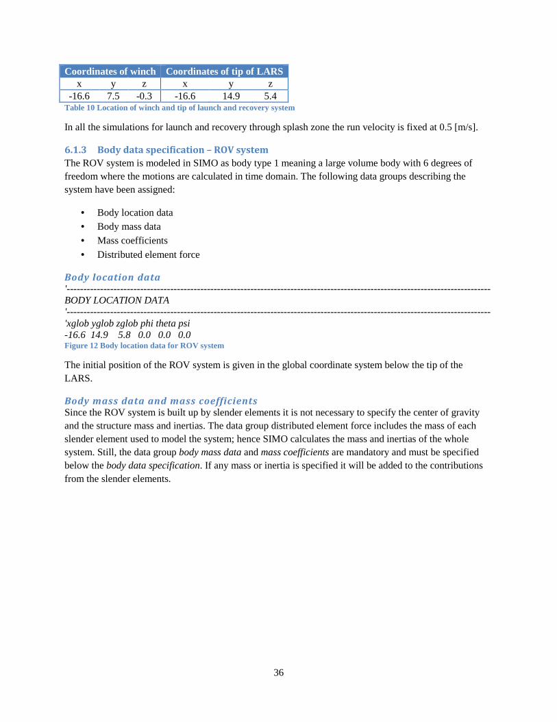
36
Coordinates of winch Coordinates of tip of LARS x y z x y z
-16.6 7.5 -0.3 -16.6 14.9 5.4 Table 10 Location of winch and tip of launch and recovery system
In all the simulations for launch and recovery through splash zone the run velocity is fixed at 0.5 [m/s].
6.1.3 Body data specification – ROV system
The ROV system is modeled in SIMO as body type 1 meaning a large volume body with 6 degrees of freedom where the motions are calculated in time domain. The following data groups describing the system have been assigned:
• Body location data • Body mass data • Mass coefficients
• Distributed element force
Body location data '------------------------------------------------------------------------------------------------------------------------------- BODY LOCATION DATA '------------------------------------------------------------------------------------------------------------------------------- 'xglob yglob zglob phi theta psi -16.6 14.9 5.8 0.0 0.0 0.0 Figure 12 Body location data for ROV system
The initial position of the ROV system is given in the global coordinate system below the tip of the LARS.
Body mass data and mass coefficients Since the ROV system is built up by slender elements it is not necessary to specify the center of gravity and the structure mass and inertias. The data group distributed element force includes the mass of each slender element used to model the system; hence SIMO calculates the mass and inertias of the whole system. Still, the data group body mass data and mass coefficients are mandatory and must be specified below the body data specification. If any mass or inertia is specified it will be added to the contributions from the slender elements.

37
Distributed element force '************************************************** *********************************** DISTRIBUTED ELEMENT FORCE '************************************************** *********************************** 'txdist Cylinder dimensions: D=1 m, L=5 Cd=2.0 (oscillatory flow) Ca=0.90, Mass = 10 tonne '---------------------------- SLENder ELEMent '---------------------------- Cross section area and distributed mass 'spevol dstmas ifoadd ivol iwdhf nstrip 0.7854 2.00 1 1 4 4 Defining force calculation options ' xel1 yel1 zel1 xel2 yel2 zel2 xref yref zref -2.50 0.00 0.00 2.50 0.00 0.00 -2.50 3.00 0.00 Body related coordinates of slender element 'c2x c2y c2z c1x c1y c1z amx amy amz 0.000 1.025 1.025 0.000 0.000 0.000 0.000 0.725 0.725 Hydrodynamic coefficients
Figure 13 Example of slender element
Since the ROV system is built up by several slender elements with different properties a simple example of a single 5 [m] long cylinder with a diameter of 1 [m] is shown above in order to simplify the explanation of slender elements for the reader. The modeling procedure of the ROV system is described in depth in chapter 6.2. The drag coefficient in oscillatory flow for a circular cylinder is CD = 2.0 [-] while the added mass coefficient is Ca = 0.90 [-].
The cross section area specifies the volume per meter of the slender element while the distributed mass is given to SIMO as [tonne/m]. The force calculation options are defined by:
ifoadd = 1 force integrated to wave surface ivol = 1 gravity and buoyancy force included iwdhf = 4 wave particle velocity and acceleration included nstrip = 4 number of strips in the element
The longitudinal axis is the slender element’s local x-axis while the y- and z- direction are in sway and heave respectively. The quadratic drag coefficient in sway and heave for the cylinder is given to the system description file by the following relation:
12 2 1.025 [ / ]
2 Dc y c z C D tonne mρ= = = (6.11)
Added mass are given in sway and heave by the following relation:
22
0.725[ / ]2 a
Damy amz C tonne mρπ
= = =
(6.12)

38
Depth dependent hydrodynamic scaling coefficients are included in the modeling in order to take into account the position of each element relative to the water level. If a slender element crosses the water surface with nearly horizontal angle and without position dependent data, large impulse forces may occur. The depth dependent scaling coefficients are applied in the centre of each strip and are intended for nearly horizontal elements.
Volume Drag coefficient Added mass In air 0.0 0.0 0.0 50 % submerged 0.5 0.6 0.5 Fully sybmerged 1.0 1.0 1.0 Table 11 Depth dependent scaling coefficients
Table 11 shows the scale factors which are applied for the hydrodynamic coefficients and volume as function of submergence. A linear relationship has been assumed for the volume and added mass while the drag coefficient is given a slightly increased scale factor when partly submerged.
6.1.4 Coupling data
Simple wire coupling The umbilical has been modeled with simple wire coupling between the winch system located in the ROV hangar and the top of the TMS. Cross sectional stiffness, initial wire length, connection flexibility and material damping are given in Table 12.
Simple Wire coupling Cross sectional stiffness (EA) 3.7692·104 [kN] Initial wire length 9.84 [m] Connection flexibility 1.00·10-7 [1/kN] Material damping 0.754·103 [kNs] Table 12 Umbilical data and connection flexibility given to SIMO
The connection flexibility is the inverse of stiffness and takes into account the flexibility of the hoisting system without the wire. Since the stiffness of the hoisting system is unknown it has been estimated to be much larger than the wire stiffness ensuring that it is only the umbilical stiffness which is taken into account when calculating snap loads etc. The material damping is normally 1-2 % of EA [15]; hence it has been estimated to 2% of EA.
6.2 Modeling the ROV system
The forces acting on the ROV system are contribution from the structure mass, buoyancy, added mass and drag. Because of this, it is important to model the hydrodynamic and structure properties as accurate as possible. Since the ROV system is a densely compounded structure with equipment with different hydrodynamic and structure properties a total number of 48 slender elements have been used in order to represent the system. The ROV is a neutrally buoyant structure with the centre of buoyancy in the upper part and the centre of gravity at the lower part of the ROV while the top hat acts like a cursor weight where both the centre of gravity and buoyancy are estimated to the center of the structure. Figure 14 shows the model of the ROV system.

39
Figure 14 ROV system modeled by slender elements
In view of the fact that the system is modeled with 48 slender elements is it nearly impossible to define the properties directly to the system description file. The MATLAB scripts ROVmodel.m and TMSmodel.m, found in Appendix C, define the geometries and the corresponding hydrodynamic and structure properties of each slender element. Further, the geometries are written to .dat-files which are imported to the sys-file.
ROV TMS TOTAL CD [-] 2.5 2.5 - FDD,surge [kNs/m] 4.65 6.15 10.79 FDD,sway [kNs/m] 7.06 6.15 13.21 FDD,heave [kNs/m] 4.54 2.27 6.80 Table 13 Drag forces acting on ROV system
Table 13 summarizes the drag forces acting on the ROV system. The drag force is presented by the following relation from Morison’s equation:
2
1
2Di
DDi pi Di
FF A C
vρ= =
(6.13)
As it can be seen from Table 13 is the TMS given a drag term in heave. This is a simple estimation calculated from the projected area of the ROV and the quadratic drag coefficient where 2/3 of the total drag force are acting on the ROV while the remaining drag force is acting on the TMS. Further, the following quadratic drag coefficient, which is compatible with SIMO as input, has been established in order to fully represent the drag forces:
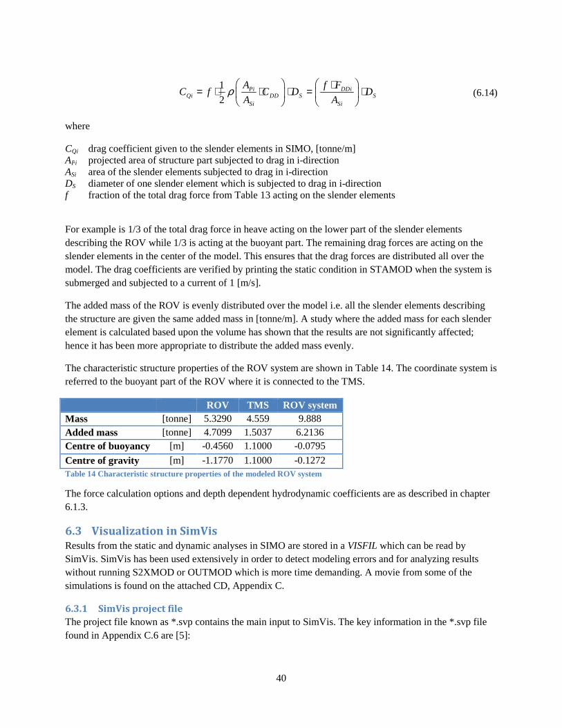
40
1
2Pi DDi
Qi DD S SSi Si
A f FC f C D D
A Aρ ⋅= ⋅ ⋅ ⋅ = ⋅
(6.14)
where
CQi drag coefficient given to the slender elements in SIMO, [tonne/m] APi projected area of structure part subjected to drag in i-direction ASi area of the slender elements subjected to drag in i-direction DS diameter of one slender element which is subjected to drag in i-direction f fraction of the total drag force from Table 13 acting on the slender elements
For example is 1/3 of the total drag force in heave acting on the lower part of the slender elements describing the ROV while 1/3 is acting at the buoyant part. The remaining drag forces are acting on the slender elements in the center of the model. This ensures that the drag forces are distributed all over the model. The drag coefficients are verified by printing the static condition in STAMOD when the system is submerged and subjected to a current of 1 [m/s].
The added mass of the ROV is evenly distributed over the model i.e. all the slender elements describing the structure are given the same added mass in [tonne/m]. A study where the added mass for each slender element is calculated based upon the volume has shown that the results are not significantly affected; hence it has been more appropriate to distribute the added mass evenly.
The characteristic structure properties of the ROV system are shown in Table 14. The coordinate system is referred to the buoyant part of the ROV where it is connected to the TMS.
ROV TMS ROV system Mass [tonne] 5.3290 4.559 9.888 Added mass [tonne] 4.7099 1.5037 6.2136 Centre of buoyancy [m] -0.4560 1.1000 -0.0795
Centre of gravity [m] -1.1770 1.1000 -0.1272 Table 14 Characteristic structure properties of the modeled ROV system
The force calculation options and depth dependent hydrodynamic coefficients are as described in chapter 6.1.3.
6.3 Visualization in SimVis
Results from the static and dynamic analyses in SIMO are stored in a VISFIL which can be read by SimVis. SimVis has been used extensively in order to detect modeling errors and for analyzing results without running S2XMOD or OUTMOD which is more time demanding. A movie from some of the simulations is found on the attached CD, Appendix C.
6.3.1 SimVis project file
The project file known as *.svp contains the main input to SimVis. The key information in the *.svp file found in Appendix C.6 are [5]:

41
• Global project settings: Information of where the VISFIL from SIMO is located and time step information which is equal to the main time step in SIMO.
• Sea floor description: The center position and dimensions of the seafloor is specified and the color and transparency is given. The texture is described by the tex_concrete.rgb file.
• Dynamic wave surfaces: The wave components are imported from the VISFIL and the wave elevation and slope is calculated in SimVis. The dimension of the calculated wave field is given in SIMO, but SimVis can repeat the wave field in order to visualize a larger ocean surface.
• Slender system: The coupling between the winch and ROV system are specified.
The SimVis project file also offer the possibility to import body geometries from external files in order to simulate a more realistic marine operation. A barge with similar size as Skandi Bergen has been used to verify that the vessel is following the wave excitation. However, in the visualization, Appendix C.4 is only the slender elements representing the ROV system shown.
6.4 Running time domain analysis in SIMO
The following time domain analyses have been carried out in SIMO:
• Stationary analysis in irregular sea • Repeated lowering through splash zone in irregular sea • Repeated retrieval through splash zone in irregular sea
• Lowering through splash zone in regular waves
A complete time domain analysis made use of the SIMO modules STAMOD, DYNMOD and S2XMOD. Macro files, *.MAC, were created in cases where multiple simulations were required and for preparing several batch runs. The macro files and batch files can be found at the enclosed CD, Appendix C.5.
6.4.1 STAMOD
After reading the system description file in STAMOD the environmental condition is chosen and the initial positions for all the bodies are established by running a static equilibrium for the entire system. The results are stored on the file prs-ROV.lis file. Finally, the initial condition file was generated in order to execute the time domain simulations in DYNMOD.
6.4.2 DYNMOD
DYNMOD read the initial condition file, set simulation parameters and initialize the time domain simulation before the analysis start. The method for calculation of waves was done by cosine series only since the ROV system is lowered through the splash zone with continuous velocity. Fast Fourier Transform has a lower computing time, but is not applicable for other than stationary analyses. For irregular sea one has to specify a seed for generation of random phase angles. Time step specification was set to 0.1 [s] with 20 subdivisions per time step for improved accuracy. Default values were applied for storage parameters since the resultant coupling force, wave elevation and motion of the bodies is included. If other forces and motions were of interest they would have been specified. Before start of the time domain simulation length and integration method were specified. The Runge-Kutta method applying constant averaged acceleration has been used as the main integration method. A visualization file for SimVis was generated for most of the simulations.

42
6.4.3 S2XMOD
The time series from the time domain simulation are exported by S2XMOD to *.m files for statistical description and presentation of results in MATLAB. The time series include: vessel responses, umbilical tension and displacements of the ROV system.
6.5 Limitations
It is to be stressed that the ROV model has limitations regarding structure and hydrodynamic properties. Even though the structure properties like volume and mass of the system are modeled correctly the uncertainty in location of gravity and buoyancy may affect the results. The hydrodynamic coefficients used to describe the ROV system are simple estimations and cannot be taken as real values unless a specific model test or similar is performed. The assumption that the drag and added mass forces are distributed all over the model may also affect the results. However, this is found to be the most convenient way to describe the model. Furthermore, it is seen from literature studies that the hydrodynamic coefficients are dependent on the KC-number and that linear damping may give contribution to the hydrodynamic forces, which not have been taken into consideration in the analyses. The stiffness of the hoisting system (umbilical, crane and winch) is also based upon simple estimation and cannot be taken as the real stiffness representing the system even though it could be a good estimation.

43
7 Results from Simplified Method
7.1 Vessel Response
The vessel responses at the tip of the launch and recovery system have been found by the MATLAB scripts RAOcalculation.m and SimplifiedMethod.m. It is to be noted that the calculations in these scripts have been verified by VeRes. The response Amplitude Operators at the tip of the launch and recovery system are presented in chapter 7.1.1 while the most probable largest velocity and acceleration in a sea state of 4.5[m] significant wave height are presented in chapter 7.1.2.
7.1.1 RAO at crane tip
Figure 15 shows the Response Amplitude Operators for the heading angles of 0º and ±15º found from the MATLAB script RAOcalculation.m, Appendix C.2.
Figure 15 Response amplitude operators at tip of the LARS for heading angles of 0º and ±15º
7.1.2 Most probable largest single amplitude responses
The most probable largest single amplitude velocity and acceleration in the sea state of 4.5 [m] are shown in Figure 16 as function of applied zero crossing period. For other sea states see the project thesis, Appendix C.3.
Figure 16 Most probable largest single amplitude velocity and acceleration at the tip of the launch and recovery system
7.2 Launch and recovery analyses
In the following subchapters are the results obtained from the calculations with the Simplified Method presented. The upward acting hydrodynamic forces are of particular interest since this may induce zero tension in the umbilical and snap loads may occur. As a consequence, the hydrodynamic forces are plotted

44
for each heading angle with the acceptance criteria given in equation (4.31). Chapter 7.2.1 presents case studies for different significant wave heights while chapter 7.2.2 presents some results when the vessel and ROV system only is subjected to significant responses. Snap loads may occur for most of the sea conditions and are presented in chapter 7.2.3.
7.2.1 Case study of the ROV system lowered through wave zone
In Figure 17and Figure 18 are the results for each load case shown for a significant wave height of 2.5 [m] and 4.5 [m] respectively. Other sea states can be found in Appendix A.
Figure 17 Case study of hydrodynamic forces in a significant wave height of 2.5 [m]
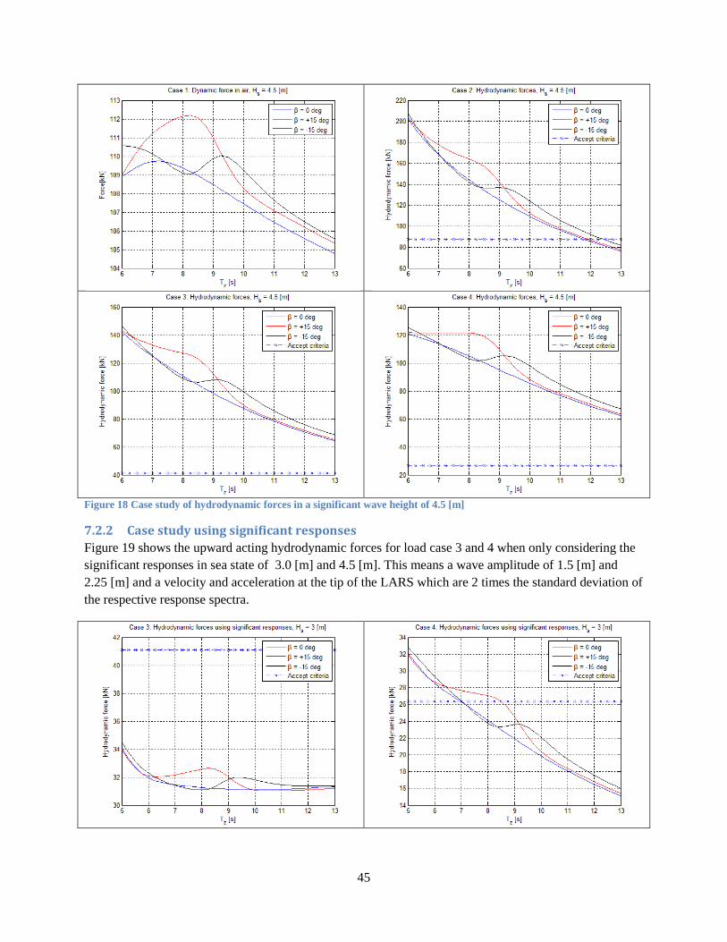
45
Figure 18 Case study of hydrodynamic forces in a significant wave height of 4.5 [m]
7.2.2 Case study using significant responses
Figure 19 shows the upward acting hydrodynamic forces for load case 3 and 4 when only considering the significant responses in sea state of 3.0 [m] and 4.5 [m]. This means a wave amplitude of 1.5 [m] and 2.25 [m] and a velocity and acceleration at the tip of the LARS which are 2 times the standard deviation of the respective response spectra.

46
Figure 19 Hydrodynamic forces when exposed for significant responses in a significant wave height of 3.0 [m] and 4.5 [m]
7.2.3 Snap loads
Since the acceptance criteria is exceeded for most of the sea conditions are snap loads for load case 4, which is the most exposed load case with respect to the acceptance criteria, presented in Figure 20 for sea states with significant wave heights of 3.0 – 4.5 [m].
Figure 20 Snap loads for load case 4 in sea states from H s = 3.0 – 4.5 [m]
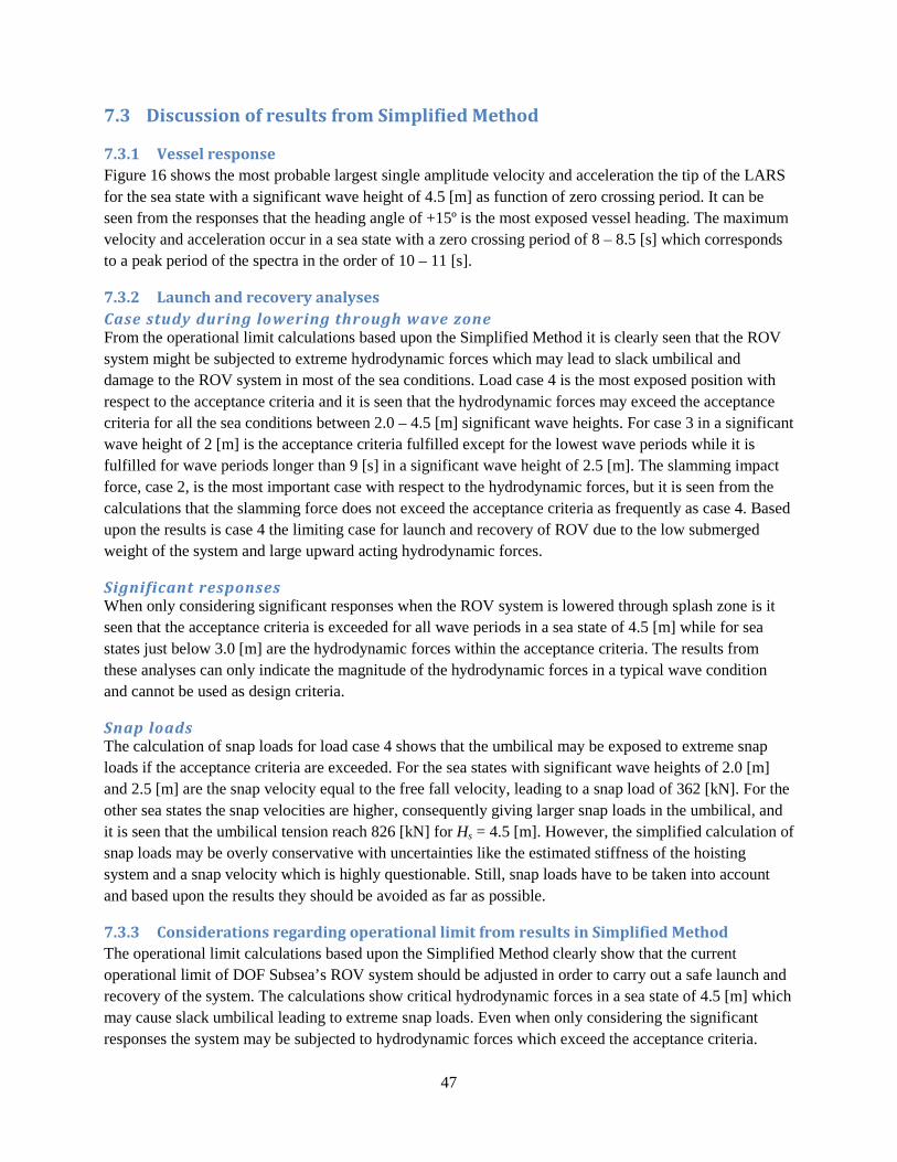
47
7.3 Discussion of results from Simplified Method
7.3.1 Vessel response
Figure 16 shows the most probable largest single amplitude velocity and acceleration the tip of the LARS for the sea state with a significant wave height of 4.5 [m] as function of zero crossing period. It can be seen from the responses that the heading angle of +15º is the most exposed vessel heading. The maximum velocity and acceleration occur in a sea state with a zero crossing period of 8 – 8.5 [s] which corresponds to a peak period of the spectra in the order of 10 – 11 [s].
7.3.2 Launch and recovery analyses
Case study during lowering through wave zone From the operational limit calculations based upon the Simplified Method it is clearly seen that the ROV system might be subjected to extreme hydrodynamic forces which may lead to slack umbilical and damage to the ROV system in most of the sea conditions. Load case 4 is the most exposed position with respect to the acceptance criteria and it is seen that the hydrodynamic forces may exceed the acceptance criteria for all the sea conditions between 2.0 – 4.5 [m] significant wave heights. For case 3 in a significant wave height of 2 [m] is the acceptance criteria fulfilled except for the lowest wave periods while it is fulfilled for wave periods longer than 9 [s] in a significant wave height of 2.5 [m]. The slamming impact force, case 2, is the most important case with respect to the hydrodynamic forces, but it is seen from the calculations that the slamming force does not exceed the acceptance criteria as frequently as case 4. Based upon the results is case 4 the limiting case for launch and recovery of ROV due to the low submerged weight of the system and large upward acting hydrodynamic forces.
Significant responses When only considering significant responses when the ROV system is lowered through splash zone is it seen that the acceptance criteria is exceeded for all wave periods in a sea state of 4.5 [m] while for sea states just below 3.0 [m] are the hydrodynamic forces within the acceptance criteria. The results from these analyses can only indicate the magnitude of the hydrodynamic forces in a typical wave condition and cannot be used as design criteria.
Snap loads The calculation of snap loads for load case 4 shows that the umbilical may be exposed to extreme snap loads if the acceptance criteria are exceeded. For the sea states with significant wave heights of 2.0 [m] and 2.5 [m] are the snap velocity equal to the free fall velocity, leading to a snap load of 362 [kN]. For the other sea states the snap velocities are higher, consequently giving larger snap loads in the umbilical, and it is seen that the umbilical tension reach 826 [kN] for Hs = 4.5 [m]. However, the simplified calculation of snap loads may be overly conservative with uncertainties like the estimated stiffness of the hoisting system and a snap velocity which is highly questionable. Still, snap loads have to be taken into account and based upon the results they should be avoided as far as possible.
7.3.3 Considerations regarding operational limit from results in Simplified Method
The operational limit calculations based upon the Simplified Method clearly show that the current operational limit of DOF Subsea’s ROV system should be adjusted in order to carry out a safe launch and recovery of the system. The calculations show critical hydrodynamic forces in a sea state of 4.5 [m] which may cause slack umbilical leading to extreme snap loads. Even when only considering the significant responses the system may be subjected to hydrodynamic forces which exceed the acceptance criteria.

48
However, the Simplified Method introduces conservative assumptions and simplifications which may lead to larger hydrodynamic forces and snap loads than desired. According to the calculations, a sea state with only 2 [m] significant wave height may exceed the acceptance criteria leading to large snap loads. However, from calculations using significant responses it is seen that the ROV system is subjected to hydrodynamic forces which is within the acceptance criteria for sea states just below Hs = 3 [m]. The relative velocity and accelerations are the main contributors to the hydrodynamic forces and the conservative approach of applying regular wave amplitude of 0.9·Hs is the main reason of the large forces acting on the system. It is highly unlikely that the ROV system will be deployed through wave zone if a nearly breaking wave with amplitude of 0.9·Hs approaches the vessel. Based upon the conservative assumptions and limitations introduced by the Simplified Method an operational limit of 2.5 [m] significant wave height could be a good estimate for launch and recovery of ROV in order to avoid snap loads. Though, it is seen that the acceptance criteria is exceeded for load case 4 and for low wave periods in case 2 and case 3. Worst case scenario in this wave condition will according to the Simplified Method lead to an umbilical tension up to 362 [kN]. It is also to be noted that DNV [16] suggests that the operational limit for launch and recovery of an unprotected ROV could be in the order of 2.5 – 3.0 [m].

49
8 Results from SIMO
8.1 Investigation of current operational limit
The sea state with a significant wave height of 4 .5 [m] has been particularly investigated since this is the current operational limit for DOF Subsea’s ROV system. The JONSWAP spectrum with different peak periods describing the sea has been applied to the simulations were stationary analyses and repeated lowering and recovery of the ROV system have been performed. The scatter diagrams in O.M. Faltinsen [8, p. 30] and DNV [7, p. appendix C] show the joint frequency of significant wave height and spectral peak period/zero crossing period for the North Sea. The tables indicate that for a significant wave height of 4.5 [m] the spectral peak periods are within a range of 6 – 22 [s] where the upper and lower tails of the peak periods rarely occur. Typical peak periods are in the range of 8 - 15 [s] in the North Sea for the given significant wave height. Since the zero up crossing period in combination with the wave height are governing the wave particle motions, and consequently dominating the hydrodynamic forces in the splash zone, peak periods within the range of 6-11 [s] have been mainly investigated. It is to be noted that a peak period of 6 [s] is an extreme wave condition which occur less than 6 out of 13289 sea states within a significant wave height of 4.5 [m] [7, p. appendix C] while the peak period of 11 [s] is the most common wave condition with respect to the given significant wave height . Figure 21 shows a typical irregular wave realization from SIMO for a sea state of Tp = 8 [s] and Hs = 4.5 [m].
Figure 21 Irregular wave realization in a sea state of Tp = 8 [s] and Hs = 4.5 [m]
The main results presented in the following subchapters are for head sea and further investigations of the heading angles ±15º are presented in chapter 8.1.4.
8.1.1 Stationary analyses in irregular sea
The most onerous position of the ROV system is when the ROV is submerged and the top hat is in air relative to still water level. This was found by monitoring the umbilical tension while the system was slowly lowered through splash zone in regular waves. However, it has been seen that the umbilical may be exposed for larger average tension when the lower part of the ROV is at the still water level and is hit by waves causing slamming impact and large quadratic drag. The combination of the total mass of the system in air and the additional hydrodynamic forces lead to large tension in the umbilical. However, it is not applicable to perform a stationary analysis in this position due to the pendulum motion of the system in air. Stationary analyses when the system is fully submerged relative to still water level have also been performed, but in comparison to the partly submerged case it is found to be a less onerous position. The stationary analysis has been executed for the sea state with a significant wave height of 4.5 [m] and peak

50
periods within the range of 6-11 [s]. The duration of the simulations is 30 minutes. Table 15 shows simple statistics from the stationary analyses while the time histories of each sea state are shown in Figure 22.
Statistics during 0.5 hour stationary analysis in different sea states Tp [s] 6 7 8 9 10 11 Mean of sample [kN] 63.59 61.06 59.64 58.79 57.47 56.70 Standard deviation of sample [kN] 24.20 20.60 18.66 17.05 15.91 15.33 Mean of local peaks [kN] 79.27 73.10 70.29 67.91 65.35 63.75 Standard deviation of local peaks [kN] 28.30 21.34 19.91 18.80 18.69 18.26 Minimum umbilical tension [kN] 0.000 0.000 0.000 0.920 9.510 18.57 Maximum umbilical tension [kN] 441.42 141.30 143.85 122.57 110.22 103.87 Table 15 Statistics from a 0.5 hour stationary analysis in a sea state of Hs = 4.5 [m] & Tp = 6 -11 [s]

51
Figure 22 Time histories from a 0.5 hour stationary analysis in sea states of Hs = 4.5 [m] & Tp = 6 -11 [s]
8.1.2 Repeated lowering through splash zone
The lowering through splash zone has been performed 40 times for each sea state with different wave realizations (random phase angles). The reason for the large number of lowering through splash zone is to ensure some statistical independence and to get a good estimate of the maximum/minimum umbilical tension. Simple statistics of the analysis for all the sea states are presented in Table 16 and time histories and graphs of the maximum/minimum umbilical tension for the sea state with Tp = 8 [s] is shown in Figure 23, for other sea states see Appendix B.1. The connection point between the top hat and umbilical is 8 [m] above free surface before the winch starts with a run velocity of 0.5 [m/s].

52
Statistics from 40 lowering through splash zone in different sea states Tp [s] 6 7 8 9 10 11 Minimum umbilical tension [kN] 0.00 0.00 0.00 0.00 5.51 10.26 Mean of minimum umbilical tension [kN] 8.84 13.90 15.22 15.73 16.89 17.51 Maximum umbilical tension [kN] 137.88 128.68 110.97 108.48 109.19 110.50 # of slack umbilical occurrences [-] 8 5 1 1 0 0 Mean of maximum tension [kN] 103.63 103.46 101.89 101.31 101.52 100.89 Standard deviation of maximum tension [kN] 6.82 6.17 3.43 3.44 3.5841 4.06 Table 16 Statistics from repeated lowering through splash zone in sea states of Hs = 4.5 [m] & Tp = 6 -11 [s]
Figure 23 Time histories and graphs of the maximum/minimum umbilical tension in a sea state of Hs = 4.5 [m] & Tp = 8 [s]
8.1.3 Repeated recovery through splash zone
The same procedure as for the lowering through splash zone has been performed for recovery of the ROV system. However, in the recovery simulations the ROV system are retrieved from 25 [m] below the tip of the LARS. The run velocity of the winch system is 0.5 [m/s]. Table 17 shows statistics of the recovery analyses while Figure 24 shows time histories of the umbilical tension during recovery for the sea state with Tp = 8 [s] and 40 simulations.

53
Statistics from 40 recovery through splash zone in different sea states Tp [s] 6 7 8 9 10 11 Minimum umbilical tension [kN] 0.00 5.91 15.58 15.00 19.38 15.08 Mean of minimum umbilical tension [kN] 19.44 20.54 23.18 22.85 24.08 23.32 Maximum umbilical tension [kN] 164.93 156.25 137.00 128.36 122.28 117.25 # of slack umbilical occurrences [-] 1 0 0 0 0 0 Mean of maximum tension [kN] 117.52 110.72 109.65 108.40 107.91 105.44 Standard deviation of maximum tension [kN] 16.39 10.77 6.89 5.77 5.81 4.86 Table 17 Statistics from repeated lowering through splash zone in sea states of Hs = 4.5 [m] & Tp = 6 -11 [s]
Figure 24 Time histories of umbilical tension during recovery in a sea state of Hs = 4.5 [m] & Tp = 8 [s]
8.1.4 Investigation of heading angles
In order to investigate the heading angles of ±15º repeated lowering in irregular sea with Tp = 10 [s] with the same wave realizations as in chapter 8.1.2 have been performed. As shown in Figure 16 in chapter 7.3.1 are the responses at the tip of the LARS largest for the zero crossing period of 8 [s] which corresponds to a peak period around 10 [s]. In Table 18 simple statistics from the lowering through wave zone are presented and in Figure 25 is the umbilical tension for each heading angle and wave realization shown.
Investigation of heading angles from 40 repeated lowering through splash zone β [deg] 15 - 15 Minimum umbilical tension [kN] 0 2.96 Mean of minimum umbilical tension [kN] 10.90 15.86 # of slack umbilical occurences [-] 7 0 Maximum umbilical tension [kN] 113.47 109.19 Table 18 Statistics from repeated lowering through splash zone in sea states of β = ±15º, Hs = 4.5 [m] & Tp = 6 -11 [s]

54
Figure 25 Time histories of umbilical tension during lowering through splash zone in a sea state of β = ±15º, Hs = 4.5 [m] & Tp = 8 [s]
8.2 Analyses in regular sea
Multiple simulations have been performed in regular sea with different wave heights and zero crossing periods in order to directly compare the operational limit found from the Simplified Method with analyses in SIMO. The results found in Figure 26 and Figure 27 show the umbilical tension when lowering the ROV system through water surface for a regular wave height corresponding to 0.9·Hs for the sea states of 2.5 and 4.5 [m] while Table 19 shows the maximum umbilical tension, UMax, and wave kinematics for sea states with Hs = 2.5 – 4.5 [m]. Figures of the umbilical tension from other sea states are enclosed in Appendix B.3. The reason why two different zero crossing periods within each sea state are applied is to show the lowest wave period, which is close to the wave breaking limit, and the lowest wave period where no slack umbilical is observed. The umbilical tension in the figures are shown as function of submergence
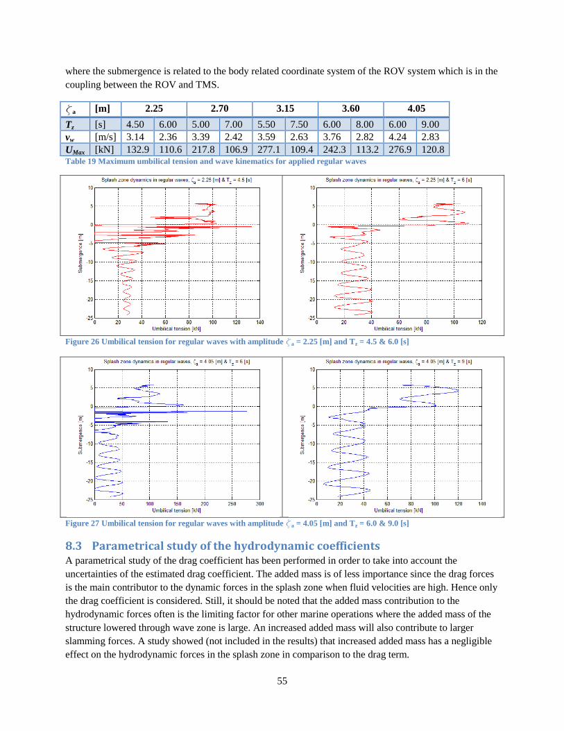
55
where the submergence is related to the body related coordinate system of the ROV system which is in the coupling between the ROV and TMS.
za [m] 2.25 2.70 3.15 3.60 4.05
Tz [s] 4.50 6.00 5.00 7.00 5.50 7.50 6.00 8.00 6.00 9.00 vw [m/s] 3.14 2.36 3.39 2.42 3.59 2.63 3.76 2.82 4.24 2.83 UMax [kN] 132.9 110.6 217.8 106.9 277.1 109.4 242.3 113.2 276.9 120.8 Table 19 Maximum umbilical tension and wave kinematics for applied regular waves
Figure 26 Umbilical tension for regular waves with amplitude za = 2.25 [m] and Tz = 4.5 & 6.0 [s]
Figure 27 Umbilical tension for regular waves with amplitude za = 4.05 [m] and Tz = 6.0 & 9.0 [s]
8.3 Parametrical study of the hydrodynamic coefficients
A parametrical study of the drag coefficient has been performed in order to take into account the uncertainties of the estimated drag coefficient. The added mass is of less importance since the drag forces is the main contributor to the dynamic forces in the splash zone when fluid velocities are high. Hence only the drag coefficient is considered. Still, it should be noted that the added mass contribution to the hydrodynamic forces often is the limiting factor for other marine operations where the added mass of the structure lowered through wave zone is large. An increased added mass will also contribute to larger slamming forces. A study showed (not included in the results) that increased added mass has a negligible effect on the hydrodynamic forces in the splash zone in comparison to the drag term.

56
Repeated lowering in irregular waves as well as regular wave analyses have been performed in order to compare the results with the drag coefficient of 2.5 [-]. In repeated lowering, the exact same wave realizations are applied for each parametrical study of drag coefficients in head sea where Tp = 10 [s] and Hs = 4.5 [m]. Table 20 shows simple statistics of the parametrical study in irregular sea while time histories of the umbilical tension are enclosed in Appendix B.2. Figure 28 shows the umbilical tension
when lowering in regular waves with ζa = 2.25 [m] and Tz = 6 [s] and different drag coefficients. Figure
28 can be compared to the results obtained for CD = 2.5 [-] in Figure 26.
Parametrical study of drag coefficients for repeated lowering through wave zone CD [-] 2.5 3.0 3.5 4.0 Minimum umbilical tension [kN] 5.51 0.73 0 0 Mean of minimum umbilical tension [kN] 16.89 15.83 14.51 8.19 # of slack umbilical occurences [-] 0 0 1 11 Maximum umbilical tension [kN] 109.19 109.19 109.19 116.77 Table 20 Statistics from parametrical study of drag coefficients in a sea state of Hs = 4.5 [m] & Tp = 10 [s]
Figure 28 Lowering through splash zone in regular waves with ζa = 2.25 [m] and Tz = 6 [s] and different drag coefficients
8.4 Discussion of results from SIMO
8.4.1 Comments on statistics
The statistics presented are found by examining the time histories in MATLAB. S2XMOD could also be used for presenting statistics, but it is far more convenient to find statistics in MATLAB because of the large number of simulations. The maximum umbilical tension has been implemented to a Gumbel and a Weibull probability paper, but for load cases which are dominated by large quadratic damping, impact forces and snap loads are these models not applicable; hence it has not been included in the results. Note also that calculation of extreme responses is not applicable for processes with a moving average or which includes transients [11]. Thus the standard deviation and estimates of the extremes by use of for example the Rayleigh distribution should not be performed when lowering a body trough splash zone. However, the standard deviations of the maximum umbilical tension for repeated lowering and recovery are included since they give the reader a better understanding of the load case.
8.4.2 Discussion of current operational limit
Stationary analyses A study of the time histories from the stationary analyses show that the upward acting hydrodynamic forces exceed the weight of the system frequently for the sea states of Tp = 6 – 8 [s], which cause snap loads in the umbilical, while for the other peak periods it is not seen any slack umbilical occurrences and consequently no snap loads. The largest peaks in the Tp range of 9 – 11 [s] are caused by impact forces and large quadratic drag. As expected, shows Table 15 that the mean and standard deviation of the umbilical

57
tension is decreasing for increasing peak period of the spectra. However, it should be noted that it is observed a slightly higher maximum umbilical tension for the peak period of 8 [s] compared to 7 [s], even though snap loads occur more frequently for the latter sea state. This may be explained by the non-linear behavior of snap loads and the larger relative motion between the tip of the launch and recovery system and ROV system for the sea state of 8 [s].
Repeated lowering through splash zone The largest umbilical tension for the sea states with peak periods if 6 [s] and 7 [s] are caused by slack umbilical causing snap loads while for the sea state of 8 [s] are the maximum tension caused by impact forces and quadratic drag. For the other sea states are the maximum umbilical tension caused by inertia force in air due to the heave acceleration at the tip of the LARS. From the time histories and statistics it can be seen that slack umbilical occur for the sea states within the peak period range 6 – 9 [s]. However, the snap loads in combination with the quadratic drag do not cause severe umbilical tension.
Repeated recovery through splash zone The maximum umbilical tension is due to water exit forces and quadratic drag when recovered through surface. In contrast to the lowering through splash zone, is it only seen one slack umbilical occurrence in the sea state with Tp = 6 [s] which do not cause any significant snap loads. However, it is seen that the umbilical tension may be exposed to larger tension during recovery in comparison to launch of the system.
Investigation of heading angles The investigation of heading angles has shown some interesting results with respect to the umbilical tension for different heading angles. Results from the Simplified Method, Chapter 7, have shown that the responses at the tip of the LARS may be larger for the heading angle of +15º compared to -15º and this is also seen in the results from SIMO where the roll motion clearly influence the results. It is not seen any slack umbilical occurrences for -15º while for the other heading angle are the umbilical slack in 7 out of 40 launches in the current sea state. This should be taken into consideration when determining an operational limit for launch and recovery of ROV, although the calculated snap loads are not severe. The maximum umbilical tensions for both heading angles are due to the weight of the ROV system in air and the heave acceleration at tip of the LARS.
8.4.3 Discussion of analyses in regular sea
By lowering the ROV system through splash zone in steep regular waves is it seen that the ROV system are subjected to large hydrodynamic forces causing slack umbilical and thereby extreme snap loads. However, waves with this amplitude and steepness rarely occur for the given significant wave height and should be taken into consideration when evaluating the operational limit for launch and recovery of ROV. The analyses in regular sea clearly show the hydrodynamic force dependency on the wave period. If a
nearly breaking wave in the most severe wave condition with an amplitude of ζa = 4.05 [m] and Tz = 6 [s]
approach, the ROV system will be lifted by the waves leading to severe snap loads. However, if the same wave amplitude with Tz = 9 [s] approach the ROV system the system will continue lowering without any slack umbilical occurrence. Similar behavior can be seen for the other sea states where zero umbilical tension induces snap loads. For the case of a regular wave amplitude of 2.25 [m] is the snap load calculated to 133 [kN] while for the other sea states the snap loads are equal to or larger than 218 [kN].
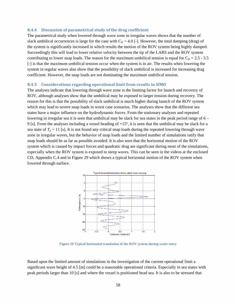
58
8.4.4 Discussion of parametrical study of the drag coefficient
The parametrical study when lowered through wave zone in irregular waves shows that the number of slack umbilical occurrences is large for the case with CD = 4.0 [-]. However, the total damping (drag) of the system is significantly increased in which results the motion of the ROV system being highly damped. Succeedingly this will lead to lower relative velocity between the tip of the LARS and the ROV system contributing to lower snap loads. The reason for the maximum umbilical tension is equal for CD = 2.5 - 3.5 [-] is that the maximum umbilical tension occur when the system is in air. The results when lowering the system in regular waves also show that the possibility of slack umbilical is increased for increasing drag coefficient. However, the snap loads are not dominating the maximum umbilical tension.
8.4.5 Considerations regarding operational limit from results in SIMO
The analyses indicate that lowering through wave zone is the limiting factor for launch and recovery of ROV, although analyses show that the umbilical may be exposed to larger tension during recovery. The reason for this is that the possibility of slack umbilical is much higher during launch of the ROV system which may lead to severe snap loads in worst case scenarios. The analyses show that the different sea states have a major influence on the hydrodynamic forces. From the stationary analyses and repeated lowering in irregular sea it is seen that umbilical may be slack for sea states in the peak period range of 6 – 9 [s]. From the analyses including a vessel heading of +15º, it is seen that the umbilical may be slack for a sea state of Tp = 11 [s]. It is not found any critical snap loads during the repeated lowering through wave zone in irregular waves, but the behavior of snap loads and the limited number of simulations ratify that snap loads should be as far as possible avoided. It is also seen that the horizontal motion of the ROV system which is caused by impact forces and quadratic drag are significant during most of the simulations, especially when the ROV system is exposed to steep waves. This can be seen in the videos at the enclosed CD, Appendix C.4 and in Figure 29 which shows a typical horizontal motion of the ROV system when lowered through surface.
Figure 29 Typical horizontal translation of the ROV system during water entry
Based upon the limited amount of simulations in the investigation of the current operational limit a significant wave height of 4.5 [m] could be a reasonable operational criteria. Especially in sea states with peak periods larger than 10 [s] and where the vessel is positioned head sea. It is also to be stressed that

59
experienced personnel should assess the wave conditions during deployment through splash zone. For sea states with a peak period lower than 10 [s] should the possibility of snap loads be taken into consideration, although it is not found any critical snap loads except for the stationary analysis in the most extreme sea state with Tp = 6 [s].
However, if considering the worst case scenarios in regular waves, it should be noted that the operational limit should be adjusted to a significant wave height of around 3.0 [m] in order to ensure a safe launch of the ROV system. The launch and recovery system has an alarm which switches on if the umbilical tension reaches 20 [tonne], and it is seen when lowering in nearly breaking regular waves corresponding to 0.9·Hs and 3 [m] significant wave height that the umbilical tension may be up to 22.2 [tonne]. On the other hand, should the operational limit be based upon irregular wave approach and not regular waves since the irregular sea states reflect realistic environmental conditions. It is highly unlikely that a wave with amplitude 2.7 [m] and zero crossing period of 5.5 [s] will approach the ROV system in this sea state, especially if the weather is assessed during deployment.
8.5 Comparison of results from Simplified Method and SIMO
It should be noted that the exact same hydrodynamic coefficients and structure properties of the ROV system and umbilical properties have been applied in the Simplified Method and SIMO.
The analytical results from DNV Recommended Practices have shown that the lowering through wave zone is impossible in a sea state of 4.5 [m] significant wave height and should only be executed in sea states up to Hs = 2.5 [m]. Even when applying significant responses are the acceptance criteria exceeded and extreme snap loads may occur in the sea state of Hs = 4.5 [m]. In contrast, the results from SIMO show that the operational limit of 4.5 [m] significant wave height could be justified. Though, it is seen that the hydrodynamic forces exceed the static weight of the ROV system leading to slack umbilical and consequently snap loads (which not have been found to be critical ) for sea states with low peak periods. One of the main problems of the analytical operational limit calculations is the low submerged weight of the ROV system which leads to a violation of the acceptance criteria for low upward acting hydrodynamic forces. Furthermore, the assessment of snap loads may be too conservative. In the calculation of snap loads are the benefits of using a time domain simulation program in comparison to the analytical approach seen clearly. More exact relative velocity between the ROV system and the LARS are calculated leading to more correct snap loads than the analytical method.
The results from the regular wave approach in SIMO have shown that the net upward acting hydrodynamic forces exceed the static weight of the ROV system for the lowest zero crossing periods, but as the zero crossing period increases there is not seen any slack umbilical occurrence. The same tendency for decreasing hydrodynamic forces is seen in the results from Simplified Method. However, the Simplified Method overestimates the hydrodynamic forces acting on the ROV system in comparison to SIMO. For instance, the results from Simplified Method show that the acceptance criteria is greatly exceeded for case 3 and case 4 and all zero crossing periods in waves equal to and above the sea state of Hs =3.0 [m]. In SIMO, when applying regular waves, there is seen that only the lowest periods induce zero umbilical tension and consequently snap loads.
The Simplified Method justifies its main purpose to give simple and conservative estimates of the forces acting in the wave zone. However, the results from SIMO have shown that marine operations which are

60
dependent on the weather conditions could truly benefit from a time domain calculation of the forces acting in the wave zone.

61
9 Conclusions
9.1 Conclusion
The author of this master thesis was completely unfamiliar with the time domain simulation program SIMO before starting the thesis and has spent a lot of time in order to be acquainted with the program. Multiple different crane operations, which not have been included in the report, have been investigated and the experience from modeling a complete marine operation in SIMO has given the author a good background for further use of SIMO. This is hopefully seen in the master thesis.
The SIMO system description file contains a complete description of the properties of the vessel Skandi Bergen by hydrodynamic coefficients and motion transfer function as found by VeRes, which can be useful for DOF Subsea for studying marine operations in SIMO. Chapter 6 which shows a step by step procedure for simulating marine operations in SIMO may be used for educational purposes or for future students planning to model their own marine operation in SIMO.
It has been a difficult task to establish the hydrodynamic properties of the ROV system because of lack of literature on the subject and the complexity of the ROV system. This has contributed to that the system’s hydrodynamic coefficients has been estimated based upon previously performed model tests for idealized subsea structures with similar properties as the ROV system. In this case it would have been very beneficial to run a model test for the ROV system in order to validate the assumptions and estimations of the hydrodynamic coefficients.
The investigation of operational limits by use of DNV-RP-H103 and SIMO have shown that DNV Recommended Practices over-estimates the hydrodynamic forces acting in the wave zone leading to a restrictive operational limit in comparison to the time domain calculations in SIMO. The calculations by the analytical method have shown that the operational limit for launch and recovery of ROV should be limited to 2.5 [m] significant wave height, while analyses in SIMO have shown that the current operational limit of 4.5 [m] could be justified. However, it is seen that the possibility for slack umbilical is present in the sea state of 4.5 [m] and peak periods in the range of Tp = 6 – 9 [s]. It is also to be noted that the slack umbilical occurrences show a thoroughly dependency of the vessel heading. Furthermore, the snap loads induced by the slack umbilical occurrences are not found to be critical in the irregular wave analyses. This can justify the operational limit of 4.5 [m] significant wave height as long as the weather is assessed by experienced personnel during deployment through wave zone and Skandi Bergen is positioned head sea. Note also that even more simulations could be performed in order to ensure a proper statistical confidence of the time domain calculations.
Videos which summarize the launch and recovery can be found at the enclosed CD, Appendix C.4.
9.2 Proposal for further work
The launch and recovery analyses by use of the DNV Recommended Practices and the time domain simulation program SIMO have introduced simplifications and estimations which lead to uncertainties in the analyses. The first priority should be to perform a model test in order to find the correct hydrodynamic coefficients which can be implemented to the analytical and time domain calculations of operational limit. The real stiffness of the hoisting system should also be quantified in order to analyze the severity of potential snap loads since this may be the limiting factor for launch and recovery of ROV. A possible new

62
time domain simulation by taking these factors into consideration could include an increased number of simulations in order to ensure a proper statistical confidence.
Regarding the calculations in SIMO it could be useful to make a MATLAB script which can communicate with SIMO in order to execute more efficient simulations. An unlimited number of simulations may be specified and a parametric study of for example hydrodynamic coefficients, heading angles and wave conditions could more easily be altered. The motions of Skandi Bergen are described by first order motion transfer functions implying that that the vessel is defined as body type 2 in SIMO. In order to include effects from impulse loads it could be better to model the ship as body type 1 implying that the motions are described by first order wave force transfer functions and retardation functions. This will contribute to a more realistic time domain simulation and make the system description file more applicable for heavy lift operations.
Another feasible task could be to obtain measured umbilical tension during an offshore deployment through splash zone and compare the measured umbilical tension with calculations in SIMO. This will also require evaluation of the sea condition.
63
10 References
1. DNV. DNV-RP-H103 Modelling and Analysis of Marine Operations. Det Norske Veritas. [S.l.]. 2010.
2. MARINTEK. VeRes, 30 April 2010. Available at: <http://www.sintef.no/Home/Marine/MARINTEK/Software-developed-at-MARINTEK/VERES/>.
3. MARINTEK. SIMO, 2009. Available at : <http://www.sintef.no/Home/Marine/MARINTEK/Software-developed-at-MARINTEK/SIMO/>.
4. MARINTEK. SIMO - User's manual Version 3.7. Trondheim. 2009.
5. SANDVIK, P. C.; SOLAAS, F. SimVis for SIMO - How to get started. MARINTEK. Trondheim. 2005.
6. ØRITSLAND, O. A summary of subsea module hydrodynamic data, 511110.05. MARINTEK. Trondheim. 1989.
7. DNV. DNV-RP-C205 Environmental conditions and environmental loads. [S.l.]: Det Norske Veritas, 2007.
8. FALTINSEN, O. M. Sea Loads On Ships and Offshore Structures. [S.l.]: Cambridge University Press, 1990.
9. MYRHAUG, D. Lecture notes in Stochastic Theory of Sea loads. NTNU. Trondheim. 2009.
10. NEWLAND, D. E. An introduction to random vibrations, spectral and wavelet analysis. [S.l.]: [s.n.], v. 3 edition, 1993.
11. MARINTEK. SIMO - Theory manual version 3.7. Trondheim. 2009.
12. ØRITSLAND, O.; LEHN, E. Hydrodynamic forces on subsea modules during lifting operations, 511003.02. MARINTEK. Trondheim. 1987.
13. ØRITSLAND, O.; LEHN, E. Hydrodynamic forces and resulting motion of subsea modules during lifting in the splash zone. Eigth International Conference on Offshore Mechanics and Arctic Engineering. The Hague: [s.n.]. 1989.
14. SAYER, P. Hydrodynamic loads during the deployment of ROV. Ocean Engineering, Glasgow, 2007.
15. MARINTEK. SIMO - User's manual Appendix A. Trondheim. 2009.
16. DNV. DNV Rules for Planning and Execution of Marine Operations. Det Norske Veritas. [S.l.]. 1996.

64

i
Appendices
Appendix figures
Appendix figure 1 Case study of hydrodynamic forces in a significant wave height of 2.0 [m] .................. ii Appendix figure 2 Case study of hydrodynamic forces in a significant wave height of 3.0 [m] ................. iii Appendix figure 3 Case study of hydrodynamic forces in a significant wave height of 3.5 [m] ................. iii Appendix figure 4 Case study of hydrodynamic forces in a significant wave height of 4.0 [m] ................. iv Appendix figure 5 Time histories and graphs of the max/min tension when Hs = 4.5 [m] & Tp = 6 [s] ....... v Appendix figure 6 Time histories and graphs of the max/min tension when Hs = 4.5 [m] & Tp = 7 [s] ...... vi Appendix figure 7 Time histories and graphs of the max/min tension when Hs = 4.5 [m] & Tp = 9 [s] ..... vii Appendix figure 8 Time histories and graphs of the max/min tension when Hs = 4.5 [m] & Tp = 10 [s] .. viii Appendix figure 9 Time histories and graphs of the max/min tension when Hs = 4.5 [m] & Tp = 11 [s] .... ix Appendix figure 10 Study of drag coefficient in a sea state of Hs = 4.5 [m] & Tp = 10 [s] and CD = 3.0 ..... x Appendix figure 11 Study of drag coefficient in a sea state of Hs = 4.5 [m] & Tp = 10 [s] and CD = 3.5 ..... x Appendix figure 12 Study of drag coefficient in a sea state of Hs = 4.5 [m] & Tp = 10 [s] and CD = 4.0 .... xi
Appendix figure 13 Umbilical tension in reg. waves with amplitude za = 2.70 [m] and Tz = 5.0 & 7.0 [s] xi
Appendix figure 14 Umbilical tension in reg. waves with amplitude za = 3.15 [m] and Tz = 5.5 & 7.5 [s]
..................................................................................................................................................................... xii
Appendix figure 15 Umbilical tension in reg. waves with amplitude za = 3.60 [m] and Tz = 6.0 & 8.0 [s]
..................................................................................................................................................................... xii
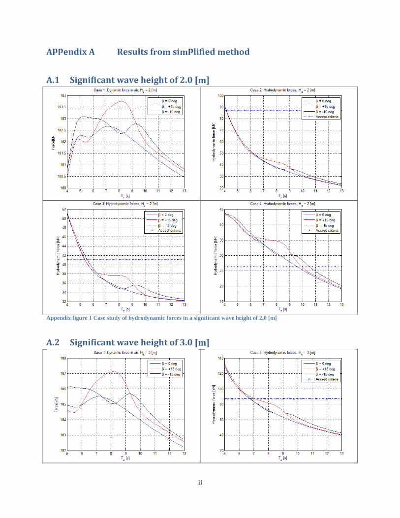
ii
Appendix A Results from simplified method
A.1 Significant wave height of 2.0 [m]
Appendix figure 1 Case study of hydrodynamic forces in a significant wave height of 2.0 [m]
A.2 Significant wave height of 3.0 [m]

iii
Appendix figure 2 Case study of hydrodynamic forces in a significant wave height of 3.0 [m]
A.3 Significant wave height of 3.5 [m]
Appendix figure 3 Case study of hydrodynamic forces in a significant wave height of 3.5 [m]
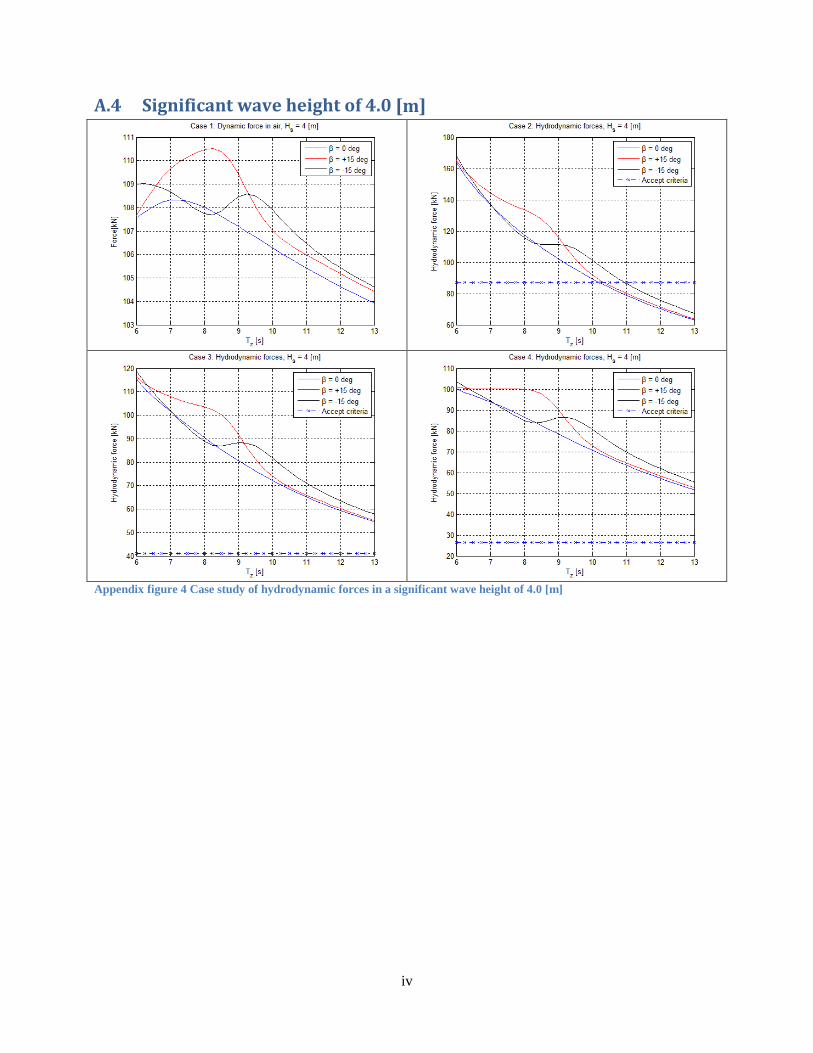
iv
A.4 Significant wave height of 4.0 [m]
Appendix figure 4 Case study of hydrodynamic forces in a significant wave height of 4.0 [m]

v
Appendix B Results from SIMO
B.1 Repeated lowering through splash zone
Appendix figure 5 Time histories and graphs of the max/min tension when Hs = 4.5 [m] & Tp = 6 [s]

vi
Appendix figure 6 Time histories and graphs of the max/min tension when Hs = 4.5 [m] & Tp = 7 [s]

vii
Appendix figure 7 Time histories and graphs of the max/min tension when Hs = 4.5 [m] & Tp = 9 [s]
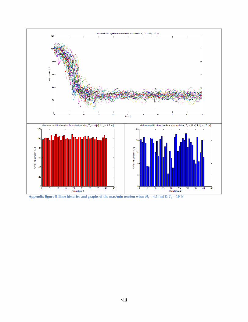
viii
Appendix figure 8 Time histories and graphs of the max/min tension when Hs = 4.5 [m] & Tp = 10 [s]

ix
Appendix figure 9 Time histories and graphs of the max/min tension when Hs = 4.5 [m] & Tp = 11 [s]

x
B.2 Parametrical study of drag coefficient
Appendix figure 10 Study of drag coefficient in a sea state of Hs = 4.5 [m] & Tp = 10 [s] and CD = 3.0
Appendix figure 11 Study of drag coefficient in a sea state of Hs = 4.5 [m] & Tp = 10 [s] and CD = 3.5
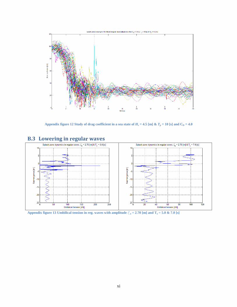
xi
Appendix figure 12 Study of drag coefficient in a sea state of Hs = 4.5 [m] & Tp = 10 [s] and CD = 4.0
B.3 Lowering in regular waves
Appendix figure 13 Umbilical tension in reg. waves with amplitude za = 2.70 [m] and Tz = 5.0 & 7.0 [s]

xii
Appendix figure 14 Umbilical tension in reg. waves with amplitude za = 3.15 [m] and Tz = 5.5 & 7.5 [s]
Appendix figure 15 Umbilical tension in reg. waves with amplitude za = 3.60 [m] and Tz = 6.0 & 8.0 [s]

xiii
Appendix C Contents on CD
C.1 Veres folder
• input.re7: Hydrodynamic coefficients for Skandi Bergen • input.re1: Motion transfer functions for Skandi Bergen
• zerofreq.re7: Hydrodynamic coefficients for Skandi Bergen at 200 [s]
C.2 MATLAB folder
• SimplifiedMethod.m: Calculation of response spectra and case study of launch of ROV • ROVmodel.m: Calculation of ROV geometry by slender elements • TMSmodel.m: Calculation of TMs geometry by slender elements • RAOcalculation: Calculation of heave RAO at tip of LARS, subfolder • RAOct0_SB.txt: Heave RAO at tip of LARS for head sea • RAOct15_SB.txt: Heave RAO at tip of LARS for +15º • RAOct_345_SB.txt: Heave RAO at tip of LARS for -15º
C.3 Documents folder
• Project_thesis_MV: Project thesis from fall 2009 • Master_thesis_MV: Master thesis spring 2010
C.4 Visualization folder
• Launch_atypical.avi: ROV system lowered through splash zone and exposed to steep waves in Hs = 4.5 [m] & Tp = 8 [s]
• Launch_typical.avi: ROV system lowered through splash zone in a typical wave condition in Hs = 4.5 [m] & Tp = 8 [s].
• Recovery.avi: Recovery of the ROV system in a typical wave condition in Hs = 4.5 [m] & Tp = 8 [s].
C.5 SIMO folder
• Lowering in irregular sea folder*: Batch file, DYN(1-40), STA, S2X, sys-ROV.dat • Recovery in irregular sea folder*: Batch file, DYN(1-40), STA, S2X, sys-ROV.dat • Stationary analyses folder: DYN, STA, sys-ROV.dat • Lowering in regular sea folder: DYN, STA, sys-ROV.dat
• Study of drag coefficients folder**: sys-Cd25.dat, sys-Cd30 .dat, sys-Cd35.dat, sys-Cd40.dat
* Contains 40 different *.MAC files for specification of random phase angles and batch file for execution of multiple simulations
** Contains system description files for different drag coefficient of the ROV system.

xiv
C.6 SimVis folder - visualization.svp: The SimVis project file for simulation/visualization of marine operations