Master+Thesis+M_Viktorovic.pdf - UPCommons
67
Load-shifting inside production lines Page 1 This thesis will have the goal to investigate possibilities for optimization of schedules of factory s production lines, to minimize the cost of electrical energy used. During this research, different operational constrains will have to be identified and taken into account, during optimization. At the end, based on discovered limitations, and other necessary assumptions, models for factory process will be devised in order to be optimized based on suitable algorithms. Acknowledgments I would like to thank my supervisor, Andreas Sumper for guiding and supporting me over the year spent in Barcelona. Special thanks here go to Luisa and Tomas, who have been, not only my supervisors, but my support through all the project, and who have taught me so much. I am proud that I have been your intern! I would like to thank my colleagues from Accenture team, based in Barcelona CoE for all of their guidance through this process; your discussion, ideas, and feedback have been absolutely invaluable. And finally I'd like to thank my fellows from Smart Cities and other KIC InnoEnergy program, and the multitude of other local and international friend who made my life in this city full of joy. I am very grateful to all of you. Thank you!
-
Upload
khangminh22 -
Category
Documents
-
view
4 -
download
0
Transcript of Master+Thesis+M_Viktorovic.pdf - UPCommons

Load-shifting inside production lines Page 1
This thesis will have the goal to investigate possibilities for optimization of schedules of
factory s production lines, to minimize the cost of electrical energy used. During this research, different operational constrains will have to be identified and taken into account, during optimization. At the end, based on discovered limitations, and other necessary assumptions, models for factory process will be devised in order to be optimized based on suitable algorithms.
Acknowledgments
I would like to thank my supervisor, Andreas Sumper for guiding and supporting me over the year spent in Barcelona.
Special thanks here go to Luisa and Tomas, who have been, not only my supervisors, but my support through all the project, and who have taught me so much. I am proud that I have been your intern!
I would like to thank my colleagues from Accenture team, based in Barcelona CoE for all of their guidance through this process; your discussion, ideas, and feedback have been absolutely invaluable.
And finally I'd like to thank my fellows from Smart Cities and other KIC InnoEnergy program, and the multitude of other local and international friend who made my life in this city full of joy. I am very grateful to all of you.
Thank you!

Page 2
ABSTRACT ___________________________________________________ 1 SUMMARY ___________________________________________________ 2 1. INTRODUCTION (STATING OBJECTIVES) _____________________ 5
1.1. Thesis structure ............................................................................................. 5 2. PROBLEM DESCRIPTION ___________________________________ 7
2.1. Process definition ........................................................................................... 7 2.2. Optimization goals ......................................................................................... 8 2.3. Production-chain constrains ......................................................................... 10
2.3.1. Beer game problem ......................................................................................... 10 2.4. Visualisation ................................................................................................. 11
3. OPTIMIZATION TECHNIQUES ______________________________ 12 3.1. Cross-correlation .......................................................................................... 12 3.2. Heuristic algorithms ..................................................................................... 13
3.2.1. Simulated annealing ........................................................................................ 14 3.3. Linear programming ..................................................................................... 15
4. METHODOLOGY PROPOSED ______________________________ 17 4.1. Cloud platform .............................................................................................. 17
4.1.1. Microsoft Azure ................................................................................................ 18 4.1.2. Stream Analytics .............................................................................................. 19 4.1.3. Azure Machine learning ................................................................................... 20
4.2. Optimization Script ....................................................................................... 20 4.2.1. R programing language ................................................................................... 21 4.2.2. AMPL ............................................................................................................... 22
4.3. Visualisation ................................................................................................. 23 4.3.1. Microsoft Power BI ........................................................................................... 23
5. APPLICATION EXAMPLE __________________________________ 26 5.1. Constrains .................................................................................................... 26 5.2. Model ........................................................................................................... 27 5.3. Process data acquisition and optimization ................................................... 28 5.4. Cloud integration .......................................................................................... 30

Load-shifting inside production lines Page 3
5.5. Dashboard .................................................................................................... 31 6. RESULTS AND DISCUSSION _______________________________ 39
6.1. Scenario 1 .................................................................................................... 40 6.2. Scenario 2 .................................................................................................... 41 6.3. Economic analysis ........................................................................................ 43
6.3.1. Expenditures and initial investment cost ......................................................... 45 6.3.2. Revenues ........................................................................................................ 46 6.3.3. NPV for Scenario 1 ......................................................................................... 47 6.3.4. NPV for Scenario 2 ......................................................................................... 47
6.4. Environmental impact ................................................................................... 49 7. CONCLUSION ___________________________________________ 50
7.1. Algorithm ...................................................................................................... 50 7.2. Technical feasibility ...................................................................................... 51 7.3. Economic feasibility ...................................................................................... 51 7.4. Future developments .................................................................................... 52
NOTES _____________________________________________________ 53 8. REFERENCES ___________________________________________ 54 9. TABLE OF FIGURES ______________________________________ 56 10. APPENDIX ______________________________________________ 59
10.1. Energy analytics dashboard ......................................................................... 59 10.2. Azure AWS comparison ............................................................................ 63

Page 4
Load-shifting inside production lines

Load-shifting inside production lines Page 5
1. Due to increasing penetration of renewables, in near future we will wittiness increasing
need to adjust our consumption. Modern electrical networks will use different types of control algorithms to keep the network stability during periods of high generation, especially in solar and wind plants. At certain point this will, for sure, lead to incentives for users who are willing to adjust their load, in order to help DSO and TSO keep the demand-production stable.
As manufacturing industries, are the biggest consumers of electrical energy, their ability to adjust their demand would be crucial. This is also the hardest part to adjust, since there are many constrains inside production process.
Solution to this problem is in full automatization of production lines, and their optimization, based on different energy related cost-functions.
Objectives of this thesis will be: Research optimization techniques Propose solutions Investigate feasibility of the solutions developed Give conclusions about general end to end solution
In order to do this, author will present possible solutions, according to his research. After propositions, one solution will be chosen to be fully developed for the reasons that author will explain during this thesis.
In the end, feasibility, both technical and economical will be investigated, for the developed project.
1.1. Thesis structure This thesis will be divided into several chapters in order to concisely explain different
aspects of the project, form the academic point of view. This chapters will be: Problem description Optimization techniques Methodology proposed Application example Results and discussion Conclusion

Page 6 M. Viktorovi
And each of them will explain one aspect of the work done, as follows: 1. Problem description will define main idea, and constrains r5elated to this project, as
well some main definitions and assumptions that the reader can comprehend the overall idea behind the whole project.
2. In the part of Optimization techniques main optimization algorithms will be cover, together with short explanation about mathematical problem they are trying to optimize.
3. Methodology proposed will focus mainly on the tools and techniques used in order to implement the overall solution, based on previously mentioned goals and optimization techniques Comparison of the software tools will be given together with the reasons why a certain tool or method has been chosen.
4. Application example chapter will cover the actual implementation of the previously proposed methodologies, using proposed tools, based on the real-case application.
5. Chapter Results and discussion will tackle performance of the optimization from the economical point of view, together with simplified cost analysis of the solution. Also in this part future development ideas will be proposed and discussed.
6. In the Conclusion, problems related to the project will be discussed, as well the overall success of it.
Load-shifting inside production lines Page 7
2. Production lines are very specific when it comes to scheduling, due to many
dependencies between different processes within the same production line. For this reason it is necessary to model processes within the production line, in such a way so that we can schedule individual process as optimal as possible within given constrains.
2.1. Process definition For the sake of modelling, basic terms need to be properly defined in order to have
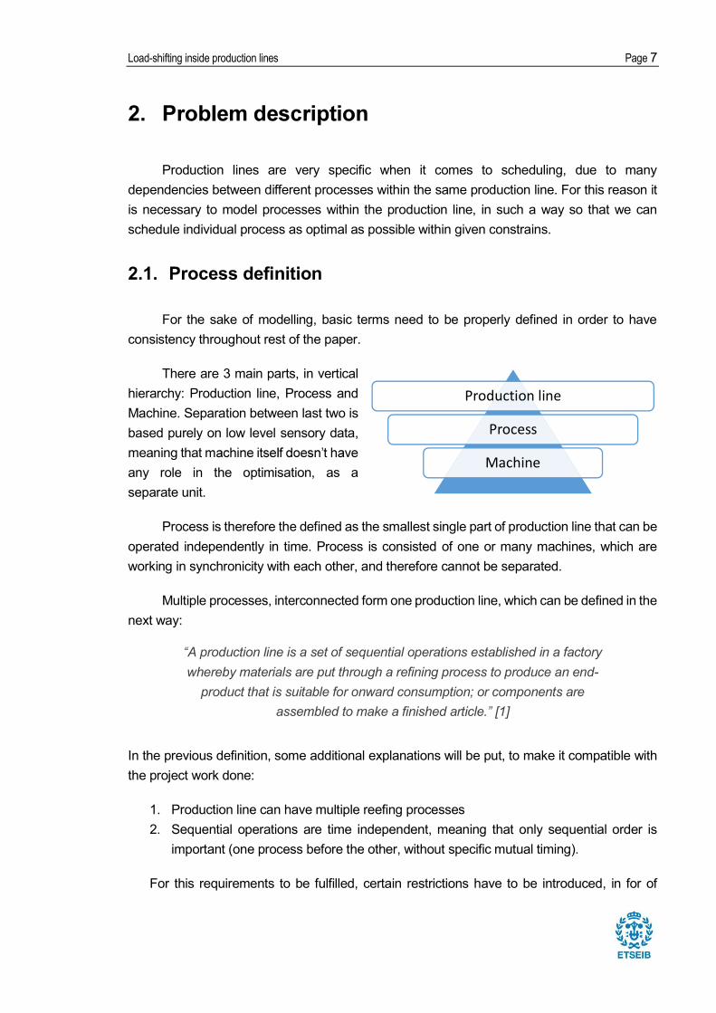
consistency throughout rest of the paper. There are 3 main parts, in vertical
hierarchy: Production line, Process and Machine. Separation between last two is based purely on low level sensory data, meaning that any role in the optimisation, as a separate unit.
Process is therefore the defined as the smallest single part of production line that can be operated independently in time. Process is consisted of one or many machines, which are working in synchronicity with each other, and therefore cannot be separated.
Multiple processes, interconnected form one production line, which can be defined in the next way:
A production line is a set of sequential operations established in a factory whereby materials are put through a refining process to produce an end-
product that is suitable for onward consumption; or components are assembled to make a finished article. [1]
In the previous definition, some additional explanations will be put, to make it compatible with the project work done:
1. Production line can have multiple reefing processes 2. Sequential operations are time independent, meaning that only sequential order is
important (one process before the other, without specific mutual timing). For this requirements to be fulfilled, certain restrictions have to be introduced, in for of
Production lineProcess
Machine

Page 8 M. Viktorovi
process constraints. While modelling constrains, we can separate them into two groups. First ones are fixed constrains like:
Working hours Maximum allowed power
Second group are semi-fixed or dependent constrains which change based on required inputs and outputs of the production line, or specific process. For example:
Production input (units/hour) Production output (units/hour)
In optimization of the whole production, these ones would be referred as first and second-stage variable within the optimization function. Second-stage variables would be scenario dependent, while first-stage ones would be fixed before decision on scenario, or on this case output production of the whole line / factory would be made.
Figure 1 shows the simple example of production line, consisting of 3 processes, where
time constrains are reflecting working hours of the factory (4 to 19h) and the other constrain is Later in the
paper, optimal scheduling of this example will be shown.
2.2. Optimization goals Goal of optimization in this project is to make the optimal schedule of the connected
processes in production line, based on hourly electricity prices, on spot markets in Europe. Idea is that, by adjusting schedules of the different processes we can achieve savings while buying electricity on spot markets, since we would consume more in lower-price periods.
Figure 1 Example of 3 processes in production line

Load-shifting inside production lines Page 9
In mathematical terms, this would mean minimising the cost function, within given constrains for the processes:
How this looks in practice we can see on the example of hourly prices in NordPool spot market in Denmark:
Figure 2 NordPool Spot hourly market prices in Denmark
In this case it is clearly visible that due to high prices, we should avoid putting high load between 9 and 10 o´clock in the morning, while we could try to shift it between hours 15 and
we took into account only process lasting for one hour.
Nevertheless the idea is the same with complicated processes, with a difference that we would compare two functions of time, or time-series, and we would try to make the cross-correlation factor as minimal as possible, within some constrained time period.
The above mentioned cross-correlation is a good tool for explanations, since it gives scaled result of -1 in case functions are oppositely correlated, which in our case means, biggest consumption in the moments of lowest price [2].

Page 10 M. Viktorovi
2.3. Production-chain constrains Top level optimization would have to take into account outputs of each individual
process, so that consistency of the production stays intact. Great example of this problem is demonstrated through a strategic , and developed at MIT [3] in order to demonstrate supply chain management problems.
Although the idea behind the game is to show how supply chain functions, it can be perfectly applied to production line, if we consider each process as an individual part of supply chain, where the end consumer is the actual projected output of the whole production line.
Figure 3 Beer game supply chain simulation
As we can see on the Figure 3, if we would exchange the names of the factory, warehouse, etc., by names of the processes we would get one example of the simple production line, where demand would be actual projected output of our production. 2.3.1. Beer game problem
When taking into account top level optimization of the production process, intermediate steps should be considered, like storage cost, in case of the increased time gap in operation two processes. This and other process management constrains are well described in the
-

Load-shifting inside production lines Page 11
fulfil incoming orders of beer by placing orders with the next upstream [3].
In problem of load shifting in production, output of one process has to be taken into account when scheduling the next one, due to interconnections in-between processes.
Adding all of this extra conditions, de facto changes and complicates our cost function we are trying to optimize.
2.4. Visualisation Beside the optimization of scheduling, aim of the project was also to visualise different
KPIs related to electrical energy consumption. Demands in this area were not clearly defined, but that used visualisation techniques and tools have to allow enough flexibility in order to be customised for specific industry domains.
Key points here are: Choice of the tools for development of flexible visualisation Choice of platform supporting chosen tool Definition of required KPIs Possibility of real-time operations
Importance of visualisation has been stressed not only by potential clients but also by various studies, of which one is saying:
, provided by energy monitors, [4]
Meaning that well defined KPIs and visuals can give us more insights, especially in terms of comparing similar processes and benchmarking their performances.

Page 12 M. Viktorovi
3. Main goal of optimization in this project is to minimize the price of electricity when buying
it on the hourly spot market. In order for this to be achieved, algorithms are supposed to devise scheduling for each process within the production line, in order to shift higher consumption periods, into time slots with lower electricity price.
For this purpose, several approaches can be used. Investigated ones were using: 1. Cross-correlation 2. Heuristic optimization algorithms 3. Linear programming
All of this approaches have a goal to find the starting time ti of the process, so that product of consumption Ci(t) and price P(t), for all processes i, be minimal. In mathematical terms, function that has to be minimised is:
Taking into account all constrains of the processes and their dependencies.
3.1. Cross-correlation This method is good when you need to optimize only one process, or multiple
independent processes. But since is method that requires n2 calculations, it is not the most optimal, especially when you have more complex constrains.
-correlation is a measure of similarity of two series as a function of the lag of one relative to the
[2] Figure 4 Cross-correlation (r) of two signals (x & y)

Load-shifting inside production lines Page 13
Idea behind this approach is to use properties of cross correlation, like it has been done in signal theory [2] to calculate delay of the signal. By definition cross correlation is:
Where n is the lag of second discrete signal.
Approach with cross correlation is to compare consumption function and price function, in the given time-range in order to determine the minimal value of normalized cross-correlation function. At this (minimal) point two functions are, in ideal case, opposite in relation to their amplitude values. For us, this is significant because we want to find shift, where our two functions (consumption and price) are in different phase, so that their product is the smallest possible.
cross-correlation function indicates the point in time where the signals are [2]
Using this feature of cross-correlation we can determine the shift of the process electrical load by simply calculating minimum argument of cross correlation function of consumption C and price P:
As seen on the Figure 4, signal y should be shifted by 3 unites (of time), which is also the argument of maximum of correlation function r in order to overlap with signal x.
3.2. Heuristic algorithms Heuristic algorithms are based on partial search of function minimums or maximums.
These algorithms are taking specific assumptions while searching for function extremums, therefore reducing the number of calculations, but decreasing the probability of getting the
usages is acceptable, compared to decrease of computation requirements [5]. In metaheuristic algorithms we can distinguish two types, based on number of
dimensions of the search. These two types are:

Page 14 M. Viktorovi
1. Single solution o Simulated annealing o Iterated local search o Variable neighbourhood search o Etc.
2. Population-based o Evolutionary computation o Genetic algorithms o Particle swarm optimization o Etc.
Single solution approaches focus on modifying and improving a single candidate solution, while population-based approaches maintain and improve multiple candidate solutions, often using population characteristics to guide the search [5]. 3.2.1. Simulated annealing
Simulated annealing is on of techniques of estimating the global minimum or maximum of given function. It is a representative of single solution heuristic optimization algorithms. Typical
discrete functions, within limited time or number of computations. Basic idea comes for metal casting process, called
to be controlled in order to keep the best arrangement of atoms in metal´s molecular structure [6].
From optimization point of view algorithm uses random steps, for which it calculates
the cost, which is then accepted with a certain probability, which is oppositely correlated to
LET S = S0 // FIRST SOLUTION CAN BE RANDOM FOR (K = 0 TO KMAX ) // EXCLUSIVE
KMAX) // TEMP. ADJUSTMENT SNEW // PICK A RANDOM NEIGHBOUR IF P(E(S), E(SNEW // MOVE TO THE NEW STATE:
NEW OUTPUT S //NEW STATE OUTPUT
Figure 5 Simulated annealing pseudo code [6]

Load-shifting inside production lines Page 15
randomised steps, probability of worse solution being accepted is higher (temperature is lower).
3.3. Linear programming Linear programing or linear optimization is a technique for maximization or minimisation
of the cost function, in a mathematical model base1d on linear relationships. In case of models with more complicated relationships, costs function can be represented as a combination of multiple linear relationship function, and then this model can be optimized using linear programming [7].
Linear programs are problems that can be expressed in canonical form as
where x represents the vector of variables (unknown), c and b are vectors of coefficients, A is a (known) matrix of coefficients, and cT is the matrix transpose of c. Constrains
, are specifying the convex polytope at which the cost function is to be optimized [7].
used in business and economics, and is also utilized for some engineering problems. Industries that use linear programming models include
transportation, energy, telecommunications, and manufacturing. It has proved useful in modelling diverse types of problems in planning, routing,
sched [8]
A linear programming problem was defined as maximizing or minimizing a linear function subject to linear constraints. All such problems can be converted into the form of a standard maximum problem [7]. Techniques for this are:
A minimum problem can be changed to a maximum problem by multiplying the
Constraints of the form can be changed into the form
When applying mentioned techniques, two problems may arise: 1. Some constraints may be equalities in this case one constraint and one variable
can be removed by solving the constraint for xj where aij is different form 0.

Page 16 M. Viktorovi
2. Variables may not be restricted to be nonnegative the unrestricted variables can be substituted by difference of two nonnegative variables. This adds one variable and two nonnegativity constraints.
As in previous chapters, optimization function is simplified, to product of price and consumption:
With a given constrains: Each process must start exactly once. Processes must start in predetermined order Processes must finish before its predetermined finishing time Processes must not start before its predetermined starting time Processes must finish before predetermined final hour (end of shift).
Figure 6 Process constraints explained

Load-shifting inside production lines Page 17
4. For the purpose of project development in the company, whole infrastructure had to be
planed and developed. As the project I join venture between two companies, roles have been shared in such a way, that one company provided hardware while author, as the representative of the other company had to devise the schematics of the whole cloud based solution (in collaboration with all stakeholders), together with optimization algorithm.
For this purpose some main parts of the infrastructure had to be built:
1. Cloud platform 2. IoT sensor infrastructure 3. Data model 4. Optimization algorithm 5. Visualisation
In the given list, author was in charge of developing last three points, and partially
develop cloud platform solution. During the project development, priorities have been changing, due to potential-
customer requirements, so decision was made to follow the top-down approach, meaning that
rest of the points should be based on the requirements of visualisation. Nevertheless in this work, author will follow the original order of priorities in order to make
logical interconnections.
4.1. Cloud platform Nowadays cloud based solutions are becoming increasingly popular due to their
scalability and simplicity of use [9]. computing is a type of Internet-based computing that provides
shared computer processing resources and data to computers and other devices on demand. It is a model for enabling ubiquitous, on-demand
access to a shared pool of configurable computing resources, which can [10]
This was the obvious choice or the project development for multiple reasons. First reason is simplicity, since actual hardware infrastructure maintenance is left to the platform provider. Second reason is scalability, which is very important due to the nature of the project, which means that in later phases of project, certain resources can be easily adopted to new
Page 18 M. Viktorovi
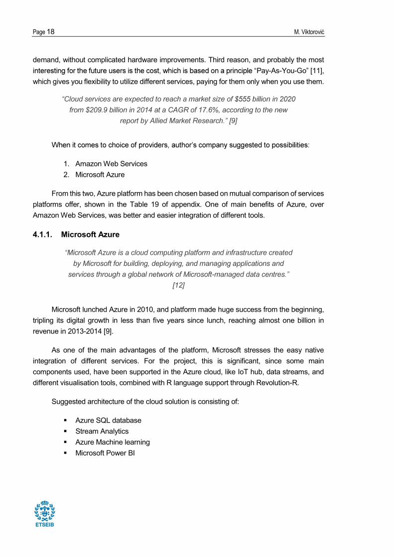
demand, without complicated hardware improvements. Third reason, and probably the most Pay-As-You-Go [11],
which gives you flexibility to utilize different services, paying for them only when you use them.
from $209.9 billion in 2014 at a CAGR of 17.6%, according to the new [9]
1. Amazon Web Services 2. Microsoft Azure
From this two, Azure platform has been chosen based on mutual comparison of services platforms offer, shown in the Table 19 of appendix. One of main benefits of Azure, over Amazon Web Services, was better and easier integration of different tools. 4.1.1. Microsoft Azure
by Microsoft for building, deploying, and managing applications and services through a global network of Microsoft-
[12]
Microsoft lunched Azure in 2010, and platform made huge success from the beginning, tripling its digital growth in less than five years since lunch, reaching almost one billion in revenue in 2013-2014 [9].
As one of the main advantages of the platform, Microsoft stresses the easy native integration of different services. For the project, this is significant, since some main components used, have been supported in the Azure cloud, like IoT hub, data streams, and different visualisation tools, combined with R language support through Revolution-R.
Suggested architecture of the cloud solution is consisting of: Azure SQL database Stream Analytics Azure Machine learning Microsoft Power BI

Load-shifting inside production lines Page 19
Figure 7 Proposed Azure architecture
4.1.2. Stream Analytics Azure stream analytics is chosen in order to be link betwe -
approach and real-time results representation. Unfortunately due to lack of data in the current stage of the project, this tool will be used only for direct real-time visualisation of different sensor data, because of its natural connection with Power BI reporting tool.
-cost solutions to gain real-time insights from devices, sensors, infrastructure,
and applications. Use it for Internet of Things (IoT) scenarios, such as real-time remote management and monitoring or gaining insights from devices
[13]
According to Microsoft, main features and abilities of this service are: Perform real-time analytics for your Internet of Things solutions Stream millions of events per second Get mission-critical reliability and performance with predictable results Create real-time dashboards and alerts over data from devices and applications Correlate across multiple streams of data Use familiar SQL-based language for rapid development

Page 20 M. Viktorovi
4.1.3. Azure Machine learning Azure ML is a tool developed to make implementation of machine learning algorithms less
complicated on the cloud platform. For this project, service was chosen because of support for programming languages like Python and Revolution-R.
a web service that can be called from any device, anywhere and that can
Other than this language support, service offers fast and intuitive, previously developed, code implementation. This future was important to the company, because of familiarity of employees with mentioned languages, so easy implementation and transition to other platform is a great benefit.
4.2. Optimization Script Optimization algorithm is the heart of this project when it comes to the importance.
Although just a small part of the whole project this essential component is the biggest added value in this end-to-end solution. Through project, this part has been changed many times, in order to improve its performance. Starting from basic R scripts, visualized using Shiny studio tool, it evolved to multi-script solution running on the Azure Machine learning.
As shown in the Figure 7, R scripts should run within Machine Learning service on the cloud, in a way that they are connected to SQL data storage from which they collect the information, which they process and then write back to the same database.
Proposed solution involves multi-script algorithm, consisting of three main parts: 1. Script for reading and formatting data from SQL database 2. Optimization script (with corresponding sub-scripts) 3. Script for formatting and writing data to SQL database

Load-shifting inside production lines Page 21
Scripts 1 and 3 are quite similar, and they require SQL coding, that can be done either through ETL tools in Azure Machine Learning, or through R script. Script 2 has been developed completely in R programming language, due to its simplicity and speed in processing reasonable amounts of data.
After discussion with people from the company, decision has been made to proceed with method of linear programming, which has been proposed as one of possible optimization techniques. For this
rogramming
necessary for optimization.
4.2.1. R programing language For the purpose of developing optimization algorithm, R programming language has been
used, primarily because of its good data handling abilities. [14]. When comparing R to some other competing languages, main advantages that come out straight away are [15]:
interactive language data structures graphics missing values functions as first class objects packages community
Taking this into account, and some extra tools, like Shiney, which allows you to make interactive web apps or data reports, R has proven to be quite handy for data analytics.
[15]
As main competitor, Python comes as other good solution, but due to availability of R experts in the company, R has chosen, although they have pretty much the same scores in most benchmarks, and they equally good int6egration with previously mention Azure cloud solutions. For engineers, R might be slightly more intuitive due to the fact it is, according to the author, very similar to Matlab.
Figure 8 Representation of relations in optimization script
Model of the processesAMPL
R execution script
Page 22 M. Viktorovi
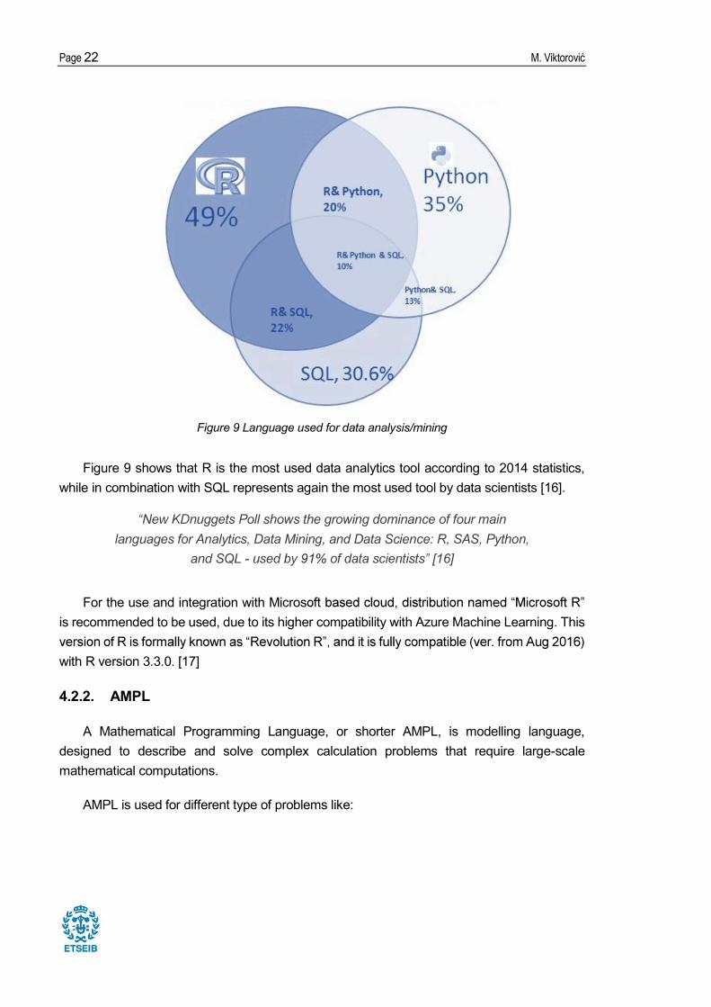
Figure 9 Language used for data analysis/mining
Figure 9 shows that R is the most used data analytics tool according to 2014 statistics, while in combination with SQL represents again the most used tool by data scientists [16].
nuggets Poll shows the growing dominance of four main languages for Analytics, Data Mining, and Data Science: R, SAS, Python,
and SQL - [16]
For the use and integration with Microsis recommended to be used, due to its higher compatibility with Azure Machine Learning. This
with R version 3.3.0. [17] 4.2.2. AMPL
A Mathematical Programming Language, or shorter AMPL, is modelling language, designed to describe and solve complex calculation problems that require large-scale mathematical computations.
AMPL is used for different type of problems like:

Load-shifting inside production lines Page 23
Linear programming Quadratic programming Nonlinear programming Mixed-integer programming Mixed-integer quadratic programming with or without convex quadratic constraints Mixed-integer nonlinear programming Second-order cone programming Global optimization Semidefinite programming problems with bilinear matrix inequalities Complementarity theory problems (MPECs) in discrete or continuous variables Constraint programming
Figure 10 AMPL lifecycle flow
For developed project, first point, linear programming is the part that will be used. Also, since regular AMPL requires 3rd party solver, instead of official release [18], packdeveloped for R should be utilized. This package uses similar interface as AMPL, but with zero cost for the licence, which makes it tool of a choice for development of models.
4.3. Visualisation Market currently offers couple of Visualisation tools, that can utilised on this project. Two
main competitors here are Power BI and Tableau. Choice of one of these is based primarily on other parts of the solution, in our case, the cloud solution by Microsoft. Since the same company is developing the Power BI and Azure Cloud, it was natural to consider this combination as the primary one. 4.3.1. Microsoft Power BI
This powerful tool has been developed by Microsoft in order to compete with different
integration with the rest of Microsoft Azure tools and services.

Page 24 M. Viktorovi
Figure 11 Comparison between data visualization tools [19]
As already mention in the previous chapter, because of requirements of the company, this tool has been chosen in the first step, as the opposite to logical order, where the visualisation tool choice should come in later stages of the project.
visualisation on the market in recent years. [19] As seen on the Figure 11, Power BI is leading in the innovations in the field of reporting tools.
When it comes to economic feasibility, Power BI is much cheaper tool, which offers more. Licence for Power BI Pro is 9.99$ per month per user (~120$/year), while Tableau is 1999$ per year, with Power BI being better in next areas, according to proficient users [19]:
Integration and sharing What really makes PBI powerful is the sharing options it provides. These allow the segmentation of users we want to send information to,
Data sources and modelling
tables, add columns and rows, import from one table to the other, join, filter and

Load-shifting inside production lines Page 25
Custom visuals
DAX (Data Analysis) expressions - calculated fields, new columns, aggregations, changes to data formats and
Table 1 Differences between Free ver. and Power BI Pro
On top of the mentioned advantages, Power BI has a free version, which has almost all the features of Pro version, just with limited amount of data. Plus Microsoft publishes update, with new features, in average every two weeks [19].
Description Free Pro
Data r
efresh
Consume content that is scheduled to refresh 10K rows/h 1M rows/h
Consume streaming data in your dashboards and report Consume live data sources with full interactivity Access on-premises data using the Data Connectivity Gateways
Collab
oratio
n
Collaborate with your team using Office 365 Groups in Power BI Create, publish and view organizational content packs Manage access control and sharing through Active Directory groups Shared data queries through the Data Catalogue Control data access with row-level security for users and groups

Page 26 M. Viktorovi
5. Optimization of this kind can be done inside any energy intensive industry that has
possibility to make their working schedule a bit flexible. In the era of complete automatization, optimization of schedules can be done in more flexible way, up to the point where factories become real prosumers and not just pure consumers of electrical energy.
5.1. Constrains
Figure 12 Example process hierarchy
For primary demonstration purposes, factory with a production line consisting of three processes has been chosen. This simple model consists of three groups of machines (usually marked as M1, M2 and M3), interconnected in a way that process 1 and 2 must be done before process 3 starts, like in Figure 12.
In terms of mathematical constrains this means:
Where tstart and tfinish represent starting and finishing hour of processes. Adding some logical constrains that process cannot be finalized its work before it has
started, we get three extra conditions:
M3M1M2

Load-shifting inside production lines Page 27
between 4am to 7pm. So we add this constrain as well to our model:
5.2. Model In order to create model for processing in AMPL and R, we need production constrains,
defined previously. This constrains should be transferred into matrix format in order to be calculated inside the model.
For order of processes we have the matrix form in which values A(i,j) = 1 represents that process i must be finished before process j.
In given example that would mean:
or in or of a matrix form:
Now, with matrix like this we can form our model our process, with of course adding the set of parameters for working hours constrains in form of arrays:
Process ID Start of working hours
1 4 2 4 3 4
Process ID Start of working hours
1 19 2 19 3 19

Page 28 M. Viktorovi
5.3. Process data acquisition and optimization After accounting for all of the time constrains, next step is use data mining to get working
hours of the processes. This is done easily by setting threshold for consumption, so that when consumption is bigger than certain value, we say that machine is working. Here small complication can be the fact that different machines inside process have multiple sensors, in which case we need to aggregate their values in form of a sum of their consumptions per unit of time.
This can be seen in the data model represented in the Figure 13.
Figure 13 Proposed data model
In used algorithm we have used time scale in hours because of simplicity, but resolution can be increased by simple aggregation of data on the level of any smaller time period. In this case, data for the electricity prices should have the same resolution.

Load-shifting inside production lines Page 29
Since the input data should have the next format: Process ID Hourly consumption, coma separated in kWh Number of working hours
Example data: 2 123, 123, 123, 123 4
Some data mining needs to be done in order to calculate working hours of the process,
Figure 14 Illustrated schematics of the optimization scripts
Figure 14 shows the proposed modular solution for script architecture. This modular approach allows for easier maintenance and code upgrades. This is very important, taking into account that actual data structure might be different than one proposed in Figure 13, in cases where companies already have energy monitoring data and/or solutions already implemented.
Figure 15 Optimization script schematics
Data read and preparationSQL query to read dataCode to format data
Optimization scriptOptimization algorytm Model of production line
Data preparation and exportScript for data formatingSQL write query
Consumption data Optimized schedule data

Page 30 M. Viktorovi
It is important to state that actual optimization script in Figure 14 is consisted of two separate parts, like in Figure 15. First and main part is the optimization script, using AMPL solver designed as library for R. This solver is then calling the model which is separated in .mod file, where all the descriptive data about production line is given, as explained in
previous chapter.
5.4. Cloud integration As discussed in the chapter describing Azure cloud services, proposed schematics of
data flow from Figure 7, can be adjusted, to better represent actual steps in the process.
As seen when comparing Figure 7 and Figure 16, Azure machine learning service is substituted by optimization script, which is real-case scenario. This is done because Azure provides support for R scripts, through Azure ML service.
Azure SQL Database - Figure 13
Optimization script - Figure 15 Figure 16 Actual schematics of Azure cloud platform
Load-shifting inside production lines Page 31
Optimization script is loaded to Azure ML through three types of building blocks: 1. Import data 2. Execute R script 3. Export data
Naturally, Import data block has native connection with azure SQL storage, therefore connection can be made simply. Similar thing is with the Export data block, which requires parameters like, DB name, Table name, etc.
Execute R script block, has slightly more complicated structure, due to modularity of proposed optimization script. Before transferring code into this block, we have to reformat it, since this block is designed to have two input and one output dataset. Also all external files, like our model file, have to be packed into zip file, and then loaded through initial R script, as the third input into the block. This things are very well explained and documented, so that transition step from development environment, like R Studio is made as simple as possible.
R code that runs in other tools, such as R Studio, might need small changes to run it in Studio. For example, input data that you provide in
CSV format must be explicitly converted to a dataset before you can use it in your code. [20]
Implementation of optimization script is the most demanding step in setting up the cloud based solution. Other settings of the Azure cloud, are user dependent and straight forward, and therefore there is no need to explain them in more details.
5.5. Dashboard As already mentioned, for the end user, visualisation of data is the most important feature
of proposed solution. Most of the potential clients already have personal in charge of energy efficiency, although in usually on very low level, meaning that there are no proper analysis of consumption, but rather analysis of aggregated data.
In this part, our main tool will be Microsoft Power BI reporting tool. Advantages of this tool have already been discussed in previous chapter, but it is important to stress one more
connections with Azure platform. Main feature of this tool is its interactivity, which provides client with much better user
experience. Example of this is auto timescale aggregation, where based on the user preferences levels of aggregation can be created and manipulated, especially with data in time

Page 32 M. Viktorovi
series. This is important especially for the aggregated consumption data. Based on feedback got from other experienced developers of supply-chain platforms,
decision has been made to divide whole dashboard into several reports, representing different steps in analytics of energy usage.
Main idea behind this was to follow the next steps:
Figure 17 Dashboard though flow
our client: 1. 2. 3.
After we have done this, we can proceed to dashboard building, following the main guidelines, given in the Figure 17.
For our case, of beer production company, we have divided dashboard in seven reports in total, shown in appendix section 10.1 Energy analytics dashboard:
Overwiev of the productionInvestigate overall production KPIsGet important notifications
Investigation of individual processesCheck and compare KPIs of processes within production line
Oppertunities for improvementOptimization posibilitiesOutput of proposed algorythm
Load-shifting inside production lines Page 33
1. My plant 2. Processes 3. Production control 4. Cost of operation 5. Optimization 6. Optimal process 7. Price forecasting
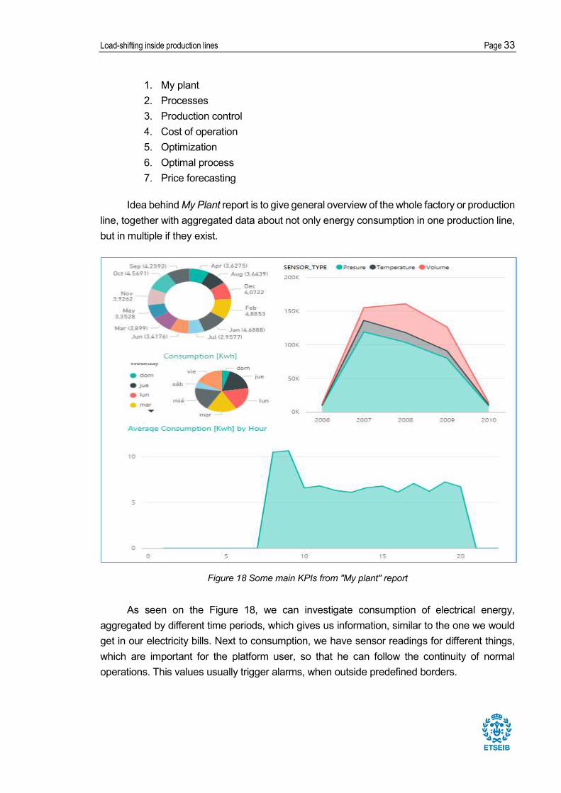
Idea behind My Plant report is to give general overview of the whole factory or production line, together with aggregated data about not only energy consumption in one production line, but in multiple if they exist.
Figure 18 Some main KPIs from "My plant" report
As seen on the Figure 18, we can investigate consumption of electrical energy, aggregated by different time periods, which gives us information, similar to the one we would get in our electricity bills. Next to consumption, we have sensor readings for different things, which are important for the platform user, so that he can follow the continuity of normal operations. This values usually trigger alarms, when outside predefined borders.

Page 34 M. Viktorovi
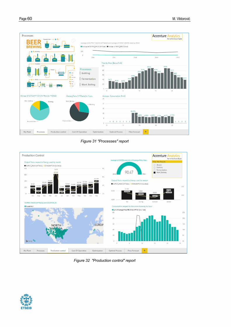
In Processes tab of dashboard, we can see the process description, together with outputs and inputs, paired with consumption and price of electricity.
Figure 19 Main KPIs from "Processes" report
In Figure 19 process is visualised, and consumption division is given, while other KPIs can be seen in Appendix section, and they include comparison of hourly consumption and price for both individual processes and their aggregated values.
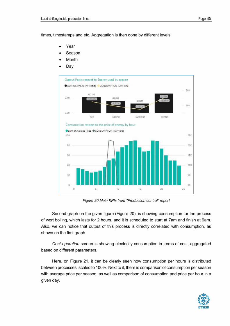
Figure 20 shows main KPIs from Production control report, which has the main idea, to show how inputs and outputs of this process behave, but as well, to show the brief description of processes electricity consumption. Thing to note here is that filtration is
inputs of different processes can scaled differently or use different units, and therefore cannot be summarised.
Also on Figure 20 we can see different aggregation levels in graphs, which are automatically done by Power BI software, since it can recognize data fields representing dates,
Load-shifting inside production lines Page 35
times, timestamps and etc. Aggregation is then done by different levels: Year Season Month Day
Figure 20 Main KPIs from "Production control" report
Second graph on the given figure (Figure 20), is showing consumption for the process of wort boiling, which lasts for 2 hours, and it is scheduled to start at 7am and finish at 9am. Also, we can notice that output of this process is directly correlated with consumption, as shown on the first graph.
Cost operation screen is showing electricity consumption in terms of cost, aggregated based on different parameters.
Here, on Figure 21, it can be clearly seen how consumption per hours is distributed between processes, scaled to 100%. Next to it, there is comparison of consumption per season with average price per season, as well as comparison of consumption and price per hour in a given day.

Page 36 M. Viktorovi
Figure 21 Main KPIs of "Cost of operation" report
Interactivity here gives great possibilities for data exploration, since, filtering is done by clicking on any of the visual elements. Some filters can be limited to only specific graphs, but by default, they are applied to whole report.
Other important thing when it comes to filtering, is to define aggregation function properly. For example, when dealing with consumption, this function should be sum, while in visualisation of prices and cost, avg (average) should be used.
Optimization report page has the purpose to show current (non-optimised) solution, together with recommendations for optimal scheduling.
Figure 22 Main KPIs of "Optimization" report

Load-shifting inside production lines Page 37
Example from the Figure 22, shows substantial savings, of around 44%, which is not realistic number.
- 5.1, are simplified,
the graph of optimized consumption in the Figure 22in the morning.
Discrepancy between two graphs (slightly different shape of consumption curve), can be explained by the fact, that for optimization, predefined period of aggregation of average consumption per hour for optimization, is different than the one for visualization of hourly consumption. In pure visualization complete historical data is taken into account, while in the process of passing data to optimization scripts, much smaller period has taken into account,
Thing to be noted here is that this numbers represent only aggregation of daily spot
market prices, while taxes, fees for contracted power, etc. are not taken into account, since they are fully dependable on the contract that producer has with the electricity provider. Also
function is independent part of it. Logical next step is to see the actual effect on individual processes, which has been
visualised in the Optimal process screen. Here (Figure 23), individual processes were shown, in their ideal scheduled working hours.
Figure 23 "Optimal process" process consumptions

Page 38 M. Viktorovi
Comparison of total consumption, scale to 100% per hour, is also shown in this report, like in Figure 24, where something similar to second graph on Figure 22 is shown, just scaled. This visualisation is very important, because it gives the clear understanding of the share in consumption between different processes, but also from it you can clearly distinguish working hours of each process.
Figure 24 "Optimal process" hourly consumption division
Apart from this, Optimal process report contains, comparison between maximum power capacity required as well as the distribution of the costs between all the processes.
The last report within the dashboard, is Price forecasting and it is intended for future developments of the platform, in which the service of price forecasting will be available, as an extra tool.

Load-shifting inside production lines Page 39
6. In previous chapter, model of the production line, consisting of three processes has been
given, and based on this model, and data available, preliminary calculations of savings have been done. In order to diversify the results, different techniques have been applied to the given data.
Data has been cleaned and resampled, in order to create more compact development environment
Added random noise to the consumption data, to model real-world conditions, in a smaller data set
3 scenarios have been developed for original schedules and production line constrains
Based on previously mentioned 2 scenarios, economic analysis will be done, taking into account several economic factors, and savings in cost of total kilowatt/hours.
All scenarios outcomes have been calculated using linear programming approach, without utilizing other proposed algorithms. This has been done as the first step, since this
later comparison, with other approaches, which have stochastic type of results. Also, main concern of the first version of solution was not the computational performance, but economic feasibility.
Figure 25 Price of kWh during one day in DK
All the prices were taken from NordPool spot Market, for DK (Denmark) region, and on daily basis, they are represented by daily curve given in the Figure 25.

Page 40 M. Viktorovi
1 Price values have been scaled for better visualization, so they
6.1. Scenario 1 In first scenario scheduling of the processes was based on next time parameters:
Process Schedule
1 6am to 1pm 2 10am to 2pm 3 3pm to 4pm
Table 2 Scenario 1 original schedule
Also, here we are taking into account working hours of the factory, which are from 6 am to 12pm. With this parameters, our load looks like this:
Figure 26 Consumption per process per hour in Scenario 11
As seen from the Figure 26, machines representing processes operate mostly during hours in which price of electricity is high.
By putting constrains as described in section Constrains5.1, taking into account operation hours of the plant, our algorithm gives us the next schedule:

Load-shifting inside production lines Page 41
Process Schedule
1 11am to 6pm 2 1pm to 5pm 3 9pm to 10pm
Table 3 Optimal schedule for scenario 1
This is directly transferred into consumption curves of processes, based on the optimal schedule from the Table 3.
Figure 27 Consumption per process per hour in optimal version of Scenario 1 1
Based on the given prices of kilowatt/hour, total prices and savings are: Cost Cost after optimization Savings per day
13.5% Table 4 Cost and savings in scenario 1
6.2. Scenario 2
ours, meaning it operates 24 hours a day. This scenario gives more flexibility for optimization

Page 42 M. Viktorovi
algorithm, and therefore it is expected to give results leading to more savings. Constrains in this case are only that process 3 must wait for processes 1 and 2 to finish.
According to the original schedule these processes have given working hours: Process Schedule
1 6am to 1pm 2 10am to 2pm 3 3pm to 4pm
Table 5 Scenario 2 original schedule
And with these limitations, model is built, and on that model, linear programing algorithm
has been applied, in order to get the optimal schedule for production. This optimization then gives the next schedule:
Process Schedule 1 0am to 7am 2 1am to 5pm 3 3pm to 4pm
Table 6 Optimal schedule for scenario 2
This scheduling gives us the consumptions per process (machine) that is represented on the next figure (Figure 28):

Load-shifting inside production lines Page 43
Figure 28 Consumption per process per hour in optimal version of scenario 2
By doing optimization under given conditions, we can reduces costs of used electricity more than in scenario 1, as it has been expected, since lowest electricity prices are during lowest load in the early morning hours.
Cost Cost after optimization Savings per day 28.5%
Table 7 Cost and savings in scenario 2
From the Table 7, we can see the savings of more than 28%, which is quite big result, taking into account that for it to be realised, we would have to have complete flexibility, when it comes to working hours. This can be achieved only in the production lines are fully automatized and where the produced good does not require special storage conditions.
6.3. Economic analysis In order to give the evaluation of economical feasibility of the project, Net Present Value
(NPV) has to be calculated. Net present Value represents difference between present cash inflow values and present cash outflows.
First stem in analysis through NPV is to construct P&L (Profit & Loss) sheet, for projected time period within which we want to see the feasibility of project.

Page 44 M. Viktorovi
Key economic parameters Inflation rate 2.00 %
Increase in electricity prices 9.72 % Length of projected period 5 years Cloud price decrease rate 3.7%
Table 8 Key parameters for economic analysis
Cloud price decrease rate is calculated based on the prediction of price decrease of 14% by year 2020 [21].
Increase in electricity price is calculated based on historical data of prices in Spain from 1980 to 2012, as shown in Figure 29, based on data from Eurostat.
Figure 29 Trend of price increase in Spain
Net Present value is calculated using the next formula for required t number of time periods (years).
Where Ct represents net cash flow in year t, r represents discount per year, in our case
020406080
100120140160180
1 5 9 13 17 21 25 29 33
$/MWh
Year (from 1980 to 2012)

Load-shifting inside production lines Page 45
-calculated within the price decrease of the cloud services. And finally C0 represents the initial investment cost, which is in our case cost of platform development. 6.3.1. Expenditures and initial investment cost
In the investment cost we include the cost of labour for development of the platform, taking into account that measurement equipment is already present on , like shown in Table 9.
Initial investments Number of working hours [hours] 900
Cost of 8.00 250.00 550.00
8000.00 Table 9 Initial investment cost
Expenditures include costs of platform maintenance, meaning the yearly cost of the cloud platform, with proposed solutions.
Expenditures per month 8.40
Number of users 1 Cost of Azure SQL S3 DB 126.00
0 0 (for first 5GB)
Az 0 134.4
Table 10 First year monthly expenditures

Page 46 M. Viktorovi
Expenditures per year 1612.80
Table 11 First year expenditures
6.3.2. Revenues Revenues have been calculated on the basis of savings, calculated for scenarios
previously shown. In this cases we will use expenditures for used electricity only, calculated based on spot market prices for DK region, and apply savings on them.
Expenditures per month for electricity Number of working days in month 30.5
Electricity consumption [kWh/month] 30 000 22.10 674.05
Table 12 Expenditures for electricity in first year
Scenario 1 revenues per month Savings [%] 13.5
91.00 Scenario 1 revenues per year
1091.96 Table 13 Scenario 1 - Revenues for first year
From the Table 13 we can see that revenues, produced by savings in electricity price are lower than expenditures per year from Table 11, which means that profitability of this scenario will be dependent of increase of electricity prices, compared to decrease in prices of cloud services.
Load-shifting inside production lines Page 47
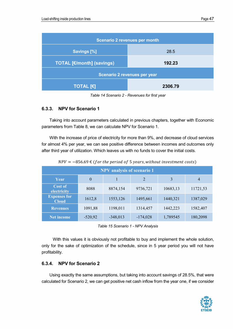
Scenario 2 revenues per month Savings [%] 28.5
(savings) 192.23 Scenario 2 revenues per year
2306.79 Table 14 Scenario 2 - Revenues for first year
6.3.3. NPV for Scenario 1 Taking into account parameters calculated in previous chapters, together with Economic
parameters from Table 8, we can calculate NPV for Scenario 1. With the increase of price of electricity for more than 9%, and decrease of cloud services
for almost 4% per year, we can see positive difference between incomes and outcomes only after third year of utilization. Which leaves us with no funds to cover the initial costs.
NPV analysis of scenario 1
Year 0 1 2 3 4 Cost of
electricity 8088 8874,154 9736,721 10683,13 11721,53 Expenses for
Cloud 1612,8 1553,126 1495,661 1440,321 1387,029 Revenues 1091,88 1198,011 1314,457 1442,223 1582,407
Net income -520,92 -348,013 -174,028 1,789545 180,2098 Table 15 Scenario 1 - NPV Analysis
With this values it is obviously not profitable to buy and implement the whole solution, only for the sake of optimization of the schedule, since in 5 year period you will not have profitability. 6.3.4. NPV for Scenario 2
Using exactly the same assumptions, but taking into account savings of 28.5%, that were calculated for Scenario 2, we can get positive net cash inflow from the year one, if we consider
Page 48 M. Viktorovi
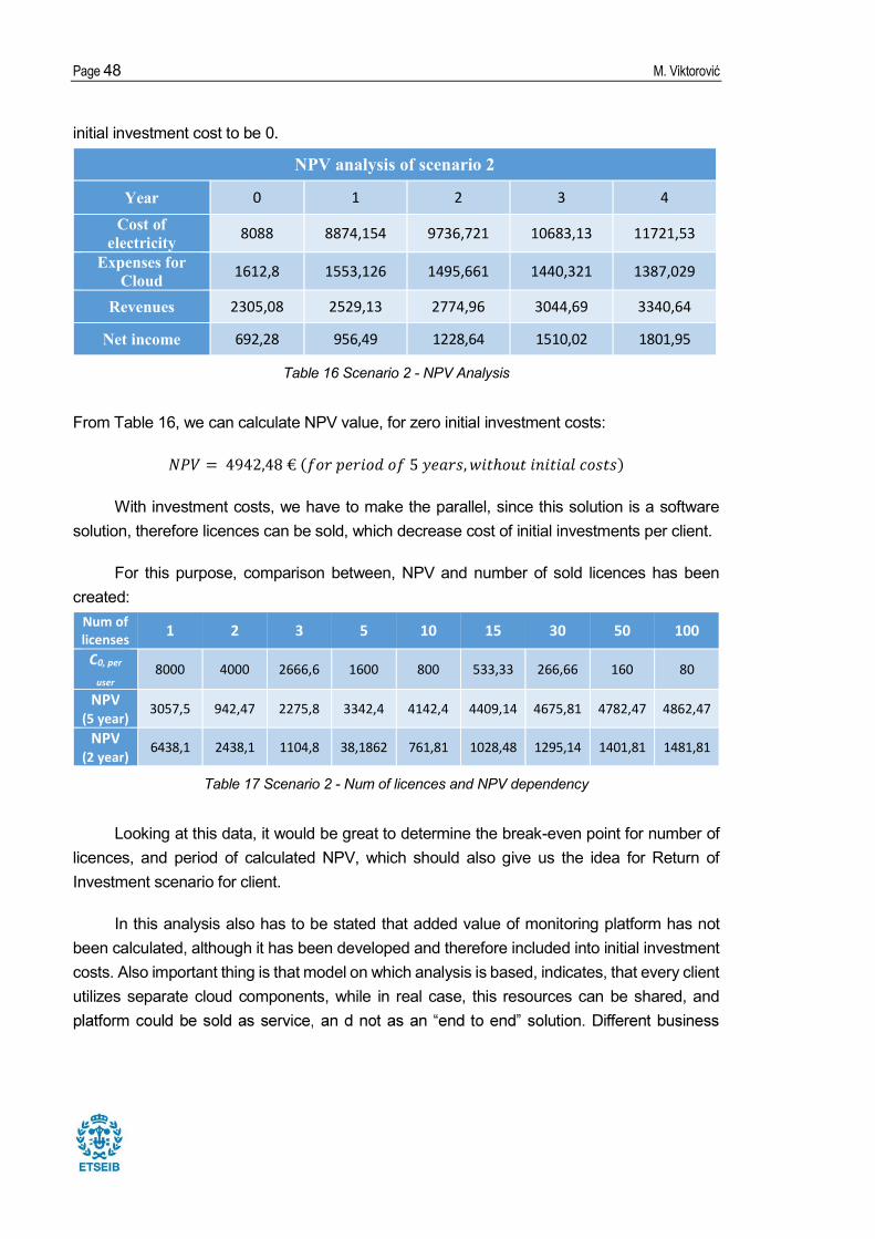
initial investment cost to be 0. NPV analysis of scenario 2
Year 0 1 2 3 4 Cost of
electricity 8088 8874,154 9736,721 10683,13 11721,53 Expenses for
Cloud 1612,8 1553,126 1495,661 1440,321 1387,029 Revenues 2305,08 2529,13 2774,96 3044,69 3340,64
Net income 692,28 956,49 1228,64 1510,02 1801,95 Table 16 Scenario 2 - NPV Analysis
From Table 16, we can calculate NPV value, for zero initial investment costs:
With investment costs, we have to make the parallel, since this solution is a software solution, therefore licences can be sold, which decrease cost of initial investments per client.
For this purpose, comparison between, NPV and number of sold licences has been created:
Num of licenses 1 2 3 5 10 15 30 50 100 C0, per
user 8000 4000 2666,6 1600 800 533,33 266,66 160 80 NPV
(5 year) 3057,5 942,47 2275,8 3342,4 4142,4 4409,14 4675,81 4782,47 4862,47 NPV
(2 year) 6438,1 2438,1 1104,8 38,1862 761,81 1028,48 1295,14 1401,81 1481,81 Table 17 Scenario 2 - Num of licences and NPV dependency
Looking at this data, it would be great to determine the break-even point for number of licences, and period of calculated NPV, which should also give us the idea for Return of Investment scenario for client.
In this analysis also has to be stated that added value of monitoring platform has not been calculated, although it has been developed and therefore included into initial investment costs. Also important thing is that model on which analysis is based, indicates, that every client utilizes separate cloud components, while in real case, this resources can be shared, and
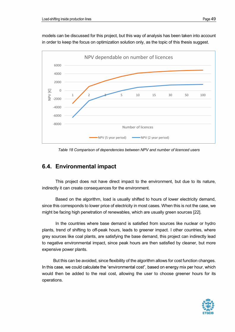
Load-shifting inside production lines Page 49
models can be discussed for this project, but this way of analysis has been taken into account in order to keep the focus on optimization solution only, as the topic of this thesis suggest.
Table 18 Comparison of dependencies between NPV and number of licenced users
6.4. Environmental impact This project does not have direct impact to the environment, but due to its nature,
indirectly it can create consequences for the environment. Based on the algorithm, load is usually shifted to hours of lower electricity demand,
since this corresponds to lower price of electricity in most cases. When this is not the case, we might be facing high penetration of renewables, which are usually green sources [22].
In the countries where base demand is satisfied from sources like nuclear or hydro plants, trend of shifting to off-peak hours, leads to greener impact. I other countries, where grey sources like coal plants, are satisfying the base demand, this project can indirectly lead to negative environmental impact, since peak hours are then satisfied by cleaner, but more expensive power plants.
But this can be avoided, since flexibility of the algorithm allows for cost function changes.
would then be added to the real cost, allowing the user to choose greener hours for its operations.
-8000-6000-4000-2000
0200040006000
1 2 3 5 10 15 30 50 100
Number of licences
NPV dependable on number of licences
NPV (5 year period) NPV (2 year period)

Page 50 M. Viktorovi
7. Through this thesis work, reader has been given an overview of the project that had the
goal to investigate possibilities for optimization of schedules of production, therefore achieving savings in cost of electricity, by shifting loads of individual processes within production line.
Secondary goal of the thesis was to investigate technical and economic feasibility, as well as to give the ideas of possible uses of the developed algorithms.
Through main part of thesis, different approaches and technologies were described and compared, in order to give reader an overview of all the possible options for development, but in the chapters 4 and 5, author demonstrated which of these proposed options have implemented and for which reason.
Working in the real-word company environment represented a specific challenge when it comes to fully new development, in the fields that are not in the main comfort zone for the most of the people around. Tasks included, were not always straight-forward, and focus was not always fully on the development. This of course represents the real side of project development, which has to be managed in different ways.
7.1. Algorithm Chosen solution for optimization of schedule, in this part of the project, was linear
programing. This was mostly because of the fact that other proposed solutions, although they might show better performance in terms of computational requirements, will give the perfect solution every time, as in contrast to heuristic approach. With this in mind, it is a great starting point, so that future development of heuristic algorithms can rely on comparison when it comes to the accuracy of solution.
Tested on multiple models, algorithm written in R, whit parts of it in AMPL language performed well and without oscillations in its performance both on the local platform and in the cloud. Testing has been done both with simple three process models and with ten process ones, and in all the cases linear programming approach gave good results within satisfactory time.
which is good, since this solution offers very basic cost optimization, without taking into account

Load-shifting inside production lines Page 51
cost of intermediate storage of goods between processes, contracted power cost, etc.
7.2. Technical feasibility Developed algorithm was tested on data set, that was modified and randomized multiple
times, and by nature of the approach viable solution has been always available. Due to proposed modularity of the algorithm, changes and upgrades to it are simple to make.
All the scripts developed in R, were, when tested, performing satisfactory in terms of speed and stability. Also, R has proven to be a great tool for data processing, with its wide application and great online community support.
Infrastructure behind the platform, consisting of Azure cloud services, has proven to be a good choice for this kind of projects, where you have to focus your resources on software and data, while not putting too much effort into infrastructure maintenance. Second great thing about using cloud solution is its price flexibility and scalability, meaning that user can easily
er to adjust it to his current needs. Key part of the Azure services was Power BI, great visualisation tool developed by
Microsoft, which gave this project the edge in part of data representation, due to its agility. This tool has been proven to be unreplaceable when it comes to utilization of created reports,
Overall experience with the cloud solution was good, although during project, learning
curve for Azure was not always optimal, and some seemingly simple things have proven to be not as easy as advertised.
7.3. Economic feasibility In order to compare different cases, two scenarios have been developed. One is
representing standard factory, while the other one fully automatized production, independent of working hours.
Net present value has been chosen as the main measure of economic feasibility of the solution, with some assumptions. Main assumption here was that only added value of this project was developed schedule optimization, which means, that only revenue measured was the saving produced by the algorithm.
There are any energy monitoring platform on the market, and they are making profits, without optimizations, or with only some basic ones. For developed solution, described in this
Page 52 M. Viktorovi
thesis, monitoring of energy is available, but it has been regarded as a secondary thing, and it was not been calculated as was first done assuming that there are no Initial investment cost. By doing this, we could immediately discard scenario one as economically feasible stand-alone solution, based on results from chapter 6.3.3.
From the other hand, chapter 6.3.4 has investigated feasibility of Scenario 2, and shown that even as a stand-alone solution, this optimization can be profitable. Here investigation has been done on the licence share model, and some discussion has been given how business model can be developed, so that it can bring more profit.
7.4. Future developments As a primarily thing to be developed next is the better model of cost function, including
different parameters, not only cost of spent electricity. Current solutions has capability for this upgrade, therefore it should be priority, since it would represent one of a kind solution on the market.
After this step, experimentation with different optimization techniques can be done, in order to compare and find the best solution in terms of cost-benefit.
Rethinking of the usage of algorithms should be done, in order to implement them in simple sequential process that we see in everyday use, like washing and drying, where user could set the time constrains, and get the optimal schedule for utilization of the machines.
market solutions, and with this success is guaranteed.

Load-shifting inside production lines Page 53
Page 54 M. Viktorovi
8.
[1] , 16 June 2016. [Online]. Available: https://en.wikipedia.org/wiki/Production_line. [Accessed 10 August 2016].
[2] -https://en.wikipedia.org/wiki/Cross-correlation. [Accessed 10 August 2016].
[3] [Online]. Available: http://www.beergame.org/the-game. [Accessed 10 August 2016].
[4] stic Energy Consumption
Science University of Southampton, Southampton, 2011. [5]
https://en.wikipedia.org/wiki/Metaheuristic. [Accessed 10 August 2016]. [6]
http://mathworld.wolfram.com/SimulatedAnnealing.html. [Accessed 10 August 2016]. [7] R. Ferguson, LINEAR PROGRAMMING, McGraw-Hill, 1958. [8]
Available: https://en.wikipedia.org/wiki/Linear_programming. [Accessed 10 August 2016].
[9] [Online]. Available: http://www.forbes.com/sites/greatspeculations/2014/12/19/microsofts-azure-cloud-platform-explained-part-1/#5dd3074b916a. [Accessed 15 August 2016].
[10] the free encyclopedia, 14 August 2016. [Online]. Available: https://en.wikipedia.org/wiki/Cloud_computing. [Accessed 15 August 2016].
[11] -

Load-shifting inside production lines Page 55
us/overview/what-is-azure/. [Accessed 15 August 2016]. [12]
https://en.wikipedia.org/wiki/Microsoft_Azure. [Accessed 15 August 2016]. [13] le: https://azure.microsoft.com/en-
us/services/stream-analytics/. [Accessed 15 August 2016]. [14]
5 May 2014. [Online]. Available: http://www.fastcompany.com/3030063/why-the-r-programming-language-is-good-for-business. [Accessed 15 August 2016].
[15] -stat.com/documents/tutorials/why-use-the-r-language/. [Accessed 15 August 2016].
[16] G. PiatetKDnuggets, 18 August 2014. [Online]. Available: http://www.kdnuggets.com/2014/08/four-main-languages-analytics-data-mining-data-science.html. [Accessed 15 August 2016].
[17] https://mran.revolutionanalytics.com/open/. [Accessed 15 August 2016].
[18] https://en.wikipedia.org/wiki/AMPL. [Accessed 15 August 2016].
[19] May 2016. [Online]. Available: https://www.linkedin.com/pulse/5-reasons-why-power-bi-taking-over-tableau-best-tool-tacoronte. [Accessed 15 August 2016].
[20] https://msdn.microsoft.com/library/azure/30806023-392b-42e0-94d6-6b775a6e0fd5. [Accessed 15 August 2016].
[21] f Consulting, 2016. [22]
2008.

Page 56 M. Viktorovi
9. Figure 1 Example of 3 processes in production line ............................................................... 8 Figure 2 NordPool Spot hourly market prices in Denmark ...................................................... 9 Figure 3 Beer game supply chain simulation ........................................................................ 10 Figure 4 Cross-correlation (r) of two signals (x and y) .......................................................... 12 Figure 5 Simulated annealing pseudo code [6] .................................................................... 14 Figure 6 Process constraints explained ................................................................................ 16 Figure 7 Proposed Azure architecture .................................................................................. 19 Figure 8 Representation of relations in optimization script ................................................... 21 Figure 9 Language used for data analysis/mining ................................................................ 22 Figure 10 AMPL lifecycle flow .............................................................................................. 23 Figure 11 Comparison between data visualization tools [14] ................................................ 24 Figure 12 Example process hierarchy .................................................................................. 26 Figure 13 Proposed data model ........................................................................................... 28 Figure 14 Illustrated schematics of the optimization scripts .................................................. 29 Figure 15 Optimization script schematics ............................................................................. 29 Figure 16 Actual schematics of Azure cloud platform ........................................................... 30 Figure 17 Dashboard though flow ........................................................................................ 32 Figure 18 Some main KPIs from "My plant" report ............................................................... 33 Figure 19 Main KPIs from "Processes" report ...................................................................... 34 Figure 20 Main KPIs from "Production control" report .......................................................... 35 Figure 21 Main KPIs of "Cost of operation" report ................................................................ 36 Figure 22 Main KPIs of "Optimization" report ....................................................................... 36 Figure 23 "Optimal process" process consumptions ............................................................ 37
Load-shifting inside production lines Page 57
Figure 24 "Optimal process" hourly consumption division .................................................... 38 Figure 25 Price of kWh during one day in DK ....................................................................... 39 Figure 26 Consumption per process per hour in Scenario 1 ................................................ 40 Figure 27 Consumption per process per hour in optimal version of Scenario 1 1 ................. 41 Figure 28 Consumption per process per hour in optimal version of scenario 2 .................... 43 Figure 29 "My plant" report ................................................................................................... 59 Figure 30 "Processes" report ................................................................................................ 60 Figure 31 "Production control" report ................................................................................... 60 Figure 32 "Cost of operation" report .................................................................................... 61 Figure 33 "Optimization" report ............................................................................................ 61 Figure 34 "Optimal process" report ....................................................................................... 62 Figure 35 "Price forecasting" report ...................................................................................... 62 Table 1 Differences between Free ver. and Power BI Pro .................................................... 25 Table 2 Scenario 1 original schedule .................................................................................... 40 Table 3 Optimal schedule for scenario 1 .............................................................................. 41 Table 4 Cost and savings in scenario 1 ................................................................................ 41 Table 5 Scenario 2 original schedule .................................................................................... 42 Table 6 Optimal schedule for scenario 2 .............................................................................. 42 Table 7 Cost and savings in scenario 2 ................................................................................ 43 Table 8 Key parameters for economic analysis .................................................................... 44 Table 9 Initial investment cost .............................................................................................. 45 Table 10 First year expenditures .......................................................................................... 46 Table 11 Expenditures for electricity in first year .................................................................. 46 Table 12 Scenario 1 - Revenues for first year ...................................................................... 46 Table 13 Scenario 2 - Revenues for first year ...................................................................... 47 Table 14 Scenario 1 - NPV Analysis..................................................................................... 47

Page 58 M. Viktorovi
Table 15 Scenario 2 - NPV Analysis .................................................................................... 48 Table 16 Scenario 2 - Num of licences and NPV dependency ............................................. 48 Table 17 Comparison of dependencies between NPV and number of licenced users ......... 49 Table 18 Amazon Web Services vs Azure ........................................................................... 63

Load-shifting inside production lines Page 59
10.
10.1. Energy analytics dashboard
Figure 30 "My plant" report
Page 60 M. Viktorovi
Figure 31 "Processes" report
Figure 32 "Production control" report

Load-shifting inside production lines Page 61
Figure 33 "Cost of operation" report
Figure 34 "Optimization" report

Page 62 M. Viktorovi
Figure 35 "Optimal process" report
Figure 36 "Price forecasting" report
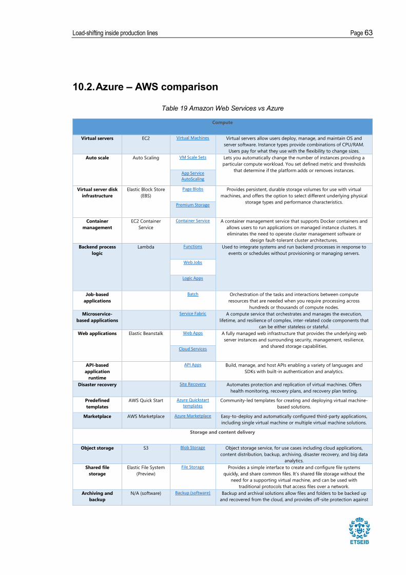
Load-shifting inside production lines Page 63
10.2. Azure AWS comparison Table 19 Amazon Web Services vs Azure
Compute Virtual servers EC2 Virtual Machines Virtual servers allow users deploy, manage, and maintain OS and server software. Instance types provide combinations of CPU/RAM. Users pay for what they use with the flexibility to change sizes.
Auto scale Auto Scaling VM Scale Sets Lets you automatically change the number of instances providing a particular compute workload. You set defined metric and thresholds that determine if the platform adds or removes instances. App Service AutoScaling
Virtual server disk infrastructure Elastic Block Store (EBS) Page Blobs Provides persistent, durable storage volumes for use with virtual machines, and offers the option to select different underlying physical storage types and performance characteristics. Premium Storage
Container management EC2 Container Service Container Service A container management service that supports Docker containers and allows users to run applications on managed instance clusters. It eliminates the need to operate cluster management software or design fault-tolerant cluster architectures.
Backend process logic Lambda Functions Used to integrate systems and run backend processes in response to events or schedules without provisioning or managing servers. Web Jobs
Logic Apps
Job-based applications Batch Orchestration of the tasks and interactions between compute resources that are needed when you require processing across hundreds or thousands of compute nodes. Microservice-based applications Service Fabric A compute service that orchestrates and manages the execution, lifetime, and resilience of complex, inter-related code components that can be either stateless or stateful.
Web applications Elastic Beanstalk Web Apps A fully managed web infrastructure that provides the underlying web server instances and surrounding security, management, resilience, and shared storage capabilities. Cloud Services
API-based application runtime API Apps Build, manage, and host APIs enabling a variety of languages and SDKs with built-in authentication and analytics.
Disaster recovery Site Recovery Automates protection and replication of virtual machines. Offers health monitoring, recovery plans, and recovery plan testing. Predefined templates AWS Quick Start Azure Quickstart templates
Community-led templates for creating and deploying virtual machine-based solutions. Marketplace AWS Marketplace Azure Marketplace Easy-to-deploy and automatically configured third-party applications, including single virtual machine or multiple virtual machine solutions.
Storage and content delivery Object storage S3 Blob Storage Object storage service, for use cases including cloud applications, content distribution, backup, archiving, disaster recovery, and big data analytics.
Shared file storage Elastic File System (Preview) File Storage Provides a simple interface to create and configure file systems
need for a supporting virtual machine, and can be used with traditional protocols that access files over a network. Archiving and backup N/A (software) Backup (software) Backup and archival solutions allow files and folders to be backed up and recovered from the cloud, and provides off-site protection against

Page 64 M. Viktorovi
Glacier and S3 (storage) Blob Storage (storage)
data loss. There are two components of backup the software service that orchestrates backup/retrieval and the underlying backup storage infrastructure. Hybrid storage Storage Gateway StorSimple Integrates on-premises IT environments with cloud storage. Automates data management and storage, plus supports in disaster recovery. Data transport Import/Export Snowball
Import/Export A data transport solution that uses secure disks and appliances to transfer large amounts of data. Also offers data protection during transit. Content delivery CloudFront Content Delivery Network
A global content delivery network that delivers audio, video, applications, images, and other files. Networking
Networking Virtual Private Cloud Virtual Network Provides an isolated, private environment in the cloud. Users have control over their virtual networking environment, including selection of their own IP address range, creation of subnets, and configuration of route tables and network gateways.
Domain name system (DNS) Route 53 DNS (Preview) A service that hosts domain names, plus routes users to Internet applications, connects user requests to datacenters, manages traffic to apps, and improves app availability with automatic failover. Traffic Manager
Dedicated network Direct Connect ExpressRoute Establishes a dedicated, private network connection from a location to the cloud provider (not over the Internet). Load balancing Elastic Load Balancing
Load Balancer Automatically distributes incoming application traffic to add scale, handle failover, and route to a collection of resources. Application Gateway
Database
SUBCATEGORY AWS SERVICE AZURE SERVICE DESCRIPTION Relational database RDS SQL Database Relational database-as-a-service (DBaaS) where the database resilience, scale, and maintenance are primarily handled by the platform.
NoSQL database DynamoDB DocumentDB A NoSQL document database service that automatically indexes JSON data for applications that require rich query and multi-document transactions. Data warehouse Redshift SQL Data Warehouse (Preview)
A fully managed data warehouse that analyzes data using business intelligence tools. It can transact SQL queries across relational and non-relational data. Table storage DynamoDB Table Storage A non-relational data store for semi-structured data. Developers store and query data items via web services requests.
SimpleDB Caching ElastiCache Azure Redis Cache An in-memory based, distributed caching service that provides a high-performance store typically used to offload non-transactional work from a database.
Database migration Database Migration Service SQL Database Migration Wizard
Typically is focused on the migration of database schema and data from one database format to a specific database technology in the cloud. Analytics and big data
Big data processing Elastic MapReduce (EMR) HDInsight Supports technologies that break up large data processing tasks into multiple jobs, and then combine the results together to enable massive parallelism.
Data orchestration Data Pipeline Data Factory Processes and moves data between different compute and storage services, as well as on-premises data sources at specified intervals. Users can create, schedule, orchestrate, and manage data pipelines.

Load-shifting inside production lines Page 65
Analytics Kinesis Analytics (Preview) Stream Analytics Storage and analysis platforms that creates insights from large quantities of data, or data that originates from many sources.
Data Lake Analytics (Preview)
Data Lake Store (Preview)
Visualization QuickSight (Preview) Power BI Business intelligence tools that build visualizations, perform ad-hoc analysis, and develop business insights from data.
Machine learning Machine Learning Machine Learning Produces an end-to-end workflow to create, process, refine, and publish predictive models that can be used to understand what might happen from complex data sets. Search Elasticsearch Service
Search Delivers full-text search and related search analytics and capabilities. Data discovery Data Catalog (Preview)
Provides the ability to better register, enrich, discover, understand, and consume data sources. Internet of Things
Streaming data Kinesis Firehose Event Hubs Services that allow the mass ingestion of small data inputs, typically from devices and sensors, to process and route the data. Kinesis Streams
Internet of Things IoT (Preview) IoT Hub Lets connected devices to interact with cloud applications and other devices to captures and analyze real-time data. Mobile services
Pro app development Mobile Hub (Beta) Mobile Apps Backend mobile services for rapid development of mobile solutions, plus provide identity management, data synchronization, and storage and notifications across devices. Cognito High-level app development PowerApps Model-driven application development for business applications with SaaS integration.
Analytics Mobile Analytics Mobile Engagement
Provides real-time analytics from mobile apps data, highlights app Notification Simple Notification Service
Notification Hubs A push notification service that delivers messages instantly to applications or users. Messages can be sent to individual devices or can be broadcasted. Application services
Email Simple Email Service Lets users send transactional email, marketing messages, or any other type of content to customers. Messaging Simple Queue Service
Queue Storage Stores large numbers of messages that can be accessed from anywhere through authenticated calls using HTTP or HTTPS. A queue can contain millions of messages, up to the total capacity limit of a storage account, and may also support more complex topologies such as publish/subscribe. Service Bus queues
Service Bus topics
Service Bus relay
Workflow Simple Workflow Service Logic Apps A state tracker and task coordinator service that allows developers to build, run, and scale background activities using a visual processes flow creation.
App testing Device Farm (Front End) Xamarin Test Cloud (Front End)
A range of services geared toward the orchestration of dev/test backend server and service application infrastructure, as well as front end client device and software testing and simulation. Azure DevTest Labs (Back End)
API management API Gateway API Management Allows developers to create, publish, maintain, monitor, and secure APIs. Handles processing concurrent API calls, including traffic management, authorization, access control, monitoring, and API version management.
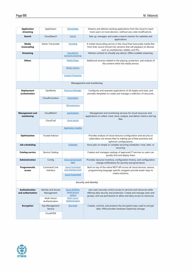
Page 66 M. Viktorovi
Application streaming AppStream RemoteApp Streams and delivers existing applications from the cloud to reach more users on more devices without any code modifications. Search CloudSearch Search Sets up, manages, and scales a search solution for websites and applications. Media transcoding Elastic Transcoder Encoding A media transcoding service in the cloud that transcodes media files from their source format into versions that will playback on devices such as smartphones, tablets, and PCs.
Streaming Live and on-demand streaming
Delivers content to virtually any device. Offers scalable streaming. Others Media Player Additional services related to the playing, protection, and analysis of the content within the media service.
Media Indexer
Content Protection
Management and monitoring Deployment orchestration OpsWorks Resource Manager Configures and operates applications of all shapes and sizes, and provides templates to create and manage a collection of resources.
CloudFormation Automation
VM extensions
Management and monitoring CloudWatch Log Analytics Management and monitoring services for cloud resources and applications to collect, track, store, analyze, and deliver metrics and log files. CloudTrail Azure portal
Application Insights
Optimization Trusted Advisor Provides analysis of cloud resource configuration and security so optimum configurations.
Job scheduling Scheduler Runs jobs on simple or complex recurring schedules now, later, or recurring. Catalog service Service Catalog Creates and manages catalogs of approved IT services so users can quickly find and deploy them. Administration Config Azure portal (audit logs)
Provides resource inventory, configuration history, and configuration change notifications for security and governance. Programmatic access Command Line Interface
Azure Command Line Interface (CLI)
Built on top of the native REST API across all cloud services, various programming language-specific wrappers provide easier ways to create solutions. Azure PowerShell
Security and identity Authentication and authorization Identity and Access Management
Azure AD/Role-based access control
Lets users securely control access to services and resources while offering data security and protection. Create and manage users and groups, and use permissions to allow and deny access to resources. Multi-Factor Authentication Multi-Factor Authentication
Encryption Key Management Service Key Vault Creates, controls, and protects the encryption keys used to encrypt data. HSM provides hardware-based key storage.
CloudHSM

Load-shifting inside production lines Page 67
Firewall Web Application Firewall A firewall that protects web applications from common web exploits. Users can define customizable web security rules. Security Inspector (Preview) Security Center (Preview)
An automated security assessment service that improves the security and compliance of applications. Automatically assess applications for vulnerabilities or deviations from best practices. Directory Directory Service Azure Active Directory
Typically provides user/group properties that can be queried and used in applications. Also can provide capabilities to integrate to on-premises Active Directory services for single sign-on scenarios and SaaS management. Azure Active Directory B2C
Azure Active Directory Domain Services