1

Contents 1. Introduction .................................................................................................................. 3 2. S-MAC Protocol ........................................................................................................... 5

2.1 Overview of S-MAC ................................................................................... 5 2.2 Periodic Sleep and Listen ............................................................................ 8 2.3 Synchronization......................................................................................... 10

2.3.1 Synchronization Related Components in S-MAC.............................. 10 2.3.2 Choosing First Schedule..................................................................... 13 2.3.3 Updating and Maintaining Schedules................................................. 14 2.3.4 Periodical Neighbor Discovery .......................................................... 16 2.3.5 Periodical Neighbor List Updating..................................................... 16

2.4 CSMA/CA in S-MAC ............................................................................... 18 2.4.1 Carrier Sense ...................................................................................... 18 2.4.2 Collision Avoidance ........................................................................... 21

2.5 Overhearing Avoidance............................................................................. 22 2.6 Message Passing........................................................................................ 24 2.7 Adaptive listening...................................................................................... 25

3. The Network Simulator .............................................................................................. 31 3.1 What is NS-2 ............................................................................................. 31 3.2 How to Get Started .................................................................................... 32

4. Simulating S-MAC with NS-2 ................................................................................... 34 4.1 S-MAC in NS-2......................................................................................... 34

4.1.1 Implemented S-MAC Features........................................................... 34 4.1.2 S-MAC Parameters Settings............................................................... 35 4.1.3 S-MAC Modes.................................................................................... 36 4.1.4 Problems and Bugs of S-MAC in NS-2.28 ........................................ 36

4.2 Preparations for Simulating S-MAC ......................................................... 41 4.2.1 NO Ad-Hoc Routing Agent (NOAH)................................................. 41 4.2.2 Exponential Traffic Source Agent...................................................... 42

4.3 An Example Tcl Script for Simulating S-MAC ........................................ 43 4.4 Tracing....................................................................................................... 49

4.4.1 How to Trace in ns-2 .......................................................................... 49 4.4.2 Trace Format....................................................................................... 50 4.4.3 Tracing Radio State change for Energy Measures ............................. 51

4.5 Abstraction and Simulation Control .......................................................... 53 4.5.1 Abstraction Methods .......................................................................... 53

2

4.5.2 Simulation Control ............................................................................. 54 4.5.3 Scripts for Abstraction and Simulation Control ................................. 55

5. Simulation Results...................................................................................................... 58 5.1 Definition of Performance Measures......................................................... 58 5.2 Simulations for Validating S-MAC in NS-2 ............................................. 60

5.2.1 Common Settings for Reproduction Simulations.................................. 60 5.2.2 Measurement of Energy Consumption............................................... 61 5.2.3 Measurement of Latency .................................................................... 62 5.2.4 Measurement of Throughput .............................................................. 64

5.3 Steady-State Simulations and Results ....................................................... 66 5.3.1 Common Settings for Steady-State Simulations ................................ 66 5.3.2 Single Traffic Source.......................................................................... 68 5.3.3 Two Traffic Sources ........................................................................... 77

6. Conclusion.................................................................................................................. 80 Bibliography ................................................................................................................... 82

3

Chapter 1

Introduction

Motivation Wireless sensor networks (WSN) are a trend of the past few years. The availability of micro-sensors; low power, yet reasonably efficient wireless communication equipments; embedded systems; distributed computation techniques and improved small-scale energy supplies have made this emerging technological vision possible.

A wireless sensor network is a network made of numerous small, independent and spacially distributed devices using sensors to monitor conditions at different locations, such as temperature, sound, vibration, pressure, motion or pollutants. These small and inexpensive devices, typically the size of a 35 mm film canister and the price about several US$s, are self-contained units consisting of a battery, radio front end, sensors, and a minimal amount of on-board computing power. All these components together in a single device form a so-called sensor node. The sensor nodes self-organize their networks, rather than having a pre-programmed network topology.

Though the WSN technology is still in its early days, the range of potential applications is mind-boggling. Applications include environmental control such as forest fire detection, air pollution and rainfall observation in agriculture; surveillance tasks of many kinds like intruder surveillance in premises; military monitoring and healthcare applications.

Due to the small and inexpensive characteristics of sensor nodes, they can be produced and deployed in large numbers, and their resources in terms of energy, memory, computational speed and bandwidth are severely constrained. In addition, sensor nodes are often deployed in hostile environments or over large geographical areas, so the battery of a sensor node is often not rechargeable. Therefore, how to reduce the energy consumption to prolong the service lifetime of sensor nodes becomes a critical issue.

As power consumption is one of the biggest problems of sensor networks and it is greatly affected by the communication between nodes, the communication protocols of different layers are designed with the energy conservation in mind. Medium access control (MAC) has been and still is one of the most active research areas for wireless sensor networks (as it is for ad hoc networks). In most of the work about the protocol of

4

MAC layer, the question is how to ensure that the sensor nodes can sleep as long as possible, not being able to communicate. Some of the more recent and relevant papers are [5, 6, 8], the PicoRadio MAC [9], the S-MAC [1,2] and the STEM work [7].

This thesis will focus on investigating and simulating S-MAC [1,2] using ns-2 framework, which is a popular network simulator [13]. Some simulations are run to evaluate the performance of S-MAC and the simulation results will be analyzed and compared to the results measured from hardware experiments presented in [2]. Organization of the thesis After this introduction about the motivation of the thesis, some important features in S-MAC will be introduced in detail in Chapter 2.

Chapter 3 gives a brief overview of Ns-2 and introduces how to get started with this popular network simulator.

Chapter 4 describes how to simulate S-MAC with ns-2 and what preparations should be done before starting simulations. The problems and bugs found in the S-MAC source code in ns-2.28 will be presented in this chapter. A tcl script sample will be explained to show how to set up a simulation for S-MAC in ns-2. How to trace in ns-2 and how to extract results from a trace file will also be discussed. Finally, a shell script will be introduced to show how to implement simulation control in ns-2.

Chapter 5 presents and analyzes the results from the simulations in ns-2. Chapter 6 summarizes the finished work and proposes further work and suggestions

on this study topic.

5

Chapter 2

S-MAC Protocol

2.1 Overview of S-MAC S-MAC, the abbreviation for Sensor-MAC, is a medium access control (MAC) protocol designed for wireless sensor networks, proposed by SCADDS project group at USC/ISI [11]. Wireless sensor networking technology is emerging in these years and becomes a popular research area of computer science and technology. Wireless sensor networks are the integration of sensor techniques, nested computation techniques, distributed computation techniques and wireless communication techniques. They can be widely used in many areas, such as environment monitoring, medical systems, and intelligent building systems. The features for wireless sensor networks are listed as below: Such networks consist of many distributed sensor nodes. Each node has one or

more sensors, an embedded processor, and a low-power radio, and is normally battery-operated.

In some applications, sensor nodes are distributed within a vast expanse, such as earthquake monitoring in desert area. Sometimes their working environments are quite dangerous and even not accessible for humans.

Normally, sensor nodes in one network collaborate for a common application. They communicate and exchange information in a peer-to-peer way (ad hoc fashion), instead of by accessing a base station.

Sensor nodes keep silent for most of the time, but they will become active suddenly when something is detected.

As time elapses in a network, some nodes may die, some nodes may move away, some new nodes may be added. The topology may change over time.

A message is a meaningful unit of data that a node can process. For saving energy, messages will be processed in a store-and-forward fashion, which is called in-network data processing, instead of being processed at a certain node in a centralized way.

From these features, we can identify the following problems that we have to solve,

when we design a good MAC protocol for wireless sensor networks.

6

1. The foremost one is energy efficiency. As stated above, sensor nodes are expected to be battery-equipped. Due to their

working environments, recharging or replacing batteries for each node is difficult and uneconomical, sometimes even impossible. Therefore, how to reduce the energy consumption to prolong the service lifetime of sensor nodes becomes a critical issue. To solve the energy problem, we should find out the sources of energy waste. As viewed from hardware layer, radio communication consumes most of energy. Moreover, the usage of radio has close relation with MAC protocols. Among existing wireless MAC protocols for shared-medium networks, we have identified the following major sources of energy waste.

The first one is idle listening. For contention-based MAC protocols, such as IEEE

802.11 ad-hoc mode, in order to perform effective carrier sense against possible collisions, it puts nodes to listen to the channel all the time when nodes are idle. And radio will consume almost the same power as in receiving state. A considerable percentage of energy will be wasted on idle listening, especially when the traffic load on the network is light. Among those factors for energy waste, idle listening is a dominant one.

The second one is collision or corruption. Normally, collision may occur when

neighboring nodes contend for free medium, and lossy channel will result in corruption of transmitted packets. When either of two cases happens, corrupted packets should be re-transmitted, which increases energy consumption.

The third source is overhearing, which happens when a node receives some packets

that are destined to other nodes. The last one is control packet overhead. Exchanging control packets between

sender and receiver also consumes some energy. 2. Scalability and self-configuration ability

As described before, for a wireless sensor network, its topology and size may change over time. So a good MAC protocol should accommodate to such changes. 3. Latency, throughput, bandwidth utilization, fairness, etc

There are common attributes for most of MAC protocols. Take latency for example, its importance depends on the actual applications. For most of sensor network applications, the speed of changes on physical objects sensed by sensor nodes is much slower than the network speed. So latency is less important and can be tolerated in a certain range in such cases.

7

From the above discussion, we can figure out that S-MAC, which is specially designed for wireless sensor networks, will differ from other traditional wireless MAC protocols in the following aspects: energy efficiency and self-configuration ability are the primary goals, while others attributes, like latency and fairness, are secondary. Now we introduce briefly what functions and features have been implemented in S-MAC.

The first feature that S-MAC introduces is periodic sleep and listen. The basic idea is to let each node follow a periodic sleep and listen schedule, as shown in Fig. 2.1. In listen period, the node wakes up for performing listening and communicating with other nodes. When sleep period comes, the nodes will try to sleep by turning off their radios. In this way, the time spent on idle listening can be significantly reduced, which accordingly saves a lot of energy, especially when traffic load is low. The duty cycle is defined as the ratio of listen period to a complete sleep and listen cycle. In S-MAC, the low-duty-cycle mode is the default operation for all nodes. We introduce this feature in section 2.2.

Listen ListenSleep Sleep

time Fig. 2.1. Periodic listen and sleep

For schedule-based MAC protocols, to synchronize nodes is a serious problem. To

achieve maximum energy saving and improve latency, S-MAC defines a complete synchronization mechanism, including periodic SYNC packets broadcast, schedule table and neighbor list maintenance, periodic neighbor discovery, periodic neighbor list updating, etc. The basic idea is as follows. Each S-MAC node puts the information of its own schedule in a SYNC packet and broadcasts it to its neighbors periodically. When a new node joins the network, it will try to follow an existing schedule before choosing one by itself. When hearing different schedules on its neighbors, the node will record them in a table and follow all of them. More details about synchronization will be introduced in section 2.3.

In shared-medium networks, how to avoid collision is a common topic for all contention-based MACs. In this aspect, S-MAC is quite similar with the DCF protocol in the IEEE 802.11 standards. The features that S-MAC has adopted include physical and virtual carrier sense, RTS/CTS/DATA/ACK sequence for hidden station problem. The contents regarding this part are put in section 2.4.

Overhearing will become another major source of energy waste, especially when the node density is high and the traffic load is heavy in the network. S-MAC tries to avoid overhearing by letting all interfering nodes, which are immediate neighbors of both the sender and receiver, go to sleep after they hear an RTS or CTS packet. We talk about this problem in section 2.5.

To efficiently transmit long messages in both energy and latency respects, S-MAC supports message passing. This function divides a long message into a number of small

8

fragments and transmits them in a burst. S-MAC uses only a pair of RTS/CTS for one message passing, but requests an ACK packet for each fragment. The RTS/CTS packets reserve the medium for transmitting all fragments. That is to say, the longer the message the node has, the more time it will occupy the medium. Obviously in this way, S-MAC trades fairness on fragment level for fairness and latency on message level. But this is reasonable for wireless sensor network applications because of its features in aspects of data management. We talk about message passing in section 2.6.

Low-duty-cycle operation reduces energy consumption at the cost of increased latency. When one node receives a data packet from its previous-hop node, it cannot retransmit the packet to its next-hop node right now. It has to wait until the next listen time for the next-hop node comes. So there exists a potential delay on each hop, when a data packet is transmitted through a multi-hop network. To reduce such latency, S-MAC proposes an important mechanism called adaptive listening. The basic idea is to give all nodes, which are involved in a transmission, an additional chance for transmitting their packets at the end of the transmission. These nodes include the sender, the receiver, and all their immediate neighbors that overhear the transmission. In this way, a data packet can be retransmitted immediately after its last transmission. We discuss adaptive listening in detail in section 2.7. 2.2 Periodic Sleep and Listen The main technique used to reduce energy consumption in S-MAC is to make each node in the network follow a listen and sleep cycle. A complete cycle of listen and sleep period is called a frame. During sleep period, the node will turn off its radio if possible. In this way, a large amount of energy consumption caused by unnecessary idle listen can be avoided especially when traffic load is light. During listen period, the node may start sending or receiving packets if necessary. S-MAC provides a controllable parameter duty cycle, whose value is the ratio of the listen period to the frame length. In fact, the listen period is normally fixed according to some physical and MAC layer parameters. The user can adjust the duty cycle value from 1% to 100% to control the length of sleep period. Normally, the frame length is the same for all nodes in network.

The listen period is further divided into two parts. The first one called SYNC period is designed for SYNC packets, which are broadcast packets and used to solve synchronization problems between neighboring nodes. We will discuss all synchronization problems in S-MAC in section 2.3. The second one called DATA period is designed for transmitting DATA packets. The format of S-MAC frame is shown is Fig. 2.2.

9

ListenSYNC DATA

Sleep

DIFS Contention window for DATA GuardtimedurCtrlSIFSProc

DelaydurCtrl

DIFS Contention window for SYNC GuardtimedurSyncSYNC

DATA

Fig. 2.2. S-MAC frame format

Each S-MAC node should have at least one schedule to follow. Each schedule is controlled by a schedule timer, which can reschedule the next period when it expires at the end of a current period. In Fig. 2.3 below, we can see that each frame will have three expiration points, which are called checking points.

SYNC DATA Sleep Sleep

1 2 3 1 2 3

SYNC DATA

Fig. 2.3. Three checking points in a frame

At any of these checking points, S-MAC will decide what to do in the coming period.

For example, at checking point 2, S-MAC checks if it has a data packet in the buffer to send. If yes, it will start carrier sensing. Otherwise, S-MAC will never try to send any data packet in this frame, if adaptive listening is not applied (adaptive listening is introduced in section 2.7). In other words, even if S-MAC receives a new data packet from its upper layer right in the middle of the DATA period, it will buffer it and wait until the next checking point 2 comes, rather than start contending for the medium right away.

Letting the node follow a sleep and listen schedule doesn’t mean that the node must keep listening in the listen period or must go to sleep when the scheduled sleep period comes. The actions of S-MAC at a certain time depend not only on the current scheduled period, but also on some other factors. Those factors include current MAC state, radio state, channel state, neighbors’ state, etc.

For example, at checking point 3, S-MAC will go to sleep by turning off its radio, only when all the following listed conditions are satisfied.

My radio is not in receiving or sending state.

10

If I have not only one schedule in my schedule table (a border node), this checking point must belong to my primary schedule. (Primary schedule is introduced in section 2.3.1)

I am idle, neither a sender nor a receiver of an ongoing data transmission. For example, I cannot go to sleep, if I have sent back a CTS packet to my neighbor in last DATA period and am now waiting for the data packet.

I am not in a neighbor discovery period. (to be introduced in section 2.3.4) I am not executing adaptive listening now. (to be introduced in section 2.7)

To know more about the behavior of S-MAC at each checking point, please refer to

the method SMAC::handleCounterTimer(int id) in the source file smac.cc1 in ns-2.28. In this section, we mainly talk about the basic idea of schedule mechanism in S-MAC.

In latter sections, you will see that not only the sleep and listen schedule, but also other features of S-MAC, such as overhearing avoidance and adaptive listening, can make the node go to sleep or wake the node up. 2.3 Synchronization 2.3.1 Synchronization Related Components in S-MAC SYNC Packet As mentioned before, each S-MAC node needs to exchange its schedule by periodically broadcasting a SYNC packet to its neighbors. The period of sending a SYNC packet is called the synchronization period. The default value in ns-2 is 10 frames (one frame = one sleep and listen cycle). Sending or receiving SYNC packets takes place in SYNC period. The definition of SYNC packet frame in ns-2 is shown in Table 2.1.

Table 2.1. The SYNC frame

Field Comment type Flag indicating this is a SYNC packet length Fixed size with 9 Bytes srcAddr ID of the sender syncNode ID of the sender’s synchronization node sleepTime Sender’s next sleep time from now state Indicating if the sender has changed its schedule recently crc Cyclic Redundancy Check

1 S-MAC source file in ns-2, locates in path ns-2.28\mac\

11

From the table above, we can see that the most valuable information in a SYNC packet is sleepTime, which tells all nodes that receive this packet when the next sleep period on the sender node comes. To avoid synchronization errors caused by clock drift on each node, the sleepTime uses a relative value rather than an absolute time.

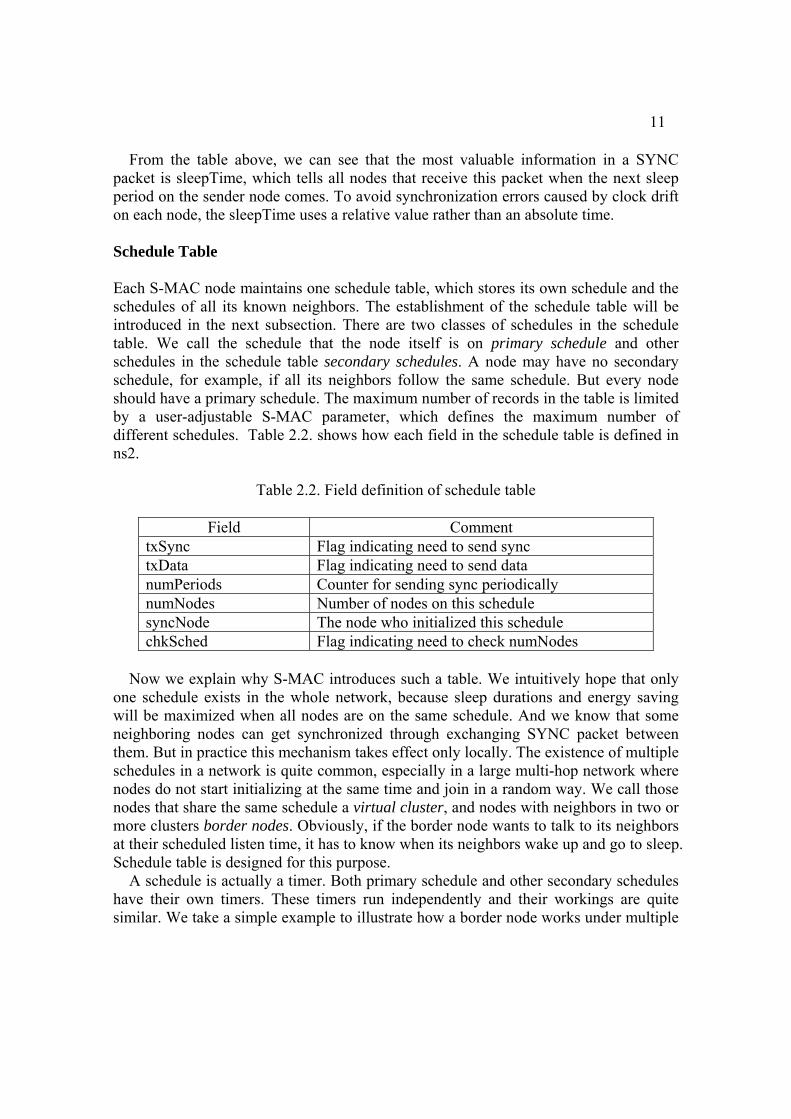
Schedule Table Each S-MAC node maintains one schedule table, which stores its own schedule and the schedules of all its known neighbors. The establishment of the schedule table will be introduced in the next subsection. There are two classes of schedules in the schedule table. We call the schedule that the node itself is on primary schedule and other schedules in the schedule table secondary schedules. A node may have no secondary schedule, for example, if all its neighbors follow the same schedule. But every node should have a primary schedule. The maximum number of records in the table is limited by a user-adjustable S-MAC parameter, which defines the maximum number of different schedules. Table 2.2. shows how each field in the schedule table is defined in ns2.

Table 2.2. Field definition of schedule table

Field Comment txSync Flag indicating need to send sync txData Flag indicating need to send data numPeriods Counter for sending sync periodically numNodes Number of nodes on this schedule syncNode The node who initialized this schedule chkSched Flag indicating need to check numNodes

Now we explain why S-MAC introduces such a table. We intuitively hope that only

one schedule exists in the whole network, because sleep durations and energy saving will be maximized when all nodes are on the same schedule. And we know that some neighboring nodes can get synchronized through exchanging SYNC packet between them. But in practice this mechanism takes effect only locally. The existence of multiple schedules in a network is quite common, especially in a large multi-hop network where nodes do not start initializing at the same time and join in a random way. We call those nodes that share the same schedule a virtual cluster, and nodes with neighbors in two or more clusters border nodes. Obviously, if the border node wants to talk to its neighbors at their scheduled listen time, it has to know when its neighbors wake up and go to sleep. Schedule table is designed for this purpose.

A schedule is actually a timer. Both primary schedule and other secondary schedules have their own timers. These timers run independently and their workings are quite similar. We take a simple example to illustrate how a border node works under multiple

12

schedules. We assume that node B has two neighbors node A and C. As shown in Fig. 2.4, B has two schedules in its schedule table. One is its own schedule (primary schedule), which is the same as A’s, and the other is heard form C. B will allocate a schedule timer for either of the two schedules. The two schedule timers run independently.

SYNC DATA SYNC DATA

SYNC DATA SYNC DATA

SYNC DATA SYNC DATA

A

B

SYNC DATA SYNC DATAC

Fig. 2.4. A border node with two schedules

We first see how B broadcasts SYNC packets. To ensure that both A and C can

receive the SYNC packets in their own SYNC period, B has to broadcast its SYNC packets periodically on both schedules. Please note that, in a SYNC packet, a border node always tells its neighbors the time from now to its next sleep time according to its primary schedule, but not to any of its secondary schedule.

The similar way is applied to broadcast data packets. When B has a data packet to broadcast, it has to broadcast it twice. One takes place on A’s DATA period and the other on C’s DATA period.

Now we discuss unicast data packets. Suppose B receives a data packet destined to C from the upper layer, it first searches in its schedule table to find out the schedule that C is following, and it sets the txData flag on that schedule to 1. When C’s next DATA period comes, the corresponding schedule timer on B will inform B that its data buffer has a data packet destined to C and now it is time to send it out.

From the above discussion, we can see that a border node has to follow several schedules to get synchronized with its neighbors that are on the different schedules. Obviously, border nodes will consume much more energy than non-border nodes. The paper [3] proposes an algorithm called global schedule algorithm that allows all nodes in a multi-hop network to converge on a single global schedule. This algorithm has been implemented in S-MAC in ns-2.28. However, studying S-MAC under multiple schedules is not the intention of this thesis.

13

Neighbor List Another important component in S-MAC is neighbor list. Each S-MAC node has to set up such a table to records the information of all its known neighbors. The number of records in the list is also limited by a user-adjustable S-MAC parameter, which defines the maximum number of neighbors for each node. Like schedule table, neighbor list is established also through exchanging SYNC packets between neighboring nodes. Table 2.3 below shows the definition for each field in neighbor list.

Table 2.3. Field definition of neighbor list

Field Comment nodeId ID of this node schedId Schedule ID in schedule table that this node followsactive Flag indicating this node is active recently state Flag indicating the node has changed schedule

Neighbor list plays an important role in S-MAC. When S-MAC processes a unicast

data request received from the upper layer, it will first check its neighbor list to see if the destination node is on the list. If not, the request will be refused. If yes, the flag txData of the schedule that the destination node follows is set (if no other sending request). Then when the next DATA period on this schedule arrives, the node will try to send out this packet. 2.3.2 Choosing First Schedule When a new node joins the network, it first listens for a fixed period (normally a synchronization period). We call this period initial listening. Either of the following two cases may happen. 1. No SYNC packet received during the initial listening.

At end of this period, the node chooses a schedule by itself and sets a schedule timer for it. Normally the first cycle starts with SYNC period. Meanwhile the schedule is added to the first entry of its schedule table. To announce this new schedule, the flag txSync of this schedule is set, which indicates that the node will try to broadcast a SYNC packet in the next SYNC period.

2. Get a SYNC packet before the initial listening ends.

That is the node’s first SYNC packet received. It immediately follows the schedule that comes with the received SYNC packet, instead of choosing by itself after the initial listening. The value of sleepTime in the SYNC packet determines the starting point of the first cycle. Meanwhile the schedule is added to the first entry of the

14

schedule table, and the sender of the SYNC packet is added to the neighbor list. The node also needs announce this schedule by setting the flag txSnyc in this schedule.

2.3.3 Updating and Maintaining Schedules Now we know from the last subsection that after initial listening the node may get its first schedule by choosing itself or by following an existing one. In this subsection, we discuss how S-MAC maintains its schedule table and neighbor list every time it receives a SYNC packet from one of its neighbors after it has chosen its first schedule. The algorithm for handling received SYNC packets is listed as follows. The method implementing this algorithm in smac.cc is SMAC::handleSYNC(Packet *p). However, there are two such methods with the same name are defined in smac.cc of ns-2.28, which are mutually exclusive at the compiling time. One is defined inside the JOURNAL_PAPER2 code and the other outside. In this thesis, we consider only the inside one, because most of our simulations use the JOURNAL_PAPER code. 1. This is my first SYNC packet.

This may happen only after I have chosen my first schedule by myself (option 1 in last sub-section). In this case, I will discard my first schedule by removing it from my schedule table and follow the new one in the SYNC packet by adding it to the first entry of the schedule table. And the schedule timer that is associated with the discarded schedule will be rescheduled according to the value of sleepTime in the SYNC packet. Of course, the node that sent this SYNC packet will be added to my neighbor list (my first neighbor).

2. This is not my first SYNC packet after I have chosen my first schedule.

We have to consider the following five possible situations. For simplification, we use N representing the sender of this SYNC packet and S representing the schedule in the SYNC packet. The algorithm is put in Table 2.4 below.

2 A macro defined in smac.h, the S-MAC header file in ns-2

15

Table 2.4. General algorithm for processing SYNC packets

Condition Action 1 N is a known neighbor

in my neighbor list and it has not changed its primary schedule since I got its last SYNC packet.

Update S in my schedule table by rescheduling its schedule timer with the value of sleepTime in the SYNC packet. This can eliminate clock drift between two nodes.

2 N is a known neighbor in my neighbor list, but it has switched its primary schedule to S, which is new to me, since I got its last SYNC packet.

Step1: Process the schedule that N has switched from. The number of the nodes on this schedule has to be decreased by one. If the number goes to 0 after decrease, this schedule has to be removed from my schedule list. If now I happen to have a DATA sending request, I must defer changing till the sending is over. Step2: Process the new schedule S that N has switched to. If my schedule table is not full, S is added and assigned to a new schedule timer. Otherwise N has to be deleted from my neighbor list. Step3: If the schedule that N switched from is my primary schedule, I need to execute check_my_schedule, which checks if I become the only one on my primary schedule. If yes, I have to choose the next available schedule in my schedule table and set it as my new primary schedule (delete the old one). But if now I happen to have a DATA sending request, I must defer check_my_schedule until the current sending is over.

3 N is a known neighbor in my neighbor list, but it has switched its primary schedule to S, which is an existing one in my schedule table, since I got its last SYNC packet.

Step1: Process the schedule that N switched from. The number of the nodes on the schedule that N used to follow has to be decreased by one. If the number goes to 0 after decrease, this schedule has to be removed from my schedule list. If now I happen to have a DATA sending request, I must defer changing till the sending is over. Step2: Process the schedule S that N has switched to. Update S in my schedule table by rescheduling its schedule timer with the value of sleepTime in the SYNC packet. And the number of nodes on S is increased by one.

4 N is an unknown neighbor to me and S is also new to me.

If neither my schedule table nor neighbor list is full, add S to my schedule table and assign a new schedule timer to S. Then add N to my neighbor list.

5 N is an unknown neighbor to me, but S is known in my schedule table.

Update S in my schedule table by rescheduling its schedule timer with the value of sleepTime in the SYNC packet. If my neighbor list is not full, N is added to it. And the number of nodes on S is increased by one.

16

2.3.4 Periodical Neighbor Discovery In S-MAC, neighboring nodes discover each other through exchanging SYNC packets. However, sometimes two neighboring nodes may miss each other forever, for example, when they follow different schedules, whose SYNC periods do not overlap. Periodical neighbor discovery can prevent this from happening.

The basic idea of neighbor discovery in S-MAC is to make each node periodically execute neighbor discovery for a whole synchronization time. During neighbor discovery time, S-MAC will never try to go to sleep when its sleep period comes, so that the node can listen more time than usually and have more chances to hear a new neighbor. For a border node, neighbor discovery is only executed on its primary schedule. The reason is that on secondary schedule, the node will not try to go to sleep when scheduled sleep period arrives.

Fig. 2.5 shows how the neighbor discovery period is defined and its relationship with other periods defined in S-MAC. The neighbor discovery period may vary, depending on the current number of its known neighbors. In ns-2, the period of executing neighbor discovery is 2 synchronization periods if the node has no neighbor. Otherwise, the period is much longer and reaches 33 synchronization periods.

SYNC DATA One Frame

One Synchronization Period = 10 Frames

Neighbour Discovery

Sleep

One Neighbour Discovery Period = 2 or 33 Synchonization Periods

Fig. 2.5. Hierarchy of periods in S-MAC 2.3.5 Periodical Neighbor List Updating The schedule table and neighbor list will be updated each time when the node gets a SYNC packet from one of its neighbors. Except that, each S-MAC node also needs to check its neighbor list periodically to see if some of its neighbors have been inactive for a certain time (moved away or died for some reason), which need to be removed from the neighbor list. Doing this is necessary and important, because it cannot only save space for the neighbor list, but also avoid unnecessary energy consumption caused by keeping trying to talk to an inactive neighbor, especially in a multi-hop mobile sensor network.

A timer is allocated to control periodical updating of the neighbor list. Its expiration period must be larger than the synchronization period. The reason for it will be

17

explained later. When the timer expires, the following steps will be executed. (Relevant methods in the source file smac.cc in ns-2.28 includes handleUpdateNeighbTimer(), update_myNeighbList(), update_neighbList()) Step 1: Check if I have a DATA sending request now. If yes, skip the following steps and defer updating till the current sending is over. If no, from now, I will be temporarily disabled from receiving new requests from the upper layer to avoid error operation during updating. (In ns-2, this is done by setting the flag txRequest to 1, which prevents S-MAC from receiving a new request from the upper layer.) Step 2: Update the number of nodes on a certain schedule if its flag chkSched is set. This may happen when I got a SYNC packet from one of my known neighbors, which had switched to another schedule since I got its last SYNC packet, and I should decrease the number of nodes on the schedule that this neighbor had switched from. But at that time I had a DATA sending request, so I had to defer decreasing. And now is time to do it. Step 3: Update neighbor list. Check each record in my neighbor list to see whether its active flag is set or not. If yes, the flag is reset. (The flag will probably be set again when I get this

neighbor’s SYNC packet next time before my next time for neighbor list updating arrives.)

If no, which means that I have not received the SYNC packet from this neighbor

node for a long time (at least a neighbor list updating period), this neighbor node has to be deleted from my neighbor list. Accordingly, the number of nodes on the schedule that the deleted neighbor used to follow should be decreased. If after decrease the number becomes 0, this schedule has to be removed from my schedule table.

Step 4: If the inactive neighbor nodes that I dropped in step 3 are on my primary schedule, I have to execute check_my_schedule, which has been introduced in Table 2.4 Part 2. Step 5: Reset the timer to schedule next neighbor list updating and enable receiving new requests from the upper layer again.

Now we explain the reason why the period for updating neighbor list must be longer than the period for synchronization. Fig. 2.6 shows an example, which has two neighboring nodes A and B. We assume the period for updating neighbor list is smaller than synchronization period, and A can always receive SYNC packets from B

18

successfully. We can see from the figure that A executes neighboring list updating twice in one synchronization period for B. It is easy to imagine that, at the second updating time for A (red arrow), A thinks that B has not been active recently and removes B from its neighbor list, because A has not got B’s SYNC packet since last time when it updated its neighbor list. B will become unknown to A until B’s next broadcasting time comes. In this blank period, A cannot talk to B, because it takes it for granted that B is not active. However, this is not true, because B keeps active all the time.

A

B

A updates B A deletes B B Broadcasts SYNC Packet

Neighbour List Updating Period

Synchronization Period

Blank for B

Fig. 2.6. Neighbor list updating period smaller than synchronization period

2.4 CSMA/CA in S-MAC S-MAC achieves energy saving mainly by utilizing the schedule mechanism. The schedule controls nodes’ periodic sleep and listen. From this point of view, S-MAC looks like a schedule-based MAC protocol, e.g. TDMA. However, with respect to transmission control and collision avoidance, S-MAC is more like a contention-based MAC protocol, especially like the DCF (Distributed Coordination Function) in IEEE 802.11 protocols. In this section, we will introduce the CSMA/CA mechanism in S-MAC, including carrier sense (including physical and virtual mechanisms) and RTS/CTS mechanism for collision avoidance and hidden station problem. 2.4.1 Carrier Sense Like DCF in 802.11, carrier sense in S-MAC is performed both through physical and virtual mechanisms. The medium is determined as free only when both of them indicate that it is free.

Physical carrier sense is performed at physical layer by checking the current radio state. Every time when the radio starts receiving or transmitting, the PHY layer will inform the MAC thereof. It happens also when the receiving or transmitting is over.

19

Obviously, the medium will be determined as busy when radio is in receiving or transmitting state.

Virtual carrier sense is performed at the MAC layer. We know that in 802.11, each station maintains a so-called network allocation vector (NAV), which is actually a counter. It will count down to zero at a uniform rate after it is assigned with a certain value. NAV mechanism requests that each packet sent by MAC contains a duration field, which indicates how long the current transmission will last. When a node receives a packet destined to another node, the duration value in the packet will tell the node how long it has to keep silent. The node’s NAV will be updated with the duration value, only if the duration value is larger than the current NAV value. Virtual carrier sense indicates that the medium is idle, when the NAV value is zero. When non-zero, the indication is busy.

The similar virtual carrier sense mechanism is also applies to S-MAC. However, unlike that in 802.11, S-MAC defines two NAVs. One is simply called NAV and used to indicate if the medium is busy or not, just the same as in 802.11. The other one is called Neighbor NAV, which tracks its neighbors’ NAV. Only when both of the NAVs have counted down to zero, the virtual carrier sense indicates the medium is free. The structure of and the way of running for two NAVs are quite similar. Table 2.5 lists all events that make two NAVs update their values. If not mentioned, the duration value used to update the NAV value is always the duration value in the packet that is received or sent in corresponding event.

Table 2.5. Differences between NAV and Neighbor NAV

NAV Neighbor NAV Receive RTS destined to other node Receive RTS destined to me Receive CTS destined to other node After CTS is sent out (for DATA

timeout) Receive DATA destined to other node

Receive DATA destined to me

Receive ACK destined to other node After DATA (unicast) is sent out Error found in received packet, NAV is updated by an EIFS value

After ACK is sent out

Collision detected when the radio is receiving a packet and another packet arrives, NAV will be updated by an EIFS value right after the radio finishes receiving

ACK timeout, but not reached maximum number of times to extend Tx time

From the above table, we can see that one node uses its NAV for virtual carrier sense

when it interferes in one of its neighbor’s transmission, and uses its Neighbor NAV when it is either a sender or a receiver during a transmission process. Besides their

20

functions for virtual carrier sense, the NAVs also play other roles in S-MAC listed as below. 1. Neighbor NAV will act as a timer for DATA timeout on the node, which has sent

out the CTS packet and is waiting for the arrival of the DATA packet. 2. Adaptive listening (to be introduced in latter parts of this chapter) will be triggered

when either of the two NAVs counts down to zero.

S-MAC obtains a transmission chance through contending for the medium in a contention window. Going back to Fig. 2.2, we find that there are two contention windows defined in one frame. One is for sending SYNC packets in the SYNC period and the other is for sending DATA packets in the DATA period. Both contention windows have fixed size (fixed number of slots), which must be 2n-1, e.g. 31 slots for SYNC and 63 for DATA. Actually, S-MAC can have a third contention window in the sleep period, if adaptive listening is applied (We will discuss adaptive listening in section 2.7). Here we consider only S-MAC without adaptive listening. Now we take a simple example and see how carrier sense is performed before sending a SYNC packet in the SYNC period. The following steps are also applicable to sending a DATA packet in the DATA period.

When the schedule timer expires at the end of the sleep period indicating the coming of a new SYNC period, it will check the conditions for sending a SYNC packet. If the syncFlag on this schedule is set and both of the NAVs have zero values (virtual carrier sense indicates free medium), the node will be ready to broadcast a SYNC packet. If the radio is in sleep state, it will be awoken first. Then the node starts physical carrier sense. The duration for carrier sense is chosen uniformly within the contention window and consists of a DIFS. One of two following possibilities may happen during this period. 1. If nothing is heard throughout the whole carrier sense period, the node will assume

that the medium is free and start transmitting the packet right away. 2. Once the medium is sensed busy during the carrier sense period, the node will stop

sensing and defer sending the packet. When the same period in the next frame arrives, the node will retry sending. While retrying, it will follow the same procedures described above.

In the above discussion, S-MAC always chooses the number of slots for carrier sense

within the fixed contention window size, uniformly and independently. This is not like the binary exponential back off introduced in 802.11.

21

2.4.2 Collision Avoidance We know that the RTS/CTS mechanism defined in the DCF can efficiently reduce the durations of collisions and solve the so-called hidden station problem. This medium reservation technique has been introduced into S-MAC. Prior to the actual DATA packet, the sender should exchange RTS and CTS packets with the receiver. But only unicast packets follow the sequence of RTS/CTS/DATA/ACK. Broadcast packets will be sent without using RTS/CTS. In this sub-section, we discuss unicast packet only.

We have learnt that the virtual carrier sense mechanism introduced in subsection 4.2.1 is achieved by distributing reservation information announcing the impending use of the medium. And the reservation information is recorded in the duration field of RTS/CTS/DATA/ACK packets. RTS/CTS packets will reserve for the whole transmission process. All immediate neighbors of both the sender and the receiver will learn the coming transmission from the RTS or CTS packets and will keep silent during the reserved period. Although the combination of carrier sense and RTS/CTS mechanisms can largely reduce the probability and durations of collisions, collisions cannot be completely avoided. If two neighboring nodes finish carrier sense and start sending at almost the same time, collision will occur. We take a simple example to see how S-MAC sends a data packet out and assume that the channel is ideal (no corruption case).

Consider two neighboring nodes A and B, which follow the same schedule and have discovered each other. A receives a sending request destined to B from the upper layer. We also assume that A does not have any other sending request at present. The carrier sense does not start immediately and needs to wait until the next DATA period comes. A will follow the steps described in last sub-section to start carrier sense.

Fig. 2.7 below shows one possible case. We can see from the figure that A and B exchange RTS/CTS within the DATA period and use their scheduled sleep time for the data packet transmission. Actually the length of DATA period is carefully designed. It is fixed according to some physical-layer and MAC layer parameters, e.g. the radio bandwidth and the contention window size. S-MAC has one feature in the DATA period that no matter how many slots for carrier sense have been chosen from the fixed size contention window, the exchange of RTS and CTS can always be done within the DATA period if no collision and corruption occurs. But the transmission of the DATA packet normally needs to be extended to the schedule sleep period. Normally, S-MAC is working under a relatively low duty cycle (e.g. 10%). The sleep period in a frame is much longer than the DATA period. So in normal cases, the whole transmission process can be done in one frame and will not be prolonged to the next SYNC period. In the following example, the transmission between A and B ends before the next SYNC period. If adaptive listening is not applied, both A and B will still have time to sleep.

22

SYNC

Tx RTS

Got RTS

TxCTS

GotCTS

TxDATA

GotDATA

TxACK

GotACKA

B

DATA Period Sleep PeriodSchedule

Carrier Sense

Fig. 2.7. A successful data transmission between two nodes

Now we see what will happen when collision occurs. If B also sent out the RTS at almost the same time when A sent the RTS out, two RTS packets collide. Neither of them will receive the RTS packet from the other and send a CTS packet back. After a short wile, A’s CTS timer expires. If now A’s primary schedule is in the sleep period, A will go to sleep by turning its radio off. When the next DATA period on the same schedule comes, A will resend the RTS. The maximum number of RTS retries for sending a DATA packet is user-adjustable in S-MAC. When the retry times reach the maximum number, A will give up sending the DATA packet and signal its upper layer about the failure of sending. The same procedures will be followed when B’s CTS timeout timer expires.

2.5 Overhearing Avoidance For contention-based protocols like IEEE-802.11, overhearing is one of the major sources of energy waste. Overhearing takes place on a node when it receives some packets that are destined for other nodes. In 802.11, measures like latency and bandwidth utilization are considered in the first place. To achieve better performance in a shared-medium network, carrier sense, especially virtual carrier sense should be performed more efficiently. The best way to achieve it is to let each node keep listening to all its neighbors’ transmissions. Obviously, this method will lead to large amounts of energy consumptions on overhearing, especially when node density is high and the traffic load in the network is heavy.

For S-MAC, saving energy is its primary goal. To avoid overhearing, S-MAC forces interfering nodes to go to sleep after they receive an RTS or a CTS packet that is not destined for them. In this way, nodes that interfere their neighbors’ transmissions will not hear DATA packets, which normally take much longer transmission time than control packets, and following ACK packets. We take an example in Fig. 2.8 to illustrate this algorithm.

23

BA DC

RTSRTS

CTSCTS

FE

Fig. 2.8. C and D overhear the transmission between A and B

The above figure shows a five-hop linear network. Each node can only hear its immediate neighbors. We assume that all the nodes share the same schedule. Suppose A is communicating with B in the same way that we discussed in Fig. 2.7. We first see which nodes should go to sleep during this transmission.

We know that collision only happens on the receiver side. Obviously, D is supposed to go to sleep, because its transmission interferes with B’s reception of the DATA packet. C is two hops away from B, so C’s transmission will not interfere with B’s reception. But if C talks to E while A is sending data to B, C will not receive any packet from E because collision happens on C. C’s transmission is a waste of energy and it also needs to go to sleep. Both E and F are at least two hops away from the nodes that are transmitting, and they will never produce interference. Therefore, E and F have no need to sleep. In a word, those nodes that are the immediate neighbors of the sender or the receiver should go to sleep.

Now we discuss when C and D should go to sleep. We first see C, who is A’s immediate neighbor. C can hear the RTS packet that A sends to B. However, C does not go to sleep after receiving the RTS, because at this moment the communication has not been really set up and may be cancelled for some reason, e.g. collision on RTS packets. Therefore, it has to keep listening for a CTS timeout period to see if it can hear the following CTS packet. If C receives the CTS packet, it will go to sleep right now. However, in this example, C cannot hear the CTS that B sends back to A. Therefore, after the CTS timeout period, C will keep listening for another CTS timeout period and try to hear the DATA packet. As soon as C hears the DATA packet, it knows from the duration field in the DATA packet that how long exactly the current transmission will last and goes to sleep right now. If no DATA packet is heard in this period, C will go to sleep only when C’s primary schedule is now in the sleep period. For D, who is B’s immediate neighbor, it can only hear the CTS packets sent by B. D will go to sleep right after it gets the CTS and updates its NAV with the duration value in the CTS and goes to sleep right after receiving the CTS.

24

2.6 Message Passing Except that overhearing leads to energy waste in contention-based protocols like IEEE 802.11, control packet overhead will be another reason. Control overhead means cost (energy or time) spent on exchanging control packets (RTS/CTS/ACK) when unicasting a data packet. In this section, we talk about how S-MAC reduces energy consumptions caused by control overhead.

We know that transmitting a long message using a single data packet through a lossy channel is hazardous and riskful. Even when a few bits in the packet are corrupted during the transmission, the whole packet must be re-transmitted. This will waste a lot of time and energy. Therefore, some MAC protocols like 802.11 support a fragmentation mechanism, which breaks a long message into some small fragments. All fragments are sent in a burst, and using one pair of RTS/CTS, if none of them is corrupted. If one of the fragments is corrupted, another pair of RTS/CTS is needed. When receiver has gotten all fragments, its MAC is responsible for assembling all the fragments into a whole and passing it upwards.

S-MAC adopts a modified fragmentation mechanism for transmitting a long message, called message passing. Its basic idea is to fragment a long message into many small fragments and send them in a burst. This means only one pair of RTS/CTS is used for all fragments, but the receiver should acknowledge each fragment it receives. RTS and CTS reserve the medium for transmitting all the fragments. When one of the fragments is corrupted during transmission, ACK timeout will happen on the sender side. The sender has to extend the reserved transmission time for one more DATA/ACK pair and resend the lost fragment immediately. S-MAC sets a limit on how many extensions can be made for one message. This prevents some nodes from occupying the medium for too long in some special cases, e.g. the receiver loses its connection with the sender during the transmission.

As for neighboring nodes that may interfere with the ongoing transmission, they will follow the same way described in section to go to sleep after they hear the RTS or CTS. However, some special cases may happen. For example, the neighboring nodes miss the chance of receiving the RTS or CTS for some reason, e.g. they were sleeping at that time, and they wake up afterwards. Or a new node happens to join the network in the middle of the transmission. Then what should these nodes do in these cases? Actually in S-MAC, besides RTS and CTS, both DATA fragment and ACK packets have the duration field, which is now the time needed for transmitting all the remaining data fragments and ACK packets. Fig. 2.9 illustrates how to set duration value (NAV value) for each packet in the transmission of a 3-fragment message in a burst. So no matter which of them is received by the interfering neighbor nodes, they will know the time the current transmission will last and how long they should sleep. This is also the reason why S-MAC requests the receiver to acknowledge each DATA fragment that it receives. Using the Fragment/ACK pair in message passing resembles the RTS/CTS pair in the way it solves the hidden station problem. Sending the ACK frequently will make the

25

neighboring nodes, which can only hear the receiver, update their NAVs in time. For example, again in Fig. 2.8, D goes to sleep right after it has received the CTS from B. However, one fragment is corrupted during the transmission and the original reserved time for the whole transmission has to be extended. When the original reserved time is over, D may wake up from sleep. It will know the extended transmission time from the ACK packet and go to sleep again.

RTS

CTS

Fragment 0

ACK 0

Fragment 1

ACK 1

Fragment 2

ACK 2

SIFS SIFS SIFS SIFS SIFS SIFS SIFS

NAV (RTS)NAV (CTS)

NAV (Fragment 0)NAV (ACK 0)

NAV (Fragment 1)NAV (ACK 1)

NAV (Fragment 2)

Sender

Receiver

Fig. 2.9. RTS/CTS/DATA/ACK and NAV settings in message passing

From the above discussion, we find that the message passing mechanism in S-MAC can effectively reduce the control overhead in transmitting a long message, by sending all fragments in a burst and using only a pair of RTS/CTS for it. When the sender fails to get an ACK for any fragment, message passing will provide some opportunities for re-transmitting the lost or corrupted fragment, instead of giving up the transmission immediately and re-contending for the medium. This approach seems to be unfair to those nodes that have a short message to send. However, in this way, application-level performance for each node can be improved greatly, if compared to the traditional MAC protocols. That is what sensor networks desire. 2.7 Adaptive listening In this section, we introduce adaptive listening, which is one of the most important and attractive features in S-MAC. In the previous sections, we have mainly discussed how S-MAC reduces energy consumptions. Among those techniques, the scheme of periodic listen and sleep contributes the most. On the other hand, the schedule mechanism will increase the latency of sending packets in a multi-hop network. Although both synchronization mechanism and message passing mechanism have decreased the latency to a certain degree, adaptive listening is the dominant technique that S-MAC has proposed to efficiently and largely reduce the latency in a multi-hop transmission.

Let us look at an example to see how S-MAC transmits a packet in a three-hop linear network. Suppose there are four nodes A, B, C, and D, which are put in a line, as shown

26

in Fig 2.10. Each node can hear only its immediate neighbors. A is the source and D is the sink. Now a data packet is generated at the source node and destined to the sink node. We assume all nodes share the same schedule and no message passing technique is applied.

DCBASource Sink

Fig. 2.10. A three-hop network with one source and one sink

We first see the case shown in Fig. 2.11. When adaptive listening is not employed, each node has at most one chance to send the data packet out in each frame, because checking to send the data packet only takes place at the beginning of each DATA period. If the arrival of the data packet at a certain node misses this checkpoint of this frame, it has to wait until the next DATA period comes. That is to say, when each node strictly follows its sleep schedule, there is a potential delay on each hop. We can see from the Fig. 2.11 that we need three frames to transmit the data packet from the source A to the sink D. The data packet travels only one hop in each frame.

A

B

C

D

C

Data

A

R

C

Data

A

R

C

Data

A

R

D Sleep Sleep SlSchedule

eep

R RTS C CTS Data DATA A ACK

S

S SYNC Period D Scheduled DATA Period

DS DS

Frame n Frame n+1 Frame n+2

Fig. 2.11. Transmitting a data packet through a three-hop network, without adaptive listening

Now we consider the case if adaptive listening is applied. The basic idea is that at the

end of one transmission, S-MAC will give those nodes, which are involved in this transmission including sender, receiver, and neighbors of both them that overhear this transmission, another chance of transmitting data packets. In this way, one node may

27

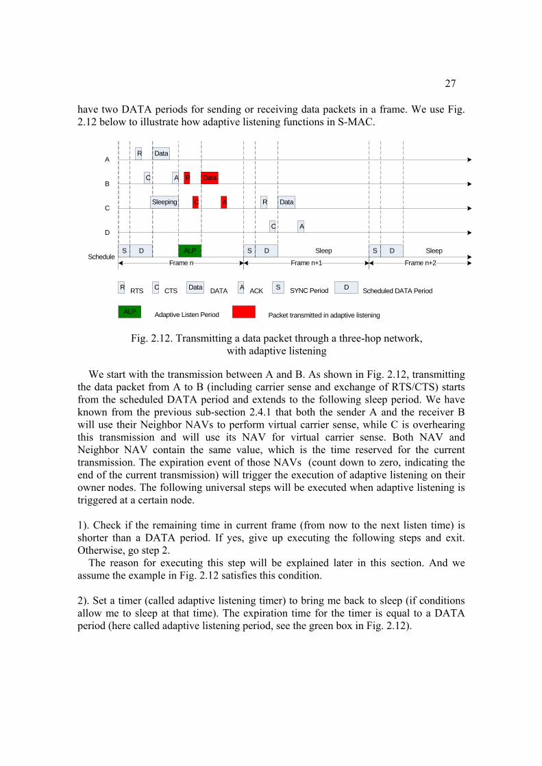
have two DATA periods for sending or receiving data packets in a frame. We use Fig. 2.12 below to illustrate how adaptive listening functions in S-MAC.

A

B

C

D

D

C

Data

A

Sleep Sleep

R

C

Data

A

R

C

Data

A

R

Schedule

R RTS C CTS Data DATA A ACK

Adaptive Listen Period

S

S SYNC Period D

DS DS

Frame n Frame n+1 Frame n+2

Sleeping

Packet transmitted in adaptive listening

ALP

ALP

Scheduled DATA Period

Fig. 2.12. Transmitting a data packet through a three-hop network,

with adaptive listening We start with the transmission between A and B. As shown in Fig. 2.12, transmitting

the data packet from A to B (including carrier sense and exchange of RTS/CTS) starts from the scheduled DATA period and extends to the following sleep period. We have known from the previous sub-section 2.4.1 that both the sender A and the receiver B will use their Neighbor NAVs to perform virtual carrier sense, while C is overhearing this transmission and will use its NAV for virtual carrier sense. Both NAV and Neighbor NAV contain the same value, which is the time reserved for the current transmission. The expiration event of those NAVs (count down to zero, indicating the end of the current transmission) will trigger the execution of adaptive listening on their owner nodes. The following universal steps will be executed when adaptive listening is triggered at a certain node. 1). Check if the remaining time in current frame (from now to the next listen time) is shorter than a DATA period. If yes, give up executing the following steps and exit. Otherwise, go step 2.

The reason for executing this step will be explained later in this section. And we assume the example in Fig. 2.12 satisfies this condition. 2). Set a timer (called adaptive listening timer) to bring me back to sleep (if conditions allow me to sleep at that time). The expiration time for the timer is equal to a DATA period (here called adaptive listening period, see the green box in Fig. 2.12).

28

3). If I am still sleeping, I have to wake up now.

This may happen to the node, such as C in Fig. 2.12, which is sleeping because it overheard its neighbor’s previous transmission. 4). Check if the flag txData on my primary schedule is set (that is to see if I have a buffered unicast data packet to send on my primary schedule). If yes, I will try to send out the data packet by following the same way I do in the schedule DATA period (described in section 2.4). Otherwise I have to keep awake, because my neighbors, who are also adaptive listening now, may want to talk to me.

Please notice that broadcast data packet will never be sent when I am adaptive listening, because I am not sure whether all my neighbors are also adaptive listening now. Some of my neighbors may not be aware of the previous transmission that I was involved in, so they do not execute adaptive listening as me and may be asleep now.

For the example shown in Fig. 2.12, only B satisfies the sending condition, because it just got the data packet from A that needs to be retransmitted to C. After exchanging RTS/CTS with C successfully, B transmits the data packet to C, as shown in the red box in Fig. 2.12. For A, it has nothing to send and has to keep awake. But it will hear the RTS that B sends to C. So A has to go to sleep to avoid overhearing the transmission between B and C. 5). The adaptive listening timer set in step 2 expires. If I am still awake only because I have nothing to send and hear nothing during this adaptive listening period, now I will go back to sleep again.

For the example in Fig. 2.12, no node goes to sleep for such reasons stated above. Both B and C are impossible, because B is transmitting to C. And A overheard this transmission and may have gone to sleep before its adaptive listening timer expires.

Now we explain why S-MAC checks the remaining time in the current frame before

starting adaptive listening. From the above discussions, we see that the essential of adaptive listening is to add another DATA period (adaptive listening period) in the scheduled sleep period, so that nodes can obtain an additional chance for sending or receiving data packet. And we do not want to see the adaptive listening period overlap the next coming SYNC period, because this may interfere with the transmission of the SYNC packets. So that is the reason. But we have to realize one fact, that is, even if the adaptive listening period is located exactly inside the sleep period, the transmission may extend to the next SYNC period. One example for such cases is shown in Fig. 2.13. So we can say only that making the adaptive listening period not overlap the next SYNC period is to give the priority to the SYNC packets, but adaptive listening does not assure that it never collides with the next SYNC period.

29

S SD D

R

C

Data

A

Sleeping

R

C

Data

A

ALP

A

B

C

ScheduleFrame n Frame n+1

Fig. 2.13. Adaptive listening extends to the next frame

From the above discussion, we see that adaptive listening can greatly reduce the

latency caused by the periodic sleep of each node in multi-hop networks. Consider one data packet, which is to be transmitted through a multi-hop network. When adaptive listening is not applied, the data packet can jump only one hop in a frame time. When adaptive listening is applied, the data packet can be retransmitted to the next-hop node immediately after its last transmission is over.

It should be mentioned that theoretically the range of adaptive listening is limited to one hop, because we assume that neighbors that are two hops away cannot hear each other. Under this assumption, one data packet is able to jump at most two hops in a frame time. We use Fig. 2.14 to illustrate this problem. At the end of the transmission between A to B, the adaptive listening is triggered and B starts to retransmit the data packet to C. As happened before, at the end of the transmission between B and C, a second adaptive listening will be triggered. We assume that the remaining time from now to the next listen time is long enough to accommodate an adaptive listening period. Now C tries to retransmit the data packet to D and sends out a RTS packet after carrier sensing. But obviously D is sleeping, because D has not been aware of the adaptive listening that has happened to its neighbors. So C will encounter a CTS timeout and have to wait until the next DATA period comes.

30

Sleeping

A

B

C

D

D

C

Data

A

Sleep

R

C

Data

A

R

Schedule

R RTS C CTS Data DATA A ACK

Adaptive Listen Period

S

S SYNC Period D

DS

Frame n Frame n+1

Sleeping

Packet transmitted in adaptive listening

ALP

ALP

Scheduled DATA Period

R

ALP

R

C

Data

A

Sleeping

Fig. 2.14. Adaptive listening triggered twice in a frame

31

Chapter 3

The Network Simulator

3.1 What is NS-2 NS-2 (Network Simulator version 2) is an object-oriented, discrete-event-driven network simulator targeted at networking research, which has been extensively used by the networking research community. The latest version for ns-2 is version 2.28, which is available on the ns-2 homepage [13].

Ns-2 is a powerful network simulator. It provides substantial support for simulation of TCP, routing, multicast protocols over wired and wireless (local and satellite) networks, etc. Users can define arbitrary network topologies composed of nodes, routers, links and shared medium. A rich set of protocol objects can then be attached to nodes, usually as agents. The simulator suite also includes a graphical visualizer called network animator (Nam) to assist the users get more insights about their simulation by visualising packet trace data.

Ns-2 is written in C++, with an Otcl interpreter as a frontend. Otcl is an object-oriented variant of the well-known scripting language tcl. C++ is utilized for per-packet processing and forms the core of the simulator. Otcl is used for simulation scenario generation, periodic or triggered action generation and for manipulating existing C++ objects.

Ns-2 is open-source software and free to use for all users. Due to its open source nature, a user can modify parameters at different layers, create his or her own applications, and develop new protocol. The freeware nature of ns-2 makes it very attractive to students and network researchers and ideal for study and research purpose.

32

3.2 How to Get Started NS-2 is powerful and attractive for every network user and researcher. But if you are a first-time user, you may find ns-2 is not easy to get started. Even though you can search out large amounts of ns-related documents on the Internet, which are written usually by experienced ns users or developers, most of them are quite obscure and not friendly to new users. So the purpose of this section is to share my experience in getting ns-2 started.

Since ns is an object-oriented simulator written in both C++ and Otcl, you should know at least one object-oriented programming language, like C++ or Java. Do not worry if you only know C++ but never used or heard of Otcl, because writing some simple simulation scripts in Otcl will not be difficult for a C++ user. But if you are already an experienced C++ programmer, you will find a lot of fun in using ns-2, because the greatest fun in ns-2 is to debug or write C++ source code. In addition, it would be a great help, if you know Perl or any other languages good at processing data file, because ns requires users to extract simulation results by themselves. And how to extract your desired information from a huge trace file correctly and efficiently is also a considerable problem especially when you plan to use ns to simulate a huge network system and have large amounts of data to analyze.

The first guide documents worth recommending for ns beginners are “Marc Greis's tutorial” and “ns by Example”, which can be found on the ns-2 homepage [13]. These two tutorials are especially written for new ns users and will give you an idea about how ns-2 looks like and works. You would better not jump to read Ns Manual (the ns-2 official reference) if you do not have any preliminary knowledge of ns, because this manual is not a tutorial for beginners. The ns manual is more like a technical document, which mainly helps ns users or developers deeply understand how each internal component of ns-2 is organized and developed. It will be one of the most valuable documents you should read and put at hand, after you have become a little familiar with ns and want to go deeper into ns-2.

Before you start to write your own tcl script, you had better first check the example folder of ns-2 to see if there are some example scripts that have similar configurations with yours. The example folder is located in, e.g. ns-2.28 \tcl\ex\, where you can find a lot of example scripts for all kinds of simulation scenarios. Besides the example folder, there also exists a test folder under the path, e.g. ns-2.28\tcl\test\, where many test scripts can be found. Those test scripts can be executed to verify the correctness of the installation of ns-2. Normally when a new protocol or module is developed or implemented in ns-2, the ns-2 developer or programmer will write such a test script for it. And this test file will be the best example, which can tell us how to configure ns-2 to simulate this new protocol or module.

If you are studying a new protocol with ns-2, reading and understanding, its source code in ns-2 is necessary. No bug, no code. So debugging work should be performed carefully before you start your experiments. Do not forget to check the ns-2 homepage

33

to see if there is a new updated version available. Though ns-2 formal release version is not likely updated frequently, there will be small updates in daily snapshot. Minding the homepage of the group that is responsible for developing this protocol or join the mailing list or forum the research group provides can make you synchronize with the latest development of the topic you are studying.

You are suggested to subscribe to ns-users mailing list, if you want to communicate with other ns users throughout the world. Especially when you encounter a hard problem, to which you cannot find out a solution even in all documents you have checked (ns-2 is such a huge system that you are very likely to encounter such problems), the mailing list is the first place where you should go for help. If you do not like to receive tens of mails sent by the mailing list everyday, you can directly use the search function provided by the ns official web site, which can be linked from the ns homepage (the link is at the bottom of that page, named “Search ns web pages”). There you can search the contents of all the publicly available WWW documents and mailing list archives at Ns and Nam's site. No matter in mailing list or on search web, quite often you can get a surprise and find what you want there. For S-MAC users, a mailing list for discussing or announcing S-MAC related problems has also been created. The web page for subscribing to S-MAC mailing list is http://mailman.isi.edu/mailman/listinfo/smac-users.

34

Chapter 4

Simulating S-MAC with NS-2

4.1 S-MAC in NS-2 4.1.1 Implemented S-MAC Features S-MAC is developed based on the Mote platform that runs TinyOS and its implementation in TinyOS reflects the latest protocol development. But as a hardware implementation, which needs real hardware as its running platform, it is not suitable for us to study S-MAC in a simulation way. S-MAC has been also implemented in ns-2, the network simulator. The latest official release is integrated in ns-2.28. If you want to use the most recent updated and debugged version, you have to download a new ns-2 daily snapshot or update to the latest CVS. More information about the updating of ns-2 and S-MAC can be found on the ns-2 homepage [13].

In this thesis, we study S-MAC with ns-2 and install the ns-2.28 all-in-one version on the SUSE Linux system (Professional 9.2). After installation, the source files (in C++) for S-MAC, smac.h and smac.cc, can be found in the path ns-2.28\mac\.

Most of the features proposed in the paper [2] have been implemented in this version. But, this version is still not the final version for S-MAC, because we found a portion of code still in testing. We call this portion code JOUNAL_PAPER code, because a macro named JOURNAL_PAPER controls compiling this portion code. By default, the definition statements for this macro are disabled in the S-MAC header file and JOURNAL_PAPER code will not be compiled when we install ns-2.28. For our purpose of study, we have to consider JOURNAL_PAPER code, because it implements some important features of S-MAC, such as adaptive listening and message passing. We list all features of S-MAC that have been implemented in ns-2-28 as follows. The detailed descriptions of these features have been presented in chapter 2.

35

Basic features Listen and sleep periodically according to schedules Both physical and virtual carrier sense Overhearing avoidance RTS/CTS mechanism for unicast data packets Synchronization algorithm (including schedule choosing, schedule updating and maintaining) Neighbor discovery Features in JOURNAL_PAPER code Adaptive listening Message passing (partially implemented) Improved synchronization algorithm Neighbor list updating Global schedule algorithm (not to be discussed in this thesis) 4.1.2 S-MAC Parameters Settings All preset parameters for S-MAC can be found and modified in the header file smac.h, including user adjustable S-MAC parameters, internal S-MAC parameters, and physical layer parameters. Some other parameters will be assigned at the start of the simulation run, because their values depend on some interactive parameters. For example, the sleep time and cycle time (frame time) depend on the value of duty cycle that users have set in the tcl script. We call those parameters, which can be set in tcl scripts in an interactive way, interactive parameters. All three interactive parameters are listed in Table 4.1 below.

Table 4.1. S-MAC Interactive Parameters

Name Comment syncFlag_ If it is set to 1, S-MAC runs with periodic sleep. If it is set to 0, S-

MAC runs without periodic sleep. dutyCycle_ The value of duty cycle in percent. It controls the length of sleep.

If not set, ns-2 uses the default value 10%. This parameter is active only when syncFlag_ is set to 1.

selfConfigFlag_ If it is set to 1, all S-MAC nodes follow the schedule initialization algorithm described in section 2.3. If it is set to 0, the schedule start time (first listen period start time) for each node is user-configurable.

36

4.1.3 S-MAC Modes For the purpose of comparison, S-MAC can be configured to run under three modes, which are listed as below: Mode 1: S-MAC without periodic sleep If the parameter syncFlag_ is set to 0, S-MAC will work under this mode. In this mode, each node does not follow periodic sleep and listen cycle and runs in a fully active mode. But overhearing avoidance is still available in this mode. That is, the node will go to sleep when it overhears its neighbor’s transmission. Please note that in ns-2.28, we cannot set S-MAC to this mode in the case of JOURNAL_PAPER defined. Mode 2: S-MAC with periodic sleep, but without adaptive listening If the parameters syncFlag_ is set to 1 and JOURNAL_PAPER code is not compiled, S-MAC will work in this mode. In this mode, only the basic features listed in sub-section 4.1.1 are available. No adaptive listening and message passing are available in this mode. Mode 3: S-MAC with periodic sleep and adaptive listening. If we compile JOURNAL_PAPER code in S-MAC source code and set syncFlag_ to 1, we can simulate all features of S-MAC, such as adaptive listening and message passing, listed in sub-section 4.1.1. 4.1.4 Problems and Bugs of S-MAC in NS-2.28 We have found the following problems and bugs for S-MAC in ns-2.28. Segmentation error As mentioned before, we cannot set S-MAC to mode 1 in the case of JOURNAL_PAPER defined. If we use the JOURNAL_PAPER code and then set the flag syncFlag_ to 0, a segmentation error will occur during the simulation run. The reason is that the JOURNAL_PAPER code is not designed to support S-MAC running in mode 1. That is to say, we cannot simulate S-MAC in mode 1 if JOURNAL_PAPER is used. In other words, if we simulate S-MAC in mode 1, some features like message passing, which are only available in the case of JOURNAL_PAPER defined, will not be supported.

37

Constant data packet size at MAC layer

When you run S-MAC without using the JOURNAL_PAPER code, you may take notice of such a confusing phenomenon. S-MAC will send all data packets with a uniform size, regardless of their actual payloads. Checking the source code of S-MAC, you will find that it defines a macro called SIZEOF_SMAC_DATAPKT. The default value of this macro found in smac.h is 50 (Bytes). When S-MAC is sending or receiving a data packet, S-MAC always uses this macro value, instead of the packet’s actual payload, to calculate the duration for transmitting this packet. Obviously this is unreasonable. But we do not think this is a bug for S-MAC, because it seems to be an author’s temporary solution. It would not be a difficult task for us to fix this problem. But we do not change it, because we are not very clear about the author’s real intention. In our simulations with message passing disabled (JOURNAL_PAPER not compiled), we can simulate S-MAC using CBR traffic source with different packet size, by directly modifying the value of SIZEOF_SMAC_DATAPKT (need to recompile S-MAC before running).

But if JOURNAL_PAPER code is compiled and message passing is enabled, the situation will be different. For message passing, see below.

One problem in message passing

The message passing mechanism has been implemented in JOURNAL_PAPER code. For simplification, S-MAC in ns-2 divides a long message into an integer number of equal-size fragments. The equal fragment size is SIZEOF_SMAC_DATAPKT. The code for calculating the number of fragments can be found in the method SMAC::sendMsg(Packet *pkt, Handler *h) in smac.cc and listed as below.

int fragNum = ch->size_ / SIZEOF_SMAC_DATAPKT ;if (fragNum == 0) fragNum = 1;

In above code, ch->size_ stands for the actual payload of the packet. The number of fragments is calculated by a division operation and the result is converted to an integer number forcibly. Obviously in this way, some information in the message may get lost during the fragmentation process. For example, if payload is 120 Bytes and SIZEOF_SMAC_DATAPKT is 50 Bytes, we get only 2 fragments with size 50 Bytes each. So we replaced the above code with the following.

38

int fragNum = ch->size_ / SIZEOF_SMAC_DATAPKT ;if (ch->size_ % SIZEOF_SMAC_DATAPKT != 0) {

fragNum ++;}

After modification, a message with 120 Bytes will be divided into 3 fragments with each 50 Bytes. It now seems more reasonable, although we have to send additional bits for it. Wrong value for neighbor list updating period

We have introduced periodical neighbor list updating in sub-section 2.3.5. The period for updating neighbor list is defined by a macro SMAC_UPDATE_NEIGHB_PERIOD in smac.h. Its default value is 50. Since this is just a number defined in the code, we have to know its unit. According to the following code in the construction function SMAC::SMAC() in smac.cc, it seems that the period is 50 seconds. (mhUpdateNeighb_ is the timer for updating neighbor list periodically) mhUpdateNeighb_.sched(SMAC_UPDATE_NEIGHB_PERIOD);

But this is not a safe value, because it may result in unexpected errors. In subsection

2.3.5, we have explained the reason why the period for updating neighbor list should be longer than the period for synchronization. The default value for synchronization period is 10 frames, while the length of one frame depends on the value of duty cycle we use. Table 4.2 below shows that when the duty cycle is 1%, the synchronization period is longer than 50s.

Table 4.2 Synchronization period vs. Duty cycle

Duty cycle One Frame Length Synchronization Period 1% 11.221 s 112.21s 10% 1.123 s 11.23 s

So we have to change the period for the neighbor list updating from 50 s to 50 frames. That is more reasonable, because it is 5 times longer than the synchronization period and independent of the duty cycle. The modified code is shown as bolow. mhUpdateNeighb_.sched(SMAC_UPDATE_NEIGHB_PERIOD*CLKTICK2SEC(cycleTime_));

39

S-MAC callback missing First, we talk about how S-MAC receives packets from its upper layer. Like other MACs, S-MAC can only process a sending request at a time. So it needs a buffer for storing packets from the upper layer. In ns-2, S-MAC is directly connected to a queue module called Interface Queue (Ifq), which buffers packets from the link layer. The queue size for Ifq is user-adjustable in ns-2, and we always use its default value 50 in our simulations. Every time S-MAC has finished the current sending request (successful or unsuccessful), it has to inform the Ifq about it (we call it callback in ns-2). Then the Ifq dequeues a packet and passes it to S-MAC, if it is not empty. If the Ifq is empty now, the Ifq will pass the packet to S-MAC as soon as it gets a new one from the link layer. In a word, the workings for Ifq can be described as no asking, no sending. That is, if S-MAC doesn’t do callback, Ifq will never send packets to it automatically. But we found somewhere in the source file smac.cc that callback is missing, which may result in occasional errors when running S-MAC.

Two such errors are found in the method SMAC::unicastMsg(int numfrags, Packet *p), which will be called when S-MAC receives a new unicast packet from the Ifq. The first error place is shown as below.

If (found == 0) {printf ("Neighbor unknown; cannot send pkt\n");txMsgDone(); // debug here, should signal upper layer before returnreturn 0;

}

The above code checks if the destination node that the received data packet is

destined for is in the neighbor list. If not, S-MAC will discard the packet and give up sending. Obviously, a callback is missing here. The consequence is that once this “Neighbor unknown” event happens for some reason, S-MAC will not receive any packet from the Ifq from then on. In S-MAC, the callback is implemented in the method txMsgDone(). So we must add this method before the return statement (code in red).

The second error place in the same method is shown as below. The same code as the following can be found also in the method SMAC::bcastMsg(Packet *p).

if (txRequest_ == 0) {txRequest_ = 1;}

else {txMsgDone(); // debug here, should signal upper layer before returnreturn 0;}

40

The above code checks if the flag txRequest_ is set or not. If yes (indicating that S-MAC already has a data packet to send), S-MAC has to discard the new received packet. Similarly, a callback statement txMsgDone() is missing before return statement. You might question the possibility of executing the else statements, because the Ifq will never send new packets to S-MAC when S-MAC has not finished with the current sending request. But there exists one exception, which has been discussed in sub-section 2.3.5. That is, S-MAC will temporarily disable receiving new sending request from the upper layer (by setting the flag txRequest_ to 1), when it is ready to update neighbor list. Different schedule starting time in JOURNAL_PAPER code We have introduced the algorithm for S-MAC to choose the first schedule in subsection 2.3.2. When a new node does not hear any SYNC packet during the initial listening period, it has to choose a schedule by itself. In S-MAC, choosing a scheduling means choosing the starting time of the first listen period. The following code is extracted from the method SMAC::setMySched(Packet *pkt) in smac.cc and will be executed for choosing the node’s own schedule after the initial listening period.

if (pkt == 0) { // freely choose my schedule#ifdef JOURNAL_PAPER

schedState_++;mhCounter_[0]->sched(CLKTICK2SEC(listenTime_+index_*10));schedTab_[0].syncNode = index_;

#elsemhCounter_[0]->sched(CLKTICK2SEC(listenTime_));

#endif...

We can see that if JOURNAL_PAPER is not defined, all nodes start their first schedules with a listen period. This means if we set the parameter selfConfigFlag_ to one, there will always be one schedule in the network. All nodes share the same schedule.

But if the JOURNAL_PAPER code is considered, the starting time of the first listen period at different nodes will differ, depending on its index (node id). The purpose of doing this for the S-MAC author is to introduce the scene of multiple schedules to S-MAC simulations. An example for this case is shown in Fig. 4.1. We can see that the starting time of the first listen period for different nodes is staggered. So this scene can be used to simulate the scenario when nodes join the network at equidistant fixed intervals.

However, the scene of multiple schedules is not involved in this thesis. So we delete the parts in red colour in above code.

41

Initial Listening

Initial Listening

Initial Listening

Initial Listening

0

1

2

3

Listen Listen

Listen

Listen

Listen

Listen

Listen

Listen

Fig. 4.1. Different schedule for each node

4.2 Preparations for Simulating S-MAC In this section, we introduce what modules we have added to ns-2 necessary for simulating S-MAC. 4.2.1 NO Ad-Hoc Routing Agent (NOAH) When we simulate a wireless network in ns-2, we should specify a routing protocol for it. NS-2.28 has implemented four ad-hoc routing protocols for wireless simulations, including DSDV (Destination-Sequenced Distance-Vector), DSR (Dynamic Source Routing), TORA (Temporally Ordered Routing Algorithm), and AODV (Ad hoc On-demand Distance Vector). Any one of these four routing protocols can be used to simulate S-MAC. But for purpose of our study, we are only interested in the performance of S-MAC, but not the routing protocols. To measure the performance of S-MAC in a pure condition, we expect to use such a special routing protocol, which provides static or manual routing mechanisms and will not produce any routing packet after the simulation starts. Unfortunately, static routing and manual routing defined in ns-2 are only available for wired simulations, but not for wireless simulations.

We found a third-party routing agent for ns-2, which accords with our desires. That is the so-called no ad-hoc routing agent (NOAH), which is a wireless routing agent that supports static multi-hop routing. NOAH is quite suitable for simulation scenarios where routing packets are not desired. For more detailed information about installation instructions and the usage of NOAH, please visit the web site listed in [12]. Although this plug-in is claimed to work with ns-2.26, we found that it works quite well with ns-2.28 as well.

42

4.2.2 Exponential Traffic Source Agent In ns-2, traffic sources generate packets in the application layer at each source node. Three traffic sources have been implemented in ns-2.28, including exponential on/off traffic source, pareto on/off traffic source, and CBR (constant bit rate) traffic source. However, we hope to generate packets with exponentially distributed inter-arrival times and packet sizes when simulating S-MAC. Someone has developed a new traffic source agent and we adapt it to our simulations, called EXPO_Traffic (its Otcl class name is Application/Traffic/MyExponential). The source code is in the file expo_traffic.cc. We will not go into details about the source code. The following steps show how to add this new traffic generator to ns-2. Step 1: place the source file expo_traffic.cc in ns-2.28/tools/ Step 2: add the following statements to the file ns-2.28/tcl/lib/ns-default.tcl (line 489) Application/Traffic/MyExponential set interval_ 1 Application/Traffic/MyExponential set packetSize_ 100 Application/Traffic/MyExponential set maxpkts_ 268435456 Note: set default values for member variables. If we create a new object without assigning these variables explicitly, ns-2 will use the default values set in ns-default.tcl. Step 3: In the file /common/packet.h

Line 166, add: PT_EXPO, Line 206, add: name_[PT_EXPO]= "expo"; Note: create a new packet type “expo” for this traffic source Step 4: In the file ns-2.28/trace/trace.cc line 200, add: || t == PT_EXPO Note: inform the trace agent of the new added packet type. And “expo” will be displayed in the trace file. Step 5: In the file ns-2.28/Makefile.in, in OBJ_CC (line 169), add:

tools/expo_traffic.o Note: configure compilation path for the new source file Step 6: Go to the directory ns-2.28/ and execute the following commands: ./configure

make clean make Note: to use the new traffic generator, we should recompile ns-2 first.

43

The EXPO traffic generator has four generation modes. Mode 1: AdPd (Deterministic inter-arrival time and deterministic packet size) Mode 2: AePd (Exponential inter-arrival time and deterministic packet size) Mode 3: AdPe (Deterministic inter-arrival time and exponential packet size) Mode 4: AePe (Exponential inter-arrival time and exponential packet size) And it defines two commands used to configure generation modes. interval-exp If called, inter-arrival time conforms to exponential distribution.

If not, inter-arrival time conforms to deterministic distribution. size-exp If called, packet size conforms to exponential distribution.

If not, packet size conforms to deterministic distribution. The member variables that parameterize this agent are: packetSize_ constant (Pd) or mean (Pe) packet size (default is 100Bytes) interval_ constant (Ad) or mean (Ae) interval between packets (default is 1s) maxpkts_ the maximum number of packets to generate (default is 268435456) The following tcl code illustrates how to create an EXPO traffic source over a UPD agent. set expo [new Application/Traffic/MyExponential] $expo set packetSize_ 500 # mean packet size, 500 Bytes $expo set interval_ 1.0 # mean inter-arrival time, 1s $expo set maxpkts_ 2000 # maximum number of packets to generate $expo size-exp # packet size conforms to exponential distribution $expo interval-exp # inter-arrival time conforms to exponential distribution $expo set-seed 0 # set seed for random number generator $expo attach-agent $udp # attach the EXPO traffic source to a UDP agent 4.3 An Example Tcl Script for Simulating S-MAC To simulate S-MAC with ns-2, we must create a tcl script first. In this section, we illustrate how to set up a tcl script for simulating S-MAC in ns-2.28. We take a ten-hop linear network as an example, because most of our simulations run over this ten-hop topology. The scenario for this example is described as below. Topology: 11 S-MAC nodes form a ten-hop linear wireless network, as shown in Fig. 4.2. Each node can hear only its immediate neighbors. The first node (node 0) is the source and the last node (node 10) is the sink.

44

Routing protocol: NOAH (NO Ad-Hoc Routing Agent) Traffic pattern: Packets are sent from the source node to the sink node. Packets’ inter-arrival times at the source node conform to an exponential distribution with mean value 10s. Packet size is fixed to 100 Bytes. The generator keeps generating until the end of the simulation. Scheduling: The generator starts generating at 60 s and stops at 2000 s.

0 1 2 8 9

Source Sink

...

... 10

Fig. 4.2. Ten-hop linear network with one source and one sink

Normally a tcl script for wireless simulation starts with a list of tcl variables definition statements. And we use those variables to store our parameters preferences for the simulation. This is convenient for parameters management. Each parameter is stored in a tcl variable using tcl command set.

Two classes of parameters are defined and listed as below. The node configuration parameters specify the components that we want to simulate in each node and will be used in later node configuration step. Running parameters include the trace file name, the number of nodes to be created for simulation and the simulation running time. # Node configuration parametersset opt(chan) Channel/WirelessChannel ;# channel typeset opt(prop) Propagation/TwoRayGround ;# radio propagation modelset opt(netif) Phy/WirelessPhy ;# network interface typeset opt(mac) Mac/SMAC ;# MAC typeset opt(ifq) Queue/DropTail/PriQueue ;# IFq typeset opt(ll) LL ,# like layer typeset opt(ant) Antenna/OmniAntenna ;# antenna modelset opt(ifqlen) 50 ;# buffer size of IFqset opt(adhocRouting) NOAH ;# routing protocol

# Running parametersset sim(tr) trace.tr ;# trace file nameset sim(nn) 11 ;# number of nodes set sim(stop) 100000.0 ;# simulation stop time

45

The following code configures parameters for S-MAC. These S-MAC parameters have been introduced in subsection 4.1.2. Mac/SMAC set syncFlag_ 1 ;# enable sleep listen cyclesMac/SMAC set dutyCycle_ 10 ;# S-MAC with 10% duty cycleMac/SMAC set selfConfigFlag_ 1 ;# disable user-configurable schedule

The following steps are quite common for wireless simulations.

set ns_ [new Simulator] ;# create a simulator instanceset wtopo [new Topography] ;# create wireless topography object$wtopo load_flatgrid 2500 200 ;# specify length and width of the topographyset tracefd [open $sim(tr) w] ;# open trace file defined before$ns_ trace-all $tracefd ;# trace all event during simulationcreate-god $sim(nn) ;# create god

The following statement sets the random seed value for random number generator. If

we want ns-2 to produce different results every time we run the simulation (independent replications), the seed value should be zero. If we expect reproducible simulation results, the seed value can be any non-zero integer number. ns-random 0 ;# independent simulations

The next step is node configuration. In ns-2, node is the basic simulation entity and

can be configured to have different components and characteristics in different simulations. In wired simulations, we normally create node objects directly using the default node configuration. But in wireless simulations, we must explicitly specify all components that each node object will have, before actually creating node objects. The node configuration parameters have been chosen at the beginning and stored in tcl variables (in the form of $opt()). In this step, we actually configure nodes with those variables. The node configuration command is shown as below. These options are easy to understand according to their names. The last three options turn on or off the trace options at Agent/Router/MAC levels. In this example, we decide to turn tracing on at the agent and router level only.

46

$ns_ node-config -adhocRouting $opt(adhocRouting) \-llType $opt(ll) \-macType $opt(mac) \-ifqType $opt(ifq) \-ifqLen $opt(ifqlen) \-antType $opt(ant) \

-propType $opt(prop) \-phyType $opt(netif) \-channelType $opt(chan) \

-topoInstance $wtopo \ -agentTrace ON \ ;# tracing at agent level turned on-routerTrace OFF \ ;# tracing at router level turned off-macTrace OFF ;# tracing at mac level turned off

Besides the configurable node, each component model inside the node is also

configurable. For example, we can set the height and gain for antenna. But in this example, we do not reconfigure any of them, and use their default values. Ns-2 has put all default parameters in the file ns-2.28\tcl\lib\ ns-default.tcl. In multi-hop simulations, one default value that we need to know is the communication range of wireless nodes. If both antenna model (Antenna/OmniAntenna) and network interface model (Phy/WirelessPhy) are configured to use their default values (like in this example), the default value for communication range is 250 meters. If another different value is desired, please follow the directions in section 18.4 (communication range) in ns-manual [14].

After node configuration is done, actual nodes can be created like following.

for {set i 0} {$i < $sim(nn) } {incr i} {set node_($i) [$ns_ node]$node_($i) random-motion 0 ;# disable random motion

}

Then we position each node in the topography that we have defined before. This

simulation scenario requires that each node can hear only its immediate neighbors. And the default radio transmission range is 250 meters. So we need to space out the nodes 200 meters apart. The following code creates the topology for this scenario.

47

for {set i 0} {$i < $sim(nn) } {incr i} {$node_($i) set Z_ 0.0$node_($i) set X_ [expr 50.0+[expr 200.0*$i]]$node_($i) set Y_ 100.0

}

We use NOAH as the routing protocol not only in this example, but also in all our S-

MAC simulation scenarios. The following code sets up a static routing table for 10-hop network using routing command. for {set i 0} {$i < $sim(nn) } {incr i} { set cmd "[$node_($i) set ragent_] routing $sim(nn)" for {set to 0} {$to < $sim(nn) } {incr to} { if {$to < $i} { set hop [expr $i - 1] } elseif {$to > $i} { set hop [expr $i + 1] } else { set hop $i } set cmd "$cmd $to $hop" } eval $cmd}

The next step is to define the traffic model. We should set up an agent at the

transportation layer. Since we are studying the behaviors of S-MAC, UDP agent is a better choice than TCP agent, because UDP is quite simple and connectionless. The following code creates a UDP agent and attaches it to the source node. Accordingly, a Null agent is created and attached to the sink node. Then we connect the udp agent and null agent together, which establishes a virtual path between the source node and the sink node.

set udp [new Agent/UDP] ;# create a new UDP agent $ns_ attach-agent $node_(0) $udp ;# attach udp to source nodeset null [new Agent/Null] ;# create a new Null agent$ns_ attach-agent $node_([expr $sim(nn)-1]) $null ;# attach null to sink node$ns_ connect $udp $null ;# connect udp to null

48

To generate packets at the source node, we need to create a traffic source and attach it to the UDP agent. The following code creates an EXPO traffic that we have introduced in sub-section 4.2.2, and configure it to work in AePd (Exponential inter-arrival time and deterministic packet size) mode. Notice that the maximum number of packet to generate is not explicitly specified, because its default value is big enough to make the generator always keep generating packets during the whole simulation time (2000 s in this example).

set expo [new Application/Traffic/MyExponential]$expo set packetSize_ 100$expo set interval_ 10.0s$expo interval-exp$expo attach-agent $udp

Ns-2 is a discrete event based simulator. When the simulation starts running, a scheduler is created to control the simulating process. In the tcl script, we should tell the scheduler the exact time when a certain event should occur. Those events are described in the following comments. $ns_ at 60.0 "$expo start" ;# when expo starts for {set i 0} {$i < $sim(nn) } {incr i} { ;# when nodes stop $ns_ at $sim(stop) "$node_($i) reset";}$ns_ at $sim(stop) "finish" ;# when call finish procedure$ns_ at $sim(stop).01 "puts \"NS EXITING...\" ; $ns_ halt"; # when stop simulation

The definition of finish procedure is shown below.

proc finish {} {global ns_ tracefd $ns_ flush-traceclose $tracefdexit 0}

In all tcl scripts for ns-2, the last statement should be: $ns_ run

49

4.4 Tracing 4.4.1 How to Trace in ns-2 Tracing is a necessary technique for each discrete-event simulator, because it tells us what has happened inside the model during its running and the output analysis is also based on the tracing results. Normally for a simulation tool, trace data can be either displayed directly during execution of the simulation, or stored in a file to be post-processed and analyzed. Ns-2 supports the latter one better, though Nam (an animation tool designed for working with ns-2) can implement the first one to a certain extent. In this section, we use the example presented in section 4.3 to show how to generate traces and record data into a trace file, and how to analyze and abstract useful information from the trace file.

Ns-2 is able to trace all packets that are received, dropped and sent by agents, routers, MAC layers or interface queues. Before the simulation starts running, we should tell ns-2 what events we want to trace. The following code taken from the example in section 4.3 is related to trace configuration.

set sim(tr) trace.tr ;# specify the trace file name…set tracefd [open $sim(tr) w] ;# open trace file defined before$ns_ trace-all $tracefd ;# record all traces in the trace file …$ns_ node-config �

-agentTrace ON \ ;# turn on tracing at agent level -routerTrace OFF \ ;# turn off tracing at router level-macTrace OFF ;# turn off tracing at mac level

…proc finish {} {

global ns_ tracefd ;# set outer variables to global, visible inside$ns_ flush-trace ;# flush the trace buffer before simulation endsclose $tracefd ;# close the opened trace file

…

For more tracing options that ns-2 provides, please refer to the ns manual[14]. We

keep using the above trace settings in all our simulations, because such settings have already satisfied our needs for measures, except for the measure energy consumption. In subsection 4.4.3, we will talk about how to trace energy consumption for S-MAC in ns-2.

50

4.4.2 Trace Format All trace data will be recorded into a specified trace file in a certain format. Ns-2 defines two trace formats, old format and new format. The old format is the default trace format in ns-2 and supports all type of simulations. The new format is especially designed for tracing wireless simulations, which is more standardized than the old one. However, S-MAC in ns-2-28 still does not support the new trace format. Therefore, we consider the old format. A trace record in a S-MAC trace file is shown in Fig. 4..3 below.

s 274.090231333 _3_ MAC --- 0 RTS 10 [0.11 4 3]

1 2 3 4 5 6 7 8 9

Fig. 4.3. S-MAC Trace format

We can know from this trace record that at 274.090231333 s, node 3 sends an RTS packet to node 4. Now we explain what these field mean in the usual case.

1. The first field represents the event type, whose value can be s (send), r (receive),

d (drop) or f (forward). 2. The second field the time this event happens.

3. The third field records the id of the node, on which this event takes place.

4. The fourth field shows the layer where this event happens. Its possible value

may be one of the following four: AGT (agent), RTR (router), IFQ (interface queue), and MAC (mac).

5. The fifth field is normally a short broken line, which is reserved for special

events. For example, when collision occurs, the broken line is replaced with COL.

6. The sixth field is the global sequence number for this packet, which is the

integer number used to identify this packet in the whole network and distinguish it from others. Sequence number is only available for data packets and not allocated for control packets, like RTS/CTS/ACK and SYNC packets in S-MAC (using a zero instead).

51

7. The seventh field is the packet type. The actual value is determined by the application or MAC layer, which creates this packet. For example, cbr represents that it is a data packet generated by a CBR traffic source.

8. The eighth field is the packet size in bytes.

9. The ninth field including three numbers in brackets concerns MAC layer

information. Originally, there will be four numbers in the brackets. But S-MAC revises this format. The first number is the duration field of this packet. In Fig. 4.3, the duration field of this RTS packet is 0.11 s, which is the remaining time reserved for the coming transmission. The second number stands for the MAC address of the receiver of this packet, and the third number for the sender.

The above nine fields are common for all traces if S-MAC is employed. But some

packets may have additional fields to record other information, like routing and IP information. But for our purpose of study, considering these nine fields are already enough.

4.4.3 Tracing Radio State change for Energy Measures Achieving remarkable energy conservation on sensor nodes is the primary design goal for S-MAC. So evaluating the performance of energy consumption for S-MAC is one of the main tasks in this thesis.

In ns-2, tracing is the usual way to get simulation data. For tracing energy consumptions of nodes in wireless simulations, ns-2 defines an energy model, which traces the energy level at each wireless node during the simulation. The tracing results will be written to the trace file. So using energy model would be the most convenient way to measure energy consumptions. Unluckily, the energy model in the ns-2.28 release version did not support S-MAC until we have done all the simulations for this thesis. Now the latest energy model has been updated to support S-MAC and released as a daily snapshot version available on the ns-2 download page. For more information about installation and usage of the new energy model updated for S-MAC, please refer to [20].

Since we could not use the energy model to measure energy consumptions directly, we had to find out a solution. We know in a normal network stack, physical layer controls radio communications. But in ns-2, S-MAC defines a virtual radio on MAC layer, which is in fact a state variable that reflects the change of radio state. There are four radio states defined in S-MAC, sleep, idle, transmitting, and receiving. S-MAC changes the value of the radio state variable according to some events. For example, when S-MAC passes a packet to the network interface (the physical layer model in ns-2)

52

through the interface between them, S-MAC assumes that the transmission of this packet starts immediately at the physical layer and sets its radio variable to transmitting state. At the same time, S-MAC calculates the duration of transmitting this packet and starts a timer called sending timer with the duration timer. When the sending timer expires, S-MAC knows the sending is over (the lower layer will not acknowledge this), then it sets the radio variable back to idle state.

The radio variable state in S-MAC gives us a hint. That is to trace the radio states, by adding a print statement after each assignment statement that changes radio state in the source file smac.cc (need to recompile ns-2). The following code is an example of this change in smac.cc. radioState_ = RADIO_SLP; //new added print statement for tracing radio state printf("@ %d %f %d\n", index_, Scheduler::instance().clock(), radioState_);

The printed information by the above statement includes the node id, the starting time of changing the state, and the current state. When S-MAC is running in ns-2, all such information will be printed out to the terminal window. Using the output redirection function of Linux, we can easily store all of them into a text file. So we can execute the following command to run a simulation. ns example.tcl > radiotrace

After the simulation ends, we can get two trace files, one is the standard ns-2 trace file that we have introduced before, and the other one is the trace file for radio states from the terminal window. The information in the radio trace file is the time when each node changes its radio from one state to another. To calculate energy consumptions, we need to write a Perl script to calculate the amount of time that the radio on each node has spent in each of these four states. The energy consumption for the radio in each state at each node is then calculated by multiplying the time with the radio power consumed in that state. The total energy consumption at a certain node is easy to get by a simple sum operation.

53

4.5 Abstraction and Simulation Control This section describes how to extract trace files and how to implement simulation control in ns-2. 4.5.1 Abstraction Methods The trace file only records the raw data obtained directly from the simulation. These raw data cannot tell us further information about the performances of the simulated objects. So we have to post-process the trace file and extract our wanted information from it. Since ns-2 is not designed for this purpose, we hope to use a third-part program that can do this job, instead of extracting the trace file by hand. By searching the Internet, we found such a powerful tool, called Trace graph, which is an ns-2 trace file analyzer and free to download on the webite [21]. Trace graph uses the ns-2 trace file as its input and analyzes it automatically. By using this tool, we can directly obtain the usual measures, such as delay and throughput, which can also be visualized in 2-D or 3-D graphs. Although this tool has been developed to support most of trace formats that ns-2 has defined so far, unfortunately it does not support the trace format in the case of S-MAC employed (mainly because it does not recognize the ninth field mentioned above that S-MAC has revised). But we still recommend trying this tool, if it does support your trace format.

Since no suitable tool is available for abstraction, we have to write programs in a certain language to extract trace files. Normally, extracting a trace file does not require a complicated algorithm. But it must be efficient and fast, especially in reading and filtering data, because sometimes a trace file can be very huge (File sizes of more than 1 Gigabytes are possible in our simulation). Nearly any programming language that supports file operation and process is able to do this work. Our choice is Perl (Practical Extraction and Report Language)[22], one of the best programming languages for data processing and filtering. There are so many advantages of using Perl to extract trace files. First, it is intended to be practical (easy to use, efficient, complete) rather than beautiful (tiny, elegant, minimal). It is easy to use without having to consider too many programming techniques. In addition, it has very powerful built-in support for text processing, so that processing a huge text file is not a difficult task for it. It is also easy to start with, if you know some other programming languages, like C and Java. All these characteristics accord with our requirements for processing trace files.

54

4.5.2 Simulation Control All simulation problems can be divided into two types, terminating simulations and steady-state simulations. In this thesis, we choose steady-state simulations, because we are more interested in the long-run behavior of S-MAC. For a steady-state simulation, two main problems should be solved. One is duration of the initial transient period. The other one is analysis of correlated data. We call both these problems simulation control. Transient period detection

One of the characteristics for steady-state simulations is that each simulation will spend a period of time to enter a stationary state after it is launched. This period is called initial transient period or warm-up period. In this period, the system is converging to a stable state. The data measured from this period fluctuate a lot and need to be discarded, because they will significantly bias our simulation results. The main reason for the existence of the initial transient period is that all the queues in the system are normally empty at the beginning of a steady-state simulation. When simulation starts, the system will need some time to make the number of customs (or packets) in queues stable. In our simulations, eleven nodes form a ten-hop linear network and each node has an interface queue (buffer queue for S-MAC) with default size 50. Such a long-queued system potentially has a rather long transient period especially when traffic load is heavy. So applying transient period detection is meaningful for our simulations.

Many methods have been developed for detecting transient period. We choose one of the rules of thumb, that is, the transient period is over if the observations have crossed the sample mean 25 times. We have implemented this rule in the Perl script extract.pl, which is used to extract results from the trace file. Replication control for correlated data The other aspect of the simulation control is called replication control. For a steady-state simulation, we must run a sufficient number of independent replications for the analysis of correlated data [4]. To make each replication independent, we have considered the following requirements: Use the same initial conditions for each replication. Apply initial transient period detection to each replication. Use different random number seed for each replication. Run each replication long enough to make the number of observations significantly

larger than that discarded in the transient period. As shown is Fig. 4.4 below, m should be much bigger than I.

55

Fig. 4.4. Independent replications for simulation control

We apply the following sequence procedure [4] to control the number of replications required for one simulation. This algorithm constructs a confidence interval for each measure, which should satisfy a specific precision.

4.5.3 Scripts for Abstraction and Simulation Control Ns-2 is a powerful network simulation tool, which is able to simulate a complicated scenario containing various network protocols and components at a satisfying speed. But as far as result abstraction and simulation control are concerned, ns-2 does not seem to be a complete simulation tool that is able to provide good support in every aspect of simulation studies. The only task for ns-2 is to run the model that a user has set up in the tcl script and record all events happening during the simulation into a text file. Once the simulation stops, all other jobs, including the abstraction of the trace file and analysis of simulation results, are left to users. To improve efficiency in doing these jobs and implement simulation control, we have written three scripts for these purposes, which include two Perl scripts (extract.pl and control.pl) and one bash shell script (run.sh). We use the following file names listed below to explain how to use these scripts to extract trace files and realize simulation control in ns-2.

56

tclFile: Tcl script for ns-2 traceFile: ns-2 trace file radioFile: trace file for radio, from terminal resultFile: file for storing extraction results

We first see how those two Perl scripts work. First of all, we run the replication using

the following command: ns tclFile > radioFile

After the simulation stops, we will get two trace files radioFile and traceFile. Then

we run the script extract.pl to extract them, by using these two trace files as input. The command is: perl extract.pl traceFile radioFile >> resultFile

The results extracted from this replication are stored in resultFile and contain the

values of three measures that we will define in section 5.1. Before we can run the script control.pl, the above steps should have been executed repeatedly at least three timers (initial replications). Running the script control.pl will use resultFile as the input file, which contains all sample values from all done replications. The command is: perl control.pl resultFile

The script control.pl checks if the sample values of all measures from the done

replications have satisfied the confidence conditions. If yes, it will print out the final result. Otherwise, we have to run more replications by repeating all the steps above until the confidence conditions are satisfied.

To save time and improve efficiency, we have written a shell script (bash), run.sh, to control the running of all the steps above. So for one simulation that requires several replications, we only need to type a shell command. The shell script is shown at the end of this section.

57

for currNumRepl in 1 2 3do

echo "NS2 is executing replication $currNumRepl ..."until ns $tclFile > $radioFiledo

echo "Error occurs! Run again..."doneecho "Ns-2 Done!"echo "Perl script is extracting results for replication $currNumRepl ..."perl extract.pl $traceFile $radioFile $currNumRepl >> $resultFileecho "Perl Done!"

donecurrNumRepl=3

until perl control.pl $resultFiledo

currNumRepl=`expr $currNumRepl + 1`echo "NS2 is executing replication $currNumRepl ..."until ns $tclFile > $radioFiledo

echo "Error occurs! Run again..."doneecho "Ns-2 Done!"echo "Perl script is extracting results for replication $currNumRepl ..."perl extract.pl $traceFile $radioFile $currNumRepl >> $resultFileecho "Perl Done!"

done

echo "Simulation ends with $currNumRepl replications"exit 0

58

Chapter 5

Simulation Results

In this chapter, we present our simulation results for studying S-MAC. First, three measures for analyzing the performance of S-MAC are defined in the first section. In the second section, we introduce the terminating simulations with ns-2 for reproducing the results of experiments on Mica Motes hardware presented in [2]. The steady-state simulation results under different scenarios are to be discussed in section 5.3. 5.1 Definition of Performance Measures To evaluate the performance of S-MAC from various aspects, we define three measures for analyzing our simulation results from the steady-state simulations, which will be described in section 5.3. Energy Consumption per Byte We have discussed in subsection 4.4.3 how to measure energy consumptions in ns-2 by tracing the radio state variable of S-MAC. Now we give the exact definition for the measure of energy consumption in our simulations.

Mean energy consumption per byte =Total energy consumptions on all nodes

Total bytes in data packets received by sink node

We do not use the total energy consumed on all nodes as the measure for energy

consumption, because they are accumulated values and will keep increasing over running time. However, as a proper measure for steady-state simulations, an averaged value is more meaningful and reasonable than an accumulated value. Moreover, the measured mean energy consumption per byte can tell us about how much energy cost S-

59

MAC should pay for sending a single byte under different traffic loads and S-MAC modes. End-to-End Delay Since S-MAC has proposed adaptive listening for reducing latency caused by the periodic sleep mechanism, we are interested in how effective the adaptive listening mechanism is in reducing latency. The second measure is defined as end-to-end delay, which is calculated from the time when one packet is generated at the source node to the time when this packet is received by the sink node. In our simulations, we compute the mean end-to-end delay over a ten-hop network, using the following definition.

Mean end-to-end delay =Sum of end-to-end delays for all received packets

Total number of packets received by sink node

End-to-End Goodput Goodput measures only data packets received at the application layer. We define the measure of goodput in the similar way that we define the end-to-end delay, using the following definition for output analysis.

End-to-end goodput = Total bytes in data packets received by sink node

Time from first packet generated at source to last packet received by sink node

60

5.2 Simulations for Validating S-MAC in NS-2

S-MAC has been implemented on the Mote hardware. To verify the design principles and demonstrate the effectiveness of S-MAC, the paper [2] presents some experiment results on Mica Motes. In this thesis, we reproduce most of these experiments with ns-2. The intention is to compare the S-MAC implementation in ns-2 with that in Mote hardware to show how close the S-MAC model built in ns-2.28 has approached its hardware implementation. To make the comparisons between network hardware and simulation software more reasonable, the parameters used in our simulations have been set as close as possible to those used in the hardware experiments.

In the following subsections, we give both the simulation configurations and the simulation results in graphs for each scenario. Moreover, we compare our simulation results with those measured from the experiments on the Mote hardware to check their consistency.

5.2.1 Common Settings for Reproduction Simulations This subsection presents the common settings for all simulation scenarios presented in this section. Topology: We only reproduce the multi-hop experiments on Mica mote presented in [2] and use the topology shown in Fig. 5.1.

0 1 2 8 9

Source Sink

...

... 10

Fig. 5.1 Ten-hop linear network with one source and one sink

The above figure shows a ten-hop linear network with 11 nodes. The first node is the source and the last node is the sink. Each node can hear only its immediate neighbors. We use an ideal channel in all our simulations. Traffic pattern: we attach a UDP agent and a CBR traffic source to the source node. The CBR source generates 20 packets (each 80 Bytes, because it will be added with 20 bytes IP header at the routing layer, so the actual size at MAC layer is 100 Bytes). We use NOAH routing protocol introduced in section 4.2.1. S-MAC modes: for comparisons, we run each simulation in three S-MAC modes introduced in section 4.1.3 and use the following configurations.

61

Mode 1: S-MAC without periodic sleep Set syncFlag_ to zero and exclude the JOURNAL_PAPER code. Mode 2: S-MAC with periodic sleep, but without adaptive listening

Set syncFlag_ to one and include the JOURNAL_PAPER code, but modify the S-MAC source code to disable the adaptive listening function.

Mode 3: S-MAC with periodic sleep and adaptive listening Set syncFlag_ to one and include the JOURNAL_PAPER code, enabling the adaptive listening.

S-MAC settings: first, we should debug the S-MAC source code in ns-2.28 according to the contents in section 4.1.4. Except for those listed in Table 5.1 below that are forced to match those used in hardware measurements, all other parameters use default values in ns-2.28.

Table 5.1. Modified parameters for reproduction simulations

SYNC_CW 15 DATA_CW 31 SIZEOF_SMAC_DATAPKT 100 Bytes

Simulation control: all the simulations presented in this section belong to terminating simulations. We use the event when the sink node receives the last CBR packet sent by the source node as the simulation stopping condition. For each simulation, we run five independent replications and compute the average value, without applying replication control. 5.2.2 Measurement of Energy Consumption Measure definition: aggregate energy consumed at all nodes on the entire network. Scenario: varying the CBR packet inter-arrival times at the source node from 0s to 10s, where 0s means all 20 packets are generated and queued at almost the same time at the source node. However, ns-2 does not support zero inter-arrival time for traffic sources, so we use 0.001s instead.

62

0

5

10

15

20

25

30

35

0 1 2 3 4 5 6 7 8 9 10 11

Packet inter-arrival time (S)

Energy consumption (J) No periodic sleep

10% duty cyclewithout adaptivelisten

10% duty cyclewith adaptivelisten

Fig. 5.2. Aggregate energy consumptions at all nodes in the network

Fig. 5.2 shows the measured aggregate energy consumptions at all nodes on the

network to transmit a fixed number of data packets from the source to the sink. We compare the results in the above figure with those in Fig. 10 in [2] and find that the results in both S-MAC without periodic sleep and S-MAC with adaptive listening show quite good consistency in both the tendency and the absolute values. However, in S-MAC without adaptive listening, the energy consumptions measured from our simulations almost double the values measured from the hardware experiments. Caused by such deviations, unlike in hardware experiments, the energy consumptions in S-MAC without adaptive listening and S-MAC with adaptive listening do not converge as the inter-arrival time increases. Theoretically, when the traffic load is very light on the network, S-MAC with adaptive listening will not achieve better energy efficiency than S-MAC without adaptive listening. The reason is that the energy consumed in transmitting packets does not dominate the total energy consumptions, when the packet inter-arrival times are long enough. Therefore, the two curves in mode 2 and mode 3 in Fig. 5.2 should get closer, when the traffic load becomes lighter. 5.2.3 Measurement of Latency Measure definition: compute mean latency of all data packets at the different number of hops across the network. The number n in the following figures means n hops counted from the source node. Scenario 1: under the lowest traffic load In the hardware experiments, the next packet is generated at the source node immediately after the sink node receives the last packet. However, this method is not

63

easy to implement in ns-2. Therefore, we generate CBR packets every 25s. The simulation results are shown in Fig. 5.3 below.

0

2

4

6

8

10

12

14

0 1 2 3 4 5 6 7 8 9 10 11

Number of hops

Mean Latency (S)

No periodic sleep

10% duty cyclewithout adaptivelisten

10% duty cyclewith adaptivelisten

Fig. 5.3. Mean latency V.S. number of hops, under the lowest traffic load

Comparing Fig. 5.3 above with Fig. 11 in [2], we do not see much difference in them.

The paper [2] has analyzed the multi-hop latency in S-MAC and proposed three theoretical equations in the three S-MAC modes. The equations show that the latency on a multi-hop network will increase linearly with the number of hops in all the three S-MAC modes. They also predict that the slope of the latency line in S-MAC with adaptive listening will be only half of that without adaptive listening. In Fig. 5.3, we can see that our simulation results accord with the theoretical analysis. Scenario 2: under the highest traffic load The packet inter-arrival time is 0.001s. The results are shown in Fig. 5.4 below.

0

20

40

60

80

100

120

0 1 2 3 4 5 6 7 8 9 10 11

Number of hops

Mean latency (S)

No periodic sleep

10% duty cyclewithout adaptivelisten

10% duty cyclewith adaptivelisten

Fig. 5.4. Mean latency V.S. number of hops, under the highest traffic load

64

Comparing Fig. 5.4 above with Fig. 12 in [2], we found that the latency values in Fig.12 do not have the same order of magnitude with ours. If we multiply all the values in Fig. 12 in [2] by 10, both the figures will be quite similar. Therefore, we infer that the paper [2] uses another measure in Fig. 12, instead of using the same measure as in measuring latency under the lowest traffic load.

In this scenario, we generate 20 packets and throw them to the queue at the source node at almost the same time. Under such an extreme heavy traffic load, we must consider the queuing delay when we analyze the mean latency. It is easy to imagine that the latter generated packets will have larger queuing delay than the previous ones. Moreover, the queuing delay at each hop will decrease as the number of hops increases. Therefore, we can see in Fig. 5.4 that the latency does not increase linearly as the number of hops increases. Compared with S-MAC without adaptive listening, S-MAC with adaptive listening shows its power in reducing latency in multi-hop transmissions. The reason is the adaptive listening can make one packet jump two hops in a frame, which reduces the latency significantly.

5.2.4 Measurement of Throughput Measure definition: we compute the throughout, using the payloads received at the MAC layer. Scenario 1: under the highest traffic load We use the same settings as in measuring latency at the different number of hops under the highest traffic load. The results are shown in Fig. 5.5 below.

0

50

100

150

200

250

0 1 2 3 4 5 6 7 8 9 10 11

Number of hops

Throughput (Byte/S)

No periodicsleep

10% duty cyclewithout adaptivelisten

10% duty cyclewith adaptivelisten

Fig. 5.5. Throughput V.S. number of hops, under the highest traffic load

65

Comparing Fig. 5.5 with Fig. 5.4, we can find that under the highest traffic load, throughput has a very close connection with latency. At the same number of hops, the larger the latency is in Fig. 5.4, the lower the throughput is in Fig. 5.5. The simulation results show that under the highest traffic load, S-MAC without periodic sleep achieves much higher bandwidth utilization than the two S-MAC modes with periodic sleep. The reason is in the S-MAC without adaptive listening, each node can send or receive only one data packet in a frame, which wastes a lot of bandwidth especially under heavy traffic loads. The adaptive listening allows the node to send or receive more than one packet in a frame. Therefore, as shown in Fig. 5.5, S-MAC with adaptive listening can achieve better bandwidth utilization than S-MAC without adaptive listening. Scenario 2: measure end-to-end throughput under different traffic loads The packet inter-arrival time varies from 0.001s to 10s. The results are shown in Fig. 5.6 below.

0

20

40

60

80

100

120

140

0 1 2 3 4 5 6 7 8 9 10 11

Packet inter-arrival time (S)

Throughput (Byte/S) No periodic sleep

10% duty cyclewithout adaptivelisten

10% duty cycle withadaptive listen

Fig. 5.6. End-to-End throughput under different traffic loads

The above figure is quite consistent with that in Fig. 14 in [2]. We can see from Fig.

5.6 that when the traffic load is very light, the three curves overlap, because the three S-MAC modes spend almost the same time to send a fixed number of packets from the source to the sink. As the traffic load increases, the throughput of all three modes increases. When the traffic load reaches maximum, we get the same results as in Fig. 5.5.

66

5.3 Steady-State Simulations and Results To investigate the long-run performance of S-MAC, we perform steady-state simulations. In this section, we introduce various scenarios that we have set up for running steady-state simulations and analyze the simulation results. 5.3.1 Common Settings for Steady-State Simulations Topology: a ten-hop linear network with one source and one sink, the same as in Fig. 5.1. We use NOAH as the routing protocol and use an ideal channel in all our simulations. S-MAC mode settings: three S-MAC modes, using the same settings as in section 5.2.1. S-MAC source code: debug S-MAC source code in ns-2.28 according to the contents in section 4.1.4. Performance measures: three measures defined in section 5.1. Simulation control: apply both initial transient period detection and replication control introduced in section 4.6.2. For each replication, we run the model for a fixed time, during which the traffic source will keep generating packets at the source node. Normally in all our steady-state simulations, the fixed model running time is chosen long enough to guarantee that at least 8000 packets will be received by the sink node in each replication. Parameters settings: some important parameters used in the steady-state simulations are listed in the following tables.

67

Table 5.2. Modified S-MAC parameters (default values in brackets)

Name Comment Value SYNC_CW Number of slots in the SYNC contention window 15 (31) DATA_CW Number of slots in the DATA contention window 31 (63) SIZEOF_SMAC_DATAPKT Fixed data packet size in bytes 100 (50) durDataPkt_ Time for transmitting a data packet in ms 83 (43) syncTime_ Length of SYNC period in ms 39.2 (55.2) dataTime_ Length of DATA period in ms 73.0 (105) listenTime_ Length of listen period in ms 112.2 (160.2) sleepTime_ (10% duty cycle) Length of sleep period in ms 1010.8 (1442.8)cycleTime_ (10% duty cycle) Length of one frame in ms 1123 (1603)

Table 5.3. Some PHY and MAC layer parameters

Name Comment Value

BANDWIDTH Radio bandwidth 20 kbps ENCODE_RATIO Manchester encoding 2 SIZEOF_SMAC_CTRLPKT Size of control packet 10 Bytes SIZEOF_SMAC_SYNCPKT Size of SYNC packet 9 Bytes slotTime_ Slot time in contention window 1 ms difs_ DCF interframe space 10 ms sifs_ Short interframe space 5 ms eifs_ Extended interframe space 50 ms durSyncPkt_ Time for transmitting a SYNC packet 10.2 ms durCtrlPkt_ Time for transmitting a control packet 11 ms timeWaitCtrl_ CTS or ACK timeout time 18 ms

Table 5.4. Parameters for replication control

Parameter Comment Value n0 Initial number of replications 3 α Confidence interval 0.01 γ Relative error 0.1

Table 5.5. Radio power in different modes for calculating energy consumption

Radio State Power (mJ) sleep 0.015 idle 14.4 transmitting 36.0 receiving 14.4

68

5.3.2 Single Traffic Source In this scenario, we attach only one traffic source to the source node. We consider two types of traffic sources, the EXPO traffic source (see section 4.2.2) or the exponential On/Off traffic source. 1. EXPO traffic source The EXPO traffic source can be configured to generate packets in four modes. We consider two extreme cases. One is AdPd, which has completely deterministic characteristic. The other one is AePe, which has completely exponential characteristic. AdPd traffic source (deterministic inter-arrival times, deterministic packet sizes) Measure 1: Mean energy consumption per byte

0

5

10

15

20

25

0 1 2 3 4 5 6 7 8 9 10 11

Mean inter-arrival time (S)

Mean energy consumption per-byte

(mJ/Byte)

No periodic sleep

10% duty cyclewithout adaptivelisten

10% duty cyclewith adaptivelisten

Fig. 5.7. Energy consumption, with AdPd traffic source

In Fig. 5.7, we can see that when the traffic load on the network is light, two S-MAC

modes with periodic sleep show great advantage over S-MAC without periodic sleep. The reason is that when the traffic load is light, idle listening dominates the total energy consumption and the periodic sleep mechanism will show its power in this case.

Comparing two S-MAC modes with periodic sleep, we see that adaptive listening can help S-MAC achieve better energy efficiency, especially when the traffic load is heavy. The reason is that adaptive listening can efficiently reduce latency caused by periodic sleep in a multi-hop transmission, which accordingly reduces the average time for transmitting a single byte.

69

Measure 2: Mean end-to-end delay

0

200

400

600

800

1000

0 1 2 3 4 5 6 7 8 9 10 11

Mean inter-arrival time (S)

Mean end-to-end delay (S)

No periodic sleep

10% duty cyclewithout adaptivelisten

10% duty cycle withadaptive listen

Fig. 5.8. End-to-End delay, with AdPd traffic source

Fig. 5.8 shows the mean end-to-end delay measured under different traffic loads. We

can see that for both S-MAC with adaptive listening and S-MAC without adaptive listening, the end-to-end delay drops sharply at a certain point. However, for S-MAC without periodic sleep the delay curve is nearly a horizontal line, which stays at a quite low level (about 1.41s), This means that even the highest traffic load in Fig. 5.8 (1s) is still low for S-MAC without periodic sleep, but this is already quite heavy for both S-MAC modes with periodic sleep.

We first look at S-MAC without adaptive listening. When the traffic load is light (inter-arrival time bigger than 7s), the end-to-end delay remains at a low value, which is about 13s. This value is quite close to that in Fig.5.3, which is measured under the lightest traffic load. As the traffic load increases, more and more packets will be stuck in the queues and the delay will increase rapidly. Finally, the delay stops increasing and reaches a saturation value, which is about 910s. The saturation delay is very huge because the network has a very large queue size (queue size is 50 at each node).

Now we analyze why the end-to-end delay will drop sharply at certain point. We use Fig.5.9, which is a part of the ten-hop network used in this simulation, to illustrate this problem. In Fig. 5.9, each node receives the packet from its previous-hop neighbor and forwards it to its next-hop neighbor. We assume that all nodes follow the same schedule and the channel is ideal (the same assumptions for all our simulations). Before discussing, we should remember that in S-MAC without adaptive listening, each node has only one chance to send the packet in a frame. If it misses this chance, it will have to wait for the next DATA period.

70

N N+1 N+2 N+3

Fig. 5.9. Interfering nodes in a linear network

We first consider the case of two one-hop neighbors. In Fig. 5.9, if both node N and node N+1 have a packet to send in the same frame, only one of them can transmit the packet successfully and the other one has to go to sleep to avoid overhearing.

Now we see what happen to two two-hop neighbors. If both node N and node N+2 has a packet to send in the same frame, one of the following cases will happen.

1. If node N and node N+2 start sending at almost the same time, collision will

occur at node N+1. The consequence is node N will encounter a CTS timeout. Then node N has to wait until the next DATA period comes. For node N+2, it will transmit the packet to node N+3 successfully, because it will not be influenced by the collision.

2. If node N sends out an RTS earlier than node N+2, node N+1 will send back a

CTS, which will be overheard by node N+2. To avoid overhearing the coming long data packet, node N+2 goes to sleep immediately.

3. If node N+2 sends out an RTS earlier than node N, node N+1 will go to sleep to

avoid overhearing. Therefore, node N will encounter a CTS timeout.

From the above discussions, we can see that if two two-hop neighbors start carrier sense for sending packets in the same frame, only one of them can send the packet successfully and the other node has to wait for the next frame. In other words, two-hop neighbors will interfere with each other, if they both have packets to send in the same frame. If we consider two three-hop neighbors, there will be no such interference between them.

Therefore, the conclusion is that if adaptive listening is not applied, the range of interference between nodes is two hops. When the packet inter-arrival time is smaller than the average time for passing a data packet over three hops, serious interference will occur on the entire multi-hop network and the average delay for each packet will be huge. The reason is that if one node misses the chance of transmitting the data packet to its next-hop neighbor in the current frame, not only this packet but also all queued packets at this node are delayed for a frame length. As time goes on, the traffic jam will become more serious.

If the packet inter-arrival time is set larger than such an average time mentioned before, the probability of interference will be largely reduced and the queuing delay for each packet will be reduced.

71

Let’s go back to our simulation results in Fig. 5.8. We notice that the turning point in the curve for S-MAC without adaptive listening is at about 4s. According to our analysis before, we can infer that 4s is the approximate average time for passing a single data packet across three hops. If we have a look at the results in Fig. 5.3, we can find that under a very light traffic load, the mean latency for passing a packet across three hops is very close to 4s, which proves our inference.

Now we consider S-MAC with adaptive listening. Fig. 5.8 shows that the end-to-end delay in S-MAC with adaptive listening reaches its saturation value at 2s, which is only half of that in S-MAC without adaptive listening. The reason is that the adaptive listening can pass a data packet across two hops in a frame, or make a node transmit two data packets to its next-hop neighbor in a frame. Therefore, we can see in Fig. 5.8 that that the saturation value of the end-to-end delay in S-MAC with adaptive listening is much smaller than that in S-MAC without adaptive listening. The simulation results prove that the adaptive listening is quite effective in reducing the latency in multi-hop transmissions.

Measure 3: End-to-end goodput

0

20

40

60

80

100

0 1 2 3 4 5 6 7 8 9 10 11

Mean inter-arrival time (S)

Mean end-to-end goodput

(Byte/S)

No periodic sleep

10% duty cyclewithout adaptivelisten

10% duty cycle withadaptive listen

Fig. 5.10 End-to-End goodput, with AdPd traffic source

Fig. 5.10 shows the measured end-to-end goodput under different traffic loads. We

see that the goodput of all the three modes increases as the traffic load increases. Three curves overlap on the right side of the above figure. The reason is that when the traffic load is very light, the three S-MAC modes spend almost the same time to transmit the same number of data packets. As the packet inter-arrival time decreases, the goodput of S-MAC without adaptive listening stops increasing at 7s. If we have a look at Fig. 5.8, we can see that the end-to-end delay of S-MAC without adaptive listening starts increasing also at 7s. The same situation happens to S-MAC with adaptive listening. When the inter-arrival time reaches 1s, the goodput of S-MAC with adaptive listening are more than twice as large as that of S-MAC without adaptive listening, which implies

72

that under a heavy traffic load, S-MAC with adaptive listening can achieve much better bandwidth utilization than S-MAC without adaptive listening. AePe traffic source (exponential inter-arrival time, exponential packet size) In this scenario, we attach an AePe traffic source to the source node. In the current S-MAC implementations in ns-2.28, if we want to simulate S-MAC with variable packet sizes instead of a fixed size, we must compile the JOURNAL_PAPER code to enable the message passing function. However, if we enable the JOURNAL_PAPER code, we cannot set S-MAC to mode 1. We have explained the reason in section 4.1.4. Therefore, we consider only S-MAC without adaptive listening and S-MAC with adaptive listening in this scenario. Fig. 5.11 shows how a data packet is generated by the AePe traffic source at the application layer and is fragmented by S-MAC at the MAC layer.

AePe Traffic SourcePayload = Exponential.sample (80 Bytes)

NOAHPayload = Payload +20 Bytes (IP header)

S-MAC

Number of Fragments = Payload/100size of each fragment = 100 Bytes

⎡ ⎤⎢ ⎥

Fig. 5.11. Flow chart of message passing with AePe traffic source The simulation results for the three measures are shown in the following figures. (Mean energy consumption per byte in Fig. 5.12, mean end-to-end delay in Fig. 5.13, end-to-end goodput in Fig. 5.14)

73

0

5

10

15

20

25

0 1 2 3 4 5 6 7 8 9 10 11

Mean inter-arrival time (S)

Mean energy consumption per-Byte

(mJ/Byte)

10% duty cyclewithout adaptivelisten

10% duty cycle withadaptive listen

Fig. 5.12. Energy consumption, with AePe traffic source

0

200

400

600

800

1000

0 1 2 3 4 5 6 7 8 9 10 11

Mean inter-arrival time (S)

Mean end-to-end delay (S)

10% duty cyclewithout adaptivelisten

10% duty cycle withadaptive listen

Fig. 5.13. End-to-End delay, with AePe traffic source

0

5

10

15

20

25

30

35

0 1 2 3 4 5 6 7 8 9 10 11

Mean inter-arrival time (S)

Mean end-to-end goodput (Byte/S

10% duty cyclewithout adaptivelisten

10% duty cycle withadaptive listen

Fig. 5.14. End-to-End goodput, with AePe traffic source

74

The main purpose of this scenario is to test the message passing function that S-MAC has proposed to achieve better energy conservation and latency in transmitting long messages. However, We compare the above three figures with those measured under AdPd respectively, and do not see big difference between each pair of them. In fact, current S-MAC implementation in ns-2.28 has not supported message passing very well. To solve the information loss problem (in section 4.1.4), we make some changes in the source code. The consequence after modification is that S-MAC has to transmit extra bytes for those messages, which are not multiples of a fragment size (the value of SIZEOF_SMAC_DATAPKT in smac.h). However, when calculating energy consumption per byte and goodput, we only count the actual payloads of the messages received at the application layer of the sink node. Therefore, the advantage of message passing is traded off. 2. Exponential On/Off traffic source The exponential On/Off traffic source is such a packet generator in ns-2, by which packets are sent at a fixed rate during on periods like an AdPd source, and no packets are sent during off periods. Both on and off periods are sampled from an exponential distribution. We use the Fig. 5.15 (the left part) below to illustrate this process.

On

Off

AdPd

Det(T), Det(P)

( )onExp λ ( )offExp λ

( ), ( )Det T Det P′ ′

Fig. 5.15. On/Off traffic source (left) and AdPd traffic source (right)

On/Off source model has been widely adopted in networks research to capture the burst nature of the network traffic. In our simulations, we attach an exponential On/Off traffic source to the source node. To compare the results using the On/Off source with those using the AdPd source, we should make the two sources generate the same traffic flow.

75

We now analyze how to choose parameters for the On/Off traffic source. We consider the following parameters:

For On/Off traffic source: 1/ onλ : the mean value for the exponential distributed time in on state 1/ offλ : the mean value for the exponential distributed time in off state T ′ : the constant inter-arrival time for generating packets in on state P′ : the constant size of the packets generated in on state For AdPd traffic source: T : the constant inter-arrival time for generating packets P : the constant packet size We define:

onπ : the long-run percentage of time in on state, and equal to off

on off

λλ λ+

offπ : the long-run percentage of time in off state, and equal to off

on

on

λλ λ+

To make the average traffic flow generated by the two sources equal (at the same average generating rate), the following equation should be satisfied.

0on off

off

on off

P PT T

PT

λπ π

λ λ⋅

′ ′⋅ + = ⋅ =′ ′+

If we let onλ = offλ and = , we can get the following result: P′ P1'2

T T=

In this scenario, we use the following parameter settings for the On/Off traffic source. P′=80 Bytes, onλ = offλ =1/(10T ′ ), T ′ varies from 0.5s to 5s, 0.5s each step The simulation results for the three measures are shown in the following figures,

(Mean energy consumption per byte in Fig. 5.16, mean end-to-end delay in Fig. 5.17, end-to-end goodput are shown in Fig. 5.18), which should be compared with those measured under AdPd traffic source. After comparison, except the results for the delay, we do not see too many differences between the results under On/Off and under AdPd. As for the results for end-to-end delay in Fig. 5.17, we can see that the exponential On/Off traffic source greatly smoothes the sharp drop of the delay in Fig. 5.8.

The simulation results show that under burst traffic loads, S-MAC has almost the same behavior as in using deterministic traffic sources.

76

0

5

10

15

20

25

0

0,5 1

1,5 2

2,5 3

3,5 4

4,5 5

5,5

Constant inter-arrival timeduring on periods (S)

Mean energy consumption per-byte

(mJ/Byte)

No periodic sleep

10% duty cycle withoutadaptive listen

10% duty cycle withadaptive listen

Fig. 5.16. Energy consumption, with On/Off traffic source

0

200

400

600

800

1000

0

0,5 1

1,5 2

2,5 3

3,5 4

4,5 5

5,5

Constant inter-arrival time during

on periods (S)

Mean end-to-end delay (S)

No periodic sleep

10% duty cycle withoutadaptive listen

10% duty cycle withadaptive listen

Fig. 5.17. End-to-end delay, with On/Off traffic source

0

20

40

60

80

100

0 0,5 1 1,5 2 2,5 3 3,5 4 4,5 5 5,5

Constant inter-arrival time

during on periods (S)

Mean end-to-end goodput

(Byte/S)

No periodic sleep

10% duty cycle withoutadaptive listen

10% duty cycle withadaptive listen

Fig. 5.18. End-to-end goodput, with On/Off traffic source

77

5.3.3 Two Traffic Sources In this scenario, we attach two traffic sources to the source node. One is AdPd traffic source and the other is exponential On/Off traffic source. Two sources generate packets with constant size (80bytes) simultaneously at the source node during the run of simulations. The packet inter-arrival time at AdPd source is fixed to 7s, which is a moderate traffic load for S-MAC. We vary the interval-times during on periods at On/Off source from 0.25 to 10s and configure the exponential On/Off traffic source in the same way as we described in section5.3.2 (simulating a single exponential On/Off traffic load).

The purpose of this simulation is to investigate that in different S-MAC modes, how information source with a constant bit rate (we suppose AdPd source a information source) will be influenced by a noise source with a burst nature (we suppose On/Off source a noise source).

Besides mean end-to-end delay that we have defined in section 5.1, we consider the coefficient of variance (CV) for end-to-end delay and use the following definition:

Standard DeviationCoefficient of Variance =Mean

Mean end-to-end delay

0

200

400

600

800

1000

0,25 1 2 3 4 5 6 7 8 9 10

Constant inter-arrival timeduring on periods (S)

Mean end-to-end delay (S)

No periodic sleep

10% duty cycle withoutadaptive listen

10% duty cycle withadaptive listen

Fig. 5.19. Mean end-to-end delay for AdPd packets,

with both AdPd source and On/Off traffic source

78

Fig. 5.19 shows the measured mean end-to-end delay of all data packets generated by AdPd traffic source. We can see from the figure that the delay in S-MAC without adaptive listening is much higher than that of the other two modes. Furthermore, the delay remains at a very high level and does not drop even when the traffic load of On/Off source is very light. Going back to Fig. 5.8, we can see that in S-MAC without adaptive listening, when the inter-arrival time is smaller than 7s, the end-to-end delay will increase rapidly. This means that 7s is the critical value for S-MAC without adaptive listening. In this scenario, the inter-arrival time of AdPd traffic souce is fixed to 7s. Therefore, no matter how the On/Off source changes its load, S-MAC without adaptive listening will be always under heavy traffic load and the end-to-end delay will be very huge.

As for S-MAC with adaptive listening, it is more sensitive to the noise source than S-MAC without adaptive listening, because its delay increases dramatically as the traffic load increases. In this scenario, S-MAC with adaptive listening encounters its critical point at 3.5s, which is actually the inter-arrival time during on periods of the On/Off source. Since we set onλ = offλ , the overall inter-arrival time for the On/Off source will be doubled and becomes 7s. Remember that the inter-arrival time of AdPd source is fixed to 7s. Therefore, the overall inter-arrival time on the network is 3.5s. This value is very close to 3s, which is the critical value for S-MAC with adaptive listening under a single AdPd traffic source (see Fig. 5.8). This value is a little bigger than 3s, because the exponential nature of the On/Off traffic source will smooth the delay curve.

79

CV of end-to-end delay

0,0

0,2

0,4

0,6

0,8

1,0

0,25 1 2 3 4 5 6 7 8 9 10

Constant inter-arrival time

during on periods (S)

Coefficient of variation

No periodic sleep

10% duty cycle withoutadaptive listen

10% duty cycle withadaptive listen

Fig. 5.20. CV of end-to-end delay for AdPd packets,

with both AdPd source and On/Off traffic source Fig. 5.20 shows the measured CV for end-to-end delay. We can see two peaks in Fig.

5.20. One is in S-MAC with adaptive listening at 3s and the other is in S-MAC without periodic sleep at 0.5s. According to the definition of CV, the closer the CV is to 1, the higher the delay jitter will be and the closer the distribution of the delay will be to exponential. When the traffic load is moderate, S-MAC with adaptive listening shows a bad jitter performance. However, when the traffic load is very heavy, S-MAC with adaptive listening will show much better jitter performance than S-MAC without periodic sleep. As for S-MAC without adaptive listening, there is no peak in its CV curve in Fig. 5.20. The reason is that in such traffic load, its delay will keep very high and will not be sensitive to the change of the traffic load. Therefore, the good jitter performance for S-MAC without adaptive listening is at the cost of high end-to-end delay and low throughput.

80

Chapter 6

Conclusion

Finished work During the course of the master thesis work, we have done the following three main tasks. 1. We have investigated the source code of S-MAC in ns-2.28 and found out how S-

MAC works internally. Some important features of S-MAC, such as message passing, schedule synchronization, adaptive listening etc, have been extracted from the ns-2.28 source code and explained in detail.

2. We have found some bugs and problems in the S-MAC source code in ns-2.28 and

proposed the solutions to them. 3. Thirdly, two types of simulations have been run for different purpose.

To reproduce the S-MAC experiments on Mote hardware, we have run some terminating simulations using the approximate settings presented in the paper [2]. The purpose of doing reproduction simulations is to compare the S-MAC model implemented in ns-2 with that in Mote hardware and see how close one is to the other. Our simulation results have shown quite good consistency between two S-MAC implementations.

To analyze the long-run performance of S-MAC, we have run many steady-state simulations and applied simulation control for each of them. We use three traffic source models in our simulations, which include three statistical characteristics, deterministic, exponential and exponential On/Off.

Through analyzing the simulation results, we have the following conclusions:

S-MAC with periodic sleep efficiently reduces the energy consumptions due to idle listening. However, periodic sleeping increases latency and reduces throughput. The adaptive listening largely reduces such cost and finds out a good balance point among energy consumption, latency and throughput.

81

Further work 1. S-MAC is being developed. Although we have found many problems and fixed

some bugs, we cannot guarantee that we have found all the problems and bugs in current version of ns-2. Before the new version of ns-2 is released, debugging work should be continued.

2. Multiple schedules for S-MAC.

In all our simulation scenarios, we only consider that all nodes on the network share the same schedule. In fact, multiple schedules are quite common in practice, especially in a large multi-hop network. The paper [3] has proposed a so-called global schedule algorithm to make all nodes converge to a single global schedule, and proposed a so-called fast path algorithm to help S-MAC find out a fast data forwarding path in multi-hop transmissions. Therefore, studying these new features of S-MAC should be our future work.

3. S-MAC with various duty-cycle settings

Duty-cycle is a use-adjustable parameter in S-MAC, which determines the length of the sleep period in a frame. Changing the duty cycle will change the performance of S-MAC. Therefore, simulating S-MAC using different duty-cycle values under different traffic loads will be an interesting topic. Furthermore, considering very-low-duty-cycle, e.g. 1% duty cycle would make more sense.

One suggestion Except in ns-2, S-MAC has also been implemented in TinyOS on the Mote platform, which reflects the latest development of S-MAC. Furthermore, current implementation of S-MAC in ns-2.28 is not quite satisfying, because there are still many unsolved problems and bugs in it. Therefore, investigating S-MAC implementation both in ns-2 and in TinyOS would be more helpful.

82

Bibliography

[1] W. Ye, J. Heidemann, and D. Estrin. An energy-efficient MAC protocol for

wireless sensor networks. In Proc. IEEE Infocom, pages 1567-1576, New York, NY, June 2002.

[2] W. Ye, J. Heidemann and D.Estrin. Medium access control with coordinated,

adpative sleeping for wireless sensor networks. ACM/IEEE Transactions Networking, 12(3):493-506, June 2004.

[3] Y. Li, W. Ye and J. Heidemann. Energy and latency control in low duty cycle

MAC protocols. USC/ISI Technical Report ISI-TR-595, August 2004. [4] A. M. Law, W. D. Kelton. Simulation, Modeling and Analysis, 3rd Edition.

McGraw-Hill, [2000]. [5] L. Bao and J. J. Garcia-Luna-Aceves. A New Approach to Channel Access

Scheduling for Ad Hoc Networks. In Proc. 7th Ann. Intl. Conf. on Mobile Computing and Networking, pages 210–220,Rome, Italy, July 2001. ACM.

[6] V. Kanodia, C. Li, A Sabharwal, B. Sadeghi, and E. W. Knightly. Distributed

Multi-Hop Scheduling and Medium Access with Delay and Throughput Constraints. In Proc. 7th Ann. Intl. Conf. on Mobile Computing and Networking, pages 200–209, Rome, Italy, July 2001. ACM.

[7] C. Schurgers, V. Tsiatsis, S. Ganeriwal, and M. B. Srivastava. Optimizing Sensor

Networks in the Energy-Latency-Density Design Space. IEEE Transactions on Mobile Computing, 1(1), 2002.

[8] A. Woo and D. Culler. A Transmission Control Scheme for Media Access in

Sensor Networks. In Proc. 7th Ann. Intl. Conf. on Mobile Computing and Networking, pages 221–235, Rome, Italy, July 2001. ACM.

[9] L. Charlie Zhong, R. C. Shah, C. Guo, and J. M. Rabaey. An Ultra-Low Power and

83

Distributed Access Protocol for Broadband Wireless Sensor Networks. In IEEE Broadband Wireless Summit, Las Vegas, NV, May 2001.

[10] R. German. Simulation and Modeling I Lecture Notes in Computer Science. Erlangen-Nürnberg University, Erlangen, Winter Term 2003/2004.

[11] SCADDS: Scalable Coordination Architectures for Deeply Distributed Systems

web page.http://www.isi.edu/scadds/projects/smac/ [12] NO Ad-Hoc Routing Agent (NOAH) web page. http://icapeople.epfl.ch/widmer/uwb/ns-2/noah/ [13] The Network Simulator - ns-2 homepage. http://www.isi.edu/nsnam/ns/ [14] The VINT project. The NS Manual. UC Berkeley, LBL, USC/ISI, and Xerox PARC. http://www.isi.edu/nsnam/ns/doc/ns_doc.pdf [15] M. Greis. Tutorial for the network simulator ns. http://www.isi.edu/nsnam/ns/tutorial/index.html [16] The Network Simulator: Building Ns web page. http://www.isi.edu/nsnam/ns/ns-build.html [17] NsNam Site Search web page. http://www.isi.edu/nsnam/htdig/search.html [18] J. Chung and M. Claypool. NS by example

Worcester Polytechnic Institute. The Department of Computer Science. http://nile.wpi.edu/NS/ [19] Smac-users -- Discussions by users of S-MAC web page. http://mailman.isi.edu/mailman/listinfo/smac-users [20] Energy Model Update in ns-2 web page.

http://www.isi.edu/ilense/software/smac/ns2_energy.html [21] Trace Graph web page.

http://www.geocities.com/tracegraph/ [22] The Perl Directory at Perl.org. Perl version 5.8.7 document. http://perldoc.perl.org/perl.pdf