On Valuing and Hedging European Options when

Volatility is Estimated Directly

Ray Popovica and David Goldsmana,∗

(European Journal of Operational Research, 218, April 2012)

Abstract

We quantify the effects on contingent claim valuation of using an estimator for

the unknown volatility σ of a geometric Brownian motion (GBM) process. The

theme of the paper is to show what difficulties can arise when failing to account

for estimation risk. Our narrative uses a direct estimator of volatility based on the

sample standard deviation of increments of the underlying Brownian motion. After

replacing the direct estimator into the GBM, we derive the resulting distribution

function of the approximated GBM for any time point. This allows us to present

post-estimation distributions and valuation formulae for an assortment of European

contingent claims that are in accord with many of the basic properties of the

underlying risk-neutral process, and yet better reflect the additional uncertainties

and risks that exist in the Black–Scholes–Merton paradigm.

aSchool of ISyE, Georgia Tech, Atlanta, Georgia, 30332, U.S.A., email

r.popovic@gmail.com and sman@gatech.edu.

∗Corresponding author. Tel.: 404 894 2365; fax: 404 894 2301.

Key words: finance; risk analysis; volatility estimation; simulation; valuation sen-

sitivities.

1 Introduction

The estimation of volatility is a crucial component in understanding the time-series prop-

erties of financial markets and the claims they trade, e.g., options markets written on

1

some specified equity, foreign exchange rate, or swap/LIBOR rate. This paper uses the

canonical constant-coefficients geometric Brownian motion (GBM) equity model to study

the effects of volatility estimation — a source of randomness that permeates all valuation

models, but has been given little attention in quantitative finance. Although the volatil-

ity of an equity is not constant over the long run, we finesse this problem by making the

reasonable assumption that it is locally constant over time periods of interest. Moreover,

one can guard against other violations of the GBM’s underlying assumptions by hedging

via the so-called Greeks [12] — for example, the quantity known as vega serves as a

stand-in for the sensitivity of the equity price to a perturbation in volatility.

In terms of method, the precursors to our paper are Boyle and Ananthanarayanan [3],

Butler and Schachter [4], and Ncube and Satchell [10]. These papers place a monetary

value on a vanilla European call by using what is informally known as the “law of the

unconscious statistician” (LUS) [1] to average the classic Black–Scholes–Merton (BSM)

call formula [2, 9] with respect to an estimator for volatility. As we show, an implication

of strictly relying on their use of the LUS methodology — as opposed to our viewpoint

— is that the stage at which the LUS is invoked has consequences for the subsequent

calculations of the option sensitivities.

In applications, the BSM option formula is typically asserted as essentially correct,

and then for calibration purposes, a fudge factor is appended to the volatility specification

so as to improve the prevailing fit-to-market. However, the problem is that the world

in which economic agents reside is more uncertain than the BSM assumptions (e.g.,

known volatility and underlying geometric Brownian motion) allow for or that a fudge

factor can typically compensate for. Our paper moves a little closer to addressing this

problem by directly estimating the volatility and studying the small-sample consequences

of such estimation on valuation. The paper’s central tenet offers an appropriate valuation

strategy that deals with a particular type of existing parameter risk. Such a systematic

inclusion and resolution of risk is then applied to an assortment of European vanilla and

2

exotic option types — those having a closed-form representation and those lacking an

explicit formula, e.g., an Asian call on the arithmetic average of the underlying.

In our set-up, there is — in the eyes of the decision maker — the basic primary

randomness associated with the GBM as well as the additional evolving perceived risk

arising from the attached volatility estimate. The approach we pursue represents one

way by which an individual agent, who attempts to value and hedge a contingent claim,

comes to grips with the uncertainty–risk dichotomy, introduced by Knight [7]. Accord-

ing to Knight, agents are placed in a context of uncertainty when they cannot assign

probabilities to potential events, e.g., when an entirely unanticipated change in σ occurs

to which one cannot react in a preemptory fashion. However, in a situation where risk

prevails — such as an anticipated change in σ — the same agents are able to attach

probabilities to the occurrence of such event types, and so ex ante, mitigate potential

unfavorable outcomes. The case of interest that concerns us most here — where σ is

unknown but estimable — falls in Knight’s second taxonomic category.

The paper is organized as follows. In §2, we review “indirect” and “direct” methods

for estimating the volatility associated with the underlying GBM process. §3 deals with

the consequences of the direct estimation method. Here we prove that our formulation

leads to an unbiased expected value for the underlying equity price — one that matches

the expectation obtained under the risk-neutral measure [12]. Next, we highlight the

effects of our procedure on the valuation and hedging functions for a variety of European

options. We find that there are cases where our option sensitivities differ from those that

would be obtained via application of a strict version of the LUS. §4 gives conclusions. The

proofs of the paper’s main results are in the Appendix. A separate On-Line Appendix

contains supplementary examples and derivations of certain technical or known results.

3

2 Basics

This section reviews two opposing methodologies to the problem of estimating volatility,

and along the way establishes some notation. In order to focus attention on valuation

risk induced by parameter estimation in a simple yet reasonably sophisticated setting, we

use the well-accepted workhorse of mathematical finance, the GBM constant-coefficients

model of the price of an equity,

S(t;σ) ≡ s exp{(r − σ2

2

)t+ σW(t)

}∼ s exp

{Nor

((r − σ2

2

)t, σ2t

)}, (1)

where s ≡ S(0;σ) is the known initial price; (W(t), t ≥ 0) is a standard Brownian

motion (BM) process driving the GBM; σ > 0 is the volatility parameter; and r is the

risk-free interest rate characterizing the risk-neutral measure attached to the GBM [12].

As S(t;σ) is lognormal, the following lemma is repeatedly used in the sequel.

Lemma 1 Suppose Y ∼ s eNor(a,b2) and let φ(·) and Φ(·) denote the Nor(0,1) probability

density function (p.d.f.) and cumulative distribution function (c.d.f.), respectively. In

addition, define ω−(y) ≡ 1b[`n( s

y) + a], ω+(y) ≡ ω−(y) + b, y > 0, and the notation

x+ ≡ max{x, 0} for all x. Then Y is lognormal with c.d.f. FY (y) = Φ(ω−(y)), y > 0,

where F (x) ≡ 1− F (x) indicates the complement of any generic c.d.f. F (x), and

E[(Y − k)+] = s ea+b2

2 Φ(ω+(k))− kΦ(ω−(k)), k ≥ 0. (2)

In particular, for a given t = T , we see that S(T ;σ) is lognormal with c.d.f. FS(T ;σ)(y) ≡

Φ(z−(s, y;σ)

), y > 0, where z±(s, y;σ) ≡ 1

σ√T

[`n( sy) + (r ± σ2

2)T ].

2.1 Indirect Estimation of σ

The indirect approach uses implied volatility [12] as an estimate of σ. As described be-

low, implied volatility is somehow “discerned” by surveying a liquid market in options

written on an underlying asset. Our examples are generally restricted to European call

4

options, though analogous results typically apply via put-call parity to puts. The stan-

dard “vanilla” European call is a contract dependent on the current equity value s, that

permits its owner to purchase the underlying asset at a pre-agreed strike price k, at a

pre-determined expiry instant T time units in the future. With υ ≡ (s, k, T ) denot-

ing this discernible vector of market data, the contract at expiry has the random value

C(υ;σ) ≡ (S(T ;σ)− k)+.

What is the contingent claim C(υ;σ) worth now? Using (2) with Y = S(T ;σ), the

present value of E[C(υ;σ)] at time 0 is

c(υ;σ) ≡ e−rTE[C(υ;σ)] = sΦ(z+(s, k;σ))− k e−rT Φ(z−(s, k;σ)), (3)

which is the classic formula of BSM [2] giving the value of a call option. In this formula,

σ is a mystery. The indirect method of resolving what σ is depends on the observed

market price of the call, say cm, which is thought to incorporate the beliefs of market

participants concerning the inherent variability of the underlying GBM over the future

[0, T ]. In particular, at time 0, given cm and the known values υ and r, the implied

volatility is obtained by numerically solving cm = c(υ;σ) for σ. This method, linked to

an equilibrium view of markets, ostensibly allows us to avoid problems associated with

utilizing historical data in the estimation of σ.

Unfortunately, the indirect strategy of obtaining σ from (3) often introduces ambi-

guity for what volatility is, since expiry dates and strike rates provide different values

for what is supposed to be the same σ referenced in Equation (1), i.e., the so-called

“smile or smirk.” Rationalizations for this artifact are that the model is an incorrect

representation of economic behavior or that the market lacks sufficient liquidity at all

strike-expiry combinations; and all this is exacerbated by the asynchronous collection

of the involved data. As a result, much effort has been expended on tweaking various

volatility specifications to better fit the formulae to the market data, but at the cost of

introducing additional — and in most cases — neglected estimation risk.

5

We now discuss, as a complementary approach, the simplest explicit accounting of

estimation risk in contingent claim valuation formulae.

2.2 Direct Estimation of σ

The idea is to estimate σ using data available in an “estimation period” occurring before

the present time, say during [−n, 0]; and then at time 0, use the estimate of σ to obtain

the present discounted value of any European contingent claim of interest.

With estimation of σ in mind, suppose we model the equity price during [−n, 0]

analogously to (1), i.e.,

S(t;σ) ≡ S(−n;σ) exp{(µ− σ2

2

)(n+ t) + σW(n+ t)

}, −n ≤ t ≤ 0,

where S(−n;σ) is the equity price at time −n, (W(n+t), −n ≤ t ≤ 0) is a standard BM,

and µ is the “market measure” deterministic drift parameter. With no loss in generality,

divide [−n, 0] into n equal increments, from which we obtain the log-returns,

Ri ≡ `n

(S(−n+ i;σ)

S(−n+ i− 1;σ)

)= µ− σ2

2+ ξi, for i = 1, 2, . . . , n,

where ξi ≡ σ[W(i) − W(i − 1)

]for i = 1, 2, . . . , n. By independent increments of BM,

R1, R2, . . . , Rn are i.i.d. Nor(µ− σ2

2, σ2) random variables; and manifestly, any increments

from the estimation segment of the underlying BM are independent of the post-estimation

segment (W(t), t ≥ 0). The task of estimating σ2 is then standard under the GBM model,

for in this case, we use the sample variance of the Ri’s as the point estimator, i.e.,

σ2n ≡

1

n− 1

n∑i=1

(Ri − Rn)2 =1

n− 1

n∑i=1

(ξi − ξn)2 ∼σ2χ2

n−1

n− 1, (4)

where Rn ≡∑n

i=1Ri/n and ξn ≡∑n

i=1 ξi/n. Thus, E[σ2n] = σ2, so that σ2

n is unbiased for

σ2. In addition, it is easy to obtain the related result E[σn] = σ√

2n−1 Γ(n

2)/Γ(n−1

2), where

Γ(·) is the gamma function; this expression converges to σ fairly quickly as n increases.

6

2.3 An Organizing Identity

We present a simple identity that is applied, in one way or another, throughout the paper.

The identity motivates us to analyze options and their sensitivities within a BSM market

when volatility is an unknown quantity that can be estimated. Consider a traded claim

whose value is represented by the random variable X(υ;σ), where υ is a known constant

vector and σ is unknown. We estimate σ2 by σ2, which has p.d.f. fσ2(w;σ), w > 0, and

which we assume to be independent of X(υ;σ). Let B represent a known function —

a decision rule defined relative to the BSM economy — dependent on the realization of

X(υ;σ). Set b(υ;σ) ≡ E[B(X(υ;σ))], where conditioned on a given σ, the expectation

is with respect to the perceived risk-neutral measure. Then

h(υ, σ) ≡∫b(υ;√w)fσ2(w;σ) dw (5)

depends on a realization of X(υ;σ), subject to the volatility p.d.f. of the estimator σ2.

The associated hedging rules (comparative statics) can all be obtained by taking the total

derivative of (5); e.g., with respect to changes in the s component of υ and σ,

dh(υ, σ) =

(∫∂b(υ;

√w)

∂sfσ2(w;σ) dw

)ds+

(∫b(υ;√w)∂fσ2(w;σ)

∂σdw

)dσ, (6)

where the interchange of integrals and derivatives typically holds in our applications.

The traditional LUS is set out in Equation (5), which explicitly converts uncertainty

about the volatility to risk. Equation (6) provides an extension of the LUS to the known

and unknown hedging parameters, and is primarily concerned with underlying uncer-

tainty. The second term in (6) is our broadening of the LUS to include the estimator

of volatility and its dependence on the parameter σ. Together, Lemma 1 and the above

identity explicitly indicate how market agents deal with an uncertain environment versus

one of risk. The sequel considers a constellation of valuation and hedging examples, all

of which can be decomposed into the components of (6) — though we will often use a

more-direct approach to obtain a particular solution. In any case, we have verified the

7

equivalence of both methods for all of our examples; the choice of method is really a

matter of convenience.

3 Consequences of Estimating σ

This section addresses the consequences encountered in valuation and hedging when we

incorporate the estimator σn in the classic BSM valuation model.

3.1 Results Concerning the Underlying Asset

Our first goal is to derive the distribution of the random variable S(T ; σn) — the equity

price at time T reflecting the estimation risk encompassed in σn. The following lemma

provides expressions for the post-estimation c.d.f. and p.d.f. of the equity process.

Lemma 2 Suppose that σ2 is an estimator of σ2 that has p.d.f. fσ2(·) and is independent

of the underlying BM process W(t). Then the c.d.f. and p.d.f. of S(T ; σ) are

FS(T ;σ)(y) =

∫ ∞0

Φ(z−(s, y;

√w ))fσ2(w) dw, y > 0, and (7)

fS(T ;σ)(y) =

∫ ∞0

1

y√wT

φ(z−(s, y;

√w ))fσ2(w) dw, y > 0. (8)

In particular, the direct estimator σ2n ∼ σ2χ2

n−1/(n − 1) and is independent of

(W(t), t ≥ 0) (since σ2n consists of data from time interval [−n, 0]). We then obtain

FS(T ;σn)(y) and fS(T ;σn)(y) by plugging fσ2n(w) = n−1

σ2 fχ2n−1

( (n−1)wσ2 ) into (7) and (8), where

fχ2n−1

(·) is the χ2n−1 p.d.f. Computationally efficient versions of FS(T ;σn)(y) and fS(T ;σn)(y)

are given in the On-Line Appendix as a special case of Lemma 2.

Example 1 Figure 1(a) depicts the post-estimation p.d.f.’s fS(T ;σn)(·) for the case T =

1/2, s = 10, r = 0.05, and σ = 1 using estimates σn based on n = 3, 4, 10, 30, and BSM

(n = ∞). For large values of n, the distinction between the post-estimation densities

8

10 20 30 40y

0.02

0.04

0.06

0.08

fSIT,Σ`

nMHyL

BSMn = 30n = 10n = 4n = 3

(a) s = 10; T = 1/2; n = 3, 4, 10, 30, and BSM; σ = 1; r = 0.05

5 10 15 20 25 30y

0.02

0.04

0.06

0.08

0.10

0.12

0.14

fSIT,Σ`

4MHyL

Σ =1�2Σ =3�4Σ =1

(b) s = 10; T = 1/2; n = 4; σ = 1/2, 3/4, 1; r = 0.05

Figure 1: A cornucopia of fS(T ;σn)(·) p.d.f’s.

9

and the BSM p.d.f. becomes inconsequential. On the other hand, we see that for small

n, the p.d.f.’s differ substantially from the limiting lognormal density. Figure 1(b) plots

the p.d.f.’s for the case n = 4, T = 1, s = 10 and r = 0.05, for true values of σ = 1/2,

3/4, and 1. Clearly, the value of σ significantly impacts the shape of the density.

The next corollary gives the moments associated with the density fS(T ;σ)(·).

Corollary 1 Under the conditions of Lemma 2, E[Sj(T ; σ)] = sjejrTMσ2

(T (j2−j)2

), where

Mσ2(·) is the moment generating function (m.g.f.) of σ2.

Notice that for any estimator σ satisfying the conditions of Lemma 2, S(T ; σ) inherits

the expected value property of the lognormally distributed asset price at time T , i.e.,

E[S(T ; σ)] = serT . Under the risk-neutral measure, this is the no-arbitrage forward price

of the underlying and is independent of the volatility estimation period. Moreover, since

the m.g.f. of the χ2ν is Mχ2

ν(y) = (1−2y)−ν/2 for y < 1/2, we easily obtain moment results

for the direct variance estimator σ2n.

Corollary 2 If j ≥ 1 and n ≥ max{2, 1 + σ2T (j2 − j)}, then

E[Sj(T ; σn)] = sjejrT(1− σ2T (j2−j)

n−1

)−n−12 .

In particular, from Corollary 2, the variance of the estimation-augmented equity price is

Var[S(T ; σn)] = s2e2rT[(

1− 2σ2Tn−1

)−n−12 − 1

].

An exact recipe for simulating from the post-estimation GBM process is needed in

order to implement some of the subsequent valuation examples. The following pseudo-

code provides one simulated realization of the underlying (S(t; σn), t ≥ 0) at times t =

0, Tm, 2Tm, . . . , T , where m ≥ 1 is a “mesh” factor.

Algorithm 1 Simulating a Sample Path of the Post-Estimation Underlying

10

-4 -2 2 4

-3

-2

-1

1

2

3

BSMn = 1000n = 30n = 10n = 4

Figure 2: Q–Q plots of `n(S(T ; σn)): s = 1; T = 1; n = 4, 10, 30, 1000; σ = 1; r = 1/2

1. Initialize n ≥ 2; σ; r; T ; s; m; and W(0) = 0.

2. Generate σ2n ← σ2

n−1 χ2n−1.

3. Generate a standard Brownian motion sample path: For i = 1, 2, . . . ,m, set

W( iTm

) ← W( (i−1)Tm

) +√

TmZi, where Z1, Z2, . . . , Zm are i.i.d. Nor(0, 1) (and in-

dependent of σ2n).

4. For i = 1, 2, . . . ,m, set S( iTm

; σn)← s exp((r − 1

2σ2n) iT

m+ σnW( iT

m)).

To generate a sample path of S(t;σ), skip Step 2 and use σ instead of σn throughout.

Example 2 Figure 2 is a sequence of overlaid quantile-quantile (Q–Q) plots to compare

the post-estimation c.d.f.’s from Lemma 2 with GBM’s lognormal c.d.f. Two c.d.f.’s

describe the same distribution if their Q–Q plot coincides with the superimposed diagonal

line. For each plot (corresponding to n = 4, 10, 30, 1000), we generated 105 replications

of `n(S(T ; σn)) with s = 1, T = 1, σ = 1, and r = 1/2. The goal is to see how close these

logs are to a Nor(0, 1) distribution. For small n, the Q–Q plots show that the differences

11

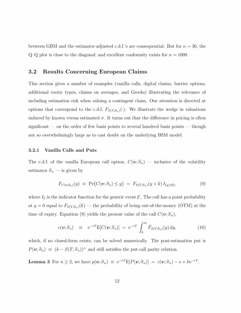
between GBM and the estimator-adjusted c.d.f.’s are consequential. But for n = 30, the

Q–Q plot is close to the diagonal; and excellent conformity exists for n = 1000.

3.2 Results Concerning European Claims

This section gives a number of examples (vanilla calls, digital claims, barrier options,

additional exotic types, claims on averages, and Greeks) illustrating the relevance of

including estimation risk when valuing a contingent claim. Our attention is directed at

options that correspond to the c.d.f. FS(T ;σn)(·). We illustrate the wedge in valuations

induced by known versus estimated σ. It turns out that the difference in pricing is often

significant — on the order of few basis points to several hundred basis points — though

not so overwhelmingly large as to cast doubt on the underlying BSM model.

3.2.1 Vanilla Calls and Puts

The c.d.f. of the vanilla European call option, C(υ; σn) — inclusive of the volatility

estimator σn — is given by

FC(υ;σn)(y) ≡ Pr(C(υ; σn) ≤ y

)= FS(T ;σn)(y + k) I{y≥0}, (9)

where IE is the indicator function for the generic event E . The call has a point probability

at y = 0 equal to FS(T ;σn)(k) — the probability of being out-of-the-money (OTM) at the

time of expiry. Equation (9) yields the present value of the call C(υ; σn),

c(υ; σn) ≡ e−rTE[C(υ; σn)] = e−rT∫ ∞k

FS(T ;σn)(y) dy, (10)

which, if no closed-form exists, can be solved numerically. The post-estimation put is

P (υ; σn) ≡ (k − S(T ; σn))+ and still satisfies the put-call parity relation.

Lemma 3 For n ≥ 2, we have p(υ; σn) ≡ e−rTE[P (υ; σn)] = c(υ; σn)− s+ ke−rT .

12

Example 3 Figure 3 plots, as a function of the current equity price s, call values c(υ; σn),

n = 3, 4, 10, 30, and BSM (n = ∞), using k = 10, T = 1/2, r = 0.05, and σ = 1. For

this example, the inclusion of estimation risk underprices the call relative to BSM, with

the underpricing progressively decreasing as we move further in-the-money (ITM) or

OTM. For instance, the at-the-money (ATM) valuations are c(υ; σ3) = 2.523, c(υ; σ4) =

2.624, c(υ; σ10) = 2.774, c(υ; σ30) = 2.829, and the BSM value c(υ;σ) = 2.854. Note

that if prices from the post-estimation valuation schedule are input into classic BSM for

the purpose of obtaining implied volatility, then one will conclude that a non-constant

volatility is indicated — a fake smile effect — even though σ is in fact constant.

2 4 6 8 10 12 14s

1

2

3

4

5

6

c

max8s-10, 0<BSM

n = 30

n = 10

n = 4

n = 3

Figure 3: BSM vs. post-estimation c(υ; σn): υ = (s, k, T ) = (s, 10, 1/2); r = 0.05; σ = 1;

n = 3, 4, 10, 30,BSM; and max{s− 10, 0} is the expiry valuation profile

In the case of a vanilla call valuation, the post-estimation Equation (10) gives the

same value as when the LUS is applied directly to the BSM formula (3) (as in [3, 4, 10]).

The results are summarized by the next proposition, proven in the On-Line Appendix.

13

Proposition 1 c(υ; σn) = E[sΦ(z+(s, k; σn)

)−k e−rT Φ

(z−(s, k; σn)

)], where the right-

hand side is the calculation via the LUS.

Though they yield the same vanilla call value, we stress that the general methods are not

equivalent, as will be demonstrated when we consider this call’s sensitivities in §3.2.6.

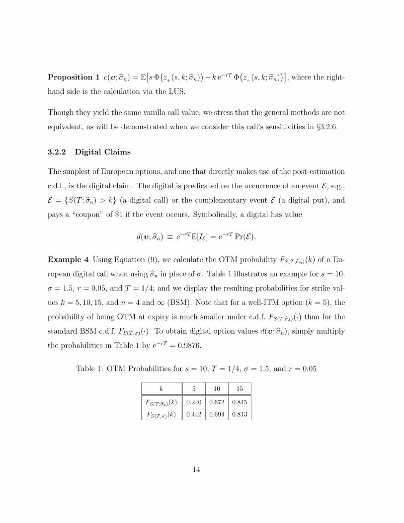
3.2.2 Digital Claims

The simplest of European options, and one that directly makes use of the post-estimation

c.d.f., is the digital claim. The digital is predicated on the occurrence of an event E , e.g.,

E = {S(T ; σn) > k} (a digital call) or the complementary event E (a digital put), and

pays a “coupon” of $1 if the event occurs. Symbolically, a digital has value

d(υ; σn) ≡ e−rTE[IE ] = e−rT Pr(E).

Example 4 Using Equation (9), we calculate the OTM probability FS(T ;σn)(k) of a Eu-

ropean digital call when using σn in place of σ. Table 1 illustrates an example for s = 10,

σ = 1.5, r = 0.05, and T = 1/4; and we display the resulting probabilities for strike val-

ues k = 5, 10, 15, and n = 4 and∞ (BSM). Note that for a well-ITM option (k = 5), the

probability of being OTM at expiry is much smaller under c.d.f. FS(T ;σ4)(·) than for the

standard BSM c.d.f. FS(T ;σ)(·). To obtain digital option values d(υ; σn), simply multiply

the probabilities in Table 1 by e−rT = 0.9876.

Table 1: OTM Probabilities for s = 10, T = 1/4, σ = 1.5, and r = 0.05

k 5 10 15

FS(T ;σ4)(k) 0.240 0.672 0.845

FS(T ;σ)(k) 0.442 0.694 0.813

14

3.2.3 Barrier Options

Here we calculate the value of a digital barrier option. Let M(T ;σ) ≡ max0≤t≤T S(t;σ)

record the maximum value of the GBM price path observed up to time T . Our choice of

claim is the digital “knock-in,” having payoff D(υ;σ) ≡ I{M(T ;σ)≥k}. If S(t;σ) hits the

barrier k by time T , the payoff is $1; otherwise, the claim pays nothing. To determine the

fair value of D(υ;σ), we calculate Pr(M(T ;σ) ≥ k) and then discount by the risk-free

rate. The c.d.f. of M(T ;σ) is [12] (cf. the On-Line Appendix)

FM(T ;σ)(k) = Pr(M(T ;σ) ≤ k) = Φ(z−(s, k;σ)

)−(ks

) 2rσ2−1

Φ(z−(k, s;σ)

). (11)

Thus, when the volatility is known, the fair value of D(υ;σ) is d(υ;σ) ≡ e−rT FM(T ;σ)(k).

For unknown σ, we employ the LUS directly via Equation (5) to obtain

d(υ; σn) ≡ e−rT Pr(M(T ; σn) ≥ k) =n− 1

σ2

∫ ∞0

d(υ;√w )fχ2

n−1

( (n−1)wσ2

)dw.

Example 5 Table 2 gives representative barrier probabilities from the two complemen-

tary c.d.f.’s FM(T ;σ4)(k) (n = 4) and FM(T ;σ)(k) (n = ∞) for the case T = 1, s = 10,

r = 0.05, with the true value of σ = 1.5. We see that as the barrier k is raised, the

difference in values is monotonically increasing.

Table 2: Barrier Probabilities for T = 1, s = 10, r = 0.05, and σ = 1.5

barrier k 11 12 13 14 15

FM(T ;σ4)(k) 0.879 0.780 0.697 0.627 0.567

FM(T ;σ)(k) 0.896 0.809 0.736 0.673 0.618

3.2.4 Other Exotics With Closed Forms

There are many non-standard options to which our methodology can be applied. One

that readily fits into our paradigm is the forward start call [12]. With 0 < T ′ ≤ T , the

15

forward start is (S(T ;σ)− xS(T ′;σ))+, x > 0, and can be interpreted as having a strike

value k = xS(T ′;σ) — now a random variable dependent on a future outcome of the

underlying. From the On-Line Appendix, we obtain the option value

e−rTE[(S(T ;σ)− xS(T ′;σ))+] = e−r(T−T′)E[C(s, xs, T − T ′;σ)], (12)

i.e., use replacements k → xs and T → T −T ′ in Equation (3). Aside from the indicated

adjustment of the parameters, the BSM formula is the same as for a vanilla option.

With a little ingenuity, other claims can be valued (see the On-Line Appendix). The

general idea is straightforward: Obtain the joint law governing the relevant process, and

then use the pre- or post-estimation c.d.f. to determine the fair price.

3.2.5 Asian Options

This section outlines relevant results for a variety of Asian options, i.e., options based on

certain averages of the equity price as it evolves over time. An interesting property of

some of these claim types is that no closed-form formulae exist for pricing or hedging. For

these we use simulation to provide valuations. There are many types of Asian options,

but in the current paper, we deal with contingent claims on “continuously” monitored

averages. A more-extensive discussion dealing with the finer points of both continuous

and discrete options on averages can be found in [11].

3.2.5.1 Geometric Average with Known σ

For discrete monitoring over [0, T ] at m equally spaced times, Tm, 2Tm, . . . , T , the geo-

metric average based on the underlying is( m∏i=1

S( iTm

;σ)

)1/m

= s exp

{1

m

m∑i=1

[(µ− σ2

2) iTm

+ σW( iTm

)]}

D→ s exp

{1

T

∫ T

0

[(µ− σ2

2)t+ σW(t)

]dt

}(13)

= exp( 1

T

∫ T

0

`n(S(t;σ)) dt)≡ G(T ;σ),

16

whereD→ denotes convergence in distribution as m → ∞, and G(T ;σ) is the continu-

ously monitored version of the geometric average of the equity price. Since

Var

(∫ T

0

W(t) dt

)=

∫ T

0

∫ T

0

Cov(W(t),W(u)

)dt du =

∫ T

0

∫ T

0

min(t, u) dt du =T 3

3,

Equation (13) implies that

G(T ;σ) ∼ s exp{

Nor(

(r − σ2

2)T2, σ

2T3

)}. (14)

Thus, G(T ;σ) is lognormal, and it follows that we can directly apply the BSM formula

to price a call on the geometric average. By (2) with Y = G(T ;σ), the BSM valuation

of the continuously monitored geometric average option CG(υ;σ) ≡ (G(T ;σ)− k)+ is

cG(υ;σ) ≡ e−rTE[CG(υ;σ)] = s e−(r+σ2

6)T2 Φ(zG+

(s, k;σ))− k e−rT Φ

(zG− (s, k;σ)

),

where

zG+(s, k;σ) ≡`n(sk

)+(r + σ2

6

)T2

σ√

T3

and zG−(s, k;σ) ≡`n(sk

)+(r − σ2

2

)T2

σ√

T3

.

3.2.5.2 Geometric Average with Unknown σ

By comparing the distributions of S(T ;σ) and G(T ;σ) from (1) and (14), and then

carrying out the same manipulations as those leading to the c.d.f. of S(T ; σn) given in

(7) of Lemma 2, we obtain for the continuously monitored case the c.d.f. of G(T ; σn),

FG(T ;σn)(y) ≡ n− 1

σ2

∫ ∞0

Φ(zG−(s, y;

√w ))fχ2

n−1

( (n−1)wσ2

)dw, y > 0.

With substitution analogous to (10), we choose to compute the call numerically via

cG(υ; σn) ≡ e−rTE[CG(υ; σn)] = e−rT∫ ∞k

FG(T ;σn)(y) dy. (15)

3.2.5.3 Arithmetic Average with Known σ

17

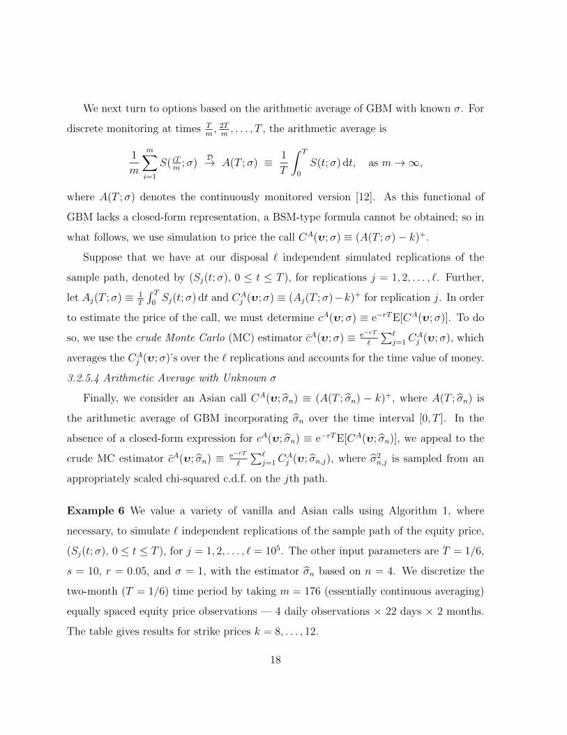
We next turn to options based on the arithmetic average of GBM with known σ. For

discrete monitoring at times Tm, 2Tm, . . . , T , the arithmetic average is

1

m

m∑i=1

S( iTm

;σ)D→ A(T ;σ) ≡ 1

T

∫ T

0

S(t;σ) dt, as m→∞,

where A(T ;σ) denotes the continuously monitored version [12]. As this functional of

GBM lacks a closed-form representation, a BSM-type formula cannot be obtained; so in

what follows, we use simulation to price the call CA(υ;σ) ≡ (A(T ;σ)− k)+.

Suppose that we have at our disposal ` independent simulated replications of the

sample path, denoted by (Sj(t;σ), 0 ≤ t ≤ T ), for replications j = 1, 2, . . . , `. Further,

let Aj(T ;σ) ≡ 1T

∫ T0Sj(t;σ) dt and CA

j (υ;σ) ≡ (Aj(T ;σ)−k)+ for replication j. In order

to estimate the price of the call, we must determine cA(υ;σ) ≡ e−rTE[CA(υ;σ)]. To do

so, we use the crude Monte Carlo (MC) estimator cA(υ;σ) ≡ e−rT

`

∑`j=1C

Aj (υ;σ), which

averages the CAj (υ;σ)’s over the ` replications and accounts for the time value of money.

3.2.5.4 Arithmetic Average with Unknown σ

Finally, we consider an Asian call CA(υ; σn) ≡ (A(T ; σn) − k)+, where A(T ; σn) is

the arithmetic average of GBM incorporating σn over the time interval [0, T ]. In the

absence of a closed-form expression for cA(υ; σn) ≡ e−rTE[CA(υ; σn)], we appeal to the

crude MC estimator cA(υ; σn) ≡ e−rT

`

∑`j=1C

Aj (υ; σn,j), where σ2

n,j is sampled from an

appropriately scaled chi-squared c.d.f. on the jth path.

Example 6 We value a variety of vanilla and Asian calls using Algorithm 1, where

necessary, to simulate ` independent replications of the sample path of the equity price,

(Sj(t;σ), 0 ≤ t ≤ T ), for j = 1, 2, . . . , ` = 105. The other input parameters are T = 1/6,

s = 10, r = 0.05, and σ = 1, with the estimator σn based on n = 4. We discretize the

two-month (T = 1/6) time period by taking m = 176 (essentially continuous averaging)

equally spaced equity price observations — 4 daily observations × 22 days × 2 months.

The table gives results for strike prices k = 8, . . . , 12.

18

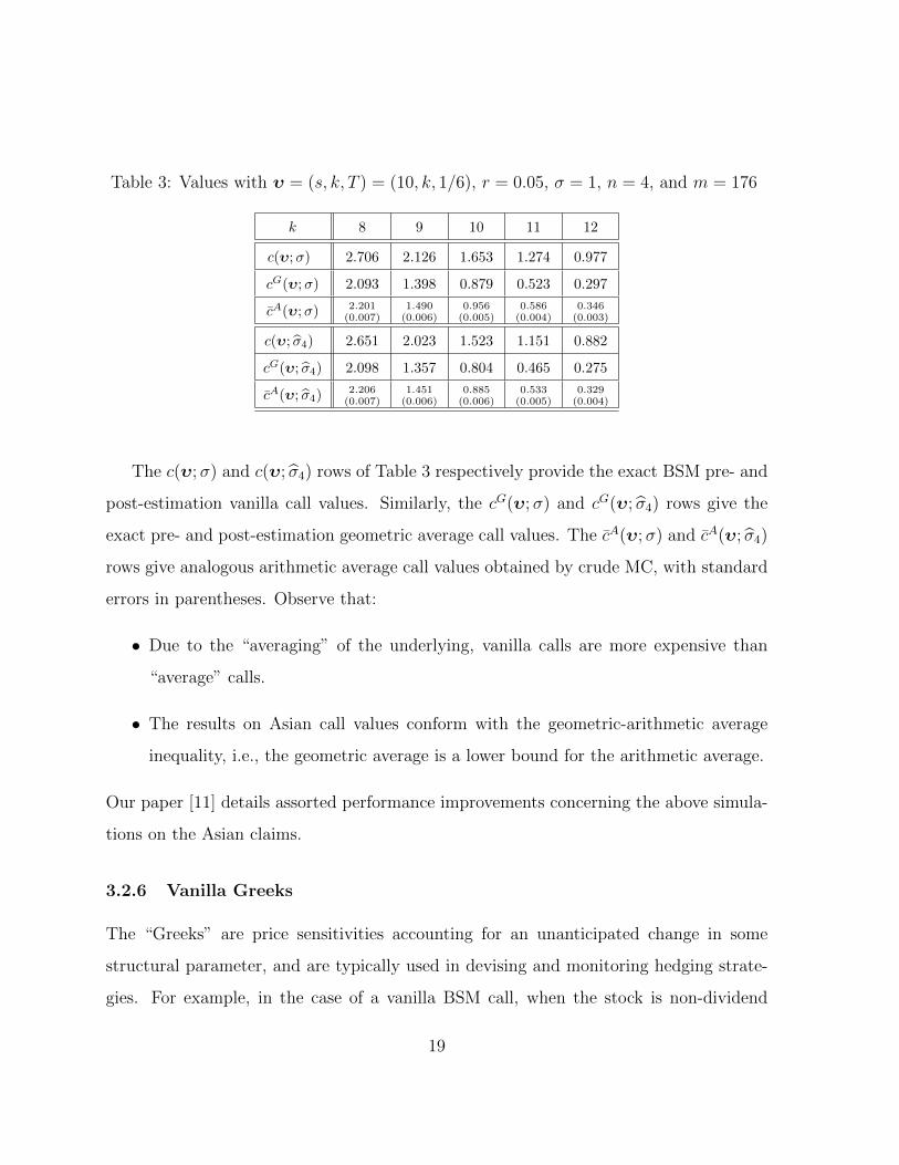
Table 3: Values with υ = (s, k, T ) = (10, k, 1/6), r = 0.05, σ = 1, n = 4, and m = 176

k 8 9 10 11 12

c(υ;σ) 2.706 2.126 1.653 1.274 0.977

cG(υ;σ) 2.093 1.398 0.879 0.523 0.297

cA(υ;σ) 2.201(0.007)

1.490(0.006)

0.956(0.005)

0.586(0.004)

0.346(0.003)

c(υ; σ4) 2.651 2.023 1.523 1.151 0.882

cG(υ; σ4) 2.098 1.357 0.804 0.465 0.275

cA(υ; σ4) 2.206(0.007)

1.451(0.006)

0.885(0.006)

0.533(0.005)

0.329(0.004)

The c(υ;σ) and c(υ; σ4) rows of Table 3 respectively provide the exact BSM pre- and

post-estimation vanilla call values. Similarly, the cG(υ;σ) and cG(υ; σ4) rows give the

exact pre- and post-estimation geometric average call values. The cA(υ;σ) and cA(υ; σ4)

rows give analogous arithmetic average call values obtained by crude MC, with standard

errors in parentheses. Observe that:

• Due to the “averaging” of the underlying, vanilla calls are more expensive than

“average” calls.

• The results on Asian call values conform with the geometric-arithmetic average

inequality, i.e., the geometric average is a lower bound for the arithmetic average.

Our paper [11] details assorted performance improvements concerning the above simula-

tions on the Asian claims.

3.2.6 Vanilla Greeks

The “Greeks” are price sensitivities accounting for an unanticipated change in some

structural parameter, and are typically used in devising and monitoring hedging strate-

gies. For example, in the case of a vanilla BSM call, when the stock is non-dividend

19

paying and σ is known, the most-frequently used Greeks are delta, gamma, theta,

rho, and vega [12]; in the current paper, we will deal with the BSM delta and vega:

δ(υ;σ) ≡ ∂c(υ;σ)∂s

= Φ(z+(s, k;σ)) and ϑ(υ;σ) ≡ ∂c(υ;σ)∂σ

= s√T φ(z+(s, k;σ)). In

the strict BSM paradigm, δ(υ;σ) indicates how many additional units of the underly-

ing one needs to go short or long so as to balance out in value a portfolio consisting of

the call, the stock, and a money market account. For the unknown σ case, the corre-

sponding LUS versions of delta and vega are, via Equation (6), E[Φ(z+(s, k; σn))] and

s√T E[φ(z+(s, k; σn))

], respectively.

Our post-estimation (unknown σ) Greeks are given in the following proposition. We

see that for the vanilla call, the post-estimation delta is the same as the corresponding

LUS version; the interesting news is that the versions of vega differ since now the change

in σ is unanticipated and therefore categorized as uncertain.

Proposition 2 For n ≥ 2,

δ(υ; σn) ≡ ∂c(υ; σn)

∂s= E[Φ(z+(s, k; σn))], (16)

ϑ(υ; σn) ≡ ∂c(υ; σn)

∂σ=

s√T

σE[σn φ(z+(s, k; σn))

]. (17)

Due to its lengthy technical nature, the proof is relegated to the On-Line Appendix.

Example 7 Figure 4 compares the BSM ϑ(υ;σ), our post-estimation ϑ(υ; σ4), and the

LUS version of vega. The operating parameters are set at s = 10, k = 10, T = 1/2,

r = 0.05, and σ = 1, with n = 4. (See the On-Line Appendix for the analogous delta

sensitivities.) Table 4 shows numerically that the post-estimation delta and vega converge

to the classical BSM Greeks as n becomes large. There is a substantial difference in the

sensitivities for low values of n; but by the time n = 30, these differences have dissipated.

20

5 10 15 20 25 30s

0.5

1.0

1.5

2.0

2.5

3.0

3.5

J

J Hs,10,1�2;Σ`

4L

LUS

BSM

Figure 4: BSM ϑ(υ;σ), ϑ(υ; σn), and LUS vega: s = 10; k = 10; T = 1/2; r = 0.05;

σ = 1; n = 4

Table 4: Delta and Vega Convergence in n: k = 10; T = 1/2; r = 0.05; σ = 1

δ(υ; σn) ϑ(υ; σn)s 5 10 15 5 10 15

n = 4 0.232 0.645 0.862 1.010 2.363 2.287

n = 10 0.259 0.649 0.842 1.112 2.527 2.524

n = 30 0.271 0.650 0.835 1.160 2.588 2.619

n = 1000 0.277 0.651 0.832 1.183 2.615 2.662

BSM 0.277 0.651 0.832 1.184 2.615 2.663

21

4 Conclusions

Our purpose in this paper was to highlight the existence and consequences of estimation

risk in financial modeling. To do so we focused on the well-known and accepted BSM view

of option markets. Our results typically hold at any given time point, and depend on both

the market structure (BSM technology) and how individuals view the risks associated

with their limited knowledge of the market parameters (estimator choice) they face. The

conclusions are in line with a general proposition from Lucas [8] — namely, within our

purview, the BSM formula “is derived from decision rules (demand and supply functions)

of agents in the economy and these decisions are, theoretically, optimal given the situation

in which each agent is placed.” In other words, people use information optimally — in

their view, at least — when considering the decisions they make.

The perturbation of the BSM model that we study herein should be viewed as a cali-

bration more in line with reality — one that will be of concern to institutions dealing with

the valuation and hedging of a portfolio marked-to-market at many billions of dollars.

Surprisingly, when it comes to gauging a “model’s fit,” great attention is paid by prac-

titioners to a few basis points, yet little concern is placed on formally incorporating the

risk attached to the fundamental parameters of a model and to what the consequences

of that risk are. Model fit may be improved by adding parameters, but at the cost of

increased out-of-sample variability. For purposes of prediction, neglecting the variability

of the available data used in the calibration of a model is analogous to failing to incor-

porate for friction or wind effects when calculating the trajectory of a missile — it can

be consequential.

Finally, in addition to providing new results on estimation-dependent BSM contingent

claim values, our working model is suggestive of approaches that can be pursued to extend

the study of estimation risk to other more-complex set-ups. For example, in models

utilizing stochastic programming [13] or VaR analysis [5], it would be interesting to

22

know the distributional effects of learning and updating of the associated VaR covariance

matrix. A further application of our methodology dealing with firm financing policies

[6] would also be insightful. Finally, we believe that it would be interesting to study

regimes that incorporate economic behavior subjected to a set of intermittent volatility

shocks drawn from some probability law that is more-or-less well-known by market agents.

Market participants will be confronted by a vector of unknown, but estimable parameters.

In turn, they proceed to make and update their estimates of the unknowns, thereby

converting situations of uncertainty to those that are characterized by degrees of risk.

Acknowledgments: We thank Paul Griffin, Steve Hackman, Bob Kertz, Alex Shapiro,

and the anonymous referees for their comments and suggestions.

Appendix

This appendix proves the various new results we introduce in the body of the paper.

Proof of Lemma 1: The p.d.f. of Y follows by the definition of the lognormal. Then

E[(Y − k)+] =

∫ ∞0

(y − k)+fY (y) dy =

∫ ∞k

(y − k)φ(`n( s

y) + a

b

) 1

ybdy

=

∫ ω−(k)

−∞(s ea−xb − k)φ(x) dx (where x = 1

b[`n( s

y) + a])

= s ea+b2

2

∫ ω−(k)

−∞

1√2π

exp{−(x+ b)2

2

}dx− kΦ(ω−(k)). 2

Proof of Lemma 2 Since σ2 is independent of W(T ), the law of total probability

implies FS(T ;σ)(y) =∫∞0FS(T ;√w )(y)fσ2(w) dw. 2

23

Proof of Corollary 1 Let ζ(w) ≡ `n(s) + (r − w2)T . Starting at (8), we find that

E[Sj(T ; σ)] =

∫ ∞0

yjfS(T ;σ)(y) dy =

∫ ∞0

yj∫ ∞0

1

y√wT

φ(z−(s, y;

√w ))fσ2(w) dw dy

=

∫ ∞0

fσ2(w)

∫ ∞0

yj−11√wT

φ

(`n(y)− ζ(w)√

wT

)dy dw

=

∫ ∞0

fσ2(w)

∫ ∞0

yj−11√

2πwTexp

{−(`n(y)− ζ(w))2

2wT

}dy dw

=

∫ ∞0

fσ2(w) eζ(w)j+wTj2

2

∫ ∞−∞

1√2πwT

exp

{−(z − (ζ(w) + wTj))2

2wT

}dz dw

= sjerT j∫ ∞0

fσ2(w) eT2(j2−j)w dw,

where the penultimate step follows upon setting y = ez and completing the square; the

final step follows after noting that the interior integrand is a normal p.d.f. 2

Proof of Lemma 3 If we denote S ≡ S(T ; σn), then by Corollary 2,

serT − k = E[S − k] = E[(S − k)+ − (k − S)+] = erT [c(υ; σn)− p(υ; σn)]. 2

References

[1] Baxter, M., Rennie, A. (1996). Financial calculus: An introduction to deriva-

tives pricing, Cambridge, UK: Cambridge University Press.

[2] Black, F., Scholes, M. (1973). The pricing of options and corporate liabilities.

Journal of Political Economy, 81, 637–654.

[3] Boyle, P. B., Ananthanarayanan, A. L. (1977). The impact of variance esti-

mation in option valuation models. Journal of Financial Economics, 5, 375–387.

[4] Butler, J. S., Schachter, B. (1986). Unbiased estimation of the Black/Scholes

formula. Journal of Financial Economics, 15, 341–357.

24

[5] Castellacci, G., Siclari, M. J. (2003). The practice of Delta–Gamma VaR:

Implementing the quadratic portfolio model. European Journal of Operational Re-

search, 150:529–545.

[6] Cifarelli, M. D., Masciandaro, D., Peccati, L., Salsa, S., Tagliani, A.

(2002). Success or failure of a firm under different financing policies: A dynamic

stochastic model. European Journal of Operational Research, 136:471–482.

[7] Knight, F. (1921). Risk, uncertainty, and profit. Boston: Hart, Schaffner, and

Marx; Houghton Mifflin Co.

[8] Lucas, R. (1976). Econometric policy evaluation: A critique. Carnegie-Rochester

Conference Series on Public Policy, 1, 19–46.

[9] Merton, R. (1973). Theory of rational option pricing. Bell Journal of Economics

and Management Science, 4, 141–183.

[10] Ncube, M., Satchell, S. (1997). The statistical properties of the Black–Scholes

option price. Mathematical Finance, 7, 287–305.

[11] Popovic, R., Goldsman, D. (2011). Inherent estimation risk and options on

averages. Technical Report, School of ISyE, Georgia Tech, Atlanta, GA.

[12] Shreve, S. E. (2004). Stochastic calculus for finance II: Continuous-time models.

New York: Springer.

[13] Topaloglou, N., Vladimirou, H., Zenios, S. A. (2008). A dynamic stochastic

programming model for international portfolio management. European Journal of

Operational Research, 185:1501–1524.

25

On-Line Appendix

In order to make the article “On Valuing and Hedging European Options when Volatility

is Estimated Directly” self-contained, we present certain results and give derivations of

miscellaneous formulae mentioned in the paper (some of which are known).

Special Case of Lemma 2 The c.d.f. and p.d.f. of S(T ; σn), n ≥ 2, are

FS(T ;σn)(y) =n− 1

σ2

∫ ∞0

Φ(z−(s, y;

√w ))fχ2

n−1

( (n−1)wσ2

)dw, and (18)

fS(T ;σn)(y) =n− 1

σ2

∫ ∞0

1

y√wT

φ(z−(s, y;

√w ))fχ2

n−1

( (n−1)wσ2

)dw (19)

=K

y3/2

∫ ∞0

exp

{−(a1(y)

w+ a2w

)}w

n−42 dw (20)

=2K

y3/2

(a1(y)

a2

)n−24 Kn−2

2

[|a0(y)|

√2a2/T

], (21)

where in (20), a0(y) ≡ `n(ys) − rT , a1(y) ≡ a20(y)

2T, a2 ≡ T

8+ n−1

2σ2 , and K ≡(n−12σ2

)n−12(Γ(n−1

2)√

2πT/s)−1

erT/2; and in (21), Kα[β] is a modified Bessel function of

the second kind with parameters α and β [A–1]. The latter is computationally useful.

Proof Expressions (18) and (19) follow from the discussion after Lemma 2. Moreover,

fS(T ;σn)(y) =n− 1

y√T σ2

∫ ∞0

φ

(a0(y) + wT

2√wT

)1√wfχ2

n−1

((n−1)wσ2

)dw

=n− 1

y√T σ2

∫ ∞0

1√2π

exp

{−(a20(y)

2wT+a0(y)

2+wT

8

)}1√w

× 1

2n−12 Γ(n−1

2)

((n− 1)w

σ2

)n−32

exp

{−(n− 1)w

2σ2

}dw,

from which we get (20). Equation (21) follows by definition of the Bessel function. 2

Proof of Proposition 1 This can be proven directly using the c.d.f. FC(υ;σn)(y) given

26

in (9). But a faster way follows from the law of total probability and the LUS itself,

c(υ; σn) =

∫ ∞0

c(υ;√w )fσ2

n(w) dw

=

∫ ∞0

[sΦ(z+(s, k;

√w ))− ke−rTΦ

(z−(s, k;

√w ))]fσ2

n(w) dw (by (3))

= E[sΦ(z+(s, k; σn)

)− ke−rTΦ

(z−(s, k; σn)

)]. 2

Proof of Barrier Equation (11) Observe that for standard BM, the individual

process U(t) ≡ max{W(s), 0 < s ≤ t}, is not Markov, whereas the bivariate process

((W(t), U(t)), t ≥ 0) is Markov. This follows because the transition probability for

(W(t), U(t)) is fully characterized by knowledge of the present state. On the other hand,

the transition probability of U(t) alone depends on both the current running maximum

as well as the current point on the Brownian path (W(t), t ≥ 0). It follows that to obtain

the probability of the event {U(t) ≥ y}, we need the joint c.d.f. FW(t),U(t)(x, y), x < y,

y > 0. With the aid of the reflection principle [A–4], the c.d.f. and p.d.f. are

FW(t),U(t)(x, y) = Pr(W(t) ≤ x, U(t) ≤ y) = Pr(W(t) ≤ x)− Pr(W(t) ≤ x, U(t) ≥ y)

= Φ( x√

t

)− Φ

(x− 2y√t

), x < y, y > 0, (22)

and

fW(t),U(t)(x, y) =

√2

πt3(2y − x) e−

(2y−x)22t , x < y, y > 0. (23)

Evidently, for any fixed t > 0, the first passage time τ ≡ min{t > 0 :W(t) = k} and the

maximum U(t) are related by the events {τ ≤ t} = {U(t) ≥ k}. So letting (x, y)→ (b, b)

in Equation (22), we obtain the c.d.f. and p.d.f. of τ ,

Fτ (b) = 2Φ( b√

t

)− 1 and fτ (b) =

√2

πte−

b2

2t , b > 0,

which is the half-normal p.d.f. (typically associated with the random variable |W(t)|).

We now follow the above steps, amended where necessary, to obtain comparable

results for GBM. Our notation for the stopping time associated with GBM is θ ≡

27

min{t > 0 : S(t;σ) = k} = min{t > 0 : W(t) = β − λt}, with β ≡ 1σ`n(k

s) and

λ ≡ 1σ(r − σ2

2). Aside from sets of measure zero, it is true that

{S(t;σ) ≥ k} ⇐⇒ {λt+W(t) ≥ 1σ`n(ks

)}.

Since the function `n(·) is strictly increasing, it follows that

Pr(θ ≤ T ) = Pr(M(T ;σ) ≥ k) = Pr(max t≤T{λt+W(t)} ≥ β).

Therefore, we conclude that Equation (11) is a probability statement concerning a stan-

dard BM with drift λt, crossing the barrier β.

A second change of measure, implemented below (Equation (24), third equality)

will induce the BM B(t) = λt + W(t) to be driftless. Specifically, the Cameron–

Martin–Girsanov Theorem [A–2] relates probability measures P and Q through dQ =

exp{−λW(T ) − λ2T2} dP. To this end, with a < k, define the new composite parameter

α ≡ 1σ`n(a

s), and use Equation (23) for the “tilting” of measure Q to measure P,

FS(t;σ),M(T ;σ)(a, k) = Pr(S(t;σ) ≤ a,M(T ;σ) ≤ k)

= Pr(λt+W(t) ≤ α, max0≤ t≤T{λt+W(t)} ≤ β

)= EQ

[dP

dQIB(t)≤α,max0≤ t≤TB(t)≤β

]= Pr

(B(t) ≤ α, max0≤ t≤TB(t) ≤ β

)=

√2

πt3

∫ ∫S

eλx−λ2T2 (2y − x)e−

(2y−x)22T dy dx, (24)

where S ≡ {(x, y) : −∞ < x < α, x ≤ y ≤ β, α < β} is a convex set.

Requiring a → k forces α → β, and so S → S∗ ≡ {(x, y) : −∞ < x ≤ y ≤ β} =

{(x, y) : −∞ < x < 0, 0 ≤ y ≤ β}∪{(x, y) : 0 < x < β, x ≤ y ≤ β}. Integrating over S∗,

and substituting for β and λ, we obtain Equation (11). For the details of the integration

over S∗, so as to obtain Equation (11), consult [A–4] or use an algebra manipulator such

28

as Mathematica. Lastly, when dealing with the post-estimation case, Lemma 2 is invoked

in the penultimate equality in (24). 2

Proof of Forward Start Equation (12) Let A ≡ exp {(r − σ2

2)T ′ + σW(T ′)} and

B ≡ s exp {(r − σ2

2)(T − T ′) + σ(W(T )−W(T ′))}. Then

E[(S(T ;σ)− xS(T ′;σ)

)+]= E

{[s exp

{(r − σ2

2

)T + σW(T )

}− xs exp

{(r − σ2

2

)T ′ + σW(T ′)

}]+}= E

{[A(B − xs)

]+}= E[A(B − xs)+] = E[A] E[(B − xs)+]

(by algebra; the fact that A ≥ 0; and the fact that A and B are independent)

= erT′E[C(s, sx, T − T ′;σ)] (since A is lognormal and B ∼ S(T − T ′;σ)). 2

Lookback Option Another option, but now path-dependent, is the digital lookback put

[12], I{M(T ;σ)−S(T ;σ)≥L}, where now we use the replacement k → L, so that υ = (s, L, T ).

This digital pays $1 if the maximum of the stock price on [0, T ] exceeds the terminal

price by at least L. Knowledge of the joint distribution of (M(t;σ), S(t;σ), t ≥ 0) is

sufficient for determining the probabilistic behavior of M(T ;σ) − S(T ;σ), and thus the

fair price of the digital lookback.

Proof of Proposition 2 As in the proof of Proposition 1, we can derive (16),

δ(υ; σn) =∂c(υ; σn)

∂s=

∫ ∞0

∂c(υ;√w )

∂sfσ2

n(w) dw (fσ2

n(w) is not a function of s)

=

∫ ∞0

δ(υ;√w )fσ2

n(w) dw =

∫ ∞0

Φ(z+(s, k;

√w ))fσ2

n(w) dw. 2

Before establishing (17), we need two preliminary results. First,

φ(z+(s, k;x)

)=

1√2π

exp

{−z2+(s, k;x)

2

}=

1√2π

exp

{−(z−(s, k;x)−

√xT )2

2

}

= φ(z−(s, k;x)

)exp{z−(s, k;x)

√xT − xT

2

}=

k e−rT

sφ(z−(s, k;x)

),

29

which leads to the second result,

dc(υ;√w )

dw=

d

dw

[sΦ(z+(s, k;

√w ))− ke−rTΦ

(z−(s, k;

√w ))]

= sφ(z+(s, k;

√w ))dz+(s,k;

√w )

dw− ke−rTφ

(z−(s, k;

√w ))dz−(s,k;

√w )

dw

= sφ(z+(s, k;

√w ))

ddw

[z+(s, k;

√w )− z−(s, k;

√w )]

= sφ(z+(s, k;

√w ))

ddw

√wT =

s

2

√T

wφ(z+(s, k;

√w )). (25)

Finally, we can derive (17). Since c(υ;√w ) is not a function of σ, we have

ϑ(υ; σn) =∂c(υ; σn)

∂σ=

∫ ∞0

c(υ;√w )

∂fσ2n

(w)

∂σdw

=

∫ ∞0

c(υ;√w ) ∂

∂σ

[n−1σ2 fχ2

n−1

((n−1)wσ2

)]dw

=

∫ ∞0

c(υ;√w )[−2(n−1)

σ3 fχ2n−1

( (n−1)wσ2

)+ n−1

σ2∂∂σfχ2

n−1

( (n−1)wσ2

)]dw

=−2c(υ; σn)

σ− 2(n− 1)

σ3

∫ ∞0

wc(υ;√w )f ′χ2

n−1

( (n−1)wσ2

)n−1σ2 dw

=−2c(υ; σn)

σ+

2(n− 1)

σ3

∫ ∞0

fχ2n−1

( (n−1)wσ2

)d[wc(υ;

√w )] (26)

=−2c(υ; σn)

σ+

2(n− 1)

σ3

∫ ∞0

fχ2n−1

( (n−1)wσ2

) [wc′(υ;

√w ) + c(υ;

√w )]dw

=2(n− 1)

σ3

∫ ∞0

fχ2n−1

((n−1)wσ2

)wc′(υ;

√w ) dw

=(n− 1)s

√T

σ3

∫ ∞0

√w φ(z+(s, k;

√w ))fχ2

n−1

( (n−1)wσ2

)dw, (27)

where f ′χ2n−1

(x) ≡ ddxfχ2

n−1(x), c′(υ;x) ≡ d

dxc(υ;x), (26) follows by integration by parts

and L’Hopital’s rule, and (27) follows by (25). 2

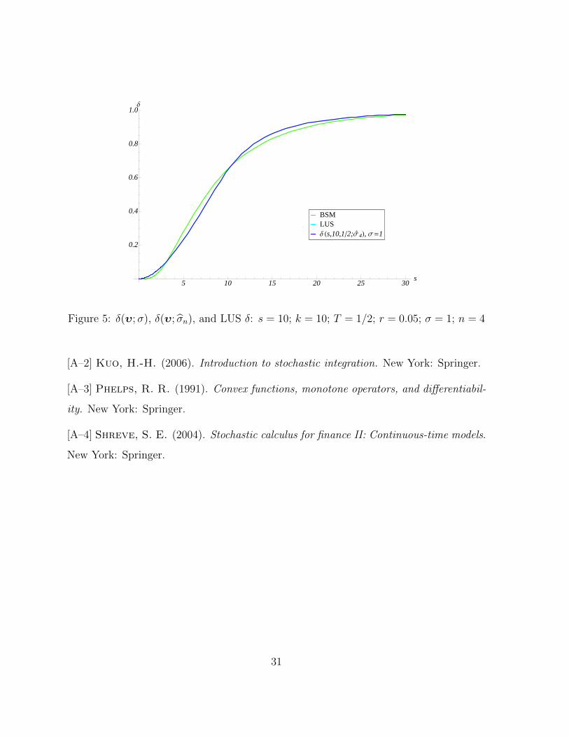
Delta Sensitivities Figure 5 visually confirms the use of (6) for the delta sensitivities.

The LUS delta sensitivity is equivalent to the post-estimation delta sensitivity.

References for On-Line Appendix

[A–1] Gradshteyn, I. S., Ryzhik, I. M. (1980). Table of integrals, series, and

products. New York: Academic Press.

30

5 10 15 20 25 30s

0.2

0.4

0.6

0.8

1.0∆

∆ Hs,10,1�2;Σ`

4L, Σ =1LUSBSM

Figure 5: δ(υ;σ), δ(υ; σn), and LUS δ: s = 10; k = 10; T = 1/2; r = 0.05; σ = 1; n = 4

[A–2] Kuo, H.-H. (2006). Introduction to stochastic integration. New York: Springer.

[A–3] Phelps, R. R. (1991). Convex functions, monotone operators, and differentiabil-

ity. New York: Springer.

[A–4] Shreve, S. E. (2004). Stochastic calculus for finance II: Continuous-time models.

New York: Springer.

31