Valuing Correlation- Dependent Derivatives Using a Structural ...
Upload
khangminh22Category
view
1download
0
Valuing multiple threatened species and ecological communities in Australia
Asha Gunawardena1, Michael Burton1, Ram Pandit1, Stephen T. Garnett2, Kerstin K. Zander2, David Pannell1
Final Report December 2020

Valuing multiple threatened species and ecological communities in Australia
Asha Gunawardena1, Michael Burton1, Ram Pandit1, Stephen T. Garnett2, Kerstin K. Zander2, David Pannell1
Final Report December 2020
1 Centre for Environmental Economics & Policy, UWA School of Agriculture and Environment, M087, University of Western Australia, Perth WA 6009, Australia 2 Northern Institute and Research Institute for the Environment and Livelihoods, Charles Darwin University, Northern Territory 0909, Australia
Cite this publication as: Gunawardena, A., Burton, M., Pandit, R., Garnett, S.T., Zander, K.K., and Pannell, D. 2020. Valuing multiple threatened species and ecological communities in Australia. Final report to the National Environment Science Program, Department of Agriculture, Water and the Environment, Brisbane. 15 December 2020.
Cover image: Brush-tailed rabbit-rat. Image: Hugh Davies
2
Species images throughout report:
Great Desert Skink. Image:Martin Whiting
Murray Cod. Image: Jabin Watson
Numbat. Image: Dilettantiquity CC-BY-SA-2.0 Wikimedia Commons
Banksia Vincentia. Image: Tony Auld
Orange-bellied Parrot. Image: JJ Harrison CC BY-SA 3.0 Wikimedia Commons
Eastern Bristlebird. Image: JJ Harrison CC BY-SA 4.0 Wikimedia Commons
Boggomoss Snail. Image: John Stanisic
Clay Pans of the Swan Coastal Plain. Image: Tim Swallow
Brush-tailed Rabbit-rat. Image: Hugh Davies
Giant Freshwater Crayfish. Image: Todd Walsh
Australasian Bittern. Image: Graeme Lembcke
Arnhem Plateau Sandstone Shrubland Complex. Image: Jaana Dielenberg
Far Eastern Curlew. Image: Micha Jackson
Shaw Galaxias. Image: Tarmo A. Raadik
Gulbaru Gecko. Image: Anders Zimny
Acacia equisetifolia. Image: Kym Brennan
Valuing multiple threatened species and ecological communities in Australia - Final Report, December 2020 3
ContentsExecutive Summary ......................................................................................................................................................................................... 5
1. Introduction ................................................................................................................................................................................................... 8
2. Methods ......................................................................................................................................................................................................... 8
2.1. Selection of threatened species and ecological communities .......................................................................................... 8
2.2. Collection of key information about species .......................................................................................................................... 9
2.3.Definingthreatstatus/extinctionrisklevels ...........................................................................................................................12
2.4. Development of choice experimental design........................................................................................................................13
2.5. Testing design of choice question with focus groups .........................................................................................................13
2.5.1 ExplicitPartialProfiles .......................................................................................................................................................13
2.5.2 ImplicitpartialProfiles ......................................................................................................................................................15
2.5.3 Standard Design ................................................................................................................................................................ 16
2.5.4 Outcome of the focus group discussion ................................................................................................................... 16
2.6. Survey development .................................................................................................................................................................... 16
2.6.1 Questionnaire ................................................................................................................................................................... 16
2.6.2 Experimental design ..............................................................................................................................................17
2.6.3 Pilot testing with online panels ......................................................................................................................................17
2.6.4 Survey design and arrangement of choice questions ............................................................................................ 19
2.6.5 Survey implementation ................................................................................................................................................... 19
2.6.6 Sample selection ..............................................................................................................................................................22
2.6.7 Data management ...........................................................................................................................................................22
2.6.8 Screening protestors and collecting additional information ................................................................................ 22
2.6.9 Other socio economic information ............................................................................................................................23
2.7 Discrete choice experiments .....................................................................................................................................................24
3. Results and discussion ..............................................................................................................................................................................26
4. Summary of estimation results ...............................................................................................................................................................31
5. How to use species values reported in this study .............................................................................................................................38
5.1 How to use these values? .......................................................................................................................................................... 41
5.1.1 Benefittransfer .................................................................................................................................................................. 41
5.1.2Benefittransferexamples ............................................................................................................................................... 41
Example 1: Painted Honeyeater ................................................................................................................................... 41
Example 2: Superb Parrot ...............................................................................................................................................43
5.1.3 Decision-making ...............................................................................................................................................................44
6. References ....................................................................................................................................................................................................51
Appendices ......................................................................................................................................................................................................52
4
LIST OF TABLES
Table ES1. Value estimate for each species (Species set 1) ................................................................................................................... 6
Table ES2. Value estimate for each species (Species set 2) ...................................................................................................................7
Table 1. Species selected for the survey with background information ............................................................................................ 9
Table 2. Comparison of threat status .........................................................................................................................................................12
Table 3. Illustration of extinction risk categories .....................................................................................................................................12
Table 4. Attributes and levels used in the experimental design ..........................................................................................................13
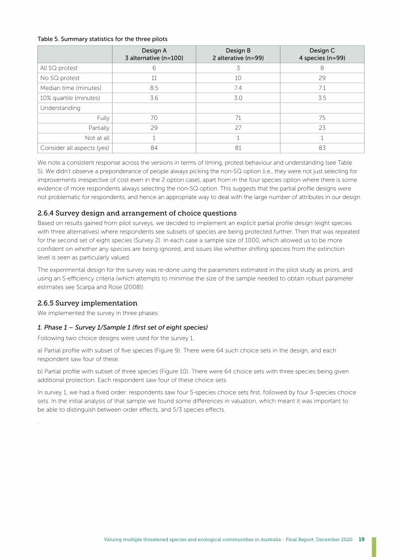
Table 5. Summary statistics for the three pilots...................................................................................................................................... 19
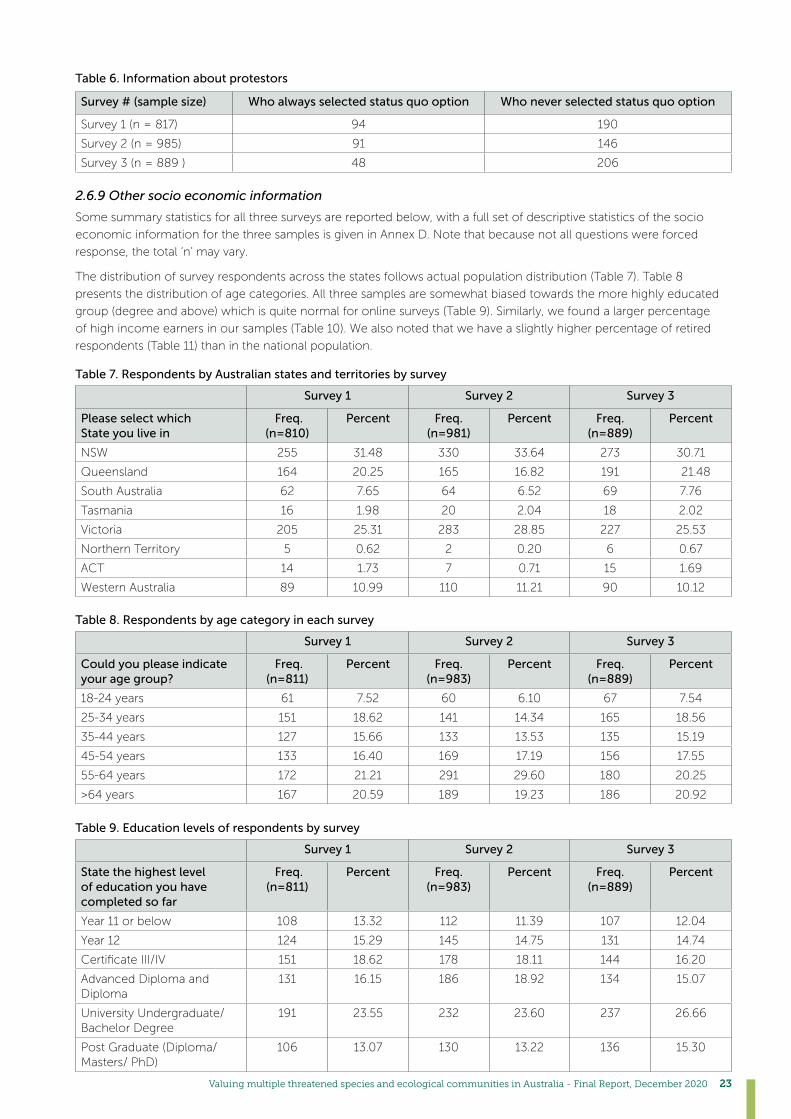
Table 6. Information about protestors ......................................................................................................................................................23
Table 7. Respondents by Australian states and territories by survey ................................................................................................. 23
Table 8. Respondents by age category in each survey ........................................................................................................................24
Table 9. Education levels of respondents by survey .............................................................................................................................24
Table 10. Respondents by income categories in each survey ...........................................................................................................24
Table 11. Respondents by employment status in each survey ...........................................................................................................24
Table 12. WTP-space model results for eight species: Survey 2 ........................................................................................................28
Table 13. WTP-space model results for eight species: Survey 1 ........................................................................................................29
Table 14. Full (unrestricted) WTP-space model results .........................................................................................................................30
Table 15. WTP-space model results for eight species: Survey 3 .........................................................................................................31
Table 16. Value estimates ($) for threatened species and ecological community studied in Survey 1 ................................... 32
Table 17. Value estimates for threatened species and ecological community studied in Survey 2 .........................................34
Table 18. Value estimates ($) for threatened species and ecological community studied in Survey 1 and Survey 3 .......... 35
Table 19. Value estimates ($) for threatened species and ecological community studied in Survey 2 ................................... 37
Table 20. Value estimate for each species (Species set 1) ...................................................................................................................39
Table 21. Value estimate for each species (Species set 2) ...................................................................................................................40
Table22.Definitionofextinctionriskcategory .....................................................................................................................................43
Table23.Benefit-costanalysistable(baseyear-year0-is2020) ................................................................................................... 52
LIST OF FIGURES
Figure1.Explicitpartialprofiledesignseekingpreferencesforfivespecies ...................................................................................14
Figure2.Explicitpartialprofiledesignseekingpreferencesforthreespecies ................................................................................14
Figure3.Implicitpartialprofiledesignseekingpreferencesforfivespecies ..................................................................................15
Figure4.Implicitpartialprofiledesignseekingpreferencesforthreespecies ...............................................................................15
Figure 5. Standard design with three alternatives .................................................................................................................................. 16
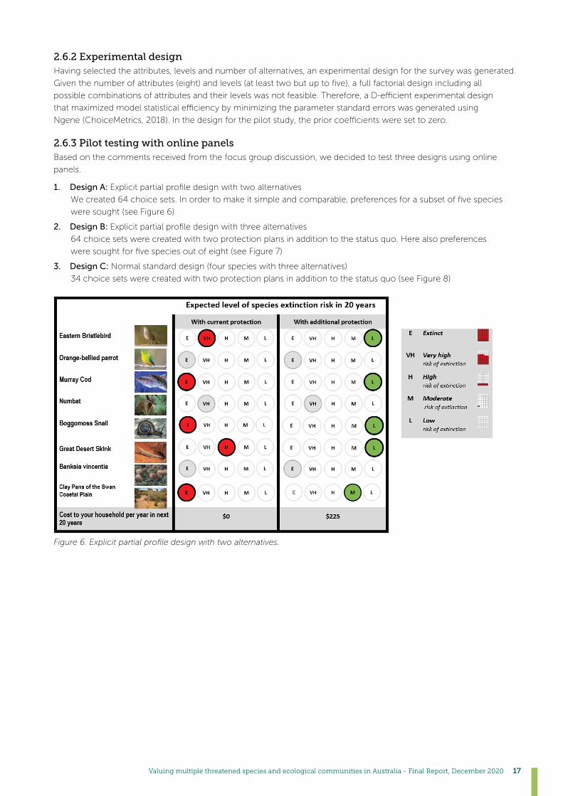
Figure6.Explicitpartialprofiledesignwithtwoalternatives ...............................................................................................................17
Figure7.Explicitpartialprofiledesignwiththreealternatives ............................................................................................................ 18
Figure 8. Standard four species design ..................................................................................................................................................... 18
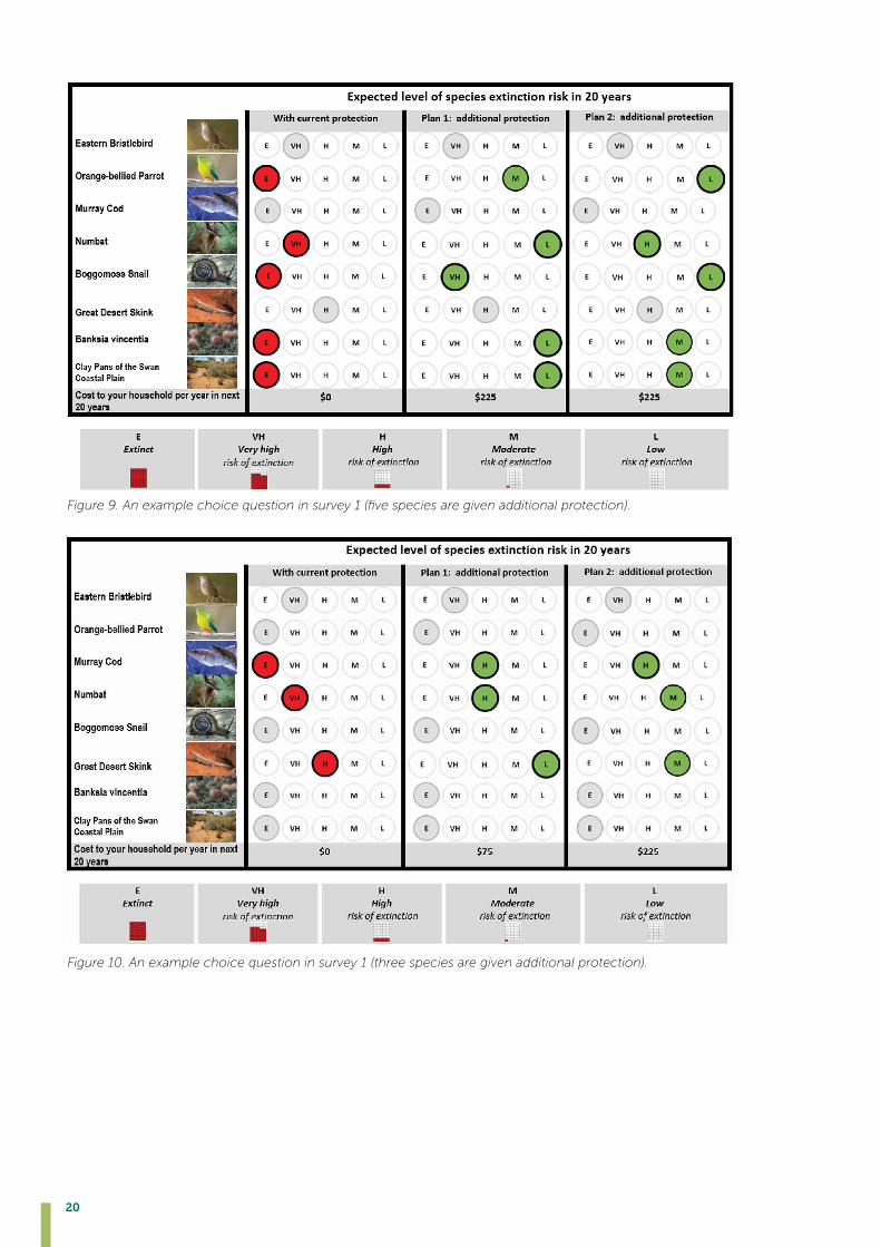
Figure9.Anexamplechoicequestioninsurvey1(fivespeciesaregivenadditionalprotection) ............................................20
Figure 10. An example choice question in survey 1 (three species are given additional protection) .......................................20
Figure11.Anexamplechoicequestioninsurvey2(fivespeciesaregivenadditionalprotection) ...........................................21
Figure 12. An example choice question in survey 2 (three species are given additional protection) .......................................21
Figure 13. An example choice question in survey 3 (all eight species are given additional protection) ................................. 22
Figure 14. Marginal willingness to pay for vegetation index ................................................................................................................45
Figure 15. Calculating exchange value of fall in vegetation index: Option 1 ..................................................................................45
Figure 16. Calculating exchange value of fall in vegetation index: Option 2 .................................................................................46
Figure 17. Consumer surplus for changes in vegetation index .......................................................................................................... 47
Figure 18. Marginal willingness to pay and probability of survival .....................................................................................................48
Figure 19. Assumed relationship between vegetation index and probability of survival .............................................................48
Valuing multiple threatened species and ecological communities in Australia - Final Report, December 2020 5
Executive SummaryAustralia has more than 1,700 species and ecological communities that are known to be threatened and at risk of
extinction. Given a large number of species to protect and limited funding, sound understanding of the values that
the Australian community places on threatened species is important for decision makers. However, values are available
only for a few of the species listed in the Australian Government’s Threatened Species Strategy (TSS).
This study investigates preferences of the Australian public for improving the levels of extinction risk of 14 species
includingbirds,mammals,fish,reptiles,plants,andtwoecologicalcommunitiesthatwereidentifiedinconsultation
withDepartmentofAgriculture,WaterandtheEnvironment,andtheThreatenedSpeciesCommissioner’sofficeof
the commonwealth government.
To investigate these preferences, we used a discrete choice experiment with three split-samples, each considering
sevenspeciesandoneecologicalcommunity.Giventhenumberofspeciestovalue,weusedapartialprofiledesign
toreducecognitiveburdenontherespondentsbylettingthemtradeoffasubsetofspeciesineachchoicetask.
Ourpilottestswithpartialprofiledesign(onlychangingthestatusoffiveorthreespeciesfromtheeightineach
choice task) and traditional design of four species revealed that there was no degradation in respondent performance
intermsoftiming,protestbehaviourandunderstandinginthepartialprofiledesigns.Wethereforecontinuedwith
partialprofiledesigninthemainsurveys.Weimplementedthreenationwideonlinesurveyswhereabout1000
respondents completed each survey. In each choice task, respondents were required to make a choice from three
alternatives: the current level of protection (status quo) and two alternative species protection plans that improve the
status of species in terms of their risk of extinction. We sought preferences using three main designs based on number
of species to protect (subset of 3, subset of 5 or all eight species) while maintaining the structure and the number of
choice questions same for each respondent. We estimated willingness-to-pay (WTP) values for reducing each species’
risk of extinction status in a 20-year period using a mixed logit model, implemented in Willingness-To-Pay space.
Ourresultsshowthatrespondentsdifferentiatebetweenspeciesintermsoftheamountthattheyvalueimproved
protection,andthedegreetowhichtheriskofextinctionisreduced.Acloserlookattheresultsoffinalmodels
estimated for the Survey 1 and Survey 2 revealed an insensitivity to scope, i.e., it appears as if the aggregate WTP
for 3 species was similar to that of 5 species (once one controls for the scale of the improvement in probability of
extinction).TheimplicationisthatthemarginalWTPforprotectionofaspeciesisaffectedbywhetherthespeciesis
seen as part of a three species or 5 species policy intervention. We suggest that this is some form of decision heuristic
being adopted by respondents i.e. they are constructing some form of ‘average’ improvement across either three
orfivespecies.Wealsoobservedascalingeffectwheretheaveragevalueestimatesfor3speciesdesignwas5/3
times higher than that of 5 species design.
Wefurtherinvestigatedhowscopeeffectandscalingwouldbechangedifweaskpeopletoprovidetheirpreferences
for all 8 species in our Survey 3. Comparison of results of all three surveys revealed that WTP values to save species
weredifferentbasedonthedesign–numberofspeciesthatwereplannedtosave.Weobserveaclearpattern,higher
thenumberofspeciestosave,lowerthevaluethatpeoplewanttopayforaspecies–forexample,valueestimates
for 3 species design were higher most of the time compared to 5 species and 8 species designs. However, results of
the 8 species design (Survey 3) was not very consistent as in the Survey 1 and 2, therefore only 3 species and 5 species
designs were considered in proposing value estimates for species.
Based on estimates from 3 species and 5 species designs, we would propose that the range in the estimates across
the designs be treated as a broader estimate, with the midpoint taken as the central estimate (see Table ES1 and ES2).
For example, the value range for one percentage point improvement in risk level per year for Great Desert Skink is
$1.16 to $2.57 using the 5 species design, but $1.93 to $4.28 for the 3 species design. Then we computed the midpoint
of the extremes ($1.16 to $4.28) to come up with an estimate of $2.72.
These results should be of interest to researchers and policy-makers, as we provide value estimates for several species.
ThesevaluesarebenefitsthatAustralianpublicderivefromhavingimprovedstatusofspeciesthatcanbeusedin
cost-benefitanalysisinspeciesrecovery/conservationprojects.However,ourresultsalsosuggestthatpeoplewere
willing to pay more per species when asked to consider conserving three species than they do when asked about
fivespeciesi.e.theresultssuggestrespondentsfaila‘scope’test.Therefore,oneshouldbewaryinaggregating
estimates of WTP that have been derived from single-species studies.
6
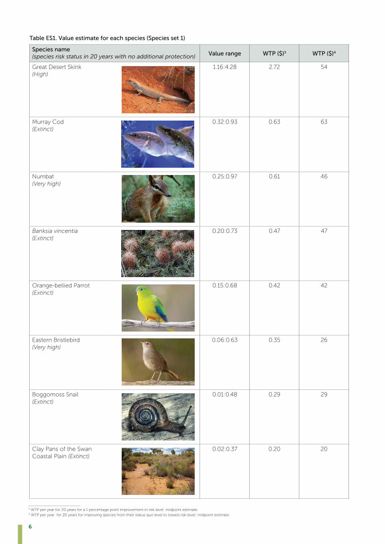
Table ES1. Value estimate for each species (Species set 1)
Species name (species risk status in 20 years with no additional protection) Value range WTP ($)3 WTP ($)4
Great Desert Skink (High)
1.16:4.28 2.72 54
Murray Cod (Extinct)
0.32:0.93 0.63 63
Numbat (Very high)
0.25:0.97 0.61 46
Banksia vincentia (Extinct)
0.20:0.73 0.47 47
Orange-bellied Parrot (Extinct)
0.15:0.68 0.42 42
Eastern Bristlebird (Very high)
0.06:0.63 0.35 26
Boggomoss Snail (Extinct)
0.01:0.48 0.29 29
Clay Pans of the Swan Coastal Plain (Extinct)
0.02:0.37 0.20 20
3 WTP per year for 20 years for a 1 percentage point improvement in risk level: midpoint estimate. 4 WTP per year for 20 years for improving species from their status quo level to lowest risk level: midpoint estimate.
©

Valuing multiple threatened species and ecological communities in Australia - Final Report, December 2020 7
Table ES2. Value estimate for each species (Species set 2)
Species name (species risk status in 20 years with no additional protection) Value range WTP ($)5 WTP ($)6
Brush-tailed Rabbit-rat (High)
2.62:7.43 5.03 101
Giant Freshwater Crayfish (High)
1.65:5.38 3.52 70
Australasian Bittern (Very high)
0.57:1.67 1.12 84
Arnhem Plateau Sandstone Shrubland Complex (Very High)
0.36:1.28 0.82 62
Far Eastern curlew (Extinct)
0.37:1.07 0.72 72
Shaw Galaxias (Extinct)
0.35:0.98 0.67 67
Gulbaru Gecko (Extinct)
0.34:0.97 0.65 65
Acacia equisetifolia (Extinct)
0.33:0.98 0.66 66
5 WTP per year for 20 years for a 1 percentage point improvement in risk level: midpoint estimate. 6 WTP per year for 20 years for improving species from their status quo level to lowest risk level: midpoint estimate.
©

8
1. IntroductionContinuousdeclineofspecies(floraandfauna)andecosystemsduetoanthropogenicandnaturalfactors
compromises the invaluable ecosystem services that humans derive from these functioning ecosystems
(Turneretal.,2007).Despiteworldwideconservationefforts,protectingbiodiversityhasbeenacriticalchallenge
at global, national and local scales due to increased threat of species extinction (Butchart et al., 2010). This is
mainly due to the complexity of ecosystems, lack of information and the large number of threatened species
that are at risk, which far exceed the resources available for conservation (Bottrill et al., 2008).
Australia is a megadiverse country with many endemic species. The rate of species extinction in Australia has
been high since European settlement; for example, mammals extinction in Australia is the highest in the world
(Woinarski et al., 2015). The Environment Protection and Biodiversity Conservation Act 1999 (the EPBC Act) is the
environmental legislation that provides a legal framework to protect and manage nationally and internationally
importantflora,fauna,ecologicalcommunitiesandheritageplaces.Thespeciesthatarenationallythreatenedand
endangeredarelistedunderthisactwiththeirthreatstatus.Apartfromthethreatstatus,costsandbenefitsalso
play a big part in decision-making around conservation actions, yet using economic theory in developing decision
frameworksforconservationhasnotbeendoneinAustralia.Understandingofthebenefitsderivedfromthreatened
speciesintheexistingliteratureisalsolimitedeitherintermsofthenumberofspeciescoveredorthetypeofbenefit
estimates(marketornon-market)available.Therefore,benefitestimatesarevaluableforsettingmanagementpriorities
and assessing proposed investments, as well as underpinning the value of investment in actions to save species.
Theaimofthisstudyhasbeentoestimatethebenefitsofmultiplethreatenedspecies(14)includinganimals,and
plants, and two ecological communities. We elicited preferences and estimated values that the Australian public place
onimprovingthestatusofthesespecies/ecologicalcommunitiesoverthenext20yearsusingachoiceexperiment.
Thebenefitestimatesgainedfromthisstudycanbeusedinmakinginvestmentdecisionsonspeciesconservation
projects.Thisstudywillalsocontributevalueestimatesforthedatabaseofnon-marketvaluesofthreatenedspecies
thatcanbeusedinrelevantbenefittransferstudies.
Section 2 discusses the methods that we used to identify species, design the choice experiment, survey implementation
and analysis of data. We present results and discussion in Section 3, and summary of estimation results and conclusion
inSection4.Section5presentspolicyimplicationsofthefindingswithexamplesonhowtousethespeciesvaluesin
decision-making contexts.
2. Methods2.1. Selection of threatened species and ecological communitiesA tentative list of threatened and endangered species (including birds, mammals, reptiles, invertebrates and plants)
and ecological communities7 was prepared based on EPBC listing of threatened and endangered species. The list was
further revised to include species from the Threatened Species Strategy as per the advice from the Department of
Agriculture, Water and the Environment. The Department’s guidance to select species was based on following criteria:
• SelectspeciesthatareofmostinteresttotheThreatenedSpeciesCommissioner’s(TSC)officeinrelationto
futurecommunicationsand/orevaluationexercises.
• Selectspeciesthatrepresentthewidestrangeofgeographiesand/orspeciescategories(i.e.,prioritywasto
ensure that birds, mammals and plants are represented).
• Selectspeciesforwhichaneworiginalstudywillhavethegreatestimpactintesting/illustratingtheutilityof
the work.
• Selectspecies,whichmakethebestuseofexistingvaluationdataintesting/illustratingtheutilityofthework.
Inadditiontotheabovecriteria,variousprojectpartnersofNationalEnvironmentalScienceProgram,Threatened
SpeciesRecoveryHubwereconsultedtomakesuretheselectionofspecieshassomerelevancetobenefittransfer.
TheinitiallistpreparedtoselectspeciesisshownintheAnnexA.Thefinallistofspeciesusedinthesurveywith
acknowledgments and credit for the sources of the images or photos is given in Annex B.
Giventheobjectiveofvaluingalargenumberofspecies,acrossthreesurveys,itwasplannedtohaveasimilar
composition in each survey. Hence, we decided to focus our study on seven species and one ecological community
ineachsurvey;comprisedoftwobirds,onefish,onemammal,oneinvertebrate,onereptile,oneplant,andone
ecological community. These species and ecological communities include:
7 Ecological communities are naturally occurring groups of native plants, animals and other organisms that are found in unique habitats.
Valuing multiple threatened species and ecological communities in Australia - Final Report, December 2020 9
Survey 1 and Survey 3 Fire severity
Great Sandy National Park Coastal heath, paperbark wetland and
woodland, Littoral Rainforest
Low-High
Bird 1 Eastern Bristlebird Far Eastern curlew
Bird 2 Orange-bellied Parrot Australasian Bittern
Fish Murray Cod Shaw Galaxias
Mammal Numbat Brush-tailed Rabbit-rat
Invertebrate Boggomoss Snail Giantcrayfish
Reptile Great desert Skink Phyllurus gulbara
Plant Banksia Vincentia Acacia Equisetiflia
Ecological community Clay Pans of the Swan Coastal Plain Arnhem Plateau Sandstone Shrubland Complex
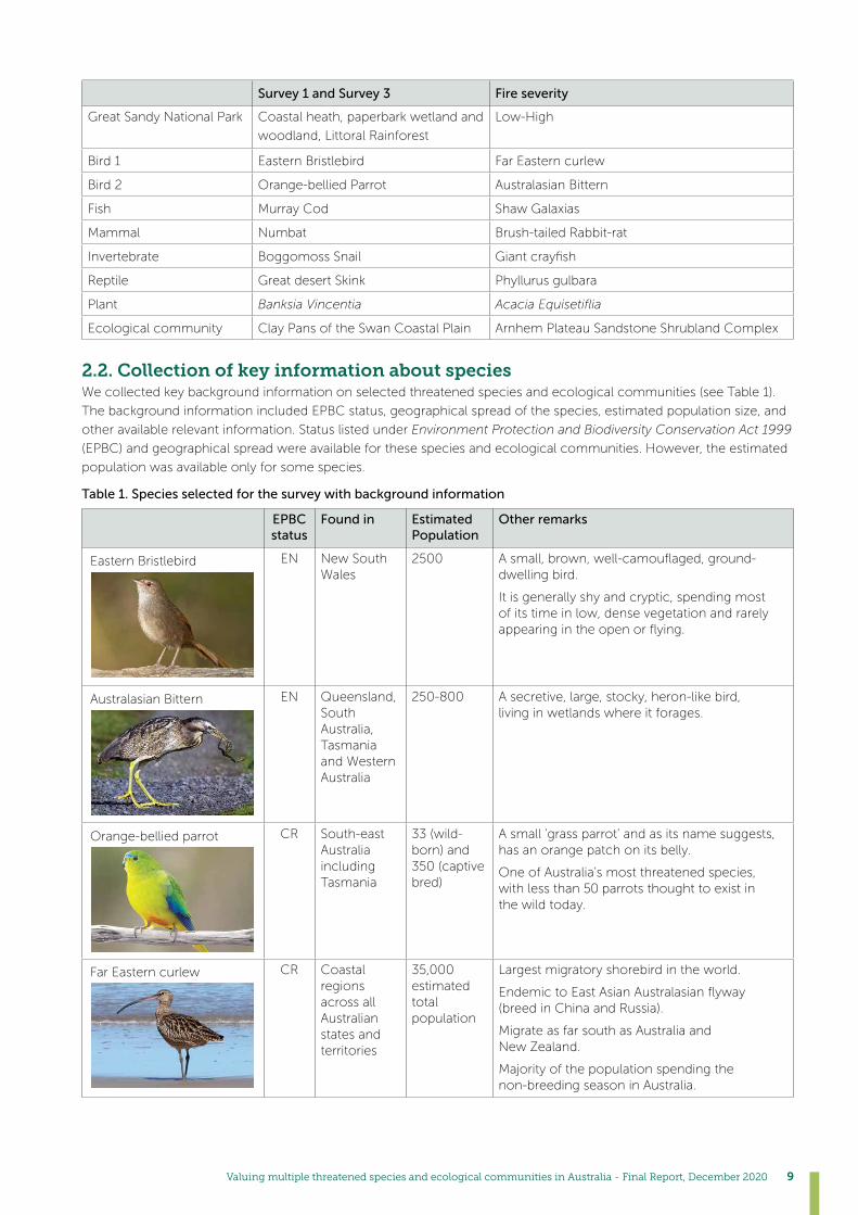
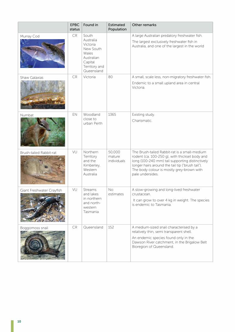
2.2. Collection of key information about speciesWe collected key background information on selected threatened species and ecological communities (see Table 1).
The background information included EPBC status, geographical spread of the species, estimated population size, and
other available relevant information. Status listed under Environment Protection and Biodiversity Conservation Act 1999
(EPBC) and geographical spread were available for these species and ecological communities. However, the estimated
population was available only for some species.
Table 1. Species selected for the survey with background information
EPBC status
Found in Estimated Population
Other remarks
Eastern Bristlebird EN New South Wales
2500 Asmall,brown,well-camouflaged,ground-dwelling bird.
It is generally shy and cryptic, spending most of its time in low, dense vegetation and rarely appearingintheopenorflying.
Australasian Bittern EN Queensland, South Australia, Tasmania and Western Australia
250-800 A secretive, large, stocky, heron-like bird, living in wetlands where it forages.
Orange-bellied parrot CR South-east Australia including Tasmania
33 (wild-born) and 350 (captive bred)
A small 'grass parrot' and as its name suggests, has an orange patch on its belly.
One of Australia's most threatened species, withlessthan50parrotsthoughttoexistin the wild today.
Far Eastern curlew CR Coastal regions across all Australian states and territories
35,000 estimated total population
Largest migratory shorebird in the world.
EndemictoEastAsianAustralasianflyway (breed in China and Russia).
Migrate as far south as Australia and New Zealand.
Majorityofthepopulationspendingthe non-breeding season in Australia.
10
EPBC status
Found in Estimated Population
Other remarks
Murray Cod CR South Australia Victoria New South Wales Australian Capital Territory and Queensland
AlargeAustralianpredatoryfreshwaterfish.
ThelargestexclusivelyfreshwaterfishinAustralia, and one of the largest in the world
Shaw Galaxias CR Victoria 80 Asmall,scaleless,non-migratoryfreshwaterfish.
Endemic to a small upland area in central Victoria.
Numbat EN Woodland close to urban Perth
1365 Existing study.
Charismatic.
Brush-tailed Rabbit-rat VU Northern Territory and the Kimberley, Western Australia
50,000 mature individuals
The Brush-tailed Rabbit-rat is a small-medium rodent (ca. 100-250 g), with thickset body and long (100-240 mm) tail supporting distinctively longer hairs around the tail tip (“brush tail”). The body colour is mostly grey-brown with pale undersides.
GiantFreshwaterCrayfish VU Streams and lakes in northern and north-western Tasmania
No estimates
A slow-growing and long-lived freshwater crustacean.
It can grow to over 4 kg in weight. The species is endemic to Tasmania.
Boggomoss snail CR Queensland 152 A medium-sized snail characterised by a relatively thin, semi transparent shell.
An endemic species found only in the Dawson River catchment, in the Brigalow Belt Bioregion of Queensland.

Valuing multiple threatened species and ecological communities in Australia - Final Report, December 2020 11
EPBC status
Found in Estimated Population
Other remarks
Gulbaru Gecko CR Queensland 600 Indigenous connection.
GreatDesertSkink,Tjakura,Warrarna,Mulyamiji
VU South Australia Northern Territory
6250 Indigenous connection.
Acacia equisetifolia CR Endemic to Northern Territory Kakadu National Park
A very distinctive perennial bush with grey-green foliage.
Banksia vincentia CR NSW Threatened species strategy species.
Listed very recently.
Arnhem Plateau Sandstone Shrubland Complex
EN Northern Australia
Widely distributed.
A type of scrublands that contains naturally large portion of plant species that found after recovery of disturbances.
Comprised mostly of native shrubs, grasses and animals (birds, mammals and reptiles) living in rock country.
Clay Pans of the Swan Coastal Plain
CR WA New recovery plan.
Narrowly distributed.
There are three critically endangered fauna known to be dependent on clay pans and the surrounding communities for a portion oftheirlife/breedingcycle.
©
©

12
2.3. Defining threat status/ extinction risk levelsInformationonspeciesthreatstatuswasavailablefromtwosources:(1)IUCNclassificationand;(2)EPBCActlisting
(see Table 2 for comparison of threat status). Since the words used to classify the threat status of species in both
of these sources may not be familiar to the general public, we translated them into an “extinction risk category”.
Theextinctionriskcategoryhadfivelevels-extinct,veryhigh,high,moderate,andlow–correspondingtothe
threat status in IUCN and EPBC listings.
Table 2. Comparison of threat status
IUCN listing status EPBC Act listing status Extinction risk category
Least Concern (LC) Not listed Low
Vulnerable (VU) Vulnerable Moderate
Endangered (EN) Endangered High
Critically Endangered (CR) Critically Endangered Very high
Extinct Extinct Extinct
Further, we illustrated the extinction risk category in the surveys in two ways: (1) bubbles with a relevant letter to
represent the corresponding risk and (2) risk grids (coloured with red to show chance of extinction) (see Table 3).
Table 3. Illustration of extinction risk categories
Illustration 1 Illustration 2
Extinct There is a 100% chance of extinction in the next 20 years.
Very high risk There is a 75% chance of extinction in the next 20 years. (i.e., at least 1 out of 50 species with this risk would be expected to go extinct in 20 years)
High risk There is a 20% chance of extinction in the next 20 years. (i.e., at least 5 out of 50 species with this risk would be expected to go extinct in 20 years)
Moderate risk There is a 2% chance of extinction in the next 20 years. (i.e., at least 38 out of 50 species with this risk would be expected to go extinct in 20 years)
Low risk Virtually no chance of extinction in the next 20 years.
Valuing multiple threatened species and ecological communities in Australia - Final Report, December 2020 13
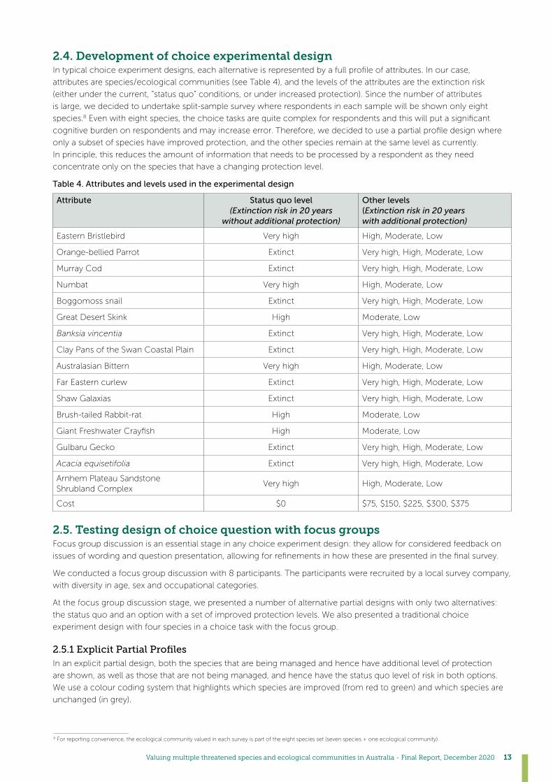
2.4. Development of choice experimental designIntypicalchoiceexperimentdesigns,eachalternativeisrepresentedbyafullprofileofattributes.Inourcase,
attributesarespecies/ecologicalcommunities(seeTable4),andthelevelsoftheattributesaretheextinctionrisk
(either under the current, “status quo” conditions, or under increased protection). Since the number of attributes
is large, we decided to undertake split-sample survey where respondents in each sample will be shown only eight
species.8Evenwitheightspecies,thechoicetasksarequitecomplexforrespondentsandthiswillputasignificant
cognitiveburdenonrespondentsandmayincreaseerror.Therefore,wedecidedtouseapartialprofiledesignwhere
only a subset of species have improved protection, and the other species remain at the same level as currently.
In principle, this reduces the amount of information that needs to be processed by a respondent as they need
concentrate only on the species that have a changing protection level.
Table 4. Attributes and levels used in the experimental design
Attribute Status quo level (Extinction risk in 20 years
without additional protection)
Other levels (Extinction risk in 20 years with additional protection)
Eastern Bristlebird Very high High, Moderate, Low
Orange-bellied Parrot Extinct Very high, High, Moderate, Low
Murray Cod Extinct Very high, High, Moderate, Low
Numbat Very high High, Moderate, Low
Boggomoss snail Extinct Very high, High, Moderate, Low
Great Desert Skink High Moderate, Low
Banksia vincentia Extinct Very high, High, Moderate, Low
Clay Pans of the Swan Coastal Plain Extinct Very high, High, Moderate, Low
Australasian Bittern Very high High, Moderate, Low
Far Eastern curlew Extinct Very high, High, Moderate, Low
Shaw Galaxias Extinct Very high, High, Moderate, Low
Brush-tailed Rabbit-rat High Moderate, Low
GiantFreshwaterCrayfish High Moderate, Low
Gulbaru Gecko Extinct Very high, High, Moderate, Low
Acacia equisetifolia Extinct Very high, High, Moderate, Low
Arnhem Plateau Sandstone Shrubland Complex
Very high High, Moderate, Low
Cost $0 $75, $150, $225, $300, $375
2.5. Testing design of choice question with focus groupsFocus group discussion is an essential stage in any choice experiment design: they allow for considered feedback on
issuesofwordingandquestionpresentation,allowingforrefinementsinhowthesearepresentedinthefinalsurvey.
We conducted a focus group discussion with 8 participants. The participants were recruited by a local survey company,
with diversity in age, sex and occupational categories.
At the focus group discussion stage, we presented a number of alternative partial designs with only two alternatives:
the status quo and an option with a set of improved protection levels. We also presented a traditional choice
experiment design with four species in a choice task with the focus group.
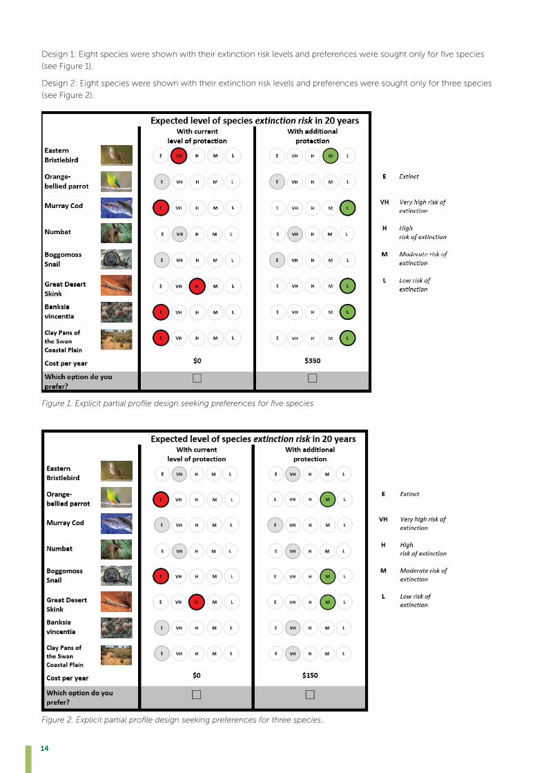
2.5.1 Explicit Partial Profiles In an explicit partial design, both the species that are being managed and hence have additional level of protection
are shown, as well as those that are not being managed, and hence have the status quo level of risk in both options.
We use a colour coding system that highlights which species are improved (from red to green) and which species are
unchanged (in grey).
8 For reporting convenience, the ecological community valued in each survey is part of the eight species set (seven species + one ecological community).
14
Design1:Eightspecieswereshownwiththeirextinctionrisklevelsandpreferencesweresoughtonlyforfivespecies
(see Figure 1).
Design 2: Eight species were shown with their extinction risk levels and preferences were sought only for three species
(see Figure 2).
Figure 1. Explicit partial profile design seeking preferences for five species.
Figure 2. Explicit partial profile design seeking preferences for three species..
©
©

Valuing multiple threatened species and ecological communities in Australia - Final Report, December 2020 15
2.5.2 Implicit partial ProfilesInanimplicitpartialdesign,theattributelevelsthatarenotbeingmodifiedarenotshownatall.
Design3:Eightspecieswereshown(withouttheirextinctionrisklevels)andpreferencesweresoughtonlyforfive
species (see Figure 3).
Design 4: Eight species were shown (without their extinction risk levels) and preferences were sought only for three
species (see Figure 4).
Figure 3. Implicit partial profile design seeking preferences for five species.
Figure 4. Implicit partial profile design seeking preferences for three species.
©
©

16
2.5.3 Standard Design In a standard design, fewer attributes are presented, but all are varied. For the purposes of comparison, we included
a 4 species conventional design for discussion in the focus groups.
Only four species were shown with their extinction risk levels and preferences were sought for all four species
(see Figure 5).
In addition to the status quo, two alternatives (plan 1 and plan 2) were shown in this design.
Figure 5. Standard design with three alternatives.
2.5.4 Outcome of the focus group discussion Manyparticipantspreferredtheexplicitpartialprofiledesignandsomeparticipantspreferredthestandarddesign.
Theyalsosuggestedthathavingthreecolumnsinanexplicitpartialprofiledesign(statusquoandtwoalternatives)
would not make the design too complicated for them to be able to respond.
2.6. Survey Development
2.6.1 Questionnaire The questionnaire that we developed and implemented in Qualtrics consisted of eight main sections. A full version
of the questionnaire is provided in Annex C.
Section 1: Introduction about the survey
Section 2: Screening questions and few socio-economic information about the respondents
Section 3: Brief explanation about threated and endangered species
Section 4: Key information about the species that are being asked for preferences
Section 5: Payment information and explanation on why additional funding is required for conservation of species
Section 6: Explanation of choice questions with examples followed by eight choice questions
Section 7: Questions to identify protestors (respondent who always selected either status quo option or non-status
quo option
Section 8: Follow- up questions
Valuing multiple threatened species and ecological communities in Australia - Final Report, December 2020 17
2.6.2 Experimental design Having selected the attributes, levels and number of alternatives, an experimental design for the survey was generated.
Giventhenumberofattributes(eight)andlevels(atleasttwobutuptofive),afullfactorialdesignincludingall
possiblecombinationsofattributesandtheirlevelswasnotfeasible.Therefore,aD-efficientexperimentaldesign
thatmaximizedmodelstatisticalefficiencybyminimizingtheparameterstandarderrorswasgeneratedusing
Ngene(ChoiceMetrics,2018).Inthedesignforthepilotstudy,thepriorcoefficientsweresettozero.
2.6.3 Pilot testing with online panelsBased on the comments received from the focus group discussion, we decided to test three designs using online
panels.
1. Design A: Explicitpartialprofiledesignwithtwoalternatives
Wecreated64choicesets.Inordertomakeitsimpleandcomparable,preferencesforasubsetoffivespecies
were sought (see Figure 6)
2. Design B: Explicitpartialprofiledesignwiththreealternatives
64 choice sets were created with two protection plans in addition to the status quo. Here also preferences
weresoughtforfivespeciesoutofeight(seeFigure7)
3. Design C: Normal standard design (four species with three alternatives)
34 choice sets were created with two protection plans in addition to the status quo (see Figure 8)
Figure 6. Explicit partial profile design with two alternatives.
©

18
Figure 7. Explicit partial profile design with three alternatives.
Figure 8. Standard four species design.
Each respondent was asked to answer eight choice questions. Three pilots were completed using the above-
mentioned designs, each with an initial sample of approximately 100. Table 5 reports some summary statistics
for the pilot surveys based on each design.
©
Valuing multiple threatened species and ecological communities in Australia - Final Report, December 2020 19
Table 5. Summary statistics for the three pilots
Design A 3 alternative (n=100)
Design B 2 alterative (n=99)
Design C 4 species (n=99)
All SQ protest 6 3 8
No SQ protest 11 10 29
Median time (minutes) 8.5 7.4 7.1
10% quartile (minutes) 3.6 3.0 3.5
Understanding
Fully 70 71 75
Partially 29 27 23
Not at all 1 1 1
Consider all aspects (yes) 84 81 83
We note a consistent response across the versions in terms of timing, protest behaviour and understanding (see Table
5).Wedidn’tobserveapreponderanceofpeoplealwayspickingthenon-SQoption(i.e.,theywerenotjustselectingfor
improvements irrespective of cost even in the 2 option case), apart from in the four species option where there is some
evidenceofmorerespondentsalwaysselectingthenon-SQoption.Thissuggeststhatthepartialprofiledesignswere
not problematic for respondents, and hence an appropriate way to deal with the large number of attributes in our design.
2.6.4 Survey design and arrangement of choice questionsBasedonresultsgainedfrompilotsurveys,wedecidedtoimplementanexplicitpartialprofiledesign(eightspecies
with three alternatives) where respondents see subsets of species are being protected further. Then that was repeated
for the second set of eight species (Survey 2). In each case a sample size of 1000, which allowed us to be more
confidentonwhetheranyspeciesarebeingignored,andissueslikewhethershiftingspeciesfromtheextinction
level is seen as particularly valued.
The experimental design for the survey was re-done using the parameters estimated in the pilot study as priors, and
usinganS-efficiencycriteria(whichattemptstominimisethesizeofthesampleneededtoobtainrobustparameter
estimates see Scarpa and Rose (2008)).
2.6.5 Survey implementationWe implemented the survey in three phases:
1. Phase 1 – Survey 1/Sample 1 (first set of eight species)
Following two choice designs were used for the survey 1.
a)Partialprofilewithsubsetoffivespecies(Figure9):Therewere64suchchoicesetsinthedesign,andeach
respondent saw four of these.
b)Partialprofilewithsubsetofthreespecies(Figure10):Therewere64choicesetswiththreespeciesbeinggiven
additional protection. Each respondent saw four of these choice sets.
Insurvey1,wehadafixedorder:respondentssawfour5-specieschoicesetsfirst,followedbyfour3-specieschoice
sets.Intheinitialanalysisofthatsamplewefoundsomedifferencesinvaluation,whichmeantitwasimportantto
beabletodistinguishbetweenordereffects,and5/3specieseffects.
.
20
Figure 9. An example choice question in survey 1 (five species are given additional protection).
Figure 10. An example choice question in survey 1 (three species are given additional protection).
©
©

Valuing multiple threatened species and ecological communities in Australia - Final Report, December 2020 21
2. Phase 2- Survey 2/Sample 2 (second set of eight species)
Similar to the survey 1, two choice designs were used (Figures 11 and 12). Each respondent saw four choice sets
from design 1 (Figure 11: 5 species) and four choice sets from design 2 (Figure 12: 3 species). However, unlike in
thefirstsurvey,inthesecondsurvey,werandomisedtheorderinwhichtheysawthefiveandthreespeciessets.
Examples of the choice sets (phase 2) are given below.
Figure 11. An example choice question in survey 2 (five species are given additional protection).
Figure 12. An example choice question in survey 2 (three species are given additional protection).
©
©

22
Thereasonfordoingthismixtureof5/3specieswasaconcernaboutthedegreetowhichrespondentsdealtwith
‘scope’ i.e., did the value of a species change as you change the number of species being protected? You might expect
there to be a degree of decreasing marginal valuation, simply because budgets become more restricted. This could
be an issue if one does ‘single species’ valuation studies, and then aggregate them to identify what people are willing
to pay for the group of species: you may overstate the value. This design was intended to give some light on this
possibility,becausewenowhavethesamespeciesbeingvaluedinafivespeciesandthreespeciescontext.
3. Phase 3- Survey 3/Sample 3 (first set of eight species)
Here,weusedthefirstsetof8speciesthatwestudiedinSurvey1.Onlythedifferencewithsurvey1wasthatthe
preferences were sought for all eight species (not a sub set of species as in the survey 1 and survey 2). An example
of a choice set is shown below (Figure 13).
Figure 13. An example choice question in survey 3 (all eight species are given additional protection)
2.6.6 Sample selectionThe survey was administered by an online survey company. We set quota through Qualtrics to make sure a
representative sample of Australian public (age, gender and state) was selected for the survey.
2.6.7 Data managementThe total number of people responding for Survey 1, Survey 2, and Survey 3 were 1026, 1131 and 1050, respectively.
Wedroppedanyonewhocompletedthesurveyinlessthanfiveminutes,asthatseemedanunreasonablyshorttime
to complete the survey and to have considered the information. Some additional analysis suggests that those who
completedinlessthanfiveminuteshadrespondedrandomlyinthechoicesets.Therefore,wehave817valid
responses for Survey 1, 985 responses for Survey 2, and 889 responses for Survey 3 (see Table 6).
2.6.8 Screening protestors and collecting additional informationWealsoidentified‘protest’respondents(ormorestrictly,thosewhoappearedtouseaheuristicwhenmakingchoices).
Those were the ones who always selected the status quo in all eight choice sets, plus an additional ‘test’ choice set
(with a very low cost), and then gave particular responses to debrief questions (see Annex C- Questionnaire for further
details). All of these indicated that these respondents were not making considered choices across all alternatives.
Wealsoidentifiedthosewhoneverselectedastatusquooption(Table6)inalleightchoicesets,orina‘test’choice
set (with a very high cost) and then gave particular responses to debrief questions. This looks like a group who are
prepared to pay any amount to achieve protection, which may not be reasonable.
©
Valuing multiple threatened species and ecological communities in Australia - Final Report, December 2020 23
Table 6. Information about protestors
Survey # (sample size) Who always selected status quo option Who never selected status quo option
Survey 1 (n = 817) 94 190
Survey 2 (n = 985) 91 146
Survey 3 (n = 889 ) 48 206
2.6.9 Other socio economic information
Some summary statistics for all three surveys are reported below, with a full set of descriptive statistics of the socio
economic information for the three samples is given in Annex D. Note that because not all questions were forced
response, the total ‘n’ may vary.
The distribution of survey respondents across the states follows actual population distribution (Table 7). Table 8
presents the distribution of age categories. All three samples are somewhat biased towards the more highly educated
group (degree and above) which is quite normal for online surveys (Table 9). Similarly, we found a larger percentage
of high income earners in our samples (Table 10). We also noted that we have a slightly higher percentage of retired
respondents (Table 11) than in the national population.
Table 7. Respondents by Australian states and territories by survey
Survey 1 Survey 2 Survey 3
Please select which State you live in
Freq. (n=810)
Percent Freq. (n=981)
Percent Freq. (n=889)
Percent
NSW 255 31.48 330 33.64 273 30.71
Queensland 164 20.25 165 16.82 191 21.48
South Australia 62 7.65 64 6.52 69 7.76
Tasmania 16 1.98 20 2.04 18 2.02
Victoria 205 25.31 283 28.85 227 25.53
Northern Territory 5 0.62 2 0.20 6 0.67
ACT 14 1.73 7 0.71 15 1.69
Western Australia 89 10.99 110 11.21 90 10.12
Table 8. Respondents by age category in each survey
Survey 1 Survey 2 Survey 3
Could you please indicate your age group?
Freq. (n=811)
Percent Freq. (n=983)
Percent Freq. (n=889)
Percent
18-24 years 61 7.52 60 6.10 67 7.54
25-34 years 151 18.62 141 14.34 165 18.56
35-44 years 127 15.66 133 13.53 135 15.19
45-54 years 133 16.40 169 17.19 156 17.55
55-64 years 172 21.21 291 29.60 180 20.25
>64 years 167 20.59 189 19.23 186 20.92
Table 9. Education levels of respondents by survey
Survey 1 Survey 2 Survey 3
State the highest level of education you have completed so far
Freq. (n=811)
Percent Freq. (n=983)
Percent Freq. (n=889)
Percent
Year 11 or below 108 13.32 112 11.39 107 12.04
Year 12 124 15.29 145 14.75 131 14.74
CertificateIII/IV 151 18.62 178 18.11 144 16.20
Advanced Diploma and Diploma
131 16.15 186 18.92 134 15.07
UniversityUndergraduate/Bachelor Degree
191 23.55 232 23.60 237 26.66
PostGraduate(Diploma/Masters/PhD)
106 13.07 130 13.22 136 15.30

24
Table 10. Respondents by income categories in each survey
Survey 1 Survey 2 Survey 3
Please indicate your current annual household income
Freq. (n=809)
Percent Freq. (n=842)
Percent Freq. (n=886)
Percent
Negative income 7 0.87 4 0.48 6 0.68
Nil income 24 2.97 29 3.44 21 2.37
$1- $7,799 per year 15 1.85 15 1.78 15 1.69
$7,800 - $15,599 per year 20 2.47 23 2.73 16 1.81
$15,600 - $20,799 per year 24 2.97 30 3.56 30 3.39
$20,800 - $25,999 per year 42 5.19 42 4.99 51 5.76
$26,000 - $33,799 per year 54 6.67 43 5.11 55 6.21
$33,800 - $41,599 per year 53 6.55 71 8.43 67 7.56
$41,600 - $51,999 per year 76 9.39 81 9.62 66 7.45
$52,000 - $64,999 per year 84 10.38 82 9.74 83 9.37
$65,000 - $77,999 per year 62 7.66 69 8.19 75 8.47
$78,000 - $90,999 per year 71 8.78 70 8.31 79 8.92
$91,000 - $103,999 per year 70 8.65 73 8.67 84 9.48
$104,000 - $155,999 per year 132 16.32 124 14.73 142 16.03
$156,000 or more per year 75 9.27 86 10.21 96 10.84
Table 11. Respondents by employment status in each survey
Survey 1 Survey 2 Survey 3
What is your current employment status?
Freq. (n=800)
Percent Freq. (n=829)
Percent Freq. (n=822)
Percent
Employed full time (35 or more hours per week)
259 32.38 271 32.69 297 33.67
Employed part time (less than35hoursperweek)/causal?
141 17.63 144 17.37 167 18.93
Unemployed and currently looking for work
40 5.00 43 5.19 42 4.76
Unemployed and not currently looking for work
8 1.00 8 0.97 10 1.13
Student 32 4.00 35 4.22 28 3.17
Retired 180 22.50 204 24.61 195 22.11
Homemaker (manages a home and family)
65 8.13 62 7.48 64 7.26
Self-employed 39 4.88 36 4.34 47 5.33
Unable to work 36 4.50 26 3.14 32 3.63
2.7 Discrete choice experiments TheDiscreteChoiceModelisaformalmodelofchoicebasedonrandomutilitytheory.Adefinitiveexpositionof
the model is given in Train (2009) but the model is widely applied. Here we follow the notation used by Hole and
Kolstad (2012).
We assume that an individual, when evaluating an option i, which can be described by a vector of attributes x, each of
whichcanhavevaryinglevels,willconstructanestimateoftheutilitythatwouldbegainedfromthatoption,definedas:
(1)
where αn and β
nareindividualspecificmarginalutilitiesassociatedwithcostandotherattributes.ε
njt is an individual
specificrandomcomponentthatisassumedtobedrawnfromanextremevaledistribution,withavarianceequalto
, where μnisanindividualspecificscaleparameter.Explicitinthisspecificationisthepossibilitythatboth
themarginalutilitiesandthevarianceoftherandomtermareindividualspecific.
Valuing multiple threatened species and ecological communities in Australia - Final Report, December 2020 25
When faced with multiple options, and required to select one of them, the assumption is that they select the option
that has highest utility. Given utility has an unobservable component, the analyst can at best predict the probability
that option i will be selected i.e.,
(2)
where Vnit
is the deterministic part of utility, i.e., the probability that option i is selected will depend on the probability
thattheutilityfromoptioniisgreaterthanthatofanotheroptionj,acrossalloptions.
If one makes an assumption about the functional form of the term ε, then one can derive a closed form expression
for the probability. A common assumption is that the random term follows a Gumbel (or type I extreme value)
distribution, in which case it can be shown (Train, 2009, Chapter 3) that the probability is given by:
(3)
which is the logit probability.
Standard statistical software can estimate this model, identifying the parameters that best explain the choices made.
A key outcome from such models is what is known as the ‘partworth’ associated with an attribute. The partworth
isdefinedasthechangeinthemonetaryattributeofanoptionthatwouldexactlyoffsettheeffectonutilityofa
unitchangeinoneoftheotherattributes,leavingtheindividualatanequallevelsofutility.Itcanbedefinedas
the maximum amount that they would be prepared to pay to gain a unit change in an attribute that they value (or
the amount they would have to be compensated by if an attribute they disliked were to increase). Analytically, the
partworth for attribute k can be calculated as:
(4)
Where αn is the parameter associated with the monetary attribute of the option.
However, there are some advantages in re-expressing the model in what is known as ‘Willingness to Pay space”
(Hole and Kolstad, 2012, Scarpa and Rose, 2008). As noted above, the partworth is expressed as a ratio of two
estimated parameters. Statistically, these are random variables, following normal distributions. The ratio of two normal
distributions does not follow a well-behaved functional form. In particular, theoretically, the denominator (the cost
coefficient)hassomeprobabilityofpassingthroughzero,makingthedistributionofthepartworthindeterminate.
Re-expressing the model in WTP space avoids this issue, and leads to estimated parameters being directly interpretable
(Scarpa et al., 2008). Dividing (1) through by μn(theindividual-specificscaleparameterthatdefinesheterogeneityin
variance) leaves the relationship fundamentally unchanged, but gives an error term that is homoscedastic:
(5)
Where and
Observing that the WTP for an attribute is given by ϒn=c
n/λ
n one can reframe (5) as:
anddirectlyestimatetheWTPassumingaspecificdistribution(e.g.,normal)forthe
WTPcoefficients.
Themodelisflexibleinthatonecanselectivelychoosewhetherattributesarefixedacrossapopulationorfollowa
distribution. It is normal to impose some restriction on the distribution of λn. Given it is a function of the marginal
utilityofcost(whichisnegative)andtheindividual-specificscalecoefficient(whichispositive),itshouldberestricted
tobenegative.Themostcommonwaytodothisistoredefinecostas-1*cost,andthenimposealognormal
distribution for λnwhichisbydefinitionalwayspositive.
The model has no closed form for the likelihood, and therefore has to be estimated using simulation methods. We use
800 Halton draws in estimation, which we arrived at by increasing draw numbers until results only changed marginally.
26
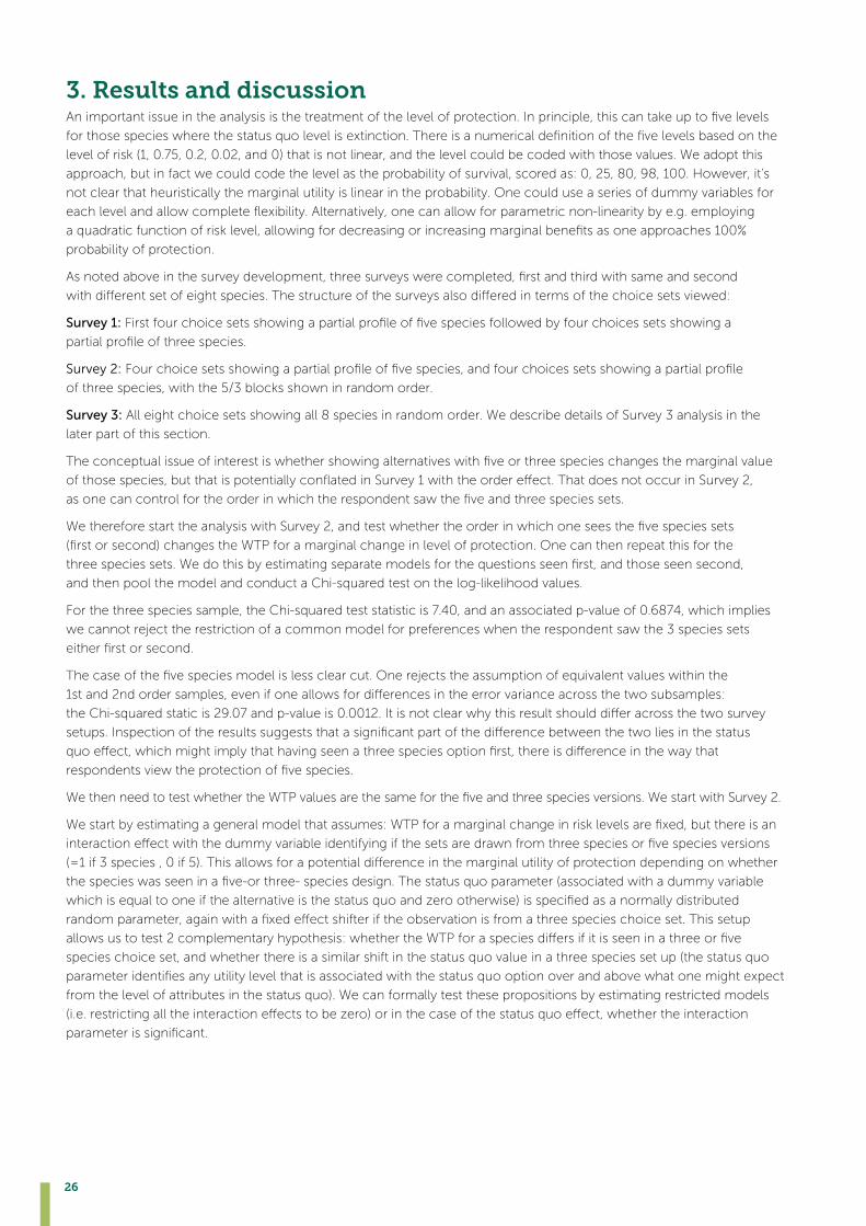
3. Results and discussion Animportantissueintheanalysisisthetreatmentofthelevelofprotection.Inprinciple,thiscantakeuptofivelevels
forthosespecieswherethestatusquolevelisextinction.Thereisanumericaldefinitionofthefivelevelsbasedonthe
level of risk (1, 0.75, 0.2, 0.02, and 0) that is not linear, and the level could be coded with those values. We adopt this
approach, but in fact we could code the level as the probability of survival, scored as: 0, 25, 80, 98, 100. However, it’s
not clear that heuristically the marginal utility is linear in the probability. One could use a series of dummy variables for
eachlevelandallowcompleteflexibility.Alternatively,onecanallowforparametricnon-linearitybye.g.employing
aquadraticfunctionofrisklevel,allowingfordecreasingorincreasingmarginalbenefitsasoneapproaches100%
probability of protection.
Asnotedaboveinthesurveydevelopment,threesurveyswerecompleted,firstandthirdwithsameandsecond
withdifferentsetofeightspecies.Thestructureofthesurveysalsodifferedintermsofthechoicesetsviewed:
Survey 1:Firstfourchoicesetsshowingapartialprofileoffivespeciesfollowedbyfourchoicessetsshowinga
partialprofileofthreespecies.
Survey 2:Fourchoicesetsshowingapartialprofileoffivespecies,andfourchoicessetsshowingapartialprofile
ofthreespecies,withthe5/3blocksshowninrandomorder.
Survey 3: All eight choice sets showing all 8 species in random order. We describe details of Survey 3 analysis in the
later part of this section.
Theconceptualissueofinterestiswhethershowingalternativeswithfiveorthreespecieschangesthemarginalvalue
ofthosespecies,butthatispotentiallyconflatedinSurvey1withtheordereffect.ThatdoesnotoccurinSurvey2,
asonecancontrolfortheorderinwhichtherespondentsawthefiveandthreespeciessets.
WethereforestarttheanalysiswithSurvey2,andtestwhethertheorderinwhichoneseesthefivespeciessets
(firstorsecond)changestheWTPforamarginalchangeinlevelofprotection.Onecanthenrepeatthisforthe
threespeciessets.Wedothisbyestimatingseparatemodelsforthequestionsseenfirst,andthoseseensecond,
and then pool the model and conduct a Chi-squared test on the log-likelihood values.
For the three species sample, the Chi-squared test statistic is 7.40, and an associated p-value of 0.6874, which implies
wecannotrejecttherestrictionofacommonmodelforpreferenceswhentherespondentsawthe3speciessets
eitherfirstorsecond.
Thecaseofthefivespeciesmodelislessclearcut.Onerejectstheassumptionofequivalentvalueswithinthe
1stand2ndordersamples,evenifoneallowsfordifferencesintheerrorvarianceacrossthetwosubsamples:
theChi-squaredstaticis29.07andp-valueis0.0012.Itisnotclearwhythisresultshoulddifferacrossthetwosurvey
setups.Inspectionoftheresultssuggeststhatasignificantpartofthedifferencebetweenthetwoliesinthestatus
quoeffect,whichmightimplythathavingseenathreespeciesoptionfirst,thereisdifferenceinthewaythat
respondentsviewtheprotectionoffivespecies.
WethenneedtotestwhethertheWTPvaluesarethesameforthefiveandthreespeciesversions.WestartwithSurvey2.
Westartbyestimatingageneralmodelthatassumes:WTPforamarginalchangeinrisklevelsarefixed,butthereisan
interactioneffectwiththedummyvariableidentifyingifthesetsaredrawnfromthreespeciesorfivespeciesversions
(=1if3species,0if5).Thisallowsforapotentialdifferenceinthemarginalutilityofprotectiondependingonwhether
thespecieswasseeninafive-orthree-speciesdesign.Thestatusquoparameter(associatedwithadummyvariable
whichisequaltooneifthealternativeisthestatusquoandzerootherwise)isspecifiedasanormallydistributed
randomparameter,againwithafixedeffectshifteriftheobservationisfromathreespecieschoiceset.Thissetup
allowsustotest2complementaryhypothesis:whethertheWTPforaspeciesdiffersifitisseeninathreeorfive
species choice set, and whether there is a similar shift in the status quo value in a three species set up (the status quo
parameteridentifiesanyutilitylevelthatisassociatedwiththestatusquooptionoverandabovewhatonemightexpect
from the level of attributes in the status quo). We can formally test these propositions by estimating restricted models
(i.e.restrictingalltheinteractioneffectstobezero)orinthecaseofthestatusquoeffect,whethertheinteraction
parameterissignificant.

Valuing multiple threatened species and ecological communities in Australia - Final Report, December 2020 27
Whenwedothiswefindthatwecannotconfidentlyrestrictthespeciesinteractioneffectstobezero(Chi-squared
test statistic of 15.49 with p-value of 0.502, but note that the value can cross the 0.05 limit by changing the number of
drawsusedintheestimationprocess).Thestatusquointeractioneffectisalsosignificant(p-value=0.001),suggesting
thatrespondentsviewthecurrentsituationdifferentlyiftheyhavethreeorfivespeciesbeingmanaged.
Thisistroubling,inthatitimpliesthatrespondentsarevaluingimprovementofaspeciesdifferentlyiftheyare
presentedinthefive-speciesdesigncomparedtoathree-speciesdesign.Inordertounderstandwhatheuristic
respondents may be using, an alternative framework was tested.
We assume that respondents’ measure of utility from protection under a particular alternative is a weighted average
ofthespeciesbeingprotected,i.e.inthecaseofafivespeciesdesignweassumethattheecologicalimprovement
isdefinedas:
While the utility from a three species design is given by:
Where‘i'isacounteridentifyingthefiveorthreespeciesthatarethesubjectofimprovedmanagement.
Notethatthisisaratherextremeassumption:althoughitallowsfordifferencesinvaluesacrossspecies(theβi)
when considering a suite of species being managed what is important is the (weighted) average improvement.
Theimplicationofthisspecificationisthatthevalueofaspecieswhenseeninathree-speciesdesignisby
construction5/3morethanitwaswhenseeninafive-speciesdesign.Asanassumptionthiscouldonlybe
justifiedifitwassupportedstatistically.Assumingthattheinitialdefinitionoftheprotectionvariableforspecies
#isdefinedas#r,wecreateanewsuiteofspeciesprotectionvariables#rp,definedas:
#rp=#r ifseeninafivespeciesdesign
#rp=#r*5/3 ifseeninathreespeciesdesign
i.e.,wenormalisethedefinitionsofweightedecologicaloutcomesothefivespeciesdesignistakenasthebaseand
thethreespeciesdesignisweightedupbyafactorof5/3(where#identifiesoneoftheeightspeciesinthedesign).
We can then estimate this model and conduct a further test: can the unrestricted model that allows parameters for
thethreeandfivespeciesdesignstovaryberestrictedtoaversionwheretheparametersarenotidentical,buthave
a5/3ratio?
Wefindthatwefailtorejecttherestrictionoftheparametershavingaproportionalityof5/3forthethreespecies
designascomparedtothefivespeciesdesign.TheChi-squaredvalueis7.85andthep-valueis0.4483,whichisrobust
to changes in the draws needed for estimation. In that case our alternative heuristic is supported: respondents are
valuingspeciesdifferentlyinthethreeandfivespeciesdesign,butinasystematicway.Ifthe‘scope’ofthepolicyis
greater i.e. protecting more species, one would expect the WTP for a bundle of species to be greater, but this does
not seem to be occurring.
It should be noted that in all of these cases, we have assumed that the marginal utility associated with a change in
the probability of extinction is constant. Introducing dummy variables for each level of protection for each species
(relativetothestatusquo)ispossible,butintroducesalargenumberofparameters,whichmakesestimationdifficult.
An alternative approach is to introduce non-linearity in marginal values by introducing a quadratic term for the risk
level for each species.
Althoughthisdoesnotintroducecompleteflexibilityinresponse,itdoesallowfordifferenceinvalues,including
diminishing marginal values associated with achieving higher levels of protection, or increasing marginal values if
respondents only care if high levels of protection are achieved.
Aformaltestofthismodel(usingthe5/3weightingspecification)foundthatonefailedtorejecttherestrictionthat
theresponseswerelinearintheprobabilityofsurvival,i.e.thatthequadraticspecificationdidnotimprovemodelfit
(Chi-squared test statistic =7.85, p-value=0.4479).

28
Table12belowreportstheresultsofthepreferredmodel:linearinrisklevels,butweightedby5/3forthethreespecies
model,relativetothefivespeciesmodelwithaweightof1.
Table 12. WTP-space model results for eight species: Survey 2
Coefficient SE 95% confidence interval
Coefficient Coefficient
Brush-tail Rabbit-rat 0.0354 0.0046 0.0262 0.0446
GiantF/wCrayfish 0.0244 0.0040 0.0165 0.0323
Australasian Bittern 0.0078 0.0010 0.0057 0.0099
Arnhem Plateau 0.0056 0.0010 0.0036 0.0077
Far Eastern curlew 0.0050 0.0006 0.0037 0.0064
Shaw Galaxias 0.0047 0.0005 0.0035 0.0058
Gulbaru Gecko 0.0046 0.0006 0.0034 0.0058
Acacia equisetifolia 0.0046 0.0006 0.0033 0.0059
SQ*sp3 0.3191 0.0794 0.1634 0.4748
SQ -1.3994 0.2741 -1.9368 -0.8620
SD(SQ) 5.0120 0.3438 4.338 5.6860
Het 0.8508 0.1072 0.6407 1.0609
/tau 1.3494 0.0795 1.193 1.5053
Number of choices 6144
Number of individuals 768
Log likelihood -4338.5223
NB:Speciesrisklevelsrescaledby5/3ifthechoicesetwasa3-speciespartialprofiledesigni.e.reportedvaluesarefora5-speciespartialprofile,andshouldbeincreasedby5/3torepresentvaluesina3-speciespartialprofiledesign.
Thecostattributehasbeendefinedin$100s,andhencecoefficientsaretheWTPexpressedin$100perunitchange
in probability of extinction in next 20 years, payable for 20 years, per household i.e. they are willing to pay 78c per
percentage point improvement for the Australasian Bittern. Also note that the implied values are for a species when
seeninthefivespeciesdesign.Thevalueswouldbeincreasedby5/3ifthespecieswasseeninathree-speciesdesign.
WethenrepeatthisprocessforSurvey1,testingtoseeifthevaluesforspeciesdifferifseeninafiveorthreespecies
design.AgainwefindthatwecannotrestricttheWTPtobeequalacrossallspecies(Chi-squaredstatistic=24.06,
p-value=0.0022) but when we employ the weighting approach, then we can accept the restriction (14.08, 0.0797
respectively). Again, we seem to have a systematic heuristic being adopted whereby the utility from an alternative is
determined by a (weighted) average of improvement in the species present, rather than the aggregate improvement
in species protection.

Valuing multiple threatened species and ecological communities in Australia - Final Report, December 2020 29
Table 13. WTP-space model results for eight species: Survey 1
Coefficient SE 95% confidence interval
-1*Cost 1 (constrained)
Great Desert Skink 0.0187 0.0036 0.0116 0.0257
Murray Cod 0.0044 0.0005 0.0032 0.0056
Numbat 0.0042 0.0008 0.0025 0.0058
Banksia vincentia 0.0032 0.0006 0.0020 0.0044
Orange-bellied Parrot 0.0029 0.0006 0.0015 0.0041
Eastern Bristlebird 0.0022 0.0008 0.0006 0.0038
Boggomoss snail 0.0020 0.0004 0.0010 0.0029
Clay Pans of the Swan Coastal Plain 0.0012 0.0005 0.0002 0.0022
SQxsp3 0.2664 0.0821 0.1055 0.4274
SQ -1.719 0.1980 -2.1076 -1.3313
SD(SQ) 3.891 0.2782 3.3460 4.4367
Het 1.2051 0.16475 0.8821 1.5280
/tau 1.708 0.1242 1.4648 1.9519
Number of choices 4104
Number of individuals 513
Log likelihood -3139.0892
NB:Speciesrisklevelsrescaledby5/3ifthechoicesetwasa3-speciespartialprofiledesigni.e.reportedvaluesarefora5-speciespartialprofile,andshouldbeincreasedby5/3torepresentvaluesina3-speciespartialprofiledesign.
Again we test for whether there is any non-linear (quadratic) change in WTP as the level of protection varies. As a group
ofeffectsthiswassignificant(chisquaredstatisticof25.55,p=0.001),butinspectionoftheestimatessuggeststhat
inonlyonecasetherewasasignificanteffect(forClayPans)wheretherewassomeevidenceofincreasingmarginal
utilityassociatedwithreducingtheriskofextinction.Forsimplicity,wereportjustthelinearmodel.
Oneissuethatwehaveidentifiedisthattheredoesappeartobeaninsensitivitytoscope,i.e.,themarginalWTP
forprotectionofaspeciesisaffectedbywhetherthespeciesisseenaspartofathreespeciesor5speciespolicy
intervention. We suggest that this is some form of decision heuristic being adopted by respondents, i.e., they are
constructingsomeformof‘average’improvementacrosseitherthreeorfivespecies.Weexploredthiseffectfurther
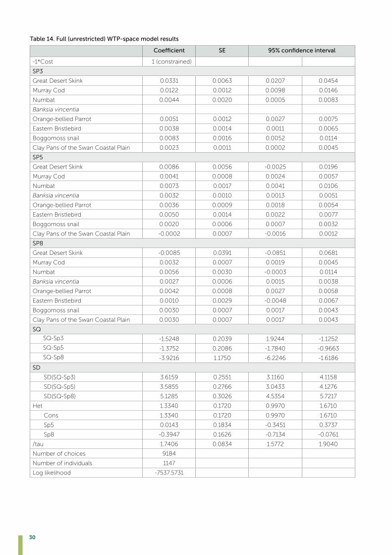
by conducting Survey 3 where preferences were sought for all eight species. We combined data sets of Survey 1 and
Survey3andestimatedanunrestrictedfullmodel(Table14),havingdifferentcoefficientsforeachset:subsetof3(SP3),
subset of 5 (SP5) and all 8 species (SP8).
30
Table 14. Full (unrestricted) WTP-space model results
Coefficient SE 95% confidence interval
-1*Cost 1 (constrained)
SP3
Great Desert Skink 0.0331 0.0063 0.0207 0.0454
Murray Cod 0.0122 0.0012 0.0098 0.0146
Numbat 0.0044 0.0020 0.0005 0.0083
Banksia vincentia
Orange-bellied Parrot 0.0051 0.0012 0.0027 0.0075
Eastern Bristlebird 0.0038 0.0014 0.0011 0.0065
Boggomoss snail 0.0083 0.0016 0.0052 0.0114
Clay Pans of the Swan Coastal Plain 0.0023 0.0011 0.0002 0.0045
SP5
Great Desert Skink 0.0086 0.0056 -0.0025 0.0196
Murray Cod 0.0041 0.0008 0.0024 0.0057
Numbat 0.0073 0.0017 0.0041 0.0106
Banksia vincentia 0.0032 0.0010 0.0013 0.0051
Orange-bellied Parrot 0.0036 0.0009 0.0018 0.0054
Eastern Bristlebird 0.0050 0.0014 0.0022 0.0077
Boggomoss snail 0.0020 0.0006 0.0007 0.0032
Clay Pans of the Swan Coastal Plain -0.0002 0.0007 -0.0016 0.0012
SP8
Great Desert Skink -0.0085 0.0391 -0.0851 0.0681
Murray Cod 0.0032 0.0007 0.0019 0.0045
Numbat 0.0056 0.0030 -0.0003 0.0114
Banksia vincentia 0.0027 0.0006 0.0015 0.0038
Orange-bellied Parrot 0.0042 0.0008 0.0027 0.0058
Eastern Bristlebird 0.0010 0.0029 -0.0048 0.0067
Boggomoss snail 0.0030 0.0007 0.0017 0.0043
Clay Pans of the Swan Coastal Plain 0.0030 0.0007 0.0017 0.0043
SQ
SQ-Sp3 -1.5248 0.2039 1.9244 -1.1252
SQ-Sp5 -1.3752 0.2086 -1.7840 -0.9663
SQ-Sp8 -3.9216 1.1750 -6.2246 -1.6186
SD
SD(SQ-Sp3) 3.6159 0.2551 3.1160 4.1158
SD(SQ-Sp5) 3.5855 0.2766 3.0433 4.1276
SD(SQ-Sp8) 5.1285 0.3026 4.5354 5.7217
Het 1.3340 0.1720 0.9970 1.6710
Cons 1.3340 0.1720 0.9970 1.6710
Sp5 0.0143 0.1834 -0.3451 0.3737
Sp8 -0.3947 0.1626 -0.7134 -0.0761
/tau 1.7406 0.0834 1.5772 1.9040
Number of choices 9184
Number of individuals 1147
Log likelihood -7537.5731

Valuing multiple threatened species and ecological communities in Australia - Final Report, December 2020 31
Thenweconstrainedthefullmodeltohavethesamecoefficients,(1)inpercentagewithoutrescalingand(2)in
percentage with rescaling. We tested two constrained models against full model using likelihood-ratio tests and found
thatbothfullmodelrestrictedtosamecoefficients,noscaling(Chi-squaredstatistic=44.92s,p-value=0.0001)andalso
fullmodelrestrictedtosamecoefficients,withscaling(Chi-squaredstatistic=50.78,p-value=0.0000)wererejected.
As the next step, we estimated a model with 3 species design and with 5 species design constrained, with scaling and
8 species design unconstrained. We tested whether this model can be constrained against the full model and was
accepted (Chi-squared statistic=8.34, p-value=0.4011). Therefore, we estimated a separate model for the Survey 3
sample which has 8 species design. The results of this model are reported in Table 15.
Table 15. WTP-space model results for eight species: Survey 3
Coefficient SE 95% confidence interval
-1*Cost 1 (constrained)
Great Desert Skink -.01009 0.0447 -0.0977 0.0775
Murray Cod 0.0030 0.0007 0.0016 0.0045
Numbat 0.0052 0.0033 -0.0013 0.0117
Banksia vincentia 0.0019 0.0007 0.0005 0.0034
Orange-bellied Parrot 0.0036 0.0009 0.0019 0.0053
Eastern Bristlebird 0.0006 0.0032 -0.0057 0.0069
Boggomoss snail 0.0028 0.0007 0.0013 0.0043
Clay Pans of the Swan Coastal Plain 0.0017 0.0008 0.0001 0.0033
SQ -3.375 1.310 -5.943 -0.8067
SD(SQ) 6.8751 0.6225 5.6552 8.0950
Het 0.8462 0.1353 0.5810 1.1112
/tau 1.763 0.1116 1.5448 1.9826
Number of choices 5080
Number of individuals 634
Log likelihood -4172.80
4. Summary of estimation resultsThefirstpointtonoteisthattherearesignificant,positivewillingnesstopayforallspecies.Further,thereare
differencesinthelevelofWTPacrossspecies.BasedonthemodelresultsofcombinedSurvey1andSurvey2,we
can summarise the willingness to pay values of threatened species and ecological communities among the public in
Australia(Table16,andTable17).Themosthighlyvaluedspeciesamongthefirstsetofeightspecies9 (Survey 1) was
the Great Desert Skink, the least valued was the (Clay pan of the Swan Coastal Plain), with the WTP estimate of
$1.87 ($0.12) per year per household for 20 years respectively for a one percentage point improvement in its status,
i.e. reduction of its extinction risk. In survey 2, the most highly valued species was the Brush-tailed Rabbit-rat, with the
least being the (Gulbaru Gecko and Acacia equisetifolia) with the WTP estimate of $3.54 ($0.46) per year per household
for 20 years for a one percentage point improvement in its status, i.e., reduction on its extinction risk. The full set of
WTPestimatesandtheir95%confidenceintervalsarereportedinTables16and17.
We also report in those Tables the WTP for moving each species from its expected outcome in 20 years, with no
further protection (i.e., the status quo level in the choice experiment) up to the lowest level of risk. It should be noted
thatdifferencesinthesevaluesacrossspeciesareacombinationofthedifferencesinvaluesperpercentagepoint
improvementforeachspecies,andthedifferencesintheirinitialriskstatus.
Whatthisanalysishasshownisthatrespondentsareabletoexpressdifferentialvaluesforthespeciesshown,andthat
thesecanbeestimatedwithrelativelyhighstatisticalprecision.Wefindtherearenonon-linearityinmarginalWTP
estimates when the risk status is expressed as a numerical probability of extinction.
9 Seven species and one ecological community.

32
AcloserlookattheresultsoffinalmodelestimatedfortheSurvey1andSurvey2revealedaninsensitivitytoscope,
i.e., it appears as if the aggregate WTP for 3 species was similar to that of 5 species (once one controls for the scale
of the improvement in probability of extinction). The implication is that the marginal WTP for protection of a species
isaffectedbywhetherthespeciesisseenaspartofathreespeciesor5speciespolicyintervention.Wesuggestthat
this is some form of decision heuristic being adopted by respondents i.e. they are constructing some form of ‘average’
improvementacrosseitherthreeorfivespecies.Wealsoobservedascalingeffectwheretheaveragevalueestimates
for3speciesdesignwas5/3timeshigherthanthatof5speciesdesign.InTable15and16,wereportvaluesassociated
withthe5-speciesdesign,whichwillgivealowerestimate.Thesevalueshavetobemultipliedby5/3ifonewere
to prefer to use the 3-species values.
Weinvestigatedhowscopeeffectandscalingwouldbechangedifweaskpeopletoprovidetheirpreferencesfor
8speciesinourSurvey3.Asmentionedintheresultssection,afullmodelwithconstraintstohavesamecoefficients
withscalingwasrejected.AsaresultweestimatedamodelforSurvey3separately.Thenwecomparedvalueestimates
obtainedfromSurvey1andSurvey3forthefirstsetofspeciesfordifferentdesigns(seeTable18).Comparisonof
resultsrevealedthatWTPvaluestosavespeciesweredifferentbasedonthedesign–numberofspeciesthatwere
planned to save. We observe a clear pattern, higher the number of species to save, lower the value that people want
topayforaspecies–forexample,valueestimatesfor3speciesdesignwerehighermostofthetimecomparedto5
species and 8 species designs. However, results of the 8 species design (Survey 3) was not very consistent as in the
Survey 1 and 2, where only 3 species and 5 species deigns were presented. The value estimates of species based
on Survey 2 for 3 species and 5 species designs are given in Table 19.
Table 16. Value estimates ($) for threatened species and ecological community studied in Survey 1
Species set 1 Status quo level
(species risk status in 20 years with
no additional protection
WTP ($) per year for 20
years for a 1 percentage
point improvement in risk status
95 % CI WTP ($) each year for 20 years
for improving species from their
status quo level to lowest risk
level
Great Desert Skink High 1.87 1.16:2.57 37.4
Murray Cod Extinct 0.44 0.32:0.56 44
Numbat Very high 0.42 0.25:0.58 31.5
Banksia vincentia Extinct 0.32 0.20:0.44 32
©

Valuing multiple threatened species and ecological communities in Australia - Final Report, December 2020 33
Species set 1 Status quo level
(species risk status in 20 years with
no additional protection
WTP ($) per year for 20
years for a 1 percentage
point improvement in risk status
95 % CI WTP ($) each year for 20 years
for improving species from their
status quo level to lowest risk
level
Orange-bellied Parrot
Extinct 0.29 0.15:0.41 29
Eastern Bristlebird Very high 0.22 0.06:0.38 16.5
Boggomoss Snail Extinct 0.20 0.10:0.29 20
Clay Pans of the Swan Coastal Plain
Extinct 0.12 0.02:0.22 12
NB:Speciesrisklevelsrescaledby5/3ifthechoicesetwasa3-speciespartialprofiledesigni.e.reportedvaluesarefora5-speciespartialprofile,andshouldbeincreasedby5/3torepresentvaluesina3-speciespartialprofiledesign.
Table 17. Value estimates for threatened species and ecological community studied in Survey 2
Species set 2 Status quo level
(species risk status in 20 years with
no additional protection
WTP ($) per year for 20
years for a 1 percentage
point improvement in risk status
95 % CI WTP ($) each year for 20 years
for improving species from their
status quo level to lowest risk
level
Brush-tailed Rabbit -rat
High 3.54 2.62:4.46 70.8
Giant Freshwater Crayfish
High 2.44 1.65:3.23 48.8

34
Species set 2 Status quo level
(species risk status in 20 years with
no additional protection
WTP ($) per year for 20
years for a 1 percentage
point improvement in risk status
95 % CI WTP ($) each year for 20 years
for improving species from their
status quo level to lowest risk
level
Australasian Bittern Very high 0.78 0.57:1.00 58.5
Arnhem Plateau Sandstone Shrubland Complex
Very high 0.56 0.36:0.77 42
Far Eastern curlew Extinct 0.51 0.37:0.64 51
Shaw Galaxias Extinct 0.47 0.35:0.59 47
Gulbaru Gecko Extinct 0.46 0.34:0.58 46
Acacia equisetifolia Extinct 0.46 0.33:0.59 46
NB:Speciesrisklevelsrescaledby5/3ifthechoicesetwasa3-speciespartialprofiledesigni.e.reportedvaluesarefora5-speciespartialprofile,andshouldbeincreasedby5/3torepresentvaluesina3-speciespartialprofiledesign.
This may be due to having large number of attributes (8 species) that contributes to complexity of choice decisions
that people have to make. Although empirical evidence on error variance and choice complexity is not conclusive
(Burton and Rigby, 2012, Rigby et al., 2016),complexity of the choice tasks can lead to response strategies not
consistent with fully compensatory rational decisions that maximize utility (Johnston et al., 2017). We also couldn’t
observescalingeffectasweobservedin3speciesand5speciesdesigns.
©
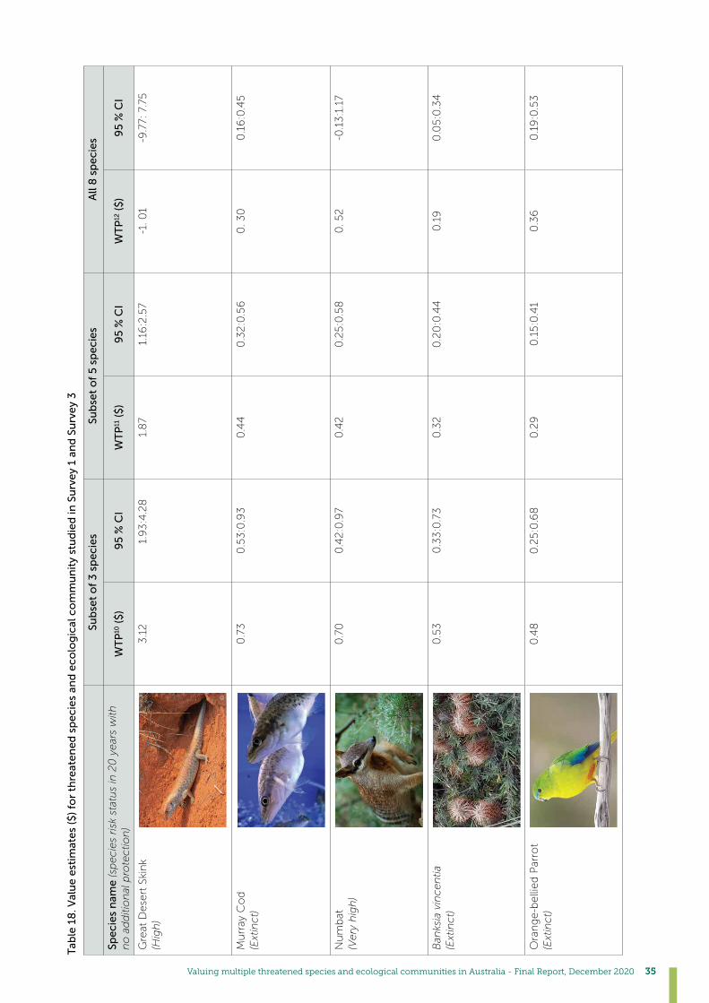
Valuing multiple threatened species and ecological communities in Australia - Final Report, December 2020 35
Tab
le 1
8. V
alu
e e
stim
ate
s ($
) fo
r th
reat
en
ed
sp
eci
es
and
eco
log
ical
co
mm
un
ity
stu
die
d in
Su
rve
y 1
and
Su
rve
y 3
Sub
set
of
3 s
pe
cie
sSu
bse
t o
f 5
sp
eci
es
All
8 s
pe
cie
s
Spe
cie
s n
ame
(sp
ecie
s risk
sta
tus
in 2
0 y
ear
s w
ith
no
ad
diti
on
al p
rote
ctio
n)
WT
P10
($
)9
5 %
CI
WT
P11
($
)9
5 %
CI
WT
P12
($
)9
5 %
CI
Gre
at D
ese
rt S
kin
k
(Hig
h)
3.1
2 1.
93
:4.2
81.
87
1.16
:2.5
7-1
. 01
-9.7
7: 7
.75
Mu
rray
Co
d
(Ext
inct)
0.7
30
.53
:0.9
30
.44
0.3
2:0
.56
0. 3
00
.16
:0.4
5
Nu
mb
at
(Very
hig
h)
0.7
00
.42
:0.9
70
.42
0.2
5:0
.58
0. 5
2-0
.13
:1.1
7
Ban
ksia
vin
cen
tia
(Ext
inct)
0.5
30
.33
:0.7
30
.32
0.2
0:0
.44
0.1
90
.05:0
.34
Ora
ng
e-b
elli
ed
Par
rot
(E
xtin
ct)
0.4
80
.25:0
.68
0.2
90
.15:0
.41
0.3
60
.19
:0.5
3
©

36
10 W
TP
per
year
fo
r 2
0 y
ear
s fo
r a
1 p
erc
en
tag
e p
oin
t im
pro
vem
en
t in
ris
k st
atu
s w
hen
pre
fere
nces
were
so
ug
ht
for
3 s
pecie
s o
ut
of
eig
ht.
11 W
TP
per
year
fo
r 2
0 y
ear
s fo
r a
1 p
erc
en
tag
e p
oin
t im
pro
vem
en
t in
ris
k st
atu
s w
hen
pre
fere
nces
were
so
ug
ht
for
5 s
pecie
s o
ut
of
eig
ht..
12 W
TP
per
year
fo
r 2
0 y
ear
s fo
r a
1 p
erc
en
tag
e p
oin
t im
pro
vem
en
t in
ris
k st
atu
s w
hen
pre
fere
nce w
ere
so
ug
ht
for
all 8
sp
ecie
s.
Sub
set
of
3 s
pe
cie
sSu
bse
t o
f 5
sp
eci
es
All
8 s
pe
cie
s
Spe
cie
s n
ame
(sp
ecie
s risk
sta
tus
in 2
0 y
ear
s w
ith
no
ad
diti
on
al p
rote
ctio
n)
WT
P10
($
)9
5 %
CI
WT
P11
($
)9
5 %
CI
WT
P12
($
)9
5 %
CI
Eas
tern
Bri
stle
bird
(V
ery
hig
h)
0.3
70
.10
:0.6
30
.22
0.0
6:0
.38
0.0
6-0
.57:
0.6
9
Bo
gg
om
oss
Sn
ail
(Ext
inct)
0.3
30
.17:
0.4
80
.20
0.1
0:0
.29
0.2
80
.13
:0.4
3
Cla
y P
ans
of
the S
wan
C
oas
tal P
lain
(E
xtin
ct)
0.1
0 0
.03
:0.3
70
.12
0.0
2:0
.22
0. 1
70
.01:
0.3
3
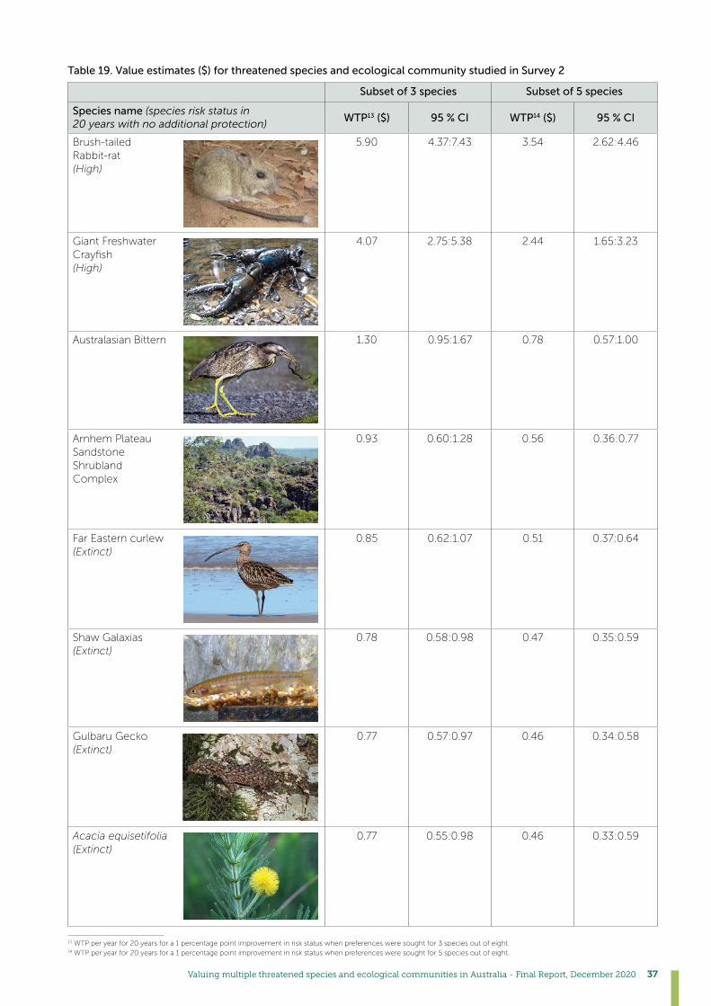
Valuing multiple threatened species and ecological communities in Australia - Final Report, December 2020 37
Table 19. Value estimates ($) for threatened species and ecological community studied in Survey 2
Subset of 3 species Subset of 5 species
Species name (species risk status in 20 years with no additional protection)
WTP13 ($) 95 % CI WTP14 ($) 95 % CI
Brush-tailed Rabbit-rat (High)
5.90 4.37:7.43 3.54 2.62:4.46
Giant Freshwater Crayfish (High)
4.07 2.75:5.38 2.44 1.65:3.23
Australasian Bittern 1.30 0.95:1.67 0.78 0.57:1.00
Arnhem Plateau Sandstone Shrubland Complex
0.93 0.60:1.28 0.56 0.36:0.77
Far Eastern curlew (Extinct)
0.85 0.62:1.07 0.51 0.37:0.64
Shaw Galaxias (Extinct)
0.78 0.58:0.98 0.47 0.35:0.59
Gulbaru Gecko (Extinct)
0.77 0.57:0.97 0.46 0.34:0.58
Acacia equisetifolia (Extinct)
0.77 0.55:0.98 0.46 0.33:0.59
13 WTP per year for 20 years for a 1 percentage point improvement in risk status when preferences were sought for 3 species out of eight. 14 WTP per year for 20 years for a 1 percentage point improvement in risk status when preferences were sought for 5 species out of eight.
©
38
5. How to use species values reported in this studyThisstudyhasfocusedonasetofspecificspeciesandecologicalcommunities.Ifmanagementactionscanbe
interpretedintermsofchangesinextinctionriskforthosespecies/communitiesthentheestimatesreportedherecanbe
used to value those improvements. There are a number of issues that need to be considered when doing so, however.
Non- linearity of extinction risk levels
Aswedefinedbytheattributelevels,extinctionrisklevelcantakeuptofivelevelsforthosespecieswherethestatus
quolevelisextinction.Thereisanumericaldefinitionofthefivelevelsbasedonthelevelofriskofextinction,(1,0.75,
0.2, 0.02, and 0), or one could recode so that they represent the probability of survival scored as: 0%, 25%, 80%, 98%,
and 100%.
However, it’s not clear that heuristically the marginal utility is linear in the probability, i.e., it could be possible that the
marginal utility loss increases as one approaches the probability of survival of zero, or that the marginal gain in utility
declines as the probability of survival approaches 100%. Instead of adopting this approach one could use a series of
dummyvariablesforeachlevelandallowcompleteflexibilityinthevaluesovertherange.Alternatively,onecanallow
for parametric non-linearity, by e.g. employing a quadratic function of risk level, allowing for decreasing or increasing
marginalbenefitsasoneapproaches100%probabilityofsurvival.Wetestedthiswithparametricquadraticfunction
andfoundthatthelinearmodelthatweemployedusingprobabilityofsurvivalprovidesabettermodelfit,butthis
couldbeinfluencedbytherangeofvaluesemployedinthedesign,i.e.,withgreaterdiscriminationatthevalues
close to extinction one may detect non-linearity. However, for large changes in probabilities one would anticipate
that the reported results will be appropriate for measuring values.
The study also explored the issue of whether the value for each species varied with the context that it was in
(i.e.,whethertherewere3,5or8speciesbeingvalued).Thishasledtodifferentvaluesforeachspecies.Although
the 3 and 5 species design appeared to have some consistency up to a scaling factor, the 8 species model diverted
fromthat.Itisperhapsnotunexpectedthatestimatesshouldbecontextspecific,butthisleavesuswithanumber
of potential estimates of values that could be used in a valuation exercise.
As mentioned above we found that the estimates from the eight species design are less consistent, in terms of wider
confidenceintervals(CI),totheextentthatsomespecieshaveinsignificantestimates.Therefore,weconsideronly
values that come from the designs with subset of 3 species and subset of 5 species. We would propose that the range
in the estimates across the designs be treated as a broader estimate, with the midpoint taken as the central estimate.
For example, the value range for Great Desert Skink is 1.16:2.57 using the 5 species design, but 1.93:4.28 for the 3
species design. Then we computed the midpoint of the extremes (1.16:4.28) to come up with an estimate of 2.72.

Valuing multiple threatened species and ecological communities in Australia - Final Report, December 2020 39
Table 20. Value estimate for each species (Species set 1)
Species name (species risk status in 20 years with no additional protection)
Value range WTP15 ($) WTP16 ($)
Great Desert Skink (High)
1.16:4.28 2.72 54
Murray Cod (Extinct)
0.32:0.93 2.75:5.38 2.44
Numbat (Very high)
0.25:0.97 0.61 46
Banksia vincentia (Extinct)
0.20:0.73 0.47 47
Orange-bellied Parrot (Extinct)
0.15:0.68 0.42 42
Eastern Bristlebird (Very high)
0.06:0.63 0.35 26
Boggomoss Snail (Extinct)
0.01:0.48 0.29 29
Clay Pans of the Swan Coastal Plain (Extinct)
0.02:0.37 0.20 20
15 WTP per year for 20 years for a 1 percentage point improvement in risk level: midpoint estimate. 16 WTP per year for 20 years for improving species from their status quo level to lowest risk level: midpoint estimate.
©

40
Table 21. Value estimate for each species (Species set 2)
Species name (species risk status in 20 years with no additional protection)
Value range WTP17 ($) WTP18 ($)
Brush-tailed Rabbit-rat (High)
2.62:7.43 5.03 101
GiantFreshwaterCrayfish (High)
1.65:5.38 3.52 70
Australasian Bittern (Very high)
0.57:1.67 1.12 84
Arnhem Plateau Sandstone Shrubland Complex (Very high)
0.36:1.28 0.82 62
Far Eastern curlew (Extinct)
0.37:1.07 0.72 72
Shaw Galaxias (Extinct)
0.35:0.98 0.67 67
Gulbaru Gecko (Extinct)
0.34:0.97 0.65 65
Acacia equisetifolia (Extinct)
0.33:0.98 0.66 66
17 WTP per year for 20 years for a 1 percentage point improvement in risk level: midpoint estimate. 18 WTP per year for 20 years for improving species from their status quo level to lowest risk level: midpoint estimate.
©
Valuing multiple threatened species and ecological communities in Australia - Final Report, December 2020 41
5.1 How to use these values?Theestimatedvaluesofspeciesandecologicalcommunitiescanbeusedindifferentways,primarilyinbenefittransfer
andconservationdecisions,withnecessaryadjustments.
5.1.1 Benefit TransferThevaluesandtherangereportedintheTable20andTable21canbeusedinbenefittransfer.However,itisimportant
to note that the values reported in this study for each species are in terms of changes in extinction risk level.
Benefittransferisrequiredwhenavaluesfromonecontextaretransferredtoanother.Onemightconsiderthecase
where values are needed for a species that has not been valued using a unique primary study. There are a number of
waystoconductabenefittransfer,whichvaryaccordingtoaccuracyandexpertiserequired.Twomainapproaches
areunit-valuetransferandbenefit-functiontransfer(Johnstonetal.,2015).Onemightconsideraunitvaluetransferi.e.
taking a value estimated here and applying it to the new context directly. However, there is a requirement that the site,
contextandcommodityaresufficientlysimilartosupportthisapproach(Batemanetal.2011;Johnstonetal.,2015).For
example,thisstudyisconductedforentireAustraliasothatonemightbeconfidentthatthevalueestimatesproduced
inthisstudycanbeappliedanywhereinAustraliausingunitvaluetransferapproachwithappropriatepost-adjustments
forthesameorsimilarspecies.Adjustmentsarerequireddependingonthenewcontextwherevalueswillbeapplied.
Johnstonetal.(2015)provideanon-exhaustivelistofspecificitemsthatshouldbeconsideredwhenmatchingthe
studycontextandnewcontextforbenefittransfersuchasbroaderpolicycontext,commoditybeingvalued,similarity
of the economic framework19 and socio-demographics of the population. Gunawardena et al. (2017) summarize a
check list, key steps and some examples on unit-value transfers using non-market values of species.
Inthecurrentcaseonecouldtakeaviewofsufficientlysimilarspeciesandsimilarpolicycontextofconserving
threatenedspeciestodecideonwhethervaluescouldbetransferred.Itmaybesufficienttoattempttomapacross
typeofspecies(i.e.frogtofrog,orbirdtobird)butwiththecaveatthatifoneofthosespeciesisiconic/charismatic
then the values may be prone to higher error (Subroy et al., 2019), indicating that even with similar species the public’s
awarenessofthemcouldaffectthetransferredvalues.
Whenthenewcontextisdissimilartothecontextwherestudywasconducted,onecoulduseabenefittransfer
approach. For example, if we want to apply the values we estimated for a particular species in a country where context
isconsiderablydifferent,useofbenefittransferfunctionismoreappropriatethanunit-valueapproach.Thisrequires
more information, resources and expertise. The most common method is the use of a function derived from
meta- analysis which requires data from several primary studies (Subroy et al., 2019; Loomis and White 1996,
Richardson and Loomis 2009; Martín-López et al. 2008).
This study estimates values for a variety of species that includes, birds, mammals, reptiles, plants and ecological
communities in Australia. These values can be added into a meta-analysis of species (for example Subroy et al)
and then possibly be used to predict values of other species.
5.1.2 Benefit transfer examplesIn this section we show two examples to illustrate how to use estimated species values in other contexts.
Example 1: Painted Honeyeater
AssumethattheGovernmentwishestofindoutbenefits(thenon-marketvalue)ofconservingPainted Honeyeater in
Gunbower Koondrook Perricoota (GKP) site in the Murray Darling Basin to help evaluate a conservation policy. If the
resources and time available are limited, and it is not possible to undertake an original non-market valuation study, one
couldthinkofapplyingbenefittransfer.Herewegothroughastep by step process to illustrate how to apply values
estimated in this study to value the Painted Honeyeater.
1. Identify any original non-market valuation studies done anywhere on Painted Honeyeater.Wecouldn’tfindany
non-market valuation study.
2. Identify species (that already have estimated non-market values) that are closely matching with the characteristics
of Painted Honeyeater.
3. Here we assume people would place similar values on Eastern Bristlebird and Painted Honeyeater as both are
small birds, endemic to Australia, and generally shy and cryptic (rarely seen by ordinary people). Therefore, we
willusevaluesthatweestimatedforEasternBristlebirdforbenefittransfer.
19 For example, if the original study measures willingness to pay (WTP) it can’t be used to infer values for a policy context that needs to measure willingness to accept compensation.

42
4. Understand details of the value estimate of Eastern Bristlebird:
a. Commodity being valued: WTP for 1 percentage point improvement of extinction risk level of
Eastern Bristlebird.
b. Table22showshowextinctionriskcategoriesweredefinedinthisvaluationstudy.
Table 22. Definition of extinction risk category
IUCN listing status EPBC Act listing status
Extinction risk category
Probability of extinction
Least Concern (LC) Not listed Low Virtually no chance of extinction in the next 20 years.
Vulnerable (VU) Vulnerable Moderate There is a 2% chance of extinction in the next 20 years.
Endangered (EN) Endangered High There is a 20% chance of extinction in the next 20 years.
Critically Endangered (CR)
Critically Endangered
Very high There is a 75% chance of extinction in the next 20 years.
Extinct Extinct Extinct There is a 100% chance of extinction in the next 20 years.
c. Mean annual WTP per household for 20 years for 1% improvement of risk level = AU$ 0.35 in 2019
d. Survey method: Discrete choice experiment
e. Survey details: Representative sample of Australian public
f. Study site: Australia
5. AdjusttheWTPvaluetosuitthenewpolicycontext.
Adjust WTP for different biological context
The value estimate AU$ 0.35 is for 1 percent improvement of risk level for all Eastern Bristlebirds available in
Australia. So we assume this value is equal to the value for 1 percent improvement in extinction risk level,
i.e. one percent reduction in extinction risk or one percent improvement is probability of survival of
Painted Honeyeater species available throughout Australia.
Our new context is GKP site in Murray Darling Basin. We assume that 80 percent of the Australian population of
Painted Honeyeaters is found in the GKP site in the Murray Darling Basin. Therefore, the value that people would
be willing to pay for 1 percent improvement of extinction risk level of Painted Honeyeaters can be lower than
improving the species found in Australia. Implicit in this assumption is that respondents’ values are responsive to
scale, in a linear fashion. In the absence of any other information this is probably the appropriate consideration.
Therefore, we can assume the value estimate for 1% improvement in extinction risk level of Painted Honeyeaters
inGKP=AU$0.35*80%=AU$0.28
6. AdjustWTPforinflation.
Thesurveyforthisstudywasconductedin2019.Therefore,theWTPvaluereflectedthevaluesthatpeopleplaced
on conserving the species in 2019.
Wecanadjustthesevaluesto2020Australiandollarbeforewetransferthemtothenewcontext.
CPI for 2019 = 115.4 (Australian Government20)
CPI for 2020 = 116.2 (Australian Government)
AdjustedWTPvaluefor2020for1%reductionofextinctionrisklevelofPainted Honeyeater at GKP site:
WTP2020=AU$0.28x116.2/115.4=AU$0.28perhouseholdperyearfor20years.
7. AdjustWTPforchangeinrealincome.
Averageadultweeklyearnings/personinAustraliainMay2019was$1237.86and$1304.70inMay202021.
Adjustingforinflation,realweeklyearnings/personin2019was1237.86*(116.2/115.4)=$1246.44.
Rateofchangeinrealincome=(1304.70–12.46.44)/1246.44=0.0467
Allowingforinflation,thisrepresentsa4.67%increaseinrealincomesfrom2019to2020.Suchincreasesarelikely
toincreasetheWTPforenvironmentalgoods,althoughthespecificrelationshipbetweenincomeandWTPfora
particular environmental asset is uncertain. For simplicity, we assume that the change in WTP is proportional to
thechangeinrealincome(assumingconstantincomeelasticityofWTPequalto1,Czajkowskietal.2017).
AdjustedWTP2020=AU$0.28+$0.28x0.467=$0.28x(1+0.0467)=AU$0.29
20AustralianGovernment/Australiantaxoffice:https://www.ato.gov.au/rates/consumer-price-index/ 21Weekly earnings data: Australian Bureau of Statistics: https://www.abs.gov.au/AUSSTATS/[email protected]/second+level+view?ReadForm&prodno=6302.0&viewtitle=Average%20Weekly%20Earnings~Mar%201975~Previous~30/05/1975&&tabname=Past%20Future%20Issues&prodno=6302.0&issue=Mar%201975&num=&view=&
Valuing multiple threatened species and ecological communities in Australia - Final Report, December 2020 43
8. We also can estimate the value people would place on improving the extinction risk of species from current level to
lowest level (see Table 22). The current risk level (Threat status) for Painted Honeyeater is Moderate (Vulnerable, i.e.
2% chance of species being extinct or 98% chance of species survival in the next 20 years). Moving the species to the
lowest risk level (i.e., 0% extinction risk or 100% survival probability in the next 20 years) would be achieved by a 2%
improvementofextinctionrisklevelwhichisequaltoAU$0.29*2=AU$0.58perhouseholdperyearfor20years.
9. Aggregatevalueofbenefitsfromconserving Painted Honeyeater
Assuming that preferences are sought from Australian public, the total number of estimated households in Australia
in 2020 is about 10 million (based on 2020 Australian Institute of Family Studies22).
10.AggregatevalueofbenefitsforconservingPainted Honeyeater (moving from the current level of extinction risk
to the lowest level) is AU$ 5.8 million per year for 20 years.
Example 2: Superb Parrot
Suppose we are asked to estimate the non-market value of Superb Parrot in GKP site in the Murray Darling basin.
We can go through the same steps we described for Painted Honeyeater.
1. In the absence of an original study on Superb Parrots, the next best alternative is to use value estimates from
a similar species. We assume that people would value both parrots similarly as Orange-bellied Parrot and
Superb Parrot share similar characteristics in terms of size and colour.
2. Understanding details of the value estimates for Orange-bellied Parrot:
a. Commodity being valued: WTP for 1 percentage point improvement of extinction risk status of
Orange-bellied Parrot (See Table 22 for further information on extinction risk categories)
b. Mean annual WTP per household : AU$ 0.42 in 2019
c. Survey method: Discrete choice experiment.
d. Survey details: Representative sample of Australian public
e. Study site: Australia
3. AdjusttheWTPvaluetosuitthenewpolicycontext.
Adjust WTP for different biological context
The value estimate AU$ 0.42 is for 1 percent improvement of extinction risk level for all Orange-bellied parrots
available in Australia. So we assume this value is equal to the value for 1 percent improvement in survival probability
or 1 percent reduction in extinction risk of Superb Parrot species available throughout Australia.
The entire range of Superb ParrotsarefoundinMurrayDarlingBasin.Therefore,wedon’tneedtoadjustthevalues
for biological context.
4. AdjustWTPforinflation.
Thesurveyforthisstudywasconductedin2019.Therefore,theWTPvaluereflectedthevaluesthatpeopleplaced
on conserving the species in 2019.
Wecanadjustthesevaluesto2020Australiandollarbeforewetransferthemtothenewcontext.
CPI for 2019 = 115.4 (Australian Government23)
CPI for 2020 = 116.2 (Australian Government)
5. AdjustedWTPvaluefor2020for1%reductionofextinctionrisklevelor1%improvementinsurvivalprobabilityof
Superb ParrotsatGKPsite:WTP2020=AU$0.42x116.2/115.4=AU$0.42perhouseholdperyearfor20years
22 Australian Institute of Family Studies: https://aifs.gov.au/facts-and-figures/households-australia/households-australia-source-data#:~:text=Number%20of%20households%20and%20families%20projections&text=The%20number%20of%20households%20in,and%2012.57%20million%20by%202036
23AustralianGovernment/Australiantaxoffice:https://www.ato.gov.au/rates/consumer-price-index/

44
6. AdjustWTPforchangeinrealincome.
Averageadultweeklyearnings/personinAustraliainMay2019was$1237.86and$1304.70inMay202024.
Adjustingforinflation,realweeklyearnings/personin2019was1237.86*(116.2/115.4)=$1246.44.
Rateofchangeinrealincome=(1304.70-1246.44)/1246.44=0.0467
Allowingforinflation,thisrepresentsa4.67%increaseinrealincomesfrom2019to2020.Suchincreasesarelikely
toincreasetheWTPforenvironmentalgoods,althoughthespecificrelationshipbetweenincomeandWTPfora
particular environmental asset is uncertain. For simplicity, we assume that the change in WTP is proportional to
thechangeinrealincome(assumingconstantincomeelasticityofWTPequalto1,Czajkowskietal.2017).
AdjustedWTP2020=AU$0.42+$0.42x0.0467=$0.42(1+0.0467)=AU$0.44
7. We also can estimate the value people would place on improving the species from current risk level to lowest risk
level. The current risk level (Threat status) for Superb parrot is Moderate (Vulnerable, i.e. 2% chance of extinction in
next 20 years). Moving the species to lowest risk level (0% chance of extinction in next 20 years) can be achieved
by2%improvementofrisklevelwhichisequalto:AU$0.44*2=AU$0.88perhouseholdperyearfor20years
8. AggregatevalueofbenefitsfromconservingSuperb parrot
Assuming that preferences are sought from Australian public, the total number of estimated households in Australia
in 2020 is about 10 million (based on 2020 Australian Institute of Family Studies25).
9. AggregatevalueofbenefitsforconservingSuperb parrot (moving from the current risk level to lowest risk level)
is AU$ 8.8 million per year for 20 years.
5.1.3 Decision-makingThe estimated values of species and ecological communities could be applicable in a range of decision-making
contexts. Some of the applications of these values are described below.
1. Informing judgements that underpin decisions: Even without utilising them in a formal accounting framework or
adecisionsupporttool(suchasBenefit:CostAnalysis),quantitativeestimatesofnon-marketvaluesforthreatened
speciescanassistdecisionmakers.Theycaninfluencethesubjectivejudgementsthatpeoplemakeabouttherelative
importanceofdifferentprojectsorinterventions,andtherebyinfluencethedecisionsthataremade.
2. Using non-market valuation to inform environmental accounting: In this section we show how the results of a non-
market valuation study (e.g., a discrete choice experiment) that is used to estimate the value of a marginal change
inanenvironmentalbenefitcanbeusedtocalculatethe“exchangevalue”foruseinenvironmentalaccounting.
Assume that the asset that is to be included in the environmental accounts is an area of native vegetation. For
convenience we assume that the stock of this vegetation is measured on an index that has a potential range from
0 to 100. The index represents the extent of native vegetation and its quality as habitat.
The aim of the environmental account is to report each year on changes in the exchange value of this area of
vegetation,calculatedasthechangeinthevegetationindextimesitsmarginalvalue(itsmarginalsocialbenefit,or
marginal willingness to pay, or marginal WTP). In principle, there is a relationship between the level of the vegetation
index and its marginal WTP. Assume we have conducted a discrete choice experiment that has allowed us to identify
the relationship. A potential shape for it is shown in Figure 14. Economists expect that most goods exhibit the illustrated
pattern of marginal value falling as the availability of the good increases.
24 Weekly earnings data :Australian Bureau of Statistics: https://www.abs.gov.au/AUSSTATS/[email protected]/second+level+view?ReadForm&prodno=6302.0&viewtitle=Average%20Weekly%20Earnings~Mar%201975~Previous~30/05/1975&&tabname=Past%20Future%20Issues&prodno=6302.0&issue=Mar%201975&num=&view=&
25 Australian Institute of Family Studies: https://aifs.gov.au/facts-and-figures/households-australia/households-australia-source-data#:~:text=Number%20of%20households%20and%20families%20projections&text=The%20number%20of%20households%20in,and%2012.57%20million%20by%202036

Valuing multiple threatened species and ecological communities in Australia - Final Report, December 2020 45
Figure 14. Marginal willingness to pay for vegetation index
Suppose that, in a reporting period, the level of the vegetation index falls from 60 to 40. The marginal WTP (Figure 14),
estimated using the discrete choice experiment, can be used to estimate the exchange value of the fall in the index.
Figure 15 and Figure 16 show two possible ways in which the exchange value could be calculated.
Figure 15. Calculating exchange value of fall in vegetation index: Option 1
Figure 16. Calculating exchange value of fall in vegetation index: Option 2
0
0.1
0.2
0.3
0.4
0.5
0.6
0.7
0.8
0.9
0 10 20 30 40 50 60 70 80 90 100
Margina
l WTP
Vegetation index
0
0.1
0.2
0.3
0.4
0.5
0.6
0.7
0.8
0.9
0 10 20 30 40 50 60 70 80 90 100
Margina
l WTP
Vegetation index
0
0.1
0.2
0.3
0.4
0.5
0.6
0.7
0.8
0.9
0 10 20 30 40 50 60 70 80 90 100
Margina
l WTP
Vegetation index

46
The shaded area in Figure 15 represents the exchange value of the fall in vegetation index if we use the marginal
WTP for the end of the reporting period, after the index has fallen. The exchange value is the change in index level (20)
times the marginal WTP at the index level for the end of the period (0.2496), equalling 9.984.
Figure 16 shows the exchange value if we use the marginal value for the start of the reporting period, before the index
has fallen. In this case, the exchange value is the change in index level (20) times the marginal WTP at the index level
for the start of the period (0.1184), which equals 7.104.
Clearly,thechoiceofwhichmarginalvaluetousecouldaffectthereportedexchangevaluemarkedly.Thereisno
theoretical reason in economics to prefer the approach in Figure 15 or Figure 16, or potentially an average of the two.
Whichever we choose, the marginal value will change over time as the vegetation index changes (unless the marginal
WTP curve in Figure 14 happens to be a horizontal line).
If the vegetation index oscillates up and down over time, there could be some asymmetry in the exchange values
reported in the accounts. For example, if we chose to use the marginal WTP at the end of each reporting period, the
exchange values reported would be higher in years when the index fell (Figure 15) than in years when it rose (Figure 16),
even if the index oscillated between the same two levels over a number of years.
As a side comment, economists note that the exchange values illustrated in Figures 15 and 16 are not equal to the
change in consumer surplus, which is a better measure of the value of the change. The consumer surplus for the
changeisshownastheshadedareainFigure17.Thedifferencereflectsthatenvironmentalaccountsarenotactually
measuring the social values of the changes they report on because, within any one report, they apply the same
marginal value to all quantities of the good, ignoring that marginal value changes as the quantity changes.
Figure 17. Consumer surplus for changes in vegetation index
0
0.1
0.2
0.3
0.4
0.5
0.6
0.7
0.8
0.9
0 10 20 30 40 50 60 70 80 90 100
Margina
l WTP
Vegetation index
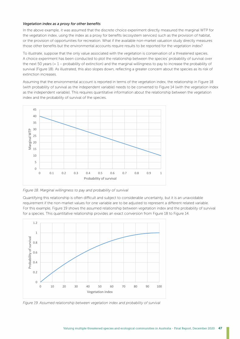
Valuing multiple threatened species and ecological communities in Australia - Final Report, December 2020 47
Vegetation index as a proxy for other benefits
In the above example, it was assumed that the discrete choice experiment directly measured the marginal WTP for
thevegetationindex,usingtheindexasaproxyforbenefits(ecosystemservices)suchastheprovisionofhabitat,
or the provision of opportunities for recreation. What if the available non-market valuation study directly measures
thoseotherbenefitsbuttheenvironmentalaccountsrequireresultstobereportedforthevegetationindex?
To illustrate, suppose that the only value associated with the vegetation is conservation of a threatened species.
A choice experiment has been conducted to plot the relationship between the species’ probability of survival over
thenext50years(=1–probabilityofextinction)andthemarginalwillingnesstopaytoincreasetheprobabilityof
survival(Figure18).Asillustrated,thisalsoslopesdown,reflectingagreaterconcernaboutthespeciesasitsriskof
extinction increases.
Assuming that the environmental account is reported in terms of the vegetation index, the relationship in Figure 18
(with probability of survival as the independent variable) needs to be converted to Figure 14 (with the vegetation index
as the independent variable). This requires quantitative information about the relationship between the vegetation
index and the probability of survival of the species.
Figure 18. Marginal willingness to pay and probability of survival
Quantifyingthisrelationshipisoftendifficultandsubjecttoconsiderableuncertainty,butitisanunavoidable
requirementifthenon-marketvaluesforonevariablearetobeadjustedtorepresentadifferentrelatedvariable.
For this example, Figure 19 shows the assumed relationship between vegetation index and the probability of survival
for a species. This quantitative relationship provides an exact conversion from Figure 18 to Figure 14.
Figure 19. Assumed relationship between vegetation index and probability of survival
0
5
10
15
20
25
30
35
40
45
0 0.1 0.2 0.3 0.4 0.5 0.6 0.7 0.8 0.9 1
Margina
l WTP
Probability of survival
0
0.2
0.4
0.6
0.8
1
1.2
0 10 20 30 40 50 60 70 80 90 100
Prob
ability of survival
Vegetation index
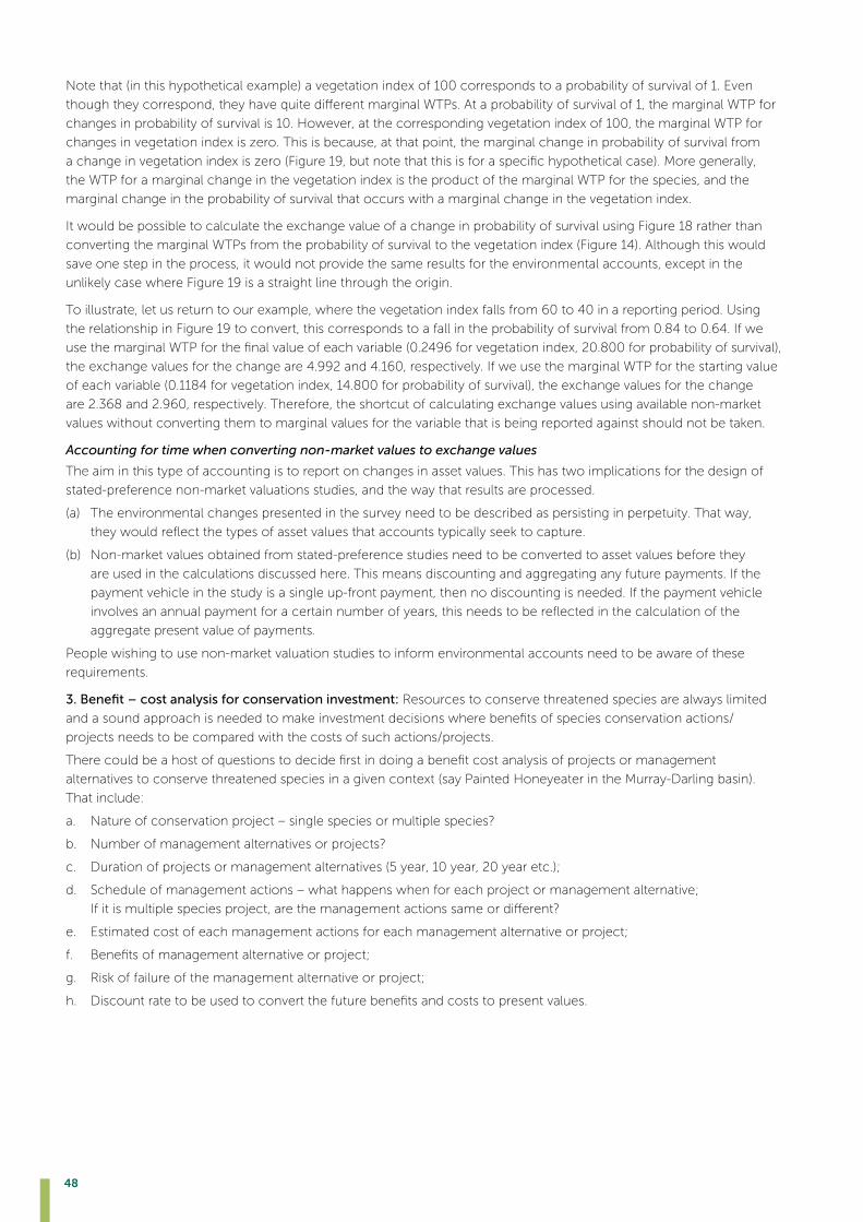
48
Note that (in this hypothetical example) a vegetation index of 100 corresponds to a probability of survival of 1. Even
thoughtheycorrespond,theyhavequitedifferentmarginalWTPs.Ataprobabilityofsurvivalof1,themarginalWTPfor
changes in probability of survival is 10. However, at the corresponding vegetation index of 100, the marginal WTP for
changes in vegetation index is zero. This is because, at that point, the marginal change in probability of survival from
achangeinvegetationindexiszero(Figure19,butnotethatthisisforaspecifichypotheticalcase).Moregenerally,
the WTP for a marginal change in the vegetation index is the product of the marginal WTP for the species, and the
marginal change in the probability of survival that occurs with a marginal change in the vegetation index.
It would be possible to calculate the exchange value of a change in probability of survival using Figure 18 rather than
converting the marginal WTPs from the probability of survival to the vegetation index (Figure 14). Although this would
save one step in the process, it would not provide the same results for the environmental accounts, except in the
unlikely case where Figure 19 is a straight line through the origin.
To illustrate, let us return to our example, where the vegetation index falls from 60 to 40 in a reporting period. Using
the relationship in Figure 19 to convert, this corresponds to a fall in the probability of survival from 0.84 to 0.64. If we
usethemarginalWTPforthefinalvalueofeachvariable(0.2496forvegetationindex,20.800forprobabilityofsurvival),
the exchange values for the change are 4.992 and 4.160, respectively. If we use the marginal WTP for the starting value
of each variable (0.1184 for vegetation index, 14.800 for probability of survival), the exchange values for the change
are 2.368 and 2.960, respectively. Therefore, the shortcut of calculating exchange values using available non-market
values without converting them to marginal values for the variable that is being reported against should not be taken.
Accounting for time when converting non-market values to exchange values
The aim in this type of accounting is to report on changes in asset values. This has two implications for the design of
stated-preference non-market valuations studies, and the way that results are processed.
(a) The environmental changes presented in the survey need to be described as persisting in perpetuity. That way,
theywouldreflectthetypesofassetvaluesthataccountstypicallyseektocapture.
(b) Non-market values obtained from stated-preference studies need to be converted to asset values before they
are used in the calculations discussed here. This means discounting and aggregating any future payments. If the
payment vehicle in the study is a single up-front payment, then no discounting is needed. If the payment vehicle
involvesanannualpaymentforacertainnumberofyears,thisneedstobereflectedinthecalculationofthe
aggregate present value of payments.
People wishing to use non-market valuation studies to inform environmental accounts need to be aware of these
requirements.
3. Benefit – cost analysis for conservation investment: Resources to conserve threatened species are always limited
andasoundapproachisneededtomakeinvestmentdecisionswherebenefitsofspeciesconservationactions/
projectsneedstobecomparedwiththecostsofsuchactions/projects.
Therecouldbeahostofquestionstodecidefirstindoingabenefitcostanalysisofprojectsormanagement
alternatives to conserve threatened species in a given context (say Painted Honeyeater in the Murray-Darling basin).
That include:
a. Natureofconservationproject–singlespeciesormultiplespecies?
b. Numberofmanagementalternativesorprojects?
c. Durationofprojectsormanagementalternatives(5year,10year,20yearetc.);
d. Scheduleofmanagementactions–whathappenswhenforeachprojectormanagementalternative;
Ifitismultiplespeciesproject,arethemanagementactionssameordifferent?
e. Estimatedcostofeachmanagementactionsforeachmanagementalternativeorproject;
f. Benefitsofmanagementalternativeorproject;
g. Riskoffailureofthemanagementalternativeorproject;
h. Discountratetobeusedtoconvertthefuturebenefitsandcoststopresentvalues.

Valuing multiple threatened species and ecological communities in Australia - Final Report, December 2020 49
FordetailsonasystematicwayofdoingaBCAforenvironmentalprojects,seePannelletal.(2013).
Oncethesequestionsareanswered,wecanthendoastandardbenefit-costanalysisofspeciesconservationprojects
oralternativemanagementoptions.Wecancomputenetpresentvalueofbenefitsorbenefitcostratiostorankthe
projectsoralternativemanagementoptions(seeTable23).
This is where the values of threatened species or ecological communities estimated through economic valuation
methods, including benefit transfer approach, would be applicable.
Example BCA: Management alternatives to conserve Painted Honeyeater in Murray-Darling basin
• Natureofconservationproject:Singlespecies(PaintedHoneyeater)
• Numberofmanagementalternativesorprojects:alternative1(focusonprivatelands),alternative2(focusonpublic
lands), and alternative 3 (focus on both private and public lands)
• Durationofprojectsormanagementalternatives:10years
• Managementactionswithineachalternativeorproject:Thesecouldvarydependingonthenatureofmanagement
alternativesorprojectsconsidered(seethetextsandtablebelowformoreonthis)
• Scheduleofmanagementactions:Timelineofmanagementactionsforeachalternativeorproject(seethetext
and table below for more on this)
• Estimated cost of each management action: See table below for more on this. The estimated cost per unit of
action is for illustrative purpose.
• Benefitofmanagementalternativesorprojects:Hereweconsiderthatthebenefitofallmanagementalternatives
orprojectsistoreducetheriskofextinctionofPaintedHoneyeaterby1%.Thevalueofthisbenefitsis$5.8million/
yearasderivedearlierinbenefit–transferexample.Dependingonhowwedefinethebenefitmeasure,itcouldjust
be something else than reducing the extinction risk by 1%, such as increase in population of Painted Honeyeater
by some number in Murray-Darling basin or increase in its habitat area in the basin by some amount.
• Riskoffailureofthemanagementalternativeorproject:Itisestimatedatthealternativeorprojectlevelthanat
theindividualactionlevel.Theassumedriskoffailuresofthemanagementalternativestogeneratebenefitsare
50%, 40% and 30% for management alternative 1, 2, and 3, respectively. Note these are assumed percentages
forillustrativepurposes,buttheyaregenerallybasedonpastprojectsorexpertopinion.
• Discountrate:Therealdiscountrateusedbythegovernmentsforenvironmentalprojects.Weuseaconservative
rate of 5%.
Following are the potential management actions that can be implemented to conserve Painted Honeyeater in
Murray-Darling basin in order to reduce its risk of extinction by 1% for the next 20 years. There are three management
alternatives: alternative 1 focuses on private lands (actions 1, 2, 3), alternative 2 focuses on public lands (actions 4, 5, 6),
and alternative 3 focuses on both types of lands (actions 1, 2, 5, 6).
Management actions:
1. Encourage private land holders to enter into stewardship agreement
2. Raise awareness among agricultural landholders of the importance of mistletoe as a resource for Painted
Honeyeaters
3. Encourage landholders to protect ground layer and mid-storey vegetation
4. Conduct strategic planting of acacia species to restore Brigalow, Boree and Yarran woodlands and connect
fragmented patches
5. Targetremovalofweedssignificantlycompromisinghabitatvalues(e.g.invasiveperennialgrasses)andrestore
native vegetation
6. Conducttargetedresearchintoidentifyingdifferentpracticalmethodsforrestoringthestructureandfunction
of the ground layer in degraded habitat

50
Table 23. Benefit-cost analysis table (base year - year 0 - is 2020)
Particulars Year (t) Extent/frequency Unit cost ($) Management alternatives and associated costs
Management alternative 1
Management alternative 2
Management alternative 3
Management actions
1 0 to 4 50landholders/year $1500.00 $340,946.30* $340,946.30
2 0 to 9 5 meetings-workshops/year
$2000.00 $81,078.22 $81,078.22
3 0 to 9 5 demonstration events/year
$2500.00 $101,347.80
4 0 to 9 50ha/year 5,000/ha $2,026,955.00
5 0 to 9 25ha/year 3,000/ha $608086.60 $608086.60
6 0 and 5
2researchprojects 30,000/project
$53,505.78 $53,505.78
Present value of costs (PVC = sum of discounted costs) $523,372.30 $2,688,548.00 1083617
Presentvalueofbenefits(PVB) $5,800,000.00 $5,800,000.00 $5,800,000.00
Probabilityofrealisingbenefitsp=1-RF 0.5 0.6 0.7
Presentvalueofexpectedbenefits(PVEB=p*PVB) $2,900,000.00 $3,480,000.00 $4,060,000.00
Netpresentvalueofbenefits(PVEB–PVC) $2,376,628.00 $791,452.20 $2,976,383.00
Benefit:costratio(PVEB/PVC) 5.54 1.29 3.75
*Presentvalueofcostofaction1formanagementalternative1==$340,946.30.Presentvaluesofothercostsarecomputed in the same way.
Basedontheaboveanalysis,itisclearthatallmanagementalternativesgeneratepositivebenefitstothesocietyby
investinginPaintedHoneyeaterconservationinMurray-Darlingbasin.However,basedonthebenefittocostratio,
managementalternative1(protectingandimprovinghabitatsonprivatelands)wouldbemosteffectiveasitgenerates
$5.54benefitsfor$1investment.
Some caveats or limitations in the use of estimated values
1. The values of threatened species or ecological communities are estimated based on reducing their extinction risk
(or increasing their probability of survival) by 1% for the next 20 years. If the metric used to consider the value of
speciesisdifferent,thenawayneedstobefoundtolinkthetwometricsinordertoadjusttheestimatedvalues.
2. ThereisafundamentaldifferenceinwhattheestimatedvaluesfromDCErepresent(welfarevalues)andwhat
kindofvaluesareusedinenvironmentalorspecies/ecosystemaccounting(exchangevalues).Thisdistinction
and potential implications need to be closely considered as discussed earlier (in section 5.1.3, part 2).

Valuing multiple threatened species and ecological communities in Australia - Final Report, December 2020 51
ReferencesBOTTRILL, M. C., JOSEPH, L. N., CARWARDINE, J., BODE, M., COOK, C., GAME, E. T., GRANTHAM, H., KARK, S., LINKE,
S.,MCDONALD-MADDEN,E.,PRESSEY,R.L.,WALKER,S.,WILSON,K.A.&POSSINGHAM,H.P.2008.
Isconservationtriagejustsmartdecisionmaking?Trends in Ecology & Evolution, 23, 649-654.
BURTON,M.&RIGBY,D.2012.TheSelfSelectionofComplexityinChoiceExperiments. American Journal of
Agricultural Economics, 94, 786-800.
BUTCHART, S. H. M., WALPOLE, M., COLLEN, B., VAN STRIEN, A., SCHARLEMANN, J. P. W., ALMOND, R. E. A., BAILLIE,
J. E. M., BOMHARD, B., BROWN, C., BRUNO, J., CARPENTER, K. E., CARR, G. M., CHANSON, J., CHENERY, A. M.,
CSIRKE, J., DAVIDSON, N. C., DENTENER, F., FOSTER, M., GALLI, A., GALLOWAY, J. N., GENOVESI, P., GREGORY,
R. D., HOCKINGS, M., KAPOS, V., LAMARQUE, J. F., LEVERINGTON, F., LOH, J., MCGEOCH, M. A., MCRAE, L.,
MINASYAN, A., MORCILLO, M. H., OLDFIELD, T. E. E., PAULY, D., QUADER, S., REVENGA, C., SAUER, J. R., SKOLNIK,
B.,SPEAR,D.,STANWELL-SMITH,D.,STUART,S.N.,SYMES,A.,TIERNEY,M.,TYRRELL,T.D.,VIÉ,J.C.&WATSON,
R. 2010. Global biodiversity: Indicators of recent declines. Science, 328, 1164-1168.
CHOICEMETRICS2018.Ngene1.2.1UserManual&ReferenceGuide.Australia.
CZAJKOWSKI,M.,AHTIAINEN,H.,ARTELL,J.&MEYERHOFF,J.2017.ChoosingaFunctionalFormforanInternational
BenefitTransfer:EvidencefromaNine-countryValuationExperiment.Ecological Economics 134, 104-113.
GUNAWARDENA,A.,ROGERS,A.,SUBROY,V.ANDPANNELL,D.(2017).BenefitTransferforEvaluatingThreatened-
SpeciesManagement:GuidelinesforExtrapolatingandAdjustingExistingNon-MarketValues.Reporttothe
National Environment Science Program, Department of the Environment and Energy, Canberra. November 2017
HOLE,A.R.&KOLSTAD,J.R.2012.Mixedlogitestimationofwillingnesstopaydistributions:acomparisonofmodelsin
preference and WTP space using data from a health-related choice experiment. Empirical Economics, 42, 445-469.
JOHNSTON, R. J., BOYLE, K. J., ADAMOWICZ, W., BENNETT, J., BROUWER, R., CAMERON, T. A., HANEMANN, W. M.,
HANLEY,N.,RYAN,M.&SCARPA,R.2017.Contemporaryguidanceforstatedpreferencestudies. Journal of the
Association of Environmental and Resource Economists, 4, 319-405.
JOHNSTON,R.J.,ROLFE,J.,ROSENBERGER,R.S.&BROUWER,R.2015.IntroductiontoBenefitTransferMethods.
Dordrecht, London 14, 19-59.
LOOMIS,J.B.&WHITE,D.S.1996.Economicbenefitsofrareandendangeredspecies:summaryandmeta-analysis.
Ecological Economics 18, 197-206.
MARTÍN-LÓPEZ,B.,MONTES,C.&BENAYAS,J.2008.Economicvaluationofbiodiversityconservation:themeaning
of numbers. Conservation Biology 22, 624-635.
PANNELL,D.J.,ROBERTS,A.M.,PARK,G.&ALEXANDER,J.2013.Designingapracticalandrigorousframework
forcomprehensiveevaluationandprioritisationofenvironmentalprojects.Wildlife Research, 40, 126-133.
RICHARDSON,L.&LOOMIS,J.2009.Thetotaleconomicvalueofthreatened,endangeredandrarespecies:
An updated meta-analysis. Ecological Economics 68, 1535-1548.
RIGBY,D.,BURTON,M.&PLUSKE,J.2016.PreferenceStabilityandChoiceConsistencyinDiscreteChoice
Experiments. Environmental and Resource Economics, 65, 441-461.
SCARPA,R.&ROSE,J.M.2008.Designefficiencyfornon-marketvaluationwithchoicemodelling:howtomeasureit,
whattoreportandwhy*.Australian Journal of Agricultural and Resource Economics, 52, 253-282.
SCARPA,R.,THIENE,M.&TRAIN,K.2008.Utilityinwillingnesstopayspace:atooltoaddressconfoundingrandom
scaleeffectsindestinationchoicetotheAlps.American Journal of Agricultural Economics, 90, 994-1010.
SUBROY,V.,GUNAWARDENA,A.,POLYAKOV,M.,PANDIT,R.&PANNELL,D.J.2019.Theworthofwildlife:Ameta-
analysis of global non-market values of threatened species. Ecological Economics, 164, 106374.
TRAIN, K. E. 2009. Discrete choice methods with simulation, Cambridge university press.
TURNER,W.R.,BRANDON,K.,BROOKS,T.M.,COSTANZA,R.,DAFONSECA,G.A.B.&PORTELA,R.2007.Global
Conservation of Biodiversity and Ecosystem Services. BioScience, 57, 868-873.
WOINARSKI,J.C.Z.,BURBIDGE,A.A.&HARRISON,P.L.2015.Ongoingunravelingofacontinentalfauna:Declineand
extinction of Australian mammals since European settlement. Proceedings of the National Academy of Sciences,
112, 4531-4540.

52
APPENDICESAnnex - A: Initial list of multiple species and there relevance under three criteria
TSS
tax
on
G
en
eti
c au
gm
en
tati
on
Fen
cin
gV
alu
atio
nTe
stin
g b
en
efi
t tr
ansf
er
Te
sts
perc
ep
tion
s o
f th
e
accep
tab
ility
of
aug
men
ting
inb
red
po
pu
latio
ns
with
gen
es
fro
m o
ther
taxa
, pri
mar
ily t
o
incre
ase f
ert
ility
. May
als
o
testdifferencesintoneof
mess
agin
g, i
nfo
rmat
ion
, co
sts
Test
s th
e e
xten
t to
wh
ich
fen
cin
g
affectsva
lueoftaxa
protectedby
afence
,includingeffectoftype
of
fen
ce (b
ovi
ph
ob
ic, s
usp
ho
bic
,
ph
elip
ho
bic
, mu
sph
ob
ic e
tc.),
are
a,
perc
ep
tion
of
cap
tivity
. May
test
difference
sintoneofmessag
ing
Sim
ultan
eo
us
mu
lti-
en
tity
valu
atio
n u
sin
g
the s
ame
wo
rdin
g
Will
co
mp
are d
irect
valu
atio
n w
ith v
alu
es
deri
ved
fro
m a
mo
del
deve
lop
ed
fro
m v
alu
es
giv
en
to
oth
er
specie
s. C
ou
ld c
om
par
e s
imila
r
specie
s p
airs
Wh
ite-t
hro
ated
gra
ssw
ren
Bird
Yes
Nig
ht
par
rot
Bird
Yes
West
ern
Gro
un
d P
arro
t (C
ritic
ally
En
dan
gere
d),
Eas
tern
Gro
un
d P
arro
t
(Near
Th
reat
en
ed
), Ta
sman
ian
Gro
un
d P
arro
t
(Leas
t C
on
cern
)
Eas
tern
bri
stle
bird
Bird
Yes
Yes
No
rth
ern
(C
R)
and
so
uth
ern
(V
U)
sub
specie
s, le
gal
ly c
on
sid
ere
d s
ame
sub
specie
s
West
ern
gro
un
d
par
rot
Bird
Yes
Yes
NightParro
t(ENhighpro
file),Eas
ternG
roundParro
t(N
ear
Th
reat
en
ed
), Ta
sman
ian
Gro
un
d P
ar-r
ot
(Leas
t C
on
cern
No
rfo
lk Is
lan
d g
reen
par
rot
Bird
Yes
No
rfo
lk Is
lan
d
bo
ob
oo
k o
wl
Bird
Yes
Yes
Pla
ins
wan
dere
rB
ird
Yes
Yes
Au
stra
lasi
an b
ittern
Bird
Yes
Swift
par
rot
Bird
Yes
Orange-belliedParro
t(C
R,h
ighpro
file,a
lsom
igratoryparro
tbutno
co
mm
erc
ial i
mp
act)
; Sw
ift P
arro
t (C
R, a
lso
mig
rato
ry n
om
ad in
sam
e
hab
itat)
Mal
lee
em
u-w
ren
Bird
Yes
Ora
ng
e b
elli
ed
par
rot
Bird
Yes
Yes
SwiftParro
t(C
R,h
ighpro
file,a
lsom
igratoryparro
tbutcommercial
imp
act
on
fo
rest
ry if
pro
tecte
d)
Yello
w c
hat
Bird
Yes
Alli
gat
or
Riv
ers
an
d C
apri
co
rnia
su
bsp
ecie
s, b
oth
th
reat
en
ed
an
d in
rem
ote
, mar
gin
al h
abita
t)
Mal
leefo
wl
Bird
Yes
Yes
Go
lden
sh
ou
ldere
d
par
rot
Yes
Yes
Yes

Valuing multiple threatened species and ecological communities in Australia - Final Report, December 2020 53
TSS
tax
on
G
en
eti
c au
gm
en
tati
on
Fen
cin
gV
alu
atio
nTe
stin
g b
en
efi
t tr
ansf
er
Te
sts
perc
ep
tion
s o
f th
e
accep
tab
ility
of
aug
men
ting
inb
red
po
pu
latio
ns
with
gen
es
fro
m o
ther
taxa
, pri
mar
ily t
o
incre
ase f
ert
ility
. May
als
o
testdifferencesintoneof
mess
agin
g, i
nfo
rmat
ion
, co
sts
Test
s th
e e
xten
t to
wh
ich
fen
cin
g
affectsva
lueoftaxa
protectedby
afence
,includingeffectoftype
of
fen
ce (b
ovi
ph
ob
ic, s
usp
ho
bic
,
ph
elip
ho
bic
, mu
sph
ob
ic e
tc.),
are
a,
perc
ep
tion
of
cap
tivity
. May
test
difference
sintoneofmessag
ing
Sim
ultan
eo
us
mu
lti-
en
tity
valu
atio
n u
sin
g
the s
ame
wo
rdin
g
Will
co
mp
are d
irect
valu
atio
n w
ith v
alu
es
deri
ved
fro
m a
mo
del
deve
lop
ed
fro
m v
alu
es
giv
en
to
oth
er
specie
s. C
ou
ld c
om
par
e s
imila
r
specie
s p
airs
Reg
en
t h
on
eye
ater
Yes
Yes
Yes
Swift
Par
rot
(CR
, als
o m
igra
tory
no
mad
in s
ame h
abita
t), R
eg
en
t
Ho
neay
ete
r (a
lso
a h
on
eye
ater
bu
t le
ss d
istin
ct
gen
etic
ally
an
d
sed
en
tary
)
Sou
thern
Cas
sow
ary
Yes
Yes
Yes
Eas
tern
cu
rlew
Yes
Yes
Cu
rlew
San
dp
iper
(als
o C
R b
ut
mu
ch
sm
alle
r)
Ho
od
ed
plo
ver
Yes
Yes
Fair
y Te
rn (
also
beac
h d
ep
en
den
t)
Red
-tai
led
bla
ck
co
cka
too
(so
uth
-
eas
tern
)
Yes
Yes
Carnab
ysBlack-Cocka
too(EN,h
ighpro
gfileurban
south-w
estW
A
species),B
audin'sBlack-Cocka
too(EN,lowpro
filesouth-w
estW
A
specie
s co
-occu
rrin
g w
ith C
arn
aby'
s). S
ou
th-w
est
ern
Red
-tai
led
Bla
ck-
Cocka
too(EN,s
amespeciesbutdifferentsu
bsp
eciesinsouth-w
est
WA
)
Helm
ete
d
ho
neye
ater
Yes
Yes
Yes
Reg
en
t H
on
eay
ete
r (a
lso
a h
on
eye
ater
bu
t m
ore
dis
tinct
gen
etic
ally
and
mig
rato
ry)
West
ern
rin
gta
il
po
ssu
m
Yes
Yes
Yes
Nu
mb
atYe
sYe
s
Gre
ater
bilb
yYe
sYe
sYe
s
West
ern
qu
oll
Yes
Yes
Yes
No
rth
ern
ho
pp
ing
mo
use
Yes
Yes
Yes
Mah
og
any
glid
er
Yes
Yes
Yes
Gilb
ert
’s p
oto
roo
Yes
Yes
Eas
tern
bar
red
ban
dic
oo
t
Yes
Yes
Yes
Bru
sh-t
aile
d
rab
bit-
rat
Yes
Yes
Yes
Mo
un
tain
pyg
my-
po
ssu
m
Yes
Yes
Yes

54
TSS
tax
on
G
en
eti
c au
gm
en
tati
on
Fen
cin
gV
alu
atio
nTe
stin
g b
en
efi
t tr
ansf
er
Te
sts
perc
ep
tion
s o
f th
e
accep
tab
ility
of
aug
men
ting
inb
red
po
pu
latio
ns
with
gen
es
fro
m o
ther
taxa
, pri
mar
ily t
o
incre
ase f
ert
ility
. May
als
o
testdifferencesintoneof
mess
agin
g, i
nfo
rmat
ion
, co
sts
Test
s th
e e
xten
t to
wh
ich
fen
cin
g
affectsva
lueoftaxa
protectedby
afence
,includingeffectoftype
of
fen
ce (b
ovi
ph
ob
ic, s
usp
ho
bic
,
ph
elip
ho
bic
, mu
sph
ob
ic e
tc.),
are
a,
perc
ep
tion
of
cap
tivity
. May
test
difference
sintoneofmessag
ing
Sim
ultan
eo
us
mu
lti-
en
tity
valu
atio
n u
sin
g
the s
ame
wo
rdin
g
Will
co
mp
are d
irect
valu
atio
n w
ith v
alu
es
deri
ved
fro
m a
mo
del
deve
lop
ed
fro
m v
alu
es
giv
en
to
oth
er
specie
s. C
ou
ld c
om
par
e s
imila
r
specie
s p
airs
Mal
aYe
sYe
s
Eas
tern
bett
on
gM
amm
alYe
sYe
s
Bla
ck-
foo
ted
rock-
wal
lab
y
Mam
mal
Yes
Yes
Eas
tern
qu
oll
Mam
mal
Yes
Cen
tral
ro
ck-
rat
Mam
mal
Yes
Yes
Lead
beat
er’s
po
ssu
m
Mam
mal
Yes
Kan
gar
oo
Isla
nd
du
nn
art
Mam
mal
Yes
Yes
Wo
ylie
Mam
mal
Yes
Yes
Go
lden
ban
dic
oo
tM
amm
alYe
sYe
s
Ch
rist
mas
Isla
nd
flying-fox
Mam
mal
Yes
Blu
e-t
op
su
n-o
rch
idP
lan
t
Mo
ng
arlo
we m
alle
eP
lan
t
Mo
rris
by'
s g
um
bat
Pla
nt
Pla
nt
Smal
l pu
rple
pea
Pla
nt
Pla
nt
Silv
er
gu
mP
lan
tP
lan
t
Glo
ssy-
leav
ed
ham
mer-
orc
hid
Pla
nt
Pla
nt
Turn
ip C
op
perb
urr
Pla
nt
Pla
nt
Mat
ch
stic
k b
anks
iaP
lan
tP
lan
t
Cen
tral
Au
stra
lian
cab
bag
e p
alm
Pla
nt
Pla
nt
Bu
lberi
n m
acad
amia
nu
t
Pla
nt
Pla
nt
Fleu
rieu
leek
orc
hid
Pla
nt
Pla
nt
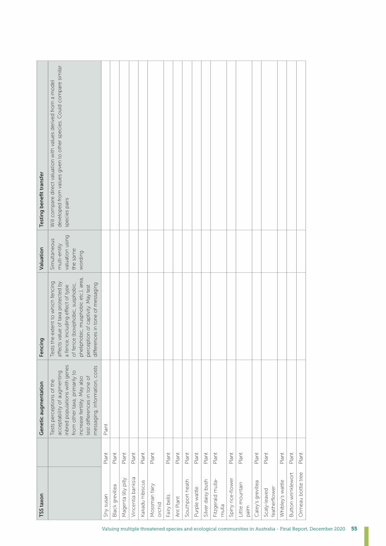
Valuing multiple threatened species and ecological communities in Australia - Final Report, December 2020 55
TSS
tax
on
G
en
eti
c au
gm
en
tati
on
Fen
cin
gV
alu
atio
nTe
stin
g b
en
efi
t tr
ansf
er
Te
sts
perc
ep
tion
s o
f th
e
accep
tab
ility
of
aug
men
ting
inb
red
po
pu
latio
ns
with
gen
es
fro
m o
ther
taxa
, pri
mar
ily t
o
incre
ase f
ert
ility
. May
als
o
testdifferencesintoneof
mess
agin
g, i
nfo
rmat
ion
, co
sts
Test
s th
e e
xten
t to
wh
ich
fen
cin
g
affectsva
lueoftaxa
protectedby
afence
,includingeffectoftype
of
fen
ce (b
ovi
ph
ob
ic, s
usp
ho
bic
,
ph
elip
ho
bic
, mu
sph
ob
ic e
tc.),
are
a,
perc
ep
tion
of
cap
tivity
. May
test
difference
sintoneofmessag
ing
Sim
ultan
eo
us
mu
lti-
en
tity
valu
atio
n u
sin
g
the s
ame
wo
rdin
g
Will
co
mp
are d
irect
valu
atio
n w
ith v
alu
es
deri
ved
fro
m a
mo
del
deve
lop
ed
fro
m v
alu
es
giv
en
to
oth
er
specie
s. C
ou
ld c
om
par
e s
imila
r
specie
s p
airs
Shy
susa
nP
lan
tP
lan
t
Bla
ck
gre
ville
aP
lan
t
Mag
en
ta li
lly p
illy
Pla
nt
Vin
cen
tia b
anks
iaP
lan
t
Kak
adu
hib
iscu
sP
lan
t
Mo
ssm
an f
airy
orc
hid
Pla
nt
Fair
y b
ells
Pla
nt
An
t P
lan
tP
lan
t
Sou
thp
ort
heat
hP
lan
t
Pu
rple
wat
tle
Pla
nt
Silv
er
dai
sy b
ush
Pla
nt
Fitz
gera
ld m
ulla
-
mu
lla
Pla
nt
Spinyrice-flower
Pla
nt
Litt
le m
ou
nta
in
pal
m
Pla
nt
Cal
ey'
s g
revi
llea
Pla
nt
Scal
y-le
aved
featherflower
Pla
nt
Wh
ible
y's
wat
tle
Pla
nt
Bu
tto
n w
rin
klew
ort
Pla
nt
Orm
eau
bo
ttle
tre
eP
lan
t
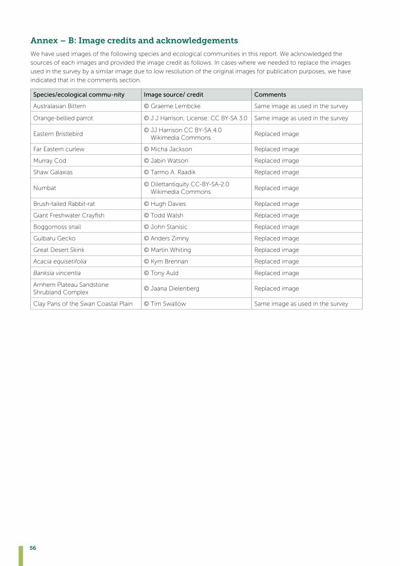
56
Annex – B: Image credits and acknowledgements
We have used images of the following species and ecological communities in this report. We acknowledged the
sources of each images and provided the image credit as follows. In cases where we needed to replace the images
used in the survey by a similar image due to low resolution of the original images for publication purposes, we have
indicated that in the comments section.
Species/ecological commu-nity Image source/ credit Comments
Australasian Bittern © Graeme Lembcke Same image as used in the survey
Orange-bellied parrot © J J Harrison; License: CC BY-SA 3.0 Same image as used in the survey
Eastern Bristlebird© JJ Harrison CC BY-SA 4.0 Wikimedia Commons
Replaced image
Far Eastern curlew © Micha Jackson Replaced image
Murray Cod © Jabin Watson Replaced image
Shaw Galaxias © Tarmo A. Raadik Replaced image
Numbat© Dilettantiquity CC-BY-SA-2.0 Wikimedia Commons
Replaced image
Brush-tailed Rabbit-rat © Hugh Davies Replaced image
Giant Freshwater Crayfish © Todd Walsh Replaced image
Boggomoss snail © John Stanisic Replaced image
Gulbaru Gecko © Anders Zimny Replaced image
Great Desert Skink © Martin Whiting Replaced image
Acacia equisetifolia © Kym Brennan Replaced image
Banksia vincentia © Tony Auld Replaced image
Arnhem Plateau Sandstone Shrubland Complex
© Jaana Dielenberg Replaced image
Clay Pans of the Swan Coastal Plain © Tim Swallow Same image as used in the survey

Valuing multiple threatened species and ecological communities in Australia - Final Report, December 2020 57
Annex – C: Model Questionnaire
Social preferences for conserving threatened speciesYou are invited to participate this online survey that seek your preferences conserving multiple species. The survey will
take about 15-20 minutes to complete.
What is the project about?
The aim of the study is to understand preferences of Australian public for conserving multiple threatened species
(animals, plants and ecological communities). The study will estimate the dollar values that people will place on
protectingdifferenttypesofspeciesthatarefacingdifferentlevelsofextinctionrisk.
What does participation involve?
The participation of the survey means that you have to answer an online survey. You will be provided with information
ofmultiplespeciesthatarefacingriskofextinctionatdifferentlevels.Thenyouwillbeaskedmakechoicesof
protection programs that involve reducing the risk of extinction of combination of species.
Voluntary Participation and Withdrawal from the Study
Your participation will be on a voluntary basis and you can withdraw your participation at any stage of research without
prejudice.However,yourparticipationwillproveimportanttocompletethisresearch.
Your privacy
Your information will be anonymously stored on the questionnaire forms initially and later on the researcher’s laptop
andfinallyinUniversityofWesternAustralia(UWA)databackupsystemforatleastsevenyears.Thisinformationwill
bekeptstrictlyconfidentialandwillnotbemadeavailabletootherpeople.
Possible Benefits
Thisresearchprojectwillestimatethemonetarybenefitsofprotectingthreatenedspecies.Benefits(values)of
threatened species are not currently available for most species listed in the Australian Government’s Threatened
Species Strategy (TSS). Decisions on program funding at Commonwealth and state levels rest on sound understanding
ofthevaluesofthreatenedspecies.Selectionofprojectsforspeciesmanagementareimproved,throughidentifying
projectsthatprovidethatbestvalueformoney.
By answering these questions, you will have the opportunity to express your opinions in protecting Australia’s
threatened animals and plants and ecological communities.
Possible Risks and Risk Management Plan
There are no foreseeable risks and potential harm associated on providing personal information and opinions. If any
aspectsofthisresearchprojectdistressesyou,youcancontactmeattheaboveaddressortheUWAHumanResearch
Ethicsofficeatthebelowaddress.
Contacts
If you have any questions with any aspects of this interview, please feel free to contact either at my work phone
number (+61864881353) or on my mobile phone number (+610422185791).
Sincerely,
Dr. Ram Pandit, Chief Investigator
Approval to conduct this research has been provided by The University of Western Australia (ethics reference number:
RA/4/20/5471),inaccordancewithitsethicsreviewandapprovalprocedures.Anypersonconsideringparticipation
inthisresearchproject,oragreeingtoparticipate,mayraiseanyquestionsorissueswiththeresearchersatanytime.
Inaddition,anypersonnotsatisfiedwiththeresponseofresearchersmayraiseethicsissuesorconcerns,andmay
makeanycomplaintsaboutthisresearchprojectbycontactingtheHumanEthicsofficeatUWAon(08)64884703
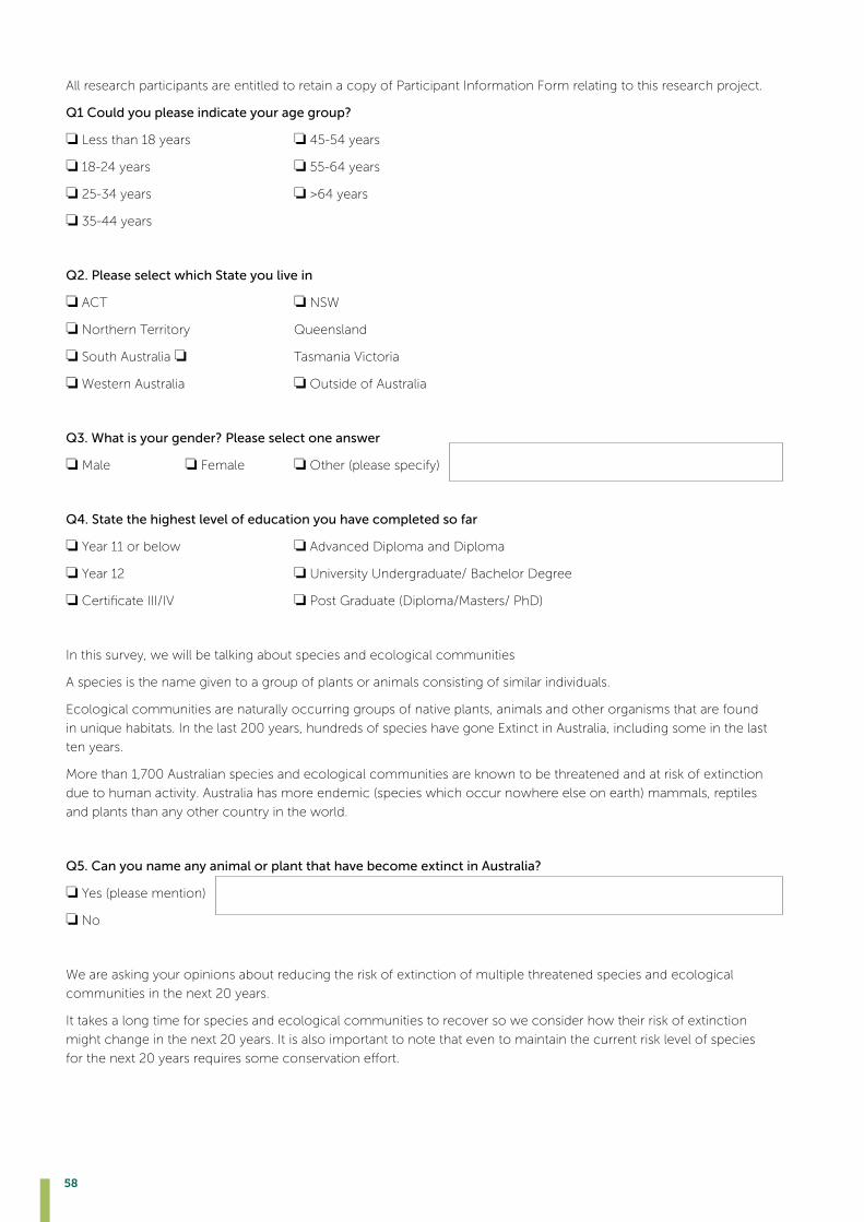
58
AllresearchparticipantsareentitledtoretainacopyofParticipantInformationFormrelatingtothisresearchproject.
Q1 Could you please indicate your age group?
❏ Less than 18 years ❏ 45-54 years
❏ 18-24 years ❏ 55-64 years
❏ 25-34 years ❏ >64 years
❏ 35-44 years
Q2. Please select which State you live in
❏ ACT ❏ NSW
❏ Northern Territory Queensland
❏ South Australia ❏ Tasmania Victoria
❏ Western Australia ❏ Outside of Australia
Q3. What is your gender? Please select one answer
❏ Male ❏ Female ❏ Other (please specify)
Q4. State the highest level of education you have completed so far
❏ Year 11 or below ❏ Advanced Diploma and Diploma
❏ Year 12 ❏UniversityUndergraduate/BachelorDegree
❏CertificateIII/IV ❏PostGraduate(Diploma/Masters/PhD)
In this survey, we will be talking about species and ecological communities
A species is the name given to a group of plants or animals consisting of similar individuals.
Ecological communities are naturally occurring groups of native plants, animals and other organisms that are found
in unique habitats. In the last 200 years, hundreds of species have gone Extinct in Australia, including some in the last
ten years.
More than 1,700 Australian species and ecological communities are known to be threatened and at risk of extinction
due to human activity. Australia has more endemic (species which occur nowhere else on earth) mammals, reptiles
and plants than any other country in the world.
Q5. Can you name any animal or plant that have become extinct in Australia?
❏ Yes (please mention)
❏ No
We are asking your opinions about reducing the risk of extinction of multiple threatened species and ecological
communities in the next 20 years.
It takes a long time for species and ecological communities to recover so we consider how their risk of extinction
might change in the next 20 years. It is also important to note that even to maintain the current risk level of species
forthenext20yearsrequiressomeconservationeffort.

Valuing multiple threatened species and ecological communities in Australia - Final Report, December 2020 59
In the next section, we describe the different levels of extinction risk that we will be using in the survey.
1. Levels of Extinction risk
We consider 5 levels of extinction risk in this survey. We provide a description of each risk level and a visual
representation of risk.
In each grid there are 50 squares, each square represents a species, and a red colour represents a species expected
to be extinct in 20 years.
Q6. Which of these two species have the higher risk of extinction?
❏ Species A ❏ Species B
2. List of Species
In this survey, we will be considering 6 different animals, one plant and one ecological community.
The table below provides information on the current level of extinction risk and geographical range of species
considered in this survey.
12
Extinct There is a 100% chance of extinction in the next 20 years.
Very high risk There is a 75% chance of extinction in the next 20 years. (i.e., at least 1 out of 50 species with this risk would be expected to go extinct in 20 years)
High risk There is a 20% chance of extinction in the next 20 years. (i.e., at least 5 out of 50 species with this risk would be expected to go extinct in 20 years)
Moderate risk There is a 2% chance of extinction in the next 20 years. (i.e., at least 38 out of 50 species with this risk would be expected to go extinct in 20 years)
Low risk Virtually no chance of extinction in the next 20 years.
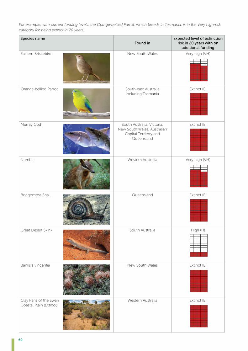
60
For example, with current funding levels, the Orange-bellied Parrot, which breeds in Tasmania, is in the Very high-risk
category for being extinct in 20 years.
Species name Found in
Expected level of extinction risk in 20 years with on
additional funding
Eastern Bristlebird New South Wales Very high (VH)
Orange-bellied Parrot South-east Australia including Tasmania
Extinct (E)
Murray Cod South Australia, Victoria, New South Wales, Australian
Capital Territory and Queensland
Extinct (E)
Numbat Western Australia Very high (VH)
Boggomoss Snail Queensland Extinct (E)
Great Desert Skink South Australia High (H)
Banksia vincentia New South Wales Extinct (E)
Clay Pans of the Swan Coastal Plain (Extinct)
Western Australia Extinct (E)

Valuing multiple threatened species and ecological communities in Australia - Final Report, December 2020 61
3. Additional funding for Conservation
We can make a prediction of the risk of extinction if the current level of funding for conservation is maintained.
However, if we were to allocate more funding to conservation then we can reduce the risk.
In the survey questions we will be asking whether you would be willing to contribute personal funds for this to happen.
These extra funds would be collected through an additional tax that would be used to create a special “Threatened
Species Conservation Fund”. This fund would be used solely for conserving threatened species and ecological
communities. However, it is not always possible to allocate enough funds to protect all species.
4. Your Choices
We are going to ask a number of questions on which species to protect from Extinction.
Before continuing, it is also important to take note of the following instructions:
Please try to consider each question independently of each other.
Whenyouaremakingchoices,itisimportanttokeepinmindyourfinancialsituation,
i.e.considermuchyoucanrealisticallyaffordtopayeachyear,givenyourhouseholdincomeandexpenses.
Please consider your answers carefully. We value your feedback greatly and the results of this study will be made
available to relevant agencies.
In the next section, we are presenting an example of a choice question
Example 1: Improvement in protection of 5 species (out of 8)
In this example, only five species were identified to provide additional protection.
The second column shows expected levels of extinction risk in 20 years under current level of protection.
The extinction risk levels are presented from extinct to low risk. The relevant level for each of the 5 species or
community that are considered are coloured in RED.
The third and fourth columns show the expected levels of extinction risk if we implement additional programs (plan
1 or plan 2) to protect the species and ecological communities. The relevant risk level for each species or ecological
community is coloured in GREEN.
You need to consider the species being protected, the change in risk levels and relevant cost (last row) when making
your choices.
Expected level of species extinction risk in 20 years In this example, only five species were identified to provide additional protection. The second column shows expected levels of extinction risk in 20 years under current level of protection. The extinction risk levels are presented from extinct to low risk. The relevant level for each of the 5 species or community that are considered are coloured in RED The third and fourth columns show the expected levels of extinction risk if we implement additional programs (plan 1 or plan 2) to protect the species and ecological communities. The relevant risk level for each species or ecological community is coloured in GREEN. You need to consider the species being protected, the change in risk levels and relevant cost (last row) when making your choices.
With current level of protection
Plan1 : additional protection
Plan2 : additional protection
Eastern Bristlebird Orange‐bellied Parrot
Murray Cod
Numbat
Boggomoss Snail
Great Desert Skink
Banksia vincentia
Clay Pans of the Swan Coastal Plain
Cost to your household per year in next 20 years
$0 $150 $250
©

62
1. Consider the following three choice options assuming that you have only these three options.
Which option will you choose?
Pleasebearinmindyourfinancialsituationwhenmakingachoice.
2. Consider the following three choice options assuming that you have only these three options.
Which option will you choose?
Pleasebearinmindyourfinancialsituationwhenmakingachoice.
Please answer this question independent of your answers to previous question.
©
©

Valuing multiple threatened species and ecological communities in Australia - Final Report, December 2020 63
3. Consider the following three choice options assuming that you have only these three options.
Which option will you choose?
Pleasebearinmindyourfinancialsituationwhenmakingachoice.
Please answer this question independent of your answers to previous question.
4. Consider the following three choice options assuming that you have only these three options.
Which option will you choose?
Pleasebearinmindyourfinancialsituationwhenmakingachoice.
Please answer this question independent of your answers to previous question.
©
©
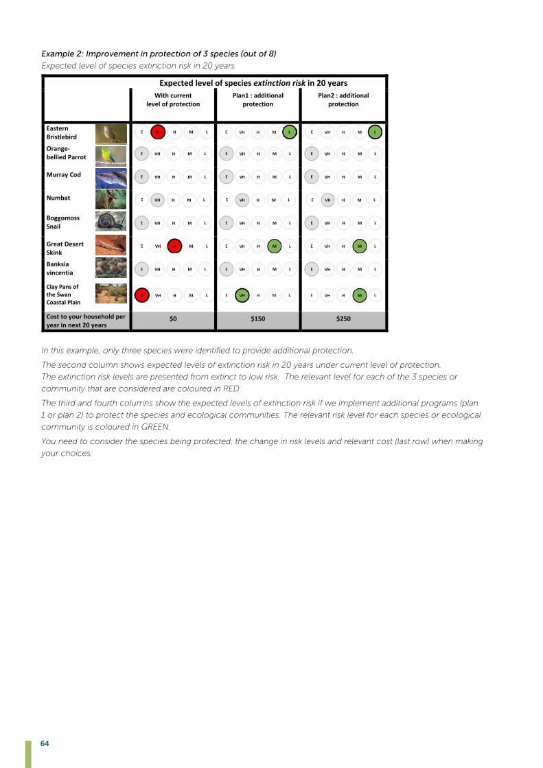
64
Example 2: Improvement in protection of 3 species (out of 8)
Expected level of species extinction risk in 20 years
In this example, only three species were identified to provide additional protection.
The second column shows expected levels of extinction risk in 20 years under current level of protection.
The extinction risk levels are presented from extinct to low risk. The relevant level for each of the 3 species or
community that are considered are coloured in RED
The third and fourth columns show the expected levels of extinction risk if we implement additional programs (plan
1 or plan 2) to protect the species and ecological communities. The relevant risk level for each species or ecological
community is coloured in GREEN.
You need to consider the species being protected, the change in risk levels and relevant cost (last row) when making
your choices.
Example 2: Improvement in protection of 3 species (out of 8)
Expected level of species extinction risk in 20 years In this example, only three species were identified to provide additional protection. The second column shows expected levels of extinction risk in 20 years under current level of protection. The extinction risk levels are presented from extinct to low risk. The relevant level for each of the 3 species or community that are considered are coloured in RED The third and fourth columns show the expected levels of extinction risk if we implement additional programs (plan 1 or plan 2) to protect the species and ecological communities. The relevant risk level for each species or ecological community is coloured in GREEN. You need to consider the species being protected, the change in risk levels and relevant cost (last row) when making your choices.
With current level of protection
Plan1 : additional protection
Plan2 : additional protection
Eastern Bristlebird Orange‐bellied Parrot
Murray Cod
Numbat
Boggomoss Snail
Great Desert Skink
Banksia vincentia
Clay Pans of the Swan Coastal Plain
Cost to your household per year in next 20 years
$0 $150 $250
©

Valuing multiple threatened species and ecological communities in Australia - Final Report, December 2020 65
5. Consider the following three choice options assuming that you have only these three options.
Which option will you choose?
Pleasebearinmindyourfinancialsituationwhenmakingachoice.
Please answer this question independent of your answers to previous question.
6. Consider the following three choice options assuming that you have only these three options.
Which option will you choose?
Pleasebearinmindyourfinancialsituationwhenmakingachoice.
Please answer this question independent of your answers to previous question.
©
©
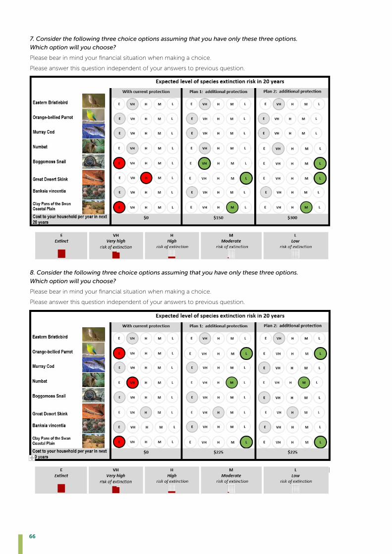
66
7. Consider the following three choice options assuming that you have only these three options.
Which option will you choose?
Pleasebearinmindyourfinancialsituationwhenmakingachoice.
Please answer this question independent of your answers to previous question.
8. Consider the following three choice options assuming that you have only these three options.
Which option will you choose?
Pleasebearinmindyourfinancialsituationwhenmakingachoice.
Please answer this question independent of your answers to previous question.
©
©
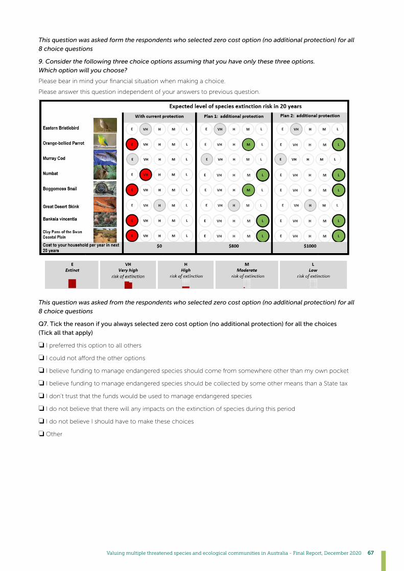
Valuing multiple threatened species and ecological communities in Australia - Final Report, December 2020 67
This question was asked form the respondents who selected zero cost option (no additional protection) for all
8 choice questions
9. Consider the following three choice options assuming that you have only these three options.
Which option will you choose?
Pleasebearinmindyourfinancialsituationwhenmakingachoice.
Please answer this question independent of your answers to previous question.
This question was asked from the respondents who selected zero cost option (no additional protection) for all
8 choice questions
Q7. Tick the reason if you always selected zero cost option (no additional protection) for all the choices
(Tick all that apply)
❏ I preferred this option to all others
❏Icouldnotaffordtheotheroptions
❏ I believe funding to manage endangered species should come from somewhere other than my own pocket
❏ I believe funding to manage endangered species should be collected by some other means than a State tax
❏ I don’t trust that the funds would be used to manage endangered species
❏ I do not believe that there will any impacts on the extinction of species during this period
❏ I do not believe I should have to make these choices
❏ Other
©

68
This question was asked from the respondents who always selected plan1 or plan 2 (additional protection) for all
8 choice questions
9. Consider the following three choice options assuming that you have only these three options.
Which option will you choose?
Pleasebearinmindyourfinancialsituationwhenmakingachoice.
Please answer this question independent of your answers to previous question.
This question was asked from the respondents who always selected plan1 or plan 2 (additional protection) for all
8 choice questions
Q8. Tick the reason/reasons if you always selected the option with additional protection for all the choices
❏ I preferred these options to all others
❏Iwashappytomakethepaymentasked,giventheprotectionthatwasoffered
❏ I ignored the cost of the option
❏ I believe you should protect all species irrespective of any cost
❏ I did not think I would ever be asked to make the payments
❏ Other
Q9. To what extent did you understand the questions in the previous section? Please select one answer
❏ Fully understood
❏ Partially understood
❏ Did not understand the questions at all
©
Valuing multiple threatened species and ecological communities in Australia - Final Report, December 2020 69
Q10. If this program of species protection was implemented, how certain are you that you would actually be asked
to pay annual additional tax to fund it?
❏ Very certain
❏ Certain
❏ Uncertain
❏ Very uncertain
Q11. Did you consider all 3 features (Cost, Species, Extinction risk) when you answered the choice questions?
❏ Yes
❏ No
Q12. If no, please indicate the features that you ignored in answering choice questions (Tick all that apply)
❏ Costs (the additional annual tax)
❏ Which species to be protected
❏ Level of improvement in protection (level of extinction risk)
❏ All of them
Q13. Number of people living in your household
❏ Adults
❏ Children <5 years
❏ Children >5 years and <18 years
Q14. Do you identify yourself as one of the following group?
❏ Aboriginal African Anglo-Saxon
❏Asian/AsianAmericanAustralian
❏Mixeddescent(e.g.White&Asian,White&Black)NorthAfricanandMiddleEastern
❏ North American
❏ North East Asian (e.g. Chinese, Japanese, Korean)
❏NorthandWestEuropean(e.g.UnitedKingdom,France,Germany,Norway,Sweden)PacificIslander
❏ South American
❏ South and East European (e.g. Spain, Italy, Greece, Hungary, Romania, Ukraine) Southern and Central Asian (e.g. Indian)
❏SouthEastAsian(e.g.Vietnamese,Filipino,Indonesian)TorresStraitIslander/IndigenousAustralian
❏ Other Oceanian
❏ Prefer not to answer
❏ Others, please specify
70
Q15. Please indicate your current annual household income (i.e. before tax and including all people living in your
household)
❏ Negative income Nil income
❏ $1- $7,799 per year
❏ $7,800 - $15,599 per year
❏ $15,600 - $20,799 per year
❏ $20,800 - $25,999 per year
❏ $26,000 - $33,799 per year
❏ $33,800 - $41,599 per year
❏ $41,600 - $51,999 per year
❏ $52,000 - $64,999 per year
❏ $65,000 - $77,999 per year
❏ $78,000 - $90,999 per year
❏ $91,000 - $103,999 per year
❏ $104,000 - $155,999 per year
❏ $156,000 or more per year
Q16. What is your current employment status?
❏ Employed full time (35 or more hours per week)
❏Employedparttime(lessthan35hoursperweek)/causal?Unemployedandcurrentlylookingforwork
❏ Unemployed and not currently looking for work Student
❏ Retired
❏ Homemaker (manages a home and family) Self-employed
❏ Unable to work
Q17. Did your household pay any taxes last year?
❏ Yes
❏ No
Q18. Do you actively support (financial donations or volunteering your time) any environmental groups or
organizations associated with conservation of Australian threatened animals or plants?
❏ Yes
❏ No
Q19. Are you currently engaged or have you ever been engaged work related to species conservation
❏ Yes
❏ No
Valuing multiple threatened species and ecological communities in Australia - Final Report, December 2020 71
Thank you! Your support of this research is much appreciated.
If you have any comments about the survey or about the conservation of threatened animals
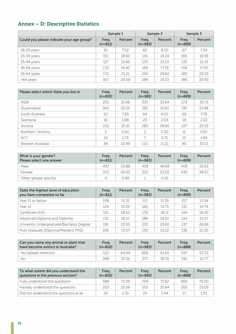
72
Annex – D: Descriptive Statistics
Sample 1 Sample 2 Sample 3
Could you please indicate your age group? Freq. (n=811)
Percent Freq. (n=983)
Percent Freq. (n=889)
Percent
18-24 years 61 7.52 60 6.10 67 7.54
25-34 years 151 18.62 141 14.34 165 18.56
35-44 years 127 15.66 133 13.53 135 15.19
45-54 years 133 16.40 169 17.19 156 17.55
55-64 years 172 21.21 291 29.60 180 20.25
>64 years 167 20.59 189 19.23 186 20.92
Please select which State you live in Freq. (n=810)
Percent Freq. (n=981)
Percent Freq. (n=889)
Percent
NSW 255 31.48 330 33.64 273 30.71
Queensland 164 20.25 165 16.82 191 21.48
South Australia 62 7.65 64 6.52 69 7.76
Tasmania 16 1.98 20 2.04 18 2.02
Victoria 205 25.31 283 28.85 227 25.53
Northern Territory 5 0.62 2 0.20 6 0.67
ACT 14 1.73 7 0.71 15 1.69
Western Australia 89 10.99 110 11.21 90 10.12
What is your gender? Please select one answer
Freq. (n=811)
Percent Freq. (n=983)
Percent Freq. (n=889)
Percent
Male 437 53.88 459 46.69 459 51.63
Female 370 45.62 523 53.20 430 48.37
Other (please specify) 4 0.49 1 0.10
State the highest level of education you have completed so far
Freq. (n=811)
Percent Freq. (n=983)
Percent Freq. (n=889)
Percent
Year 11 or below 108 13.32 112 11.39 107 12.04
Year 12 124 15.29 145 14.75 131 14.74
CertificateIII/IV 151 18.62 178 18.11 144 16.20
Advanced Diploma and Diploma 131 16.15 186 18.92 134 15.07
UniversityUndergraduate/BachelorDegree 191 23.55 232 23.60 237 26.66
PostGraduate(Diploma/Masters/PhD) 106 13.07 130 13.22 136 15.30
Can you name any animal or plant that have become extinct in Australia?
Freq. (n=810)
Percent Freq. (n=983)
Percent Freq. (n=888)
Percent
Yes (please mention) 522 64.44 606 61.65 597 67.23
No 288 35.56 377 38.35 291 32.77
To what extent did you understand the questions in the previous section?
Freq. (n=810)
Percent Freq. (n=983)
Percent Freq. (n=888)
Percent
Fully understood the questions 588 72.59 704 71.62 666 75.00
Partially understood the questions 203 25.06 255 25.94 205 23.09
Did not understand the questions at all 19 2.35 24 2.44 17 1.91
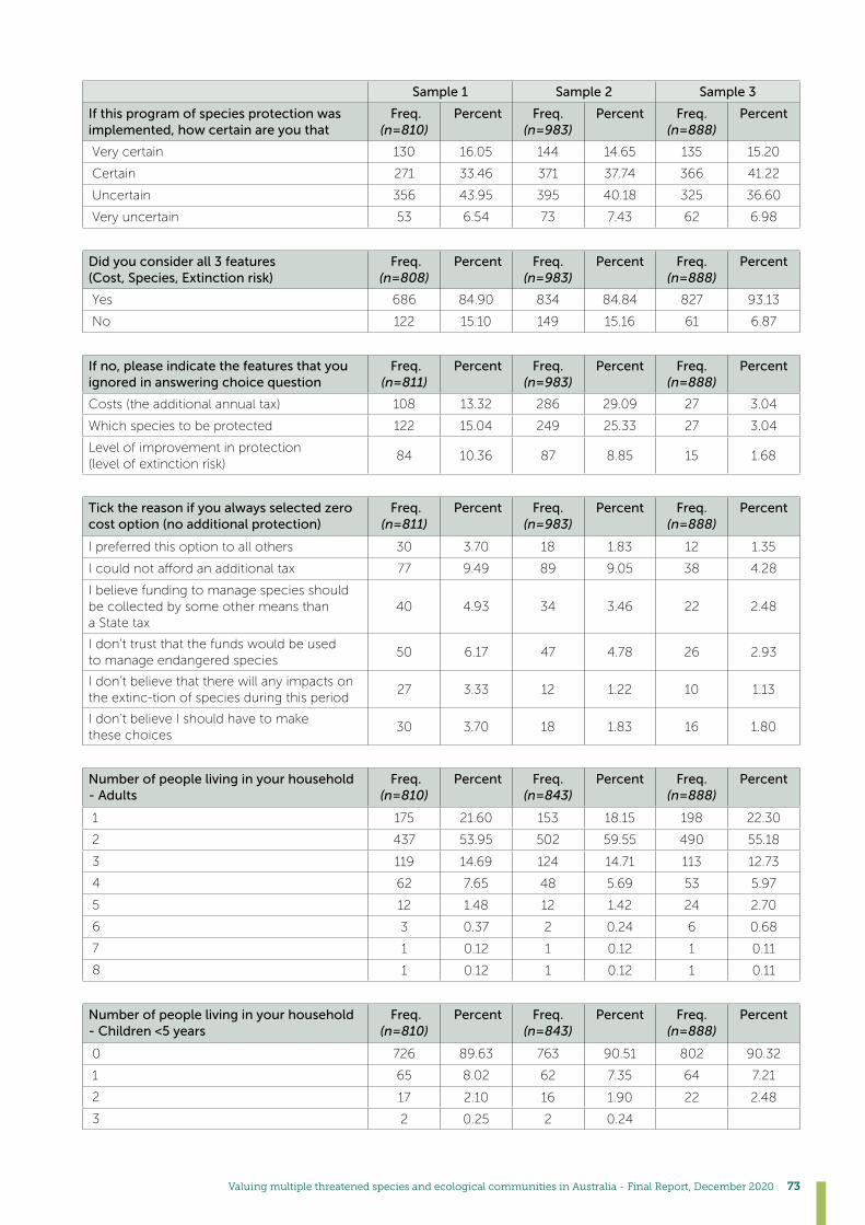
Valuing multiple threatened species and ecological communities in Australia - Final Report, December 2020 73
Sample 1 Sample 2 Sample 3
If this program of species protection was implemented, how certain are you that
Freq. (n=810)
Percent Freq. (n=983)
Percent Freq. (n=888)
Percent
Very certain 130 16.05 144 14.65 135 15.20
Certain 271 33.46 371 37.74 366 41.22
Uncertain 356 43.95 395 40.18 325 36.60
Very uncertain 53 6.54 73 7.43 62 6.98
Did you consider all 3 features (Cost, Species, Extinction risk)
Freq. (n=808)
Percent Freq. (n=983)
Percent Freq. (n=888)
Percent
Yes 686 84.90 834 84.84 827 93.13
No 122 15.10 149 15.16 61 6.87
If no, please indicate the features that you ignored in answering choice question
Freq. (n=811)
Percent Freq. (n=983)
Percent Freq. (n=888)
Percent
Costs (the additional annual tax) 108 13.32 286 29.09 27 3.04
Which species to be protected 122 15.04 249 25.33 27 3.04
Level of improvement in protection (level of extinction risk)
84 10.36 87 8.85 15 1.68
Tick the reason if you always selected zero cost option (no additional protection)
Freq. (n=811)
Percent Freq. (n=983)
Percent Freq. (n=888)
Percent
I preferred this option to all others 30 3.70 18 1.83 12 1.35
Icouldnotaffordanadditionaltax 77 9.49 89 9.05 38 4.28
I believe funding to manage species should be collected by some other means than a State tax
40 4.93 34 3.46 22 2.48
I don’t trust that the funds would be used to manage endangered species
50 6.17 47 4.78 26 2.93
I don’t believe that there will any impacts on the extinc-tion of species during this period
27 3.33 12 1.22 10 1.13
I don’t believe I should have to make these choices
30 3.70 18 1.83 16 1.80
Number of people living in your household - Adults
Freq. (n=810)
Percent Freq. (n=843)
Percent Freq. (n=888)
Percent
1 175 21.60 153 18.15 198 22.30
2 437 53.95 502 59.55 490 55.18
3 119 14.69 124 14.71 113 12.73
4 62 7.65 48 5.69 53 5.97
5 12 1.48 12 1.42 24 2.70
6 3 0.37 2 0.24 6 0.68
7 1 0.12 1 0.12 1 0.11
8 1 0.12 1 0.12 1 0.11
Number of people living in your household - Children <5 years
Freq. (n=810)
Percent Freq. (n=843)
Percent Freq. (n=888)
Percent
0 726 89.63 763 90.51 802 90.32
1 65 8.02 62 7.35 64 7.21
2 17 2.10 16 1.90 22 2.48
3 2 0.25 2 0.24
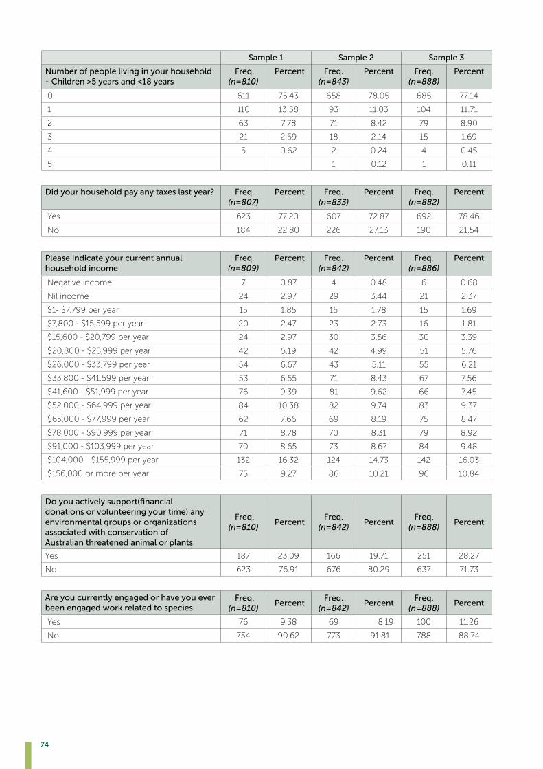
74
Sample 1 Sample 2 Sample 3
Number of people living in your household - Children >5 years and <18 years
Freq. (n=810)
Percent Freq. (n=843)
Percent Freq. (n=888)
Percent
0 611 75.43 658 78.05 685 77.14
1 110 13.58 93 11.03 104 11.71
2 63 7.78 71 8.42 79 8.90
3 21 2.59 18 2.14 15 1.69
4 5 0.62 2 0.24 4 0.45
5 1 0.12 1 0.11
Did your household pay any taxes last year? Freq. (n=807)
Percent Freq. (n=833)
Percent Freq. (n=882)
Percent
Yes 623 77.20 607 72.87 692 78.46
No 184 22.80 226 27.13 190 21.54
Please indicate your current annual household income
Freq. (n=809)
Percent Freq. (n=842)
Percent Freq. (n=886)
Percent
Negative income 7 0.87 4 0.48 6 0.68
Nil income 24 2.97 29 3.44 21 2.37
$1- $7,799 per year 15 1.85 15 1.78 15 1.69
$7,800 - $15,599 per year 20 2.47 23 2.73 16 1.81
$15,600 - $20,799 per year 24 2.97 30 3.56 30 3.39
$20,800 - $25,999 per year 42 5.19 42 4.99 51 5.76
$26,000 - $33,799 per year 54 6.67 43 5.11 55 6.21
$33,800 - $41,599 per year 53 6.55 71 8.43 67 7.56
$41,600 - $51,999 per year 76 9.39 81 9.62 66 7.45
$52,000 - $64,999 per year 84 10.38 82 9.74 83 9.37
$65,000 - $77,999 per year 62 7.66 69 8.19 75 8.47
$78,000 - $90,999 per year 71 8.78 70 8.31 79 8.92
$91,000 - $103,999 per year 70 8.65 73 8.67 84 9.48
$104,000 - $155,999 per year 132 16.32 124 14.73 142 16.03
$156,000 or more per year 75 9.27 86 10.21 96 10.84
Do you actively support(financial donations or volunteering your time) any environmental groups or organizations associated with conservation of Australian threatened animal or plants
Freq. (n=810)
PercentFreq.
(n=842)Percent
Freq. (n=888)
Percent
Yes 187 23.09 166 19.71 251 28.27
No 623 76.91 676 80.29 637 71.73
Are you currently engaged or have you ever been engaged work related to species
Freq. (n=810)
PercentFreq.
(n=842)Percent
Freq. (n=888)
Percent
Yes 76 9.38 69 8.19 100 11.26
No 734 90.62 773 91.81 788 88.74
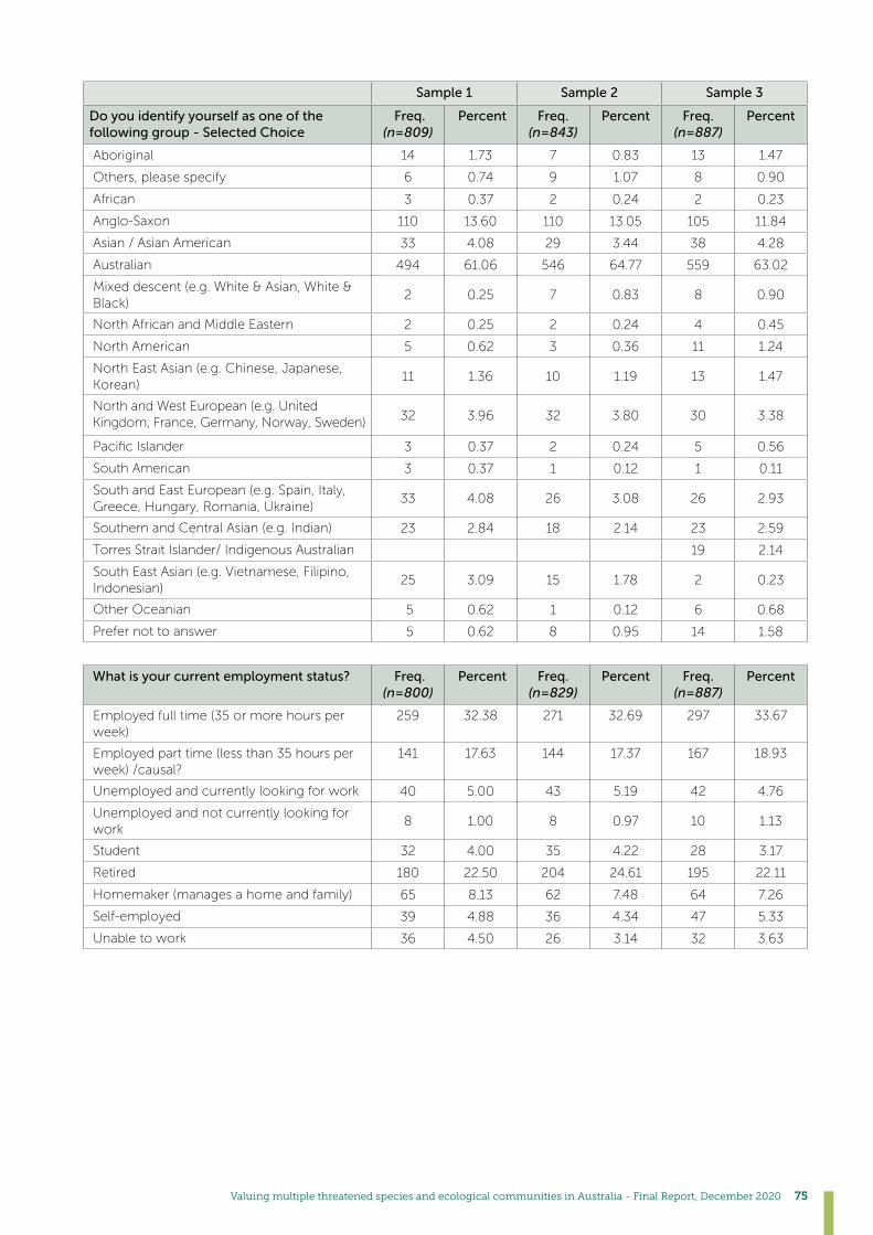
Valuing multiple threatened species and ecological communities in Australia - Final Report, December 2020 75
Sample 1 Sample 2 Sample 3
Do you identify yourself as one of the following group - Selected Choice
Freq. (n=809)
Percent Freq. (n=843)
Percent Freq. (n=887)
Percent
Aboriginal 14 1.73 7 0.83 13 1.47
Others, please specify 6 0.74 9 1.07 8 0.90
African 3 0.37 2 0.24 2 0.23
Anglo-Saxon 110 13.60 110 13.05 105 11.84
Asian/AsianAmerican 33 4.08 29 3.44 38 4.28
Australian 494 61.06 546 64.77 559 63.02
Mixeddescent(e.g.White&Asian,White& Black)
2 0.25 7 0.83 8 0.90
North African and Middle Eastern 2 0.25 2 0.24 4 0.45
North American 5 0.62 3 0.36 11 1.24
North East Asian (e.g. Chinese, Japanese, Korean)
11 1.36 10 1.19 13 1.47
North and West European (e.g. United Kingdom, France, Germany, Norway, Sweden) 32 3.96 32 3.80 30 3.38
PacificIslander 3 0.37 2 0.24 5 0.56
South American 3 0.37 1 0.12 1 0.11
South and East European (e.g. Spain, Italy, Greece, Hungary, Romania, Ukraine)
33 4.08 26 3.08 26 2.93
Southern and Central Asian (e.g. Indian) 23 2.84 18 2.14 23 2.59
TorresStraitIslander/IndigenousAustralian 19 2.14
South East Asian (e.g. Vietnamese, Filipino, Indonesian)
25 3.09 15 1.78 2 0.23
Other Oceanian 5 0.62 1 0.12 6 0.68
Prefer not to answer 5 0.62 8 0.95 14 1.58
What is your current employment status? Freq. (n=800)
Percent Freq. (n=829)
Percent Freq. (n=887)
Percent
Employed full time (35 or more hours per week)
259 32.38 271 32.69 297 33.67
Employed part time (less than 35 hours per week)/causal?
141 17.63 144 17.37 167 18.93
Unemployed and currently looking for work 40 5.00 43 5.19 42 4.76
Unemployed and not currently looking for work
8 1.00 8 0.97 10 1.13
Student 32 4.00 35 4.22 28 3.17
Retired 180 22.50 204 24.61 195 22.11
Homemaker (manages a home and family) 65 8.13 62 7.48 64 7.26
Self-employed 39 4.88 36 4.34 47 5.33
Unable to work 36 4.50 26 3.14 32 3.63

This project is supported through funding from the Australian Government’s National Environmental Science Program.
http://www.nespthreatenedspecies.edu.au
Further information:
Copyright © 2022 FDOKUMEN