Valuing Volatility Spillovers - OPUS at UTS

Valuing Volatility Spillovers∗

George Milunovich

Division of Economic and Financial Studies

Macquarie University

Sydney

Susan Thorp

School of Finance and Economics

University of Technology

Sydney

March 2006

Contact details:

George Milunovich, Division of Economic and Financial Studies, Macquarie University,

NSW, 2109, Australia. Tel:+61 2 9850 8543 Fax: +61 2 9850 6096

Email: [email protected]

Susan Thorp, School of Finance and Economics, University of Technology, Sydney,

Broadway NSW 2007, Australia. Tel: +61 2 9514 7784 Fax: +61 2 9514 7722

Email: [email protected]

∗ We thank Lance Fisher, Tony Hall, David Michayluk, Adrian Pagan, Minxian Yang, and participants at the 2005 Applied Econometrics Conference, Venice, and the 2005 Global Finance Conference, Trinity College, Dublin for helpful comments. Thorp acknowledges the support of the Australian Research Council.

- 1 -

ABSTRACT

We show that volatility spillovers are large enough to matter to investors. We

demonstrate that standard deviations of returns to mean-variance portfolios of

European equities fall by 1-1.5% at daily, weekly, and monthly rebalancing horizons

when volatility spillovers are included in covariance forecasts. We estimate the

conditional second moment matrix of (synchronized) daily index returns for the

London, Frankfurt and Paris stock markets via two asymmetric dynamic conditional

correlation models (A-DCC): the unrestricted model includes volatility spillovers and

the restricted model does not. We combine covariance forecasts from the restricted

and unrestricted models with a wide range of assumed returns relatives via a polar co-

ordinates method, and compute out-of-sample realized portfolio returns and variances

for testing. Diebold-Mariano tests confirm that most risk reductions are statistically

significant. Stochastic dominance tests indicate that portfolios accounting for

volatility spillover would be preferred by risk averse agents.

Keywords: GARCH, volatility spillover, portfolio risk, forecasting

JEL Classification: G11 G15 C53 C32

- 2 -

1. Introduction

There are many empirical studies of time-varying second moments but fewer studies

which actually measure whether new models will benefit investors. Since a key ingredient

in successful portfolio selection is an accurate prediction of covariance between asset

returns, better forecasting models should generate measurably lower portfolio risk.

Volatility spillovers, for example, have been extensively documented as a feature of

financial data but their importance for efficient investment has not been evaluated. In this

study, we incorporate volatility spillovers into covariance forecasts, form mean-variance

portfolios of European equities, and quantify any resulting benefits to investors.

A volatility spillover occurs when changes in price volatility in one market produce

a lagged impact on volatility in other markets, over and above local effects. Volatility

spillover patterns appear to be widespread in financial markets. There is evidence for

spillovers between equity markets (see for example Hamao, Masulis and Ng 1990, and

Lin, Engle and Ito 1994), bond markets (Christiansen 2003), futures contracts (Abhyankar

1995, Pan and Hsueh 1998), exchange rates (Engle, Ito and Lin 1990, and Baillie and

Bollerslev 1990), equities and exchange rates (Apergis and Rezitis 2001), various

industries (Kaltenhauser 2002), size-sorted portfolios (Conrad, Gultekin and Kaul 1991),

commodities (Apergis and Rezitis 2003), and swaps (Eom, Subrahmanyam and Uno

2002). Despite the interest that investors might have in these pervasive spillover effects,

we are not aware of any study that investigates the question of their impact on efficient

asset allocation.

Our first step towards answering this question is to construct a covariance model to

comprehensively capture the data while isolating the impact of volatility spillovers.

Investors in our study hold mean-variance portfolios allocated among the risk-free asset

and equities in two of three major European stock markets, London, Frankfurt and Paris.

- 3 -

Portfolio weights therefore depend on forecasts of the bivariate conditional covariance

matrix of stock market returns. To generate these forecasts while isolating the impact of

volatility spillovers on portfolio efficiency, we estimate two nested models of returns

volatility using an Asymmetric Dynamic Conditional Correlation (A-DCC) set up

(Cappiello, Engle and Sheppard 2004). The benchmark (restricted) model captures time-

varying volatility and correlation, including asymmetric effects, but omits volatility

spillover terms, which we add to the unrestricted model1. We estimate the models over

the first part of the sample and then forecast the conditional covariance matrix over

remaining data at a range of horizons, computing optimal portfolio weights at each

forecast.

Mean-variance portfolio weights depend on expected returns as well as expected

second-order moments, and it is well known that out-of-sample portfolio performance is

often degraded by a poor choice of expected returns (Chopra and Ziemba 1993). A new

approach, developed by Engel and Colacito (2004), offers a method for minimizing the

impact of expected return choice on out-of-sample portfolio efficiency: in a two-asset

portfolio, relative rather than absolute returns matter to optimal portfolio weighting, so by

computing weights for a wide range of returns ratios, we can better separate the effects of

covariance forecasting from returns forecasting. Finally, using optimal weights, we

compute realized portfolio returns and variances, and then test for significant difference

between the volatility spillover formulation and the benchmark.

We find that accounting for volatility spillovers in conditional covariance forecasts

results in small but significant improvements in portfolio efficiency, relative to

benchmark. The efficiency gains arising from modelling volatility spillovers range from a

0.02 to a 1.51 per cent reduction in portfolio standard deviation. For a portfolio returning,

say, 10 per cent per year, this represents a small risk-adjusted improvement of at most

0.15 per cent, however tests confirm that, in the majority of cases, these risk reductions

- 4 -

are statistically significant at all forecasting horizons. In addition, stochastic dominance

tests point to significant improvements in investor utility arising from volatility spillover

forecasting.

Since including volatility spillover effects in the portfolio selection process does

not incur any additional transactions costs, even small gains can represent improvement

for investors.

This paper proceeds as follows. The next section reviews relevant features of the

volatility spillover literature. We outline the benchmark and alternative models in Section

3, and describe portfolio construction in Section 4. Section 5 describes the data and

reports parameter estimates, and presents results of tests comparing the performance of

portfolios constructed from the benchmark and volatility spillover models. Section 6

concludes.

2. Literature Review

Interest in volatility spillovers across international equity markets intensified after the

October 19, 1987 stock market crash when a sharp drop in the US equity markets

appeared to create a widespread volatility ripple across international markets. In an

attempt to explain this, King and Wadhwani (1990) put forward a ‘market contagion’

hypothesis, arguing that stock price turbulence in one country is partly driven by

turbulence in other countries, beyond the influence of fundamentals. Identifying and

testing the transmission of turbulence between markets has been the focus of the volatility

spillover literature.

Early studies of volatility spillovers typically focus on developed country equity

markets, and the transmission of volatility from larger to smaller country markets in

particular. For example, Hamao, Masulis and Ng (1990) find unidirectional volatility

spillovers from US markets to the UK and Japan, and the UK to Japan, while

- 5 -

Theodossiou and Lee (1993) argue for additional transmissions from the US market to

Canada and Germany.

Further, the large-small country effect appears to be mirrored within equity markets

on a firm-size level. Studies document volatility spillover from large to small firms

(Conrad, Gultekin and Kaul 1991, and Reyes 2001), although bad news may cause

spillover in the reverse direction as well (Pardo and Torro 2003).

More recent studies investigate spillover effects between developed and emerging

markets, and among emerging markets themselves. A typical finding (see, for example,

Wei et al, 1995) is that volatility transmits from developed to emerging markets, and that

the smaller, less developed markets are likely to be more sensitive to transmitted shocks.

Geographic locality, regardless of market size, is also likely to be a factor in

volatility spillover. Bekaert and Harvey (1997) are able to distinguish between local and

global shocks, studying volatility spillovers across emerging stock markets. Regional

factors are important for Pacific Basin markets, over and above the world-market effects

of spillovers from the US (Ng 2000). In a related study, Miyakoshi (2003) goes further,

arguing that regional effects are stronger than world market influence for markets in the

Asian region.

Europe represents a particularly interesting geographic area for volatility spillover

studies since it encompasses a number of developed markets with common economic and

financial features, and overlapping trading hours. Thirteen European markets and the US

are studied by Baele (2003), who decomposes volatility spillovers into country specific,

regional and world shocks. (The model also allows for regime switches in the spillover

effects.) Both regional and world effects are reported as significant. Further, spillovers

appear to have intensified over the 1980s and 1990s, with a more pronounced rise among

European Union (EU) markets. In a related study, Billio and Pelizzon (2003) find that

volatility spillovers to most European stock markets from both the world index and the

- 6 -

German index have increased since the European Monetary Union (EMU) came into

effect.

The importance of regional spillovers for Europe is not restricted to equity markets.

Testing for volatility spillover effects in European bond markets, Christiansen (2003)

finds evidence of spillover from both the US and Europe to individual country’s bond

markets. The European volatility spillover effects are stronger than the US volatility

spillovers in both bond and equity markets.

An important methodological issue for transmission studies is whether volatility

spillovers can be identified separately from lags in information transfer due to non-

overlapping trading hours between markets. For example, in the foreign exchange market

Engle, Ito and Lin (1990) investigate volatility spillovers across Tokyo and New York for

the Yen/USD exchange rate. Since these two markets trade a common security, but

operate in different time zones, the authors argue for a ‘Meteor Shower’ effect, whereby

surprises in one market while the other is closed show up as soon as the second market

opens. In addition, by studying open-to-close against close-to-open equity returns, Lin,

Engle and Ito (1994) find that shocks to New York daytime equity returns are correlated

with overnight Tokyo returns and vice versa. In the latter case they conclude that

information revealed during the trading hours of one market has a simultaneous impact on

the returns of the other market. Any study of volatility spillovers needs to distinguish

between contemporaneous shocks that appear lagged because of staggered trading hours,

and real-time lead-lag effects between security markets (Martens and Poon 2001).

Existing empirical research provides evidence of volatility spillovers both across

and within various markets. Our choice of equity markets (London, Frankfurt and Paris)

facilitates investigation of larger-smaller market effects as well as the intra-regional

influences which appear to be strengthening in Europe. In addition, we restrict the study

- 7 -

to synchronous price observations, avoiding the confusion that can arise from trading

lags.

3. Model Specification and Estimation

We build two bivariate Asymmetric Conditional Correlation (ADCC) models to capture

time-varying volatility and asymmetric effects while also allowing correlations between

security returns to vary over time. Recent studies (Cappiello, Engle and Sheppard 2003,

Kearney and Poti 2005) have established the importance of correctly modelling time-

varying correlation, particularly among European security markets.

Consider a vector of returns for two equity markets, 1 2[ ]′=rt t tr r such that

(1) = +r c ut t

t , (2) t t=u D ε

where is the unconditional mean vector of r , contains conditional standard

deviations on the main diagonal and zeros elsewhere, are the innovations standardized

by their conditional standard deviations, and

c t Dt

tε

1−Ψ t represents the conditioning information

set at time t such that

. (3) (1| ~ ,t t t−Ψε 0 R )

tObserve that is also the conditional correlation matrix of the

standardized innovations. We can therefore specify the conditional covariance matrix for

the returns vector r as

1t t tE ′⎛ ⎞⎜ ⎟− ⎝ ⎠

=ε ε R

t

( )( )

( )

1 11

1

1

( ) ( )t t t t t tt

t t t t t

t t t tt

Var Var E

E

E

′− −−

′⎡ ⎤⎢ ⎥− ⎢ ⎥⎣ ⎦

′⎡ ⎤⎢ ⎥− ⎢ ⎥⎣ ⎦

⎡ ⎤= = − −| Ψ ⎣ ⎦

=

= ,

r r r c r

D ε D ε

D ε ε D

c

(4)

- 8 -

and since is a function only of information at tD 1−t , we can write the conditional

covariance matrix as

(5) 1

1

( )t t t

t t t t t

Var

E−

′⎛ ⎞⎜ ⎟− ⎝ ⎠

≡

=

H r

D ε ε D

(6) = D R Dt t t .

The elements of the matrix are the conditional standard deviations, where Dt

11

22

0

0

⎡ ⎤⎢ ⎥,⎢⎢⎢ ⎥⎢ ⎥,⎣ ⎦

=Dt

t

t

h

h⎥⎥ . (7)

We use two specifications of conditional variances to separately capture the effects

of asymmetric dynamics and volatility spillover:

Asymmetric GJR(1,1,1)2:

( ) 21 1, − , −= + + +ii t t ii t ii th I uω α δ β 1, −h (8)

where ,

,

1 00 0

ii tt

ii t

uI

u| <⎧

= .⎨ | ≥⎩

Asymmetric GJR(1,1,1) with volatility spillover:

( ) 21 1 1, − , − , − , −= + + + +ii t t ii t ii t jj th I u hω α δ β γ 2

1u (9)

where and ,

,

1 00 0

ii tt

ii t

uI

u| <⎧

= ⎨ | ≥⎩≠ .ii jj 3

- 9 -

Next we model the conditional correlation matrix following Cappiello, Engle

and Sheppard (2004). From (1) and (2) above, the standardized residuals can be

calculated as

Rt

1t t t− = ,D u ε (10)

where the elements of have been derived from estimated equations for each of the

formulations for

1−Dt

,ii th above. By using these standardized residuals we are able to estimate

a conditional correlation matrix of the form:

(11) 1−⎡ ⎤ ⎡ ⎤⎢ ⎥ ⎢ ⎥⎣ ⎦ ⎣ ⎦=R Q Q Qt t tdiag diag 1−

t

1 1 1 1 1(1 )t t t tφ η ϕ φ ϕ η′ ′t t− − − −= − − − + + +Q Q m ε ε m m Q −

where ,φ ϕ and η are scalar parameters. The vector [ ]0t tI= <m ε o tε (where is the

Hadamard product) isolates observations where standardized residuals are negative.

Notice that Q resembles a GJR(1,1,1) process in the standardized volatilities. Finally,

we implement variance targeting, where

o

t

1t tT

′= ∑Q ε ε and 1 ′= ∑m mt tT m

t

. Combining

estimates for (6) and (10) results in a conditional covariance matrix for the returns vector

which can be used, along with a vector of expected returns, to predict optimal portfolio

weights -periods ahead:

rt

t

(12) = .H D R Dt t t

4. Portfolio construction

In this study, investors use short-horizon mean-variance strategies to create

portfolios from two equity market indices and the (zero-return) risk-free asset, relying on

- 10 -

forecasts of conditional covariance from dynamic models. On one hand, mean-variance

portfolios are not ideal for equity investors, since they maximize utility only when asset

returns are elliptically distributed, but on the other hand, mean-variance modelling is a

well-understood analytic tool that maps into the portfolio performance literature, is

commonly applied in funds management practice, and can be simply adapted to changing

levels of risk aversion.

4.1 Weight selection

A single-horizon investor chooses portfolio weights to minimize portfolio variance

subject to a required return µ0.

(13) min ′w H wt

t t tw

ts t oµ′. . =w µ (14)

deriving an optimal weighting vector:

1

1t

tt

oµ−

′ −=H µw

µ H µ, (15)

where µ is an assumed vector of expected returns to be described below, and 0µ is

the required rate of return to the portfolio, here set to unity. is the expected

(forecasted) covariance matrix of returns. We do not impose full investment or short-sales

constraints on the portfolio allocations, so any wealth not accounted for by is

implicitly invested in the risk-free (assumed zero return) asset, and the weight vector may

include negative values.

Ht

wt

The individual variance formulations described by equations (8) and (9), in

combination with the A-DCC correlation estimates, generate two sets of conditional

- 11 -

covariance matrices for each pair of market returns,{ }21=itH , where model i=2 includes

volatility spillover effects and model i=1 does not. We forecast Ht and rebalance the

portfolio at daily, weekly (5 days) two-weekly (10 days) and monthly (20 days)

frequencies, using the A-DCC models described above, testing to see if the impact of

volatility spillover tapers off over longer rebalancing horizons.

4.2 Expected Returns

Engle and Colacito (2004) propose a solution to the problem of forecasting

expected returns. Expected return estimation errors are not only usually large, but also

amplified in the mean-variance optimization process, causing poor out-of-sample

portfolio performance. Engle and Colacito point out that, for two-asset portfolios, optimal

weights are functions of relative returns, not of the absolute size of expected return to

each asset. Since it is the return ratio that matters, a wide spectrum of relative returns

between two assets can be mapped out over the zero-one interval. By applying their

method, we can test for the impact of volatility spillover on portfolio efficiency without

jointly testing a peripheral hypothesis about expected returns.

We span a wide range of returns relatives by choosing pairs of expected returns as

polar co-ordinates, sin ,cos20 20

j jπ π⎡= ⎢⎣ ⎦µ ⎤

⎥ and allowing j to vary from 0 to 10,

{ }0 10∈ ,..., .j The resulting values (listed in Table 1 ) range from zero to one for each

asset, including a mid-point where the expected returns of both assets are equal.

Combined with forecast covariance matrices 2

1

it i

⎧ ⎫⎨ ⎬⎩ ⎭ =H , these eleven expected return pairs

allow us to compute optimal portfolio weights from (15). If one conditional

covariance model performs better for all eleven expected returns relatives, we can be

confident that it is a better model for any choice of returns vector.

11

1

kt k

⎧ ⎫⎨ ⎬⎩ ⎭ =µ

- 12 -

[INSERT TABLE 1 HERE]

Since comparison between eleven portfolios is cumbersome we also derive a

Bayesian probability for each value of j and compute a probability-weighted summary

measure of portfolio risk and return. Again following Engle and Colacito (2004), we

compute non-overlapping sample means (using 40 observations) { }1 2 1=,l l

lµ µ ,

L

1 ,d D

from the

sample data for each market pairing. Any mean pair where either value is negative is

dropped, leaving a subset of size = ,... . D From this sample we back out values of

2

2 22 1

2 cos ,

, ,+

⎛= ⎜⎝ ⎠

d

d dd a µ

π µ µθ ⎞

⎟ and use these values of θ to calculate maximum likelihood

parameters of the Beta distribution and b . Finally, we infer the empirical probability

of each pair of the eleven polar co-ordinate returns

a ˆ

( )20 20sin cos= ,j jk π πµ by computing

the value

ˆˆ 1 1

1 ˆˆ 1 1

0

(1 )1Pr( )

− −⎛ ⎞⎜ ⎟⎝ ⎠ − −

−= =

ϒ ∫

a bj j

j a bt t dt

θ θθ θ . (16)

where 1ϒ

is a normalizing constant (and ( ) ( )( )

1 ˆˆ 1 1

0( )a b a b

t t dta b

− − Γ Γ=

Γ +∫ ) for each pair

of markets.

Figure 1 graphs the probability density functions for θ computed from this

procedure, with all showing some skewness across the range of relative returns. All but

the most extreme values of θ have some weight in the density, so focusing on the most

likely value may be misleading.

[INSERT FIGURE 1 HERE]

- 13 -

4.3 Performance measurement

Portfolio performance is a guide to forecasting accuracy, since the best model of

covariance will generate the least risk. Engle and Colacito (2004) show that, for a given

required rate of return µ0, the portfolio with the smallest realized standard deviation will

be a portfolio constructed from the true covariance matrix. We infer that a covariance

forecasting model that is closer to the underlying data generating process (DGP) will

predict better than other models, and generate lower portfolio risk. So if ∗σ is the

portfolio standard deviation achieved using the true covariance matrix, and σ is the

standard deviation from an inefficiently estimated covariance matrix, then ∗σ will be less

than for ˆ ,σ such that

ˆ∗

<o o

.σ σµ µ

(17)

Consequently, if including volatility spillover effects improves conditional

covariance forecasts then portfolios constructed from the better forecasts will have

lower realized standard deviations. Another way of expressing this efficiency gain is

by computing the required rate of return we would need in order to maintain a

constant risk-to-reward ratio while switching covariance forecasts. Let *0µ be the

required rate of return associated with the true covariance matrix and 0µ be the

required rate of return associated with an inefficient covariance matrix, and rewrite

(17) as an equality:

*0 0

ˆˆ

σ σµ µ

∗

= (18)

where *0µ < 0µ . Equivalently we can write (18) as:

- 14 -

0*0

ˆ ˆµ σµ σ ∗= (19)

The ratio on the left hand side of equation (19) measures the addition to returns

which would compensate the investor for a less efficient covariance matrix. (We

report estimates of portfolio standard deviation ratios in Tables 4 –6 below.)

5. Empirical Results

5.1 Data and estimation

We estimate4 the A-DCC models using daily returns from three major European

stock market price indices, valued in US dollars: FTSE 100 (London); DAX 30

(Frankfurt); and CAC 40 (Paris). Returns are calculated as log differences and do not

include dividends. No currency hedging is implemented. Trading hours for the London,

Frankfurt and Paris stock exchanges overlap imperfectly, so to ensure synchronous prices

we take index values at London 16:00 time (Frankfurt and Paris 17:00 time).5 The models

were estimated using the first 2700 observations of the 3523 size sample, leaving the

remaining 823 observations for testing. The estimation period runs from 1 January 1992

to 6 May 2002, and predictive power for portfolio formation is tested over the three years

from 7 May 2002 to 4 July 2005.

Martens and Poon (2001) point out the importance of synchronous data for studies

of daily conditional correlation and volatility spillover. Substantial mis-estimation of

returns correlation and spillovers can result from a failure to account for timing

differences at the daily level. Correlations will be under-estimated, and estimated

spillover patterns changed, if non-synchronous daily data are used in correlation models.

By synchronizing prices we ensure that estimated spillovers and correlations more

- 15 -

accurately expose real-time interactions, rather than representing lags in information

flows, misalignments in trading, or mismatched data collection.

Table 2 reports key features of the data sample. Average returns are highest for the

DAX 30 index, which also displays the largest standard deviation and degree of

skewness. The FTSE 100 has annualized returns around two per cent lower than the DAX

30 and the least variance of the three markets. All three daily returns series show

considerable non-normality manifested in negative skewness and excess kurtosis.

Average skewness is -0.11, and kurtosis, 5.35.


A graph of the daily returns in Figure 2 shows clusters of volatility, where groups

of large or small changes persist for a number of periods. More frequent periods of

turbulence are evident from 1998 to 2003 (when volatility begins to drop off) and

volatility patterns appear related, as might be expected among such closely-aligned equity

markets.


Table 3 reports estimates for a total of six bivariate A-DCC models: two for each of

the three pairs of returns series (London-Frankfurt, London-Paris and Frankfurt-Paris).

We compute a benchmark without volatility spillover and an alternative with volatility

spillover for each market pair. (Appendix 1 gives details of the estimation method.)


The top portion of Table 3 reports parameter estimates and standard errors for the

variance equations, and the lower portion reports estimates of the parameters of the

correlation matrices. With the exception of statistically insignificant volatility spillover

parameter from Paris to Frankfurt, all parameters have the expected (positive) sign. All

models show evidence of high levels of volatility persistence, with parameters on lagged

variables summing to just below one. Estimates from the benchmark model (GJR (1,1,1))

- 16 -

show significant asymmetry effects ( )δ in all three markets. We find that the asymmetric

effect is strongest for the UK market, dominating the symmetric volatility shock

component.

In terms of volatility spillover ( )γ , we find significant transmission from Frankfurt

and Paris to London, and from Frankfurt to Paris, so we observe that Frankfurt is

unaffected by lagged volatility shocks from the other markets in this sample. Although all

volatility spillover coefficients are small, Frankfurt to Paris shocks are greatest in

magnitude. Estimates of volatility spillover effects from London to the continental

markets are positive, but smaller and poorly estimated, a surprising result given the

relative sizes of the markets.6

Figure 3 presents graphs of estimated conditional variance series for the volatility

spillover model. Conditional variances confirm earlier observations (Figure 2) that the

three markets have become increasingly volatile since early 1997, possibly in connection

with the beginning of the Asian crisis. The German market shows the most, and the UK

market, the least, volatility over the whole sample.7


Conditional correlation parameter estimates ( ), ,φ η ϕ for the benchmark and

alternative models differ only slightly. This result should help us isolate the effects of

volatility spillovers on the portfolio selection process. The Frankfurt-Paris combination

displays the most persistence (η ) in conditional correlations8. Asymmetric effects in

conditional correlations are smaller than their symmetric counterparts in all three

combinations, with the London-Frankfurt pair exhibiting the largest asymmetric effect

and London-Paris, the smallest. Kearney and Poti (2005) report weak asymmetry effects

for conditional correlations among Euro-zone equity markets.

- 17 -

Figure 4 graphs the conditional correlation series from the volatility spillover

model, showing that time-variation in conditional correlation is an important feature of

the second-moment dynamics.


5.2 Portfolio Standard Deviations

We forecast from estimated benchmark and volatility spillover models, generate

predicted covariances at 1, 5, 10 and 20-step horizons, and compute optimal

portfolio weights from equation (15), for two equity markets and the risk-

free asset. This procedure simulates realized portfolio returns from the remaining

(823) observations of the data set:

2

11i k,⎧ ⎫

t .

1

it i

⎧ ⎫⎨ ⎬⎩ ⎭ =H

1t k⎨ ⎬⎩ ⎭ =

,w

(20) 'i k i kt tπ , ,= w r

where corresponds to the benchmark and alternative portfolios and

indicates the vector of expected returns.

1 2= ,i 1,...,11k =

As outlined in Section 4, we expect the more efficient covariance model to produce

a lower portfolio risk for any required return. (Here, 1= .oµ ) Tables 6-8 set out realized

standard deviations for the benchmark and volatility spillover models for London-

Frankfurt, London-Paris and Frankfurt-Paris, respectively. We report volatility ratios for

daily, weekly, ten-day and monthly forecasting and rebalancing horizons. In each row, we

set the least standard deviation equal to 100, and then report the larger standard deviation

as a proportional increase over the smaller. The last row in each column reports the

probability weighted average of the whole column of standard deviations, where the

weighting applied to each row is given by the Bayesian probabilities associated with each

return relative for that data. (These are graphed in Figure 1.) For example, in Table 4,

- 18 -

which gives the standard deviations for the London-Frankfurt market pairing, the last row

under 10-steps-ahead forecasts shows that the portfolio standard deviation for the

benchmark model was 1.52 per cent bigger than the standard deviation for portfolios

computed using the volatility spillover model.9 On a weighted-average basis, the

volatility spillover model performs better than the benchmark at every forecast horizon,

and for all market pairs.

[INSERT TABLES 4, 5 AND 6 HERE]

In terms of economic value, the relative efficiency gains are not large. The greatest

efficiency gain for the volatility spillover model on a weighted-average basis is for the 5-

step-ahead forecast model for London-Frankfurt, where the benchmark model standard

deviation is 101.52, meaning that neglecting volatility spillover effects increases portfolio

risk by about 1.52 per cent of standard deviation. Or, in terms of risk-adjusted returns, if

investors who allow for volatility spillover ∗⎛ ⎞⎟⎠

⎜⎝σ are receiving 10 per cent returns

, then investors who forecast using the benchmark ( 10=µ )∗ ( )σ would need

ˆ 10 152µ = . per cent returns to equalize the return to risk ratio such that *

0ˆ0ˆ

µ µσσ ∗ = . The

efficiency gains to predicting covariance using the volatility spillover model thus

represent risk-free return improvements around 15 basis points on a ten per cent return

portfolio. Nevertheless these small efficiency improvements do not disappear at longer

forecast horizons, as can be seen from weekly, fortnightly and monthly portfolio standard

deviations. In fact as Figures 2. 1 – 2. 4. (in Appendix 2) suggest, gains seem to peak

between weekly and monthly forecasting horizons before they start to diminish at longer

horizons where the forecasts converge to unconditional values.

- 19 -

5.3 Diebold-Mariano Tests

We test the statistical significance of any risk reductions by the Diebold and Mariano

(1995) method for distinguishing between forecasted volatilities. The Diebold-Mariano

test statistic is derived from the estimated difference between realised variance for the

benchmark symmetric and alternative asymmetric models, calculated as

(21) 21 2k k k

t t tv π π, ,⎛ ⎞ ⎛ ⎞⎜ ⎟ ⎜ ⎟⎝ ⎠ ⎝ ⎠

= −2,

forming 11 series for each market pairing, 11

1

kt k

v⎧ ⎫⎨ ⎬⎩ ⎭ =

. Under the null hypothesis the

expected value of is zero, such that including volatility spillover effects in

covariance models does not reduce portfolio variance

11⎧ ⎫

1

kt k

v⎨ ⎬⎩ ⎭ =

10.

We conduct a joint test of this null hypothesis using a GMM estimate of the parameter β

from the regression tV tβι ε= + .11k⎧ ⎫ We first stack all values of

1t kv⎨ ⎬

⎩ ⎭ = and estimate a single

moment condition for the coefficient β . We also construct a system of eleven moment

conditions, one for each , again restricting the system to a single estimate of ktv .β We

report t -tests of the null hypothesis that 0= ,β using robust Newey-West standard errors

from the GMM estimation. Table 7 reports results for each market pairing and forecast

horizon. The majority of tests of β (including short-horizon forecasts for London and

Paris) reject the null hypothesis and confirm that portfolio variances are significantly

lower when volatility spillover is modelled in the conditional covariance matrix. But the

volatility spillover model does not get unqualified support, with significant negative

values for β at the longer horizon tests of the London-Paris pair.


- 20 -

5.5 Stochastic dominance tests

Tests for second-degree stochastic dominance can tell us whether risk-reductions are

likely to matter to any risk averse investor. Consider two samples of portfolio returns

1{ } =M

I IY and 1{ } =M

I IX with cumulative distributions (CDFs) G and . Second degree

stochastic dominance (SD2) establishes the conditions under which any risk averse agent

prefers one portfolio to another: Portfolio Y will be preferred to portfolio

F

X by any

agent whose utility over portfolio returns ( )U π obeys , when

for all

( ) 0U π′ ≥ ′′

π π

( ) 0U π ≤

( ) ( )o o

G t dt F t dt≤∫ ∫ π .

Barrett and Donald (2003) derive a Kolmogorov-Smirnov style test for stochastic

dominance of any degree, evaluating the CDFs at all points in the support. This technique

avoids the problem of choosing an arbitrary set of comparison points which can result in

inconsistency.11 The null hypothesis to be tested is that (weakly) dominates to the

second degree, against the alternative that it does not. From random samples of equal size,

the test statistic is given by:

G F

1 22 22ˆ ˆ ˆ( ) sup( ( ) ( ))

2 MMM I IS G

ππ π/= ; − F; , (22)

where 2 21 1

1 1ˆ ˆ( ) 1( )( ) ( ) 1( )(M M

i i iMMi i

)iI Y Y I XG FM Mπ π π π π

= =

; = ≤ − , ; = ≤ −∑ ∑ Xπ ,

)

and

is the indicator function, returning the value 1 when (1( )⋅ iX π≤ and zero otherwise.

Under the null hypothesis, the test statistic is no greater than zero. Bald comparisons

between CDFs or their integrals are subject to non-trivial sampling error when the

population density is unknown, so we need some approximation to the sampling

distribution, here derived by block bootstrapping.

- 21 -

We follow Linton, Maasoumi and Whang (2002), and Lim, Maasoumi and Martin

(2004), and adjust the bootstrapping method to keep underlying serial dependence intact.

Block size is set at where 28=B = ,B Tα α is a positive constant and T is sample

size, here 823.12 Each set of portfolio returns is divided into overlapping blocks of size ,B

then a random selection is made, choosing sufficient (contemporaneous) blocks to create a

distribution of size Bootstrap samples are used to build an empirical distribution of the

test statistic.

.T

We report results for one-step-ahead forecasts and two-steps-ahead forecasts, since

5 and other multi-step forecasting generates samples too small for reliable testing. We

conduct the test on a weighted average of returns to the portfolios, where weights are

the Bayesian probabilities shown in Figure 1. Results in Table 8 show that the null

hypothesis that the benchmark model dominates the volatility spillover model can be

rejected in all but one of six tests. So we can infer that in five of six cases, the volatility

spillover forecasting model is preferred by risk averse investors.

k


6. Conclusions

Recent advances in modelling time-varying second moments have highlighted an

array of features in security returns volatilities that were previously overlooked.

Among these, volatility spillovers are both significant and widespread, well-identified

in a large number of studies across a range of security markets and geographic

locations. However the economic importance of any aspect of time series dynamics,

including volatility spillovers, depends not on whether it can be statistically identified,

but on whether it can alter investment outcomes.

- 22 -

In this study we value volatility spillovers for investors who select mean-

variance equity portfolios from stock markets in London, Frankfurt and Paris. We

isolate the portfolio risk reductions that can be attributed to adding volatility

spillovers to asymmetric dynamic conditional correlation forecasting models. ADCC

models capture both time-variation and asymmetry effects in variance and

correlations, allowing us to identify volatility spillovers in a nested model. We also

minimize the impact of expected return choice on out-of-sample portfolio efficiency

by combining covariance forecasts with a full range of assumed expected returns

relatives using polar co-ordinates.

Portfolio efficiency gains due to volatility spillover effects are small, but

significant, measurably reducing standard deviations over 1, 5, 10 and 20-step

horizons in the majority of cases. In addition, stochastic dominance tests confirm that

in five of six cases, risk averse investors will prefer portfolios that allow for volatility

spillover effects in covariance forecasts. On a portfolio returning, say 10 per cent p.a.,

efficiency gains arising from modelling spillovers translate to risk-free return

improvements close to 0.15 per cent, without additional transactions costs.

- 23 -

Appendix 1

A-DCC Estimation

We follow Engle (2002) and estimate the models in two steps. Assuming that the

standardized residuals are conditionally normally distributed so

that , the log likelihood function for the vector of returns can be

expressed as

tε

(1| ~ ,t t tN−Ψε 0 R ) ,rt

( ) 1

1

1 log 2 log2

T

t t t tt

L n π ′ −⎛⎜⎝

=

= − + + .∑ H u H u ⎞⎟⎠

(1.1)

Now let the mean parameters, ,c and the univariate GARCH parameters in be

represented by

Dt

,ψ and the conditional correlation parameters in , by Rt .ζ The log

likelihood can be written as the sum of a volatility part and a correlation part:

( ) ( )( ), = + |V CL L L ,ψ ζ ψ ζ ψ (1.2)

where the volatility term is

( ) 2

1

1( ) log 2 2 log2

′ −⎛ ⎞⎜ ⎟⎝ ⎠

=

= − + +∑ D u D uT

Vt

L nψ π ,t t t t (1.3)

and the correlation component is

( ) 1

1

1 log2

T

C t t tt

L ζ ψ ′ ′⎛⎜⎝

=t t t

− ⎞⎟⎠

| = − − + + .∑ ε ε R ε R ε (1.4)

The procedure is further simplified by recognizing that the volatility part of the log

likelihood is just the sum of the individual univariate GARCH likelihoods:

- 24 -

( )2

1 1

1( ) log 2 log2

⎛ ⎞⎜ ⎟,⎝ ⎠

= = ,

⎛ ⎞= − +⎜⎜

⎝ ⎠∑∑

T nit

Vt i i t

uLh

ψ π + .⎟⎟i th

).

(1.5)

The two-step estimation method involves maximizing each univariate GARCH

term separately, standardizing the returns by estimated standard deviations and then

jointly estimating elements of by maximizing the correlation component of the log

likelihood

Rt

( ,CL ψ ζ We maximize log likelihoods numerically using the Max SQP

procedure in OX 3.4. This procedure implements a sequential quadratic programming

technique to maximize a non-linear function subject to non-linear constraints.

Although the assumption of normality in tε is convenient for estimation, it is not

necessary for consistency, since quasi-maximum likelihood arguments apply as long as

the conditional mean and variance equations are correctly specified (Hamilton, 1994,

p.126). However the standard errors need to be adjusted according to the method

described for the univariate GARCH volatility equations. Standard errors for the

correlation parameters require a more complicated process explained in Engle (2002).

- 25 -

Appendix 2

Figures 2.1-2.3 graph volatility ratios for different forecasting horizons (not all reported

in the paper) and show the relative risk reduction as horizon increases. Tables of volatility

ratios for additional forecasting horizons are available from the authors on request.

[INSERT FIGURES 2.1-2.3 HERE].

- 26 -

References

Abhyankar, A.H. (1995), ‘Trading round-the-clock: Return, volatility and volume

spillovers in the Eurodollar futures markets’, Pacific-Basin Finance Journal, 3,

75-92.

Apergis, N., and Rezitis, A. (2001) , ‘Asymmetric cross-market volatility spillovers:

evidence from daily data on equity and foreign exchange markets’, Manchester

School, 69, 81-96.

Apergis, N., and Rezitis, A. (2003) , ‘Agricultural price volatility spillover effects: the

case of Greece’, European Review of Agricultural Economics, 30(3), 389-406.

Baillie, R., and Bollerslev, T. (1990), ‘A multivariate generalized ARCH approach to

modelling risk premia in forward foreign exchange rate markets,’ Journal of

International Money and Finance, 9(3), 309-324.

Baele, L, (2003), ‘Volatility spillover effects in European equity markets’, Ghent

University Working Paper, Ghent.

Bekaert, G., and Wu, G. (2000), ‘Asymmetric volatility and risk in equity markets’,

Review of Financial Studies, 13(1), 1-42.

Barrett, G.F., and Donald, S.G. (2003), ‘Consistent tests for stochastic dominance’,

Econometrica, 71(1), 71-104.

Bekaert, G., and Harvey, C. (1997), ‘Emerging equity market volatility’, Journal of

Financial Economics, 43(1), 29-77.

Billio M., and Pelizzon, L. (2003), ‘Volatility and shocks spillover before and after EMU

in European stock markets’, Journal of Multinational Financial Management, 13

(4/5), 323-340.

- 27 -

Black, F. (1976), ‘Studies of stock price volatility changes’, Proceedings of the 1976

Meetings of the American Statistical Association, Business and Economical

Statistics Section, 177-181.

Bollerslev, T., and Wooldridge, J.M. (1992), ‘Quasi-maximum likelihood estimation and

inference in dynamic models with time-varying covariances’, Econometric

Reviews, 11, 143-172.

Campbell, J.Y., and Hentschel, L. (1992), ‘No news is goods news: An asymmetric model

of changing volatility in stock returns’, Journal of Financial Economics, 31, 281-

318.

Cappiello, L., Engle, R.F., and Sheppard, K. (2004), ‘Asymmetric dynamics in the

correlations of global equity and bond returns’, European Central Bank Working

Paper No.204, European Central Bank, Frankfurt. URL: http://www.ecb.int.

Christiansen, C. (2003), ‘Volatility-spillover effects in European bond markets’, Working

Paper Series No. 162, November 2003, Centre for Analytical Finance, Aarhus

School of Business, University of Aarhus, Aarhus.

Chopra, R., and Ziemba, W. (1993), ‘The effect of errors in means, variances and

covariances on optimal portfolio choice’, Journal of Portfolio Management, 6-11

Conrad, J., Gultekin, M., and Kaul, G. (1991), ‘Asymmetric predictability of conditional

variances’, Review of Financial Studies, 4, 597-622.

Diebold, F.X., and Mariano, R.S. (1995), ‘Comparing predictive accuracy’, Journal of

Business and Economics Statistics, 13(3), 253-263.

Engle, R.F. (2002), ‘Dynamic conditional correlation - A simple class of multivariate

GARCH models’, Journal of Business and Economic Statistics, 20(3), 339-350.

Engle, R.F., and Colacito, R. (2004), ‘Testing and valuing dynamic correlations for asset

allocations’, unpublished manuscript, New York University, New York.

- 28 -

Engle, R.F., Ito, T., and Lin, W. (1990), ‘Meteor showers or heat waves? Heteroskedastic

intra-daily volatility in the foreign exchange market’, Econometrica, 58(3), 525-

542.

Eom, Y., Subrahmanyam, M., and Uno, J. (2002), ‘The transmission of swap spreads and

volatilities in the international swap markets’, Journal of Fixed Income, 12(1), 6-

28.

Glosten, L., Jagannathan, R., and Runkle, D. (1993), ‘On the relationship between the

expected value and the volatility of the nominal excess return on stocks’, Journal

of Finance, 48(5), 1779-1801.

Hamao, Y., Masulis, R., and Ng, V. (1990), ‘Correlations in price changes and volatility

across international stock markets’, Review of Financial Studies, 3, 281-307.

Hamilton, J. D. (1994), Time Series Analysis, Princeton University Press, Princeton.

Harju, K., and Hussain, S.M. (2005) ‘Intraday linkages across international equity

markets’, Unpublished manuscript, Department of Finance, Hanken-Swedish

School of Economics and Business Administration, Vasa, Finland.

Kaltenhauser, B. (2002), ‘Return and volatility spillovers to industry returns: does EMU

play a role?’, Center for Financial Studies Working Paper No. 2002-05, an der

Johann Wolfgang Goethe-Universitat Frankfurt am Main.

Kearney, C., and Poti, V. (2005) ‘Correlation dynamics in European equity markets’,

Research in International Business and Finance, (forthcoming).

King, M., and Wadhwani, S. (1990), ‘Transmission of volatility between stock markets’,

Review of Financial Studies, 3, 5-33.

Koutmos, G. (1992), ‘Asymmetric volatility and risk trade off in foreign stock markets’,

Journal of Multinational Financial Management, 2, 27-42.

- 29 -

Lim, G.C., Maasoumi, E., and Martin, V.L. (2004), ‘Discounting the equity premium

puzzle’, unpublished manuscript, Economics Department, University of

Melbourne, Melbourne.

Lin, W., Engle, R., and Ito, T. (1994), ‘Do bulls and bears move across borders?

International transmission of stock returns and volatility’, Review of Financial

Studies, 7, 507-38.

Linton, O., Maasoumi, E., and Whang, Y-J. (2002), ‘Consistent tests for stochastic

dominance: a subsampling approach’, Cowles Foundation Discussion Paper no.

1356, Cowles Foundation for Research in Economics, Yale University, New

Haven.

Martens, M., and Poon, S.-H. (2001), ‘Returns synchronization and daily correlation

dynamics between international stock markets,’ Journal of Banking and Finance,

25, 1805-1827.

Miyakoshi, T. (2003), ‘Spillovers of stock return volatility to Asian equity markets from

Japan and the US’, International Financial Markets, Institutions & Money, 13,

383-399.

Nelson, D. (1991), ‘Conditional heteroskedasticity in asset returns: A new approach’,

Econometrica, 59, 347–70.

Ng, A. (2000), ‘Volatility spillover effects from Japan and the U.S. to the Pacific-Basin’,

Journal of International Money and Finance, 19, 207-233.

Pan, M., and Hsueh, P. (1998), ‘Transmission of stock returns and volatility between the

U.S. and Japan: evidence from stock index futures markets’, Asia-Pacific

Financial Markets, 5, 211-225.

Pardo, A., and Torro, H. (2003), ‘Trading with asymmetric volatility spillovers’, Working

paper, Universitat de Valencia, Valencia.

- 30 -

Poon, S., and Taylor, S. (1992),‘Stock returns and stock market volatility: An empirical

study of the U.K. stock market’, Journal of Banking and Finance, 16, 37-59.

Reyes, M.G. (2001), ‘Asymmetric volatility spillover in the Tokyo Stock Exchange’,

Journal of Economics and Finance, 25(2), 206-213.

Theodossiou, P., and Lee, U. (1993), ‘Mean and volatility spillovers across major

international stock markets: further empirical evidence’, Journal of Financial

Research, 16, 337-350.

Wei, K.C.J., Liu, Y.J., Yang, C.C., and Chaung, G.S. (1995), ‘Volatility and price change

spillover effects across the developed and emerging markets’, Pacific-Basin

Finance Journal, 3, 113–136.

Wu, G. (2001), ‘The determinants of asymmetric volatility’, Review of Financial Studies,

14(3), 837-859.

- 31 -

Table 1: Pairs of expected returns

Range of expected returns used to calculate portfolio weights where ⎥⎦⎤

⎢⎣⎡=

20cos,

20sin jj ππµ

j

µ(1)

µ(2)

θ

0 0.000 1.000 0 1 0.156 0.988 0.1 2 0.309 0.951 0.2 3 0.454 0.891 0.3 4 0.588 0.809 0.4 5 0.707 0.707 0.5 6 0.809 0.588 0.6 7 0.891 0.454 0.7 8 0.951 0.309 0.8 9 0.988 0.156 0.9

10 1.000 0.000 1

- 32 -

Table 2: Summary statistics- daily stock index returns, % p.a. Daily returns calculated as from price indices synchronized at London 16:00 time, 2 January 1992 to 4 July 2005. All indices are in USD, unhedged. Data supplied by Datastream.

)/ln(100 1−= ttt ppr

FTSE 100 DAX 30 CAC 40

Mean 5.1 7.3 6.1 Std. Dev. 16.4 21.6 20.0 Skewness 0.03 -0.23 -0.08 Kurtosis 5.6 5.8 5.0

Jarque-Bera 957.6 1205 570.8

Observations 3523 3523 3523

- 33 -

Table 3: Parameter estimates, A-DCC models. Columns show estimated parameters for GJR ADCC and GJR-ADCC with Volatility Spillover conditional covariance models. P-values are in brackets. GJR and GJR(volatility spillover) equations were computed for every market using de-meaned returns, and then standardised residuals were used to compute estimates for the ADCC and ADCC(volatility spillover) models. Estimated over 2700 daily returns, sampling 2/1/1992 – 6/5/2002. Parameter London-Frankfurt London-Paris Frankfurt-Paris

GJR (1,1,1)

GJR (1,1,1)

Volatility spillover

GJR (1,1,1)

GJR (1,1,1)


GJR (1,1,1)

GJR (1,1,1)


UK

DE

UK

DE

UK

FR

UK

FR

DE

FR

DE

FR

ω

0.0272 (0.079)

0.0251 (0.028)

0.0259 (0.018)

0.0248 (0.048)

0.0272 (0.079)

0.0246 (0.099)

0.0236 (0.044)

0.0259 (0.220)

0.0251 (0.028)

0.0246 (0.099)

0.0259 (0.042)

0.0297 (0.079)

α 0.0162 (0.304)

0.0428 (0.001)

0.0017 (0.894)

0.0431 (0.002)

0.0162 (0.304)

0.0210 (0.006)

0.0021 (0.862)

0.0186 (0.063)

0.0428 (0.001)

0.0210 (0.006)

0.0436 (0.004)

0.0013 (0.887)

β 0.9242 (0.000)

0.9220 (0.000)

0.9160 (0.000)

0.9212 (0.000)

0.9242 (0.000)

0.9426 (0.000)

0.9168 (0.000)

0.9397 (0.000)

0.9220 (0.000)

0.9426 (0.000)

0.9223 (0.000)

0.9341 (0.000)

δ 0.0595 (0.000)

0.0352 (0.042)

0.0665 (0.000)

0.0334 (0.053)

0.0595 (0.000)

0.0363 (0.011)

0.0660 (0.000)

0.0329 (0.020)

0.0352 (0.042)

0.0363 (0.011)

0.0362 (0.036)

0.0461 (0.0018)

γ 0.0133 0.0021 (0.033)

(0.819)

0.0151 0.0088 (0.077) (0.374)

-0.0021 0.0185 (0.803) (0.026)

φ

0.0229

0.0216

0.0317

0.0317

0.0318

0.0321

η 0.9391 0.9412 0.9149 0.9115 0.9609 0.9600ϕ 0.0241 0.0278 0.0143 0.0182 0.0161 0.0187

- 34 -

Table 4: Portfolio standard deviations, London – Frankfurt Notes: Smallest portfolio standard deviation for each pair of expected returns is scaled to 100. Values over 100 represent proportional increases in standard deviations. The final row is a weighted average of the preceding rows where weights are the Bayesian probabilities reported in Figure 1.

One-step-ahead forecasts

Five-steps-ahead forecasts

Ten-steps-ahead forecasts

Twenty-steps-ahead forecasts

J GJR(1,1,1)

GJR(1,1,1) VOLATILITY SPILLOVER GJR(1,1,1)



GJR(1,1,1) VOLATILITY SPILLOVER

0.00 100.00 100.35 102.12 100.00 101.24 100.00 100.00 100.301.00 100.00 100.24 100.90 100.00 100.23 100.00 100.00 100.032.00 100.52 100.00 100.00 100.22 100.17 100.00 100.74 100.003.00 100.85 100.00 100.37 100.00 101.17 100.00 100.43 100.004.00 100.12 100.00 102.68 100.00 103.10 100.00 100.00 100.025.00 100.00 100.06 103.10 100.00 102.58 100.00 100.31 100.006.00 100.13 100.00 101.31 100.00 100.49 100.00 100.62 100.007.00 100.35 100.00 100.37 100.00 100.36 100.00 100.77 100.008.00 100.59 100.00 100.40 100.00 101.27 100.00 100.99 100.009.00 100.83 100.00 100.78 100.00 102.20 100.00 101.32 100.0010.00 101.03 100.00 101.25 100.00 102.92 100.00 101.67 100.00

100.31 100.00 101.39 100.00 101.52 100.00 100.49 100.00

- 35 -

Table 5: Portfolio standard deviations, London – Paris Notes: Smallest portfolio standard deviation for each pair of expected returns is scaled to 100. Values over 100 represent proportional increases in standard deviations. The final row is a weighted average of the preceding rows where weights are the Bayesian probabilities reported in Figure 1.





J GJR(1,1,1)





0.00 100.00 100.17 104.04 100.00 102.27 100.00 101.81 100.001.00 100.00 100.31 102.37 100.00 101.39 100.00 100.74 100.002.00 100.07 100.00 100.00 100.25 100.00 100.38 100.00 100.223.00 100.70 100.00 100.00 101.51 100.00 101.37 100.00 100.554.00 100.38 100.00 100.48 100.00 100.00 100.62 100.00 100.275.00 100.01 100.00 102.41 100.00 100.72 100.00 100.50 100.006.00 100.19 100.00 101.83 100.00 100.93 100.00 100.70 100.007.00 100.32 100.00 100.15 100.00 100.09 100.00 100.07 100.008.00 100.49 100.00 100.00 101.23 100.00 100.90 100.00 100.849.00 100.70 100.00 100.00 101.99 100.00 101.71 100.00 101.6310.00 100.89 100.00 100.00 102.24 100.00 102.27 100.00 102.16

100.28 100.00 100.73 100.00 100.02 100.00 100.05 100.00

- 36 -

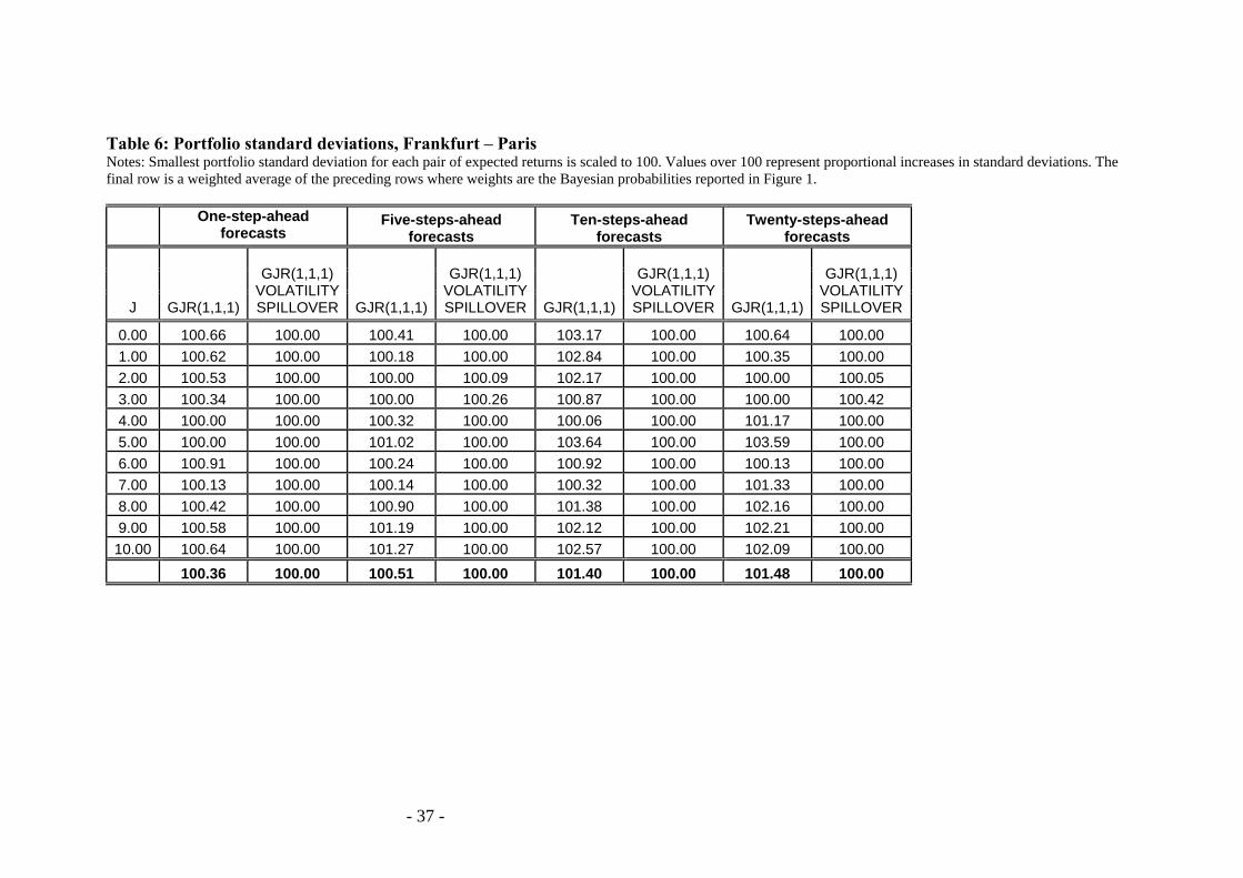
Table 6: Portfolio standard deviations, Frankfurt – Paris Notes: Smallest portfolio standard deviation for each pair of expected returns is scaled to 100. Values over 100 represent proportional increases in standard deviations. The final row is a weighted average of the preceding rows where weights are the Bayesian probabilities reported in Figure 1.





J GJR(1,1,1)





0.00 100.66 100.00 100.41 100.00 103.17 100.00 100.64 100.001.00 100.62 100.00 100.18 100.00 102.84 100.00 100.35 100.002.00 100.53 100.00 100.00 100.09 102.17 100.00 100.00 100.053.00 100.34 100.00 100.00 100.26 100.87 100.00 100.00 100.424.00 100.00 100.00 100.32 100.00 100.06 100.00 101.17 100.005.00 100.00 100.00 101.02 100.00 103.64 100.00 103.59 100.006.00 100.91 100.00 100.24 100.00 100.92 100.00 100.13 100.007.00 100.13 100.00 100.14 100.00 100.32 100.00 101.33 100.008.00 100.42 100.00 100.90 100.00 101.38 100.00 102.16 100.009.00 100.58 100.00 101.19 100.00 102.12 100.00 102.21 100.0010.00 100.64 100.00 101.27 100.00 102.57 100.00 102.09 100.00

100.36 100.00 100.51 100.00 101.40 100.00 101.48 100.00

- 37 -

Table 7: Diebold-Mariano tests for portfolio variance equality. GMM estimates of coefficients and robust p-values for the test that difference in portfolio variances (u) is jointly zero for all expected returns. An asterisk indicates rejection at the 1% (***), 5 % (**) or 10 % (*) level. Significant positive values for β indicate that portfolio variances are less under the volatility spillover model, negative values indicate that they are more.

Single moment condition Multiple moment conditions

Market pairing 1 step ahead 5-steps ahead

10 steps ahead

20-steps ahead 1 step ahead 5-steps

ahead 10 steps ahead

20-steps ahead

London –Frankfurt

0.009** (0.02)

0.152* (0.07)

0.315** (0.01)

0.174* (0.10)

0.002** (0.02)

0.060*** (0.00)

0.122* (0.06)

0.130 (0.00)

London - Paris

0.0079**

(0.05) 0.047 (0.34)

-0.030 (0.44)

-0.023 (0.72)

0.001* (0.10)

0.031*** (0.00)

-0.02*** (0.00)

-0.017*** (0.00)

Frankfurt -

Paris

0.010** (0.021)

0.047 (0.34)

0.291*** (0.01)

0.552* (0.10)

0.006*** (0.00)

0.032*** (0.00)

0.159*** (0.01)

0.386*** (0.00)

- 38 -

Table 8: Stochastic Dominance relations, one-step-ahead and two-steps-ahead forecasts. Bootstrapped P-values for tests of second degree stochastic dominance relations between pairs of portfolio returns where portfolios are formed on the basis of one- or two-step-ahead forecasts from the benchmark and volatility spillover models. Portfolio returns are a weighted average over all values of θ where weights are the Bayesian probabilities reported in Figure 1. An asterisk indicates rejection at the 1%(***), 5 % (**) or 10 % (*) level when the reverse null is not rejected. Failure to reject both nulls is inconclusive.

1-step-ahead 2-steps ahead

Null Hypothesis Null Hypothesis

Market pairing

Volatility Spillover

dominates Benchmark

Benchmark dominates Volatility Spillover

Volatility Spillover

dominates Benchmark

Benchmark dominates Volatility Spillover

London

Frankfurt

0.92 0.07* 0.92 0.07*

London Paris

0.93 0.00*** 0.88 0.04**

Frankfurt

Paris

0.06* 0.95 0.74 0.00***

Figure 1: Probability density functions

Empirical Bayesian estimate of the probability of assumed expected returns such that each pair is )2

cos( θπ

and )2

sin( θπ. Numerical values are listed in Table 5.

0

0.05

0.1

0.15

0.2

0.25

0 0.1 0.2 0.3 0.4 0.5 0.6 0.7 0.8 0.9 1

London-Paris London-Frankfurt Frankfurt-Paris

Prob

abili

ty

Theta

40

Figure 2: Daily stock index returns, 2 January 1992 – 4 July 2005. De-meaned daily equity index returns: London (FTSE), Frankfurt (DAX), Paris (CAC)

Jan-92 Jan-93 Jan-94 Jan-95 Jan-96 Jan-97 Jan-98 Jan-99 Jan-00 Jan-01 Jan-02 Jan-03 Jan-04 Jan-05

London Frankfurt Paris

41

Figure 3: Daily conditional variances, 2 January 1992 – 8 May 2002. In-sample conditional variance predictions from GJR(1,1,1) model.

0

2

4

6

8

10

12

Jan-92 Jan-93 Jan-94 Jan-95 Jan-96 Jan-97 Jan-98 Jan-99 Jan-00 Jan-01 Jan-02

London Paris Frankfurt

42

Figure 4: Daily conditional correlations, 2 January 1992 – 8 May 2002. In sample conditional correlation predictions from GJR(1,1,1) ADCC model.

0

0.1

0.2

0.3

0.4

0.5

0.6

0.7

0.8

0.9

1

Jan-92 Jan-93 Jan-94 Jan-95 Jan-96 Jan-97 Jan-98 Jan-99 Jan-00 Jan-01 Jan-02

London-Paris London-Frankfurt Frankfurt-Paris

43

Figure 2.1: Loss of portfolio efficiency as forecasting horizon increases, London-Frankfurt. Columns measure increase in portfolio standard deviation for benchmark over volatility spillover model, where the volatility spillover portfolio standard deviation is scaled to 100, and the benchmark is a proportional increase.

102

101.5

101

100.5

100

99.5

99 30 1 2 3 5 10 15 20 25

Forecasting (portfolio rebalancing) Horizon

44

Figure 2.2: Loss of portfolio efficiency as forecasting horizon increases, London-Paris. Columns measure increase in portfolio standard deviation for benchmark over volatility spillover model, where the volatility spillover portfolio standard deviation is scaled to 100, and the benchmark is a proportional increase.

99.60

99.80

100.00

100.20

100.40

100.60

100.80

1 2 3 5 10 15 20 25 30


45

Figure 2.3: Loss of portfolio efficiency as forecasting horizon increases, Frankfurt-Paris. Columns measure increase in portfolio standard deviation for benchmark over volatility spillover model, where the volatility spillover portfolio standard deviation is scaled to 100, and the benchmark is a proportional increase.

99.00

99.50

100.00

100.50

101.00

101.50

1 2 3 5 10 15 20 25 30


46

47

[0, ]

1 Volatility asymmetry was first introduced to the financial literature by Black (1976), and has since become a well-documented feature of volatility patterns hence a failure to account for asymmetries may result in distorted estimates of volatility spillover. See, for example, Nelson (1991), Koutmos (1992), Poon and Taylor, (1992), Campbell and Hentschel (1992), Bekaert and Wu (2000), and Wu (2001). 2 Glosten, Jagannathan and Runkle (1993). 3 Engle (2002) shows that a Bollerslev-Wooldridge (1992) covariance matrix gives consistent standard errors for the estimates. 4 We use a two-step estimation process following Engle (2002). Appendix 1 sets out details of the maximum likelihood procedure. 5 Datastream supplies London 16:00 data for a group of major markets. Codes for the series described here are FOOTC16(PI) , DAXIN16(PI), and CAC4016(PI). 6 Harju and Hussain (2005) find that the UK and German markets respond to each other’s innovations using intra-daily data. 7We note that daily returns to the DAX 30 have the largest unconditional variance of the three indices. 8 Estimated unconditional correlations are London-Frankfurt 0.77, London-Paris, 0.69 and Frankfurt-Paris, 0.66. 9 Appendix 2 presents results for forecasting horizons of 15, 25 and 30 days. 10 Following Engle and Colacito (2004), we also calculated a heteroscedasticity-adjusted measure of the Diebold-Mariano test-statistic and conduct the same hypothesis tests. Results, not reported here, were substantially unchanged. 11To make the test tractable, each pairing of returns distributions was shifted to the right by the same fixed positive amount, sufficient to ensure a lower bound of zero for a support π π% where π < ∞%

1 1( 1) 2

/ : <⎧⎪= : ≤ ≤ − + ,⎨⎪ − + / : − + ≤ ≤⎩

t

t B t BB t T B

T t B T B t Tω

t

. 12 Before forming the blocks, the returns from each portfolio are weighted to adjust for the number of times they are sampled in the overlapping blocks. The weights that follow the rule:

where ω is the weight and B is block size.

Valuing Volatility Spillovers - OPUS at UTS

Documents

Transcript of Valuing Volatility Spillovers - OPUS at UTS