Hedging Mismatched Currencies with Options and Futures

Hedging Mismatched Currencies with Options and Futures ∗

Donald LIEN �

University of Texas at San Antonio

Maurice K. S. TSE �

University of Hong Kong

Kit Pong WONG §

University of Hong Kong

November 2002

JEL classification: F23; F31; D81

Keywords: Options; Futures; Multiple currency risks; Hedging effectiveness

∗We would like to thank Ho Yin Yick for excellent research assistance.�Department of Economics, College of Business, University of Texas at San Antonio, 6900 North

Loop 1604 West, San Antonio, TX 78249-0631, U.S.A. Tel.: 210-458-7312, fax: 210-458-5837, e-mail:[email protected] (D. Lien).

�School of Economics and Finance, University of Hong Kong, Pokfulam Road, Hong Kong. Tel.: 852-2857-8636, fax: 852-2548-1152, e-mail: [email protected] (M. K. S. Tse).

§Corresponding author. School of Economics and Finance, University of Hong Kong, Pokfulam Road,Hong Kong. Tel.: 852-2859-1044, fax: 852-2548-1152, e-mail: [email protected] (K. P. Wong).

Hedging mismatched currencies 1

Hedging Mismatched Currencies with Options and Futures

Abstract

This paper develops an expected utility model of an exporting Þrm in a developing country wherecurrency derivative markets do not exist. The Þrm faces exchange rate risk exposure to a foreigncurrency cash ßow. To cross-hedge against this risk exposure, the Þrm uses currency futures andoptions between the foreign currency and a third currency. Since a triangular parity condition holdsamong the three given currencies, this available hedging opportunity, albeit incomplete, is provedto be useful in reducing the Þrm�s exchange rate risk exposure. We show that currency optionsare redundant under two rather restrictive conditions: (i) logarithmic utility functions and/or (ii)independent spot exchange rates. In a more realistic cross-hedging environment, we show thatcurrency options are optimally used by the Þrm to incompletely span the missing currency futuresbetween the domestic and foreign currencies. We also estimate the beneÞts of using currency optionsfor cross-hedging purposes. Hedging effectiveness is shown to be improved substantially.

JEL classification: F23; F31; D81

Keywords: Options; Futures; Multiple currency risks; Hedging effectiveness

1. Introduction

Since the collapse of the Bretton Woods Agreement in 1973, exchange rates have be-

come substantially volatile (Meese, 1990), making exchange rate risk management a fact of

Þnancial life (Rawls and Smithson, 1990). As documented by Bodnar, Hayt, and Marston

(1996, 1998) and Bodnar and Gebhardt (1999), the use of currency forwards, futures, and

options is the norm rather than the exception among non-Þnancial corporations.

While currency derivative markets are the hallmark of industrialized countries, they

are seldom readily available in less developed countries (LDCs) wherein capital markets are

embryonic and foreign exchange markets are heavily controlled.1 Also, in many of the newly

industrializing countries of Latin America and Asia PaciÞc, currency derivative markets are

1Even if currency forward contracts are available in some LDCs, they are deemed to be forward-coverinsurance schemes rather than Þnancial instruments whose prices are freely determined by market forces(Jacque, 1996).

https://www.researchgate.net/publication/227374176_Strategic_Risk_Management?el=1_x_8&enrichId=rgreq-82bcdeea-8a83-4bc0-b6d2-2592726f5afc&enrichSource=Y292ZXJQYWdlOzIyODg2NTQ5MTtBUzoxMDI0MDAwNDgyMzg1OThAMTQwMTQyNTQ4Mzk1NQ==

https://www.researchgate.net/publication/4727245_Currency_Fluctuations_in_the_Post-Bretton_Woods_Era?el=1_x_8&enrichId=rgreq-82bcdeea-8a83-4bc0-b6d2-2592726f5afc&enrichSource=Y292ZXJQYWdlOzIyODg2NTQ5MTtBUzoxMDI0MDAwNDgyMzg1OThAMTQwMTQyNTQ4Mzk1NQ==


just starting to develop in a rather slow pace.2 To indirectly hedge against their exchange

rate risk exposure, exporting Þrms in these countries are obliged to use derivative securities

on related currencies. Such an exchange rate risk management technique is referred to as

�cross-hedging� (Sercu and Uppal, 1985).

The purpose of this paper is to study the hedging decision of an exporting Þrm in a

developing country where currency derivatives markets do not exist. We are particularly

interested in examining the hedging role of currency options in the context of cross-hedging.3

To this end, we develop an expected utility model of the exporting Þrm facing exchange

rate uncertainty. There is a third country which has well-developed currency futures and

options markets. Since a triangular parity condition holds among the domestic, foreign,

and third currencies, this available hedging opportunity, albeit incomplete, remains useful

in reducing the Þrm�s exchange rate risk exposure. We show that currency options are

redundant under two rather restrictive conditions: (i) logarithmic utility functions and/or

(ii) independent spot exchange rates. In a more realistic cross-hedging environment, we

show that currency options are optimally used by the Þrm to incompletely span the missing

currency futures between the domestic and foreign currencies. The driving force is the

triangular parity condition which gives rise to an exchange rate risk that is multiplicative,

thereby non-linear, in nature. This source of non-linearity creates a hedging demand for

non-linear currency options, as distinct from that for linear currency futures.

To estimate the beneÞts of using currency options for cross-hedging purposes, we con-

sider a Taiwanese exporting Þrm which encounters a unit cash ßow denominated in one of

the Þve currencies: (i) the Australian dollar, (ii) the Indonesian Rupiah, (iii) the Japanese

yen, (iv) the Philippine peso, and (v) the Thai baht. The United States is taken as the

third country. We Þnd that including currency options in hedge positions always improves

the hedging effectiveness as compared to using currency futures alone for all of the Þve

2See Eiteman, Stonehill, and Moffett (1998) for a description of the currency regime and the status ofcurrency derivatives in many of these so-called �exotic currencies.�

3Indeed, as shown by Benninga and Blume (1985), investors in the Black-Scholes (1973) world wouldpurchase options only when their utility functions exhibit bizarre properties, which is highly unlikely. Seealso Leland (1980), Brennan and Solanki (1981), and Franke, Stapleton, and Subrahmanyam (1998) for thedemand for options in the setting of portfolio insurance.


currencies. The improvements in hedging effectiveness range from 3.89% (the Indonesia

rupiah) to 40.10% (the Australian dollar) and thus can be quite substantial.

This paper is closest in the spirit of Chang and Wong (2002) who also examine the

hedging role of currency options in the context of cross-hedging. The main difference is

on how market incompleteness is introduced. In Chang and Wong (2002), no derivative

securities exist for the foreign currency but there are currency futures and options between

the domestic and third currencies. The degree of incompleteness is less sever in their setting

because the hedging instruments are directly related to the domestic currency. The source of

non-linearity is shown to be quadratic in nature, which makes the analytical results elegant.

In our model, however, the hedging instruments do not involve the domestic currency and

the source of non-linearity is of a higher order, thereby making the analysis rather difficult.

Due to the more non-linear structure, the improvements in hedging effectiveness in our

setting are in general much higher than those reported by Chang and Wong (2002) when

currency options are included in hedge positions.4

The rest of the paper is organized as follows. In the next section, we develop an expected

utility model of an exporting Þrm facing multiple currency risks and cross-hedging oppor-

tunities. Section 3 derives sufficient conditions under which currency options are never

used by the Þrm. Section 4 shows how the Þrm can incompletely span the missing cur-

rency futures between the domestic and foreign currencies with currency options. Section

5 offers empirical evidence on the hedging effectiveness of including currency options for

cross-hedging purposes. The Þnal section concludes.

2. The model

Consider a one-period, two-date (0 and 1) model of an exporting Þrm domiciled in a

developing country where currency derivatives markets do not exist. At date 0, the Þrm

4In Chang and Wong (2002), the improvements in hedging effectiveness range from 0.6% to 5.34%.

https://www.researchgate.net/publication/227406368_Cross-Hedging_with_Currency_Options_and_Futures?el=1_x_8&enrichId=rgreq-82bcdeea-8a83-4bc0-b6d2-2592726f5afc&enrichSource=Y292ZXJQYWdlOzIyODg2NTQ5MTtBUzoxMDI0MDAwNDgyMzg1OThAMTQwMTQyNTQ4Mzk1NQ==




concludes a transaction in a foreign country, which results in a net foreign currency cash

ßow, X , to be received at date 1. While the size of X is known with certainty ex ante, the

Þrm does not know the then prevailing spot exchange rate at date 1, denoted by �S, which

is expressed in units of the domestic currency per unit of the foreign currency.5 The Þrm

as such encounters exchange rate risk exposure of �SX.

To hedge against its exchange rate risk exposure, the Þrm has to rely on a related

currency of a third country which has well-developed currency derivative markets. DeÞne

�S1 as the spot exchange rate of the domestic currency against the third currency at date

1. Likewise, deÞne �S2 as the spot exchange rate of the third currency against the foreign

currency at date 1. Based on these two spot exchange rates, one can derive the cross-rate of

the domestic currency against the foreign currency at date 1 as �S1�S2. It follows immediately

from the Law of One Price that �S = �S1�S2. Such a triangular parity condition is depicted

in Figure 1.

�S = �S1�S2

�S1�S2

home country foreign country@@

@@

@@

@@

¡¡

¡¡

¡¡

¡¡

third country

Figure 1. Triangular parity condition

At date 0, the Þrm can trade inÞnitely divisible currency futures and options (calls and

puts) which call for delivery of the third currency per unit of the foreign currency at date

1. Without any loss of generality, we restrict the Þrm to use currency futures and put

options only.6 Furthermore, for the pure sake of simplicity, we consider only one strike5Throughout the paper, random variables have a tilde (∼) while their realizations do not.6Because payoffs of any combinations of futures, calls, and puts can be replicated by any two of these

three Þnancial instruments (Sercu and Uppal, 1995), one of them is redundant.


price, denoted by K, for the currency put options. The strike price, K, is exogenously

determined, thereby not a choice variable of the Þrm. Let F be the futures price at date

0 and P be the premium on the currency put options, where P is compounded to date 1.

To isolate the Þrm�s hedging motive from its speculative motive, it suffices to restrict our

attention to the case where the currency futures and put options are perceived as jointly

unbiased by the Þrm. As such, we assume throughout the paper that F equals the expected

value of �S2 and P equals that of max(K − �S2, 0).7

The Þrm�s date 1 proÞt denominated in the domestic currency is given by

�Π = �S1�S2X + �S1(F − �S2)H + �S1[P −max(K − �S2, 0)]Z, (1)

where H and Z are the numbers of the currency futures and put options sold (purchased

if negative) by the Þrm at date 0, respectively. The Þrm possesses a von Neumann-

Morgenstern utility function, U(Π), deÞned over its domestic currency proÞt, Π, with

U 0(Π) > 0 and U 00(Π) < 0, indicating the presence of risk aversion.8

The Þrm is an expected utility maximizer and has to solve the following ex ante decision

problem at date 0:

maxH,Z

E[U(�Π)], (2)

where E(·) is the expectation operator with respect to the Þrm�s subjective joint probabil-ity distribution function of �S1 and �S2, and �Π is deÞned in equation (1). The Þrst-order

conditions for program (2) are given by

E[U 0(�Π∗) �S1(F − �S2)] = 0, (3)

E{U 0(�Π∗) �S1[P −max(K − �S2, 0)]} = 0, (4)

7Our intention here is not to impose an ad hoc option pricing theory but to focus on the hedging role ofthe put currency options.

8For privately held, owner-managed Þrms, risk-averse behavior prevails. Even for publicly listed Þrms,managerial risk aversion (Stulz, 1984), corporate taxes (Smith and Stulz, 1985), costs of Þnancial distress(Smith and Stulz, 1985), and capital market imperfections (Stulz, 1990; and Froot, Scharfstein, and Stein,1993) all imply a concave objective function for Þrms, thereby justifying the use of risk aversion as anapproximation. See Tufano (1996) for evidence that managerial risk aversion is a rationale for corporate riskmanagement in the gold mining industry.


where an asterisk (∗) indicates an optimal level.9

3. Redundancy of options

Since F = E( �S2) and P = E[max(K − �S2, 0)], we can write equations (3) and (4) as10

Cov[U 0(�Π∗) �S1, �S2] = 0, (5)

Cov[U 0(�Π∗) �S1,max(K − �S2, 0)] = 0, (6)

where Cov(·, ·) is the covariance operator with respect to the Þrm�s subjective joint proba-bility distribution function of �S1 and �S2. Partially differentiating E[U

0(�Π∗) �S1|S2] yields

∂

∂S2E[U 0(�Π∗) �S1|S2] = E

½U 0(�Π∗)[1−R(�Π∗)]∂

�S1

∂S2

+U 00(�Π∗) �S21

·X −H∗ − ∂

∂S2max(K − S2, 0)Z

∗¸¯̄̄̄S2

¾, (7)

where R(Π) = −ΠU 00(Π)/U 0(Π) is the Arrow-Pratt measure of relative risk aversion. If∂ �S1/∂S2 ≡ 0 (i.e., �S1 and �S2 are independent), or if R(Π) ≡ 1 for all Π (i.e., U(Π) is

logarithmic), it is evident from equation (7) that E[U 0(�Π∗) �S1|S2] would be invariant to

different realizations of �S2 when H∗ = X and Z∗ = 0 and thus equations (5) and (6) hold

simultaneously.

To see the underlying intuition, consider Þrst the case that the Þrm�s utility function,

U(Π), is logarithmic. In this case, the objective function of program (2) becomes

E(ln �Π) = E(ln �S1) + E

½ln{ �S2X + (F − �S2)H + [P −max (K − �S2, 0)]Z}

¾.

It is evident that �S1 does not affect the Þrm�s optimal hedge position and thus the celebrated

full-hedging theorem applies. Now, consider the case where the two random spot exchange9The second-order conditions for a maximum are satisÞed given risk aversion.

10For any two random variables, �X and �Y , Cov( �X, �Y ) = E( �X �Y )− E( �X)E( �Y ).


rates, �S1 and �S2, are independent. When H = X and Z = 0, equation (1) implies that

�Π = �S1FX. Thus, it follows that equations (5) and (6) hold simultaneously at H∗ = X and

Z∗ = 0. In either case, the currency put options are not used by the Þrm for cross-hedging

purposes.

4. Hedging role of options

In the previous section, we have shown that currency options are redundant under

logarithmic utility functions and/or independent spot exchange rates. However, it is unduly

restrictive to assume either condition to hold. In other words, in a more realistic cross-

hedging environment, we would expect currency options to be an integral part of the optimal

hedge positions of exporting Þrms in developing countries.

To verify the above conjecture, let us consider the following simple example. Suppose

that �S1 = S1 + β�θ and �S2 = S2 + �θ, where Si is the expected value of �Si (i = 1, 2), β is

a scalar, and �θ is a zero-mean random variable. Thus, �S1 and �S2 are perfectly negatively

(positively) correlated if β < (>) 0. Let �θ take on three possible values: −Θ with probabilityp, 0 with probability 1− 2p, and Θ with probability p. Then, we have

�S = �S1�S2 = (S1 + β�θ)(S2 + �θ) = S1S2 + (S1 + βS2)�θ + β�θ

2. (8)

Given the assumed three-point probability distribution function of �θ, we have �θ2 = Θ[�θ +

2max(−�θ, 0)]. Thus, using this fact and equation (8), the exchange rate risk exposure facedby the Þrm is given by

�SX = S1S2X + (S1 + βS2 + βΘ)�θX + 2βΘmax(−�θ, 0)X. (9)

Let K = F . Since F equals the expected value of �S2, we have F = K = S2. Then, the

payoff of a hedge position, (H,Z), is given by

�V = (S1 + β�θ){�θH + [max(−�θ, 0)− P ]Z}. (10)


Given the assumed three-point probability distribution function of �θ, we have �θ2 = Θ[�θ +

2max(−�θ, 0)] and �θmax(−�θ, 0) = −Θmax(−�θ, 0). Thus, equation (10) can be written as

�V = [(S1 + βΘ)H − βPZ]�θ + [2βΘH + (S1 − βΘ)Z]max(−�θ, 0)− S1PZ. (11)

Inspection of equations (9) and (11) reveals that the Þrm�s exchange rate risk exposure can

be completely eliminated by the hedge position, (H∗, Z∗), which satisÞes

[S1 + βS2 + βΘ]X = (S1 + βΘ)H∗ − βPZ∗, (12)

2βΘX = 2βΘH∗ + (S1 − βΘ)Z∗. (13)

Solving equations (12) and (13) yields

H∗ = X − S1 − βΘ2βΘ

Z∗,

Z∗ = − 2β2S2ΘX

(S1 − βΘ)(S1 + βΘ) + 2β2PΘ.

As long as β 6= 0, we have Z∗ < 0. Thus, in order to synthesize a short position of the

missing currency futures between the domestic and foreign currencies, a long position of

the currency put options between the foreign and third currencies is called for irrespective

of whether �S1 and �S2 are negatively or positively correlated.

In general, complete spanning of the missing currency futures contracts between the

domestic and foreign currencies is not feasible. To facilitate the empirical study of hedging

effectiveness in the next section, we hereafter restrict our attention to the case where the

Þrm�s objective is to minimize the variance of its domestic currency proÞt:

minH,Z

Var(�Π) = E{[ �Π− E(�Π)]2}, (14)

where Var(·) is the variance operator with respect to the Þrm�s subjective joint probabilitydistribution function of �S1 and �S2, and �Π is deÞned in equation (1).


The Þrst-order conditions for program (14) are given by

Cov[�Π∗, �S1(F − �S2)] = 0, (15)

Cov{�Π∗, �S1[P −max(K − �S2, 0)]} = 0. (16)

where an asterisk (∗) indicates an optimal level.11 Solving equations (15) and (16) yields H∗

Z∗

= −A−1BX, (17)

where

A =

Var[ �S1(F − �S2)] Cov{ �S1(F − �S2), �S1[P −max(K − �S2, 0)]}

Cov{ �S1(F − �S2), �S1[P −max(K − �S2, 0)]} Var{ �S1[P −max(K − �S2, 0)]}

,

B =

Cov[ �S1�S2, �S1(F − �S2)]

Cov{ �S1�S2, �S1[P −max(K − �S2, 0)]}

.Inspection of equation (17) reveals that Z∗ is in general non-zero. However, without speci-

fying the underlying joint probability distribution function of �S1 and �S2, the sign of Z∗ is

a priori indeterminate.

When the currency put options are absent (i.e., Z ≡ 0), it is easily shown that the Þrm�soptimal futures position, H0, is given by

H0 = −Cov[�S1�S2, �S1(F − �S2)]

Var[ �S1(F − �S2)]. (18)

The sign of H0 is opposite to that of Cov[ �S1�S2, �S1(F − �S2)], which is also a priori indeter-

minate without knowing the functional form of the joint probability distribution function

of �S1 and �S2.

11The second-order conditions for a minimum are satisÞed.


5. Hedging effectiveness

To implement the empirical tests, we assume that �S1 and �S2 are jointly log-normally

distributed: ln �S1

ln �S2

∼ N µ1

µ2

, σ2

1 ρσ1σ2

ρσ1σ2 σ22

.

Alternatively, we can write �S1 = exp(µ1 + σ1�ε1) and �S2 = exp(µ2 + σ2�ε2), where �ε1 and �ε2

are both standard normal random variables with Cov(�ε1, �ε2) = ρ. In Appendix A, we prove

the following useful result:

E

µ�Sm1 �S

n2 I{S̃2<K}

¶= exp

µmµ1 + nµ2 +

m2σ21

2+mnρσ1σ2 +

n2σ22

2

¶

× ΦµlnK − µ2

σ2−mρσ1 − nσ2

¶, (19)

where I{S̃2<K} is the indicator function for the event that�S2 < K, and Φ(·) is the cumulative

standard normal distribution function.

Equation (19) can be used repeatedly to express all the moments in equation (17) as

functions of the underlying distribution parameters. For example, by setting m = 0, n = 1,

and K =∞ in equation (19), we have

F = E( �S2) = exp

µµ2 +

σ22

2

¶. (20)

Note that

P = E[max(K − �S2, 0)] = E

·(K − �S2)I{S̃2<K}

¸= KE

µI{S̃2<K}

¶− E

µ�S2I{S̃2<K}

¶.

The Þrst term on the right-hand side of the above equation corresponds to equation (19)

when m = n = 0 and the second term to m = 0 and n = 1. Thus, we have

P = KΦ

µlnK − µ2

σ2

¶− E( �S2)Φ

µlnK − µ2

σ2− σ2

¶.


When K = E( �S2), the above equation can be further reduced to

P = exp

µµ2 +

σ22

2

¶·1− 2Φ

µ− σ2

2

¶¸. (21)

In Appendix B, we report all the variances and covariances contained in equation (17)

in terms of the underlying distribution parameters. It is interesting to observe that µ1 and

µ2, albeit essential for all the relevant moments, do not appear in the ultimate optimal

hedge ratios. As such, no information on the means of ln �S1 and ln �S2 is needed for Þnding

the optimal hedge rations.

The empirical exercises are as follows. We always refer to Taiwan as the home country

and the United States as the third country. The foreign currency cash ßow, X, is normalized

to one unit of the foreign currency so that the Þrm�s hedge position is simply the hedge

ratio. The prices of the currency futures and put options with K = F are artiÞcially set

equal to equations (20) and (21), respectively. The data on daily spot exchange rates are

extracted from Datastream for the period from January 1, 1997 to December 31, 2001.

We Þrst consider Japan as the foreign country. In this case, �S1 is the random spot

exchange rate for the Taiwanese dollar against the US dollar (NTD/USD) and �S2 is that

for the US dollar against the Japanese yen (USD/JPY). Since we assume that �S1 and �S2

are jointly log-normally distributed, the logs of these two random variables provide us the

time series, lnS1,t and lnS2,t, for our empirical analysis.

Applying the Perron-Philips tests for unit roots (Philips and Perron, 1988) to the

NTD/USD series, the Perron-Philips statistic for lnS1,t is −1.712 and that for the Þrstdifference of lnS1,t is −15.55. The hypothesis of a unit root cannot be rejected in theformer but can be rejected in the latter. For the USD/JPY series, the two Perron-Philips

statistics are −1.649 and −35.70, respectively. Once again, we cannot reject the hypothesisof a unit root in lnS2,t but can reject that in the Þrst difference of lnS2,t. As such, both

lnSi,t and lnS2,t are integrated of order one, i.e., I(1). Using the Johansen (1988) method,

we Þnd that lnS1,t and lnS2,t are cointegrated. The cointegrating variable is given by

zt = lnS2,t + 0.9925 lnS1,t − 1.3413, (22)


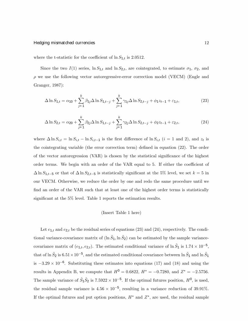
where the t-statistic for the coefficient of lnS1,t is 2.0512.

Since the two I(1) series, lnS1,t and lnS2,t, are cointegrated, to estimate σ1, σ2, and

ρ we use the following vector autoregressive-error correction model (VECM) (Engle and

Granger, 1987):

∆ lnS1,t = α10 +kXj=1

β1j∆ lnS1,t−j +kXj=1

γ1j∆ lnS2,t−j + φ1zt−1 + ε1,t, (23)

∆ lnS2,t = α20 +kXj=1

β2j∆ lnS1,t−j +kXj=1

γ2j∆ lnS2,t−j + φ2zt−1 + ε2,t, (24)

where ∆ lnSi,t = lnSi,t − lnSi,t−1 is the Þrst difference of lnSi,t (i = 1 and 2), and zt is

the cointegrating variable (the error correction term) deÞned in equation (22). The order

of the vector autoregression (VAR) is chosen by the statistical signiÞcance of the highest

order terms. We begin with an order of the VAR equal to 5. If either the coefficient of

∆ lnS1,t−5 or that of ∆ lnS2,t−5 is statistically signiÞcant at the 5% level, we set k = 5 in

our VECM. Otherwise, we reduce the order by one and redo the same procedure until we

Þnd an order of the VAR such that at least one of the highest order terms is statistically

signiÞcant at the 5% level. Table 1 reports the estimation results.

(Insert Table 1 here)

Let e1,t and e2,t be the residual series of equations (23) and (24), respectively. The condi-

tional variance-covariance matrix of (ln �S1, ln �S2) can be estimated by the sample variance-

covariance matrix of (e1,t, e2,t). The estimated conditional variance of ln �S1 is 1.74× 10−5,

that of ln �S2 is 6.51×10−5, and the estimated conditional covariance between ln �S1 and ln �S1

is −3.29 × 10−6. Substituting these estimates into equations (17) and (18) and using the

results in Appendix B, we compute that H0 = 0.6822, H∗ = −0.7280, and Z∗ = −2.5756.The sample variance of �S1

�S2 is 7.5922× 10−5. If the optimal futures position, H0, is used,

the residual sample variance is 4.56 × 10−5, resulting in a variance reduction of 39.91%.

If the optimal futures and put option positions, H∗ and Z∗, are used, the residual sample


variance is 2.91×10−5, resulting in variance reductions of 61.68% compared to the no hedge

case and 36.22% compared to using the currency futures as the sole hedging instrument.

As a robustness check, we also separately consider four other currencies as the foreign

currency: (i) the Australian dollar, (ii) the Indonesian rupiah, (iii) the Philippine peso, and

(iv) the Thai baht. Tables 2 to 5 present the estimation results for the VECM of each of

these four currencies.12

(Insert Tables 2 to 5 here)

Table 6 reports the optimal hedge positions and the resulting hedging effectiveness for

each of the above currencies, including the Japanese yen. As shown in Table 6, using the

currency futures and put options for cross-hedging purposes results in variance reductions

ranging from 61.24% (the Philippine peso) to 94.86% (the Indonesian rupiah) as compared

to the no hedge case. When the hedging effectiveness with and without using the currency

put options are contrasted, we Þnd that including the currency options always contributes

positively to further variance reductions among all Þve currencies. The improvements in

hedging effectiveness range from 3.89% (the Indonesia rupiah) to 40.10% (the Australian

dollar) and thus can be quite substantial.

(Insert Table 6 here)

6. Conclusions

In the post-Bretton Woods era, exchange rates have been increasingly volatile, making

non-Þnancial Þrms take exchange rate risk management very seriously. This paper has stud-

ied how a risk-averse exporting Þrm, confronting a foreign currency cash ßow but possessing

no direct hedging opportunities, can employ derivative securities on a related currency to re-

12We consider a partial cointegrating system for each of these currencies. A complete cointegrating systemthat includes all these currencies is not examined.


duce its exchange rate risk exposure. Currency options play no role as a hedging instrument

under two rather restrictive conditions of logarithmic utility functions and/or independent

spot exchange rates. In a more realistic cross-hedging environment, we have shown how the

Þrm can use currency options to incompletely replicate the missing risk-sharing contract.

The driving force is a triangular parity condition which gives rise to an exchange rate risk

that is multiplicative, thereby non-linear, in nature. This source of non-linearity creates a

hedging demand for non-linear currency options, as distinct from that for linear currency

futures.

Cross-hedging is important because it expands the opportunity set of hedging alterna-

tives. Given the fact that currency derivative markets are not readily available in developing

countries and are just starting to develop in many of the newly industrializing countries

of Latin America and Asia PaciÞc, it is clear that, for many exporting Þrms exposed to

currencies of these countries, cross-hedging will continue to be a major risk management

technique for the reduction of their foreign exchange risk exposure.


Appendix

A. Derivation of equation (19)

Using the fact that �Si = exp(µi + σi�εi), i = 1 and 2, we have

E

µ�Sm1�Sn2 I{S̃2<K}

¶=

1

2πp1− ρ2

Z ∞

−∞

Z lnK−µ2σ2

−∞exp[m(µ1 + σ1ε1)] exp[n(µ2 + σ2ε2)]

× exp

·− ε

21 + ε

22 − 2ρε1ε2

2(1− ρ2)

¸dε1 dε2

=1

2πp1− ρ2

Z ∞

−∞exp

·m(µ1 + σ1ε1)− ε2

1

2(1− ρ2)

¸

×½Z lnK−µ2

σ2

−∞exp[n(µ2 + σ2ε2)] exp

·− ε

22 − 2ρε1ε2

2(1− ρ2)

¸dε2

¾dε1

=exp(mµ1 + nµ2)

2πp1− ρ2

Z ∞

−∞exp

½mσ1ε1 +

[ρε1 + (1− ρ2)nσ2]2 − ε2

1

2(1− ρ2)

¾

×½Z lnK−µ2

σ2

−∞exp

½− [ε2 − ρε1 − (1− ρ2)nσ2]

2

2(1− ρ2)

¾dε2

¾dε1

=1√2πexp

µmµ1 + nµ2 +

m2σ21

2+mnρσ1σ2 +

n2σ22

2

¶

×Z ∞

−∞exp

·− (ε1 −mσ1 − nρσ2)

2

2

¸Φ

· lnK−µ2σ2

− ρε1 − (1− ρ2)nσ2p1− ρ2

¸dε1

=1√2πexp

µmµ1 + nµ2 +

m2σ21

2+mnρσ1σ2 +

n2σ22

2

¶

×Z ∞

−∞exp

µ− z

2

2

¶Φ

µ lnK−µ2

σ2− ρz −mρσ1 − nσ2p

1− ρ2

¶dz

=1√2πexp

µmµ1 + nµ2 +

m2σ21

2+mnρσ1σ2 +

n2σ22

2

¶


× Ez·Φ

µ lnK−µ2σ2

− ρz −mρσ1 − nσ2p1− ρ2

¶¸, (A-1)

where z = ε1−mσ1−nρσ2 is a standard normal random variable and Ez(·) is the expectationoperator with respect to Φ(z). Lien (1985) shows that

Ez[Φ(α+ βz)] = Φ

µαp1 + β2

¶. (A-2)

Using equation (A-2) by setting α = lnK−µ2

σ2−mρσ1−nσ2 and β =

ρ√1−ρ2

, equation (A-1)

reduces to equation (19).

B. Derivation of variances and covariances

Note that Var[ �S1(F − �S2)] = E[ �S21(F − �S2)

2]−E[ �S1(F − �S2)]2, which can be written as

E( �S21)F

2 − 2E( �S21�S2)F + E( �S

21�S2

2)− E( �S1)2F 2 + 2E( �S1)E( �S1

�S2)F − E( �S1�S2)

2.

Using equation (19) repeatedly, we have

Var[ �S1(F − �S2)] =M × [exp(σ21)− 2 exp(σ2

1 + 2ρσ1σ2) + exp(σ21 + 4ρσ1σ2 + σ

22)

−1 + 2 exp(ρσ1σ2)− exp(2ρσ1σ2)],

where M = exp(2µ1 + 2µ2 + σ21 + σ

22). Similarly, we can show that

Cov[ �S1�S2, �S1(F − �S2)] =M × [exp(2σ2

1 + 2ρσ1σ2)− exp(σ21 + 4ρσ1σ2 + σ

22)

− exp(ρσ1σ2) + exp(2ρσ1σ2)],

Var{ �S1[P −max(K − �S2, 0)]} =M ×½exp(σ2

1)

·2Φ

µσ2

2

¶− 1

¸·2Φ

µσ2

2

¶− 1− 2Φ

µσ2

2− 2ρσ1

¶¸

+4 exp(σ21 + 2ρσ1σ2)

·Φ

µσ2

2

¶− 1

¸Φ

µ− σ2

2− 2ρσ1

¶


+ exp(σ21)Φ

µσ2

2− 2ρσ1

¶+ exp(σ2

1 + 4ρσ1σ2 + σ22)Φ

µ− 3σ2

2− 2ρσ1

¶

−·2Φ

µσ2

2

¶− 1− Φ

µσ2

2− ρσ1

¶+ exp(ρσ1σ2)Φ

µ− σ2

2− ρσ1

¶¸2¾,

Cov{ �S1(F − �S2), �S1[P −max(K − �S2, 0)]} =M ×½[exp(σ2

1)− exp(σ21 + 2ρσ1σ2)]

·2Φ

µσ2

2

¶− 1

¸

− exp(σ21)Φ

µσ2

2− 2ρσ1

¶+ 2exp(σ2

1 + 2ρσ1σ2)Φ

µ− σ2

2− 2ρσ1

¶

− exp(σ21 + 4ρσ1σ2 + σ

22)Φ

µ− 3σ2

2− 2ρσ1

¶

−[1− exp(ρσ1σ2)]

·1− Φ

µσ2

2− ρσ1

¶+ exp(ρσ1σ2)Φ

µ− σ2

2− ρσ1

¶¸¾,

Cov{ �S1�S2, �S1[P −max(K − �S2, 0)]} =M ×

½[exp(σ2

1 + 2ρσ1σ2)− exp(ρσ1σ2)]

·2Φ

µσ2

2

¶− 1

¸

− exp(σ21 + 2ρσ1σ2)Φ

µ− σ2

2− 2ρσ1

¶− exp(2ρσ1σ2)Φ

µ− σ2

2− ρσ1

¶¾

+2 exp(σ21 + 4ρσ1σ2 + σ

22)Φ

µ− 3σ2

2− 2ρσ1

¶+ exp(ρσ1σ2)Φ

µσ2

2− ρσ1

¶,

Var( �S1S2) =M × [exp(σ21 + 4ρσ1σ2 + σ

22)− exp(2ρσ1σ2)].


References

Benninga, S., and M. E. Blume, 1985, �On the Optimality of Portfolio Insurance.� Journal

of Finance 40, 1341�1352.

Black, F., and M. J. Scholes, 1973, �The Pricing of Options and Corporate Liabilities.�

Journal of Political Economy 81, 637�659.

Bodnar, G. M., and G. Gebhardt, 1999, �Derivatives Usage in Risk Management by US

and German Non-Financial Firms: A Comparative Survey.� Journal of International

Financial Management and Accounting 10, 153�187.

Bodnar, G. M., G. Hayt, and R. C. Marston, 1996, �1995 Wharton Survey of Derivative

Usage by US Non-Financial Firms.� Financial Management 25, 113�133.

Bodnar, G. M., G. Hayt, and R. C. Marston, 1998, �1998 Wharton Survey of Financial

Risk Management by US Non-Financial Firms.� Financial Management 27, 70�91.

Brennan, M. J., and R. Solanki, 1981, �Optimal Portfolio Insurance.� Journal of Financial

and Quantitative Analysis 16, 279�300.

Chang, E. C., and K. P. Wong, 2002, �Cross-Hedging with Currency Options and Futures.�

Journal of Financial and Quantitative Analysis, forthcoming.

Eiteman, D. K., A. I. Stonehill, and M. H. Moffett, 1998, Multinational Business Finance.

Massachusetts: Addison-Wesley.

Engle, R. F., and C. W. J. Granger, 1987, �Co-integration and Error Correction: Repre-

sentation, Estimation and Testing.� Econometrica 66, 251�276.

Franke, G., R. C. Stapleton, and M. G. Subrahmanyam, 1998, �Who Buys and Who Sells

Options: The Role of Options in an Economy with Background Risk.� Journal of

Economic Theory 82, 89�109.

Froot, K. A., D. S. Scharfstein, and J. C. Stein, 1993, �Risk Management: Coordinating

Corporate Investment and Financing Policies,� Journal of Finance 48, 1629�1658.


Jacque, L. L., 1996, Management and Control of Foreign Exchange Risk. Boston: Kluwer

Academic Publishers.

Johansen, S., 1988, �Statistical Analysis of Cointegration Vectors.� Journal of Economic

Dynamics and Control 12, 231�254.

Leland, H. E., 1980, �Who Should Buy Portfolio Insurance.� Journal of Finance 35, 581�

594.

Lien, D., 1985, �Moments of Truncated Bivariate Log-Normal Distributions.� Economics

Letters 19, 243�247.

Meese, R., 1990, �Currency Fluctuations in the Post-Bretton Woods Era.� Journal of

Economic Perspectives 4, 117�134.

Philips, P. C. B., and P. Perron, 1988, �Testing for a Unit Root in Time Series Regressions.�

Biometrika 75, 335�346.

Rawls, S. W., and C. W. Smithson, 1990, �Strategic Risk Management.� Journal of Applied

Corporate Finance 1, 6�18.

Sercu, P., and R. Uppal, 1995, International Financial Markets and the Firm. Cincinnati:

South-Western College Publishing.

Smith, C. W., and R. Stulz, 1985, �The Determinants of Firms� Hedging Policies.� Journal

of Financial and Quantitative Analysis 20, 391�405.

Stulz, R., 1984, �Optimal Hedging Policies.� Journal of Financial and Quantitative Analy-

sis 19, 127�140.

Stulz, R., 1990, �Managerial Discretion and Optimal Financial Policies.� Journal of Finan-

cial Economics 26, 3�27.

Tufano, P., 1996, �Who Manages Risk? An Empirical Examination of Risk Management

Practices in the Gold Mining Industry.� Journal of Finance 51, 1097�1137.


Table 1. Estimates of the VECM: The Japanese Yen

Variable ∆ lnS1,t ∆ lnS2,t

Constant 0.0002 −0.0001(0.0001) (0.0002)

zt−1 −0.0030 −0.0030(0.0014) (0.0027)

∆ lnS1,t−1 −0.0590 −0.0023(0.0279) (0.0539)

∆ lnS1,t−2 −0.0726 −0.0220(0.0278) (0.0539)

∆ lnS1,t−3 0.0600 −0.0504(0.0277) (0.0535)

∆ lnS2,t−1 −0.0628 0.0113(0.0144) (0.0280)

∆ lnS2,t−2 −0.0262 0.0278(0.0145) (0.0282)

∆ lnS2,t−3 0.0010 −0.0222(0.0146) (0.0282)

R2 0.0317 0.0031

F-statistic 6.0411 0.5683

This table shows the estimates of the VECM in equations (23) and (24). S1,t is the spot

exchange rate for the Taiwanese dollar against the US dollar and S2,t is that for the US

dollar against the Japanese yen. ∆ lnSi,t = lnSi,t − lnSi,t−1 is the Þrst difference of lnSi,t(i = 1 and 2), and zt is the the error correction term deÞned in equation (22). The order

of the VAR is 3. The numbers in parentheses are the standard errors.


Table 2. Estimates of the VECM: The Australian Dollar


Constant 0.0002 −0.0003(0.0001) (0.0002)

zt−1 −0.0018 0.0009(0.0008) (0.0015)

∆ lnS1,t−1 −0.0497 −0.1529(0.0278) (0.0491)

∆ lnS1,t−2 −0.0750 −0.0085(0.0278) (0.0490)

∆ lnS1,t−3 0.0586 −0.0085(0.0277) (0.0490)

∆ lnS2,t−1 −0.0480 −0.0554(0.0158) (0.0279)

∆ lnS2,t−2 −0.0438 −0.0054(0.0159) (0.0281)

∆ lnS2,t−3 −0.0050 −0.0307(0.0158) (0.0280)

R2 0.0271 0.0111




dollar against the Australian dollar. ∆ lnSi,t = lnSi,t − lnSi,t−1 is the Þrst difference of

lnSi,t (i = 1 and 2), and zt = lnS2,t + 3.0838 lnS1,t − 10.1897 is the error correction term.The order of the VAR is 3. The numbers in parentheses are the standard errors.


Table 3. Estimates of the VECM: The Indonesian Rupiah


Constant 0.0002 −0.0011(0.0001) (0.0009)

zt−1 0.0001 −0.0119(0.0005) (0.0038)

∆ lnS1,t−1 −0.0650 −0.2770(0.0283) (0.2113)

∆ lnS1,t−2 −0.0875 0.3370(0.0281) (0.2100)

∆ lnS1,t−3 0.0596 −0.0328(0.0281) (0.2098)

∆ lnS2,t−1 −0.0125 0.0366(0.0038) (0.0281)

∆ lnS2,t−2 −0.0144 0.0130(0.0038) (0.0283)

∆ lnS2,t−3 −0.0011 −0.0447(0.0038) (0.0283)

R2 0.0298 0.0150




dollar against the Indonesian rupiah. ∆ lnSi,t = lnSi,t − lnSi,t−1 is the Þrst difference of

lnSi,t (i = 1 and 2), and zt = lnS2,t + 6.0202 lnS1,t − 11.9543 is the error correction term.The order of the VAR is 3. The numbers in parentheses are the standard errors.


Table 4. Estimates of the VECM: The Philippine Peso


Constant 0.0002 −0.0005(0.0001) (0.0003)

zt−1 −0.0010 0.0008(0.0005) (0.0012)

∆ lnS1,t−1 −0.0626 −0.1654(0.0281) (0.0639)

∆ lnS1,t−2 −0.0814 0.0883(0.0281) (0.0638)

∆ lnS1,t−3 0.0660 −0.1110(0.0280) (0.0636)

∆ lnS2,t−1 −0.0506 0.0795(0.0123) (0.0281)

∆ lnS2,t−2 −0.0281 −0.0062(0.0124) (0.0282)

∆ lnS2,t−3 0.0006 −0.0671(0.0124) (0.0282)

R2 0.0317 0.0238




dollar against the Philippine peso. ∆ lnSi,t = lnSi,t− lnSi,t−1 is the Þrst difference of lnSi,t(i = 1 and 2), and zt = lnS2,t + 5.3720 lnS1,t − 14.8923 is the error correction term. Theorder of the VAR is 3. The numbers in parentheses are the standard errors.


Table 5. Estimates of the VECM: The Thai Baht


Constant 0.0002 −0.0004(0.0001) (0.0003)

zt−1 −0.0024 0.0047(0.0009) (0.0023)

∆ lnS1,t−1 −0.0746 −0.1525(0.0281) (0.0724)

∆ lnS1,t−2 −0.0826 0.0866(0.0280) (0.0723)

∆ lnS1,t−3 0.0702 −0.2952(0.0277) (0.0716)

∆ lnS2,t−1 −0.0598 0.0254(0.0108) (0.0280)

∆ lnS2,t−2 −0.0301 −0.0055(0.0109) (0.0282)

∆ lnS2,t−3 0.0029 −0.1397(0.0109) (0.0283)

R2 0.0486 0.0375




dollar against the Thai baht. ∆ lnSi,t = lnSi,t − lnSi,t−1 is the Þrst difference of lnSi,t(i = 1 and 2), and zt = lnS2,t + 3.5004 lnS1,t − 8.6343 is the error correction term. Theorder of the VAR is 3. The numbers in parentheses are the standard errors.


Table 6. Optimal Hedge Ratios and Hedging Effectiveness

Currency Australian Indonesian Japanese Philippine ThaiDollar Rupiah Yen Peso Baht

H0 0.6470 0.9606 0.6822 0.7436 0.7909

H∗ −0.6461 1.0467 −0.7280 −0.4039 0.2556

Z∗ −2.4354 0.1691 −2.5756 −2.0476 −0.9658ProÞt 6.8222 95.2910 7.5922 9.6244 11.7930Variance

Residual 4.5409 5.0983 4.5625 4.6257 4.6615Variancewith Futures

Residual 2.7200 4.9000 2.9100 3.7300 4.3400Variancewith Futuresand Options

Hedging 33.44% 94.65% 39.91% 51.94% 60.47%Effectivenesswith Futures

Hedging 60.13% 94.86% 61.68% 61.24% 63.20%Effectivenesswith Futuresand Options

This table shows the estimates of the optimal hedge ratios in equations (17) and (18).

Hedging effectiveness is gauged by the percentage decrease in variance relative to the no

hedge case.

Hedging Mismatched Currencies with Options and Futures

Documents

Transcript of Hedging Mismatched Currencies with Options and Futures