Some results on quadratic hedging with insider

trading ∗

(Revised version)

Luciano CAMPI †‡

Abstract

We consider the hedging problem in an arbitrage-free financial market, where thereare two kinds of investors with different levels of information about the future priceevolution, described by two filtrations F and G = F ∨ σ(G) where G is a given r.v.representing the additional information. We focus on two types of quadratic approachesto hedge a given square-integrable contingent claim: local risk minimization (LRM) andmean-variance hedging (MVH). By using initial enlargement of filtrations techniques,we solve the hedging problem for both investors and compare their optimal strategiesunder both approaches.

In particular, for LRM, we show that for a large class of additional non trivial r.v.sG both investors will pursue the same locally risk minimizing portfolio strategy and thecost process of the ordinary agent is just the projection on F of that of the insider. Inthe MVH setting, we study also some general stochastic volatility model, including Hulland White, Heston and Stein and Stein models. In this more specific setting and forr.v.s G which are measurable with respect to the filtration generated by the volatilityprocess, we obtain an expression for the insider optimal strategy in terms of the ordinaryagent optimal strategy plus a process admitting a simple backward-type representation.

Keywords: insider trading, initial enlargement of filtrations, martingale preservingmeasure, local risk minimization, mean-variance hedging, stochastic volatility models

JEL Classification: D81, D82, D52, D40MS Classification (2000): 91B28, 60G48, 91B70

∗This research has been supported by the EU HCM-project Dynstoch (IMP, Fifth Framework Pro-gramme).

†Laboratoire de Probabilites et Modeles Aleatoires, Universite Paris 6, France & Dipartimento di Scienze,Universita ”G. D’Annunzio”, Pescara, Italy. E-mail: campi@ccr.jussieu.fr

‡I wish to thank Marc Yor for his support and also Huyen Pham and Francesca Biagini for their interestin this work.

1

1 Introduction

In this paper we begin the study of an hedging problem for a future stochastic cash flow X(delivered at some instant t < T , where T is a given finite horizon) in an arbitrage-free andincomplete financial market characterized by the presence of two kinds of investors, whichhave different levels of information on the future price evolution.

When the given financial market is complete, every contingent claim can be perfectlyreplicated by a self-financing portfolio strategy based on the underlying assets, usuallymodelled by an Rd-valued semimartingale S. In this case, one can reduce to zero the risk ofthe claim by a suitable dynamic strategy. In the incomplete case, this is no longer possiblefor a general claim. Every agent then faces the problem of managing the risk they incur bybuying or selling the claim.

In the mathematical finance literature, there are two main quadratic approaches totackle this difficulty: local risk minimization (abbr. LRM) and mean-variance hedging(abbr. MVH). Since one cannot ask simultaneously for the perfect replication of a givengeneral claim by a portfolio strategy and the self-financing property of this strategy, wehave to relax one of these two conditions. The LRM keeps then the replicability and relaxesthe self-financing condition, by requiring it only on average. On the other hand, the MVHkeeps the self-financing condition and relaxes the replicability, by requiring it approximatelyin L2-sense.

To be a little more precise, Follmer and Sondermann (1986) introduced the risk min-imization approach, which consists in comparing strategies by means of a risk measure interms of a conditional mean square error process. When the price process is a (local) mar-tingale under P , it was shown that a unique risk-minimizing strategy exists and it can becomputed using the Galtchouck-Kunita-Watanabe (abbr. GKW) decomposition (for a shortreview on this topic, see Ansel and Stricker (1993)). The case of a semimartingale price pro-cess is much more delicate and it induced Schweizer (1988) to introduce the concept of LRM.Existence of a LRM-strategy is now related to the existence of a so-called Follmer-Schweizerdecomposition, which can be viewed as a generalization of the GKW-decomposition andcharacterized by means of the minimal martingale measure (abbr. MMM) introduced byFollmer and Schweizer (1991).

On the other hand, in the MVH approach, one looks for self-financing strategies whichminimize the residual risk between the contingent claim and the terminal portfolio value.Again, existence and construction of an optimal strategy in the martingale case are statedby means of the GKW-decomposition of the given claim we search to hedge. In the semi-martingale case, we have two kinds of characterization of the optimal strategy obtained byGourieroux et al. (1998) (by means of a suitable change of numeraire) and by Rheinlanderand Schweizer (1997), who obtained a representation of it in a feedback form. Anyway,in both papers, the variance-optimal martingale measure (abbr. VOMM), introduced bySchweizer (1996) plays a fundamental role.

All these papers deal with financial market models in which all agents have the sameinformation flow, represented by a filtration which in most cases is generated either by theunderlying price processes or by the driving brownian motions, as in the classical diffusion

2

models as well as in the stochastic volatility models.An important and natural development of this study is the introduction, in a general

semimartingale model, of an insider. While the ordinary agent chooses his trading strategyaccording to the “public” information flow F = (Ft)t∈[0,T ], the insider possesses from thebeginning additional information about the outcome of some random variable G and there-fore has the large filtration G = (Gt)t∈[0,T ] with Gt = ∩ε>0(Ft+ε∨σ(G)) at his disposal. Forinstance, the insider may know the price of a stock at time T , or the price range of a stockat time T , or the price of a stock at time T distorted by some noise and so on.

In the past few years, there has been an increasing interest in asymmetry of information,and the enlargement of filtrations techniques, developed by the French School of Probability,revealed a crucial mathematical tool to investigate this topic. The reader could look at thepaper by Bremaud and Yor (1978), the Lecture Notes by Jeulin (1980) and the seriesof papers in the Seminaire de Calcul Stochastique (1982/83) of the University Paris VIpublished in 1985, containing among others the important paper by Jacod (1985).

On the other hand, the mathematical finance literature focuses mainly on the problemof portfolio optimization of an insider. We refer here to Karatzas and Pikovsky (1996),Amendinger et al. (1998), Grorud and Pontier (1998) and Imkeller et al. (2001). All theseworks consider the differential of utility between the two agents (as previously described)and one important conclusion is that the differential is the relative entropy of the additionalr.v. G with respect to the original probability measure P . We quote also a recent paper byBiagini and Øksendal (2002), which adopts a different approach based on forward integralswith respect to the brownian motion, and a preprint by Baudoin and Nguyen-Ngoc (2002),who study a financial market where the price process may jump and there is an insiderpossessing some weak anticipation on the future evolution of a stock (i.e. he knows the lawof some functional of the price process).

The present paper uses the same probabilistic tools as in these articles, but deals withthe hedging problem of a given contingent claim X ∈ L2(P ) in a general semimartingalefinancial market admitting the phenomenon of asymmetry of information as formalizedabove. In particular, we would compare the hedging strategies of the ordinary agent andthe insider, when they both adopt the LRM or the MVH approach. We will search toanswer the following natural questions: for what kind of additional information will the twoagents pursue the same optimal hedging strategies? How are the two optimal strategies andthe two intrinsic risks of the claim different?

The remainder of the paper is structured as follows. In Section 2 we collect the mainresults about initial enlargement of filtrations. In particular, we recall that if the additionalr.v. G satisfies P [G ∈ · |Ft](ω) ∼ P [G ∈ · ] for all t ∈ [0, T ), then there exists a version of theconditional density (px

t )t∈[0,T ) of G possessing good measurability properties (Jacod (1985)and Amendinger (2000)). We quote also a result by Jacod (1985) who states that, underthe above assumptions, S is also a semimartingale with respect to the enlarged filtration Gand provides its canonical decomposition. Finally, we recall the representation of pG andits inverse as a stochastic exponential (Amendinger et al. (1998)).

Section 3 deals with LRM for a claim X ∈ L2(P,Ft) with t < T given. We first review thedefinitions of cost process and locally risk minimizing strategy (abbr. LRM-strategy) and

3

then its characterization in terms of the Follmer-Schweizer decomposition and the minimalmartingale measure. We then establish a relation between the MMMs of the ordinary agentand the insider and we use it to compare the LRM-strategies for a large class of r.v.s G.More precisely, we show that for such a G the two agents pursue the same optimal strategyand the cost process of the ordinary agent is just the projection on his filtration F of thatof the insider.

In Section 4 we investigate the MVH approach with insider trading. After havingrecalled the main features of this approach, in particular the Rheinlander-Schweizer feedbackrepresentation of the optimal strategy ϑMV H,H for H ∈ F,G, we compare the MVH-strategies in the martingale case, when the price process S is a (local) P -martingale underboth F and G, and we that their optimal strategies are equal. Then, we show that thisequality still hold for the “optimal strategies” of the two agents calculated under theirrespective VOMMs. Unfortunately, we are not able to compare the MVH-strategies in thegeneral case, but nonetheless we can give a feedback representation of the difference processξMV H = ϑMV H,G − ϑMV H,F in a quite general stochastic volatility model (including Hulland White, Stein and Stein and Heston models) for all r.v.s G that are measurable withrespect to the filtration generated by the volatility process.

2 Preliminaries on initial enlargement of filtrations

Let a probability space (Ω,F , P ) be given and equipped with a filtration F = (Ft)t∈[0,T ]

satisfying the usual conditions of completeness and right continuity, where T ∈ [0,∞] is afixed time horizon. We also assume that F0 is trivial.

Given an F-measurable random variable G taking values in a Polish space (U,U), wedenote by G = (Gt)t∈[0,T ] the filtration F initially enlarged by G and made right-continuous,i.e.

Gt :=⋂ε>0

(Ft+ε ∨ σ(G)) t ∈ [0, T ].

Furthermore, we set F0 := (Ft)t∈[0,T ) and G0 := (Gt)t∈[0,T ); note the difference between[0, T ] and [0, T ). For a given t ∈ [0, T ), we will frequently use also the notations Ft :=(Fs)s∈[0,t] and Gt := (Gs)s∈[0,t].

Now, we make the following fundamental technical assumption:

P [G ∈ · |Ft](ω) ∼ P [G ∈ · ] (1)

for all t ∈ [0, T ) and P -a.e. ω ∈ Ω. In other words we are assuming that the regulardistributions of G given Ft, t ∈ [0, T ), are equivalent to the law of G for P -almost allω ∈ Ω. It is known that, under this assumption, also the enlarged filtration G satisfies theusual conditions (Proposition 3.3 in Amendinger (2000)).

We now quote a result by Amendinger (2000), which is based on a previous lemma byJacod (1985), and which states that there exists “nice” version of the conditional densityprocess resulting from the previous assumption. By O(H0) (H0 ∈ F0,G0) we will denotethe optional σ-field corresponding to the filtration H0.

4

Lemma 1 Under assumption (1), there exists a strictly positive O(F0) ⊗ U-measurableprocess (ω, t, x) 7→ px

t (ω), which is right-continuous with left-limits (RCLL) in t and suchthat

1. for all x ∈ U , px is a (P,F0)-martingale, and

2. for all t ∈ [0, T ), the measure pxt P [G ∈ dx] on (U,U) is a version of the conditional

distributions P [G ∈ dx|Ft].

We now assume that on the stochastic basis (Ω,F ,F, P ) a continuous, F-adapted, Rd-valuedsemimartingale S = (St)t∈[0,T ] is defined, which models the discounted price evolution of drisky assets and with canonical decomposition S = S0 + M + A, where M ∈ H2

0,loc(F) andA is an F-predictable process with locally square-integrable variation |A|.

For H ∈ F,G, we will denote by M2(H) (resp. Me2(H)) the set of all (P,H)-

absolutely continuous (resp. equivalent) (local) martingale measures with square-integrableRadon-Nikodym densities. More formally

M2(H) =Q P : dQ/dP ∈ L2(P ), S is a (Q,H)-local martingale

and

Me2(H) = Q ∈M2(H) : Q ∼ P ,

where L2(P ) = L2(P,F). In order to stress the dependence from the underlying probabilitymeasure, we will write sometimes Me

2(H, P ).We make the following standing assumption:

Me2(H) 6= ∅, (2)

for H ∈ F,G. By Girsanov’s theorem, the existence of an element Q ∈ Me2(F) implies

that the predictable process A in the canonical decomposition of S must have the form:

At =∫ t

0λ′sd 〈M〉s , t ∈ [0, T ],

for some predictable Rd-valued process λ. We denote

Kt =∫ t

0λ′sd 〈M〉s λs, t ∈ [0, T ],

and call this the mean-variance tradeoff process of S under F (F-MVT process).The following fundamental results by Amendinger (2000), Jacod (1985) and Amendinger

et al. (1998), respectively, will be very useful in the sequel of the paper.

Theorem 2 Let Q be in Me2(F) and let Z denote its density process with respect to P .

Moreover, let pG = (px)|x=G. Then, under assumptions (1) and (2), the following assertionshold for every t ∈ [0, T ]:

1. Z := Z/pG is a (P,G0)-martingale, and

5

2. the [0, t]-martingale preserving probability measure (abbr. t-MPM) (under initialenlargement)

Qt(A) :=∫

A

Zt

pGt

dP for A ∈ Gt (3)

has the following properties

(a) the σ-algebra Ft and σ(G) are independent under Qt,

(b) Qt = Q on (Ω,Ft), and Qt = P on (Ω, σ(G)), i.e. for all A ∈ Ft and B ∈ U ,

Qt[A ∩ G ∈ B] = Q[A]P [G ∈ B] = Qt[A]Qt[B]

3. for every p ∈ [1,∞], Hp(loc)(Q,Ft) = Hp

(loc)(Qt,Ft) ⊆ Hp(loc)(Qt,Gt).

Proof. See Amendinger (2000), Theorem 3.1 and Theorem 3.2, p. 104.

Remark 3 Theorem 2 implies that, under assumption (2) for H = F, there exists anequivalent local martingale measure for S also under the enlarged filtration G, whose Radon-Nikodym derivative with respect to P is not necessarily in L2(P ). Assumption (2) is thennecessary also for H = G.

The next theorem (due to J. Jacod) claims that under the fundamental assumption (1), theprice process S is also a G0-semimartingale and it gives its canonical decomposition underthe enlarged filtration.

Theorem 4 For i = 1, ..., d, there exists a P(F0)-measurable function (ω, x, t) 7→ (µxt (ω))i

such that ⟨px,M i

⟩=∫

(µx)ipx−d⟨M i⟩.

For every such function (µ·)i, we consider (µG)i = (µx)i|x=G and we have

1.∫ t0 |(µ

Gs )i|d〈M i〉s < ∞ P − a.s. for all t ∈ [0, T ), and

2. M i is a (P,G0)-semimartingale, and the continuous local (P,G0)-martingale in itscanonical decomposition is

M it := M i

t −∫ t

0

(µG

s

)id⟨M i⟩s, t ∈ [0, T ). (4)

Proof. See Theoreme 2.1 of Jacod (1985).

This theorem with the standing assumption (2) for H = G implies that the finitevariation process A in the canonical decomposition of S under G must satisfy

At =∫ t

0

(λs + µG

s

)′d⟨M⟩

s=∫ t

0

(λs + µG

s

)′d 〈M〉s , t ∈ [0, T ],

6

and then the corresponding G-MVT process of S is given by

KGt =

∫ t

0

(λs + µG

s

)′d 〈M〉s

(λs + µG

s

), t ∈ [0, T ].

Finally, the theorem quoted below gives a stochastic exponential representation of theconditional density pG and its inverse.

Theorem 5 1. There exists a local (P,G0)-martingale N null at 0, which is (P,G0)-orthogonal to M (i.e. 〈M i, N〉 = 0 for i = 1, ..., d) and such that

1pG

t

= E(−∫ (

µG)′

dM + N

)t

, t ∈ [0, T ). (5)

2. Given x ∈ U , there exists a local F0-martingale Nx null at 0 which is orthogonal toS and such that

pxt = E

(∫µxdS + Nx

)t

, t ∈ [0, T ]. (6)

Proof. See Proposition 2.9, p. 270, of Amendinger et al. (1998).

Remark 6 In the sequel, without further mention, all equalities between strategies or inte-grands will hold a.s. d〈M〉dP .

3 The LRM approach

3.1 Preliminaries and terminology

We collect in this subsection the main definitions and results of the LRM approach andto do this, we will essentially follow the two survey papers by Pham (2000) and Schweizer(2001). All the objects we will introduce in this section refer to the initially non-trivialfiltration H ∈ F,G.

A portfolio strategy is a pair ϕ = (V, ϑ) where V is a real-valued adapted process suchthat VT ∈ L2(P ) and ϑ belongs to Θ = ΘH, which denotes the set of all H-predictable,Rd-valued, S-integrable processes ϑ such that

∫ T0 ϑsdSs ∈ L2(P ) and

∫ϑdS is a (Q,H)-

martingale for all Q ∈Me2(H), which is closed in L2(P ).

We now associate to each portfolio strategy ϕ = (V, ϑ) a process, which will be veryuseful in the sequel in describing the main features of the LMR approach: the cost processC(ϕ).

The cost process of a portfolio strategy ϕ = (V, ϑ) is defined by

Ct(ϕ) = Vt −∫ t

0ϑudSu, t ∈ [0, T ].

A portfolio strategy ϕ is called self-financing if its cost process C(ϕ) is constant P a.s.. Itis called mean self-financing if C(ϕ) is a martingale under P .

7

Fix now a square-integrable, FT -measurable contingent claim X. We say that a portfoliostrategy ϕ = (V, ϑ) is X-admissible if VT = X, P a.s.. Therefore, an X-admissible portfoliostrategy ϕ is called locally risk minimizing (abbr. LRM-strategy) if the corresponding costprocess C(ϕ) belongs to H2(P,H) and is orthogonal to S under (P,H). There exists aLRM-strategy if and only if X admits a decomposition:

X = X0 +∫ T

0ϑX

t dSt + LXT , P a.s., (7)

where X0 is H0-measurable, ϑX ∈ Θ and LX ∈ H2(P,H) is orthogonal to S. Such a de-composition is called Follmer-Schweizer decomposition of X under (P,H), and the portfoliostrategy ϕLRM = (V LRM , ϑLRM ) with ϑLRM = ϑX and

V LRMt = X0 +

∫ t

0ϑX

s dSs + LXt , P a.s., t ∈ [0, T ].

is a LRM-strategy for X.There exists also a very useful characterization of the LRM-strategy by means of the

Galtchouk-Kunita-Watanabe decomposition (abbr. GKW-decomposition) of X under asuitable equivalent martingale measure, namely the minimal martingale measure (abbr.MMM) introduced by Follmer and Schweizer (1991). We recall now some basic facts aboutthis measure and its very deep relation with the LRM approach.

We denote by Zmin,H, for H ∈ F,G, the minimal martingale density under H, i.e.for the ordinary agent

Zmin,Ft = E

(−∫

λdM

)t

, t ∈ [0, T ),

and for the insider

Zmin,Gt = E

(−∫ (

λ + µG)dM

)t

, t ∈ [0, T ).

Since our goal is comparing the LRM-strategies, we have to assume that, given a contingentclaim X ∈ L2(Ft) for some t < T , there exists a LRM-strategy (to hedge X) for the ordinaryagent as well as for the insider. We make then the following

Assumption 7 Zmin,H is a uniformly integrable H0-martingale satisfying R2(P ) for H0 ∈F0,G0, i.e. for all t ∈ [0, T ) there exists a constant C > 0 such that

E

(Zmin,Ht

Zmin,Hs

)2∣∣∣∣∣∣Hs

≤ C, s ∈ [0, t].

Since Delbaen et al (1997) we know that this assumption is equivalent to assuming theexistence of a Follmer-Schweizer decomposition (and so of a unique LRM-strategy) forevery X ∈ L2(P,Ft), for any t ∈ [0, T ), under both F and G.

8

Moreover, under Assumption 7, we can define on Ft, for all t ∈ [0, T ), a P -equivalentH-martingale measure Pmin,H for S, given by

dPmin,H

dP

∣∣∣∣Ht

= Zmin,Ht ,

which is called minimal martingale measure for S under H (abbr. H-MMM).We now quote without proof (for whom we refer to Follmer and Schweizer (1991),

Theorem 3.14, p. 403) the following fundamental result relating the MMM and the LRM-strategy:

Theorem 8 (We drop here, for simplicity, the dependence on H) Let X be a contingentclaim in L2(P,Ft) for some t ∈ [0, T ). The LRM-strategy ϕLRM , hence also the corre-sponding Follmer-Schweizer decomposition (7), is uniquely determined. It can be computedin terms of the MMM Pmin: if (V min,X

s )s∈[0,t] denotes a right-continuous version of thePmin-martingale (E[X|Hs])s∈[0,t] with GKW-decomposition

V min,Xs = V min,X

0 +∫ s

0ϑmin,X

u dSu + Lmin,Xs , s ∈ [0, t],

then the portfolio strategy ϕmin,X = (V min,X , ϑmin,X) is the LRM-strategy for X and itscost process is given by C(ϕLRM ) = Emin[X|H0] + Lmin,X .

3.2 Comparing the LRM-strategies

In this subsection, we want to compare the LRM-strategies of the two differently informedagents. We start with a simple but very useful lemma establishing a relation between therespective MMMs. We recall that if Q is any P -absolutely continuous martingale measurefor S and Z its density process under F, then Q and Z denote respectively the correspondingMPM and its density process (under G).

Lemma 9 The minimal martingale densities Zmin,H for H ∈ F,G satisfy the followingrelation:

E(N)Zmin,G = Zmin,F, (8)

where N is the local (P,G0)-martingale, null at 0 and (P,G0)-orthogonal to S appearing inTheorem 5.

Proof. By developing the stochastic exponential, we find immediately that

Zmin,G = E(−∫ (

λ + µG)dM

)= E

(−∫

λdM

)E(−∫

µGdM

)= Zmin,FE

(−∫

µGdM

).

9

If we multiply both sides of the above equality by E(N) and apply Yor’s formula on stochasticexponentials, we have

E(N)Zmin,G = Zmin,FE(−∫

µGdM + N +[∫

µGdM, N

]).

Since M is continuous and orthogonal to N , we have[∫µGdM, N

]=⟨∫

µGdM, N

⟩= 0

Then the representation of 1/pG provided by Theorem 5 implies

E(N)Zmin,G = Zmin,F 1pG

= Zmin,F

and the proof is now complete.

Remark 10 The previous lemma states in particular that if the orthogonal part N in thestochastic exponential representation (5) of the conditional density pG vanishes, then theMMM of the insider is just the MPM corresponding to the MMM of the ordinary agent.

We now compare the LRM-strategies of both agents when the additional r.v. G issuch that N = 0. The next proposition shows that in this case they will adopt the samebehaviour and their cost processes satisfy a simple projection relation.

Proposition 11 Assume N = 0 and let X be a contingent claim in L2(P,Ft) for somet < T . Then:

1. ϑLRM,Fs = ϑLRM,G

s for all s ∈ [0, t];

2. Lmin,Ft + (Emin,F[X]− Emin,G[X|G0]) = Lmin,G

t .

In particular, Cs(ϕLRM,F) = E[Cs(ϕLRM,G)|Fs] for all s ∈ [0, t].

Proof. Associate firstly to X the (Pmin,G,G)-martingale Xmin,Gs := Emin,G[X|Gs], s ≤ t,

and consider its GKW-decomposition under (Pmin,G,G):

Xmin,Gs = Emin,G[X|G0] +

∫ s

0ϑmin,G

u dSu + Lmin,Gs , s ∈ [0, t], (9)

where ϑmin,G ∈ L1(S, Pmin,G) and Lmin,G is a (Pmin,G,G)-martingale, orthogonal to S.On the other hand consider the (Pmin,F,F)-martingale Xmin,F

s := Emin,F[X|Fs], s ≤ t. ItsGKW-decomposition under (Pmin,F,F) is given by

Xmin,Fs = Emin,F[X] +

∫ s

0ϑmin,F

u dSu + Lmin,Fs , s ∈ [0, t], (10)

10

where ϑmin,F ∈ L1(S, Pmin,F) and Lmin,F is a (Pmin,F,F)-martingale, orthogonal to S.

Observe now that ϑmin,F ∈ L1(S, Pmin,G) and moreover, since Pmin,G = Pmin,F, item 3 ofTheorem 2 implies that Lmin,F is also a (Pmin,G,G)-martingale orthogonal to S and so isLmin,F + (Emin,F[X] − Emin,G[X|G0]). Finally, since the two processes we are consideringhave the same terminal value X, the uniqueness property of the LRM-strategies implies thefirst two items of the proposition. The claimed relation between the cost processes is nowquite clear. Indeed, since Lmin,H is a local (P,H)-martingale for H ∈ F,G (see Ansel andStricker (1992) or Schweizer (1995)), the usual localization procedure allows us to assume,without loss of generality, that it is a true (P,H)-martingale and then, for all s ∈ [0, t],

Cs(ϕLRM,F) = Emin,F[X] + Lmin,Fs =

= E[Emin,F[X] + Lmin,F

t |Fs

]=

= E[Emin,G[X|G0] + Lmin,G

t |Fs

]=

= E[Emin,G[X|G0] + Lmin,G

s |Fs

]=

= E[Cs(ϕLRM,G)|Fs

].

The proof is now complete.

Remark 12 The conclusion of Proposition 11 is not so surprising. Indeed, under the MPMcorresponding to the insider MMM the additional r.v. G is independent to the claim X,which is assumed to be Ft-measurable. Then, in this case the additional knowledge of theinsider does not produce any effect on his behaviour.

Even if it is clearly hard to check the assumption N ≡ 0 on G in a general incompletemarket, it is nonetheless not difficult to exhibit several examples of such r.v.s. Indeed,it suffices to consider the stochastic volatility model described in Subsection 4.3 with Gequaling the terminal value of the first driving brownian motion W 1

T or G = 1W 1T∈(a,b)

with a, b ∈ R∪−∞,∞, or G = αW 1T +(1−α)ε where the random variable ε is independent

of FT and normally distributed with mean 0 and variance σ2 > 0, and α is a real number in(0, 1). To verify this the reader could easily adapt the computations contained in the paperby Amendinger et al. (1998) to the incomplete market setting provided by our stochasticvolatility model.

4 The MVH approach

4.1 Preliminaries and terminology

Given a contingent claim X ∈ L2(P ) and an initial investment h ∈ L2(H0), we are interestedin the following two quadratic optimization problems:

minϑH∈ΘH

E[X − h−

∫ T

0ϑH

t dSt

]2

(11)

11

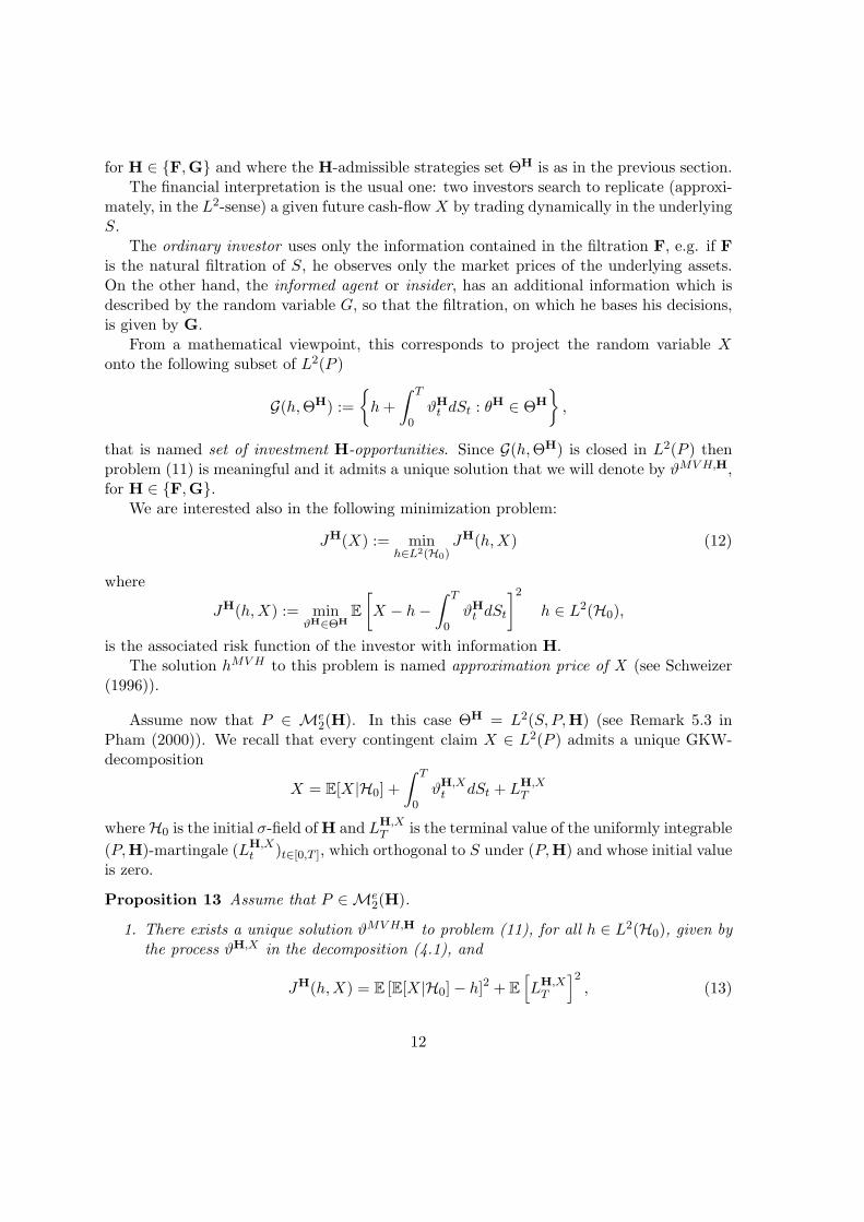
for H ∈ F,G and where the H-admissible strategies set ΘH is as in the previous section.The financial interpretation is the usual one: two investors search to replicate (approxi-

mately, in the L2-sense) a given future cash-flow X by trading dynamically in the underlyingS.

The ordinary investor uses only the information contained in the filtration F, e.g. if Fis the natural filtration of S, he observes only the market prices of the underlying assets.On the other hand, the informed agent or insider, has an additional information which isdescribed by the random variable G, so that the filtration, on which he bases his decisions,is given by G.

From a mathematical viewpoint, this corresponds to project the random variable Xonto the following subset of L2(P )

G(h, ΘH) :=

h +∫ T

0ϑH

t dSt : θH ∈ ΘH

,

that is named set of investment H-opportunities. Since G(h, ΘH) is closed in L2(P ) thenproblem (11) is meaningful and it admits a unique solution that we will denote by ϑMV H,H,for H ∈ F,G.

We are interested also in the following minimization problem:

JH(X) := minh∈L2(H0)

JH(h, X) (12)

where

JH(h, X) := minϑH∈ΘH

E[X − h−

∫ T

0ϑH

t dSt

]2

h ∈ L2(H0),

is the associated risk function of the investor with information H.The solution hMV H to this problem is named approximation price of X (see Schweizer

(1996)).

Assume now that P ∈ Me2(H). In this case ΘH = L2(S, P,H) (see Remark 5.3 in

Pham (2000)). We recall that every contingent claim X ∈ L2(P ) admits a unique GKW-decomposition

X = E[X|H0] +∫ T

0ϑH,X

t dSt + LH,XT

whereH0 is the initial σ-field of H and LH,XT is the terminal value of the uniformly integrable

(P,H)-martingale (LH,Xt )t∈[0,T ], which orthogonal to S under (P,H) and whose initial value

is zero.

Proposition 13 Assume that P ∈Me2(H).

1. There exists a unique solution ϑMV H,H to problem (11), for all h ∈ L2(H0), given bythe process ϑH,X in the decomposition (4.1), and

JH(h, X) = E [E[X|H0]− h]2 + E[LH,X

T

]2, (13)

12

2. the approximation price for the agent is given by hMV H = E[X|H0], and

JH(X) = E[LH,X

T

]2.

Proof.

1. By using GKW-decomposition of X with respect to the filtration H, and conditioningto H0, which is not necessarily trivial, one obtains

E[X − h−

∫ T

0ϑH

t dSt

]2

= E[E[X|H0]− h +

∫ T

0

(ϑH,X

t − ϑHt

)dSt + LH,X

T

]2

= E [E[X|H0]− h]2 + E[∫ T

0

(ϑH,X

t − ϑHt

)dSt

]2

+

+ E[LH,X

T

]2. (14)

Then the strategy ϑH,X solves problem (11) and we also have the desired formula forthe associated value function JH(h, X), for all h ∈ L2(H0).

2. By relation (14),

JH(h, X) = E [E[X|H0]− h]2 + E[LH,X

T

]2,

that implies hMV H = E[X|H0] and concludes the proof of the proposition.

If P is not an H-martingale measure, Rheinlander and Schweizer (1997) and Gourierouxet al. (1998) (see also Pham (2000)) have nonetheless obtained two characterizations of thesolution of problem (11), under the assumption H0 trivial. But it is very easy to check thatall those results still hold even without this assumption. We now recall some basic facts ofthe first approach.

We know since Delbaen and Schachermayer (1996) that, being the price process S con-tinuous, the variance optimal martingale measure (abbr. VOMM) can be defined as theunique martingale probability measure PH,opt solution to the problem

minQ∈M2(H)

E[dQ

dP

]2

, (15)

and that this measure is in fact equivalent to P . Moreover, the process

ZH,optt := EH,opt

[dPH,opt

dP

∣∣∣∣Ht

], t ∈ [0, T ]

can be written as

ZH,optt = Zopt

0 +∫ t

0ζH,opts dSs, t ∈ [0, T ] (16)

for some constant Zopt0 (independent from the underlying filtration) and some process

ζH,opt ∈ ΘH. The following theorem contains the characterization of the optimal mean-variance strategy for a given contingent claim X ∈ L2(P ) in a feedback form.

13

Theorem 14 Let X ∈ L2(P ) be a contingent claim and let h ∈ L2(H0) be an initialinvestment. The GKW-decomposition of X under (PH,opt,H) with respect to S is

X = EH,opt[X|H0] +∫ T

0ϑH,opt

s dSs + LH,optT = V H,opt

T (17)

with

V H,optt = EH,opt[X|Ht] = EH,opt[X|H0] +

∫ t

0ϑH,opt

s dSs + LH,optt , t ∈ [0, T ].

Then, the mean-variance optimal strategy for X is given by

ϑMV H,Ht = ϑH,opt

t − ζH,optt

ZH,optt

(V H,opt

t− − h−∫ t

0ϑMV H,H

s dSs

)(18)

= ϑH,optt − ζH,opt

t

(V H,opt

0 − h

ZH,opt0

+∫ t−

0

1

ZH,opts

dLH,opts

), (19)

for all t ∈ [0, T ]. Moreover the approximation price for X is given by hMV H = EH,opt[X|H0].

For the proof of this result and many remarks, the reader may look at the survey articleby Schweizer (2001).

4.2 Comparing the optimal MVH-strategies

4.2.1 The martingale case under both F and G

Firstly we assume that the price process S is a P -martingale with respect to both F and G.Given an instant t ∈ [0, T ) and a contingent claim X ∈ L2(P,Ft) we compare the strategiesand the risk functions of the informed and the ordinary agent. This means that we areconsidering a MVH-problem for the ordinary agent and the insider until time t < T .

For a given t ∈ [0, T ), we will denote by ϑMV H,H(X) the optimal strategy for an H-investor to hedge the claim X. Moreover, we fix two initial investments for the agents,c ∈ R for the ordinary one and g ∈ L2(G0) = L2(G) for the informed one. It is importantto point out that in this case the information drift µG vanishes.

The next technical result states a relation between the insider optimal hedging strategiesϑMV H,G(X) under P and the integrand ϑX/Zt,G in the GKW-decomposition of the claimX/Zt under the corresponding MPM P .

Lemma 15 Assume that P ∈Me2(G) and let X ∈ L2(P,Ft) for a given t ∈ [0, T ). Then

ϑMV H,G(X) = Z−ϑX/Zt,G

and

JG(g,X) = E[E[X|G0]− g]2 + E[∫ t

0Zs−dLG,X

s +∫ t

0V G

s−dNs

]2

,

14

where V Gs := E[X|Gs], ϑX/Zt,G is the integrand with respect to S in the GKW-decomposition

of X/Zt under (P ,G), LG,X is a (P,G)-martingale strongly orthogonal to S, and N as inTheorem 5.

Proof. We start by considering the (P,G)-martingale V Gs := E[X|Gs], s ∈ [0, t]. Since

V G := V G/Z is a local (P ,Gt)-martingale, we can write the following GKW-decomposition

V Gs = V G

0 +∫ s

0ϑG,X

u dSu + LG,Xs , s ∈ [0, t], (20)

where ϑG,X ∈ Lloc(S, P ,Gt) and LG,X is a (P ,Gt)-martingale orthogonal to S.Integration by parts formula gives

dV Gs = d

(V GZ

)s

= Zs−dV Gs + V G

s−dZs +[Z, V G

]s.

By using the decomposition (20) and since, by Theorem 5, Z satisfies dZs = Zs−dNs (inthis easy case the process µ of Theorem 5 is null), where N is a local (P,Gt)-martingaleorthogonal to S, we also have

dV Gs = Zs−ϑG,X

s dSs + Zs−dLG,Xs + V G

s−Zs−dNs + Zs−d[N, LG,X

]s.

Now, we use Girsanov’s Theorem to write

LG,X = LG,X + AG,X

where LG,X := LG,X − 1

Z−〈LG,X , Z〉 is a local (P,Gt)-martingale, orthogonal to S and

AG,X = 1

Z−〈LG,X , Z〉.

But since V G is a (P,Gt)-martingale, we must have Zsd(AG,X + [N, LG,X ])s = 0 andso

dV Gs = Zs−ϑG,X

s dSs + Zs−dLG,Xs + V G

s−Zs−dNs.

This concludes the proof of the lemma.

Finally, the next proposition gives a complete answer to the comparison problem in themartingale case.

Proposition 16 Assume that P ∈Me2(G).

1. If X ∈ L2(P,Ft), then

ϑMV H,Gs = ϑMV H,F

s , s ∈ [0, t].

2. The risk functions of both agents satisfy

JF(X)− JG(X) = E [E[X]− E[X|G0]]2 .

15

Proof.

1. To the random variable X ∈ L2(Ft) we associate the (P,Ft)-martingale Vs := V Fs :=

E[X|Fs], for which the GKW-decomposition holds:

Vs = V0 +∫ s

0ϑF,X

u dSu + LF,Xs s ∈ [0, t] (21)

where ϑF,X ∈ ΘF and LF,X is a (P,Ft)-martingale, strongly orthogonal to S for(P,Ft). Moreover, Ys := Vsp

Gs is a (P ,Gt)-local martingale and its GKW-decomposition

under (P ,Gt) is given by

Ys = Y0 +∫ s

0ϑG,Y

u dSu + LG,Ys s ∈ [0, t]. (22)

By (6) the process pGs satisfies

pGs = 1 +

∫ s

0pG

u−dNGu

and by the integration by parts formula applied to Ys, we obtain

Ys = VspGs = Y0 +

∫ s

0pG

u−ϑX,Fu dSu +

∫ s

0pG

u−dLX,Fu

+∫ s

0Vu−pG

u−dNGu +

[V, pG

]s.

Since Y is a (P ,Gt)-local martingale, the finite variation part in the above decompo-sition vanishes and then

Ys = VspGs = Y0 +

∫ s

0pG

u−ϑX,Fu dSu +

∫ s

0pG

u−dLX,Fu

+∫ s

0Vu−pG

u−dNGu . (23)

If we compare this orthogonal decomposition with (22), we obtain that

ϑY,Gs = pG

s−ϑX,Fs .

We finally apply Lemma (15) and we have

ϑMV H,Gs (X) = Zs−ϑX/Zt,G

s

= Zs−ϑYt,Gs

= Zs−pGs−ϑX,F

s

= ϑX,Fs .

16

2. From the GKW-decompositions of X under F and G, one can deduce

LF,Xt = X − E[X]−

∫ t

0ϑF,X

s dSs

= (E[X|G0]− E[X]) + X − E[X]−∫ t

0ϑG,X

s dSs

+∫ t

0

(ϑG,X

s − ϑF,Xs

)dSs

= (E[X|G0]− E[X]) +∫ t

0

(ϑG,X

s − ϑF,Xs

)dSs + LG,X

t .

By item 1 of this proposition, we have

E[LF,X

t

]2= E[E[X|G0]− E[X]]2 + E

[LG,X

t

]2,

that isJF(X) = JG(X) + E[E[X|G0]− E[X]]2.

The proof is now complete.

Remark 17 If both investors are allowed to minimize only over all pairs (c, ϑ) ∈ R×ΘH

(H ∈ F,G), then the risk functions are equal, i.e. JF(X) = JG(X). Indeed, by (13) andsince

LH,Xt = X − E[X|H0]−

∫ t

0ϑH,X

s dSs,

we have

JF(c,X) = E [E[X]− c]2 + E [E[X|G0]−X]2 + E[∫ t

0

(ϑG,X

s − ϑF,Xs

)2d〈S〉s

]= JG(c′, X) + E [E[X]− c]2 + E [E[X|G0]−X]2 − E

[E[X|G0]− c′

]2= JG(c′, X) + E[X − c]2 − E[X − c′]2,

where c and c′ are two given initial real investment for, respectively, the ordinary and theinformed agent. By setting c = c′ = E[X], which is in this case the approximation price forboth investors, we have the claimed equality JF(X) = JG(X).

4.2.2 The semimartingale case

For the general case, that is S is a continuous (P,F)-semimartingale, the Rheinlander-Schweizer feedback representation (18) of the optimal MVH-strategies suggests to compare

• the “optimal strategies” ϑopt,F := ϑX,P opt,Fand ϑopt,G := ϑX,P opt,G

of the ordinaryagent and the insider under their own VOMMs P opt,F and P opt,G, and

17

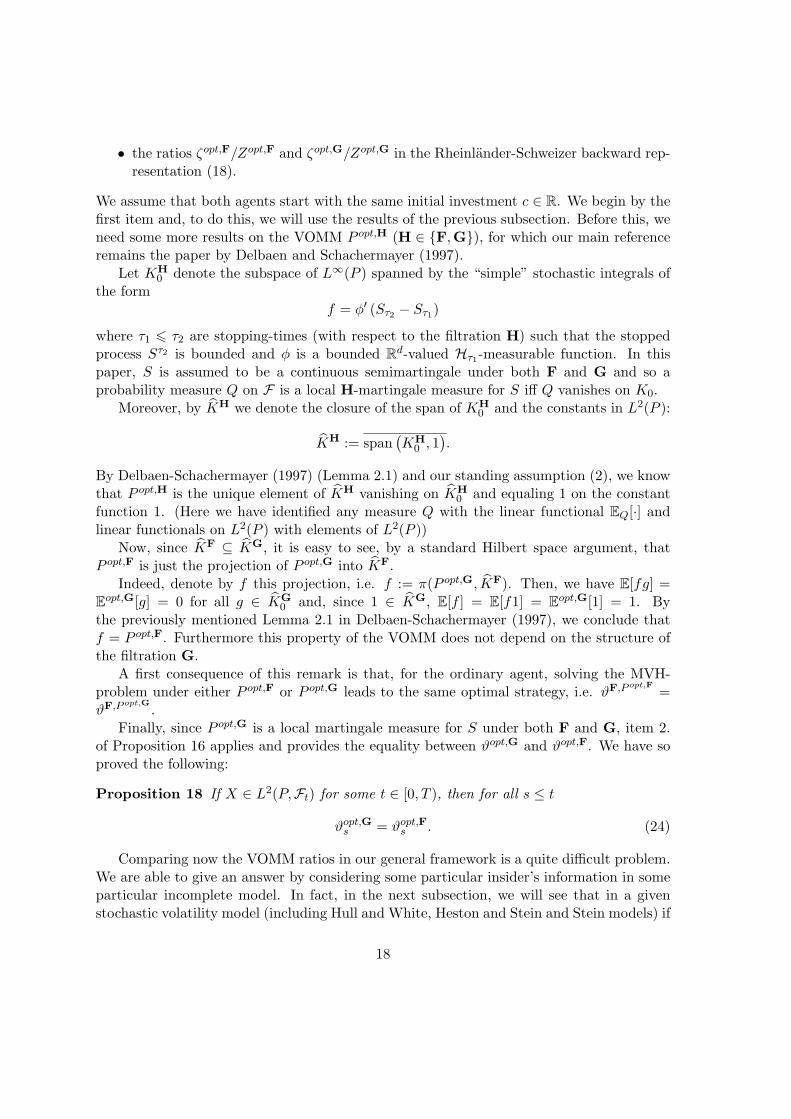
• the ratios ζopt,F/Zopt,F and ζopt,G/Zopt,G in the Rheinlander-Schweizer backward rep-resentation (18).

We assume that both agents start with the same initial investment c ∈ R. We begin by thefirst item and, to do this, we will use the results of the previous subsection. Before this, weneed some more results on the VOMM P opt,H (H ∈ F,G), for which our main referenceremains the paper by Delbaen and Schachermayer (1997).

Let KH0 denote the subspace of L∞(P ) spanned by the “simple” stochastic integrals of

the formf = φ′ (Sτ2 − Sτ1)

where τ1 6 τ2 are stopping-times (with respect to the filtration H) such that the stoppedprocess Sτ2 is bounded and φ is a bounded Rd-valued Hτ1-measurable function. In thispaper, S is assumed to be a continuous semimartingale under both F and G and so aprobability measure Q on F is a local H-martingale measure for S iff Q vanishes on K0.

Moreover, by KH we denote the closure of the span of KH0 and the constants in L2(P ):

KH := span(KH

0 , 1).

By Delbaen-Schachermayer (1997) (Lemma 2.1) and our standing assumption (2), we knowthat P opt,H is the unique element of KH vanishing on KH

0 and equaling 1 on the constantfunction 1. (Here we have identified any measure Q with the linear functional EQ[·] andlinear functionals on L2(P ) with elements of L2(P ))

Now, since KF ⊆ KG, it is easy to see, by a standard Hilbert space argument, thatP opt,F is just the projection of P opt,G into KF.

Indeed, denote by f this projection, i.e. f := π(P opt,G, KF). Then, we have E[fg] =Eopt,G[g] = 0 for all g ∈ KG

0 and, since 1 ∈ KG, E[f ] = E[f1] = Eopt,G[1] = 1. Bythe previously mentioned Lemma 2.1 in Delbaen-Schachermayer (1997), we conclude thatf = P opt,F. Furthermore this property of the VOMM does not depend on the structure ofthe filtration G.

A first consequence of this remark is that, for the ordinary agent, solving the MVH-problem under either P opt,F or P opt,G leads to the same optimal strategy, i.e. ϑF,P opt,F

=ϑF,P opt,G

.Finally, since P opt,G is a local martingale measure for S under both F and G, item 2.

of Proposition 16 applies and provides the equality between ϑopt,G and ϑopt,F. We have soproved the following:

Proposition 18 If X ∈ L2(P,Ft) for some t ∈ [0, T ), then for all s ≤ t

ϑopt,Gs = ϑopt,F

s . (24)

Comparing now the VOMM ratios in our general framework is a quite difficult problem.We are able to give an answer by considering some particular insider’s information in someparticular incomplete model. In fact, in the next subsection, we will see that in a givenstochastic volatility model (including Hull and White, Heston and Stein and Stein models) if

18

the additional r.v. G is measurable with respect to the filtration generated by the volatilityprocess, then the two VOMM ratios coincide. This result will allow us to obtain a feedbackrepresentation for the difference process between the two optimal strategies ϑMV H,F andϑMV H,G.

4.3 Stochastic volatility models

We consider the following stochastic volatility model for a discounted price process S:

dSt = σ(t, St, Yt)St[λ(t, St, Yt)dt + dW 1t ] (25)

where W 1 is a brownian motion and Y is assumed to satisfy the following SDE

dYt = α(t, St, Yt)dt + γ(t, St, Yt)dW 2t (26)

with W 2 another brownian motion independent from the first one. The coefficients are as-sumed to satisfy the usual hypotheses ensuring the existence of a unique strong solution andof an equivalent local martingale measure with square integrable Radon-Nikodym density.Furthermore, we assume that the underlying filtration F = (Ft) is that generated by thetwo driving brownian motions, i.e. Ft = σ(W 1

s ,W 2s : s 6 t) for all t ∈ [0, T ], and that λ

does not depend on the process S, that is λ(t, St, Yt) = λ(t, Yt). We point out that thisassumption is satisfied by the Hull and White, Heston and Stein and Stein models (e.g. seeHobson (1998b)).

We will denote by F1 = (F1t ) (resp. F2 = (F2

t )) the filtration generated by W 1 (resp.W 2).

We assume that the additional random variable G is F2T -measurable, e.g. G = W 2

T ,G = 1(W 2

T∈[a,b]) with a < b < ∞ or G = YT when Y and W 2 generate the same filtration(for example, in the Hull and White model).

In this case, the VOMM is the same for the ordinary and the informed agent. Indeed,by Biagini et al. (2000) (Theorem 1.16), we have for H ∈ F,G,

dPH,opt

dP=

E(−∫ ·0 βH

t dSt

)T

E[E(−∫ ·0 βH

t dSt

)T

] (27)

with βHt = λ(t,Yt)−hH

tσ(t,St,Yt)St

. So, we focus on the process hH. Now, by assumption the process λ

does not depend on S and then, again by Biagini et al. (2002) (Section 2), hF = 0.Moreover, being G F2

T -measurable and since W 1 and W 2 are independent, the dynamicsof S does not change if we pass from F to G. Indeed, since in this case assumption (1) isequivalent to assume P (G ∈ · |F2

t ) ∼ P (G ∈ · ) for all t ∈ [0, T ), it is easy to see that theconditional density process (pG

s )s∈[0,T ) can be chosen F02-optional, where F0

2 := (F2t )t∈[0,T ).

The equality

d

⟨pG,

∫σ(u, Su, Yu)SudW 1

u

⟩t

= σ(t, St, Yt)Std⟨pG,W 1

⟩t= 0, t ∈ [0, T ),

19

implies, thanks to Theorem 4, µG ≡ 0.So, always by Biagini et al. (2002) (Section 2), hG = 0. This implies βF = βG and then

PF,opt = PG,opt =: P opt.

Proposition 19 Let G be F2T -measurable, X ∈ L2(P,Ft) with t < T , c ∈ R and g ∈ L2(G0)

two given initial investments for, respectively, the ordinary agent and the insider. Then

ϑMV H,Gs = ϑMV H,F

s + ξMV Hs , s ∈ [0, t], (28)

where the process ξMV H has the following backward representation:

ξMV Hs = ρopt

s

(V opt,G

s− − V opt,Fs− +

∫ s

0ξMV Hu dSu

)(29)

= ζF,optt

V G,opt0 − g −

(V F,opt

0 − c)

ZF,opt0

+∫ t−

0

1

ZF,opts

dV G,opts

, (30)

for all s ∈ [0, t], where V opt,Hs := Eopt[X|Hs] for H ∈ F,G and ρopt

s := ζopt,Fs /Zopt,F

s =ζopt,Gs /Zopt,G

s , s ∈ [0, t].

Proof. Since P opt,F = P opt,G = P opt, it is easy to remark that by isometry ζopt,Fs = ζopt,G

s

and so ζopt,Fs /Zopt,F

s = ζopt,Gs /Zopt,G

s =: ρopts for s 6 t. Indeed, since by localization we

can assume that S is a true martingale under P opt, it suffices to note that Zopt,FT = Zopt,G

T

implies∫ T0 ζopt,F

s dSs =∫ T0 ζopt,G

s dSs and so, by isometry, we have

Eopt

[∫ T

0

(ζopt,Fs − ζopt,G

s

)2d 〈S〉s

]= 0.

Then, by Proposition 16, the optimal strategies of the two agents under the VOMM areequal, i.e. ϑF,opt = ϑG,opt. Finally, by comparing the backward representations (18) of thetwo optimal hedging strategies ϑMV H,F and ϑMV H,G, we have the representation (29) ofthe difference process ξMV H .

For the representation (30), we have to compare the characterizations provided by (19)for H ∈ F,G. By doing this, we obtain for all s 6 t

ξMV Hs = ζF,opt

t

V G,opt0 − g −

(V G,opt

0 − c)

ZF,opt0

+∫ t−

0

1

ZF,opts

(dLG,opt

s − dLF,opts

) . (31)

It remains to study the last stochastic differential appearing in (31). From the GKW-decomposition of X under (PF,opt,F) and (PG,opt,G) and by Proposition 18 we deducethat

LF,optt = LG,opt

t +(Eopt[X|G0]− Eopt[X]

).

Thus, for every s 6 t,

LG,opts = E

[LF,opt

t |Gs

]−(Eopt[X|G0]− Eopt[X]

).

20

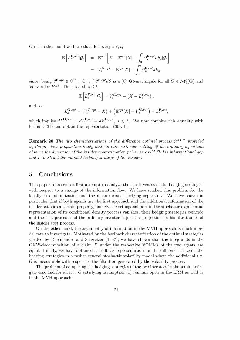
On the other hand we have that, for every s 6 t,

E[LF,opt

t |Gs

]= Eopt

[X − Eopt[X]−

∫ t

0ϑF,opt

s dSs|Gs

]= V G,opt

s − Eopt[X]−∫ s

0ϑF,opt

u dSu,

since, being ϑF,opt ∈ ΘF ⊆ ΘG,∫

ϑF,optdS is a (Q,G)-martingale for all Q ∈ Me2(G) and

so even for P opt. Thus, for all s 6 t,

E[LF,opt

t |Gs

]= V G,opt

s −(X − LF,opt

s

),

and soLG,opt

s =(V G,opt

s −X)

+(Eopt[X]− V G,opt

0

)+ LF,opt

s ,

which implies dLG,opts = dLF,opt

s + dV G,opts , s 6 t. We now combine this equality with

formula (31) and obtain the representation (30).

Remark 20 The two characterizations of the difference optimal process ξMV H providedby the previous proposition imply that, in this particular setting, if the ordinary agent canobserve the dynamics of the insider approximation price, he could fill his informational gapand reconstruct the optimal hedging strategy of the insider.

5 Conclusions

This paper represents a first attempt to analyze the sensitiveness of the hedging strategieswith respect to a change of the information flow. We have studied this problem for thelocally risk minimization and the mean-variance hedging separately. We have shown inparticular that if both agents use the first approach and the additional information of theinsider satisfies a certain property, namely the orthogonal part in the stochastic exponentialrepresentation of its conditional density process vanishes, their hedging strategies coincideand the cost processes of the ordinary investor is just the projection on his filtration F ofthe insider cost process.

On the other hand, the asymmetry of information in the MVH approach is much moredelicate to investigate. Motivated by the feedback characterization of the optimal strategiesyielded by Rheinlander and Schweizer (1997), we have shown that the integrands in theGKW-decomposition of a claim X under the respective VOMMs of the two agents areequal. Finally, we have obtained a feedback representation for the difference between thehedging strategies in a rather general stochastic volatility model where the additional r.v.G is measurable with respect to the filtration generated by the volatility process.

The problem of comparing the hedging strategies of the two investors in the semimartin-gale case and for all r.v. G satisfying assumption (1) remains open in the LRM as well asin the MVH approach.

21

Moreover, a natural development of this study would be to investigate the hedgingproblem in a financial market with an insider possessing either a weak anticipation on thefuture evolution of the stock price (Baudoin (2003) and Baudoin and Nguyen-Ngoc (2002))or an additional dynamical information (as in Corcuera et al. (2002)).

References

[1] Amendinger, J. (2000): Martingale representation theorems for initially enlarged fil-trations. Stochastic Process. Appl. 89, 101-116.

[2] Amendinger, J., Imkeller, P., Schweizer, M. (1998): Additional logarithmic utility ofan insider. Stochastic Process. Appl. 75, 263-286.

[3] Ansel, J.P., Stricker, C. (1992): Lois de Martingale, Densites et Decomposition deFollmer et Schweizer. Ann. Inst. Henri Poincare, 28, 375-392.

[4] Ansel, J.P., Stricker, C. (1993): Decomposition de Kunita-Watanabe. Seminaire deProbabilites XXVII. Lectures Notes in Math., 1557, 30-32. Springer Verlag.

[5] Baudoin, F. (2003): Modelling Anticipations on Financial Markets. In: Carmona, R.A.,Cinclair, E., Ekeland, I., Jouini, E., Scheinkman, J.A. and Touzi, N. (eds), Paris-Princeton Lectures on Mathematical Finance 2002. Lecture Notes in Mathematics.Springer Verlag.

[6] Baudoin, F., Nguyen-Ngoc, L. (2002): The financial value of a weak information flow.Technical Report, Universite Pierre et Marie Curie. To appear in Finance Stochast..

[7] Biagini, F., Guasoni, P., Pratelli, M. (2000): Mean-Variance Hedging for StochasticVolatility Models. Mathematical Finance, 10, number 2, 109-123.

[8] Biagini, F., Øksendal, B. (2002): A general stochastic calculus approach to insidertrading. Technical Report, University of Oslo.

[9] Bremaud, P., Yor, M. (1978): Changes of filtrations and of probability measures. Z.Wahrscheinlichkeitstheorie und verw. Geb. 45, 269-295.

[10] Corcuera, J.M., Imkeller, P., Kohatsu-Higa, A., Nualart, D. (2002): Additional utilityof insiders with imperfect dynamical information. Technical Report, Universitat deBarcelona.

[11] Delbaen, F., Schachermayer, W. (1997): The Variance-Optimal Martingale Measurefor Continuous Processes. Bernoulli 2, 81-105.

[12] Delbaen, F., Monat, P., Schachermayer, W., Schweizer, M., Stricker, C. (1997):Weighted Norm Inequalities and Closedness of a Space of Stochastic Integrals. Financeand Stochastics, 1 (3), 181-227.

22

[13] Follmer, H., Schweizer, M. (1991): Hedging of contingent claims under incomplete in-formation. In: Davis, M.H.A., Elliott, R.J. (eds.), Applied Stochastic Analysis, Stochas-tic Monographs 5, 389-414. Gordon Breach, London/New York.

[14] Follmer, H., Sondermann, D. (1986): Hedging of non-redundant contingent claims.In: Mas-Collel, A., Hildebrand, W. (eds.), Contributions to Mathematical Economics,205-223. North Holland, Amsterdam.

[15] Gourieroux, C., Laurent, J.P., Pham, H. (1998): Mean-variance hedging andnumeraire. Mathematical Finance, 8 (3), 179-200.

[16] Grorud, A., Pontier, M. (1998): Insider Trading in a Continuous Time Market Model.International Journal of Theoretical and Applied Finance, 1, 331-347.

[17] He, S., Wang, J., Yan, J. (1992): Semimartingale Theory and Stochastic Calculus.Science Press and CRC Press Inc., Beijing/Boca Raton.

[18] Hobson, D.G. (1998): Stochastic volatility. In: Hand, D., Jacka, S. (eds.) Statistics inFinance. Applications of Statistics Series. Arnold, London.

[19] Imkeller, P. , Pontier, M., Weisz, M. (2001): Free lunch and arbitrage possibilities in afinancial market with an insider. Stochastic Proc. Appl., 92, 103-130.

[20] Jacod, J. (1979): Calcul Stochastique et probleme de martingales. Lectures Notes inMath., 714. Springer Verlag.

[21] Jacod, J. (1985): Grossissement Initial, Hypothese (H’) et Theoreme de Girsanov. In:Jeulin, Th., Yor, M. (eds.), Grossissements de Filtrations: Exemples et Applications,Lecture Notes in Mathematics 1118. Springer Verlag, Berlin.

[22] Jeulin, Th. (1980): Semi-martingales et Grossissement d’une Filtration. Lectures Notesin Math., 833. Springer Verlag.

[23] Karatzas, I., Pivovsky, I. (1996): Anticipative portfolio optimization. Adv. Appl. Prob.,28, 1095-1122.

[24] Laurent, J.P., Pham, H. (1999): Dynamic programming and mean-variance hedging.Finance Stochast., 3, 83-110.

[25] Pham, H. (2000): On quadratic hedging in continuous time. Math. Methods of Opera-tions Research 51, 315-339.

[26] Pham, H., Rheinlander, T., Schweizer, M. (1998): Mean-variance hedging for continu-ous processes: New proofs and examples. Finance Stochast., 2, 173-198.

[27] Rheinlander, T., Schweizer, M. (1997): On L2-Projections on a Space of StochasticIntegrals. Ann. Probab 25, 1810-1831.

23

[28] Schweizer, M. (1988): Hedging of options in a general semimartingale model. DoctoralDissertation, ETH Zurich.

[29] Schweizer, M. (1995): On the Minimal Martingale Measure and the Follmer-SchweizerDecomposition. Stochastic Analysis and Application, 13, 573-599.

[30] Schweizer, M. (1996): Approximation Pricing and the Variance-Optimal MartingaleMeasure. Ann. Probab. 64, 206-236.

[31] M. Schweizer (2001): A Guided Tour through Quadratic Hedging Approaches. In:Jouini, E., Cvitanic, J., Musiela, M. (eds.), Option Pricing, Interest Rates and RiskManagement, 538-574. Cambridge University Press.

24