MANUFACTURING & SERVICEOPERATIONS MANAGEMENT

Vol. 7, No. 2, Spring 2005, pp. 103–120issn 1523-4614 �eissn 1526-5498 �05 �0702 �0103

informs ®

doi 10.1287/msom.1040.0061©2005 INFORMS

Hedging Inventory Risk Through Market Instruments

Vishal Gaur, Sridhar SeshadriDepartment of Information, Operations and Management Science, Leonard N. Stern School of Business,

New York University, Suite 8-160, 44 West 4th Street, New York, New York 10012{vgaur@stern.nyu.edu, sseshadr@stern.nyu.edu}

We address the problem of hedging inventory risk for a short life cycle or seasonal item when its demand iscorrelated with the price of a financial asset. We show how to construct optimal hedging transactions that

minimize the variance of profit and increase the expected utility for a risk-averse decision maker. We show thatfor a wide range of hedging strategies and utility functions, a risk-averse decision maker orders more inventorywhen he or she hedges the inventory risk. Our results are useful to both risk-neutral and risk-averse decisionmakers because (1) the price information of the financial asset is used to determine both the optimal inventorylevel and the hedge, (2) this enables the decision maker to update the demand forecast and the financial hedgeas more information becomes available, and (3) hedging leads to lower risk and higher return on inventoryinvestment. We illustrate these benefits using data from a retailing firm.

Key words : demand forecasting; financial hedging; newsboy model; real options; risk aversionHistory : Received: April 2, 2003; accepted: October 29, 2004. This paper was with the authors 8 months for3 revisions.

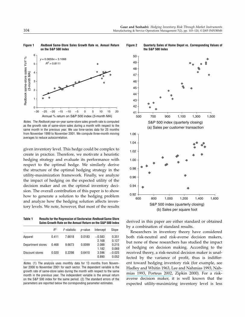
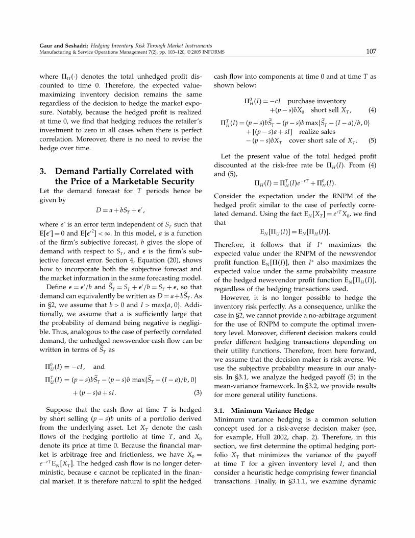
1. IntroductionThe demand for discretionary purchase items, suchas apparel, consumer electronics, and home furnish-ings, is widely believed to be correlated with eco-nomic indicators. Our analysis not only supports thisbelief but also shows that the correlation can be quitesignificant. For example, The Redbook Average monthlytime-series data1 for the period November 1999 toNovember 2001 have a correlation coefficient of 0.90with the same-period returns on the S&P 500 index(R2 = 81%, see Figure 1). Furthermore, using sec-torwise data, we find that the value of R2 is corre-lated with the fraction of discretionary items sold asa percentage of total sales. For example, discretionaryitems constitute a larger fraction of total sales forapparel stores and department stores than discountstores. Correspondingly, apparel stores and depart-ment stores have a higher correlation of demand withthe S&P 500 index than discount stores (see Table 1).Our results are also supported by firm-level analysis.

1 The Redbook Average is a seasonally adjusted sales-weighted aver-age of year-to-year same-store sales growth in a sample of 60 largeU.S. general merchandise retailers representing about 9,000 stores(Instinet Research 2001a, b). It is released by Instinet Research onthe first Thursday of every month.

Figure 2 shows that for The Home Depot Inc.,2 salesper customer transaction and sales per square footboth have statistically significant correlation with thevalue of the S&P 500 index. Their R2 values are equalto 79.11% and 39.92%, respectively.These findings present an opportunity to use finan-

cial market information to improve demand fore-casting and inventory planning, and use financialcontracts to mitigate (hedge) the risk in carryinginventory. This paper addresses these problems fordiscretionary purchase items based on a forecastingmodel that incorporates the subjective assessment ofthe retailer and the price information of a financialasset.We show how to construct static hedging strate-

gies in both the mean-variance framework and themore general utility-maximization framework. In themean-variance framework, we determine the optimalportfolio that minimizes the variance of profit for a

2 Home Depot is a retail chain selling home construction and homefurnishing products. We use public data from the first quarter offiscal 1997 to the second quarter of fiscal 2001, a total of 22 quar-terly observations. The data are obtained from the 10-K and 10-Qreports that Home Depot files with the Securities and ExchangeCommission.

103

Gaur and Seshadri: Hedging Inventory Risk Through Market Instruments104 Manufacturing & Service Operations Management 7(2), pp. 103–120, © 2005 INFORMS

Figure 1 Redbook Same-Store Sales Growth Rate vs. Annual Returnon the S&P 500 Index

y = 0.0659x + 3.1066

R2 = 0.8111

0

1

2

3

4

5

6

–30 –25 –20 –15 –10 –5 0 5 10 15 20

Annual % return on S&P 500 index (3-month MA)

Red

book

sam

e-st

ore

sale

s Y

oY %

(3-m

onth

MA

)

Notes. The Redbook year-on-year same-store sales growth rate is computedas the growth rate of same-store sales during a month with respect to thesame month in the previous year. We use time-series data for 25 monthsfrom November 1999 to November 2001. We compute three-month movingaverages to reduce autocorrelation.

given inventory level. This hedge could be complex tocreate in practice. Therefore, we motivate a heuristichedging strategy and evaluate its performance withrespect to the optimal hedge. We similarly derivethe structure of the optimal hedging strategy in theutility-maximization framework. Finally, we analyzethe impact of hedging on the expected utility of thedecision maker and on the optimal inventory deci-sion. The overall contribution of this paper is to showhow to generate a solution to the hedging problemand analyze how the hedging solution affects inven-tory levels. We note, however, that most of the results

Table 1 Results for the Regression of Sectorwise Redbook Same StoreSales Growth Rate on the Annual Return on the S&P 500 Index

R2 F -statistic p-value Intercept Slope

Apparel 0�411 7�6618 0�0183 −0�583 0�3512�168 0�127

Department stores 0�468 9�6673 0�0099 2�088 0�2151�182 0�069

Discount stores 0�020 0�2298 0�6410 3�596 −0�0250�890 0�052

Notes. (1) The analysis uses monthly data for 13 months from Novem-ber 2000 to November 2001 for each sector. The dependent variable is thegrowth rate of same-store sales during the month with respect to the samemonth in the previous year. The independent variable is the annual returnon the S&P 500 index for the same period. (2) The standard errors of theparameters are reported below the corresponding parameter estimates.

Figure 2 Quarterly Sales of Home Depot vs. Corresponding Values ofthe S&P 500 Index

(a) Sales per customer transaction

(b) Sales per square foot

41

42

43

44

45

46

47

48

49

50

500 700 900 1,100 1,300 1,500

S&P 500 index (quarterly closing)

0.92

0.94

0.96

0.98

1.00

1.02

1.04

1.06

600 800 1,000 1,200 1,400 1,600

S&P 500 index (quarterly closing)

derived in this paper are either standard or obtainedby a combination of standard results.Researchers in inventory theory have considered

both risk-neutral and risk-averse decision makers,but none of these researchers has studied the impactof hedging on decision making. According to thereceived theory, a risk-neutral decision maker is unaf-fected by the variance of profit, thus is indiffer-ent toward hedging inventory risk (for example, seeHadley and Whitin 1963, Lee and Nahmias 1993, Nah-mias 1993, Porteus 2002, Zipkin 2000). For a risk-averse decision maker, it is well known that theexpected utility-maximizing inventory level is less

Gaur and Seshadri: Hedging Inventory Risk Through Market InstrumentsManufacturing & Service Operations Management 7(2), pp. 103–120, © 2005 INFORMS 105

than the expected value-maximizing inventory level(for example, see Agrawal and Seshadri 2000a, b;Chen and Federgruen 2000; Eeckhoudt et al. 1995;and the papers cited therein). Although it seems rea-sonable to conjecture that risk-averse decision makerswill prefer to hedge inventory risk, it is less obviousthat the hedge will also lead to an increase in thequantity ordered. We show that hedging impacts bothtypes of decision makers:(1) Hedging reduces the variance of profit and

increases expected utility. The reduction in the vari-ance of profit is directly proportional to the correla-tion of demand with the price of the asset.(2) It provides an incentive to a risk-averse deci-

sion maker to order a quantity that is closer to theexpected value-maximizing quantity. This result holdsfor a wide range of hedging strategies and for allincreasing concave utility functions with constant ordecreasing absolute risk aversion.(3) The hedging transactions do not require addi-

tional investment. On the contrary, the funds requiredto finance inventory at the beginning of the planningperiod are offset by the cash flows from the hedgingtransactions, so that the net inventory investment ofthe firm is reduced.The last result shows that hedging is useful even to

a risk-neutral decision maker although he or she maynot be interested in reducing the variance of profitin a perfect market.3 Hedging is especially useful tosmall privately owned firms, e.g., the so-called Momand Pop retail stores, because risk reduction providesthem access to capital, reduces the cost of financialdistress, and enables the owners to diversify their riskand increase their return on investment.We present a numerical study using data from a

retailing firm to quantify the impact of our resultson forecasting demand, optimal inventory planning,risk reduction, and return on investment. Because theforecast is a function of the asset price, the retailer candynamically update it with changes in asset price orthe volatility of the asset. Therefore, it improves theoptimal inventory decision and impacts the expectedprofit of the retailer. The increase in the expected

3 When there are market imperfections, for example, if bankruptcyis costly, then even a risk-neutral decision maker may prefer topurchase insurance.

profit in our numerical study is as high as 7%. Thenumerical study also shows that hedging reduces thevariance of profit by 12.5% to 56.5%. The amount ofreduction is a function of the correlation of demandwith the asset price, the volatility of the asset, andthe lead time. Compared with the optimal hedge,the heuristic hedge proposed by us achieves 6% lessreduction in the variance of profit. Dynamic hedgingusing the heuristic strategy reduces the variance ofprofit to within 0.5% of the optimal hedge.This paper is also related to the real-options litera-

ture. For example, Dasu and Li (1997), Huchzermeierand Cohen (1996), Kogut and Kulatilaka (1994), andKouvelis (1999) consider the valuation of real optionswherein the cash flows from real assets depend on theprice of a traded security, such as the exchange rate.Other authors, including Birge (2000), Brennan andSchwartz (1985), McDonald and Siegel (1986), Triantisand Hodder (1990), and Trigeorgis (1996) consider thevaluation of real options using the assumption thatthe cash flows from a basecase scenario or a port-folio of marketed securities, or both, can be used toreplicate the cash flows from the real option. Whenthis assumption holds, the value of the option canbe set equal to the value of the replicating portfo-lio. (This assumption is called the Marketed AssetDisclaimer. See Copeland and Antikarov 2001, p. 94.)Our paper differs from this literature in two aspects.First, we do not focus on valuation. Instead, we focuson the interaction between real options and finan-cial hedging by analyzing how the optimal inventorydecision changes with hedging and with the degreeof correlation of demand with the underlying asset.Second, we use neither the marketed asset disclaimernor the assumption that the cash flows correspondingto each inventory level are traded in a perfect marketto construct the hedge. Instead, as set out in the firstparagraph of the paper, we justify the application ofrisk-neutral valuation by demonstrating the correla-tion of demand with financial assets, and show in §4how to incorporate this information in a forecastingmodel to plan inventory.The paper is organized as follows. We set up the

framework of our analysis in §2 by using a modelin which demand is perfectly correlated with theprice of an underlying asset. In §3, we analyze themodel with partial demand correlation and establish

Gaur and Seshadri: Hedging Inventory Risk Through Market Instruments106 Manufacturing & Service Operations Management 7(2), pp. 103–120, © 2005 INFORMS

the properties of the hedged payoff function result-ing from the newsvendor model. Section 4 presentsa numerical example to illustrate the results of ourmodel. Section 5 concludes the paper with directionsfor future research.

2. Demand Perfectly Correlated withthe Price of a Marketable Security

We consider a single-period, single-item inventorymodel with stochastic demand, i.e., the newsvendormodel. To establish the basic ideas, we first considerthe case when the demand forecast for the item isperfectly correlated with the price at time T of anunderlying asset that is actively traded in the finan-cial markets. The analysis in this section is based onthe theory of valuing real options.Let p denote the selling price of the item, c the

unit cost, s the salvage value, I the stocking quantity,and D the demand. The firm purchases quantity I attime 0 and demand occurs at a future time T . Demandin excess of I is lost, and any excess inventory is liqui-dated at the salvage price of s. The firm’s cash flowsat times 0 and T , respectively, are

�0U I�=−cI� and

�TU I�= pmin D� I�+ sI −D�+� (1)

We use the subscript U to denote unhedged cash flows,i.e., cash flows before any financial transactions, andthe subscript H to denote hedged cash flows, i.e., cashflows including financial transactions.Let S0 be the current price of the financial asset, ST be

its price at time T , and r be the risk-free rate of returnper annum. We assume that the financial market iscomplete and has a unique risk-neutral pricing mea-sure (RNPM).4 Let EN denote the expectation underthe risk-neutral probability measure. Thus, we haveS0 = e−rTENST . To distinguish expectation under theRNPM from expectation under the decision maker’ssubjective probability measure, we shall denote expec-tation under the subjective measure as E�·�, and condi-tional expectation under the subjective measure overa random variable � as E� �·�.

4 This assumption can be relaxed further because market comple-tion is not a necessary condition. All we need is that the no-arbitrage principle should hold in the market and that the claimST should have a unique price at time 0 (see Pliska 1999, chap. 1).

We use the correlation of demand with ST in threeways: to value the newsvendor profit function, to con-struct transactions to hedge inventory risk, and toexploit the benefits of hedging. Because the demandis perfectly correlated with ST , we specify it as D =a+ bST , where a and b are constants. We assume thatb > 0 to ensure that the demand is nonnegative, andthat I > max a�0�, otherwise �T

U I� will be a deter-ministic quantity equal to pmax a�0� that requires norisk analysis. We also assume that p > cerT > s, other-wise the newsvendor problem has trivial solutions ateither I = 0 or I =�.Substituting the demand forecast in (1) and simpli-

fying the expression for �TU , we get

�TU I� = p− s�min a+ bST � I�+ sI

= p− s�bST + �p− s�a+ sI�

− p− s�bmax ST − I − a�/b�0�� (2)

Equation (2) reveals that the random payoff from thenewsvendor model can be represented as a portfoliocomprising only financial assets. This portfolio is saidto replicate the newsvendor payoff function. It followsfrom standard valuation theory that this portfolio canbe used not only to value �T

U I�, but also to hedgethe inventory risk. Because demand is perfectly cor-related with ST , the hedge is perfect and completelyeliminates the uncertainty in newsvendor profits. Thehedging transactions at time 0 are(1) Borrow and sell p− s�b units of the underlying

asset at the current price S0. The borrowed asset is tobe replaced at time T by purchasing p− s�b units ofthe asset from the market at price ST .(2) Buy p− s�b call options on this asset with exer-

cise price I − a�/b and settlement date T .(3) Borrow a sum of money equal to �p − s�a +

sI�e−rT at the risk-free rate to be repaid at time T .These hedging transactions have several benefits.

Through hedging, the net payoff to the retailer in allstates of nature at time T is zero, and the hedgedprofit is realized at time 0 itself. This profit is given by

�HI� = p− s�bS0+ e−rT �p− s�a+ sI�

− p− s�be−rTEN �max ST − I − a�/b�0��− cI �

The hedged profit is identical to the expected news-vendor profit for any inventory I , i.e.,

EN ��U I��=�HI� and Var��HI��= 0�

Gaur and Seshadri: Hedging Inventory Risk Through Market InstrumentsManufacturing & Service Operations Management 7(2), pp. 103–120, © 2005 INFORMS 107

where �U·� denotes the total unhedged profit dis-counted to time 0. Therefore, the expected value-maximizing inventory decision remains the sameregardless of the decision to hedge the market expo-sure. Notably, because the hedged profit is realizedat time 0, we find that hedging reduces the retailer’sinvestment to zero in all cases when there is perfectcorrelation. Moreover, there is no need to revise thehedge over time.

3. Demand Partially Correlated withthe Price of a Marketable Security

Let the demand forecast for T periods hence begiven by

D= a+ bST + �′�

where �′ is an error term independent of ST such thatE��′�= 0 and E��′2� <�. In this model, a is a functionof the firm’s subjective forecast, b gives the slope ofdemand with respect to ST , and � is the firm’s sub-jective forecast error. Section 4, Equation (20), showshow to incorporate both the subjective forecast andthe market information in the same forecasting model.Define � = �′/b and �ST = ST + �′/b = ST + �, so that

demand can equivalently be written as D= a+b �ST . Asin §2, we assume that b > 0 and I >max a�0�. Addi-tionally, we assume that a is sufficiently large thatthe probability of demand being negative is negligi-ble. Thus, analogous to the case of perfectly correlateddemand, the unhedged newsvendor cash flow can bewritten in terms of �ST as

�0U I� = −cI� and

�TU I� = p− s�b �ST − p− s�b max �ST − I − a�/b�0�

+ p− s�a+ sI � (3)

Suppose that the cash flow at time T is hedgedby short selling p − s�b units of a portfolio derivedfrom the underlying asset. Let XT denote the cashflows of the hedging portfolio at time T , and X0

denote its price at time 0. Because the financial mar-ket is arbitrage free and frictionless, we have X0 =e−rTEN �XT �. The hedged cash flow is no longer deter-ministic, because � cannot be replicated in the finan-cial market. It is therefore natural to split the hedged

cash flow into components at time 0 and at time T asshown below:

�0HI�=−cI purchase inventory

+p− s�bX0 short sell XT � (4)

�THI�= p− s�b �ST − p− s�bmax �ST − I − a�/b�0�

+ �p− s�a+ sI� realize sales− p− s�bXT cover short sale of XT . (5)

Let the present value of the total hedged profitdiscounted at the risk-free rate be �HI�. From (4)and (5),

�HI�=�THI�e

−rT +�0HI��

Consider the expectation under the RNPM of thehedged profit similar to the case of perfectly corre-lated demand. Using the fact EN �XT �= erT X0, we findthat

EN ��U I��= EN ��HI���

Therefore, it follows that if I∗ maximizes theexpected value under the RNPM of the newsvendorprofit function EN ��I��, then I∗ also maximizes theexpected value under the same probability measureof the hedged newsvendor profit function EN ��HI��,regardless of the hedging transactions used.However, it is no longer possible to hedge the

inventory risk perfectly. As a consequence, unlike thecase in §2, we cannot provide a no-arbitrage argumentfor the use of RNPM to compute the optimal inven-tory level. Moreover, different decision makers couldprefer different hedging transactions depending ontheir utility functions. Therefore, from here forward,we assume that the decision maker is risk averse. Weuse the subjective probability measure in our analy-sis. In §3.1, we analyze the hedged payoff (5) in themean-variance framework. In §3.2, we provide resultsfor more general utility functions.

3.1. Minimum Variance HedgeMinimum variance hedging is a common solutionconcept used for a risk-averse decision maker (see,for example, Hull 2002, chap. 2). Therefore, in thissection, we first determine the optimal hedging port-folio XT that minimizes the variance of the payoffat time T for a given inventory level I , and thenconsider a heuristic hedge comprising fewer financialtransactions. Finally, in §3.1.1, we examine dynamic

Gaur and Seshadri: Hedging Inventory Risk Through Market Instruments108 Manufacturing & Service Operations Management 7(2), pp. 103–120, © 2005 INFORMS

hedging, i.e., the rebalancing of the hedging portfoliowhen new information regarding the asset price andthe demand forecast becomes available over time. Theoptimal solution to the problem of minimizing thevariance of �T

HI� with respect to XT for given I can beobtained from a standard result in probability theory;see, for example, §9.4 in Williams (1991). Specifically,

Lemma 1. The variance of �THI� is minimized by set-

ting X∗T = E���T

U I� � ST �.Proof. Omitted. �

Figure 3 depicts the cash flows of the minimumvariance hedge as a function of ST . For comparison,it also shows the hedging portfolio when �= 0. It caneasily be shown that the hedge is a concave increasingfunction of ST . Thus, the hedge can be approximatedby short selling the underlying asset and purchasinga series of call options with settlement date T and dif-ferent exercise prices. As a first-order approximation,consider a hedging portfolio consisting of a short saleof the asset and a purchase of call options with a sin-gle exercise price, sp. Let

XT = p− s�b�ST − p− s�b max ST − sp�0��

We refer to this portfolio as the heuristic hedge withparameters �, , and sp, where � and are thehedge ratios. Let Csp� denote the cost at time 0 ofpurchasing a European call option on the underly-ing financial asset with an exercise price of sp and

Figure 3 Cash Flows of the Minimum Variance Hedging Portfolio X ∗T

as a Function of ST

400

600

800

1,000

1,200

1,400

1,600

800 1,200 1,600 2,000 S (T )

Variance

Hedging portfolio under partial correlation

Hedging portfolio under perfect correlation

Notes. This example uses dataset B described in §4 with l = 6.

settlement date T . From Hull (2002, chap. 11), Csp�=e−rTEN �max ST − sp�0���The decision maker seeks to determine �, , and

sp, such that the variance of �THI� is minimized. For

simplicity, we shall ignore the constant scale factorp− s�b in (5). We first determine � and for given sp.

min��

Var[ �ST −max �ST − I − a�/b�0�

−�ST + max ST − sp�0�]� (6)

Because � is independent of ST , it follows that

Cov �ST � ST � = VarST � and

Cov �ST �max ST − sp�0�� = CovST �max ST − sp�0���

Expanding (6) and using this simplification, we obtain

min��

[1−��2VarST �+ 2Var�max ST −sp�0��

+2�CovST �max �ST −I−a�/b�0��−2� CovST �max ST −sp�0��+2 CovST �max ST −sp�0��−2 Covmax ST −sp�0��max �ST −I−a�/b�0��

+terms independent of �, and sp]� (7)

Let A�B�C�D, and E denote VarST �, CovST �max ST − sp�0��, Covmax ST − sp�0�� max �ST −I − a�/b�0��, CovST � max �ST − I − a�/b�0��, andVar�max ST − sp�0��, respectively. Ignoring the termsindependent of �, , and sp, we rewrite (7) as

min��

[1−��2A+2 1−��B−2 C+2�D+ 2E]� (8)

This problem is similar to the minimization of thesquared error in regression. Therefore, by apply-ing standard procedures, we obtain the followingproposition:

Proposition 1. If sp > 0, then the function in (8) isstrictly convex in � and , and the minimum variancehedge is obtained by setting

�= 1− DE−BC

AE−B2(9)

= AC −BD

AE−B2� (10)

Gaur and Seshadri: Hedging Inventory Risk Through Market InstrumentsManufacturing & Service Operations Management 7(2), pp. 103–120, © 2005 INFORMS 109

Proof: Omitted. �

Now consider the choice of sp. As pointed out bya referee, it is no longer optimal in general to setsp = I − a�/b as it was in the case of perfectly corre-lated demand in §2. Furthermore, we found examplesin which the variance function is not jointly quasi-convex in �, , and sp. Therefore, the optimal valueof sp has to be determined numerically by doing a linesearch on sp with the values of � and , as given byProposition 1. This method gives the correct answer,because the variance is strictly convex in � and fora given sp.The following example illustrates how the variance

of the hedged profit behaves as a function of sp.Example. Let S0 = $660, r = 10% per annum, and

ST have a log-normal distribution with % = 10% perannum and & = 20% per annum. Let T = 6 months.Let the demand for the item be 10ST + �, where �

is normally distributed with mean 0 and standarddeviation 600. Let p= $1� c= $0�60, and s = $0�10.Let I = 7�000. The variance of the unhedged profit

function is equal to 371,280. Figure 4 shows the vari-ance of the hedged profit as a function of sp for dif-ferent values of � and . Whereas I−a�/b is equal to700, the optimal value of sp differs from 700 for eachset of � and values. For example, when �= 1�1 and

Figure 4 Variance of Hedged Profit as a Function of sp for DifferentValues of Hedge Ratios and �

0

100,000

200,000

300,000

400,000

500,000

600,000

700,000

550 650 750 850 950 1,050 1,150

Variance

(1.1, 0.8) (1, 1)

(0.8, 0.75) (0.65, 0.9)

Sp

Notes. The legend gives the values of and �, respectively.

= 0�8, then the minimum variance is 161,301 and isrealized at sp = 630; when �= 0�65 and = 0�9, thenthe minimum variance is 155,145 and is realized atsp = 770. The global optimal solution is � = = 0�75and sp = 722, and gives a variance of 146,400.Now let I = 8�950. It can be shown that for � =

0�851 and = 0�02, the variance function has a localmaximum at sp = 472 and a local minimum at sp = 762.Thus, the variance function is not quasiconvex in sp.Theminimum variance hedge, as given by Lemma 1,

gives a lower bound for the variance of the hedgedprofit. Thus, the effectiveness of the heuristic hedgecan be ascertained by benchmarking it against thislower bound. We provide such comparisons in §4.We note that the optimal values of � and in

the heuristic hedge are always nonnegative. Thus, thehedging transactions always consist of a short sale ofthe asset and a purchase of call options (the interestedreader is referred to Appendix B in Gaur and Seshadri2004). This implies that the payoffs from these twotransactions offset each other, so that the market expo-sure of the firm is reduced. Moreover, the sale of theasset at time 0 provides cash to finance the invest-ment in inventory. Thus, the net investment requiredby the firm is reduced and its return on investmentis increased. The numerical study in §4 shows theimpact of minimum variance hedging on risk, inven-tory levels, and return on investment.Our method for computing the hedge parameters

can easily be generalized to the case when several calloptions with different exercise prices are consideredin the hedging portfolio. Even for this case, the vari-ance function remains convex in the hedge ratios andthe formulas for the optimal hedge ratios can be com-puted similarly.

3.1.1. Dynamic Hedging. When demand is par-tially correlated with the price of the underlyingfinancial asset, the demand forecast may change withtime as new information is revealed. Suppose thatthere are T + 1 trading time instants, t = 0� � � � � T .At each time t, the price, St , of the underlying assetis observed. Also suppose that the forecast error attime t is given by �t , where E��t� = 0. In this man-ner, the demand forecast is updated with time. Thus,the decision maker can use dynamic hedging, i.e., heor she can trade between times t = 0 and t = T torebalance the hedging portfolio.

Gaur and Seshadri: Hedging Inventory Risk Through Market Instruments110 Manufacturing & Service Operations Management 7(2), pp. 103–120, © 2005 INFORMS

Such information revelation has implications onwhether the hedging strategy is self-financing. A trad-ing strategy is said to be self-financing if the time tvalues of the portfolio just before and just after anytime t transactions are equal. In a self-financing trad-ing strategy, no money is added to or withdrawn fromthe portfolio at times t = 1 to T − 1. Such a tradingstrategy has a unique value at time t = 0 (see Pliska1999, chap. 3). In our case, the following propositiongives the implications of information revelation onthe hedging strategy:

Proposition 2. If new information is revealed at timest = 0� � � � � T − 1 about ST but not about �, then the min-imum variance trading strategy, X∗

T , defined in Lemma 1is self-financing. If, instead, new information is revealed attimes t = 0� � � � � T − 1 about both ST and �, then the min-imum variance trading strategy, X∗

T , defined in Lemma 1is not in general self-financing.

Thus, if both the asset price and the subjective fore-cast error are updated with time, then dynamic hedg-ing can result in net cash flows different from zeroat intermediate time instants. The hedging strategycan no longer be uniquely valued at time 0 becauseit depends on the decision maker’s utility func-tion. Nevertheless, dynamic hedging can give furtherreduction in the variance of the profit. Section 4 eval-uates the benefits of such dynamic hedging.The benefits of revising the hedge possibly increase

when inventory commitments can be changed or canbe made at more than one time epoch. Analysis ofthese issues is deferred to future work.

3.2. Risk AversionThis section analyzes whether a risk-averse decisionmaker will choose to hedge, the form of the hedgingportfolio for such a decision maker, and the impact ofhedging on operational decisions.Consider a risk-averse decision maker with a con-

cave utility function, u) →. Let W0 denote the ini-tial wealth of the decision maker before investing ininventory or undertaking any financial transactions.To facilitate comparison between the hedged andunhedged payoffs, we transfer all payoffs to time Tby investing the certain payoffs at time 0 at the risk-free rate, denoted r . Thus, the expected utility of the

decision maker after purchasing inventory I takes theform

E�u�U I��� = E[uW0e

rT +p−s�bmin ST +��I−a�/b�+p−s�a−cerT −s�I�]�

Without loss of generality, we scale all cash flowsby 1/p − s�b. Let c1 denote cerT − s�/ p − s�b�, andW denote W0e

rT + p− s�a�/ p− s�b�. Thus, we write�UI�=min ST + �� I − a�/b�− c1I and

E�u�U I���

= E[uW +min ST + �� I − a�/b�− c1I�

]� (11)

The decision maker can access the financial marketand construct a portfolio derived from the underly-ing asset ST at zero transaction cost. Given this alter-native, the decision maker may or may not preferto invest in inventory depending on the parametersof the newsvendor model. The following propositionspecifies the range of parameter values under whichthe decision maker prefers to invest in inventory.

Proposition 3. Any risk-averse decision maker withutility function, u·�, prefers to invest in inventory I

than to invest solely in the financial market if c1I <EN �E��min ST + �� I − a�/b� � ST ��. In particular, thedecision maker prefers to invest in inventory I if c1I <EN �min ST � I − a�/b�� − E����� and does not prefer toinvest in inventory I if c1I > EN �min ST � I − a�/b��.

This result can be explained as follows: The pay-off E��min ST + �� I − a�/b� � ST � can be constructedfrom derivative instruments with ST as the under-lying asset. This payoff is larger than �U + c1I inthe second-order stochastic dominance sense andcosts EN �E��min ST + �� I − a�/b � ST ���. Thus, if c1I >EN �E��min ST + �� I − a�/b � ST ���, then we obtain afinancial asset that is preferred to the profits frominventory I and costs less than the investment of c1Iin inventory. Thus, any risk-averse decision makerchooses to invest in this asset rather than in inventorylevel I .In the rest of the analysis, we assume that c1I

is such that the decision maker prefers to invest ininventory I . Let there be a hedging portfolio withthe random payoff at time T denoted as XT , and theprice at time 0 denoted as X0. We assume that XT is a

Gaur and Seshadri: Hedging Inventory Risk Through Market InstrumentsManufacturing & Service Operations Management 7(2), pp. 103–120, © 2005 INFORMS 111

fair gamble, i.e., e−rT XT is a martingale and the deci-sion maker must construct the hedge subject to thisassumption. Thus, we require that

E�XT −X0erT �= 0� (12)

If, instead, XT had a positive risk premium, then therewill be two effects of investing in XT on the decisionmaker’s expected utility: a wealth effect and a risk-reduction effect. By assuming that XT is a fair gamble,we examine the risk-reduction effect while controllingfor the wealth effect.First, consider the problem of determining XT such

that the expected utility of the decision maker is max-imized for a given inventory level I , i.e.,

max E[uW +�UI�−XT +X0e

rT �]

such that E�XT −X0erT �= 0� (13)

The following proposition specifies the form ofthe hedge using the Karush-Kuhn-Tucker conditions(KKT). It provides broad insights but is primarily use-ful for the purposes of constructing an optimal hedge:

Proposition 4. For a strictly concave utility function,u·�, the optimal solution of Problem (13) is given by X∗∗

T

that satisfies the following equations for some + ∈:E��u′W +�UI�−X∗∗

T +X∗∗0 e

rT ��= +�

E�X∗∗T −X∗∗

0 erT �= 0�

For example, note that for a quadratic utility func-tion, Proposition 4 yields the same solution as givenin Lemma 1. To see this, let ux� = ax − bx2/2 wherea� b > 0. Then, Proposition 4 gives

E�[a− bW +�UI�−X∗∗

T +X∗∗0 e

rT �]

= a− bW −X∗∗T +X∗∗

0 erT �− bE���U I��= +�

Because a� b�W are constants, X∗∗T = E���U I��=X∗

T isan optimal solution to the above problem. As stated in§3.1, Figure 3 depicts X∗

T as a function of ST . Optimalhedges for other utility functions could be similarlyderived.We now consider the questions whether the ex-

pected utility of the decision maker increases withhedging, and whether the optimal inventory levelincreases in the degree of hedging. In practice, sim-pler hedges than the hedge in Proposition 4 may be

used. Therefore, we consider a fairly general class ofhedges in the remaining analysis. We assume that XT

is an increasing function of ST because it should off-set the subject cash flows as closely as possible. Theminimum variance hedge considered in §3.1 satisfiesthis assumption. The heuristic hedge in §3.1 also sat-isfies this assumption when ≤ � regardless of thevalue of sp. Furthermore, the hedging strategy permitsthe use of several call options with different exerciseprices in order to match �U more closely. To facilitatethe analysis, we also assume that XT is a piecewisecontinuous function of ST , and is differentiable withrespect to ST almost everywhere.The following properties of utility functions are

useful in the remaining analysis. The Arrow andPratt measure of absolute risk aversion of a util-ity function u·� of wealth w is defined as the ratioRAw�=−u′′w�/u′w� (Arrow 1971). Note that RAw�is always nonnegative for an increasing concave-utility function. The utility function is said to dis-play decreasing absolute risk aversion (DARA) whenRAw� is decreasing in w, and constant absoluterisk aversion (CARA) when RAw� is a constant.Both DARA and CARA further imply that u′′w� isdecreasing in absolute value (i.e., u′′′w� ≥ 0). Abso-lute prudence is defined as the ratio −u′′′w�/u′′w�(Kimball 1990). Decreasing or constant absolute pru-dence implies that u′′′w� is decreasing in w. Manycommonly used classes of utility functions, such asthe power utility function, the negative exponentialutility function, and the logarithmic utility function,satisfy the properties of constant or decreasing abso-lute prudence (DAP).Suppose that the risk-averse firm shorts an amount

� of the portfolio XT . Thus, the expected utility of thedecision maker from the investment in inventory andfrom the hedging transactions is given by

E�u�HI����� = E[uW +min ST + �� I − a�/b�

− c1I −�XT +�X0erT �

]� (14)

Proposition 5 shows that a risk-averse decisionmaker prefers the hedged newsvendor payoff to theunhedged newsvendor payoff for any given I .

Proposition 5. For any concave and differentiableutility function, u·�,

d

d�E�u�HI�������=0 ≥ 0� (15)

Gaur and Seshadri: Hedging Inventory Risk Through Market Instruments112 Manufacturing & Service Operations Management 7(2), pp. 103–120, © 2005 INFORMS

Although this result by itself is not surpris-ing, it should be considered as a counterpart toProposition 3. Together they show that, under appro-priate conditions, a risk-averse decision maker willboth invest in inventory and hedge the risk usingfinancial instruments. We now examine the impli-cations of hedging on the optimal inventory level.Propositions 6 and 7 give two sufficient conditionsunder which the optimal stocking quantity chosen bya risk-averse decision maker increases when he or shedecides to hedge the newsvendor risk. Given the util-ity function, Proposition 6 gives a sufficient condi-tion on the structure of the hedging portfolio, derivedusing the form of the newsvendor payoff and Jensen’sinequality. Given the hedging portfolio, Proposition 7gives a sufficient condition on the utility function.

Proposition 6. For any increasing, concave, and dif-ferentiable utility function, u·�, the value of inventory thatmaximizes E�u�H�� is greater than the value of inventorythat maximizes E�u�U �� if XT is such that

E� u′�HI��−u′�U I��� · 1 �≤ I − a�/b− ST �� ≤ 0�

(16)

and

E�u′I − a�/b− c1I −�XT +�X0erT ��

−u′I − a�/b− c1I�≥ 0� (17)

If u·� is additionally CARA or DARA, then (17) is auto-matically satisfied.

Proposition 6 is primarily useful for constructing anoptimal hedge. The intuitive content of the proposi-tion is that when ST , and thus, �U is small (i.e., when(16) applies), then the hedge increases the utility ofthe decision maker. When ST is large (i.e., when (17)applies), however, then the hedge decreases the utilityof the decision maker.Proposition 7 considers hedging portfolios that

are increasing in ST , and gives a sufficient condi-tion on the decision maker’s utility function. Thus,Proposition 7 supplements the result in Proposition 6.Let I∗��≡ argmaxI E�u�HI������ denote the stock-ing quantity that maximizes expected utility for agiven value of �. Also, let � be the largest value of� such that E���HI��� � ST � is nondecreasing in ST .We focus attention on hedging ratios in the range

0 ≤ � ≤ � because higher values of � correspond tooverhedging.

Proposition 7. For any increasing, concave, and dif-ferentiable utility function, u·�, with constant or decreas-ing absolute risk aversion and constant or decreasingabsolute prudence, dI∗/d�≥ 0 for 0≤ �≤ �.

We relate these results to the research on the impactof risk aversion on operational decisions, specificallyon the newsvendor model. Eeckhoudt et al. (1995)show that the optimal inventory level for a risk-averse newsvendor is lower than that for a risk-neutralnewsvendor under both CARA and DARA prefer-ences. Similar conclusions are to be found in Agrawaland Seshadri (2000a, b) and Chen and Federgruen(2000). Propositions 6 and 7 add to the above researchby showing that financial hedging changes the opti-mal inventory decision for a risk-averse newsvendorunder various conditions. In particular, financial hedg-ing increases the optimal inventory level for the risk-averse newsvendor, and brings it closer to the risk-neutral profit-maximizing quantity. Thus, it increasesexpected profit, decreases the effect of risk aversion,and brings the market closer to efficiency.We also note that Eeckhoudt et al. (1995) make

similar assumptions on the utility function as inProposition 7, and show that the optimal inventorylevel decreases when an uncorrelated background riskis added. Our result differs from their results becausethe new risk XT is correlated with the investment ininventory. Therefore, although Eeckhoudt et al. (1995)find that optimal inventory decreases with the addi-tion of the background risk, we find that the optimalinventory increases with hedging.

4. Numerical ExampleIn this section, we quantify the impact of our methodon expected profit, risk reduction, and return oninvestment using a numerical example. We show howthe benefits of hedging change with the degree of cor-relation of demand with the price of the underlyingfinancial asset, with the volatility of the asset price,and with dynamic hedging. The example is based onsales data for computer game CDs sold at a consumerelectronics retailing chain.We are given the following datasets.(1) A fit sample consisting of historical monthly

forecasts and sales data for 42 items for one year

Gaur and Seshadri: Hedging Inventory Risk Through Market InstrumentsManufacturing & Service Operations Management 7(2), pp. 103–120, © 2005 INFORMS 113

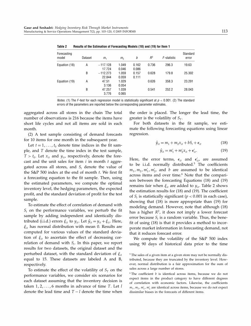
Table 2 Results of the Estimation of Forecasting Models (18) and (19) for Item 1

Forecasting Standardmodel Dataset m1 m2 b R2 F -statistic error

Equation (18) A −117�128 1�049 0�162 0�736 296�3 19�6317�724 0�046 0�086

B −112�273 1�059 0�157 0�628 179�8 25�30222�844 0�059 0�111

Equation (19) A 47�51 1�029 0�626 358�3 23�2913�136 0�054

B 47�257 1�039 0�541 252�2 28�0433�776 0�065

Notes. (1) The F -test for each regression model is statistically significant at p < 0�001. (2) The standarderrors of the parameters are reported below the corresponding parameter estimates.

aggregated across all stores in the chain The totalnumber of observations is 216 because the items haveshort life cycles and not all items are sold in eachmonth.(2) A test sample consisting of demand forecasts

for 10 items for one month in the subsequent year.Let t = 1� � � � � t0 denote time indices in the fit sam-

ple, and T denote the time index in the test sample,T > t0. Let xit and yit , respectively, denote the fore-cast and the unit sales for item i in month t aggre-gated across all stores, and St denote the value ofthe S&P 500 index at the end of month t. We first fita forecasting equation to the fit sample. Then, usingthe estimated parameters, we compute the optimalinventory level, the hedging parameters, the expectedprofit, and the standard deviation of profit for the testsample.To estimate the effect of correlation of demand with

St on the performance variables, we perturb the fitsample by adding independent and identically dis-tributed (i.i.d.) errors 1it to yit . Let yit = yit + 1it . Here,1it has normal distribution with mean 0. Results arecomputed for various values of the standard devia-tion of 1it to ascertain the effect of decreasing cor-relation of demand with St . In this paper, we reportresults for two datasets, the original dataset and theperturbed dataset, with the standard deviation of 1itequal to 15. These datasets are labeled A and B,respectively.To estimate the effect of the volatility of ST on the

performance variables, we consider six scenarios foreach dataset assuming that the inventory decision istaken 1�2� � � � �6 months in advance of time T . Let ldenote the lead time and T − l denote the time when

the order is placed. The longer the lead time, thegreater is the volatility of ST .For both datasets in the fit sample, we esti-

mate the following forecasting equations using linearregression.

yit =m1+m2xit + bSt + �it (18)

yit =m′1+m′

2xit + �′it � (19)

Here, the error terms, �it and �′it , are assumedto be i.i.d. normally distributed.5 The coefficientsm1�m2�m

′1�m

′2, and b are assumed to be identical

across items and over time.6 Note that the compari-son between the forecasting Equations (18) and (19)remains fair when 1it are added to yit . Table 2 showsthe estimation results for (18) and (19). The coefficientof St is statistically significant (p < 0�001 in each case),showing that (18) is more appropriate than (19) formodeling demand. However, note that although (18)has a higher R2, it does not imply a lower forecasterror because St is a random variable. Thus, the bene-fit of using (18) is that it provides a method to incor-porate market information in forecasting demand, notthat it reduces forecast error.We compute the volatility of the S&P 500 index

using 90 days of historical data prior to the time

5 The sales of a given item at a given store may not be normally dis-tributed, because they are truncated by the inventory level. How-ever, normal distribution is a fair approximation for the sum ofsales across a large number of stores.6 The coefficient b is identical across items, because we do notexpect items in the product category to have different degreesof correlation with economic factors. Likewise, the coefficientsm1�m2�m

′1�m

′2 are identical across items, because we do not expect

dissimilar biases in the forecasts of different items.

Gaur and Seshadri: Hedging Inventory Risk Through Market Instruments114 Manufacturing & Service Operations Management 7(2), pp. 103–120, © 2005 INFORMS

Table 3 Optimal Inventory Level and Expected Profit for Item 1 Obtained Using Forecasting Models (18) and (19) forEach Dataset for Different Degrees of Volatility of St

Optimal inventory Expected profit Increase in expected profitLead time

Dataset l (months) Model (18) Model (19) Model (18) Model (19) Mean Standard error Percent increase

A 1 179 153 1,299.53 1,221.66 77.87 20.41 6.37A 2 181 153 1,274.60 1,198.19 76.41 22.62 6.38A 3 183 153 1,250.20 1,175.55 74.65 24.11 6.35A 4 183 153 1,226.23 1,153.56 72.66 24.34 6.30A 5 183 153 1,202.73 1,132.09 70.63 24.98 6.24A 6 184 153 1,179.56 1,111.04 68.52 25.55 6.17B 1 181 155 1,270.68 1,208.27 62.41 19.88 5.17B 2 182 155 1,248.83 1,186.23 62.61 21.64 5.28B 3 183 155 1,226.83 1,164.70 62.13 23.00 5.33B 4 184 155 1,204.84 1,143.63 61.22 24.05 5.35B 5 184 155 1,182.90 1,122.93 59.97 24.49 5.34B 6 184 155 1,161.00 1,102.54 58.46 24.51 5.30

of inventory decision for month T by the methodgiven in Hull (2002, §11.3). The volatility is givenby the standard deviation of logSd/Sd−1�, where Sdis the closing value of the index for day d. Thevalue of the daily standard deviation is obtainedas 1.3984%, and the annual standard deviation as22.1982%, assuming 252 trading days in the year. Therisk-free rate of return is assumed to be 5% per year.

Optimal Inventory Level and Expected Profit.Using the estimates of Model (18), the demand fore-cast for item i in the test sample can be written as

DiT = a+ bST + �iT � (20)

where a=m1+m2xiT . We compute the optimal inven-tory level and the profit with and without hedging inthis model. As a benchmark, we compute the inven-tory level and profit for Model (19). Note that in (19)the demand forecast for item i in the test sample isgiven by m′

1+m′2xiT + �′iT .

Table 3 compares the inventory levels and theexpected profits obtained using demand distributionsestimated from the two forecasting models. Resultsare reported for one item in the test sample. Otheritems give similar insights. We find that using (18)instead of (19) changes the inventory decision signif-icantly and increases the expected profit by 5.1% to6.6% for different datasets. The values of the standarddeviation show that the increase in expected profit isstatistically significant. The reasons for the increaseare as follows.

(1) The two models use different probability distri-butions for the forecast error. In (19), the forecast error�′it is normally distributed, whereas in (18) the distri-bution of the forecast error is a convolution of the log-normal distribution of St and the normal distributionof �it . Because the lognormal distribution is skewedto the right, the convolution results in a higher inven-tory level. See Figure 5 for a Q-Q plot of the demanddistribution.(2) In Model (18), up-to-date information from the

financial markets has been used to augment the firm’shistorical data. Thus, forecasts based on (18) adjust tochanges in St . When the market moves up (down), theforecasts are revised upward (downward).

Figure 5 Q-Q Plot of the Demand for Item 1 Shows that the DemandDistribution Is Skewed to the Right

50

100

150

250

300

350

400

450

0 0.5 1.0 1.5 2.0 2.5 3.0 3.5–3.5 –3.0 –2.5 –2.0 –1.5 –1.0 –0.5

200

0

Gaur and Seshadri: Hedging Inventory Risk Through Market InstrumentsManufacturing & Service Operations Management 7(2), pp. 103–120, © 2005 INFORMS 115

Table 4 Variance of Profit with Different Hedging Strategies

Lower bound (LB) Static hedge− LB Dynamic hedge− LB

Lead time Standard � (Static � (DynamicDataset l (months) Variance error (� ) Variance hedge− LB) Variance hedge− LB)

A 1 80�16 2.87 85.71 0.29 80.40 0.23A 2 67�5 3.81 73.73 0.51 67.88 0.36A 3 58�61 4.10 65.02 0.65 59.07 0.42A 4 52�47 4.20 59.15 0.97 52.98 0.46A 5 47�47 4.14 54.28 1.02 47.99 0.46A 6 43�44 4.04 50.72 1.05 43.97 0.46B 1 87�65 1.98 92.66 0.39 87.79 0.15B 2 78�56 3.00 84.13 0.57 78.83 0.27B 3 71�43 3.56 77.22 0.64 71.79 0.35B 4 65�67 3.87 71.55 0.83 66.10 0.41B 5 61�09 4.05 67.39 0.94 61.58 0.45B 6 57�39 4.15 63.96 1.20 57.92 0.48

Notes. All variances are expressed as percentages of the variance of unhedged profit. The lower bound is obtained fromthe minimum variance hedge in §3.1. The static hedge is identical to the heuristic hedge in §3.1. The dynamic hedgeis constructed by dynamically rebalancing the heuristic hedge once at time �T − l�/2 as new information is revealed.

By comparing the results for different values of l,we find that Model (18) enables the decision maker torespond to the increase in volatility of St by increasingthe inventory level whereas Model (19) does not. Fur-thermore, hedging gives a greater reduction of risk asthe volatility of St increases, as shown below.

Risk and Investment. Table 4 compares the vari-ance of unhedged profit at the optimal inventorylevel with the variance of hedged profit. It comparesresults from the minimum variance hedge of §3.1 andfrom the heuristic hedge of §3.1 with no rebalanc-ing of the hedging portfolio (static hedge), and witha rebalancing of the hedging portfolio once at timeT − l/2 (dynamic hedge). Because the minimum vari-ance hedge gives a lower bound on the variance ofhedged profit, it provides a benchmark for the staticand dynamic hedges.The static hedge parameters, �, , and sp, are com-

puted as described in §3.1. The dynamic hedge iscomputed by dynamic programming. Thus, at timeT − l/2, the following actions take place: (i) the assetprice ST−l/2 and the preliminary forecast error, �T−l/2are observed7; (ii) the hedge parameters, (�1, 1�and sp1), are computed. These hedge parameters yield

7 We assume that the subjective forecast is reevaluated at timeT − l/2, and that the forecast error is a sum of two components,�T−l/2 observed at time T − l/2, and �T observed at time T . Here,we let Var��T−l/2�=Var��T �=Var���/2�

Table 5 Initial Investments Required Without Hedging and With StaticHedging for the Inventory Levels Corresponding to Tables 3and 4

Initial investment

Lead time Without With static PercentDataset l (months) hedging hedging difference

A 1 3,502.58 1,573.79 55.07A 2 3,535.56 1,484.95 58.00A 3 3,562.47 1,449.96 59.30A 4 3,563.47 1,424.20 60.03A 5 3,576.19 1,417.16 60.37A 6 3,588.22 1,417.31 60.50B 1 3,524.59 1,761.46 50.02B 2 3,547.35 1,675.63 52.76B 3 3,570.36 1,634.52 54.22B 4 3,590.07 1,613.15 55.07B 5 3,597.64 1,596.92 55.61B 6 3,596.34 1,582.51 56.00

the cash flows at time T − l/2. Thus, the hedgeparameters at time 0, �0� 0� and sp0, are then com-puted in order to hedge the cash flows at time T − l/2.From Proposition 2, rebalancing the hedge is not

a self-financing activity, because it uses informationabout �T−l/2. Thus, we reinvest the cash flow at timeT − l/2 at the risk-free rate to evaluate the varianceof hedged profit at time T . Identical series of sam-ple paths are used to evaluate all hedging strate-gies. Many simulation runs are conducted to computeaverage performance statistics and estimate the statis-tical significance of the results.

Gaur and Seshadri: Hedging Inventory Risk Through Market Instruments116 Manufacturing & Service Operations Management 7(2), pp. 103–120, © 2005 INFORMS

All figures in Table 4 are expressed as percent-ages of the variance of unhedged profit. We find thatthe lower bound on the variance of hedged profitvaries between 87.7% and 43.4%. Thus, the potentialreduction in variance that can be obtained by hedgingvaries between 12.4% and 56.6%. Static hedging has agap of about 6% with respect to the lower bound. Thisgap is statistically significant at p = 0�01. Dynamichedging realizes almost the full potential for variancereduction. Its gap with respect to the lower boundis about 0.4%, and is not statistically significant. Thisperformance is notable, because both dynamic andstatic hedging use only two financial instruments. Inparticular, the results on dynamic hedging show thateven though the decision maker is unable to modifythe inventory level after time t, he or she can still usenew information to manage the exposure to risk.We further find that the percent reduction in vari-

ance increases significantly with the volatility of St . Forexample, for dataset A the percent reduction in vari-ance under the minimum variance hedge is 20% whenl= 1 and 56.6%when l= 6. Thus, hedging is more ben-eficial when the market volatility is higher, or, equiv-alently, when the lead time is longer. As expected,we also find that the percent reduction in variancedecreases when demand is less correlated with St .Table 5 shows the initial investment in inven-

tory with and without hedging for each scenariocorresponding to Table 5. Note that hedging reducesthe initial investment by about 60% because theinflow from the short sale of the stock offsets thecash required for buying inventory and call options.

Table 6 Comparison of Optimal Inventory Level, Expected Profit, Standard Deviation of Profit, and Expected Utility forEach Item for a Risk-Averse Decision Maker Without and With Hedging

Optimal inventory level Expected profit Standard deviation of profit Expected utility

Without With Without With Without With Without WithItem hedging hedging hedging hedging hedging hedging hedging hedging

1 159 165 1�241�92 1,288.15 82.50 89.94 1�199�37 1,235.722 159 165 1�286�76 1,314.75 61.97 68.18 1�248�36 1,268.273 159 165 1�282�37 1,311.24 61.04 68.44 1�245�11 1,264.394 160 164 1�285�8 1,305.33 67.40 68.67 1�240�38 1,258.175 158 164 1�276�8 1,306.02 64.91 74.79 1�234�67 1,250.096 158 162 1�276�61 1,296.39 70.19 74.87 1�227�34 1,240.337 163 171 1�315�53 1,340.02 60.47 53.98 1�278�97 1,310.888 163 175 1�322�04 1,349.92 52.85 33.29 1�294�11 1,338.849 165 175 1�328�63 1,350.78 55.74 19.85 1�297�56 1,346.84

10 164 176 1�326�99 1,351.23 53.48 15.85 1�298�4 1,348.72

Note. These results are obtained using the original dataset, i.e., �it = 0.

Furthermore, the investment decreases as the volatil-ity of St increases. This is surprising: We wouldexpect both the amount of inventory and the priceof the call option to increase with volatility, result-ing in larger investment. We find that � increaseswith volatility, however. Thus, a larger quantity ofthe underlying asset is sold short, offsetting theadditional investment required in inventory and calloptions.Therefore, from Tables 4 and 5 we conclude that the

benefits of hedging increase with the volatility of St .Interestingly, this implies that items with longer leadtimes will benefit more from hedging than items withshorter lead times.

Risk-Averse Decision Maker. To evaluate the ef-fect of hedging on the optimal inventory deci-sion of the risk-averse decision maker, we assumethe expected utility representation E�uw�� = E�w� −4Var�w�� where w denotes wealth. The value of 4 istaken as 0.01. Table 6 presents the inventory levelsthat maximize the expected utility for each of the 10items in the test sample with and without hedging.Observe that hedging increases the optimal inven-tory level. It brings the inventory level closer to theexpected value maximizing quantity, restoring effi-ciency in the market.

5. ConclusionsWe have shown how to generate a solution to thehedging of inventory risk using the newsvendormodel when demand is correlated with the price of

Gaur and Seshadri: Hedging Inventory Risk Through Market InstrumentsManufacturing & Service Operations Management 7(2), pp. 103–120, © 2005 INFORMS 117

a financial asset. Hedging reduces the variance ofprofit and the investment in inventory, increases theexpected utility of a risk-averse decision maker, andincreases the optimal inventory level for a broad classof utility functions. Our numerical analysis showsthat hedging is more beneficial when the price of theunderlying asset is more volatile or the product hasa longer order lead time. Dynamic hedging providesadditional risk reduction even when the retailer can-not change her initial inventory commitment.Our forecasting model could be extended to incor-

porate macroeconomic variables such as interest ratesand foreign exchange rates that provide demand sig-nals. It might also be customized for specific busi-nesses by using more securities from the equitiesmarket, such as sector-specific indices or portfoliosof firms in similar businesses. Furthermore, the evo-lution of the price of the underlying asset may beused to update the demand forecast and modify orderquantities even in the absence of early demand data.An important aspect of our analysis is that the

demand risk is not fully spanned by the financialmarket. Our analysis of the effects of financial hedg-ing on operational decisions under such a scenariomay be extended to other problems that have beenconsidered in the real-options literature, such as pro-duction switching (Dasu and Li 1997, Huchzermeierand Cohen 1996, Kouvelis 1999), capacity planning(Birge 2000), and global contracting (Scheller-Wolfeand Tayur 1999).

AcknowledgmentsThe authors thank Marti Subrahmanyam and seminar par-ticipants at Case Western Reserve University, NorthwesternUniversity, Rutgers University, the University of Michigan,and the University of Texas Dallas for helpful comments.They also thank Garrett J. van Ryzin, the senior editor, andtwo anonymous referees for many helpful suggestions. Thework of the second author is partially supported by NSFGrant DMI-0200406.

AppendixProof of Proposition 2. According to Lemma 1, the

optimal hedge at time t is given by E�t ��TU I� � St�. If

no additional information about � is available at time tcompared with time 0, then the optimal hedge at time tequals E���T

U I� � St�. However, E���TU I� � St� is a martingale

with respect to the filtration generated by St�. Thus, thedynamic hedging strategy, E���T

U I� � St�� is self-financing.

If, however, additional information about � is available attime t, then E�t ��

TU I� � St� is not a martingale with respect to

the filtration generated by St�. Thus, the dynamic hedgingstrategy is not, in general, self-financing. �

Proof of Proposition 3. We show that if

c1I > EN[E�min ST + �� I − a�/b � ST ��

]�

then there exists a portfolio XT that is preferred to �U byall risk-averse decision makers. Let

XT = E�min ST + �� I − a�/b � ST ���Then XT is a strictly increasing function of ST . The newven-dor profit function can be written in terms of XT , as

�U =XT − c1I + 5ST ��

where E�5ST � �XT �= E�5ST � � ST �= 0. From the conditionalJensen’s inequality,

E�u�U ��= E[E�uXT − c1I + 5� � ST �

]≤ E�uXT − c1I���

Now, note that the time-zero cost of portfolio XT is X0 =e−rTEN �XT �. Thus, if

c1I > EN[E�min ST + �� I − a�/b � ST ��

]�

then investment of an amount less than e−rT c1I in XT yieldsa higher expected utility than the inventory investment.The second part of the proposition follows from the

fact that EN �min ST � I − a�/b�� and EN �min ST � I − a�/b��−E�����, respectively, are upper and lower bounds on

EN[E�min ST + �� I − a�/b � ST ��

]� �

Proof of Proposition 4. Let + ∈ be the Lagrangianmultiplier for the constraint E�XT −X0e

rT �= 0. The decisionmaker solves the problem

maxE[uW +�UI�−XT +X0e

rT �++XT −+X0erT]�

Because u is concave, the first-order conditions of optimalityare sufficient. The optimal solution is obtained by maximiz-ing the utility function pointwise at each value of ST . Thus,the first-order conditions are

E�[u′W +�UI�−XT +X0e

rT �]= +� (21)

E�XT −X0erT �= 0� (22)

A feasible solution to this system of equations can befound as follows: Fix +. For each value of ST , find XT suchthat (21) is satisfied. This value of XT exists and is uniquebecause u′ is strictly decreasing. Substitute XT into (22).If E�XT − X0e

rT � > 0, then reduce + (and correspondinglyreduce all XT ) until a solution is obtained. Otherwise,increase + and correspondingly increase all XT .Suppose that there exist two distinct solutions to (21)–

(22), denoted +�X∗∗T +�� and +′�X∗∗

T +′��. Clearly, + = +′.

Gaur and Seshadri: Hedging Inventory Risk Through Market Instruments118 Manufacturing & Service Operations Management 7(2), pp. 103–120, © 2005 INFORMS

This further shows that X∗∗T +� is equal to X∗∗

T +′� almost

everywhere. Thus, the two solutions are equal except pos-sibly on a set of measure zero. �

Proof of Proposition 5. The first derivative of the ex-pected utility function evaluated at �= 0 gives

E[u′W +min ST + �� I − a�/b�− c1I� −XT +X0e

rT �]�

Here, u′·� is a decreasing function of ST at �= 0, and −XT +X0e

rT is also decreasing in ST . Thus, they have a positivecovariance, which gives

E[u′W +min ST + �� I − a�/b�− c1I� −XT +X0e

rT �]

≥ E[u′W +min ST + �� I − a�/b�− c1I�]

·E�−XT +X0erT �

= 0�

where the last equality follows from (12). �

Proof of Proposition 6. The value of inventory thatmaximizes E�u�H�� is greater than the value of inventorythat maximizes E�u�U �� if

E[ u′�HI��−u′�U I���

6�U

6I

]≥ 0�

Here, we have used the fact that 6�H/6I = 6�U/6I . Let G��denote the distribution function of �. Conditioning on STand taking expectation with respect to �, we get

E�

[ u′�HI��−u′�U I���

6�

6I

∣∣∣∣ST]

=−c1∫ I−a�/b

−� u′�HI��−u′�U I��� dG��

+ u′I − a�/b− c1I −�XT +�X0erT �

−u′I − a�/b− c1I��Pr{�≥ I − a�/b− ST

}�

Consider the expectation over ST of the second term in theabove equation. We use the facts that

Pr �≥ I − a�/b− ST �≥ Pr �≥ I − a�/b��

and that ST is independent of � to write

E[ u′I − a�/b− c1I −�XT +�X0e

rT �−u′I − a�/b− c1I��

·Pr �≥ I − a�/b− ST �]

≥ E[ u′I − a�/b− c1I −�XT +�X0erT �

−u′I − a�/b− c1I��Pr �≥ I − a�/b�]

≥ [E�u′I − a�/b− c1I −�XT +�X0e

rT ��

−u′I − a�/b− c1I�]Pr �≥ I − a�/b�� (23)

Thus, if

E[u′I − a�/b− c1I −�XT +�X0e

rT �]≥ u′I − a�/b− c1I��

then the second term is nonnegative. This inequality com-bined with the first term gives sufficient conditions on thehedging portfolio under which the hedged optimal inven-tory level is larger than the unhedged optimal inventorylevel.When u·� is CARA or DARA, then u′·� is convex in

wealth. Thus, applying Jensen’s inequality to (23), we get

E[u′I−a�/b−c1I−�XT +�X0e

rT �]−u′I−a�/b−c1I�

≥u′(I−a�/b−c1I−�E�XT −X0erT �

)−u′I−a�/b−c1I�=0� �

The following lemma is a standard result. It is useful forproving Proposition 7.

Lemma 2. Let X be any random variable, and f ) →be a decreasing function such that E�f X�� = 0. Then, (i) forany decreasing nonnegative function wx�, E�wX�f X�� > 0;(ii) for any increasing nonnegative function wx�,E�wX�f X�� < 0.

Proof. Consider (i). Let GX� denote the cumulative dis-tribution function of X. Because f x� is decreasing in x,there exists x0 such that f x� > 0 for all x < x0 and f x� < 0for all x > x0. Then,

E�wx�f X�� =∫ x0

0wx�f x�dGx�+

∫ �

x0

wx�f x�dGx�

>∫ x0

0wx0�f x�dGx�+

∫ �

x0

wx0�f x�dGx�

≥ wx0�E�f X��

≥ 0�

Now consider (ii). We have

E�wx�f X�� =∫ x0

0wx�f x�dGx�+

∫ �

x0

wx�f x�dGx�

<∫ x0

0wx0�f x�dGx�+

∫ �

x0

wx0�f x�dGx�

≤ wx0�E�f X��

≤ 0� �

Proof of Proposition 7. Let the hedged profit bedenoted � (the subscript H is ignored for simplicity). Weneed to show that 62E�u���/6I 6� is greater than or equalto zero. We have

62

6I 6�E�u��� = E

[u′′��

6�

6I

6�

6�

]

= E[E�

[u′′��

6�

6I

∣∣∣∣ST]6�

6�

](24)

= E[−c1E��u′′�� � ST �

6�

6�− 1bRA�0�u

′�0�

·Pr � > I − a�/b− ST �6�

6�

]� (25)

Gaur and Seshadri: Hedging Inventory Risk Through Market InstrumentsManufacturing & Service Operations Management 7(2), pp. 103–120, © 2005 INFORMS 119

where (24) follows because 6�/6� is independent of �. For(25), note that

6�

6I=−c1+

1b1 � > I − a�/b− ST �� (26)

Also note that � is independent of � for � > I − a�/b− ST ,and we write

�0 = I − a�/b− c1I −�XT +�X0�

Finally, u′′��=−RA��u′��.

Consider E��u′′�� � ST �. Let G�� denote the distributionfunction of �. We have

E��u′′�� � ST �=∫ I−a�/b−ST

−�u′′ST + �− c1I −�XT +�X0� dG��

+∫ �

I−a�/b−STu′′I − a�/b− c1I −�XT +�X0� dG���

Because u′′·� < 0, the above expression shows thatE��u′′�� � ST � is negative for all ST . Furthermore, differenti-ating E��u′′�� � ST � with respect to ST , we getd

dSTE��u

′′�� �ST �

=∫ I−a�/b−ST

−�u′′′ST +�−c1I−�XT +�X0�

(1−�dXT

dST

)dG��

−∫ �

I−a�/b−STu′′′I−a�/b−c1I−�XT +�X0��

dXT

dSTdG���

Letf �� ST �= 1 � < I − a�/b− ST �−�dXT /dST �

f ·� is decreasing in �. Furthermore, E��f ·� � ST �, which isequal to the slope of E��� � ST � with respect to ST , is positivefor all � ∈ �0� ��. Thus, f ·� is a decreasing function with anonnegative conditional expectation with respect to �.In addition, u′′′·� > 0 because u·� is CARA or DARA.

Furthermore, from the assumption of constant or decreasingabsolute prudence, we have that u′′′·� is decreasing in �.Combining these observations and applying Lemma 2(i), wefind that E��u′′�� � ST � is increasing in ST .Consider the first term in (25): 6�/6� is decreasing in ST

and has zero expectation (due to the first condition for anoptimum with respect to �); −c1E��u′′�� � ST � is decreasingin ST and is nonnegative for all ST . Thus, all conditions ofLemma 2(i) are satisfied. Therefore, applying Lemma 2(i),we find that the first term in (25) is nonnegative.Consider the second term in (25). Here, �0 is decreas-

ing in ST . Thus, RA�0�, u′�0�, and Pr � > I − a�/b − ST �are increasing in ST ; 6�/6� is decreasing in ST and haszero expectation. Therefore, applying Lemma 2(ii), we findthat the second term in (25) (i.e., 1/b�RA�0�u

′�0�Pr � >I − a�/b− ST �6�/6�) is negative.Thus, dI∗/d�≥ 0 for 0≤ �≤ �. �

ReferencesAgrawal, V., S. Seshadri. 2000a. Effect of risk aversion on pricing

and order quantity decisions. Manufacturing Service Oper. Man-agement 2(4) 410–423.

Agrawal, V., S. Seshadri. 2000b. Risk intermediation in supplychains. IIE Trans. 32(9) 819–831.

Arrow, K. 1971. Essays in the Theory of Risk-Bearing. North-Holland,Amsterdam, The Netherlands.

Birge, J. 2000. Option methods for incorporating risk into linearcapacity planning models. Manufacturing Service Oper. Manage-ment 2(1) 19–31.

Brennan, M., E. Schwartz. 1985. Evaluating natural resource invest-ments. J. Bus. 58(2) 135–157.

Chen, F., A. Federgruen. 2000. Mean-variance analysis of basicinventory models. Working paper, Graduate School of Busi-ness, Columbia University, New York.

Copeland, T., V. Antikarov. 2001. Real Options: A Practitioner’s Guide.Texere Publishers, London, UK.

Dasu, S., L. Li. 1997. Optimal operating policies in the pres-ence of exchange rate variability. Management Sci. 43(5)705–722.

Eeckhoudt, L., C. Gollier, H. Schlesinger. 1995. The risk-averse (andprudent) newsboy. Management Sci. 41(5) 786–794.

Gaur, V., S. Seshadri. 2004. Hedging inventory risk through mar-ket instruments. Technical report, Leonard N. Stern School ofBusiness, New York University, New York (October). Availableat http://pages.stern.nyu.edu/∼vgaur/research.html.

Hadley, G., T. M. Whitin. 1963. Analysis of Inventory Systems.Prentice-Hall Inc., Englewood Cliffs, NJ.

Huchzermeier, A., M. Cohen. 1996. Valuing operational flexibilityunder exchange rate risk. Oper. Res. 44(1) 100–113.

Hull, J. C. 2002. Options, Futures, and Other Derivatives, 4th ed.Prentice-Hall Inc., Englewood Cliffs, NJ.

Instinet Research. 2001a. Redbook Retail Sales Monthly. (November)New York.

Instinet Research. 2001b. The Redbook Average. (December 4)New York.

Kimball, M. S. 1990. Precautionary saving in the small and in thelarge. Econometrica 58(1) 53–73.

Kimball, M. S. 1993. Standard risk aversion. Econometrica 61(3)589–611.

Kogut, B., N. Kulatilaka. 1994. Operating flexibility, global manu-facturing, and the option value of multinational network.Man-agement Sci. 40(1) 123–139.

Kouvelis, P. 1999. Global sourcing strategies under exchange rateuncertainty, Chap. 20. S. Tayur, R. Ganeshan, M. Magazine,eds. Quantitative Models for Supply Chain Management. KluwerAcademic Publishers, Boston, MA.

Lee, H. L., S. Nahmias. 1993. Single product single loca-tion models, Chap. 1. S. C. Graves, A. H. G. RinnooyKan, P. H. Zipkin, eds. Handbooks in OR and MS, Vol. 4.Logistics of Production and Inventory. North-Holland Publishers,The Netherlands.

McDonald, R., D. Siegel. 1986. The value of waiting to invest. Quart.J. Econom. 101(4) 707–728.

Nahmias, S. 1993. Production and Operations Analysis, 2nd ed. IrwinPublishers, Boston, MA.

Pliska, S. 1999. Introduction to Mathematical Finance: Discrete TimeModels. Blackwell Publishers, Malden, MA.

Porteus, E. 2002. Foundations of Stochastic Inventory Theory. StanfordUniversity Press, Stanford, CA.

Gaur and Seshadri: Hedging Inventory Risk Through Market Instruments120 Manufacturing & Service Operations Management 7(2), pp. 103–120, © 2005 INFORMS

Scheller-Wolfe, A., S. Tayur. 1999. Managing supply chains inemerging markets. S. Tayur, R. Ganeshan, M. Magazine, eds.Quantitative Models for Supply Chain Management, Chap. 22.Kluwer Academic Publishers, Boston, MA.

Triantis, A., J. Hodder. 1990. Valuing flexibility as a complex option.J. Finance 45(2) 549–565.

Trigeorgis, L. 1996. Real Options. MIT Press, Cambridge, MA.

Williams, D. 1991. Probability with Martingales. Cambridge Univer-sity Press, Cambridge, UK.

Zipkin, P. H. 2000. Foundations of Inventory Management. McGraw-Hill, New York.