Quadratic semiparametric Von Mises calculus

Metrika (2009) 69:227–247DOI 10.1007/s00184-008-0214-3

Quadratic semiparametric Von Mises calculus

James Robins · Lingling Li · Eric Tchetgen ·Aad W. van der Vaart

Published online: 4 December 2008© The Author(s) 2008. This article is published with open access at Springerlink.com

Abstract We discuss a new method of estimation of parameters in semiparametricand nonparametric models. The method is based on U -statistics constructed from qua-dratic influence functions. The latter extend ordinary linear influence functions of theparameter of interest as defined in semiparametric theory, and represent second orderderivatives of this parameter. For parameters for which the matching cannot be perfectthe method leads to a bias-variance trade-off, and results in estimators that convergeat a slower than n−1/2-rate. In a number of examples the resulting rate can be shownto be optimal. We are particularly interested in estimating parameters in models witha nuisance parameter of high dimension or low regularity, where the parameter ofinterest cannot be estimated at n−1/2-rate.

Keywords Von Mises calculus · Semiparametric models · Missing data ·Tangent space · Influence function · Rate of convergence

1 Introduction

Let X1, X2, . . . , Xn be a random sample from a distribution Pη with density pη rel-ative to a measure µ on a sample space (X ,A), where the parameter η is knownto belong to a subset H of a normed space. We wish to estimate the value χ(η) ofa functional χ : H → R with the help of the observations X1, . . . , Xn . Our main

J. Robins · L. Li · E. TchetgenDepartment of Biostatistics and Epidemiology, School of Public Health, Harvard University,Cambridge, USA

A. W. van der Vaart (B)Department of Mathematics, Vrije Universiteit Amsterdam, Amsterdam, The Netherlandse-mail: [email protected]

123

228 J. Robins et al.

interest is in the situation of a semiparametric or nonparametric model, where H is aninfinite-dimensional set, and the dependence η �→ pη is smooth.

This problem has been studied under the heading “semiparametric statistics” inthe 1980s and 1990s. A theory of asymptotic lower bounds for “regular parameters”χ(η) based on Le Cam’s concept of local asymptotic normality (Le Cam 1960) wasdeveloped starting with Koševnik and Levit (1976) and Pfanzagl (1982), and workedout for many examples in, among others, Begun et al. (1983), van der Vaart (1988)and Bickel et al. (1993). There are many examples of ad-hoc estimators that attainthese bounds, and the behaviour of principled methods such as maximum likelihood(including its sieved and penalized variants) or estimating equations is understood toa certain extent (e.g., van der Vaart 1994; Murphy and van der Vaart 2000; Bolthausenet al. 2002; Wellner et al. 1993; van der Laan and Robins 2003).

Certain combinations of models (Pη: η ∈ H) and parameter χ(η) possess struc-tural properties that allow to estimate the parameter at n−1/2-rate, no matter the sizeof the parameter set H . In this paper we are interested in the other situations, wherethe rate of estimation drops when the complexity of the model exceeds a certain limit.Such examples arise for instance when many covariates must be included in a modelto correct for possible confounding in a causal study, or for modelling the probabil-ity that an individual is included in a sample in a study with missing observations.If simple (e.g., linear) models for the dependence on these covariates are not plau-sible, which is typical in epidemiological studies, then the resulting model must betaken so large that the usual methods fail. These methods typically focus on varianceonly, because the bias is negligible due to the structure of the model, or by explic-itly assuming a “no-bias condition” (see Klaassen 1987; Murphy and van der Vaart2000). In this paper we develop new methods that make a bias-variance trade-off whennecessary.

These methods are based on quadratic estimating equations rather than the usuallinear estimating equations.

Quadratic expansions for semiparametric models were previously investigated byPfanzagl and Wefelmeyer (Pfanzagl 1985), but from the very different perspectiveof second order efficiency, i.e., the refinement of first order bounds by adding alower order term. Our aim is to show that second order influence functions canbe used for first order inference, because they permit balancing of bias and vari-ance.

Following linear and quadratic is cubic, and so on. Extension of our approach to stillhigher orders is possible, but comes with many new complications. We shall pursuethis elsewhere.

The paper is organized as follows. In Sect. 2 we review linear estimators from ourcurrent perspective. Next in Sect. 3 we introduce our new method of constructingquadratic estimators. This section has mostly a heuristic nature. In Sects. 4 and 5we give rigorous constructions and results for two examples. The first is a classicaltheoretical example. The second is more extensive and concerns estimating a meanresponse when the response is not always observed.

Notation Let Pn and Un denote the empirical measure and empirical U -statisticmeasure, viewed as an operators on functions: for given functions f : X → R and

123

Quadratic semiparametric Von Mises calculus 229

g: X 2 → R these are given by

Pn f = 1

n

n∑

i=1

f (Xi ), Ung = 1

n(n − 1)

∑ ∑

1≤i �= j≤n

g(Xi , X j ).

We use the notation Un f also for f : X → R a function of one argument, with theinterpretation Un f = Pn f . This is consistent with the given formulas if a function ofone argument is considered as a function of 2 arguments that is constant in its secondargument.

We write PnUng = P2g for the expectation of Ung if X1, . . . , Xn are distributed

according to the probability measure P . We also use the operator notation for theexpectations of statistics in general.

We call a measurable function g: X 2 → R degenerate relative to P if∫g(x1, x2) d P(xi ) = 0 for i = 1, 2, and we call it symmetric if g(x1, x2) = g(x2, x1)

for every x1, x2 ∈ X .Given two functions g, h: X → R we write g × h for the function (x, y) �→

g(x)h(y). Such tensor products functions are degenerate if both functions f and ghave mean zero. The corresponding notation P × Q of two measures P and Q givesthe product measure.

2 Linear estimator

Given an initial estimator η of η, the plug-in estimator χ(η) is typically a consistentestimator of the parameter of interest χ(η), but it may not be a good estimator. Inparticular, if η is a general purpose estimator, not specially constructed to yield agood plug-in, then χ(η) will often have a suboptimal precision. To gain insight in thissituation we assume that the parameter permits a Taylor expansion of the form

χ(η) = χ(η) + χ ′η(η − η) + O

(‖η − η‖2

). (1)

Such an expansion suggests that the plug-in estimator will have an error of the orderOP

(‖η − η‖), unless the linear term in the expansion vanishes.The expansion (1) also suggests that better estimators can be obtained by “esti-

mating” the linear term in the expansion. To achieve this we assume a “generalizedvon-Mises representation” of the derivative of the form

χ ′η(η − η) =

∫χη d(Pη − Pη) =

∫χη d Pη + O

(‖η − η‖2

), (2)

for some measurable function χη: X → R, referred to as an influence function. Thesecond equality is valid if χη is degenerate relative to Pη (i.e., Pηχη = 0) for every η,which can always be arranged by a recentering, as

∫1 d(Pη − Pη) = 0. The von-Mises

representation and Eq. (1) suggest the “corrected plug-in estimator”

χ(η) + Pnχη. (3)

123


This estimator should have an error of the order OP (n−1/2) + OP(‖η − η‖2

), as

the difference (Pn − Pη)χη is “centered” and ought to have “variance” of the orderO(1/n).

We put “centered” and “variance” in quotes, because the randomness in the initialestimator η prevents a simple calculation of mean and variance. Empirical processtheory can be used to show that the effect of replacing χη by χη is negligible, if theclass of functions χη is not too rich. In the present paper we are interested in ordersof magnitude only, and then a simpler approach is to split the sample and use sepa-rate observations to construct η and to construct Pn . Then the orders can be justifiedby reasoning conditionally on the first sample, and it suffices that

∫χ2

ηd Pη remains

bounded in probability.Von Mises (1947) originally introduced the expansions that are named after him in

order to investigate functionals of empirical distributions. The idea to use expansions(1) for estimation in nonparametric models occurs in Emery et al. (2000). Our situationis more involved, because we are interested in models (Pη: η ∈ H) that are structuredthrough a map η �→ pη, and we are interested in a functional χ(η) of the parameter.In this situation a von-Mises type expansion can fail for two reasons. First a derivativeχ ′

η is by definition a continuous, linear map on the underlying normed space, andsuch maps may or may not be representable as an integral, depending on the normedspace. Second, our von Mises expansion (2) represents this derivative as an integralrelative to the distribution Pη and hence also involves the inverse map Pη → η fromthe distribution of the data to the parameter. We require representation through Pη,because this allows us to construct the estimator (3) by replacing Pη by the empiricaldistribution.

These issues are related to investigations in the theory of semiparametric models(see Koševnik and Levit 1976; Pfanzagl 1982; van der Vaart 1988; Bickel et al. 1993).These papers define a tangent set of a semiparametric model (Pη: η ∈ H) as the setof functions gη: X → R obtainable as

12 gη

√pη = lim

t↓0

√pηt − √

pη

t,

where the limit is taken in the L2-sense, and t �→ ηt ranges over a collection of mapsfrom [0, 1] ⊂ R to H for which the limit exists. Informally, a “tangent vector” gη isjust a score function

gη = ∂

∂t |t=0log pηt =

∂∂t |t=0 pηt

pη

, (4)

of a one-dimensional submodel (Pηt : t ≥ 0) at t = 0, where η0 = η. (Taking thederivative in the L2-sense is appropriate for asymptotic information theory, but notnecessarily so for the present heuristic discussion.) An influence function is definedas a measurable map χη: X → R such that, for all paths t �→ ηt considered,

d

dt |t=0χ(ηt ) = Pηχη gη. (5)

123


It is not difficult to see that the latter influence function is the same as the influencefunction needed in the von-Mises expansion (2), if the various types of derivativesmatch up. (Note that the middle expression in (2) with η replaced by ηt and η by η

expands to Pηχη gη + o(t), as pηt − pη = t gη pη + o(t).) Necessary and sufficientconditions for existence of an influence function in terms of the derivatives of the mapsη �→ χ(η) and η �→ pη were investigated in van der Vaart (1991).

An influence function is not necessarily unique, as only its inner products withelements gη of the tangent set matter. The projection of any influence function thatis contained in the closed linear span of the tangent set is called the efficient influ-ence function or canonical gradient, as it is the influence function of asymptoticallyefficient estimators. It minimizes the variance varη Pnχη over all influence functions.

3 Quadratic estimator

If the preliminary estimator η attains a rate of convergence ‖η − η‖ = oP (n−1/4),then the plug-in estimator (3) attains a n−1/2-rate of convergence. Typically this willrequire that the parameter set H is not too big. If the preliminary estimator is lessprecise, then the remainder term of the expansion (1) will dominate. This suggests totake the expansion further to

χ(η) = χ(η) + χ ′η(η − η) + 1

2χ ′′η(η − η, η − η) + O

(‖η − η‖3

). (6)

The generalization of the first order construction now requires a von Mises type rep-resentation of the form, for measurable functions χη: X → R and χη: X 2 → R,

χ ′η(η − η) + 1

2χ ′′η(η − η, η − η) =

∫χη d(Pη − Pη) + 1

2

∫ ∫χη d(Pη − Pη)

×(Pη − Pη) + O(‖η − η‖3

). (7)

We assume without loss of generality that the functions χη and χη are degeneraterelative to Pη. The von-Mises representation then suggests the “corrected plug-inestimator”

χ(η) + Pnχη + 12 Unχη. (8)

The empirical measure and two-sample U -statistic serve as unbiased estimators of theexpectations of their kernels. For simplicity we may again base the initial estimatorη and these two U -statistics on independent samples of observations. Because thevariance of a U -statistic is of order O(1/n), this estimator ought to have an error ofthe order OP (n−1/2) + OP

(‖η − η‖3). We shall discuss the validity of this later.

To characterize the first and second order influence functions we can again employsmooth one-dimensional submodels (Pηt : t ≥ 0). With the first and second order

123


derivatives of these models denoted by

gη =∂∂t |t=0 pηt

pη

, gη =∂2

∂t2 |t=0pηt

pη

, (9)

the von Mises expansion (7) can informally be seen to imply

d

dt |t=0χ(ηt ) = Pηχη gη, (10)

d2

dt2 |t=0χ(ηt ) = Pηχη gη + P2

η χη(gη × gη). (11)

The Eq. (10) is identical to Eq. (5), and hence a first order influence function χη canbe taken as before. Following Pfanzagl (1985) we define a second order influencefunction χη as a measurable function χη: X 2 → R that satisfies (11) for every patht �→ ηt under consideration. From Eq. (11) we see that χη is unique only up to func-tions that are orthogonal to functions of the form gη × gη, for gη belonging to thetangent set. In particular, a second order influence function χη can always be taken tobe symmetric and degenerate relative to Pη. It must be taken so in the construction ofthe estimator (8).

The two influence functions occur together in Eq. (11), and hence should be con-sidered a pair (χη, χη) of functions rather than as two separate functions. This isparticularly important if the tangent set is not “full”, i.e., smaller than the set of allmean-zero functions in L2(Pη), the tangent set of a nonparametric model. Both firstand second order influence functions are then non-unique, but their different versionscannot be freely combined into valid pairs (χη, χη). This is connected to the factthat first and second order derivatives gη and gη are also not clearly separated. Asimple change of speed t �→ φ(t) of a path through a second order diffeomorphismφ: [0, 1] → [0, 1] leads to the submodel (Pηφ(t) : t ≥ 0) with first and second orderderivatives, by the chain rule,

φ′(0)gη, φ′(0)2 gη + φ′′(0)gη.

Thus the first order derivative becomes part of the second order derivative after repa-rameterization. Pfanzagl (Pfanzagl 1985, 2.4.4) has shown, under assumptions ofsmoothness of the tangent set as a function of the parameter, that the sum of everyfirst order derivative and every second order derivative occurs as the second orderderivative of some path. Thus the set of second order derivatives gη is only defined upto equivalence modulo the tangent set.

From Eq. (11) it is also clear that second order influence functions involve the jointdistribution of two observations. Correspondingly, we prefer to define a second ordertangent space of the model not through the second order derivatives gη along paths

123


t �→ pηt , but through the functions of two arguments

sη : =∂2

∂t2 |t=0(pηt × pηt )

pη × pη

= gη × 1 + 2 gη × gη + 1 × gη. (12)

The function sη is a second order score for the model (Pη × Pη: η ∈ H) for twoobservations. The corresponding first order scores are

sη : =∂∂t |t=0(pηt × pηt )

pη × pη

= gη × 1 + 1 × gη. (13)

With these notations the Eqs. (10), (11) defining the influence functions can also bewritten as, if χη is chosen degenerate,

d

dt |t=0χ(ηt ) = P2

η

(χη + 1

2 χη

)sη = d

dt |t=0P2

ηt

(χη + 1

2 χη

), (14)

d2

dt2 |t=0χ(ηt ) = P2

η

(χη + 1

2 χη

)sη = d2

dt2 |t=0P2

ηt

(χη + 1

2 χη

). (15)

Here we interprete the function χη: X → R as a function χη: X 2 → R that dependson the first argument only (and is constant in the second), or (better) replace it by itssymmetrization (x1, x2) �→ 1

2

(χη(x1) + χη(x2)

). The equations show that the over-

all influence function χη + 12 χη is characterized by having “correct” inner products

with the overall scores sη and sη. This overall influence function uniquely definesits constituents χη and 1

2 χη provided χη is restricted to be degenerate. The overallinfluence function is itself unique only up to projection onto the closed linear span inL2(Pη × Pη) of all functions sη and sη.

The equality of the far left and right sides of Eqs. (14), (15) gives an alternativecharacterization of the overall influence function (at η0) as a function such that themaps η �→ χ(η) and η �→ P2

η (χη0 + 12 χη0) possess the same first and second order

derivatives at η0. Because the derivatives of a map φ on an open subset H of a normedspace are completely characterized by the derivatives of the maps t �→ φ(η0 + th),for h ranging over the space (“Gateaux derivatives”), we conclude that in the caseof such parameters sets H it suffices to consider linear paths t �→ ηt = η0 + th.(The mixed second derivative φ′′

η0(g, h) can be recovered from φ′′

η0(g + h, g + h) and

φ′′η0

(g −h, g −h) by “polarization”.) This is true more generally for parameter spacesH defined by a linear constraint, but in the case of nonlinear constraints the use ofcurved paths is necessary.

The plug-in estimator (8) can be written χ(η) + Un(χη + 12 χη). A definition of

an efficient or canonical second order influence function, should therefore refer tothe variance of the U -statistic Un(χη + 1

2 χη). Unlike in the linear case this does nottranslate in the variance of the influence function χη + 1

2 χη itself (except for n = 2if χη is interpreted as the symmetric function (x1, x2) �→ 1

2

(χη(x1) + χη(x2)

)). By

123


Eq. (5), if χη is chosen degenerate and symmetric,

n varη Un(χη + 12 χη) = Pηχ

2η + 1

2(n − 1)P2

η χ2η .

Thus the second order part adds a term of order O(1/n) relative to the first ordercontribution. The norm of the function χη + 1

2 χη in L2(Pη × Pη) is irrelevant, eventhough the inner product of this space determines the influence functions.

It is possible to resolve this discrepancy by working in the model with n observa-tions. From the expansion

n∏

i=1

pηt

pη

(xi ) =n∏

i=1

(1 + t gη(xi ) + 1

2 t2gη(xi ) + · · ·)

= 1 + tn∑

i=1

gη(xi ) + t2

⎛

⎝ 12

n∑

i=1

gη(xi ) +∑ ∑

1≤i< j≤n

gη(xi )gη(x j )

⎞

⎠ + · · · ,

we see that first and second order scores for the model (Pnη : η ∈ H) take the forms

s(n)η =

∂∂t |t=0(pηt × · · · × pηt )

pη × · · · × pη

= nPn gη, (16)

s(n)η =

∂2

∂t2 |t=0(pηt × · · · × pηt )

pη × · · · × pη

= nPn gη + n(n − 1)Un(gη × gη). (17)

Rather than in the form Eqs. (14), (15), the Eqs. (10), (11) that define the influencefunctions can then be written in the form

d

dt |t=0χ(ηt ) = Pn

η

(Un

(χη + 1

2 χη

))s(n)η , (18)

d2

dt2 |t=0χ(ηt ) = Pn

η

(Un

(χη + 1

2 χη

))s(n)η . (19)

We conclude that the influence functions are determined by the inner products of theU -statistic Un

(χη + 1

2 χη

)in L2(Pn

η ) with the score functions s(n)η and s(n)

η . The influ-ence functions that yield a minimal variance are found by projecting this U -statisticonto the closed linear span of these score functions. Thus it is natural to define thelatter span as the second order tangent space of the model.

For computation in examples the defining Eq. (11) or (15) of a second order influ-ence function can be tedious. It is usually easier to apply the rule that a second derivativeis the derivative of the first derivative. In the present situation this takes the followingform (Pfanzagl 1985, 4.3.11): if χη: X 2 → R is a function such that x2 �→ χη(x1, x2)

is a first order influence function of the parameter η �→ χη(x1), for every fixed x1 anda first order influence function χη (not necessarily degenerate), then χη is a secondorder influence function.

123


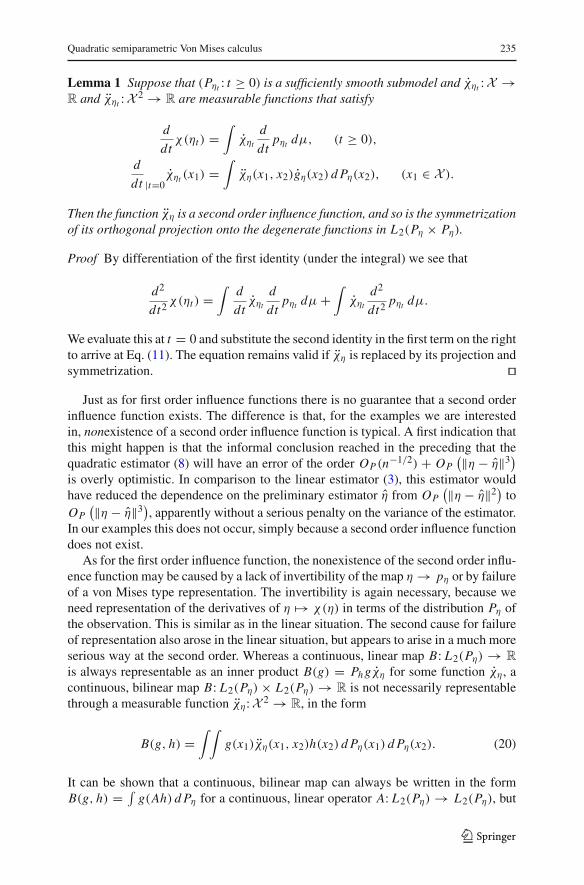
Lemma 1 Suppose that (Pηt : t ≥ 0) is a sufficiently smooth submodel and χηt : X →R and χηt : X 2 → R are measurable functions that satisfy

d

dtχ(ηt ) =

∫χηt

d

dtpηt dµ, (t ≥ 0),

d

dt |t=0χηt (x1) =

∫χη(x1, x2)gη(x2) d Pη(x2), (x1 ∈ X ).

Then the function χη is a second order influence function, and so is the symmetrizationof its orthogonal projection onto the degenerate functions in L2(Pη × Pη).

Proof By differentiation of the first identity (under the integral) we see that

d2

dt2 χ(ηt ) =∫

d

dtχηt

d

dtpηt dµ +

∫χηt

d2

dt2 pηt dµ.

We evaluate this at t = 0 and substitute the second identity in the first term on the rightto arrive at Eq. (11). The equation remains valid if χη is replaced by its projection andsymmetrization. �

Just as for first order influence functions there is no guarantee that a second orderinfluence function exists. The difference is that, for the examples we are interestedin, nonexistence of a second order influence function is typical. A first indication thatthis might happen is that the informal conclusion reached in the preceding that thequadratic estimator (8) will have an error of the order OP (n−1/2) + OP

(‖η − η‖3)

is overly optimistic. In comparison to the linear estimator (3), this estimator wouldhave reduced the dependence on the preliminary estimator η from OP

(‖η − η‖2)

toOP

(‖η − η‖3), apparently without a serious penalty on the variance of the estimator.

In our examples this does not occur, simply because a second order influence functiondoes not exist.

As for the first order influence function, the nonexistence of the second order influ-ence function may be caused by a lack of invertibility of the map η → pη or by failureof a von Mises type representation. The invertibility is again necessary, because weneed representation of the derivatives of η �→ χ(η) in terms of the distribution Pη ofthe observation. This is similar as in the linear situation. The second cause for failureof representation also arose in the linear situation, but appears to arise in a much moreserious way at the second order. Whereas a continuous, linear map B: L2(Pη) → R

is always representable as an inner product B(g) = Ph gχη for some function χη, acontinuous, bilinear map B: L2(Pη) × L2(Pη) → R is not necessarily representablethrough a measurable function χη: X 2 → R, in the form

B(g, h) =∫ ∫

g(x1)χη(x1, x2)h(x2) d Pη(x1) d Pη(x2). (20)

It can be shown that a continuous, bilinear map can always be written in the formB(g, h) = ∫

g(Ah) d Pη for a continuous, linear operator A: L2(Pη) → L2(Pη), but

123


the latter operator is not necessarily a kernel operator in that Ah(x1) = ∫χη(x1, x2)

h(x2) d Pη(x2) for some kernel χη. The latter representation is necessary for thevon-Mises representation (7) of the second derivative.

Failure of existence of χη does not mean that the idea to use a quadratic expansionfor improved estimation is not fruitful. Failure does mean that we cannot constructthe estimator (8) and the estimation rate OP (n−1/2) + OP

(‖η − η‖3)

may not beattainable. However, we may return to Eq. (6) and try and estimate the quadratic termas well as possible, and still improve on the linear estimator. A key observation is thata bilinear map on a finite-dimensional subspace L × L ⊂ L2(Pη) × L2(Pη) is alwaysrepresentable by a kernel.

Lemma 2 If L ⊂ L2(Pη) is a finite-dimensional subspace and B: L × L → R iscontinuous and bilinear, then there exists a function χη ∈ L2(Pη × Pη) such that (20)holds for every g, h ∈ L.

Proof For an arbitrary orthonormal basis e1, . . . , ek of L we can express an elementg ∈ L as g = ∑k

i=1〈g, ei 〉ηei , for 〈·, ·〉η the inner product of L2(Pη). By bilinearity

B(g, h) =k∑

i=1

k∑

j=1

〈g, ei 〉η〈h, e j 〉η B(ei , e j )

=∫ ∫

g(x1)h(x2)

k∑

i=1

k∑

j=1

B(ei , e j )ei (x1)e j (x2) d Pη(x1) d Pη(x2).

Thus the function (x1, x2) �→ ∑ki=1

∑kj=1 B(ei , e j )ei (x1)e j (x2) is a kernel for the

map B. � If the invertibility η �→ pη can be resolved, we can therefore always represent the

second derivative in Eq. (6) at differences η − η within a given finite-dimensionallinear space. The estimator (8) based on the resulting “partial second order influencefunction” then will add a representation error to the remainder OP

(‖η − η‖3). This

representation error can be made arbitrarily small by choosing the finite-dimensionallinear space sufficiently large. However, the corresponding partial influence functionsdepend on the approximating linear spaces, the estimator now having the form

χ(η) + Pnχη + 12 UnχL ,η, (21)

where χL ,η is a partial second order influence function based on an approximatingspace L . To obtain a good estimator we must balance the representation error, remain-der O

(‖η − η‖3), and the variance of the estimator. In an asymptotic framework we

let the approximating space L increase to the full space when n → ∞. We shall seethat this may cause the variance of UnχL ,η to dominate the variance of the linearterm Pnχη and the overall variance may be bigger than O(1/n). However, by properbalancing of the three terms we do never worse than the linear estimator (3), and wegain over it if the parameter set H is large.

123


4 Estimating the square of a density

Consider the problem of estimating the functional χ(p) = ∫p2 dµ based on a random

sample of size n from the density p. This problem was discussed among others inBickel and Ritov (1988) and Laurent (1996), Laurent (1997). We shall rederive theestimator by Laurent (1996) through our general approach.

As the underlying model P we use a set of densities that is restricted only qualita-tively, for instance a Hölder space of functions on the unit square in R

d . We param-eterize this model by the density itself, which we denote by p (hence pη = η = p).The tangent space of the model can then be taken equal to the set of all mean zerofunctions gp: X → R in L2(P), and the first order influence function takes the form

χp(x) = 2 (p(x) − χ(p)) . (22)

To see this, it suffices to note that this function is mean-zero (i.e., degenerate) andsatisfies

d

dt |t=0χ(pt ) =

∫2pt pt dµ|t=0 = P2pgp = Pχp gp,

for any sufficiently regular path t �→ pt with p0 = p and score function gp = p0/p0at t = 0. This first order influence function exists without making assumptions on por P .

We compute a second order influence function as the influence function of thefunctional p �→ χp(x1) = 2p(x1), which is the first order influence function up tocentering. This entails point evaluation at a fixed point x1, which, unfortunately, is nota differentiable functional in the sense of possessing an influence function. For anysufficiently regular path t �→ pt with score function gp,

d

dt |t=0pt (x1) = gp(x1)p(x1).

Existence of an influence function of the functional p �→ p(x1) would require themap g �→ g(x1)p(x1) to be representable as an inner product in L2(P) on the tangentspace. Such a representation is not possible (unless p has finite support), because themap is not continuous relative to the L2(P)-norm.

Thus we content ourselves with partial representation of the second derivative. Tothis aim it is useful to think of the point evaluation map as integrating versus theDirac measure (at x1). Full representation of the functional g �→ g(x1)p(x1) wouldbe possible if there existed a function �: X × X → R such that,

g(x1)p(x1) =∫

�(x1, x2)g(x2)p(x2) dµ(x2). (23)

If this were true for every function g, then the measure B �→ ∫B �(x1, x2) dµ(x2)

would, for each fixed x1, act as a Dirac measure at x1. In other words, the desired,

123


but not existing, function � would be a “Dirac measure” on the diagonal of X × X .Our second best is a function for which Eq. (23) is true, if not for all, then for a largecollection of g. The kernel � of a projection operator �: L2(µ) → L2(µ) onto a(large) subspace is a candidate, because it satisfies the display whenever gp is in thesubspace: if � f (x1) = ∫

�(x1, x2) f (x2) dµ(x2), then the equation gp = �(gp),which is valid for every gp in the range of the projection, gives the preceding display.

Lemma 3 An orthogonal projection �: L2(µ) → L ⊂ L2(µ) onto a finite-dimensional subspace L can be represented as � f (x1) = ∫

�(x1, x2) f (x2) dµ(x2)

for the kernel function �(x1, x2) = ∑ki=1ei (x1)ei (x2) and e1, . . . , ek an orthonormal

basis of L. This kernel satisfies∫

�2 dµ × µ = k.

Proof We have � f (x1) = ∑ki=1〈 f, ei 〉µei (x1) for 〈 f, ei 〉µ = ∫

f ei dµ. The repre-sentation follows by exchanging the order of summation and integration.

The square kernel is∑k

i=1∑k

j=1ei (x1)e j (x1)ei (x2)e j (x2). By the orthonormalityof the basis (ei ) the (double) integral of the off-diagonal terms (i �= j) vanishes andthe double integral of the diagonal terms is equal to 1. Thus the double integral is k.

� We also arrive at a projection operator from the formula χ ′′

p(g, h) = 2∫

gh p2 dµ

for the second derivative ofχ . We can write this in the formχ ′′p(g, h) = 2

∫g(Aph) d P

for the operator Ap: L2(P) → L2(P) given by Aph = hp. The operator Ap is notof kernel form, but we can approximate it by �Ap, leading to the approximation2

∫g(�Aph) d P = 2

∫gp (�(hp)) dµ for χ ′′

p(g, h).For a given orthonormal basis e1, e2, . . . of L2(µ) we take the kernel �(x1, x2) of

the projection onto the span of the first k elements, given by Lemma 3, as a “partial”influence function of the functional p �→ p(x1), and x2 �→ 2�(x1, x2) as a “partial”influence function of the functional p �→ χp(x1). The projection of this function ontothe degenerate functions is

χp(x1, x2) = 2�(x1, x2) − 2�p(x1) − 2�p(x2) + 2∫

(�p)2 dµ. (24)

The quadratic estimator (8), given the initial estimator p, takes the form

χ( p) + Pnχ p + Unχ p = Un� + Un((I − �) p

)

= Un

(k∑

i=1

ei × ei

)+ Un

( ∞∑

i=k+1

θi ei

),

for θi = ∫pei dµ the Fourier coefficients of p. If we choose the initial estimator to

take values in the range of �, then θi = 0 for i > k and the second term vanishes. Theresulting estimator reduces to the estimator considered by Laurent (1996, 1997), whoshowed that the estimator is minimax if p is a-priori known to belong to a multipleof the unit ball in the Hölder space Cβ [0, 1] of regularity β and (ei ) is a basis suitedto this a-priori model. In fact, mean and variance ofthe estimator satisfy, with θi the

123


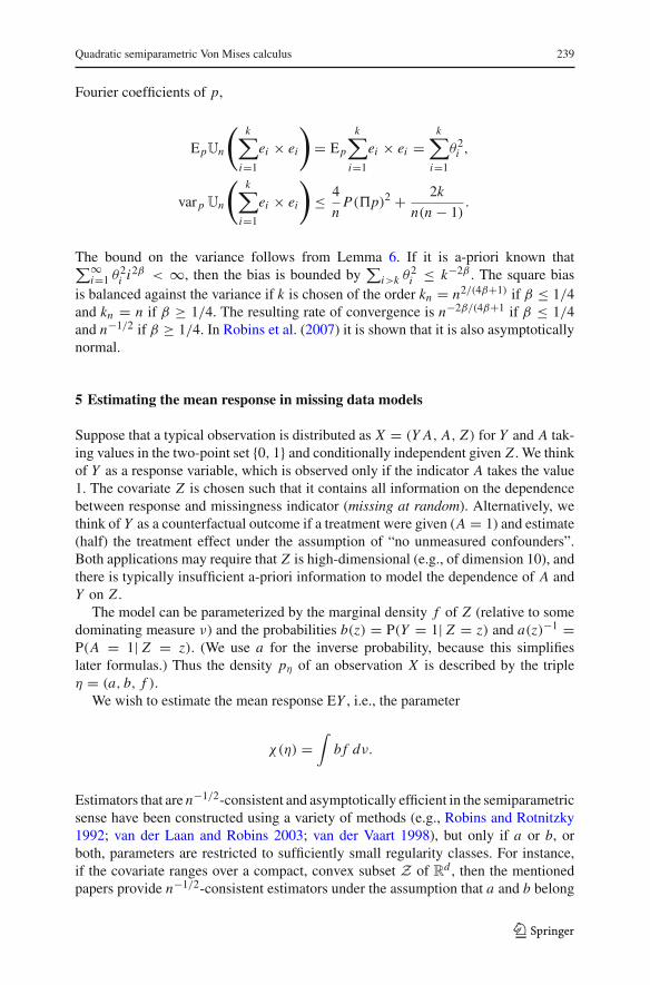
Fourier coefficients of p,

EpUn

(k∑

i=1

ei × ei

)= Ep

k∑

i=1

ei × ei =k∑

i=1

θ2i ,

var p Un

(k∑

i=1

ei × ei

)≤ 4

nP(�p)2 + 2k

n(n − 1).

The bound on the variance follows from Lemma 6. If it is a-priori known that∑∞i=1 θ2

i i2β < ∞, then the bias is bounded by∑

i>k θ2i ≤ k−2β . The square bias

is balanced against the variance if k is chosen of the order kn = n2/(4β+1) if β ≤ 1/4and kn = n if β ≥ 1/4. The resulting rate of convergence is n−2β/(4β+1 if β ≤ 1/4and n−1/2 if β ≥ 1/4. In Robins et al. (2007) it is shown that it is also asymptoticallynormal.

5 Estimating the mean response in missing data models

Suppose that a typical observation is distributed as X = (Y A, A, Z) for Y and A tak-ing values in the two-point set {0, 1} and conditionally independent given Z . We thinkof Y as a response variable, which is observed only if the indicator A takes the value1. The covariate Z is chosen such that it contains all information on the dependencebetween response and missingness indicator (missing at random). Alternatively, wethink of Y as a counterfactual outcome if a treatment were given (A = 1) and estimate(half) the treatment effect under the assumption of “no unmeasured confounders”.Both applications may require that Z is high-dimensional (e.g., of dimension 10), andthere is typically insufficient a-priori information to model the dependence of A andY on Z .

The model can be parameterized by the marginal density f of Z (relative to somedominating measure ν) and the probabilities b(z) = P(Y = 1| Z = z) and a(z)−1 =P(A = 1| Z = z). (We use a for the inverse probability, because this simplifieslater formulas.) Thus the density pη of an observation X is described by the tripleη = (a, b, f ).

We wish to estimate the mean response EY , i.e., the parameter

χ(η) =∫

b f dν.

Estimators that are n−1/2-consistent and asymptotically efficient in the semiparametricsense have been constructed using a variety of methods (e.g., Robins and Rotnitzky1992; van der Laan and Robins 2003; van der Vaart 1998), but only if a or b, orboth, parameters are restricted to sufficiently small regularity classes. For instance,if the covariate ranges over a compact, convex subset Z of R

d , then the mentionedpapers provide n−1/2-consistent estimators under the assumption that a and b belong

123


to Hölder classes Cα(Z) and Cβ(Z) with α and β large enough that

α

2α + d+ β

2β + d≥ 1

2. (25)

For moderate to large dimensions d this is a restrictive requirement. We shall showthat a quadratic estimator of the type (8) can attain a n−1/2-rate in a bigger model andobtains a strictly better rate than the usual estimators if the n−1/2-rate is not obtainable.

Prelimary estimators The parameter 1/a(z) = E(A| Z = z) is the regression of Aon Z and hence can be estimated by any nonparametric regression estimator, such asa kernel or a truncated series estimator. Similarly, the function b(z) = P(Y = 1| Z =z, A = 1) is the regression of the observed Y on Z and can be estimated by nonpara-metric regression based on the subsample (Yi : Ai = 1) on the corresponding Zi . Weshall see below that the parameter f/a is more fundamental than the parameter f . ByBayes’ rule ( f/a)(z) = P(A = 1| Z = z) f (z) is P(A = 1) times the conditionaldensity of Z given A = 1. Therefore, we may estimate f/a by a nonparametric densityestimator based on the subsample (Zi : Ai = 1) times n−1∑n

i=1 Ai .

Tangent space and first order influence function The one-dimensional submodelst �→ pηt induced by paths of the form at = a + tα, bt = b + tβ, and ft = f (1 + tφ)

for given directions α, β and φ yield scores Bη(α, β, φ) = Baηα + Bb

ηβ + B fη φ, for

Baη , Bb

η , B fη the score operators for the three parameters, given by

Baηα(X) = − Aa(Z) − 1

a(Z)(a − 1)(Z)α(Z), a − score,

Bbηβ(X) = A (Y − b(Z))

b(Z)(1 − b)(Z)β(Z), b − score,

B fη φ(X) = φ(Z), f − score.

The first-order influence function is well known to take the form

χη(X) = Aa(Z) (Y − b(Z)) + b(Z) − χ(η). (26)

To see this it must be verified that this function satisfies, for every path t �→ pηt asdescribed previously,

d

dt |t=0χ(ηt ) = Eηχη(X) Bη(α, β, φ)(X).

For the paths at = a+ tα, bt = b+ tβ and ft = f (1+ tφ) the left side of this equationis

∫(β + bφ) f dν. The right side can easily be evaluated to be the same, where it may

be noted that conditional expectations of functions of Y and A given Z factorize, withE(Y − b(Z)| Z) = E(Aa(Z) − 1| Z) = 0 and E

((Y − b(Z)2| Z

) = b(1 − b)(Z).

123


The advantage of choosing a an inverse probability is clear from the form of the(random part of the) influence function, which is a bilinear function in (a, b). Theerror of the corresponding von-Mises representation can be computed to be, for agiven initial estimator η = (a, b, f ),

χ(η) − χ(η) + Pηχη = −∫

(a − a)(b − b)f

adν. (27)

This is quadratic in the errors of the initial estimators. Actually, the form of the biasterm is special in that square estimation errors of the two initial estimators a and b dono arise, but only the product of their errors. This property, termed “double robust-ness” in Rotnitzky and Robins (1995), Robins and Rotnitzky (2001), van der Laanand Robins (2003), makes that it suffices that one of the two parameters is estimatedwell. A prior assumption that the parameters a and b are α and β regular, respectively,would allow estimation errors with rates n−α/(2α+d) and n−β/(2β+d). If the productof these rates is o(n−1/2), then the bias term is negligible, and the linear estimator (3)attains a rate n−1/2. This leads to the condition (25). If this condition fails, then the“bias” (27) is greater than O(n−1/2). The linear estimator then does not balance biasand variance and is suboptimal.

It may be noted that the marginal density f does not enter the first order influencefunction. Even though the functional depends on f , a rate on the initial estimator ofthis function is not needed for the construction of the first order estimator. This willbe different at second order.

Quadratic estimator We proceed to the computation of a second order influencefunction using Lemma 1, by searching a function χη: X 2 → R such that, for everyx1 = (y1a1, a1, z1), and all directions α, β, φ,

a1 (y1 − b(z1)) α(z1) − (a1a(z1) − 1) β(z1) = d

dt |t=0

[χηt (x1) + χ(ηt )

](28)

= Eηχη(x1, X2) Bη(α, β, φ)(X2).

Here the expectation is relative to the variable X2 only. Let Kη: Z2 → R be the kernelof an operator Kη: L2( f ) → L2( f ) (i.e., Kηg(x1)=

∫K (x1, x2)g(x2) f (x2) dµ(x2)),

and define

χη(X1, X2) = −A1 (Y1 − b(Z1)) a(Z2) (A2a(Z2) − 1) Kη(Z1, Z2)

− (A1a(Z1) − 1) a(Z2)A2 (Y2 − b(Z2)) Kη(Z1, Z2). (29)

For this choice the right side of Eq. (28) can be seen to reduce to

a1 (y1 − b(z1)) Kηα(z1) − (a1a(z1) − 1) Kηβ(z1).

(Note that var (Aa(Z)| Z) = a(Z) − 1.) Thus the choice Eq. (29) of χη satisfiesEq. (28) for every (α, β, φ) such that Kηα = α and Kηβ = β. Were Kη equal to theidentity operator, then Eq. (28) would be satisfied for every (α, β, φ), and an exact

123


second order influence function would exist. Unfortunately, the identity operator isnot given by a kernel. As in Sect. 4 we have to be satisfied with an influence functionthat gives partial representation.

To ensure that χη is symmetric we choose Kη(z1, z2) = �η(z1, z2)/a(z2) for �η

a symmetric function. Specifically, we choose �η the kernel of an orthogonal pro-jection �η: L2( f/a) → L2( f/a) onto a space L . The corresponding operators then(trivially) satisfy Kηg = �ηg for every g ∈ L2( f/a), and hence Kη will approximatethe identity if L is large. The function (29) that results from this choice can be seento be both symmetric and degenerate, and hence is a candidate “approximate” influ-ence function. If S2 symmetrizes a function of two variables (i.e., 2 S2 g(X1, X2) =g(X1, X2) + g(X2, X1)), then this influence function can be written as

χη(X1, X2) = − S2[A1 (Y1 − b(Z1))�η(Z1, Z2) (A2a(Z2) − 1)

]. (30)

For an initial estimator η based on independent observations we now construct theestimator (8).

Let E and ˆvar denote conditional expectations given the observations used to con-struct η, and let ‖ · ‖2 be the norm of L2( f/a). Assume that the true functions a, fand the estimators a, f are bounded away from 0 and ∞.

Theorem 1 The estimator χn = χ(η)+Pnχη + 12 Unχη with (approximate) influence

functions χη and χη defined by (26) and (30) with �η the kernel of an orthogonalprojection in L2( f/a) onto a k-dimensional linear subspace satisfies

Eηχn − χ(η) = OP

(‖a − a‖2‖b − b‖2

∥∥∥∥∥f

a− f

a

∥∥∥∥∥2

)

+OP(‖a − �ηa‖2‖b − �ηb‖2

),

ˆvarηχn = OP

(k

n2 ∨ 1

n

).

Proof From Eqs. (27) and (30) we have

Eχn − χ(η) = −∫

(a − a)(b − b)f

adν

−EA1

(Y1 − b(Z1)

)�η(Z1, Z2)

(A2a(Z2) − 1

)�η(Z1, Z2)

= −∫

(a − a)(b − b)f

adν +

∫ ∫ ((a − a) × (b − b)

)

×�η

(f

a× f

a

)dν × ν.

The double integral on the far right with �η replaced by �η can be written as the

single integral∫(a − a)�η(b − b) ( f/a) dν. Added to the first integral on the right

123


this gives

−∫

(a − a)(I − �η)(b − b) ( f/a) dν.

By the Cuachy-Schwarz inequality this is bounded in absolute value by the secondterm in the upper bound for the bias.

Replacement of �η by �η in the double integral gives a difference

∫ ∫ ((a − a) × (b − b)

)(�η − �η)

(f

a× f

a

)dν × ν

=∫

(a − a)

(�η

((b − b)

f/a

f /a

)− �η(b − b)

)f

adν.

By the Cauchy-Schwarz inequality the absolute value of this is bounded above by

‖a − a‖2

∥∥∥(�η ◦ Mw − �η)(b − b)

∥∥∥2,ν

‖w‖∞.

Here Mw is multiplication by the function w = ( f/a)/( f /a) (defined by Mwg = gw),and ‖ · ‖2,ν is the L2(ν)-norm for the measure ν defined by d ν = ( f /a) dν. Consider-ing �η as the projection in L2(ν) with weight 1, and �η as the weighted projection inL2(ν) with weight function w, we can apply Lemma 4 to the middle term and concludethat this is bounded in absolute value by ‖�η‖2,ν |‖w − 1‖∞‖b − b‖2,ν . Because weassume that the functions f/a and f /a are bounded away from zero and infinity, thiscan be seen to yield the first term in the upper bound on the bias.

The function χη is uniformly bounded and hence the (conditional) variance ofPnχη is of the order OP (1/n). Thus for the variance bound it suffices to consider the(conditional) variance of Unχη. In view of Lemma 6 this is bounded above by

4n EηEη

(χη(X1, X2)| X1

)2 + 2n(n−1)

Eηχ2η(X1, X2).

The variables A(

Y − b(Z))

and(

Aa(Z) − 1)

are uniformly bounded. Hence the last

term on the right is bounded above by a multiple of n−2∫ ∫

�2η( f/a × f/a) dν × ν,

which is bounded by ‖w‖2∞k/n2, by Lemma 3. The first order term is of the orderO(1/n). To see this we first note that

Eη

(χη(X1, X2)| X1

) = −A1

(Y1 − b(Z1)

)�η

((a − a)w

)(X1)

− (A1a(Z1) − 1

)�η

((b − b)w

)(X1).

Here the variables A1

(Y1 − b(Z1)

)and

(A1a(Z1) − 1

)are uniformly bounded, and

the second moment of �ηg is bounded by ‖w‖∞ times the second moment of g inL2(ν), for every g. �

123


Conclusion Assume that the parameters a, b and f/a are known to be “regular” ofdegrees α, β and φ, respectively, in the sense that there exists a sequence of k-dimen-sional linear spaces Lk such that, for some constant C ,

‖a − Lk‖2 ≤ C

(1

k

)α/d

, ‖b − Lk‖2 ≤ C

(1

k

)β/d

,

∥∥∥∥f

a− Lk

∥∥∥∥2

≤ C

(1

k

)β/d

.

This is true, for instance, if the functions a, b and f/a are defined on a compact, convexdomain in R

d and are known to belong to Hölder (or Besov) spaces of functions ofsmoothness α, β and φ. The approximation is then valid even with the uniform normon the left side, where the spaces Lk can be taken to be generated by polynomials,splines or wavelets.

In this case there also exist estimators a and b and f /a that achieve convergencerates n−α/(2α+d), n−β/(2β+d) and n−φ/(2φ+d), respectively, uniformly over these a-pri-ori models. Then the estimator χn of Theorem 1 attains the square rate of convergence

k

n2 ∨ 1

n∨

(1

n

)2α/(2α+d)+2β/(2β+d)+2φ/(2φ+d)

∨(

1

k

)(2α+2β)/d

.

The optimal value of k balances the first and fourth terms and is of the orderk ∼ n2d/(d+2α+2β). The resulting rate is n−γ for

γ =(

1

2

)∧

(α

2α + d+ β

2β + d+ φ

2φ + d

)∧

(2α + 2β

d + 2α + 2β

).

This reduces to the rate n−1/2 under condition (25), but also if (α + β)/2 ≥ d/4 andφ is sufficiently large:

φ

2φ + d≥ 1

2− α

2α + d− β

2β + d.

(In this case we can also choose k = n independent of α and β.) In case the rate n−γ

is slower than n−1/2, then it is still better than the rate n−α/(2α+d)−β/(2β+d) obtainedby the linear estimator (3).

Thus the quadratic estimator outperforms the linear estimator.

6 Technical results

Let L be a given closed subspace of L2(X ,A, µ) and w: X → R a bounded, measur-able function. Define operators �,�w: L2(µ) → L2(µ) by

�g = argminl∈L

∫(g − l)2 dµ,

�wg = argminl∈L

∫(g − l)2 w dµ.

123


Thus � is the ordinary orthogonal projection on the space L , and �w is a weightedprojection. The projections can be characterized by the orthogonality relationships∫(g − �g)l dµ = 0 and

∫(g − �g)l w dµ = 0, for every l ∈ L .

Lemma 4 Let �w and � be the weighted projections onto a fixed subspace L of L2(µ)

relative to the weight functions w and 1, respectively, and let Mw be multiplication bythe function w. Then ‖�w − �Mw‖2 ≤ ‖�w‖2‖w − 1‖∞.

Proof The orthogonality relationships for the projections � and �w imply that, forevery l ∈ L and g,

∫�(wg)l dµ =

∫wgl dµ =

∫w(�wg)l dµ.

Because �wg − �(wg) is contained in L ,

‖�wg − �(wg)‖22 =

∫(�wg − �(wg)) (�wg − �(wg)) dµ,

=∫

(�wg − �(wg)) (�wg − (�wg)w) dµ.

An application of the Cauchy-Schwarz inequality and next cancellation of one factor‖�wg − �(wg)‖2 gives that ‖�wg − �(wg)‖2 ≤ ‖(�wg)(1 − w)‖2. The right sideis bounded above by ‖�w‖2‖g‖2‖1 − w‖∞. � Lemma 5 For degenerate, symmetric functions f, g: X 2 → R we have Pn

Un f = 0and

Pn(Un f )(Ung) = 1(n2

) P2 f g.

Lemma 6 For any measurable function f : X 2 →R, and f1(x1)=∫

f (x1, x2) d P(x2),

var Un f ≤ 4

nP f 2

1 + 2

n(n − 1)P f 2.

Proof The first lemma follows by writing the square sum (Un f )2 as a double sum(over ordered pairs i < j). The expected values of the off-diagonal terms vanish bydegeneracy.

For a general measurable function f : X 2 → R the mean P f 2 is the projectiononto the constant functions, and the function f1 defined by f1(x1) = ∫

f (x1, x2)

d P(x2) − P2 f is the projection of f in L2(P2) onto the mean zero functions of onevariable. The decomposition

f (x1, x2) = P2 f + f1(x1) + f1(x2) + f12(x1, x2),

123


where f12 is defined by the equation yields the Hoeffding decomposition Un f =P2 f + 2Pn f1 + Un f12 of the U -statistic in orthogonal parts, with Un f12 degen-erate. Using Lemma 5 we see that the variance of Un f is equal to (4/n)P f 2

1 +2/(n(n − 1))P2 f 2

12. The norm of f1 is smaller than the norm of f1. Because f12 is aprojection of f , its norm is bounded by the norm of f . �

Open Access This article is distributed under the terms of the Creative Commons Attribution Noncom-mercial License which permits any noncommercial use, distribution, and reproduction in any medium,provided the original author(s) and source are credited.

References

Begun JM, Hall WJ, Huang WM, Wellner JA (1983) Information and asymptotic efficiency in parametric–nonparametric models. Ann Stat 11(2):432–452

Bickel PJ, Ritov Y (1988) Estimating integrated squared density derivatives: sharp best order of conver-gence estimates. Sankhya Ser A 50(3):381–393

Bickel PJ, Klaassen CAJ, Ritov Y, Wellner JA (1993) Efficient and adaptive estimation for semiparametricmodels. Johns Hopkins series in the mathematical sciences. Johns Hopkins University Press, Baltimore

Bolthausen E, Perkins E, van der Vaart A (2002) Lectures on probability theory and statistics. In: Lecturenotes in mathematics, Lectures from the 29th summer school on probability theory held in Saint-Flour,vol 1781. Springer, Berlin. July 8–24, 1999 (edited by Bernard P)

Emery M, Nemirovski A, Voiculescu D (2000) Lectures on probability theory and statistics, In: Lecturenotes in mathematics, Lectures from the 28th summer school on probability theory held in Saint-Flour,vol. 1738. Springer, Berlin. 17 August–3 September, 1998 (edited by Bernard P)

Klaassen CAJ (1987) Consistent estimation of the influence function of locally asymptotically linear esti-mators. Ann Stat 15(4):1548–1562

Koševnik JA, Levit BJ (1976) On a nonparametric analogue of the information matrix. Teor Verojatnost iPrimenen 21(4):759–774

Laurent B (1996) Efficient estimation of integral functionals of a density. Ann Stat 24(2):659–681Laurent B (1997) Estimation of integral functionals of a density and its derivatives. Bernoulli 3(2):181–211Le Cam L (1960) Locally asymptotically normal families of distributions. Certain approximations to fam-

ilies of distributions and their use in the theory of estimation and testing hypotheses. Univ californiaPubl Stat 3:37–98

Murphy SA, van der Vaart AW (2000) On profile likelihood. J Am Stat Assoc 95(450):449–485 (withcomments and a rejoinder by the authors)

Pfanzagl J (1982) Contributions to a general asymptotic statistical theory. In: Lecture notes in statistics,vol 13. Springer, New York (with the assistance of Wefelmeyer W)

Pfanzagl J (1985) Asymptotic expansions for general statistical models. In: Lecture notes in statistics,vol 31. Springer, Berlin (with the assistance of Wefelmeyer W)

Robins J, Rotnitzky A (2001) Comment on the bickel and kwon article, “inference for semiparametricmodels: Some questions and an answer”. Stat Sin 11(4):920–936

Robins J, Li L, Tchetgen E, van der Vaart A (2007) Asymptotic normality of quadratic estimators. Ann Stat(submitted)

Robins JM, Rotnitzky A (1992) Recovery of information and adjustment for dependent censoring usingsurrogate markers pp 297–331

Rotnitzky A, Robins JM (1995) Semi-parametric estimation of models for means and covariances in thepresence of missing data. Scand J Stat 22(3):323–333

van der Laan MJ, Robins JM (2003) Unified methods for censored longitudinal data and causality. SpringerSeries in Statistics. Springer, New York

van der Vaart A (1991) On differentiable functionals. Ann Stat 19(1):178–204van der Vaart A (1994) Maximum likelihood estimation with partially censored data. Ann Stat 22(4):1896–

1916van der Vaart AW (1988) Statistical estimation in large parameter spaces, CWI Tract, vol 44. Stichting

Mathematisch Centrum Centrum voor Wiskunde en Informatica, Amsterdam

123


van der Vaart AW (1998) Asymptotic statistics. Cambridge series in statistical and probabilistic mathemat-ics., vol 3 Cambridge University Press, Cambridge

Von Mises R (1947) On the asymptotic distribution of differentiable statistical functions. Ann Math Stat18:309–348

Wellner JA, Klaassen CAJ, Ritov Y (1993) Semiparametric models: a review of progress since BKRW.In: Frontiers in statistics, pp 25–44. Imp Coll Press, London (2006)

123

Quadratic semiparametric Von Mises calculus

Documents

Transcript of Quadratic semiparametric Von Mises calculus