Generalized Semiparametric Binary Prediction

ANNALS OF ECONOMICS AND FINANCE 3, 117–134 (2002)

Generalized Semiparametric Binary Prediction

Jeff Racine

Department of EconomicsUniversity of South Florida

Tampa, FL 33620, USAE-mail: [email protected]

This paper proposes a semiparametric approach to the estimation of ‘gener-alized’ binary choice models. A ‘generalized’ binary choice model is one withseparate indices for each conditioning variable which constitutes a generaliza-tion of the standard single-index approach typically employed in applied work.The choice probability distribution is therefore a joint distribution across theseindices as opposed to the typical univariate distribution on a scalar index com-monly found in applied work. Interest lies in estimating choice probabilitiesand the gradient of choice probabilities with respect to the conditioning in-formation, and these are estimated nonparametrically using the method ofkernels. A data-driven cross-validatory method for bandwidth selection andindex-parameter estimation is proposed for maximization of the nonparametriclikelihood function. The functional form of the indices enters this nonpara-metric likelihood function thereby permitting data-driven determination of theindex functions in addition to the shape of the joint cumulative distributionfunction itself. Applications are considered. c© 2002 Peking University Press

Key Words: Semiparametric; Nonparametric methods.JEL Classification Number : C14

1. INTRODUCTION

Binary choice models are characterized by a dependent variable whichcan take on only two discrete values. Such models are widely used in a num-ber of disciplines, and occur frequently in economics because the decisionof an economic unit frequently involves binary choice, for instance, whetheror not a person joins the labor force or makes an automobile purchase, orwhether or not a firm issues a bond. The goal of modeling such choices isfirst to predict whether or not a choice will be made (choice probability)and second to assess the response of the probability of the choice beingmade to changes in variables believed to influence choice (choice gradient).

1171529-7373/2002

Copyright c© 2002 by Peking University PressAll rights of reproduction in any form reserved.

118 JEFF RACINE

Existing approaches to modeling binary choice fall into two camps, para-metric and semiparametric. Both camps typically assume the existence ofa single threshold given by an index function beyond which it is morelikely than not that a choice will be made, hence they are often called‘single-index’ models. Such models can be quite powerful and they enjoywidespread use, however, the use of a single-index can impose some strongrestrictions on the underlying process. For example, one such restrictionis that choice gradients are forced to have identical shape for each variableinfluencing choice and differing only by the value of a scalar parameter.

This paper considers a generalization of such approaches in which thereexist separate thresholds and indices for each variable believed to influencechoice. This is quite different from existing ‘multiple-index’ models whichare typically used to model multinomial discrete choice. In this paperthe choice remains binary in nature, but multiple thresholds are admitted.The resulting method is more flexible than the standard approach andconstitutes an alternative to single-index models when modeling binarychoice.

Existing approaches are now briefly summarized in order to compare andcontrast them from the proposed approach.

1.1. Parametric Estimation of Single-Index Binary Choice Mod-els

Logit and probit models remain the most widely used parametric meth-ods for the estimation of binary choice models. Such approaches dependon two assumptions; a known index which is assumed to influence choice,and a known parametric form for a distribution function (CDF) which isassumed to yield choice probabilities. The index is assumed to yield a pos-itive choice when it exceeds a threshold (with error), and a negative choiceotherwise.

Parametric models are typically chosen due to their tractability and easeof interpretation. For excellent overviews of estimation and inference basedupon parametric binary choice models see Amemiya (1981), Mcfadden(1984), Blundell (1987), and Davidson & Mackinnon (1993). Typically,parametric models of binary choice are based on the concept of an un-observed or ‘latent’ variable Y ∗

i (see Davidson & Mackinnon (1993, page514).

The traditional parametric approach to modeling binary choice is asfollows:

1. Assume that the true data generating processes (DGP) is given by

Y ∗i = E[Y ∗|Xi] + Ui = X ′

iβ + Ui,

GENERALIZED SEMIPARAMETRIC BINARY PREDICTION 119

where Xi ∈ Rk, but that we only observe Yi = 1 if Y ∗i > 0 otherwise we

observe Yi = 0.2. Yi = 1 therefore occurs when X ′

iβ +Ui > 0, that is, when Ui > −X ′iβ.

3. Pr[Yi = 1] is therefore equal to Pr[Ui > −X ′iβ] = 1−Pr[Ui < −X ′

iβ].4. Assuming symmetry of the distribution of U , 1 − Pr[Ui < −X ′

iβ] =Pr[Ui < X ′

iβ] = F (X ′iβ).

5. Assuming that the distribution of U is of known parametric form, thenwe can estimate β by the maximum likelihood method1.

6. Empirical choice probabilities are given by F (x′β), while the gradientof choice probability with respect to the conditioning information is givenby ∂F (x′β)/∂x, where β is the maximum likelihood estimator of β.

Clearly this approach has its origins in regression modeling and the useof a scalar index function X ′

iβ plays a key role. The choice probabilityfunction F (·) (the CDF of U) is independent of the distribution of thosevariables believed to influence choice by assumption, and symmetry of F (·)is typically assumed. This assumed symmetry therefore imposes symmetryon the choice probability gradient, each element having identical shape anddiffering only by βj , j = 2, . . . , k. In this framework there is no way forus to estimate the shape of the error distribution, either parametricallyor nonparametrically since we do not observe U and cannot estimate Usince we do not observe Y ∗

i . This stands in stark contrast to a standardregression model in which the vector of residuals U = Y −Xβ can be usedto nonparametrically estimate the density of U since we actually observethe underlying dependent variable in this case. If we adopt a parametricapproach we must simply presume a parametric distribution for U whoselocation and scale is determined by the observed choices Y ∈ {0, 1} and byX ′

iβ.

1.2. Semiparametric Estimation of Single-Index Binary ChoiceModels

There exists a rich and very impressive variety of approaches towardssemiparametric estimation of discrete choice models including that ofCoslett (1983), Ichimura (1986), Manski (1985), Rudd (1986), Ichimura& Lee (1991), Coslett (1991), Klein & Spady (1993), Lee (1995), Chen &Randall (1997), Picone & Butler (1998), and Ichimura & Thompson (1998)to name but a few. For a recent survey of semiparametric approaches tothe estimation of discrete choice models see Pagan & Ullah (1999 Chapter7).

In this framework note that Pr[Yi = 1] = E[Yi|X ′iβ], hence one cannot

proceed by estimating E[Yi|Xi] using standard nonparametric regression

1For example, assuming a Gaussian distribution for U leads to the widely-used ‘Probit’model, while assuming a Logistic distribution yields the widely-used ‘Logit’ model.

120 JEFF RACINE

techniques as this fails to capture the single-index nature of the model. Anumber of leading approaches therefore use nonparametric techniques toestimate E[Yi|X ′

iβ] (see, for example, Ichimura (1986) and Klein & Spady(1993)), and the resulting estimators are essentially ratios of nonparametricdensity estimates which may require trimming both to deal with behaviorof the numerator at boundary points and to obtain asymptotic results.These approaches are very similar in spirit to univariate Nadaraya-Watsonregression (Nadaraya (1965), Watson (1964)) with the index function itselfserving as conditioning information.

Existing semiparametric approaches share a number of features; theytypically assume an underlying latent variable specification; they typicallyemploy a scalar-index which restricts the choice threshold to be a hyper-plane; they typically model the (univariate) distribution of the scalar indexfunction in order to generate empirical choice probabilities; data-drivenmethods for bandwidth selection or its counterpart when using flexiblefunctional forms are not employed, and they do not permit data-drivenindex choice.

1.3. Semiparametric Estimation of Generalized Binary ChoiceModels

In this paper, a semiparametric approach to the estimation of ‘general-ized’ binary choice models is proposed. A ‘generalized’ binary choice modelis one with separate indices for each conditioning variable which constitutesa generalization of the standard single-index approach typically employedin applied work. The choice probability distribution is therefore a jointdistribution across these indices as opposed to the typical univariate dis-tribution on a scalar index commonly found in applied work.

In this paper the approach taken is to focus on modeling Pr[Yi = 1]via kernel estimation of a (joint) CDF rather than by modeling E[Yi|X ′

iβ]via a ratio of density estimates. It was noted that existing semiparamet-ric approaches are similar in spirit to Nadaraya-Watson kernel regression(Nadaraya (1965), Watson (1964)), and the proposed approach is similar inspirit to the Priestly-Chow regression estimator (Priestley & Chao (1972)).One immediate benefit will be the absence of trimming in this approach.In addition, the proposed approach adopts the use of multiple thresholdsthe modeling of which will be straightforward and natural in this setting.

This paper builds upon existing work and develops a number of ideasin the context of binary choice modeling. First, the joint distribution oftransformations of the conditioning variables is estimated nonparametri-cally using the method of kernels. This extends existing approaches whichemploy a univariate distribution defined over a scalar index, and the dis-tribution of variables influencing choice influences both choice probabilitiesand associated gradients. Second, the indices are assumed to be of known


form but are generalized to allow for multiple thresholds. Third, bothbandwidth and parameter selection is data-driven using a new likelihood-based cross-validatory method. The value added by the proposed approachlies in its ability to model situations wherein a single index may be appro-priate, but in addition is capable of handling a richer range of phenomenathan those which single-index models are capable of handling. Finally, thefunctional form of the index can be data-driven since it enters the non-parametric likelihood function thereby generalizing existing approaches inwhich the index is assumed to be known.

The modeling of binary choice via multiple thresholds is now outlined,and then a semiparametric implementation is proposed.

2. BACKGROUND AND ASSUMPTIONS

Consider a situation for which

Yi ={

1 if a choice is made0 otherwise i = 1, . . . , n (2)

Yi ∈ R1 is assumed to be a random variable that depends on a randomvector of characteristics, Xi ∈ Rk. Interest lies in predicting the probabilitythat Yi = 1 given a realization of the vector of characteristics, xi, and inassessing how this probability changes with changes in these characteristics.

As noted, this paper considers the case in which choices are governed ingeneral by multiple thresholds defined over the choice variables or trans-formations thereof, one for each variable influencing choice. In this setting,Pr[Yi = 1] can be expressed as a joint distribution function given by

Pr[Yi = 1] = Pr[g1(xi1, θ1) ≥ g1 and g2(xi2, θ

2) ≥ g2 . . . and gk(xik, θk) ≥ gk]

= F (g1 − g1(xi1, θ1), . . . , gk − gk(xik, θk))

(3)

where the functions gj(xij , θj), j = 1, . . . , k, are (unknown) functions which

influence choices, θj a vector of parameters, gis thresholds above whichchoices tend to be made, and F (·) a joint distribution function. It is notedthat

Pr[Yi = 0] = 1− Pr[Yi = 1] = Pr[g1(xi1, θ1) < g1

and g2(xi2, θ2) < g2 . . . and gk(xik, θk) < gk]

= 1− F (g1 − g1(xi1, θ1), . . . , gk − gk(xik, θk))

(4)

As usual, the choice probability gradient is defined as

∇xPr[Yi = 1] =∂Pr[Yi = 1]

∂x∈ Rk (5)

122 JEFF RACINE

which tells us the response of the choice probability due to changes in thefactors influencing choice.

We can write the PDF of the choice Yi as

f(yi) =[F (g1 − g1(xi1, θ

1), . . . , gk − gk(xik, θk))]yi

×[1− F (g1 − g1(xi1, θ

1), . . . , gk − gk(xik, θk))](1−yi)

(6)

where yi ∈ {0, 1}, and for independent realizations of Yi the joint densityfunction is given by

f(y1, . . . , yn) =n∏

i=1

f(yi)

=n∏

i=1

[F (g1 − g1(xi1, θ

1), . . . , gk − gk(xik, θk))]yi

×[1− F (g1 − g1(xi1, θ

1), . . . , gk − gk(xik, θk))](1−yi)

(7)

Estimation of binary choice models is typically based upon the methodof maximum likelihood where the log-likelihood function is given by

L =n∑

i=1

yi ln[F (g1 − g1(xi1, θ

1), . . . , gk − gk(xik, θk))]

+ (1− yi) ln[1− F (g1 − g1(xi1, θ

1), . . . , gk − gk(xik, θk))] (8)

and the resulting estimators will be referred to collectively as θ.Hypothesis testing can often be based on the asymptotic variance-covariance

matrix. For example, the variance-covariance matrices for linear indices isgiven by

V [θ] =n∑

i=1

[f2(xi, θ)

F (xi, θ)[1− F (xi, θ)]xix

′i

]−1

(9)

where θ denotes a vector of all parameters in the model and where xi

a vector of realizations of all variables influencing choice. An estimateis obtained by evaluating Equation 9 at θ. Alternatively, one could usethe method of obtaining Equation 9 via computation of the Hessian ofthe likelihood function which often must be obtained numerically due tononlinearities in the likelihood function itself.

3. SEMIPARAMETRIC GENERALIZED BINARY CHOICEWITH KNOWN INDICES

The approach taken in this paper involves the nonparametric estima-tion of a joint distribution function which has as its arguments generalized


known indices of each conditioning variable. Estimation proceeds via themethod of kernels based on a nonparametric likelihood function which ismaximized using cross-validatory techniques. Cross-validation is employedfor both bandwidth and parameter selection and, in addition, the paramet-ric form of the index itself can also be selected via cross-validation by lettingthe nature of the index be an argument of the cross-validatory likelihoodfunction.

Kernel estimation of distribution functions can be based upon an es-timator such as the Nadaraya-Watson (Nadaraya (1965), Watson (1964))estimator of a joint density function. The kernel estimator of a joint densityfunction is given by

f(x1, . . . , xi) =1

n∏k

j=1 hj

n∑i=1

K

(x1 − xi1

h1, . . . ,

xk − xik

hk

)(10)

The kernel estimator of the joint distribution function (Prakasa & Rao(1983 page 397)) is therefore given by

F (x1, . . . , xk) =

∫ x1,...,xk

−∞f(t1, . . . , ti) dt1, . . . , dtk

=1

n∏k

j=1 hj

n∑i=1

∫ x1,...,xk

−∞K

(t1 − xi1

h1, . . . ,

tk − xik

hk

)dt1, . . . , dtk

=1

n

n∑i=1

Kint

(x1 − xi1

h1, . . . ,

xk − xik

hk

)(11)

where Kint(·) =∫ x1,...,xk

−∞ K(·) dt1, . . . , dtk is a kernel distribution function.Once we assume a specific parametric function for the indices (gj(xij , θ

j),j = 1, 2, . . . , k) we can then obtain the kernel estimator of the joint distri-bution function of these indices via simple transformation of variables. Forthe commonly used linear index this involves nothing more than simplyreplacing variable j with the index itself.

It should be noted that we have used the standard Rosenblatt-Parzenestimator (Silverman (1986 page 40, 76)), but this approach remains un-changed when using other nonparametric density estimators such as gen-eralized nearest-neighbor (Silverman (1986 page 21)) and adaptive (Silver-man (1986 page 21)) approaches.

By way of example, consider a situation in which the indices are linearin nature, hence an index for variable j would be given by θj

0 + θj1xij .

124 JEFF RACINE

The kernel estimator of the joint distribution function (Pr[Yi = 1]) wouldbe given by

F (θ10 + θ1

1xi1, . . . , θk0 + θk

1xik)

=1n

n∑i=1

Kint

[(θ10 + θ1

1(x1 − xi1)h1

), . . . ,

(θk0 + θk

1 (xk − xik)hk

)](12)

while the gradient vector ∇F (θ10 +θ1

1xi1, . . . , θk0 +θk

1xik) would have typicalelement

∂F (θ10 + θ1

1xi1, . . . , θk0 + θk

1xik)∂xj

=1n

n∑i=1

∂

∂xjKint

[(θ10 + θ1

1(x1 − xi1)h1

), . . . ,

(θk0 + θk

1 (xk − xik)hk

)](13)

This estimator is very similar to the Priestly-Chow regression estimator(Priestley & Chao (1972)) outside of the obvious difference in the natureof the kernel function.

4. ESTIMATION OF THE MODEL.

In applied settings we clearly require a method of determining the smooth-ing parameters h, the parameters of the index function θ, and possibly thefunctional forms of the indices themselves.

Suppose for the moment that the form of the index is of known linearform. We could therefore express the log-likelihood function as

L(θ, h) =n∑

i=1

yi ln[F (θ1

0 + θ11xi1, . . . , θ

k0 + θk

1xik)]

+ (1− yi) ln[1− F (θ1

0 + θ11xi1, . . . , θ

k0 + θk

1xik)] (14)

We would like to proceed to select h and θ in a manner similar to that usedin a parametric framework.

Unfortunately, as is common in nonparametric settings, this objectivefunction is unbounded. We therefore considering maximizing the cross-validatory log-likelihood function using a leave-one-out kernel estimatorin which observation i is omitted when computing F (θ1

0 + θ11xi1, . . . , θ

k0 +

θk1xik). This now allow us to conduct data driven bandwidth and parameter

estimation. Letting L−i(θ, h) denote the cross-validatory likelhood function


in which observation i is omitted when computing F (θ10 + θ1

1xi1, . . . , θk0 +

θk1xik), we define

(θ, h) = argmaxθ,h

L−i(θ, h) (15)

and consistency of this method would be expected to follow given the resultsof Stone (1974) though a rigorous proof of this statement is not attemptedhere.

At this point it should be evident that we could admit the functionalform of the index as yet another argument entering this likelihood functionso that, in addition to the bandwidths h and index parameters θ, choiceof the index functions themselves could be data-driven thereby removingthe need to assume that the functional form of the index is known prior toestimation.

Much of the focus of a number of excellent recent papers has been onestimation of the index parameters themselves. However, Amemiya (1981page 1488) notes that “when one wants to compare models with differ-ent probability functions, it is generally better to compare probabilitiesdirectly rather than comparing the estimates of the coefficients even afteran appropriate conversion.” He also suggests that “an alternative way ofcomparing different models is to look at the derivatives of the probabilitieswith respect to a particular independent variable.” In light of this, in thispaper interest will center on estimation of the choice probabilities F (·) andtheir gradient ∂F (·)/∂x in this generalized setting when the distributionfunction is not assumed to be of known parametric form.

We now turn to the behavior of the proposed method relative to existingsingle-index methods. For comparison purposes, we consider a traditionalparametric approach along with the proposed approach.

5. SOME SIMPLE EXAMPLES

One key difference between many existing approaches and the proposedapproach lies in the modeling of the choice distribution itself. For instance,the traditional parametric approach requires the presumption of a knownfunctional form for the distribution of an error term U , and the shape ofthis distribution is independent of the distribution of the variables whichinfluence choice. However, in the proposed approach the distribution de-pends on the variables influencing choice, which is also assumed by Klein& Spady (1993) for instance though in a single-index setting.

We first consider the case of one conditioning variable in order to high-light this difference. We first consider the case in which a Logit modelwould be appropriate in that the distribution of X is symmetric, and then

126 JEFF RACINE

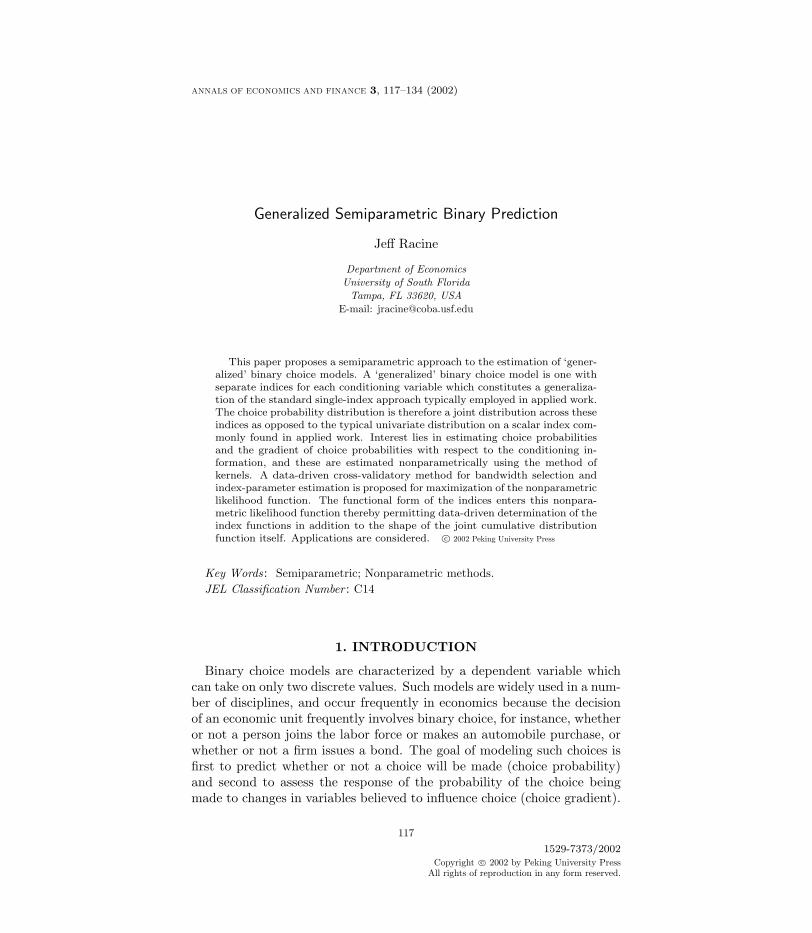
FIG. 1. Choice probability and gradient vector for simulated normal data x ∼N(0, 1), n = 250. Fl represents that based on the logistic parametric specification,

while Fk represents that based on a nonparametric kernel estimator. All bandwidthswere selected via maximization of the cross-validatory maximum likelihood function.

�

� � �

� � �

� � �

� � �

� � �

� �

� �

� � �

� � �

�

�

�

� � � � � �

��

�

� � � � � ! � $ � � � � � � �

�� (

* �� ( + * �

�� ,

* �� , + * �

�

� � �

� � �

� � �

� � �

� � �

� �

� �

� � �

� � �

�

�

�

� � � � � �

��

�

� � � � � ! � $ � � � � �

�� (

* �� ( + * �

�� ,

* �� , + * �

�

� � �

� � �

� � �

� � �

� � �

� �

� �

� � �

� � �

�

�

�

� � � � � �

��

�

� � � � � ! � $ � � � � �

�� (

* �� ( + * �

�� ,

* �� , + * �

� � �

� � �

�

� � �

� � �

� �

� � �

�

�

�

� � � � � �

��

�

� � � � � ! � $ � � �

� �

�� (

* �� ( + * �

�� ,

* �� , + * �

consider the case where X is bimodal in order to contrast the proposedapproach from existing approaches.

5.1. Univariate: Symmetric Distribution of X

We begin by considering the behavior of the proposed estimator relativeto that based on the widely-used logistic specification when the distributionof the variables influencing choice is symmetric.

For the experiments, the choice probabilities were determined from theLogit model

yi ={

1 if[1/(1 + e−(θ0+θ1xi)) + ui

]≥ 0.5

0 otherwisei = 1, . . . , n (16)

where x ∼ N(0, 1) and u ∼ N(0, 0.252). The values of (θ0, θ1) were varied,and results for four simulated data sets are plotted in Figure 1.

As can be seen, even for a sample which is small by nonparametric stan-dards, the proposed approach appears to give reasonable estimates of thechoice probabilities and gradient which are consistent with the underlyingDGP.

However, suppose that the distribution of X was bimodal, for example.The proposed approach would use this information while standard models


FIG. 2. Choice probability and gradient vector for simulated bimodal normal datax ∼ N(−2.5 : 2.5, 0.52 : 1.0), n = 250. Fl represents that based on the logistic paramet-

ric specification, while Fk represents that based on a nonparametric kernel estimator. Allbandwidths were selected via maximization of the cross-validatory maximum likelihoodfunction.

�

� � �

� � �

� � �

� � �

� � �

� �

� �

� � �

� � �

�

�

�

�

� � � � � � �

��

�

� � � � � ! � $ � � � � � � �

�� (

* �� ( , * �

�� -

* �� - , * �

�

� � �

� � �

� � �

� � �

� � �

� �

� �

� � �

� � �

�

�

�

�

� � � � � � �

��

�

� � � � � ! � $ � � � � �

�� (

* �� ( , * �

�� -

* �� - , * �

�

� � �

� � �

� � �

� � �

� � �

� �

� �

� � �

� � �

�

�

�

�

� � � � � � �

��

�

� � � � � ! � $ � � � � �

�� (

* �� ( , * �

�� -

* �� - , * �

� � �

� � �

�

� � �

� � �

� �

� � �

�

�

�

�

� � � � � � �

��

�

� � � � � ! � $ � � �

� �

�� (

* �� ( , * �

�� -

* �� - , * �

cannot as they assume that choice probabilities are independent of thedistribution of the variables influencing choice.

5.2. Univariate: Bimodal Distribution of X

We now consider the behavior of the proposed estimator and the logisticestimator when the data on X is bimodal, x ∼ N(−2.5 : 2.5, 0.52 : 1.0).

Which approach is appropriate? Clearly, if the latent-variable model isdriving choices then the Logit model is appropriate. However, if choicesare governed by variables influencing choices and not by an independenterror process, then the proposed approach will be able to capture suchbehavior. In either case, predicted choice probabilities will be similar, butchoice gradients will differ.

5.3. Multivariate: Symmetric distribution of X1, X2

128 JEFF RACINE

FIG. 3. Choice probability and predicted choices for simulated data with X1, X2 ∼N(), n = 500. The first column contains that for the kernel estimator, the second forthe Logit.

� � � � � � �

� �

��

� � �

�

� ��

�

� � � � ! �

� �

��

� � �

�

� ��

�

# � � % � ( ! � % � � � � � � + - � � ( �

� �

��

� � �

�

� ��

�

# � � % � ( ! � % � � � � ! + - � � ( �

� �

��

� � �

�

� ��

�

For the experiments, the choice probabilities were determined from theLogit model

yi =

{1 if

[1

(1+e−(θ01+θ11xi1))1

(1+e−(θ02+θ12xi2))+ ui

]≥ 0.5

0 otherwisei = 1, . . . , n

(17)where x1, x2 ∼ N(0, 1) and u ∼ N(0, 0.52). The values of (θ01, θ11, θ02, θ12)were varied, and results for four simulated data sets are plotted in Figure3. Note that the true choices should be Yi = 1 if X1, X2 is in the northwestquadrant of the input space. However, there is noise thrown on top ofthe inputs hence the somewhat gradual response of the probability due tochanges in the inputs.

An examination of Figure 3 reveals that models such as the Logit can-not capture this simple thresholding which would be expected in simpleeconomic models. The Logit model can only fit one hyperplane throughthe input space which falls down the diagonal axis. However, the kernelestimator permits two (K) such hyperplanes thereby permitting consistentestimation of the choice probabilities conditional upon the index specifica-tion.

An examination of the choice gradients graphed in Figure 4 reveals boththe appeal of a multiple threshold approach and the limitations of single-index models. The gradient with respect to X1 is everywhere negative andeverywhere positive with respect to X2. By way of example, note that,


FIG. 4. Choice gradients for simulated data with X1, X2 ∼ N(), n = 250. The firstcolumn contains that for the kernel estimator, the second for the Logit.

� � � � � � ��

� ��

�

�

� ��

��

� � " $ ��

� ��

�

�

� ��

��

� � � � � � ��

� ��

��

� ��

��

� � " $ ��

� ��

��

� ��

��

when x2 = −3.5, the gradient with respect to X1 is zero almost everywhere.The kernel estimator picks this up, but the Logit specification imposesnon-zero gradient where in fact there is none. The same phenomena canbe observed when X1 = 3.5 whereby the true gradient with respect to X2

is zero almost everywhere, but again the logistic specification imposes adiscernibly non-zero gradient.

This effect occurs when the data is in fact jointly symmetrically dis-tributed. When the data is skewed, asymmetric, and/or bimodal, thegradients given by widely-used parametric models should be viewed withextreme caution.

6. SIMULATIONS - LATENT VARIABLE SPECIFICATION

We consider a simple simulation in order to gauge how the proposedmethod performs relative to widely-used parametric methods. We considerthe case for which a Probit model is the correctly-specified single-thresholdparametric model. The second-order Epanechnikov kernel was employed forthe following set of simulations, and both the bandwidth and index param-eters were selected via the proposed method of likelihood cross-validation.For both the parametric and semiparametric approaches, we employ linearindices throughout.

130 JEFF RACINE

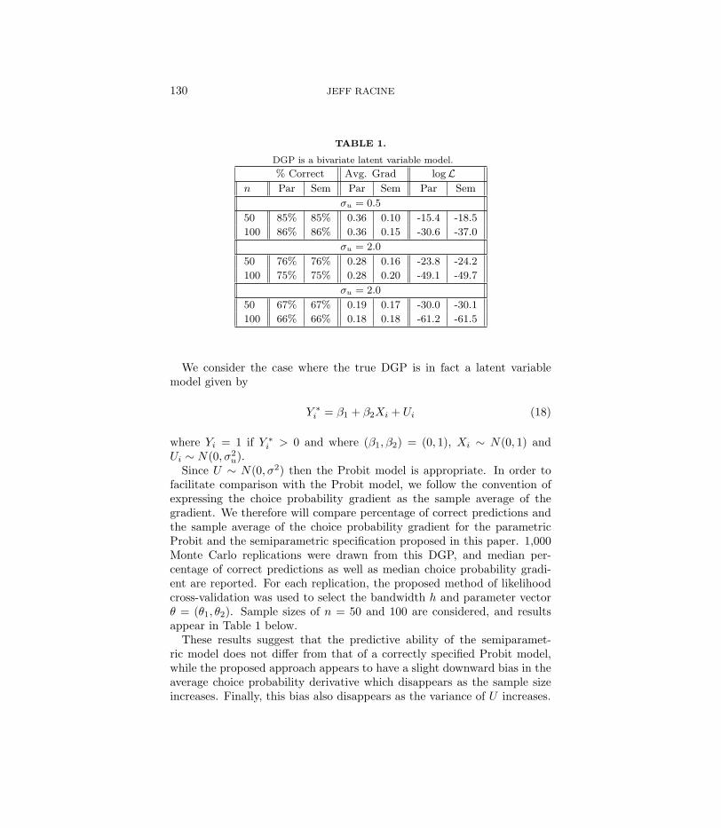
TABLE 1.

DGP is a bivariate latent variable model.

% Correct Avg. Grad logLn Par Sem Par Sem Par Sem

σu = 0.5

50 85% 85% 0.36 0.10 -15.4 -18.5

100 86% 86% 0.36 0.15 -30.6 -37.0

σu = 2.0

50 76% 76% 0.28 0.16 -23.8 -24.2

100 75% 75% 0.28 0.20 -49.1 -49.7

σu = 2.0

50 67% 67% 0.19 0.17 -30.0 -30.1

100 66% 66% 0.18 0.18 -61.2 -61.5

We consider the case where the true DGP is in fact a latent variablemodel given by

Y ∗i = β1 + β2Xi + Ui (18)

where Yi = 1 if Y ∗i > 0 and where (β1, β2) = (0, 1), Xi ∼ N(0, 1) and

Ui ∼ N(0, σ2u).

Since U ∼ N(0, σ2) then the Probit model is appropriate. In order tofacilitate comparison with the Probit model, we follow the convention ofexpressing the choice probability gradient as the sample average of thegradient. We therefore will compare percentage of correct predictions andthe sample average of the choice probability gradient for the parametricProbit and the semiparametric specification proposed in this paper. 1,000Monte Carlo replications were drawn from this DGP, and median per-centage of correct predictions as well as median choice probability gradi-ent are reported. For each replication, the proposed method of likelihoodcross-validation was used to select the bandwidth h and parameter vectorθ = (θ1, θ2). Sample sizes of n = 50 and 100 are considered, and resultsappear in Table 1 below.

These results suggest that the predictive ability of the semiparamet-ric model does not differ from that of a correctly specified Probit model,while the proposed approach appears to have a slight downward bias in theaverage choice probability derivative which disappears as the sample sizeincreases. Finally, this bias also disappears as the variance of U increases.


7. APPLICATION - PREDICTING VOTING BEHAVIOR

We consider an example in which we model voting behavior given infor-mation on various economic characteristics on individuals. For this examplewe consider the choice of voting ‘yes’ or ‘no’ for a local school tax refer-endum. Two economic variables used to predict choice outcome in thesesettings are income and education. This is typically modeled using a Logitor Probit model in which the covariates are expressed in logarithm() form.

Interest lies in the predictive power of the proposed approach versusmodels such as the widely-used Logit or Probit models. This aim of thismodest example is simply to gauge the performance of the proposed methodin a real-world setting. Data was taken from Pindyck & Rubinfeld (1998page 332-333), and there were a total of n = 95 observations available.Table 2 summarizes the results from this modest exercise.

TABLE 2.

Comparison of models of voting behavior.

Average Derivative

Method % Correct log(income) log(education)

Logit 65.3% 0.04 0.20

Probit 65.3% 0.05 0.20

Kernel 67.4% 0.04 0.19

It appears that, for this example, the proposed method yields improvedprediction probabilities. As well, the average derivatives are extremelyclose for both methods. However, an examination of Figure 5 reveals thatthe derivatives are quite different which is missed when quoting the averagederivative as is typically done. As well, note the well-known fact that Logitmodels impart the same shape on all derivatives when using the standardlinear index, but as can be seen this restriction is not imposed by theproposed method.

This modest example is in no way intended to be a serious investigationinto the prediction of voting outcomes. For this simple application, thepredictive ability of the model increases when admitting multiple thresh-olds, and the average choice probability gradient is in line with that fromstandard models of binary choice. These results suggest that allowing formultiple thresholds may improve predictive ability when modeling binarychoice and may constitute a tool which could benefit applied researchers intheir quest to model binary choice outcomes.

132 JEFF RACINE

FIG. 5. Choice probabilities and gradient vectors for voting data where X1 islog(income) and X2 is log(education). The light lined surfaces (left hand side graphs)are those for the proposed method while the dark liked surfaces (right hand side graphs)are those for the Logit model. For this example both approaches employ linear indices.

� � � � � �

� � �

� � � �

� � � � ��

� � � � � � � � ! # %� � � � # ( * � + - � � � %

0 1 2 3 4 6 7

8 9 : ; <

� � �

� � � �

� � � � ��

� � � � � � � � ! # %� � � � # ( * � + - � � � %

0 1 2 3 4 6 7

� � �

� � � �

� � � � �� @ ��

� � � � � � � � ! # %� � � � # ( * � + - � � � %

B 0 1 2 3 4 6 7B � � � � � � � %

� � �

� � � �

� � � � ��

� � � � � � � � ! # %� � � � # ( * � + - � � � %

B 0 1 2 3 4 6 7B � � � � � � � %

� � �

� � � �

� � � � ��

� � � � � � � � ! # %� � � � # ( * � + - � � � %

B 0 1 2 3 4 6 7B � � � � # ( %

� � �

� � � �

� � � � �� @ � �� @ @ �

� � � � � � � � ! # %� � � � # ( * � + - � � � %

B 0 1 2 3 4 6 7B � � � � # ( %


8. CONCLUSION

It is widely known that misspecification of parametric models can yieldbiased and inconsistent estimates and inference based on such models wouldbe invalid. This paper proposes a method for estimating generalized binarychoice models admitting multiple thresholds for which the joint distributionis estimated nonparametrically and the functional form of the index is data-dependent. It is demonstrated how standard parametric models such as theLogit model can distort both the choice probabilities and choice probabilitygradient in simple situations. The proposed approach uses nonparametricmethods for estimation of the choice probabilities and associated gradients.

Future work includes orthogonality tests for a subset of variables andextension of the index to include a fully nonparametric index in additionto the choice probability distribution.

REFERENCESAmemiya, T., 1981, Qualitative response models: A survey. Journal of EconomicLiterature 19, 1483-1536.

Blundell, R., ed., 1987, Journal of Econometrics 34, North Holland.

Chen, H. Z. and A. Randall, 1997, Semi-nonparametric estimation of binary responsemodels with an application to natural resource valuation. Journal of Econometrics76, 323-340.

Coslett, S. R., 1983, Distribution-free maximum likelihood estimation of the binarychoice model. Econometrica 51, 765-782.

Coslett, S. R., 1991, Semiparametric Estimation of a Regressioin Model with SamplingSelectivity, Cambridge, pp. 175-198.

Davidson, R. and J. G. MacKinnon, 1993, Estimation and Inference in Econometrics.Oxford University Press.

Ichimura, H., 1986, Estimation of single index models. Unpublished Manuscript.

Ichimura, H. and L. F. Lee, 1991, Semiparametric Estimation of Multiple Index Mod-els, Cambridge, pp. 3-50.

Ichimura, H. and T. S. Thompson, 1998, Maximum likelihood estimation of a binarychoice model with random coefficients of unknown distribution. Journal of Econo-metrics 86(2), 269-295.

Klein, R. W. and R. H. Spady, 1993, An efficient semiparametric estimator fo binaryresponse models. Econometrica 61, 387-421.

Lee, L. F., 1995, Semiparametric maximum likelihood estimation of polychotomousand sequential choice models. Journal of Econometrics 65, 381-428.

Manski, C. F., 1985, Semiparametric analysis of discrete response: Asymptotic prop-erties of the maximum score estimator. Journal of Econometrics 27, 313-333.

McFadden, D., 1984, Econometric analysis of qualitative response models, in Z.Griliches and M. Intriligator, eds, Handbook of Econometrics, North Holland, pp.1385-1457.

Nadaraya, E., 1965, On nonparametric estimates of density functions and regressioncurves. Theory of Applied Probability 1O, 186-190.

134 JEFF RACINE

Pagan, A. and A. Ullah, 1999, Nonparametric Econometrics, Cambridge UniversityPress.

Picone, G. and J. S. Butler, 1998, Semiparametric estimation of multiple equationindex models. Unpublished Manuscript.

Pindyck, R. S. and D. L. Rubinfeld, 1998, Econometric Models and Economic Fore-casts, Irwin McGraw-Hill.

Prakasa Rao, B., 1983, Nonparametric Functional Estimation, Academic Press.

Priestley, M. B. and M. T. Chao, 1972, Nonparametric function fitting. Journal ofthe Royal Statistical Society 34, 385-392.

Rudd, P., 1986, Consistent estimation of limited dependent variable models despitemis-speification of distribution. Journal of Econometrics 32, 157-187.

Silverman, B. W., 1986, Density Estimation for Statistics and Data Analysis, Chap-man and Hall.

Stone, C. J., 1974, Cross-validatory choice and assessment of statistical predictions(with discussion). Journal of the Royal Statistical Society 36, 111-147.

Watson, G., 1964, Smooth regression analysis. Sanikhya 26:15, 175-184.

Generalized Semiparametric Binary Prediction

Documents

Transcript of Generalized Semiparametric Binary Prediction