SEMIPARAMETRIC FIXED-EFFECTS

ESTIMATOR

FRANÇOIS LIBOIS & VINCENZO VERARDI

WP 1201 DEPARTMENT OF ECONOMICS

WORKING PAPERS SERIES

Semiparametric Fixed-Effects Estimator∗

Francois Libois†and Vincenzo Verardi

‡

Abstract

This paper describes the Stata implementation of Baltagi and Li’s (2002) series

estimator of partially linear panel data models with fixed effects. After a brief

description of the estimator itself, we describe the new command xtsemipar. We

then simulate data to show that this estimator performs better than a fixed effect

estimator if the relationship between two variables is unknown or quite complex.

Keywords: xtsemipar, semiparametric estimations

JEL Classification: C14, C21

1 Introduction

The objective of this note is to present our Stata implementation of Baltagi and Li’s

(2002) series estimation of partially linear panel data models.

The structure of the note is the following: section 2 describes Baltagi and Li’s (2002)

fixed effects semiparametric regression estimator is described. Section 3 presents the

implemented Stata command (xtsemipar). Some simple simulations assessing the

performance of the estimator are shown in Section 4. Section 5 concludes.

∗We would like to thank our colleagues at CRED and ECARES and especially Wouter Gelade and

Peter-Louis Heudtlass who helped improve the quality of the paper. The usual disclaimer applies.†Corresponding author, CRED, Facultes Universitaires Notre Dame de la Paix de Namur. E-mail:

flibois@fundp.ac.be.‡CRED, Facultes Universitaires Notre Dame de la Paix de Namur; ECARES, CKE, Universite

Libre de Bruxelles. E-mail: vverardi@fundp.ac.be. Vincenzo Verardi is Associated Researcher of the

FNRS and gratefully acknowledges their financial support.

1

2 Estimation method

2.1 Baltagi and Li’s (2002) semiparametric fixed effects re-

gression estimator

Consider a general panel data semiparametric model with distributed intercept of the

type:

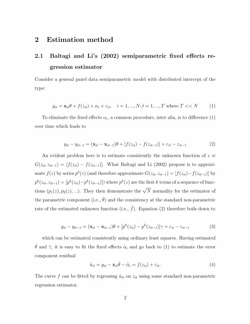
yit = xitθ + f(zit) + αi + εit, i = 1, ..., N ; t = 1, ..., T where T << N (1)

To eliminate the fixed effects αi, a common procedure, inter alia, is to difference (1)

over time which leads to

yit − yit−1 = (xit − xit−1)θ + [f(zit)− f(zit−1)] + εit − εit−1 (2)

An evident problem here is to estimate consistently the unknown function of z ≡

G(zit, zit−1) = [f(zit) − f(zit−1)]. What Baltagi and Li (2002) propose is to approxi-

mate f(z) by series pk(z) (and therefore approximate G(zit, zit−1) = [f(zit)−f(zit−1)] by

pk(zit, zit−1) = [pk(zit)−pk(zit−1)]) where pk(z) are the first k terms of a sequence of func-

tions (p1(z), p2(z), ...). They then demonstrate the√N normality for the estimator of

the parametric component (i.e., θ) and the consistency at the standard non-parametric

rate of the estimated unknown function (i.e., f). Equation (2) therefore boils down to

yit − yit−1 = (xit − xit−1)θ + [pk(zit)− pk(zit−1)]γ + εit − εit−1 (3)

which can be estimated consistently using ordinary least squares. Having estimated

θ and γ, it is easy to fit the fixed effects αi and go back to (1) to estimate the error

component residual

uit = yit − xitθ − αi = f(zit) + εit. (4)

The curve f can be fitted by regressing uit on zit using some standard non-parametric

regression estimator.

2

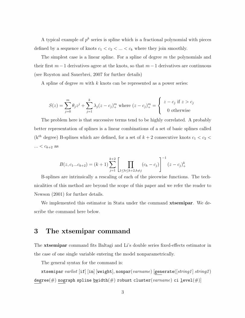
A typical example of pk series is spline which is a fractional polynomial with pieces

defined by a sequence of knots c1 < c2 < ... < ck where they join smoothly.

The simplest case is a linear spline. For a spline of degree m the polynomials and

their first m−1 derivatives agree at the knots, so that m−1 derivatives are continuous

(see Royston and Sauerbrei, 2007 for further details)

A spline of degree m with k knots can be represented as a power series:

S(z) =m�

j=0

θjzj+

k�

j=1

λj(z − cj)m+ where (z − cj)

m+ =

z − cj if z > cj

0 otherwise

The problem here is that successive terms tend to be highly correlated. A probably

better representation of splines is a linear combinations of a set of basic splines called

(kth

degree) B-splines which are defined, for a set of k + 2 consecutive knots c1 < c2 <

... < ck+2 as

B(z, c1...ck+2) = (k + 1)

k+2�

j=1

��

1≤h≤k+2,h �=j

(ch − cj)

�−1

(z − cj)k+

B-splines are intrinsically a rescaling of each of the piecewise functions. The tech-

nicalities of this method are beyond the scope of this paper and we refer the reader to

Newson (2001) for further details.

We implemented this estimator in Stata under the command xtsemipar. We de-

scribe the command here below.

3 The xtsemipar command

The xtsemipar command fits Baltagi and Li’s double series fixed-effects estimator in

the case of one single variable entering the model nonparametrically.

The general syntax for the command is:

xtsemipar varlist [if] [in] [weight], nonpar(varname) [generate([string1 ] string2 )

degree(#) nograph spline bwidth(#) robust cluster(varname) ci level(#)]

3

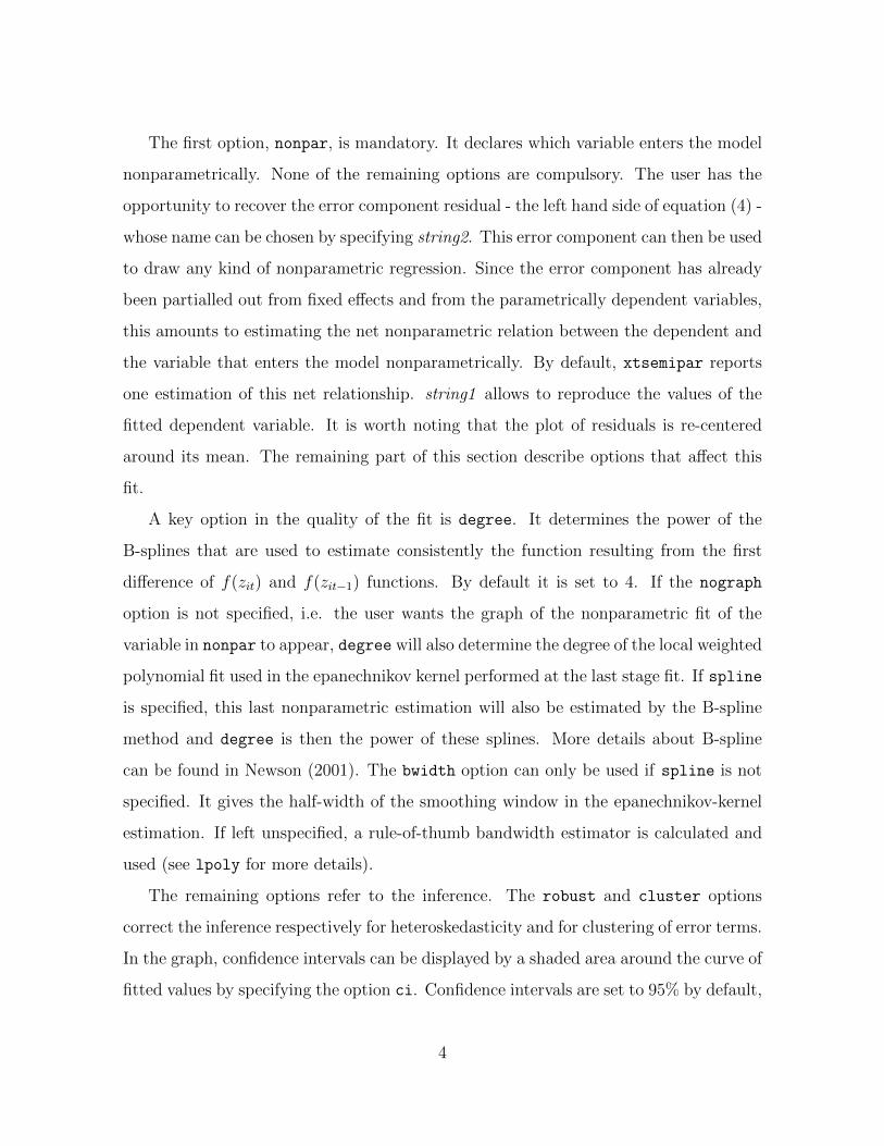
The first option, nonpar, is mandatory. It declares which variable enters the model

nonparametrically. None of the remaining options are compulsory. The user has the

opportunity to recover the error component residual - the left hand side of equation (4) -

whose name can be chosen by specifying string2. This error component can then be used

to draw any kind of nonparametric regression. Since the error component has already

been partialled out from fixed effects and from the parametrically dependent variables,

this amounts to estimating the net nonparametric relation between the dependent and

the variable that enters the model nonparametrically. By default, xtsemipar reports

one estimation of this net relationship. string1 allows to reproduce the values of the

fitted dependent variable. It is worth noting that the plot of residuals is re-centered

around its mean. The remaining part of this section describe options that affect this

fit.

A key option in the quality of the fit is degree. It determines the power of the

B-splines that are used to estimate consistently the function resulting from the first

difference of f(zit) and f(zit−1) functions. By default it is set to 4. If the nograph

option is not specified, i.e. the user wants the graph of the nonparametric fit of the

variable in nonpar to appear, degree will also determine the degree of the local weighted

polynomial fit used in the epanechnikov kernel performed at the last stage fit. If spline

is specified, this last nonparametric estimation will also be estimated by the B-spline

method and degree is then the power of these splines. More details about B-spline

can be found in Newson (2001). The bwidth option can only be used if spline is not

specified. It gives the half-width of the smoothing window in the epanechnikov-kernel

estimation. If left unspecified, a rule-of-thumb bandwidth estimator is calculated and

used (see lpoly for more details).

The remaining options refer to the inference. The robust and cluster options

correct the inference respectively for heteroskedasticity and for clustering of error terms.

In the graph, confidence intervals can be displayed by a shaded area around the curve of

fitted values by specifying the option ci. Confidence intervals are set to 95% by default,

4

however it is possible to modify them by setting a different confidence level through

the level option. This affects the confidence intervals both in the nonparametric and

in the parametric part of estimations.

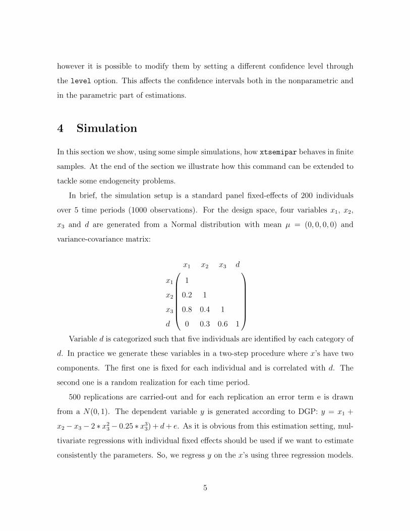
4 Simulation

In this section we show, using some simple simulations, how xtsemipar behaves in finite

samples. At the end of the section we illustrate how this command can be extended to

tackle some endogeneity problems.

In brief, the simulation setup is a standard panel fixed-effects of 200 individuals

over 5 time periods (1000 observations). For the design space, four variables x1, x2,

x3 and d are generated from a Normal distribution with mean µ = (0, 0, 0, 0) and

variance-covariance matrix:

x1 x2 x3 d

x1 1

x2 0.2 1

x3 0.8 0.4 1

d 0 0.3 0.6 1

Variable d is categorized such that five individuals are identified by each category of

d. In practice we generate these variables in a two-step procedure where x’s have two

components. The first one is fixed for each individual and is correlated with d. The

second one is a random realization for each time period.

500 replications are carried-out and for each replication an error term e is drawn

from a N(0, 1). The dependent variable y is generated according to DGP: y = x1 +

x2 − x3 − 2 ∗ x23 − 0.25 ∗ x3

3) + d+ e. As it is obvious from this estimation setting, mul-

tivariate regressions with individual fixed effects should be used if we want to estimate

consistently the parameters. So, we regress y on the x’s using three regression models.

5

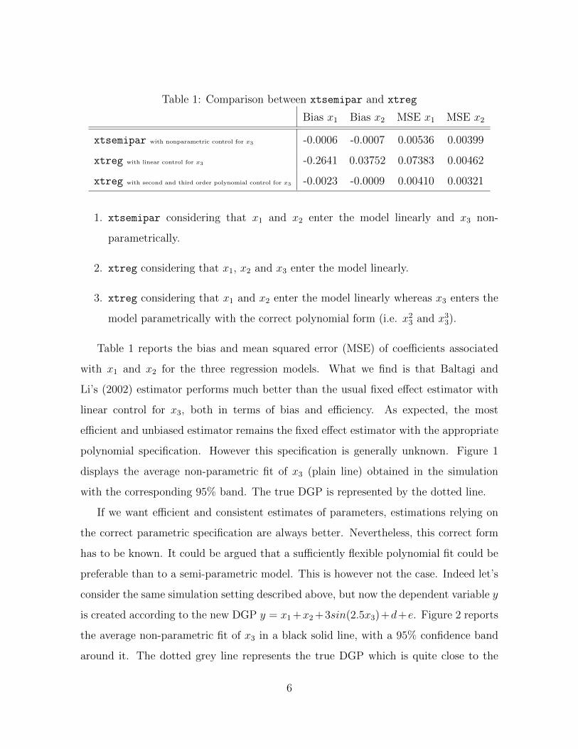
Table 1: Comparison between xtsemipar and xtreg

Bias x1 Bias x2 MSE x1 MSE x2

xtsemipar with nonparametric control for x3 -0.0006 -0.0007 0.00536 0.00399

xtreg with linear control for x3 -0.2641 0.03752 0.07383 0.00462

xtreg with second and third order polynomial control for x3 -0.0023 -0.0009 0.00410 0.00321

1. xtsemipar considering that x1 and x2 enter the model linearly and x3 non-

parametrically.

2. xtreg considering that x1, x2 and x3 enter the model linearly.

3. xtreg considering that x1 and x2 enter the model linearly whereas x3 enters the

model parametrically with the correct polynomial form (i.e. x23 and x3

3).

Table 1 reports the bias and mean squared error (MSE) of coefficients associated

with x1 and x2 for the three regression models. What we find is that Baltagi and

Li’s (2002) estimator performs much better than the usual fixed effect estimator with

linear control for x3, both in terms of bias and efficiency. As expected, the most

efficient and unbiased estimator remains the fixed effect estimator with the appropriate

polynomial specification. However this specification is generally unknown. Figure 1

displays the average non-parametric fit of x3 (plain line) obtained in the simulation

with the corresponding 95% band. The true DGP is represented by the dotted line.

If we want efficient and consistent estimates of parameters, estimations relying on

the correct parametric specification are always better. Nevertheless, this correct form

has to be known. It could be argued that a sufficiently flexible polynomial fit could be

preferable than to a semi-parametric model. This is however not the case. Indeed let’s

consider the same simulation setting described above, but now the dependent variable y

is created according to the new DGP y = x1+x2+3sin(2.5x3)+d+e. Figure 2 reports

the average non-parametric fit of x3 in a black solid line, with a 95% confidence band

around it. The dotted grey line represents the true DGP which is quite close to the

6

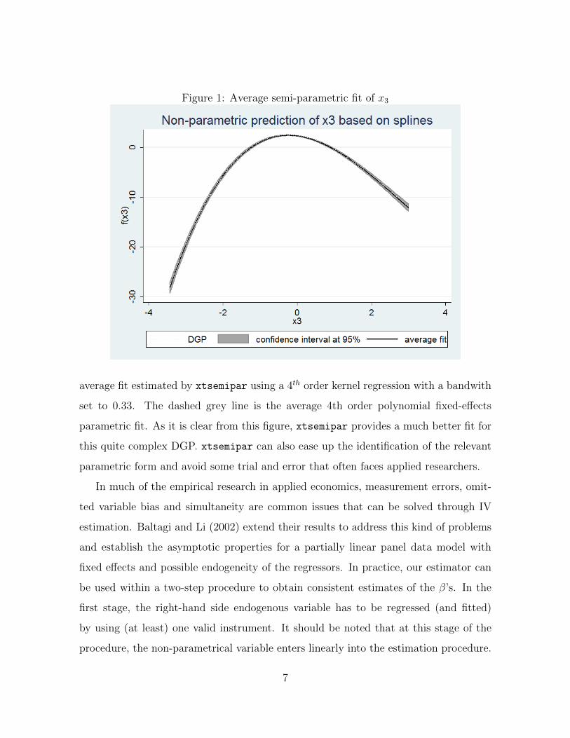
Figure 1: Average semi-parametric fit of x3

average fit estimated by xtsemipar using a 4thorder kernel regression with a bandwith

set to 0.33. The dashed grey line is the average 4th order polynomial fixed-effects

parametric fit. As it is clear from this figure, xtsemipar provides a much better fit for

this quite complex DGP. xtsemipar can also ease up the identification of the relevant

parametric form and avoid some trial and error that often faces applied researchers.

In much of the empirical research in applied economics, measurement errors, omit-

ted variable bias and simultaneity are common issues that can be solved through IV

estimation. Baltagi and Li (2002) extend their results to address this kind of problems

and establish the asymptotic properties for a partially linear panel data model with

fixed effects and possible endogeneity of the regressors. In practice, our estimator can

be used within a two-step procedure to obtain consistent estimates of the β’s. In the

first stage, the right-hand side endogenous variable has to be regressed (and fitted)

by using (at least) one valid instrument. It should be noted that at this stage of the

procedure, the non-parametrical variable enters linearly into the estimation procedure.

7

Figure 2: Average semi-parametric fit of x3

In the second stage, the semi-parametric fixed effect panel data model can be used to

estimate the relation between the dependent variable and the set of regressors. The

non-parametrical variable now enters the model nonparametrically, exactly as explained

before. If the instrument is valid, this procedure leads to consistent estimations.

Another problem can arise if the non-parametrical variable is subject to endogeneity

problems. In this case, we suggest, as first step of the estimation procedure, to use a

control functional approach as explained by Ahamada and Flachaire (2008). However

we believe that the technicalities associated to this method go well beyond the scope

of this note.

5 Conclusion

In econometrics, semiparametric regression estimators are becoming standard tools for

applied researchers. In this paper, we present Baltagi and Li’s (2002) series semipara-

8

metric fixed effects regression estimator. We then introduce the Stata codes we created

to implement it in practice. Some simple simulations to illustrate the usefulness and

the performance of the procedure are also shown.

References

[1] Baltagi, B. H. and Li, D. (2002). ”Series Estimation of Partially Linear Panel Data

Models with Fixed Effects”. Annals of Economics and Finance 3: 103-116.

[2] Ahamada, I. and Flachaire, E. (2008). ”Econometrie non parametrique”,Eds, Eco-

nomica (Corpus Economie).

[3] Royston P., Sauerbrei W. (2007). ”Multivariable modeling with cubic regression

splines: a principled approach”. Stata Journal 7: 45-70.

[4] Newson R., (2001). ”B-splines and splines parameterized by their values at reference

points on the x-axis,” Stata Technical Bulletin, StataCorp LP, vol. 10(57)

9

DEPARTMENT OF ECONOMICS WORKING PAPERS SERIES

UNIVERSITY OF NAMUR !

Faculty of economics, social sciences and management 8 Rempart de la Vierge — 5000 Namur — Belgium

marie-helene.mathieu@fundp.ac.be www.fundp.ac.be/eco/economie/recherche

RECENT ISSUES WP 1119 Paolo Casini and Lore Vandewalle Public good provision in Indian rural areas: the returns to col lective action by microf inance groups. WP 1118 Lore Vandewalle The role of accountants in Indian microf inance groups: a trade-off between f inancial and non-f inancial benefits. WP 1117 Jean-Marie Baland, Rohini Somanathan and Lore Vandewalle Social ly disadvantaged groups and microf inance in India. WP 1116 Jean-Marie Baland, Sanghamitra Das and Dilip Mookherjee Forest degradation in the Himalayas: determinants and pol icy options. WP 1115 Vincenzo Bove and Petros G. Sekeris Economic determinants of third party intervention in civi l war. WP 1114 Martin Carree and Marcus Dejardin Firm entry and exit in local markets: market pul l and unemployment push. WP 1113 Maoliang Ye, Sam Asher, Lorenzo Caraburi, Plamen Nikolov One step at a t ime: does gradual ism bui ld coordination? WP 1112 Marcus Dejardin Entrepreneurship and rent-seeking behaviour. WP 1111 Gani Aldashev and Catherine Guirkinger Deadly anchor: gender biais under Russian colonization of Kazakhstan 1898-1908.