arX

iv:0

809.

2797

v1 [

astr

o-ph

] 16

Sep

200

8DRAFT VERSIONJANUARY 14, 2014Preprint typeset using LATEX style emulateapj v. 7/8/03

AN IMPROVED CLUSTER RICHNESS ESTIMATOR

EDUARDO ROZO1, ELI S. RYKOFF2, BENJAMIN P. KOESTER3,4, TIMOTHY MCKAY 5,6,7, JIANGANG HAO5, AUGUST EVRARD5,6,7, RISAH. WECHSLER8, SARAH HANSEN3,4, ERIN SHELDON9, DAVID JOHNSTON10, MATTHEW BECKER3,4, JAMES ANNIS11, L INDSEY

BLEEM3, RYAN SCRANTON12

Draft version January 14, 2014

ABSTRACTMinimizing the scatter between cluster mass and accessibleobservables is an important goal for cluster cos-mology. In this work, we introduce a new matched filter richness estimator, and test its performance usingthe maxBCG cluster catalog. Our new estimator significantlyreduces the variance in theLX −richness rela-tion, fromσ2

ln LX= (0.86±0.02)2 to σ2

ln LX= (0.69±0.02)2. Relative to the maxBCG richness estimate, it also

removes the strong redshift dependence of the richness scaling relations, and is significantly more robust tophotometric and redshift errors. These improvements are largely due to our more sophisticated treatment ofgalaxy color data. We also demonstrate the scatter in theLX −richness relation depends on the aperture usedto estimate cluster richness, and introduce a novel approach for optimizing said aperture which can be easilygeneralized to other mass tracers.Subject headings: galaxies: clusters – X-rays: galaxies: clusters

1. INTRODUCTION

The dependence of the halo mass function on cosmologyis a problem that is well understood both analytically (Press& Schechter 1974; Bond et al. 1991; Sheth & Tormen 2002)and numerically (Jenkins et al. 2001; Warren et al. 2006; Tin-ker et al. 2008). In principle, this detailed understandingal-lows one to place tight constraints on the amplitude of the pri-mordial power spectrum and on dark energy parameters (e.g.Holder et al. 2001; Haiman et al. 2001). In practice, life is notso simple. Cluster mass is not an observable, and so we mustrely on other quantities that trace mass to estimate the halomass function. In this context, observables that are tightlycorrelated with mass and whose scatter is well understood arehighly desirable, as they permit a more accurate measurementof the mass function.

One such mass tracer, and the subject of interest for thiswork, is the so called cluster richness, a measure of the galaxycontent of a cluster. Relative to other popular mass tracerssuch as X-ray properties, SZ-decrements, and galaxy velocitydispersion, optical richness has unique advantages and disad-vantages. Its unique advantages are:

1 Center for Cosmology and Astro-Particle Physics (CCAPP), The OhioState University, Columbus, OH 43210

2 TABASGO Fellow, Physics Department, University of California atSanta Barbara, 2233B Broida Hall, Santa Barbara, CA 93106

3 Department of Astronomy and Astrophysics, The University of Chicago,Chicago, IL 60637

4 Kavli Institute for Cosmological Physics, The University of Chicago,Chicago, IL 60637

5 Physics Department, University of Michigan, Ann Arbor, MI 481096 Astronomy Department, University of Michigan, Ann Arbor, MI 481097 Michigan Center for Theoretical Physics, Ann Arbor, MI 481098 Kavli Institute for Particle Astrophysics & Cosmology, Physics Depart-

ment, and Stanford Linear Accelerator Center, Stanford University, Stanford,CA 94305

9 Center for Cosmology and Particle Physics, Physics Department, NewYork University, New York, NY 10003

10 Jet Propulsion Laboratory, 4800 Oak Grove Drive, Pasadena,CA 9110911 Fermi National Accelerator Laboratory, P.O. Box 500, Batavia, IL

6051012 Department of Physics and Astronomy, Universityof Pittsburgh, 3941

O’Hara St., Pittsburgh, PA 15260

1. cluster richness can be easily estimated with inexpen-sive, photometric optical data.

2. cluster richness can be estimated for both massive clus-ters and low mass groups.

The first of these two properties is significant because it im-plies that cluster richness estimates are readily available givenany large, photometric optical survey such as the SDSS (Yorket al. 2000a) , DES13, or LSST14. The latter property, on theother hand, is an important advantage for a much more inter-esting reason.

Beginning with White et al. (1993), cosmological con-straints from galaxy clusters have been presented as a degen-eracy relationσ8Ω

γm = constant whereγ ≈ 0.5,σ8 is a param-

eter specifying the amplitude of the primordial power spec-trum, andΩm is the matter density of the universe in units ofthe critical density. The existence of this degeneracy is easyto explain (Rozo et al. 2004): suppose that we only measuredthe abundance of galaxy clusters at a single mass scale. Sincethe halo mass function depends on bothσ8 andΩm, it is evi-dent that with just one observable there must be a degeneracybetween these two parameters. But what if we measure thehalo mass function over a range of scales? This is roughlyequivalent to measuring the amplitude and slope of the halomass function at the statistical pivot point. If the mass rangeprobed is small, then the slope of the mass function is not wellconstrained, and the degeneracy betweenσ8 andΩm will re-main. In order to break this degeneracy, a measurement of thehalo mass function over a large range of masses is necessary.Currently, only spectroscopic velocity measurements and op-tical richness estimates can probe a mass range wide enoughto successfully break this degeneracy, but the former requiresconsiderably more observing resources.

There are, however, important disadvantages to using clus-ter richness as a mass tracer. For instance, historically, thefact that the relation between cluster richness and mass can-not be predicted a priori based on simple physical argumentswas viewed as a significant drawback. Nowadays, however,

13 http://www.darkenergysurvey.org/14 http://www.lsst.org/lsst_home.shtml

2 ROZO ET AL.

this argument holds little sway, since the level of accuracyre-quired for precision comsology in our a priori knowledge ofcluster scaling relations is pushing current research towards aself-calibrating approach, in which both cosmology and clus-ter scaling relations are simultaneously constrained fromthedata (Lima & Hu 2004; Majumdar & Mohr 2004; Lima & Hu2005; Hu & Cohn 2006; Wu et al. 2008). Thus, in so far asself-calibration is necessary to insure one-self against possiblebiases in cosmological estimates, the lack of a simple physi-cal model for predicting cluster richness is no longer a seriousdrawback.

Another reason why optical richness estimates fell out offavor relative to other mass tracers is that, in the past, rich-ness estimates were known to suffer from significant projec-tion effects, which resulted in impure cluster samples as wellas large scatter in the mass-richness relation. Abell made oneof the first systematic attempts at measuring richness (Abell1958; Abell et al. 1989) in defining his richness classes. Hetried to minimize projection by only counting galaxies dim-mer thanm3, the magnitude of the third brightest clustergalaxy, but brighter thanm3 + 2. The bright cut is aimed atforeground interlopers, while the dim cut reduces the contri-bution of the galaxy background. Later methods used simi-lar counting techniques but included a proper account of thebackground (e.g. Bahcall 1981) . Since then, more sophisti-cated algorithms have been developed and applied to CCD-based imaging (e.g. matched-filter methods Postman et al.1996; Bramel et al. 2000; Yee & López-Cruz 1999; Kochaneket al. 2003; Dong et al. 2008).

Projection effects are now a much more benign problemthanks to these more sophisticated richness measurementtechniques, the advent of accurate photometric data enabledby modern CCDs, and most recently, the well-known obser-vations that ellipticals and cluster E/S0 galaxies in particulartend to form a tight ridgeline in color-magnitude space (Vis-vanathan & Sandage 1977; Bower et al. 1992; Gladders & Yee2000; Koester et al. 2007b). This color clustering has beenintegral to richness measurements in the SDSS (Goto et al.2002; Miller et al. 2005; Koester et al. 2007b) and the RedSequence Cluster Survey (RCS: Gladders & Yee 2005), andsuch color-based measures have been shown to be effectivemass tracers (Yee & Ellingson 2003; Muzzin et al. 2007; Shel-don et al. 2007a; Johnston et al. 2007; Rykoff et al. 2008b;Becker et al. 2007a).

While richness estimates show a strong correlation withother mass proxies (e.g. Yee & Ellingson 2003; Dai et al.2007; Sheldon et al. 2007a; Johnston et al. 2007; Becker et al.2007a; Rykoff et al. 2008a), considerable scatter in the mass–richness relation still remains. For instance, the richness mea-sure used in the RCS cluster catalog has a logarithmic scatterof σln M ≈ 0.8 (Gladders et al. 2007), while for maxBCG clus-ters the number is closer toσln M ≈0.5 (Rozo et al. 2008). Thisis to be compared to the scatter for X-ray mass tracers, whichis expected to be as low as≈ 8% forYX based on simulations(Kravtsov et al. 2006), or as high as≈ 25% for non-core ex-tracted soft X-ray band luminosities (e.g. Stanek et al. 2006;Vikhlinin et al. 2008a). Clearly, much improvement is neededto bring the scatter of richness measures to the level of X-raymass tracers.

This work is aimed at reducing the variance in the richness-mass relation. We do this by explicitly constructing a newrichness estimator that significantly reduces the scatter inmass at fixed richness for maxBCG clusters. Relative toN200of maxBCG, we introduce two significant differences. The

first of these involves using a matched filter algorithm to es-timate cluster richness. Matched filters have been used in theliterature before (Postman et al. 1996; Kochanek et al. 2003).Unlike those works, however, our matched filter includes acolor component, which is of critical importance for reduc-ing projection effects over the redshift range spanned by ourcluster sample.15 In that sense, our filter is closer in spirit tothat of Dong et al. (2008), who include a photometric red-shift filter into their richness estimate. We also note here thatgroup-scale studies suggest that some measure of the averagecolor in the cluster is indicative of mass, particularly below∼ 1014M⊙ (Martínez et al. 2002; Martínez & Muriel 2006;Weinmann et al. 2006; Hansen et al. 2007) .

The second difference we introduce is the way in whichthe aperture used to estimate cluster richness is determined.Generically, cluster richness estimators involve counting thenumber of galaxies within some specified aperture, which canthus be interpreted as defining the “size” of the cluster. Thisbegs the question, then, of how is one to select the correctsize of a cluster a priori? Theoretically, halo sizes are usu-ally defined in terms ofR∆, a radius which encompasses amean density that is∆ times either the mean or the criti-cal density of the universe (conventions vary from author toauthor). Unfortunately, not only is such a definition not ap-plicable observationally, authors vary both on the referencebackground density (critical versus mean mass density), andon the specific overdensity value. Thus, even though signifi-cant progress has been made (Cuesta et al. 2008), a definitivedefinition of halo size remains elusive.

In this work, we approach this question with observationsin mind. That is, rather than coming with a preconceived no-tion of what the radius of a cluster is, we let the data tell uswhat the optimal radii for our clusters is by demanding thatoptical richness be as tightly correlated as possible with X-rayluminosity. The idea is as follows: first, one posits a scalingrelation between cluster richness and cluster radius. Whenes-timating cluster richness, one then demands that the richness-radius scaling relation be satisfied. For instance, given a clus-ter, one can simply make an initial guess for its richness. Us-ing the richness-radius scaling relation, one can then drawa circle of the appropriate radius, and count the number ofgalaxies within it. If the richness was underestimated, onewill find too many galaxies, signaling that the richness es-timate must be increased. Proceeding in this way, one canquickly zero in on the appropriate richness for the object.

This does, however, leave open the question of what thecorrect richness-radius relation is. Since we are interested infinding a new richness estimator that is tightly correlated withhalo mass, we can use the scatter in the mass–richness rela-tion as our figure of merit to determine the “correct” richness-radius relation. In practice, we use theLX −richness scatterrather than the mass–richness scatter because the scatter inmass is not directly observable. We emphasize that since themass scatter at fixed X-ray luminosity (see e.g. Vikhlinin etal.2008b) is considerably tighter than the corresponding scatterat fixed richness (Rozo et al. 2008), the use of X-ray luminos-ity as a mass tracer for our purposes is well justified.

The layout of the paper is as follows. We describe the datasets used in this work in § 2. Our matched filter estimator isintroduced in § 3, followed by our method for determining the

15 In Kochanek et al. (2003), the low redshift of the clusters make singleband magnitudes better proxies for distance than colors, sothe lack of a colorfilter in the richness estimator is less important for their work.

Improved Richness Estimates 3

optimal radius-richness relation in § 4. We present our resultsin section § 5. In investigating the properties of our new rich-ness measure, we have discovered that the redshift evolutionof the richness-mass relation of our new estimator is muchmore mild than that measured forN200. These results and thecorresponding discussion are presented in § 6. We summarizeour results and present our conclusions in § 7. Throughout,whenever needed a flatΛCDM cosmology withΩM = 0.3 andh = 1.0 was assumed.

2. DATA

The data for the analysis presented in this work comes fromtwo large area surveys, the Sloan Digital Sky Survey (SDSS:York et al. 2000b) and the ROSAT All-Sky Survey (RASS:Voges et al. 1999). SDSS imaging data are used to selectclusters and to measure their matched filter richness; RASSdata provide 0.1-2.4 keV X-ray fluxes, which we convert intoestimates of the X-ray luminosity of the clusters.

2.1. SDSS

The imaging and spectroscopic surveys that comprise theSDSS are currently in the sixth Data Release (Adelman-McCarthy et al. 2008). This release includes nearly 8500square degrees of drift-scan imaging in the the NorthernGalactic Cap, and another 7500 square degrees of spectro-scopic observations of stars, galaxies, and quasars.

The camera design (Gunn et al. 2006) and drift-scan imag-ing strategy of the SDSS enable acquisition of nearly simul-taneous observations in theu,g,r, i,z filter system (Fukugitaet al. 1996). Calibration (Hogg et al. 2001; Smith et al. 2002;Tucker et al. 2006), astrometric (Pier et al. 2003), and pho-tometric (Lupton et al. 2001) pipelines reduce the data intoobject catalogs containing a host of measured parameters foreach object.

The maxBCG cluster sample and the galaxy catalogs usedto remeasure cluster richness in this paper are derived fromthe SDSS. The galaxy catalogs are drawn from an area ap-proximately coincident with DR4 (Adelman-McCarthy et al.2006). Galaxies are selected from SDSS object catalogs asdescribed in (Sheldon et al. 2007b). In this work we useCMODEL_COUNTS as our total magnitudes, andMODEL_COUNTSwhen computing colors. Bright stars, survey edges and re-gions of poor seeing are masked as previously described(Koester et al. 2007a; Sheldon et al. 2007b).

2.2. Cluster Sample

We obtain sky locations, redshift estimates, and initial rich-ness values from the maxBCG cluster catalog. Details ofthe selection algorithm and catalog properties are publishedelsewhere (Koester et al. 2007a,b). In brief, maxBCG selec-tion relies on the observation that the galaxy population ofrich clusters is dominated by luminous, red galaxies clusteredtightly in color (the E/S0 ridgeline). Since these galaxieshaveold, passively evolving stellar populations, theirg − r colorclosely reflects their redshift. The brightest such red galaxy,typically located at the peak of the galaxy density, defines thecluster center.

The maxBCG catalog is approximately volume limited inthe redshift range 0.1 ≤ z ≤ 0.3, with very accurate photo-metric redshifts (δz ∼ 0.01). Studies of the maxBCG algo-rithm applied to mock SDSS catalogs indicate that the com-pleteness and purity are very high, above 90% (Koester et al.2007a; Rozo et al. 2007). The maxBCG catalog has beenused to investigate the scaling of galaxy velocity dispersion

with cluster richness (Becker et al. 2007b) and to derive con-straints on the power spectrum normalization,σ8, from clusternumber counts (Rozo et al. 2007).

The primary richness estimator used in the maxBCG cata-log isN200, defined as the number of galaxies withg − r colorswithin 2σ of the E/S0 ridgeline as defined by the BCG color,brighter than 0.4L∗ (in i-band), and found withinrgal

200 of thecluster center.rgal

200 is a cluster radius that depends upon thenumber of galaxies within a fixed aperture 1h−1 Mpc of theBCG, labeledNgals, with the relationrgal

200(Ngals) being cali-brated so that, on average, the galaxy overdensity withinrgal

200is 200Ω−1

m assumingΩm = 0.3 (Hansen et al. 2005). The fullcatalog comprises 13,823 objects with a richness thresholdN200 ≥ 10, corresponding toM & 5 · 1013 h−1 M⊙ (Johnstonet al. 2007).

As mentioned in the introduction, we re-estimate the clusterrichness for every object in the maxBCG catalog, and measurethe corresponding scatter in theLX −richness relation. Whendoing so, we always limit ourself to the 2000 richest clusters,ranked according to the new richness estimate. This cut ismade to ensure that our results are insensitive to theN200≥ 10cut of the maxBCG catalog. That is, the number of clusterswith N200≥ 10 that fall within the 2000 richest clusters for anyof the new richness measures considered has no impact on therecovered scatter. We also note that our choice of always se-lecting the 2000 richest clusters also implies that the specificcluster sample used to estimate the scatter in theLX −richnessrelation varies somewhat as we vary the richness estimator.

2.3. X-ray Measurements

The scatter inLX at fixed richness is estimated using aslight variant of the method presented in Rykoff et al. (2008b).Briefly, we use the RASS photon maps to estimate the 0.5-2.0 keV X-ray flux at the location of each cluster, which isused to deriveLX [0.1-2.4 keV] using the cluster photomet-ric redshift (the conversion factors are similar to those usedin Böhringer et al. 2004). We then perform a Bayesian lin-ear least squares fit to lnLx as a function of lnN, whereN isthe richness parameter to be tested. The variance in lnLX isincluded as a free parameter. The fit is done following thealgorithm presented in Kelly (2007), and correctly takes intoaccount upper limits forLX for those clusters with upper lim-its on X-ray emission.

It is important to note here that the estimated X-ray lumi-nosity of a cluster depends on the aperture used to measureLX . Rykoff et al. (2008b) used a fixed 750h−1kpc aperture asa compromise between needing a large aperture to avoid los-ing X-ray photons due to the ROSAT PSF and cluster miscen-tering, and the need for a small aperture in order to increasethe signal to noise of the cluster emission. Further work hasshown that the scatter inLX at fixedN200 is minimized whenusing an aperture of 1h−1Mpc. The corresponding scatter forthe top 2000 maxBCG clusters isσln LX |N200 = 0.96±0.03.16

The nature of the present exercise has the benefit of as-signing a cluster radiusRc, to each individual cluster, so itis natural to measureLX in the same scale as the optical rich-

16 The attentive reader will note that the quoted scatter inLX at fixed rich-ness is significantly larger than the scatter in mass at fixed richness quotedin the introduction, which was closer to 0.5. Given a slope of≈ 1.6 in theLX − M relation, a scatter of 0.96 in LX corresponds to≈ 0.96/1.6 ≈ 0.6scatter in mass. The remaining 10% difference is because thescatter in Rozoet al. (2008) uses the scatter of the 1000 richest clusters, which is smaller thanthat of the 2000 richest clusters by 0.1.

4 ROZO ET AL.

ness. Thus, in this work, we estimateLX using a variableaperture which depends upon the cluster’s richness. Using afixed 1h−1Mpc aperture to estimateLX does not have a largeeffect on our results, for reasons that will be discussed be-low. Finally, we note that very small physical apertures areimpractical for the most distant clusters due to the large sizeof the RASS PSF, which corresponds to a physical scale of300h−1kpc (FWHM) atz = 0.23, the median redshift of themaxBCG catalog. Therefore, we place a fixed minimum aper-ture of 500h−1kpc for each cluster. We discuss the small ef-fect of this aperture cutoff in § 4.

2.4. Cleaning the Sample

Our analysis depends on a combination of optical and X-raymeasurements of maxBCG clusters using SDSS and RASSdata. As discussed in detail in Rykoff et al. (2008b, see § 5.6),there is clear evidence that cool core clusters increase thescat-ter in X-ray cluster properties. High resolution X-ray imagingof clusters allows the exclusion of cluster cores, reducingthescatter in observed X-ray properties (e.g. O’Hara et al. 2006;Chen et al. 2007; Maughan 2007). Unfortunately, the broadPSF of RASS means that it is impossible to exclude the coresof clusters in this work. In order to asses how robust our re-sults are to the presence or absence of cooling flow clustersin the cluster sample, we have created a “clean” sample ofmaxBCG clusters by removing all known cool core clustersthat might have boosted global X-ray luminosity and may sig-nificantly bias our results. In addition, we have removed ap-parently X-ray bright maxBCG clusters that were determinedvia inspection to have their X-ray flux significantly contami-nated by foreground objects such as stars, low redshift galaxyclusters, and AGN.

There does not exist a complete, unbiased catalog of coolcore X-ray clusters. The presently described cleaning pro-cedure is not intended to be complete, and is intended onlyto give some sense of the robustness of our results to thepresence of cooling flow clusters. Following Rykoff et al.(2008b), we have assembled all the known cool core clus-ters from the literature. This includes: A750, A1835,Z2701, Z3146, Z7160, RXC 2129.6+0005 (Bauer et al. 2005),A1413 (Chen et al. 2007), A2244 (Peres et al. 1998), andRXC J1504.1−0248 (Böhringer et al. 2005). From here on,the maxBCG catalog presented in Koester et al. (2007b) isreferred to as the “full” cluster sample, and the subsample de-scribed above is referred to as the “clean” cluster sample.

3. MATCHED FILTER RICHNESS ESTIMATORS

3.1. Derivation of the Matched Filter Richness Estimator

Let x be a vector characterizing the observable propertiesof a galaxy (e.g. galaxy color and magnitude). We modelthe projected galaxy distribution around clusters as a sumS(x) = λu(x|λ) + b(x) whereλ is the number of cluster galax-ies, u(x|λ) is the cluster’s galaxy density profile normalizedto unity, andb(x) is density of background (i.e. non-member)galaxies. The probability that a galaxy found near a clusterisactually a cluster member is given by

p(x) =λu(x|λ)

λu(x|λ) + b(x). (1)

Consequently, the total number of cluster galaxiesλ must sat-isfy the constraint equation

λ =∑

p(x|λ) =∑ λu(x|λ)

λu(x|λ) + b(x)(2)

where the sum is over all galaxies in the cluster field. If the fil-tersu(x|λ) andb(x) are known, then given an observed galaxydistributionx1, ...,xN around a cluster we can define a rich-ness estimatorλ as the solution to equation 2. As it turns out,one can also derive this expression using a maximum likeli-hood approach. Interested readers are referred to appendixAfor details. From now on, the letterλ shall always refer to amatched filter richness estimate obtained with equation 2.

3.2. Cluster Radii and Matched Filter Richness Estimates

Consider again Eqn. 2. As mentioned before, the sum usedin Eqn. 2 needs to extend over all galaxies. In practice, ofcourse, one needs to add over all galaxies within some cutoffradiusRc. Operationally, this is equivalent to settingu = 0for all galaxies with radiiR > Rc, so it is natural to interpretthe cutoff radiusRc as a cluster radius. In this light, it seemsobvious that considerable care must be taken to choose thecorrect cluster radius when estimating richness, but how togoabout doing just that is a less straightforward question.

In this work, we propose that cluster radii be selected onthe basis of a model radius-richness relation. Specifically, weassume that the size of a cluster of richnessλ scales as a powerlaw of λ,

Rc(λ) = R0(λ/100.0)α. (3)

Naively, we expectR0 ≈ 1 Mpc, as that is the characteristicsize of clusters, andα ≈ 1/3 assuming thatR ∝ M1/3 ∝ λ1/3.We postpone the discussion of how we go about selectingR0andα to section 4. For the time being, we shall simply assumethatR0 andα are known. In that case, equation 2 becomes

λ =∑

p(x|λ) =∑

R<Rc(λ)

λu(x|λ)λu(x|λ) + b(x)

. (4)

Note that we have explicitly included the cutoff radiusRc inthe sum above, and that this cutoff radius now depends onλ.Moreover, one can see that in the above equation,the clusterrichness λ is the only unknown, so we can numerically solvefor λ. In other words, by positing a richness-radius relationwe are able to simultaneously estimate both a cluster radiusand the corresponding cluster richness.17

3.3. The Filters

In this work we consider three observable properties ofgalaxies:R, the projected distance from a galaxy to the as-signed cluster center,m, the galaxy magnitude, andc, thegalaxies’g − r color. We adopt a separable filter function

u(x) = [2πRΣ(R)]φ(m)G(c) (5)

whereΣ(R) is the two dimensional cluster galaxy density pro-file, φ(m) is the cluster luminosity function (expressed in ap-parent magnitudes), andG(c) is color distribution of clustergalaxies. The prefactor 2πR in front of Σ(R) accounts for thefact that givenΣ(R), the radial probability density distribu-tion is given by 2πRΣ(R). Also, note the separability condi-tion makes the implicit assumption that these three quantitiesare fully independent of each other, which is not true in detail(for a discussion of the galaxy population of maxBCG clusterssee Hansen et al. 2007). For instance, the tilt of the ridgeline

17 Note that since we are explicitly settingu = 0 for R > Rc, the fact thatumust be normalized to unity necessarily introduces a dependence ofu on λ.That is, changingλ will not only change the range of the sum in equation 4,it will also change the value of the summands.

Improved Richness Estimates 5

implies that the mean color of a red sequence cluster galaxyvaries slightly as a function of magnitude. We postpone aninvestigation of how including the correlation between thesevarious observables affects our conclusions to future work(Koester et al, in preparation). We now describe each of ourthree filters in detail. We note that defining said filters requiresus to specify parameters governing the shape of the filters (e.g.Rs for the radial filter,α for the luminosity filter, etc.). A de-tailed study on the dependence of our matched filter richnessestimates on the shape of our filters will be presented in futurework.

3.3.1. The Radial Filter

N-body simulations show that the matter distribution ofmassive halos can be well described by the so called NFWprofile (see e.g. Navarro et al. 1995, 1997),

ρ(r) ∝ 1(r/rs)(1+ r/rs)2

(6)

wherers is characteristic scale radius at which the logarithmicslope of the density profile is equal to−2. The correspondingtwo dimensional surface density profile (Bartelmann 1996) is

Σ(R) ∝ 1(R/Rs)2 − 1

f (R/Rs) (7)

whereRs = rs and

f (x) = 1−2√

x2 − 1tan−1

√

x − 1x + 1

. (8)

This formula assumesx > 1. Forx < 1, one uses the identitytan−1(ix) = i tanh(x).

Here, we assume that the NFW profile can also reasonablydescribe the density distribution of galaxies in clusters (Lin& Mohr 2004; Hansen et al. 2005; Popesso et al. 2007), andfollow Koester et al. (2007a) in settingRs = 150h−1kpc. Inprinciple, one could optimize the value of this parameter, butwe do not expect our final results to be overly sensitive toour chosen value (see e.g. Dong et al. 2008). Also, in order toavoid the singularity atR = 0 in the above expression, we setΣ

to a constant forR ≤ Rcore = 100h−1kpc. This core density ischosen so that the mass distributionΣ(R) is continuous. Ourresults are insensitive to the particular choice of core radiusfor Rcore ≤ 200h−1kpc. Finally, the profileΣ(R) is truncatedat the cluster radiusRc(λ), and is normalized such that

1 =∫ Rc(λ)

0dR 2πRΣ(R). (9)

We emphasize that this condition implies that the normaliza-tion constant for the density profile is richness dependent,andmust be recomputed for eachλ value when solving forλ inequation 4.

3.3.2. The Luminosity Filter

At z . 0.3, the luminosity distribution of satellite clus-ter galaxies is well-represented by a Schechter function (e.gHansen et al. 2007) which we write as

φ(m) = 0.4ln(10)φ∗10−0.4(m−m∗)(α+1) exp(

−10−0.4(m−m∗))

(10)

We takeα = 0.8 independent of redshift. The characteris-tic magnitude,m∗, is corrected for the distance modulus, k-corrected, and passively-evolved using stellar population syn-thesis models described in Koester et al. (2007b). When ap-plying the luminosity filter,m∗ is chosen from these models,

appropriate to the redshift of the cluster under consideration,and the filter is normalized by integrating down to a magni-tude corresponding to 0.4L∗ at the cluster redshift, or an abso-lute magnitudeMi = −20.25. The latter is simply a luminositycut bright enough to make the maxBCG sample volume lim-ited.

3.3.3. The Color Filter

Early type galaxies are known to dominate the inner re-gions of low redshift galaxy clusters (see e.g. Dressler 1984;Kormendy & Djorgovski 1989; Hansen et al. 2007). Therest-frame spectra of these galaxies typically exhibit a signif-icant drop at about 4000 Å, that gives early type galaxies atthe same redshift nearly uniformly red colors when observedthrough filters that encompass this break. In the SDSS sur-vey, the corresponding filters for galaxies atz . 0.35 aregandr, and we find that theg − r colors of early type galaxiesare found to be gaussianly distributed with a small intrinsicdispersion of about 0.05 magnitudes. Consequently, we takethe color filterG(c) to be

G(c|z) =1√2πσ

exp

[

(c − 〈c|z〉)2

2σ2

]

(11)

wherec = g − r is the color of interest,〈c|z〉 is the mean ofthe Gaussian color distribution of early type galaxies at red-shift z, andσ is the width of the distribution. The mean color〈c|z〉 = 0.625+ 3.149z was determined by matching maxBCGcluster members to the SDSS LRG (Eisenstein et al. 2001)and MAIN (Strauss et al. 2002) spectroscopic galaxy samples.The net dispersionσ is taken to be the sum in quadrature ofthe intrinsic color dispersionσint , set toσint = 0.05, and the es-timated photometric errorσm. In g−r, the typical photometricerror on the red-sequence cluster galaxies brighter than 0.4L∗

is σm ≈ 0.01 magnitudes forz = 0.1, but can be as as large asσm ≈ 0.05 magnitudes forz = 0.3.

3.3.4. Background Estimation

To fully specify our filters, we also need to describe ourbackground model. We assume the background galaxy den-sity is constant in space, so thatb(x) = 2πRΣg(mi,c) whereΣg(mi,c) is the galaxy density as a function of galaxyi−bandmagnitude andg − r color. Σg(mi,c) is estimated by distribut-ing 106 random points throughout the same SDSS photomet-ric survey footprint that defines our galaxy sample. All galax-ies within an angular separation of 0.05 degrees of the ran-dom points (about 1h−1Mpc at z = 0.25) are used to empir-ically determine the mean galaxy densityΣg(mi,c) using atop hat cloud-in-cells (CIC) algorithm (e.g. Hockney & East-wood 1981). For our cells, we used 60 evenly-spaced bins ing − r ∈ [0,2] and 40 bins ini ∈ [14,20]. In each 2 dimensionalbin, the number density of galaxies is normalized by the totalnumber of random points, the width of each color and mag-nitude bin (0.05 mags and 0.1 mags, respectively), and areasearched (0.052π degrees).

This process creates an estimate of the global background,i.e. the number density of galaxies as a function of color andmagnitude in the full SDSS survey. Not surprisingly, a sim-ilar result is obtained by binning the whole galaxy catalogin color and magnitude with CIC and dividing by the surveyarea. However, the procedure we employ above can readilybe adapted to returning alternative background estimates,e.gthe local cluster density as a function of redshift, by replacingrandom points with clusters.

6 ROZO ET AL.

4. METHODS

We have now fully specified our richness estimators, exceptfor the valuesR0 andα that govern the radius-richness scalingrelation. We now discuss how we go about selecting optimalvalues for these parameters.

As we mentioned earlier, we wish to find the cluster rich-ness estimator that minimizes the scatter in the richness-massrelation. Cluster mass, however, is not an observable, and thuswe must rely on other mass tracers. Here, we use X-ray lumi-nosity (LX ) as our mass proxy, primarily because it is a wellknown mass tracer (e.g. Reiprich & Böhringer 2002; Staneket al. 2006; Rykoff et al. 2008a) that is readily accessible to usand for which we can quickly estimate the scatter for multiplerichness measures (see Rykoff et al. 2008b).

We proceed as follows: we begin by defining a coarse gridin R0 andα, given by

R0 =0.5,0.75,1.0,1.25,1.5 (12)α =−0.05,0.05,0.15,0.25,0.35,0.45 (13)

whereR0 is measured in units ofh−1Mpc. Each of these gridpoints defines a distinct richness estimator through equation4. For each grid point, we estimate the corresponding richnessfor every cluster in the maxBCG catalog. We then select the2000 richest clusters and calculate the scatter inLX at fixedrichness of those top 2000 clusters. Note that, because therank ordering of the clusters changes as we vary our richnessestimate, the clusters used to estimate the scatter inLX variesslightly across the grid. We limit ourselves to the richest 2000clusters to ensure our results are insensitive to theN200 ≥ 10cut in the maxBCG catalog.

From our measurements of the scatterσln LX |λ(R0,α) at eachgrid point, we can directly read which parameter combinationminimizes the scatter. We emphasize that because the scat-ter in mass at fixedLX is much lower than the correspondingscatter at fixed richness (Rozo et al. 2008), for our purposesLX is a nearly perfect mass tracer. We note that the X-raymeasurements described in 2.3 require a minimum aperture of500h−1kpc. For the 2000 richest clusters, this cutoff is onlyemployed whenR0 = 0.5h−1Mpc andα ≥ 0.15, which is a re-gion of parameter space that already does not appear to havea strong correlation betweenLX and richness. Therefore, weconclude that the aperture cutoff does not have a significanteffect on our results.

To determine the uncertainty in the recovered parametersR0andα, we need to understand the errors in our measurement ofthe Lx-richness scatter. We estimate these errors using boot-strap resampling. We proceed as follows: letµ be an indexthat runs over all grid points (R0,α), andσµ be the scatter atthe µth grid point. We resample (with replacement) the fullmaxBCG catalog, and measure the scatterσµ at every gridpoint. The procedure is iterated 100 times, and the measure-ments are used to estimate the mean and covariance matrixof σµ.18 Assuming that the probability distributionP(σµ) isa multi-variate Gaussian characterized by the observed meanand covariance matrix, we generate 105 Monte Carlo realiza-tions of the scatter, and estimate the fraction of times thateachgrid point is observed to have the lowest scatter among all gridpoints.

To use the grid to zero in on a particular value forR0 andα,and to estimate errors in these values, we fit each of the 105

18 The measurement of the scatter inLX at fixed richness is very timeconsuming, and needs to be done independently for every point in the grid.This explains why we restrict ourselves to only 100 bootstrap resamplings.

realizations of the scatterσln LX |λ(R0,α) with a 2D parabola.From the fits, we can read off the values ofR0 andα at whichthe minimum occurs, giving us 105 samplings of the probabil-ity distribution of the location of the minimum in parameterspace. The probability distribution of the resulting 105 min-ima is exactly what we desired.

As it turns out, and as discussed in § 5, the coarse grid de-fined above is too broad for a parabolic fit to adequately de-scribe the functionσln LX |λ(R0,α). However, if we restrict our-selves to a smaller region of parameter space near the mini-mum determined from the coarse grid, a quadratic fit becomesadequate. Therefore, we have defined a narrower fine grid,

R0 =1.0,1.1,1.2,1.3,1.4 (14)α =0.22,0.26,0.30,0.34,0.38,0.42 (15)

with R0 measured in units ofh−1Mpc. It is this grid that weuse to report our final results and to select the optimal param-etersR0 andα.

To summarize, we first do a rough exploration of the pa-rameter spaceR0 andα using a coarse grid, and then use asmaller but finer grid to statistically constrain the location ofthe scatter minimum.

5. RESULTS

5.1. The Full Sample

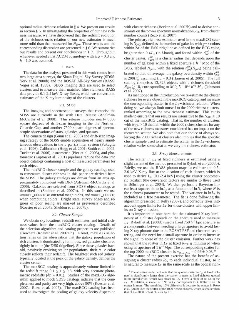
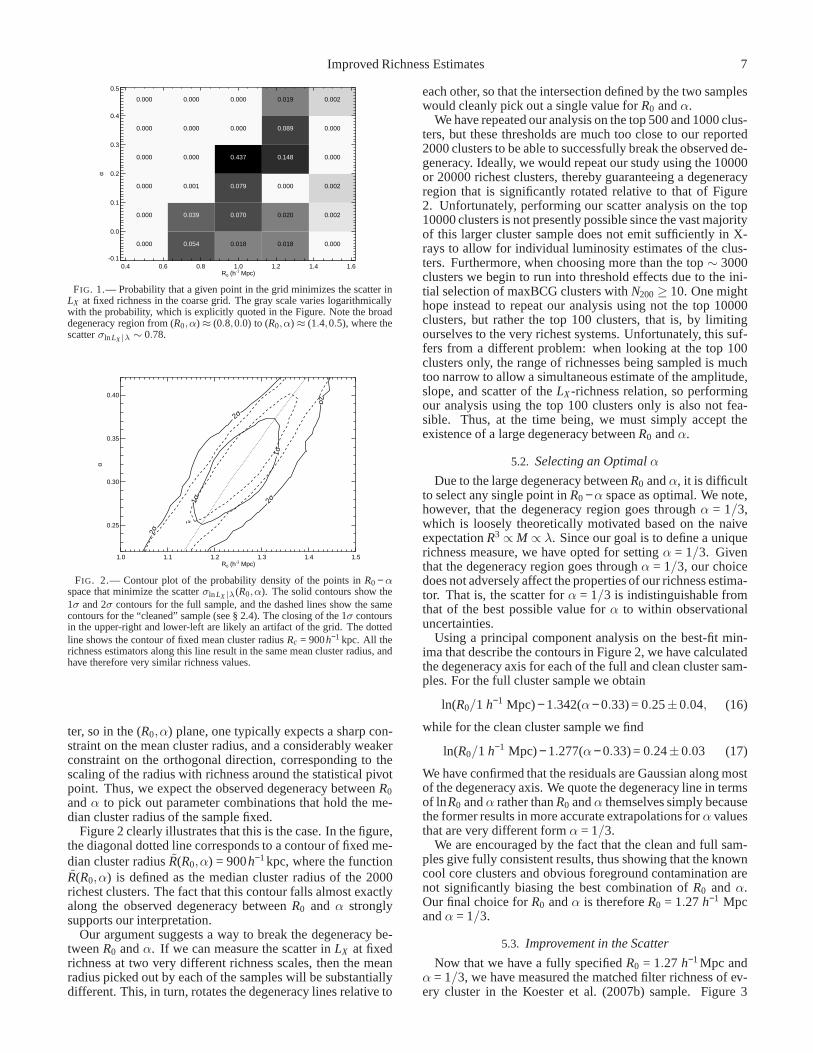
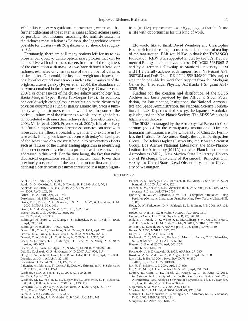
Figure 1 illustrates the probability that each coarse gridpoint is found to minimize the scatter of the 2000 richestclusters when resampling our data as described in § 4. Forthis plot, we have used the full cluster sample, though a sim-ilar result holds when using the clean cluster sample. Eachsquare is shaded in gray on a log scale according to the frac-tion of trials that point is found to have the minimum scat-ter. The primary feature of this plot is a broad degeneracyregion from (R0,α) ≈ (0.8,0.0) to (R0,α) ≈ (1.4,0.5), cor-responding to a scatterσln LX |λ ≈ 0.78. Note this scatter isa significant improvement relative to theLX −richness scat-ter measured forN200, σln LX |N200 = 0.96. The scatter inLXincreases as we move away from the degeneracy region, rang-ing from σln LX |λ ∼ 0.86 in the lower-right corner of Figure 1to σln LX |λ > 1.0 in the upper-left corner. Further discussionof why our new richness estimator results in significantly re-duced scatter is presented in § 6.

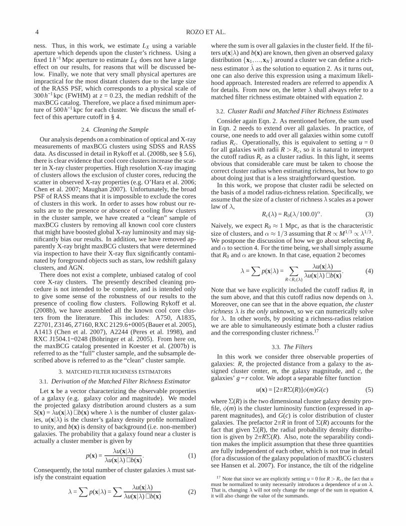
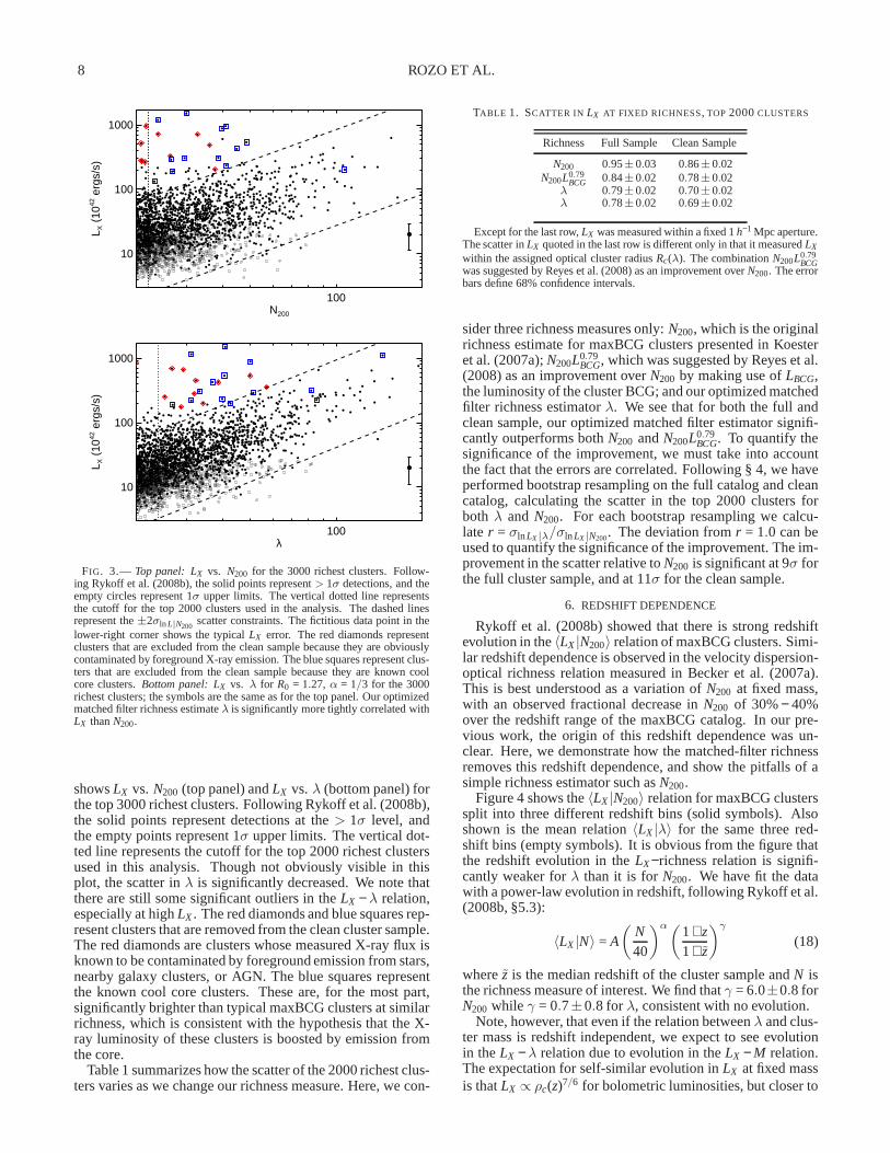
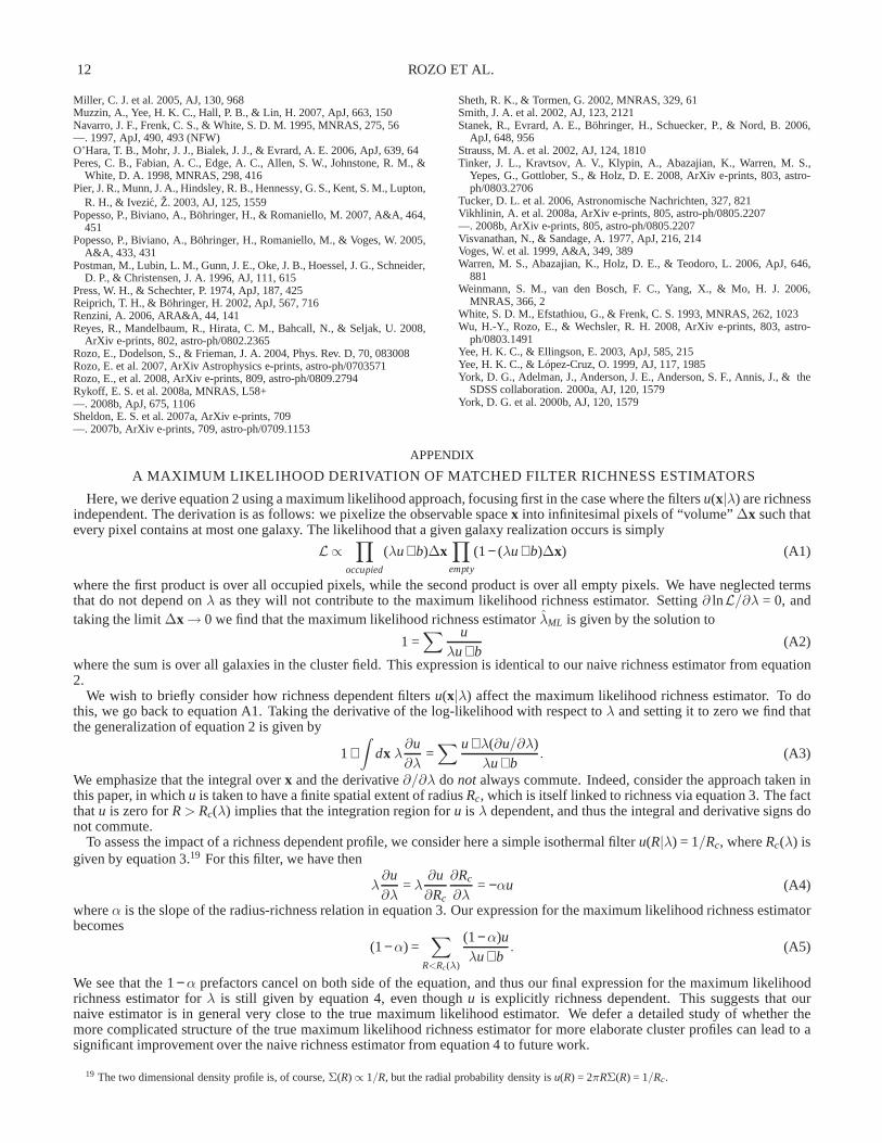
Figure 2 shows the probability density of the points inR0 − α space that minimize the scatter inLX at fixed richnessfor the fine grid, as estimated through the parabolic fits to thefunction σln LX |λ(R0,α) described in section § 4. The solidcontours are for the full cluster sample and the dashed con-tours are for the clean cluster sample. The diagonal degener-acy suggested in the previous plot is now very obvious, espe-cially in the 2σ contour. Importantly, both the full and cleansample produce very similar results, although the contoursarenoticeably smoother for the clean sample. We note that theclosing of the 1σ contours in the upper-right and lower-left islikely an artifact of the grid boundaries. As demonstrated inthe coarse grid in Figure 1, the degeneracy region extends atleast toα ∼ 0 andα ∼ 0.5.

The existence of the degeneracy region is relatively simpleto explain. Consider the problem we are trying to address:what is the correct size of a cluster? Roughly speaking, thisinvolves two parts: one, determining the correct cluster sizeof the average cluster, and two, determining how the clustersize scales with richness as one moves away from the averagecluster. The former is much better determined than the lat-

Improved Richness Estimates 7

0.4 0.6 0.8 1.0 1.2 1.4 1.6R0 (h

-1 Mpc)

-0.1

0.0

0.1

0.2

0.3

0.4

0.5

α

0.000

0.000

0.000

0.000

0.000

0.000

0.054

0.039

0.001

0.000

0.000

0.000

0.018

0.070

0.079

0.437

0.000

0.000

0.018

0.020

0.000

0.148

0.089

0.019

0.000

0.002

0.002

0.000

0.000

0.002

FIG. 1.— Probability that a given point in the grid minimizes thescatter inLX at fixed richness in the coarse grid. The gray scale varies logarithmicallywith the probability, which is explicitly quoted in the Figure. Note the broaddegeneracy region from (R0,α) ≈ (0.8,0.0) to (R0,α) ≈ (1.4,0.5), where thescatterσln LX |λ ∼ 0.78.

1.0 1.1 1.2 1.3 1.4 1.5R0 (h

-1 Mpc)

0.25

0.30

0.35

0.40

α

2σ

2σ

2σ

2σ1σ

1σ

FIG. 2.— Contour plot of the probability density of the points inR0 − αspace that minimize the scatterσln LX |λ(R0,α). The solid contours show the1σ and 2σ contours for the full sample, and the dashed lines show the samecontours for the “cleaned” sample (see § 2.4). The closing ofthe 1σ contoursin the upper-right and lower-left are likely an artifact of the grid. The dottedline shows the contour of fixed mean cluster radiusRc = 900h−1 kpc. All therichness estimators along this line result in the same mean cluster radius, andhave therefore very similar richness values.

ter, so in the (R0,α) plane, one typically expects a sharp con-straint on the mean cluster radius, and a considerably weakerconstraint on the orthogonal direction, corresponding to thescaling of the radius with richness around the statistical pivotpoint. Thus, we expect the observed degeneracy betweenR0andα to pick out parameter combinations that hold the me-dian cluster radius of the sample fixed.

Figure 2 clearly illustrates that this is the case. In the figure,the diagonal dotted line corresponds to a contour of fixed me-dian cluster radiusR(R0,α) = 900h−1kpc, where the functionR(R0,α) is defined as the median cluster radius of the 2000richest clusters. The fact that this contour falls almost exactlyalong the observed degeneracy betweenR0 and α stronglysupports our interpretation.

Our argument suggests a way to break the degeneracy be-tweenR0 andα. If we can measure the scatter inLX at fixedrichness at two very different richness scales, then the meanradius picked out by each of the samples will be substantiallydifferent. This, in turn, rotates the degeneracy lines relative to

each other, so that the intersection defined by the two sampleswould cleanly pick out a single value forR0 andα.

We have repeated our analysis on the top 500 and 1000 clus-ters, but these thresholds are much too close to our reported2000 clusters to be able to successfully break the observed de-generacy. Ideally, we would repeat our study using the 10000or 20000 richest clusters, thereby guaranteeing a degeneracyregion that is significantly rotated relative to that of Figure2. Unfortunately, performing our scatter analysis on the top10000 clusters is not presently possible since the vast majorityof this larger cluster sample does not emit sufficiently in X-rays to allow for individual luminosity estimates of the clus-ters. Furthermore, when choosing more than the top∼ 3000clusters we begin to run into threshold effects due to the ini-tial selection of maxBCG clusters withN200≥ 10. One mighthope instead to repeat our analysis using not the top 10000clusters, but rather the top 100 clusters, that is, by limitingourselves to the very richest systems. Unfortunately, thissuf-fers from a different problem: when looking at the top 100clusters only, the range of richnesses being sampled is muchtoo narrow to allow a simultaneous estimate of the amplitude,slope, and scatter of theLX -richness relation, so performingour analysis using the top 100 clusters only is also not fea-sible. Thus, at the time being, we must simply accept theexistence of a large degeneracy betweenR0 andα.

5.2. Selecting an Optimal α

Due to the large degeneracy betweenR0 andα, it is difficultto select any single point inR0 −α space as optimal. We note,however, that the degeneracy region goes throughα = 1/3,which is loosely theoretically motivated based on the naiveexpectationR3 ∝ M ∝ λ. Since our goal is to define a uniquerichness measure, we have opted for settingα = 1/3. Giventhat the degeneracy region goes throughα = 1/3, our choicedoes not adversely affect the properties of our richness estima-tor. That is, the scatter forα = 1/3 is indistinguishable fromthat of the best possible value forα to within observationaluncertainties.

Using a principal component analysis on the best-fit min-ima that describe the contours in Figure 2, we have calculatedthe degeneracy axis for each of the full and clean cluster sam-ples. For the full cluster sample we obtain

ln(R0/1 h−1 Mpc)− 1.342(α− 0.33) = 0.25±0.04, (16)

while for the clean cluster sample we find

ln(R0/1 h−1 Mpc)− 1.277(α− 0.33) = 0.24±0.03 (17)

We have confirmed that the residuals are Gaussian along mostof the degeneracy axis. We quote the degeneracy line in termsof lnR0 andα rather thanR0 andα themselves simply becausethe former results in more accurate extrapolations forα valuesthat are very different formα = 1/3.

We are encouraged by the fact that the clean and full sam-ples give fully consistent results, thus showing that the knowncool core clusters and obvious foreground contamination arenot significantly biasing the best combination ofR0 and α.Our final choice forR0 andα is thereforeR0 = 1.27 h−1 Mpcandα = 1/3.

5.3. Improvement in the Scatter

Now that we have a fully specifiedR0 = 1.27 h−1Mpc andα = 1/3, we have measured the matched filter richness of ev-ery cluster in the Koester et al. (2007b) sample. Figure 3

8 ROZO ET AL.

100N200

10

100

1000

L X (

1042

erg

s/s)

100λ

10

100

1000

L X (

1042

erg

s/s)

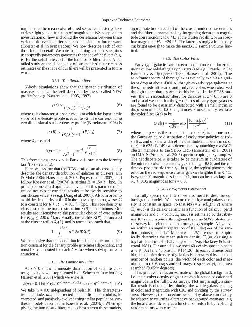
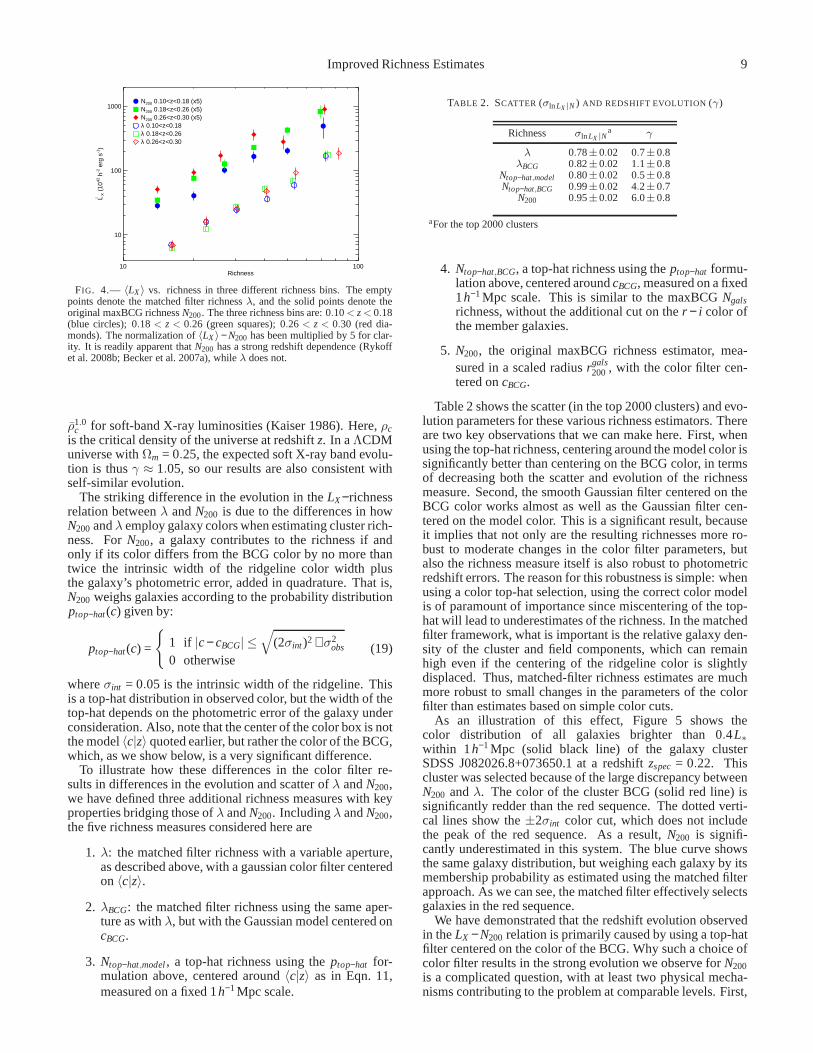
FIG. 3.— Top panel: LX vs. N200 for the 3000 richest clusters. Follow-ing Rykoff et al. (2008b), the solid points represent> 1σ detections, and theempty circles represent 1σ upper limits. The vertical dotted line representsthe cutoff for the top 2000 clusters used in the analysis. Thedashed linesrepresent the±2σln L|N200

scatter constraints. The fictitious data point in thelower-right corner shows the typicalLX error. The red diamonds representclusters that are excluded from the clean sample because they are obviouslycontaminated by foreground X-ray emission. The blue squares represent clus-ters that are excluded from the clean sample because they areknown coolcore clusters.Bottom panel: LX vs. λ for R0 = 1.27, α = 1/3 for the 3000richest clusters; the symbols are the same as for the top panel. Our optimizedmatched filter richness estimateλ is significantly more tightly correlated withLX thanN200.

showsLX vs. N200 (top panel) andLX vs. λ (bottom panel) forthe top 3000 richest clusters. Following Rykoff et al. (2008b),the solid points represent detections at the> 1σ level, andthe empty points represent 1σ upper limits. The vertical dot-ted line represents the cutoff for the top 2000 richest clustersused in this analysis. Though not obviously visible in thisplot, the scatter inλ is significantly decreased. We note thatthere are still some significant outliers in theLX − λ relation,especially at highLX . The red diamonds and blue squares rep-resent clusters that are removed from the clean cluster sample.The red diamonds are clusters whose measured X-ray flux isknown to be contaminated by foreground emission from stars,nearby galaxy clusters, or AGN. The blue squares representthe known cool core clusters. These are, for the most part,significantly brighter than typical maxBCG clusters at similarrichness, which is consistent with the hypothesis that the X-ray luminosity of these clusters is boosted by emission fromthe core.

Table 1 summarizes how the scatter of the 2000 richest clus-ters varies as we change our richness measure. Here, we con-

TABLE 1. SCATTER IN LX AT FIXED RICHNESS, TOP 2000CLUSTERS

Richness Full Sample Clean Sample

N200 0.95±0.03 0.86±0.02N200L0.79

BCG 0.84±0.02 0.78±0.02λ 0.79±0.02 0.70±0.02λ 0.78±0.02 0.69±0.02

Except for the last row,LX was measured within a fixed 1h−1 Mpc aperture.The scatter inLX quoted in the last row is different only in that it measuredLX

within the assigned optical cluster radiusRc(λ). The combinationN200L0.79BCG

was suggested by Reyes et al. (2008) as an improvement overN200. The errorbars define 68% confidence intervals.

sider three richness measures only:N200, which is the originalrichness estimate for maxBCG clusters presented in Koesteret al. (2007a);N200L0.79

BCG, which was suggested by Reyes et al.(2008) as an improvement overN200 by making use ofLBCG,the luminosity of the cluster BCG; and our optimized matchedfilter richness estimatorλ. We see that for both the full andclean sample, our optimized matched filter estimator signifi-cantly outperforms bothN200 andN200L0.79

BCG. To quantify thesignificance of the improvement, we must take into accountthe fact that the errors are correlated. Following § 4, we haveperformed bootstrap resampling on the full catalog and cleancatalog, calculating the scatter in the top 2000 clusters forboth λ and N200. For each bootstrap resampling we calcu-late r = σln LX |λ/σln LX |N200. The deviation fromr = 1.0 can beused to quantify the significance of the improvement. The im-provement in the scatter relative toN200 is significant at 9σ forthe full cluster sample, and at 11σ for the clean sample.

6. REDSHIFT DEPENDENCE

Rykoff et al. (2008b) showed that there is strong redshiftevolution in the〈LX |N200〉 relation of maxBCG clusters. Simi-lar redshift dependence is observed in the velocity dispersion-optical richness relation measured in Becker et al. (2007a).This is best understood as a variation ofN200 at fixed mass,with an observed fractional decrease inN200 of 30%− 40%over the redshift range of the maxBCG catalog. In our pre-vious work, the origin of this redshift dependence was un-clear. Here, we demonstrate how the matched-filter richnessremoves this redshift dependence, and show the pitfalls of asimple richness estimator such asN200.

Figure 4 shows the〈LX |N200〉 relation for maxBCG clusterssplit into three different redshift bins (solid symbols). Alsoshown is the mean relation〈LX |λ〉 for the same three red-shift bins (empty symbols). It is obvious from the figure thatthe redshift evolution in theLX −richness relation is signifi-cantly weaker forλ than it is forN200. We have fit the datawith a power-law evolution in redshift, following Rykoff etal.(2008b, §5.3):

〈LX |N〉 = A

(

N40

)α (

1+ z1+ z

)γ

(18)

wherez is the median redshift of the cluster sample andN isthe richness measure of interest. We find thatγ = 6.0±0.8 forN200 while γ = 0.7±0.8 for λ, consistent with no evolution.

Note, however, that even if the relation betweenλ and clus-ter mass is redshift independent, we expect to see evolutionin theLX − λ relation due to evolution in theLX − M relation.The expectation for self-similar evolution inLX at fixed massis thatLX ∝ ρc(z)7/6 for bolometric luminosities, but closer to

Improved Richness Estimates 9

10 100Richness

10

100

1000L

X (

1042

h-2 e

rg s

-1)

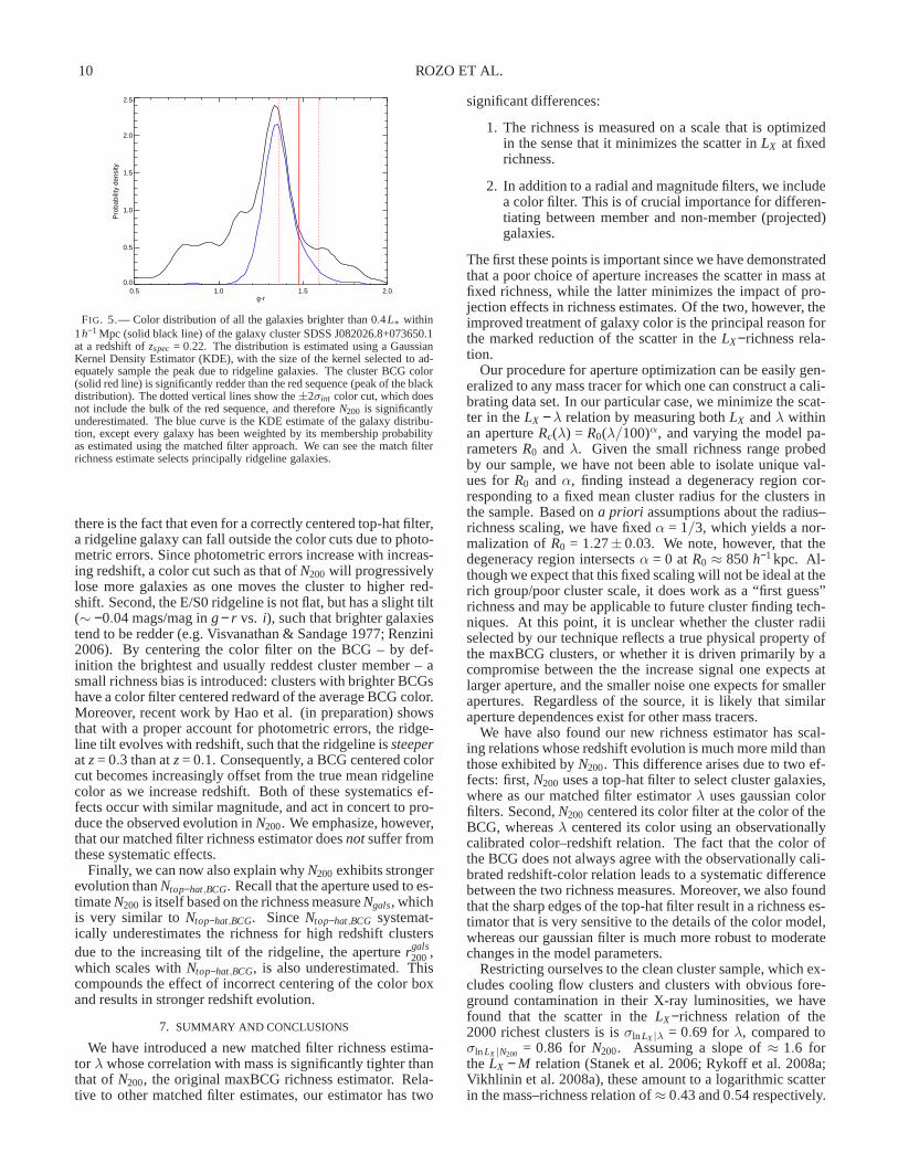
N200 0.10<z<0.18 (x5)N200 0.18<z<0.26 (x5)N200 0.26<z<0.30 (x5)λ 0.10<z<0.18λ 0.18<z<0.26λ 0.26<z<0.30

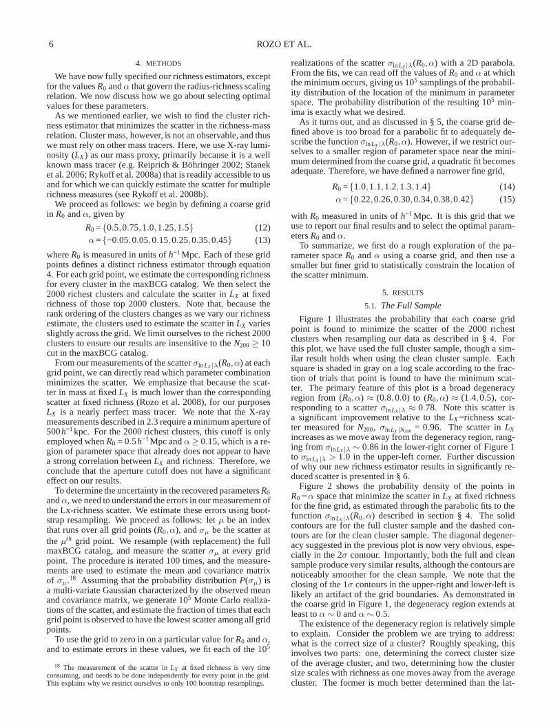
FIG. 4.— 〈LX 〉 vs. richness in three different richness bins. The emptypoints denote the matched filter richnessλ, and the solid points denote theoriginal maxBCG richnessN200. The three richness bins are: 0.10< z < 0.18(blue circles); 0.18 < z < 0.26 (green squares); 0.26 < z < 0.30 (red dia-monds). The normalization of〈LX 〉− N200 has been multiplied by 5 for clar-ity. It is readily apparent thatN200 has a strong redshift dependence (Rykoffet al. 2008b; Becker et al. 2007a), whileλ does not.

ρ1.0c for soft-band X-ray luminosities (Kaiser 1986). Here,ρc

is the critical density of the universe at redshiftz. In aΛCDMuniverse withΩm = 0.25, the expected soft X-ray band evolu-tion is thusγ ≈ 1.05, so our results are also consistent withself-similar evolution.

The striking difference in the evolution in theLX −richnessrelation betweenλ andN200 is due to the differences in howN200 andλ employ galaxy colors when estimating cluster rich-ness. ForN200, a galaxy contributes to the richness if andonly if its color differs from the BCG color by no more thantwice the intrinsic width of the ridgeline color width plusthe galaxy’s photometric error, added in quadrature. That is,N200 weighs galaxies according to the probability distributionptop−hat(c) given by:

ptop−hat(c) =

1 if |c − cBCG| ≤√

(2σint)2 + σ2obs

0 otherwise(19)

whereσint = 0.05 is the intrinsic width of the ridgeline. Thisis a top-hat distribution in observed color, but the width ofthetop-hat depends on the photometric error of the galaxy underconsideration. Also, note that the center of the color box isnotthe model〈c|z〉 quoted earlier, but rather the color of the BCG,which, as we show below, is a very significant difference.

To illustrate how these differences in the color filter re-sults in differences in the evolution and scatter ofλ andN200,we have defined three additional richness measures with keyproperties bridging those ofλ andN200. Includingλ andN200,the five richness measures considered here are

1. λ: the matched filter richness with a variable aperture,as described above, with a gaussian color filter centeredon 〈c|z〉.

2. λBCG: the matched filter richness using the same aper-ture as withλ, but with the Gaussian model centered oncBCG.

3. Ntop−hat,model , a top-hat richness using theptop−hat for-mulation above, centered around〈c|z〉 as in Eqn. 11,measured on a fixed 1h−1Mpc scale.

TABLE 2. SCATTER (σln LX |N ) AND REDSHIFT EVOLUTION (γ)

Richness σln LX |Na γ

λ 0.78±0.02 0.7±0.8λBCG 0.82±0.02 1.1±0.8

Ntop−hat,model 0.80±0.02 0.5±0.8Ntop−hat,BCG 0.99±0.02 4.2±0.7

N200 0.95±0.02 6.0±0.8

aFor the top 2000 clusters

4. Ntop−hat,BCG, a top-hat richness using theptop−hat formu-lation above, centered aroundcBCG, measured on a fixed1h−1Mpc scale. This is similar to the maxBCGNgalsrichness, without the additional cut on ther − i color ofthe member galaxies.

5. N200, the original maxBCG richness estimator, mea-sured in a scaled radiusrgals

200 , with the color filter cen-tered oncBCG.

Table 2 shows the scatter (in the top 2000 clusters) and evo-lution parameters for these various richness estimators. Thereare two key observations that we can make here. First, whenusing the top-hat richness, centering around the model color issignificantly better than centering on the BCG color, in termsof decreasing both the scatter and evolution of the richnessmeasure. Second, the smooth Gaussian filter centered on theBCG color works almost as well as the Gaussian filter cen-tered on the model color. This is a significant result, becauseit implies that not only are the resulting richnesses more ro-bust to moderate changes in the color filter parameters, butalso the richness measure itself is also robust to photometricredshift errors. The reason for this robustness is simple: whenusing a color top-hat selection, using the correct color modelis of paramount of importance since miscentering of the top-hat will lead to underestimates of the richness. In the matchedfilter framework, what is important is the relative galaxy den-sity of the cluster and field components, which can remainhigh even if the centering of the ridgeline color is slightlydisplaced. Thus, matched-filter richness estimates are muchmore robust to small changes in the parameters of the colorfilter than estimates based on simple color cuts.

As an illustration of this effect, Figure 5 shows thecolor distribution of all galaxies brighter than 0.4L∗

within 1h−1Mpc (solid black line) of the galaxy clusterSDSS J082026.8+073650.1 at a redshiftzspec = 0.22. Thiscluster was selected because of the large discrepancy betweenN200 andλ. The color of the cluster BCG (solid red line) issignificantly redder than the red sequence. The dotted verti-cal lines show the±2σint color cut, which does not includethe peak of the red sequence. As a result,N200 is signifi-cantly underestimated in this system. The blue curve showsthe same galaxy distribution, but weighing each galaxy by itsmembership probability as estimated using the matched filterapproach. As we can see, the matched filter effectively selectsgalaxies in the red sequence.

We have demonstrated that the redshift evolution observedin theLX − N200 relation is primarily caused by using a top-hatfilter centered on the color of the BCG. Why such a choice ofcolor filter results in the strong evolution we observe forN200is a complicated question, with at least two physical mecha-nisms contributing to the problem at comparable levels. First,

10 ROZO ET AL.

0.5 1.0 1.5 2.0g-r

0.0

0.5

1.0

1.5

2.0

2.5

Pro

babi

lity

dens

ity

FIG. 5.— Color distribution of all the galaxies brighter than 0.4L∗ within1h−1 Mpc (solid black line) of the galaxy cluster SDSS J082026.8+073650.1at a redshift ofzspec = 0.22. The distribution is estimated using a GaussianKernel Density Estimator (KDE), with the size of the kernel selected to ad-equately sample the peak due to ridgeline galaxies. The cluster BCG color(solid red line) is significantly redder than the red sequence (peak of the blackdistribution). The dotted vertical lines show the±2σint color cut, which doesnot include the bulk of the red sequence, and thereforeN200 is significantlyunderestimated. The blue curve is the KDE estimate of the galaxy distribu-tion, except every galaxy has been weighted by its membership probabilityas estimated using the matched filter approach. We can see thematch filterrichness estimate selects principally ridgeline galaxies.

there is the fact that even for a correctly centered top-hat filter,a ridgeline galaxy can fall outside the color cuts due to photo-metric errors. Since photometric errors increase with increas-ing redshift, a color cut such as that ofN200 will progressivelylose more galaxies as one moves the cluster to higher red-shift. Second, the E/S0 ridgeline is not flat, but has a slighttilt(∼ −0.04 mags/mag ing − r vs. i), such that brighter galaxiestend to be redder (e.g. Visvanathan & Sandage 1977; Renzini2006). By centering the color filter on the BCG – by def-inition the brightest and usually reddest cluster member – asmall richness bias is introduced: clusters with brighter BCGshave a color filter centered redward of the average BCG color.Moreover, recent work by Hao et al. (in preparation) showsthat with a proper account for photometric errors, the ridge-line tilt evolves with redshift, such that the ridgeline issteeperatz = 0.3 than atz = 0.1. Consequently, a BCG centered colorcut becomes increasingly offset from the true mean ridgelinecolor as we increase redshift. Both of these systematics ef-fects occur with similar magnitude, and act in concert to pro-duce the observed evolution inN200. We emphasize, however,that our matched filter richness estimator doesnot suffer fromthese systematic effects.

Finally, we can now also explain whyN200 exhibits strongerevolution thanNtop−hat,BCG. Recall that the aperture used to es-timateN200 is itself based on the richness measureNgals, whichis very similar toNtop−hat,BCG. SinceNtop−hat,BCG systemat-ically underestimates the richness for high redshift clustersdue to the increasing tilt of the ridgeline, the aperturergals

200 ,which scales withNtop−hat,BCG, is also underestimated. Thiscompounds the effect of incorrect centering of the color boxand results in stronger redshift evolution.

7. SUMMARY AND CONCLUSIONS

We have introduced a new matched filter richness estima-tor λ whose correlation with mass is significantly tighter thanthat of N200, the original maxBCG richness estimator. Rela-tive to other matched filter estimates, our estimator has two

significant differences:

1. The richness is measured on a scale that is optimizedin the sense that it minimizes the scatter inLX at fixedrichness.

2. In addition to a radial and magnitude filters, we includea color filter. This is of crucial importance for differen-tiating between member and non-member (projected)galaxies.

The first these points is important since we have demonstratedthat a poor choice of aperture increases the scatter in mass atfixed richness, while the latter minimizes the impact of pro-jection effects in richness estimates. Of the two, however,theimproved treatment of galaxy color is the principal reason forthe marked reduction of the scatter in theLX −richness rela-tion.

Our procedure for aperture optimization can be easily gen-eralized to any mass tracer for which one can construct a cali-brating data set. In our particular case, we minimize the scat-ter in theLX − λ relation by measuring bothLX andλ withinan apertureRc(λ) = R0(λ/100)α, and varying the model pa-rametersR0 and λ. Given the small richness range probedby our sample, we have not been able to isolate unique val-ues forR0 and α, finding instead a degeneracy region cor-responding to a fixed mean cluster radius for the clusters inthe sample. Based ona priori assumptions about the radius–richness scaling, we have fixedα = 1/3, which yields a nor-malization ofR0 = 1.27± 0.03. We note, however, that thedegeneracy region intersectsα = 0 at R0 ≈ 850 h−1kpc. Al-though we expect that this fixed scaling will not be ideal at therich group/poor cluster scale, it does work as a “first guess”richness and may be applicable to future cluster finding tech-niques. At this point, it is unclear whether the cluster radiiselected by our technique reflects a true physical property ofthe maxBCG clusters, or whether it is driven primarily by acompromise between the the increase signal one expects atlarger aperture, and the smaller noise one expects for smallerapertures. Regardless of the source, it is likely that similaraperture dependences exist for other mass tracers.

We have also found our new richness estimator has scal-ing relations whose redshift evolution is much more mild thanthose exhibited byN200. This difference arises due to two ef-fects: first,N200 uses a top-hat filter to select cluster galaxies,where as our matched filter estimatorλ uses gaussian colorfilters. Second,N200 centered its color filter at the color of theBCG, whereasλ centered its color using an observationallycalibrated color–redshift relation. The fact that the color ofthe BCG does not always agree with the observationally cali-brated redshift-color relation leads to a systematic differencebetween the two richness measures. Moreover, we also foundthat the sharp edges of the top-hat filter result in a richnesses-timator that is very sensitive to the details of the color model,whereas our gaussian filter is much more robust to moderatechanges in the model parameters.

Restricting ourselves to the clean cluster sample, which ex-cludes cooling flow clusters and clusters with obvious fore-ground contamination in their X-ray luminosities, we havefound that the scatter in theLX −richness relation of the2000 richest clusters is isσln LX |λ = 0.69 for λ, compared toσln LX |N200 = 0.86 for N200. Assuming a slope of≈ 1.6 forthe LX − M relation (Stanek et al. 2006; Rykoff et al. 2008a;Vikhlinin et al. 2008a), these amount to a logarithmic scatterin the mass–richness relation of≈ 0.43 and 0.54 respectively.

Improved Richness Estimates 11

While this is a very significant improvement, we expect thatfurther tightening of the scatter in mass at fixed richness mustbe possible. For instance, assuming the intrinsic scatter inthe richness-mass relation is Poisson, the logarithmic scatterpossible for clusters with 20 galaxies or so should be roughly≈ 0.2.

Fortunately, there are still many options left for us to ex-plore in our quest to define optical mass proxies that can becompetitive with other mass tracers in terms of the tightnessof the correlation with mass. As we have defined it here, ourrichness estimates only makes use of the number of galaxiesin the cluster. One could, for instance, weigh our cluster rich-ness by other optical mass tracers such as the luminosity of thebrightest cluster galaxy (Reyes et al. 2008), the abundanceofbaryons contained in the intracluster light (e.g. Gonzalezet al.2007), or other aspects of the cluster galaxy morphology (e.g.Bautz-Morgan Type, Bautz & Morgan 1970). In addition,one could weigh each galaxy’s contribution to the richness byphysical observables such as galaxy luminosity. Such a lumi-nosity weighted richness estimate would be a measure of theoptical luminosity of the cluster as a whole, and might be bet-ter correlated with mass than richness itself (see also Lin et al.2003; Miller et al. 2005; Popesso et al. 2005). It is also likelythat further improvements in richness estimates can arise withmore accurate filters, a possibility we intend to explore in fu-ture work. Finally, we know that even with today’s filters, partof the scatter we observe must be due to systematics effectssuch as failures of the cluster finding algorithm in identifyingthe correct center of a cluster, a problem which we have notaddressed in this work. For the time being, the fact that naivetheoretical expectations result in a scatter much lower thanpreviously observed, and the fact that on our first attempt atdefining a better richness estimator resulted in a highly signif-

icant (≈ 11σ) improvement overN200, suggest that the futureis rife with opportunities for this kind of work.

ER would like to thank David Weinberg and ChristopherKochanek for interesting discussions and their careful readingof the manuscript. ESR would like to thank the TABASGOfoundation. RHW was supported in part by the U.S. Depart-ment of Energy under contract number DE-AC02-76SF00515and by a Terman Fellowship at Stanford University. TMand JH gratefully acknowledge support from NSF grant AST0807304 and DoE Grant DE-FG02-95ER40899. This projectwas made possible by workshop support from the MichiganCenter for Theoretical Physics. AE thanks NSF grant AST-0708150.

Funding for the creation and distribution of the SDSSArchive has been provided by the Alfred P. Sloan Foun-dation, the Participating Institutions, the National Aeronau-tics and Space Administration, the National Science Founda-tion, the U.S. Department of Energy, the Japanese Monbuka-gakusho, and the Max Planck Society. The SDSS Web site ishttp://www.sdss.org/.

The SDSS is managed by the Astrophysical Research Con-sortium (ARC) for the Participating Institutions. The Par-ticipating Institutions are The University of Chicago, Fermi-lab, the Institute for Advanced Study, the Japan ParticipationGroup, The Johns Hopkins University, the Korean ScientistGroup, Los Alamos National Laboratory, the Max-Planck-Institute for Astronomy (MPIA), the Max-Planck-InstituteforAstrophysics (MPA), New Mexico State University, Univer-sity of Pittsburgh, University of Portsmouth, Princeton Uni-versity, the United States Naval Observatory, and the Univer-sity of Washington.

REFERENCES

Abell, G. O. 1958, ApJS, 3, 211Abell, G. O., Corwin, Jr., H. G., & Olowin, R. P. 1989, ApJS, 70, 1Adelman-McCarthy, J. K. et al. 2008, ApJS, 175, 297—. 2006, ApJS, 162, 38Bahcall, N. A. 1981, ApJ, 247, 787Bartelmann, M. 1996, A&A, 313, 697Bauer, F. E., Fabian, A. C., Sanders, J. S., Allen, S. W., & Johnstone, R. M.

2005, MNRAS, 359, 1481Bautz, L. P., & Morgan, W. W. 1970, ApJ, 162, L149+Becker, M. R. et al. 2007b, ApJ, 669, 905—. 2007a, ApJ, 669, 905Böhringer, H., Burwitz, V., Zhang, Y.-Y., Schuecker, P., & Nowak, N. 2005,

ApJ, 633, 148Böhringer, H. et al. 2004, A&A, 425, 367Bond, J. R., Cole, S., Efstathiou, G., & Kaiser, N. 1991, ApJ,379, 440Bower, R. G., Lucey, J. R., & Ellis, R. S. 1992, MNRAS, 254, 601Bramel, D. A., Nichol, R. C., & Pope, A. C. 2000, ApJ, 533, 601Chen, Y., Reiprich, T. H., Böhringer, H., Ikebe, Y., & Zhang,Y.-Y. 2007,

A&A, 466, 805Cuesta, A. J., Prada, F., Klypin, A., & Moles, M. 2008, MNRAS,846Dai, X., Kochanek, C. S., & Morgan, N. D. 2007, ApJ, 658, 917Dong, F., Pierpaoli, E., Gunn, J. E., & Wechsler, R. H. 2008, ApJ, 676, 868Dressler, A. 1984, ARA&A, 22, 185Eisenstein, D. J. et al. 2001, AJ, 122, 2267Fukugita, M., Ichikawa, T., Gunn, J. E., Doi, M., Shimasaku,K., & Schneider,

D. P. 1996, AJ, 111, 1748Gladders, M. D., & Yee, H. K. C. 2000, AJ, 120, 2148—. 2005, ApJS, 157, 1Gladders, M. D., Yee, H. K. C., Majumdar, S., Barrientos, L. F., Hoekstra,

H., Hall, P. B., & Infante, L. 2007, ApJ, 655, 128Gonzalez, A. H., Zaritsky, D., & Zabludoff, A. I. 2007, ApJ, 666, 147Goto, T. et al. 2002, AJ, 123, 1807Gunn, J. E. et al. 2006, AJ, 131, 2332Haiman, Z., Mohr, J. J., & Holder, G. P. 2001, ApJ, 553, 545

Hansen, S. M., McKay, T. A., Wechsler, R. H., Annis, J., Sheldon, E. S., &Kimball, A. 2005, ApJ, 633, 122

Hansen, S. M., Sheldon, E. S., Wechsler, R. H., & Koester, B. P. 2007, ArXive-prints, 710, astro-ph/0710.3780

Hockney, R. W., & Eastwood, J. W. 1981, Computer Simulation UsingParticles (Computer Simulation Using Particles, New York:McGraw-Hill,1981)

Hogg, D. W., Finkbeiner, D. P., Schlegel, D. J., & Gunn, J. E. 2001, AJ, 122,2129

Holder, G., Haiman, Z., & Mohr, J. J. 2001, ApJ, 560, L111Hu, W., & Cohn, J. D. 2006, Phys. Rev. D, 73, 067301Jenkins, A., Frenk, C. S., White, S. D. M., Colberg, J. M., Cole, S., Evrard,

A. E., Couchman, H. M. P., & Yoshida, N. 2001, MNRAS, 321, 372Johnston, D. E. et al. 2007, ArXiv e-prints, 709, astro-ph/0709.1159Kaiser, N. 1986, MNRAS, 222, 323Kelly, B. C. 2007, ApJ, 665, 1489Kochanek, C. S., White, M., Huchra, J., Macri, L., Jarrett, T. H., Schneider,

S. E., & Mader, J. 2003, ApJ, 585, 161Koester, B. P. et al. 2007a, ApJ, 660, 239—. 2007b, ApJ, 660, 221Kormendy, J., & Djorgovski, S. 1989, ARA&A, 27, 235Kravtsov, A. V., Vikhlinin, A., & Nagai, D. 2006, ApJ, 650, 128Lima, M., & Hu, W. 2004, Phys. Rev. D, 70, 043504—. 2005, Phys. Rev. D, 72, 043006Lin, Y.-T., & Mohr, J. J. 2004, ApJ, 617, 879Lin, Y.-T., Mohr, J. J., & Stanford, S. A. 2003, ApJ, 591, 749Lupton, R., Gunn, J. E., Ivezic, Z., Knapp, G. R., & Kent, S. 2001,

in Astronomical Society of the Pacific Conference Series, Vol. 238,Astronomical Data Analysis Software and Systems X, ed. F. R.Harnden,Jr., F. A. Primini, & H. E. Payne, 269–+

Majumdar, S., & Mohr, J. J. 2004, ApJ, 613, 41Martínez, H. J., & Muriel, H. 2006, MNRAS, 370, 1003Martínez, H. J., Zandivarez, A., Domínguez, M., Merchán, M.E., & Lambas,

D. G. 2002, MNRAS, 333, L31Maughan, B. J. 2007, ApJ, 668, 772

12 ROZO ET AL.

Miller, C. J. et al. 2005, AJ, 130, 968Muzzin, A., Yee, H. K. C., Hall, P. B., & Lin, H. 2007, ApJ, 663,150Navarro, J. F., Frenk, C. S., & White, S. D. M. 1995, MNRAS, 275, 56—. 1997, ApJ, 490, 493 (NFW)O’Hara, T. B., Mohr, J. J., Bialek, J. J., & Evrard, A. E. 2006,ApJ, 639, 64Peres, C. B., Fabian, A. C., Edge, A. C., Allen, S. W., Johnstone, R. M., &

White, D. A. 1998, MNRAS, 298, 416Pier, J. R., Munn, J. A., Hindsley, R. B., Hennessy, G. S., Kent, S. M., Lupton,

R. H., & Ivezic, Ž. 2003, AJ, 125, 1559Popesso, P., Biviano, A., Böhringer, H., & Romaniello, M. 2007, A&A, 464,

451Popesso, P., Biviano, A., Böhringer, H., Romaniello, M., & Voges, W. 2005,

A&A, 433, 431Postman, M., Lubin, L. M., Gunn, J. E., Oke, J. B., Hoessel, J.G., Schneider,

D. P., & Christensen, J. A. 1996, AJ, 111, 615Press, W. H., & Schechter, P. 1974, ApJ, 187, 425Reiprich, T. H., & Böhringer, H. 2002, ApJ, 567, 716Renzini, A. 2006, ARA&A, 44, 141Reyes, R., Mandelbaum, R., Hirata, C. M., Bahcall, N., & Seljak, U. 2008,

ArXiv e-prints, 802, astro-ph/0802.2365Rozo, E., Dodelson, S., & Frieman, J. A. 2004, Phys. Rev. D, 70, 083008Rozo, E. et al. 2007, ArXiv Astrophysics e-prints, astro-ph/0703571Rozo, E., et al. 2008, ArXiv e-prints, 809, astro-ph/0809.2794Rykoff, E. S. et al. 2008a, MNRAS, L58+—. 2008b, ApJ, 675, 1106Sheldon, E. S. et al. 2007a, ArXiv e-prints, 709—. 2007b, ArXiv e-prints, 709, astro-ph/0709.1153

Sheth, R. K., & Tormen, G. 2002, MNRAS, 329, 61Smith, J. A. et al. 2002, AJ, 123, 2121Stanek, R., Evrard, A. E., Böhringer, H., Schuecker, P., & Nord, B. 2006,

ApJ, 648, 956Strauss, M. A. et al. 2002, AJ, 124, 1810Tinker, J. L., Kravtsov, A. V., Klypin, A., Abazajian, K., Warren, M. S.,

Yepes, G., Gottlober, S., & Holz, D. E. 2008, ArXiv e-prints,803, astro-ph/0803.2706

Tucker, D. L. et al. 2006, Astronomische Nachrichten, 327, 821Vikhlinin, A. et al. 2008a, ArXiv e-prints, 805, astro-ph/0805.2207—. 2008b, ArXiv e-prints, 805, astro-ph/0805.2207Visvanathan, N., & Sandage, A. 1977, ApJ, 216, 214Voges, W. et al. 1999, A&A, 349, 389Warren, M. S., Abazajian, K., Holz, D. E., & Teodoro, L. 2006,ApJ, 646,

881Weinmann, S. M., van den Bosch, F. C., Yang, X., & Mo, H. J. 2006,

MNRAS, 366, 2White, S. D. M., Efstathiou, G., & Frenk, C. S. 1993, MNRAS, 262, 1023Wu, H.-Y., Rozo, E., & Wechsler, R. H. 2008, ArXiv e-prints, 803, astro-

ph/0803.1491Yee, H. K. C., & Ellingson, E. 2003, ApJ, 585, 215Yee, H. K. C., & López-Cruz, O. 1999, AJ, 117, 1985York, D. G., Adelman, J., Anderson, J. E., Anderson, S. F., Annis, J., & the

SDSS collaboration. 2000a, AJ, 120, 1579York, D. G. et al. 2000b, AJ, 120, 1579

APPENDIX

A MAXIMUM LIKELIHOOD DERIVATION OF MATCHED FILTER RICHNESS ESTIMATORS

Here, we derive equation 2 using a maximum likelihood approach, focusing first in the case where the filtersu(x|λ) are richnessindependent. The derivation is as follows: we pixelize the observable spacex into infinitesimal pixels of “volume”∆x such thatevery pixel contains at most one galaxy. The likelihood thata given galaxy realization occurs is simply

L∝∏

occupied

(λu + b)∆x∏

empty

(1− (λu + b)∆x) (A1)

where the first product is over all occupied pixels, while thesecond product is over all empty pixels. We have neglected termsthat do not depend onλ as they will not contribute to the maximum likelihood richness estimator. Setting∂ lnL/∂λ = 0, andtaking the limit∆x → 0 we find that the maximum likelihood richness estimatorλML is given by the solution to

1 =∑ u

λu + b(A2)

where the sum is over all galaxies in the cluster field. This expression is identical to our naive richness estimator from equation2.

We wish to briefly consider how richness dependent filtersu(x|λ) affect the maximum likelihood richness estimator. To dothis, we go back to equation A1. Taking the derivative of the log-likelihood with respect toλ and setting it to zero we find thatthe generalization of equation 2 is given by

1+∫

dx λ∂u∂λ

=∑ u + λ(∂u/∂λ)

λu + b. (A3)

We emphasize that the integral overx and the derivative∂/∂λ do not always commute. Indeed, consider the approach taken inthis paper, in whichu is taken to have a finite spatial extent of radiusRc, which is itself linked to richness via equation 3. The factthatu is zero forR > Rc(λ) implies that the integration region foru is λ dependent, and thus the integral and derivative signs donot commute.

To assess the impact of a richness dependent profile, we consider here a simple isothermal filteru(R|λ) = 1/Rc, whereRc(λ) isgiven by equation 3.19 For this filter, we have then

λ∂u∂λ

= λ∂u∂Rc

∂Rc

∂λ= −αu (A4)

whereα is the slope of the radius-richness relation in equation 3. Our expression for the maximum likelihood richness estimatorbecomes

(1− α) =∑

R<Rc(λ)

(1− α)uλu + b

. (A5)

We see that the 1− α prefactors cancel on both side of the equation, and thus our final expression for the maximum likelihoodrichness estimator forλ is still given by equation 4, even thoughu is explicitly richness dependent. This suggests that ournaive estimator is in general very close to the true maximum likelihood estimator. We defer a detailed study of whether themore complicated structure of the true maximum likelihood richness estimator for more elaborate cluster profiles can lead to asignificant improvement over the naive richness estimator from equation 4 to future work.

19 The two dimensional density profile is, of course,Σ(R) ∝ 1/R, but the radial probability density isu(R) = 2πRΣ(R) = 1/Rc.