A comparative simulation study on the IFS distribution function estimator

Nonlinear Analysis: Real World Applications 6 (2005) 858–873www.elsevier.com/locate/na

A comparative simulation study on the IFSdistribution function estimator

Stefano M. Iacus∗, Davide La TorreDepartment of Economics, University of Milan, Via Conservatorio 7, I-20122 Milan, Italy

Received 10 August 2004; accepted 15 November 2004

Abstract

In this paper, we do a comparative simulation study of the standard empirical distribution functionestimator versus a new class of nonparametric estimators of a distribution functionF, called theiterated function system (IFS)estimator.The target distribution functionF is supposed tohavecompactsupport. The IFS estimator of a distribution functionF is considered as the fixed point of a contractiveoperatorT defined in terms of a vector of parametersp and a family of affine mapsW which can beboth dependent on the sample(X1, X2, . . . , Xn). GivenW, the problem consists in finding a vectorpsuch that the fixed point ofT is “sufficiently near” toF. It turns out that this is a quadratic constrainedoptimization problem that we propose to solve by penalization techniques. Analytical results provethat IFS estimators forF are asymptotically equivalent to the empirical distribution function (EDF)estimator. We will study the relative efficiency of the IFS estimators with respect to the empiricaldistribution function for small samples via the Monte Carlo approach.For well-behaved distribution functionsF and for a particular family of the so-called wavelet maps

the IFS estimators can be dramatically better than the empirical distribution function in the presenceof missing data, i.e. when it is only possible to observe data on subsets of the whole support ofF.� 2005 Elsevier Ltd. All rights reserved.

MSC:41A; 65D15; 62G05

Keywords:Iterated function systems; Distribution function estimation; Nonparametric estimation; Missing data;Density estimation

∗ Corresponding author. Tel.: +390250321461; fax: +390250321505.E-mail address:[email protected](S.M. Iacus).

1468-1218/$ - see front matter� 2005 Elsevier Ltd. All rights reserved.doi:10.1016/j.nonrwa.2004.11.002

http://www.elsevier.com/locate/na

mailto:[email protected]

S.M. Iacus, D. La Torre / Nonlinear Analysis: Real World Applications 6 (2005) 858–873 859

1. Introduction

LetX1, X2, . . . , Xn be an i.i.d. sample drawn from a random variableXwith unknowndistribution functionF with compact support[0,1]. The empirical distribution function(EDF)

Fn(x)= 1

n

n∑i=1

�(Xi�x)

is one commonly used estimator of the unknown distribution functionF (here�A is theindicator function of the setA). The EDF has an impressive set of good statistical propertiessuch as it is first-order efficient in the minimax sense (see[2,4,8,14,15]). More or lessrecently, other second-order efficient estimators have been proposed in the literature forspecial classes of distribution functionsF. Golubev and Levit[9,10] and Efromovich[5]are two such examples. It is rather curious that a step-wise function can be such a goodestimator and, in fact, Efromovich[5] shows that, for the class of analytic functions, forsmall sample sizes, the EDF is not the best estimator. In this paper, we study the propertiesof a new class of distribution function estimators based on iterated function systems (IFSs)introduced by the authors in a previous work[12]. IFSs have been introduced in[1,11]. Themain idea on which this method is based consists of considering the estimation ofF as thefixed point of a contractionTon a complete metric space. The operatorT is defined in termsof a family of affinemapsW and a vector of parametersp. For a given familyW,Tdependsonly on the choicep. The idea, known asinverse approach(see Section 2), is to determinepby solving a constrained quadratic optimization problem built in terms of sample moments.The nature of affine maps allow to derive easily the Fourier transform ofF and, whenavailable, an explicit formula for the density ofF via anti-Fourier transform. In this way,givenW andpwe have at the same time estimators for the distribution, characteristic anddensity functions.The paper is organized as follows. In Section 2 some details concerning IFS techniques

are recalled. In Section 3 numerical results and comparisons with classical estimators areshown for small samples via Monte Carlo analysis. Finally, we show an application of theseestimators when the empirical distribution function (or the kernel density estimator) cannotbe applied.Wewill consider situations of missing data when, for example, the data can onlybe observed on some windows of the support ofF. This can be the case of directional dataanalysis when, for some reason, instruments are not able for technical or physical reasonsto collect data in same range of angles sayA andB, A,B ⊆ [0,2�]. For x in A or B theEDF will be constant and, at the same time, the kernel density estimator will estimate aplurimodal distribution for these data. In this case we will show some examples in whichthe IFS estimator works better than classical estimators.

2. An IFS estimator

The theory of distribution function approximation via IFSs that we will use to deriveestimators is due to Forte and Vrscay[6]. Results from this section, are from the cited

860 S.M. Iacus, D. La Torre / Nonlinear Analysis: Real World Applications 6 (2005) 858–873

authors. LetM(X) be the set of probability measures onB(X), the�-algebra of Borelsubsets ofX where(X, d) is a compact metric space (if not otherwise remarked, in thispaperXwill be [0,1] andd the Euclidean metric even if all the results can be extended toX = [�,�]).In the IFSs literature the followingHutchinson metricplays a crucial role:

dH(�, �)= supf∈Lip(X)

{∫X

f d� −∫X

f d�}, �, � ∈ M(X),

where

Lip(X)= {f : X → R, |f (x)− f (y)|�d(x, y), x, y ∈ X},thus(M(X), dH) is a complete metric space (see[11]).We denote by(w,p) anN-maps contractive IFS on X with probabilitiesor simply an

N-maps IFS, that is, a set ofN affine contraction maps,w = (w1, w2, . . . , wN),wi = ai + bix, with |bi |<1, bi, ai ∈ R, i = 1,2, . . . , N ,

with associated probabilitiesp= (p1, p2, . . . , pN), pi�0, and∑Ni=1pi = 1. The IFS has

a contractivity factor defined as

c = max1� i�N

|bi |<1.

Consider the following (usually calledMarkov) operatorM : M(X)→ M(X) defined as

M� =N∑i=1

pi� ◦ w−1i , � ∈ M(X), (1)

wherew−1i is the inverse function ofwi and ◦ stands for the composition. In [11] it

was shown thatM is a contraction mapping on(M(X), dH) i.e. for all �, � ∈ M(X),dH(M�,M�)�cdH(�, �). Thus, there exists a unique measure� ∈ M(X), the invariantmeasureof the IFS, such thatM� = � by Banach theorem. Associated to each measure� ∈ M(X), there exists a distribution functionF. In terms of this the previous operatorMcan be rewritten as

T F(x)=

0 if x�0,N∑i=1piF (w

−1i (x)) if 0<x <1,

1 if x�1.

2.1. Minimization approach

For affine IFSs there exists a simple and useful relation between the moments of prob-ability measures onM(X). Given anN-maps IFS(w,p) with associated Markov operatorM, and given a measure� ∈ M(X) then, for any continuous functionf : X → R,

∫X

f (x)d�(x)=∫X

f (x)d(M�)(x)=N∑i=1

pi

∫X

(f ◦ wi)(x)d�(x), (2)


where� = M�. In our caseX = [0,1] ⊂ R so we readily have a relation involving themoments of� and�. Let

gk =∫X

xkd�, hk =∫X

xkd�, k = 0,1,2, . . . , (3)

be the moments of the two measures, withg0 = h0 = 1. Then, by (2), withf (x)= xk, wehave

hk =k∑j=0

(k

j

){ N∑i=1

pibji ak−ji

}gj , k = 1,2, . . . .

Let � and�(j) ∈ M(X), j = 1,2, . . ., with associated moments of any ordergk and

g(j)k =

∫X

xk d�(j).

Then, the following statements are equivalent (asj → ∞ and∀k�0):

1. g(j)k → gk,2. ∀f ∈ C(X),

∫Xf d�(j) → ∫

Xf d�, (weak* convergence),

3. dH(�(j),�)→ 0.

(hereC(X) is the space of continuous functions onX). This result gives a way for findingout an appropriate set ofmaps and probabilities by solving the so-called problemofmomentmatching. With the solution in hand, given the convergence of the moments, we also havethe convergence of the measures and then the stationary measure ofM approximates withgiven precision (in a sense specified by the collage theorem below) the target measure�(see[1]).The next result, called thecollagetheorem, is a standard product of the IFS theory and

is a consequence of Banach theorem.

Collage theorem. Let(Y, dY ) be a complete metric space. Giveny ∈ Y , suppose that thereexists a contractive map f onY with contractivity factor0�c <1such thatdY (y, f (y))< �.If y is the fixed point of f, i.e.f (y)= y, thendY (y, y)< �/(1− c).

So if one wishes to approximate a functiony with the fixed pointy of an unknowncontractivemapf, it is only needed to solve the inverse problemof findingfwhichminimizesthe collage distancedY (y, f (y)).The main result in [6,7] that we will use to build one of the IFS estimators is that the

inverse problem can be reduced to minimize a suitable quadratic form in terms of thepigiven a set of affine mapswi and the sequence of momentsgk of the target measure. Let

N ={p= (p1, p2, . . . , pN) : pi�0,

N∑i=1

pi = 1}


be the simplex of probabilities. Letw = (w1, w2, . . . , wN), N = 1,2, . . . , be subsets ofW= {w1, w2, . . .} the infinite set of affine contractive maps onX= [0,1] and letg be theset of the moments of any order of� ∈ M(X). Denote byM the Markov operator of theN-maps IFS(w,p) and by�N =M�, with associated moment vector of any orderhN . Thecollage distance between the moment vector of� and�N

(p)= ‖g− hN‖l2 : N → R

is a continuous function and attains an absolute minimum valuemin onN , where

‖x‖l2 = x20 +∞∑k=1

x2k

k2.

Moreover,Nmin → 0 asN → ∞. Thus, the collage distance can be made arbitrarily smallby choosing a suitable number of maps and probabilities.The above inverse problem can be posed as a quadratic programming one in the following

notation:

S(p)= ((p))2=∞∑k=1

(hk − gk)2k2

,

D(X)= {g= (g0, g1, . . .) : gk =∫X

xk d�, k = 0,1, . . . ,� ∈ M(X)}.

Then by (2) there exists a linear operatorA : D(X) → D(X) associated toM such thathN = Ag. In particular,

hk =N∑i=1

Akipi, k = 1,2, . . . where Aki =∞∑j=0

(k

j

)bji ak−ji gj . (4)

Thus,

(QP) S(p)= ptQp+ Btp+ C,where

Q= [qij ], qij =∞∑k=1

AkiAkj

k2, i, j = 1,2, . . . , N ,

Bi = −2∞∑k=1

gk

k2Aki, i = 1,2, . . . , N andC =

∞∑k=1

g2k

k2. (5)

Theaboveseriesare convergent as0�Ani�1and theminimumcanbe foundbyminimizingthe quadratic form on the simplexN .In [6] the following two sets of wavelet-type maps are proposed for solving the inverse

problem. Fixed and indexi∗ ∈ N, define

�ij = x + (j − 1)2i

, i = 1,2, . . . , i∗, j = 1,2, . . . ,2i


and

�ij = x + (j − 1)i

, i = 2, . . . , i∗, j = 2, . . . , i.

Then setN =∑i∗i=1 2i orN = i∗(i∗ − 1)/2, respectively. To choose the maps, consider the

natural ordering of the maps ij and operate as follows:

W1= {w1= �11, w2= �12, w3= �21, . . . , w6= �24, w7= �31, . . . , wN = �i∗2i∗ }and

W2= {w1= �22, w2= �32, w3= �33, w4= �42, . . . , w6= �44, . . . , wN = �i∗i∗},respectively.

2.2. Fourier analysis results

We now recall some results concerning Fourier analysis of IFS operators[7]. These willbe very useful for doing density estimation in the presence of missing data. We recall that,without loss of generality, the support of the measures isX = [0,1].Given a measure� ∈ M(X), the Fourier transform (FT)� : R → C, whereC is the

complex space, is defined by the relation

�(t)=∫X

e−itxd�(x), t ∈ R,

with the well-known properties�(0) = 1 and|�(t)|�1, ∀t ∈ R. It can be shown that thespace of characteristic functionsFT(X) is complete with an opportune metric (see again[7]). Thus, given anN-maps affine IFS(w,p) it is possibile to define a new linear operatorB : FT(X)→ FT(X) whose unique fixed point reads as

�(t)=N∑k=1

pke−itak �(bkt), t ∈ R.

This �(t) is the FT of the fixed point of theN-maps affine IFS(w,p). Now (see e.g.[16]),suppose that the target distributionF admits a densityf. It is possible to write the densityfvia Fourier expansion. In fact,

�(t)=∫ 1

0f (x)e−itx dx =

∫ 1

0e−itx dF(x),

thus

f (x)= 1

2�

+∞∑k=−∞

Bkeikx whereBk = �(k).


3. Estimation by IFSs

After showing some classical results concerning IFSmethodology, we are now interestedin applying this procedure to estimation. To do this, first of all we need to specify somecomputational details concerning:

(a) the solution of the inverse problem by quadratic optimization and(b) the choice of the affine maps.

In the previous section we saw that the inverse problem can be reduced to (QP). However,whenpractical casesare considered theseries in the functionShave tobe truncatedandso thematrixQcould not be definite positive. Standard numerical procedures for theminimizationof constrained quadratic optimization problems involving positive definite quadratic formscannot be used in this context. To solve this problem an approach is to build the followingpenalized functionL�:

L�(p)= ptQp+ Btp+ C + �

(1−

N∑i=1pi

)2

and then to study the following problem:

(LOP) min L�(p), 0�pi�1.

Trivially, an optimizerp∗ of (LOP) such that∑Ni=1p∗

i = 1 is also an optimizer for theproblem

(OP) min S(p), p ∈ N

To solve (LOP) numerically, we use the L-BFGS-B method due to Byrd et al.[3] whichallows to minimize a nonlinear function with box constraints, i.e. when each variable canbe given a lower and/or upper bound. The initial value of this procedure must satisfy theconstraints. This uses a limited-memory modification of the BFGS quasi-Newton method.Themethod “BFGS” is a quasi-Newtonmethod (also knownas a variablemetric algorithm).As for point (b): in the previous section we recalled two types of wavelet maps proposed

by Forte and Vrscay. In[12] we proposed the following quantile-based maps:

Q1= {wi(x)= (qi+1− qi)x + qi, i = 1,2, . . . , N},whereqi = F−1(ui), and 0= u1<u2< · · ·<uN <uN+1 = 1 areN + 1 equally spacedpoints on[0,1]. With these maps, it has been shown that, there is no need to use a momentmatching approach. In particular, givenpi = 1/N , the IFSs turn out to be a smoother ofthe EDF and so it has nice small sample and asymptotic statistical properties (see citedreference) even for noncompact support distribution functionsF. Here we will also mix thequantile information with the moment matching idea. To distinguish the two cases (fixedpi = 1/N or p solution of (QP) in the following we will use the notationQ1 andQ2.Suppose we were to have an i.i.d. (independent and identically distributed) sample onn

observationsX1, X2, . . . , Xn with common unknown distribution functionFwith compact


support on[0,1] which has all the moments up to orderM. An IFS estimator ofF is thefixed point of the functionalTFwhere theNmaps are chosen in advance and thepi are thesolution of the (QP) quadratic programming problem where inAik, Bi andC we replacethe true momentsgk with the sample momentsmk (see Eqs. (5) and (4)),k = 0,1, . . . ,Mfor a fixedM and we consider the firstM terms of the series involved. Sample moments arecalculated as follows:

mk = 1

n

n∑i=1

Xki , k�0

Given the solution of (QP), we have an estimator forF and an estimator for the characteristicfunction ofF, say�. Suppose thatF possesses a densityf then we also have a (Fourier)density estimator forf

f (x)= 1

2�

+m∑k=−m

Bkeikx

= 1

2�+ 1

�

m∑i=1

{Re(Bk) cos(kx)− Im(Bk) sin(kx)

},

whereBk = �(k) andm, the number of Fourier terms, is chosen in the usual way, i.e.

if |Bm+1|2 and |Bm+2|2< 2

n+ 1 then use the firstm coefficients

(see again[16]).

3.1. Monte Carlo analysis

Tables 1and2 show some comparisons between the empirical cumulative distributionfunction Fn and the IFS estimator, sayTN , for some target distributionsF, in terms ofaveragemean square error (AMSE) and sup-norm (SUP) distance. For assessing the qualityof the IFSestimator, we choose target distribution functions in the family of beta distributionfunctions. This allows to test the estimator against a wide family of shapes of distributionfunctions, i.e. symmetric and asymmetric, heavy tails or no tails, U-shaped and uniform.In particular we focus our attention on the following beta family members: beta(0.9,0.1),beta(0.1,0.9), beta(0.1,0.1), beta(2,2), beta(5,5), beta(3,5), beta(5,3) and beta(1,1). For eachtarget distribution we run 100 simulations for different sample sizes, i.e. we draw 100samples of sizen = 10, 20 or 30 (small sample sizes, respectively,n = 50, 100, 250 formoderate sample sizes) from the corresponding beta distribution and we evaluate both theIFS estimator and the empirical distribution function on each sample. Then wemeasure, foreach sample, the quality of the estimation using the AMSE and the SUP distance definedas follows:

AMSE1= 1

512

512∑i=1(TN(zi)− F(zi))2


Table 1Relative efficiency of IFS estimators with different set of mapsW1,W2,Q1 andQ2 with respect to the empiricaldistribution function (i.e. IFS/EDF)

Parameters AMSE SUP

n Law W1 W2 Q1 Q2 W1 W2 Q1 Q2

10 beta(0.9,0.1) 81.08 77.05 203.53 149.68 85.76 75.44 110.11 110.8110 beta(0.1,0.9) 211.78 2024.68 203.39 258.88 175.32 441.32 114.51 161.5510 beta(0.1,0.1) 118.27 416.17 182.88 104.07 114.87 192.94 119.57 106.5610 beta(2,2) 56.47 80.53 67.68 112.46 53.31 69.24 70.36 98.2110 beta(5,5) 52.77 57.90 110.35 152.29 53.99 54.83 81.61 125.6710 beta(3,5) 55.95 71.07 99.92 142.52 51.93 60.58 81.72 116.7910 beta(5,3) 52.50 57.34 91.75 131.37 51.74 52.47 77.97 109.8410 beta(1,1) 73.35 119.04 79.01 102.04 65.63 90.40 70.89 90.85



Based on 100 Monte Carlo simulations for each target beta(�,�) distribution. Small sample sizesn = 10, 20and 30.

and the SUP distance

SUP1= maxi=1,...,512 |TN(zi)− F(zi)|,

wherezi , i=1, . . . ,512 are equally spaced points on[0,1],F is one of the beta distributionsandTN is the IFS estimator. The same applies for the empirical distribution function, i.e.we calculate

AMSE2= 1

512

512∑i=1(Fn(zi)− F(zi))2

and the SUP distance

SUP2= maxi=1,...,512|Fn(zi)− F(zi)|.


Table 2Relative efficiency of IFS estimators with different set of mapsW1,W2,Q1 andQ2 with respect to the empiricaldistribution function (i.e. IFS/EDF)

Parameters AMSE SUP

n Law W1 W2 Q1 Q2 W1 W2 Q1 Q2




Based on 100 Monte Carlo simulations for each target beta(�,�) distribution. Moderate to large sample sizesn= 50, 100, 250.

Finally, as usual in statistics, the comparison between estimators is measured in terms ofrelative efficiency, which means that we actually consider the following ratios:

AMSE= 100∗ AMSE1AMSE2

, SUP= 100∗ SUP1SUP2

.

Values lower than 100 in AMSE and SUP mean that the IFS estimatorTN is more efficientthan the empirical distribution functionFn in estimating the unknownF. Tables 1and2report the average of AMSE and SUP over 100 replications for different sample sizes andfor TN using four different sets of mapsW1,W2, Q1 andQ2 (for wavelet maps we makeuse of the first 30 sample moments). It is possible to notice that the IFS estimator based onmapsW1 hasgoodproperties for symmetric bell-shapeddistributions anddistributionswithnot so heavy tails (see alsoFig. 2). From our numerical results the asymptotic equivalencebetween IFSs and EDF is also evident when quantile maps are used. Note that we used


Fig. 1. Data from a Beta(2,2) distribution when only the observations in(0.1,0.15)∪ (0.37,0.43)∪ (0.7,0.8) areavailable to the observer all the others being truncated by the instrument. The observations are marked as verticalticks. The IFS estimator withW1 maps seems to be able to reconstruct the underlying distribution and densityfunction, whilst, for obvious reasons both the edf and the kernel estimators fail. Notice that the arbitrary choice ofthe window of observation can be changed without substantial loss or gain. In this example the relative efficiency(IFS/EDF) is 7% for the AMSE and 23% for the SUP-norm.

62 maps forW1, 28 maps forW2 andn/2 quantiles for the quantile mapsQ1 andQ2(Figs. 1–4).

3.2. What if data are missing?

Suppose now that for some reason, the sample ofn observations fromF are in fact asubset of a larger sample, of unknown size. In practice we do not observe the data on the


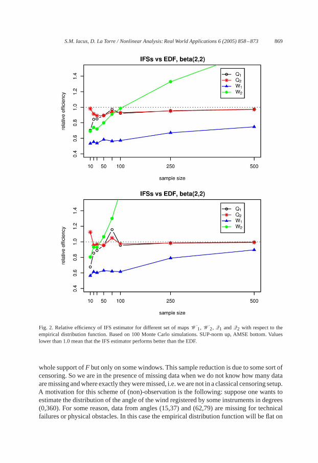
Fig. 2. Relative efficiency of IFS estimator for different set of mapsW1,W2, Q1 andQ2 with respect to theempirical distribution function. Based on 100 Monte Carlo simulations. SUP-norm up, AMSE bottom. Valueslower than 1.0 mean that the IFS estimator performs better than the EDF.

whole support ofF but only on some windows. This sample reduction is due to some sort ofcensoring. So we are in the presence of missing data when we do not know how many dataaremissingandwhereexactly theyweremissed, i.e.wearenot in a classical censoring setup.A motivation for this scheme of (non)-observation is the following: suppose one wants toestimate the distribution of the angle of the wind registered by some instruments in degrees(0,360). For some reason, data from angles (15,37) and (62,79) are missing for technicalfailures or physical obstacles. In this case the empirical distribution function will be flat on



these windows and a kernel density estimator will probably show a multimodal shape. Thisis due to the fact that quantile estimation is inappropriate in this context. At the same time,moment estimation tends to be more robust, in particular if the distribution is symmetric.We only report a graphical example of what can happen.Fig. 1 is about a sample from aBeta(2,2) distribution when only the observations in(0.1,0.15)∪ (0.37,0.43)∪ (0.7,0.8)are available to the observer all the others being truncated by the instrument (we have chosenthis interval by hazard). The IFS estimator withW1 maps seems to be able to reconstruct



the underlying distribution and density function, while, for obvious reasons, both the EDFand the kernel estimators fail. In this example the relative efficiency (IFS/EDF) is 7% forthe AMSE and 23% for the SUP-norm which is dramatically better than expected!

3.3. Algorithm flow for estimation

1. Choose the family of mapsW.


2a. IfW=W1 orW2,

(i) calculate sample moments,(ii) build the quadratic form and solve it forp.

2b. W=Q1 orQ2

(i) estimate the sample quantiles.

3. If you want to estimateF at pointx: take any distribution function, for example theuniform over[0,1] and start to iterateT.

4. Stop after a few iterations (normally 5 is enough).5. The “fixed point” ofT evaluated inx is the estimate ofF(x).

In case the support ofF is not known one case uses the range of the sample but the re-sulting IFS estimator will then try to approximate a distribution function which has ex-actly that support. If any hints on the shape of the distributionF is available, use it tochoose the maps. All the examples, tables and graphics have been done by some soft-ware developed by the authors. In particular, a package calledifs is freely availablefor the R environment system[13] in the CRAN (Comprehensive R Archive Network)http://cran.R-project.org under thecontributedsection.

4. Conclusions

It seems that this kind of approach can be used to make nonparametric inference whendata are missing or sample size are small. Note that with this method it is only possible towork with distributions with compact support. Moreover, a knowledge of the support itselfit is needed. Nevertheless, it seems a promising approach and the use of different sets ofmaps can be the object of further investigations.

References

[1] M.F. Barnsley, S. Demko, Iterated function systems and the global construction of fractals, Proc. R. Soc.London, Ser. A 399 (1985) 243–275.

[2] R. Beran, Estimating a distribution function, Ann. Stat. 5 (1977) 400–404.[3] R.H. Byrd, P. Lu, J. Nocedal, C. Zhu,A limitedmemory algorithm for bound constrained optimization, SIAMJ. Sci. Comput. 16 (1995) 1190–1208.

[4] A. Dvoretsky, J. Kiefer, J. Wolfowitz, Asymptotic minimax character of the sample distribution function andof the classical multinomial estimators, Ann. Math. Stat. 27 (1956) 642–669.

[5] S. Efromovich, Second order efficient estimating a smooth distribution function and its applications, MethodsComput. Appl. Probab. 3 (2001) 179–198.

[6] B. Forte, E.R. Vrscay, Solving the inverse problem for function/image approximation using iterated functionsystems, I. Theoretical basis, Fractal 2 (3) (1995) 325–334.

[7] B. Forte, E.R.Vrscay, Inverse problemmethods for generalized fractal transforms, in:Y. Fisher (Ed.), FractalImage Encoding and Analysis, NATOASI Series F, vol. 159, Springer, Heidelberg, 1998.

[8] R.D. Gill, B.Y. Levit, Applications of the van Trees inequality: a Bayesian Cramér–Rao bound, Bernoulli 1(1995) 59–79.

http://cran.R-project.org


[9] G.K. Golubev, B.Y. Levit, On the second order minimax estimation of distribution functions, Math. MethodsStat. 5 (1996) 1–31.

[10] G.K. Golubev, B.Y. Levit, Asymptotic efficient estimation for analytic distributions, Math. Methods Stat. 5(1996) 357–368.

[11] J. Hutchinson, Fractals and self-similarity, Indiana Univ. J. Math. 30 (5) (1981) 713–747.[12] S.M. Iacus, D. La Torre, Approximating distribution functions by iterated function systems, J. Appl. Math.

Decision Sci., accepted for publication.[13] R. Ihaka, R. Gentleman, R: a language for data analysis and graphics, J. Comput. Graphical Stat. 5 (1996)

299–314.[14] B.Y. Levit, Infinite-dimensional information inequalities, Theory Probab. Appl. 23 (1978) 371–377.[15] P.W. Millar, Asymptotic minimax theorems for sample distribution functions, Z. Warschein. Verb. Geb. 48

(1979) 233–252.[16] M.E. Tarter, M.D. Lock, Model Free Curve Estimation, Chapman & Hall, NewYork, 1993.

A comparative simulation study on the IFS distribution function estimator

Documents

Transcript of A comparative simulation study on the IFS distribution function estimator