A SELECTIVITY CORRECTED TIME-VARYING BETA RISK ESTIMATOR

Robert D. Brooks*, Jonathan Dark*, Robert W. Faff** and Tim R.L. Fry***

* Department of Econometrics and Business Statistics, Monash University ** Department of Accounting and Finance, Monash University *** School of Economics and Finance, RMIT Business

ABSTRACT

This paper explores two issues in beta risk estimation, namely, time variation of risk and the impact of thin trading (data censoring). Within a multivariate GARCH setting, the paper first conducts an analysis of the importance of assumptions made about the correlation structure. Collectively, the results of Monte Carlo analysis and an empirical application to a sample of individual Australia stock returns, demonstrate that it is preferable to allow for time variation in the correlation structure. The paper then develops a selectivity corrected time-varying beta risk estimator. The results of a Monte Carlo experiment demonstrate that the new estimator performs well in handling censored data. Finally, we confirm that when the new model is applied to our Australian dataset it successfully captures the impact of censoring and thin trading on time-varying beta risk. Keywords: Time-varying betas; GARCH; Censoring; Thin trading; Sample selectivity model JEL Classification: G12, C24 Acknowledgements: The authors acknowledge the financial support of Australian Research Council Discovery Grant DP0345680 – A Complex Systems Approach to Modelling Time-varying Risk in the Presence of Market Frictions. The authors wish to thank Diana Maldonado and Michael Gangemi for their work as research assistants on this project. The authors also wish to thank the participants at the 2005 Quantitative Methods in Finance conference and seminars at Deakin and ANU for their helpful comments on earlier versions of this paper. Correspondence to: Robert Faff, Department of Accounting and Finance, Monash University, VIC 3800, Australia, Phone: 61-3-99052387, Fax: 61-3-99052339, Email: robert.faff@buseco.monash.edu.au

2

A SELECTIVITY CORRECTED TIME-VARYING BETA RISK ESTIMATOR

ABSTRACT

This paper explores two issues in beta risk estimation, namely, time variation of risk and the impact of thin trading (data censoring). Within a multivariate GARCH setting, the paper first conducts an analysis of the importance of assumptions made about the correlation structure. Collectively, the results of Monte Carlo analysis and an empirical application to a sample of individual Australia stock returns, demonstrate that it is preferable to allow for time variation in the correlation structure. The paper then develops a selectivity corrected time-varying beta risk estimator. The results of a Monte Carlo experiment demonstrate that the new estimator performs well in handling censored data. Finally, we confirm that when the new model is applied to our Australian dataset it successfully captures the impact of censoring and thin trading on time-varying beta risk. Keywords: Time-varying betas; GARCH; Censoring; Thin trading; Sample selectivity model JEL Classification: G12, C24

1. Introduction

The modelling of the risk-return trade off remains a core issue in finance, and for

several decades the workhorse in this area has been the capital asset pricing model

(CAPM), (Sharpe, 1964 and Lintner, 1965). The CAPM is a simple model which

suggests that there is a positive and linear relationship between risk and (expected)

return. More formally, the model says that the expected return of an asset comprises a

risk-free component and a risk premium component. Further, it defines the asset's risk

premium as being equal to the risk of the asset multiplied by the market risk premium.

To complete the picture, according to the CAPM the asset's risk — referred to as β

(beta) risk — is defined as the covariance of returns between the asset and the market,

divided by the variance of market returns.

Despite the controversies associated with it (for example, see, Fama and

French, 1992, 1993 and Daniel and Titman, 1997), the CAPM remains the central

theoretical model of the risk-return relation in asset pricing. Ferson and Harvey

(1991a, 1991b) in their modelling of US stock returns discuss two main problems that

arise in the empirical application of the CAPM, namely, time-varying risk premia and

time-varying betas. The present paper focuses its attention on the problem of

estimating time-varying betas.

There are a number of modelling challenges that arise in the estimation of

time-varying betas. The first, and perhaps most fundamental, of these is around the

choice of model to parameterise the time variation. A range of techniques exist in this

regard including: variable parameter regression models estimated using the Kalman

filter (see Black, Fraser and Power (1992), Wells (1994)); modelling the time

variation in beta as a function of economic variables (see Abell and Kreuger (1989),

Faff and Brooks (1998)); or using a member of the multivariate GARCH family of

models (see, for example, Braun, Nelson and Sunier (1995), Giannopoulos (1995),

2

McClain, Humprehys and Boscan (1996), Brooks, Faff and McKenzie (1998)). The

present paper focuses its attention on the multivariate GARCH approach. In this

regard a number of choices still need to be made around parameterisation, particularly

to keep the number of parameters sufficiently small for estimation (see Pagan (1996)).

These choices typically relate to the degree of flexibility that is allowed in the

correlation structure of the model. The simplest model is that of Bollerslev (1990)

which fixes the correlation to be constant over time. While this simplifies estimation

considerably it is quite restrictive and is often at odds with reality. To provide a more

robust setting, this paper considers the more complex model of Tse and Tsui (2002)

which allows the correlation to evolve over time following an ARMA process.

The second area of empirical challenge that arises in modelling beta risk for

individual stock data is around correcting for thin trading. In the simplest context of

estimating a constant beta, a number of time-series based techniques exist in this

regard (see, for example, Scholes and Williams (1977), Dimson (1979), Fowler and

Rorke (1983)). However, it is very likely that these techniques perform rather poorly

in cases of extreme thin trading where numerous zero return observations are evident

i.e. when a non-trivial data censoring problem occurs.1 We argue that in the current

context it is preferable to utilise a sample selectivity model along the lines of

Heckman (1979) to correct for thin trading/ censoring. Such an approach has been

successfully utilised in estimating constant betas (see Brooks, Faff, Fry and

Maldonado (2004), Brooks, Faff, Fry and Gunn (2005)) and the present paper extends

this analysis to the time-varying beta case.

The plan of this paper is as follows. Section two briefly reviews the relevant

literature on using multivariate GARCH models to estimate time-varying betas, and

1 In related work the percentage of zero returns has been used to construct a liquidity measure – see, for example, Lesmond, Ogden and Trzincka (1999), Lesmond, Schill and Zhou (2004), Lesmond (2005), Bekaert, Harvey and Lundblad (2003).

3

on thin trading, censoring and zero returns. Section three sets out the multivariate

GARCH models and then reports the results of a Monte Carlo comparison of the

properties of the time-varying beta estimators, as well as an empirical application of

the models to individual stock data for Australia. Section four then extends the

analysis to incorporate a correction for censoring, and also reports the results of a

Monte Carlo comparison and application of the model to individual stock data for

Australia. Section five contains some concluding remarks.

2. Relevant Literature

2.1 Time-varying Betas

The estimation of time-varying betas for individual stocks and industry portfolios has

proven to be quite popular in the literature. Braun, Nelson and Sunier (1995) use a

bivariate EGARCH specification to model time-varying betas for US industry and

size based portfolios. Despite the presence of leverage effects in the market return,

such effects are absent in the estimated betas. Gonzalez-Rivera (1996) applies a

bivariate GARCH-M model using the parameterisation in Engle and Kroner (1995) to

model the risk-return trade off in US computer industry stocks and find that the

history of the variance of individual stock returns is critical in explaining expected

returns. McClain, Humprehys and Boscan (1996) use the parameterisation in

Bollerslev, Engle and Wooldridge (1988) to model time-varying betas for US mining

industry stocks. They find considerable instability in beta risk, and also document a

role for sample size in detecting significant GARCH effects. Brooks, Faff, Ho and

McKenzie (2000) use the Bollerslev (1990) constant correlation model to examine the

impact of regulatory change on US banking stocks beta risk. They document strong

association between beta risk and regulatory change. Brooks, Faff, Ho and McKenzie

(2000) also observe some extreme beta estimates for individual stocks (as do

4

Gonzalez-Rivera (1996) and McClain, Humprheys and Boscan (1996)). This issue is

then explored in McKenzie, Brooks, Faff and Ho (2000) who find that these extreme

beta events can be linked to economic news about the particular stocks.

The use of multivariate GARCH models to estimate time-varying betas has

also been explored in markets other than the US. Brooks, Faff and McKenzie (1998)

use the Bollerslev (1990) constant correlation model to analyse Australian industry

portfolio time-varying betas and find that the GARCH approach performs well

relative to other models (primarily Kalman filter based). McKenzie, Brooks and Faff

(2000) extend this comparison to consider whether a domestic or world index should

be chosen as the market index, and their results support the use of the domestic index.

Giannopoulos (1995) and Brooks, Faff and McKenzie (2002) have also used the

GARCH family of models to analyse time-varying country beta risk.

2.2 Thin Trading and Data Censoring

A particular challenge in modelling individual stock data is to deal with thin trading

effects – especially in the context of estimating beta risk. Thin trading arises when the

returns on the individual stock moves in a non-synchronous manner relative to the

return on the market index. There are a range of standard techniques designed to

correct for the bias induced in beta estimates by thin trading effects such as those

suggested by Scholes and Williams (1977), Dimson (1979) and Fowler and Rorke

(1983). Each of these techniques deals with the thin trading problem by making a time

series adjustment. They typically involve utilising leads and lags of the market return,

as well as making some allowance for any autocorrelation observed in the market

return. While all these alternative techniques tend to modify the beta estimate in the

appropriate direction (i.e. increase the estimated betas for thinly traded stocks), they

are unlikely to work well (or even adequately) in the case of extreme thin trading in

5

which many zero return observations are occur. In such circumstances we effectively

have a data censoring problem.

The incidence of zero returns has been used to construct a measure of

transaction costs by Lesmond, Ogden and Trizincka (1999) for US data, who find that

such a measure performs well relative to other available measures. Further, Lesmond,

Schill and Zhou (2004) find that such a measure of transaction costs can be important

in testing the profitability of a momentum trading strategy in the US market. Thin

trading, zero returns and transaction costs are found to be even more extreme in the

case of emerging markets (see Lesmond (2005), Bekaert, Harvey and Lundblad

(2003)).

Brooks, Faff, Fry and Gunn (2005) incorporate the impact of thin trading, zero

returns and censoring to estimate selectivity corrected static betas for Australia, while

Brooks, Faff, Fry and Maldonado (2004) do similar for a range of Latin American

markets. These papers use a sample selectivity model following Heckman (1979),

using volume as the key variable in the first stage probit. This produces a upward

correction in the estimated betas that adjusts for the thin trading bias. The key factor

in the sample selectivity approach is choice of the variables used in the first stage, and

the factors chosen need to vary sufficiently over time for an individual stock to

explain its temporal zero return pattern. This is an issue for exploration in the current

paper.

6

3. Time-varying Beta in a Multivariate GARCH Model Setting

3.1 Stage 1: Monte Carlo Estimation of Multivariate GARCH Models

The first part of the analysis of time-varying betas is a Monte Carlo analysis with a

dual-pronged experimental setup. The data generating process (DGP) for the first

experiment is the constant correlation (CC) GARCH(1,1) model of Bollerslev (1990),

while the DGP for the second experiment is the varying correlation (VC)

GARCH(1,1) model of Tse and Tsui (2002). This part of the experimental design

enables an analysis of the potential impact of a restrictive correlation structure in the

generation of time-varying betas.

To define the more complex model let ,i tr represent the return for asset i,

where 1i = for the individual asset and 2i = for the market. The DGP for the VC

GARCH model is given by:

1, 1,

2, 2,

t t

t t

rr

ε

ε

=

= (1)

where

2,2,12

,122,1

,2

,1 ,00

~tt

tt

t

t Nrr

σσ

σσ (2)

and

2 2 2, , 1 , 1i t i i i t i i tσ ω α ε β σ− −= + + 1, 2i = (3)

with

( )1 2 1 1 2 11t t tρ θ θ ρ θ ρ θ ϕ− −= − − + + (4)

where

( )( )2

1, 2,11 2 22 2

1, 2,1 1

t h t hht

t h t hh h

z z

z zϕ − −=

−

− −= =

= ∑∑ ∑

(5)

7

with , , ,i t i t i tzε σ= for 1, 2i = , all the α and β elements are non-negative and both ω

elements are positive. If all the roots of 0I L Lα β− − = are outside the unit circle

(where I is a 2x2 identity matrix, ( )1 2,diagα α α= and ( )1 2,diagβ β β= ), the

volatility process is stationary (Ling and McAleer, 2003). This model nests the CC

GARCH model ( 1 2 0θ θ= = ).

To perform the Monte Carlo experiment we need to set ‘true’ values for all the

parameters of the model. We do this through a combined strategy of taking values

similar to those used by Tse and Tsui (2002), while achieving beta risk values close to

unity (i.e. an average risk stock). Accordingly, our chosen set of parameter values are:

ω1 = 0.4; α1 = 0.2; β1 = 0.7; ω2 = 0.2; α2 = 0.2; β2 = 0.7; ρ = 0.71; θ1 = 0.8; θ2 = 0.1.

For each DGP, 1000 samples are generated, each of length 1000 observations.2 Using

MLE the bias and MSE of the estimates are determined. Our analysis extends the

simulations in Tse and Tsui (2002) by considering the performance of both models,

i.e. for each DGP, both the CC and VC GARCH models are estimated. Table 1

summarises the results via examination of the bias and MSE for all of the key

parameters in the model.

(Insert Table 1 about here)

For the first experiment in which the simple constant correlation structure is

true (Panel A), the most striking observation is that the performance of both models

with respect to the GARCH parameter estimates is comparable. As such, modelling

with a more complex structure than is needed, does not seem to overfit the data in

terms of altering the estimates of the parameters of the GARCH model. This can be

primarily explained via consideration of the 1θ parameter which is the key parameter

2 To avoid start up problems, samples of size 10,000 observations are generated, with the first 9,000 observations being discarded.

8

in driving the behaviour of the time-varying correlation in the VC GARCH model.

Specifically, the 1θ estimate averages 0.5286 and has a very large MSE. In unreported

results, we find that for 293 simulations 1 0.01θ ≤ , while for 216 simulations

1 0.99θ > . While these two cases lie near the boundaries of the parameter space, they

both have the same impact on the time-varying correlations, that is, the estimated

correlations are virtually time invariant. The VC GARCH model is therefore

observationally equivalent to the CC GARCH model. These results suggest that

overfitting of the data via the VC GARCH model is not too problematic.

For the second experiment in which the more complex VC GARCH

correlation structure is true (Panel B), the VC GARCH model is estimated quite

tightly via MLE. The CC GARCH model, however, considerably overestimates (by

around 25%) the iω parameters and underestimates the iα , iβ and ρ parameters. The

underestimation of the ρ parameter is consistent with the results in Tse and Tsui

(2002). These findings generally suggest that the consequences of underfitting are far

more serious than the consequences of overfitting. As such, it would seem that there is

not a great cost in erring on the side of fitting the more complex model.

3.2 Stage 2: Time-varying Betas from Monte Carlo Multivariate GARCH

Models

In the second stage of the Monte Carlo experiment, both models are used to estimate

time-varying betas that can be constructed from the estimated covariances, variances

and correlation parameters:

2,2

,2,1,1 ˆ

ˆˆˆˆt

tttt σ

σσρβ = (6)

9

where tρ̂ = ρ for the CC GARCH model or tρ̂ is estimated according to Equation (4)

in the case of the VC GARCH model.

Table 2 compares the average of the moments of the estimated betas to the

average of the moments of the betas from the DGP. For the first experiment (Panel A,

in which the CC GARCH model is the DGP), the CC GARCH and VC GARCH

models estimate the beta moments equally well, with both means very close to the

‘true’ value (1.0385) and the higher moments very similar for both cases. This is

consistent with the results obtained with respect to the parameter estimates in the first

stage of the Monte Carlo comparison, thus reinforcing the earlier view that there is

not a significant penalty from overfitting the data.

For the second experiment (Panel B, in which the VC GARCH model is the

DGP), the CC GARCH model performs poorly. While the mean value of the time-

varying beta is quite close to its ‘true’ value, the CC GARCH model considerably

understates (by more than 50%) the variability in the betas and substantially

overstates the skewness (> 50%) and kurtosis (> 30%). Once again, this is consistent

with the results obtained with respect to the parameter estimates in the first stage of

the Monte Carlo analysis. These results further emphasise that the consequences of

underfitting are more serious than the consequences of overfitting.

(Insert Table 2 about here)

3.3 Stage 3: Empirical Estimates of Time-varying Betas from Multivariate

GARCH Models

The second part of the analysis of time-varying betas is an empirical analysis of

individual stock data. For these purposes we choose an Australian sample for two

primary reasons: (a) because such data display a wide spread of thin trading effects;

and (b) because the issue of thin trading in the context of static betas has been

extensively analysed in this setting. As such, an Australian sample gives us a good

10

point of comparison. Specifically, data are collected on stocks in the Australian All

Ordinaries Index over the period from January 2000 to December 2002. The All

Ordinaries Index is composed of the 500 largest stocks on the exchange, and market

capitalisation is the only requirement for inclusion. As a major benchmark index that

covers most of the market (in terms of market capitalization), stocks in this index are

of great relevance to investors and fund managers in their investment decision

making. From the DataStream database, daily data were obtained for 441 of the stocks

in this index over the sample period.

In the first stage of the empirical analysis the multivariate CC GARCH and

VC GARCH models were estimated between the returns on the individual stocks in

the AOI and the returns on the AOI itself. In unreported results, the autocorrelation

function for the AOI returns showed no signs of temporal dependence, so a constant

mean equation was fitted. To capture any serial correlation in the stock returns, an

AR(1) mean equation was employed.

Table 3 compares selected parameter estimates for the CC GARCH and VC

GARCH models, over the total number of stocks for which the models converged. 3

While all of the stocks in the analysis are in a main benchmark index, the bottom end

of the index is still characterised by some lowly priced and thinly traded stocks.4

(Insert Table 3 about here)

The results in each panel of Table 3 are reported for a number of different

combinations of the data. First, they are reported for the overall sample of stocks.

3 Several points are worthy of note. First, the models were estimated imposing the covariance stationarity condition above. Second, the CC GARCH model was estimated without the imposition of the restriction. The results and conclusions were unchanged. Third, for 40 of the stocks, the CC GARCH model experienced convergence difficulties, while for 95 of the 441 stocks, the VC GARCH model experienced convergence difficulties. Fourth, only those results where strong convergence was achieved within 100 iterations have been reported. 4 The results in Lange (1999), Brooks, Faff and Fry (2001) and Amilon (2003) suggest that there can even be challenges in the testing and estimation of univariate GARCH models in these cases. As such, one might expect that the estimation of our more complex multivariate models is also going to be problematic. The focus of the analysis is therefore on the results for the remaining stocks where the respective models were able to strongly converge.

11

Second, they are reported in categories according to the degree of censoring

(proportion of zero return observations) in the data. While over a quarter of the

sample has low censoring (less than 10%), there are still around 10% of stocks in this

major Australian benchmark index for which censoring is greater than 50%. For these

stocks, thin trading and the associated transaction costs represent a considerable

problem.5 Third, given the findings of the Monte Carlo experiment that iω is likely to

be over-estimated when correlation dynamics are ignored, results are also reported for

two iω categories. Finally, the Nyblom (1989) test is used to test for time-varying

correlations in the data. The results of this test indicate that around only 10% of the

sample have time-varying correlations. Accordingly, results in Table 3 are also

reported for cases where the test is both significant and insignificant.

Generally, the results reported in Table 3 clearly demonstrate that for both

models as the degree of censoring increases, the estimate of ρ decreases, whilst the

sum 1 1α β+ estimates increases (see Panels A and B). The decrease in ρ is consistent

with expectations, as is the increase in the 1 1α β+ estimates, as one potential impact

of censoring is to introduce a structural break like effect into the data. Consistent with

the Monte Carlo results the 1 1α β+ estimates are much less persistent for cases of

high iω values. Interestingly, for the CC GARCH model (Panel A) the distribution of

the parameter estimates becomes more leptokurtic for the most extreme censoring

category, where the censoring level exceeds 50%.

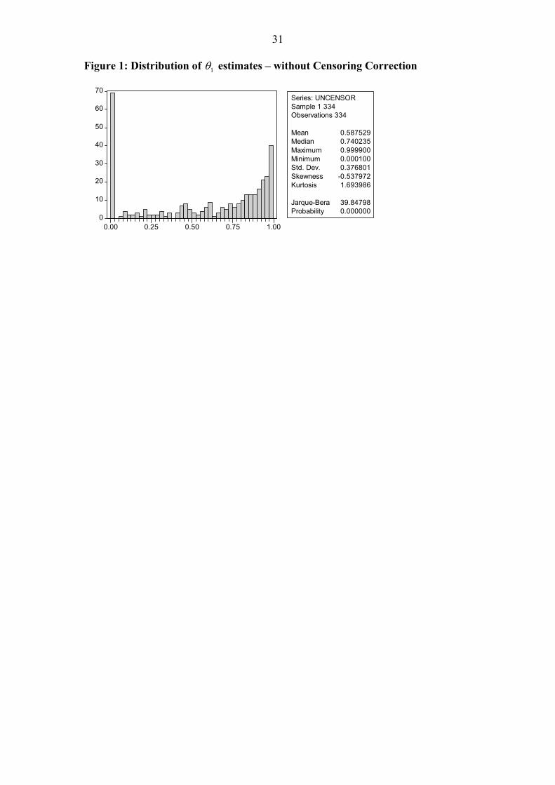
Finally, with regard to Table 3 consider the dynamic correlation parameters.

The 1θ and 2θ estimates appear unaffected by the degree of censoring or the stability

of the ρ estimate, as measured by the Nyblom (1989) test. The distribution of 1θ is

5 Interestingly, problems in the convergence of the models are spread across the range of censoring categories, suggesting a wider range of factors are important in GARCH parameter estimation.

12

shown in the histogram in Figure 1, as well as the kernel density estimate in Figure 3.

The results are consistent with there being very little difference between the average

of the ρ estimates for the CC and VC GARCH models.

(Insert Figure 1 about here)

Table 4 examines the average of the moments of the time-varying betas

estimated by each model. Results are again presented for all of the same categories

shown in Table 3. It is notable to observe that as the degree of censoring in the data

increases, average betas fall, consistent with the downward bias induced by thin

trading effects (see Scholes and Williams (1977), Dimson (1979), Fowler and Rorke

(1983)). This suggests the need for a sample selectivity type correction along the lines

of Heckman (1979) – an approach has been successfully used in estimating static

betas by Brooks, Faff, Fry and Maldonado (2004), and Brooks, Faff, Fry and Gunn

(2005). This decrease in the average betas is similar to the pattern reported in Table 3

for the ρ estimates. The same patterns are not as apparent in the higher order

moments for the betas.

The overall findings are consistent with the simulation where the DGP is the

VC GARCH model. The CC GARCH model betas have a smaller variance and a

higher degree of skewness and kurtosis than the VC GARCH betas. This result

provides further evidence supporting the VC GARCH model over the CC GARCH

model for the majority of stocks.

(Insert Table 4 about here)

13

4. Time-varying Beta in a Multivariate GARCH Model Setting: The Impact

of Censoring and Thin Trading

4.1 Probit Model Component of Selectivity Model

This section of the analysis extends the modelling outlined in the previous section by

accounting for censoring and thin trading effects in the data. This is achieved by

employing a sample selectivity approach. The first stage of this analysis requires a

decision on which variable(s) need to be included in the probit component of the

sample selectivity model. The candidate variables must plausibility be related to the

factors/forces that we believe underlie why stocks do not trade in any given

observation (i.e. why these stocks have zero returns on some days). Logically, such

variable(s) will have some link to transaction cost or similar metric of trading

impediment.

To this end, for each of the Australian stocks for which returns data were

analysed to calculate the time-varying betas in Section 3, data were also collected on

firm size (measured by market capitalisation), volume (measured by number of shares

traded) and the bid-ask spread from the Datastream database. This produced data on

249 stocks. We consider trading volume as a candidate variable for the probit

regression because such measures have been found to work well in similar sample

selectivity investigations of constant betas by Brooks, Faff, Fry and Maldonado

(2004) and Brooks, Faff, Fry and Gunn (2005). Also, the bid-ask spread as a measure

of transaction costs has been found to be well explained by the transaction costs

measure generated by Lesmond, Ogden and Trizincka (1999) and Lesmond (2005)

using the degree of censoring in the data. Finally, it is plausible that firm size will be

highly correlated with transaction cost and thin trading.

The analysis involves the estimation of probit models for each of the 249

stocks. The dependent variable in the probit model (yi) is defined as yi=1 for cases

14

where a non-zero return is observed on a given day and yi=0 for cases where a zero

return is observed on a given day. In the probit model, as foreshadowed above, three

explanatory variables are considered, namely, the daily market capitalisation, daily

trading volume and daily bid-ask spread. A summary of the results of the probit

estimation is reported in Table 5 in terms of the proportion of cases where particular

variables are found to be significant.

(Insert Table 5 about here)

These results show that the most important variable in explaining the time

series variation in censoring for an individual stock is trading volume. At the 1%

significance level, trading volume is significant in the first stage probit for one third

of the stocks, and this increases to a little over half of the stocks at the 10%

significance level. In contrast, size and bid-ask spread are much less significant in the

first stage probit. This is an interesting result, and is most likely a reflection of the fact

that at the level of a given stock there is insufficient temporal variation in either the

bid-ask spread, or size, to explain the time series of censoring.

The number of cases in the first stage probit where two of the three variables

are significant is much lower with the strongest pair being size and volume which is

jointly significant in 18.9% of cases at the 10% level. In contrast, size and bid-ask

spread is only jointly significant in 6.4% of cases at the 10% level. The number of

cases where all three variables are significant is very small, with only 4% of such

cases at the 10% level.

4.2 Monte Carlo Analysis of a Selectivity-corrected VC GARCH Model

The next step in this stage of the analysis is to specify the sample selectivity model.

The results of the probit analysis indicate that the trading volume variable is clearly

the most significant of the three potential explanatory variables. Thus, the stage one

15

model includes only volume as an explanatory variable. In specifying the model, we

assume that there is independence between the selectivity and GARCH components

of the model. This greatly simplifies the analysis as it separates the likelihood

function into two parts to be maximised.

The first component of the likelihood function is concerned solely with the

selectivity equation, while the second component is concerned with the multivariate

GARCH equations. Effectively, the selectivity correction causes the GARCH

estimation to have two components: the normal cases when individual stock returns

are not censored; and a restricted component when the individual stock returns are

censored which is only concerned with the market return.

The next stage of the analysis is a Monte Carlo comparison of the properties of

the selectivity corrected time-varying beta estimator. Given that the results of the

Monte Carlo comparison in the uncorrected case strongly supported the VC GARCH

model of Tse and Tsui (2002), the Monte Carlo analysis in the selectivity corrected

case is confined to that model. To conduct such a Monte Carlo analysis we need to

define a DGP for the variable that is driving the selectivity component of the model,

namely in the current setting, daily trading volume. An inspection of the histograms

of daily trading volume for the individual stocks suggests that the distribution of this

variable is approximately χ2 with three degrees of freedom. Thus for the purpose of

our Monte Carlo exercise, simulated volume figures are drawn from this distribution.

The selectivity component of our model can be specified as:

iti'it

*it uγz += w (7)

where:

>= ,0 if1

otherwise. 0*it

itz z

Or equivalently,

16

= ,return zero-non if1

return. zero if 0 zit

and wit includes a constant and trading volume as the explanatory variables. Thus in

the Monte Carlo design, the level of censoring is capable of being altered by changing

the threshold value of z*it above which a non-zero return is observed. The analysis

explores two specifications. The first case is a low censoring case where the value of

censoring is set at 20% which corresponds to the median level of censoring in the

stocks analysed in this paper. The second case is a high censoring case where the

value of censoring is 60% which corresponds to the median level of censoring in the

sample analysed by Brooks, Faff, Fry and Gunn (2005). We apply the ‘true’ values to

each parameter as used in the previous section.

The results reported in Table 6 show the impact on the estimated parameters

of the VC GARCH model with and without a censoring correction in both the low

(Panel A) and high (Panel B) censoring cases. As revealed in Panel A, in general the

biases and mean squared errors of the parameter estimates are small in the low

censoring case. There is little material difference between the cases which do and

don’t apply a censoring correction. In contrast, and consistent with expectations,

Panel B shows that there are much larger biases in some of the parameters in the high

censoring setting. This is particularly so for the ω and ρ parameters. Most notably, for

the ρ parameter the bias is large when no selectivity correction is made, however the

bias is significantly reduced after selectivity correction. This is to be expected, as the

zero returns in the individual stocks induce a downward bias in the estimated

correlation, which is also consistent with the empirical results reported in Table 3 of

this paper. Thus, it would appear that selectivity correction has the potential to correct

for this problem in high censoring cases.

(Insert Table 6 about here)

17

4.3 Time-varying Betas from a Monte Carlo Selectivity-corrected VC

GARCH Model

The issue that remains to be considered is whether this impact on the parameter

estimates, in particular the correlation parameter, as shown in Table 6 manifests itself

in the time-varying beta parameters generated from the VC GARCH model. This

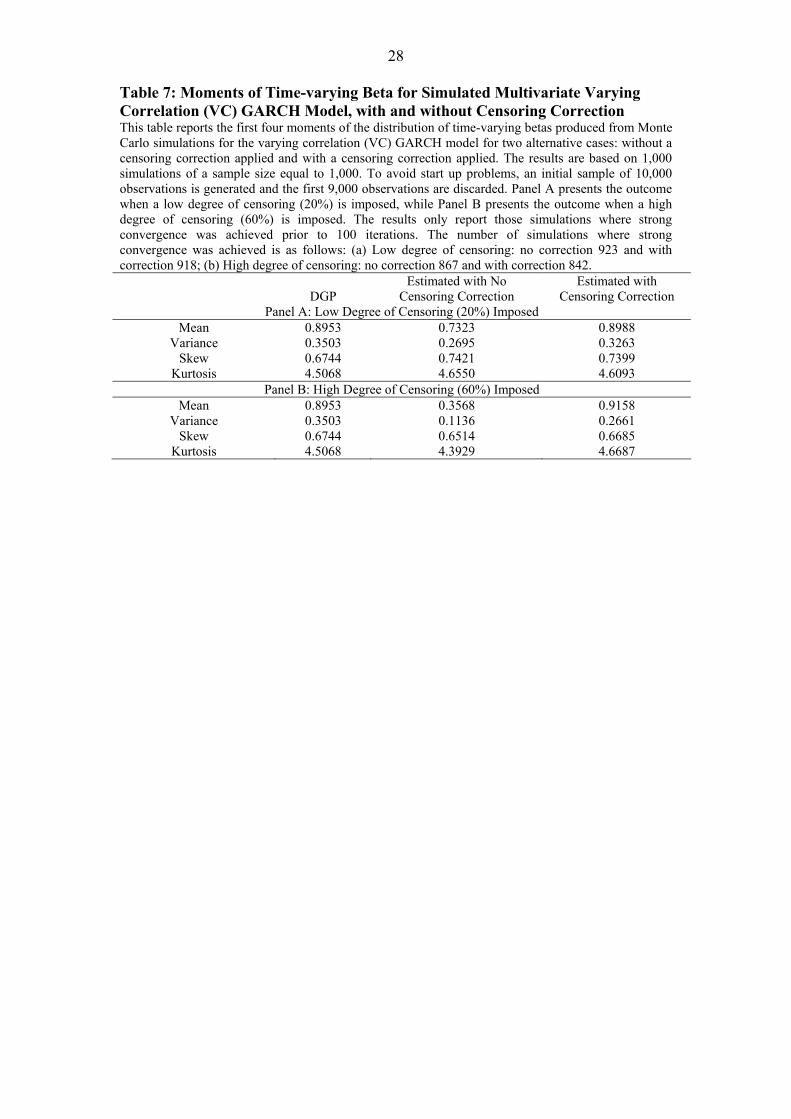
issue is explored in the results presented in Table 7.

Table 7 presents results on the first four moments of the distribution of the

estimated time-varying betas in both the low (Panel A) and high (Panel B) censoring

cases. In the low censoring case the absence of a censoring adjustment induces a

slight downward movement in the mean and variance of the estimated betas which is

corrected for by the selectivity model. As clearly seen in Panel B, this effect is much

stronger in the high censoring case where the impact is a significant downward

movement, particularly so for the mean of the estimated betas. Specifically, the mean

beta for the approach that makes no adjustment is 0.3568 – which represents a 60%

downward bias relative to the ‘true’ value. This significant downward movement is

adjusted for completely by the selectivity correction – the mean beta in this latter case

is 0.9158 (compared to the ‘true’ value = 0.8953). Thus, it would appear that the

impact of selectivity correction on ρ noted in Table 6 carries across to have a strong

impact on the estimated betas in Table 7. Thus, it would again appear that where

censoring is high that selectivity correction has a strong role to play. Moreover, the

Monte Carlo results suggest that there is not a great cost in erring on the side of

making the selectivity correction.

(Insert Table 7 about here)

18

4.4 Empirical Estimates of Time-varying Betas from Selectivity-corrected

Multivariate GARCH Models

In the final stage of the empirical analysis, similar to Section 3.3, the selectivity-

corrected CC GARCH and VC GARCH models were estimated between the returns

on individual stocks in the AOI and the returns on the AOI itself. Consistent with our

approach in Sections 4.2 and 4.3, we apply a correction that relies on trading volume

only. This has the added advantage that we can retain the same sample as analysed in

Section 3.3, since trading volume data are available for that same group of stocks –

the advantage being comparability.

The models were again estimated imposing the covariance stationarity

condition. Interestingly, there are less convergence problems once the selectivity

correction is made. There are now only 19 cases where the selectivity-corrected CC

GARCH model fails to converge and only 41 cases where the selectivity-corrected

VC GARCH model fails to converge. This suggests that the selectivity correction is

effective in overcoming the estimation problems that are induced by censoring.6

The results are reported in a similar format to those earlier where the

selectivity correction was not utilised and are contained in Tables 8 and 9 (similar to

Tables 3 and 4). The results in Table 8 compares selected parameter estimates when

the selectivity-corrected CC GARCH and VC GARCH models were estimated over

the total number of stocks for which the models converged for both the uncorrected

and selectivity corrected analysis.

Consistent with the earlier results for the case where no selectivity correction

is made, the findings reported in Table 8 clearly demonstrate that for both models as

the degree of censoring increases, the estimate of ρ generally decreases, even after a

selectivity correction is made. In general, the average values for the moments of ρ are 6 For comparability reasons we restrict our current focus to the same set of stocks for which convergence was achieved in the uncorrected analysis of Section 3.3.

19

similar between the cases when a selectivity correction is made or not in the lower

censoring categories (censoring is below 40%). For the two highest censoring

categories there is a small increase in the estimated correlation parameter after

censoring correction is made. Interestingly, the sum 1 1α β+ estimate remains

relatively steady across low and moderate censoring levels and then dips down

somewhat at higher levels of censoring (contrary to the results reported in Table 3).

This suggests that the models are now less persistent than they were in the

uncorrected case, which is again consistent with censoring inducing a structural break

like effect into the data, thus leading to an overstatement of the persistence in the

estimated GARCH parameters. Further, the excess kurtosis for the CC GARCH

parameter estimates in the most extreme censoring category is now removed. Finally,

with regard to this analysis, the distribution of 1θ in the selectivity-corrected case is

shown in the histogram in Figure 2, as well as the kernel density estimate in Figure 3.

(Insert Table 8 about here)

(Insert Figures 2 and 3 about here)

The results revealed in Table 9 examine the average of the moments of the

time-varying betas estimated by each model. Results are again presented for all of the

same categories as Table 4. In general, the findings are consistent for both the CC

GARCH and VC GARCH estimators. As the degree of censoring in the data

increases, average betas fall when estimated by both selectivity-corrected models. For

the lower censoring categories (censoring below 40%) there is no strong impact on

either the mean or variance of the estimated betas. This is consistent with the lack of

impact on the parameter estimates observed in Table 8. However, for the two higher

censoring categories the mean and variance of the beta estimates are increased

(relative to their uncorrected Table 4 counterparts) consistent with the simulation

results reported in Table 7. This would again appear to be due to the adjustment made

20

by selectivity correction in the correlation parameter reported in Table 8. Finally, in

terms of higher order moments, the selectivity corrected betas generally seem to be

more skewed and leptokurtic for both models as compared to the uncorrected betas

for both models. Collectively, the empirical and simulation results presented in

Section 4 suggest that there is not a great cost in erring on the side of making the

selectivity correction.

(Insert Table 9 about here)

5. Conclusion

This paper has conducted an analysis of two key issues in beta risk estimation,

namely, time variation of risk and the impact of thin trading (data censoring). Our

analysis was performed within the framework of the multivariate GARCH family of

models, but specifically compared the performance of a simple constant correlation

model (CC GARCH) to a more complex varying correlation model (VC GARCH).

The results of both a Monte Carlo comparison and an empirical analysis of individual

stock data for Australia indicated that it is better to overfit the data by making

allowance for time variation in the correlation structure. The results also showed that

the standard multivariate GARCH estimation of time-varying betas is impacted by the

downward bias induced by censoring and thin trading effects.

The analysis was then extended to deal with censoring and thin trading effects.

While three possible variables are considered for the probit component of the model,

trading volume appears to be the most important of these variables. Hence, it was

employed in the analysis. Selectivity-corrected multivariate GARCH models were

then simulated and estimated, and the findings show that selectivity-correction

reduces estimation problems.

21

Accordingly, two basic “takeaways” emanate from our analysis: (1) the

consequences of underfitting (e.g. assuming constant correlation) are more serious

than the consequences of overfitting (e.g. time-varying correlation) in such

approaches that seek to model time-varying beta risk and (2) in such models, there is

not a great cost in erring on the side of making the selectivity correction to counter the

problems of thin trading and data censoring.

22

Table 1: Bias and Mean Squared Error Metric for Simulated Multivariate Constant Correlation (CC) and Varying Correlation (VC) GARCH Models This table reports the outcome of Monte Carlo simulations for the constant correlation (CC) and varying correlation (VC) GARCH models. The results are based on 1,000 simulations of a sample size equal to 1,000. To avoid start up problems, an initial sample of 10,000 observations is generated and the first 9,000 observations are discarded. Using MLE, the bias and mean square error (MSE) are reported in the table. Panel A presents the outcome when the CC GARCH model is ‘true’, while Panel B presents the outcome when the VC GARCH model is ‘true’. Estimated CC GARCH Estimated VC GARCH

True value Bias MSE Bias MSE Panel A: DGP is the CC GARCH Model

ω1 0.4 0.0235 0.0117 0.0225 0.0116 α1 0.2 0.0009 0.0010 0.0027 0.0010 β1 0.7 -0.0072 0.0022 -0.0083 0.0022 ω2 0.2 0.0133 0.0028 0.0127 0.0028 α2 0.2 0.0005 0.0009 0.0023 0.0010 β2 0.7 -0.0088 0.0023 -0.0098 0.0023 ρ 0.71 0.0004 0.0002 0.0088 0.0005

1θ 0.5286 0.4644

2θ 0.0093 0.0003

Panel B: DGP is the VC GARCH Model ω1 0.4 0.0970 0.0301 0.0268 0.0129 α1 0.2 -0.0166 0.0014 0.0008 0.0011 β1 0.7 -0.0149 0.0035 -0.0083 0.0023 ω2 0.2 0.0489 0.0076 0.0136 0.0031 α2 0.2 -0.0176 0.0014 -0.0004 0.0010 β2 0.7 -0.0152 0.0038 -0.0083 0.0025 ρ 0.71 -0.0959 0.0108 -0.0029 0.0012

1θ 0.8 -0.0098 0.0024

2θ 0.1 0.0017 0.0005

23

Table 2: Moments of Time-varying Beta for Simulated Multivariate Constant Correlation (CC) and Varying Correlation (VC) GARCH Models This table reports the first four moments of the distribution of time-varying betas produced from Monte Carlo simulations for the constant correlation (CC) and varying correlation (VC) GARCH models. The results are based on 1,000 simulations of a sample size equal to 1,000. To avoid start up problems, an initial sample of 10,000 observations is generated and the first 9,000 observations are discarded. Panel A presents the outcome when the CC GARCH model is ‘true’, while Panel B presents the outcome when the VC GARCH model is ‘true’.

DGP Estimated CC GARCH Estimated VC GARCH Panel A: DGP is the CC GARCH Model

Mean 1.0385 1.0413 1.0417 Variance 0.0721 0.0730 0.0744 Skewness 1.0459 1.0465 1.0606 Kurtosis 5.7920 5.8688 5.8885

Panel B: DGP is the VC GARCH Model Mean 0.8987 0.8997 0.9004

Variance 0.1242 0.0537 0.1254 Skewness 0.6702 1.0796 0.6647 Kurtosis 4.5029 6.1085 4.5625

24

Table 3: Multivariate Constant Correlation (CC) and Varying Correlation (VC) GARCH Model Parameter Estimates – No Censoring Correction This table reports mean sample moments of selected coefficient estimates for the constant correlation (CC) and varying correlation (VC) GARCH models, in Panels A and B respectively. These estimates come from a sample of constituent stocks in the Australian All Ordinaries Index, subject to data availability and model convergence. The results in each panel are reported for a number of different combinations of the data: (a) overall sample of stocks; (b) categories according to the degree of censoring (proportion of zero return observations); (c) split based on whether the variance equation intercept is greater than or less than unity; and (d) split based on whether the Nyblom statistic testing for time-varying correlation is significant, or not, at the 5% level (Panel B only). No Mean Std dev Skew Kurt Mean Std dev Skew Kurt

Panel A: Selected Parameter Estimates for CC GARCH Model ρ

1 1α β+ Overall 358 0.1760 0.1091 1.4400 6.5321 0.8400 0.1901 -1.7254 5.8867

Censoring 0.1c ≤ 103 0.2482 0.1262 1.1347 5.1220 0.8084 0.2247 -1.7235 5.6149

0.1 0.2c< ≤ 77 0.2046 0.0852 1.2625 6.6541 0.8168 0.2009 -1.2816 3.8195

0.2 0.3c< ≤ 77 0.1541 0.0624 1.0264 7.1284 0.8462 0.1693 -1.3662 4.0159

0.3 0.4c< ≤ 52 0.1138 0.0605 1.2100 5.6284 0.8619 0.1637 -1.6043 4.9491

0.4 0.5c< ≤ 22 0.0684 0.0385 0.1175 2.2292 0.8876 0.1274 -1.3480 4.3626

0.5c > 27 0.0886 0.0944 3.7274 17.456 0.9281 0.0935 -1.9781 6.2904

1 1ω > 104 0.6647 0.2340 -0.6521 2.7631

1 1ω ≤ 254 0.9118 0.1037 -1.7556 6.1664

Panel B: Selected Parameter Estimates for VC GARCH Model

ρ 1 1α β+

Overall 306 0.1874 0.1204 1.2890 5.8831 0.8481 0.1923 -1.9885 6.9781

Censoring 0.1c ≤ 91 0.2476 0.1465 0.8447 4.2589 0.8331 0.2093 -1.9813 6.9452

0.1 0.2c< ≤ 64 0.2099 0.0913 0.1580 3.3090 0.8600 0.1697 -1.7387 5.6452

0.2 0.3c< ≤ 73 0.1787 0.0968 2.1400 10.560 0.8358 0.2120 -1.9091 6.0710

0.3 0.4c< ≤ 48 0.1267 0.0731 1.5804 6.3690 0.8398 0.1904 -1.5765 5.1884

0.4 0.5c< ≤ 18 0.0654 0.0401 0.4684 2.5986 0.9076 0.1207 -1.9763 6.8364

0.5c > 12 0.0904 0.0666 0.8542 2.3128 0.9178 0.0558 -0.5005 2.3586

1 1ω > 86 0.6867 0.2555 -0.8818 2.8390

1 1ω ≤ 220 0.9111 0.1084 -1.8810 6.4243

1θ 2θ Overall 306 0.5902 0.3751 -0.5626 1.7209 0.0395 0.0441 1.4737 5.0275

Censoring

0.1c ≤ 91 0.6665 0.3489 -0.9208 2.3362 0.0367 0.0373 1.7381 6.5679

0.1 0.2c< ≤ 64 0.5591 0.3888 -0.4028 1.5414 0.0406 0.0502 1.2657 3.4930

0.2 0.3c< ≤ 73 0.6173 0.3501 -0.7823 2.1339 0.0355 0.0378 1.3665 5.3709

0.3 0.4c< ≤ 48 0.5274 0.3731 -0.2026 1.4753 0.0546 0.0554 1.1044 3.6580

0.4 0.5c< ≤ 18 0.3649 0.4231 0.4467 1.3493 0.0295 0.0292 0.4527 1.9183

0.5c > 12 0.6019 0.3753 -0.7365 1.9215 0.0337 0.0466 1.3222 3.2200

ρ stability

0.47Nyb > 37 0.6592 0.3411 -0.9654 2.5107 0.0456 0.0406 0.8752 3.1875

0.47Nyb ≤ 269 0.5807 0.3785 -0.5122 1.6527 0.0387 0.0445 1.5494 5.2638

25

Table 4: Moments of Time-varying Beta for Estimated Multivariate Constant Correlation (CC) and Varying Correlation (VC) GARCH Models – No Censoring Correction This table reports the first four moments of the distribution of time-varying betas produced from estimation of the constant correlation (CC) and varying correlation (VC) GARCH models. These estimates come from a sample of constituent stocks in the Australian All Ordinaries Index, subject to data availability and model convergence. The results are reported for a number of different combinations of the data: (a) overall sample of stocks; (b) categories according to the degree of censoring (proportion of zero return observations); (c) split based on whether the Nyblom statistic testing for time-varying correlation is significant, or not, at the 5% level. Estimated CC GARCH Estimated VC GARCH

No Mean Std dev Skew Kurt No Mean Std dev Skew Kurt Overall 358 0.6056 0.1838 1.3767 11.461 306 0.5976 0.3114 0.9084 7.1854

Censoring

0.1c ≤ 103 0.6554 0.1727 1.3470 12.939 91 0.6138 0.2326 0.8479 6.9495

0.1 0.2c< ≤ 77 0.6942 0.2233 1.7431 15.138 64 0.6552 0.2979 1.2330 10.878

0.2 0.3c< ≤ 77 0.6806 0.2076 1.3009 8.5924 73 0.6830 0.3916 0.8987 5.9668

0.3 0.4c< ≤ 52 0.4627 0.1564 1.1971 9.1539 48 0.4972 0.3742 0.5939 4.4012

0.4 0.5c< ≤ 22 0.3785 0.1245 1.2317 8.7785 18 0.3736 0.2587 0.8989 7.5174

0.5c > 27 0.4098 0.1469 1.1257 10.143 12 0.3853 0.3214 0.9666 7.3314

ρ stability

0.47Nyb > 70 0.6584 0.1924 1.0758 8.6345 37 0.6206 0.2864 0.8583 6.8624

0.47Nyb ≤ 288 0.5928 0.1817 1.4498 12.148 269 0.5944 0.3149 0.9153 7.2298

26

Table 5: Summary of Significant Variables in First Stage Probit Model Estimations This table reports a summary of the first stage probit estimation results in terms of the proportion of stocks for which individual variables are found to be significant. Results are reported at the 1%, 5% and 10% significance levels, and for cases where individual variables are significant, pairs of variables are significant, and for where all three variables are significant. Significance Level 1% 5% 10%

Panel A: Percentage of Sample for which Individual Variables Significant Size 12.0 25.7 30.5 Volume 33.7 45.8 53.0 Bid-Ask 5.6 14.1 22.5

Panel B: Percentage of Sample for which Pairs of Variables Significant Size & Volume 5.2 14.5 18.9 Size & Bid-Ask 0.1 3.6 6.4 Volume & Bid-Ask 0.1 8.0 12.1

Panel C: Percentage of Sample for which all Three Variables Significant Size, Volume & Bid-Ask 0.0 1.6 4.0

27

Table 6: Bias and Mean Squared Error Metric for Simulated Multivariate Varying Correlation (VC) GARCH Model, with and without Censoring Correction This table reports the outcome of Monte Carlo simulations for the varying correlation (VC) GARCH model for two alternative cases: without a censoring correction applied and with a censoring correction applied. The results are based on 1,000 simulations of a sample size equal to 1,000. To avoid start up problems, an initial sample of 10,000 observations is generated and the first 9,000 observations are discarded. Using MLE, the bias and mean square error (MSE) are reported in the table. Panel A presents the outcome when a low degree of censoring (20%) is imposed, while Panel B presents the outcome when a high degree of censoring (60%) is imposed. The results only report those simulations where strong convergence was achieved prior to 100 iterations. The number of simulations where strong convergence was achieved is as follows: (a) Low degree of censoring: no correction 923 and with correction 918; (b) High degree of censoring: no correction 867 and with correction 842. Estimated with No Censoring

Correction Estimated with Censoring

Correction True value Bias MSE Bias MSE

Panel A: Low Degree of Censoring (20%) Imposed µ1 0.05 -0.0111 0.0024 -0.0041 0.0029 µ2 0.05 -0.0003 0.0014 -0.0008 0.0014 ω1 0.4 -0.0487 0.0152 0.0303 0.0199 α1 0.2 -0.0477 0.0033 -0.0132 0.0015 β1 0.7 0.0361 0.0046 0.0367 0.0044 ω2 0.2 0.0141 0.0039 0.0146 0.0038 α2 0.2 -0.0091 0.0013 -0.0111 0.0012 β2 0.7 -0.0003 0.0029 0.0008 0.0027 ρ 0.71 -0.0759 0.0076 0.0470 0.0047

1θ 0.8 0.0017 0.0064 0.0023 0.0051

2θ 0.1 -0.0219 0.0009 -0.0146 0.0007

Panel B: High Degree of censoring (60%) Imposed µ1 0.05 -0.0301 0.0023 -0.0015 0.0067 µ2 0.05 0.0003 0.0016 -0.0003 0.0015 ω1 0.4 -0.1519 0.0733 0.2074 0.2833 α1 0.2 -0.1244 0.0166 -0.0142 0.0049 β1 0.7 0.0565 0.0334 0.0679 0.0261 ω2 0.2 0.0235 0.0054 0.0273 0.0053 α2 0.2 -0.0076 0.0014 -0.0132 0.0014 β2 0.7 -0.0065 0.0036 -0.0051 0.0034 ρ 0.71 -0.2755 0.0798 0.0468 0.0133

1θ 0.8 -0.0330 0.0447 -0.1624 0.1210

2θ 0.1 -0.0601 0.0043 -0.0412 0.0028

28

Table 7: Moments of Time-varying Beta for Simulated Multivariate Varying Correlation (VC) GARCH Model, with and without Censoring Correction This table reports the first four moments of the distribution of time-varying betas produced from Monte Carlo simulations for the varying correlation (VC) GARCH model for two alternative cases: without a censoring correction applied and with a censoring correction applied. The results are based on 1,000 simulations of a sample size equal to 1,000. To avoid start up problems, an initial sample of 10,000 observations is generated and the first 9,000 observations are discarded. Panel A presents the outcome when a low degree of censoring (20%) is imposed, while Panel B presents the outcome when a high degree of censoring (60%) is imposed. The results only report those simulations where strong convergence was achieved prior to 100 iterations. The number of simulations where strong convergence was achieved is as follows: (a) Low degree of censoring: no correction 923 and with correction 918; (b) High degree of censoring: no correction 867 and with correction 842.

DGP

Estimated with No Censoring Correction

Estimated with Censoring Correction

Panel A: Low Degree of Censoring (20%) Imposed Mean 0.8953 0.7323 0.8988

Variance 0.3503 0.2695 0.3263 Skew 0.6744 0.7421 0.7399

Kurtosis 4.5068 4.6550 4.6093 Panel B: High Degree of Censoring (60%) Imposed

Mean 0.8953 0.3568 0.9158 Variance 0.3503 0.1136 0.2661

Skew 0.6744 0.6514 0.6685 Kurtosis 4.5068 4.3929 4.6687

29

Table 8: Multivariate Constant Correlation (CC) and Varying Correlation (VC) GARCH Model Parameter Estimates – with Censoring Correction This table reports mean sample moments of selected coefficient estimates for the constant correlation (CC) and varying correlation (VC) GARCH models, in Panels A and B respectively. The censoring correction described in the text has been applied. These estimates come from a sample of constituent stocks in the Australian All Ordinaries Index, subject to data availability and model convergence. The results in each panel are reported for a number of different combinations of the data: (a) overall sample of stocks; (b) categories according to the degree of censoring (proportion of zero return observations); (c) split based on whether the variance equation intercept is greater than or less than unity; and (d) split based on whether the Nyblom statistic testing for time-varying correlation is significant, or not, at the 5% level (Panel B only). No Mean Std dev Skew Kurt Mean Std dev Skew Kurt

Panel A: Selected Parameter Estimates for CC GARCH Model ρ

1 1α β+ Overall 358 0.1794 0.1081 1.3123 6.2242 0.7862 0.2514 -1.4784 4.3633

Censoring 0.1c ≤ 103 0.2510 0.1271 1.1054 5.0391 0.8042 0.2302 -1.6350 5.1414

0.1 0.2c< ≤ 77 0.2048 0.0783 0.7910 4.1585 0.8130 0.1977 -1.2111 3.6305

0.2 0.3c< ≤ 77 0.1584 0.0698 1.0156 6.1902 0.7926 0.2503 -1.4853 4.4066

0.3 0.4c< ≤ 52 0.1153 0.0798 1.4053 5.7432 0.8084 0.2023 -1.3861 4.2286

0.4 0.5c< ≤ 22 0.0724 0.0382 0.4662 3.1123 0.7282 0.2965 -0.8003 2.1383

0.5c > 27 0.1051 0.0537 0.1749 2.6869 0.6282 0.4043 -0.5708 1.5086

1 1ω > 131 0.5853 0.2830 -0.4553 2.1243

1 1ω ≤ 227 0.9022 0.1294 -2.7463 14.077

Panel B: Selected Parameter Estimates for VC GARCH Model ρ

1 1α β+ Overall 306 0.1972 0.1305 1.3053 6.1334 0.8004 0.2402 -1.5429 4.6210

Censoring

0.1c ≤ 91 0.2465 0.1474 0.8234 4.3155 0.8329 0.2076 -1.8913 6.5510

0.1 0.2c< ≤ 64 0.2117 0.0904 0.3804 3.4364 0.7945 0.2267 -1.3768 4.0665

0.2 0.3c< ≤ 73 0.1938 0.1187 2.3294 11.020 0.7984 0.2564 -1.6715 4.9051

0.3 0.4c< ≤ 48 0.1314 0.0992 1.5218 6.0029 0.8026 0.2279 -1.3507 4.0173

0.4 0.5c< ≤ 18 0.1017 0.0931 2.4241 9.2458 0.7519 0.2907 -0.8993 2.2123

0.5c > 12 0.1725 0.1906 1.4664 5.5791 0.6601 0.3232 -0.7126 2.2081

1 1ω > 105 0.6048 0.2791 -0.5287 2.1561

1 1ω ≤ 201 0.9025 0.1294 -2.2926 9.4930

1θ 2θ

Overall 306 0.5363 0.3859 -0.2859 1.4419 0.0399 0.0449 1.5804 6.0620

Censoring 0.1c ≤ 91 0.5950 0.3730 -0.5284 1.6559 0.0345 0.0366 2.1170 9.4973

0.1 0.2c< ≤ 64 0.4921 0.4016 -0.0422 1.2843 0.0366 0.0446 1.5024 4.9770

0.2 0.3c< ≤ 73 0.5578 0.3752 -0.4508 1.6024 0.0396 0.0403 1.1027 3.6471

0.3 0.4c< ≤ 48 0.4761 0.3785 -0.0339 1.4357 0.0544 0.0573 1.3858 5.3905

0.4 0.5c< ≤ 18 0.4013 0.4100 0.3464 1.4032 0.0321 0.0530 1.6243 4.4283

0.5c > 12 0.6396 0.3300 -0.9139 2.6542 0.0557 0.0451 0.2003 1.4164

ρ stability

0.47Nyb > 37 0.5784 0.3549 -0.5152 1.6843 0.0435 0.0395 1.5824 6.5927

0.47Nyb ≤ 269 0.5306 0.3896 -0.2551 1.4177 0.0394 0.0456 1.5858 6.0061

30

Table 9: Moments of Time-varying Beta for Estimated Multivariate Constant Correlation (CC) and Varying Correlation (VC) GARCH Models – with Censoring Correction This table reports the first four moments of the distribution of time-varying betas produced from estimation of the constant correlation (CC) and varying correlation (VC) GARCH models. The censoring correction described in the text has been applied. These estimates come from a sample of constituent stocks in the Australian All Ordinaries Index, subject to data availability and model convergence. The results are reported for a number of different combinations of the data: (a) overall sample of stocks; (b) categories according to the degree of censoring (proportion of zero return observations); (c) split based on whether the Nyblom statistic testing for time-varying correlation is significant, or not, at the 5% level.

Estimated CC GARCH Estimated VC GARCH No Mean Std dev Skew Kurt No Mean Std dev Skew Kurt

Overall 358 0.6140 0.1959 1.6192 15.470 306 0.6056 0.3190 1.0912 9.7734

Censoring 0.1c ≤ 103 0.6579 0.1840 1.5742 17.987 91 0.6257 0.2321 1.0987 12.273

0.1 0.2c< ≤ 77 0.7001 0.2199 1.6931 16.130 64 0.6588 0.2926 1.4056 12.390

0.2 0.3c< ≤ 77 0.6882 0.2171 1.4379 10.501 73 0.6746 0.3900 0.9953 6.8064

0.3 0.4c< ≤ 52 0.4683 0.1789 1.5809 10.485 48 0.5043 0.4003 0.7886 5.4036

0.4 0.5c< ≤ 22 0.3649 0.1338 1.7841 15.306 18 0.4289 0.2730 1.3336 12.918

0.5c > 27 0.4736 0.1953 2.0366 27.895 12 0.4209 0.4309 0.7867 7.6791

ρ stability

0.47Nyb > 64 0.6486 0.1816 1.0089 8.4790 37 0.6442 0.2416 0.7145 5.7687

0.47Nyb ≤ 294 0.6065 0.1990 1.7521 16.992 269 0.6003 0.3297 1.1430 10.324

31

Figure 1: Distribution of 1θ estimates – without Censoring Correction

0

10

20

30

40

50

60

70

0.00 0.25 0.50 0.75 1.00

Series: UNCENSORSample 1 334Observations 334

Mean 0.587529Median 0.740235Maximum 0.999900Minimum 0.000100Std. Dev. 0.376801Skewness -0.537972Kurtosis 1.693986

Jarque-Bera 39.84798Probability 0.000000

32

Figure 2: Distribution of 1θ estimates – with Censoring Correction

0

10

20

30

40

50

60

70

80

90

0.00 0.25 0.50 0.75 1.00

Series: CENSORSample 1 334Observations 334

Mean 0.522093Median 0.604270Maximum 0.999900Minimum 0.000100Std. Dev. 0.389754Skewness -0.225435Kurtosis 1.398221

Jarque-Bera 38.53499Probability 0.000000

33

Figure 3: Kernel Densities of 1θ Estimates

0

0.2

0.4

0.6

0.8

1

1.2

1.4

1.6

1.8

-0.5 0 0.5 1 1.5

Uncensored Censored

Note: Kernel density estimates obtained via EViews 4.1, where normality is assumed and a Silverman bandwidth with 100 points is applied.

34

References Abell, J. and Kreuger, T. 1989, ‘Macroeconomic Influences on Beta’, Journal of

Economics and Business, 41, 185-193. Amilon, H. 2003, `GARCH Estimation and Discrete Stock Prices: An Application to

Low-Priced Australian Stocks’, Economics Letters, 81, 215-222. Bekaert, G., Harvey, C. and Lundblad, C. 2003, ‘Liquidity and Expected Returns:

Lessons from Emerging Markets’, Working paper, Duke University. Black, A., Fraser, P. and Power, D. 1992, ‘UK Unit Trust Performance 1980-1989: A

Passive Time Varying Approach’, Journal of Banking and Finance, 16, 1015-1033.

Bollerslev, T. 1990, ‘Modelling the Coherence in Short-Run Nominal Exchange

Rates: A Multivariate Generalised ARCH Model’, Review of Economics and Statistics, 72, 498-505.

Bollerslev, T., Engle, R. and Wooldridge, J. 1988, ‘A Capital Asset Pricing Model

with Time Varying Covariances’, Journal of Political Economy, 96, 116-131. Braun, P., Nelson, D. and Sunier, A. 1995, ‘Good News, Bad News, Volatility and

Betas’, Journal of Finance, 50, 1575-1603. Brooks, R., Dark, J., Faff, R., Fry, T. and Maldonado, D. 2005, ‘A Comparison of

Two Time Varying Beta Estimators for Latin American Stocks’, mimeo, Monash University.

Brooks, R., Faff, R. and Fry, T. 2001, ‘GARCH Modelling of Individual Stock Data:

the Impact of Censoring, Firm Size and Trading Volume’, Journal of International Financial Markets, Institutions and Money, 11, 215-222.

Brooks, R., Faff, R., Fry, T. and Gunn, L. 2005, ‘Censoring and its Impact on Beta

Estimation’, Advances in Investment Analysis and Portfolio Management, 1, 111-137.

Brooks, R., Faff, R., Fry, T.R.L. and Maldonado, D. 2004, ‘Alternative Beta Risk

Estimators in Emerging Markets: The Latin American Case’, International Finance Review, 5, 333-347.

Brooks, R., Faff, R., Ho, Y. and McKenzie, M. 2000, ‘US Banking Sector Risk in an

Era of Regulatory Change’, Review of Quantitative Finance and Accounting, 14, 17-44.

Brooks, R., Faff, R. and McKenzie, M. 1998, ‘Time Varying Beta Risk of Australian

Portfolios: A Comparison of Modelling Techniques’, Australian Journal of Management, 23, 1-22.

35

Brooks, R., Faff, R. and McKenzie, M. 2002, ‘Time Varying Country Risk: An Assessment of Alternative Modelling Techniques’, European Journal of Finance, 8, 249-274.

Daniel, K. and Titman, S. 1997, ‘Evidence on the Characteristics of Cross-sectional

Variation in Stock Returns’, Journal of Finance, 52, 1-33. Dimson, E. 1979, ‘Risk Measurement when Stocks are Subject to Infrequent

Trading’, Journal of Financial Economics, 17, 197-226. Engle, R. and Kroner, K. 1995, ‘Multivariate Simultaneous Generalised ARCH’, Econometric Theory, 11, 122-150. Faff, R and Brooks, R. 1998, ‘Time Varying Beta Risk for Australian Industry

Portfolios: An Exploratory Analysis’, Journal of Business, Finance and Accounting, 25, 721-745.

Fama, E., and French, K. 1992, ‘The Cross-section of Expected Stock Returns’,

Journal of Finance, 47, 427-465. Fama, E., and French, K. 1993, ‘Common Risk Factors in the Returns on Stocks and

Bonds’, Journal of Financial Economics, 33, 3-56. Ferson, W.E., and Harvey, C.R. 1991a, ‘Sources of Predictability in Portfolio

Returns’, Financial Analyst Journal, 47 (3), 49-56. Ferson. W.E., and Harvey, C.R. 1991b, ‘The Variation of Economic Risk Premiums’,

Journal of Political Economy, 99, 385-415. Fowler, D. and Rorke, C. 1983, ‘Risk Measurement when Shares are Subject to

Infrequent Trading: Comment’, Journal of Financial Economics, 12, 279-283. Giannopoulos, K. 1995, ‘Estimating the Time Varying Components of International

Stock Markets’ Risk’, European Journal of Finance, 1, 129-164. Gonzalez-Rivera, G. 1996, ‘Time-Varying Risk: The Case of the American Computer

Industry’, Journal of Empirical Finance, 2, 333-342. Heckman, J. 1979, ‘Sample Selection Bias as Specification Error’, Econometrica, 47,

153-161. Lange, S. 1999, ‘Modelling Asset Volatility in a Small Market: Accounting for Non-

Synchronous Trading Effects’, Journal of International Financial Markets, Institutions and Money, 9, 1-18.

Lesmond, D.A. 2005, ‘Liquidity of Emerging Markets’, Journal of Financial

Economics, 77, 411-452. Lesmond, D.A., Ogden, J.P. and Trizincka, C.A. 1999, ‘A New Estimate of

Transaction Costs’, Review of Financial Studies, 12, 1113-1141.

36

Lesmond, D.A., Schill, M.J. and Zhou, C. 2004, ‘The Illusory Nature of Momentum Profits’, Journal of Financial Economics, 71, 349-380.

McClain, K.T., Humphreys, H.B. and Boscan, A. 1996, ‘Measuring Risk in the

Mining Sector with ARCH Models with Important Observations on Sample Size’, Journal of Empirical Finance, 3, 369-391.

McKenzie, M. Brooks, R. and Faff, R. 2000, ‘The Use of Domestic and World

Market Indexes in the Estimation of Time Varying Betas’, Journal of Multinational Financial Management, 10, 91-106.

McKenzie, M., Brooks, R., Faff, R. and Ho, Y. 2000, ‘Exploring the Economic

Rationale of Extremes in GARCH Generated Betas: The Case of US Banks’, Quarterly Review of Economics and Finance, 40, 85-106.

Lintner, J. 1965, ‘The Valuation of Risky Assets and the Selection of Risky

Investments in Stock Portfolios and Capital Budgets’, Review of Economics and Statistics, 13-37.

Nyblom, J. 1989, ‘Testing for the Constancy of Parameters over Time’, Journal of the

American Statistical Association, 84, 223-230. Pagan, A. 1996, ‘The Econometrics of Financial Markets’, Journal of Empirical

Finance, 3, 15-102. Scholes, M. and Williams, J. 1997, ‘Estimating Betas from Non-Synchronous Data’,

Journal of Financial Economics, 5, 309-327. Sharpe, W. 1964, ‘Capital Asset Prices: A Theory of Market Equilibrium under

Conditions of Risk’, Journal of Finance, 19, 425-42. Tse, Y. and Tsui, A. 2002, ‘A Multivariate Generalised Autoregressive Conditional

Heteroscedasticity Model with Time Varying Correlations’, Journal of Business and Economic Statistics, 20, 351-362.

Wells, C. 1994, ‘Variable Betas on the Stockholm Exchange 1971-1989’, Applied

Financial Economics, 4, 75-92.