Stahel-Donoho Estimator Based on HuberizedOutlyingness

S. Van Aelsta,∗, E. Vandervierenb, G. Willemsa

aDepartment of Applied Mathematics and Computer Science, Ghent University, Krijgslaan281 S9, B-9000 Ghent, Belgium

bDepartment of Mathematics and Computer Science, University of Antwerp,Middelheimlaan 1, B-2020 Antwerp, Belgium

Abstract

The Stahel-Donoho estimator is defined as a weighted mean and covariance,where the weight of each observation depends on a measure of its outlyingness.In high dimensions, it can easily happen that an amount of outlying measure-ments is present in such a way that the majority of the observations is contami-nated in at least one of its components. In these situations, the Stahel-Donohoestimator has difficulties in identifying the actual outlyingness of the contami-nated observations. An adaptation of the Stahel-Donoho estimator is presentedwhere the data are huberized before the outlyingness is computed. It is shownthat the huberized outlyingness better reflects the actual outlyingness of eachobservation towards the non-contaminated observations. Therefore, the result-ing adapted Stahel-Donoho estimator can better withstand large amounts ofoutliers. It is demonstrated that the Stahel-Donoho estimator based on huber-ized outlyingness works especially well when the data are heavily contaminated.

Key words: robust multivariate estimators, outlier identification,outlyingness, huberization.

1. Introduction

The Stahel-Donoho (SD) estimator, proposed independently in [21] and [8],is a well-known robust estimator of multivariate location and scatter. It wasthe first affine equivariant estimator with breakdown point (i.e., the maximumfraction of outliers that the estimator can withstand) close to 50% for anydimension. It has excellent robustness properties as shown in [18, 11, 23, 7],which make the estimator useful for multivariate outlier detection (see [9, 4, 22]).

The SD estimator weighs the observations depending on a measure of their“outlyingness”. This measure is based on the one-dimensional projection in

∗Corresponding author. Email: Stefan.VanAelst@UGent.be Phone: +32-9-2644908. Fax:+32-9-2644995.

Preprint submitted to Computational Statistics & Data Analysis August 18, 2011

which the observation is most outlying. The underlying idea is that every mul-tivariate outlier must be a univariate outlier in some projection. Hence, obser-vations with large outlyingness receive a small weight. Recent applications ofthe Stahel-Donoho outlyingness measure can be found in [3, 15, 14, 6].

To study the performance of robust estimators, contamination or mixturemodels are used. Most multivariate contamination models assume that the ma-jority of the observations comes from a nominal distribution such as a multivari-ate normal distribution, while the remainder comes from another distributionthat generates outliers (see e.g. [12, 17]). Unfortunately, such models are notrealistic for many large multivariate data sets. In high dimensions, it can easilyhappen that outlying measurements are present in such a way that the majorityof the observations is contaminated in at least one of the components. To handlethis case [2] proposed a new contamination model that can allow for instancecontamination that appears in each of the variables independently. In such sit-uations, the SD estimator has difficulties in identifying the actual outlyingnessof the contaminated observations if the percentage of outlying observations ap-proaches or exceeds its breakdown point. Indeed, the SD estimator considers allone-dimensional projections of the data and selects the projection in which theobservation is most outlying. An observation that is contaminated in only oneof its components is visible in the projection along the component in which theobservation is contaminated. However, observations which are contaminated inmore than one component usually have an outlyingness that far exceeds thecomponentwise outlyingnesses. This outlyingness is then achieved in a direc-tion which is a linear combination of the various components. Now, if there isa majority of outlying observations in the data, then every such direction willproduce a majority of projected outliers and this may prevent the detection oflarge outlyingness in that direction due to masking.

To overcome the masking effect when measuring outlyingness in this setting,we pull the outliers back to the bulk of the data, componentwise, before com-puting the outlyingness of an observation. This is done by using a lower and anupper bound for the various components of the observations. Extreme low andhigh values are set equal to the lower respectively upper bound as proposed in[13]. This componentwise shrinking of the extreme data is called huberization orwinsorization (see e.g. [1, 16]) and makes it possible to determine more reliablythe outlyingness of each observation by reducing the effect of other outliers.

In this paper we investigate to what extent the adapted SD estimator basedon huberized outlyingness can withstand large amounts of contamination. Sec-tion 2 provides a review of the contamination model introduced in [2] with anemphasis on the case of independent contamination in the components. In Sec-tion 3 we discuss the standard calculation of outlyingness and the resulting SDestimator. In Section 4 we present our proposal for adapting the outlyingnessby using huberization of the data. A simulation study is performed in Sec-tion 5, which investigates to what extent our proposal succeeds in giving largeroutlyingness to contaminated observations, while Section 6 concludes.

2

2. Contamination models for high dimensions

The standard contamination model assumes that a majority of the obser-vations are regular (outlier-free) observations following some underlying modeldistribution, while the remaining minority (outliers) can be anything. In highdimensional data, outlying measurements can come from different sources forvarious reasons. As a result, it is often unrealistic to assume that there exists amajority of completely uncontaminated data, but likely that most observationsare contaminated in some of their measurements. Alternative contaminationmodels are needed to handle this case. Therefore, [2] proposed the followingflexible contamination model to study robustness properties at high dimensionaldata. Let X,Y and Z be p-dimensional random vectors, where Y follows someregular distribution F with mean µ and scatter matrix Σ and Z has an arbitrarydistribution that generates the outliers. Then, the observed random variable Xfollows the model

X = (I−B)Y +BZ, (1)

where B = diag (B1, B2, ..., Bp) is a diagonal matrix and B1, B2, ..., Bp areBernoulli random variables with P (Bi = 1) = ϵi. As in [2] we consider thecase where Y , Z and B are independent.

Different contamination models can now be obtained as special cases of (1)by making different assumptions about the joint distribution of B1, B2, ..., Bp.For example, the standard contamination model corresponds to the assumptionP (B1 = B2 = · · · = Bp) = 1, that is full dependence. In this case an observationis considered to be either completely contaminated or completely clean. Suchcontaminated observations are called structural outliers. Note that the fractionof contaminated observations in this model equals ϵ1 = · · · = ϵp = ϵ and thisfraction remains fixed under affine transformations.

Another interesting case at the other end of the spectrum is the (fully)independent contamination model which corresponds to the assumption thatB1, B2, ..., Bp are independent. Hence, this model assumes that contaminationin each variable is independent from the other variables, which leads to com-ponentwise outliers. If P (Bi = 1) = ϵ for all components (1 ≤ i ≤ p), then eachvariable contains on average a fraction (1 − ϵ) of clean measurements, but theprobability that an observation is completely uncontaminated is only (1 − ϵ)p

under this model. Even for moderate fractions ϵ this probability quickly exceeds50% if the dimension p increases, such that there is no majority of outlier-freeobservations anymore. It is important to note that contrary to the fully de-pendent case, the independent contamination model does not support affinetransformations anymore. Indeed, while each of the components contains onaverage a fraction 1 − ϵ of outlier-free measurements, linear combinations ofthese components may contain a much lower fraction of clean measurements.This phenomenon is called outlier propagation. As a consequence, estimationmethods that are affine equivariant are not very robust (low breakdown point)under the independent contamination model as shown in [2] for well-known es-timators such as the Minimum Covariance Determinant (MCD) and MinimumVolume Ellipsoid (MVE) estimators [20] and S-estimators [5]. It was empirically

3

illustrated in [2] that also the SD lacks robustness in the independent conta-mination model. Moreover, using a similar argument as for the coordinatewisemedian in [2] it can easily be shown that the SD has the same low breakdownpoint in this model as other affine equivariant methods. In the next sectionswe provide more empirical evidence that the SD is heavily biased if the datacontains a substantial fraction of componentwise contamination. Hence, estima-tion methods that aim to be robust under the independent contamination modelneed to give up on affine equivariance and resort to coordinatewise procedures.

In the next section, we study the outlyingness measure and correspondingSD estimator in the context of the independent contamination model. By us-ing huberization we then reduce the effect of componentwise contamination onthe SD outlyingness. Note that in practice componentwise outliers and struc-tural outliers can occur simultaneously as discussed in [2]. Therefore, we donot completely restrict ourselves to coordinatewise procedures to avoid lack ofrobustness against the possible presence of structural outliers in the data.

3. Stahel-Donoho estimator

Let X be an n × p data matrix that contains n observations x1, . . . , xn inIRp. Let µ and σ be shift and scale equivariant univariate location and scalestatistics. Then, for any y ∈ IRp, the Stahel-Donoho outlyingness is defined as

r(y,X) = supa∈Sp

|y′a− µ(Xa)|σ(Xa)

, (2)

with Sp = {a ∈ IRp : ||a|| = 1}. From now on, we will denote r(xi,X) by ri.The Stahel-Donoho estimator of location and scatter (TSD, SSD) is defined

as

TSD =

∑ni=1 wixi∑ni=1 wi

,

and

SSD =

∑ni=1 wi (xi − TSD)(xi − TSD)′∑n

i=1 wi,

where wi = w(ri) and w : IR+ → IR+ is a weight function so that observa-tions with large outlyingness get small weights (see [21, 8]).

Following [18], we use for w the Huber-type weight function, defined as

w(r) = I(r≤c) + (c/r)2I(r>c), (3)

for some threshold c. The choice of the threshold c is a trade-off between robust-ness and efficiency. Small values of c quickly start to downweigh observationswith increasing outlyingness while larger values of c only downweigh observa-tions with extreme outlyingness value. Several choices for the threshold c havebeen proposed in the literature, see e.g. [17]. [19] argues that a small value of thethreshold c is needed to obtain robust estimates in high dimensions. Following

their proposals for c, we choose the threshold as c = min(√χ2p(0.50), 4).

4

To attain maximum breakdown point (see e.g. [18, 10]) the univariate lo-cation statistic µ is taken to be the median (MED) and the scale statistic σ ischosen to be the modified MAD, defined as

MAD∗(Xa) =|Xa−MED(Xa)|⌈n+p−1

2 ⌉:n + |Xa−MED(Xa)|(⌊n+p−12 ⌋+1):n

2β,

(4)where β = Φ−1( 12 (

n+p−12n +1)), ⌈x⌉ and ⌊x⌋ indicate the ceiling and the floor of

x respectively and vi:n denotes the ith order statistic of the data vector v.

−2 0 2 4 6 8 10 12 14 16−4

−2

0

2

4

6

8

10

12

14

16

Figure 1: Data set of size n = 50 from a two-dimensional standard normal distribution with20% componentwise outliers independently in both components.

As an example, we generated a data set of size n = 50 from a bivariatestandard normal distribution and introduced componentwise outliers in bothcomponents independently, by randomly replacing 20% of its values with valuesgenerated from a normal distribution with mean 10

√2 and standard deviation

0.1. The resulting data are shown in Figure 1. To ease interpretation lateron, we use squares to mark observations that are outlying in both components.Furthermore, circles correspond to observations that are only outlying in the firstcomponent and triangles are used for observations that are only contaminatedin the second component.

Since exact computation of the supremum in the outlyingness (2) is imprac-tical (see [24]), usually a random search algorithm based on subsampling is used.We use a Matlab implementation of the algorithm in [18]. The number of ran-dom directions considered by the algorithm is a trade-off between computationalfeasibility and quality of the obtained approximate solution, see [18] for an ex-tensive discussion. For bivariate data, the computations are performed quickly,

5

0 10 20 30 40 50

2

4

6

8

10

12

14

16

18

20O

utly

ingn

ess

SD

0 10 20 30 40 500

0.1

0.2

0.3

0.4

0.5

0.6

0.7

0.8

0.9

1

Wei

ghts

SD

(a) (b)

Figure 2: Plot of (a) the SD outlyingnesses and (b) the corresponding weights of the obser-vations in Figure 1.

so we used 10000 random directions. This is most likely much more than needed,but we want to obtain a very good approximation to the SD outlyingnesses.

The outlyingnesses and the corresponding weights of the observations areshown in Figures 2(a) and 2(b) respectively. The majority of observations re-ceive a low outlyingness ri and hence their weight wi is close to 1. The largeoutlyingnesses correspond to the outliers in the data set and lead to weights wi

that are approximately zero. The intermediate weights shown in Figure 2(b),stem from the most remote regular observations.

For more insight in the computation of the outlyingnesses ri, we look at the

directional outlyingnesses|x′

ia−µ(Xa)|σ(Xa) (i = 1, . . . , n) for some specific directions

a ∈ Sp. In Figure 3(a) we depict the outlyingness for a = (1, 0)′. Clearly, thelargest values correspond to observations indicated with a square or a circle.Indeed, only these observations have a contaminated first component and hencethey are more aberrant than the other observations in this direction. Figure3(b) shows the results for direction a = (1, 1)′. The squared observations nowhave the largest outlyingness as both of their components are contaminated. Thecircles and triangles have a somewhat smaller outlyingness here because only oneof their components is contaminated. Finally, the majority of the observationshave small outlyingness, because both components were non-contaminated.

It can be seen from Figures 3(a) and 3(b) that the outlyingnesses of thesquared points in direction (1,1) are lower than the outlyingnesses in direction(1,0), even though their distance to the uncontaminated points is clearly max-imized in a projection close to (1,1) (as can be seen from Figure 1). The largenumber of other outliers, mainly the circles and triangles, have affected the pro-jection in direction (1,1) and somewhat masked the outlyingness of the squares.In this example the impact of this masking effect is small, since all contaminatedobservations obtained sufficiently high outlyingnesses in other directions than

6

0 10 20 30 40 50

0

2

4

6

8

10

12

14

16

18O

utly

ingn

ess

in [1

0]

SD

0 10 20 30 40 50

0

2

4

6

8

10

12

14

16

18

Out

lyin

gnes

s in

[1 1

]

SD

(a) (b)

Figure 3: Simulated data in Figure 1: plot of the directional outlyingnesses for (a) direction(1,0) and (b) direction (1,1).

(1,1), and all non-contaminated points have a relatively small SD outlyingness.Our next example illustrates a more severe case of masking. Moreover,

this example also illustrates that a swamping effect can occur. That is, someregular observations receive a large outlyingness and therefore are incorrectlydownweighted. Figure 4 again shows 50 bivariate standard normal observations(using the same symbols as before), but now the amount of componentwiseoutliers in both components is increased to 40%. The corresponding SD out-lyingnesses and weights of the observations are shown in Figures 5(a) and 5(b)respectively. Clearly, the SD does not succeed in identifying the outliers. In-deed, while the outliers do receive a fairly low weight, the same holds for thenon-contaminated points and hence the estimator of the mean and covariancewill be severely affected by the outliers.

Figures 6(a) and 6(b) show the directional outlyingnesses in directions (1,0)and (1,1) respectively. In direction (1,0), the squared and circled observationshave the largest outlyingness, as expected. In direction (1,1) however, the un-contaminated observations are among the points with highest outlyingness. Infact, the outlyingness of these observations is such that they will be consideredas outlying by the SD, an effect known as swamping. This swamping effect iscaused by the large amount of outliers. Indeed, from Figure 4 it can be seenthat the observations indicated with a triangle or circle constitute the bulk ofthe projected data in direction (1,1) on which the median and MAD will bebased. As a result, the SD is severely affected by the outliers in the data.

4. Stahel-Donoho estimator with huberized outlyingness

To avoid the masking and swamping effects explained in the previous sec-tion, we propose an adaptation of the SD outlyingness by first huberizing the

7

−2 0 2 4 6 8 10 12 14 16

−2

0

2

4

6

8

10

12

14

16

Figure 4: Data set of size n = 50 from a two-dimensional standard normal distribution with40% componentwise outliers independently in both components.

0 10 20 30 40 50

2

4

6

8

10

12

Out

lyin

gnes

s

SD

0 10 20 30 40 500

0.1

0.2

0.3

0.4

0.5

0.6

0.7

0.8

0.9

1

Wei

ghts

SD

(a) (b)

Figure 5: Plot of (a) the SD outlyingnesses and (b) the corresponding weights of the obser-vations in Figure 4.

data before the SD outlyingness is computed. These adapted outlyingness mea-sures should yield a better approximation of what could be perceived as theoutlyingness of an observation. The calculation of the huberized outlyingnessof an observation xi can be summarized as follows:

(i) Huberize the data to obtain the modified data matrix XH (i.e. component-

8

0 10 20 30 40 50

0

1

2

3

4

5

6

7

8

9O

utly

ingn

ess

in [1

0]

SD

0 10 20 30 40 50

0

1

2

3

4

5

6

7

8

9

Out

lyin

gnes

s in

[1 1

]

SD

(a) (b)

Figure 6: Simulated data in Figure 4: plot of the directional outlyingnesses for (a) direction(1,0) and (b) direction (1,1).

wise winsorize the data)

(ii) For each direction a that is considered, compute the corresponding projec-tion of XH and the accompanying median and (modified) MAD.

(iii) Compute the outlyingness of each original observation xi with respect toXH (that is, using the medians and MADs obtained in step (ii).

The huberized observations x1,H , . . . , xn,H of the data matrix XH in step(i) are defined as

xij,H =

MED(Xj)− cH MAD(Xj) if cij < −cHxij if − cH ≤ cij ≤ cH ,MED(Xj) + cH MAD(Xj) if cij > cH

where xij,H denotes the j-th component of xi,H , cij =xij−MED(Xj)

MAD(Xj), MED(Xj)

is the median of Xj = {x1j , . . . , xnj} and MAD(Xj) = MED(|Xj −MED(Xj)|).The cutoff parameter cH determines the amount of huberization. This cutoff isagain a trade-off between robustness and efficiency. We choose cH = Φ−1(0.975),i.e. the 97,5% quantile of a standard normal distribution, which is a standardchoice for univariate outlier identification. While small changes in the value ofcH do not have much effect on the resulting outlyingnesses and correspondingweights in our experience, large changes in cH (e.g. 1 instead of almost 2) havean impact on the properties of the resulting estimator.

For any y ∈ IRp, the huberized Stahel-Donoho outlyingness in step (iii) isnow defined as

rH(y,X) = supa∈Sp

|y′a− µ(XHa)|σ(XHa)

. (5)

For each direction a, µ(XHa) is the median of the projected data obtained instep (ii) and σ(XHa) is the corresponding modified MAD of the projected data

9

as defined in (4). Note that in practice Sp is a finite set of selected directions.By huberizing the data in step (i), we reduce the effect of the outliers on the

location and scale estimates in the projections when searching for the maximaloutlyingness of an observation. Consequently, µ(XHa) and σ(XHa) better re-flect the location and scale of the uncontaminated projected data. Note thatsteps (i) and (ii) need to be performed only once. An alternative would beto huberize all observations except xi in step (i). However, this would requiresteps (i) and (ii) to be repeated for each observation xi and this may become acomputational burden. Both alternatives yield very similar results.

After computing the huberized Stahel-Donoho outlyingnesses rH(xi,X), de-noted by ri,H in the rest of the paper, the huberized Stahel-Donoho (HSD)estimator of location and scatter (THSD,SHSD) is defined as

THSD =

∑ni=1 wi,Hxi∑ni=1 wi,H

,

and

SHSD =

∑ni=1 wi,H (xi − THSD)(xi − THSD)′∑n

i=1 wi,H,

where wi,H = w(ri,H) and w is the Huber-type weight function in (3) as before.To illustrate the effect of huberization, we focus again on the examples from

the previous section. In Figure 7, the data set from Figure 1 is shown after

−2 0 2 4 6 8 10 12 14 16−4

−2

0

2

4

6

8

10

12

14

16

Figure 7: Plot of the huberized data corresponding to the data in Figure 1.

huberizing the observations. Clearly, all outliers (squares, circles and triangles)have been pulled back, componentwise, to the bulk of the data. This can be very

10

helpful when computing a measure of outlyingness. Indeed, the huberized SDoutlyingness replaces the original data setX by the huberized data setXH whencomputing the univariate measures of location and scale in each of the directionsconsidered. By doing so, the influence of the outliers is reduced. Consequently,the huberized outlyingness much better reflect how outlying a given observationis with respect to the noncontaminated data. This is confirmed by Figures 8(a)and 8(b) where the HSD outlyingnesses and weights are shown respectively.Clearly, the outlying observations correspond to large HSD outlyingnesses andhence small weights. This indicates that HSD succeeds in detecting the outliers.As shown in Figures 2(a) and 2(b), SD also succeeded in identifying the outliersin the data, but Figures 3(a) and 3(b) indicated that some SD outlyingnesseswere not as large as expected due to masking in directions close to (1,1).

0 10 20 30 40 50

2

4

6

8

10

12

14

16

18

20

Hub

eriz

ed o

utly

ingn

ess

HSD

0 10 20 30 40 500

0.1

0.2

0.3

0.4

0.5

0.6

0.7

0.8

0.9

1

Hub

eriz

ed w

eigh

ts

HSD

(a) (b)

Figure 8: Based on the simulated data in Figure 1: Plot of (a) the HSD outlyingnesses and(b) the corresponding HSD weights of the observations.

Figures 9(a) and 9(b) show the directional outlyingnesses|x′

ia−µ(XHa)|σ(XHa) in

direction a = (1, 0)′ and a = (1, 1)′ respectively. First note that Figure 9(a) isvery similar to Figure 3(a). That is, the outlyingnesses in direction (1,0) arelargely unaffected by the huberization. On the other hand, in Figure 9(b) wesee that the squared observations, which are outlying in both components, nowhave very high HSD outlyingness in direction (1,1), which is in fact higher thanin direction (1,0). As HSD makes use of the huberized data for the computationof µ and σ in each direction, its directional outlyingnesses were less influencedby outliers. This result is what would be expected and hence, we can say thatthe squared observations now receive the outlyingness they “deserve”.

Now, let us apply the HSD to the highly contaminated data set in Figure 4.By huberizing the data, the outliers have been pulled back towards the center ofthe data as shown in Figure 10. The HSD outlyingnesses and weights are shownin Figures 11(a) and 11(b). As opposed to the SD estimator, HSD succeeds in

11

0 10 20 30 40 50

0

2

4

6

8

10

12

14

16

18H

uber

ized

out

lyin

gnes

s in

[1 0

]HSD

0 10 20 30 40 50

0

2

4

6

8

10

12

14

16

18

Hub

eriz

ed o

utly

ingn

ess

in [1

1]

HSD

(a) (b)

Figure 9: Based on the simulated data in Figure 1: plot of the directional HSD outlyingnessesfor (a) direction (1,0) and (b) direction (1,1).

−2 0 2 4 6 8 10 12 14 16

−2

0

2

4

6

8

10

12

14

16

Figure 10: Plot of the huberized data corresponding to the data in Figure 4.

detecting the outliers in the data set. Every contaminated observation has alarge HSD outlyingness ri,H and a small weight wi,H . Furthermore, the non-contaminated points did not obtain a high HSD outlyingness, which means thatthe swamping effect has disappeared.

Figure 12(a) shows that the HSD outlyingnesses in direction (1,0) are nat-urally very similar to those in Figure 6(a). From Figures 12(b) we see that in

12

0 10 20 30 40 50

2

4

6

8

10

12H

uber

ized

out

lyin

gnes

sHSD

0 10 20 30 40 500

0.1

0.2

0.3

0.4

0.5

0.6

0.7

0.8

0.9

1

Hub

eriz

ed w

eigh

ts

HSD

(a) (b)

Figure 11: Based on the simulated data in Figure 4: Plot of (a) the HSD outlyingnesses and(b) the corresponding HSD weights of the observations.

0 10 20 30 40 50

0

1

2

3

4

5

6

7

8

9

Hub

eriz

ed o

utly

ingn

ess

in [1

0]

HSD

0 10 20 30 40 50

0

1

2

3

4

5

6

7

8

9

Hub

eriz

ed o

utly

ingn

ess

in [1

1]

HSD

(a) (b)

Figure 12: Based on the simulated data in Figure 4: plot of the directional HSD outlyingnessesfor (a) direction (1,0) and (b) direction (1,1).

direction (1,1) the squared observations have the largest HSD outlyingness, inaccordance to the fact that they are outlying in both components. Note thatthere is only a slight difference between the HSD outlyingnesses of the remainingoutliers and the uncontaminated points (as opposed to Figure 9(b)). This is dueto the large amount of outliers in the data (66% of the observations are conta-minated). Hence, in direction a = (1, 1)′ the majority of points is contaminated,which leads to the median of the projected points being shifted upwards. Thisresults in a lower HSD outlyingness for the circled and triangled observationsin this direction. However, this is not a problem because these points achieve

13

their actual outlyingness in other projections.

5. Simulation study

In this section we investigate through simulation the effect of our adaptationof the outlyingness measure on the precision and the robustness of the corre-sponding HSD estimator. Here, precision is meant to represent the variance ofthe estimators, while by robustness we mainly refer to the bias. In particular,we compare the mean squared errors (MSEs) of the SD and HSD estimators.The componentwise huberization that is used to calculate the adjusted outly-ingness does not take correlation among variables into account. Therefore, wealso investigate how effective the HSD is for correlated data.

We generated correlated normal data as in [19]. That is, samples X ={x1, . . . , xn} were generated from a p-variate normal distribution with meanzero and covariance matrix R2 where R is a matrix with elements Rjj =1 (j = 1, . . . , p) and Rkl = ρ (1 ≤ k = l ≤ p). Following [19] we consid-ered values of ρ such that the multiple correlation coefficient R2 between anycomponent of the p-variate distribution and all the other components takes thevalues 0, 0.5, 0.7, 0.9 or 0.999. In this paper, we report the results for data withR2 = 0 and R2 = 0.9. These two cases are quite representative and show wellthe effect of correlation on the performance of the estimators. For the dimen-sion p we considered the values 5, 7 and 10, and the sample size was n = 50 (forp = 5) and n = 100 (for p = 7, 10). Subsequently, in the first d components(d ≤ p), we independently introduced a fraction ϵ of univariate outliers. Weconsider the cases d = 2 (p = 5), d = 5 (p = 7, 10), and d = 7 (p = 7). For eachcontaminated component, the outlying values were generated from a univariatenormal distribution with mean k/

√d and standard deviation 0.1. For several

combinations of ϵ and d in the simulations, the fraction of outlying observationscan exceed the breakdown point (50% ) of the SD, so we expect that the SD hasa large MSE in these cases. The main purpose of these simulation settings isto see to what extent the HSD can withstand these amounts of contaminationand thus avoids the adverse effect on the SD.

We considered outlying distances k = 6, 24, 64 and 160. For each situation,N = 500 samples were generated. Then, for each sample X (l); l = 1, . . . , N and

for each observation x(l)i in X (l), we computed the SD outlyingness r

(l)i and the

HSD outlyingness r(l)i,H , and subsequently the corresponding location and scatter

estimates (T(l)SD,S

(l)SD) and (T

(l)HSD,S

(l)HSD). The MSE for the location estimators

of both methods was calculated as

MSE(T.) = avej=1,...,p

(ave

l=1,...,N(T (l)

. )2j

).

For both methods we also calculated the MSE for the diagonal elements of thecovariance matrix R2 as

MSE(Sdiag. ) = ave

j=1,...,p

(ave

l=1,...,N[(S(l)

. )jj − (R2)jj ]2

),

14

and similarly for the MSE for the off-diagonal elements. The number of randomdirections in the SD/HSD algorithms was set equal to 200p which correspondswith the choice of [19] for data sets in higher dimensions.

ρ = 0 ρ = 0 ρ = 0.9 ρ = 0.9ϵ Comp k = 6 k = 64 k = 6 k = 64

center 0.20 All 0.85 1.09 1.04 1.07center 0.20 Cont 0.82 1.29 1.06 1.10center 0.35 All 0.90 0.02 1.07 0.03center 0.35 Cont 0.90 0.02 1.11 0.02diag 0.20 All 0.66 0.70 1.16 1.21diag 0.20 Cont 0.63 0.68 1.14 1.14diag 0.35 All 0.91 0.02 1.22 0.01diag 0.35 Cont 0.91 0.02 1.22 0.01

offdiag 0.20 All 0.90 0.61 1.09 1.19offdiag 0.20 1 cont 0.92 1.00 1.08 1.18offdiag 0.20 2 cont 0.81 0.38 1.04 1.15offdiag 0.35 all 0.95 0.01 1.14 0.02offdiag 0.35 1 cont 0.99 0.07 1.13 0.30offdiag 0.35 2 cont 0.92 0.01 1.17 0.01

Table 1: MSE ratios of HSD vs SD for data in 5 dimensions with ϵ = 20% or ϵ = 35% ofindependent contamination in the first two components for k = 6 or k = 64. Both uncorrelateddata and correlated data (R2 = 0.9) are considered. The ratio of the overall MSE averages(all) are shown as well as the ratio of the MSE averages of the contaminated components(Cont). For the off-diagonal elements we further differentiate between elements with only onecontaminated component (1 cont) and elements with both components contaminated (2 cont).

We first consider the case p = 5 and d = 2. The fraction of independentcontamination in each of the first two components was taken equal to ϵ = 20%and ϵ = 35%. In Table 1 we show the MSE ratio MSE(THSD)/MSE(TSD) forthe location and similar ratios for the diagonal and off-diagonal elements of thescatter matrix. Table 1 contains the overall MSE ratio for the various settingswhen all components are taken into account, as well as the MSE ratio whenonly the contaminated components are taken into account when calculatingthe MSE. The latter provides information about the difference in bias betweenthe two estimators due to the contamination in these components. For theoff-diagonal elements we further differentiate between elements related to twocontaminated components (2 cont) and elements related to a contaminated andan uncontaminated component (1 cont).

From the results in Table 1 we can see that for ϵ = 20% the HSD is generallysomewhat worse than the SD in case of (highly) correlated data. For uncorre-lated data the HSD often yields a small improvement over the MSE of the SD,especially for small k. However, in general the difference between the estimatorsis relatively small here as can be seen from the top panel of Figure 13. In thisfigure we show boxplots of the absolute errors of the estimates for the com-

15

SD−NC HSD−NC SD−C HSD−C

0.0

0.2

0.4

0.6

0.8

1.0

1.2

k= 6ab

solu

te e

rror

s

SD−NC HSD−NC SD−C HSD−C

0.0

0.2

0.4

0.6

k= 64

abso

lute

err

ors

SD−NC HSD−NC SD−C HSD−C

0.0

0.2

0.4

0.6

0.8

1.0

1.2

1.4

k= 6

abso

lute

err

ors

SD−NC HSD−NC SD−C HSD−C

0.0

0.2

0.4

0.6

0.8

1.0

k= 64

abso

lute

err

ors

SD−NC HSD−NC SD−C HSD−C

0.0

0.5

1.0

1.5

2.0

k= 6

abso

lute

err

ors

SD−NC HSD−NC SD−C HSD−C

05

1015

20

k= 64

abso

lute

err

ors

SD−NC HSD−NC SD−C HSD−C

0.0

0.5

1.0

1.5

2.0

2.5

k= 6

abso

lute

err

ors

SD−NC HSD−NC SD−C HSD−C

05

1015

20

k= 64

abso

lute

err

ors

Figure 13: Boxplots of absolute errors of the estimates of the uncontaminated and contami-nated components of the center. Data were generated in 5 dimensions with a fraction ϵ ofindependent contamination in the first two components for different values of k. The toppanels correspond to ϵ = 20% and the bottom panels correspond to ϵ = 35%. The left plotsshows the results for uncorrelated data and the right plots contain the results for correlateddata (R2 = 0.9).

ponents of the center. Separate boxplots are shown for the contaminated anduncontaminated components. The figures for the elements of the scatter matrixare similar and therefore not shown. The top panel of Figure 13 correspondsto ϵ = 20%. From these plots we see that the absolute errors for both SD andHSD are small. Further examination of the results has shown that both SD andHSD succeed well in identifying the contaminated observations, by assigning alarge outlyingness measure to them.

The results in Table 1 and the bottom panel of Figure 13 reveal the effect onthe estimators when the fraction of contamination is increased to 35%. Whenthe contamination is close by (k = 6) the effect on the SD remains small ascan be seen from Figure 13. In this case the huberization only yields a smallimprovement for uncorrelated data, but has a small adverse effect for highlycorrelated data. When the contamination lies further away from the bulk of thedata, its effect on the SD becomes much larger. The reason is that due to thelarge amount of componentwise contamination in some samples, the SD suffersfrom the swamping effect illustrated in Figure 5, i.e. regular observations receive

16

an outlyingness ri that is far too large, whereas the SD outlyingness of the out-liers is underestimated. This effect does not occur in all samples, but it stronglyaffects the MSE of the SD. In these situations, the HSD succeeds in reducing theeffect of the componentwise contamination. Due to the huberization, the HSDoutlyingnesses do not suffer from the swamping problem and hence the outliersare recognized and receive a large ri,H whereas regular observations receive asmall ri,H . Therefore, the bias on the contaminated components is much smallerfor the HSD as shown in Figure 13 which results in a much lower MSE as canbe seen in Table 1. These results indicate that the HSD can potentially copewith larger amounts of (componentwise) contamination than the original SD.

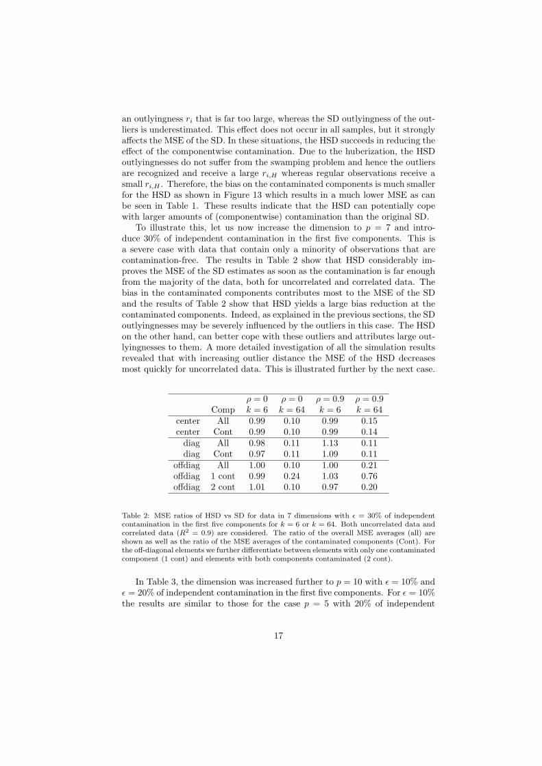
To illustrate this, let us now increase the dimension to p = 7 and intro-duce 30% of independent contamination in the first five components. This isa severe case with data that contain only a minority of observations that arecontamination-free. The results in Table 2 show that HSD considerably im-proves the MSE of the SD estimates as soon as the contamination is far enoughfrom the majority of the data, both for uncorrelated and correlated data. Thebias in the contaminated components contributes most to the MSE of the SDand the results of Table 2 show that HSD yields a large bias reduction at thecontaminated components. Indeed, as explained in the previous sections, the SDoutlyingnesses may be severely influenced by the outliers in this case. The HSDon the other hand, can better cope with these outliers and attributes large out-lyingnesses to them. A more detailed investigation of all the simulation resultsrevealed that with increasing outlier distance the MSE of the HSD decreasesmost quickly for uncorrelated data. This is illustrated further by the next case.

ρ = 0 ρ = 0 ρ = 0.9 ρ = 0.9Comp k = 6 k = 64 k = 6 k = 64

center All 0.99 0.10 0.99 0.15center Cont 0.99 0.10 0.99 0.14diag All 0.98 0.11 1.13 0.11diag Cont 0.97 0.11 1.09 0.11

offdiag All 1.00 0.10 1.00 0.21offdiag 1 cont 0.99 0.24 1.03 0.76offdiag 2 cont 1.01 0.10 0.97 0.20

Table 2: MSE ratios of HSD vs SD for data in 7 dimensions with ϵ = 30% of independentcontamination in the first five components for k = 6 or k = 64. Both uncorrelated data andcorrelated data (R2 = 0.9) are considered. The ratio of the overall MSE averages (all) areshown as well as the ratio of the MSE averages of the contaminated components (Cont). Forthe off-diagonal elements we further differentiate between elements with only one contaminatedcomponent (1 cont) and elements with both components contaminated (2 cont).

In Table 3, the dimension was increased further to p = 10 with ϵ = 10% andϵ = 20% of independent contamination in the first five components. For ϵ = 10%the results are similar to those for the case p = 5 with 20% of independent

17

ρ = 0 ρ = 0 ρ = 0.9 ρ = 0.9ϵ Comp k = 6 k = 64 k = 6 k = 64

center 0.10 All 0.90 1.03 0.89 0.99center 0.10 Cont 0.87 1.03 0.89 1.00center 0.20 All 0.93 0.53 0.92 1.05center 0.20 Cont 0.92 0.47 0.93 1.07diag 0.10 All 0.76 0.58 1.17 0.85diag 0.10 Cont 0.67 0.58 1.09 0.59diag 0.20 All 0.87 0.32 1.15 0.86diag 0.20 Cont 0.85 0.32 1.05 0.85

offdiag 0.10 All 0.94 0.65 1.12 1.26offdiag 0.10 1 cont 0.95 0.88 1.12 1.26offdiag 0.10 2 cont 0.91 0.48 1.05 1.22offdiag 0.20 all 0.97 0.16 1.06 1.00offdiag 0.20 1 cont 0.97 0.69 1.07 1.11offdiag 0.20 2 cont 0.98 0.15 1.00 0.76

Table 3: MSE ratios of HSD vs SD for data in 10 dimensions with ϵ = 10% or ϵ = 20% ofindependent contamination in the first five components for k = 6 or k = 64. Both uncorrelateddata and correlated data (R2 = 0.9) are considered. The ratio of the overall MSE averages(all) are shown as well as the ratio of the MSE averages of the contaminated components(Cont). For the off-diagonal elements we further differentiate between elements with only onecontaminated component (1 cont) and elements with both components contaminated (2 cont).

contamination in the first two components. In this setting there is a majorityof contamination-free observations. Therefore, the SD has a small MSE and theHSD yields similar results. For uncorrelated data, the HSD often gives smallimprovements over the SD, but for highly correlated data the effect reverses.

For ϵ = 20% there is no majority of contamination free observations anymore.The MSE of the SD increases due to bias problems. As can be seen fromTable 3, for uncorrelated data the HSD yields an improvement already for closeby outliers with increasing effect if the distance of the outliers increases. Forhighly correlated data on the other hand, the outliers need to be much furtheraway before the HSD can improve on the SD. Table 3 shows that for k = 64 theHSD still cannot improve the MSE of the SD.

We repeated the simulation study for large data sets with n = 5000 (forp = 5) and n = 10000 (for p = 7, 10). The results were similar and are omittedhere.

6. Conclusion

We presented a huberized version of the SD outlyingness where the outly-ingness of the observations is calculated w.r.t. the huberized data set in whichoutliers are componentwise pulled back to the bulk of the data. The huber-ization clearly improves the outlyingness measure in settings with independent

18

componentwise contamination. Contamination models that include component-wise outliers are realistic for many high dimensional settings. Such models arenot affine equivariant anymore and the overall fraction of contamination caneasily exceed 50% in higher dimensions. It was shown that in such cases theHSD suffers less from masking and swamping effects. Hence, HSD can betterwithstand the outliers as shown in a simulation study. The improvement ofHSD over SD is largest for data that are uncorrelated or weakly correlated. Forhighly correlated data, the contamination needs to lie further from the bulk ofthe measurements before the HSD can improve on the SD. In some cases theincreased variability of HSD makes its MSE worse than for SD, even thoughthe HSD has a smaller bias due to the outliers. A further improvement of theprocedure would be desirable to avoid that its performance is worse than that ofthe SD in such cases. Adapted weight functions for the huberized outlyingnessesmay be of interest for this matter, but this requires further research.

As an alternative to our huberization approach, one could consider applyinga univariate outlier detection rule to each of the variables separately to removecomponentwise outliers from the data. A multivariate outlier identification rulecan then be applied to the cleaned data to detect structural outliers. A drawbackof such an approach is that the removal of the componentwise outliers in thefirst step creates several empty cells in the data matrix. For the multivariateoutlier detection robust estimates are needed, but multivariate robust estimationprocedures in general cannot easily handle data with empty cells. Restrictingto the observations without empty cells is often not possible either becausethe number of complete observations may have become to low (lower than thedimension). Huberization on the other hand does not create empty cells, butmodifies the outlying values to make them more regular which allows a morerobust multivariate estimation procedure in the second step.

Acknowledgment

Research of the first author is supported by a grant of the Fund for Scientific

Research-Flanders (FWO-Vlaanderen) and by IAP research network grant nr. P6/03

of the Belgian government (Belgian Science Policy).

References

[1] Alqallaf, F.A., Konis, K.P., Martin, R.D., Zamar, R.H., 2002. ScalableRobust Covariance and Correlation Estimates for Data Mining, Proceed-ings of the Seventh ACM SIGKDD International Conference on KnowledgeDiscovery and Data Mining, Edmonton, Alberta, 14-23.

[2] Alqallaf, F., Van Aelst, S., Yohai, V.J., Zamar, R.H., 2009. Propagation ofOutliers in Multivariate Data, Ann. Statist. 37, 311-331.

[3] Boudt K., Croux, C., Laurent, S., 2009. Outlyingness weighted covariation,Technical Report, ORSTAT Research Center, KULeuven, Belgium.

19

[4] Cerioli A., Farcomeni, A., 2011. Error rates for multivariate outlier detec-tion, Computat. Statist. Data Anal. 55, 544-553.

[5] Davies, P.L., 1987. Asymptotic behavior of S-estimates of multivariate lo-cation parameters and dispersion matrices, Ann. Stat. 15, 1269-1292.

[6] Debruyne M. 2009. An outlier map for support vector machine classifica-tion, Ann. Applied Statist., 3, 1566-1580.

[7] Debruyne M., Hubert, M., 2009. The influence function of the Stahel-Donoho covariance estimator of smallest outlyingness, Statist. Probab.Lett. 79, 275-282.

[8] Donoho, D.L., 1982. Breakdown Properties of Multivariate Location Esti-mators, Ph.D. diss., Harvard University.

[9] Filzmoser, P., Maronna, R., Werner, M., 2008. Outlier identification in highdimensions, Computat. Statist. Data Anal. 52, 1694-1711.

[10] Gather, U., Hilker, T., 1997. A Note on Tyler’s Modification of the MADfor the Stahel-Donoho Estimator, Ann. Statist. 25, 2024-2026.

[11] Gervini, D., 2002. The influence function of the Stahel-Donoho estimatorof multivariate location and scatter, Statist. Probab. Lett. 60, 425-435.

[12] Hampel, F.R., Ronchetti, E.M., Rousseeuw, P.J., Stahel, W.A., 1986. Ro-bust Statistics: The Approach Based on Influence Functions, John Wileyand Sons, New York.

[13] Huber, P.J., 1981. Robust Statistics, Wiley, New York.

[14] Hubert M., Verboven, S., 2003. A robust PCR method for high-dimensionalregressors, J. Chemom. 17, 438-452.

[15] Hubert, M., Rousseeuw, P.J., Vanden Branden, K., 2005. ROBPCA: a newapproach to robust principal component analysis, Technometrics 47, 64-79.

[16] Khan, J.A., Van Aelst, S., Zamar, R.H., 2007. Robust linear model selectionbased on least angle regression, J. Amer. Statist. Assoc. 102, 1289-1299.

[17] Maronna, R.A., Martin, D.R., Yohai, V.J., 2006. Robust Statistics: Theoryand Methods, Wiley, New York.

[18] Maronna, R.A., Yohai, V.J., 1995. The behavior of the Stahel-Donoho Ro-bust Multivariate Estimator, J. Amer. Statist. Assoc. 90, 329-341.

[19] Maronna, R.A., Zamar R.H., 2002. Robust estimates of location and dis-persion for high-dimensional datasets, Technometrics, 44, 307-317.

[20] Rousseeuw, P.J., 1984. Least median of squares regression, J. Amer. Statist.Assoc. 79, 871-880.

20

[21] Stahel, W.A., 1981. Breakdown of Covariance Estimators, Research Report31, Fachgruppe fur Statistik, E.T.H. Zurich, Switzerland.

[22] Van Aelst, S., Vandervieren, E., Willems, G., 2011. Stahel-Donoho Esti-mators with Cellwise Weights, J. Stat. Comput. Simul. 81, 1-27.

[23] Zuo, Y., Cui, H., He, X., 2004. On the Stahel-Donoho estimator and depth-weighted means of multivariate data, Ann. Statist. 32, 167-188.

[24] Zuo, Y., Laia, S., 2011. Exact computation of bivariate projection depthand the StahelDonoho estimator, Computat. Statist. Data Anal. 55, 1173-1179.

21