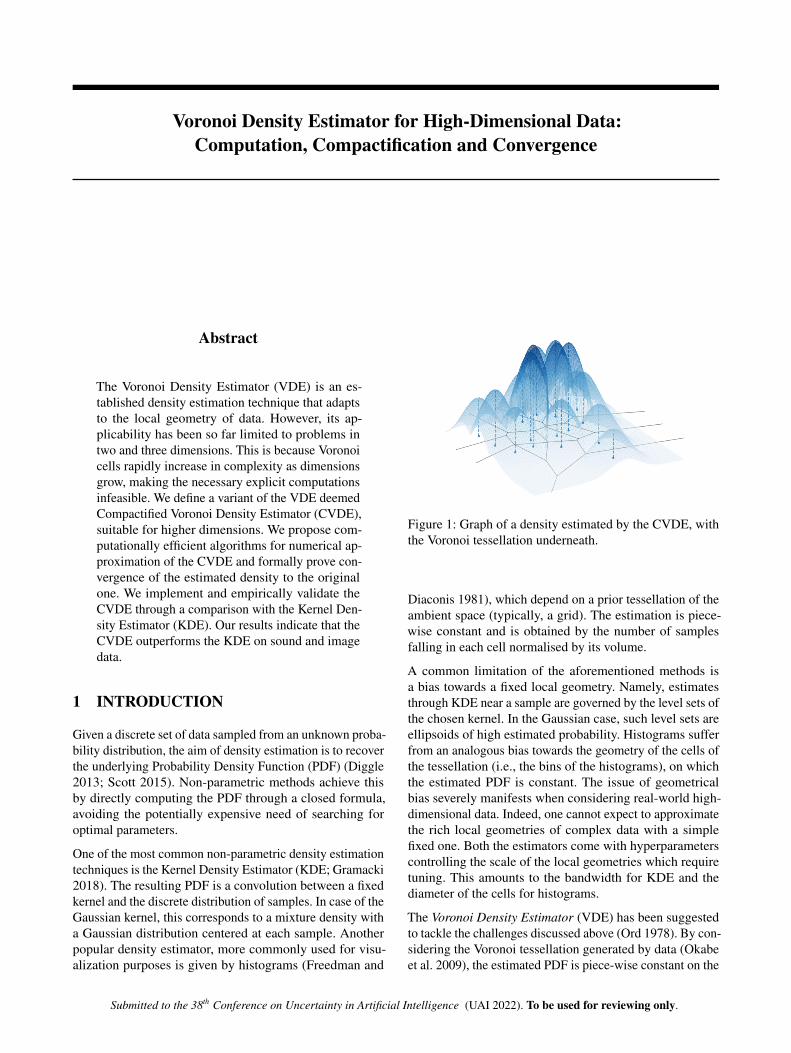
Voronoi Density Estimator for High-Dimensional Data:Computation, Compactification and Convergence

Abstract

The Voronoi Density Estimator (VDE) is an es-tablished density estimation technique that adaptsto the local geometry of data. However, its ap-plicability has been so far limited to problems intwo and three dimensions. This is because Voronoicells rapidly increase in complexity as dimensionsgrow, making the necessary explicit computationsinfeasible. We define a variant of the VDE deemedCompactified Voronoi Density Estimator (CVDE),suitable for higher dimensions. We propose com-putationally efficient algorithms for numerical ap-proximation of the CVDE and formally prove con-vergence of the estimated density to the originalone. We implement and empirically validate theCVDE through a comparison with the Kernel Den-sity Estimator (KDE). Our results indicate that theCVDE outperforms the KDE on sound and imagedata.

1 INTRODUCTION

Given a discrete set of data sampled from an unknown proba-bility distribution, the aim of density estimation is to recoverthe underlying Probability Density Function (PDF) (Diggle2013; Scott 2015). Non-parametric methods achieve thisby directly computing the PDF through a closed formula,avoiding the potentially expensive need of searching foroptimal parameters.

One of the most common non-parametric density estimationtechniques is the Kernel Density Estimator (KDE; Gramacki2018). The resulting PDF is a convolution between a fixedkernel and the discrete distribution of samples. In case of theGaussian kernel, this corresponds to a mixture density witha Gaussian distribution centered at each sample. Anotherpopular density estimator, more commonly used for visu-alization purposes is given by histograms (Freedman and

Figure 1: Graph of a density estimated by the CVDE, withthe Voronoi tessellation underneath.

Diaconis 1981), which depend on a prior tessellation of theambient space (typically, a grid). The estimation is piece-wise constant and is obtained by the number of samplesfalling in each cell normalised by its volume.

A common limitation of the aforementioned methods isa bias towards a fixed local geometry. Namely, estimatesthrough KDE near a sample are governed by the level sets ofthe chosen kernel. In the Gaussian case, such level sets areellipsoids of high estimated probability. Histograms sufferfrom an analogous bias towards the geometry of the cells ofthe tessellation (i.e., the bins of the histograms), on whichthe estimated PDF is constant. The issue of geometricalbias severely manifests when considering real-world high-dimensional data. Indeed, one cannot expect to approximatethe rich local geometries of complex data with a simplefixed one. Both the estimators come with hyperparameterscontrolling the scale of the local geometries which requiretuning. This amounts to the bandwidth for KDE and thediameter of the cells for histograms.

The Voronoi Density Estimator (VDE) has been suggestedto tackle the challenges discussed above (Ord 1978). By con-sidering the Voronoi tessellation generated by data (Okabeet al. 2009), the estimated PDF is piece-wise constant on the

Submitted to the 38th Conference on Uncertainty in Artificial Intelligence (UAI 2022). To be used for reviewing only.

cells and proportional to their inverse volume. The Voronoitessellation adapts local polytopes so that each datapoint isequally likely to be the closest when sampling from the re-sulting PDF. This has enabled successful application of theVDE to geometrically articulated real-world distributions inlower dimensions (Duyckaerts, Godefroy, and Hauw 1994;Ebeling and Wiedenmann 1993; Vavilova et al. 2021).

The goal of the present work is to enable the VDE forhigh-dimensional scenarios. Although the VDE constitutes apromising candidate due to its local adaptivity, the followingaspects have to be addressed:

Computation. The Voronoi cells are arbitrary convex poly-topes and their volume is thus challenging to compute ex-plicitly, which yields the necessity for fast approximatecomputations.

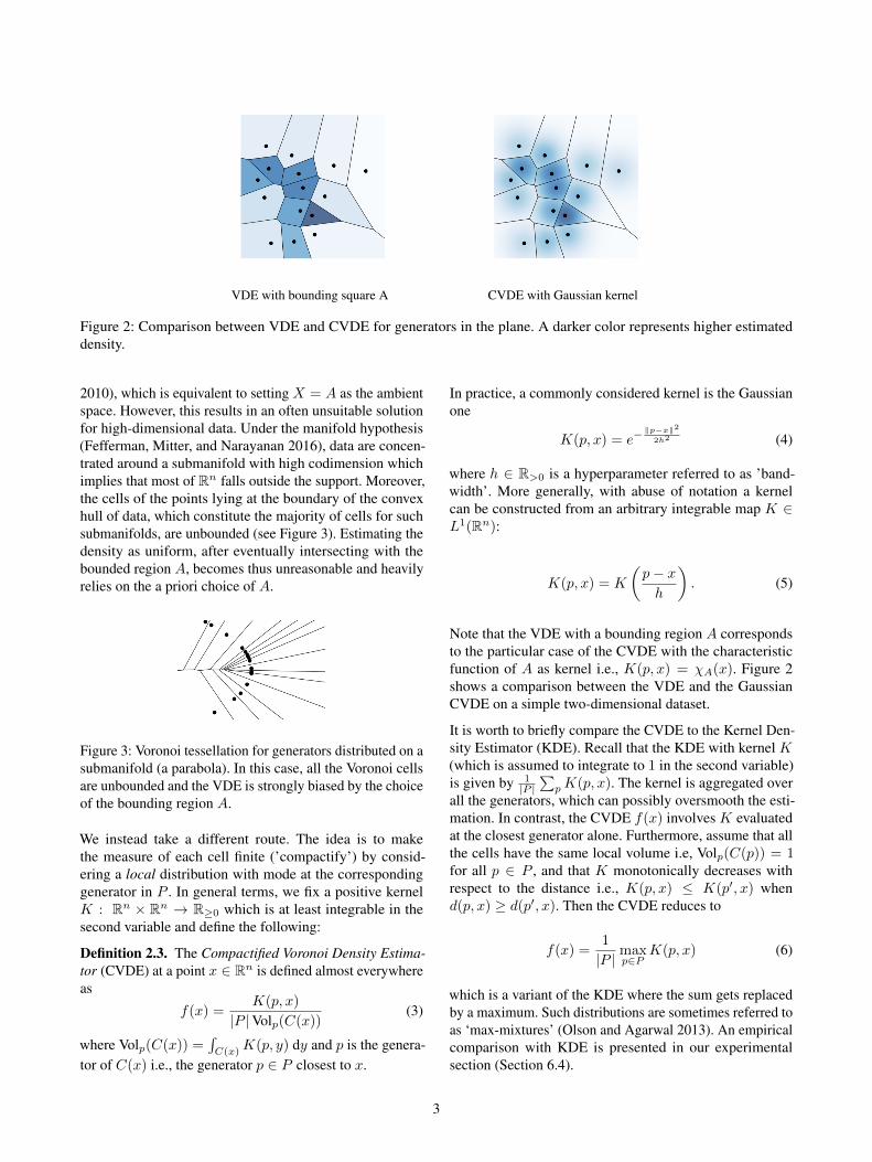
Compactification. Data is often concentrated around low-dimensional submanifolds, which makes most of the ambi-ent space empty and several Voronoi cells unbounded, i.e.of infinite volume (see Figure 3). One still needs to producea finite estimate on those cells, a process we refer to as’compactification’.

We propose solutions to the problems above. First, wepresent efficient algorithmic procedures for volume com-putation and sampling from the estimated density. We for-mulate the cell volumes as integrals over a sphere, whichcan then be approximated by Monte Carlo methods. Further-more, we propose a sampling procedure for the distributionestimated by the VDE. This consists in randomly traversingthe Voronoi cells via a ’hit-and-run’ Markov chain (M.-H.Chen and Schmeiser 1996). The proposed algorithms arehighly parallelizable, allowing efficient computations on theGPU.

In order to compactify the cells, we place a finite measureon each of them by means of a fixed kernel (typically, aGaussian one), leading to an altered version of the VDEwhich we refer to as Compactified Voronoi Density Esti-mator (CVDE). Figure 1 shows an example of an estimateby the CVDE on a simple two-dimensional dataset. All thecomputational and sampling procedures naturally extend tothe CVDE.

A further contribution of the present work is a theoreticalproof of convergence for the CVDE. Assuming the originaldensity has support in the whole ambient space, we showthat the PDF estimated by the CVDE converges (with re-spect to an appropriate notion for random measures) to theground-truth one as the number of datapoints increases. Theconvergence holds without any continuity assumptions onthe ground-truth PDF nor on the kernel and does not requirethe kernel bandwidth to vanish asymptotically. This is incontrast with the convergence properties of the KDE. Dueto the aforementioned local geometric bias of the KDE, thebandwidth has to decrease at an appropriate rate in order to

amend for the local influence of the kernel and guaranteeconvergence to the underlying distribution (LP Devroye andWagner 1979; Jiang 2017).

Finally, we implement the CVDE in C++ and parallelizecomputations via the OpenCL framework. Our code, with aprovided Python interface, is included in the supplementarymaterial.

2 COMPACTIFIED VORONOI DENSITYESTIMATOR

This section presents Voronoi cell compactification andCompactified Voronoi Density Estimator, CVDE. We beginby defining the Voronoi tessellations in a general setting (seeOkabe et al. 2009 for a comprehensive treatment). Supposethat (X, d) is a connected metric space and P ⊆ X isa finite collection of distinct points referred to as generators.

Definition 2.1. The Voronoi cell1 of p ∈ P is defined as

C(p) = {x ∈ X | ∀q ∈ P d(x, q) ≥ d(x, p)}. (1)

The Voronoi cells intersect at the boundary and cover the am-bient space X . The collection {C(p)}p∈P is called Voronoitessellation generated by P . For a point x ∈ X not on theboundary of any cell, we write C(x) for the unique cellcontaining it. When X = Rn with Euclidean distance, theVoronoi cells are convex n-dimensional polytopes whichare possibly unbounded.

Assume now that X is equipped with a finite Borel measuredenoted by Vol. An additional technical condition is thatthe boundaries of the Voronoi cells have vanishing measure.

Definition 2.2. The Voronoi Density Estimator (VDE) at apoint x ∈ X is defined almost everywhere as

f(x) =1

|P |Vol(C(x))(2)

where | · | denotes cardinality.

The function f defines a locally constant PDF on X and thusa probability measure f Vol. With respect to this distributionthe cells are equally likely, and the restriction to each cellcoincides with the normalisation of Vol.

We focus on the case where X = Rn equipped with Eu-clidean distance. One major issue for the choice of Vol isthat the standard Lebesgue measure does not satisfy thefiniteness requirement. A common solution in the literatureis to restrict the measure to a fixed bounded region A ⊆ Rn

containing P (Moradi et al. 2019; Barr and Schoenberg1Sometimes referred to as Dirichlet cell.

2

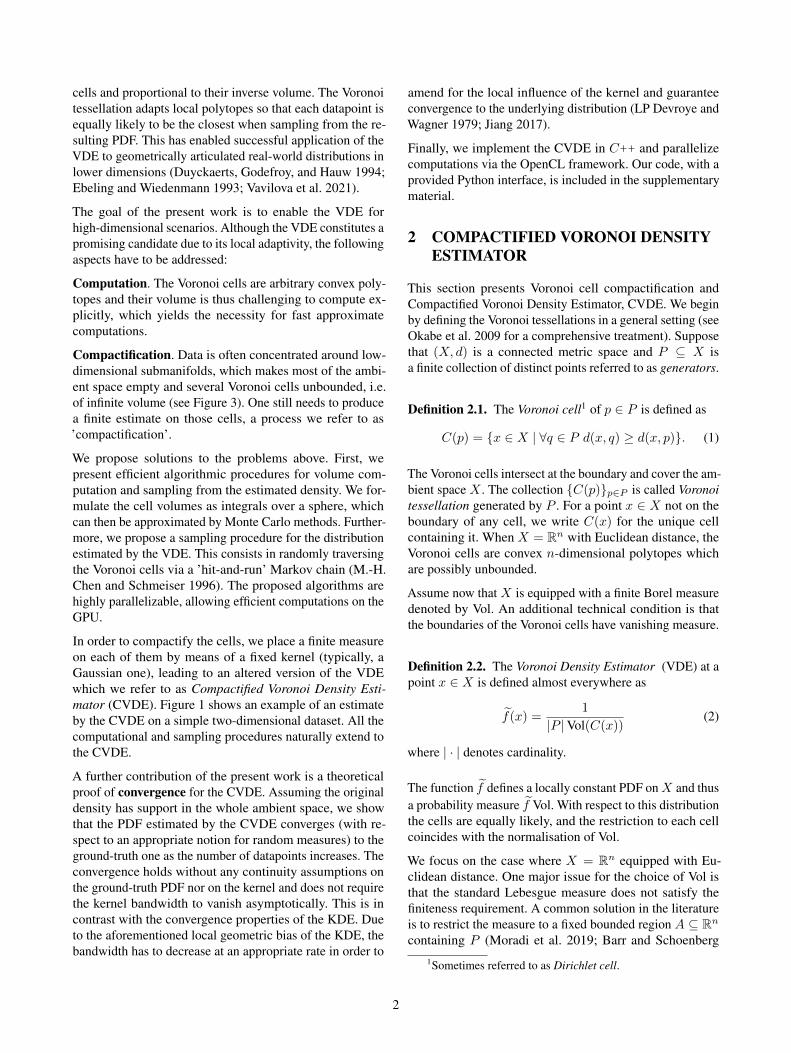
VDE with bounding square A CVDE with Gaussian kernel

Figure 2: Comparison between VDE and CVDE for generators in the plane. A darker color represents higher estimateddensity.

2010), which is equivalent to setting X = A as the ambientspace. However, this results in an often unsuitable solutionfor high-dimensional data. Under the manifold hypothesis(Fefferman, Mitter, and Narayanan 2016), data are concen-trated around a submanifold with high codimension whichimplies that most of Rn falls outside the support. Moreover,the cells of the points lying at the boundary of the convexhull of data, which constitute the majority of cells for suchsubmanifolds, are unbounded (see Figure 3). Estimating thedensity as uniform, after eventually intersecting with thebounded region A, becomes thus unreasonable and heavilyrelies on the a priori choice of A.

Figure 3: Voronoi tessellation for generators distributed on asubmanifold (a parabola). In this case, all the Voronoi cellsare unbounded and the VDE is strongly biased by the choiceof the bounding region A.

We instead take a different route. The idea is to makethe measure of each cell finite (’compactify’) by consid-ering a local distribution with mode at the correspondinggenerator in P . In general terms, we fix a positive kernelK : Rn × Rn → R≥0 which is at least integrable in thesecond variable and define the following:

Definition 2.3. The Compactified Voronoi Density Estima-tor (CVDE) at a point x ∈ Rn is defined almost everywhereas

f(x) =K(p, x)

|P |Volp(C(x))(3)

where Volp(C(x)) =∫C(x)

K(p, y) dy and p is the genera-tor of C(x) i.e., the generator p ∈ P closest to x.

In practice, a commonly considered kernel is the Gaussianone

K(p, x) = e−∥p−x∥2

2h2 (4)

where h ∈ R>0 is a hyperparameter referred to as ’band-width’. More generally, with abuse of notation a kernelcan be constructed from an arbitrary integrable map K ∈L1(Rn):

K(p, x) = K

(p− x

h

). (5)

Note that the VDE with a bounding region A correspondsto the particular case of the CVDE with the characteristicfunction of A as kernel i.e., K(p, x) = χA(x). Figure 2shows a comparison between the VDE and the GaussianCVDE on a simple two-dimensional dataset.

It is worth to briefly compare the CVDE to the Kernel Den-sity Estimator (KDE). Recall that the KDE with kernel K(which is assumed to integrate to 1 in the second variable)is given by 1

|P |∑

p K(p, x). The kernel is aggregated overall the generators, which can possibly oversmooth the esti-mation. In contrast, the CVDE f(x) involves K evaluatedat the closest generator alone. Furthermore, assume that allthe cells have the same local volume i.e, Volp(C(p)) = 1for all p ∈ P , and that K monotonically decreases withrespect to the distance i.e., K(p, x) ≤ K(p′, x) whend(p, x) ≥ d(p′, x). Then the CVDE reduces to

f(x) =1

|P |maxp∈P

K(p, x) (6)

which is a variant of the KDE where the sum gets replacedby a maximum. Such distributions are sometimes referred toas ‘max-mixtures’ (Olson and Agarwal 2013). An empiricalcomparison with KDE is presented in our experimentalsection (Section 6.4).

3

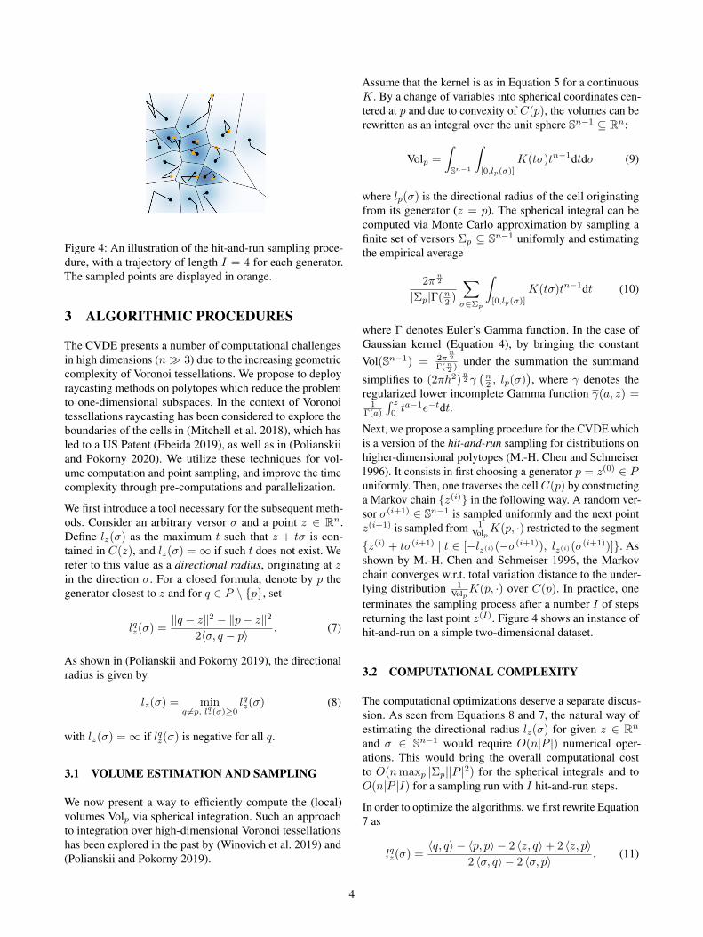
Figure 4: An illustration of the hit-and-run sampling proce-dure, with a trajectory of length I = 4 for each generator.The sampled points are displayed in orange.

3 ALGORITHMIC PROCEDURES

The CVDE presents a number of computational challengesin high dimensions (n ≫ 3) due to the increasing geometriccomplexity of Voronoi tessellations. We propose to deployraycasting methods on polytopes which reduce the problemto one-dimensional subspaces. In the context of Voronoitessellations raycasting has been considered to explore theboundaries of the cells in (Mitchell et al. 2018), which hasled to a US Patent (Ebeida 2019), as well as in (Polianskiiand Pokorny 2020). We utilize these techniques for vol-ume computation and point sampling, and improve the timecomplexity through pre-computations and parallelization.

We first introduce a tool necessary for the subsequent meth-ods. Consider an arbitrary versor σ and a point z ∈ Rn.Define lz(σ) as the maximum t such that z + tσ is con-tained in C(z), and lz(σ) = ∞ if such t does not exist. Werefer to this value as a directional radius, originating at zin the direction σ. For a closed formula, denote by p thegenerator closest to z and for q ∈ P \ {p}, set

lqz(σ) =∥q − z∥2 − ∥p− z∥2

2⟨σ, q − p⟩. (7)

As shown in (Polianskii and Pokorny 2019), the directionalradius is given by

lz(σ) = minq =p, lqz(σ)≥0

lqz(σ) (8)

with lz(σ) = ∞ if lqz(σ) is negative for all q.

3.1 VOLUME ESTIMATION AND SAMPLING

We now present a way to efficiently compute the (local)volumes Volp via spherical integration. Such an approachto integration over high-dimensional Voronoi tessellationshas been explored in the past by (Winovich et al. 2019) and(Polianskii and Pokorny 2019).

Assume that the kernel is as in Equation 5 for a continuousK. By a change of variables into spherical coordinates cen-tered at p and due to convexity of C(p), the volumes can berewritten as an integral over the unit sphere Sn−1 ⊆ Rn:

Volp =

∫Sn−1

∫[0,lp(σ)]

K(tσ)tn−1dtdσ (9)

where lp(σ) is the directional radius of the cell originatingfrom its generator (z = p). The spherical integral can becomputed via Monte Carlo approximation by sampling afinite set of versors Σp ⊆ Sn−1 uniformly and estimatingthe empirical average

2πn2

|Σp|Γ(n2 )∑σ∈Σp

∫[0,lp(σ)]

K(tσ)tn−1dt (10)

where Γ denotes Euler’s Gamma function. In the case ofGaussian kernel (Equation 4), by bringing the constantVol(Sn−1) = 2π

n2

Γ(n2 ) under the summation the summand

simplifies to (2πh2)n2 γ

(n2 , lp(σ)

), where γ denotes the

regularized lower incomplete Gamma function γ(a, z) =1

Γ(a)

∫ z

0ta−1e−tdt.

Next, we propose a sampling procedure for the CVDE whichis a version of the hit-and-run sampling for distributions onhigher-dimensional polytopes (M.-H. Chen and Schmeiser1996). It consists in first choosing a generator p = z(0) ∈ Puniformly. Then, one traverses the cell C(p) by constructinga Markov chain {z(i)} in the following way. A random ver-sor σ(i+1) ∈ Sn−1 is sampled uniformly and the next pointz(i+1) is sampled from 1

VolpK(p, ·) restricted to the segment

{z(i) + tσ(i+1) | t ∈ [−lz(i)(−σ(i+1)), lz(i)(σ(i+1))]}. Asshown by M.-H. Chen and Schmeiser 1996, the Markovchain converges w.r.t. total variation distance to the under-lying distribution 1

VolpK(p, ·) over C(p). In practice, one

terminates the sampling process after a number I of stepsreturning the last point z(I). Figure 4 shows an instance ofhit-and-run on a simple two-dimensional dataset.

3.2 COMPUTATIONAL COMPLEXITY

The computational optimizations deserve a separate discus-sion. As seen from Equations 8 and 7, the natural way ofestimating the directional radius lz(σ) for given z ∈ Rn

and σ ∈ Sn−1 would require O(n|P |) numerical oper-ations. This would bring the overall computational costto O(nmaxp |Σp||P |2) for the spherical integrals and toO(n|P |I) for a sampling run with I hit-and-run steps.

In order to optimize the algorithms, we first rewrite Equation7 as

lqz(σ) =⟨q, q⟩ − ⟨p, p⟩ − 2 ⟨z, q⟩+ 2 ⟨z, p⟩

2 ⟨σ, q⟩ − 2 ⟨σ, p⟩. (11)

4

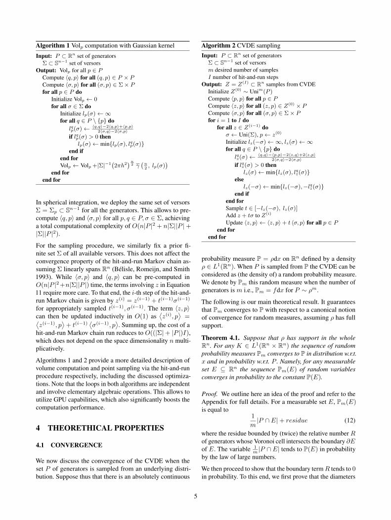
Algorithm 1 Volp computation with Gaussian kernel

Input: P ⊂ Rn set of generatorsΣ ⊂ Sn−1 set of versors

Output: Volp for all p ∈ PCompute ⟨q, p⟩ for all (q, p) ∈ P × PCompute ⟨σ, p⟩ for all (σ, p) ∈ Σ× Pfor all p ∈ P do

Initialize Volp ← 0for all σ ∈ Σ do

Initialize lp(σ)←∞for all q ∈ P \ {p} do

lqp(σ)← ⟨q,q⟩−2⟨q,p⟩+⟨p,p⟩2⟨σ,q⟩−2⟨σ,p⟩

if lqp(σ) > 0 thenlp(σ)← min{lp(σ), lqp(σ)}

end ifend forVolp ← Volp +|Σ|−1

(2πh2

)n2 γ

(n2, lp(σ)

)end for

end for

In spherical integration, we deploy the same set of versorsΣ = Σp ⊂ Sn−1 for all the generators. This allows to pre-compute ⟨q, p⟩ and ⟨σ, p⟩ for all p, q ∈ P, σ ∈ Σ, achievinga total computational complexity of O(n|P |2 + n|Σ||P |+|Σ||P |2).

For the sampling procedure, we similarly fix a prior fi-nite set Σ of all available versors. This does not affect theconvergence property of the hit-and-run Markov chain as-suming Σ linearly spans Rn (Bélisle, Romeijn, and Smith1993). While ⟨σ, p⟩ and ⟨q, p⟩ can be pre-computed inO(n|P |2+n|Σ||P |) time, the terms involving z in Equation11 require more care. To that end, the i-th step of the hit-and-run Markov chain is given by z(i) = z(i−1) + t(i−1)σ(i−1)

for appropriately sampled t(i−1), σ(i−1). The term ⟨z, p⟩can then be updated inductively in O(1) as

⟨z(i), p

⟩=⟨

z(i−1), p⟩+ t(i−1)

⟨σ(i−1), p

⟩. Summing up, the cost of a

hit-and-run Markov chain run reduces to O((|Σ|+ |P |)I),which does not depend on the space dimensionality n multi-plicatively.

Algorithms 1 and 2 provide a more detailed description ofvolume computation and point sampling via the hit-and-runprocedure respectively, including the discussed optimiza-tions. Note that the loops in both algorithms are independentand involve elementary algebraic operations. This allows toutilize GPU capabilities, which also significantly boosts thecomputation performance.

4 THEORETHICAL PROPERTIES

4.1 CONVERGENCE

We now discuss the convergence of the CVDE when theset P of generators is sampled from an underlying distri-bution. Suppose thus that there is an absolutely continuous

Algorithm 2 CVDE samplingInput: P ⊂ Rn set of generators

Σ ⊂ Sn−1 set of versorsm desired number of samplesI number of hit-and-run steps

Output: Z = Z(I) ⊂ Rn samples from CVDEInitialize Z(0) ∼ Unim(P )Compute ⟨p, p⟩ for all p ∈ PCompute ⟨z, p⟩ for all (z, p) ∈ Z(0) × PCompute ⟨σ, p⟩ for all (σ, p) ∈ Σ× Pfor i = 1 to I do

for all z ∈ Z(i−1) doσ ← Uni(Σ), p← z(0)

Initialize lz(−σ)←∞, lz(σ)←∞for all q ∈ P \ {p} do

lqz(σ)← ⟨q,q⟩−⟨p,p⟩−2⟨z,q⟩+2⟨z,p⟩2⟨σ,q⟩−2⟨σ,p⟩

if lqz(σ) > 0 thenlz(σ)← min{lz(σ), lqz(σ)}

elselz(−σ)← min{lz(−σ),−lqz(σ)}

end ifend forSample t ∈ [−lz(−σ), lz(σ)]Add z + tσ to Z(i)

Update ⟨z, p⟩ ← ⟨z, p⟩+ t ⟨σ, p⟩ for all p ∈ Pend for

end for

probability measure P = ρdx on Rn defined by a densityρ ∈ L1(Rn). When P is sampled from P the CVDE can beconsidered as (the density of) a random probability measure.We denote by Pm this random measure when the number ofgenerators is m i.e., Pm = fdx for P ∼ ρm.

The following is our main theoretical result. It guaranteesthat Pm converges to P with respect to a canonical notionof convergence for random measures, assuming ρ has fullsupport.

Theorem 4.1. Suppose that ρ has support in the wholeRn. For any K ∈ L1(Rn × Rn) the sequence of randomprobability measures Pm converges to P in distribution w.r.t.x and in probability w.r.t. P . Namely, for any measurableset E ⊆ Rn the sequence Pm(E) of random variablesconverges in probability to the constant P(E).

Proof. We outline here an idea of the proof and refer to theAppendix for full details. For a measurable set E, Pm(E)is equal to

1

m|P ∩ E|+ residue (12)

where the residue bounded by (twice) the relative number Rof generators whose Voronoi cell intersects the boundary ∂Eof E. The variable 1

m |P ∩ E| tends to P(E) in probabilityby the law of large numbers.

We then proceed to show that the boundary term R tends to 0in probability. To this end, we first prove that the diameters

5

of the Voronoi cells intersecting E tend uniformly to 0(Proposition D.3), which in turn requires a preliminary result(Proposition D.2) constraining such cells in a neighbourof E (which is assumed to be bounded). Given that, weconclude that R tends to P(∂E) by the law of large numbers.By the Portmanteau Lemma (Van der Vaart 2000), we canassume that P(∂E) = 0 (and that E is bounded), whichconcludes the proof.

Note that the above results holds for any (integrable) kernel,thus even for discontinuous ones. The kernel is fixed, andthere is no need for an eventual bandwidth (Equation 5) tovanish asymptotically. This is in contrast with KDE, whichrequires h to tend to 0 at an appropriate rate in order toobtain convergence to ρ (LP Devroye and Wagner 1979;Jiang 2017). This is because of the local geometric biasinherent to the KDE, as discussed in Section 1. In order toobtain convergence, such bias has to be amended with avanishing bandwidth that annihilates the local geometry ofthe kernel.

4.2 BANDWIDTH ASYMPTOTICS

Consider a kernel in the form of Equation 5. The asymptoticswith respect to h (with fixed set of generators P ) can beeasily deduced:

Proposition 4.2. For a continuous K : Rn → R≥0, thefollowing hold:

(i) As h tends to 0, f converges in distribution to the empiri-cal measure 1

|P |∑

p∈P δp, where delta denotes the Dirac’sdelta.

(ii) Consider the restriction of the kernel to a bounded regionA (i.e., its product with χA). As h tends to +∞, f convergesin distribution to the VDE f .

Proof. The first statement follows directly from the factthat 1

hnK(xh ) is an approximator of unity and thus tends toδ0. As for the second part, observe that K(x, p) tends toK(0) by continuity of K and thus f(x) tends to f(x) for al-most every x. To conclude, point-wise convergence of PDFsimplies convergence in distribution (Scheffé’s Lemma).

The asymptotics for small bandwidth are the same as forthe KDE. For bandwidth tending to infinity, however, theKDE tends to the uniform distribution over A, while theCVDE still gives reasonable estimates in the form of itsnon-compactified version.

5 RELATED WORK

Non-parametric Density Estimation. The first traces ofsystematic density estimation date back to the introduc-

tion of histograms (Pearson 1894). Those have been subse-quently considered with a variety of cell geometries suchas rectangles, triangles (Scott 1988) and hexagons (Carr,Olsen, and White 1992). The choice of geometry constitutesthe main source of bias for the histogram-based densityestimator.

Arguably, the most popular density estimator is the KDE,first discussed by Rosenblatt 1956 and Parzen 1962. Nu-merous extensions have followed, for example, to the multi-variate case (Izenman 1991; Dehnad 1987) and bandwidthselection methods (Marron 1987; Wand, Jones, et al. 1994).Among applications, the KDE has been deployed to esti-mate traffic incidents (Xie and Yan 2008), archeologicaldata (Baxter, Beardah, and Wright 1997) and wind speed(Bo et al. 2017) to name a few.

VDE and its Applications. The VDE has been originallyintroduced by (Ord 1978) under the name ’ideal estimator’because of its local geometric adaptivity. Subsequent workshave discussed regularisation (Moradi et al. 2019) and lower-dimensional aspects (Barr and Schoenberg 2010). The VDEhas seen a applications to a variety of real-world densitiessuch as neurons in the brain (Duyckaerts, Godefroy, andHauw 1994), photons (Ebeling and Wiedenmann 1993) andstars in a galaxy (Vavilova et al. 2021). Although promising,the VDE has been previously limited to low-dimensionalproblems.

Theoretical Convergence. Convergence of the VDEhas been previously considered in the literature, usu-ally in the language of Poisson point processes. Foruniform underlying distribution, point-wise convergenceof the averaged estimated density (i.e., unbiasedness:limm→∞ EP∼ρm [f(x)] = ρ(x) for almost all x) has beenproven by Last 2010. For non-uniform distributions, thesame convergence has been shown by Moradi et al. 2019with strong continuity assumptions on the density, whichallows a reduction to the uniform case. Our theoretical resultis based on a different, non-averaged notion of convergenceand holds for the more general CVDE with no continuityassumptions.

6 EXPERIMENTS

6.1 DATASET DESCRIPTION

In our experiments, we evaluate the CVDE on datasets ofdifferent nature: simple synthetic distributions of Gaussiantype, image data in pixel-space, and sound data in a fre-quency space. The datasets we deploy are the following:

Gaussians and Gaussian mixtures: for synthetic exper-iments we generate two types of datasets, each contain-ing 1000 training and 1000 test points. The first one con-sists of samples from an n-dimensional standard Gaus-sian distribution. The second one is sampled from a Gaus-

6

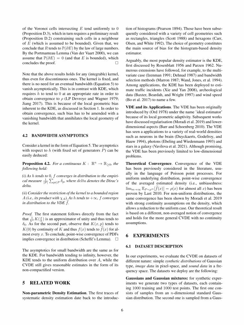
n = 2 n = 10

Original

VDE

CVDE

Figure 5: Visual comparison between samples from theCVDE and the VDE estimating an n-dimensional Gaussianfor n = 2, 10. In the 10-dimensional case, points are pro-jected onto a plane. In high dimensions, the VDE appearsas biased towards a uniform distribution. This is becauseof abundance of unbounded cells, over which the estimateddensity is constant.

sian mixture density ρ = 12 (ρ1 + ρ2). Here, ρ1, ρ2 are

Gaussian distributions with means µ1 = (−0.5, 0, · · · , 0),µ2 = (0.5, 0, · · · , 0) and standard deviations σ1 = 0.1,σ2 = 100 respectively.

MNIST (Deng 2012): the dataset consists of 28 × 28grayscale images of handwritten digits which are normalisedin order to lie in [0, 1]28×28. For each experimental run, wesample half of the 60000 training datapoints in order toevaluate the variance of the estimation. The test set size is10000.

Anuran Calls (Dua and Graff 2017): the datasets consists of7195 calls from 10 species of frogs which are represented by21 normalised mel-frequency cepstral coefficients in [0, 1]21.We retain 10% of data for testing and again sample half ofthe training data at each experimental run.

6.2 COMPARISON WITH VDE

In this section, we evaluate empirically the necessity ofcompactification for high-dimensional data. To this end, wevisually compare samples from the CVDE (with Gaussiankernel) and from the the VDE. The VDE is implementedwith a bounding hypercube A = [− 7

2 ,72 ]

n as described in

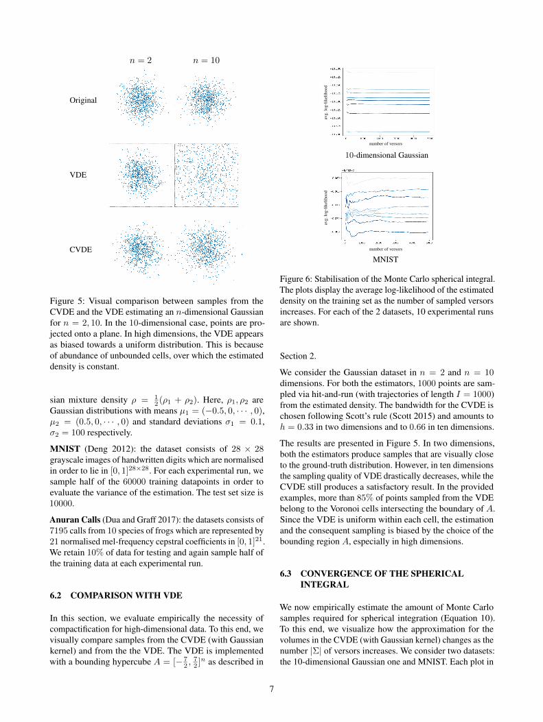
10-dimensional Gaussian

MNIST

number of versors

avg.

log-

likel

ihoo

d

number of versors

avg.

log-

likel

ihoo

d

Figure 6: Stabilisation of the Monte Carlo spherical integral.The plots display the average log-likelihood of the estimateddensity on the training set as the number of sampled versorsincreases. For each of the 2 datasets, 10 experimental runsare shown.

Section 2.

We consider the Gaussian dataset in n = 2 and n = 10dimensions. For both the estimators, 1000 points are sam-pled via hit-and-run (with trajectories of length I = 1000)from the estimated density. The bandwidth for the CVDE ischosen following Scott’s rule (Scott 2015) and amounts toh = 0.33 in two dimensions and to 0.66 in ten dimensions.

The results are presented in Figure 5. In two dimensions,both the estimators produce samples that are visually closeto the ground-truth distribution. However, in ten dimensionsthe sampling quality of VDE drastically decreases, while theCVDE still produces a satisfactory result. In the providedexamples, more than 85% of points sampled from the VDEbelong to the Voronoi cells intersecting the boundary of A.Since the VDE is uniform within each cell, the estimationand the consequent sampling is biased by the choice of thebounding region A, especially in high dimensions.

6.3 CONVERGENCE OF THE SPHERICALINTEGRAL

We now empirically estimate the amount of Monte Carlosamples required for spherical integration (Equation 10).To this end, we visualize how the approximation for thevolumes in the CVDE (with Gaussian kernel) changes as thenumber |Σ| of versors increases. We consider two datasets:the 10-dimensional Gaussian one and MNIST. Each plot in

7

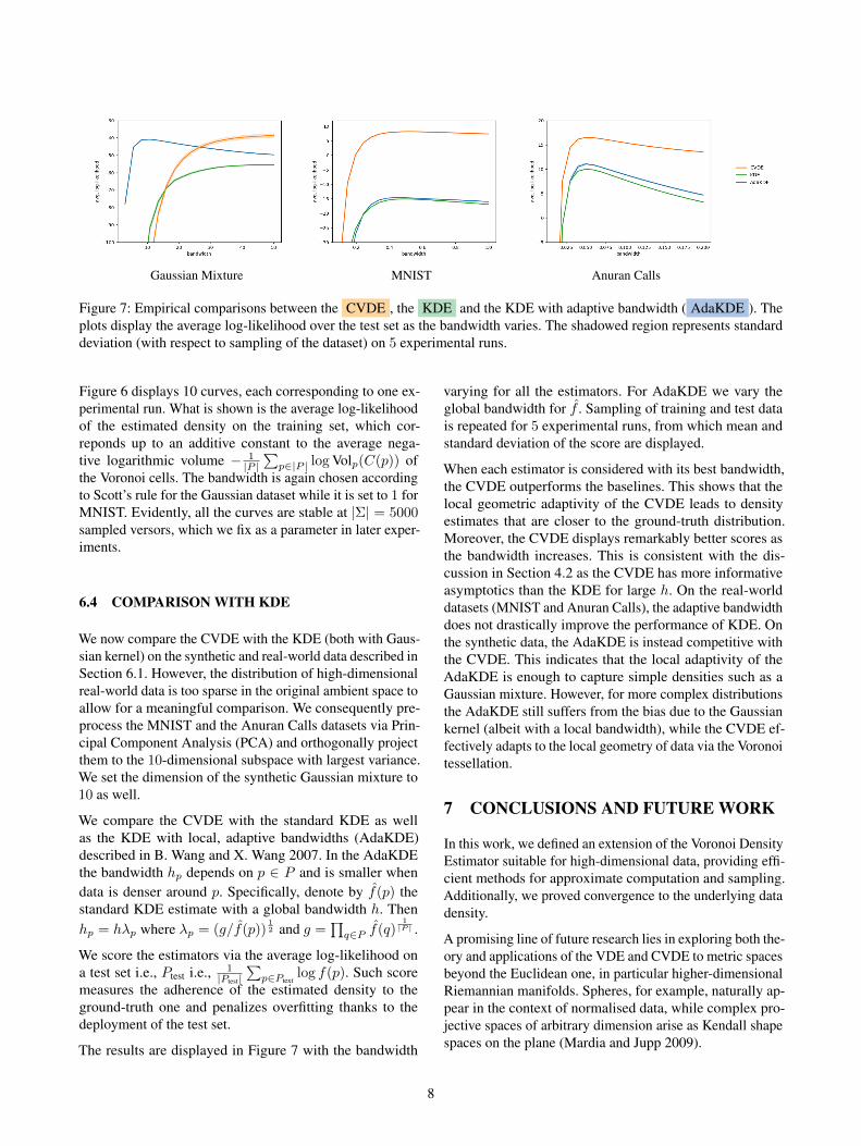
Gaussian Mixture MNIST Anuran Calls

Figure 7: Empirical comparisons between the CVDE , the KDE and the KDE with adaptive bandwidth ( AdaKDE ). Theplots display the average log-likelihood over the test set as the bandwidth varies. The shadowed region represents standarddeviation (with respect to sampling of the dataset) on 5 experimental runs.

Figure 6 displays 10 curves, each corresponding to one ex-perimental run. What is shown is the average log-likelihoodof the estimated density on the training set, which cor-reponds up to an additive constant to the average nega-tive logarithmic volume − 1

|P |∑

p∈|P | logVolp(C(p)) ofthe Voronoi cells. The bandwidth is again chosen accordingto Scott’s rule for the Gaussian dataset while it is set to 1 forMNIST. Evidently, all the curves are stable at |Σ| = 5000sampled versors, which we fix as a parameter in later exper-iments.

6.4 COMPARISON WITH KDE

We now compare the CVDE with the KDE (both with Gaus-sian kernel) on the synthetic and real-world data described inSection 6.1. However, the distribution of high-dimensionalreal-world data is too sparse in the original ambient space toallow for a meaningful comparison. We consequently pre-process the MNIST and the Anuran Calls datasets via Prin-cipal Component Analysis (PCA) and orthogonally projectthem to the 10-dimensional subspace with largest variance.We set the dimension of the synthetic Gaussian mixture to10 as well.

We compare the CVDE with the standard KDE as wellas the KDE with local, adaptive bandwidths (AdaKDE)described in B. Wang and X. Wang 2007. In the AdaKDEthe bandwidth hp depends on p ∈ P and is smaller whendata is denser around p. Specifically, denote by f(p) thestandard KDE estimate with a global bandwidth h. Thenhp = hλp where λp = (g/f(p))

12 and g =

∏q∈P f(q)

1|P | .

We score the estimators via the average log-likelihood ona test set i.e., Ptest i.e., 1

|Ptest|∑

p∈Ptextlog f(p). Such score

measures the adherence of the estimated density to theground-truth one and penalizes overfitting thanks to thedeployment of the test set.

The results are displayed in Figure 7 with the bandwidth

varying for all the estimators. For AdaKDE we vary theglobal bandwidth for f . Sampling of training and test datais repeated for 5 experimental runs, from which mean andstandard deviation of the score are displayed.

When each estimator is considered with its best bandwidth,the CVDE outperforms the baselines. This shows that thelocal geometric adaptivity of the CVDE leads to densityestimates that are closer to the ground-truth distribution.Moreover, the CVDE displays remarkably better scores asthe bandwidth increases. This is consistent with the dis-cussion in Section 4.2 as the CVDE has more informativeasymptotics than the KDE for large h. On the real-worlddatasets (MNIST and Anuran Calls), the adaptive bandwidthdoes not drastically improve the performance of KDE. Onthe synthetic data, the AdaKDE is instead competitive withthe CVDE. This indicates that the local adaptivity of theAdaKDE is enough to capture simple densities such as aGaussian mixture. However, for more complex distributionsthe AdaKDE still suffers from the bias due to the Gaussiankernel (albeit with a local bandwidth), while the CVDE ef-fectively adapts to the local geometry of data via the Voronoitessellation.

7 CONCLUSIONS AND FUTURE WORK

In this work, we defined an extension of the Voronoi DensityEstimator suitable for high-dimensional data, providing effi-cient methods for approximate computation and sampling.Additionally, we proved convergence to the underlying datadensity.

A promising line of future research lies in exploring both the-ory and applications of the VDE and CVDE to metric spacesbeyond the Euclidean one, in particular higher-dimensionalRiemannian manifolds. Spheres, for example, naturally ap-pear in the context of normalised data, while complex pro-jective spaces of arbitrary dimension arise as Kendall shapespaces on the plane (Mardia and Jupp 2009).

8

REFERENCES

Barr, Christopher D and Frederic Paik Schoenberg (2010).“On the Voronoi estimator for the intensity of an inho-mogeneous planar Poisson process.” In: Biometrika 97.4,pp. 977–984.

Baxter, Michael J, Christian C Beardah, and Richard VSWright (1997). “Some archaeological applications of ker-nel density estimates.” In: Journal of Archaeological Sci-ence 24.4, pp. 347–354.

Bélisle, Claude JP, H Edwin Romeijn, and Robert L Smith(1993). “Hit-and-run algorithms for generating multi-variate distributions.” In: Mathematics of Operations Re-search 18.2, pp. 255–266.

Bo, HU et al. (2017). “Wind speed model based on kerneldensity estimation and its application in reliability as-sessment of generating systems.” In: Journal of ModernPower Systems and Clean Energy 5.2, pp. 220–227.

Carr, Daniel B, Anthony R Olsen, and Denis White (1992).“Hexagon mosaic maps for display of univariate and bi-variate geographical data.” In: Cartography and Geo-graphic Information Systems 19.4, pp. 228–236.

Chen, Ming-Hui and Bruce W Schmeiser (1996). “Generalhit-and-run Monte Carlo sampling for evaluating multi-dimensional integrals.” In: Operations Research Letters19.4, pp. 161–169.

Dehnad, Khosrow (1987). Density estimation for statisticsand data analysis.

Deng, Li (2012). “The mnist database of handwritten digitimages for machine learning research.” In: IEEE SignalProcessing Magazine 29.6, pp. 141–142.

Devroye, LP and TJ Wagner (1979). “The L1 convergenceof kernel density estimates.” In: The Annals of Statistics,pp. 1136–1139.

Devroye, Luc et al. (Dec. 2015). “On the measure of Voronoicells.” In: Journal of Applied Probability 54. DOI: 10.1017/jpr.2017.7.

Diggle, Peter J (2013). Statistical analysis of spatial andspatio-temporal point patterns. CRC press.

Dua, Dheeru and Casey Graff (2017). UCI Machine Learn-ing Repository. URL: http://archive.ics.uci.edu/ml.

Duyckaerts, Charles, Gilles Godefroy, and Jean-JacquesHauw (1994). “Evaluation of neuronal numerical densityby Dirichlet tessellation.” In: Journal of neurosciencemethods 51.1, pp. 47–69.

Ebeida, Mohamed Salah (May 2019). Generating an im-plicit voronoi mesh to decompose a domain of arbitrarilymany dimensions. US Patent 10,304,243.

Ebeling, H and G Wiedenmann (1993). “Detecting structurein two dimensions combining Voronoi tessellation andpercolation.” In: Physical Review E 47.1, p. 704.

Fefferman, Charles, Sanjoy Mitter, and HariharanNarayanan (2016). “Testing the manifold hypothesis.”

In: Journal of the American Mathematical Society 29.4,pp. 983–1049.

Freedman, David and Persi Diaconis (1981). “On the his-togram as a density estimator: L 2 theory.” In: Zeitschriftfür Wahrscheinlichkeitstheorie und verwandte Gebiete57.4, pp. 453–476.

Gibbs, Isaac and Linan Chen (2020). “Asymptotic propertiesof random Voronoi cells with arbitrary underlying den-sity.” In: Advances in Applied Probability 52.2, pp. 655–680.

Gramacki, Artur (2018). Nonparametric kernel density esti-mation and its computational aspects. Springer.

Izenman, Alan Julian (1991). “Review papers: Recent de-velopments in nonparametric density estimation.” In:Journal of the american statistical association 86.413,pp. 205–224.

Jiang, Heinrich (2017). “Uniform convergence rates forkernel density estimation.” In: International Conferenceon Machine Learning. PMLR, pp. 1694–1703.

Last, Günter (2010). “Stationary random measures on homo-geneous spaces.” In: Journal of Theoretical Probability23.2, pp. 478–497.

Mardia, Kanti V and Peter E Jupp (2009). Directional statis-tics. Vol. 494. John Wiley & Sons.

Marron, JS (1987). “A comparison of cross-validation tech-niques in density estimation.” In: The Annals of Statistics,pp. 152–162.

Mitchell, Scott A et al. (2018). “Spoke-darts for high-dimensional blue-noise sampling.” In: ACM Transactionson Graphics (TOG) 37.2, pp. 1–20.

Moradi, M Mehdi et al. (2019). “Resample-smoothing ofVoronoi intensity estimators.” In: Statistics and comput-ing 29.5, pp. 995–1010.

Okabe, Atsuyuki et al. (2009). Spatial tessellations: con-cepts and applications of Voronoi diagrams. Vol. 501.John Wiley & Sons.

Olson, Edwin and Pratik Agarwal (2013). “Inference onnetworks of mixtures for robust robot mapping.” In: TheInternational Journal of Robotics Research 32.7, pp. 826–840.

Ord, JK (1978). “How many trees in a forest.” In: Mathe-matical Scientist 3, pp. 23–33.

Parzen, Emanuel (1962). “On estimation of a probabilitydensity function and mode.” In: The annals of mathemati-cal statistics 33.3, pp. 1065–1076.

Pearson, Karl (1894). “Contributions to the mathematicaltheory of evolution.” In: Philosophical Transactions ofthe Royal Society of London. A 185, pp. 71–110.

Polianskii, Vladislav and Florian T Pokorny (2019).“Voronoi boundary classification: A high-dimensionalgeometric approach via weighted monte carlo integra-tion.” In: International Conference on Machine Learning.PMLR, pp. 5162–5170.

– (2020). “Voronoi Graph Traversal in High Dimensionswith Applications to Topological Data Analysis and Piece-

9

wise Linear Interpolation.” In: Proceedings of the 26thACM SIGKDD International Conference on KnowledgeDiscovery & Data Mining, pp. 2154–2164.

Rosenblatt, Murray (1956). “Remarks on Some Nonpara-metric Estimates of a Density Function.” In: The An-nals of Mathematical Statistics 27.3, pp. 832–837. ISSN:00034851. URL: http : / / www . jstor . org /stable/2237390.

Scott, David W (1988). “A note on choice of bivariate his-togram bin shape.” In: Journal of Official Statistics 4.1,p. 47.

– (2015). Multivariate density estimation: theory, practice,and visualization. John Wiley & Sons.

Van der Vaart, Aad W (2000). Asymptotic statistics. Vol. 3.Cambridge university press.

Vavilova, Iryna et al. (2021). “The Voronoi tessella-tion method in astronomy.” In: Intelligent Astrophysics.Springer, pp. 57–79.

Wand, Matt P, M Chris Jones, et al. (1994). “Multivariateplug-in bandwidth selection.” In: Computational Statis-tics 9.2, pp. 97–116.

Wang, Bin and Xiaofeng Wang (2007). “Bandwidth selec-tion for weighted kernel density estimation.” In: arXivpreprint arXiv:0709.1616.

Winovich, Nickolas et al. (2019). Rigorous Data Fusion forComputationally Expensive Simulations. Tech. rep. San-dia National Lab.(SNL-NM), Albuquerque, NM (UnitedStates); Sandia . . .

Xie, Zhixiao and Jun Yan (2008). “Kernel density estimationof traffic accidents in a network space.” In: Computers,environment and urban systems 32.5, pp. 396–406.

10

APPENDIX

We provide here a proof of our main theoretical result with full details.

Theorem D.1. Suppose that ρ has support in the whole Rn. For any K ∈ L1(Rn ×Rn) the sequence of random probabilitymeasures Pm = fdx defined by the CVDE with m generators converges to P in distribution w.r.t. x and in probability w.r.t.P . Namely, for any measurable set E ⊆ Rn the sequence Pm(E) of random variables over P sampled from ρ converges inprobability to the constant P(E).

We shall first build up some machinery necessary for the proof. First of all, the following fact on higher-dimensionalEuclidean geometry will come in hand.

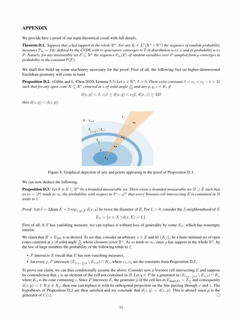
Proposition D.2. (Gibbs and L. Chen 2020, Lemma 5.3) Let x ∈ Rn, δ > 0. There exist constants 1 < c1 < c2 − 1 < 31such that for any open cone K ⊆ Rn centered at x of solid angle π

12 and any p, q, z ∈ K, if

d(x, p) < δ, c1δ ≤ d(x, q) < c2δ, d(x, z) ≥ 32δ

then d(z, q) < d(z, p).

Figure 8: Graphical depiction of sets and points appearing in the proof of Proposition D.3.

We can now deduce the following.

Proposition D.3. Let ∅ = E ⊆ Rn be a bounded measurable set. There exists a bounded measurable set B ⊇ E such thatas m = |P | tends to ∞, the probability with respect to P ∼ ρm that every Voronoi cell intersecting E is contained in Btends to 1.

Proof. Let δ = 2diam E = 2 supx,y∈E d(x, y) be twice the diameter of E. For L > 0, consider the L-neighbourhood of E

EL = {x ∈ X | d(x,E) < L}.

First of all, if E has vanishing measure, we can replace it without loss of generality by some EL, which has nonemptyinterior.

We claim that B = E32δ is as desired. To see that, consider an arbitrary x ∈ E and let {Kj}j be a finite minimal set of opencones centered at x of solid angle π

12 whose closures cover Rn. As m tends to ∞, since ρ has support in the whole Rn, bythe law of large numbers the probability of the following tends to 1:

• P intersects E (recall that E has non-vanishing measure),

• for every j, P intersects (E(c2− 12 )δ

\ Ec1δ) ∩Kj , where c1, c2 are the constants from Proposition D.2.

To prove our claim, we can thus conditionally assume the above. Consider now a Voronoi cell intersecting E and supposeby contradiction that z is an element of the cell not contained in B. Let q ∈ P be a generator in (E(c2− 1

2 )δ\ Ec1δ) ∩Kj

where Kj is the cone containing z. Since P intersects E, the generator p of the cell lies in Ediam(E) = E δ2

and consequentlyd(x, p) < δ. If p ∈ Kj , then one can replace it with its orthogonal projection on the line passing through x and z. Thehypotheses of Proposition D.2 are then satisfied and we conclude that d(z, q) < d(z, p). This is absurd since p is thegenerator of C(z).

11

For a bounded measurable set E ⊆ Rn, denote by

DE = maxp∈P

C(p)∩E =∅

diam C(p)

the maximum diameter of a Voronoi cell intersecting E.

Proposition D.4. DE , thought as a random variable in P , converges in probability to 0 as m = |P | tends to ∞.

Proof. The proof is inspired by Theorem 4 in Luc Devroye et al. 2015. Consider a finite minimal set of open cones {Kj}jcentered at 0 of solid angle π

12 whose closures cover Rn. Then there is a constant c > 0 such that for each p ∈ P

diam C(p) ≤ cmaxj

Rp,j

where Rp,j = minq∈P∩(p+Kj) d(p, q) denotes the distance from p to its closest neighbour in the cone Kj centered in p (andRp,j = ∞ if P ∩ (p +Kj) = ∅). This follows from Proposition D.2 applied with x = p to all the cones centered at thegenerators, with an opportune δ for each of them. For each ε > 0 we thus have an inclusion of events

{DE > ε} ⊆

maxp,j

C(p)∩E =∅

Rp,j >ε

c

⊆⋃i,j

{P ∩ (pi +Kj) ∩B

(pi,

ε

c

)= ∅ and C(pi) ∩ E = ∅

}where B(x, r) is the open ball centered in x of radius r. In the above, we assumed that the set P is equipped with an ordering.For x ∈ Rn denote by Ex,j the event appearing at the right member of the above expression for x = pi. We can then boundthe probability with respect to a random P ∼ ρm, with m = |P | fixed, as

PP∼ρm(DE > ε) ≤∑i,j

PP∼ρm(Epi,j) = m∑j

∫Rn

ρ(x)PP∼ρm(Ex,j | p1 = x) dx.

Since the points in P are sampled independently we have

PP∼ρm(Ex,j | p1 = x, C(x) ∩ E = ∅) =(1− P

((x+Kj) ∩B

(x,

ε

c

)))m−1

:= (1−M(x))m−1.

Pick the set B guaranteed by Proposition D.3. We can then conditionally assume that every Voronoi cell intersecting E iscontained in B, which implies PP∼ρm(Ex,j) = 0 for x ∈ B. The limit we wish to estimate reduces to

limm→∞

m∑j

∫Rn

ρ(x)PP∼ρm(Ex,j | p1 = x) dx =∑j

limm→∞

∫B

ρ(x)m(1−M(x))m−1 dx.

Since B is bounded and ρ has support in the whole Rn, M(x) is (essentially) bounded from below by a strictly positiveconstant as x varies in B. The limit can thus be brought under the integral and putting everything together we get:

limm→∞

PP∼ρm(DE > ε) ≤∑j

∫B

ρ(x) limm→∞

m(1−M(x))m−1 dx = 0.

We are now ready to prove Theorem D.1.

Proof. By the Portmanteau Lemma (Van der Vaart 2000), it is sufficient to that Pm(E) converges to P(E) in probabilityfor any bounded measurable set E ⊆ Rn which is a continuity set for P i.e., P(∂E) = 0 where ∂E is the (topological)boundary of E. Pick such E. By definition of the CVDE, for a fixed set P of generators we have that

12

Pm(E) =1

m|{p ∈ P | C(p) ⊆ E}|+

R︷ ︸︸ ︷1

m

∑p∈P

C(p)⊆EC(p)∩E =∅

Volp(C(p) ∩ E)

Volp(C(p))

=1

m|P ∩ E|+R− 1

m|{p ∈ P ∩ E | C(p) ⊆ E}|.

(13)

Since the Voronoi cells are closed, any cell intersecting E not contained in E intersects ∂E. Thus∣∣R− 1m |{p ∈ P ∩ E | C(p) ⊆ E}|

∣∣ ≤ 2R where R := 1m |{p ∈ P | C(p) ∩ ∂E = ∅}|. Now, the random variable

1m |P ∩E| tends to P(E) in probability as m tends to ∞ by the law of large numbers. In order to conclude, we need to showthat R tends to 0 in probability.

Fix ε > 0. For L > 0, consider the L-neighbour ∂EL = {x ∈ X | d(x, ∂E) < L} of the boundary ∂E. If the diameter ofthe Voronoi cells intersecting ∂E is less than L then all such cells are contained in ∂EL. Thus:

PP∼ρm (R > ε) ≤ PP∼ρm

(1

m|P ∩ ∂EL| > ε and D∂E < L

)+ PP∼ρm (D∂E ≥ L)

≤ PP∼ρm

(1

m|P ∩ ∂EL| > ε

)+ PP∼ρm (D∂E ≥ L)

≤ PP∼ρm

(∣∣∣∣P(∂EL)−1

m|P ∩ ∂EL|

∣∣∣∣ > ε− P(∂EL)

)+ PP∼ρm (D∂E ≥ L) .

(14)

Since ∂E is closed, ∂E = ∩L>0∂EL and thus limL→0 P(∂EL) = P(∩L∂EL) = P(∂E) = 0 since E is a continuity set.This implies that there is an L such that ε > P(∂EL). The right hand side of Equation 14 tends then to 0 by the law of largenumbers and Proposition D.4, which concludes the proof.

13