1

CATEGORIES: (5)

Title:

Exploration of a Cluttered Environment using Voronoi Transform and Fast Marching Method

Authors:

• Prof. Santiago Garrido, Robotics Lab., System Engineering and Automation Dept., Carlos III University,

Madrid, Spain. e-mail: sgarrido@ing.uc3m.es

• Prof. Luis Moreno, Robotics Lab., System Engineering and Automation Dept., Carlos III University, Madrid,

Spain. e-mail: moreno@ing.uc3m.es

• Prof. Dolores Blanco, Robotics Lab., System Engineering and Automation Dept., Carlos III University, Madrid,

Spain. e-mail: dblanco@ing.uc3m.es

Abstract

The Extended Voronoi Transform and the Fast Marching Method combination provide potential maps for robot

navigation in previously unexplored dynamic environments. The Extended Voronoi Transform of a binary image of

the environment gives a grey scale that is darker near obstacles and walls and lighter when far from them. The

Logarithm of the Extended Voronoi Transform imitates the repulsive electric potential from walls and obstacles.

The method proposed, called the Voronoi Fast Marching method, uses a Fast Marching technique on the Extended

Voronoi Transform of the environment’s image provided by sensors to determine a motion plan. The computational

efficiency of the method lets the planner operate at high rate sensor frequencies. This avoids the need for collision

avoidance algorithms. The robot is directed towards the most unexplored and free zones of the environment so as

to be able to explore all the workspace. This method is very fast and reliable and the trajectories are similar to the

human trajectories: smooth and not very close to obstacles and walls. In this article we propose its application in

the exploration task of unknown environments.

Keywords:

Navigation map, mobile robots, global localization, evolutive algorithm, robot mapping.

2

I. INTRODUCTION

Sensor based exploration is a fundamental function for mobile robot intelligence. There is a variety of potential

applications for autonomous mobile robots in such diverse areas as forestry, space, nuclear reactors, environmental

disasters, industry, and offices. Tasks in these environments are often hazardous to humans, in a remote located area,

or tedious to perform. Potential tasks for autonomous mobile robots include maintenance, delivery, and security

surveillance, which all require some form of intelligent navigational capabilities. A mobile robot is a useful addition

to these domains only when it is capable of [30] functioning robustly under a wide variety of environmental

conditions, [20] operating without human intervention for long periods of time, and [18] providing some guarantee

of task performance. The environments in which mobile robots mustfunction are dynamic, unpredictable and not

completely specifiable by a map beforehand. In order for the robot to successfully complete a set of tasks, it must

dynamically adapt to changing environmental circumstances. Sensor-based discovery path planning is the guidance

of an agent - a robot - without a complete a priori map, by discovering and negotiating the environment so as to

reach a goal location while avoiding all encountered obstacles. Sensor-based discovery (i.e., dynamic) path planning

is problematic because the path needs to be continually recomputed as new information is discovered.

In order to explore an unknown environment, this paper presents a exploration and path planning method based

on the Logarithm of the Extended Voronoi Transform and the Fast Marching Method. In each step of the exploration

process the sensors provide a binary image of the visible environment having distinguished the detected obstacles

of the free space. The Extended Voronoi Transform of an image gives a grey scale that is darker near the obstacles

and walls and lighter when far from them. The Logarithm of the Extended Voronoi Transform imitates the repulsive

electric potential in 2D from walls and obstacles. This potential impels the robot to follow a trajectory far from

obstacles.

The last step is to calculate the trajectory in the image generated by the Logarithm of the Extended Voronoi Trans-

form using the Fast Marching Method. Then, the path obtained verifies the smoothness and safety considerations

required for mobile robot path planning.

The Fast Marching Method has been applied to Path Planning [30], and their trajectories are of minimal distance,

but they are not very safe because the path is too close to obstacles and what is more important, the path is not

3

smooth enough.

In order to improve the safety of the trajectories calculated by the Fast Marching Method, two solutions are

possible:

The first possibility, in order to avoid unrealistic trajectories produced when the areas are narrower than the robot,

the segments with distances to the obstacles and walls smaller than the size of the robot need to be removed from

the Voronoi diagram previous to the Extended Voronoi Transform.

The second possibility, used in this work, it is to dilate the objects and walls in a security distance that assure

that the robot not collide and does not accept passages narrower than the robot’s size.

The advantages of this method are its easy implementation, its speed and the quality of the trajectories. The

method works in 2D and 3D, and can be used on a local scale operating with sensor information.

II. PREVIOUS AND RELATED WORKS

A. Representations of the world

Roughly speaking there are two main forms for representing the spatial relations in an environment: metric maps

and topological maps. Metric maps are characterized by a representation where the position of the obstacles are

indicated by coordinates in a global frame of reference. Some of them represent the environment with grids of

points, defining regions that can be occupied or not by obstacles or goals [18], [20]. Topological maps represent

the environment with graphs that connect landmarks or places with special features [24] [3]. In our approach we

choose the grid-based map to represent the environment. The clear advantage is that with grids we already have

a discrete environment representation and ready to be used in conjunction with the Extended Voronoi Transform

function and Fast Marching Method for path planning. The pioneer method for environment representation in a

grid-based model was the certainty grid method developed at Carnegie Mellon University [18] by Moravec. He

represents the environment as a 3D or 2D array of cells. Each cell stores the probability of the related region

being occupied. The uncertainty related to the position of objects is described in the grid as a spatial distribution

of these probabilities within the occupancy grid. The larger the spatial uncertainty, the greater the number of cells

occupied by the observed object. The update of these cells is performed during the navigation of the robot or

4

through the exploration process by using an update rule function. Many researchers have proposed their own grid-

based methods. The main difference among them is the function used to update the cell. Some of them are, for

example: Fuzzy [13], Bayesian [19], Heuristic Probability [10], Gaussian [11], etc. In the Histogramic In-Motion

Mapping (HIMM), each cell, has a certainty value, which is updated whenever it is being observed by the robots

sensors. The update is performed by increasing the certainty value by 3 (in the case of detection of an object) or

by decreasing it by 1 (when no object is detected), where the certainty value is an integer between 0 and 15.

B. Approaches to exploration

This section relates some interesting techniques used for exploratory mapping. They mix different localization

methods, data structures, search strategies and map representations. Kuipers and Byun [4] proposed an approach to

explore an environment and to represent it in a structure based on layers called Spatial Semantic Hierarchy (SSH)

[3]. The algorithm defines distinctive places and paths, which are linked to form an environmental topological

description. After this, a geometrical description is extracted. The traditional approaches focus on geometric

description before the topological one. The distinctive places are defined by their properties and the distinctive

paths are defined by the twofold robot control strategy: follow-the-mid-line or follow-the-left-wall. The algorithm

uses a lookup table to keep information about the place visited and the direction taken. This allows a search

in the environment for unvisited places. Lee [23] developed an approach based on Kuipers work [4] on a real

robot. This approach is successfully tested in indoor office-like spaces. This environment is relatively static during

the mapping process. Lee’s approach assumes that walls are parallel or perpendicular to each other. Furthermore,

the system operates in a very simple environment comprised of cardboard barriers. Mataric [24] proposed a map

learning method based on a subsumption architecture. Her approach models the world as a graph, where the

nodes correspond to landmarks and the edges indicate topological adjacencies. The landmarks are detected from

the robot movement. The basic exploration process is wall-following combined with obstacle avoidance. Oriolo

et al. [14] developed a grid-based environment mapping process that uses fuzzy logic to update the grid cells.

The mapping process runs on-line [13], and the local maps are built from the data obtained by the sensors and

integrated into the environment map as the robot travels along the path defined by theA∗ algorithm to the goal.

The algorithm has two phases. The first one is the perception phase. The robot acquires data from the sensors and

5

updates its environment map. The second phase is the planning phase. The planning module re-plans a new safe

path to the goal from the new explored area. Thrun and Bucken [28][29] developed an exploration system which

integrates both evidence grids and topological maps. The integration of the two approaches has the advantage of

disambiguating different positions through the grid-based representation and performing fast planning through the

topological representation. The exploration process is performed through the identification and generation of the

shortest paths between unoccupied regions and the robot. This approach works well in dynamic environments,

although, the walls have to be flat and cannot form angles that differ more than15◦ from the perpendicular. Feder

et al. [17] proposed a probabilistic approach to treat the concurrent mapping and localization using a sonar. This

approach is an example of a feature-based approach. It uses the extended Kalman filter to estimate the localization

of the robot. The essence of this approach is to take actions that maximize the total knowledge about the system in

the presence of measurement and navigational uncertainties. This approach was tested successfully in wheeled land

robot and autonomous underwater vehicles (AUVs). Yamauchi [35][5] developed the Frontier-Based Exploration

to build maps based on grids. This method uses a concept of frontier, which consists of boundaries that separate

the explored free space from the unexplored space. When a frontier is explored, the algorithm detects the nearest

unexplored frontier and attempts to navigate towards it by planning an obstacle free path. The planner uses a depth-

first search on the grid to reach that frontier. This process continues until all the frontiers are explored. Zelek [37]

proposed a hybrid method that combines a local planner based on a harmonic function calculation in a restricted

window with a global planning module that performs a search in a graph representation of the environment created

from a CAD map. The harmonic function module is employed to generate the best path given the local conditions

of the environment. The goal is projected by the global planner in the local windows to direct the robot. Recently,

Prestes el al. [33] have investigated the performance of an algorithm for exploration based on partial updates of a

harmonic potential in an occupancy grid. They consider that while the robot moves, it carries along an activation

window whose size is of the order of the sensors range.

Prestes and coworkers [34] propose an architecture for an autonomous mobile agent that explores while mapping

a two-dimensional environment. The map is a discretized model for the localization of obstacles, on top of which

a harmonic potential field is computed. The potential field serves as a fundamental link between the modeled

6

(discrete) space and the real (continuous) space where the agent operates.

The proposed method in this paper can be included in the sensor-based global planner paradigm. It is a potential

method but it does not have the typical problems of these methods enumerated by Koren- Borenstein [3]: 1) Trap

situations due to local minima (cyclic behavior). 2) No passage between closely spaced obstacles. 3) Oscillations

in the presence of obstacles. 4) Oscillations in narrow passages. The proposed method is conceptually close to the

navigation functions of Rimon-Koditscheck [6], because the potential field has only one local minimum located

at the single goal point. This potential and the paths are smooth (the same as the repulsive potential function)

and there are no degenerate critical points in the field. These properties are similar to the characteristics of the

electromagnetic waves propagation in Geometrical Optics (for monochromatic waves with the approximation that

length wave is much smaller than obstacles and without considering reflections nor diffractions).

The Fast Marching Method has been used previously in Path Planning by Sethian [32], [31], but using only an

attractive potential. This method has some problems. The most important one that typically arises in mobile robotics

is that optimal motion plans may bring robots too close to obstacles (including people), which is not safe. This

problem has been dealt with by Latombe [22], and the resulting navigation function is calledNF2. The Voronoi

Method also tries to follow a maximum clearance map [16]. Melchior, Poty and Oustaloup [26], [1], present a

fractional potential to diminish the obstacle danger level and improve the smoothness of the trajectories, Philippsen

[27] introduces an interpolated Navigation Function, but with trajectories too close to obstacles and without smooth

properties and Petres [7], introduces efficient path-planning algorithms for Underwater Vehicles taking advantage

of the underwaters currents.

To achive a smooth and safe path,it is necessary to have smooth attractive and repulsive potentials, connected in

such a way that the resulting potential and the trajectories have no local minima and curvature continuity to facilitate

path tracking design. The main improvement of the proposed method are these good properties of smoothness and

safety of the trajectory. Moreover, the associated vector field allows the introduction of nonholonomic constraints.

It is important to note that in the proposed method the important ingredients are the attractive and the repulsive

potentials, the way of connecting them describing the attractive potential using the wave equation (or in a simplified

way, the eikonal equation). This equation can be solved in other ways: Mauch[25] uses a Marching with Correctness

7

Criterion with a computational complexity that can reduced toO(N). Covello[8] presents a method that can be

used on nodes that are located on highly distorted grids or on nodes that are randomly located.

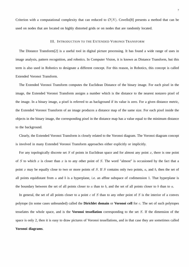
III. I NTRODUCTION TO THEEXTENDED VORONOI TRANSFORM

The Distance Transform[2] is a useful tool in digital picture processing. It has found a wide range of uses in

image analysis, pattern recognition, and robotics. In Computer Vision, it is known as Distance Transform, but this

term is also used in Robotics to designate a different concept. For this reason, in Robotics, this concept is called

Extended Voronoi Transform.

The Extended Voronoi Transform computes the Euclidean Distance of the binary image. For each pixel in the

image, the Extended Voronoi Transform assigns a number which is the distance to the nearest nonzero pixel of

the image. In a binary image, a pixel is referred to as background if its value is zero. For a given distance metric,

the Extended Voronoi Transform of an image produces a distance map of the same size. For each pixel inside the

objects in the binary image, the corresponding pixel in the distance map has a value equal to the minimum distance

to the background.

Clearly, the Extended Voronoi Transform is closely related to the Voronoi diagram. The Voronoi diagram concept

is involved in many Extended Voronoi Transform approaches either explicitly or implicitly.

For any topologically discrete setS of points in Euclidean space and for almost any pointx, there is one point

of S to which x is closer thanx is to any other point ofS. The word "almost" is occasioned by the fact that a

point x may be equally close to two or more points ofS. If S contains only two points,a, andb, then the set of

all points equidistant froma and b is a hyperplane, i.e. an affine subspace of codimension 1. That hyperplane is

the boundary between the set of all points closer toa than tob, and the set of all points closer tob than toa.

In general, the set of all points closer to a pointc of S than to any other point ofS is the interior of a convex

polytope (in some cases unbounded) called theDirichlet domain or Voronoi cell for c. The set of such polytopes

tesselates the whole space, and is theVoronoi tessellation corresponding to the setS. If the dimension of the

space is only 2, then it is easy to draw pictures of Voronoi tessellations, and in that case they are sometimes called

Voronoi diagrams.

8

a) b) c) d)

Fig. 1. Propagation of a wave and the corresponding minimum time path when there are two media of different slowness (diffraction)

index. (a), the same with an vertical gradient (b), Wavefront propagating with velocity F (c), and Formulation of the arrival functionT (x),

for an unidimensional wavefront.(d).

The close relation between EVT and the Voronoi Diagram implies that it is possible to compute one of them

from the other. The majority of the EVT methods use the Voronoi Diagram as an intermediate step.

For more than two dimensions, the Extended Voronoi Transform uses a nearest-neighbor search on an optimized

kd-tree, as described by Friedman[12].

The algorithm used in this work for two dimensions, is based on the second algorithm work carried out by Breu

et al. [6]. In this work, the special properties of the Euclidean metric are exploited. They designed two linear-time

algorithms based on Voronoi transforms where the second algorithm could have been improved if they had used

the result of the previous row to reduce the set of possible candidates. It is anO(m × n) algorithm, where the

image size ism× n.

The Voronoi approach to path planning has the advantage of providing the safest trajectories in terms of distance

to obstacles but because its nature is purely geometric and it does not achieve enough smoothness.

IV. I NTUITIVE INTRODUCTION OF THE EIKONAL EQUATION AND THE FAST MARCHING PLANNING METHOD

Intuitively, Fast Marching Method gives the propagation of a front wave in an inhomogeneous media as shown

in fig 1a and b.

Let us imagine that the curve or surface moves in its normal direction with a known speedF (see fig. 1c). The

objective would be to follow the movement of the interface while this one evolves. A large part of the challenge,

in the problems modeled as fronts in evolution, consists in defining a suitable speed, which faithfully represents

9

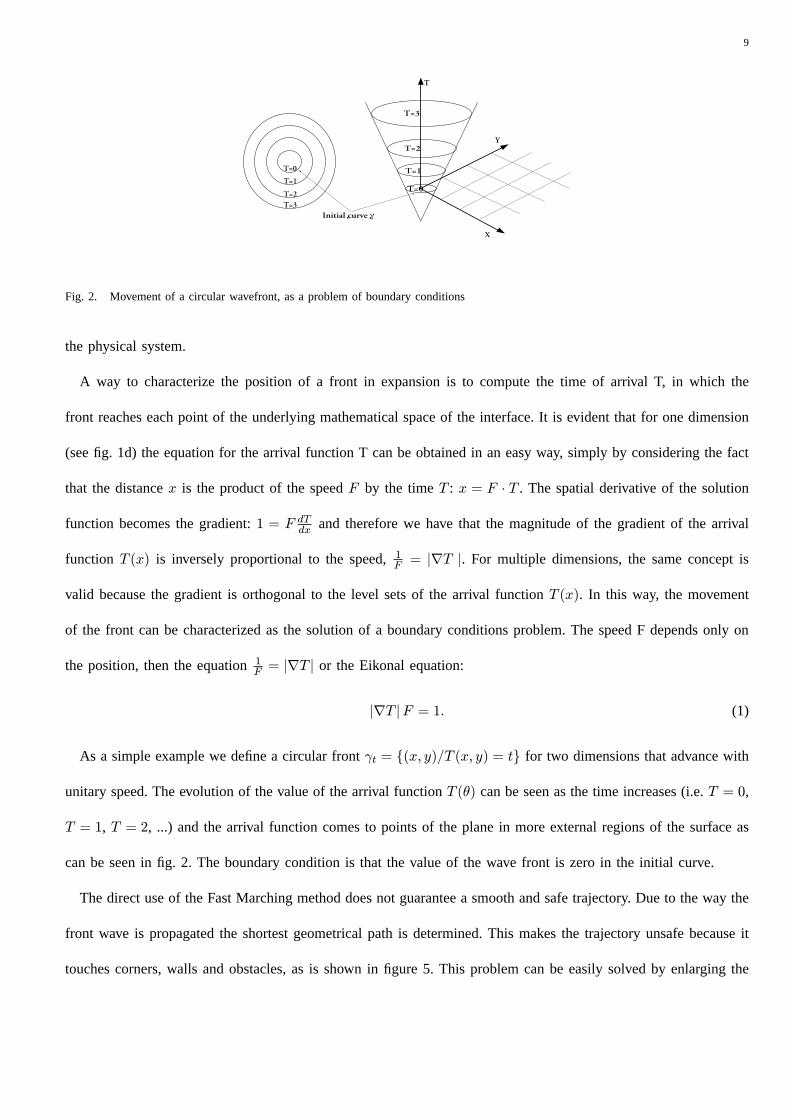
Fig. 2. Movement of a circular wavefront, as a problem of boundary conditions

the physical system.

A way to characterize the position of a front in expansion is to compute the time of arrival T, in which the

front reaches each point of the underlying mathematical space of the interface. It is evident that for one dimension

(see fig. 1d) the equation for the arrival function T can be obtained in an easy way, simply by considering the fact

that the distancex is the product of the speedF by the timeT : x = F ∙ T . The spatial derivative of the solution

function becomes the gradient:1 = F dTdx and therefore we have that the magnitude of the gradient of the arrival

function T (x) is inversely proportional to the speed,1F = |∇T |. For multiple dimensions, the same concept is

valid because the gradient is orthogonal to the level sets of the arrival functionT (x). In this way, the movement

of the front can be characterized as the solution of a boundary conditions problem. The speed F depends only on

the position, then the equation1F = |∇T | or the Eikonal equation:

|∇T |F = 1. (1)

As a simple example we define a circular frontγt = {(x, y)/T (x, y) = t} for two dimensions that advance with

unitary speed. The evolution of the value of the arrival functionT (θ) can be seen as the time increases (i.e.T = 0,

T = 1, T = 2, ...) and the arrival function comes to points of the plane in more external regions of the surface as

can be seen in fig. 2. The boundary condition is that the value of the wave front is zero in the initial curve.

The direct use of the Fast Marching method does not guarantee a smooth and safe trajectory. Due to the way the

front wave is propagated the shortest geometrical path is determined. This makes the trajectory unsafe because it

touches corners, walls and obstacles, as is shown in figure 5. This problem can be easily solved by enlarging the

10

a) b)

Fig. 3. Union of the two potentials: the second one having the first one as refractive index. a) Associated vector field and a typical trajectory

obtained with this method. b) The Funnel shaped potential applied to the first potential of a H-shaped environment and the path calculated

with the gradient method.

obstacles, but even in that case the trajectory tends to get close to the walls and it is not smooth and safe enough.

The use of the Fast Marching method over a slowness (refraction or inverse of velocity) potential improves the

quality of the calculated trajectory considerably. On one hand, the trajectories tend to go close to the Voronoi

skeleton because of the optimal conditions of this area for robot motion[15]. On the other hand, the trajectories are

also considerably smooth. For a small and easy H-shaped environment, the slowness (velocity inverse) potential

in 3D is shown in fig. 3b and the funnel shaped potential given by the wave propagation of and the trajectory

calculated by the gradient method is shown in fig. 3a.

For further details and summaries of level set and fast marching techniques for numerical purposes, see (Sethian

[31]). The Fast Marching Method is anO(n) algorithm as has been demonstrated by Yatziv [36].

V. I NTUITIVE INTRODUCTION TO THE VORONOI FAST MARCHING METHOD (VFM)

Which properties and characteristics are desirable for a Motion Planner of a mobile robot? The first one is that

the planner always drives the robot in a smooth and safe way to the goal point. In Nature there are phenomena

with the same way of working: electromagnetic waves. If in the goal point, there is an antenna that emits an

electromagnetic wave, then the robot could drive himself to the destination following the waves to the source. The

concept of the electromagnetic wave is especially interesting because the potential and its associated vector field,

11

see figure 3, have all the good properties desired for the trajectory, such as smoothness (it isC∞) and the absence

of local minima.

This attractive potential still has some problems. The most important one that typically arises in mobile robotics

is that optimal motion plans may bring robots too close to obstacles, which is not safe. This problem has been

dealt with by Latombe [22], and the resulting navigation function is calledNF2. The Voronoi Method also tries to

follow a maximum clearance map [16]. To get a safe path, it is necessary to add a component that repels the robot

away from obstacles. In addition, this repulsive potential and its associated vector field should have good properties

such those of electrical field. If we consider that the robot has an electrical charge of the same sign as obstacles,

then the robot would be pushed away from obstacles. The properties of this electric field are very good because it

is smooth and there are no singular points in the interest space (Cfree).

The third part of the problem consists in how to mix the two fields together. This union between an attractive and

a repulsive fields has been the biggest problem for the potential fields in path planning since the works of Khatib

[21]. In our exposition, this problem has been solved in the same way that Nature does so: the electromagnetic

waves, as light, have a propagation velocity that depends on the media. For example flint glass has a refraction

index of 1.6, while in the air it is approximately one. This refraction index of a medium is the quotient between

the velocity of light in the vacuum and the velocity in the medium. That is the slowness index of the front wave

propagation of a medium.

For this reason, in theVFM proposed method, the repulsive potential is used as refraction index of the wave

emitted from the goal point. This way a unique field is obtained and its associated vector field is attractive to

the goal point and repulsive from the obstacles. This method inherits the properties of the electromagnetic field.

Intuitively, theVFM Method gives the propagation of a front wave in an inhomogeneous media as shown in fig 1a

and b.

VI. A LMOST FLAT WAVE APPROACH OF THE WAVEEQUATION: THE EIKONAL EQUATION

Maxwell’s laws govern the propagation of the electromagnetic waves and can be modeled with the wave equation:

∂2φ

∂t2= c2∇2φ

12

In electrodynamics, each component of the fields satisfies the wave equation wherec2 = c20με . (c0 is the speed of

light in a vacuum,μ is the permeability andε is the dielectric constant). A solution of the wave equation is called

a wave. The moving boundary of a disturbance is called a wave front. In this section we will show how the wave

front can be described by an eikonal equation. We follow the reasoning presented in [9]. Ifc is constant, then there

are plane traveling wave solutions of the form

φ = φ0ei(kx−ωt)

(We can take the real or imaginary part to obtain a real-valued solution). Here the constantφ0 is the amplitude and

ω is the frequency. The wave number vectork is in the direction of the wave. This is perpendicular to the wave

fronts which satisfykx − ωt = constant. The wave numberk is the length of the wave vector,k =√k ∙ k and

satisfiesk = ωc . The index of refractionη is defined byc = c0

η . Let k0 be the wave number in a vacuum where the

index of refraction is unity. For simplicity, consider a wave propagating in the first coordinate direction.

φ = φ0eik0(ηx−c0t) (2)

Here we have factorized outk0 because we will be considering the case where the wave number is large. Now

we consider the case that the index of refractionη is spatially dependent. We seek a solution that is similar to the

plane wave in eq. 2.

φ = exp(A(x) + ik0(ψ(x)− c0t)) (3)

Here the amplitudeeA and the phasek0ψ are determined by the slowly varying functionsA(x) andψ(x).

To study the transmission of rays, a useful approach is the "almost flat waves" (i.e. the optical wave propagates

at wavelengths much smaller than image objects so that ray optics can approximate wave optics) in isotropic and

possibly non homogeneous media for a monochromatic wave. These equations along with the mentioned approach,

allow us to develop the theories based on rays such as: geometrical optics, the theory of sound waves, etc. We

compute the derivatives of this approximate almost flat wave.

∇φ = φ∇(A+ ik0ψ)

13

∇2φ = φ(∇2A+ ik0∇2ψ + (∇A)2 − k20(∇ψ)

2 + i2k0∇A ∙ ∇ψ)

We substitute eq. 3 into the wave equation.

η2

c20= ∇2φ

−k20η2 = ∇2A+ ik0∇

2ψ + (∇A)2 − k20(∇ψ)2 + i2k0∇A ∙ ∇ψ

SinceA andψ are real-valued, we equate the real and imaginary parts.

∇2A+ (∇A)2 + k0(η2 − (∇ψ)2) = 0

2∇A ∙ ∇ψ +∇2ψ = 0

We assume thatη varies slowly on the length scale of a wavelength,λ = 2π/k. Alternatively, for a fixed function

η, we assume that the frequency is high (the wavelength is short). This is the geometrical optics approximation.

For largek0, the first equation is approximately solved by an eikonal equation:

|∇ψ|2 = η2

We rewrite this eikonal equation in terms of the phaseu of the wave.

φ = exp(A(x) + i(u(x)− ωt))

|∇u|2 =ω2

c2

Surfaces of constant u describe the wave fronts. In the Sethian [30] notation

|∇T |F = 1

whereT (x) represents the wavefront (time),F (x) is the slowness index of the medium.

In Geometrical Optics, Fermat’sleast time principlefor light propagation in a medium with space varying

refractive indexη(x) is equivalent to the eikonal equation and can be written as||∇Φ(x)|| = η(x) where the

eikonalΦ(x) is a scalar function whose isolevel contours are normal to the light rays. This equation is also known

as Fundamental Equation of the Geometrical Optics.

The eikonal (from the Greek "eikon", which means "image") is the phase function in a situation for which the

phase and amplitude are slowly varying functions of position. Constant values of the eikonal represent surfaces of

14

constant phase, or wavefronts. The normals to these surfaces are rays (the paths of energy flux). Thus the eikonal

equation provides a method for "ray tracing" in a medium of slowly varying index of refractive (or the equivalent

for other kinds of waves).

VII. D ETAILS OF THE VFM ALGORITHM

This method starts with the calculation of the Logarithm of the Extended Voronoi Transform of the 2D a priori

map of the environment (or the Extended Voronoi Transform in case of 3D maps). Each white point of the initial

image (which represents free cells in the map) is associated with a level of grey that is the logarithm of the 2D

distance to nearest obstacles (or the Extended Voronoi Transform in 3D). As a result of this process, a kind of

potential proportional to the distance to the nearest obstacles to each cell is obtained, see figure 4. Zero potential

indicates that a given cell is part of an obstacle and maxima potential cells corresponds to cells located in the

Voronoi diagrams (which are the cells located equidistant to the obstacles).

This function introduces a potential similar to a repulsive electric potential (in 2D) as shown in figure 4, that

can be expressed by

φ = c1 log(r) + c2. (4)

wherec1 is a negative constant.

If n > 2 , (n is the space dimension), the potential is

φ =c3rn−1

+ c4. (5)

wherer is the distance from the origin.

In a second step, the technique proposed here uses Fast Marching to calculate the shortest trajectory in the

potential surface defined by logarithm of the Extended Voronoi Transform. The calculated trajectory is the geodesic

one in the potential surface, i.e. with a viscous distance. This viscosity is done by the grey level. If the Fast

Marching Method were used directly on the environment map, we would obtain the shortest geometrical trajectory,

as shown in fig. 5, but the trajectory is not safe nor smooth.

The potential created has local minima as shown in fig. 6 and 7, but the trajectories are not stuck in these points

because the Fast Marching Method gives the trajectories that correspond to the propagation of a wave front which

15

Fig. 4. Potential of the Logarithm of the inverse of Extended Voronoi Transform.

Fig. 5. Trajectory calculated with Fast Marching without the Logarithm Extended Voronoi Transform.

is faster in lighter regions and slower in the darker ones.

The trajectories obtained by using the logarithm of the EVT tend to go by the Voronoi diagram but properly

smoothed as shown figure 6.

VIII. P ROPERTIES

The proposedV FM algorithm has the following key properties:

• Fast response. The planner needs to be fast enough to be used reactively in case unexpected obstacles make it

necessary to plan a new trajectory. To obtain this fast response, a fast planning algorithm and fast and simple

treatment of the sensor information is necessary. This requires a low complexity order algorithm for a real

time response to unexpected situations. As shown in table I, the proposed algorithm has a fast response time

16

Fig. 6. Trajectory calculated with Fast Marching with the Logarithm Extended Voronoi Transform.

to allow its implementation on real time, even in environments with moving obstacles using a normal PC

computer.

Smooth trajectories. The planner must be able to provide a smooth motion plan which can be executed by the

robot motion controller. In other words, the plan does not need to be refined, avoiding the need for a local

refinement of the trajectory. The solution of the eikonal equation used in the proposed method is given by

equation 2:

φ = φ0eik0(ηx−c0t)

As this solution is an exponential, if the potentialη(x) is C∞ then the potentialφ is alsoC∞ and therefore

the trajectories calculated by the gradient method over this potential would be of the same class.

This smoothness property can be observed in figure 6, where trajectory is clearly good, safe and smooth. One

advantage of the method is that it not only generates the optimum path, but also the velocity of the robot at

each point of the path. The velocity reaches its highest values in the light areas and minimum values in the

greyer zones. TheV FM Method simultaneously provides the path and maximum allowable velocity for a

mobile robot between the current location and the goal.

• Reliable trajectories. The proposed planner provides a safe (reasonably far from a priori and detected obstacles)

and reliable trajectory (free from local traps). This avoids the coordination problem between the local collision

avoidance controllers and the global planners, when local traps or blocked trajectories exist in the environment.

17

This is due to the refraction index, which causes higher velocities far from obstacles.

• Completeness.As the method consists of the propagation of a wave, if there is a path from the the initial

position to the objective, the method is capable of finding it.

• Stability. The V FM 1st-step builds the slowness potential of the robot:x = f(x) and the second step builds

the corresponding Lyapunov potentialV (x) that is radially unbounded. By construction this potential has zero

value in the destination point and as it is the expansion of a wave with time as its last axis, it has positive

values and it increases with time (see figure 2a).

Using the Lyapunov Stability theorem:

If V : D → R is a continuously differentiable scalar function in a neighborhoodD of x = 0 such that:

V (0) = 0 andV (x) > 0, ∀x ∈ D − {0}

V (x) ≤ 0, ∀x ∈ D

(6)

then the origin is globally asymptotically stable.

Therefore, we can establish that the destination point (x = 0) is globally asymptotically stable.

IX. I MPLEMENTATION OF THE EXPLORER

In order to solve the problem of the exploration of an unknown environment, our algorithm can work in two

different ways. In the first one, the initial information is the localization of the final goal. In this way, the robot has a

general direction of movement towards the goal. In each movement of the robot, information about the environment

is used to build a binary image distinguishing occupied space represented by value 0 (obstacles and walls) from

free space, with value 1. The Extended Voronoi Transform of the known map at that moment, gives a grey scale

that is darker near the obstacles and walls and lighter far from them. The Voronoi Fast Marching Method gives the

trajectory from the pose of the robot to the goal point using the known information.

In this first case, the robot has a final goal: the exploration process the robot performs in the algorithm described

in the flowchart of figure 7.

In the second way of working of the algorithm, the goal location is unknown and robot behavior is truly

exploratory. We propose an approach based on the incremental calculation of a map for path planning. We define

18

Fig. 7. Flowchart of case 1.

an neighborhood window, that travels with the robot, with roughly the size of its laser sensor range. This window

indicates the new grid cells that are recruited for update, i.e., if a cell was at a given time in the neighborhood

window, it becomes part of the explored space by participating in the EVT and Fast Marching Method calculation

for all times. The set of activated cells that compose the explored space is called the neighborhood region. Cells

that were never inside the neighborhood window indicate unexplored regions. Their potential values are set to

zero and define the knowledge frontier of the state space, the real space in our case. The detection of the nearest

unexplored frontier comes naturally from the Extended Voronoi Transform calculation. It can also be understood

from the physical analogy with electrical potentials that obstacles repel while frontiers attract.

Consider that the robot starts from a given position in an initially unknown environment. In this second method,

there is no direction of the place where the robot must go. The first step consists of calculating a first matrix W

that gives us the EVT of the obstacles found up until the moment. A matrix with zeros in the obstacles and value

1 in the free zones is considered. The EVT is applied and a matrixW of grays with values between 0 (obstacles)

and 1 is obtained. The second matrix VT is built darkening the zones that the robot already has visited for which

it assigns value 1 to the points of the trajectory. Then, it calculates the EVT of the obtained image. Finally, matrix

WV is the sum of the matrices VT and W, with weights 0.5 and 1 respectively. In this way, it is possible to darken

19

the zones already visited for the robot and impel it to go to the unexplored zones. The whitest point of matrix WV

is calculated as max(WV), that is, the most unexplored region that is in a free space. This is the point chosen as the

new goal point. Applying Fast Marching method on WV, the trajectory towards that goal is calculated. The robot

moves following this trajectory. In the following steps, the trajectory to follow is computed, calculating at every

moment first W and VT, and therefore WV, but without changing the objective point. Once the robot has been

arrived at the objective, (that is to say, that path calculated is very small), a new objective is selected as max(WV).

Therefore, the robot moves maximizing knowledge gain. In this case or in any other situation where there is no

gradient to guide the robot, it simply follows the forward direction. The exploration process the robot performs in

the second method described is summarized in the flowchart of figure 8.

The algorithms laid out in Figure 7 (Flowchart of Case 1) can be inefficient in very large environments. To

increase speed it is possible to pick a goal point, put a neighborhood window the size of the sensor range, then run

into the goal point, then look at the maximal initial boundary, recast and terminate when one reaches the boundary

of the computed region. Similar improvements can be made to Algorithm 2.

X. RESULTS

The method proposed, can be used for sensor based planning, working directly on a raw sensor image of the

environment, as shown in figures 9 and 10.

To illustrate the method possibilities, a trajectory in a typical office’s indoor environment has been used for

planning as shown in figure 11 . The dimensions of the environment are 116x14 meters (the cell resolution is 12

cm), that is the image has 966x120 pixels. For this environment the first step (Log of inverse Extended Voronoi

Transform) takes 0.06 seconds in a Pentium 4 at 2.2 Ghz, and the second step (Fast Marching) takes 0.20 seconds

for a long trajectory.

The method provides smooth trajectories that can be used at low control levels without any additional smooth

interpolation process. The results are shown in figure 12 (Log of the inverse Extended Voronoi Transform of the

environment map of the Robotics Lab known a priori), some of the steps of the process in the figure 13 (the red

line represents the crossed path and the blue one represents the calculated trajectory from the present position to

the destination point). In each moment the illuminated area represents the front wave propagation from the present

20

Fig. 8. Flowchart of algorithm 2.

position of the robot to the destination point. The EVT computation is made over the sensory map that the robot

has in its memory. Finally in figure 14 the path obtained after applying the Fast Marching method to the previous

potential image is shown.

For the case of exploration that this paper contemplates, the results of two different tests are presented to illustrate

both cases described for the application of the proposed method.

Figure 15 represents the first case for implementing the exploration method. A final goal is provided for the

robot, which is located with respect to a global reference system; the starting point of the robot movement is also

known with respect to that reference system. The algorithm allows calculating the trajectory towards that final goal

with the updated information of the surroundings that the sensors obtain in each step of the movement. When the

robot reaches the defined goal, a new destination in an unexplored zone is defined, as it can be seen in the seventh

image of the figure. In this case the size of image is 628x412.

The results of one of the tests done for the second case of exploration described are shown in figure 16. Any

21

Fig. 9. Laser data read by the robot.

Fig. 10. Trajectory calculated with Fast Marching using the laser data (Local map).

Fig. 11. Environment map of the Robotics Lab.

Fig. 12. Log of the Extended Voronoi Transform applied of the environment map of the Robotics Lab.

22

Fig. 13. Consecutive steps of the process (the red line represents the crossed path and the blue one represents the calculated trajectory

from the present position to the destination point).

23

Fig. 14. Trajectory calculated to avoid obstacles in a cluttered environment with Fast Marching and the Logarithm Extended Voronoi

Transform (Global map).

final goal is defined. The algorithm leads the robot towards the zones that are free of obstacles and unexplored

simultaneously.

The proposed method is highly efficient from a computational point of view because the method operates directly

over a 2D image map (without extracting adjacency maps), and due to the fact that Fast Marching complexity is

O(m× n) and the Extended Voronoi Transform is also of complexityO(m× n), wherem× n is the number of

cells in the environment map. In table I, orientative results of the cost average in time appear (measured in ms),

and each step of the algorithm for different trajectory lengths to calculate (the computational cost is depending on

the number of points of the image).

TABLE I

COMPUTATIONAL COST (MS) FOR THE ROOM ENVIRONMENT OF FIG. 13 (966X120 PIXELS)

Alg. Step/Trajectorylength Long Medium Short

Obst. Enlarging 0.008 0.008 0.008

Ext. Voronoi Transf. 0.039 0.039 0.039

FM Exploration 0.172 0.078 0.031

PathExtraction 0.125 0.065 0.035

Total time 0.344 0.190 0.113

XI. CONCLUSION

The results obtained show that the Logarithm of Extended Voronoi Transform can be used to improve the results

obtained with Fast Marching method applied to environment exploration, providing smooth and safe trajectories

24

Fig. 15. Simulation results with method 1, with final objective.

25

Fig. 16. Simulation results with method 2, without final objective

26

along the exploratory process.

The algorithm complexity isO(m× n), wherem× n is the number of cells in the environment map, which let

us use the algorithm on line. Furthermore, the algorithm can be used directly with raw sensor data to implement a

sensor based local path planning exploratory module.

REFERENCES

[1] A. O. A. Poty, P. Melchior, “Dynamic path planning by fractional potential,” inSecond IEEE International Conference on Computational

Cybernetics, 2004.

[2] J. L. P. A. Rosenfeld, “Sequential operations in digital picture processing,”J. of the ACM, vol. 13, no. 4, pp. 471–494, 1966.

[3] T. L. B. Kuipers, “Navigation and mapping in large-scale space,”AI Magazine, vol. 9, pp. 25–43, 1988.

[4] Y. B. B. Kuipers, “A robot exploration and mapping strategy based on a semantic hierarchy of spatial representations,”Robotics and

Autonomous Systems, vol. 8, pp. 47–63, 1991.

[5] W. A. K. G. B. Yamauchi, A. Schultz, “Integrating map learning, localization and planning in a mobile robot,” inProceedings of the

IEEE International Symposium on Computational Intelligence in Robotics and Automation, Gaithersburg, MD, 1998, pp. 331–336.

[6] H. Breu, J. Gil, D. Kirkpatrick, and M. Werman, “Linear time euclidean distance transform algorithms,”IEEE Transactions on Pattern

Analysis and Machine Intelligence, vol. 17, no. 5, pp. 529–533, 1995.

[7] P. P. Y. P. J. E. D. L. C. Petres, Y. Pailhas, “Path planning for autonomous underwater vahicles,”IEEE Trans. on Robotics, vol. 23,

no. 2, pp. 331–341, 2007.

[8] P. Covello and G. Rodrigue, “A generalized front marching algorithm for the solution of the eikonal equation,”J. Comput. Appl. Math.,

vol. 156, no. 2, pp. 371–388, 2003.

[9] J. L. Davis,Wave propagation in solids and fluids. Springer, 1988.

[10] A. Elfes, “Sonar-based real world mapping and navigation,”IEEE Journal of Robotics and Automation, vol. 3, no. 3, pp. 249–265,

1987.

[11] A. Elfes, “Using occupancy grids for mobile robot perception and navigation,”Computer Magazine, pp. 46–57, 1989.

[12] J. H. Friedman, J. L. Bentley, and R. A. Finkel, “An algorithm for finding best matches in logarithmic expected time,”ACM Transactions

on Mathematics Software, vol. 3, no. 3, pp. 209–226, September 1997.

[13] M. V. G. Oriolo, G. Ulivi, “On-line map-building and navigation for autonomous mobile robots,” inProceedings of the IEEE

International Conference on Robotics and Automation, 1995, pp. 2900–2906.

[14] M. V. G. Oriolo, G. Ulivi, “Fuzzy maps: A new tool for mobile robot perception and planning,”Journal of Robotic Systems, vol. 3,

no. 14, pp. 179–197, 1997.

[15] S. Garrido, L.Moreno, and D.Blanco., “Voronoi diagram and fast marching applied to path planning.” in2006 IEEE International

conference on Robotics and Automation. ICRA 2006., pp. 3049–3054.

27

[16] S. Garrido, L. Moreno, M. Abderrahim, and F. Martin, “Path planning for mobile robot navigation using voronoi diagram and fast

marching.” inProc of IROS’06. Beijing. China., 2006, pp. 2376–2381.

[17] C. S. H. Feder, J. Leonard, “Adaptive mobile robot navigation and mapping,”International Journal of Robotics Research, vol. 7, no. 18,

pp. 650–668, 1999.

[18] A. E. H. Moravec, “High resolution maps from wide angle sonar,” inProceedings of the IEEE International Conference on Robotics

and Automation, 1985.

[19] L. K. A. Howard, “Generating sonar maps in highly specular environments,” inProceedings of the Fourth International Conference on

Control, Automation, Robotics and Vision, 1996.

[20] Y. K. J. Borenstein, “Histogramic in-motion mapping for mobile robot obstacle avoidance,”IEEE Journal of Robotics, vol. 7, no. 4,

1991.

[21] M. Khatib and R. Chatila, “An extended potential field approach for mobile robot sensor-based motions,” inProceedings of the IEEE

Int. Conf. on Intelligent Autonomus Systems, 1995.

[22] J.-C. Latombe,Robot motion planning. Dordrecht, Netherlands: Kluwer Academic Publishers, 1991.

[23] W. Lee, “Spatial semantic hierarchy for a physical robot,” Ph.D. dissertation, Department of Computer Sciences, The University of

Texas, 1996.

[24] M. Mataric, “Integration of representation into goal-driven behavior-based robots,”IEEE Transaction on Robotics and Automation,

vol. 3, pp. 304–312, 1992.

[25] S. Mauch, “Efficient algorithms for solving static hamilton-jacobi equations,” Ph.D. dissertation, California Inst. of Technology, 2003.

[26] P. Melchior, B. Orsoni, O. Laviale, A. Poty, and A. Oustaloup, “Consideration of obstacle danger level in path planning using a* and

fast marching optimisation: comparative study,”Journal of Signal Processing, vol. 83, no. 11, pp. 2387–2396, 2003.

[27] R. S. R. Philippsen, “An interpolated dynamic navigation function,” in2005 IEEE Int. Conf. on Robotics and Automation, 2005.

[28] A. B. S. B. Thrun, “Integrating grid-based and topological maps for mobile robot,” inProceedings of the 13th National Conference on

Artificial Intelligence (AAAI-96), 1996, pp. 944–950.

[29] A. B. S. Thrun, “Learning maps or indoor mobile robot navigation,” CMU-CS-96-121, Carnegie Mellon University, Pittsburgh, PA,

Tech. Rep., 1996.

[30] J. A. Sethian, “A fast marching level set method for monotonically advancing fronts,”Proc. Nat. Acad Sci. U.S.A., vol. 93, no. 4, pp.

1591–1595, 1996.

[31] J. A. Sethian, “Theory, algorithms, and aplications of level set methods for propagating interfaces,”Acta numerica, pp. 309–395, 1996,

cambridge Univ. Press.

[32] J. Sethian,Level set methods. Cambridge University Press, 1996.

[33] E. P. Silva., P. Engel, M. Trevisan, and M. Idiart, “Exploration method using harmonic functions,”Journal of Robotics and Autonomous

Systems, vol. 40, no. 1, pp. 25–42, 2002.

[34] E. P. Silva, P. Engel, M. Trevisan, and M. Idiart, “Autonomous learning architecture for environmental mapping,”Journal of Intelligent

28

and Robotic Systems, vol. 39, pp. 243–263, 2004.

[35] B. Yamauchi, “A frontier-based exploration for autonomous exploration,” inIEEE International Symposium on Computational

Intelligence in Robotics and Automation, Monterey, CA, 1997, pp. 146–151.

[36] L. Yatziv, A. Bartesaghi, and G. Sapiro, “A fast o(n) implementation of the fast marching algorithm,”Journal of Computational Physics,

vol. 212, pp. 393–399, 2005.

[37] J. Zelek, “A framework for mobile robot concurrent path planning and execution in incomplete and uncertain environments,” in

Proceedings of the AIPS-98 Workshop on Integrating Planning, Scheduling and Execution in Dynamic and Uncertain Environments,

Pittsburgh, PA, 1988.