arX

iv:1

511.

0657

2v1

[ph

ysic

s.da

ta-a

n] 2

0 N

ov 2

015

On non-Poissonian Voronoi tessellations

M. Ferraro and L. Zaninetti

Dipartimento di Fisica

Via Pietro Giuria 1

10125, Turin, Italy∗Corresponding author: zaninetti@ph.unito.it

July 26, 2021

Abstract

The Voronoi tessellation is the partition of space for a given seedspattern and the result of the partition depends completely on the type ofgiven pattern ”random”, Poisson-Voronoi tessellations (PVT), or ”non-random”, Non Poisson-Voronoi tessellations. In this note we shall considerproperties of Voronoi tessellations with centers generated by Sobol quasirandom sequences which produce a more ordered disposition of the centerswith respect to the PVT case. A probability density function for volumesof these Sobol Voronoi tessellations (SVT) will be proposed and comparedwith results of numerical simulations. An application will be presentedconcerning the local structure of gas (CO2) in the liquid-gas coexistencephase. Furthermore a probability distribution will be computed for thelength of chords resulting from the intersections of random lines with athree-dimensional SVT. The agreement of the analytical formula with theresults from a computer simulation will be also investigated. Finally anew type of Voronoi tessellation based on adjustable positions of seedshas been introduced which generalizes both PVT and SVT cases.

Keywords:

07.05.Tp ;Computer modeling and simulation89.75.Da ; Scaling phenomena in complex systems

1 Introduction

Three-dimensional Voronoi tessellations produce a random partition of the spacewhich have found applications ranging from geology, (Blower et al., 2002) andmolecular biology (Poupon, 2004; Dupuis et al., 2011) to numerical computing(for a review see (Du and Wang, 2005) and references therein), and chemistry(Jedlovszky et al., 2004; Idrissi et al., 2011).

In most studies Voronoi tessellations have been considered in which the posi-tions of the centers are randomly distributed, giving rise to the so called Poisson-Voronoi tessellations (PVT) (Okabe et al., 2000) even though examples of non

∗zaninetti@ph.unito.it

1

Poissonian Voronoi Tessellation can be found in the literature (Heinrich and Schiile,1995; Chiu and Quine, 2001; Gonzalez and Einstein, 2011). Non uniform distri-butions of the centers can be of interest to model regular physical configurations;we shall consider here the properties of Voronoi tessellations whose center aregenerated by Sobol quasi random sequences (Sobol, 1967; Bratley, P. and Fox, B. L.,1988).

A probability density function (PDF) for volumes of these Sobol Voronoitessellations (SVT) will be proposed and compared with the results of numericalsimulations.

In section 3.1 SVT and PVT will be used in an application concerning thelocal structure of gas (CO2) in the liquid-gas coexistence phase.

In addition, we shall consider the relations between these three-dimensionalstructures and their lower dimensional sections; in particular we shall studychord length distributions resulting from the random intersection of SVT withstraight lines. In case of PVT probability density functions of chords can be de-rived rigorously (Muche and Stoyan, 1992; Muche, 2010), see also (Okabe et al.,2000); here we shall present an empirical method to calculate a PDF of chordlengths in the case of SVT.

Finally Voronoi tessellations derived by perturbating the positions of pointslying on a regular lattice will be considered.

2 Probability density functions

In the case of one-dimensional PVT, with average linear density λ, it has beenproved (Kiang, 1966) that the distribution of the lengths of the segments hasPDF

p(l) = 4λ2l exp (−2λl). (1)

At the present time there are no analytical formulae for the area’s and volume’sdistribution and we limited ourself to explore the available conjectures. Nu-merical experiments have shown that for PVT an approximate solution can beobtained via a 3 parameters generalized Gamma distribution, that in case of avariable x is

G(x; a, b, c) =ab

c

axc−1e−bxa

Γ(

ca

) , (2)

see (Hinde and Miles, 1980; Tanemura, 2003; Khodabin and Ahmadabadi, 2010;Lazar et al., 2013). The main moments of G(x; a, b, c) are:

〈x〉 = b−a−1

Γ(

1+ca

)

Γ(

ca

) , (3)

σ2 =b−2 a−1

(

Γ(

c+2

a

)

Γ(

ca

)

−(

Γ(

1+ca

))2)

(

Γ(

ca

))2, (4)

the skewness γ is

γ =Γ(

3+ca

) (

Γ(

ca

))2 − 3 Γ(

1+ca

)

Γ(

c+2

a

)

Γ(

ca

)

+ 2(

Γ(

1+ca

))3

(

Γ(

c+2

a

)

Γ(

ca

)

−(

Γ(

1+ca

))2)3/2

, (5)

2

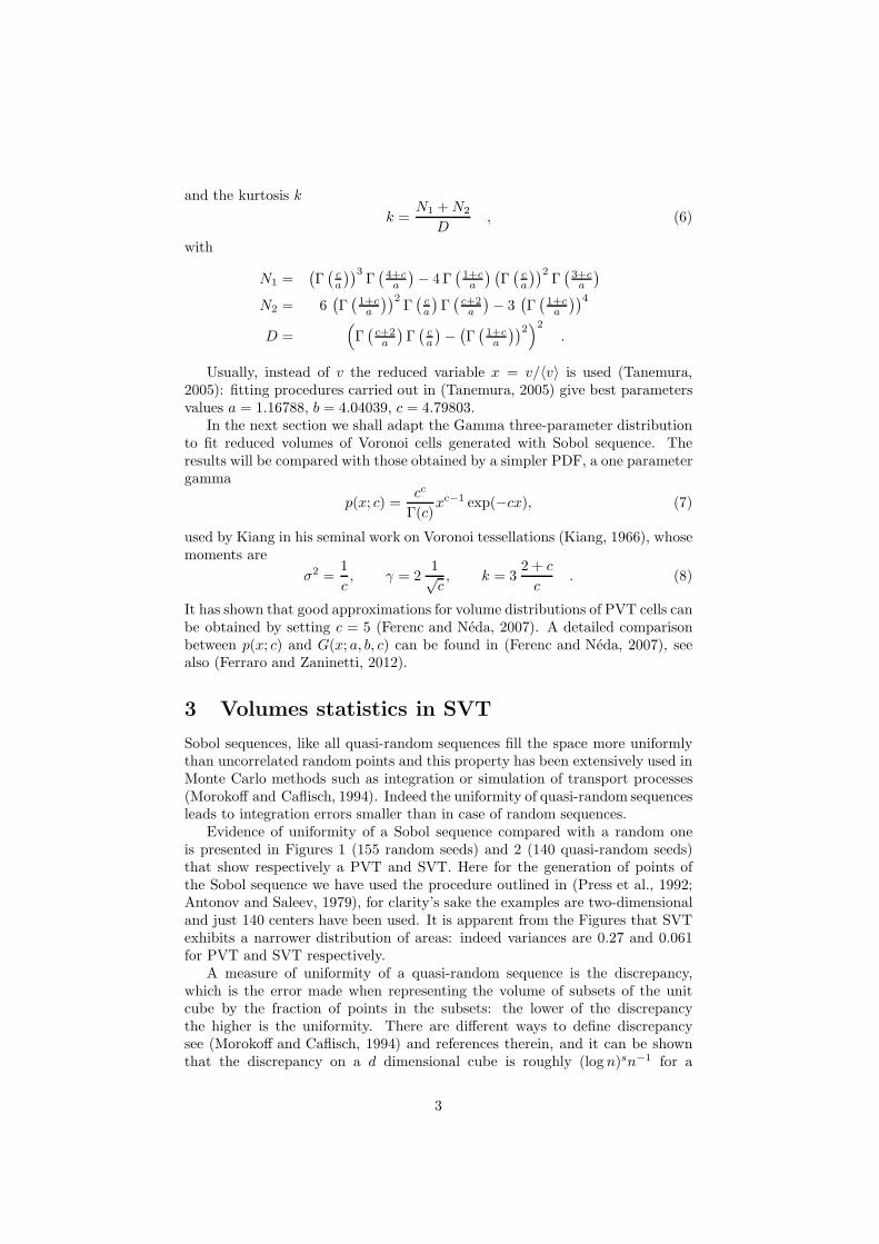
and the kurtosis k

k =N1 +N2

D, (6)

with

N1 =(

Γ(

ca

))3Γ(

4+ca

)

− 4 Γ(

1+ca

) (

Γ(

ca

))2Γ(

3+ca

)

N2 = 6(

Γ(

1+ca

))2Γ(

ca

)

Γ(

c+2

a

)

− 3(

Γ(

1+ca

))4

D =(

Γ(

c+2

a

)

Γ(

ca

)

−(

Γ(

1+ca

))2)2

.

Usually, instead of v the reduced variable x = v/〈v〉 is used (Tanemura,2005): fitting procedures carried out in (Tanemura, 2005) give best parametersvalues a = 1.16788, b = 4.04039, c = 4.79803.

In the next section we shall adapt the Gamma three-parameter distributionto fit reduced volumes of Voronoi cells generated with Sobol sequence. Theresults will be compared with those obtained by a simpler PDF, a one parametergamma

p(x; c) =cc

Γ(c)xc−1 exp(−cx), (7)

used by Kiang in his seminal work on Voronoi tessellations (Kiang, 1966), whosemoments are

σ2 =1

c, γ = 2

1√c, k = 3

2 + c

c. (8)

It has shown that good approximations for volume distributions of PVT cells canbe obtained by setting c = 5 (Ferenc and Neda, 2007). A detailed comparisonbetween p(x; c) and G(x; a, b, c) can be found in (Ferenc and Neda, 2007), seealso (Ferraro and Zaninetti, 2012).

3 Volumes statistics in SVT

Sobol sequences, like all quasi-random sequences fill the space more uniformlythan uncorrelated random points and this property has been extensively used inMonte Carlo methods such as integration or simulation of transport processes(Morokoff and Caflisch, 1994). Indeed the uniformity of quasi-random sequencesleads to integration errors smaller than in case of random sequences.

Evidence of uniformity of a Sobol sequence compared with a random oneis presented in Figures 1 (155 random seeds) and 2 (140 quasi-random seeds)that show respectively a PVT and SVT. Here for the generation of points ofthe Sobol sequence we have used the procedure outlined in (Press et al., 1992;Antonov and Saleev, 1979), for clarity’s sake the examples are two-dimensionaland just 140 centers have been used. It is apparent from the Figures that SVTexhibits a narrower distribution of areas: indeed variances are 0.27 and 0.061for PVT and SVT respectively.

A measure of uniformity of a quasi-random sequence is the discrepancy,which is the error made when representing the volume of subsets of the unitcube by the fraction of points in the subsets: the lower of the discrepancythe higher is the uniformity. There are different ways to define discrepancysee (Morokoff and Caflisch, 1994) and references therein, and it can be shownthat the discrepancy on a d dimensional cube is roughly (log n)sn−1 for a

3

Figure 1: An example of PVT in 2D.

large number of points n, whereas random sequences have discrepancy of size(log logn)1/2n−1.

A simple measure of uniformity can be also defined as follows: for a Soboltessellation with n seeds of an unit area the minimum distance dmin betweenany two seeds is first computed and next dmin is divided by dL = 1

n , the distancebetween two seeds in the case of a regular lattice of unit area. Thus the ratiodmin

dLshould be larger for a quasi-random sequence of seeds compared with a

random one. When n=1000 the ratio dmin

dLis 0.093 in the case of 2D Sobol seeds

and 0.0056 in the case of random (Poissonian) seeds.Thus, Sobol sequences present a repulsion effect that can be also found in

other quasi-random sequences such as, for example, those generated by theeigenvalues of complex random matrices, see (Le Caer and Ho, 1990).

The eigenvalues seeds can be found starting from a random N ×N complexmatrix. The matrix elements are given by x + iy where x and y are pseudorandom real numbers taken from a normal ( Gaussian ) distribution with meanzero and standard deviation 1/

√2. Once obtained the complex elements we

diagonalize the complex matrix using the subroutine CG from the EISPACKlibrary. The points seeds have the x and y coordinates corresponding to thereal and imaginary parts of the complex eigenvalues and an example which hasvariance 0.06 is reported in Figure 3.

Next we have generated a three-dimensional SVT with 104 cells: the his-

4

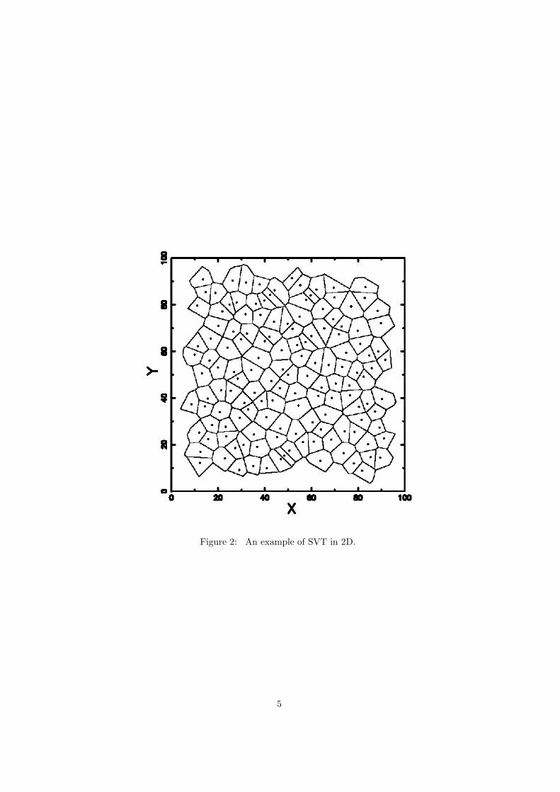
Figure 2: An example of SVT in 2D.

5

Figure 3: Tessellation generated by 174 eigenvalues from complex matrix in2D.

6

togram of their volumes has been fitted with the generalized gamma G(x; a, b, c),as given by (2), and the one parameter gamma p(x; c), see (7), respectively.

The statistical parameters of the two fits and the sample’s parameters arereported in Table 1, were the first line shows numerical values of the parametersfor generalized three-parameter and the one-parameter gamma, respectively,obtained from the fit of empirical data, the next lines report values of mean,variance, skewness and the kurtosis for the two distributions and the sample,here the number of cells is 104 and the number of bins is 40.

Table 1: Parameters for generalized three-parameter and the one-parametergamma, respectively, obtained from the fit of normalized volumes.

Moment Generalized gamma One parameter gamma Samplea = 2.3317, b = 2.86816, c = 7.32528 c = 16.32099

〈xSV T 〉 0.99993 1 1σ2SV T 0.0613809 0.06127 0.06127

γSV T 0.191594 0.49505 0.20973kSV T 2.94336 3.36762 3.15243

The goodness of the fit has been assessed by first computing the PDF of bothG and p and next applying the Kolmogorov-Smirnov (K-S) test (Kolmogoroff,1941; Smirnov, 1948; Massey, 1951).

The three- parameter PDF G fits well the simulated volumes: the maximumdistance between the empirical and computed distributions functions dmax =0.01 and the result of the K-S test, implemented with the FORTRAN subroutineKSONE (Press et al., 1992), gives PKS = 0.21. Note also that its momentsappear to be close with those derived from the empirical distribution.

As concerns p(x:c) the results of the K-S test are worse, dmax = 0.024,PKS = 1.9 10−5. Figure 4 shows the histogram of volumes generated by thesimulation, the number of Sobol centers is 104, the number of division n=40,and the graph of the generalized gamma used to fit the data with parametervalues given by Table (1). In Figure 5 we report the comparison between theempirical distribution and the distribution function (DF) of G with parametersas in Table 1.

It can be interesting to compare values of the moments obtained here withthose derived for PVT, by using estimate of a, b, c given in (Tanemura, 2005),namely

σ2PV T = 0.1787603, γPV T = 0.7766972, kPV T = 3.849375.

Volumes distribution of SVT shows a smaller variance, as result of the factthe centers are distributed in a more regular fashion than in case of PVT;furthermore the PDF is more symmetric for SVT (γSV T < γPV T ); finally kSV T

is very close to 3, the value of the Gaussian kurtosis.A comparison between the generalized gamma PDFs for the two cases is

shown in Figure 6.

7

Figure 4: Histogram (step-diagram) of the SVT reduced volume distribution.

Figure 5: Simulated volume distribution (small circles) and DF of the gener-alized gamma (full line).

8

Figure 6: Plot of reduced gamma PDFs for the PVT (full line) and SVT case(broken line) .

3.1 An application

In this section it has been shown that the main differences between distributionsof volumes in case of SVT vs PVT are that the former have a smaller varianceand are more symmetric and it has been argued that, clearly, these differencesare related to the more regular distributions of centers in case of SVTs. Thissuggests a possible application in understanding different PDF for volumes ob-tained in simulations of local structure of gases, in the liquid-gas phase. In(Idrissi et al., 2010) CO2 was considered and simulations were carried out todetermine the volumes available to each molecule that were considered as thecenter of a Voronoi tessellation. From the simulation the empirical PDF of vol-umes P (V ) can be computed and results show an increase of mean volume 〈V 〉and standard deviation σV as temperature rises: the former effect is due to thethermal expansion of the system (Idrissi et al., 2010), whereas the increase ofσV points to more disordered distribution of the centers at higher temperaturesand to increasing volume fluctuations. To compare our results with the datain (Idrissi et al., 2010), see Table 2, we have computed the standard deviation

Table 2: Mean values and standard deviations of the Voronoi polyhedra,V, andc of the Kiang function.

T/K 250 270 285 298 303 306 313

〈V 〉/A369.7± 10.3 77.5± 13.8 87.1± 19.4 105.3± 31.1 114.4± 38.2 156.8± 68.8 156.8± 65.1

c 45.79 31.53 20.15 11.46 8.96 5.19 5.8

for the reduced volumes x = V/〈V 〉, namely σ = σV /〈V 〉, and compared themwith the standard deviations σSV T and σPV T of the PDFs derived in 3. As an

9

example when T = 250 K, 〈V 〉 = 69.7A3, σ = 10.3/69.7 = 0.147, σ2 = 0.0218

and c = 1/0.0218 = 45.79. We briefly recall that the data of the previous Ta-ble are theoretical values computed with the Voronoi polyhedra (VP) analysisbased on numerical codes developed by (Jedlovszky, 1999, 2000; Tokita et al.,2004).

In the temperature range from T = 250 to T = 303 σ increases from 0.15 to0.33 and σSV T = 0.25 is in the middle of this range. At higher temperatures,T = 303 and T = 313 one obtains σ = 0.43 and σ = 0.41, respectively, matchingclosely the standard deviation derived for for PVT, namely σPV T = 0.43. Moreimportantly, the shape of the PDF , which is quite symmetric at the lower endof the T range, increasingly deviates symmetry as T increases and develops anexponentially decaying tail at high volume values (Idrissi et al., 2010). This isalso what happens in the transition from SVT to PVT, see Figure 6. Theseresults can be explained as follows: as T increases positions of molecules be-come more random and a transition takes place from a PDF relatively narrowand symmetric (like in the SVT case) to a more asymmetric PDF with largervariance corresponding to a PVT. The relation between the distributions of oc-cupied volumes and the temperature T can be made clearer by considering theparameter c of the Kiang distribution (7). It is clear that small values of c char-acterize distributions with relatively large variance and skweness, whereas as cincrease distributions become narrower and more simmetric. The parameter cof the Kiang function can be parameterised as function of the temperature asfollows

c = C1Tα1 , (9)

where C1 and α1 can be found from the data of Table 2. A numerical proceduregives C1 = 5.7 1025 and α1 = −10.

4 Chords length distribution

In many experimental conditions it is not possible to directly observe the three-dimensional cells forming a tessellation, just their linear sections: thus it is ofinterest to study the relationships between the geometric properties of three-dimensional structures and their chords (Ruan et al., 1988; Okabe et al., 2000;Stoyan et al., 2011).

One can distinguish three main ways to generate chords (Coleman, 1969),(Kellerer, 1984): isotropic uniform randomness results when the body is exposedto an uniform isotropic flow of infinite straight lines; weighted randomness oc-curs when a uniformly distributed random point is chosen and is traversed by astraight line with uniform random direction; two-point randomness is obtainedwhen a straight line traverses two random points that are independently anduniformly distributed. The first case, which will be considered here since morerelevant for practical applications (Kellerer, 1984); relations among PDFs ofchords generated by different methods can be found in (Kellerer, 1984).

In order to obtain formulas for the distributions of the chords generated bythe intersections of lines with SVTs some simplifications are needed: here thepolyhedrons forming the cells will be approximated by spheres and the one-parameter distribution p as given by Equation(7), will be used to fit the cellsvolumes distribution. With these assumptions a formula for the PDF of chordslength can been obtained, a simple iterative procedure will then be used to adapt

10

this distribution to the simulated data, thus correcting the errors resulting fromthe approximations. Let px be the probability density function for the reducedcell volumes, then the PDF py for the lengths of the diameters is given by

py(y) =π

2px

(

1

6πy3

)

y2 , (10)

and the probability density function g of chords length l is

g(l) =2l

〈y2〉

∫

∞

l

py(y)dy , (11)

see, for instance, (Ruan et al., 1988), (Watson, 1971). In the present case then,with PDF of volumes given by the Kiang function, Eq. (7), with c = 16, thedistribution of diameters is

py(y) =1

2

1616π16

615Γ(16)y47 exp

(

−8π

3y3)

. (12)

The use of the generalized gamma function, Eq.(2), for the PDF in volumesmeans conversely that the integrals which follow can be done only in a numericalway. The probability density gSV T can be found by making use of Eq. (11) withpy given by (12), the result is

gSV T (l) =a0a1

exp

(

−8

3πl3

) 9∑

k=0

bkπkl3k+1 , (13)

where the coefficients are large numbers, whose values are reported in the Ap-pendix. The previous formula and the following ones are not an exact analyticalresult but results from the approximation of the volume of the Voronoi’s poly-hedrons by spheres. In order to check the validity of this PDF we inserted ina box 50000 seeds which produce a network of irregular faces belonging to theVoronoi’s polyhedra. We selected 120 random lines which will intercept thenetwork of the irregular faces: the chord’s length is evaluated as the distancebetween a face and the following one on the considered line. A typical runprocesses a total number of ≈ 3200 chords. The corresponding histogram isshown in Figure 7: note that here the results has been rescaled so that theaverage value of chord length is equal to 1. It is apparent that the results ofthe simulations do not agree with the PDF given by Eq. (13): it is enoughto note that gSV T (0) = 0, is in contrast with the histogram of Figure 7. Inorder to overcome this problem a new variable z has been defined by a shift ofl: z = l − a, so that g1,SV T (z) = gSV T (z + a). The shift parameter a shouldnot be confused with the parameter of the generalized gamma PDF (compareEq. (2)). An explanation for this shift is given by the fact that the length ofthe chord which touches only in one point the sphere is zero conversely a chordwhich lies on a irregular face of the Voronoi’s polyhedron has a finite length.This means that we have more short lengths in the simulation of the chordswith the real polyhedrons in respect to the length’s of theoretical intersectionswith the spheres: i.e. the PDF of having short chords is finite rather than zero.

Next, to obtain a reduced variable, a scale change has been applied resultingin u = bz . The scale parameter b used here is different from the parameter

11

Figure 7: Histogram (step-diagram) for SVT chord length with average value1

of the generalized gamma PDF (compare Eq. (2)). In conclusion, followingtranslation and scale change, the final PDF is now

gf,SV T (u; a, b) =C

bgSV T

(u

b+ a

)

(14)

=Ca0ba1

exp

(

−8

3π(u

b+ a

)3) 9∑

k=0

bkπk(u

b+ a

)3k+1

,

where C is a normalizing constant, which has value 1.4717.Numerical values of a and b have been obtained by an interactive procedure

that at each step computes the DF

F (u; a, b) =

∫ u

0

gf,SV T (z; a, b)dz : (15)

the agreement between the calculated and simulated distribution function isthen been verified by the K-S test. The procedure is halted when dmax, themaximum distance between the distribution functions, reaches a minimum (thatis when the significance level PKS is maximum) and the corresponding pair a, bis selected; Table 4 reports the adopted values. Calculated and empirical DFsof chords length are shown in Figure 8, the K-S test gives dmax = 0.0165,PKS = 0.251. The moments of gf,SV T are presented in Table 3 with parametersas in Table 4.

The results can also be presented as a PDF, see Figure 9, parameters as inTable 4; the reduced χ2 is 1.09. The shifted PDF, gf,SV T , for SVT chords canbe reported as a Taylor expansion around x=0 , when the average value is one

gf,SV T (x; 0.7, 3.27) = 0.411 + 0.179 x− 0.444 10−5 x2

−0.243 10−4x3 − 0.958 10−3 x4 − 0.285 10−3 x5. (16)

12

Figure 8: Comparison between data (empty circles) and theoretical DF forgf,SV T (continuous line) for chords length.

Table 3: Moments of the probability density function gf,SV T , Sobol seeds.

Parameter value

Mean 1

V ariance 0.308

Skewness 0.0888Kurtosis 2.164

13

Figure 9: Histogram (step-diagram) for SVT chord length with average value1 and PDF gf,SV T ( line).

It is clear that at x = 0 this PDF takes a finite value.

4.1 The PVT chord

Chords length distribution in case of PVT can be obtained with the samemethod, by adopting now as the volumes PDF Eq. (7) with c = 5, whichis known to give a good fit of simulated data (Ferenc and Neda, 2007). Theresulting integral for the chord as given by eqn.(11) is

gPV T (l) =125 l13π14/352/3 3

√6

39424 Γ (2/3)(

eπ l3)5/6

+75 l10π11/352/3 3

√6

4928 Γ (2/3)(

eπ l3)5/6

+135 l7π8/352/3 3

√6

2464 Γ (2/3)(

eπ l3)5/6

+81 l4π5/352/3 3

√6

616 Γ (2/3)(

eπ l3)5/6

(17)

+243 lπ2/352/3 3

√6

1540 Γ (2/3)(

eπ l3)5/6

.

We now apply translation and scale change

gf,PV T (u; a, b) =C

bgPV T

(u

b+ a

)

, (18)

and Table4 reports the parameters adopted. Figure 10 reports a comparisonof the previous result, integration of PDF (18)and parameters as in Table 4,as a dashed line with the tabulated result as deduced from Table 5.7.4 in(Okabe et al., 2000) when the average value of both PDFs is one. Table 5reports the two numerical sequences.

14

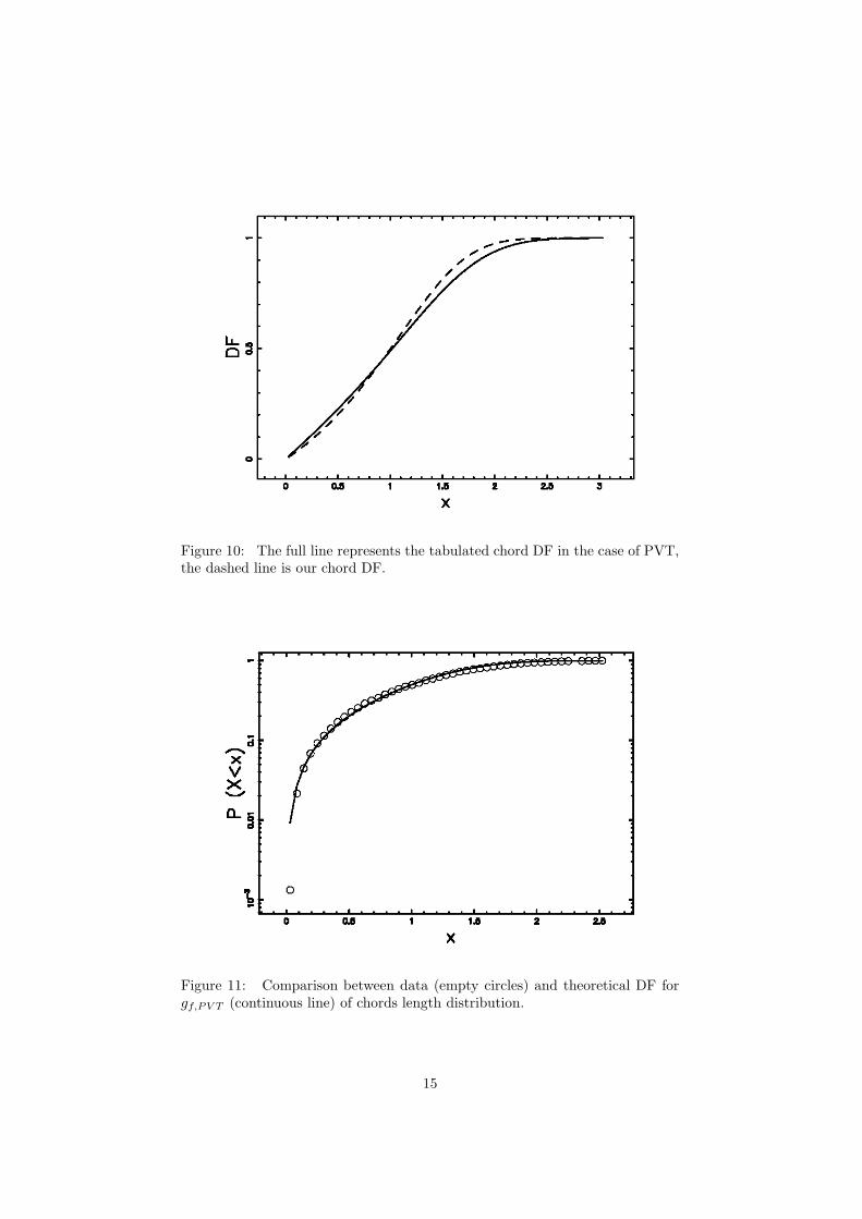
Figure 10: The full line represents the tabulated chord DF in the case of PVT,the dashed line is our chord DF.

Figure 11: Comparison between data (empty circles) and theoretical DF forgf,PV T (continuous line) of chords length distribution.

15

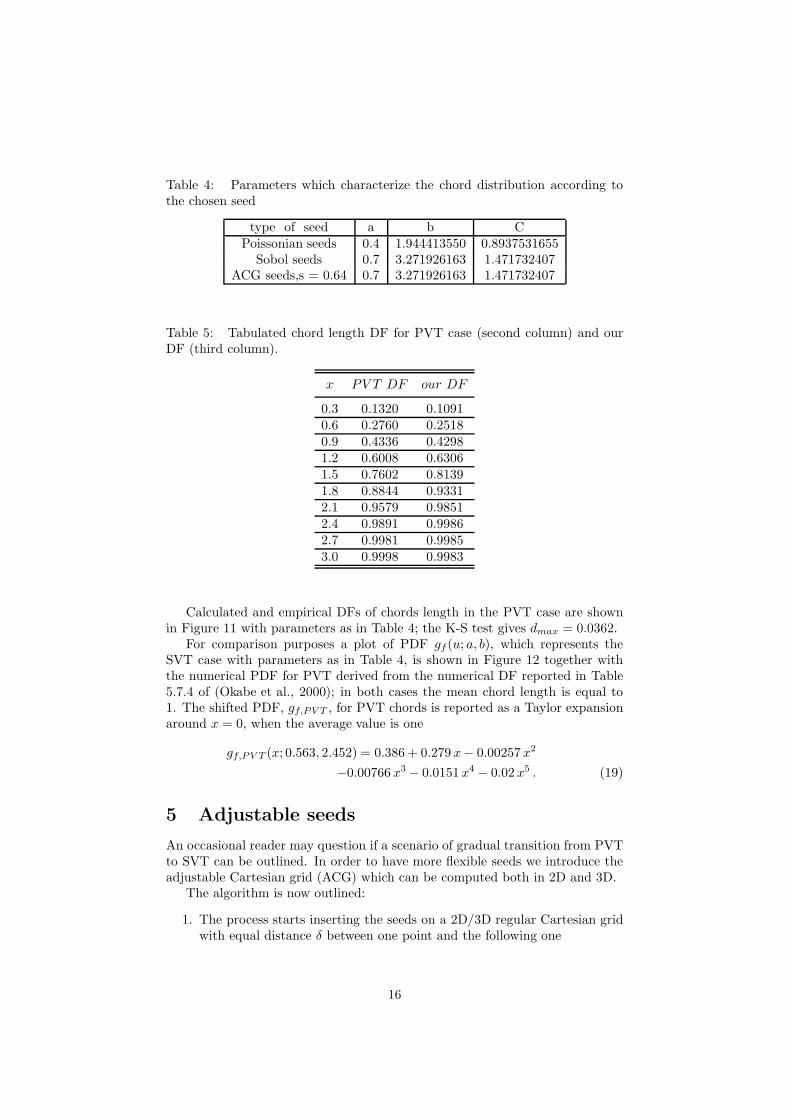
Table 4: Parameters which characterize the chord distribution according tothe chosen seed

type of seed a b CPoissonian seeds 0.4 1.944413550 0.8937531655

Sobol seeds 0.7 3.271926163 1.471732407ACG seeds,s = 0.64 0.7 3.271926163 1.471732407

Table 5: Tabulated chord length DF for PVT case (second column) and ourDF (third column).

x PV T DF our DF

0.3 0.1320 0.10910.6 0.2760 0.25180.9 0.4336 0.42981.2 0.6008 0.63061.5 0.7602 0.81391.8 0.8844 0.93312.1 0.9579 0.98512.4 0.9891 0.99862.7 0.9981 0.99853.0 0.9998 0.9983

Calculated and empirical DFs of chords length in the PVT case are shownin Figure 11 with parameters as in Table 4; the K-S test gives dmax = 0.0362.

For comparison purposes a plot of PDF gf (u; a, b), which represents theSVT case with parameters as in Table 4, is shown in Figure 12 together withthe numerical PDF for PVT derived from the numerical DF reported in Table5.7.4 of (Okabe et al., 2000); in both cases the mean chord length is equal to1. The shifted PDF, gf,PV T , for PVT chords is reported as a Taylor expansionaround x = 0, when the average value is one

gf,PV T (x; 0.563, 2.452) = 0.386 + 0.279 x− 0.00257 x2

−0.00766 x3 − 0.0151 x4 − 0.02 x5 . (19)

5 Adjustable seeds

An occasional reader may question if a scenario of gradual transition from PVTto SVT can be outlined. In order to have more flexible seeds we introduce theadjustable Cartesian grid (ACG) which can be computed both in 2D and 3D.

The algorithm is now outlined:

1. The process starts inserting the seeds on a 2D/3D regular Cartesian gridwith equal distance δ between one point and the following one

16

Figure 12: The full line represents the PDF of chords length in case of PVT,the dashed line is the graph of gf,SV T .

2. A random radius is generated according to the half Gaussian ,HN(x),which is defined in the interval [0,∞]

HN(x; s) =2

s(2π)1/2exp(− x2

2s2) 0 < x < ∞ . (20)

The main moments of HN(x; s) are:

〈x〉 = s√2√π

, (21)

and

σ2 =s2 (π − 2)

π. (22)

3. A random direction is chosen in 2D/3D and the two/three Cartesian co-ordinates of the generated radius are evaluated. These two/three smallCartesian components are added to the regular 2D/3D grid which repre-sent the seeds. In order to have small corrections we express s in δ units.The parameter s is a good ”disorder parameter” for the generated con-figurations. At s = 0 we will have the seeds disposed on a perfect latticewith all the volumes of the irregular polyhedra equal, increasing s we willreach before c=16 in the PDF of volumes (SVD) and subsequently c=5(PVT).

Figure 13 reports an example of 2D tessellation from ACG which areas havevariance 0.047, the same value of the 2D sobol seeds.

17

Figure 13: An example of 2D tessellation generated by 127 ACG seeds.

18

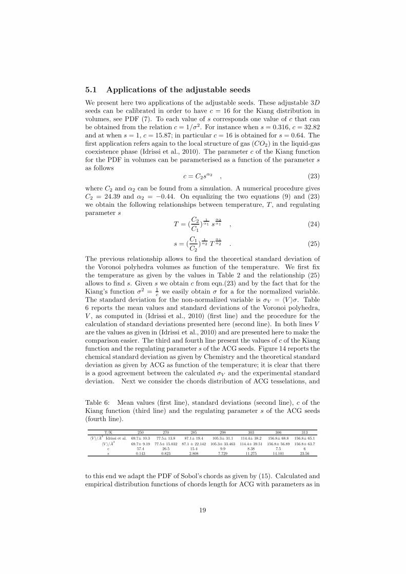
5.1 Applications of the adjustable seeds

We present here two applications of the adjustable seeds. These adjustable 3Dseeds can be calibrated in order to have c = 16 for the Kiang distribution involumes, see PDF (7). To each value of s corresponds one value of c that canbe obtained from the relation c = 1/σ2. For instance when s = 0.316, c = 32.82and at when s = 1, c = 15.87; in particular c = 16 is obtained for s = 0.64. Thefirst application refers again to the local structure of gas (CO2) in the liquid-gascoexistence phase (Idrissi et al., 2010). The parameter c of the Kiang functionfor the PDF in volumes can be parameterised as a function of the parameter sas follows

c = C2sα2 , (23)

where C2 and α2 can be found from a simulation. A numerical procedure givesC2 = 24.39 and α2 = −0.44. On equalizing the two equations (9) and (23)we obtain the following relationships between temperature, T , and regulatingparameter s

T = (C2

C1

)1

α1 sα2

α1 , (24)

s = (C1

C2

)1

α2 Tα1

α2 . (25)

The previous relationship allows to find the theoretical standard deviation ofthe Voronoi polyhedra volumes as function of the temperature. We first fixthe temperature as given by the values in Table 2 and the relationship (25)allows to find s. Given s we obtain c from eqn.(23) and by the fact that for theKiang’s function σ2 = 1

c we easily obtain σ for a for the normalized variable.The standard deviation for the non-normalized variable is σV = 〈V 〉σ. Table6 reports the mean values and standard deviations of the Voronoi polyhedra,V , as computed in (Idrissi et al., 2010) (first line) and the procedure for thecalculation of standard deviations presented here (second line). In both lines Vare the values as given in (Idrissi et al., 2010) and are presented here to make thecomparison easier. The third and fourth line present the values of c of the Kiangfunction and the regulating parameter s of the ACG seeds. Figure 14 reports thechemical standard deviation as given by Chemistry and the theoretical standarddeviation as given by ACG as function of the temperature; it is clear that thereis a good agreement between the calculated σV and the experimental standarddeviation. Next we consider the chords distribution of ACG tesselations, and

Table 6: Mean values (first line), standard deviations (second line), c of theKiang function (third line) and the regulating parameter s of the ACG seeds(fourth line).

T/K 250 270 285 298 303 306 313

〈V 〉/A3Idrissi et al. 69.7± 10.3 77.5± 13.8 87.1± 19.4 105.3± 31.1 114.4± 38.2 156.8± 68.8 156.8± 65.1

〈V 〉/A369.7± 9.19 77.5± 15.032 87.1 ± 22.142 105.3± 33.463 114.4± 39.51 156.8± 56.89 156.8± 63.7

c 57.4 26.5 15.4 9.9 8.38 7.5 6s 0.143 0.823 2.808 7.729 11.275 14.101 23.56

to this end we adapt the PDF of Sobol’s chords as given by (15). Calculated andempirical distribution functions of chords length for ACG with parameters as in

19

Figure 14: Standard deviation as given by Chemistry (empty stars) and the-oretical standard deviation as given by variables volumes in ACG (full points)as function of the temperature.

Table 4 are shown in Figure 15; the K-S test gives dmax = 0.028, PKS = 0.0051.

6 Conclusion

In this paper new types of three-dimensional Voronoi tessellations have been pre-sented whose centers are not sampled from an uniform distribution, as in PoissonVoronoi (PVT) case, but rather are derived from more regular sequences. FirstSobol-Voronoi Tesselations (SVT) have been considered in which cells formingthe partition have as centers points generated by a Sobol quasi-random se-quence. To make the notion of regularity of seeds configurations more precisea measure of uniformity has been presented. In analogy with the case of PVTwe have used a generalized gamma distribution, denoted with GSV T , to fit thevolumes obtained by numerical simulations. One should expect that the moreregular configuration of centers in the SVT is reflected in the distributions ofcell volumes and this is indeed the case: comparisons between the PDFs showthat GSV T have smaller variance and are more symmetric than the distributionGPV T of volumes in respect to PVT. It should be noted that volumes distri-butions of PVT cells can be fitted satisfactorily by different types of gammadistributions, as mentioned in Section 2; in contrast for volumes of SVT onlythe generalized three-parameters gamma provides a good fit.

As concerns applications, SVT may be relevant in modelling partitions ofsystems that follow a more regular distribution than the usual Poisson distri-bution and, what is more interesting, transitions from ordered to disordered

20

Figure 15: Data (empty circles) and theoretical DF for ACG seeds. Thetheoretical DF is the integral of PDF (gf,SV T ) (continuous line).

states of the system must be mirrored by a corresponding change from SVT toPVT. An example has been presented in which volumes occupied by moleculesof CO2 in liquid-gas phases undergo a transformation from regular to morerandom distributions as the temperature increases. Transitions from regular todisordered partitions of space can be cast in a more general setting by consider-ing the case in which center are first situated on the nodes of a regular grid andthen positions are perturbed with a gaussian noise regulated by a parameterdisorder s, thus creating an Adjustable Cartesian Grid (ACG). By increasing sone can reach first SVT distributions and next PVT. In this case a transitionfrom ordered to disordered states can be parametrized by s. Considering againto local structure of CO2 a relation has been derived between s and T , fromwhich the standard deviation has been computed and next compared with theexperimental one, showing a good agreement. Finally statistics of chords result-ing from intersections of line with elements of PVT, SVT and ACG have alsobeen investigated. The interest of such type of statistics resides in the fact thatin many experimental conditions only chords of three-dimensional cells can bedetermined. Results show a good agreement between the analytical formula,obtained with a semi-empirical procedure and data obtained from a simulation,despite the approximations that have been used, namely considering cells to bea sphere and using an one-parameter gamma distribution to fit cells volumes,from which chords distributions have been derived.

Appendix

Numerical values of coefficients in Eq. (13).

21

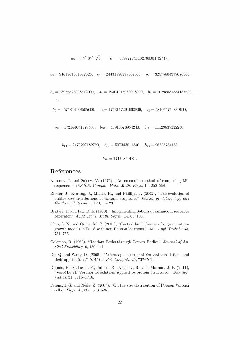
a0 = π2/382/33√3, a1 = 63997774118278000 Γ (2/3) .

b0 = 9161961861677625, b1 = 24431898297807000, b2 = 32575864397076000,

b3 = 28956323908512000, b4 = 19304215939008000, b5 = 10295581834137600,

k

b6 = 4575814148505600, b7 = 1743167294668800, b8 = 581055764889600,

b9 = 172164671078400, b10 = 45910578954240, b11 = 11129837322240,

b12 = 2473297182720, b13 = 507343011840, b14 = 96636764160

b15 = 17179869184.

References

Antonov, I. and Saleev, V. (1979), “An economic method of computing LP-sequences.” U.S.S.R. Comput. Math. Math. Phys., 19, 252–256.

Blower, J., Keating, J., Mader, H., and Phillips, J. (2002), “The evolution ofbubble size distributions in volcanic eruptions,” Journal of Volcanology and

Geothermal Research, 120, 1 – 23.

Bratley, P. and Fox, B. L. (1988), “Implementing Sobol’s quasirandom sequencegenerator.” ACM Trans. Math. Softw., 14, 88–100.

Chiu, S. N. and Quine, M. P. (2001), “Central limit theorem for germination-growth models in R**d with non-Poisson locations.” Adv. Appl. Probab., 33,751–755.

Coleman, R. (1969), “Random Paths through Convex Bodies,” Journal of Ap-

plied Probability, 6, 430–441.

Du, Q. and Wang, D. (2005), “Anisotropic centroidal Voronoi tessellations andtheir applications.” SIAM J. Sci. Comput., 26, 737–761.

Dupuis, F., Sadoc, J.-F., Jullien, R., Angelov, B., and Mornon, J.-P. (2011),“Voro3D: 3D Voronoi tessellations applied to protein structures,” Bioinfor-

matics, 21, 1715–1716.

Ferenc, J.-S. and Neda, Z. (2007), “On the size distribution of Poisson Voronoicells,” Phys. A , 385, 518–526.

22

Ferraro, M. and Zaninetti, L. (2012), “On the statistics of area size in two-dimensional thick Voronoi diagrams,” Physica A Statistical Mechanics and

its Applications, 391, 4575–4582.

Gonzalez, D. L. and Einstein, T. L. (2011), “Voronoi cell patterns: Theoreticalmodel and applications,” Phys. Rev. E , 84, 051135.

Heinrich, L. and Schiile, E. (1995), “Generation of the typical cell of anon-poissonian Johnson-Mehl tessellation,” Communications in Statistics.

Stochastic Models, 11, 541–560.

Hinde , A. L. and Miles, R. (1980), “Monte Carlo estimates of the distributionsof the random polygons of the Voronoi tessellation with respect to a Poissonprocess ,” J. Stat. Comput. Simul., 10, 205–223.

Idrissi, A., Vyalov, I., Damay, P., Kiselev, M., Puhovski, Y., and Jedlovszky, P.(2010), “Local structure in sub- and supercritical CO2: A Voronoi polyhedraanalysis study,” Journal of Molecular Liquids, 153, 20–24.

Idrissi, A., Vyalov, I., Kiselev, M., Fedorov, M. V., and Jedlovszky, P. (2011),“Heterogeneity of the Local Structure in Sub-and Supercritical Ammonia:A Voronoi Polyhedra Analysis,” The Journal of Physical Chemistry B, 115,9646–9652.

Jedlovszky, P. (1999), “Voronoi polyhedra analysis of the local structure of waterfrom ambient to supercritical conditions,” The Journal of chemical physics,111, 5975–5985.

Jedlovszky, P. (2000), “The local structure of various hydrogen bonded liquids:Voronoi polyhedra analysis of water, methanol, and HF,” Journal of Chemical

Physics , 113, 9113–9121.

Jedlovszky, P., Medvedev, N. N., and Mezei, M. (2004), “Effect of Cholesterolon the Properties of Phospholipid Membranes. 3. Local Lateral Structure,”The Journal of Physical Chemistry B, 108, 465–472.

Kellerer, A. M. (1984), “Chord-Length Distributions and Related Quantities forSpheroids,” Radiation Research, 98, 425–437.

Khodabin, M. and Ahmadabadi, A. (2010), “Some properties of generalizedgamma distribution.” Math. Sci. Q. J., 4, 9–28.

Kiang, T. (1966), “Random Fragmentation in Two and Three Dimensions,” Z.

Astrophys. , 64, 433–439.

Kolmogoroff, A. (1941), “Confidence Limits for an Unknown Distribution Func-tion,” The Annals of Mathematical Statistics, 12, 461–463.

Lazar, E. A., Mason, J. K., MacPherson, R. D., and Srolovitz, D. J. (2013), “Sta-tistical topology of three-dimensional Poisson-Voronoi cells and cell boundarynetworks,” Phys. Rev. E, 88, 063309.

Le Caer, G. and Ho, J. S. (1990), “The Voronoi tessellation generated fromeigenvalues of complex randommatrices,” Journal of Physics A: Mathematical

and General, 23, 3279.

23

Massey, Frank J., J. (1951), “The Kolmogorov-Smirnov Test for Goodness ofFit,” Journal of the American Statistical Association, 46, 68–78.

Morokoff, W. J. and Caflisch, R. E. (1994), “Quasi-random sequences and theirdiscrepancies,” SIAM Journal on Scientific Computing, 15, 1251–1279.

Muche, L. (2010), “Contact and chord length distribution functions of thePoisson-Voronoi tessellation in high dimensions,” Adv. in Appl. Probab., 42,48–68.

Muche, L. and Stoyan, D. (1992), “Contact and Chord Length Distributionsof the Poisson Voronoi Tessellation,” Journal of Applied Probability, 29, pp.467–471.

Okabe, A., Boots, B., Sugihara, K., and Chiu, S. (2000), Spatial tessellations.Concepts and Applications of Voronoi diagrams, 2nd ed., Chichester, NewYork: Wiley.

Poupon, A. (2004), “Voronoi and Voronoi-related tessellations in studies of pro-tein structure and interaction,” Current Opinion in Structural Biology, 14,233 – 241.

Press, W. H., Teukolsky, S. A., Vetterling, W. T., and Flannery, B. P. (1992),Numerical Recipes in FORTRAN. The Art of Scientific Computing, Cam-bridge, UK: Cambridge University Press.

Ruan, J. Z., Litt, M. H., and Krieger, I. M. (1988), “Pore size distributions offoams from chord distributions of random lines: Mathematical inversion andcomputer simulation,” Journal of Colloid and Interface Science, 126, 93 –100.

Smirnov, N. (1948), “Table for Estimating the Goodness of Fit of EmpiricalDistributions,” The Annals of Mathematical Statistics, 19, 279–281.

Sobol, I. M. (1967), “The distribution of points in a cube and the approximateevaluation of integrals,” USSR Comp. Math. Math. Phys., 7, 86–112.

Stoyan, D., Wagner, A., Hermann, H., and Elsner, A. (2011), “Statistical char-acterization of the pore space of random systems of hard spheres,” Journal

of Non-Crystalline Solids, 357, 1508–1515.

Tanemura, M. (2003), “Statistical Distributions of Poisson Voronoi Cells in Twoand Three Dimensions,” Forma, 18, 221–247.

— (2005), “Statistical distributions of the shape of Poisson Voronoi cells.” inVoronoi’s impact on modern science. Book III. Proceedings of the 3rd Voronoi

conference on analytic number theory and spatial tessellations, ed. H. Syta,pp. 193–202.

Tokita, N., Hirabayashi, M., Azuma, C., and Dotera, T. (2004), “Voronoi spacedivision of a polymer: Topological effects, free volume, and surface end seg-regation,” The Journal of chemical physics, 120, 496–505.

Watson, G. S. (1971), “Estimating functionals of particle size distributions,”Biometrika, 58, 483–490.

24