arX

iv:0

808.

1923

v3 [

mat

h.D

G]

24

Sep

2013

Connections on Non-Abelian Gerbes and their Holonomy

Urs Schreiber and Konrad Waldorf

Abstract

We introduce an axiomatic framework for the parallel transport of connections on gerbes. Itincorporates parallel transport along curves and along surfaces, and is formulated in terms ofgluing axioms and smoothness conditions. The smoothness conditions are imposed with respectto a strict Lie 2-group, which plays the role of a band, or structure 2-group. Upon choosingcertain examples of Lie 2-groups, our axiomatic framework reproduces in a systematical way severalknown concepts of gerbes with connection: non-abelian differential cocycles, Breen-Messing gerbes,abelian and non-abelian bundle gerbes. These relationships convey a well-defined notion of surfaceholonomy from our axiomatic framework to each of these concrete models. Till now, holonomywas only known for abelian gerbes; our approach reproduces that known concept and extends itto non-abelian gerbes. Several new features of surface holonomy are exposed under its extensionto non-abelian gerbes; for example, it carries an action of the mapping class group of the surface.

Keywords: Parallel transport, surface holonomy, path 2-groupoid, gerbes, 2-bundles, 2-groups,

non-abelian differential cohomology, non-abelian bundle gerbes

MSC 2010: Primary 53C08, Secondary 55R65, 18D05

Contents

1 Introduction 2

2 Foundations of the Transport Functor Formalism 6

2.1 The Path 2-Groupoid of a Smooth Manifold . . . . . . . . . . . . . . . . . . . . . . . . . 6

2.2 Local Trivializations and Descent Data . . . . . . . . . . . . . . . . . . . . . . . . . . . . 7

2.3 Smooth 2-Functors . . . . . . . . . . . . . . . . . . . . . . . . . . . . . . . . . . . . . . . 10

2.4 Transport Functors . . . . . . . . . . . . . . . . . . . . . . . . . . . . . . . . . . . . . . . 10

3 Transport 2-Functors 12

3.1 Smooth Descent Data . . . . . . . . . . . . . . . . . . . . . . . . . . . . . . . . . . . . . 12

3.2 Transport 2-Functors . . . . . . . . . . . . . . . . . . . . . . . . . . . . . . . . . . . . . . 15

3.3 Some Features of Transport 2-Functors . . . . . . . . . . . . . . . . . . . . . . . . . . . . 18

3.4 Curvature 2-Functors . . . . . . . . . . . . . . . . . . . . . . . . . . . . . . . . . . . . . . 22

4 Transport 2-Functors are Non-Abelian Gerbes 25

4.1 Differential Non-Abelian Cohomology . . . . . . . . . . . . . . . . . . . . . . . . . . . . 25

4.2 Abelian Bundle Gerbes with Connection . . . . . . . . . . . . . . . . . . . . . . . . . . . 33

4.3 Non-Abelian Bundle Gerbes with Connection . . . . . . . . . . . . . . . . . . . . . . . . 36

4.4 2-Bundles with Connections . . . . . . . . . . . . . . . . . . . . . . . . . . . . . . . . . . 41

5 Surface Holonomy 46

5.1 Markings and Fundamental Bigons . . . . . . . . . . . . . . . . . . . . . . . . . . . . . . 46

5.2 Reduced Surface Holonomy . . . . . . . . . . . . . . . . . . . . . . . . . . . . . . . . . . 49

5.3 Properties of Reduced Surface Holonomy . . . . . . . . . . . . . . . . . . . . . . . . . . 52

References 56

1 Introduction

Giraud introduced gerbes in order to achieve a geometrical understanding of non-abelian cohomology

[Gir71]. However, already abelian gerbes turned out to be interesting: Brylinski introduced the notion

of a connection on an abelian gerbe, and showed that these represent classes in a certain differential

cohomology theory, namely Deligne cohomology [Bry93]. Deligne cohomology in degree two has before

been related to two-dimensional conformal field theory by Gawedzki [Gaw88]. This relation is estab-

lished by means of the surface holonomy of a connection on an abelian gerbe, which provides a term

in the action functional of the field theory.

Surface holonomy of connections on abelian gerbes is today well understood; see [Wal10, FNSW08]

for reviews. While definitions of connections on non-abelian gerbes have appeared [BM05, ACJ05], it

remained unclear what the surface holonomy of these connections is supposed to be, how it is defined,

and how it can be used.

In the present article we propose a general and systematic approach to connections on non-abelian

gerbes, including notions of parallel transport and surface holonomy. Our approach is general in the

sense that it works for gerbes whose band is an arbitrary Lie 2-groupoid, and whose fibres are modelled

by an arbitrary 2-category. Our approach is systematic in the sense that it is solely based on axioms

for parallel transport along surfaces, formulated in terms of gluing laws and smoothness conditions.

The whole theory of connections on non-abelian gerbes is then derived as a consequence.

In order to illustrate how this axiomatic formulation works we shall briefly review a corresponding

formulation in a more familiar setting, namely the one of connections on fibre bundles; see [SW09].

It shows that for a Lie group G the category of principal G-bundles with connection over a smooth

manifold X is equivalent to a category consisting of functors

F : P1(X) // G-Tor. (1.1)

These functors are defined on the path groupoid P1(X) of the manifold X ; its objects are the points

of X , and its morphisms are (certain classes of) paths in X . The functors (1.1) take values in the

category of G-torsors, i.e. smooth manifolds with a free and transitive G-action.

The correspondence between principal G-bundles with connection and functors (1.1) is established

by letting the functor F assign to points the fibres of a given bundle, and to paths the corresponding

parallel transport maps. The gluing laws of parallel transport are precisely the axioms of a functor.

The smoothness conditions of parallel transport are more involved; they can be encoded in the functors

(1.1) by requiring smooth descend data with respect to an open cover of X . Functors (1.1) with smooth

descend data are called transport functors with G-structure – they constitute an axiomatic formulation

of the parallel transport of connections in G-bundles.

In Sections 2 and 3 of the present article we generalize this axiomatic formulation to connections on

gerbes. Our formulation does not use any existing concept of a gerbe with connection — such concepts

are an output of our approach. It is based on 2-functors defined on the path 2-groupoid P2(X) of X ,

with values in some “target” 2-category T ,

F : P2(X) // T . (1.2)

– 2 –

In Section 2.1 we review the path 2-groupoid: it is like the path groupoid but with additional 2-

morphisms, which are essentially fixed-end homotopies between paths.

For example, if T is the 2-category of algebras (over some fixed field), bimodules, and intertwiners,

a 2-functor (1.2) provides for each point x ∈ X an algebra F (x), which is supposed to be the fibre

of the gerbe at the point x. Further, it provides for each path γ from x to y a F (x)-F (y)-bimodule

F (γ), which is supposed to be the parallel transport of the connection on that gerbe along the curve

parameterized by γ. Finally, it provides for each homotopy Σ between paths γ and γ′ an intertwiner

F (Σ) : F (γ) // F (γ′),

which is supposed to be the parallel transport of the connection on that gerbe along the surface

parameterized by Σ. The axioms of the 2-functor (1.2) describe how these parallel transport structures

are compatible with the composition of paths and gluing of homotopies. These axioms and all other

2-categorical structure we use can be looked up in [SW, Appendix A].

Apart from the evident generalization from functors to 2-functors, more work has to be invested into

the generalization of the smoothness conditions. Imposing smoothness conditions relies on a notion of

local triviality for 2-functors defined on path 2-groupoids. A 2-functor

F : P2(X) // T

is considered to be trivializable, if it factors through a prescribed 2-functor i : Gr // T , with

Gr a strict Lie 2-groupoid. The Lie 2-groupoid Gr plays the role of the “typical fibre”, and the 2-

functor i indicates how the typical fibre is realized in the target 2-category T . A local trivialization

of the 2-functor F is a cover of X by open sets Uα, a collection of locally defined “trivial” 2-functors

trivα : P2(Uα) // Gr and of equivalences

tα : F |Uα

∼= // i trivα

between 2-functors defined on Uα. Local trivializations lead to descend data, generalizing the transition

functions of a bundle. The descent data of a 2-functor with a local trivialization consists of the 2-

functors trivα, of transformations

gαβ : i trivα // i trivβ

between 2-functors over Uα ∩ Uβ, and of higher coherence data that we shall ignore for the purposes

of this introduction. The theory of local trivializations and descent data for 2-functors is developed in

our paper [SW] and reviewed in Section 2.2.

The smoothness conditions we want to formulate are imposed with respect to descent data; they

are the content of Section 3. First of all, we require that the 2-functors trivα are smooth. This makes

sense since they take values in the Lie 2-groupoid Gr. For certain Lie 2-groupoids, a theory developed

in our paper [SW11] identifies the smooth functors trivα with certain 2-forms Bα on Uα — the curving

of the gerbe connection. In order to treat the transformations gαβ, we apply an observation in abstract

2-category theory: the transformations gαβ can be regarded as a collection of functors

F (gαβ) : P1(Uα ∩ Uβ) // ΛT ,

for ΛT a certain category of diagrams in T . The smoothness condition that we impose for the trans-

formation gαβ is that the functors F (gαβ) are transport functors. According to the before-mentioned

– 3 –

correspondence between transport functors and fibre bundles with connection, we thus obtain a smooth

fibre bundle F (gαβ) with connection over two-fold overlaps Uα∩Uβ — a significant feature of a gerbe.

Summarizing this overview, our axiomatic formulation of connections on gerbes consists of transport

2-functors: 2-functors F : P2(X) // T that are locally trivializable with respect to a typical fibre

i : Gr // T , and have smooth descent data.

In Section 4 of this article we test our axiomatic formulation by choosing examples of target 2-

categories T and 2-functors i : Gr // T . In these examples the Lie 2-groupoids are “deloopings” of

strict Lie 2-groups, Gr = BG; these Lie 2-groups G play the same role for gerbes as Lie groups for

principal bundles. We find the following results:

(i) For a general Lie 2-group G and the identity 2-functor

i = idBG : BG // BG

we prove (Theorem 4.1.6) that there is a bijection

h0TransBG(X,BG) ∼= H2(X,G)

between isomorphism classes of transport 2-functors and the degree two differential non-abelian

cohomology of X with coefficients in G. These cohomology groups have been explored in [BM05]

and [BS07]; they are an extension of Giraud’s non-abelian cohomology by differential form data.

Upon setting G = BS1 it reduces to Deligne cohomology.

(ii) The Lie 2-group BS1 has a monoidal functor BS1 // S1-Tor to the monoidal category of S1-

torsors, by sending the single objects of BS1 to S1 considered as a torsor over itself. Delooping

yields a 2-functor

i : BBS1 // B(S1-Tor).

We prove (Theorem 4.2.1) that there is an equivalence of 2-categories

TransBBS1(X,B(S1-Tor)) ∼=

S1-bundle gerbes with

connection over X

.

Bundle gerbes have been introduced by Murray [Mur96]. The equivalence arises by realizing

that the transport functor F (gαβ) in the descent data corresponds in the present situation to an

S1-bundle with connection.

(iii) Let H be a Lie group and let AUT(H) be the automorphism 2-group of H . It has a monoidal

functor AUT(H) // H-BiTor to the monoidal category of H-bitorsors. Delooping yields a

2-functor

i : BAUT(H) // B(H-BiTor).

We prove (Theorem 4.3.1) that there is an equivalence of 2-categories

TransBAUT(H)(X,B(H-BiTor)) ∼=

Non-abelian H-bundle gerbes

with connection over X

.

Non-abelian bundle gerbes are a generalization of S1-bundle gerbes introduced in [ACJ05], and

the above equivalence arises by proving that the transport functor F (gαβ) corresponds in the

present situation to a “principal H-bibundle with twisted connection”.

– 4 –

The relations (i) to (iii) show that all these existing concepts of gerbes with connection fit into our

axiomatic formulation.

Apart from these relations to existing gerbes with connection, transport 2-functors are able to

determine systematically new concepts in cases when only the target 2-category T and the 2-group G

are given. We demonstrate this in Section 4.4 with the examples of connections on vector 2-bundles,

string 2-bundles, and principal 2-bundles.

Finally, we discuss in Section 5 the notion of parallel transport along surfaces, which is manifestly

included in the concept of a transport 2-functor. We introduce a notion of surface holonomy for

transport 2-functors, defined for closed oriented surfaces with a marking, i.e. a certain presentation

of its fundamental group. It is obtained by evaluating the transport 2-functor on a homotopy that

realizes the single relation in this presentation.

The existing notion of surface holonomy for abelian gerbes takes values in S1 [Gaw88, Mur96],

while our notion of surface holonomy takes values in the 2-morphisms of the target 2-category T . In

order to compare the two notions, we propose a “reduction” procedure which can be applied in the

case that typical fibre of the transport 2-functor is of the form i : BG // T , where G is a Lie 2-group.

The first part of this procedure is the definition of an abelian group Gred which can be formed for

any Lie 2-group G (Definition 5.2.2). Heuristically, it generalizes the abelianization of an ordinary Lie

group. As the second part of the reduction procedure, we show (Proposition 5.2.5) that the surface

holonomy of every transport 2-functor with BG-structure can consistently be reduced to a function

with values in Gred.

Our main results in Section 5 concern this reduced surface holonomy of transport 2-functors with

BG-structure. We prove in Theorem 5.3.2 a rigidity result for reduced surface holonomy, namely that

it depends only on the isomorphism class of the transport 2-functor, and only on the equivalence

class of the marking. The isomorphism invariance allows us to transfer the reduced surface holonomy

from transport 2-functors through the equivalences (i), (ii), and (iii) described above. In particular,

we equip non-abelian G-gerbes with a well-defined notion of a Gred-valued surface holonomy; such a

concept was not known before.

Finally, we show that our new concept of reduced surface holonomy is compatible with the existing

notion of S1-valued surface holonomy of abelian gerbes. Namely, in the case G = BS1 we find for

the reduction (BS1)red = S1, so that both concepts take values in the same set. We prove then in

Proposition 5.3.3 that the two concepts indeed coincide. Thus, our new notion of (reduced) surface

holonomy consistently extends the existing notion from abelian to non-abelian gerbes.

Acknowledgements. The project described here has some of its roots in ideas of John Baez and in

his joint work with US, and we are grateful for all discussions and suggestions. We are also grateful

for opportunities to give talks about this project at an unfinished state, namely at the Fields Institute,

at the VBAC 2007 meeting in Bad Honnef, at the MedILS in Split and at the NTNU in Trondheim.

In addition, we thank the Hausdorff Research Institute for Mathematics in Bonn for kind hospitality

and support during several visits.

– 5 –

2 Foundations of the Transport Functor Formalism

The present paper is the last part of a project carried out in a sequence of papers [SW09, SW11, SW].

In these papers, we have prepared the foundations for transport 2-functors – our axiomatic formulation

of connection on non-abelian gerbes. The purpose of this section is to make the present paper self-

contained; we collect and review the most important definitions and results from the previous papers.

2.1 The Path 2-Groupoid of a Smooth Manifold

The basic idea of the path 2-groupoid is very simple: for a smooth manifold X , it is a strict 2-category

whose objects are the points of X , whose 1-morphisms are smooth paths in X , and whose 2-morphisms

are smooth homotopies between these paths. We recall some definitions from [SW09, SW11].

For points x, y ∈ X , a path γ : x // y is a smooth map γ : [0, 1] // X with γ(0) = x and

γ(1) = y. Since the composition γ2 γ1 of two paths γ1 : x // y and γ2 : y // z should again

be a smooth map we require sitting instants for all paths: a number 0 < ǫ < 12 with γ(t) = γ(0) for

0 ≤ t < ǫ and γ(t) = γ(1) for 1 − ǫ < t ≤ 1. The set of these paths is denoted by PX . In order to

make the composition associative and to make paths invertible, we consider the following equivalence

relation on PX : two paths γ, γ′ : x // y are called thin homotopy equivalent if there exists a smooth

map h : [0, 1]2 // X such that

(1) h is a homotopy from γ to γ′ through paths x // y and has sitting instants at γ and γ′.

(2) the differential of h has at most rank 1.

The set of equivalence classes is denoted by P 1X . We remark that any path γ is thin homotopy

equivalent to any orientation-preserving reparameterization of γ. The composition of paths induces a

well-defined associative composition on P 1X for which the constant paths idx are identities and the

reversed paths γ−1 are inverses; see [SW09, Section 2.1] for more details.

A homotopy h between two paths γ0 and γ1 like above but without condition (2) on the rank of its

differential is called a bigon in X and denoted by Σ : γ0 +3 γ1. These bigons form the 2-morphisms

of the path 2-groupoid of X . We denote the set of bigons in X by BX . Bigons can be composed in

two natural ways. For two bigons Σ : γ1 +3 γ2 and Σ′ : γ2 +3 γ3 we have a vertical composition

Σ′ • Σ : γ1 +3 γ3.

If two bigons Σ1 : γ1 +3 γ′1 and Σ2 : γ2 +3 γ′2 are such that γ1(1) = γ2(0), we have a horizontal

composition

Σ2 Σ1 : γ2 γ1 +3 γ′2 γ′1.

Like in the case of paths, we consider an equivalence relation on BX in order to make the two

compositions associative and to make bigons invertible: two bigons Σ : γ0 +3 γ1 and Σ′ : γ′0 +3 γ′1are called thin homotopy equivalent if there exists a smooth map h : [0, 1]3 // X such that

(1) h is a homotopy from Σ to Σ′ through bigons and has sitting instants at Σ and Σ′.

(2) the induced homotopies γ0 +3 γ′0 and γ1 +3 γ′1 are thin.

(3) the differential of h has at most rank 2.

– 6 –

Condition (1) assures that we have defined an equivalence relation on BX , and condition (2) asserts

that two thin homotopy equivalent bigons Σ : γ0 +3 γ1 and Σ′ : γ′0 +3 γ′1 start and end on thin

homotopy equivalent paths γ0 ∼ γ′0 and γ1 ∼ γ′1. We denote the set of equivalence classes by B2X .

The two compositions and • between bigons induce a well-defined composition on B2X . The path

2-groupoid P2(X) is the 2-category whose set of objects is X , whose set of 1-morphisms is P 1X and

whose set of 2-morphisms is B2X . The path 2-groupoid is strict and all 1-morphisms are strictly

invertible. We refer the reader to [SW11, Section 2.1] for a detailed discussion.

In this article we describe connections on gerbes by transport 2-functors – certain (not necessarily

strict) 2-functors

F : P2(X) // T ,

for some 2-category T , the target 2-category. We note that 2-functors can be pulled back along smooth

maps f :M // X : such a map induces a strict 2-functor f∗ : P2(M) // P2(X), and we write

f∗F := F f∗.

If we drop condition (3) from the definition of thin homotopy equivalence between bigons we

would still get a strict 2-groupoid, which we denote by Π2(X) and which we call the fundamental

2-groupoid of X . The projection defines a strict 2-functor P2(X) // Π2(X). We say that a 2-functor

F : P2(M) // T is flat if it factors through the 2-functor P2(M) // Π2(M). We show in Section

3.4 that this abstract notion of flatness is equivalent to the vanishing of a certain curvature 3-form.

2.2 Local Trivializations and Descent Data

Let T be a 2-category. A key feature of a transport 2-functor is that it is locally trivializable. Local

trivializations of a 2-functor F : P2(M) // T are defined with respect to three attributes:

1. A strict 2-groupoid Gr, the structure 2-groupoid . In Section 2.3 we will require that Gr is a Lie

2-groupoid, and formulate smoothness conditions with respect to its smooth structure.

2. A 2-functor i : Gr // T that indicates how the structure 2-groupoid is realized in the target

2-category.

3. A surjective submersion π : Y // M , which serves as an “open cover” of the base manifold M .

For a surjective submersion π : Y // M the fibre products Y [k] := Y ×M ...×M Y are again smooth

manifolds in such a way that the projections πi1...ip : Y [k] // Y [p] (to the indexed factors) are smooth

maps. An example is an open cover U = Uα of M , for which the disjoint union of all open sets Uαtogether with the projection to M is a surjective submersion. In this example, the k-fold fibre product

is the disjoint union of the k-fold intersections of the open sets Uα.

Definition 2.2.1. A π-local i-trivialization of a 2-functor F : P2(M) // T is a pair (triv, t) of a

strict 2-functor

triv : P2(Y ) // Gr

– 7 –

and a pseudonatural equivalence

P2(Y )π∗ //

triv

P2(M)

t

v~

F

Gr

i// T .

For the notion of a pseudonatural equivalence we refer to [SW, Appendix A]. According to the

conventions we fixed there, it includes a weak inverse t together with modifications

it : t t +3 idπ∗F and jt : idtrivi+3 t t (2.2.1)

satisfying the so-called zigzag identities.

In the following we use the abbreviation trivi := i triv, and we write Triv2π(i) for the 2-category

of 2-functors F : P2(M) // T with π-local i-trivializations (together with all pseudonatural trans-

formations and all modifications). Next we come to the definition of a 2-category Des2π(i) of descent

data with respect to a surjective submersion π : Y // M and a structure 2-groupoid i : Gr // T .

Definition 2.2.2. A descent object is a quadruple (triv, g, ψ, f) consisting of a strict 2-functor

triv : P2(Y ) // Gr,

a pseudonatural equivalence

g : π∗1trivi // π∗

2trivi,

and invertible, coherent modifications

ψ : idtrivi+3 ∆∗g and f : π∗

23g π∗12g +3 π∗

13g.

The coherence conditions for the modifications ψ and f can be found in [SW, Definition 2.2.1].

Let us briefly rephrase the above definition in case that Y is the union of open sets Uα: first there

are strict 2-functors trivα : P2(Uα) // Gr. To compare the difference between trivα and trivβ on a

two-fold intersection Uα ∩ Uβ there are pseudonatural equivalences gαβ : (trivα)i // (trivβ)i. If we

assume for a moment that gαβ was the transition function of some fibre bundle, one would demand

that 1 = gαα on every Uα and that gβγgαβ = gαγ on every three-fold intersection Uα ∩ Uβ ∩ Uγ . In

the present situation, however, these equalities have been replaced by modifications: the first one by

a modification ψα : id(trivα)i+3 gαα and the second one by a modification fαβγ : gβγ gαβ +3 gαγ .

Next we describe how to extract a descend object from a local trivialization of a 2-functor following

[SW, Section 2.3]. Let F : P2(M) // T be a 2-functor with a π-local i-trivialization (triv, t). Using

the weak inverse t : trivi // π∗F of t we define

g := π∗2t π

∗1 t : π

∗1trivi

// π∗2trivi.

This composition is well-defined since π∗1π

∗F = π∗2π

∗F . Let it andjt be the modifications (2.2.1). We

obtain ∆∗g = t t, so that the definition ψ := jt yields the invertible modification ψ : idtrivi+3 ∆∗g.

Similarly, one defines with it the invertible modification f . The quadruple (triv, g, ψ, f) obtained like

this is a descend object in the sense of Definition 2.2.2; see [SW, Lemma 2.3.1].

– 8 –

Next suppose (triv, g, ψ, f) and (triv′, g′, ψ′, f ′) are descent objects. A descent 1-morphism

(triv, g, ψ, f) // (triv′, g′, ψ′, f ′) is a pair (h, ǫ) consisting of a pseudonatural transformation

h : trivi // triv′i

and an invertible modification

ǫ : π∗2h g +3 g′ π∗

1h

satisfying two natural coherence conditions; see [SW, Definition 2.2.2]. Finally, we suppose that

(h1, ǫ1) and (h2, ǫ2) are descent 1-morphisms from a descent object (triv, g, ψ, f) to another descent

object (triv′, g′, ψ′, f ′). A descent 2-morphism (h1, ǫ1) +3 (h2, ǫ2) is a modification

E : h1 +3 h2

satisfying another coherence condition; see [SW, Definition 2.2.3].

Descent objects, 1-morphisms and 2-morphisms form a 2-category Des2π(i), called the descent 2-

category. In concrete examples of the target 2-category T these structures have natural interpretations

in terms of smooth maps and differential forms, as we show in Section 4. The extraction of a descent

object from a local trivialization outlined above extends to a 2-functor

Exπ : Triv2π(i) // Des2π(i), (2.2.2)

which we have described in [SW, Section 2.3].

In order to avoid the dependence to the fixed surjective submersion π : Y // M , we have shown in

[SW, Section 4.2] that the two 2-categories Triv2π(i) and Des2π(i) form a direct system for refinements

of surjective submersions over M . The corresponding direct limits are 2-categories

Triv2(i)M := lim−→π

Triv2π(i) and Des2(i)M := lim−→π

Des2π(i).

For instance, an object in the direct limit is a pair of a surjective submersion π and an object in the

corresponding 2-category Triv2π(i) orDes2π(i). 1-morphisms and 2-morphisms are defined over common

refinements. The 2-functor Exπ from (2.2.2) induces an equivalence

Triv2(i)M ∼= Des2(i)M

between these two direct limit 2-categories [SW, Proposition 4.2.1].

Finally, we want to get rid of the chosen trivializations that are attached to the objects of Triv2(i)M .

We denote by Functi(P2(M), T ) the 2-category of locally i-trivializable 2-functors, i.e. 2-functors which

admit a π-local i-trivialization, for some surjective submersion π. We have shown [SW, Theorem 4.3.1]:

Theorem 2.2.3. There is an equivalence

Functi(P2(M), T ) ∼= Des2(i)M

between 2-categories of locally i-trivializable 2-functors and their descend data.

In Section 3 we select a sub-2-category of Des2(i)M consisting of smooth descend data. The corre-

sponding sub-2-category of Functi(P2(M), T ) is the one we are aiming at – the 2-category of transport

2-functors.

– 9 –

2.3 Smooth 2-Functors

This section and the forthcoming Section 2.4 prepare two tools we need in Section 3.1 in order to

specify the sub-2-category of smooth descend data. The first tool is the concept of smooth 2-functors .

The general idea behind “smooth functors” is to consider them internal to smooth manifolds. That

is, the sets of objects and morphisms of the involved categories are smooth manifolds, and a smooth

functor consists of a smooth map between the objects and a smooth map between the morphisms.

Categories internal to smooth manifolds are called Lie categories , internal groupoids are called Lie

groupoids . The same idea applies to 2-functors between 2 -categories.

In the context of the present paper, we want to consider smooth 2-functors defined on the path

2-groupoid P2(X) of a smooth manifold X , respectively. However, P2(X) is not internal to smooth

manifolds, not even infinite-dimensional ones. Instead, we consider it internal to a larger category

of generalized manifolds, so-called diffeological spaces [Sou81]. Diffeological spaces and diffeological

maps form a category D∞ that enlarges the category C∞ of smooth manifolds by means of a full and

faithful functor C∞ // D∞. For an introduction to diffeological spaces we refer the reader to [BH11]

or [SW09, Appendix A.2].

Diffeological spaces admit many constructions that are not possible in the category of smooth

manifolds. We need three of them. Firstly, if X and Y are diffeological spaces, the set D∞(X,Y )

of smooth maps from X to Y is again a diffeological space. In particular, the set of smooth maps

between smooth manifolds is a diffeological space. Secondly, every subset of a diffeological space is

a diffeological space. Thirdly, the quotient of every diffeological space by any equivalence relation is

a diffeological space. These constructions are relevant because they show that the set P 1X of thin

homotopy classes of paths in X as well as the set B2X of thin homotopy classes of bigons in X are

diffeological spaces. We conclude that the path 2-groupoid P2(X) of a smooth manifold X is internal

to diffeological spaces, and we have a corresponding 2-category Funct∞(P2(X), S) of smooth 2-functors

with values in some Lie 2-category S.

2.4 Transport Functors

The second tool we need for Section 3 is the concept of a transport functor. Transport functors are

an axiomatic formulation of connections in fibre bundles – they are the one-dimensional analogue of

transport 2-functors, the axiomatic formulation of connections on non-abelian gerbes we are aiming at

in the present article. We have introduced and discussed transport functors in [SW09].

From a general perspective, the definition of a “transport n-functor” is supposed to rely on a

recursive principle in the sense that it uses transport (n − 1)-functors. This is one reason to recall

the definition of a transport functor. The other reason is to highlight the analogy between the two

definitions, which might be helpful to notice:

(a) Instead of the path 2-groupoid P2(X), we are looking at the path groupoid P1(X), obtained by

just taking objects and 1-morphisms of P2(X). A transport functor is a certain functor

F : P1(X) // T ,

for some target category T : it assigns objects in T – the “fibres” – to the points of X , and

morphisms in T – the “parallel transport maps” – to paths in X .

– 10 –

(b) In order to say which functors are transport functors we need a Lie groupoid Gr and a functor

i : Gr // T . A local i-trivialization of F is a surjective submersion π : Y // X , a functor

triv : P1(Y ) // Gr, and a natural equivalence

P1(Y )π∗ //

triv

P1(X)

ttttttt

v~ tttttttt F

Gr

i// T .

(c) Associated to a local trivialization is a descent object : it is a pair (triv, g) consisting of the functor

triv : P1(Y ) // Gr and of a natural equivalence

g : π∗1trivi // π∗

2trivi

satisfying a cocycle condition.

The final step in the definition of a transport functor is the characterization of smooth descent data.

(d) A descent object (triv, g) is called smooth, if the functor

triv : P1(X) // Gr

is smooth, i.e. internal to diffeological spaces, and if the components map

g : Y [2] // Mor(T )

of the natural equivalence g is the composition of a smooth map g : Y [2] // Mor(Gr) with

i : Gr // T .

In view of the analogy between (a) - (c) and Sections 2.1 and 2.2, (d) is the analogue of the forthcoming

Section 3.1. Summarizing, we have:

Definition 2.4.1 ([SW09, Definition 3.6]). A transport functor on X with values in T and with

Gr-structure is a locally i-trivializable functor

F : P1(X) // T

with smooth descent data.

Transport functors form a category which we denote by Trans1Gr(X,T ). The main result of our

paper [SW09] is that transport functors are an axiomatic formulation of connection on fibre bundles.

In order to illustrate that, and since we need this result later several times, we provide the following

example. letG be a Lie group, and letBun∇G(X) be the category of principalG-bundles with connection

over X . Further, we denote by BG the Lie groupoid with one object and morphisms G, by G-Tor the

category of G-torsors, and by i : BG // G-Tor the functor that sends the single object of BG to G,

regarded as a G-torsor over itself. Then, we have:

Theorem 2.4.2 ([SW09, Theorem 5.8]). Let X be a smooth manifold. The assignment

Bun∇G(X) // Trans1BG(X,G-Tor) : (P, ω) // FP,ω

defined by

FP,ω(x) := Px and FP,ω(γ) := τγ ,

where x ∈ X, γ ∈ PX, and τγ is the parallel transport of ω along γ, establishes a surjective equivalence

of categories.

– 11 –

3 Transport 2-Functors

In this section we introduce the central definition of this paper: transport 2-functors. For this purpose,

we define in Section 3.1 a 2-category of smooth descent data, based on the notions of smooth 2-

functors and transport functors. In Section 3.2 we define transport 2-functors as those 2-functors that

correspond to smooth descent data under the equivalence of Theorem 2.2.3. Section 3.3 describes some

basic properties of transport 2-functors, and in Section 3.4 we construct an explicit example.

3.1 Smooth Descent Data

In this section we select a sub-2-category Des2π(i)∞ of smooth descent data in the 2-category Des2π(i)

of descent data described in Section 2.2. If (triv, g, ψ, f) is a descent object, we demand that the strict

2-functor triv : P2(Y ) // Gr has to be smooth in the sense of Section 2.3, i.e. internal to diffeological

spaces. Imposing smoothness conditions for the pseudonatural transformation g and the modifications

ψ and f is more subtle since they do not take values in the Lie 2-category Gr but in the 2-category T

which is not assumed to be a Lie 2-category.

Briefly, we proceed in the following two steps. We explain first how the pseudonatural transforma-

tion

g : π∗1trivi // π∗

2trivi

can be viewed as a certain functor F (g) defined on P1(Y[2]). Secondly, we impose the condition that

F (g) is a transport functor. A little motivation might be the observation that F (g) corresponds then

(at least in some cases, by Theorem 2.4.2) to a principal bundle with connection over Y [2] – one of the

well-known ingredients of a (bundle) gerbe, see Sections 4.2 and 4.3.

Let us first explain in general how a pseudonatural transformation between two 2-functors can

be viewed as a functor. We consider 2-functors F and G between 2-categories S and T . Since a

pseudonatural transformation ρ : F // G assigns 1-morphisms in T to objects in S and 2-morphisms

in T to 1-morphisms in S, the general idea is to construct a category S0,1 consisting of objects and

1-morphisms of S and a category ΛT consisting of 1-morphisms and 2-morphisms of T such that ρ

yields a functor

F (ρ) : S0,1// ΛT .

We assume that S is strict, so that forgetting its 2-morphisms produces a well-defined category S0,1.

The construction of the category ΛT is more involved.

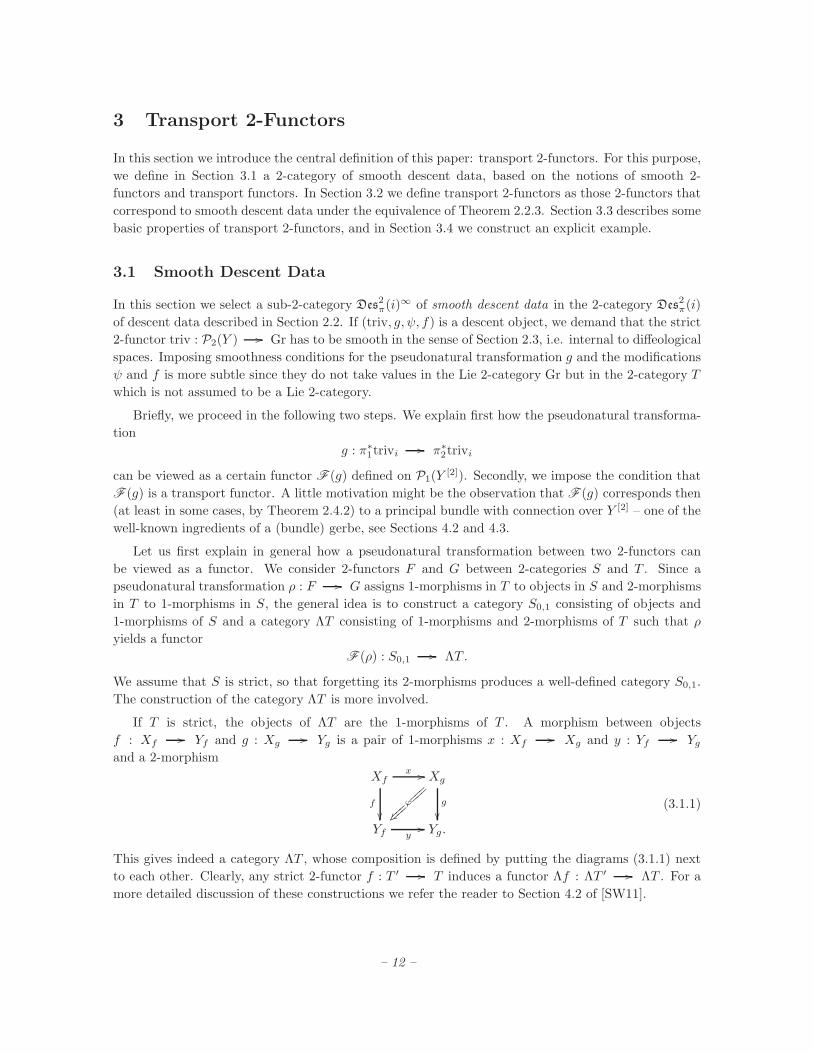
If T is strict, the objects of ΛT are the 1-morphisms of T . A morphism between objects

f : Xf// Yf and g : Xg

// Yg is a pair of 1-morphisms x : Xf// Xg and y : Yf // Yg

and a 2-morphism

Xfx //

f

Xg

ϕ⑤⑤⑤⑤⑤⑤

z ⑤⑤⑤⑤⑤⑤ g

Yf y

// Yg.

(3.1.1)

This gives indeed a category ΛT , whose composition is defined by putting the diagrams (3.1.1) next

to each other. Clearly, any strict 2-functor f : T ′ // T induces a functor Λf : ΛT ′ // ΛT . For a

more detailed discussion of these constructions we refer the reader to Section 4.2 of [SW11].

– 12 –

Now let ρ : F // G be a pseudonatural transformation between two strict 2-functors from S

to T . Sending an object X in S to the 1-morphism ρ(X) and sending a 1-morphism f in S to the

2-morphism ρ(X) now yields a functor

F (ρ) : S0,1// ΛT .

It respects the composition due to axiom (T1) for ρ and the identities due to [SW, Lemma A.7].

Moreover, a modification A : ρ1 +3 ρ2 defines a natural transformation F (A) : F (ρ1) +3 F (ρ2),

so that the result is a functor

F : Hom(F,G) // Funct(S0,1,ΛT ) (3.1.2)

between the category of pseudonatural transformations between F and G and the category of functors

from S0,1 to ΛT , for S and T strict 2-categories and F and G strict 2-functors.

In case that the 2-category T is not strict, the construction of ΛT suffers from the fact that the

composition is not longer associative. The situation becomes treatable if one requires the objectsXf , Yfand Xg, Yg and the 1-morphisms x and y in (3.1.1) to be contained the image of a strict 2-category

T str under some 2-functor i : T str // T . The result is a category ΛiT , in which the associativity

i(X)

f

i(Y )

,

i(Xf )i(x) //

f

i(Xg)

ϕ

w g

i(Yf )

i(y)// i(Yg)

and

i(Xf)

i(x′x)

c−1

x,x′

i(x) //

f

i(Xg)

ϕ

w g

i(x′) // i(Xh)

h

ϕ′

w

i(Yf )

i(y′y)

BB

cy,y′

i(y)// i(Yg)

i(y′)

// i(Yh).

Figure 1: Objects, morphisms and the composition of the category ΛiT (the

diagram on the right hand side ignores the associators and the bracketing of

1-morphisms). Here, c is the compositor of the 2-functor i.

of the composition is restored by axiom (F3) on the compositor of the 2-functor i. We omit a more

formal definition and refer the reader to Figure 1 for an illustration. For any 2-functor f : T // T ′,

a functor

ΛF : ΛiT // ΛFiT′

is induced by applying f to all involved objects, 1-morphisms, and 2-morphisms. We may now consider

strict 2-functors F and G from S to T str. Then, the functor (3.1.2) generalizes straightforwardly to a

functor

F : Hom(i F, i G) // Funct(S0,1,ΛiT )

between the category of pseudonatural transformations between i F and i G and the category of

functors from S0,1 to ΛiT . The following lemma follows directly from the definitions.

Lemma 3.1.1. The functor F has the following properties:

– 13 –

(i) It is natural with respect to strict 2-functors f : S′ // S in the sense that the diagram

Hom(i F, i G)

f∗

F // Funct(S0,1,ΛiT )

f∗

Hom(i F f, i G f)

F

// Funct(S′0,1,ΛiT )

is strictly commutative.

(ii) It preserves the composition of pseudonatural transformations in the sense that if

F,G,H : S // T str are three strict 2-functors, the diagram

Hom(iG, iH)×Hom(iF, iG)

F ×F // Funct(S0,1,ΛiT )×Funct(S0,1,ΛiT )

⊗

Hom(i H, i F )

F

// Funct(S0,1,ΛiT )

is commutative.

In Lemma 3.1.1 (ii) the symbol ⊗ has the following meaning. The composition of morphisms in

ΛiT was defined by putting the diagrams (3.1.1) next to each other as shown in Figure 1. But one can

also put the diagrams of appropriate morphisms on top of each other, provided that the arrow on the

bottom of the upper one coincides with the arrow on the top of the lower one. This is indeed the case

for the morphisms in the image of composable pseudonatural transformations under F × F , so that

the diagram in (ii) makes sense. In a more formal context, the tensor product ⊗ can be discussed in

the formalism of weak double categories , but we will not stress this point.

In the following discussion the strict 2-category S is the path 2-groupoid of some smooth manifold,

S = P2(X). Notice that S0,1 = P1(X) is then the path groupoid of X . The 2-category T is the target

2-category, and the strict 2-category T str is the Lie 2-groupoid Gr.

Let (triv, g, ψ, f) be a descent object in the descent 2-category Des2π(i). The pseudonatural trans-

formation g : π∗1trivi // π∗

2trivi induces a functor

F (g) : P1(Y[2]) // ΛiT .

In order to impose the condition that F (g) is a transport functor, we will use the functor

Λi : ΛGr // ΛiT

as its structure Lie groupoid. Further, the modification ψ : idtrivi// ∆∗g induces via Lemma 3.1.1

(i) a natural transformation

F (ψ) : F (idtrivi) +3 ∆∗

F (g).

Finally, the modification f induces via Lemma 3.1.1 (i) and (ii) a natural transformation

F (f) : π∗23F (g) ⊗ π∗

12F (g) +3 π∗13F (g).

Definition 3.1.2. A descent object (triv, g, ψ, f) is called smooth if the following conditions are satis-

fied:

(i) the 2-functor triv : P2(Y ) // Gr is smooth.

– 14 –

(ii) the functor F (g) is a transport functor with ΛGr-structure.

(iii) the natural transformations F (ψ) and F (f) are morphisms between transport functors.

In the same way we qualify smooth descent 1-morphisms and descent 2-morphisms. A descent

1-morphism

(h, ǫ) : (triv, g, ψ, f) // (triv′, g′, ψ′, f ′)

is converted into a functor

F (h) : P1(Y ) // ΛiT

and a natural transformation

F (ǫ) : π∗2F (h) ⊗ F (g) +3 F (g′) ⊗ π∗

1F (h).

We say that (h, ǫ) is smooth, if F (h) is a transport functor with ΛGr-structure and F (ǫ) is a 1-

morphism between transport functors. A descent 2-morphism E : (h, ǫ) +3 (h′, ǫ′) is converted into a

natural transformation

F (E) : F (h) +3 F (h′),

and we say that E is smooth, if F (E) is a 1-morphism between transport functors. We claim two

obvious properties of smooth descent data:

(i) Compositions of smooth descent 1-morphisms and smooth descent 2-morphisms are again smooth,

so that smooth descent data forms a sub-2-category of Des2π(i), which we denote by Des2π(i)∞.

(ii) Pullbacks of smooth descend objects, 1-morphisms and 2-morphisms along refinements of surjec-

tive submersions are again smooth, so that the direct limit

Des2(i)∞M := lim−→π

Des2π(i)∞

is a well-defined sub-2-category of Des2(i)M .

In Section 4 we show that the 2-category Des2(i)∞M of smooth descent data becomes nice and familiar

upon choosing concrete examples for the structure 2-groupoid i : Gr // T .

3.2 Transport 2-Functors

Now we come to the central definition of this paper.

Definition 3.2.1. Let M be a smooth manifold, Gr be a strict Lie 2-groupoid, T be a 2-category and

i : Gr // T be a 2-functor. A transport 2-functor on M with values in T and with Gr-structure is a

2-functor

tra : P2(M) // T

such that there exists a surjective submersion π : Y // M and a π-local i-trivialization (triv, t) whose

descent object Exπ(tra, triv, t) is smooth.

A 1-morphism between transport 2-functors tra and tra′ is a pseudonatural transformation

A : tra // tra′ such that there exists a surjective submersion π together with π-local i-trivializations

of tra and tra′ for which the descent 1-morphism Exπ(A) is smooth. 2-morphisms are defined in the

– 15 –

same way. Transport 2-functors tra : P2(M) // T with Gr-structure, 1-morphisms, and 2-morphisms

form a sub-2-category of the 2-category of locally i-trivializable 2-functor Functi(P2(M), T ), and we

denote this sub-2-category by Trans2Gr(M,T ). We emphasize that being a transport 2-functor is a

property, not additional structure. In particular, no surjective submersion or open cover is contained

in the structure of a transport 2-functor: they are manifestly globally defined objects.

We want to establish an equivalence between transport 2-functors and their smooth descent data.

In order to achieve this equivalence we have to make a slight assumption on the 2-functor i. We call a

2-functor i : Gr // T full and faithful , if it induces an equivalence on Hom-categories. In particular,

i is full and faithful if it is an equivalence of 2-categories, which is in fact true in all examples we are

going to discuss.

Theorem 3.2.2. Let M be a smooth manifold, and let i : Gr // T be a full and faithful 2-functor.

Then, the equivalence of Theorem 2.2.3 restricts to an equivalence

Trans2Gr(M,T ) ∼= Des2(i)∞M

between transport 2-functors and their smooth descent data.

Theorem 3.2.2 is proved by the following two lemmata. As an intermediate step we introduce –

for a surjective submersion π – the sub-2-category Triv2π(i)∞ of Triv2π(i) as the preimage of Des2π(i)

∞

under the 2-functor Exπ.

Lemma 3.2.3. The 2-functor Exπ restricts to an equivalence of 2-categories

Triv2π(i)∞ ∼= Des2π(i)

∞.

Proof. It is clear that Exπ restricts properly. Recall from [SW, Section 3] that inverse to Exπ is

a “reconstruction” 2-functor Recπ. In order to prove that the image of the restriction of Recπ is

contained in Triv2π(i)∞ we have to check that Exπ Recπ restricts to an endo-2-functor of Des2π(i)

∞.

In the proof of [SW, Lemma 4.1.2] we have explicitly computed this 2-functor, and by inspection of

the corresponding expressions one recognizes its image as smooth descent data.

The second part of the proof is to show that the components of two pseudonatural equivalences

ρ : Exπ Recπ // id and η : id // Recπ Exπ that establish the equivalence of [SW, Proposition

4.1.1] are inDes2π(i)∞ and Triv2π(i)

∞, respectively. For the transformation ρ, this is again by inspection

of the formulae in the proof of [SW, Lemma 4.1.2]. For the transformation η, we suppose F is a 2-

functor with a π-local i-trivialization (t, triv) with smooth descent data (triv, g, ψ, f). We have to

prove that the descent 1-morphism Exπ(η(F, t, triv)) is smooth. Indeed, according to the definition of

η given in the proof of [SW, Lemma 4.1.3] it is given by the pseudonatural transformation g and a

modification composed from the modifications f and ψ. The descent object is by assumption smooth,

and so is η(F ). The same argument shows that the component η(A) of a pseudonatural transformation

A : F // F ′ with smooth descent data is smooth.

Next we go to the direct limit

Triv2(i)∞M := lim−→π

Triv2π(i)∞.

The equivalence of Lemma 3.2.3 induces an equivalence

Ex : Triv2(i)∞M// Des2π(i)

∞

– 16 –

in the direct limit. Next we show that the 2-categories Triv2(i)∞M and Trans2Gr(M,T ) are equivalent.

We have an evident 2-functor

v∞ : Triv2(i)∞M// Trans2Gr(X,T )

induced by forgetting the chosen trivialization.

Lemma 3.2.4. Under the assumption that the 2-functor i is full and faithful, the 2-functor v∞ is an

equivalence of 2-categories.

Proof. It is clear that an inverse functor w∞ takes a given transport 2-functor and picks some

smooth local trivialization for some surjective submersion π : Y // M . It follows immediately that

v∞ w∞ = id. It remains to construct a pseudonatural equivalence id ∼= w∞ v∞, i.e. a 1-isomorphism

A : (tra, π, triv, t) // (tra, π′, triv′, t′)

in Triv2(i)∞M , where the original π-local trivialization (triv, t) has been forgotten and replaced by a

new π′-local trivialization (triv′, t′). But since the 1-morphisms in Triv2(i)∞M are just pseudonatural

transformation between the 2-functors ignoring the trivializations, we only have to prove that the

identity pseudonatural transformation

A := idtra : tra // tra

of a transport 2-functor tra has smooth descent data (h, ǫ) with respect to any two trivializations

(π, triv, t) and (π′, triv′, t′).

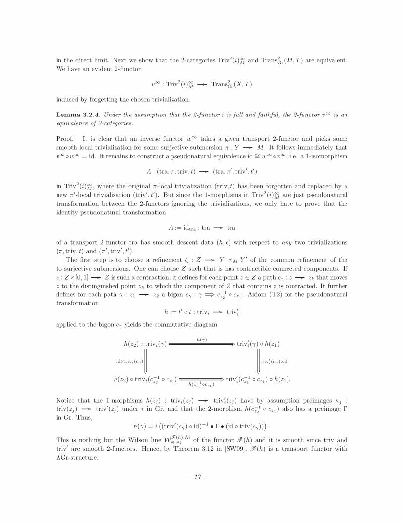
The first step is to choose a refinement ζ : Z // Y ×M Y ′ of the common refinement of the

to surjective submersions. One can choose Z such that is has contractible connected components. If

c : Z×[0, 1] // Z is such a contraction, it defines for each point z ∈ Z a path cz : z // zk that moves

z to the distinguished point zk to which the component of Z that contains z is contracted. It further

defines for each path γ : z1 // z2 a bigon cγ : γ +3 c−1z2

cz1 . Axiom (T2) for the pseudonatural

transformation

h := t′ t : trivi // triv′i

applied to the bigon cγ yields the commutative diagram

h(z2) trivi(γ)h(γ) +3

idtrivi(cγ)

triv′i(γ) h(z1)

triv′

i(cγ)id

h(z2) trivi(c

−1z2

cz1)h(c−1

z2cz1)

+3 triv′i(c−1z2

cz1) h(z1).

Notice that the 1-morphisms h(zj) : trivi(zj) // triv′i(zj) have by assumption preimages κj :

triv(zj) // triv′(zj) under i in Gr, and that the 2-morphism h(c−1z2

cz1) also has a preimage Γ

in Gr. Thus,

h(γ) = i((triv′(cγ) id)

−1 • Γ • (id triv(cγ))).

This is nothing but the Wilson line WF(h),Λiz1,z2 of the functor F (h) and it is smooth since triv and

triv′ are smooth 2-functors. Hence, by Theorem 3.12 in [SW09], F (h) is a transport functor with

ΛGr-structure.

– 17 –

It remains to prove that the modification ǫ : π∗2h g +3 g′ π∗

1h induces a morphism F (ǫ) of

transport functors. This simply follows from the general fact that under the assumption that the

functor i : Gr // T is full, every natural transformation η between transport functors with Gr-

structure is a morphism of transport functors. We have not stated that explicitly in [SW09] but it

can easily be deduced from the naturality conditions on trivializations t and t′ and on η, evaluated for

paths with a fixed starting point.

With Theorem 3.2.2 we have established an equivalence between globally defined transport 2-

functors and locally defined smooth descent data. In Section 4 we will identify smooth descent data

with various models of gerbes with connections. Under this identifications, Theorem 3.2.2 describes

the relation between these gerbes with connections and their parallel transport.

3.3 Some Features of Transport 2-Functors

In this section we provide several features of transport 2-functors.

3.3.1 Operations on Transport 2-Functors

It is straightforward to see that transport 2-functors allow a list of natural operations.

(i) Pullbacks : Let f : M // N be a smooth map. The pullback f∗tra of any transport 2-functor

on N is a transport 2-functor on M .

(ii) Tensor products : Let ⊗ : T × T // T be a monoidal structure on a 2-category T . For

transport 2-functors tra1, tra2 : P2(M) // T with Gr-structure, the pointwise tensor product

tra1 ⊗ tra2 : P2(M) // T is again a transport 2-functor with Gr-structure, and makes the

2-category Trans2Gr(M,T ) a monoidal 2-category.

(iii) Change of the target 2-category: Let T and T ′ be two target 2-categories equipped with 2-

functors i : Gr // T and i′ : Gr // T ′, and let F : T // T ′ be a 2-functor together with a

pseudonatural equivalence

ρ : F i // i′.

If tra : P2(M) // T is a transport 2-functor with Gr-structure, F tra is also a transport

2-functor with Gr-structure. In particular, this is the case for i′ := F i and ρ = id.

(iv) Change of the structure 2-groupoid : Let tra : P2(M) // T be a transport 2-functor with

Gr-structure, for a 2-functor i : Gr // T which is a composition

GrF // Gr′

i′ // T

in which F is a smooth 2-functor. Then, tra is also a transport 2-functor with Gr′-structure,

since for any local i-trivialization (triv, t) of tra we have a local i′-trivialization (F triv, t).

3.3.2 Structure Lie 2-Groups

We describe some examples of Lie 2-groupoids and outline the role of the corresponding transport

2-functors. First we recall the following generalization of a Lie group.

Definition 3.3.1. A Lie 2-group is a strict monoidal Lie category (G,⊠, I) together with a smooth

– 18 –

functor inv : G // G such that

X ⊠ inv(X) = I = inv(X)⊠X and f ⊠ inv(f) = idI = inv(f)⊠ f

for all objects X and all morphisms f in G.

The strict monoidal category (G,⊠, I) defines a strict 2-category BG with a single object [SW,

Example A.2]. The additional functor inv assures that BG is a strict 2-groupoid . All our examples in

Section 4 discuss transport 2-functors with BG-structure, for G a Lie 2-group.

Lie 2-groups can be obtained from the following structure.

Definition 3.3.2. A smooth crossed module is a quadruple (G,H, t, α) of Lie groups G and H, of a

Lie group homomorphism t : H // G, and of a smooth left action α : G ×H // H by Lie group

homomorphisms such that

a) t(α(g, h)) = gt(h)g−1 for all g ∈ G and h ∈ H.

b) α(t(h), x) = hxh−1 for all h, x ∈ H.

The construction of a Lie 2-groupG = G(G,H, t, α) from a given smooth crossed module (G,H, t, α)

can be found in the Appendix of [SW11]. We shall explicitly describe the corresponding Lie 2-groupoid

BG. It has one object denoted ∗ . A 1-morphism is a group element g ∈ G, the identity 1-morphism

is the neutral element, and the composition of 1-morphisms is the multiplication, g2 g1 := g2g1. The

2-morphisms are pairs (g, h) ∈ G ×H , considered as 2-morphisms

∗

g

g′

CCh

∗

with g′ := t(h)g. The vertical composition is

∗ g′ //

g

g′′

EE

h

h′

∗ = ∗

g

g′′

CCh′h

∗

with g′ = t(h)g and g′′ = t(h′)g′ = t(h′h)g, and the horizontal composition is

∗

g1

g′1

CCh1

∗

g2

g′2

CCh2

∗ = ∗

g2g1

g′2g′

1

AAh2α(g2, h1)

∗.

– 19 –

Summarizing, one can go from smooth crossed modules to Lie 2-groups, and then to Lie 2-groupoids.

Example 3.3.3.

(i) Let A be an abelian Lie group. A smooth crossed module is defined by G = 1 and H := A.

This fixes the maps to t(a) := 1 and α(1, a) := a. Notice that axiom b) is satisfied because A is

abelian. The associated Lie 2-group is denoted by BA. Transport 2-functors with BBA-structure

play the role of abelian gerbes with connection; see Section 4.2.

(ii) LetG be a Lie group. A smooth crossed module is defined byH := G, t = id and α(g, h) := ghg−1.

The associated Lie 2-group is denoted by EG. This notation is devoted to the fact that the

geometric realization of the nerve of the category EG yields the universalG-bundle EG. Transport

2-functors with BEG-structure arise as the curvature of transport functors; see Section 3.4.

(iii) Let H be a connected Lie group, so that the group of Lie group automorphisms of H is again a

Lie group G := Aut(H). The definitions t(h)(x) := hxh−1 and α(ϕ, h) := ϕ(h) yield a smooth

crossed module whose associated Lie 2-group is denoted by AUT(H), it is called the automorphism

2-group of H . Transport 2-functors with BAUT(H)-structure play the role non-abelian gerbes

with connection; see Section 4.3.

(iv) Let

1 // Nt // H

p // G // 1

be an exact sequence of Lie groups, not necessarily central. There is a canonical action α of H

on N defined by requiring

t(α(h, n)) = ht(n)h−1.

This defines a smooth crossed module, whose associated Lie 2-group we denote by N. Transport

2-functors with BN-structure correspond to (non-abelian) lifting gerbes . They generalize the

abelian lifting gerbes [Bry93, Mur96] for central extensions to arbitrary short exact sequences of

Lie groups.

3.3.3 Transgression to Loop Spaces

Transport 2-functors on a smooth manifold M induce interesting structure on the loop space LM .

This comes from the fact that there is a canonical smooth functor

ℓ : P1(LM) // ΛP2(M)

expressing that a point in LM is just a particular path inM , and that a path in LM is just a particular

bigon in M [SW11, Section 4.2]. If tra : P2(M) // T is a transport 2-functor, then the composition

of ℓ with

Λtra : ΛP2(M) // ΛtraT

yields a functor

Ttra := Λtra ℓ : P1(LM) // ΛtraT

that we call the transgression of tra to the loop space. In order abbreviate the discussion of the functor

Ttra we make three simplifying assumptions:

(i) We restrict our attention to the based loop space ΩM (for some fixed base point) and identify

Ttra with its pullback along the embedding ι : ΩM // LM .

– 20 –

(ii) We assume that there exists a surjective submersion π : Y // M for which tra admits smooth

local trivializations and for which Ωπ : ΩY // ΩM is also a surjective submersion.

(iii) We assume that the target 2-category T is strict, so that ΛT is the target category of the functor

Ttra.

Proposition 3.3.4. Let tra : P2(M) // T be a transport 2-functor with Gr-structure satisfying (ii)

and (iii). Then,

Ttra : P1(ΩM) // ΛT

is a transport functor with ΛGr-structure.

Proof. Let t : π∗tra // trivi be a π-local i-trivialization of tra for π a surjective submersion satisfying

(ii). A local trivialization t of Ttra is given by

P1(ΩY )

ℓ

(Ωπ)∗ // P1(ΩM)

ℓ

ΛP2(Y )

Λtriv

π∗// ΛP2(M)

Λtrrrr

rrrr

t| rrrrrrrr Λtra

ΛGr

Λi// ΛT

in which the upper subdiagram is commutative on the nose. If g : π∗1trivi // π∗

2trivi is the pseudona-

tural transformation in the smooth descent object Exπ(tra, t, triv), and g is the natural transformation

in the descent object Exπ(Ttra, t, ℓ∗Λtriv) associated to the above trivialization, we find g = ℓ∗Λg.

Since F (g) is a transport 2-functor with ΛGr-structure, it has smooth Wilson lines [SW09]: for a

fixed point α ∈ Y [2] there exists a smooth natural transformation g′ : π∗1ℓ

∗Λtriv // π∗2ℓ

∗Λtriv with

g = i(g′). This shows that g factors through a smooth natural transformation ℓ∗Λg′, so that Ttra is a

transport functor.

Having in mind that transport functors correspond to fibre bundles with connection, Proposition

3.3.4 shows that transport 2-functors on a manifold M naturally induce fibre bundles with connection

on the loop space ΩM . In general, these are so-called groupoid bundles [MM03, SW09], whose structure

groupoid is ΛGr. However, in the abelian case, i.e. Gr = BBA for an abelian Lie group A, we have

ΛGr ∼= BA (see Lemma 4.2.3 below), so that the transgression Ttra is – via Theorem 2.4.2 – a principal

A-bundle with connection over ΩM . This fits well into Brylinski’s picture of transgression [Bry93].

3.3.4 Curving and Curvature

Suppose tra : P2(M) // T is a transport 2-functor with BG-structure, for G some Lie 2-group coming

from a smooth crossed module (G,H, t, α). Since such 2-functors are supposed to describe (non-abelian)

gerbes with connection, we want to identify a 3-form curvature. Just as for (non-abelian) principal

bundles, this curvature is only locally defined.

First we need the following fact: if g and h denote the Lie algebras of the Lie groups G and H ,

respectively, there is a bijection

Smooth 2-functors

F : P2(X) → BG

∼=

Pairs (A,B) ∈ Ω1(X, g) × Ω2(X, h)

satisfying t∗(B) = dA+ [A ∧A]

, (3.3.1)

– 21 –

where t∗ : h // g is the differential of t. This bijection is the lowest level of an equivalence of

2-categories that we will review in more detail in Section 4.1; see Theorem 4.1.1.

Definition 3.3.5. Let tra : P2(M) // T be a transport functor with BG-structure over M , let

π : Y // M be a surjective submersion, and let (t, triv) be a π-local trivialization with smooth

descent data.

(i) The differential forms A ∈ Ω1(Y, g) and B ∈ Ω2(Y, h) that correspond to the smooth 2-functor

triv under the above bijection, are called the 1-curving and the 2-curving of tra.

(ii) The 3-form

curv(tra) = dB + α∗(A ∧B) ∈ Ω3(Y, h),

where α∗ : g × h // h is the differential of the action α : G ×H // H of the crossed module,

is called the curvature of tra.

We recall that we called a 2-functor tra : P2(M) // T flat if it factors through the projection

P2(M) // Π2(M) of thin homotopy classes of bigons to homotopy classes. The next proposition

shows that this notion of flatness is equivalent to the vanishing of the curvature.

Proposition 3.3.6. Suppose that the 2-functor i : BG // T is injective on 2-morphisms. A trans-

port 2-functor tra : P2(M) // T with BG-structure is flat if and only if its local curvature 3-form

curv(tra) ∈ Ω3(Y, h) with respect to any smooth local trivialization vanishes.

Proof. We proceed in two parts. (a): curv(tra) vanishes if and only if triv is a flat 2-functor, and

(b): tra is flat if and only if triv is flat. The claim (a) follows from Lemma A.11 in [SW11]. To see

(b) consider two bigons Σ1 : γ +3 γ′ and Σ2 : γ +3 γ′ in Y which are smoothly homotopic so that

they define the same element in Π2(Y ). Suppose tra is flat and let Σ := Σ−12 •Σ1. Axiom (T2) for the

trivialization t is then

t(y) π∗tra(γ)t(γ) +3

idt(y)π∗tra(Σ)

trivi(γ) t(x)

trivi(Σ)idt(x)

t(y) π∗tra(γ)

t(γ)+3 trivi(γ) t(x)

and since π∗tra(Σ) = id by assumption it follows that trivi(Σ) = id, i.e. triv is flat. Conversely,

assume that triv is flat. The latter diagram shows that tra is then flat on all bigons in the image of

π∗. This is actually enough: let h : [0, 1]3 // M be a smooth homotopy between two bigons Σ1 and

Σ2 which are not in the image of π∗. Like explained in Appendix A.3 of [SW11] the cube [0, 1]3 can be

decomposed into small cubes such that h restricts to smooth homotopies between small bigons that

bound these cubes. The decomposition can be chosen so small that each of these bigons is contained

in the image of π∗, so that tra assigns the same value to the source and the target bigon of each small

cube. By 2-functorality of tra, this infers tra(Σ1) = tra(Σ2).

3.4 Curvature 2-Functors

In this section we provide a class of examples of transport 2-functors coming from transport functors,

i.e. fibre bundle with connections. If P is a principal G-bundle with connection ω over M , one can

– 22 –

compare the parallel transport maps along two paths γ1, γ2 : x // y by an automorphism of Py,

namely the holonomy around the loop γ2 γ−11 ,

τγ2 = Holω(γ2 γ−11 ) τγ1 .

If the paths γ1 and γ2 are the source and the target of a bigon Σ : γ1 +3 γ2, this holonomy is related

to the curvature of ∇. So, a principal G-bundle with connection does not only assign fibres Px to

points x ∈ M and parallel transport maps τγ to paths, it also assigns a curvature-related quantity to

bigons Σ.

Under the equivalence between principal G-bundles with connection and transport functors on X

with BG-structure (Theorem 2.4.2), the principal bundle (P, ω) corresponds to the transport functor

traP : P1(M) // G-Tor

that assigns the fibres Px to points x ∈ M and the parallel transport maps τγ to paths γ. Adding an

assignment for bigons yields a “curvature 2-functor”

K(traP ) : P2(M) // G-Tor

where G-Tor is the category G-Tor regarded as a strict 2-category with a unique 2-morphism between

each pair of 1-morphisms. The uniqueness of the 2-morphisms expresses the fact that the curvature is

determined by the parallel transport.

More generally, let us start with a transport functor tra : P1(M) // T with BG-structure for some

Lie group G and some functor i : BG // T . The curvature 2-functor of tra is the strict 2-functor

K(tra) : P2(M) // T

which is on objects and 1-morphisms equal to tra and on 2-morphisms determined by the fact that T

has a exactly one 2-morphism between each pair of 1-morphisms. In the same way, we obtain a strict

2-functor

K(i) : BG // T

We observe that the Lie 2-groupoids BG and BEG (see Section 3.3) are canonically isomorphic under

the assignment

∗

g1

g2

CC∗

∗ // ∗

g1

g2

BBg2g−11

∗,

so that we obtain a 2-functor BEG // BG // T . Now we are in the position to introduce our

explicit example of a transport 2-functor.

Theorem 3.4.1. The curvature 2-functor K(tra) is a transport 2-functor with BEG-structure.

Proof. We construct a local trivialization of K(tra) starting with a local trivialization (triv, t) of

tra with respect to some surjective submersion π : Y // M . Let dtriv : P2(Y ) // BEG be the

derivative 2-functor associated to triv [SW11]: on objects and 1-morphisms it is given by triv, and it

sends every bigon Σ : γ1 +3 γ2 in Y to the unique 2-morphism in BEG between the images of γ1 and

γ2 under triv. A pseudonatural equivalence

K(t) : π∗K(tra) // K(i) dtriv

– 23 –

is defined as follows. Its component at a point a ∈ Y is the 1-morphism

K(t)(a) := t(a) : tra(π(a)) // i(∗)

in T . Its component t(γ) at a path γ : a // b is the unique 2-morphism in T . Notice that since t is

a natural transformation, we have a commutative diagram

tra(π(a))tra(π(γ)) //

t(a)

tra(π(b))

t(b)

i(∗)

trivi(γ)// i(∗)

meaning that t(γ) = id. This defines the pseudonatural transformation t as required.

Now we assume that the descent data (triv, gt) associated to the local trivialization (triv, t) is

smooth, and show that then also the descent object (dtriv, gK(t), ψ, f) is smooth. As observed in

[SW11], the derivative 2-functor dtriv is smooth if and only if triv is smooth. To extract the remaining

descent data according to the procedure described in Section 2.2. It turns out that the only non-trivial

descent datum is the pseudonatural transformation

gK(t) : π∗1dtrivK(i)

// π∗2dtrivK(i).

Its component at a point α ∈ Y [2] is given by gK(t)(α) := gt(α), and its component at some path

Θ : α // α′ is the identity.

The last step is to show that

F (gK(t)) : P1(Y[2]) // ΛK(i)T

is a transport functor with ΛBEG-structure. To do so we have to find a local trivialization with smooth

descent data. This is here particulary simple: the functor F (gK(t)) is globally trivial in the sense that

it factors through the functor

ΛK(i) : ΛBEG // ΛK(i)T .

To see this we use the smoothness condition on the natural transformation gt, namely that it factors

through a smooth natural transformation gt. We obtain a smooth pseudonatural transformation

gK(t) : π∗1dtriv // π∗

2dtriv such that gK(t) = K(i)(gK(t)). This finally gives us

F (gK(t)) = ΛK(i) F (gK(t))

meaning that F (gK(t)) is a transport functor with ΛBEG-structure.

Since the value of the curvature 2-functor K(tra) on bigons does not depend on the bigon itself

but only on its source and target path, we have the following.

Proposition 3.4.2. The curvature 2-functor K(tra) of any transport functor is flat.

This proposition gains a very nice interpretation when we relate the curvature of a connection ω in

a principal G-bundle p : P // M to the curvature 2-functor K(traP ) associated to the corresponding

transport functor traP . First we show:

Lemma 3.4.3. The curvature 2-functor K(traP ) : P2(M) // G-Tor has a canonical smooth p-local

trivialization (p, t, triv). The classical curvature curv(ω) ∈ Ω2(P, g) is the 2-curving of K(traP ) with

respect to the trivialization (p, t, triv).

– 24 –

Proof. As described in detail in [SW09, Section 5.1], traP admits local trivializations with respect to

the surjective submersion p : P // M and with smooth descent data (triv′, g) such that the connection

1-form ω ∈ Ω1(P, g) of the bundle P corresponds to the smooth functor triv′ : P1(P ) // BG under

the bijection of [SW09, Proposition 4.7]. Then, by [SW11, Lemma 3.5], the 2-form B′ associated to

dtriv′ under the bijection (3.3.1), which is by Definition 3.3.5 (i) the 2-curving of K(traP ), is given by

B′ = dω + [ω ∧ ω].

The latter is by definition the curvature of the connection ω.

The announced interpretation of Proposition 3.4.2 now is as follows: using Lemma 3.4.3 one can

calculate the curvature curv(K(traP )) of the curvature 2-functor of traP . The calculation involves the

second Bianchi identity for the connection ω on the principal G-bundle P , and the result is

curv(K(traP )) = 0,

which is according to Proposition 3.3.6 an independent proof of Proposition 3.4.2. In other words,

Proposition 3.4.2 is equivalent to the second Bianchi identity for connections on fibre bundles.

4 Transport 2-Functors are Non-Abelian Gerbes

In this section we show that transport 2-functors reproduce – systematically, by choosing appropriate

target 2-categories and structure 2-groups – four known concepts of gerbes with connections: Deligne

cocycles and Breen-Messing cocycles (Section 4.1), abelian bundle gerbes (Section 4.2), and non-

abelian bundle gerbes (Section 4.3). In Section 4.4 we establish a further relation between transport

2-functors and 2-vector bundles with connection. Conversely, all these structures are examples of

transport 2-functors.

4.1 Differential Non-Abelian Cohomology

In this section we set up a classifying theory for transport 2-functors P2(M) // T with structure Lie

2-groupoid i : BG // T , for G a Lie 2-group coming from a smooth crossed module (G,H, t, α), T an

arbitrary 2-category, and i an equivalence of categories. The latter condition together with Theorem

3.2.2 implies that we have equivalences

Trans2BG(M,T ) ∼= Des2(i)∞M

∼= Des2(idBG)∞M (4.1.1)

of 2-categories.

Our strategy is to translate the structure of the 2-category Des2(idBG)∞M into an equivalent 2-

category of “non-abelian differential cocycles” made up of smooth functions and differential forms,

with respect to open covers of M . Isomorphism classes of non-abelian differential cocycles form a set

which we define as the non-abelian differential cohomology of M ; it classifies transport 2-functors on

M with BG-structure up to isomorphism.

4.1.1 Smooth Functors and Differential Forms

For the translation of the 2-categoryDes2(idBG)∞M into smooth functions and differential forms we recall

a general result about the 2-category Funct∞(P2(X),BG) of smooth 2-functors, smooth pseudonatural

– 25 –

transformations, and smooth modifications defined on a smooth manifold X , with values in the Lie

2-groupoid BG. Following [SW11, Section 2.2], it corresponds to the following structure expressed in

terms of smooth functions and differential forms:

(i) A smooth 2-functor F : P2(X) // BG induces a pair of differential forms: a 1-form A ∈ Ω1(X, g)

with values in the Lie algebra of G, and a 2-form B ∈ Ω2(X, h) with values in the Lie algebra of

H , such that

dA+ [A ∧A] = t∗ B. (4.1.2)

(ii) A smooth pseudonatural transformation ρ : F // F ′ gives rise to a 1-form ϕ ∈ Ω1(X, h) and a

smooth map g : X // G, such that

A′ + t∗ ϕ = Adg(A)− g∗θ (4.1.3)

B′ + α∗(A′ ∧ ϕ) + dϕ+ [ϕ ∧ ϕ] = (αg)∗ B. (4.1.4)

The identity id : F // F has ϕ = 0 and g = 1. If ρ1 and ρ2 are composable pseudonatural

transformations, the 1-form of their composition ρ2 ρ1 is (αg2)∗ ϕ1 +ϕ2, and the smooth map

is g2g1 : X // G.

(iii) A smooth modification A : ρ +3 ρ′ gives rise to a smooth map a : X // H , such that

g′ = (t a) · g and ϕ′ + (r−1a αa)∗(A

′) = Ada(ϕ)− a∗θ. (4.1.5)

The identity modification idρ has a = 1. If two modifications A1 and A2 are vertically compos-

able, A2 • A1 has the map a2a1. If two modifications A1 : ρ1 +3 ρ′1 and A2 : ρ2 +3 ρ′2 are

horizontally composable, A2 A1 has the map a2α(g2, a1).

The structure (i), (ii) and (iii) forms a strict 2-category Z2X(G)∞, which we call the 2-category of

G-connections on X [SW11].

Theorem 4.1.1 ([SW11, Theorem 2.20]). The correspondences described above furnish a strict 2-

functor

Funct∞(P2(X),BG)D // Z2

X(G)∞,

which is an isomorphism of 2-categories.

We remark that we have already used this isomorphism on the level of objects as a bijection (3.3.1).

For a general Lie 2-group G the correspondence between a smooth 2-functor F : P2(X) // BGand the pair (A,B) with A ∈ Ω1(X, g) and B ∈ Ω2(X, h) is established by an iterated integration and

described in detail in [SW11, Section 2.3.1]. For the Lie 2-group G = BS1 it reduces to the following

relation.

Lemma 4.1.2. Let B ∈ Ω2(X) be a 2-form. Then, the smooth 2-functor F : P2(X) // BBS1 that

corresponds to B under the isomorphism of Theorem 4.1.1 is given by

F (Σ) = exp

(−

∫

[0,1]2Σ∗B

),

for all bigons Σ ∈ BX.

– 26 –

Proof. We go through the construction in [SW11, Section 2.3.1] and reduce everything to the case

G = BS1. The 1-form AΣ in [SW11, Equation 2.26] is

AΣ = −

∫

[0,1]

Σ∗B ∈ Ω1([0, 1]),

with the integration performed over the second factor of [0, 1]2. It extends (due to the sitting in-

stants of Σ) to a 1-form on R, and so corresponds via [SW09, Proposition 4.7] to a smooth functor

FAΣ : P1(R) // BS1, which is just a smooth map fΣ : R ×R // S1. The correspondence between

the 1-form AΣ and the function fΣ is by [SW09, Lemma 4.1]:

fΣ(t0, t1) = exp

(∫ t1

t0

−AΣ

).

According to the prescription, [SW11, Equation 2.27] and [SW11, Proposition 2.17] define

F (Σ) = fΣ(0, 1)−1 = exp

(∫ 1

0

AΣ

)= exp

(−

∫

[0,1]2Σ∗B

).

4.1.2 Non-abelian Differential Cocycles

We want to translate the structure of the 2-categoryDes2π(idBG)∞ of smooth descent data with respect

to a surjective submersion π : Y // M into smooth functions and differential forms, using Theorem

4.1.1 as a dictionary.

We recall that an object in Des2π(idBG)∞ is a collection (triv, g, ψ, f) containing a smooth 2-functor

triv : P2(Y ) // BG, a pseudonatural transformation g : π∗1triv // π∗

2triv whose associated functor

F (g0) : P1(Y[2]) // BG is a transport functor, and modifications ψ and f whose associated natural

transformations F (ψ) and F (f) are morphisms between transport functors.

We begin with looking at a sub-2-category U ⊆ Des2π(idBG)∞ in which all pseudonatural transfor-

mations and modifications are smooth, i.e. correspond to trivial transport functors and morphisms

between trivial transport functors. An object (triv, g∞, ψ∞, f∞) in U corresponds under Theorem 4.1.1

to the following structure:

(a) an object (A,B) := D(triv) in Z2Y (G)∞, i.e. differential forms A ∈ Ω1(Y, g) and B ∈ Ω2(Y, h)

satisfying relation (4.1.2).

(b) a 1-morphism

(g, ϕ) := D(g∞) : π∗1(A,B) // π∗

2(A,B)

in Z2Y [2](G)∞, i.e. a smooth function g : Y [2] // G and a 1-form ϕ ∈ Ω1(Y [2], h) satisfying the

relations (4.1.3) and (4.1.4).

(c) a 2-morphism

f := D(f∞) : π∗23(g, ϕ) π

∗12(g, ϕ) +3 π∗

13(g, ϕ)

in Z2Y [3](G)∞ and a 2-morphism

ψ := D(ψ∞) : id(A,B)+3 ∆∗(g, ϕ)

in Z2Y (G)∞; these are smooth functions f : Y [3] // H and ψ : Y // H satisfying relations

(4.1.5).

– 27 –

The coherence conditions for f∞ and ψ∞ [SW, Definition 2.2.1] imply the following equations of smooth

functions, expressed as pasting diagrams:

π∗2(A,B)

π∗

23(g,ϕ) //OO

π∗

12(g,ϕ)

π∗3(A,B)

π∗

34(g,ϕ)

π∗1(A,B)

π∗

13(g,ϕ)④④④④④④④④

==④④④④④④④④

π∗

123f

%

π∗

14(g,ϕ)// π∗

4(A,B)π∗

134f

=

π∗2(A,B)

π∗

24(g,ϕ)

!!

π∗

23(g,ϕ) //OO

π∗

12(g,ϕ)

π∗3(A,B)

π∗

34(g,ϕ)

yπ∗

234f④④④ ④④④

④④④④

π∗1(A,B)

π∗

14(g,ϕ)//

π∗

124f

π∗4(A,B)

(4.1.6)

in the 2-category Z2Y [4](G)∞ and

π∗2(A,B)

∆∗

22(g,ϕ)

idπ∗2 (A,B)

π∗

2ψrrrr

u rrrr

π∗1(A,B)

(g,ϕ)

BB

(g,ϕ)// π∗

2(A,B)

∆∗

122f

= id(g,ϕ) =

π∗1(A,B)

(g,ϕ)

π∗1(A,B)

∆∗

11(g,ϕ)

BB

idπ∗1 (A,B) --

π∗

1ψ

!)

(g,ϕ)// π∗

2(A,B)

∆∗

112f

(4.1.7)

in the 2-category Z2Y [2](G)∞. We call the structure (a), (b), (c) subject to the two conditions (4.1.6)

and (4.1.6) a differential G-cocycle for the surjective submersion π : Y // X .

We proceed similarly with a 1-morphism (h∞, ǫ∞) between objects (triv, g∞, ψ∞, f∞) and

(triv′, g′∞, ψ′∞, f

′∞) in U , and obtain:

(d) a 1-morphism (h, φ) := D(h∞) : (A,B) // (A′, B′) in Z2Y (G)∞, i.e. a smooth function

h : Y // G and a 1-form φ ∈ Ω1(Y, h) satisfying relations (4.1.3) and (4.1.4),

(e) a 2-morphism ǫ := D(ǫ) : π∗2(h, φ) (g, ϕ) +3 (g′, ϕ′) π∗

1(h, φ) in Z2Y [2](G)∞, i.e. a smooth

function ǫ : Y [2] // H satisfying (4.1.5).

The coherence conditions of Definition [SW, Definition 2.2.2] result in the identities

(A,B)

id

∆∗(g,ϕ) //

ψ

(h,φ)

(A,B)

(h,φ)

∆∗ǫ

v~

(A′, B′)∆∗(g′,ϕ′)

// (A′, B′)

=

(A,B)id //

(h,φ)

(A,B)

(h,φ)

id(h,φ)

v~

(A′, B′)

∆∗(g′,ϕ′)

CCid // (A′, B′)

ψ′

(4.1.8)

– 28 –

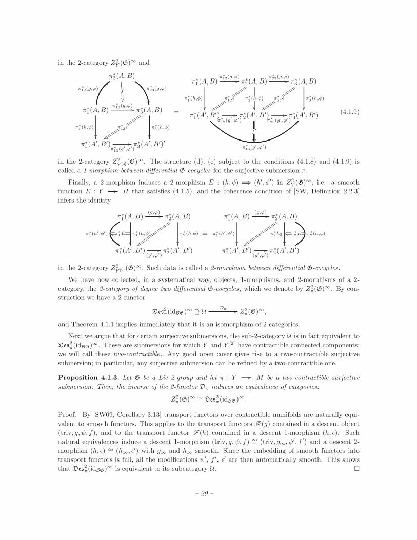
in the 2-category Z2Y (G)∞ and

π∗2(A,B)

π∗

23(g,ϕ)

π∗1(A,B)

π∗

12(g,ϕ)

::

π∗

13(g,ϕ) //

f

π∗

1 (h,φ)

π∗3(A,B)

π∗

3(h,φ)

π∗

13ǫsssss

sssss

u ssssssssss

π∗1(A

′, B′)π∗

13(g′,ϕ′)

// π∗3(A

′, B′)′

=

π∗1(A,B)

π∗

1 (h,φ)

π∗

12(g,ϕ)// π∗2(A,B)

π∗

2(h,φ)

π∗

12ǫ

v~

π∗

23(g,ϕ)// π∗3(A,B)

π∗

3 (h,φ)

π∗

23ǫ

v~

π∗1(A

′, B′)

π∗

13(g′,ϕ′)

??

f ′

π∗

12(g′,ϕ′)

// π∗2(A

′, B′)π∗

23(g′,ϕ′)

// π∗3(A

′, B′)(4.1.9)

in the 2-category Z2Y [3](G)∞. The structure (d), (e) subject to the conditions (4.1.8) and (4.1.9) is

called a 1-morphism between differential G-cocycles for the surjective submersion π.

Finally, a 2-morphism induces a 2-morphism E : (h, φ) +3 (h′, φ′) in Z2Y (G)∞, i.e. a smooth

function E : Y // H that satisfies (4.1.5), and the coherence condition of [SW, Definition 2.2.3]

infers the identity

π∗1(A,B)

(g,ϕ) //

π∗

1(h′,φ′)

%%

π∗

1 (h,φ)

π∗

1Eks

π∗2(A,B)

ǫ

v~ π∗

2 (h,φ)

π∗1(A

′, B′)(g′,ϕ′)

// π∗2(A

′, B′)

=

π∗1(A,B)

(g,ϕ) //

π∗

1(h′,φ′)

π∗2(A,B)

π∗

2(h,φ)

yy

ǫ′

v~ π∗

2h2

π∗

2Eks

π∗1(A

′, B′)(g′,ϕ′)

// π∗2(A

′, B′)

in the 2-category Z2Y [2](G)∞. Such data is called a 2-morphism between differential G-cocycles .

We have now collected, in a systematical way, objects, 1-morphisms, and 2-morphisms of a 2-

category, the 2-category of degree two differential G-cocycles , which we denote by Z2π(G)∞. By con-

struction we have a 2-functor

Des2π(idBG)∞ ⊇ U

Dπ // Z2π(G)∞,

and Theorem 4.1.1 implies immediately that it is an isomorphism of 2-categories.

Next we argue that for certain surjective submersions, the sub-2-category U is in fact equivalent to

Des2π(idBG)∞. These are submersions for which Y and Y [2] have contractible connected components;

we will call these two-contractible. Any good open cover gives rise to a two-contractible surjective

submersion; in particular, any surjective submersion can be refined by a two-contractible one.

Proposition 4.1.3. Let G be a Lie 2-group and let π : Y // M be a two-contractible surjective

submersion. Then, the inverse of the 2-functor Dπ induces an equivalence of categories:

Z2π(G)∞ ∼= Des2π(idBG)

∞.

Proof. By [SW09, Corollary 3.13] transport functors over contractible manifolds are naturally equi-

valent to smooth functors. This applies to the transport functors F (g) contained in a descent object

(triv, g, ψ, f), and to the transport functor F (h) contained in a descent 1-morphism (h, ǫ). Such

natural equivalences induce a descent 1-morphism (triv, g, ψ, f) ∼= (triv, g∞, ψ′, f ′) and a descent 2-

morphism (h, ǫ) ∼= (h∞, ǫ′) with g∞ and h∞ smooth. Since the embedding of smooth functors into

transport functors is full, all the modifications ψ′, f ′, ǫ′ are then automatically smooth. This shows

that Des2π(idBG)∞ is equivalent to its subcategory U .

– 29 –

4.1.3 Explicit Local Data

In order to make the structure of the 2-category Z2π(G)∞ of degree two differential G-cocycles more

transparent, we shall spell out all details in case that the surjective submersion π comes from an

open cover V = Vi of M . In particular, we express the diagrammatic equations above in terms of

actual equations, using the relation between the Lie 2-groupoid BG and the crossed module (G,H, t, α)

established in Section 3.3.

Firstly, a differential G-cocycle ((A,B), (g, ϕ), ψ, f) has the following smooth functions and differ-

ential forms:

(a) On every open set Vi,

ψi : Vi // H , Ai ∈ Ω1(Vi, g) and Bi ∈ Ω2(Vi, h).

(b) On every two-fold intersection Vi ∩ Vj ,

gij : Vi ∩ Vj // G and ϕij ∈ Ω1(Vi ∩ Vj , h).

(c) On every three-fold intersection Vi ∩ Vj ∩ Vk,

fijk : Vi ∩ Vj ∩ Vk // H .

The cocycle conditions are the following:

1. Over every open set Vi,

dAi + [Ai ∧ Ai] = t∗(Bi) (4.1.10)

gii = t(ψi) (4.1.11)

ϕii = −(r−1ψi

αψi)∗(Ai)− ψ∗

i θ.

2. Over every two-fold intersection Vi ∩ Vj ,

Aj = Adgij (Ai)− g∗ij θ − t∗(ϕij)

Bj = (αgij )∗(Bi)− α∗(Aj ∧ ϕij)− dϕij − [ϕij ∧ ϕij ]

1 = fijjψj = fiij αgij (ψi). (4.1.12)

3. Over every three-fold intersection Vi ∩ Vj ∩ Vk,

gik = t(fijk)gjkgij

Adfijk (ϕik) = (αgjk )∗(ϕij) + ϕjk + (r−1fijk

αfijk )∗(Ak) + f∗ijk θ.

4. Over every four-fold intersection Vi ∩ Vj ∩ Vk ∩ Vl,

fiklα(gkl, fijk) = fijlfjkl. (4.1.13)

Additionally, the curvature of the differential cocycle is according to Definition 3.3.5 given by

Hi := dBi + α∗(Ai ∧Bi) ∈ Ω3(Vi, h).

– 30 –

Secondly, a 1-morphism ((h, ǫ), φ) between differential cocycles ((A,B), (g, ϕ), ψ, f) and

((A′, B′), (g′, ϕ′), ψ′, f ′) has the following structure:

(a) On every open set Vi,

hi : Vi // G and φi ∈ Ω1(V, h).

(b) On every two-fold intersection Vi ∩ Vj ,

ǫij : Vi ∩ Vj // H .

The following conditions have to be satisfied:

1. Over every open set Vi,

B′i = (αhi

)∗(Bi)− α∗(A′i ∧ φi)− dφi − [φi ∧ φi] (4.1.14)

A′i = Adhi

(Ai)− t∗(φi)− h∗i θ (4.1.15)

ψ′i = ǫiiα(hi, ψi). (4.1.16)

2. Over every two-fold intersection Vi ∩ Vj ,

g′ij = t(ǫij)hjgijh−1i (4.1.17)

ϕ′ij = Adǫij ((αhj

)∗(ϕij) + φj)− (αg′ij )∗(φi)− (r−1ǫij

αǫij )∗(A′j)− ǫ∗ij θ (4.1.18)

3. Over every three-fold intersection Vi ∩ Vj ∩ Vk,

f ′ijk = ǫikα(hk, fijk)α(g

′ik, ǫ

−1ij )ǫ−1

jk . (4.1.19)

Finally, a 2-morphism E between differential cocycles has, for any open set Vi, a smooth function

Ei : Vi // H such that on every open set Vi

h′i = t(Ei)hi

φ′i = AdEi(φi)− (r−1

Ei αEi

)∗(A′i)− E∗

i θ

and, on every 2-fold intersection Vi ∩ Vj ,

ǫ′ij = α(g′ij , Ei)ǫijE−1j .

Concluding this discussion we note the following normalization lemma, which we need for the

discussion of surface holonomy. It can be seen as a variant of the maybe familiar normalization result

for Cech cocycles.

Lemma 4.1.4. Every differential G-cocycle with respect to an open cover Vii∈I is 1-isomorphic to

a differential G-cocycle with

ψi = 1 , gii = 1 , fiij = fijj = 1 and fiji = y−1ij α(xij , yij)

for all i, j ∈ I, and elements xij ∈ G and yij ∈ H. In particular, if G = BA for an abelian Lie group

A, then fiji = 1.

– 31 –

Proof. Suppose ((A,B), (g, ϕ), ψ, f) is a differential G-cocycle with respect to Vi. It is easy to see

that one can always pass to a1-isomorphic cocycle with ψi = 1, gii = 1, and fiij = fijj = 1. In order to

achieve the remaining condition for fiji, we choose a total order on the index set I of the open cover,

and look at smooth maps

ǫij :=

1 i ≤ j

fiji i > j

defined on Vi ∩ Vj . Then we define yet another differential G-cocycle ((A′, B′), (g′, ϕ′), ψ′, f ′) via

equations (4.1.14) to (4.1.19), and it is straightforward to see that this one has the claimed form.

4.1.4 Non-abelian Differential Cohomology

The 2-categories Z2π(G)∞ of degree two differential G-cocycles form a direct system for surjective

submersions over M , and so do the sets h0(Z2π(G)∞) of isomorphism classes of objects.

Definition 4.1.5. The direct limit

H2(M,G) := lim−→π

h0(Z2π(G)∞)

is called the degree two differential non-abelian cohomology of M with values in G.

The terminology “non-abelian differential cohomology” is motivated by the following observation.

If one drops all differential forms from the local data described in Section 4.1.3, and only keeps the

smooth functions, the corresponding limit coincides with the non-abelian cohomology H2(M,G), as

it appears for instance in [Gir71, Bre94, Bar04, Woc11]. Thus, Definition 4.1.5 extends ordinary

non-abelian cohomology by differential form data.

We remark that by Lemma 4.1.4 and the fact that every surjective submersion can be refined by

an open cover, one can define non-abelian differential cohomology by only using cocycles that are

normalized in the sense of Lemma 4.1.4.

Since every surjective submersion can be refined to a two-contractible one (for example, by a good

open cover), it also suffices to take the limit over the two-contractible surjective submersions. Then,

Proposition 4.1.3 and Theorem 3.2.2 imply via (4.1.1) the following classification result.

Theorem 4.1.6. Let G be a Lie 2-group, and let i : BG // T be an equivalence of 2-categories.

Then, there is a bijection

h0Trans2Gr(M,T ) ∼= H2(M,G).

In other words, transport 2-functors on M with BG-structure are classified up to isomorphism by the

non-abelian differential cohomology of M with values in G.

Let us specify two particular examples of differential non-abelian cohomology which have appeared

before in the literature:

1. The Lie 2-group G = BS1. We leave it as an easy exercise to the reader to check that our

differential non-abelian cohomology is precisely degree two Deligne cohomology,

H2(M,BS1) = H2(M,D(2)).

Deligne cohomology [Bry93] is a well-known local description of abelian gerbes with connection.

– 32 –

2. The Lie 2-group G = AUT(H) for H some ordinary Lie group H . We also leave it to the reader

to check that our differential cocycles are precisely the local description of connections in non-

abelian gerbes given by Breen and Messing [BM05] (see Remark 4.1.7 below). Thus, we have an

equality

H2(M,AUT(H)) =

Equivalence classes of local data

of Breen-Messing H-gerbes

with connection over M

.

Summarizing, the theory of transport 2-functors covers both Deligne cocycles and Breen-Messing

cocycles.

Remark 4.1.7. We remark that condition (4.1.10) between the 1-curving A and the 2-curving B of a

differential G-cocycle is present neither in Breen-Messing gerbes [BM05] nor in the non-abelian bundle

gerbes of [ACJ05], which we discuss in Section 4.3. Breen and Messing call the local 2-form

t∗(Bi)− dAi − [Ai ∧ Ai]

which is here zero by (4.1.10), the fake curvature of the gerbe. In this terminology, transport 2-functors

only cover Breen-Messing gerbes with vanishing fake curvature.

The crucial point is here that unlike transport 2-functors, neither Breen-Messing gerbes nor non-

abelian bundle gerbes have concepts of holonomy or parallel transport. And indeed, equation (4.1.10)

comes from an important consistency condition on this parallel transport, namely from the target-

source matching condition for the transport 2-functor, which makes it possible to decompose parallel

transport into pieces. So we understand equation (4.1.10) as an integrability condition which is neces-

sarily for a consistent parallel transport. In other words, vanishing fake curvature is not specifying a

subclass of connections, it is a necessary condition every connection has to satisfy.

4.2 Abelian Bundle Gerbes with Connection

In this section we consider the target 2-category T = B(S1-Tor), the monoidal category of S1-torsors

viewed as a 2-category with a single object [SW, Example A.2]. Associated to this 2-category is the

2-functor

iS1 : BBS1 // B(S1-Tor)

that sends the single 1-morphism of BBS1 to the circle, viewed as an S1-torsor over itself. The main

result of this section is:

Theorem 4.2.1. There is an equivalence

TransBBS1(M,B(S1-Tor)) ∼= BGrb∇(M)

between the 2-category of transport 2-functors onM with values in B(S1-Tor) and with BBS1-structure,

and the 2-category of bundle gerbes with connection over M .

Let us first recall the definition of bundle gerbes following [Mur96, MS00, Ste00, Wal07]. For a

surjective submersion π : Y // M , we first define the following 2-category BGrb∇(π):

1. An object is a tuple (B,L, ω, µ) consisting of a 2-form B ∈ Ω2(Y ), a principal S1-bundle L

with connection ω over Y [2] of curvature curv(ω) = π∗1B − π∗

2B, and an associative, connection-

preserving bundle isomorphism

µ : π∗23L ⊗ π∗

12L// π∗

13L

– 33 –

over Y [3].

2. A 1-morphism (B,L, ω, µ) // (B′, L′, ω′, µ′), also known as stable isomorphism, is a principal

S1-bundle A with connection ς over Y of curvature curv(ς) = B−B′ together with a connection-

preserving bundle isomorphism

α : π∗2A ⊗ L // L′ ⊗ π∗

1A

over Y [2], such that the diagram

π∗3A ⊗ π∗

23L ⊗ π∗12L

id⊗µ //

π∗

23α⊗id

π∗3A ⊗ π∗

13L

π∗

13α

π∗23L

′ ⊗ π∗2A ⊗ L

id⊗π∗

12α

π∗23L

′ ⊗ π∗12L

′ ⊗ π∗1A

µ′⊗id

// π∗13L

′ ⊗ π∗1A

(4.2.1)

of bundle isomorphisms over Y [3] is commutative.

3. A 2-morphism (A, ς, α) +3 (A′, ς ′, α′) is a connection-preserving bundle isomorphism ϕ :

A // A′ over Y , such that the diagram

π∗2A ⊗ L

π∗

2ϕ⊗idL

α // L′ ⊗ π∗1A

idL′ ⊗π∗

1ϕ

π∗2A

′ ⊗ Lα′

// L′ ⊗ π∗1A

′

(4.2.2)

of bundle isomorphisms over Y [2] is commutative.

The full 2-category of bundle gerbes with connection over M is then defined as the direct limit

BGrb∇(M) := lim−→π

BGrb∇(π).

The strategy to prove Theorem 4.2.1 is to first establish the equivalence on a local level:

Proposition 4.2.2. For every surjective submersion π : Y // M there is a surjective equivalence of

2-categories:

Des2π(iS1)∞ ∼= BGrb∇(π).

A 2-functorDes2π(iS1)∞ // BGrb∇(π) realizing the claimed equivalence is defined in the following

way. For a smooth descent object (triv, g, ψ, f), the smooth 2-functor triv : P2(Y ) // BBS1 defines by

Theorem 4.1.1 a 2-form B ∈ Ω2(Y ), this is the first ingredient of the bundle gerbe. The pseudonatural

transformation g yields a transport functor

F (g) : P1(Y[2]) // ΛiS1B(S

1-Tor)

– 34 –

with ΛBBS1-structure. Despite of the heavy notation, the following lemma translates this functor into

familiar language.

Lemma 4.2.3. For X a smooth manifold, there is a canonical surjective equivalence of monoidal

categories

Bun∇S1(X) ∼= Trans1ΛBBS1

(X,ΛiS1B(S1-Tor))

between principal S1-bundles with connection and transport functors with ΛBBS1-structure.

Proof. First of all, we have evidently ΛBBS1 = BS1. Second, there is a canonical equivalence of

categories

ΛiS1B(S1-Tor) ∼= S1-Tor. (4.2.3)

This comes from the fact that an object is in both categories an S1-torsor. A morphism between

S1-torsors V and W in ΛiS1B(S

1-Tor) is by definition a 2-morphism

∗S1

//

V

∗

W

f⑧⑧⑧⑧

⑧⑧⑧⑧

⑧⑧⑧⑧⑧⑧

∗S1

// ∗

in B(S1-Tor), and this is in turn an S1-equivariant map

f :W ⊗ S1 // S1 ⊗ V .

It can be identified canonically with an S1-equivariant map f−1 : V // W , i.e. a morphism in

S1-Tor. It is straightforward to see that (4.2.3) is even a monoidal equivalence. Then, the claim is

proved by Theorem 2.4.2.

Now, via Lemma 4.2.3 the transport functor F (g) is a principal S1-bundle L with connection ω

over Y [2]. This circle bundle will be the second ingredient of the bundle gerbe.

Lemma 4.2.4. The curvature of the connection ∇ on the circle bundle L satisfies

curv(ω) = π∗1B − π∗

2B.

Proof. Let Uα be open sets covering Y [2], and let (triv, t) be a local iS1-trivialization of the transport

functor F (g) consisting of smooth functors trivα : P1(Uα) // BS1 and natural transformations

tα : F (g)|Uα// (trivα)iS1 .

We observe that the functors trivα and the natural transformation tα lie in the image of the functor

F , such that there exist smooth pseudonatural transformations ρα : π∗1triv|Uα

// π∗2triv|Uα

and

modifications tα : g|Uα+3 ρα with

trivα = F (ρα) and tα = F (tα).

As found in [SW11] and reviewed in Section 2.3 of the present article, associated to the smooth

pseudonatural transformation ρα is a 1-form ϕα ∈ Ω1(Uα), and equation (4.1.4) infers in the present

situation

π∗1B − π∗

2B = dϕα.

– 35 –

It remains to trace back the relation between ϕα and the curvature of the connection ω on circle bundle

L. Namely, if Aα is the 1-form corresponding to the smooth functor trivα, we have

Aα = ϕα and dAα = curv(ω).

This shows the claim.

In order to complete the construction of the bundle gerbe, we note that the modification f : π∗23g

π∗12g

+3 π∗13g induces an isomorphism

F (f) : π∗23F (g) ⊗ π∗

12F (g) // π∗13F (g)

of transport functors; again by Lemma 4.2.3 this defines an isomorphism

µ : π∗12L ⊗ π∗

23L// π∗

13L

of circle bundles with connection, which is the last ingredient of the bundle gerbe. The coherence

axiom of [SW, Definition 2.2.1] implies the associativity condition on µ. This shows that (B,L,∇, µ)

is a bundle gerbe with connection. The descent datum ψ has been forgotten by this construction.

Using Lemma 4.2.3 in the same way as just demonstrated it is easy to assign bundle gerbe 1-

morphisms to descent 1-morphisms and bundle gerbe 2-morphisms to descent 2-morphisms. Here the

coherence conditions of [SW, Definitions 2.2.2 and 2.2.3] translate into the commutative diagrams

(4.2.1) and (4.2.2). The composition for 1-morphisms and 2-morphisms of bundle gerbes (which we

have not carried out above) is precisely reproduced by the composition laws of the descent 2-category

Des2π(iS1)∞. This defines the 2-functor of Proposition 4.2.2.

It is evident that this 2-functor is an equivalence of 2-categories, since all manipulations we have

made are equivalences according to Lemma 4.2.3 and Theorem 4.1.1. It remains to remark that the

descent datum ψ can be reproduced in a canonical way from a given bundle gerbe using the existence

of dual circle bundles, see Lemma 1 in [Wal07]. This finishes the proof of Proposition 4.2.2.

It is clear that the equivalence of Proposition 4.2.2 is compatible with the refinement of surjective

submersions, so that it given an equivalence in the direct limits:

Des2(iS1)∞M∼= BGrb∇(M).

With Theorem 3.2.2 this proves Theorem 4.2.1.

4.3 Non-Abelian Bundle Gerbes with Connection

In this section we generalize the equivalence of the previous section to so-called non-abelian bundle

gerbes, as defined in [ACJ05]. The difference between abelian and non-abelian bundle gerbes can

roughly be summarized as follows:

1. The Lie group S1 is replaced by some connected Lie group H .

2. Principal S1-bundles are replaced by principal H-bibundles , bundles with commuting left and

right principal H-action. Morphisms between H-bibundles are bi-equivariant bundle morphisms.

3. Connections on S1-bundles are replaced by so-called twisted connections on bibundles.

– 36 –

Non-abelian H-bundle gerbes with connection over M form a 2-category which we denote by

H-BGrb∇(M); some details are reviewed below. There is a sub-2-categoryH-BGrb∇ff (M) of fake-flat

non-abelian H-bundle gerbes, related to Remark 4.1.7.

On the side of transport 2-functors, we write H-BiTor for the category whose objects are smooth

manifolds with commuting, free and transitive, smooth left and right H-actions, and whose morphisms

are smooth bi-equivariant maps. Using the product over H this is naturally a (non-strict) monoidal

category, and we write B(H-BiTor) for the corresponding one-object (non-strict) 2-category. Let

AUT(H) be the Lie 2-group associated to H via Example 3.3.3 (iii). A 2-functor

i : BAUT(H) // B(H-BiTor) (4.3.1)

is defined as follows. It sends a 1-morphism ϕ ∈ Aut(H) to the H-bitorsor ϕH which is the group H

on which an element h acts from the right by multiplication and from the left by multiplication with

ϕ(h). The compositors of i are given by the canonical identifications

cg1,g2 : g1H ×H g2H //g2g1H ,

and the unitor is the identity. The 2-functor i further sends a 2-morphism h : ϕ1+3 ϕ2 to the

bi-equivariant map

ϕ1H //ϕ2H : x // hx.

While the bi-equivariance with respect to the right action is obvious, the one with respect to the left

action follows from the condition ϕ2(x) = hϕ1(x)h−1 we have for the 2-morphisms in AUT(H) for all

x ∈ H .

The main result of this section is:

Theorem 4.3.1. There is a canonical injective map

h0(H-BGrb∇ff (M)) // h0(Trans2BAUT(H)(M,B(H-BiTor)))

from isomorphism classes of fake-flat non-abelian H-bundle gerbes to transport 2-functors with values

in B(H-BiTor) and BAUT(H)-structure.

That we do not achieve a bijection or an equivalence of 2-categories is due to the fact that the

category of bibundles with twisted connections – as defined in [ACJ05] – oversees a class of morphisms,

which in principle should be allowed and arise naturally from the theory of transport functors.

Anyway, Theorem 4.3.1 provides non-trivial examples of transport 2-functors. The injective map

of Theorem 4.3.1 is constructed as

H-BGrb∇ff (M) // Des2(i)∞M∼= Trans2BAUT(H)(M,B(H-BiTor)),

where the first 2-functor is constructed in Proposition 4.3.8 and the equivalence is the one of Theorem

3.2.2. We first review necessary material.

4.3.1 Twisted Connections on Bibundles

Let P be a principal H-bibundle over X . We denote the left and right actions by an element h ∈ H

on P by lh and rh, respectively. Measuring the difference between the left and the right action in the

sense of lh(p) = rg(h)(p) furnishes a smooth map

g : P // Aut(H). (4.3.2)

– 37 –

In the following we denote by aut(H) the Lie algebra of Aut(H). Further, we denote by t :

H // Aut(H) the assignment of inner automorphisms and by α : Aut(H)×H // H the evaluation.

Definition 4.3.2 ([ACJ05]). Let p : P // X be a principal H-bibundle, and let A ∈ Ω1(X, aut(H))

be a 1-form on the base space. An A-twisted connection on P is a 1-form φ ∈ Ω1(P, h) satisfying

φρh

(d

dt(ρh)

)= Ad−1

h

(φρ

(dρ

dt

))− (rh αh)∗ (p

∗A) + θh

(dh

dt

)(4.3.3)

for all smooth curves ρ : [0, 1] // P and h : [0, 1] // H. A morphism f : P // P ′ respects

A-twisted connections φ on P and φ′ on P ′ if f∗φ′ = φ.

We write Bibun∇H(X,A) for the category of principal H-bibundles with A-twisted connection over

X , and Bibun∇H(X) for the union of these categories over all 1-forms A.

Remark 4.3.3. For A = 0 an A-twisted connection on P is the same as an ordinary connection on P

regarded as a right principal bundle.

Lemma 4.3.4 ([ACJ05]). Let A ∈ Ω1(X, aut(H)) be a 1-form and let p : P // X be a principal

H-bibundle. For any A-twisted connection φ on P there exists a unique 1-form Aφ ∈ Ω1(X, aut(H))

satisfying

p∗Aφ = Adg(p∗A)− g∗θ − t∗ φ,

where g is the map from (4.3.2).

A twisted connection in a principal bibundle P gives rise to parallel transport maps

τγ : Px // Py

between the fibres of P over points x, y associated to any path γ : x // y. It is obtained in the same

way as in an ordinary principal bundle but using equation (4.3.3) instead of the usual one. As a result

of the twist, the maps τγ are not bi-equivariant; they satisfy

τγ(lFφ(γ)(h)(p)) = lh−1(τγ(p)) and τγ(rh(p)) = rF (γ)−1(h−1)τγ(p) (4.3.4)

where F, Fφ : PX // Aut(H) are the parallel transport maps associated to the 1-forms A and Aφ;

see [SW09, Proposition 4.7]. These complicated relations have a very easy interpretation, as we will

see in the next section.

Finally, an A-twisted connection φ on a principal H-bundle P has a curvature: this is the 2-form

curv(φ) := dφ+ [φ ∧ φ] + α∗(A ∧ φ) ∈ Ω2(P, h).

For two principal H-bibundles P and P ′ over X one can fibrewise take the tensor product of P

and P ′ yielding a new principal H-bibundle P ×H P over X . If the two bibundles are equipped with

twisted connections, the bibundle P×HP′ inherits a twisted connection only if the two twists satisfy an

appropriate matching condition. Suppose the principal H-bibundle P is equipped with an A-twisted

connection φ, and P ′ is equipped with an A′-twisted connection φ′, and suppose that the matching

condition

A′φ′ = A (4.3.5)

– 38 –

is satisfied. Then, the tensor product bibundle P×HP′ carries anA′-twisted connection φtot ∈ Ω1(P×H

P, h) characterized uniquely by the condition that

pr∗φtot = (g p′)∗ p∗φ+ p′∗φ′,

where pr : P×XP′ // P×HP

′ is the projection to the tensor product and p and p′ are the projections

to the two factors. This tensor product, defined only between appropriate pairs of bibundles with

twisted connections, turns Bibun∇H(X) into a “monoidoidal” category.

A better point of view is to see it as a 2-category: the objects are the twists, i.e. 1-forms

A ∈ Ω1(X, aut(H)), a 1-morphism A // A′ is a principal H-bibundle P with A′-twisted connection φ

such that A′φ′ = A, and a 2-morphism (P, φ) +3 (P ′, φ′) is just a morphism of principal H-bibundles

that respects the A′-twisted connections.

4.3.2 Transport Functors for Bibundles with Twisted Connections

We are now going to relate the categoryBibun∇H(X) of principal H-bibundles with twisted connections

over X to a category of transport functors. Using the terminology of Section 3.1, we have:

Proposition 4.3.5. There is a surjective and faithful functor

Bibun∇H(X) // Trans1ΛBAUT(H)(X,ΛiB(H-BiTor)).

Proof. Given a principal H-bibundle P with A-twisted connection, we define the associated transport

functor by

traP : xγ // y

//

i(∗)

Px

i(F (γ)) // i(∗)

τ−1γ

②②②②②②②②②②

x ②②②②②②②②

Py

i(∗)

i(Fφ(γ))// i(∗).

Here F, Fφ : PX // Aut(H) are the maps defined by A and Aφ that we have already used in

the previous section. The definition contains the claim that the parallel transport map τγ gives a

bi-equivariant map

τ−1γ : Py ×H F (γ)H //

Fφ(γ)H ×H Px;

it is indeed easy to check that this is precisely the meaning of equations (4.3.4). A morphism

f : P // P ′ between bibundles with A-twisted connections induces a natural transformation

ηf : traP // traP ′ between the associated functors, whose component at a point x is the bi-

equivariant map fx : Px +3 P ′x. This is a particular morphism in ΛiB(H-BiTor) for which the

horizontal 1-morphisms are identities. Here it becomes clear that the assignments

(P, φ) // traP and f // ηf

define a functor which is faithful but not full.

It remains to check that the functor traP is a transport 2-functor. We leave it as an exercise for

the reader to construct a local trivialization (t, triv) of traP with smooth descent data. Hint: use an

ordinary local trivialization of the bibundle P and follow the proof of Proposition 5.2 in [SW09].

– 39 –

Both categories in Proposition 4.3.5 have the feature that they have tensor products between

appropriate objects. Concerning the bibundles with twisted connections, we have described this in

terms of the matching condition (4.3.5) on the twists. Concerning the category of transport functors,

this tensor product is inherited from the one on ΛiB(H-BiTor), which has been discussed in Section

3.1.

Lemma 4.3.6. The matching condition (4.3.5) corresponds to the required condition for tensor prod-

ucts in ΛiB(H-BiTor) under the functor of Proposition 4.3.5. Moreover, the functor respects tensor

products whenever they are well-defined.

Proof. Suppose that the matching condition A′φ′ = A holds, so that principal H-bibundles P and

P ′ with connections φ and φ have a tensor product. It follows that the map Fφ′ which labels the

horizontal 1-morphisms at the bottom of the images of traP ′ is equal to the map F which labels the

ones at the top of the images of traP ; this is the required condition for the existence of the tensor

product traP ′ ⊗ traP . That the tensor products are respected follows from the definition of the twisted

connection φtot on the tensor product bibundle.

An alternative formulation of Lemma 4.3.6 would be that the functor of Proposition 4.3.5 respects

the “monoidoidal structures”, or, that it is a double functor between (weak) double categories.

4.3.3 Non-Abelian Bundle Gerbes as Transport 2-Functors

Let π : Y // M be a surjective submersion. We recall:

Definition 4.3.7 ([ACJ05]). A non-abelian H-bundle gerbe with connection with respect to π is a

2-form B ∈ Ω2(Y, h), a 1-form A ∈ Ω1(Y, aut(H)), a principal H-bibundle p : P // Y [2] with

A-twisted connection φ such that

curv(φ) = (π1 p)∗B − (αg)∗ (π2 p)

∗B, (4.3.6)

and an associative morphism

µ : π∗23P ×H π∗

12P // π∗13P

of bibundles over Y [3] that respects the twisted connections.

In (4.3.6), g is the smooth map (4.3.2) and α : Aut(H)×H // H is the evaluation. The definitions

of 1-morphisms and 2-morphisms generalize in a straightforward way the definitions from the abelian

case. This defines the 2-category H-BGrb∇(π). The 2-category H-BGrb∇(M) of non-abelian H-

bundle gerbes over M is defined as the direct limit,

H-BGrb∇(M) := lim−→πH-BGrb∇(π).

We remark:

(i) A non-abelian S1-bundle gerbe is not the same as an abelian S1-bundle gerbe: for the non-

abelian bundle gerbes also the automorphisms are important, and Aut(S1) ∼= Z2. For transport

2-functors this is even more obvious: the Lie 2-groups BS1 and AUT(S1) are not equivalent.

(ii) The non-abelian bundle gerbes of Definition 4.3.7 are a priori not “fake-flat”, i.e. the relation

t∗(B) = dA+ [A ∧A]

– 40 –

may not be satisfied, see Remark 4.1.7. We denote the sub-2-categories of fake-flat non-abelian

H-bundle gerbes by H-BGrb∇ff (−).

Proposition 4.3.8. For every surjective submersion π : Y // M , there is a 2-functor

H-BGrb∇ff (π) // Des2π(i)∞.

which is surjective and faithful on Hom-categories. In particular, it induces an injective map on

isomorphism classes of objects.

Proof. All relations concerning the bimodules are analogous to those in the abelian case, upon

generalizing Lemma 4.2.3 to Proposition 4.3.5 and Lemma 4.3.6. Relation (4.3.6) for the 2-form B can

be proved in the same way as Lemma 4.2.4, but now using the full version of equation (4.1.4). The

comments concerning the descent datum ψ also remain valid.

In the direct limit, the 2-functors of Proposition 4.3.8 induce a 2-functor

H-BGrb∇ff (M) // Des2(i)∞M . (4.3.7)

Since the direct limit respects the operation of forming isomorphism classes of objects, and on the level

of sets a direct limit of injective maps is injective, the 2-functor (4.3.7) induces an injective map on

isomorphism classes of objects. This completes the proof of Theorem 4.3.1.

4.4 2-Bundles with Connections

Apart from the equivalence between transport functors and principalG-bundles with connection (Theo-

rem 2.4.2), our paper [SW09] also contains an analogous equivalence for vector bundles with connection.

It has an immediate generalization to 2-vector bundles with many applications, on which we shall give

a brief outlook.

Suppose 2Vect is some 2-category of 2-vector spaces. Given a 2-group G, a representation of G on

such a 2-vector space is a 2-functor

ρ : BG // 2Vect.

A 2-vector bundle with connection and structure 2-group G is nothing but a transport 2-functor

tra : P2(X) // 2Vect with BG-structure. Important classes of 2-vector bundles are line 2-bundles

and string bundles.

4.4.1 Models for 2-Vector Spaces

Depending on the precise application there is some flexibility in what one may want to understand

under a 2-vector space. Usually 2-vector spaces are abelian module categories over a given monoidal

category. For k a field, two important classes of examples are the following. First, let k be the discrete

monoidal category over k. Then, 2Vect is 2-category of module categories over k. This is equivalent

to the 2-category of categories internal to k-vector spaces. These Baez-Crans 2-vector spaces [BC04]

are appropriate for the discussion of Lie 2-algebras.

The second model for 2Vect is the 2-category of module categories over the monoidal category

Vect(k) of k-vector spaces,

2Vect := Vect(k)-Mod.

– 41 –

In its totality this is rather unwieldy, but it contains two important sub-2-categories: the 2-category

KV(k) of Kapranov-Voevodsky 2-vector spaces [KV94] and the 2-category Bimod(k), whose objects

are k-algebras, whose 1-morphisms are bimodules over these algebras and whose 2-morphisms are

bimodule homomorphisms [Shu08]. Indeed, there is an inclusion 2-functor

ι : Bimod(k)

// Vect(k)-Mod

that sends a k-algebra A to the category A-Mod of ordinary (say, right) A-modules. This is a module

category over Vect(k) by tensoring a right module from the left by a vector space. A 1-morphism, an

A-B-bimodule N , is sent to the functor that tensores a right A-module from the right by N , yielding a

right B-module. A bimodule morphism induces evidently a natural transformation of these functors.

If one restricts the 2-functor ι to the full sub-2-category formed by those algebras that are direct

sums A = k⊕n of the ground field algebra, the 2-vector spaces in the image of ι are of the form Vect(k)n,

i.e. tuples of vector spaces. The 1-morphisms in the image are (m × n)-matrices whose entries are

k-vector spaces. These form the 2-category of Kapranov-Voevodsky 2-vector spaces [KV94].

4.4.2 The canonical Representation of a 2-Group

Every automorphism 2-group AUT(H) of a Lie group H has a canonical representation on 2-vector

spaces, namely

BAUT(H)A // Bimod(k)

ι // Vect(k)-Mod, (4.4.1)

where the 2-functor A is defined similar as the one we have used for the non-abelian bundle gerbes in

(4.3.1). It sends the single object to k regarded as a k-algebra, it sends a 1-morphism ϕ ∈ Aut(H) to

the bimodule ϕk in the notation of Section 4.3.2, and it sends a 2-morphism (ϕ, h) : ϕ +3 ch ϕ to

the multiplication with h from the left.

Now let G be any smooth Lie 2-group corresponding to a smooth crossed module (G,H, t, α). We

have a canonical 2-functor

BG // BAUT(H) : ∗

g

g′

CCh

∗ // ∗

αg

αg′

CCh

∗ (4.4.2)

whose composition with (4.4.1) gives a representation of G, that we call the canonical k-representation.

Example 4.4.1. A very simple but useful example is the canonical C-representation of BC×. In this

case the composition (4.4.1) is the 2-functor

ρ : BBC× // Vect(C)-Mod : ∗

id

id

CCz

∗ // Vect(C)

−⊗C

$$

−⊗C

::−·z

Vect(C)

for all z ∈ C×. Notice that Vect(C) is the canonical 1-dimensional 2-vector space over C in the same

sense in that C is the canonical 1-dimensional complex 1-vector space. Therefore, transport 2-functors

tra : P2(M) // Vect(C)-Mod

– 42 –

with BBC×-structure deserve to be addressed as line 2-bundles with connection. Two remarks:

1. Going through the discussion of abelian bundle gerbes with connection in Section 4.2 it is easy to

see that line 2-bundles with connection are equivalent to bundle gerbes with connection defined

via line bundles instead of circle bundles.

2. The fibre tra(x) of a line 2-bundle tra at a point x is an algebra which is Morita equivalent to the

ground field C. These are exactly the finite rank operators on a separable Hilbert space. Thus,

line 2-bundles with connection are a form of bundles of finite rank operators with connection,

this is the point of view taken in [BCM+02].

The 2-functor A : BAUT(H) // Bimod(k) we have used above can be deformed to a 2-functor

Aρ using an ordinary representation ρ : BH // Vect(k) of H . It sends the object of BAUT(H) to

the algebra Aρ(∗) which is the vector space generated from all the linear maps ρ(h). A 1-morphism

ϕ ∈ Aut(H) is again sent to the bimodule ϕAρ(∗), and the 2-morphisms as before to left multiplications.

The original 2-functor is reproduced by A = Atrivk from the trivial representation of H on k.

Example 4.4.2. For G a compact simple and simply-connected Lie group, we consider the level k

central extension Hk := ΩkG of the group of based loops in G. For a positive energy representation

ρ : BΩkG // Vect(k) the algebra Aρ(∗) turns out to be a von Neumann-algebra while the bimodules

ϕAρ(∗) are Hilbert bimodules. In this infinite-dimensional case we have to make the composition of

1-morphisms more precise: here we take not the algebraic tensor product of these Hilbert bimodules

but the Connes fusion tensor product [ST04]. Connes fusion product still respects the composition: for

A a von Neumann algebra and ϕA the bimodule structure on it induced from twisting the left action

by an algebra automorphism ϕ, we have

ϕA ⊗ ϕ′A ≃ ϕ′ϕA

under the Connes fusion tensor product. Now let G = Stringk(G) be the string 2-group defined from

the crossed module ΩkG // P0G of Frechet Lie groups [BCSS07]. Together with the projection

2-functor (4.4.2) we obtain an induced representation

i : BStringk(G) // BimodCF(k)

The fibres of a transport 2-functor

tra : P2(M) // BimodCF(k) (4.4.3)

with BStringk(G)-structure are hence von Neumann algebras, and its parallel transport along a path is

a Hilbert bimodule for these fibres. In conjunction with the result [BS09, BBK12] that Stringk(G)-2-

bundles have the same classification as ordinary fibre bundles whose structure group is the topological

String group, this says that transport 2-functors (4.4.3) have to be addressed as String 2-bundles with

connection, see [ST04].

4.4.3 Twisted Vector Bundles

Vector bundles over M twisted by a class ξ ∈ H3(M,Z) are the same thing as gerbe modules for

a bundle gerbe G whose Dixmier-Douady class is ξ [BCM+02]. These modules are in turn nothing

else but certain (generalized) 1-morphisms in the 2-category of bundle gerbes BGrb(M) [Wal07]. The

– 43 –

same is true for connections on twisted vector bundles. More precisely, a twisted vector bundle with

connection is the same as a 1-morphism

E : G // Iρ

from the bundle gerbe G with connection to the trivial bundle gerbe I equipped with the connection

2-form ρ ∈ Ω2(M).

Now let

tra : P2(M) // Vect(C)-Mod

be a transport 2-functor which plays the role of the bundle gerbe G, but we allow an arbitrary structure

2-group G and any representation ρ : BG // Vect(C)-Mod. Let tra∞ : P2(M) // BG be a

smooth 2-functor which plays the role of the trivial bundle gerbe. We shall now consider transport

transformations

A : tra // tra∞ρ .

Let π : Y // M be a surjective submersion for which tra admits a local trivialization with smooth

descent data (triv, g, ψ, f). The descent data of tra∞ is of course (π∗tra∞, id, id, id). Now the transport

transformation A has the following descent data: the first part is a pseudonatural transformation

h : triv // π∗tra∞ whose associated functor F (h) : P1(Y ) // Λρ(Vect(C)-Mod) is a transport

functor with ΛBG-structure. The second part is a modification ǫ : π∗2hg +3 idπ∗

1h whose associated

natural transformation

F (ǫ) : π∗2F (h) ⊗ F (g) // π∗

1F (h)

is a morphism of transport functors over Y [2]. According to the coherence conditions on descent

1-morphisms, it fits into the commutative diagram

π∗3F (h) ⊗ π∗

23F (g) ⊗ π∗12F (g)

π∗

23F(ǫ)⊗id //

id⊗F(f)

π∗2F (h) ⊗ π∗

12F (g)

π∗

12F(ǫ)

π∗3F (h) ⊗ π∗

13F (g)π∗

13F(ǫ)// π∗

1F (h)

(4.4.4)

of morphisms of transport functors over Y [3] and satisfies ∆∗F (ǫ)F (ψ) = id. The transport functor

F (h) : P1(Y ) // Λρ(Vect(C)-Mod)

together with the natural transformation F (ǫ) is the general version of a vector bundle with connection

twisted by a transport 2-functor tra. According to Sections 4.1 and 4.3, the twists can thus be Breen-

Messing gerbes or non-abelian bundle gerbes with connection.

Depending on the choice of the representation ρ, our twisted vector bundles can be translated into

more familiar language. Let us demonstrate this in the case of Example 4.4.1, in which the twist is a

line 2-bundle with connection, i.e. a transport 2-functor

tra : P2(M) // Vect(C)-Mod

with BBC×-structure. In order to obtain the usual twisted vector bundles, we restrict the target

2-category to BVect(C), the monoidal category of complex vector spaces considered as a 2-category.

The following Lie category Gl is appropriate: its objects are the natural numbers N, and it has only

morphisms between equal numbers, namely all matrices Gln(C). The composition is the product of

– 44 –

matrices. The Lie category Gl is strictly monoidal: the tensor product of two objects m,n ∈ N is

the product nm ∈ N, and the one of two matrices A ∈ Gl(m) and B ∈ Gl(n) is the ordinary tensor

product A ⊗B ∈ Gl(m × n). In fact, Gl carries a second monoidal structure coming from the sum of

natural numbers and the direct sum of matrices, so that Gl is actually a bipermutative category, see

Example 3.1 of [BDR04].

Notice that we have a canonical inclusion functor ι : BC×

// Gl, which induces another inclusion

ι∗ : Trans2BBC×(M,BVect(C)) // Trans2BGl(M,BVect(C))

of line 2-bundles with connection into more general vector 2-bundles with connection. Here we have

used the representation

ρ : BGl // BVect

obtained as a generalization of Example 4.4.1 from C× = Gl1(C) to Gln(C) for all n ∈ N. The

composition ρ ι reproduces the representation of Example 4.4.1.

Using the above inclusion, the given transport 2-functor tra induces a transport 2-functor ι∗ tra :

P2(M) // BVect(C) with BGl-structure, and one can study transport transformations

A : tra // tra∞ρ

in that greater 2-category Trans2BGl(M,BVect(C)). Along the lines of the general procedure described

above, we have transport functors F (g) and F (h) coming from the descent data of tra and A, respec-

tively. In the present particular situation, the first one takes values in the category ΛριBVect1(C)

whose objects are one-dimensional complex vector spaces and whose morphisms from V to W are

invertible linear maps f : W ⊗ C // C ⊗ V . Similar to Lemma 4.2.3, this category is equivalent to

the category Vect1(C) of one dimensional complex vector spaces itself. Thus, the transport functor

F (g) with BC×-structure is a complex line bundle L with connection over Y [2]. The second transport

functor, F (h), takes values in the category ΛριBVect(C). This category is equivalent to the category

Vect(C) itself. It has ΛιBGl-structure, which is equivalent to Gl. Thus, F (h) is a transport functor

with values in Vect(C) and Gl-structure. It thus corresponds to a finite rank vector bundle E over Y

with connection.

Since all identifications we have made so far a functorial, the morphisms F (f) and F (ǫ) of transport

functors induce morphisms of vector bundles that preserve the connections, namely an associative

morphism

µ : π∗23L ⊗ π∗

12L // π∗13L

of line bundles over Y [2], and a morphism

: π∗2E ⊗ L // π∗

1E

of vector bundles over Y which satisfies a compatibility condition corresponding to (4.4.4). This

reproduces the definition of a twisted vector bundle with connection [BCM+02]. We remark that

the 2-form ρ that corresponds to the smooth 2-functor tra∞ρ which was the target of the transport

transformation A we have considered, is related to the curvature of the connection on the vector bundle

E: it requires that

curv(E) = In · (curv(L)− π∗ρ),

where In is the identity matrix and n is the rank of E. This condition can be derived similar to Lemma

4.2.4.

– 45 –

5 Surface Holonomy

From the viewpoint of a transport 2-functor, parallel transport and holonomy are basically evaluation

on paths or bigons. Let tra : P2(M) // T be a transport 2-functor with BG-structure on M . Its

fibres over points x, y ∈ M are objects tra(x) and tra(y) in T , and we say that its parallel transport

along a path γ : x // y is given by the 1-morphism

tra(γ) : tra(x) // tra(y)

in T , and its parallel transport along a bigon Σ : γ +3 γ′ is given by the 2-morphism

tra(Σ) : tra(γ) +3 tra(γ′)

in T . The rules how parallel transport behaves under the composition of paths and bigons are precisely

the axioms of the 2-functor tra; see [SW, Definition A.5]. We give some examples. If γ1 : x // y and

γ2 : y // z are composable paths, the separate parallel transports along the two paths are related to

the one along their composition by the compositor

cγ1,γ2 : tra(γ2) tra(γ1) +3 tra(γ2 γ1)

of the 2-functor tra. If idx is the constant path at x, the parallel transport along idx is related to the

identity at the fibre tra(x) by the unitor

ux : tra(idx) +3 idtra(x).

The parallel transports along vertically composable bigons Σ : γ1 +3 γ2 and Σ′ : γ2 +3 γ3 obey

tra(Σ′ • Σ) = tra(Σ′) • tra(Σ).

In the following we focus on certain bigons that parameterize surfaces; the parallel transport along

these bigons will be called the holonomy of the transport 2-functor tra.

5.1 Markings and Fundamental Bigons

Surface holonomy of gerbes has so far only be studied in the abelian case, i.e. for gerbes with structure

2-group G = BS1; see e.g. [Mur96]. It is understood that an abelian gerbe with connection over M

provides an S1-valued surface holonomy for smooth maps φ : S // M defined on closed oriented

surfaces S. Various extensions have been studied for oriented surfaces with boundary [CJM02, GR02],

closed unoriented (in particular unorientable) surfaces [SSW07], and unoriented surfaces with boundary

[GSW11].

Let us try to explain why the step from abelian to non-abelian surface holonomy is so difficult,

by looking at the analogous but easier situation of ordinary holonomy of a connection on a principal

bundle P over M . In the abelian case, say with structure group S1, holonomy is defined for closed

oriented curves in M . Passing to a non-abelian structure group G, we have two possibilities. The first

is to choose additional structure on the closed oriented curve, namely a point x ∈ M , in which case the

holonomy is a well-defined automorphism of the fibre Px of the bundle P over the point x. The second

possibility is to project the value of the holonomy into an appropriate quotient, for example along the

map Aut(Px) // Gred into the set Gred of conjugacy classes of G. This quotient is designed such

– 46 –

that a different choice of x yields the same element in Gred, and so P has a well-defined Gred-valued

holonomy for closed oriented curves.

Choosing a point in a closed oriented curve means to represent it as a path (up to thin homotopy).

The objective of this section is to describe how to represent a closed oriented surface φ : S // Mas a bigon in M . It will be convenient to adapt the following standard terminology from the theory

of Riemann surfaces to our setting. Suppose S is a closed oriented surface of genus g. A marking of

S is a point x ∈ S together with a set M = αi, βigi=1 of paths αi : x // x and βi : x // x such

that the homotopy classes [αi] and [βi] of the paths form a presentation of the fundamental group of

S based at x with the relation that [τM] = 1, where

τM := β−1g α−1

g βg αg . . . β−11 α−1

1 β1 α1.

In other words,

π1(S, x) = 〈[αi], [βi] | [τM] = 1〉 .

Next we formulate — in the language of bigons — the statement that the path τM can be collapsed

to the point x in such a way that the collapsing homotopy parameterizes the surface S. The challenge

is that such a homotopy cannot simultaneously be a bigon and a good parameterization. We propose

the following notion.

Definition 5.1.1. A fundamental bigon with respect to the marking (x,M) is a bigon Σ : τM +3 idxsuch that there exist:

(a) a polygon P ⊆ R2 and a surjective smooth map π : P // S that is an embedding when restricted

to the interior of P and preserves the orientations.

(b) a surjective continuous map k : [0, 1]2 // P that restricts to a diffeomorphism between the

interiors and preserves the orientations, such that there exists a vertex v0 of P with v0 = k(s, 0) =

k(s, 1) = k(1, t) for all 0 ≤ s, t ≤ 1.

(c) a smooth map h : [0, 1] ×P // S with h0 = π and h1 k = Σ, such that for each edge e of P the

restriction h|[0,1]×e has rank one, and h(−, v) = x for each vertex v.

In this definition the polygon P serves as the standard parameter domain of the surface, and the

map π : P // S is such a parameterization. The map k : [0, 1]2 // P is responsible for the transition

between the standard parameter domain P and the parameter domain [0, 1]2 for bigons. The map h

ensures that the fundamental bigon Σ is homotopic to the “bigonized” standard parameterization,

π k. The various conditions on k and h ensure that the homotopy h k is constantly equal to x

over the boundary parts of [0, 1]2 that are parameterized by (s, 0), (s, 1), and (1, t), and ensure that it

restricts to a thin homotopy between the path (π k)(0,−) and τM over the remaining boundary part

(0, t).

A marking will be called good , if it admits a fundamental bigon. The following three lemmata

elaborate some properties of good markings and fundamental bigons.

Lemma 5.1.2. Every closed oriented surface S has a good marking.

Proof. It is well-known that every surface S of positive genus g > 0 has a “fundamental polygon”

P ⊆ C with 4g edges, together with a map π : P // S that has all required properties. It can be

– 47 –

arranged such that all vertices go to a single point x ∈ S, and — if the 4g edges are parameterized by

A1, B1, A′1, B

′1, A2, ... : [0, 1] // P in counter-clockwise order starting at a vertex v0 — then

π(Ai(1 − t)) = π(A′i(t)) and π(Bi(1− t)) = π(B′

i(t)). (5.1.1)

Let D ⊆ C denote the disc centered at −1 ∈ C. It is obvious that P and D are homeomorphic. The

homeomorphism can be arranged such that (i) it preserves orientations, (ii) it is a smooth embedding

when restricted to the complement of the vertices of P , and (iii) the vertices map to points equidistantly

distributed over the boundary of D, with v0 at 0 ∈ C. We define

k′ : [0, 1]2 // D : (s, t) // (1 − s)(e2πit − 1).

Under the homeomorphism between P and D, this gives the map k with all required properties.

The map h : [0, 1] × P // S is chosen such that h1 : P // S is constantly equal to x in

neighborhoods of all vertices, and such that (5.1.1) remains true with h1 instead of π. Then we define

Σ := h1 k

This is smooth because h1 is locally constant at all points where k is not smooth. We consider for

0 ≤ k ≤ 4g − 1 the map pk : [0, 1] // [0, 1] : t // k+t4g that squeezes the interval into the k-th of 4g

many pieces. Then, we define for i = 1, .., g

αi := π Σ(0,−) p4i−4 and βi := π Σ(0,−) p4i−3,

which give smooth maps with sitting instants, each going from x to x, Thus, (x,M) with M := αi, βi

is a marking, and (5.1.1) imply that Σ is a bigon Σ : τM +3 idx.The case of genus g = 0 can be treated in a similar way using the disc D1 with one marked point;

this is left as an exercise.

The main idea behind the definition of a fundamental bigon is that the integral of a 2-form ω ∈ Ω2(S)

over S can be computed over a fundamental bigon.

Lemma 5.1.3. Suppose S is a closed oriented surface with a good marking (x,M). Let Σ be a funda-

mental bigon with respect to (x,M). Then,∫

S

ω =

∫

[0,1]2Σ∗ω

for all 2-forms ω ∈ Ω2(S).

Proof. We choose the structure (P , k, π, h) of Definition 5.1.1. Then,

∫

S

ω =

∫

P

π∗ω =

∫

P

h∗1ω =

∫

int(P)

h∗1ω =

∫

(0,1)2Σ∗ω =

∫

[0,1]2Σ∗ω.

The second equality holds because the homotopy h between h0 = π and h1 has rank one on the

boundary. The other equalities hold immediately due to the assumptions on all the involved maps.

Finally, we show that the choice of a fundamental bigon is essentially unique.

Lemma 5.1.4. Let S be a closed oriented surface and (x,M) be a marking. Suppose Σ : τM +3 idxand Σ′ : τM +3 idx are two fundamental bigons with respect to the marking (x,M). Then, Σ and Σ′

are thin homotopy equivalent in the sense of Section 2.1.

– 48 –

Proof. We choose for both fundamental bigons the structures (P , k, π, h) and (P ′, k′, π′, h′) of De-

finition 5.1.1. We can assume that P = P ′, since any two polygons are diffeomorphic, and such

diffeomorphism can be absorbed into π′ and k′. We can assume that P is convex; in that case it is

easy to see that k and k′ are homotopic, with the homotopy fixing the three boundary components

that map to v0, and restricting to a homotopy with values in ∂P over the forth boundary component.

The homotopies h and h′ restrict on the boundary to thin homotopies π|∂P ≃ τM and π′|∂P ≃ τM.

By a version of Alexander’s trick, we obtain a smooth homotopy π ≃ π′ that fixes all vertices and has

rank one over the edges. Then we have chains of homotopies

Σ ≃ h1 k ≃ h0 k ≃ π k ≃ π k′ ≃ π′ k′ ≃ h′0 k′ ≃ h′1 k

′ ≃ Σ′

which are all smooth and have rank one restricted over the boundary. By dimensional reasons, this

homotopy can at most have rank two everywhere. This means that it is a thin homotopy between Σ

and Σ′.

Next we come to the definition of surface holonomy. Since the generic transport 2-functor is not

strict, we have to deal with the difference between the 1-morphism tra(φ∗τM) and the 1-morphism

traφ,M :=

g∏

i=1

tra(αi) tra(βi) tra(α−1i ) tra(β−1

i ),

for which we may agree for an arbitrary convention how to put parentheses in case T has a non-trivial

associator. The relation between these two 1-morphisms is given by a 2-morphism

cφ,tra : traφ,M +3 tra(φ∗τM)

made up from the compositors of tra in a unique way, due to the coherence axiom for compositors

(this is axiom (F3) in [SW, Appendix A]).

Definition 5.1.5. Let tra : P2(M) // T be a transport 2-functor. Suppose S is a closed oriented

surface equipped with a good marking (x,M) and a smooth map φ : S // M . Let Σ be a fundamental

bigon for (x,M). The 2-morphism

Holtra(φ, x,M) := tra(φ∗Σ) • cφ,tra : traφ,M +3 tra(idφ(x))

in T is called the surface holonomy of tra.

Note that the surface holonomy is independent of the choice of the fundamental bigon due to

Lemma 5.1.4. On the other hand, the surface holonomy does depend on the choice of the marking

(x,M). Even worse, it is not invariant under isomorphisms between transport 2-functors. It is the

purpose of the following discussion to improve these dependence issues.

5.2 Reduced Surface Holonomy

We consider a Lie 2-group G defined from a smooth crossed module (G,H, t, α), and restrict our

attention to transport 2-functors

tra : P2(M) // T

with BG-structure. Our goal is to replace the 2-functor tra by another 2-functor which takes values

in a certain quotient of G where surface holonomy becomes more rigid. In order to construct this

– 49 –

quotient, we write [G,H ] ⊆ H for the subgroup of H that is generated by all elements of the form

h−1α(g, h), for h ∈ H and g ∈ G. The following lemma follows from the axioms of a crossed module;

see Definition 3.3.2).

Lemma 5.2.1. The subgroup [G,H ] is normal in H and contains the commutator subgroup,

[H,H ] [G,H ] H.

We come to the following important definition.

Definition 5.2.2. Let G be a Lie 2-group. Then, the group Gred := H/[G,H ] is called the reduction

of G.

By Lemma 5.2.1, the reduction Gred is a subgroup of the abelianizationH/[H,H ] and hence abelian.

Note that the projection to the quotient yields a strict 2-functor

Red : BG // BBGred.

Example 5.2.3. Let us look at examples for Lie 2-groups G:

(a) In the case of the 2-group BA for A an ordinary abelian Lie group, [1, A] is the trivial group, and

(BA)red = A.

(b) Let G be a Lie group and let EG the associated 2-group of inner automorphisms, see Section 3.

Since α here is the conjugation action of G on itself, [G,G] is indeed the commutator subgroup.

Thus (EG)red is an abelian Lie group, the abelianization of G.

(c) Let H be a connected Lie group and let AUT(H) be its automorphism 2-group, with G = Aut(H).

In this case [H,H ] = [G,H ] if and only if all automorphisms of H are inner. For H = S1 with

Aut(S1) = Z2 we get [Z2, S1] = S1, so that AUT(S1)red = 1.

Let tra : P2(M) // T be a transport 2-functor with BG-structure. The following definition

introduces the replacement for tra that we want to consider.

Definition 5.2.4. A reduction of tra is a transport 2-functor trared : P2(M) // BG with BG-structure

such that the following two conditions are satisfied:

(i) There exists a pseudonatural equivalence i trared ∼= tra.

(ii) The 2-functor Red trared is normalized in the sense of [SW, Appendix A].

In the following proposition we prove an existence and uniqueness result for reductions.

Proposition 5.2.5. If i : BG // T is an equivalence of categories, then every transport 2-functor

with i-structure admits a reduction. Moreover, two reductions of the same transport 2-functor are

pseudonaturally equivalent.

Proof. Since i : BG // T is an equivalence of 2-categories we can choose an inverse 2-functor

j : T // BG, so that tra′ := j tra : P2(M) // BG is a transport 2-functor with BG-structure;

see Section 3.3.1. Since j is inverse to i it is clear that i tra′ ∼= tra. The 2-functor tra′ is the first

approximation of the reduction whose existence we want to prove.

– 50 –

We consider for any surjective submersion π : Y // M the following strictly commutative diagram

of 2-categories and 2-functors:

Z2π(G)∞

P // Des2π(idBG)∞

Rec

Red− // Des2π(Red)∞

Rec

Trans2BG(M,BG)

Red−// Trans2BG(M,BBGred).

By Theorem 4.1.6 the surjective submersion π : Y // M can be chosen such that RecP is essentially

surjective, i.e. we can chose a degree two differential G-cocycle ξ′ ∈ Z2π(G)∞ such that Rec(P(ξ)) ∼=

tra′. After a refinement of the surjective submersion to an open cover, Lemma 4.1.4 allows us to assume

that ξ′ is isomorphic to another cocycle ξ′′ = ((A,B), (g, ϕ), ψ, f) with ψi = 1, gii = 1, fiij = fijj = 1

and fiji = y−1ij α(xij , yij) for all i ∈ I and elements xij ∈ G, yij ∈ H . Let tra′′ := Rec(P(ξ′′)); we will

prove that this is the reduction we a looking for.

Condition (i) for reductions is satisfied because tra′′ = Rec(P(ξ′′)) ∼= Rec(P(ξ′)) ∼= tra′. In order

to show that the second condition is satisfied, we claim that the object Red P(ξ′′) in Des2π(Red)∞

is normalized in the sense of [SW, Definition 2.2.1]. Then, by [SW, Lemma 3.3.4], the reconstructed

transport 2-functor is normalized. By commutativity of the diagram, this 2-functor is Red tra′′.

In order to prove that claim, we first remark that (triv, g, ψ, f) := P(ξ′′) is “almost” normalized.

Indeed, the conditions gii = 1 and ψi = 1 imply under the 2-functor P that idtrivi= ∆∗g and

ψ = id∆∗g. The remaining conditions g ∆∗21g = idπ∗

1 triviand ∆∗

121f = id∆∗11g

are not satisfied.

However, since fiji = y−1ij α(xij , yij), after composing with Red we do have Red(fiji) = 1; and hence

satisfy the remaining conditions for a normalized descent object.

Finally, the claim that the reduction is unique up to pseudonatural equivalence follows immediately

from the assumption that i is an equivalence.

In the following we will always replace a given transport 2-functor tra : P2(M) // T with BG-

structure by a reduction trared : P2(M) // BG, and consider the reduced surface holonomy

RHoltra(φ, x,M) := HolRedtrared(φ, x,M) ∈ Gred.

The following lemma shows that the reduced surface holonomy is well-defined.

Lemma 5.2.6. The reduced surface holonomy is independent of the choice of the reduction trared.

Proof. Suppose we have two choices, whose compositions with Red we denote by

t1, t2 : P2(M) // BBGred. Since t1 and t2 are normalized we have RHolti(φ, x,M) = ti(φ∗Σ) • cφ,ti

for i = 1, 2.

By Lemma 5.2.5 t1 and t2 are related by a pseudonatural equivalence η : t1 // t2. In the

following we use that the target 2-category BBGred of t1 and t2 is strict, and both horizontal and

vertical composition of 2-morphisms is just multiplication in the group Gred. Since this group is

abelian, it follows that an arbitrary composition of 2-morphisms is just the product of their values, in

any order.

Under these preliminaries, axiom (T2) for η applied to the 2-morphism φ∗Σ becomes the identity

η(φ∗τM) · t2(φ∗Σ) = t1(φ∗Σ) · η(idφ(x)). (5.2.1)

Axiom (T1) for η applied to the 1-morphism φ∗τM becomes

η(φ∗τM) · cφ,t1 = cφ,t2 ·

g∏

i=1

η(αi)η(βi)η(α−1i )η(β−1

i ). (5.2.2)

– 51 –

We are allowed to permute the factors on the right hand side. Since t1 and t2 are normalized, we have

by [SW, Lemma A.7 (ii)] that η(idφ(x)) = 1 and η(αi)η(α−1i ) = 1. Now combining (5.2.1) with (5.2.2)

yields t1(φ∗Σ) • cφ,t1 = t2(φ∗Σ) • c

φ,t2 , which is the equality between the surface holonomies.

5.3 Properties of Reduced Surface Holonomy

The reduced surface holonomy has nice properties that we will reveal in the following. First we treat

the dependence of the reduced surface holonomy on the marking.

We arrange the set of markings of S into equivalence classes, as it is common in the theory of

Riemann surfaces. Two markings (x,M) and (x′,M′), with M = αi, βi and M′ = α′

i, β′i, are

called equivalent , if there exists a path γ : x // x′ and bigons ∆i : αi +3 γ α′i γ

−1 and ∆′i :

βi +3 γ β′i γ

−1.

Lemma 5.3.1. Let (x,M) and (x′,M′) be equivalent good markings. Then,

RHoltra(φ, x,M) = RHoltra(φ, x′,M′).

Proof. Each equivalence between markings splits into a sequence of steps, in which a step is either

conjugation of all paths in the marking by a path γ : x // y, or changing one of the paths via a

bigon. Thus it suffices to prove the invariance of the reduced surface holonomy under each of these

steps. Let trared : P2(M) // BG be a reduction of tra, and let t := Red trared.

In the first part of the proof we look at a conjugation. Let Σ : τM +3 idx be a fundamental bigon

for a marking (x,M). Denote by (x′,Mγ) the marking obtained by conjugating all paths with γ. We

have τMγ= γ τM γ−1, and Σγ := idγ Σ idγ−1 is a fundamental bigon for (x′,Mγ). We have the

two paths tφ,M and tφ,Mγand the compositors cφ,t : tφ,M +3 t(τM) and cφ,tγ : tφ,Mγ

+3 t(τMγ), so

that

Holt(φ, x,M) = t(Σ) · cφ,t and Holt(φ, x′,M′) = t(Σγ) · cφ,tγ .

Here, and in the following we will suppress writing φ∗ when we apply t to paths or bigons in S.

There is a unique compositor 2-morphism c : tφ,Mγ+3 t(γ) tφ,M t(γ)

−1, and another unique

compositor 2-morphism c′ : t(τMγ) +3 t(γ) t(τM) t(γ)−1. We claim that the diagram

tφ,Mγ

c

cφ,tγ +3 t(τMγ

)

c′

t(Σγ) +3 idt(φ(x))

id

t(γ) tφ,M t(γ)−1

idcφ,tid

+3 t(γ) t(τM) t(γ)−1

idt(Σ)id+3 t(γ) id t(γ)−1

is commutative. The subdiagram on the left commutes because of the coherence of compositors en-

forced by axiom (F3). In order to see that the subdiagram on the right commutes we note that

c′ = cτMγγ−1,γ · cγ−1,τMγ

. Axiom (F2) applied to the 2-morphisms id, Σγ and id gives the commuta-

tivity with cγ−1,γ · cγ−1,id on the right hand side of the diagram. But the latter expression is equal to

1 for the normalized 2-functor t.

Next we compute c. We note the compositor between t(γ α γ−1) and t(γ) t(α) t(γ−1) is

cαγ−1,γ ·cγ−1,α, while the one between t(γα−1 γ−1) and t(γ)t(α−1)t(γ−1) is cα−1γ−1,γ ·cγ−1,α−1 .

These two compositors are actually inverse to each other; this follows from axiom (F3) for compositors

– 52 –

and the fact that t is normalized. Also note that t(γ) t(γ−1) = id; again since t is normalized. Thus,

we see that c = 1. All together, we see that Holt(φ, x,M) = Holt(φ, x′,M′).

In the second part of the proof we look at a change of one of the paths via a bigon. IfM = αi, βigi=1

is a marking, we look at another marking M′ consisting of the same paths except for an index i0 where

a different path α′i0

is present, related to αi0 by a bigon ∆ : α′i0

+3 αi0 . Let ∆# : α′−1i0

+3 α−1i0

be

the “horizontally inverted” bigon given by ∆#(s, t) := ∆(s, 1 − t). We consider the 2-morphism

∆ := id (∆ idβi0∆# idβ−1

i0

) id : τM′+3 τM,

with the outer identities meant for all factors with indices not equal to i0. We also consider the

2-morphism

t∆ := id (t(∆) id t(∆#) id) id : tφ,M′+3 tφ,M.

If Σ : τM +3 idx is a fundamental bigon for M, then Σ′ := Σ • ∆ is a fundamental bigon for M′. We

claim that the diagram

tφ,M′

c′ φ,t+3

t∆

t(τM′)t(Σ′)

#+PPPPPPPPP

PPPPPPPPP

t(∆)

id

tφ,Mcφ,t

+3 t(τM)Σ

3;♥♥♥♥♥♥♥♥♥♥

♥♥♥♥♥♥♥♥♥♥

is commutative. Indeed, the rectangular part commutes due to axiom (F2) for the 2-functor t, and

the triangular part commutes by definition of Σ′. It remains to notice that t∆ = 1 ∈ Gred, since

the contributions of ∆ and ∆# cancel. Then, the diagram implies the coincidence of the surface

holonomies.

We summarize our results about the surface holonomy of non-abelian gerbes in the following theo-

rem, which constitutes the main result of this section.

Theorem 5.3.2. Let G be a Lie 2-group, T be a 2-category, and i : BG // T be an equivalence of

2-categories. Let tra : P2(M) // T be a transport 2-functor with BG-structure. Let S be a closed

oriented surface with a good marking (x,M), and let φ : S // M be a smooth map. Then, the reduced

surface holonomy

RHoltra(φ, x,M) ∈ Gred

depends only on the equivalence class of the marking, and only on the isomorphism class of tra.

Proof. After Lemma 5.3.1 it only remains to prove that the reduced surface holonomy only depends

on the isomorphism class of tra. Indeed, if tra ∼= tra′ is an isomorphism we can choose the same

reduction for both.

In Section 4 we have collected various equivalences between transport 2-functors and concrete

models of gerbes with connections. These equivalences were mostly established by zigzags of canonically

defined 2-functors. On the level of isomorphism classes, such zigzags give a well-defined bijection. Since

the reduced surface holonomy is invariant under isomorphisms, these bijections convey the concept of

reduced surface holonomy to a well-defined, isomorphism-invariant concept for each of these concrete

models:

(i) The bijection

H2(M,G) ∼= h0Trans2Gr(M,T )

– 53 –

of Theorem 4.1.6 between the non-abelian differential cohomology and transport 2-functors equips

non-abelian cohomology with a well-defined, isomorphism-invariant concept of surface holonomy.

In particular, it equips degree two Deligne cocycles and (fake-flat) Breen-Messing cocycles with a

well-defined, isomorphism-invariant concept of surface holonomy. We show below in Proposition

5.3.3 in the case of Deligne cocycles it reproduces the existing concept of surface holonomy. In

the case of Breen-Messing cocycles such a concept was previously unknown; its is one of the main

results of this article.

(ii) The equivalence of Theorem 4.2.1 induces a canonical bijection

h0BGrb∇(M) ∼= h0TransBBS1(M,B(S1-Tor))

of between isomorphism classes of bundle gerbes with connections and isomorphism classes

of transport 2-functors, and so equips bundle gerbes with connection with a well-defined,

isomorphism-invariant concept of surface holonomy. We show below in Proposition 5.3.3 that

it reproduces the existing concept of surface holonomy for abelian gerbes.

(iii) The injective map

h0(H-BGrb∇ff (M)) // h0(Trans2BAUT(H)(M,B(H-BiTor)))

of Theorem 4.3.1 between isomorphism classes of fake-flat non-abelian H-bundle gerbes with con-

nection and transport 2-functors, equips fake-flat non-abelian H-bundle gerbes with connection

with a well-defined, isomorphism-invariant concept of surface holonomy. Such a concept was

previously unknown; it is one of the main results of this article.

Now we prove that the reduced surface holonomy of Theorem 5.3.2 reduces in the case G = BS1

to the established notion of surface holonomy for connections on BS1-gerbes. Let us first recall that

established notion.

It can be given for an element ξ ∈ H2(M,BS1) of the (abelian) differential cohomology group

which classifies BS1-gerbes. It is solely based on the fact that differential cohomology sits in an exact

sequence

1 // Ω2cl,Z(M) // Ω2(M)

I // H2(M,BS1) // H3(M,Z) // 0 ,

in which Ω2cl,Z(M) denotes the closed 2-forms with integral periods [Bry93]. If φ : S // M is a smooth

map from a closed oriented surface S to M , then φ∗ξ ∈ H2(S,BS1) projects to zero in 0 ∈ H3(S,Z)

for dimensional reasons, and so is the image of a 2-form B ∈ Ω2(S) under the map I in the sequence.

The abelian surface holonomy of ξ around φ is then defined as

AbHolξ(φ) := exp

(−

∫

S

B

)∈ S1.

Since the difference between two choices of 2-forms is a closed 2-form with integral periods, this integral

is independent of the choice of B.

Proposition 5.3.3. Let tra : P2(M) // T be a transport 2-functor with BBS1-structure. Let

ξ ∈ H2(M,BS1) be the associated class under the bijection of Theorem 4.1.6. Then,

RHoltra(φ, x,M) = AbHolξ(φ),

i.e. the reduces surface holonomy of tra coincides with the established notion of surface holonomy for

abelian gerbes. In particular, it is independent of the marking.

– 54 –

Proof. For any smooth manifold X , we have an equality between Ω2(X) and the objects of the

2-category Z2X(BS1)∞. The latter is isomorphic to the 2-category Funct∞(P2(X),BS1) of smooth

2-functors via Theorem 4.1.1, and we have computed in Lemma 4.1.2 that

F (Σ) = exp

(−

∫

Σ

B

)(5.3.1)

for any bigon Σ ∈ BX . By construction we have a commutative diagram

Ω2(X)I //

H2(X,BS1)

Funct∞(P2(X),BS1) // h0Trans

2BBS1(X,BBS1),

in which the map on the bottom is the inclusion of smooth 2-functors in transport 2-functors.

Note that Gred = S1 with Example 5.2.3 (a) and Red = idBBS1 . Let trared be a reduction of the

given transport 2-functor, corresponding to the class ξ under the vertical map on the right hand side of

the diagram. After pullback along φ : S // M we obtain the 2-form B ∈ Ω2(S) such that I(B) = ξ.

Let F : P2(S) // BS1 be the smooth 2-functor that corresponds to B. By commutativity of the

diagram, we find an isomorphism

F ∼= φ∗trared (5.3.2)

between transport 2-functors.

If now Σ is a fundamental bigon for the marking (x,M), then we have on one side

AbHolξ(φ) := exp

(−

∫

S

B

)Lemma 5.1.3

= exp

(−

∫

Σ

B

)(5.3.1)= F (Σ) = HolF (id, x,M),

where the last equality is Definition 5.1.5 combined with the fact that F is a strict 2-functor (with

trivial compositors). Lemma 5.2.6 applied to the equivalence (5.3.2) shows that

HolF (id, x,M) = Holφ∗trared(id, x,M).

We have on the other side

Holφ∗trared(id, x,M) = Holtrared(φ, x,M) = RHoltra(φ, x,M),

this shows the claimed coincidence.

Finally, let us comment on the dependence of the reduced surface holonomy on the equivalence

class of a marking. Let S be a closed oriented surface, and let (x,M) and (x′,M′) two markings. A

standard result from the theory of Riemann surfaces is:

(i) There exists an orientation-preserving diffeomorphism f : S // S such that (x′,M′) = f(x,M),

(ii) The diffeomorphism f is homotopic to the identity map idS if and only if (x,M) and (x′,M′) are

equivalent.

The quotient of the group of orientation-preserving diffeomorphisms modulo those homotopic to the

identity is the mapping class group of S, denoted M(S). Thus, M(S) acts on the reduced surface

holonomies of a surface φ : S // M . Currently we do not know what this action is; in particular, we

do not know if it is trivial or not.

– 55 –

References

[ACJ05] P. Aschieri, L. Cantini, and B. Jurco, “Nonabelian bundle gerbes, their differential geometry and

gauge theory”. Commun. Math. Phys., 254:367–400, 2005. [arxiv:hep-th/0312154]

[Bar04] T. Bartels, 2-bundles and higher gauge theory. PhD thesis, University of California, Riverside,

2004. [arxiv:math/0410328]

[BBK12] N. A. Baas, M. Bokstedt, and T. A. Kro, “Two-categorical bundles and their classifying spaces”.

J. K-Theory, 10(2):299–369, 2012. [arxiv:math/0612549]

[BC04] J. C. Baez and A. S. Crans, “Higher-dimensional algebra VI: Lie 2-algebras”. Theory Appl.

Categ., 12:492–528, 2004. [arxiv:math/0307263]

[BCM+02] P. Bouwknegt, A. L. Carey, V. Mathai, M. K. Murray, and D. Stevenson, “Twisted K-theory and

K-theory of bundle gerbes”. Commun. Math. Phys., 228(1):17–49, 2002.

[arxiv:hep-th/0106194]

[BCSS07] J. C. Baez, A. S. Crans, D. Stevenson, and U. Schreiber, “From loop groups to 2-groups”.

Homology, Homotopy Appl., 9(2):101–135, 2007. [arxiv:math.QA/0504123]

[BDR04] N. A. Baas, B. I. Dundas, and J. Rognes, “Two-vector bundles and forms of elliptic cohomology”.

In Topology, geometry and quantum field theory, volume 308 of London Math. Soc. Lecture Note

Ser. Cambridge Univ. Press, 2004. [arxiv:0706.0531]

[BH11] J. C. Baez and A. E. Hoffnung, “Convenient categories of smooth spaces”. Trans. Amer. Math.

Soc., 363(11):5789–5825, 2011. [arxiv:0807.1704]

[BM05] L. Breen and W. Messing, “Differential geometry of gerbes”. Adv. Math., 198(2):732–846, 2005.

[arxiv:math.AG/0106083]

[Bre94] L. Breen, “On the classification of 2-gerbes and 2-stacks”. Asterisque, 225, 1994.

[Bry93] J.-L. Brylinski, Loop spaces, characteristic classes and geometric quantization, volume 107 of

Progr. Math. Birkhauser, 1993.

[BS07] J. C. Baez and U. Schreiber, “Higher gauge theory”. In A. Davydov, editor, Categories in

Algebra, Geometry and Mathematical Physics, Proc. Contemp. Math. AMS, Providence, Rhode

Island, 2007. [arxiv:math/0511710]

[BS09] J. C. Baez and D. Stevenson, “The classifying space of a topological 2-group”. In N. Baas, editor,

Algebraic Topology, volume 4 of Abel Symposia, pages 1–31. Springer, 2009. [arxiv:0801.3843]

[CJM02] A. L. Carey, S. Johnson, and M. K. Murray, “Holonomy on D-branes”. J. Geom. Phys.,

52(2):186–216, 2002. [arxiv:hep-th/0204199]

[FNSW08] J. Fuchs, T. Nikolaus, C. Schweigert, and K. Waldorf, “Bundle Gerbes and Surface Holonomy”.

In A. Ran, H. te Riele, and J. Wiegerinck, editors, Proceedings of the 5th European Congress of

Mathematics, pages 167–197. EMS, 2008.

[Gaw88] K. Gawedzki, “Topological actions in two-dimensional quantum field theories”. In G. ’t Hooft,

A. Jaffe, G. Mack, K. Mitter, and R. Stora, editors, Non-perturbative quantum field theory, pages

101–142. Plenum Press, 1988.

[Gir71] J. Giraud, “Cohomologie non-ablienne”. Grundl. Math. Wiss., 197, 1971.

[GR02] K. Gawedzki and N. Reis, “WZW branes and gerbes”. Rev. Math. Phys., 14(12):1281–1334, 2002.

[arxiv:hep-th/0205233]

[GSW11] K. Gawedzki, R. R. Suszek, and K. Waldorf, “Bundle gerbes for orientifold sigma models”. Adv.

Theor. Math. Phys., 15(3):621–688, 2011. [arxiv:0809.5125]

[KV94] M. Kapranov and V. A. Voevodsky, “2-categories and Zamolodchikov tetrahedra equations”.

Proc. Amer. Math. Soc, 56:177–259, 1994.

– 56 –

[MM03] I. Moerdijk and J. Mrcun, Introduction to foliations and Lie groupoids, volume 91 of Cambridge

Studies in Adv. Math. Cambridge Univ. Press, 2003.

[MS00] M. K. Murray and D. Stevenson, “Bundle gerbes: stable isomorphism and local theory”. J. Lond.

Math. Soc., 62:925–937, 2000. [arxiv:math/9908135]

[Mur96] M. K. Murray, “Bundle gerbes”. J. Lond. Math. Soc., 54:403–416, 1996. [arxiv:dg-ga/9407015]

[Shu08] M. Shulman, “Framed bicategories and monoidal fibrations”. Theory Appl. Categ.,

20(18):650–738, 2008. [arxiv:0706.1286]

[Sou81] J.-M. Souriau, “Groupes differentiels”. In Lecture Notes in Math., volume 836, pages 91–128.

Springer, 1981.

[SSW07] U. Schreiber, C. Schweigert, and K. Waldorf, “Unoriented WZW models and holonomy of bundle

gerbes”. Commun. Math. Phys., 274(1):31–64, 2007. [arxiv:hep-th/0512283]

[ST04] S. Stolz and P. Teichner, “What is an elliptic object?” In Topology, geometry and quantum field

theory, volume 308 of London Math. Soc. Lecture Note Ser., pages 247–343. Cambridge Univ.

Press, 2004. Available as: http://math.berkeley.edu/~teichner/Papers/Oxford.pdf

[Ste00] D. Stevenson, The geometry of bundle gerbes. PhD thesis, University of Adelaide, 2000.

[arxiv:math.DG/0004117]

[SW] U. Schreiber and K. Waldorf, “Local theory for 2-functors on path 2-groupoids”. Preprint.

[arxiv:1303.4663]

[SW09] U. Schreiber and K. Waldorf, “Parallel transport and functors”. J. Homotopy Relat. Struct.,

4:187–244, 2009. [arxiv:0705.0452v2]

[SW11] U. Schreiber and K. Waldorf, “Smooth functors vs. differential forms”. Homology, Homotopy

Appl., 13(1):143–203, 2011. [arxiv:0802.0663]

[Wal07] K. Waldorf, “More morphisms between bundle gerbes”. Theory Appl. Categ., 18(9):240–273,

2007. [arxiv:math.CT/0702652]

[Wal10] K. Waldorf, “Surface Holonomy”. In V. Cortes, editor, Handbook of pseudo-Riemannian

Geometry and Supersymmetry, IRMA Lectures in Mathematics and Theoretical Physics, pages

653–682. EMS, 2010.

[Woc11] C. Wockel, “Principal 2-bundles and their gauge 2-groups”. Forum Math., 23:565–610, 2011.

[arxiv:0803.3692]

Urs Schreiber a (urs.schreiber@googlemail.com)

Konrad Waldorf b (konrad.waldorf@mathematik.uni-regensburg.de)

a Faculty of Science, Radboud University Nijmegen

Heyendaalseweg 135, 6525 AJ Nijmegen, The Netherlands

b Fakultat fur Mathematik, Universitat Regensburg

Universitatsstraße 31, D-93053 Regensburg, Germany

– 57 –